Published in Mathematical Biosciences and Engineering 11 (2014) 1375-1393.DOI: 10.3934/mbe.2014.11.1375

Threshold dynamics of an SIR epidemic modelwith hybrid of multigroup and patch structures

Toshikazu KuniyaGraduate School of System Informatics, Kobe University

1-1 Rokkodai-cho, Nada-ku, Kobe 657-8501, JapanE-mail: tkuniya@port.kobe-u.ac.jp

Yoshiaki MuroyaDepartment of Mathematics, Waseda University

3-4-1 Ohkubo, Shinjuku-ku, Tokyo, 169-8555, JapanE-mail: ymuroya@waseda.jp

Yoichi EnatsuGraduate School of Mathematical Sciences, University of Tokyo

3-8-1 Komaba Meguro-ku, Tokyo 153-8914, JapanE-mail: yenatsu@ms.u-tokyo.ac.jp

Abstract. In this paper, we formulate an SIR epidemic model with hybrid of multigroup and patch structures, whichcan be regarded as a model for the geographical spread of infectious diseases or a multi-group model with perturbation.We show that if a threshold value, which corresponds to the well-known basic reproduction number R0, is less than orequal to unity, then the disease-free equilibrium of the model is globally asymptotically stable. We also show that if thethreshold value is greater than unity, then the model is uniformly persistent and has an endemic equilibrium. Moreover,using a Lyapunov functional technique, we obtain a sufficient condition under which the endemic equilibrium is globallyasymptotically stable. The sufficient condition is satisfied if the transmission coefficients in the same groups are largeor the per capita recovery rates are small.

Keywords: SIR epidemic model, multigroup, patch, global asymptotic stability, Lyapunov functional.MSC2010: Primary: 34D20, 34D23; Secondary: 92D30.

1 Introduction

From the beginning of the 20th century, for the sake of clarifying the pattern of disease spread, various mathematicalmodels have been formulated as systems of differential or difference equations (see, for instance, Anderson [1] andDiekmann and Heesterbeek [6]). Studying the mathematical properties of such models contributes to obtain a suitablemeasure for the control of diseases and therefore, authors have studied various epidemic models and obtained manyresults on the analytical properties such as the existence, uniqueness of solutions and stability of each equilibrium of themodels (see [1–3,6–10,12,13,16–21,23,24,26,27] and references therein).

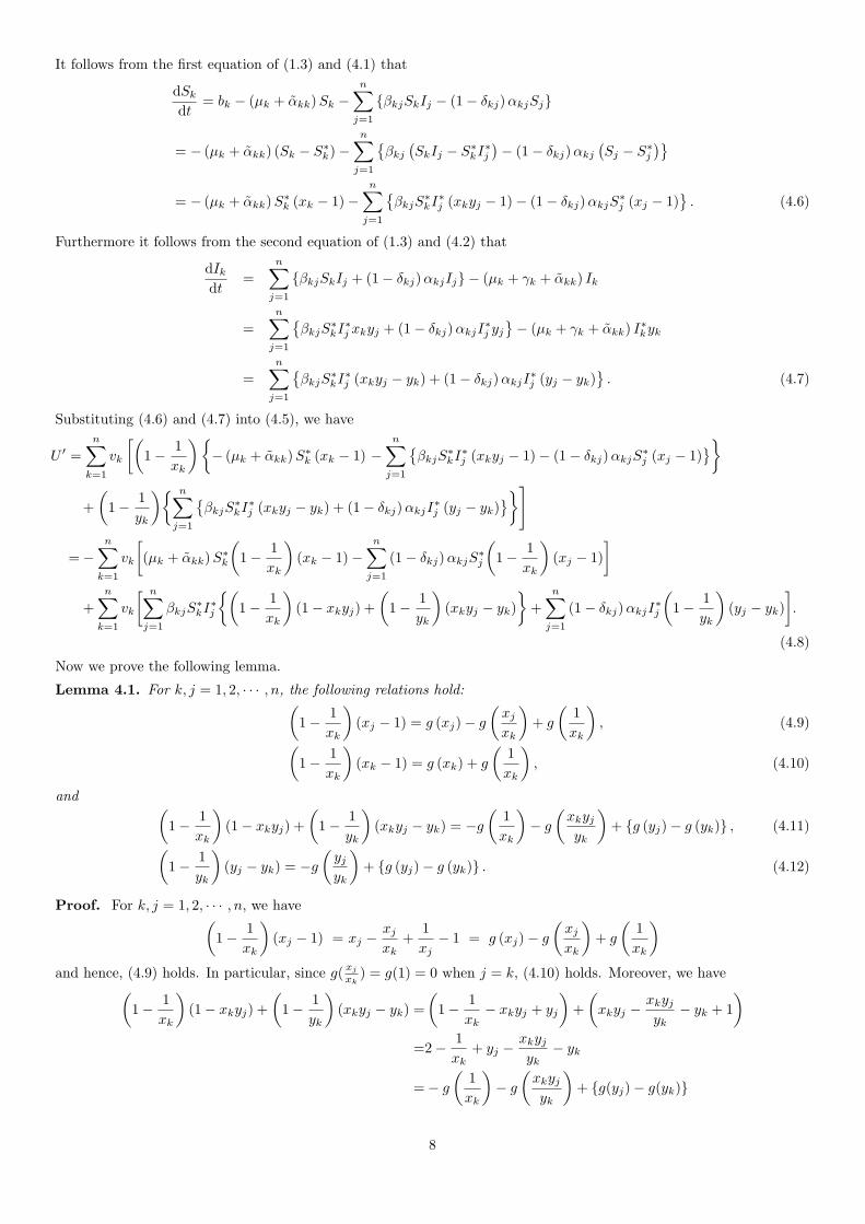
The recent development of worldwide transportation is thought to be one of the causes of the global pandemic ofdiseases. Thus, some types of space-structured models are expected to play an important role in clarifying how suchtransportation affects the pattern of disease prevalence. In this paper, we focus on the dynamics of the following SIRepidemic model with hybrid of multi-group and patch structures, which can be regarded as a type of space-structuredmodel:

dSk

dt= bk −

µk +

n∑j=1

(1− δjk)αjk

Sk − Sk

n∑j=1

βkjIj +

n∑j=1

(1− δkj)αkjSj ,

dIkdt

= Sk

n∑j=1

βkjIj −

µk + γk +n∑

j=1

(1− δjk)αjk

Ik +n∑

j=1

(1− δkj)αkjIj ,

dRk

dt= γkIk −

µk +

n∑j=1

(1− δjk)αjk

Rk +

n∑j=1

(1− δkj)αkjRj , k = 1, 2, · · · , n

(1.1)

with initial condition {Sk (0) = ϕk

1 , Ik (0) = ϕk2 , Rk (0) = ϕk

3 , k = 1, 2, · · · , n,(ϕ11, ϕ

12, ϕ

13, · · · , ϕn

1 , ϕn2 , ϕ

n3

)∈ R3n

+ ,

1

Figure 1: Diagram of the SIR epidemic model (1.1) with hybrid of multi-group and patch structures

where R3n+ :=

{(x1, y1, z1, · · · , xn, yn, zn) ∈ R3n : xk, yk, zk ≥ 0, k = 1, 2, · · · , n

}.

In system (1.1), Sk(t), Ik(t) and Rk(t) denote the densities of susceptible, infective and recovered individuals ingroup k at time t, respectively. bk > 0 denotes the number of newborns per unit time in group k, µk > 0 denotes the percapita mortality rate for individuals in group k (we do not consider the disease-induced mortality rates here), γk ≥ 0denotes the per capita recovery rate for infective individuals in group k, αkj ≥ 0 denotes the per capita rate at whichan individual in group j moves to group k, βkj ≥ 0 denotes the disease transmission coefficient between a susceptibleindividual in group k and an infective individual in group j, and δkj denotes the Kronecker delta such that δkj = 1 ifk = j and δkj = 0 otherwise. For a diagram of system (1.1), see Figure 1.

Note that Li and Shuai [17] investigated the case βkj = 0, j = k, k = 1, 2, . . . , n with three restricted cases for moregeneral patch structures than (1.1). In this model (1.1), the disease transmission can occur not only individuals in thesame groups but also different groups, that is, it can occur that βkj > 0 for some k = j. We call this kind of system themodel with hybrid of multi-group (see, for instance, Guo et al. [9]) and patch (see, for instance, Arino [2], Wang andZhao [26], Jin and Wang [12] and Li and Shuai [17]) structures. One of the previous studies on such a model was doneby Bartlett [3, Section 8]. In the reference, the author considered the following two-group model:

dS1

dt= b1 − S1 (β1I1 + β2I2) +mS (S2 − S1) ,

dI1dt

= S1 (β1I1 + β2I2)− (d+ ρ)µI1 +mI (I2 − I1) ,

dS2

dt= b2 − S2 (β1I1 + β2I2) +mS (S1 − S2) ,

dI2dt

= S2 (β1I1 + β2I2)− (d+ ρ)µI2 +mI (I1 − I2) .

Here the symbols are slightly modified from the original ones. In Bartlett [3, Section 8], this system was explained asthe model for the “interaction” of the actual diffusion or migration of individuals between groups and the chance ofinfection over the groups due to the visit of infective individuals to other groups and then returning. In Faddy [7], thistype of model with hybrid of multi-group and patch structures was also studied. In the reference, such a system withhybrid structure was proposed as the model for considering both the mobility of infective individuals with respect tothe space-region system and the contact infection among the neighborhood of each region. Recently, Muroya et al. [20]investigated a multi-group SIR epidemic model with general patch structure and Kuniya and Muroya [14] established

2

the complete global dynamics of a multi-group SIS epidemic model.Under (i) of the following assumption, system (1.1) can be regarded as the generalization of usual patch models such

that βkj = 0 for k = j and βkj > 0 for k = j and therefore, the analysis would have much mathematical interest:

Assumption 1.1. Either one of the following conditions holds.

(i) The n-square matrix A := (αkj)1≤k,j≤n is irreducible.

(ii) The n-square matrix B := (βkj)1≤k,j≤n is irreducible.

(i) of Assumption 1.1 implies that there exists a path such that an individual in each group can move to any othergroup. (ii) of Assumption 1.1 implies that there exists an infection path such that an infective individual in eachgroup can contact to a susceptible individual in any other group. Note that now we are also assuming that the ratesαkj , k, j = 1, 2, . . . , n are independent of the class (that is, S, I or R) of each individual. Similar assumption is foundin, for instance, Arino [2] and Hyman and LaForce [11]. Note also that we have

n∑k=1

n∑j=1

(1− δjk)αjkSk =

n∑k=1

n∑j=1

(1− δkj)αkjSj (1.2)

(similar equalities hold also for Ij and Rj , j = 1, 2, . . . , n) and hence, in each class, the total emigration is always inbalance with the total immigration and the only input to the system is the recruitment of newborns.

Biologically, we can regard system (1.1) as a model for the geographical spread of disease (see Section 7.1). Inthis case, as explained in Bartlett [3] and Faddy [7], βkj , k = j can imply the effect of contact infection among theneighborhood of each region, which is not due to the actual diffusion or migration. On the other hand, we can alsoregard (1.1) as a multi-group model with perturbation with respect to coefficient αkj . In this case, as in the model of asexually transmitted disease in Section 7.2, αkj , k = j imply the transfer rate from a state to other states (e.g., sexualtransformation).

Due to the complex form, to our knowledge, there are very few studies on the models with hybrid of multi-group andpatch structures (see for example, Muroya et al. [20] for a general SIR model with patch structure). In this paper, westudy the global dynamics of system (1.1) and obtain a threshold condition which can determine the global asymptoticstability of each equilibrium.

From the viewpoint of application, we expect that the threshold condition can play an important role in controllingthe geographical spread of diseases.

Note that the first and second equations of system (1.1) are independent from Rk, k = 1, 2, . . . , n. This allows ushereafter to consider only the following reduced system:

dSk

dt= bk −

µk +

n∑j=1

(1− δjk)αjk

Sk − Sk

n∑j=1

βkjIj +

n∑j=1

(1− δkj)αkjSj ,

dIkdt

= Sk

n∑j=1

βkjIj −

µk + γk +n∑

j=1

(1− δjk)αjk

Ik +n∑

j=1

(1− δkj)αkjIj , k = 1, 2, · · · , n

(1.3)

with initial condition {Sk (0) = ϕk

1 , Ik (0) = ϕk2 , k = 1, 2, · · · , n,(

ϕ11, ϕ

12, ϕ

21, ϕ

22, · · · , ϕn

1 , ϕn2

)∈ R2n

+ .

We define the feasible region for system (1.3) by

Γ :=

{(S1, I1, · · · , Sn, In) ∈ R2n

+ : Sk ≤ S0k,

n∑k=1

(Sk + Ik) ≤b

µ, k = 1, 2, · · · , n

}, (1.4)

where b :=∑n

k=1 bk and µ := min1≤k≤n µk.As in the previous studies of multi-group epidemic models (see, for instance, [9, 10, 18, 19, 21, 23, 27]), we can expect

that a threshold value for the global dynamics of system (1.3) is obtained as the spectral radius of a nonnegativeirreducible matrix, which corresponds to the well-known next generation matrix (see, for instance, van den Driesscheand Watmough [24]). Let H and b be a matrix and a vector defined by

H :=

µ1 + α11 −α12 · · · −α1n

−α21 µ2 + α22 · · · −α2n

......

. . ....

−αn1 −αn2 · · · µn + αnn

and b :=

b1b2...bn

, (1.5)

3

respectively, where

αkk :=n∑

j=1

(1− δjk)αjk. (1.6)

We define a positive n-column vector S0 := (S01 , S

02 , · · · , S0

n)T by

S0 = H−1b, (1.7)

where T denotes the transpose operation for a vector or a matrix. Note that it follows from (1.6) that H is an M -matrixand hence, the positive inverse H−1 exists (see, for instance, Berman and Plemmons [4] or Varga [25]). Let V be ann-dimensional diagonal matrix defined by

V := diag1≤k≤n (µk + γk + αkk)

=

µ1 + γ1 + α11 0 · · · 0

0 µ2 + γ2 + α22 · · · 0...

.... . .

...0 0 · · · µn + γn + αnn

(1.8)

and F be a matrix-valued operator on Rn+ defined by

F(S) :=

S1β11 S1β12 + α12 · · · S1β1n + α1n

S2β21 + α21 S2β22 · · · S2β2n + α2n

......

. . ....

Snβn1 + αn1 Snβn2 + αn2 · · · Snβnn

,

where S := (S1, S2, · · · , Sn)T . Under these settings, we define a matrix M(S) := V−1F(S) = (Mkj)n×n,

Mkj :=Skβkj + (1− δkj)αkj

µk + γk + αkk, k, j = 1, 2, · · · , n

and a threshold valueR0 := ρ(M(S0)), (1.9)

where ρ denotes the spectral radius of a matrix. The definition of this value R0 is slightly different from that of thewell-known basic reproduction number R0 (see Diekmann and Heesterbeek [6] or van den Driessche and Watmough [24]).But on analysis of multi-group SIR epidemic models, a lot of researchers used this R0 in place of R0 (see for example,Guo et al. [9]). In this paper, we shall use R0 in our analysis mainly for a technical reason such that we can constructa suitable Lyapunov function L making use of the form of matrix M(S) (see Section 3), because we shall show that R0

has an equivalent threshold condition to that of R0, Hence, we can use both of them as the threshold value for system(1.3) (see Section 5). The main purpose of this paper is to establish the following theorem which states that R0 (andthus, R0) plays the role of the threshold value for the global asymptotic stability of equilibria of system (1.3):

Theorem 1.1. Let Γ and R0 be defined by (1.4) and (1.9), respectively.

(1) If R0 ≤ 1, then the disease-free equilibrium E0 = (S01 , 0, S

02 , 0, · · · , S0

n, 0) of system (1.3) is globally asymptoticallystable in region Γ.

(2) If R0 > 1, then system (1.3) is uniformly persistent in the interior Γ0 of Γ and has at least one endemic equilibriumE∗ = (S∗

1 , I∗1 , S

∗2 , I

∗2 , · · · , S∗

n, I∗n) in Γ0. Moreover, if

min1≤k≤n

{βkk(S∗k + I∗k)− γk} ≥ 0, (1.10)

then the endemic equilibrium E∗ is globally asymptotically stable in Γ0.

Remark 1.1. Condition (1.10) holds if βkk is large or γk is small (for details, see Corollary 6.1). Moreover, thiscondition (1.10) is a sufficient condition of (4.16) which is satisfied for a sufficiently small patch parameters of αjk. Inthis meaning, the condition (1.10) can be seen as a perturbation result from a well known result of Guo et al. for amulti-group SIR epidemic model.

4

For the proof of Theorem 1.1, we shall use a Lyapunov functional method (see also Korobeinikov [13]). One of thecore ideas of the construction of such a Lyapunov function is using a Laplacian matrix B and linear system Bv = 0as in Guo et al. [9]. The other one of the core ideas is using function g(x) = x − 1 − lnx to evaluate the derivative ofthe Lyapunov function in an appropriate way. Then, we succeed in omitting the argument about the cycles, which wasneeded in the graph theoretic approach in Guo et al. [9]. The result would remind us the importance of using functiong(x) = x− 1− lnx in the Lyapunov functional methods to analysis for epidemic models.

The organization of this paper is as follows: In Section 2, we show the positivity and boundedness of solutions ofsystem (1.3). In Section 3, we prove (1) of Theorem 1.1. In Section 4, we prove (2) of Theorem 1.1. In Section 5, wederive the basic reproduction number R0 for system (1.3) and show that it has a similar threshold property as R0 inthe sense that R0 ≤ 1 if and only if R0 ≤ 1. In Section 7, we perform some numerical simulations to show the validityof Theorem 1.1.

2 Positivity and boundedness of solutions

In this section, we prove the following proposition.

Proposition 2.1. For system (1.3), it holds that

Sk (t) > 0, Ik (t) ≥ 0, ∀k = 1, 2, · · · , n, t ∈ (0,+∞)

and

lim supt→+∞

n∑k=1

{Sk (t) + Ik (t)} ≤ b

µ, lim sup

t→+∞Sk (t) ≤ S0

k, k = 1, 2, · · · , n, (2.1)

where b > 0 and µ > 0 are positive constants defined in (1.4).

Proof. It follows from the first equation of (1.3) that limSk→+0ddtSk ≥ bk > 0. Hence, initial condition Sk (0) = ϕk

1 ≥ 0implies that there exists a positive constant tk0 such that Sk (t) > 0 for all 0 < t < tk0. Let t0 := min1≤k≤n tk0.

First, we claim that Sk (t) > 0 for all k = 1, 2, · · · , n and 0 < t < +∞. In fact, if it is not true, then there exist apositive constant t1 > t0 and a positive integer k1 ∈ {1, 2, · · · , n} such that Sk1(t1) = 0 and Sk1 (t) > 0 for all 0 < t < t1.However, the first equation of (1.3) yields d

dtSk1(t1) ≥ bk1

> 0, which contradicts to the fact that Sk1(t) > 0 = Sk1

(t1)for all 0 < t < t1.

Next, we claim that Ik(t) ≥ 0 for all k = 1, 2, · · · , n and 0 < t < +∞. In fact, if it is not true, then there exist positiveconstant t2 > 0 and positive integer k2 ∈ {1, 2, · · · , n} such that Ik2(t2) < 0. Let s2 := inf {0 < t < t2 : Ik2 (t) < 0},which must satisfy 0 ≤ s2 < t2 and Ik2(s2) = 0. However, the second equation of (1.3) yields d

dtIk2(s2) ≥ 0, whichcontradicts to the fact that Ik2 (t) < 0 = Ik2(s2) for all s2 < t < t2.

Finally, we prove (2.1). It follows from (1.2) and (1.6) that

d

dt

{n∑

k=1

(Sk + Ik)

}=

n∑k=1

bk − (µk + αkk)Sk − (µk + γk + αkk) Ik +n∑

j=1

(1− δkj) (αkjSj + αkjIj)

=

n∑k=1

{bk − µkSk − (µk + γk) Ik} ≤n∑

k=1

bk −(

min1≤k≤n

µk

) n∑k=1

(Sk + Ik) ,

from which we obtain the first inequality of (2.1). It follows from the first equation of (1.3) that

dSk

dt≤ bk − (µk + αkk)Sk +

n∑j=1

(1− δkj)αkjSj , k = 1, 2, · · · , n.

Then, it follows from (1.7) and the theory of linear differential equations that

dS

dt≤

(S (0)− S0

)exp (−Ht) + S0.

Since H defined by (1.5) is an M -matrix, all of its eigenvalues have negative real parts. Therefore, we have

lim supt→+∞

exp (−Ht) = 0

and hence, lim supt→+∞ Sk (t) ≤ S0k, k = 1, 2, · · · , n. □

5

3 Global stability of the disease-free equilibrium E0 for R0 ≤ 1

In this section, we give the proof of (1) of Theorem 1.1.

Proof of (1) of Theorem 1.1. First we show that there do not exist any endemic equilibria E∗ in Γ. Since solutionsbelong to Γ, we have 0 < Sk ≤ S0

k for 1 ≤ k ≤ n and hence 0 ≤ M (S) ≤ M(S0). Assumption 1.1 guarantees the

irreducibility of matrices M (S), M(S0) and M (S) + M(S0). Therefore, it follows from the Perron-Frobenius theoremon nonnegative irreducible matrices (see, for instance, Berman and Plemmons [4, Corollary 2.1.5]) that

ρ(M (S)) < ρ(M(S0

)) = R0 ≤ 1

for S = S0. Hence,M (S) I = I

has only the trivial solution I = 0. This implies that the disease-free equilibrium E0 is the only equilibrium of system(1.3) in Γ.

Let (ω1, ω2, · · · , ωn) be a left eigenvector of matrix M(S0

)corresponding to the eigenvalue ρ(M(S0)), that is,

(ω1, ω2, · · · , ωn) M(S0

)= (ω1, ω2, · · · , ωn) ρ(M

(S0)

).

The irreducibility of matrix M(S0

)yields the strict positive vector (ω1, ω2, · · · , ωn) with ωk > 0 for k = 1, 2, · · · , n (see

Berman and Plemmons [4, Theorem 2.1.4]). Let L be a Lyapunov function on Rn+ defined by

L := (ω1, ω2, · · · , ωn)

µ1 + γ1 + α11 0 · · · 0

0 µ2 + γ2 + α22 · · · 0...

.... . .

...0 0 · · · µn + γn + αnn

−1

I1I2...In

.

The derivative along the trajectories of system (1.3) is

L′ = (ω1, ω2, · · · , ωn)[M (S) I− I

]≤ (ω1, ω2, · · · , ωn)

[M

(S0

)I− I

]=

{ρ(M

(S0

))− 1

}(ω1, ω2, · · · , ωn) I

= (R0 − 1) (ω1, ω2, · · · , ωn) I ≤ 0. (3.1)

Thus, for R0 < 1, we have that L′ = 0 if and only if I = 0. For R0 = 1, we see from the first equality of (3.1) thatL′ = 0 implies

(ω1, ω2, · · · , ωn) M (S) I = (ω1, ω2, · · · , ωn) I. (3.2)

In this situation, if S = S0, then we have

(ω1, ω2, · · · , ωn) M (S) < (ω1, ω2, · · · , ωn) M(S0

)= (ω1, ω2, · · · , ωn) ,

and hence, (3.2) has only the trivial solution I = 0. Consequently, for R0 ≤ 1, we have that L′ = 0 if and only ifI = 0 or S = S0. This implies that the only compact invariant subset of the set where L′ = 0 is the singleton

{E0

}.

Therefore, it follows from the LaSalle invariance principle (see LaSalle [15]) that the disease-free equilibrium E0 isglobally asymptotically stable in Γ. □

4 Global stability of the endemic equilibrium E∗ for R0 > 1

We first prove the following proposition.

Proposition 4.1. Let Γ and R0 be defined by (1.4) and (1.9), respectively. If R0 > 1, then the disease-free equilibriumE0 =

(S01 , 0, · · · , S0

n, 0)∈ Γ is unstable.

Proof. Let ωk, k = 1, 2, . . . , n and L be as in the proof of (1) of Theorem 1.1. Since

(ω1, ω2, · · · , ωn) M(S0

)− (ω1, ω2, · · · , ωn) =

{ρ(M

(S0

))− 1

}(ω1, ω2, · · · , ωn)

=(R0 − 1

)(ω1, ω2, · · · , ωn) > 0,

6

it follows from the continuity of M (S) with respect to S that

L′ = (ω1, ω2, · · · , ωn)[M (S) I− I

]> 0

in a neighborhood of E0 in Γ0. This implies that E0 is unstable. □From Freedman et al. [8], using an argument as in the proof of Proposition 3.3 of Li et al. [16], we can prove that theinstability of E0 implies the uniform persistence of system (1.3).

From Smith and Waltman [22, Theorem D.3], we see that the uniform persistence of system (1.3) together withthe uniform boundedness of solutions in Γ0 implies the existence of an endemic equilibrium in Γ0. Consequently, fromPropositions 2.1 and 4.1, we obtain the following proposition.

Proposition 4.2. Let Γ and R0 be defined by (1.4) and (1.9), respectively. If R0 > 1, then system (1.3) is uniformlypersistent and has at least one endemic equilibrium E∗ = (S∗

1 , I∗1 , S

∗2 , I

∗2 , · · · , S∗

n, I∗n) in the interior Γ0 of Γ.

In the remainder of this section, we assume that R0 > 1. It follows from (1.3) that each component of the endemicequilibrium E∗ = (S∗

1 , I∗1 , S

∗2 , I

∗2 , · · · , S∗

n, I∗n) ∈ Γ0 satisfies the following equations:

bk = (µk + αkk)S∗k +

n∑j=1

{βkjS

∗kI

∗j − (1− δkj)αkjS

∗j

}, (4.1)

(µk + γk + αkk) I∗k =

n∑j=1

{βkjS

∗kI

∗j + (1− δkj)αkjI

∗j

}, k = 1, 2, · · · , n. (4.2)

Letβkj := {βkjS

∗k + (1− δkj)αkj} I∗j , 1 ≤ k, j ≤ n,

B :=

∑

j =1 β1j −β21 · · · −βn1

−β12

∑j =2 β2j · · · −βn2

......

. . ....

−β1n −β2n · · ·∑

j =n βnj

and

(v1, v2, · · · , vn) := (C1, C2, · · · , Cn) ,

where Ck denotes the cofactor of the k-th diagonal entry of B. Using arguments as in Guo et al. [9], we have

Bv = 0

and hence, from (4.2), we have

n∑j=1

vj{βjkS∗j + (1− δjk)αjk} = vk(µk + γk + αkk), k = 1, 2, · · · , n. (4.3)

Using (v1, v2, · · · , vn), we define a Lyapunov functional on R2n+ by

U :=n∑

k=1

vk

{S∗kg

(Sk

S∗k

)+ I∗kg

(IkI∗k

)}, (4.4)

where g (x) := x− 1− lnx is a function defined on (0,+∞). Note that g (x) ≥ 0 for all x > 0 and the global minimumg (x) = 0 is attained if and only if x = 1. The derivative of U along the trajectories of system (1.3) is

U ′ =n∑

k=1

vk

{(1− 1

xk

)dSk

dt+

(1− 1

yk

)dIkdt

}, (4.5)

where

xk =Sk

S∗k

, yk =IkI∗k

, k = 1, 2, · · · , n.

7

It follows from the first equation of (1.3) and (4.1) that

dSk

dt= bk − (µk + αkk)Sk −

n∑j=1

{βkjSkIj − (1− δkj)αkjSj}

= − (µk + αkk) (Sk − S∗k)−

n∑j=1

{βkj

(SkIj − S∗

kI∗j

)− (1− δkj)αkj

(Sj − S∗

j

)}= − (µk + αkk)S

∗k (xk − 1)−

n∑j=1

{βkjS

∗kI

∗j (xkyj − 1)− (1− δkj)αkjS

∗j (xj − 1)

}. (4.6)

Furthermore it follows from the second equation of (1.3) and (4.2) that

dIkdt

=

n∑j=1

{βkjSkIj + (1− δkj)αkjIj} − (µk + γk + αkk) Ik

=n∑

j=1

{βkjS

∗kI

∗j xkyj + (1− δkj)αkjI

∗j yj

}− (µk + γk + αkk) I

∗kyk

=n∑

j=1

{βkjS

∗kI

∗j (xkyj − yk) + (1− δkj)αkjI

∗j (yj − yk)

}. (4.7)

Substituting (4.6) and (4.7) into (4.5), we have

U ′ =n∑

k=1

vk

[(1− 1

xk

){− (µk + αkk)S

∗k (xk − 1) −

n∑j=1

{βkjS

∗kI

∗j (xkyj − 1)− (1− δkj)αkjS

∗j (xj − 1)

}}

+

(1− 1

yk

){ n∑j=1

{βkjS

∗kI

∗j (xkyj − yk) + (1− δkj)αkjI

∗j (yj − yk)

}}]

=−n∑

k=1

vk

[(µk + αkk)S

∗k

(1− 1

xk

)(xk − 1)−

n∑j=1

(1− δkj)αkjS∗j

(1− 1

xk

)(xj − 1)

]

+

n∑k=1

vk

[ n∑j=1

βkjS∗kI

∗j

{(1− 1

xk

)(1− xkyj) +

(1− 1

yk

)(xkyj − yk)

}+

n∑j=1

(1− δkj)αkjI∗j

(1− 1

yk

)(yj − yk)

].

(4.8)

Now we prove the following lemma.

Lemma 4.1. For k, j = 1, 2, · · · , n, the following relations hold:(1− 1

xk

)(xj − 1) = g (xj)− g

(xj

xk

)+ g

(1

xk

), (4.9)(

1− 1

xk

)(xk − 1) = g (xk) + g

(1

xk

), (4.10)

and (1− 1

xk

)(1− xkyj) +

(1− 1

yk

)(xkyj − yk) = −g

(1

xk

)− g

(xkyjyk

)+ {g (yj)− g (yk)} , (4.11)(

1− 1

yk

)(yj − yk) = −g

(yjyk

)+ {g (yj)− g (yk)} . (4.12)

Proof. For k, j = 1, 2, · · · , n, we have(1− 1

xk

)(xj − 1) = xj −

xj

xk+

1

xj− 1 = g (xj)− g

(xj

xk

)+ g

(1

xk

)and hence, (4.9) holds. In particular, since g(

xj

xk) = g(1) = 0 when j = k, (4.10) holds. Moreover, we have(

1− 1

xk

)(1− xkyj) +

(1− 1

yk

)(xkyj − yk) =

(1− 1

xk− xkyj + yj

)+

(xkyj −

xkyjyk

− yk + 1

)=2− 1

xk+ yj −

xkyjyk

− yk

=− g

(1

xk

)− g

(xkyjyk

)+ {g(yj)− g(yk)}

8

and (1− 1

yk

)(yj − yk) = yj −

yjyk

− yk + 1 = −g

(yjyk

)+ {g (yj)− g (yk)} .

Thus, (4.11) and (4.12) hold. □Using Lemma 4.1, we give the proof of (2) of Theorem 1.1.

Proof of (2) of Theorem 1.1. Substituting (4.9)-(4.12) into (4.8), we have

U ′ =−n∑

k=1

vk (µk + αkk)S∗k

{g (xk) + g

(1

xk

)}+

n∑k=1

vk

n∑j=1

(1− δkj)αkjS∗j

{g (xj)− g

(xj

xk

)+ g

(1

xk

)}

−n∑

k=1

vk

n∑j=1

[βkjS

∗kI

∗j

{g

(1

xk

)+ g

(xkyjyk

)}+ (1− δkj)αkjI

∗j g

(yjyk

)]

+n∑

k=1

vk

n∑j=1

(βkjS∗k + (1− δkj)αkj) I

∗j {g (yj)− g (yk)} . (4.13)

The last term of the right-hand side of (4.13) is rewritten as

n∑k=1

vk

n∑j=1

(βkjS∗k + (1− δkj)αkj) I

∗j {g(yj)− g(yk)}

=n∑

k=1

vk

n∑j=1

(βkjS∗k + (1− δkj)αkj) I

∗j g (yj)−

n∑k=1

vk

n∑

j=1

(βkjS∗k + (1− δkj)αkj) I

∗j

g (yk)

=n∑

j=1

vj

n∑k=1

(βjkS

∗j + (1− δjk)αjk

)I∗kg (yk)−

n∑k=1

vk (µk + γk + αkk) I∗kg (yk)

=n∑

k=1

n∑

j=1

vj(βjkS

∗j + (1− δjk)αjk

)− vk (µk + γk + αkk)

I∗kg (yk) . (4.14)

Substituting (4.14) into (4.13), we have

U ′ =−n∑

k=1

vk (µk + αkk)S∗k

{g (xk) + g

(1

xk

)}+

n∑k=1

vk

n∑j=1

(1− δkj)αkjS∗j

{g (xj)− g

(xj

xk

)+ g

(1

xk

)}

−n∑

k=1

vk

n∑j=1

[βkjS

∗kI

∗j

{g

(1

xk

)+ g

(xkyjyk

)}+ (1− δkj)αkjI

∗j g

(yjyk

)]

+n∑

k=1

n∑

j=1

vj(βjkS

∗j + (1− δjk)αjk

)− vk (µk + γk + αkk)

I∗kg (yk)

=−n∑

k=1

vk (βkkI∗k + (µk + αkk))−

n∑j=1

vj (1− δjk)αjk

S∗kg (xk)

−n∑

k=1

vk

n∑

j=1

βkjI∗j + (µk + αkk)

S∗k −

n∑j=1

(1− δkj)αkjS∗j

g

(1

xk

)

−n∑

k=1

vk

n∑j=1

(1− δkj)αkjS∗j g

(xj

xk

)−

n∑k=1

vk

n∑j=1

{βkjS

∗kI

∗j g

(xkyjyk

)+ (1− δkj)αkjI

∗j g

(yjyk

)}

+

n∑k=1

n∑

j=1

vj(βjkS

∗j + (1− δjk)αjk

)− vk (µk + γk + αkk)

I∗kg(yk).

9

Hence, from (4.1) and (4.3), we have

U ′ =−n∑

k=1

{vk (βkkI

∗k + (µk + αkk))−

n∑j=1

vj (1− δjk)αjk

}S∗kg (xk)

−n∑

k=1

vkbkg

(1

xk

)−

n∑k=1

vk

n∑j=1

(1− δkj)αkjS∗j g

(xj

xk

)−

n∑k=1

vk

n∑j=1

{βkjS

∗kI

∗j g

(xkyjyk

)+ (1− δkj)αkjI

∗j g

(yjyk

)}.

(4.15)

We note that assumption (1.10) implies

n∑j=1

vjβjkS∗j ≥ vk(γk − βkkI

∗k), ∀k = 1, 2, · · · , n,

which is equivalent to

vk(βkkI∗k + (µk + αkk))−

n∑j=1

vj(1− δjk)αjk ≥ 0, ∀k = 1, 2, · · · , n. (4.16)

From (4.15) and (4.16), it follows that U ′ ≤ 0. Furthermore, we see that the equality U ′ = 0 holds if and only if

xk = 1 and yk = yj ∀k, j = 1, 2, · · · , n. (4.17)

(4.17) implies that there exists a positive constant c > 0 such that

IkI∗k

= c ∀k = 1, 2, · · · , n.

Thus, substitutingSk = S∗

k and Ik = cI∗k ∀k = 1, 2, · · · , n

into the first equation of system (1.3), we have

0 = bk − (µk + αkk) + cn∑

j=1

βkjS∗kI

∗j − (1− δkj)αkjS

∗j , ∀k = 1, 2, · · · , n. (4.18)

Since the right-hand side of (4.18) is strictly monotone decreasing with respect to c, equality (4.18) holds if and only ifc = 1. This implies that the only compact invariant subset where U ′ = 0 is the singleton {E∗}.

From a similar argument as in Section 3, we can conclude that E∗ is globally asymptotically stable in Γ0. □

5 Relation between R0 and the basic reproduction number R0

In this section, we calculate the basic reproduction number R0 for system (1.3) and investigate the relation between itand R0. First we derive the next generation matrix (see van den Driessche and Watmough [24]) for system (1.3), whosespectral radius is the desired R0. Let V be an n-square matrix defined by

V =

µ1 + γ1 + α11 −α12 · · · −α1n

−α21 µ2 + γ2 + α22 · · · −α2n

......

. . ....

−αn1 −αn2 · · · µn + γn + αnn

. (5.1)

Note that the diagonal entries of matrixV imply the rate of transfer of individuals out of each group, and the nondiagonalentries imply the rate of transfer of individuals into each group by means different from the new infection. Let F be amatrix-valued operator on Rn

+ defined by

F(S) =

S1β11 S1β12 · · · S1β1n

S2β21 S2β22 · · · S2β2n

......

. . ....

Snβn1 Snβn2 · · · Snβnn

.

Note that the (k, j) entry of matrix F (S) implies the rate at which an infective individual in group j produces a newinfective individual in group k when the density of susceptible individuals is given by S. Since V is an M -matrix, the

10

positive inverse V−1 exists and hence, M(S) := F (S)V−1 exists. Following the definition in [24], we obtain the nextgeneration matrix as M

(S0

)and hence, the basic reproduction number R0 is obtained by the spectral radius

R0 = ρ(M

(S0

)). (5.2)

Note thatF(S∗)−V = F(S∗)− V = 0, (5.3)

where S∗ = (S∗1 , S

∗2 , · · · , S∗

n)T.

From (5.3) we haveF (S∗)V−1 = V−1F (S∗) = E,

where E denotes the identity matrix. Hence

ρ(M(S∗)) = ρ(M(S∗)) = 1

and it follows from (1.9), (5.2), Proposition 2.1 and the theory of nonnegative irreducible matrices (see, for instance,Varga [25, Chapter 2]) that

R0 < 1 if and only if R0 < 1,

that is,sign(R0 − 1) = sign(R0 − 1).

Hence, we conclude that R0 plays the role of a threshold for system (1.3) similar to R0 and Theorem 1.1 can be rewrittenas follows.

Theorem 5.1. Let Γ and R0 be defined by (1.4) and (5.2), respectively.

(1) If R0 ≤ 1, then the disease-free equilibrium E0 = (S01 , 0, S

02 , 0, · · · , S0

n, 0) of system (1.3) is globally asymptoticallystable in region Γ.

(2) If R0 > 1, then system (1.3) is uniformly persistent in the interior Γ0 and has at least one endemic equilibriumE∗ = (S∗

1 , I∗1 , S

∗2 , I

∗2 , · · · , S∗

n, I∗n) in Γ0. Moreover, if (1.10) holds, then the endemic equilibrium E∗ is globally

asymptotically stable in Γ0.

6 Corollary

In this section, we provide a sufficient condition under which condition (1.10) holds. The condition is expressed only bygiven coefficients in (1.3) and therefore, it plays an important role in checking whether the condition (1.10) holds.

If R0 > 1 (or, equivalently, R0 > 1), then it follows from the first statement of (2) of Theorem 1.1 (or Theorem 5.1)that system (1.3) has an endemic equilibrium E∗ in Γ0. Adding the first and second equations of system (1.3), we have

d

dt(Sk + Ik) = bk −

{µk +

n∑j=1

(1− δjk)αjk

}(Sk + Ik) +

n∑j=1

(1− δkj)αkj (Sj + Ij)− γkIk, k = 1, 2, · · · , n.

Thus, each component of the endemic equilibrium E∗ = (S∗1 , I

∗1 , · · · , S∗

n, I∗n) must satisfy the following relation:

0 = bk −{µk +

n∑j=1

(1− δjk)αjk

}(S∗

k + I∗k) +n∑

j=1

(1− δkj)αkj

(S∗j + I∗j

)− γkI

∗k

≥ bk −{µk + γk +

n∑j=1

(1− δjk)αjk

}(S∗

k + I∗k) +n∑

j=1

(1− δkj)αkj

(S∗j + I∗j

)for k = 1, 2, · · · , n. Thus, we have 0 ≥ b−V (S∗

1 + I∗1 , · · · , S∗n + I∗n)

T. Hence, it holds that

(S∗1 + I∗1 , · · · , S∗

n + I∗n)T ≥ V−1b,

where b and V are given by (1.5) and (5.1), respectively. Thus, we obtain the following sufficient condition:

min1≤k≤n

{βkk

(V−1b

)k− γk

}≥ 0, (·)k denotes the k-th entry of a vector, (6.1)

under which the condition (1.10) holds.

Corollary 6.1. Let Γ, R0 and R0 be defined by (1.4), (1.9) and (5.2), respectively. If R0 > 1 (or, equivalently, R0 > 1)and (6.1) holds, then system (1.3) has a globally stable endemic equilibrium E∗ in the interior Γ0 of Γ.

Since the left-hand side of (6.1) is explicitly expressed by the given coefficients in (1.3), we can easily check whether itholds by performing numerical calculations.

11

0.0 0.5 1.0 1.5 2.0 t0.1

0.2

0.3

0.4

0.5

IHtL=âk=1

100

IkHtL

(a) Fraction of the total density of infective individuals I =∑100k=1 Ik versus time t

010

2030

4050

6070

8090

100

k

0

1

2

3

4

t

0

0.0005

0.001

IkHtL

(b) Fractions of the total densities of infective individuals Ik(k = 1, 2, · · · , 100) versus time t

Figure 1: Behavior of the solution of infective individuals of system (1.1) for (7.1) and p = 1. In this case, R0 =0.44046 · · · ≤ 1.

7 Numerical examples

In this section, we perform numerical simulations to verify the validity of Theorem 1.1. First, based on the interpretationin Bartlett [3] and Faddy [7], we regard system (1.1) as a model for a geographically spreading disease. Next, we regardsystem (1.1) as a multi-group model with perturbation with respect to αkj and simulate the spread of a sexuallytransmitted disease.

7.1 A geographically spreading disease

To model the geographical spread of a disease, we fix n = 100 as the number of regions. We further fix the followingcoefficients.

bk =

{3 + 2 sin

(2π

100k

)}× 10−2, µk = 3 + 2 sin

(2π

100k

),

γk =

{1 + 0.5 sin

(2π

100k

)}× 10−2,

αkj =

{1 + 0.5 sin

(2π

100(k − j)

)}× 102, k = j, αkj = 0, k = j,

βkj = p×(αkj × 10−1 + 1

), k, j = 1, 2, · · · , 100.

(7.1)

We observe the behavior of solution of (1.1) with varying p. Note that the asymmetric case αkj = αjk for j = k isconsidered in (7.1). Under (7.1), we have

N (t) :=

100∑k=1

{Sk (t) + Ik (t) +Rk (t)} → N∗ = 1 as t → +∞

for any N (0) > 0. Thus, setting (Sk(0), Ik(0), Rk(0)) = (0.009, 0.001, 0) for all k ∈ {1, 2, · · · , 100}, we let the totalpopulation N(t) attains its equilibrium N∗ = 1 at t = 0.

First we set p = 0.1. In this case, we have R0 = 0.999797 · · · ≤ 1 and hence, from (1) of Theorem 1.1, the disease-freeequilibrium E0 of system (1.1) is globally asymptotically stable in region Γ. In fact, we obtain Figure 1 which exhibitsthis result.

Next we set p = 5. In this case, we have R0 = 1.0052 · · · > 1 and

min1≤k≤100

{βkk

(V−1b

)k− γk

}= 0.0348339 · · · > 0.

Hence, from Corollary 6.1, system (1.1) has a unique endemic equilibrium E∗ in Γ0 which is globally asymptoticallystable. In fact, we obtain Figure 2 which exhibits this result.

12

0.0 0.5 1.0 1.5 2.0 t0.2

0.4

0.6

0.8

1.0

IHtL=âk=1

100

IkHtL

(a) Fraction of the total density of infective individuals I =∑100k=1 Ik versus time t

010

2030

4050

6070

8090

100

k

1

2

3

4

t

0.0094

0.00942

0.00943

0.00944

IkHtL

(b) Fractions of the total densities of infective individuals Ik(k = 1, 2, · · · , 100) versus time t

Figure 2: Behavior of the solution of infective individuals of system (1.1) for (7.1) and p = 5. In this case, R0 =1.0052 · · · > 1.

7.2 A sexually transmitted disease

Next, to model a sexually transmitted disease, we let n = 2 and k = 1 and k = 2 be subscripts representing female andmale, respectively. Fix

b1 = b2 = 1.5, µ1 = µ2 = 3,

γ1 = γ2 = 0.01,

α11 = α22 = 0, α12 = α21 = 0.1,

β11 = p, β22 = 0.5× p, β12 = β21 = 1

(7.2)

and observe the behavior of solution of system (1.1) with varying p. Under (7.2), we have

N (t) :=2∑

k=1

{Sk (t) + Ik (t) +Rk (t)} → N∗ = 1 as t → +∞

for any N (0) > 0. Thus, let us set the initial condition as (Sk(0), Ik(0), Rk(0)) = (0.49, 0.01, 0) for k = 1, 2.First we set p = 5. In this case, we have R0 = 0.881475 · · · ≤ 1 and hence, from (1) of Theorem 1.1, the disease-free

equilibrium E0 of system (1.1) is globally asymptotically stable in region Γ. In fact, we obtain Figure 3 (a) whichexhibits this result.

Next we set p = 6. In this case, we have R0 = 1.03231 · · · > 1 and

min1≤k≤100

{βkk

(V−1b

)k− γk

}= 1.48502 · · · > 0.

Hence, from Corollary 6.1, system (1.1) has a unique endemic equilibrium E∗ in Γ0 which is globally asymptoticallystable. In fact, we obtain Figure 3 (b) which exhibits this result.

8 Discussion

In this paper, we have formulated an SIR epidemic model (1.1) with hybrid of multi-group and patch structures. Wehave defined a threshold value R0 by the spectral radius of a nonnegative irreducible matrix M(S0) (see (1.9)), and wehave shown that if R0 ≤ 1, then the disease-free equilibrium E0 of the system is globally asymptotically stable, whileif R0 > 1, then the system is uniformly persistent and there exists an endemic equilibrium E∗. Moreover, under thecondition (1.10), we have shown that if R0 > 1, then the endemic equilibrium E∗ is globally asymptotically stable.Moreover, we obtained a sufficient condition for (1.10), which is expressed only by given coefficients and therefore, wecan easily testify whether it holds or not by numerical calculation (see Section 7). We have also shown that R0 ≤ 1 ifand only if R0 ≤ 1. This implies that we can use both R0 and R0 to predict the eventual size of epidemic.

Compared to Li and Shuai [17], we see that from (6.1), the condition (1.10) holds if the transmission coefficientsβkk, k = 1, 2, . . . , n in the same groups are sufficiently large and/or the per capita recovery rates γk, k = 1, 2, . . . , nare sufficiently small. This situation seems to be realistic for a disease with high infectiousness and long (or, lifelong)infection period. Thus, the geographical spread of HIV/AIDS infection might be thought to be the one of importantexamples for applications of our stability results.

13

I1HtL

I2HtL

0 5 10 15 20 t0.002

0.004

0.006

0.008

0.010

0.012

0.014

(a) Fractions of infective individuals I1 and I2 versus time t forp = 5. In this case, R0 = 0.881475 · · · < 1.

I1HtL

I2HtL

20 40 60 80 100 120t

0.005

0.010

0.015

(b) Fractions of infective individuals I1 and I2 versus time t forp = 6. In this case, R0 = 1.03231 · · · > 1 (I∗1 = 0.0170 · · · ,I∗2 = 0.0062 · · · )

Figure 3: Behavior of the solution of infective individuals of system (1.1) for (7.2)

Acknowledgments

The authors greatly appreciate the Editor and anonymous referees for their helpful comments and valuable suggestionswhich improved the quality of this paper in the present style. The first author is supported by Grant-in-Aid for ResearchActivity Start-up, No.25887011 of Japan Society for the Promotion of Science. The second author is supported byScientific Research (c), No.24540219 of Japan Society for the Promotion of Science. The third author is supported byJSPS Fellows, No.257819 and Grant-in-Aid for Young Scientists (B), No.26800066 of Japan Society for the Promotionof Science.

References

[1] R.M. Anderson and R.M. May, Infectious Diseases of Humans, Oxford University, Oxford, 1991.

[2] J. Arino, Diseases in metapopulations, in Modeling and Dynamics of Infectious Diseases (eds. Z. Ma, Y. Zhou andJ. Wu), Higher Education Press, 2009, 65-122.

[3] M.S. Bartlet, Deterministic and stochastic models for recurrent epidemics, in Proceedings of the Third BerkeleySymposium on Mathematical Statistics and Probability, University of California Press, 1956, 81-109.

[4] A. Berman and R.J. Plemmons, Nonnegative Matrices in the Mathematical Sciences, Academic Press, New York,1979.

[5] H. Chen and J. Sun, Global stability of delay multigroup epidemic models with group mixing nonlinear incidencerates, Appl. Math. Comput. 218 (2011) 4391-4400.

[6] O. Diekmann and J.A.P. Heesterbeek, Mathematical Epidemiology of Infectious Diseases: Model Building, Analysisand Interpretation, 1st edition, John Wiley and Sons, Chichester, 2000.

[7] M.J. Faddy, A note on the behavior of deterministic spatial epidemics, Math. Biosci. 80 (1986) 19-22.

[8] H.I. Freedman, M.X. Tang and S.G. Ruan, Uniform persistence and flows near a closed positively invariant set, J.Dynam. Diff. Equat. 6 (1994) 583-600.

[9] H. Guo, M.Y. Li and Z. Shuai, Global stability of the endemic equilibrium of multigroup SIR epidemic models,Canadian Appl. Math. Quart. 14 (2006) 259-284.

[10] H. Guo, M.Y. Li and Z. Shuai, A graph-theoretic approach to the method of global Lyapunov functions, Proc.Amer. Math. Soc. 136 (2008) 2793-2802.

[11] J.M. Hyman and T. LaForce, Modeling the spread of influenza among cities, in Bioterrorism (eds. H. T. Banks andC. Castillo-Chavez), SIAM, 2003, 211-236.

[12] Y. Jin and W. Wang, The effect of population dispersal on the spread of a disease, J. Math. Anal. Appl. 308 (2005)343-364.

14

[13] A. Korobeinikov, Lyapunov functions and global properties for SEIR and SEIS epidemic model, Math. Med. Biol.21 (2004) 75-83.

[14] T. Kuniya and Y. Muroya, Global stability of a multi-group SIS epidemic model for population migration, DiscreteCont. Dyn. Sys. Series B 19 (2014) 1105-1118.

[15] J.P. LaSalle, The Stability of Dynamical Systems, SIAM, Philadelphia, 1976.

[16] M.Y. Li, J.R. Graef, L. Wang and J. Karsai, Global dynamics of a SEIR model with varying total population size,Math. Biosci. 160 (1999) 191-213.

[17] M.Y. Li and Z. Shuai, Global stability of an epidemic model in a patchy environment, Canadian Appl. Math. Quart.17 (2009) 175-187.

[18] M.Y. Li and Z. Shuai, Global-stability problem for coupled systems of differential equations on networks, J. Diff.Equat. 284 (2010) 1-20.

[19] M.Y. Li, Z. Shuai and C. Wang, Global stability of multi-group epidemic models with distributed delays, J. Math.Anal. Appl. 361 (2010) 38-47.

[20] Y. Muroya, Y. Enatsu and T. Kuniya, Global stability of extended multi-group SIR epidemic models with patchesthrough migration and cross patch infection, Acta Mathematica Scientia, 33 (2013) 341-361.

[21] H. Shu, D. Fan and J. Wei, Global stability of multi-group SEIR epidemic models with distributed delays andnonlinear transmission, Nonlinear Anal. RWA 13 (2012) 1581-1592.

[22] H.L. Smith and P. Waltman,, The Theory of the Chemostat: Dynamics of Microbial Competition, CambridgeUniversity Press, Cambridge, 1995.

[23] R. Sun, Global stability of the endemic equilibrium of multigroup SIR models with nonlinear incidence, Comput.Math. Appl. 60 (2010) 2286-2291.

[24] P. van den Driessche and J. Watmough, Reproduction numbers and sub-threshold endemic equilibria for compart-mental models of disease transmission, Math. Biosci. 180 (2002) 29-48.

[25] R.S. Varga, Matrix Iterative Analysis, Prentice-Hall, Inc., Englewood Cliffs, N.J., 1962.

[26] W. Wang and X. Zhao, An epidemic model in a patchy environment, Math. Biosci. 190 (2004) 97-112.

[27] Z. Yuan and L. Wang, Global stability of epidemiological models with group mixing and nonlinear incidence rates,Nonlinear Anal. RWA 11 (2010) 995-1004.

15