Three Notes on Distributed Property TestingGuy Even∗1, Orr Fischer2, Pierre Fraigniaud†3, Tzlil Gonen2, ReutLevi4, Moti Medina4, Pedro Montealegre‡5, Dennis Olivetti6,Rotem Oshman§2, Ivan Rapaport¶7, and Ioan Todinca8

1 Tel-Aviv University, School of Electrical Engineering, Israelguy@eng.tau.ac.il

2 Tel Aviv University, Computer Science Department, Israelorrfischer@mail.tau.ac.il,tzlilgon@mail.tau.ac.il,roshman@tau.ac.il

3 CNRS and University Paris Diderot, Francepierre.fraigniaud@irif.fr

4 Max Planck Institute for Informatics, Saarland Informatics Campus, Germanyrlevi@mpi-inf.mpg.de, mmedina@mpi-inf.mpg.de

5 Facultad de Ingeniería y Ciencias, Universidad Adolfo Ibáñez, Chilep.montealegre@uai.cl

6 Gran Sasso Science Institute, L’Aquila, Italydennis.olivetti@gssi.infn.it

7 DIM-CMM (UMI 2807 CNRS), Universidad de Chile, Chilerapaport@dim.uchile.cl

8 Université d’Orléans, INSA Centre Val de Loire, LIFO EA 4022, Franceioan.todinca@univ-orleans.fr

AbstractIn this paper we present distributed property-testing algorithms for graph properties in thecongest model, with emphasis on testing subgraph-freeness. Testing a graph property P meansdistinguishing graphs G = (V,E) having property P from graphs that are ε-far from having it,meaning that ε|E| edges must be added or removed from G to obtain a graph satisfying P.

We present a series of results, including:

Testing H-freeness in O(1/ε) rounds, for any constant-sized graph H containing an edge (u, v)such that any cycle in H contain either u or v (or both). This includes all connected graphsover five vertices except K5. For triangles, we can do even better when ε is not too small.A deterministic congest protocol determining whether a graph contains a given tree as asubgraph in constant time.For cliques Ks with s ≥ 5, we show that Ks-freeness can be tested in O(m

12−

1s−2 · ε−

12−

1s−2 )

rounds, where m is the number of edges in the network graph.We describe a general procedure for converting ε-testers with f(D) rounds, where D denotesthe diameter of the graph, to work in O((logn)/ε) + f((logn)/ε) rounds, where n is thenumber of processors of the network. We then apply this procedure to obtain an ε-tester fortesting whether a graph is bipartite and testing whether a graph is cycle-free. Moreover, forcycle-freeness, we obtain a corrector of the graph that locally corrects the graph so that thecorrected graph is acyclic. Note that, unlike a tester, a corrector needs to mend the graph inmany places in the case that the graph is far from having the property.

∗ Work done while visiting Max Planck Institute for Informatics.† Additional support from ANR Project DESCARTES, and from INRIA Project GANG.‡ This work was partially supported by CONICYT via Basal in Applied Mathematics§ Orr Fischer, Tzlil Gonen and Rotem Oshman are supported by the Israeli Centers of Research Excellence(I-CORE) program, (Center No.4/11) and by BSF Grant No. 2014256.¶ This work was partially supported by Fondecyt 1170021, Núcleo Milenio Información y Coordinaciónen Redes ICM/FIC RC130003

© Guy Even, Orr Fischer, Pierre Fraigniaud , Tzlil Gonen, Reut Levi, Moti Medina, Pedro Montealegre,Dennis Olivetti, Rotem Oshman, Ivan Rapaport and Ioan Todinca;

licensed under Creative Commons License CC-BY31st International Symposium on Distributed Computing (DISC 2017).Editor: Andréa Richa; Article No. 15; pp. 15:1–15:30

Leibniz International Proceedings in InformaticsSchloss Dagstuhl – Leibniz-Zentrum für Informatik, Dagstuhl Publishing, Germany

15:2 Three Notes on Distributed Property Testing

These protocols extend and improve previous results of [Censor-Hillel et al. 2016] and [Fraigniaudet al. 2016].

1998 ACM Subject Classification F.2 ANALYSIS OF ALGORITHMS AND PROBLEM COM-PLEXITY

Digital Object Identifier 10.4230/LIPIcs.DISC.2017.15

1 General Introduction

Distributed decision refers to tasks in which the computing elements of a distributed systemhave to collectively decide whether the system satisfies some given boolean predicate onsystem states. If the system state is legal, i.e., it satisfies the given predicate, then allcomputing elements must accept; if the system state is illegal, then at least one computingelement must reject. Distributed property testing is a relaxed variant of distributed decision,which only requires distinguishing legal states from states that are “far from” being legal.(The notion of “farness” depends on the context.)

In the context of distributed network computing, one is interested in deciding or testingwhether the actual network, modeled as a simple connected graph, satisfies some givenpredicate on graphs; e.g., bipartiteness, cycle-freeness, subgraph-freeness, etc. For a positivedistance parameter ε ≤ 1, a graph G with m edges is said to be ε-far from satisfying a givenproperty P if removing and/or adding up to εm edges from/to G cannot result in a graphsatisfying P .

In this paper we study distributed decision in general, and distributed property testing inparticular, in the framework of distributed network computing, under the standard congestmodel. This paper is the result of merging the three papers [16], [17], and [18] that wereconcurrently submitted to the 31st International Symposium on Distributed Computing(DISC 2017), which independently showed overlapping results, using different methods andideas. To highlight the different approaches to the problem, we chose to present a shortversion of each of the three papers in the form of three notes.

The Subgraph-Freeness Problem. Each of the three notes presented here gives results onsubgraph-freeness: we are given a constant-size graph H, and we wish to determine whetherthe network graph contains H as a subgraph or not. In the property testing relaxation ofthe problem, we only need to distinguish the case where the network graph is H-free fromthe case where it is ε-far from H-free, in the sense that at least an ε-fraction of the graph’sedges must be removed to eliminate all copies of H.

Hereafter, we provide a summary of the results and methods in each paper.

1.1 Summary of the Results and TechniquesNote #1: Color-Coding Based Algorithms for Testing Subgraph-Freeness. This noteuses a technique called color-coding [4] to design randomized algorithms for property-testingsubgraph-freeness in O(1/ε) rounds, for any subgraph H that contains an edge (u, v) suchthat any cycle in H contains at least one of u and v. In the case of trees, the color-codingtechnique yields an O(1)-round algorithm for testing exactly whether the graph contains thegiven tree or not. In addition, for cliques Ks with s ≥ 3, we show that Ks-freeness can betested in O(m

12−

1s−2 ·ε−

12−

1s−2 ) rounds, wherem is the number of edges in the network graph.

Even et. al. 15:3

In the special case of triangles, K3-freeness can actually be solved in O(1) rounds in n-nodenetworks, i.e., in a number of rounds independent from ε, assuming ε ≥ minm− 1

3 , nm.

Note #2: Deterministic Tree Detection and Applications in Distributed Prop-erty Testing. In this note, we propose a generic construction for designing deterministicdistributed algorithms detecting the presence of any given tree T as a subgraph of the inputnetwork, performing in a constant number of rounds in the congest model. Our construc-tion also provides randomized algorithms for testing H-freeness for every graph pattern Hthat can be decomposed into an edge and a tree, with arbitrary connections between them,also running in O(1) rounds in the congest model. This generalizes the results in [9, 19, 20],where algorithms for testing K3, K4, and Ck-freeness for every k ≥ 3 were provided.

Note #3: Algorithms for Testing and Correcting Graph Properties in the CON-GEST Model. In Section 4, we design and analyze distributed testers in the distributedcongest model all of which work in the general model. Stating that our testers work inthe general model means that our measure of distance between two graphs is measured byadding or removing ε ·m edges.

Diameter dependency reduction and its Applications. In Section 4.2 we describe a generalprocedure for converting ε-testers with f(D) rounds, where D denotes the diameter of thegraph, to work in O((logn)/ε) + f((logn)/ε) rounds, where n is the number of processorsof the network. We then apply this procedure to obtain an ε-tester for testing whether agraph is bipartite. The improvement of this tester over state of the art is twofold: (a) theround complexity is O(ε−1 logn), which improves over the Poly(ε−1 logn)-round algorithmby Censor-Hillel et al. [9, Thm. 5.2], and (b) our tester works in the general model while [9]works in the more restrictive bounded degree model. Moreover, the number of rounds ofour bipartiteness tester meets the Ω(logn) lower bound by [9, Thm. 7.3], hence our tester isasymptotically optimal in terms of n. We then apply this “compiler” to obtain a cycle-freetester with number of rounds of O(ε−1 · logn), thus revisiting the result by [9, Thm. 6.3].The last application that we consider is “how to obtain a corrector of the graph by usingthis machinery?” Namely, how to design an algorithm that locally corrects the graph so thatthe corrected graph satisfies the property. For cycle-freeness, we are able to obtain also anε-corrector. Note that, unlike a tester, a corrector needs to mend the graph in many placesin the case that the graph is far from having the property.

Testers for H-freeness for |V (H)| ≤ 4. In Section 4.3 we design algorithms for testing (inthe general model) whether the network is H-free for any connected H of size up to fourwith round complexity of O(ε−1).

Testers for tree-freeness. In Section 4.4, we first generalize the global tester by Iwama andYoshida [25] of testing k-path freeness to testing the exclusion of any tree, T , of order k.Our tester has a one sided error and it works in the general graph model with random edgequeries. This algorithm can be simulated in the CONGEST model in O(kk2+1 ·ε−k) rounds.

DISC 2017

15:4 Three Notes on Distributed Property Testing

2 Note #1: Color-Coding Based Algorithms for TestingSubgraph-Freeness

2.1 IntroductionThe aim of this part of the paper is to improve our understanding of the question: “whichtypes of excluded subgraphs can be tested in constant time?”. We also explore severalrelated questions, such as whether limiting the maximum degree in the graphs helps (byanalogy to the bounded-degree model in sequential property testing), whether we can testH-freeness in sublinear time for some subgraphs H for which no constant-time algorithmis known, and whether there are cases where we can test H-freeness with no dependenceon the distance parameter ε, even when ε is sub-constant (e.g., ε = O(1/

√n)). Using new

ideas and combining them with previous techniques, we are able to simplify and extend priorwork, and point out some surprising answers to the questions above, which point to severalaspects where distributed property testing for subgraph-freeness differs from the sequentialanalogue.

Our Results. First we give simple randomized algorithms for testing subgraph-freeness,using the color-coding technique from [4], originally used to find cycles of fixed constant sizesequentially.

We begin by giving a color-coding based algorithm which tests k-cycle freeness in O(1/ε)rounds (for constant k). Next we show that for any tree T , we can test T -freeness exactly(without the property-testing relaxation) in constant time. Both of the results extend todirected graphs in the directed version of the congestmodel. Combining the two algorithms,we give a class of graphs H such that for any constant-sized H ∈ H, we can test H-freenessin O(1/ε) rounds. The class H consists of all graphs H containing an edge u, v such thateach cycle in H includes either u or v (or both). This includes all graphs of size 5 exceptfor the 5-clique, K5.

We then turn our attention to the special case of cliques. We present a different approachfor detecting triangles, which allows us to eliminate the dependence of the running time onε when ε is not too small: if n is the number of nodes and m is the number of edges,and we are promised that ε ≥ min

m−1/3, n/m

, then we can test triangle-freeness in O(1)

rounds (independent of the actual value of ε). We extend this approach to cliques of any sizes ≥ 3, and show that Ks-freeness can be tested in O

(ε−1/2−1/(s−2)m1/2−1/(s−2)) rounds.

In particular, for constant ε and s = 5, we can test K5-freeness in O(m1/6) rounds. We alsomodify the algorithm to work in constant time in graphs whose maximum degree ∆ is nottoo large with respect to the total number of edges, ∆ = O((εm)1/(s−2)).

2.2 PreliminariesWe generally work with undirected graphs, unless indicated otherwise. We let N(v) denotethe neighbors of v, and d(v) the degree of v. Note that throughout the paper, when weuse the term subgraph, we do not mean induced subgraph; we say that G′ = (V ′, E′) is asubgraph of G = (V,E) if V ′ ⊆ V,E′ ⊆ E.

We say that a graph G = (V,E) is ε-far from property P if at least ε|E| edges need tobe added to or removed from E to obtain a graph satisfying P.

The goal in distributed property testing for H-freeness is to solve the following problem:if the network graph G is H-free, then with probability 2/3, all nodes should accept. Onthe other hand, if G is ε-far from being H-free, then with probability 2/3, some node shouldreject.

Even et. al. 15:5

We rely on the following fundamental property, which serves as the basis for most se-quential property testers for H-freeness:I Property 1. Let G be ε-far from being H-free, then G has εm/|E(H)| edge-disjoint copiesof H.

Our algorithms assign random colors to vertices of the graph, and then look for a copyof the forbidden subgraph H which received the “correct colors”. Formally we define:

I Definition 1 Properly-colored subgraphs. Let G = (V,E) and H = ([k], F ) be graphs,and let G′ = (V ′, E′) be a subgraph of G that is isomorphic to H. We say that G′ is properlycolored with respect to a mapping colorV : V → [k] if there is an isomorphism ϕ : V ′ → [k]from G′ to H such that for each u ∈ V ′ we have colorV (v) = ϕ(v).

2.3 Detecting Constant-Size CyclesIn this section we show that Ck-freeness can be tested in O(1/ε) rounds in the congestmodel for any constant integer k > 2.

I Theorem 2. For any constant k > 2, there is a 1-sided error distributed algorithm fortesting Ck-freeness which uses O(1/ε) rounds.

The key idea of the algorithm is to assign each node u of the graph a random colorcolor(u) ∈ [k]. The node colors induce a coloring of both orientations of each edge, wherecolor(u, v) = (color(u), color(v)). We discard all edges that are not colored (i, (i+1) mod k)for some i ∈ [k]; this eliminates all cycles of size less than k, while preserving a constantfraction of k-cycles with high probability.

Next, we look for a properly-colored k-cycle by choosing a random directed edge (u0, u1)1and carrying out a k-round color-coded BFS from node u0: in each round r = 0, . . . , k − 1,the BFS only explores edges colored (r, (r + 1) mod k). After k rounds, if the BFS reachesnode u0 again, then we have found a k-cycle.

Next we describe the implementation of the algorithm in more detail. We do not attemptto optimize the constants. To simplify the analysis, fix a set C of εm/k edge-disjoint k-cycles(which we know exist if the graph is ε-far from being Ck-free). We abuse notation by alsotreating C as the set of edges participating in the cycles in C.

For the analysis, it is helpful to think of the algorithm as first choosing a random edgeand then choosing random colors, and this is the way we describe it below.

Choosing a Random Edge. It is not possible to get all nodes of the graph to explicitlyagree on a uniformly random directed edge in constant time (unless the graph has constantdiameter), but we can emulate the effect as follows: each node u ∈ V chooses a uniformlyrandom weight w(e) ∈ [n4] for each of its edges e. (Note that each edge has two weights, onefor each of its orientations.) Implicitly, the directed edge we selected is the edge with thesmallest weight in the graph, assuming that no two directed edges have the same weight.I Observation 1. With probability at least 1− 1/n2, all weights in the graph are unique.

Let EU be the event that all edge weights are unique. Conditioned on EU , the directededge with the smallest weight is uniformly random. Let e0 be this edge; implicitly, e0 is theedge we select. (However, nodes do not initially know which edge was selected, or even if asingle edge was selected.)

1 What we really want to do is choose a random node with probability proportional to its degree;choosing random edge is a simple way to do that.

DISC 2017

15:6 Three Notes on Distributed Property Testing

Since the set C contains εm/k edge-disjoint k-cycles, and the graph has a total of medges, we have:I Observation 2. We have Pr [e0 ∈ C | EU ] = ε.Let ECyc be the event that e0 ∈ C, and let C0 = u0, u1, . . . , uk−1 be the cycle to which e0belongs given EC , where e0 = (u0, u1).

Color Coding. In order to eliminate cycles of length less than k, we assign to eachnode u a uniformly random color color(u) ∈ [k]. Node u then broadcasts color(u) to itsneighbors.

Since the colors are independent of the edge weights, we have:I Observation 3. Pr [∀i ∈ [k] : color(ui) = i | EC , EU ] = 1

kk .Let ECol be the event that each ui received color i. Combining our observations above yields:

I Corollary 3. Pr [EU ∩ ECyc ∩ ECol] > ε2kk .

Next we show thatn when EU , ECyc and ECol all occur, we find a k-cycle.Color-Coded BFS. Each node u stores the weight wgtu associated with the lightest

edge it has heard of so far, and the root rootu of the BFS tree to which it currently belongs.Initially, wgtu is set to the weight of the lightest of u’s outgoing edges, and rootu is set to u.

In each round r = 0, . . . , k − 1 of the BFS, nodes u with color r send (u,wgtu, rootu) totheir neighbors, and nodes v with color r + 1 update their state: if they received a message(u,wgtu, rootu) from a neighbor u, they set wgtv to the lightest weight they received, androotv to the root associated with that weight.

After k rounds, if some node colored 0 receives a message (v,wgtv, rootv) where rootv = u,then it has found a k-cycle, and it rejects.

In Section 2.5, we will use the same Ck-freeness algorithms, but some nodes will beprohibited from taking certain colors. We incorporate this in Algorithm 1 by having somenodes whose state is abort. These nodes do not forward BFS messages and do not participatein the algorithm.

I Lemma 4. If EU , ECyc and ECol all occur, and if in addition the cycle C0 contains nonodes whose state is abort, then u0 returns 1 and Algorithm 1 finds a k-cycle (i.e., returns1).

Proof of Theorem 2. Suppose that G is ε-far from being Ck-free. We have no nodes whosestate is abort (as we said, the abort state will be used in Section 2.5). Drawing random colorsand weights, the probability that EU , ECyc and ECol all occur is at least ε

2kk ; therefore, theprobability that we fail to detect a k-cycle after d20kk/εe attempts is at most 1/10. J

2.4 Detecting Constant-Size TreesIn this section we show that for any constant-size tree T , we can test T -freeness exactly(that is, without the property-testing relaxation) in O(1) rounds. Let the nodes of T be0, . . . , k − 1. We arbitrarily assign node 0 to be the root of T , and orient the edges of thetree upwards toward node 0. Let R be the depth of the tree, that is, the maximum numberof hops from any leaf of T to node 0. Finally, let children(x) be the children of node x inthe tree.

In the algorithm, we map each node of the network graph G onto a random node of Tby assigning it a random color from [k]. Then we check if there is a copy of T in G that wasmapped “correctly”, with each node receiving the color of the vertex in T it corresponds to.

Even et. al. 15:7

Algorithm 1: Procedure ColorCodedBFS, code for node u1 root ← u

2 wgt ← min w(u, v) | v ∈ N(u)3 for r = 0, . . . , k − 1 do4 if color = r and state 6= abort then send (wgt, root) to neighbors5 receive (w1, r1), . . . , (wt, rt) from neighbors6 if color = (r + 1) mod k then7 i← argmin w1, . . . , wt8 if wi < wgt then9 root ← ri,wgt ← wi

10 if r = k − 1 and u ∈ r1, . . . , rt then return 111 return 0

Initially the state of each node is “open” if it is an inner node of T , and “closed” if it is aleaf. The algorithm has R rounds, in each of which all nodes broadcast their state and theircolor to their neighbors. When a node with color j hears “closed” messages from nodes withcolors matching all the children of node j in T , it changes its status to “closed”. After Rrounds, if node 0’s state is “closed”, we reject.

Let x ∈ 0, . . . , k − 1 be a node of T , let T ′ be the sub-tree rooted at x, and letG′ = (U,E′) be a subgraph of G = (V,E) isomorphic to T ′. We say that G′ is properlycolored if there is an isomorphism ϕ from G′ to T ′, such that color(u) = ϕ(u). (There maybe more than one possible isomorphism from G′ to T ′.)

I Lemma 5. Let u be a node with color color(u) = x, and let T ′ be the sub-tree of T rootedat x. Let hx be the height of x, that is, the length of the longest path from a leaf of T ′ tox. Then at any time t ≥ hx in the execution of Algorithm 2, we have stateu(t) = closed iffthere is a subgraph G′ containing u, which is isomorphic to T ′ and properly colored.

I Corollary 6. For any node u ∈ V , at time h we have stateu(h) = closed iff u is the rootof a properly-colored copy of T .

I Corollary 7. If G contains a copy of T , then repeating Algorithm 2 yields an constantprobability one sided-error algorithm for detecting a copy of T .

Proof. Fix a subgraph G′ which is isomorphic to T . Each time we pick a random coloring,the probability that G′ is properly colored is at least 1/kk (perhaps more, if there is morethan one isomorphism mapping the nodes of G′ to T ). By Corollary 6, if G′ is properlycolored, the root of the tree will discover this and return 1. Therefore the probability thatwe fail d10kke times is at most 1/10. J

2.5 Detecting Constant-Size Complex Graphs

In this section we define a class H of graphs, and give an algorithm for detecting thosegraphs in constant number of round (taking the size of the graph as a constant). The classH includes all graphs of size 5 except K5 (see full paper).

DISC 2017

15:8 Three Notes on Distributed Property Testing

Algorithm 2: Procedure CheckTree, code for node u1 if children(color) = ∅ then2 state ← closed3 else4 state ← open5 missing ← children(color)6 for r = 1, . . . , R do7 send (color , state) to neighbors8 receive (c1, s1), . . . , (ct, st) from neighbors9 foreach i = 1, . . . , t do

10 if ci ∈ missing and si = closed then11 missing ← missing \ ci12 if missing = ∅ then state ← closed

13 if color = 0 and state = closed then14 return 115 else16 return 0

Definition of the Class H

The class H contains all graphs that have the following property: there exists an edge (u, v)such that any cycle in the graph contain at least one of u and v. Equivalently, the class Hcontains all connected graphs that can be constructed using the following procedure:

1. We start with two nodes, 0 and 1, with an edge between them2. Add any number of cycles C1, . . . , C` using new nodes, such that:

Each cycle Ci contains either node 0 or node 1 or both; andWith the exception of nodes 0, 1, the cycles are node-disjoint.

3. Select a subset R of the nodes added so far, and for each node x selected, attach a tree Txrooted at x using “fresh” nodes (that is, with the exception of node x, each tree Tx thatwe attach is node-disjoint from the graph constructed so far, including trees Ty addedfor other nodes y 6= x).

4. For each x ∈ 0, 1, add edges Ex between node x and some subset of nodes added inthe previous steps.

The class H includes all connected nodes over five vertices, except the clique K5. InFigure 1 we show a labeling consistent with the construction above (once the “correct” edgeto label as (0, 1) is identified, the rest is easy to verify).

Our algorithm for testing H-freeness for H ∈ H combines the ideas from the previoussections. We begin by color-coding the nodes of G, mapping each node onto a random nodeof H. Next, we choose a random directed edge (u0, u1) from among the edges mapped to(0, 1), and begin the task of verifying that the various components of H are present andattached properly.

Even et. al. 15:9

Figure 1 A good labeling for each connected graph over five vertices, except K5

For simplicity, below we describe the verification process assuming that we really dochoose a unique random edge, and all nodes know what it is; however, we cannot really dothis, so we substitute using random edge weights as in Section 2.3.

(I) Nodes u0 and u1 broadcast the chosen edge (u0, u1) for diam(H) rounds.(II) Any node whose color is 0 or 1 but which is not u0 or u1 (resp.) sets its state to abort.(III) For each edge b, x ∈ Eb, where b ∈ 0, 1, nodes colored x verify that they have an

edge to node ub; if they do not, they set their state to abort.(IV) For each tree Tx added in stage 3 of the construction, we verify that a properly-

colored copy of Tx is present, by having nodes colored x call Algorithm 2, with thecolors replaced by the names of the nodes in Tx. We denote this by CheckTree(Tx).If a node colored x fails to detect a copy of Tx for which it is the root, it sets its stateto abort for the rest of the current attempt.

(V) For each i = 1, . . . , `, we test for a properly-colored copy of Ci. We define the ownerof Ci, denoted owner(Ci), to be node 0 if C0 contains 0, and otherwise node 1. Toverify the presence of Ci, we call Algorithm 1, using the names of the nodes in Ci ascolors: instead of color 0 we use owner(Ci), and the remaining colors are mapped tothe other nodes of Ci in order (in a arbitrary orientation of Ci). We denote this call byColorBFS(Ci). (As indicated in Alg. 1, nodes whose state is abort do not participate.)

(VI) If both u0 and u1 are not in state abort, u0 rejects, otherwise it accepts. All othernodes accept.

The analysis and pseudo-code of this algorithm appear in the full paper.

2.6 Testing Ks-Freeness

In previous sections it was shown how to test K3 and K4 freeness in O(1/ε) rounds of com-munication. In this section we describe how to test Ks-freeness for cliques of any constantsize s, in a sublinear number of rounds. Moreover, we show that triangle-freeness can betested in O(1) rounds, with no dependence on ε, when min

(nm ,m

−1/3) ≤ ε ≤ 1. Finally, weshow that if the maximal degree is bounded by O((εm)

1s−2 ) then Ks-freeness can be tested

in O(1) rounds, but due to lack of space, this appears in the full paper version only.

DISC 2017

15:10 Three Notes on Distributed Property Testing

2.6.1 Algorithm OverviewThe basic idea is the following simple observation: suppose that each node u could learn theentire subgraph induced by N(u), that is, node u knew for any two v1, v2 ∈ N(u) whetherthey are neighbors or not. Then u could check if there is a set of s neighbors in N(u) thatare all connected to each other, and thus know if it participates in an s-clique or not. Howcan we leverage this observation?

For nodes u with high degree, we cannot afford to have u learn the entire subgraphinduced by N(u), as this requires of N(u)2 bits of information. But fortunately, if G is ε-farfrom Ks-free, then there are many copies of Ks that contain some fairly low-degree nodes,as observed in [20]:

I Lemma 8 [20]. Let I(G) be the set of edges in some maximum set of edge-disjoint copies ofH, and let g(G) = (u, v) | d(u)d(v) ≤ 2m|E(H)|/ε. Then |I(G) ∩ g(G)| ≥ εm/(4|E(H)|).

I Remark. [20] considers only subgraphs H with 4 vertices and constant ε, but their proofworks for any subgraph H and any 0 < ε ≤ 1.

The focus in [20] is on good edges, which are edges satisfying the condition in Lemma 8,but here we need to focus on the endpoints of such edges. We call u ∈ V a good vertex ifits degree is at most

√2m|E(H)|/ε, and we say that a copy of H in G is a good copy if it

contains a good vertex. Since each copy of H in I(G) contributes at most |E(H)| edges tog(G),

I Corollary 9. If G is ε-far from H-free, then G contains at least εm/(4|E(H)|2) edge-disjoint good copies of H.

Because there are many good edge-disjoint copies of Ks, we can sparsify the graph andstill retain at least one good copy of Ks.

We partition G into many edge-disjoint sparse subgraphs, by having each vertex u choosefor each neighbor v ∈ N(u) a random color color(v) ∈ 1, . . . , C(u), where the size of thecolor range, C(u), will be fixed later. This induces a partition of G’s edges into C(v) colorclasses; let Nc(u) denote the set of neighbors v ∈ N(u) with color(v) = c. The expected sizeof Nc(u) is d(v)/C(v).

With this partition in place, we begin by showing how to solve triangle-freeness in con-stant time, and then extend the algorithm to other cliques Ks with s > 3.

2.6.2 Triangle-Freeness for ε ∈ [minm−1/3, n/m

, 1] in O(1) rounds

Assume that ε is not too small with respect to n and m: ε ≥ minm−1/3, n/m

. Then we

can improve the algorithm from Section 2.3 and test triangle-freeness in constant time thatdoes not depend on ε.

To test triangle-freeness, we set C(v) = dd(v)/200e. Each node chooses a random colorfor each neighbor from the range 1, . . . , C(v). Then, we go through the color classesc = 1, . . . , C(v) in parallel, and for each color class c, we look for a triangle containing twoedges from Nc(u): let Nc(u) = v1, . . . , vtc. for R = 202e2 rounds r = 1, . . . , R, node usends vr to all neighbors v1, . . . , vr in Nc(u), and each neighbor vi responds by telling uwhether it is also connected to vr, that is, whether vr ∈ N(vi) (note that we do not insiston the edge (vr, vi) having color c). If vr ∈ N(vi), then node u has found a triangle, and itrejects. If after 202e2 attempts node u has not found a triangle in any color class, it accepts.

Even et. al. 15:11

I Lemma 10. If G is ε-far from being triangle-free, then with probability 2/3, at least onevertex detects a triangle.

Proof. Let T be a set of edge-disjoint good triangles in G, of size |T | ≥ εm/(4|E(T )|2) =εm/36. By Corollary 9 we know that there is such a set.

Assume that T = T1, . . . , Tt. By definition, each good triangle has a good vertex; letvi be a good vertex from the i’th triangle Ti.

For each i ∈ 1, . . . , t, let Ai be the event that vi assigned the same color, ci, to theother two vertices in Ti, and let Xi be an indicator for Ai. We have Pr [Xi = 1] = 1/C(vi) =200/d(vi). Also, since the triangles in T are edge-disjoint, X1, . . . , Xt are independent. Nowlet X =

∑ti=1 Xi be their sum; then

Pr[X = 0] = Pr[t⋂i=1

(Xi = 0)] =t∏i=1

(1− 1

C(vi)

)=

t∏i=1

(1− 200

d(vi)

).

We divide into two cases:

I. m < n3/2: then ε ≥ min(nm ,m

−1/3) = m−1/3. Recall vi is a good vertex, which meansd(vi) ≤

√6m/ε, and therefore

t∏i=1

(1− 200

d(vi)

)≤

(1− 200√

6m/ε

)t≤ e− 200t√

6m/ε ≤ e− 200εm

36√

6m/ε = e− 200ε3/2√m

36√

6 ≤ e−2.

II. m ≥ n3/2: then ε ≥ min(nm ,m

−1/3) = nm . The degree of each vertex is no more than

n, and hencet∏i=1

(1− 200

d(vi)

)≤(

1− 200n

)t≤ e− 200t

n ≤ e− 200εm36n ≤ e−2.

So in any case we get Pr[X = 0] ≤ e−2.Conditioned on X ≥ 1, there is at least one vertex vi which put two of its triangle

neighbors in the same color class ci, which means that if Nc(vi) is no larger than 200e2,node vi will go through all neighbors in Nc(vi) and find the triangle. Because the colors ofthe edges are independent of each other, conditioning on Ai does not change the expectedsize of Nci(vi) by much: we know that the other two vertices in Ti received color ci, butthe remaining neighbors are assigned to a color class independently. The expected size of|Nci(vi)| is therefore (d(vi)−2)/C(vi)+2 < 202 = R/e2, and by Markov, Pr [|Nci(vi)| > R] ≤1/e2.

To conclude, by union bound, the probability that no node vi has Xi = 1, or that thesmallest node vi with Xi = 1 has |Nc(vj)| > 200e2 for the smallest color class c containingtwo triangle neighbors, is at most 1/e2 + 1/e2 < 1/3. J

2.6.3 General Tester for Ks-FreenessUse the same algorithm but with a different setting of the parameters, we can test Ks-freeness for any s ≥ 3.

I Theorem 11. There is a 1-sided error distributed property-testing algorithm for Ks-freeness, for any constant s ≥ 4, with running time O(ε

−s2(s−2)m

s−42(s−2) ).

I Corollary 12. There is a 1-sided error distributed property-testing algorithm for K5-freeness, with running time O(m1/6).

DISC 2017

15:12 Three Notes on Distributed Property Testing

We set

C(u) =⌈(

12s4 εm

) 1s−2⌉

to be the number of color classes at node u, and

R = 2s4e2[ε−1/2−1/(s−2)m1/2−1/(s−2) + s− 1

]to be the timeout. For R rounds, each node u sends the next node vr from each color classto all neighbors v1, . . . , vtc in that color class, and each neighbor vi responds by telling uwhether vr is its neighbor or not. Node u remembers this information; if at any point itknows of a subset S ⊆ Nc(u) of |S| = s nodes that are all neighbors of each other, then ithas found an s-clique, and it rejects. After R rounds u gives up and accepts.

I Lemma 13. If G is ε-far from Ks-free, then with probability at least 2/3, at least onevertex detects a copy of Ks.

I Remark. For s ≥ 5, the algorithm requires a linear estimate of m to get good runningtime. Ifm is unknown, then the vertices may run the algorithm logn times for exponentially-increasing guesses m = [n, 2n, ...n2] , and as the protocol has one sided error, correctness ismaintained; however, the running time increases to O(ε

−s2(s−2)n

s−4(s−2) ) rounds.

3 Note #2: Deterministic Tree Detection and Applications inDistributed Property Testing

3.1 Context and ObjectiveGiven a fixed graph H (e.g., a triangle, a clique on four nodes, etc.), a graph G is H-free if itdoes not contain H as a subgraph2. Detecting copies of H or deciding H-freeness has beeninvestigated in many algorithmic frameworks, including classical sequential computing [2],parametrized complexity [32], streaming [8], property-testing [3], communication complex-ity [27], quantum computing [5], etc. In the context of distributed network computing,deciding H-freeness refers to the task in which the processing nodes of a network G mustcollectively detect whether H is a subgraph of G, according to the following decision rule:

if G is H-free then every node outputs accept;otherwise, at least one node outputs reject.

In other words, G is H-free if and only if all nodes output accept.Recently, deciding H-freeness for various types of graph patterns H has received lots of

attention (see, e.g., [9, 10, 12, 13, 26, 19, 20]) in the congest model [36], and in variants ofthis model. (Recall that the congest model is a popular model for analyzing the impact oflimited link bandwidth on the ability to solve tasks efficiently in the context of distributednetwork computing). In particular, it has been observed that deciding H-freeness mayrequire nodes to consume a lot of bandwidth, even for very simple graph patterns H. Forinstance, it has been shown in [13] that deciding C4-freeness requires Ω(

√n) rounds in

n-node networks in the congest model. Intuitively, the reason why so many rounds of

2 Recall that H is a subgraph of G if V (H) ⊆ V (G) and E(H) ⊆ E(G).

Even et. al. 15:13

computation are required to decide C4-freeness is that the limited bandwidth capacity ofthe links prevents every node with high degree from sending the entire list of its neighborsthrough one link, unless consuming a lot of rounds. The lower bound Ω(

√n) rounds for C4-

freeness can be extended to larger cycles Ck, k ≥ 4, obtaining a lower bound of Ω(poly(n))rounds, where the exponent of the polynomial in n depends on k [13]. Hence, not only“global” tasks such as minimum-weight spanning tree [11, 28, 34], diameter [1, 21], andall-pairs shortest paths [24, 30, 33] are bandwidth demanding, but also “local” tasks suchas deciding H-freeness are bandwidth demanding, at least for some graph patterns H.

In this note, we focus on a generic set of H-freeness decision tasks which includes severalinstances deserving full interest on their own right. In particular, deciding Pk-freeness,where Pk denotes the k-node path, is directly related to the NP-hard problem of computingthe longest path in a graph. Also, detecting the presence of large complete binary trees,or of large binomial trees, is of interest for implementing classical techniques used in thedesign of efficient parallel algorithms (see, e.g., [29]). Similarly, detecting large Polytrees ina Bayesian network might be used to check fast belief propagation [35]. Finally, as it will beshown in this note, detecting the presence of various forms of trees can be used to tests thepresence of graph patterns of interest in the framework of distributed property-testing [9].Hence, this note addresses the following question:

For which tree T is it possible to decide T -freeness efficiently in the congestmodel, that is, in a number of rounds independent from the size n of theunderlying network?

At a first glance, deciding T -freeness for some given tree T may look simpler than detect-ing cycles, or even just deciding C4-freeness. Indeed, the absence of cycles enables to ignorethe issue of checking that a path starts and ends at the same node, which is bandwidthconsuming because it requires maintaining all possible partial solutions corresponding togrowing paths from all starting nodes. When detecting cycles, discarding even just a fewstarting nodes may result in missing the unique cycle including these nodes. However, evendeciding Pk-freeness requires to overcome many obstacles. First, as mentioned before, find-ing a longest simple path in a graph is NP-hard, which implies that it is unlikely that analgorithm deciding Pk-freeness exists in the congest model, with running time polynomialin k at every node. Second, and more importantly, there exists potentially up to Θ(nk) pathsof length k in a network, which makes impossible to maintain all of them in partial solutions,as the overall bandwidth of n-node networks is at most O(n2 logn) in the congest model.

3.2 Our ResultsWe show that, in contrast to Ck-freeness, Pk-freeness can be decided in a constant numberof rounds, for any k ≥ 1. In fact, our main result is far more general, as it applies to anytree. Stated informally, we prove the following:

Theorem A. For every tree T , there exists a deterministic algorithm for deciding T -freenessperforming in a constant number of rounds under the congest model.

For establishing Theorem A, we present a distributed implementation of a pruning tech-nique based on a combinatorial result due to Erdős et al. [15] that roughly states the fol-lowing. Let k > t > 0. For any set V of n elements, and any collection F of subsets of V ,all with cardinality at most t, let us define a witness of F as a collection F ⊆ F of subsetsof V such that, for any X ⊆ V with |X| ≤ k − t, the following holds:(∃Y ∈ F : Y ∩X = ∅

)=⇒

(∃Y ∈ F : Y ∩X = ∅

).

DISC 2017

15:14 Three Notes on Distributed Property Testing

Of course, every F is a witness of itself. However, Erdős et al. have shown that, for everyk, t, and F , there exists a compact witness F of F , that is, a witness whose cardinalitydepends on k and t only, and hence is independent of n. To see why this result is importantfor detecting a tree T in a network G, consider V as the set of nodes of G, k as the numberof nodes in T , and F as a collection of subtrees Y of size at most t, each isomorphic to somesubtree of T . The existence of compact witnesses allows an algorithm to keep track of only asmall subset F of F . Indeed, if F contains a partial solution Y that can be extended into aglobal solution isomorphic to T using a set of nodes X, then there is a representative Y ∈ Fof the partial solution Y ∈ F that can also be extended into a global solution isomorphicto T using the same set X of nodes. Therefore, there is no need to keep track of all partialsolutions Y ∈ F , it is sufficient to keep track of just the partial solutions Y ∈ F . Thispruning technique has been successfully used for designing fixed-parameter tractable (FPT)algorithms for the longest path problem [32], as well as, recently, for searching cycles in thecontext of distributed property-testing [19]. Using this technique for detecting the presenceof a given tree however requires to push the recent results in [19] much further. First, thedetection algorithm in [19] is anchored at a fixed node, i.e., the question addressed in [19] iswhether there is a cycle Ck passing through a given node. Instead, we address the detectionproblem in its full generality, and we do not restrict ourselves to detecting a copy of Tincluding some specific node. Second, detecting trees requires to handle partial solutionsthat are not only composed of sets of nodes, but that offer various shapes, depending on thestructure of the tree T , representing all possible combinations of subtrees of T .

Theorem A, which establishes the existence of distributed algorithms for detecting thepresence of trees, has important consequences on the ability to test the presence of morecomplex graph patterns in the context of distributed property-testing. Recall that, for ε ∈(0, 1), a graph G is ε-far from being H-free if removing less than a fraction ε of its edgescannot result in an H-free graph. A (randomized) distributed algorithm tests H-freeness ifit decides H-freeness according to the following decision rule:

if G is H-free then Pr[every node outputs accept] ≥ 2/3;if G is ε-far from being H-free then Pr[at least one node outputs reject] ≥ 2/3.

That is, a testing algorithm separates graphs that are H-free from graphs that are farfrom being H-free. So far, the only non-trivial graph patterns H for which distributedalgorithms testing H-freeness are known are:

the complete graphs K3 and K4 (see [9, 20]), andthe cycles Ck, k ≥ 3 (see [19]).

Using our algorithm for detecting the presence of trees, we show the following (statedinformally):

Theorem B. For every graph pattern H composed of an edge and a tree with arbitraryconnections between them, there exists a (randomized) distributed algorithm for testing H-freeness performing in a constant number of rounds under the congest model.

At a first glance, the family of graph patterns H composed of an edge and a tree witharbitrary connections between them (like, e.g., the graph depicted on the top-left corner ofFig. 2) may look quite specific and artificial. This is not the case. For instance, every cycleCk for k ≥ 3 is a “tree plus one edge”. This also holds for 4-node complete graph K4. In fact,all known results about testing H-freeness for some graph H in [9, 19, 20] are just directconsequence of Theorem B. Moreover, Theorem B enables to test the presence of other graph

Even et. al. 15:15

T e

C3 CkK4

K2,k

Figure 2 All these graphs are composed of a tree T and edge e with arbitrary connectionsbetween them.

patterns, like the complete bipartite graph K2,k with k + 2 nodes, for every k ≥ 1, or thegraph pattern depicted on the top-right corner of Fig. 2, in O(1) rounds. It also enables totest the presence of connected 1-factors as a subgraph in O(1) rounds. (Recall that a graphH is a 1-factor if its edges can be directed so that every node has out-degree 1).

In fact, our algorithm is 1-sided, that is, if G is H-free, then all nodes output accept withprobability 1.

3.3 Detecting the Presence of TreesIn this section, we establish our main result:

I Theorem 14. For every tree T , there exists an algorithm performing in O(1) rounds inthe congest model for detecting whether the given input network contains T as a subgraph.

Proof. Let k be the number of nodes in tree T . The nodes of T are labeled arbitrarily byk distinct integers in [1, k]. We arbitrarily choose a vertex r ∈ [1, k] of T , and view T asrooted in r. For any vertex ` ∈ V (T ), let T` be the subtree of T rooted in `. We say thatT` is a shape of T . Our algorithm deciding T -freeness proceeds in depth(Tr) + 1 rounds.At round t, every node u of G constructs, for each shape T` of depth at most t, a set ofsubtrees of G all rooted at u, denoted by sosu(T`), such that each subtree in sosu(T`) isisomorphic to the shape T`. The isomorphism is considered in the sense of rooted trees, i.e.,it maps u to `. If we were in the local model3, we could afford to construct the set of allsuch subtrees of G. However, we cannot do that in the congest model because there aretoo many such subtrees. Therefore, the algorithm acts in a way which guarantees that:

1. the set sosu(T`) is of constant size, for every node u of G, and every node ` of T ;

3 The local model is similar to the congest model, but it has no restriction on the size of the mes-sages [36].

DISC 2017

15:16 Three Notes on Distributed Property Testing

2. for every set C ⊆ V of size at most k−|V (T`)|, if there is some subtree W of G rooted atu that is isomorphic to T`, and that is not intersecting C, then sosu(Tl) contains at leastone such subtree W ′ not intersecting C. (Note that W ′ might be different from W ).

The intuition for the second condition is the following. Assume that there exists somesubtree W of G rooted at u, corresponding to some shape T`, which can be extended into asubtree isomorphic to T by adding the vertices of a set C. The algorithm may well not keepthe subtree W in sosu(Tl). However, we systematically keep at least one subtree W ′ of G,also rooted at u and isomorphic to T`, that is also extendable to T by adding the vertices ofC. Therefore the sets sosu(T`), over all shapes T` of depth at most t, are sufficient to ensurethat the algorithm can detect a copy of T in G, if it exists. Our approach is described inAlgorithm 3. (Observe that, in this algorithm, if we omit Lines 13 to 15, which prune theset sosu(T`), we obtain a trivial algorithm detecting T in the local model). Implementingthe pruning of the sets sosu(T`) for keeping them compact, we make use of the followingcombinatorial lemma, which has been rediscovered several times, under various forms (see,e.g., [19, 32]).

I Lemma 15 Erdős, Hajnal, Moon [15]. Let V be a set of size n, and consider two integerparameters p and q. For any set F ⊆ P(V ) of subsets of size at most p of V , there exists acompact (p, q)-representation of F , i.e., a subset F of F satisfying:

1. For each set C ⊆ V of size at most q, if there is a set L ∈ F such that L ∩ C = ∅, thenthere also exists L ∈ F such that L ∩ C = ∅;

2. The cardinality of F is at most(p+qp

), for any n ≥ p+ q .

By Lemma 15, the sets sosu(T`) can be reduced to constant size (i.e., independent ofn), for every shape T` and every node u of G. Moreover, the number of shapes is at most k,and, for each shape T`, each element of sosu(T`) can be encoded on k logn bits. Thereforeeach vertex communicates only O(logn) bits per round along each of its incident edges. So,the algorithm does perform in O(1) rounds in the congest model4.

Proof of correctness. First, observe that if sosu(T`) contains a graphW , thenW is indeeda tree rooted at u, and isomorphic to T`. This is indeed the case at round t = 0, and we canproceed by induction on t. Let T` be a shape of depth `. Each graph W added to sosu(T`)is obtained by gluing vertex-disjoint trees at the root u. These latter trees are isomorphicto the shapes Tj1 , . . . , Tjs , where j1, . . . , js are the children of node j in T . Therefore W isisomorphic to T`. In particular, if the algorithm rejects at some node u, it means that thereexists a subtree of G isomorphic to T .

We now show that if G contains a subgraph W isomorphic to T , then the algorithmrejects in at least one node. For this purpose, we prove a stronger statement:

I Lemma 16. Let u be a node of G, T` be a shape of T , and C be a subset of vertices of G,with |C| ≤ k − |V (Tu)|. Let us assume that there exists a subgraph Wu of G, satisfying thefollowing two conditions: (1) Wu is isomorphic to T`, and the isomorphism maps u on `,and (2) Wu does not contain any vertex of C. Then sosu(T`) contains a tree W ′u satisfyingthese two conditions.

4 We may assume that, for compacting a set sosu(T`) in Lines 13-15, every node u applies Lemma 15 bybrute force (e.g., by testing all candidates F ). In [32], an algorithmic version of Lemma 15 is proposed,producing a set F of size at most

∑q

i=1 pi in time O((p+q)! ·n3), i.e., in time poly(n) for fixed p and q.

Even et. al. 15:17

Algorithm 3: Tree-detection, for a given tree T . Algorithm executed by node u.1 for each leaf ` of T do2 let sosu(T`) be the unique tree with single vertex u3 exchange the sets sos with all neighbors4 for t = 1 to depth(T ) do5 for each node ` of T with depth(T`) = t do6 sosu(T`)← ∅7 let j1, . . . , js be the children of ` in T8 for every s-uple (v1, . . . , vs) of nodes in N(u) do9 for every (W1, . . . ,Ws) ∈ sosv1(Tj1)× · · · × sosvs

(Tjs) do

10 if u and W1, . . . ,Ws are pairwise disjoint then11 let W be the tree with root u, and subtrees W1, . . . ,Ws

12 add W to sosu(T`) // each Wi is glued to u by its root

13 let F = V (W ) |W ∈ sosu(Tl)// collection of vertex sets for trees in sosu(Tl)

14 construct a (|V (T`)|, k − |V (T`)|)-compact representation F ⊆ F// cf. Lemma 15

15 remove from sosu(T`) all trees W with vertex set not in F16 exchange sosu(T`) with all neighbors

17 if sosu(Tr) = ∅ then // r denotes the root of T

18

19 return accept20 else21 return reject

We prove the lemma by induction on the depth of T`. If depth(T`) = 0 then ` is a leafof T`, and sosu(T`) just contains the tree formed by the unique vertex u. Il particular, itsatisfies the claim. Assume now that the claim is true for any node of T whose subtree hasdepth at most t− 1, and let ` be a node of depth t. Let j1, . . . , js be the children of ` in T .For every i, 1 ≤ i ≤ s, let vi be the vertex of Wu mapped on ji. By induction hypothesis,sosv1(Tj1) contains some tree W ′v1

isomorphic to Tj1 and avoiding the nodes in C ∪ u, aswell as all the nodes of Wv2 , . . .Wvs

. Using the same arguments, we proceed by increasingvalues of i = 2, . . . , s, and we choose a tree W ′vi

∈ sosvi(Tji) isomorphic to Tji that avoidsC ∪ u, as well as all the nodes in W ′v1

, . . . ,W ′vi−1and the nodes of Wvi+1 , . . . ,Wvs

. Now,observe that the treeW ′′ obtained from gluing u toW ′v1

, . . . ,W ′vshas been added to sosu(T`)

before compacting this set, by Line 11 of Algorithm 3. SinceW ′′ does not intersect C, we getthat, by compacting the set sosu(T`) using Lemma 15, the algorithm keeps a representativesubtree W ′ of G that is isomorphic to Tl and not intersecting C. This completes the proofof the lemma.

To complete the proof of Theorem 14, let us assume there exists a subtree W of G iso-morphic to T , and let u be the vertex that is mapped to the root r of T by this isomorphism.By Lemma 16, sosu(Tr) 6= ∅, and thus the algorithm rejects at node u. J

DISC 2017

15:18 Three Notes on Distributed Property Testing

3.4 Distributed Property TestingIn this section, we show how to construct a distributed tester for H-freeness in the sparsemodel, based on Algorithm 3. This tester is able to test the presence of every graph pat-tern H composed of an edge e and a tree T connected in an arbitrary manner, by distin-guishing graphs that include H from graphs that are ε-far5 from being H-free.

Specifically, we consider the set H of all graph patterns H with node-set V (H) =x, y, z1, . . . , zk for k ≥ 1, and edge-set E(H) = f ∪ E(T ) ∪ E , where f = x, y, T is atree with node set z1, . . . , zk, and E is some set of edges with one end-point equal to x ory, and the other end-point zi for i ∈ 1, . . . , k. Hence, a graph H ∈ H can be described bya triple (f, T, E) where E is a set of edges connecting a node in T with a node in f .

We now establish our second main result, i.e., Theorem B, stated formally below asfollows:

I Theorem 17. For every graph pattern H ∈ H, i.e., composed of an edge and a tree con-nected in an arbitrary manner, there exists a randomized 1-sided error distributed propertytesting algorithm for H-freeness performing in O(1/ε) rounds in the congest model.

Proof. Let H = (f, T, E), with f = x, y. Let us assume that there are ν copies of H in G,and let us call these copies H1 = (f1, T1, E1), . . . ,Hν = (fν , Tν , Eν)). Let E = f1, . . . , fν.Our tester algorithm for H-freeness is composed by the following two phases:

1. determine a candidate edge e susceptible to belong to E;2. checking the existence of a tree T connected to e in the desired way.

In order to find the candidate edge, we exploit the following lemma:

I Lemma 18 [20]. Let H be any graph. Let G be an m-edge graph that is ε-far from beingH-free. Then G contains at least εm/|E(H)| edge-disjoint copies of H.

Hence, if the actualm-edge graphG is ε-far from beingH-free, we have |E| ≥ εm/|E(H)|.Thus, by randomly choosing an edge e and applying Lemma 18, e ∈ E with probability atleast ε/|E(H)|.

As shown in [19], the first phase can be computed in the following way. First, every edgeis assigned to the endpoint having the smallest identifier. Then, every node picks a randominteger r(e) ∈ [1,m2] for each edge e assigned to it. The candidate edge of Phase 1 is theedge emin with minimum rank, and indeed Pr[emin ∈ E] ≥ ε/|E(H)|.

It might be the case that emin is not unique though. However: Pr[emin is unique] ≥ 1/e2

where e denotes here the basis of the natural logarithm. Also, every node picks, for every edgee = v1, v2 assigned to it, a random bit b. Assume, w.l.o.g., that ID(v1) < ID(v2). If b = 0,then the algorithm will start Phase 2 for testing the presence of H with (x, y) = (v1, v2),and if b = 1, then the algorithm will start Phase 2 for testing the presence of H with(x, y) = (v2, v1). We have Pr[emin is considered in the right order] ≥ 1/2. It follows that theprobability emin is unique, considered in the right order, and part of E is at least ε

2|E(H)|e2 .Using a deterministic search based on Algorithm 3, H will be found with probability at

least ε2|E(H)|e2 . To boost the probability of detecting H in a graph that is ε-far from being

H-free, we repeat the search 2e2|E(H)| ln 3/ε times. In this way, the probability that H isdetected in at least one search is at least 2/3 as desired.

5 For ε ∈ (0, 1), a graph G is ε-far from being H-free if removing less than a fraction ε of its edges cannotresult in an H-free graph.

Even et. al. 15:19

During the second phase, the ideal scenario would be that all the nodes of G search forH = (f, T, E) by considering only the edge emin as candidate for f , to avoid congestion.Obviously, making all nodes aware of emin would require diameter time. However, there isno needs to do so. Indeed, the tree-detection algorithm used in the proof of Theorem 14runs in depth(T ) rounds. Hence, since only the nodes at distance at most depth(T )+1 fromthe endpoints of emin are able to detect T , it is enough to broadcast emin at distance upto 2 (depth(T ) + 1) rounds. This guarantees that all nodes participating to the executionof the algorithm for emin will see the same messages, and will perform the same operationsthat they would perform by executing the algorithm for emin on the full graph. So, everynode broadcasts its candidate edge with the minimum rank, at distance 2 (depth(T ) + 1).Two contending broadcasts, for two candidate edges e and e′ for f , resolve contention bydiscarding the broadcast corresponding to the edge e or e′ with largest rank. (If e and e′ havethe same rank, then both broadcast are discarded). After this is done, every node is assignedto one specific candidate edge, and starts searching for T . Similarly to the broadcast phase,two contending searches, for two candidate edges e and e′, resolve contention by abortingthe search corresponding to the edge e or e′ with largest rank. From now on, one can assumethat a single search in running, for the candidate edge emin.

It remains to show how to adapt Algorithm 3 for checking the presence of a tree Tconnected to a fixed edge e = x, y ∈ E(G) as specified in E . Let us consider Instruction 5of Algorithm 3, that is: “for each node ` of T with depth(T`) = t do”. At each step of thisfor-loop, node u tries to construct a tree W that is isomorphic to the subtree of T rootedat `. In order for u to add W to sosu(T`), we add the condition that:

if `, x ∈ E(H) then u, x ∈ E(G), andif `, y ∈ E(H) then u, y ∈ E(G).

Note that this condition can be checked by every node u. If this condition is not satisfied,then u sets sosu(T`) = ∅.

This modification enables to test H-freeness. Indeed, if the actual graph G is H-free,then, since at each step of the modified algorithm, the set sosu(T`) is a subset of the setsosu(T`) generated by the original algorithm, the acceptance of the modified algorithm isguaranteed from the correctness of the original algorithm.

Conversely, let us show that, in a graph G that is ε far of being H-free, the algorithmrejects G as desired. In the first phase of the algorithm, it holds that emin ∈ E happensin at least one search whenever G is ε-far from being H-free, with probability at least 2/3.Following the same reasoning of the proof of Lemma 16, since the images of the isomorphismsatisfy the condition of being linked to nodes x, y in the desired way, the node of G thatis mapped to the root of T correctly detects T , and rejects, as desired. J

3.5 ConclusionIn this note, we have proposed a generic construction for designing deterministic distributedalgorithms detecting the presence of any given tree T as a subgraph of the input network,performing in a constant number of rounds in the congest model. Therefore, there is aclear dichotomy between cycles and trees, as far as efficiently solvingH-freeness is concerned:while every cycle of at least four nodes requires at least a polynomial number of rounds to bedetected, every tree can be detected in a constant number of rounds. It is not clear whetherone can provide a simple characterization of the graph patterns H for which H-freenesscan be decided in O(1) rounds in the congest model. Indeed, the lower bound Ω(

√n) for

C4-freeness can be extended to some graph patterns containing C4 as induced subgraphs.

DISC 2017

15:20 Three Notes on Distributed Property Testing

However, the proof does not seem to be easily extendable to all such graph patterns as,in particular, the patterns containing many overlapping C4 like, e.g., the 3-dimensionalhypercube Q3, since this case seems to require non-trivial extensions of the proof techniquesin [13]. An intriguing question is to determine the round-complexity of deciding Kk-freenessin the congest model for k ≥ 3, and in particular to determine the exact round-complexityof deciding C3-freeness.

Our construction also provides randomized algorithms for testing H-freeness (i.e., fordistinguishing H-free graphs from graphs that are far from being H-free), for every graphpattern H that can be decomposed into an edge and a tree, with arbitrary connectionsbetween them, also running in O(1) rounds in the congest model. This generalizes theresults in [9, 19, 20], where algorithms for testing K3, K4, and Ck-freeness for every k ≥ 3were provided. Interestingly, K5 is the smallest graph pattern H for which it is not knownwhether testing H-freeness can be done in O(1) rounds, and this is also the smallest graphpattern that cannot be decomposed into a tree plus an edge. We do not know whether thisis just coincidental or not.

4 Note #3: Algorithms for Testing and Correcting Graph Propertiesin the CONGEST Model

4.1 Computational ModelsNotations. Let G = (V,E) denote a graph, were V is the set of vertices and E is the set ofedges. Let n , |V (G)|, and let m , |E(G)|. For every v ∈ V , let NG(v) , u ∈ V | u, v ∈E denote the neighborhood of v in G. For every v ∈ V , let dG(v) , |NG(v)| denote thedegree of v. When the graph at hand is clear from the context we omit the subscript G.

4.1.1 Distributed CONGEST ModelComputation in the distributed congest [36] model is done as follows. Let G = (V,E)denote a network where each vertex is a processor and each edge is a communication linkbetween its two endpoints. Each processor is given a local input. Each processor v has adistinct ID - for brevity we say that the ID of processor v is simply v.6 The computation issynchronized and is measured in terms of rounds. In each round, each processor performs thefollowing steps: (1) Receive the messages that were sent by its neighbors in the previousround. (2) Execute a local (randomized) computation. (3) Sends (different) messages ofO(logn) bits to every neighbor neighbors (or a possible “empty message”). In the lastround all the processors stop and output a local output.

4.1.2 (Global) Testing ModelGraph property testing [22, 23] is defined as follows. A graph property P is a subset of all(undirected and unlabeled) graphs e.g., the graph is cycle-free, the graph is bipartite, etc.We focus on edge monotone (with respect to deletions) properties.

I Definition 19. A graph property P is edge-monotone if G ∈ P and G′ is obtained fromG by the removal of edges, then G′ ∈ P.

6 In this paper we focus on randomized algorithms. Note that, with high probability, distinct IDs canbe randomly generated using O(logn) bits.

Even et. al. 15:21

We define the edge-distance between two graphs G = (V,E) and G′ = (V,E′) as thenumber edges in the symmetric difference E 4 E′. We say that a graph G is ε-far (in thegeneral model) from having the property P if |E4E′| ≥ ε · |E|, for every G′ = (V,E′) ∈ P.

The tester accesses the graph via queries. The type of queries we consider are: (1) whatis the degree of v for v ∈ V ? (2) who is the ith neighbor of v ∈ V ?

We say that an algorithm is a one sided ε-tester for property P in the general modelif given query access to the graph G the algorithm ACCEPTS the graph G if G has theproperty P, i.e, completeness, and REJECTS the graph G with probability at least 2/3 ifG is ε-far from having the property P, i.e., soundness.

We note that since the tester must accept graphs G ∈ P, a reject occurs if only if thetester has a proof that that G /∈ P. Such a proof is called a witness against G ∈ P. In fact,in [9], it is required that the witness is an induced proper subgraph of G.

The complexity measure of this model is the number of queries made to G. The goal isto design an ε-tester with as few as possible queries. In particular, the number of queriesshould be sublinear in the size of the graph.

In Section 4.4 an additional query type is allowed; this query is called a random edgequery, and enables on to pick an edge e u.a.r. from E.

4.1.3 Distributed Testing in the CONGEST modelLet G = (V,E) be a graph and let P denote a graph property. We say that a randomizeddistributed CONGEST algorithm is an ε-tester for property P in the general model [9] ifwhen G has the property P then all the processors v ∈ V output ACCEPT, and if G isε-far from having the property P, then there is a processor v ∈ V that outputs REJECTwith probability at least 2/3.

4.1.4 Distributed CorrectingIn this section we define correction in the distributed setting. We then explain how to obtaincorrection for the property of cycle-freeness. We focus here on edge-monotone properties,and therefore, consider only corrections that delete edges. One can view an ε-correctoras an approximation algorithm to the distance to property P, where the approximation isadditive.

I Definition 20. In the distributed CONGEST model, we say that an algorithm is anε-corrector for an edge-monotone property P if the following holds.

1. Let G = (V,E) denote the network’s graph. When the algorithm terminates, eachprocessor v knows which edges in E that intersect with v are in the set of deleted edgesE′ ⊆ E.

2. G(V,E \ E′) is in P.3. |E′| ≤ dist(G,P) + ε|E|, where dist(G,P) denotes the minimum number of edges that

should be removed from G in order to obtain the property P.

4.2 Reducing the Dependency on the Diameter and ApplicationsIn this section we present a general technique that reduces the dependency of the roundcomplexity on the diameter. The technique is based on graph decompositions defined below.

I Definition 21 [31]. Let G = (V,E) denote an undirected graph. A (β, d)-decompositionof G is a partition of V into disjoint subsets V1, . . . , Vk such that (i) For all 1 ≤ i ≤ k,

DISC 2017

15:22 Three Notes on Distributed Property Testing

diam(G[Vi]) ≤ d, where G[Vi] is the vertex induced subgraph of of G that is induced by Vi.(ii) The number of edges with endpoints belonging to different subsets is at most β · |E|. Werefer to these as cut-edges of the decomposition.

Note that the diameter constraint refers to strong diameter, in particular, each inducedsubgraph G[Vi] must be connected.

Algorithms for (ε, (logn)/ε)-decompositions were developed in many contexts (e.g., par-allel algorithms [6, 7, 31]). An implementation in the CONGEST-model is presented in [14].

I Theorem 22 [14]. A (ε,O(logn/ε))-decomposition can be computed in the randomizedCONGEST-model in O((logn)/ε) rounds with probability at least 1− 1/Poly(n).

A nice feature of the algorithm based on random exponential shifts is that at the end of thealgorithm, there is a spanning BFS-like rooted tree Ti for each subset Vi in the decomposition.Moreover, each vertex v ∈ Vi knows the center of Ti as well as its parent in Ti. In addition,every vertex knows which of the edges incident to it are cut-edges.

The following definition captures the notion of connected witnesses against a graphsatisfying a property.

I Definition 23 [9]. 7 A graph property P is non-disjointed if for every witness G′ againstG ∈ P, there exists an induced subgraph G′′ of G′ that is connected such that G′′ is also awitness against G ∈ P.

The main result of this section is formulated in the following theorem. We refer to adistributed algorithm in which all vertices accept iff G ∈ P as a verifier for P.

I Theorem 24. Let P be an edge-monotone non-disjointed graph property that can be verifiedin the CONGEST-model in O(diam(G)) rounds, where G is the input graph. Then thereis an ε-tester for P in the randomized CONGEST-model with O((logn)/ε) rounds.

Proof. The algorithm tries to “fix” the input graph G so that it satisfies P by remov-ing less than ε · m edges. The algorithm consists of two phases. In the first phase, an(ε′, O((logn)/ε′)) decomposition is computed in O((logn)/ε′) rounds, for ε′ = ε/2. Thealgorithm removes all the cut-edges of the decomposition. (There are at most ε · m/2such edges.) In the second phase, in each subgraph G[Vi], an independent execution ofthe verifier algorithm for P is executed. The number of rounds of the verifier in G[Vi] isO(diam(G[Vi])) = O((logn)/ε).

We first prove completeness. Assume that G ∈ P. Since P is an edge-monotone property,the deletion of the cut-edges does not introduce a witness against P. This implies that eachinduced subgraph G[Vi] does not contain a witness against P, and hence the verifiers do notreject, and every vertex accepts.

We now prove soundness. If G is ε-far from P, then after the removal of the cut-edges(at most εm/2 edges) property P is still not satisfied. Let G′ be a witness against theremaining graph satisfying P. Since property P is non-disjointed, there exists a connectedwitness G′′ in the remaining graph. This witness is contained in one of the subgraphs G[Vi],and therefore, the verifier that is executed in G[Vi] will reject, hence at least one vertexrejects, as required. J

7 An alternative (nonequivalent) definition which suffices for proving Theorem 24 is as follows. A propertyP is non-disjointed if, for every nonconnected graph G, the following holds:

G ∈ P ⇐⇒ for every connected component G′ of G: G′ ∈ P.

Even et. al. 15:23

We remark that if the round complexity of the verifier is f(diam(G), n) (e.g., f(∆, n) =∆ + logn), then the round complexity of the ε-tester is O((logn)/ε) + f((logn)/ε, n). Thisfollows directly from the proof.

Extensions to ε-Testers

The following “bootstrapping” technique can be applied. If there exists an ε-tester in theCONGEST-model with round complexity O(diam(G)), then there exists an ε-tester withround complexity O((logn)/ε). The proof is along the same lines, expect that instead of averifier, an ε′-tester is executed in each subgraph G[Vi]. Indeed, if G is ε-far from P, thenthere must exist a subset Vi such that G[Vi] is ε′-far from P. Otherwise, we could “fix” allthe parts by deleting at most ε′ ·m edges, and thus “fix” G by deleting at most 2ε′ ·m = εm

edges, a contradiction.

4.2.1 Testing BipartitenessTheorem 24 can be used to test whether a graph is bipartite or ε-far from being bipartite.A verifier for bipartiteness can be obtained by attempting to 2-color the vertices (e.g., BFSthat assigns alternating colors to layers). In our special case, each subgraph G[Vi] has a rootwhich is the only vertex that initiates the BFS. In the general case, one would need to dealwith “collisions” between searches, and how one search “kills” the other searches initiatedby vertices of lower ID.

4.2.2 Testing Cycle-FreenessTheorem 24 can be used to test whether a graph is acyclic or ε-far from being acyclic. Asin the case of bipartiteness, any scan (e.g., DFS, BFS) can be applied. A second visit to avertex indicates a cycle, in which case the vertex rejects.

I Corollary 25. There exists an ε-tester in the randomized CONGEST-model for bipart-iteness and cycle-freeness with round complexity O((logn)/ε).

4.2.3 Corrector for Cycle-FreenessOur ε-testers for testing cycle freeness can be easily converted into ε-correctors as follows::(1) All the cut-edges are removed. (2) In each G[Vi], all the edges which are not in theBFS-like spanning tree Ti are removed.

I Theorem 26. There exists an ε-corrector for cycle-freeness in the randomized CONGEST-model with round complexity O((logn)/ε).

Proof sketch. The remaining edges form a forest of disjoint trees, and are therefore acyclic.The proof that the number of deleted edges is at most dist(G,P) + ε · |E| is based on thefollowing two observations. Let G′ denote the graph obtained from G by deleting all thecut-edges. dist(G′,P) ≤ dist(G,P) and dist(G′[Vi],P) = |E(G[Vi]) \ E(Ti)|. J

4.3 Testing H-Freeness in Θ(1/ε) Rounds for |V (H)| ≤ 44.3.1 Testing Triangle-FreenessIn this section we present an ε-tester for triangle-freeness that works in the CONGEST-model. The number of rounds is O(1/ε).

DISC 2017

15:24 Three Notes on Distributed Property Testing

Consider a triangle ABC in the input graph G = (V,E). This triangle can be detected ifA tells B about a neighbor C ∈ N(A) with the hope that C is also a neighbor of B. VertexB checks that C is also its neighbor, and if it is then the triangle ABC is detected. Hence,A would like to send to B the name of a vertex C such that C ∈ N(A)∩N(B). Since A candiscover N(A) in a single round, it proceeds by telling B about a neighbor C ∈ N(A) \ Bchosen uniformly at random. Let MA→B denote the random neighbor that A reports to B.A listing of the distributed ε-tester for triangle-freeness appears as Algorithm 4. Note thatall the messages MA→B(A,B)∈E are independent, and that the messages are rechosen foreach iteration.

I Claim 27. For every triangle x, the probability that triangle x is detected is at least 1/m.

Proof. Label the vertices of x arbitrarily by A,B,C. The event that triangle x is detectedis contained in the event that MA→B ∈ N(B). Since ABC is a triangle, C ∈ N(A)∩N(B),and Pr [MA→B ∈ N(B)] ≥ 1/d(A) ≥ 1/m. J

I Claim 28. If a graph G is ε-far from being triangle-free, then it contains at least ε ·m/3edge-disjoint triangles.

Proof. Consider the following procedure for “covering” all the triangles: while the graphcontains a triangle, delete all three edges of the triangle. When the procedure ends, theremaining graph is triangle-free, hence at least εm edges were removed. The set of deletedtriangles is edge disjoint and hence contains at least εm/3 triangles. J

I Theorem 29. Algorithm 4 is an ε-tester for triangle-freeness.

Proof. Completeness: If G is triangle free then Line 4 is never satisfied, hence for every vAlgorithm 4 terminates at Line 5.

Soundness: Let G = (V,E) be a graph which is ε-far from being triangle free. ByClaim 28 there are ε ·m/3 edge disjoint triangles in G. Edge disjointness implies that thedetection of these triangles are independent events8. Hence, the probability of not detectingany of these triangles in a single iteration is at most (1− 1/m)εm/3. The reject probabilityis amplified to 2/3 by setting the number of iterations to be t = Θ(1/ε). J

Algorithm 4: Triangle-free-test(v)1 Send v to all u ∈ N(v) // 1st round: each v learns N(v)2 for t , Θ(1/ε) times do3 For all u ∈ N(v), simultaneously: send u the message Mv→u ∼ U(N(v) \ u).4 If ∃w ∈ N(v) such that Mw→v ∈ N(v) then return REJECT5 return ACCEPT

4.3.2 Testing C4-Freeness in Θ(1/ε) RoundsIn this section we present an ε-tester in the CONGEST-model for C4-freeness that runs inO(1/ε) rounds.

8 In fact, the events are independent even for triangles which are not edge disjoint.

Even et. al. 15:25

Uniform Sampling of 2-paths

Let P2(v) denote the set of all paths of length 2 that start at v. The algorithm is basedon the ability of each vertex v to uniformly sample a path from P2(v). How many pathsin P2(v) start with the edge (v, w)? Clearly, there are (d(w) − 1) such paths. Hencethe first edge should be chosen according to the degree distribution over N(v) defined byπv(w) , (d(w)− 1)/

∑x∈N(v)(d(x)− 1). Moreover, for each x ∈ N(w) \ v, the (directed)

edge (w, x) appears exactly once as the second edge of a path in P2(v). Hence, given thefirst edge, the second edge is chosen uniformly.

This implies that v can pick a random path p ∈ P2(v) as follows: (1) Each neighborw ∈ N(v) sends v its degree and a uniformly randomly chosen neighbor Bv(w) ∈ N(w)\v.The edge (w,Bv(w)) is a candidate edge for the second edge of p. (2) v picks a neighborA(v) ∈ N(v) where A(v) ∼ πv. The random path p is p = 〈v,A(v), Bv(A(v))〉, and it isuniformly distributed over P2(v).

In the algorithm, vertex v reports a path to each neighbor. We denote by pu(v) thepath in P2(v) that v reports to u ∈ N(v). This is done by independently picking neigh-bors Au(v) ∈ N(v), where each Au(v) ∼ πv. Hence, the path that v reports to u ispu(v) , 〈v,Au(v), Bv(Au(v))〉 Algorithm 5 uses this process for reporting paths of length 2.Interestingly, these paths are not independent, however for the case of edge disjoint copies ofC4, their “usefulness” in detecting copies of C4 turns out to be independent (see Lemma 31).

Detecting a Cycle

Consider a copy C = (v, w, x, u) of C4 in G. If the 2-path pu(v) that v reports to u ispu(v) = (v, w, x), then u can check whether the last vertex x in pu(v) is also in N(u). Ifx ∈ N(u), then the copy C in G of C4 is detected. (The vertex u also needs to verify thatw 6= u.)

Description of the Algorithm

The ε-tester for C4-freeness is listed as Algorithm 5. In the first round, each vertex v learnsits neighborhood N(v) and the degree of each neighbor. The for-loop repeats t = O(1/ε)times. Each iteration consists of three rounds. In the first round, v independently drawsfresh values for Au(v) and Bu(v) for each of its neighbors u ∈ N(v), and sends Bu(v) to u.In the second round, for each neighbor u ∈ N(v), v sends the path 〈v,Au(v), Bv(Au(v))〉.In the third round, v checks if it received a path 〈w, a, b〉 for a neighbor w ∈ N(v) wherea 6= v and b ∈ N(v). If this occurs, then (v, w, a, b) is a copy of C4, and vertex v rejects. Ifv did not reject in all the iterations, then it finally accepts.

Analysis of the Algorithm

I Definition 30. We say that pu(v) is a success (wrt C = (v, w, x, u)) if pu(v) = (v, w, x).Let Iv,u denote the indicator variable of the event that pu(v) is a success.

I Lemma 31. Let Cj(vj , wj , xj , uj)j∈J denote a set of edge-disjoint copies of C4 in G.Then the random variables Ivj ,uj

are independent.

Proof. The event Iv,u = 1 occurs iff Au(v) = w and Bv(w) = x. Both Au(v) and Bv(w) arerandom variables assigned to (directed) edges. By construction, all the random variablesAu(v)(u,v∈E ∪ Bv(w)(v,w)∈E are independent. Since the cycles are edge-disjoint, thelemma follows. J

DISC 2017

15:26 Three Notes on Distributed Property Testing

I Claim 32. Pr[Iv,u = 1 | C] ≥ 1/(2m).

Proof. The path pu(v) equals (v, w, x) iff Au(v) = w and Bv(w) = x. As Au(v) and Bv(w)are independent, we obtain

Pr [Iv,u = 1 | C] = Pr [Au(v) = w|C] · Pr [Bv(w) = x | C]

= d(w)− 1∑x∈N(v)(d(x)− 1) ·

1d(w)− 1 ≥

12m.

J

I Claim 33. If a graph G is ε-far from being C4-free, then it contains at least ε · m/4edge-disjoint copies of C4.

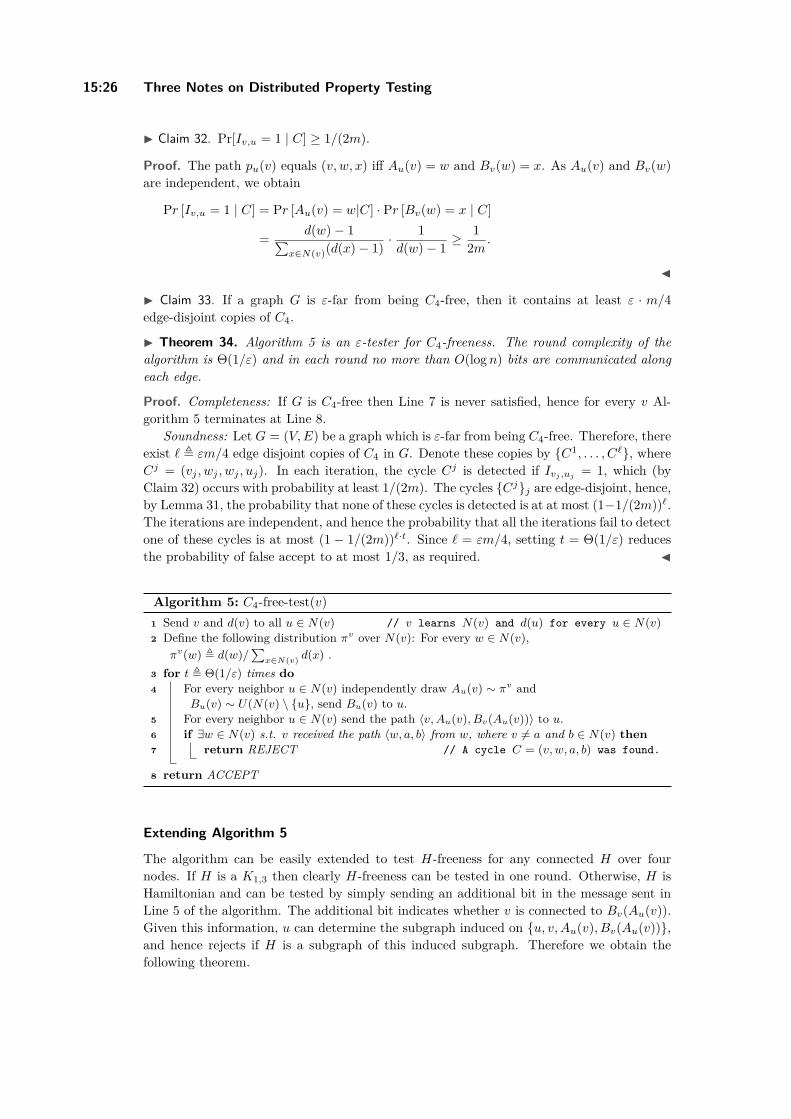
I Theorem 34. Algorithm 5 is an ε-tester for C4-freeness. The round complexity of thealgorithm is Θ(1/ε) and in each round no more than O(logn) bits are communicated alongeach edge.

Proof. Completeness: If G is C4-free then Line 7 is never satisfied, hence for every v Al-gorithm 5 terminates at Line 8.

Soundness: Let G = (V,E) be a graph which is ε-far from being C4-free. Therefore, thereexist ` , εm/4 edge disjoint copies of C4 in G. Denote these copies by C1, . . . , C`, whereCj = (vj , wj , wj , uj). In each iteration, the cycle Cj is detected if Ivj ,uj

= 1, which (byClaim 32) occurs with probability at least 1/(2m). The cycles Cjj are edge-disjoint, hence,by Lemma 31, the probability that none of these cycles is detected is at at most (1−1/(2m))`.The iterations are independent, and hence the probability that all the iterations fail to detectone of these cycles is at most (1 − 1/(2m))`·t. Since ` = εm/4, setting t = Θ(1/ε) reducesthe probability of false accept to at most 1/3, as required. J

Algorithm 5: C4-free-test(v)1 Send v and d(v) to all u ∈ N(v) // v learns N(v) and d(u) for every u ∈ N(v)2 Define the following distribution πv over N(v): For every w ∈ N(v),

πv(w) , d(w)/∑

x∈N(v) d(x) .3 for t , Θ(1/ε) times do4 For every neighbor u ∈ N(v) independently draw Au(v) ∼ πv and

Bu(v) ∼ U(N(v) \ u, send Bu(v) to u.5 For every neighbor u ∈ N(v) send the path 〈v,Au(v), Bv(Au(v))〉 to u.6 if ∃w ∈ N(v) s.t. v received the path 〈w, a, b〉 from w, where v 6= a and b ∈ N(v) then7 return REJECT // A cycle C = (v, w, a, b) was found.

8 return ACCEPT

Extending Algorithm 5

The algorithm can be easily extended to test H-freeness for any connected H over fournodes. If H is a K1,3 then clearly H-freeness can be tested in one round. Otherwise, H isHamiltonian and can be tested by simply sending an additional bit in the message sent inLine 5 of the algorithm. The additional bit indicates whether v is connected to Bv(Au(v)).Given this information, u can determine the subgraph induced on u, v,Au(v), Bv(Au(v)),and hence rejects if H is a subgraph of this induced subgraph. Therefore we obtain thefollowing theorem.

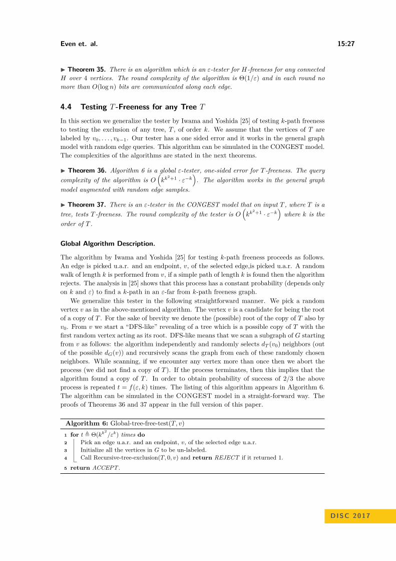
Even et. al. 15:27

I Theorem 35. There is an algorithm which is an ε-tester for H-freeness for any connectedH over 4 vertices. The round complexity of the algorithm is Θ(1/ε) and in each round nomore than O(logn) bits are communicated along each edge.

4.4 Testing T -Freeness for any Tree T

In this section we generalize the tester by Iwama and Yoshida [25] of testing k-path freenessto testing the exclusion of any tree, T , of order k. We assume that the vertices of T arelabeled by v0, . . . , vk−1. Our tester has a one sided error and it works in the general graphmodel with random edge queries. This algorithm can be simulated in the CONGEST model.The complexities of the algorithms are stated in the next theorems.

I Theorem 36. Algorithm 6 is a global ε-tester, one-sided error for T -freeness. The querycomplexity of the algorithm is O

(kk

2+1 · ε−k). The algorithm works in the general graph

model augmented with random edge samples.

I Theorem 37. There is an ε-tester in the CONGEST model that on input T , where T is atree, tests T -freeness. The round complexity of the tester is O

(kk

2+1 · ε−k)where k is the

order of T .

Global Algorithm Description.

The algorithm by Iwama and Yoshida [25] for testing k-path freeness proceeds as follows.An edge is picked u.a.r. and an endpoint, v, of the selected edge,is picked u.a.r. A randomwalk of length k is performed from v, if a simple path of length k is found then the algorithmrejects. The analysis in [25] shows that this process has a constant probability (depends onlyon k and ε) to find a k-path in an ε-far from k-path freeness graph.

We generalize this tester in the following straightforward manner. We pick a randomvertex v as in the above-mentioned algorithm. The vertex v is a candidate for being the rootof a copy of T . For the sake of brevity we denote the (possible) root of the copy of T also byv0. From v we start a “DFS-like” revealing of a tree which is a possible copy of T with thefirst random vertex acting as its root. DFS-like means that we scan a subgraph of G startingfrom v as follows: the algorithm independently and randomly selects dT (v0) neighbors (outof the possible dG(v)) and recursively scans the graph from each of these randomly chosenneighbors. While scanning, if we encounter any vertex more than once then we abort theprocess (we did not find a copy of T ). If the process terminates, then this implies that thealgorithm found a copy of T . In order to obtain probability of success of 2/3 the aboveprocess is repeated t = f(ε, k) times. The listing of this algorithm appears in Algorithm 6.The algorithm can be simulated in the CONGEST model in a straight-forward way. Theproofs of Theorems 36 and 37 appear in the full version of this paper.

Algorithm 6: Global-tree-free-test(T, v)1 for t , Θ(kk2

/εk) times do2 Pick an edge u.a.r. and an endpoint, v, of the selected edge u.a.r.3 Initialize all the vertices in G to be un-labeled.4 Call Recursive-tree-exclusion(T, 0, v) and return REJECT if it returned 1.5 return ACCEPT .

DISC 2017

15:28 Three Notes on Distributed Property Testing

Procedure Recursive-tree-exclusion(T, i, v)1 If v was already labeled then return 0, otherwise, label v by i. // The recursion

returns 0 if the revealed labeled subgraph is not T.2 Define ` = dT (vi)− 1 if i > 0 and ` = dT (vi) otherwise.3 Let vi1 , . . . , vi` denote the labels of the children of vi in T (in which v0 is the root).4 Pick u.a.r. ` vertices u1, . . . , u` from NG(v) and recursively call

Recursive-tree-exclusion(T, ij , uj) for each j ∈ [`]5 If one of the calls returned 0, then return 0, otherwise return 1.

References1 Amir Abboud, Keren Censor-Hillel, and Seri Khoury. Near-linear lower bounds for distrib-

uted distance computations, even in sparse networks. In 30th International Symposium inDistributed Computing (DISC), pages 29–42, 2016.

2 Noga Alon, Sonny Ben-Shimon, and Michael Krivelevich. A note on regular ramsey graphs.Journal of Graph Theory, 64(3):244–249, 2010.

3 Noga Alon, Eldar Fischer, Michael Krivelevich, and Mario Szegedy. Efficient testing oflarge graphs. Combinatorica, 20(4):451–476, 2000.

4 Noga Alon, Raphael Yuster, and Uri Zwick. Color-coding. J. ACM, 42(4):844–856, 1995.5 Noga Alon, Raphael Yuster, and Uri Zwick. Finding and counting given length cycles.

Algorithmica, 17(3):209–223, 1997.6 Baruch Awerbuch, Bonnie Berger, Lenore Cowen, and David Peleg. Low-diameter graph

decomposition is in nc. In Scandinavian Workshop on Algorithm Theory, pages 83–93.Springer, 1992.

7 Guy E Blelloch, Anupam Gupta, Ioannis Koutis, Gary L Miller, Richard Peng, and KanatTangwongsan. Nearly-linear work parallel sdd solvers, low-diameter decomposition, andlow-stretch subgraphs. Theory of Computing Systems, 55(3):521–554, 2014.

8 Luciana Buriol, Gereon Frahling, Stefano Leonardi, Alberto Marchetti-Spaccamela, andChristian Sohler. Counting triangles in data streams. In 25th ACM Symposium on Prin-ciples of Database Systems (PODS), pages 253–262, 2006.

9 Keren Censor-Hillel, Eldar Fischer, Gregory Schwartzman, and Yadu Vasudev. Fast dis-tributed algorithms for testing graph properties. In 30th Int. Symposium on DistributedComputing (DISC), volume 9888 of LNCS, pages 43–56. Springer, 2016.

10 Keren Censor-Hillel, Petteri Kaski, Janne H. Korhonen, Christoph Lenzen, Ami Paz, andJukka Suomela. Algebraic methods in the congested clique. In ACM Symposium on Prin-ciples of Distributed Computing (PODC), pages 143–152, 2015.

11 Atish Das Sarma, Stephan Holzer, Liah Kor, Amos Korman, Danupon Nanongkai, GopalPandurangan, David Peleg, and Roger Wattenhofer. Distributed verification and hardnessof distributed approximation. In 43rd ACM Symposium on Theory of Computing (STOC),pages 363–372, 2011.

12 Danny Dolev, Christoph Lenzen, and Shir Peled. Tri, tri again: Finding triangles andsmall subgraphs in a distributed setting. In 26th International Symposium on DistributedComputing, pages 195–209, 2012.

13 Andrew Drucker, Fabian Kuhn, and Rotem Oshman. On the power of the congested cliquemodel. In ACM Symposium on Principles of Distributed Computing (PODC), pages 367–376, 2014.

14 Michael Elkin and Ofer Neiman. Efficient algorithms for constructing very sparse spannersand emulators. In Proceedings of the Twenty-Eighth Annual ACM-SIAM Symposium onDiscrete Algorithms, pages 652–669. SIAM, 2017.

Even et. al. 15:29

15 Paul Erdős, András Hajnal, and J. W. Moon. A problem in graph theory. The AmericanMathematical Monthly, 71(10):1107–1110, 1964.

16 Guy Even, Reut Levi, and Moti Medina. Faster and simpler distributed algorithms fortesting and correcting graph properties in the congest-model. CoRR, abs/1705.04898, 2017.URL: http://arxiv.org/abs/1705.04898.

17 Orr Fischer, Tzlil Gonen, and Rotem Oshman. Distributed property testing for subgraph-freeness revisited. CoRR, abs/1705.04033, 2017. URL: http://arxiv.org/abs/1705.04033.

18 Pierre Fraigniaud, Pedro Montealegre, Dennis Olivetti, Ivan Rapaport, and Ioan Todinca.Distributed subgraph detection. CoRR, abs/1706.03996, 2017. URL: http://arxiv.org/abs/1706.03996.

19 Pierre Fraigniaud and Dennis Olivetti. Distributed detection of cycles. In 29th ACM onSymposium on Parallelism in Algorithms and Architectures (SPAA), 2017.

20 Pierre Fraigniaud, Ivan Rapaport, Ville Salo, and Ioan Todinca. Distributed testing ofexcluded subgraphs. In 30th Int. Symposium on Distributed Computing (DISC), volume9888 of LNCS, pages 342–356. Springer, 2016.

21 Silvio Frischknecht, Stephan Holzer, and Roger Wattenhofer. Networks cannot computetheir diameter in sublinear time. In 23rd ACM-SIAM Symposium on Discrete Algorithms(SODA), pages 1150–1162, 2012.

22 Oded Goldreich, Shari Goldwasser, and Dana Ron. Property testing and its connection tolearning and approximation. Journal of the ACM (JACM), 45(4):653–750, 1998.

23 Oded Goldreich and Dana Ron. Property testing in bounded degree graphs. Algorithmica,32(2):302–343, 2002.

24 Stephan Holzer and Roger Wattenhofer. Optimal distributed all pairs shortest paths andapplications. In ACM Symposium on Principles of Distributed Computing (PODC), pages355–364, 2012.

25 Kazuo Iwama and Yuichi Yoshida. Parameterized testability. In Innovations in TheoreticalComputer Science, ITCS’14, Princeton, NJ, USA, January 12-14, 2014, pages 507–516,2014. URL: http://doi.acm.org/10.1145/2554797.2554843, doi:10.1145/2554797.2554843.

26 Taisuke Izumi and François Le Gall. Triangle finding and listing in CONGEST networks.In ACM Symposium on Principles of Distributed Computing (PODC), 2017.

27 Stasys Jukna and Georg Schnitger. Triangle-freeness is hard to detect. Combinatorics,Probability, & Computing, 11(6):549–569, 2002.

28 Shay Kutten and David Peleg. Fast distributed construction of small k-dominating setsand applications. J. Algorithms, 28(1):40–66, 1998.

29 Tom Leighton. Introduction to Parallel Algorithms and Architectures. Morgan Kaufmann,1992.

30 Christoph Lenzen and Boaz Patt-Shamir. Fast partial distance estimation and applications.In ACM Symposium on Principles of Distributed Computing (PODC), pages 153–162, 2015.

31 Gary L Miller, Richard Peng, and Shen Chen Xu. Parallel graph decompositions usingrandom shifts. In Proceedings of the twenty-fifth annual ACM symposium on Parallelismin algorithms and architectures, pages 196–203. ACM, 2013.

32 Burkhard Monien. How to find long paths efficiently. In Analysis and design of algorithmsfor combinatorial problems, volume 109 of North-Holland Math. Stud., pages 239–254.North-Holland, Amsterdam, 1985.

33 Danupon Nanongkai. Distributed approximation algorithms for weighted shortest paths.In ACM Symposium on Theory of Computing (STOC), pages 565–573, 2014.

DISC 2017

15:30 Three Notes on Distributed Property Testing

34 Hiroaki Ookawa and Taisuke Izumi. Filling logarithmic gaps in distributed complexityfor global problems. In 41st International Conference on Current Trends in Theory andPractice of Computer Science (SOFSEM), pages 377–388, 2015.

35 Judea Pearl. Fusion, propagation, and structuring in belief networks. Artif. Intell.,29(3):241–288, 1986.

36 David Peleg. Distributed Computing: A Locality-Sensitive Approach. SIAM, 2000.