Embed Size (px)
Citation preview

THREE CONTRIBUTIONS IN REPRESENTATION THEORY:
(1) CLUSTER ALGEBRAS AND GRASSMANNIANS OF TYPE G2
(2) YANGIANS AND QUANTUM LOOP ALGEBRAS
(3) MONODROMY OF THE TRIGONOMETRIC CASIMIR CONNECTION OF sl2
A dissertation presented
by
Sachin Gautam
to
The Department of Mathematics
In partial fulfillment of the requirements for the degree of
Doctor of Philosophy
in the field of
Mathematics
Northeastern University
Boston, Massachusetts
June 2011
1

UMI Number: 3460116
All rights reserved
INFORMATION TO ALL USERS The quality of this reproduction is dependent upon the quality of the copy submitted.
In the unlikely event that the author did not send a complete manuscript
and there are missing pages, these will be noted. Also, if material had to be removed, a note will indicate the deletion.
UMI 3460116
Copyright 2011 by ProQuest LLC. All rights reserved. This edition of the work is protected against
unauthorized copying under Title 17, United States Code.
ProQuest LLC 789 East Eisenhower Parkway
P.O. Box 1346 Ann Arbor, MI 48106-1346
2
THREE CONTRIBUTIONS IN REPRESENTATION THEORY:
(1) CLUSTER ALGEBRAS AND GRASSMANNIANS OF TYPE G2
(2) YANGIANS AND QUANTUM LOOP ALGEBRAS
(3) MONODROMY OF THE TRIGONOMETRIC CASIMIR CONNECTION OF sl2
by
Sachin Gautam
Abstract of Dissertation
Submitted in partial fulfillment of the requirements
for the degree of Doctor of Philosophy in the field of Mathematics
in the Graduate School of Arts and Sciences of
Northeastern University, June 2011
ABSTRACT OF DISSERTATION 3
Abstract
The aim of the current dissertation is to address certain problems in the representation theory
of simple Lie algebras and associated quantum algebras.
In Part I, we study the simple Lie group of type G2 from the cluster point of view. We prove a
conjecture of Geiss, Leclerc and Schroer [25], relating the geometry of the partial flag varieties to
cluster algebras in the case of G2.
In Part II, we establish a concrete relationship between certain infinite dimensional quantum
groups, namely the quantum loop algebra U�(Lg) and the Yangian Y�(g), associated with a simple
Lie algebra g. The main result of this part gives a construction of an explicit isomorphism between
completions of these algebras, thus strengthening the well known Drinfeld’s degeneration homo-
morphism [10, 27].
In Part III, we give a proof of the monodromy conjecture of Toledano Laredo [50] for the case
of g = sl2. The monodromy conjecture relates two classes of representations of the affine braid
group, the first arising from the quantum Weyl group operators of the quantum loop algebra and
the second coming from the monodromy of the trigonometric Casimir connection, a flat connection
introduced by Toledano Laredo [50].

Acknowledgments
There are a number of people to whom I wish to express my deepest gratitude.
To Prof. Andrei Zelevinsky, for introducing me to the theory of cluster algebras and for innu-
merable helpful and stimulating discussions.
To Prof. Valerio Toledano Laredo, for teaching me the monodromy side of quantum groups,
for your constant availability and for having great patience with me during all our joint projects.
To my teachers at Northeastern University, Profs. Marc Levine, Venkatraman Laskhmibai,
Mikhail Shubin, Jerzy Weyman, Peter Topalov, Maxim Braverman, Jonathan Weitsman, Gordana
Todorov, Alexander Martsinkovsky, for offering several excellent courses over the years.
To my friends and colleagues Oleksandr Foksha, David Jordan, Martina Balagovic, Jeremy
Russell, Andrea Appel, Salvatore Stella, Nate Bade, Gufang Zhao and Yaping Yang, for all your
awe–inspiring talks in our reading courses and making the learning experience the most enjoyable
one.
And finally I would like to thank my parents and my brother to whom I dedicate this thesis.
4
Contents
Abstract 2
Acknowledgments 4
Table of Contents 5
Chapter 1. Introduction 8
1.1. Cluster algebras and partial flag varieties 8
1.2. Monodromy theorems in the trigonometric setting: context 11
1.3. Monodromy theorems in the trigonometric setting – results 13
1.4. Monodromy of the trigonometric Casimir connection of sl2 17
1.5. Outline of the dissertation 19
Part 1. Cluster algebras and Grassmannians of type G2 23
Chapter 2. Cluster algebras and based affine spaces 24
2.1. Cluster algebras of geometric type 24
2.2. Double Bruhat cell Ge,w0 and based affine space 27
2.3. Initial seeds for Ge,w0 30
Chapter 3. Grassmannians of type G2 33
3.1. Recollections from the representation theory of G2 33
3.2. GLS conjecture 37
3.3. Alternate construction 39
3.4. Equivalence of the two constructions 40
Chapter 4. A proof of the GLS conjecture 43
4.1. Explanation of the choice of initial seeds 43
4.2. Proof for i = 1 case 44
4.3. Proof for i = 2 case 46
5
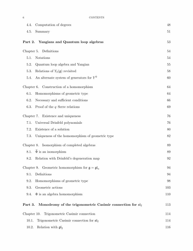
6 CONTENTS
4.4. Computation of degrees 48
4.5. Summary 51
Part 2. Yangians and Quantum loop algebras 53
Chapter 5. Definitions 54
5.1. Notations 54
5.2. Quantum loop algebra and Yangian 55
5.3. Relations of Y�(g) revisited 58
5.4. An alternate system of generators for Y 0 60
Chapter 6. Construction of a homomorphism 64
6.1. Homomorphisms of geometric type 64
6.2. Necessary and sufficient conditions 66
6.3. Proof of the q–Serre relations 69
Chapter 7. Existence and uniqueness 76
7.1. Universal Drinfeld polynomials 76
7.2. Existence of a solution 80
7.3. Uniqueness of the homomorphism of geometric type 82
Chapter 8. Isomorphism of completed algebras 89
8.1. Φ is an isomorphism 89
8.2. Relation with Drinfeld’s degeneration map 92
Chapter 9. Geometric homomorphism for g = gln 94
9.1. Definitions 94
9.2. Homomorphisms of geometric type 98
9.3. Geometric actions 103
9.4. Φ is an algebra homomorphism 110
Part 3. Monodromy of the trigonometric Casimir connection for sl2 113
Chapter 10. Trigonometric Casimir connection 114
10.1. Trigonometric Casimir connection for sl2 114
10.2. Relation with gl2 116

CONTENTS 7
Chapter 11. Dual pair (glk, gln) 123
11.1. Dual pair (glk, gl2) and the trigonometric KZ equations 123
11.2. Monodromy of the trigonometric KZ connection 126
11.3. The dual pair (U�glk, U�gln) 128
11.4. Proof of Etingof–Geer–Schiffmann theorem 131
Chapter 12. Quantum Weyl group 137
12.1. Quantum loop algebra U�(Lgl2) 137
12.2. Quantum Weyl groups 144
Chapter 13. Equivalence of representations 153
13.1. Statement of the main theorem 153
13.2. Proof of the equivalence 155
Bibliography 161
CHAPTER 1
Introduction
My doctoral work consists of two parts described in more detail in Sections 1.1 and 1.2–1.4
respectively. The first project lies in the realm of cluster algebras and was carried out under the
supervision of Prof. A. Zelevinsky. It resulted in the publication of [22], where the simple Lie
group of type G2 is studied from the cluster point of view. The main results obtained in [22] prove
a conjecture of Geiss, Leclerc and Schroer, relating the geometry of partial flag varieties to cluster
algebras in the case of G2.
The second project revolves around a principle which first appeared in the work of T. Kohno
and V. G. Drinfeld and states, roughly speaking, that quantum groups are natural receptacles for
the monodromy representations of certain flat connections of Fuchsian type [12], [31]. It stems
more specifically from the monodromic interpretation of quantum Weyl groups obtained by V.
Toledano Laredo in [47, 48, 49]. Our main goal is to extend these results to the affine setting.
Our results link two distinct appearances of affine braid groups in the representation theory
of quantum affine algebras and Yangians. They are aimed at relating the quantum Weyl group
operators coming from the quantum affine algebra and the monodromy of the trigonometric Casimir
connection, a flat connection introduced by Toledano Laredo in [50].
1.1. Cluster algebras and partial flag varieties
1.1.1. Context and statement of the problem. The theory of cluster algebras was founded
and developed by S. Fomin and A. Zelevinsky in a series of publications [1, 19, 20, 21], in order to
construct a combinatorial framework for dual canonical bases. Ever since their appearance in [19],
cluster algebras have found their place in several areas of mathematics: Poisson geometry, tropical
geometry and quiver representations to name a few.
8
1.1. CLUSTER ALGEBRAS AND PARTIAL FLAG VARIETIES 9
The link between the theory of cluster algebras and representation theory of simple Lie groups
was made in [1]. Let G be a simple algebraic group over C, B± ⊂ G a pair of opposite Borel
subgroups and let N± be the unipotent radicals of B±. Let I be the vertex set of the Dynkin
diagram of G. The following facts are well known in the representation theory of simple Lie groups:
(1) There is a free abelian group of rank |I|, denoted by P = ⊕i∈IZωi (the weight lattice)
such that finite–dimensional irreducible representations of G are parametrized by the pos-
itive cone P+ :=∑
Nωi ⊂ P (the set of dominant weights). We denote the irreducible
representation corresponding to λ ∈ P+ by Vλ.
(2) Let A be the algebra of N− invariant functions on G. Then, as G–modules
A ∼=⊕λ∈P+
Vλ
The study of A is therefore central in order to uniformly construct a nice basis for all finite–
dimensional irreducible representations of G.
1.1.2. A cluster algebra is an algebra A equipped with (a) a distinguished set of algebraically
independent elements which generate the field of fractions of A (called initial cluster) and (b) a
skew–symmetrizable integer matrix (called exchange matrix). The data of an initial cluster and
exchange matrix is called an initial seed. Central to the theory of cluster algebras is an algorithmic
procedure, called Fomin–Zelevinsky mutation, which produces new seeds starting from the initial
one. An algebra A together with a choice of initial seed is said to be a cluster algebra if A is
generated by elements of clusters obtained from the initial one by successive mutations. The pre-
cise definition of a cluster algebra is recalled in §2.1. Once a given algebra A is known to admit a
cluster structure, the process of mutation produces a nice basis of A. Thus, one way to understand
the irreducible finite–dimensional representations of G is to produce a cluster algebra structure on
A = C[G]N−.
A solution to this problem was proposed in [1], where the authors give an explicit construction
of an initial seed for A and conjecture that A equipped with this data is a cluster algebra. A slightly
weaker form of this conjecture was also proved in [1], establishing that A is an upper cluster algebra.
We review this construction in §2.3.
10 1. INTRODUCTION
1.1.3. More generally let J ⊂ I be a subset and set K = I \J . Define P+J =
∑j∈J Nωj ⊂ P+
and let AJ ⊂ A be the subalgebra given by
AJ =⊕λ∈P+
J
Vλ
In geometric terms, AJ is the homogeneous coordinate ring of partial flag variety defined as B−K\G,where B−K ⊃ B− is the standard parabolic subgroup.
Generalizing the results of [1], C. Geiss, B. Leclerc and J. Schroer gave a conjectural cluster
algebra structure on AJ [25]. They also confirm their conjecture (GLS conjecture) for a few special
cases using the theory of preprojective algebras. We recall the construction of [25] for the case at
hand in §3.2. The following points are worth mentioning about [25].(1) When J = I, the cluster structure on AJ = A given in [25] (GLS structure) is not the
same as the one given in [1] (BFZ structure). A priori, it is not even clear that the two
are isomorphic.
(2) It is not clear whether the GLS structures on AJ and AJ ′ are compatible if J ⊂ J ′. More
precisely, it is not known that the inclusion AJ ⊂ AJ ′ is an inclusion of cluster algebras.
(3) The methods of [25] rely heavily upon the use of preprojective algebras and hence are
constrained to the simply-laced cases.
1.1.4. Results obtained. The first part of this dissertation is aimed at proving the GLS
conjecture for the G2 case. In particular we study the connection between the representation
theory of the simple, simply–connected Lie group of type G2 and the cluster algebra structures on
the double Bruhat cells.
There are two main difficulties in proving that the coordinate ring of a given space X is a cluster
algebra. Assuming one has a candidate for an initial seed, say Σ = (x, B), and an assignment
xi �→ fi ∈ C[X], it will remain to prove the following two statements:
(a) Every sequence of mutations produces a regular function on X, since the process of mu-
tations, a priori, produces only rational functions on X.
(b) Every regular function on X can be expressed as a polynomial in the cluster variables.
The main steps of our proof of the GLS conjecture can be outlined as follows.
(1) We begin with the BFZ construction and get an alternate construction of the initial seeds
forAi. The result of this step is produced in §3.3 and its relation with the BFZ construction
1.2. MONODROMY THEOREMS IN THE TRIGONOMETRIC SETTING: CONTEXT 11
is given in §4.1. The essential point of this alternate construction is that it allows us touse the results of [1] to prove part (a) of the desired statement.
(2) We prove that our alternate construction is mutation equivalent to the GLS construction
in §3.4. Thus reducing the GLS conjecture to a similar assertion about our initial seed.(3) Finally part (b) is proved by exhibiting explicitly that all the weight vectors of the funda-
mental representations can be obtained via the process of mutation. This step is carried
out in §4.2–§4.3.
Remark. The method of obtaining a cluster structure on AJ using the one on A and elementary
operations, as mentioned in (1) above, can be used for other types as well. One advantage over
the GLS construction is that the restriction of G being simply–laced is lifted. Also the inclusion
AJ ⊂ AJ ′ (for J ⊂ J ′ ⊂ I) is a priori an inclusion of cluster algebras. However, a uniform
description of this method is not completely worked out at present.
1.2. Monodromy theorems in the trigonometric setting: context
1.2.1. The KZ connection. Around 1990, T. Kohno and V. G. Drinfeld [12], [31] proved
a rather astonishing result, now known as the Kohno-Drinfeld Theorem. Roughly speaking, the
theorem states that quantum groups can be used to describe monodromy of certain first order
Fuchsian PDE’s known as Knizhnik-Zamolodchikov (KZ) equations. To be more precise, given a
simple Lie algebra g, a representation V of g and a positive integer n, the KZ equations are the
following system of PDE’s:
∂Φ
∂zi= �
∑j �=i
Ωij
zi − zjΦ
where
(1) Φ is a function on the configuration space
Xn := {(z1, · · · , zn) ∈ Cn : zi = zj}
with values in V ⊗n,
(2) Ω ∈ g⊗ g is the Casimir tensor and
(3) � is a complex deformation parameter.
12 1. INTRODUCTION
This system is integrable and invariant under the natural Sn action and hence defines a one
parameter family of monodromy representations of Artin’s braid group Bn = π1(Xn/Sn). The
Kohno-Drinfeld theorem asserts that this representation is equivalent to the R-matrix representa-
tion of Bn on V⊗n arising from the quantum group U�g. Here V is a quantum deformation of V ,
that is a U�g–module such that V/�V ∼= V .
1.2.2. The rational Casimir connection. In subsequent years, J. Millson and V. Toledano
Laredo [36], [48] and independently C. De Concini constructed another flat connection ∇C , now
known as the Casimir connection of a simple Lie algebra g which is described as follows. Let
h be a Cartan subalgebra of g and let hreg be the complement of the root hyperplanes in h.
For a finite-dimensional g module V , ∇C is the following connection on the trivial vector bundle
hreg × V → hreg:
∇C = d− �∑α>0
dα
αCα
where
(1) the summation is over a set of chosen positive system of roots relative to pair (g, h),
(2) Cα is the Casimir operator of the sl2–subalgebra of g corresponding to the root α
This connection gives rise to a one parameter family of mondromy representations of the generalized
braid group
Bg = π1(hreg/W )
If V is a U�g module such that V/�V ∼= V , the quantum Weyl group operators Ti ∈ U�g (defined
by G. Lusztig, A. Kirillov, N. Reshetikhin and Y. Soibelman, [30, 34, 43]) define a representation
of Bg on V. In this setting a Kohno-Drinfeld type theorem was obtained by V. Toledano Laredo,
stating the equivalence of above two representations of Bg ([47, 48, 49]).
1.2.3. The trigonometric Casimir connection. V. Toledano Laredo recently constructed
a trigonometric extension of ∇C [50]. This trigonometric Casimir connection ∇C lives on the
trivial vector bundle Hreg × V where Hreg is the set of regular elements of a maximal torus in the
simply connected Lie group G with Lie algebra g. In this setting the ‘correct’ V turns out to be a
finite-dimensional representation of the Yangian Y�(g) and ∇C has the form:

1.3. MONODROMY THEOREMS IN THE TRIGONOMETRIC SETTING – RESULTS 13
∇C = d− �∑α>0
dα
eα − 1Cα −
∑i
duiτi
where
(1) {ui} is a basis of h∗,(2) dui are the corresponding translation invariant 1-forms on H and
(3) τ i are certain elements of Y�(g)
The connection ∇C is flat and W -equivariant and its monodromy yields a one parameter family of
monodromy representations of the affine braid group
Bg = π1(Hreg/W )
1.2.4. The monodromy conjecture. By analogy with [47, 48, 49], Toledano Laredo conjec-
tured that these monodromy representations are equivalent to the affine braid group representations
arising from the quantum Weyl group operators of the quantum loop algebra U�Lg [50]. We shall
refer to this conjecture as the monodromy conjecture. Its study and solution are the main objective
of the later part of this dissertation.
Problem 1 (Monodromy Conjecture). Let V be a finite–dimensional module over the Yangian
Y�(g). Prove that the action of the affine braid group Bg on V arising from the monodromy of the
trigonometric Casimir connection is equivalent to the one obtained from the quantum Weyl group
operators on the corresponding representation of the quantum loop algebra U�Lg.
1.3. Monodromy theorems in the trigonometric setting – results
1.3.1. Foundational aspects. One significant difficulty in addressing Problem 1, which is ab-
sent in the rational setting, is understanding the precise relationship between the finite–dimensional
representations of Y�g and U�Lg. These two algebras are closely related, and generally believed to
share the same representation theory in view of the following list of known results:
(1) The algebra U�Lg (resp. Y�g) gives rise to trigonometric (resp. rational) solutions to the
quantum Yang Baxter equation (QYBE) [6], [9]. These rational solutions can be obtained
by degenerating the trigonometric ones.
(2) Strenghtening (1), the Yangian Y�g itself is a degeneration of the quantum loop algebra
U�Lg [10, 27].
14 1. INTRODUCTION
(3) The irreducible, finite-dimensional representations of the quantum loop algebra are classi-
fied by an r-tuple of polynomials Pi(u) satisfying Pi(0) = 1, called the Drinfeld polynomials
[5]. Similarly, the finite-dimensional irreducible representations of the Yangian are clas-
sified by an r-tuple of monic polynomials Qi(u), again called the Drinfeld polynomials
[4].
(4) Both algebras admit similar geometric realizations. Specifically, for a simply–laced Dynkin
graph Γ = (I, E), and for every w ∈ NI , Nakajima constructed a Steinberg–type variety
Z(w) which admits an action of GL(w) × C× [38]. Nakajima [39] and Varagnolo [53]
proved respectively the existence of algebra homomorphisms:
ΨU : U�(Lg)→ KGL(w)×C×(Z(w)) (1.3.1)
ΨY : Y�(g) → HGL(w)×C×(Z(w)) (1.3.2)
Similar algebra homomorphisms were constructed earlier for g = gln by V. Ginzburg and
E. Vasserot in [26, 54].
1.3.2. Algebra homomorphisms. Despite the above mentioned results, no natural (i.e.,
functorial) relationship is known between the finite–dimensional representation categories of the
quantum loop algebra and the Yangian.
Part 2 of this thesis is aimed at constructing an algebra homomorphism
Φ : U�(Lg) −→ Y�(g)
where Y�(g) is the completion of Y�(g) with respect to its N–grading. The results of this part were
obtained in a joint work with V. Toledano Laredo in [23].
In more detail, recall that U�(Lg) and Y�(g) are deformations of the enveloping algebras
U(g[z, z−1]) and U(g[s]) respectively, and denote by
U�(Lh), U�(Lb±) ⊂ U�(Lg) and Y�(h), Y�(b±) ⊂ Y�(g)
the subalgebras deforming U(h[z, z−1]), U(b±[z, z−1]) and U(h[s]), U(b±[s]) respectively, where
h ⊂ g is the Lie algebra of H and b± ⊂ g are the opposite Borel subalgebras corresponding to a
choice {αi}i∈I of simple roots of g. For any αi, let sli2 ⊂ g be the corresponding 3–dimensional
1.3. MONODROMY THEOREMS IN THE TRIGONOMETRIC SETTING – RESULTS 15
subalgebra and denote by
U�(Lsli2) ⊂ U�(Lg) and Y�(sl
i2) ⊂ Y�(g)
the subalgebras which deform U(sli2[z, z−1]) and U(sli2[s]) respectively. Then the main results of
Part 2 can be summarized as:
Theorem. There exists an explicit algebra homomorphism Φ : U�(Lg)→ Y�(g) with the following
properties
(1) Φ is defined over Q[[�]].
(2) Φ induces an isomorphism U�(Lg)∼→ Y�(g) where U�(Lg) is the completion of U�(Lg) with
respect to the ideal of z = 1.
(3) Φ induces Drinfeld’s degeneration of U�(Lg) to Y�(g).
(4) Φ restricts to a homomorphism U�(Lh)→ Y�(h). Moreover, it induces the exponentiation
of roots on Drinfeld polynomials for Y�(g) and U�(Lg).
(5) Φ restricts to a homomorphism U�(Lb±)→ Y�(b±).
(6) Φ restricts to a homomorphism U�(Lsli2)→ Y�(sl
i2) for any i ∈ I.
1.3.3. Our homomorphism Φ has a simple form described as follows. Let {Ei,r, Fi,r, Hi,r}i∈I,r∈Zbe the loop generators of U�(Lg) and {x±i,r, ξi,r}i∈I,r∈N those of Y�(g) (see [11] and Section 5.2 for
definitions). Then,
Φ(Hi,r) =�
qi − q−1i
∑k≥0
ti,krk
k!
Φ(Ei,r) = erσ+i
∑m≥0
g+i,m x+i,m
Φ(Fi,r) = erσ−i
∑m≥0
g−i,m x−i,m
In the formulae above, q = e�/2 and qi = qdi , where the di are the symmetrising integers for
the Cartan matrix of g. The {ti,r}i∈I,r∈N are an alternative set of generators of the commutative
subalgebra Y�(h) ⊂ Y�(g) generated by the elements {ξi,r}i∈I,r∈N which are defined in [32] by
equating the coefficients of u in
�∑r≥0
ti,ru−r−1 = log(1 + �
∑r≥0
ξi,ru−r−1)

16 1. INTRODUCTION
The elements {g±i,m}i∈I,m∈N lie in the completion of Y 0 and are constructed as follows. Consider
the formal power series
G(v) = log
(v
ev/2 − e−v/2
)∈ Q[[v]]
and define γi(v) ∈ Y 0[v] by
γi(v) = �∑r≥0
ti,rr!(−∂v)r+1G(v)
Then, ∑m≥0
g±i,mvm =
(�
qi − q−1i
)1/2
exp
(γi(v)
2
)(1.3.3)
Finally, σ±i are the homomorphisms of the subalgebras Y�(b±) ⊂ Y�(g) generated by {ξj,r, x±j,r}j∈I,r∈Nwhich fix the ξj,r and act on the remaining generators as the shifts x
±j,r → x±j,r+δij
.
1.3.4. We also construct a similar homomorphism for g = gln by relying on the geometric
realisation of U�(Lgln) constructed by V. Ginzburg and E. Vasserot in [26, 54]. More precisely, fix
a positive integer d ∈ N and let F be the variety of n–step flags in Cd,
F = {0 = V0 ⊆ V1 ⊆ · · · ⊆ Vn = Cd}
The cotangent bundle T ∗F may be realised as
T ∗F = {(V•, x) ∈ F × End(Cd)|x(Vi) ⊂ Vi−1}
and therefore admits a morphism T ∗F → N via the second projection, whereN = {x ∈ End(Cd)|xn =0} is the cone of n–step nilpotent endomorphisms. Define the Steinberg variety Z = T ∗F ×N T ∗F .The group GLd × C× acts on T ∗F and Z and there are surjective algebra homomorphisms
ΨU : U�(Lgln)→ KGLd×C×(Z)
ΨY : Y�(gln)→ HGLd×C×(Z)
see [26, 54] for the definition of ΨU .
To understand these more explicitly, one can use the convolution actions of KGLd×C×(Z) on
KGLd×C×(T ∗F) and HGLd×C×
(Z) on HGLd×C×(T ∗F), which are faithful. By using the equivariant
Chern character, we construct an algebra homomorphism
Φ : U�(Lgln)→ Y�(gln)
1.4. MONODROMY OF THE TRIGONOMETRIC CASIMIR CONNECTION OF sl2 17
which intertwines these two actions (see Theorem 9.3.8).
1.4. Monodromy of the trigonometric Casimir connection of sl2
Part 3 of this thesis gives a proof of the monodromy conjecture when g = sl2 and V is a
tensor product of evaluation representations of Yh (sl2). This part is based on a joint work with V.
Toledano Laredo [24].
1.4.1. To state the main result of this part, let V1, . . . , Vk be finite–dimensional sl2–modules,
z1, . . . , zk points in C, and
V (z) = V1(z1)⊗ · · · ⊗ Vk(zk)
the tensor product of the corresponding evaluation representations of the Yangian Yhsl2. Then, the
monodromy of the trigonometric Casimir connection defines an action of the affine braid group Baff
of sl2 on the completion V (z) of V (z) with respect to the h–adic topology.
For any i = 1, . . . , n, let Vi be a quantum deformation of Vi, that is a U�sl2–module such that
Vi/�Vi ∼= Vi. Set ζi = exp(�(za + 12)) and consider the following tensor product of evaluation
representations of the quantum loop algebra U�(Lsl2)
V(ζ) = V1(ζ1)⊗ · · · ⊗ Vn(ζk)
The quantum Weyl group operators S0, S1 of U�(Lsl2) yield a representation of Baff on V(ζ) [30,34, 43]. Then, the main result of the third part of this dissertation is the following.
Theorem. The monodromy action of the affine braid group Baff on V (z) is equivalent to its quan-
tum Weyl group action on V(ζ).
1.4.2. The proof of the above theorem relies on the duality between the Casimir connection
for sln (here, n = 2) and the KZ connection on n points for a dual slk discovered in [48].
This duality stems from the joint action of (slk, sln) on k × n matrices and was applied in [48]
to describe the monodromy of the rational Casimir connection ∇C for sln in terms of the quantum
Weyl group operators of U�sln in the following way. The duality identifies the monodromy of ∇C
with that of the KZ connection for slk. In turn, the Kohno–Drinfeld theorem describes the latter
in terms of the R–matrix representation of the quantum group U�slk. The computation is then
completed by observing that the R–matrices (i i + 1)Ri i+1, i = 1, . . . , n − 1, acting on a tensor
product of n representations of U�slk coincide with the quantum Weyl group operators S1, . . . , Sn−1

18 1. INTRODUCTION
of the dual U�sln. This coincidence may be regarded as the quantum counterpart of the duality of
the corresponding connections.
1.4.3. We apply a similar strategy in the trigonometric setting.
As in [48], it is more convenient to work with the pair (glk, gln) rather than (slk, sln). The
trigonometric Casimir connection ∇slnC for sln extends to a flat connection ∇gln
C on the maximal
torus T of diagonal matrices of the group GLn(C) which takes values in the Yangian Yhgln [50]. Its
specialisation ∇glnC,z to a tensor product of k evaluation representations coincides with the trigono-
metric dynamical differential equations with coefficients in Ugl⊗kn defined in [46].
The duality between Casimir and KZ connections in the trigonometric setting identifies the
monodromy of ∇glnC,z with that of the trigonometric KZ connection on n points for glk[46]. The
monodromy of this connection was computed by Etingof–Geer by using the Etingof–Kazhdan quan-
tisation functor [15] (see also [17, Appendix 2]). 1 Let Π2 be the fundamental group of Treg/W .
For the case n = 2 this group is presented on three generators {b,X1,X2} subject to the relations
X1X2 = X2X1 and bX1b = X2
Then, the monodromy of ∇gl2C,z is equivalently described by the universal R–matrix of U�glk and by
mapping X1,X2 to two elements X1,X2 ∈ U�gl⊗2k [15].
Given the identification of R–matrices for U�glk with quantum Weyl group elements of U�gln
obtained in [48], this reduces the proof of Theorem 1.4.1 to describing the elements X1,X2 in
terms of quantum Weyl group elements of the dual loop algebra U�(Lgl2). This strategy can be
summarized in the following diagram:
∇glkKZ,z
��Mk,2
����
EG
��
∇gl2C,z��
��(U�gl
⊗2k
)R∨,X1,X2��
M�
k,2
�� S,L1,L2 (U�(Lgl2))
1The proof in [17] had a few inaccuracies (as was pointed out by A. Haviv) and was removed from the
further editions of the book

1.5. OUTLINE OF THE DISSERTATION 19
1.4.4. To the best of our knowledge, the quantum Weyl group operators of U�(Lgl2) corre-
sponding to the lattice subgroup {X1,X2} of Π2 have not been defined. Moreover, even for U�(Lsl2),
no explicit formulas for the element S0S1 which gives the action of the generator of the coroot lattice
of sl2 are known.
Let t ⊂ gl2, h ⊂ sl2 be the Cartan subalgebras of diagonal and traceless diagonal matrices
respectively, and U0 ⊂ U�(Lgl2), U′0 ⊂ U�(Lsl2) the commutative subalgebras deforming U(t[z, z
−1])
and U(h[z, z−1]).
Theorem.
(1) There exist elements L1,L2 in a completion of U0 such that {S = S1,L1,L2} satisfy the
defining relations of the affine braid group Π2 of GL2.
(2) The element L = L2L−11 lies in U ′0 and coincides with the quantum Weyl group element
S0S1 giving the action of the generator of the coroot lattice of sl2.
A direct computation shows that the action of L1,L2 on quantum k×n matrix space coincides
with that of the elements X1,X2. Theorem 1.4.1 follows as a direct consequence.
1.5. Outline of the dissertation
1.5.1. In Chapter 2 we recall the theory of cluster algebras and its connections with the study
of double Bruhat cells, especially the double Bruhat cell Ge,w0 which is closely related to the based
affine spaces. The definition of a cluster algebra of geometric type is recalled in §2.1. We review the
construction of generalized minors in §2.2 and the BFZ construction of initial seeds for the double
Bruhat cell Ge,w0 in §2.3.
Chapter 3 begins the study of the simple, simply–connected Lie group of type G2. We recall
the basics of the representation theory of this group in §3.1. §3.2 is aimed at stating the GLS
conjecture for G2. As a first step towards the proof of this conjecture, we relate the construction
of [25] to the one given in [22] in §3.3–§3.4.
Finally we finish the proof of the GLS conjecture for G2 in Chapter 4. The proof consists
of relating our construction of initial seeds to the ones provided by the BFZ construction (§4.1)
20 1. INTRODUCTION
and finally obtaining all the weight vectors of the fundamental representations of G via mutations
(§4.2–§4.4).
1.5.2. Chapter 5 is aimed at reviewing the definitions of the quantum loop algebra and the
Yangian associated to a simple Lie algebra g (see §5.2). We introduce the shift operator (§5.3) andan alternate system of generators for Y 0 (§5.4).
We give the main construction of Part 2 in chapter 6. In this chapter we introduce the notion of
a homomorphism of geometric type (§6.1) and provide an important set of necessary and sufficientconditions for an assignment of geometric type to be an algebra homomorphism (§6.2 Theorem6.2.1).
Chapter 7 contains two important results asserting respectively the existence of a homomor-
phism of geometric type and its uniqueness up to conjugation (§7.2–§7.3), namely theorems 7.2.1,7.3.11.
In chapter 8 we prove that a homomorphism of geometric type extends to an isomorphism of
completed algebras (see Theorem 8.1.2). We recall the Drinfeld’s isomorphism between the Yangian
and the associated graded algebra of the quantum loop algebra in §8.2 and prove that the associatedgraded of our homomorphism is inverse to Drinfeld’s map (see Proposition 8.2.2).
Chapter 9 contains similar constructions and results for the case of g = gln. We review the
geometric actions of the quantum loop algebra and the Yangian on equivariant K–theory and
equivariant Borel–Moore homology respectively of the variety of n–step flags in Cd (§9.3). We also
construct an algebra homomorphism which intertwines these actions (see Theorem 9.3.8).
1.5.3. In Chapter 10, we review the definition of the Yangian Yhg and of the trigonometric
Casimir connection for the Lie algebra g = sl2, gl2. §10.2 describes the trigonometric Casimir
connection for g = gl2 and the relationship between its monodromy and that of its sl2 counterpart.
Chapter 11 reviews the fact that, under (glk, gl2)–duality, the trigonometric Casimir connection
for gl2 is identified with the trigonometric KZ connection for glk. In §11.2, we state Etingof andGeer’s result on the computation of the monodromy of the trigonometric KZ connection. A proof
of this theorem is sketched in §11.4.Chapter 12 contains the main constructions of this part of the thesis. In §12.1, we review
the definition of the quantum loop algebras U�(Lgl2) and U�(Lsl2) of the quantum Weyl group
operators S0, S1 of U�(Lsl2). We also compute the action of the lattice element L = S0S1 on the

1.5. OUTLINE OF THE DISSERTATION 21
loop generators of U�(Lsl2). In §12.2 we define elements L1,L2 in an appropriate completion of
the commutative subalgebra of U�(Lgl2) and show that, together with the element S1, they give
rise to a representation of the braid group Π2 on any finite–dimensional (filtered) representation of
U�(Lgl2). We also show that the element L2L−11 coincides with the quantum Weyl group operator
S0S1.
Chapter 13 contains the proof of the equivalence of the monodromy of the trigonometric Casimir
connection and the quantum Weyl group representation of the affine braid group Baff (Theorem
13.1.3).


Part 1
Cluster algebras and Grassmannians of type
G2

CHAPTER 2
Cluster algebras and based affine spaces
In this chapter we review the definition of a cluster algebra (of geometric type). We also recall
an important special case of the construction of [1] which equips the coordinate ring of a double
Bruhat cell with a structure of an upper cluster algebra.
2.1. Cluster algebras of geometric type
2.1.1. Definitions. Let m ≥ n be two non–negative integers and let us fix two indexing sets
I ⊂ I of cardinality n and m respectively. Let F be the field of rational functions in m variables
with rational coefficients: F = Q(ui : i ∈ I).
Definition. [1, 19, 21] A seed Σ =(x, B
)is a pair of
(1) x = (xi : i ∈ I) is an m–tuple of algebraically independent elements from F which
generate F over Q. The collection x is called the extended cluster of the seed Σ. Its
subset x = (xi : i ∈ I) is called the cluster. The elements of x are called the cluster
variables and the elements of x \ x are called the coefficients.
(2) B = (bij) is an m × n matrix with integer entries such that B = (bij)i,j∈I is skew–
symmetrizable. That is, there exist pairwise coprime positive integers di (i ∈ I) such that
dibij = djbji. The matrix B is called the exchange matrix and B is called the principal
part of B.
Given a seed Σ =(x, B
)and k ∈ I we define Σ′ = μk (Σ) =
(x, B′
)another seed obtained from
Σ by mutation in direction k as follows:
(1) B′ = (b′ij) is defined by:
b′ij =
⎧⎨⎩ −bij if i = k or j = k
bij + sign(bik)[bikbkj ]+ otherwise(2.1.1)
24

2.1. CLUSTER ALGEBRAS OF GEOMETRIC TYPE 25
(2) x′ = (x′i : i ∈ I) is defined by:
x′i =
⎧⎪⎨⎪⎩xi if i = k∏m
j=1 x[bjk]+j +
∏mj=1 x
[−bjk]+j
xkif i = k
(2.1.2)
where we use the notation [b]+ = max(b, 0).
It is easy to check that the process of mutation produces another seed and is involutive on the
set of seeds in F : μk(μk(Σ)) = Σ. This allows us to define an equivalence relation on the set of
seeds in F : we say Σ and Σ′ are mutation equivalent, Σ ∼ Σ′, if there exists a sequence (k1, · · · kl)of indices from the set I such that
Σ′ = μkl · · ·μk1 (Σ)
2.1.2. Cluster algebra. Let Σ =(x, B
)be a seed in F . It is clear that the process of
mutation does not change the coefficients, namely the elements of the set {xj : j ∈ I \ I}. Let usfix a ground ring R as an arbitrary subring of the ring of Laurent polynomials in the coefficients
such that R contains the ring of polynomials in the coefficients (over Z):
Z[xj : j ∈ I \ I] ⊂ R ⊂ Z[x±1j : j ∈ I \ I]
Definition. The cluster algebra associated to the initial seed Σ is an R–subalgebra A(Σ) of Fgenerated by all the cluster variables belonging to the seeds Σ′ mutation equivalent to Σ
A(Σ) := R
[ ⋃Σ′∼Σ
x′(cluster of the seed Σ′
)]
One defines an upper cluster algebra A(Σ) as the subring of F consisting of all the functions f ∈ Fsuch that for every Σ′ ∼ Σ, f can be expressed as a Laurent polynomial in the cluster variables of
Σ′ with coefficients from R.
The following result is the well–known Laurent phenomena in the theory of cluster algebras
Theorem. [1, Corollary 1.12] [19, Theorem 3.1] A(Σ) ⊂ A(Σ)
2.1.3. In [1] several sufficient conditions for the inclusion of Theorem 2.1.2 to be an equality
have been obtained. In particular we have the following
Theorem. [1, Theorem 1.18, Corollary 1.19] If B has full rank and is acyclic (i.e, the quiver
encoding the signs of B has no cycles), then the inclusion of Theorem 2.1.2 is an equality.
26 2. CLUSTER ALGEBRAS AND BASED AFFINE SPACES
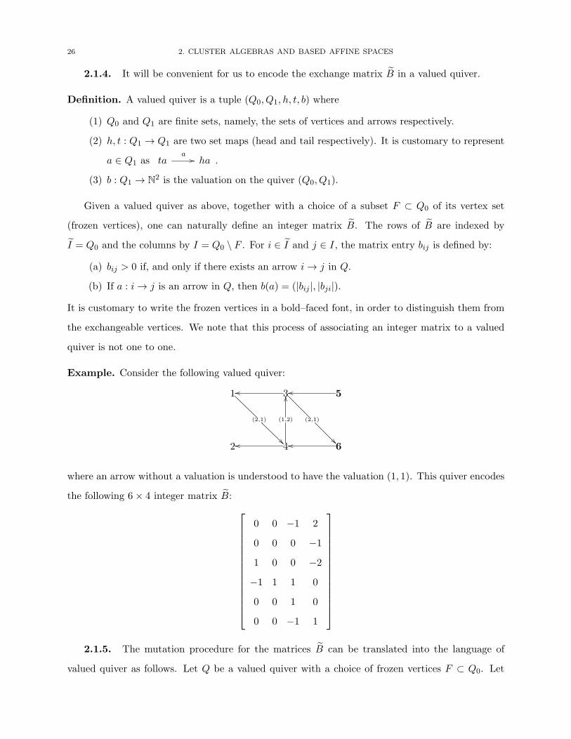
2.1.4. It will be convenient for us to encode the exchange matrix B in a valued quiver.
Definition. A valued quiver is a tuple (Q0, Q1, h, t, b) where
(1) Q0 and Q1 are finite sets, namely, the sets of vertices and arrows respectively.
(2) h, t : Q1 → Q1 are two set maps (head and tail respectively). It is customary to represent
a ∈ Q1 as taa �� ha .
(3) b : Q1 → N2 is the valuation on the quiver (Q0, Q1).
Given a valued quiver as above, together with a choice of a subset F ⊂ Q0 of its vertex set
(frozen vertices), one can naturally define an integer matrix B. The rows of B are indexed by
I = Q0 and the columns by I = Q0 \ F . For i ∈ I and j ∈ I, the matrix entry bij is defined by:
(a) bij > 0 if, and only if there exists an arrow i→ j in Q.
(b) If a : i→ j is an arrow in Q, then b(a) = (|bij |, |bji|).It is customary to write the frozen vertices in a bold–faced font, in order to distinguish them from
the exchangeable vertices. We note that this process of associating an integer matrix to a valued
quiver is not one to one.
Example. Consider the following valued quiver:
2 4 6
1 3 5
�� ��
�� ��
(2,1) (1,2) (2,1)
��
��
��
where an arrow without a valuation is understood to have the valuation (1, 1). This quiver encodes
the following 6× 4 integer matrix B: ⎡⎢⎢⎢⎢⎢⎢⎢⎢⎢⎢⎢⎢⎢⎣
0 0 −1 2
0 0 0 −11 0 0 −2−1 1 1 0
0 0 1 0
0 0 −1 1
⎤⎥⎥⎥⎥⎥⎥⎥⎥⎥⎥⎥⎥⎥⎦2.1.5. The mutation procedure for the matrices B can be translated into the language of
valued quiver as follows. Let Q be a valued quiver with a choice of frozen vertices F ⊂ Q0. Let
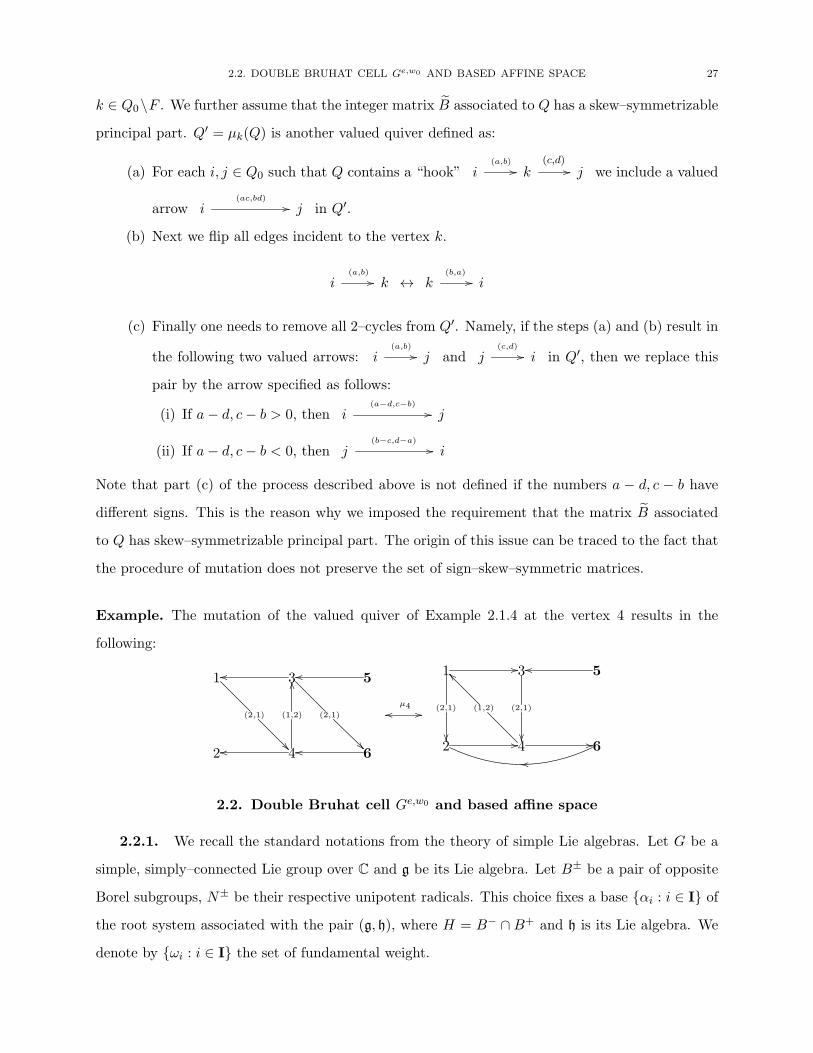
2.2. DOUBLE BRUHAT CELL Ge,w0 AND BASED AFFINE SPACE 27
k ∈ Q0\F . We further assume that the integer matrix B associated to Q has a skew–symmetrizable
principal part. Q′ = μk(Q) is another valued quiver defined as:
(a) For each i, j ∈ Q0 such that Q contains a “hook” i(a,b)
�� k(c,d)
�� j we include a valued
arrow i(ac,bd)
�� j in Q′.
(b) Next we flip all edges incident to the vertex k.
i(a,b)
�� k ↔ k(b,a)
�� i
(c) Finally one needs to remove all 2–cycles from Q′. Namely, if the steps (a) and (b) result in
the following two valued arrows: i(a,b)
�� j and j(c,d)
�� i in Q′, then we replace this
pair by the arrow specified as follows:
(i) If a− d, c− b > 0, then i(a−d,c−b)
�� j
(ii) If a− d, c− b < 0, then j(b−c,d−a)
�� i
Note that part (c) of the process described above is not defined if the numbers a − d, c − b have
different signs. This is the reason why we imposed the requirement that the matrix B associated
to Q has skew–symmetrizable principal part. The origin of this issue can be traced to the fact that
the procedure of mutation does not preserve the set of sign–skew–symmetric matrices.
Example. The mutation of the valued quiver of Example 2.1.4 at the vertex 4 results in the
following:
2 4 6
1 3 5
�� ��
�� ��
(2,1) (1,2) (2,1)
��
��
�� 2 4 6
1 3 5
�� ��
�� ��
��
(2,1) (1,2) (2,1)
��
��
��
��μ4 ��
2.2. Double Bruhat cell Ge,w0 and based affine space
2.2.1. We recall the standard notations from the theory of simple Lie algebras. Let G be a
simple, simply–connected Lie group over C and g be its Lie algebra. Let B± be a pair of opposite
Borel subgroups, N± be their respective unipotent radicals. This choice fixes a base {αi : i ∈ I} ofthe root system associated with the pair (g, h), where H = B− ∩ B+ and h is its Lie algebra. We
denote by {ωi : i ∈ I} the set of fundamental weight.
28 2. CLUSTER ALGEBRAS AND BASED AFFINE SPACES
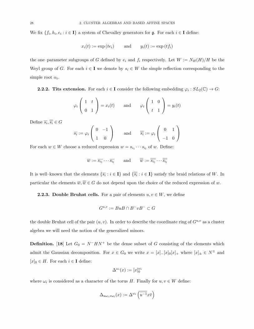
We fix {fi, hi, ei : i ∈ I} a system of Chevalley generators for g. For each i ∈ I define:
xi(t) := exp (tei) and yi(t) := exp (tfi)
the one–parameter subgroups of G defined by ei and fi respectively. Let W := NH(H)/H be the
Weyl group of G. For each i ∈ I we denote by si ∈ W the simple reflection corresponding to the
simple root αi.
2.2.2. Tits extension. For each i ∈ I consider the following embedding ϕi : SL2(C)→ G:
ϕi
⎛⎝ 1 t
0 1
⎞⎠ = xi(t) and ϕi
⎛⎝ 1 0
t 1
⎞⎠ = yi(t)
Define si, si ∈ G
si := ϕi
⎛⎝ 0 −11 0
⎞⎠ and si := ϕi
⎛⎝ 0 1
−1 0
⎞⎠For each w ∈W choose a reduced expression w = si1 · · · sil of w. Define:
w := si1 · · · sil and w := si1 · · · sil
It is well–known that the elements {si : i ∈ I} and {si : i ∈ I} satisfy the braid relations of W . In
particular the elements w,w ∈ G do not depend upon the choice of the reduced expression of w.
2.2.3. Double Bruhat cells. For a pair of elements u, v ∈W , we define
Gu,v := BuB ∩B−vB− ⊂ G
the double Bruhat cell of the pair (u, v). In order to describe the coordinate ring of Gu,v as a cluster
algebra we will need the notion of the generalized minors.
Definition. [18] Let G0 = N−HN+ be the dense subset of G consisting of the elements which
admit the Gaussian decomposition. For x ∈ G0 we write x = [x]−[x]0[x]+ where [x]± ∈ N± and
[x]0 ∈ H. For each i ∈ I define:
Δωi(x) := [x]ωi0
where ωi is considered as a character of the torus H. Finally for u, v ∈W define:
Δuωi,vωi(x) := Δωi
(u−1xv
)

2.2. DOUBLE BRUHAT CELL Ge,w0 AND BASED AFFINE SPACE 29
Proposition. [1, Proposition 2.8] Gu,v is defined as a subset of G satisfying:
Δu′ωi,ωi= 0 whenever u′ωi ≤ uωi
Δωi,v′ωi= 0 whenever v′ωi ≤ v−1ωi
Δuωi,ω0 = 0 and Δωi,v−1ωi= 0
In [1, §2.2] the authors associate to each reduced expression i of (u, v) ∈ W ×W , a seed Σ(i)
in C(Gu,v). We recall the definition of these seeds for the special case of u = e and v = w0 (the
longest element of W ) in §2.3.
2.2.4. Based affine space. Let P = ⊕i∈IZωi be the weight lattice of G and P+ =∑
i∈INωi ⊂P be the set of dominant integral weights. For each λ ∈ P+ let Vλ be the unique finite–dimensional
irreducible representation of G of highest–weight λ. Then as (right) G–modules we have the fol-
lowing isomorphism: ⊕λ∈P+
Vλ∼= C[N−\G] =: A
The homogeneous affine variety N−\G is known as the based affine space of G.
More generally for a subset J ⊂ I we define:
AJ :=⊕λ∈PJ
+
Vλ
where P J+ =
∑j∈JNωj ⊂ P+. Clearly AJ ⊂ A is a subalgebra.
From now onwards we restrict ourselves to the case of Ge,w0 and generalized minors of the form
Δωi,uωi . Consequently, for the sake of notational convenience we will write Δuωi := Δωi,uωi . For
each u ∈ W the function Δuωi is an N−–invariant function on G (see Definition 2.2.3). Moreover
as an element of ⊕λVλ we have:
Δuωi ∈ Vωi [uωi]
where for a finite–dimensional representation V of G, V [μ] denotes the μ weight space of V .
The inclusionGe,w0 ⊂ G composed with the natural projectionG→ N−\G allows us to consider
A = C[N−\G] as a subalgebra of C[Ge,w0 ]. As an application of Proposition 2.2.3 we obtain
30 2. CLUSTER ALGEBRAS AND BASED AFFINE SPACES
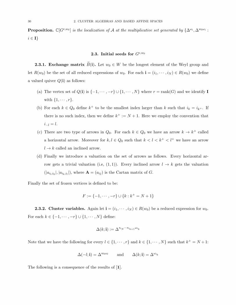
Proposition. C[Ge,w0 ] is the localization of A at the multiplicative set generated by {Δωi ,Δw0ωi :
i ∈ I}
2.3. Initial seeds for Ge,w0
2.3.1. Exchange matrix B(i). Let w0 ∈ W be the longest element of the Weyl group and
let R(w0) be the set of all reduced expressions of w0. For each i = (i1, · · · , iN ) ∈ R(w0) we define
a valued quiver Q(i) as follows:
(a) The vertex set of Q(i) is {−1, · · · ,−r} ∪ {1, · · · , N} where r = rank(G) and we identify I
with {1, · · · , r}.(b) For each k ∈ Q0 define k+ to be the smallest index larger than k such that ik = ik+ . If
there is no such index, then we define k+ := N + 1. Here we employ the convention that
i−l = l.
(c) There are two type of arrows in Q0. For each k ∈ Q0 we have an arrow k → k+ called
a horizontal arrow. Moreover for k, l ∈ Q0 such that k < l < k+ < l+ we have an arrow
l→ k called an inclined arrow.
(d) Finally we introduce a valuation on the set of arrows as follows. Every horizontal ar-
row gets a trivial valuation (i.e, (1, 1)). Every inclined arrow l → k gets the valuation
(|ail,ik |, |aik,il |), where A = (aij) is the Cartan matrix of G.
Finally the set of frozen vertices is defined to be:
F := {−1, · · · ,−r} ∪ {k : k+ = N + 1}
2.3.2. Cluster variables. Again let i = (i1, · · · , iN ) ∈ R(w0) be a reduced expression for w0.
For each k ∈ {−1, · · · ,−r} ∪ {1, · · · , N} define:
Δ(k; i) := ΔsiN ···sik+1ωik
Note that we have the following for every l ∈ {1, · · · , r} and k ∈ {1, · · · , N} such that k+ = N +1:
Δ(−l; i) = Δw0ωl and Δ(k; i) = Δωik
The following is a consequence of the results of [1].
2.3. INITIAL SEEDS FOR Ge,w0 31
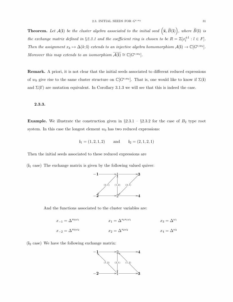
Theorem. Let A(i) be the cluster algebra associated to the initial seed(x, B(i)
), where B(i) is
the exchange matrix defined in §2.3.1 and the coefficient ring is chosen to be R = Z[x±1l : l ∈ F ].
Then the assignment xk �→ Δ(k; i) extends to an injective algebra homomorphism A(i)→ C[Ge,w0 ].
Moreover this map extends to an isomorphism A(i) ∼= C[Ge,w0 ].
Remark. A priori, it is not clear that the initial seeds associated to different reduced expressions
of w0 give rise to the same cluster structure on C[Ge,w0 ]. That is, one would like to know if Σ(i)
and Σ(i′) are mutation equivalent. In Corollary 3.1.3 we will see that this is indeed the case.
2.3.3.
Example. We illustrate the construction given in §2.3.1 – §2.3.2 for the case of B2 type root
system. In this case the longest element w0 has two reduced expressions:
i1 = (1, 2, 1, 2) and i2 = (2, 1, 2, 1)
Then the initial seeds associated to these reduced expressions are
(i1 case) The exchange matrix is given by the following valued quiver:
−2 2 4
−1 1 3�� ��
�� ��
(2,1) (1,2) (2,1)
��
��
��
And the functions associated to the cluster variables are:
x−1 = Δw0ω1 x1 = Δs2s1ω1 x3 = Δω1
x−2 = Δw0ω2 x2 = Δs2ω2 x4 = Δω2
(i2 case) We have the following exchange matrix:
−2 1 3
−1 2 4�� ��
�� ��
(1,2) (2,1) (1,2)
��
��
��
32 2. CLUSTER ALGEBRAS AND BASED AFFINE SPACES
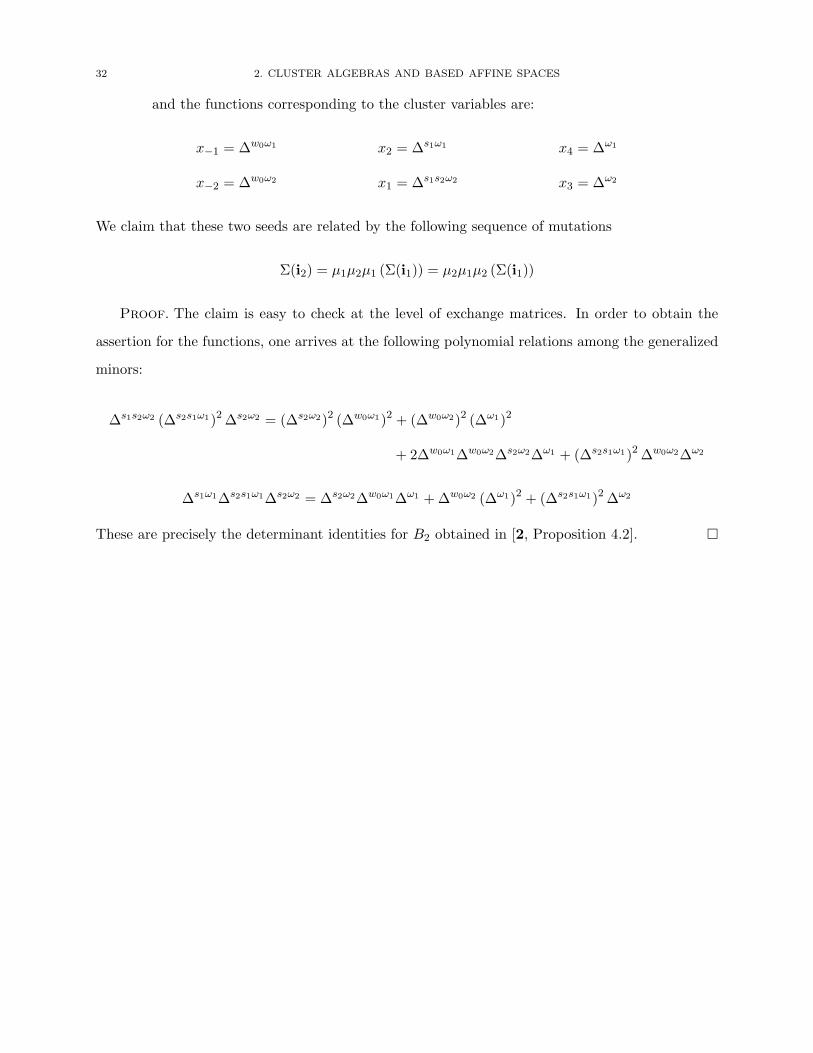
and the functions corresponding to the cluster variables are:
x−1 = Δw0ω1 x2 = Δs1ω1 x4 = Δω1
x−2 = Δw0ω2 x1 = Δs1s2ω2 x3 = Δω2
We claim that these two seeds are related by the following sequence of mutations
Σ(i2) = μ1μ2μ1 (Σ(i1)) = μ2μ1μ2 (Σ(i1))
Proof. The claim is easy to check at the level of exchange matrices. In order to obtain the
assertion for the functions, one arrives at the following polynomial relations among the generalized
minors:
Δs1s2ω2 (Δs2s1ω1)2Δs2ω2 = (Δs2ω2)2 (Δw0ω1)2 + (Δw0ω2)2 (Δω1)2
+ 2Δw0ω1Δw0ω2Δs2ω2Δω1 + (Δs2s1ω1)2Δw0ω2Δω2
Δs1ω1Δs2s1ω1Δs2ω2 = Δs2ω2Δw0ω1Δω1 +Δw0ω2 (Δω1)2 + (Δs2s1ω1)2Δω2
These are precisely the determinant identities for B2 obtained in [2, Proposition 4.2]. �
CHAPTER 3
Grassmannians of type G2
3.1. Recollections from the representation theory of G2
3.1.1. We now assume that G is the simple, simply–connected Lie group of type G2. The
vertices of the Dynkin diagram of G are labeled by {1, 2} so that the entries of the Cartan matrix A
are given by a12 = −3 and a21 = −1. For i = 1, 2 we have the following subalgebra of A = C[N−\G](see §2.2.4)
Ai =⊕n∈N
Vnωi ⊂ A
Note that Ai is the homogeneous coordinate ring of the Grassmannians corresponding to vertex
j = i.
3.1.2. The longest element w0 of the Weyl group of G has the following two reduced expres-
sions:
i1 = (1, 2, 1, 2, 1, 2) and i2 = (2, 1, 2, 1, 2, 1)
corresponding to which we have the following two initial seeds for Ge,w0 (see also Example 2.3.3):
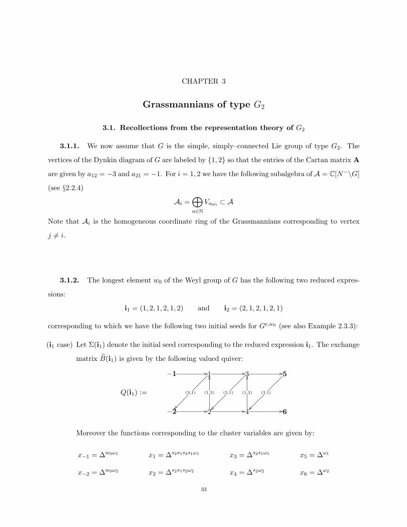
(i1 case) Let Σ(i1) denote the initial seed corresponding to the reduced expression i1. The exchange
matrix B(i1) is given by the following valued quiver:
−1 1 3 5
−2 2 4 6
(3,1) (1,3) (3,1) (1,3) (3,1)
�� �� ��
�� �� ��
��
��
��
��
��
Q(i1) :=
Moreover the functions corresponding to the cluster variables are given by:
x−1 = Δw0ω1 x1 = Δs2s1s2s1ω1 x3 = Δs2s1ω1 x5 = Δω1
x−2 = Δw0ω2 x2 = Δs2s1s2ω2 x4 = Δs2ω2 x6 = Δω2
33

34 3. GRASSMANNIANS OF TYPE G2
(i2 case) Again let Σ(i2) be the initial seed corresponding to the reduced expression i2. The exchange
matrix B(i2) is then given by the following valued quiver:
−1 2 4 6
−2 1 3 5
(1,3) (3,1) (1,3) (3,1) (1,3)
�� �� ��
�� �� ����
��
��
��
��
Q(i2) :=
and the functions corresponding to the cluster variables are given by
x−1 = Δw0ω1 x2 = Δs1s2s1ω1 x4 = Δs1ω1 x6 = Δω1
x−2 = Δw0ω2 x1 = Δs1s2s1s2ω2 x3 = Δs1s2ω2 x5 = Δω2
Remark. As in the case of B2 it can be shown that the two initial seeds defined above are mutation
equivalent:
Σ(i1) = μ1μ3μ2μ1μ2μ4μ2μ1μ2μ3μ1 (Σ(i2))
However the computation for G2 is more complicated. The reader could use the quiver mutation
software of Prof. B. Keller to obtain the polynomial relations among the generalized minors, which
are in fact the determinant identities of type G2 proved in [2, Proposition 4.2]. As a consequence of
this computation one obtains the following result, which is not a priori clear from the definitions.
However this result will not be needed in this work.
3.1.3.
Corollary. For arbitrary semisimple group G, and two reduced expressions i, i′ ∈ R(w0), the initial
seeds Σ(i) and Σ(i′) defined in §2.3 are mutation equivalent.
Proof. Since any two reduced expressions of w0 are related by a sequence of Tits moves, one
is reduced to verifying the assertion for A1 × A1, A2, B2 and G2 types. The first two verifications
are immediate. The case of B2 is given in Example 2.3.3 and the case of G2 is treated in Remark
3.1.2. �
3.1.4. Fundamental representations. Let Vω1 and Vω2 be the two fundamental representa-
tions of G. It is clear that the algebras Ai are generated by the weight vectors of Vωi . We describe
these representations explicitly:

3.1. RECOLLECTIONS FROM THE REPRESENTATION THEORY OF G2 35
Figure 3.1.1. First fundamental representation
Δs1ω1
f2
Δω1f1��
Δs1s2s1ω1
f2
X0f2
�� Δs2s1ω1
f1/2��
Δw0ω1 Δs2s1s2s1ω1
f1��
(1) Vω1 has a realization in terms of certain N−–invariant functions on G, given in Figure
3.1.1.
In Figure 3.1.1 the function X0 is a chosen non–zero vector from the zero weight space of
Vω1 and the figure itself can be taken as the definition of X0, namely:
X0 :=f12(Δs2s1ω1)
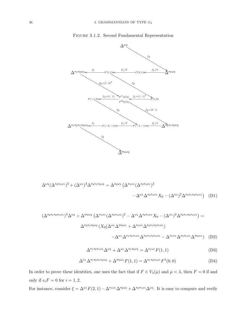
(2) Again Vω2 has a realization in terms of certain N−–invariant functions on G, given in
Figure 3.1.2.
In Figure 3.1.2, each function represents a chosen basis vector of the respective weight
space and the arrows indicate action of lowering operators. For instance
Δs1s2ω2f2=(1 2)T
��F1(0, 0)
F 2(0, 0)
means that f2(Δs1s2ω2) = F 1(0, 0)+2F 2(0, 0). The functions F (i, j) have weight α1i+α2j
and Figure 3.1.2 can be taken as definition of these functions. For example
F (1, 1) =1
6f21Δ
s2ω2
F 1(0, 0) = (2f1f2 − f2f1)(F (1, 1))
F 2(0, 0) = (f2f1 − f1f2)(F (1, 1))
3.1.5. Determinant identities. For future purposes we record the following polynomial re-
lations among the weight vectors of Vωi .
36 3. GRASSMANNIANS OF TYPE G2
Figure 3.1.2. Second Fundamental Representation
Δω2
Δs2ω2F (2,1)F (1,1)Δs1s2ω2
F (1,0)F1(0,0)
F2(0,0)
Δw0ω2
Δs2s1s2ω2F (−1,−1)F (−2,−1)Δs1s2s1s2ω2
F (−1,0)
f2
f1/3��f1/2��f1��
f2
f2=(1 2)t
f1=(1 1)t��f1=(1 1)��
f2
f2=(0 1)
f2
f1/3��f1/2��f1��
Δω2(Δs2s1ω1)3 + (Δω1)3Δs2s1s2ω2 = Δs2ω2(Δs1ω1(Δs2s1ω1)2
−Δω1Δs2s1ω1X0 − (Δω1)2Δs2s1s2s1ω1)
(D1)
(Δs2s1s2s1ω1)3Δω2 +Δw0ω2(Δs1ω1(Δs2s1ω1)2 −Δω1Δs2s1ω1X0 − (Δω1)2Δs2s1s2s1ω1
)=
Δs2s1s2ω2 (X0(Δω1Δw0ω1 +Δs1ω1Δs2s1s2s1ω1)
−Δω1Δs1s2s1ω1Δs2s1s2s1ω1 −Δs1ω1Δs2s1ω1Δw0ω1) (D2)
Δs1s2s1ω1Δω2 +Δω1Δs1s2ω2 = Δs1ω1F (1, 1) (D3)
Δω1Δs1s2s1s2ω2 +Δw0ω1F (1, 1) = Δs1s2s1ω1F 1(0, 0) (D4)
In order to prove these identities, one uses the fact that if F ∈ Vλ(μ) and μ < λ, then F = 0 if and
only if eiF = 0 for i = 1, 2.
For instance, consider ξ = Δω1F (2, 1)−Δs1ω1Δs2ω2 +Δs2s1ω1Δω2 . It is easy to compute and verify
3.2. GLS CONJECTURE 37
that e1ξ = e2ξ = 0 and hence ξ = 0. More relations of this kind can be obtained by applying
f1, f2 to ξ (there are in fact 35 relations of this type, out of which 27 (=dim(V2ω1)) can be obtained
from ξ). The relations (D1)-(D4) can be checked by direct calculation (for instance, (D3) is in fact
obtained by applying (f1)2 to the equality ξ = 0).
3.1.6. Plucker relations. We also have the following Plucker relations among the weight
vectors of Vω2
F (2, 1)2 +Δω2F (1, 0) = Δs2ω2F (1, 1) (P1)
F (1, 0)Δs1s2s1s2ω2 = F 1(0, 0)F (−2,−1) + F (1, 1)Δw0ω2 (P2)
Δω2Δw0ω2 = F (1, 0)F (−1, 0)− F 1(0, 0)F 2(0, 0) (P3)
F (−2,−1)F (2, 1) + F (1, 0)F (−1, 0) = F (1, 1)F (−1,−1) (P4)
F (1, 1)2 = F (2, 1)Δs1s2ω2 −Δω2F (−1, 0) (P5)
Δω2Δs1s2s1s2ω2 = F (1, 1)F (−1, 0)− F 1(0, 0)Δs1s2ω2 (P6)
Δω2(F 1(0, 0) + F 2(0, 0)
)= Δs2ω2Δs1s2ω2 − F (2, 1)F (1, 1) (P7)
The proof of these relations is exactly same as the one in previous section. For example, the relation
(P1) is equivalent to: ei(F (2, 1)2+Δω1F (1, 0)−Δs2ω2F (1, 1)) = 0 for i = 1, 2, which can be verified
directly using the action of operators ei from Figure 3.1.2. Other relations are obtained by applying
lowering operators to both sides of (P1). For instance, (P5) can be obtained by applying (1/4)f21
to (P1).
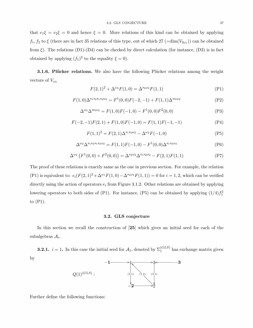
3.2. GLS conjecture
In this section we recall the construction of [25] which gives an initial seed for each of the
subalgebras Ai.
3.2.1. i = 1. In this case the initial seed for A1, denoted by Σ(GLS)1 has exchange matrix given
by−1 1 3 −3
−2 2
(3,1) (1,3) (3,1)
�� �� ��
����
��
��
Q(1)(GLS) :
Further define the following functions:

38 3. GRASSMANNIANS OF TYPE G2
X(GLS)−1 = Δw0ω1 X
(GLS)−3 = Δω1 X
(GLS)3 = Δs1ω1
and
X(GLS)−2 = X0(Δ
ω1Δw0ω1 +Δs1ω1Δs2s1s2s1ω1)
−Δω1Δs1s2s1ω1Δs2s1s2s1ω1 −Δs1ω1Δs2s1ω1Δw0ω1
X(GLS)1 = −Δω1Δs1s2s1ω1 +Δs1ω1X0
X(GLS)2 = Δs2s1ω1(Δs1ω1)2 − 2Δω1Δs1ω1X0 + (Δω1)2Δs1s2s1ω1
3.2.2. i = 2. The initial seed for A2, denoted by Σ(GLS)2 has exchange matrix given by:
−1 1 3 −3
−2 2
(1,3) (3,1) (1,3)
�� �� ��
����
��
��
Q(2)(GLS) :
with corresponding functions given by
Y(GLS)−1 = Δw0ω2 Y
(GLS)−2 = F 1(0, 0) Y
(GLS)−3 = Δω2
Y(GLS)2 = F (2, 1) Y
(GLS)3 = Δs2ω2
and
Y(GLS)1 = F (2, 1)F (1, 0)−Δs2ω2F 1(0, 0)
3.2.3. Let i ∈ {1, 2} and let A(Σ(GLS))i ) be the cluster algebra associated to the initial seed
Σ(GLS)i , where we take the ground ring to be R = Z[x−1, x−2, x−3]. We consider the definitions
given in §3.2.1 and §3.2.2 as defining a map
A(Σ(GLS)i )→ Ai
Theorem. [25, Conjecture 10.4] The map given above extends to an algebra isomorphism when
A(Σ(GLS)i ) is localized at x−3 and Ai is localized at Δωi.
3.3. ALTERNATE CONSTRUCTION 39
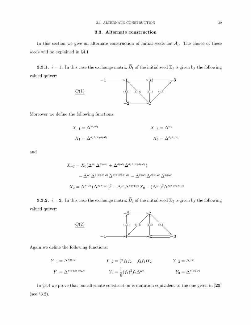
3.3. Alternate construction
In this section we give an alternate construction of initial seeds for Ai. The choice of these
seeds will be explained in §4.1
3.3.1. i = 1. In this case the exchange matrix B1 of the initial seed Σ1 is given by the following
valued quiver:−1 1 3 −3
−2 2
(3,1) (1,3) (3,1) (1,3)
�� �� ����
����
��
��
��
Q(1)
Moreover we define the following functions:
X−1 = Δw0ω1 X−3 = Δω1
X1 = Δs2s1s2s1ω1 X3 = Δs2s1ω1
and
X−2 = X0(Δω1Δw0ω1 +Δs1ω1Δs2s1s2s1ω1)
−Δω1Δs1s2s1ω1Δs2s1s2s1ω1 −Δs1ω1Δs2s1ω1Δw0ω1
X2 = Δs1ω1(Δs2s1ω1)2 −Δω1Δs2s1ω1X0 − (Δω1)2Δs2s1s2s1ω1
3.3.2. i = 2. In this case the exchange matrix B2 of the initial seed Σ2 is given by the following
valued quiver:
−1 1 3 −3
−2 2
(1,3) (3,1) (1,3) (3,1)
�� �� ����
����
��
��
��
Q(2)
Again we define the following functions:
Y−1 = Δw0ω2 Y−2 = (2f1f2 − f2f1)Y2 Y−3 = Δω2
Y1 = Δs1s2s1s2ω2 Y2 =1
6(f1)
2f2Δω2 Y3 = Δs1s2ω2
In §3.4 we prove that our alternate construction is mutation equivalent to the one given in [25](see §3.2).
40 3. GRASSMANNIANS OF TYPE G2
3.4. Equivalence of the two constructions
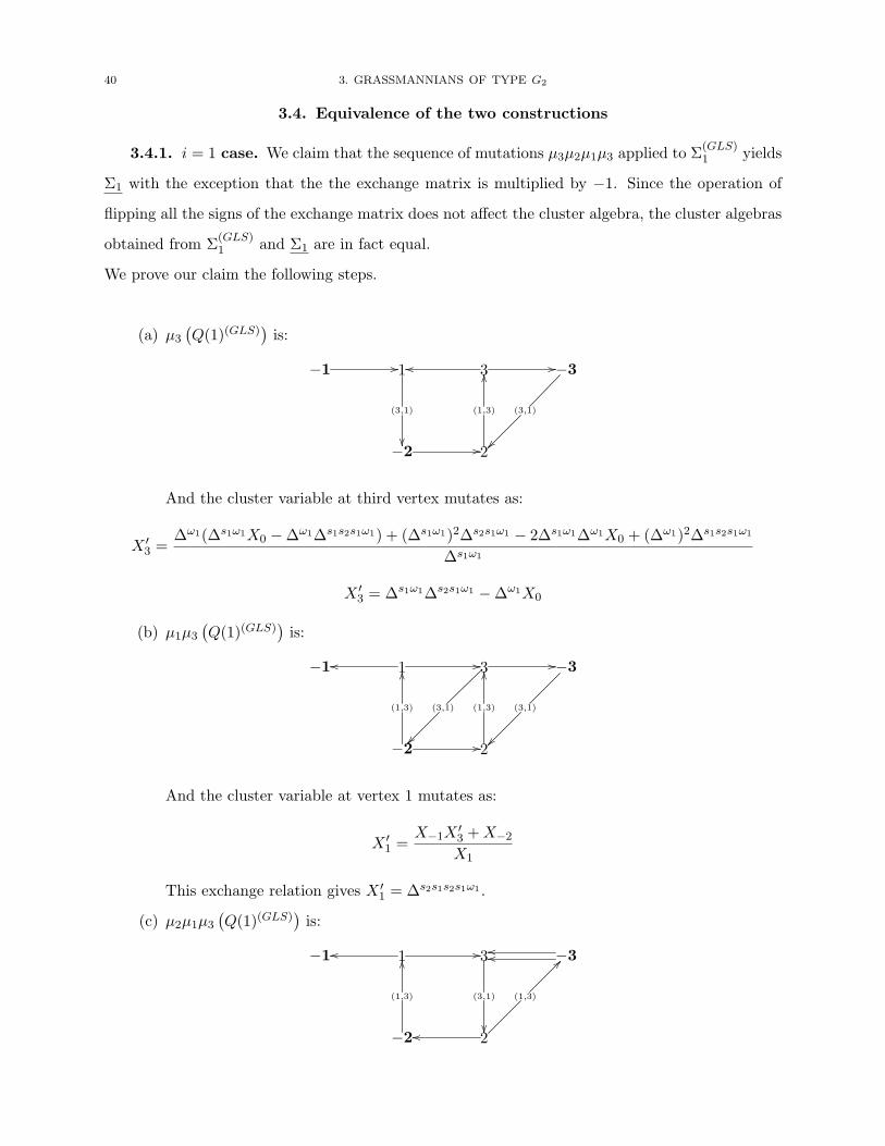
3.4.1. i = 1 case. We claim that the sequence of mutations μ3μ2μ1μ3 applied to Σ(GLS)1 yields
Σ1 with the exception that the the exchange matrix is multiplied by −1. Since the operation of
flipping all the signs of the exchange matrix does not affect the cluster algebra, the cluster algebras
obtained from Σ(GLS)1 and Σ1 are in fact equal.
We prove our claim the following steps.
(a) μ3
(Q(1)(GLS)
)is:
−1 1 3 −3
−2 2
(3,1) (1,3) (3,1)
�� �� ��
����
��
��
And the cluster variable at third vertex mutates as:
X ′3 =
Δω1(Δs1ω1X0 −Δω1Δs1s2s1ω1) + (Δs1ω1)2Δs2s1ω1 − 2Δs1ω1Δω1X0 + (Δω1)2Δs1s2s1ω1
Δs1ω1
X ′3 = Δs1ω1Δs2s1ω1 −Δω1X0
(b) μ1μ3
(Q(1)(GLS)
)is:
−1 1 3 −3
−2 2
(1,3) (3,1) (1,3) (3,1)
�� �� ��
��
��
��
��
��
And the cluster variable at vertex 1 mutates as:
X ′1 =
X−1X ′3 +X−2X1
This exchange relation gives X ′1 = Δs2s1s2s1ω1 .
(c) μ2μ1μ3
(Q(1)(GLS)
)is:
−1 1 3 −3
−2 2
(1,3) (3,1) (1,3)
�� ��
��
������
��
��
3.4. EQUIVALENCE OF THE TWO CONSTRUCTIONS 41
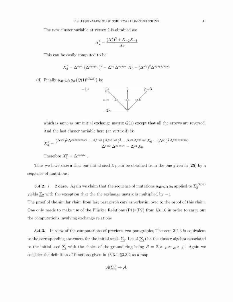
The new cluster variable at vertex 2 is obtained as:
X ′2 =
(X ′3)
3 +X−2X−1X2
This can be easily computed to be
X ′2 = Δs1ω1(Δs2s1ω1)2 −Δω1Δs2s1ω1X0 − (Δω1)2Δs2s1s2s1ω1
(d) Finally μ3μ2μ1μ3
(Q(1)(GLS)
)is:
−1 1 3 −3
−2 2
(1,3) (3,1) (1,3) (3,1)
�� �� ����
��
��
��
��
��
which is same as our initial exchange matrix Q(1) except that all the arrows are reversed.
And the last cluster variable here (at vertex 3) is:
X ′′3 =
(Δω1)2Δs2s1s2s1ω1 +Δs1ω1(Δs2s1ω1)2 −Δω1Δs2s1ω1X0 − (Δω1)2Δs2s1s2s1ω1
Δs1ω1Δs2s1ω1 −Δω1X0
Therefore X ′′3 = Δs2s1ω1 .
Thus we have shown that our initial seed Σ1 can be obtained from the one given in [25] by a
sequence of mutations.
3.4.2. i = 2 case. Again we claim that the sequence of mutations μ3μ2μ1μ3 applied to Σ(GLS)2
yields Σ2 with the exception that the the exchange matrix is multiplied by −1.The proof of the similar claim from last paragraph carries verbatim over to the proof of this claim.
One only needs to make use of the Plucker Relations (P1)–(P7) from §3.1.6 in order to carry outthe computations involving exchange relations.
3.4.3. In view of the computations of previous two paragraphs, Theorem 3.2.3 is equivalent
to the corresponding statement for the initial seeds Σi. Let A(Σi) be the cluster algebra associated
to the initial seed Σi with the choice of the ground ring being R = Z[x−1, x−2, x−3]. Again we
consider the definition of functions given in §3.3.1–§3.3.2 as a map
A(Σi)→ Ai
42 3. GRASSMANNIANS OF TYPE G2
Theorem. The map given above extends to an algebra isomorphism when A(Σi) is localized at x−3
and Ai is localized at Δωi.
Remark. Let Σ =(x, B
)be a given seed and B be another algebra. In order to prove that an
assignment xi �→ bi extends to an algebra isomorphism between the cluster algebra associated to Σ
and B one has to prove the following two statements:
(1) Every cluster variable is mapped to a well defined element of B. This part seems to be themore difficult one since it involves checking that any sequence of mutation will produce
an element of B and will not involve denominators that do not cancel.
(2) Every element of B can be expressed as a polynomial in the image of cluster variables.
This part can be tackled assuming one has a hold on a convenient set of generators of B.In our situation the first problem is reduced to Theorem 2.3.2 by means of §4.1. Thus the proofof Theorem 3.4.3 is reduced to checking that all the weight vectors of Vωi can be obtained by a
sequence of mutations starting from the initial seed Σi.

CHAPTER 4
A proof of the GLS conjecture
4.1. Explanation of the choice of initial seeds
In this section we explain the “greedy approach” to obtain the initial seeds of Ai, starting from
the initial seeds of A as given in §3.1.2. The idea is to apply the least number of mutations to getthe seed whose all the cluster variables belong to a single Ai.
4.1.1. i = 1. We start from initial seed Σ1 (see §3.1.2) and apply mutations μ2μ4 to obtain
the following:−1 1 3 5
−2 2 4 6
(3,1) (1,3) (3,1) (1,3)
�� �� ����
�� ��
��
��
��
��
��
The following computation follows from the determinant identities (D1)–(D4) given in §3.1.5.
Lemma. Let X ′2 and X ′
4 be functions obtained by applying mutations μ2μ4 to initial seed Σ1. Then
we have
X ′2 = X0(Δ
ω1Δw0ω1 +Δs1ω1Δs2s1s2s1ω1)−Δω1Δs1s2s1ω1Δs2s1s2s1ω1 −Δs1ω1Δs2s1ω1Δw0ω1
X ′4 = Δs1ω1(Δs2s1ω1)2 −Δω1Δs2s1ω1X0 − (Δω1)2Δs2s1s2s1ω1
This lemma proves that the initial seed Σ1 defined in §3.3.1 is precisely the one obtained
from μ2μ4(Σ1) by “freezing” the vertex labeled 2 (and renaming vertices, just for convenience of
notation). In the mutated seed μ2μ4(Σ1) all cluster variables belong to representations of type Vnω1
except for ones corresponding to vertices −2 and 6 which are only linked to vertex 2. Therefore if
we do not allow mutation at this vertex, all the functions we shall obtain will again belong to Vnω1
(for some n) and hence to A1.
43
44 4. A PROOF OF THE GLS CONJECTURE
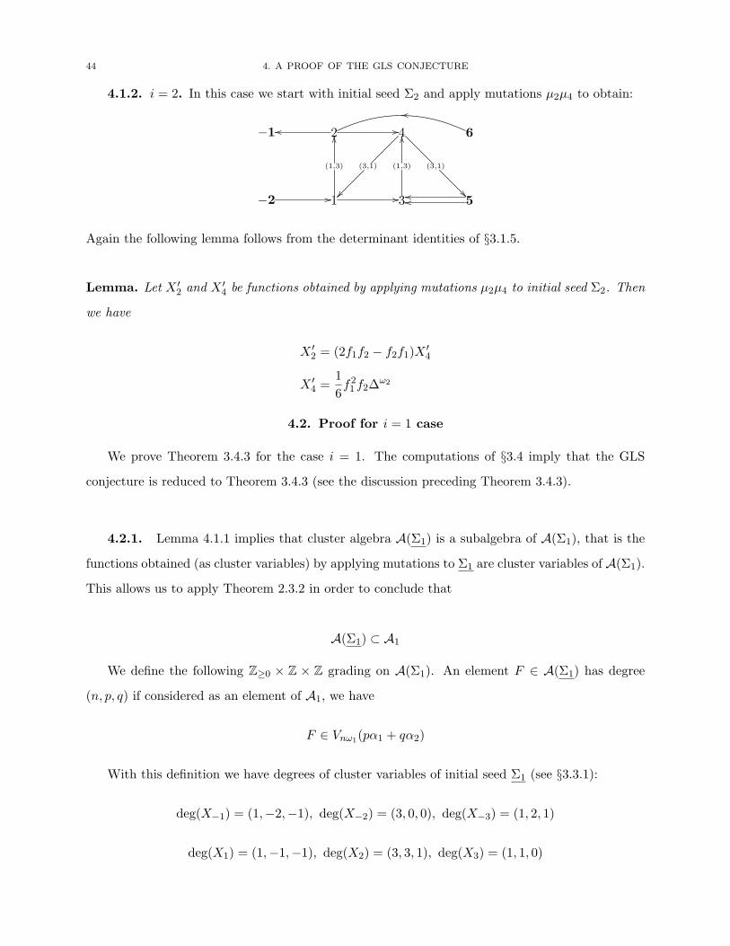
4.1.2. i = 2. In this case we start with initial seed Σ2 and apply mutations μ2μ4 to obtain:
−2 1 3 5
−1 2 4 6
(1,3) (3,1) (1,3) (3,1)
�� �� ����
�� ��
��
��
��
��
��
Again the following lemma follows from the determinant identities of §3.1.5.
Lemma. Let X ′2 and X ′
4 be functions obtained by applying mutations μ2μ4 to initial seed Σ2. Then
we have
X ′2 = (2f1f2 − f2f1)X
′4
X ′4 =
1
6f21 f2Δ
ω2
4.2. Proof for i = 1 case
We prove Theorem 3.4.3 for the case i = 1. The computations of §3.4 imply that the GLS
conjecture is reduced to Theorem 3.4.3 (see the discussion preceding Theorem 3.4.3).
4.2.1. Lemma 4.1.1 implies that cluster algebra A(Σ1) is a subalgebra of A(Σ1), that is the
functions obtained (as cluster variables) by applying mutations to Σ1 are cluster variables of A(Σ1).
This allows us to apply Theorem 2.3.2 in order to conclude that
A(Σ1) ⊂ A1
We define the following Z≥0 × Z × Z grading on A(Σ1). An element F ∈ A(Σ1) has degree
(n, p, q) if considered as an element of A1, we have
F ∈ Vnω1(pα1 + qα2)
With this definition we have degrees of cluster variables of initial seed Σ1 (see §3.3.1):
deg(X−1) = (1,−2,−1), deg(X−2) = (3, 0, 0), deg(X−3) = (1, 2, 1)
deg(X1) = (1,−1,−1), deg(X2) = (3, 3, 1), deg(X3) = (1, 1, 0)

4.2. PROOF FOR i = 1 CASE 45
4.2.2. Since the algebra A1 is generated by the weight vectors of Vω1 , in order to prove
Theorem 3.4.3, we need to prove that the inclusion A(Σ1) ⊂ A1 becomes equality when localized
at Δω1 . Thus it would suffice to prove the following two statements.
(a) There are cluster variables W,Y such that
deg(W ) = (1,−1, 0), deg(Y ) = (1, 1, 1)
(b) X0Δω1 can be written in terms of cluster variables (i.e, it belongs to algebra generated by
cluster variables localized at Δω1).
4.2.3. We begin by applying μ3 to Σ1. Let X′3 be cluster variable obtained at vertex 3.
X ′3 =
X1X2−3 +X2
X3= Δs1ω1Δs2s1ω1 −Δω1X0
Therefore we have Δω1X0 in terms of other cluster variables (assuming that Δs1ω1 and Δs2s1ω1
are cluster variables: the assertion of part (a)).
Let us define Σ10 := μ2μ3(Σ1). The exchange matrix at this cluster is given by
−1 1 3 −3
−2 2
(3,1) (1,3) (3,1) (1,3)
�� �� ��
����
��
��
��
Therefore the seed Σ10 is bipartite. Following [21] we define
μ+ = μ1μ2, μ− = μ3
As long as we restrict ourselves to “the bipartite belt” the mutations μ1 and μ2 commute (since
vertices 1 and 2 are not linked). Further we define
Σ1r =
⎧⎪⎪⎪⎪⎨⎪⎪⎪⎪⎩· · ·μ−μ+μ−μ+︸ ︷︷ ︸
r terms
(Σ10) if r ≥ 0
· · ·μ+μ−μ+μ−︸ ︷︷ ︸−r terms
(Σ10) if r < 0
We denote by X(r)i , the cluster variables at seed Σ1
r and d(r)i ∈ N × Z × Z its degree. Then
part a) follows from following proposition: to see that there exist cluster variables with degrees
46 4. A PROOF OF THE GLS CONJECTURE
(1,−1, 0) and (1, 1, 1) we just observe that d(−3)1 = (1, 1, 1) and d(−7)1 = (1,−1, 0). This proposition
will be proved in §4.4.
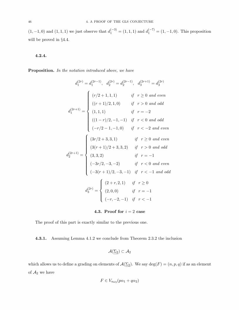
4.2.4.
Proposition. In the notation introduced above, we have
d(2r)1 = d
(2r−1)1 , d
(2r)2 = d
(2r−1)2 , d
(2r+1)3 = d
(2r)3
d(2r+1)1 =
⎧⎪⎪⎪⎪⎪⎪⎪⎪⎪⎪⎨⎪⎪⎪⎪⎪⎪⎪⎪⎪⎪⎩
(r/2 + 1, 1, 1) if r ≥ 0 and even
((r + 1)/2, 1, 0) if r > 0 and odd
(1, 1, 1) if r = −2((1− r)/2,−1,−1) if r < 0 and odd
(−r/2− 1,−1, 0) if r < −2 and even
d(2r+1)2 =
⎧⎪⎪⎪⎪⎪⎪⎪⎪⎪⎪⎨⎪⎪⎪⎪⎪⎪⎪⎪⎪⎪⎩
(3r/2 + 3, 3, 1) if r ≥ 0 and even
(3(r + 1)/2 + 3, 3, 2) if r > 0 and odd
(3, 3, 2) if r = −1(−3r/2,−3,−2) if r < 0 and even
(−3(r + 1)/2,−3,−1) if r < −1 and odd
d(2r)3 =
⎧⎪⎪⎪⎨⎪⎪⎪⎩(2 + r, 2, 1) if r ≥ 0
(2, 0, 0) if r = −1(−r,−2,−1) if r < −1
4.3. Proof for i = 2 case
The proof of this part is exactly similar to the previous one.
4.3.1. Assuming Lemma 4.1.2 we conclude from Theorem 2.3.2 the inclusion
A(Σ2) ⊂ A2
which allows us to define a grading on elements of A(Σ2). We say deg(F ) = (n, p, q) if as an element
of A2 we have
F ∈ Vnω2(pα1 + qα2)

4.3. PROOF FOR i = 2 CASE 47
In this notation the cluster variables have following degrees
deg(Y−1) = (1,−3,−2), deg(Y−2) = (1, 0, 0), deg(Y−3) = (1, 3, 2)
deg(Y1) = (1,−3,−1), deg(Y2) = (1, 1, 1), deg(Y3) = (1, 0, 1)
Again it suffices to prove the following two statements
(a) There exist cluster variables with degrees (1, 3, 1); (1, 2, 1); (1, 1, 0); (1,−1, 0); (1, 0,−1); (1,−1,−1)and (1,−2,−1).
(b) Δω2 .F 2(0, 0) can be written as a polynomial in cluster variables.
4.3.2. Similar to previous part, we define Σ20 to be μ2μ3(Σ2) to make it bipartite:
−1 1 3 −3
−2 2
(1,3) (3,1) (1,3) (3,1)
�� �� ��
����
��
��
��
And define
μ+ = μ1μ2, μ− = μ3
The bipartite belt consists of following seeds
Σ2r =
⎧⎪⎪⎪⎪⎨⎪⎪⎪⎪⎩· · ·μ−μ+μ−μ+︸ ︷︷ ︸
r terms
(Σ20) if r ≥ 0
· · ·μ+μ−μ+μ−︸ ︷︷ ︸−r terms
(Σ20) if r < 0
Again we let Y(r)i be the cluster variables in Σ2
0 and let g(r)i be its degree. Also let U and Z be
cluster variables appearing at vertex 2 in μ2μ3μ1(Σ20) and μ2μ3μ2(Σ2
0). Then part a) follows from
following degree computation: again we only need to observe that g(−3)1 = (1, 3, 1), g
(−3)2 = (1, 2, 1),
g(−7)1 = (1, 0,−1), g(−5)2 = (1,−1,−1), g(−3)2 = (1,−2,−1). This together with the first statementof the proposition exhausts the list of weights demanded in part (a). Part (b) will follow from
above proposition together with following Plucker relation ((P7) of §3.1.6):
Δω2(F 1(0, 0) + F 2(0, 0)) = Δs2ω2Δs1s2ω2 − F (1, 1)F (2, 1)
Again the proof of this proposition is given in §4.4.

48 4. A PROOF OF THE GLS CONJECTURE
4.3.3.
Proposition. We have
deg(U) = (1, 1, 0), deg(Z) = (1,−1, 0)
Moreover we have
g(2r)1 = g
(2r−1)1 , g
(2r)2 = g
(2r−1)2 , g
(2r+1)3 = g
(2r)3
g(2r+1)1 =
⎧⎪⎪⎪⎪⎪⎪⎪⎪⎪⎪⎨⎪⎪⎪⎪⎪⎪⎪⎪⎪⎪⎩
(r/2 + 2, 3, 1) if r ≥ 0 and even
((r + 1)/2, 0, 1) if r > 0 and odd
(1, 3, 1) if r = −2((1− r)/2,−3,−1) if r < 0 and odd
(−r/2− 1, 0,−1) if r < −2 and even
g(2r+1)2 =
⎧⎪⎪⎪⎪⎪⎪⎪⎪⎪⎪⎨⎪⎪⎪⎪⎪⎪⎪⎪⎪⎪⎩
(r/2 + 1, 2, 1) if r ≥ 0 and even
((r + 3)/2, 1, 1) if r > 0 and odd
(1, 2, 1) if r = −1(−r/2,−2,−1) if r < 0 and even
(−(r + 1)/2,−1,−1) if r < −1 and odd
g(2r)3 =
⎧⎪⎪⎪⎨⎪⎪⎪⎩(2 + r, 3, 2) if r ≥ 0
(2, 0, 0) if r = −1(−r,−3,−2) if r < −1
4.4. Computation of degrees
This section is devoted to the computation of degrees. We begin by stating the problem in a
purely combinatorial way.
4.4.1. Consider the following quivers (transpose of each other):
−1 1 3 −3
−2 2
(3,1) (1,3) (3,1) (1,3)
�� �� ��
����
��
��
��
Γ01
4.4. COMPUTATION OF DEGREES 49
−1 1 3 −3
−2 2
(1,3) (3,1) (1,3) (3,1)
�� �� ��
����
��
��
��
Γ02
It is clear that if two vertices i and j are not connected then μiμj = μjμi. This allows us to
unambiguously define μ+ = μ1μ2 and μ− = μ3. Set
Γri :=
⎧⎪⎪⎪⎪⎨⎪⎪⎪⎪⎩· · ·μ−μ+μ−μ+︸ ︷︷ ︸
r terms
Γ0i if r ≥ 0
· · ·μ+μ−μ+μ−︸ ︷︷ ︸−r terms
Γ0i if r < 0
4.4.2. Structure of graphs Γri . It is clear that between vertices 1, 2 and 3 the above graphs
have following structure:
2
1 3��
��2
1 3�� ��
r is even r is odd
Since there are no arrows between vertices −1,−2 and −3, in order to completely determine thestructure of graphs Γr
i we need to compute the following matrix
C(r)ij := Number of arrows from i to j
where i ∈ {−1,−2,−3} and j ∈ {1, 2, 3}. It is clear that both the graphs Γ1 and Γ2 have same
C-matrix.
The mutation rules define following recurrence relations among entries of C(r) (where the notation
[x]− := [−x]+ = max(0,−x) is used):
C(r+1) =
⎛⎜⎜⎜⎝−C(r)
−1,1 −C(r)−1,2 C
(r)−1,3 − [C
(r)−1,1]− − 3[C
(r)−1,2]−
−C(r)−2,1 −C(r)
−2,2 C(r)−2,3 − [C
(r)−2,1]− − [C
(r)−2,2]−
−C(r)−3,1 −C(r)
−3,2 C(r)−3,3 − [C
(r)−3,1]− − 3[C
(r)−3,2]−
⎞⎟⎟⎟⎠ if r is even
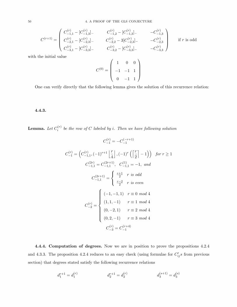
50 4. A PROOF OF THE GLS CONJECTURE
C(r+1) =
⎛⎜⎜⎜⎝C
(r)−1,1 − [C
(r)−1,3]− C
(r)−1,2 − [C
(r)−1,3]− −C(r)
−1,3
C(r)−2,1 − [C
(r)−2,3]− C
(r)−2,2 − 3[C
(r)−2,3]− −C(r)
−2,3
C(r)−3,1 − [C
(r)−3,3]− C
(r)−3,2 − [C
(r)−3,3]− −C(r)
−3,3
⎞⎟⎟⎟⎠ if r is odd
with the initial value
C(0) =
⎛⎜⎜⎜⎝1 0 0
−1 −1 1
0 −1 1
⎞⎟⎟⎟⎠One can verify directly that the following lemma gives the solution of this recurrence relation:
4.4.3.
Lemma. Let C(r)i be the row of C labeled by i. Then we have following solution
C(r)−1 = −C(−r+1)
−1
C(r)−1 =
(C
(r)−1,1, (−1)r+1
⌊r4
⌋, (−1)r
(⌈r2
⌉− 1
))for r ≥ 1
C(2r)−1,1 = C
(2r+1)−1,1 , C
(1)−1,1 = −1, and
C(2r+1)−1,1 =
⎧⎨⎩r+12 r is odd
r−22 r is even
C(r)−2 =
⎧⎪⎪⎪⎪⎪⎪⎪⎨⎪⎪⎪⎪⎪⎪⎪⎩
(−1,−1, 1) r ≡ 0 mod 4
(1, 1,−1) r ≡ 1 mod 4
(0,−2, 1) r ≡ 2 mod 4
(0, 2,−1) r ≡ 3 mod 4
C(r)−3 = C
(r+4)−1
4.4.4. Computation of degrees. Now we are in position to prove the propositions 4.2.4
and 4.3.3. The proposition 4.2.4 reduces to an easy check (using formulae for C ′ijs from previous
section) that degrees stated satisfy the following recurrence relations
dr+11 = d
(r)1 dr+1
2 = d(r)2 d
(s+1)3 = d
(s)3

4.5. SUMMARY 51
for every odd r and even s. Furthermore, we have the following for every even r and odd s:
d(r+1)1 = −d(r)1 + [C
(r)−1,1]−(1,−2,−1) + [C
(r)−2,1]−(3, 0, 0) + [C
(r)−3,1]−(1, 2, 1)
d(r+1)2 = −d(r)2 + 3[C
(r)−1,2]−(1,−2,−1) + [C
(r)−2,1]−(3, 0, 0) + 3[C
(r)−3,2]−(1, 2, 1)
d(s+1)3 = −d(s)3 + [C
(s)−1,3]−(1,−2,−1) + [C
(s)−2,3]−(3, 00) + [C
(s)−3,3]−(1, 2, 1)
together with initial values d(0)1 = (1,−1,−1), d(0)2 = (2, 2, 1) and d
(0)3 = (3, 3, 2).
Similarly proposition 4.3.3 reduces to checking that degrees stated satisfy following recurrence
relations:
gr+11 = g
(r)1 gr+1
2 = g(r)2 g
(s+1)3 = g
(s)3
for every odd r and even s. Moreover we have the following for every even r and odd s:
g(r+1)1 = −g(r)1 + [C
(r)−1,1]−(1,−3,−2) + 3[C
(r)−2,1]−(1, 0, 0) + [C
(r)−3,1]−(1, 3, 2)
g(r+1)2 = −g(r)2 + [C
(r)−1,2]−(1,−3,−2) + [C
(r)−2,1]−(1, 0, 0) + [C
(r)−3,2]−(1, 3, 2)
g(r+1)3 = −g(r)3 + [C
(r)−1,3]−(1,−3,−2) + 3[C
(r)−2,3]−(1, 0, 0) + [C
(r)−3,3]−(1, 3, 2)
together with initial condition g(0)1 = (1,−3,−1), g(0)2 = (1, 2, 1) and g
(0)3 = (2, 3, 2).
4.5. Summary
In this section we give brief summary of the results proved in this part.
4.5.1. Case i = 1.
- The initial seed Σ1 can be obtained from initial seed Σ1 of A by applying mutations μ2μ4
and freezing vertex 2 (see §4.1).- The cluster algebra associated to initial seed Σ1 is isomorphic to the algebra A1 localized
at multiplicative set {(Δω1)n}n∈Z≥0. Explicitly we obtain all the weight vectors of Figure
3.1.1 by applying mutations to Σ1, as follows:
Δω1 = X−3, Δw0ω1 = X−1, Δs2s1ω1 = X3, Δs2s1s2s1ω1 = X1
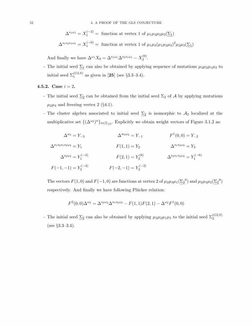
52 4. A PROOF OF THE GLS CONJECTURE
Δs1ω1 = X(−2)1 = function at vertex 1 of μ1μ3μ2μ3(Σ1)
Δs1s2s1ω1 = X(−6)1 = function at vertex 1 of μ1μ3(μ1μ2μ3)
2μ2μ3(Σ1)
And finally we have Δω1X0 = Δs1ω1Δs2s1ω1 −X(0)3 .
- The initial seed Σ1 can also be obtained by applying sequence of mutations μ3μ2μ1μ3 to
initial seed Σ(GLS)1 as given in [25] (see §3.3–3.4).
4.5.2. Case i = 2.
- The initial seed Σ2 can be obtained from the initial seed Σ2 of A by applying mutations
μ2μ4 and freezing vertex 2 (§4.1).- The cluster algebra associated to initial seed Σ2 is isomorphic to A2 localized at the
multiplicative set {(Δω2)n}n∈Z≥0. Explicitly we obtain weight vectors of Figure 3.1.2 as:
Δω2 = Y−3 Δw0ω2 = Y−1 F 1(0, 0) = Y−2
Δs1s2s1s2ω2 = Y1 F (1, 1) = Y2 Δs1s2ω2 = Y3
Δs2ω2 = Y(−2)1 F (2, 1) = Y
(0)2 Δs2s1s2ω2 = Y
(−6)1
F (−1,−1) = Y(−4)2 F (−2,−1) = Y
(−2)2
The vectors F (1, 0) and F (−1, 0) are functions at vertex 2 of μ2μ3μ1(Σ20) and μ2μ3μ2(Σ2
0)
respectively. And finally we have following Plucker relation:
F 2(0, 0)Δω2 = Δs2ω2Δs1s2ω2 − F (1, 1)F (2, 1)−Δω2F 1(0, 0)
- The initial seed Σ2 can also be obtained by applying μ3μ2μ1μ3 to the initial seed Σ(GLS)2
(see §3.3–3.4).
Part 2
Yangians and Quantum loop algebras
CHAPTER 5
Definitions
In this chapter we recall the definitions of the quantum loop algebra and the Yangian associated
to a simple Lie algebra.
5.1. Notations
5.1.1. Let g be a complex, semisimple Lie algebra and (·, ·) a non–degenerate, invariant
bilinear form on g. Let h ⊂ g be a Cartan subalgebra of g, {αi}i∈I ⊂ h∗ a basis of simple roots of
g relative to h and aij = 2(αi, αj)/(αi, αi) the entries of the corresponding Cartan matrix A. Set
di = (αi, αi)/2, so that diaij = djaji for any i, j ∈ I. Let ν : h→ h∗ be the isomorphism determined
by the inner product (·, ·) and set hi = ν−1(αi)/di. Choose root vectors ei ∈ gαi , fi ∈ g−αi such
that [ei, fi] = hi. Recall that g is presented on generators {ei, fi, hi} subject to the relations
[hi, hj ] = 0
[hi, ej ] = aijej [hi, fj ] = −aijfj
[ei, fj ] = δijhi
for any i, j ∈ I and, for any i = j ∈ I
ad(ei)1−aijej = 0
ad(fi)1−aijfj = 0
A closely related, but slightly less standard presentation may be obtained by setting ti =
ν−1(αi) = dihi and choosing, for any i ∈ I, root vectors x±i ∈ g±αi such that [x+i , x
−i ] = ti. Then g
54
5.2. QUANTUM LOOP ALGEBRA AND YANGIAN 55
is presented on {x±i , ti}i∈I subject to the relations
[ti, tj ] = 0
[ti, x±j ] = ±diaijx±j
[x+i , x−j ] = δijti
ad(x±i )1−aijx±j = 0
5.1.2. Throughout this part, q and � are formal variables related by q2 = e�. For any i ∈ I,
we set qi = qdi = e�di/2. We use the standard notation for Gaussian integers
[n]q =qn − q−n
q − q−1
[n]q! = [n]q[n− 1]q · · · [1]q⎡⎣ n
k
⎤⎦q
=[n]q!
[k]q![n− k]q!
5.2. Quantum loop algebra and Yangian
5.2.1. Quantum loop algebra. Let U�(Lg) be the algebra over C[[�]] topologically generated
by elements {Ei,k, Fi,k, Hi,k}i∈I,k∈Z subject to the following relations
(QL1) For i, j ∈ I and r, s ∈ Z
[Hi,r, Hj,s] = 0
(QL2) For any i, j ∈ I and k ∈ Z,
[Hi,0, Ej,k] = aijEj,k [Hi,0, Fj,k] = −aijFj,k
(QL3) For any i, j ∈ I and r ∈ Z×,
[Hi,r, Ej,k] =[raij ]qi
rEj,r+k [Hi,r, Fj,k] = − [raij ]qi
rFj,r+k
(QL4) For i, j ∈ I and k, l ∈ Z
Ei,k+1Ej,l − qaiji Ej,lEi,k+1 = q
aiji Ei,kEj,l+1 − Ej,l+1Ei,k
Fi,k+1Fj,l − q−aiji Fj,lFi,k+1 = q
−aiji Fi,kFj,l+1 − Fj,l+1Fi,k

56 5. DEFINITIONS
(QL5) For i, j ∈ I and k, l ∈ Z
[Ei,k, Fj,l] = δijψi,k+l − φi,k+l
qi − q−1i
(QL6) Let i = j ∈ I and set m = 1− aij . For every k1, . . . , km ∈ Z and l ∈ Z
∑π∈Sm
m∑s=0
(−1)s⎡⎣ m
s
⎤⎦qi
Ei,kπ(1)· · ·Ei,kπ(s)
Ej,lEi,kπ(s+1)· · ·Ei,kπ(m)
= 0
∑π∈Sm
m∑s=0
(−1)s⎡⎣ m
s
⎤⎦qi
Fi,kπ(1)· · ·Fi,kπ(s)
Fj,lFi,kπ(s+1)· · ·Fi,kπ(m)
= 0
where the elements ψi,r, φi,r are defined by
ψi(z) =∑r≥0
ψi,rz−r = exp
(�di2
Hi,0
)exp
⎛⎝ (qi − q−1i )∑s≥1
Hi,sz−s
⎞⎠φi(z) =
∑r≥0
φi,−rzr = exp
(−�di
2Hi,0
)exp
⎛⎝−(qi − q−1i )∑s≥1
Hi,−szs
⎞⎠with ψi,−k = φi,k = 0 for every k ≥ 1.
We shall denote by U0 ⊂ U�(Lg) the commutative subalgebra generated by the elements
{Hi,r}i∈I,r∈Z.
5.2.2. The Yangian. Let Y�(g) be the C[�]–algebra generated by elements {x±i,r, ξi,r}i∈I,r∈N,subject to the following relations
(Y1) For any i, j ∈ I and r, s ∈ N
[ξi,r, ξj,s] = 0
(Y2) For i, j ∈ I and s ∈ N
[ξi,0, x±j,s] = ±diaijx±j,s
(Y3) For i, j ∈ I and r, s ∈ N
[ξi,r+1, x±j,s]− [ξi,r, x
±j,s+1] = ±
diaij�2
(ξi,rx±j,s + x±j,sξi,r)
(Y4) For i, j ∈ I and r, s ∈ N
[x±i,r+1, x±j,s]− [x±i,r, x
±j,s+1] = ±
diaij�2
(x±i,rx±j,s + x±j,sx
±i,r)

5.2. QUANTUM LOOP ALGEBRA AND YANGIAN 57
(Y5) For i, j ∈ I and r, s ∈ N
[x+i,r, x−j,s] = δijξi,r+s
(Y6) Let i = j ∈ I and set m = 1− aij . For any r1, · · · , rm ∈ N and s ∈ N
∑π∈Sm
[x±i,rπ(1)
,[x±i,rπ(2)
, · · · ,[x±i,rπ(m)
, x±j,s]· · ·
]]= 0
Y�(g) is an N–graded algebra by deg(ξi,r) = deg(x±i,r) = r and deg(�) = 1.
5.2.3. PBW theorem for the Yangian. For any positive root β of g, choose a sequence of
simple roots αi1 , . . . , αik such that β = αi1 + · · ·+ αik and
[x±i1 , [x±i2, · · · , [x±ik−1
, x±ik ] · · · ]] ∈ g±β
are non–zero vectors. For any r ∈ N, define x±β,r ∈ Y�(g) by choosing a partition r = r1 + · · ·+ rk
of length k and setting
x±β,r = [x±i1,r1 , [x±i2,r2
, · · · , [x±ik−1,rk−1, x±ik,rk ] · · · ]]
Theorem ([33]). Fix a total order on the set G = {ξi,r, x±β,r}i∈I,r∈N,β∈Σ+. Then, the ordered
monomials in the elements of G form a basis of Y�(g).
Let Y 0, Y ± ⊂ Y�(g) be the subalgebras generated by the elements {ξi,r}i∈I,r∈N (resp. {x±i,r}i∈I,r∈N)and Y ≥0, Y ≤0 ⊂ Y�(g) the subalgebras generated by Y 0, Y + and Y 0, Y − respectively. The following
is a direct consequence of Theorem 5.2.3.
Corollary.
(1) Y 0 is a polynomial algebra in the generators {ξi,r}i∈I,r∈N.(2) Y ± is the algebra generated by elements {x±i,r}i∈I,r∈N subject to the relations (Y4) and
(Y6).
(3) Y ≥0 (resp. Y ≤0) is the algebra generated by elements {ξi,r, x±i,r}i∈I,r∈N subject to the
relations (Y1)–(Y4) and (Y6).
(4) Multiplication induces an isomorphism of vector spaces
Y − ⊗ Y 0 ⊗ Y + → Y�(g)

58 5. DEFINITIONS
5.3. Relations of Y�(g) revisited
5.3.1. The shift operators σ±i . Fix i ∈ I. By Corollary 5.2.3 (3), the assignment
x±j,r → x±j,r+δij, ξj,r → ξj,r
extends to an algebra homomorphism Y ≥0 → Y ≥0 (resp. Y ≤0 → Y ≤0) which we shall denote by
σ±i .
5.3.2. The relations (Y2)–(Y3). We rewrite below the defining relations (Y2)–(Y3) of Y�(g)
in terms of the shift operators σ±j and the generating series
ξi(u) = 1 + �∑r≥0
ξi,ru−r−1 ∈ Y�(g)[[u
−1]] (5.3.1)
Lemma. The relations (Y2)–(Y3) are equivalent to
[ξi(u), x±j,s] =
±�diaiju− σ±j ± �diaij/2
ξi(u)x±j,s
where the right–hand side is expanded in powers of u−1.
Proof. Set a = ±�diaij/2. Multiplying (Y3) by �u−r−1 and summing over r ≥ 0 yields
u[ξi(u)− 1− �u−1ξi,0, x±j,s]− [ξi(u)− 1, x±j,s+1] = a{x±j,s, ξi(u)− 1}
where {x, ξ} = xξ + ξx. Using (Y2) and {x, ξ} = [x, ξ] + 2ξx, yields
(u− σ±j + a)[ξi(u), x±j,s] = 2aξi(u)x
±j,s (5.3.2)
as claimed. Conversely, taking the coefficients of u0 and u−r−1 in (5.3.2) yields (Y2) and (Y3)
respectively. �
5.3.3. The relations (Y4) and (Y6). We shall use the following notation
• for an operator T ∈ End(V ), T(i) ∈ End(V ⊗m) is defined as
T(i) = 1⊗i−1 ⊗ T ⊗ 1⊗m−i
• for an algebra A, define ad(m) : A⊗m → End(A) as
ad(m) (a1 ⊗ · · · ⊗ am) = ad(a1) ◦ · · · ◦ ad(am)

5.3. RELATIONS OF Y�(g) REVISITED 59
Proposition.
(1) The relation (Y4) for i = j is equivalent to the requirement that the following holds for
any A(v1, v2) ∈ C[[v1, v2]]
A(σ±i , σ±j )(σ
±i − σ±j ∓ a�)x±i,0x
±j,0 = A(σ±i , σ
±j )(σ
±i − σ±j ± a�)x±j,0x
±i,0
where a = diaij/2.
(2) The relation (Y4) for i = j is equivalent to the requirement that the following holds for
any B(v1, v2) ∈ C[[v1, v2]] such that B(v1, v2) = B(v2, v1)
μ(B(σ±i,(1), σ
±i,(2))(σ
±i,(1) − σ±i,(2) ∓ di�)x
±i,0 ⊗ x±i,0
)= 0 (5.3.3)
where μ : Y�(g)⊗2 → Y�(g) is the multiplication.
(3) The relation (Y6) for i = j is equivalent to the requirement that the following holds for
any A(v1, . . . , vm) ∈ C[v1, . . . , vm]Sm
ad(m)
(A(σ±i,(1), . . . , σ
±i,(m))
(x±i,0
)⊗m)x±j,l = 0
where m = 1− aij.
Proof. (1) The relation (Y4)
[x±i,r+1, x±j,s]− [x±i,r, x
±j,s+1] = ±a�(x±i,rx±j,s + x±j,sx
±i,r)
may be rewritten as
σ±ri σ±sj
(σ±i − σ±j ∓ a�
)x±i,0x
±j,0 = σ±ri σ±sj
(σ±i − σ±j ± a�
)x±j,0x
±i,0
(2) If i = j, a = di and the above reads
μ(σ±ri,(1)σ
±si,(2)
(σ±i,(1) − σ±i,(2) ∓ di�
)x±i,0 ⊗ x±i,0
)=
μ(σ±si,(1)σ
±ri,(2)
(σ±i,(2) − σ±i,(1) ± di�
)x±i,0 ⊗ x±i,0
)which is equivalent to
μ((
σ±ri,(1)σ±si,(2) + σ±si,(1)σ
±ri,(2)
)(σ±i,(1) − σ±i,(2) ∓ di�
)x±i,0 ⊗ x±i,0
)= 0

60 5. DEFINITIONS
(3) is just the reformulation of (Y6). �
Corollary. If (5.3.3) holds for some B ∈ C[[v1, v2]], then B(v1, v2) = B(v2, v1).
Proof. By (2) of Proposition 5.3.3, we may assume that B(v1, v2) = −B(v2, v1) and thereforethat B = (v1− v2)B where B is symmetric in v1 ↔ v2. Using the grading on Y�(g), we may further
assume that B is proportional to vr1vs2 + vs1v
r2 for some r ≥ s ∈ N. An application of (Y4) yields
μ((σ±i,(1) − σ±i,(2))(σ
±ri,(1)σ
±si,(2) + σ±si,(1)σ
±ri,(2))(σ
±i,(1) − σ±i,(2) ∓ di�)x
±i,0 ⊗ x±i,0
)= 2
((x±i,r+2x
±i,s − x±i,r+1x
±i,s+1 ∓ di�x
±i,r+1x
±i,s)− (x±i,r+1x
±i,s+1 − x±i,rx
±i,s+2 ∓ di�x
±i,rx
±i,s+1)
)If r ≥ s + 2, the above is not zero by the PBW Theorem 5.2.3 and B = 0. If r = s + 1, a further
application of (Y4) shows that the second of the above two parenthesized summands is zero and
again B = 0 by Theorem 5.2.3. Finally, if r = s, (Y4) implies that the two parenthesized summands
are opposites of each other and again B = 0. �
5.4. An alternate system of generators for Y 0
5.4.1. The following system of generators of Y 0 was introduced in [32]. For any i ∈ I, define
the formal power series
ti(u) = �∑r≥0
ti,ru−r−1 ∈ Y 0[[u−1]]
by
ti(u) = log(ξi(u)) = log
⎛⎝1 + �∑r≥0
ξi,ru−r−1
⎞⎠ (5.4.1)
Since (5.4.1) can be inverted, {ti,r}i∈I,r∈N is another system of generators of Y 0 which are homo-
geneous with deg(ti,r) = r. Moreover, ti,0 = ξi,0 and ti,r = ξi,r mod � for any r ≥ 1 since
ti(u) = �∑r≥0
ξi,ru−r−1 mod �2
In order to compute the commutation relations between ti,r and x±j,s, we introduce the following
formal power series (inverse Borel transform of ti(u))
Bi(v) = B(ti(u)) = �∑r≥0
ti,rvr
r!∈ Y 0[[v]] (5.4.2)
5.4. AN ALTERNATE SYSTEM OF GENERATORS FOR Y 0 61
Lemma. For any i, j ∈ I we have
[Bi(v), x
±j,s
]= ±q
aijvi − q
−aijvi
veσ
±j v x±j,s
Proof. To simplify notation set a = ±�diaij/2, so that ea = q±aiji . By Lemma 5.3.2
ξi(u)x±j,sξi(u)
−1 =u− σ±j + a
u− σ±j − ax±j,s
so that
[ti(u), x±j,s] = log
(u− σ±j + a
u− σ±j − a
)x±j,s
Using
B(log(1− pu−1)
)=1− epv
v(5.4.3)
this yields
[Bi(v), x±j,s] = B
(log
(1− (σ±j − a)u−1
)− log
(1− (σ±j + a)u−1
))x±j,s
=
(1− e(σ
±j −a)v
v− 1− e(σ
±j +a)v
v
)x±j,s
=eav − e−av
veσ
±j vx±j,s
as claimed. �
Remark. In order to use Lemma 5.4.1 to compute the commutators [ti,r, x±j,s], one needs to expand
the right–hand side as power series in v. This yields following explicit expression
[ti,r, x±j,s] = ±diaij
�r/2�∑l=0
⎛⎝ r
2l
⎞⎠ (�diaij/2)2l
2l + 1x±j,r+s−2l
These commutation relations were obtained in this form in [32, Lemma 1.4].
5.4.2. The operators λ±i (v). We introduce operators λ±i;s ∈ End(Y 0) which straighten mono-
mials of the form x±i,mξ, ξ ∈ Y 0, into elements of Y 0 · Y ±.
Proposition. There are operators {λ±i;s}i∈I,s∈N on Y 0 such that the following holds

62 5. DEFINITIONS
(1) For any ξ ∈ Y 0, the elements λ±i;s(ξ) ∈ Y 0 are uniquely determined by the requirement
that, for any m ∈ N,
x±i,mξ =∑s≥0
λ±i;s(ξ)x±i,m+s (5.4.4)
(2) For any ξ, η ∈ Y 0,
λ±i;s(ξη) =∑
k+l=s
λ±i;k(ξ)λ±i;l(η) (5.4.5)
(3) The operator λi;s : Y0 → Y 0 is homogeneous of degree −s.
(4) Let λ±i (v) : Y0 → Y 0[v] be given by
λ±i (v)(ξ) =∑s≥0
λ±i;s(ξ) vs
and extend the N–grading on Y 0 to Y 0[v] by deg(v) = 1. Then λ±i (v) is an algebra
homomorphism of degree 0.
(5) λε1i1(v1) and λε2
i2(v2) commute for any i1, i2 ∈ I and ε1, ε2 ∈ {±1}.
(6) For any i ∈ I,
λ+i (v)λ
−i (v) = Id = λ−i (v)λ
+i (v)
(7) For any i, j ∈ I,
λ±j (v1) (Bi(v2)) = Bi(v2)∓ qaijv2i − q
−aijv2i
v2ev1v2
(8) For any i ∈ I and r ∈ N,
λ±j (v)(ti,r) = ti,r ∓ diaijvr mod �
Proof. (1)–(2) by Lemma 5.3.2, (5.4.4) holds when ξ is one of the generators ξj,r of Y0. Since
(5.4.4) holds for ξη if it holds for ξ, η ∈ Y 0, with λi;s(ξη) given by (5.4.5), the λi;s can be defined
as operators on Y 0. The fact they are uniquely characterised by (5.4.4) and satisfy (5.4.5) follows
from Corollary 5.2.3.
(3) the linear independence of the elements on the right–hand side of (5.4.4) implies that
deg(λi;s(ξ)) = deg(ξ)− s for any homogeneous ξ ∈ Y 0. (4) is a rephrasing of (2) and (3). (5) and
(6) follow from (7) since the elements {ti,n} generate Y 0. (7) follows from Lemma 5.4.1. (8) is a
direct consequence of (7). �
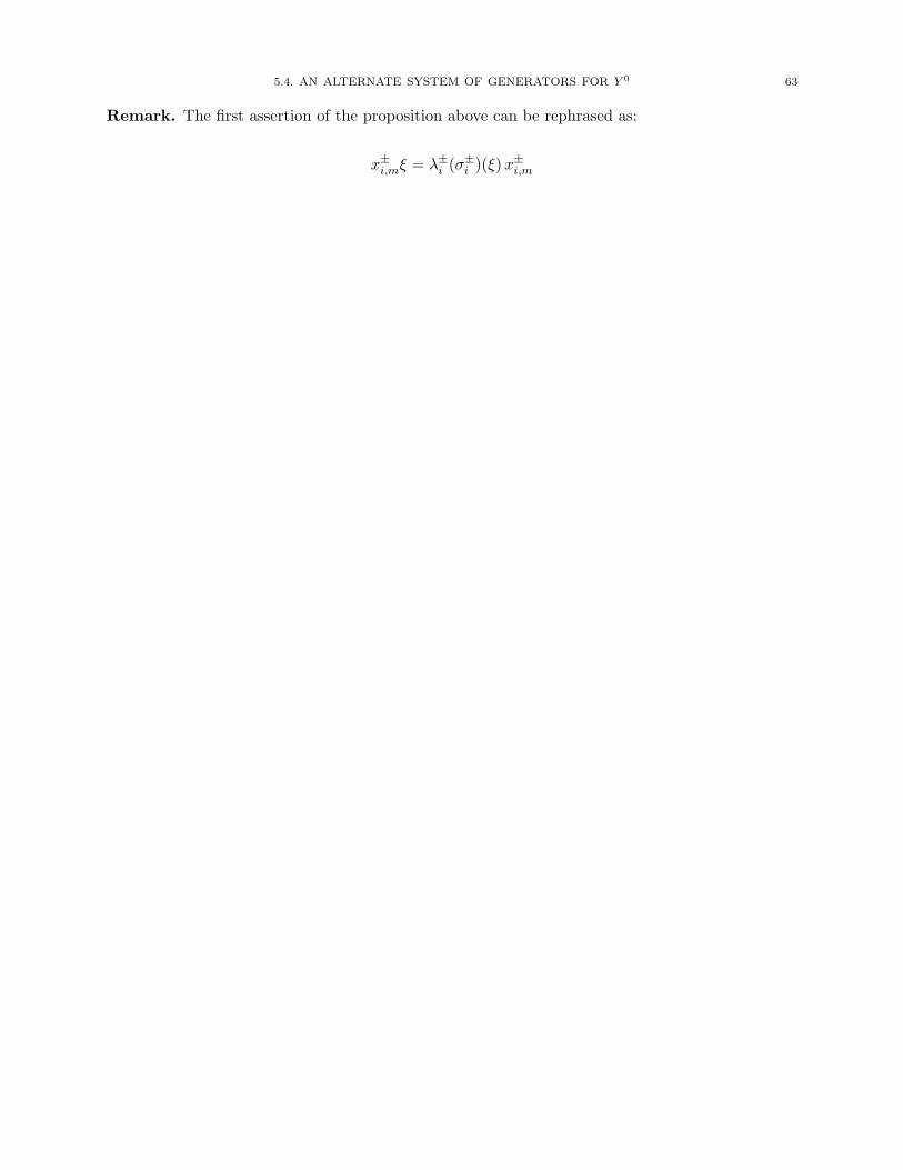
5.4. AN ALTERNATE SYSTEM OF GENERATORS FOR Y 0 63
Remark. The first assertion of the proposition above can be rephrased as:
x±i,mξ = λ±i (σ±i )(ξ)x
±i,m

CHAPTER 6
Construction of a homomorphism
Let Y�g be the completion of Y�(g) with respect to its N–grading. In this section, we define an
assignment
Φ : {Hi,r, Ei,r, Fi,r}i∈I,r∈Z −→ Y�g
and find necessary and sufficient conditions for Φ to extend to an algebra homomorphism U�(Lg)→Y�g.
6.1. Homomorphisms of geometric type
6.1.1. Definition of Φ0. Define
Φ(Hi,0) = d−1i ti,0
and, for r ∈ Z×
Φ(Hi,r) =Bi(r)
qi − q−1i
=�
qi − q−1i
∑k≥0
ti,krk
k!
where Bi(v) is the formal power series (5.4.2). The above assignment extends to an algebra homo-
morphism U0 → Y 0 which will be denoted by Φ0.
6.1.2. Definition of Φ. Let now {g±i,m}i∈I,m∈N be elements of Y 0 and define further
Φ(Ei,0) =∑m≥0
g+i,mx+i,m
Φ(Fi,0) =∑m≥0
g−i,mx−i,m
In terms of the shift operators σ±i , the above is equal to
Φ(Ei,0) = g+i (σ+i )x
+i,0 (6.1.1)
Φ(Fi,0) = g−i (σ−i )x
−i,0 (6.1.2)
64

6.1. HOMOMORPHISMS OF GEOMETRIC TYPE 65
where
g±i (v) =∑m≥0
g±i,mvm ∈ Y 0[v]
with the completion of Y 0[v] taken with respect to the N–grading which extends that on Y 0 by
deg(v) = 1.
If Φ : U�(Lg)→ Y�(g) is an algebra homomorphism of the above form, we shall say that it is of
of geometric type.
6.1.3. The following result shows that the requirement that Φ extends to an algebra homo-
morphism determines its value on generators Ei,k, Fi,k.
Proposition. The assignment Φ is compatible with relations (QL2)–(QL3) if, and only if
Φ(Ei,k) = ekσ+i g+i (σ
+i )x
+i,0 (6.1.3)
Φ(Fi,k) = ekσ−i g−i (σ
−i )x
−i,0 (6.1.4)
Proof. We only consider the case of the E′s. Let i, j ∈ I and k ∈ Z. By (Y2),
[Φ(Hi,0),Φ(Ej,k)] = [d−1i ξi,0, ekσ+
j g+j (σ+j )x
+j,0]
= ekσ+j g+j (σ
+j )[d
−1i ξi,0, x
+j,0]
= aijΦ(Ej,k)
so that Φ is compatible with (QL2). Next, if r ∈ Z×, Lemma 5.4.1 yields
[Φ(Hi,r),Φ(Ej,k)] =1
qi − q−1i
[Bi(r), ekσ+
j g+j (σ+j )x
+j,0]
=qraiji − q
−raiji
r(qi − q−1i )erσ
+j ekσ
+j g+j (σ
+j )x
+j,0
=[raij ]qi
rΦ(Ej,r+k)
and Φ is compatible with (QL3).
Conversely, if Φ is compatible with (QL3) then Φ(Ei,r) = r/[2r]qi [Hi,r, Ei,0] for r = 0 and the
computation above shows that this is equal to erσ+i Φ(Ei,0). �
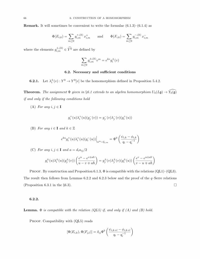
66 6. CONSTRUCTION OF A HOMOMORPHISM
Remark. It will sometimes be convenient to write the formulae (6.1.3)–(6.1.4) as
Φ(Ei,k) =∑m≥0
g+,(k)i,m x+i,m and Φ(Fi,k) =
∑m≥0
g−,(k)i,m x−i,m
where the elements g±,(k)i,m ∈ Y 0 are defined by
∑m≥0
g±,(k)i,m vm = ekvg±i (v)
6.2. Necessary and sufficient conditions
6.2.1. Let λ±i (v) : Y0 → Y 0[v] be the homomorphism defined in Proposition 5.4.2.
Theorem. The assignment Φ given in §6.1 extends to an algebra homomorphism U�(Lg)→ Y�(g)
if and only if the following conditions hold
(A) For any i, j ∈ I
g+i (u)λ+i (u)(g
−j (v)) = g−j (v)λ
−j (v)(g
+i (u))
(B) For any i ∈ I and k ∈ Z
ekug+i (u)λ+i (u)(g
−i (u))
∣∣∣um=ξi,m
= Φ0
(ψi,k − φi,k
qi − q−1i
)(C) For any i, j ∈ I and a = diaij/2
g±i (u)λ±i (u)(g
±j (v))
(eu − ev±a�
u− v ∓ a�
)= g±j (v)λ
±j (v)(g
±i (u))
(ev − eu±a�
v − u∓ a�
)Proof. By construction and Proposition 6.1.3, Φ is compatible with the relations (QL1)–(QL3).
The result then follows from Lemmas 6.2.2 and 6.2.3 below and the proof of the q–Serre relations
(Proposition 6.3.1 in the §6.3). �
6.2.2.
Lemma. Φ is compatible with the relation (QL5) if, and only if (A) and (B) hold.
Proof. Compatibility with (QL5) reads
[Φ(Ei,k),Φ(Fj,l)] = δijΦ0
(ψi,k+l − φi,k+l
qi − q−1i
)
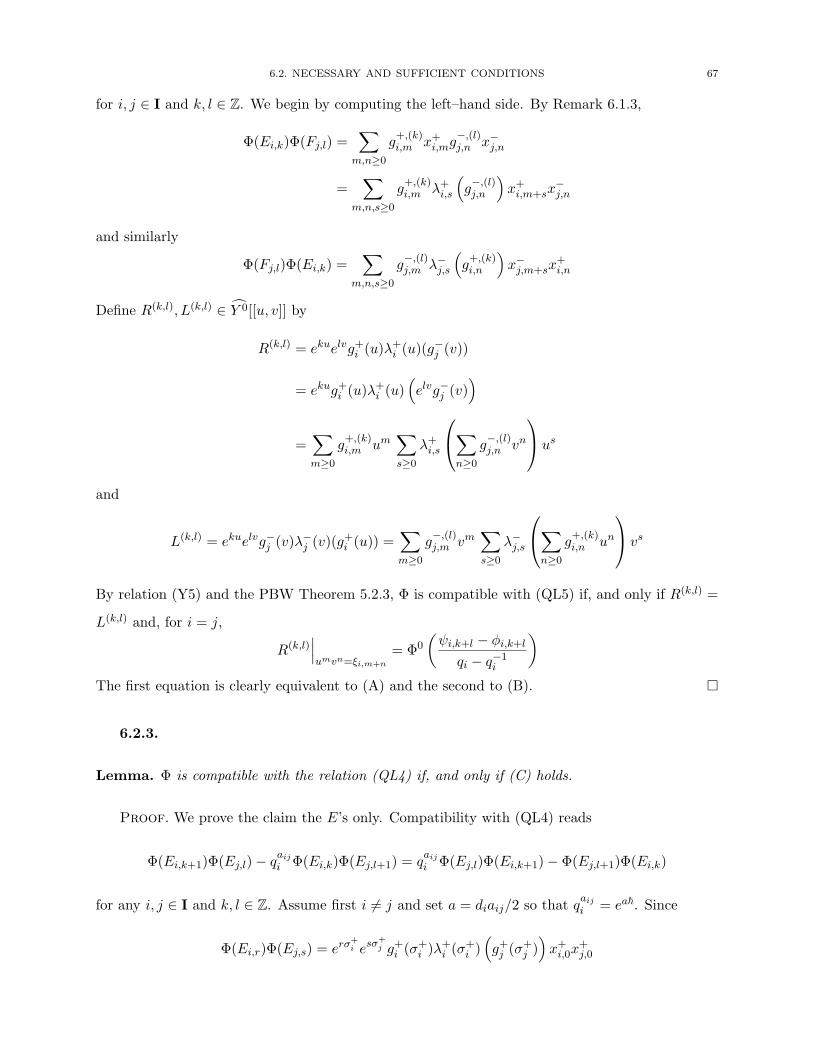
6.2. NECESSARY AND SUFFICIENT CONDITIONS 67
for i, j ∈ I and k, l ∈ Z. We begin by computing the left–hand side. By Remark 6.1.3,
Φ(Ei,k)Φ(Fj,l) =∑
m,n≥0g+,(k)i,m x+i,mg
−,(l)j,n x−j,n
=∑
m,n,s≥0g+,(k)i,m λ+
i,s
(g−,(l)j,n
)x+i,m+sx
−j,n
and similarly
Φ(Fj,l)Φ(Ei,k) =∑
m,n,s≥0g−,(l)j,m λ−j,s
(g+,(k)i,n
)x−j,m+sx
+i,n
Define R(k,l), L(k,l) ∈ Y 0[[u, v]] by
R(k,l) = ekuelvg+i (u)λ+i (u)(g
−j (v))
= ekug+i (u)λ+i (u)
(elvg−j (v)
)
=∑m≥0
g+,(k)i,m um
∑s≥0
λ+i,s
⎛⎝∑n≥0
g−,(l)j,n vn
⎞⎠us
and
L(k,l) = ekuelvg−j (v)λ−j (v)(g
+i (u)) =
∑m≥0
g−,(l)j,m vm
∑s≥0
λ−j,s
⎛⎝∑n≥0
g+,(k)i,n un
⎞⎠ vs
By relation (Y5) and the PBW Theorem 5.2.3, Φ is compatible with (QL5) if, and only if R(k,l) =
L(k,l) and, for i = j,
R(k,l)∣∣∣umvn=ξi,m+n
= Φ0
(ψi,k+l − φi,k+l
qi − q−1i
)The first equation is clearly equivalent to (A) and the second to (B). �
6.2.3.
Lemma. Φ is compatible with the relation (QL4) if, and only if (C) holds.
Proof. We prove the claim the E’s only. Compatibility with (QL4) reads
Φ(Ei,k+1)Φ(Ej,l)− qaiji Φ(Ei,k)Φ(Ej,l+1) = q
aiji Φ(Ej,l)Φ(Ei,k+1)− Φ(Ej,l+1)Φ(Ei,k)
for any i, j ∈ I and k, l ∈ Z. Assume first i = j and set a = diaij/2 so that qaiji = ea�. Since
Φ(Ei,r)Φ(Ej,s) = erσ+i esσ
+j g+i (σ
+i )λ
+i (σ
+i )
(g+j (σ
+j )
)x+i,0x
+j,0
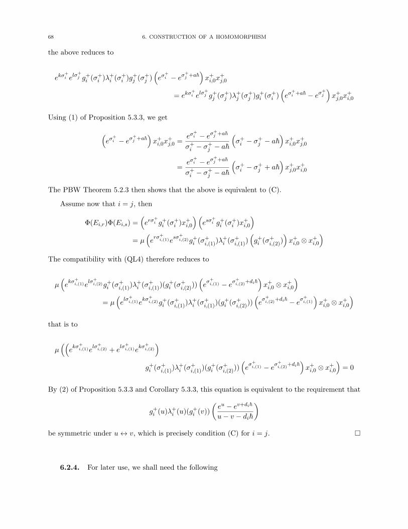
68 6. CONSTRUCTION OF A HOMOMORPHISM
the above reduces to
ekσ+i elσ
+j g+i (σ
+i )λ
+i (σ
+i )g
+j (σ
+j )
(eσ
+i − eσ
+j +a�
)x+i,0x
+j,0
= ekσ+i elσ
+j g+j (σ
+j )λ
+j (σ
+j )g
+i (σ
+i )
(eσ
+i +a� − eσ
+j
)x+j,0x
+i,0
Using (1) of Proposition 5.3.3, we get
(eσ
+i − eσ
+j +a�
)x+i,0x
+j,0 =
eσ+i − eσ
+j +a�
σ+i − σ+
j − a�
(σ+i − σ+
j − a�)x+i,0x
+j,0
=eσ
+i − eσ
+j +a�
σ+i − σ+
j − a�
(σ+i − σ+
j + a�)x+j,0x
+i,0
The PBW Theorem 5.2.3 then shows that the above is equivalent to (C).
Assume now that i = j, then
Φ(Ei,r)Φ(Ei,s) =(erσ
+i g+i (σ
+i )x
+i,0
)(esσ
+i g+i (σ
+i )x
+i,0
)= μ
(erσ+
i,(1)esσ+
i,(2)g+i (σ+i,(1))λ
+i (σ
+i,(1))
(g+i (σ
+i,(2))
)x+i,0 ⊗ x+i,0
)The compatibility with (QL4) therefore reduces to
μ(ekσ+
i,(1)elσ+
i,(2)g+i (σ+i,(1))λ
+i (σ
+i,(1))(g
+i (σ
+i,(2)))
(eσ+i,(1) − e
σ+i,(2)
+di�)x+i,0 ⊗ x+i,0
)= μ
(elσ+
i,(1)ekσ+
i,(2)g+i (σ+i,(1))λ
+i (σ
+i,(1))(g
+i (σ
+i,(2)))
(eσ+i,(2)
+di� − eσ+i,(1)
)x+i,0 ⊗ x+i,0
)that is to
μ((
ekσ+
i,(1)elσ+
i,(2) + elσ+
i,(1)ekσ+
i,(2)
)g+i (σ
+i,(1))λ
+i (σ
+i,(1))(g
+i (σ
+i,(2)))
(eσ+i,(1) − e
σ+i,(2)
+di�)x+i,0 ⊗ x+i,0
)= 0
By (2) of Proposition 5.3.3 and Corollary 5.3.3, this equation is equivalent to the requirement that
g+i (u)λ+i (u)(g
+i (v))
(eu − ev+di�
u− v − di�
)be symmetric under u↔ v, which is precisely condition (C) for i = j. �
6.2.4. For later use, we shall need the following
6.3. PROOF OF THE q–SERRE RELATIONS 69
Lemma. Let {g±i (u)}i∈I ⊂ Y 0[u] be elements satisfying condition (B) of Theorem 6.2.1. Then,
g±i (u) =1
d±imod Y 0[u]+
where {d±i }i∈I ⊂ C× satisfy d+i d−i = di for each i ∈ I. In particular, each g±i (u) is invertible.
Proof. Condition (B) for k = 0 yields
g+i (u)λ+i (u)
(g−i (u)
)∣∣um=ξi,m
= Φ0
(e
�di2
Hi,0 − e−�di2
Hi,0
qi − q−1i
)
Computing mod �, and a fortiori mod Y 0[u]+, yields
Φ0
(e
�di2
Hi,0 − e−�di2
Hi,0
qi − q−1i
)= Φ0 (Hi,0) = d−1i ti,0
Write g±i (u) = p±i mod Y 0[u]+, where p±i ∈ C[tj,0]j∈I. Computing mod Y 0[u]+, we get
g+i (u)λ+i (u)
(g−i (u)
)∣∣um=ξi,m
= p+i (tj,0)λ+i;0(p
−i (tj,0))ξi,0 = p+i (tj,0)p
−i (tj,0 − diaij)ξi,0
where we used (8) of Proposition 5.4.2. Comparing both sides and using ξi,0 = ti,0 yields the
claim. �
6.3. Proof of the q–Serre relations
6.3.1. The aim of this section is to prove the following
Proposition. Let Φ be the assignment {Ei,k, Fi,k, Hi,k} → Y�(g) given in §6.1 and assume that
the relations (A) and (B) of Theorem 6.2.1 hold. Then, Φ is compatible with the q–Serre relations
(QL6).
For i = j ∈ I, set m = 1− aij . Define, for any k = (k1, . . . , km) ∈ Zm and l ∈ Z
Sqij(k, l) =
∑π∈Sm
m∑s=0
(−1)s⎡⎣ m
s
⎤⎦qi
Φ(Ei,kπ(1)) · · ·Φ(Ei,kπ(m−s)
)Φ(Ej,l)
Φ(Ei,kπ(m−s+1)) · · ·Φ(Ei,kπ(m)
) ∈ Y�(g) (6.3.1)
70 6. CONSTRUCTION OF A HOMOMORPHISM
and let Sqij = Sq
ij(0, 0), explicitly given as follows
Sqij =
m∑s=0
(−1)s⎡⎣ m
s
⎤⎦qi
(Φ(Ei,0))m−sΦ(Ej,0) (Φ(Ei,0))
s (6.3.2)
Our aim is to show that Sqij(k, l) = 0. Let us outline the the main steps of the proof.
(1) We first reduce the proof of Sqij(k, l) = 0 to Sq
ij = 0. This is achieved in Lemma 6.3.5.
(2) By a standard argument using the representation theory of U�sl2, we deduce in Lemma
6.3.6 that Sqij acts by zero on any finite–dimensional representation of Y�(g).
(3) Finally, we show that these representations separate points in Y�(g), and hence that Sqij =
0. §6.3.8 and 6.3.9 are devoted to the proof of this fact (Corollary 6.3.9) which was
communicated to us by V. G. Drinfeld.
6.3.2. The algebra Y . Define an auxiliary algebra Y to be the unital, associative C[�]–algebra
generated by {ξi,r, xi,r}i∈I,r∈N subject to the following relations
(1) For every i, j ∈ I and r, s ∈ N
[ξi,r, ξj,s] = 0
(2) For every i, j ∈ I and s ∈ N
[ξi,0, xj,s] = diaijxj,s
(3) For every i, j ∈ I and r, s ∈ I
[ξi,r+1, xj,s]− [ξi,r, xj,s+1] =diaij�2
(ξi,rxj,s + xj,sξi,r)
We denote by Y0 ⊂ Y the commutative subalgebra generated by {ξi,r}i∈I,r∈N and by Y
>0
the subalgebra of Y generated by {xi,r}i∈I,r∈N. The latter is a free C[�]–algebra over this set of
generators. Moreover, by Corollary 5.2.3, Y ∼= Y0 ⊗ Y
>0.
6.3.3. The operators σi,(k) and σj. The algebra Y has a grading by the root lattice Q given
by
deg(ξi,r) = 0 and deg(xi,r) = αi
6.3. PROOF OF THE q–SERRE RELATIONS 71
Fix henceforth i = j ∈ I, set m = 1− aij and let Y mαi+αj be the homogeneous component of Y of
degree mαi + αj .
Define operators σj , σi,(k) on Y mαi+αj as follows. Since Y mαi+αj∼= Y
0 ⊗ Y>0mαi+αj
and Y>0
is
free, we have
Y>0mαi+αj
∼= Y0 ⊗
m⊕s=0
Y (i)⊗m−s ⊗ Y (j)⊗ Y (i)⊗s
where, for a = i, j, Y (a) = Y>0αa
is spanned by {xa,r}r∈N. Let σa denote the C[�]–linear map on
Y (a) given by σa(xa,r) = xa,r+1. For any k = 1, . . . ,m, define the Y 0–linear operator σi,(k) on
Y mαi+αj by letting it act on the summand Y (i)⊗m−s ⊗ Y (j)⊗ Y⊗s(i) as
σi,(k) =
⎧⎨⎩ 1⊗k−1 ⊗ σi ⊗ 1⊗m+1−k if k ≤ m− s
1⊗k ⊗ σi ⊗ 1⊗m−k otherwise
Similarly, let σj ∈ EndY 0(Y mαi+αj ) be given by 1⊗m−s ⊗ σj ⊗ 1⊗s on Y (i)⊗m−s ⊗ Y (j)⊗ Y (i)⊗s.
6.3.4. The projection pij. Let p : Y → Y�(g) be the algebra homomorphism obtained by
sending ξa,r �−→ ξa,r and xa,r �−→ x+a,r for every a ∈ I and r ∈ N, and let pij be the restriction of p
to Y mαi+αj . The following holds by Proposition 5.3.3.
Lemma. The kernel of pij is the C[�]–linear span of the following elements
(1) For any 0 ≤ s ≤ m− 1 and A(u1, . . . , um, w) ∈ Y0[u1, . . . , um, w]
A(σi,(1), . . . , σi,(m), σj)((σi,(m−s) − σj − a�)xm−si,0 xj,0x
si,0
− (σi,(m−s) − σj + a�)xm−s−1i,0 xj,0xs+1i,0
)where a = diaij/2.
(2) For any 0 ≤ s ≤ m, k ∈ {1, . . . ,m−1}\{m−s} and A(u1, . . . , um, w) ∈ Y0[u1, . . . , um, w](k k+1)
A(σi,(1), . . . , σi,(m), σj)(σi,(k) − σi,(k+1) − di�)xm−si,0 xj,0x
si,0
(3) For every A(u1, . . . , um, w) ∈ Y0[u1, . . . , um, w]Sm
A(σi,(1), . . . , σi,(m), σj)
⎛⎝ m∑s=0
(−1)s⎛⎝ m
s
⎞⎠xm−si,0 xj,0xsi,0
⎞⎠
72 6. CONSTRUCTION OF A HOMOMORPHISM
Corollary. Let X ∈ Ker(pij) and A(u1, . . . , um, w) ∈ Y0[u1, . . . , um, w]Sm. Then,
A(σi,(1), . . . , σi,(m), σj)X ∈ Ker(pij)
6.3.5. Reduction step. Let Sqij(k, l),Sq
ij denote the elements of Y mαi+αj defined by the same
expressions as (6.3.1)–(6.3.2). Then,
Sqij(k, l) =
( ∑π∈Sm
ekπ(1)σi,(1) · · · ekπ(m)σi,(m)elσj
)Sqij
Using Corollary 6.3.4, we obtain the following
Lemma. Sqij = 0 implies Sq
ij(k, l) = 0 for every k1, · · · , km, l ∈ Z.
6.3.6. By a finite–dimensional representation of Y�(g) we shall mean a finitely–generated
topologically free C[[�]]–module endowed with a C[[�]]–linear action of Y�(g).
Lemma. Let V be a finite–dimensional representation of Y�(g). Then, Sqij acts by zero on V.
Proof. Let Ui be the subalgebra of Y�(g) generated by
Ei = Φ(Ei,0) Fi = Φ(Fi,0) Hi = Φ(Hi,0)
By Lemma 6.2.2, {Ei,Fi,Hi} satisfy the defining relations of the quantum group U�isl2, where
�i = di�/2. We use the following notation of q–adjoint operator (see [28, §4.18]) which gives a
representation of Ui on any algebra containing it
adq(Ei)(X) = EiX −KiXK−1i Ei
adq(Fi)(X) = FiXKi −XFiKi
adq(Hi)(X) = [Hi, X]
where Ki = qHii = e�iHi . Let ρ : Y�(g)→ End(V) be the representation. Then,
adq(ρ(Fi))ρ(Ej) = 0
adq(ρ(Hi))ρ(Ej) = aijρ(Ej)
6.3. PROOF OF THE q–SERRE RELATIONS 73
where the first identity follows from Lemma 6.2.2. Thus, as a Ui–module, End(V) contains thelowest weight vector ρ(Ej) of weight aij . By the representation theory of U�isl2, we get
adq(ρ(Ei))mρ(Ej) = ρ (adq(Ei)mEj) = 0
and the assertion follows from the well–known identity (see [28, Lemma 4.18])
adq(Ei)mEj =m∑s=0
(−1)s⎡⎣ m
s
⎤⎦qi
Em−si EjEsi
�
6.3.7. Let I� ⊂ Y�(g) be the ideal defined by
I� =⋂(V,ρ)
Ker(ρ)
where V runs over all finite–dimensional graded modules over Y�(g), that is finitely–generated
torsion–free C[�]–modules admitting a C[�]–linear action ρ : Y�(g) → End(V) and a Z–grading
compatible with that on Y�(g).
Lemma. I� = 0 implies Sqij = 0.
Proof. The action of Y�(g) on any finite–dimensional graded module V extends to one of Y�(g)on the completion V of V with respect to its grading. By Lemma 6.3.6, Sq
ij acts by 0 on V and
therefore so do its homogeneous components Sqij;n ∈ Y�(g), n ≥ 0 on V. Thus, Sq
ij;n ∈ I� for any n
and Sqij = 0. �
6.3.8. The following result, and its proof are due to V. Drinfeld [14]
Proposition. The ideal I� ⊂ Y�(g) is trivial.
Proof. It suffices to show that I = I�/�I� is trivial. Indeed, if I� = �I�, then I� =⋂
k �kI� ⊂⋂
k �kY�(g) = 0. By definition of I�, I� ∩ �Y�(g) = �Y�(g) so that I embeds into Y�(g)/�Y�(g) =
U(g[s]). Since graded representations are stable under tensor product, I� is a Hopf ideal of Y�(g),
that is
Δ(I�) ⊂ Y�(g)⊗ I� + I� ⊗ Y�(g)

74 6. CONSTRUCTION OF A HOMOMORPHISM
It follows that I is a co–Poisson Hopf ideal of U(g[s]). By Corollary 6.3.9 below, any such ideal
is either trivial or equal to U(g[s]). Since Y�(g) possesses non–trivial finite–dimensional graded
representations, for example the action on C[�] given by the counit, I� is a proper ideal of Y�(g)
and is therefore equal to zero. �
6.3.9. Recall that a co–Poisson Hopf algebra A is a Hopf algebra together with a Poisson
cobracket δ : A→ A ∧A satisfying the following compatibility condition (see [6, §6.2] for details):
δ(xy) = δ(x)Δ(y) + Δ(x)δ(y)
For a Lie algebra a, there is a one to one correspondence between co–Poisson structures on Ua and
Lie bialgebra structures on a [6, Proposition 6.2.3]. Moreover, there is a one to one correspondence
between co–Poisson Hopf ideals of Ua and Lie bialgebra ideals of a.
The Lie bialgebra structure on g[s] is given by:
δ : g[s]→ g[s]⊗ g[s] ∼= (g⊗ g)[s, t] (6.3.3)
δ(f)(s, t) = (ad(f(s))⊗ 1 + 1⊗ ad(f(t)))
(Ω
s− t
)(6.3.4)
where Ω ∈ g⊗ g is the Casimir tensor. Note that δ lowers the degree by 1.
Let a ⊂ g[s] be the Lie bialgebra ideal corresponding to co–Poisson Hopf ideal I ⊂ U(g[s]). By
the discussion given in previous paragraph,
δ(a) ⊂ a⊗ g[s] + g[s]⊗ a (6.3.5)
Lemma. Let a ⊂ g[s] be an ideal. Then a is of the form a = g⊗gC[s] for some polynomial g ∈ C[s].
Proof. Let S ⊂ C[s] be the set of all polynomials f such that there exists some non zero x ∈ g
for which x⊗ f ∈ a. We claim that S is an ideal of C[s]. Let f ∈ S and g ∈ C[s]. Let 0 = x ∈ g be
such that x⊗ f ∈ a, and choose y ∈ g such that [x, y] = 0. Then
[x, y]⊗ fg = [x⊗ f, y ⊗ g] ∈ a
and hence fg ∈ S.
6.3. PROOF OF THE q–SERRE RELATIONS 75
Now for any f ∈ S, the set {x ∈ g : x ⊗ f ∈ a} is an ideal in g, which is non–zero and hence
equal to g. This proves that a = g ⊗ S. Since C[s] is a principal ideal domain, the lemma is
proved. �
Corollary. Let a ⊂ g[s] be a Lie bialgebra ideal. Then either a = 0 or a = g[s].
Proof. Let g ∈ C[s] be such that a = g⊗(g) ⊂ g[s]. By (6.3.3), we know that the Lie cobracket
δ lowers the degree by 1. Using (6.3.5), we conclude that g is a constant polynomial. �

CHAPTER 7
Existence and uniqueness
7.1. Universal Drinfeld polynomials
Until §7.2, we assume that g = sl2 so that |I| = 1, aii = 2 and di = 1. To simplify notations,
we drop the subscript i ∈ I. In particular, the generators of U0 will be denoted by {Hr}r∈Z and
{ψr, φ−r}r∈N and those of Y 0 by {tr}r∈N and {ξr}r∈N.
7.1.1. Universal Drinfeld polynomials. Fix an integer m ≥ 1. Following [39] and [53],
consider the rings
S(m) = C[q±1, A±11 , . . . , A±1m ]Sm
R(m) = C[�, a1, . . . , am]Sm
Define a homomorphism DU : U0 → S(m) by
DU (ψ(z)) =
m∏i=1
qz − q−1Ai
z −Ai= DU (φ(z)) (7.1.1)
where the first (resp. second) equality is obtained by expanding the middle term in powers of z−1
and (resp. z). Similarly, define a homomorphism DY : Y 0 → R(m) by
DY (ξ(u)) =
m∏i=1
u+ �− aiu− ai
(7.1.2)
Remark. The homomorphism DU (resp. DY ) gives the action of ψ(z), φ(z) (resp. ξ(u)) on the
highest weight vector of the indecomposable simple U�(Lsl2) (resp. Y�(sl2)) module with Drinfeld
polynomial (1−A1z) · · · (1−Amz) (resp. (u− a1) · · · (u− am)).
7.1.2. The following result spells out the image of the generators of U0 and Y 0 under DU and
DY respectively.
Proposition.
76
7.1. UNIVERSAL DRINFELD POLYNOMIALS 77
(1) The homomorphism DU maps H0 to m and, for any r ∈ N∗,
DU (ψr) = (q − q−1)m∑i=1
Ari
∏j �=i
qAi − q−1Aj
Ai −Aj(7.1.3)
DU (φ−r) = −(q − q−1)m∑i=1
A−ri
∏j �=i
qAi − q−1Aj
Ai −Aj(7.1.4)
Moreover, for any r ∈ Z∗,
DU ((q − q−1)Hr) =1− q−2r
r
m∑i=1
Ari (7.1.5)
(2) The homomorphism DY maps ξ0 to m and, for any r ∈ N∗
DY (ξr) =
m∑i=1
ari∏j �=i
ai − aj + �ai − aj
(7.1.6)
Moreover, for any r ∈ N,
DY (tr) =1
r + 1
m∑i=1
ar+1i − (ai − �)r+1
�(7.1.7)
(3) If B(v) ∈ Y 0[[v]] is the series defined by (5.4.2), then
DY (B(v)) =1− e−�v
v
m∑i=1
eaiv (7.1.8)
Proof. (1) The fact that DU (H0) = m follows by evaluating the middle term in (7.1.1) at
z = 0. The partial fraction decomposition of this term is readily seen to be
m∏i=1
qz − q−1Ai
z −Ai= qm + (q − q−1)
m∑i=1
Ai
⎛⎝∏j �=i
qAi − q−1Aj
Ai −Aj
⎞⎠ 1
z −Ai
The relations (7.1.3)–(7.1.4) follow by expanding this into positive and negative powers of z respec-
tively. Since DU (ψ0) = qm, we get
DU
⎛⎝exp⎛⎝(q − q−1)
∑s≥1
Hsz−s
⎞⎠⎞⎠ = DU (ψ−10 ψ(z)) =
m∏i=1
z − q−2Ai
z −Ai
taking the log of both sides and expanding in powers of z−1 yields (7.1.5) for r > 0. The case r < 0
follows by expanding in powers of z.
78 7. EXISTENCE AND UNIQUENESS
(2) The fact that DY (ξ0) = n follows by taking the coefficient of u−1 in (7.1.2). The partial
fraction decomposition of DY (ξ(u)) is
m∏i=1
u+ �− aiu− ai
= 1 + �m∑i=1
⎛⎝∏j �=i
ai − aj + �ai − aj
⎞⎠ 1
u− ai
and (7.1.6) follows by taking the coefficient of u−r−1. Taking the log of both sides of (7.1.2) yields
DY (t(u)) =∑i
− log (1− aiu−1)+ log
(1− (ai − �)u−1
)(7.1.9)
and therefore (7.1.7).
(3) The equation (7.1.8) follows by applying (5.4.3) to (7.1.2). �
Corollary. The homomorphism Y 0 →⊕m≥1R(m) is injective.
Proof. This follows from (7.1.7) and the fact that the power sums pr =∑
i ari are algebraically
independent. �
7.1.3. Let R(m) be the completion of R(m) with respect to the N–grading defined by deg(�) =
deg(ai) = 1. Since the map DY : Y 0 → R(m) preserves the grading, it extends to a homomorphism
Y 0 → R(m).
Corollary. Let ch : S(m)→ R(m) be the algebra homomorphism defined by
q �−→ e�/2 and Ai �−→ eai
Then the following diagram commutes
U0DU
��
Φ0
��
S(m)
ch��
Y 0DY
�� R(m)
where Φ0 is defined in §6.1.1.
Proof. It suffices to check the commutativity on the generators {Hr}r∈Z of U0. The statement
now follows from (7.1.5), (7.1.8) and the fact that, for r = 0, Φ0(Hr) = B(v)/(q − q−1)∣∣v=r
. �
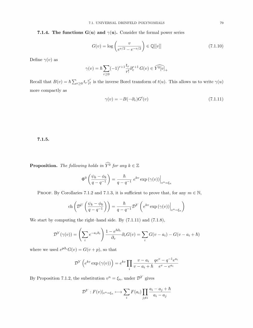
7.1. UNIVERSAL DRINFELD POLYNOMIALS 79
7.1.4. The functions G(u) and γ(u). Consider the formal power series
G(v) = log
(v
ev/2 − e−v/2
)∈ Q[[v]] (7.1.10)
Define γ(v) as
γ(v) = �∑r≥0
(−1)r+1 trr!∂r+1v G(v) ∈ Y 0[v]+
Recall that B(v) = �∑
r≥0 trvr
r! is the inverse Borel transform of t(u). This allows us to write γ(u)
more compactly as
γ(v) = −B(−∂v)G′(v) (7.1.11)
7.1.5.
Proposition. The following holds in Y 0 for any k ∈ Z
Φ0
(ψk − φk
q − q−1
)=
�q − q−1
ekv exp (γ(v))∣∣∣vn=ξn
Proof. By Corollaries 7.1.2 and 7.1.3, it is sufficient to prove that, for any m ∈ N,
ch
(DU
(ψk − φk
q − q−1
))=
�q − q−1
DY
(ekv exp (γ(v))
∣∣∣vn=ξn
)We start by computing the right–hand side. By (7.1.11) and (7.1.8),
DY (γ(v)) =
(∑i
e−ai∂v)1− e�∂v
∂v∂vG(v) =
∑i
G(v − ai)−G(v − ai + �)
where we used ep∂vG(v) = G(v + p), so that
DY(ekv exp (γ(v))
)= ekv
∏i
v − aiv − ai + �
qev − q−1eai
ev − eai
By Proposition 7.1.2, the substitution vn = ξn, under DY gives
DY : F (v)|vn=ξn �−→∑i
F (ai)∏j �=i
ai − aj + �ai − aj

80 7. EXISTENCE AND UNIQUENESS
which in our case implies that
DY
(ekv exp (γ(v))
∣∣∣vn=ξn
)=
q − q−1
�
∑i
ekai∏j �=i
ai − ajai − aj + �
qeai − q−1eaj
eai − eajai − aj + �ai − aj
=q − q−1
�ch
⎛⎝∑i
Aki
∏j �=i
qAi − q−1Aj
Ai −Aj
⎞⎠and we are done by (7.1.3)–(7.1.4) if k = 0. The lemma below and the fact that DU (ψ0) = qm
settles the case k = 0. �
Lemma. The following holds for any m ≥ 1,
m∑i=1
∏j �=i
qAi − q−1Aj
Ai −Aj= [m]q
Proof. Let F (z) =1
z
∏i
qz − q−1Ai
z −Ai. The partial fraction decomposition of F is
F (z) =q−m
z+ (q − q−1)
∑i
⎛⎝∏j �=i
qAi − q−1Aj
Ai −Aj
⎞⎠ 1
z −Ai
Multiplying both sides by z and letting z →∞ we get
qm = q−m + (q − q−1)m∑i=1
∏j �=i
qAi − q−1Aj
Ai −Aj
as claimed. �
7.2. Existence of a solution
We return now to the case of a semisimple Lie algebra g of arbitrary rank.
7.2.1. Let G(v) be the formal power series defined in §7.1.4 and, for any i ∈ I define γi(v) ∈Y 0[v]+ by
γi(v) = −Bi(−∂v)G′(v) = �∑r≥0
(−1)r+1 ti,rr!
∂r+1v G(v)
Let gi(v) ∈ Y 0[v]×be given by
gi(v) =
(�
qi − q−1i
) 12
exp
(γi(v)
2
)(7.2.1)
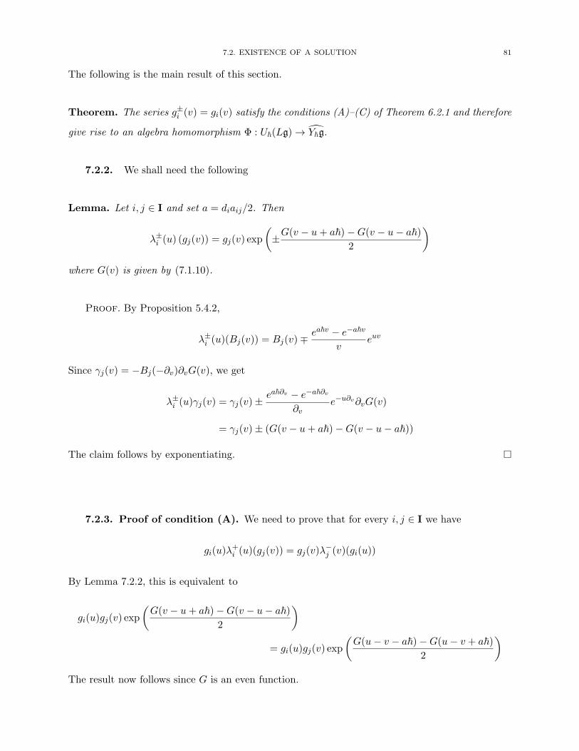
7.2. EXISTENCE OF A SOLUTION 81
The following is the main result of this section.
Theorem. The series g±i (v) = gi(v) satisfy the conditions (A)–(C) of Theorem 6.2.1 and therefore
give rise to an algebra homomorphism Φ : U�(Lg)→ Y�g.
7.2.2. We shall need the following
Lemma. Let i, j ∈ I and set a = diaij/2. Then
λ±i (u) (gj(v)) = gj(v) exp
(±G(v − u+ a�)−G(v − u− a�)
2
)where G(v) is given by (7.1.10).
Proof. By Proposition 5.4.2,
λ±i (u)(Bj(v)) = Bj(v)∓ ea�v − e−a�v
veuv
Since γj(v) = −Bj(−∂v)∂vG(v), we get
λ±i (u)γj(v) = γj(v)± ea�∂v − e−a�∂v
∂ve−u∂v∂vG(v)
= γj(v)± (G(v − u+ a�)−G(v − u− a�))
The claim follows by exponentiating. �
7.2.3. Proof of condition (A). We need to prove that for every i, j ∈ I we have
gi(u)λ+i (u)(gj(v)) = gj(v)λ
−j (v)(gi(u))
By Lemma 7.2.2, this is equivalent to
gi(u)gj(v) exp
(G(v − u+ a�)−G(v − u− a�)
2
)= gi(u)gj(v) exp
(G(u− v − a�)−G(u− v + a�)
2
)The result now follows since G is an even function.
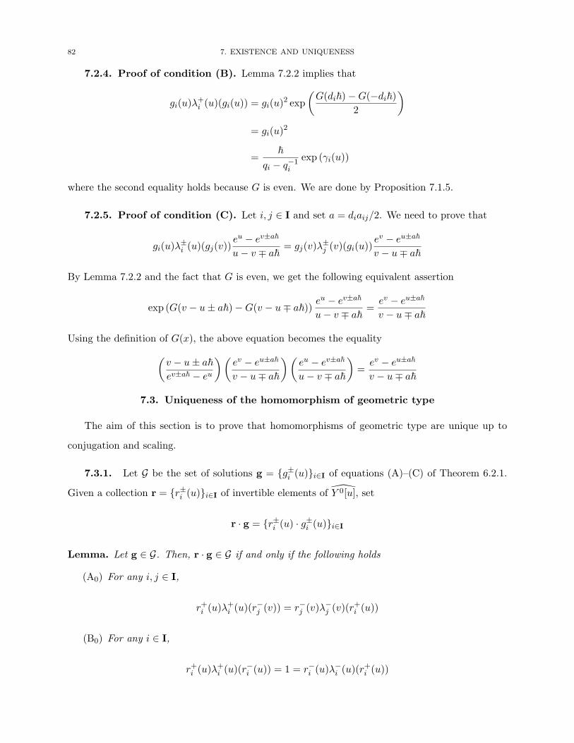
82 7. EXISTENCE AND UNIQUENESS
7.2.4. Proof of condition (B). Lemma 7.2.2 implies that
gi(u)λ+i (u)(gi(u)) = gi(u)
2 exp
(G(di�)−G(−di�)
2
)= gi(u)
2
=�
qi − q−1i
exp (γi(u))
where the second equality holds because G is even. We are done by Proposition 7.1.5.
7.2.5. Proof of condition (C). Let i, j ∈ I and set a = diaij/2. We need to prove that
gi(u)λ±i (u)(gj(v))
eu − ev±a�
u− v ∓ a�= gj(v)λ
±j (v)(gi(u))
ev − eu±a�
v − u∓ a�
By Lemma 7.2.2 and the fact that G is even, we get the following equivalent assertion
exp (G(v − u± a�)−G(v − u∓ a�))eu − ev±a�
u− v ∓ a�=
ev − eu±a�
v − u∓ a�
Using the definition of G(x), the above equation becomes the equality(v − u± a�ev±a� − eu
)(ev − eu±a�
v − u∓ a�
)(eu − ev±a�
u− v ∓ a�
)=
ev − eu±a�
v − u∓ a�
7.3. Uniqueness of the homomorphism of geometric type
The aim of this section is to prove that homomorphisms of geometric type are unique up to
conjugation and scaling.
7.3.1. Let G be the set of solutions g = {g±i (u)}i∈I of equations (A)–(C) of Theorem 6.2.1.
Given a collection r = {r±i (u)}i∈I of invertible elements of Y 0[u], set
r · g = {r±i (u) · g±i (u)}i∈I
Lemma. Let g ∈ G. Then, r · g ∈ G if and only if the following holds
(A0) For any i, j ∈ I,
r+i (u)λ+i (u)(r
−j (v)) = r−j (v)λ
−j (v)(r
+i (u))
(B0) For any i ∈ I,
r+i (u)λ+i (u)(r
−i (u)) = 1 = r−i (u)λ
−i (u)(r
+i (u))
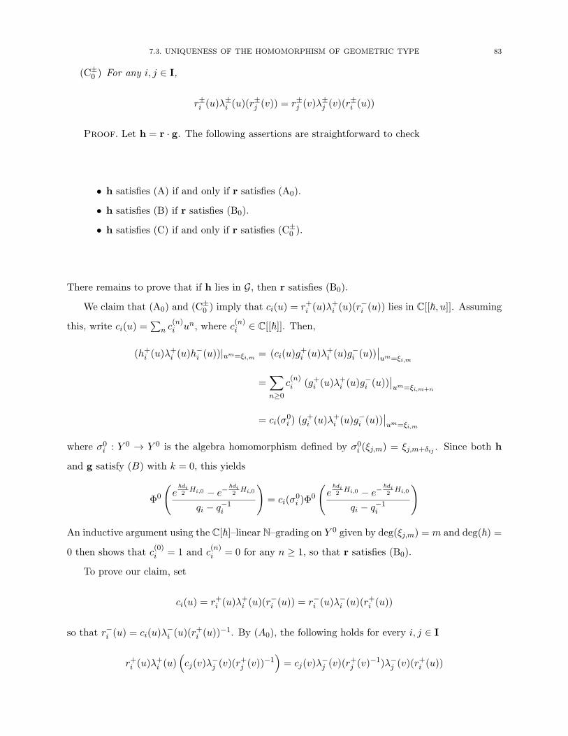
7.3. UNIQUENESS OF THE HOMOMORPHISM OF GEOMETRIC TYPE 83
(C±0 ) For any i, j ∈ I,
r±i (u)λ±i (u)(r
±j (v)) = r±j (v)λ
±j (v)(r
±i (u))
Proof. Let h = r · g. The following assertions are straightforward to check
• h satisfies (A) if and only if r satisfies (A0).
• h satisfies (B) if r satisfies (B0).
• h satisfies (C) if and only if r satisfies (C±0 ).
There remains to prove that if h lies in G, then r satisfies (B0).
We claim that (A0) and (C±0 ) imply that ci(u) = r+i (u)λ
+i (u)(r
−i (u)) lies in C[[�, u]]. Assuming
this, write ci(u) =∑
n c(n)i un, where c
(n)i ∈ C[[�]]. Then,
(h+i (u)λ+i (u)h
−i (u))|um=ξi,m = (ci(u)g
+i (u)λ
+i (u)g
−i (u))
∣∣um=ξi,m
=∑n≥0
c(n)i (g+i (u)λ
+i (u)g
−i (u))
∣∣um=ξi,m+n
= ci(σ0i ) (g
+i (u)λ
+i (u)g
−i (u))
∣∣um=ξi,m
where σ0i : Y
0 → Y 0 is the algebra homomorphism defined by σ0i (ξj,m) = ξj,m+δij . Since both h
and g satisfy (B) with k = 0, this yields
Φ0
(e
�di2
Hi,0 − e−�di2
Hi,0
qi − q−1i
)= ci(σ
0i )Φ
0
(e
�di2
Hi,0 − e−�di2
Hi,0
qi − q−1i
)
An inductive argument using the C[�]–linear N–grading on Y 0 given by deg(ξj,m) = m and deg(�) =
0 then shows that c(0)i = 1 and c
(n)i = 0 for any n ≥ 1, so that r satisfies (B0).
To prove our claim, set
ci(u) = r+i (u)λ+i (u)(r
−i (u)) = r−i (u)λ
−i (u)(r
+i (u))
so that r−i (u) = ci(u)λ−i (u)(r
+i (u))
−1. By (A0), the following holds for every i, j ∈ I
r+i (u)λ+i (u)
(cj(v)λ
−j (v)(r
+j (v))
−1)= cj(v)λ
−j (v)(r
+j (v)
−1)λ−j (v)(r+i (u))
84 7. EXISTENCE AND UNIQUENESS
Since λ+i (u) and λ−j (v) commute, we get
λ+i (u)(cj(v))
(r+i (u)λ
−j (v)(r
+j (v))
)= cj(v)λ
−j (v)
(r+i (u)λ
+i (u)(r
+j (v))
)= cj(v)λ
−j (v)
(r+j (v)λ
+j (v)(r
+i (u))
)= cj(v)
(r+i (u)λ
−j (v)(r
+j (v))
)where the second equality uses (C+
0 ) and the third one λ−j (v)λ
+j (v) = 1. We have therefore proved
that
λ+i (u)(cj(v)) = cj(v) for every i, j ∈ I
By definition of the operators λ±i , this implies that the coefficients of cj(v) lie in the center of Y�(g),
which is trivial. �
7.3.2. The uniqueness of homomorphisms of geometric type relies on the following
Proposition. Let {r+i (u)}i∈I ⊂ 1+Y 0[u]+ be a collection of invertible elements satisfying condition
(C+0 ) of Lemma 7.3.1. Then, there exists an element ξ ∈ 1 + Y 0
+ such that, for any i ∈ I
r+i (u) = ξ · λ+i (u)(ξ)
−1
Moreover, if ζ ∈ Y 0×
is any element such that r+i (u) = ζ · λ+i (u)(ζ)
−1 then ζ = c(�)ξ for some
c(�) ∈ C[[�]]×.
The proof of Proposition 7.3.2 is given in §7.3.3–§7.3.9.
7.3.3. We begin by linearising the problem. Set
ri(u) = log(ri(u)) ∈ Y 0[u]+
By condition (C+0 ), the following holds for any i, j ∈ I
(λ+i (u)− 1)(rj(v)) = (λ+
j (v)− 1)(ri(u)) (7.3.1)
and we need to show that
ri(u) = (λ+i (u)− 1)η (7.3.2)
for some η ∈ Y 0+.
7.3. UNIQUENESS OF THE HOMOMORPHISM OF GEOMETRIC TYPE 85
7.3.4. Rank 1 case. We assume first that |I| = 1 and accordingly drop the subscript i from
our formulae. We shall prove (7.3.2) by working with an adapted system of generators of Y 0.
Recall that, by Proposition 5.4.2,
(λ+(u)− 1)B(v) = −e�v − e−�v
veuv
Define B′(v) =∑k≥0
vk
k!t′k by equating the coefficients of v in
B′(v) = − v
e�v − e−�vBt(v) = − �v
e�v − e−�v∑n≥0
vn
n!tn
The elements {t′k}k∈N give another system of generators of Y 0 which are homogeneous, with
deg(t′k) = k = deg(tk) for any k ∈ N, and satisfy
λ+(u)(t′k) = t′k + uk (7.3.3)
7.3.5. Since the operator λ+(u) : Y 0 → Y 0[u] is homogeneous with respect to the N–grading
extending that on Y 0 by deg(u) = 1, it suffices to prove (7.3.2) when r(u) is homogeneous of degree
n ∈ N. Moreover, since λ+(u) is C[�]–linear and the formulae (7.3.3) do not involve �, we may
further assume that the coefficients of r(u) lie in the C–subalgebra Y 0 ⊂ Y 0 generated by the {t′k}.An element of Y 0[u]n has the form
r(u) =∑|μ|≤n
aμt′μu
n−|μ| (7.3.4)
where aμ ∈ C[t′0] and, for a partition μ of length l, we define t′μ = t′μ1· · · t′μl
. The proof of the
existence of η ∈ Y 0n such that (λ
+(u)− 1)(η) = r(u) proceeds in two steps:
(1) Show that, modulo elements of the form (λ+(u)− 1)(η),
r(u) =∑|μ|<n
aμt′μu
n−|μ| (7.3.5)
where aμ ∈ C do not depend on t′0.
(2) Show that any r(u) of the form (7.3.5) is equal to (λ+(u)− 1)(η) for some η ∈ Y 0n.
86 7. EXISTENCE AND UNIQUENESS
7.3.6. Proof of (1). For r(u) ∈ Y 0n of the form (7.3.4), choose bν ∈ C[t′0] for every ν � n
such that
bν(t′0 + 1)− bν(t
′0) = aν(t
′0)
Then
r(u)− (λ+(u)− 1)
(∑ν n
bνt′ν
)=
∑|μ|<n
a′μt′μu
n−|μ|
for some a′μ ∈ C[t′0], so that we may assume that r(u) is of the form (7.3.4) with aμ = 0 for any
μ � n.
Write now
(λ+(v)− 1)r(u)
=∑|μ|<n
(aμ(t0 + 1)− aμ(t0)) t′μu
n−|μ| +∑|μ|<n
aμ(t0 + 1)
⎛⎝∑ν�μ
c(ν, μ)t′νv|μ|−|ν|
⎞⎠un−|μ|
where c(ν, μ) is the number of ways of obtaining ν by removing rows from μ. By (7.3.1), the above
expression is symmetric in u and v. Its value at u = 0, which is 0, must therefore equal its value
at v = 0, thus leading to ∑|μ|<n
(aμ(t0 + 1)− aμ(t0)) t′μu
n−|μ| = 0
which implies that aμ ∈ C for any μ.
7.3.7. Proof of (2). Let r(u) be of the form (7.3.5). For any 0 ≤ l ≤ n, write
rl(u) =∑|μ|<nl(μ)=l
aμt′μu
n−|μ|
so that r(u) =∑
l rl(u). We proceed by induction on the largest positive integer k such that
rk(u) = 0. If k = 0, then r(u) = cun = (λ+(u)− 1)(ct′n).
Assume now that k > 0 and let D(u) : Y 0 → Y 0[u] be the differential operator D(u) =∑m≥1 u
m∂t′m . Since (λ+(u)− 1)(t′k) = uk we get, for any partition μ
(λ+(u)− 1)(t′μ) = D(u)(t′μ) + terms of smaller length
Thus, (7.3.1) implies that
D(u)rk(v) = D(v)rk(u)
7.3. UNIQUENESS OF THE HOMOMORPHISM OF GEOMETRIC TYPE 87
This cross–derivative condition implies the existence of η ∈ Y 0n such that rk(u) = D(u)η. This
implies that r(u)− (λ+(u)− 1)(η) has smaller k.
This completes the proof of the existence part of Proposition 7.3.2 when g is of rank 1.
7.3.8. Arbitrary rank. The argument for arbitrary g rests on the following
Lemma. There exist generators {�i,r}i∈I,r∈N of Y 0 which are homogeneous, with deg(�i,r) = r
and such that
λ±i (u)�j,r = �j,r ± δi,jur
Proof. By Proposition 5.4.2, the generating series Bj(v) = �∑
r≥0 tj,rvr/r! satisfy
(λ±i (u)− 1)�−1Bj(v) = ∓Qij(v)euv
where Qij(v) = 2 sinh(�diaijv/2)/�v. Since Qij = diaij mod �, the matrix Q = (Qij) is invertible.
Set B′i(v) = −�−1∑
j Q−1ij Bj(v). Then (λ
±i (u)−1)B′j(v) = ±δijeuv which, in terms of the expansion
B′i(v) =∑
�i,rvr/r! yields the required transformation property.
Since deg(v) = 1, the homogeneity of the �i,r is equivalent to Ad(ζ)(B′i(v)) = B′i(ζ
2v) where
Ad(ζ) denotes the action of ζ ∈ C× on Y�(g)[[v]] corresponding to the N–grading. This in turn
follows from the fact that Ad(ζ)(�−1Bj(v)) = Bj(ζ2v) and Ad(ζ)Q(v) = Q(ζ2v). �
Using the generators �i,r, the proof of the existence part of Proposition 7.3.2 in higher rank
follows the same argument as the one used for proving the sufficiency of cross derivative condition
(here the existence of a primitive for any i ∈ I is guaranteed by the rank 1 case).
7.3.9. Uniqueness of ξ. Let ζ ∈ Y 0×be an element such that r+i (u) = ζ · λ+
i (u)(ζ)−1 for
each i ∈ I. Then
λ+i (u)(ζξ
−1) = λ+i (u)(ζ)λ
+i (u)(ξ)
−1
= r+i (u)−1ζr+i (u)ξ
−1
= ζξ−1
By Proposition 5.4.2 (6), we get that λ±i (u)(ζξ−1) = ζξ−1 for each i ∈ I. By definition of the
operators λ±i (u), this implies that the coefficients of ζξ−1 lie in the center of Y�(g), which is trivial.
This completes the proof of the last assertion of Proposition 7.3.2.

88 7. EXISTENCE AND UNIQUENESS
7.3.10. Torus action. The adjoint action of h on Y�(g) exponentiates to one of the algebraic
torus H = HomZ(Q,C×) where Q ⊂ h∗ is the root lattice. This action preserves homomorphisms
of geometric type and acts on the corresponding formal power series by ζ · {g±i (u)} = {ζ±i g±i (u)}where H � ζ → ζi = ζ(αi) is the ith coordinate function on H.
7.3.11. Uniqueness of homomorphisms of geometric type.
Theorem. Let Φ,Φ′ : U�(Lg) → Y�(g) be two homomorphisms of geometric type. Then, there
exists ζ ∈ H and ξ ∈ Y 0×
such that
Φ′ = Ad(ξ) ◦ (ζ · Φ)
Moreover, ζ is unique and ξ is unique up to multiplication by c ∈ C[[�]]×.
Proof. Let {g±i (u)}, {h±i (u)} ⊂ Y 0[[u]] be elements of G corresponding to Φ and Φ′ respec-
tively. By Lemma 7.3.1, the elements r±i (u) = h±i (u) · g±i (u)−1 satisy conditions (A0)–(C±0 ). By
Lemma 6.2.4, we may use the action of H to assume that g±i (u) = h±i (u) mod Y 0[u]+. By Propo-
sition 7.3.2, we may find an element ξ ∈ 1 + Y 0+ such that r+i (u) = ξ · λ+
i (u)(ξ−1). It follows that
for any i ∈ I
Φ′(Ei,0) = h+i (σ+i )x
+i,0
= r+i (σ+i )g
+i (σ
+i )x
+i,0
= ξλ+i (σ
+i )(ξ
−1)g+i (σ+i )x
+i,0
= ξg+i (σ+i )x
+i,0ξ
−1
Moreover, for any r ∈ Z,
Φ′(Ei,r) = erσ+i Φ′(Ei,0) = erσ
+i ξΦ(Ei,0)ξ
−1 = ξΦ(Ei,r)ξ−1
By (B0), r−i (u) = λ−i (u)(r
+i (u)
−1) = ξλ−i (u)(ξ−1) and it follows similarly that Φ′(Fi,r) = ξΦ(Fi,r)ξ
−1
for any i ∈ I and r ∈ Z. Since Φ and Φ′ coincide on U0 and Ad(ξ)(η) = η for any η ∈ Y 0 it follows
that Φ′ = Ad(ξ) ◦ Φ. The last assertion of Proposition 7.3.2 implies the uniqueness of ξ up to
multiplication by an element of C[[�]]×. �

CHAPTER 8
Isomorphism of completed algebras
We prove in this chapter that any homomorphism of geometric type Φ : U�(Lg)→ Y�(g) extends
to an isomorphism of completed algebras and induces Drinfeld’s degeneration of U�(Lg) to Y�(g).
8.1. Φ is an isomorphism
8.1.1. Classical limit. The specialisations of the quantum loop algebra U�(Lg) and Yangian
Y�(g) at � = 0 are the enveloping algebras U(g[z, z−1]) and U(g[s]) respectively. Specifically, if
{ei, fi, hi}i∈I are the generators of g given in §5.1.1, the assignments
ei ⊗ zk → Ei,k, fi ⊗ zk → Fi,k, hi ⊗ zr → Hi,r
and
ei ⊗ sr → 1√di
x+i,r, fi ⊗ sr → 1√di
x−i,r, hi ⊗ sr → 1
diξi,r
extend respectively to isomorphisms
U(g[z, z−1]) ∼→ U�(Lg)/�U�(Lg) and U(g[s])∼→ Y�(g)/�Y�(g)
Proposition. Let Φ : U�(Lg) → Y�(g) be the homomorphism given by Theorem 7.2.1. Then, the
specialisation of Φ at � = 0 is the homomorphism
exp∗ : U(g[z, z−1]) −→ U(g[[s]]) ⊂ U(g[s])
given on g[z, z−1] by exp∗(X ⊗ zk) = X ⊗ eks.
Proof. Since Φ(Hi,0) = d−1i ti,0 and, for r ≥ 1,
Φ(Hi,r) =�
qi − q−1i
∑k≥0
ti,krk
k!
89
90 8. ISOMORPHISM OF COMPLETED ALGEBRAS
setting � = 0 yields Φ|�=0 (hi ⊗ z0) = hi ⊗ s0, and
Φ|�=0 (hi ⊗ zr) =1
di
∑k≥0
dihi ⊗ skrk
k!= hi ⊗ ers
Further, since g+i (u) =1√di
mod � by (7.2.1), we get
Φ|�=0 (ei ⊗ zr) =1√dierσ
+i
√diei ⊗ s0 =
∑k≥0
ei ⊗ skrk
k!= ei ⊗ ers
where we used the fact that, in the classical limit, the operator σ+i corresponds to multiplication
by s. Similarly, Φ|�=0 (fi ⊗ zr) = fi ⊗ ers. �
8.1.2. Let J ⊂ U�Lg be the kernel of the composition
U�Lg�→0−−−→ U(Lg)
z→1−−−→ Ug
and let
U�(Lg) = lim←− U�(Lg)/J n
be the completion of U�(Lg) with respect to the ideal J .
Theorem. Let Φ : U�(Lg)→ Y�g be a homomorphism of geometric type. Then,
(1) Φ maps J to the ideal Y�(g)+ =∏
n≥1 Y�(g)n.
(2) The corresponding homomorphism
Φ : U�(Lg)→ Y�(g)
is an isomorphism.
Proof. (1) Note first that J is generated by �U�(Lg) and the elements {Hi,r − Hi,s, Ei,r −Ei,s, Fi,r−Fi,s}i∈I,r,s∈Z since its image in U(g[z, z−1]) is generated by the classes of these elements.
Note next that, for r, s = 0
Φ(Hi,r −Hi,s) =�
qi − q−1i
∑k≥1
rk − sk
k!ti,k

8.1. Φ IS AN ISOMORPHISM 91
while
Φ(Hi,r −Hi,0) =�
qi − q−1i
∑k≥1
rk
k!ti,k +
(�
qi − q−1i
− d−1i
)ti,0
which lies in∏
n≥1 Y�(g)n since �/(qi − q−1i ) = d−1i mod �. Finally, for r, s ∈ Z,
Φ(Ei,r − Ei,s) = (erσ+i − esσ
+i )g+i (σ
+i )ei,0 ∈ J
and similarly Φ(Fi,r − Fi,s) ∈ J .(2) By Theorem 7.3.11, it suffices to prove this for the explicit homomorphism given by Theorem
7.2.1. The result then follows Proposition 8.1.3 below and the fact that, by Proposition 8.1.1, the
specialisation of Φ at � = 0 is an isomorphism U(g[z, z−1])→ U(g[s]). �
8.1.3. Let J ⊂ U(g[z, z−1]) be the kernel of evaluation at z = 1 and U(Lg) the completion of
U(Lg) with respect to J .
Proposition.
(1) U�(Lg) is a flat deformation of U(g[z, z−1]).
(2) Y�(g) is a flat deformation of U(g[s]) over C[[�]].
Proof. (1) Set for brevity U = U�(Lg) and U = U(g[z, z−1]). By [29, Prop XVI.2.4], it
suffices to prove that U is a separated, complete and torsion–free C[[�]]–module. To show that it
is separated, note that � ∈ J , so that �kU ⊂ limn>k J k/J n and
⋂k≥0
�kU = {0}
To show completeness, note that
U/�kU = lim←−n
(U/J n)/(�kU/�kU ∩ J n) = lim←−n
⎧⎨⎩ U/J n if n ≤ k
U/�kU + J n if n > k
from which it reasily follows that the map
U −→ lim←−k
U/�kU

92 8. ISOMORPHISM OF COMPLETED ALGEBRAS
is surjective. Finally, to prove that U is torsion–free, note that the kernel of multiplication by � on
U/J n is �−1(�U ∩ J n)/J n. We claim that �U ∩ J n = �J n−1. Assuming this for now yields that
the kernel of � on U is limn J n−1/J n = {0}. To prove the claim, use the flatness of U to identify it
with the C[[�]]–module U [[�]], so that J = J ⊕�U [[�]]. Let a1, . . . , an ∈ J and write ai = a0i +�ai,
where a0i ∈ J and ai ∈ U [[�]]. Then
a1 · · · an = a01a2 · · · an mod �J n−1 = · · · = a01 · · · a0n mod �J n−1
from which the claim follows.
(2) Since Y�(g) is the completion of Y�(g) with respect to the ideal Y�(g)+ of elements of positive
degree, it follows as in (1) that it is a separated and complete C[[�]]–module. The lack of torsion
of Y�(g) implies that �Y�(g) ∩ Y�(g)n+ = �Y�(g)
n−1+ and therefore that Y�(g) is torsion–free. Thus,
Y�(g) is a flat deformation of
Y�(g)/�Y�(g) ∼= Y�(g)/�Y�(g) ∼= U(g[s])
as claimed. �
8.2. Relation with Drinfeld’s degeneration map
8.2.1. Drinfeld’s degeneration. Consider the descending filtration
U�(Lg) = J 0 ⊃ J ⊃ J 2 ⊃ · · · (8.2.1)
defined by the powers of J and let grJ (U�(Lg)) =⊕
n≥0 J n/J n+1 be its associated graded.
Theorem ([10, 27]). Let {d±i }i∈I ⊂ C× be such that d+i d−i = di. Then the following assignment
extends uniquely to an isomorphism of graded algebras Y�(g)∼→ grJ (U�(Lg))
ξi,0 �−→ diHi,0 ∈ U�(Lg)/J
x+i,0 �−→ d+i Ei,0 ∈ U�(Lg)/J , x−i,0 �−→ d−i Fi,0 ∈ U�(Lg)/J
x+i,1 �−→ d+i (Ei,1 − Ei,0) ∈ J /J 2, x−i,1 �−→ d−i (Fi,1 − Fi,0) ∈ J /J 2
Remark. The fact that U�(Lg) degenerates to Y�(g) was stated, without proof, in [10, §6]. Theformulae above and the proof that they define an isomorphism Y�(g) ∼= grJ (U�g) are given in [27].
8.2. RELATION WITH DRINFELD’S DEGENERATION MAP 93
8.2.2. Relation to Drinfeld’s degeneration. By Theorem 8.1.2, a homomorphism of geo-
metric type Φ induces a homomorphism
gr(Φ) : grJ (U�(Lg)) −→ Y�(g) = grY�(g)+
Y�(g)
Let {g±i (v)} ⊂ Y 0[v]×be the elements defining Φ. By Lemma 6.2.4,
g±i (v) =1
d±imod Y 0[v]+ (8.2.2)
for some d±i ∈ C× such that d+i d−i = di.
Proposition. gr(Φ) is the inverse of the degeneration isomorphism ı : Y�(g)∼→ U�(Lg) given by
Theorem 8.2.1.
Proof. It suffices to verify the claim on the generators {ξi,0, x±i,0, x±i,1}i∈I of Y�(g). Now,
gr(Φ) ◦ ı(ξi,0) = gr(Φ)(diHi,0) = ξi,0
Moreover,
gr(Φ) ◦ ı(x+i,0) = d+i Φ(Ei,0) mod Y�(g)+
= d+i g+i (σ+i )x
+i,0 mod Y�(g)+
= x+i,0
by (8.2.2). Moreover,
gr(Φ) ◦ ı(x+i,1) = d+i Φ(Ei,1 − Ei,0) mod Y�(g)≥2
= d+i (eσ+i − 1)g+i (σ
+i )x
+i,0 mod Y�(g)≥2
= x+i,1
And similarly gr(Φ) ◦ ı(x−i,r) = x−i,r for r = 0, 1. �
CHAPTER 9
Geometric homomorphism for g = gln
In this chapter, we construct a homomorphism of geometric type for gln and show that it
intertwines the geometric realisations of the corresponding loop algebra and Yangian.
9.1. Definitions
9.1.1. The quantum loop algebra [8]. Throughout this section, we fix n ≥ 2 and mostly
follow the notation of [54]. Set I = {1, . . . , n − 1} and J = {1, . . . , n}. Then, U�(Lgln) is topo-
logically generated over C[[�]] by elements {Ei,r, Fi,r, Dj,r}i∈I,j∈J,r∈Z. To describe the relations,
introduce the formal power series
Ei(z) =∑r∈Z
Ei,rz−r Fi(z) =
∑r∈Z
Fi,rz−r
and
Θ±j (z) = exp
(±�Dj,0
2
)exp
⎛⎝±(q − q−1)∑s≥1
Dj,±sz∓s
⎞⎠The relations are
(QL1-gl) For any j, j′ ∈ J and r, s ∈ Z,
[Dj,r, Dj′,s] = 0
(QL2-gl) For any i ∈ I and j ∈ J,
Θ±j (z)Ei(w)Θ±j (z)
−1 = θcji(qcjiz/w)Ei(w)
Θ±j (z)−1Fi(w)Θ
±j (z) = θcji(q
cjiz/w)Fi(w)
where cji = −δji+δj i+1, θm(ζ) =qmζ − 1
ζ − qm, and the right–hand side is expanded in powers
of z∓1.1
1note that the expansions in z±1 are related by the symmetry θm(ζ−1) = θ−m(ζ).
94
9.1. DEFINITIONS 95
(QL3-gl) For any i, i′ ∈ I,
Ei(z)Ei′(w) = θaii′ (qi−i′z/w)Ei′(w)Ei(z)
Fi(z)Fi′(w) = θaii′ (qi−i′z/w)−1Fi′(w)Fi(z)
where aii′ = 2δii′ − δ|i−i′|,1 are the entries of the Cartan matrix of sln and the equalities
are understood as holding after both side have been multiplied by the denominator of the
function θm.
(QL4-gl) For any i, i′ ∈ I,
(q − q−1)[Ei(z), Fi′(w)] = δi,i′δ(z/w)
(Θ+
i+1(z)
Θ+i (z)
− Θ−i+1(z)
Θ−i (z)
)
where δ(ζ) =∑
r∈Z ζr is the formal delta function.
(QL5-gl) For any i, i′ ∈ I such that |i− i′| = 1,
Ei(z1)Ei(z2)Ei′(w) − (q + q−1)Ei(z1)Ei′(w)Ei(z2) + Ei′(w)Ei(z1)Ei(z2) + (z1 ↔ z2) = 0
Fi(z1)Fi(z2)Fi′(w) − (q + q−1)Fi(z1)Fi′(w)Fi(z2) + Fi′(w)Fi(z1)Fi(z2) + (z1 ↔ z2) = 0
For any i, i′ ∈ I such that |i− i′| ≥ 2,
Ei(z)Ei′(w) = Ei′(w)Ei(z)
Fi(z)Fi′(w) = Fi′(w)Fi(z)
We denote by U0 ⊂ U�(Lgln) the commutative subalgebra generated by the elements Dj,r.
9.1.2. The Yangian Y�(gln). The following definition can be found in [37, §3.1]. Y�(gln) is
the algebra over C[�] generated by {ei,r, fi,r, θj,r}i∈I,j∈J,r∈N. In order to describe the relations we

96 9. GEOMETRIC HOMOMORPHISM FOR g = gln
introduce the following formal power series
θj(u) = 1 + �∑r≥0
θj,ru−r−1
ei(u) = �∑r≥0
ei,ru−r−1
fi(u) = �∑r≥0
fi,ru−r−1
(Y1-gl) For any j, j′ ∈ J and r, s ∈ N,
[θj,r, θj′,s] = 0
(Y2-gl) For any j ∈ J and i ∈ I,
(u− v)[θj(u), ei(v)] = �(δji − δj,i+1)(ei(u)− ei(v))θj(u)
(u− v)[θj(u), fi(v)] = �(δji − δj,i+1)θj(u)(fi(v)− fi(u))
(Y3-gl) For any i ∈ I,
(u− v)[ei(u), ei(v)] = −�(ei(u)− ei(v))2
(u− v)[fi(u), fi(v)] = �(fi(u)− fi(v))2
For any i ∈ I \ {n− 1} and r, s ∈ N,
[ei,r+1, ei+1,s]− [ei,r, ei+1,s+1] = −�ei+1,sei,r
[fi,r+1, fi+1,s]− [fi,r, fi+1,s+1] = �fi,rfi+1,s
(Y4-gl) For any i, i′ ∈ I,
(u− v)[ei(u), fi′(v)] = δi,i′�(θi+1(v)
θi(v)− θi+1(u)
θi(u)
)(Y5-gl) For any i, i′ ∈ I be such that |i− i′| = 1,
[ei,r1 , [ei,r2 , ei′,s]] + [ei,r2 , [ei,r1 , ei′,s]] = 0
[fi,r1 , [fi,r2 , fi′,s]] + [fi,r2 , [fi,r1 , fi′,s]] = 0

9.1. DEFINITIONS 97
For i, i′ ∈ I such that |i− i′| > 1,
[ei,r, ei′,s] = 0 = [fi,r, fi′,s]
The Yangian Y�(gln) is N–graded by deg(ei,r) = deg(fi,r) = deg(θj,r) = r and deg(�) = 1.
9.1.3. Shift homomorphisms. Let Y 0 ⊂ Y�(gln) be the commutative subalgebra generated
by the elements {θj,r} and Y +, Y − ⊂ Y�(gln) the subalgebras generated by Y 0 and the elements
{ei,r} (resp. {fi,r}), i ∈ I, r ∈ N.
For any i ∈ I, define, as in §5.3.1, a Y 0–linear homomorphism σ±i of Y ± by ei′,r → ei′,r+δii′
(resp. fi′,r → fi′,r+δii′ ). The definition of σ±i relies on the PBW theorem for Y�(gln), which is
proved in [41].
9.1.4. Alternative generators for Y 0. Define an alternative family of generators {dj,r}j∈J,r∈Nof Y 0 by
dj(u) = �∑r≥0
dj,ru−r−1 = log(θj(u))
Set Bj(v) = �∑r≥0
dj,rvr
r!∈ Y 0[[v]]. The following commutation relations are proved exactly as
their counterparts in Lemma 5.4.1.
Lemma. The following holds for any j ∈ J and i ∈ I,
[Bj(v), ei,s] =1− e−cji�v
veσ
+i v ei,s
[Bj(v), fi,s] = −1− e−cji�v
veσ
−i v fi,s
9.1.5. The operators λ±i (v). Similar to the construction of §5.4.2, we have the followingresult.
Proposition. There are operators {λ±i;s}i∈I,s∈N on Y 0 such that the following holds.
(1) For any ξ ∈ Y 0,
ei,rξ =∑s≥0
λ+i;s(ξ)ei,r+t
fi,rξ =∑s≥0
λ−i;s(ξ)fi,r+t

98 9. GEOMETRIC HOMOMORPHISM FOR g = gln
(2) The operator λ±i (v) : Y0 → Y 0[v] given by
λ±i (v)(ξ) =∑s∈N
λ±i;s(ξ)vs
is an algebra homomorphisms of degree 0 with respect to the N–grading on Y 0[v] extending
that on Y 0 by deg(v) = 1.
(3) The operators λεi(v) and λε′
i′ (v′) commute for any i, i′ ∈ I and ε, ε′ ∈ {±1}. Moreover,
λ+i (v)λ
−i (v) = Id
(4) For any i ∈ I and j ∈ J,
(λ±i (v1)− 1)Bj(v2) = ±e−cji�v2 − 1
v2ev1v2 (9.1.1)
9.2. Homomorphisms of geometric type
9.2.1. Let {g±i (u)}i∈I be a collection of elements in Y 0[u]. Define, as in §6.1, an assignmentΦ : {Ei,r, Fi,r, Dj,r} → Y�(gln) by
Φ(Dj,0) = θj,0
Φ(Dj,r) =Bj(r)
q − q−1for r = 0
Φ(Ei,k) = ekσ+i g+i (σ
+i ) ei,0
Φ(Fi,k) = ekσ−i g−i (σ
−i ) fi,0
and denote the restriction of Φ to U0 by Φ0 : U0 → Y 0.
Theorem. The assignment Φ extends to an algebra homomorphism if and only if the following
conditions hold.
(A) For any i, i′ ∈ I,
g+i (u)λ+i (u)(g
−i′ (v)) = g−i′ (v)λ
−i′ (v)(g
+i (u))
(B) For any i ∈ I and k ∈ Z,
ekug+i (v)λ+i (v)(g
−i (v))|vm=ξi,m = Φ0
(P+i,k − P−i,kq − q−1
)
9.2. HOMOMORPHISMS OF GEOMETRIC TYPE 99
where
ξi(u) = 1 + �∑r≥0
ξi,ru−r−1 = θi+1(u)θi(u)
−1 ∈ Y 0[[u−1]]
and
P±i (z) =∑s≥0
P±i,±sz∓s = Θ±i+1(z)Θ
±i (z)
−1 ∈ U0[[z∓1]]
(C0) For any i, i′ ∈ I such that |i− i′| > 1,
g±i (u)λ±i (u)(g
±i′ (v)) = g±i′ (v)λ
±i′ (v)(g
±i (u))
(C1) For any i ∈ I
g±i (u)λ±i (u)(g
±i (v))
eu − ev±�
u− v ∓ �= g±i (v)λ
±i (v)(g
±i (u))
ev − eu±�
v − u∓ �
(C2) For any i ∈ I \ {n− 1},
g±i (u)λ±i (u)(g
±i+1(v))
(eu − ev
u− v
)±1= g±i+1(v)λ
±i+1(v)(g
±i (u))
(eu−�/2 − ev+�/2
u− v − �
)±1The proof of Theorem 9.2.1 is given in 9.2.2–9.2.6. It follows the same lines as that of Theorem
6.2.1, with the exception of the q–Serre relations (QL5-gl) which are proved directly.
9.2.2. A proof similar to that of Lemmas 6.2.2 and 6.2.3 yields the following
(1) Φ is compatible with the relation (QL4-gl) if, and only if (A) and (B) hold.
(2) Φ is compatible with the relation (QL3-gl) if, and only if (C0)–(C2) hold.
By virtue of condition (C0), Φ is compatible with the the q–Serre relations (QL5-gl) whenever
|i − i′| > 1. We therefore need only consider the case |i − i′| = 1. We shall in fact restrict to
i′ = i+ 1 since the case i′ = i− 1 is dealt with similarly.
9.2.3. The essential ingredient is the following analogue of Lemma 6.3.4. We leave it to the
reader to carry out the construction of the auxiliary algebra Y (see §6.3.2), the operators σi,(1), σi,(2)
and σi′ on Y 2αi+αi′ (§6.3.3) and the map pii′ : Y 2αi+αi′ → Y�(gln).
Lemma. The kernel of pii′ is the C[�]–linear span of the following elements
100 9. GEOMETRIC HOMOMORPHISM FOR g = gln
(1) For any A(u1, u2, v) ∈ Y0[u1, u2, v]
A(σi,(1), σi,(2), σi′)((σi,(2) − σi′)e
2i,0ei′,0 − (σi,(2) − σi′ − �)ei,0ei′,0ei,0
)A(σi,(1), σi,(2), σi′)
((σi,(1) − σi′)ei,0ei′,0ei,0 − (σi,(1) − σi′ − �)ei′,0e
2i,0
)(2) For any B(u1, u2, v) = B(u2, u1, v) ∈ Y
0[u1, u2, v]
B(σi,(1), σi,(2), σi′)(σi,(1) − σi,(2) − �)e2i,0ei′,0
B(σi,(1), σi,(2), σi′)(σi,(1) − σi,(2) − �)ei′,0e2i,0
(3) For any B(u1, u2, v) = B(u2, u1, v) ∈ Y0[u1, u2, v]
B(σi,(1), σi,(2), σi′)(e2i,0ei′,0 − 2ei,0ei′,0ei,0 + ei′,0e
2i,0
)Corollary. The kernel of pii′ is stable under the action of A(σi,(1), σi,(2), σi′), for any A(u1, u2, v) =
A(u2, u1, v) ∈ Y0[u1, u2, v].
Remark. In the next sections we use the following convention for notational convenience: for each
X ∈ Y 2αi+αi′ and X = pii′(X), we set
A(σi,1, σi,2, σi′)(X) = pi,i′(A(σi,(1), σi,(2), σi′)(X)
)9.2.4. We shall only prove the q–Serre relations for the case of the E’s and consequently drop
the superscript +. We need to show that the following holds for any k1, k2, l ∈ Z
Φ(Ei,k1)Φ(Ei,k2)Φ(Ej,l)− (q + q−1)Φ(Ei,k1)Φ(Ej,l)Φ(Ei,k2)
+ Φ(Ej,l)Φ(Ei,k1)Φ(Ei,k2) + (k1 ↔ k2) = 0
As in § 6.3.5, an application of Corollary 9.2.3 shows that this reduces to showing that
Φ(Ei,0)2Φ(Ej,0)− (q + q−1)Φ(Ei,0)Φ(Ej,0)Φ(Ei,0) + Φ(Ej,0)Φ(Ei,0)
2 = 0
9.2.5. With Corollary 9.2.3 in mind, we seek to factor a common symmetric function out of
each of the above summands. This is achieved by the following result.

9.2. HOMOMORPHISMS OF GEOMETRIC TYPE 101
Lemma. There exists H(u1, u2, v) ∈ Y0[[u1, u2, v]] symmetric in u1 ↔ u2, such that
Φ(Ei,0)2Φ(Ei′,0) = H(σi,1, σi,2, σi′)P0(σi,1, σi,2, σi′)ei,0ei,0ei′,0
Φ(Ei,0)Φ(Ei′,0)Φ(Ei,0) = H(σi,1, σi,2, σi′)P1(σi,1, σi,2, σi′)ei,0ei′,0ei,0
Φ(Ei′,0)Φ(Ei,0)2 = H(σi,1, σi,2, σi′)P2(σi,1, σi,2, σi′)ei′,0ei,0ei,0
where P0,P1,P2 ∈ C[[u1, u2, v]] are given in terms of the function
P (x, y) =ex − ey
x− y∈ C[[x, y]]S2
by
P0 = P (u1 + �, u2)P (u1 − �/2, v + �/2)P (u2 − �/2, v + �/2)
P1 = P (u1 + �, u2)P (u1 − �/2, v + �/2)P (u2, v)
P2 = P (u1 + �, u2)P (u1, v)P (u2, v)
Proof. Define Gab(x, y) ∈ Y0[[x, y]] by λa(x)(gb(y)) = gb(y)Gab(x, y). Then, in obvious nota-
tion,
Φ(Ea,0)Φ(Eb,0)Φ(Ec,0) = ga(σa)ea,0gb(σb)eb,0gc(σb)ec,0
= ga(σa)λa(σa)(gb(σb))λa(σa) ◦ λb(σb)(gc(σc))ea,0eb,0ec,0
= ga(σa)gb(σb)gc(σb)Gab(σa, σb)Gac(σa, σc)λa(σa)(Gbc(σb, σc))ea,0eb,0ec,0
We record for later use the symmetry in the interchange a↔ b of the term
Gac(σa, σc)λa(σa)(Gbc(σb, σc)) = λa(σa) ◦ λb(σb)(gc(σc))/gc(σc)
= Gbc(σb, σc)λb(σb)(Gac(σa, σc))(9.2.1)
where the second equality follows from the commutativity of λa(σa) and λb(σb).
Set now F = gi(σi,1)gi(σi,2)gi′(σi′) ∈ Y0[[σi,1, σi,2, σi′ ]]
S2 . Then, the above yields
Φ(Ei,0)2Φ(Ei′,0) = F Gii(σi,1, σi,2)Gii′(σi,1, σi′)λi(σi,1)(Gii′(σi,2, σi′))e
2i,0ei′,0
Φ(Ei,0)Φ(Ei′,0)Φ(Ei,0) = F Gii′(σi,1, σi′)Gii(σi,1, σi,2)λi(σi,1)(Gi′i(σi′ , σi,2))ei,0ei′,0ei,0
Φ(Ei′,0)Φ(Ei,0)2 = F Gi′i(σi′ , σi,1)Gi′i(σi′ , σi,2)λi′(σi′)(Gii(σi,1, σi,2))ei′,0e
2i,0
102 9. GEOMETRIC HOMOMORPHISM FOR g = gln
We claim that Gii(u1, u2) = Gii(u1, u2)P (u1 + �, u2), where G is symmetric in u1, u2. Indeed,
by condition (C1)
Gii(u1, u2)P (u1, u2 + �) = Gii(u2, u1)P (u2, u1 + �)
whence the result with Gii(u1, u2) = Gii(u1, u2)/P (u1 + �, u2). It follows that
Φ(Ei,0)2Φ(Ei′,0) = H(σi,1, σi,2, σi′)P (σi,1 + �, σi,2)e2i,0ei′,0
where
H(u1, u2, v) = F (u1, u2, v)Gii(u1, u2)Gii′(u1, v)λi(u1)(Gii′(u2, v)) ∈ Y 0[[u1, u2, v]]
is symmetric in u1, u2 by (9.2.1).
Next, assuming that i′ = i+ 1, condition (C2) yields
Gii′(u, v)P (u, v) = Gi′i(v, u)P (u− �/2, v + �/2)
so that
Φ(Ei,0)Φ(Ei′,0)Φ(Ei,0) =
H(σi,1, σi,2, σi′)P (σi,1 + �, σi,2)P (σi,2, σi′)
P (σi,2 − �/2, σi′ + �/2)ei,0ei′,0ei,0
Finally, using (9.2.1) again, with a = i, b = i′, c = i and the previous calculation yields
Φ(Ei′,0)Φ(Ei,0)2 =
H(σi,1, σi,2, σi′)P (σi,1 + �, σi,2)P (σi,1, σi′)
P (σi,1 − �/2, σi′ + �/2)P (σi,2, σi′)
P (σi,2 − �/2, σi′ + �/2)ei′,0e
2i,0
as claimed. �
9.2.6. By Lemma 9.2.5 and Corollary 9.2.3, we are reduced to proving the following
Sq = P0(σi,1, σi,2, σi′)e2i,0ei′,0 − (q + q−1)P1(σi,1, σi,2, σi′)ei,0ei′,0ei,0
+ P2(σi,1, σi,2, σi′)ei′,0e2i,0 = 0

9.3. GEOMETRIC ACTIONS 103
Step 1. We first observe that
P (u1 + �, u2)− 1 + e�
2P (u1, u2) ∈ (u1 − u2 − �)C[[�, u1, u2]]S2
This allows us to use (2) of Lemma 9.2.3 to obtain
Sq = P ′0(σi,1, σi,2, σi′)e2i,0ei′,0 − 2P ′1(σi,1, σi,2, σi′)ei,0ei′,0ei,0 + P ′2(σi,1, σi,2, σi′)ei′,0e2i,0
where
P ′0 = e�/2P (u1, u2)P (u1 − �/2, v + �/2)P (u2 − �/2, v + �/2)
P ′1 = P (u1 + �, u2)P (u1 − �/2, v + �/2)P (u2, v) = P1
P ′2 = e�/2P (u1, u2)P (u1, v)P (u2, v)
Step 2. We use next (3) of Lemma 9.2.3 with B = P ′2 to get
Sq = (P ′0 − P ′2)e2i,0ei′,0 − 2(P ′1 − P ′2)ei,0ei′,0ei,0
One can easily check that P ′1 − P ′2 is divisible by u2 − v − �, which together with (1) of Lemma
9.2.3, with A = 2P ′1 − P ′2
u2 − v − �, yields
Sq =
(P ′0 − P ′2 − 2
P ′1 − P ′2u2 − v − �
(u2 − v)
)e2i,0ei′,0
Step 3. Finally we can directly verify that the function
F = P ′0 − P ′2 − 2P ′1 − P ′2
u2 − v − �(u2 − v)
is divisible by u1 − u2 − �. Moreover the quotientF
u1 − u2 − �is symmetric in u1, u2. This allows
us to use (2) of Lemma 9.2.3 to conclude that Sq = 0.
9.3. Geometric actions
9.3.1. The variety F . Fix d ∈ N, let
F ={0 = V0 ⊆ V1 ⊆ · · · ⊆ Vn = Cd
}

104 9. GEOMETRIC HOMOMORPHISM FOR g = gln
denote the variety of n–step flags in Cd and T ∗F its cotangent bundle. We describe below the
GLd(C)× C×–equivariant K–theory and Borel–Moore homology of T ∗F following [26, 54].
The connected components of F are parametrised by the set P of partitions of [1, d] into n
intervals, i.e.,
P = {d = (0 = d0 ≤ d1 ≤ · · · ≤ dn = d)}
where d ∈ P labels the component Fd consisting of flags such that dimVk = dk. The symmetric
group Sd acts on the rings
S = C[q±1, X±11 , · · · , X±1
d ]
R = C[�, x1, · · · , xd]
by permuting the variables X1, . . . , Xd and x1, . . . , xd respectively. For any d ∈ P, denote by
S(d) = Sd1−d0 × · · · ×Sdn−dn−1 ⊂ Sd
the subgroup preserving the corresponding partition. Then, the following holds
KGLd(C)×C×(T ∗F) ∼=
⊕d∈P
SS(d)
HGLd(C)×C×(T ∗F) ∼=
⊕d∈P
RS(d)
where KC×(pt) = C[q, q−1] and HC×
(pt) = C[�].
9.3.2. For any partition d ∈ P and i ∈ I, set
d±i = (0 = d0 ≤ · · · ≤ di−1 ≤ di ± 1 ≤ di+1 ≤ · · · ≤ dn = d)
if the right–hand side makes sense as a partition.
If d,d′ ∈ P are two partitions, and P is one of the rings R,S, we denote by σ(d,d′) the
symmetrisation operator
σ(d,d′) : PS(d)∩S(d′) → PS(d′), σ(d,d′)(p) =∑
τ∈S(d)/S(d)∩S(d′)
τ(p)

9.3. GEOMETRIC ACTIONS 105
9.3.3. U�(Lgln)–action [26, 54]. Consider the following operators acting on
S(P) =⊕d∈P
SS(d)
(1) For any j ∈ J, ΨU (Θ±j (z)) acts on SS(d) as multiplication by
dj−1∏k=1
qz − q−1Xk
z −Xk
d∏k=dj+1
z −Xk
q−1z − qXk∈ SS(d)[[z∓1]]
(2) For any i ∈ I, the operators
ΨU (Ei(z)) : SS(d) → SS(d+
i )[[z, z−1]]
ΨU (Fi(z)) : SS(d) → SS(d−
i )[[z, z−1]]
act by 0 if d±i /∈ P, and by
ΨU (Ei(z))p = σ(d,d+i )
⎛⎝pδ(Xdi+1/z)∏k∈Ii
qXdi+1 − q−1Xk
Xdi+1 −Xk
⎞⎠ΨU (Fi(z))p = σ(d,d−i )
⎛⎝pδ(Xdi+1/z)∏
k∈Ii+1
q−1Xdi − qXk
Xdi −Xk
⎞⎠otherwise, where Ii is the interval [di−1 + 1, . . . , di].
The following result is due to Ginzburg and Vasserot and is proved in [54, §2.2]
Theorem. The assignment ΨU extends to an algebra homomorphism
ΨU : U�(Lgln)→ EndC[q,q−1](S(P))
9.3.4. Y�(gln)–action. Consider the following operators acting on
R(P) =⊕d∈P
RS(d)
(1) For any j ∈ J, ΨY (θj(u)) acts on RS(d) as multiplication by
dj−1∏k=1
u− xk + �u− xk
d∏k=dj+1
u− xku− xk − �
∈ RS(d)[[u−1]]

106 9. GEOMETRIC HOMOMORPHISM FOR g = gln
(2) For any i ∈ I,
ΨY (ei(u)) : RS(d) → RS(d+
i )[[u−1]]
ΨY (fi(u)) : RS(d) → RS(d−
i )[[u−1]]
act as zero if d±i /∈ P, and by
ΨY (ei(u))p = �σ(d,d+i )
⎛⎝ p
u− xdi+1
∏k∈Ii
xdi+1 − xk + �xdi+1 − xk
⎞⎠ΨY (fi(u))p = �σ(d,d−i )
⎛⎝ p
u− xdi
∏k∈Ii+1
xdi − xk − �xdi − xk
⎞⎠otherwise.
The following result is proved in a similar way to Theorem 9.3.3
Proposition. The assignment ΨY extends to an algebra homomorphism
ΨY : Y�(gln)→ EndC[�](R(P))
Remark. The above formulae are degenerations of those of the previous section obtained by setting
z = etu, q = et�/2, Xk = etxk and letting t→ 0.
9.3.5.
Lemma. The homomorphism ΨY maps the center Z of Y�(gln) surjectively to C[�, x1, . . . , xd]Sd.
In particular, there exists an element
Δ(u) = 1 + �∑r≥0
Δru−r−1 ∈ Z[[u−1]]
such that
ΨY (Δ(u)) =
d∏k=1
u− xk − �u− xk
Proof. By [37, Cor. 1.11.8], Z is generated by the coefficients of the element
qdet(u) = θ1(u)θ2(u− �) · · · θn(u− (n− 1)�) ∈ Y�(gln)[[u−1]]

9.3. GEOMETRIC ACTIONS 107
It readily follows from 9.3.4 that
ΨY (qdet(u)) =d∏
k=1
u− xku− xk − (n− 1)�
By (5.4.3), L(v) = B(log(qdet(u))) ∈ Z[[v]] therefore satisfies
ΨY (L(v)) =
d∑k=1
e(xk+(n−1)�)v − exkv
v=
∑r≥1
(pr({xk + (n− 1)�})− pr({xk})
)vr−1r!
which yields the surjectivity since the power sums pr(x1, . . . , xd) =∑
k xrk generate C[x1, . . . , xd]
Sd .
�
9.3.6. We will need the following
Lemma. For any i ∈ I, there exists Td±i (v) =∑
r≥0Td±i,r v
r ∈ Y 0[v] such that
ΨY
(Td+i (v)
)=
∏k∈Ii
v − xk1− e−v+xk
1− e−v+xk−�
v − xk + �
ΨY
(Td−i (v)
)=
∏k∈Ii+1
v − xk1− e−v+xk
1− e−v+xk+�
v − xk − �
The proof of this lemma is given in §9.3.9.
9.3.7. A compatible assignment. Let Φ : {Ei,0, Fi,0, Dj,r}i∈I,j∈J,r∈N → Y�(gln) be the as-
signment defined by
Φ(Dj,0) = θj,0
Φ(Dj,r) =Bj(v)
q − q−1
∣∣∣∣v=r
Φ(Ei,0) =∑s≥0
ei,sTd+i,s q−Δ0−θi,0
Φ(Fi,0) =∑s≥0
fi,sTd−i,s qΔ0+θi+1,0
where Δ0 is given by Lemma 9.3.5. Extend Φ to the generators Ei,r, Fi,r, r ∈ Z by defining, as in
Section 6.1.3,
Td±,(r)i (v) =
∑m≥0
Td±,(r)i,m vm = erv Td±i (v) ∈ Y 0[[v]]
108 9. GEOMETRIC HOMOMORPHISM FOR g = gln
and setting
Φ(Ei,r) =∑s≥0
ei,sTd+,(r)i,s q−Δ0−θi,0
Φ(Fi,r) =∑s≥0
fi,sTd−,(r)i,s qΔ0+θi+1,0
9.3.8. Let R(P) be the completion with respect to the N–grading given by deg(xk) = deg(�) =
1. Define an algebra homomorphism ch : S(P)→ R(P) mapping each SS(d) to RS(d) by
q2 �−→ e� and Xk �−→ exk
Theorem. The assignment Φ above intertwines the geometric realisations of U�(Lgln) and Y�(gln)
on S(P) and R(P) respectively. Thus for any X ∈ U�(Lgln) and p ∈ S(P) we have ch(X · p) =Φ(X) · ch(p).
Proof. Consider first the case X = Dj,r, j ∈ J, r ∈ Z. By definition of ΨU and ΨY , Dj,0 =
2/� log(Θj,0) and θj,0 act on SS(d) and RS(d) respectively as multiplication by d − (dj − dj−1).
Further, (5.4.3) yields
ΨY (Bj(v)) =1
v
⎛⎝(1− e−�v)dj−1∑k=1
exkv + (e�v − 1)
d∑k=dj+1
exkv
⎞⎠Similarly, taking log in
ΨU
⎛⎝exp⎛⎝(q − q−1)
∑s≥1
Dj,sz−s
⎞⎠⎞⎠ =
dj−1∏k=1
z − q−2Xk
z −Xk
d∏k=dj+1
z −Xk
z − q2Xk
yields
ΨU ((q − q−1)Dj,r) =1
r
⎛⎝(1− q−2r)dj−1∑k=1
Xrj + (q2r − 1)
d∑k=dj+1
Xrk
⎞⎠Thus, ch(ΨU (Dj,r)p) = ΨY
(Bj(r)p/(q − q−1)
)for any p ∈ SS(d).
We turn next to X = Ei,0. Let P ∈ SS(d) and set p = ch(π) ∈ RS(d). Since Δ0 acts on RS(d) as

9.3. GEOMETRIC ACTIONS 109
multiplication by −d by Lemma 9.3.5, and θj,0 acts as multiplication by d− (dj − dj−1), we get
Φ(Ei,0)(p) =∑s≥0
ei,s
(Td+i,s p
)qdj−dj−1
= σ(d,d+i )
⎛⎝∑s≥0
Td+i,s xsdi+1p
∏k∈Ii
xdi+1 − xk + �xdi+1 − xk
⎞⎠ qdj−dj−1
= σ(d,d+i )
⎛⎝Td+i (xdi+1) p∏k∈Ii
xdi+1 − xk + �xdi+1 − xk
⎞⎠ qdj−dj−1
= σ(d,d+i )
⎛⎝p∏k∈Ii
exdi+1 − exk−�
exdi+1 − exk
⎞⎠ qdj−dj−1
= σ(d,d+i )
⎛⎝p ch∏k∈Ii
qXdi+1 − q−1Xk
Xdi+1 −Xk
⎞⎠= ch (Ei,0 π)
The proof for the rest of the generators is identical. �
9.3.9. Proof of Lemma 9.3.6. Let Δ(u) be the formal series given in Lemma 9.3.5 and set
z(u) = �∑r≥0
zru−r−1 = log(Δ(u))
For any j ∈ J, define yj(u) ∈ Y 0[[u−1]] by
yj(u) = z(u+ (j − 1)�) + dj(u) +
j−1∑s=1
(dj−s(u+ s�)− dj−s(u+ (s− 1)�)) (9.3.1)
A computation similar to the one given in 9.3.8 shows that for any j ∈ J,
ΨY (B(yj(u))) =1− e�v
v
∑k∈Ij
exkv (9.3.2)
Set now2
J(v) = log
(v
1− e−v
)∈ Q[[v]]
2Note the difference between J(v) and the function G(v) used in Section 7.1.4 for constructing the solutions for simpleLie algebras: J(v) = G(v) + v
2.
110 9. GEOMETRIC HOMOMORPHISM FOR g = gln
and, for any i ∈ I, define
td+i (v) = Byi(−∂)J ′(v + �) (9.3.3)
td−i (v) = −Byi+1(−∂)J ′(v) (9.3.4)
where ∂ = d/dv. We claim that Td±i (u) = exp(td±i (u)) satisfy the conditions of the Lemma. By
(9.3.2) we have
ΨY
(td+i (v)
)=
⎛⎝1− e−�∂
−∂∑k∈Ii
e−xk∂
⎞⎠ ∂J(v + �)
Using formal Taylor expansions, i.e., e−p∂f(v) = f(v − p), we get
ΨY (td+i (v)) =
∑k∈Ii
J(v − xk)− J(v − xk + �)
=∑k∈Ii
log
(v − xk
1− e−v+xk
1− e−v+xk−�
v − xk + �
)
= log
⎛⎝∏k∈Ii
v − xk1− e−v+xk
1− e−v+xk+�
v − xk + �
⎞⎠The proof for the − case is same.
9.4. Φ is an algebra homomorphism
9.4.1. Standard form of Φ. We rewrite below the assignment Φ in the form in which The-
orem 9.2.1 can be applied, and use this to prove that Φ extends to an algebra homomorphism
U�(Lgln)→ Y�(gln).
Lemma. Let yj(v) be given by (9.3.1), and λ±i (u) the operators of Proposition 9.1.5. Then,
(λ±i (u)− 1)Byj(v) = ±(δi,j − δj,i+1)e�v − 1
veuv
The proof of this lemma essentially follows from Proposition 9.1.5.
Corollary. For any i, i′ ∈ I, we have
λ+i (u)(Td
+i′ (v))
Td+i′ (u)=
Td+i′ (v)
λ−i (u)(Td+i′ (v))
=
(v − u+ �1− e−v+u−�
1− e−v+u
v − u
)δi,i′−δi,i′−1
λ+i (u)(Td
−i′ (v))
Td−i′ (u)=
Td−i′ (v)λ−i (u)(Td
−i′ (v))
=
(v − u
1− e−v+u
1− e−v+u+�
v − u− �
)δi,i′−δi,i′+1

9.4. Φ IS AN ALGEBRA HOMOMORPHISM 111
It follows that
Φ(Ei,k) = ekσ+i g+i (σ
+i )ei,0
Φ(Fi,k) = ekσ−i g−i (σ
−i )fi,0
where
g+i (u) = q−Δ0−θi,0 �q − q−1
Td+i (u)
g−i (u) = qΔ0+θi+1,0�
q − q−1Td−i (u)
(9.4.1)
9.4.2. We record the action of the operators λ±i′ (u) on g±i (v) using Corollary 9.4.1
λ+i (u)(g
+i (v)) = λ−i−1(u)(g
+i (v)) = g+i (v)
v − u+ �ev+�/2 − eu−�/2
ev − eu
v − u(9.4.2)
λ+i+1(u)(g
−i (v)) = λ−i (u)(g
−i (v)) = g−i (v)
v − u− �ev−�/2 − eu+�/2
ev − eu
v − u(9.4.3)
Using the fact that λ+i (u)λ
−i (u) = Id, we get four more equations from these. Moreover, λ±i′ (u)(g
+i (v)) =
g+i (v) for i′ = i, i− 1 and λ±i′ (u)(g
−i (v)) = g−i (v) for i
′ = i, i+ 1.
9.4.3.
Theorem. The series g±i (u) satisfy the conditions (A),(B),(C0)–(C2) of Theorem 9.2.1 and there-
fore give rise to an algebra homomorphism Φ : U�(Lgln)→ Y�(gln).
9.4.4. Proof of (A). We need to prove that for every i, i′ ∈ I, we have
g+i (u)λ+i (u)(g
−i′ (v)) = g−i′ (v)λ
−i′ (v)(g
+i (u))
If i = i′, i′ + 1, both sides are equal to g+i (u)g−i′ (v). For i = i′, by (9.4.2)–(9.4.3), the left and
right–hand sides are respectively equal to
v − u
ev − euev−�/2 − eu+�/2
v − u− �and
u− v
eu − eveu+�/2 − ev−�/2
u− v + �
The case i = i′ + 1 follows in the same way.
112 9. GEOMETRIC HOMOMORPHISM FOR g = gln
9.4.5. Proof of (B). Let i ∈ I. By (9.4.3),
g+i (u)λ+i (u)(g
−i (u)) = g+i (u)g
−i (u)
q − q−1
�
= qθi+1,0−θi,0 �q − q−1
Td+i (u) Td−i (u)
=�
q − q−1exp
(�(θi+1,0 − θi,0)
2+ td+i (u) + td−i (u)
)By definition of td±i ,
td+i (u) + td−i (u) = −Byi+1(−∂)J ′(u) +Byi(−∂)J ′(u+ �)
= −B(yi+1(v)− yi(v + �))|v=−∂ J ′(u)
where the second equality follows from J ′(u + �) = e�∂J ′(u) and the fact that epvB(f(u)) =
B(f(u+ p)). Next, the definition of yi yields
yi+1(v)− yi(v + �) = di+1(v)− di(v)
hence
td+i (u) + td−i (u) = �∑r≥0
(−1)r+1di+1,r − di,rr!
J (r+1)(u)
which implies that
�(θi+1,0 − θi,0)
2+ td+i (u) + td−i (u) = �
∑r≥0
(−1)r+1di+1,r − di,rr!
G(r+1)(u)
and the proof of (B) follows from Proposition 7.1.5
9.4.6. Proof of (C0)–(C2). The condition (C0) follows from the fact that (λ±i (u)−1)(g±i′ (v)) =0 if |i− i′| > 1. Since the proof of (C1) is the same as the one given in the verification of (A), we
are left with checking (C2). We need to show that, for any i ∈ I \ {n− 1},
g+i (u)λ+i (u)g
+i+1(v)
eu − ev
u− v= g+i+1(v)λ
±i+1(v)g
+i (u)
eu−�/2 − ev+�/2
u− v − �
Using (9.4.2)–(9.4.3), the left and right–hand sides are respectively equal to
u− v
eu − eveu−�/2 − ev+�/2
u− v − �eu − ev
u− vand
eu−�/2 − ev+�/2
u− v − �
Part 3
Monodromy of the trigonometric Casimir
connection for sl2

CHAPTER 10
Trigonometric Casimir connection
10.1. Trigonometric Casimir connection for sl2
In this section we recall the definition of the trigonometric Casimir connection for g = sl2 as
given in [50, §3].
10.1.1. The Yangian Yh (sl2). Let us recall the definition of the Yangian (see §5.2.2) for thecase of g = sl2.
Definition. The Yangian of sl2, Yh (sl2) is a unital associative algebra over C[h] generated by
{ξr, er, fr : r ∈ N}. These generators are subject to the following relations:
(Y1) For each r, s ∈ N, we have [ξr, ξs] = 0.
(Y2) For each s ∈ N
[ξ0, er] = 2er and [ξ0, fr] = −2fr
(Y3) For each r, s ∈ N
[ξr+1, es]− [ξr, es+1] = h (ξres + esξr)
[ξr+1, fs]− [ξr, fs+1] = −h (ξrfs + fsξr)
(Y4) For each r, s ∈ N
[er+1, es]− [er, es+1] = h (eres + eser)
[fr+1, fs]− [fr, fs+1] = −h (frfs + fsfr)
(Y5) For each r, s ∈ N
[er, fs] = ξr+s
Yh (sl2) is an N–graded algebra with deg(xr) = r and deg h = 1.
114
10.1. TRIGONOMETRIC CASIMIR CONNECTION FOR sl2 115
Moreover Yh (sl2) has a structure of a Hopf algebra with the coproduct determined by:
Δ(e0) = e0 ⊗ 1 + 1⊗ e0
Δ(f0) = f0 ⊗ 1 + 1⊗ f0
Δ(ξ0) = ξ0 ⊗ 1 + 1⊗ ξ0
Δ(ξ1) = ξ1 ⊗ 1 + 1⊗ ξ1 + h (ξ0 ⊗ ξ0 − 2f0 ⊗ e0) (10.1.1)
10.1.2. Trigonometric Casimir connection. Let G = SL2(C) and H ⊂ G be the maximal
torus consisting of the diagonal matrices. Following [50] we define a (flat, W–equivariant) connec-
tion over H with values in Yh (sl2), which has logarithmic singularities along the root hyper-tori.
Definition. [50, Definition 3.2] The trigonometric Casimir connection for sl2 is given by:
∇C := d− hdα
eα − 1κ+ dα
(ξ1 − h
2ξ20
)(10.1.2)
where κ = e0f0 + f0e0 is the truncated Casimir element. Let t1 := ξ1 − h
2ξ20 (see §5.4)
Let W ∼= Z2 be the Weyl group of sl2. Then we have the following
Theorem. [50, Theorem 3.8] The trigonometric Casimir connection ∇C is flat and W–equivariant.
10.1.3. Evalution homomorphism. For each s ∈ C we have a surjective algebra homomor-
phism evs : Yh (sl2)→ Usl2[h] given by:
e0 �→ e f0 �→ f and ξ0 �→ h
ξ1 �→ h
(sh− 1
2
(κ− h2
))
Recall that we have defined t1 = ξ1 − h
2ξ20 . In terms of this element we have the following
expression, which follows directly from (10.1.1).
Δ(t1) = t1 ⊗ 1 + 1⊗ t1 − 2hf0 ⊗ e0 (10.1.3)
and
evs(t1) = h
(sh− 1
2κ
)(10.1.4)
116 10. TRIGONOMETRIC CASIMIR CONNECTION
10.1.4. Let s = (s1, · · · , sk) ∈ Ck and consider the following algebra homomorphism:
evs := (evs1 ⊗ · · · ⊗ evsk) ◦Δ(k) : Yh (sl2)→ (Usl2)⊗k [h]
where Δ(k) : Yh (sl2)→ Yh (sl2)⊗k is the iterated coproduct.
The following computation follows directly from the equations (10.1.3) and (10.1.4).
Proposition. The image of ∇C under the homomorphism evs is the following (Usl2)⊗k–valued
connection:
∇C,s = d− hdα
eα − 1Δ(k)(κ) + hdαD (10.1.5)
where D is given by:
D =
k∑a=1
sa(h)a − 1
2
k∑a=1
(κ)a − 2∑a<b
(f)a(e)b
where for an element X ∈ Usl2 we write (X)a ∈ Usl⊗k2 for 1⊗a−1 ⊗X ⊗ 1⊗k−a.
10.2. Relation with gl2
In this section we define a connection ∇′C for gl2, whose restriction to the sl2 case gives the
connection ∇C defined in (10.1.5).
10.2.1. The Yangian Yhgl2. The following definition can be found in [37, Chapter 1]. The
RTT definition of the Yangian of gl2 was discovered by V. O. Tarasov [44, 45].
Definition. Yhgl2 is a unital associative algebra over C[h] generated by {t(r)ij : 1 ≤ i, j ≤ 2, r ∈ N}.In order to describe the relations, let V = C2 with standard basis {e1, e2}. Consider the followingformal power series:
tij(u) := δij + h∑r≥0
t(r)ij u−r−1
and let T (u) :=∑
i,j Eij ⊗ tij(u) ∈ End(V )⊗ Yhgl2[[u−1]]. Define
R(u) := 1− hPu−1 ∈ End(V ⊗ V )[[u−1]][h] (10.2.1)
where P ∈ End(V ⊗ V ) acts as the permutation of the two tensor factors. Then the generators
{t(r)ij } are subject to the following ternary relations:
R(u− v)T1(u)T2(v) = T2(v)T1(u)R(u− v) (10.2.2)

10.2. RELATION WITH gl2 117
where we define:
T1(u) :=∑i,j
Eij ⊗ 1⊗ tij(u) and T2(v) :=∑i,j
1⊗ Eij ⊗ tij(u)
Note that the equation (10.2.2) is equivalent to
(u− v)[tij(u), tkl(v)] = h (tkj(u)til(v)− tkj(v)til(u))
which can be expanded to give the following relations (for every r, s ≥ 0).
[t(r+1)ij , t
(s)kl ]− [t
(r)ij , t
(s+1)kl ] = h
(t(r)kj t
(s)il − t
(s)kj t
(r)il
)(10.2.3)
[t(0)ij , t
(s)kl ] = δkjt
(s)il − δilt
(s)kj (10.2.4)
which directly implies that Eij �→ t(0)ij gives an embedding of Ugl2 into Yhgl2 and that Yhgl2 is an
N–graded algebra with
deg(t(r)ij ) = r and deg(h) = 1
Moreover Yhgl2 has a structure of a Hopf algebra given by:
Δ(tij(u)) =∑k
tik(u)⊗ tkj(u) (10.2.5)
10.2.2. Evaluation homomorphism. The Yangian Yhgl2 possesses an evaluation homomor-
phism ev : Yhgl2 → Ugl2[h] given by
ev(tij(u)) = δij + hEiju−1 (10.2.6)
There is a one–parameter family of Hopf algebra automorphisms of Yhgl2, denoted by {τa : a ∈ C},given by
τa(tij(u)) = tij(u− ah) (10.2.7)
Thus we obtain a one–parameter family of algebra homomorphisms eva : Yhgl2 → Ugl2[h] defined
by eva = ev ◦τa.
10.2.3. Trigonometric Casimir connection. Let T be the maximal torus of the group GL2,
consisting of the diagonal matrices. Define
∇′C = d− hd(ε1 − ε2)
eε1−ε2 − 1κ− (dε1D1 + dε2D2) (10.2.8)

118 10. TRIGONOMETRIC CASIMIR CONNECTION
where
(1) {ε1, ε2} is the coordinate basis of t∗:
εi
⎛⎝ 2∑j=1
sjEjj
⎞⎠ = si
and dεi is the corresponding invariant 1–form on T .
(2) We define:
κ := E12E21 + E21E12
(3) Finally the elements Di of Yhgl2 are given by:
D1 = 2t(1)11 − hE2
11
D2 = 2t(1)22 − hκ− hE2
22
The following theorem is proved in [50, §5.6].
Theorem. [50, Theorem 5.4] The trigonometric Casimir connection ∇′C (10.2.8) is a flat, S2–
equivariant connection on the trivial vector bundle T × Yhgl2.
We note that the action of S2 on Yhgl2 is given by
σt(r)ij = t
(r)σ(i),σ(j)
10.2.4. Now let (s1, · · · , sk) ∈ Ck and consider the following algebra homomorphism:
evs := (evs1 ⊗ · · · ⊗ evsk) ◦Δ(k) : Yhgl2 → (Ugl2)⊗k [h] (10.2.9)
In order to relate the connection ∇′C (10.2.8) to ∇C,s (10.1.5) one needs to choose the evaluation
points suitably. Let us take s′a = −sa − 12I2, where I2 is the identity matrix. Then the image of
the trigonometric Casimir connection for gl2 under evs′ is computed in [50, Proposition 5.6].
Proposition. [50, Proposition 5.6] The image of ∇′C under the evaluation homomorphism evs is
given by:
∇′C,s = d− hd(ε1 − ε2)
eε1−ε2 − 1κ+ 2h (dε1D1 + dε2D2) (10.2.10)

10.2. RELATION WITH gl2 119
where the elements D1, D2 are given by:
D1 =k∑
a=1
sa(E11)a − 1
2
∑a
(E11E22)a −∑a<b
(E12)a(E21)b
D2 =k∑
a=1
sa(E22)a − 1
2
∑a
(E11E22)a −∑a<b
(E21)a(E12)b +1
2Δ(k)(κ)
In particular the connection ∇′C,s is flat and S2–equivariant. Moreover the restriction of ∇′C,s to
Hreg ⊂ Treg coincides with ∇C,s (see Proposition 10.1.4).
10.2.5. The fundamental groups. Recall that we have the canonical W–equivariant em-
bedding Hreg ⊂ Treg . Identifying H with C× and T with (C×)2, identifies Hreg∼= C× \ {±1} and
Treg∼= Y2(C×) the configuration space of two ordered points on C×. Moreover the inclusion is
explicitly given by:
z �→ (z, z−1)
Let Baff := π1(Hreg/W ) and Π2 := π1(Treg/W ). The later is the fundamental group of the configu-
ration space of two unordered points on C×. The following results is well known:
Proposition. (1) [7, 35] Baff is the braid group of type A1, and hence has the following
Coxeter presentation:
Baff = 〈S0, S1| no relations 〉
(2) [15, Proposition 3.2] Π2 can be realized as the subgroup of the Artin braid group on three
strands B3, consisting of braids with a fixed strand at position 0. Hence we obtain:
Π2 = 〈b,X1|bX1bX1 = X1bX1b〉
(3) Baff is a subgroup of Π2.
The inclusion of (3) can be written explicitly. We do this in §10.2.6 – 10.2.8.
10.2.6. In view of (1) of Proposition 10.2.5 the fundamental group π1(Hreg/W ) is free group
on two generators. Recall that Hreg is identified with C× \ {±1} on which W ∼= Z2 acts by
σ : z ↔ z−1. The following description of the generators S0, S1 is well known and we refer the
reader to [3, 7, 40, 51, 52] for further details.
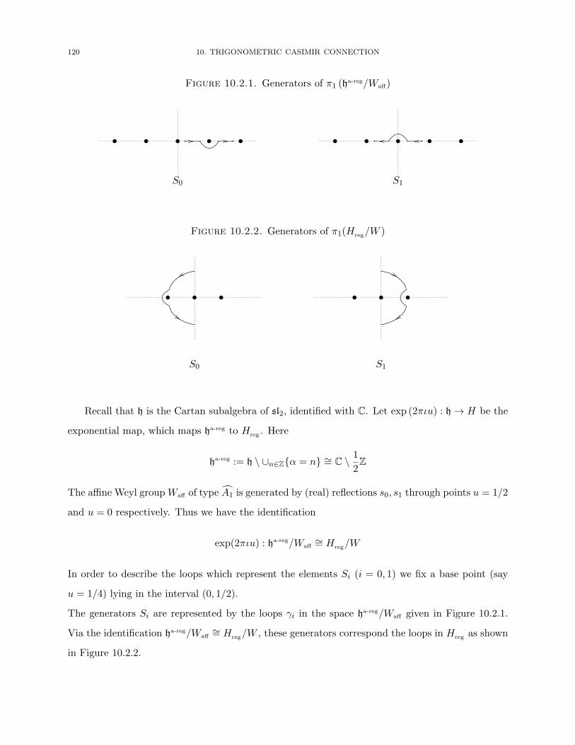
120 10. TRIGONOMETRIC CASIMIR CONNECTION
Figure 10.2.1. Generators of π1 (ha-reg/Waff)
• • • • •· ·�� ��
S0
• • • • •·· ����
S1
Figure 10.2.2. Generators of π1(Hreg/W )
• ••
��
S0
• ••
��
S1
Recall that h is the Cartan subalgebra of sl2, identified with C. Let exp (2πιu) : h→ H be the
exponential map, which maps ha-reg to Hreg . Here
ha-reg := h \ ∪n∈Z{α = n} ∼= C \ 12Z
The affine Weyl groupWaff of type A1 is generated by (real) reflections s0, s1 through points u = 1/2
and u = 0 respectively. Thus we have the identification
exp(2πιu) : ha-reg/Waff∼= Hreg/W
In order to describe the loops which represent the elements Si (i = 0, 1) we fix a base point (say
u = 1/4) lying in the interval (0, 1/2).
The generators Si are represented by the loops γi in the space ha-reg/Waff given in Figure 10.2.1.
Via the identification ha-reg/Waff∼= Hreg/W , these generators correspond the loops in Hreg as shown
in Figure 10.2.2.
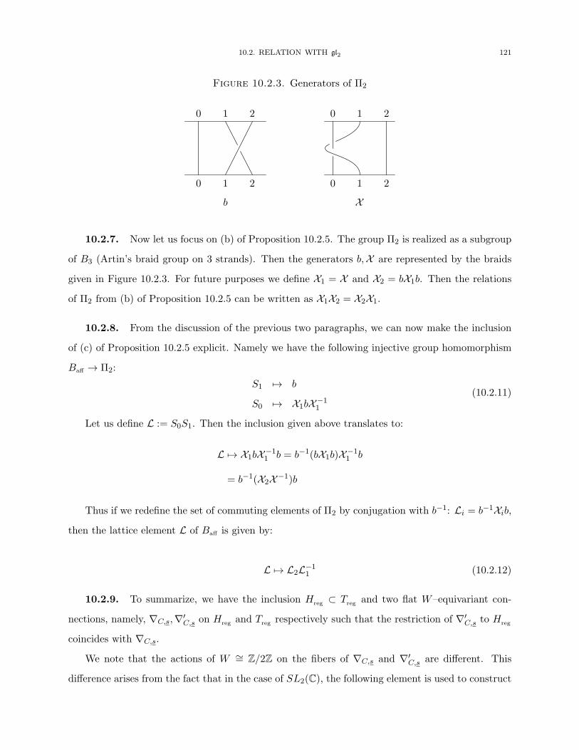
10.2. RELATION WITH gl2 121
Figure 10.2.3. Generators of Π2
0 1 2
0 1 2
b
0 1 2
0 1 2
X
10.2.7. Now let us focus on (b) of Proposition 10.2.5. The group Π2 is realized as a subgroup
of B3 (Artin’s braid group on 3 strands). Then the generators b,X are represented by the braids
given in Figure 10.2.3. For future purposes we define X1 = X and X2 = bX1b. Then the relations
of Π2 from (b) of Proposition 10.2.5 can be written as X1X2 = X2X1.
10.2.8. From the discussion of the previous two paragraphs, we can now make the inclusion
of (c) of Proposition 10.2.5 explicit. Namely we have the following injective group homomorphism
Baff → Π2:
S1 �→ b
S0 �→ X1bX−11
(10.2.11)
Let us define L := S0S1. Then the inclusion given above translates to:
L �→ X1bX−11 b = b−1(bX1b)X−11 b
= b−1(X2X−1)b
Thus if we redefine the set of commuting elements of Π2 by conjugation with b−1: Li = b−1Xib,
then the lattice element L of Baff is given by:
L �→ L2L−11 (10.2.12)
10.2.9. To summarize, we have the inclusion Hreg ⊂ Treg and two flat W–equivariant con-
nections, namely, ∇C,s,∇′C,s on Hreg and Treg respectively such that the restriction of ∇′C,s to Hreg
coincides with ∇C,s.
We note that the actions of W ∼= Z/2Z on the fibers of ∇C,s and ∇′C,s are different. This
difference arises from the fact that in the case of SL2(C), the following element is used to construct
122 10. TRIGONOMETRIC CASIMIR CONNECTION
a group homomorphism W → SL2(C) (see the discussion preceding [48, Corollary 3.6]).
σ �→⎛⎝ 0 1
−1 0
⎞⎠Let πC,s and π′C,s denote the representations of Baff and Π2 respectively obtained from the mon-
odromy of the connections ∇C,s and ∇′C,s respectively. Then we have:
Theorem.
πC,s(b) = π′C,s(−1)D1
πC,s(L) = π′C,s(L2L−11 )

CHAPTER 11
Dual pair (glk, gln)
11.1. Dual pair (glk, gl2) and the trigonometric KZ equations
In this section we consider the combined action of the pair (glk, gln) on the algebra of polynomial
functions on the space of k × n matrices with C coefficients. We follow the notational conventions
of [48, §3]. In our case n = 2.
11.1.1. The dual pair. Let S(M∗
k,2
)be the coordinate ring of the space of k × 2 matrices:
S(M∗
k,2
):= C[xai : 1 ≤ a ≤ k, i = 1, 2]
We consider the joint action of glk and gl2 on S(M∗
k,2
). To distinguish between the elements of
these Lie algebras, we denote by X(p) the element X from glp (for p = k, 2).
E(k)ab �→
2∑i=1
xai∂bi E(2)ij �→
k∑a=1
xai∂aj (11.1.1)
Proposition. The assignment (11.1.1) defines an action of glk × gl2 on S(M∗
k,2
).
11.1.2. It is clear from the definitions that as a glk (resp. gl2) module we have:
S(M∗
k,2
) ∼= S(M∗
k,1
)⊗2(resp. S
(M∗1,2
)⊗k)
Let us denote by θa (1 ≤ a ≤ k) the linear forms on the Cartan subalgebra of glk consisting of
diagonal matrices, defined by:
θa
(∑b
λbE(k)bb
)= λa
Similarly we define the linear forms {εi : i = 1, 2} on the Cartan subalgebra of gl2 consisting of thediagonal matrices.
123
124 11. DUAL PAIR (glk, gln)
For λ = (λ1, · · · , λk) ∈ Nk and μ = (μ1, μ2) ∈ N2 let us denote by S(M∗
k,2
)[λ, μ] the subspace
of homogeneous polynomials spanned by:⎧⎨⎩∏a,i
xmaiai :
∑a
mai = μi and∑i
mai = λa
⎫⎬⎭Proposition. The action (11.1.1) identifies the space S
(M∗
k,2
)[λ, μ] with the following weight
spaces for glk and gl2 respectively.
(Sμ1Ck ⊗ Sμ2Ck
)[k∑
a=1
λaθa
]∼=
(Sλ1C2 ⊗ · · · ⊗ SλkC2
)[μ1ε1 + μ2ε2]
for every (λ1, · · · , λk) ∈ Nk and (μ1, μ2) ∈ N2.
11.1.3. Trigonometric KZ equations. Let r be the Drinfeld r–matrix for glk
r :=1
2
k∑a=1
E(k)aa +
∑1≤a<b≤k
E(k)ab ⊗ E
(k)ba
and define the trigonometric r–matrix r(u) :=reu + r21eu − 1
. Then we have the following trigonometric
analogue of [48, Theorem 3.5].
Theorem. A function f : Treg → S(M∗
k,2
)[λ, μ] is a horizontal section of the trigonometric
Casimir connection ∇′C,s (see equation (10.2.10)) if, and only if g = f(z1 − z2)−�|μ|(z1z2)�|μ| is a
horizontal section of the trigonometric KZ connection
∇KZ = d− 2h (d(ε1 − ε2)r12(ε1 − ε2)− (dε1(s)1 + dε2(s)2) (11.1.2)
where zi = eεi and
s =
k∑a=1
saE(k)aa
Proof. Let f : Treg → S(M∗
k,2
)[λ, μ] be a horizontal section of ∇′C,s. Then we have the
following partial differential equations:∂f
∂zi= Dif
11.1. DUAL PAIR (glk, gl2) AND THE TRIGONOMETRIC KZ EQUATIONS 125
where
D1 = h
(Δ(k)(κ)
z1 − z2− 2D1 +Δ(k)(κ)
z1
)
D2 = −h(Δ(k)(κ)
z1 − z2+2D2
z2
)
Using (11.1.1) one can easily verify the following coincidence of operators on the space S(M∗
k,2
)[λ, μ]:
(a)
Δ(k)(κ) = 2(r + r21) + |μ|
(b) ∑a<b
(E(2)12 )a(E
(2)21 )b = r − 1
2E(k)
aa ⊗ E(k)aa
(c) ∑a<b
(E(2)21 )a(E
(2)12 )b = r21 − 1
2E(k)
aa ⊗ E(k)aa
(d)
(E(2)11 E
(2)22 )a = E(k)
aa ⊗ E(k)aa
Thus we have the following alternate expressions of Di:
D1 = 2h
(r + r21z1 − z2
− r21 + s1z1
+|μ|2
(z2
z1(z1 − z2)
))D2 = −2h
(r + r21z1 − z2
+r + s2z2
+|μ|2
(z1
z2(z1 − z2)
))The assertion of the theorem follows from these computations. �
Thus we have the following analogue of [48, Corollary 3.6].
Corollary. Let π′C,s and π′KZ,s be the monodromy representations of Π2 corresponding to the con-
nections (10.2.10) and (11.1.2) respectively:
π′C,s, π′KZ,s : Π2 → GL
⎛⎝ ⊕ν∈S2μ
S(M∗
k,2
)[λ, μ][[h]]
⎞⎠
126 11. DUAL PAIR (glk, gln)
Then we have (see §10.2.7)π′KZ,s(b) = πC,s(b)e
−πιh12
π′KZ,s(X1) = πC,s(X1)e2πιh12
π′KZ,s(X2) = πC,s(X2)
(11.1.3)
11.2. Monodromy of the trigonometric KZ connection
In this section we recall the main theorem of [15] which computes the monodromy of the
trigonometric KZ equations.
11.2.1. Quantum group U�glp. The Drinfeld–Jimbo quantum group U�glp is defined as a
unital associative C[[�]]–algebra, topologically generated by {Di, Ej , Fj : 1 ≤ i ≤ p; 1 ≤ j ≤ p− 1}subject to the following relations (where q2 = e�):
(QG1) [Di, Di′ ] = 0 for each i, i′ ∈ {1, · · · , p}.(QG2) For each i, j, 1 ≤ i ≤ p and 1 ≤ j ≤ p− 1 we have
[Di, Ej ] = (δij − δi,j+1)Ej [Di, Fj ] = (δi,j+1 − δij)Fj
(QG3) For each j, j′ ∈ {1, · · · , p− 1} we have
[Ej , Fj′ ] = δj,j′qHj − q−Hj
q − q−1
(QG4) For each j = j′ ∈ {1, · · · , p− 1} we have:1−ajj′∑t=0
(−1)t⎡⎣ 1− ajj′
t
⎤⎦q
E1−ajj′−ti EjE
ti = 0
1−ajj′∑t=0
(−1)t⎡⎣ 1− ajj′
t
⎤⎦q
F1−ajj′−ti FjF
ti = 0
where Hi = Di −Di+1. We have used the standard notations of the Gaussian integers.
[n]q :=qn − q−n
q − q−1and [n]q! = [n]q[n− 1]q · · · [1]q⎡⎣ n
m
⎤⎦q
:=[n]q!
[m]q![n−m]q!
11.2. MONODROMY OF THE TRIGONOMETRIC KZ CONNECTION 127
and ajj′ are entries of the Cartan matrix of type Ap−1:
ajj′ := 2− δ[j−j′|=1
U�glp is a topological Hopf algebra with coproduct and counit given by:
Δ(Di) = Di ⊗ 1 + 1⊗Di
Δ(Ej) = Ej ⊗ qHj + 1⊗ Ej
Δ(Fj) = Fj ⊗ 1 + q−Hj ⊗ Fj
(11.2.1)
and
ε(Ej) = ε(Fj) = ε(Di) = 0 (11.2.2)
Let Ip := D1+ · · ·+Dp ∈ U�glp. It is clear from the definition above that Ip is a central element
of U�glp, and the coproduct on Ip is given by Δ(Ip) = Ip ⊗ 1 + 1 ⊗ Ip. We have the following
isomorphism of Hopf algebras:
U�glp = U�slp ⊗ C[Ip][[�]]
Moreover U�glp has a quasi–triangular structure. Let R be the R–matrix of U�glp. Recall that
the Drinfeld element u is defined by:
u := (m ◦ (S ⊗ 1)) (R21) (11.2.3)
The following theorem is proved in [13].
Theorem. The square of the antipode is an inner automorphism given by:
S2(x) = uxu−1
Remark. In this note R denotes the R–matrix of U�glp, which differs from the R–matrix of U�slp
(the one used in [48]) by:
Rglp = qIp⊗Ip
p Rslp (11.2.4)
11.2.2. Monodromy of the trigonometric KZ equations. As before, let r ∈ glk ⊗ glk be
the Drinfeld r–matrix and define r(u) :=reu + r21eu − 1
. Let s ∈ glk be a diagonal matrix. Consider the
following system of partial differential equations for F (u1, · · · , un) ∈ V ⊗n for a finite–dimensional
glk –module V :
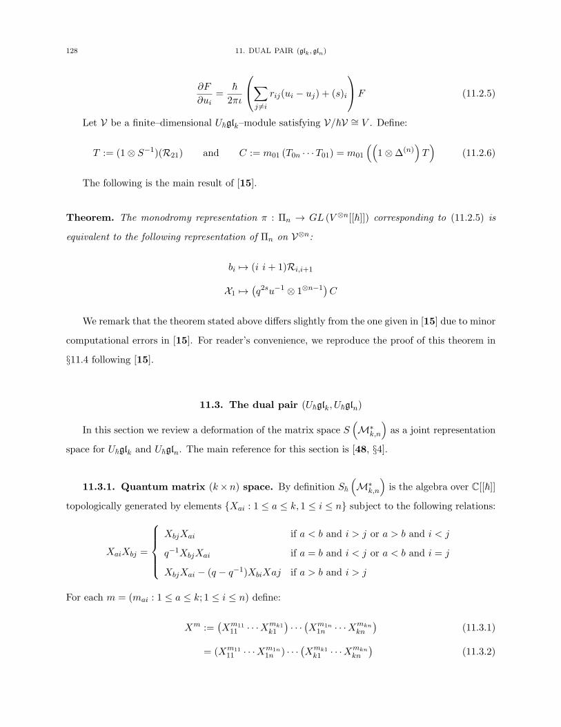
128 11. DUAL PAIR (glk, gln)
∂F
∂ui=
�2πι
⎛⎝∑j �=i
rij(ui − uj) + (s)i
⎞⎠F (11.2.5)
Let V be a finite–dimensional U�glk–module satisfying V/�V ∼= V . Define:
T := (1⊗ S−1)(R21) and C := m01 (T0n · · ·T01) = m01
((1⊗Δ(n)
)T)
(11.2.6)
The following is the main result of [15].
Theorem. The monodromy representation π : Πn → GL (V ⊗n[[�]]) corresponding to (11.2.5) is
equivalent to the following representation of Πn on V⊗n:
bi �→ (i i+ 1)Ri,i+1
X1 �→(q2su−1 ⊗ 1⊗n−1
)C
We remark that the theorem stated above differs slightly from the one given in [15] due to minor
computational errors in [15]. For reader’s convenience, we reproduce the proof of this theorem in
§11.4 following [15].
11.3. The dual pair (U�glk, U�gln)
In this section we review a deformation of the matrix space S(M∗
k,n
)as a joint representation
space for U�glk and U�gln. The main reference for this section is [48, §4].
11.3.1. Quantum matrix (k×n) space. By definition S�
(M∗
k,n
)is the algebra over C[[�]]
topologically generated by elements {Xai : 1 ≤ a ≤ k, 1 ≤ i ≤ n} subject to the following relations:
XaiXbj =
⎧⎪⎪⎪⎨⎪⎪⎪⎩XbjXai if a < b and i > j or a > b and i < j
q−1XbjXai if a = b and i < j or a < b and i = j
XbjXai − (q − q−1)XbiXaj if a > b and i > j
For each m = (mai : 1 ≤ a ≤ k; 1 ≤ i ≤ n) define:
Xm :=(Xm11
11 · · ·Xmk1k1
) · · · (Xm1n1n · · ·Xmkn
kn
)(11.3.1)
= (Xm1111 · · ·Xm1n
1n ) · · · (Xmk1k1 · · ·Xmkn
kn
)(11.3.2)
11.3. THE DUAL PAIR (U�glk, U�gln) 129
Then the set {Xm : m ∈ Mk×n(N)} is a basis for S�
(M∗
k,n
)over C[[�]] (see [42, Theorem
3.5.1], [48, Theorem 5.1]).
11.3.2. The joint action of (U�glk, U�gln). Define the following operators on S�
(M∗
k,n
), for
each b ∈ {1, · · · , k} and a ∈ {1, · · · , k − 1}:
D(k)b Xm =
∑i
mbiXm (11.3.3)
E(k)a Xm =
n∑i=1
[ma+1,i]
n∏j=i+1
q(maj−ma+1,j)Xm+εai−εa+1,i (11.3.4)
F (k)a Xm =
n∑i=1
[mai]
i−1∏j=1
q−(maj−ma+1,j)Xm−εaj+εa+1,j (11.3.5)
Similarly define the operators for each j ∈ {1, · · · , n} and i ∈ {1, · · · , n− 1}:
D(n)j Xm =
k∑a=1
majXm (11.3.6)
E(n)i Xm =
k∑a=1
[ma,i+1]k∏
b=a+1
qmb,i−mb,i+1Xm+εai−εa,i+1 (11.3.7)
F(n)i Xm =
k∑a=1
[mai]
a−1∏b=1
q−(mb,i−mb,i+1)Xm−εai+εa,i+1 (11.3.8)
Theorem. The operators above define a structure of an algebra module on S�
(M∗
k,n
)over U�glk⊗
U�gln. Moreover as a U�glk (resp. U�gln) module we have:
S�(M∗
k,n
) ∼= S�(M∗
k,1
)⊗n (resp. S�
(M∗1,n
)⊗k)11.3.3. Corollary of Theorem 11.2.2. Combining the results stated in Corollary 11.1.3 and
Theorem 11.2.2 we have the following computation (for the case n = 2). Let � = 2πιh.
Corollary. The monodromy of the trigonometric KZ connection (11.1.2) for n = 2 is given by:
π′KZ,s(b1) = (12)R
π′KZ,s(X1) =(q−2s ⊗ 1
)R−121
π′KZ,s(X2) = R21
(1⊗ q−2s
)where recall that s =
∑a saEaa.

130 11. DUAL PAIR (glk, gln)
Proof. We use Theorem 11.2.2 for n = 2. It only remains to check the assignment for X1,X2.
Recall that by definition (11.2.6)
C = m01(T02T01)
where T = (1⊗ S−1)R21. Let us write R = αi ⊗ βi. Then we get:
C = βiβjS−1(αj)⊗ S−1(αi)
We claim that βjS−1(αj) = u. Assuming this we have the following computation:
X1 �→ (q−2su−1 ⊗ 1)(βiu⊗ S−1αi
)= (q−2s ⊗ 1)
(u−1βiu⊗ S−1αi
)= (q−2s ⊗ 1)(S−2 ⊗ S−1)(R21)
= (q−2s ⊗ 1)R−121
where we have used the fact that (S−1 ⊗ S−1)(R) = R and (S−1 ⊗ 1)(R21) = R−121 . Similarly we
have:
X2 = b1X1b1
= (12)R(q−2s ⊗ 1)R−121 (12)R
= (12)R(q−2s ⊗ 1)(12)
= R21(1⊗ q−2s)
Proof of the claim: Let us write v = βjS−1(αj).
S2(v) = S2(βj)S(αj)
= S(βj)αj
= u
where we have used the fact that (S ⊗ S)(R) = R. Since S2 = Ad(u) we get that uvu−1 = u and
the assertion follows. �

11.4. PROOF OF ETINGOF–GEER–SCHIFFMANN THEOREM 131
11.4. Proof of Etingof–Geer–Schiffmann theorem
In this section, we sketch a proof of [15, Theorem 3.3]. The contents of this part follow [15]
closely. The main result of [15] encompasses the case of Lie super–algebras as well, but we restrict
ourselves to the case of ordinary Lie algebras which shall be sufficient for our purposes. For ordinary
Lie algebras, the following computation also appeared in [17, Appendix 2]. But the proof given in
[17] contained a few mistakes, pointed out by A. Haviv, and was removed from the further editions
of the book.
11.4.1. Let A be a unital, associative algebra over C and let r ∈ A⊗A be a classical r–matrix:
[r12, r23] + [r12, r13] + [r13, r23] = 0 (11.4.1)
Define r(u) :=reu + r21eu − 1
and let s ∈ A be such that
[r, 1⊗ s+ s⊗ 1] = 0 (11.4.2)
Consider the following system of partial differential equations for a function F (u1, · · · , uN ) ∈ V ⊗N ,
for an A–module V :
∂F
∂uk=
�2πι
⎛⎝∑j �=k
r(uk − uj) + s(k)
⎞⎠F (11.4.3)
Using (11.4.1) one can easily verify that (11.4.3) is a consistent SN–invariant system. Thus
the monodromy of (11.4.3) yields a representation of ΠN = π1(Confn(C×)), the fundamental group
of the configuration space of N points on C×. We have the following presentation of ΠN (see
Proposition 10.2.5 for the case of N = 2).
Proposition. [15, Proposition 3.2] ΠN is generated by {bi,Xj : 1 ≤ i ≤ N − 1, 1 ≤ j ≤ N} subject
to the following relations:
bibi′ = bi′bi if |i− i′| > 1
bibi+1bi = bi+1bibi+1 for every 1 ≤ i ≤ N − 2
biXibi = Xi+1
XjXk = XkXj
132 11. DUAL PAIR (glk, gln)
Let πKZ be the representation of ΠN on V ⊗N obtained by the monodromy of (11.4.3).
πKZ : ΠN → GL(V ⊗N [[�]]
)(11.4.4)
11.4.2. Etingof–Kazhdan quantization. In order to describe the monodromy representa-
tion (11.4.4) one uses the machinery of Etingof–Kazhdan quantization [16]. Define the following
subspaces of A:
g+ := {(1⊗ f)(r) : f ∈ A∗}
g− := {(g ⊗ 1)(r) : g ∈ A∗}
The following proposition follows from the classical Yang–Baxter equation (11.4.1)
Proposition. g± are finite–dimensional Lie subalgebras of A. Moreover we have the following
non–degenerate bilinear pairing 〈., .〉 : g+ × g− → C:
〈(1⊗ f)(r), (g ⊗ 1)(r)〉 = (g ⊗ f)(r)
Thus (g = g+ ⊕ g−, g+, g−) is a finite–dimensional Manin triple. The canonical element r ∈ g⊗ g
maps to r under the homomorphism π : g→ A whose restriction to g± is the canonical inclusion.
Using the quantization theorem for a finite–dimensional Manin triple [16, §3] we obtain a quasi–triangular Hopf algebra U�g, R ∈ U�g⊗U�g and sub-Hopf-algebras U�g± in duality with each other.
Moreover there is a canonical isomorphism ζ : U�g → Ug[[�]] which allows us to extend the map
π : g → A to an algebra homomorphism U�g → A[[�]] (again denoted by π). Let us denote by Vthe U�g–module obtained from V [[�]] via the homomorphism π.
We define the following elements (compare with (11.2.6)):
T :=(1⊗ S−1
)R21 ∈ U�g
⊗2 (11.4.5)
C := m01 (T0N · · ·T01) = m01
((1⊗Δ(N)
)T)∈ U�g
⊗N (11.4.6)
Then we have the following:

11.4. PROOF OF ETINGOF–GEER–SCHIFFMANN THEOREM 133
Theorem. The monodromy representation πKZ is equivalent to the following action of ΠN on
V⊗N :
bi �→ (i i+ 1)Ri,i+1
X1 �→(e�su−1 ⊗ 1⊗N−1
)C
where u = m(S ⊗ 1)(R21) is the Drinfeld element.
A proof of this theorem is sketched in §11.4.3 – §11.4.5.
11.4.3. The first step towards the proof of Theorem 11.4.2 is to relate the trigonometric KZ
connection on N points (11.4.3) to the rational KZ connection on N +1 points. In order to achieve
this, we extend the Manin triple of Proposition 11.4.2 to (g′, g′+, g′−) by including a derivation.
Let us define ρ′r = m(rop) ∈ A, i.e, if r = ai ⊗ bi then ρ′r = biai. Let t = s + ρ′r ∈ A and let
∂ = adA(t). Using the equation (11.4.2) one can verify that g± ⊂ A are preserved under ∂. Thus it
makes sense to define g′+ = g+ ⊕ Ct where [t, .] = ∂ on g+. We extend the Lie bialgebra structure
of g+ to g′+ by declaring δ(t) = 0. Let us define g′− = g− ⊕ Ct∗ as dual to g′+. Note that t∗ is
central and the Lie cobracket is trivial on t∗. We extend the algebra homomorphism Ug → A to
U := U(g′)/(t∗) → A by t �→ s + ρ′r. Thus V can be considered as a g′–module on which t∗ acts
trivially and t acts by s+ ρ′r. Similarly V is considered as a U�g′–module.
Now let M± := U(g∓)1± be g′–modules determined by:
(a) g±1± = 0.
(b) t1± = 0.
(c) t∗1± = ±1±.
Consider the following (rational) system of partial differential equations for a function
Ψ(z0, · · · , zN ) ∈ Homg
(M+,M
∗− ⊗ V ⊗N
)∂Ψ
∂zk=
�2πι
⎛⎝∑j �=k
Ω′kjzk − zj
⎞⎠Ψ (11.4.7)
where Ω′ is the Casimir tensor of g′. We have
134 11. DUAL PAIR (glk, gln)
Proposition. Under the Frobenius reciprocity isomorphism
θ : Homg
(M+,M
∗− ⊗ V ⊗N
) ∼→ V ⊗N
the restriction of (11.4.7) to z0 = 0 is identical with (11.4.3).
11.4.4. Let U�g′ be the Etingof–Kazhdan quantization of g′ (and similarly for its subalgebras).
We denote by R′ the R–matrix of U�g′ which equips it with the structure of a quasi–triangular
Hopf algebra.
The following is a consequence of the theory developed by P. Etingof and D. Kazhdan in [16],
together with the observations of §11.4.3.
Proposition. The monodromy representation (11.4.4) is equivalent to the following representation
of ΠN on HomU�g
((M q
+,∗M q
− ⊗ V⊗N).
bj �→ (j j + 1)R′j,j+1
X1 �→ R′10R′01
where M q± := U�g∓1
q± are U�g
′–modules defined by:
(a) U�g±1q± = 0.
(b) t1q± = 0.
(c) t∗1q± = ±1q±.
and ∗M q− is the left dual module.
11.4.5. In view of the Proposition 11.4.4 and the isomorphism:
θ : HomU�g
(M q
+,∗M q
− ⊗ V⊗N) ∼→ V⊗N
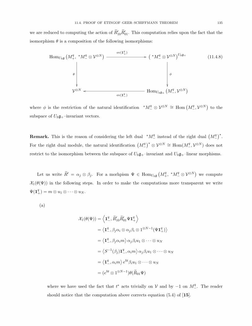
11.4. PROOF OF ETINGOF–GEER–SCHIFFMANN THEOREM 135
we are reduced to computing the action of R′10R′01. This computation relies upon the fact that the
isomorphism θ is a composition of the following isomorphisms:
HomU�g
(M q
+,∗M q
− ⊗ V⊗N)
θ
��
ev(1q+)
��( ∗M q
− ⊗ V⊗N)U�g+
φ
��
V⊗N HomU�g+
(M q−,V⊗N
)ev(1q
−)
��
(11.4.8)
where φ is the restriction of the natural identification ∗M q− ⊗ V⊗N ∼= Hom
(M q−,V⊗N
)to the
subspace of U�g+–invariant vectors.
Remark. This is the reason of considering the left dual ∗M q− instead of the right dual
(M q−)∗.
For the right dual module, the natural identification(M q−)∗ ⊗ V⊗N ∼= Hom(M q
−,V⊗N ) does notrestrict to the isomorphism between the subspace of U�g+–invariant and U�g+–linear morphisms.
Let us write R′ = αj ⊗ βj . For a morhpism Ψ ∈ HomU�g
(M q
+,∗M q
− ⊗ V⊗N)we compute
X1(θ(Ψ)) in the following steps. In order to make the computations more transparent we write
Ψ(1q+) = m⊗ u1 ⊗ · · · ⊗ uN .
(a)
X1(θ(Ψ)) =⟨1q−, R
′10R
′01Ψ1
q+
⟩=
⟨1q−, βjαi ⊗ αjβi ⊗ 1⊗N−1(Ψ1q+)
⟩=
⟨1q−, βjαim
⟩αjβiu1 ⊗ · · · ⊗ uN
=⟨S−1(βj)1
q−, αim
⟩αjβiu1 ⊗ · · · ⊗ uN
=⟨1q−, αim
⟩e�tβiu1 ⊗ · · · ⊗ uN
= (e�t ⊗ 1⊗N−1)θ(R01Ψ)
where we have used the fact that t∗ acts trivially on V and by −1 on M q−. The reader
should notice that the computation above corrects equation (5.4) of [15].

136 11. DUAL PAIR (glk, gln)
(b) Let us write R = aj ⊗ bj . Using the commutativity of (11.4.8) we get:
X1(θ(Ψ)) =⟨1q−, aim
⟩e�tbiu1 ⊗ · · · ⊗ uN
=(e�tbi ⊗ 1⊗N−1
) ⟨S−1(ai)1
q−,m
⟩u1 ⊗ · · · ⊗ uN
=(e�tbi ⊗ 1⊗N−1
) ⟨1q−,m
⟩Δ(N)(S−1(ai)) (u1 ⊗ · · · ⊗ uN )
=(e�tbi ⊗ 1⊗N−1
)Δ(N)(S−1(ai))θ(Ψ)
(c) It follows from the axioms of the quasi–triangular Hopf algebra that
(bi ⊗ 1⊗N−1
)Δ(N)(S−1(ai)) = m01(T0N · · ·T01) = C
where T = (1⊗ S−1)(R21) (as defined in (11.4.6)). Hence we obtain:
X1 �→ (e�sw ⊗ 1⊗N−1)C
where w = e�ρ′r under the identification of U�g with Ug[[�]].
(d) In order to determine the element w, we restrict ourselves to the case of s = 0 and N = 1.
In this case the monodromy is trivial and hence we get:
w.m(T ) = w(biS−1(ai)) = 1
We have already proved (see the proof of Corollary 11.3.3) that biS−1(ai) = u is the
Drinfeld element. Thus we get that w = u−1. This finishes the proof of theorem 11.4.2.
CHAPTER 12
Quantum Weyl group
12.1. Quantum loop algebra U�(Lgl2)
In this section we review the definition of the quantum loop algebra U�(Lgl2) (see §9.1.1).
12.1.1. Definition. U�(Lgl2) is a unital associative algebra over C[[�]] generated by {D1,r, D2,r, Er, Fr :
r ∈ Z}. In order to state the relations concisely, we introduce the following formal series:
Θ±j (z) := q±Dj,0 exp
⎛⎝±(q − q−1)∑r≥1
Dj,±rz∓r
⎞⎠ (12.1.1)
E(z) :=∑r∈Z
Erz−r and F (z) :=
∑r∈Z
Frz−r (12.1.2)
Then the relations of U�(Lgl2) can be written as:
(QL1) The elements {Dj,r : j = 1, 2; r ∈ Z} commute. Let U0 be the commutative subalgebra of
U�(Lgl2) generated by these elements.
(QL2)
Θ±1 (z)E(w)Θ±1 (z)
−1 =q−1z − qw
z − wE(w)
Θ±2 (z)E(w)Θ±2 (z)
−1 =qz − q−1w
z − wE(w)
Θ±1 (z)−1F (w)Θ±1 (z) =
q−1z − qw
z − wF (w)
Θ±2 (z)−1F (w)Θ±1 (z) =
qz − q−1wz − w
F (w)
(QL3)
E(z)E(w) =qz − q−1wq−1z − qw
E(w)E(z)
F (z)F (w) =q−1z − qw
qz − q−1wF (w)F (z)
137

138 12. QUANTUM WEYL GROUP
(QL4)
(q − q−1)[E(z), F (w)] = δ(zw−1)(Θ+
2 (z)
Θ+1 (z)
− Θ−2 (z)Θ−1 (z)
)where δ(z) =
∑n∈Z z
n is the formal delta function.
Let ψ±(z) := Θ±1 (z)−1Θ±2 (z), so that
ψ±(z) = K±1 exp
⎛⎝±(q − q−1)∑r≥1
H±rz∓r
⎞⎠ (12.1.3)
where K = qH0 and Hr := D2,r −D1,r for every r ∈ Z.
Lemma. (1) The relation (QL2) can be equivalently written as follows. For every r ≥ 1 and
k ∈ Z we have:
[Dj,0, Ek] = (−1)jEk and [Dj,0, Fk] = (−1)j+1Fk
[D1,r, Ek] = −qr [r]rEk+r [D2,r, Ek] = q−r
[r]
rEk+r (12.1.4)
[D1,r, Fk] = qr[r]
rFk+r [D2,r, Fk] = −q−r [r]
rFk+r (12.1.5)
And hence we have the following commutation relations:
[H0, Ek] = 2Ek and [H0, Fk] = −2Fk
[Hr, Ek] =[2k]
kEr+k [Hr, Fk] = − [2r]
rFr+k (12.1.6)
(2) The relation (QL4) can be written in the following equivalent form:
[Ek, Fl] =ψ+k+l − ψ−k+l
q − q−1(12.1.7)
where we use the convention that ψ+−p = ψ−p = 0 for every p > 0.
12.1.2. Quantum determinant. Using the relation (QL1) and (QL2) it is easy to see that
the coefficients of the series Θ±1 (qz)Θ±2 (q
−1z) belong to the center of U�(Lgl2). The following result
in well–known (see [37, Theorem 1.8.2] for analogous assertion about the Yangians).
Proposition. Let U�(Lsl2) be the subalgbera of U�(Lgl2) generated by {Er, Fr : r ∈ Z}. Define:
qdet±(z) := Θ±1 (qz)Θ±2 (q
−1z) (12.1.8)
12.1. QUANTUM LOOP ALGEBRA U�(Lgl2) 139
Then the coefficients of the series qdet±(z) generate the center of U�(Lgl2), denoted by Z. Moreover
we have:
U�(Lgl2)∼= Z ⊗ U�(Lsl2) (12.1.9)
12.1.3. Hopf structure. The algebra U�(Lgl2) is a Hopf algebra with comultiplication de-
termined by:
Δ(qdet±(z)
)= qdet±(z)⊗ qdet±(z)
Δ(Dj,0) = Dj,0 ⊗ 1 + 1⊗Dj,0
Δ(E0) = E0 ⊗K + 1⊗ E0
Δ(F0) = F0 ⊗ 1 +K−1 ⊗ F0
Δ(E−1) = E−1 ⊗K−1 + 1⊗ E−1
Δ(F1) = F1 ⊗ 1 +K ⊗ F1
(12.1.10)
12.1.4. Evaluation homomorphism. Let us define for each ζ ∈ 1 + �C[[�]], a surjective
algebra homomorphism evζ : U�(Lgl2)→ U�gl2 given by:
H0 �→ D1 −D2 E0 �→ E F0 �→ F
E−1 �→ qζ−1K−1E F1 �→ q−1ζFK
Finally we define:
qdet±(z) �→ q±I(1− q∓Iζ±1z∓1
1− q±Iζ±1z∓1
)where I = I2 = D1 +D2 ∈ U�gl2.
Let V be a U�gl2–module and ζ ∈ 1 + �C[[�]]. We define V(ζ) := ev∗ζ (V) the U�(Lgl2)– module
obtained via evζ .
More generally, for k ≥ 1 and ζ = (ζ1, · · · , ζk) ∈ (1 + �C[[�]])k we have
evζ := (evζ1 ⊗ · · · ⊗ evζk) ◦Δ(k) : U�(Lgl2)→ (U�gl2)⊗k
Combining with the observations of §11.3.2 we get:

140 12. QUANTUM WEYL GROUP
Proposition. Let λ = (λ1, · · · , λk) ∈ Nk and ζ = (ζ1, · · · , ζk) as above. Let S�
(M∗
k,2
)[λ] be the
subspace spanned by
{Xm : ma1 +ma2 = λa∀a = 1, · · · , k}
Then the action of U�(Lgl2) on S�
(M∗
k,2
)[λ] via the homomorphism evζ identifies:
S�(M∗
k,2
)[λ] ∼= Vλ1(ζ1)⊗ · · · ⊗ Vλk
(ζk) (12.1.11)
12.1.5. Kac–Moody presentation. Define the following elements of U�(Lsl2):
H := D2,0 −D1,0
E1 := E0 F1 := F0
E0 := F1K−1 F0 := KE−1
(12.1.12)
These generators give a Kac–Moody presentation of U�(Lsl2) (see [5] for details).
Proposition. U�(Lsl2) is generated by {H, Ei,Fi : i = 0, 1} subject to the following relations:
(KM1) For each i = 0, 1 we have:
[H, Ei] = (−1)i+12Ei and [H,Fi] = (−1)i2Fi
(KM2) For i, j ∈ {0, 1} we have:
[Ei,Fj ] = δij(−1)i+1 qH − q−H
q − q−1
(KM3) Let i = j ∈ {0, 1}. Then:
E3i Ej − [3]E2i EjEi + [3]EiEjE2i + EjE3i = 0
F3i Fj − [3]F2
i FjFi + [3]FiFjF2i + FjF3
i = 0
Note that the loop presentation of U�(Lsl2) is given in terms of the generating series {E(z), F (z), ψ±(z) =Θ±1 (z)
−1Θ±2 (z)}.
12.1.6. Quantum Weyl group for U�(Lsl2). For each i = 0, 1 we have Si in a certain
completion (with respect to finite–dimensional representations) of U�(Lsl2), given by:
S0 := expq−1
(q−1E0qH
)expq−1 (−F0) expq−1
(qE0q−H
)q
H(H−1)2
S1 := expq−1
(q−1E1q−H
)expq−1 (−F1) expq−1
(qE1qH
)q
H(H+1)2
(12.1.13)

12.1. QUANTUM LOOP ALGEBRA U�(Lgl2) 141
where the q–exponential is defined by:
expq(x) =∑n≥0
qn(n−1)
2xn
[n]!
Let Ti = Ad(Si). Then the action of Ti on U�(Lsl2) can be explicitly computed as (see [34], [28,
§8.14]):
Proposition. For each i = 0, 1 Ti is an algebra automorphism of U�(Lsl2) given by:
T0(H) = T1(H) = −H
T0(E0) = −F0q−H T0(F0) = −qHE0
T1(E1) = −F1qH T1(F1) = −q−HE1
T0(E1) = E(2)0 E1 − q−1E0E1E0 + q−2E1E(2)0
T0(F1) = F1F (2)0 − qF0F1F0 + q2F (2)
0 F1
T1(E0) = E(2)1 E0 − q−1E1E0E1 + q−2E0E(2)1
T0(F1) = F0F (2)1 − qF1F0F1 + q2F (2)
1 F0
Definition. Define ω to be the automorphism of U�(Lsl2) determined by H ↔ −H, E0 ↔ E1 andF0 ↔ F1. In terms of loop generators the action of ω can be written as:
ω(E0) = F1K−1 ω(F0) = KE1 (12.1.14)
ω(E−1) = KF0 ω(F1) = E0K−1 (12.1.15)
where K = qH.
Corollary. ω ◦ T0 ◦ ω = T1
12.1.7. Lattice element L = T0T1. In this paragraph we compute the action of L := T0T1
on the loop generators of U�(Lsl2).

142 12. QUANTUM WEYL GROUP
Proposition. We have the following:
L(ψ±(z)) = ψ±(z)
L(E(z)) = q4z−2E(z)
L(F (z)) = q−4z2F (z)
(12.1.16)
Proof. Since L is an algebra automorphism, it suffices to prove its action on the following
set of generators: {H0, E0, F0, E−1, F1}. Using the isomorphism (12.1.12) between the Kac–Moody
generators and the loop generators of U�(Lsl2) and the action of T0, T1 given in Proposition 12.1.6
we have:
Claim: The action of T0 on the loop generators is given by:
T0 (F1) = −q2E−1K−1 T0 (E−1) = −q−2KF1
T0 (E0) = −q−2F2K−1 T0 (F0) = −q2KE−2
(12.1.17)
Assuming the claim, we can proceed with the computation of L. This is done in the following
steps.
(1) The easier part of the computations is for the case of H0, E0, F0. Clearly L(H0) = H0.
Further using the isomorphism (12.1.12) we have:
L(E0) = T0(T1(E0)) = T0(−F0K)
= −(−q2KE−2)K−1 = q4E−2
L(F0) = T0(T1(F0)) = T0(−K−1E0)
= −K(−q−2F2K−1) = q−4F2
(2) Next we compute L(F1). We have:
T1(F1) =1
[2]
(E2
0F1 − (q−2 + q−4)E0F1E0 + q−6F1E20
)K−2
Combining with the result of the previous paragraph we have:
L(F1) =1
[2]
(−q−2F2K−1F2K
−1E−1K−1+
(q−4 + q−6)F2K−1E−1K−1F2K
−1 − q−8E−1K−1F2K−1F2K
−1)K2
12.1. QUANTUM LOOP ALGEBRA U�(Lgl2) 143
Let us compute each of the terms on the right–hand side individually:
(a)
−q−2F2K−1F2K
−1E−1K−1K2 = q−2F 22E−1K
−1
(b)
(q−4 + q−6)F2K−1E−1K−1F2K
−1K2 = (q−2 + q−4)F2E−1F2K−1
= (q−2 + q−4)(F 22E−1K
−1 + F2H1
)where we have used the relation [E−1, F2] = (q − q−1)−1ψ1 = KH1 (see (12.1.7) and
(12.1.3)).
(c)
−q−8E−1K−1F2K−1F2K
−1K2 = −q−2E−1F 22K
−1
= −q−2 (F2E−1 +KH1)F2K−1
= −q−2 (F 22E−1 + (1 + q−2)F2KH1 − q−2[2]F3K
)K−1
where we have used the relation (12.1.6): [H1, F2] = −[2]F3.
Combining these computations we obtain:
L(F1) =1
[2]
(q−4[2]F3
)= q−4F3
(3) The equation L(E−1) = q4E−3 is proved exactly as above, and its verification is skipped
here.
Proof of the claim: The first set of equations, namely T0(F1) = −q2E−1K−1 and T0(E−1) =
−q−2KF1, follow immediately from (12.1.12) and Proposition 12.1.6. We only check the first of
the remaining two equations since the second one is verified with an identical computation. Again
we have:
T0(E0) =1
[2]
(F1K
−1F1K−1E0 − (1 + q−2)F1K
−1E0F1K−1 + q−2E0F1K
−1F1K−1)
Once again we simplify each of the term on the right–hand side individually:

144 12. QUANTUM WEYL GROUP
(a)
F1K−1F1K
−1E0 = q−2F 21E0K
−2
(b)
(1 + q−2)F1K−1E0F1K
−1 = (1 + q−2)F1E0F1K−2
= (1 + q−2)F1 (F1E0 +KH1)K−2
= (1 + q−2)(F 21E0 + F1H1
)K−2
where we have used the fact that [E0, F1] = KH1.
(c)
q−2E0F1K−1F1K
−1 = E0F21K
−2
= F 21E0 + (1 + q−2)F1KH1 − q−2[2]F2K
where we have used the relation [H1, F1] = −[2]F2.
Combining these computations we get that
T0(E0) =1
[2]
(−q−2[2]F2K−1) = −q−2F2K
−1
The proposition is proved. �
Remark. Thus it seems reasonable to expect that L can be obtained as conjugation by a certain
element from the commutative subalgebra of U�(Lsl2). This expectation is fulfilled in the next
section where we give an explicit expression for L ∈ U0 (Lsl2) such that
L = Ad(L)
12.2. Quantum Weyl groups
In this section we define certain operators S,L1,L2 which lie in a completion of ˜U�(Lgl2) and
satisfy the relations of Π2. We also compute the expression of L = S0S1 in terms of the elements
from the commutative subalgebra of U�(Lsl2). These realizations of the corresponding braid groups
are related by L = L2L−11 (compare with (10.2.11) and (10.2.12)).

12.2. QUANTUM WEYL GROUPS 145
12.2.1. Completions. In this section let U := U�(Lsl2) and U ′ := U�(Lgl2). We define certain
completions of these algebras.
Definition. Let J and J ′ be the ideals of U and U ′ respectively defined as the kernels of the
following algebra homomorphism
J := Kernel
(U�(Lsl2)
�=0 �� U(sl2[z, z
−1]) z=1 �� Usl2
)
J ′ := Kernel
(U�(Lgl2)
�=0 �� U(gl2[z, z
−1]) z=1 �� Ugl2
)
For each r ≥ 0, t ∈ Z and x ∈ {Θ1,Θ2, E, F} define the following “binomial elements” of U ′:
xr;t :=
r∑s=0
(−1)t⎛⎝ r
s
⎞⎠xs+t
and let Kr be the two–sided ideal of U ′ generated by the set of binomial elements {xr′;t : r′ ≥ r, t ∈Z}. Let Fr ⊂ U ′ be the ideal:
Fr :=r∑
i=0
Ki
(J ′)r−iWe consider the filtration on U given by the powers of the ideal J and the filtration on U ′ givenby {Fr : r ≥ 0}.
The reason for considering the filtration F on U ′ will become clear in the next section (see
Remark 12.2.3).
Let U and U ′ be the completions of U and U ′ respectively, with respect to their respective
filtrations.
U := lim← U/J n and U ′ := lim← U ′/Fn
Remark. The lattice elements L1,L2,L defined in the next section lie in these completed algebras.
However in order to consider the quantum Weyl group operator S we need to further complete
these algebras with respect to finite–dimensional representations.
12.2.2.
Proposition. The center of U�(Lsl2) is trivial.

146 12. QUANTUM WEYL GROUP
Proof. The proposition follows from the corresponding assertion for the classical case and
the fact that U�(Lsl2) (resp. U�(Lsl2)) is a flat deformation of U (Lsl2) (resp. U (Lsl2)) (see, for
example, Proposition 8.1.3 [23, Proposition 6.3]). �
12.2.3. Definition of the lattice operators. Define:
Di,r := Dj,0 +r∑
s=1
(−1)s⎛⎝ r
s
⎞⎠ qss
[s]Di,s (12.2.1)
Hr := H0 +
r∑s=1
(−1)s⎛⎝ r
s
⎞⎠ qss
[s]Hs (12.2.2)
Proposition. For each i = 1, 2 and r ∈ N, the element Dj,r ∈ Fr. Similarly Hr ∈ J r for each
r ∈ N.
Proof. We prove the proposition for the case of U�(Lsl2). The first assertion for U�(Lgl2) is
proved similarly.
Following [27] let us define for eachX = {E,F, φ}, t ∈ Z and n ≥ 0 the following binomial elements:
Xn;t :=
n∑s=0
(−1)s⎛⎝ n
s
⎞⎠Xs+t
where we define φl :=ψ+l − ψ−lq − q−1
.
Then it is proved in [27, §2.3] that each of the elements Xn;t ∈ J n. Using the transformation
formula between ψ± and Hr given in (12.1.3) we obtain the corresponding assertion for H′s: for
every n ≥ 0 and t > 0 we have
H0 +q − q−1
�
⎛⎝ n∑s=1
(−1)s⎛⎝ n
s
⎞⎠Hs
⎞⎠ ∈ J n
n∑s=0
(−1)s⎛⎝ n
s
⎞⎠Hs+t ∈ J n
Note the slight dissymmetry at the zero node. This stems from the fact that φ0 and φk have
different expressions in terms of H’s if k ∈ Z×.
In order to prove that Hr ∈ J r we will need the following standard observation:
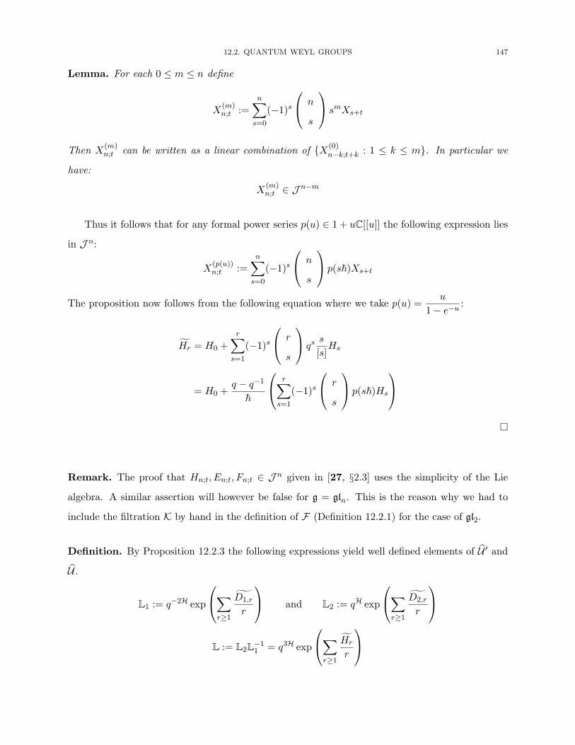
12.2. QUANTUM WEYL GROUPS 147
Lemma. For each 0 ≤ m ≤ n define
X(m)n;t :=
n∑s=0
(−1)s⎛⎝ n
s
⎞⎠ smXs+t
Then X(m)n;t can be written as a linear combination of {X(0)
n−k;t+k : 1 ≤ k ≤ m}. In particular we
have:
X(m)n;t ∈ J n−m
Thus it follows that for any formal power series p(u) ∈ 1 + uC[[u]] the following expression lies
in J n:
X(p(u))n;t :=
n∑s=0
(−1)s⎛⎝ n
s
⎞⎠ p(s�)Xs+t
The proposition now follows from the following equation where we take p(u) =u
1− e−u:
Hr = H0 +r∑
s=1
(−1)s⎛⎝ r
s
⎞⎠ qss
[s]Hs
= H0 +q − q−1
�
⎛⎝ r∑s=1
(−1)s⎛⎝ r
s
⎞⎠ p(s�)Hs
⎞⎠�
Remark. The proof that Hn;t, En;t, Fn;t ∈ J n given in [27, §2.3] uses the simplicity of the Lie
algebra. A similar assertion will however be false for g = gln. This is the reason why we had to
include the filtration K by hand in the definition of F (Definition 12.2.1) for the case of gl2.
Definition. By Proposition 12.2.3 the following expressions yield well defined elements of U ′ andU .
L1 := q−2H exp
⎛⎝∑r≥1
D1,r
r
⎞⎠ and L2 := qH exp
⎛⎝∑r≥1
D2,r
r
⎞⎠L := L2L
−11 = q3H exp
⎛⎝∑r≥1
Hr
r
⎞⎠

148 12. QUANTUM WEYL GROUP
12.2.4. The operators Li = Ad (Li). Let us define the algebra automorphism of U ′ given byconjugation with the element Li:
Li(x) = LixL−1i for every x ∈ U ′
Proposition. The operators Li are given by:
L1
(Θ±i (z)
)= Θ±i (z) (12.2.3)
L1(E(z)) = q−2zE(z) L1(F (z)) = q2z−1F (z) (12.2.4)
L2
(Θ±i (z)
)= Θ±i (z) (12.2.5)
L2(E(z)) = q2z−1E(z) L2(F (z)) = q−2zF (z) (12.2.6)
Proof. Since the elements Li are defined in terms of the elements of U0, the commutative
subalgebra of U�(Lgl2), the commutation with Θ±i (z) is trivial. Moreover using the relation (12.1.4)
we have:
[D1,r, E(z)] = −(1− q2z)rE(z)
which proves that the conjugation with L1 := exp
(∑r≥1
D1,r
r
)yields:
Ad(L1
)(E(z)) = q2zE(z)
The relation Ad(L1)(E(z)) = q−2zE(z) now follows from this computation and the fact that
[H, E(z)] = 2E(z). The remaining relations are proved analogously. �
Corollary. Let L := T0T1 be the lattice element of the quantum Weyl group of U�(Lsl2). Then we
have:
L = Ad(L2L−11 ) = Ad(L)
Since the center of U�(Lsl2) is trivial, we obtain the following
S0S1 = L (12.2.7)
12.2.5. Following [5, §4.4] let us denote by X± the subspaces of U�(Lgl2) spanned by Ek and
Fk respectively (for k ∈ Z). Then we have
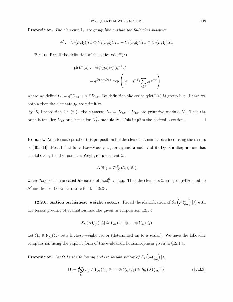
12.2. QUANTUM WEYL GROUPS 149
Proposition. The elements Li are group-like modulo the following subspace
N := U�(Lgl2)X+ ⊗ U�(Lgl2)X− + U�(Lgl2)X− ⊗ U�(Lgl2)X+
Proof. Recall the definition of the series qdet±(z)
qdet+(z) := Θ+1 (qz)Θ
+2 (q
−1z)
= qD1,0+D2,0 exp
⎛⎝(q − q−1)∑r≥1
zrz−r
⎞⎠where we define zr := qrD2,r + q−rD1,r. By definition the series qdet
+(z) is group-like. Hence we
obtain that the elements zr are primitive.
By [5, Proposition 4.4 (iii)], the elements Hr = D2,r − D1,r are primitive modulo N . Thus the
same is true for Dj,r and hence for Dj,r modulo N . This implies the desired assertion. �
Remark. An alternate proof of this proposition for the element L can be obtained using the results
of [30, 34]. Recall that for a Kac–Moody algebra g and a node i of its Dynkin diagram one has
the following for the quantum Weyl group element Si:
Δ(Si) = R21i,0 (Si ⊗ Si)
where Ri,0 is the truncated R–matrix of U�sl(i)2 ⊂ U�g. Thus the elements Si are group–like modulo
N and hence the same is true for L = S0S1.
12.2.6. Action on highest–weight vectors. Recall the identification of S�
(M∗
k,2
)[λ] with
the tensor product of evaluation modules given in Proposition 12.1.4:
S�(M∗
k,2
)[λ] ∼= Vλ1(ζ1)⊗ · · · ⊗ Vλk
(ζk)
Let Ωa ∈ Vλa(ζa) be a highest–weight vector (determined up to a scalar). We have the following
computation using the explicit form of the evaluation homomorphism given in §12.1.4.
Proposition. Let Ω be the following highest–weight vector of S�
(M∗
k,2
)[λ]:
Ω :=⊗a
Ωa ∈ Vλ1(ζ1)⊗ · · · ⊗ Vλk(ζk) ∼= S�
(M∗k,2
)[λ] (12.2.8)

150 12. QUANTUM WEYL GROUP
Then we have the following action of Li on Ω:
L1Ω =
(k∏
a=1
q−2λa
)Ω
L2Ω =
(k∏
a=1
qλaζ−λaa
)Ω
Proof. In view of the Proposition 12.2.5 it suffices to prove this proposition for k = 1. Con-
sequently we drop the subscript a from the computations below.
Claim:
Θ±1 (z)Ω = Ω
Θ±2 (z)Ω = q±λ1− q∓(λ+1)ζ±1z∓1
1− q±(λ−1)ζ±1z∓1Ω
Assuming the claim we have: D1,rΩ = 0 and
D2,rΩ = q−r[λr]
rζrΩ
which implies (by definition given in (12.2.1))
D2,rΩ =
(λ−1∑t=0
(1− ζqλ−1−2t
)r)Ω
Thus by definition 12.2.3 we get:
L2Ω = qλζ−λΩ
which prove the proposition.
Proof of the claim: We begin by recording the action of ψ±(z) on Ωa given in [5, §4.2].
Θ±2 (z)Θ±1 (z)
Ωa = ψ±(z)Ωa = q±λa1− q∓(λa+1)ζ±1z∓1
1− q±(λa−1)ζ±1z∓1Ωa (12.2.9)
Moreover by the definition of evaluation homomorphism given in §12.1.4 we have:
Θ±2 (q−1z)Θ±1 (qz)Ωa = q±λa
1− q∓λaζ±1z∓1
1− q±λaζ±1z∓1(12.2.10)
The assertion now follows by solving for Θ±i (z) from the equations (12.2.9) and (12.2.10). �
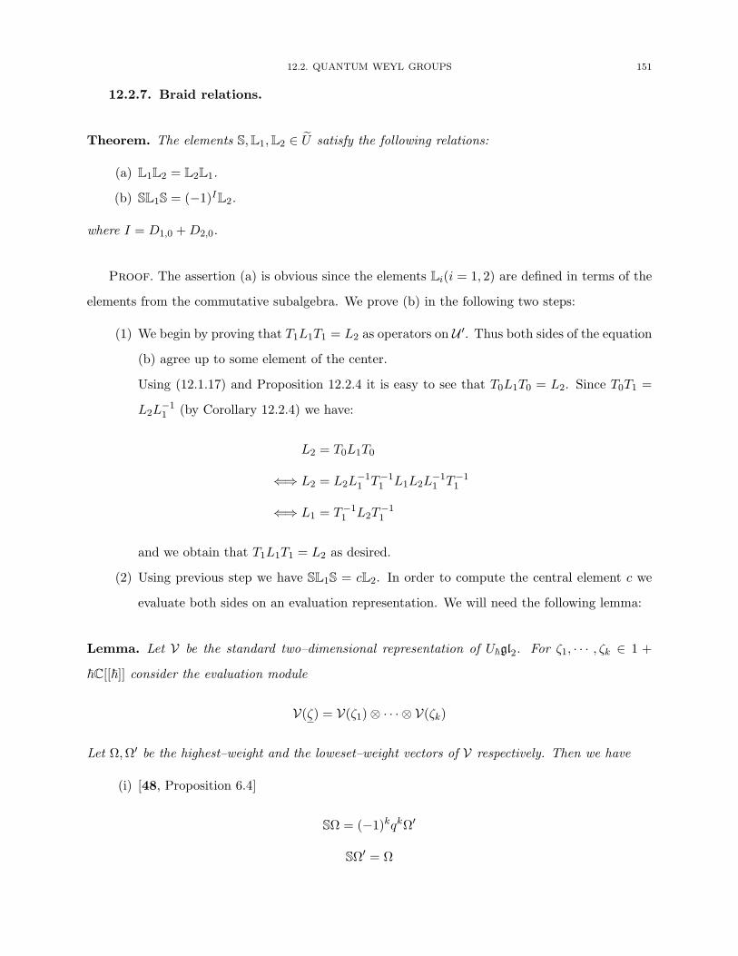
12.2. QUANTUM WEYL GROUPS 151
12.2.7. Braid relations.
Theorem. The elements S,L1,L2 ∈ U satisfy the following relations:
(a) L1L2 = L2L1.
(b) SL1S = (−1)IL2.
where I = D1,0 +D2,0.
Proof. The assertion (a) is obvious since the elements Li(i = 1, 2) are defined in terms of the
elements from the commutative subalgebra. We prove (b) in the following two steps:
(1) We begin by proving that T1L1T1 = L2 as operators on U ′. Thus both sides of the equation(b) agree up to some element of the center.
Using (12.1.17) and Proposition 12.2.4 it is easy to see that T0L1T0 = L2. Since T0T1 =
L2L−11 (by Corollary 12.2.4) we have:
L2 = T0L1T0
⇐⇒ L2 = L2L−11 T−11 L1L2L
−11 T−11
⇐⇒ L1 = T−11 L2T−11
and we obtain that T1L1T1 = L2 as desired.
(2) Using previous step we have SL1S = cL2. In order to compute the central element c we
evaluate both sides on an evaluation representation. We will need the following lemma:
Lemma. Let V be the standard two–dimensional representation of U�gl2. For ζ1, · · · , ζk ∈ 1 +
�C[[�]] consider the evaluation module
V(ζ) = V(ζ1)⊗ · · · ⊗ V(ζk)
Let Ω,Ω′ be the highest–weight and the loweset–weight vectors of V respectively. Then we have
(i) [48, Proposition 6.4]
SΩ = (−1)kqkΩ′
SΩ′ = Ω

152 12. QUANTUM WEYL GROUP
(ii) Let zr := qrD2,r + q−rD1,r be the coefficients of the series qdet±(z) = Θ2(q−1z)Θ1(qz).
zr =[r]
r
(k∑
a=1
ζra
)
as operator on V.
Proof of the lemma: The first part is a special case of [48, Proposition 6.4]. The second part
follows from the explicit form of the evaluation homomorphism given in §12.1.4. �
Let us compute the action of both sides of the equation (b) on Ω′:
SL1SΩ′ = SL1Ω
= q−2kS(Ω)
= (−1)kq−kΩ′
L2Ω′ = q−kΩ′
Hence c acts as (−1)I on each of the modules V(ζ). Using (ii) of Lemma 12.2.7 we obtainthat c = (−1)I . The theorem is proved.
�

CHAPTER 13
Equivalence of representations
In this chapter we prove that the two representations of the affine braid group Π2 (see Proposi-
tion 10.2.5) constructed via the monodromy of the trigonometric Casimir connection (10.2.8) and
via the operators S,L1,L2 (see Theorem 12.2.7) are equivalent.
13.1. Statement of the main theorem
13.1.1. Recall that S�
(M∗
k,2
)is the algebra of functions on the quantum (k × 2) matrix
space (see §11.3). We fix λ = (λ1, · · · , λk) ∈ Nk and consider the subspace S�
(M∗
k,2
)[λ] spanned
by monomials Xm such that
ma1 +ma2 = λa for every a ∈ {1, · · · , k}
The first action of Π2 on S�
(M∗
k,2
)[λ] is obtained using Corollary 11.3.3:
ρEG : Π2 → GL(S�
(M∗k,2
)[λ]
)(13.1.1)
given by:
b �→ (12)RX1 �→ (
q−2s ⊗ 1)R−121
X2 �→ R21
(1⊗ q−2s
) (13.1.2)
where R is the R–matrix of U�glk and s :=∑k
a=1 saDa ∈ U�glk. Note that this action is obtained
by identifying S�
(M∗
k,2
) ∼= S�
(M∗
k,1
)⊗2on which we have an action of U�gl
⊗2k (see §11.3.2).
13.1.2. The second action of Π2 on S�
(M∗
k,2
)is given by Theorem 12.2.7:
ρqW : Π2 → GL(S�
(M∗k,2
)[λ]
)(13.1.3)
153
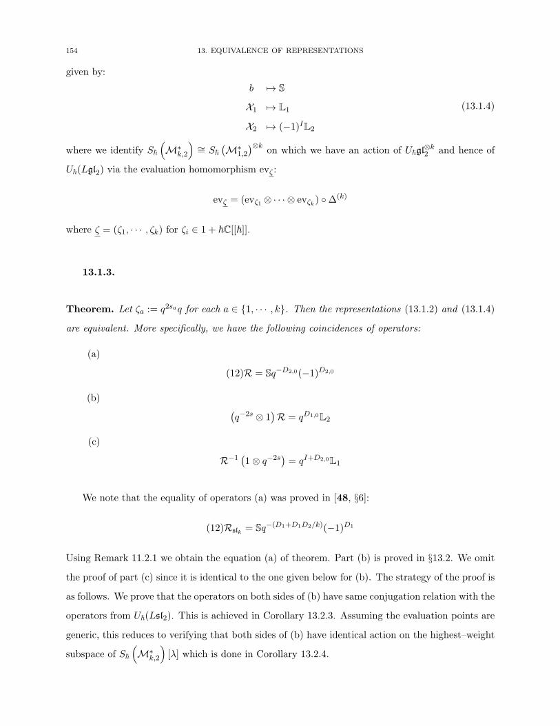
154 13. EQUIVALENCE OF REPRESENTATIONS
given by:
b �→ S
X1 �→ L1
X2 �→ (−1)IL2
(13.1.4)
where we identify S�
(M∗
k,2
) ∼= S�(M∗
1,2
)⊗kon which we have an action of U�gl
⊗k2 and hence of
U�(Lgl2) via the evaluation homomorphism evζ :
evζ = (evζ1 ⊗ · · · ⊗ evζk) ◦Δ(k)
where ζ = (ζ1, · · · , ζk) for ζi ∈ 1 + �C[[�]].
13.1.3.
Theorem. Let ζa := q2saq for each a ∈ {1, · · · , k}. Then the representations (13.1.2) and (13.1.4)
are equivalent. More specifically, we have the following coincidences of operators:
(a)
(12)R = Sq−D2,0(−1)D2,0
(b) (q−2s ⊗ 1
)R = qD1,0L2
(c)
R−1 (1⊗ q−2s)= qI+D2,0L1
We note that the equality of operators (a) was proved in [48, §6]:
(12)Rslk = Sq−(D1+D1D2/k)(−1)D1
Using Remark 11.2.1 we obtain the equation (a) of theorem. Part (b) is proved in §13.2. We omit
the proof of part (c) since it is identical to the one given below for (b). The strategy of the proof is
as follows. We prove that the operators on both sides of (b) have same conjugation relation with the
operators from U�(Lsl2). This is achieved in Corollary 13.2.3. Assuming the evaluation points are
generic, this reduces to verifying that both sides of (b) have identical action on the highest–weight
subspace of S�
(M∗
k,2
)[λ] which is done in Corollary 13.2.4.
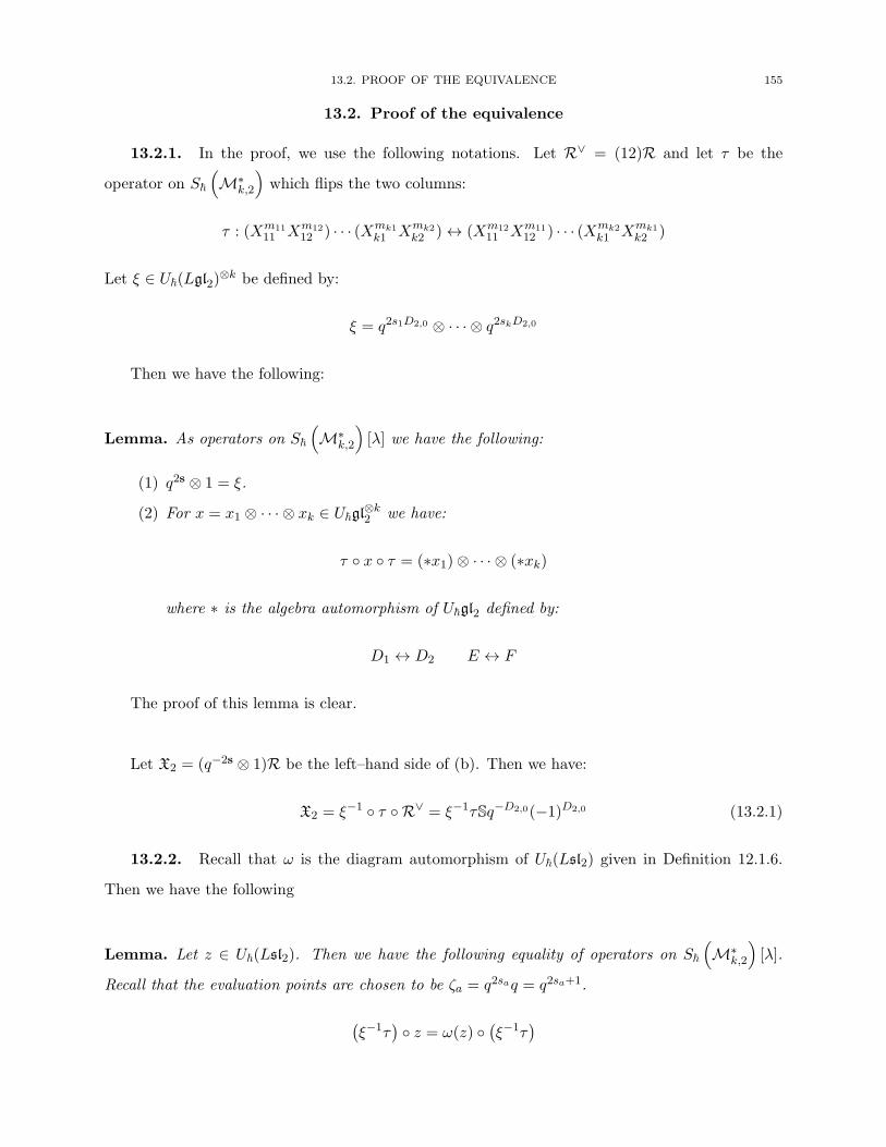
13.2. PROOF OF THE EQUIVALENCE 155
13.2. Proof of the equivalence
13.2.1. In the proof, we use the following notations. Let R∨ = (12)R and let τ be the
operator on S�
(M∗
k,2
)which flips the two columns:
τ : (Xm1111 Xm12
12 ) · · · (Xmk1k1 Xmk2
k2 )↔ (Xm1211 Xm11
12 ) · · · (Xmk2k1 Xmk1
k2 )
Let ξ ∈ U�(Lgl2)⊗k be defined by:
ξ = q2s1D2,0 ⊗ · · · ⊗ q2skD2,0
Then we have the following:
Lemma. As operators on S�
(M∗
k,2
)[λ] we have the following:
(1) q2s ⊗ 1 = ξ.
(2) For x = x1 ⊗ · · · ⊗ xk ∈ U�gl⊗k2 we have:
τ ◦ x ◦ τ = (∗x1)⊗ · · · ⊗ (∗xk)
where ∗ is the algebra automorphism of U�gl2 defined by:
D1 ↔ D2 E ↔ F
The proof of this lemma is clear.
Let X2 = (q−2s ⊗ 1)R be the left–hand side of (b). Then we have:
X2 = ξ−1 ◦ τ ◦ R∨ = ξ−1τSq−D2,0(−1)D2,0 (13.2.1)
13.2.2. Recall that ω is the diagram automorphism of U�(Lsl2) given in Definition 12.1.6.
Then we have the following
Lemma. Let z ∈ U�(Lsl2). Then we have the following equality of operators on S�
(M∗
k,2
)[λ].
Recall that the evaluation points are chosen to be ζa = q2saq = q2sa+1.
(ξ−1τ
) ◦ z = ω(z) ◦ (ξ−1τ)
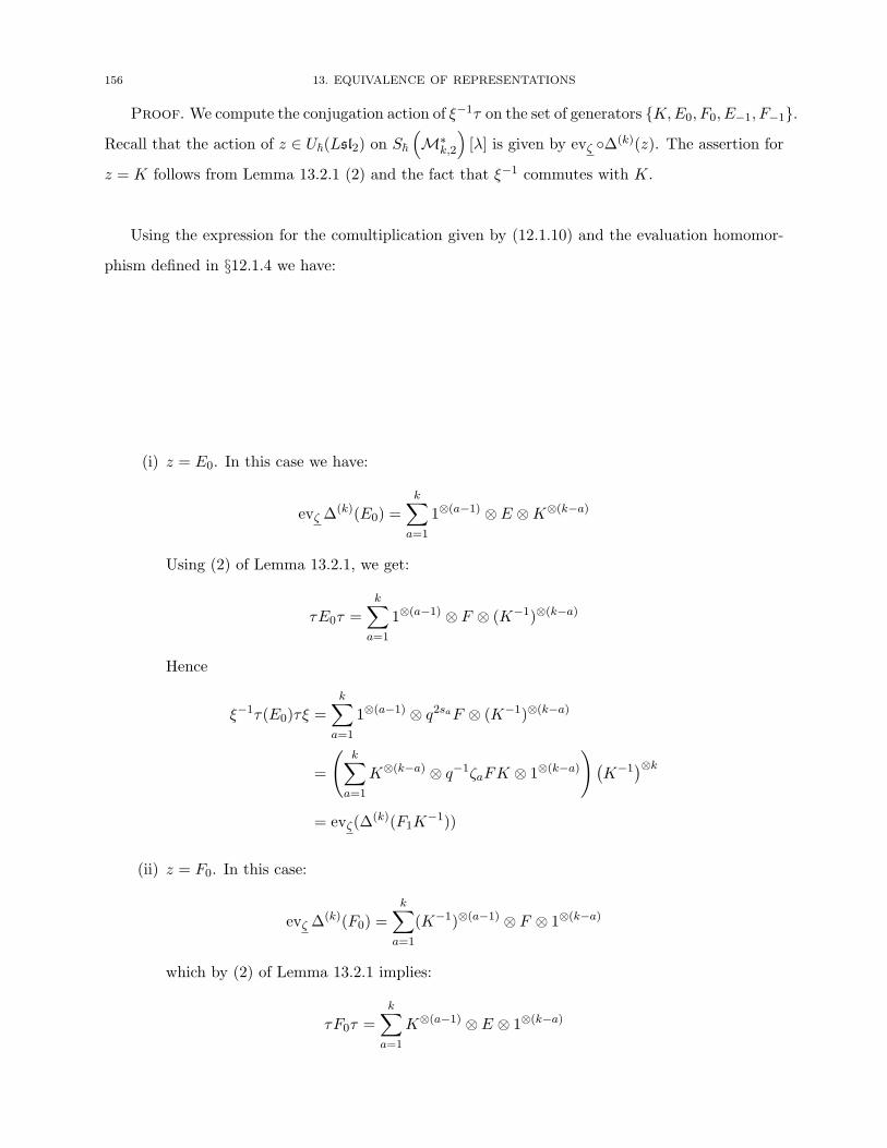
156 13. EQUIVALENCE OF REPRESENTATIONS
Proof. We compute the conjugation action of ξ−1τ on the set of generators {K,E0, F0, E−1, F−1}.Recall that the action of z ∈ U�(Lsl2) on S�
(M∗
k,2
)[λ] is given by evζ ◦Δ(k)(z). The assertion for
z = K follows from Lemma 13.2.1 (2) and the fact that ξ−1 commutes with K.
Using the expression for the comultiplication given by (12.1.10) and the evaluation homomor-
phism defined in §12.1.4 we have:
(i) z = E0. In this case we have:
evζ Δ(k)(E0) =
k∑a=1
1⊗(a−1) ⊗ E ⊗K⊗(k−a)
Using (2) of Lemma 13.2.1, we get:
τE0τ =
k∑a=1
1⊗(a−1) ⊗ F ⊗ (K−1)⊗(k−a)
Hence
ξ−1τ(E0)τξ =
k∑a=1
1⊗(a−1) ⊗ q2saF ⊗ (K−1)⊗(k−a)
=
(k∑
a=1
K⊗(k−a) ⊗ q−1ζaFK ⊗ 1⊗(k−a))(
K−1)⊗k= evζ(Δ
(k)(F1K−1))
(ii) z = F0. In this case:
evζ Δ(k)(F0) =
k∑a=1
(K−1)⊗(a−1) ⊗ F ⊗ 1⊗(k−a)
which by (2) of Lemma 13.2.1 implies:
τF0τ =
k∑a=1
K⊗(a−1) ⊗ E ⊗ 1⊗(k−a)
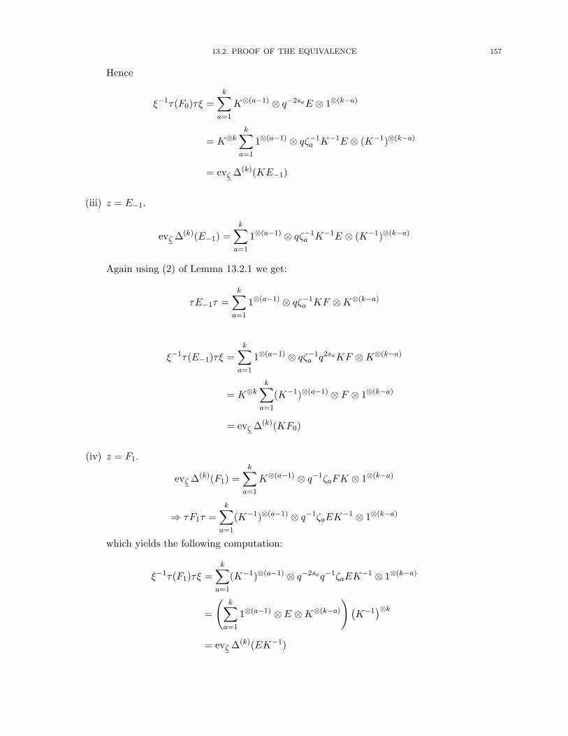
13.2. PROOF OF THE EQUIVALENCE 157
Hence
ξ−1τ(F0)τξ =k∑
a=1
K⊗(a−1) ⊗ q−2saE ⊗ 1⊗(k−a)
= K⊗kk∑
a=1
1⊗(a−1) ⊗ qζ−1a K−1E ⊗ (K−1)⊗(k−a)
= evζ Δ(k)(KE−1)
(iii) z = E−1.
evζ Δ(k)(E−1) =
k∑a=1
1⊗(a−1) ⊗ qζ−1a K−1E ⊗ (K−1)⊗(k−a)
Again using (2) of Lemma 13.2.1 we get:
τE−1τ =k∑
a=1
1⊗(a−1) ⊗ qζ−1a KF ⊗K⊗(k−a)
ξ−1τ(E−1)τξ =k∑
a=1
1⊗(a−1) ⊗ qζ−1a q2saKF ⊗K⊗(k−a)
= K⊗kk∑
a=1
(K−1)⊗(a−1) ⊗ F ⊗ 1⊗(k−a)
= evζ Δ(k)(KF0)
(iv) z = F1.
evζ Δ(k)(F1) =
k∑a=1
K⊗(a−1) ⊗ q−1ζaFK ⊗ 1⊗(k−a)
⇒ τF1τ =k∑
a=1
(K−1)⊗(a−1) ⊗ q−1ζaEK−1 ⊗ 1⊗(k−a)
which yields the following computation:
ξ−1τ(F1)τξ =k∑
a=1
(K−1)⊗(a−1) ⊗ q−2saq−1ζaEK−1 ⊗ 1⊗(k−a)
=
(k∑
a=1
1⊗(a−1) ⊗ E ⊗K⊗(k−a))(
K−1)⊗k= evζ Δ
(k)(EK−1)
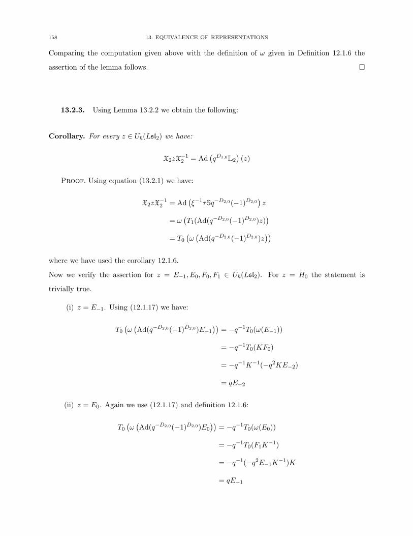
158 13. EQUIVALENCE OF REPRESENTATIONS
Comparing the computation given above with the definition of ω given in Definition 12.1.6 the
assertion of the lemma follows. �
13.2.3. Using Lemma 13.2.2 we obtain the following:
Corollary. For every z ∈ U�(Lsl2) we have:
X2zX−12 = Ad
(qD1,0L2
)(z)
Proof. Using equation (13.2.1) we have:
X2zX−12 = Ad
(ξ−1τSq−D2,0(−1)D2,0
)z
= ω(T1(Ad(q
−D2,0(−1)D2,0)z))
= T0
(ω(Ad(q−D2,0(−1)D2,0)z
))where we have used the corollary 12.1.6.
Now we verify the assertion for z = E−1, E0, F0, F1 ∈ U�(Lsl2). For z = H0 the statement is
trivially true.
(i) z = E−1. Using (12.1.17) we have:
T0
(ω(Ad(q−D2,0(−1)D2,0)E−1
))= −q−1T0(ω(E−1))
= −q−1T0(KF0)
= −q−1K−1(−q2KE−2)
= qE−2
(ii) z = E0. Again we use (12.1.17) and definition 12.1.6:
T0
(ω(Ad(q−D2,0(−1)D2,0)E0
))= −q−1T0(ω(E0))
= −q−1T0(F1K−1)
= −q−1(−q2E−1K−1)K
= qE−1
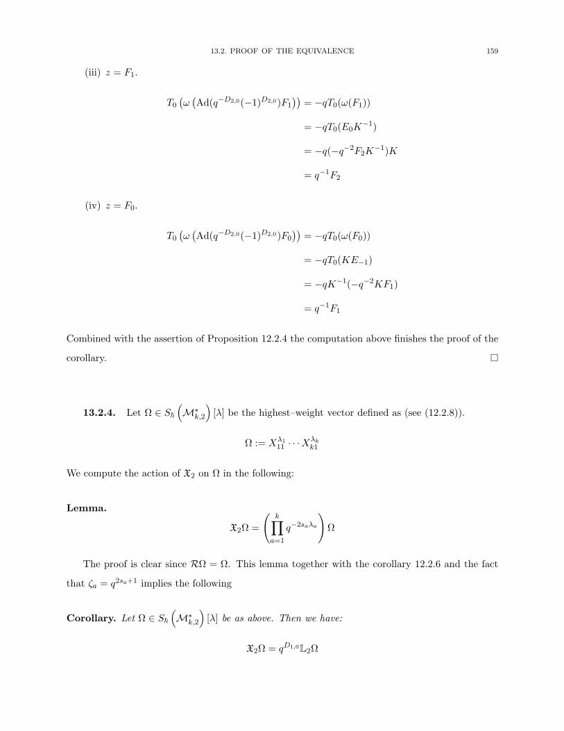
13.2. PROOF OF THE EQUIVALENCE 159
(iii) z = F1.
T0
(ω(Ad(q−D2,0(−1)D2,0)F1
))= −qT0(ω(F1))
= −qT0(E0K−1)
= −q(−q−2F2K−1)K
= q−1F2
(iv) z = F0.
T0
(ω(Ad(q−D2,0(−1)D2,0)F0
))= −qT0(ω(F0))
= −qT0(KE−1)
= −qK−1(−q−2KF1)
= q−1F1
Combined with the assertion of Proposition 12.2.4 the computation above finishes the proof of the
corollary. �
13.2.4. Let Ω ∈ S�
(M∗
k,2
)[λ] be the highest–weight vector defined as (see (12.2.8)).
Ω := Xλ111 · · ·Xλk
k1
We compute the action of X2 on Ω in the following:
Lemma.
X2Ω =
(k∏
a=1
q−2saλa
)Ω
The proof is clear since RΩ = Ω. This lemma together with the corollary 12.2.6 and the fact
that ζa = q2sa+1 implies the following
Corollary. Let Ω ∈ S�
(M∗
k,2
)[λ] be as above. Then we have:
X2Ω = qD1,0L2Ω
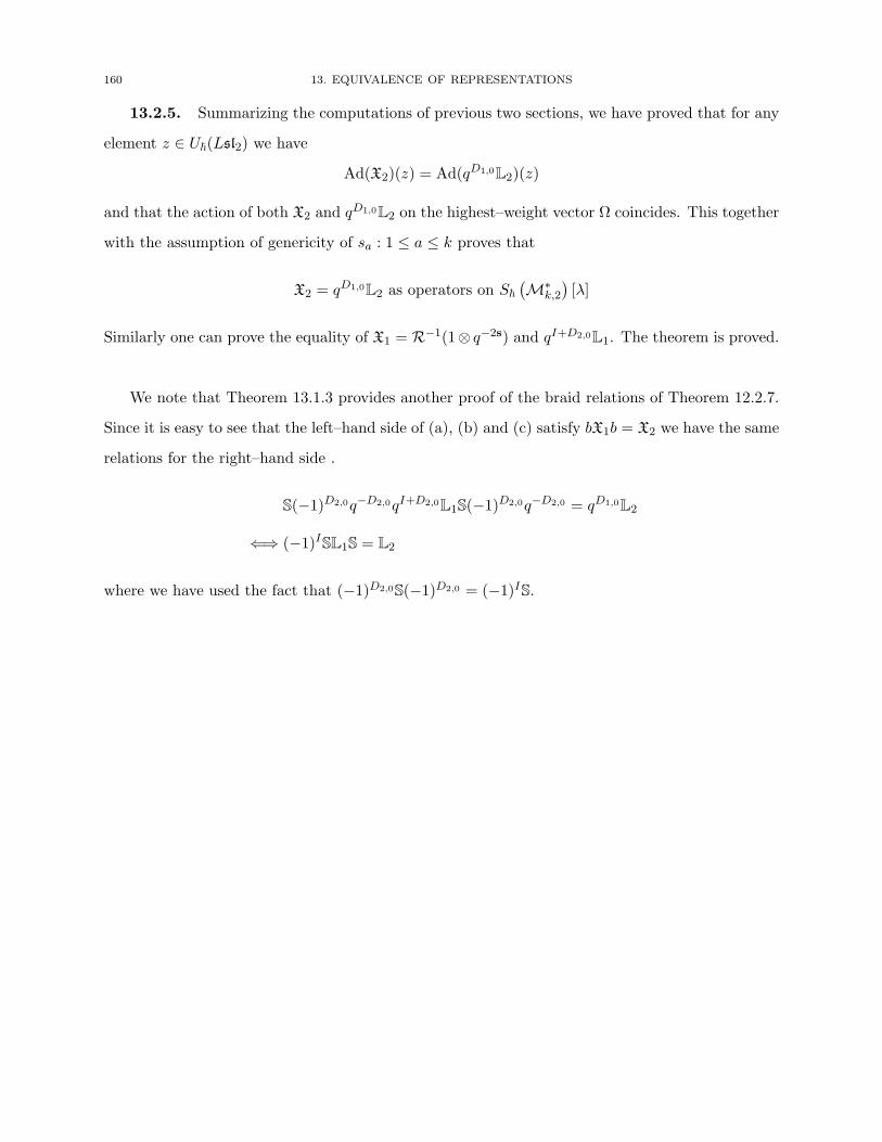
160 13. EQUIVALENCE OF REPRESENTATIONS
13.2.5. Summarizing the computations of previous two sections, we have proved that for any
element z ∈ U�(Lsl2) we have
Ad(X2)(z) = Ad(qD1,0L2)(z)
and that the action of both X2 and qD1,0L2 on the highest–weight vector Ω coincides. This together
with the assumption of genericity of sa : 1 ≤ a ≤ k proves that
X2 = qD1,0L2 as operators on S�(M∗
k,2
)[λ]
Similarly one can prove the equality of X1 = R−1(1⊗ q−2s) and qI+D2,0L1. The theorem is proved.
We note that Theorem 13.1.3 provides another proof of the braid relations of Theorem 12.2.7.
Since it is easy to see that the left–hand side of (a), (b) and (c) satisfy bX1b = X2 we have the same
relations for the right–hand side .
S(−1)D2,0q−D2,0qI+D2,0L1S(−1)D2,0q−D2,0 = qD1,0L2
⇐⇒ (−1)ISL1S = L2
where we have used the fact that (−1)D2,0S(−1)D2,0 = (−1)IS.
Bibliography
1. A. Berenstein, S. Fomin, and A. Zelevinsky, Cluster algebras 3: Upper bounds and double Bruhat cells, Duke
Mathematical Journal 126 (2005), no. 1, 1–52.
2. A. Berenstein and A. Zelevinsky, Total positivity in Schubert varieties, Comment. Math. Helv. 72 (1997), no. 1,
128–166.
3. E. Brieskorn, Die Fundamentalgruppe des Raumes der regularen Orbits einer endlichen komplexen Spiegelungs-
gruppe, Invent. Math. 12 (1971), 57–61.
4. V. Chari and A. Pressley, Yangians and R-matrices, L’Enseignement Mathematique 36 (1990), 267–302.
5. , Quantum affine algebras, Communications in Mathematical Physics 142 (1991), 261–283.
6. , A guide to quantum groups, Cambridge University Press, 1994.
7. I. Cherednik, Double affine Hecke algebras, Cambridge University Press, 2005.
8. J. Ding and I. Frenkel, Isomorphism of two realizations of the quantum affine algebra Uq(gl(n)), Communications
in Mathematical Physics (1994), no. 156, 277–300.
9. V. G. Drinfeld, Hopf algebras and the quantum Yang-Baxter equation, Soviet Math. Dokl. 32 (1985), no. 1,
254–258.
10. , Quantum groups, Proceedings of the I.C.M., Berkeley (1986), 798–820.
11. , A new realization of Yangians and quantum affine algebras, Soviet Math. Dokl. 36 (1988), no. 2, 212–216.
12. , Quasi Hopf algebras and the KZ equations, in Problems of modern QFT (1989), 1–13.
13. , On almost cocommutative Hopf algebras, Leningrad Math. J. 1 (1990), no. 2, 321–342.
14. , personal communication, (2009).
15. P. Etingof and N. Geer, Monodromy of trigonometric KZ equations, International Mathematics Research Notices
(2007), 1–15.
16. P. Etingof and D. Kazhdan, Quantization of Lie bialgebras - I, Selecta Mathematica, New Series 2 (1996), no. 1,
1–41.
17. P. Etingof and O. Schiffmann, Lectures on quantum groups, 1 ed., International Press, 1998.
18. S. Fomin and A. Zelevinsky, Double Bruhat cells and total positivity, Journal of the A.M.S. 12 (1999), no. 2,
335–380.
19. , Cluster algebras 1: Foundations, Journal of the A.M.S. 15 (2002), no. 2, 497–529.
20. , Cluster algebra 2: Finite type classification, Invent. Math. 154 (2003), no. 1, 63–121.
21. , Cluster algebras 4: Coefficients, Compos. Math. 143 (2007), no. 1, 112–164.
161

162 BIBLIOGRAPHY
22. S. Gautam, Cluster algebras and grassmannians of type G2, Algebras and representation theory 13 (2010), no. 3,
335–357.
23. S. Gautam and V. Toledano Laredo, Yangians and quantum loop algebras, arXiv:1012.3687v1 (2010), submitted.
24. , Monodromy of the trigonometric Casimir connection for sl2, preprint (2011).
25. C. Geiss, B. Leclerc, and J. Schroer, Partial flag varieties and preprojective algebras, Annales de l’institut Fourier
58 (2008), no. 3, 825–876.
26. V. Ginzburg and E. Vasserot, Langlands reciprocity for affine quantum groups of type An, International Mathe-
matics Research Notices (1993), no. 3, 67–85.
27. N. Guay and X. Ma, From quantum loop algebras to Yangians, submitted, 2010.
28. J. C. Jantzen, Lectures on quantum groups, Graduate studies in Mathematics, A.M.S., 1996.
29. C. Kassel, Quantum groups, Graduate texts in mathematics, Springer-Verlag, 1995.
30. A. N. Kirillov and N. Reshetikhin, q-Weyl group and a multiplicative formula for universal R–matrices, Comm.
Math. Phys. (1990), no. 134, 421–441.
31. T. Kohno, Monodromy representations of braid groups and Yang-Baxter equations, Annales de l’insitut Fourier
37 (1987), no. 4, 139–160.
32. S. Z. Levendorskii, On generators and defining relations of Yangians, Journal of Geometry and Physics 12 (1992),
1–11.
33. , On PBW bases for Yangians, Letters in Mathematical Physics 27 (1993), 37–42.
34. G. Lusztig, Introduction to quantum groups, Birkhauser Boston, 1993.
35. I. G. Macdonald, Affine Hecke algebras and orthogonal polynomials, Cambridge University Press, 2003.
36. J. Millson and V. Toledano Laredo, Casimir operator and monodromy representations of generalized braid groups,
Transformation Groups 10 (2005), no. 2, 217–254.
37. A. Molev, Yangians and classical Lie algebras, Mathematical Surveys and Monographs, vol. 143, American
Mathematical Society, 2007.
38. H. Nakajima, Quiver varieties and Kac–Moody algebras, Duke Mathematical Journal 91 (1998), no. 3, 515–560.
39. , Quiver varieties and finite dimensional representations of quantum affine algebras, Journal of the A.M.S.
14 (2001), 145–238.
40. V. D. Nguyen, The fundamental group of the spaces of regular orbits of the affine Weyl groups, Topology 22
(1983), 425–435.
41. G. I. Olshanskii, Representations of infinite–dimensional classical groups, limits of enveloping algebras, and Yan-
gians, Topics in representation theory, Adv. Soviet Math., 2, A.M.S., 1991, pp. 1–66.
42. B. Parshall and J. P. Wang, Quantum linear groups, Memoirs of the A.M.S. 89 (1991), no. 439.
43. Y. S. Soibelman, Algebra of functions on a compact quantum group and its representations, Leningrad Math. J.
(1991), no. 2, 161–178.
44. V. O. Tarasov, Structure of quantum L–operators for the R–matrix of the XXZ–model, Theoretical and Mathe-
matical Physics 61 (1984), 1065–1071.

BIBLIOGRAPHY 163
45. , Irreducible monodromy matrices for the R–matrix of the XXZ–model and lattice local quantum Hamil-
tonians, Theoretical and Mathematical Physics 63 (1985), 440–454.
46. V. O. Tarasov and A. Varchenko, Duality for Knizhnik–Zamolodchikov and dynamical equations, Acta Appl.
Math. 73 (2002), 141–154.
47. V. Toledano Laredo, Flat connections and quantum groups, Acta Appl. Math. 73 (2002), no. 1-2, 155–173.
48. , A Kohno–Drinfeld theorem for quantum Weyl groups, Duke Mathematical Journal 112 (2002), no. 3,
421–451.
49. , Quasi–Coxeter algebras, Dynkin diagram cohomology and quantum Weyl groups, Int. Math. Res. Pap.
(2008).
50. , The trigonometric Casimir connection of a simple Lie algebra, Journal of Algebra 329 (2011), 286–327.
51. H. van der Lek, Extended Artin groups, Singularities (Arcata, California), Proceedings of Symposia in Pure
Mathematics, vol. 40, AMS, 1983, pp. 117–121.
52. , The homotopy type of hyperplane complements, Ph.D. thesis, Katholieke Universiteit Nijmegen, 1983.
53. M. Varagnolo, Quiver varieties and Yangians, Letters in Mathematical Physics 53 (2000), no. 4, 273–283.
54. E. Vasserot, Affine quantum groups and equivariant K-theory, Transformation Groups 3 (1998), no. 3, 269–299.