1

Three or More Factors: Latin SquaresExample:

Three factors, A (block factor), B (block factor), and C (treatment factor), each at three levels. A possible arrangement:

B 1 B 2 B 3

A1

C1 C1 C1

A C2 C2 C2

A3 C3 C3 C3

2

2

Notice, first, that these designs are squares; all factors are at the same number of levels, though there is no restriction on the nature of the levels themselves. Notice, that these squares are balanced: each letter (level) appears the same number of times; this insures unbiased estimates of main effects.

How to do it in a square? Each treatment appears once in every column and row.

Notice, that these designs are incomplete; of the 27 possible combinations of three factors each at three levels, we use only 9.

3

Example:

Three factors, A (block factor), B (block factor), and C (treatment factor), each at three levels, in a Latin Square design; nine combinations.

B 1 B 2 B 3

A1

C1 C2 C3

A C2 C3 C1

A3 C3 C1 C2

2

4

Example with 4 Levels per FactorExample with 4 Levels per Factor

AutomobilesAutomobiles A A four levelsfour levelsTire positionsTire positions B B four levelsfour levelsTire treatments Tire treatments C C four levelsfour levels

FACTORSFACTORS

Lifetime of a tire Lifetime of a tire (days)(days)

VARIABLEVARIABLE

A 1

A 2

A 3

A 4

B1 B2 B3 B4

C 4

8 5 5C 3

8 7 7C 2

8 9 0C 1

9 9 7

C 1

9 6 2C 2

8 1 7C 3

8 4 5C 4

7 7 6

C 3

8 4 8C 4

8 4 1C 1

7 8 4C 2

7 7 6

C 2

8 3 1C 1

9 5 2C 4

8 0 6C 3

8 7 1

5

The Model for (Unreplicated) The Model for (Unreplicated) Latin SquaresLatin Squares

Example:

Note that interaction is not present in the model.

Threefactors , ,andeachat mlevels,

yijk = +

i+ j + k + ijk

i= 1,... m

j=1, ..., m

k=1, ... ,m

Same three assumptions: normality, constant variances, and randomness.

Y = A + B + C + eAB, AC, BC, ABC

6

Putting in Estimates:Putting in Estimates:

Total variability

among yields

Variability among yields

associated with Rows

Variability among yields

associated with

Columns

Variability among yields

associated with Inside

Factor

where R =

or bringing y••• to the left – hand side,

(y ijk –y ...) = (y i .. – y ...) + (y .j . – y...) + (y ..k – y ...) + R,

= + +

y ijk =y ... + (y i.. – y ... ) + (y . j. – y ...) + (y ..k – y ... ) + R

yijk – y i.. – y . j. – y.. k + 2y...

7

Actually, Actually, R R

An “interaction-like” term. (After all, there’s no replication!)

= y ijk - y i .. - y . j. - y ..k + 2y...= (y ijk - y ...)

-

(y i.. - y ...)

(y . j. - y ...)

(y ..k - y ...),-

-

8

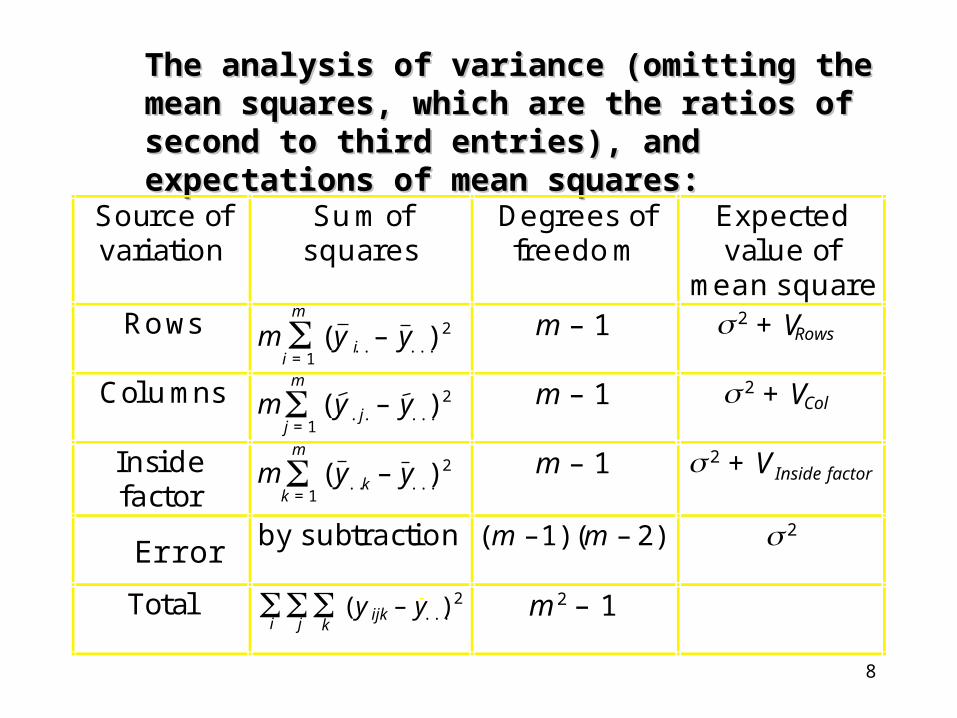
The analysis of variance (omitting the mean squares, The analysis of variance (omitting the mean squares, which are the ratios of second to third entries), and which are the ratios of second to third entries), and expectations of mean squares:expectations of mean squares:

Source ofvariation

Sum ofsquares

Degrees offreedom

Expectedvalue of

mean squareRows

m (y i.. – y ...)2

i = 1

m m – 1 2 + VRows

Columns m (y . j . – y ...)

2j = 1

m m – 1 2 + VCol

Insidefactor

m (y ..k – y ...)

2k = 1

m m – 1 2 + V Inside factor

by subtraction (m – 1)( m – 2) 2

Total i

j(y ijk – y ...)

2k

m 2 – 1

Error

9

The expected values of the mean squares immediately suggest the F ratios appropriate for testing null hypotheses on rows, columns and inside factor.

10

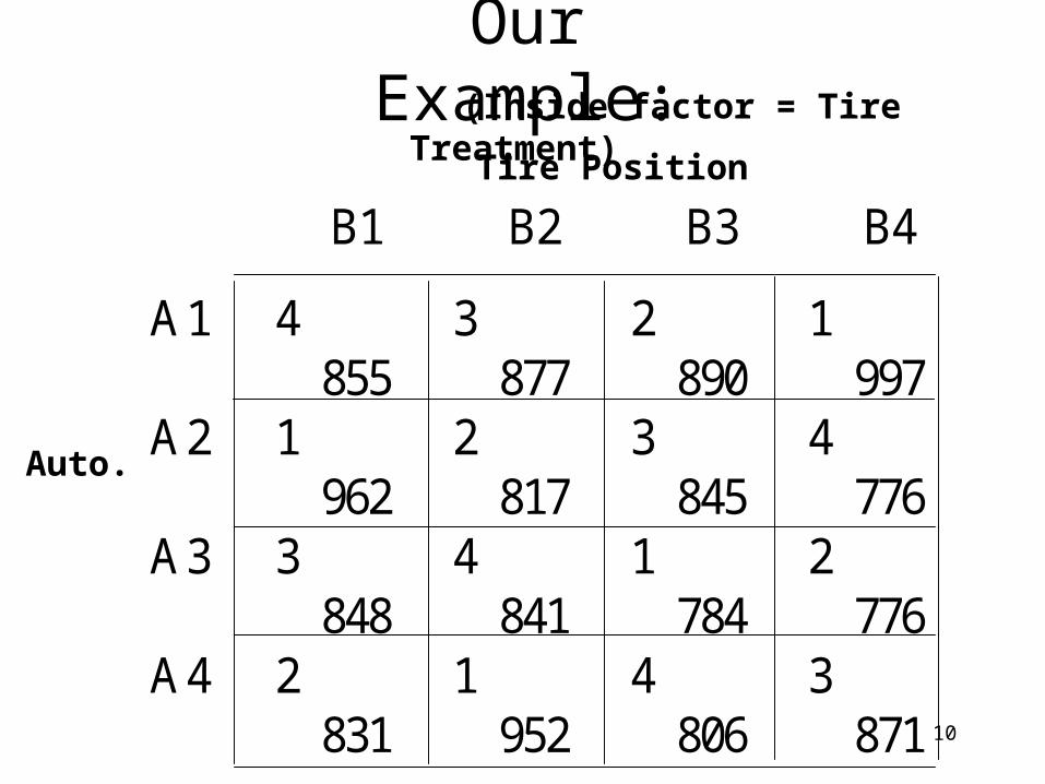
Our Example:

B1 B2 B3 B4

A1 4855

3877

2890

1997

A2 1962

2817

3845

4776

A3 3848

4841

1784

2776

A4 2831

1952

4806

3871

Tire Position

Auto.

(Inside factor = Tire Treatment)

11

General Linear Model: Lifetime versus Auto, Postn, Trtmnt

Factor Type Levels Values Auto fixed 4 1 2 3 4Postn fixed 4 1 2 3 4Trtmnt fixed 4 1 2 3 4

Analysis of Variance for Lifetime, using Adjusted SS for Tests

Source DF Seq SS Adj SS Adj MS F PAuto 3 17567 17567 5856 2.17 0.192Postn 3 4679 4679 1560 0.58 0.650Trtmnt 3 26722 26722 8907 3.31 0.099Error 6 16165 16165 2694Total 15 65132

Unusual Observations for Lifetime

Obs Lifetime Fit SE Fit Residual St Resid 11 784.000 851.250 41.034 -67.250 -2.12R

12

OUR EXAMPLEB1 B2 B3 B4

A1 C4 C3 C2 C1855 877 890 997

A2 C1 C2 C3 C4962 817 845 776

A3 C3 C4 C1 C2848 841 784 776

A4 C2 C1 C4 C3831 952 806 871

SPSS:

Sum of MeanSource of Variation Squares DF Square F p-value

Service Policy 17566.5 3 5855.5 2.173 .192 Hours Open 4678.5 3 1559.5 .579 .650 Amenities 26722.5 3 8907.5 3.306 .099 Residual 16164.5 6 2694.1 Total 65132.0 15

13

SPSS/Minitab DATA ENTRYVAR1 VAR2 VAR3 VAR4

855 1 1 4962 2 1 1848 3 1 3831 4 1 2877 1 2 3817 2 2 2. . . .. . . .. . . .871 4 4 3

14

Latin Square with REPLICATION

• Case One: using the same rows and columns for all Latin squares.

• Case Two: using different rows and columns for different Latin squares.

• Case Three: using the same rows but different columns for different Latin squares.

15

Treatment Assignments for n Replications

• Case One: repeat the same Latin square n times.

• Case Two: randomly select one Latin square for each replication.

• Case Three: randomly select one Latin square for each replication.

16

Example: n = 2, m = 4, trtmnt = A,B,C,D

Case One:

column

row 1 2 3 4

1 A B C D

2 B C D A

3 C D A B

4 D A B C

column

row 1 2 3 4

1 A B C D

2 B C D A

3 C D A B

4 D A B C

• Row = 4 tire positions; column = 4 cars

17

column

row 1 2 3 4

1 A B C D

2 B C D A

3 C D A B

4 D A B C

column

row 5 6 7 8

5 B C D A

6 A D C B

7 D B A C

8 C A B D

Case Two

• Row = clinics; column = patients; letter = drugs for flu

18

5 6 7 8

B C D A

A D C B

D B A C

C A B D

Case Three

column

row 1 2 3 4

1 A B C D

2 B C D A

3 C D A B

4 D A B C

• Row = 4 tire positions; column = 8 cars

19

ANOVA for Case 1

SSBR, SSBC, SSBIF are computed the same way as before, except that the multiplier of (say for

rows) m (Yi..-Y…)2 becomes

mn (Yi..-Y…)2

and degrees of freedom for error becomes

(nm2 - 1) - 3(m - 1) = nm2 - 3m + 2

20

ANOVA for other cases:

Using Minitab in the same way can give Anova tables for all cases.

1. SS: please refer to the book, Statistical Principles of research Design and Analysis by R. Kuehl.

2. DF: # of levels – 1 for all terms except error. DF of error = total DF – the sum of the rest DF’s.

21

Graeco-Latin SquaresIn an unreplicated m x m Latin square there are m2

yields and m2 - 1 degrees of freedom for the total sum of squares around the grand mean. As each studied factor has m levels and, therefore, m-1 degrees of freedom, the maximum number of factors which can be accommodated, allowing no degree of freedom for factors not studied, is

A design accommodating the maximum number of factors is called a complete Graeco-Latin square:

m 2 – 1m – 1

= m + 1

22

Example 1:Example 1:m=3; four factors can be accommodatedm=3; four factors can be accommodated

B1 B2 B3

A1 C1 D1 C2 D2 C3 D3

A2 C2 D3 C3 D1 C1 D2

A3 C3 D2 C1 D3 C2 D1

23

Example 2:m = 5; six factors can be accommodated

B1 B2 B3 B4 B5

A1 C1 D1 E1 F1 C2 D2 E2 F2 C3 D3 E3 F3 C4 D4 E4 F4 C5 D5 E5 F5

A2 C2 D3 E4 F5 C3 D4 E5 F1 C4 D5 E1 F2 C5 D1 E2 F3 C1 D2 E3 F4

A3 C3 D5 E2 F4 C4 D1 E3 F5 C5 D2 E4 F1 C1 D3 E5 F2 C2 D4 E1 F3

A4 C4 D2 E5 F3 C5 D3 E1 F4 C1 D4 E2 F5 C2 D5 E3 F1 C3 D1 E4 F2

A5 C5 D4 E3 F2 C1 D5 E4 F3 C2 D1 E5 F4 C3 D2 E1 F5 C4 D3 E2 F1

24

In an unreplicated complete Graeco-Latin square all degrees of freedom are used up by factors studied. Thus, no estimate of the effect of factors not studied is possible, and analysis of variance cannot be completed.

25

But, consider incomplete Graeco-Latin Squares:b1 b2 b3 b4 b5

a1

a2

a3

a4

a5

c1d1 c2d2 c3d3 c4d4 c5d5

c2d3 c3d4 c4d5 c5d1 c1d2

c3d5

c4d2

c5d4

c4d1 c5d2 c1d3 c2d4

c5d3 c1d4 c2d5 c3d1

c1d5 c2d1 c3d2 c4d3

26

We test 4 different Hypotheses.

ANOVA TABLE

A

B

C

D

Error

SSBA

SSBB

SSBC

SSBD

SSW

4

4

4

4

8

TSS 24

•

•

•

•

•

by Subtraction

SOURCE SSQ df