Embed Size (px)
Citation preview
Three New Connections Between Complexity Theory and
Algorithmic Game Theory
Tim Roughgarden (Stanford)
Three New Connections Between Complexity Theory and
Algorithmic Game Theory
(case studies in “applied complexity theory”)
Tim Roughgarden (Stanford)
Overview
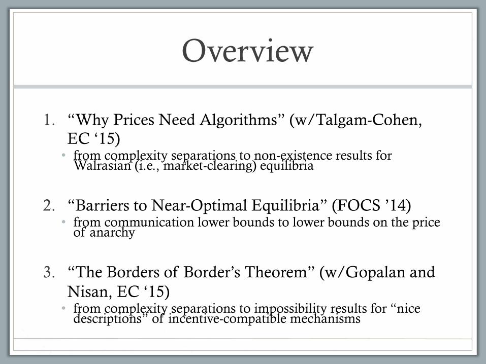
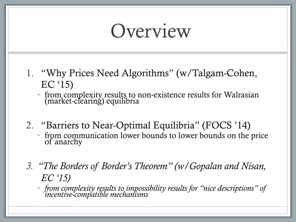
1. “Why Prices Need Algorithms” (w/Talgam-Cohen, EC ‘15) • from complexity separations to non-existence results for
Walrasian (i.e., market-clearing) equilibria
2. “Barriers to Near-Optimal Equilibria” (FOCS ’14) • from communication lower bounds to lower bounds on the price
of anarchy
3. “The Borders of Border’s Theorem” (w/Gopalan and Nisan, EC ‘15) • from complexity separations to impossibility results for “nice
descriptions” of incentive-compatible mechanisms
€
Overview
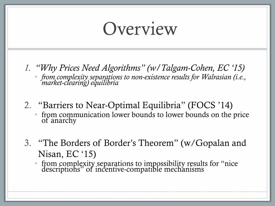
1. “Why Prices Need Algorithms” (w/Talgam-Cohen, EC ‘15) • from complexity separations to non-existence results for Walrasian (i.e.,
market-clearing) equilibria
2. “Barriers to Near-Optimal Equilibria” (FOCS ’14) • from communication lower bounds to lower bounds on the price
of anarchy
3. “The Borders of Border’s Theorem” (w/Gopalan and Nisan, EC ‘15) • from complexity separations to impossibility results for “nice
descriptions” of incentive-compatible mechanisms
€
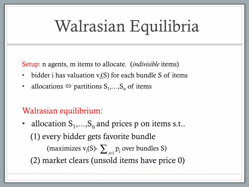
Walrasian Equilibria
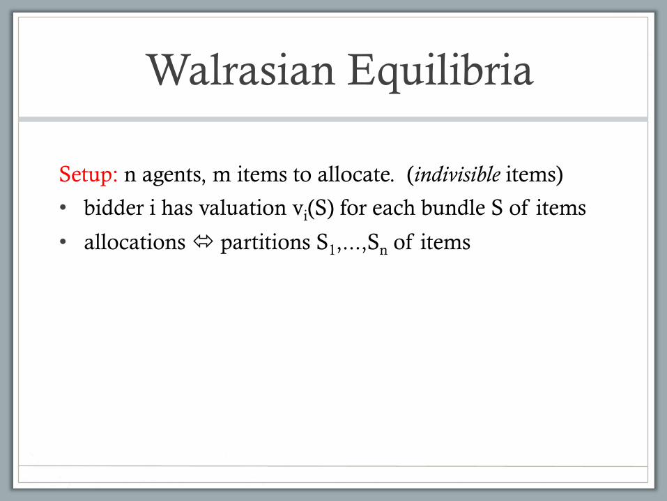
Setup: n agents, m items to allocate. (indivisible items)
• bidder i has valuation vi(S) for each bundle S of items
• allocations ó partitions S1,...,Sn of items
Walrasian Equilibria
Setup: n agents, m items to allocate. (indivisible items)
• bidder i has valuation vi(S) for each bundle S of items
• allocations ó partitions S1,...,Sn of items
Walrasian equilibrium:
• allocation S1,...,Sn and prices p on items s.t..
(1) every bidder gets favorite bundle (maximizes vi(S)- pj over bundles S)
(2) market clears (unsold items have price 0) j∈S∑
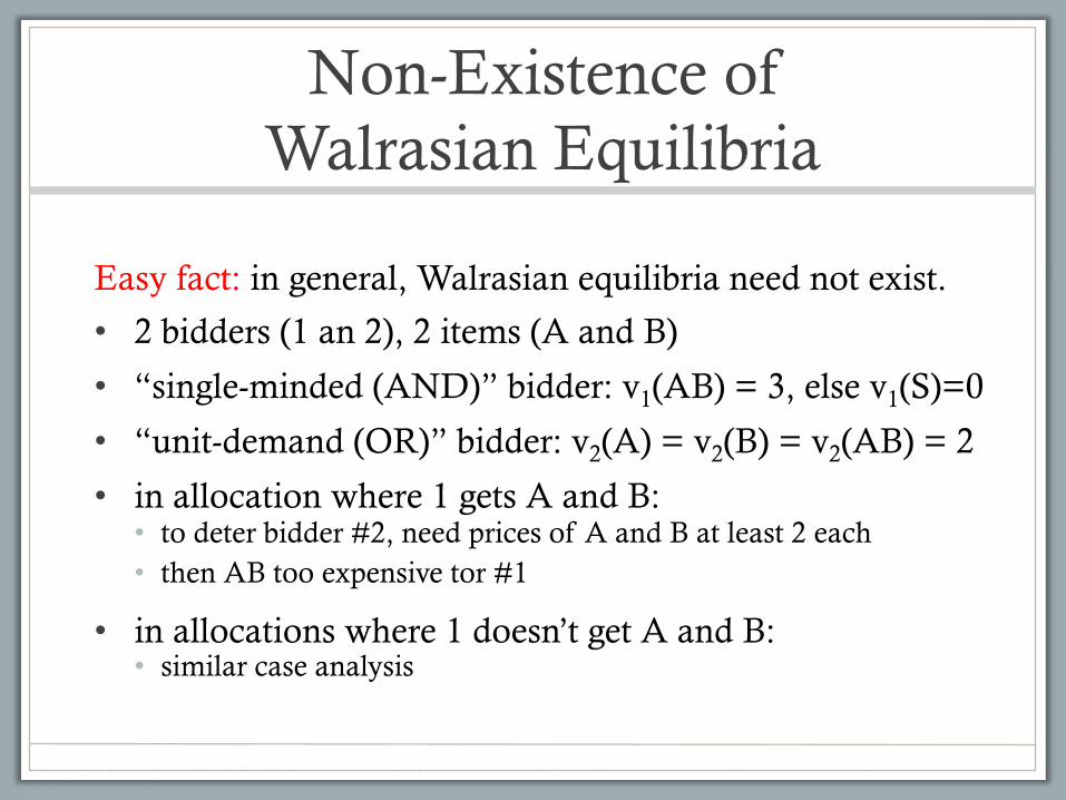
Non-Existence of Walrasian Equilibria
Easy fact: in general, Walrasian equilibria need not exist.
• 2 bidders (1 an 2), 2 items (A and B)
• “single-minded (AND)” bidder: v1(AB) = 3, else v1(S)=0
• “unit-demand (OR)” bidder: v2(A) = v2(B) = v2(AB) = 2
• in allocation where 1 gets A and B: • to deter bidder #2, need prices of A and B at least 2 each • then AB too expensive tor #1
• in allocations where 1 doesn’t get A and B: • similar case analysis
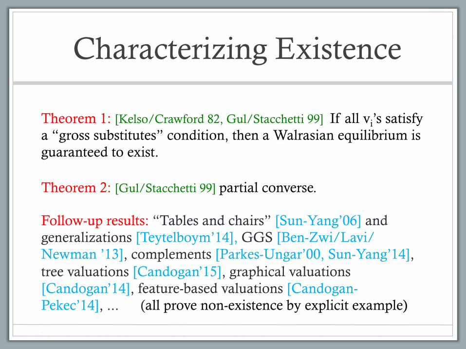
Characterizing Existence
Theorem 1: [Kelso/Crawford 82, Gul/Stacchetti 99] If all vi’s satisfy a “gross substitutes” condition, then a Walrasian equilibrium is guaranteed to exist.
Theorem 2: [Gul/Stacchetti 99] partial converse.
Follow-up results: “Tables and chairs” [Sun-Yang’06] and generalizations [Teytelboym’14], GGS [Ben-Zwi/Lavi/Newman ’13], complements [Parkes-Ungar’00, Sun-Yang’14], tree valuations [Candogan’15], graphical valuations [Candogan’14], feature-based valuations [Candogan-Pekec’14], ... (all prove non-existence by explicit example)
€
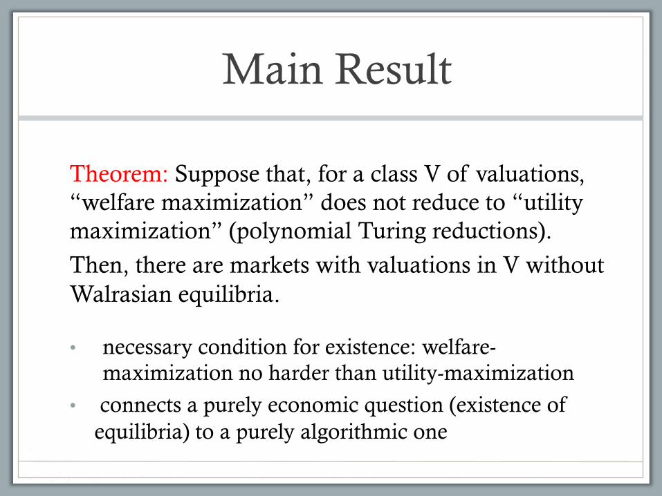
Main Result
Theorem: Suppose that, for a class V of valuations, “welfare maximization” does not reduce to “utility maximization” (polynomial Turing reductions).
Then, there are markets with valuations in V without Walrasian equilibria.
• necessary condition for existence: welfare-maximization no harder than utility-maximization
• connects a purely economic question (existence of equilibria) to a purely algorithmic one
€
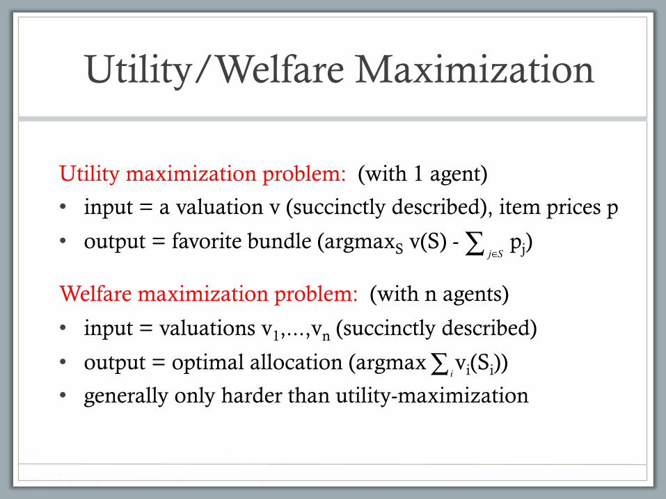
Utility/Welfare Maximization
Utility maximization problem: (with 1 agent)
• input = a valuation v (succinctly described), item prices p
• output = favorite bundle (argmaxS v(S) - pj)
Welfare maximization problem: (with n agents)
• input = valuations v1,...,vn (succinctly described)
• output = optimal allocation (argmax vi(Si))
• generally only harder than utility-maximization
€
j∈S∑
i∑
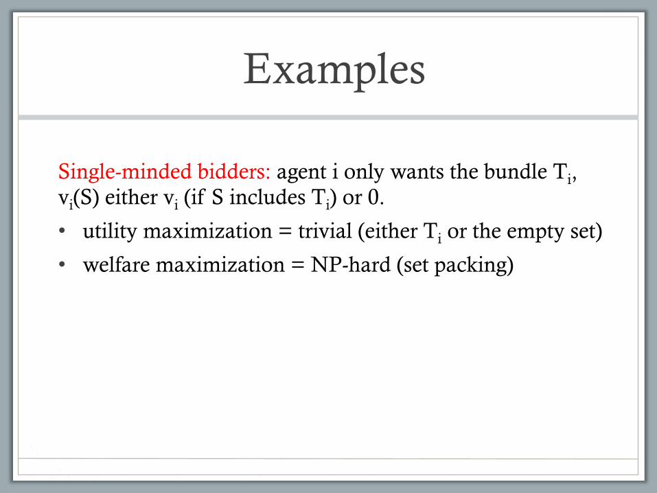
Examples
Single-minded bidders: agent i only wants the bundle Ti, vi(S) either vi (if S includes Ti) or 0.
• utility maximization = trivial (either Ti or the empty set)
• welfare maximization = NP-hard (set packing)
€
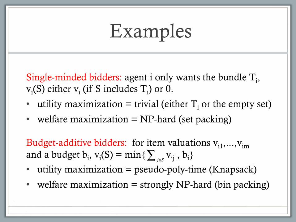
Examples
Single-minded bidders: agent i only wants the bundle Ti, vi(S) either vi (if S includes Ti) or 0.
• utility maximization = trivial (either Ti or the empty set)
• welfare maximization = NP-hard (set packing)
Budget-additive bidders: for item valuations vi1,...,vim and a budget bi, vi(S) = min{ vij , bi}
• utility maximization = pseudo-poly-time (Knapsack)
• welfare maximization = strongly NP-hard (bin packing)
€ j∈S∑
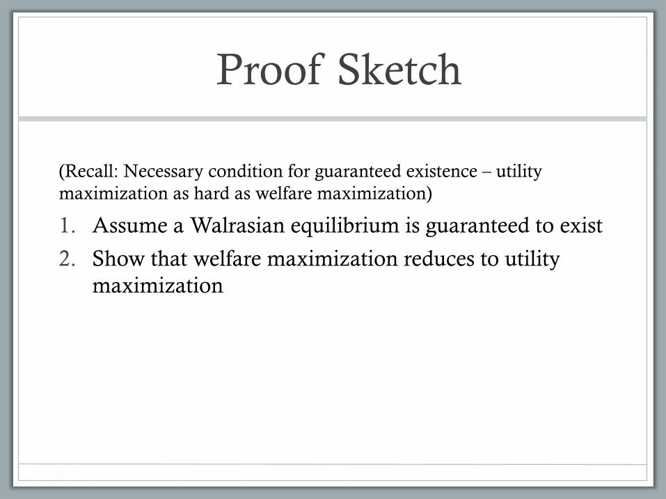
Proof Sketch
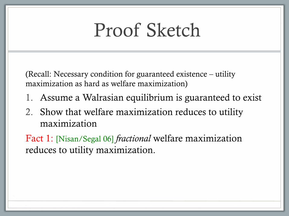
(Recall: Necessary condition for guaranteed existence – utility maximization as hard as welfare maximization)
1. Assume a Walrasian equilibrium is guaranteed to exist
2. Show that welfare maximization reduces to utility maximization
€
Proof Sketch
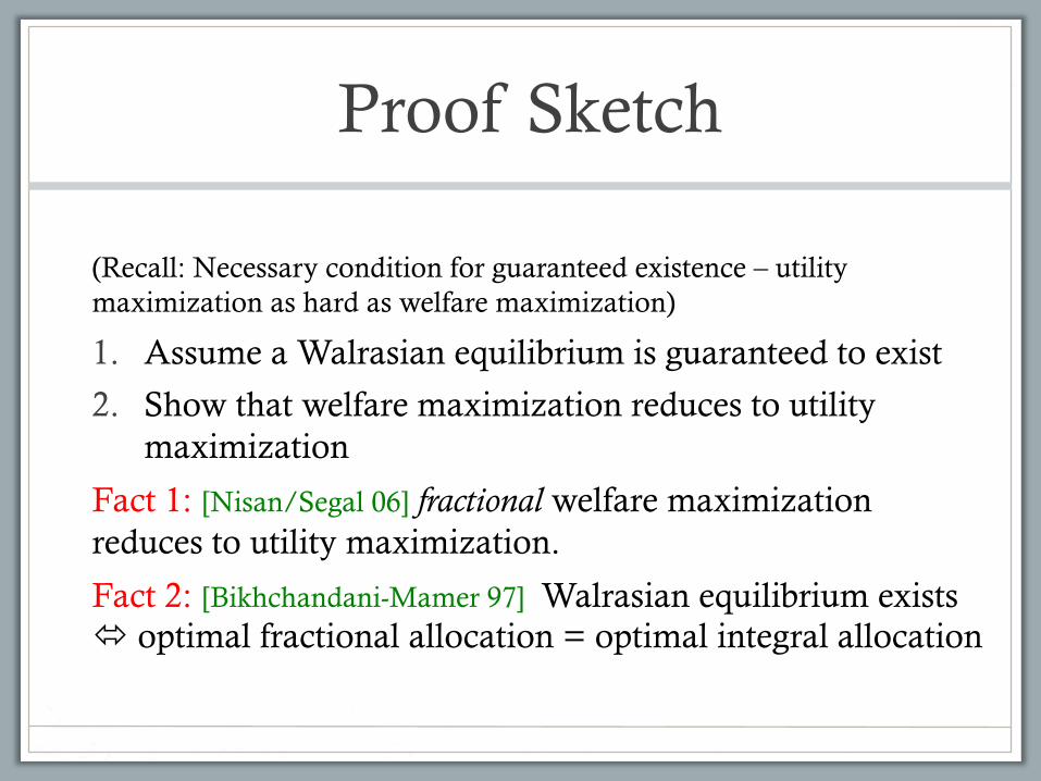
(Recall: Necessary condition for guaranteed existence – utility maximization as hard as welfare maximization)
1. Assume a Walrasian equilibrium is guaranteed to exist
2. Show that welfare maximization reduces to utility maximization
Fact 1: [Nisan/Segal 06] fractional welfare maximization reduces to utility maximization.
€
Proof Sketch
(Recall: Necessary condition for guaranteed existence – utility maximization as hard as welfare maximization)
1. Assume a Walrasian equilibrium is guaranteed to exist
2. Show that welfare maximization reduces to utility maximization
Fact 1: [Nisan/Segal 06] fractional welfare maximization reduces to utility maximization.
Fact 2: [Bikhchandani-Mamer 97] Walrasian equilibrium exists ó optimal fractional allocation = optimal integral allocation
€
Other Results
• Similar results for oracle models
• With more general anonymous prices Q, efficiently verifiable equilibria exist only when welfare maximization reduces to utility-maximization (with prices in Q)
• Complexity-theoretic explanation for why no useful generalizations of Walrasian equilibria: would require a non-standard polynomial-time algorithm for welfare-maximization
€
Overview
1. “Why Prices Need Algorithms” (w/Talgam-Cohen, EC ‘15) • from complexity separations to non-existence results for
Walrasian (i.e., market-clearing) equilibria
2. “Barriers to Near-Optimal Equilibria” (FOCS ’14) • from communication lower bounds to lower bounds on the price of
anarchy
3. “The Borders of Border’s Theorem” (w/Gopalan and Nisan, EC ‘15) • from complexity separations to impossibility results for “nice
descriptions” of incentive-compatible mechanisms
€
Equilibria vs. Algorithms
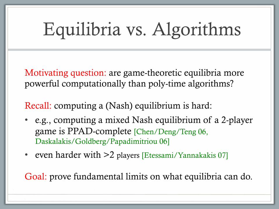
Motivating question: are game-theoretic equilibria more powerful computationally than poly-time algorithms?
Recall: computing a (Nash) equilibrium is hard:
• e.g., computing a mixed Nash equilibrium of a 2-player game is PPAD-complete [Chen/Deng/Teng 06, Daskalakis/Goldberg/Papadimitriou 06]
• even harder with >2 players [Etessami/Yannakakis 07]
Goal: prove fundamental limits on what equilibria can do.
€
Results in a Nutshell
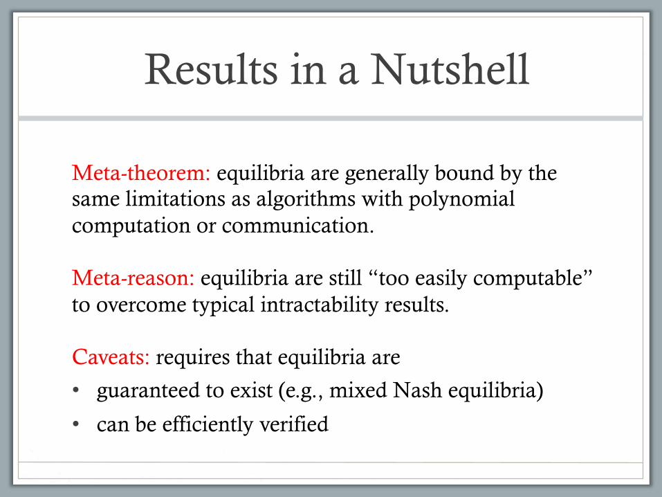
Meta-theorem: equilibria are generally bound by the same limitations as algorithms with polynomial computation or communication.
Meta-reason: equilibria are still “too easily computable” to overcome typical intractability results.
Caveats: requires that equilibria are
• guaranteed to exist (e.g., mixed Nash equilibria)
• can be efficiently verified
€
Combinatorial Auctions
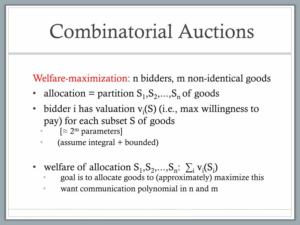
Welfare-maximization: n bidders, m non-identical goods
• allocation = partition S1,S2,...,Sn of goods
• bidder i has valuation vi(S) (i.e., max willingness to pay) for each subset S of goods • [≈ 2m parameters] • (assume integral + bounded)
• welfare of allocation S1,S2,...,Sn: ∑i vi(Si) • goal is to allocate goods to (approximately) maximize this • want communication polynomial in n and m
When Do Simple Mechanisms Work Well?
When Do Simple Mechanisms Work Well?
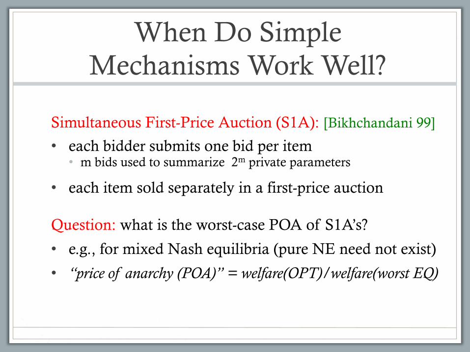
Simultaneous First-Price Auction (S1A): [Bikhchandani 99]
• each bidder submits one bid per item • m bids used to summarize 2m private parameters
• each item sold separately in a first-price auction
Question: what is the worst-case POA of S1A’s?
• e.g., for mixed Nash equilibria (pure NE need not exist)
• “price of anarchy (POA)” = welfare(OPT)/welfare(worst EQ)
From Protocol Lower Bounds to POA Lower Bounds
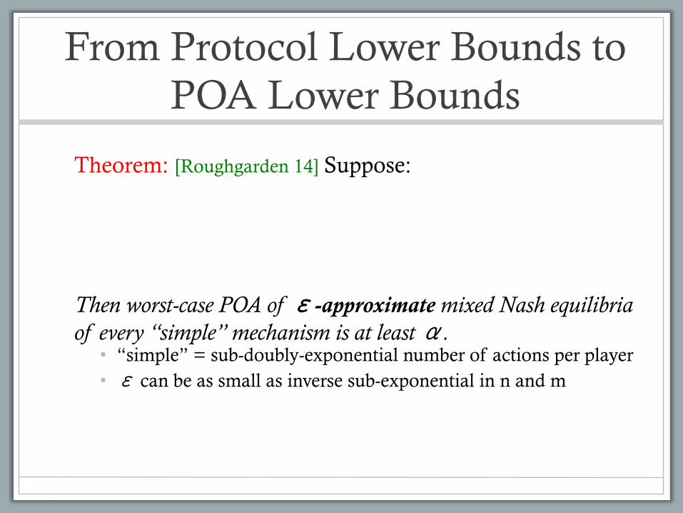
Theorem: [Roughgarden 14] Suppose:
Then worst-case POA of ε-approximate mixed Nash equilibria of every “simple” mechanism is at least α. • “simple” = sub-doubly-exponential number of actions per player • ε can be as small as inverse sub-exponential in n and m
From Protocol Lower Bounds to POA Lower Bounds
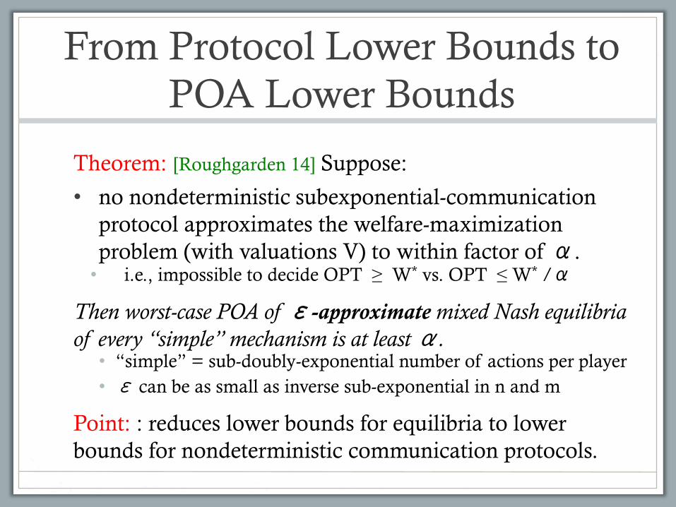
Theorem: [Roughgarden 14] Suppose:
• no nondeterministic subexponential-communication protocol approximates the welfare-maximization problem (with valuations V) to within factor of α. • i.e., impossible to decide OPT ≥ W* vs. OPT ≤ W* /α
Then worst-case POA of ε-approximate mixed Nash equilibria of every “simple” mechanism is at least α. • “simple” = sub-doubly-exponential number of actions per player • ε can be as small as inverse sub-exponential in n and m
Point: : reduces lower bounds for equilibria to lower bounds for nondeterministic communication protocols.
Ex: Subadditive Valuations
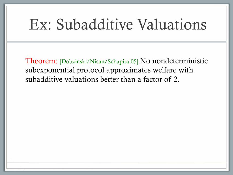
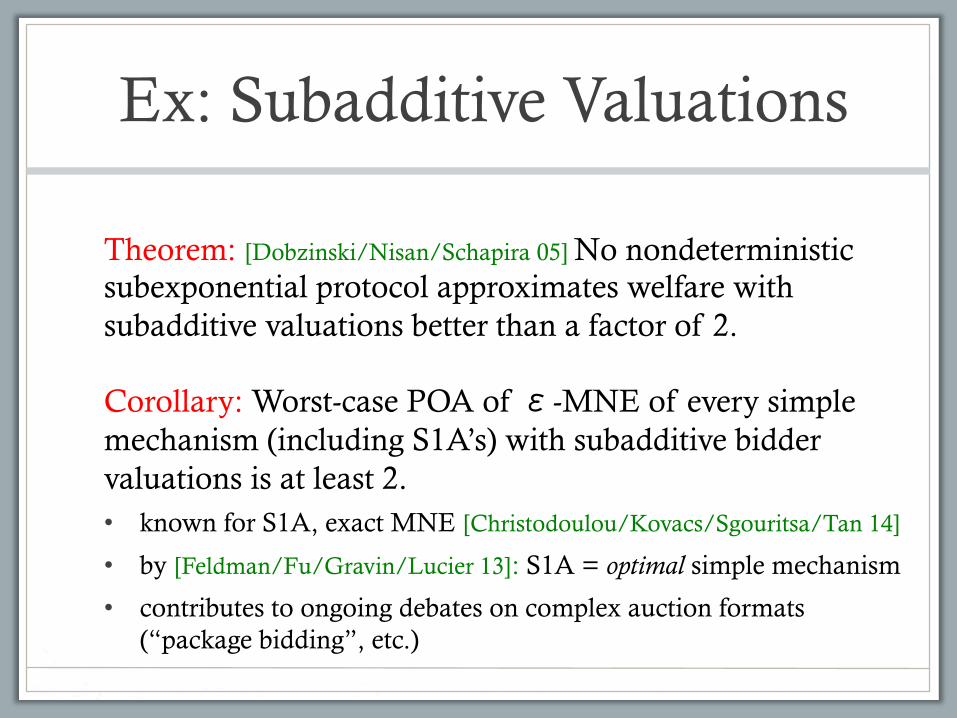
Theorem: [Dobzinski/Nisan/Schapira 05] No nondeterministic subexponential protocol approximates welfare with subadditive valuations better than a factor of 2.
Ex: Subadditive Valuations
Theorem: [Dobzinski/Nisan/Schapira 05] No nondeterministic subexponential protocol approximates welfare with subadditive valuations better than a factor of 2.
Corollary: Worst-case POA of ε-MNE of every simple mechanism (including S1A’s) with subadditive bidder valuations is at least 2. • known for S1A, exact MNE [Christodoulou/Kovacs/Sgouritsa/Tan 14]
• by [Feldman/Fu/Gravin/Lucier 13]: S1A = optimal simple mechanism
• contributes to ongoing debates on complex auction formats (“package bidding”, etc.)
Why Approximate MNE?
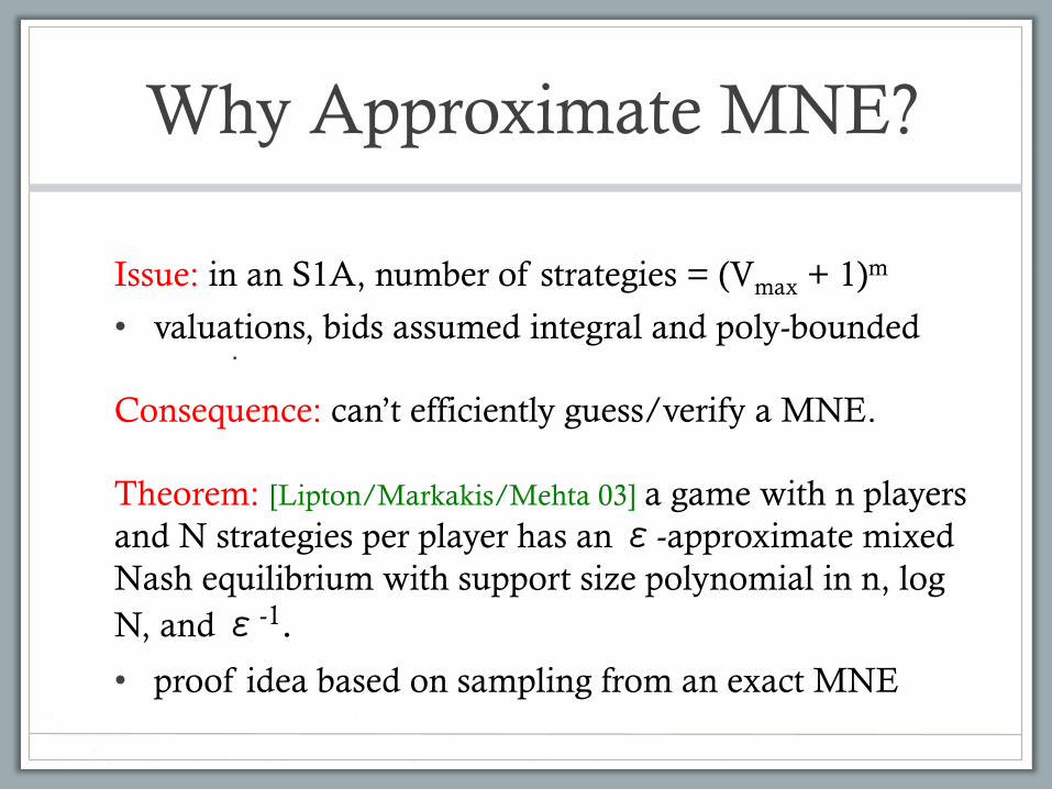
Issue: in an S1A, number of strategies = (Vmax + 1)m
• valuations, bids assumed integral and poly-bounded •
Consequence: can’t efficiently guess/verify a MNE.
Theorem: [Lipton/Markakis/Mehta 03] a game with n players and N strategies per player has an ε-approximate mixed Nash equilibrium with support size polynomial in n, log N, and ε-1. • proof idea based on sampling from an exact MNE
From Protocol Lower Bounds to POA Lower Bounds
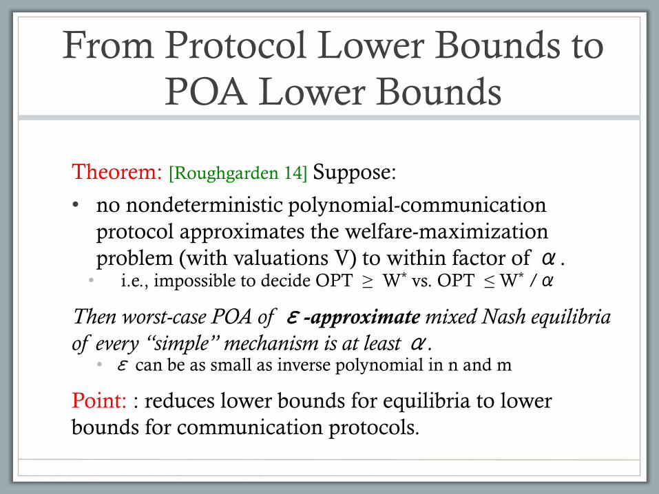
Theorem: [Roughgarden 14] Suppose:
• no nondeterministic polynomial-communication protocol approximates the welfare-maximization problem (with valuations V) to within factor of α. • i.e., impossible to decide OPT ≥ W* vs. OPT ≤ W* /α
Then worst-case POA of ε-approximate mixed Nash equilibria of every “simple” mechanism is at least α. • ε can be as small as inverse polynomial in n and m
Point: : reduces lower bounds for equilibria to lower bounds for communication protocols.
Proof of Theorem
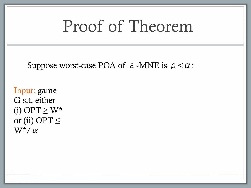
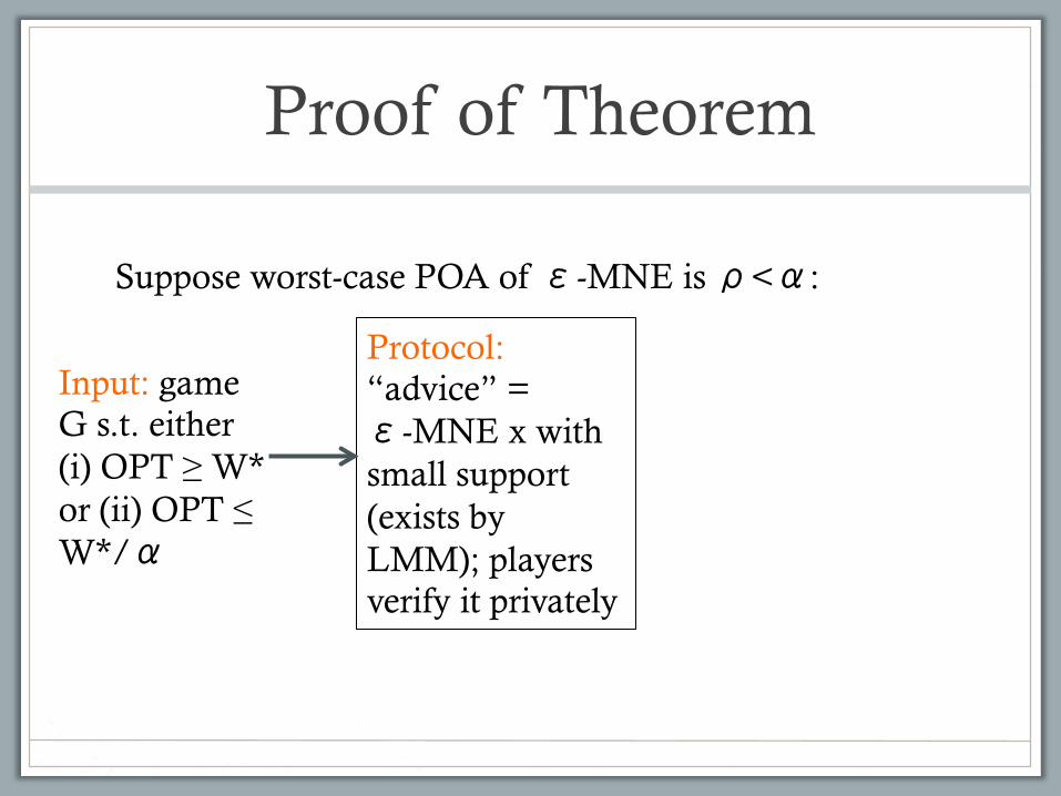
Suppose worst-case POA of ε-MNE is ρ<α:
Input: game G s.t. either (i) OPT ≥ W* or (ii) OPT ≤ W*/α
Proof of Theorem
Suppose worst-case POA of ε-MNE is ρ<α:
€
Input: game G s.t. either (i) OPT ≥ W* or (ii) OPT ≤ W*/α
Protocol: “advice” = ε-MNE x with small support (exists by LMM); players verify it privately
Proof of Theorem
Suppose worst-case POA of ε-MNE is ρ<α:
€
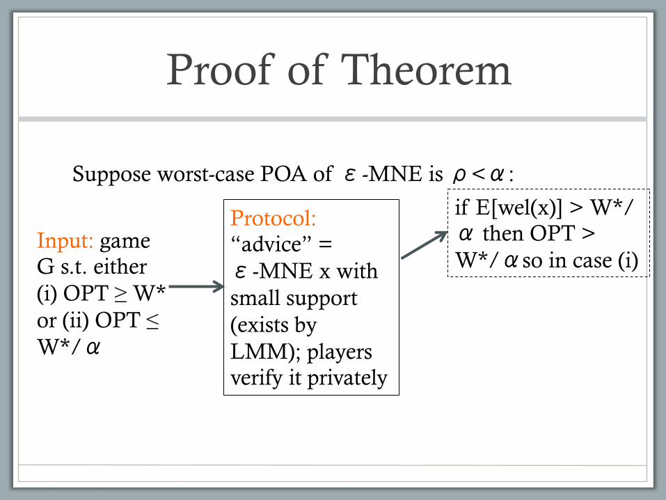
Input: game G s.t. either (i) OPT ≥ W* or (ii) OPT ≤ W*/α
Protocol: “advice” = ε-MNE x with small support (exists by LMM); players verify it privately
if E[wel(x)] > W*/α then OPT > W*/αso in case (i)
Proof of Theorem
Suppose worst-case POA of ε-MNE is ρ<α:
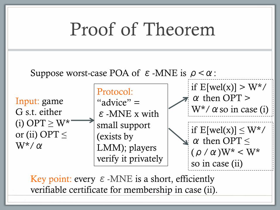
Key point: every ε-MNE is a short, efficiently verifiable certificate for membership in case (ii).
€
Input: game G s.t. either (i) OPT ≥ W* or (ii) OPT ≤ W*/α
Protocol: “advice” = ε-MNE x with small support (exists by LMM); players verify it privately
if E[wel(x)] > W*/α then OPT > W*/αso in case (i)
if E[wel(x)] ≤ W*/α then OPT ≤ (ρ/α)W* < W* so in case (ii)
More Applications
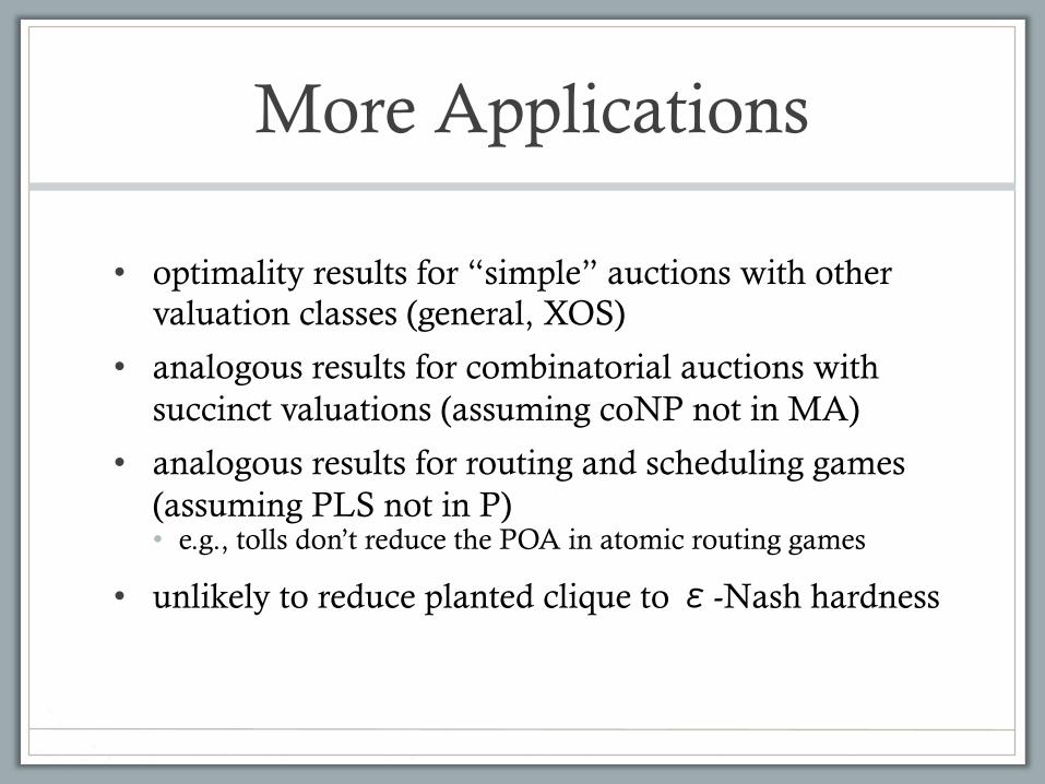
• optimality results for “simple” auctions with other valuation classes (general, XOS)
• analogous results for combinatorial auctions with succinct valuations (assuming coNP not in MA)
• analogous results for routing and scheduling games (assuming PLS not in P) • e.g., tolls don’t reduce the POA in atomic routing games
• unlikely to reduce planted clique to ε-Nash hardness
Overview
1. “Why Prices Need Algorithms” (w/Talgam-Cohen, EC ‘15) • from complexity results to non-existence results for Walrasian
(market-clearing) equilibria
2. “Barriers to Near-Optimal Equilibria” (FOCS ’14) • from communication lower bounds to lower bounds on the price
of anarchy
3. “The Borders of Border’s Theorem” (w/Gopalan and Nisan, EC ‘15) • from complexity results to impossibility results for “nice descriptions” of
incentive-compatible mechanisms
€
Single-Item Auctions
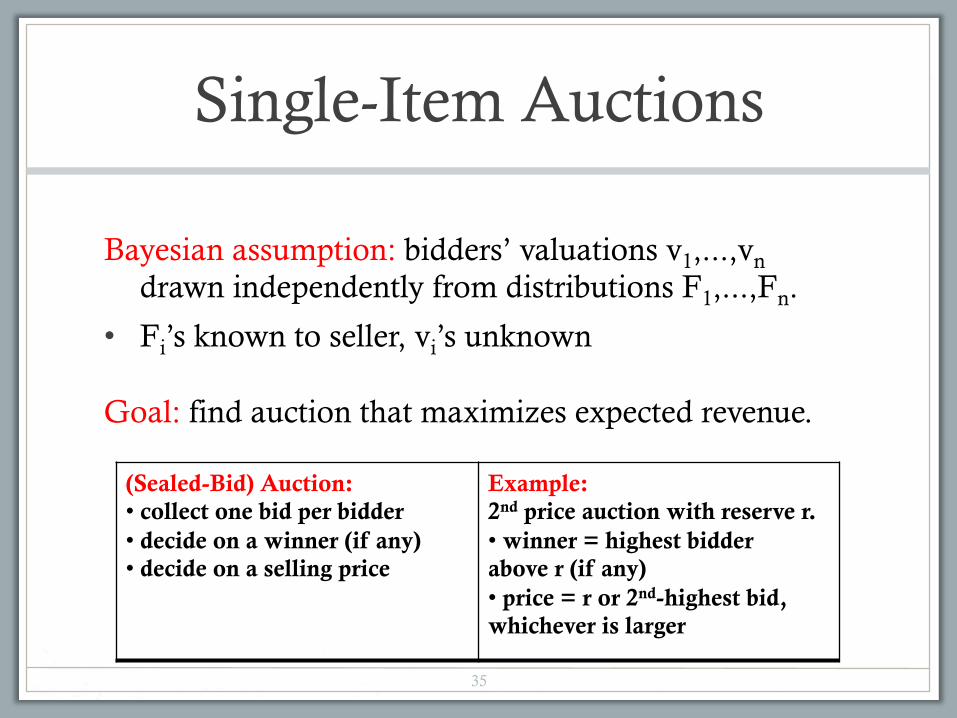
Bayesian assumption: bidders’ valuations v1,...,vn drawn independently from distributions F1,...,Fn.
• Fi’s known to seller, vi’s unknown
Goal: find auction that maximizes expected revenue.
35
(Sealed-Bid) Auction: • collect one bid per bidder • decide on a winner (if any) • decide on a selling price
Example: 2nd price auction with reserve r. • winner = highest bidder above r (if any) • price = r or 2nd-highest bid, whichever is larger
Optimal Single-Item Auctions
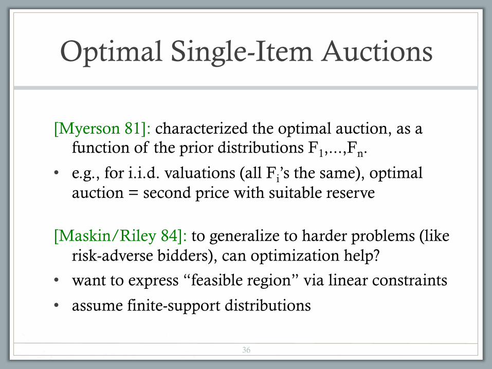
[Myerson 81]: characterized the optimal auction, as a function of the prior distributions F1,...,Fn.
• e.g., for i.i.d. valuations (all Fi’s the same), optimal auction = second price with suitable reserve
[Maskin/Riley 84]: to generalize to harder problems (like risk-adverse bidders), can optimization help?
• want to express “feasible region” via linear constraints
• assume finite-support distributions
36
A Naive Linear Program
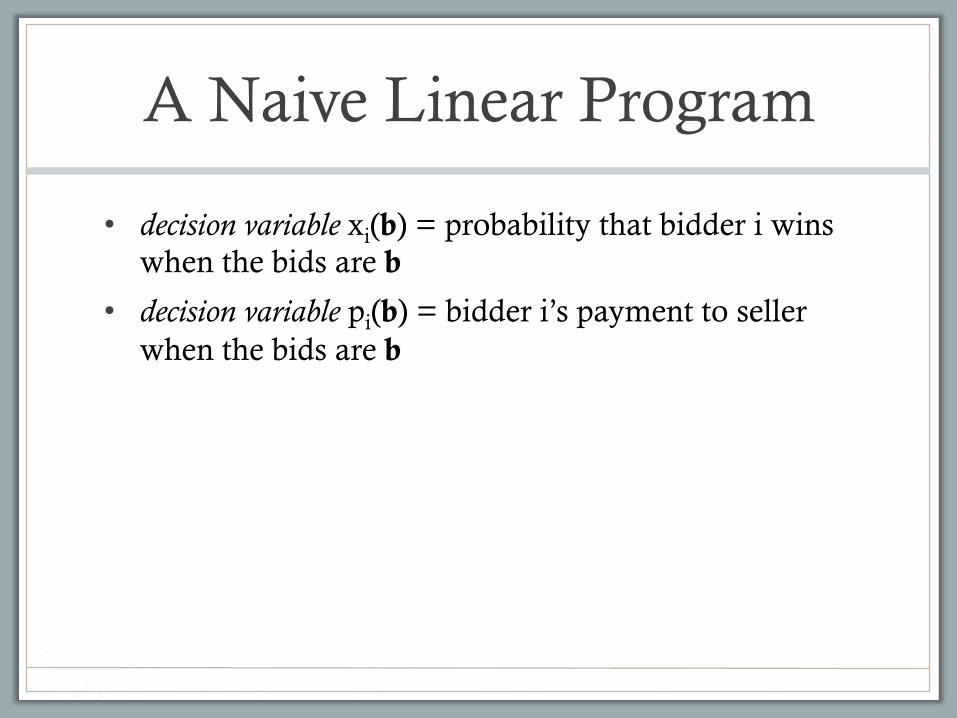
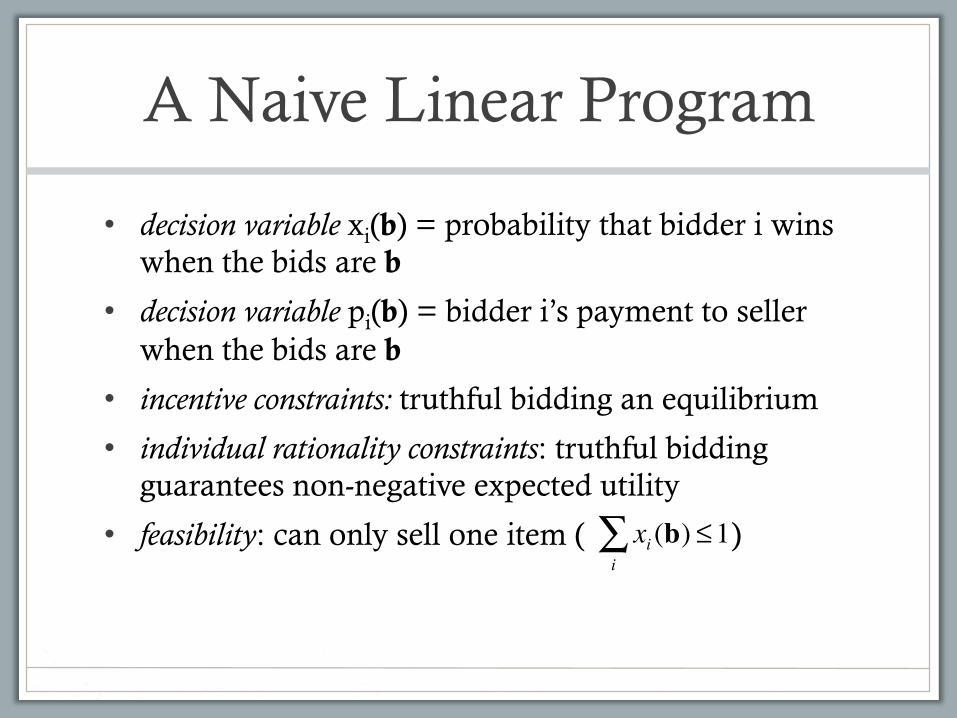
• decision variable xi(b) = probability that bidder i wins when the bids are b
• decision variable pi(b) = bidder i’s payment to seller when the bids are b
A Naive Linear Program
• decision variable xi(b) = probability that bidder i wins when the bids are b
• decision variable pi(b) = bidder i’s payment to seller when the bids are b
• incentive constraints: truthful bidding an equilibrium
• individual rationality constraints: truthful bidding guarantees non-negative expected utility
• feasibility: can only sell one item ( ) xi (b) ≤1i∑
A Naive Linear Program
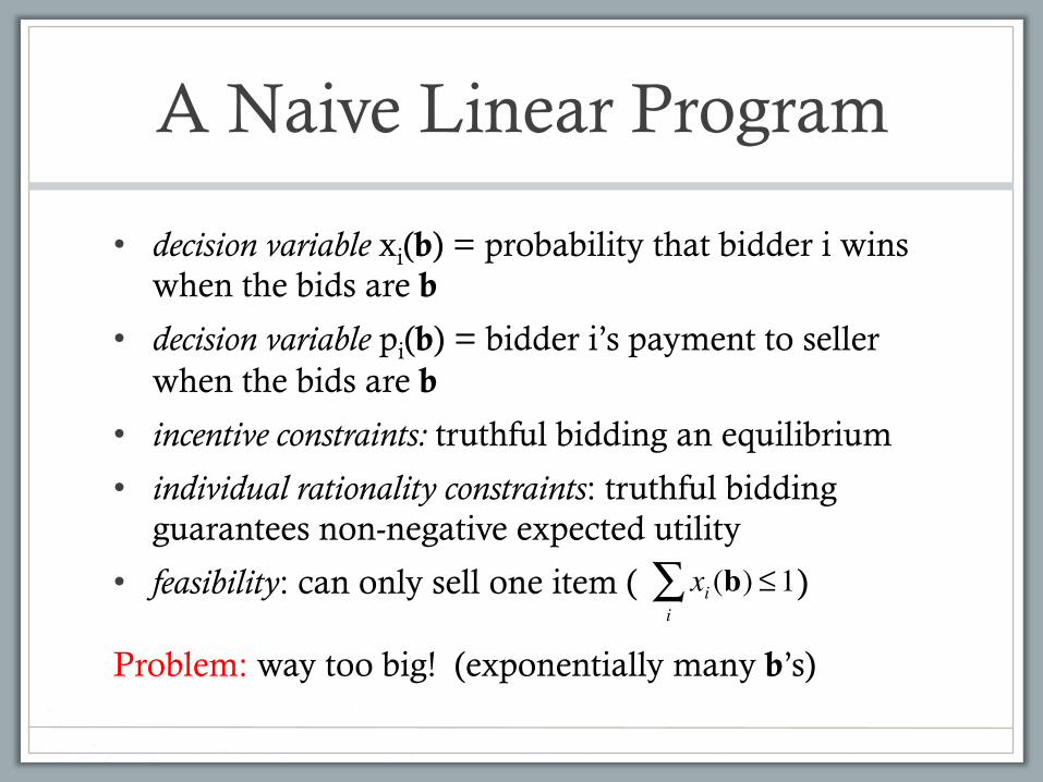
• decision variable xi(b) = probability that bidder i wins when the bids are b
• decision variable pi(b) = bidder i’s payment to seller when the bids are b
• incentive constraints: truthful bidding an equilibrium
• individual rationality constraints: truthful bidding guarantees non-negative expected utility
• feasibility: can only sell one item ( )
Problem: way too big! (exponentially many b’s)
xi (b) ≤1i∑
A Projected Linear Program
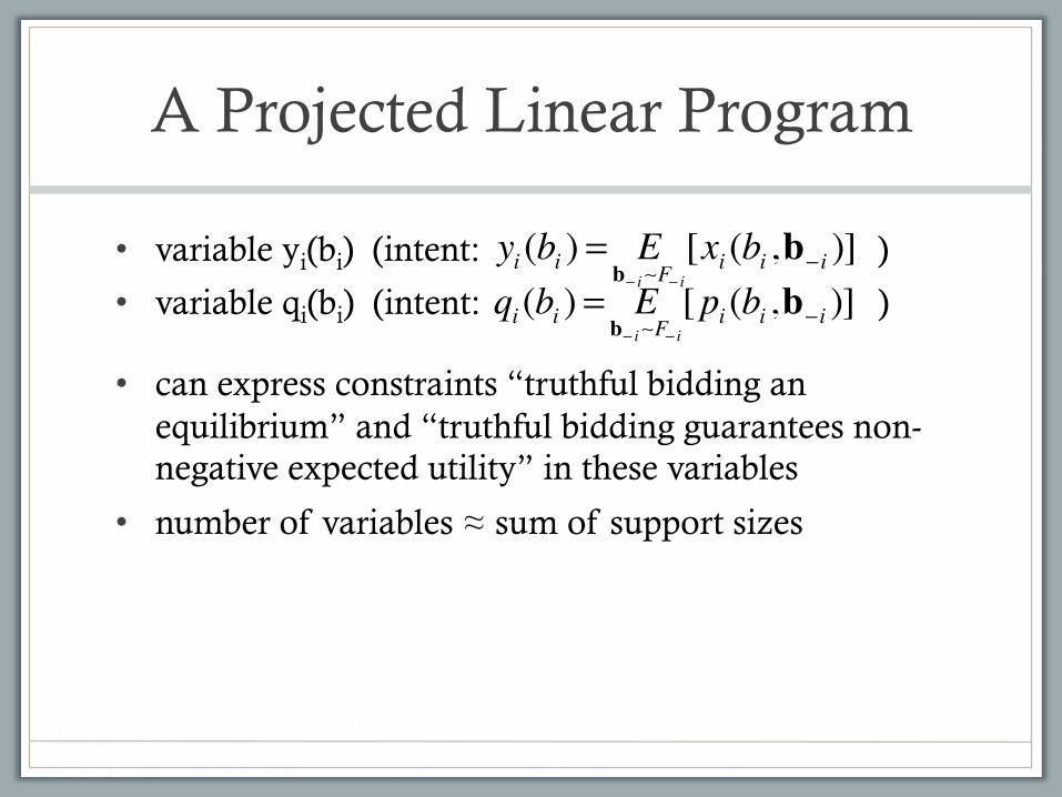
• variable yi(bi) (intent: )
• variable qi(bi) (intent: )
• can express constraints “truthful bidding an equilibrium” and “truthful bidding guarantees non-negative expected utility” in these variables
• number of variables ≈ sum of support sizes
yi (bi ) = E
b− i∼F− i[xi (bi ,b− i )]
qi (bi ) = E
b− i∼F− i[pi (bi ,b− i )]
A Projected Linear Program
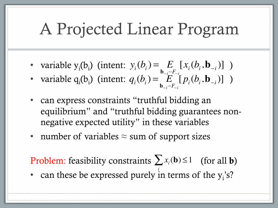
• variable yi(bi) (intent: )
• variable qi(bi) (intent: )
• can express constraints “truthful bidding an equilibrium” and “truthful bidding guarantees non-negative expected utility” in these variables
• number of variables ≈ sum of support sizes
Problem: feasibility constraints (for all b)
• can these be expressed purely in terms of the yi’s?
xi (b) ≤1i∑
yi (bi ) = E
b− i∼F− i[xi (bi ,b− i )]
qi (bi ) = E
b− i∼F− i[pi (bi ,b− i )]
Interim Feasibility
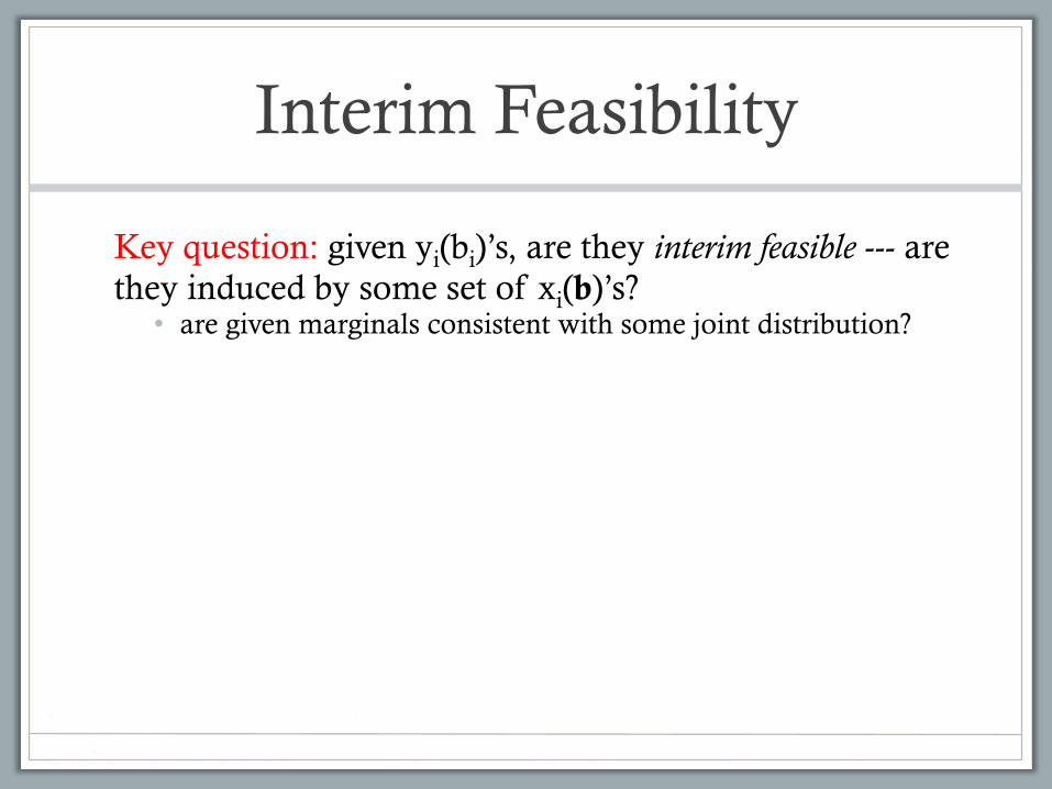
Key question: given yi(bi)’s, are they interim feasible --- are they induced by some set of xi(b)’s? • are given marginals consistent with some joint distribution?
Interim Feasibility
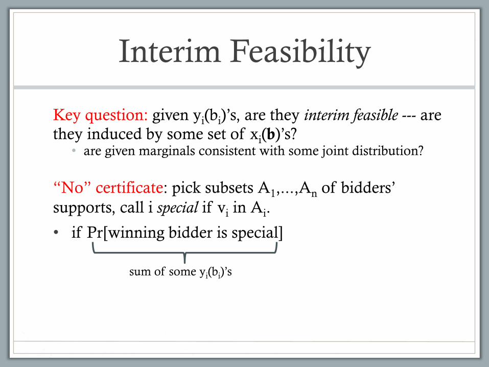
Key question: given yi(bi)’s, are they interim feasible --- are they induced by some set of xi(b)’s? • are given marginals consistent with some joint distribution?
“No” certificate: pick subsets A1,...,An of bidders’ supports, call i special if vi in Ai.
• if Pr[winning bidder is special]
sum of some yi(bi)’s
Interim Feasibility
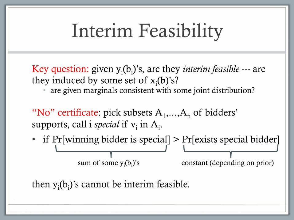
Key question: given yi(bi)’s, are they interim feasible --- are they induced by some set of xi(b)’s? • are given marginals consistent with some joint distribution?
“No” certificate: pick subsets A1,...,An of bidders’ supports, call i special if vi in Ai.
• if Pr[winning bidder is special] > Pr[exists special bidder]
then yi(bi)’s cannot be interim feasible.
sum of some yi(bi)’s constant (depending on prior)
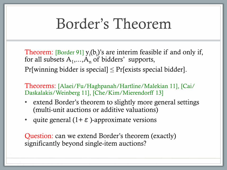
Border’s Theorem
Theorem: [Border 91] yi(bi)’s are interim feasible if and only if, for all subsets A1,...,An of bidders’ supports,
Pr[winning bidder is special] ≤ Pr[exists special bidder].
Border’s Theorem
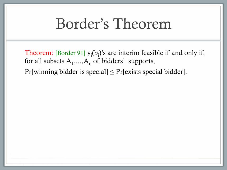
Theorem: [Border 91] yi(bi)’s are interim feasible if and only if, for all subsets A1,...,An of bidders’ supports,
Pr[winning bidder is special] ≤ Pr[exists special bidder].
Theorems: [Alaei/Fu/Haghpanah/Hartline/Malekian 11], [Cai/Daskalakis/Weinberg 11], [Che/Kim/Mierendorff 13]
• extend Border’s theorem to slightly more general settings (multi-unit auctions or additive valuations)
• quite general (1+ε)-approximate versions
Question: can we extend Border’s theorem (exactly) significantly beyond single-item auctions?
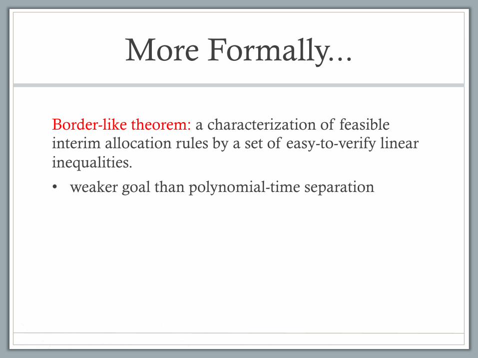
More Formally...
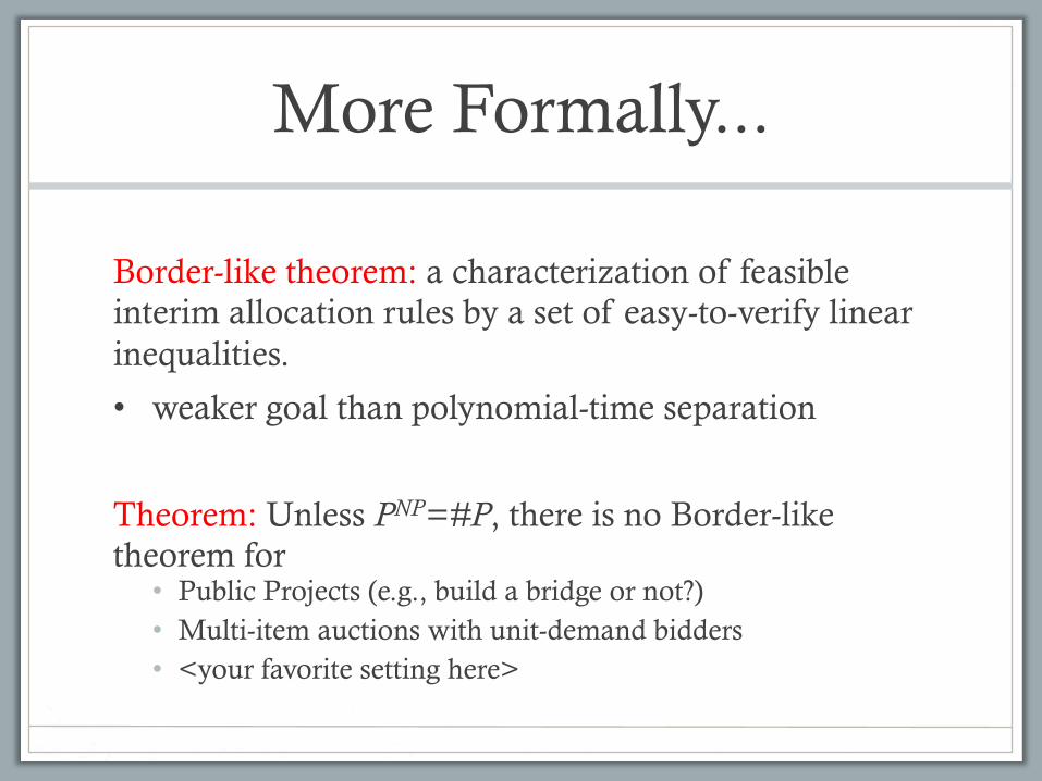
Border-like theorem: a characterization of feasible interim allocation rules by a set of easy-to-verify linear inequalities.
• weaker goal than polynomial-time separation
More Formally...
Border-like theorem: a characterization of feasible interim allocation rules by a set of easy-to-verify linear inequalities.
• weaker goal than polynomial-time separation
Theorem: Unless PNP=#P, there is no Border-like theorem for • Public Projects (e.g., build a bridge or not?) • Multi-item auctions with unit-demand bidders • <your favorite setting here>
Proof Structure
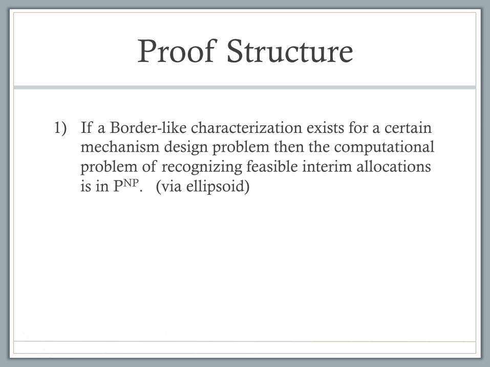
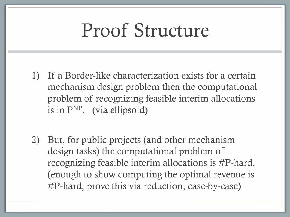
1) If a Border-like characterization exists for a certain mechanism design problem then the computational problem of recognizing feasible interim allocations is in PNP. (via ellipsoid)
Proof Structure
1) If a Border-like characterization exists for a certain mechanism design problem then the computational problem of recognizing feasible interim allocations is in PNP. (via ellipsoid)
2) But, for public projects (and other mechanism design tasks) the computational problem of recognizing feasible interim allocations is #P-hard. (enough to show computing the optimal revenue is #P-hard, prove this via reduction, case-by-case)
Connection to Boolean Function Analysis
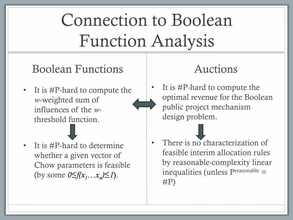
Boolean Functions
• It is #P-hard to compute the w-weighted sum of influences of the w-threshold function.
• It is #P-hard to determine whether a given vector of Chow parameters is feasible (by some 0≤f(x1…xn)≤1).
Auctions
• It is #P-hard to compute the optimal revenue for the Boolean public project mechanism design problem.
• There is no characterization of feasible interim allocation rules by reasonable-complexity linear inequalities (unless Preasonable = #P)
Take-Aways
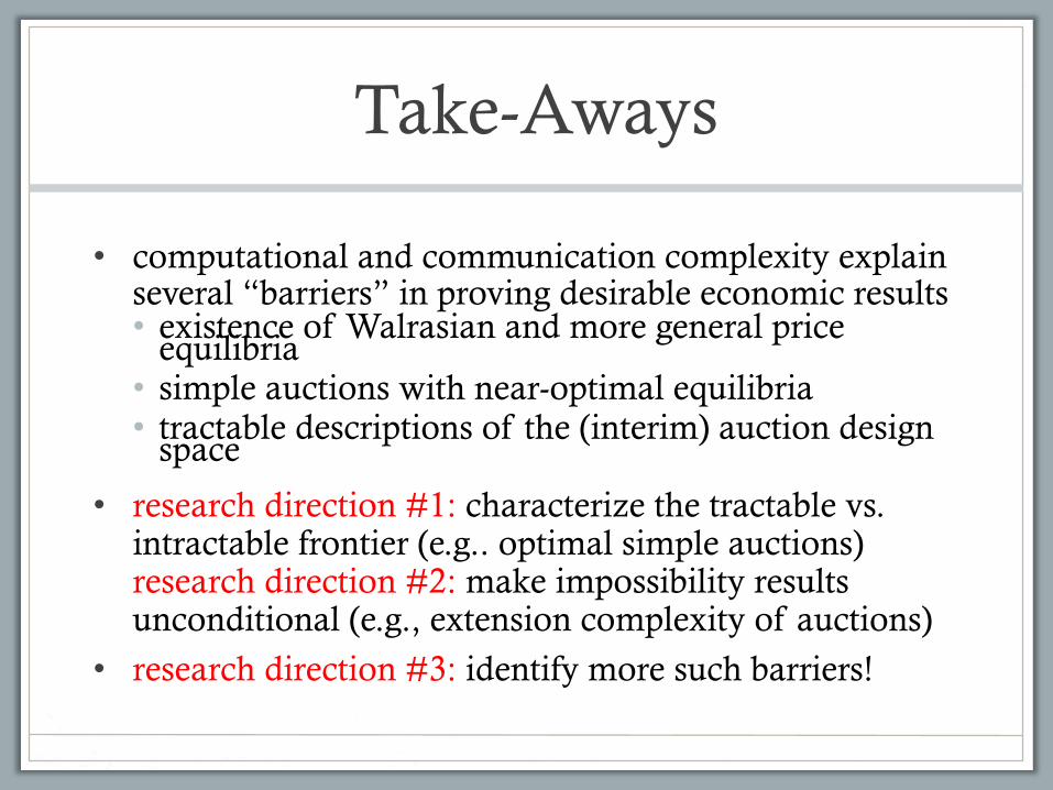
• computational and communication complexity explain several “barriers” in proving desirable economic results • existence of Walrasian and more general price
equilibria • simple auctions with near-optimal equilibria • tractable descriptions of the (interim) auction design
space
• research direction #1: characterize the tractable vs. intractable frontier (e.g.. optimal simple auctions) research direction #2: make impossibility results unconditional (e.g., extension complexity of auctions)
• research direction #3: identify more such barriers!
€
FIN