Adv. Technol. 2021, 1(1), 207-234

https://doi.org/10.31357/ait.v1i1.4844

Research Paper

Three Layer Super Learner Ensemble with

Hyperparameter Optimization to Improve the

Performance of Machine Learning Model

K. T. S. Kasthuriarachchia,* and Liyanage S. Rb

a Faculty of Graduate Studies, University of Kelaniya, Dalugama, Kelaniya 11300, Sri

Lanka b Faculty of Computing and Technology, University of Kelaniya, Dalugama 11300, Sri

Lanka

Email correspondence: sanvithat85@gmail.com (K. T. S. Kasthuriarachchi) Received: 13 March 2021; Revised: 30 March 2021; Accepted: 19 April 2021; Published: 31 May 2021

Abstract

A combination of different machine learning models to form a super learner can definitely lead to improved predictions in any domain. The super learner ensemble discussed in this study collates several machine learning models and proposes to enhance the performance by considering the final meta- model accuracy and the prediction duration. An algorithm is proposed to rate the machine learning models derived by combining the base classifiers voted with different weights. The proposed algorithm is named as Log Loss Weighted Super Learner Model (LLWSL). Based on the voted weight, the optimal model is selected and the machine learning method derived is identified. The meta- learner of the super learner uses them by tuning their hyperparameters. The execution time and the model accuracies were evaluated using two separate datasets inside LMSSLIITD extracted from the educational industry by executing the LLWSL algorithm. According to the outcome of the evaluation process, it has been noticed that there exists a significant improvement in the proposed algorithm LLWSL for use in machine learning tasks for the achievement of better performances. Keywords: Classifier, ensemble, feature selection, hyperparameter, optimization, random search, super learning

Adv. Technol. 2021, 1(1), 207-234

208

Introduction

Rating the scores and early prediction of domain specific data has

become very important in many research contexts. Most prediction

tasks can be conducted by utilizing different machine learning

algorithms. Prediction algorithms can be categorized based on their

predictive tasks. Decision tree classifier, Random Forest classifier,

Naïve Bayes analyzer, Artificial Neural Network, Linear Regression,

Logistic Regression, Support Vector Classifier and K-Nearest Neighbor

classifier are several such machine learning mechanisms designated to

perform classification, clustering, association rule mining etc. A

substantial number of research studies have been carried out in various

subject domains with these machine learning algorithms to provide

predictive and analytical decisions [23].

The choice of the algorithm, most appropriate for a given dataset, is not

a trivial task since that decision influences the overall accuracy of the

predicted model [21]. Generally, researchers would compare the

performance of selected algorithms on a test data set and select the

algorithm that statistically outperforms the other algorithms in a

significant manner [27, 32]. However, there is the uncertainty whether

the selected algorithm will be the best for all possible real-world

datasets. As stated in the “No free lunch theorem” the computational

cost of finding a solution, averaged over all problems in the class, is the

same for any solution method. Recently, methods such as boosting and

bagging have outperformed a single best classifier when predicting on

real world datasets [38]. Therefore, when none of the algorithms

significantly outperforms other methods it is pragmatic to select a few

algorithms and to determine the best during runtime [12].

Ensemble methods are more apt for the use in similar situations where

the researcher is able to develop various models using different

machine learning algorithms to a selected data set and combine into a

single classifier. Many prediction algorithms can be collated on a single

model to construct an ensemble. This ensemble is constructed to reduce

Adv. Technol. 2021, 1(1), 207-234

209

bias and variance [11]. The super learner is an ensemble machine

learning method which could combine several machine learning

models and configure to produce a single predictive model for efficient

and robust predictions. Data analyzer cannot strictly prioritize a

specific machine learning technique, rather they can select several

techniques.

This study focuses on implementing a priori-specified hyper

parameterized ensembling machine learning approach which combines

several machine learning algorithms into a single algorithm and

returns a prediction method with the best cross validated Log Loss

Error (CLLE). The individual modeling techniques of K-Nearest

Neighbor (KNN), Random Forest (RF), Naïve Bayes (NB), Support

Vector Machine (SVM), Decision Tree (DT) and Logistic Regression

(LR) approach-based sensitivity estimation were used.

Hyperparameters refer to parameters whose values are set by the user

before training the algorithm. They affect the entire ensemble’s

performance structure and the complexity [43]. Super learner

algorithm occupies a set of candidates learning algorithms and apply

them to a data set to choose the optimal learner or learner combination

so that it will perform better than other learners [21].

This paper is motivated to discuss the proposed super

hyperparameterized ensembling machine learner in three aspects. First,

the implementation of the new learner with the weights, then the

evaluation procedure of the learner on predicting tasks using different

datasets from a variety of educational disciplines and finally, focus on

using this novel super learner in future applications by optimizing the

parameters. The paper is organized as follows. Section 2 presents the

existing problems of super learner ensemble and the approaches

followed by previous studies to overcome it by using hyperparameter

optimization. Section 3 presents the methodology followed to

implement the super learner ensemble with random hyperparameter

optimizer. Finally, section 4 presents a comprehensive discussion about

Adv. Technol. 2021, 1(1), 207-234

210

the experiments with results and validation of the ensemble against

deep learning Convolutional Neural Network.

Background

The ensembles are of three types. Bagging, Boosting, Blending/

Stacking. Bagging and boosting are two of the common ensemble

techniques used in machine learning. Bagging is the method for

generating multiple versions of predictors and form an aggregated

predictor by voting each version and getting the average of them [7].

Bagging meta-estimator and the random forest are the algorithms

followed bagging approach. Boosting works in a similar way to

bagging by combining several poor performing base learners in an

adaptive way. Experimental work showed that bagging is effective for

data sets with noisy values [39]. In boosting, the learning algorithms

are given different distribution or weighting according to the errors of

the base learners [8, 31]. AdaBoost, Gradient Boosting (GBM), eXtream

Gradient Boosting (XGBM), Light GBM, and CatBoost are considered

as Boosting techniques. The third approach is blending/stacking which

takes the output of selected base learners on the training data and

applies another learning algorithm on them to predict the response

values [22]. Stacking uses a first- level ensemble of classifiers to form

the second- level meta –input [45]. Research experiments have shown

that the stacking has better robustness properties [10]. Super learner is

an application of stacked generalization approach.

The main research task incorporated into this article is the

implementation of a super learner ensemble with high accuracy and

low computational time. Super learning concept could be easily

adopted to any domain where an analytical model needed to be

generated. Accordingly, the super learner ensemble is implemented by

dividing the tasks into two steps. First, the base learner selection

through weighted prediction scoring. Second, optimize the

hyperparameters used by the super learner ensemble to obtain the best

prediction accuracy in minimal duration. This section discusses the

Adv. Technol. 2021, 1(1), 207-234

211

background details, characteristics, current research contribution,

drawbacks and advantages of each important area of study.

Super Learning

It is in fact impractical to identify a priori the machine learning

algorithms use in the regression of classification problem in decision

making. This leads the data analyst to use many different machine

learning algorithms to develop different models and evaluate the

performance of them using resampling by cross validation. Once the

evaluation is performed many times in different configurations, the

best out of the all models is selected to predict the target attribute and

make decisions. A single machine learning algorithm may be unable to

capture the complete underline structure of the data to derive optimal

predictions. This is where the integration of multiple models were

gathered into a single meta – model [40]. The main intuition behind the

concept of Super learning is to address the point which “Why all the

prediction models are not considered and select the best model out of

all for the machine learning problem”. It is a fact that the super learner

ensemble approach encourages to collate different machine learning

models (base learner models) and construct a single predictive model

(meta- model) with high predictive performance. Super learner concept

was first introduced by a set of researchers in a biological study. This is

an application of stacked generalization to k- fold cross validation since

all the analysis models use the same k-fold splits of the data and a

meta- model fits into the out-of-fold predictions of each of the models.

The traditional machine learning approaches build a single hypothesis

based on the training data but, the ensemble approach attempts to

develop a set of hypotheses and combine them to form a new

hypothesis [36]. Different studies were carried out based on the super

learning concept. Once multiple prediction models are combined, more

information could be captured in the fundamental structure of the data

[8]. A researcher highlighted the importance of recognizing the

uncertainty when selecting models, and the prospective role of

Adv. Technol. 2021, 1(1), 207-234

212

assembling can play in combining several models to create one that

outperforms single models [41]. In a study about improving accuracy

and reducing variance of behavior classification in accelerometer done

by researchers has shown that super learning can be easily adapted to

any type of industry to achieve better accuracy in the predicted model

[21]. Also they emphasized the importance of the human intervention

and the computation time required to implement a super learner for

the machine learning tasks. The ensemble learning performs better

than the individual base learners [36]. A researcher has pointed out

that the high computational time and the memory requirement for the

smooth execution of super learner approach is significant and thereby,

super learner can be potentially flawed too [35].

Base Classifiers

The proposed super learner ensemble has base classifiers and a meta-

classifier. (1) The base classifier/ learner fits the dataset using different

machine learning algorithms. KNN, RF, NB, SVM, ANN and DT were

used as base learners in this study. (2) The meta- learner is fitted on the

predictions of the base learners. LR algorithm is used as the meta-

learner in forming the super learner. The following section provides a

brief description of the base learners and the meta-learner incorporated

to this study. KNN is the most simple and straight forward data

mining algorithms [34]. K is the number of nearest neighbors that are

used to make the prediction and it calculates the distance between data

points using the Euclidean distance measurement [9]. RF gives more

precise predictions even for a large sample size. It captures the

discrepancy of several input variables at the same time and allows high

number of observations to participate in the prediction [30]. NB

simplifies the calculation of probabilities by assuming that the

probability of each attribute of a given class value is independent of all

other attributes [2]. SVM used for both classification and regression

tasks. The SVM algorithm plots the data items as a point in n-

dimensional space regarding the number of features in the dataset.

Adv. Technol. 2021, 1(1), 207-234

213

Then each feature is represented in a particular coordinate in x and y

axis. Then, the classification is performed by finding the hyper-plane

by differentiating the classes successfully [15]. DT algorithm uses to

select attributes of the data set based on the information gain

measurement which is known as entropy of the attribute. The

attributes which have the high information gain value and high gain

ratio value will be selected for splitting the attributes [18]. ANN is a

machine learning algorithm which is modeled for data handling and

especially useful for distinguishing the key relationships among an

arrangement of factors or patterns in the data [1].

Meta Classifier

Logistic Regression

Logistic regression is used to describe data and the relationship

between one dependent binary variable and one or more nominal,

ordinal, interval or ratio level independent variables. The classified

observations and a low percentage of misclassified observations [32].

This model is frequently used in situations where more predictor

variables are considered in the analysis [37].

Hyperparameter Optimization

The parameters which define the model architecture are known as

hyperparameters. The process of identifying the ideal model

architecture is done in order to change these parameter values and

measures the performance attributes of the predicted model is known

as hyperparameter tuning or hyperparameter optimization. This is

achieved in three different methods, namely; (1) Grid search (2)

Random search and (3) Bayesian optimization. Grid search is the most

basic method. The prediction model will be created for each possible

combination of all the hyperparameter value and will evaluate each

model and select the architecture which produces the best result.

Random search finds better models by effectively searching a larger,

less promising configuration space than grid search method [14]. The

next method, bayesian optimization is also called the surrogate method

Adv. Technol. 2021, 1(1), 207-234

214

which keeps track of past evaluation results which are used to form a

probabilistic model, maps the hyperparameters to a probability of a

score on the objective function that it uses. It could find a better set of

hyperparameters in less time because they study about the best set of

hyperparameters to evaluate, based on past trials.

Researchers have focused on this hyperparameter optimization in

different forms. A researcher has done a study to find a method to

accelerate the search process by transferring information from previous

trials to other datasets [4]. The key challenge they faced was the

accuracy measurement. It was a relatively difficult task to maintain the

accuracy of the model while maintaining the speed of the analysis

through hyperparameter tuning [46]. Another team of researchers

introduced a systematic framework to build ensembles with optimal

weights for regression problems [33]. They were able to find the

optimized ensemble weights that minimize both bias and variance of

the predictions while tuning the hyperparameters of the base learners.

A study about the use of baysian optimization to hyperparameter

tuning in ensemble learning has been mentioned in a study and they

could build an optimized strategy to exploit trained models and

improved ensembles to use as a classifier at the lower cost of regular

hyperparameter optimization [17]. It could be observed that the

existing ensemble techniques consider the base model construction and

the weighted averaging to be independent steps. However, the

researchers concluded that combining these two components will lead

to a low performing ensemble learner. A study has proposed a

weighted ensemble approach by assigning estimated weights in order

to obtain more accurate ensemble result than the classical ensemble

[33]. Another researcher has introduced a probabilistic ensemble

weighting approach used on cross-validation for hyperparameter

optimization [22].

There have not been studies where the base learner had been modeled

with hyperparameter optimization and the model weight assignment

Adv. Technol. 2021, 1(1), 207-234

215

for the implementation of an optimal ensemble learner in achieving the

optimal accuracy of the prediction.

Materials and Methods

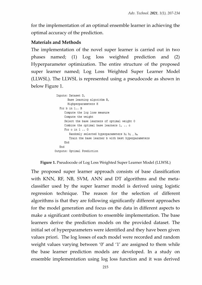
The implementation of the novel super learner is carried out in two

phases named; (1) Log loss weighted prediction and (2)

Hyperparameter optimization. The entire structure of the proposed

super learner named; Log Loss Weighted Super Learner Model

(LLWSL). The LLWSL is represented using a pseudocode as shown in

below Figure 1.

Figure 1. Pseudocode of Log Loss Weighted Super Learner Model (LLWSL)

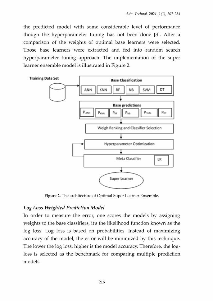
The proposed super learner approach consists of base classification

with KNN, RF, NB, SVM, ANN and DT algorithms and the meta-

classifier used by the super learner model is derived using logistic

regression technique. The reason for the selection of different

algorithms is that they are following significantly different approaches

for the model generation and focus on the data in different aspects to

make a significant contribution to ensemble implementation. The base

learners derive the prediction models on the provided dataset. The

initial set of hyperparameters were identified and they have been given

values priori. The log losses of each model were recorded and random

weight values varying between ‘0’ and ‘1’ are assigned to them while

the base learner prediction models are developed. In a study on

ensemble implementation using log loss function and it was derived

Adv. Technol. 2021, 1(1), 207-234

216

the predicted model with some considerable level of performance

though the hyperparameter tuning has not been done [3]. After a

comparison of the weights of optimal base learners were selected.

Those base learners were extracted and fed into random search

hyperparameter tuning approach. The implementation of the super

learner ensemble model is illustrated in Figure 2.

Figure 2. The architecture of Optimal Super Learner Ensemble.

Log Loss Weighted Prediction Model

In order to measure the error, one scores the models by assigning

weights to the base classifiers, it’s the likelihood function known as the

log loss. Log loss is based on probabilities. Instead of maximizing

accuracy of the model, the error will be minimized by this technique.

The lower the log loss, higher is the model accuracy. Therefore, the log-

loss is selected as the benchmark for comparing multiple prediction

models.

Adv. Technol. 2021, 1(1), 207-234

217

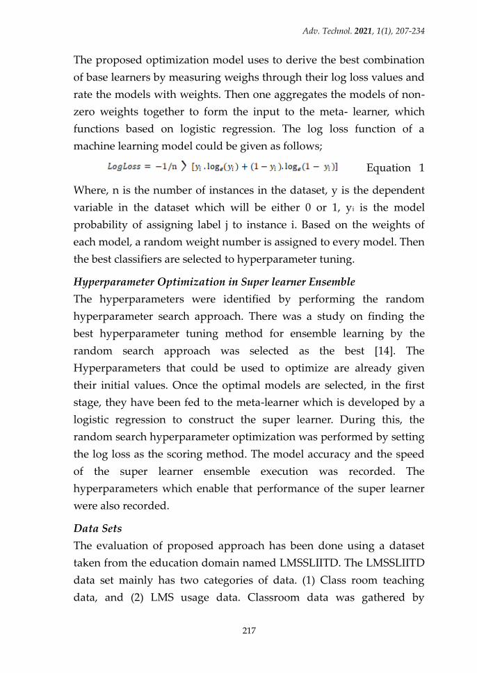
The proposed optimization model uses to derive the best combination

of base learners by measuring weighs through their log loss values and

rate the models with weights. Then one aggregates the models of non-

zero weights together to form the input to the meta- learner, which

functions based on logistic regression. The log loss function of a

machine learning model could be given as follows;

Equation 1

Where, n is the number of instances in the dataset, y is the dependent

variable in the dataset which will be either 0 or 1, yi is the model

probability of assigning label j to instance i. Based on the weights of

each model, a random weight number is assigned to every model. Then

the best classifiers are selected to hyperparameter tuning.

Hyperparameter Optimization in Super learner Ensemble

The hyperparameters were identified by performing the random

hyperparameter search approach. There was a study on finding the

best hyperparameter tuning method for ensemble learning by the

random search approach was selected as the best [14]. The

Hyperparameters that could be used to optimize are already given

their initial values. Once the optimal models are selected, in the first

stage, they have been fed to the meta-learner which is developed by a

logistic regression to construct the super learner. During this, the

random search hyperparameter optimization was performed by setting

the log loss as the scoring method. The model accuracy and the speed

of the super learner ensemble execution was recorded. The

hyperparameters which enable that performance of the super learner

were also recorded.

Data Sets

The evaluation of proposed approach has been done using a dataset

taken from the education domain named LMSSLIITD. The LMSSLIITD

data set mainly has two categories of data. (1) Class room teaching

data, and (2) LMS usage data. Classroom data was gathered by

Adv. Technol. 2021, 1(1), 207-234

218

distributing a structured questionnaire among the university students

who were enrolled in an Information Technology degree program. The

second, LMS data set was collected by accessing the MOODLE data of

a course module offered for thirteen weeks of an Information

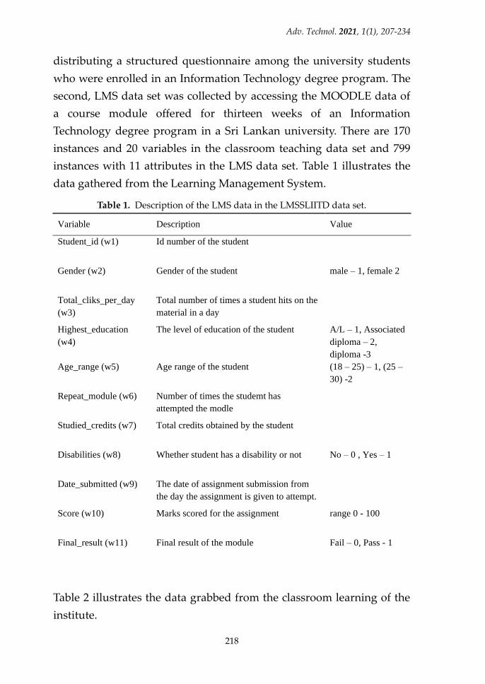
Technology degree program in a Sri Lankan university. There are 170

instances and 20 variables in the classroom teaching data set and 799

instances with 11 attributes in the LMS data set. Table 1 illustrates the

data gathered from the Learning Management System.

Table 1. Description of the LMS data in the LMSSLIITD data set.

Variable Description Value

Student_id (w1) Id number of the student

Gender (w2) Gender of the student male – 1, female 2

Total_cliks_per_day

(w3)

Total number of times a student hits on the

material in a day

Highest_education

(w4)

The level of education of the student A/L – 1, Associated

diploma – 2,

diploma -3

Age_range (w5) Age range of the student (18 – 25) – 1, (25 –

30) -2

Repeat_module (w6) Number of times the studemt has

attempted the modle

Studied_credits (w7) Total credits obtained by the student

Disabilities (w8) Whether student has a disability or not No – 0 , Yes – 1

Date_submitted (w9) The date of assignment submission from

the day the assignment is given to attempt.

Score (w10) Marks scored for the assignment range 0 - 100

Final_result (w11) Final result of the module Fail – 0, Pass - 1

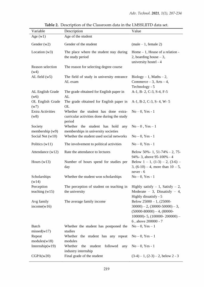
Table 2 illustrates the data grabbed from the classroom learning of the

institute.

Adv. Technol. 2021, 1(1), 207-234

219

Table 2. Description of the Classroom data in the LMSSLIITD data set.

Variable Description Value

Age (w1) Age of the student

Gender (w2) Gender of the student (male – 1, female 2)

Location (w3) The place where the student stay during

the study period

Home – 1, House of a relation -

2, boarding house – 3,

university hostel - 4

Reason selection

(w4)

The reason for selecting degree course

AL field (w5) The field of study in university entrance

AL exam

Biology – 1, Maths – 2,

Commerce – 3, Arts – 4,

Technology - 5

AL English Grade

(w6)

The grade obtained for English paper in

AL

A-1, B- 2, C-3, S-4, F-5

OL English Grade

(w7)

The grade obtained for English paper in

OL

A-1, B-2, C-3, S- 4, W- 5

Extra Activities

(w8)

Whether the student has done extra-

curricular activities done during the study

period

No – 0, Yes - 1

Society

membership (w9)

Whether the student has hold any

memberships in university societies

No – 0 , Yes – 1

Social Net (w10) Whether the student used social networks No – 0, Yes - 1

Politics (w11) The involvement to political activities No – 0, Yes - 1

Attendance (w12) Rate the attendance to lectures Below 50%- 1, 51-74% - 2, 75-

94%- 3, above 95-100% - 4

Hours (w13) Number of hours spend for studies per

day

Below 1 – 1, (1-3) – 2, (3-6) –

3, (6-10) – 4, more than 10 – 5,

never - 6

Scholarships

(w14)

Whether the student won scholarships No – 0, Yes - 1

Perception

teaching (w15)

The perception of student on teaching in

the university

Highly satisfy – 1, Satisfy – 2,

Moderate – 3, Dissatisfy – 4,

Highly dissatisfy - 5

Avg family

income(w16)

The average family income Below 25000 – 1, (25000-

30000) – 2, (30000-50000) – 3,

(50000-80000) – 4, (80000-

100000)- 5, (100000- 200000) –

6 , above 200000 - 7

Batch

missed(w17)

Whether the student has postponed the

studies

No – 0, Yes – 1

Repeat

modules(w18)

Whether the student has any repeat

modules

No – 0, Yes – 1

Internship(w19) Whether the student followed any

industry internship

No – 0, Yes - 1

CGPA(w20) Final grade of the student (3-4) – 1, (2-3) – 2, below 2 - 3

Adv. Technol. 2021, 1(1), 207-234

220

Data Preparation and Feature Extraction

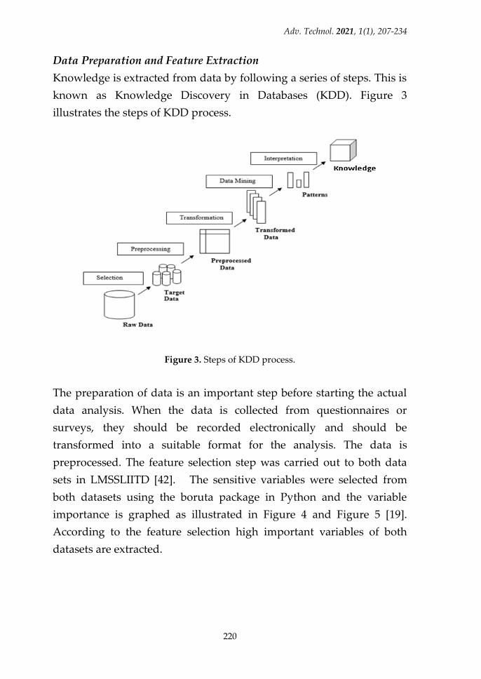
Knowledge is extracted from data by following a series of steps. This is

known as Knowledge Discovery in Databases (KDD). Figure 3

illustrates the steps of KDD process.

Figure 3. Steps of KDD process.

The preparation of data is an important step before starting the actual

data analysis. When the data is collected from questionnaires or

surveys, they should be recorded electronically and should be

transformed into a suitable format for the analysis. The data is

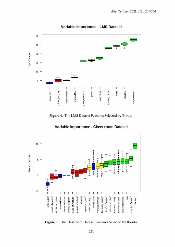
preprocessed. The feature selection step was carried out to both data

sets in LMSSLIITD [42]. The sensitive variables were selected from

both datasets using the boruta package in Python and the variable

importance is graphed as illustrated in Figure 4 and Figure 5 [19].

According to the feature selection high important variables of both

datasets are extracted.

Adv. Technol. 2021, 1(1), 207-234

221

Figure 4. The LMS Dataset Features Selected by Boruta.

Figure 5. The Classroom Dataset Features Selected by Boruta.

Adv. Technol. 2021, 1(1), 207-234

222

Performance Evaluation of LLWSL algorithm

The proposed novel algorithm is applied to the datasets mentioned in

above and the accuracy rate derived for each is recorded. The derived

results are compared against the accuracies of the datasets given before

apply the proposed algorithm. The time taken for both situations are

also recorded to see the complexity of the proposed algorithm.

Model Evaluation

The results of the experiment is statistically validated using a

hypothesis test and evaluated the model performance to prove the

suitability of the proposed approach for the data mining tasks.

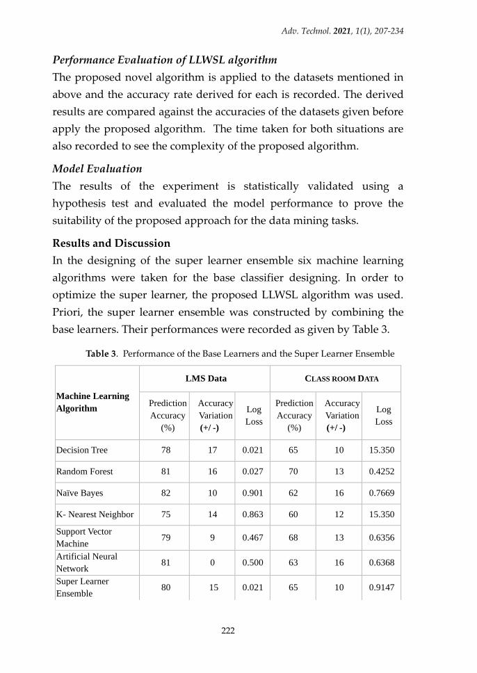
Results and Discussion

In the designing of the super learner ensemble six machine learning

algorithms were taken for the base classifier designing. In order to

optimize the super learner, the proposed LLWSL algorithm was used.

Priori, the super learner ensemble was constructed by combining the

base learners. Their performances were recorded as given by Table 3.

Table 3. Performance of the Base Learners and the Super Learner Ensemble

Machine Learning

Algorithm

LMS Data CLASS ROOM DATA

Prediction

Accuracy

(%)

Accuracy

Variation

(+/ -)

Log

Loss

Prediction

Accuracy

(%)

Accuracy

Variation

(+/ -)

Log

Loss

Decision Tree 78 17 0.021 65 10 15.350

Random Forest 81 16 0.027 70 13 0.4252

Naïve Bayes 82 10 0.901 62 16 0.7669

K- Nearest Neighbor 75 14 0.863 60 12 15.350

Support Vector

Machine 79 9 0.467 68 13 0.6356

Artificial Neural

Network 81 0 0.500 63 16 0.6368

Super Learner

Ensemble 80 15 0.021 65 10 0.9147

Adv. Technol. 2021, 1(1), 207-234

223

The 10 fold cross validation was used as the validation method. The

entire process was repeated 5 times. The number of iterations for

random search was selected as 10. The Randomized SearchCV package

from Scikit-learn library was used to perform the hyperparameter

tuning task [26]. The Sequential Least Square Programming Algorithm

(SLSQP) from Phython SciPy optimization library was used to solve the

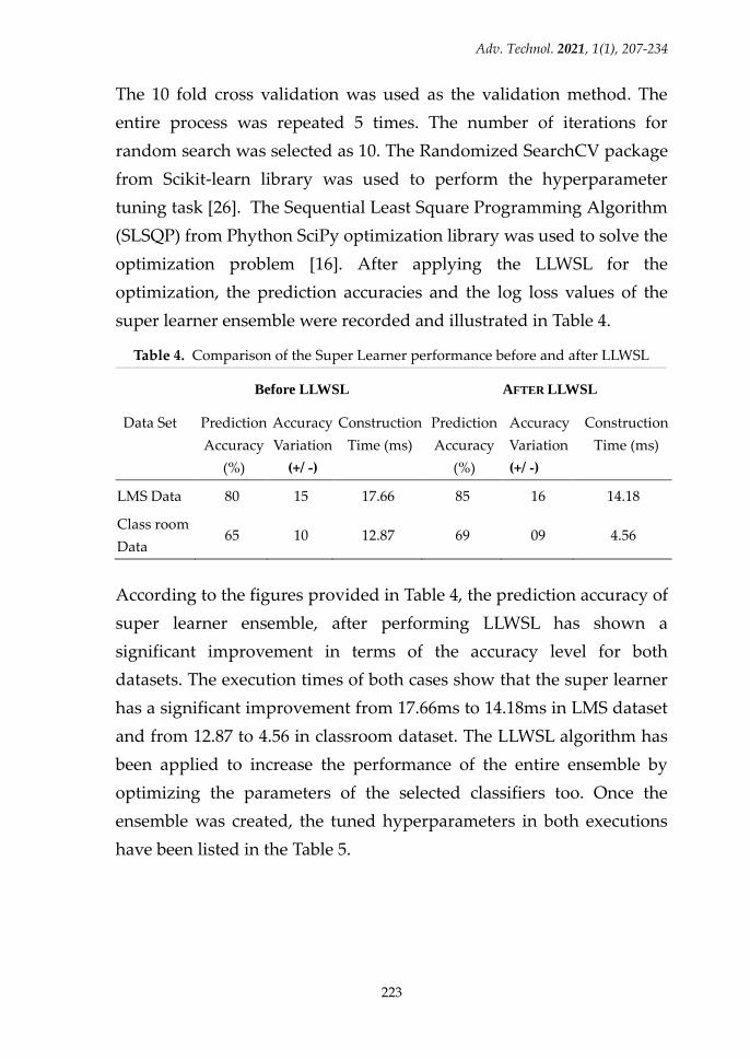
optimization problem [16]. After applying the LLWSL for the

optimization, the prediction accuracies and the log loss values of the

super learner ensemble were recorded and illustrated in Table 4.

Table 4. Comparison of the Super Learner performance before and after LLWSL

Before LLWSL AFTER LLWSL

Data Set

Prediction

Accuracy

(%)

Accuracy

Variation

(+/ -)

Construction

Time (ms)

Prediction

Accuracy

(%)

Accuracy

Variation

(+/ -)

Construction

Time (ms)

LMS Data 80 15 17.66 85 16 14.18

Class room

Data 65 10 12.87 69 09 4.56

According to the figures provided in Table 4, the prediction accuracy of

super learner ensemble, after performing LLWSL has shown a

significant improvement in terms of the accuracy level for both

datasets. The execution times of both cases show that the super learner

has a significant improvement from 17.66ms to 14.18ms in LMS dataset

and from 12.87 to 4.56 in classroom dataset. The LLWSL algorithm has

been applied to increase the performance of the entire ensemble by

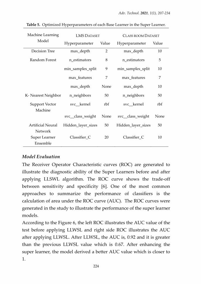
optimizing the parameters of the selected classifiers too. Once the

ensemble was created, the tuned hyperparameters in both executions

have been listed in the Table 5.

Adv. Technol. 2021, 1(1), 207-234

224

Table 5. Optimized Hyperparameters of each Base Learner in the Super Learner.

Machine Learning

Model

LMS DATASET CLASS ROOM DATASET

Hyperparameter Value Hyperparameter Value

Decision Tree max_depth 2 max_depth 10

Random Forest n_estimators 8 n_estimators 5

min_samples_split 9 min_samples_split 10

max_features 7 max_features 7

max_depth None max_depth 10

K- Nearest Neighbor n_neighbors 50 n_neighbors 50

Support Vector

Machine

svc__kernel rbf svc__kernel rbf

svc__class_weight None svc__class_weight None

Artificial Neural

Network

Hidden_layer_sizes 50 Hidden_layer_sizes 50

Super Learner

Ensemble

Classifier_C 20 Classifier_C 10

Model Evaluation

The Receiver Operator Characteristic curves (ROC) are generated to

illustrate the diagnostic ability of the Super Learners before and after

applying LLSWL algorithm. The ROC curve shows the trade-off

between sensitivity and specificity [6]. One of the most common

approaches to summarize the performance of classifiers is the

calculation of area under the ROC curve (AUC). The ROC curves were

generated in the study to illustrate the performance of the super learner

models.

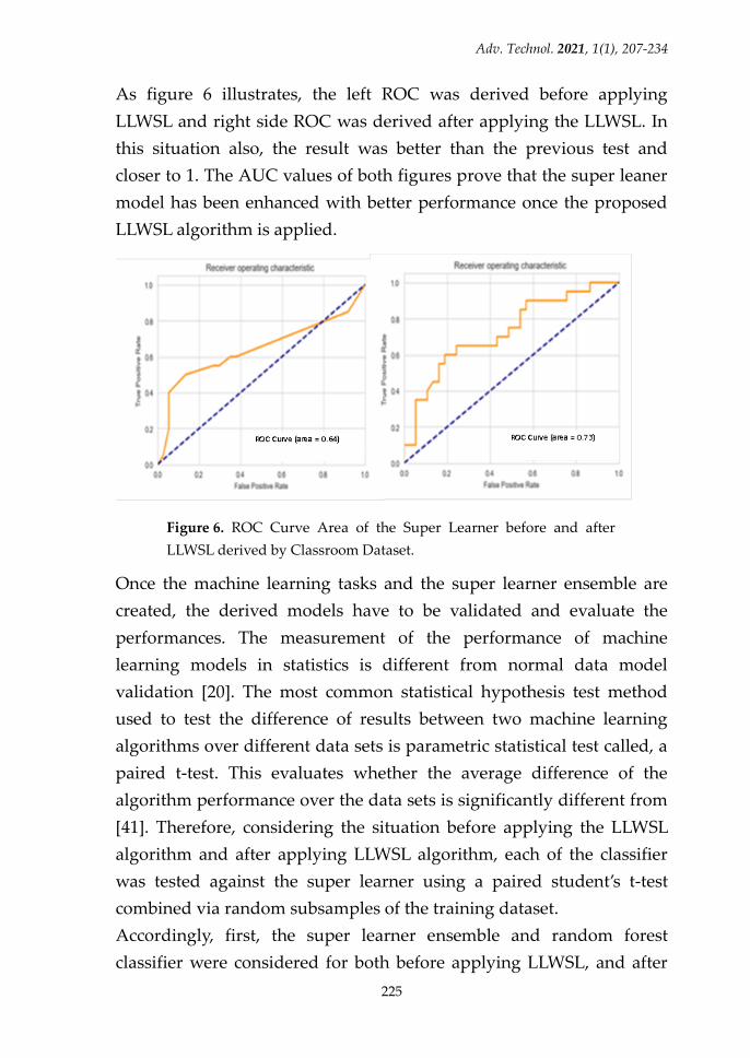
According to the Figure 6, the left ROC illustrates the AUC value of the

test before applying LLWSL and right side ROC illustrates the AUC

after applying LLWSL. After LLWSL, the AUC is, 0.92 and it is greater

than the previous LLWSL value which is 0.67. After enhancing the

super learner, the model derived a better AUC value which is closer to

1.

Adv. Technol. 2021, 1(1), 207-234

225

As figure 6 illustrates, the left ROC was derived before applying

LLWSL and right side ROC was derived after applying the LLWSL. In

this situation also, the result was better than the previous test and

closer to 1. The AUC values of both figures prove that the super leaner

model has been enhanced with better performance once the proposed

LLWSL algorithm is applied.

Figure 6. ROC Curve Area of the Super Learner before and after

LLWSL derived by Classroom Dataset.

Once the machine learning tasks and the super learner ensemble are

created, the derived models have to be validated and evaluate the

performances. The measurement of the performance of machine

learning models in statistics is different from normal data model

validation [20]. The most common statistical hypothesis test method

used to test the difference of results between two machine learning

algorithms over different data sets is parametric statistical test called, a

paired t-test. This evaluates whether the average difference of the

algorithm performance over the data sets is significantly different from

[41]. Therefore, considering the situation before applying the LLWSL

algorithm and after applying LLWSL algorithm, each of the classifier

was tested against the super learner using a paired student’s t-test

combined via random subsamples of the training dataset.

Accordingly, first, the super learner ensemble and random forest

classifier were considered for both before applying LLWSL, and after

Adv. Technol. 2021, 1(1), 207-234

226

applying LLWSL. The test commenced once the null and alternative

hypotheses were made.

The paired student’s t- test is assumed that the data used to perform

the test should be sampled independently from the two populations

being compared [29]. However, since the data in the training and

testing sets are overlapped in different iterations, the independence

assumption is violated. As a solution, researchers of a study have

suggested a novel variance estimation to compute the P- value and

embedded it to paired student’s t-test [49].

Before LLWSL on LMS dataset, the null hypothesis (H0) assumed that

both models perform the same and alternative (H1) assumed that the

models perform differently.

H0: There is no difference between the performance of the super learner

ensemble and the Random Forest classifiers before applying LLWSL.

H1: There is a difference between the performance of the super learner

ensemble and the Random Forest classifiers before applying LLWSL.

Once the paired student’s t- test is performed, it has been observed that

the p-value was about 0.458, which exceeded the standard significant

level of 0.05 (0.458 > 0.05). This implies that the null hypothesis cannot

be rejected, and it has been statistically convincing evidence that

random forest and super learner ensemble perform almost a similar

prediction and no difference between them before applying LLSWL on

LMS data was reported. Similar steps were followed after LLWSL as

well. The null and alternative hypotheses are:

H0: There is no difference between the performance of the super learner

ensemble and the Random Forest classifiers after applying LLWSL.

H1: There is a difference between the performance of the super learner

ensemble and the Random Forest classifiers after applying LLWSL.

After the statistical test, the p-value was about 0.0486, which is below

the significant level of 0.05. This implies that the null hypothesis is

rejected, and it has been statistically proven that the random forest and

super learner ensemble performed differently after applying LLWSL on

Adv. Technol. 2021, 1(1), 207-234

227

LMS data. This is a positive finding on the performance of the super

learner ensemble. Once the LLWSL algorithm is applied and the super

learner is tuned to perform better, it could execute the machine

learning task and could show a significantly different result than the

result if only the Random Forest algorithm had been used. Further, this

statistical test implies that rather than selecting only the Random Forest

algorithm for the prediction task, the super learner ensemble could be

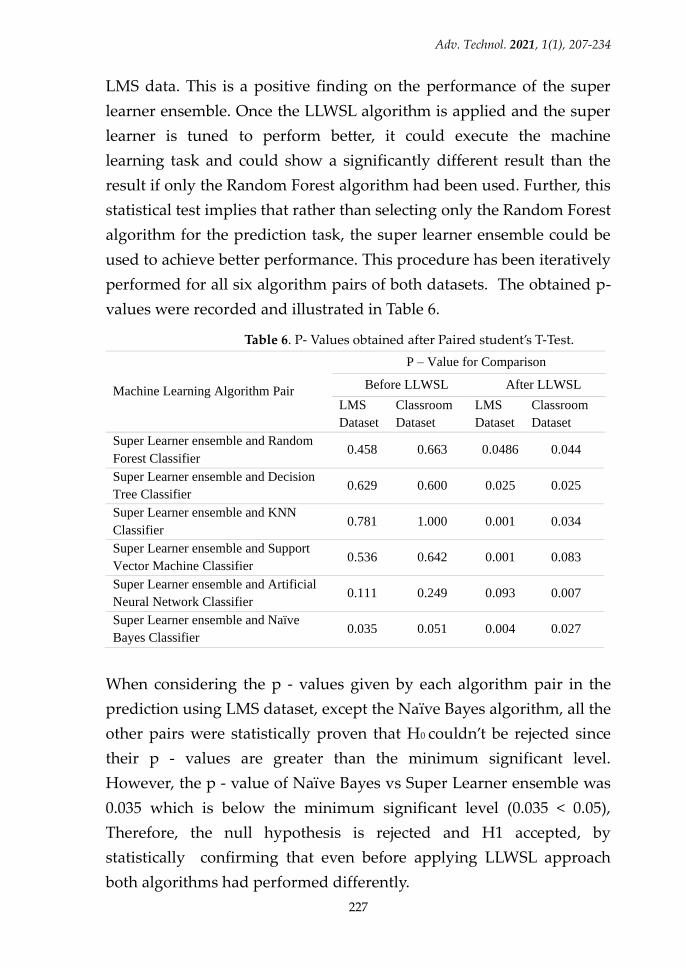
used to achieve better performance. This procedure has been iteratively

performed for all six algorithm pairs of both datasets. The obtained p-

values were recorded and illustrated in Table 6.

Table 6. P- Values obtained after Paired student’s T-Test.

Machine Learning Algorithm Pair

P – Value for Comparison

Before LLWSL After LLWSL

LMS

Dataset

Classroom

Dataset

LMS

Dataset

Classroom

Dataset

Super Learner ensemble and Random

Forest Classifier 0.458 0.663 0.0486 0.044

Super Learner ensemble and Decision

Tree Classifier 0.629 0.600 0.025 0.025

Super Learner ensemble and KNN

Classifier 0.781 1.000 0.001 0.034

Super Learner ensemble and Support

Vector Machine Classifier 0.536 0.642 0.001 0.083

Super Learner ensemble and Artificial

Neural Network Classifier 0.111 0.249 0.093 0.007

Super Learner ensemble and Naïve

Bayes Classifier 0.035 0.051 0.004 0.027

When considering the p - values given by each algorithm pair in the

prediction using LMS dataset, except the Naïve Bayes algorithm, all the

other pairs were statistically proven that H0 couldn’t be rejected since

their p - values are greater than the minimum significant level.

However, the p - value of Naïve Bayes vs Super Learner ensemble was

0.035 which is below the minimum significant level (0.035 < 0.05),

Therefore, the null hypothesis is rejected and H1 accepted, by

statistically confirming that even before applying LLWSL approach

both algorithms had performed differently.

Adv. Technol. 2021, 1(1), 207-234

228

As illustrated in the above Table 6, the p -values derived by each pair

for LMS data after LLWSL, are below the significance level 0.05, which

implies that all null hypothesis developed to test them are rejected by

proving that there exists a significant difference between the individual

performance of the base learner and the performance of the super

learner ensemble.

The p - value analysis of each algorithm pair in the prediction using

classroom dataset, has shown a similar pattern to LMS dataset. Except

the p- value of Naïve Bayes vs Super Learner classifier, others have

shown that H0 could not be rejected and the individual classifiers do

not show a significantly different performance than the super learner

ensemble before applying LLWSL. After applying LLWSL, the

optimized ensemble has shown an improved prediction behavior

except the p- value of support vector machine vs super learner, others

are below the significance level 0.05. Their null hypothesis is rejected

by proving that the super learner behaves differently during the

prediction task. According to the research findings, it is evident that,

the super learner ensemble shows optimal performance.

Discussion

The researchers intend to further the discussion into another grooming

technology called Deep Learning and compare the performance of the

high performing super learner ensemble developed in this study with

Convolutional Neural Network (CNN) technology [5]. Two separate

CNNs were developed in TensorFlow and trained to classify the LMS

dataset and the classroom dataset which were used to construct the

super learner ensemble. According to the test results obtained, the

CNN could obtain 42.5% of an accuracy in training the LMS dataset

whereas the super learner could achieve 85% of an accuracy level.

When the classroom dataset was trained by the CNN algorithm, it

could obtain 63% of an accuracy while the super learner could achieve

69% of an accuracy. Although these accuracy measures are impressive

on the part of the the super learner ensemble, external factors may

Adv. Technol. 2021, 1(1), 207-234

229

affect the performance of deep learning CNN classifier. In most of the

situations deep learning performs better in large volumes of data and

even the goodness of the dataset has a large impact on the performance

of deep learning [47]. A group of researchers have implemented a

super learner to test it against a deep learning algorithm and they

concluded that most of the times their deep learning classifier

outperformed the super learner model [28].

In evaluating the super learner performance, two data sets were

selected from the education domain. Students’ interaction with a course

module through online LMS system was available in LMSD dataset

and the interactive classroom data was available in the classroom

dataset. The number of instances in the data set are different, classroom

dataset has 170 rows and the LMS Data file contains 799 records after

preprocess the data. Both datasets consist of demographic, social and

the performance details of the students. Researchers have mentioned

that if the number of features/ dimensions in the dataset is less, the

model is more accurate. If multiple dimensions are available in the

training dataset, it will negatively impact the accuracies of some

algorithms such as Support Vector Machine and Random Forest [25].

This leads to overfitting the classification algorithm; requires additional

computational time and efforts such as preprocessing and develop

relatively complex machine learning models [13]. Since the model

derived by the algorithm depends on the behavior of the dataset, it is

considerably difficult to produce evidence for the characteristics of the

dataset which can interact negatively with the data and make low

performance [24]. Generally, the machine learning algorithms are

applied on the preprocessed, error free, noiseless and non- redundant

data. Therefore, those obvious reasons do not affect the accuracies of

algorithms of this study. The analysis commenced by performing

feature selection as well. Therefore, the number of dimensions may not

affect the performance of the machine learning algorithms.

As illustrated in the Table 4, it can be observed that no noteworthy

variation exists between the accuracy between the super learner

Adv. Technol. 2021, 1(1), 207-234

230

ensemble used for a dataset before and after LLWSL. Post LLWSL

accuracies were also relatively closer to the Pre- LLWSL accuracies in

each data set. This implies that the properties of the dataset have an

impact on the accuracies of the algorithms. Once the feature selection is

performed, the feature reduction has been done and resulted with

similar number of features in both datasets. The number of instances

can be considered as once such property which may have a direct

impact on the performance. When comparing the LMS dataset with

classroom data set, classroom dataset has fewer instances than LMS

Data and the accuracy is lower than the model derived using LMS

dataset.

The environment in which the experiment has been conducted can be

considered as another property which may affect the performance of

the accuracies of the super learner ensemble. However, the entire

experiments were run on an Intel Core (R) i5 72000 CPU @ 2.7GHz

machine with NVDIA TITAN GPU processor of which the prediction

result was independent from the execution environment.

Conclusion

Rather than adhering to a model generated by a single machine

learning algorithm, after a comparison of several machine learning

models, an optimal super learner was implemented with improved

accuracy and a high speed in generating the predicted model in this

study. The model was tested using two main datasets in the education

domain from several Sri Lankan universities. The prediction accuracy

of the super learner model remained consistent though several changes

were performed to the super learner model by the LLWSL algorithm.

Moreover, a significantly greater execution time was shown by the

super learner after the application of LLWSL algorithms. The proposed

LLWSL algorithm was tested using two separate data sheets to validate

the accuracy. After a successful validation process, it can be concluded

that the proposed LLWSL algorithm results in an optimal super learner

model. The study will be continued with more advanced

Adv. Technol. 2021, 1(1), 207-234

231

hyperparameter optimization methods to obtain higher accuracy level

and to apply the proposed approach to regression problems.

Conflicts of Interest

The authors declare no conflict of interest.

Acknowledgement

The authors would like to express their gratitude to University of

Kelaniya and Sri Lanka Institute of Information Technology for the

fullest support provided in gathering data for this study.

References

[1] O. I. Abiodun, A. Jantan, A. E. Omolara, K. V. Dada, N. A. Mohamed, H. Arshad.

State-of-the-art in artificial neural network applications: A survey. Heliyon, 2018, 4,

e00938.

[2] A. McCallum, K. Nigam. A comparison of event models for naïve bayes text

classification, J. Mach. Learn. Res. 2003, 3, 1265-1287.

[3] K. Babalyan, R. Sultanov, E. Generozov, E. Sharova, E. Kostryukova, A. Larin, A., A.

Kanygina, V. Govorun, G. Arapidi. LogLoss-BERAF: An ensemble-based machine

learning model for constructing highly accurate diagnostic sets of methylation

sites accounting for heterogeneity in prostate cancer. PloS One, 2018, 13, e0204371.

[4] M. B. Bardenet, K. Balázs, S. Michèle. Collaborative hyperparameter tuning. In

Proceedings of the 30th International Conference on International Conference on

Machine Learning. 2013,28, II–199–II–207.

[5] P. Bambharolia. Overview of Convolutional Neural Networks, 2017.

[6] A.P. Bradley. The use of the area under the ROC curve in the evaluation of

machine learning algorithms. Pattern Recognit. 1997, 30, 1145–1159.

[7] L. Breiman, Bagging predictors. Mach. Learn. 1996, 24, 123-140

[8] G. Brown. Ensemble Learning. In C. Sammut and G. I. Webb (Eds.), Encyclopedia

of Machine Learning and Data Mining Springer US, 2017, pp. 393-402

[9] D. Cheng, S. Zhang, Z. Deng, Y. Zhu, M. Zong. kNN Algorithm with Data-Driven

k Value. 2014, 499-512.

[10] B. Clarke. Comparing Bayes model averaging and stacking when model

approximation error cannot be ignored 2003, 4, 683–712.

[11] T. G. Dietterich. Ensemble Methods in Machine Learning. In: Multiple Classifier

Systems. MCS 2000. Lecture Notes in Computer Science, Springer, 2000, 1857.

[12] R. Felder, R. Brent. Active learning: An introduction. ASQ Higher Education Brief.

2009, 2.

Adv. Technol. 2021, 1(1), 207-234

232

[13] R. Genuer, J. M. Poggi, C. Tuleau-Malot. VSURF: An R Package for Variable

Selection Using Random Forests. The R J. 2015, 7, 19–33.

[14] J. Bergstra, Y. Bengio. Random Search for Hyper-Parameter Optimization, J. Mach.

Learn. Res. 2012, 13, 281- 305.

[15] T. Joachims. Text Categorization with Support Vector Machines: Learning with

Many Relevant Features, In: European Conference on Machine Learning,

Chemnitz, Germany, 1998, pp.137-142.

[16] E. Jones, T. Oliphant, P. Peterson. SciPy: Open source scientific tools for Python,

2001

[17] L. Julien-Charles,C. Gagné, R. Sabourin. Bayesian Hyperparameter Optimization

for Ensemble Learning. 2016.

[18] J. W. Kim, B. H. Lee, M. J. Shaw, H. Chang and M. Nelson, Application of

Decision Tree Induction Techniques to Personalized Advertisements on Internet

Storefronts, Int. J. Electron. Commer. 2001, 5, 45-62.

[19] M. Kursa, W. Rudnicki. Feature selection with boruta package. J. Stat. Softw. 2010,

36, 1-13

[20] L. I. Kuncheva, C.J. Whitaker. Measures of Diversity in Classifier Ensembles and

Their Relationship with the Ensemble Accuracy. Mach. Learn., 2003, 51, 181–207.

[21] M. Ladds, A. Thompson and J. Kadar, D. Slip, D. Hocking, R. Harcourt. Super

machine learning: Improving accuracy and reducing variance of behaviour

classification from accelerometry. Anim. Biotelemetry. 2017. 5, 1-9

[22] J. Large, J. Lines, A. Bagnall. A probabilistic classifier ensemble weighting scheme

based on cross-validated accuracy estimate, Data Min. Knowl. Discov. 2019, 33,

1674–1709.

[23] C. Li, J. Wang, L. Hu, P. Gong. Comparison of classification algorithms and

training sample sizes in urban land classification with landsat thematic mapper

imagery. Remote Sens. 2014, 6, 964-983

[24] F. Löw, F., U. Michel, S. Dech, C. Conrad. Impact of feature selection on the

accuracy and spatial uncertainty of per-field crop classification using support

vector machines. ISPRS J. Photogramm. and Remote Sens., 2013, 85, 102–119.

[25] M. Pal, G. M. Foody. Feature selection for classification of hyperspectral data by

svm. IEEE Transactions on Geoscience and Remote Sensing, 2010, 48, 2297–2307.

[26] F. Pedregosa, G. Varoquaux, A. Gramfort, V. Michel, B. Thirion, O. Grisel, et al.

Scikit-learn: Machine learning in Python. J. Mach. Learn. Res. 2011, 12, 2825-2830

[27] P. K. Douglas, S. Harris, A. Yuille, M. S. Cohen. Performance comparison of

machine learning algorithms and number of independent components used in

fMRI decoding of belief vs. disbelief, NeuroImage, 2011, 56, 544-553

[28] S. Purushotham, C. Meng, Z. Che, Y. Liu. Benchmark of Deep Learning Models

on Large Healthcare MIMIC Datasets. J. Biomed. Inform. 2017, 83, 112-134

Adv. Technol. 2021, 1(1), 207-234

233

[29] R. Markovic, S. Wolf, J. Cao, E. Spinnräker, D. Wölki, J. Frisch, C. van Treeck.

Comparison of different classification algorithms for the detection of user's

interaction with windows in office buildings, Energy Procedia, 2017, 122, 337-342

[30] H.C. Romesburg. Cluster analysis for researchers. Melbourne, 2014, FL: Krieger.

[31] M. Re, G. Valentini. Ensemble methods: A review. 2012.

[32] K.T. S. Kasthuriarachchi, S. R. Liyanage, C. M. Bhatt. A data mining approach to

identify the factors affecting the academic success of tertiary students in sri

lanka. In: Caballé S., Conesa J. (eds) software data engineering for network

elearning environments. lecture notes on data engineering and communications

technologies, 2018, 11. Springer, Cham

[33] M. Shahhosseini, G. Hu, H. Pham. Optimizing ensemble weights for machine

learning models: a case study for housing price prediction. 2020.

[34] H. Shee, K. Cheruiyot,S. Kimani. Application of k-nearest neighbor classification

in medical data mining, 2014, 4.

[35] R. Sherri. Mortality risk score prediction in an elderly population using machine

learning, Am. Journal of Epidemiology, 2013, 177, 443–452.

[36] S. Soheily-Khah, Y. Wu. Ensemble learning using frequent itemset mining for

anomaly detection. 2018.

[37] S. Sperandei. Understanding logistic regression analysis. Biochemia Medica. 2014.

[38] I. Syarif, E. Zaluska, A. Prugel-Bennett, G. Wills. Application of bagging, boosting

and stacking to intrusion detection. 2012.

[39] T. G. Dietterich. An experimental comparison of three methods for constructing

ensembles of decision trees: Bagging, boosting and randomization. Mach. Learn.

2000, 40, 139–158.

[40] J. Vamathevan, D. Clark, P. Czodrowski, I. Dunham, E. Ferran, G. Lee, B. Li, A.

Madabhushi, P. Shah, M. Spitzer, S. Zhao. Applications of machine learning in

drug discovery and development. Nature reviews. Drug Discov. 2019, 18, 463–

477.

[41] H. R. Varian. Big Data: New Tricks for Econometrics. J. Econ. Perspect. 2014, 28, 3-

28.

[42] S. Wang, J. Tang, H. Liu. Feature Selection. 2016.

[43] J. Wong, T. Manderson, M. Abrahamowicz, D. Buckeridge, R. Tamblyn. Can

hyperparameter tuning improve the performance of a super learner: a case study.

Epidemiology. 2019.

[44] D. H. Wolpert. Stacked generalization. Neural Networks, 1992, 5,241–259

[45] D. Wolpert, W. Macready. No free lunch theorems for search 1996.

[46] D. Yogatama, G. Mann. Efficient transfer learning method for automatic

hyperparameter tuning. AISTATS., 2014.

[47] G. Zhou, K. Sohn, H. Lee. Online incremental feature learning with denoising

Adv. Technol. 2021, 1(1), 207-234

234

autoencoders. In: International Conference on Artificial Intelligence and

Statistics. JMLR.org. 2014, 1453–1461

[48] J. Demsar. Statistical comparisons of classifiers over multiple data sets, J. Mach.

Learn. Research, 2007 ,7, 1-30.

[49] C. Nadeau, Y. Bengio. Inference for the generalization error, J. Mach. Learn. 2003,

52, 239-281