water

Article

Variation of Diatoms and Silicon in a Tributary of theThree Gorges Reservoir: Evidence of Interaction

Wei Xiao 1,†, Yubo Huang 2,†, Wujuan Mi 2, Hongyan Wu 1 and Yonghong Bi 2,*1 School of Civil Engineering, Architecture and Environment, Hubei University of Technology,

Wuhan 430068, China2 State Key Laboratory of Freshwater Ecology and Biotechnology, Institute of Hydrobiology, Chinese

Academy of Sciences, Wuhan 430072, China* Correspondence: biyh@ihb.ac.cn† Equally contributed.

Received: 16 May 2019; Accepted: 28 June 2019; Published: 2 July 2019�����������������

Abstract: To gain insight into the variation of diatoms and silicon and their interaction in a tributaryof the Three Gorges Reservoir (TGR), the Xiangxi River was chosen as a representative tributary,and dissolved silicon (DSi) and biogenic silicon (BSi) were investigated monthly from February2015 to December 2016, accompanied by diatom species composition and cell density analyses.The results showed that the diatom population and its relationship with silicon concentration weresignificantly different between the lacustrine zone and riverine zone (P < 0.05). The cell density inthe lacustrine zone (6.20 × 105 ~ 9.97 × 107 cells/L) was significantly higher than that in the riverinezone (7.90 × 104 ~ 1.81 × 107 cells/L) (P < 0.01). Water velocity was a key factor in determiningthe diatom species composition. Centric diatoms were the dominant species in the lacustrine zone,and pennate diatoms were the primary species in the riverine zone, which indicated that centricdiatoms outcompete pennate diatoms under the influence of the TGR’s operation. BSi showed asignificant linear relationship with the cell density. DSi had a significant negative relationship withthe cell density in the lacustrine zone, while no significant relationship was found in the riverinezone. This meant that the main contributor to BSi was diatoms, but DSi was primarily affected bywater discharge, not diatom uptake. It could be deduced that the spatiotemporal heterogeneity ofdiatom communities was influenced by the TGR’s operation. Silicon cycling in the tributary wassignificantly affected by diatoms, and the current concentration of DSi was sufficient for diatomgrowth and showed no significant effects on the diatom community.

Keywords: diatom; cell density; dissolved silicon; biogenic silicon

1. Introduction

Silicon originates from rock weathering and is transported from land to the ocean mainly byrivers. It was estimated that 371 million tons of dissolved silicon (DSi) and 8835 million tons ofparticulate silicon (PSi) drain into the ocean every year from the continental surfaces in the world [1].DSi and biogenic silicon (BSi) are considered bioavailable silicon in natural waters. DSi can be directlyassimilated by algae and hydrophytes. BSi can contribute to DSi because of its regeneration inthe water and sediment. The recycling of BSi provides the major source of soluble reactive siliconrequired for diatom proliferation [2]. Silicon is a key nutrient for diatom growth because it is a kind ofnecessary element to form the diatom’s rigid cell wall [3]. BSi is generated when diatoms, plants andother organisms uptake DSi during photosynthesis, and it is an important source of DSi due to itstypically amorphous form; it plays an important role in the earth’s Si cycle. DSi mainly originatesfrom weathering, and anthropogenic activities can scarcely compensate for the loss of DSi from this

Water 2019, 11, 1369; doi:10.3390/w11071369 www.mdpi.com/journal/water

Water 2019, 11, 1369 2 of 13

source. Dsi and Bsi are not two independent variations in the water. With plenty of time, DSi can beconverted to biological available silicon (BSi). When water velocity is high, the hydraulic retention timeis short and can’t meet the need of converting procedure. Thus, in the lacustrine area, diatom coulddeplete DSi and produce BSi in a stable environment. Decreased silicon has been observed in manyrivers and lakes worldwide [4–6]. Diatom growth is related to silicate and other nutrient availability.Under conditions in which the silicate concentration was higher than 2 µmol/L and other nutrientswere sufficient, diatoms were observed to dominate the phytoplankton community, accounting formore than 70% of the total cell density in the community [7]. The distribution patterns of epipelic andepipsammic diatoms were related to nutrient availability, especially of silicate and ammonium [8].It was observed that silicate availability by river supply and strong tidal mixing of the water columnseemed to determine the year-round dominance of diatoms over dinoflagellates in a Spanish estuary [9].Studies also found that the ratio between silicates and other nutrients, such as carbon, nitrogen,or phosphorus, affected diatom growth in the phytoplankton succession. Skeletonema costatum isinfluenced by silicate availability and by changes in dissolved inorganic carbon (DIC) pool [10]. Speciessuccession from diatom to blue-green algae was controlled by carbon and silicate in karst cascadereservoirs in Southwest China [11]. It has been proven that decreasing silicon and increasing nitrogenand phosphorus in the Yangtze River estuary resulted in eutrophication, decreased diatom compositionin the algal community and frequent harmful algal blooms in coastal waters [12]. Therefore, there wasa direct causal relationship between diatom growth and silicate availability.

In addition to silicate availability, algal growth is primarily related to changes in environmentalfactors, such as the water stability, water renewal rate and water retention time. In reservoirs withconsiderable hydraulic dynamics, the water renewal rate explained the selection of secondary species,and dominant species adapted to a broad range of environmental conditions [13]. Fast growth was theresponse of diatoms to changes in physical environmental factors, especially the daily variations inriver discharge, which continuously modify the suspended particulate matter concentrations and waterretention time [14], while low flow conditions lead to a progressive depletion of dissolved silicon [15].On the other hand, diatom species varied depending on the environmental conditions. In comparisonwith pennate diatoms, centric diatoms favour relatively lower temperatures and photoperiods. Pennatediatoms depend more on light and grazer abundance [16]. Therefore, the relationship between diatomsand environmental factors is complex and requires further research.

Three Gorges Reservoir (TGR) is the largest deep river-type reservoir in the world. Large amountsof nutrients and pollutants from headwaters and tributaries drained into the reservoir after ThreeGorges Dam began operation, causing severe problems such as eutrophication [17] and algal bloom [18].Many studies have been conducted to elucidate algal succession [19] and nutrient distribution underTGR’s operation [20–24]. It was observed that the frequency and duration of algal blooms has risenin recent years [25]. Furthermore, water intrusion from the main channel of the Yangtze River to thetributaries has worsened eutrophication in tributaries such as the Daning River [26] and the XiangxiRiver [27]. Consequently, biogeochemical cycling of some nutrients, such as nitrogen, phosphorus,and silicon, has changed. Previous studies have demonstrated silicon retention in the TGR dueto dam construction and its impact on the silicon efflux to the eastern sea through the YangtzeRiver [5,28,29]. These studies mainly focused on silicon dynamics and its fluxes. Other studies haveemphasized algal succession and its relationship with nitrogen and phosphorus in the TGR [30].However, the relationship between diatoms and silicon in the TGR has not yet been investigated indetail. After the impoundment of the TGR, silicon retention in the reservoir was increased, and thedischarge amount of biogenic silicon was gradually reduced. Lower water velocity and higher watertransparency accelerated the growth of diatoms and led to frequent diatom blooms in the tributaries ofthe TGR. In this study, the Xiangxi River was selected as a representative of the tributaries in the TGR,and silicon and diatoms were screened in two distinct zones: The riverine zone and the lacustrinezone. This study aims to understand (i) the diatom community in different water areas of the TGRand (ii) the interactive relationship between the available silicate or hydrodynamics and the diatom

Water 2019, 11, 1369 3 of 13

community in the TGR. A monthly investigation was conducted, including diatom species, cell density,silicon concentration, and environmental parameters. This study will help us to gain insight into theinteraction between silicon concentration and diatom communities in the TGR and the variation ofsilicon and changes in the diatom community.

2. Materials and Methods

2.1. Study Site

The water level of the TGR was artificially regulated according to the dam operation strategy.In summer, the water level was low for power generation and flood prevention, and in winter, the waterlevel was high for drought relief and navigation improvement. A typical hydrological year of the TGRwas divided into four periods according to a series of specific operations. The impounding period wasin autumn from September to October, and the water level increased from 145 m to 175 m. The nextthree months (November to January) were the high water level period, with the water level maintainedat approximately 175 m. Then, in the discharge period (February to June), the water level was decreasedfrom 175 m to 145 m. The last period (July to August) was the low water level period, with the waterlevel remaining at 145 m. The water discharge and sand transport rate displayed opposite trendsagainst the water level in the TGR, which was caused by seasonal variations in precipitation [31].

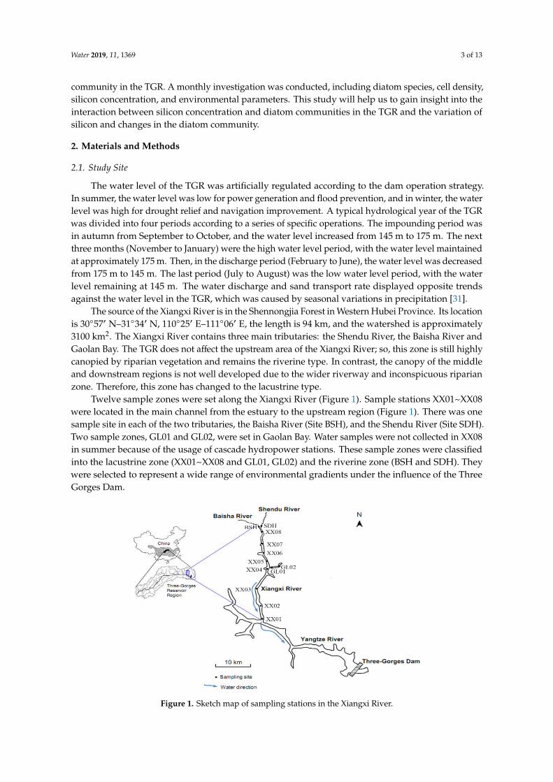
The source of the Xiangxi River is in the Shennongjia Forest in Western Hubei Province. Its locationis 30◦57′ N–31◦34′ N, 110◦25′ E–111◦06′ E, the length is 94 km, and the watershed is approximately3100 km2. The Xiangxi River contains three main tributaries: the Shendu River, the Baisha River andGaolan Bay. The TGR does not affect the upstream area of the Xiangxi River; so, this zone is still highlycanopied by riparian vegetation and remains the riverine type. In contrast, the canopy of the middleand downstream regions is not well developed due to the wider riverway and inconspicuous riparianzone. Therefore, this zone has changed to the lacustrine type.

Twelve sample zones were set along the Xiangxi River (Figure 1). Sample stations XX01~XX08were located in the main channel from the estuary to the upstream region (Figure 1). There was onesample site in each of the two tributaries, the Baisha River (Site BSH), and the Shendu River (Site SDH).Two sample zones, GL01 and GL02, were set in Gaolan Bay. Water samples were not collected in XX08in summer because of the usage of cascade hydropower stations. These sample zones were classifiedinto the lacustrine zone (XX01~XX08 and GL01, GL02) and the riverine zone (BSH and SDH). Theywere selected to represent a wide range of environmental gradients under the influence of the ThreeGorges Dam.

Water 2019, 10, x FOR PEER REVIEW 3 of 14

species, cell density, silicon concentration, and environmental parameters. This study will help us to gain insight into the interaction between silicon concentration and diatom communities in the TGR and the variation of silicon and changes in the diatom community.

2. Materials and Methods

2.1. Study Site

The water level of the TGR was artificially regulated according to the dam operation strategy. In summer, the water level was low for power generation and flood prevention, and in winter, the water level was high for drought relief and navigation improvement. A typical hydrological year of the TGR was divided into four periods according to a series of specific operations. The impounding period was in autumn from September to October, and the water level increased from 145 m to 175 m. The next three months (November to January) were the high water level period, with the water level maintained at approximately 175 m. Then, in the discharge period (February to June), the water level was decreased from 175 m to 145 m. The last period (July to August) was the low water level period, with the water level remaining at 145 m. The water discharge and sand transport rate displayed opposite trends against the water level in the TGR, which was caused by seasonal variations in precipitation [31].

The source of the Xiangxi River is in the Shennongjia Forest in Western Hubei Province. Its location is 30°57′ N–31°34′ N, 110°25′ E–111°06′ E, the length is 94 km, and the watershed is approximately 3100 km2. The Xiangxi River contains three main tributaries: the Shendu River, the Baisha River and Gaolan Bay. The TGR does not affect the upstream area of the Xiangxi River; so, this zone is still highly canopied by riparian vegetation and remains the riverine type. In contrast, the canopy of the middle and downstream regions is not well developed due to the wider riverway and inconspicuous riparian zone. Therefore, this zone has changed to the lacustrine type.

Twelve sample zones were set along the Xiangxi River (Figure 1). Sample stations XX01~XX08 were located in the main channel from the estuary to the upstream region (Figure 1). There was one sample site in each of the two tributaries, the Baisha River (Site BSH), and the Shendu River (Site SDH). Two sample zones, GL01 and GL02, were set in Gaolan Bay. Water samples were not collected in XX08 in summer because of the usage of cascade hydropower stations. These sample zones were classified into the lacustrine zone (XX01~XX08 and GL01, GL02) and the riverine zone (BSH and SDH). They were selected to represent a wide range of environmental gradients under the influence of the Three Gorges Dam.

Figure 1. Sketch map of sampling stations in the Xiangxi River. Figure 1. Sketch map of sampling stations in the Xiangxi River.

Water 2019, 11, 1369 4 of 13

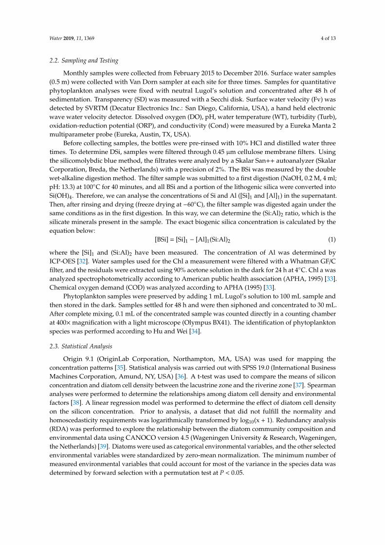
2.2. Sampling and Testing

Monthly samples were collected from February 2015 to December 2016. Surface water samples(0.5 m) were collected with Van Dorn sampler at each site for three times. Samples for quantitativephytoplankton analyses were fixed with neutral Lugol’s solution and concentrated after 48 h ofsedimentation. Transparency (SD) was measured with a Secchi disk. Surface water velocity (Fv) wasdetected by SVRTM (Decatur Electronics Inc.: San Diego, California, USA), a hand held electronicwave water velocity detector. Dissolved oxygen (DO), pH, water temperature (WT), turbidity (Turb),oxidation-reduction potential (ORP), and conductivity (Cond) were measured by a Eureka Manta 2multiparameter probe (Eureka, Austin, TX, USA).

Before collecting samples, the bottles were pre-rinsed with 10% HCl and distilled water threetimes. To determine DSi, samples were filtered through 0.45 µm cellulose membrane filters. Usingthe silicomolybdic blue method, the filtrates were analyzed by a Skalar San++ autoanalyzer (SkalarCorporation, Breda, the Netherlands) with a precision of 2%. The BSi was measured by the doublewet-alkaline digestion method. The filter sample was submitted to a first digestion (NaOH, 0.2 M, 4 ml;pH: 13.3) at 100◦C for 40 minutes, and all BSi and a portion of the lithogenic silica were converted intoSi(OH)4. Therefore, we can analyse the concentrations of Si and Al ([Si]1 and [Al]1) in the supernatant.Then, after rinsing and drying (freeze drying at −60◦C), the filter sample was digested again under thesame conditions as in the first digestion. In this way, we can determine the (Si:Al)2 ratio, which is thesilicate minerals present in the sample. The exact biogenic silica concentration is calculated by theequation below:

[BSi] = [Si]1 − [Al]1(Si:Al)2 (1)

where the [Si]1 and (Si:Al)2 have been measured. The concentration of Al was determined byICP-OES [32]. Water samples used for the Chl a measurement were filtered with a Whatman GF/Cfilter, and the residuals were extracted using 90% acetone solution in the dark for 24 h at 4◦C. Chl a wasanalyzed spectrophotometrically according to American public health association (APHA, 1995) [33].Chemical oxygen demand (COD) was analyzed according to APHA (1995) [33].

Phytoplankton samples were preserved by adding 1 mL Lugol’s solution to 100 mL sample andthen stored in the dark. Samples settled for 48 h and were then siphoned and concentrated to 30 mL.After complete mixing, 0.1 mL of the concentrated sample was counted directly in a counting chamberat 400×magnification with a light microscope (Olympus BX41). The identification of phytoplanktonspecies was performed according to Hu and Wei [34].

2.3. Statistical Analysis

Origin 9.1 (OriginLab Corporation, Northampton, MA, USA) was used for mapping theconcentration patterns [35]. Statistical analysis was carried out with SPSS 19.0 (International BusinessMachines Corporation, Amund, NY, USA) [36]. A t-test was used to compare the means of siliconconcentration and diatom cell density between the lacustrine zone and the riverine zone [37]. Spearmananalyses were performed to determine the relationships among diatom cell density and environmentalfactors [38]. A linear regression model was performed to determine the effect of diatom cell densityon the silicon concentration. Prior to analysis, a dataset that did not fulfill the normality andhomoscedasticity requirements was logarithmically transformed by log10(x + 1). Redundancy analysis(RDA) was performed to explore the relationship between the diatom community composition andenvironmental data using CANOCO version 4.5 (Wageningen University & Research, Wageningen,the Netherlands) [39]. Diatoms were used as categorical environmental variables, and the other selectedenvironmental variables were standardized by zero-mean normalization. The minimum number ofmeasured environmental variables that could account for most of the variance in the species data wasdetermined by forward selection with a permutation test at P < 0.05.

Water 2019, 11, 1369 5 of 13

3. Results

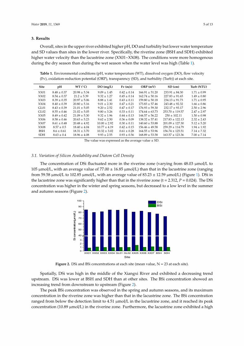
Overall, sites in the upper river exhibited higher pH, DO and turbidity but lower water temperatureand SD values than sites in the lower river. Specifically, the riverine zone (BSH and SDH) exhibitedhigher water velocity than the lacustrine zone (XX01~XX08). The conditions were more homogenousduring the dry season than during the wet season when the water level was high (Table 1).

Table 1. Environmental conditions (pH, water temperature (WT), dissolved oxygen (DO), flow velocity(Fv), oxidation-reduction potential (ORP), transparency (SD), and turbidity (Turb)) at each site.

Site pH WT (◦C) DO (mg/L) Fv (m/s) ORP (mV) SD (cm) Turb (NTU)

XX01 8.48 ± 0.37 20.98 ± 5.34 9.09 ± 1.45 0.42 ± 0.14 166.91 ± 51.20 233.91 ± 84.30 1.71 ± 0.99XX02 8.54 ± 0.37 21.2 ± 5.39 9.32 ± 1.27 0.45 ± 0.14 162.74 ± 50.16 227.83 ± 91.65 1.49 ± 0.80XX03 8.39 ± 0.35 20.97 ± 5.06 8.88 ± 1.41 0.43 ± 0.11 159.80 ± 50.18 234.13 ± 91.73 1.71 ± 0.95XX04 8.40 ± 0.39 20.80 ± 5.16 9.01 ± 2.30 0.47 ± 0.21 173.83 ± 57.46 243.48 ± 92.32 1.66 ± 0.86GL01 8.43 ± 0.39 21.01 ± 5.05 9.20 ± 2.52 0.47 ± 0.17 176.93 ± 59.30 232.17 ± 93.17 2.50 ± 2.96GL02 8.55 ± 0.46 21.02 ± 5.05 9.80 ± 3.26 0.33 ± 0.11 174.64 ± 63.73 253.70 ± 119.57 2.47 ± 2.97XX05 8.49 ± 0.42 21.09 ± 5.30 9.32 ± 1.96 0.44 ± 0.13 144.57 ± 56.22 250 ± 102.11 1.50 ± 0.98XX06 8.58 ± 0.46 20.63 ± 5.23 9.62 ± 2.50 0.36 ± 0.09 138.32 ± 57.41 217.83 ± 122.13 2.32 ± 2.43XX07 8.61 ± 0.48 20.48 ± 4.92 10.00 ± 2.92 0.30 ± 0.11 140.60 ± 53.88 201.09 ± 127.30 5.12 ± 5.20XX08 8.57 ± 0.5 18.40 ± 4.04 10.77 ± 4.19 0.42 ± 0.15 156.46 ± 49.58 259.29 ± 114.79 1.94 ± 1.92BSH 8.6 ± 0.61 18.31 ± 3.70 10.32 ± 3.02 0.61 ± 0.28 164.55 ± 53.96 156.74 ± 125.51 7.14 ± 7.32SDH 8.63 ± 0.4 18.96 ± 4.08 9.93 ± 2.55 0.93 ± 0.56 168.89 ± 53.58 163.57 ± 123.36 7.00 ± 7.14

The value was expressed as the average value ± SD.

3.1. Variation of Silicon Availability and Diatom Cell Density

The concentration of DSi fluctuated more in the riverine zone (varying from 48.03 µmol/L to105 µmol/L, with an average value of 77.00 ± 16.85 µmol/L) than that in the lacustrine zone (rangingfrom 59.58 µmol/L to 102.85 µmol/L, with an average value of 83.23 ± 12.59 µmol/L) (Figure 1). DSi inthe lacustrine zone was significantly higher than that in the riverine zone (t = 2.312, P = 0.024). The DSiconcentration was higher in the winter and spring seasons, but decreased to a low level in the summerand autumn seasons (Figure 2).

Water 2019, 10, x FOR PEER REVIEW 6 of 14

Figure 2. DSi and BSi concentrations at each site (mean value, N = 23 at each site).

Spatially, DSi was high in the middle of the Xiangxi River and exhibited a decreasing trend upstream. DSi was lower at BSH and SDH than at other sites. The BSi concentration showed an increasing trend from downstream to upstream (Figure 2).

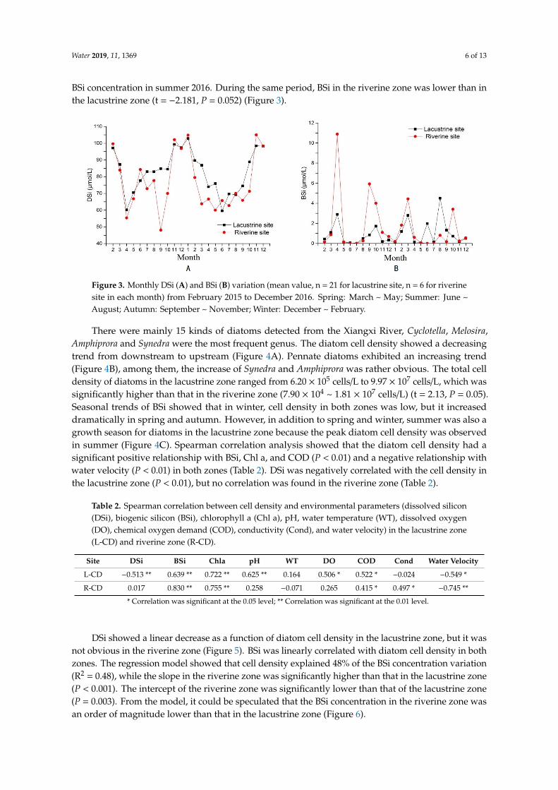
The peak BSi concentration was observed in the spring and autumn seasons, and its maximum concentration in the riverine zone was higher than that in the lacustrine zone. The BSi concentration ranged from below the detection limit to 4.51 μmol/L in the lacustrine zone, and it reached its peak concentration (10.89 μmol/L) in the riverine zone. Furthermore, the lacustrine zone exhibited a high BSi concentration in summer 2016. During the same period, BSi in the riverine zone was lower than in the lacustrine zone (t = −2.181, P = 0.052) (Figure 3).

Figure 3. Monthly DSi (A) and BSi (B) variation (mean value, n = 21 for lacustrine site, n = 6 for riverine site in each month) from February 2015 to December 2016. Spring: March ~ May; Summer: June ~ August; Autumn: September ~ November; Winter: December ~ February.

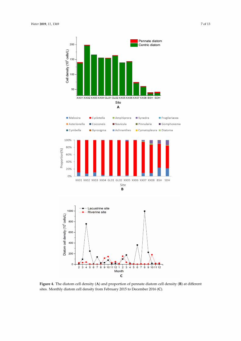
There were mainly 15 kinds of diatoms detected from the Xiangxi River, Cyclotella, Melosira, Amphiprora and Synedra were the most frequent genus. The diatom cell density showed a decreasing trend from downstream to upstream (Figure 4A). Pennate diatoms exhibited an increasing trend (Figure 4B), among them, the increase of Synedra and Amphiprora was rather obvious. The total cell density of diatoms in the lacustrine zone ranged from 6.20 × 105 cells/L to 9.97 × 107 cells/L, which was significantly higher than that in the riverine zone (7.90 × 104 ~ 1.81 × 107 cells/L) (t = 2.13, P = 0.05). Seasonal trends of BSi showed that in winter, cell density in both zones was low, but it increased dramatically in spring and autumn. However, in addition to spring and winter, summer was also a growth season for diatoms in the lacustrine zone because the peak diatom cell density was observed

XX01 XX02 XX03 XX04 GL01 GL02 XX05 XX06 XX07 BSH SDH0123

40

50

60

70

80

90

100

Si c

once

ntra

tion(

μmol

/L)

Site

DSi BSi

Figure 2. DSi and BSi concentrations at each site (mean value, N = 23 at each site).

Spatially, DSi was high in the middle of the Xiangxi River and exhibited a decreasing trendupstream. DSi was lower at BSH and SDH than at other sites. The BSi concentration showed anincreasing trend from downstream to upstream (Figure 2).

The peak BSi concentration was observed in the spring and autumn seasons, and its maximumconcentration in the riverine zone was higher than that in the lacustrine zone. The BSi concentrationranged from below the detection limit to 4.51 µmol/L in the lacustrine zone, and it reached its peakconcentration (10.89 µmol/L) in the riverine zone. Furthermore, the lacustrine zone exhibited a high

Water 2019, 11, 1369 6 of 13

BSi concentration in summer 2016. During the same period, BSi in the riverine zone was lower than inthe lacustrine zone (t = −2.181, P = 0.052) (Figure 3).

Water 2019, 10, x FOR PEER REVIEW 6 of 14

Figure 2. DSi and BSi concentrations at each site (mean value, N = 23 at each site).

Spatially, DSi was high in the middle of the Xiangxi River and exhibited a decreasing trend upstream. DSi was lower at BSH and SDH than at other sites. The BSi concentration showed an increasing trend from downstream to upstream (Figure 2).

The peak BSi concentration was observed in the spring and autumn seasons, and its maximum concentration in the riverine zone was higher than that in the lacustrine zone. The BSi concentration ranged from below the detection limit to 4.51 μmol/L in the lacustrine zone, and it reached its peak concentration (10.89 μmol/L) in the riverine zone. Furthermore, the lacustrine zone exhibited a high BSi concentration in summer 2016. During the same period, BSi in the riverine zone was lower than in the lacustrine zone (t = −2.181, P = 0.052) (Figure 3).

Figure 3. Monthly DSi (A) and BSi (B) variation (mean value, n = 21 for lacustrine site, n = 6 for riverine site in each month) from February 2015 to December 2016. Spring: March ~ May; Summer: June ~ August; Autumn: September ~ November; Winter: December ~ February.

There were mainly 15 kinds of diatoms detected from the Xiangxi River, Cyclotella, Melosira, Amphiprora and Synedra were the most frequent genus. The diatom cell density showed a decreasing trend from downstream to upstream (Figure 4A). Pennate diatoms exhibited an increasing trend (Figure 4B), among them, the increase of Synedra and Amphiprora was rather obvious. The total cell density of diatoms in the lacustrine zone ranged from 6.20 × 105 cells/L to 9.97 × 107 cells/L, which was significantly higher than that in the riverine zone (7.90 × 104 ~ 1.81 × 107 cells/L) (t = 2.13, P = 0.05). Seasonal trends of BSi showed that in winter, cell density in both zones was low, but it increased dramatically in spring and autumn. However, in addition to spring and winter, summer was also a growth season for diatoms in the lacustrine zone because the peak diatom cell density was observed

XX01 XX02 XX03 XX04 GL01 GL02 XX05 XX06 XX07 BSH SDH0123

40

50

60

70

80

90

100

Si c

once

ntra

tion(

μmol

/L)

Site

DSi BSi

Figure 3. Monthly DSi (A) and BSi (B) variation (mean value, n = 21 for lacustrine site, n = 6 for riverinesite in each month) from February 2015 to December 2016. Spring: March ~ May; Summer: June ~August; Autumn: September ~ November; Winter: December ~ February.

There were mainly 15 kinds of diatoms detected from the Xiangxi River, Cyclotella, Melosira,Amphiprora and Synedra were the most frequent genus. The diatom cell density showed a decreasingtrend from downstream to upstream (Figure 4A). Pennate diatoms exhibited an increasing trend(Figure 4B), among them, the increase of Synedra and Amphiprora was rather obvious. The total celldensity of diatoms in the lacustrine zone ranged from 6.20 × 105 cells/L to 9.97 × 107 cells/L, which wassignificantly higher than that in the riverine zone (7.90 × 104 ~ 1.81 × 107 cells/L) (t = 2.13, P = 0.05).Seasonal trends of BSi showed that in winter, cell density in both zones was low, but it increaseddramatically in spring and autumn. However, in addition to spring and winter, summer was also agrowth season for diatoms in the lacustrine zone because the peak diatom cell density was observedin summer (Figure 4C). Spearman correlation analysis showed that the diatom cell density had asignificant positive relationship with BSi, Chl a, and COD (P < 0.01) and a negative relationship withwater velocity (P < 0.01) in both zones (Table 2). DSi was negatively correlated with the cell density inthe lacustrine zone (P < 0.01), but no correlation was found in the riverine zone (Table 2).

Table 2. Spearman correlation between cell density and environmental parameters (dissolved silicon(DSi), biogenic silicon (BSi), chlorophyll a (Chl a), pH, water temperature (WT), dissolved oxygen(DO), chemical oxygen demand (COD), conductivity (Cond), and water velocity) in the lacustrine zone(L-CD) and riverine zone (R-CD).

Site DSi BSi Chla pH WT DO COD Cond Water Velocity

L-CD −0.513 ** 0.639 ** 0.722 ** 0.625 ** 0.164 0.506 * 0.522 * −0.024 −0.549 *

R-CD 0.017 0.830 ** 0.755 ** 0.258 −0.071 0.265 0.415 * 0.497 * −0.745 **

* Correlation was significant at the 0.05 level; ** Correlation was significant at the 0.01 level.

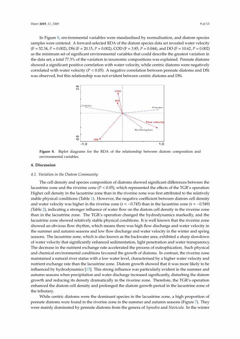
DSi showed a linear decrease as a function of diatom cell density in the lacustrine zone, but it wasnot obvious in the riverine zone (Figure 5). BSi was linearly correlated with diatom cell density in bothzones. The regression model showed that cell density explained 48% of the BSi concentration variation(R2 = 0.48), while the slope in the riverine zone was significantly higher than that in the lacustrine zone(P < 0.001). The intercept of the riverine zone was significantly lower than that of the lacustrine zone(P = 0.003). From the model, it could be speculated that the BSi concentration in the riverine zone wasan order of magnitude lower than that in the lacustrine zone (Figure 6).

Water 2019, 11, 1369 7 of 13

Water 2019, 10, x FOR PEER REVIEW 7 of 14

in summer (Figure 4C). Spearman correlation analysis showed that the diatom cell density had a significant positive relationship with BSi, Chl a, and COD (P < 0.01) and a negative relationship with water velocity (P < 0.01) in both zones (Table 2). DSi was negatively correlated with the cell density in the lacustrine zone (P < 0.01), but no correlation was found in the riverine zone (Table 2).

Figure 4. The diatom cell density (A) and proportion of pennate diatom cell density (B) at differentsites. Monthly diatom cell density from February 2015 to December 2016 (C).

Water 2019, 11, 1369 8 of 13

Water 2019, 10, x FOR PEER REVIEW 8 of 14

Figure 4. The diatom cell density (A) and proportion of pennate diatom cell density (B) at different sites. Monthly diatom cell density from February 2015 to December 2016 (C).

Table 2. Spearman correlation between cell density and environmental parameters (dissolved silicon (DSi), biogenic silicon (BSi), chlorophyll a (Chl a), pH, water temperature (WT), dissolved oxygen (DO), chemical oxygen demand (COD), conductivity (Cond), and water velocity) in the lacustrine zone (L-CD) and riverine zone (R-CD).

Site DSi BSi Chla pH WT DO COD Cond Water

velocity L-CD −0.513** 0.639** 0.722** 0.625** 0.164 0.506* 0.522* −0.024 −0.549* R-CD 0.017 0.830** 0.755** 0.258 −0.071 0.265 0.415* 0.497* −0.745**

*Correlation was significant at the 0.05 level; **Correlation was significant at the 0.01 level.

DSi showed a linear decrease as a function of diatom cell density in the lacustrine zone, but it was not obvious in the riverine zone (Figure 5). BSi was linearly correlated with diatom cell density in both zones. The regression model showed that cell density explained 48% of the BSi concentration variation (R2 = 0.48), while the slope in the riverine zone was significantly higher than that in the lacustrine zone (P < 0.001). The intercept of the riverine zone was significantly lower than that of the lacustrine zone (P = 0.003). From the model, it could be speculated that the BSi concentration in the riverine zone was an order of magnitude lower than that in the lacustrine zone (Figure 6).

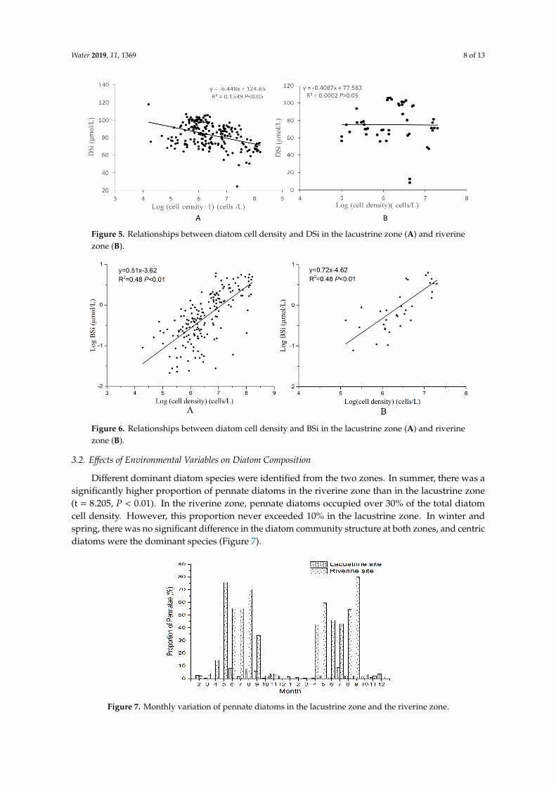
Figure 5. Relationships between diatom cell density and DSi in the lacustrine zone (A) and riverine zone (B).

Figure 6. Relationships between diatom cell density and BSi in the lacustrine zone (A) and riverine zone (B).

Figure 5. Relationships between diatom cell density and DSi in the lacustrine zone (A) and riverinezone (B).

Water 2019, 10, x FOR PEER REVIEW 8 of 14

Figure 4. The diatom cell density (A) and proportion of pennate diatom cell density (B) at different sites. Monthly diatom cell density from February 2015 to December 2016 (C).

Table 2. Spearman correlation between cell density and environmental parameters (dissolved silicon (DSi), biogenic silicon (BSi), chlorophyll a (Chl a), pH, water temperature (WT), dissolved oxygen (DO), chemical oxygen demand (COD), conductivity (Cond), and water velocity) in the lacustrine zone (L-CD) and riverine zone (R-CD).

Site DSi BSi Chla pH WT DO COD Cond Water

velocity L-CD −0.513** 0.639** 0.722** 0.625** 0.164 0.506* 0.522* −0.024 −0.549* R-CD 0.017 0.830** 0.755** 0.258 −0.071 0.265 0.415* 0.497* −0.745**

*Correlation was significant at the 0.05 level; **Correlation was significant at the 0.01 level.

DSi showed a linear decrease as a function of diatom cell density in the lacustrine zone, but it was not obvious in the riverine zone (Figure 5). BSi was linearly correlated with diatom cell density in both zones. The regression model showed that cell density explained 48% of the BSi concentration variation (R2 = 0.48), while the slope in the riverine zone was significantly higher than that in the lacustrine zone (P < 0.001). The intercept of the riverine zone was significantly lower than that of the lacustrine zone (P = 0.003). From the model, it could be speculated that the BSi concentration in the riverine zone was an order of magnitude lower than that in the lacustrine zone (Figure 6).

Figure 5. Relationships between diatom cell density and DSi in the lacustrine zone (A) and riverine zone (B).

Figure 6. Relationships between diatom cell density and BSi in the lacustrine zone (A) and riverine zone (B).

Figure 6. Relationships between diatom cell density and BSi in the lacustrine zone (A) and riverinezone (B).

3.2. Effects of Environmental Variables on Diatom Composition

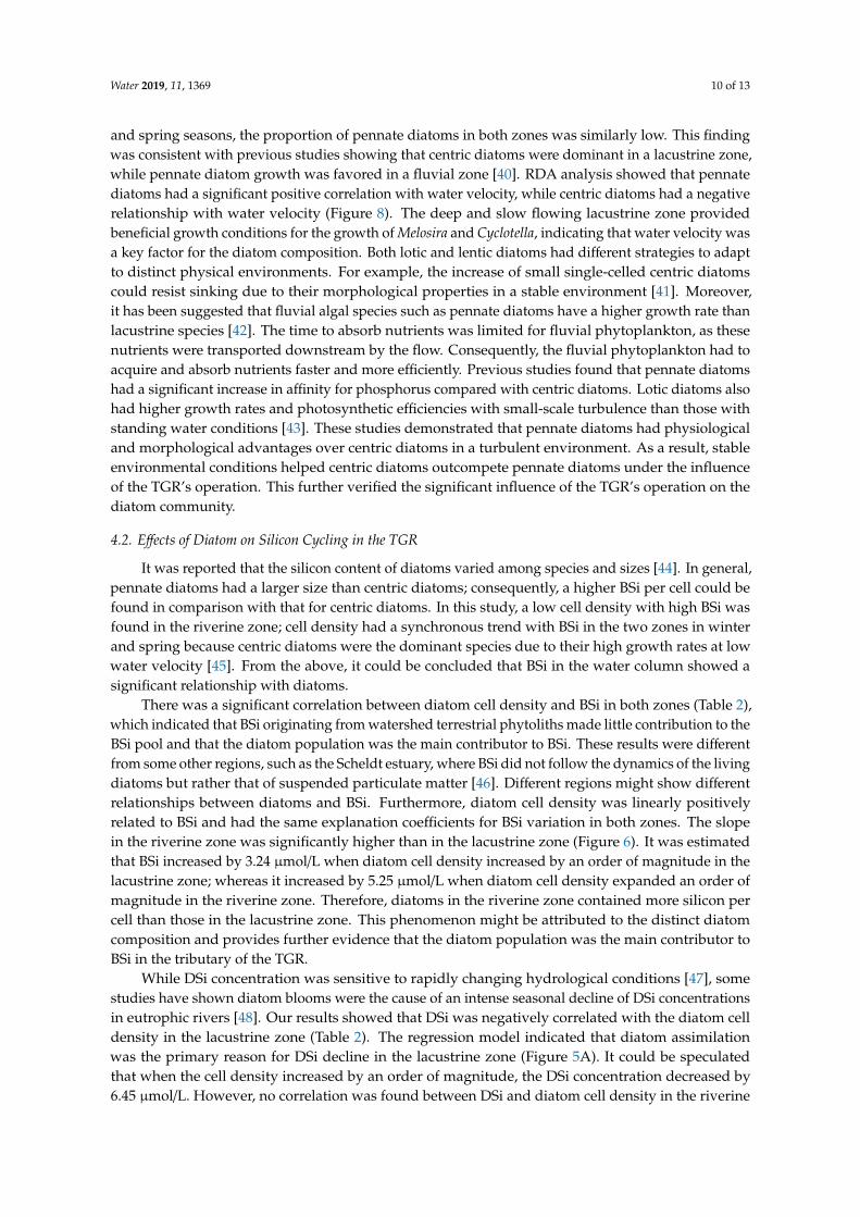
Different dominant diatom species were identified from the two zones. In summer, there was asignificantly higher proportion of pennate diatoms in the riverine zone than in the lacustrine zone(t = 8.205, P < 0.01). In the riverine zone, pennate diatoms occupied over 30% of the total diatomcell density. However, this proportion never exceeded 10% in the lacustrine zone. In winter andspring, there was no significant difference in the diatom community structure at both zones, and centricdiatoms were the dominant species (Figure 7).

Water 2019, 10, x FOR PEER REVIEW 9 of 14

3.2. Effects of Environmental Variables on Diatom Composition

Different dominant diatom species were identified from the two zones. In summer, there was a significantly higher proportion of pennate diatoms in the riverine zone than in the lacustrine zone (t = 8.205, P < 0.01). In the riverine zone, pennate diatoms occupied over 30% of the total diatom cell density. However, this proportion never exceeded 10% in the lacustrine zone. In winter and spring, there was no significant difference in the diatom community structure at both zones, and centric diatoms were the dominant species (Figure 7).

Figure 7. Monthly variation of pennate diatoms in the lacustrine zone and the riverine zone.

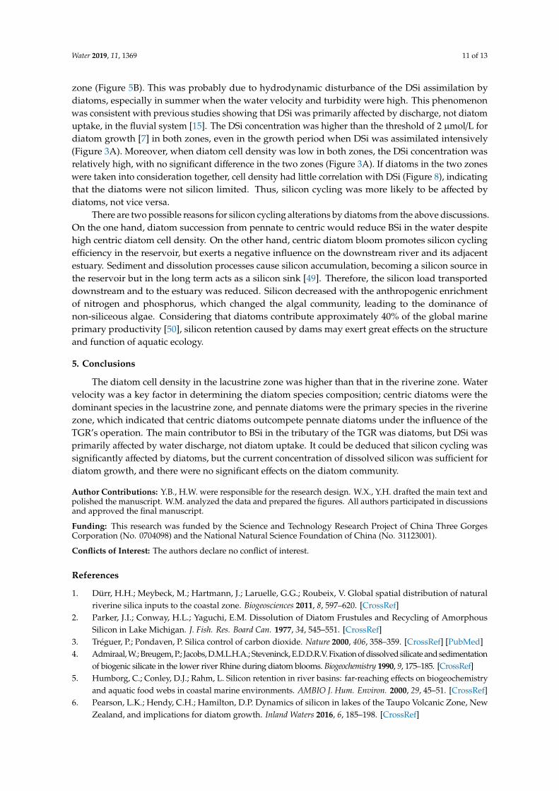
In Figure 8, environmental variables were standardised by normalisation, and diatom species samples were centered. A forward-selected RDA of the diatom species data set revealed water velocity (F = 52.34, P = 0.002), DSi (F = 20.15, P = 0.002), COD (F = 3.85, P = 0.044), and DO (F = 10.62, P = 0.002) as the minimum set of significant environmental variables that could describe the greatest variation in the data set; a total 77.3% of the variation in taxonomic compositions was explained. Pennate diatoms showed a significant positive correlation with water velocity, while centric diatoms were negatively correlated with water velocity (P < 0.05). A negative correlation between pennate diatoms and DSi was observed, but this relationship was not evident between centric diatoms and DSi.

Figure 8. Biplot diagrams for the RDA of the relationship between diatom composition and environmental variables.

4. Discussion

4.1. Variation in the Diatom Community

Figure 7. Monthly variation of pennate diatoms in the lacustrine zone and the riverine zone.

Water 2019, 11, 1369 9 of 13

In Figure 8, environmental variables were standardised by normalisation, and diatom speciessamples were centered. A forward-selected RDA of the diatom species data set revealed water velocity(F = 52.34, P = 0.002), DSi (F = 20.15, P = 0.002), COD (F = 3.85, P = 0.044), and DO (F = 10.62, P = 0.002)as the minimum set of significant environmental variables that could describe the greatest variation inthe data set; a total 77.3% of the variation in taxonomic compositions was explained. Pennate diatomsshowed a significant positive correlation with water velocity, while centric diatoms were negativelycorrelated with water velocity (P < 0.05). A negative correlation between pennate diatoms and DSiwas observed, but this relationship was not evident between centric diatoms and DSi.

Water 2019, 10, x FOR PEER REVIEW 9 of 14

3.2. Effects of Environmental Variables on Diatom Composition

Different dominant diatom species were identified from the two zones. In summer, there was a significantly higher proportion of pennate diatoms in the riverine zone than in the lacustrine zone (t = 8.205, P < 0.01). In the riverine zone, pennate diatoms occupied over 30% of the total diatom cell density. However, this proportion never exceeded 10% in the lacustrine zone. In winter and spring, there was no significant difference in the diatom community structure at both zones, and centric diatoms were the dominant species (Figure 7).

Figure 7. Monthly variation of pennate diatoms in the lacustrine zone and the riverine zone.

In Figure 8, environmental variables were standardised by normalisation, and diatom species samples were centered. A forward-selected RDA of the diatom species data set revealed water velocity (F = 52.34, P = 0.002), DSi (F = 20.15, P = 0.002), COD (F = 3.85, P = 0.044), and DO (F = 10.62, P = 0.002) as the minimum set of significant environmental variables that could describe the greatest variation in the data set; a total 77.3% of the variation in taxonomic compositions was explained. Pennate diatoms showed a significant positive correlation with water velocity, while centric diatoms were negatively correlated with water velocity (P < 0.05). A negative correlation between pennate diatoms and DSi was observed, but this relationship was not evident between centric diatoms and DSi.

Figure 8. Biplot diagrams for the RDA of the relationship between diatom composition and environmental variables.

4. Discussion

4.1. Variation in the Diatom Community

Figure 8. Biplot diagrams for the RDA of the relationship between diatom composition andenvironmental variables.

4. Discussion

4.1. Variation in the Diatom Community

The cell density and species composition of diatoms showed significant differences between thelacustrine zone and the riverine zone (P < 0.05), which represented the effects of the TGR’s operation.Higher cell density in the lacustrine zone than in the riverine zone was first attributed to the relativelystable physical conditions (Table 1). However, the negative coefficient between diatom cell densityand water velocity was higher in the riverine zone (r = −0.745) than in the lacustrine zone (r = −0.549)(Table 2), indicating a stronger influence of water flow on the diatom cell density in the riverine zonethan in the lacustrine zone. The TGR’s operation changed the hydrodynamics markedly, and thelacustrine zone showed relatively stable physical conditions. It is well known that the riverine zoneshowed an obvious flow rhythm, which means there was high flow discharge and water velocity inthe summer and autumn seasons and low flow discharge and water velocity in the winter and springseasons. The lacustrine zone, which is also known as the backwater area, exhibited a sharp slowdownof water velocity that significantly enhanced sedimentation, light penetration and water transparency.The decrease in the nutrient exchange rate accelerated the process of eutrophication. Such physicaland chemical environmental conditions favoured the growth of diatoms. In contrast, the riverine zonemaintained a natural river status with a low water level, characterised by a higher water velocity andnutrient exchange rate than the lacustrine zone. Diatom growth showed that it was more likely to beinfluenced by hydrodynamics [15]. This strong influence was particularly evident in the summer andautumn seasons when precipitation and water discharge increased significantly, disturbing the diatomgrowth and reducing its density dramatically in the riverine zone. Therefore, the TGR’s operationenhanced the diatom cell density and prolonged the diatom growth period in the lacustrine zone ofthe tributary.

While centric diatoms were the dominant species in the lacustrine zone, a high proportion ofpennate diatoms were found in the riverine zone in the summer and autumn seasons (Figure 7). Theywere mainly dominated by pennate diatoms from the genera of Synedra and Navicula. In the winter

Water 2019, 11, 1369 10 of 13

and spring seasons, the proportion of pennate diatoms in both zones was similarly low. This findingwas consistent with previous studies showing that centric diatoms were dominant in a lacustrine zone,while pennate diatom growth was favored in a fluvial zone [40]. RDA analysis showed that pennatediatoms had a significant positive correlation with water velocity, while centric diatoms had a negativerelationship with water velocity (Figure 8). The deep and slow flowing lacustrine zone providedbeneficial growth conditions for the growth of Melosira and Cyclotella, indicating that water velocity wasa key factor for the diatom composition. Both lotic and lentic diatoms had different strategies to adaptto distinct physical environments. For example, the increase of small single-celled centric diatomscould resist sinking due to their morphological properties in a stable environment [41]. Moreover,it has been suggested that fluvial algal species such as pennate diatoms have a higher growth rate thanlacustrine species [42]. The time to absorb nutrients was limited for fluvial phytoplankton, as thesenutrients were transported downstream by the flow. Consequently, the fluvial phytoplankton had toacquire and absorb nutrients faster and more efficiently. Previous studies found that pennate diatomshad a significant increase in affinity for phosphorus compared with centric diatoms. Lotic diatoms alsohad higher growth rates and photosynthetic efficiencies with small-scale turbulence than those withstanding water conditions [43]. These studies demonstrated that pennate diatoms had physiologicaland morphological advantages over centric diatoms in a turbulent environment. As a result, stableenvironmental conditions helped centric diatoms outcompete pennate diatoms under the influenceof the TGR’s operation. This further verified the significant influence of the TGR’s operation on thediatom community.

4.2. Effects of Diatom on Silicon Cycling in the TGR

It was reported that the silicon content of diatoms varied among species and sizes [44]. In general,pennate diatoms had a larger size than centric diatoms; consequently, a higher BSi per cell could befound in comparison with that for centric diatoms. In this study, a low cell density with high BSi wasfound in the riverine zone; cell density had a synchronous trend with BSi in the two zones in winterand spring because centric diatoms were the dominant species due to their high growth rates at lowwater velocity [45]. From the above, it could be concluded that BSi in the water column showed asignificant relationship with diatoms.

There was a significant correlation between diatom cell density and BSi in both zones (Table 2),which indicated that BSi originating from watershed terrestrial phytoliths made little contribution to theBSi pool and that the diatom population was the main contributor to BSi. These results were differentfrom some other regions, such as the Scheldt estuary, where BSi did not follow the dynamics of the livingdiatoms but rather that of suspended particulate matter [46]. Different regions might show differentrelationships between diatoms and BSi. Furthermore, diatom cell density was linearly positivelyrelated to BSi and had the same explanation coefficients for BSi variation in both zones. The slopein the riverine zone was significantly higher than in the lacustrine zone (Figure 6). It was estimatedthat BSi increased by 3.24 µmol/L when diatom cell density increased by an order of magnitude in thelacustrine zone; whereas it increased by 5.25 µmol/L when diatom cell density expanded an order ofmagnitude in the riverine zone. Therefore, diatoms in the riverine zone contained more silicon percell than those in the lacustrine zone. This phenomenon might be attributed to the distinct diatomcomposition and provides further evidence that the diatom population was the main contributor toBSi in the tributary of the TGR.

While DSi concentration was sensitive to rapidly changing hydrological conditions [47], somestudies have shown diatom blooms were the cause of an intense seasonal decline of DSi concentrationsin eutrophic rivers [48]. Our results showed that DSi was negatively correlated with the diatom celldensity in the lacustrine zone (Table 2). The regression model indicated that diatom assimilationwas the primary reason for DSi decline in the lacustrine zone (Figure 5A). It could be speculatedthat when the cell density increased by an order of magnitude, the DSi concentration decreased by6.45 µmol/L. However, no correlation was found between DSi and diatom cell density in the riverine

Water 2019, 11, 1369 11 of 13

zone (Figure 5B). This was probably due to hydrodynamic disturbance of the DSi assimilation bydiatoms, especially in summer when the water velocity and turbidity were high. This phenomenonwas consistent with previous studies showing that DSi was primarily affected by discharge, not diatomuptake, in the fluvial system [15]. The DSi concentration was higher than the threshold of 2 µmol/L fordiatom growth [7] in both zones, even in the growth period when DSi was assimilated intensively(Figure 3A). Moreover, when diatom cell density was low in both zones, the DSi concentration wasrelatively high, with no significant difference in the two zones (Figure 3A). If diatoms in the two zoneswere taken into consideration together, cell density had little correlation with DSi (Figure 8), indicatingthat the diatoms were not silicon limited. Thus, silicon cycling was more likely to be affected bydiatoms, not vice versa.

There are two possible reasons for silicon cycling alterations by diatoms from the above discussions.On the one hand, diatom succession from pennate to centric would reduce BSi in the water despitehigh centric diatom cell density. On the other hand, centric diatom bloom promotes silicon cyclingefficiency in the reservoir, but exerts a negative influence on the downstream river and its adjacentestuary. Sediment and dissolution processes cause silicon accumulation, becoming a silicon source inthe reservoir but in the long term acts as a silicon sink [49]. Therefore, the silicon load transporteddownstream and to the estuary was reduced. Silicon decreased with the anthropogenic enrichmentof nitrogen and phosphorus, which changed the algal community, leading to the dominance ofnon-siliceous algae. Considering that diatoms contribute approximately 40% of the global marineprimary productivity [50], silicon retention caused by dams may exert great effects on the structureand function of aquatic ecology.

5. Conclusions

The diatom cell density in the lacustrine zone was higher than that in the riverine zone. Watervelocity was a key factor in determining the diatom species composition; centric diatoms were thedominant species in the lacustrine zone, and pennate diatoms were the primary species in the riverinezone, which indicated that centric diatoms outcompete pennate diatoms under the influence of theTGR’s operation. The main contributor to BSi in the tributary of the TGR was diatoms, but DSi wasprimarily affected by water discharge, not diatom uptake. It could be deduced that silicon cycling wassignificantly affected by diatoms, but the current concentration of dissolved silicon was sufficient fordiatom growth, and there were no significant effects on the diatom community.

Author Contributions: Y.B., H.W. were responsible for the research design. W.X., Y.H. drafted the main text andpolished the manuscript. W.M. analyzed the data and prepared the figures. All authors participated in discussionsand approved the final manuscript.

Funding: This research was funded by the Science and Technology Research Project of China Three GorgesCorporation (No. 0704098) and the National Natural Science Foundation of China (No. 31123001).

Conflicts of Interest: The authors declare no conflict of interest.

References

1. Dürr, H.H.; Meybeck, M.; Hartmann, J.; Laruelle, G.G.; Roubeix, V. Global spatial distribution of naturalriverine silica inputs to the coastal zone. Biogeosciences 2011, 8, 597–620. [CrossRef]

2. Parker, J.I.; Conway, H.L.; Yaguchi, E.M. Dissolution of Diatom Frustules and Recycling of AmorphousSilicon in Lake Michigan. J. Fish. Res. Board Can. 1977, 34, 545–551. [CrossRef]

3. Tréguer, P.; Pondaven, P. Silica control of carbon dioxide. Nature 2000, 406, 358–359. [CrossRef] [PubMed]4. Admiraal, W.; Breugem, P.; Jacobs, D.M.L.H.A.; Steveninck, E.D.D.R.V. Fixation of dissolved silicate and sedimentation

of biogenic silicate in the lower river Rhine during diatom blooms. Biogeochemistry 1990, 9, 175–185. [CrossRef]5. Humborg, C.; Conley, D.J.; Rahm, L. Silicon retention in river basins: far-reaching effects on biogeochemistry

and aquatic food webs in coastal marine environments. AMBIO J. Hum. Environ. 2000, 29, 45–51. [CrossRef]6. Pearson, L.K.; Hendy, C.H.; Hamilton, D.P. Dynamics of silicon in lakes of the Taupo Volcanic Zone, New

Zealand, and implications for diatom growth. Inland Waters 2016, 6, 185–198. [CrossRef]

Water 2019, 11, 1369 12 of 13

7. Egge, J.K.; Aksnes, D.L. Silicate as regulating nutrient in phytoplankton competition. Mar. Ecol. Prog. Ser1992, 83, 281–289. [CrossRef]

8. Scholz, B.; Liebezeit, G. Microphytobenthic dynamics in a Wadden Sea intertidal flat – Part I: Seasonal andspatial variation of diatom communities in relation to macronutrient supply. Eur. J. Phycol. 2012, 47, 105–119.[CrossRef]

9. Trigueros, J.M.; Orive, E. Seasonal variations of diatoms and dinoflagellates in a shallow, temperate estuary,with emphasis on neritic assemblages. Hydrobiologia 2001, 444, 119–133. [CrossRef]

10. Gong, Y.; Hu, H. Effect of silicate and inorganic carbon availability on the growth and competition of adiatom and two red tide dinoflagellates. Phycologia 2014, 53, 433–442. [CrossRef]

11. Wang, B.; Qiu, X.L.; Peng, X.; Wang, F. Phytoplankton community structure and succession in karst cascadereservoirs, SW China. Inland Waters 2018, 8, 229–238. [CrossRef]

12. Li, M.; Xu, K.; Watanabe, M.; Chen, Z. Long-term variations in dissolved silicate, nitrogen, and phosphorusflux from the Yangtze River into the East China Sea and impacts on estuarine ecosystem. Estuar. Coast. ShelfSci. 2007, 71, 3–12. [CrossRef]

13. López, N.L.; Rondón, C.A.R.; Zapata, A.; Jiménez, J.; Villamil, W.; Arenas, G.; Rincón, C.; Sánchez, T. Factorscontrolling phytoplankton in tropical high-mountain drinking-water reservoirs. Limnetica 2012, 31, 305–321.

14. Gao, M.; Zhu, K.; Bi, Y.; Hu, Z. Spatiotemporal patterns of surface-suspended particulate matter in the ThreeGorges Reservoir. Environ. Sci. Pollut. Res. 2016, 23, 3569–3577. [CrossRef]

15. Arndt, S.; Vanderborght, J.P.; Regnier, P. Diatom growth response to physical forcing in a macrotidal estuary:Coupling hydrodynamics, sediment transport, and biogeochemistry. J. Geophys. Res. Oceans 2007, 112.[CrossRef]

16. Shatwell, T.; Köhler, J.; Nicklisch, A. Temperature and photoperiod interactions with silicon-limited growthand competition of two diatoms. J. Protein Chem. 2013, 7, 509–525. [CrossRef]

17. Shi, Z.; Wang, Y.; Wen, A.; Yan, D.; Chen, J. Tempo-spatial variations of sediment-associated nutrients andcontaminants in the Ruxi tributary of the Three Gorges Reservoir, China. J. Mt. Sci. 2018, 15, 319–326.[CrossRef]

18. Zeng, H.; Song, L.; Yu, Z.; Chen, H. Distribution of phytoplankton in the Three-Gorge Reservoir during rainyand dry seasons. Sci. Total Environ. 2006, 367, 999–1009. [CrossRef] [PubMed]

19. Li, Z.; Wang, S.; Guo, J.; Fang, F.; Xu, G.; Long, M. Responses of phytoplankton diversity to physicaldisturbance under manual operation in a large reservoir, China. Hydrobiologia 2012, 684, 45–56. [CrossRef]

20. Peng, C.; Lang, Z.; Zheng, Y.; Li, D. Seasonal succession of phytoplankton in response to the variation of environmentalfactors in the Gaolan River, Three Gorges Reservoir, China. Chin. J. Oceanol. Limnol. 2013, 31, 737–749. [CrossRef]

21. Ran, X.; Bouwman, L.; Yu, Z.; Beusen, A.; Chen, H.; Yao, Q. Nitrogen transport, transformation, and retentionin the Three Gorges Reservoir: A mass balance approach. Limnol. Oceanogr. 2017, 62, 2323–2337. [CrossRef]

22. Ran, X.; Chen, H.; Wei, J.; Yao, Q.; Mi, T.; Yu, Z. Phosphorus speciation, transformation and retention in theThree Gorges Reservoir, China. Mar. Freshw. Res. 2015, 67, 209–228. [CrossRef]

23. Yan, Q.; Yu, Y.; Feng, W.; Yu, Z.; Chen, H. Plankton community composition in the Three Gorges Reservoir Regionrevealed by PCR-DGGE and its relationships with environmental factors. J. Environ. Sci. 2008, 20, 732–738. [CrossRef]

24. Zhou, G.; Zhao, X.; Bi, Y.; Liang, Y.; Hu, J.; Yang, M.; Mei, Y.; Zhu, K.; Zhang, L.; Hu, Z. Phytoplankton variationand its relationship with the environment in Xiangxi Bay in spring after damming of the Three-Gorges,China. Environ. Monit. Assess. 2011, 176, 125–141. [CrossRef] [PubMed]

25. Mao, J.; Jiang, D.; Dai, H. Spatial–temporal hydrodynamic and algal bloom modelling analysis of a reservoirtributary embayment. J. Hydro-environ. Res. 2015, 9, 200–215. [CrossRef]

26. Zhao, Y.; Zheng, B.; Wang, L.; Qin, Y.; Li, H.; Cao, W. Characterization of Mixing Processes in the ConfluenceZone between the Three Gorges Reservoir Mainstream and the Daning River Using Stable Isotope Analysis.Environ. Sci. Technol. 2015, 50, 9907. [CrossRef] [PubMed]

27. Yang, Z.; Cheng, B.; Xu, Y.; Liu, D.; Ma, J.; Ji, D. Stable isotopes in water indicate sources of nutrients thatdrive algal blooms in the tributary bay of a subtropical reservoir. Sci. Total Environ. 2018, 634, 205–213.[CrossRef]

28. Ran, X.; Liu, S.; Liu, J.; Zang, J.; Che, H.; Ma, Y.; Wang, Y. Composition and variability in the export of biogenic silicain the Changjiang River and the effect of Three Gorges Reservoir. Sci. Total Environ. 2016, 571, 1191–1199. [CrossRef]

29. Ran, X.; Yu, Z.; Chen, H. Silicon and sediment transport of the Changjiang River (Yangtze River): Could theThree Gorges Reservoir be a filter? Environ. Earth Sci. 2013, 70, 1881–1893.

Water 2019, 11, 1369 13 of 13

30. Zhou, C.; Jian-Jun, Y.U.; Li, F.U.; Cui, Y.J.; Liu, D.F.; Jiang, W.; Haffner, D.; Zhang, L. Temporal and SpatialDistribution of Environmental Factors and Phytoplankton During Algal Bloom Season in Pengxi River, ThreeGorges Reservoir. Environ. Sci. 2016, 37, 873–883.

31. Han, C.; Zheng, B.; Qin, Y.; Ma, Y.; Yang, C.; Liu, Z.; Cao, W.; Chi, M. Impact of upstream river inputsand reservoir operation on phosphorus fractions in water-particulate phases in the Three Gorges Reservoir.Sci. Total Environ. 2018, 610, 1546–1556. [CrossRef] [PubMed]

32. Ran, X.; Yu, Z.; Yao, Q.; Chen, H.; Guo, H. Silica retention in the Three Gorges reservoir. Biogeochemistry 2013,112, 209–228. [CrossRef]

33. Walter, W.G. Standard Methods for the Examination of Water and Wastewater; American Public Health Association:Washington, DC, USA, 1995.

34. Hu, H.J.; Wei, Y.X. The Freshwater Algae of China – Systematics, Taxonomy and Ecology; Science Press: Beijing,China, 2006.

35. Edwards, P.M. Origin 7.0: Scientific Graphing and Data Analysis Software. J. Chem. Inf. Comput. Sci. 2002,42, 1270–1271. [CrossRef]

36. Vogel, M. Review of SPSS/PC + statistical package. Comput. Stat. Data. Anal. 1988, 6, 71–84. [CrossRef]37. Peng, L.; Tong, T. A note on a two-sample T test with one variance unknown. Stat. Methodol. 2011, 8, 528–534.

[CrossRef]38. Curran, P.A. Monte Carlo error analyses of Spearman’s rank test. arXiv 2014, 1411, 3816.39. Ter Braak, C.J.F. Canonical Correspondence Analysis: A New Eigenvector Technique for Multivariate Direct

Gradient Analysis. Ecology 1986, 67, 1167–1179. [CrossRef]40. Bahnwart, M.; Hübener, T.; Schubert, H. Downstream changes in phytoplankton composition and biomass

in a lowland river–lake system (Warnow River, Germany). Hydrobiologia 1998, 391, 99–111. [CrossRef]41. Moss, B.; Balls, H. Phytoplankton distribution in a floodplain lake and river system. II Seasonal changes in

the phytoplankton communities and their control by hydrology and nutrient availability. J. Plankton Res.1989, 11, 839–867. [CrossRef]

42. Wetzel, R.G. Limnology: lake and river ecosystems. Eos Trans. Am. Geophys. Union 2001, 21, 1–9.43. Wang, P.; Shen, H.; Xie, P. Can Hydrodynamics Change Phosphorus Strategies of Diatoms?—Nutrient Levels

and Diatom Blooms in Lotic and Lentic Ecosystems. Microb. Ecol. 2012, 63, 369–382. [CrossRef] [PubMed]44. Durbin, E.G. Studies of the autoecology of the marine diatom Thalassiosira nordenskioeldii. II. The influence

of cell size on growth rate, and carbon, nitrogen, chlorophyll a and silica content. J. Phycol. 1977, 13, 150–155.45. Mitrovic, S.M.; Hitchcock, J.N.; Davie, A.W.; Ryan, D.A. Growth responses of Cyclotella meneghiniana

(Bacillariophyceae) to various temperatures. J. Plankton Res. 2010, 32, 1217–1221. [CrossRef]46. Carbonnel, V.; Vanderborght, J.P.; Lionard, M. Diatoms, silicic acid and biogenic silica dynamics along the salinity;

gradient of the Scheldt estuary (Belgium/The Netherlands). Biogeochemistry 2013, 113, 657–682. [CrossRef]47. Chen, N.; Wu, Y.; Wu, J.; Yan, X.; Hong, H. Natural and human influences on dissolved silica export from

watershed to coast in Southeast China. J. Geophys. Res. Biogeosci. 2014, 119, 95–109. [CrossRef]48. Triplett, L.D.; Engstrom, D.R.; Conley, D.J. Changes in amorphous silica sequestration with eutrophication of

riverine impoundments. Biogeochemistry 2012, 108, 413–427. [CrossRef]49. Panizzo, V.N.; Swann, G.E.A.; Mackay, A.W.; Vologina, E.; Alleman, L.; André, L.; Pashley, V.H.;

Horstwood, M.S.A. Constraining modern-day silicon cycling in Lake Baikal. Global Biogeochem. Cycles 2017,31, 556–574. [CrossRef]

50. Nelson, D.M.; Tréguer, P.; Brzezinski, M.A.; Leynaert, A.; Quéguiner, B. Production and dissolution ofbiogenic silica in the ocean: revised global estimates, comparison with regional data and relationship tobiogenic sedimentation. Global Biogeochem. Cycles 1995, 9, 359–372. [CrossRef]

© 2019 by the authors. Licensee MDPI, Basel, Switzerland. This article is an open accessarticle distributed under the terms and conditions of the Creative Commons Attribution(CC BY) license (http://creativecommons.org/licenses/by/4.0/).