1

THREE FACTS ABOUT MARIJUANA PRICES

by

Kenneth W Clements*

Economics Program

The University of Western Australia

Abstract

Australians are among the largest consumers of marijuana in the world, and

estimates show that their expenditure on marijuana is about twice that on wine. In this paper we analyse the evolution of Australian marijuana prices over the last decade and show that they have declined in real terms by almost 40 per cent. This decline is far above that experienced by most agricultural products. Why has this occurred and what are the implications? One possible reason is the adoption of hydroponic growing techniques that have enhanced productivity and lowered costs and prices. Another reason is that laws have become softer and penalties reduced. We find patterns in the prices that divide the country into three broad regions: (i) Sydney, where prices are highest; (ii) Melbourne and Canberra, which have somewhat lower prices; and (iii) everywhere else, where marijuana is cheapest. An exploratory analysis indicates the extent to which the price declines have stimulated marijuana consumption and inhibited the consumption of a substitute product, alcohol.

* I would like to acknowledge the help of Kym Anderson, Mark Hazell, Carol Howard, Bill Malcolm, Bob Marks, David Sapsford, MoonJoong Tcha, Don Weatherburn, David Wesney and Xueyan Zhao, who generously provided advice and/or data; and the research assistance of Andrew Ainsworth, Renae Bothe, Joan Coffey, Yihui Lan, Vitaly Pershin, Clare Yu, Patricia Wang and Robin Wong. Additionally, in revising the paper I have benefited from helpful comments from Chris O’Donnell, Co-Editor of this journal, an Associate Editor and two anonymous referees. This research was supported financially by the Economics Program, University of Western Australia, and the Australian Research Council.

2

1. Introduction

Over the longer term, higher productivity, together with Engel’s law, has led

to average annual price declines of many agricultural products of the order of 1-2 per

cent. In this paper we demonstrate that a similar process seems to have operated for

marijuana, with one important difference. Marijuana prices have declined much more

rapidly than those of most other agricultural products -- by about 5 per cent p. a. in

real terms over the past decade. Research on the behaviour of marijuana prices is of

interest due to the widespread use of the product. Surveys indicate that in some

countries up to one third of the adult population have used marijuana and in Australia,

one of world’s biggest consumers, over 40 per cent of people favour its

decriminalisation. Expenditure on marijuana by Australians has been estimated to be

about twice that on wine.1

Why have marijuana prices fallen so much? What is the nature of the

marijuana market in Australia? To what extent has the decline in marijuana prices

been responsible for the high level of consumption? In this paper we address these

issues and argue that there are three defining characteristics of the behaviour of

marijuana prices, which we refer to as “three facts”:

• There seems to exist regional markets for marijuana, rather than one national

market. Prices are substantially more expensive in the Sydney market, followed

by Melbourne and Canberra, and then the rest of Australia.

• The real price of marijuana has fallen by almost 40 per cent over the 1990s in

Australia. As indicated above, this fall is much more than that of most agricultural

products. One explanation for the substantial fall is the widespread adoption of

hydroponic techniques of production, which has enhanced productivity and

lowered costs. Another explanation is that because of changing community

attitudes, laws have become softer and penalties reduced, thus lowering part of the

“expected full cost” of transacting marijuana.

1 For details, see Clements and Daryal (2003). Australian marijuana prices have been analysed previously in the context of the demand for marijuana, tobacco and alcohol by Cameron and Williams (2001) and Zhao and Harris (2003).

3

• Lower prices have stimulated marijuana consumption and reduced alcohol

consumption. As marijuana and alcohol would appear to both satisfy a similar

want of the consumer, they are probably substitutes in consumption. Under

certain scenarios, the lower marijuana prices would have resulted in a substantial

rise in marijuana consumption and a corresponding fall in alcohol consumption.

The next section of the paper provides information regarding the data on

marijuana prices. Section 3 deals with the identification of regional markets of

marijuana. The substantial decline in prices is analysed in some depth in Section 4 and

compared to the behaviour of the prices of other commodities. Section 5 provides an

exploratory analysis of the extent to which lower prices have encouraged marijuana

usage and discouraged the consumption of a substitute product, alcohol. Section 6

contains some concluding comments.

2. The Prices2

The data on Australian marijuana prices were generously supplied by Mark

Hazell of the Australian Bureau of Criminal Intelligence. These prices were collected

by law enforcement agencies in the various states and territories during undercover

buys. In general, the data are quarterly and refer to the period 1990-1999, for each

state and territory. The different types of marijuana identified separately are leaf,

heads, hydroponics, skunk, hash resin and hash oil. However, we focus on only the

prices of “leaf” and “heads”, as these products are the most popular. The data are

described by Australian Bureau of Criminal Intelligence (1996) who discuss some

difficulties with them regarding different recording practices used by the various

agencies and missing observations. While it is unlikely that these data constitute a

random sample, a common problem when studying the prices of almost any illicit

good, it is not clear that they would be biased either upwards or downwards. In any

event, they are the only data available.

The prices are usually recorded in the form of ranges and the basic data are

listed in Clements and Daryal (2001). The data are “consolidated” by: (i) Using the

2 This section draws on Clements and Daryal (2001).

4

mid-point of each price range; (ii) converting all gram prices to ounces by multiplying

by 28; and (iii) annualising the data by averaging the quarterly or semi-annual

observations. Annualising has the effect of reducing the considerable noise in the

quarterly/semi-annual data. Plotting the data revealed several outliers which probably

reflect some of the above-mentioned recording problems. Observations are treated as

outliers if they are either less than one-half of the mean for the corresponding state, or

greater than twice the mean. This rule led to five outlying observations which are

omitted and replaced with the relevant means, based on the remaining observations.

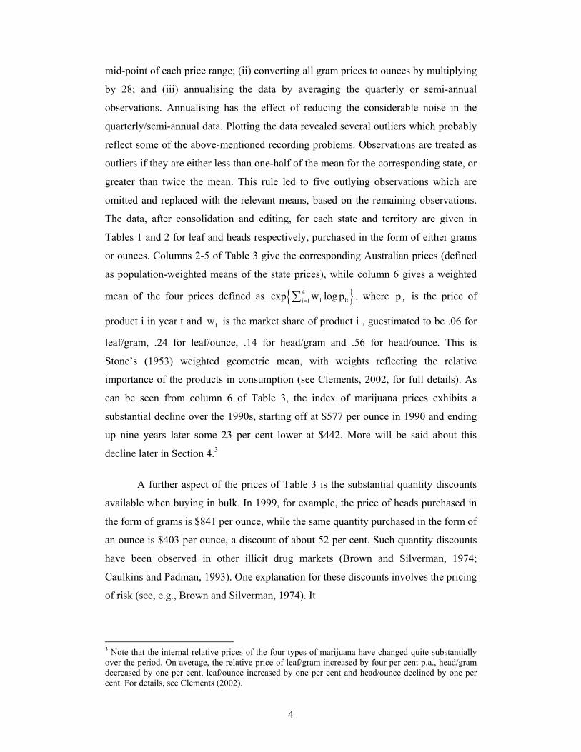
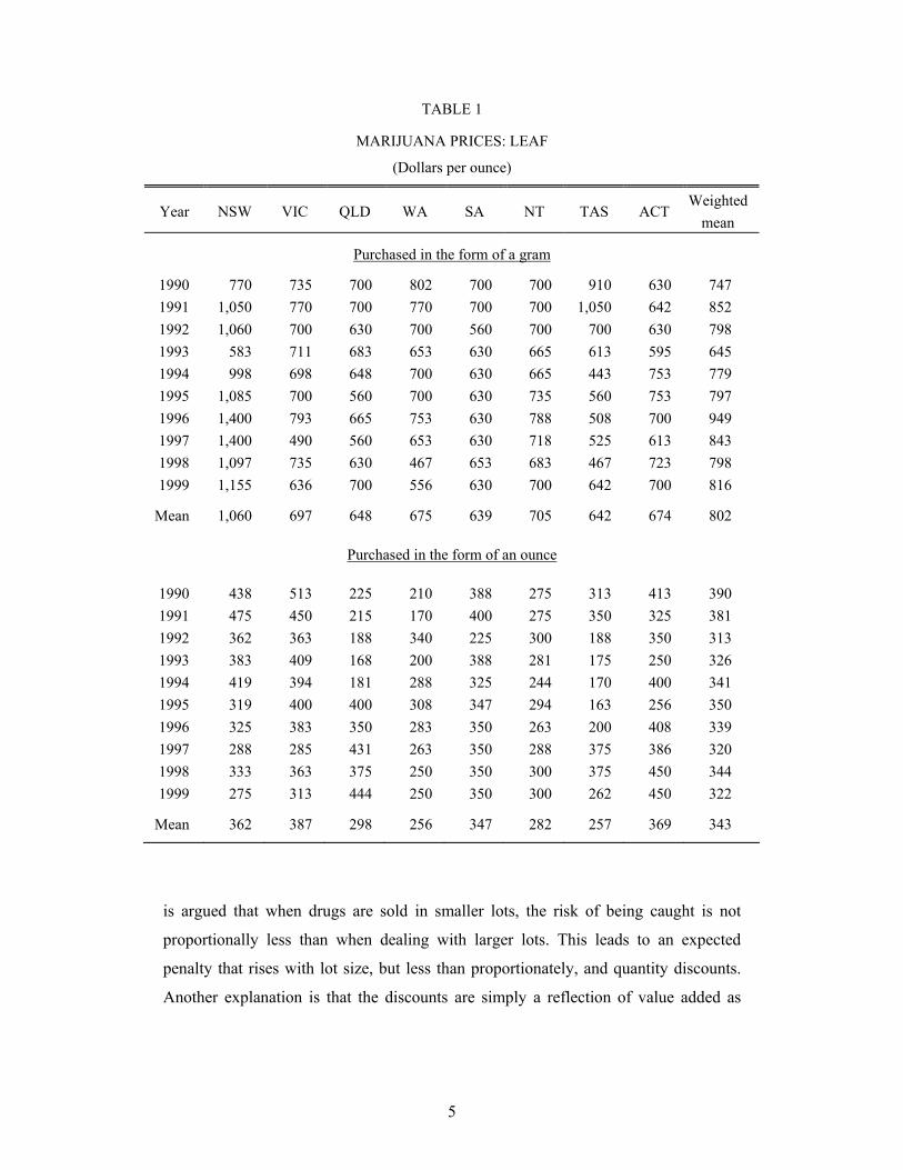
The data, after consolidation and editing, for each state and territory are given in

Tables 1 and 2 for leaf and heads respectively, purchased in the form of either grams

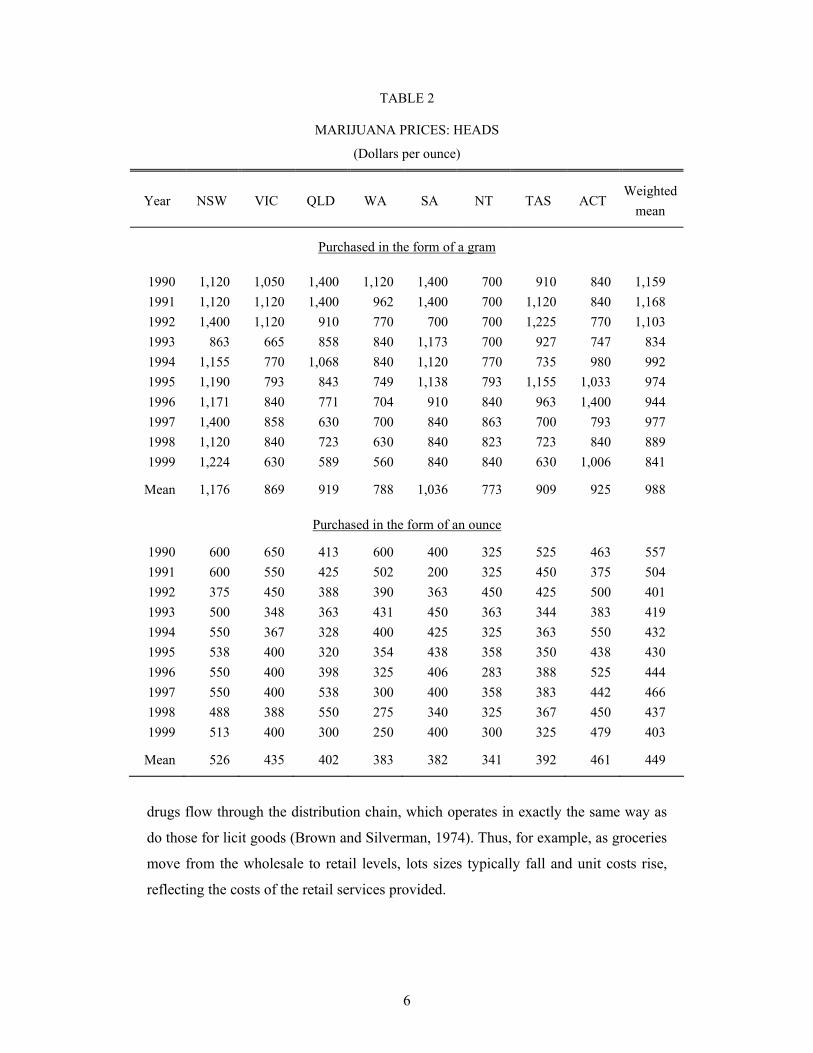
or ounces. Columns 2-5 of Table 3 give the corresponding Australian prices (defined

as population-weighted means of the state prices), while column 6 gives a weighted

mean of the four prices defined as { }4i iti 1exp w log p=∑ , where itp is the price of

product i in year t and iw is the market share of product i , guestimated to be .06 for

leaf/gram, .24 for leaf/ounce, .14 for head/gram and .56 for head/ounce. This is

Stone’s (1953) weighted geometric mean, with weights reflecting the relative

importance of the products in consumption (see Clements, 2002, for full details). As

can be seen from column 6 of Table 3, the index of marijuana prices exhibits a

substantial decline over the 1990s, starting off at $577 per ounce in 1990 and ending

up nine years later some 23 per cent lower at $442. More will be said about this

decline later in Section 4.3

A further aspect of the prices of Table 3 is the substantial quantity discounts

available when buying in bulk. In 1999, for example, the price of heads purchased in

the form of grams is $841 per ounce, while the same quantity purchased in the form of

an ounce is $403 per ounce, a discount of about 52 per cent. Such quantity discounts

have been observed in other illicit drug markets (Brown and Silverman, 1974;

Caulkins and Padman, 1993). One explanation for these discounts involves the pricing

of risk (see, e.g., Brown and Silverman, 1974). It

3 Note that the internal relative prices of the four types of marijuana have changed quite substantially over the period. On average, the relative price of leaf/gram increased by four per cent p.a., head/gram decreased by one per cent, leaf/ounce increased by one per cent and head/ounce declined by one per cent. For details, see Clements (2002).

5

TABLE 1

MARIJUANA PRICES: LEAF

(Dollars per ounce)

Year NSW VIC QLD WA SA NT TAS ACT Weighted

mean

Purchased in the form of a gram

1990 770 735 700 802 700 700 910 630 747 1991 1,050 770 700 770 700 700 1,050 642 852 1992 1,060 700 630 700 560 700 700 630 798 1993 583 711 683 653 630 665 613 595 645 1994 998 698 648 700 630 665 443 753 779 1995 1,085 700 560 700 630 735 560 753 797 1996 1,400 793 665 753 630 788 508 700 949 1997 1,400 490 560 653 630 718 525 613 843 1998 1,097 735 630 467 653 683 467 723 798 1999 1,155 636 700 556 630 700 642 700 816

Mean 1,060 697 648 675 639 705 642 674 802

Purchased in the form of an ounce

1990 438 513 225 210 388 275 313 413 390 1991 475 450 215 170 400 275 350 325 381 1992 362 363 188 340 225 300 188 350 313 1993 383 409 168 200 388 281 175 250 326 1994 419 394 181 288 325 244 170 400 341 1995 319 400 400 308 347 294 163 256 350 1996 325 383 350 283 350 263 200 408 339 1997 288 285 431 263 350 288 375 386 320 1998 333 363 375 250 350 300 375 450 344 1999 275 313 444 250 350 300 262 450 322

Mean 362 387 298 256 347 282 257 369 343

is argued that when drugs are sold in smaller lots, the risk of being caught is not

proportionally less than when dealing with larger lots. This leads to an expected

penalty that rises with lot size, but less than proportionately, and quantity discounts.

Another explanation is that the discounts are simply a reflection of value added as

6

TABLE 2

MARIJUANA PRICES: HEADS

(Dollars per ounce)

Year NSW VIC QLD WA SA NT TAS ACT Weighted

mean

Purchased in the form of a gram

1990 1,120 1,050 1,400 1,120 1,400 700 910 840 1,159 1991 1,120 1,120 1,400 962 1,400 700 1,120 840 1,168 1992 1,400 1,120 910 770 700 700 1,225 770 1,103 1993 863 665 858 840 1,173 700 927 747 834 1994 1,155 770 1,068 840 1,120 770 735 980 992 1995 1,190 793 843 749 1,138 793 1,155 1,033 974 1996 1,171 840 771 704 910 840 963 1,400 944 1997 1,400 858 630 700 840 863 700 793 977 1998 1,120 840 723 630 840 823 723 840 889 1999 1,224 630 589 560 840 840 630 1,006 841

Mean 1,176 869 919 788 1,036 773 909 925 988

Purchased in the form of an ounce

1990 600 650 413 600 400 325 525 463 557 1991 600 550 425 502 200 325 450 375 504 1992 375 450 388 390 363 450 425 500 401 1993 500 348 363 431 450 363 344 383 419 1994 550 367 328 400 425 325 363 550 432 1995 538 400 320 354 438 358 350 438 430 1996 550 400 398 325 406 283 388 525 444 1997 550 400 538 300 400 358 383 442 466 1998 488 388 550 275 340 325 367 450 437 1999 513 400 300 250 400 300 325 479 403

Mean 526 435 402 383 382 341 392 461 449

drugs flow through the distribution chain, which operates in exactly the same way as

do those for licit goods (Brown and Silverman, 1974). Thus, for example, as groceries

move from the wholesale to retail levels, lots sizes typically fall and unit costs rise,

reflecting the costs of the retail services provided.

7

TABLE 3

MARIJUANA PRICES, AUSTRALIA

(Dollars per ounce)

Purchase form

Gram Ounce

Year Leaf Heads Leaf Heads

Total (Weighted

mean)

(1) (2) (3) (4) (5) (6)

1990 747 1,159 390 557 577 1991 852 1,168 381 504 547 1992 798 1,103 313 401 454 1993 645 834 326 419 446 1994 779 992 341 432 475 1995 797 974 350 430 476 1996 949 944 339 444 484 1997 843 977 320 466 489 1998 798 889 344 437 473 1999 816 841 322 403 442

Mean 802 988 343 449 486

3. Fact 1: Marijuana is Expensive in New South Wales

Is the market for marijuana a nationally-organised activity, or is it merely a

“cottage industry” that just satisfies local demand? To put it another way, is marijuana

a (nationally) traded good, or is it nontraded? If there were a national market for

marijuana, then after appropriate allowance for transport costs etc., marijuana prices

should be more or less equalised across states and territories. This section investigates

these issues.

South Australia decriminalised marijuana in 1987 and recent media reports

have focused on Adelaide as the centre of the marijuana industry. Radio National

(1999) recently noted that:

8

“Cannabis is by far and away the illicit drug of choice for Australians. There is a multi billion dollar industry to supply it, and increasingly, the centre of action is the city of churches.”

That program quoted a person called “David” as saying:

“Say five, ten years ago, everyone spoke of the country towns of New South Wales and the north coast, now you never hear of it; those towns have died in this regard I’d say, because they’re lost out to the indoor variety, the hydro, and everyone was just saying South Australia, Adelaide, Adelaide, Adelaide, and that’s where it all seems to be coming from.”

In a similar vein, the Australian Bureau of Criminal Intelligence (1999, p. 18)

commented on marijuana being exported from South Australia to other states as

follows:

“New South Wales Police reported that cannabis has been found secreted in the body parts of motor vehicles from South Australia… It is reported that cannabis originating in South Australia is transported to neighbouring jurisdictions. South Australia Police reported that large amounts of cannabis are transported from South Australia by air, truck, hire vehicles, buses and private motor vehicles. Queensland Police reported that South Australian cannabis is sold on the Gold Coast. New South Wales Police reported South Australian vehicles returning to that state have been found carrying large amounts of cash or amphetamines, or both. It also considers that the decrease in the amount of locally grown cannabis is the result of an increase in the quantity of South Australian cannabis in New South Wales. The Australian Federal Police in Canberra reported that the majority of cannabis transported to the Australian Capital Territory is from the Murray Bridge area of South Australia…”

As the above comments point to Adelaide being a major exporter of marijuana

to other parts of Australia, this would seem to imply that the market is a national, not

local, one. In turn, this would mean that marijuana prices would tend to be equalised

across Australia if transport and differences in other distribution costs were relatively

minor. The validity of this hypothesis can be examined with our regional-level data

and Panel I of Table 4 gives the results of regressing the prices on

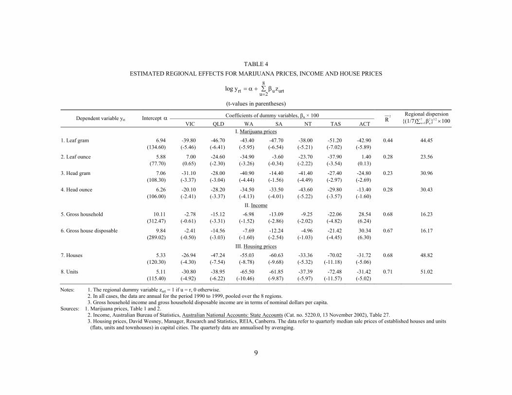
9

TABLE 4 ESTIMATED REGIONAL EFFECTS FOR MARIJUANA PRICES, INCOME AND HOUSE PRICES

(t-values in parentheses) Coefficients of dummy variables, βu × 100 Dependent variable yrt Intercept α

VIC QLD WA SA NT TAS ACT 2

R Regional dispersion

100}β{(1/7) 71u

1/22u ×∑ =

I. Marijuana prices 1. Leaf gram 6.94 -39.80 -46.70 -43.40 -47.70 -38.00 -51.20 -42.90 0.44 44.45 (134.60) (-5.46) (-6.41) (-5.95) (-6.54) (-5.21) (-7.02) (-5.89) 2. Leaf ounce 5.88 7.00 -24.60 -34.90 -3.60 -23.70 -37.90 1.40 0.28 23.56 (77.70) (0.65) (-2.30) (-3.26) (-0.34) (-2.22) (-3.54) (0.13) 3. Head gram 7.06 -31.10 -28.00 -40.90 -14.40 -41.40 -27.40 -24.80 0.23 30.96 (108.30) (-3.37) (-3.04) (-4.44) (-1.56) (-4.49) (-2.97) (-2.69) 4. Head ounce 6.26 -20.10 -28.20 -34.50 -33.50 -43.60 -29.80 -13.40 0.28 30.43 (106.00) (-2.41) (-3.37) (-4.13) (-4.01) (-5.22) (-3.57) (-1.60)

II. Income 5. Gross household 10.11 -2.78 -15.12 -6.98 -13.09 -9.25 -22.06 28.54 0.68 16.23 (312.47) (-0.61) (-3.31) (-1.52) (-2.86) (-2.02) (-4.82) (6.24) 6. Gross house disposable 9.84 -2.41 -14.56 -7.69 -12.24 -4.96 -21.42 30.34 0.67 16.17 (289.02) (-0.50) (-3.03) (-1.60) (-2.54) (-1.03) (-4.45) (6.30)

III. Housing prices 7. Houses 5.33 -26.94 -47.24 -55.03 -60.63 -33.36 -70.02 -31.72 0.68 48.82 (120.30) (-4.30) (-7.54) (-8.78) (-9.68) (-5.32) (-11.18) (-5.06) 8. Units 5.11 -30.80 -38.95 -65.50 -61.85 -37.39 -72.48 -31.42 0.71 51.02

(115.40) (-4.92) (-6.22) (-10.46) (-9.87) (-5.97) (-11.57) (-5.02)

Notes: 1. The regional dummy variable zurt = 1 if u = r, 0 otherwise. 2. In all cases, the data are annual for the period 1990 to 1999, pooled over the 8 regions. 3. Gross household income and gross household disposable income are in terms of nominal dollars per capita.

Sources: 1. Marijuana prices, Table 1 and 2. 2. Income, Australian Bureau of Statistics, Australian National Accounts: State Accounts (Cat. no. 5220.0, 13 November 2002), Table 27. 3. Housing prices, David Wesney, Manager, Research and Statistics, REIA, Canberra. The data refer to quarterly median sale prices of established houses and units (flats, units and townhouses) in capital cities. The quarterly data are annualised by averaging.

8rt u urtu 2

log y z=

= α + β∑

10

dummy variables for each state and territory. In this panel, the dependent variable is

rtlog p , where prt is the price of the relevant type of marijuana in region r

(r = 1, …, 8) and year t (t = 1990, …, 1999). As the data are pooled over time and

regions, the total number of observations for each equation is 8 × 10 = 80 . Given the use

of the logarithm of the price and as NSW is used as the base, when multiplied by 100, the

coefficient of a given dummy variable is interpreted as the approximate percentage

difference between the price in the corresponding region and that in NSW.

In Panel I of Table 4 there are seven dummy variable coefficients for each of the

four products. Only two of these 28 coefficients are positive, leaf/ounce in Victoria and

ACT, but these are both insignificantly different from zero. The vast majority of the other

coefficients are significantly negative, which says that marijuana prices are significantly

lower in all regions relative to NSW. While the 2R values for these equations are low,

this is not necessarily a problem given that the purpose is to test for regional price

differences rather than to explain how prices are determined. As the market share of head

ounce is the largest (see the previous section), let us concentrate on the results for this

product given in row 4 of Table 4. This row reveals that for this product NT is the

cheapest region with marijuana costing about 44 per cent less than that in NSW. Then

comes WA (35 per cent less), SA (34 per cent), Tasmania (30 per cent), Queensland (28

per cent), Victoria (20 per cent) and, finally, ACT (13 per cent). The last column of Table

4 gives a measure of the dispersion of prices around those in NSW, 2 1/27

u=1 u{(1/7) β } × 100∑ , where uβ is the coefficient of the dummy variable for region u .

This measure is approximately the percentage standard deviation of prices around NSW

prices. If prices are equalized across regions, then this measure is zero. But as can be

seen, the standard deviation ranges from 24 to 44 per cent.

It is clear from the significance of the regional dummies in Panel I of Table 4 that

marijuana prices are not equalised nationally. But this conclusion does raise the question

of what could be the possible barriers to inter-regional trade that would prevent prices

from being equalised? Or to put it another way, what prevents an entrepreneur buying

marijuana in NT and selling in NSW to realise a (gross) profit of more than 40 per cent

11

for head ounce? While such a transaction is certainly not risk free, is it plausible for the

risk premium to be more than 40 per cent? Are there other substantial costs to be paid that

would rule out arbitraging away the price differential? To what extent do the regional

differences in marijuana prices reflect the cost of living in the location where it is sold?

Panels II and III of Table 4 explore this issue by using per capita incomes and housing

prices as proxies for regional living costs.4 In Panel II, we regress the logarithm of

income on seven regional dummies. All the coefficients are negative, except those for the

ACT. As can be seen from the last column of Panel II, the dispersion of income

regionally is considerably less than that of marijuana prices, roughly about one half,

which could reflect the operation of the fiscal equalisation feature of the federal system.

Panel III repeats the analysis with housing prices replacing incomes, and the results in the

last column show that the regional dispersion of housing prices is of the same order of

magnitude of that of marijuana prices.

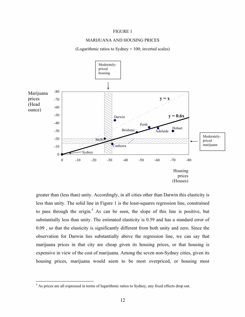
The comparison of prices for marijuana and housing is facilitated in Figure 1

which plots the two sets of prices relative to NSW/Sydney by using the regional dummy-

variable coefficients for head ounce (given in row 4 of Table 4) and those for houses (row

7 of Table 4). As the housing prices refer to capital cities in each region, while the

marijuana prices refer to regions as a whole, for ease of exposition in what follows we

shall refer to just capital cities rather than the region (for marijuana prices) and the

corresponding capital city (for housing prices) simultaneously. The broken ray from the

origin has a slope of 450 and as the scales of both axes are inverted, the vertical distance

between this line and any point measures the difference in the housing-marijuana relative

price between the city in question and that in Sydney. This relative price is thus higher for

Darwin, and lower for the rest. An equivalent way of interpreting the figure is to note that

as the two price differences, relative to Sydney, are equal along the 450-line, all points on

the line correspond to the elasticity of marijuana prices with respect to housing prices

being equal to unity; and for the points above (below) the line the elasticity is

4 While the Australian Bureau of Statistics publish a Consumer Price Index for each of the six capital cities, these indexes are not harmonised. Accordingly, the levels of the CPI cannot be compared across cities to provide information on the level of regional living costs.

12

FIGURE 1

MARIJUANA AND HOUSING PRICES

(Logarithmic ratios to Sydney × 100; inverted scales)

y = .5856 x 2R = .4596 (.0874)

greater than (less than) unity. Accordingly, in all cities other than Darwin this elasticity is

less than unity. The solid line in Figure 1 is the least-squares regression line, constrained

to pass through the origin.5 As can be seen, the slope of this line is positive, but

substantially less than unity. The estimated elasticity is 0.59 and has a standard error of

0.09 , so that the elasticity is significantly different from both unity and zero. Since the

observation for Darwin lies substantially above the regression line, we can say that

marijuana prices in that city are cheap given its housing prices, or that housing is

expensive in view of the cost of marijuana. Among the seven non-Sydney cities, given its

housing prices, marijuana would seem to be most overpriced, or housing most

5 As prices are all expressed in terms of logarithmic ratios to Sydney, any fixed effects drop out.

-80

-70

-60

-50

-40

-30

-20

-10

0-80-70-60-50-40-30-20-100

Melb.

Darwin

Brisbane Perth

Hobart

y = x

y = 0.6x

Adelaide

Marijuana prices (Head ounce)

Sydney

Moderately- priced marijuana

Moderately- priced housing

Housing prices

(Houses)

Canberra

13

underpriced, in Hobart.6 The final interesting feature of the figure is that it can be used to

naturally divide up Australia into three super regions/cities: (i) NSW/Sydney -- expensive

marijuana and housing. (ii) Victoria/Melbourne and ACT/Canberra – moderately-priced

marijuana and housing. (iii) The rest -- cheap marijuana and housing.

The above discussion shows that to the extent that housing costs are a good proxy

for living costs, marijuana prices are at least partially related to costs in general. As a

substantial part of the overall price of marijuana is likely to reflect local distribution

activities, which differ significantly across different regions, this could explain the

finding that the market is not a national one, but a series of regional markets that are not

too closely linked. Understanding the pricing of marijuana is enhanced if we split the

product into (i) a (nationally) traded component comprising mainly the “raw” product,

whose price is likely to be approximately equalised in different regions; and (ii) a

nontraded component associated with packaging and local distribution, the price of which

is less likely to be equalised. As such services are likely to be labour intensive, their

prices will mainly reflect local wages which, in turn, would partly reflect local living

costs. The results of this section point to the importance of the nontraded component of

marijuana prices.

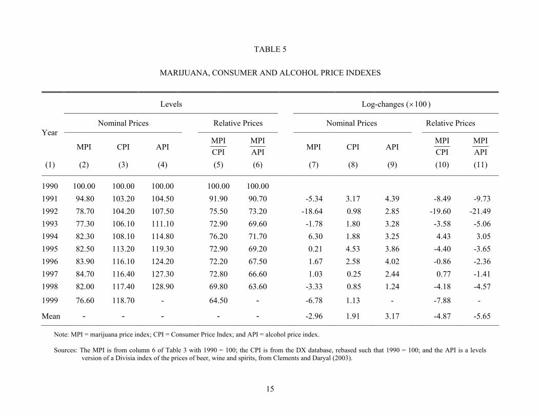
4. Fact 2: Marijuana has Become Substantially Cheaper7

This section documents the fall in marijuana prices and canvases some possible

explanations for the fall. Table 5 shows that over the 1990s marijuana prices have fallen

by about 23 per cent in nominal terms (column 2), and 35 per cent relative to the CPI

(column 5). The last entries in columns 10 and 11 of this table reveal that on average over

the decade, marijuana prices in terms of consumer prices fell by 4.9 per cent p.a. and by

6 The slope of a ray from the origin to any of the seven cities in Figure 1 is the elasticity of marijuana prices with respect to housing prices for the city in question. Visually, it can be seen that this elasticity is a bit lower for Canberra than Hobart. But as this elasticity is the percentage change in marijuana prices for a unit percentage change in housing prices, it should not be confused with using the regression line to identify anomalies in the pricing of marijuana. The vertical distance between any observation and the regression line represents the extent of mispricing. 7 The first part of this section is based on Clements and Daryal (2001), except that here we use population-weighted marijuana prices.

14

5.7 per cent p.a. in terms of alcohol prices. No matter if the CPI or alcohol prices are used

as the deflator, the result is the same: The relative price of marijuana has fallen

substantially.

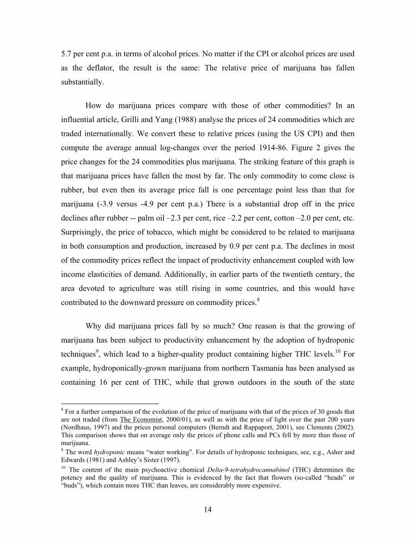
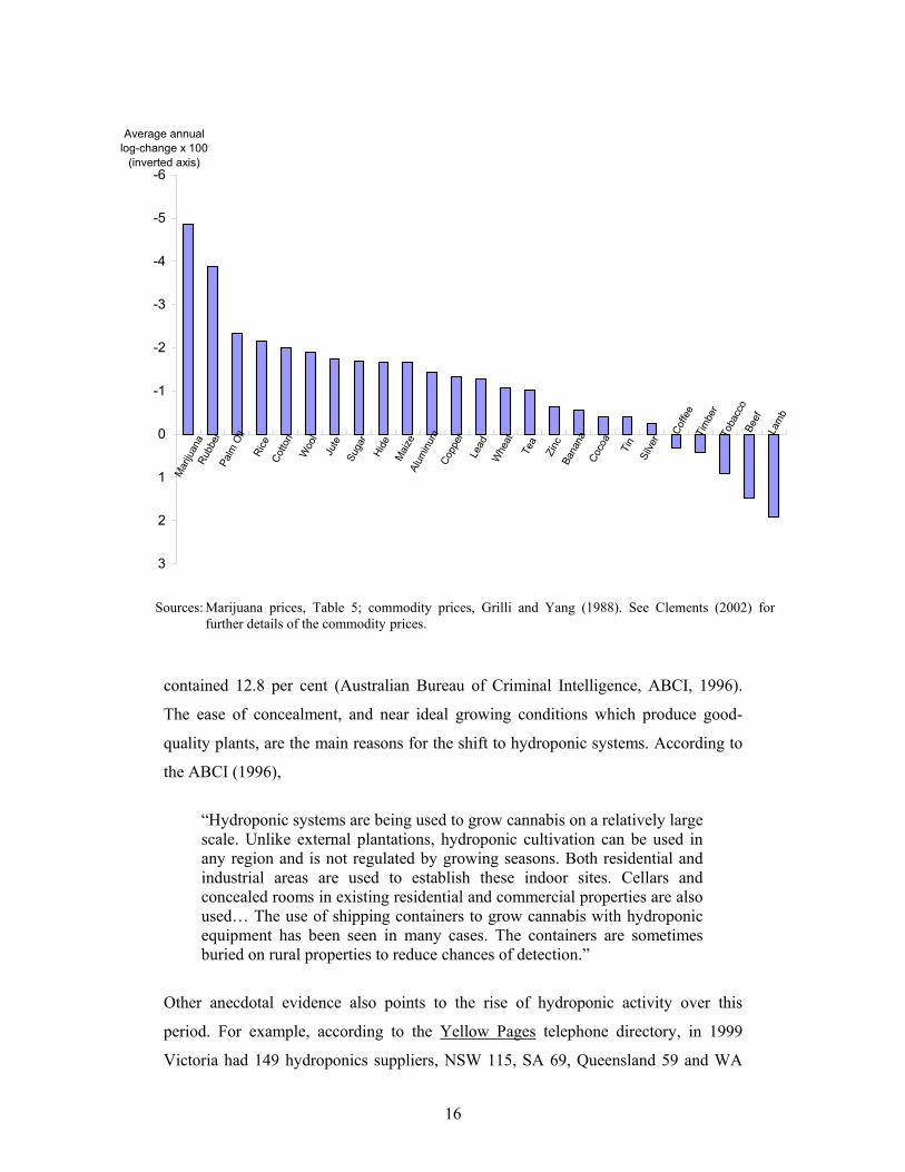
How do marijuana prices compare with those of other commodities? In an

influential article, Grilli and Yang (1988) analyse the prices of 24 commodities which are

traded internationally. We convert these to relative prices (using the US CPI) and then

compute the average annual log-changes over the period 1914-86. Figure 2 gives the

price changes for the 24 commodities plus marijuana. The striking feature of this graph is

that marijuana prices have fallen the most by far. The only commodity to come close is

rubber, but even then its average price fall is one percentage point less than that for

marijuana (-3.9 versus -4.9 per cent p.a.) There is a substantial drop off in the price

declines after rubber -- palm oil –2.3 per cent, rice –2.2 per cent, cotton –2.0 per cent, etc.

Surprisingly, the price of tobacco, which might be considered to be related to marijuana

in both consumption and production, increased by 0.9 per cent p.a. The declines in most

of the commodity prices reflect the impact of productivity enhancement coupled with low

income elasticities of demand. Additionally, in earlier parts of the twentieth century, the

area devoted to agriculture was still rising in some countries, and this would have

contributed to the downward pressure on commodity prices.8

Why did marijuana prices fall by so much? One reason is that the growing of

marijuana has been subject to productivity enhancement by the adoption of hydroponic

techniques9, which lead to a higher-quality product containing higher THC levels.10 For

example, hydroponically-grown marijuana from northern Tasmania has been analysed as

containing 16 per cent of THC, while that grown outdoors in the south of the state

8 For a further comparison of the evolution of the price of marijuana with that of the prices of 30 goods that are not traded (from The Economist, 2000/01), as well as with the price of light over the past 200 years (Nordhaus, 1997) and the prices personal computers (Berndt and Rappaport, 2001), see Clements (2002). This comparison shows that on average only the prices of phone calls and PCs fell by more than those of marijuana. 9 The word hydroponic means “water working”. For details of hydroponic techniques, see, e.g., Asher and Edwards (1981) and Ashley’s Sister (1997). 10 The content of the main psychoactive chemical Delta-9-tetrahydrocannabinol (THC) determines the potency and the quality of marijuana. This is evidenced by the fact that flowers (so-called “heads” or “buds”), which contain more THC than leaves, are considerably more expensive.

15

TABLE 5

MARIJUANA, CONSUMER AND ALCOHOL PRICE INDEXES

Levels Log-changes ( 100× )

Nominal Prices Relative Prices Nominal Prices Relative Prices Year

MPI

CPI

API

CPIMPI

APIMPI

MPI

CPI

API

CPIMPI

APIMPI

(1) (2) (3) (4) (5) (6) (7) (8) (9) (10) (11)

1990 100.00 100.00 100.00 100.00 100.00

1991 94.80 103.20 104.50 91.90 90.70 -5.34 3.17 4.39 -8.49 -9.73

1992 78.70 104.20 107.50 75.50 73.20 -18.64 0.98 2.85 -19.60 -21.49

1993 77.30 106.10 111.10 72.90 69.60 -1.78 1.80 3.28 -3.58 -5.06

1994 82.30 108.10 114.80 76.20 71.70 6.30 1.88 3.25 4.43 3.05

1995 82.50 113.20 119.30 72.90 69.20 0.21 4.53 3.86 -4.40 -3.65

1996 83.90 116.10 124.20 72.20 67.50 1.67 2.58 4.02 -0.86 -2.36

1997 84.70 116.40 127.30 72.80 66.60 1.03 0.25 2.44 0.77 -1.41

1998 82.00 117.40 128.90 69.80 63.60 -3.33 0.85 1.24 -4.18 -4.57

1999 76.60 118.70 - 64.50 - -6.78 1.13 - -7.88 -

Mean - - - - - -2.96 1.91 3.17 -4.87 -5.65

Note: MPI = marijuana price index; CPI = Consumer Price Index; and API = alcohol price index. Sources: The MPI is from column 6 of Table 3 with 1990 = 100; the CPI is from the DX database, rebased such that 1990 = 100; and the API is a levels

version of a Divisia index of the prices of beer, wine and spirits, from Clements and Daryal (2003).

16

Tim

ber

Coffe

e

Silve

r

Tin

Coco

a

Bana

na

ZincTea

Whe

at

Lead

Copp

er

Alum

inum

Mai

ze

Hide

Suga

r

Jute

Woo

l

Cotto

n

Rice

Palm

Oil

Rubb

er

Mar

ijuan

a

Lam

b

Beef

Toba

cco

-6

-5

-4

-3

-2

-1

0

1

2

3

Average annuallog-change x 100

(inverted axis)

contained 12.8 per cent (Australian Bureau of Criminal Intelligence, ABCI, 1996).

The ease of concealment, and near ideal growing conditions which produce good-

quality plants, are the main reasons for the shift to hydroponic systems. According to

the ABCI (1996),

“Hydroponic systems are being used to grow cannabis on a relatively large scale. Unlike external plantations, hydroponic cultivation can be used in any region and is not regulated by growing seasons. Both residential and industrial areas are used to establish these indoor sites. Cellars and concealed rooms in existing residential and commercial properties are also used… The use of shipping containers to grow cannabis with hydroponic equipment has been seen in many cases. The containers are sometimes buried on rural properties to reduce chances of detection.”

Other anecdotal evidence also points to the rise of hydroponic activity over this

period. For example, according to the Yellow Pages telephone directory, in 1999

Victoria had 149 hydroponics suppliers, NSW 115, SA 69, Queensland 59 and WA

Sources: Marijuana prices, Table 5; commodity prices, Grilli and Yang (1988). See Clements (2002) for further details of the commodity prices.

17

58. One suspects that many of these operations supply marijuana growers. For a

further discussion of this anecdotal evidence, see Clements (2002).

A second possible reason for the decline in marijuana prices is that because of

changing community attitudes, laws have become softer and penalties reduced.

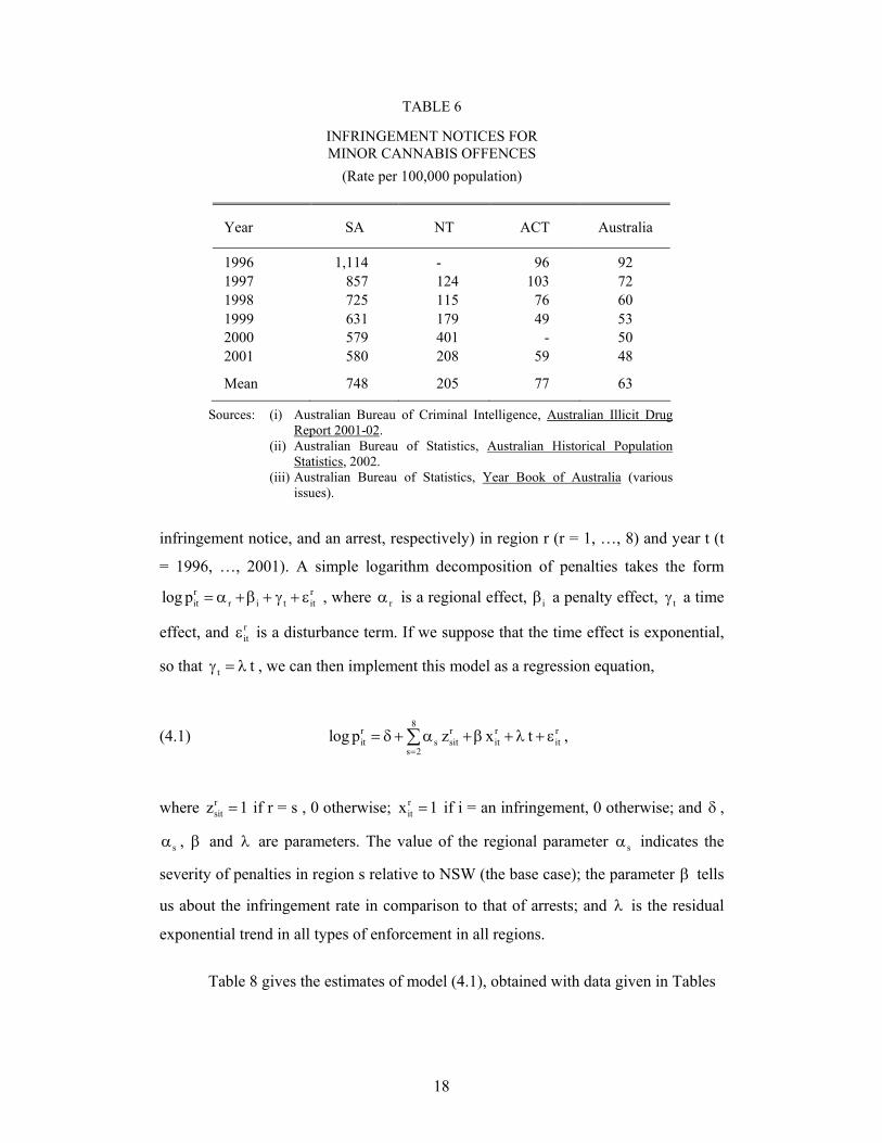
Information on the enforcement of marijuana laws distinguishes between

(i) infringement notices issued for minor offences and (ii) arrests. Table 6 presents the

available data on infringement notices for the three states/territories that use them, SA,

NT and ACT. As can be seen, per capita infringement notices have declined

substantially in SA since 1996, increased in NT, first increased and then declined in

ACT, and declined noticeably for Australia as a whole, where they have fallen by

almost 50 per cent. This information points in the direction of a lower policing effort.

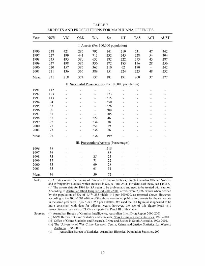
Data on arrests and prosecution for marijuana offences are given in Table 7. Panel I

shows that the arrest rate for NSW was more or less stable over the six-year period,

while that for Victoria fell substantially due to a “redirection of police resources away

from minor cannabis offences” (ABCI, 1998). For Queensland, the arrest rate rose by

more than 50 per cent in 1997, and then fell back to a more or less stable value, but in

WA the rate fell markedly in 1999 with the introduction of a trial of cautioning and

mandatory education to “reduce the resources previously used to pursue prosecutions

for simple cannabis offences” (ABCI, 2000). For Australia, the arrest rate fell from

342 in 1996 to 232 in 2001 (per 100,000 population), a decline of 32 per cent. Data on

successful prosecution of marijuana cases for three states are given in Panel II of

Table 7 (data for the other states/territories are not available). For both NSW and SA,

the prosecution rate has fallen substantially. Not only has the prosecution rate fallen,

lighter sentences have become much more common. Interestingly, in the early 1990s

the prosecution rate was much higher in SA than in NSW, but by the end of the

decade the rate was approximately the same in the two states. In WA, the prosecution

rate is fairly stable, but the period is much shorter. No clear pattern emerges from the

information on the percentage of arrests that result in a successful prosecution, as

shown in Panel III of Table 7.

To understand further the evolution of enforcement of marijuana laws, it is

useful to consider a simple model. Let ritp be the penalty of type i (i = 1, 2, for an

18

TABLE 6

INFRINGEMENT NOTICES FOR MINOR CANNABIS OFFENCES

(Rate per 100,000 population)

Year SA NT ACT Australia

1996 1,114 - 96 92 1997 857 124 103 72 1998 725 115 76 60 1999 631 179 49 53 2000 579 401 - 50 2001 580 208 59 48

Mean 748 205 77 63

Sources: (i) Australian Bureau of Criminal Intelligence, Australian Illicit Drug Report 2001-02.

(ii) Australian Bureau of Statistics, Australian Historical Population Statistics, 2002.

(iii) Australian Bureau of Statistics, Year Book of Australia (various issues).

infringement notice, and an arrest, respectively) in region r (r = 1, …, 8) and year t (t

= 1996, …, 2001). A simple logarithm decomposition of penalties takes the form r rit r i t itlog p = α +β + γ + ε , where rα is a regional effect, iβ a penalty effect, tγ a time

effect, and ritε is a disturbance term. If we suppose that the time effect is exponential,

so that t tγ = λ , we can then implement this model as a regression equation,

(4.1) 8

r r r rit s sit it it

s 2log p z x t

== δ + α +β + λ + ε∑ ,

where rsitz 1= if r = s , 0 otherwise; r

itx 1= if i = an infringement, 0 otherwise; and δ ,

sα , β and λ are parameters. The value of the regional parameter sα indicates the

severity of penalties in region s relative to NSW (the base case); the parameter β tells

us about the infringement rate in comparison to that of arrests; and λ is the residual

exponential trend in all types of enforcement in all regions.

Table 8 gives the estimates of model (4.1), obtained with data given in Tables

19

TABLE 7 ARRESTS AND PROSECUTIONS FOR MARIJUANA OFFENCES

Year NSW VIC QLD WA SA NT TAS ACT AUST

I. Arrests (Per 100,000 population)

1996 238 421 286 795 141 210 531 47 342 1997 227 199 441 713 232 245 228 54 304 1998 245 195 380 633 182 222 253 45 287 1999 247 198 385 330 172 183 156 28 256 2000 220 157 386 363 210 62 170 - 242 2001 211 136 366 389 151 224 223 48 232

Mean 231 218 374 537 181 191 260 37 277

II. Successful Prosecutions (Per 100,000 population)

1991 112 - - - - - - - - 1992 123 - - - 273 - - - - 1993 113 - - - 315 - - - - 1994 94 - - - 350 - - - - 1995 83 - - - 326 - - - - 1996 90 - - - 304 - - - - 1997 81 - - - 205 - - - - 1998 85 - - 222 46 - - - - 1999 92 - - 234 38 - - - - 2000 77 - - 251 59 - - - - 2001 73 - - 238 76 - - - -

Mean 93 - - 236 199 - - - -

III. Prosecutions/Arrests (Percentages)

1996 38 - - - 215 - - - - 1997 36 - - - 88 - - - - 1998 35 - - 35 25 - - - - 1999 37 - - 71 22 - - - - 2000 35 - - 69 28 - - - - 2001 35 - - 61 51 - - - -

Mean 36 - - 59 72 - - - - Notes: (i) Arrests exclude the issuing of Cannabis Expiation Notices, Simple Cannabis Offence Notices

and Infringement Notices, which are used in SA, NT and ACT. For details of these, see Table 6. (ii) The arrests data for 1996 for SA seem to be problematic and need to be treated with caution.

According to Australian Illicit Drug Report 2000-2001, arrests were 2,076, which when divided by the population of SA of 1,474,253 yields 141 per 100,000, as reported above. However, according to the 2001-2002 edition of the above mentioned publication, arrests for the same state in the same year were 18,477, or 1,253 per 100,000. We used the 141 figure as it appeared to be more consistent with data for adjacent years; however, the use of this figure leads to a prosecutions/arrests rate of 215%, as reported in Panel III of this table.

Sources: (i) Australian Bureau of Criminal Intelligence, Australian Illicit Drug Report 2000-2001. (ii) NSW Bureau of Crime Statistics and Research, NSW Criminal Courts Statistics, 1991-2001. (iii) Office of Crime Statistics and Research, Crime and Justice in South Australia, 1992-2001. (iv) The University of WA Crime Research Centre, Crime and Justice Statistics for Western

Australia, 1996-2001. (v) Australian Bureau of Statistics, Australian Historical Population Statistics, 200

20

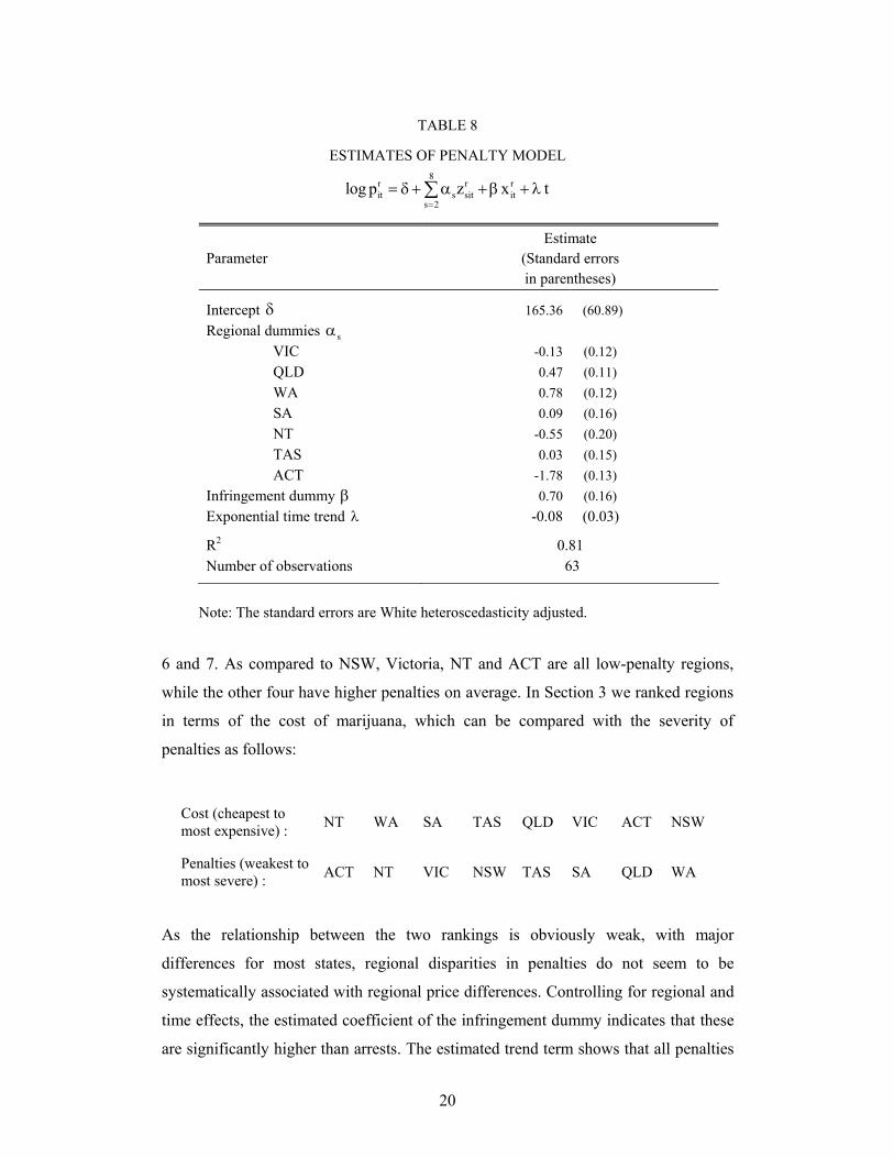
TABLE 8

ESTIMATES OF PENALTY MODEL

8r r rit s sit it

s 2log p z x t

== δ + α +β + λ∑

Parameter Estimate

(Standard errors in parentheses)

Intercept δ 165.36 (60.89) Regional dummies sα

VIC -0.13 (0.12) QLD 0.47 (0.11) WA 0.78 (0.12) SA 0.09 (0.16) NT -0.55 (0.20) TAS 0.03 (0.15) ACT -1.78 (0.13)

Infringement dummy β 0.70 (0.16) Exponential time trend λ -0.08 (0.03)

R2 0.81 Number of observations 63

Note: The standard errors are White heteroscedasticity adjusted. 6 and 7. As compared to NSW, Victoria, NT and ACT are all low-penalty regions,

while the other four have higher penalties on average. In Section 3 we ranked regions

in terms of the cost of marijuana, which can be compared with the severity of

penalties as follows:

Cost (cheapest to most expensive) : NT WA SA TAS QLD VIC ACT NSW

Penalties (weakest to most severe) : ACT NT VIC NSW TAS SA QLD WA

As the relationship between the two rankings is obviously weak, with major

differences for most states, regional disparities in penalties do not seem to be

systematically associated with regional price differences. Controlling for regional and

time effects, the estimated coefficient of the infringement dummy indicates that these

are significantly higher than arrests. The estimated trend term shows that all penalties

21

are falling on average by about 8 per cent p.a., a fall that is significantly different from

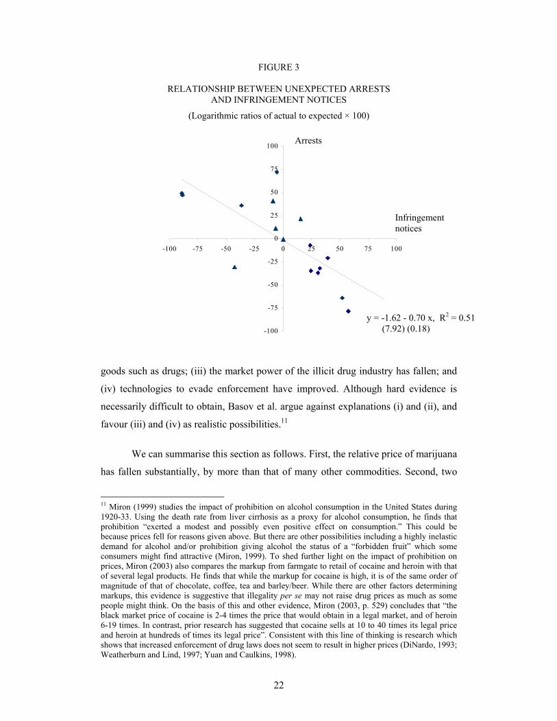
zero. Consider those three regions that have infringement notices. To what extent have

infringement notices partially displaced arrests? In other words, are the two forms of

penalties substitutes for one another? For example, in the NT the infringements rate

rose from 179 in 1999 to 401 in 2000, while over the same period the arrest rate fell

from 183 to 62. This would seem to support the idea that the two types of penalties

are substitutes. However, to proceed more systematically, we need to control for all

the effects of factors determining penalties in model (4.1) by using the residuals, and

examine the comovement of infringements and arrests in the three regions over the six

years. Figure 3 is a scatter plot of these residuals and as can be clearly seen, there is a

significant negative relationship between arrests and infringements. This means that

more infringement notices are associated with fewer arrests, other factors remaining

unchanged. This, of course, must have been one of the key objectives associated with

the introduction of the infringement regime.

Taken as a whole, the above analysis seems to support the idea that

participants in the marijuana industry have faced a declining probability of being

arrested/successfully prosecuted; and even if they are arrested and successfully

prosecuted, the expected penalty is now lower. In other words, both the effort devoted

to the enforcement of existing laws and penalties seem to have decreased.

Accordingly, the expected value of this component of the “full cost” of using

marijuana has fallen. During the period considered, NSW, Victoria, WA and

Tasmania all introduced marijuana cautioning programs (ABCI, 2000) and SA, NT

and ACT all issued marijuana offence notices. This seems to indicate changing

community attitudes to marijuana associated with the reduced “policing effort”. It is

plausible that this has also led to lower marijuana prices. As the riskiness of buying

and selling marijuana has fallen, so may have any risk premium built into prices. This

explanation of lower prices has, however, been challenged by Basov et al. (2001) who

analyse illicit drug prices in the United States. They show that while drug prohibition

enforcement costs have risen substantially over the past 25 years, the relative prices

of drugs have nonetheless declined. Basov et al. suggest four possible reasons for the

decrease in prices: (i) Production costs of drugs have declined; (ii) tax and regulatory

cost increases have raised the prices of legal goods, but not illicit

22

FIGURE 3

RELATIONSHIP BETWEEN UNEXPECTED ARRESTS AND INFRINGEMENT NOTICES

(Logarithmic ratios of actual to expected × 100)

-100

-75

-50

-25

0

25

50

75

100

-100 -75 -50 -25 0 25 50 75 100

goods such as drugs; (iii) the market power of the illicit drug industry has fallen; and

(iv) technologies to evade enforcement have improved. Although hard evidence is

necessarily difficult to obtain, Basov et al. argue against explanations (i) and (ii), and

favour (iii) and (iv) as realistic possibilities.11

We can summarise this section as follows. First, the relative price of marijuana

has fallen substantially, by more than that of many other commodities. Second, two

11 Miron (1999) studies the impact of prohibition on alcohol consumption in the United States during 1920-33. Using the death rate from liver cirrhosis as a proxy for alcohol consumption, he finds that prohibition “exerted a modest and possibly even positive effect on consumption.” This could be because prices fell for reasons given above. But there are other possibilities including a highly inelastic demand for alcohol and/or prohibition giving alcohol the status of a “forbidden fruit” which some consumers might find attractive (Miron, 1999). To shed further light on the impact of prohibition on prices, Miron (2003) also compares the markup from farmgate to retail of cocaine and heroin with that of several legal products. He finds that while the markup for cocaine is high, it is of the same order of magnitude of that of chocolate, coffee, tea and barley/beer. While there are other factors determining markups, this evidence is suggestive that illegality per se may not raise drug prices as much as some people might think. On the basis of this and other evidence, Miron (2003, p. 529) concludes that “the black market price of cocaine is 2-4 times the price that would obtain in a legal market, and of heroin 6-19 times. In contrast, prior research has suggested that cocaine sells at 10 to 40 times its legal price and heroin at hundreds of times its legal price”. Consistent with this line of thinking is research which shows that increased enforcement of drug laws does not seem to result in higher prices (DiNardo, 1993; Weatherburn and Lind, 1997; Yuan and Caulkins, 1998).

Arrests

Infringement notices

y = -1.62 - 0.70 x, R2 = 0.51 (7.92) (0.18)

23

possible explanations for this decline are (a) productivity improvement in the

production of marijuana associated with the adoption of hydroponic techniques; and

(b) the lower expected penalties for buying and selling marijuana. On the basis of the

evidence currently available, both explanations seem to be equally plausible.

5. Fact 3: Lower Prices have Boosted Marijuana Consumption and Reduced Acohol

Consumption

The section contains some explorations of the likely impact of lower

marijuana prices on usage, as well as their role in determining the consumption of a

product that shares important common characteristics, alcohol. It should be

acknowledged that our price and quantity data for marijuana are imperfect and are

subject to more than the usual uncertainties. Moreover, as we have data for only a

decade, we are severely constrained in carrying out an econometric analysis of the

price responsiveness of consumption. Although Clements and Daryal (2003)

attempted such an analysis, in this section we explore the alternative approach of

drawing on the previous literature and putting sufficient structure on the problem to be

able to derive numerical values of the price elasticities of demand. This approach is

used extensively in the literature on CGE and equilibrium displacement modeling.

We assume that alcohol and marijuana consumption as a group is weakly

separable from all other goods in the consumer’s utility function. While this rules out

any specific substitutability/complementarity relationships between members of the

group, on the one hand, and products outside the group, on the other, it is a fairly mild

assumption. This assumption means that we can proceed conditionally and analyse

consumption within the group independently of the prices of other goods, (see, e.g.,

Clements, 1987). Next, we make the simplifying assumption that tastes with respect to

alcohol and marijuana can be characterized by a utility function of the preference

independent form. This means that if there are n goods in the group, the utility

function is the sum of n sub-utility functions, one for each good,

∑= =n

1i iin1 )(qu)q..., ,u(q , where qi is the quantity consumed of good i . Preference

independence (PI) means that the marginal utility of each good is independent of the

consumption of all others. The implications of PI are that all income elasticities are

positive, so that inferior goods are ruled out, and all pairs of goods are Slutsky

24

substitutes. The hypothesis of PI has been recently tested with alcohol data for seven

countries by Clements et al. (1997) and, using a variety of tests, they find that the

hypothesis cannot be rejected.12 There have been nine prior studies of the relationship

between alcohol and marijuana consumption, eight for the United States and one for

Australia (Cameron and Williams, 2001). Four of the nine studies find substitutability

between alcohol and marijuana (Cameron and Williams, 2001; Chaloupka and

Laixuthai, 1997; DiNardo and Lemieux, 1992; Model, 1993), two find

complementarity (Pacula, 1997, 1998), one finds the relationship to be mostly

complementarity (Saffer and Chaloupka, 1998), while two are inconclusive (Saffer

and Chaloupka, 1995; Theis and Register, 1993). Thus while these studies do not give

a completely unambiguous picture, the weight of the evidence seems to point to

alcohol and marijuana being substitutes, which is not inconsistent with the PI

assumption.

The further implications of PI are as follows. Let ip be the price of good i

i(i 1, , n), q= … be the corresponding quantity demanded, ∑= =n

1i iiqpM be total

expenditure (“income” for short), and i i iw p q / M= be the budget share of good i.

Furthermore, let ( )ij i jlog q / (log p )η = ∂ ∂ be the compensated elasticity of demand for

good i with respect to the price of good j , φ be the price elasticity of demand for the

group of goods as a whole, and iη be the income elasticity of demand for good i . We

then have the fundamental relationship linking the price and income elasticities under

PI,

(5.1) ij i ij j j( w )η = φη δ − η ,

where ijδ is the Kronecker delta ij(δ 1 if i j, 0= = otherwise). For the derivation of

equation (5.1) and more details, see, e.g., Clements et al. (1995). We shall obtain

numerical values of the price elasticities by using equation (5.1) in conjunction with

values of iandφ η that have appeared in the literature.

12 Earlier studies tended to reject PI (see Barten, 1977, for a survey), but it is now understood that the source of many of these rejections was the use of asymptotic tests, which were biased against the null (Selvanathan, 1987, 1993).

25

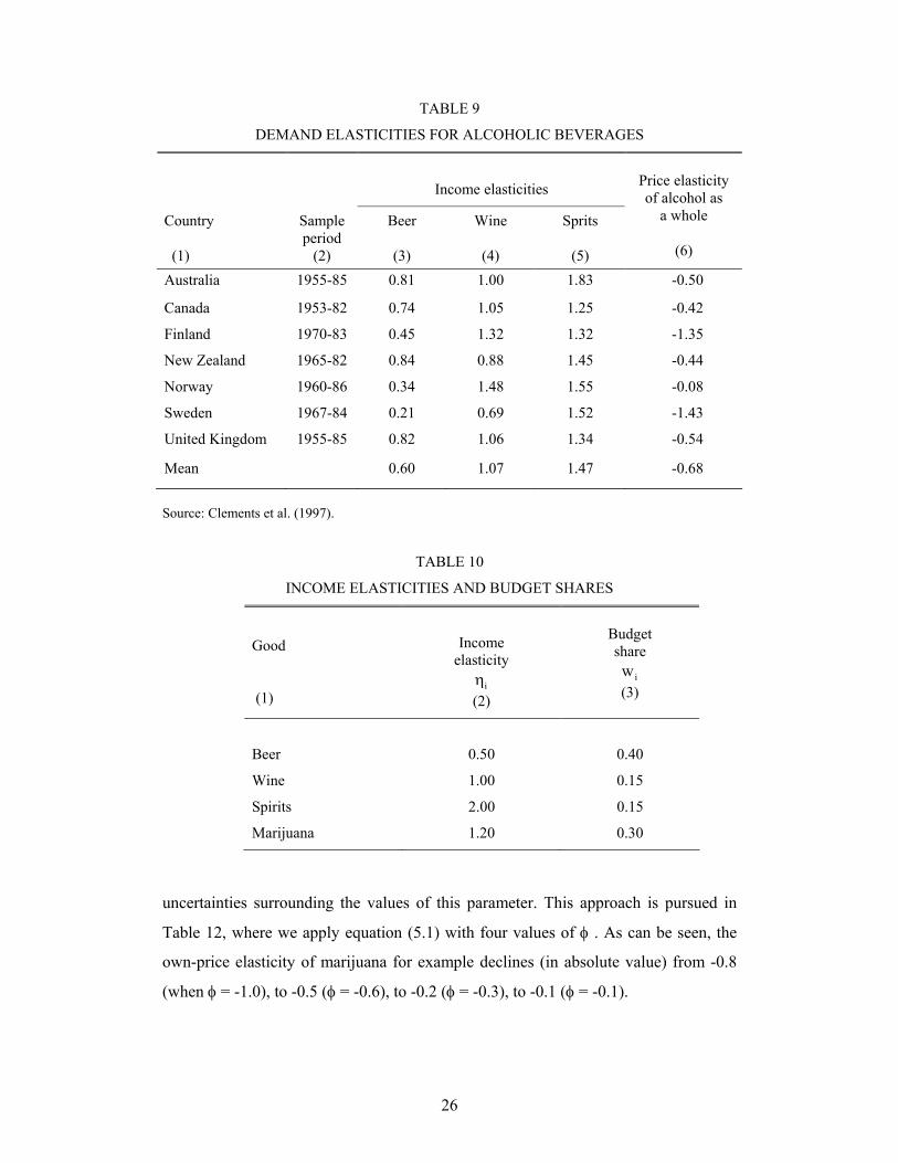
Table 9 presents for several countries estimates of the income elasticities for

three alcoholic beverages, beer, wine and spirits, as well as the price elasticity of

alcohol as a whole. These elasticities are derived from estimates of the Rotterdam

model under preference independence. We use them as a guide to the values of

income elasticities of the members of the broader group alcohol and marijuana, as set

out in Table 10. As can be seen from column 2 of Table 10, beer is taken to have an

income elasticity of 0.5 (so that it is a necessity), wine 1.0 (a borderline case) and

spirits 2.0 (a strong luxury). We shall come back to the elasticity for marijuana.

Column 3 gives the four budget shares which are based on the means given in the last

row of Table 11. We derive the income elasticity of marijuana from the constraint 4i 1 i iw 1=Σ η = . This yields 4 1.2η = , as indicated by the last entry of column 2 of Table

10, which implies that marijuana is a mild luxury.13

The only remaining parameter on the right-hand side of equation (5.1) to

discuss is φ , the own-price elasticity of demand for the group (alcohol and marijuana)

as a whole. It can be seen from equation (5.1) that φ acts as a “scaling” parameter.

Prior estimates of φ for the alcohol are given in column 6 of Table 10, and these

average -0.7 . As marijuana is likely to be a substitute for alcohol, the effect of

expanding the group of goods in question from alcoholic beverages to alcohol plus

marijuana would be for the price elasticity to fall in absolute value. This means that

we should use for the alcohol and marijuana group a |φ|-value of less than 0.7.

Clements and Daryal (2003) estimate φ for Australia for alcohol or marijuana to be -

0.4 ; while going in the right direction, this estimate is subject to some qualifications

due to the uncertainties associated with the limited data available. It would thus seem

sensible to use several values of φ to reflect the genuine

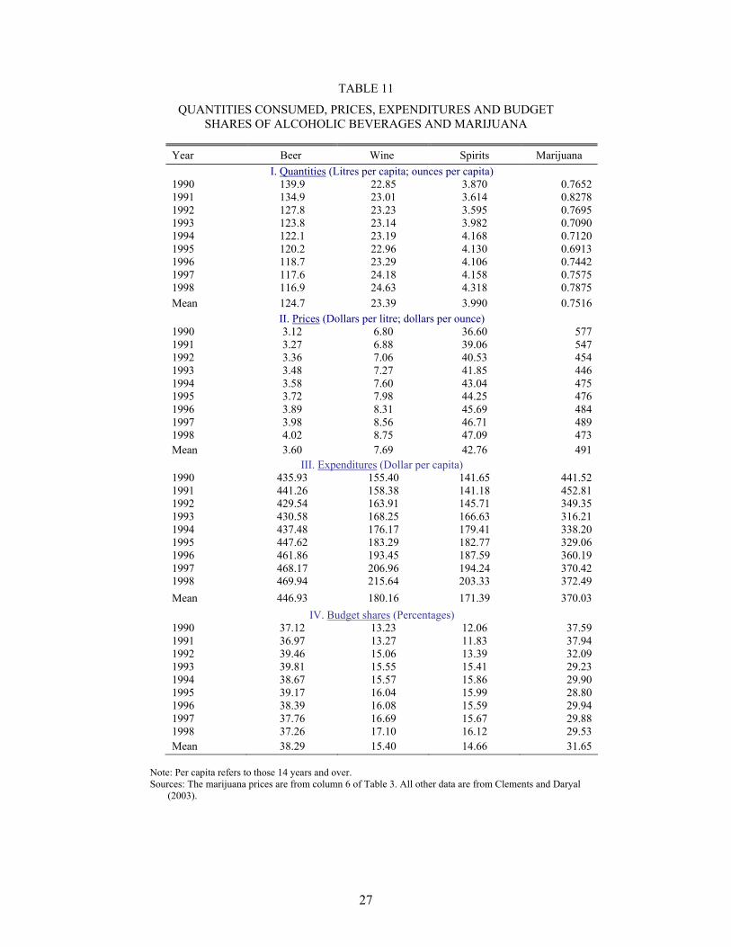
13 It is appropriate to say a few words about the consumption data in Table 11. The quantity consumed of marijuana is estimated on the basis of the National Drug Strategy Household Survey (various issues), together with some plausible assumptions that link intensity of use to frequency of use; see Clements and Daryal (2003) for details. Although all care was taken in preparing these estimates, and they are not inconsistent with independent estimates, it must be acknowledged that they are likely to be subject to a substantial margin of error. Panel I of Table 11 reveals that over the 1990s, per capita beer consumption fell from 140 to 117 litres, wine increased from 22.9 to 24.6, spirits grew from 3.87 to 4.32, and marijuana consumption increased from 0.765 to 0.788 ounces per capita. In what follows, we analyse the extent to which the fall in marijuana prices caused alcohol consumption to grow at a slower rate than would otherwise be the case. The final thing to note about Table 11 is that from Panel IV, on average the budget shares are roughly 0.40, 0.15, 0.15 and 0.30 for beer, wine, spirits and marijuana, respectively. Accordingly, expenditure on marijuana is about equal to the sum of that on wine and spirits, or to put it another way, about twice wine expenditure.

26

TABLE 9

DEMAND ELASTICITIES FOR ALCOHOLIC BEVERAGES

Income elasticities

Country (1)

Sample period

(2)

Beer

(3)

Wine

(4)

Sprits

(5)

Price elasticity of alcohol as

a whole

(6)

Australia 1955-85 0.81 1.00 1.83 -0.50

Canada 1953-82 0.74 1.05 1.25 -0.42

Finland 1970-83 0.45 1.32 1.32 -1.35

New Zealand 1965-82 0.84 0.88 1.45 -0.44

Norway 1960-86 0.34 1.48 1.55 -0.08

Sweden 1967-84 0.21 0.69 1.52 -1.43

United Kingdom 1955-85 0.82 1.06 1.34 -0.54

Mean 0.60 1.07 1.47 -0.68

Source: Clements et al. (1997).

TABLE 10

INCOME ELASTICITIES AND BUDGET SHARES

uncertainties surrounding the values of this parameter. This approach is pursued in

Table 12, where we apply equation (5.1) with four values of φ . As can be seen, the

own-price elasticity of marijuana for example declines (in absolute value) from -0.8

(when φ = -1.0), to -0.5 (φ = -0.6), to -0.2 (φ = -0.3), to -0.1 (φ = -0.1).

Good (1)

Income

elasticity iη

(2)

Budget share

iw (3)

Beer

0.50

0.40

Wine 1.00 0.15

Spirits 2.00 0.15

Marijuana 1.20 0.30

27

TABLE 11

QUANTITIES CONSUMED, PRICES, EXPENDITURES AND BUDGET SHARES OF ALCOHOLIC BEVERAGES AND MARIJUANA

Year Beer Wine Spirits Marijuana

I. Quantities (Litres per capita; ounces per capita) 1990 139.9 22.85 3.870 0.7652 1991 134.9 23.01 3.614 0.8278 1992 127.8 23.23 3.595 0.7695 1993 123.8 23.14 3.982 0.7090 1994 122.1 23.19 4.168 0.7120 1995 120.2 22.96 4.130 0.6913 1996 118.7 23.29 4.106 0.7442 1997 117.6 24.18 4.158 0.7575 1998 116.9 24.63 4.318 0.7875 Mean 124.7 23.39 3.990 0.7516

II. Prices (Dollars per litre; dollars per ounce) 1990 3.12 6.80 36.60 577 1991 3.27 6.88 39.06 547 1992 3.36 7.06 40.53 454 1993 3.48 7.27 41.85 446 1994 3.58 7.60 43.04 475 1995 3.72 7.98 44.25 476 1996 3.89 8.31 45.69 484 1997 3.98 8.56 46.71 489 1998 4.02 8.75 47.09 473 Mean 3.60 7.69 42.76 491

III. Expenditures (Dollar per capita) 1990 435.93 155.40 141.65 441.52 1991 441.26 158.38 141.18 452.81 1992 429.54 163.91 145.71 349.35 1993 430.58 168.25 166.63 316.21 1994 437.48 176.17 179.41 338.20 1995 447.62 183.29 182.77 329.06 1996 461.86 193.45 187.59 360.19 1997 468.17 206.96 194.24 370.42 1998 469.94 215.64 203.33 372.49 Mean 446.93 180.16 171.39 370.03

IV. Budget shares (Percentages) 1990 37.12 13.23 12.06 37.59 1991 36.97 13.27 11.83 37.94 1992 39.46 15.06 13.39 32.09 1993 39.81 15.55 15.41 29.23 1994 38.67 15.57 15.86 29.90 1995 39.17 16.04 15.99 28.80 1996 38.39 16.08 15.59 29.94 1997 37.76 16.69 15.67 29.88 1998 37.26 17.10 16.12 29.53 Mean 38.29 15.40 14.66 31.65

Note: Per capita refers to those 14 years and over. Sources: The marijuana prices are from column 6 of Table 3. All other data are from Clements and Daryal (2003).

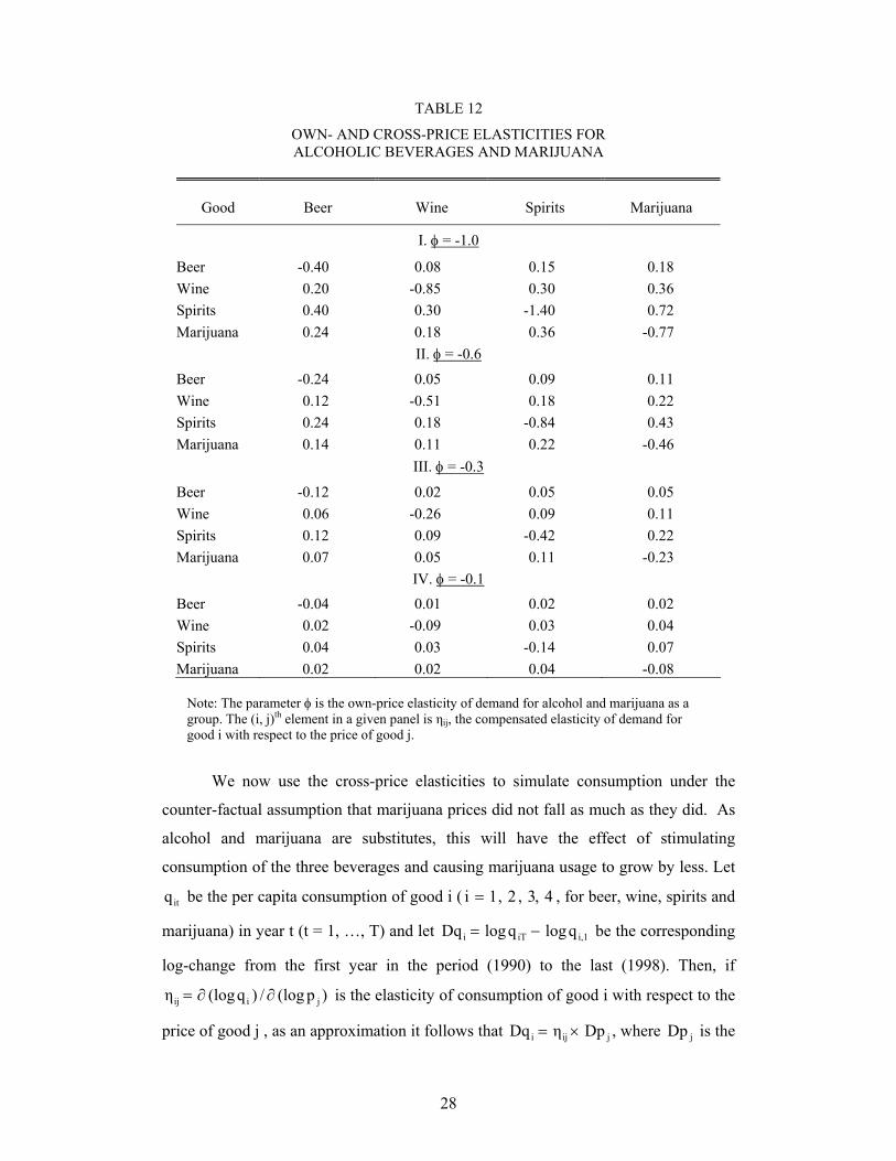
28

TABLE 12

OWN- AND CROSS-PRICE ELASTICITIES FOR ALCOHOLIC BEVERAGES AND MARIJUANA

Good Beer Wine Spirits Marijuana

I. φ = -1.0

Beer -0.40 0.08 0.15 0.18 Wine 0.20 -0.85 0.30 0.36 Spirits 0.40 0.30 -1.40 0.72 Marijuana 0.24 0.18 0.36 -0.77

II. φ = -0.6

Beer -0.24 0.05 0.09 0.11 Wine 0.12 -0.51 0.18 0.22 Spirits 0.24 0.18 -0.84 0.43 Marijuana 0.14 0.11 0.22 -0.46

III. φ = -0.3

Beer -0.12 0.02 0.05 0.05 Wine 0.06 -0.26 0.09 0.11 Spirits 0.12 0.09 -0.42 0.22 Marijuana 0.07 0.05 0.11 -0.23

IV. φ = -0.1

Beer -0.04 0.01 0.02 0.02 Wine 0.02 -0.09 0.03 0.04 Spirits 0.04 0.03 -0.14 0.07 Marijuana 0.02 0.02 0.04 -0.08

Note: The parameter φ is the own-price elasticity of demand for alcohol and marijuana as a group. The (i, j)th element in a given panel is ηij, the compensated elasticity of demand for good i with respect to the price of good j.

We now use the cross-price elasticities to simulate consumption under the

counter-factual assumption that marijuana prices did not fall as much as they did. As

alcohol and marijuana are substitutes, this will have the effect of stimulating

consumption of the three beverages and causing marijuana usage to grow by less. Let

itq be the per capita consumption of good i ( 4,3,2,1i = , for beer, wine, spirits and

marijuana) in year t (t = 1, …, T) and let i,1iTi qlogqlogDq −= be the corresponding

log-change from the first year in the period (1990) to the last (1998). Then, if

)p(log/)q(logη jiij ∂∂= is the elasticity of consumption of good i with respect to the

price of good j , as an approximation it follows that jiji DpηDq ×= , where jDp is the

29

log-change in the jth price over the nine years. In the simulation, let all determinants of

consumption be unchanged except the price of marijuana, which is specified to take

the value 4p̂D . The associated simulated value of the change in consumption of

good i is then 44i p̂Dη . This change in consumption holds everything else constant.

The impact on consumption of the observed changes in all factors, including the price

of marijuana, is incorporated in the observed log-change, iDq . We shall allow these

factors to vary as in fact they did, but we need to take out the impact of the observed

changes in marijuana prices. Let the observed log-change in marijuana prices over the

whole period be α . If marijuana prices were constant and the other determinants took

their observed values, then the change in the consumption of good i would be

αηDq i4i − . Adding back the effect due to the simulated price change 4p̂D , the

simulated change in consumption of good i over the whole period is

(5.2a) α)p̂(DηDqq̂D 4i4ii −+= .

As i,1iTi qlogq̂logq̂D −= and i,1iTi qlogqlogDq −= , where iTq̂ is simulated

consumption of good i in year T, it follows that equation (5.2a) simplifies to

(5.2b) α)p̂(Dηqq̂ log 4i4

iT

iT −=

.

In words, simulated consumption in the last year, relative to actual in that year, is

equal to the relevant price elasticity applied to the counterfactual change in the price

of marijuana, adjusted for the observed change.

To implement equation (5.2b), we go back to Table 11, which gives in Panels I

and II the observed quantities and prices in terms of levels. Columns 2 to 5 of Table

13 convert these data to annual log-changes. Column 7 contains the Divisia volume

and price indexes for alcohol and marijuana as a group, defined as

(5.3a) ∑==

4

1iititt DqwDQ , ∑=

=

4

1iititt DpwDP ,

30

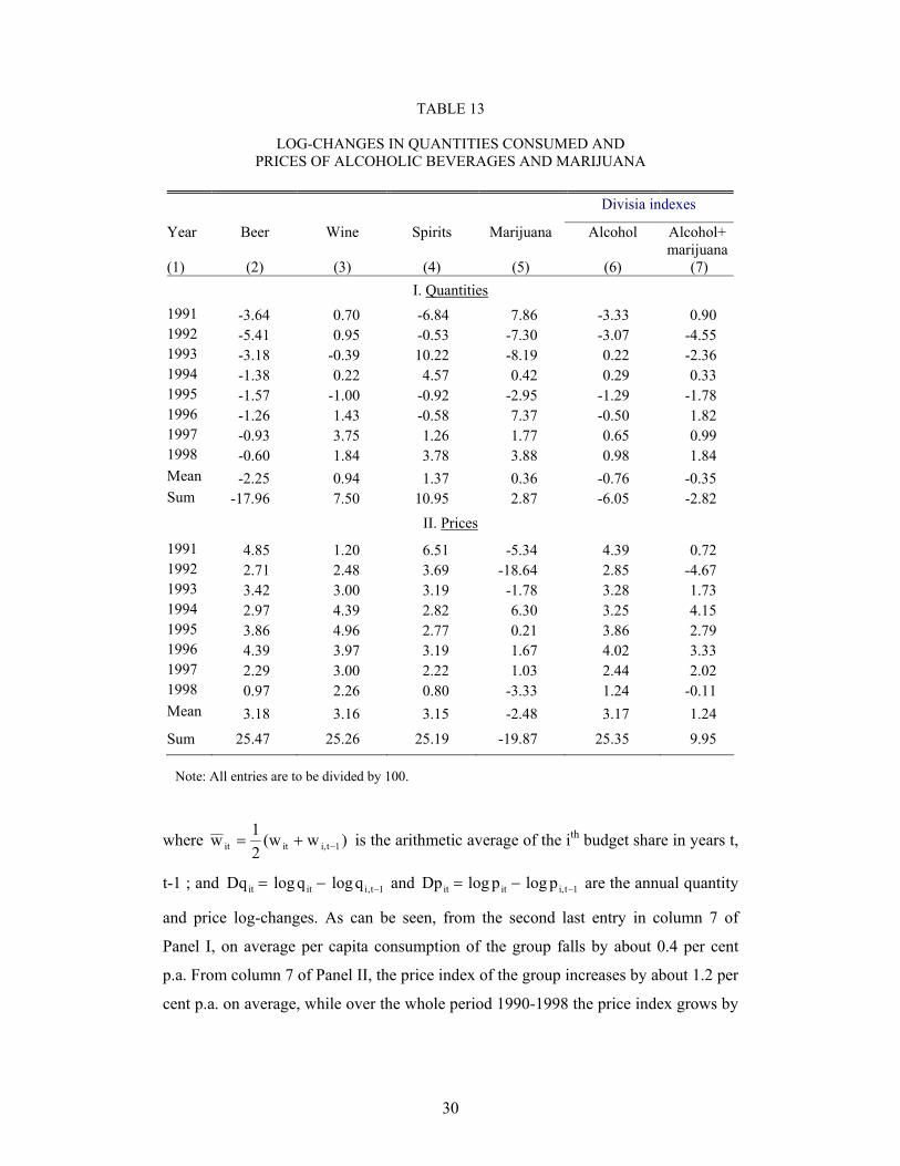
TABLE 13

LOG-CHANGES IN QUANTITIES CONSUMED AND PRICES OF ALCOHOLIC BEVERAGES AND MARIJUANA

Divisia indexes

Year (1)

Beer

(2)

Wine

(3)

Spirits

(4)

Marijuana

(5)

Alcohol

(6)

Alcohol+ marijuana

(7) I. Quantities

1991 -3.64 0.70 -6.84 7.86 -3.33 0.90 1992 -5.41 0.95 -0.53 -7.30 -3.07 -4.55 1993 -3.18 -0.39 10.22 -8.19 0.22 -2.36 1994 -1.38 0.22 4.57 0.42 0.29 0.33 1995 -1.57 -1.00 -0.92 -2.95 -1.29 -1.78 1996 -1.26 1.43 -0.58 7.37 -0.50 1.82 1997 -0.93 3.75 1.26 1.77 0.65 0.99 1998 -0.60 1.84 3.78 3.88 0.98 1.84 Mean -2.25 0.94 1.37 0.36 -0.76 -0.35 Sum -17.96 7.50 10.95 2.87 -6.05 -2.82

II. Prices

1991 4.85 1.20 6.51 -5.34 4.39 0.72 1992 2.71 2.48 3.69 -18.64 2.85 -4.67 1993 3.42 3.00 3.19 -1.78 3.28 1.73 1994 2.97 4.39 2.82 6.30 3.25 4.15 1995 3.86 4.96 2.77 0.21 3.86 2.79 1996 4.39 3.97 3.19 1.67 4.02 3.33 1997 2.29 3.00 2.22 1.03 2.44 2.02 1998 0.97 2.26 0.80 -3.33 1.24 -0.11 Mean 3.18 3.16 3.15 -2.48 3.17 1.24

Sum 25.47 25.26 25.19 -19.87 25.35 9.95

Note: All entries are to be divided by 100.

where )w(w21w 1ti,itit −+= is the arithmetic average of the ith budget share in years t,

t-1 ; and 1t,iitit qlogqlogDq −−= and 1ti,itit plogplogDp −−= are the annual quantity

and price log-changes. As can be seen, from the second last entry in column 7 of

Panel I, on average per capita consumption of the group falls by about 0.4 per cent

p.a. From column 7 of Panel II, the price index of the group increases by about 1.2 per

cent p.a. on average, while over the whole period 1990-1998 the price index grows by

31

10.0 per cent.14 Denoting the alcohol group by the subscript A, the within-alcohol

version of equation (5.3a) is

(5.3b) it

3

1i 4t

itAt Dq

w1w

DQ

∑

−

==

, it

3

1i 4t

itAt Dp

w1w

DP ∑

−

==

.

It follows from equation (5.3a) and (5.3b) that the two sets of indexes are related

according to 4t4tAt4tt Dqw)DQw(1DQ +−= , 4t4tAt4tt Dpw)DPw(1DP +−= . The

alcohol indexes are presented in column 6 of Table 13. According to the price index

for alcohol (Panel II, column 6), on average, the price of this group grew faster than

that of alcohol plus marijuana (column 7) as marijuana prices rise much slower (in

fact, they fall on average) than those of the three alcoholic beverages. Exactly the

opposite situation occurs with the volume indexes of the two groups, given in Panel I.

We are now in a position to evaluate equation (5.2b) for i = beer, wine, spirits

and marijuana. From the last entry in column 5 of Table 13, the log-change in the

price of marijuana over the whole period 1990-1998, α , is –19.87×10-2 . Regarding

the counter-factual trajectory of marijuana prices, we first assume that they were

constant over the period, so that 0p̂D 4 = . Using these values, together with the

elasticities involving marijuana prices, ηi4, given in the last column of Table 12, we

obtain the counter-factual quantity changes.

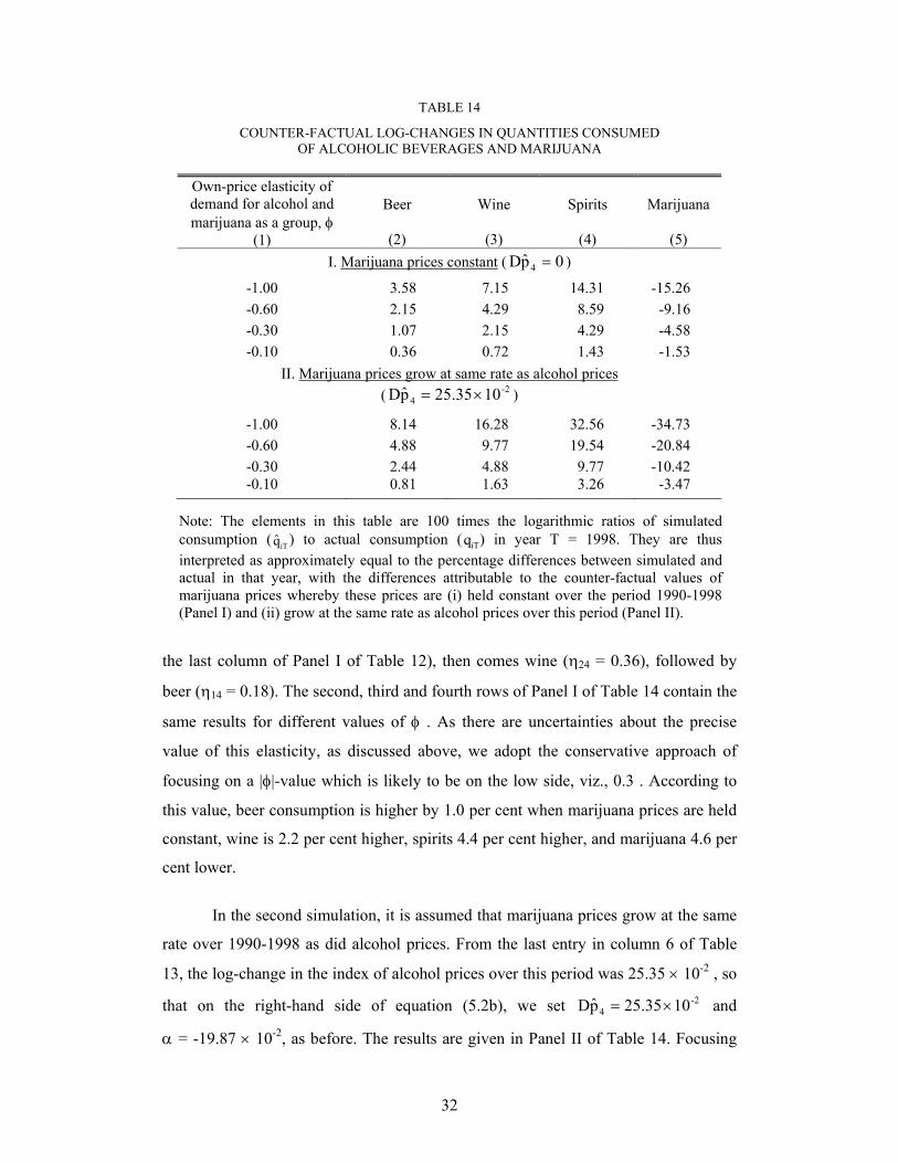
Panel I of Table 14 contains the results. According to the first row of this

panel, which is based on group price elasticity φ taking a value of –1.0 , if marijuana

prices had been constant over the whole period, rather than falling by about 20 per

cent, beer consumption in 1998 is simulated to be about 3.6 per cent higher than

actual, wine 7.2 per cent higher, spirits 14.3 per cent higher, and marijuana 15.3 per

cent lower. The differences among the three alcoholic beverages reflect the values of

their elasticities with respect to the price of marijuana. Spirits consumption increases

the most as it has the largest cross-price elasticities with η34 = 0.72 (from

14 Note that the log-change over the whole period is just the sum of the component annual log-changes. The see this, consider T positive numbers x1, …, xT. Then ∑ −=− = −

T2t 1tt1T ) xlog x(log xlog xlog , as

adjacent values in the sum cancel.

32

TABLE 14

COUNTER-FACTUAL LOG-CHANGES IN QUANTITIES CONSUMED OF ALCOHOLIC BEVERAGES AND MARIJUANA

Own-price elasticity of demand for alcohol and marijuana as a group, φ

(1)

Beer

(2)

Wine

(3)

Spirits

(4)

Marijuana

(5)

I. Marijuana prices constant ( 0p̂D 4 = )

-1.00 3.58 7.15 14.31 -15.26 -0.60 2.15 4.29 8.59 -9.16 -0.30 1.07 2.15 4.29 -4.58 -0.10 0.36 0.72 1.43 -1.53

II. Marijuana prices grow at same rate as alcohol prices ( -2

4 1025.35p̂D ×= )

-1.00 8.14 16.28 32.56 -34.73 -0.60 4.88 9.77 19.54 -20.84 -0.30 2.44 4.88 9.77 -10.42 -0.10 0.81 1.63 3.26 -3.47

Note: The elements in this table are 100 times the logarithmic ratios of simulated consumption ( iTq̂ ) to actual consumption ( iTq ) in year T = 1998. They are thus interpreted as approximately equal to the percentage differences between simulated and actual in that year, with the differences attributable to the counter-factual values of marijuana prices whereby these prices are (i) held constant over the period 1990-1998 (Panel I) and (ii) grow at the same rate as alcohol prices over this period (Panel II).

the last column of Panel I of Table 12), then comes wine (η24 = 0.36), followed by

beer (η14 = 0.18). The second, third and fourth rows of Panel I of Table 14 contain the

same results for different values of φ . As there are uncertainties about the precise

value of this elasticity, as discussed above, we adopt the conservative approach of

focusing on a |φ|-value which is likely to be on the low side, viz., 0.3 . According to

this value, beer consumption is higher by 1.0 per cent when marijuana prices are held

constant, wine is 2.2 per cent higher, spirits 4.4 per cent higher, and marijuana 4.6 per

cent lower.

In the second simulation, it is assumed that marijuana prices grow at the same

rate over 1990-1998 as did alcohol prices. From the last entry in column 6 of Table

13, the log-change in the index of alcohol prices over this period was 25.35 × 10-2 , so

that on the right-hand side of equation (5.2b), we set -24 1025.35p̂D ×= and

α = -19.87 × 10-2, as before. The results are given in Panel II of Table 14. Focusing

33

again on the case where φ = -0.3 , it can be seen that when the alcohol: marijuana

relative price is held constant, beer consumption is 2.4 per cent higher than actual in

1998, wine 4.9 per cent higher, spirits 9.8 per cent higher, and marijuana consumption

is 10.4 per cent lower. While these differences are not huge, there are still far from

trivial and demonstrate clearly the interrelationships between alcohol and marijuana

prices.15

6. Concluding Comments

This paper has identified a substantial decline in the relative price of marijuana

over the 1990s, discussed the possible causes and analysed some of the implications.

We also investigated some regional dimensions of the market for marijuana. Rather

than reiterating the findings, we comment briefly on some of their broader

implications:

• By their very nature, illicit goods and services are excluded from official

statistics. If the prices of other illicit activities have fallen as much as that of

marijuana, the CPI will be overstated, and real incomes and productivity

measures will be understated.

• Further studies of illicit sectors of the economy could be rewarding in

understanding how incentives operate to encourage the adoption of new

technology. This may provide some guidance regarding appropriate policies to

boost productivity in legal activities, and in the identification of impediments to

the introduction of technological improvements.

• Our analysis indicates that the lower price of marijuana is likely to have

reduced consumption of a substitute product, alcohol. In some scenarios, this

reduction is substantial. Producers of beer, wine and spirits may thus be

tempted to argue that on the basis of considerations of competitive neutrality,

15 Note that it follows from equations (5.2a) and (5.2b) that the elements of Table 14 are also interpreted as ii Dqq̂D − , the difference between )/qq̂( log i1iT and )/q(q log i1iT . Accordingly, we can compute iq̂D by simply adding the relevant entry in Table 14 to iDq .

34

marijuana production should be legalised and subject to the same hefty taxes as

they are.

• Suppose marijuana were legalised and its production taxed. Who would bear

most of the burden of this tax -- growers or consumers? In view of the apparent

ease with which marijuana can now be grown with hydroponic techniques and

because demand is almost surely price inelastic, it would be consumers who

would bear the bulk of the incidence of the tax, not growers. In such a case,

maybe the incentives for growers to continue to innovate would remain more or

less unchanged in a legalised regime.

35

REFERENCES Asher, C. J. and D. G. Edwards (1981). Hydroponics for Beginners. St Lucia:

Department of Agriculture, University of Queensland. Ashley’s Sister (1997). The Marijuana Hydroponic Handbook. Carlton South:

Waterfall. Australian Bureau of Criminal Intelligence (1996). Australian Illicit Drug Report

1995-1996. Canberra: ABCI. Australian Bureau of Criminal Intelligence (1998). Australian Illicit Drug Report

1998-1999. Australian Bureau of Criminal Intelligence (1999). Australian Illicit Drug Report

1997-1998. Canberra: ABCI. Australian Bureau of Criminal Intelligence (2000). Australian Illicit Drug Report

1999-2000. Barten, A. P. (1977). “The Systems of Consumer Demand Functions Approach: A

Review.” Econometrica 45: 23-51. Basov, S., M. Jacobson and J. Miron (2001). “Prohibition and the Market for Illegal

Drugs: An Overview of Recent History.” World Economics 2: 133-57. Berndt, E. R. and N. J. Rappaport (2001). “Price and Quality of Desktop and Mobile

Personal Computers: A Quarter-Century Historical Overview.” American Economic Review 91: 268-73.

Brown, G. F. and L. P. Silverman (1974). “The Retail Price of Heroin: Estimation and Applications.” Journal of the American Statistical Association 69: 595-606.

Cameron, L. and J. Williams (2001). “Cannabis, Alcohol and Cigarettes: Substitutes or Complements?” Economic Record 77: 19-34.

Caulkins, J. P. and R. Padman (1993). “Quantity Discounts and Quality Premia for Illicit Drugs.” Journal of the American Statistical Association 88: 748-57.

Chaloupka, F. and A. Laixuthai (1997). “Do Youths Substitute Alcohol and Marijuana? Some Econometric Evidence.” Eastern Economic Journal 23: 253-76.

Clements, K. W. (1987). “The Demand for Groups of Goods and Conditional Demand.” Chapter 4 in H. Theil and K. W. Clements Applied Demand Analysis: Results from System-Wide Approaches. Cambridge, Massachusetts: Ballinger. Pp. 163-84.

Clements, K. W. (2002). “Three Facts about Marijuana Prices.” Discussion Paper No 02.10, Department of Economics, The University of Western Australia.

Clements, K. W. and M. Daryal (2001). “Marijuana Prices in Australia in the 1990s.” Discussion Paper No 01.01, Department of Economics, The University of Western Australia.

Clements, K. W. and M. Daryal (2003). “The Economics of Marijuana Consumption.” In E. A. Selvanathan and S. Selvanathan (eds) The Demand for Alcohol, Tobacco, Marijuana and Other Evils, London: Ashgate, forthcoming.

Clements, K. W., S. Selvanathan and E. A. Selvanathan (1995). “The Economic Theory of the Consumer.” Chapter 1 in E. A. Selvanathan and K. W. Clements (eds) Recent Developments in Applied Demand Analysis: Alcohol, Advertising and Global Consumption. Berlin: Springer Verlag. Pp. 1-72.

Clements, K. W., W. Yang and S. W. Zheng (1997). “Is Utility Additive? The Case of Alcohol.” Applied Economics 29: 1163-67.

DiNardo, J. (1993). “Law Enforcement, the Price of Cocaine and Cocaine Use.” Mathematical and Computer Modeling 17: 53-64.

DiNardo, J. and T. Lemieux (1992). “Alcohol, Marijuana and American Youth: The Unintended Effects of Government Regulation.” Working Paper No. 4212, National Bureau of Economic Research.

36

Grilli, E. R. and M. C. Yang (1988). “Primary Commodity Prices, Manufactured Goods Prices, and the Terms of Trade of Developing Countries: What the Long Run Shows.” World Bank Economic Review 2: 1-47.

Miron, J. A. (1999). “The Effect of Alcohol Prohibition on Alcohol Consumption.” Unpublished paper, Department of Economics, Boston University.

Miron, J. A. (2003). “The Effects of Drug Prohibition on Drug Prices: Evidence from the Markets for Cocaine and Heroin.” Review of Economics and Statistics 85: 522-30.

Model, K. (1993). “The Effect of Marijuana Decriminalisation on Hospital Emergency Drug Episodes: 1975-1980.” Journal of the American Statistical Association 88: 737-47.

National Drug Strategy Household Survey (computer file, various issues). Canberra: Social Data Archives, The Australian National University.

Nordhaus, W. D. (1997). “Do Real-Output and Real-Wage Measures Capture Reality? The History of Lighting Suggests Not.” In T. F. Bresnahan and R. J. Gordon (eds) The Economics of New Goods. Chicago: The University of Chicago Press. Pp. 29-66.

Pacula, R. L. (1997). “Does Increasing the Beer Tax Reduce Marijuana Consumption?” Journal of Health Economics 17: 577-85.

Pacula, R. L. (1998). “Adolescent Alcohol and Marijuana Consumption: Is There Really a Gateway Effect?” Working Paper No. 6348, National Bureau of Economic Research.

Radio National (1999). “Adelaide -- Cannabis Capital.” Background Briefing 28 November. Transcript available at http: www.abc.net.au/rn/talks/bbing/stories/s69754.htm. Consulted 7 February 2000.

Saffer, H. and F. Chaloupka (1995). “The Demand for Illicit Drugs.” Working Paper No. 5238, National Bureau of Economic Research.

Saffer, H. and F. Chaloupka (1998). “Demographic Differentials in the Demand for Alcohol and Illicit Drugs.” Working Paper No. 6432, National Bureau of Economic Research.

Selvanathan, S. (1987). “A Monte Carlo Test of Preference Independence.” Economics Letters 25: 259-61.

Selvanathan, S. (1993). A System-Wide Analysis of International Consumption Patterns. Dordrecht: Kluwer Academic Publishers.

Stone, J. R. N. (1953). The Measurement of Consumer Expenditure and Behaviour in the United Kingdom, 1920-1938. Vol. 1. Cambridge: Cambridge University Press.

The Economist (2000/01). “The Price of Age.” December 23, 2000 to January 5, 2001. Pp. 91-94.

Thies, C. and F. Register (1993). “Decriminalisation of Marijuana and the Demand for Alcohol, Marijuana and Cocaine.” The Social Science Journal 30: 385-99.

Weatherburn, D. and B. Lind (1997). “The Impact of Law Enforcement Activity on a Heroin Market.” Addiction 92: 557-69.

Yuan, Y. and J. P. Caulkins (1998). “The Effect of Variation in High-Level Domestic Drug Enforcement on Variation in Drug Prices.” Socio-Economic Planning Sciences 32: 265-76.

Zhao, X. and M. N. Harris (2003). “Demand for Marijuana, Alcohol and Tobacco: Participation, Frequency and Cross-Equation Correlations.” Unpublished Paper, Department of Econometrics and Business Statistics, Monash University.