Embed Size (px)
Citation preview
University of ConnecticutOpenCommons@UConn
Doctoral Dissertations University of Connecticut Graduate School
6-21-2013
Three Essays on the Property Rights Theory of theFirmLeshui HeDepartment of Economics, [email protected]
Follow this and additional works at: https://opencommons.uconn.edu/dissertations
Recommended CitationHe, Leshui, "Three Essays on the Property Rights Theory of the Firm" (2013). Doctoral Dissertations. 160.https://opencommons.uconn.edu/dissertations/160
Three Essays on the Property RightsTheory of the Firm
Leshui He, Ph.D.
University of Connecticut, 2013
ABSTRACT
My dissertation research focuses on the efficiency of various governance struc-
tures using the basic framework of the Grossman-Hart-Moore (GHM) property rights
model. The first two chapters expand the GHM framework to describe a richer spec-
trum of governance structures—including not only fully integrated firms and fully
disintegrated market transactions but also asset-less firms and exclusive dealing be-
tween firms. The general framework combines the GHM model with a model of
bargaining control rights, yielding an allocation of ownership rights that may differ
from what the GHMmodel implies. The results are related to the general principles of
employment law. The third chapter offers a formal economic theory that analyzes the
differences between the subsidiary and the division as alternative governance struc-
tures of an internal business unit. Subsidiaries and divisions are widely observed as
alternative governance structures, and one does not seem to completely dominate the
other. Formal economic theory is almost silent on the topic of subsidiaries.
Three Essays on the Property RightsTheory of the Firm
Leshui He
M.A. Economics, University of Connecticut, 2012
B.S. Business Administration, Beihang University, 2006
A Dissertation
Submitted in Partial Fulfillment of the
Requirements for the Degree of
Doctor of Philosophy
at the
University of Connecticut
2013

Copyright by
Leshui He
2013
APPROVAL PAGE
Doctor of Philosophy Dissertation
Three Essays on the Property RightsTheory of the Firm
Presented by
Leshui He, B.S. Business Administration, M.A. Economics
Major AdvisorRichard N. Langlois
Co-ChairRobert Gibbons
Associate AdvisorChristian Zimmermann
Associate AdvisorVicki Knoblauch
University of Connecticut
2013
ii

ACKNOWLEDGMENTS
I am deeply indebted to my academic advisor, Richard N. Langlois, who intro-
duced me to the field of organizational economics. I benefited from countless hours of
discussion with him about research ideas, besides his generous help with my writing.
His encouragement and support pulled me through during the most difficult times in
my graduate study.
I am especially grateful to my co-chair, Robert Gibbons, for his generosity with
his time, advice and financial support. I am blessed with the privilege to study
with him and work at the Sloan School of Management. This incredible experience
transformed me from a student interested in the organizational topics to a dedicated
junior scholar.
I would also like to thank Vicki Knoblauch and Christian Zimmermann for their
help and comments as my dissertation committee members. I also thank Dennis
Heffley for being an exceptional mentor and teacher. I thank Steven P. Lanza for
his kindness and guidance toward my graduate assistant work. I am also grateful to
Daniel Barron, Hongyi Li, James Malcomson, Michael Powell and Birger Wernerfelt
for their help and comments.
I thank my parents, Ming He and Jinyun Zhao, and my grandparents, Ziyun He
and Sanxiang Fang, who raised me with nothing but love, hope and encouragement.
Finally, I thank my wife, Mengxi, and my lovely daughter, Miya, who endured
much loneliness during my work on this dissertation.
iii
Contents
Ch. 1. Beyond Asset Ownership: Employment and Asset-less Firmsin a Property-Rights Theory of the Firm 1
1.1 Introduction . . . . . . . . . . . . . . . . . . . . . . . . . . . . . . . . . . . 1
1.2 Related Literature . . . . . . . . . . . . . . . . . . . . . . . . . . . . . . . 6
1.3 A Model of Three Parties . . . . . . . . . . . . . . . . . . . . . . . . . . 91.3.1 Economic Environment . . . . . . . . . . . . . . . . . . . . . . . . 101.3.2 Interpreting Six Candidate Governance Structures . . . . . . . 19
1.4 A Parametrized Example . . . . . . . . . . . . . . . . . . . . . . . . . . 221.4.1 Model Setup . . . . . . . . . . . . . . . . . . . . . . . . . . . . . . 231.4.2 “Horse Races” Among Six Governance Structures . . . . . . . . 26
1.5 Analysis of the Model of Three Parties . . . . . . . . . . . . . . . . . . 341.5.1 ex post Bargaining Payoffs . . . . . . . . . . . . . . . . . . . . . . 351.5.2 ex ante Investment Incentives . . . . . . . . . . . . . . . . . . . . 40
1.6 Concluding Remarks . . . . . . . . . . . . . . . . . . . . . . . . . . . . . 49
1.A Omitted Proofs for Propositions in Section 1.3 . . . . . . . . . . . . . . 55
Ch. 2. Extensions of the Basic Framework: n Parties 57
2.1 Setup of the Model . . . . . . . . . . . . . . . . . . . . . . . . . . . . . . 58
2.2 Generalized Results . . . . . . . . . . . . . . . . . . . . . . . . . . . . . . 63
2.A Omitted Proofs for Propositions in Section 2.1 . . . . . . . . . . . . . . 69
2.B Omitted Statements and Proofs for the General n-Party Model . . . . 76
Ch. 3. Subsidiaries vs. Divisions in a Property-Rights Theory of theFirm 79
3.1 Introduction . . . . . . . . . . . . . . . . . . . . . . . . . . . . . . . . . . . 79
3.2 Discussion of Modeling Assumptions . . . . . . . . . . . . . . . . . . . . 82
iv
3.2.1 Legal Foundations . . . . . . . . . . . . . . . . . . . . . . . . . . . 823.2.2 Modeling Assumptions . . . . . . . . . . . . . . . . . . . . . . . . 85
3.3 Model Setup . . . . . . . . . . . . . . . . . . . . . . . . . . . . . . . . . . 86
3.4 The Analysis . . . . . . . . . . . . . . . . . . . . . . . . . . . . . . . . . . 933.4.1 Bargaining Payoffs at τ = 3 . . . . . . . . . . . . . . . . . . . . . 933.4.2 Takeover Bargaining Payoffs at τ = 2 . . . . . . . . . . . . . . . . 953.4.3 Expected Payoff Comparison at τ = 1: Subsidiaries vs. Divisions 973.4.4 Investment Levels . . . . . . . . . . . . . . . . . . . . . . . . . . . 98
3.5 Conclusion . . . . . . . . . . . . . . . . . . . . . . . . . . . . . . . . . . . 105
3.A Omitted Proofs . . . . . . . . . . . . . . . . . . . . . . . . . . . . . . . . 106
Bibliography 107
v
Chapter 1
Beyond Asset Ownership:Employment and Asset-less Firmsin a Property-Rights Theory of theFirm
1.1 Introduction
Although most firms own alienable assets, many firms do not. Professional-services
firms such as law firms, accounting firms, consulting firms, design firms and many
health care providers own few if any alienable assets. Instead, as Holmstrom and
Roberts (1998) and others have observed, such firms rely on inalienable human assets
that inhere in and move with the firm’s employees. On the other hand, a key feature
of the duly celebrated Grossman-Hart-Moore (GHM) theory of the firm (Grossman
and Hart, 1986; Hart and Moore, 1990; Hart, 1995) is the role of alienable assets in
explaining the boundaries of the firm. How then to explain asset-less firms?
1
2
This paper approaches the problem by embedding the GHM model within a larger
theoretical framework that can describe a richer spectrum of governance structures—
including not only fully integrated firms and fully disintegrated market transactions,
but also asset-less firms and exclusive dealing between firms. This larger framework
combines the GHM model of property rights with a model of bargaining control rights.
Different from the residual rights of control over alienable assets that is endowed
by asset ownership, bargaining control rights are institutional restrictions designed
and controlled by the upper level of the economic organization imposed to limit the
freedom to bargain of the lower-level parties. We find that the optimal governance
structure often involves not only allocating property rights, as in GHM, but also
restricting bargaining rights for some players. In some cases, we also find that the
optimal allocation of property rights differs from what the GHM model implies.
When we interpret the model at the level of individuals as opposed to the level of
business units, the paper shows that it can be efficient to prohibit employees within
one firm from side-contracting with each other. Furthermore, the model shows that
preventing other firms from side-contracting with one firm’s employees could also
improve efficiency. These results are consistent with what we observe in employment
law. An important benefit of our approach is a clear interpretation of the employment
relationship.
The GHM approach is close to silent on employment issues. For example, consider
a model with three parties and two assets, and suppose that the GHM analysis
prescribes non-integrated asset ownership as the optimal governance structure. Who,
then, does the third party (the one without an asset) work for, if anyone? This paper
enriches the GHM approach so as to answer this question.
The model assumes that all parties are free to bargain with all other parties,
3
unless a party has endogenously restricted bargaining rights resulting from the ex
ante institutional design. We interpret a party with unrestricted bargaining rights as
the owner of a firm (although that firm might consist of only that party, in the case
of self employment). If this party controls the bargaining rights of any other parties,
then the controlling party is the boss and the controlled parties are subordinates, such
as employees and divisions. That is, the bosses of the firms, are free to bargain with
their own subordinates. And the bosses are free to bargain with any other bosses.
However, the bosses of firms have bargaining control rights over their subordinates,
who are endogenously restricted to bargaining with only their employer.
Many observations about the business firm fit the characteristics of bargaining
control rights. When it comes to bargaining over decisions, the owner of the firm
bargains for the firm as a whole.1 She bargains, representing her employees, against
other business firms and customers. And she also bargains against her own employees,
representing the outside contractual relationships with other firms and customers.
The subordinates have very limited rights to bargain with anyone other than their
bosses. For simplicity, in this model, the boss can restrict its employees to bargain
only with the firm itself.2
To illustrate the model another way, the boss can block direct bargaining among
the employees themselves as well as bargaining between her employee and any outside
party in the transaction. For example, a grocer cannot deal with his favorite customer
if he does not work for the supermarket anymore. And the customer of the supermar-
1We quote from Holmstrom (1999): “One possible explanation is that ownership strengthens thefirm’s bargaining power vis-a-vis outsiders. Suppliers and other outsiders will have to deal with thefirm as a unit rather than as individual members... The general point though is that institutionalaffiliation, and not just asset allocation, can significantly influence the nature of bargaining.”
2All qualitative results of the model still hold when this modeling assumption is relaxed. Whatthe model needs is that the boss can at least block some bargaining between the subordinate andany third party. See more discussion on robustness in Section 1.6.
4
ket cannot obtain services from her favorite grocer without shopping at the market he
works for, which she might dislike. As another example, non-compete clauses in em-
ployment contracts are ex ante voluntarily engaged restriction over ex post bargaining
freedom. They are a reinforced and explicit form of bargaining control. Although
non-compete clauses present issues regarding enforcement, they are still frequently
observed in employment contracts between the firm and its critical employees. For
example, Kaplan and Stromberg (2003) document that it is common—more than 70%
of contracts in their sample—for venture capital firms to use non-complete clauses.
Why do we interpret those unrestricted parties as bosses and those restricted as
employees? There are at least two factors that give the firm the advantage of bar-
gaining control rights over employees, divisions and other internal entities. First,
firms are legal persons in business contracts, whereas employees or divisions are not
(Iacobucci and Triantis, 2007; Hansmann and Kraakman, 2000). With very few ex-
ceptions, all employees bargain with their employer over their employment contracts.
In stark contrast, most employees do not participate directly in bargaining with other
employees and with other outsiders. When they do, they bargain on behalf of their
employer firm for the contract, not on behalf of themselves.
Second, it is a stylized fact that side contracts between employees within a firm
or between an employee and other outsiders are rarely permitted in firms. Employees
are forbidden, and rarely observed, to formally side-contract among themselves, such
as to game the incentive systems of their employer. First, although employees are free
to leave the firm, firms tend to implement the bargaining control rights by committing
not to frequently renegotiate their employment contracts. Second, according to the
employment laws, employees have a fiduciary duty to act in the best interest of their
employer. So side-contracting among employees or between an employee and an
5
outside party also tends to violate this legal restriction.
Bargaining control rights are not exclusive to the hierarchical structure within a
firm. When we interpret the parties in the model at the level of business units, the
parties whose bargaining rights are restricted are interpreted differently depending
on their ownership of assets. If they do not own any asset, they are interpreted as
internal business units within a firm, such as divisions or subsidiaries. If they own
assets, then they are interpreted as firms under exclusive dealing contract with those
firms who have bargaining control over them.
Similar to our modeling assumption, Segal and Whinston (2000) also consider
bargaining control rights as designed instruments to govern transactions. Focusing
their interpretation at the business unit level, Segal and Whinston (2000) characterize
exclusive contracts as restricted bargaining rights between a seller-buyer relationship.
The current model shares the common characteristic with their work in that we both
emphasize the role of bargaining rights as a special instrument in the governance
structure different from regular asset ownership. But this paper departs from theirs in
two aspects. First, we consider the effect of bargaining control rights simultaneously
with that of asset ownership, whereas they focus on studying bargaining control
rights given fixed asset ownership structure. Segal and Whinston (2000) discuss the
conditions under which exclusive dealing is more efficient than non-integration. In
particular, they found that if one trading party’s investment has very high marginal
product, it is efficient for her to control the other firm through an exclusive dealing
contract. However, they do not explore whether exclusive dealing can still be efficient
if this firm can simply integrate the other. In other words, can exclusive dealing be
more efficient than both non-integration and integration? My paper explores this
question by considering bargaining control rights together with allocation of asset
6
ownership. My model shows that exclusive dealing can indeed be more efficient than
both integration and non-integration. Second, we generalize their interpretation of
bargaining control rights beyond the exclusive dealing contracts to associate with the
boss-subordinate relationship, which consequently provides an interpretation of asset-
less firms. To some extent, one can also see the current paper as a generalization of
Segal and Whinston (2000) that applies to the boundaries of the firm problem with
asset allocation.
The paper proceeds as follows. Section 1.2 reviews some of the most related
literature to highlight the paper’s contributions. Section 1.3 describes the setup of
the model as well as the rules of interpretation under the three-party case.3 Section 1.4
provides an example to highlight the most important findings of the model. Section
1.5 provides an analysis of the three-party model and offers propositions that explain
the observed patterns in the example. Section 1.6 concludes.
1.2 Related Literature
Our model shares the spirit of the subeconomy theory of the firm (Holmstrom and
Milgrom, 1991; Holmstrom, 1999). In their works, the firm can use various incentive
instruments for their employees to selectively isolate those employees from undesirable
activities. In Holmstrom and Milgrom (1991), the principal can choose a set of
allowable tasks for the agent. In Holmstrom (1999), the firm can “regulate trade
within a firm” as a subeconomy in the sense that the principle is able to set rules over
different activities of its employees, such as working from home. We do not study
3Because the key ingredient of the bargaining control rights is the ability of one party to bargainwith a third party without going through the second one, the model operates with at least threeparties.
7
the problem with a contracting approach, nor do we emphasize the information or
measurement problem in organizations as they do. Instead, we analyze a structure
that allows the firm to isolate outsiders and its employees from each other.
Rajan and Zingales (1998) is also a theory of the boundaries of the firm that does
not rely on the ownership of assets and that sees the firm as a hierarchical structure.
Assuming that the owner of the firm is fixed, Rajan and Zingales (1998) focus on
the allocation of ex ante contractible access to the productive resource controlled by
the owner. Those agents granted access become employees of the firm and those who
do not have access are interpreted as outsiders. The present paper is different in
several respects. First, I emphasize different characteristics of the firm. The model
emphasizes the ability for the firm to bargain as a whole vis-a-vis different parties, not
the right to grant or deny the access to the resources that are under the firm’s control.
Second, in their model, the identity of the party who controls the firm, as well as the
ownership of the critical productive asset, are exogenous and fixed. By contrast, one
of the major purposes of this model is precisely to answer these two questions: who
should control the firm and who should own which assets? The answers to these two
questions are the core endogenous results of the model. Third, their original model
has only one focal firm, i.e., the firm except for the possible outside contractors. By
contrast, the present model allows the number of firms involved in the transaction to
be a fully endogenous choice; with a model of more than three parties, we can have
multiple firms with subordinates. Although a simple extension of their model with
multiple critical assets can also model an environment with multiple firms involved in
the transaction, this feature is always exogenously fixed at the number of parties who
control the critical assets. Fourth, We interpret the hierarchical structure differently.
Their work interprets the party who gives out access as the boss, those who receive
8
access as the subordinates, and those who do not receive access as the outsiders. This
model interprets those who can freely bargain as the bosses, those who cannot freely
bargain as the subordinates.
There have been studies of the GHM model with alternative bargaining solutions.
Most importantly, de Meza and Lockwood (1998) consider alternating-offer bargain-
ing in place of the Shapley value used in GHM.4 The main purpose of their paper is
to evaluate the robustness of the results in GHM when the model adopts a different
bargaining solution. Instead of replacing the bargaining solution of Shapley value in
GHM, our paper adopts a more general bargaining game which makes GHM a spe-
cial case in our framework. And, more importantly, we use the generalized bargaining
network to model an additional governance structure other than asset ownership. For
this reason, our model is more closely related to Segal and Whinston (2000) than to
de Meza and Lockwood (1998).
de Fontenay and Gans (2005) and Kranton and Minehart (2000) are similar to
this paper in that they both study vertical integration and networks. de Fontenay
and Gans (2005) adopt the GHM framework to compare outcomes under upstream
competition and monopoly. Both de Fontenay and Gans (2005) and the current paper
study integrations and both involve endogenous incomplete bargaining networks. The
main difference is that I focus on analyzing governance structures with asset allocation
in one given transaction that involves at least three parties. Whereas they study
governance structures involving pairs of upstream and downstream parties across
multiple such pairwise transactions without asset allocation. Most importantly, the
network in our model represents status in the hierarchy, i.e. whether a party is free to
4The generalized Nash bargaining solution with equal bargaining power under the two-party caseis a special case of the Shapley value.
9
bargain in the market as a firm or is restricted to bargain as a subordinate. However,
in de Fontenay and Gans (2005), the network represents the various transaction flows
across different pairs of upstream and downstream players.
Kranton and Minehart (2000) studies the tradeoff between a vertically integrated
transaction versus a network of supplier relationships in an environment with special-
ization and individual demand shocks. Their network is different from mine in that
it describes a supply structure involving, mostly, one buyer and multiple competing
suppliers with uncertainty, whereas my network describes a chain of jointly producing
parties without competition or uncertainty.
Our work is the first formal model that study asset-less firms and exclusive dealing
contracts side-by-side with classical integrated and non-integrated firms in economic
theory of the firm. Other economic theories of the asset-less firms, such as Dow (1993),
offer specialized models of this particular type of organization and do not consider
integration between firms. Hansmann (1988) offers a conceptual framework to study
a broad scope of various firm structures, but it does not consider asset ownership.
1.3 A Model of Three Parties
In this section, we introduce the modeling framework with a three-party model. It
illustrates all the key ingredients of the general model and delivers most (but not all)
of the results. 5
5See Section 2.1 the setup and results of a general model with any number of players and anynumber of assets.
10
1.3.1 Economic Environment
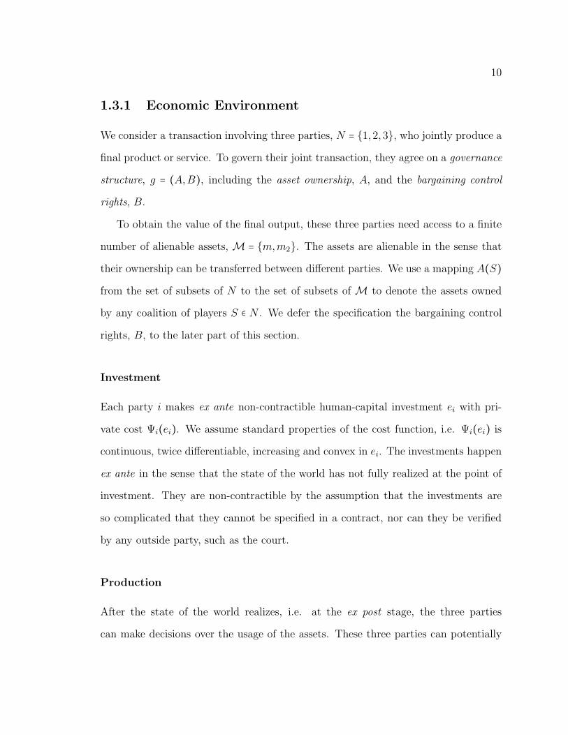
We consider a transaction involving three parties, N = 1,2,3, who jointly produce a
final product or service. To govern their joint transaction, they agree on a governance
structure, g = (A,B), including the asset ownership, A, and the bargaining control
rights, B.
To obtain the value of the final output, these three parties need access to a finite
number of alienable assets, M = m,m2. The assets are alienable in the sense that
their ownership can be transferred between different parties. We use a mapping A(S)from the set of subsets of N to the set of subsets of M to denote the assets owned
by any coalition of players S ∈ N . We defer the specification the bargaining control
rights, B, to the later part of this section.
Investment
Each party i makes ex ante non-contractible human-capital investment ei with pri-
vate cost Ψi(ei). We assume standard properties of the cost function, i.e. Ψi(ei) iscontinuous, twice differentiable, increasing and convex in ei. The investments happen
ex ante in the sense that the state of the world has not fully realized at the point of
investment. They are non-contractible by the assumption that the investments are
so complicated that they cannot be specified in a contract, nor can they be verified
by any outside party, such as the court.
Production
After the state of the world realizes, i.e. at the ex post stage, the three parties
can make decisions over the usage of the assets. These three parties can potentially
11
produce in different coalitions among themselves. Specifically, any coalition S ⊆ Ncan produce a value vS. For instance, 1 and 2 might decide to produce together
without 3, which will generate a value of v12. For these three parties, there are seven
production possibilities in total, including v123, v12, v13, v23, v1, v2 and v3.
The value that any coalition S can produce, vS(e,A) is determined jointly by the
vector of ex ante investments e and the asset owned by players in S. It is important to
remark that the production function vS(e,A) may depends on investment of parties
who are not in S. This feature is called cross-investment, in the sense that one
party’s investment also benefit other parties’ productions. As an example of cross-
investment, a firm’s investment in R&D is likely to accumulate valuable experiences
for the engineers and scientists. If these experiences are not entirely specific to the
investor firm, then these investments increase the value of production for the engineers
and scientists even if they do not work with the investor firm.6 Our analysis in later
sections shows that cross-investment is critical for the bargaining control rights to be
efficient.
Following Hart and Moore (1990), we assume the following properties for the
value functions vS(e,A). (i) Given asset allocation A, vS(e,A) is non-decreasing,
continuous, twice differentiable and concave in ei, for any i ∈ N . Moreover, an empty
coalition produces nothing, v∅(e,A) = 0. (ii) Assets are complementary to the in-
vestments. That is ∂vS(e,A′)
∂ei< ∂vS(e,A)
∂eiif A′(S) ⊂ A(S) (iii) The investments are weak
strategic complements, i.e.∂v2
S(e,A)
∂ei∂ej≥ 0 for i ≠ j. (iv) To make sure the problem
6These following two examples are provided in Che and Hausch (1999): Nishiguchi (1994) p.138reports that suppliers “send engineers to work with automakers in design and production. They playinnovative roles in ... gathering information about the automakers’ long-term product strategies.”After Honda chose Donnelly Corporation as its sole supplier of mirrors for its U.S.-manufactured
cars, “Honda sent engineers swarming over the two Donnelly plants, scrutinizing the operations forkinks in the flow. Honda hopes Donnelly will reduce costs about 2% a year, with the two companiessplitting the savings” (Magnet, 1994).
12
is interesting, we assume that, other things equal, the value of production is super-
additive. That is, any two coalitions produce a smaller total value than they could
if they were producing as a joint coalition.7 Specifically, given investment level e,
vS′(e,A) + vS/S′(e,A) < vS(e,A) for any S′ ⊂ S. To economize on notation, whenever
the investment level e and asset ownership A is fixed, we write vS = vS(e,A).As a result of the bargaining structure we adopt, the players always reaches ex
post efficient renegotiation result.8 Therefore under assumption (iv), only the grand-
coalition production v123 will be produced at the final stage. However, each party can
use other production possibilities vS as outside options to deviate a bigger share of
the total payoff v123 toward herself during the bargaining.
Bargaining with Incomplete Networks
We apply the Myerson-Shapley value (Myerson, 1977), or Myerson value, to charac-
terize the payoff for each party from the joint production. Myerson shows that this
solution generalizes the Shapley value to bargaining in incomplete networks, in two
senses: (i) the Myerson value equals the Shapley value when the bargaining network
is complete; and (ii) the Myerson value is the unique solution satisfying axioms akin
to those that produce the Shapley value.
In terms of rights to bargain, we require each party to be one of two types. A
party is either restricted to bargain—she is restricted to bargain with one and only
7This is a somewhat restrictive assumption. If it does not hold, there is no benefit for theseparties to produce together, so the problem is no longer interesting. In fact, this is an maintainedassumption in almost the entire literature of property rights theory.
8Grossman and Hart (1986) assumes Nash bargaining solution, which delivers efficient bargainingex post. Here in this model, we adopt the Myerson value which allows for incomplete bargainingnetworks. But since the network is always connected under the grand coalition (a result of the waywe construct the network, see Section 2.1), the ex post bargaining is still always efficient.
13
one other party. Or the party is free to bargain—she can bargain with the other two
parties.9
The requirement that each party has to be restricted to bargain or free to bar-
gain implies that the bargaining networks that we consider have to be connected.10
We use i ∶ j to denote the bargaining link between any two parties i and j. A
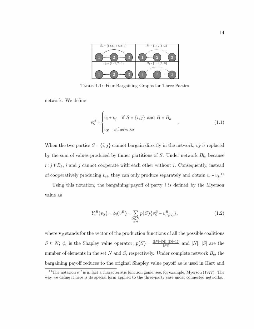
bargaining network is a set of bargaining links. For three parties, there are four
possible connected bargaining networks (Table 1.1). There is one complete network,
Bc = 1 ∶ 2,1 ∶ 3,2 ∶ 3, in which each party is free to bargain, they can form any coali-
tions to jointly produce. And there are three incomplete networks, Bi = i ∶ j, i ∶ k fori, j, k ∈ N and i ≠ j ≠ k. In these networks, party i is the only “connecting” party who
can bargain with the other two. In a model with only three parties, we will sometimes
refer to party i as the nexus because of i’s central position in the network. We will
also say party i has bargaining control over party j if j is restricted to bargain with
i. The key implication of the incomplete bargaining network is ruling out coalition
between j and k. In Bi, j and k cannot bargain with each other without i. So j and
k are not able to form coalition to produce vjk together without the participation of
party i.
This following definition is the key for us to model the incomplete bargaining
9In a model with more than three parties, we require that the free-to-bargain party needs tobe able to bargain with at least two parties, and, moreover, all free-to-bargain parties are able tobargain with each and everyone of themselves. Within a three-party model, it is equivalent to thegeneral definition to be able to bargain with the other two parties.
10See Section 2.1 for the proof in an N party model.
14
Bc = 1 ∶ 2,1 ∶ 3,2 ∶ 3 B1 = 1 ∶ 2,1 ∶ 3
1 2 3 1 2 3B2 = 1 ∶ 2,2 ∶ 3 B3 = 1 ∶ 3,2 ∶ 3
1 2 3 1 2 3
Table 1.1: Four Bargaining Graphs for Three Parties
network. We define
vBS =⎧⎪⎪⎪⎪⎪⎨⎪⎪⎪⎪⎪⎩
vi + vj if S = i, j and B = Bk
vS otherwise
. (1.1)
When the two parties S = i, j cannot bargain directly in the network, vS is replaced
by the sum of values produced by finner partitions of S. Under network Bk, because
i ∶ j ∉ Bk, i and j cannot cooperate with each other without i. Consequently, instead
of cooperatively producing vij , they can only produce separately and obtain vi + vj .11
Using this notation, the bargaining payoff of party i is defined by the Myerson
value as
Y Bi (vS) = φi(vB) = ∑
S⊆NS∋i
p(S)vBS − vBS/i, (1.2)
where vS stands for the vector of the production functions of all the possible coalitions
S ⊆ N ; φi is the Shapley value operator; p(S) = (∣N ∣−∣S∣)!(∣S∣−1)!∣N ∣! and ∣N ∣, ∣S∣ are the
number of elements in the set N and S, respectively. Under complete network Bc, the
bargaining payoff reduces to the original Shapley value payoff as is used in Hart and
11The notation vB is in fact a characteristic function game, see, for example, Myerson (1977). Theway we define it here is its special form applied to the three-party case under connected networks.
15
Moore (1990). This feature allows us to compare the implications of the incomplete
bargaining network with the benchmark of their original model.
Governance Structure
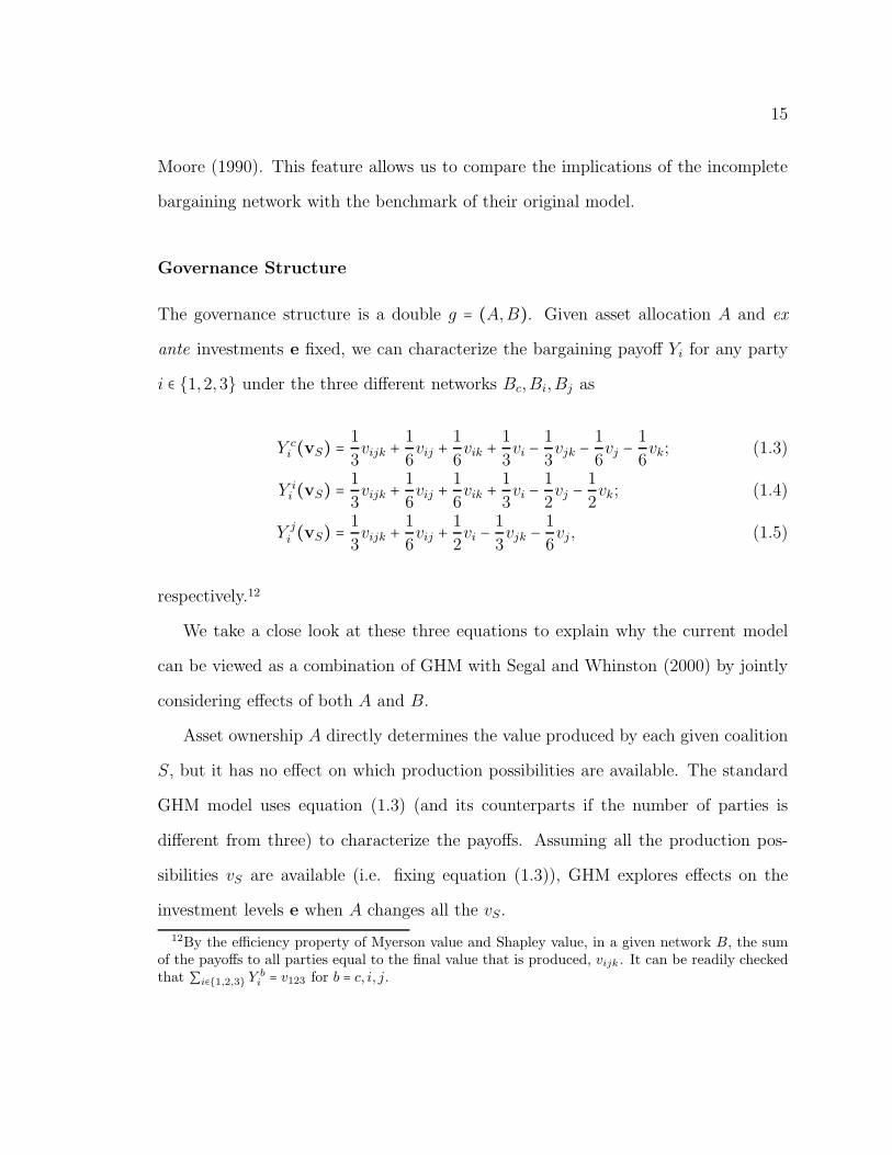
The governance structure is a double g = (A,B). Given asset allocation A and ex
ante investments e fixed, we can characterize the bargaining payoff Yi for any party
i ∈ 1,2,3 under the three different networks Bc,Bi,Bj as
Y ci (vS) =
1
3vijk +
1
6vij +
1
6vik +
1
3vi −
1
3vjk −
1
6vj −
1
6vk; (1.3)
Y ii (vS) = 1
3vijk + 1
6vij + 1
6vik + 1
3vi − 1
2vj − 1
2vk; (1.4)
Yji (vS) = 1
3vijk + 1
6vij + 1
2vi − 1
3vjk − 1
6vj , (1.5)
respectively.12
We take a close look at these three equations to explain why the current model
can be viewed as a combination of GHM with Segal and Whinston (2000) by jointly
considering effects of both A and B.
Asset ownership A directly determines the value produced by each given coalition
S, but it has no effect on which production possibilities are available. The standard
GHM model uses equation (1.3) (and its counterparts if the number of parties is
different from three) to characterize the payoffs. Assuming all the production pos-
sibilities vS are available (i.e. fixing equation (1.3)), GHM explores effects on the
investment levels e when A changes all the vS.
12By the efficiency property of Myerson value and Shapley value, in a given network B, the sumof the payoffs to all parties equal to the final value that is produced, vijk . It can be readily checkedthat ∑i∈1,2,3 Y
bi = v123 for b = c, i, j.
16
The bargaining network B has no direct effect on the values produced by each
coalition. But it determines whether a particular coalition is able to pursue joint
production. For example, v23 can be produced under Bc,B2,B3, but not under B1.
B determines which payoff function among equations (1.3) through (1.5) determines
party i’s bargaining payoff. Segal and Whinston (2000) can be viewed as a model
analyzing the effects of the bargaining network B by comparing equation (1.3) with
equations (1.4) and (1.5), assuming A is fixed.
Timing
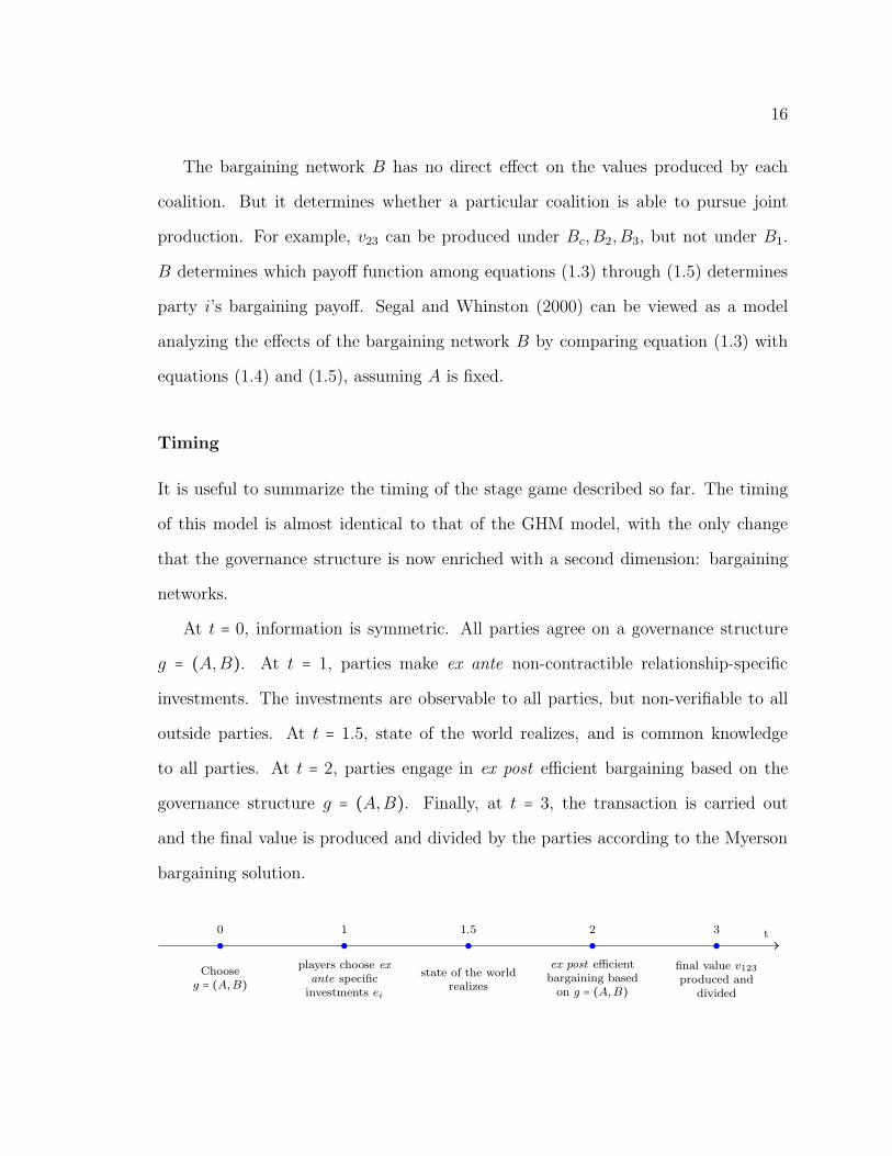
It is useful to summarize the timing of the stage game described so far. The timing
of this model is almost identical to that of the GHM model, with the only change
that the governance structure is now enriched with a second dimension: bargaining
networks.
At t = 0, information is symmetric. All parties agree on a governance structure
g = (A,B). At t = 1, parties make ex ante non-contractible relationship-specific
investments. The investments are observable to all parties, but non-verifiable to all
outside parties. At t = 1.5, state of the world realizes, and is common knowledge
to all parties. At t = 2, parties engage in ex post efficient bargaining based on the
governance structure g = (A,B). Finally, at t = 3, the transaction is carried out
and the final value is produced and divided by the parties according to the Myerson
bargaining solution.
t0 1 1.5 2 3
Chooseg = (A,B)
players choose ex
ante specificinvestments ei
state of the worldrealizes
ex post efficientbargaining basedon g = (A,B)
final value v123produced and
divided
17
Similar to almost all other property rights models, the only inefficiency in this
model rises from the ex ante investment stage. Because parties maximize their in-
dividual bargaining returns instead of the joint return of the entire transaction, the
presence of such externality biases their investment levels away from the first-best.
The governance structure affects the efficiency of the transaction because the ex ante
agreed governance structure determines the outcome of the ex post bargaining return
for each individual, and thus it in turn governs each parties’ investment decision ex
ante. The most efficient governance structure is the one associated with the invest-
ments that delivers highest level of final product net of the costs of investments.
An Example of Six Governance Structures
In the remaining part of this section, we present the model in its simplest form
by focusing on a limited types of asset ownership and bargaining networks. Without
losing much generality, these simplifications allow us to focus on several representative
governance structures by ruling out many economically identical ones. Neither the
modeling framework nor the propositions that follow in the analysis section hinge on
these restrictions. We only put them in place to help demonstrate the key features
of the model.
In this example, we suppose that parties 2 and 3 are identical in production
technologies and costs. This assumption rules out all the governance structures where
party 3 owns either asset(s) or has bargaining control, because these structures are
economically identical to the ones where party 2 is in the same position.
In terms of asset ownership, A, we choose to follow the tradition of most appli-
cations of the GHM models to focus on the two cases that are most closely related
18
to empirical works: the integrated asset ownership case, in which the assets are col-
lectively owned and the non-integrated asset ownership case, in which the assets are
separately owned. To evaluate these two cases, we assume that there are only two
productive alienable assets, m and m2. As a normalization, we shall always assign
ownership of m2 to party 2 but choose between allocating ownership of m to either
party 1 or party 2. We will then denote these two cases by A = AN for non-integrated
asset ownership, i.e. if 1 owns m. And we denote A = AI for integrated asset owner-
ship, i.e. if 2 owns m.13
Without loss of generality, our model only considers connected bargaining net-
works. Because the bargaining control rights are institutional restrictions on the
ability to bargain, rather than technological difficulties that fundamentally block
communication among parties, the three parties can always eventually reach agree-
ments together. As 2 and 3 are identical, we will rule out B3 and only consider three
possible candidates for the optimal bargaining network: the original GHM complete
bargaining network Bc and the incomplete bargaining networks B1 and B2, in which
party 1 or party 2 has bargaining control rights, respectively.
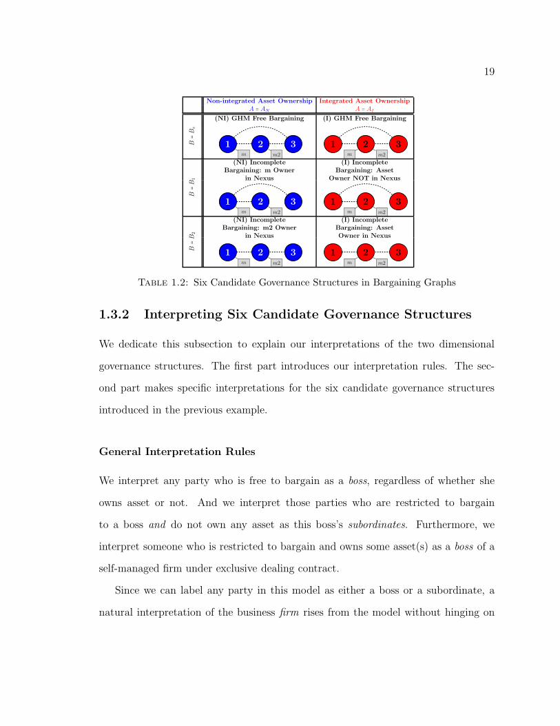
The simplest model is thus a choice over 6 candidate governance structures, g ∈AN ,AI×Bc,B1,B2. And they are presented graphically in Table 1.2. In these
graphs, the dashed lines represents the bargaining links, which indicates the ability
for any two parties to bargain with each other.
13These assumptions reduce the problem of choosing the correspondence A to a binary choice.Formally, in this case, A ∈ AN ,AI, where AN(1) = m,AN(2) = m2, and AI(1) =∅,AI(2) = m,m2.
19
Non-integrated Asset Ownership Integrated Asset OwnershipA = AN A = AI
B=B
c
(NI) GHM Free Bargaining (I) GHM Free Bargaining
1 2 3m m2
1 2 3m m2
B=B
1
(NI) IncompleteBargaining: m Owner
in Nexus
(I) IncompleteBargaining: Asset
Owner NOT in Nexus
1 2 3m m2
1 2 3m m2
B=B
2
(NI) IncompleteBargaining: m2 Owner
in Nexus
(I) IncompleteBargaining: AssetOwner in Nexus
1 2 3m m2
1 2 3m m2
Table 1.2: Six Candidate Governance Structures in Bargaining Graphs
1.3.2 Interpreting Six Candidate Governance Structures
We dedicate this subsection to explain our interpretations of the two dimensional
governance structures. The first part introduces our interpretation rules. The sec-
ond part makes specific interpretations for the six candidate governance structures
introduced in the previous example.
General Interpretation Rules
We interpret any party who is free to bargain as a boss, regardless of whether she
owns asset or not. And we interpret those parties who are restricted to bargain
to a boss and do not own any asset as this boss’s subordinates. Furthermore, we
interpret someone who is restricted to bargain and owns some asset(s) as a boss of a
self-managed firm under exclusive dealing contract.
Since we can label any party in this model as either a boss or a subordinate, a
natural interpretation of the business firm rises from the model without hinging on
20
the ownership of assets. That is, a firm is consisted of a boss and her subordinates,
if she has any.
Interpretation of the Example with Six Governance Structures
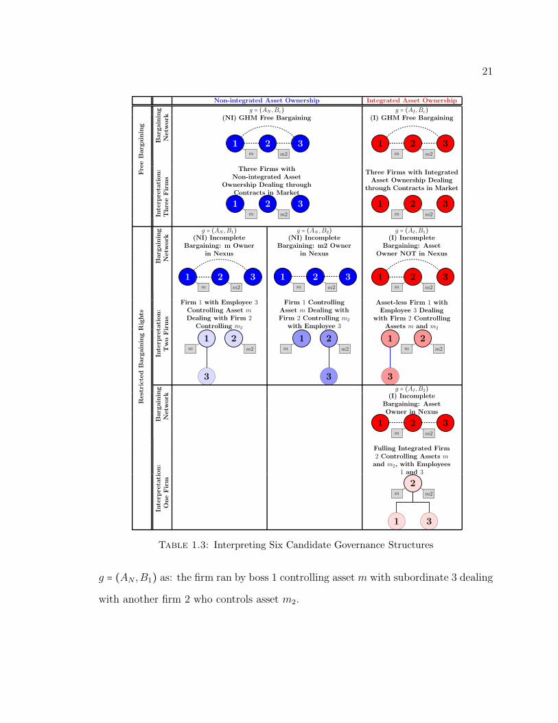
We apply these interpretation rules to the six candidate governance structures from
Table 1.2. In Table 1.3, we present the bargaining graphs on the top, and the inter-
pretation graphs right below them. In the interpretation graphs, the vertical position
represents our interpreted hierarchical structure. The bosses are placed on the top
level, and outlined with thick and black circles. The subordinates are placed on the
bottom level, and outlined with thin circles. We organize the rows in the table by
the decreasing order of the number of firms involved in the transaction.
Under the complete bargaining network Bc, every party has freedom to bargain
with everyone else, so all three parties are interpreted as bosses, with or without asset.
Thus the two GHM cases on the top row of Table 1.3 are interpreted as three firms
dealing in the market.
The next pair of cases under non-integrated asset ownership offers clearly iden-
tified employment relationship that we cannot always identify in the classical GHM
framework. Under network B1, when asset ownership is non-integrated, 2 is inter-
preted as an independent firm because she has ownership over asset m2.14 3 is seen
as the subordinate of 1 because he cannot bargain freely with 2. So we interpret case
14Whether 2 has an exclusive dealing contract with 1 is ambiguous in the three-party two-firmsetting, as we do not explicitly see whether 2 has the right to freely bargain with a third firm. If anapplication has a specific setting, introducing a forth party as necessary could help ameliorate thisambiguity.
21
Non-integrated Asset Ownership Integrated Asset Ownership
FreeBarg
aining
Barg
aining
Netw
ork
g = (AN ,Bc) g = (AI ,Bc)(NI) GHM Free Bargaining (I) GHM Free Bargaining
1 2 3m m2
1 2 3m m2
Interp
retation:
ThreeFirms
Three Firms withNon-integrated Asset
Ownership Dealing throughContracts in Market
Three Firms with IntegratedAsset Ownership Dealing
through Contracts in Market
1 2 3m m2
1 2 3m m2
RestrictedBarg
ainingRights
Barg
aining
Netw
ork
g = (AN ,B1) g = (AN ,B2) g = (AI ,B1)(NI) Incomplete
Bargaining: m Ownerin Nexus
(NI) IncompleteBargaining: m2 Owner
in Nexus
(I) IncompleteBargaining: Asset
Owner NOT in Nexus
1 2 3m m2
1 2 3m m2
1 2 3m m2
Interp
retation:
TwoFirms
Firm 1 with Employee 3Controlling Asset m
Dealing with Firm 2Controlling m2
Firm 1 ControllingAsset m Dealing withFirm 2 Controlling m2
with Employee 3
Asset-less Firm 1 withEmployee 3 Dealing
with Firm 2 ControllingAssets m and m2
1
3
2m m2
1 2
3
m m2
2m m2
1
3
Barg
aining
Netw
ork
g = (AI ,B2)(I) Incomplete
Bargaining: AssetOwner in Nexus
1 2 3m m2
Interp
retation:
OneFirm
Fulling Integrated Firm2 Controlling Assets m
and m2, with Employees1 and 3
2
1 3
m m2
Table 1.3: Interpreting Six Candidate Governance Structures
g = (AN ,B1) as: the firm ran by boss 1 controlling asset m with subordinate 3 dealing
with another firm 2 who controls asset m2.
22
Similarly, g = (AN ,B2) is interpreted as a transaction involving two firms, each
controlling one asset, dealing through the market. The only difference from the
g = (AN ,B1) case is that party 3 is the subordinate of firm 2, instead of firm 1. This
difference between these two cases cannot be formally modeled in a classical GHM
model. This feature highlights a benefit of introducing bargaining control rights.
g = (AI ,B1) offers a case of an asset-less firm in the transaction. As the graph
shows, party 1 is a boss with subordinate 3, dealing with another firm 2. In this
case, the firm ran by 1 with subordinate 3 does not have control over any asset. All
the assets needed for production is owned by party 2. We interpret this case as a
asset-less firm dealing with another firm abundant with productive assets, such as a
consulting firm providing services to a manufacturer.
g = (AI ,B2) describes a classical firm in the sense that the owner of the firm is
also the owner of all the assets. This case thus represents a fully vertically integrated
transaction.
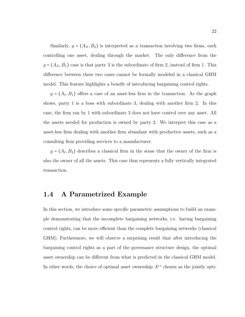
1.4 A Parametrized Example
In this section, we introduce some specific parametric assumptions to build an exam-
ple demonstrating that the incomplete bargaining networks, i.e. having bargaining
control rights, can be more efficient than the complete bargaining networks (classical
GHM). Furthermore, we will observe a surprising result that after introducing the
bargaining control rights as a part of the governance structure design, the optimal
asset ownership can be different from what is predicted in the classical GHM model.
In other words, the choice of optimal asset ownership A∗∗ chosen as the jointly opti-
23
mal governance structure g∗∗ = (A∗∗,B∗∗) ∈ AN ,AI × Bc,B1,B2 can be different
from the optimal asset ownership g∗ = A∗ ∈ AN ,AI fixing bargaining network Bc.
Finally, in some situations, we will be able to see that, as one party’s investment be-
comes more and more important relative to others’, the ownership of the same asset
is transferred for multiple times between the same dyad of parties. This result is in
stark contrast to the standard property rights models where the party who makes
more important investment tends to own more assets.
In the following sections, we will very often compare a governance structure with
incomplete bargaining network, say g′, with one that has a complete network, say g.
In these comparisons, we will discuss it as if the governance structure changed from
g to g′. To put it another way, in the thought experiments, we will pretend as if the
party who has bargaining control under g′ acquired the bargaining control rights over
her subordinate. Therefore we will refer to the boss in g′ with bargaining control
rights as the integrating party, and refer to the subordinate as the integrated party.
1.4.1 Model Setup
Specific Parametrization of Production Functions
We follow Whinston (2003)’s linear-quadratic setup to formulate the model. Each
party i makes ex ante non-contractible relationship-specific investment ei.
We assume that the parties’ investments have two potential benefits, it has a
self-investment aspect and a cross-investment aspect. Self-investments means that
the investments benefit the productions in which the investor participates. On the
contrary, cross-investments means that investments benefit the productions that the
investor is not a part of. For example, if Apple Inc. invests in improving its iphone’s
24
compatibility with Google Inc.’s map application, it is likely to not only benefit
Apple, but also benefit Google by attracting more users who contributes usage data.
Consequently, the effect of the usage data may spillover to Google’s own mobile
devices.
We assume the three parties make investments at private costs with a quadratic
form Ψi(ei) = e2i2 . The production functions for the seven possible coalitions are
assumed to take a linear form as follows.
v123(e,A) = α1e1 +αe2 + αe3
v3(e,A) = βcrosse1 + βcrosse2 + e3
v1(e,A) = (Ω1m + (1 −Ω1))(e1 + βcrosse2 + βcrosse3)
v2(e,A) = (Ω1 + (1 −Ω1)m)(βcrosse1 + e2 + βcrosse3)
v12(e,A) =m(kse1 + kse2 + βcrosskce3)
v13(e,A) = (Ω1m + (1 −Ω1))(kse1 + βcrosskce2 + kse3)
v23(e,A) = (Ω1 + (1 −Ω1)m)(βcrosskce1 + kse2 + kse3)
From the top down, in these equations, α1 (α) is the marginal product of party 1’s
(party 2 and 3’s) investment in the final production. The higher α1 is relative to α,
the more important is party 1’s investment.
βcross is an indicator variable controlling whether there is cross investment. If
βcross = 0, party i’s investment does not have an effect on the productions that she
does not participate in.
Ω1 is the indicator variable controlling whether party 1 owns the asset m. Ω1 = 1if A = AN , and Ω1 = 0 if A = AI .
25
m is the multiplicative effect of owning the alienable asset m. We assume m > 1,so that the asset is always productive. If the asset is under control of party i, then
the marginal product of all the productions that i participates in is multiplied by m.
ks is the marginal product of self-investment in joint production of the investing
party and any other party; whereas kc is the marginal product of cross-investment in
joint production of the other two parties. We assume ks, kc > 2 so the investments are
more productive in bigger coalitions.
Investment Choices Given g = (A,B)
At the ex ante stage, each party i chooses non-contractible investment ei at pri-
vate cost Ψi(ei) to maximize her own bargaining payoff Yi. The network Bc, Bi or
Bj determines which equation in (1.3) to (1.5) is party i’s bargaining payoff. The
asset ownership A determines the values of productions by entering into the seven
production functions vS for S ⊆ 1,2,3.The equilibrium choice of ei under governance structure g = (A,B) is characterized
by
egi = argmax
eiY B
i (vS(e,A)) −e2i2.
The social surplus from the transaction under this governance structure g is thus
given by
πg = Y Bi (vS(eg,A)) −
(egi )22
.
The most efficient governance structure is the one among all others that generates
26
the highest level of social surplus.
1.4.2 “Horse Races” Among Six Governance Structures
In the remaining part of this section, we compare the efficiency of the six governance
structures in Table 1.3. We will show that, in this example, only when some party’s
investment has a cross-investment aspect, having bargaining control rights can be
more efficient than using complete bargaining networks. Moreover, in some cases,
after introducing the the incomplete bargaining network, the optimal asset ownership
prediction can be different from the GHM result.
To demonstrate these findings, we discuss three sets of “horse races”. In Case
I, every party’s investment only has a self-investment aspect (βcross = 0), we call it
no-cross-investment case. Complete bargaining network is always more efficient. In
Case II, we allow for the cross-investment aspect in production functions (βcross =1). Incomplete bargaining networks can be more efficient than complete bargaining
networks, but the optimal asset allocation predictions remain the same as in GHM. In
Case III, we allow the marginal products of cross- and self-investments to be different
(kcross ≠ kself), the optimal asset allocation predictions are different from the GHM
predictions.
We choose to fix values for some variables and directly demonstrate the results
with figures reporting the optimal governance structure under different parameter
values. In what follows, we fix m = 2, α = 20. We let βcross, α1, ks and kc vary as
choice variables and report the optimal governance structures.15
15Ω1 is not an exogenous choice variable, because it is determined endogenously by asset ownershipA.
27
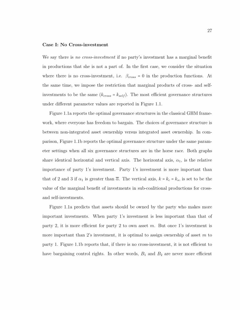
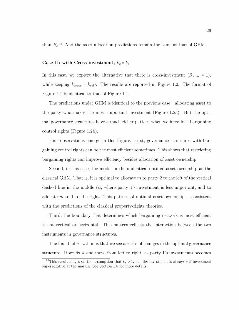
Case I: No Cross-investment
We say there is no cross-investment if no party’s investment has a marginal benefit
in productions that she is not a part of. In the first case, we consider the situation
where there is no cross-investment, i.e. βcross = 0 in the production functions. At
the same time, we impose the restriction that marginal products of cross- and self-
investments to be the same (kcross = kself). The most efficient governance structures
under different parameter values are reported in Figure 1.1.
Figure 1.1a reports the optimal governance structures in the classical GHM frame-
work, where everyone has freedom to bargain. The choices of governance structure is
between non-integrated asset ownership versus integrated asset ownership. In com-
parison, Figure 1.1b reports the optimal governance structure under the same param-
eter settings when all six governance structures are in the horse race. Both graphs
share identical horizontal and vertical axis. The horizontal axis, α1, is the relative
importance of party 1’s investment. Party 1’s investment is more important than
that of 2 and 3 if α1 is greater than α. The vertical axis, k = kc = ks, is set to be the
value of the marginal benefit of investments in sub-coalitional productions for cross-
and self-investments.
Figure 1.1a predicts that assets should be owned by the party who makes more
important investments. When party 1’s investment is less important than that of
party 2, it is more efficient for party 2 to own asset m. But once 1’s investment is
more important than 2’s investment, it is optimal to assign ownership of asset m to
party 1. Figure 1.1b reports that, if there is no cross-investment, it is not efficient to
have bargaining control rights. In other words, B1 and B2 are never more efficient
28
8 Α 321
3
Α1
k
GHM
(a) (AN ,Bc) vs. (AI ,Bc)
8 Α 321
3
Α1
k
g=8A,B<
(b) All Six Gov.Structures
(I)
Incomplete
Bargaining
(B2)
(I) GHM
Free
Bargaining
(I)
Incomplete
Bargaining
(B1)
(NI)
Incomplete
Bargaining
(B2)
(NI) GHM
Free
Bargaining
(NI)
Incomplete
Bargaining
(B1)
2
1 3
m m2
1 2 3m m2
2m m2
1
3
1 2
3
m m2
1 2 3m m2
1
3
2m m2
Figure 1.1: Optimal Governance Structures without Cross-investment
29
than Bc.16 And the asset allocation predictions remain the same as that of GHM.
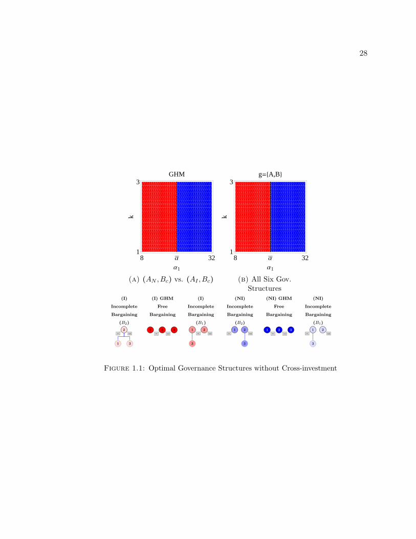
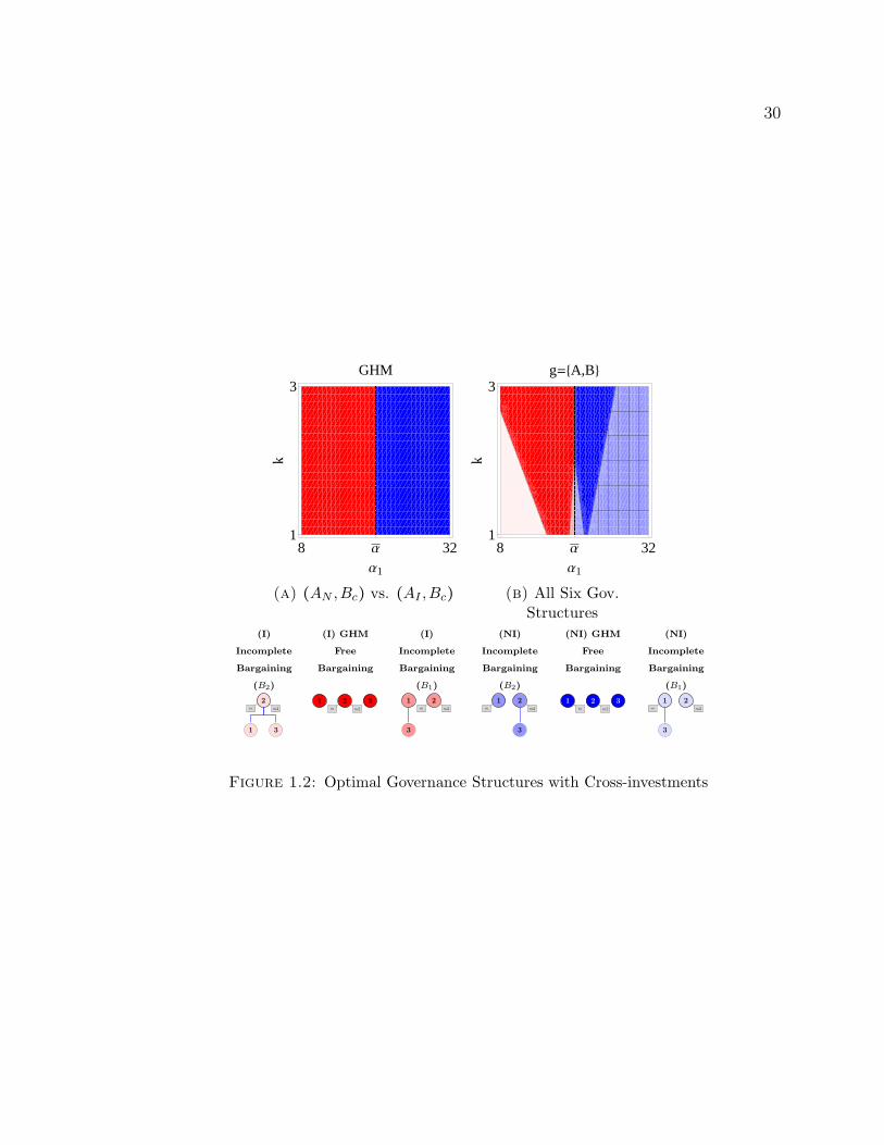
Case II: with Cross-investment, kc = ks
In this case, we explore the alternative that there is cross-investment (βcross = 1),
while keeping kcross = kself . The results are reported in Figure 1.2. The format of
Figure 1.2 is identical to that of Figure 1.1.
The predictions under GHM is identical to the previous case—allocating asset to
the party who makes the most important investment (Figure 1.2a). But the opti-
mal governance structures have a much richer pattern when we introduce bargaining
control rights (Figure 1.2b).
Four observations emerge in this Figure. First, governance structures with bar-
gaining control rights can be the most efficient sometimes. This shows that restricting
bargaining rights can improve efficiency besides allocation of asset ownership.
Second, in this case, the model predicts identical optimal asset ownership as the
classical GHM. That is, it is optimal to allocate m to party 2 to the left of the vertical
dashed line in the middle (α, where party 1’s investment is less important, and to
allocate m to 1 to the right. This pattern of optimal asset ownership is consistent
with the predictions of the classical property-rights theories.
Third, the boundary that determines which bargaining network is most efficient
is not vertical or horizontal. This pattern reflects the interaction between the two
instruments in governance structures.
The fourth observation is that we see a series of changes in the optimal governance
structure. If we fix k and move from left to right, as party 1’s investments becomes
16This result hinges on the assumption that ks > 1, i.e. the investment is always self-investmentsuperadditive at the margin. See Section 1.5 for more details.
30
8 Α 321
3
Α1
k
GHM
(a) (AN ,Bc) vs. (AI ,Bc)
8 Α 321
3
Α1
k
g=8A,B<
(b) All Six Gov.Structures
(I)
Incomplete
Bargaining
(B2)
(I) GHM
Free
Bargaining
(I)
Incomplete
Bargaining
(B1)
(NI)
Incomplete
Bargaining
(B2)
(NI) GHM
Free
Bargaining
(NI)
Incomplete
Bargaining
(B1)
2
1 3
m m2
1 2 3m m2
2m m2
1
3
1 2
3
m m2
1 2 3m m2
1
3
2m m2
Figure 1.2: Optimal Governance Structures with Cross-investments
31
more important, it is efficient for her to own more assets, and to have more bargaining
rights. The optimal governance structure changes as party 1’s investment becomes
more and more important. When party 1’s investment is very unimportant (left of
Figure 1.2b), (AI ,B2) wins. It is efficient to give party 2 all the asset ownership
and the bargaining control over 1, i.e. 2 integrating 1 to work as a subordinate. As
1 becomes more important, (AI ,Bc) is the most efficient. That is to give party 1
bargaining freedom and let her participate in the transaction as an independent firm.
As 1 becomes even more important but not more so than 2, it can be efficient to
choose (AI ,B1). That is to let 1 have bargaining control over 3 and deal with 2, who
controls all the assets. This is the case in which party 1 runs an asset-less firm, such
as a professional services firm, and deals with firm 2 that controls both productive
assets, such as a manufacturing firm. As soon as party 1’s investment becomes more
important than 2’s, (AN ,B2) wins. The asset ownership shifts across the vertical line
of α. But in order to balance 2’s investment incentives, it is efficient to let 2 having
bargaining control over party 3. When 1’s investment gets even more important, case
(AI ,Bc) wins. It is efficient to give 1 and 3 their freedom to bargain with each other.
And, finally, case (AI ,B1) wins. Giving 1 both the bargaining control and the asset
ownership is optimal when 1 is much more important than 2.17
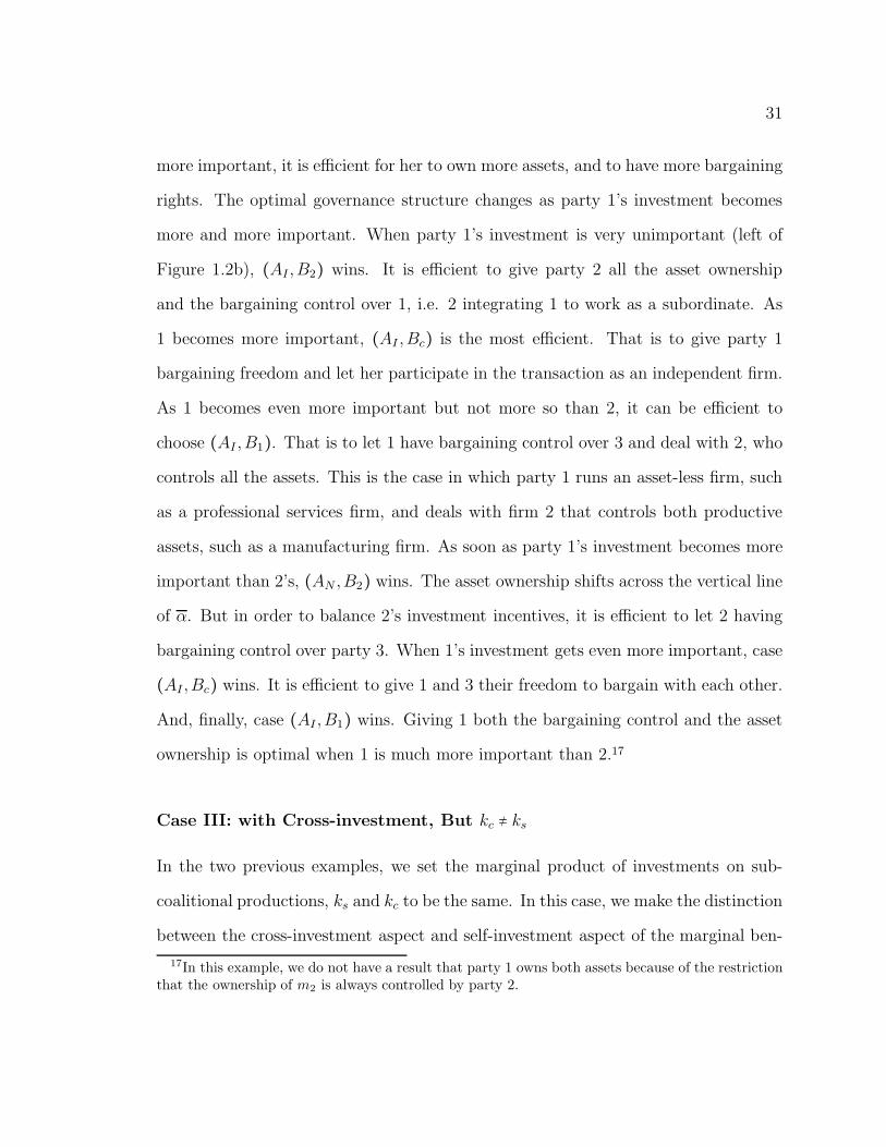
Case III: with Cross-investment, But kc ≠ ks
In the two previous examples, we set the marginal product of investments on sub-
coalitional productions, ks and kc to be the same. In this case, we make the distinction
between the cross-investment aspect and self-investment aspect of the marginal ben-
17In this example, we do not have a result that party 1 owns both assets because of the restrictionthat the ownership of m2 is always controlled by party 2.
32
8 Α 321
kc
3
Α1
k s
GHM
(a) (AN ,Bc) vs. (AI ,Bc)
8 Α 321
kc
3
Α1
k s
g=8A,B<
(b) All Six Gov.Structures
(I)
Incomplete
Bargaining
(B2)
(I) GHM
Free
Bargaining
(I)
Incomplete
Bargaining
(B1)
(NI)
Incomplete
Bargaining
(B2)
(NI) GHM
Free
Bargaining
(NI)
Incomplete
Bargaining
(B1)
2
1 3
m m2
1 2 3m m2
2m m2
1
3
1 2
3
m m2
1 2 3m m2
1
3
2m m2
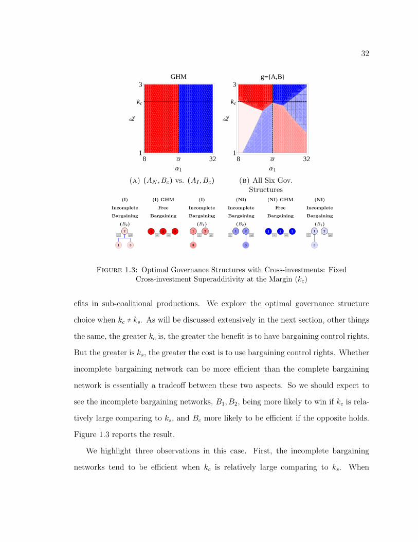
Figure 1.3: Optimal Governance Structures with Cross-investments: FixedCross-investment Superadditivity at the Margin (kc)
efits in sub-coalitional productions. We explore the optimal governance structure
choice when kc ≠ ks. As will be discussed extensively in the next section, other things
the same, the greater kc is, the greater the benefit is to have bargaining control rights.
But the greater is ks, the greater the cost is to use bargaining control rights. Whether
incomplete bargaining network can be more efficient than the complete bargaining
network is essentially a tradeoff between these two aspects. So we should expect to
see the incomplete bargaining networks, B1,B2, being more likely to win if kc is rela-
tively large comparing to ks, and Bc more likely to be efficient if the opposite holds.
Figure 1.3 reports the result.
We highlight three observations in this case. First, the incomplete bargaining
networks tend to be efficient when kc is relatively large comparing to ks. When
33
ks < kc, the benefit of having bargaining control rights tends to overweight its cost.
The two GHM governance structures are dominated towards the bottom part of
Figure 1.3b. As ks gets closer to the magnitude of kc and goes above, the structures
using bargaining control rights start to lose to GHM.
Second, this model predicts that, once we introduce bargaining control rights,
the optimal asset ownership can be different from what is predicted in GHM. In
Figure 1.3b, the optimal governance structures are not all integrated asset ownership
to the left of α and all non-integrated asset ownership to the right. This indicates
that it can be efficient for party 1 to control the asset even though her investment
is not as important as 2’s. The intuition for this case is the following. When the
benefit of using bargaining control is relatively large comparing to its cost, having
bargaining control can more effectively motivate investment. In this case, bargaining
control rights become a more effective instrument than asset ownership. The party
who makes relatively more important investment should have the bargaining control
rights. So as party 1’s investment gets important but not more so than 2, it is efficient
to have her run an independent firm with asset (case (AN ,B2)), rather than making
her control a firm with the subordinate (case (AI ,B1)). This pattern is in stark
contrast to what is predicted in the previous case where kc = ks. In fact, in the lower
part of Figure 1.3b, when 1’s investment is less important than 2’s, 2 always has
bargaining control rights over 1. And it is always efficient for 1 to hold bargaining
control rights over 2 once 1’s investment becomes more important.
Third, fixing ks and moving from the left to the right, as α1 increases, there are
multiple rounds of transfers of asset ownership. When α1 is very small, the asset m
is controlled by party 2. As α1 gets greater and approaches α = α2 = α3, it is efficient
for 1 to control the asset. We see another round of transfer of asset ownership once
34
α1 becomes greater than α. When α1 crosses the vertical dashed line of α, the asset
ownership changes back to party 2, then changes back again to party 1 as α1 gets
very large relative to α. This pattern is not consistent with the classical prediction
that assets should be owned by the party who makes more important investments
(Hart and Moore, 1990). In fact, in the presence of bargaining control rights, their
prediction does not always generalize. This result provides one possible explanation
to the fact that, in many transactions, parties who provides very valuable services
owns asset-less firms.
To briefly summarize the findings in this section, among the observations, two
stand out as the most interesting. First, the model shows that with cross-investment,
introducing bargaining control rights as instruments in the governance structure can
further improve the efficiency of transactions in addition to using allocation of asset
ownership. Second, the model can predict different optimal asset ownership as GHM
does.
1.5 Analysis of the Model of Three Parties
After observing some of the interesting features in the previous section, we devote
this section to rigorous analysis of the effects of incomplete bargaining networks in
the presence of asset ownership allocation. The different propositions provide the
general intuitions behind the patterns we observe previously in the example. We
offer discussions of the propositions regarding their interpretations relating to the
vertical integration of transactions. All proofs of the propositions are omitted and
included in the Appendix 1.A.
35
We analyze the model backwards. First, we analyze the bargaining payoffs at
the ex post stage under different governance structures. Then we move on to study
how different bargaining payoffs affect the three parties’ ex ante investment incen-
tives. From the associated investment incentives, we are able to draw some general
conclusions regarding the choice of the optimal governance structure.
1.5.1 ex post Bargaining Payoffs
Having characterized the bargaining payoffs for the three-party case under different
governance structures in equations (1.3) through (1.5), we start by analyzing obser-
vations from them.
By subtracting the three equations from each other, we have
Y ii − Y c
i =1
3(vjk − vj − vk); (1.6)
Yji − Y c
i = −1
6(vik − vi − vk). (1.7)
By the assumption that the production is superadditive, i.e. vij > vi+vj ,∀i, j = 1,2,3,we have the following result.
Remark 1.1. Given fixed ex ante investment levels and fixed asset allocation, bar-
gaining control rights provide extra bargaining payoff. Specifically, Y ii > Y c
i > Y ji .
18
Intuitively, party i obtains a higher payoff under Bi because, comparing to Bc,
she is no longer jointly threatened by k and j together. Party i is able to prevents
18In terms of the timing of the model, this result confirms that the bargaining control over otherparty is “sub-game perfect”. That is, once a party obtains bargaining control from the agreedgovernance structure, she will not give up the control right in the ex post bargaining stage to let theother two parties freely bargain with each other.
36
j and k from bargaining with each other to form a contract without her. In reality,
an employee is unable to reach a side-contract with an outside firm or with another
employee at the same firm. Thus they are unable to jointly make a credible threat
against the employer firm for a more favorable term in their respective contracts. As
a consequence, j and k’s bargaining payoffs are lower comparing to those under Bc.
In all the incomplete bargaining networks, the control rights over other parties’
ability to bargain diverts a greater share of final value from those who lost the bar-
gaining rights to the party who obtains bargaining control.
By observation from equations (1.3) through (1.5), the following proposition be-
comes obvious.
Proposition 1.1. Comparing to all other cases in which party j is free to bargain, if
some party i has bargaining control rights over party j, then we have (i. Insulation
Effect) the outside option vjk between j and the party other than i is insulated from
every parties’ bargaining payoff. Specifically, for any k ≠ i,∂Y b
l
∂vjk≠ 0,∀l = 1,2,3 for
b ≠ i. But∂Y i
l
∂vjk= 0,∀l = 1,2,3. (ii. Concentration Effect) the individual outside
options vj and vk have higher weight in every parties’ bargaining payoff. Specifically,
for any k ≠ i, ∣∂Y il
∂vj∣ > ∣∂Y c
l
∂vj∣ and ∣∂Y i
l
∂vk∣ > ∣∂Y c
l
∂vk∣,∀l = 1,2,3.
These effects follow directly from the way we defined the incomplete bargaining
networks. The intuition is that if party j can only bargain directly with party i, no one
other than i is able to form an agreement with j without involving i. Consequently,
vjk is no longer a credible threat for either j or k against i. As a result, j and k will
have no incentive to invest ex ante in vjk. The benefit of this effect is that if party
i’s investment has an cross-investment aspect that also benefits vjk, she will have
greater incentive to invest. Because she need not be concerned about increasing vjk
37
that will turn into a potential threat against her own payoff. More specific discussions
regarding the influence of this property will continue in our analysis about the ex ante
stage investments.
Following our interpretation of the bargaining control rights as a hierarchical struc-
ture, the proposition says that integration of party j by party i fundamentally changes
the payoff structure of every party. Besides parties i and j, this effect influences all
parties involved in the transaction, including, in this case, firm k.19
The insulation effect describes the benefit of bargaining control rights. By remov-
ing some potential outside options from all the parties involved in the transaction, it
can help align the interests of some parties with the social interest, v123.
Unsurprisingly, the bargaining control rights comes with a cost as well. The con-
centration effect highlights the cost side of limited bargaining rights. A comparison
between equations (1.6) and (1.7) highlights that restriction in bargaining rights only
shifts parties’ interests from pursuing a joint sub-coalitional outside option to pur-
suing individual outside options. 20 The efficiency of using bargaining control rights
depends on the tradeoff between lighter weights spread on more outside options and
heavier weights condensed on less smaller-scale outside options.
If we interpret Proposition 1.1 in the context of vertical integration, it says that
as a result of integration, by which we mean obtaining control over another party’s
19In a three-party model, one might argue that in Bi, j and k simultaneously lose their bargainingrights to party i. So it seems too strong to make the point that the insulation effect also affectsthose parties who are not integrated. However, we show that the insulation effect indeed generalizesto a model with any number of parties. Following the integration of any party, all outside optionsthat involves joint production with this party are insulated from all parties’ payoffs. Specifically, inany network B that j can only bargain with i, ∂Yl
∂vS= 0, for all parties l and all coalitions S such
that S ∌ i and S ∋ j. For the specific statement and proof, see Proposition 2.4.20However, it offers an efficiency improving opportunity if putting more concerns over the indi-
vidual outside option, in place of the joint sub-coalitional outside options, improves the productiveinvestment incentives or reduces the wasteful investment incentives. See Holmstrom and Milgrom(1991); Gibbons (2005).
38
bargaining rights, the incentives of all the parties involved in the transaction become
more focused. On one hand, they are more focused in the sense that they care about
less types of outside options (the insulation effect). One the other hand, they are more
focused because they care more about some particular smaller-scale outside options
(the concentration effect).
This model predicts that integration of one other firm fundamentally changes
outside options for all transaction-related parties. Integration protects the integrating
firm from joint hold-up threats that involves the integrated party. And integration
removes all other, integrated or not-yet-integrated, parties’ incentives to invest toward
these sub-coalitional outside options. However, as its downside, it creates more narrow
minded parties who puts a heavier weight on their own outside opportunities.
Bargaining Payoffs under Different Asset Ownership
Previously we have only discussed the bargaining payoffs given a fixed asset ownership
structure. In this part of the section, we analyze the interactions between asset
ownership and bargaining control rights.
Consider two otherwise identical asset allocation rules, A and A, except that
one asset is assigned differently. Recall that the asset ownership affects the ex post
bargaining payoffs through the production functions, vS(e,A). We can obtain the
bargaining payoff for party i under governance structure g = (A,B) for A ∈ A,Aand B ∈ Bc,B1,B2,B3 as
Y bi = Y b
i ∣A=A,
Y bi = Y b
i ∣A=A,
39
where Y bi is given in equations (1.3) through (1.5).
Let us define the following operation ∆(vS(e)) = vS(e,A)− vS(e,A) as the differ-ence in the production value vS under the two asset ownership structures for coalition
S. In a similar form as equations (1.6) and (1.7), we have
Y ii − Y i
i = Y ci − Y c
i +1
3∆(vjk − vj − vk); (1.8)
Y ji − Y j
i = Y ci − Y c
i −1
6∆(vik − vi − vk). (1.9)
The following result follows immediately from these two equations.
Proposition 1.2. The change of asset ownership can have different effects on payoffs
under different bargaining networks. Specifically, there is difference in payoffs across
different networks if the asset ownership changes the superadditivity in sub-coalitional
cooperation, i.e. ∆(vjk − vj − vk) ≠ 0.
Proposition 1.2 offers the interaction between the two dimensions of the seemingly
independent governance structures. It says that the effect of the asset ownership can
vary across different allocations of bargaining control rights.
With our interpretation, Proposition 1.2 predicts that the transfer of ownership
over the same asset between the same pair of parties can cause different changes
in payoff distribution. The amount of payoff each party can gain or lose from the
transfer can depend on the level of integration in the transaction. Suppose there are
two cases, in the first, i and j are both free to bargain and controls no other party;
whereas in the second case, i has bargaining control over some other party k. Then
the ex post rent distribution can differ in these two cases following a transfer of the
same asset from i to j.21
21With more than three parties, we can possibly identify a firm under exclusive dealing restrictions
40
To summarize our analysis up to now, bargaining control rights diverts a greater
bargaining payoff from those parties who become restricted to bargain toward those
who have control. This shift removes all the outside options of joint productions that
involve the integrated parties. It shifts the parties’ interests to focus more heavily
on outside options involving less parties. The asset ownership and the allocation of
bargaining control rights can interact with each other. The ex post benefit or loss from
obtaining the ownership of the same asset from the same party may differ depending
on the bargaining control rights. The answer regarding whether restricting bargaining
rights can improve efficiency, however, depends on the specific nature of investments.
The following subsection studies these implications in further detail.
1.5.2 ex ante Investment Incentives
In the ex ante stage, each party i chooses her non-contractible relationship-specific
investment level ei at private cost Ψi(ei) to maximize her future bargaining payoff
given the agreed upon governance structure. In this section, we analyze different
investment incentives under different governance structures. And consequently, we
are able to draw some implications from the model regarding the efficiency of the
respective structures.
First-best Benchmark
Before specifying the ex ante investment problem under any specific governance struc-
ture, we will analyze the first-best investment level as a benchmark.
in the model. A generalization of Proposition 1.2 then implies that the payoff changes following atransfer of the same asset between a firm restricted by exclusive dealing and another firm can bedifferent should the restricted party were an independent firm.
41
The first-best level of investment eFBi is the choice of ei that maximizes the final
value of production v123(e,A) given the costs Ψi(ei) for all parties. It is characterizedby
∂v123(e,m,m2)∂ei
= Ψ′i(ei). (1.10)
Investments Given Fixed Asset Ownership
We first characterize the ex ante investment levels, eA,Bc
i , eA,B1
i and eA,B2
i under the
three different bargaining networks given fixed asset ownership A.22
Party i obtains her associated payoff Yi under the particular bargaining network.
Under Bc, party i will obtain Y ci ex post, so e
A,Bc
i is characterized by
∂Y ci (vS)∂ei
= Ψ′i(ei). (1.11)
where Y ci (vS) is given in equation (1.3), and each vS in vector vS is a function of
both investment level e and asset allocation rule A.
Similarly, eA,Bi
i and eA,Bj
i are characterized by∂Y i
i (vS(e,A))
∂ei= Ψ′i(ei) and
∂Yji(vS(e,A))
∂ei=
Ψ′i(ei), respectively. But we can utilize equations (1.6) and (1.7) to rewrite them as
∂Y ci (vS)∂ei
+ 13
∂(vjk − vj − vk)∂ei
= Ψ′i(ei). (1.12)
∂Y ci (vS)∂ei
− 1
6
∂(vik − vi − vk)∂ei
= Ψ′i(ei). (1.13)
Assumption 1.1. We assume that the marginal product of each party i’s invest-
22The efficiency implications regarding the optimal asset ownership given the free bargainingnetwork Bc is very well studied in the seminal work of Hart and Moore (1990).
42
ment ei is strictly lower in the sub-coalitional productions comparing to that in the
production of the grand coalition, i.e. ∂vS∂ei< ∂vN
∂ei,∀S ⊂ N .23
Proposition 1.3. Under assumption 1.1, there is always under-investment in any
bargaining network Bc, Bi and Bj. That is eA,Bi < eFB
i for any i ∈ 1,2,3 and any
B ∈ Bc,Bi,Bj.
Proposition 1.4. If any governance structure g induces a higher investment vector eg
than the alternative g′ does, then g is more efficient than g′. That is v123(eg,m,m2)−
∑iΨi(egi ) ≥ v123(eg′,m,m2) −∑iΨi(eg
′
i ) if eg ≥ eg′.24
Having laid the ground for evaluating the relative efficiencies of different gover-
nance structures, we move on to compare the complete bargaining network Bc with
the incomplete bargaining networks Bi.
At this point, it is convenient for what follows to introduce some definitions.
Definition. We say there is cross investment for ei if for any S ∌ i, ∂vS∂ei> 0.25
Definition. We say the investment ei is cross-investment superadditive at the margin
(CSM) with respect to coalition S if for coalition S ∌ i and S′ ⊂ S, ∂vS∂ei> ∂vS′
∂ei+ ∂vS/S′
∂ei
We say the investment ei is cross-investment superadditive at the margin if ei is cross-
investment superadditive at the margin with respect to all coalitions..
One sufficient condition for investments to satisfy CSM is if the nature of the
investment is (i) non-specific to the investor (∂vS−i∂ei> 0 for some S−i ∌ i), such as
23Assumption 1.1 is in place so we can anchor the relative relationship between the first-best andsecond-best investment levels. We do not think the assumption is substantive as long as the sign ofthe inequality is consistently positive or negative. The sign can be understood as the direction wechoose to interpret the nature of the investment.
24Proposition 1.3 and Proposition 1.4 together are the counterparts of Proposition 1 in Hart andMoore (1990).
25This definition of cross investment is also introduced in Whinston (2003).
43
investment in capabilities, knowledge, process or routine that benefits other parties,
but (ii) generates more marginal benefits when other parties jointly participate with
their resources (∂vjk∂ei> ∂vj
∂ei+ ∂vk
∂ei). One such example is investment in workers’ skills
to operate a information system that are not specific to the investor but specific to,
say, the supplier company of the investor. For another instance, investment in a
complicated early-stage R&D project that requires joint work of designing specialists
and marketing specialists.
Definition. We say the investment ei is self-investment superadditive at the margin
(SSM) with respect to coalition S if for coalition S ∋ i and S′ ⊂ S, ∂vS∂ei> ∂vS′
∂ei+ ∂vS/S′
∂ei.
We say the investment ei is self-investment superadditive at the margin if ei is self-
investment superadditive at the margin with respect to all coalitions.
One sufficient condition for investments to satisfy SSM is if the nature of the
investment is specific to the investor (∂vj∂ei= 0), such as investment in assets that’s
currently under control, but complementary to other parties’ existing resources (∂vij∂ei>
∂vi∂ei
). For example, investment in firm-specific human capital.
Some investment can be both SSM and CSM. For example, investment in knowl-
edge (∂vij∂ei> 0) that is specific to the particular transaction (
∂vj∂ei= 0), but not specific
to the investor (∂vjk∂ei> 0).
Moving on to the analysis, equations (1.12) and (1.13) provides two interesting
observations regarding the effect of bargaining control rights on the investment in-
centives.
First, comparing to the complete bargaining network case, obtaining bargaining
control over another party only increases the marginal benefit of this party’s invest-
ment if and only if her investment is CSM. This is shown by the second term in
44
equation (1.12),∂(vjk−vj−vk)
∂ei.
Second, comparing to the complete bargaining network case, losing bargaining
rights to some other party j reduces the marginal benefit of this party’s investment
if and only if her investment is SSM, which is shown by the second term in equation
(1.13), ∂(vik−vi−vk)∂ei
.
Although the first-order effects of bargaining control rights is clear, the net ef-
fect on the equilibrium investment levels are ambiguous in general conditions due to
second-order interactions in parties’ investments. The following Remark summarizes
these “asymmetric” first-order effects under a special environment.
Definition. We say the investments of any two parties i and j are technologically
independent if their investments has no effect on each other’s marginal product, i.e.
∂v2S
∂ei∂ej= 0,∀S.
Remark 1.2. If all parties’ investments are technologically independent, then com-
paring to the baseline of complete bargaining network, suppose party i obtains bar-
gaining control rights over party j, ei increases after the fact if and only if it is CSM
with respect to coalition jk; ej and ek decreases after the fact if and only if they are
SSM with respect to coalition jk.
The following remark is a counterpart of the previous one presented in a comparative-
static manner.
Remark 1.3. Comparing to the baseline of complete bargaining network, suppose
party i obtains bargaining control over party j, (i) if only i makes investment, then
the change is more efficient if and only if ei is CSM with respect to coalition jk; (ii)
if only j (or k) makes investment, then the change is less efficient if and only if ej (or
ek) is SSM with respect to coalition jk.
45
Remark 1.3 provides the basis for a thought experiment under the general envi-
ronment where every party makes investments. The efficiency of having bargaining
control rights depends on whether the increased investment incentives by alleviating
investor’s concern in cross-investment can overweight the reduced investment incen-
tives due to restricted outside options.26
Indeed, remark 1.3 is the counterpart of the result in Hart and Moore (1990)
regarding the optimal governance structure if only one party makes investment. GHM
predicts that if only one party makes investment, she should own all the assets as
long as her investments are complementary with the assets. Our model predicts that
the only investor should obtain bargaining control rights over others if and only if her
investment supports other parties’ cooperation without her.
The following proposition outlines the tradeoff in an extreme case without assum-
ing technological independence in investments.
Proposition 1.5. If there is no CSM, and every parties’ investments are SSM with
respect to all coalitions S ⊆ 1,2,3, then it is never efficient to have bargaining
control rights, i.e. Bc is always more efficient.
Corollary 1.1. If there is no cross investment, then under Assumption 1.1, it is
never efficient to have bargaining control rights, i.e. Bc is always more efficient.
We interpret Proposition 1.5 and Corollary 1.1 in the backward order.
Indeed, Corollary 1.1 is a very strong result based on a simple, although not nec-
essarily weak, assumption. The environment without cross-investment corresponds
26Reducing self-interested investments need not be efficiency reducing, we have this result becausethere is always under investment. This is not the case, if the investment is purely rent-seekingwithout being productive. But the predictions for the latter situation can be easily induced fromour results with minimal differeces in the signs. This case can be readily studied by a straightforwardextension of the current framework with a multi-tasking agent model.
46
to a situation where the effects of every party’s investment is well-contained in the
productions that she is a part of. Loosely speaking, this property describes a world
without externality. If we follow our interpretation that bargaining control rights is a
hierarchy in the firm, we can read Corollary 1.1 as saying that if there is no externality,
there should not be vertically integrated firms in the transaction. In this situation,
market transaction, Bc, is the most efficient governance structure. In other words, by
stating that a hierarchical structure is inefficient without externality, Corollary 1.1
implies that the firm is an institution that helps reducing certain externalities among
those parties involved in a transaction.
Proposition 1.5 describes the specific type of externality on which integration
has effect. Should the investment be CSM, integration would help motivate invest-
ment of the integrating party by protecting her from joint hold-up threats. But if
her investment is not CSM, then replacing the joint hold-up threats with individ-
ual hold-up threats actually lowers her investment incentives. Proposition 1.5 says
that integration into a hierarchical structure is never efficient if protecting the owner
from larger-scope joint threats worsens her overall hold-up concerns, even though
Proposition 1.1 shows the integrating party obtains a higher level of payoff.
As a comparison to Proposition 1.5, we provide the following result, which is an
opposite result that describes an extreme condition in which it is always efficient to
use bargaining control rights.
Proposition 1.6. If all parties’ investments are only SSM with respect to coalitions
that include party i, and suppose party i’s investment is weakly CSM with respect to
other coalitions, then it is always optimal for i to have bargaining control rights over
47
others.27
To interpret, loosely speaking, Proposition 1.6 says that if every parties’ invest-
ments are only “complementary” to one party, then this party should be the boss of
everyone. In other words, all parties should be integrated into the same firm that is
controlled by this party who is complementary to every one’s investments.
We can relate the main results in this section to the classical Coasean tradeoff
between the cost to use the market and the cost to use fiat. In this model, the cost
of using the market is exposing the integrating party to potential joint hold-up by
others. Integration can help protect investment incentives by reducing the externality
from her investments and replacing it with several individual level hold-up threats.
Integration would help in this case only if the investment is productive to other
parties’ productions and helpful for other parties’ cooperation. But it comes with
the cost of lowering the investment incentives for the integrated party due to a worse
agency problem. Moreover, our model highlights that integration also worsens the
agency problem for all other parties involved in the transaction.
Most interestingly, although the benefit of integration is rooted in externality, the
cost of integration is not. All these parties’ investment incentives tend to be lower
because they are restricted to work with their boss, which in turn restricts their
outside options.
Investments under Different Asset Ownership
From observations of equations (1.8) and (1.9), we find that the effect of a given
asset ownership change over the marginal benefit of the ex ante investments can vary
27By “weakly CSM”, we refer to a condition ∂vS∂ei≥ ∂vS′
∂ei+ ∂vS/S′
∂ei, which need not necessarily hold
in its strict form.
48
depending on the allocation of bargaining rights.
The following remark compares the “likelihood” of a asset being owned by one
party rather than another in a fixed dyad under different bargaining networks. Taking
derivatives of equations (1.8) and (1.9) with respect to the ex ante investments yields
the following remark.
Remark 1.4. Under different bargaining networks, a given transfer of asset own-
ership between two parties can have different first-order effects on parties’ marginal
benefit of investments. Specifically, compare the transfer of the asset m from j to i
under network Bi and Bc. Suppose all other things equal. (i) If losing m decreases
(increases) the level of SSM for party j and k, then the transfer is associated with
less (more) of a drop in ej and ek under Bi than under Bc. (ii) If gaining m increases
(decreases) the level of CSM for party i, then the transfer is associated with more
(less) of an increase in ei under Bi than under Bc.
Roughly speaking, Remark 1.4 states the conditions which increase the likelihood
that bargaining control rights and ownership of assets are allocated to the same party.
In other words, given it is efficient for a party to have bargaining control rights,
it might be more likely for her to have asset ownership in the optimal governance
structure.
For example, if the ownership of an asset plays an important role in the cooperation
between j and k (decreases the level of SSM for party j and k), then after party i
obtains bargaining control over one of j or k (under Bi), this asset is more likely to
be owned by party i, instead of one of j or k. In this case, bargaining control rights
and ownership of assets are likely to be jointly owned.
The logic of Remark 1.4 provides the intuition behind the pattern in Section 1.4
49
Case III. In fact, in Section 1.4 Case III, bargaining control rights and asset ownership
are likely to be owned together. Because as ks increases, the SSM decreases when
someone loses the asset m.28 This is why, in the lower part of the figure (b), the two
boundary lines demarcating the shift of assets between 2 and 1 (lines separating blue
from red, except for the middle line) tilt toward the center. In the south-west part,
given the it is optimal for party 2 to have bargaining control rights, fix the importance
of party 1’s investment, α1, as ks increases, it is more likely for 2 to own the asset.
Similarly, in the south-east part, given that 1 has bargaining control is optimal, fix
α1, it is more likely for party 1 to own the asset as ks increases.
1.6 Concluding Remarks
Main Results
This paper studies the effect of an endogenous institutional restriction that limits
some parties’ ability to bargain freely with each other when asset ownership is also in
place as an organizational design instrument. In this particular model, we embed this
idea in the framework of the property-rights theory of the firm to evaluate whether
introducing such restrictions in bargaining rights can improve efficiency in addition to
using allocation of property rights over assets. Our main finding is that, when there
is cross-investment, restricting some parties’ ability to bargain with others in the
transaction can improve efficiency in addition to using asset ownership. Furthermore,
the predicted optimal asset allocation can differ from the result prescribed in classical
28In the example, the SSM for party j and k when they own m is kself − 2, the SSM when i ownsm is mkself −m − 1. Subtracting one term from another, the change in SSM before and after losingthe asset to be (m − 1)(1 − kself ), which is decreasing in kself . The change in SSM for party 1 and3 before and after losing the asset to 2 is exactly the same.
50
property-rights model without restriction in bargaining rights.
Other results from the model include: (i) Restricting bargaining rights insulates
some of the outside options from all parties’ objectives, but replaces them with
smaller-scale outside options. (ii) Bargaining control rights and asset ownership can
interact with each other. (iii) Under mild assumptions, cross-investment is a neces-
sary condition for the efficiency of restricting any party’s bargaining rights. (iv) In
the presence of cross-investment, it tends to be optimal to allocate bargaining control
rights to the party who makes important non-contractible investments. (v) When
one party obtains or loses bargaining control rights of some party, it does not affect
the investment incentives for those parties who are already under bargaining control
of the first party (See Chapter 2 for more details).
Interpretation and Discussion
We interpret this modeling framework to match many observed governance structures
in the real world. We claim that the bargaining control rights resembles the vertical
hierarchical structure in a business firm. This interpretation and our model together
offer a theory of the boundary of the firm without relying on the asset ownership.
This feature allows us to expand the scope of the traditional theories of the firm to
understand asset-less firms and employment relationships. The model suggests that
all these different forms of governance structures can be rationalized within the same
framework. The answer regarding the optimal choice of governance structure depends
on the specific characteristics of the industry and technology.
The efficiency of the rich set of governance structures under different scenarios
helps us rationalize the real life counterparts of these structures, such as asset-less
51
firms and non-compete contracts.
Using our interpretation of the model, this paper makes the following predictions.
(i) Asset-less firms are efficient governance structures adapted to different economic
environments. (ii) Integration insulates the firm’s subordinates from contractual ex-
ternalities in the market, and it also attenuates the externalities for outside firms and
their subordinates; but at the possible cost of worsening the motivation problems.
(iii) Under some conditions, the firm that has bargaining control rights tends to own
all the productive alienable assets. (iv) Under mild assumptions, cross-investment is
a necessary condition for the firm to be a more efficient governance structure than
the market. (v) In the presence of cross-investment, the party who makes important
non-contractible investments should control the firm. (vi) Establishing control over
another firm through exclusive dealing or integrating existing independent contractors
does not affect the investment incentives for existing subordinates of the integrating
firm.
It is worth noting that the insulation effect and concentration effect from the
model together resembles the spirit of the subeconomy view of the firm (Holmstrom,
1999). The model suggests that the firm is an institution that reduces externalities
and trade it off with motivation problems. This is the case in this model because
the firm isolates its subordinates from outside options involving external parties in
the transaction. On one hand, this isolation can possibly better align the incentives
of the subordinates and the external parties with those of the boss of the firm to
protect the investment incentives of the boss. But, as its cost, the isolation dulls the
motivation of all other parties.
52
Robustness of the Results
In reality, firms very rarely have the full control over subordinates’ bargaining power
to totally block bargaining between the outsiders and subordinates. For instance,
different states in the U.S. treats non-compete clauses very differently in court Gar-
maise (2011). However, given the reasons we have discussed in the introduction, it is
likely that the real-world firms have significant control over their subordinates’ bar-
gaining rights. Thus the insights of the model remains because the reality seems to
lie somewhere between the two extremes.
The qualitative implications of our analysis holds true even if the firm has imper-
fect bargaining control rights. To see this point, consider a straightforward extension
of our model. The firms are assigned with an exogenous value describing the intensity
of bargaining control rights, which may be determined by the local institutions, such
as enforcement of non-compete clauses. Let the intensity, q be a value between 0 and
1. Then the bargaining payoff for each party is modeled by a linear combination of
the payoff under complete network and the payoff under the corresponding incom-
plete network, such as (1− q)Y ci + qY i
i . In this model, all the qualitative implications
would be identical to the insights of the current model.
Future Directions
The current modeling framework has the potential to be extended to study the dif-
ference among independent firms, subsidiaries and divisions. In non-wholly owned
subsidiaries, each parent firm may not have residual rights of control over the assets
that are legally owned the subsidiary. Classical GHM model does not have enough
details in governance structures to distinguish an independent firm from a subsidiary
53
that owns assets. However, our model sketches one aspect that differentiates the sub-
sidiaries from independent firms—bargaining control rights. The non-wholly owned
subsidiary can be modeled as a party who owns assets but under bargaining control
of its parent firm. In this aspect, this paper provides an elementary model that can
potentially contribute to a more sophisticated model to study the differences among
independent firms, subsidiaries and divisions.
Although left unmodeled, our results provide a hint that incentives provided within
the firm can never, and should not, resemble those at the market. This idea echos
previous models such as Baker et al. (2002), but holds by a different logic in this
paper. In our model, even with the same asset ownership allocation profile, every
party has very different objectives regarding the outside options when some parties
are restricted to bargain comparing to the alternative case in which every party is
free to bargain. Therefore, the same incentive contract between independent firms
would perform differently if it were used within a firm versus between two firms.
To maintain the generality of our modeling framework, we chose not to impose
much specific institutional or technological details in this paper. As a consequence,
this paper does not extensively discuss any specific governance structure, such as the
asset-less firms. In future works, it will be fruitful to apply modeling framework of
this paper to more specific settings with more institutional details.
As a restriction, this paper starts with the assumption that firms are able to control
the bargaining rights of its subordinates without going into the microeconomic details
regarding how the employment contract, or ownership of the firm translates into the
control of bargaining rights. We suspect that one important channel that links the
two ends lies in specialization through job assignments. Microfounding any possible
channel that links the ownership of the firm to the bargaining control rights may

54
provide more insights about the theory of the firm.
55
1.A Omitted Proofs for Propositions in Section 1.3
Proposition 1.3. Under assumption 1.1, there is always under-investment in any bargain-ing network Bc, Bi and Bj . That is e
A,Bi < eFB
i for any i ∈ 1,2,3 and any B ∈ Bc,Bi,Bj.
Proof. For any coalition S such that S ⊂ 1,2,3 and S ∋ i, assumption 1.1 guarantees
that∂v123(e,m,m2)
∂ei> ∂vS(e,m,m2)
∂ei. Furthermore, by the assumption that assets are com-
plementary to investments, under any asset ownership A,∂vS(e,m,m2)
∂ei≥ ∂vS(e,A)
∂eibecause
A(S) ⊆ m,m2. So ∂v123(e,m,m2)∂ei
> ∂vS(e,A)∂ei
.
Then for bargaining payoffs under Bc, by equation (1.3), we have∂Y c
i
∂ei< ∂[13v123 + 1
6vij +16vik + 1
3vi]/∂ei <∂v123(e,m,m2)
∂ei, the first inequality holds because of the assumption that
any production vS is increasing in investments ei. Therefore by equations (1.10) and (1.11),eA,Bc
i < eFBi ∀i = 1,2,3. Similar reasoning also applies to e
A,B1
i and eA,B2
i .
Proposition 1.4. If any governance structure g induces a higher investment vector eg
than the alternative g′ does, then g is more efficient than g′. That is v123(eg,m,m2) −∑iΨi(egi ) ≥ v123(eg
′,m,m2) −∑iΨi(eg
′
i ) if eg ≥ eg′.
Proof. By Proposition 1.3 and the assumption that v123 is non-decreasing in investments,an increase in investment vector e increases the social surplus. The result then follows foreg > eg′ .
Proposition 1.5. If there is no cross-investment superadditivity at the margin, it is neverefficient to have bargaining control rights. Bc is always more efficient.
Proof. Suppose i obtains bargaining control, i.e. the new governance structure is undernetwork Bi. Then by equation (1.13) and self-investment superadditivity at the margin,eA,Bi
j < eA,Bc
j for any party j ≠ i who does not gain bargaining control.But by equation (1.12), if there is no cross-investment superadditivity at the margin,
eA,Bi
i ≤ eA,Bc
i for the party who obtains bargaining control rights. Further by complemen-
tarity assumption∂v2S
∂ei∂ej> 0, Bc induces at least as high investments as in Bi even for the
party i who gains bargaining control.Thus by Proposition 1.4, Bc is always more efficient than any incomplete network Bi.
Proposition 1.6. If all parties’ investments are only SSM with respect to coalitions thatinclude party i, and suppose party i’s investment is weakly CSM with respect to othercoalitions, then it is always optimal for i to have bargaining control rights over others.
Proof. The result follows from Remark 1.2. If all parties’ investments are only SSM withrespect to coalitions that include party i, then comparing to Bc, under network Bi, exceptfor party i, no party’s marginal benefit of investment is lower.
56
And because party i’s investment is weakly CSM with respect to other coalitions, partyi’s marginal benefit of investment is at least as high under Bi than under Bc. Therefore Bi
necessarily induces a higher investment vector than Bc. So the result follows by Proposition1.4.
Chapter 2
Extensions of the BasicFramework: n Parties
This chapter is devoted to extensions of the basic framework established in the pre-
vious chapter. The n-party model provides new insights regarding the effect of bar-
gaining control rights on the bargaining payoffs for different parties under a richer
environment. Most importantly, we show that integration of a firm in terms of bar-
gaining control rights has no effect on the bargaining payoff or the marginal product
of investment for the existing subordinates of the firm. In other words, the firm insu-
lates both level effects and marginal effects from further integration or dis-integration
for its subordinates.
The main propositions under the 3-party model generalize to the n-party case
with one mild additional assumption, but since the results are basically restating the
previous propositions, we leave the statements and the proofs in Appendix 2.A.
57
58
2.1 Setup of the Model
Let there be a finite set of risk neutral players N = 1,2, ..., n and a finite set of
alienable assets M = m1,m2, . . . ,mN. There is a contractual network B connecting
all parties in N . For given coalition S ⊆ N , we denote the asset allocation rule by
A(S) → M , which assigns each asset to certain party. Each party makes ex ante
noncontractible, relationship-specific investments e = e1, e2, . . . , en at private cost
Ψi(ei). The production function, or characteristic function of the coalitional form
game, is a function of the coalition S, the asset allocation rule by A and the ex ante
noncontractible investments x of different players, formally we write vS(e,A) ∈ R.The governance structure in the general model is a two-dimensional object g =
(A,B), including the asset allocation rule A, and the bargaining network structure
B.
The timing of the stage game and the assumptions on Ψi and vS are exactly the
same as in Section 1.3.
Bargaining Networks
According to terminologies and notations of Myerson (1977), a link is an unordered
set i ∶ j for i, j ∈ N . And a network (graph) on the players N is a set of links, such
as B = 1 ∶ 2,2 ∶ 3,3 ∶ 4,1 ∶ 4 for 1,2,3,4 ∈ N . Let Bc be the complete network that
contains all links between any two parties in N , i.e. Bc = i ∶ j∣i, j ∈ N, i ≠ j.
Definition. A party, i, is restricted to bargain under a network B if she is connected
with one and only one party, j, under network B, i.e. i ∶ j ∈ B, and i ∶ k ∉ B,∀k ≠ j.And we denote the set of all the restricted-to-bargain parties under network B by
59
RB.
Definition. We say a party, i, is free to bargain under a network B if she can bargain
with at least two parties, and she can bargain with any other party who is not
restricted to bargain. Specifically, we define the set of parties who are free to bargain
under bargaining network B as FB = i∣i ∶ j, i ∶ k ∈ B for some j ≠ k, and i ∶ j ∈B for any j ∈ N/RB.
In this model, we are interested in two types of parties. One that behaves like
a firm, who acts as nexus of contracts and is able to form employement contracts
with its employees, as well as forming business contracts directly with any other
firms. The other type of party, however, behaves like subordinates in the firm, such
as employees, divisions or subsidiaries. They are usually disciplined by the contract
with their employers or headquarters. The subordinates are incapable to bargain
and form contracts directly with ourside suppliers, downstream custormers or even
other employees while still working for their employer. Their role in the transaction
is governed by a vetical relationship closely related with their firms. But they do not
directly involve in contracts with outside parties or with each other.
We require the parties to be either restricted to bargain, or be free to bargain. The
restricted-to-bargain parties should be able to bargain with only one party. And this
party should be free-to-bargain, since she represents the subordinates’ boss. Further-
more, the free-to-bargain parties should be able to bargain with anyone among them-
selves. We define the set of bargaining networks as B = B∣i ∈ RB or i ∈ FB, and ifi ∈RB, j ∈ FB for i ∶ j ∈ B.
By definition, RB and FB are mutually exclusive. Thus our definiton of B imme-
diately implies that for any bargaining network B ∈ B, the two sets RB and FB form
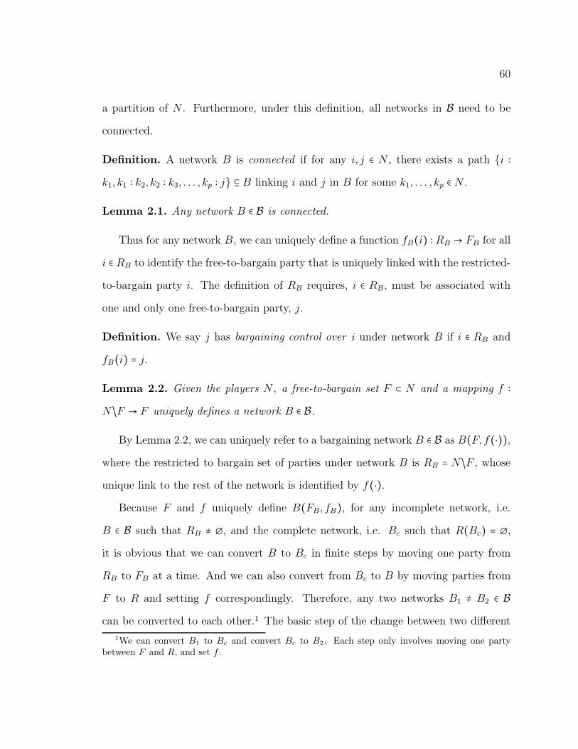
60
a partition of N . Furthermore, under this definition, all networks in B need to be
connected.
Definition. A network B is connected if for any i, j ∈ N , there exists a path i ∶k1, k1 ∶ k2, k2 ∶ k3, . . . , kp ∶ j ⊆ B linking i and j in B for some k1, . . . , kp ∈ N .
Lemma 2.1. Any network B ∈ B is connected.
Thus for any network B, we can uniquely define a function fB(i) ∶ RB → FB for all
i ∈ RB to identify the free-to-bargain party that is uniquely linked with the restricted-
to-bargain party i. The definition of RB requires, i ∈ RB, must be associated with
one and only one free-to-bargain party, j.
Definition. We say j has bargaining control over i under network B if i ∈ RB and
fB(i) = j.
Lemma 2.2. Given the players N , a free-to-bargain set F ⊂ N and a mapping f ∶N/F → F uniquely defines a network B ∈ B.
By Lemma 2.2, we can uniquely refer to a bargaining network B ∈ B as B(F, f(⋅)),where the restricted to bargain set of parties under network B is RB = N/F , whose
unique link to the rest of the network is identified by f(⋅).Because F and f uniquely define B(FB, fB), for any incomplete network, i.e.
B ∈ B such that RB ≠ ∅, and the complete network, i.e. Bc such that R(Bc) = ∅,it is obvious that we can convert B to Bc in finite steps by moving one party from
RB to FB at a time. And we can also convert from Bc to B by moving parties from
F to R and setting f correspondingly. Therefore, any two networks B1 ≠ B2 ∈ Bcan be converted to each other.1 The basic step of the change between two different
1We can convert B1 to Bc and convert Bc to B2. Each step only involves moving one partybetween F and R, and set f .
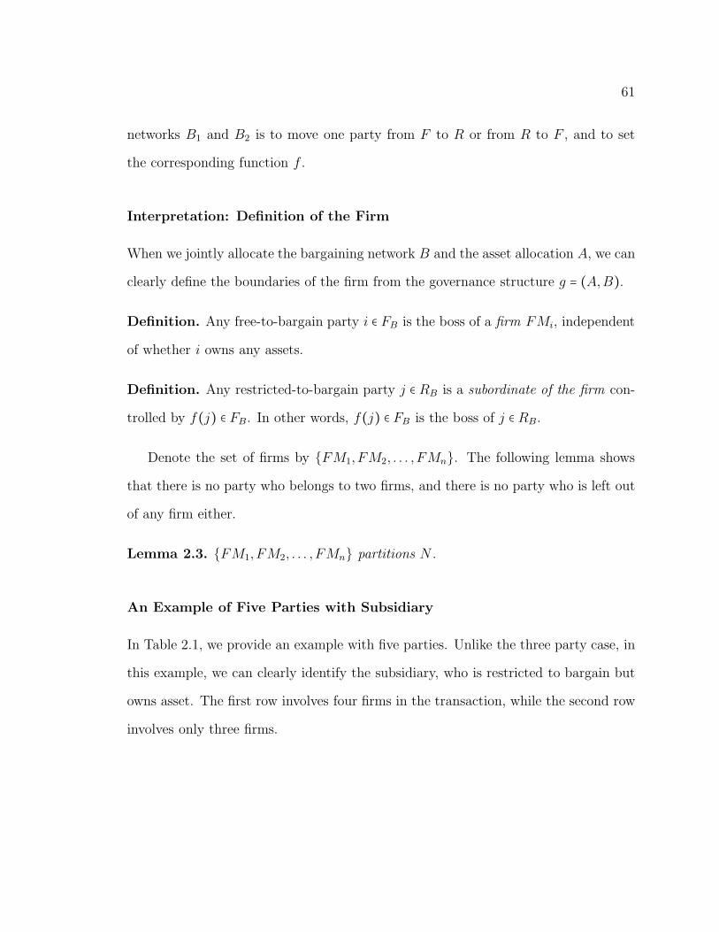
61
networks B1 and B2 is to move one party from F to R or from R to F , and to set
the corresponding function f .
Interpretation: Definition of the Firm
When we jointly allocate the bargaining network B and the asset allocation A, we can
clearly define the boundaries of the firm from the governance structure g = (A,B).
Definition. Any free-to-bargain party i ∈ FB is the boss of a firm FMi, independent
of whether i owns any assets.
Definition. Any restricted-to-bargain party j ∈ RB is a subordinate of the firm con-
trolled by f(j) ∈ FB. In other words, f(j) ∈ FB is the boss of j ∈ RB.
Denote the set of firms by FM1, FM2, . . . , FMn. The following lemma shows
that there is no party who belongs to two firms, and there is no party who is left out
of any firm either.
Lemma 2.3. FM1, FM2, . . . , FMn partitions N .
An Example of Five Parties with Subsidiary
In Table 2.1, we provide an example with five parties. Unlike the three party case, in
this example, we can clearly identify the subsidiary, who is restricted to bargain but
owns asset. The first row involves four firms in the transaction, while the second row
involves only three firms.
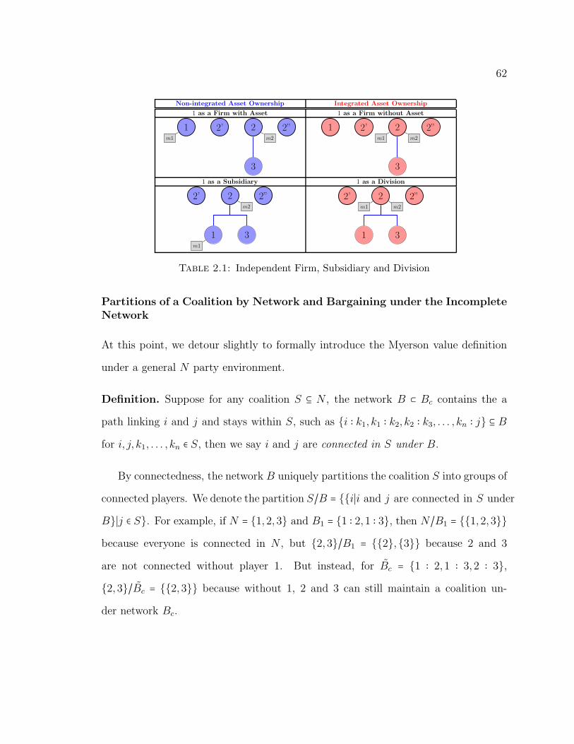
62
Non-integrated Asset Ownership Integrated Asset Ownership
1 as a Firm with Asset 1 as a Firm without Asset
2
3
2’ 2”1
m1 m2
2
3
2’ 2”1
m1 m2
1 as a Subsidiary 1 as a Division
2
1 3
2’ 2”
m1
m2
2
1 3
2’ 2”
m1 m2
Table 2.1: Independent Firm, Subsidiary and Division
Partitions of a Coalition by Network and Bargaining under the IncompleteNetwork
At this point, we detour slightly to formally introduce the Myerson value definition
under a general N party environment.
Definition. Suppose for any coalition S ⊆ N , the network B ⊂ Bc contains the a
path linking i and j and stays within S, such as i ∶ k1, k1 ∶ k2, k2 ∶ k3, . . . , kn ∶ j ⊆ Bfor i, j, k1, . . . , kn ∈ S, then we say i and j are connected in S under B.
By connectedness, the network B uniquely partitions the coalition S into groups of
connected players. We denote the partition S/B = i∣i and j are connected in S under
B∣j ∈ S. For example, if N = 1,2,3 and B1 = 1 ∶ 2,1 ∶ 3, then N/B1 = 1,2,3because everyone is connected in N , but 2,3/B1 = 2,3 because 2 and 3
are not connected without player 1. But instead, for Bc = 1 ∶ 2,1 ∶ 3,2 ∶ 3,2,3/Bc = 2,3 because without 1, 2 and 3 can still maintain a coalition un-
der network Bc.
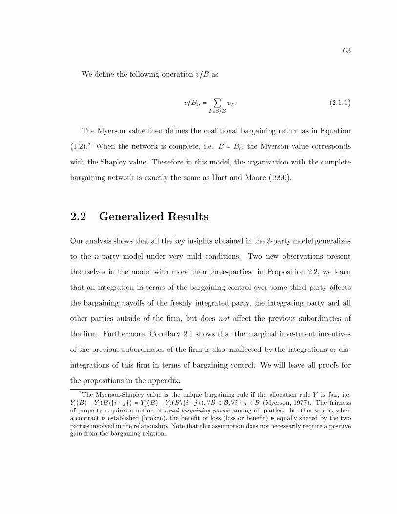
63
We define the following operation v/B as
v/BS = ∑T⊆S/B
vT . (2.1.1)
The Myerson value then defines the coalitional bargaining return as in Equation
(1.2).2 When the network is complete, i.e. B = Bc, the Myerson value corresponds
with the Shapley value. Therefore in this model, the organization with the complete
bargaining network is exactly the same as Hart and Moore (1990).
2.2 Generalized Results
Our analysis shows that all the key insights obtained in the 3-party model generalizes
to the n-party model under very mild conditions. Two new observations present
themselves in the model with more than three-parties. in Proposition 2.2, we learn
that an integration in terms of the bargaining control over some third party affects
the bargaining payoffs of the freshly integrated party, the integrating party and all
other parties outside of the firm, but does not affect the previous subordinates of
the firm. Furthermore, Corollary 2.1 shows that the marginal investment incentives
of the previous subordinates of the firm is also unaffected by the integrations or dis-
integrations of this firm in terms of bargaining control. We will leave all proofs for
the propositions in the appendix.
2The Myerson-Shapley value is the unique bargaining rule if the allocation rule Y is fair, i.e.Yi(B) − Yi(B/i ∶ j) = Yj(B) − Yj(B/i ∶ j),∀B ∈ B,∀i ∶ j ∈ B (Myerson, 1977). The fairnessof property requires a notion of equal bargaining power among all parties. In other words, whena contract is established (broken), the benefit or loss (loss or benefit) is equally shared by the twoparties involved in the relationship. Note that this assumption does not necessarily require a positivegain from the bargaining relation.
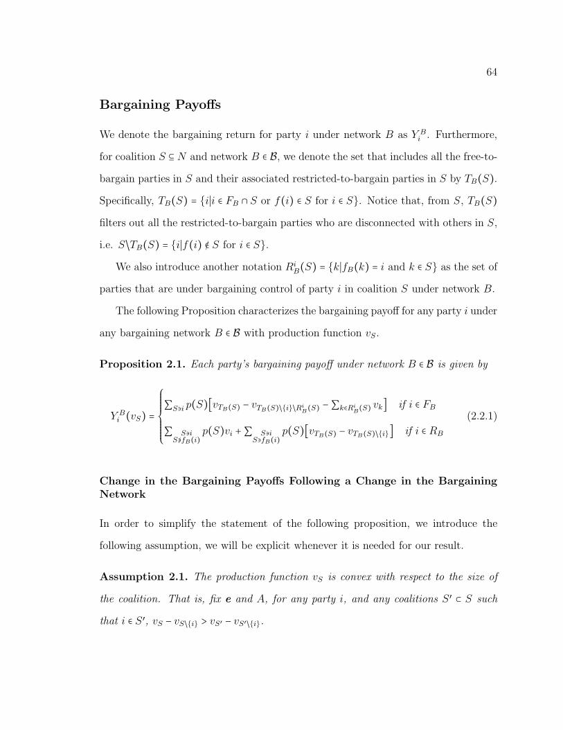
64
Bargaining Payoffs
We denote the bargaining return for party i under network B as Y Bi . Furthermore,
for coalition S ⊆ N and network B ∈ B, we denote the set that includes all the free-to-bargain parties in S and their associated restricted-to-bargain parties in S by TB(S).Specifically, TB(S) = i∣i ∈ FB ∩ S or f(i) ∈ S for i ∈ S. Notice that, from S, TB(S)filters out all the restricted-to-bargain parties who are disconnected with others in S,
i.e. S/TB(S) = i∣f(i) ∉ S for i ∈ S.We also introduce another notation Ri
B(S) = k∣fB(k) = i and k ∈ S as the set ofparties that are under bargaining control of party i in coalition S under network B.
The following Proposition characterizes the bargaining payoff for any party i under
any bargaining network B ∈ B with production function vS.
Proposition 2.1. Each party’s bargaining payoff under network B ∈ B is given by
Y Bi (vS) =
⎧⎪⎪⎪⎪⎪⎪⎨⎪⎪⎪⎪⎪⎪⎩
∑S∋i p(S)[vTB(S) − vTB(S)/i/RiB(S) −∑k∈Ri
B(S) vk] if i ∈ FB
∑ S∋iS∌fB(i)
p(S)vi +∑ S∋iS∋fB(i)
p(S)[vTB(S) − vTB(S)/i] if i ∈ RB
(2.2.1)
Change in the Bargaining Payoffs Following a Change in the BargainingNetwork
In order to simplify the statement of the following proposition, we introduce the
following assumption, we will be explicit whenever it is needed for our result.
Assumption 2.1. The production function vS is convex with respect to the size of
the coalition. That is, fix e and A, for any party i, and any coalitions S′ ⊂ S such
that i ∈ S′, vS − vS/i > vS′ − vS′/i.
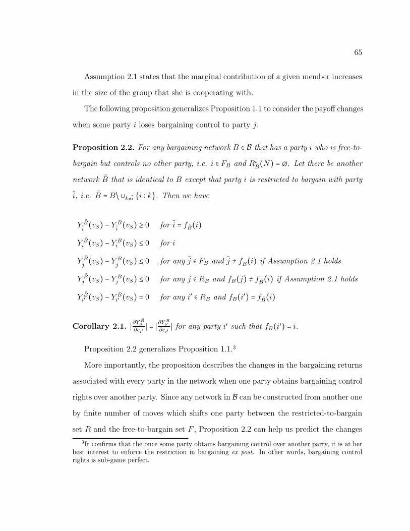
65
Assumption 2.1 states that the marginal contribution of a given member increases
in the size of the group that she is cooperating with.
The following proposition generalizes Proposition 1.1 to consider the payoff changes
when some party i loses bargaining control to party j.
Proposition 2.2. For any bargaining network B ∈ B that has a party i who is free-to-
bargain but controls no other party, i.e. i ∈ FB and RiB(N) = ∅. Let there be another
network B that is identical to B except that party i is restricted to bargain with party
i, i.e. B = B/ ∪k≠i i ∶ k. Then we have
Y B
i(vS) − Y B
i(vS) ≥ 0 for i = fB(i)
Y Bi (vS) − Y B
i (vS) ≤ 0 for i
Y B
j(vS) − Y B
j(vS) ≤ 0 for any j ∈ FB and j ≠ fB(i) if Assumption 2.1 holds
Y Bj (vS) − Y B
j (vS) ≤ 0 for any j ∈ RB and fB(j) ≠ fB(i) if Assumption 2.1 holds
Y Bi′ (vS) − Y B
i′ (vS) = 0 for any i′ ∈ RB and fB(i′) = fB(i)
Corollary 2.1. ∣∂YBi′
∂ei′∣ = ∣∂Y
Bi′
∂ei′∣ for any party i′ such that fB(i′) = i.
Proposition 2.2 generalizes Proposition 1.1.3
More importantly, the proposition describes the changes in the bargaining returns
associated with every party in the network when one party obtains bargaining control
rights over another party. Since any network in B can be constructed from another one
by finite number of moves which shifts one party between the restricted-to-bargain
set R and the free-to-bargain set F , Proposition 2.2 can help us predict the changes
3It confirms that the once some party obtains bargaining control over another party, it is at herbest interest to enforce the restriction in bargaining ex post. In other words, bargaining controlrights is sub-game perfect.
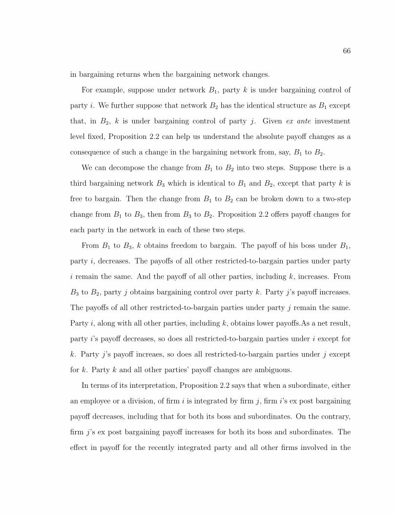
66
in bargaining returns when the bargaining network changes.
For example, suppose under network B1, party k is under bargaining control of
party i. We further suppose that network B2 has the identical structure as B1 except
that, in B2, k is under bargaining control of party j. Given ex ante investment
level fixed, Proposition 2.2 can help us understand the absolute payoff changes as a
consequence of such a change in the bargaining network from, say, B1 to B2.
We can decompose the change from B1 to B2 into two steps. Suppose there is a
third bargaining network B3 which is identical to B1 and B2, except that party k is
free to bargain. Then the change from B1 to B2 can be broken down to a two-step
change from B1 to B3, then from B3 to B2. Proposition 2.2 offers payoff changes for
each party in the network in each of these two steps.
From B1 to B3, k obtains freedom to bargain. The payoff of his boss under B1,
party i, decreases. The payoffs of all other restricted-to-bargain parties under party
i remain the same. And the payoff of all other parties, including k, increases. From
B3 to B2, party j obtains bargaining control over party k. Party j’s payoff increases.
The payoffs of all other restricted-to-bargain parties under party j remain the same.
Party i, along with all other parties, including k, obtains lower payoffs.As a net result,
party i’s payoff decreases, so does all restricted-to-bargain parties under i except for
k. Party j’s payoff increaes, so does all restricted-to-bargain parties under j except
for k. Party k and all other parties’ payoff changes are ambiguous.
In terms of its interpretation, Proposition 2.2 says that when a subordinate, either
an employee or a division, of firm i is integrated by firm j, firm i’s ex post bargaining
payoff decreases, including that for both its boss and subordinates. On the contrary,
firm j’s ex post bargaining payoff increases for both its boss and subordinates. The
effect in payoff for the recently integrated party and all other firms involved in the
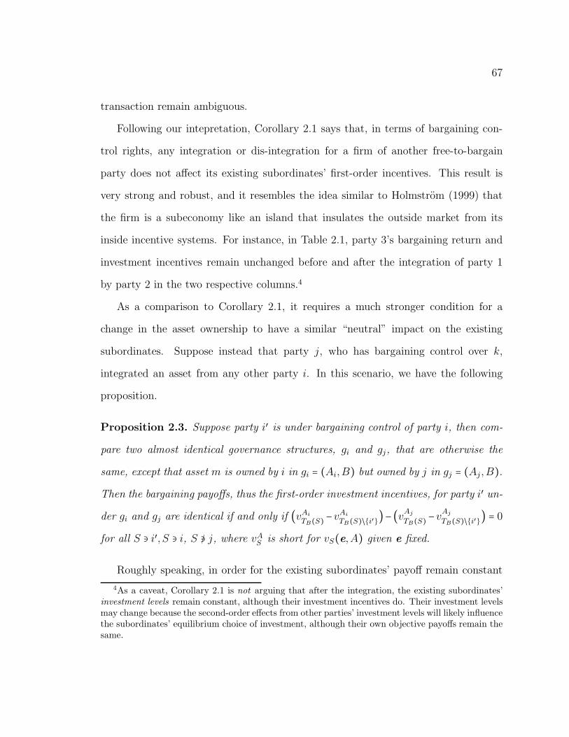
67
transaction remain ambiguous.
Following our intepretation, Corollary 2.1 says that, in terms of bargaining con-
trol rights, any integration or dis-integration for a firm of another free-to-bargain
party does not affect its existing subordinates’ first-order incentives. This result is
very strong and robust, and it resembles the idea similar to Holmstrom (1999) that
the firm is a subeconomy like an island that insulates the outside market from its
inside incentive systems. For instance, in Table 2.1, party 3’s bargaining return and
investment incentives remain unchanged before and after the integration of party 1
by party 2 in the two respective columns.4
As a comparison to Corollary 2.1, it requires a much stronger condition for a
change in the asset ownership to have a similar “neutral” impact on the existing
subordinates. Suppose instead that party j, who has bargaining control over k,
integrated an asset from any other party i. In this scenario, we have the following
proposition.
Proposition 2.3. Suppose party i′ is under bargaining control of party i, then com-
pare two almost identical governance structures, gi and gj, that are otherwise the
same, except that asset m is owned by i in gi = (Ai,B) but owned by j in gj = (Aj ,B).Then the bargaining payoffs, thus the first-order investment incentives, for party i′ un-
der gi and gj are identical if and only if (vAi
TB(S)−vAi
TB(S)/i′)−(vAj
TB(S)−vAj
TB(S)/i′) = 0
for all S ∋ i′, S ∋ i, S ∌ j, where vAS is short for vS(e,A) given e fixed.
Roughly speaking, in order for the existing subordinates’ payoff remain constant
4As a caveat, Corollary 2.1 is not arguing that after the integration, the existing subordinates’investment levels remain constant, although their investment incentives do. Their investment levelsmay change because the second-order effects from other parties’ investment levels will likely influencethe subordinates’ equilibrium choice of investment, although their own objective payoffs remain thesame.
68
following an acquisition of an asset by his boss, the subordinates’ contribution to all
productions with his boss should remain the same, with or without the asset. In other
words, the statement is true if the subordinates’ participation is not complementary
to the asset. This is a much stronger condition comparing to Proposition 2.2 and
Corollary 2.1, which holds true without any additional assumptions for the existing
subordinates, i′, of the integrating party.
69
2.A Omitted Proofs for Propositions in Section 2.1
Lemma 2.1. Any network B ∈ B is connected.
Proof. We will prove that any two parties i, j ∈ N are connected under any given networkB ∈ B.
If i, j ∈ FB , i and j are connected by definition of FB . If i ∈ RB and j ∈ FB , then i ∶ i ∈ Bfor some i ∈ FB by definition of RB . But we also have i ∶ j ∈ B because i, j ∈ FB . Thus i
and j are connected.Otherwise if i, j ∈ RB , then i ∶ i ∈ B and j ∶ j ∈ B for some i, j ∈ FB . But it must be
either i = j or i ∶ j ∈ B. So i and j are connected.
Lemma 2.2. Given the players N , a free-to-bargain set F ⊂ N and a mapping f ∶ N/F → F
uniquely defines a network B ∈ B.
Proof. Suppose F and f(⋅) define both B and B ∈ B s.t. B ≠ B. Then for F = FB = FB
and f = fB = fB, there must exist a link i ∶ i in one of the networks B or B, but not in the
other, for some i ∈N . With out loss of generality, we suppose i ∶ i ∈ B but i ∶ i ≠ B.Since i ∶ i ≠ B, either i or i is not in F by the definition of F . Without loss of generality,
let i ∈ F and i ∈N/F = R. Since i ∶ i ≠ B, i ≠ f (i).But since F and f(⋅) also defines B, for i ∈ N/F, i ∶ i ∈ B implies that i = f (i) by
definition of R. Thus it must be that fB ≠ fB, therefore we reach a contradiction.
Lemma 2.3. FM1, FM2, . . . , FMn partitions N .
Proof. First, we show that any party i ∈ N is in a firm.Sets FB and RB partitions N by definition. Suppose party i ∈ F . Then i is a firm. Sup-
pose, instead, i ∈ R, then i is the subordinate for firm fB(i) ∈ F . The above categorizationexhausts N , thus all parties in N is in a firm.
Next, we show that no i ∈ N belongs to two firms.Suppose i ∈ FM1 and i ∈ FM2 for FM1 ≠ FM2. By definition of B and the definition
of firms, i cannot be a subordinate for both firms. And i cannot be a subordinate for onefirm and the boss the other because RB and FB partition N . Moreover, by definition of theboss, a party cannot be the boss for two firms. This concludes the proof.
Proposition 2.1. Each party’s bargaining payoff under network B ∈ B is given by
Y Bi (vS) =
⎧⎪⎪⎪⎨⎪⎪⎪⎩
∑S∋i p(S)[vTB(S) − vTB(S)/i/RiB(S) −∑k∈Ri
B(S) vk] if i ∈ FB
∑ S∋iS∌fB(i)
p(S)vi +∑ S∋iS∋fB(i)
p(S)[vTB(S) − vTB(S)/i] if i ∈ RB
Before proving the Propositions, it is convenient to prove some lemmas first.
Lemma 2.4. TB(S) is the only element in S/B that contains more than one party.
70
Proof. Suppose there exists T ′B(S) ∩ TB(S) = ∅ such that i, j ∈ T ′B(S) for some i ≠ j.Because T ′B(S) ∈ S/B, by definition, i and j are connected in S under B. Thus there
must be a link i ∶ k1, k1 ∶ k2, ..., kn ∶ j ⊆ B for i, j, k1, ..., kn ∈ S. By definition of B, it cannotbe the case that none of them is in F while being connected to each other. But supposeany one of them is in FB , T
′B(S) ∩ TB(S) ≠ ∅, we reach a contradiction.
Lemma 2.5. For all S ⊆ N , we have
vBS = vTB(S) + ∑k∈S
k∉TB(S)
vk. (2.A.1)
Proof. By Lemma 2.4, all k ∉ TB(S) are singleton components containing only one party.For any S ⊆ N , S/B contains only one connected non-singleton component TB(S) and agroup of other unconnected singleton components. Then the result follows by the definitionof vBS .
Lemma 2.6. For all S ⊆ N , we have
vBS/i =⎧⎪⎪⎪⎨⎪⎪⎪⎩
vBS − vi if i ∉ TB(S)vTB(S)/i/R
iB(S) +∑ k∈S/i
fB(k)∉S
vk +∑k∈RiB(S) vk if i ∈ TB(S) (2.A.2)
Proof. Lemma 2.5 helps unpack vBS into the form of vS . We can also apply Lemma 2.5again to unpack vB
S/i.By Lemma 2.5,
vBS/i = vTB(S/i) + ∑k∈S/i
k∉TB(S/i)
vk.
Furthermore, by definition of TB(S),
TB(S/i) =⎧⎪⎪⎨⎪⎪⎩TB(S) if i ∉ TB(S),TB(S)/i/Ri
B(S) if i ∈ TB(S).
Therefore, if i ∉ TB(S),
vBS/i = vTB(S) + ∑k∈S/ik∉TB(S)
vk
= vTB(S) + ∑k∈S
k∉TB(S)
vk − vi
= vBS − vi.
71
Otherwise if i ∈ TB(S),
vBS/i = vTB(S)/i/RiB(S) + ∑
k∈S/i
k∉TB(S)/i/RiB(S)
vk
= vTB(S)/i/RiB(S) + ∑
k∈S/ifB(k)∉S
vk + ∑k∈S/ifB(k)=i
vk
= vTB(S)/i/RiB(S) + ∑
k∈S/ifB(k)∉S
vk + ∑k∈Ri
B(S)
vk.
Proof of Proposition 2.1
Proof. By definition of the Myerson value, to specify the bargaining payoff Y Bi (vS), we
need to specify the term vBS − vBS/i.Subtract Equation (2.A.2) from Equation (2.A.1), we have
vBS − vBS/i =⎧⎪⎪⎨⎪⎪⎩vi if i ∉ TB(S),vTB(S) − vTB(S)/i/R
iB(S) −∑k∈Ri
B(S) vk if i ∈ TB(S).
(2.A.3)
Plug Equation (2.A.3) into the definition of Myerson value, we have
Y Bi (vS) = ∑
S∋iTB(S)∌i
p(S)vi + ∑S∋i
TB(S)∋i
p(S)vTB(S) − vTB(S)/i/RiB(S) − ∑
k∈RiB(S)
vk (2.A.4)
When i is free to bargain, the first term in Equation (2.A.4) drops out, which yields thepayoff for any free-to-bargain party. When i is restricted to bargain with a given party, thefirst term in Equation (2.A.4) remains. And the second term in Equation (2.A.4) reducesto vTB(S)−vTB(S)/i because R
iB(S) = ∅ when i is restricted to bargain. Therefore we have
Y Bi (vS) =
⎧⎪⎪⎪⎨⎪⎪⎪⎩
∑S∋i p(S)[vTB(S) − vTB(S)/i/RiB(S) −∑k∈Ri
B(S) vk] if i ∈ FB
∑ S∋iS∌fB(i)
p(S)vi +∑ S∋iS∋fB(i)
p(S)[vTB(S) − vTB(S)/i] if i ∈ RB
Proposition 2.2. For any bargaining network B ∈ B that has a party i who is free-to-bargain but controls no other party, i.e. i ∈ FB and Ri
B(N) = ∅. Let there be anothernetwork B that is identical to B except that party i is restricted to bargain with party i,
72
i.e. B = B/ ∪k≠i i ∶ k. Then we have
Y Bi(vS) − Y B
i(vS) ≥ 0 for i = fB(i)
Y Bi (vS) − Y B
i (vS) ≤ 0 for i
Y Bj(vS) − Y B
j(vS) ≤ 0 for any j ∈ FB and j ≠ fB(i)
Y Bj (vS) − Y B
j (vS) ≤ 0 for any j ∈ RB and fB(j) ≠ fB(i)Y Bi′ (vS) − Y B
i′ (vS) = 0 for any i′ ∈ RB and fB(i′) = fB(i)
Lemma 2.7. Given B and B defined in Proposition 2.2, for any S ⊆ N and i = fB(i),
TB(S) =⎧⎪⎪⎨⎪⎪⎩TB(S) if i ∉ S or if i ∈ STB(S)/i if i ∈ S but i ∉ S
Proof. First of all, for any j ≠ i, j ∈ FB if and only if j ∈ FB , and j ∈ RB if and only if j ∈ RB
with fB(j) = fB(j). So j ∈ TB(S) if and only if j ∈ TB(S) for any j ≠ i and any S ⊆ N .Thus if i ∉ S, then ∀j ∈ S, j ∈ TB(S) if and only if j ∈ TB(S). So TB(S) = TB(S) if i ∉ S.If i ∈ S and i ∈ S, then i ∈ TB(S) if i ∈ S, and i ∉ TB(S) if i ∉ S. Under network B, we
also have i ∈ TB(S) if and only if i ∈ S because i ∈ FB . Thus TB(S) = TB(S) if i ∈ S andi ∈ S.
Otherwise if i ∈ S and i ∉ S, then i ∈ TB(S) because i ∈ FB , but i ∉ TB(S) since i ∉ S. Yet
as is shown, for all other j ≠ i, j ∈ TB(S) if and only if j ∈ TB(S). So T
B(S) = TB(S)/i.
Proof of Proposition 2.2
Proof. We will use Lemma 2.7 repeatedly in the following calculations to help us simplifythe expressions.
For party i, who becomes restricted to bargain under party i, we have, by Proposition2.1,
Y Bi (vS) − Y B
i (vS) =∑S∋iS∌i
p(S)vi +∑S∋iS∋i
p(S)[vTB(S) − vT
B(S)/i]
−∑S∋i
p(S)[vTB(S) − vTB(S)/i/RiB(S) − ∑
k∈RiB(S)
vk]
=∑S∋iS∌i
p(S)vi +∑S∋iS∋i
p(S)[vTB(S) − vTB(S)/i] −∑S∋i
p(S)[vTB(S) − vTB(S)/i]
= −∑S∋iS∌i
p(S)[vTB(S) − vTB(S)/i − vi]. (2.A.5)
73
The second step is by Lemma 2.7. So Y Bi (vS) − Y B
i (vS) ≤ 0 by the assumption thatproduction functions vS are superadditive.
For party i, who obtains bargaining control over party i, by definition,
RiB(S) =
⎧⎪⎪⎨⎪⎪⎩Ri
B(S) ∪ i if S ∋ iRi
B(S) if S ∌ i .
Therefore, we have, again by Proposition 2.1,
Y Bi(vS) − Y B
i(vS) = ∑
S∋i
p(S)[vTB(S) − vT
B(S)/i/Ri
B(S)− ∑
k∈Ri
B(S)
vk]
−∑S∋i
p(S)[vTB(S) − vTB(S)/i/RiB(S)− ∑
k∈RiB(S)
vk]
= ∑S∋iS∌i
p(S)[vTB(S) − vTB(S)/i/RiB(S)− ∑
k∈RiB(S)
vk]
+∑S∋iS∋i
p(S)[vTB(S) − vTB(S)/i/RiB(S)/i
− ∑k∈Ri
B(S)
vk − vi]
−∑S∋i
p(S)[vTB(S) − vTB(S)/i/RiB(S)− ∑
k∈RiB(S)
vk]
= ∑S∋iS∋i
p(S)[vTB(S)/i/Ri
B(S)− v
TB(S)/i/RiB(S)/i
− vi]. (2.A.6)
Again, by the assumption that production functions vS are superadditive, Y Bi(vS)−Y B
i(vS) ≥
0.For any other free-to-bargain party j ∈ FB who does not gain bargaining control over
74
party i, j ≠ fB(i), we have Rj
B(S) = Rj
B(S),∀S. So we have
Y Bj(vS) − Y B
j(vS) = ∑
S∋j
p(S)[vTB(S) − vT
B(S)/j/Rj
B(S)− ∑
k∈Rj
B(S)
vk]
− ∑S∋j
p(S)[vTB(S) − vTB(S)/j/Rj
B(S)− ∑
k∈Rj
B(S)
vk]
= ∑S∋j
S∋i,S∌i
p(S)[vTB(S) − vT
B(S)/j/Rj
B(S)] − ∑
S∋j
S∋i,S∌i
p(S)[vTB(S) − vTB(S)/j/Rj
B(S)]
= ∑S∋j
S∋i,S∌i
p(S)[vTB(S)/i − vTB(S)/i/j/Rj
B(S)] − ∑
S∋jS∋i,S∌i
p(S)[vTB(S) − vTB(S)/j/Rj
B(S)]
= − ∑S∋j
S∋i,S∌i
p(S)[(vTB(S) − vTB(S)/i) − (vTB(S)/j/Rj
B(S)− v
TB(S)/j/Rj
B(S)/i
)]
(2.A.7)
By Assumption 2.1, the production function is convex in participation. Party i’s marginal
contribution is greater in a larger coalition. Thus Y Bj(vS) − Y B
j(vS) ≤ 0.
For any restricted-to-bargain party j under any party other than i, i.e. fB(j) = fB(j) =j ≠ fB(i) = i, we have
Y Bj (vS) − Y B
j (vS) = ∑S∋j
S∌j
p(S)vj + ∑S∋j
S∋j
p(S)[vTB(S) − vT
B(S)/j]
− ∑S∋j
S∌j
p(S)vj − ∑S∋j
S∋j
p(S)[vTB(S) − vTB(S)/j]
= ∑S∋j,S∋jS∋i,S∌i
p(S)[vTB(S) − vT
B(S)/j] − ∑
S∋j,S∋jS∋i,S∌i
p(S)[vTB(S) − vTB(S)/j]
= ∑S∋j,S∋j
S∋i,S∌i
p(S)[vTB(S)/i − vTB(S)/j/i] − ∑S∋j,S∋j
S∋i,S∌i
p(S)[vTB(S) − vTB(S)/j]
= − ∑S∋j,S∋jS∋i,S∌i
p(S)[(vTB(S) − vTB(S)/i) − (vTB(S)/j − vTB(S)/j/i)]
(2.A.8)
Again, by Assumption 2.1, Y Bj (vS) − Y B
j (vS) ≤ 0.For any restricted-to-bargain party i′ under party i, i.e. fB(i′) = fB(i′) = fB(i) = i, we
75
have
Y Bi′ (vS) − Y B
i′ (vS) = ∑S∋i′
S∌i
p(S)vi′ + ∑S∋i′
S∋i
p(S)[vTB(S) − vT
B(S)/i′]
− ∑S∋i′
S∌i
p(S)vi′ − ∑S∋i′
S∋i
p(S)[vTB(S) − vTB(S)/i′]
= ∑S∋i′
S∋i
p(S)[vTB(S) − vT
B(S)/i′] − ∑
S∋i′
S∋i
p(S)[vTB(S) − vTB(S)/i′]
= 0 (2.A.9)
Therefore, for any party i′ who is already under bargaining control of party i, when i obtainsbargaining control over some other party i, i′’s bargaining payoff does not change.
Proposition 2.3. Suppose party i′ is under bargaining control of party i, then comparetwo almost identical governance structures, gi and gj , that are otherwise the same, exceptthat asset m is owned by i in gi = (Ai,B) but owned by j in gj = (Aj ,B). Then thebargaining payoffs, thus the first-order investment incentives, for party i′ under gi and gj
are identical if and only if (vAi
TB(S)−vAi
TB(S)/i′)−(vAj
TB(S)−vAj
TB(S)/i′) = 0 for all S ∋ i′, S ∋ i,
S ∌ j, where vAS is short for vS(e,A) given e fixed.
Proof. Given network B such that i′ is under bargaining control of party i, and party j isfree-to-bargain.
Let’s denote the production functions as viS and vjS
for asset allocations Ai and Aj ,respectively. Then we have for party i′’s payoff following an asset transfer from j to i as
Y Bi′ (viS) − Y B
i′ (vjS) = ∑S∋i′
S∋i
p(S)vii′ + ∑S∋i′
S∋i
[viTB(S)− viTB(S)/i′
] − ∑S∋i′
S∋i
p(S)vji′ − ∑S∋i′
S∋i
[vjTB(S)
− vjTB(S)/i′
]
= ∑S∋i′
S∋i
[(vAi
TB(S)− vAi
TB(S)/i′) − (vAj
TB(S)− vAj
TB(S)/i′)]
= ∑S∋i′
S∋i,S∌j
[(vAi
TB(S)− vAi
TB(S)/i′) − (vAj
TB(S)− vAj
TB(S)/i′)]
The last step follows because if both i and j are in S, then viS = vjS .
76
2.B Omitted Statements and Proofs for the Gen-
eral n-Party Model
Proposition 2.4. (Insulation Effect) Let Sj be any non-singleton coalition that include
j but not j. Under any network B such that j ∈ RB, f
B(j) = j, we have
∂Y Bi
∂vSj
= 0 for any
party i ∈ N . Otherwise under any network B such that j ∈ FB, we have∂Y B
i
∂vSj
≠ 0 for any
party i ∈ N .
Proof. By definition of TB(S), if j ∈ RB, we have j ∉ TB(S) for any non-singleton setS ∌ j. In other words, TB(S) cannot be a non-singleton set that includes j. So there is nocoalition S that has a corresponding Sj = T
B(S) that is non-singular, contains j but not
j. By Proposition 2.1, the bargaining payoff for any party i does not include the term vSj.
Thus∂Y B
i
∂vSj
= 0 for any i ∈ N .
Instead, if j ∈ FB , we always have j ∈ TB(Sj) as long as Sj ∋ j. Therefore for any S ∋ j,we have Sj = TB(S) that is non-singleton, including j, and not including some other partyj. Again, by Proposition 2.1, vSj
= vTB(S) shows up in the payoff function for party i.Furthermore, whenever i ∈ Sj, the weight on vSj
= vTB(S) is always positive, and otherwise,
the weight is negative. Thus∂Y B
i
∂vSj
≠ 0.
Proposition 2.5. (Concentration Effect) ∣∂YBi
∂vj∣ > ∣∂Y
Bi
∂vj∣ for any party i such that fB(i) ≠
j. Moreover, let S−j be any coalition such that S ∌ j,S ∌ j. Then we have ∣ ∂YBi
∂vS−j∣ > ∣ ∂Y
Bi
∂vS−j∣
for any party i such that fB(i) ≠ j.
Proof. The result follows directly taking derivatives from equations (2.A.5) to (2.A.9) withrespect to vi and vS for S ∋ i, S ∌ i.
Proposition 2.6. The shift of asset ownership can have different effects on payoffs under
different bargaining networks.
Proof. Using operation ∆N−I , we can apply the same operations to equations (2.A.5) to(2.A.9), then a similar result to Proposition 1.2 follows.
Proposition 2.7. Under any governance structure g = (A,B), there is always under-
investment. That is eA,Bi < eFB
i for any i ∈ N .
Proof. The first-best level of investment is characterized by ∂vN∂ei= Ψ′i(ei). And the second-
best investments are characterized by∂Y
gi(e,A)
∂ei= Ψ′i(ei).
77
By definition of Myerson value
Y Bi = ∑
S∋i
p(S)vBS − vBS/i
< ∑S∋i
p(S)vBS
< ∑S∋i
p(S)vS
< ∑S∋i
p(S)vN ,
where the last inequality holds by Assumption 1.1.
Thus∂Y
gi(e,A)
∂ei< ∂vN
∂ei, which implies that the second-best investment is strictly less than
the first-best level.
Proposition 2.8. If there is no CSM, and every parties’ investments are SSM with respect
to all coalitions S ⊆ N , then it is never efficient to have bargaining control rights.
Proof. Suppose in network BK , there are K parties who are restricted to bargain. We cancompare the network BK with a similar network, BK−1, that is otherwise identical, but withonly K−1 parties restricted to bargain. Without loss of generality, label this party as i, thenthe payoff comparisons between these two networks for any party k, Y BK
k(vS)−Y BK−1
k(vS),
are given by equations (2.A.5) to (2.A.9), depending on the bargaining rights of each party.If there is no cross-investment superadditivity at the margin, it can be readily verified
from equations (2.A.5) and (2.A.6) that∂Y
BKk(vS)
ek− ∂Y
BK−1k
(vS)
ek< 0 for party k = i and party
k = i.We can rewrite equation (2.A.7) as
Y Bj(vS) − Y B
j(vS) = − ∑
S∋j
S∋i,S∌i
p(S)[(vTB(S) − vTB(S)/i) − (vTB(S)/j/Rj
B(S)− v
TB(S)/j/Rj
B(S)/i
)]
= − ∑S∋j
S∋i,S∌i
p(S)[(vTB(S) − vTB(S)/i − vi) − (vTB(S)/j/Rj
B(S)− v
TB(S)/j/Rj
B(S)/i
− vi)].
By self-investment superadditivity at the margin, the partial derivative of the first term inbracket with respect to ej is positive. And since there is no cross-investment superadditivityat the margin, the the partial derivative of the second term in bracket with respect to ej is
negative. So overall,∂Y
BKk(vS)
ek− ∂Y
BK−1k
(vS)
ek< 0 for all free-to-bargain parties j ≠ i. Same
logic applies to equation (2.A.8) and so the result also follows for all k such that fBK−1≠ i.
By equation (2.A.9),∂Y
BKk(vS)
ek− ∂Y
BK−1k
(vS)
ek= 0 for all k such that fBK−1
= i.Therefore, we have eBK
i ≤ eBK−1i . Thus given asset allocation A, bargaining network BK
is strictly less efficient than BK−1.

78
We can then repeat the same logic and iterate all the way through K = 1 and compareit with the complete bargaining network Bc. As a consequence, Bc is strictly more efficientthan any incomplete bargaining network.
Corollary 2.2. If there is no cross-investment, then under Assumption 1.1, it is never
efficient to have bargaining control rights.
Proof. If there is no cross-investment, there cannot be cross-investment superadditivity atthe margin. Then the result follows from Proposition 2.8.
Chapter 3
Subsidiaries vs. Divisions in aProperty-Rights Theory of theFirm
3.1 Introduction
Subsidiaries and unincorporated divisions are alternative governance structures for
large corporations and business groups to organize their internal business units. Both
forms are widely observed, and one form does not seem to dominate another. Why is
one form used as oppose to another is both a curious case to be solved for researchers
and an important issue to be understood for strategic and policy purposes.
Subsidiaries are ubiquitous in modern corporations. Squire (2011) documents that
“in 2010, the one hundred US public companies with the highest annual revenues
reported an average of 245 major subsidiaries, with 114 as the median. Only five
reported fewer than five major subsidiaries”. Alfaro and Charlton (2009) observe in
79
80
their data that, as of 1999, “2,248 entities that report to General Motors Corporation
as their ‘global ultimate parent.’
Divisions are also widely adopted as the governance structure for business units.
Hewlett-Packard has 58 divisions in 1992 versus 40 in 1980 (Beer and Rogers, 1995).
The animation business in Disney is governed as a division, and Pixar was incorpo-
rated from the computer division from Lucasfilm (Alcacer et al., 2010).
The legal distinctions between the subsidiaries and the divisions are relatively
clear. From the legal perspective, subsidiaries are distinct and independent legal
entities from their parent firms. Whereas unincorporated divisions are integrated
parts within the large firm’s corporate shell.1
From the economics perspective, the differences between these two seemingly sim-
ilar organizational forms are much more subtle and formal economic theory provides
little guidance on the tradeoff between these two alternatives. In fact, given the
fact that the parent firm has control over the business unit, the classical theories of
the firm do not even capture the differences in the legal ownership of assets under
subsidiaries and divisions. Under the scope of classical property-rights theory of the
firm by Grossman and Hart (1986); Hart and Moore (1990); Hart (1995) (GHM), the
owner of the business, either the parent firm of a subsidiary or the headquarter of
a division, has residual rights of control over the assets to which the business unit
1The classical literature on corporate law mainly emphasizes a credit monitoring theory (Posner,1976; Hansmann and Kraakman, 2000; Hansmann et al., 2006). This theory argues that, becauseof the separate legal entity status, subsidiaries are protected from limited liabilities and entitiesshielding. Thus the creditors of a business unit is much easier to assess the financial conditions ifthe business unit were a subsidiary rather than a division. However, we choose not to emphasizethis particular theory for two reasons. First, Squire (2011) points out that typical large corporationsextensively uses debt guarantees to override liability barriers provided by the corporate shell. Second,the credit monitoring theory one-sidedly favors subsidiaries and therefore fail to explain the co-existence of divisions with subsidiaries.
81
has access.2 Therefore, although the legal ownership of asset differ for subsidiaries
and divisions, in the GHM framework, subsidiaries and divisions are identical forms
of organizations, whose parent or headquarter controls the (economic) ownership of
assets that are used for production.
The current paper provides a formal economic theory that studies the subsidiaries-
versus-divisions distinction from a different perspective—the transferability of busi-
ness units. Instead of emphasizing the differences in the legal ownership of the assets,
we build the model based on the legal foundation that, for its owner, a business is
easier to be transferred as a subsidiary than as a division (Ayotte and Hansmann,
2012). We focus on studying the implications of this particular legal implication
on the economic outcomes. The model utilizes a modified GHM framework without
assets and focus on the inefficiencies in ex ante investment.
Although the model is built on the idea that subsidiaries are easier to be trans-
ferred, the main results are contrary to the modeling presumption that subsidiaries
are setup to be sold. When the original owner’s investment is the primary concern
for efficiency purposes, the model predicts that setting up a business as a subsidiary
is more efficient than making it a division when (i) the chance of the business being
taken over is low; (ii) investments by the owner of the business unit are non-specific
with respect to the owner’s identity of the business unit. These two conditions are
likely to hold when the business unit is a generic one. And the analysis shows that
using division is more efficient if (i) the chance of the business being taken over is high;
2Ayotte and Hansmann (2012): “Theories of this sort (property rights theory of the firm)... havenothing to say, however, about why a corporation would create wholly-owned subsidiary corpora-tions. Indeed, for the purposes of these theories there is no difference between, on the one hand,a single corporation with its various businesses operated as divisions and, on the other hand, thesame businesses operated as separately incorporated but wholly-owned subsidiaries of the parent. Ineither case, the parent corporation controls all of the assets, so these configurations are equivalentfrom the perspective of the property rights theory.”
82
(ii) investments by the owner of the business unit are specific. These two conditions
are likely to hold when the business unit is a distinct one.
The paper is organized as the following. Section 3.2 explains the legal founda-
tions regarding the distinct transferability of subsidiaries and divisions. Section 3.3
introduces the setup of the formal model. Section 3.4 analyzes the model and provide
predictions of the model. Section 3.5 discusses the results and concludes.
3.2 Discussion of Modeling Assumptions
3.2.1 Legal Foundations
Ayotte and Hansmann (2011, 2012) proposes a theory of legal entities as a bundle
of reassignable contracts. This model relies on the concept of this theory to model
divisions and subsidiaries as different organizational forms in a transaction.
Ayotte and Hansmann (2012) provides the following two facts. On one hand: “The
Law of Bundled Assignability The law of contracts provides that a party’s rights and
obligations under a contract may or may not be transferable (or, as we will somewhat
loosely say, assignable) to a third party without the permission of the other party to
the contract, depending on the subject of the contract and the circumstances.”
On the other hand: “If a business corporation (or other legal entity) is a party to a
contract, a transfer of some or even all of the ownership shares in the corporation is not
considered an assignment of the contract. The corporation, and not its shareholders,
is considered to be a party to the contracts, and the corporation maintains its identity
as its ownership changes. This rule is generally interpreted quite broadly.”3
3Ayotte and Hansmann (2012): “If the counterparty to a contract with a corporation wishes
83
Ayotte and Hansmann (2012, 2011) highlights the tension between liquidity needs
and opportunistic assignment of contracts. On one hand, the owner of a business (O)
has liquidity needs, she might want to sell the business ex post. Suppose the business
relies on one supplier (S) and one leasing company (L) who provide the space for the
business. Were the contracts with S and L non-assignable, upon the time of takeover,
O is likely to be held up by S and L. Expecting this, O is likely to make inefficiently
low ex ante investments, which result in inefficiency. On the other hand, should these
two contracts individually assignable by O, S and L may be discouraged to make
inefficiently low ex ante relationship-specific investments.
To release this tension, Ayotte and Hansmann (2012, 2011) argue that contracts
should be individually non-assignable, but assignable with the transfer of the owner-
ship of the legal entity.
Notice, however, that in our example, S will not be discouraged to make relationship-
specific investments as long as her individual contract can only be reassigned with the
contract of L, as well as possibly some particular assets of O. In this case, it might be
possible to achieve this “bundled assignability” without relying on the legal entity.
However, Ayotte and Hansmann (2012) argues that using the legal entity is likely
to be the most simple and efficient way. Because “entities make it possible to identify
a constantly changing bundle of assets and contracts”. If the assignability is achieved
“without an entity by way of a general description of the bundle, ...in the event
that the owner wishes to separate” the business “from another business she owns, or
from her personal assets...(for example, because of shared facilities or overhead). The
suppliers might argue, for example, that the definition of the bundle being sold is
to limit the persons to whom ownership or control of the corporation can be sold, they must dothis through specific language to that effect in the contract (a ‘change of control’ clause); a non-assignment clause will not suffice.”
84
under-inclusive.” This contractual incompleteness regarding the assignability again
creates hold-up opportunities that deter ex ante investments.4
As a caveat, they also point out that, from the empirical point of view, (i) not all
contracts are individually non-reassignable;5 (ii) a small proportion of contracts are
not reassignable even with the transfer of the ownership of the legal entity; and (iii)
although creating legal entity is likely to be the most convenient way, creating the legal
entity is not the only way to create transferability for an individually non-assignable
contract.
Using a sample of “287 lease and supply agreements from the SEC Edgar database
between 2007 and 2009, filed as a ‘Material Contract’ (Exhibit 10)”, Ayotte and
Hansmann (2012) shows that 95.5% of the contracts “explicitly impose restrictions
on assignment of the contract on an individual basis”.
These 287 contracts can be divided into four groups. (i) 14.3% explicitly forbid
transfer of the contract even with the transfer of the legal entity.6 (ii) 40.1% explicitly
allow for transfer of the contracts with and only with the legal entity.7 (iii) 23% permit
4Ayotte and Hansmann (2012): “One way is for the owner to sign personal contracts that arenonassignable, but that enumerate, in each contract, the other components of the bundle withwhich the counterparty wishes to be tied, allowing for assignment to occur only with all the othercontracts in the defined bundle. For a business of any measurable complexity, however, this would beextremely costly and unreliable”. “Boeing uses 700 different suppliers to create one of its airplanes.Attempting to identify and bundle each of the 700 supply contracts with the 699 other contractswould be messy, labor-intensive, and potentially fraught with error and ambiguities in identification.Moreover, because suppliers change over time, each contract would need to anticipate these futurecontracts and identify them in some way before they come into existence. In short, this is unlikelyto be a practical solution in most realistic cases.”
5Ayotte and Hansmann (2012): “The rights of a promisee under a simple contract for paymentof a definite sum of money are, as a default rule of contract law, generally presumed assignable. Incontrast, the rights of an employer to receive labor services from an employee are generally presumednon-assignable.”
6Ayotte and Hansmann (2012) Table 2.7Ayotte and Hansmann (2012) Table 2 and Table 3 combined, 40.1% of entire sample is entity
bundles only (Table 3: 63.5% in the 36.1%, which yields 40.1%), which means “assignment ispermitted in the event of a merger, acquisition, or a sale of all or substantially all of the assetsof the debtor party to the contract.”
85
the transfer of the contracts as a “bundle” that does not necessarily include the legal
entity (among these 23%, 83.3% also refers to the legal entity, but not restricting only
to the legal entity).8 (iv) 22.6% of the sample do not explicitly forbid transfer of the
contracts as a bundle.
3.2.2 Modeling Assumptions
In this framework, the parent firm of a subsidiary may transfer all of the contractual
relations of the subsidiary as well as the assets under its legal ownership as a bundle
to an alternative holding company without consent from all these related parties
under contracts with the subsidiary. This is possible, because the transfer of all these
contracts and assets follows from the transfer of legal ownership of the subsidiary from
one parent firm to another. The transfer of the ownership only involves bargaining
between the two parent firms.
In stark contrast, when the parent firm of a division wants to transfer its “own-
ership” of the division to another firm, it may not generally be able to reassign the
contracts due to their individual non-assignability. For example, labor contracts are
generally presumed nonassignable by the employer (Ayotte and Hansmann, 2011).
Following this idea, in this model, upon the transfer of the “ownership” of this di-
vision, we assume that all of the contractually related parties of the division will
participate in the bargaining over ownership transfer in addition to the current and
future parents.
8Ayotte and Hansmann (2012) Table 2 and Table 3 combined, 23% of the sample permitassignability as a non-entity bundle (Table 3: 36.5% in the 36.1%, which yields 23%). “A bun-dle is defined as a non-entity bundle if assignment is permitted with (a) includes specific asset(s)or contract(s) or uses a general definition without specifically reference the debtor entity, such as‘business’ or ‘segment’.”
86
My paper loosely relates to Hellmann and Thiele (2012) because both papers con-
sider governance structures that provide freedom to unilaterally dissolve a contract
ex post. But we differ both in the governance structure of interest and the empha-
sized source of inefficiency. Instead of studying subsidiaries and divisions, Hellmann
and Thiele (2012) studies the tradeoff between integrated joint ownership and non-
integration. In their model, under integration, both partners need to agree to dissolve
the integrated firm in order for one of the partners to depart and pursue better op-
portunities. But under non-integration, each party is free to unilaterally terminate
the cooperation if better opportunities present themselves. Regarding the model, the
current paper differs from Hellmann and Thiele (2012) in the emphasized source of
inefficiency. The current model utilizes the framework of property rights approach.
I assume efficient ex post renegotiation and analyzes the inefficiency in ex ante in-
vestments. So the cooperation will never be inefficiently dissolved. But Hellmann
and Thiele (2012) poses a ex post wealth constraint and therefore rules out perfect
renegotiations. Their core result relies on the feature that parties will inefficiently
dissolve the cooperation.
3.3 Model Setup
Governance Structure
There is a transaction that involves three entities, say, a major airline (M), a regional
airline as a business unit under control of M and a airline food provider who is an
independent firm (F) that supplies to the regional. We assume the food supplier is
an independent firm. And we suppose the regional may be a subsidiary or a division
87
of the major. The governance structure is thus g = D,S.
Investment and Production
We assume only M makes two-dimensional ex ante non-contractible investments e =(e1, e2) at strictly increasing and convex private cost Ψ(e). And we assume the
production functions vS for any coalition S are increasing and weakly concave in the
investments.
Let viS(e) denote the partial derivative of function vS(e) with respect to i ∈ 1,2,i.e. viS(e) = ∂vMF (e)
∂ei. We make the following assumptions on the technology.
Assumption 3.1. v1MF (e) > v1M ′F (e); v2MF (e) < v2M ′F (e);∂v2S(e)
∂e1∂e2= 0 for any S; and
∂Ψ2(e)∂e1∂e2
= 0.
Intuitively, Assumption 3.1 boils down to saying that e1 and e2 are different types
of investments. We will refer to e1 as the “(incumbent) owner-specific investment”
because of its higher marginal benefit on the “inside option”, vMF , than that on
the value of output after takeover, vM ′F . In other words, e1 is more useful when
the incumbent owner is part of the production. We refer to e2 as the “cooperative
investment” because e2 creates more benefit for other parties than for the investor
herself.9 The last part assumes the cross-partials between the two investments to be
zero. This part can be called the “technological independence” assumption, which is
a simplifying assumption that allows us to treat the first order conditions with respect
to these two investments separately.
9For a detailed discussion on cooperative investments, see Che and Hausch (1999).
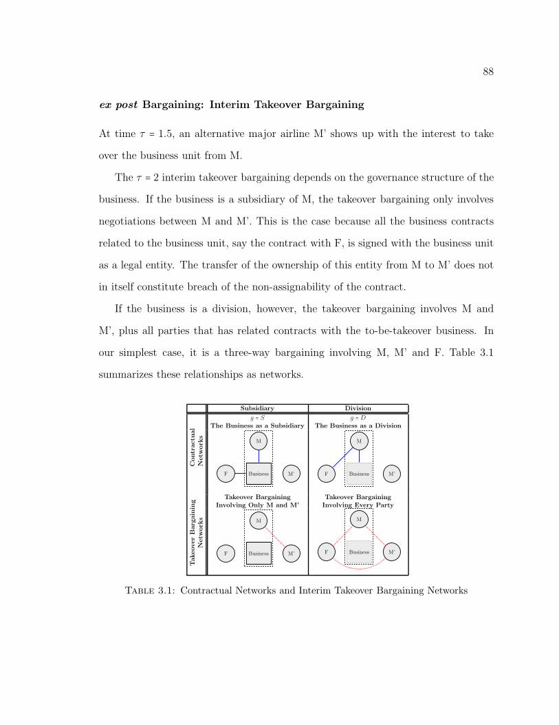
88
ex post Bargaining: Interim Takeover Bargaining
At time τ = 1.5, an alternative major airline M’ shows up with the interest to take
over the business unit from M.
The τ = 2 interim takeover bargaining depends on the governance structure of the
business. If the business is a subsidiary of M, the takeover bargaining only involves
negotiations between M and M’. This is the case because all the business contracts
related to the business unit, say the contract with F, is signed with the business unit
as a legal entity. The transfer of the ownership of this entity from M to M’ does not
in itself constitute breach of the non-assignability of the contract.
If the business is a division, however, the takeover bargaining involves M and
M’, plus all parties that has related contracts with the to-be-takeover business. In
our simplest case, it is a three-way bargaining involving M, M’ and F. Table 3.1
summarizes these relationships as networks.
Subsidiary Division
Contractu
al
Netw
ork
s
g = S g = DThe Business as a Subsidiary The Business as a Division
M
BusinessF M’
M
BusinessF M’
TakeoverBarg
aining
Netw
ork
s
Takeover BargainingInvolving Only M and M’
Takeover BargainingInvolving Every Party
M
BusinessF M’
M
BusinessF M’
Table 3.1: Contractual Networks and Interim Takeover Bargaining Networks
89
ex post Bargaining: τ = 3
There are four sub-bargaining-games we need to consider at τ = 3. For simplicity,
we assume the following: (a) each of these three parties always has an individual
outside option of 0; (b) equal bargaining power for all parties; and (c) the bargaining
solutions are determined by Shapley value.
(i) No takeover : If no M’ shows up (with probability 1−λ), there is no bargaining
over the takeover decision. The game proceeds as M owning the business. The
contract between M and F is still effective. M and F bargain over the final value of
production, vMF , at τ = 3. This bargaining is the same regardless of whether the
business is a subsidiary or a division.
If M’ shows up (with probability λ), there are several sub-cases depending on the
decisions made at the takeover bargaining at τ = 2.(ii) Unsuccessful takeover : If any one of M and M’ disagrees to the takeover deal,
M and F continues to deal and produce vMF as before because M still have control over
the business. What’s different from case (i) is that M’ has shown up. We assume that
although M’ failed in taking over the business, M’ and F may still find it profitable to
reach a contract between themselves without the business. In this case, M’ and F also
bargains over a final value of production without the business, vnM ′F with superscript
n stands for no takeover.
If both M and M’ agrees to the takeover deal, the ownership of the business will be
turned over to M’. But the relationship between F and the business may or may not
be transferred with the ownership of the business, depending on what the governance
structure is and whether F agrees to the reassignment of contract.
(iii) Successful takeover without reassigning contract with F. This case never hap-
90
pens under g = S. If M and M’ agree to the takeover deal, but g = D and F rejects
to reassign the contract from M to M’, then the business is turn over to M’, but
M and F still maintains the original contract, operating without the business. We
assume M’ and F may reach a separate contract through renegotiation for F to serve
the business, which is now under control of M’, while still working with M. Similar
to the previous case, we assume M and F creates no extra surplus dealing with each
other after M’ takes over the business. But M’ and F can still reach a side agreement
through renegotiation to produce a value of vrM ′F where superscript r stands for no
reassignment. We assume that vrM ′F is only a fraction of vMF due to the fact that F
is still bonded by its contract with M.
(iv) Successful takeover with reassigning contract with F. If the business is set up
as a subsidiary (g = S), the contract between F and the business is automatically
transferred after M’ takes control. F has no decision on this matter. If, instead, the
business is set up as a division (g = D), then the contract between F and the owner
of the business, M, will only be transferred under F’s consent. In this case, M’ and
F bargains over the value of the final product vM ′F . We assume that M and F will
not generate any value by keeping their contract once M lost the business, i.e. they
can only jointly produce a value that is equal to the sum of their respective outside
options. Otherwise, the reassignment would be unnecessary.10
It is convenient to relate the partial value vrM ′F to the full value vM ′F . Recall that
vrM ′F is the value M’ and F can produce with the business while F is still supplying
to M. And vM ′F is the full value they could produce with the business and without
10A relaxation of this assumption can be modeled with straightforward extension, which allowsfor M and F to produce a fraction of what they were able to produce together when the business isstill under control of M. This extension, however, does not change our main qualitative results. Seethe following Section for details.
91
the burden of contract with M. vrM ′F should be bounded above by vM ′F , and bounded
below by the sum of their individual outside options without cooperation, which is
assumed to be 0. Thus we introduce an exogenous variable ρ ∈ [0,1] and define
vrM ′F = ρvM ′F . ρ can be interpreted as the remainder in value of production that
can be obtained by M’ and F due to the burden of non-reassigned contract. This
setting accounts for the cases that, for example, F may run into a binding capacity
constraint when it serves both M and M’.11 ρ = 1 corresponds to a case in which
F faces no capacity constraint, or in which F simply do not deliver anything to M
anymore. Whereas ρ = 0 corresponds to a case where F is completely lock-in by the
contract with M and cannot renegotiate with M’.
Similarly, We also relate the partial value vnM ′F to the full value of production
vM ′F . Recall that vnM ′F is the value M’ and F can produce without the business while
F is still supplying to M. So it is intuitive to assume vnM ′F to be bounded above by
vrM ′F , and bounded below by the sum of their individual outside options without
cooperation, which is assumed to be 0. We introduce another exogenous variable η
and define vnM ′F = (ρ − η)vM ′F , such that η ∈ [0,1] and ρ − η > 0. Because η is the
further reduced share of production value from vrM ′F , η can be interpreted as the
essentialness of the business for the value creation involving M’ and F given that F
is stilling supplying M.
11For example, with the non-reassigned contract between M and F, F still has obligations to supplythe intermediate product to M, and M still has the contractual obligation to purchase the product.If F has exhausted its capacity to the production of supply for M, F would not be able to committo supplying the business unit, which is under control of M’.
92
ex post Takeover Bargaining: τ = 2
We assume that vM ′F is sufficiently high relative to vMF such that vM ′F > vMF +vnM ′F ,
so that M and M’ will always agreed on the takeover deal.12 Given that ρ > 0, wealways have vM ′F > vrM ′F , so given M and M’ agrees on the takeover, it is always
optimal for F to agree to reassign the contract in renegotiation.
The τ = 2 takeover bargaining bargains over each parties’ decision over whether
agreeing to the takeover deal or whether endorse the reassignment of the contract in
exchange for a payment. In our setup, once M’ shows up, it is always optimal for all
three parties to agree to the takeover as well as reassignment of the supplying contract.
To put it another way, once M’ shows up, the only subgame on the equilibrium path
is the case (iv) defined above (successful takeover with reassigned contract). Case (ii)
and (iii), however, serve as party M and F’s outside options.
Timing
The timing of the stage game is summarized in the following graph.
12This assumption is not substantive because what matters for the analysis is the marginal product.
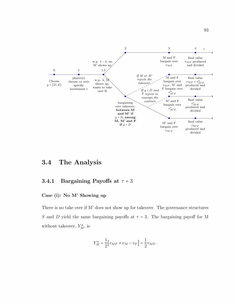
93
τ
0 1 1.5
w.p. 1 − λ, noM’ shows up
2 3 4
w.p. λ, M’shows up,
wants to takeover R
Chooseg = D,S
player(s)choose ex ante
specificinvestment e
M and Fbargain over
vMF
final valuevMF producedand divided
bargainingover takeover:between Mand M’ if
g = S; amongM, M’ and F
if g =DM’ and F
bargain overvM ′F
final valuevM ′F
produced anddivided
M and Fbargain overvMF , M’ andF bargain over
vnM ′F
final valuevMF + v
nM ′F
produced anddivided
M’ and Fbargain over
vrM ′F
final valuevrM ′F
produced anddivided
If M or M’
rejects the
takeover
If g =D and
F rejects to
reassign the
contract
3.4 The Analysis
3.4.1 Bargaining Payoffs at τ = 3
Case (i): No M’ Showing up
There is no take over if M’ does not show up for takeover. The governance structures
S and D yield the same bargaining payoffs at τ = 3. The bargaining payoff for M
without takeover, Y nM , is
Y nM =
1
2[vMF + vM − vF ] = 1
2vMF .
94
Case (ii): No Takeover (n)
If M’ shows up, but either M or M’ rejects the takeover, the governance structures
S and D yield the same bargaining payoffs at τ = 3. The bargaining payoff for M
without takeover, is also Y nM as if no M’ shows up.
The bargaining payoff for M’ without takeover, Y nM ′ , is
Y nM ′ = 1
2[vnM ′F + vM ′ − vF ] = 1
2(ρ − η)vM ′F .
The bargaining payoff for F without takeover, Y nF , is
Y nF =
1
2[vnM ′F + vF − vM ′] + 1
2[vnMF + vF − vM] =
1
2(ρ − η)vM ′F +
1
2vMF .
Case (iii): Successful Takeover without Reassignment of Contract (r)
The three parties wind up in this case if M’ shows up, both M and M’ agrees to the
takeover, but g = D and F rejects the reassignment of the contract. The bargaining
payoff for M after the business is taken by M’, is Y rM = 0.
The bargaining payoff for M’ in this case, Y rM ′ , is
Y rM ′ = 1
2[vrM ′F + vM ′ − vF ] = 1
2ρvM ′F .
The bargaining payoff for F without reassigning the contract, Y rF , is
Y rF =
1
2[vrM ′F + vF − vM ′] = 1
2ρvM ′F .
95
Case (iv): Successful Takeover without Reassignment of Contract (t)
If both M and M’ agrees under g = S or all three of M, M’ and F agrees under g =D,
the takeover is successful with reassigned contract. The bargaining payoff for M after
the business is taken by M’, is Y tM = 0.
The bargaining payoff for M’ in this case, Y tM ′ , is
Y tM ′ = 1
2[vM ′F + vM ′ − vF ] = 1
2vM ′F .
The bargaining payoff for F without reassigning the contract, Y tF , is
Y tF =
1
2[vrM ′F + vF − vM ′] = 1
2vM ′F .
3.4.2 Takeover Bargaining Payoffs at τ = 2
Takeover bargaining under g = S
Under g = S, the takeover bargaining involves only M and M’. M demands a payment
from M’ that is no less than what she could have made rejecting the takeover offer. In
the takeover bargaining, the an outside option of M is Y nM .13 However, M’ is unwilling
to offer anything more than Y tM ′ , which is the entire payoff that M ′ could earn after
the takeover. So M’s bargaining payoff in the takeover stage, Y S,tM , is
YS,tM = 1
2Y nM +
1
2[Y t
M ′ − Y nM ′] = 1
4[vMF + (1 + η − ρ)vM ′F ]. (3.4.1)
13If Y nM > Y t
M ′ , the agreement cannot be reached because there is no gains from trade, and thegame goes to the no-takeover case. Thus λ can be interpreted as the probability that the projectvalue vMF falls below the market level.
96
Takeover bargaining under g = D
Under g = D, M and M’ jointly determine whether the takeover deal is successful,
while F determines whether the contract will be reassigned. By Shapley value, the
payoff for M, Y D,tM is
YD,tM = 1
3Y nM +
1
6[Y n
M + Y nF − Y n
F ] +1
6[Y r
M + Y rM ′ − Y n
M ′] + 13[Y t
M + Y tM ′ + Y t
F − Y nM ′ − Y n
F ]
= 16[vMF + (4 + 5η − 4ρ)vM ′F ]. (3.4.2)
Comparing the bargaining solutions under the two governance structures provides
the intuition regarding the different implications of takeover bargaining under g = Dand g = S. Checking the interim steps in equations (3.4.1) and (3.4.2), the sum of the
first two terms in equation (3.4.2) yields the same result as the first term in equation
(3.4.1), 12Y
nM . The difference comes from the third and fourth terms in equation
(3.4.2).
First, M obtains a lower bargaining payoff under g = D in the takeover stage
because she has less control rights over the assignability of the contract with F.
Under g = S, M can unilaterally decide to transfer both the business unit and the
associated contract with F without consent from F. But under g = D, M faces the
threat from F that he might not agree to reassign the contract, which lowers the
value of the business unit after the takeover. This makes M’s decision regarding the
transfer of the business unit less valuable under g = D. This intuition is reflected by
the third term in equation (3.4.2), Y rM + Y r
M ′ − Y nM ′, which is the value of the business
unit without the original contract with F. This value is presumably smaller than the
value when the business unit is transferred with the the contract with F by default,
97
as in g = S, which is Y tM ′ − Y n
M ′ .
Second, given our setup that F does not participate in the takeover bargaining
under g = S, M has a different advantage under g = D comparing to g = S. That is,
under g =D, M can potentially appropriate more rents during the takeover bargaining
from F by threatening to reject the takeover deal. This threat can potentially extract
a share of future rents that F can obtain after the takeover, Y tF −Y n
F .14 This intuition
is captured by comparing the second term in equation (3.4.1), Y tM ′ − Y n
M ′ , with the
fourth term in equation (3.4.2), which equals to Y tM ′ −Y n
M ′ + Y tF − Y n
F because Y tM = 0.
3.4.3 Expected Payoff Comparison at τ = 1: Subsidiaries vs.Divisions
The expected payoffs at τ = 1 for M under g = S and g = D are
Y SM = (1 − λ)Y n
M + λ(Y S,tM + Y t
M),
Y DM = (1 − λ)Y n
M + λ(Y D,tM + Y t
M).
Subtracting Y SM from Y D
M , and substituting the bargaining payoffs with our previ-
ous characterizations, we have
Y SM − Y D
M =1
12λ[2vMF − (1 + 2η − ρ)vM ′F ]. (3.4.3)
This result shows that, comparing to g = D, M always extracts more rents under
14Under g = S, M does not have this advantage because we assume that F does not participatein the takeover bargaining. One might argue that even under g = S, M can still potentially reachout to F and threaten in the same way to extract rents. This would eliminate M’s advantage underg =D relative to g = S. However, this alternative setting does not change our qualitative results.
98
g = S in the takeover bargaining from her “insider option”, vMF , that she produces
with F. Moreover, comparing to g =D, M always extracts less rents under g = S from
the value produced after the business is taken over, vM ′F .15
3.4.4 Investment Levels
Investments at τ = 1: First-best Benchmark
The total surplus is s(e) = (1 − λ)vMF (e) + λvM ′F (e) −Ψ(e), so the first-best level of
investment is defined by
(1 − λ)v′MF (eFB) + λv′M ′F (eFB) = Ψ(eFB), (3.4.4)
where v′(⋅) denotes the partial derivative of the function v with respect to its argument—
investment e.
Investments at τ = 1: g = S vs. g = D
In equilibrium, M’s ex ante investment levels under governance structure g—eS and
eD for g = S,D respectively—are characterized by
Yg′M (eg) = Ψ′(eg). (3.4.5)
We can derive the difference in M’s marginal benefit of investment under the two
15Equation (3.4.3) shows that only if ρ = 1 and η = 0, M’ obtains the same share of output fromvM ′F . But given the assumption that ρ < η, this case never holds.
99
governance structures from Equation (3.4.3). That is
Y S′M (e) − Y D′
M (e) =1
12λ(2v′MF (e) − (1 + 2η − ρ)v′M ′F (e)). (3.4.6)
Proposition 3.1. (i) e1 is always higher under subsidiary than under division, i.e.
eS1 > eD1 . (ii) e2 is higher under subsidiary than under division if e2 is sufficiently
non-specific to the future value of output after takeover. Specifically, there exists a
cutoff value ω = 1+2η−ρ2 < 1, such that e2 is higher under subsidiary than under division
ifv2MF
v2M′F
> ω, and vice versa. That is eS2 > eD2 ifv2MF
v2M′F
> ω; and eS2 < eD2 ifv2MF
v2M′F
< ω.
Proof. From equation (3.4.6), we can write
(Y S′M (e) −Ψ(e)) − (Y D′
M (e) −Ψ(e)) =1
12λ(2v′MF (e) − (1 + 2η − ρ)v′M ′F (e)). (3.4.7)
Notice that the two terms on the left-hand side are the respective first-order conditions
under S and D. And given that the production functions v are concave in investments
and Ψ is convex, the result follows by Assumption 3.1.
Efficiency: g = S vs. g =D
Definition. We say that there is under-investment (over-investment) in ei under
a governance structure g ∈ S,D if the equilibrium investment level, eg, is below
(above) the first-best level, eFB.
Lemma 3.1. (i) There is always under-investment in e2 under both subsidiary and
division. (ii) There is over-investment in e1 under subsidiary if and only if 23 <
λ < 1 andv1M′F
v1MF
< 3λ−2λ(3−η+ρ) , otherwise there is underinvestment. (iii) There is over-
100
investment in e1 under division if and only if 67 < λ < 1 and
v1M′F
v1MF
< 7λ−6λ(8+5η−4ρ) , otherwise
there is underinvestment.
Proof. See Appendix 3.A.
Proposition 3.2. Setting up a business as a subsidiary is more efficient than making
it a division if (i) the cooperative investment e2 is sufficiently non-specific to the value
of output after takeover; and one of the two following: (ii.a) the chance of the takeover
opportunity is small, i.e. λ is sufficiently small; or (ii.b) the chance of the takeover
opportunity is large, i.e. λ is large, but the owner-specific investment, e1, is sufficiently
non-specific to the investor herself.
Proof. By Lemma 3.1, there is always under-investment for e2. When λ < min23 , 67 =23 or if 2
3 < λ < 1 butv1M′F
v1MF
> max 3λ−2λ(3−η+ρ) ,
7λ−6λ(8+5η−4ρ) = 3λ−2
λ(3−η+ρ) , there is under-
investment under both S and D for e1.
By Proposition 3.1, eS2 > eD2 , whenv2M′F
v2MF
> ω. Furthermore, it is always true that
eS1 > eD1 . Therefore, S is always more efficient than D when (i)v2M′F
v2MF
> ω and one of
the two following: (ii.a) λ < 23 ; or (ii.b)
23 < λ < 1 but
v1M′F
v1MF
> 3λ−2λ(3−η+ρ) .
Proposition 3.3. Setting up a business as a division is more efficient than making
it a subsidiary if all three of the following conditions are satisfied (i) the coopera-
tive investment, e2, is sufficiently specific to the value of output after takeover; (ii)
the chance of the takeover opportunity is high, i.e. λ is sufficiently large; and (iii)
the owner-specific investment, e1, is sufficiently specific to the investor, i.e.v1M′F
v1MF
is
sufficiently small.
Proof. The proof is similar to the previous proposition. By Lemma 3.1, there is always
under-investment for e2. Under conditions (ii) and (iii), when λ > max23 , 67 = 67 , and
101
v1M′F
v1MF
< min 3λ−2λ(3−η+ρ) ,
7λ−6λ(8+5η−4ρ) = 7λ−6
λ(8+5η−4ρ) , there is over-investment under both S and
D for e1.
By Proposition 3.1, eS2 < eD2 , whenv2M′F
v2MF
< ω. Furthermore, it is always true that
eS1 > eD1 . Therefore, D is always more efficient than S when (i)v2M′F
v2MF
< ω, (ii) λ > 67 ,
and (iii)v1M′F
v1MF
< 7λ−6λ(8+5η−4ρ) .
Propositions 3.2 and Proposition 3.3 form a pair of surprising results regarding the
probability of takeover, λ. As the chance of the business being taken over increases,
the model predicts that division is more efficient. This is by itself against the modeling
assumption that firms use subsidiaries as oppose to divisions when the owner of the
business (M in our model) has stronger intention to sell the business in the future.
However, this pattern does correspond to the reality where subsidiaries have very
stable relationships with their parent firms in that they tend not to be sold very
frequently.
The intuition behind this result is subtle. Setting up the business as a subsidiary
provides the owner with better bargaining position in the takeover bargaining stage.
Specifically, the owner is able to extract a greater share of its potential output, vMF .
This advantage attracts the owner to invest more ex ante toward this “inside op-
tion”—vMF—rather than the value of output after takeover, vM ′F . But when the
chance of takeover happening increases (higher λ), high investment toward the “in-
side option” becomes wasteful and low investment toward the future product becomes
inefficient. Thus subsidiary becomes less efficient than division.
Regarding the specificity of investment, the model predicts that the business that
uses more specific investment—no matter it is owner-specific investments or cooper-
ative investments that is specific to other parties—should be housed inside the firm.
102
Particularly in this case, it means using the division rather than the subsidiary. But
this result comes out of the current model in a rather subtle manner. As is discussed
above, the main benefit of subsidiary is that it provides better ex ante investment
incentives for the owner toward the “inside option”. And since the owner is more fo-
cused on building the “inside option”, an cooperative investment that is very specific
to the value of output after takeover is unattractive to the owner. This is the case
because such specific cooperative investment has little benefit in boosting the “inside
option”. Comparing to the case under division, under subsidiary, the owner tends
to over-invest in “inside option” (i.e. owner-specific investment) and under-invest in
value of output after takeover (i.e. cooperative investment). This pattern is particu-
larly inefficient when the takeover deal is likely to happen. Because when a takeover is
likely, the owner-specific investment is likely to be a waste for the total surplus, while
the cooperative investment tends to be crucial for efficiency. Thus when investments
are specific, divisions tend to be more efficient than subsidiaries.
We present a comparative statics result on the two parameters ρ and η. We say
a supplier F is dedicated (non-dedicated) to the contract if ρ is small (large). This is
the case because ρ measures the discount in the value F is able to produce with the
new owner M’ after takeover but without assigning the contract. If F is dedicated
to the original contract, it is likely that he will run into capacity constraints, which
corresponds to a low value of ρ. In the opposite case, if F is non-dedicated, it is
unlikely for him to be constrained by the existing contract with M. Thus F is likely
to be able to renegotiate with M’ and produce a high value of output with very little
discount, which corresponds to a high value of ρ.
Moreover, we say that the business unit is essential (inessential) for the transac-
tion if η is high (low). η measures the further discount of the value produced by F
103
and M’ if M’ does not control the business unit given that F still carries liability from
a binding contract with M.16 If the business unit is very essential for the transaction
between F and M’, the discount should be large, which corresponds to a large value
of η.
Proposition 3.4. All other things the same, the subsidiary is more likely to dominate
the division if the supplier is non-dedicated (high ρ) or if the business is inessential
(low η). The division is more likely to dominate the subsidiary if the supplier is
dedicated (low ρ) or if the business is essential (high η), given that the chances of
takeover happening is high enough.
Proof. From Propositions 3.2, we learned that: given the specificity of the investments
(v1M′F
v1MF
orv2MF
v2M′F
) fixed, the likelihood of subsidiaries being more efficient than divisions
increases if ω = 1−2η−ρ2 is lower and if 3λ−2
λ(3−η+ρ) is lower given λ > 23 . But notice that
both of these terms decreases in ρ and increases in η. So need them to be smaller
is equivalent to having a lower η and a higher ρ. For λ < 23 , there is always over-
investment in e1 under both S and D, then we only need e2 to be higher under S than
under D. This boils down to a lower ω, which also corresponds to a lower η and a
higher ρ. Thus we established the first part of the proposition.
Similarly, from Proposition 3.3, for divisions to be more efficient, we need ω to be
large and 7λ−6λ(8−5η+4ρ) to be large given that λ > 6
7 . These two conditions corresponds
to a higher η and a lower ρ. This holds because, again, these two terms are both
increasing in η and decreasing in ρ.
As of the essentialness of business for the potential buyer, η, our model predicts
that subsidiary is efficient when the business is relatively inessential for the potential
16See definition of Y nM ′ in the setup of the model.
104
buyer (higher η), and division should be used in the opposite case. Our model shows
that, comparing to subsidiary, division puts the owner in a weaker position to extract
the “inside option”, but provides the owner a better position to extract the additional
surplus created after the buyer, M’, acquires the business. When the business is
inessential, the additional surplus created from the takeover is small. Thus there is
not much for the present owner to extract under division. In this case, the owner
is reluctant to make as high level of ex ante investment toward future output. So
divisions are less efficient than subsidiaries. When the business is relatively essential
(lower η), however, the intuition works in the opposite direction. The owner has
stronger incentives to invest toward future product under division, thus divisions
tend to be more efficient than subsidiaries.
The degree of the supplier’s dedication, ρ, affects the result because of the role
of the supplier in the takeover bargaining when the business unit is a division. If
g = D, the supplier has the opportunity to threaten M and M’ that he will not
agree to reassign the contract. Dedication gives the supplier commitment power
in not renegotiating with M’ after rejecting to reassign the contract. Thus the more
dedicated M is, the more powerful this threat will be, which actually helps the supplier
extracting a greater share of vM ′F from M and M’. Under g = S, M is immune from
this threat. And furthermore, the dedication of the supplier becomes M’s advantage
to bargain against M’ because M’s decision over whether to agree to takeover includes
the reassignment of the supplying contract with M.
105
3.5 Conclusion
This paper provides a formal economic theory of the subsidiary versus division. The
idea of the model builds on the legal foundation that, for its owner, a business is
easier to be transferred as a subsidiary than as a division. The model utilizes the
framework of property-rights theory of the firm and focus on the inefficiencies in ex
ante investment. Although the model is built on the idea that subsidiary is easier to
be transferred, the main result is contrary to the common intuition that subsidiary
is setup to be sold. The model predicts that setting up a business as a subsidiary
is more efficient than making it a division when (i) the cooperative investment by
the owner is relatively non-specific; and one of the two following: (ii.a) the chances
that the business will be taken over is low; or (ii.b) the owner-specific investment
is relatively non-specific. And using division is more efficient if (i) the cooperative
investment by the owner is relatively specific to the value that can be produced after
the takeover; (ii) the chance of the business being taken over is high; and (iii) the
owner-specific investment is relatively specific.
It is important to remark that Propositions 3.2 and Proposition 3.3 do not exhaust
the entire parameter space. Without further assumptions about the production tech-
nology, there are cases in which we are unable to draw clear conclusions over which
governance structure is more efficient. For example, as indicated by Lemma 3.1, it
could be that there is under-investment in e1 under S but over-investment in e1 under
D (e.g. when 23 < λ < 6
7). Then we would not be able to draw clear conclusions over
which structure is more efficient. Such cases, however, may be studied when more
detailed institutional structures are added to the model.
106
3.A Omitted Proofs
Lemma 3.1. (i) There is always under-investment in e2 under both subsidiary and division.
(ii) There is over-investment in e1 under subsidiary if and only if 23 < λ < 1 and
v1FM′
v1MF
<3λ−2
λ(3−η+ρ) , otherwise there is underinvestment. (iii) There is over-investment in e1 under
division if and only if 67 < λ < 1 and
v1FM′
v1MF
< 7λ−6λ(8+5η−4ρ) , otherwise there is underinvestment.
Proof. By our assumptions that Ψ is strictly convex and the production functions are weaklyconcave, the equilibrium investments for the first-best, subsidiary case and division caseare all unique. Comparing equations (3.4.4) with (3.4.5), because they all have the samemarginal cost function, when a governance structure has a higher (lower) marginal bene-fit than the first-best for any given level of investments, there is over-investment (under-investment).
Furthermore, because our assumption that the cross-partials of the two investments arezero, we can separate the first-order conditions to evaluate e1 and e2 separately for anygiven governance structure.
Subtracting the left-hand-side of equation (3.4.5) from the left-hand-side of equation(3.4.4) for each governance structure, there is over-investment if the difference is negative,and positive-investment if the difference is positive. Denote the marginal benefit undersubsidiary and division as MBs and MBd, respectively. Then we have:
(1 − λ)viMF + λviM ′F −MBs = 1
4((2 − 3λ)vMF + λ(3 − η + ρ)vFM ′) (3.A.1)
(1 − λ)viMF + λviM ′F −MBd = 1
12((6 − 7λ)vMF + λ(8 − 5η + 4ρ)vFM ′) , (3.A.2)
in which Assumption 3.1 holds for i = 1,2 respectively.Requiring (3.A.1) to be negative (over-investment) boils down to 2
3 < λ < 1 and 0 ≤viM ′F <
(3λ−2)viMF
λ(3−η+ρ) . This can only be satisfied for e1 since v2MF < v2M ′F . So we always have
under-investment in e2 and over-investment in e1 when 23 < λ < 1 and 0 ≤ v1
M′F
v1MF
< 3λ−2λ(3−η+ρ) ,
and under-investment in e1 otherwise.Similarly, (3.A.2) yields the similar result that is provided in the statement.
Bibliography
Alcacer, Juan, David J. Collis, and Mary Furey, “The Walt Disney Company
and Pixar Inc.: To Acquire or Not to Acquire?,” Harvard Business School Case
709-462, Harvard Business School 2010.
Alfaro, Laura and Andrew Charlton, “Intra-Industry Foreign Direct Invest-
ment,” The American Economic Review, 2009, 99 (5), pp. 2096–2119.
Ayotte, Kenneth and Henry Hansmann, “A Nexus of Contracts Theory of Legal
Entities,” Working Paper 2011.
and , “Legal Entities as Transferable Bundles of Contracts,” Working Paper
3597, Yale Law School Legal Scholarship Repository Faculty Scholarship Series
2012.
Baker, George, Robert Gibbons, and Kevin J. Murphy, “Relational Contracts
And The Theory Of The Firm,” The Quarterly Journal of Economics, February
2002, 117 (1), 39–84.
Beer, Michael and Gregory C. Rogers, “Human Resources at Hewlett-Packard
(A),” Harvard Business School Case 495-051, Harvard Business School 1995.
107
108
Che, Yeon-Koo and Donald B. Hausch, “Cooperative Investments and the Value
of Contracting,” The American Economic Review, 1999, 89 (1), pp. 125–147.
de Fontenay, Catherine C. and Joshua S. Gans, “Vertical integration in the
presence of upstream competition,” RAND Journal of Economics, 2005, 36 (3),
544–572.
de Meza, David and Ben Lockwood, “Does Asset Ownership Always Motivate
Managers? Outside Options and the Property Rights Theory of the Firm,” The
Quarterly Journal of Economics, 1998, 113 (2), 361–386.
Dow, Gregory K, “Why Capital Hires Labor: A Bargaining Perspective,” American
Economic Review, March 1993, 83 (1), 118–34.
Garmaise, Mark J., “Ties that Truly Bind: Noncompetition Agreements, Ex-
ecutive Compensation, and Firm Investment,” Journal of Law, Economics, and
Organization, 2011, 27 (2), 376–425.
Gibbons, Robert, “Four Forma(lizable) Theories of the Firm?,” Journal of Eco-
nomic Behavior & Organization, October 2005, 58 (2), 200–245.
Grossman, Sanford J. and Oliver D. Hart, “The Costs and Benefits of Owner-
ship: A Theory of Vertical and Lateral Integration,” Journal of Political Economy,
August 1986, 94 (4), 691–719.
Hansmann, Henry, “Ownership of the Firm,” Journal of Law, Economics, and
Organization, 1988, 4 (2), 267–304.
and Reinier Kraakman, “The Essential Role of Organizational Law,” The Yale
Law Journal, 2000, 110 (387).
109
, , and Richard Squire, “Law and the Rise of the Firm,” Harvard Law Review,
2006, 119 (5), pp. 1333–1403.
Hart, Oliver D., Firms, Contracts, and Financial Structure, Clarendon Press, Ox-
ford, 1995.
and John Moore, “Property Rights and the Nature of the Firm,” Journal of
Political Economy, December 1990, 98 (6), 1119–58.
Hellmann, Thomas F. and Veikko Thiele, “A Theory of the Firm based on Part-
ner Displacement,” Working Paper 18495, National Bureau of Economic Research
October 2012.
Holmstrom, Bengt, “The Firm as a Subeconomy,” Journal of Law, Economics and
Organization, April 1999, 15 (1), 74–102.
and John Roberts, “The Boundaries of the Firm Revisited,” The Journal of
Economic Perspectives, 1998, 12 (4), pp. 73–94.
and Paul Milgrom, “Multitask Principal-Agent Analyses: Incentive Contracts,
Asset Ownership, and Job Design,” Journal of Law, Economics and Organization,
Special I 1991, 7 (0), 24–52.
Iacobucci, Edward M. and George G. Triantis, “Economic and Legal Bound-
aries of Firms,” Virginia Law Review, 2007, 93 (515).
Kaplan, Steven N. and Per Johan Stromberg, “Financial contracting theory
meets the real world: An empirical analysis of venture capital contracts,” Review
of Economic Studies, 2003, 70 (2), 281–315.
110
Kranton, Rachel E. and Deborah F. Minehart, “Networks versus Vertical In-
tegration,” RAND Journal of Economics, Autumn 2000, 31 (3), 570–601.
Magnet, Myron, “The New Golden Rule of Business,” Fortune, 1994, February,
60–64.
Myerson, Roger B., “Graphs and Cooperation in Games,” Mathematics of Opera-
tions Research, 1977, 2 (3), pp. 225–229.
Nishiguchi, Toshihiro, Strategic industrial sourcing: The Japanese advantage, New
York: Oxford University Press, 1994.
Posner, Richard A., “The Rights of Creditors of Affiliated Corporations,” The
University of Chicago Law Review, 1976, 43 (3), pp. 499–526.
Rajan, Raghuram G. and Luigi Zingales, “Power In A Theory Of The Firm,”
The Quarterly Journal of Economics, May 1998, 113 (2), 387–432.
Segal, Ilya R. and Michael D. Whinston, “Exclusive Contracts and Protection
of Investments.,” RAND Journal of Economics, 2000, 31 (4), 603 – 633.
Squire, Richard C., “Strategic Liability in the Corporate Group,” University of
Chicago Law Review, 2011, 78, 606.
Whinston, Michael D., “On the Transaction Cost Determinants of Vertical Inte-
gration,” Journal of Law, Economics, and Organization, 2003, 19 (1), 1.