Embed Size (px)
Citation preview
Three Essays on Stock Market Dynamics
By
Copyright 2013
Peng Chen
Submitted to the graduate degree program in the Department of Economics and the Graduate
Faculty of the University of Kansas in partial fulfillment of the requirements for the degree of
Doctor of Philosophy.
________________________________
Shu Wu (Co-chairperson)
________________________________
Elizabeth Asiedu (Co-chairperson)
________________________________
Mohamed El-Hodiri
________________________________
John Keating
________________________________
Jianbo Zhang
________________________________
Yaozhong Hu
Date Defended: April 19, 2013
ii
The Dissertation Committee for Peng Chen
certifies that this is the approved version of the following dissertation:
Three Essays on Stock Market Dynamics
________________________________
Shu Wu (Co-chairperson)
________________________________
Elizabeth Asiedu (Co-chairperson)
Date approved: April 19, 2013
iii
ABSTRACT
This this dissertation aims to understand the comovements of international stock markets,
financial contagion, and the relationship between international stock market comovements and
macroeconomic factors. It contains three essays as follows:
The first essay investigates the common movements of stock market returns across the world
and the regions. I employ a Bayesian dynamic latent factor model to decompose stock market
returns into common world, regional, and idiosyncratic country-specific factors simultaneously.
The results indicate that a common world factor is a significantly important source of the
fluctuations for most stock markets, providing evidence of the international stock market
comovements. I also find that the regional factor is another important reason for the fluctuations
in emerging markets, but not in most developed markets. Persistence properties of the factors are
examined to measure the adjusting speed to different shocks, and variance decomposition
analysis is also performed to investigate the role of each factor in the volatility of stock markets.
The roles of the world and regional factors, however, differ substantially across stock markets
within different regions, as well as across developed and emerging markets. I reassess simple
correlation analysis of bilateral linkages and find that although it can partially mimic actual stock
market integration, this method provides an imperfect and biased depiction. In a partially
integrated global economy, the degree of a market's comovement with international stock
markets is closely related with that of its own country's economic integration in the world.
The second essay aims to investigate the linkage of Asian markets through the channel of
stock market realized volatility. When examining the weekly realized stock market volatility in
Asia, I find significant change of stock market volatility over time, especially in the financial
crisis. Further, several different models, including simple pair-wise correlation model, DCC-
GARCH model, and time-invariant and time-varying VAR model, are employed to investigate
the volatility comovements in the main Asian stock markets. The empirical result shows that the
correlations of stock market volatility among most of the Asian markets have increased after the
crisis. The study also provides evidence that there is a contagion effect among the Asian markets
during the crisis. Interestingly, from both the impulse response and variance decomposition
analysis, the result shows that the Hong Kong market has a stronger impact on other Asian
iv
markets than the Thailand market. The responses of other Asian markets to either the Hong Kong
or Thailand market were greatly increased after the crisis. And from the variance decomposition
analysis, it shows that the contribution to the variance of other Asian markets from either the
Hong Kong or Thailand market both showed an increase during the crisis.
The third essay investigates the relationship between international stock market
comovements and macroeconomic factors across a large group of countries over 1995-2009 in a
global perspective. I use Bayesian dynamic factor models to decompose stock market prices and
other major macroeconomic variables of 34 economies into common global factors and
idiosyncratic country-specific factors. The result shows that the global factors account for a
significant portion of an individual country's stock market volatility as well as its
macroeconomic fluctuations. The global macroeconomic shocks have strong effects on the price
movement of the global stock market as well as that of an individual market. And the result also
indicates that a country's exposure to the global stock market risk can be largely explained by
that country's exposure to the global macroeconomic risks.

v
ACKNOWLEDGEMENTS
Many people, in one way or another, have contributed to the completion of this dissertation to
whom I want to express my gratitude.
First and foremost, my deepest gratitude must go to my co-advisors Dr. Shu Wu and Dr.
Elizabeth Asiedu. Dr. Shu Wu encouraged me to develop independent thinking and research
skills and patiently provided the vision and advice necessary to be successful in the doctoral
program. I believe the completion of this dissertation would never be possible without his great
supervision, comments, encouragement, and support. It is impossible for me to express my
appreciation for him with words.
I also want to express my heartfelt appreciation to co-advisor Dr. Elizabeth Asiedu. During
the hard time of my graduate study, she became a friend and also my advisor and counselor and
put me back on the track. I believe the completion of my graduate study would never go
smoothly without her always supervision, encouragement and support.
I am also grateful to the dissertation committee members Dr. Mohamed El-Hodiri, Dr. John
Keating, Dr. Jianbo Zhang and Dr. Yaozhong Hu who aroused my curiosity and shared their
deep knowledge with me. Their thoughtful criticisms and suggestions improved the manuscript
and ultimately made this a better work. And, I’d also like to further thank Dr. Shigeru Iwata for
his comments and suggestions in early stages of the second chapter of this dissertation.
Further, I would like to thank Dr. Joshua Rosenbloom, Dr. Donna Ginther, and Dr. Ted Juhl
for the great opportunity to work with you all. I am grateful for the financial support from the
project and also the great experience which facilitates my research and dissertation.
Many other people provided assistance in obtaining academic resources and the database
which was necessary for undertaking this study. Specifically, I would like to express my thanks
to the librarian John Stratton and Dr. Jianing Zhang for their kind help.
I am also grateful to the Department of Economics at KU, particularly the staff including Teri
Chambers, Michelle Lawrence, and Leanea Wales for all of their great help over the past years.

vi
This dissertation would never be complete were it not the support of my beloved family.
They were always positive, encouraging and supportive at my hard times. Especially to my
dearest Mom Suyan Huang, thank you so much for always being there during my whole study
journey. I always felt the power of her prayers on my work. All the beauties in my life are due to
their continuous supports and encouragements.
vii
Contents
ABSTRACT ........................................................................................................... III
ACKNOWLEDGEMENTS ................................................................................... V
LIST OF TABLES ................................................................................................. IX
LIST OF FIGURES .............................................................................................. XI
CHAPTER 1 INTRODUCTION ............................................................................ 1
CHAPTER 2 UNDERSTANDING THE COMOVEMENTS OF
INTERNATIONAL STOCK MARKETS .............................................................. 5
2.1 INTRODUCTION ...................................................................................................................5
2.2 EMPIRICAL METHODOLOGY ................................................................................................8
2.3 DATA DESCRIPTION ...........................................................................................................13
2.4 EMPIRICAL RESULTS .........................................................................................................14 2.4.1 The dynamic factors ........................................................................................................................ 14
2.4.2 Difference of the trends among emerging and developed markets ................................................. 16
2.4.3 Persistence properties of the dynamic factors ................................................................................. 18
2.4.4 Variance decompositions for different factors ................................................................................ 20
2.4.5 Robustness test ................................................................................................................................ 23
2.5 DO SIMPLE CORRELATIONS MIMIC THE MEASURES OF BILATERAL LINKAGES ON THE BASIS
OF BAYESIAN DYNAMIC FACTOR ANALYSES? ...............................................................................25
2.6 CAN INTERNATIONAL STOCK MARKET COMOVEMENTS BE JUSTIFIED BY REAL ECONOMIC
INTEGRATIONS? ...........................................................................................................................26
2.7 CONCLUSION ....................................................................................................................28
CHAPTER 3 DYNAMIC CORRELATION ANALYSIS OF THE
REALIZED VOLATILITY COMOVEMENTS IN ASIAN MARKETS ......... 30
3.1 INTRODUCTION .................................................................................................................30
3.2 DATA DESCRIPTION AND PRELIMINARY STATISTICS ...........................................................33
3.3 EMPIRICAL METHODOLOGY ..............................................................................................35 3.3.1 Simple and adjusted simple correlation model ............................................................................... 35
3.3.2 Dynamic conditional correlation model .......................................................................................... 36
3.3.3 VAR Model ..................................................................................................................................... 39
3.4 EMPIRICAL RESULTS .........................................................................................................43 3.4.1 Simple pair-wise correlation analysis ............................................................................................. 43
3.4.2 Dynamic conditional correlation analysis using GARCH Model ................................................... 43
3.4.3 Constant correlation analysis using time-invariant VAR Model ..................................................... 46
3.4.4 Dynamic correlation analysis using time-varying VAR Model ...................................................... 46
3.5 TRANSMISSION OF STOCK MARKET VOLATILITY ...............................................................48

viii
3.6 CONCLUSION ....................................................................................................................50
CHAPTER 4 ON INTERNATIONAL STOCK MARKET COMOVEMENT
AND MACROECONOMIC FUNDAMENTALS ............................................... 52
4.1 INTRODUCTION .................................................................................................................52
4.2 EMPIRICAL METHODOLOGY ..............................................................................................56 4.2.1 Bayesian dynamic factor model ...................................................................................................... 56
4.2.2 Vector Autoregression (VAR) Model .............................................................................................. 58
4.3 DATA AND DESCRIPTIVE STATISTICS ..................................................................................59 4.3.1 Data of stock markets ...................................................................................................................... 59
4.3.2 Data of macroeconomic fundamentals ............................................................................................ 60
4.4 EMPIRICAL RESULTS .........................................................................................................62 4.4.1 International stock market Comovements and global macroeconomic factors ............................... 63
4.4.2 Measuring the effects of global macroeconomic factors................................................................. 67
4.4.3 Does market integration reflect economic integration? .................................................................. 71
4.5 ROBUSTNESS TEST ............................................................................................................73
4.6 CONCLUSION ....................................................................................................................75
REFERENCES ....................................................................................................... 77
APPENDIX ............................................................................................................. 85
A1: MCMC APPROACH TO DYNAMIC FACTOR ANALYSIS .................... 85
A2: PROCEDURES FOR TIME-VARYING VAR MODEL ............................. 93
ix
List of Tables
Table 2.1: Regional Definition and Classification ...................................................................................... 95
Table 2.2: First-order Auto-regression Coefficients ................................................................................... 96
Table 2.3: Factors Coefficients and Country Factors AR(1) Coefficients .................................................. 97
Table 2.4.1: Variance Decompositions for Stock Market Returns ............................................................. 98
Table 2.4.2: Variance Decompositions for Developed and Emerging Market Returns .............................. 99
Table 2.5: Bilateral Correlation Coefficients ............................................................................................ 100
Table 3.1: Date when Infected Markets were Impacted ........................................................................... 101
Table 3.2: Summary statistics for the Realized Volatility (RV) Indices ...................................................... 102
Table 3.3.1: Simple Correlation of the Realized Volatility ........................................................................ 103
Table 3.3.2: Correlation of the Realized Volatility (After Adjusted) ......................................................... 104
Table 3.4: Constant Correlation of the Realized Volatility (in VAR Model) .............................................. 105
Table 3.5: Mean-DCC of the Market Volatility in GARCH Model .............................................................. 106
Table 3.6: Mean-DCC of the Market Volatility in Time-varying VAR Model ............................................. 106
Table 3.7: Decomposition of Variance for Asian Markets ........................................................................ 107
Table 4.1: Monthly Data Descriptions (1995.01-2009.12) ........................................................................ 109
Table 4.2: Summary Statistics for Real Returns ........................................................................................ 110
Table 4.4.3: Variance Share of Global Factor ............................................................................................ 111
Table 4.4: Average of Variance Share of Global Factor ............................................................................ 112
Table 4.5: Pair-wise Correlation among Different Global Factors ............................................................ 112
Table 4.6: Results of VAR Analysis ............................................................................................................ 113
Table 4.7: Variance Decomposition (Real Returns) .................................................................................. 114
Table 4.8: Factor Loadings of Global Factor .............................................................................................. 115
Table 4.9: R^2 Statistics from VAR Analysis .............................................................................................. 116
Table 4.10: Variance Decomposition for Country’s Stock market real returns ........................................ 117

x
Table 4.11: Results of OLS Analysis ........................................................................................................... 118
Table 4.12: Variance Decomposition (Nominal Returns) .......................................................................... 119
Table 4.13: Variance Decomposition (Real Returns) ................................................................................ 120
xi
List of Figures
Figure 2.1: World Factor ........................................................................................................................... 121
Figure 2.2: Regional Factors ..................................................................................................................... 122
Figure 2.3: World Factor, Regional Factor and Actual Stock Market Returns ......................................... 123
Figure 2.4: Return Variance Due to World Factor .................................................................................... 125
Figure 2.5: Relationship between Correlation Coefficients ...................................................................... 126
Figure 2.6: Relationship between Variance Shares of Global Factor ....................................................... 127
Figure 3.1: Realized Volatility Indices (1995.01-1999.12) ......................................................................... 128
Figure 3.2.1: Dynamic Correlation between Hong Kong and other Asian Markets in DCC-GARCH Model
.................................................................................................................................................................. 130
Figure 3.2.2: Dynamic Correlation between Thailand and other Asian Markets in DCC-GARCH Model .. 132
Figure 3.3.1: Dynamic Correlation between Hong Kong and other Asian Markets in Time-varying VAR
Model ........................................................................................................................................................ 134
Figure 3.3.2: Dynamic Correlation between Thailand and other Asian Markets in Time-varying VAR
Model ........................................................................................................................................................ 136
Figure 3.4.1: Impulse Response Analysis (Realized Volatility Index before Crisis) ................................... 138
Figure 3.4.2: Impulse Response Analysis (Realized Volatility Index after Crisis) ...................................... 140
Figure 3.4.3: Impulse Response Analysis (Realized Volatility Index before Crisis) ................................... 142
Figure 3.4.4: Impulse Response Analysis (Realized Volatility Index after Crisis) ...................................... 144
Figure 4.1: Dynamic Global Factors .......................................................................................................... 146
Figure 4.2: Actual and Fitted Values of Variance Share ............................................................................ 147
1
Chapter 1 Introduction
In recent decades, with the increasing global economic integration, understanding the cross-
market linkages or international stock market comovements becomes central interest for
financial academic researcher as well as policy makers. There is wide agreement among
theoretical and empirical studies in the literature that provide evidences of the international stock
market comovements, cross-market linkage, interdependence, and even financial contagion in
financial crisis. In particular, there has been a rapid rise in the volume of cross-country capital
flows, especially the capital flows into emerging market securities. Accurate specification of
financial market linkage and understanding the underlying possible sources is of very importance
in financial decisions, such as portfolio allocation, risk management for risk-averse investors,
and other business decisions. Therefore, investigating the difference of financial market
integration among developed and emerging markets in the world will provide insights of better
understanding the global financial system. In particular, the new remunerative emerging markets
have attracted the attention of international fund agents as an opportunity for portfolio
diversification and have also intensified the curiosity of academics in exploring international
market linkages. All these together raise interests to have further and detailed investigation of
financial integration cross different markets in the world.
Financial literatures have already addressed many on the issues of the impacts of
macroeconomic factors on stock markets. From multi-factors asset pricing models, any variables
that can affect the future investment of the level of consumption could be price factor in
equilibrium (see Merton, 1973; Breeden, 1979).Therefore, macroeconomic factors, which affect
the returns of risky equity, need to be priced in a risk-averse economy (Ross, 1976). There are
various financial theories and empirical studies that have investigated the relationship between
macroeconomic factors and stock markets. Enhanced understanding the regularities and
determinants of stock markets fluctuations is important for studies on financial markets and
corporate finance; however, it is still in a blurred phase in understanding observable facts of the
relationships between macroeconomic variables and stock markets. In particular, the more
increased global economic and financial integrations, the more stock market linkages and
2
interactions among different markets in the world exist, all together making it more complex to
investigate the relationship between macroeconomic variables and international stock markets.
Unfortunately, to my knowledge, there has not been any study investigating the relationships
between stock markets and the underlying macroeconomic factors in a global perspective;
effectively, the relationship between macroeconomic variables and stock markets cannot be
modeled in isolation neither from the interaction of other markets nor the spillover effects of
macroeconomic variables from other countries in the world. Especially, I am particularly
interested in the link between stock market movements and the underlying macroeconomic
factors in a perhaps partially integrated global economy. Therefore, of more interest in terms of
understanding their relationship is to examine the link between international stock markets and
macroeconomic factors in a global perspective.
Motivated by all these interesting issues of the comovements of international stock markets
and their potential macroeconomic factors, in the first two essays I want to focus on the studies
of the comovements of international stock markets, including investigation of the comovements
of stock markets worldwide as well as regional simultaneously, and the financial contagion
among Asian markets during the financial crisis. And the third essay aims to further investigate
the relationship between macroeconomic factors and international stock markets in a global
perspective, hence helping us to how an individual country's stock market simultaneously
responds to the world business cycle shocks as well as its own macroeconomic fluctuations in a
partially integrated world economy. Specifically, they are detailed as follows:
In Chapter 2, I aim to investigate the common movements of stock market returns across
main markets in the world. I employ a Bayesian dynamic latent factor model to decompose the
stock market returns into common world, regional and country-specific factors and estimate the
model by using the Gibbs Sampling simulation. I investigate whether there exists some common
global factor which can capture the comovements of stock market returns cross main countries in
the world. I also examine whether there exist some common regional factors which are another
important possible reasons for the fluctuations of stock market returns among different
developed and emerging markets within different regions. Furthermore, the first-order
autoregression analysis is employed to investigate their persistence properties of these factors to
measure the speed of the adjustment to different shocks, and variance decomposition analysis is
3
also performed to examine the role of each factor accounting for the volatility of stock market
returns. And then I investigate the characteristics of international stock market comovements
across different regions, as well as across developed and emerging markets. Further, I reassess
simple correlation analysis of bilateral linkages and compare it with the method derived from the
Bayesian factor model in this study on measuring bilateral stock market comovements. Lastly, I
investigate the link between financial market integration and economic integration on the basis
of the analysis in this paper. This essay fill the gap in the literature to investigate the international
stock market comovements by estimating different factors simultaneously, including the
common world, regional and idiosyncratic country-specific factors, especially the different
characteristics of international stock market comovements across developed and emerging
markets beyond what is implied by previous studies.
Furthermore, in Chapter 3, the essay aims to investigate to what degree there exist
comovements amongst the main stock markets in Asia, especially the comovement of the stock
market volatility beyond what is implied by previous literatures. I study the linkage of Asian
markets through the channel of stock market volatility. By investigating the relationships of
realized volatility indices of the main Asian markets, I apply four different models, including
simple pair-wise correlation model, DCC-GARCH model, and time-invariant and time-varying
VAR models, to study the stock market volatility comovements in the main Asian markets. I
investigate whether the correlations among these main Asian markets have increased after the
crisis, compared with those before the crisis. Hence, I can investigate whether there exist
contagion effects among these main Asian markets during/after the crisis. Further, both impulse
response and variance decomposition analyses are employed to investigate the transmission of
the two main financial crisis sources in Asian markets, i.e. the Hong Kong and Thailand markets,
before and after the crisis, respectively. The response analysis can help us to understand the
responses of other Asian markets to the Hong Kong and Thailand markets in these two different
periods. And variance decomposition analysis can help us to understand the contribution to the
variance of other Asian markets from the Hong Kong and Thailand markets in the two different
periods. The characteristics of the effects of the Hong Kong and Thailand markets on other Asian
markets are examined, hence enhancing understating the impacts of two main financial sources
on the Asian crisis.
4
In Chapter 4, the study aims to investigate the relationship between international stock
market and underlying macroeconomic fundamentals across a large number of main countries
over the period of 1995-2009. First of all, I investigate both international stock market
comovements and economic integration by employing the Bayesian dynamic factor model to
estimate the global factors, which capture the common movements across countries in the world.
Secondly, I perform two different VAR analyses with a detailed examination of the relationships
between international stock markets and macroeconomic fundamentals. Further, variance
decomposition analysis is employed to investigate the different impacts of global and country
macroeconomic factors on the fluctuations of international stock markets. Lastly, I investigate to
what extent the degree of the comovements of international stock markets reflects the degree of
global economic integration. Therefore, I use the variance shares of global factor for
international stock markets estimated as dependent variable and estimate a pooled-sectional
regression on the variance shares of global macroeconomic variables. All this aims to investigate
the relationship between a country's exposure to the global stock market risk and that country's
exposure to the global macroeconomic factors.
5
Chapter 2 Understanding the Comovements of
International Stock Markets
2.1 Introduction
With increased economic globalization in recent decades, there has been a rapid rise in cross-
economy capital flows, especially into emerging markets. All these have accelerated financial
market linkages across countries in the world. There is a wide agreement among theoretical and
empirical studies on financial market integrations that provide evidence of the comovements of
international stock markets. In the literature, there are a wide variety of studies of cross-market
linkages and interdependence, spillover effect from one market to others, and common factors
across the globe (Forbes and Figobon, 2002; Hamao et al, 1990; Brooks and Del Negro, 2005,
among others).
Studies of international stock market comovements can be realized through measure of the
correlation coefficients, providing evidence of cross-market linkages and relationships on the
basis of correlation analysis.1 In earlier studies of international market linkages, Hamao et al.
(1990), Koch and Koch (1991), and Longin and Solnik (1995), among others, exploit
sophisticated econometric techniques to measure cross-market correlations, providing evidence
of significant cross-market linkages in the world.2 Studies of cross-market correlations have been
boosted in recent decades due to the frequent crises in emerging markets. Financial crises, which
result in the significantly increased correlation across markets, are generally referred to
"contagion" (Boyer et al., 1999; Loretan et al., 2000; and Forbes and Figobon, 2002, among
1 Based on the notion which describes a phenomenon of a market (or asset price) “moving with” another market
(asset price, respectively), comovements can be defined as a pattern of positive correlation (Barberis et al., 2005).
Therefore, the correlation analysis can be used to investigate the phenomenon of stock market comovements.
2 Among other much earlier studies, see Levy and Sarnat (1970), Solnik (1974), Eun and Shim (1989), Lin, et al.
(1994), Janakiramanan and Lamba (1998).
6
others). They find that there is an increase in correlation coefficients, conditional on stock market
volatility, when there is a high level of stock market comovements.
Studies of international stock market comovements can also be measured via investigation of
the common factors among markets. Previous studies of common factors show the comovements
across stock markets, indicating either the world effects on all markets, or the regional effects
across a group of markets within some specific region (Fama and French, 1995; Bodurtha et al.,
1995; Richards, 1995; Barberis et al., 2005; Corsetti, et al., 2005; and Beltratti and Morana, 2008,
among others). This provides evidence of common fluctuations across the markets they studied.
In particular, a few of them have shown some strong common trends for geographically financial
integration among the markets in the same region. For example, Ng (2000) uses the aggregate
price indices to examine the effects of Japan and the U.S. on six Pacific-Basin equity markets,
and finds that Japan as a regional factor and the U.S. as a world factor are important for the
markets in the region. Mapa and Briones (2006) investigate a group of Asian-Pacific stock
markets and find that common components significantly explain the national stock market
returns in this region. However, Pukthuanthong and Roll (2009) show that the correlation
analysis employed by many previous studies to measure the broad cross-market integration, has
been found to poorly mimic other measures of the actual integration. Thus, they derive a new
integration measure based on the more explanatory power of a multi-factor model to investigate
global integration via principal components.
In sum, what is common in all previous studies of the comovements of international stock
market is that they are not studies of world, regional and idiosyncratic country-specific factors
simultaneously.3 In particular, among the studies of the correlation between stock markets, most
only examine bilateral correlation, which provides an imperfect and biased empirical depiction
of actual market integration (Pukthuanthong and Roll, 2009). Furthermore, data limitation and
3 Several similar studies of stock market returns comovements employ the latent factor approaches that are probably
closer to the methods in my study. However, their focus is on individual firms' stock returns. For example, Brooks
and Negro (2005) use the latent factor model to decompose the international stock returns into global, country, and
industry components. Bekaert, et al. (2009) develop time-varying factor model and decompose the country-style
individual portfolios into global and regional factors, potentially capturing the world market integration or regional
integration. Heston and Rouwenhorst (1994) investigate the individual firms in 12 European markets and decompose
international returns into region effects, within-region country effects and also industry effects.
7
econometric intractability have heretofore limited attention to either a few stock markets or only
a small group of stock markets within some special region, such as Asia, South America, or
Europe. There has not been a comprehensive and detailed study regarding how and to what
extent the fluctuations across stock markets are associated with the worldwide, regional, and
country-specific shocks simultaneously. Under a partial economic global integration economy as
well as geographically regional integration economy, we not only contend that financial market
development could be globally integrated, but also to some degree, it could be geographically
regionally integrated for their increasingly more regional economic cooperation and financial
cooperation among economies within the same region. Therefore, I argue that it would be more
reliable and subsequently imperative to distinguish between world and regional effects.
In this study, I aim to address these and related issues by employing a Bayesian dynamic
latent factor model to estimate common factors of stock market returns in a group of 34
economies covering several regions in the world. Specifically, I aim to simultaneously uncover
worldwide comovements among international stock markets, regional factors across a subgroup
of markets within the same region, and idiosyncratic country factors for individual countries. I
also investigate the characteristics and differences among developed and emerging markets,
which are beyond what has been implied by previous studies. Furthermore, I reassess how simple
correlation analysis, a widely used measure of bilateral market linkages, can mimic the measure
of stock market comovements on the basis of the Bayesian dynamic factor analysis. Lastly, I
explore the relationship between market comovements and real economic integration in a
partially integrated global economy.
The study has several important implications for financial literature. First of all, we can better
capture the common movements for all of the global markets or only for the markets within a
region, because the method can investigate a large group of markets simultaneously instead of
through bilateral market correlation. No representative stock market is needed. Further, the
framework of the dynamic factor model allows us to separate the world and regional factors, and
thus it can help us to investigate the pure different factor's effects, so as to not mix up the
regional effects with global effect if we studied only the global or regional factor or if we used
the VAR model or others. It can help us to better separately uncover common movements across
the world as well as among a specific subgroup of regional markets. For example, when studying
8
only a group of stock markets in Europe, it may lead one to believe that observed comovements
are particular to the European stock markets. In fact, the result in this study shows that those so-
called comovements among the European stock markets are actually mainly due to worldwide
movements, instead of regional factor in many previous studies. Similarly, when studying only a
group of stock markets in Asia, we can also find there are strong comovements among the Asian
stock markets. However, the result in my study demonstrates that the observed comovements in
Asia are actually partially due to worldwide movements, and also partially due to regional
movements specific to the region of Asia. Thus, this study can help identify and distinguish the
differences of international stock market comovements across different regions. Lastly, through
this framework, we can collate the dynamics of factors with historical stock market fluctuations
over decades, and also investigate the persistence properties of international stock markets.
The remainder of the study is organized as follows: Section 2.2 defines the model and
statistics procedures; Section 2.3 describes the data used in my study; Section 2.4 presents major
empirical results on the basis of Bayesian dynamic factor analyses; Section 2.5 reassesses simple
correlation analysis of bilateral linkages; Section 2.6 examines the link between market
integration and real economic integration; and the final section summarizes the findings.
2.2 Empirical methodology
In this study, I employ a Bayesian dynamic latent factor model to estimate the common dynamic
factors across 34 stock markets covering 6 regions in the world. Specifically, the following
factors are estimated simultaneously in this study: (1) A dynamic factor common to all the stock
markets (world factor); (2) A set of regional dynamic factors only common to the markets within
each specific region, but not common outside the region; 4 (3) 34 different idiosyncratic country-
specific factors to capture dynamic influences for each individual market due to its own
idiosyncratic dynamic characteristics.
4 The study includes 6 main regions in the world: Oceanian Developed, Asian Developed, Asian Emerging,
European Developed, North America Developed and South America Emerging.
9
As in the latent factor model literature (Cho, et al, 1986), these factors are unobserved.
However, borrowing from the identified vector autoregression (VAR) in stock market
comovements (Eun and Shim, 1989; and Forbes and Rigobon, 2002, among others), structural
VAR (SVAR) to analyze the volatility or disturbance by breaking it into several sections
(Engsted and Tanggaard, 2002; and Chow and Kim, 2003, among others), and also the dynamic
latent factor model in investigating the firms' stock return comovements (Brooks and Del Negro,
2005; and Bekaert, et al. 2009, among others), we can identify these factors simultaneously by
imposing restrictions on the factor exposures of markets in the world.
The model is built on several assumptions. First, I assume that aggregate stock market returns
could be decomposed into world, regional, and idiosyncratic country-specific factors. The world
factor represents the global shock to all of the international stock markets. A typical example of
global shocks is the recent 2007-2009 global financial crisis causing the global financial
contagion. The regional factor, similarly, embodies the shock only to the markets within the
same region simultaneously but is relatively innocuous to the markets outside, while the country-
specific factor represents the idiosyncratic effect on each individual market due to its own
structure and characteristics. Furthermore, these factors are assumed to be contemporaneously
uncorrelated. This assumption is necessary for the model to be identifiable. Both the world and
regional factors have different effects on individual markets, as indicated by different factor
coefficients.
Therefore, in this study there are 7 common dynamic and unobserved factors designed to
characterize the temporal comovements of international stock markets. Let N denote the number
of markets, and T the length of time series. Observable variables of stock market returns are
denoted ,i tR , for i=1,…,N, and t=1,…,T. There are two main types of dynamic factors I want to
identify in this study, i.e. factor world
tf and regional factors ,
region
r tf (where r=1,2,…,R (R=6)). 5
Thus for country i, the specification of factor model can be written as:
5 Here r=1,2,…,R (R=6); and one each for developed markets in Oceania, developed markets in Asia, emerging
markets in Asia, developed markets in Europe, developed markets in North America, and emerging markets in South
America, respectively.
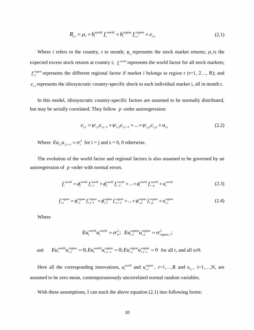
10
, , ,
world world region region
i t i i t i r t i tR b f b f (2.1)
Where i refers to the country, t to month; ,i tR represents the stock market returns; i is the
expected excess stock returns at country i; world
tf represents the world factor for all stock markets;
,
region
r tf represents the different regional factor if market i belongs to region r (r=1, 2…, R); and
,i t represents the idiosyncratic country-specific shock to each individual market i, all in month t.
In this model, idiosyncratic country-specific factors are assumed to be normally distributed,
but may be serially correlated. They follow p -order autoregression:
, ,1 , 1 ,2 , 2 , , ,...i t i i t i i t i p i p i tu (2.2)
Where 2
, ,i t j t s iEu u for i = j and s = 0, 0 otherwise.
The evolution of the world factor and regional factors is also assumed to be governed by an
autoregression of p -order with normal errors.
1 1 2 2 ...world world world world world world world world
t t t t t p tf f f f u (2.3)
, ,1 , 1 ,2 , 2 , , ,...region region region region region region region region
r t r r t r r t r p r p r tf f f f u (2.4)
Where
2 2
, , ,; ;world world region region
t t w r t r t region rEu u Eu u
and , , , ,0; 0; 0world region world region region region
t r t t r t s r t r t sEu u Eu u Eu u for all r, and all s≠0.
Here all the corresponding innovations, world
tu and ,
region
r tu , r=1,…,R and ,i tu , i=1,…,N, are
assumed to be zero mean, contemporaneously uncorrelated normal random variables.
With these assumptions, I can stack the above equation (2.1) into following forms:
11
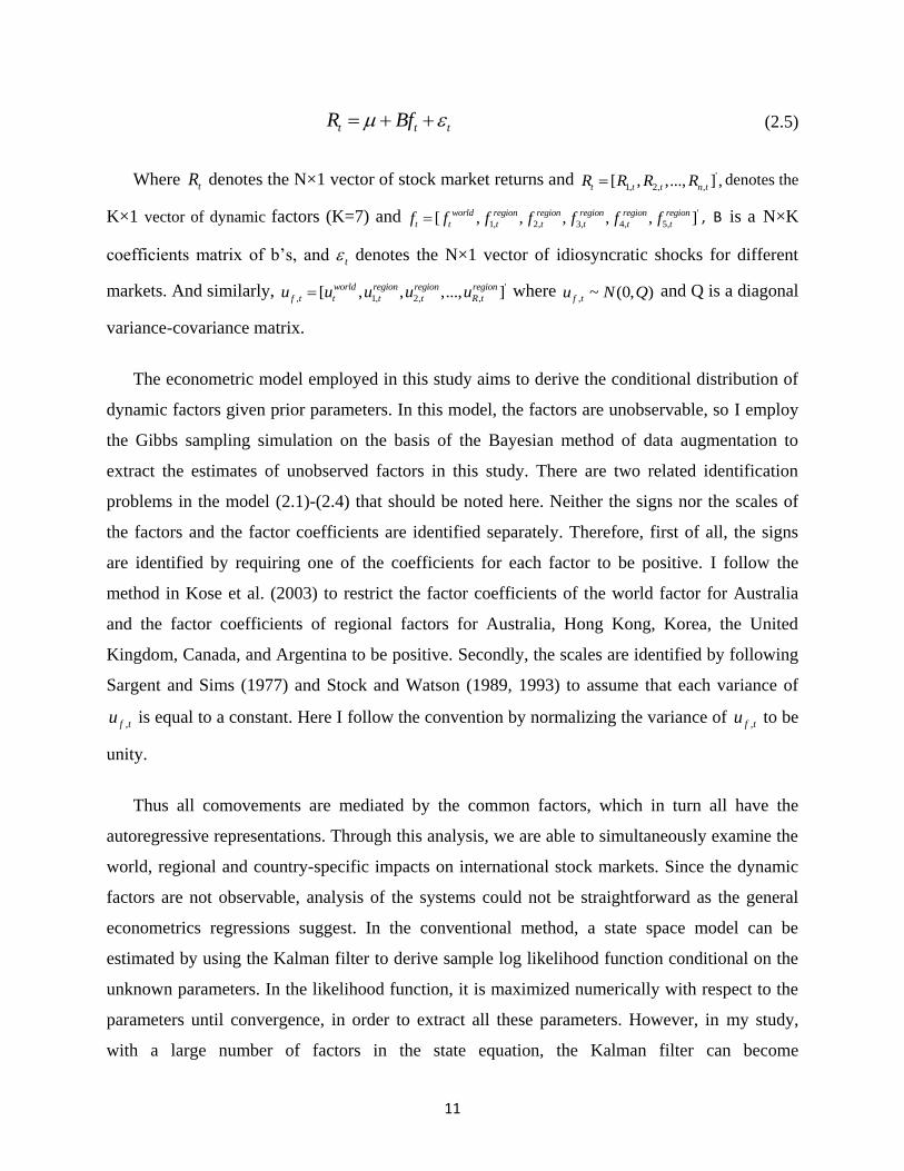
t t tR Bf (2.5)
Where tR denotes the N×1 vector of stock market returns and '
1, 2, ,[ , ,..., ] ,t t t n tR R R R denotes the
K×1 vector of dynamic factors (K=7) and '
1, 2, 3, 4, 5,[ , , , , , ]world region region region region region
t t t t t t tf f f f f f f , B is a N×K
coefficients matrix of b’s, and t denotes the N×1 vector of idiosyncratic shocks for different
markets. And similarly, '
, 1, 2, ,[ , , ,..., ]world region region region
f t t t t R tu u u u u where , ~ (0, )f tu N Q and Q is a diagonal
variance-covariance matrix.
The econometric model employed in this study aims to derive the conditional distribution of
dynamic factors given prior parameters. In this model, the factors are unobservable, so I employ
the Gibbs sampling simulation on the basis of the Bayesian method of data augmentation to
extract the estimates of unobserved factors in this study. There are two related identification
problems in the model (2.1)-(2.4) that should be noted here. Neither the signs nor the scales of
the factors and the factor coefficients are identified separately. Therefore, first of all, the signs
are identified by requiring one of the coefficients for each factor to be positive. I follow the
method in Kose et al. (2003) to restrict the factor coefficients of the world factor for Australia
and the factor coefficients of regional factors for Australia, Hong Kong, Korea, the United
Kingdom, Canada, and Argentina to be positive. Secondly, the scales are identified by following
Sargent and Sims (1977) and Stock and Watson (1989, 1993) to assume that each variance of
,f tu is equal to a constant. Here I follow the convention by normalizing the variance of ,f tu to be
unity.
Thus all comovements are mediated by the common factors, which in turn all have the
autoregressive representations. Through this analysis, we are able to simultaneously examine the
world, regional and country-specific impacts on international stock markets. Since the dynamic
factors are not observable, analysis of the systems could not be straightforward as the general
econometrics regressions suggest. In the conventional method, a state space model can be
estimated by using the Kalman filter to derive sample log likelihood function conditional on the
unknown parameters. In the likelihood function, it is maximized numerically with respect to the
parameters until convergence, in order to extract all these parameters. However, in my study,
with a large number of factors in the state equation, the Kalman filter can become

12
computationally rather burdensome. Therefore, in this study I use the method of Markov Chain
Monte Carlo (MCMC) to estimate the posterior distribution of unobserved factors and the
parameters. MCMC has been widely used by Kim and Nelson (1999) and Aguilar and West
(2000), among others, to estimate the factors. The setup is a dynamic factor model where each
level admits a state-space representation. In this study, I take advantage of Bayesian Gibbs
sampling procedure allowing us to estimate a large cross-section state space system with a large
number of unknown factors and parameters. The main idea of this method is to determine the
posterior distributions for all unobserved factors given the observable data and other parameters,
and then to determine the posterior distributions for all unknown parameters condition on the
dynamic factors and observable data. All of the joint posterior distribution for all unobservable
factors and unknown parameters can be drawn by using the MCMC procedures on the full set of
conditional distributions.
In this implementation in this study, for simplicity and also for saving the degree of freedom,
I assume that the lengths of all factor autoregressive polynomials are 1. It should be noted that
the model, in principle, works well for the general case of AR(p) autoregression. In Bayesian
econometrics, unknown parameters are usually treated as random variables followed by
underlying stochastic distribution, and the prior on all factor distribution is N(0,1). Given
appropriate prior distributions and arbitrary starting values for the model's parameters, Gibbs-
sampling can be implemented by successive iteration of the following three steps: Firstly, I
generate the posterior distribution of the factors conditional on all the stock market returns data
and all the prior parameters of the model, including: draw world factor conditional on the prior
parameters and regional factors; and then draw each regional factor conditional on the world
factor and prior parameters. Secondly, I generate the parameters from the conditional
distribution conditional on the dynamic factors. Thirdly, I generate i , ib , 2
i based on the
equations (2.1) and (2.2) conditional on the dynamic factor and the returns data for the i-th stock
market. Step 2 and step 3 are carried out by using independent Normal-Gamma priors.
All the steps are iterated S times, in which the first S1 draws are discarded as burning-in
replications to remove the effect of initial values. Under the regularity conditions satisfied here,
13
we can produce the convergence of the Markov Chains and generate the parameters and the
unobserved factors. The detail procedures can be found in Appendix A.
2.3 Data description
In this essay, I investigate a group of main 34 stock markets in the world from January 1993
through December 2009.6 7 All national stock price indices are the closed observations of market
prices expressed in local currency from Datastream International.
<Table 2.1 here>
Table 2.1 shows the countries and regions included in this study, and also presents the
definition of the markets in same region. In this study, I follow the MCSI Criteria to classify
different markets into developed and emerging markets. Based on the criterion of geographical
closeness, market developments and interactions, international stock markets in this study are
classified into 6 different regions. 8
I follow the conventional way to calculate the monthly stock market returns for country i, i.e.
, , , 1100*(log log )i t i t i tR p p (2.6)
Where i: stock market 1,2,..,N; t: month 1,2,…,T; ,i tR represents the stock market returns;
,i tp is the stock price index in local currency. Instead of choosing the price index ,i tp in a fixed
date as monthly price for stock market, here I use the average of price index in order to eliminate
the excess volatilities of price. These average price benchmarks are measured by applying the
average price index in all trading dates in each entire month.
6 The detail of national stock market indices included in this study can be found in Table 2.1 in Appendix B.
7 Some stock markets are not included in this study for the data is not available from the start date of January, 1993.
8 The details can be found in Table 2.1 in Appendix.
14
One concern with the procedure is whether big stock markets may have more power in
affecting the world factor or regional factor just because of the big size of its market. In this
study, I use stock market returns, which actually are the changing rate of stock price index, so the
size of stock market can have no direct impact on this study of international stock market
comovements. The way I follow in this study is to ensure that all the series have equal weight
irrespective of its relative market size in the world.
2.4 Empirical results
In order for this empirical analysis to be conducted, it is attempted in numerous ways. First, the
initial values are checked to see if they would affect the results. Random values are used
repeatedly as the initial parameters to simulate the results. Within these parameters, the
procedure always came to the same results across the repetition. Additionally, the simulation is
iterated in different lengths, ranging from 5,000 to 30,000. As the Gibbs sampler converges to
the same results if the iteration is greater than 5,000, for this study, this Gibbs sampler is iterated
20,000 times, of which the first 5,000 are discarded as burn-in replications.
2.4.1 The dynamic factors
In this section, the Bayesian dynamic latent factor model is employed to estimate the set of
dynamic factors designed to measure the comovements across the markets in the world, as well
as within each region. The main objective is to investigate whether the dynamics of world factor
could reveal main financial crises or events across global markets. Further, the objective aims to
examine whether regional factors could exhibit ups and downs across the stock markets within
each region. With this in mind, the country-specific factors are then studied to determine whether
these factors are able to reflect the idiosyncratic dynamics of each individual market.
<Figure 2.1 here>
Figure 2.1 illustrates the median of the posterior distribution of world factor for stock
markets in the world, along with the 5 percent and 95 percent quantiles. The narrowness of three
15
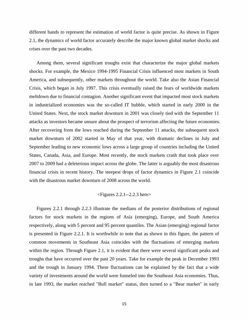
different bands to represent the estimation of world factor is quite precise. As shown in Figure
2.1, the dynamics of world factor accurately describe the major known global market shocks and
crises over the past two decades.
Among them, several significant troughs exist that characterize the major global markets
shocks. For example, the Mexico 1994-1995 Financial Crisis influenced most markets in South
America, and subsequently, other markets throughout the world. Take also the Asian Financial
Crisis, which began in July 1997. This crisis eventually raised the fears of worldwide markets
meltdown due to financial contagion. Another significant event that impacted most stock markets
in industrialized economies was the so-called IT bubble, which started in early 2000 in the
United States. Next, the stock market downturn in 2001 was closely tied with the September 11
attacks as investors became unsure about the prospect of terrorism affecting the future economies.
After recovering from the lows reached during the September 11 attacks, the subsequent stock
market downturn of 2002 started in May of that year, with dramatic declines in July and
September leading to new economic lows across a large group of countries including the United
States, Canada, Asia, and Europe. Most recently, the stock markets crash that took place over
2007 to 2009 had a deleterious impact across the globe. The latter is arguably the most disastrous
financial crisis in recent history. The steepest drops of factor dynamics in Figure 2.1 coincide
with the disastrous market downturn of 2008 across the world.
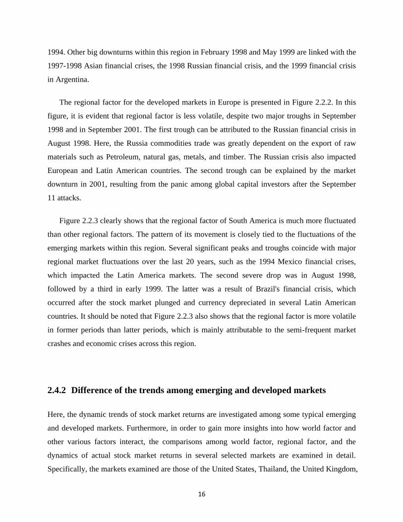
<Figures 2.2.1--2.2.3 here>
Figures 2.2.1 through 2.2.3 illustrate the medians of the posterior distributions of regional
factors for stock markets in the regions of Asia (emerging), Europe, and South America
respectively, along with 5 percent and 95 percent quantiles. The Asian (emerging) regional factor
is presented in Figure 2.2.1. It is worthwhile to note that as shown in this figure, the pattern of
common movements in Southeast Asia coincides with the fluctuations of emerging markets
within the region. Through Figure 2.1, it is evident that there were several significant peaks and
troughs that have occurred over the past 20 years. Take for example the peak in December 1993
and the trough in January 1994. These fluctuations can be explained by the fact that a wide
variety of investments around the world were funneled into the Southeast Asia economies. Thus,
in late 1993, the market reached "Bull market" status, then turned to a "Bear market" in early
16
1994. Other big downturns within this region in February 1998 and May 1999 are linked with the
1997-1998 Asian financial crises, the 1998 Russian financial crisis, and the 1999 financial crisis
in Argentina.
The regional factor for the developed markets in Europe is presented in Figure 2.2.2. In this
figure, it is evident that regional factor is less volatile, despite two major troughs in September
1998 and in September 2001. The first trough can be attributed to the Russian financial crisis in
August 1998. Here, the Russia commodities trade was greatly dependent on the export of raw
materials such as Petroleum, natural gas, metals, and timber. The Russian crisis also impacted
European and Latin American countries. The second trough can be explained by the market
downturn in 2001, resulting from the panic among global capital investors after the September
11 attacks.
Figure 2.2.3 clearly shows that the regional factor of South America is much more fluctuated
than other regional factors. The pattern of its movement is closely tied to the fluctuations of the
emerging markets within this region. Several significant peaks and troughs coincide with major
regional market fluctuations over the last 20 years, such as the 1994 Mexico financial crises,
which impacted the Latin America markets. The second severe drop was in August 1998,
followed by a third in early 1999. The latter was a result of Brazil's financial crisis, which
occurred after the stock market plunged and currency depreciated in several Latin American
countries. It should be noted that Figure 2.2.3 also shows that the regional factor is more volatile
in former periods than latter periods, which is mainly attributable to the semi-frequent market
crashes and economic crises across this region.
2.4.2 Difference of the trends among emerging and developed markets
Here, the dynamic trends of stock market returns are investigated among some typical emerging
and developed markets. Furthermore, in order to gain more insights into how world factor and
other various factors interact, the comparisons among world factor, regional factor, and the
dynamics of actual stock market returns in several selected markets are examined in detail.
Specifically, the markets examined are those of the United States, Thailand, the United Kingdom,
17
and Argentina. To make the scales more comparable, the medians of the factors are multiplied by
their respective median factor loadings in the markets returns equation. The results for these 4
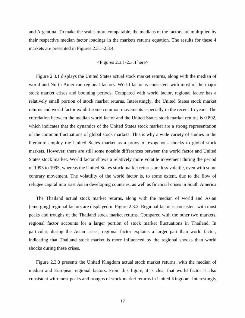
markets are presented in Figures 2.3.1-2.3.4.
<Figures 2.3.1-2.3.4 here>
Figure 2.3.1 displays the United States actual stock market returns, along with the median of
world and North American regional factors. World factor is consistent with most of the major
stock market crises and booming periods. Compared with world factor, regional factor has a
relatively small portion of stock market returns. Interestingly, the United States stock market
returns and world factor exhibit some common movements especially in the recent 15 years. The
correlation between the median world factor and the United States stock market returns is 0.892,
which indicates that the dynamics of the United States stock market are a strong representation
of the common fluctuations of global stock markets. This is why a wide variety of studies in the
literature employ the United States market as a proxy of exogenous shocks to global stock
markets. However, there are still some notable differences between the world factor and United
States stock market. World factor shows a relatively more volatile movement during the period
of 1993 to 1995, whereas the United States stock market returns are less volatile, even with some
contrary movement. The volatility of the world factor is, to some extent, due to the flow of
refugee capital into East Asian developing countries, as well as financial crises in South America.
The Thailand actual stock market returns, along with the median of world and Asian
(emerging) regional factors are displayed in Figure 2.3.2. Regional factor is consistent with most
peaks and troughs of the Thailand stock market returns. Compared with the other two markets,
regional factor accounts for a larger portion of stock market fluctuations in Thailand. In
particular, during the Asian crises, regional factor explains a larger part than world factor,
indicating that Thailand stock market is more influenced by the regional shocks than world
shocks during these crises.
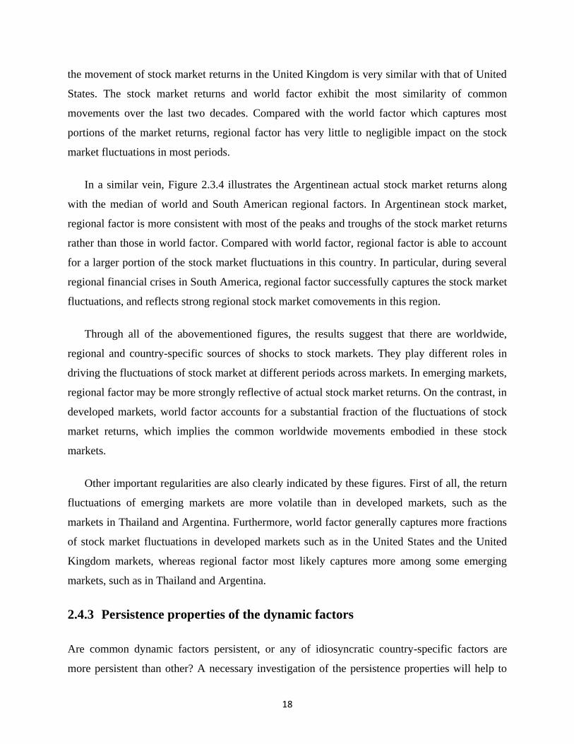
Figure 2.3.3 presents the United Kingdom actual stock market returns, with the median of
median and European regional factors. From this figure, it is clear that world factor is also
consistent with most peaks and troughs of stock market returns in United Kingdom. Interestingly,
18
the movement of stock market returns in the United Kingdom is very similar with that of United
States. The stock market returns and world factor exhibit the most similarity of common
movements over the last two decades. Compared with the world factor which captures most
portions of the market returns, regional factor has very little to negligible impact on the stock
market fluctuations in most periods.
In a similar vein, Figure 2.3.4 illustrates the Argentinean actual stock market returns along
with the median of world and South American regional factors. In Argentinean stock market,
regional factor is more consistent with most of the peaks and troughs of the stock market returns
rather than those in world factor. Compared with world factor, regional factor is able to account
for a larger portion of the stock market fluctuations in this country. In particular, during several
regional financial crises in South America, regional factor successfully captures the stock market
fluctuations, and reflects strong regional stock market comovements in this region.
Through all of the abovementioned figures, the results suggest that there are worldwide,
regional and country-specific sources of shocks to stock markets. They play different roles in
driving the fluctuations of stock market at different periods across markets. In emerging markets,
regional factor may be more strongly reflective of actual stock market returns. On the contrast, in
developed markets, world factor accounts for a substantial fraction of the fluctuations of stock
market returns, which implies the common worldwide movements embodied in these stock
markets.
Other important regularities are also clearly indicated by these figures. First of all, the return
fluctuations of emerging markets are more volatile than in developed markets, such as the
markets in Thailand and Argentina. Furthermore, world factor generally captures more fractions
of stock market fluctuations in developed markets such as in the United States and the United
Kingdom markets, whereas regional factor most likely captures more among some emerging
markets, such as in Thailand and Argentina.
2.4.3 Persistence properties of the dynamic factors
Are common dynamic factors persistent, or any of idiosyncratic country-specific factors are
more persistent than other? A necessary investigation of the persistence properties will help to
19
understand the insight of adjustment speeds. Here, persistence property is considered as a
measure of adjusting speeds to different shocks. Thus, this section aims to assess the persistence
properties of dynamic factors in the investigation of different characteristics of shocks to stock
markets.
To measure persistence, the coefficient of first order autocorrelation is calculated as follows::
, ,1 , 1 , k t k k t k tf f u (2.7)
and
, ,1 , 1 , i t i i t i tu (2.8)
Based on these equations, it is possible to measure the persistence of different shocks over
the last two decades by analyzing the autocorrelation coefficients of different factors, including
world, regional and country-specific factors. The medians of first order autocorrelation for world
and regional factors are reported in Table 2.2, and country-specific factors are reported in Table
2.3. The larger coefficients represent the higher degrees of their persistence, implying the longer
impacts of its past shocks. Thus, the persistence properties of factors can be used as an indicator
of adjustment speed.
<Tables 2.2 and 2.3 here>
As shown in Tables 2.2 and 2.3, the results indicate that world factor has relatively larger and
positive autocorrelation of 0.371. The coefficients of first order autocorrelations for regional
factors are 0.243, 0.289, 0.437, 0.310, 0.220, and 0.234 for the Oceania, Asia (developed), Asia
(emerging), Europe, North America, and South America, respectively. Compared with five other
coefficients, the persistence of the Southeast Asian regional factor is the most persistent. The
coefficient is 0.437, indicating that the adjustment to regional shocks is slow for the stock
markets in this region. The other four coefficients are relatively close, ranging from 0.22 to 0.31.
The smallest one is the coefficient of North American regional factor with only 0.220. This
coefficient indicates that the stock markets in the North America respond fastest to regional
shocks.
20
The autocorrelation of country-specific factors varies across different markets. In 26 out of
34 markets, the coefficients of first-order autocorrelation of country-specific factors range from
0.1 to 0.3. The autocorrelations are either more than 0.3 or less than 0.1 in very few markets. The
lowest autocorrelation is 0.065 for Spain, while the largest is 0.726 for Brazil. Among them, only
the Brazil-specific factor is more persistent than world and regional factors, which indicates the
longer impacts of country-specific factors on its own stock market.
The results show that most of the persistent comovements across markets in the world are
captured by world factor. In only a few markets, such as Brazil and Chile, the higher-frequency
comovements are captured by regional or country-specific factors.
2.4.4 Variance decompositions for different factors
For the purposes of this study, the analysis of variance decomposition is conducted to measure
the relative contribution of the world, regional, and country idiosyncratic factors to the variance
of stock market returns. In other words, its variance is decomposed into the fractions of the parts
corresponding to world, regional, and country idiosyncratic factors. Since the two factors and
idiosyncratic one are orthogonal, the variance of ,i ty can be written as:
2 2
, , ,var( ) ( ) var( ) ( ) var( ) var( )world world region region
i t i t i r t i tR b f b f (2.9)
Based on equation (2.9) above, the share of the variance of stock market returns attributable
to these three factors can be estimated. Hence, it is possible to measure the roles relating to what
extent the different factors impact the fluctuations of stock market returns. They are expressed as
follows:
2
,
( ) var( );
var( )world
i
world world
i t
fi t
b fS
R
,
2
,
,
( ) var( );
var( )region
i r
region region
i r t
fi t
b fS
R ,
,
var( );
var( )
i t
i
i t
SR
(2.10)
Where i=1,…, N; r=1,…, R; and world
ifS ,
,region
i rfS and iS are the shares of world, regional factors and
country-specific component of the variance of stock market returns for country i, respectively.
21
Table 2.4.1 presents the variance shares of stock market returns contributable to each factor
across 34 markets. Similarly, Table 2.4.2 presents the average variance shares for the markets
within each region, as well as within the developed and emerging markets studied for this study.
<Tables 2.4.1 and 2.4.2 here>
Table 2.4 clearly indicates that world factor accounts for a large fraction of the variances of
the stock market among most countries. More surprisingly, world factor explains more than 30
percent of the stock market variance in 29 out of 34 markets and more than 50 percent in 20 out
of 34 markets. In particular, on average, world factor accounts for more than 65 percent of the
variance in developed markets. In the context of economic globalization and financial integration,
the results indicates that world factor plays an important role in driving the fluctuations of
international stock markets, especially in developed markets. For example, world factor explains
84.23% of the stock market variance in Australia; 83.70% in the United States; 80.10% in the
Netherlands; 79.55% in Canada; 75.83% in Norway; 74.18% in the United Kingdom; 71.40% in
Austria; 69.24% in France; 67.78% in Ireland; 67.55% in Belgium; 65.57% in New Zealand;
66.18% in Denmark; 65.11% in Germany; 64.87% in Spain; 63.12% in Sweden; 61.93% in
Switzerland; 60.13% in Hong Kong; 58.21% in Singapore; 55.00% in Italy; and 53.83% in
Portugal. All these together suggest that the comovements of international stock market returns
are mainly captured by world factor, especially in developed markets.
The regions with relatively apparent strong regional comovements of stock markets are Asia
(developed), Asia (emerging), and South America. In these regions, regional factors attribute to
relatively a bigger portion of the fluctuations of stock markets. For example, among six markets
in Asia (emerging), regional factor accounts for an average of 27.08% of the stock market
variances in the region. Surprisingly, in four out of six Asian markets, regional factors account
for more than 25% of the variance, such as 42.36% in Thailand, 39.59% in Malaysia, 33.51% in
Philippines, and 24.46% in Indonesia. In South America, regional factor also accounts for a
significant fraction of the variance of stock markets, such as 32.88% in Argentina and 13.55% in
Mexico. However, regional factors are of no real significant impact in the markets in North
America and Europe, which is less than 5% of stock market return variance among 10 markets in
these two regions. In particular, there is no crucial impact in the markets of Ireland and Norway,
22
which are 1.74% and 0.76%, respectively. Yet, there are some exceptional markets in European
region. For example, regional factor accounts for 22.61% and 22.54% of the variances in France
and Germany markets.
On average, the idiosyncratic country-specific factor accounts for 32% of the variance of
stock markets. Country-specific factors explain 1.44%, 33.01%, 40.72%, 26.30%, and 47.03% of
the variances of the markets in Oceania, Asia (developed), Asia (emerging), Europe, North
America, and South America. On the whole, in 14 out of 34 markets, country-specific factor
accounts for more than 30 percent of the variances. Specifically in the following markets,
country-specific factor accounts for more than 50 percent of its variation, such as 68.99% in
Brazil; 64.14% in Taiwan; 57.52% in Chile; 57.30% in South Korea; 55.88% in Greece; 54.88%
in Peru; and 50.71% in Japan.
<Figure 2.4 here>
From both Tables 2.4.1 and 2.4.2, there are also some important regularities:
Firstly, strong international stock market comovements exist since world factor accounts for
a substantial portion of return variance in most markets. As shown in the histogram of Figure 2.4
of the return variance due to world factor, world factor explains a bigger portion of return
variance in most markets. Specifically, world factor accounts for a significant fraction from 30%
to 80% of return variance in more than 80% of the stock markets in my study.
As shown in Table 2.4.2, world factor plays a more important role in the shocks to developed
markets than emerging markets. Here, world factor, on average, explains more than 65% of the
stock market variances in developed markets. On the other hand, world factor explains
approximately 32% in emerging markets. Among developed markets within different regions,
world factor accounts for a much larger portion of return variances in Oceania at 75%, Asia
(developed) at 56%, Europe at 64%, and North America at 82%. For emerging markets in South
America and Asia (emerging), world factor accounts for 30% and 36% of the variances.
Next, regional factor plays a much more important role in the shocks of stock market returns
for the markets in Asia (emerging) than other regions. On average, the Asian regional factor can
23
explain 27% of the stock market variances in this region, which explains almost the same
fraction of the impacts of world factor. Regional factors also account for a larger fraction of the
stock market variances in Oceania, Asia (developed), and South America. Oppositely, the stock
market variances are less attributable to region factor in North America and Europe. This
suggests that a higher degree of comovements exists within regional stock markets, especially
among emerging markets in Asia and South America.
Referring back to Table 2.4.1, it is evident that the roles of country-specific factors vary
greatly across markets. In some markets, such as in Brazil and Taiwan, country-specific factors
explain more than 60% of the variances. However, country-specific factors only account for
3.79% and 6.35% of the stock market variances in Hong Kong and Singapore. As shown in
Table 2.4.2, it indicates that country-specific factors, on average, play a much larger role in
accounting for the stock market variances in emerging markets than developed markets.
Lastly, both world and country-specific factors account for the main portion of the variances
for most markets in this study. Together, the two factors account for more than 90% of the stock
market variances in 17 out of 34 markets, especially in Europe and North America. This suggests
that regional factors are less contributed to the fluctuations of stock markets in the two regions.
The finding shows that there is no clear evidence of strong common regional factors that can be
attributed to the fluctuations of European stock markets. This finding is in stark opposition to
many studies that indicate the common European regional factors have been attributed to the
stock market fluctuations in Europe. In contrast, world factor accounts for a substantial fraction
of the stock market fluctuations in the region. That is, when the European markets display
comovements, the main source is not distinctly from the European region, but rather worldwide.
However, for the stock markets in such Asian (emerging) markets as Malaysia, the Philippines
and Thailand, regional factor accounts for a large portion with more than 30% of the variances.
This finding is consistent with those of several previous studies that examine the important role
of regional impacts on stock markets because of their own characteristics of regional financial
and economic integration in this region.
2.4.5 Robustness test
24
The robustness test of these results is considered with respect to examining the stock market real
returns instead of nominal returns. This also extends the study for a different classification of
region division. 9
First of all, it is necessary to check whether the pattern of comovements of international stock
markets would be altered if stock market real returns were employed instead of nominal returns
in the above analysis. By using real returns rather than the aforementioned nominal returns, a
very similar pattern of the comovements across international stock markets is uncovered.
Furthermore, it is evident as that the factors that explain the fluctuations of stock markets have
almost same role as above.
Secondly, a different way to sort the group of stock markets into different regions is utilized.
Here, an alternative way to classify the stock markets for different regions has been followed. 10
Regarding the new classification of regions, the results indicate that the global factor plays
almost the same role in driving the fluctuations of international stock markets. Moreover, under
the different scenario of regional division, the results show that the regional factor also
demonstrated a similar pattern.
In sum, although there may be some small quantitative differences between the estimates in
this basic model and those in the various extensions previously discussed, the results of the
patterns of international stock market comovements are very similar. All of the results show the
important role of global factor in driving the fluctuations of international stock markets and the
differences of stock market integration among developed and emerging markets.
9 The results of these analyses are not reported here for saving space. The detailed results are available upon request.
10 Here I use another way to sort stock markets into different regions. Specially, among them, the regions of
Oceania, Europe, and South America are same as original ones; Asian-Pacific developed region include stock
markets of Canada, the United States, Japan, Hong Kong, and Singapore; and Asian emerging region include stock
markets of Indonesia, Malaysia, Philippines, South Korea, Taiwan, and Thailand.
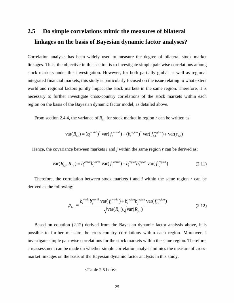
25
2.5 Do simple correlations mimic the measures of bilateral
linkages on the basis of Bayesian dynamic factor analyses?
Correlation analysis has been widely used to measure the degree of bilateral stock market
linkages. Thus, the objective in this section is to investigate simple pair-wise correlations among
stock markets under this investigation. However, for both partially global as well as regional
integrated financial markets, this study is particularly focused on the issue relating to what extent
world and regional factors jointly impact the stock markets in the same region. Therefore, it is
necessary to further investigate cross-country correlations of the stock markets within each
region on the basis of the Bayesian dynamic factor model, as detailed above.
From section 2.4.4, the variance of ,i tR for stock market in region r can be written as:
2 2
, , ,var( ) ( ) var( ) ( ) var( ) var( )world world region region
i t i t i r t i tR b f b f
Hence, the covariance between markets i and j within the same region r can be derived as:
, , ,var( , ) var( ) var( )world world world region region region
i t j t i j t i j r tR R b b f b b f (2.11)
Therefore, the correlation between stock markets i and j within the same region r can be
derived as the following:
,
,
, ,
var( ) var( )
var( ) var( )
world world world region region region
i j t i j r t
i j
i t j t
b b f b b f
R R
(2.12)
Based on equation (2.12) derived from the Bayesian dynamic factor analysis above, it is
possible to further measure the cross-country correlations within each region. Moreover, I
investigate simple pair-wise correlations for the stock markets within the same region. Therefore,
a reassessment can be made on whether simple correlation analysis mimics the measure of cross-
market linkages on the basis of the Bayesian dynamic factor analysis in this study.
<Table 2.5 here>
26
Panel A and B in Table 2.5 present the results of the coefficients of both simple pair-wise
correlation analysis and correlation analysis on the basis of the Bayesian dynamic factor analysis.
On one hand, the results show that although simple pair-wise correlation analysis can partially
measure the actual comovements of bilateral stock markets across the globe, it provides an
imperfect and biased empirical depiction of actual market integration. For example, based on the
correlation analysis from the Bayesian dynamic factor model, the bilateral stock market
correlations of Australia-New Zealand, Canada-United States, Hong Kong-Singapore, and Hong
Kong-Japan are highly integrated, while those bilateral correlations are not observed in the
results of simple pair-wise correlation analysis. On the other hand, consistent with the findings
based on variance decomposition in the Bayesian dynamic factor analysis, the results of simple
correlation analysis provide evidence that developed markets are more highly correlated than
emerging markets.
<Figure 2.5 here>
To better understand two different measures of bilateral correlations for different stock
markets, Figure 2.5 plots the relationship between simple pair-wise correlation coefficients and
the correlation coefficients estimated on the basis of equation (2.12) from the Bayesian dynamic
factor model. As shown in Figure 2.5, the results indicate that simple pair-wise correlation
analysis can partly measure the actual linkages among stock markets. However, in the presence
of different modeling and some restrictions, there are some differences between these two
correlation analyses. Simple correlation analysis cannot provide perfect depiction of their actual
market linkages, especially for those higher or lower degrees of bilateral stock market
correlations.
2.6 Can international stock market comovements be justified by
real economic integrations?
In the previous sections, the results show that there are some differences of financial-market
integration across developed and emerging markets. In a partially integrated global economy, the
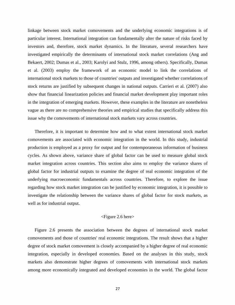
27
linkage between stock market comovements and the underlying economic integrations is of
particular interest. International integration can fundamentally alter the nature of risks faced by
investors and, therefore, stock market dynamics. In the literature, several researchers have
investigated empirically the determinants of international stock market correlations (Ang and
Bekaert, 2002; Dumas et al., 2003; Karolyi and Stulz, 1996, among others). Specifically, Dumas
et al. (2003) employ the framework of an economic model to link the correlations of
international stock markets to those of countries' outputs and investigated whether correlations of
stock returns are justified by subsequent changes in national outputs. Carrieri et al. (2007) also
show that financial linearization policies and financial market development play important roles
in the integration of emerging markets. However, these examples in the literature are nonetheless
vague as there are no comprehensive theories and empirical studies that specifically address this
issue why the comovements of international stock markets vary across countries.
Therefore, it is important to determine how and to what extent international stock market
comovements are associated with economic integration in the world. In this study, industrial
production is employed as a proxy for output and for contemporaneous information of business
cycles. As shown above, variance share of global factor can be used to measure global stock
market integration across countries. This section also aims to employ the variance shares of
global factor for industrial outputs to examine the degree of real economic integration of the
underlying macroeconomic fundamentals across countries. Therefore, to explore the issue
regarding how stock market integration can be justified by economic integration, it is possible to
investigate the relationship between the variance shares of global factor for stock markets, as
well as for industrial output.
<Figure 2.6 here>
Figure 2.6 presents the association between the degrees of international stock market
comovements and those of countries' real economic integrations. The result shows that a higher
degree of stock market comovement is closely accompanied by a higher degree of real economic
integration, especially in developed economies. Based on the analyses in this study, stock
markets also demonstrate higher degrees of comovements with international stock markets
among more economically integrated and developed economies in the world. The global factor
28
accounts for substantial fractions of stock market volatility in the most integrated economies,
such as 84.23% in Australia; 83.70% in the United States; 80.10% in Netherlands; 79.55% in
Canada; 75.83% in Norway; 74.18% in the United Kingdom; 71.40% in Austria; 69.24% in
France; 67.79% in Ireland; 70.89% in Belgium; 66.18% in Denmark; 65.11% in Germany; and
64.87% in Spain. Thus, these findings provide some support that economic integration provides a
channel for financial integration. This partly explains the high degree of comovements of
international stock markets documented in this study.
2.7 Conclusion
In this essay, I examine the common movements of stock market returns of a group of 34
countries across regions in the world. Specifically, I employ a Bayesian dynamic latent factor
model to decompose stock market returns into world, regional, and idiosyncratic country-specific
factors. I provide an in-depth analysis of the comovements of international stock markets across
the world as well as within each region simultaneously. The main empirical findings are as
follows.
Firstly, the results indicate that there is a significant world factor embodied in the
fluctuations of stock market returns across markets in the world. Evidently, there exists a high
degree of international stock market comovements. In particular, world factor accounts for a
substantial fraction of the fluctuations of stock market returns in developed markets. The
findings also indicate that the regional factor is another important source for the stock market
fluctuations in South America and Asia, providing evidence of regional comovements of stock
markets within the same region.
Secondly, the results indicate that the markets which co-move more with the worldwide
markets are mainly developed markets, whose returns are less volatile. On the contrary, in
emerging markets, regional factor and country-specific factor together account for more portion
of the variance of stock market returns. In some particular emerging markets, such as Brazil,
29
Korea, and Taiwan, among others, idiosyncratic country factor accounts for the bigger portion in
explaining the fluctuations of these stock markets than the world and regional factors together.
The investigation of the property of factor persistence indicates that both the world factor and
the Asian (emerging) regional factor have larger coefficients than other regional factors. This
indicates the higher degrees of their persistence and the longer impacts of the past shocks. On the
contrary, compared with higher degree of the persistence in the world factor, most country-
specific factors with relatively smaller coefficients show their faster adjustments to their country-
specific shocks. This demonstrates the longer impacts from world and regional shocks than from
each country-specific shock.
Further, while investigating cross-country correlations of stock markets within each region,
both simple pair-wise correlation analysis and the correlation analysis derived from the Bayesian
dynamic factor model in this essay are applied to investigate bilateral stock market linkages
within the same region. The result indicates that although simple pair-wise correlation analysis
can partially measure actual bilateral stock market linkages within the same region, it provides
an imperfect and biased empirical depiction of actual market integration. This finding is
consistent with the finding in Pukthuanthong and Roll (2009). However, the results of simple
correlation analysis provide evidence that developed markets are more highly correlated than
emerging markets, which is consistent with the findings based on variance decomposition in the
Bayesian dynamic factor analysis.
Lastly, when investigating the comovements of international stock markets, the analysis is
extended to search for possible channel of the differences of international stock market
comovements documented in this study. In a partially integrated global economy, the analysis
indicates that the higher degree of a country's stock market comovement with international stock
markets, the higher degree of its own real economic integration, especially in developed
economies. The results suggest that real economic integration provides a channel for
understanding international stock market comovements. These findings indicate that the degree
of a market's comovement with international stock markets is closely related with that of its own
country's economic integration in the world.
30
Chapter 3 Dynamic Correlation Analysis of the
Realized Volatility Comovements in Asian Markets
3.1 Introduction
Cross-market linkages have been a prevalent phenomenon in modern financial theoretical and
empirical research over recent decades. Accurate specification of stock market linkages is of
very importance in financial decisions, such as portfolio allocation and risk management for risk-
averse investors. For example, in a global integrated financial system, a shock in the Hong Kong
market may make investors adjust their exposure to other international markets due to the
possible information spillover of the Hong Kong market on other markets. One aspect of cross-
market linkage researches usually examines the pattern of information flow across different
markets. The interest of studying this aspect is motivated by the series of financial crisis in recent
decades, such as East Asian “Asian flu” in 1997, “Russian virus” in 1998, Brazil crisis in 1999,
and especially the recent global financial crisis over 2007-2009.
When we look at the fluctuations across different stock markets in the world, there
always exist some strong movements in one market, which may correspond with the similarly
strong movements in another one. If the definition of comovements can be based on the notion
which describes a phenomenon of a market (or asset price) “moving with” other market (asset
price, respectively), then we can conclude that the comovements can be defined as a pattern of
positive correlation (Barberis et al., 2005). In other words, comovements can be defined with the
correlation coefficient. The study of correlation is given as the comovements of stock markets
with focusing on the markets in special region, such as Asian markets, or as the term “contagion”
which is often considered as the “excessive” correlation among stock markets (Barberis, et al.,
2005). Many studies use the term “correlation coefficient” to measure the comovements across
stock markets (Boyer et al., 1999; Loretan et al., 2000; Forbes and Figobon, 2002; Corsetti et al.,
etc, 2005). Therefore, analysis of common movements among stock markets is an important and
possibly effective way to better understand the functioning of regional financial system.
31
There are many studies in the literature on stock market comovements, market linkage,
interdependence, and even spillovers of one market onto another, providing evidence of cross-
market linkage. Although cross-markets linkage is a topic of ongoing interest to researchers and
practitioners, it seems that we are still in the preliminary stage to fully understand cross-market
linkage, and even far from being able to prevent the crisis transmitting across markets. The
recent financial crises provide us with more opportunities to examine market correlation and
information spillover across markets. This is particularly important when investigating financial
crisis and their contagious effects, providing policy makers more sources to perfect the national
and even the international financial system.
Previous studies on the stock market linkage and the financial contagion in financial
crisis have not provided consistent results. In the earliest studies on international stock market
linkages, Levy and Sarnat (1970) and Solnik (1974) examine short-term correlations of the
returns across national markets and pointed out the existence of substantial possibilities to
diversify internationally. Some recent studies (Hamao et al., 1990; Koch and Koch, 1991; and
Longin and Solnik, 1995; etc) have exploited some more sophisticated econometric techniques to
measure cross-market correlations, and find the evidence of significant linkages among stock
markets in the world. Janakiramanan and Lamba (1998) empirically examine the correlation
between the Pacific-Basin stock markets and they find that the US market influences all other
markets, except for the relatively isolated market of Indonesia. Stock markets that are
geographically and economically close and have a large number of cross-border listings tends to
exert significant influence on one another, such as the stock markets in Asia.
Many previous studies have also shown the changes in stock market volatility over time
(French et al, 1987; Schwert, 1989; Bekaert and Harvey, 1997; Corradi et al, 2009; etc). In
particular, the degree of the dynamics of stock market volatility showed a great increase in the
financial crisis. During the period of heighted volatility, stock markets are much more positively
correlated (Kupiec, 1991; Forbes and Rigobon, 2002; etc). Several studies find that the increased
volatility can increase the (extreme) degree of comovements, or there is increase in correlation
coefficients conditional on the volatility of stock market when there is high degree of market
comovements. Furthermore, in financial crisis, there often exists the phenomenon of volatility
32
clustering11
, with periods of high and low (conditional or unconditional) variance. Mandelbrot
(1963) notes the “volatility clustering” as follows: large changes tend to be followed by large
changes, of either sign, and small changes tend to be followed by small changes. Especially
when in financial crises, there often exists the phenomenon of volatility clustering. Kupiec (1991)
shows there exists the phenomenon of the correlations in the stock market volatility and also
finds that correlations among the volatilities of monthly stock market returns have increased over
time. The results show that volatilities, particularly among the major markets, were more
positively correlated in the second half of 1980s as compared with the first half of the decade.
Other studies on financial contagion also find significant increase in cross-market
correlation of stock volatility in the Asia (Sachs et al, 1996). Ng (2000) finds that there exists
volatility spillover effect from the Japan and the US markets to the Pacific-Basin markets.
Similarly, some studies find volatility spillover effects among the stock markets in North and
South America (Diebold, 2009). And Corradi et al. (2009) investigate conditional independence
and find volatility transmission among international stock markets in their selected markets.
When in the financial crisis, stock markets tend to move together with higher volatility, as large
price change moves are interpreted as global news through the non-trading zones induced by
costs of international transactions. During the period of heighted volatility, stock markets tend to
be more positively correlated. All this raises the question whether the correlation of stock market
volatility is higher during the financial crisis than before the crisis.
Motivated by previous studies, in this essay I want to investigate whether there are some
common movements among Asian markets through the channel of the stock market volatility
beyond what is implied by previous literature. Specifically, this essay aims to examine whether
there is an increase in the comovements of stock market volatility among the main Asian markets
after the crisis by employing correlation analyses of stock market linkages.
Unlike previous analyses focusing on the correlation of stock market price or market
returns, this study aims to investigate the correlation of stock market comovements through
11 Time series of financial assets often exhibit the property of volatility clustering: large changes in prices tend to
cluster together, resulting in persistence of the amplitudes of price changes. Volatility clustering often refers to the
property if most heteroskedastic stochastic processes used in finance and economics.
33
higher moment of stock market volatility. Specifically, in this study I estimate time-invariant and
time-varying correlation coefficients of stock market volatility in Asia and investigate whether
there exists contagion effect among the Asian markets during the financial crisis. All this aims to
further examine the regional stock market comovements through the channel of stock market
volatility, and also to have a further and detailed investigation of financial contagion in Asia,
thus helping us to understand the regional comovements during the financial crisis.
The remainder of the study is organized as follows. Section 3.2 describes the data and
presents descriptive statistics. Section 3.3 presents the models employed in this study. Section
3.4 reports the empirical results. Section 3.5 investigates the transition of the realized volatility.
And Section 3.6 contains the conclusions.
3.2 Data description and preliminary statistics
The data in this study are daily stock-price indices from the main Asian markets in the period of
January 1st, 1995 to December 31st, 1999, 12
which consist of the closed observations of stock
market prices expressed in local currency from Datastream International.13
The indices of weekly
realized volatility are estimated by using the daily stock market returns. Further, following the
way by French, Schwert, and Stambaugh (1987) and Schwert (1989), I estimate the indices of
weekly realized volatility, which are the sum of squared daily returns in each week as follows:
, , , , , , 1
2 2
, , ,
1
100*(log log );
t
i t j i t j i t j
N
i t i t j
j
r p p
r
(3.1)
12 These markets were seriously affected by the 1997-1998 Asian financial crises.
13 Stock market index prices in this study are as follows: The Hang Seng Price Index for Hong Kong; the Korean
Stock Exchange composite for Korea; the Kuala Lumpur Stock Exchange Composite Price Index for Malaysia; the
Singapore Straits Times Price Index for Singapore; the Taiwan Stock Exchange weighted-price index for Taiwan;
the Bangkok S.E.T. Price Index for Thailand; the Msdumaf Index for Malaysia; the Mseusinf Price Index for
Indonesia; and the Nikkei 225 Price Index for Japan.
34
Where i is country i, t is week t in the period, and j is the trading day in week t; , ,i t jp is
the daily stock price index on date j in local currency; , ,i t jr is daily stock returns; and tN is the
number of trading days in week t.
The reason to employ the weekly volatility in this study, instead of monthly ones, is to
avoid the problem of non-synchronous trading and the day-of-the-week effects (see Dubois and
Louvet, 1996; Ramchand and Susmel, 1998; Aggarwal et al., 1999; and Ng, 2000, among others).
Moreover, the weekly realized volatility which is computed from the sum of the daily volatility
in the week, largely overlap and thus information is shared among different markets.
<Table 3.1 here>
Furthermore, it aims to help investigate the dynamic relationship among stock markets
during this special period. In particular, the different infected markets were impacted one after
the other so frequently during the Asian crisis (see Table 3.114
), so it is necessary to examine
how the Asian financial crisis affected the realized volatility of Asian markets one after another.
<Table 3.2 here>
Table 3.2 presents the summary statistics for the weekly realized volatility of the 9 Asian
markets. Following the way in previous studies, I us the July 2nd
, 1997 to split the sample period
into two parts: Before crisis and after crisis.15
As shown in Table 3.2, the mean of weekly
realized volatility indices in the Asian markets is significantly higher after the crisis than before
the crisis, even more than 10 times higher in both Malaysian and Indonesia. 16
<Figure 3.1 here>
14 Table 3.1 presents the date when stock markets were impacted during the 1997 Asian crisis.
15 On July 2nd, 1997, the Thailand Government gave up defending the value of its currency, the Baht, which
triggered a significant depreciation of the currencies of Thailand and it neighboring Asian countries.
16 When the realized volatility in some markets is equal to zero, it means there were no trading days during the
respective week for the market instead of the existence of no realized volatility.
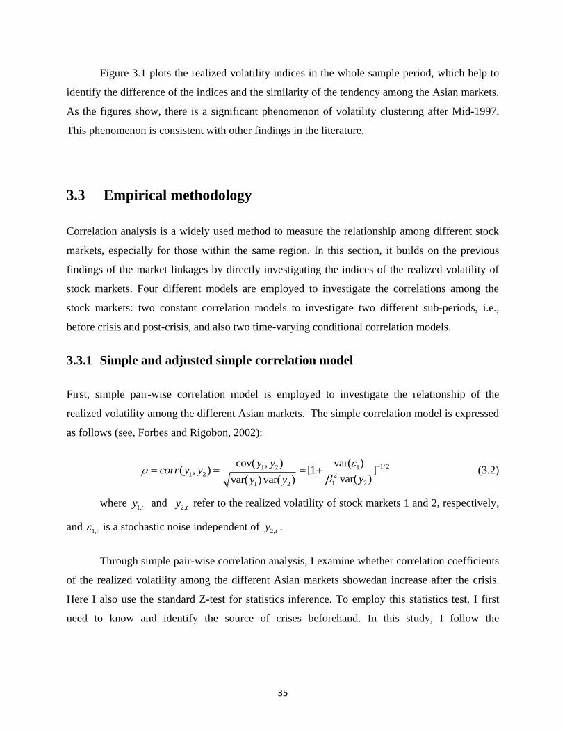
35
Figure 3.1 plots the realized volatility indices in the whole sample period, which help to
identify the difference of the indices and the similarity of the tendency among the Asian markets.
As the figures show, there is a significant phenomenon of volatility clustering after Mid-1997.
This phenomenon is consistent with other findings in the literature.
3.3 Empirical methodology
Correlation analysis is a widely used method to measure the relationship among different stock
markets, especially for those within the same region. In this section, it builds on the previous
findings of the market linkages by directly investigating the indices of the realized volatility of
stock markets. Four different models are employed to investigate the correlations among the
stock markets: two constant correlation models to investigate two different sub-periods, i.e.,
before crisis and post-crisis, and also two time-varying conditional correlation models.
3.3.1 Simple and adjusted simple correlation model
First, simple pair-wise correlation model is employed to investigate the relationship of the
realized volatility among the different Asian markets. The simple correlation model is expressed
as follows (see, Forbes and Rigobon, 2002):
1/ 21 2 11 2 2
1 21 2
cov( , ) var( )( , ) [1 ]
var( )var( ) var( )
y ycorr y y
yy y
(3.2)
where 1,ty and
2,ty refer to the realized volatility of stock markets 1 and 2, respectively,
and 1,t is a stochastic noise independent of
2,ty .
Through simple pair-wise correlation analysis, I examine whether correlation coefficients
of the realized volatility among the different Asian markets showedan increase after the crisis.
Here I also use the standard Z-test for statistics inference. To employ this statistics test, I first
need to know and identify the source of crises beforehand. In this study, I follow the
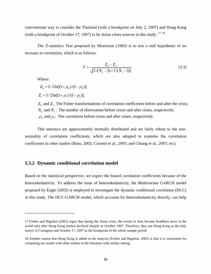
36
conventional way to consider the Thailand (with a breakpoint on July 2, 1997) and Hong Kong
(with a breakpoint of October 17, 1997) to be Asian crises sources in this study. 17
18
The Z-statistics Test proposed by Morrrison (1983) is to test a null hypothesis of no
increase in correlation, which is as follows:
0 1
0 1
[1/( 3) 1/( 3)]
Z ZT
N N
(3.3)
Where:
0 0 01/ 2ln[(1 ) /(1 )]; Z
1 1 11/ 2ln[(1 ) /(1 )];Z
0 1
0 1
0 1
and : The Fisher transformations of correlation coefficients before and after the crisis;
and : The number of obersvatons before crises and after crises, respectively;
and : The correla
Z Z
N N
tion before cirses and after crises, respectively.
This statistics are approximately normally distributed and are fairly robust to the non-
normality of correlation coefficients, which are also adopted to examine the correlation
coefficients in other studies (Basu, 2002; Corsetti et al., 2005; and Chiang et al., 2007; etc).
3.3.2 Dynamic conditional correlation model
Based on the statistical perspective, we expect the biased correlation coefficients because of the
heteroskedasticity. To address the issue of heteroskedasticity, the Multivariate GARCH model
proposed by Engle (2002) is employed to investigate the dynamic conditional correlation (DCC)
in this study. The DCC-GARCH model, which accounts for heteroskedasticity directly, can help
17 Forbes and Rigobon (2002) argue that during the Asian crisis, the events in Asia became headlines news in the
world only after Hong Kong market declined sharply in October 1997. Therefore, they use Hong Kong as the only
source of Contagion and October 17, 1997 as the breakpoint of the whole sample period.
18 Another reason that Hong Kong is added in the analysis (Forbes and Rigobon, 2002) is that it is convenient for
comparing my results with other studies in the literature with similar setting.
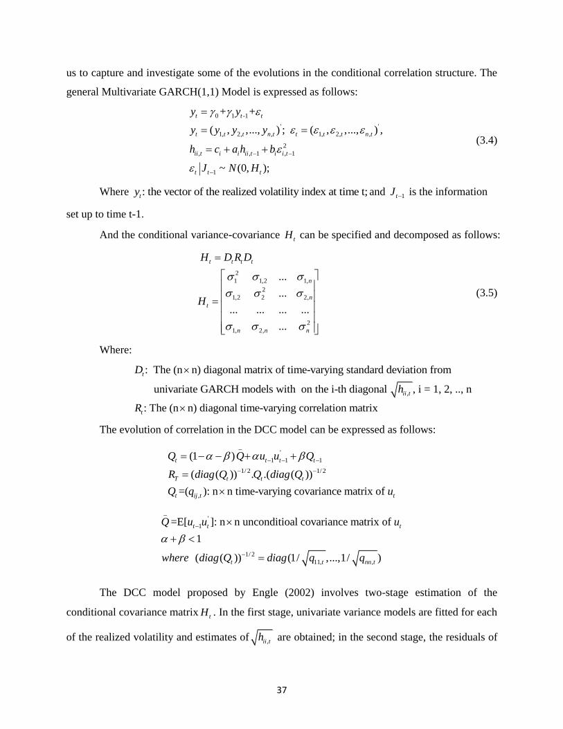
37
us to capture and investigate some of the evolutions in the conditional correlation structure. The
general Multivariate GARCH(1,1) Model is expressed as follows:
0 1 -1
' '
1, 2, , 1, 2, ,
2
, , 1 , 1
1
+ +
( , ,..., ) ; ( , ,..., ) ,
~ (0, );
t t t
t t t n t t t t n t
ii t i i ii t i i t
t t t
y y
y y y y
h c a h b
J N H
(3.4)
Where : the vector of the realized volatility index at time t;ty and 1tJ is the information
set up to time t-1.
And the conditional variance-covariance tH can be specified and decomposed as follows:
2
1 1,2 1,
2
1,2 2 2,
2
1, 2,
...
...
... ... ... ...
...
t t t t
n
n
t
n n n
H D R D
H
(3.5)
Where:
,
: The (n n) diagonal matrix of time-varying standard deviation from
univariate GARCH models with on the i-th diagonal , i = 1, 2, .., n
: The (n n) diagonal time-varying correlation m
t
ii t
t
D
h
R
atrix
The evolution of correlation in the DCC model can be expressed as follows:
_'
1 1 1
1/ 2 1/ 2
,
(1 )
( ( )) . .( ( ))
=( ): n n time-varying covariance matrix of
t t t t
T t t t
t ij t t
Q Q u u Q
R diag Q Q diag Q
Q q u
_'
1
1/ 2
11, ,
=E[ ]: n n unconditioal covariance matrix of
1
( ( )) (1/ ,...,1/ )
t t t
t t nn t
Q u u u
where diag Q diag q q
The DCC model proposed by Engle (2002) involves two-stage estimation of the
conditional covariance matrixtH . In the first stage, univariate variance models are fitted for each
of the realized volatility and estimates of ,ii th are obtained; in the second stage, the residuals of

38
market’s realized volatility are transformed by their estimated standard deviations from the first
stage. That is, , , ,/i t i t ii tu h , where ,i tu is then used to estimate the parameters of the
conditional correlation.
Therefore, the correlation in the model can be written as follows:
,
,
, ,
, , , , 1 , 1 , , 1
, , 1,2,..., ,
1
ij t
ij t
ii t jj t
i j t i j i t j t i j t
qi j n and i j
q q
q q
(3.6)
This model captures not only the individual effects of volume and volatility, but also their
interaction effects on any serial dependence in the residuals of OLS equations. Significant
coefficient indicates which term adds information to the forecast of volume at time t and/or
volatility. Thus, the GARCH formulation considers current variance, past variance and past error
of the forecast of the variable in question (as well as information on the variance and the error of
other variables and the covariability effects) to adjust the current forecast of the variable in
question.
In this study, I only investigate the bivariate case, so the correlation coefficient under this
condition can be written as follows:
_
12 1, 1 2, 1 12, 1
12,_ _
2 2
11 1, 1 11, 1 22 2, 1 22, 1
(1 )
[(1 ) ] [(1 ) ]
t t t
t
t t t t
q u u q
q u q q u q
(3.7)
As proposed by Engel (2002), the DCC model can be estimated through using the two-
stage approach to maximize the log-likelihood function. Let denote the parameters in tD ,
denote the parameters in tR , and then the log-likelihood function is:
2
1
2
1
1( , ) [ ( log(2 ) log ' )]
2
1 [ (log ' ' )]
2
T
t t t tt
T
t t t t t tt
l n D D
R u D u u u
(3.8)
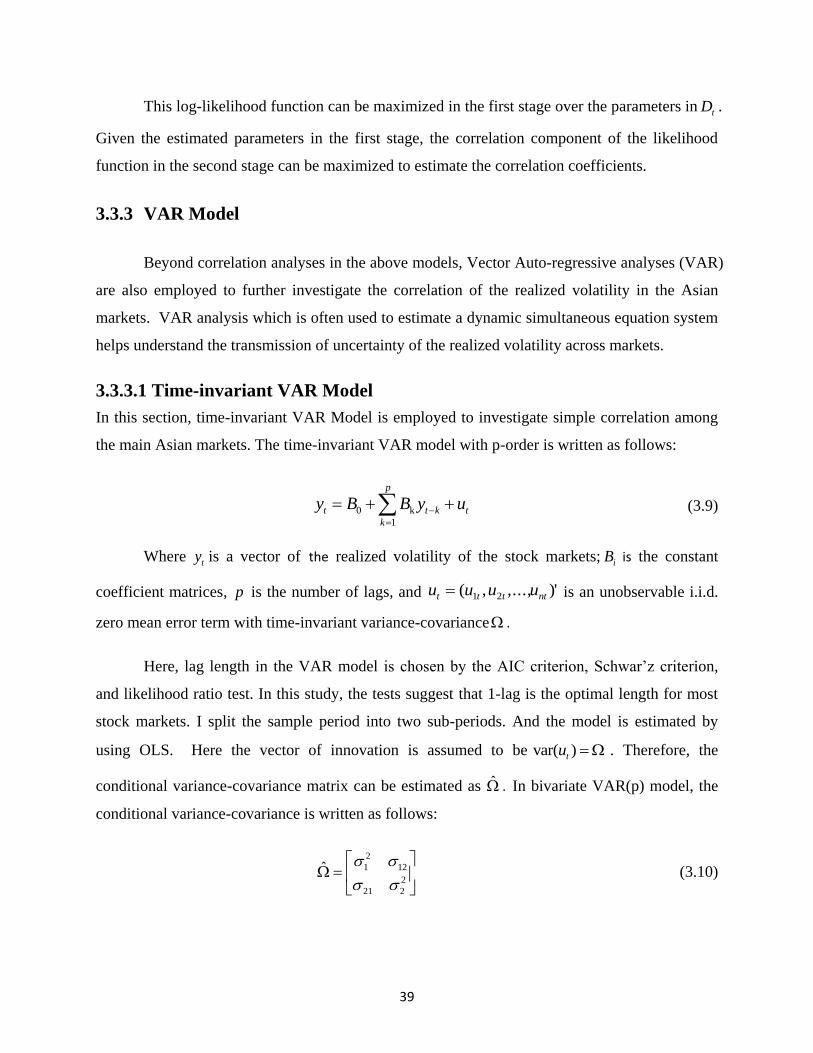
39
This log-likelihood function can be maximized in the first stage over the parameters in tD .
Given the estimated parameters in the first stage, the correlation component of the likelihood
function in the second stage can be maximized to estimate the correlation coefficients.
3.3.3 VAR Model
Beyond correlation analyses in the above models, Vector Auto-regressive analyses (VAR)
are also employed to further investigate the correlation of the realized volatility in the Asian
markets. VAR analysis which is often used to estimate a dynamic simultaneous equation system
helps understand the transmission of uncertainty of the realized volatility across markets.
3.3.3.1 Time-invariant VAR Model
In this section, time-invariant VAR Model is employed to investigate simple correlation among
the main Asian markets. The time-invariant VAR model with p-order is written as follows:
0 k
1
p
t t k t
k
y B B y u
(3.9)
Where ty is a vector of the realized volatility of the stock markets; iB is the constant
coefficient matrices, p is the number of lags, and )',...,,( 21 ntttt uuuu is an unobservable i.i.d.
zero mean error term with time-invariant variance-covariance .
Here, lag length in the VAR model is chosen by the AIC criterion, Schwar’z criterion,
and likelihood ratio test. In this study, the tests suggest that 1-lag is the optimal length for most
stock markets. I split the sample period into two sub-periods. And the model is estimated by
using OLS. Here the vector of innovation is assumed to be var( )tu . Therefore, the
conditional variance-covariance matrix can be estimated as ̂ . In bivariate VAR(p) model, the
conditional variance-covariance is written as follows:
2
1 12
2
21 2
ˆ
(3.10)
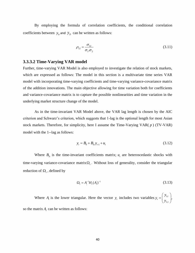
40
By employing the formula of correlation coefficients, the conditional correlation
coefficients between 1ty and 2ty can be written as follows:
1212
1 2.
(3.11)
3.3.3.2 Time-Varying VAR model
Further, time-varying VAR Model is also employed to investigate the relation of stock markets,
which are expressed as follows: The model in this section is a multivariate time series VAR
model with incorporating time-varying coefficients and time-varying variance-covariance matrix
of the addition innovations. The main objective allowing for time variation both for coefficients
and variance-covariance matrix is to capture the possible nonlinearities and time variation in the
underlying market structure change of the model.
As in the time-invariant VAR Model above, the VAR lag length is chosen by the AIC
criterion and Schwarz’s criterion, which suggests that 1-lag is the optional length for most Asian
stock markets. Therefore, for simplicity, here I assume the Time-Varying VAR( p ) (TV-VAR)
model with the 1--lag as follows:
0 1t -1 t t ty B B y u (3.12)
Where 1tB is the time-invariant coefficients matrix; tu are heteroscedastic shocks with
time-varying variance-covariance matrix t . Without loss of generality, consider the triangular
reduction of t , defined by
1 ' 1( ) tt t tA H A (3.13)
Where tA is the lower triangular. Here the vector ty includes two variables1,
2,
t
t
t
yy
y
,
so the matrix tA can be written as follows:
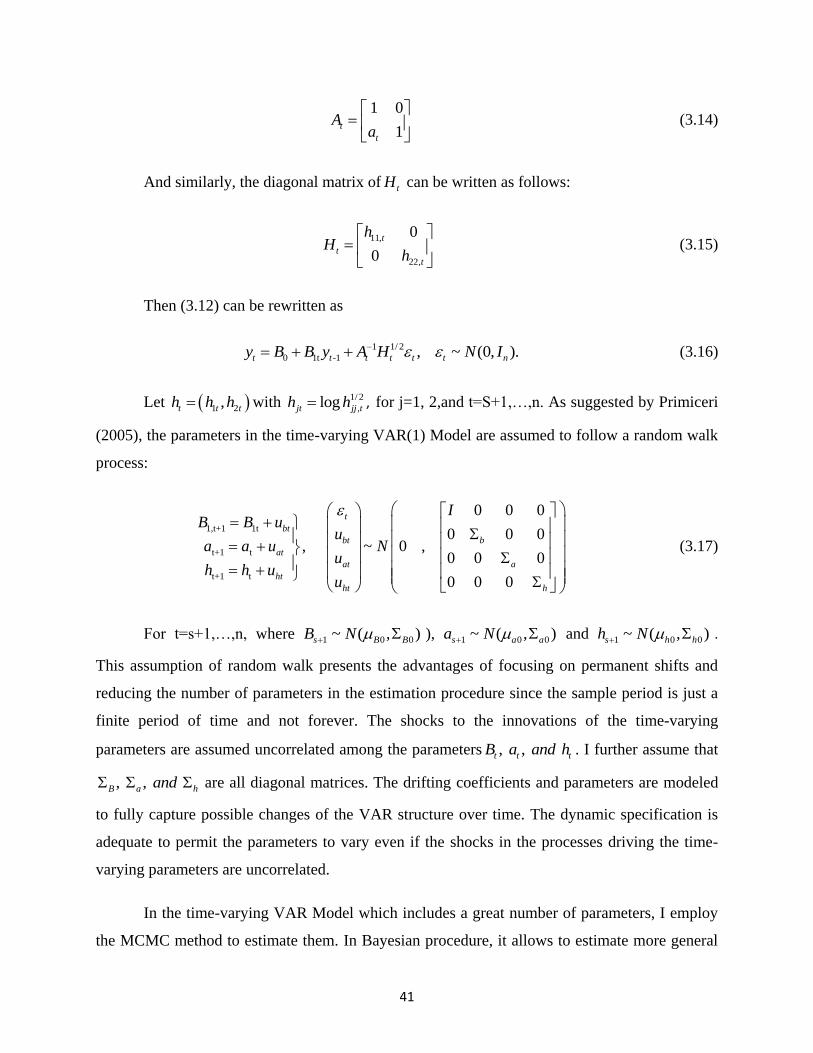
41
1 0
1t
t
Aa
(3.14)
And similarly, the diagonal matrix of tH can be written as follows:
11,
22,
0
0
t
t
t
hH
h
(3.15)
Then (3.12) can be rewritten as
1 1/ 2
0 1t -1 , ~ (0, ).t t t t t t ny B B y A H N I (3.16)
Let 1 2,t t th h h with 1/ 2
,logjt jj th h , for j=1, 2,and t=S+1,…,n. As suggested by Primiceri
(2005), the parameters in the time-varying VAR(1) Model are assumed to follow a random walk
process:
1,t+1 1t
t+1 t
t+1 t
,
bt
at
ht
B B u
a a u
h h u
0 0 0
0 0 0~ 0 ,
0 0 0
0 0 0
t
bt b
at a
ht h
I
uN
u
u
(3.17)
For t=s+1,…,n, where 1 0 0~ ( , )s B BB N ), 1 0 0~ ( , )s a aa N and 1 0 0~ ( , )s h hh N .
This assumption of random walk presents the advantages of focusing on permanent shifts and
reducing the number of parameters in the estimation procedure since the sample period is just a
finite period of time and not forever. The shocks to the innovations of the time-varying
parameters are assumed uncorrelated among the parameters , , t t tB a and h . I further assume that
, , B a hand are all diagonal matrices. The drifting coefficients and parameters are modeled
to fully capture possible changes of the VAR structure over time. The dynamic specification is
adequate to permit the parameters to vary even if the shocks in the processes driving the time-
varying parameters are uncorrelated.
In the time-varying VAR Model which includes a great number of parameters, I employ
the MCMC method to estimate them. In Bayesian procedure, it allows to estimate more general
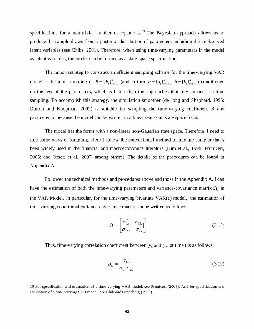
42
specifications for a non-trivial number of equations.19
The Bayesian approach allows us to
produce the sample drawn from a posterior distribution of parameters including the unobserved
latent variables (see Chibs, 2001). Therefore, when using time-varying parameters in the model
as latent variables, the model can be formed as a state-space specification.
The important step to construct an efficient sampling scheme for the time-varying VAR
model is the joint sampling of 1{ }n
t t sB B (and in turn, 1{ }n
t t sa a , 1{ }n
t t sh h ) conditioned
on the rest of the parameters, which is better than the approaches that rely on one-at-a-time
sampling. To accomplish this strategy, the simulation smoother (de Jong and Shephard, 1995;
Durbin and Koopman, 2002) is suitable for sampling the time-varying coefficient B and
parameter a because the model can be written in a linear Gaussian state space form.
The model has the forms with a non-linear non-Gaussian state space. Therefore, I need to
find some ways of sampling. Here I follow the conventional method of mixture sampler that’s
been widely used in the financial and macroeconomics literature (Kim et al., 1998; Primiceri,
2005; and Omori et al., 2007, among others). The details of the procedures can be found in
Appendix A.
Followed the technical methods and procedures above and those in the Appendix A, I can
have the estimation of both the time-varying parameters and variance-covariance matrix t in
the VAR Model. In particular, for the time-varying bivariate VAR(1) model, the estimation of
time-varying conditional variance-covariance matrix can be written as follows:
2
1, 12,
2
12, 2.
t t
t
t t
(3.18)
Thus, time-varying correlation coefficient between 1ty and 2ty at time t is as follows:
12,
12
1, 2,.
t
t t
(3.19)
19 For specification and estimation of a time-varying VAR model, see Primiceri (2005). And for specification and
estimation of a time-varying SUR model, see Chib and Greenberg (1995).
43
Investigating time-invariant and time-varying correlation coefficient on the basis of the
VAR models, it can help us to better understand how the realized volatility comovements among
the main Asian markets have been evolved before the crisis and after the crisis.
3.4 Empirical results
3.4.1 Simple pair-wise correlation analysis
<Table 3.3 here>
First, I simply choose the July 2nd
, 1997 as the breakpoint mentioned above. The results of the
simple pair-wise correlation coefficients between the realized volatility of different markets
during the two periods are reported in Table 3.3.1. The results show that the null hypothesis of
no correlation increase is rejected by 28 out 36 coefficients. Among the remaining 8 coefficients,
half of them are with Malaysia market due to the capital control in this country in 1998.
Secondly, some questions are raised whether the source country of financial crisis matters.
Thus, if I change the crises source of country, I use the country as the crises source according to
the order of date when the infected markets were impacted during the crises.20
The whole sample
period is divided into two periods based on the date of the order, and then the new simple pair-
wise correlation coefficients are estimated for the Asian markets. As shown in Table 3.3.2, the
result shows that the null hypothesis of no correlation increase is rejected by 29 out 36
coefficients. It is similar to what is presented in the above section. By using Z-test, I only find
that the null hypothesis is rejected at the 10% level in 25 out of 36 cases after adjusting the
infected markets according to the impacted date.
3.4.2 Dynamic conditional correlation analysis using GARCH Model
As simple-correlation analysis highlights the realized volatility in the different periods with a
given window, I further discuss this issue by investigating the time-varying characteristics of
20 The dates the infected markets were impacted during the crisis can be found in Table 3.3.1 in the Appendix.
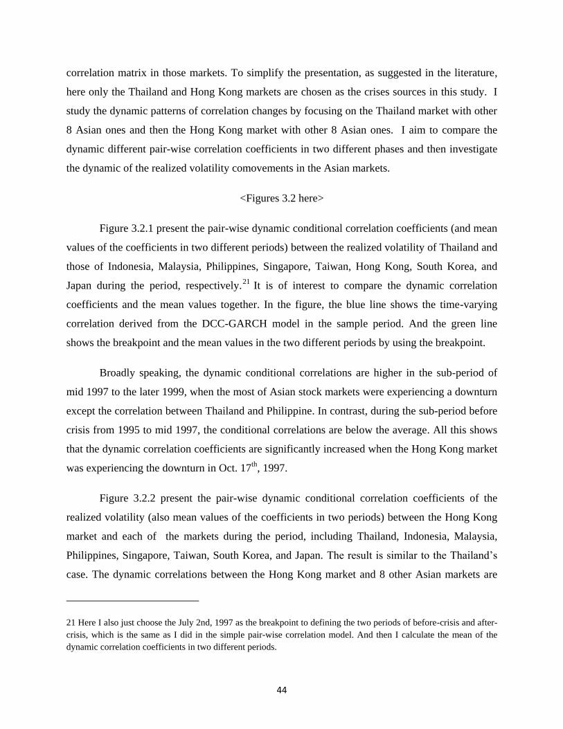
44
correlation matrix in those markets. To simplify the presentation, as suggested in the literature,
here only the Thailand and Hong Kong markets are chosen as the crises sources in this study. I
study the dynamic patterns of correlation changes by focusing on the Thailand market with other
8 Asian ones and then the Hong Kong market with other 8 Asian ones. I aim to compare the
dynamic different pair-wise correlation coefficients in two different phases and then investigate
the dynamic of the realized volatility comovements in the Asian markets.
<Figures 3.2 here>
Figure 3.2.1 present the pair-wise dynamic conditional correlation coefficients (and mean
values of the coefficients in two different periods) between the realized volatility of Thailand and
those of Indonesia, Malaysia, Philippines, Singapore, Taiwan, Hong Kong, South Korea, and
Japan during the period, respectively.21
It is of interest to compare the dynamic correlation
coefficients and the mean values together. In the figure, the blue line shows the time-varying
correlation derived from the DCC-GARCH model in the sample period. And the green line
shows the breakpoint and the mean values in the two different periods by using the breakpoint.
Broadly speaking, the dynamic conditional correlations are higher in the sub-period of
mid 1997 to the later 1999, when the most of Asian stock markets were experiencing a downturn
except the correlation between Thailand and Philippine. In contrast, during the sub-period before
crisis from 1995 to mid 1997, the conditional correlations are below the average. All this shows
that the dynamic correlation coefficients are significantly increased when the Hong Kong market
was experiencing the downturn in Oct. 17th
, 1997.
Figure 3.2.2 present the pair-wise dynamic conditional correlation coefficients of the
realized volatility (also mean values of the coefficients in two periods) between the Hong Kong
market and each of the markets during the period, including Thailand, Indonesia, Malaysia,
Philippines, Singapore, Taiwan, South Korea, and Japan. The result is similar to the Thailand’s
case. The dynamic correlations between the Hong Kong market and 8 other Asian markets are
21 Here I also just choose the July 2nd, 1997 as the breakpoint to defining the two periods of before-crisis and after-
crisis, which is the same as I did in the simple pair-wise correlation model. And then I calculate the mean of the
dynamic correlation coefficients in two different periods.
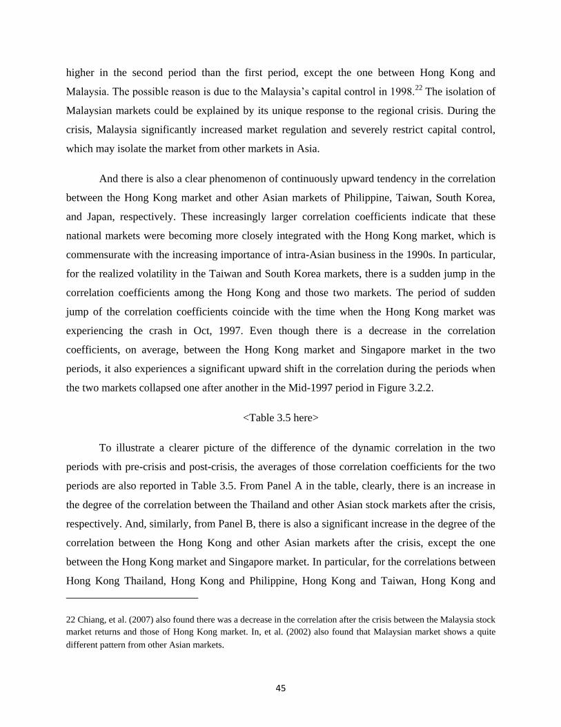
45
higher in the second period than the first period, except the one between Hong Kong and
Malaysia. The possible reason is due to the Malaysia’s capital control in 1998.22
The isolation of
Malaysian markets could be explained by its unique response to the regional crisis. During the
crisis, Malaysia significantly increased market regulation and severely restrict capital control,
which may isolate the market from other markets in Asia.
And there is also a clear phenomenon of continuously upward tendency in the correlation
between the Hong Kong market and other Asian markets of Philippine, Taiwan, South Korea,
and Japan, respectively. These increasingly larger correlation coefficients indicate that these
national markets were becoming more closely integrated with the Hong Kong market, which is
commensurate with the increasing importance of intra-Asian business in the 1990s. In particular,
for the realized volatility in the Taiwan and South Korea markets, there is a sudden jump in the
correlation coefficients among the Hong Kong and those two markets. The period of sudden
jump of the correlation coefficients coincide with the time when the Hong Kong market was
experiencing the crash in Oct, 1997. Even though there is a decrease in the correlation
coefficients, on average, between the Hong Kong market and Singapore market in the two
periods, it also experiences a significant upward shift in the correlation during the periods when
the two markets collapsed one after another in the Mid-1997 period in Figure 3.2.2.
<Table 3.5 here>
To illustrate a clearer picture of the difference of the dynamic correlation in the two
periods with pre-crisis and post-crisis, the averages of those correlation coefficients for the two
periods are also reported in Table 3.5. From Panel A in the table, clearly, there is an increase in
the degree of the correlation between the Thailand and other Asian stock markets after the crisis,
respectively. And, similarly, from Panel B, there is also a significant increase in the degree of the
correlation between the Hong Kong and other Asian markets after the crisis, except the one
between the Hong Kong market and Singapore market. In particular, for the correlations between
Hong Kong Thailand, Hong Kong and Philippine, Hong Kong and Taiwan, Hong Kong and
22 Chiang, et al. (2007) also found there was a decrease in the correlation after the crisis between the Malaysia stock
market returns and those of Hong Kong market. In, et al. (2002) also found that Malaysian market shows a quite
different pattern from other Asian markets.
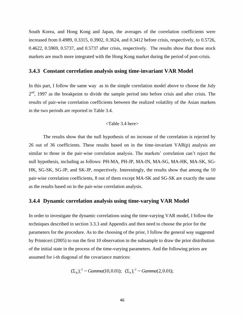
46
South Korea, and Hong Kong and Japan, the averages of the correlation coefficients were
increased from 0.4989, 0.3315, 0.3902, 0.3624, and 0.3412 before crisis, respectively, to 0.5726,
0.4622, 0.5969, 0.5737, and 0.5737 after crisis, respectively. The results show that those stock
markets are much more integrated with the Hong Kong market during the period of post-crisis.
3.4.3 Constant correlation analysis using time-invariant VAR Model
In this part, I follow the same way as in the simple correlation model above to choose the July
2nd
, 1997 as the breakpoint to divide the sample period into before crisis and after crisis. The
results of pair-wise correlation coefficients between the realized volatility of the Asian markets
in the two periods are reported in Table 3.4.
<Table 3.4 here>
The results show that the null hypothesis of no increase of the correlation is rejected by
26 out of 36 coefficients. These results based on in the time-invariant VAR(p) analysis are
similar to those in the pair-wise correlation analysis. The markets’ correlation can’t reject the
null hypothesis, including as follows: PH-MA, PH-JP, MA-IN, MA-SG, MA-HK, MA-SK, SG-
HK, SG-SK, SG-JP, and SK-JP, respectively. Interestingly, the results show that among the 10
pair-wise correlation coefficients, 8 out of them except MA-SK and SG-SK are exactly the same
as the results based on in the pair-wise correlation analysis.
3.4.4 Dynamic correlation analysis using time-varying VAR Model
In order to investigate the dynamic correlations using the time-varying VAR model, I follow the
techniques described in section 3.3.3 and Appendix and then need to choose the prior for the
parameters for the procedure. As to the choosing of the prior, I follow the general way suggested
by Primiceri (2005) to run the first 10 observation in the subsample to draw the prior distribution
of the initial state in the process of the time-varying parameters. And the following priors are
assumed for i-th diagonal of the covariance matrices:
2 2( ) ~ (10,0.01); ( ) ~ (2,0.01);B i h iGamma Gamma
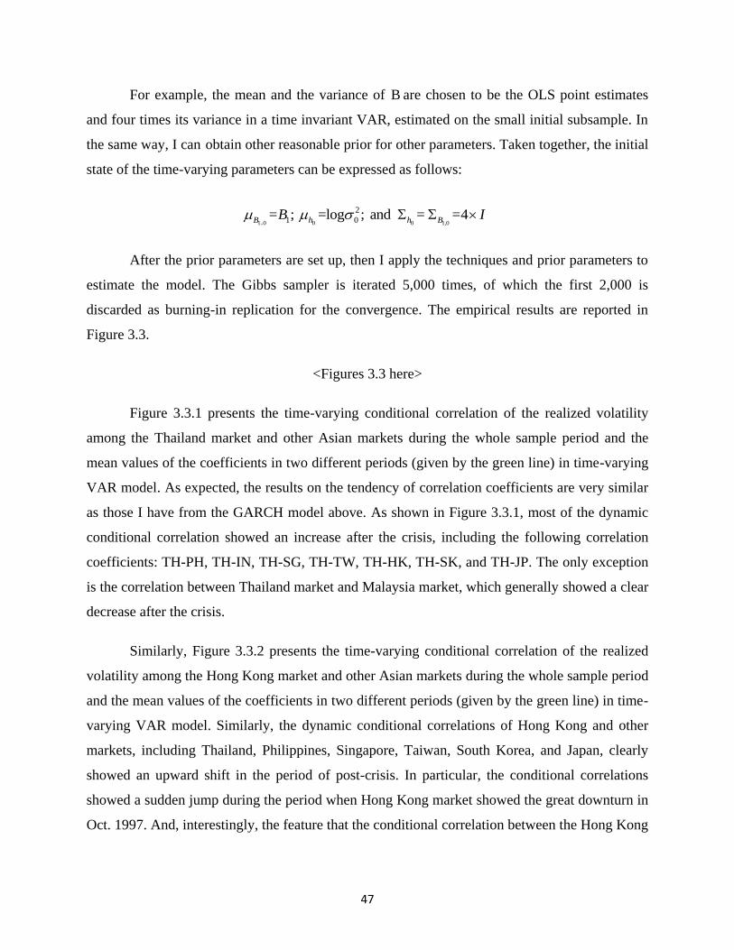
47
For example, the mean and the variance of B are chosen to be the OLS point estimates
and four times its variance in a time invariant VAR, estimated on the small initial subsample. In
the same way, I can obtain other reasonable prior for other parameters. Taken together, the initial
state of the time-varying parameters can be expressed as follows:
1 0 0 0 1,0
2
1 0= ; =log ; and = =4 B h h BB I ,
After the prior parameters are set up, then I apply the techniques and prior parameters to
estimate the model. The Gibbs sampler is iterated 5,000 times, of which the first 2,000 is
discarded as burning-in replication for the convergence. The empirical results are reported in
Figure 3.3.
<Figures 3.3 here>
Figure 3.3.1 presents the time-varying conditional correlation of the realized volatility
among the Thailand market and other Asian markets during the whole sample period and the
mean values of the coefficients in two different periods (given by the green line) in time-varying
VAR model. As expected, the results on the tendency of correlation coefficients are very similar
as those I have from the GARCH model above. As shown in Figure 3.3.1, most of the dynamic
conditional correlation showed an increase after the crisis, including the following correlation
coefficients: TH-PH, TH-IN, TH-SG, TH-TW, TH-HK, TH-SK, and TH-JP. The only exception
is the correlation between Thailand market and Malaysia market, which generally showed a clear
decrease after the crisis.
Similarly, Figure 3.3.2 presents the time-varying conditional correlation of the realized
volatility among the Hong Kong market and other Asian markets during the whole sample period
and the mean values of the coefficients in two different periods (given by the green line) in time-
varying VAR model. Similarly, the dynamic conditional correlations of Hong Kong and other
markets, including Thailand, Philippines, Singapore, Taiwan, South Korea, and Japan, clearly
showed an upward shift in the period of post-crisis. In particular, the conditional correlations
showed a sudden jump during the period when Hong Kong market showed the great downturn in
Oct. 1997. And, interestingly, the feature that the conditional correlation between the Hong Kong
48
market and the Malaysia market is generally decreased after the crisis is the same as that of
between Thailand and Malaysia shown in Figure 3.3.1.
<Table 3.6 here>
As in GARCH analysis above, here the mean values of the dynamic correlation
coefficients when using time-varying VAR model during the two different periods are reported
in Table 3.6. From Panel A in Table 3.6, it shows there is a significant increase in the degree of
the correlation between the Thailand market and other Asian markets after the crisis, except the
one between Thailand market and Malaysia market. Similarly, And, Panel B in Table 3.6 also
shows there is an obvious increase in the degree of the correlation between the Hong Kong
market and other Asian markets after the crisis, except the one between Hong Kong market and
Malaysia market.
Taken all together, the results show that the correlation, whether the constant correlation
or the dynamic conditional correlation among most Asian markets, generally showed an increase
after the crisis. In another words, there exist much more significant and stronger comovements of
the stock market volatility for most markets in this region after the crisis.
3.5 Transmission of stock market volatility
Based on the VAR analyses above, the stock market volatility in the Asian markets has stronger
impact to one another, especially after the crisis. Therefore, I further investigate how the
fluctuation of the stock market volatility in one market affects other Asian markets and thus help
understand the transmission of uncertainty from the volatility in the two periods, which can be
achieved by impulse response analysis and variance decomposition analysis.
The impulse response analysis can be used to investigate the effects of a shock to one
endogenous variable to other variables in the VAR system. It also can trace the speed and the
persistence of the shocks and then enables the examination of time structure of the transmission.
Furthermore, the analysis of variance decomposition is used to investigate the importance of the
49
innovation of other variables in the system, which reveals to what extent the innovation of the
variable can be explained by the shock from other different variables.
<Figures 3.4 and 3.5 here>
Figures 3.4 and 3.5 plot the results of impulse response analysis and Monte Carlo
simulated 95% confidence in dashed red line. Figure 3.4 plots the impulse response functions of
different Asian markets response to a one S.D. innovation of the Thailand market before crisis
and after crisis, respectively. And Figure 3.5 plots the impulse response functions of different
Asian markets response to a one S.D. innovation of the Hong Kong market before and after crisis,
respectively.
A few results stand out. First, the responses of different Asian markets to the innovation
of the Hong Kong market are generally much stronger than to the Thailand market. This finding
reflects that the Hong Kong market has a strong impact on other Asian stock markets than the
Thailand market. Secondly, the responses of realized volatility of other Asian markets to both
Hong Kong and Thailand markets are much stronger after the crisis than before crises. This
finding indicates the comovements of the Asian markets are stronger after the crisis. In particular,
the responses of Malaysia, Indonesia, and Singapore to Hong Kong and Thailand markets were
greatly increased after the crisis. Finally, the response of other Asian stock markets to Thailand
and Hong Kong greatly decreased over the time, and the innovation of realized volatility from
these two markets has a very small influence on other Asian markets after 3 periods (3 weeks).
<Table 3.7 here>
The results of the variance decomposition analysis for each period are reported in Table
3.7.23
Similarly, the analysis of variance decomposition is also divided into two periods as before.
In decomposition analysis, I examine the degree of Thailand contribution and Hong Kong
contribution to the innovation of other Asian markets and also to investigate whether the sock
market volatility linkage among the Asian markets consolidated during the financial crisis.
23 For saving the space, here I just report the decomposition of variances for the 1st, 5th and 10th Period.
50
From Table 3.7, it shows that the variance of each Asian stock market is mainly due to its
own variance instead of from the Hong Kong market or the Thailand market. The patter was as
expected. An interesting feature of the decomposition of the Asian markets is that the domestic
contribution of its own variation substantially decreases in the period after the crisis. In another
words, there is a significant upward shift on the portion of contribution from both the Thailand
and Hong Kong markets after the crisis, compared with those before the crisis.
Based on the impulse response analysis and variance decomposition analysis, I find the
strong information transmission structure across the Asian markets by using the realized
volatility index during the two periods. And such linkage structure is much stronger during the
financial crisis.
3.6 Conclusion
This study investigates the comovements among the main Asian stock markets by the channel of
studying the correlation of the realized volatility among these markets during the 1997 Asian
financial crisis. I first estimated the simple pair-wise correlation between the Asian stock markets
and then applied the DCC-GARCH model of Engel (2002) to estimate the time-varying
conditional correlation. Furthermore, I employ both time-invariant VAR(p) model and time-
varying VAR(p) model to investigate the time-invariant and time-varying conditional correlation
of the realized volatility among those markets, respectively.
Taken all of those results together, it shows that there is a significant increase of
correlation coefficients after the crisis for most of the Asian stock markets. Although the markets
dynamic correlations show some fluctuation, it provides a detailed description of the strong
comovements of the realized volatility among the Asian stock markets. These correlations are
significantly higher after the crisis, suggesting there are higher comovements between most of
the Asian stock markets. In particular, the dynamic conditional correlations of Hong Kong and
most of other Asian stock markets showed a sudden jump during the period when Hong Kong
market experienced the great downturn in October, 1997.

51
Overall, from the impulse response analysis and variance decomposition analysis, I can
conclude that the Hong Kong market has a stronger impact on other Asian stock markets through
the realized volatility than the Thailand market. The response of other Asian stock markets to the
innovation of the Hong Kong and Thailand markets were greatly increased after the crisis. And
in the variance decomposition analysis, I can also find that the contribution to the variance of
other Asian markets from the Hong Kong market and Thailand market showed an increase after
the crisis.
And one more interesting feature of the correlations is the relationship between Malaysia
market and other Asian stock markets. It shows the isolationist responses of the Malaysian
authorities to the crisis appear to have contributed to a lessening in Malaysia’s linkage within
other Asian stock markets.
52
Chapter 4 On International Stock Market
Comovement and Macroeconomic Fundamentals
4.1 Introduction
Globalization has accelerated in the past two decade. There are rapid increases in both cross-
country financial flows and international trade in goods and services. Nowadays almost every
single country's macroeconomic performance and financial market are no longer immune to the
development in other parts of the world. These increased financial and trade linkages across
countries have stimulated a large literature on international business cycle comovements such as
Kose et al. (2008) as well as on measuring financial market integration such as Pukthuanthong
and Roll (2009) and Carrieri et al. (2007) among many others.
In this chapter, I study jointly the comovements of stock market prices as well as other
major macroeconomic variables from a large group of countries. I am particularly interested in
the link between stock market movements and the underlying macroeconomic fundamentals in a
perhaps partially integrated global economy. International integration can fundamentally alter the
nature of risks faced by investors and, therefore, stock market dynamics. For example, in an
isolated economy, the market risk of that country is a priced systematic risk. In a perfectly
integrated world economy, however, only the exposure to the global stock market risk will be
priced. Similarly, the underlying macroeconomic risks that drive much of the stock market
movements will also be different. In an isolated economy, the macroeconomic fluctuations of
that country are perhaps the most important driving force of its stock market movement. In an
integrated world economy, an individual country's stock market will probably respond more to
the world business cycle shocks than to its own macroeconomic fluctuations. Indeed, using a
dynamic factor model estimated on monthly data on a group of 34 countries from 1995 to 2009
via Bayesian methods, I find that the global factors account for a significant portion of an
individual country's stock market volatility as well as its macroeconomic fluctuations. The global
macroeconomic shocks have strong effects on the price movement of the global stock market as
53
well as that of an individual market, and a country's exposure to the global stock market risk can
be largely explained by that country's exposure to the global macroeconomic risks.
This essay is related to the two strands of literatures. One strand is the empirical study of
international stock market integration. In the literature, there are a wide variety of studies of
market integration through measure of markets’ correlation or common factor (Forbes and
Figobon, 2002; Hamao et al, 1990; Brooks and Del Negro, 2005; among others). Instead of
focusing only on markets, some recent studies have further explored the market integration
through correlation analysis by incorporating part of macroeconomic fundamentals. For example,
Dumas et al. (2003) propose a framework that contains a model for output and an intertemporal
financial model for the stock market. Their results indicate that under the hypothesis of
integrated financial markets, the international stock market correlations can be matched to the
levels of actual stock market linkages. Carrieri et al. (2007) employ GARCH model to
investigate the evolution of market integration in eight emerging countries. They find that the
correlations of national index returns with the world are significantly lower than estimated
integration indices on the basis of real activity.24
My focus on market integration differentiates my work from other previous studies that
only examine the market’s correlation or common factor. Pukthuanthong and Roll (2009)
illustrate that as in previous studies, the correlation analysis of measuring the broad cross-
markets integration poorly mimics other measures of integration. They further discover that there
has been increased market integration for most countries over the years, but this cannot be
indicated by the simple correlation analysis. Thus, they derive a new integration measure based
on the explanatory power of a multi-factor model to investigate the global integration.25 Similarly,
Bekaert et al. (2009) employ risk-based factor models to investigate country-industry and
country-style portfolios. Their results provide the evidence of international stock return
comovements and also show that the factor model can better capture the covariance structure
24 A similar study by Chambet and Gibson (2008) utilized the GARCH-M model to investigate the relationship
between the level of financial integration in emerging markets and the indicator of country’s trade openness and
concentration. They find that countries with an undiversified trade structure have more integrated financial markets.
25 Similar studies of market integration that employ the factor model have also been conducted by Eiling and
Gerard (2007) and Brooks and Del Negro (2005).
54
more successfully than the previous popular Heston-Rouwenhorst model (Heston-Rouwenhorst,
1994). However, these studies of common factor usually only focus on markets without
incorporating the underlying macroeconomic fundamentals. In particular, the macroeconomic
variables will especially important as they will most likely have strong effects on the price
movement of stock markets and thus, may also affect the evolution of their financial market
integration. Therefore, I argue that it is more conceivable and subsequently imperative to
incorporate the underlying macroeconomic fundamentals when investigating market integration.
This essay is also related to the recent literature on the comovements of international
business cycles. Over the recent decades, there are a wide variety of studies of the
macroeconomic activity comovements via investigation of the common factor. In recent
prominent examples, including Kose et al. (2003, 2008), Canova et al. (2007), Crucini et al.
(2008), and Artis and Okubo (2009), among others, dynamic factor model is used to investigate
the common shocks to macroeconomic fundamentals across countries. In this vein, because
global factor is an important tool to investigate the common macroeconomic shocks across
counties and because it can be also employed to measure the underlying global macroeconomic
risks for the global stock market, it is therefore necessary for us to briefly review the studies in
the literature of global factor of macroeconomic fundamentals.
The existing research on global macroeconomic developments is primarily focused on the
common movements of industrial output and productivity across various countries.26 Gregory et
al. (1997) employ a dynamic factor model to identify the common factor of macroeconomic
aggregates fluctuations in G7 countries.27 Moreover, research conducted by Stockman (1988)
and Norrbin and Schlagenhauf (1996) find that a substantial fraction of the variation in industrial
production is due to global and country-specific components in main industrialized economies.
26 For additional details on the summary of recent evidence on the evolution of dynamic international business
cycles, see Stock and Watson (2005).
27 Doyle and Faust (2005), Kose et al. (2005) and Stock and Waston (2003, 2005), also investigated the fluctuation
among G7 economies. Each of these studies found an increased importance of common shocks as a driving force of
output fluctuation across countries.
55
Furthermore, it should be noted that the inflation fluctuations across countries are similar to the
regularities of real business activity. Numerous recent studies focusing on the investigation of
global inflation movements provide the evidence of the so-called “worldwide great inflation.”
For example, Ciccarelli and Mojon (2010) use a dynamic factor model to measure the inflations
and subsequently found that the inflations in industrialized countries are largely a global
phenomenon. Their results showed that the common factor accounts for a significant fraction of
the variances in 22 OECD countries, which are similar to the results of Neely and Rapach
(2009).28
Finally, some studies have explored global monetary markets and have further
investigated to what extent monetary policies across countries move together (Henriksen et al.,
2009). One of the main purposes of this study is to examine whether these changes, such as
monetary integration in Europe, have impacted monetary policies across countries. A variety of
channels may potentially affect monetary policies across countries. For example, in the European
Economic and Monetary Union, the member countries will most likely influence each other to
adopt similar monetary policies. The global macroeconomic shocks may also potentially
influence the common movement of monetary policies. All these factors could impact the central
banks in their response to common shocks, and thus result in the comovements of their monetary
policies (Henriksen et al., 2009). In summary, a variety of macroeconomic shocks, as well as the
economic and political pressures for central banks to respond similarly to the shocks, is capable
of driving the comovements of monetary policies across countries.
Therefore, it can be argued that these global factors can be used to measure the common
macroeconomic fundamental shocks in the world. Furthermore, these global factors can also be
employed to characterize common global macroeconomic risks. For example, global factor,
which measures the common shock to industrial productivity across countries in the world, can
be utilized as a proxy for global macroeconomic risk from economic activity.
28 Neely and Rapach (2009) employ the Bayesian dynamic factor model to investigate the international
comovments in inflation rates for a larger sample, which include industrialized and emerging countries. The findings
of other studies on the dynamic factor on global inflation (Hakkio, 2009; Mumtaz and Surico, 2008) are similar to
the findings that comovements of global inflation exist across countries (Ciccarelli and Mojon, 2002)
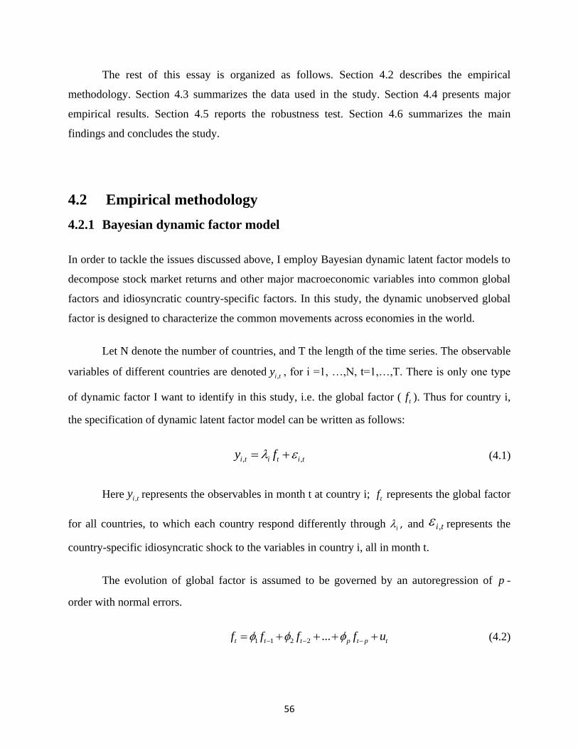
56
The rest of this essay is organized as follows. Section 4.2 describes the empirical
methodology. Section 4.3 summarizes the data used in the study. Section 4.4 presents major
empirical results. Section 4.5 reports the robustness test. Section 4.6 summarizes the main
findings and concludes the study.
4.2 Empirical methodology
4.2.1 Bayesian dynamic factor model
In order to tackle the issues discussed above, I employ Bayesian dynamic latent factor models to
decompose stock market returns and other major macroeconomic variables into common global
factors and idiosyncratic country-specific factors. In this study, the dynamic unobserved global
factor is designed to characterize the common movements across economies in the world.
Let N denote the number of countries, and T the length of the time series. The observable
variables of different countries are denoted ,i ty , for i =1, …,N, t=1,…,T. There is only one type
of dynamic factor I want to identify in this study, i.e. the global factor ( tf ). Thus for country i,
the specification of dynamic latent factor model can be written as follows:
, , i t i t i ty f (4.1)
Here ,i ty represents the observables in month t at country i; tf represents the global factor
for all countries, to which each country respond differently through i , and ,i t represents the
country-specific idiosyncratic shock to the variables in country i, all in month t.
The evolution of global factor is assumed to be governed by an autoregression of p -
order with normal errors.
1 1 2 2 ...t t t p t p tf f f f u
(4.2)
57
Where 2 ; t t fEu u and 0;t t sEu u for all s≠0.
Similarly, the country-specific idiosyncratic terms ,i t , they are also assumed to be
normally distributed, following p -order Autoregression, i.e.,
, ,1 , 1 ,2 , 2 , , ,...i t i i t i i t i p i p i tu (4.3)
Where 2
, ,i t j t s iEu u for i = j and s = 0, 0 otherwise.
Here all the corresponding innovations, tu and ,i tu , i=1,…,N, are also assumed to be zero
mean, contemporaneously uncorrelated normal random variables.
There are two related identification problems in the model (4.1) - (4.3) should be noted
here. Neither the signs nor the scales of the factors and the factor coefficients are identified
separately. Therefore, first of all, the signs are identified by requiring one of the coefficients for
the each factor to be positive. In particular, I handle this by require the factor coefficients for the
global factor are positive. Secondly, the scales are identified by following Sargent and Sims
(1977) and Stock and Watson (1989, 1993) to assume that each variance of tu is equal to a
constant. Here I follow the convention by normalizing the variance of tu to be unity.
Thus, the comovements across countries can be mediated by the common global factor.
Through this factor analysis, we are able to measure the impact of both global factor and
country-specific factor on the volatility of each country’s stock market as well as on its
macroeconomic fluctuations. Since the dynamic factor is not observable, analysis of the systems
could not be as straightforward as in the general econometrics regressions. In the conventional
method, a state space model can be estimated by using the Kalman filter to derive sample log
likelihood conditional on the unknown parameters. In the likelihood function, it is maximized
numerically with respect to the parameters until convergence, in order to extract all these
parameters. However, in this essay, with a large number of factors in the equation, the Kalman
filter can become computationally rather burdensome. Therefore, in this study I use the method
of Markov Chain Monte Carlo (MCMC) to estimate the posterior distribution of unobserved
58
factors and the parameters, which has been widely used by Chib and Greenberg (1996), and
Aguilar and West (2000), among others.
In this essay, I take advantage of Bayesian Gibbs sampling procedure allowing us to
estimate a large state space system with a large number of unknown factors and parameters. In
Bayesian econometrics, unknown parameters are usually treated as random variables followed by
underlying stochastic distribution. Here the prior on all the factor distribution is N(0,1). Given
appropriate prior distributions and arbitrary starting values for the model’s parameters, Gibbs-
sampling can be implemented by the successive iteration of the following three steps: Firstly, I
generate the posterior distribution of the factors conditional on the data and prior parameters of
the model. Secondly, I generate the parameters from the conditional distribution conditional
on the dynamic factors. Thirdly, I generate i , i , 2
i based on the equations (4.1)-(4.3)
conditional on the data and dynamic factors for country i. Steps 2 and 3 are carried out by using
independent Normal-Gamma priors. All the steps are iterated S times, in which the first S1 draws
are discarded as burning-in replications to remove the effect of initial values. Under the
regularity conditions satisfied here, I can produce the convergence of Markov Chains and
generate the unobserved factors and unknown parameters.
4.2.2 Vector Autoregression (VAR) Model
By employing Bayesian dynamic latent factor model mentioned in above section 4.2.1, I can
estimate the dynamic global factors for stock market returns as well as for different
macroeconomic variables. These global factors are designed to measure the common movements
across countries, and can therefore be used as proxies for the global stock market comovements
and global macroeconomic shocks. I argue that the linkage among global stock markets and a set
of main macroeconomic variables in a global framework can be realized through investigating
the relationship of these global factors. Therefore, the objective can be achieved by estimating a
VAR system composed of global macroeconomic shocks and global factor which measure the
comovements of global stock markets.
59
The VAR analysis provides us broad information of the relationship of endogenous
variables. For a set of n time series variables1 2 ,( , ..., ) 't t t nty y y y , the VAR model with p-order
can be written as:
0
1
p
t l t l t
l
y A A y
(4.5)
Where p is the lag length; ty is a (nx1) column vector of variables; 0A is the constant
vector; lA ’s are (nxn) coefficient matrices and 1 2( , ,..., ) 't t t nt is an unobservable i.i.d. zero
mean error term, i.e., 2 2( ) 0, ( ) ,t tE E and ( , ) 0, for t sE t s .
In this study, VAR analysis is employed to investigate the relationship between
macroeconomic factors and stock market. The lag length in the model is chosen on the basis of
the AIC criterion. Variance decomposition and impulse response analyses are also conducted to
measure how and to what extent different endogenous variables impact one another in the VAR
system. With this in mind, it is helpful to trace the relationships of endogenous variables in the
system. Furthermore, it is beneficial to take a closer look at how the change in a variable is due
to its own shocks, as well as to the shocks from other variables.
4.3 Data and descriptive statistics
4.3.1 Data of stock markets
The dataset consists of monthly national stock market indices from January 1995 to December
2009 in a group of 34 economies.29
The dataset is chosen because it can help us to maximize the
29 The countries included in this study are mainly from Asia-Pacific Economic Cooperation (APEC) and European
Union (EU). This is because a wide variety of theoretical and empirical studies provide the evidences of the
increasing economic and financial integrations in these regions. The EU was established in November, 1993.
Although APEC was established in 1989, economic progress of free and open trade and investment in the Asia-
Pacific region was not achieved until a 1994 meeting in Bogor, Indonesia, when the so-called Bogor Goals were met.
60
number of countries in this study, as not all countries have the data of stock market and
macroeconomic variables over a longer period. In particular, the data of short-term interest rates
is not available among several countries before 1993. Furthermore, considering the limitation of
the availability of macroeconomic variables, monthly data is the best observation of stock market
fluctuations. The monthly data is more successful at capturing the fluctuations of stock market
than the quarterly and annual ones as stock markets are frequently fluctuated. Finally, since this
study focuses on the economies in APEC and EU regions, it better allows us to study the global
factors and international comovements because of the increasing globalization and financial
integration in these regions since the mid-1990s.
Monthly data for stock markets consists of the closed price indices expressed in local
currency. The data are obtained from Datastream International. I follow the conventional method
to calculate the monthly returns of stock market for country i at time t, i.e.:
, , , 1100*(log log )i t i t i tR p p (4.5)
Where i refers to stock market, t to month; ,i tR represents the stock market returns; ,i tp is
the stock market price index in local currency, all in month t for country i. Instead of choosing
the price index ,i tp in a fixed date as the monthly data for stock market, here I use the average of
price index in order to eliminate the excess volatilities of price. The price benchmark is to
calculate the average price indices in all trading dates in each entire month.
Before estimation, one concern with the procedures is whether or not the larger stock
markets have more power in affecting the global factors solely because of their big market sizes.
In this study, I use the stock market returns, which are actually the changing rate of stock price
index, so the size of stock market has no direct impact on the research of stock market
commovments. I adhere to this in the study by ensuring that all the series have equal weight
irrespective of their relative market sizes in the world.
4.3.2 Data of macroeconomic fundamentals

61
In this study, the selection of macroeconomic variables is based on theoretical propositions and
existing evidence in the literature. I appeal to economic and financial theories and previous
empirical evidences to select the potential macroeconomic variables. As financial theories and
studies have addressed, macroeconomic factors, such as output, inflation, and money policy are
proposed variables.
Previous research has identified the relationship between stock market and real business
activity. For one, many studies find that real economic activity is the most important factor
influencing the fluctuation of stock market (Fama, 1990; Chen et al., 1986; Schwert, 1990; and
Lee, 1992, among others). Thus, industrial production is included as a proxy for real economic
activity and macroeconomic development factor in this study.
Secondly, changing inflation may also affect stock market through the channel of
changing the discount rates. A higher inflation would increase the discount rate and then lower
stock market returns. Fluctuations and uncertainty about fundamentals are also potential factors
affecting the stock market. For example, inflation and earnings uncertainty are identified as the
sources of the fluctuation of stock market returns (Lee, 1992; and Boudoukh and Richardson,
1993). Therefore, I also consider the measures of macroeconomic shocks to account for the
uncertainty of inflation factor. Specifically, I construct a proxy for monthly year-to-year inflation
on the basis of the Consumer Price Index (CPI).
Finally, money policies may affect stock market through various channels. Take for
instance the money supply. An increase in money supply would lead to inflation and thus
negatively affect stock market returns. On the other hand, an increase in money supply may
lower the interest rates which could in turn bring firms more investment opportunities and
decrease discount rates. According to the so-called “fisher effect” expected nominal rates of
interest on financial assets should move one-to-one with expected inflation. Moreover, changes
in both short term and long term interest rates are expected to impact the discount rate through
their effect on nominal risk-free rate (Mukherjee and Naka, 1995; and Lee, 1992). Interest rates
are also expected to be directly related to stock market through either inflationary or discount
62
factor effects. Therefore, I use short-term interest rate as a proxy for monetary policy in this
analysis.30
In sum, I construct the following macroeconomic variables in this study: industrial
production growth rate (IP), inflation rate (Inflation), and short-term interest rate (Interest).31
Logarithmic differences are taken to measure the changing rates of the first two variables. I
follow the approach suggested by James et al. (1985) to measure these macroeconomic variables,
i.e., year-to-year industrial production growth and CPI changing rate which, by construction,
have no seasonal patterns. For consistency with the measurement of the macroeconomic
variables, stock market returns are multiplied by 12 to make them annual. Table 4.1 presents the
description of all variables in this study: their symbols, calculation methods, and data sources.
<Tables 4.1 and 4.2 here>
The summary statistics of monthly stock market returns across countries are presented in
Table 4.2.32 As expected, real returns of emerging markets are, on average, smaller but more
volatile than those of developed markets. Interestingly, real returns for most markets are positive,
while nominal returns are all positive with exception of Japan and Thailand. The most likely
reasons for the negative returns in these two countries is Thailand’s substantial economic
downturn during following 1997 Asian crises and Japan’s persistent economic depression since
the early 1990s.
4.4 Empirical results
30 Some alternative measure of monetary policies such as money supply M2 is also supposed to be consider in the
model. However, the monthly data is not available for a large group of countries in the sample because of the
limitation of data resources.
31 Money market interest rates are used as the substitute of short-term interest rates because of unavailability of that
data in a few countries.
32 For saving space, the descriptive statistics for macroeconomic variables across countries are not reported here.
63
In the implementation of this study, for simplicity and for saving the degree of freedom, I assume
that both the lengths of idiosyncratic terms and factor autoregressive polynomials are 2. It should
be noted that the model, in principle, works well for the general case of AR (p) autoregression.
Gibbs-sampling can be implemented by successive iteration of the three steps discussed in
Section 4.2, given appropriate prior distributions and arbitrary starting values for the model’s
parameters. The simulation has been iterated in different lengths ranging from 5,000 to 30,000.
The Gibbs sampler converges to the same results if the iteration is greater than 5,000. In this
study, I report the results of the Gibbs sampler with iteration 25,000 times, in which the first
5000 draws are discarded as burning-in replications to remove the effect of initial values.
4.4.1 International stock market Comovements and global macroeconomic
factors
4.4.1.1 Dynamic global factors
<Figure 4.1 here>
Figures 4.1.1 through 4.1.5 present the median of the posterior distribution of global factors for
industrial production, inflation rate, interest rates and stock market real and nominal returns
across countries, respectively. First of all, Figure 4.1.1 presents the median of the posterior
distribution of global factor for industrial production. The fluctuations in the factor well describe
the major global economic activities in the recent 15 years: the recession from mid-1997,
associated with the Asian financial crisis; and the downturn of early 2000, associated with the IT
bubble that began in the United States early 2000, and also associated with the impact from the
September 11 attacks in 2001. In particular, the deepest trough in the figure reflects the recent
economic recession from 2007 to 2009.
The common inflation movements across countries are reported in Figure 4.1.2. The
dynamics and trends in the global inflation really reflect world-wide inflation events over the
past 15 years. The global factor of inflation generates the fluctuation around zero except for two
troughs, suggesting that the world showed small waves of inflation and deflation in most periods.
64
However, there are two exceptions. The first is from 1995 until 1999. This time frame is
associated with the decline of economy and tight monetary policies and financial crises during
these periods. The second trough is associated with economic recession in recent two years from
2008 until 2009. Here, the findings are very consistent with those of Ciccarelli and Mojon
(2010).33
Furthermore, Figure 4.1.3 presents the global impacts on the monetary policy through the
channel of interest rates. The global monetary factor displays a strong downward trend starting in
mid-1995. The first trough is reached in mid-1999. After that, it follows an upward trend for one
and half year, and then continues to display a strong downward trend from late 2000 to 2005.
Interestingly, the significant fluctuations as characterized by negative values reflect the
decreasing interest rates of the time.
Finally, Figures 4.1.4 and 4.1.5 present the median of posterior distribution of global
factors for stock market real and nominal returns across economies in the world. Similarly, as
shown in the figures, the dynamics of global factor vividly illustrate the major global stock
market shocks over the last 15 years. Among them, there are several significant troughs that
clearly characterize the major global market shocks. For example, the Asian Financial Crisis,
which started in July 1997, raised the fears of a worldwide stock markets meltdown due to
financial contagion. Additionally, most stock markets in industrialized economies were greatly
affected when the "IT bubble" started in the early 2000s in the United States. The stock market
was then negatively impacted in 2001 following the September 11 attacks. Subsequently, after
recovering from lows reached during that time period, the stock market downturn of 2002
dramatically impacted the economies of a large group of countries, including the United States,
Canada, Asia, and Europe. Most recently, the 2007-2009 markets crash impacted economies
across the globe, making it the disastrous financial crises over the recent decades. The steepest
drops of factor dynamics in this figure are consistent with the disastrous market downturn of
2008 cross countries in the world.
33 Ciccarelli and Mojon (2010) use quarterly data to study the global inflations among main OECD countries
between 1960:1 and 2008:2 by employing dynamic factor model. My findings relating to the pattern of global
inflation is similar to their findings during the common period from 1995 to 2007.
65
4.4.1.2 Variance decomposition analysis of dynamic factors
To measure relative contribution of global factor to the variation of macroeconomic variables
and stock market returns, I estimate the share of the variance of each variable due to different
factors. I decompose the variance of each variable into the global factor and country
idiosyncratic component. Since these two factors are orthogonal, the variance of ,i ty for country i
can be written as:
2
, ,var( ) var( ) var( )i t i t i ty f (4.6)
Based on equation (4.6), I estimate the share of the variance of each variable attributable
to these two factors. Therefore, I can investigate to what extent the global and country-specific
idiosyncratic factors affect the variation of each variable. They are expressed as follows:
2
,
var( );
var( )
world i ti
i t
fS
y
,
,
var( );
var( )
i t
i
i t
Sy
(4.7)
Where i=1,…, N for country i; and world
iS and iS represent the shares of global factor and
country idiosyncratic component for the variation of each variable in country i, respectively.
<Tables 4.3 and 4.4 here>
Table 4.3 presents the variance shares of national series attributable to the global factor
for macroeconomic fundamentals, as well as stock market returns across countries. Similarly,
Table 4.4 presents the average of variance shares for both pooled countries and developed
countries, respectively.
First of all, the global factor, on average, accounts for approximately 50% of the
fluctuations of countries’ industrial output. Among them, the global factor can explain more than
50% of the fluctuations in 13 out of 33 countries, particularly in developed countries such as
66
75.91% in Austria, 76.25% in Japan, 79.17% in Belgium, 79.68% in the USA, 83.69% in
Sweden, 84.62% in Spain, 86.25% in Germany, 86.26% in Finland, 86.95% in France, 86.97% in
the United Kingdom, and 88.03% in Italy. Furthermore, in terms of the results of the average of
variance shares attributable to global factor in Table 4.4, I find that the global factor can explain
around 56.12% of the fluctuations of industrial output in developed countries.
Secondly, the global factor, on average, can explain more than one-third of country’s
inflation fluctuations. Among 16 out of 34 countries, the global factor accounts for more than
40% of the inflation fluctuations. Following the comparison analysis above, I find that the global
factor, on average, explains around 43.42% of the inflation fluctuations in developed countries.
However, I find no evidence that the global factor has significant effects on the individual
country’s inflation fluctuations in South America. For example, the global factor only explains a
very small portion of national inflation fluctuations in some countries, such as 0.60% in
Argentina, 0.66% in Mexico, 1.53% in Brazil, and 4.10% in Peru. In contrast, a high degree of
inflation rate comovements can be found across European countries for the implementation of
monetary union in this region. In Europe, the global factor accounts for a large portion of
individual country’s inflation fluctuations, such as 62.10% in Germany, 67.69% in Belgium,
67.92% in France, 71.60% in Austria, 76.19% in Switzerland, and 81.10% in Spain.
Thirdly, there exist strong comovements of interest rates across countries, which are
consistent with the findings in recent studies (see Henriksen et al., 2009; Diebold et al., 2008;
and Byrne et al., 2010, among others). Generally, the global factor accounts for a substantial
fraction of the interest rate fluctuations in developed countries, whereas a very small in some
emerging countries. For example, the global factor only explains 0.01% of interest rates
fluctuations in Argentina and 3.78% in Indonesia. This indicates that the fluctuations of interest
rates in these countries are mainly driven by their own characteristics, instead of by the global
factor. Interestingly, as shown from column four in Table 4.3, the global factor accounts for
around 91.76% of the Euro fluctuations. This demonstrates that the Euro currency is strongly co-
moved with the global monetary market.
Finally, columns five and six in Table 4.3 present the variance shares attributable to the
global factors for each individual country’s stock market real returns as well as nominal returns.
67
The results show that the degree of the comovements of global stock markets is much higher
than that among macroeconomic fundamentals discussed above, for the global factor has a more
explanatory power of accounting for the fluctuations, whether averaging the countries as a whole
or individually. For example, the global factor can, on average, account for around 56 percent of
the country’s stock market volatility. In particular, the global factor, on average, explains around
66 percent of the stock market volatility in the developed countries. In terms of the results for
each individual country, the global factor can explain more than 50% of the stock market
volatility in 19 out of 34 markets in my sample. In particular, the global factor accounts for a
significantly large portion of the variations of stock market real returns in developed markets: for
example 81.11% in the United Kingdom, 81.24% in the United States, 83.68% in Germany,
87.02% in France, and 90.82% in Netherlands. All these indicate that there exists a high degree
of stock market comovements across economies, especially in developed markets.
4.4.2 Measuring the effects of global macroeconomic factors
As argued in the above section, here I will employ the VAR analysis to measure the effects of
global macroeconomic factors on the price movement of the global stock markets as well as that
of each individual stock market. There are two main purposes in this subsection: the first aims to
investigate how the global macroeconomic shocks have effects on the movements of global stock
markets in a global perspective; the second aims to investigate to what extent each individual
country’s stock market will respond to the global macroeconomic shocks and its own
macroeconomic fluctuations.
4.4.2.1 Empirical results of VAR analysis
To address the first issue, I employ the VAR analysis to answer it. Before I begin this analysis, I
first employ a preliminary Pearson correlation analysis to examine the relationship between
global macroeconomic factors and global stock market movements. The correlation results are
reported in Table 4.5. Interestingly, the results show that industrial production is weakly but
positively correlated with both real and nominal stock market returns. However, the inflation is
68
significantly and negatively correlated with both real and nominal stock market returns, and the
interest rate is also negatively correlated with them, but weakly.
<Table 4.5 here>
These findings together make us even more curious about the interactions among global
macroeconomic factors and global stock market movements. Therefore, I precede a VAR
analysis to have a detailed examination of their relationship. The presence of the common shocks
and comovements among the variables implies that the ordering is important. Based on the
literature and the following models of Balvers et al. (1990), Canova and De Nocolo (1995) and
Cochrane (1991), it is reasonable that industrial production factor is placed first, followed by
inflation factor, interest rate factor.
<Table 4.6 here>
In this analysis, my main intent aims to understand how the main global macroeconomic
factors affect international stock market movements. Therefore, I present only the results of the
effects of global macroeconomic factors, represented by industrial production, inflation, and
interest rates, on stock markets from the VAR analysis in Table 4.6. The results show that
international stock market movements is positively correlated with industrial production factor,
which is consistent with those findings in a variety of previous studies that there is a positive
effect of industrial output on stock market returns (see Chen et al., 1986; Fama, 1990; Canova
and De Nicolo, 1995; and Lamont, 2000, among others), for the innovation of industrial
production can be linked to the changing expectations of future cash flow (Balvers et al., 1990).
Furthermore, the results show that global inflation has negative effects on international stock
market movements. The finding demonstrates that the inflation directly influence stock market
returns (negatively), which is also consistent with previous studies (see Chen et al., 1986; Fama,
1990; and Boudoukh and Richardson, 1993, among others). Inflation can affect the discount rate,
thus reducing the present value of future corporate cash flows. The rising inflation also initially
negatively affect corporate income due to the immediate rising costs and adjusting output prices,
causing the profits decline and therefore, the stock prices decline. Therefore, the global inflation
has negative impact on the international stock markets. Finally, in terms of monetary policy,
results show that stock market movements are negatively related with global interest rate factor.
69
The negative response is consistent with the findings in previous studies (see Bulmash and
Trivoli, 1991; and Mukherjee and Naka, 1995), as interest rates can affect stock market
movements through two channels: endogenous response to macroeconomic activity and through
discount rate. On the one hand, interest rate innovation could be the driving force in determining
industrial production (due to changes in investment), which might affect stock market returns as
argued above. On the other hand, interest rate innovations could also directly influence stock
market returns through the channel of discount rate since a change of discount rate can affect
present value of future cash flows and then the cumulative sum of income and returns.
To further understand the role regarding how the global macroeconomic fundamental
shocks influence the volatility of global stock markets, variance decomposition is also conducted
on the basis of the VAR analysis above and hence can address the effects of global
macroeconomic fundamentals on the fluctuations of global stock markets.
<Table 4.7 here>
Table 4.7 presents the results of variance decompositions after one, three, six, and twelve
months for the explanatory variables. Global market own movements are the major role in
effecting the global stock market volatility, explaining from 86.71%, 80.09%, 71.99%, and
66.09% of the variance after one, three, six, and twelve months, respectively. However, global
macroeconomic factors, represented by global output factor, global inflation factor, and global
interest factor, explain 13.29%, 19.91%, 28.01%, and 33.91% of the variance after one, three, six,
and twelve months, respectively. Among global macroeconomic fundamentals, the global
interest factor explains the largest part of the variance of global stock markets after one month,
taking 7.64%. However, the global inflation factor plays the major role in affecting the variation
after twelve months, explaining 16.66% of the forecast variance, followed by the global output
factor with 9.46% and the global interest factor with 7.79%.
4.4.2.2 Individual country’s stock market and global macroeconomic factors
To address the second question regarding how an individual country’s stock market will respond
to the global macroeconomic shocks and its own macroeconomic fluctuations, I conduct the
70
VAR analyses in two different cases for each country in my sample: the first is the VAR system
consisting of the country’s own macroeconomic fluctuations, global macroeconomic factors, and
stock market returns; the second is the one consisting only of its own macroeconomic
fluctuations and stock market returns without including global macroeconomic factors.
<Table 4.9 here>
Table 4.9 presents the 2R statistics in the VAR analysis for each country’s real stock
market returns in both cases.34
The 2R statistic is a measure that can give some information about
the goodness of fit of a model. I find that in most countries the 2R values are significantly
increased in the VAR analyses consisting of the global macroeconomic factors. On average, the
results show that there is an increase of more than 50 percent in the 2R values for both pooled
and developed markets. In particular, the 2R statistics are greatly increased in developed markets;
for example from 0.240 to 0.411 in Hong Kong, from 0.111 to 0.318 in Japan, from 0.081 to
0.191 in the United Kingdom, and from 0.280 to 0.440 in the USA. The 2R statistics reported in
Table 4.9 imply that a standard F-test would reject the zero coefficients on the global
macroeconomic factors for many countries in these regressions. Therefore, I argue that it would
be more reliable to include the global macroeconomic shocks when investigating the relationship
between macroeconomic fundamentals and an individual country’s stock market movements.
<Table 4.10 here>
Therefore, variance decomposition on the basis of the VAR analysis in the first case is
conducted to have a further look at how an individual country’s stock market volatility is
associated with the global macroeconomic shocks and its own macroeconomic fluctuations.
Table 4.10 presents the results of variance decompositions after twelve months on the basis of
the VAR analysis. The results in Table 4.10 show that global macroeconomic factors,
represented by global industrial production, global inflation, and global interest factor, on
average, explain 20.59% of the individual country’s stock market fluctuations after twelve
34 For saving the space, the results of VAR analysis and variance decompositions for all these individual countries
are not reported here. The detail results can be available upon request.
71
months. In most developed economies, the global macroeconomic factors account for a larger
portion of the country’s stock market fluctuations than their own macroeconomic fluctuations do,
particularly in prominent countries such as Australia, Canada, Japan, Portugal, Switzerland, and
the USA. However, in several emerging economies, the stock market movements are driven
more by their own macroeconomic fluctuations than by global macroeconomic factors.
All these findings indicate that the global macroeconomic shocks have strong effects on
the movement of global stock markets as well as that of individual stock markets. In most
developed economies, the global macroeconomic shocks accounts for a larger part of the forecast
variances of individual stock markets than their own macroeconomic shocks. These results
suggest that in an increasingly integrated global economy, we have to look beyond national
borders in order to correctly identify and measure the underlying macroeconomic risks in
financial markets. We may miss important sources of macroeconomic risks if we only use
domestic macroeconomic variables in our empirical studies.
4.4.3 Does market integration reflect economic integration?
In the previous section, the results show that there are some differences in financial-market
integration across developed and emerging markets. The findings also indicate that the global
macroeconomic shocks play different roles in driving the price movements of stock markets in
different economies. Thus, I am curious whether and to what extent market integration is
associated with economic integration in the world. In the literature, Bekart and Harvey (1995)
and Bhattacharya and Daouk (2002) provide evidence that certain variables might be linked to
the information of the dynamics of integration. Carrieri et al. (2007) also indicate that financial
market development and financial linearization policies play important roles in the integration of
emerging markets. However, these examples in the literature are nonetheless vague as there are
no comprehensive theories and empirical studies that specifically address this issue.
As shown above, the variance shares of global factor can be used to measure the degrees
of integration of financial markets across countries as well as those of global macroeconomic
fundamentals, represented by industrial production, inflation, and interest rate. To address this, I
72
investigate the relationship between these variance shares of global factors. Therefore, it is
possible to explore whether and to what extent the market integration reflects economic
integration.
<Table 4.8 here>
Column one in Table 4.8 presents the “impact” coefficients of real returns for different
countries. The result presents the differences of each individual country’s exposure to the global
stock market risk. The coefficients range from 0.793 to 2.193 in the sample, indicating that the
global factor plays different roles the fluctuation of each individual stock market.
To better understand the evolution of market integration and the corresponding exposure
to global market risks, I use the variance shares of global factor for the real returns ,Re
world
i alS
estimated above as the dependent variable. In this analysis, I estimate the regression of ,Re
world
i alS on
the variance shares of global macroeconomic factors for both pooled and developed countries.
The equation is written as:
,Re 0 1 , 2 , 3 ,
world world world world
i al i IP i Inflation i Interest iS S S S (4.8)
<Table 4.11 here>
In this analysis, it can help us investigate to what extent market integration is associated
with the macroeconomic fundamentals integration in the world. Table 4.11 presents the estimates
and the 2R statistics of the regression for 32 pooled and 24 developed economies, respectively.35
There is no significant difference between these two samples. In both cases, the estimated
coefficients are large and positive, indicating that the degree of market integration is associated
with the degree of the integration of global macroeconomic fundamentals. Among the three
coefficients, only the estimated coefficient of global inflation is significant, but not for the other
two.
35 Countries of Philippines and Taiwan are not included here since the data of industrial production for Philippines
and interest rates for Taiwan are not available.
73
<Figure 4.2 here>
To better understand the goodness of the fit of the model, in Figure 4.2 I plot the
relationships between the actual values and the fitted values for both pooled countries and
developed countries. The actual values are from the variation shares of global factor for stock
market real returns, and the fitted values are estimated on the basis of the regression. The results
show that the fitted line works well for most countries. As shown in the figures, the fitted values
well reflect the actual ones of market integration. The findings also indicate that the level of
market integration is really associated with the level of economic integration in the world,
especially in developed countries. For example, based on the analysis in this study, the USA, the
United Kingdom, Germany, France and the Netherlands are the five most integrated markets in
the world, with the global factor accounting for substantial fractions of stock market volatility at
81.11%, 81.24%, 83.68%, 87.02%, and 90.82%, respectively. Apparently, all five of these
economies are among the most economically integrated and developed in the world. Therefore, I
argue that, in a partially integrated global economy, a country’s exposure to the global stock
market risk can be largely explained by that country’s exposure to the global macroeconomic
risks.
4.5 Robustness test
I consider the robustness of the results with respect to examination of stock market nominal
returns instead of real returns as above. Further, I also extend the study to allow for a different
group sample group, such as OECD countries.
<Table 4.12 here>
First of all, I want to check whether the relationship between macroeconomic factors and
stock market would be altered if the nominal returns were employed instead in the analysis. By
using the nominal returns rather than the real returns in above section, I find a very similar
pattern for the relationship between macroeconomic factors and stock market, which are reported

74
in Table 4.12. From the variance decomposition analysis by employing nominal returns, I
produce slightly higher contribution of inflation for the variation of market returns.
<Table 4.13 here>
Secondly, the above investigations are based on the main countries in APEC and EU,
which represents the studies for developed and developing countries together in a global
perspective. I shall expect that under the same market integration scenario, the relationship
between macroeconomic variables and stock market, should demonstrate similar patterns among
those OECD countries. Therefore, I conduct the robustness tests by using the data from the main
OECD countries. The results are presented in Table 4.13. The results show that the global
macroeconomic factors play the similar roles in driving the comovements of international stock
markets returns.
Thirdly, instead of study the interrelationship in a global perspective, I also want to
investigate whether the constancy of the relationship between macroeconomic variables and
stock market works in individual country. For example, I choose USA, which a lot of previous
studies have investigated and Germany, which is more strongly linked to other European
continental economies than other countries since the sample countries in the analysis above are
mainly from European Union.36
The results show that the relationship in these two typical
countries has the same pattern with those previous results of the relationship I have.
In sum, my main findings are robust for market integration based on the relationship
between macroeconomic variables and stock market. Using different measures of stock returns,
including the real and nominal returns, I find that the results do not change. And even when the
data is adopted from a different source (OECD) in the analysis, it turns out that the results are
similar to I have for pooled countries. Given these two concerns, the results discussed above can
be served as a robustness check for the relationship between macroeconomic variables and stock
market in a global perspective. This investigation can also be extended to study the same
36 For saving the space, I do not report the results of VAR analysis and variance decompositions for countries of
USA and Germany here. The detail results can be available upon request from the authors.
75
relationship in some individual countries, and I find that the relationship between
macroeconomic variables and stock market does not change.
4.6 Conclusion
In the context of a partially integrated global economy, I am particularly interested in the
relationship between international stock market movements and the underlying macroeconomic
fundamentals. I investigate global stock market integration by incorporating the underlying
macroeconomic fundamentals across a large group of countries with two main objectives. The
first aims to investigate how and to what extent the global macroeconomic shocks impact the
price movement of the global stock market as well as that of an individual market. The second
focuses on the investigation of the relationship between the degrees of market integration across
countries and those of their own economic integration and thus, can help us better understand
whether a country’s exposure to the global market risk is associated with that country’s exposure
to global macroeconomic risks.
In this study, I employ a framework of several economical models to study a group of 34
countries over the years 1995-2009, covering main developed and emerging economies in both
APEC and EU regions. I use Bayesian dynamic factor models to decompose stock market returns
and other major macroeconomic variables into common global and idiosyncratic country-specific
factors. My main findings are summarized as follows.
Firstly, when I examine both international stock market comovements and world business
cycles, the findings are similar to the results in previous studies in the literature. I find that there
is a significantly common global factor present in the fluctuations of all variables in almost all of
the countries in the sample. Further variance decomposition analysis shows that the global factor
accounts for a substantial fraction of stock market volatility as well as the macroeconomic
fundamental fluctuations in most economies. In particular, on average, the global factor, can
explain more than 66 percent of a country’s stock market fluctuations in developed economies.
Interestingly, the findings also indicate that the degree of the comovements of international stock
markets is much larger than that of main macroeconomic fundamentals. All these together
76
indicate that there exists a high degree of international market integration, especially in the
developed economies.
Secondly, when I measure the effects of global macroeconomic factors on the price
movement of global and each individual stock market, I find that the results indicate that the
global macroeconomic shocks have strong effects on the price movement of global stock market
as well that of an individual market. I also find that a country’s stock market movement is driven
more by the global macroeconomic shocks than by their own macroeconomic fluctuations in
most developed economies. These results suggest that in an increasingly integrated global
economy, we have to look beyond national borders in order to correctly identify and measure the
underlying macroeconomic risks in financial markets. We may miss important sources of
macroeconomic risks if we only use domestic macroeconomic variables in our empirical studies.
Lastly, I address the relationship between market integration and economic integration in
a global framework. In a partially integrated global economy, I find that strong financial market
integration exists across countries along with their own strong economic integration in the world,
especially in developed economies. The results indicate that the degree of a country’s market
integration is closely related with the degree of its own economic integration in the world. In
another words, a country’s exposure to the global stock market risk can be largely explained by
that country’s exposure to the global macroeconomic risks.
77
References
Aguilar, O. and M. West, 2000, Bayesian dynamic factor models and portfolio allocation,
Journal of Business and Economic Statistics 18, 338-357.
Akaike, H., 1974, A new look at the statistical model identification, IEEE Transactions on
Automatic Control 19 (6), 716–723.
Artis, M. and T. Okubo, 2009, Globalization and business cycle transmission, The North
American Journal of Economics and Finance 20(2), 91-99.
Baca, S. P., B. L. Garbe and R. A. Weiss, 2000, The rise of sector effects in major equity
markets, Financial Analysts Journal 56, 34-40.
Balvers, R. J., T. F. Cosimano, and B. McDonald, 1990, Predicting stock returns in an efficient
market. Journal of Finance 45, 1109-1135.
Barberis, N., A. Shleifer, and J. Wurgler, 2005, Comovement, Journal of Financial Economics 75,
283-318.
Basu, R., 2002, Financial contagion and investor “learning”: an empirical investigation. IMF
working paper no. 02/218.
Beck, T. and R. Levine, 2001, Stock markets, banks, and growth: Correlation or causality?
Working paper, University of Minnesota.
Bekaert, G. and C.R. Harvey, 1995, Time-varying world integration, Journal of Finance 51, 403–
444.
Bekaert, G. and C.R. Harvey, 1997, Emerging equity market volatility, Journal of Financial
Economics 43, 29-77
Bekaert, G. and C.R. Harvey, 2000, Foreign speculators and emerging equity markets, Journal of
Finance 55, 565–614.
Bekaert, G. and C.R. Harvey, 2003. Emerging markets finance, Journal of Empirical finance 10,
3–55.
Bekaert, G., C.R. Harvey, and Lundblad, C., 2003, Does financial liberalization spur growth?,
Working paper, Columbia University.
Bekaert, G., R. Hodrick, J. and X. Zhang, 2009, International stock returns comovements, The
Journal of Finance, 64(6), 2591–2626.
Bernanke, B., 1986, Alternative explanations for the money-income correlation, Carnegie-
Rochester Series on Public Policy 25 (Autumn), 49–99.
78
Bodurtha, J. N., Jr. D-S. Kim, and C.M.C. Lee, 1995, Closed-end country funds and U.S. market
sentiment, The Review of Financial Studies 8(3), 879-918.
Boudoukh, J. and M. Richardson, 1993, Stock returns and inflation: A long-horizon perspective,
American Economic Review 83, 1346 - 1355.
Boyer, B.H., M.S.Gibson, and M. Loretan, 1999, Pitfalls in tests for changes in correlations.
Federal Reserve Board International finance discussion paper, no. 597R.
Breeden, D.T., 1979, An international asset pricing model with stochastic investment
opportunities, Journal of Financial Economics 7, 265-296.
Brooks, R. and M. Del Negro, 2004, The Rise in comovement across national stock markets:
Market integration or IT bubble?, Journal of Empirical Finance 11, 659–680.
Brooks, R. and M. Del Negro, 2005, A latent factor model ith global, country, and industry
shocks for international stock returns, IMF Working Papers 0552.
Bulmash, S.B. and G.W Trivoli, 1991, Time-lagged interactions between stock prices and
selected economic variables, Journal of Portfolio Management 17 (4), 61–67.
Bhattacharya, U., and H. Daouk, 2002, The world price of insider trading, Journal of Finance 57,
75-108.
Byrne,J. P. , G. Fazio and N. M. Fiess, 2010, Interest rate co-movements, global factors and the
long end of the term spread, University of Glasgow working papers No.2010_10.
Calvet, L. and A. Fisher, 2004, How to forecast long-run volatility: regime-switching and the
estimation of multifractal processes, Journal of Financial Econometrics 2, 49–83.
Calvo, G.A. and E.G. Mendoza, 2000, Rational contagion and the globalization of securities
markets, Journal of International Economics 51, 79–113.
Canova, F. and G. De Nicolo, 1995, Stock returns and real activity: A structural approach,
European Economic Review 39(5), 981-1015.
Canova, F., M. Ciccarelli, and E. Ortega, 2007, Similarities and convergence in G-7 cycles,
Journal of Monetary Economics 54, 850–878.
Carrieri, F., V. Errunza, and k. Hogan, 2007, Characterizing world market integration through
time, Journal of Financial and Quantitative Analysis 42, 915–940.
Carrieri, F., V. Errunza, and Majerbi, B., 2006, Does emerging market exchange risk affect
global equity price?, Journal of Financial and Quantitative Analysis 41, 511–540.
Carrieri, F., V. Errunza, and S. Sarkissian, 2004, Industry risk and market integration,
Management Science 50, 207–221.
79
Carter, C. K. and R. Kohn, 1994, On Gibbs Sampling for State Space Models, Biometrika 81,
541–553.
Cavaglia, S., C, Brightman and M. Aked, 2000, The increasing importance of industry factors,
Financial Analysts Journal 56, 41-54.
Cecchetti, S. G., P. Hooper, B. C. Kasman, K. L. Schoenholtz, and M.W. Watson, 2007,
Understanding the evolving inflation process, in Proceedings of the U.S. Monetary Policy Forum.
Chambet, A. and R. Gibson, 2008, Financial integration, economic instability, and trade structure
in emerging markets. Journal of International Money and Finance 27, 654–675.
Chen, N., R. Roll, and S.A. Ross, 1986, Economics forces and the stock market. Journal of
Business 59, 383–403.
Chiang, T. C., B. N. Jeon, and H. Li, 2005, Dynamic correlation analysis of financial contagion:
Evidence from Asian Markets, Journal of International Money and Finance 26, 1206-1228.
Chib, S., 2001. Markov chain Monte Carlo methods: Computation and inference. In J. J.
Heckman and E. Leamer (Eds.), Handbook of Econometrics, Vol. 5, 3569–3649. Amsterdam:
North-Holland.
Chib, S. and E. Greenberg, 1995, Understanding the Metropolis-Hastings algorithm, The
American Statistician 49, 327–335.
Cho, D., C. Eun, and L. Senbet, 1986, International arbitrage pricing theory: An empirical
investigation, Journal of Finance XLI, 313–29.
Chow, H. K. and Y. Kim, 2003, A common currency peg in east Asia? Perspectives from
western Europe, Journal of Macroeconomics 25, 331-350.
Ciccarelli, M. and B. Mojon, 2010, Global inflation, The Review of Economics and Statistics
92(3), 524-535,
Cochrane, John H., 1991, Production-based asset pricing and the link between stock returns and
economic fluctuation, Journal of Finance 46, 209–237.
Corradi, V., W. Distaso and N.Swanson, 2009, Predictive Density Estimators for Daily Volatility
Based on the Use of Realized Measures, Journal of Econometrics 150, 119-138.
Corsetti, G., M. Pericoli, and M. Sbracia, 2005, Some contagion, some interdependence: more
pitfalls in tests of financial contagion. Journal of International Money and Finance 24 (8), 1177-
1199.
Crucini, M. J., A. M. Kose And C. Otrok, 2008, What are the driving forces of international
business cycle?, Mimeo, Vanderbilt University, University of Virginia and International
Monetary Funds.
80
DeFina, R. H., 1991, Does inflation depress the stock market?, Business Review, Federal
Reserve Bank of Philadelphia, issue Nov, pages 3-12.
de Jong, P. and N. Shephard, 1995, The simulation smoother for time series models. Biometrika
82, 339–350.
Diebold, F. X. and K. Yilmaz, 2009, Measuring financial asset return and volatility spillovers,
with application to global equity markets, Economic Journal 119, 158-171.
Diebold, F. X., C. Li, and V. Yue, 2008, Global yield curve dynamics and interactions: A
generalized Nelson-Siegel approach, Journal of Econometrics 146, 351-363.
Doyle, B., and J. Faust, 2005, Breaks in the variability and comovement of G-7 economic growth,
The Review of Economics and Statistics 87 (4), 721-740.
Dubois, M. and P. Louvet, 1996, The Day-of-the-week Effect: The International Evidence.
Journal of Banking and Finance 20, 1463-1484.
Duffee, G.R., 1999, Estimating the price of default risk, Review of Financial Studies 12, 197–
226.
Dumas, B., C. Harvey, and P. Ruiz, 2003, Are correlations of stock returns justified by
subsequent changes in national outputs? Journal of International Money and Finance 22, 777-811.
Durbin, J. and S. J. Koopman, 2002. Simple and efficient simulation smoother for state space
time series analysis. Biometrika 89, 603–616.
Eiling, E. and Gerard, B., 2007, Dispersion, equity returns correlations and market integration,
Unpublished working paper, University of Toronto.
Engle, R. F., 1982, Autoregressive conditional heteroskedasticity with estimates of the variance
of United Kingdom inflation, Econometrica 50, 987–1007.
Engle, R. F., 2002. Dynamic conditional correlation: a simple class of multivariate generalized
autoregressive conditional heteroskedasticity models, Journal of Business and Economic
Statistics 20, 339-350.
Engle, R. F., and K.F. Kroner, 1995, Multivariate simultaneous generalized ARCH. Econometric
Theory 11, 122–150.
Engle, R. F., D.M. Lilien, and R.P. Robins, 1987, Estimating time-varying risk premia in term
structure: the ARCH-M model. Econometrica 55, 391–407.
Eun, C. and S. Shim, 1989, International transmission of stock market movements, Journal of
Financial and Quantitative Analysis 24, 241-256.
Fama, E. F., 1981, Stock returns, real activity, inflation, and money, American Economic
Review 71, 545-565,
81
Fama, E. F., 1990, Stock returns, expected returns, and real activity, Journal of Finance 45, 1089-
1108.
Fama, E. F. and K. R. French, 1989, Business conditions and expected returns on stocks and
bonds, Journal of Financial Economics 25, 23-49.
Fama, E. F. and K.R. French, 1995, Size and book-to-market factors in earnings and returns,
Journal of Finance 50, 131-155.
Fong, W.M., 2003. Correlation jumps. Journal of Applied Finance Spring, 29-45.
Forbes, K., and R. Rigobon, 2002, No Contagion, Only Interdependence: Measuring Stock
Market Co-movements, Journal of Finance 57(5), 2223-2261
Forni, M., M. Hallin, M. Lippi, and L. Reichlin, 2000, The generalized dynamic factor model:
Identification and estimation, The Review of Economics and Statistics 82(4), 540-552.
French, K. R., G. W. Schwert and R. F. Stambaugh, 1987, Expected stock returns and volatility,
Journal of Financial Economics 19, 3-29.
Griffin, J. M., and A. G. Karolyi, 1998, Another look at the role of the industrial structure of
markets for international diversification strategies, Journal of Financial Economics 50, 351-373.
Gregory, A., A. Head and J. Raynaud, 1997, Measuring world business cycles, International
Economic Review 38, 677–701.
Hansen, L.P. and R.J. Hodrick, 1983, Risk averse speculation in forward foreign exchange
markets: an econometric analysis of linear models, in: Frankel, J.A. (Ed.), Exchange Rates and
International Macroeconomics, University of Chicago Press, Chicago, 113–152.
Hamao, Y., R. W. Masulis, and V. Ng, 1990, Correlations in Price Changes and Volatility
Across International Stock Markets. Review of Financial Studies, 3, 281-307.
Heston, S. and K. Rouwenhorst, 1994, Does industrial structure explain the benefits of
international diversification?, Journal of Financial Economics 36, 3–27.
Harvey, C.R., 1991, The world price of covariance risk. Journal of Finance 46, 111–157.
Hakkio, C. S., 2009. Global inflation dynamics, Research working paper RWP09-01, Federal
Reserve Bank of Kansas City.
Henriksen, E., F.E. Kydland, and R. Sustek, 2009, The high cross-country correlations of prices
and interest rates, NBER Working Paper 15123.
Heston, S. and K. G. Rouwenhorst, 1994, Does industrial structure explain the benefits of
international diversification?, Journal of Financial Economics 46, 111-157.
In, F., Kim, S. and J. H. Yoon, 2002, International stock market linkages: Evidence from the
Asian financial crisis. Journal of Emerging Market Finance 1, 1-29.

82
James, C., S. Koreisha and M. Partch 1985, A VARMA analysis of the causal relations among
stock returns, real output and nominal interest rates, Journal of Finance, 40, 1375-1384.
Janakiramanan, S. and A. S. Lamba. 1998, An Empirical Examination of Linkages Between
Pacific-Basin Stock Markets, Journal of International Financial Markets, Institutions and Money
8 (2), 155-173.
Kallberg, J. and P. Pasquariello, 2008, Time-series and cross-sectional excess comovement in
stock indexes, Journal of Empirical Finance 15, 481–502
Kim, C.J. and C. R. Nelson, 1999, State-space models with regime switching. MIT Press,
Cambridge, Massachusetts.
Kim, S., N. Shephard and S. Chib, 1998, Stochastic Volatility: Likelihood Inference and
Comparison with ARCH Models, Review of Economic Studies 65, 361–393.
King, R.G. and R. Levine, 1993, Finance, entrepreneurship and growth, Journal of Monetary
Economics 32, 513–542.
Koch, P.D. and T.W.Koch, 1991, Evolution in dynamic linkages across daily national stock
indices, Journal of International Money and Finance 10, 231-251.
Kose, A. M., C. Otrok, and C.H. Whiteman, 2003, International business cycles: World, region
and country specific factors, American Economic Review 93(4), 1216-1239.
Kupiec, P., 1991. Noise traders, excess volatility, and securities transaction tax, Finance and
Economics Discussion Series 166, Board of Governors of the Federal Reserve System (U.S.).
Lamont, O. A., 2000, Investment plans and stock returns, Journal of Finance 55, 2719–2745.
Lee, B.S., 1992, Causal relations among stock returns, interest rates, real activity, and inflation,
Journal of Finance 47, 1591–1603.
LeRoy, S., and R. Porter, 1981, The present value relation: Tests based on variance bounds.
Econometrica 49, 555-574.
Levine, R.,and S. Zervos, 1998, Stock markets, banks, and economic growth, American
Economic Review 88, 537–558.
Levy, H. and M. Sarnat, 1970, International diversification of investment portfolios, American
Economic Review 60, 668−675.
Lin, W., R.F. Engle, and T. Ito, 1994, Do bulls and bears move across borders? International
transmission of stock returns and volatility, Review of Financial Studies 7(3), 507-538.
Longin, F. and B. Solnik, 1995. Is the correlation in international equity returns constant: 1960-
1990? Journal of International Money and Finance 14, 3-26.
83
Longstaff, F., and E. Schwartz, 1995, A simple approach to valuing risky fixed and floating rate
debt, Journal of Finance 50, 789–819.
Loretan, M. and W. B. English, 2000, Evaluating Correlation Breakdowns during Periods of
Market Volatility, Board of Governors of the Federal Reserve System, International Finance
Discussion Papers, No.658
Mandelbrot, B. B., 1963, The variation of certain speculative prices, Journal of Business,
XXXVI (1963), pp. 392–417.
Mapa, D.S. and K.S. Briones, 2006, Measuring common component of stock market fluctuations
in the Asia-Pacific region, The Philippine Statistician 55, 103-107.
Merton R., 1973, An international asset price model, Econometrica 41, 867-887.
Monacelli, T. and L. Sala, 2007, The international dimension of inflation: Evidence from
disaggregated consumer price data, IGIER mimeograph.
Morrison, D., 1983. Applied Linear Statistical Methods. Prentice-Hall, Inc., New Jersey.
Mukherjee, T.K. and A. Naka, 1995, Dynamic linkage between macroeconomic variables and
the Japanese stock market: An application of a vector error correction model, Journal of
Financial Research 18, 223-37.
Mumtaz, H. and P. Surico, 2008, Evolving international inflation dynamics: World and country
specific factors, CEPR working paper no. 6767.
Ng, A., 2000, Volatility Spillover effects from Japan and the US to the Pacific-Basin. Journal of
International Money and Finance 19, 207-233.
Neely, C.J. and D. E. Rapach, 2009, International comovements in inflation rates and country
characteristics, Federal Reserve Bank of St. Louis Working Paper No. 2008-025C.
Omori, Y., S. Chib, N. Shephard, and J. Nakajima, 2007. Stochastic volatility with leverage: fast
likelihood inference. Journal of Econometrics 140, 425–449.
Otrok, C. and C. H. Whiteman, 1998, Bayesian leading indicators: Measuring and predicting
economic conditions in Iowa, International Economic Review 39(4), 997-1014.
Primiceri, G. E., 2005, Time Varying Structural Vector Autoregressions and Monetary Policy,
The Review of Economic Studies 72, 821-852
Pukthuanthong, K and R. W. Roll, 2009, Global market integration: An alternative measure and
its application, Journal of Financial Economics 94, 214–232.
Ramchand, L. and R. Susmel, 1998, Volatility and cross correlation across major stock markets,
Journal of Empirical Finance, 5, 397-416.
84
Richards, A. J., 1995, Comovements in national stock market returns: Evidence of predictability,
but not cointegration, Journal of Monetary Economics 36, 631-654.
Ross, S., 1976, The arbitrage theory of capital asset pricing, Journal of Economic Theory 13 (3),
341–360.
Sato, K., Z. Zhang, and M. McAleer, 2003, Shocking aspects of east Asian monetary integration:
An optimum currency area approach, Working Paper, WP 2003-01, Central for International
Trade Studies, Faculty of Economics, Yokohama National University CITS.
Schwert, G.W., 1990, Stock returns and real activity: A century of evidence, Journal of Finance
45, 1237–1257.
Sargent, T. J. and C. A. Sims, 1977, .Business cycle modeling without pretending to have too
much a priori economic theory, in Christopher A. Sims et al., New Methods in Business Cycle
Research, (Minneapolis: Federal Reserve Bank of Minneapolis).
Schwert, G. William, 1989, Why does Stock Market Volatility Change Over Time?, Journal of
Finance, 44, 1115-1153.
Serra, A., 2000, Country and industry factors in returns: evidence from emerging markets’ stocks,
Emerging Markets Review 1 (2), 127-151.
Sims, C., 1986, Are forecasting models usable for policy analysis?, Federal Reserve Bank of
Minneapolis Quarterly Review 10, 2–16.
Solnik, B., 1974, An equilibrium model of the international capital market, Journal of Economic
Theory 8, 500-524.
Stock, J. and M. Watson, 1989, New indexes of coincident and leading economic indicators,.
NBER Macroeconomics Annual 1989, (Cambridge: The MIT Press), 351-394.
Stock, J. and M. Watson, 1993, A procedure for predicting recessions with leading indicators:
econometric issues and recent experience, in James H. Stock and Mark W. Watson eds. Business
Cycles, Indicators, and Forecasting (The University of Chicago Press), 95-153.
Stock, J. and M. Watson, 2001, Macroeconomic forecasting using diffusion indexes, Journal of
Business and Economic Statistics 20, 147-162.
Stock, J. and M. Watson, 2003, Has the business cycle changed and why?, NBER
Macroeconomics Annual (Cambridge, Massachusetts: National Bureau of Economic Research).
Stock, J. and M. Watson, 2005, Understanding changes in international business cycle Dynamics,
Journal of the European Economic Association 3 (5), 405-430.
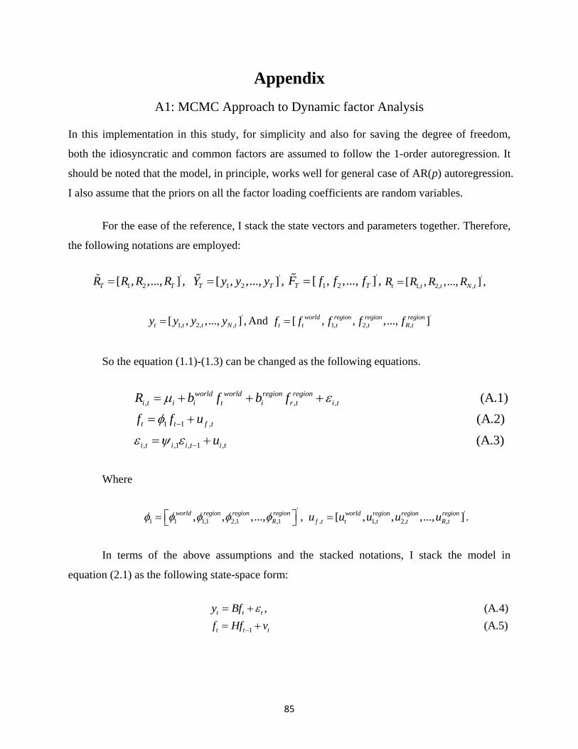
85
Appendix
A1: MCMC Approach to Dynamic factor Analysis
In this implementation in this study, for simplicity and also for saving the degree of freedom,
both the idiosyncratic and common factors are assumed to follow the 1-order autoregression. It
should be noted that the model, in principle, works well for general case of AR(p) autoregression.
I also assume that the priors on all the factor loading coefficients are random variables.
For the ease of the reference, I stack the state vectors and parameters together. Therefore,
the following notations are employed:
'
1 2[ , ,..., ] ,T TR R R R '
1 2[ , ,..., ] ,T TY y y y'
1 2[ , ,..., ] ,T TF f f f '
1, 2, ,[ , ,..., ] ,t t t N tR R R R
'
1, 2, ,[ , ,..., ] ,t t t N ty y y y And '
1, 2, ,[ , , ,..., ]world region region region
t t t t R tf f f f f
So the equation (1.1)-(1.3) can be changed as the following equations.
, , ,
1 1 ,
, ,1
(A.1)
(A.2)
world world region region
i t i i t i r t i t
t t f t
i t i
R b f b f
f f u
, 1 , (A.3)i t i tu
Where
'
1 1 1,1 2,1 ,1, , ,..., ,world region region region
R '
, 1, 2, ,[ , , ,..., ] .world region region region
f t t t t R tu u u u u
In terms of the above assumptions and the stacked notations, I stack the model in
equation (2.1) as the following state-space form:
1
, (A.4)
(A.5)
t t t
t t t
y Bf
f Hf v
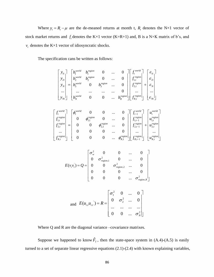
86
Where t ty R are the de-meaned returns at month t, tR denotes the N×1 vector of
stock market returns and tf denotes the K×1 vector (K=R+1) and, B is a N×K matrix of b’s, and
tv denotes the K×1 vector of idiosyncratic shocks.
The specification cans be written as follows:
1 11 1
2 1,2 2
3 2,3 3
,
0 ... 0
0 ... 0
0 ... 0
... ...... ... ... ... 0
0 0 ...
worldworld regiont t
regionworld regiont t
regionworld regiont t
regionworld regionNt R tN R
y fb b
y fb b
y fb b
y fb b
2
3
...
t
t
t
Nt
1 1
1, 1,1 1, 1
2, 2,1 2, 1
, ,1 , 1
0 0 ... 0
0 0 ... 0
0 0 ... 0
... 0 0 0 ... 0 ...
0 0 0 ...
world world world
t t
region region region
t t
region region region
t t
region region region
R t R R t
f f
f f
f f
f f
1,
2,
,
...
world
t
region
t
region
t
region
R t
u
u
u
u
2
2
,1
' 2
,2
2
,
0 0 ... 0
0 0 ... 0
( ) 0 0 ... 0
0 0 0 ... 0
0 0 0 ...
w
region
t t region
region R
E v v Q
and
2
1
2
' 2
, ,
2
0 ... 0
0 ... 0( )
... ... ... ...
0 0 ...
i t i t
N
E u u R
Where Q and R are the diagonal variance –covariance matrixes.
Suppose we happened to knowTF , then the state-space system in (A.4)-(A.5) is easily
turned to a set of separate linear regressive equations (2.1)-(2.4) with known explaining variables,
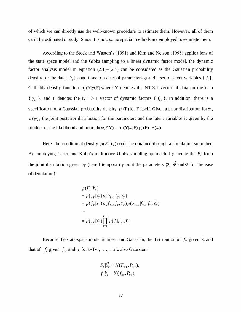
87
of which we can directly use the well-known procedure to estimate them. However, all of them
can’t be estimated directly. Since it is not, some special methods are employed to estimate them.
According to the Stock and Waston’s (1991) and Kim and Nelson (1998) applications of
the state space model and the Gibbs sampling to a linear dynamic factor model, the dynamic
factor analysis model in equation (2.1)--(2.4) can be considered as the Gaussian probability
density for the data { tY } conditional on a set of parameters and a set of latent variables { tf }.
Call this density function y (Y| ,F)p where Y denotes the NT×1 vector of data on the data
{,i ty }, and F denotes the KT ×1 vector of dynamic factors {
,i tf }. In addition, there is a
specification of a Gaussian probability density f (F)p for F itself. Given a prior distribution for ,
( ) , the joint posterior distribution for the parameters and the latent variables is given by the
product of the likelihood and prior, y fh( ,F|Y) = p (Y| ,F).p (F) . ( ).
Here, the conditional density ( | )T Tp F Y could be obtained through a simulation smoother.
By employing Carter and Kohn’s multimove Gibbs-sampling approach, I generate the TF from
the joint distribution given by (here I temporarily omit the parameters , and for the ease
of denotation)
1
1 2 1
1
1
1
( | )
( | ) ( | , )
( | ) ( | , ) ( | , )
...
( | ) ( | , )
T T
T T T T T
T T T T T T T T T
T
T T t t t
t
p F Y
p f Y p F f Y
p f Y p f f Y p F f f Y
p f Y p f f Y
Because the state-space model is linear and Gaussian, the distribution of Tf given TY and
that of tf given 1tf and ty for t=T-1, …, 1 are also Gaussian:
T|T T|T
|T |T
| ~ ( , ),
|y ~ ( , ),
T T
t t t t
F Y N F P
f N f P
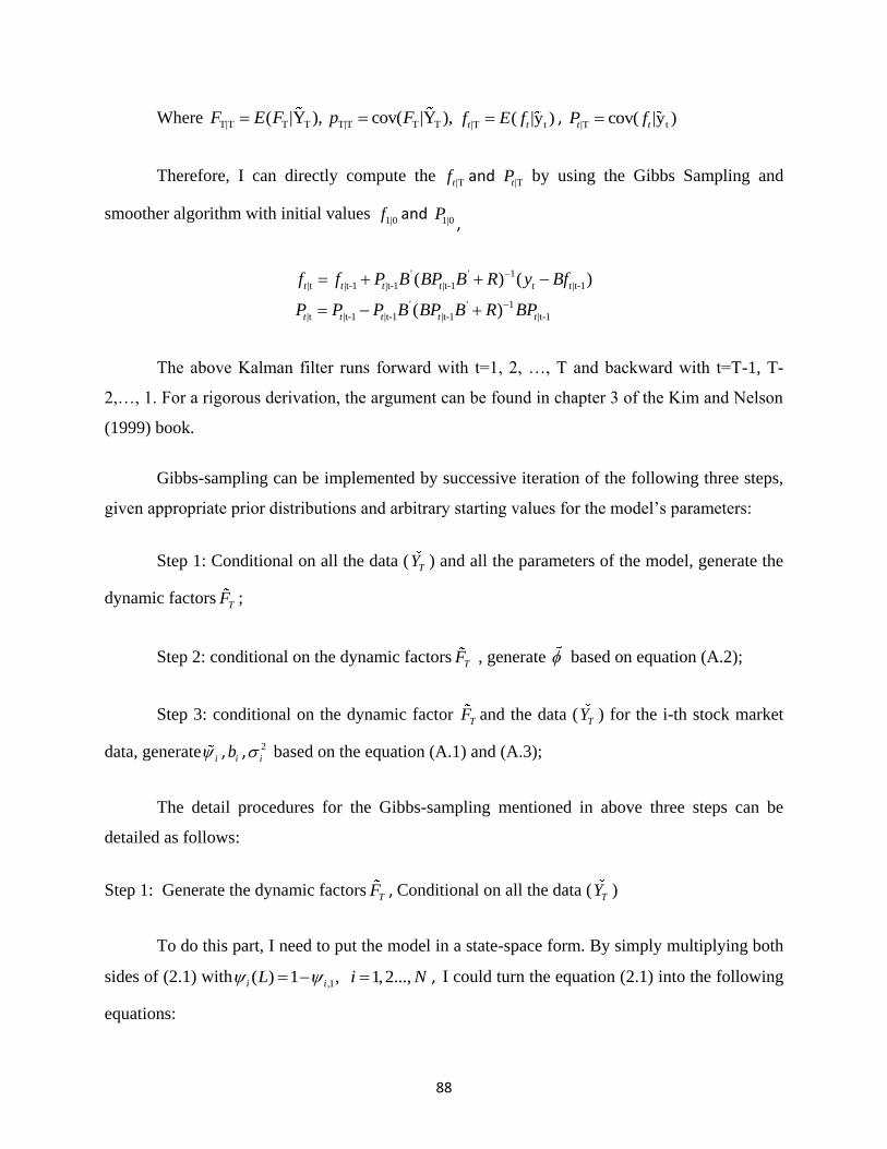
88
Where T|T T T( |Y ),F E F T|T T Tcov( |Y ),p F|T t( |y )t tf E f ,
|T tcov( |y )t tP f
Therefore, I can directly compute the |Ttf and
|TtP by using the Gibbs Sampling and
smoother algorithm with initial values 1|0f and
1|0P,
' ' 1
|t |t-1 |t-1 |t-1 |t-1
' ' 1
|t |t-1 |t-1 |t-1 |t-1
( ) ( )
( )
t t t t t t
t t t t t
f f P B BP B R y Bf
P P P B BP B R BP
The above Kalman filter runs forward with t=1, 2, …, T and backward with t=T-1, T-
2,…, 1. For a rigorous derivation, the argument can be found in chapter 3 of the Kim and Nelson
(1999) book.
Gibbs-sampling can be implemented by successive iteration of the following three steps,
given appropriate prior distributions and arbitrary starting values for the model’s parameters:
Step 1: Conditional on all the data (TY ) and all the parameters of the model, generate the
dynamic factorsTF ;
Step 2: conditional on the dynamic factorsTF , generate based on equation (A.2);
Step 3: conditional on the dynamic factor TF and the data (
TY ) for the i-th stock market
data, generate i , ib , 2
i based on the equation (A.1) and (A.3);
The detail procedures for the Gibbs-sampling mentioned in above three steps can be
detailed as follows:
Step 1: Generate the dynamic factorsTF , Conditional on all the data (
TY )
To do this part, I need to put the model in a state-space form. By simply multiplying both
sides of (2.1) with,1( ) 1 , 1,2...,i iL i N , I could turn the equation (2.1) into the following
equations:
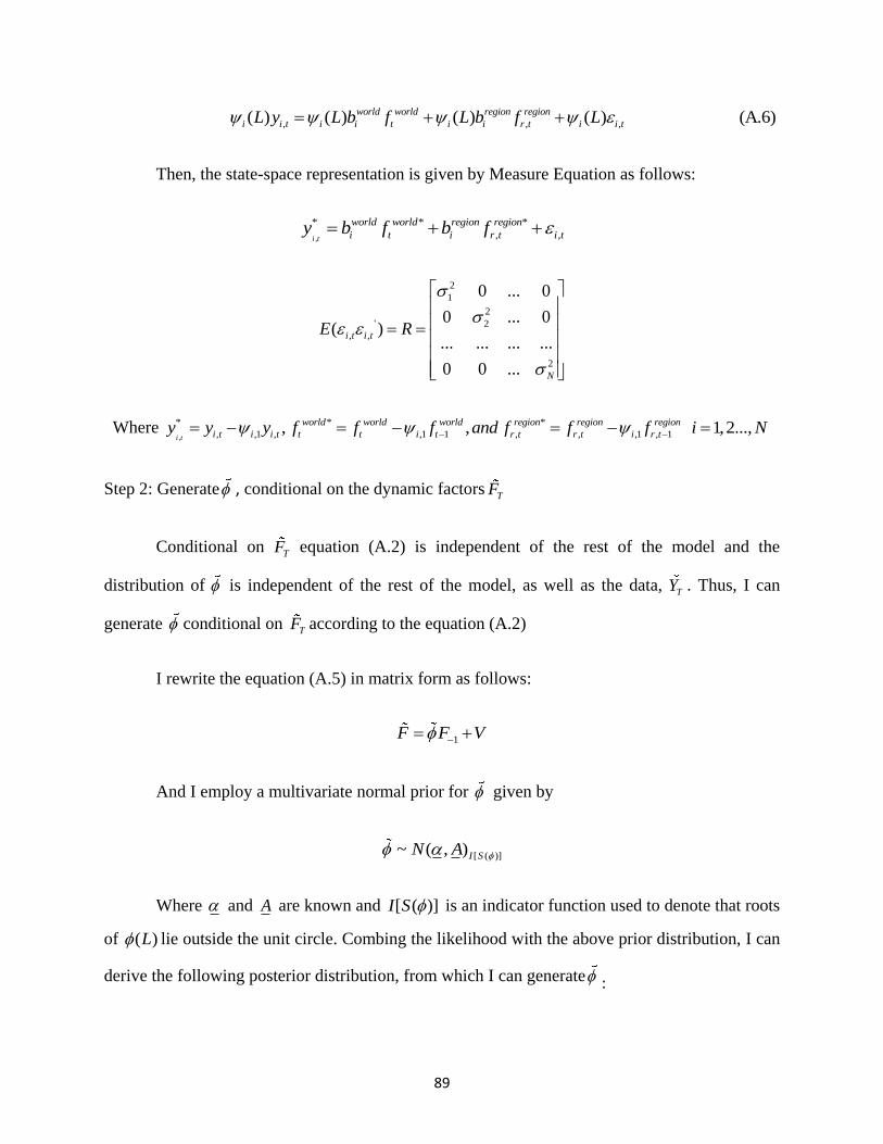
89
, , ,( ) ( ) ( ) ( ) (A.6)world world region region
i i t i i t i i r t i i tL y L b f L b f L
Then, the state-space representation is given by Measure Equation as follows:
,
* * *
, , i t
world world region region
i t i r t i ty b f b f
2
1
2
' 2
, ,
2
0 ... 0
0 ... 0( )
... ... ... ...
0 0 ...
i t i t
N
E R
Where ,
* * *
, ,1 , ,1 1 , , ,1 , 1, , 1,2...,i t
world world world region region region
i t i i t t t i t r t r t i r ty y y f f f and f f f i N
Step 2: Generate , conditional on the dynamic factorsTF
Conditional on TF equation (A.2) is independent of the rest of the model and the
distribution of is independent of the rest of the model, as well as the data, TY . Thus, I can
generate conditional on TF according to the equation (A.2)
I rewrite the equation (A.5) in matrix form as follows:
1F F V
And I employ a multivariate normal prior for given by
[ ( )]~ ( , )I SN A
Where and A are known and [ ( )]I S is an indicator function used to denote that roots
of ( )L lie outside the unit circle. Combing the likelihood with the above prior distribution, I can
derive the following posterior distribution, from which I can generate :
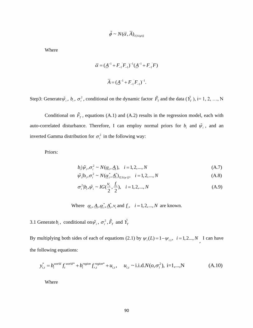
90
[ ( )]~ ( , )I SN A
Where
1 ' 1 1 '
1 1 1( ) ( )A F F A F F
1 ' 1
1 1( ) .A A F F
Step3: Generate i , ib , 2
i , conditional on the dynamic factor TF and the data (
TY ), i= 1, 2, …, N
Conditional on TF , equations (A.1) and (A.2) results in the regression model, each with
auto-correlated disturbance. Therefore, I can employ normal priors for ib and i , and an
inverted Gamma distribution for 2
i in the following way:
Priors:
2
i
2 * *
i i [ ( )]
2
i
| , ~ ( , ), 1,2,..., (A.7)
|b , ~ ( , ) , 1,2,..., (A.8)
| , ~ ( ,2
i i i i
i i i I S
i ii i
b N A i N
N A i N
v fb IG
), 1,2,..., (A.9)2
i N
Where * *, , , ,i i i i iA A v and , 1,2,...,if i N are known.
3.1 Generate ib , conditional on i , 2
i , TF and TY
By multiplying both sides of each of equations (2.1) by ,1( ) 1 , 1,2...,i iL i N
, I can have
the following equations:
* * * 2
, , , ,, ~ i.i.d. ( , ), i=1,...,N (A.10)world world region region
i t i t i r t i t i t iy b f b f u u N o
Where

91
*
, , ,1 , 1i t i t i i ty y y , *
,1 1
world world world
t t i tf f f , *
, , ,1 , 1
region region region
r t r t i r tf f f , and , ,1 , 1 ,i t i i t i tu
If I stack all the factors together in matrix notation, I can have
* * * *
, , = ,world world region region
i T i T i r T i i T iy b f b f U b F U
2
1where U ~i.i.d. ( , ), i=1,...,N i i TN o I
Combining with the likelihood with prior distribution in (A.7), I can derive the following
posterior distribution, from which I can generate the parameters ib , i=1,...,N ,
Posterior:
2
i| , , , ~ ( , ), 1,2,...,i i T T i ib F Y N A i N
Where
1 2 *' * 1 1 2 *' *
1 1 2 *' * 1
( ) ( ),
( ) ,
i i i T T i i i T T
i i i T T
A F F A F Y
A A F F
3.2 Generate i , conditional on ib , 2
i , TF and TY
To derive a posterior distribution of i , I can turn to equation (A.3):
2
, ,1 , 1 , ,, ~ . . . ( , ), i=1,...,N (A.11)i t i i t i t i t iu u i i d N o
Where , , , ,
world world region region
i t i t i t i r t i t i ty b f b f y b f for i=1,...,N .
If I stack all the factors together in matrix notation, I can have
2
, 1, U ~ . . . ( , ), i=1,...,N i T i i i i i TE U i i d N o I

92
Combining with the likelihood with prior distribution in (A.8), I can derive the following
posterior distribution, from which I can generate the parameters , i=1,...,N i ,
Posterior:
2 * *
i [ ( )]| , , , ~ ( , ) , 1,2,..., i i T T i i I Sb F Y N A i N
Where
* * 1 2 *' * 1 * 1 * 2 *'
,
* * 1 2 *' * 1
( ) ( ),
( ) ,
i i i i i i i i i i T
i i i i i
A E E A E
A A E E
3.3 Generate 2
i conditional on ib , i , TF and
TY
Now, given ib and i , I focus on (A.10) to get the likelihood of 2
i . Combining the likelihood
with the prior distribution in (A.10), the posterior distribution from which 2
i can be drawn is
given as the following:
Posterior:
* ' *
, i , i2
i
( ) ( )1| , , , ~ ( , ), 1,2,...,
2 2
i i T i i T iii i T T
f E Ev Tb F Y IG i N
These steps are iterated S times, of which the first S1 draws are discarded as a burning-in
replications to remove the effects of initial values.
93
A2: Procedures for Time-varying VAR Model
In time-varying VAR Model, I need to estimate a number of parameters, including
coefficients tB and tA , time-varying variance-covariance matrix t , and the hyper-parameters of
matrix V. In this study, I employ the MCMC algorithm to construct the estimation of the
parameters. The Prior distributions are assigned to the hyper-parameters in the model and then
are combined with the information contained in the data (via the form of likelihood function).
Together with a set of initial conditions, joint posterior distribution of the parameters can be
estimated through Bayesian methods. Marginal posterior distributions are then obtained by
integrating out other parameters from the joint posterior distribution.
Through the procedure of MCMC method, I can implement the analysis of the joint
posterior distribution from Bayesian reference. It includes the following main steps:
Step 1: Priors Choosing
As suggested by Nakajima, et al (2011), I need to carefully choose the priors because the
time-varying VAR (i.e., TV-VAR) model has many state variables for specification and their
process is modeled as a non-stationary random walk process. In the TV-VAR model, flexible
state variables can capture the changes of underlying financial shock because it allows time
variation in each parameter in the model. Following Primiceri (2005), to avoid the implausible
behaviors of time-varying parameters, I need tight prior for the covariance-matrix of the
disturbance in the random walk process, which is helpful for the identification in the model.
In this study, the time-varying coefficient (B) needs a tighter prior than the simultaneous
relations (A) and the variance (h) of the financial shock for the variance of the disturbance in
their time-varying process. The financial shock may unexpectedly hits the financial system and
the variance might widely fluctuate over time. In the following estimation procedures, I set a
slightly tighter prior for B and a rather diffuse prior for A and h . In addition, since the time-
varying parameters are random walks, I need to set the prior of the normal distribution for the
initial state of each time-varying parameter. As suggested by Primiceri (2005), the estimates
from the time-invariant VAR model during pre-sample period are used as the priors in the model.
94
Step 2: Simulation method to generate the posterior distribution
The model is estimated by simulating the distribution of the parameters, given the real
data. In this section, I employ the MCMC algorithm to generate a sample from the joint posterior
of tB , tA , t , and V. The Gibbs sampling is used in order to exploit the blocking structure of the
unknowns. In this study, Gibbs sampling is carried out in four steps, drawing in turn the time
varying coefficients ( tB ), simultaneous relations ( tA ), volatilities ( t ) and the hyper-parameters
(V), conditional on the observed real data ( ty ) and the remaining parameters. Given the real data
y, I draw sample from the posterior distribution by using the MCMC method. The main MCMC
algorithm for this study is as follows.
Since the state space form given is linear and Gaussian, the conditional posterior of tB is
a product of Gaussian densities and tB can be drawn using a standard simulation smoother
(Carter and Kohn, 1994) conditional on tA and t . Similarly, the posterior of tA conditional on
tB and t is also a product of normal distributions. Hence, tA can also be drawn in the same
way. Drawing t is more involved and relies mostly on the method presented in Kim et al.
(1998). It needs to transform a nonlinear and non-Gaussian state space form to a linear and
approximately Gaussian one, which again, allows the use of simulation smoothers. Simulating
the conditional posterior of V is standard, since it is the product of independent inverse-Wishart
distributions. Simply taken together, the algorithm of MCMC is summarized as follows:
1): Initialize B, A, and V;
2): Sample B conditional on A, , V and real data y;
3): Sample A conditional on B, , V and real data y;
4) Sample V conditional on B, A, , and real data y;
5) Sample c
onditional on B, A, V and real data y.
As discussion on Gibbs sampling above, the iteration will go to step 2 again after all the
steps are conducted. Steps 2 to 4 are conducted with the simulation smoother, and step 5 requires
the multi-move sampler for the stochastic volatility. For further details of the Gibbs Sampling for
state space model, see the book of Kim and Nelson (1999) as reference.
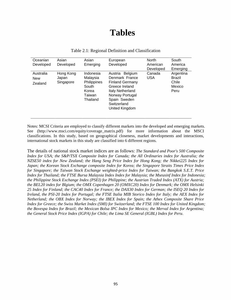
95
Tables
Table 2.1: Regional Definition and Classification
Oceanian Developed
Asian Developed
Asian Emerging
European Developed
North American Developed
South America Emerging
Australia
New
Zealand
Hong Kong Japan Singapore
Indonesia Malaysia Philippines South Korea Taiwan Thailand
Austria Belgium Denmark France Finland Germany Greece Ireland Italy Netherland Norway Portugal Spain Sweden Switzerland United Kingdom
Canada USA
Argentina Brazil Chile Mexico Peru
Notes: MCSI Criteria are employed to classify different markets into the developed and emerging markets.
See (http://www.msci.com/equity/coverage_matrix.pdf) for more information about the MSCI
classifications. In this study, based on geographical closeness, market developments and interactions,
international stock markets in this study are classified into 6 different regions.
The details of national stock market indices are as follows: The Standard and Poor's 500 Composite
Index for USA; the S&P/TSX Composite Index for Canada; the All Ordinaries index for Australia; the
NZSE50 index for New Zealand; the Hang Seng Price Index for Hong Kong; the Nikkei225 Index for
Japan; the Korean Stock Exchange composite Index for Korea; the Singapore Straits Times Price Index
for Singapore; the Taiwan Stock Exchange weighted-price Index for Taiwan; the Bangkok S.E.T. Price
Index for Thailand; the FTSE Bursa Malaysia Index Index for Malaysia; the Mseusinf Index for Indonesia;
the Philippine Stock Exchange Index (PSEI) for Philippine; the Austrian Traded Index (ATX) for Austria;
the BEL20 index for Blgium; the OMX Copenhagen 20 (OMXC20) Index for Denmark; the OMX Helsinki
25 Index for Finland; the CAC40 Index for France; the DAX30 Index for German; the ISEQ 20 Index for
Ireland, the PSI-20 Index for Portugal; the FTSE Italia MIB Storico Index for Italy; the AEX Index for
Netherland; the OBX Index for Norway; the IBEX Index for Spain; the Athex Composite Share Price
Index for Greece; the Swiss Market Index (SMI) for Switzerland; the FTSE 100 Index for United Kingdom;
the Bovespa Index for Brazil; the Mexican Bolsa IPC Index for Mexico; the Merval Index for Argentina;
the General Stock Price Index (IGPA) for Chile; the Lima SE General (IGBL) Index for Peru.
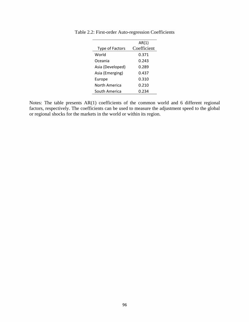
96
Table 2.2: First-order Auto-regression Coefficients
Type of Factors
AR(1)
Coefficient
World 0.371
Oceania 0.243
Asia (Developed) 0.289
Asia (Emerging) 0.437
Europe 0.310
North America 0.210
South America 0.234
Notes: The table presents AR(1) coefficients of the common world and 6 different regional
factors, respectively. The coefficients can be used to measure the adjustment speed to the global
or regional shocks for the markets in the world or within its region.
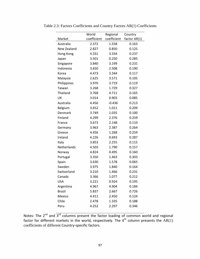
97
Table 2.3: Factors Coefficients and Country Factors AR(1) Coefficients
Market World coefficient
Regional coefficient
Country factor AR(1)
Australia 2.372 1.558 0.163
New Zealand 2.827 0.850 0.125
Hong Kong 4.331 3.334 0.237
Japan 3.501 0.250 0.285
Singapore 3.840 3.199 0.231
Indonesia 3.650 2.508 0.190
Korea 4.473 3.344 0.117
Malaysia 2.625 3.571 0.105
Philippines 3.970 3.719 0.119
Taiwan 3.268 1.729 0.327
Thailand 3.768 4.711 0.165
UK 3.014 0.903 0.085
Australia 4.456 -0.436 0.213
Belgium 3.652 1.011 0.209
Denmark 3.749 1.035 0.100
Finland 4.299 2.376 0.259
France 3.673 2.148 0.110
Germany 3.963 2.387 0.264
Greece 4.456 1.268 0.259
Ireland 4.226 0.693 0.287
Italy 3.853 2.255 0.115
Netherlands 4.503 1.790 0.157
Norway 4.824 0.495 0.160
Portugal 3.350 1.463 0.303
Spain 3.630 1.578 0.065
Sweden 3.975 1.840 0.164
Switzerland 3.210 1.466 0.231
Canada 3.366 1.077 0.212
USA 3.221 0.924 0.195
Argentina 4.967 4.904 0.184
Brazil 5.837 2.667 0.726
Mexico 4.411 2.450 0.124
Chile 2.478 1.335 0.188
Peru 4.252 2.297 0.346
Notes: The 2nd and 3rd columns present the factor loading of common world and regional factor for different markets in the world, respectively. The 4th column presents the AR(1)
coefficients of different Country-specific factors.
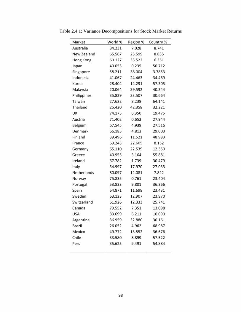
98
Table 2.4.1: Variance Decompositions for Stock Market Returns
Market World % Region % Country %
Australia 84.231 7.028 8.741
New Zealand 65.567 25.599 8.835
Hong Kong 60.127 33.522 6.351
Japan 49.053 0.235 50.712
Singapore 58.211 38.004 3.7853
Indonesia 41.067 24.463 34.469
Korea 28.404 14.291 57.305
Malaysia 20.064 39.592 40.344
Philippines 35.829 33.507 30.664
Taiwan 27.622 8.238 64.141
Thailand 25.420 42.358 32.221
UK 74.175 6.350 19.475
Austria 71.402 0.653 27.944
Belgium 67.545 4.939 27.516
Denmark 66.185 4.813 29.003
Finland 39.496 11.521 48.983
France 69.243 22.605 8.152
Germany 65.110 22.539 12.350
Greece 40.955 3.164 55.881
Ireland 67.782 1.739 30.479
Italy 54.997 17.970 27.033
Netherlands 80.097 12.081 7.822
Norway 75.835 0.761 23.404
Portugal 53.833 9.801 36.366
Spain 64.871 11.698 23.431
Sweden 63.123 12.907 23.970
Switzerland 61.926 12.333 25.741
Canada 79.552 7.351 13.098
USA 83.699 6.211 10.090
Argentina 36.959 32.880 30.161
Brazil 26.052 4.962 68.987
Mexico 49.772 13.552 36.676
Chile 33.580 8.899 57.522
Peru 35.625 9.491 54.884
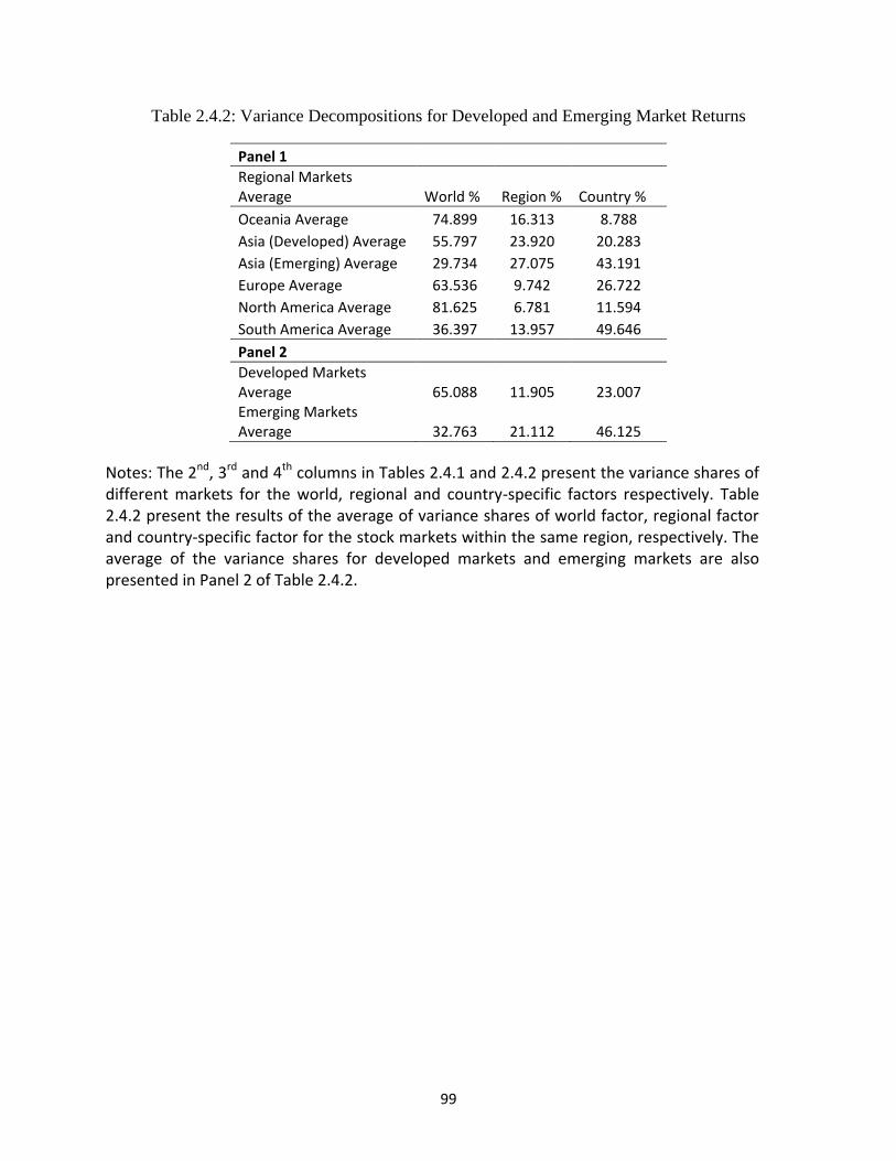
99
Table 2.4.2: Variance Decompositions for Developed and Emerging Market Returns
Panel 1
Regional Markets Average World % Region % Country %
Oceania Average 74.899 16.313 8.788
Asia (Developed) Average 55.797 23.920 20.283
Asia (Emerging) Average 29.734 27.075 43.191
Europe Average 63.536 9.742 26.722
North America Average 81.625 6.781 11.594
South America Average 36.397 13.957 49.646
Panel 2
Developed Markets Average 65.088 11.905 23.007 Emerging Markets Average 32.763 21.112 46.125
Notes: The 2nd, 3rd and 4th columns in Tables 2.4.1 and 2.4.2 present the variance shares of different markets for the world, regional and country-specific factors respectively. Table 2.4.2 present the results of the average of variance shares of world factor, regional factor and country-specific factor for the stock markets within the same region, respectively. The average of the variance shares for developed markets and emerging markets are also presented in Panel 2 of Table 2.4.2.
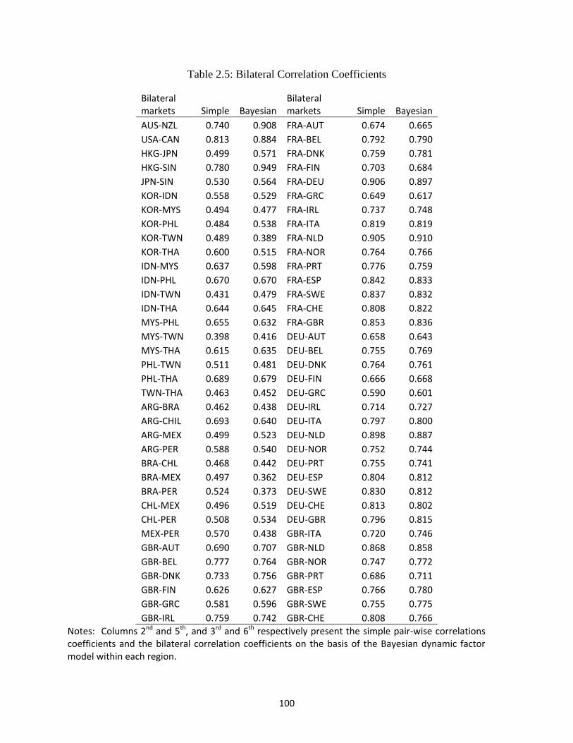
100
Table 2.5: Bilateral Correlation Coefficients
Bilateral markets Simple Bayesian
Bilateral markets Simple Bayesian
AUS-NZL 0.740 0.908 FRA-AUT 0.674 0.665
USA-CAN 0.813 0.884 FRA-BEL 0.792 0.790
HKG-JPN 0.499 0.571 FRA-DNK 0.759 0.781
HKG-SIN 0.780 0.949 FRA-FIN 0.703 0.684
JPN-SIN 0.530 0.564 FRA-DEU 0.906 0.897
KOR-IDN 0.558 0.529 FRA-GRC 0.649 0.617
KOR-MYS 0.494 0.477 FRA-IRL 0.737 0.748
KOR-PHL 0.484 0.538 FRA-ITA 0.819 0.819
KOR-TWN 0.489 0.389 FRA-NLD 0.905 0.910
KOR-THA 0.600 0.515 FRA-NOR 0.764 0.766
IDN-MYS 0.637 0.598 FRA-PRT 0.776 0.759
IDN-PHL 0.670 0.670 FRA-ESP 0.842 0.833
IDN-TWN 0.431 0.479 FRA-SWE 0.837 0.832
IDN-THA 0.644 0.645 FRA-CHE 0.808 0.822
MYS-PHL 0.655 0.632 FRA-GBR 0.853 0.836
MYS-TWN 0.398 0.416 DEU-AUT 0.658 0.643
MYS-THA 0.615 0.635 DEU-BEL 0.755 0.769
PHL-TWN 0.511 0.481 DEU-DNK 0.764 0.761
PHL-THA 0.689 0.679 DEU-FIN 0.666 0.668
TWN-THA 0.463 0.452 DEU-GRC 0.590 0.601
ARG-BRA 0.462 0.438 DEU-IRL 0.714 0.727
ARG-CHIL 0.693 0.640 DEU-ITA 0.797 0.800
ARG-MEX 0.499 0.523 DEU-NLD 0.898 0.887
ARG-PER 0.588 0.540 DEU-NOR 0.752 0.744
BRA-CHL 0.468 0.442 DEU-PRT 0.755 0.741
BRA-MEX 0.497 0.362 DEU-ESP 0.804 0.812
BRA-PER 0.524 0.373 DEU-SWE 0.830 0.812
CHL-MEX 0.496 0.519 DEU-CHE 0.813 0.802
CHL-PER 0.508 0.534 DEU-GBR 0.796 0.815
MEX-PER 0.570 0.438 GBR-ITA 0.720 0.746
GBR-AUT 0.690 0.707 GBR-NLD 0.868 0.858
GBR-BEL 0.777 0.764 GBR-NOR 0.747 0.772
GBR-DNK 0.733 0.756 GBR-PRT 0.686 0.711
GBR-FIN 0.626 0.627 GBR-ESP 0.766 0.780
GBR-GRC 0.581 0.596 GBR-SWE 0.755 0.775
GBR-IRL 0.759 0.742 GBR-CHE 0.808 0.766
Notes: Columns 2nd and 5th, and 3rd and 6th respectively present the simple pair-wise correlations coefficients and the bilateral correlation coefficients on the basis of the Bayesian dynamic factor model within each region.
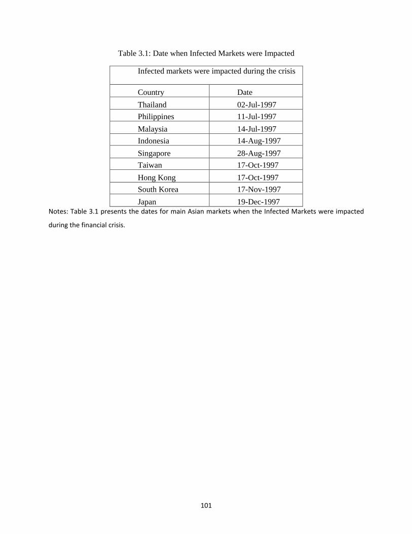
101
Table 3.1: Date when Infected Markets were Impacted
Infected markets were impacted during the crisis
Country Date
Thailand 02-Jul-1997
Philippines 11-Jul-1997
Malaysia 14-Jul-1997
Indonesia 14-Aug-1997
Singapore 28-Aug-1997
Taiwan 17-Oct-1997
Hong Kong 17-Oct-1997
South Korea 17-Nov-1997
Japan 19-Dec-1997
Notes: Table 3.1 presents the dates for main Asian markets when the Infected Markets were impacted
during the financial crisis.
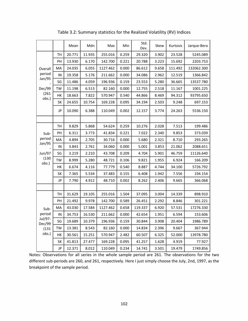
102
Table 3.2: Summary statistics for the Realized Volatility (RV) Indices
Mean Mdn Max Min Std.
Dev. Skew Kurtosis Jarque-Bera
Overall period Jan/95
-Dec/99
(261 obs.)
TH 20.771 11.935 255.016 0.259 29.320 3.902 23.528 5245.089
PH 13.930 6.170 142.700 0.221 20.788 3.223 15.692 2203.753
MA 24.035 6.055 1127.462 0.000 86.612 9.658 111.492 132062.300
IN 19.358 5.176 211.662 0.000 34.086 2.962 12.519 1366.842
SG 11.486 4.059 196.936 0.159 23.553 5.280 36.665 13537.780
TW 11.198 6.513 82.160 0.000 12.755 2.518 11.167 1001.225
HK 18.663 7.822 570.947 0.540 44.866 8.469 94.312 93795.650
SK 24.655 10.754 169.228 0.095 34.194 2.503 9.248 697.153
JP 10.090 6.388 110.049 0.002 12.157 3.774 24.263 5536.150
Sub-
period Jan/95
-Jun/97
(130 obs.)
TH 9.829 5.868 54.624 0.259 10.276 2.028 7.513 199.486
PH 6.311 3.773 41.834 0.221 7.022 2.340 9.853 373.039
MA 4.894 2.705 30.716 0.000 5.680 2.321 8.710 293.265
IN 3.843 2.761 34.060 0.000 5.001 3.853 21.062 2088.651
SG 3.219 2.210 43.708 0.209 4.704 5.901 46.759 11126.640
TW 8.999 5.280 48.721 0.106 9.821 1.955 6.924 166.209
HK 6.674 4.116 77.779 0.540 8.887 4.744 34.100 5726.792
SK 7.365 5.534 37.483 0.155 6.408 1.942 7.556 194.154
JP 7.790 4.912 48.710 0.002 8.262 2.406 9.665 366.068
Sub-period Jul/97-Dec/99
(131 obs.)
TH 31.629 19.105 255.016 1.504 37.095 3.004 14.339 898.910
PH 21.492 9.978 142.700 0.589 26.451 2.292 8.846 301.221
MA 43.030 17.584 1127.462 0.658 119.337 6.920 57.531 17276.330
IN 34.753 16.530 211.662 0.000 42.654 1.951 6.594 153.606
SG 19.689 10.379 196.936 0.159 30.844 3.908 20.404 1986.789
TW 13.381 8.543 82.160 0.000 14.834 2.396 9.667 367.944
HK 30.561 15.251 570.947 2.482 60.507 6.325 52.000 13978.780
SK 41.813 27.477 169.228 0.095 41.257 1.628 4.919 77.927
JP 12.371 8.012 110.049 0.234 14.741 3.501 19.479 1749.856
Notes: Observations for all series in the whole sample period are 261. The observations for the two
different sub-periods are 260, and 261, respectively. Here I just simply choose the July, 2nd, 1997, as the
breakpoint of the sample period.
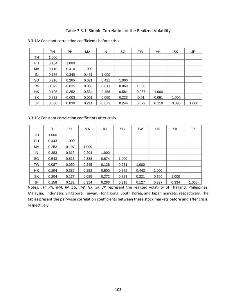
103
Table 3.3.1: Simple Correlation of the Realized Volatility
3.3.1A: Constant correlation coefficients before crisis
TH PH MA IN SG TW HK SK JP
TH 1.000
PH 0.184 1.000
MA 0.110 0.410 1.000
IN 0.175 0.340 0.461 1.000
SG 0.216 0.265 0.621 0.421 1.000
TW -0.029 -0.035 0.030 -0.011 0.069 1.000
HK 0.195 0.252 0.534 0.458 0.581 0.037 1.000
SK 0.222 -0.003 0.051 0.060 0.223 -0.01 0.091 1.000
JP 0.080 0.030 0.211 -0.073 0.244 0.072 0.118 0.396 1.000
3.3.1B: Constant correlation coefficients after crisis
TH PH MA IN SG TW HK SK JP
TH 1.000
PH 0.443 1.000
MA 0.252 0.197 1.000
IN 0.383 0.613 0.204 1.000
SG 0.543 0.615 0.338 0.674 1.000
TW 0.087 0.050 0.245 0.128 0.231 1.000
HK 0.294 0.387 0.252 0.500 0.572 0.442 1.000
SK 0.204 0.177 0.085 0.272 0.323 0.221 0.360 1.000
JP 0.158 0.132 0.314 0.266 0.215 0.127 0.337 0.334 1.000
Notes: TH, PH, MA, IN, SG, TW, HK, SK, JP represent the realized volatility of Thailand, Philippines,
Malaysia, Indonesia, Singapore, Taiwan, Hong Kong, South Korea, and Japan markets, respectively. The
tables present the pair-wise correlation coefficients between these stock markets before and after crisis,
respectively.
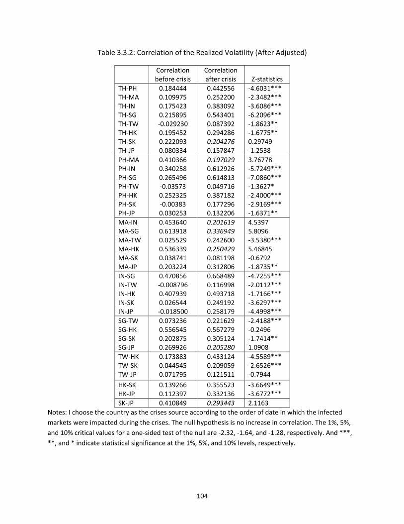
104
Table 3.3.2: Correlation of the Realized Volatility (After Adjusted)
Correlation before crisis
Correlation after crisis
Z-statistics
TH-PH TH-MA TH-IN TH-SG TH-TW TH-HK TH-SK TH-JP
0.184444 0.109975 0.175423 0.215895 -0.029230 0.195452 0.222093 0.080334
0.442556 0.252200 0.383092 0.543401 0.087392 0.294286 0.204276 0.157847
-4.6031*** -2.3482*** -3.6086*** -6.2096*** -1.8623** -1.6775** 0.29749 -1.2538
PH-MA PH-IN PH-SG PH-TW PH-HK PH-SK PH-JP
0.410366 0.340258 0.265496 -0.03573 0.252325 -0.00383 0.030253
0.197029 0.612926 0.614813 0.049716 0.387182 0.177296 0.132206
3.76778 -5.7249*** -7.0860*** -1.3627* -2.4000*** -2.9169*** -1.6371**
MA-IN MA-SG MA-TW MA-HK MA-SK MA-JP
0.453640 0.613918 0.025529 0.536339 0.038741 0.203224
0.201619 0.336949 0.242600 0.250429 0.081198 0.312806
4.5397 5.8096 -3.5380*** 5.46845 -0.6792 -1.8735**
IN-SG IN-TW IN-HK IN-SK IN-JP
0.470856 -0.008796 0.407939 0.026544 -0.018500
0.668489 0.116998 0.493718 0.249192 0.258179
-4.7255*** -2.0112*** -1.7166*** -3.6297*** -4.4998***
SG-TW SG-HK SG-SK SG-JP
0.073236 0.556545 0.202875 0.269926
0.221629 0.567279 0.305124 0.205280
-2.4188*** -0.2496 -1.7414** 1.0908
TW-HK TW-SK TW-JP
0.173883 0.044545 0.071795
0.433124 0.209059 0.121511
-4.5589*** -2.6526*** -0.7944
HK-SK HK-JP
0.139266 0.112397
0.355523 0.332136
-3.6649*** -3.6772***
SK-JP 0.410849 0.293443 2.1163
Notes: I choose the country as the crises source according to the order of date in which the infected
markets were impacted during the crises. The null hypothesis is no increase in correlation. The 1%, 5%,
and 10% critical values for a one-sided test of the null are -2.32, -1.64, and -1.28, respectively. And ***,
**, and * indicate statistical significance at the 1%, 5%, and 10% levels, respectively.
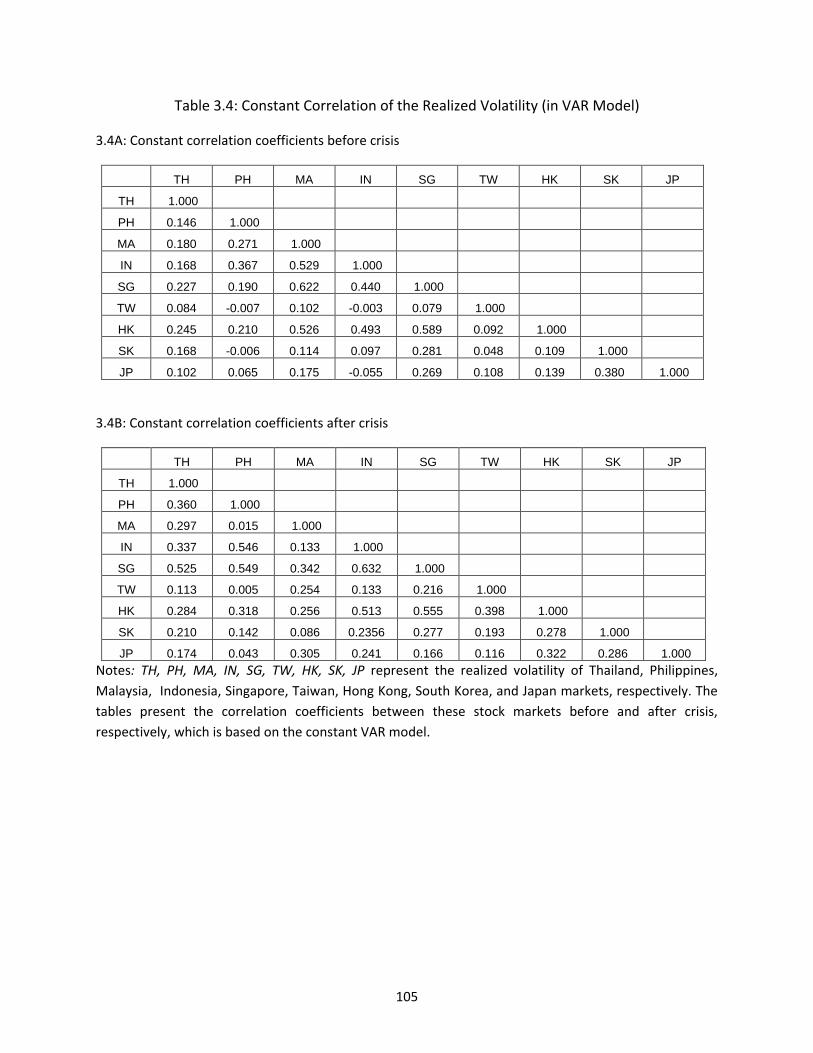
105
Table 3.4: Constant Correlation of the Realized Volatility (in VAR Model)
3.4A: Constant correlation coefficients before crisis
TH PH MA IN SG TW HK SK JP
TH 1.000
PH 0.146 1.000
MA 0.180 0.271 1.000
IN 0.168 0.367 0.529 1.000
SG 0.227 0.190 0.622 0.440 1.000
TW 0.084 -0.007 0.102 -0.003 0.079 1.000
HK 0.245 0.210 0.526 0.493 0.589 0.092 1.000
SK 0.168 -0.006 0.114 0.097 0.281 0.048 0.109 1.000
JP 0.102 0.065 0.175 -0.055 0.269 0.108 0.139 0.380 1.000
3.4B: Constant correlation coefficients after crisis
TH PH MA IN SG TW HK SK JP
TH 1.000
PH 0.360 1.000
MA 0.297 0.015 1.000
IN 0.337 0.546 0.133 1.000
SG 0.525 0.549 0.342 0.632 1.000
TW 0.113 0.005 0.254 0.133 0.216 1.000
HK 0.284 0.318 0.256 0.513 0.555 0.398 1.000
SK 0.210 0.142 0.086 0.2356 0.277 0.193 0.278 1.000
JP 0.174 0.043 0.305 0.241 0.166 0.116 0.322 0.286 1.000
Notes: TH, PH, MA, IN, SG, TW, HK, SK, JP represent the realized volatility of Thailand, Philippines,
Malaysia, Indonesia, Singapore, Taiwan, Hong Kong, South Korea, and Japan markets, respectively. The
tables present the correlation coefficients between these stock markets before and after crisis,
respectively, which is based on the constant VAR model.
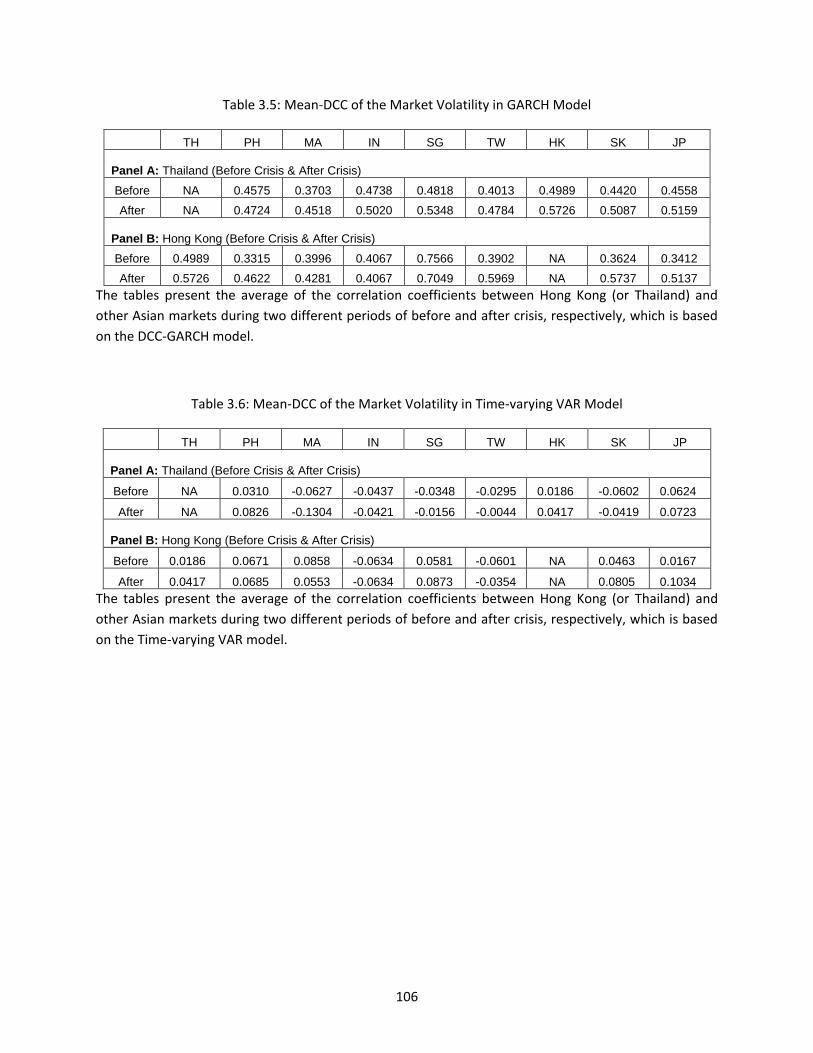
106
Table 3.5: Mean-DCC of the Market Volatility in GARCH Model
TH PH MA IN SG TW HK SK JP
Panel A: Thailand (Before Crisis & After Crisis)
Before NA 0.4575 0.3703 0.4738 0.4818 0.4013 0.4989 0.4420 0.4558
After NA 0.4724 0.4518 0.5020 0.5348 0.4784 0.5726 0.5087 0.5159
Panel B: Hong Kong (Before Crisis & After Crisis)
Before 0.4989 0.3315 0.3996 0.4067 0.7566 0.3902 NA 0.3624 0.3412
After 0.5726 0.4622 0.4281 0.4067 0.7049 0.5969 NA 0.5737 0.5137
The tables present the average of the correlation coefficients between Hong Kong (or Thailand) and
other Asian markets during two different periods of before and after crisis, respectively, which is based
on the DCC-GARCH model.
Table 3.6: Mean-DCC of the Market Volatility in Time-varying VAR Model
TH PH MA IN SG TW HK SK JP
Panel A: Thailand (Before Crisis & After Crisis)
Before NA 0.0310 -0.0627 -0.0437 -0.0348 -0.0295 0.0186 -0.0602 0.0624
After NA 0.0826 -0.1304 -0.0421 -0.0156 -0.0044 0.0417 -0.0419 0.0723
Panel B: Hong Kong (Before Crisis & After Crisis)
Before 0.0186 0.0671 0.0858 -0.0634 0.0581 -0.0601 NA 0.0463 0.0167
After 0.0417 0.0685 0.0553 -0.0634 0.0873 -0.0354 NA 0.0805 0.1034
The tables present the average of the correlation coefficients between Hong Kong (or Thailand) and
other Asian markets during two different periods of before and after crisis, respectively, which is based
on the Time-varying VAR model.
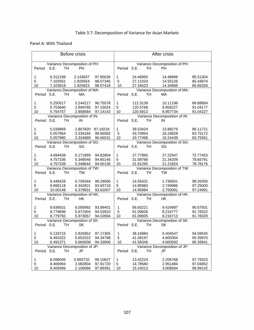
107
Table 3.7: Decomposition of Variance for Asian Markets
Panel A: With Thailand
Before crisis After crisis
Variance Decomposition of PH: Period S.E. TH PH 1 6.312198 2.143637 97.85636 5 7.102561 1.926554 98.07345 10 7.103918 1.925823 98.07418
Variance Decomposition of PH: Period S.E. TH PH 1 24.46950 14.48696 85.51304 5 27.11024 14.55126 85.44874 10 27.34523 14.34666 85.65334
Variance Decomposition of MA: Period S.E. TH MA 1 5.250517 3.244217 96.75578 5 5.753640 2.849765 97.15024 10 5.754757 2.858584 97.14142
Variance Decomposition of MA: Period S.E. TH MA 1 112.3139 10.11196 89.88804 5 120.5768 8.958227 91.04177 10 120.5813 8.957734 91.04227
Variance Decomposition of IN: Period S.E. TH IN 1 5.039869 2.807820 97.19218 5 5.057964 3.334184 96.66582 10 5.057980 3.334689 96.66531
Variance Decomposition of IN: Period S.E. TH IN 1 39.53424 13.88279 86.11721 5 43.70854 16.24828 83.75172 10 43.77498 16.24439 83.75561
Variance Decomposition of SG: Period S.E. TH SG 1 4.694438 5.171959 94.82804 5 4.757336 5.348546 94.65145 10 4.757339 5.348644 94.65136
Variance Decomposition of SG: Period S.E. TH SG 1 27.77865 27.22547 72.77453 5 31.58768 21.34209 78.65791 10 31.81265 21.21824 78.78176
Variance Decomposition of TW: Period S.E. TH TW 1 9.449428 0.709344 99.29066 5 9.999118 6.342821 93.65718 10 10.00148 6.379931 93.62007
Variance Decomposition of TW: Period S.E. TH TW 1 14.55431 1.736501 98.26350 5 14.95983 2.749996 97.25000 10 14.95984 2.750091 97.24991
Variance Decomposition of HK: Period S.E. TH HK 1 8.636631 6.005992 93.99401 5 8.779696 5.971904 94.02810 10 8.779750 5.973057 94.02694
Variance Decomposition of HK: Period S.E. TH HK 1 56.60221 9.424987 90.57501 5 61.09828 8.216777 91.78322 10 61.09935 8.216713 91.78329
Variance Decomposition of SK: Period S.E. TH SK 1 6.133715 2.826952 97.17305 5 6.491022 5.652022 94.34798 10 6.491371 5.660938 94.33906
Variance Decomposition of SK: Period S.E. TH SK 1 38.16984 5.404547 94.59545 5 41.58197 4.600304 95.39970 10 41.58346 4.600592 95.39941
Variance Decomposition of JP: Period S.E. TH JP 1 8.098045 0.893732 99.10627 5 8.406994 2.082804 97.91720 10 8.409489 2.106086 97.89391
Variance Decomposition of JP: Period S.E. TH JP ` 1 13.42224 2.206768 97.79323 5 14.78580 2.951484 97.04852 10 15.24013 3.008584 96.99142
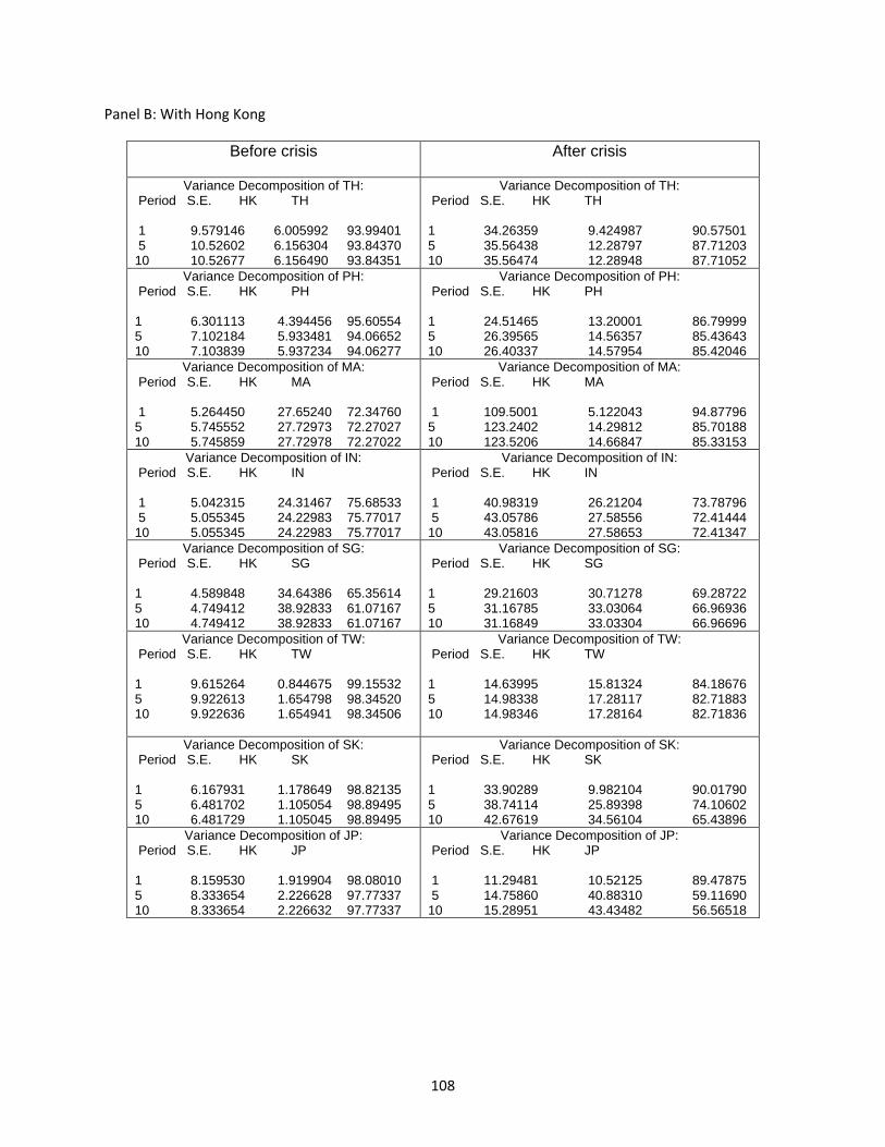
108
Panel B: With Hong Kong
Before crisis After crisis
Variance Decomposition of TH: Period S.E. HK TH 1 9.579146 6.005992 93.99401 5 10.52602 6.156304 93.84370 10 10.52677 6.156490 93.84351
Variance Decomposition of TH: Period S.E. HK TH 1 34.26359 9.424987 90.57501 5 35.56438 12.28797 87.71203 10 35.56474 12.28948 87.71052
Variance Decomposition of PH: Period S.E. HK PH 1 6.301113 4.394456 95.60554 5 7.102184 5.933481 94.06652 10 7.103839 5.937234 94.06277
Variance Decomposition of PH: Period S.E. HK PH 1 24.51465 13.20001 86.79999 5 26.39565 14.56357 85.43643 10 26.40337 14.57954 85.42046
Variance Decomposition of MA: Period S.E. HK MA 1 5.264450 27.65240 72.34760 5 5.745552 27.72973 72.27027 10 5.745859 27.72978 72.27022
Variance Decomposition of MA: Period S.E. HK MA 1 109.5001 5.122043 94.87796 5 123.2402 14.29812 85.70188 10 123.5206 14.66847 85.33153
Variance Decomposition of IN: Period S.E. HK IN 1 5.042315 24.31467 75.68533 5 5.055345 24.22983 75.77017 10 5.055345 24.22983 75.77017
Variance Decomposition of IN: Period S.E. HK IN 1 40.98319 26.21204 73.78796 5 43.05786 27.58556 72.41444 10 43.05816 27.58653 72.41347
Variance Decomposition of SG: Period S.E. HK SG 1 4.589848 34.64386 65.35614 5 4.749412 38.92833 61.07167 10 4.749412 38.92833 61.07167
Variance Decomposition of SG: Period S.E. HK SG 1 29.21603 30.71278 69.28722 5 31.16785 33.03064 66.96936 10 31.16849 33.03304 66.96696
Variance Decomposition of TW: Period S.E. HK TW 1 9.615264 0.844675 99.15532 5 9.922613 1.654798 98.34520 10 9.922636 1.654941 98.34506
Variance Decomposition of TW: Period S.E. HK TW 1 14.63995 15.81324 84.18676 5 14.98338 17.28117 82.71883 10 14.98346 17.28164 82.71836
Variance Decomposition of SK: Period S.E. HK SK 1 6.167931 1.178649 98.82135 5 6.481702 1.105054 98.89495 10 6.481729 1.105045 98.89495
Variance Decomposition of SK: Period S.E. HK SK 1 33.90289 9.982104 90.01790 5 38.74114 25.89398 74.10602 10 42.67619 34.56104 65.43896
Variance Decomposition of JP: Period S.E. HK JP 1 8.159530 1.919904 98.08010 5 8.333654 2.226628 97.77337 10 8.333654 2.226632 97.77337
Variance Decomposition of JP: Period S.E. HK JP 1 11.29481 10.52125 89.47875 5 14.75860 40.88310 59.11690 10 15.28951 43.43482 56.56518
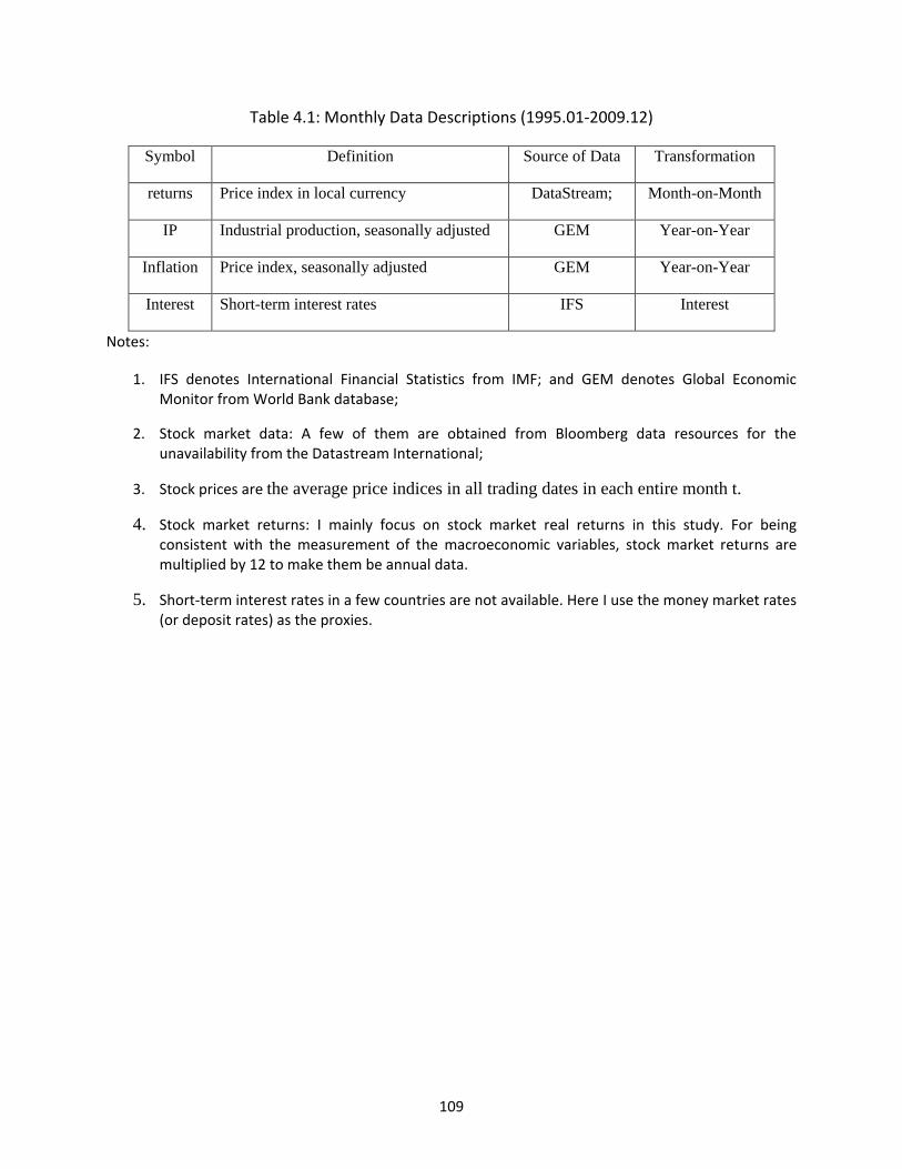
109
Table 4.1: Monthly Data Descriptions (1995.01-2009.12)
Symbol Definition Source of Data Transformation
returns Price index in local currency DataStream; Month-on-Month
IP Industrial production, seasonally adjusted GEM Year-on-Year
Inflation Price index, seasonally adjusted GEM Year-on-Year
Interest Short-term interest rates IFS Interest
Notes:
1. IFS denotes International Financial Statistics from IMF; and GEM denotes Global Economic Monitor from World Bank database;
2. Stock market data: A few of them are obtained from Bloomberg data resources for the unavailability from the Datastream International;
3. Stock prices are the average price indices in all trading dates in each entire month t.
4. Stock market returns: I mainly focus on stock market real returns in this study. For being consistent with the measurement of the macroeconomic variables, stock market returns are multiplied by 12 to make them be annual data.
5. Short-term interest rates in a few countries are not available. Here I use the money market rates (or deposit rates) as the proxies.
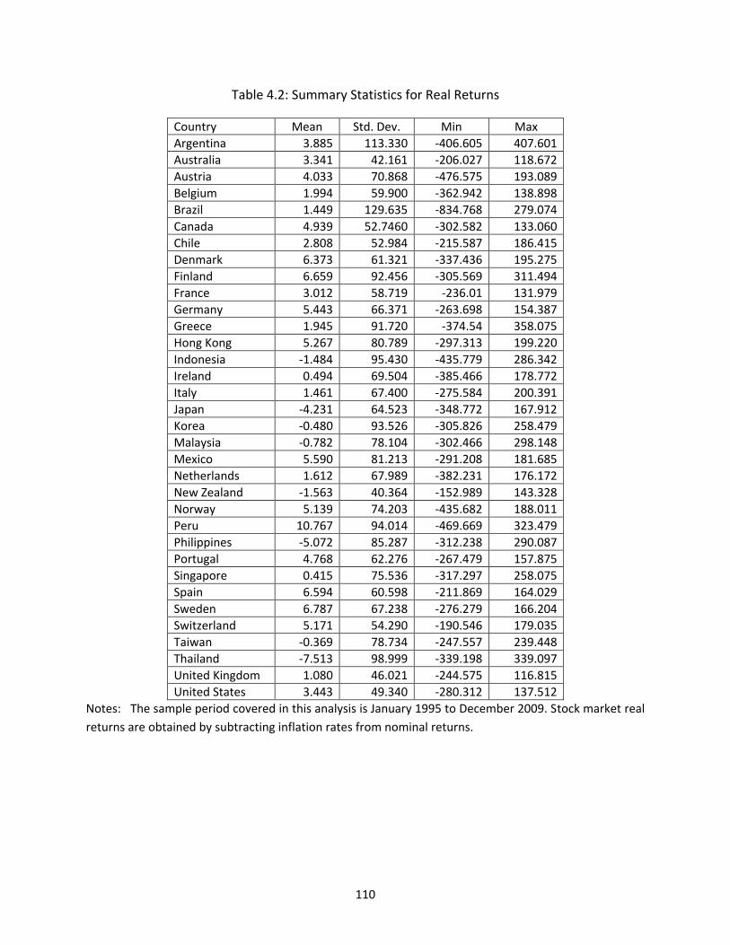
110
Table 4.2: Summary Statistics for Real Returns
Country Mean Std. Dev. Min Max
Argentina 3.885 113.330 -406.605 407.601
Australia 3.341 42.161 -206.027 118.672
Austria 4.033 70.868 -476.575 193.089
Belgium 1.994 59.900 -362.942 138.898
Brazil 1.449 129.635 -834.768 279.074
Canada 4.939 52.7460 -302.582 133.060
Chile 2.808 52.984 -215.587 186.415
Denmark 6.373 61.321 -337.436 195.275
Finland 6.659 92.456 -305.569 311.494
France 3.012 58.719 -236.01 131.979
Germany 5.443 66.371 -263.698 154.387
Greece 1.945 91.720 -374.54 358.075
Hong Kong 5.267 80.789 -297.313 199.220
Indonesia -1.484 95.430 -435.779 286.342
Ireland 0.494 69.504 -385.466 178.772
Italy 1.461 67.400 -275.584 200.391
Japan -4.231 64.523 -348.772 167.912
Korea -0.480 93.526 -305.826 258.479
Malaysia -0.782 78.104 -302.466 298.148
Mexico 5.590 81.213 -291.208 181.685
Netherlands 1.612 67.989 -382.231 176.172
New Zealand -1.563 40.364 -152.989 143.328
Norway 5.139 74.203 -435.682 188.011
Peru 10.767 94.014 -469.669 323.479
Philippines -5.072 85.287 -312.238 290.087
Portugal 4.768 62.276 -267.479 157.875
Singapore 0.415 75.536 -317.297 258.075
Spain 6.594 60.598 -211.869 164.029
Sweden 6.787 67.238 -276.279 166.204
Switzerland 5.171 54.290 -190.546 179.035
Taiwan -0.369 78.734 -247.557 239.448
Thailand -7.513 98.999 -339.198 339.097
United Kingdom 1.080 46.021 -244.575 116.815
United States 3.443 49.340 -280.312 137.512
Notes: The sample period covered in this analysis is January 1995 to December 2009. Stock market real
returns are obtained by subtracting inflation rates from nominal returns.
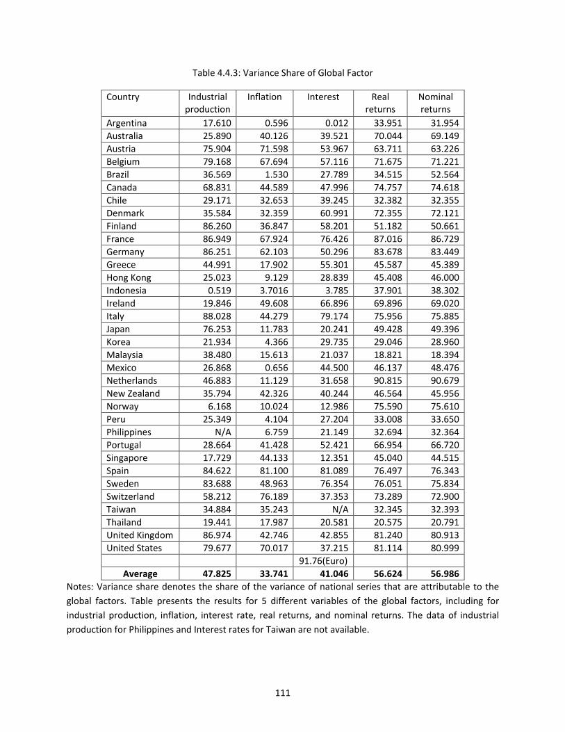
111
Table 4.4.3: Variance Share of Global Factor
Country Industrial production
Inflation Interest Real returns
Nominal returns
Argentina 17.610 0.596 0.012 33.951 31.954
Australia 25.890 40.126 39.521 70.044 69.149
Austria 75.904 71.598 53.967 63.711 63.226
Belgium 79.168 67.694 57.116 71.675 71.221
Brazil 36.569 1.530 27.789 34.515 52.564
Canada 68.831 44.589 47.996 74.757 74.618
Chile 29.171 32.653 39.245 32.382 32.355
Denmark 35.584 32.359 60.991 72.355 72.121
Finland 86.260 36.847 58.201 51.182 50.661
France 86.949 67.924 76.426 87.016 86.729
Germany 86.251 62.103 50.296 83.678 83.449
Greece 44.991 17.902 55.301 45.587 45.389
Hong Kong 25.023 9.129 28.839 45.408 46.000
Indonesia 0.519 3.7016 3.785 37.901 38.302
Ireland 19.846 49.608 66.896 69.896 69.020
Italy 88.028 44.279 79.174 75.956 75.885
Japan 76.253 11.783 20.241 49.428 49.396
Korea 21.934 4.366 29.735 29.046 28.960
Malaysia 38.480 15.613 21.037 18.821 18.394
Mexico 26.868 0.656 44.500 46.137 48.476
Netherlands 46.883 11.129 31.658 90.815 90.679
New Zealand 35.794 42.326 40.244 46.564 45.956
Norway 6.168 10.024 12.986 75.590 75.610
Peru 25.349 4.104 27.204 33.008 33.650
Philippines N/A 6.759 21.149 32.694 32.364
Portugal 28.664 41.428 52.421 66.954 66.720
Singapore 17.729 44.133 12.351 45.040 44.515
Spain 84.622 81.100 81.089 76.497 76.343
Sweden 83.688 48.963 76.354 76.051 75.834
Switzerland 58.212 76.189 37.353 73.289 72.900
Taiwan 34.884 35.243 N/A 32.345 32.393
Thailand 19.441 17.987 20.581 20.575 20.791
United Kingdom 86.974 42.746 42.855 81.240 80.913
United States 79.677 70.017 37.215 81.114 80.999
91.76(Euro)
Average 47.825 33.741 41.046 56.624 56.986
Notes: Variance share denotes the share of the variance of national series that are attributable to the
global factors. Table presents the results for 5 different variables of the global factors, including for
industrial production, inflation, interest rate, real returns, and nominal returns. The data of industrial
production for Philippines and Interest rates for Taiwan are not available.
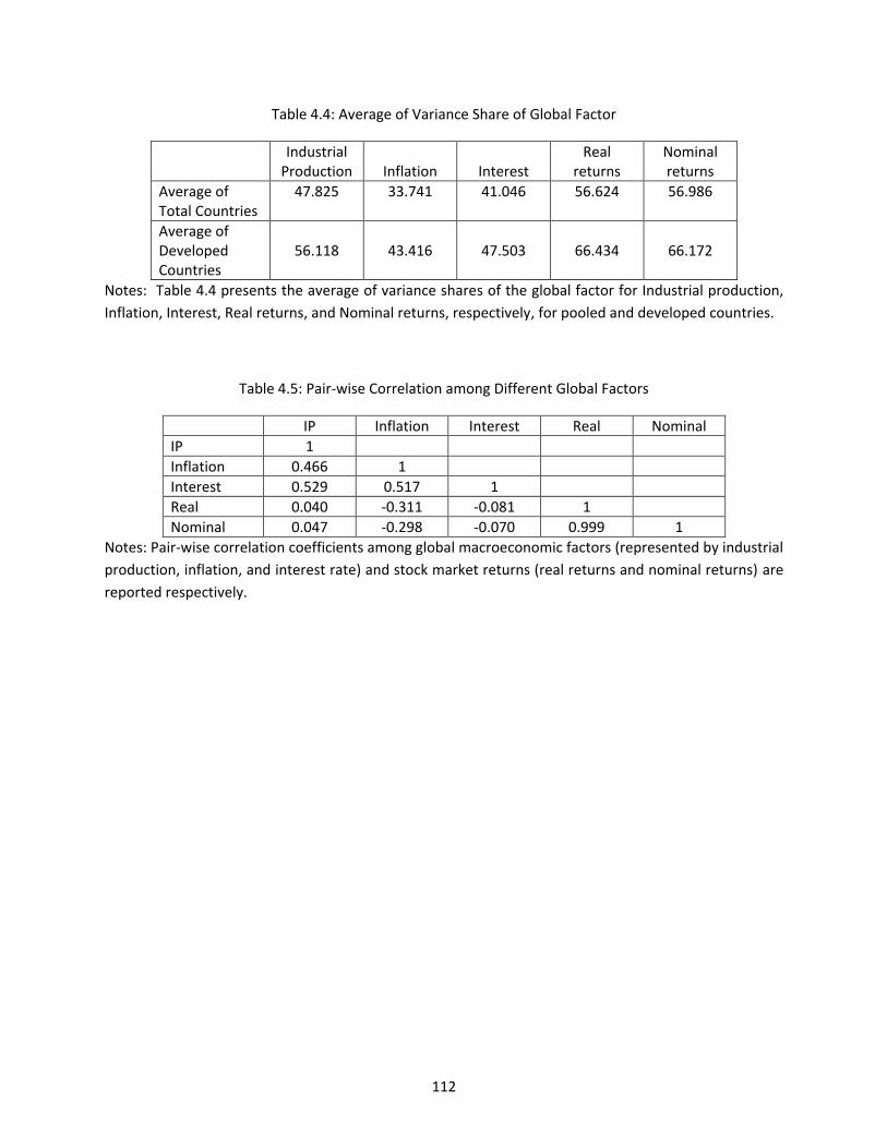
112
Table 4.4: Average of Variance Share of Global Factor
Industrial
Production Inflation Interest Real
returns Nominal returns
Average of Total Countries
47.825 33.741 41.046 56.624 56.986
Average of Developed Countries
56.118
43.416
47.503
66.434
66.172
Notes: Table 4.4 presents the average of variance shares of the global factor for Industrial production,
Inflation, Interest, Real returns, and Nominal returns, respectively, for pooled and developed countries.
Table 4.5: Pair-wise Correlation among Different Global Factors
IP Inflation Interest Real Nominal
IP 1
Inflation 0.466 1
Interest 0.529 0.517 1
Real 0.040 -0.311 -0.081 1
Nominal 0.047 -0.298 -0.070 0.999 1
Notes: Pair-wise correlation coefficients among global macroeconomic factors (represented by industrial
production, inflation, and interest rate) and stock market returns (real returns and nominal returns) are
reported respectively.
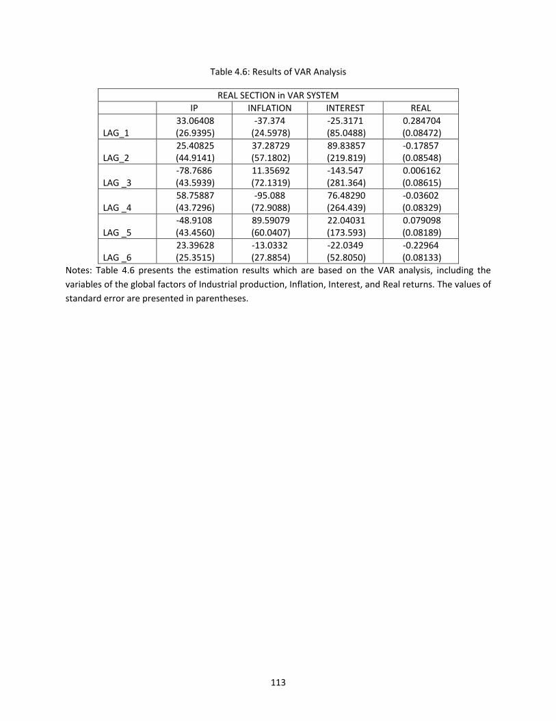
113
Table 4.6: Results of VAR Analysis
REAL SECTION in VAR SYSTEM
IP INFLATION INTEREST REAL
LAG_1 33.06408 (26.9395)
-37.374 (24.5978)
-25.3171 (85.0488)
0.284704 (0.08472)
LAG_2 25.40825 (44.9141)
37.28729 (57.1802)
89.83857 (219.819)
-0.17857 (0.08548)
LAG _3 -78.7686
(43.5939) 11.35692 (72.1319)
-143.547 (281.364)
0.006162 (0.08615)
LAG _4 58.75887 (43.7296)
-95.088 (72.9088)
76.48290 (264.439)
-0.03602 (0.08329)
LAG _5 -48.9108
(43.4560) 89.59079 (60.0407)
22.04031 (173.593)
0.079098 (0.08189)
LAG _6 23.39628 (25.3515)
-13.0332 (27.8854)
-22.0349 (52.8050)
-0.22964 (0.08133)
Notes: Table 4.6 presents the estimation results which are based on the VAR analysis, including the
variables of the global factors of Industrial production, Inflation, Interest, and Real returns. The values of
standard error are presented in parentheses.
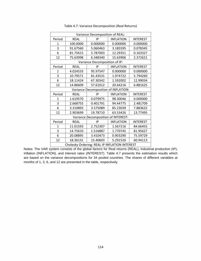
114
Table 4.7: Variance Decomposition (Real Returns)
Variance Decomposition of REAL:
Period REAL IP INFLATION INTEREST
1 100.0000 0.000000 0.000000 0.000000
3 91.67560 5.060463 3.185595 0.078345
6 81.75615 5.787003 12.29351 0.163327
12 75.63998 6.348340 15.63906 2.372621
Variance Decomposition of IP:
Period REAL IP INFLATION INTEREST
1 4.024533 95.97547 0.000000 0.000000
3 10.79571 81.43531 1.974722 5.794260
6 18.11424 67.30342 1.592002 12.99034
12 14.86609 57.61012 20.64216 6.881625
Variance Decomposition of INFLATION:
Period REAL IP INFLATION INTEREST
1 1.619570 0.079975 98.30046 0.000000
3 2.668755 0.401791 94.44775 2.481709
6 3.310893 3.575089 85.23039 7.883632
12 2.903699 19.78710 63.53426 13.77495
Variance Decomposition of INTEREST:
Period REAL IP INFLATION INTEREST
1 11.01593 2.752307 1.567216 84.66455
3 14.75610 1.516887 1.770745 81.95627
6 20.08895 3.410473 0.903290 75.59729
12 18.36131 15.40603 5.291526 60.94113
Cholesky Ordering: REAL IP INFLATION INTEREST Notes: The VAR system consists of the global factors for Real returns (REAL), Industrial production (IP),
Inflation (INFLATION), and Interest rates (INTEREST). Table 4.7 presents the estimation results which
are based on the variance decompositions for 34 pooled countries. The shares of different variables at
months of 1, 3, 6, and 12 are presented in the table, respectively.
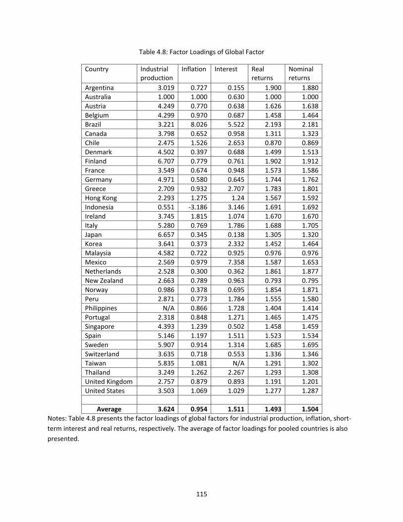
115
Table 4.8: Factor Loadings of Global Factor
Country Industrial production
Inflation Interest Real returns
Nominal returns
Argentina 3.019 0.727 0.155 1.900 1.880
Australia 1.000 1.000 0.630 1.000 1.000
Austria 4.249 0.770 0.638 1.626 1.638
Belgium 4.299 0.970 0.687 1.458 1.464
Brazil 3.221 8.026 5.522 2.193 2.181
Canada 3.798 0.652 0.958 1.311 1.323
Chile 2.475 1.526 2.653 0.870 0.869
Denmark 4.502 0.397 0.688 1.499 1.513
Finland 6.707 0.779 0.761 1.902 1.912
France 3.549 0.674 0.948 1.573 1.586
Germany 4.971 0.580 0.645 1.744 1.762
Greece 2.709 0.932 2.707 1.783 1.801
Hong Kong 2.293 1.275 1.24 1.567 1.592
Indonesia 0.551 -3.186 3.146 1.691 1.692
Ireland 3.745 1.815 1.074 1.670 1.670
Italy 5.280 0.769 1.786 1.688 1.705
Japan 6.657 0.345 0.138 1.305 1.320
Korea 3.641 0.373 2.332 1.452 1.464
Malaysia 4.582 0.722 0.925 0.976 0.976
Mexico 2.569 0.979 7.358 1.587 1.653
Netherlands 2.528 0.300 0.362 1.861 1.877
New Zealand 2.663 0.789 0.963 0.793 0.795
Norway 0.986 0.378 0.695 1.854 1.871
Peru 2.871 0.773 1.784 1.555 1.580
Philippines N/A 0.866 1.728 1.404 1.414
Portugal 2.318 0.848 1.271 1.465 1.475
Singapore 4.393 1.239 0.502 1.458 1.459
Spain 5.146 1.197 1.511 1.523 1.534
Sweden 5.907 0.914 1.314 1.685 1.695
Switzerland 3.635 0.718 0.553 1.336 1.346
Taiwan 5.835 1.081 N/A 1.291 1.302
Thailand 3.249 1.262 2.267 1.293 1.308
United Kingdom 2.757 0.879 0.893 1.191 1.201
United States 3.503 1.069 1.029 1.277 1.287
Average 3.624 0.954 1.511 1.493 1.504
Notes: Table 4.8 presents the factor loadings of global factors for industrial production, inflation, short-
term interest and real returns, respectively. The average of factor loadings for pooled countries is also
presented.
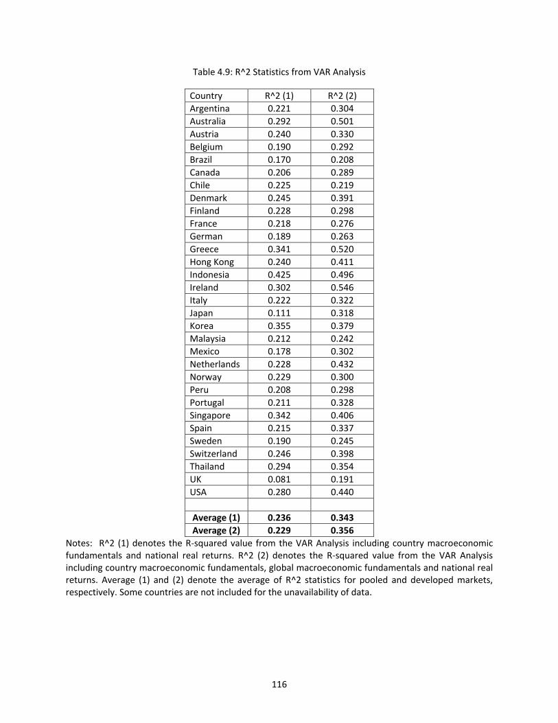
116
Table 4.9: R^2 Statistics from VAR Analysis
Country R^2 (1) R^2 (2)
Argentina 0.221 0.304
Australia 0.292 0.501
Austria 0.240 0.330
Belgium 0.190 0.292
Brazil 0.170 0.208
Canada 0.206 0.289
Chile 0.225 0.219
Denmark 0.245 0.391
Finland 0.228 0.298
France 0.218 0.276
German 0.189 0.263
Greece 0.341 0.520
Hong Kong 0.240 0.411
Indonesia 0.425 0.496
Ireland 0.302 0.546
Italy 0.222 0.322
Japan 0.111 0.318
Korea 0.355 0.379
Malaysia 0.212 0.242
Mexico 0.178 0.302
Netherlands 0.228 0.432
Norway 0.229 0.300
Peru 0.208 0.298
Portugal 0.211 0.328
Singapore 0.342 0.406
Spain 0.215 0.337
Sweden 0.190 0.245
Switzerland 0.246 0.398
Thailand 0.294 0.354
UK 0.081 0.191
USA 0.280 0.440
Average (1) 0.236 0.343
Average (2) 0.229 0.356
Notes: R^2 (1) denotes the R-squared value from the VAR Analysis including country macroeconomic fundamentals and national real returns. R^2 (2) denotes the R-squared value from the VAR Analysis including country macroeconomic fundamentals, global macroeconomic fundamentals and national real returns. Average (1) and (2) denote the average of R^2 statistics for pooled and developed markets, respectively. Some countries are not included for the unavailability of data.
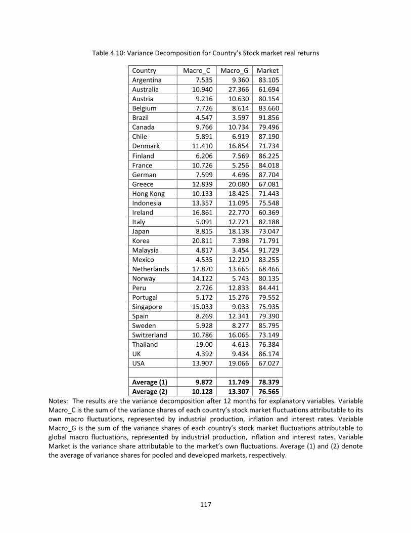
117
Table 4.10: Variance Decomposition for Country’s Stock market real returns
Country Macro_C Macro_G Market
Argentina 7.535 9.360 83.105
Australia 10.940 27.366 61.694
Austria 9.216 10.630 80.154
Belgium 7.726 8.614 83.660
Brazil 4.547 3.597 91.856
Canada 9.766 10.734 79.496
Chile 5.891 6.919 87.190
Denmark 11.410 16.854 71.734
Finland 6.206 7.569 86.225
France 10.726 5.256 84.018
German 7.599 4.696 87.704
Greece 12.839 20.080 67.081
Hong Kong 10.133 18.425 71.443
Indonesia 13.357 11.095 75.548
Ireland 16.861 22.770 60.369
Italy 5.091 12.721 82.188
Japan 8.815 18.138 73.047
Korea 20.811 7.398 71.791
Malaysia 4.817 3.454 91.729
Mexico 4.535 12.210 83.255
Netherlands 17.870 13.665 68.466
Norway 14.122 5.743 80.135
Peru 2.726 12.833 84.441
Portugal 5.172 15.276 79.552
Singapore 15.033 9.033 75.935
Spain 8.269 12.341 79.390
Sweden 5.928 8.277 85.795
Switzerland 10.786 16.065 73.149
Thailand 19.00 4.613 76.384
UK 4.392 9.434 86.174
USA 13.907 19.066 67.027
Average (1) 9.872 11.749 78.379
Average (2) 10.128 13.307 76.565
Notes: The results are the variance decomposition after 12 months for explanatory variables. Variable Macro_C is the sum of the variance shares of each country’s stock market fluctuations attributable to its own macro fluctuations, represented by industrial production, inflation and interest rates. Variable Macro_G is the sum of the variance shares of each country’s stock market fluctuations attributable to global macro fluctuations, represented by industrial production, inflation and interest rates. Variable Market is the variance share attributable to the market’s own fluctuations. Average (1) and (2) denote the average of variance shares for pooled and developed markets, respectively.
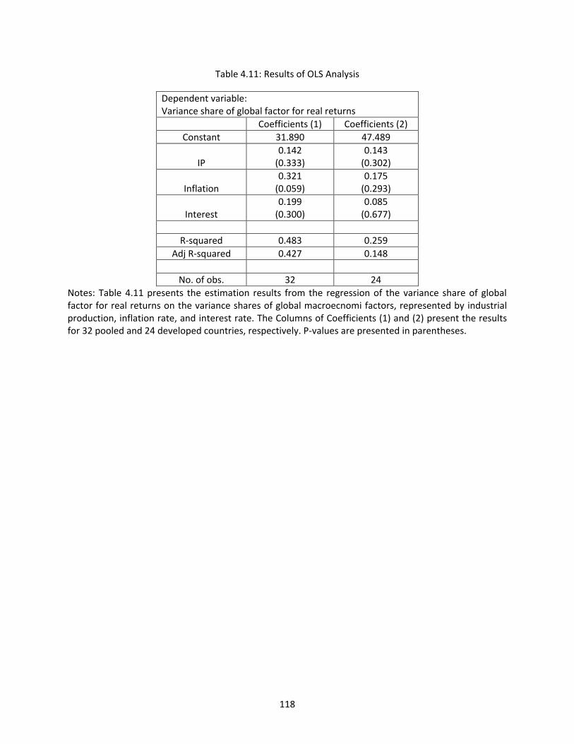
118
Table 4.11: Results of OLS Analysis
Dependent variable: Variance share of global factor for real returns
Coefficients (1) Coefficients (2)
Constant 31.890 47.489
IP 0.142
(0.333) 0.143
(0.302)
Inflation 0.321
(0.059) 0.175
(0.293)
Interest 0.199
(0.300) 0.085
(0.677)
R-squared 0.483 0.259
Adj R-squared 0.427 0.148
No. of obs. 32 24
Notes: Table 4.11 presents the estimation results from the regression of the variance share of global factor for real returns on the variance shares of global macroecnomi factors, represented by industrial production, inflation rate, and interest rate. The Columns of Coefficients (1) and (2) present the results for 32 pooled and 24 developed countries, respectively. P-values are presented in parentheses.
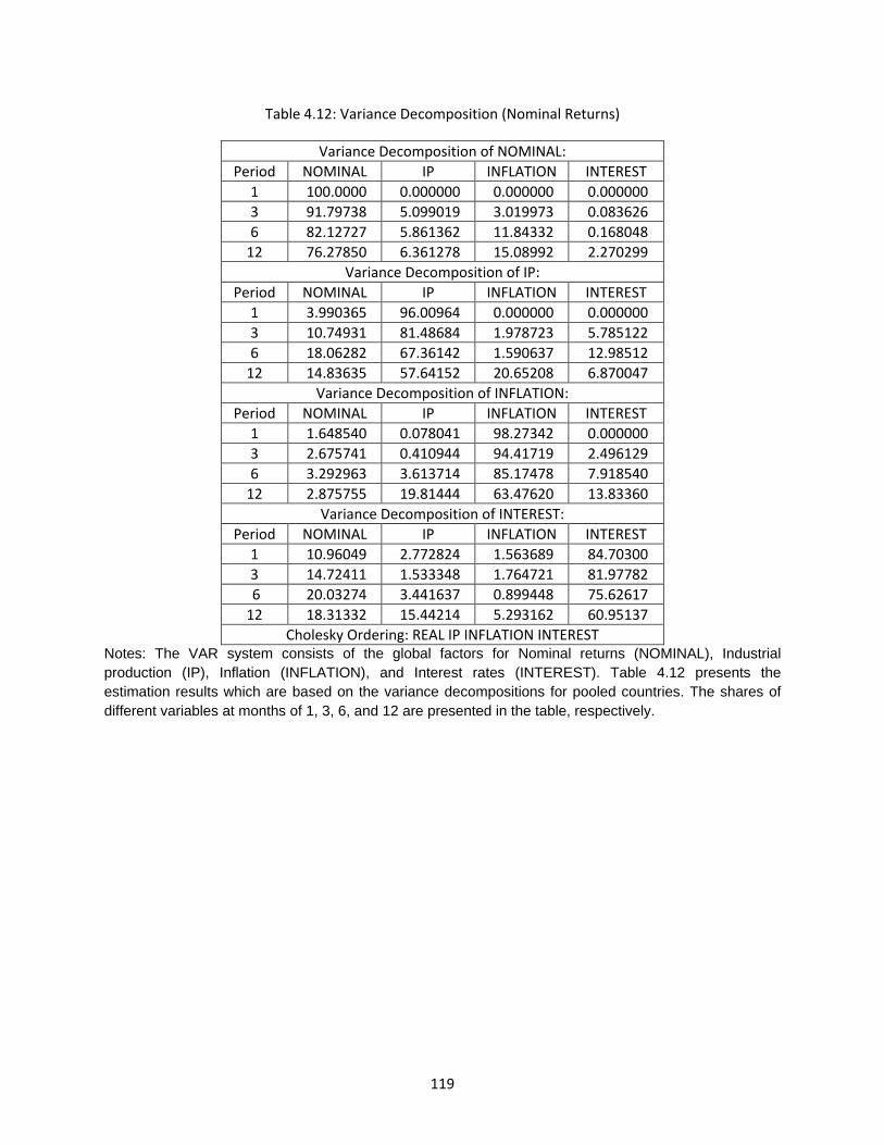
119
Table 4.12: Variance Decomposition (Nominal Returns)
Variance Decomposition of NOMINAL:
Period NOMINAL IP INFLATION INTEREST
1 100.0000 0.000000 0.000000 0.000000
3 91.79738 5.099019 3.019973 0.083626
6 82.12727 5.861362 11.84332 0.168048
12 76.27850 6.361278 15.08992 2.270299
Variance Decomposition of IP:
Period NOMINAL IP INFLATION INTEREST
1 3.990365 96.00964 0.000000 0.000000
3 10.74931 81.48684 1.978723 5.785122
6 18.06282 67.36142 1.590637 12.98512
12 14.83635 57.64152 20.65208 6.870047
Variance Decomposition of INFLATION:
Period NOMINAL IP INFLATION INTEREST
1 1.648540 0.078041 98.27342 0.000000
3 2.675741 0.410944 94.41719 2.496129
6 3.292963 3.613714 85.17478 7.918540
12 2.875755 19.81444 63.47620 13.83360
Variance Decomposition of INTEREST:
Period NOMINAL IP INFLATION INTEREST
1 10.96049 2.772824 1.563689 84.70300
3 14.72411 1.533348 1.764721 81.97782
6 20.03274 3.441637 0.899448 75.62617
12 18.31332 15.44214 5.293162 60.95137
Cholesky Ordering: REAL IP INFLATION INTEREST Notes: The VAR system consists of the global factors for Nominal returns (NOMINAL), Industrial
production (IP), Inflation (INFLATION), and Interest rates (INTEREST). Table 4.12 presents the
estimation results which are based on the variance decompositions for pooled countries. The shares of
different variables at months of 1, 3, 6, and 12 are presented in the table, respectively.
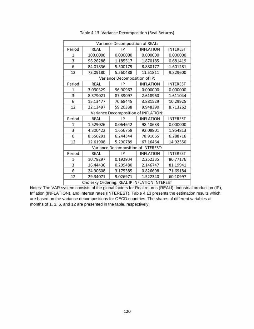
120
Table 4.13: Variance Decomposition (Real Returns)
Variance Decomposition of REAL:
Period REAL IP INFLATION INTEREST
1 100.0000 0.000000 0.000000 0.000000
3 96.26288 1.185517 1.870185 0.681419
6 84.01836 5.500179 8.880177 1.601281
12 73.09180 5.560488 11.51811 9.829600
Variance Decomposition of IP:
Period REAL IP INFLATION INTEREST
1 3.090329 96.90967 0.000000 0.000000
3 8.379021 87.39097 2.618960 1.611044
6 15.13477 70.68445 3.881529 10.29925
12 22.13497 59.20338 9.948390 8.713262
Variance Decomposition of INFLATION:
Period REAL IP INFLATION INTEREST
1 1.529026 0.064642 98.40633 0.000000
3 4.300422 1.656758 92.08801 1.954813
6 8.550291 6.244344 78.91665 6.288716
12 12.61908 5.290789 67.16464 14.92550
Variance Decomposition of INTEREST:
Period REAL IP INFLATION INTEREST
1 10.78297 0.192934 2.252335 86.77176
3 16.44436 0.209480 2.146747 81.19941
6 24.30608 3.175385 0.826698 71.69184
12 29.34071 9.026971 1.522340 60.10997
Cholesky Ordering: REAL IP INFLATION INTEREST Notes: The VAR system consists of the global factors for Real returns (REALl), Industrial production (IP),
Inflation (INFLATION), and Interest rates (INTEREST). Table 4.13 presents the estimation results which
are based on the variance decompositions for OECD countries. The shares of different variables at
months of 1, 3, 6, and 12 are presented in the table, respectively.
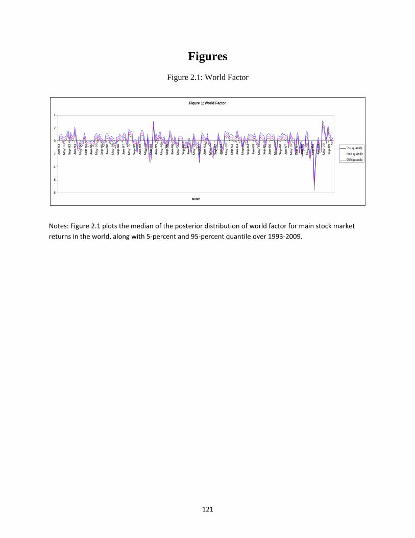
121
Figures
Figure 2.1: World Factor
Figure 1: World Factor
-8
-6
-4
-2
0
2
4
Ja
n-9
3
Ma
y-9
3
Se
p-9
3
Ja
n-9
4
Ma
y-9
4
Se
p-9
4
Ja
n-9
5
Ma
y-9
5
Se
p-9
5
Ja
n-9
6
Ma
y-9
6
Se
p-9
6
Ja
n-9
7
Ma
y-9
7
Se
p-9
7
Ja
n-9
8
Ma
y-9
8
Se
p-9
8
Ja
n-9
9
Ma
y-9
9
Se
p-9
9
Ja
n-0
0
Ma
y-0
0
Se
p-0
0
Ja
n-0
1
Ma
y-0
1
Se
p-0
1
Ja
n-0
2
Ma
y-0
2
Se
p-0
2
Ja
n-0
3
Ma
y-0
3
Se
p-0
3
Ja
n-0
4
Ma
y-0
4
Se
p-0
4
Ja
n-0
5
Ma
y-0
5
Se
p-0
5
Ja
n-0
6
Ma
y-0
6
Se
p-0
6
Ja
n-0
7
Ma
y-0
7
Se
p-0
7
Ja
n-0
8
Ma
y-0
8
Se
p-0
8
Ja
n-0
9
Ma
y-0
9
Se
p-0
9
Month
5% quantile
50% quantile
95%quantile
Notes: Figure 2.1 plots the median of the posterior distribution of world factor for main stock market
returns in the world, along with 5-percent and 95-percent quantile over 1993-2009.
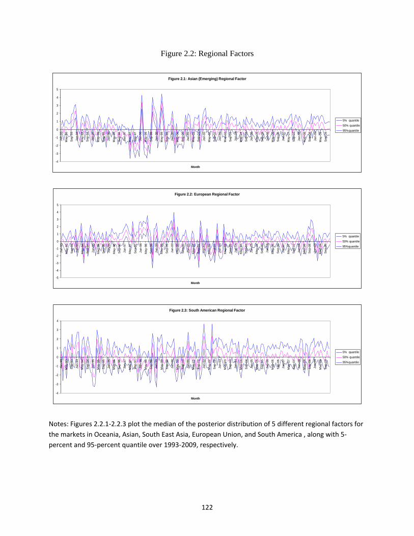
122
Figure 2.2: Regional Factors
Figure 2.1: Asian (Emerging) Regional Factor
-4
-3
-2
-1
0
1
2
3
4
5
Jan-9
3
May-9
3
Sep-9
3
Jan-9
4
May-9
4
Sep-9
4
Jan-9
5
May-9
5
Sep-9
5
Jan-9
6
May-9
6
Sep-9
6
Jan-9
7
May-9
7
Sep-9
7
Jan-9
8
May-9
8
Sep-9
8
Jan-9
9
May-9
9
Sep-9
9
Jan-0
0
May-0
0
Sep-0
0
Jan-0
1
May-0
1
Sep-0
1
Jan-0
2
May-0
2
Sep-0
2
Jan-0
3
May-0
3
Sep-0
3
Jan-0
4
May-0
4
Sep-0
4
Jan-0
5
May-0
5
Sep-0
5
Jan-0
6
May-0
6
Sep-0
6
Jan-0
7
May-0
7
Sep-0
7
Jan-0
8
May-0
8
Sep-0
8
Jan-0
9
May-0
9
Sep-0
9
Month
5% quantile
50% quantile
95%quantile
Figure 2.2: European Regional Factor
-5
-4
-3
-2
-1
0
1
2
3
4
5
Jan-9
3
May-9
3
Sep-9
3
Jan-9
4
May-9
4
Sep-9
4
Jan-9
5
May-9
5
Sep-9
5
Jan-9
6
May-9
6
Sep-9
6
Jan-9
7
May-9
7
Sep-9
7
Jan-9
8
May-9
8
Sep-9
8
Jan-9
9
May-9
9
Sep-9
9
Jan-0
0
May-0
0
Sep-0
0
Jan-0
1
May-0
1
Sep-0
1
Jan-0
2
May-0
2
Sep-0
2
Jan-0
3
May-0
3
Sep-0
3
Jan-0
4
May-0
4
Sep-0
4
Jan-0
5
May-0
5
Sep-0
5
Jan-0
6
May-0
6
Sep-0
6
Jan-0
7
May-0
7
Sep-0
7
Jan-0
8
May-0
8
Sep-0
8
Jan-0
9
May-0
9
Sep-0
9
Month
5% quantile
50% quantile
95%quantile
Figure 2.3: South American Regional Factor
-4
-3
-2
-1
0
1
2
3
4
Jan-9
3
May-9
3
Sep-9
3
Jan-9
4
May-9
4
Sep-9
4
Jan-9
5
May-9
5
Sep-9
5
Jan-9
6
May-9
6
Sep-9
6
Jan-9
7
May-9
7
Sep-9
7
Jan-9
8
May-9
8
Sep-9
8
Jan-9
9
May-9
9
Sep-9
9
Jan-0
0
May-0
0
Sep-0
0
Jan-0
1
May-0
1
Sep-0
1
Jan-0
2
May-0
2
Sep-0
2
Jan-0
3
May-0
3
Sep-0
3
Jan-0
4
May-0
4
Sep-0
4
Jan-0
5
May-0
5
Sep-0
5
Jan-0
6
May-0
6
Sep-0
6
Jan-0
7
May-0
7
Sep-0
7
Jan-0
8
May-0
8
Sep-0
8
Jan-0
9
May-0
9
Sep-0
9
Month
5% quantile
50% quantile
95%quantile
Notes: Figures 2.2.1-2.2.3 plot the median of the posterior distribution of 5 different regional factors for
the markets in Oceania, Asian, South East Asia, European Union, and South America , along with 5-
percent and 95-percent quantile over 1993-2009, respectively.
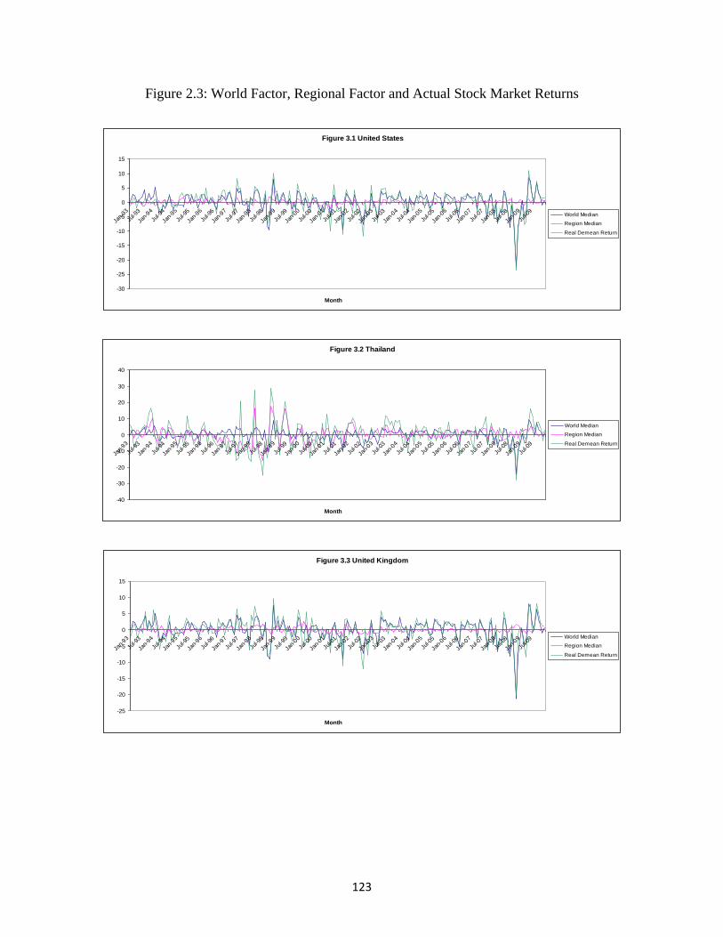
123
Figure 2.3: World Factor, Regional Factor and Actual Stock Market Returns
Figure 3.1 United States
-30
-25
-20
-15
-10
-5
0
5
10
15
Jan-
93
Jul-9
3
Jan-
94
Jul-9
4
Jan-
95
Jul-9
5
Jan-
96
Jul-9
6
Jan-
97
Jul-9
7
Jan-
98
Jul-9
8
Jan-
99
Jul-9
9
Jan-
00
Jul-0
0
Jan-
01
Jul-0
1
Jan-
02
Jul-0
2
Jan-
03
Jul-0
3
Jan-
04
Jul-0
4
Jan-
05
Jul-0
5
Jan-
06
Jul-0
6
Jan-
07
Jul-0
7
Jan-
08
Jul-0
8
Jan-
09
Jul-0
9
Month
World Median
Region Median
Real Demean Return
Figure 3.2 Thailand
-40
-30
-20
-10
0
10
20
30
40
Jan-
93
Jul-9
3
Jan-
94
Jul-9
4
Jan-
95
Jul-9
5
Jan-
96
Jul-9
6
Jan-
97
Jul-9
7
Jan-
98
Jul-9
8
Jan-
99
Jul-9
9
Jan-
00
Jul-0
0
Jan-
01
Jul-0
1
Jan-
02
Jul-0
2
Jan-
03
Jul-0
3
Jan-
04
Jul-0
4
Jan-
05
Jul-0
5
Jan-
06
Jul-0
6
Jan-
07
Jul-0
7
Jan-
08
Jul-0
8
Jan-
09
Jul-0
9
Month
World Median
Region Median
Real Demean Return
Figure 3.3 United Kingdom
-25
-20
-15
-10
-5
0
5
10
15
Jan-
93
Jul-9
3
Jan-
94
Jul-9
4
Jan-
95
Jul-9
5
Jan-
96
Jul-9
6
Jan-
97
Jul-9
7
Jan-
98
Jul-9
8
Jan-
99
Jul-9
9
Jan-
00
Jul-0
0
Jan-
01
Jul-0
1
Jan-
02
Jul-0
2
Jan-
03
Jul-0
3
Jan-
04
Jul-0
4
Jan-
05
Jul-0
5
Jan-
06
Jul-0
6
Jan-
07
Jul-0
7
Jan-
08
Jul-0
8
Jan-
09
Jul-0
9
Month
World Median
Region Median
Real Demean Return
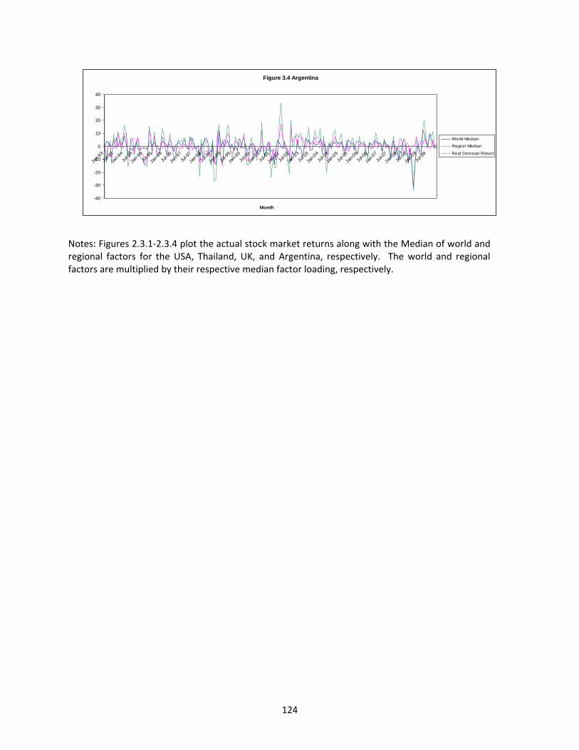
124
Figure 3.4 Argentina
-40
-30
-20
-10
0
10
20
30
40
Jan-
93
Jul-9
3
Jan-
94
Jul-9
4
Jan-
95
Jul-9
5
Jan-
96
Jul-9
6
Jan-
97
Jul-9
7
Jan-
98
Jul-9
8
Jan-
99
Jul-9
9
Jan-
00
Jul-0
0
Jan-
01
Jul-0
1
Jan-
02
Jul-0
2
Jan-
03
Jul-0
3
Jan-
04
Jul-0
4
Jan-
05
Jul-0
5
Jan-
06
Jul-0
6
Jan-
07
Jul-0
7
Jan-
08
Jul-0
8
Jan-
09
Jul-0
9
Month
World Median
Region Median
Real Demean Return
Notes: Figures 2.3.1-2.3.4 plot the actual stock market returns along with the Median of world and regional factors for the USA, Thailand, UK, and Argentina, respectively. The world and regional factors are multiplied by their respective median factor loading, respectively.
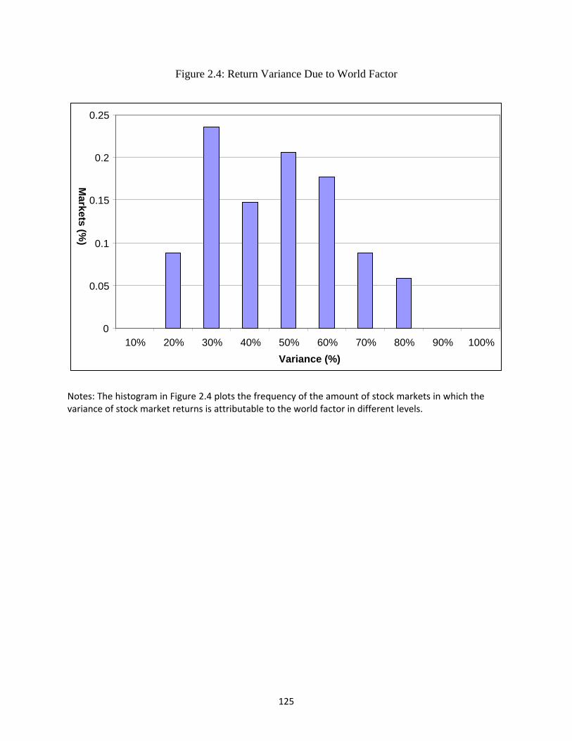
125
Figure 2.4: Return Variance Due to World Factor
Notes: The histogram in Figure 2.4 plots the frequency of the amount of stock markets in which the variance of stock market returns is attributable to the world factor in different levels.
0
0.05
0.1
0.15
0.2
0.25
10% 20% 30% 40% 50% 60% 70% 80% 90% 100%
Variance (%)
Mark
ets
(%)
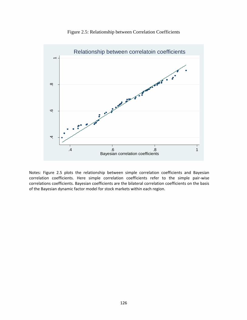
126
Figure 2.5: Relationship between Correlation Coefficients
.4.6
.81
Sim
ple
co
rrela
toin
coeffic
ients
.4 .6 .8 1Bayesian correlation coefficients
Relationship between correlatoin coefficients
Notes: Figure 2.5 plots the relationship between simple correlation coefficients and Bayesian correlation coefficients. Here simple correlation coefficients refer to the simple pair-wise correlations coefficients. Bayesian coefficients are the bilateral correlation coefficients on the basis of the Bayesian dynamic factor model for stock markets within each region.
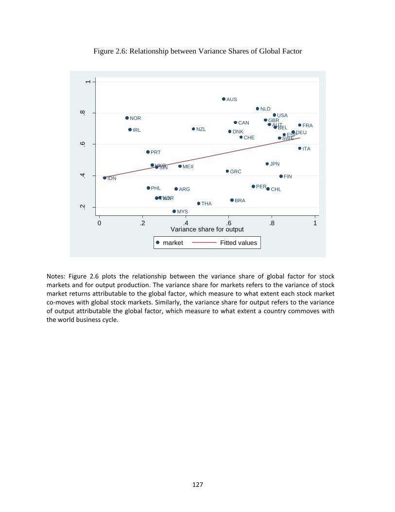
127
Figure 2.6: Relationship between Variance Shares of Global Factor
Notes: Figure 2.6 plots the relationship between the variance share of global factor for stock markets and for output production. The variance share for markets refers to the variance of stock market returns attributable to the global factor, which measure to what extent each stock market co-moves with global stock markets. Similarly, the variance share for output refers to the variance of output attributable the global factor, which measure to what extent a country commoves with the world business cycle.
AUS
NZL
CAN
USA
HKG JPN
IDN
MYS
KOR
SIN
PHL
TWNTHA
GBRAUT
BELDNK
FIN
FRA
DEU
GRC
IRL
ITA
NLD
NOR
PRT
ESPSWECHE
ARG
BRA
CHL
MEX
PER
.2.4
.6.8
1
Va
ria
nc s
ha
re fo
r m
ark
ets
0 .2 .4 .6 .8 1Variance share for output
market Fitted values
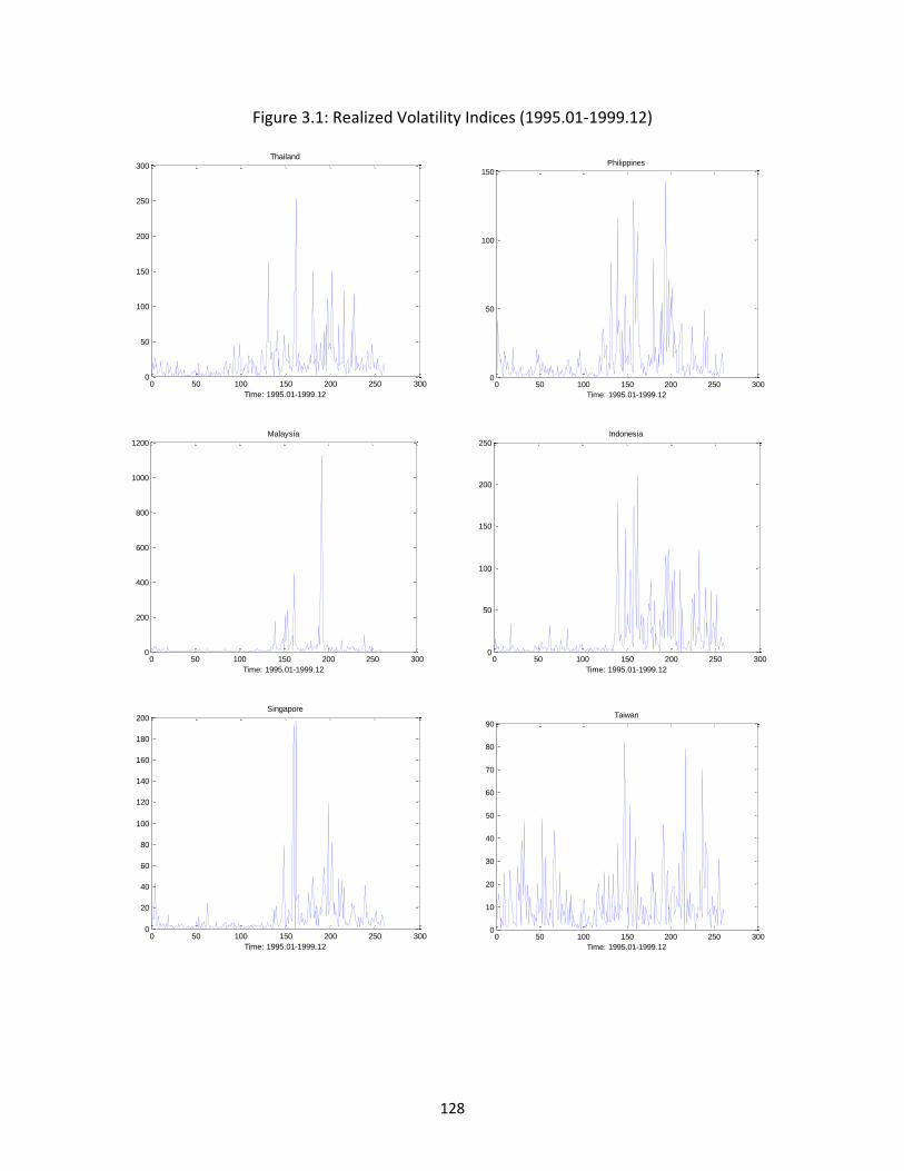
128
Figure 3.1: Realized Volatility Indices (1995.01-1999.12)
0 50 100 150 200 250 3000
50
100
150
200
250
300
Time: 1995.01-1999.12
Thailand
0 50 100 150 200 250 3000
50
100
150
Time: 1995.01-1999.12
Philippines
0 50 100 150 200 250 3000
200
400
600
800
1000
1200
Time: 1995.01-1999.12
Malaysia
0 50 100 150 200 250 3000
50
100
150
200
250
Time: 1995.01-1999.12
Indonesia
0 50 100 150 200 250 3000
20
40
60
80
100
120
140
160
180
200
Time: 1995.01-1999.12
Singapore
0 50 100 150 200 250 3000
10
20
30
40
50
60
70
80
90
Time: 1995.01-1999.12
Taiwan
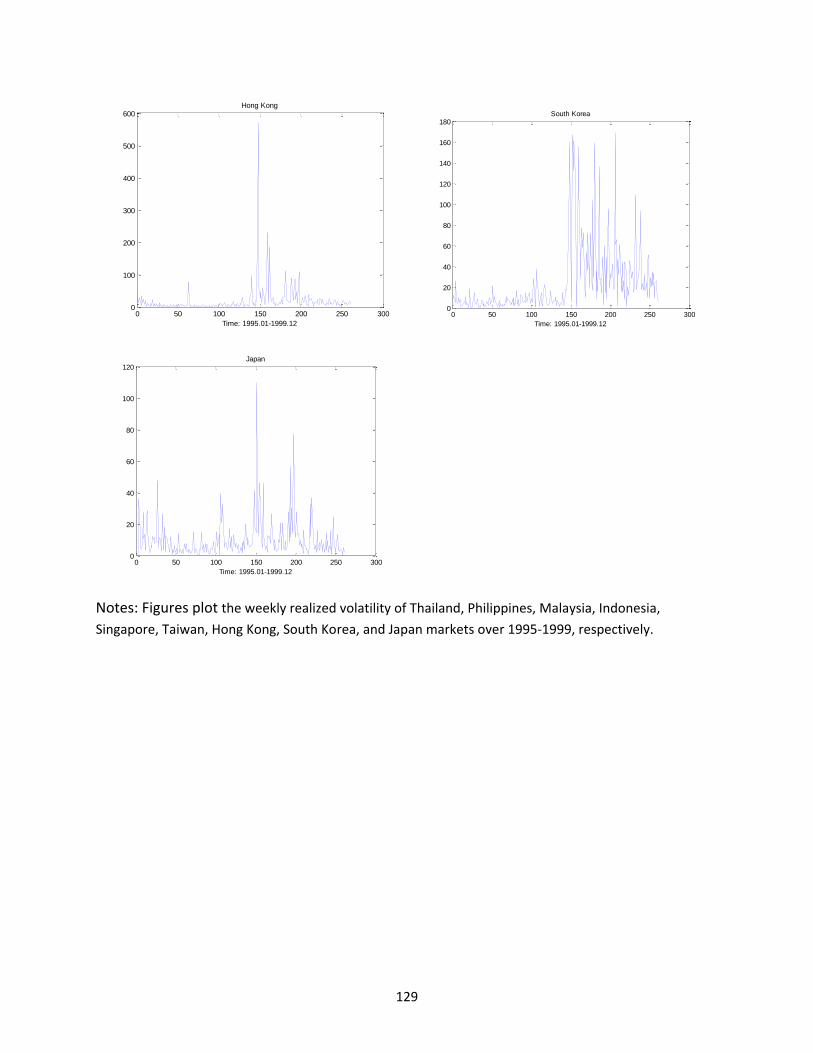
129
0 50 100 150 200 250 3000
100
200
300
400
500
600
Time: 1995.01-1999.12
Hong Kong
0 50 100 150 200 250 3000
20
40
60
80
100
120
140
160
180
Time: 1995.01-1999.12
South Korea
0 50 100 150 200 250 3000
20
40
60
80
100
120
Time: 1995.01-1999.12
Japan
Notes: Figures plot the weekly realized volatility of Thailand, Philippines, Malaysia, Indonesia,
Singapore, Taiwan, Hong Kong, South Korea, and Japan markets over 1995-1999, respectively.
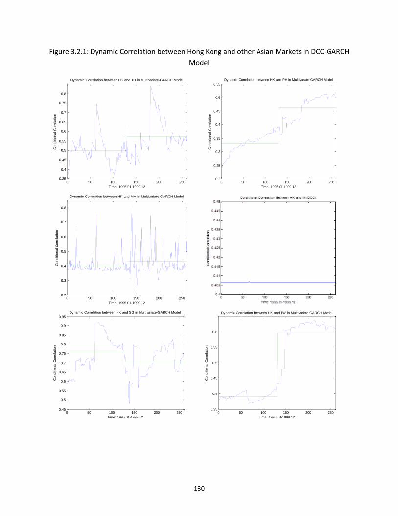
130
Figure 3.2.1: Dynamic Correlation between Hong Kong and other Asian Markets in DCC-GARCH
Model
0 50 100 150 200 2500.35
0.4
0.45
0.5
0.55
0.6
0.65
0.7
0.75
0.8
Time: 1995.01-1999.12
Conditio
nal C
orr
ela
tion
Dynamic Correlation between HK and TH in Multivariate-GARCH Model
0 50 100 150 200 2500.2
0.25
0.3
0.35
0.4
0.45
0.5
0.55
Time: 1995.01-1999.12
Conditio
nal C
orr
ela
tion
Dynamic Correlation between HK and PH in Multivariate-GARCH Model
0 50 100 150 200 2500.2
0.3
0.4
0.5
0.6
0.7
0.8
Time: 1995.01-1999.12
Conditio
nal C
orr
ela
tion
Dynamic Correlation between HK and MA in Multivariate-GARCH Model
0 50 100 150 200 2500.45
0.5
0.55
0.6
0.65
0.7
0.75
0.8
0.85
0.9
0.95
Time: 1995.01-1999.12
Conditio
nal C
orr
ela
tion
Dynamic Correlation between HK and SG in Multivariate-GARCH Model
0 50 100 150 200 2500.35
0.4
0.45
0.5
0.55
0.6
Time: 1995.01-1999.12
Conditio
nal C
orr
ela
tion
Dynamic Correlation between HK and TW in Multivariate-GARCH Model
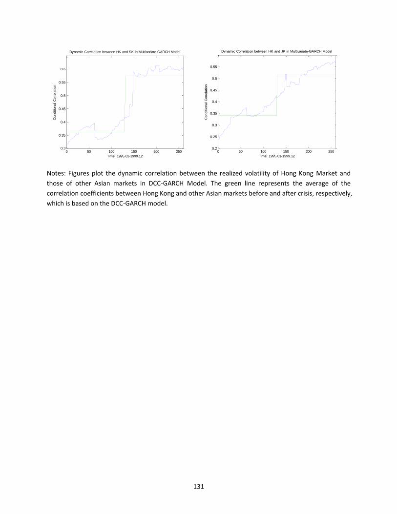
131
0 50 100 150 200 2500.3
0.35
0.4
0.45
0.5
0.55
0.6
Time: 1995.01-1999.12
Conditio
nal C
orr
ela
tion
Dynamic Correlation between HK and SK in Multivariate-GARCH Model
0 50 100 150 200 2500.2
0.25
0.3
0.35
0.4
0.45
0.5
0.55
Time: 1995.01-1999.12
Conditio
nal C
orr
ela
tion
Dynamic Correlation between HK and JP in Multivariate-GARCH Model
Notes: Figures plot the dynamic correlation between the realized volatility of Hong Kong Market and
those of other Asian markets in DCC-GARCH Model. The green line represents the average of the
correlation coefficients between Hong Kong and other Asian markets before and after crisis, respectively,
which is based on the DCC-GARCH model.
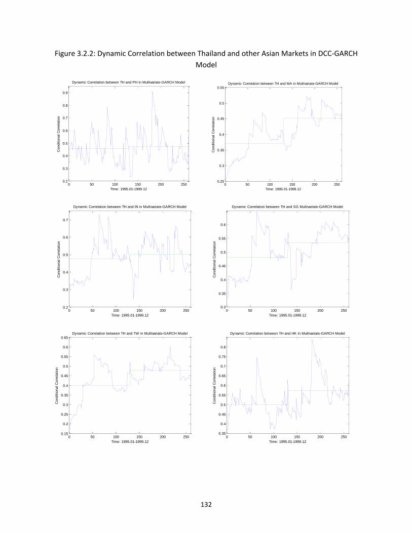
132
Figure 3.2.2: Dynamic Correlation between Thailand and other Asian Markets in DCC-GARCH
Model
0 50 100 150 200 2500.2
0.3
0.4
0.5
0.6
0.7
0.8
0.9
Time: 1995.01-1999.12
Conditio
nal C
orr
ela
tion
Dynamic Correlation between TH and PH in Multivariate-GARCH Model
0 50 100 150 200 250
0.25
0.3
0.35
0.4
0.45
0.5
0.55
Time: 1995.01-1999.12
Conditio
nal C
orr
ela
tion
Dynamic Correlation between TH and MA in Multivariate-GARCH Model
0 50 100 150 200 2500.2
0.3
0.4
0.5
0.6
0.7
Time: 1995.01-1999.12
Conditio
nal C
orr
ela
tion
Dynamic Correlation between TH and IN in Multivariate-GARCH Model
0 50 100 150 200 2500.3
0.35
0.4
0.45
0.5
0.55
0.6
Time: 1995.01-1999.12
Conditio
nal C
orr
ela
tion
Dynamic Correlation between TH and SG Multivariate-GARCH Model
0 50 100 150 200 2500.15
0.2
0.25
0.3
0.35
0.4
0.45
0.5
0.55
0.6
0.65
Time: 1995.01-1999.12
Conditio
nal C
orr
ela
tion
Dynamic Correlation between TH and TW in Multivariate-GARCH Model
0 50 100 150 200 2500.35
0.4
0.45
0.5
0.55
0.6
0.65
0.7
0.75
0.8
Time: 1995.01-1999.12
Conditio
nal C
orr
ela
tion
Dynamic Correlation between TH and HK in Multivariate-GARCH Model
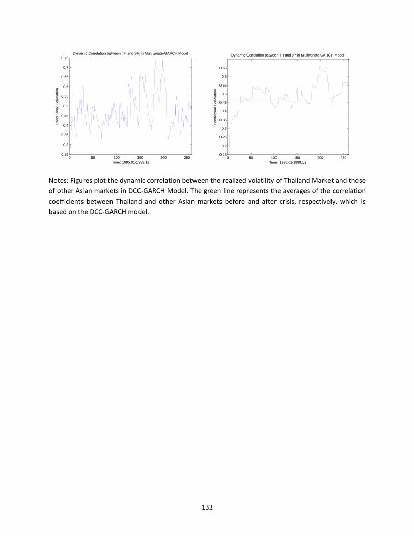
133
0 50 100 150 200 2500.25
0.3
0.35
0.4
0.45
0.5
0.55
0.6
0.65
0.7
0.75
Time: 1995.01-1999.12
Conditio
nal C
orr
ela
tion
Dynamic Correlation between TH and SK in Multivariate-GARCH Model
0 50 100 150 200 2500.15
0.2
0.25
0.3
0.35
0.4
0.45
0.5
0.55
0.6
0.65
Time: 1995.01-1999.12
Conditio
nal C
orr
ela
tion
Dynamic Correlation between TH and JP in Multivariate-GARCH Model
Notes: Figures plot the dynamic correlation between the realized volatility of Thailand Market and those
of other Asian markets in DCC-GARCH Model. The green line represents the averages of the correlation
coefficients between Thailand and other Asian markets before and after crisis, respectively, which is
based on the DCC-GARCH model.
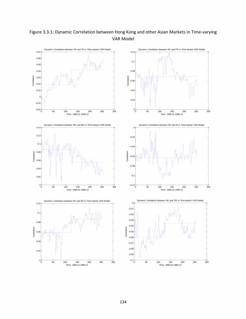
134
Figure 3.3.1: Dynamic Correlation between Hong Kong and other Asian Markets in Time-varying
VAR Model
0 50 100 150 200 250 300-0.02
-0.01
0
0.01
0.02
0.03
0.04
0.05
0.06
0.07
Time: 1995.01-1999.12
Corr
ela
tion
Dynamic Correlation between HK and TH in Time-variant VAR Model
0 50 100 150 200 250 3000
0.02
0.04
0.06
0.08
0.1
0.12
Time: 1995.01-1999.12
Corr
ela
tion
Dynamic Correlation between HK and PH in Time-variant VAR Model
0 50 100 150 200 250 3000
0.02
0.04
0.06
0.08
0.1
0.12
0.14
Time: 1995.01-1999.12
Corr
ela
tion
Dynamic Correlation between HK and MA in Time-variant VAR Model
0 50 100 150 200 250 300-0.12
-0.1
-0.08
-0.06
-0.04
-0.02
0
Time: 1995.01-1999.12
Corr
ela
tion
Dynamic Correlation between HK and IN in Time-variant VAR Model
0 50 100 150 200 250 3000
0.02
0.04
0.06
0.08
0.1
0.12
Time: 1995.01-1999.12
Corr
ela
tion
Dynamic Correlation between HK and SG in Time-variant VAR Model
0 50 100 150 200 250 300-0.1
-0.09
-0.08
-0.07
-0.06
-0.05
-0.04
-0.03
-0.02
-0.01
0
Time: 1995.01-1999.12
Corr
ela
tion
Dynamic Correlation between HK and TW in Time-variant VAR Model
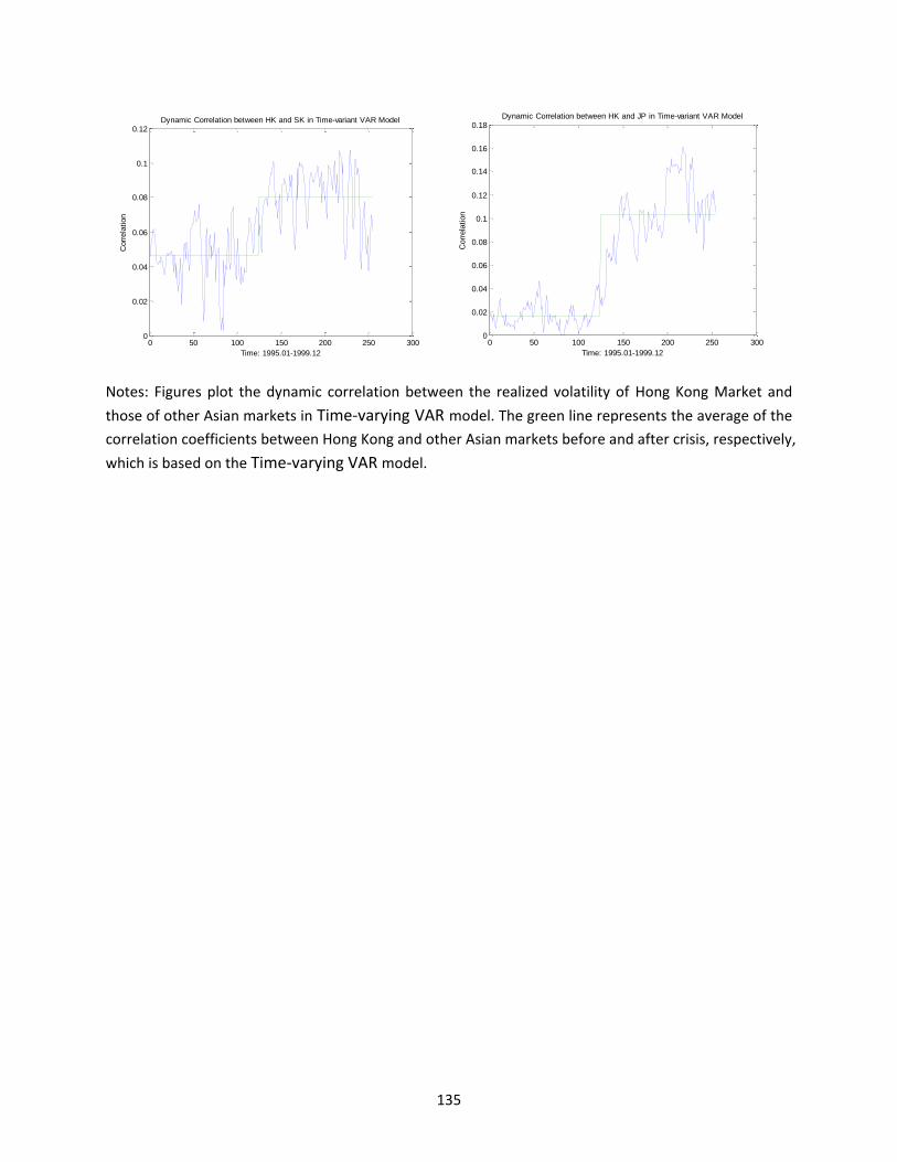
135
0 50 100 150 200 250 3000
0.02
0.04
0.06
0.08
0.1
0.12
Time: 1995.01-1999.12
Corr
ela
tion
Dynamic Correlation between HK and SK in Time-variant VAR Model
0 50 100 150 200 250 3000
0.02
0.04
0.06
0.08
0.1
0.12
0.14
0.16
0.18
Time: 1995.01-1999.12
Corr
ela
tion
Dynamic Correlation between HK and JP in Time-variant VAR Model
Notes: Figures plot the dynamic correlation between the realized volatility of Hong Kong Market and
those of other Asian markets in Time-varying VAR model. The green line represents the average of the
correlation coefficients between Hong Kong and other Asian markets before and after crisis, respectively,
which is based on the Time-varying VAR model.
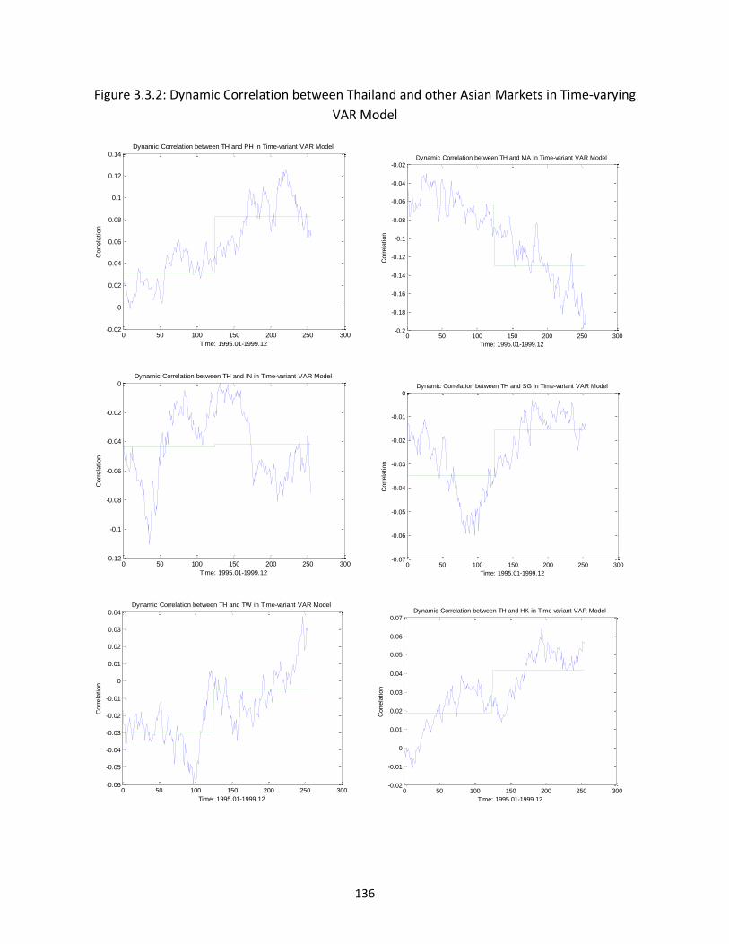
136
Figure 3.3.2: Dynamic Correlation between Thailand and other Asian Markets in Time-varying
VAR Model
0 50 100 150 200 250 300-0.02
0
0.02
0.04
0.06
0.08
0.1
0.12
0.14
Time: 1995.01-1999.12
Corr
ela
tion
Dynamic Correlation between TH and PH in Time-variant VAR Model
0 50 100 150 200 250 300-0.2
-0.18
-0.16
-0.14
-0.12
-0.1
-0.08
-0.06
-0.04
-0.02
Time: 1995.01-1999.12
Corr
ela
tion
Dynamic Correlation between TH and MA in Time-variant VAR Model
0 50 100 150 200 250 300-0.12
-0.1
-0.08
-0.06
-0.04
-0.02
0
Time: 1995.01-1999.12
Corr
ela
tion
Dynamic Correlation between TH and IN in Time-variant VAR Model
0 50 100 150 200 250 300-0.07
-0.06
-0.05
-0.04
-0.03
-0.02
-0.01
0
Time: 1995.01-1999.12
Corr
ela
tion
Dynamic Correlation between TH and SG in Time-variant VAR Model
0 50 100 150 200 250 300-0.06
-0.05
-0.04
-0.03
-0.02
-0.01
0
0.01
0.02
0.03
0.04
Time: 1995.01-1999.12
Corr
ela
tion
Dynamic Correlation between TH and TW in Time-variant VAR Model
0 50 100 150 200 250 300-0.02
-0.01
0
0.01
0.02
0.03
0.04
0.05
0.06
0.07
Time: 1995.01-1999.12
Corr
ela
tion
Dynamic Correlation between TH and HK in Time-variant VAR Model
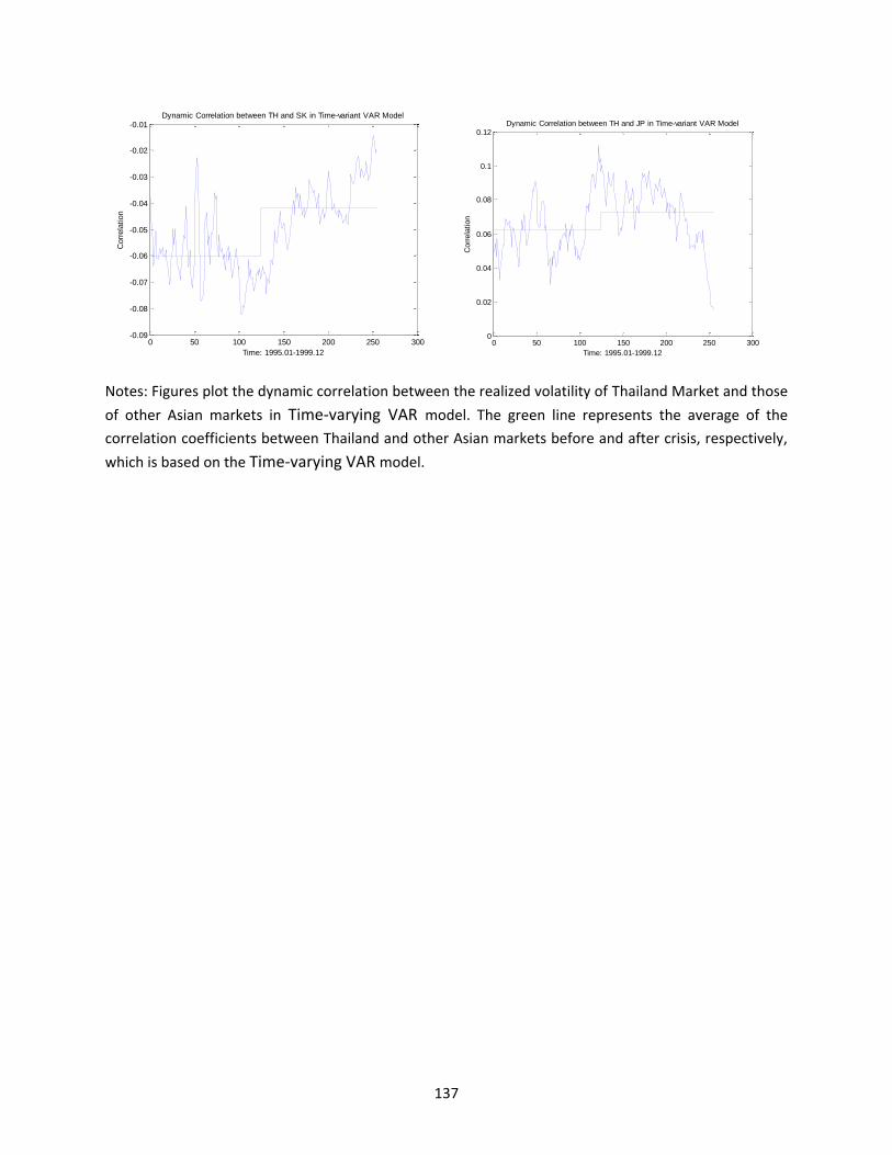
137
0 50 100 150 200 250 300-0.09
-0.08
-0.07
-0.06
-0.05
-0.04
-0.03
-0.02
-0.01
Time: 1995.01-1999.12
Corr
ela
tion
Dynamic Correlation between TH and SK in Time-variant VAR Model
0 50 100 150 200 250 3000
0.02
0.04
0.06
0.08
0.1
0.12
Time: 1995.01-1999.12
Corr
ela
tion
Dynamic Correlation between TH and JP in Time-variant VAR Model
Notes: Figures plot the dynamic correlation between the realized volatility of Thailand Market and those
of other Asian markets in Time-varying VAR model. The green line represents the average of the
correlation coefficients between Thailand and other Asian markets before and after crisis, respectively,
which is based on the Time-varying VAR model.
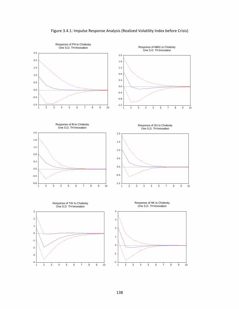
138
Figure 3.4.1: Impulse Response Analysis (Realized Volatility Index before Crisis)
-1.0
-0.5
0.0
0.5
1.0
1.5
2.0
2.5
1 2 3 4 5 6 7 8 9 10
Response of PH to CholeskyOne S.D. TH Innovation
-1.2
-0.8
-0.4
0.0
0.4
0.8
1.2
1.6
2.0
1 2 3 4 5 6 7 8 9 10
Response of MA01 to CholeskyOne S.D. TH Innovation
-0.8
-0.4
0.0
0.4
0.8
1.2
1.6
2.0
1 2 3 4 5 6 7 8 9 10
Response of IN to CholeskyOne S.D. TH Innovation
-1.0
-0.5
0.0
0.5
1.0
1.5
2.0
1 2 3 4 5 6 7 8 9 10
Response of SG to CholeskyOne S.D. TH Innovation
-4
-3
-2
-1
0
1
2
3
1 2 3 4 5 6 7 8 9 10
Response of TW to CholeskyOne S.D. TH Innovation
-2
-1
0
1
2
3
4
1 2 3 4 5 6 7 8 9 10
Response of HK to CholeskyOne S.D. TH Innovation
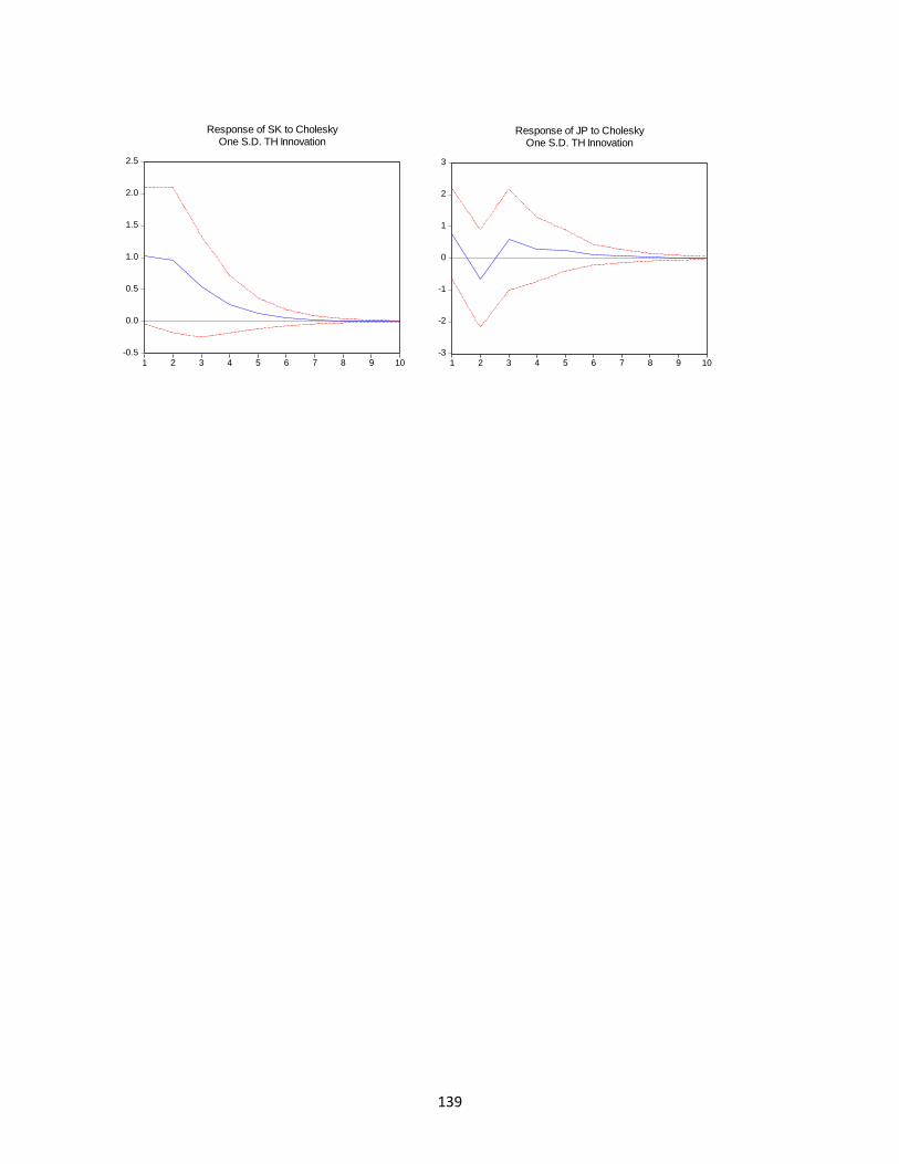
139
-0.5
0.0
0.5
1.0
1.5
2.0
2.5
1 2 3 4 5 6 7 8 9 10
Response of SK to CholeskyOne S.D. TH Innovation
-3
-2
-1
0
1
2
3
1 2 3 4 5 6 7 8 9 10
Response of JP to CholeskyOne S.D. TH Innovation
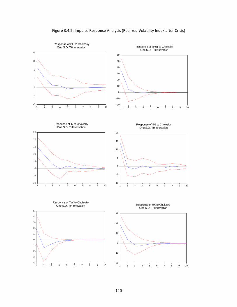
140
Figure 3.4.2: Impulse Response Analysis (Realized Volatility Index after Crisis)
-8
-4
0
4
8
12
16
1 2 3 4 5 6 7 8 9 10
Response of PH to CholeskyOne S.D. TH Innovation
-20
-10
0
10
20
30
40
50
60
1 2 3 4 5 6 7 8 9 10
Response of MA01 to CholeskyOne S.D. TH Innovation
-10
-5
0
5
10
15
20
25
1 2 3 4 5 6 7 8 9 10
Response of IN to CholeskyOne S.D. TH Innovation
-10
-5
0
5
10
15
20
1 2 3 4 5 6 7 8 9 10
Response of SG to CholeskyOne S.D. TH Innovation
-4
-3
-2
-1
0
1
2
3
4
5
1 2 3 4 5 6 7 8 9 10
Response of TW to CholeskyOne S.D. TH Innovation
-20
-10
0
10
20
30
1 2 3 4 5 6 7 8 9 10
Response of HK to CholeskyOne S.D. TH Innovation
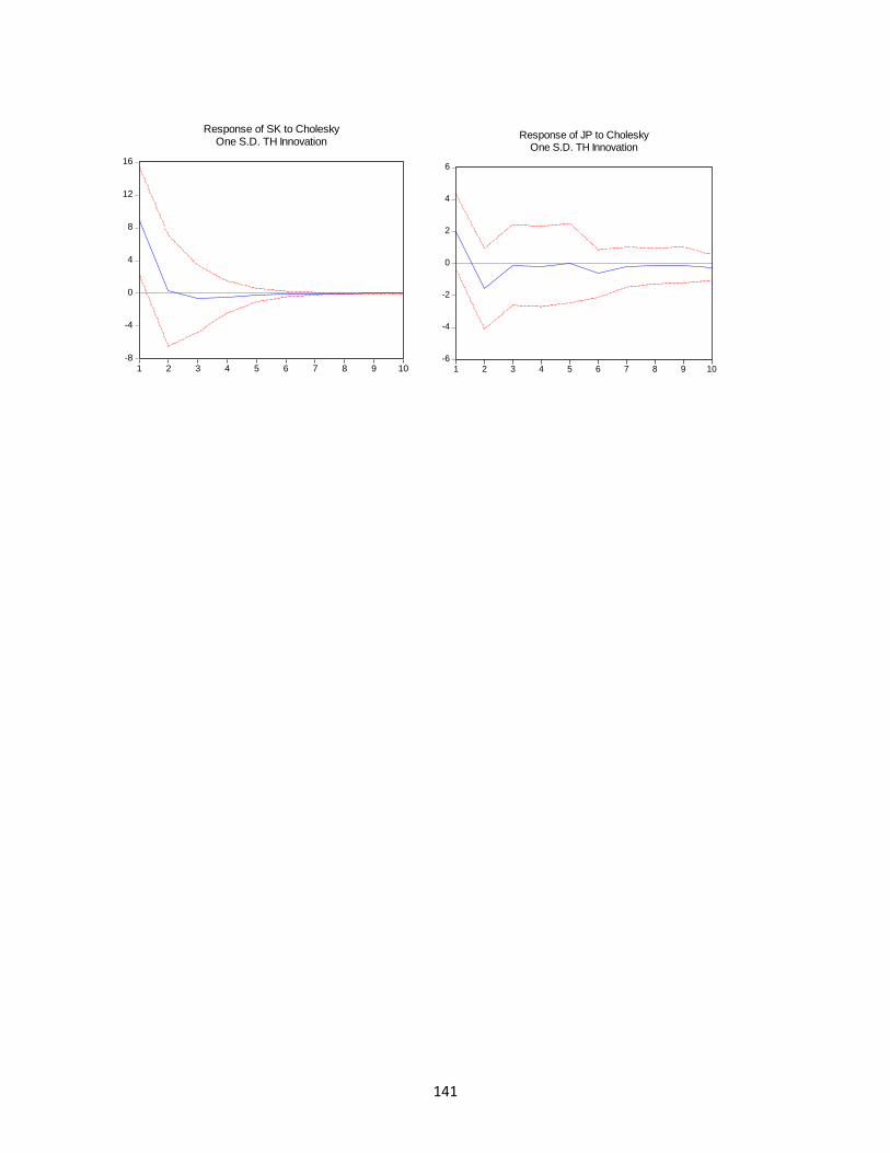
141
-8
-4
0
4
8
12
16
1 2 3 4 5 6 7 8 9 10
Response of SK to CholeskyOne S.D. TH Innovation
-6
-4
-2
0
2
4
6
1 2 3 4 5 6 7 8 9 10
Response of JP to CholeskyOne S.D. TH Innovation
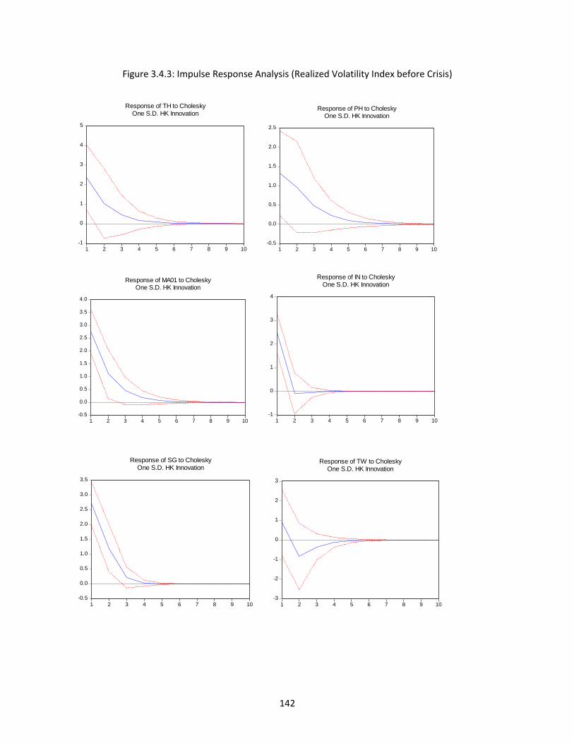
142
Figure 3.4.3: Impulse Response Analysis (Realized Volatility Index before Crisis)
-1
0
1
2
3
4
5
1 2 3 4 5 6 7 8 9 10
Response of TH to CholeskyOne S.D. HK Innovation
-0.5
0.0
0.5
1.0
1.5
2.0
2.5
1 2 3 4 5 6 7 8 9 10
Response of PH to CholeskyOne S.D. HK Innovation
-0.5
0.0
0.5
1.0
1.5
2.0
2.5
3.0
3.5
4.0
1 2 3 4 5 6 7 8 9 10
Response of MA01 to CholeskyOne S.D. HK Innovation
-1
0
1
2
3
4
1 2 3 4 5 6 7 8 9 10
Response of IN to CholeskyOne S.D. HK Innovation
-0.5
0.0
0.5
1.0
1.5
2.0
2.5
3.0
3.5
1 2 3 4 5 6 7 8 9 10
Response of SG to CholeskyOne S.D. HK Innovation
-3
-2
-1
0
1
2
3
1 2 3 4 5 6 7 8 9 10
Response of TW to CholeskyOne S.D. HK Innovation
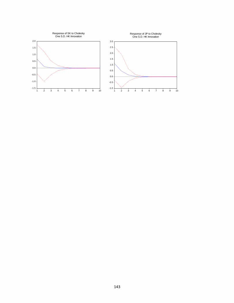
143
-1.5
-1.0
-0.5
0.0
0.5
1.0
1.5
2.0
1 2 3 4 5 6 7 8 9 10
Response of SK to CholeskyOne S.D. HK Innovation
-1.0
-0.5
0.0
0.5
1.0
1.5
2.0
2.5
3.0
1 2 3 4 5 6 7 8 9 10
Response of JP to CholeskyOne S.D. HK Innovation
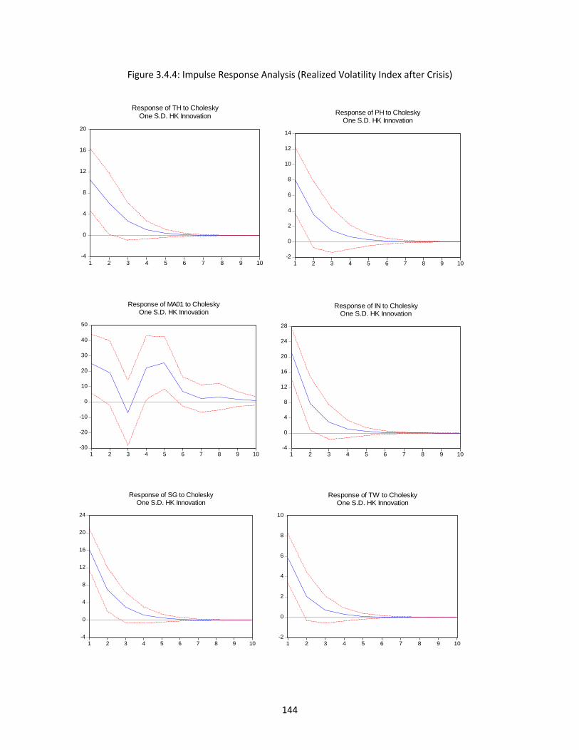
144
Figure 3.4.4: Impulse Response Analysis (Realized Volatility Index after Crisis)
-4
0
4
8
12
16
20
1 2 3 4 5 6 7 8 9 10
Response of TH to CholeskyOne S.D. HK Innovation
-2
0
2
4
6
8
10
12
14
1 2 3 4 5 6 7 8 9 10
Response of PH to CholeskyOne S.D. HK Innovation
-30
-20
-10
0
10
20
30
40
50
1 2 3 4 5 6 7 8 9 10
Response of MA01 to CholeskyOne S.D. HK Innovation
-4
0
4
8
12
16
20
24
28
1 2 3 4 5 6 7 8 9 10
Response of IN to CholeskyOne S.D. HK Innovation
-4
0
4
8
12
16
20
24
1 2 3 4 5 6 7 8 9 10
Response of SG to CholeskyOne S.D. HK Innovation
-2
0
2
4
6
8
10
1 2 3 4 5 6 7 8 9 10
Response of TW to CholeskyOne S.D. HK Innovation
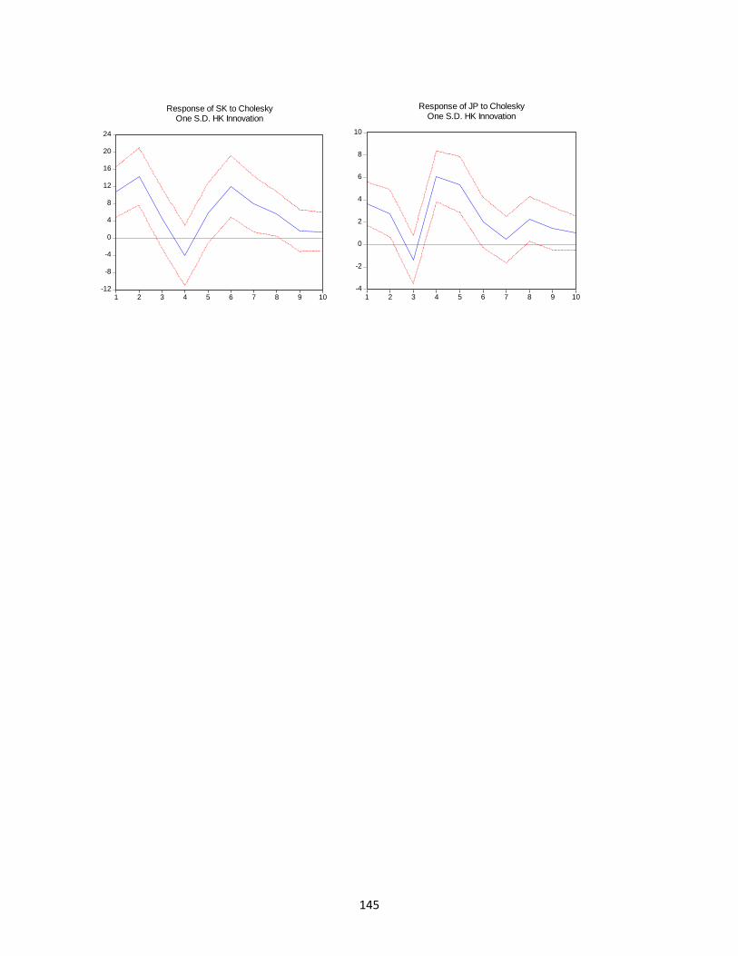
145
-12
-8
-4
0
4
8
12
16
20
24
1 2 3 4 5 6 7 8 9 10
Response of SK to CholeskyOne S.D. HK Innovation
-4
-2
0
2
4
6
8
10
1 2 3 4 5 6 7 8 9 10
Response of JP to CholeskyOne S.D. HK Innovation
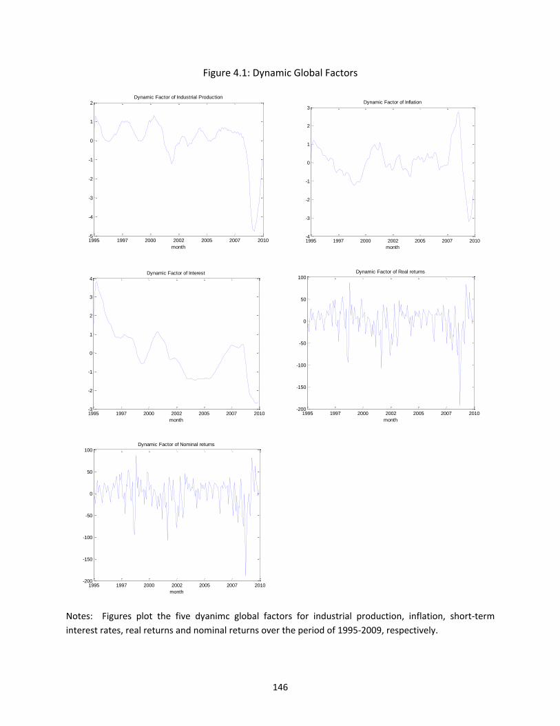
146
Figure 4.1: Dynamic Global Factors
1995 1997 2000 2002 2005 2007 2010-5
-4
-3
-2
-1
0
1
2
month
Dynamic Factor of Industrial Production
1995 1997 2000 2002 2005 2007 2010-4
-3
-2
-1
0
1
2
3
month
Dynamic Factor of Inflation
1995 1997 2000 2002 2005 2007 2010-3
-2
-1
0
1
2
3
4
month
Dynamic Factor of Interest
1995 1997 2000 2002 2005 2007 2010-200
-150
-100
-50
0
50
100
month
Dynamic Factor of Real returns
1995 1997 2000 2002 2005 2007 2010-200
-150
-100
-50
0
50
100
month
Dynamic Factor of Nominal returns
Notes: Figures plot the five dyanimc global factors for industrial production, inflation, short-term
interest rates, real returns and nominal returns over the period of 1995-2009, respectively.
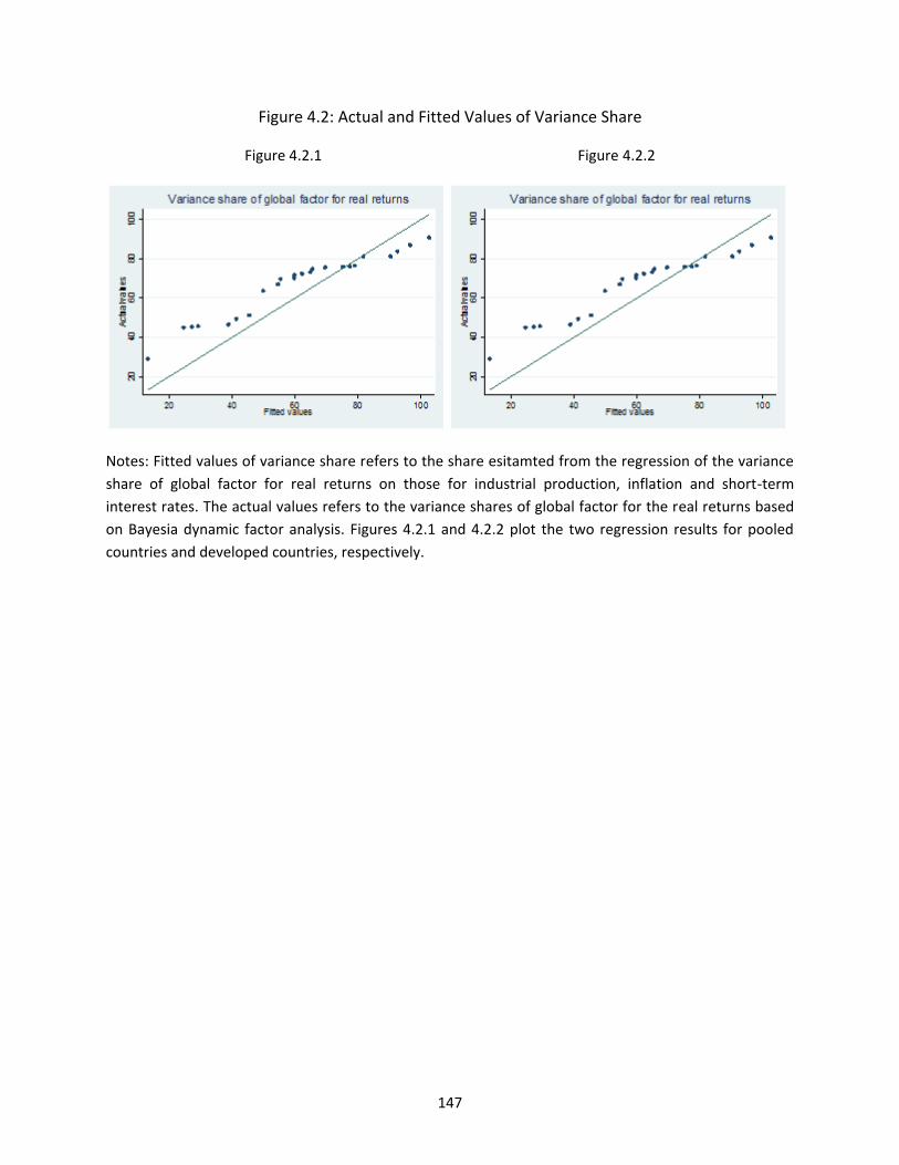
147
Figure 4.2: Actual and Fitted Values of Variance Share
Figure 4.2.1 Figure 4.2.2
Notes: Fitted values of variance share refers to the share esitamted from the regression of the variance
share of global factor for real returns on those for industrial production, inflation and short-term
interest rates. The actual values refers to the variance shares of global factor for the real returns based
on Bayesia dynamic factor analysis. Figures 4.2.1 and 4.2.2 plot the two regression results for pooled
countries and developed countries, respectively.