Three Essays on Real-Financial Linkage in

Dynamic Stochastic General Equilibrium Models

by

Abeer Reza

A thesis submitted to the Faculty of Graduate and Postdoctoral Affairs

in partial fulfilment of the requirements for the degree of

Doctor of Philosophy

in

Economics

Department of Economics

Carleton University

Ottawa, Ontario, Canada

c©2013

Abeer Reza

Abstract

In this thesis, I contribute to the growing literature on the linkage between real

and financial sectors, and study how financial frictions affect responses of important

economic variables to different shocks in a New-Keynesian dynamic stochastic general

equilibrium (DSGE) framework.

The first chapter of this thesis shows that financial frictions can mitigate an im-

portant puzzle in the literature related to investment-specific technology shocks. Ev-

idence from estimated DSGE models and SVAR analysis suggests that investment

shocks are an important source of business cycle fluctuation in the post-war U.S.

economy. In most models that include investment shocks, consumption falls on im-

pact, contradicting its observed comovement with investment, hours worked and out-

put over the business cycle. This chapter shows that introducing financial frictions

alongside endogenous capacity utilization in a New-Keynesian model can produce a

positive consumption response to an investment shock. By attenuating the response

of investment, the financial accelerator mechanism suppresses households’ intertem-

poral substitution towards savings and allows consumption to rise. Search frictions in

the labour market introduce a wedge between marginal product of labour and wages

determined through Nash bargaining and magnify the positive consumption response.

The second chapter of this thesis documents a new challenge for a class of models

with binding borrowing constraints related to government spending shocks. We high-

light that DSGE models with housing and collateralized borrowing predict a fall in

ii

both house prices and consumption following positive government spending shocks.

The quasi-constant shadow value of lenders’ housing and the negative wealth effect of

future tax increases on their consumption are the key reasons for this result. By con-

trast, we show house prices and consumption in the U.S. rise after identified positive

government spending shocks, using a structural vector autoregression methodology

and accounting for anticipated effects. The counterfactual joint response of house

prices and consumption poses a new challenge when using this class of models to

address policy issues for the housing market which have come to fore due to the weak

recovery after the 2008 financial crisis.

The final chapter of this thesis develops a search-theoretic banking model in a New

Keynesian DSGE framework that can simultaneously explain cyclical movements in

interest spreads and flows in gross loan creation and destruction, that were recently

emphasized in the literature. The model features endogenous match separation, and

allows bank loans for productive capital purchases to vary in both intensive and ex-

tensive margins. Search frictions in the banking sector generates a counter-cyclical

interest spread that amplifies business-cycles. In addition, the model generates re-

sponses in gross loan destruction and net loan flows to a credit supply shock that can

qualitatively match empirical responses estimated in a vector auto-regression frame-

work.

iii

To my daughters,

Mayabee Reza and Mohini Reza,

and to my younger sister,

Krishty Reza

May you find joy in learning and discovery.

iv

Acknowledgements

I thank my thesis supervisor, teacher, and mentor, Hashmat Khan, for his invaluable

guidance and constant encouragement throughout the dissertation process, despite

the occasional physical distance between us. He taught me vital computation skills,

and supported me in developing them further through external training. He taught

me to ask the right questions, and to remain determined in following a research

project to its end. I especially enjoyed working with him in the ongoing project that

has resulted in the second chapter of the dissertation. I look forward to many fruitful

collaborations with him in the future.

I thank my committee members, Lilia Karnizova and Chris Gunn, for timely and

helpful feedback. I am particularly thankful to Huntley Schaller for his insightful

comments, and for raising difficult questions that has helped me clarify the core

economic mechanisms involved in the models presented here. He taught me, through

trial by fire, important presentation skills, and how to develop solid arguments.

I am very thankful to Lynda Khalaf, who has also been a true mentor for me. Her

own work has provided me with important perspective about mine. The experience

of working as a teaching assistant for her research methodology course has taught me

much about good research skills, and helped me further develop my own arguments

for this dissertation. I am extremely grateful for her constant encouragement that was

invaluable to me on a personal level in sustaining my focus throughout the dissertation

process.

v

I am grateful to Makoto Nirei for his choice of teaching material for the PhD

macro core course. Without it, I would not have the background to continue working

in my current field of interest, and this dissertation would have looked very different.

I thank Larry Schembri for providing me with an opportunity for an internship

at the Bank of Canada; and Ali Dib, whose work inspired me to pursue research on

real-financial linkage. I am grateful to Silvio Contessi and Yuriy Gorodnichenko for

providing me with valuable data used in the last two chapters of this dissertation.

I am thankful to my friends and forerunners, Subrata Sarkar, Sadaquat Junayed,

Faisal Arif, and Rizwana Arif, for paving the way ahead. I am particuarly thankful

to Subrata Sarker for his valuable comments on the final chapter of this dissertation.

I have benefited greatly from discussions with my colleagues and classmates, Af-

shan Dar, Charles Saunders, and Anand Acharya on matters economic and otherwise.

Thanks also to the many faculty and staff of the Economics department at Carleton

University for their encouragement and support, that has made my time at the de-

partment enjoyable.

I am especially thankful for my oasis during the long years at Carleton – Bangla

boys and fellow grad students, Mahbub Choudhuri, Mohammad Zulhasnine, Jakir

Talukar, Salehin Khan-Chowdhury, and Hossain Rabbi; as well as Aad-Yean Faisal

and Asfin Haidar. I am particular thankful to Humayra Kabir for looking after my

daughter, Mayabee, at a crucial juncture, whithout which I would have had a harder

time getting started on my dissertation.

I am deeply grateful to my parents, my aunts and uncles, my in-laws, and my

younger sister, without whose love and support, I would not be here. Thanks es-

pecially to my grandfather, Shamsul Haque, my aunt Shamima Ferdous, and my

parents, Afroza Banu and Mohsin Reza for raising me with a love and respect for

life-long learning. Thank you for understanding how important this has been to me,

vi

and for being patient as I finished.

Thanks to my two daughters, pieces of my heart, Mayabee and Mohini, for your

love and patience (even though you don’t know how patient you have been), as your

Baba spent late nights at the library.

Finally, my greatest thanks go to my wife, Emily Reza, without whose endless

patience and support, none of this would be possible. She encouraged me to fulfill my

dream, supported the family, and patiently dealt with life during my long working

hours away from home. She is the rock that holds our family together, and the source

of my inspiration to constantly strive to better myself.

vii

Table of Contents

Abstract ii

Acknowledgements v

1 Introduction 1

2 Financial Frictions, Consumption Response and Investment Shocks 9

2.1 Introduction . . . . . . . . . . . . . . . . . . . . . . . . . . . . . . . . 9

2.2 The Benchmark Model . . . . . . . . . . . . . . . . . . . . . . . . . . 13

2.2.1 Households . . . . . . . . . . . . . . . . . . . . . . . . . . . . 13

2.2.2 Entrepreneurs . . . . . . . . . . . . . . . . . . . . . . . . . . . 15

2.2.3 Employment Agencies . . . . . . . . . . . . . . . . . . . . . . 18

2.2.4 Capital Producers . . . . . . . . . . . . . . . . . . . . . . . . . 24

2.2.5 Retailers . . . . . . . . . . . . . . . . . . . . . . . . . . . . . . 25

2.2.6 Monetary Policy and Aggregation . . . . . . . . . . . . . . . . 26

2.3 Calibration . . . . . . . . . . . . . . . . . . . . . . . . . . . . . . . . 26

2.4 Results . . . . . . . . . . . . . . . . . . . . . . . . . . . . . . . . . . 29

2.5 Conclusion . . . . . . . . . . . . . . . . . . . . . . . . . . . . . . . . 38

Bibliography . . . . . . . . . . . . . . . . . . . . . . . . . . . . . . . . . . 42

3 House Prices, Consumption, and Government Spending Shocks 43

3.1 Introduction . . . . . . . . . . . . . . . . . . . . . . . . . . . . . . . . 43

3.2 Empirical Evidence . . . . . . . . . . . . . . . . . . . . . . . . . . . 47

3.3 A DSGE Model with Housing . . . . . . . . . . . . . . . . . . . . . . 54

3.3.1 Households . . . . . . . . . . . . . . . . . . . . . . . . . . . . 54

3.3.2 Firms . . . . . . . . . . . . . . . . . . . . . . . . . . . . . . . 59

3.3.3 Fiscal and Monetary Policies . . . . . . . . . . . . . . . . . . . 61

3.3.4 Aggregation . . . . . . . . . . . . . . . . . . . . . . . . . . . . 62

3.3.5 Linearization, Calibration, and Model Solution . . . . . . . . . 63

viii

3.4 The Effects of Government Spending Shocks on House Prices and Con-

sumption . . . . . . . . . . . . . . . . . . . . . . . . . . . . . . . . . 66

3.4.1 Housing Production . . . . . . . . . . . . . . . . . . . . . . . 74

3.4.2 Greenwood et al. [1988] Preferences . . . . . . . . . . . . . . . 80

3.5 Conclusion . . . . . . . . . . . . . . . . . . . . . . . . . . . . . . . . . 81

Bibliography . . . . . . . . . . . . . . . . . . . . . . . . . . . . . . . . . . 87

4 Search Frictions, Bank Leverage, and Gross Loan Flows 88

4.1 Introduction . . . . . . . . . . . . . . . . . . . . . . . . . . . . . . . . 88

4.2 The Benchmark Model . . . . . . . . . . . . . . . . . . . . . . . . . . 92

4.2.1 Households . . . . . . . . . . . . . . . . . . . . . . . . . . . . 96

4.2.2 Matching . . . . . . . . . . . . . . . . . . . . . . . . . . . . . 97

4.2.3 Banks . . . . . . . . . . . . . . . . . . . . . . . . . . . . . . . 98

4.2.4 Intermediate Goods Firm . . . . . . . . . . . . . . . . . . . . 102

4.2.5 Nash Bargaining . . . . . . . . . . . . . . . . . . . . . . . . . 105

4.2.6 Capital Producing Firms . . . . . . . . . . . . . . . . . . . . . 107

4.2.7 Retail Sector . . . . . . . . . . . . . . . . . . . . . . . . . . . 108

4.2.8 Resource Constraint and Policy . . . . . . . . . . . . . . . . . 109

4.2.9 Calibration . . . . . . . . . . . . . . . . . . . . . . . . . . . . 110

4.3 Counter-cyclical Interest Spread . . . . . . . . . . . . . . . . . . . . 115

4.3.1 Explanation of the Core Mechanism . . . . . . . . . . . . . . 116

4.4 Credit Supply Shock and Gross Loan Flows . . . . . . . . . . . . . . 123

4.4.1 Data and Estimation . . . . . . . . . . . . . . . . . . . . . . . 125

4.4.2 Model Analysis . . . . . . . . . . . . . . . . . . . . . . . . . . 131

4.5 Conclusion . . . . . . . . . . . . . . . . . . . . . . . . . . . . . . . . 138

Bibliography . . . . . . . . . . . . . . . . . . . . . . . . . . . . . . . . . . 143

A Appendix for Chapter 2 144

A.1 Non-linear Equations for Benchmark Model . . . . . . . . . . . . . . 144

A.2 Log-linearized Equations for Benchmark Model . . . . . . . . . . . . 146

B Appendix for Chapter 3 150

B.1 Data for VAR Analysis . . . . . . . . . . . . . . . . . . . . . . . . . . 150

B.2 Factor Augmented VAR . . . . . . . . . . . . . . . . . . . . . . . . . 151

B.3 Sign Restriction . . . . . . . . . . . . . . . . . . . . . . . . . . . . . . 153

B.4 Non-linear Equations for Benchmark Model . . . . . . . . . . . . . . 155

B.5 Non-linear Equations for Model with Housing Production . . . . . . . 157

ix

B.6 GHH Preferences . . . . . . . . . . . . . . . . . . . . . . . . . . . . . 160

C Appendix for Chapter 4 162

C.1 Timing . . . . . . . . . . . . . . . . . . . . . . . . . . . . . . . . . . 162

C.2 Non-linear Equations for Benchmark Model . . . . . . . . . . . . . . 164

C.3 Log-linearized Equations for Benchmark Model . . . . . . . . . . . . 167

x

List of Tables

2.1 Parameter and steady-state calibration . . . . . . . . . . . . . . . . . 28

3.1 Parameter and steady-state ratios . . . . . . . . . . . . . . . . . . . 65

4.1 Calibration of parameters and steady-state ratios . . . . . . . . . . . 112

4.2 Calibration of parameters and steady-state ratios contd. . . . . . . . . 113

4.3 Correlation of gross loan flows with output . . . . . . . . . . . . . . . 137

4.4 Standard deviation of gross loan flows relative to output . . . . . . . 137

xi

List of Figures

2.1 Impulse responses to investment shock, search frictions in labour market. 31

2.2 Impulse responses to investment shock, competitive labour market. . 33

2.3 Impusle responses to investment shock, comparison of models with and

without labour search. . . . . . . . . . . . . . . . . . . . . . . . . . . 36

3.1 Impulse responses of key variables to a government spending shock

from a Cholesky-identified VAR . . . . . . . . . . . . . . . . . . . . . 50

3.2 Impulse responses of key variables to a government spending shock,

controlling for anticipation effects. . . . . . . . . . . . . . . . . . . . . 53

3.3 Impulse responses of key variables to a government spending shock

from a FAVAR specification. . . . . . . . . . . . . . . . . . . . . . . . 55

3.4 Response to a positive government spending shock. Benchmark model

with fixed housing. . . . . . . . . . . . . . . . . . . . . . . . . . . . . 67

3.5 Robustness to the proportion of impatient borrowers. . . . . . . . . . 71

3.6 Robustness to the loan-to-value ratio. Benchmark model with fixed

housing. . . . . . . . . . . . . . . . . . . . . . . . . . . . . . . . . . . 72

3.7 Robustness to the steady-state housing stock-to-output ratio. . . . . . 73

3.8 The effect of wage stickiness in model with housing production . . . . 78

3.9 The effect of price stickiness in housing . . . . . . . . . . . . . . . . . 79

3.10 Greenwood et al. [1988] preferences in benchmark model with fixed

housing stock . . . . . . . . . . . . . . . . . . . . . . . . . . . . . . . 82

4.1 Model Economy . . . . . . . . . . . . . . . . . . . . . . . . . . . . . . 94

4.2 Comparison of the benchmark model with search frictions in the bank-

ing sector and the standard new Keyenesian model. . . . . . . . . . . 117

4.3 Impulse responses for selected banking sector variables. . . . . . . . . 118

4.4 Sensitivity to the cost of posting loan vacancies. . . . . . . . . . . . . 121

4.5 Sensitivity to the cost of separating existing loans. . . . . . . . . . . . 122

4.6 VAR Impulse responses to an increase in the excess bond premium. . 127

xii

4.7 Net percentage of banks tightening lending and the excess bond premium.128

4.8 VAR impulse responses to an increase in the net percentage of banks

tightening lending standards. . . . . . . . . . . . . . . . . . . . . . . 129

4.9 Benchmark model impulse responses to credit supply shock . . . . . . 133

4.10 Comparison of impulse responses to credit supply shock for different

investment elasticities . . . . . . . . . . . . . . . . . . . . . . . . . . . 134

4.11 Model impulse responses to credit supply shock for elastic investment 135

xiii

Chapter 1

Introduction

Until recently, the literature on business cycle fluctuations seldom considered finan-

cial markets as an important channel through which shocks affect the real economy.

The Modigliani and Miller [1958] theorem, which states that under perfect financial

markets, a firm’s value is independent of its source of funding, was largely interpreted

to imply that financial or credit market conditions have negligible effect on the real

economy. Consequently, notwithstanding a handful of notable exceptions (such as

Bernanke et al. [1999] and Kiyotaki and Moore [1997]), workhorse Neoclassical or

New-Keynesian Dynamic Stochastic General Equilibrium (DSGE) models used by

academics and policy-makers to study the sources and transmission mechanisms of

bysiness cycles, abstracted from the details of financial markets.

The 2007 financial crisis, however, has highlighted that financial markets are an

important channel through which shocks to the economy are transmitted and propa-

gated, and has suggested that they may themselves be important sources of business

cycle fluctuations. Consequently, a growing literature has emerged that studies the

implications of financial frictions on the real economy, and develops DSGE models

that introduce frictions in the financing arragements of agents in the economy. In

these models, the balance-sheet condition of firms or banks, or the presence of par-

1

ticular forms of financing constraints, have important implications for the cyclical

dynamics of aggregate variables.

In this fast-growing literature, frictions are often introduced in financial markets

as a wedge between interest rates paid for internally and externally sourced funds, or

through binding constraints on the quantity of funding available. Such financial fric-

tions amplify cyclical responses to shocks affecting aggregate demand, and attenuate

responses to shocks affecting aggregate supply (Gerali et al. [2010], Christensen and

Dib [2008]). Financial frictions have already been shown to allow general equilbrium

macroeconomic models to achieve a better fit with data (Christensen and Dib [2008]),

or explain a number of outstanding puzzles in the literature related to cyclical dy-

namics of macroeconomic variables.1 At the same time, a number of empirical studies

have found that shocks originating within the financial sector have an important ef-

fect on the real economy, using both reduced-form estimation methods (Gilchrist and

Zakrajsek [2012], Boivin et al. [2012]) as well as estimated DSGE models (Nolan and

Thoenissen [2009]).

In this thesis, I contribute to the growing literature on the linkage between real

and financial sectors, and study how financial frictions affect responses of important

economic variables to different shocks in a DSGE framework. The first chapter of my

thesis shows that financial frictions can mitigate an important puzzle in the literature

related to investment-specific technology shocks, while the second chapter documents

a new challenge for a class of models with binding borrowing constraints related to

government spending shocks. In the third chapter, I develop a search-theoretic model

of the banking sector that can simultaneously explain aggregate movements in interest

spreads, as well as those in disaggregated flows in loan creation and destruction.

1Petrosky-Nadeau and Wasmer [2010] show that financial frictions aid in mitigating a volatilitypuzzle related to labour search models. Monacelli [2009] suggests that financial frictions can mitigatea co-movement puzzle for durable goods production in response to a monetary shock.

2

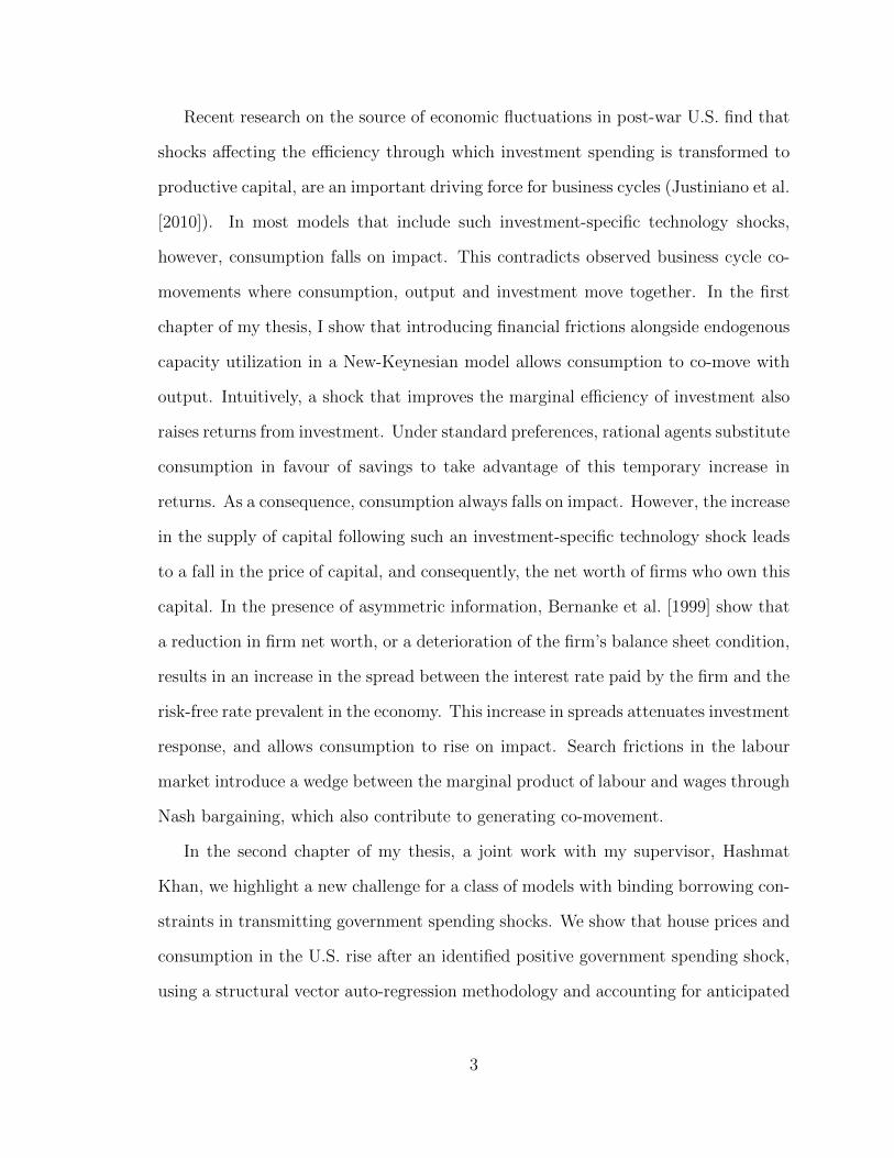
Recent research on the source of economic fluctuations in post-war U.S. find that

shocks affecting the efficiency through which investment spending is transformed to

productive capital, are an important driving force for business cycles (Justiniano et al.

[2010]). In most models that include such investment-specific technology shocks,

however, consumption falls on impact. This contradicts observed business cycle co-

movements where consumption, output and investment move together. In the first

chapter of my thesis, I show that introducing financial frictions alongside endogenous

capacity utilization in a New-Keynesian model allows consumption to co-move with

output. Intuitively, a shock that improves the marginal efficiency of investment also

raises returns from investment. Under standard preferences, rational agents substitute

consumption in favour of savings to take advantage of this temporary increase in

returns. As a consequence, consumption always falls on impact. However, the increase

in the supply of capital following such an investment-specific technology shock leads

to a fall in the price of capital, and consequently, the net worth of firms who own this

capital. In the presence of asymmetric information, Bernanke et al. [1999] show that

a reduction in firm net worth, or a deterioration of the firm’s balance sheet condition,

results in an increase in the spread between the interest rate paid by the firm and the

risk-free rate prevalent in the economy. This increase in spreads attenuates investment

response, and allows consumption to rise on impact. Search frictions in the labour

market introduce a wedge between the marginal product of labour and wages through

Nash bargaining, which also contribute to generating co-movement.

In the second chapter of my thesis, a joint work with my supervisor, Hashmat

Khan, we highlight a new challenge for a class of models with binding borrowing con-

straints in transmitting government spending shocks. We show that house prices and

consumption in the U.S. rise after an identified positive government spending shock,

using a structural vector auto-regression methodology and accounting for anticipated

3

effects. In contrast, DSGE models with housing and collateralized borrowing sim-

ilar to Iacoviello [2005] and Iacoviello and Neri [2010], predict a fall in both house

prices and consumption following a positive government spending shock. The quasi-

constant shadow value of lenders’ housing and the negative wealth effect of future

tax increases on their consumption are the key reasons for this result. Introducing

endogenous housing production, rigidities in house prices or wages, or allowing Green-

wood et al. [1988] preferences do not overturn this result. The counterfactual joint

response of house prices and consumption poses a new challenge when using this class

of models to address policy issues related to the housing market, which have come to

fore due to the weak recovery after the 2008 financial crisis.

In the third and final chapter of my thesis, I develop a banking model that serves

both as a transmission channel for shocks, as well as a point of origin for recessions.

Recently, a growing stream of literature has focused on developing quantitative busi-

ness cycle models that emphasize the bank leverage ratio (the ratio between total

bank assets and bank equity) as a channel for generating counter-cyclical interest

spreads that amplify and prolong business cycles, and consider the banking sector

as a possible source for cyclical movements.2 At the same time, a second stream

of inquiry has used disaggregated bank lending data to reveal important patterns

within the banking sector that are not captured at the aggregate level. In particu-

lar, Dell’Ariccia and Garibaldi [2005] and Contessi and Francis [2010] find that gross

flows in new loan creation move pro-cyclically, while those in loan destruction move

counter-cyclically in the U.S. However, currently available business-cycle models fea-

turing a banking sector cannot account for these movements in disaggregated loan

flows.

The third chapter of my thesis fills this gap in the literature by developing a

2See, among others, the work in Gertler and Karadi [2011], deWalque et al. [2010], Meh andMoran [2010], Gerali et al. [2010], and references therein.

4

search-theoretic banking model that can simultaneously explain cyclical movements

in interest spreads, as well as in disaggregated flows in loan creation and destruction.

Search frictions generate a counter-cyclical wedge between loan and deposit rates

for shocks that have a primary affect on both the supply and demand of loans. In

this economy, loans are generated when a banking loan officer is matched with an

unfunded project. Banks incur costs while searching for new funding opportunities,

or in maintaining existing relationships. A negative shock to bank equity increases the

leverage ratio in banks. To bring the leverage ratio back to its regulated steady-state,

banks reduce their efforts in searching for new matches or in maintaining existing

ones. On the other hand, when a negative technology, or monetary shock hits the

economy, loan-demand falls, as does expected profits for banks. Banks again respond

by reducing search efforts, and hence, new matches. In the benchmark calibration,

the model produces a reduction in the supply of new matches large enough to generate

a counter-cyclical rise in the spread between the policy interest rate determined by a

Taylor-type rule and loan rates facing firms.

Moreover, the model generates responses in gross loan creation and destruction

flows to a credit supply shock that qualitatively match empirical evidence. To show

this, I estimate the effect of a credit supply shock on loan creation and destruction

margins in a VAR framework. I then consider two shocks that can proxy the effects of

a credit supply shock – a one time reduction in bank equity, and a one time increase in

the match separation rate. I show that the shock to bank equity can produce impulse

responses that qualitatively match evidence when investment is elastic to capital

price. Overall, the chapter demonstrates that a search-theoretic banking model is a

step in the right direction in jointly explaining movements in the interest rate spread

and gross loan flows.

5

Bibliography

Ben S. Bernanke, Mark Gertler, and Simon Gilchrist. The financial accelerator in

a quantitative business cycle framework. In J. B. Taylor and M. Woodford, ed-

itors, Handbook of Macroeconomics, volume 1 of Handbook of Macroeconomics,

chapter 21, pages 1341–1393. Elsevier, 1999.

Jean Boivin, Marc P. Giannoni, and Dalibor Stevanovic. Dynamic effects of credit

shocks in a data-rich environment. Manuscript, 2012.

Ian Christensen and Ali Dib. The financial accelerator in an estimated New Keynesian

model. Review of Economic Dynamics, 11(1):155–178, January 2008.

Silvio Contessi and Johanna L. Francis. U.S. commercial bank lending through

2008:q4: new evidence from gross credit flows. Economic Inquiry, 51(1), 2010.

Giovanni Dell’Ariccia and Pietro Garibaldi. Gross credit flows. Review of Economic

Studies, 72(3):665–685, 07 2005.

Gregory deWalque, Olivier Pierrard, and Abdelaziz Rouabah. Financial (in)stability,

supervision and liquidity injections: A dynamic general equilibrium approach. Eco-

nomic Journal, 120(549):1234–1261, December 2010.

Andrea Gerali, Stefano Neri, Luca Sessa, and Federico M. Signoretti. Credit and

banking in a DSGE model of the euro area. Journal of Money, Credit and Banking,

42(s1):107–141, 09 2010.

Mark Gertler and Peter Karadi. A model of unconventional monetary policy. Journal

of Monetary Economics, 58(1):17–34, January 2011.

Simon Gilchrist and Egon Zakrajsek. Credit spreads and business cycle fluctuations.

American Economic Review, 102(4):1692–1720, June 2012.

6

Jeremy Greenwood, Zvi Hercowitz, and Gregory W Huffman. Investment, capacity

utilization, and the real business cycle. American Economic Review, 78(3):402–17,

June 1988.

Matteo Iacoviello. House prices, borrowing constraints, and monetary policy in the

business cycle. American Economic Review, 95(3):739–764, June 2005.

Matteo Iacoviello and Stefano Neri. Housing market spillovers: Evidence from an

estimated DSGE model. American Economic Journal: Macroeconomics, 2(2):125–

64, April 2010.

Alejandro Justiniano, Giorgio E. Primiceri, and Andrea Tambalotti. Investment

shocks and business cycles. Journal of Monetary Economics, 57(2):132–145, March

2010.

Nobuhiro Kiyotaki and John Moore. Credit cycles. Journal of Political Economy,

105(2):211–48, April 1997.

Csaire A. Meh and Kevin Moran. The role of bank capital in the propagation of

shocks. Journal of Economic Dynamics and Control, 34(3):555–576, March 2010.

F. Modigliani and M.H. Miller. The cost of capital, corporation finance and the

theory of investment. The American Economic Review, 48(3):261–297, 1958. ISSN

0002-8282.

Tommaso Monacelli. New Keynesian models, durable goods, and collateral con-

straints. Journal of Monetary Economics, 56(2):242–254, March 2009.

Charles Nolan and Christoph Thoenissen. Financial shocks and the us business cycle.

Journal of Monetary Economics, 56(4):596–604, May 2009.

7

Nicolas Petrosky-Nadeau and Etienne Wasmer. The cyclical volatility of labor mar-

kets under frictional financial markets. IZA Discussion Papers 5131, Institute for

the Study of Labor (IZA), August 2010.

8

Chapter 2

Financial Frictions, Consumption

Response and Investment Shocks

2.1 Introduction

Recent evidence from estimated Dynamic Stochastic General Equilibrium (DSGE)

models (Justiniano et al. [2010], Christensen and Dib [2008]) and Structural Vector

Auto-Regression (SVAR) analysis (Fisher [2006]) suggest that of all macroeconomic

shocks, the one affecting investment technology accounts for the highest proportion

of variation in output, hours and investment seen in post-war U.S. data.1 A com-

mon shortfall for most models in the literature, however, is that consumption falls

on impact for investment shocks. This is in stark contrast to the comovement of

consumption with investment, output and hours observed over the business cycle. In

1Justiniano et al. [2010] estimate a standard new-Keynesian DSGE model similar to Smets andWouters [2007] using Bayesian techniques and find that more than three-quarters of the variation ininvestment, and half the variaion in output in post-war U.S. economy can be explained by shocksto the marginal productity of investment. Christensen and Dib [2008] use maximum likelihood toestimate a monetary DSGE model with financial frictions and also find investment shocks to be themain driver for variations in output and investment. Fisher [2006] differentiates between neutraland investment-specific technology shocks in a SVAR framework and find that the later account fortwo-thirds of the variation in output.

9

this chapter, I show that introducing financial frictions and capacity utilization in a

standard new-Keynesian framework can generate a positive consumption response on

impact for an investment-specific shock. I also show that introducing search frictions

in the labour market increases the magnitude of the positive consumption response,

as well as responses in output, investment and total hours.

The importance of shocks affecting the marginal productivity of investment in

generating business cycles was first emphasized by Keynes [1936]. In contrast to

such investment-specific technology shocks (or investment-shocks), neutral technology

shocks affect the productivity of both installed and new capital as well as that of

labour. Shocks to the marginal productivity of investment, however, are unable to

produce comovement of consumption, hours and output in the standard neoclassical

model. Barro and King [1984] show that under time-separable preferences, temporary

investment shocks increase the real rate of return from investment. In response,

optimizing households postpone consumption in favour of savings through the inter-

temporal substitution channel to take advantage of the temporary rise in returns.

For the same reason, households postpone leisure in favour of labour. Therefore,

consumption and wages move inversely with investment and hours in response to

investment shocks. Since then, the literature has highlighted three mechanisms that

can reduce the limitations of the neoclassical model in generating consumption co-

movement – (a) variable capacity utilization in production (Greenwood et al. [1988],

Khan and Tsoukalas [2011]), (b) wage and price rigidities (Justiniano et al. [2010]),

and (c) differences in the preference structure of households (Furlanetto and Seneca

[2010]).

Greenwood et al. [1988] shows that an endogenous increase in capacity utilization

following an investment shock boosts output, making it more likely to generate posi-

tive consumption co-movement. Khan and Tsoukalas [2011] argues that modelling the

10

cost of capacity utilization as a faster depreciation of installed capital, rather than a

direct reduction in output, is important for a model’s ability to generate consumption

co-movement. Justiniano et al. [2010] find that including both price and wage rigidi-

ties significantly increase the variation in output to investment shocks. Greenwood

et al. [1988], Khan and Tsoukalas [2011] and Furlanetto and Seneca [2010] propose

that special preferences that restrict wealth effects on labour supply are helpful in

generating an increase in hours worked, and consumption, following an investment

shock.

Acknowledging the difficulty of generating a positive consumption co-movement

following a shock to the marginal productivity of investment, Christiano et al. [2010]

make a distinction between investment shocks affecting capital supply and those af-

fecting demand. The later is able to generate positive co-movement of all important

variables, including consumption. Even in the presence of shocks affecting the demand

for capital, Christiano et al. [2010] finds that investment shocks that solely affect cap-

ital supply account for more than a third of the movement in investment for the U.S.

in business cycle frequencies. Consistent with the co-movement problem, however,

these shocks explain only a small proportion of the movement in consumption.

In this chapter, I propose financial frictions as a fourth mechanism that, along

with variable capacity utilization, can generate a positive consumption response. No

other restrictions on wealth effects, or wage rigidities are necessary for this result.

In addition, I show that search frictions in the labour market enhance the positive

consumption response afforded by financial frictions, but is not a necessary element.

Bernanke and Gertler [1989] show that under asymmetric information, the opti-

mal debt contract between a financer and a borrowing firm involves a variable loan-

premium on the cost of lending that depends on the borrowing firm’s balance sheet

position. The resulting financial accelerator mechanism amplifies the effects of de-

11

mand shocks, and attenuates the effects of supply shocks.2 Christensen and Dib

[2008] estimate a sticky-price DSGE model with financial frictions and find that the

financial accelerator mechanism improves the response of macro variables to a variety

of shocks other than to neutral technology. In particular, they also find investment

shocks to be the most important driver of output and investment. However, con-

sumption still responds negatively in their study. This chapter improves their result

by adding capacity utilization, habit formation, and labour search, and generates a

positive consumption response.3

Intuitively, a shock to the marginal productivity of investment increases the supply

of capital in the economy, reducing its price, and consequently the net worth of firms

that own capital. Because of the financial accelerator mechanism, firms with low

net worth are then charged a higher interest rate for loans needed to finance new

investment. This rise in funding cost for firms attenuates their investment activity.

The resulting dampening of the response of savings allows households to increase

their consumption.

The rest of the chapter is organized as follows: section 2.2 describes the benchmark

model that includes financial frictions and labour search. Section 2.3 describes model

calibration. Section 2.4 discusses the impulse reponses to investment shock, offers

explanations for the results, and identifying the contribution of search friction in the

labour market. Section 2.5 provides concluding comments.

2Iacoviello [2005] find a similar property for models using binding borrowing constraints to modelfinancial frictions.

3Note, however, that the main results presented in this chapter is robust to the inclusion of habitformation and search frictions in the labour market. A version of this chapter prepared for journalsubmission, therefore, dispenses of these two assumptions.

12

2.2 The Benchmark Model

The benchmark model adds capacity utilization and labour search to a closed-economy

DSGE model with financial frictions as in Bernanke et al. [1999] and Christensen and

Dib [2008]. The setup for capacity utilization in production technology follows Khan

and Tsoukalas [2011], where the cost of increased capacity utilization is modeled as

faster depreciation of installed capital. Search frictions in the labour market allow

both hours (intensive margin) and employment (extensive margin) to vary across

time.

The economy is populated by a representative household, a continuum of en-

trepreneurs or firms, capital producers, employment agencies, retailers, and a mon-

etary authority. Entrepreneurs produce intermediate goods, invest in capital, and

demand labour inputs. Employment agencies post vacancies to create jobs on be-

half of entrepreneurs, and bargain for wages with workers. Although not explicitly

modeled, the economy also includes financial intermediaries that take deposits from

households, and converts them into business loans that entrepreneurs use to fund

capital investment. Following Bernanke et al. [1999], I assume that asymmetric in-

formation between financiers and entrepreneurs leads to an optimal contract that

imposes a loan premium or markup from financiers to entrepreneurs that depend on

the financial position of entrepreneurs. A retail sector exists to motivate rigidities in

price. Capital producers convert investment spending into productive capital used by

entrepreneurs.

2.2.1 Households

The representative household can be thought of as an extended family containing a

continuum of members indexed on the unit interval. In equilibrium, some members

are employed, while some others are unemployed and searching for jobs. All members

13

are assumed to participate in the labour force. Each member has the following period

utility function:

U(ct, ht) = u(ct)− g(ht)

u(ct) = ln (ct − act−1)

g(ht) =Υ

1 + ζh1+ζt

where ct is real per capita consumption of a final good and ht is hours worked by

an employed member. ζ is the inverse of the Frisch elasticity of labour supply, Υ is

a structural parameter denoting the relative weight of leisure in utility, and a is the

habit persistence parameter.

The representative household maximizes expected lifetime utility:

E0

∞∑t=0

βt [u (ct)−Gt]

subject to the following budget constraint:

ct + dt ≤ wtlt +Rdt−1

dt−1

πt(2.1)

where Gt represents the family’s disutility of labour supply and includes the disutility

from hours for only the employed members of the household.4 lt represents total

labour supplied by the household in return for wages, wt, and dt represents real

savings in financial institutions that earn a gross interest of Rdt . πt = Pt/Pt−1 is

the rate of inflation. Following Merz [1995] and Andolfatto [1996], we assume that

household members perfectly insure each other against fluctuations in consumption.

4Since the level of hours worked is not a choice variable for households, but rather is determinedas an outcome of bargaining between firms and workers, the family’s disutility of labour need notbe specified further. See Trigari [2009] for details.

14

The solution to the household problem implies the following optimality conditions:

1

Rdt

= βEtλt+1

λt

1

πt+1

(2.2)

λt =1

ct − act−1

− βEta

ct+1 − act(2.3)

Equation 2.2 gives the intertemporal Euler condition, while 2.3 relates the shadow

value of income, λt, to current, past, and future consumption in the presence of habit

formation (a > 0).

2.2.2 Entrepreneurs

There is a continuum of entrepreneurs indexed by j ∈ (0, 1) that own capital kjt ,

purchase labour services ljt from employment agencies, and determine capacity uti-

lization ujt to produce a single intermediate good yjt that is sold in a competitive

market at a common real price pwt . Individual firms are subject to an idiosyncratic

shock ωjt ∈ (0, 1) that hits them after decisions on capital and labour services pur-

chasing, and capacity utilization have been made. The firm’s constant returns to

scale production function is given as:

yjt = ωjt(ujtk

jt

)α (ljt)1−α

(2.4)

where α is the share of capital in the production function. The idiosyncratic shock is

normalized so that∫ 1

0ωjtdj = 1 and Etωt+1 = 1.

At the end of each period, entrepreneurs purchase capital kjt+1 at price qt, which is

used for production in the next period. Part of the funds for this capital acquisition

is funded by the firm’s net worth, nwjt , while the remainder is funded through loans

from the financial intermediary.

The financial intermediary takes deposits from households at a gross interest rate

15

of Rdt and provides loans to entrepreneurs for capital purchase at a gross rate of Rl

t.

The financial intermediary does not observe the idiosyncratic shock that hits indi-

vidual entrepreneurs. If the idiosyncratic shock ωjt falls above a threshold parameter

ω, the entrepreneur pays off the debt with interest to the intermediary and adds the

remaining profits from production, net of labour service costs, to their net worth. If,

however, the idiosyncratic shock falls below ω, the entrepreneur claims bankruptcy.

In this case, the financial intermediary retains all profits, and the entrepreneur gets

nothing. Bankruptcy claims require financial intermediaries to conduct costly audits

of the firms before settling claims. Bernanke et al. [1999] show that under this set-

up, the optimal contract between entrepreneurs and financiers imply a loan premium

S (·) that depends on the entrepreneur’s balance sheet position. Specifically, the

loan premium is increasing in the firm’s leverage ratio, i.e., the ratio of assets to net

worth. Underlying microeconomic parameter values, including parameters describing

the threshold idiosyncratic shock and monitoring costs, determine the elasticity of

the loan premium to firm’s leverage ratio.

The financial intermediary sets the gross loan rate as a markup on its expected

opportunity costs of funding:

Rlt = Et

[S

(qtkt+1

nwt

)Rt

πt+1

](2.5)

where we assume that the deposit interest rate, Rdt , equals the risk-free rate, Rt,

by arbitrage. Letting the loan premium elasticity be ψ, we assume that the loan

premium takes the following functional form:

S (·) =

(qtkt+1

nwt

)ψ(2.6)

Following Greenwood et al. [1988] and Khan and Tsoukalas [2011], I model the

16

cost of capacity utilization as faster depreciation of existing capital. In particular, I

assume that the capital depreciation rate, δ(·), is increasing in capacity utilization,

δ′ (u) > 0.

The firm’s optimal choice for labour, capital, and capacity utilization is given by

the following conditions:

wet = (1− α)ϕtytlt

(2.7)

Rlt = Et

[αϕt+1

yt+1

kt+1+ qt+1 (1− δ (ut+1))

qt

](2.8)

αϕtyt

ujt= qtδ

′ (ut) kt (2.9)

where ϕt is the firm’s marginal cost of production. Equation 2.7 equates the firm’s

unit labour cost paid to the employment agency, wet , to the marginal productivity

of labour. Equation 2.8 equates entrepreneurs’ marginal cost of loans, Rlt, to their

marginal benefit. Loans secured in period t are used to purchase capital kt+1 at price

qt. A unit of capital purchased at period t yields a flow benefit to entrepreneurs equal

to the marginal product of capital in the following period, and can be sold at the

prevailing price qt+1, net of depreciation. Finally, equation 2.9 equates the marginal

benefit of increasing capacity utilization to its marginal cost of a faster depreciation

of existing capital.

For firm j that survives bankruptcy this period, the difference between the ex-post

contribution from capital and the ex-ante financing cost of capital available in the

current period is added to its net worth.

nwjt =

[αϕt

yjt

kjt+ qt

(1− δ

(ujt))]

kjt − Et−1

[Rlt−1

(qt−1k

jt − nw

jt−1

)]To ensure that entrepreneurial net worth is never enough to fully finance new

17

capital acquisition without requiring external financing, I follow Bernanke et al. [1999]

and assume that only a fraction ν of firms survive each period. The end-of-period net

worth of the 1 − ν proportion of firms that go out of business is transferred to new

entrants as seed capital sct. Aggregating across firms gives the following expression

for economy-wide net worth:

nwt = ν

[{αϕt

ytkt

+ qt (1− δ (ut))

}kt − Et−1

{Rlt−1 (qt−1kt − nwt−1)

}]+ (1− ν) sct (2.10)

where the ex-ante cost of capital, Et−1Rlt−1 reflects the optimal loan rate determined

by the financial intermediary, and given in equations 2.5 and 2.6.

2.2.3 Employment Agencies

To make the problems of labour market search and financial frictions more tractable,

I separate hiring and vacancy posting activities from the entrepreneur’s problem.

Following Christiano et al. [2011], I assume the existence of employment agencies

that create vacancies and conduct hiring on behalf of entrepreneurs to meet firms’

labour demand. Employment agencies take the price of labour services paid by en-

trepreneurs, wet , as given revenue for each labour hour supplied. Final wages received

by the household, wt, is determined through Nash bargaining between workers and

the employment agencies. To allow labour inputs to vary both on the extensive (em-

ployment) margin as well as the intensive (hours) margin, I assume that each agency

creates a single job, which can either be filled or vacant.

Vacancies, vt, are matched with job seekers, ut, to create new jobs, mt, in each

period through a constant returns to scale matching function:

mt = σmuσt v

1−σt (2.11)

18

where σm is a parameter reflecting the efficiency of the matching process. The prob-

ability that any open vacancy is matched with an job seeker at period t, %t, is given

by:

%t =mt

vt(2.12)

Similarly, the probability that a searching worker will be able to find a job at period

t, ςt, is given by:

ςt =mt

ut(2.13)

I assume that workers that are newly matched in period t start producing in

the next period. An existing match can be separated exogenously each period with

probability ρ. Aggregate employment, nt, therefore, equals the fraction of matched

workers that survived separation, plus the newly formed matches from the last period

that become productive in this period:

nt = (1− ρ)nt−1 +mt−1 (2.14)

Workers separated from their jobs in period t start looking for new jobs immedi-

ately. Since the labour force is normalized to one, the number of searching workers

in period t, ut, is given by:

ut = 1− (1− ρ)nt (2.15)

Bellman Equations

The employment agency gets wet from entrepreneurs and pays wt to the household

for each hour of labour supplied. The value of a filled and active job, Jt, includes

current period’s profits from channeling ht hours of labour from the household to

19

entrepreneurs, plus the continuation value of the job:

Jt = wetht − wtht + Etβλt+1

λt(1− ρ) Jt+1 (2.16)

where the probability of the match surviving till next period is given by (1− ρ).

Since employment agencies are owned by households, the continuation value of the

an active job is discounted by the same stochastic discount factor facing households.

Assume now that it costs an employment agency κ per period to keep a vacancy

open. With probability %t(1 − ρ), net of separation, a vacancy will be filled in this

period and become productive in the next. With probability (1− %t), a vacancy will

remain unfilled in the current period. The value of an open vacancy to an employment

agency, Vt, expressed in terms of current consumption, is therefore given as:

Vt = − κλt

+ Etβλt+1

λt[%t (1− ρ) Jt+1 + (1− %t)Vt+1] (2.17)

As long as the value of a vacancy is positive, new employment agencies will enter

the market and open new vacancies. Free entry ensures that in equilibrium, Vt = 0

at any period of time t. The equilibrium condition for posting new vacancies is:

κ

λt%t= Etβ

λt+1

λt(1− ρ) Jt+1 (2.18)

Equation 2.18 implies that in equilibrium the cost of posting a vacancy is equal to

the expected benefit to the agency from a succesful match that becomes active in the

next period. Note that equation 2.18 can be re-written as:

κ

λt%t= Etβ

λt+1

λt(1− ρ)

[wet+1ht+1 − wt+1ht+1 +

κ

λt+1%t+1

](2.19)

The value to the household of having one more member employed, Wt, can be

20

written as:

Wt = wtht −g (ht)

λt+ Etβ

λt+1

λt[(1− ρ)Wt+1 + ρUt+1] (2.20)

whereg (ht)

λtis the disutility of labour expressed in terms of current consumption. The

continuation value of employment takes into account the fact that with probability ρ

the worker will loose the job and become unemployed in the next period.

The value to the household of having one more member unemployed, Ut, is given

by:

Ut = b+ Etβλt+1

λt[ςt {(1− ρ)Wt+1 + ρUt+1}+ (1− ςt)Ut+1] (2.21)

where b is a flow value of remaining unemployed, such as unemployment benefits. The

continuation value of unemployment takes into account the probability of finding a

job in the next period, net of separation, ςt (1− ρ).

Nash Bargaining

Firms and workers negotiate hours worked and wages through a Nash bargaining

process.5 The Nash bargained wage rate maximizes the following joint surplus from

a successful match that accrue to workers and firms:

max{wt,ht}

(Wt − Ut)η (Jt − Vt)(1−η)

where the first term in parentheses denotes the worker’s surplus from the match, the

second denotes the firm’s surplus, and η denotes the relative bargaining power of the

worker.

The optimal wage rate, given that in equilibrium, Vt = 0, satisfies the following

5Trigari [2009] introduces two types of bargaining - an efficient bargaining where workers andemployers negotiate to set both wages and hours, and right to manage bargaining, where wagesare negotiated, but hours are unilaterally chosen by the firm and imposed on the worker. Ourformulation follows the efficient bargaining assumption.

21

condition:

ηJt = (1− η) (Wt − Ut) (2.22)

Substituting in expressions for Jt, Wt and Ut into equation 2.22 and solving for

wt yields the Nash bargained wage rate:

wtht = η

[wetht +

ςt%t

(1− ρ)κ

λt

]+ (1− η)

[b+

g (ht)

λt

](2.23)

The wage equation implies that η portion of the employment agency’s benefit

from posting vacancies accrues to the worker. Workers are also compensated for a

fraction (1− η) of the disutility of supplying hours and for the foregone flow benefit

from unemployment. In the neoclassical model, the equilibrium wage rate equates the

marginal rate of substituion between consumption and leisure to the marginal product

of labour. In contrast, the Nash bargained wage rate includes a wedge between the

two in the form of market tightness, expressed as the proportion of the two match

probabilities:

(ςt%t

=utvt

).

Note that equations 2.19 and 2.23, along with 2.14 describe the important move-

ments pertaining to labour search, and can be expressed in terms of cyclical move-

ments in market tightness. Define labour market tightness, θt, as the ratio of vacancies

to unemployment, θt =vtut

. Then, given the Cobb-Douglas matching function from

equation 2.11, the probabilities of filling a vacancy and finding a job can be given,

respectively, as follows:

%t = θ−σt (2.24)

ςt = θ1−σt (2.25)

Now, substituting in expressions for %t from equation 2.24, ςt from equation 2.25, and

22

ut from equation 2.15 into equations 2.14, 2.19 and 2.23, we get the key equations

describing labour search in terms of θt as follows:

nt = (1− ρ)nt−1 + θ1−σt−1 [1− (1− ρ)nt−1] (2.26)

κ

λtθσt = β

λt+1

λt(1− ρ)

[wet+1ht+1 − wt+1ht+1 +

κ

λt+1

θσt+1

](2.27)

wtht = (1− η)

[b+

g(ht)

λt

]+ η

[wetht + (1− ρ)

κ

λtθt

](2.28)

The first order condition of the Nash bargaining problem with respect to hours,

ht, gives:

(1− η) (Wt − Ut) (wet − wt) = −ηJt[wt −

g′ (ht)

λt

](2.29)

Substituting in the optimality condition from equation 2.22, as well as the expres-

sion for the disutility of labour supply, and simplifying, we get the expression for

equilibrium hours per worker:

wet =Υ

λthζt (2.30)

Note that given the firms’ labour demand from equation 2.7, the above condi-

tion equates marginal product of labour to the marginal rate of substition between

consumption and leisure, much like the neoclassical model. The friction in matching

model imposed here creates a wedge in wages and employment, but the determination

of hours per capita follows the same rule as the neoclassical model. In this sense, the

method of determining per capita hours is efficient.

Finally, the aggregate labour market clearing condition is given by:

lt = ntht (2.31)

which says that aggregate labour supply equals hours per worker times number of

employed workers.

23

Competitive Labour Market

As mentioned earlier, the main results of this chapter holds in the absence of search

frictions in the labour market. The discussion in the following sections, therefore,

also include a version of the model with competitive labour markets. In that case,

equations 2.11 through 2.29 are reduntant, and the wages paid by firms, wt, and that

received by households, wt, are the same. Since movements in the extensive margin

of employment, nt, is now zero, we have that lt = ht. The remaining calibrations

presented below are the same across the two versions of the model.

2.2.4 Capital Producers

Capital producers purchase a fraction of final goods from retailers as investment to

produce new capital using a linear technology, and sell this new capital to firms at

price qt. The production of capital is subject to an investment-specific technology

shock, ξt, which is a shock to the marginal efficiency of investment, as in Greenwood

et al. [1988]. The capital producers’ problem is to choose the quantity of investment,

it, to maximize their profits:

maxit

Et

[qtξtit − it −

χI2

(itit−1

− 1

)2

it

]

which includes an investment adjustment cost.

The solution to the capital producers’ problem gives the following Q-type rela-

tionship:

qtξt = Et

[1 + χI

(itit−1

− 1

)itit−1

+χI2

(itit−1

− 1

)2

− χI(it+1

it− 1

)(it+1

it

)2]

(2.32)

24

The aggregate capital stock evolves according to:

kt+1 = ξtit + (1− δ (ut)) kt (2.33)

and the investment specific shock ξt follows a first-order auto-regressive process:

log (ξt) = ρξ log (ξt−1) + εξ,t (2.34)

2.2.5 Retailers

The purpose of the retail sector in this model is to introduce price rigidities in the

economy. Retailers purchase wholesale goods from entrepreneurs at real price pwt ,

equal to the entrepreneurs’ marginal cost ϕt, and costlessly differentiate them into a

continuum of final goods, yjt , j ∈ (0, 1), which they sell at price pjt in a monopolistically

competitive market. The continuum of final goods make up a composite consumption

good, yt, according to the Dixit-Stiglitz aggregator: yt =

(∫ 1

0

yj ε−1ε

t dj

) εε−1

, which

implies an aggregate price of pt =

(∫ 1

0

pj1−εt dj

) 11−ε

.

Following Calvo [1983], I assume that only a fraction, 1−φ, of retailers reoptimize

their selling price at each period. This implies that with probability φ, the retailer

keeps the price the same. These conditions lead to the following new-Keynesian

Philips curve:

πt = βEtπt+1 +(1− βφ) (1− φ)

φϕt (2.35)

where hats indicate log-deviations for the variables from their respective steady-states.

25

2.2.6 Monetary Policy and Aggregation

In the aggregate, final goods are distributed between consumption and investment:

yt = ct + it (2.36)

Finally, assume that the central bank adjusts the nominal interest rate, Rt, in

response to deviations in inflation, πt, and output, yt, according to the following

standard Taylor rule:

Rt

R=(πtπ

)%π (yty

)%y(2.37)

where R, π and y are steady-state values of the nominal risk-free interest rate, inflation

and output respectively. Parameters %π and %y are response coefficients for inflation

and the output gap.

2.3 Calibration

The calibration of parameters and steady-states in the benchmark model, summarized

in Table 2.1, closely follows Christensen and Dib [2008] and Justiniano et al. [2009].

The former study estimates a model similar to the benchmark case described here

using maximum likelihood, while the later study estimates a model without financial

frictions using Bayesian techniques. Values for parameters related to labour search

are taken from Trigari [2009].

A discount rate, β, of 0.9928 imply an annual steady-state interest rate of 2.93%.

An inverse Frisch elasticity of labour supply, ζ, of 3.79, matches the median value esti-

mated in Justiniano et al. [2009].6 A value of 0.45 for the habit formation parameter,

6A low value for ζ is often assumed in the macro literature. However, studies using micro data,such as Card [1991] and Chetty et al. [2011] suggest a much higher value. Trigari [2009] also usesa high inverse Frisch elasticity (ζ = 10) in the presence of labour search. The qualitative resultspresented in this paper is robust to the calibration of ζ.

26

a, suggest a moderate degree of habit persistence.

The parameter ε, measuring the degree of the retail sector’s monopoly power, is

set to 6, implying a steady-state price markup of 20%. The investment adjustment

cost parameter, χI , is set to 2.85. Both are consistent with median estimates from

Justiniano et al. [2009]. The Calvo [1983] parameter describing the probability of

keeping prices fixed, is set to 0.74, corresponding to the mean value estimated in

Christensen and Dib [2008]. The response parameters in the Taylor-rule for inflation,

%π, and output, %y, are set to 1.5 and 0.25 respectively, and are common in the

literature.

The steady-state ratio of capital to net worth is set to 2, implying a ratio of

debt to assets of 0.5. The survival rate of entrepreneurs, ν, is set to 0.97, implying

an expected working life of entrepreneurs of 36 years. The parameter determining

the degree of financial acceleration, ψ, is set to 0.06, and is consistent with values

estimated in Christensen and Dib [2008]. The steady-state value for S implies a 3%

annualized spread between loan and risk-free interest rates.

An endogenous job separation rate, ρ, of 0.08 is in line with values computed by

Davis et al. [1998]. A steady-state employment rate of 0.8 is adopted from Trigari

[2009]. The steady-state probability of finding a job, ς, is set to 0.25, implying an

average job searching spell of 4 quarters. A steady-state proability of filling a vacancy,

%, of 0.7, a flow benefit from unemployment, b, of 0.4, and a vacancy posting cost, κ,

of 0.01, are common in the labour search literature and follow Trigari [2009].

The second derivative of endogenous depreciation with respect to capacity utiliza-

tion, δ′′ (u) is set to 0.02, which is close to the mean value estimated by by Khan and

Tsoukalas [2011] using Bayesian techniques.7

7In the log-linearized version of Khan and Tsoukalas [2011], this parameter determines the en-

dogenous response of capacity utilization via the following equation: ut = rk

δ′′(u)

(rkt − qt

), where rkt

is the marginal product of capital, and rk is its steady-state value. In the current chapter, however,

capacity utilization responds according to the following: ut =(

rk

rk+δ′′(u)

) (rkt − qt

). Given a steady

27

Table 2.1: Parameter and steady-state calibration

Parameters Definition Valuea Habit formation parameter 0.45β Discount factor 0.9928ζ Inverse Frisch elasticity of labour 1α Capital share in output 0.34δ Capital depreciation rate 0.025ν Entrepreneurial survival probability 0.97χI Investment adjustment cost 2.83ε Dixit-Stiglitz elasticity of substitution 6φ Calvo probability of prices remaining fixed 0.74ψ Risk premium elasticity 0.06%π Inflation coefficient of Taylor rule 1.5%y Output gap coefficient for Taylor rule 0.25ρξ Persistence of investment shock 0.8knw

Steady state capital to net-worth ratio 2iy

Investment share in output 0.2

S Steady-state risk premium 1.0072δ′′(u) Marginal depreciation cost of utilization 0.02ρ Exogenous job separation rate 0.08σ Elasticity in matching technology 0.5η Workers’ bargaining power 0.5% Probability of filling vacancy 0.7ς Probability of finding job 0.25b Flow value of unemployment 0.4n Steady-state employment rate 0.8κ Vacancy posting cost 0.01

28

I solve the model in log-linear form using Dynare.

2.4 Results

Figure 2.1 shows impulse responses to an investment shock for three cases with search

frictions in the labour market – the benchmark model with financial frictions (solid

line), a model without financial frictions (dashed line), and one with constant capacity

utilization (dotted line). Figure 2.2 shows the same impulse responses for three similar

cases with competitive labour markets. The key finding is that regardless of frictions

in the labour market, consumption is positive on impact only under the benchmark

specification, i.e., in the presence of both variable capacity utilization and financial

frictions. Both in the model with labour search and the one without, assuming a

frictionless financial market or a constant rate of capacity utilization results in a

decline in consumption following an investment shock.

In a standard neoclassical framework, temporary shocks to the marginal produc-

tivity of investment are unlikely to generate comovement of investment and consump-

tion. Intuitively, an increase in the marginal productivity of investment increases the

return to investment. This gives households an incentive to postpone consumption

in favour of saving, and take advantage of this temporary and unexpected rise in re-

turns. The same intertemporal substitution effect also provides incentives to postpone

leisure. All else equal, the resulting increase in labour supply leads to an increase in

hours and output and a decrease in wages. This way, investment and output moves

inversely with consumption and wages in response to investment shocks. This result

is shown by the dashed lines in figure 2.2.

To understand the inverse comovement issue in more detail, consider the equilib-

state value of rk equal to 0.035, my calibration of 0.02 is close to the mean value reported in Khanand Tsoukalas [2011].

29

rium condition in the standard neoclassical framework which equates the marginal

rate of substitution (MRS) between consumption and labour to the marginal prod-

uct of labour (MPL). With standard preferences and technology, the MRS depends

positively on consumption and hours, while the MPL depends negatively on hours.

MRS (C+, L+) = MPL (L−)

Intertemporal substitution effects increase hours on impact. This reduces the MPL

and increases the MRS. To remain in equilibrium, consumption must therefore nec-

essarily decline.

Justiniano et al. [2010] highlight three margins through which frictions can be

introduced in the equilibrium condition above to generate comovement in consump-

tion. First, introducing habit formation in the utility function changes the form of

the MRS. Households’ preference to smooth consumption prevents any rapid decline

in consumption on impact of the shock. Second, endogenous capacity utilization

shifts the MPL schedule outward. By inceasing utilization of existing capital, invest-

ment shocks increase output, and hence MPL, on impact. This mechanism was first

analyzed by Greenwood et al. [1988] and adopted in some form by all subsequent

studies by researchers studying investment shocks. Finally, rigid prices and wages

modelled through monopolistic competition in the new-Keynesian framework intro-

duce counter-cyclical markups of price over marginal cost, and real wage over MRS,

respectively. Subsequently, both price and wage rigidities have been used in the lit-

erature to increase the variation in output to investment shocks. However, as the

dashed line in figure 2.2 shows, in the absense of financial frictions, the combination

of habit formation, capacity utilization, and price rigidities is not enough to produce

consumption co-movement in the benchmark calibration.8

8Wage rigidities are absent in this analysis. Note, however, that even in the presence of wage

30

Figure 2.1: Impulse responses to investment shock, search frictions in labour market.

2 4 6 8 10−5

0

5

10

Consumption

2 4 6 8 10

0

50

100

Investment

2 4 6 8 100

10

20

Output

2 4 6 8 100

10

20

Utilization

2 4 6 8 10

−40

−20

0Capital Price

2 4 6 8 10

−80

−60

−40

−20

0Net Worth

2 4 6 8 100

1

2

Risk Premium

2 4 6 8 10

0

10

20

Total Hours

2 4 6 8 100

5

10

Wages

Note: All responses from models with search frictions in the labour market. Solid linerepresents benchmark case with financial frictions and capacity utilization. Dashedline represents model without financial frictions. Dotted line represents model withoutcapacity utilization.

31

The key result of this chapter is that financial frictions can generate consumption

co-movement to investment shocks, without having to resort to restricting wealth ef-

fects in the labour supply, or assuming wage-rigidities.The financial accelerator mech-

anism adds another margin of frictions by directly attenuating the level of savings

induced by investment shocks.

Christensen and Dib [2008] show that financial frictions magnify the response of

shocks that work by affecting demand, such as consumption preference shocks or

monetary policy shocks in their model, and attenuate the response of shocks that

work through the supply side, such as technology and investment shocks. This char-

acteristic of financial frictions is also supported by Iacoviello [2005], who considers a

binding constraint on the level of debt determined by the value of collateral used to

secure loans. It is precisely this attenuating effect that generates a positive wedge

between the loan interest rate paid by entrepreneurs and the deposit rate received

by households for their savings. The resulting higher loan rate dampens investment

demand, allowing consumers to save less and consume more.

A positive shock to the marginal efficiency of investment increases the level of new

capital produced per unit of investment. This increase in capital supply reduces the

price of capital. In choosing capacity utilization, firms balance the benefit of increased

output from higher utilization with the cost of higher depreciation of installed capital.

Since there is no difference between new and installed capital in this framework, the

value of installed capital falls on impact. From the firm’s point of view, depreciating

installed capital at a higher rate is now less costly. Consequently, firms increase

capacity utilization. This boosts output and raises marginal returns to capital. In

the standard model, inter-temporal substitution effects induce households to postpone

consumption in favor of savings to take advantage of this temporary higher return on

rigidities, Justiniano et al. [2010] find that consumption falls following an investment shock.

32

Figure 2.2: Impulse responses to investment shock, competitive labour market.

2 4 6 8 10

−10

0

10

Consumption

2 4 6 8 10

0

50

100

Investment

2 4 6 8 100

5

10

Output

2 4 6 8 100

10

20

Utilization

2 4 6 8 10

−40

−20

0Capital Price

2 4 6 8 10−100

−50

0Net Worth

2 4 6 8 100

1

2

3

Risk Premium

2 4 6 8 10

0

2

4

Total Hours

2 4 6 8 10

−5

0

5

10

Wages

Note: All responses from models with competitive labour market. Solid line repre-sents benchmark case with financial frictions and capacity utilization. Dashed linerepresents model without financial frictions. Dotted line represents model withoutcapacity utilization.

33

investment and capital, which, in turn, results in a fall in consumption on impact.

In the presence of the financial accelerator, however, the reduction in capital prices

brought forth by a positive investment shock reduces the value of current capital

holdings, and hence, firms’ net worth. With net worth reduced through lower capital

prices, firms must now finance an even higher proportion of their investment activity

through loans. Higher loans and lower net worth deteriorates the firms’ balance sheet

positions, increasing the leverage ratio. The optimal financial contract now requires

firms to pay a higher loan premium to compensate financiers for the increased riskiness

of firms. As a consequence, the spread between the deposit and loan rate rises. This

higher loan premium, in turn, attenuates investment activity. This way, financial

friction abates the investment response to a positive shock. Since financial firms

channel savings to investment, an attenuated investment response translates to a

comparatively smaller increase in savings from households, allowing consumption to

rise on impact. This result is demonstrated by the solid lines in figures 2.1 and 2.2,

and is preserved regardless of whether the labour market is competitive or subject to

search frictions.

The effect of investment shocks in the Neoclassical framework can also be ex-

plained as the combination to two conflicting effects on consumption. First, a substi-

tution effect, which implies that to take advantage of the temporary rise in returns to

capital, households substitute current consumption for savings. This effect reduces

consumption. Second, an income effect, which implies that the rise in output and

earning following an investment shock increases lifetime income of households. This

effect increases consumption. In the model without financial frictions, the substitu-

tion effect dominates, and consumption falls. In the presence of financial frictions,

however, a wedge is created between the cost of investment by entrepreneurs and the

returns to investment received by households. This wedge reduces the substitution

34

effect of increased savings, allowing consumption to rise. Total output, however, may

increase by less, depending on the parameterization and specification of labour mar-

ket competitiveness. This, in turn, may also reduce the positive effect of the income

effect identified above. However, the attenuation of the substitution effect due to

the interest wedge is sufficient to generate a positive consumption response in this

chapter.9

Although consumption response is positive for both labour market specifications,

the magnitude of consumption response depends on the dynamics of total hours.

In the standard neoclassical model, the response of hours worked depend on both

the intertemporal substitution effect as well as the wealth effect in labour supply

decisions. Following an investment shock, intertemporal substitution effects in labour

supply decisions direct households to postpone leisure in favour of labour. Through

an increase in productive capital, the wealth effect, in contrast, pushes households to

reduce labour supply. By completely shutting off the wealth effect channel in labour

supply, Greenwood et al. [1988] preferences allow higher labour inputs in equilibrium,

resulting in higher output and consumption. Empricial evidence, however, does not

support such a stringent restriction. Using Bayesian techniques Khan and Tsoukalas

[2011] estimate a model with Jaimovich and Rebelo [2009] preferences that allow

for variable degrees of wealth effect, and find that post-war U.S. data support the

presence of an intermediate degree of wealth effects in labour supply.

Instead of restricting wealth effects through special preferences, this paper intro-

duces search frictions in the labour market, allowing labour inputs to vary both in

9Note that the substitution effect is muted in a small open economy framework, where the homecountry’s real interest rate is equalized to the world interest rate. In this case, any rise in returnsto capital in the home country will invite capital flows from the rest of the world. In this way, theburden on domestic savings to fulfill investment needs is lessened, as is the substitution effect onconsumption. However, the empirical evidence cited in the first section of this chapter documentingthe consumption co-movement puzzle is based on data from the U.S., which is thought to be closerto the closed economy, or at least large open economy, framework.

35

Figure 2.3: Impusle responses to investment shock, comparison of models with andwithout labour search.

2 4 6 8 100

5

10

Consumption

2 4 6 8 10

0

20

40

60

Investment

2 4 6 8 100

5

10

Output

2 4 6 8 100

10

20

Utilization

2 4 6 8 10

−40

−20

0Capital Price

2 4 6 8 10

−80

−60

−40

−20

0Net Worth

2 4 6 8 100

1

2

Risk Premium

2 4 6 8 10

0

2

4

6

Total Hours

2 4 6 8 10

−20246

Wages

Note: Solid line represents benchmark case with search frictions in labour market.Dashed line represents model with competitive labour market. Workers’ bargain-ing power, η = 0.5. Both models feature financial frictions and variable capacityutilization.

36

the intensive margin (hours per worker) as well as the extensive margin (number of

workers). Figure 2.3 compares impulse responses for two models – the solid line repre-

senting the benchmark model with search frictions, and the broken line representing a

model with competitive labour market. Both specifications include financial frictions

and capacity utilization. In the case of search frictions, the response for total hours

include movements in both the intensive and extensive margins. As the figure shows,

search frictions allow for a higher initial response in consumption, investment, and

output, stemming from a larger response in total hours worked.

Search frictions in the labour market introduce a pro-cyclical spread betweeen the

marginal productivity of labour and wages received by the household. As the Nash

bargaining wage equation 2.28 specifies, part of this spread is due to movements in

labour market tightness, θt. From the employment agency’s perspective, a higher dif-

ference between the marginal productivity of labour and wages paid out to households

create incentives to post more vacancies and hire more workers. This increases labour

inputs in the extensive margin.The large movements in the extensive margin, in which

household decisions to supply hours do not factor in, generate a large response in total

hours, leading to higher output, investment and consumption. By separating total

hours into intensive and extensive margins, search frictions reduce the amount of

control households have in determining labour supply.10 Consequently, the negative

influence of wealth effects on labour supply identified by Greenwood et al. [1988] is

reduced under the presence of search frictions.

10The amount of control households have on determining wages is represented by the households’relative bargaining power, η. If housholds were to have complete power in the Nash bargain process,i.e., if η = 1, then impulse responses form the two cases would closely resemble each other.

37

2.5 Conclusion

This paper shows that adding financial frictions and endogenous capacity utilization

to a new-Keynesian DSGE model can generate a positive consumption response on

impact for an investment shock. Financial frictions attenuate the effect of a shock to

the marginal productivity of investment. A reduction in the price of installed capital

lowers firms’ net worth, which in turn increases the wedge between the loan interest

rate and the policy interest rate. A dampened response of investment results in a

moderated response in household savings, allowing consumption to rise. This result

is robust to the level of competitiveness in the labour market, and does not require

special preference structures that restrict the wealth effect on labour supply, or wage

stickiness.

Introducing search frictions in the labour market, however, contribute positively

to the magnitude of consumption response, by allowing movements in both intensive

and extensive margins of labour inputs. Nash bargained wages restrict the amount of

control households have in determining labour supply. A pro-cyclical wedge between

the marginal product of labour and wages paid to households provide incentives for

employment agencies to post more vacancies and increase labour inputs in the exten-

sive margin – enough so that output, investment and consumption increase compared

to the competitive labour market case.

Note, however, that the solution to the consumption co-movement problem pro-

posed in this paper hinges on (a) a counter-cyclical movement in the price of capital,

which is characteristic of shocks affecting the supply of capital (Christiano et al.

[2010]); and (b) the fact that financial frictions amplify the effects of demand shocks

on investment, but dampen those of supply shocks (Christensen and Dib [2008]; Ia-

coviello [2005]). Despite this dampening effect, however, Christensen and Dib [2008]

find that investment shocks explain the highest proportion of movements in invest-

38

ment for the U.S. Moreover, Christiano et al. [2010] show that even in the presence of

shocks affecting the demand for capital, investment shocks that solely affect capital

supply account for more than a third of the movement in investment for the U.S.

in business cycle frequencies. Consistent with the co-movement problem, however,

investment shocks explain only a small proportion of the movement in consumption

in these studies. Adding both capacity utilization and financial frictions, as outlined

in this paper, should bring consumption response in line with stylized facts, allowing

for an improved analysis of the effects of investment shocks.

39

Bibliography

David Andolfatto. Business cycles and labor-market search. American Economic

Review, 86(1):112–32, March 1996.

Robert J Barro and Robert G King. Time-separable preferences and intertemporal-

substitution models of business cycles. The Quarterly Journal of Economics, 99

(4):817–39, November 1984.

Ben Bernanke and Mark Gertler. Agency costs, net worth, and business fluctuations.

American Economic Review, 79(1):14–31, March 1989.

Ben S. Bernanke, Mark Gertler, and Simon Gilchrist. The financial accelerator in

a quantitative business cycle framework. In J. B. Taylor and M. Woodford, ed-

itors, Handbook of Macroeconomics, volume 1 of Handbook of Macroeconomics,

chapter 21, pages 1341–1393. Elsevier, 1999.

G. Calvo. Staggered pricing in a utility maximizing framework. Journal of Monetary

Economics, 12:383–96, 1983.

David Card. Intertemporal labor supply: An assessment. NBER Working Papers

3602, National Bureau of Economic Research, Inc, January 1991.

Raj Chetty, Adam Guren, Day Manoli, and Andrea Weber. Are micro and macro

labor supply elasticities consistent? a review of evidence on the intensive and

extensive margins. American Economic Review, 101(3):471–75, May 2011.

Ian Christensen and Ali Dib. The financial accelerator in an estimated New Keynesian

model. Review of Economic Dynamics, 11(1):155–178, January 2008.

Lawrence Christiano, Roberto Motto, and Massimo Rostagno. Financial factors in

40

economic fluctuations. Working Paper Series 1192, European Central Bank, May

2010.

Lawrence J. Christiano, Mathias Trabandt, and Karl Walentin. Introducing financial

frictions and unemployment into a small open economy model. Journal of Economic

Dynamics and Control, 35(12):1999–2041, 2011.

Steven J. Davis, John C. Haltiwanger, and Scott Schuh. Job Creation and Destruction,

volume 1 of MIT Press Books. The MIT Press, 1998.

Jonas D. M. Fisher. The dynamic effects of neutral and investment-specific technology

shocks. Journal of Political Economy, 114(3):413–451, June 2006.

Fransesco Furlanetto and Martin Seneca. Investment-specific technology shocks and

consumption. Economics wp49, Department of Economics, Central bank of Iceland,

July 2010.

Jeremy Greenwood, Zvi Hercowitz, and Gregory W Huffman. Investment, capacity

utilization, and the real business cycle. American Economic Review, 78(3):402–17,

June 1988.

Matteo Iacoviello. House prices, borrowing constraints, and monetary policy in the

business cycle. American Economic Review, 95(3):739–764, June 2005.

Nir Jaimovich and Sergio Rebelo. Can news about the future drive the business cycle?

American Economic Review, 99(4):1097–1118, September 2009.

Alejandro Justiniano, Giorgio E. Primiceri, and Andrea Tambalotti. Investment

shocks and business cycles. NBER Working Papers 15570, National Bureau of

Economic Research, Inc, December 2009.

41

Alejandro Justiniano, Giorgio E. Primiceri, and Andrea Tambalotti. Investment

shocks and business cycles. Journal of Monetary Economics, 57(2):132–145, March

2010.

John Maynard Keynes. The General Theory of Employment, Interest and Money.

London:Macmillan, 1936.

Hashmat Khan and John Tsoukalas. Investment shocks and the comovement problem.

Journal of Economic Dynamics and Control, 35(1):115–130, January 2011.

Monika Merz. Search in the labor market and the real business cycle. Journal of

Monetary Economics, 36(2):269–300, November 1995.

Frank Smets and Rafael Wouters. Shocks and frictions in us business cycles: A

bayesian DSGE approach. American Economic Review, 97(3):586–606, June 2007.

Antonella Trigari. Equilibrium unemployment, job flows, and inflation dynamics.

Journal of Money, Credit and Banking, 41(1):1–33, 02 2009.

42

Chapter 3

House Prices, Consumption, and

Government Spending Shocks

3.1 Introduction

House price changes determine the amount of funds that financially constrained home-

owners can borrow against the value of their homes for current consumption. If fiscal

policies affect house prices, they can provide a channel for influencing private con-

sumption, and hence, aggregate demand in the economy. This is important in the

context of the U.S. economy for two reasons. First, the slow recovery following the

2008 financial crisis has coincided with a renewed interest in determining the effects

of fiscal policy and a better understanding of its transmission mechanism.1 Second,

the weakness in the housing market continues to be a major concern for economic

recovery. Although the federal spending allotment of $14.7 billion under the Amer-

ican Recovery and Reinvestment Act (ARRA) of 2009 and housing policies under

the Making Home Affordable Program may have slowed the decline in house prices,

it is estimated that by mid-2012, in 22.3% of residential properties with mortgages,

1See, for example, Romer [2011].

43

borrowers owed more on their mortgages than the value of their homes.2 For both

reasons, empirical evidence on the effects of fiscal policies on house prices and con-

sumption can help inform policy on the housing market. At the same time, models

used for policy analysis should reflect this evidence. Surprisingly, however, such evi-

dence has not been adequately established.

The objectives of this chapter are twofold: First, to determine the effects of gov-

ernment spending shocks on house prices empirically, and second, to examine whether

dynamic stochastic general equilibrium (DSGE) models with housing can account for

these effects as these models are widely used in informing policy.3

We employ the Blanchard and Perotti [2002] approach and identify government

spending shocks using U.S. data, and examine their effects on house prices and con-

sumption. As emphasized by Ramey [2011], however, this approach misses the timing

of anticipated government spending and gives a result different from the narrative

approach of Ramey and Shapiro [1998]. To account for anticipated effects in the

identification of shocks, we follow Auerbach and Gorodnichenko [2012] and include

forecasts and forecast errors for the growth rate of government spending in the VAR

system. Our main empirical finding is that house prices rise in a persistent manner

after a positive government spending shock.4 The increase in house prices is statisti-

cally significant and peaks between 5 and 8 quarters in the baseline specification that

accounts for anticipation effects.

In sharp contrast to the empirical evidence, house prices fall in a DSGE model

2CoreLogic Report (September 2012)and Sengupta and Tam [2009].3The nexus between the housing market and the macroeconomy has received renewed interest

from both academics and policy makers. See Iacoviello [2010] for a recent perspective and Leung[2004] for an early review.

4We are aware of only one previous study by Afonso and Sousa [2008] who examined the effects ofgovernment spending shocks on U.S. house prices. Although they do not control for expectations inthe identification of shocks, our findings are still consistent with theirs. As it turns out, controllingfor expectations has a big effect on the timing of the peak response of consumption to governmentspending shock. A second difference is that they do not explore the implications for DSGE modelsof housing which is one of the objectives of our paper.

44

with housing after a positive government spending shock. We highlight this coun-

terfactual result relative to the SVAR evidence by introducing government spending

shocks in the Iacoviello [2005] model of housing, with (patient) lenders and (impa-

tient) borrowers. Both types of agents make housing purchases and receive utility

from housing services. Housing also serves as a collateral in borrowing funds. The

borrowers, however, face a collateral constraint which limits their borrowing to a

certain fraction of the expected value of their housing stock. This framework is a

natural starting point for studying the dynamic effects of shocks on house prices and

consumption and has been widely used in the literature for this purpose. A recent

example is Andres et al. [2012] who augment the Iacoviello [2005] model with search

and matching frictions to study the size of fiscal multipliers in response to govern-

ment spending shocks. But even in their more general model, house prices fall after a

government spending shock.5 Since Andres et al. [2012] focus on studying fiscal multi-

pliers, they do not examine whether the house price response to a positive government

spending shock is consistent with empirical evidence as we do.

Why do house prices fall after positive government spending shocks in the model?

The intuition follows from the approximately constant shadow value of housing for

lenders. Housing is a long-lived good and provides a service-flow for many periods

in the future. The property of near-constant shadow value of long-lived goods was

first pointed out in Barsky et al. [2007] in the context of durable goods and per-

manent monetary policy shocks.6 In a lender-borrower DSGE model, the shadow

value of housing for the lender, defined as the product of the relative price of housing

and marginal utility of consumption, is determined by the expected infinite sum of

5See Figures 2, 3, and 4 in Andres et al. [2012].6More recently, Sterk [2010] highlights the role of the quasi-constancy property to re-examine the

extent to which credit frictions can resolve the lack of comovement between durable and non-durableconsumption in New Keynesian models following a monetary tightening as studied by Monacelli[2009].

45

discounted marginal utility of housing. Two key features make the shadow value of

housing approximately constant. First, the marginal utility of housing depends on

the stock of housing. Housing flows do not contribute much to the variation in this

stock and thus it remains close to its steady state. Second, temporary government

spending shocks exert little influence on future marginal utility of housing. A positive

government spending shock has a negative wealth effect on lenders as they expect an

increase in future taxes. This causes them to cut current consumption, thereby rais-

ing the marginal utility of consumption. Since the shadow value of housing remains

approximately constant, it follows that the relative price of housing must fall.

Aggregate consumption in the model also falls after a positive government spend-

ing shock. For lenders, the negative wealth effect that reduces their current consump-

tion is reinforced by the fall in the value of the housing stock. For borrowers, the fall

in the current and expected price of housing constrains consumption for two reasons.

First, their initial housing stock is less valuable and, second, the expected real value

of their collateral falls. These effects resemble the ones discussed in Callegari [2007]

who shows that in the presence of durable goods, a positive government spending

shock no longer leads to an increase in consumption as in a model with rule-of-thumb

consumers considered in Galı et al. [2007].

Increasing either the proportion of impatient-borrowers or the loan-to-value ratio

in the model continues to produce the joint decline in house prices and consumption

to a government spending shock. Next, we consider a model with housing production

and nominal wage rigidities as proposed by Iacoviello and Neri [2010], and introduce

government spending shocks in that model. Even with housing production, both

house prices and consumption fall upon impact after a government spending shock.

This case confirms that the counterfactual movement in house prices in the benchmark

model relative to the SVAR evidence is not driven by either the assumption of fixed

46

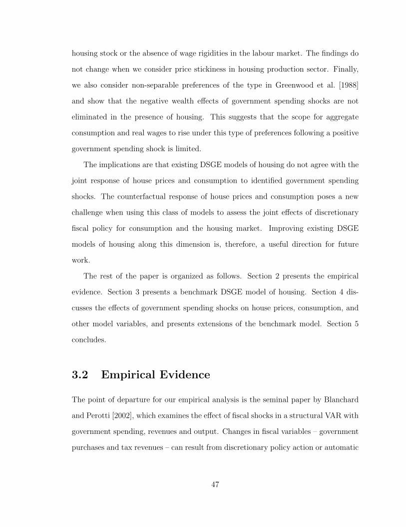
housing stock or the absence of wage rigidities in the labour market. The findings do

not change when we consider price stickiness in housing production sector. Finally,

we also consider non-separable preferences of the type in Greenwood et al. [1988]

and show that the negative wealth effects of government spending shocks are not

eliminated in the presence of housing. This suggests that the scope for aggregate

consumption and real wages to rise under this type of preferences following a positive

government spending shock is limited.

The implications are that existing DSGE models of housing do not agree with the

joint response of house prices and consumption to identified government spending

shocks. The counterfactual response of house prices and consumption poses a new

challenge when using this class of models to assess the joint effects of discretionary

fiscal policy for consumption and the housing market. Improving existing DSGE

models of housing along this dimension is, therefore, a useful direction for future

work.

The rest of the paper is organized as follows. Section 2 presents the empirical

evidence. Section 3 presents a benchmark DSGE model of housing. Section 4 dis-

cusses the effects of government spending shocks on house prices, consumption, and

other model variables, and presents extensions of the benchmark model. Section 5

concludes.

3.2 Empirical Evidence

The point of departure for our empirical analysis is the seminal paper by Blanchard

and Perotti [2002], which examines the effect of fiscal shocks in a structural VAR with

government spending, revenues and output. Changes in fiscal variables – government

purchases and tax revenues – can result from discretionary policy action or automatic

47

responses to innovations in output.7 Fiscal shocks are then identified by assuming that

discretionary fiscal responses do not occur within the same quarter as any innovation

in output. By the time policy-makers realize that a shock has affected the economy,

and go through the planning and legal processes of implementing an appropriate

policy response, a quarter would have passed. Non-discretionary responses, on the

other hand, can be identified through spending or revenue elasticities of output either

estimated using institutional information or through auxiliary regressions. In this

setting, any innovation to fiscal variables that are not predicted within the VAR

system are interpreted as unexpected shocks to spending or revenues.

Since we are interested in estimating the effects of government spending shocks

only (and not the effects of taxes on output), the timing assumption essentially re-

duces to a Cholesky-ordering of the VAR with government spending ordered first.8

Specifically, this implies that other shocks in the system do not affect government

spending within a quarter, while government spending affects the remaining variables

in the same quarter. This approach has been widely used (see Galı et al. [2007], Fa-

tas and Mihov [2001]) in demonstrating that increases in government spending raises

output, consumption and wages. We start by following these earlier studies and es-

timating a quarterly VAR in Xt =

[Gt Tt Yt Ct Qt

]′with four lags, a constant,

and linear and quadratic time trends as follows:

Xt = α0 + α1t+ α2t2 + A(L)Xt−1 + et

Here, A(L) is a lag polynomial of degree 4, Gt is government consumption and gross

investment, Tt is government tax receipts less transfer payments, Yt is output, Ct

7For example, an exogenous increase in output may result in an increase in total tax revenues ifthe tax base increases and tax rates remain the same.

8For the effects of taxation on output, see Romer and Romer [2010] and Mertens and Ravn [2012],who provide evidence on the aggregate effects of tax shocks in the U.S. and Cloyne [2012] for theU.K.

48

is total private consumption less consumption of housing services and utilities, and

Qt is an index of the median price of new houses. All variables are deflated by the

GDP deflator, and expressed in log per-capita terms where appropriate.9 Further

descriptions and sources of the data is provided in Appendix ??. The data span from

the third quarter of 1963 through the last quarter of 2007. The start date is limited

by the availability of house prices, and the end date set to exclude the 2008 financial

crisis. Spending shocks are then identified as a Cholesky-ordered innovation to Gt.

Figure 3.1 shows the impulse responses of a shock to government spending in this

baseline VAR specification, along with one-standard deviation Monte Carlo confidence

intervals. All impulse reponses are normalized their relative standard-deviations.10

Clearly, following a positive government spending shock, both consumption and house

prices rise.

Ramey [2011], however, argues that if fiscal shocks are anticipated by private

agents, the above identification scheme will be misleading. The timing of the shock

plays a crucial role in identification. Alongside decision lags, there may be imple-

mentation lags in realizing fiscal policy. Often, governments announce their intended

spending in advance, and the actual spending occurs in a staggered manner over a

longer period of time. Private agents, then, would anticipate government spending

well in advance and adjust their optimal consumption behaviour accordingly, while

the econometrician would only see the effect of the policy when actual spending

increases. If, contrary to the finding of Blanchard and Perotti [2002], private con-

sumption were to decline upon the announcement of future increases in spending, a

mis-timed VAR analysis would only capture the return of consumption to steady-

9The DSGE model preseted in section 3.3 portrays a one-good economy where the numeraire isthe final good. In particular, the real house price presented in the model is implicitly normalized bythe final good price. It therefore makes sense to deflate the corresponding nominal variables in theempirical section by the GDP deflator.

10E.g. a one standard deviation shock in government spending leads consumption to increase byaround 0.26 standard deviations on impact.

49

Figure 3.1: Impulse responses of key variables to a government spending shock froma Cholesky-identified VAR

5 10 15 200

0.5

1

Gov Spending

5 10 15 20

0

0.2

0.4

Output

5 10 15 20

0

0.2

0.4

Consumption

5 10 15 20

0

0.1

0.2

0.3

0.4

House Prices

Notes : Dotted lines show the 16th and 84th percentile of the related distributionfrom 1000 Monte Carlo simulations.

50

state, and not the initial decline. Thus, the econometrician will mistakenly infer that

consumption rises following a spending increase. Using narrative records of govern-

ment accounts, Ramey and Shapiro [1998] and Ramey [2011] identify spending shocks

as dates when a large amount of national defence spending was announced and find

that consumption declines following a positive fiscal shock. The anticipation issue is

emphasized in Ramey [2011] by showing that lagged defence spending dates Granger

cause the VAR shocks identified by Blanchard and Perotti [2002], suggesting that

their identification scheme misses information already available to private agents.

Auerbach and Gorodnichenko [2012] also finds that a sizeable fraction of innovations

identified by VAR is predictable.11

The anticipation problem arises because private agents have access to more in-

formation than the econometrician, which allows them to develop a forecast of gov-

ernment spending that the econometrician does not observe. As discussed in Leeper

et al. [2011], this issue can cause an invertibility problem, in that, it may not be

possible to recover the structural shocks facing private agents from the identified

shocks. Finding ways to address this issue is an area of ongoing research.12 We

consider two approaches that can help account for the anticipation effects and also

mitigate the invertibility problem. First, we include variables containing private sec-

tor forecasts of future spending in the VAR specification. Following Auerbach and

Gorodnichenko [2012], we control for the forecastable components by including in

the VAR a variable that captures forecasted government spending from two sources:

(i) the Survey of Professional Forecasters (SPF) and (ii) forecasts prepared by the

Federal Reserve Board staff for the meetings of the Federal Open Market Committee

11Specifically, they find that residuals from projecting private sector forecasts of government spend-ing growth on lags of variables included in the VAR is positively correlated with residuals fromprojecting actual government spending growth on the same variables. If the VAR innovations wereunexpected, then the two residuals should be uncorrelated.

12See, for example, Dupor and Han [2011], Forni and Gambetti [2011], and Sims [2012].

51

(Greenbook). The SPF forecasts are available from 1982 onward, while the Green-

book forecasts are available from 1966 through 2004. We take the variable used in

Auerbach and Gorodnichenko [2012] generated by splicing the two series to create a

continuous forecast series starting in 1966.13 The variable contains forecasts made

in period t − 1 for the period-t spending value. We augment the baseline VAR by

considering Xt =

[FEG

t Gt Tt Yt Ct Qt

]′, where FEG

t is the forecast error for

the growth rate of government spending. The unanticipated shock, then, is identified

as the innovation in the forecast error itself, rather than an innovation to Gt.

Second, following Forni and Gambetti [2011], we estimate a factor-augmented

VAR (FAVAR) with 110 variables, 13 static factors, 4 lags and 6 structural shocks.14

We identify government spending shocks by imposing the following sign restrictions

on the impulse response functions: total government spending, federal government

spending, total government deficit, federal government deficit and output all increase

in the fifth quarter following the shock. Imposing the restriction a few quarters after

the impact period allows for anticipation effects. This strategy, however, does not

allow us to differentiate between an expected and an unexpected shock.

Figure 3.2 shows the impulse responses of a shock to the one-step-ahead forecast

error of government spending in the expectation-augmented VAR specification. The

differences in the shape of the IRF’s suggest that expectations do play a role in deter-

mining the effects of government spending shocks. While in the baseline case (Figure

3.1), the largest effect of an increase in spending occurs in the first period, we see that

the largest effect on output and consumption occurs about 5 quarters after the spend-

ing shock impact (Figure 3.2). Even after controlling for expectations, however, house

prices clearly increase in a persistent manner following an unanticipated government

13We thank Yuriy Gorodnichenko for providing us with the data on government spending forecasts.14The dataset is almost identical to Forni and Gambetti [2011], with few exceptions, and is de-

scribed in a separate appendix available upon request. All data are in quarterly frequencies andcover the period from 1963:1 through 2007:4.

52

Figure 3.2: Impulse responses of key variables to a government spending shock, con-trolling for anticipation effects.

5 10 15 200

0.2

0.4

0.6

Gov Spending

5 10 15 20

0

0.2

0.4

0.6

Output

5 10 15 200

0.2

0.4

Consumption

5 10 15 20

0

0.1

0.2

0.3

House Prices

Notes : The VAR specification includes one-step-ahead forecast errors from privatesector forecasts of government spending (Auerbach and Gorodnichenko [2012]). Gov-ernment spending shock is identified as a Cholesky-ordered shock to the forecast error.Confidence bands show the 16th and 84th percentile of the related distribution from1000 Monte Carlo simulations.

53

spending shock. Figure 3.3 shows the impulse responses for the FAVAR specification

along with one-standard error boot-strapped confidence bands. The FAVAR specifi-

cation also shows that house prices and consumption increase following a government

spending shock.

3.3 A DSGE Model with Housing

In this section we describe a DSGE model with housing based on Iacoviello [2005]

with an exogenous fixed supply of housing.15

3.3.1 Households

There are two types of agents in the economy characterized by their different rates of

time preference. The size of the total population is normalized to one. A fraction, 0 <

α < 1, of the population denotes the proportion of impatient agents who discount the

future at a rate higher than patient agents. Both agents receive utility from consuming

a non-durable good, from the services of the stock of housing they own, and from

leisure. In addition, only the patient agents hold government debt, and own physical

capital which they rent out to the production sector. Both agents supply labour

services to the production sector. In this setting, patient households are net lenders

and impatient households are net borrowers in the steady state. Due to the presence

of financial frictions, the borrowers face a constraint on the amount they can borrow

in each period by using their stock of housing as collateral. As in Iacoviello [2005],

the amount of uncertainty in the economy is small enough such that for borrowers,

the effect of impatience on borrowing always dominates the precautionary motive for

self-saving and consequently the collateral constraint is always binding in equilibrium.

15In section 3.4.1 we consider housing production.

54

Figure 3.3: Impulse responses of key variables to a government spending shock froma FAVAR specification.

5 10 15 200

0.1

0.2

0.3

Gov Spending

5 10 15 20

0

0.2

0.4

Output

5 10 15 20

0

0.1

0.2

0.3

0.4

Consumption

5 10 15 20

0

0.2

0.4

0.6

House Prices

Notes : Government spending shock identified using sign restrictions specifying anincrease in total and federal government spending, deficits and real output on the 5thquarter following the shock. Bootstrapped confidence bands show the 16th and 84thpercentile of the related distribution

55

The optimization problems of patient-lenders and impatient-borrowers are to max-

imize the expected discounted lifetime utility given by

E0

∞∑t=0

βtj

[ln cjt + Υj lnhjt −

1

1 + η

(njt)1+η

](3.1)

where j = ` for the patient-lenders and j = b for the impatient-borrowers. The

variables cjt , hjt , and njt denote consumption, housing, and labour supplied to the

production sector, respectively. The parameters βj, Υj, and η denote the discount

factor, the weight of housing in the utility function, and the inverse Frisch elasticity

of labour supply, respectively.

The budget constraint facing a patient-lender is

c`t + qth`t + it + bgt + bt = wtn

`t + qth

`t−1 + rtkt−1 + d`t +

rnt−1bgt−1

πt

+rnt−1bt−1

πt− τ `t (3.2)

where qt is the relative price of housing stock, kt is capital rented out to the production

sector, rt is the real rental return on capital, and δ is the capital depreciation rate.

Alongside investing in capital, patient households own firms in the production sector

from which they receive dividends, d`t, lend an amount bt (in real terms) to borrowers,

and hold government debt bgt (in real terms), both for the same rate of real gross

return rnt−1/πt, where rnt−1 is the nominal interest rate and πt is the inflation rate.

Finally, τ `t is a lump-sum tax imposed by the government on patient-lenders.16 The

capital accumulation process is given as

kt = (1− δ)kt−1 + φ

(itkt−1

)kt−1 (3.3)

16We have also experimented with a distortionary labour tax instead of a lump-sum tax, and theresults presented in section 3.4 remain the same. We concentrate on the lump-sum formulation forease of exposition and reference to relevant literature.

56

Where φ(.) denotes capital adjustment costs which are increasing in the rate of in-

vestment it/kt−1, and which have the following properties: φ′(.) > 0, φ′′(.) ≤ 0,

φ′(i/k) = 1, and φ(i/k) = i/k, implying zero costs in the steady state. The budget

constraint facing the impatient-borrowers is

cbt + qthbt +

rnt−1bt−1

πt= wtn

bt + qth

bt−1 + bt − τ bt (3.4)

where τ bt is a lump-sum tax. The impatient-borrowers also face a collateral constraint

bt ≤ mEt

{qt+1h

btπt+1

rnt

}(3.5)

which says that the real debt service due next period cannot exceed a fraction m ∈

[0, 1] of the expected real value of the housing stock held as collateral. Since only a

fraction 0 < m < 1 of the expected discounted value of housing stock is available for

borrowing, (1−m) can be interpreted as a down-payment requirement, and m the

loan-to-value (LTV) ratio.

Denoting the Lagrange multipliers on the constraints (3.2) and (3.3) as λ`1t and λ`2t,

respectively, the first-order necessary conditions for the patient-lenders which charac-

terize the optimal choices of their consumption, labour supply, housing, investment,

57

capital, lending and government bonds are as follows:

1

c`t= λ`1t(

n`t)η

wt= λ`1t

Υ`

h`t= λ`1tqt − β`Et[λ`1t+1qt+1]

1 = ψtφ′(

itkt−1

)ψt = β`Et

[λ`1t+1

λ`1t

(rt+1 + ψt+1

((1− δ)φ

(it+1

kt

)− φ′

(it+1

kt

)it+1

kt

))]1 = β`Et

[λ`1t+1

λ`1t

rntπt+1

]

where ψt, defined as λ`2t/λ`1t, represents the marginal value of capital in terms of the

consumption, or the Tobin’s Q.

Denoting the Lagrange multipliers on the constraints (3.4) and (3.5) as λb1t and λb2t,

respectively, the first-order-conditions for the impatient-borrowers that characterize

the optimal choices of their consumption, labour supply, housing, and borrowing are

as follows:

1

cbt= λb1t(

nbt)η

wt= λb1t

Υb

hbt= λb1tqt − βbEt

[λb1t+1qt+1

]− λb2tmEt

[qt+1πt+1

rnt

]λb1t = βbEt

[λb1t+1

rntπt+1

]+ λb2t

58

3.3.2 Firms

The production side in this model follows the standard New Keynesian approach

which we briefly describe here. There is a perfectly competitive final good sector

in which firms produce a non-durable consumption good, yt, using a continuum of

intermediate goods, xt(s) with s ∈ [0, 1], and the Dixit-Stiglitz aggregation technology

yt =

(∫ 1

0

xt(s)ε−1ε ds

) εε−1

, ε > 0 (3.6)

where 1/(ε−1) > 0 is the constant elasticity of substitution between the intermediate

goods. Profit maximization in the final goods sector, maxyt(s){ptyt−∫ 1

0pt(s)xt(s)ds}

subject to (3.6) generates the demand for each type of intermediate good as

xt(s) =

(pt(s)

pt

)−εyt, s ∈ [0, 1]

where pt is the price of a unit of final good given by the zero-profit condition as

pt =

[∫ 1

0

(pt(s))1−ε ds

] 11−ε

, s ∈ [0, 1]

The firms in the intermediate goods sector operate under monopolistic competition.

Each firm uses labour, capital, and a constant returns to scale technology to produce

a differentiated good. The production function for a firm s ∈ [0, 1] is

yt(s) = kt−1(s)γnt(s)γ, 0 < γ < 1

where labour services, nt(s) are supplied by both agents while capital, kt−1(s) is sup-

plied by lenders only.17 The factor markets are assumed to be perfectly competitive

17Note that we normalize the productivity shock to 1 since we are interested in studying solelythe responses to government spending shocks.

59

and firms take the real wage and the real rental cost of capital as given.18 Cost

minimization implies

rt = γmctytkt−1

wt = (1− γ)mctytnt

mct = γ−γ(1− γ)γ−1wγt r1−γt

where mct is the real marginal cost, same for all the firms..

Nominal prices of intermediate goods firms are assumed to be sticky. Following the

standard Calvo [1983] approach to introduce nominal price stickiness and staggered

price setting, only a fraction, 0 < (1 − θ) < 1, of firms are assumed to re-set their

prices optimally in a given period while the remaining fraction, θ, keep their prices

unchanged. The optimization problem of a price-setting firm, s ∈ [0, 1], in period t is

maxpt

Et

∞∑j=0

Λ`t,t+jθ

j [ptyt+j(s)− pt+jmct+j]

subject to a sequence of demand curves

yt+j(s) = xt+j(s) =

(ptpt+j

)−εyt+j

The term Λ`t,t+j ≡ βj`

(c`tc`t+j

ptpt+j

)represents the nominal stochastic discount factor of

the patient-lenders who are the owners of the firms in the intermediate goods sector.

18The assumption of perfectly competitive factor markets allows us to highlight the basic mecha-nism behind the response of house prices to government spending shocks. Andres et al. [2012], forexample, allow job search and unionized bargaining in the labour market to study the magnitude offiscal multipliers.

60

The optimal price, p∗t , satisfies the first-order condition

Et

∞∑j=0

Λ`t,t+jθ

jyt+j(s)

[p∗t −

ε

ε− 1mct+jpt+j

]= 0

where

pt =[θp1−ε

t−1 + (1− θ)p∗(1−ε)t

] 11−ε

is the aggregate price level.

3.3.3 Fiscal and Monetary Policies

We follow Galı et al. [2007] for the fiscal and monetary policy specifications. The

government faces a budget constraint of the form (in real terms):

τt + bgt =rnt−1b

gt−1

πt+Gt

where τt is lump-sum tax revenue (which equals (1−α)τ `t +ατ bt ) and Gt is government

spending.The government sets taxes according to the following fiscal rule

τt = %bbgt−1 + %ggt

where gt ≡ Gt−GY

, τt ≡ τt−τY

and bt ≡ Bt−BY

are deviations of the fiscal variables from

a steady state with zero debt and balanced primary budget (normalized by steady-

state level of output). %b and %g are weights assigned by the fiscal authority on debt

and current government spending. Note that government debt is not modelled as

discountable bonds, and pays nominal gross interest, rnt , each period. This form of

government debt makes it easier to compare intertemporal decisions of households

61

across different saving instruments. Government purchases are assumed to follow an

exogenously determined auto-regressive process

gt = ρggt−1 + εt

where 0 < ρg < 1 and εt is an i.i.d. government spending shock with variance σ2ε .

Since our focus is to illustrate the effects of government spending shocks we assume

a simple monetary policy rule as in Galı et al. [2007] which determines the nominal

interest rate in the economy.19 This rule is given as

rntrn

=(πtπ

)%πwhere rnt = rnt − 1. And rn and π are the steady state levels of the (net) nominal

interest rate and inflation, respectively.

3.3.4 Aggregation

Aggregate consumption, labor and housing (all denoted in upper case) are weighted

averages of the variables corresponding to patient-lenders and impatient-borrowers

and are given as

Ct = αcbt + (1− α) c`t

Nt = αnbt + (1− α)n`t

H = αhbt + (1− α)h`t

19This assumption can be further justified by Clarida et al. [2000]’s finding that the output gapcoefficient in an estimated policy reaction function for the Federal Reserve is statistically insignificantin the post Volcker era.

62

Since capital is owned only by patient-lenders, aggregate investment and capital are

given as

It = (1− α)it

Kt = (1− α)kt

Finally, the aggregate resource constraint is given as

Ct + It + φ

(It

Kt−1

)Kt−1 +Gt = Yt ≈ Kγ

t−1N1−γt

where the aggregate production function holds up to a first-order approximation as

shown in Woodford [2003]. The economy is in equilibrium when all the first-order

necessary conditions are satisfied and all the goods and factor markets clear.

3.3.5 Linearization, Calibration, and Model Solution

We log-linearize the first-order optimality conditions of the households and firms, and

the aggregate market clearing conditions around a steady state. We use hats on vari-

ables to denote the percentage deviations from their steady-state values, respectively.

We linearize the government budget constraint (3.7) around a steady state with zero

debt and primary balanced budget.20

The model is set in a quarterly frequency. The discount factors of the patient-

lenders and the impatient-borrowers are set to 0.9925 and 0.97, respectively. Iacoviello

and Neri [2010] and Iacoviello [2005] argue that this calibration value suffices to

ensure that the borrowing constraint is binding in equilibrium. The captial share

20Note that hatted variables are expressed in percentage deviations, i.e., deviations from theirsteady state values, normalized by their steady state values. Government variables marked with atilde, on the other hand, are deviations from their steady state values, normalized by the steady-statelevel of output. In other words, Xt = lnXt− lnX ≈ Xt−X

X and Xt = Xt−XY where Y is steady-state

level of output.

63

of output, γ, is set to 0.33, and the depreciation rate δ is set to 0.025. We assume

a steady-state price markup of 0.15, implying a steady-state marginal cost mc of

11.15≈ 0.87. The inverse of the Frisch-elasticity of labour supply, η, is set to 1. The

elasticity of capital adjustment cost parameter, φ′′( ik) is set to -14.25, to match the

correspondponding parameter estimated by Iacoviello and Neri [2010] using Bayesian

methods. The benchmark value of KY

and qHY

is taken from Iacoviello and Neri [2010].

The later figure corresponds to the total value of household real estate assets in the

U.S., as specified in the Flow of Funds Account (B.100 line 4). We set the Calvo

price-adjustment frequency to 0.75, corresponding to an average price duration of

one year, and the Taylor rule parameter measuring the response of the monetary

authority to inflation, %π, to 1.5, a value commonly used in the literature. We match

the benchmark values of the fiscal response parameters to those in Galı et al. [2007],

and set the tax response to government spending, %g, to 0.1, the tax response to

outstanding government debt, %b, to 0.33, and the persistence of government shock,

ρg to 0.9.

The dynamics presented in this paper depend importantly on the different optimal

responses of patient-lenders and impatient-borrowers to a government spending shock.

The exposition of these differences in dynamics become easier if we start off the two

households with identical consumption and housing levels. As such, we set c`

Y= cb

Y=

CY

= 0.5 and qh`

Y= qhb

Y= qH

Y. The first can be easily achieved by assuming different

levels of steady-state lump-sum taxes 21. The later can be achieved by setting different

values for the weight of housing in utility.22 Accordingly, we set Υ` to 0.0816 and

Υb to 0.1102. The benchmark loan-to-value ratio is set at 0.85, following Iacoviello

and Neri [2010], and the implications of changing this value is explored in section

21See the discussion in Galı et al. [2007].22Manipulating the first order conditions for households with respect to housing in the steady-

state, we get the following expressions: Υ` =qHYCY

(1− β`), and Υb =qHYCY

[1− βb −

(1− βb

β`

)mβ`

]

64

Table 3.1: Parameter and steady-state ratiosParameter Description Valueα Proportion of impatient-borrowers 0.5β` Patient-lenders’ discount factor 0.9925βb Impatient-borrowers’ discount factor 0.97η Inverse Frisch-elasticity of labour supply 1Υ` Patient-lenders’ utility weight on housing 0.0816Υb Impatient-borrowers’ utility weight on housing 0.1102γ Output elasticity of capital 0.33δ Capital depreciation rate 0.025θ Calvo price-adjustment frequency 0.75%π Taylor rule response parameter for inflation 1.5%b Fiscal respose parameter to outstanding government debt 0.33%g Fiscal response parameter to government spending 0.1m Loan-to-value ratio 0.85ρg Persistence parameter for government shock 0.9

φ′′(i

k) Capital adjustment cost parameter 1 -14.25

φ′(i

k) Capital adjustment cost parameter 2 1

φ(i

k) Capital adjustment cost parameter 3 δ

R Steady-state interest rate1

β`

r Steady-state return on capital1

β`− (1− δ)

mc Steady-state marginal cost1

1.15wn

YSteady-state wage earnings to output ratio (1− γ)mc

C

YSteady-state consumption to output ratio 0.5

K

YSteady-state capital to output ratio 2.05× 4

qH

YSteady-state housing value to output ratio 1.36× 4

b

YSteady-state loans to output ratio mβ`

qH

Y

65

3.4. Iacoviello and Neri [2010] estimate the proportion of borrowers α to be 0.21,

and consequently, the proportion of savers to be 0.79. However, the rule-of-thumb

literature often sets the proportion of non-Ricardian agents to 0.5. As argued below,

the counterfactually negative response of housing prices stem from the particular

manner in which savers value housing stock. A high proportion of savers lowers the

response of housing price. We therefore set the benchmark value of α to 0.5 for ease

of exposition. Table 3.1 summarizes the calibration values. Alternative values of α

are considered in section 3.4. We use Dynare to solve the model.23

3.4 The Effects of Government Spending Shocks

on House Prices and Consumption

Figure 3.4 presents the effects of a one standard deviation positive shock to gov-

ernment spending for the benchmark calibration of Table 3.1. The relative price of

housing falls immediately after a positive government spending shock. This response

is in sharp contrast to the evidence based on SVAR reported in section 3.2 and the

key finding that we wish to highlight in this chapter.

Why does the relative price of housing fall after a positive government spending

shock? The intuition follows from the approximately constant shadow value of hous-

ing for lenders. Housing is a long-lived good and provides a service-flow for many

periods in the future. The property of near-constant shadow value of long-lived goods

was first pointed out in Barsky et al. [2007] in the context of durable goods and tem-

porary monetary policy shocks. We can define the shadow value of housing for the

patient-lender as v`t ≡ λ`1tqt and, using the first-order-condition for optimal housing,

23See Adjemian et al. [2011] and http://www.dynare.org/.

66

Figure 3.4: Response to a positive government spending shock. Benchmark modelwith fixed housing.

5 10 15 20

−0.05

0House Prices

5 10 15 20

00.020.040.06

Shadow Value of Housing

5 10 15 20

−0.2

−0.1

0Borrowing

5 10 15 20

−0.1

−0.05

0Consumption

5 10 15 20

−0.10

0.1

Housing

5 10 15 200

0.5

Collateral Constraint

5 10 15 20

−0.02

−0.01

0Wages

5 10 15 200

0.05

0.1

Labour Supply

5 10 15 200

0.02

0.04

Interest Rate

5 10 15 20

−0.05

0Total Consumption

5 10 15 20

−0.05

0Investment

5 10 15 200

0.02

0.04

Output

Note: Dashed-dotted line (lender), Dotted line (borrower)

67

express it in log-linearized form as

v`t ≡ λ`1t + qt = (β` − 1)∞∑j=0

βj` h`t+j (3.7)

≈ 0 (3.8)

There are two key features which make the deviations of shadow value of housing

from its steady state, v`t , approximately zero, as indicated in (3.8). First, the housing

flows do not contribute much to the variation in the stock, which means that the

marginal utility of housing remains close to its steady state (i.e., the h`t+j terms are

close to zero). Second, temporary government spending shocks have little influence

on future marginal utility of housing (i.e., the h`t+j = 0 as j increases). Now, a

temporary positive government spending shock induces a negative wealth effect and

causes the patient-lenders to reduce current consumption. This raises their marginal

utility of consumption, λ`1t > 0. Since the shadow value of housing is approximately

zero, it implies that the the price of housing necessarily falls relative to its steady

state value, i.e, qt < 0. As in Barsky et al. [2007], the quasi-constancy property here

implies a near-infinite elasticity of inter-temporal substitution for the patient-lenders.

The fall in the price of housing causes them to immediately increase their housing

purchases. It is important to note that this result does not depend on the structure

of the labour market. Indeed, Andres et al. [2012] introduce job search and unionized

bargaining and provide a significant departure from the competitive labour market we

consider here in an attempt to account for a positive consumption response following

a government shock. Yet, even under that labour market structure they report that

house prices fall. Thus, relative to the SVAR evidence reported in section 3.2, the

counterfactual response of housing to a government spending shock arises not only in

the benchmark model but also in variants with a richer labour market structure.

68

In contrast to the patient-lenders, the shadow value of housing for the impatient-

borrowers rises after the government spending shock. This rise reflects the desire to

increase housing to use it as collateral for future consumption. From (3.6), we define

the shadow value of housing to the impatient-borrower as vbt ≡ λb1tqt and express it

in log-linearized form (after simplifying the coefficients using steady state conditions)

as

vbt ≡ λb1t + qt = (βb − 1)Et

∞∑j=0

βjb hbt+j

+m(β` − βb)Et∞∑j=0

βjb

(λb2t+j + πt+1+j − rnt+j + qt+1+j + hbt+j

)(3.9)

The increase in the shadow value of housing, vbt > 0, is driven by the sharp tightening

of the current and expected future collateral constraints λb2t+j(> 0), as shown in

Figure 3.4 (second row, third column). The coefficient m(β` − βb) shows that the

loan-to-value ratio and the relative impatience of the two agents together determine

the gap vbt − v`t . While on impact, the housing demand of lenders decreases, they

build up their stock of housing in view of increasing future borrowing, and hence

consumption.

Turning to the response of consumption, for the patient-lenders, consumption

always falls after a positive government spending shock. The negative wealth effects

due to the lower present value of after-tax income, the reduced value of the housing

stock due to a fall in the price of housing, and the reduced expected income from

loans to borrowers all reinforce each other. Consumption of the impatient-borrowers

also falls because the value of their collateral declines when house prices fall. This

lowers their ability to borrow, which in turn, lowers consumption. This collateral

constraint effect that limits borrowing is in addition to the negative wealth effect

from the increased government spending, and works to lower the impatient-borrowers’

69

consumption. As borrowing slowly increases and returns to the steady state level,

the housing stock of impatient-borrowers rises along with their consumption. Total

consumption and investment are crowded out while output rises after the positive

government spending shock.24 Note that the strong negative wealth effect on labour

supply causes the real wage to fall. We discuss this point further in section 4.2 below.

We examine the robustness of the effects on house prices and consumption to

changing the proportion of impatient-borrowers. Figure 3.5 shows the responses of

house prices, shadow values of housing, consumption, and housing demand when the

share of impatient-borrowers, α, goes from zero to 80%. The responses are similar to

the benchmark calibration. Both house prices and consumption fall after a positive

government spending shock.

Figure 3.6 shows the results of relaxing the collateral constraint by increasing

the loan-to-value ratio from zero to 0.95. House prices fall in all the cases. Note

that consumption response of the impatient-borrowers is even more negative when

m = 0.95 relative to the benchmark calibration of 0.85. On the one hand these agents

are able to secure more loans but on the other the interest payments on the loans are

also higher which constrains their consumption.

To demonstrate that housing assets are behind the negative consumption re-

sponses, we consider reducing the steady-state value of housing stock in the model.

Note that this is akin to reducing the weight on housing in the utility function. In the

benchmark case, where the housing stock-to-output ratio, qhHY

, is set to 5.44 which

is the total value of household real estate assets in the U.S. The timing of the model

implicitly assumes that both households sell their housing assets at the end of each

period, and use the proceeds from this wealth, along with other income to purchase

24These responses are consistent with those reported in Callegari [2007] who focuses on how inthe presence of durable goods the response of consumption to government spending shock changesrelative to when rule-of-thumb consumers are considered as in Galı et al. [2007].

70

Figure 3.5: Robustness to the proportion of impatient borrowers.

5 10 15 20

−0.06

−0.04

−0.02

0

House Prices

5 10 15 20

−0.02

−0.015

−0.01

−0.005

0Lender Shadow value

5 10 15 200

0.05

0.1

Borrower Shadow value

5 10 15 20

−0.06

−0.04

−0.02

0

Lender Consumption

5 10 15 20

−0.15

−0.1

−0.05

0Borrower Consumption

5 10 15 20

−0.2

−0.15

−0.1

−0.05

0Borrower Housing

alpha=0 alpha=0.25 alpha=0.5 alpha=0.75 alpha=0.8

Note: Impulse responses to a positive government spending shock in the benchmarkmodel with fixed housing. Dashed-dotted line (lender), Dotted line (borrower)

71

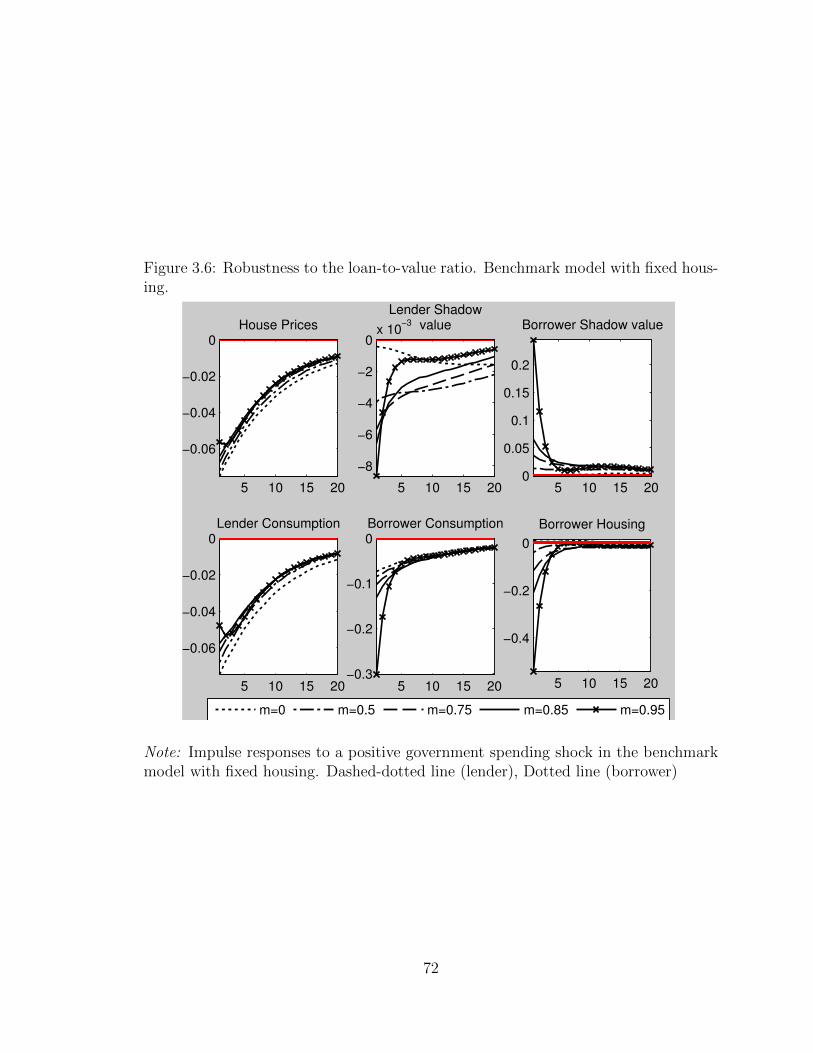
Figure 3.6: Robustness to the loan-to-value ratio. Benchmark model with fixed hous-ing.

5 10 15 20

−0.06

−0.04

−0.02

0House Prices

5 10 15 20

−8

−6

−4

−2

0x 10

−3

Lender Shadowvalue

5 10 15 200

0.05

0.1

0.15

0.2

Borrower Shadow value

5 10 15 20

−0.06

−0.04

−0.02

0Lender Consumption

5 10 15 20−0.3

−0.2

−0.1

0Borrower Consumption

5 10 15 20

−0.4

−0.2

0

Borrower Housing

m=0 m=0.5 m=0.75 m=0.85 m=0.95

Note: Impulse responses to a positive government spending shock in the benchmarkmodel with fixed housing. Dashed-dotted line (lender), Dotted line (borrower)

72

Figure 3.7: Robustness to the steady-state housing stock-to-output ratio.

5 10 15 20

−0.1

−0.05

0House Prices

5 10 15 20

−5

0

5

10

15

20x 10

−3

Lender Shadowvalue

5 10 15 20

−0.2

−0.1

0

Borrower Shadow value

5 10 15 20

−0.15

−0.1

−0.05

0Lender Consumption

5 10 15 20

−0.1

−0.05

0

0.05

0.1

Borrower Consumption

5 10 15 20−0.1

−0.08

−0.06

−0.04

−0.02

0

Total Consumption

qH/Y=5.44 qH/Y=0.54 qH/Y=0.11 qH/Y=0.05 qH/Y=0.013

Note: Impulse responses to a positive government spending shock in the benchmarkmodel with fixed housing.

73

the optimal amount of housing and consumption goods in the next period. Cali-

brating to the total value of household real estate assets therefore makes sense. We,

however, consider calibrations which produce a positive response of consumption. We

first note that qhHY

also determines the steady-state collateralized loans-to-GDP ra-

tio. The alternative calibration uses single family residential mortgages outstanding

in U.S. commercial bank balance sheets. We get a ratio that is roughly a tenth of

the benchmark value. This can be justified by noting that not all housing assets are

traded every period as the model implies, and should not have a direct effect on con-

sumption levels. To capitalize on any increase in house prices, however, a borrower

must instead re-mortgage her current housing stock. As such, the mortgage assets

are a better guide for calibrating this ratio. As shown in Figure 3.7, even under this

alternative calibration of qhHY

= 0.54, both consumption and house prices decline fol-

lowing a positive government spending shock. Moreover, the lower the steady-state

housing value-to-GDP ratio, the bigger the drop in house prices. It turns out that

for substantially smaller value 0.013 relative to the baseline calibration of 5.44 and a

slightly larger share of borrowers (α = 0.6), the consumption response turns positive.

However, at this extreme calibration, the decline in house prices is also the largest.

3.4.1 Housing Production

In this section we relax the fixed housing stock assumption described in section 3.3,

and consider housing production. Our starting point is the DSGE model with hous-

ing production developed by Iacoviello and Neri [2010]. We introduce government

74

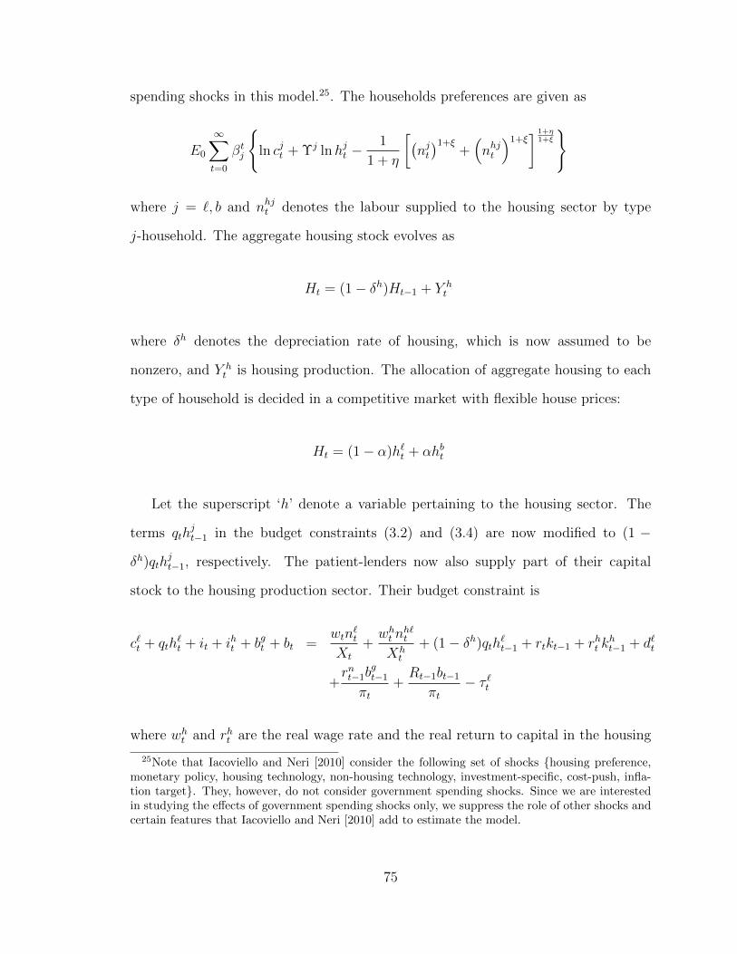
spending shocks in this model.25. The households preferences are given as

E0

∞∑t=0

βtj

{ln cjt + Υj lnhjt −

1

1 + η

[(njt)1+ξ

+(nhjt

)1+ξ] 1+η

1+ξ

}

where j = `, b and nhjt denotes the labour supplied to the housing sector by type

j-household. The aggregate housing stock evolves as

Ht = (1− δh)Ht−1 + Y ht

where δh denotes the depreciation rate of housing, which is now assumed to be

nonzero, and Y ht is housing production. The allocation of aggregate housing to each

type of household is decided in a competitive market with flexible house prices:

Ht = (1− α)h`t + αhbt

Let the superscript ‘h’ denote a variable pertaining to the housing sector. The

terms qthjt−1 in the budget constraints (3.2) and (3.4) are now modified to (1 −

δh)qthjt−1, respectively. The patient-lenders now also supply part of their capital

stock to the housing production sector. Their budget constraint is

c`t + qth`t + it + iht + bgt + bt =

wtn`t

Xt

+wht n

h`t

Xht

+ (1− δh)qth`t−1 + rtkt−1 + rht kht−1 + d`t

+rnt−1b

gt−1

πt+Rt−1bt−1

πt− τ `t

where wht and rht are the real wage rate and the real return to capital in the housing

25Note that Iacoviello and Neri [2010] consider the following set of shocks {housing preference,monetary policy, housing technology, non-housing technology, investment-specific, cost-push, infla-tion target}. They, however, do not consider government spending shocks. Since we are interestedin studying the effects of government spending shocks only, we suppress the role of other shocks andcertain features that Iacoviello and Neri [2010] add to estimate the model.

75

production sector, respectively. The labour markets in the consumption and housing

sectors are imperfectly competitive to allow for the possibility of nominal wage stick-

iness. The terms Xt and Xht denote the markup wedges between the wages received

by the households and those paid by the firm to a labour market intermediary or

union in the two sectors, respectively. The capital stock of the housing sector evolves

as

kht = (1− δh)kht−1 + iht − φh(

ihtkht−1

)kht−1

The housing sector is perfectly competitive. A representative firm produces new

housing using labour, capital and land (L) via a Cobb-Douglas technology. Land is

considered a fixed asset used to its capacity in equilibrium. New housing produc-

ing firms determine their optimal demand for factor inputs by solving the following

optimization problem

maxKht−1,N

ht

[qtY

ht − rhtKh

t−1 − whtNht

]subject to

Y ht =

(L)µl (Kh

t−1

)µ (Nht

)1−µ−µl

Finally, the presence of nominal wage rigidities imply that wage dynamics follow the

76

standard wage-Phillips curves given as follows:

ωt = β`ωt+1 −(1− θw)

(1− β`θw

)θw

Xt

ωht = β`ωht+1 −(1− θhw)

(1− β`θhw

)θhw

Xht

ωt =wtπtwt−1

ωht =wht πtwht−1

where θw and θhw are the probabilities of non-adjustment in a given period (Calvo

[1983])). Finally, the additional aggregation conditions relative to the benchmark

model are

Nht = αnhbt + (1− α)nh`t

Ht = αhbt + (1− α)h`t

Iht = (1− α)iht

Kht = (1− α)kht

Y Ht =

(L)µl (Kh

t−1

)µ (Nht

)1−µ−µl = Ht − (1− δh)Ht−1

The rest of the model is similar to the benchmark model.

Figure 3.8 displays the impulse responses for two variants of the model – one with

nominal wage rigidities, and one without. The key point to note is that house prices

fall upon impact after the government spending shock, as in the benchmark model.

This case confirms that the counterfactual movement in house prices in the benchmark

model relative to the VAR evidence is not driven by either the assumption of fixed

housing stock or wage rigidities in the labour market. Finally, Figure 3.9 displays

the impulse responses of the model when housing prices are assumed to be sticky. As

evident, the conclusions do not change.

77

Figure 3.8: The effect of wage stickiness in model with housing production

5 10 15 20

−0.1

−0.05

0Consumption

5 10 15 20

−0.04

−0.03

−0.02

−0.01

0Business Investment

5 10 15 20

−0.1

−0.05

0

Residential Investment

5 10 15 20

−0.06

−0.04

−0.02

0House Prices

5 10 15 200

0.01

0.02

0.03

GDP

5 10 15 20

−0.05

0

0.05

Nominal Wage (non−housing)

Note: Response to a positive government spending shock in a DSGE model withhousing production. Dashed line (flexible wage), solid line (sticky wages).

78

Figure 3.9: The effect of price stickiness in housing

5 10 15 20

−0.06

−0.04

−0.02

0House Prices

5 10 15 20

0

0.02

0.04

0.06

Shadow Value of Housing

5 10 15 20

0

1

2

3

Collateral Constraint

5 10 15 20

−0.1

−0.05

0

0.05

0.1

Housing Stock

5 10 15 200

1

2

3

4

x 10−4Total Housing Stock

5 10 15 20

−0.1

−0.05

0Consumption

Note: Response to a positive government spending shock in a DSGE model withhousing production. Dashed-dotted line (lender), Dotted line (borrower). Stickyhousing prices.

79

3.4.2 Greenwood et al. [1988] Preferences

Greenwood et al. [1988] (GHH) propose a special case of non-separable preferences

which eliminate the wealth effects on labour supply. The key property of GHH pref-

erences

U(c, n) = U(c−G(n))

is that the marginal rate of substitution of consumption for leisure is independent

of consumption which implies that the labour supply relation depends only on the

real wage. In the context of government spending shocks, Monacelli and Perotti

[2009] show that assuming GHH preferences and nominal price stickiness can lead real

wage and consumption to increase after a positive government spending shock.26 As

discussed above, the negative wealth effect on lenders which lowers their consumption

is the reason why house prices fall in the model. Can GHH preferences and nominal

price stickiness mitigate the negative wealth effect on lenders’ consumption to allow

an increase in house prices following a positive government spending shock?

To answer this question, we consider GHH preferences over consumption, housing,

and leisure27

U(cjt , hjt , n

jt) =

1

1− γ

[xj(1−γ)t − 1

](3.10)

26Bilbiie [2009] provides a detailed general analysis of non-separable preferences and the conditionswhich allow for consumption to increase following a positive government spending shock. Cloyne[2011] considers the role of distortionary labour and capital taxes in the transmission of governmentspending shocks. Like Monacelli and Perotti [2009], both papers, however, consider only non-durableconsumption. Kilponen [2012] considers non-separable preferences in the Iacoviello [2005] model toestimate a consumption Euler equation.

27Two recent papers have examined the role of non-separable preferences in resolving the Barskyet al. [2007] puzzle of lack of comovement between non-durable and durable consumption followinga monetary shock. Kim and Katayama [2012] consider general non-separable preferences and Deyand Tsai [2011] consider GHH preferences.

80

where

xjt = (cjt)1−ψh(hjt)

ψh − nj(1+η)t

1 + η(3.11)

Parameter ψh is the weight of housing in the utility function. The labour supply

relation is given as

njt =

(1− ψh)wt

(hjt

cjt

)ψh 1η

Similar to Dey and Tsai [2011], the wealth effect on labour supply, njt , is not elim-

inated as long as ψh > 0 (positive weight on housing in the utility function). Since

the negative wealth effect of government spending shock in the case of housing is

even greater than in the case of non-durable consumption alone, the real wage and

consumption fall immediately after the positive government shock. As can be seen in

figure 3.10, the combination of GHH preferences with sticky nominal prices of con-

sumption is insufficient to deliver a positive consumption and real wage response to

a government spending shock. The quasi-constancy property then implies that house

prices also fall.

3.5 Conclusion

We highlight that a broad class of DSGE models with housing and collateralized bor-

rowing predict both house prices and consumption to fall after positive government

spending shocks. The quasi-constant shadow value of lenders’ housing and the neg-

ative wealth effect of future tax increases on their consumption are the key reasons

for this prediction. By contrast, we present evidence that house prices and consump-

tion in the U.S. rise following positive government spending shocks, estimated using

81

Figure 3.10: Greenwood et al. [1988] preferences in benchmark model with fixedhousing stock

5 10 15 20

−0.05

0House Prices

5 10 15 200

0.1

0.2

Shadow Value of Housing

5 10 15 20

−0.4

−0.2

0Borrowing

5 10 15 20

−0.2

−0.1

0Consumption

5 10 15 20

−0.20

0.2

Housing

5 10 15 200

0.5

1

Collateral Constraint

5 10 15 20

−4−2

02

x 10−3Wages

5 10 15 20

−0.020

0.020.040.060.08

Labour Supply

5 10 15 200

0.02

Interest Rate

5 10 15 20

−0.1

−0.05

0Total Consumption

5 10 15 20

−0.1

−0.05

0Investment

5 10 15 2005

1015

x 10−3Output

Note: Response to a positive government spending shock in a DSGE model withGreenwood et al. [1988] preferences. Dashed-dotted line (lender), Dotted line (bor-rower). No housing production.

82

a structural vector autoregression methodology that accounts for anticipated effects.

The counterfactual joint response of house prices and consumption poses a new chal-

lenge when using DSGE models to address policy issues related to the housing market

which have come to fore due to the weak recovery after the 2008 financial crisis. Our

findings suggest scope for further model improvements.

83

Bibliography

Stephane Adjemian, Houtan Bastani, Michel Juillard, Ferhat Mihoubi, George Peren-

dia, Marco Ratto, and Sebastien Villemot. Dynare: Reference manual, version 4.

Dynare Working Papers 1, CEPREMAP, 2011.

Antonio Afonso and Ricardo M. Sousa. Fiscal policy, housing, and stock prices. NIPE

Working paper 21/2008, University do Minho, December 2008.

Javier Andres, Jose Bosca, and Francisco Ferri. Household leverage and fiscal multi-

pliers. Banco de Espana Working Papers 1215, Banco de Espana, Mar 2012.

Alan J. Auerbach and Yuriy Gorodnichenko. Measuring the output responses to fiscal

policy. American Economic Journal: Economic Policy, 4(2):1–27, 2012.

Robert B. Barsky, Christopher L. House, and Miles S. Kimball. Sticky-price models

and durable goods. American Economic Review, 97(3):984–998, June 2007.

F. Bilbiie. Non-separable preferences, frisch labour supply and the consumption mul-

tiplier of government spending: one solution to a fiscal policy puzzle. Journal of

Money, Credit and Banking, 41(2-3):443–450, 2009.

Olivier Blanchard and Roberto Perotti. An empirical characterization of the dynamic

effects of changes in government spending and taxes on output. The Quarterly

Journal of Economics, 117(4):1329–1368, November 2002.

Giovanni Callegari. Fiscal policy and consumption. Open Access publications from

European University Institute urn:hdl:1814/7007, European University Institute,

2007.

G. Calvo. Staggered pricing in a utility maximizing framework. Journal of Monetary

Economics, 12:383–96, 1983.

84

Richard Clarida, Jordi Gal, and Mark Gertler. Monetary policy rules and macroeco-

nomic stability: Evidence and some theory. The Quarterly Journal of Economics,

115(1):147–180, February 2000.

James Cloyne. government spending shocks, wealth effects and distortionary taxes.

Manuscript, University College London, 2011.

James Cloyne. Discretionary tax changes and the macroeconomy: New narrative

evidence from the United Kindom. American Economic Review (forthcoming),

2012.

J. Dey and Y-C Tsai. Explaining the durable goods co-movement puzzle with non-

separable preferences: a Bayesian approach. Manuscript, University of Tokyo, 2011.

B. Dupor and J. Han. Handling non-invertibility: theory and applications.

Manuscript, Ohio State University, 2011.

Antonio Fatas and Ilian Mihov. Government size and automatic stabilizers: interna-

tional and intranational evidence. Journal of International Economics, 55(1):3–28,

October 2001.

M. Forni and L. Gambetti. Fiscal foresight and the effects of government spending.

Manuscript, Universitat Autonoma de Barcelona, 2011.

Jordi Galı, J. David Lopez-Salido, and Javier Valles. Understanding the effects of gov-

ernment spending on consumption. Journal of the European Economic Association,

5(1):227–270, 03 2007.

J. Greenwood, Z. Hercowitz, and G. Huffman. Investment, capacity utilization, and

the real business cycle. American Economic Review, 78(3):402–417, 1988.

85

M. Iacoviello. Housing Markets in Europe: A Macroeconomic Perspective, chapter

Housing in DSGE Models: Findings and New Directions, pages 3–16. Springer-

Verlag, 2010.

Matteo Iacoviello. House prices, borrowing constraints, and monetary policy in the

business cycle. American Economic Review, 95(3):739–764, June 2005.

Matteo Iacoviello and Stefano Neri. Housing market spillovers: Evidence from an

estimated DSGE model. American Economic Journal: Macroeconomics, 2(2):125–

64, April 2010.

J. Kilponen. Consumption, leisure and borrowing constraints. The B.E. Journal of

Macroeconomics, 12(1):Article 10, 2012.

K. Kim and M. Katayama. Non-separability and sectoral comovement in a sticky

price model. Manuscript, Yonsei University/Louisiana State University, 2012.

Eric M. Leeper, Todd B. Walker, and Shu-Chun Susan Yang. Foresight and informa-

tion flows. NBER Working Papers 16951, National Bureau of Economic Research,

Inc, Apr 2011.

Charles Leung. Macroeconomics and housing: a review of the literature. Journal of

Housing Economics, 13:249–267, 2004.

Karel Mertens and Morten Ravn. Empirical evidence on the aggregate effects of

anticipated and unanticipated U.S. tax policy shocks. American Economic Journal:

Economic Policy, 4(2):145–81, 2012.

T. Monacelli and R. Perotti. Fiscal policy, wealth effects, and markups. Manuscript,

University of Bocconi, 2009.

86

Tommaso Monacelli. New Keynesian models, durable goods, and collateral con-

straints. Journal of Monetary Economics, 56(2):242–254, March 2009.

Valerie A. Ramey. Identifying government spending shocks: It’s all in the timing.

The Quarterly Journal of Economics, 126(1):1–50, 2011.

Valerie A. Ramey and Matthew D. Shapiro. Costly capital reallocation and the effects

of government spending. Carnegie-Rochester Conference Series on Public Policy,

48(1):145–194, June 1998.

Christina Romer. What do we know about the effects of fiscal policy? Separating

evidence from ideology. Speech given at Hamilton College, November 2011.

Christina Romer and David Romer. The macroeconomic effects of tax changes: Esti-

mates based on a new measure of fiscal shocks. American Economic Review, (100):

763–801, June 2010.

Rajdeep Sengupta and Yu Man Tam. Home prices: A case for cautious optimism.

Economic Synopses 42, Federal Reserve Bank of St. Louis, 2009.

E. Sims. News, non-invertibility, and structural VARs. Advances in Econometrics

(forthcoming), 2012.

Vincent Sterk. Credit frictions and the comovement between durable and non-durable

consumption. Journal of Monetary Economics, 57(2):217–225, March 2010.

M. Woodford. Interest and Prices. Princeton University Press, 2003.

87

Chapter 4

Search Frictions, Bank Leverage,

and Gross Loan Flows

4.1 Introduction

The financial crisis of 2007-08 has highlighted the importance of the banking sector

in influencing business cycle dynamics. Consequently, a growing stream of literature

has focused on developing quantitative business cycle models that emphasize the bank

leverage ratio (the ratio between total bank assets and bank equity) as a channel for

generating counter-cyclical interest spreads that amplify and prolong business cycles,

and consider the banking sector as a possible source for cyclical movements.1 At

the same time, a second stream of inquiry has used disaggregated bank lending data

to reveal important patterns within the banking sector that are not captured at the

aggregate level.2 First, Ivashina and Scharfstein [2010] documents that bank loans

1See, among others, the work in Gertler and Karadi [2011], deWalque et al. [2010], Meh andMoran [2010], Gerali et al. [2010], and references therein.

2At the onset of the 2008 recession, Chari et al. [2008] argued that although there was little doubtthat the U.S. was undergoing a financial crisis, aggregate data on bank lending showed no signs of thedownturn. In response, Cohen-Cole et al. [2008] argued that a deeper look at disaggregated lendingdata shows evidence of the credit crunch. In particular, aggregate lending data hides movements innew loan creation, which had collapsed early in the recession.

88

vary both at the intensive margin (amount of loans), as well as the extensive margin

(number of loans). Second, Dell’Ariccia and Garibaldi [2005] and Contessi and Francis

[2010] find that gross flows in new loan creation move pro-cyclically, while those in

loan destruction move counter-cyclically in the U.S.3 Moreover, unlike other recent

downturns in the U.S., those featuring an erosion of bank equity led to a decline in net

loan flows. However, currently available business-cycle models featuring a banking

sector cannot account for these movements in disaggregated loan flows.

This chapter fills this gap in the literature by developing a search-theoretic banking

model that can simultaneously explain cyclical movements in interest spreads, as well

as in disaggregated flows in loan creation and destruction. A search-theoretic banking

model also provides a symmetric-information interpretation of the nature of frictions

in the banking sector, and introduces a number of shocks that directly affect the

supply of credit.

The model introduces costly search in a banking sector, a bank leverage ratio

channel, and endogenous match separation to an otherwise standard New Keynesian

DSGE model similar to Christiano et al. [2005] and Smets and Wouters [2007]. Bank

loans are used by firms to finance productive capital purchases, and are allowed to

vary both in extensive and intensive margins. I use the model to study responses to

two shocks that affect credit supply – a one time decline in bank equity, and a one

time increase in match separation. I also look at responses to traditional technology

and monetary shocks, as well as a capital quality shock that has been shown by

Gertler and Karadi [2011] to replicate well important movements related to the bank

leverage channel during the crisis.4

3Gross loan flows calculated using both bank balance sheet data (Contessi and Francis [2010],Dell’Ariccia and Garibaldi [2005]) and firm-level compustat data (Herrera et al. [2011]) confirm thiscyclical pattern.

4The intuition for the capital quality shock is as follows. A negative shock to the quality ofcapital reduces the productivity of capital, and hence, its market price. This reduction in assetvalues is translated through the bank balance sheet identity to an erosion of bank equity, and a

89

First, I find that the model generates a counter-cyclical interest spread that am-

plifies and prolongs recessions for all shocks considered. This is similar to the results

of Gertler and Karadi [2011] who find that compared to the standard New Keynesian

case, a model with a banking sector amplifies and prolongs recessions for technology,

monetary, and capital quality shocks by generating a counter-cyclical interest spread.

5 Moreover, just like their model, the one presented in this chapter also generates

a counter-cyclical spread and ensuing recession following a negative shock to bank

equity.

To get an intuition for this result, consider first shocks that directly affect credit

supply. In this economy, loans are generated when a banking loan officer is matched

with an unfunded project. Banks incur costs while searching for new funding oppor-

tunities, or in maintaining existing relationships. A negative shock to bank equity

increases the leverage ratio in banks. To bring the leverage ratio back to its regulated

steady-state, banks reduce their efforts in searching for new matches or in maintaining

existing ones. This reduces the supply of credit in the extensive margin, makes new

matches scarcer, and increases the surplus from successful matches. Through Nash

bargaining, this increase in match-surplus is translated to a higher loan interest rate.

Now, consider shocks that first affect credit demand. When a negative technology,

or monetary shock hits the economy, loan-demand falls, as does expected profits for

banks. Banks again respond by reducing search efforts, and hence, the supply of

credit in the extensive margin. In the benchmark calibration, the model produces a

reduction in the supply of new matches large enough to generate a counter-cyclical

rise in the spread between the policy interest rate determined by a Taylor-type rule,

consequent rise in the leverage ratio. This, in turn, reduces future lending and exacerbates therecession. Although a shock to capital quality leads to a recession on its own merit, it also providesa much larger secondary effect by generating a persistent decline in asset values in the bank balancesheet, as seen during the sub-prime crisis.

5In contrast, Gerali et al. [2010] finds that the presence of the banking sector amplifies responsesto financial shocks, but attenuates the effects of technology shocks.

90

and loan rates facing firms.6 This counter-cyclical rise in the interest spread reduces

loan demand even further following negative shocks, and generates deeper and more

prolonged recessions compared to the standard New Keynesian setup.

In addition, I find that the search-theoretic framework is useful in generating

movements in loan creation and destruction flows that qualitatively match empirical

evidence. First, the model generates pro-cyclical movements in loan creation, and

counter-cyclical movements in loan destruction. Second, the model generates impulse

responses that qualitatively match estimated responses for an identified credit supply

shock.7 To show this, I first estimate responses to gross loan creation and destruction

margins to a credit supply shock in a VAR framework. I find that the interest rate

spread and loan destruction margin rise, while loan creation falls after a credit supply

shock. The model is able to generate responses for the capital quality and bank equity

shocks that are qualitatively similar to empirical responses to credit supply shocks,

when investment elasticity to capital price matches evidence from disaggregate data.

Early studies exploring the effect of search frictions on credit markets include den

Haan et al. [2003], and Wasmer and Weil [2004]. However, none of these papers

use search frictions to study business-cycle dynamics of bank loans. In that respect,

the papers closest to this study are Dell’Ariccia and Garibaldi [2000] and Beaubrun-

Diant and Tripier [2009]. The former considers a search model only to match the

second moments of gross loan flows, and the later explores the ability of a costly

search setup in generating a counter-cyclical interest spread for technology shocks in

an RBC model. On top of considering a New-Keynesian setting, my model differs

from Beaubrun-Diant and Tripier [2009] by allowing an endogenous bank leverage

6Beaubrun-Diant and Tripier [2009] provides an analysis of the calibration necessary for searchmodels to generate a counter-cyclical spread for a technology shock in an RBC model.

7The idea that conditions in the financial sector can be an independent source of business cyclefluctuations has recently been emphasized in the literature. Gilchrist and Zakrajsek [2012a] andBoivin et al. [2012] estimate the effect of a credit shock on U.S. data and find that a reduction incredit supply negatively affects the real economy.

91

channel and loans that are used for capital purchases to vary both in the intensive

and extensive margins. In contrast, their model specifies loans used for intermediate

good purchases, allows only movements in the extensive margin, and abstracts from

both productive capital and bank equity.

To the best of my knowledge, this is the first study that considers a full-fledged

banking model using search-frictions in a New-Keynesian setting, and explicitly mod-

els loan variation in both intensive and extensive margins. This is also the first study

to consider both simulated and empirical impulse responses of gross loan flows to

financial shocks.

The rest of the paper is organized as follows. Section 4.2 describes the benchmark

model and calibration. Section 4.3 demonstrates the capacity of the model to amplify

and propagate the effects of shocks to the economy, and explains the core search

mechanism in generating a counter-cyclical interest spread. Section 4.4 determines the

empirical responses for gross loan creation and destruction margins for a credit supply

shock, and compares them with model responses. Section 4.5 provides concluding

comments.

4.2 The Benchmark Model

In this section, I describe the benchmark model and calibration. The starting point

is the workhorse New Keynesian DSGE model with nominal rigidities developed by

Christiano et al. [2005] and Smets and Wouters [2007]. To this canonical framework,

I add a banking sector that intermediates loanable funds between households and

firms. Banks face a Mortensen and Pissarides [1994] type search friction that creates

a wedge between the loan and deposit interest rates.8 Precisely, household deposits

8The mechanism parallels the creation of a wedge between wages and the marginal product oflabor in the job-search models of Pissarides [1985] and Andolfatto [1996].

92

are transferred to firms as loans for capital asset purchases when a banking loan officer

is matched with a project that requires financing.9 The search process resulting in

a matched pair of loan officer and project generates a countercyclical wedge between

the loan interest rate charged to the firm and the deposit interest rate paid by the

bank.

The model economy is explained graphically in figure 4.1. There are five types

of private agents in the economy: households, banks, intermediate goods producers

(referred to as firms here on), capital producers, and monopolistically competitive

retailers. This setup closely follows Gertler and Karadi [2011], with the exception

that the financing friction in this model is generated by search activity, rather than

an agency problem stemming from information asymmetries between banks and de-

positors. Households consume, supply labour to firms, and save in bank deposits.

They own banks, intermediate and capital goods producing firms, and retail insti-

tutions. Income from these institutions are repatriated to households in the form of

dividends. Capital, however, is owned by firms, and can be bought only through funds

secured from banks as loans. Firms use labour and capital to produce a homogenous

intermediate good.

The representative firm is best thought of as the head office of a continuum of

projects on a unit interval. The firm head office determines the amount of aggregate

capital, and hence aggregate loans in each period, and distributes it evenly across

active projects. Production and financing, however, occurs at the individual project

level, and only if the project is matched with a loan officer who provides financing.10

Similar to the firm, the representative bank is best thought of as the head office to

9Consistent with the literature on banking sector models in DSGE settings, I assume that house-hold savings and bank equity are the only sources for private sector credit. Note, however, that thisassumption overlooks the growing importance of corporate savings, and abstracts from bond marketand other sources of funding available to firms.

10This assumption is inoccuous, given the free-movement of resources across projects, and ismaintained for ease of tractability.

93

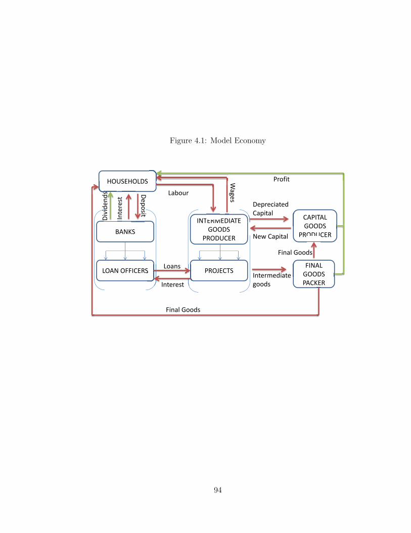
Figure 4.1: Model Economy

HOUSEHOLDS

BANKS INTERMEDIATE

GOODS PRODUCER

CAPITAL GOODS

PRODUCER

LOAN OFFICERS PROJECTS FINAL

GOODS PACKER

Loans LOAN OFFICERS

Interest Intermediate goods

PRODUCER

Final Goods

Depreciated Capital

New Capital

INTERMEDIATE

Labour Deposit Inte

rest

Wages

Final Goods

Divi

dend

s

Profit

94

a collection of loan officers, who can either be actively financing an existing project,

or searching for potential projects to finance. The bank head office determines the

total number of loan officers in each period in accordance with a balance sheet con-

straint that equates total loans to total deposits plus bank equity, and a quadratic

cost imposed on banks if the leverage ratio deviates from regulation. Following an

aggregate shock, the bank head office determines how many new projects to finance,

and how many of the currently existing relationships to keep. Separation of existing

relationships, therefore, is endogenous, and modeled by introducing an idiosyncratic

cost of continuing an existing match, imposed on the individual loan officer.11 Each

period, new matches occur between loan officers looking for projects to finance, and

unfunded projects. This generates an extensive margin for financing. Banks pay a

deposit interest rate to households that equals the risk-free rate by arbitrage. Loan

interest rates to firms are determined through Nash bargaining.

At the end of the period, worn out capital is replaced by the capital goods produc-

ing sector, which, following Bernanke et al. [1999] and Gertler and Karadi [2011], is

considered separately to keep the problem of intermediate goods producers tractable

in the face of financial frictions. A monopollistically competitive retail sector intro-

duces nominal price rigidities by costlessly differentiating the homogeneous intermedi-

ate good into a continuum of differentiated goods, and repackaging them to produce a

final good. A central bank conducts conventional monetary policy to control inflation.

In the absence of financial frictions, the loan interest rate and the deposit rate are

equal, and the question of matching is moot. In this case, the model reduces to the

canonical New Keynesian model of Christiano et al. [2005] and Smets and Wouters

[2007].

11This is similar to the cost of managing a portfolio of clients and servicing their credit requirementsin a traditional relationship-banking enterprise. This may also be seen as a reduced form way ofmodelling monitoring costs on existing clients.

95

The remainder of this section describes the benchmark model in detail. Appendix

C.1 provides a summary of the timing of events.

4.2.1 Households

There is a representative household that consumes, supplies labour and saves in bank

deposits to maximize the following discounted sum of utilities:

maxEt

∞∑i=0

βi[ln (Ct+i − hCt+i−1)− 1

1 + ϕ(LHt+i)

1+ϕ

](4.1)

where Ct is consumption, LHt is labour supplied, 0 < β < 1 is the discount factor,

0 < ϕ is the inverse Frisch elasticity of labour supply, and 0 ≤ h < 1 determines the

degree of habit formation.

In each period, the household faces the following budget constraint

Ct = WtLHt +RtB

Ht−1 −BH

t +Divt (4.2)

where BHt is this period’s savings deposited in banks, which earn real gross interest

rate Rt in each period. Wt is the real wage rate, and Divt is the sum of dividends

repatriated to households from private enterprises in each period. The superscript

H on aggregate household savings and labour supply helps distinguish them from

labour demanded by individual projects, and deposits used by individual loan officers

to fund projects.

Let λt be the shadow value of income. The household’s first order conditions

96

governing labour supply and savings are as follows:

(LHt )ϕ = λtWt (4.3)

λt = (Ct − hCt)−1 − hβEt (Ct+1 − hCt)−1 (4.4)

1 = βEtλt+1

λtRt (4.5)

Equation 4.3 gives an expression for the household’s optimal labour supply. Equation

4.5 gives the intertemporal Euler equation, where the shadow value of income is given

in 4.4.

4.2.2 Matching

As mentioned earlier, the banking sector is a collection of individual loan officers, while

the firm is a collection of projects. A project can either be funded and productive,

or looking for funding. Each period, the bank head office determines the number

of loan officers, vt, that are actively searching for projects to fund. Let ut be the

number of projects looking for funding. At the end of each period, after production

takes place, and all factor payments and loan repayment commitments are completed,

new matches, mt, are made between searching loan officers and unfunded projects

according to the following Cobb-Douglas matching function:

mt = muχt v1−χt (4.6)

where m is a parameter capturing the productivity of new match formation, and

0 ≤ χ ≤ 1 is the match elasticity.12 A pair of loan officer and project matched in

period t becomes active in period t+ 1.

12A time-varying specification for match productivity, mt, would allow for shocks to be introducedin the supply of matches. In the current chapter, however, we abstract from such assumptions, andnormalize m to one.

97

Let qt be the probability with which an individual searching loan officer finds a

match in period t, and pt be the probability of an unmatched project finding a match.

Then we have the following relationships:

qt =mt

vt= mθ−χt (4.7)

pt =mt

ut= mθ1−χ

t (4.8)

θt =vtut

=ptqt

(4.9)

where θt captures the tightness in the credit market. A low value for θt makes it more

difficult for an unmatched project to secure funding.

4.2.3 Banks

A bank head office manages a continuum of loan officers. Although aggregate funding

allocation decisions are taken by the head office, matching, lending and loan collection

is undertaken by individual loan officers. The timing is as follows: the bank enters

period t with nt−1 matched projects to fund, and household savings deposits of BHt−1.

At the beginning of the period, the bank head office allocates a portion of deposits,

Bj,t−1, and net worth to each matched loan officer j. The active loan officer then

lends out an amount Sj,t to the project with which it is matched, collects gross real

loan interest rate Rlt and repays the head office Rt for use of deposit funds, which is

then repaid to the household as deposit interest rate.

After all loan commitments have been fulfilled and loan payments collected, an

active loan officer is hit by an idiosyncratic ‘relationship shock’, ωj,t ∈ [ω, ω], repre-

senting the cost of continuing an existing relationship. The loan officer can either pay

a cost Υωj,t, and continue the relationship, or pay a fixed amount T , and separate the

existing relationship. After separation takes place, the bank posts new loan vacancies

98

at a unit cost of cv, each of which finds a match with probability qt. The pool of

matched projects nt is then funded in the next period.

In a symmetric equilibrium, all loan officers receive the same amount of deposits,

Bt = Bj,t, and give out the same amount of loans, St = Sj,t. Since the shock hits the

loan officer after all loan obligations are cleared, profits vary across loan officers ex-

post. Let Πb,ct be the flow profit of a loan officer if the existing relationship continues

to the next period, and Πb,xt be the flow profit if the relationship separates. Then, in

a symmetric equilibrium, we have that:

Πb,ct (ωj) =

[RltSt −RtBt−1

]−Υωj,t

Πb,xt (ωj) =

[RltSt −RtBt−1

]− T

Let ωt be the reservation continuation cost, such that the existing relationship

survives if ωj,t ≤ ωt and separates if ωj,t > ωt. The flow profit of the average loan

officer, Πbt , is then given by:

Πbt =

[RltSt −RtBt−1

]−Υ

∫ ωt

ω

ωdG(ω)−∫ ω

ωt

TdG(ω) (4.10)

where G(ω) is the distribution function for the idiosyncratic shock ωj,t.

Two conditions restrict the total amount of loans given out by the banking sector.

First, a balance sheet constraint equates total loans to the sum of deposits and bank

equity:

nt−1St = nt−1Bt−1 +N bt (4.11)

where nt−1Bt−1 = BHt−1 is the amount of savings deposit available to the bank at

period t, and N bt is bank equity. Second, a regulatory authority imposes a capital

99

adequacy constraint on the bank. Specifically, the bank incurs a quadratic cost if

its leverage ratio, defined as the ratio between bank loans (assets) and bank equity,

exceeds a maximum regulated value, κ. Precisely, the regulator wantsnt−1StN bt

≤ κ,

and banks pay a deviation cost otherwise.

Given the one-period lag between the time a match is created and loans are

disbursed, the bank can only influence the number of matches that will become active

in the next period. The bank searches for new matches by posting a loan vacancy at

a fixed marginal cost of cv per unit, and finds one with probability qt each period.

The head office also determines the number of existing matches that are separated.In

every period, the aggregate banking sector receives an average profit of Πbt from each

of the nt−1 active matches, and pays a loan vacancy posting cost of cvvt as well as a

quadratic penalty if it deviates from the regulated leverage ratio of κ. The bank’s job

is to chose the number of loan vacancies, vt, and the reservation cost of continuation,

ωt, in order maximize the following value function

max{vt,ωt}

V B(nt−1) = nt−1Πbt − cvvt −

Ψ

2

[nt−1StN bt

− κ]2N bt

St+ βEtΛt,t+1V (nt)

subject to the law of motion for active matches

nt = nt−1

∫ ωt

ω

dG(ω) + qtvt (4.12)

= xtnt−1 + qtvt (4.13)

where the endogenous survival rate, xt, is related to the threshold continuation shock

by

xt =

∫ ωt

ω

dG(ω)

100

and the match separation rate is given as 1 − xt. The optimality conditions with

respect to vt, nt, ωt, and the envelope condition are as follows:

cv = λbtqt (4.14)

βEtΛt,t+1∂V B(nt)

∂nt= λbt (4.15)

Υωt = T + λbt (4.16)

∂V B(nt−1)

∂nt−1

= Πbt −Ψ

[nt−1StN bt

− κ]

+ λbt

∫ ωt

ω

dG(ω) (4.17)

where λbt is the Lagrange multiplier for the constraint (4.13). The envelope condition

(4.17) provides an expression for the value to the bank of an additional match, and

represents the match surplus.

Combining equations (4.14), (4.15) and the envelope condition (4.17), we get the

optimal rule for posting new loan vacancies:

cvqt

= βEtΛt,t+1

{Rlt+1St+1 −Rt+1Bt −Υ

∫ ωt+1

ω

ωdG(ω)− (1− xt+1)T

−Ψ

[ntSt+1

N bt+1

− κ]

+cvqt+1

xt+1

}(4.18)

Recall that qt = mt/vt. Equation (4.18) then implies that an expected increase in

future profit will prompt the bank to post more loan vacancies in order to increase the

number of active loans. Similarly, an expected increase in the actual leverage ratio

from the regulated level of κ, and a subsequent penalty for deviation, will induce the

bank to reduce the number of active loans. The optimal separation rule follows a

similar logic and is found by combining equations (4.14) and (4.16):

Υωt = T +cvqt

(4.19)

The bank adds its profits net of vacancy posting and regulatory costs to its capital

101

base. Each period, the bank repatriates a fixed proportion δn of its net worth to

households as dividends. The law of motion determining bank equity is therefore

given by:

N bt = nt−1Πb

t − cvvt −Ψ

2

[nt−1StN bt

− κ]2N bt

St+ (1− δn)N b

t−1 − εnt (4.20)

where εnt is a direct shock to level of bank equity, and is meant to capture a financial

shock that erodes the equity base of the banking sector.13 In this model, we abstract

from capital issuance from the banking sector.

4.2.4 Intermediate Goods Firm

The representative firm manages a continuum of projects in the unit interval, and

produces a homogeneous intermediate good that is sold to retailers at price Pmt .

Capital and labour allocation decisions are taken by the firm head office, while search,

matching and production activities take place at the level of individual projects.

I assume perfect capital and labour mobility across projects.14 This implies that

capital and labour allocation decisions by the firm head office does not depend on the

number of firms that are matched. Capital allocation across projects is conducted in

a competitive market, at the prevailing market price.

The timing of events is as follows: the firm enters period t with nt−1 matched

projects, and KYt−1 units of aggregate capital available for production. Each matched

project i takes a loan of Si,t from the bank at loan rate Rlt, and purchases Ki,t−1 units

of capital at price Qt. The head office hires labour at wage Wt and allocates Li,t

13This is similar to the net worth shock considered in Gertler and Karadi [2011]. A similar shockfor entrepreneur net worth has been shown to be more important in explaining output fluctuationsin post-war U.S. data than monetary shocks by Nolan and Thoenissen [2009].

14This is similar to the assumption of consumption sharing across family members in models oflabour search, such as Merz [1995] and Monacelli et al. [2010]. With this assumption, there is noneed to keep track of the match state of individual projects.

102

amount per project. Production occurs only in matched projects according to the

following Cobb-Douglas function:

Yi,t = zt (ξtKi,t−1)α (Li,t)1−α (4.21)

where zt is a standard technology shock and ξt is a capital quality shock common to all

projects, similar to Gertler and Karadi [2011], making ξtKi,t−1 the effective quantity

of productive capital at time t. While zt affects total factor productivity, ξt affects

solely the productivity of capital. Unlike the former shock, ξt therefore influences

the sales price of capital, which, in turn, affects the balance sheet and leverage of

banks. The capital share of output is given by α. Once production is complete,

project i repays the loan and interest to the bank, and sells the capital back to the

market at price Qt for reallocation in the next period amongst projects that will be

in production.

Depending on the match-specific continuation cost ωi,t that each project’s loan

officer faces, the project either continues the match into the next period (if ωi,t < ωt)

or separates (otherwise). Separated projects start looking for another match in the

same period. The number of unmatched projects looking for funding at the end of

period t is denoted by ut and defined as:

ut = 1−∫ ωt

ω

nt−1dG(ω) (4.22)

Each period, a proportion δ of capital is depreciated, and is replaced at unit cost.

Firms do not face capital adjustment costs.15

The flow benefit of a matched project, Πei,t takes into account the marginal product

of capital, the value of capital stock sold back to the market after production, and

15Following Gertler and Karadi [2011], adjustment costs occur on net rather than gross investment,and is borne by capital goods producers.

103

the loan cost:

Πei,t =

[αPm

t

Yi,tξtKi,t−1

+ (Qt − δ)]ξtKi,t−1 −Rl

tSi,t (4.23)

where the loan amount is spend only on purchasing capital:

Si,t = QtKi,t−1 (4.24)

Let Hct (ωi,t) be the value function of a project that continues its match, and Hx

t (ωi,t)

be the value function of a project that separates after production in period t. Then

we have that:

Hct (ωi,t) = Πe

i,t + βEtΛt,t+1Ht+1 (4.25)

Hxt (ωi,t) = Πe

i,t + Ut (4.26)

where Ht+1 is the ex-ante or average match value in period t + 1, and Ut is the

value function of an unmatched project. An unmatched project finds a match with

probability pt, and remains unmatched with probability 1 − pt. The value of an

unmatched project is then given by:

Ut = ptβEtΛt,t+1Ht+1 + (1− pt)βEtΛt,t+1Ut+1 (4.27)

In a symmetric equilibrium, all projects receive the same amount of labour, Lt =

Li,t, and capital inputs, Kt−1 = Ki,t−1, and consequently produce the same amount

104

of output Y = Yi,t. Defining the surplus from the match as V Ft , we have that:

V Ft =

∫ ω

ω

Ht(ωt)dG(ω)− Ut

=

[Pmt α

YtKt−1

+Qt(1− δ)ξt]Kt−1 −Rl

tSt + xt (1− pt) βEtΛt,t+1VFt+1(4.28)

where the surplus from the match rises if the marginal product of capital increases,

or if the resale value of capital rises. In contrast, an increase in loan interest rate or

an increase in the probability of finding a new match reduces surplus to firms.

Since the firm head office makes the labour allocation decision, the optimality

condition for labour demand is standard:

Wt = (1− α)Pmt

YtLt

(4.29)

where Wt is the real wage rate. Capital is owned by the firm head office, and is

transferred inter-temporally. The optimal condition for capital demand equates the

return of capital to the cost of financing:

Rlt = Et

[αPm

tYt

Kt−1+ (Qt+1 − δ)ξt

]Qt

(4.30)

Note that the value of capital stock left over after production takes into account the

unit replacement cost of depreciated capital, and is given by Et(Qt+1−δ)ξtKt−1. The

capital quality shock ξt generates variation in the return to capital, as well as in the

price of capital Qt.

4.2.5 Nash Bargaining

At the beginning of the period, the loan interest rate Rlt is determined via Nash

bargaining by maximizing the joint match surpluses accruing to the bank and the

105

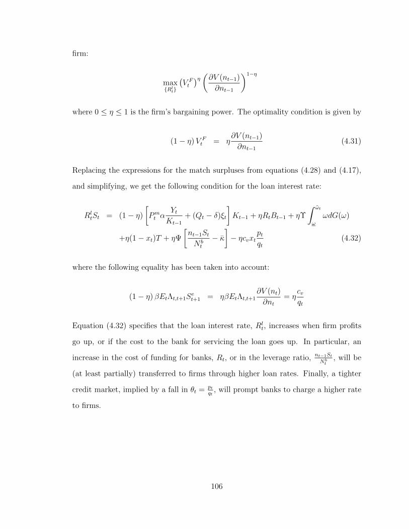
firm:

max{Rlt}

(V Ft

)η (∂V (nt−1)

∂nt−1

)1−η

where 0 ≤ η ≤ 1 is the firm’s bargaining power. The optimality condition is given by

(1− η)V Ft = η

∂V (nt−1)

∂nt−1

(4.31)

Replacing the expressions for the match surpluses from equations (4.28) and (4.17),

and simplifying, we get the following condition for the loan interest rate:

RltSt = (1− η)

[Pmt α

YtKt−1

+ (Qt − δ)ξt]Kt−1 + ηRtBt−1 + ηΥ

∫ ωt

ω

ωdG(ω)

+η(1− xt)T + ηΨ

[nt−1StN bt

− κ]− ηcvxt

ptqt

(4.32)

where the following equality has been taken into account:

(1− η) βEtΛt,t+1Set+1 = ηβEtΛt,t+1

∂V (nt)

∂nt= η

cvqt

Equation (4.32) specifies that the loan interest rate, Rlt, increases when firm profits

go up, or if the cost to the bank for servicing the loan goes up. In particular, an

increase in the cost of funding for banks, Rt, or in the leverage ratio, nt−1StNbt

, will be

(at least partially) transferred to firms through higher loan rates. Finally, a tighter

credit market, implied by a fall in θt = ptqt

, will prompt banks to charge a higher rate

to firms.

106

4.2.6 Capital Producing Firms

At the end of period t, capital producing firms buy capital from intermediate goods

producing firms, repair depreciated capital at unit cost, build new capital and sell it at

price Qt. Following Gertler and Karadi [2011], I assume that the cost of refurbishing

depreciated capital is unity. Accordingly, there is no adjustment cost associated with

refurbishing depreciated capital, but there are flow adjustment costs with producing

new capital. These adjustment costs are imposed on net investment flow, which,

by definition, excludes depreciated capital, rather than gross investment flow that

include them. The capital producing firms’ problem is to chose net investment to

maximize the following sum of discounted profits:

max{Int }

Et

∞∑τ=0

βt+τΛt,t+τ

[Qt+τI

nt+τ − Int+τ − f

(Int+τ + I

Int+τ−1 + I

)(Int+τ + I)

]

where Int is net capital created, and I is steady-state investment. The adjustment

cost function satisfies f(1) = f ′(1) = 0, f ′′(1) > 0.

The definition of net new capital and the law of motion of capital stock is given

by:

Int ≡ It − δξtKYt−1 (4.33)

KYt = ξtK

Yt−1 + Int (4.34)

where It is gross capital created, and aggregate capital, KYt = ntKt. Any profit from

the capital producing firms is rebated back to the household. The optimal condition

for the capital producing sector gives the following relation for net investment:

Qt = 1 + f(·) +Int + I

Int−1 + If ′(·)− EtβΛt,t+1

(Int+1 + I

Int + I

)2

f ′(·) (4.35)

107

4.2.7 Retail Sector

Following Bernanke et al. [1999] and Gertler and Karadi [2011], I model the retail

sector in two steps. First, a continuum of monopolistically competitive retail firms

indicated by i ∈ [0, 1] purchases the homogeneous intermediate good at price Pmt

and costlessly differentiates them to a continuum of retail goods. Second, these

differentiated goods Yi,t are combined into a composite final good Y Ft by a packaging

firm using a Dixit-Stiglitz aggregating technology :

Y Ft =

[∫ 1

0

Yε−1ε

i,t di

] εε−1

, ε > 0

where 1/(ε − 1) > 0 is the constant elasticity of substitution between differentiated

retail goods. Cost minimization by the final good packer gives the following demand

for each type of retail good

Yi,t =

(Pi,tPt

)−εY Ft

where Pt is the price of a unit of final good determined by the zero profit condition:

Pt =

[∫ 1

0

P 1−εi,t di

]1/(1−ε)

The marginal cost faced by the monopolistically competitive retail firms is the price,

Pmt , of intermediate goods. Following Calvo [1983], nominal price stickiness is intro-

duced by assuming staggered price setting by the retail firm. Each period a fraction,

0 < 1− Θ < 1, of retail firms re-sets their sales price optimally, while the remaining

fraction Θ keeps their prices unchanged. The retail firm’s problem is to chose the

108

optimal sales price, P ∗t , given the staggered price setting mechanism

maxp∗t

Et

∞∑j=0

Λt,t+jΘj[P ∗t Yf,t+j − Pt+jPm

t+j

]subject to a sequence of demand curves

Yi,t+j =

(P ∗tPt+j

)−εY Ft+j

The optimal price, P ∗t , satisfies the first-order condition

Et

∞∑j=0

Λt,t+jΘjYi,t+j

[P ∗t −

ε

ε− 1Pmt+jPt+j

]= 0 (4.36)

where the aggregate price level is given by

Pt =[ΘP 1−ε

t−1 + (1−Θ)P∗(1−ε)t

] 11−ε

(4.37)

Log-linearizing equations (4.36) and (4.37) around a steady-state inflation rate of 1,

we get the following expression for the New-Keynesian Philips curve

πt = βEtπt+1 +(1− βΘ)(1−Θ)

ΘPmt (4.38)

where πt = Pt/Pt−1 is the inflation rate, and hats represent variables that are log-

linearized around their respective steady-states.

4.2.8 Resource Constraint and Policy

Final output is the sum of output from each individual project, and is divided be-

tween consumption, investment, adjustment costs, and costs incurred by banks for

109

separation and search for new projects.

Y Ft ≡ nt−1Yt = Ct + It + f

(Int + I

Int−1 + I

)(Int + I) + cvvt + nt−1Υ

∫ ω

ω

ωdG(ω)

+nt−1

∫ ω

ω

TdG(ω) + Ψ

[nt−1StN bt

− κ]

(4.39)

A central bank determines monetary policy by setting the nominal gross interest

rate it, according to a Taylor rule with interest rate smoothing, expressed in log-

linearized form

it ≡ Rt + Etπt+1 = %r it−1 + (1− %r)(%ππt + %yY

Ft

)+ εmt (4.40)

where the smoothing parameter, %r, lies between zero and unity, εmt is an i.i.d. shock

to the nominal interest rate, and the link between nominal and real interest rates

follow a Fisher relationship, and the real interest rate equals the real deposit rate,

Rt, by arbitrage. %π and %Y are the Taylor response coefficients for inflation and the

output gap, respectively.

This concludes the description of the model. Appendix C.2 summarizes the list

of non-linear equations defining the model.

4.2.9 Calibration

I log-linearize the model around its steady-state16 and solve using Dynare.17 The

system of log-linearized equations is presented in appendix C.3. Tables 4.1 and 4.2

summarize the choice of parameter values and steady-state ratios for the benchmark

model. Calibration values of the discount factor, β, the depreciation rate, δ, and

16Note that the steady-state value of net investment Int is zero. I linearize the equations containingInt and normalize by output. All log-linearized variables presented in appendix C.3 are denoted bya hat, and linearized variables denoted by a tilde.

17See Adjemian et al. [2011] and http://www.dynare.org/.

110

the capital share of income, α, are standard. The depreciation rate, δ, and the

steady-state capital to output ratio, KY

, implies a steady-state investment to output

ratio, IY

, of 0.2. I set the habit parameter to 0 in the benchmark, and the inverse

Frisch elasticity of labour supply to 1. The elasticity of net investment to capital

price parameter is set to 1.728, following Gertler and Karadi [2011]. The elasticity of

substitution among retail goods, ε, is chosen to match a markup of 15 per cent. The

Calvo parameter for the frequency of price adjustment is set to 0.8, which is common

in the literature. Following Gertler and Karadi [2011], I set the interest smoothing

parameter in the Taylor rule, %r to 0.8, the inflation response parameter, %π, to 1.5,

and the output response parameter, %Y , to 0.5/4.

There are no standard values prescribed in the literature for the parameters and

steady-state values pertaining to the matching variables. I follow Beaubrun-Diant

and Tripier [2009] and set the match probability of searching projects, p, to 0.4 and

the loan market tightness, θ, to 0.6. The former value implies an average search

duration of two-and-half quarter for projects. The match elasticity parameter, χ, is

set to 0.5 and the bargaining power of the firm, η, is equated to this value in order

to observe the Hosios [1990] condition of match efficiency. The steady state annual

gross loan interest rate is set to 1.05, implying a 3 percent spread between loan and

deposit interest rates.

Using disaggregated quarterly data from the U.S. banking system from 1999

through 2008, Contessi and Francis [2010] calculate a net growth rate in gross loans

(NET ) of 4.67 percent, and in loan reductions (NEG) of 2.42 per cent. To account

for the trend growth in gross loans, I set the loan survival rate, x, to match the

following

x =1−NEG1 +NET

111

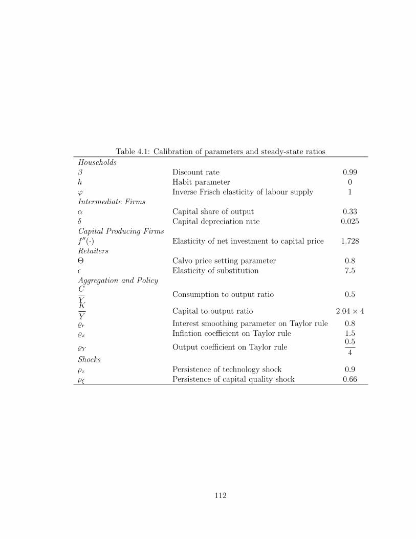
Table 4.1: Calibration of parameters and steady-state ratios

Householdsβ Discount rate 0.99h Habit parameter 0ϕ Inverse Frisch elasticity of labour supply 1Intermediate Firmsα Capital share of output 0.33δ Capital depreciation rate 0.025Capital Producing Firmsf ′′(·) Elasticity of net investment to capital price 1.728RetailersΘ Calvo price setting parameter 0.8ε Elasticity of substitution 7.5Aggregation and PolicyC

YConsumption to output ratio 0.5

K

YCapital to output ratio 2.04× 4

%r Interest smoothing parameter on Taylor rule 0.8%π Inflation coefficient on Taylor rule 1.5

%Y Output coefficient on Taylor rule0.5

4Shocksρz Persistence of technology shock 0.9ρξ Persistence of capital quality shock 0.66

112

Table 4.2: Calibration of parameters and steady-state ratios contd.Matchingp Match probability of searching projects 0.4θ Loan market tightness 0.6χ Elasticity of match 0.5η Bargaining power of firm 0.5Banks

Rl SS loan interest rate 1.051/4

R SS deposit interest rate1

βx SS match survival rate 0.95ω Threshold continuation shock x/2

n SS number of matchesp

1− x(1− p)κ SS bank loan to capital ratio

1

0.08δn Bank dividend payout rate 0.37S

YSS loan to output ratio

1

n× K

YN b

YSS bank capital to output ratio

1

κ× S

YncvN b

v Elasticity of bank equity to vacancy posting 0.1470

nT

N b(1− x) Elasticity of bank equity to separating existing match 0.3921

nΥ

N bωx Elasticity of bank equity to continuing existing match 6.1582

Ψ

YQuadratic cost for deviating from capital adequacy 0.1

113

This gives a separation rate of 0.95. I assume a uniform distribution for the ‘relation-

ship shock’ on a unit spread (i.e., ω−ω = 1 ), and set the threshold value for ω such

that total cost to maintaining loan relationships in the steady-state equals zero.18

I set the steady-state capital price to equal 1 , and the total loan to output ratio

to equal the capital to output ratio. The parameter κ is set such that bank equity is

equal to 8 per cent of total assets. This matches the requirements set out in the 1988

Basel-I accord. In the steady-state, bank equity matches this requirement. I set the

bank dividend payout rate, δn, such that dividends equal net profits of the banking

sector, including interest income, loan vacancy posting cost, and separation cost.19

The dynamics of the search mechanism depends importantly on the loan vacancy

posting cost, cv, and the parameters determining the cost of continuing or separating

existing relationships, Υ and T . Since the literature is silent on prescribing values

for these parameters, I choose benchmark values to give reasonable impulse responses

to the four types of shocks considered. In particular, the values are chosen to give a

non-negative interest spread response on impact for technology and monetary shocks.

The benchmark value for cv implies an elasticity of bank equity to vacancies of 0.147

percent. The benchmark value for T implies an elasticity of bank equity to the match

separation rate of 0.392. Finally, the benchmark value for Υ implies an elasticity of

bank equity to the match continuation rate of 6.158. I check the sensitivity of model

results to the calibration of these parameters in section 4.3.1.

18A uniform distribution implies

∫ ωt

ω

ωdG(ω) =ω2t − ω

2(ω − ω). So, ω must follow the following two

conditions x =ω − ωω − ω

and 0 =ω2 − ω2

2(ω − ω).

19Precisely, δn is set such that δnN b

Y= n

[Rl −R

(1− 1

κ

)]S

Y− n(1− x)

T

Y− v cv

Y.

114

4.3 Counter-cyclical Interest Spread

In this section, I analyze the responses of the benchmark model to three different

shocks that have a primary effect on credit demand – a technology shock, a monetary

shock, and a shock to productive capital quality. I show the results for shocks that

directly affect credit supply to the next section.

First, I show that the banking model amplifies and propagates the responses to all

three shocks. The amplification is due to a counter-cyclical spread between the loan

rate and the deposit rate. I then explain the core mechanism of the search framework

that generates the interest spread. Finally, I consider alternate calibration values for

a few key parameters. I frame my results below in terms of contractionary shocks

in an attempt to make the discussion relevant to current times. The magnitude and

direction of the impulse responses, however, are symmetric around the steady state,

and depend on the sign of the exogenous shock.

Figure 4.2 compares impulse responses from the benchmark model with those from

a standard New Keynesian one. The New Keynesian specification is constructed by

eliminating the banking sector from the benchmark model, and equating the loan

interest rate Rlt to the deposit rate Rt. The remaining sections and calibrations

are the same across the two specifications. The first three columns show responses

for a one percent shock to technology, interest rate and capital quality, respectively.

The persistence parameter of the technology shock, ρz, is set to 0.8, and that of the

capital shock, ρξ, is set to 0.66, following Gertler and Karadi [2011]. Figure 4.3 shows

responses of selected financial market variables to the same shocks, presented in the

same order.

The presence of a banking sector amplifies and propagates the responses to all

shocks. In contrast, using exogenous borrowing constraints in a monopolistically

competitive banking model, Gerali et al. [2010] find that the presence of banks at-

115

tenuates the economy’s responses to monetary and technology shocks. Moreover,

all negative shocks generate a counter-cyclical interest rate spread and a persistent

recession.

Following Gertler and Karadi [2011], I consider a negative shock to capital quality

in an attempt to capture the effects of a financial crisis. A decline in capital quality

reduces the productivity of capital and, in itself, can generate a recession. However,

the resulting decline in capital prices also induces a persistent decline in the value of

bank assets, as seen during the sub-prime crisis. It is this secondary effect working

through the financial system that is of interest here. Figure 4.2 shows that a reduc-

tion in the effectiveness of capital induces a modest recession in the NK model. In

the presence of a banking sector, however, this decline is greatly amplified. The fall

in capital value reduces the size of banking assets. This loss in assets is translated to

a strong and persistent reduction in bank equity through the balance sheet identity.

Interest spreads rise on impact, further reducing the demand for capital and invest-

ment by the firm. Capital prices fall even further, exacerbating the balance sheet

position of banks. As a result, the overall contraction in the economy is magnified.

4.3.1 Explanation of the Core Mechanism

Search frictions generate a counter-cyclical wedge between loan and deposit interest

rates that amplifies business cycles. The mechanism can be explained by considering

equations 4.18 and 4.32. They are reproduced below for ease of reference, where

the match finding probabilities pt and qt have been expressed in terms of the market

tightness variable θt, and the expression for average bank profit from loan officers,

116

Figure 4.2: Comparison of the benchmark model with search frictions in the bankingsector and the standard new Keyenesian model.

5 10 15 20

−0.06

−0.04

−0.02

0

Ou

tpu

t

Technology

5 10 15 20

−0.2

−0.1

0

Inve

stm

ent

5 10 15 20

0

0.2

0.4

0.6

Spre

ad

5 10 15 20

−0.4

−0.2

0Monetary

5 10 15 20

−1.5

−1

−0.5

0

5 10 15 20

0

5

10

5 10 15 20

−0.4

−0.2

0Capital Quality

5 10 15 20

−1

−0.5

0

5 10 15 20

0

2

4

6

8

Notes: Solid lines represent impulse responses from the benchmark model with abanking sector, broken line represents a standard New Keynesian model. The firstcolumn represents impulse responses to a negative technology shock, the second to acontractionary monetary shock, and the third to a negative capital quality shock.

117

Figure 4.3: Impulse responses for selected banking sector variables.

5 10 15 20

−0.04−0.02

00.02

Th

eta

Technology

5 10 15 20

−0.03

−0.02

−0.01

Ban

k E

qu

ity

5 10 15 20

−0.04

−0.02

0

Int M

arg

in

5 10 15 20

−5

0

5

x 10−3

Ext

Ma

rgin

5 10 15 20

−0.8−0.6−0.4−0.2

00.2

Monetary

5 10 15 20

−0.2

−0.1

0

5 10 15 20

−0.2

−0.1

0

5 10 15 20−0.1

−0.05

0

5 10 15 20

−0.4−0.2

00.20.4

Capital Quality

5 10 15 20

−0.4

−0.2

0

5 10 15 20

−0.4

−0.2

0

5 10 15 20−0.04−0.02

00.020.040.060.08

Notes: The first column represents impulse responses to a negative technology shock,the second to a contractionary monetary shock, the third to a negative capital qualityshock.

118

Πbt , is given in equation 4.10.

cvmθχt = βEtΛt,t+1

{Πbt+1 −Ψ

[ntSt+1

N bt+1

− κ]

+ θχt+1

∫ ωt+1

ω

cvmdG(ω)

}(4.41)

RltSt = (1− η)

[αPm

t

YtKt−1

+ (Qt − δ)ξt]Kt−1 + ηRt

(St −

N bt

nt−1

)+ηΥ

∫ ωt

ω

ωdG(ω) + η

∫ ω

ωt

TdG(ω) + ηΨ

[nt−1StN bt

− κ]

−ηθt∫ ωt

ω

cvdG(ω) (4.42)

We know that whenever a negative technology shock reduces output, Yt, a con-

tractionary monetary shock increases interest rate, Rt, or a negative capital quality

shock, ξt, hits the economy, the firm’s demand for loans, and consequently, its surplus

from an active match declines. Through Nash bargaining, this reduction in the firm’s

surplus calls for a reduction in the loan rate, Rlt. Despite this downward pressure

on Rlt from reduced loan demand, search frictions imply a counter-cyclical rise in the

spread between loan and deposit interest rates.

The intuition is as follows. Lower loan demand means less profit for banks. Faced

with lower expected profits, banks reduce their effort in searching for new matches,

or in maintaining existing matches. Consequently, matches become scarcer, and the

market tightness variable, θt =vtut

, decreases. This can be readily seen in the vacancy

creation condition, equation 4.41. Holding all else constant, a reduction in θt provides

upward pressure on the loan rate through the Nash bargaining condition in equation

4.42. In the benchmark calibration, this upward pressure from θt is enough to generate

a counter-cyclical spread between Rlt and Rt.

20 In essence, a reduction in loan demand

from the firm’s side is met with a reduction in the supply of credit in the extensive

margin by the banking sector. The resulting rise in spreads further exacerbates loans

20Beaubrun-Diant and Tripier [2009] provides an analysis of the calibration necessary to produce acounter-cyclical rise in spreads for technology and monetary shocks in an RBC model in the absenceof an endogenous bank leverage ratio.

119

in equilibrium. Consequently, investment and output fall by more than the standard

New Keynesian case.

Two additional channels in the benchmark model aid in generating a counter-

cyclical interest spread. First, through the balance sheet identity, a reduction in

bank profits is translated to a fall in bank equity, which raises the bank leverage ratio

counter-cyclically. Since banks incur a cost for deviating from a regulated leverage

ratio, they respond by reducing the number of loan vacancies. Consequetly, θt in

equation 4.41 falls, and Rlt rises through equation 4.42.

Second, endogenous match separation in the benchmark model is triggered by

the same mechanism as search efforts. Since banks are required to pay an idiosyn-

cratic servicing cost to maintain existing matches, a reduction in expected profits

for banks prompts them to reduce the number of existing relationships. A reduc-

tion in the match survival rate

∫ ωt

ω

dG(ω) (or an increase in the separation rate)

increases the number of unmatched firms searching for matches, further reduces θt,

and consequently further enhances the accelerator effect described above.

Therefore, for technology, monetary, or capital quality shocks, a counter-cyclical

rise in interest spread is triggered by the banking sector’s decision to reduce credit

supply in the extensive margin in response to the decline in credit demand from the

firm. In contrast, shocks to bank equity works by directly reducing the supply of

credit. In particular, a fall in bank equity leads to a rise in the leverage ratio. To

bring the leverage ratio back to the steady-state, banks reduce vacancy postings, and

consequently, the loan rate, Rlt, rises relative to the deposit rate, Rt. The effects of a

supply-side shock to credit is shown in the next section.

Finally, the vacancy posting cost cv, and the cost of separating an existing match,

T , are important in determining the dynamics of interest spreads. Figure 4.4 provides

sensitivity analysis for the elasticity of bank net worth to loan vacancy posting. If

120

Figure 4.4: Sensitivity to the cost of posting loan vacancies.

5 10 15 20

−0.08

−0.06

−0.04

−0.02

0

Ou

tput

Technology

5 10 15 20

0

0.5

1

Sp

read

5 10 15 20−0.1

−0.05

0

0.05

Tig

htn

ess

5 10 15 20

−0.6

−0.4

−0.2

0

Monetary

5 10 15 20

0

5

10

15

5 10 15 20

−1.5

−1

−0.5

0

5 10 15 20

−0.4

−0.2

0

Capital Quality

5 10 15 20

0

5

10

5 10 15 20

−1

−0.5

0

0.5

Note: Solid line represents benchmark value for the elasticity of bank net worth to loanvacancy posting, n cv

Nbv = 0.15, broken line represents a bigger value of n cvNbv = 0.3,

and dotted line represents a lower value of n cvNbv = 0.08. The first column represents

impulse responses to a negative technology shock, the second to a contractionarymonetary shock, and the third to a negative capital quality shock.

121

Figure 4.5: Sensitivity to the cost of separating existing loans.

5 10 15 20

−0.1

−0.05

0

Ou

tput

Technology

5 10 15 20

−1

0

1

2

3

Sp

read

5 10 15 20

−0.1

−0.05

0

0.05

Tig

htn

ess

5 10 15 20

−1

−0.5

0

Monetary

5 10 15 20

0

20

40

5 10 15 20

−1.5

−1

−0.5

0

0.5

5 10 15 20

−0.6

−0.4

−0.2

0

0.2Capital Quality

5 10 15 20

−10

0

10

20

5 10 15 20−1

−0.5

0

Note: Solid line represents benchmark value for the elasticity of bank net worth toseparating existing loans, n T

Nb (1− x) = 0.39, broken line represents a bigger value ofn TNb (1−x) = 0.52, and dotted line represents a lower value of n T

Nb (1−x) = 0.26. Thefirst column represents impulse responses to a negative technology shock, the secondto a contractionary monetary shock, and the third to a negative capital quality shock.

122

the cost of loan vacancy posting is higher, the response in credit market tightness is

subdued. In this case, the effect of technology and monetary shocks on the Nash-

bargained loan rate is not overturned by the reduction in the extensive margin of

loans by the banking sector. As a result, the interest spread falls on impact for these

two shocks. In contrast, a lower cost of loan vacancy posting allows for a higher

response in spreads.

Figure 4.5 provides sensitivity analysis for the elasticity of bank net worth to

separating existing loans. Similar to the explanation above, if the cost of separating

existing loans is higher, the movement in credit market tighness is subdued, and the

negative effect of technology and monetary shocks on the interest spread becomes

stronger. This produces a lower initial credit spread response. In contrast, a lower

cost of separation increases the volatility of the tightness variable, and allows for a

higher initial response in spreads. However, this higher response in spreads is followed

by a large correction, which is difficult to imagine in real life. A careful analysis on

the empirical response of credit spreads to technology, monetary and capital quality

shocks would spread light on the appropriate calibration warranted in this model.

4.4 Credit Supply Shock and Gross Loan Flows

In this section, I show that the model produces empirically plausible responses in

loan creation and destruction flows for a credit supply shock. First, I estimate the

empirical response of gross loan flows and loan levels to an orthogonal credit supply

shock in a VAR framework. Second, I show that a negative shock to bank equity

generates counter-cyclical spreads, and movements in loan creation and destruction

margins that qualitatively match VAR results when investment is elastic to capital

price. However, quantitatively, the model generates insufficient variations in gross

loan flows compared to data.

123

Gilchrist and Zakrajsek [2012a] and Boivin et al. [2012] find that a shock to credit

supply has a substantial effect on the real economy. Gilchrist and Zakrajsek [2012b]

finds that a negative shock to credit supply reduces aggregate bank lending to firms

using a VAR framework. However, whether this decline in aggregate loans is carried

through by a reduction in new loan creation, or by destroying existing lending relations

has not been studied.

Creation and destruction margins may respond differently to shocks affecting the

economy for several reasons. First, extending new loans and retiring existing ones

are two distinct activities involving different costs. The former may involve the cost

of information acquisition, searching for new clients, or evaluating new projects. On

the other hand, contractions in loans may depend on the liquidity of borrowers or on

the legal steps involved in ensuring repayment or separation of relationships.

Second, loan expansion and contraction decisions may vary differently across

banks. Regional and sectoral differences in both borrowers and lenders may result

in overall loan contraction in some banks and expansion in others. Moreover, these

idiosyncratic differences may depend on the type of shock affecting the economy. The

2008-09 recession was brought forth by a shock to the entire financial system. All

banks were more-or-less negatively affected by the crisis.21 This is not necessarily the

case for other recessions.

Finally, Contessi and Francis [2010] finds that gross loan flows followed a unique

pattern during the 2008 and 1990-91 recessions – both of which coincide with an ero-

sion of bank equity. During most recessions, loan destruction increases and creation

decreases. However, the magnitude of the changes are such that net loans, defined as

expansion minus contraction, usually remains a small positive in level terms. More-

over, loan destruction does not usually persist beyond the initial quarter of the reces-

21See Brunnermeier [2009] for a summary of the economic mechanisms that characterized thefinancial crisis.

124

sion. In contrast, during the two recessions involving stress on the financial system,

loan destruction exceeded creation so that the net loan flow became negative. This

suggests that credit shocks may have a unique effect on the dynamics of these two

variables. The goal of this section is to capture the pattern of response from a credit

shock and to see whether the benchmark model is able to match it.

In the remainder of the section, I first provide a brief description of the data and

estimation. I then describe the empirical findings and compare them with model

results.

4.4.1 Data and Estimation

I use quarterly data series on gross loan flows constructed using bank-level balance

sheet information for 1979 through 1999 by Dell’Ariccia and Garibaldi [2005] and

extended from 1999 through 2008 by Contessi and Francis [2010].22 Loan creation,

POSt, is defined as the weighted sum of changes in loans for banks that increased

loans in any given quarter. Loan destruction, NEGt, is defined as the absolute value

of the weighted sum of changes in loans for all banks that decreased their loans since

the previous quarter.23

Note that the data represents all types of loans extended by commercial banks,

including mortgages, lines of credit, and commercial and industrial loans. The model

considered in the remainder of the paper, however, considers only commercial and

industrial loans. Although this difference may be non-trivial for shocks to technology

22The two gross loan series are constructed using quarterly bank-level balance sheet informationpublicly available in the Reports of Condition and Income database (commonly called Call ReportFiles). Consolidation, entry and exits of banks during the time period is corrected for by matching thedata with the National Information Center’s (NIC) transformation table to avoid double counting.See Contessi and Francis [2010] for a full description of the data construction methodology. I jointhe series calculated by Contessi and Francis [2010] to that from Dell’Ariccia and Garibaldi [2005]and consider an unbroken series running from 1979:Q2 through 2008:Q2.

23This approach of constructing gross loan flows mirrors the calculation of gross job flows in Daviset al. [1998], where net employment changes in the economy is decomposed into the two componentsof job creation and job destruction.

125

or monetary policy, it is not unreasonable to expect the general response of aggregate

loans to carry through for other loan categories for a financial shock that affects bank

balance sheets on a systemic scale.

Following Gilchrist and Zakrajsek [2012b], I estimate a VAR with two lags, and

identify a bank credit supply shock as an orthogonal shock to the ‘GZ excess bond

premium’.24 The VAR includes the following variables, ordered accordingly: (1) the

log-difference in real investment, (2) the log-difference in real GDP, (3) log-difference

in the GDP deflator, (4) the excess bond-premium, (5) the log-difference in real busi-

ness loans outstanding in all commercial banks, (6) the effective (nominal) federal

funds rate, (7) real loan creation (POS) and (8) real loan destruction (NEG).25 This

ordering allows the first three variables, which are traditionally viewed as ‘slow mov-

ing’, to respond to a shock in credit supply only after a quarter. The variables ordered

after the excess bond-premium, however, are allowed to respond contemporaneously

to a shock in credit supply. The data are in quarterly frequencies, and span the

period from 1979:Q2 through 2008:Q2, for which information on loan creation and

destruction are available.

Figure 4.6 shows the impulse responses to a Cholesky-ordered shock to the excess

bond-premium, along with their 68th and 95th percentile Monte Carlo confidence

bands. An increase in the excess bond-premium generates a recession driven by a

24This variable is constructed by Gilchrist and Zakrajsek [2012a] to measure the deviation in thepricing of corporate debt claims relative to the expected default risk of the issuer, and captures shiftsin risk attitudes of financial intermediaries. Using a large panel of corporate bonds issued by non-financial firms, credit spreads associated with individual firms are decomposed into two components:one capturing the risk of default, and another capturing the cyclical-fluctuations of the relationshipbetween default risk and credit spreads. Gilchrist and Zakrajsek [2012a] and Gilchrist and Zakrajsek[2012b] show that the majority of the information contained in credit spreads commonly used in theliterature is attributable to movements in the excess bond premium, and that shocks to the excessbond premium that are orthogonal to current macroeconomic conditions have significant effects onthe real economy, as well as on outstanding bank loans. Accordingly, I take the lag structure of theVAR and the Cholesk-ordered identification scheme as given in Gilchrist and Zakrajsek [2012a] andGilchrist and Zakrajsek [2012b].

25Real values of aggregate business loans, and disaggregated flows in loan creation and destructionare calculated by dividing the relevant variables with the GDP deflator.

126

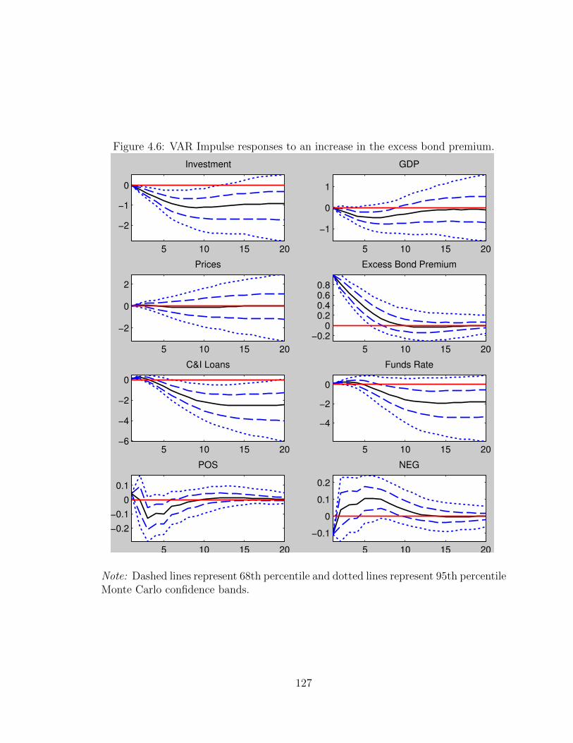
Figure 4.6: VAR Impulse responses to an increase in the excess bond premium.

5 10 15 20

−2

−1

0

Investment

5 10 15 20

−1

0

1

GDP

5 10 15 20

−2

0

2

Prices

5 10 15 20

−0.2

0

0.2

0.4

0.6

0.8

Excess Bond Premium

5 10 15 20−6

−4

−2

0

C&I Loans

5 10 15 20

−4

−2

0

Funds Rate

5 10 15 20

−0.2

−0.1

0

0.1

POS

5 10 15 20

−0.1

0

0.1

0.2

NEG

Note: Dashed lines represent 68th percentile and dotted lines represent 95th percentileMonte Carlo confidence bands.

127

Figure 4.7: Net percentage of banks tightening lending and the excess bond premium.

-1.5

-1

-0.5

0

0.5

1

1.5

2

2.5

-40.0

-20.0

0.0

20.0

40.0

60.0

80.0

100.0

19

90

-Q2

19

91

-Q1

19

91

-Q4

19

92

-Q3

19

93

-Q2

19

94

-Q1

19

94

-Q4

19

95

-Q3

19

96

-Q2

19

97

-Q1

19

97

-Q4

19

98

-Q3

19

99

-Q2

20

00

-Q1

20

00

-Q4

20

01

-Q3

20

02

-Q2

20

03

-Q1

20

03

-Q4

20

04

-Q3

20

05

-Q2

20

06

-Q1

20

06

-Q4

20

07

-Q3

20

08

-Q2

20

09

-Q1

20

09

-Q4

20

10

-Q3

Net Tightening Standards Excess Bond Premium

Note: Solid line represents the net percentage of banks reported as tightening lendingstandards for commercial and industrial loans to large and medium firms. Markedline represents the Gilchrist and Zakrajsek [2012a] excess bond premium.

128

Figure 4.8: VAR impulse responses to an increase in the net percentage of bankstightening lending standards.

5 10 15 20

−2

−1

0

Investment

5 10 15 20−2

−1

0

GDP

5 10 15 20

−0.5

0

0.5

Tighten Lending

5 10 15 20−0.5

0

0.5

Excess Bond Premium

5 10 15 20

−6

−4

−2

0

C&I Loans

5 10 15 20

−20

−10

0

Funds Rate

5 10 15 20

−0.3

−0.2

−0.1

0

0.1

POS

5 10 15 20

−0.2

0

0.2

0.4

NEG

Note: Dashed lines represent 68th percentile and dotted lines represent 95th percentileMonte Carlo confidence bands.

129

reduction in investment. Aggregate commercial and industrial loans outstanding at

all banks decline. Most importantly, loan creation, POSt, falls and loan destruction,

NEGt, rises a few quarters after the initial shock. Therefore, in so far as the excess

bond-premium captures information about the supply of bank credit, we can say that

a negative supply shock increases loan destruction, and reduces loan creation.

A more direct measure of bank credit supply, however, can be gathered from survey

results on banks’ willingness to lend. The Federal Reserve Board’s Senior Loan Officer

Opinion Survey on Banking Lending Practices, conducted each quarter on 60 U.S.

banks, asks senior officers whether banks have changed their credit standards over the

past three months. The data, available from 1990:Q2, is plotted in figure 4.7, along

with the excess bond premium.26 The solid line represents the net percentage of

banks that reported tightening their credit standards on commercial and industrial

loans to large and medium-sized firms. The net percentage value is calculated as

the percentage of banks that report tightening less the percentage that report not

tightening lending standards.27 As the figure shows, banks tighten their lending

standards counter-cyclically, and at the height of the financial crisis, almost all banks

reported doing so.

With this arguably more direct measure of bank credit supply, I run a VAR

with two lags that includes the following variables, ordered accordingly: (1) the log-

difference in real investment, (2) the log-difference in real GDP, (3) net percentage

of banks tightening lending standards, (4) the excess bond-premium, (5) the log-

difference in real business loans outstanding in all commercial banks, (6) the effective

(nominal) federal funds rate, (7) real loan creation (POS) and (8) real loan destruc-

26Indeed, one of the merits of the GZ excess bond-premium listed in Gilchrist and Zakrajsek[2012b] is its strong co-movement properties with the change in lending standards, which is clearlydemonstrated in the figure.

27See http://www.federalreserve.gov/boarddocs/SnLoanSurvey/ for a description of the questionsand more information on the survey.

130

tion (NEG). The impulse responses from an orthogonalized shock to bank lending

standards is reported in figure 4.8. A tightening of lending standards increases the

excess bond premium on impact. Consequently, outstanding commercial and indus-

trial bank loans fall gradually, as do investment and output. Loan creation declines

with a lag, and loan destruction rises on impact.

Overall, I take the above evidence to suggest that a reduction in bank credit

supply has a negative effect on the real economy, driven by a rise in interest spreads,

and a consequent fall in loans to firms. Moreover, following a credit supply shock,

disaggregated loan destruction rises and loan creation falls.

4.4.2 Model Analysis

In this subsection, I compare model results on loan creation and destruction flows

from a credit supply shock with empirical evidence outlined above. Note that the

empirical definition of these flows include changes in loans from both the intensive

and extensive margins. To conform with data, I derive the following parallel in the

benchmark model:

POSt =mt−1Stnt−2St−1

NEGt = −xtStSt−1

POSt −NEGt =nt−1Stnt−2St−1

where POSt −NEGt equals the change in total loans from period t− 1 to period t.

I find that the model can generate impulse responses for loan creation and destruc-

tion flows to a credit supply shock that qualitatively match evidence, if investment

is allowed to be less sluggish than usually assumed in the literature. To capture the

concept of a shock to credit supply, I consider an i.i.d. shock to bank equity, as well

131

as an i.i.d. increase to the match separation rate. The former shock is specified in

the law of motion of banke equity (equation 4.20), while the later is modelled as an

exogenous drop in the survival rate, xt. The optimal separation condition (equation

4.19) is then changed to

Υxtεxt

= (T −Υω) +cvqt

where εxt is an i.i.d. shock to the survival rate.

Figure 4.9 shows impulse responses for both these shocks for the benchmark cal-

ibration. For comparison, the ‘crisis experiment’ case of a negative capital quality

shock is also included in the figure. We see that all three shocks result in a counter-

cyclical rise in the interest spread, and an ensuing recession. However, apart from

the rise on impact for NEG, and the eventual decline in POS for the capital quality

shock, the response for disaggregated flows do not conform with data.

To see why this may be the case, note that net loan flows, which equal loan

creation less loan destruction, captures changes in loan levels. For each of the shocks

considered, we see a large temporary drop in capital prices, followed by a gradual

decline in capital stock. Since loans are used in this model to purchase capital, the

impulse response of total real loans reflect both the large initial drop in real capital

prices as well as the small gradual decline in capital levels. As such, the impulse

response for loans does not match the smooth response seen in the data. Since

responses in disaggregated loan flows capture the curvature of the response in loan

levels, we see the counter-factual result shown in figure 4.9.

If however, investment were allowed to be more responsive to capital prices, we

may generate loan responses of the shape seen in the data. In the benchmark model,

the parameter capturing the inverse of the elasticity of net investment to the price

of capital was set to 1.728, as adopted by Gertler and Karadi [2011]. This is repre-

132

Figure 4.9: Benchmark model impulse responses to credit supply shock

5 10 15 20

−0.4

−0.2

0

Ou

tput

Capital Quality

5 10 15 20

0

2

4

6

Sp

rea

d

5 10 15 20

−0.04

−0.02

0

PO

S

5 10 15 20−0.05

0

0.05

0.1

0.15

NE

G

5 10 15 20−0.02

−0.01

0Bank Equity

5 10 15 200

2

4

6

5 10 15 20

0

10

20

x 10−4

5 10 15 20−0.01

0

0.01

5 10 15 20

−8−6−4−2

02

x 10−3 Separation

5 10 15 200

0.5

1

5 10 15 20

0

2

4

x 10−3

5 10 15 20

0

2

4

x 10−3

Note: First column represents a negative shock to productive capital quality, secondcolumn represents an i.i.d. reduction in bank equity, and the third column representsan i.i.d. increase in the separation rate. Benchmark calibration implies an inverseinvestment elasticity to capital price of 1.728.

133

Figure 4.10: Comparison of impulse responses to credit supply shock for differentinvestment elasticities

5 10 15 20−4

−2

0

Investm

en

t

Capital Quality

5 10 15 20

−0.6

−0.4

−0.2

0

Loan

s

5 10 15 20

−0.15

−0.1

−0.05

0

Ca

pita

l P

rice

5 10 15 20

−0.6

−0.4

−0.2

0

Cap

ita

l

5 10 15 20

−0.4

−0.2

0

Bank Equity

5 10 15 20

−0.02

−0.01

0

5 10 15 20

−15

−10

−5

0x 10

−3

5 10 15 20

−0.02

−0.01

0

5 10 15 20

−0.08

−0.06

−0.04

−0.02

0

Separation

5 10 15 20

−6

−4

−2

0x 10

−3

5 10 15 20

−4

−2

0x 10

−3

5 10 15 20

−6

−4

−2

0x 10

−3

Note: First column represents a negative shock to productive capital quality, secondcolumn represents an i.i.d. reduction in bank equity, and the third column representsan i.i.d. increase in the separation rate. Dashed lines represent the benchmarkcalibration of an inverse investment elasticity to capital price of 1.728. Solid linerepresents an inverse investment elasticity to capital price of 0.11.

134

Figure 4.11: Model impulse responses to credit supply shock for elastic investment

5 10 15 20

−0.5

0

Ou

tput

Capital Quality

5 10 15 20−1

0

1

2

Sp

rea

d

5 10 15 20

−0.5

0

Lo

ans

5 10 15 20

−0.05

0

PO

S

5 10 15 20

−0.05

0

0.05

0.1

NE

G

5 10 15 20

−0.05

0Bank Equity

5 10 15 200

2

4

5 10 15 20

−0.02

−0.01

0

5 10 15 20−3

−2

−1

0x 10

−3

5 10 15 20

0

5

10

x 10−3

5 10 15 20−0.02

−0.01

0Separation

5 10 15 200

0.5

1

5 10 15 20

−5

0x 10

−3

5 10 15 20

0

2

4

x 10−3

5 10 15 20

0

2

4

x 10−3

Note: First column represents a negative shock to productive capital quality, secondcolumn represents an i.i.d. reduction in bank equity, and the third column representsan i.i.d. increase in the separation rate. The inverse investment elasticity to capitalprice is set to 0.11.

135

sentative of the values commonly assumed in the macro literature. However, using

disaggregated data from 18 U.S. manufacturing industries, Groth and Khan [2010]

estimate the weighted average of the elasticity of investment to the current shadow

price of capital to be 15.2, suggesting a value of the inverse elasticity parameter of

around 0.067. Figure 4.10 shows impulse responses of investment, aggregate loans,

real capital price, and capital levels for credit supply shocks for two calibrations. The

dashed line represents the benchmark calibration with a high inverse elasticity pa-

rameter, and the solid line represents a calibration of 0.11, a value between the two

extremes mentioned above. We see that with a more elastic investment, the impulse

response for loans are smoother, with a much higher drop in investment for a credit

supply shock.

Figure 4.11 shows the responses for output, spreads, and both aggregate loans and

disaggregated loan flows to the same three shocks for the highly elastic investment

case. We see now that both for the bank equity shock, as well as the capital quality

shock, loan destruction, NEGt, increases on impact, and loan creation, POSt, falls

persistently. This result is more in tune with the empirical results seen in figures 4.6

and 4.8. A one-time reduction in the separation rate, however, does not generate im-

pulse responses of disaggregated loan flows that match evidence, despite the smooth

reaction of investment. Loan destruction, NEGt, rises due to the shock to the sep-

aration rate. However, in light of an increased interest spread, and in the absence

of a shock affecting loan demand, banks have no reason to continue reducing loans.

Rather, banks increase their efforts to find new matches, which in turn, increases loan

creation. This result suggests that a more meaningful representation of credit supply

shocks is needed to match movements in disaggregated loan flows seen in the data. In

this manner, the search-theoretic banking model proves useful in separating plausible

explanations of supply-side shocks from implausible ones.

136

From a quantitative perspective, I find that the model generates cyclical co-

movements in gross loan flows that are comparable to empirical findings. The data cal-

culated from bank balance sheet information shows that loan creation is pro-cyclical,

while loan destruction is counter-cyclical. Herrera et al. [2011] calculate similar flows

using non-financial firm-level data from S&P full coverage Compustat tapes, and find

cyclical correlations of a similar magnitude. Table 4.3 compares the correlation of

gross loan flows with output from the Dell’Ariccia and Garibaldi [2005] and Con-

tessi and Francis [2010] dataset and those derived from model simulations for each of

the shocks considered in the model for the benchmark calibration.28 For all shocks

considered, the correlation of gross loan flows with output are comparable to evidence.

Table 4.3: Correlation of gross loan flows with output

Variables data technology monetary capital quality bank equityPOS 0.20 0.17 0.31 0.47 0.35NEG -0.21 -0.19 -0.34 -0.12 -0.24NET 0.20 0.38 0.37 0.51 0.30

The model fails, however, to generate volatilities in gross loan flows comparable to

evidence. Dell’Ariccia and Garibaldi [2005] find that both variations in loan destruc-

tion and loan creation are larger in magnitude than variations in output. Moreover,

destruction is more volatile than creation of loans. Table 4.4 summarizes the stan-

dard deviations of creation and destruction flows relative to output for each of the

shocks considered in the model for the benchmark calibration, along with the relevant

empirical values for aggregate loans.

Table 4.4: Standard deviation of gross loan flows relative to output

Variables data technology monetary capital quality bank capitalPOS 23.85 0.10 0.11 0.18 0.11NEG 26.71 0.17 0.25 0.35 0.33

28i.e. the relative standard deviation if the economy were subject to one type of shock only.

137

We see that for each shock, model generated flows in loan creation and destruction

are less volatile than output. The values for the corresponding relative standard

deviations in the high investment elasticity case are comparable with the benchmark

calibration of low investment elasticity shown here. This suggests, if anything, that

the model requires an even stronger variation in endogenous separation.

4.5 Conclusion

In this chapter, I develop a search-theoretic banking model in a New-Keynesian DSGE

framework that can simultaneously explain movements in gross flows in loan creation

and destruction, and the interest rate spread. The model demonstrates that the

presence of the banking sector amplifies and propagates the economy’s response of a

number of shocks by generating a counter-cyclical interest rate spread. Shocks that

disproportionately affect the balance sheets of banks are particularly amplified. More-

over, shocks originating within the banking sector also lead to prolonged recessions.

I show that the model generates responses in gross loan creation and destruction

flows to a credit supply shock that qualitatively match empirical evidence. I estimate

the effect of a credit supply shock on loan creation and destruction margins in a VAR

framework. I then consider two shocks that can proxy the effects of a credit supply

shock – a one time reduction in bank equity, and a one time increase in the match

separation rate. I also consider a negative shock to the quality of productive capital,

which works through the bank balance sheet identity and reproduces well important

movements related to the bank leverage channel observed during the recent crisis. I

show that both the capital quality shock, as well as the shock to bank equity can

produce impulse responses that qualitatively match evidence, if investment is elastic

to capital price. An exogenous increase in the separation rate, however, does not

produce empirically plausible responses for disaggregated loan flows.

138

A limitation of the model, however, is that it cannot quantitatively match the

business cycle volatilities of gross loan creation and destruction flows. In particular,

volatilities of these two margins are far lower than seen in the data. Overall, however,

the paper demonstrates that a search-theoretic banking model is a step in the right

direction in jointly explaining movements in the interest rate spread and gross loan

flows.

139

Bibliography

Stephane Adjemian, Houtan Bastani, Michel Juillard, Ferhat Mihoubi, George Peren-

dia, Marco Ratto, and Sebastien Villemot. Dynare: Reference manual, version 4.

Dynare Working Papers 1, CEPREMAP, 2011.

David Andolfatto. Business cycles and labor-market search. American Economic

Review, 86(1):112–32, March 1996.

Kevin E. Beaubrun-Diant and Fabien Tripier. The credit spread cycle with matching

friction. Working Papers hal-00430809, HAL, November 2009.

Ben S. Bernanke, Mark Gertler, and Simon Gilchrist. The financial accelerator in

a quantitative business cycle framework. In J. B. Taylor and M. Woodford, ed-

itors, Handbook of Macroeconomics, volume 1 of Handbook of Macroeconomics,

chapter 21, pages 1341–1393. Elsevier, 1999.

Jean Boivin, Marc P. Giannoni, and Dalibor Stevanovic. Dynamic effects of credit

shocks in a data-rich environment. Manuscript, 2012.

Markus K. Brunnermeier. Deciphering the liquidity and credit crunch 2007-2008.

Journal of Economic Perspectives, 23(1):77–100, Winter 2009.

G. Calvo. Staggered pricing in a utility maximizing framework. Journal of Monetary

Economics, 12:383–96, 1983.

V.V. Chari, Lawrence J. Christiano, and Patrick J. Kehoe. Facts and myths about

the financial crisis of 2008. Technical report, 2008.

Lawrence J. Christiano, Martin Eichenbaum, and Charles L. Evans. Nominal rigidi-

ties and the dynamic effects of a shock to monetary policy. Journal of Political

Economy, 113(1):1–45, February 2005.

140

Ethan Cohen-Cole, Burcu Duygan-Bump, Jos Fillat, and Judit Montoriol-Garriga.

Looking behind the aggregates: a reply to facts and myths about the financial crisis

of 2008. Technical report, 2008.

Silvio Contessi and Johanna L. Francis. U.S. commercial bank lending through

2008:q4: New evidence from gross credit flows. Economic Inquiry, 51(1), 2010.

ISSN 1465-7295. doi: 10.1111/j.1465-7295.2010.00356.x.

Steven J. Davis, John C. Haltiwanger, and Scott Schuh. Job Creation and Destruction,

volume 1 of MIT Press Books. The MIT Press, 1998.

Giovanni Dell’Ariccia and Pietro Garibaldi. Gross credit flows. CEPR Discussion

Papers 2569, C.E.P.R. Discussion Papers, September 2000.

Giovanni Dell’Ariccia and Pietro Garibaldi. Gross credit flows. Review of Economic

Studies, 72(3):665–685, 07 2005.

Wouter J. den Haan, Garey Ramey, and Joel Watson. Liquidity flows and fragility of

business enterprises. Journal of Monetary Economics, 50(6):1215–1241, September

2003.

Gregory deWalque, Olivier Pierrard, and Abdelaziz Rouabah. Financial (in)stability,

supervision and liquidity injections: A dynamic general equilibrium approach. Eco-

nomic Journal, 120(549):1234–1261, December 2010.

Andrea Gerali, Stefano Neri, Luca Sessa, and Federico M. Signoretti. Credit and

banking in a DSGE model of the euro area. Journal of Money, Credit and Banking,

42(s1):107–141, 09 2010.

Mark Gertler and Peter Karadi. A model of unconventional monetary policy. Journal

of Monetary Economics, 58(1):17–34, January 2011.

141

Simon Gilchrist and Egon Zakrajsek. Credit spreads and business cycle fluctuations.

American Economic Review, 102(4):1692–1720, June 2012a.

Simon Gilchrist and Egon Zakrajsek. Bank lending and credit supply shocks. In

Franklin Allen, Masahiko Aoki, Nobuhiro Kiyotaki, Roger Gordon, Joseph E.

Stiglitz, and Jean-Paul Fitoussi, editors, The Global Macroeconomy and Finance,

pages 154–176. Palgrave Macmillan, 2012b.

Charlotta Groth and Hashmat Khan. Investment adjustment costs: An empirical

assessment. Journal of Money, Credit and Banking, 42(8):1469–1494, December

2010.

Ana Maria Herrera, Marek Kolar, and Raoul Minetti. Credit reallocation. Journal

of Monetary Economics, 58(6):551–563, 2011.

Arthur J Hosios. On the efficiency of matching and related models of search and

unemployment. Review of Economic Studies, 57(2):279–98, April 1990.

Victoria Ivashina and David Scharfstein. Bank lending during the financial crisis of

2008. Journal of Financial Economics, 97(3):319–338, September 2010.

Csaire A. Meh and Kevin Moran. The role of bank capital in the propagation of

shocks. Journal of Economic Dynamics and Control, 34(3):555–576, March 2010.

Monika Merz. Search in the labor market and the real business cycle. Journal of

Monetary Economics, 36(2):269–300, November 1995.

Tommaso Monacelli, Roberto Perotti, and Antonella Trigari. Unemployment fiscal

multipliers. Journal of Monetary Economics, 57(5):531–553, July 2010.

Dale T Mortensen and Christopher A Pissarides. Job creation and job destruction

142

in the theory of unemployment. Review of Economic Studies, 61(3):397–415, July

1994.

Charles Nolan and Christoph Thoenissen. Financial shocks and the us business cycle.

Journal of Monetary Economics, 56(4):596–604, May 2009.

Christopher A Pissarides. Short-run equilibrium dynamics of unemployment vacan-

cies, and real wages. American Economic Review, 75(4):676–90, September 1985.

Frank Smets and Rafael Wouters. Shocks and frictions in us business cycles: A

bayesian DSGE approach. American Economic Review, 97(3):586–606, June 2007.

Etienne Wasmer and Philippe Weil. The macroeconomics of labor and credit market

imperfections. American Economic Review, 94(4):944–963, September 2004.

143

Appendix A

Appendix for Chapter 2

A.1 Non-linear Equations for Benchmark Model

Household

λt =1

ct − act−1

− βEta

ct+1 − act(A.1)

1

Rdt

= βEtλt+1

λt

1

πt+1

(A.2)

144

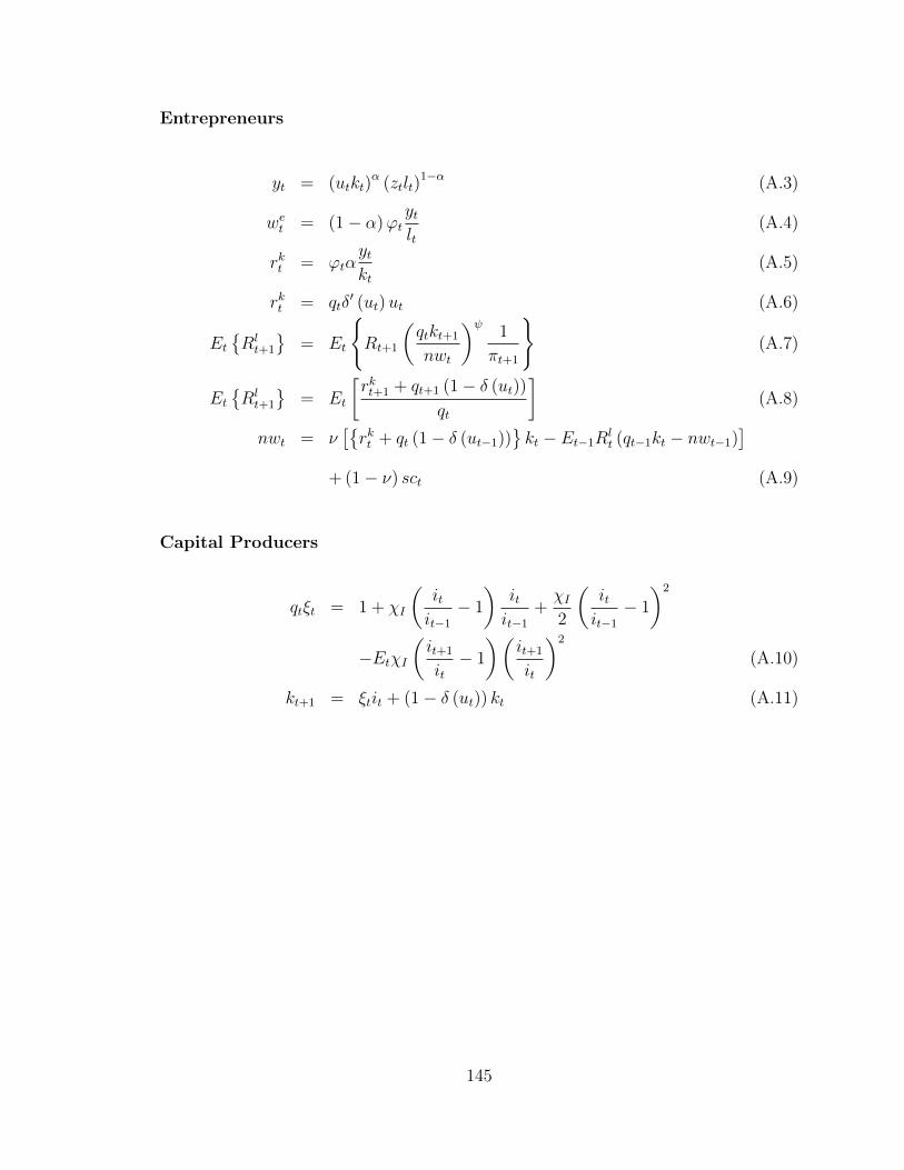
Entrepreneurs

yt = (utkt)α (ztlt)

1−α (A.3)

wet = (1− α)ϕtytlt

(A.4)

rkt = ϕtαytkt

(A.5)

rkt = qtδ′ (ut)ut (A.6)

Et{Rlt+1

}= Et

{Rt+1

(qtkt+1

nwt

)ψ1

πt+1

}(A.7)

Et{Rlt+1

}= Et

[rkt+1 + qt+1 (1− δ (ut))

qt

](A.8)

nwt = ν[{rkt + qt (1− δ (ut−1))

}kt − Et−1R

lt (qt−1kt − nwt−1)

]+ (1− ν) sct (A.9)

Capital Producers

qtξt = 1 + χI

(itit−1

− 1

)itit−1

+χI2

(itit−1

− 1

)2

−EtχI(it+1

it− 1

)(it+1

it

)2

(A.10)

kt+1 = ξtit + (1− δ (ut)) kt (A.11)

145

Employment Agencies

mt = σmuσt v

1−σt (A.12)

%t =mt

vt(A.13)

ςt =mt

ut(A.14)

nt = (1− ρ)nt−1 +mt−1 (A.15)

ut = 1− (1− ρ)nt (A.16)

κ

λt%t= Etβ

λt+1

λt(1− ρ)

[wetht − wtht +

κ

λt+1%t+1

](A.17)

wtht = η

[wetht +

ςt%t

(1− ρt)κ

λt

]+ (1− η)

[b+

g (ht)

λt

](A.18)

wet =Υ

λthζt (A.19)

lt = ntht (A.20)

Model Closing

Rt

R=

(πtπ

)%π (yty

)%yexp (εR,t) (A.21)

πt = βEtπt+1 +(1− βφ) (1− φ)

φϕt (A.22)

yt = ct + it (A.23)

A.2 Log-linearized Equations for Benchmark Model

Household

λt =1

(1− a)(1− aβ)[ct − act−1]− aβ

(1− a)(1− aβ)[Etct+1 − act] (A.24)

Rt = λt + Etπt+1 − Etλt+1 (A.25)

146

Entrepreneurs

yt = αut + αkt + (1− α) zt + (1− α) lt (A.26)

wet = ϕt + yt − lt (A.27)

rkt = ϕt + yt − kt (A.28)

ut =

(rk

rk + δ′′ (u)

)(rkt − qt

)(A.29)

EtRlt+1 = Et

[Rt+1 + ψ

(qt + kt+1 − nwt

)− πt+1

](A.30)

EtRlt+1 =

[rk

rk + (1− δ)

]Etr

kt+1 +

[(1− δ)

rk + (1− δ)

]Etqt+1 − qt

−[

rk

rk + (1− δ)

]Etut+1 (A.31)

nwtν

=

(k

nw

)[rkrkt + (1− δ) qt −Rlqt−1 − rkut

]−ψ

(k

nw− 1

)Rl[kt + qt−1

]−(k

nw− 1

)Rl(Rt − πt

)+Rl

[ψ

(k

nw− 1

)+ 1

]nwt−1 (A.32)

Capital Producers

qt = 2χI ıt − χI ıt−1 − χIEtıt+1 − ξt (A.33)

Etkt+1 = δξt + δıt + (1− δ) kt − rkut (A.34)

147

Employment Agencies

mt = σut + (1− σ) vt (A.35)

%t = mt − vt (A.36)

ςt = mt − ut (A.37)

nt = (1− ρ) nt−1 + ρmt−1 (A.38)

ut = − n

1− (1− ρ)n(1− ρ) nt (A.39)

wet = ζht − λt (A.40)

%t = βλ (1− ρ)

[(whλ%

κ

)Et(wt+t − wet+t

)+ Et%t+1

](A.41)

wt = ηwet +

[η + (1− η)

Υhζ

λw− 1

]ht

− 1

wh

[η (1− ρ)

κς

λ%+ (1− η)

g

λ

]λt

+η (1− ρ)κς

whλ%(ςt − %t) (A.42)

lt = nt + ht (A.43)

(A.44)

Model Closing

Rt = %ππt + %Y yt + εR,t (A.45)

πt = βEtπt+1 +(1− βφ) (1− φ)

φϕt (A.46)

yt =c

yct +

i

yyt (A.47)

ξt = ρξ ξt−1 + εξ,t (A.48)

148

Important Steady-States

weh

Y= (1− α)

φ

n

λY =

[1− aβ1− a

]Y

c

wh

Y=

weh

Y− κθσ

λY

[1− β(1− ρ)

β(1− ρ)

]g(h)

λY=

Υ

1 + ζ

h1+ζ

λY=

weh

Y (1 + ζ)

g′(h)h

λY=

Υh1+ζ

λY=weh

Y

149

Appendix B

Appendix for Chapter 3

B.1 Data for VAR Analysis

Tax Revenue: Current tax receipts + Income receipts on assets + Current transfer

receipts - Current transfer payments - Interest payments - Subsidies. Source: Table

3.1. Government Current Receipts and Expenditures, Bureau of Economic Analysis.

Government Spending: Government consumption expenditures and gross invest-

ment. Source: Table 3.9.5. Government Consumption Expenditures and Gross In-

vestment, Bureau of Economic Analysis.

Output: Gross domestic product. Source: Table 1.1.5. Gross Domestic Product,

Bureau of Economic Analysis.

Consumption: Nondurable goods (Personal Consumption) + Services (Personal

Consumption minus housing and utilities services consumption). Source: Table 1.1.5.

Gross Domestic Product, Bureau of Economic Analysis.

House Prices: Median price for new, single-family houses sold (including land).

Monthly, US Census Bureau. Converted into quarterly frequency by taking simple

average across months, and normalized by the average sales price for 2005.

The data are seasonally adjusted at annual rates. We transformed this into log

150

real per capita terms by first normalizing the original data by Total Population: All

Ages including Armed Forces Overseas (Quarterly Average, Source: Monthly National

Population Estimates, US Department of Commerce: Census Bureau) and the GDP

implicit price deflator (Seasonally adjusted, 2005=100, Source: Table 1.1.9. Implicit

Price Deflators for Gross Domestic Product, Bureau of Economic Analysis) and then

taking logarithm.

B.2 Factor Augmented VAR

The mismatch in information sets between the econometrician and private agents, and

the resulting anticipation issues, may cause a deeper problem than the one described

in section 3.2. Leeper et al. [2011] show that in the presence of fiscal foresight, the

MA representation of a limited set of variables can be non-fundamental, and VAR

techniques would fail to recover the structural shocks. To understand the issue of

fundamentalness, consider an MA representation of a solution from a DSGE model:

Xt = B(L)ut

Here, X is an n-vector of macroeconomic variables of interest and u is the q-vector

structural shock, with n ≥ q. This representation is fundamental if Xt lies in the

space spanned by present and past values of ut and, conversely, ut lies in the space

spanned by present and past values of Xt. In this case, observing Xt is enough to

recover ut. The second part of the above definition, however, holds generically for

tall systems when n > q, but not for square systems where n = q.

If the econometrician wants to estimate B(L) and ut by running an n-dimensional

VAR on Xt, we would end up with n linearly independent shocks, more than the

number of structural shocks given by theory. In this case, the econometrician may opt

151

to estimate a VAR on a square q-dimensional subsystem A(L)Xt = εt and attempt

to recover the structural shocks by imposing identifying restriction on a matrix D

such that εt = Dut. If the square subsystem is non-fundamental, however, the space

spanned by Xt will not contain the structural shocks, and the VAR will not be able

to recover them, regardless of the identification scheme used to determine D.

Leeper et al. [2011] analytically shows how expectations about future tax changes

in a simple model can misallign the information sets available to private agents, who

receive news about the tax changes well in advance, and the econometrician who

sees the changes only when they occur. Without correctly modelling the flow of

information, the smaller subset of information available to the econometrician gives

rise to non-fundamentalness in VAR models. In this situation, the Blanchard and

Perotti [2002] scheme of identifying tax shocks give different results from the case

where information flow is taken into consideration.

Forni and Gambetti [2011] suggest that one way of overcoming the limitations of

the reduced rank VAR model is to consider a factor model, where information present

in a large number of variables is reduced to a fundamental rectangular system by tak-

ing linear combinations of the variables. In a factor model, each macroeconomic

variable xit is represented as a sum of a common component χit and an idiosyncratic

component ξit. The common components are in turn assumed to be linear combina-

tions of a relatively small number r of factors χit = aift. The factors, in turn, are

responsible for most of the co-movement between macroeconomic variables, and are

assumed to have a fundamental MA representation:

ft = N(L)ut

A reduced rank estimate of the dynarmic factors would then recover the structural

shocks ut. Identification, however, becomes less straight forward as the factors them-

152

selves lose a direct economic interpretation. In this case, identification can be achieved

via sign restrictions on the final macroeconomic variables.

Following Forni and Gambetti [2011], we estimate a factor-augmented VAR with

110 variables, 13 static factors, 4 lags and 6 structural shocks. The dataset is almost

identical to Forni and Gambetti [2011], with few exceptions. All data are in quarterly

frequencies and cover the period from 1963:1 through 2007:4.

B.3 Sign Restriction

To understand the method of identification through sign restrictions, consider the

MA representation of a VAR:

yt = D (l) et

where yt is a vector of economic variables of interest, D (l) is a matrix of lag operators,

and et ∼ (0,Σe) is the vector of reduced form errors. The problem of identification

arises precisely because there is no direct structural interpretation of the reduced

form errors, which is assumed to be a linear combination of the orthogonal structural

shocks. If, however, we can find a matrix P , such that PP ′ = Σe, we can generate

impulse response functions to orthogonal shocks from the following MA representa-

tion:

yt = D (l)PP−1et = D (l) εt

where εt = P−1et are orthogonal shocks such that εt ∼ (0, P−1ΣeP−1′ = I). The

Cholesky (lower triangular) factorization of the estimated error covariance Σe is one

way of generating such a matrix P .

Note, however that this factorization of Σe is not unique. In particular, for any

153

orthogonal matrix Q,such that QQ′ = I, we can have

yt = D (l)PQQ′P−1et = D (l) εt

where εt ∼ (0, Q′P−1ΣeP−1′Q = I). So, for any orthogonal matrix Q, we can generate

impulse responses of orthogonal shocks by identifying εt = Q′P−1et. The method

of sign restricted identification considers those Q matrices that result in impulse

responses that conform to a pre-defined scheme derived from minimal theory.

In this study, we identify government spending shocks by imposing the following

sign restrictions on the impulse response functions: total government spending, federal

government spending, total government deficit, federal government deficit and output

all increase in the 5 quarter following the shock. Imposing the restriction on further

from the impact period allows for anticipation effects. This strategy, however, does

not allow us to differentiate between an expected and an unexpected shock.

154

B.4 Non-linear Equations for Benchmark Model

Patient household

c`t + qth`t + it = wtn

`t + qth

`t−1 + rtkt−1 + d`t +

rnt−1bgt−1

πt+Rt−1bt−1

πt

−bgt − bt − τ `t (B.1)

kt = (1− δ)kt−1 + φ

(itkt−1

)kt−1 (B.2)

1

c`t= λ`1t (B.3)(

n`t)η

wt= λ`1t (B.4)

Υ`

h`t= λ`1tqt − β`Et[λ`1t+1qt+1] (B.5)

1 = ψtφ′(

itkt−1

)(B.6)

ψtEtλ`tλ`t+1

= β`Et

[rt+1 + ψt+1

{(1− δ) + φ

(it+1

kt

)− φ′

(it+1

kt

)it+1

kt

}](B.7)

1 = β`Et

[λ`1t+1

λ`1t

rntπt+1

](B.8)

Borrowing Households

cbt + qthbt +

rnt−1bt−1

πt= wtn

bt + qth

bt−1 + bt − τ bt (B.9)

bt = mEt

{qt+1h

btπt+1

Rt

}(B.10)

1

cbt= λb1t (B.11)(

nbt)η

wt= λb1t (B.12)

Υb

hbt= λb1tqt − βbEt

[λb1t+1qt+1

]− λb2tEt

[mqt+1πt+1

Rt

](B.13)

λb1t = βbEt

[λb1t+1

Rt

πt+1

]+ λb2t (B.14)

155

Firms

yt = kγt−1n1−γt (B.15)

rt = γmctytkt−1

(B.16)

wt = (1− γ)mctytnt

(B.17)

mct = γ−γ(1− γ)γ−1wγt r1−γt (B.18)

Nominal Rigidities and Monetary Policy

πt = β`Etπt+1 +(1− θπ) (1− β`θπ)

θπmct (B.19)

rntrn

=(πtπ

)%π(B.20)

Government

τt + bgt =Rgt−1b

gt−1

πt+Gt (B.21)

τt = %bbgt−1 + %ggt (B.22)

gt = ρggt−1 + εgt (B.23)

Aggregation

Ct = αcbt + (1− α) c`t (B.24)

Nt = αnbt + (1− α)n`t (B.25)

Ht = αhbt + (1− α)h`t (B.26)

It = (1− α)it (B.27)

Kt = (1− α)kt (B.28)

Yt ≈ Kγt−1N

1−γt = Ct + φ

(It

Kt−1

)Kt−1 +Gt (B.29)

156

B.5 Non-linear Equations for Model with Housing

Production

Patient Households

c`t + it + iht =wtn

`t

Xt

+wht n

h`t

Xht

+ (1− δh)qth`t−1 + rtkt−1 + rht kht−1 + d`t

+rnt−1b

gt−1

πt+Rt−1bt−1

πt− bgt − bt − qth`t − τ `t (B.30)

kt = (1− δ)kt−1 + φ

(itkt−1

)kt−1 (B.31)

kht = (1− δh)kht−1 + iht − φh(

ihtkht−1

)kht−1 (B.32)

1

c`t= λ`1t (B.33)

Υ`

h`t= λ`1tqt − β`Et[λ`1t+1qt+1] (B.34)

λ`twct =

[(ncpt )1+ξ +

(nhpt

)1+ξ] 1+η

1+ξ−1

(ncpt )ξ (B.35)

λ`twht =

[(ncpt )1+ξ +

(nhpt

)1+ξ] 1+η

1+ξ−1 (

nhpt

)ξ(B.36)

1 = ψtφ′(

itkt−1

)(B.37)

ψtEtλ`tλ`t+1

= β`Et

[rt+1 + ψt+1

{(1− δ) + φ

(it+1

kt

)− φ′

(it+1

kt

)it+1

kt

}](B.38)

1 = ψht φ′h

(ihtkht−1

)(B.39)

ψht Etλ`tλ`t+1

= β`Et

[rht+1 + ψht+1

{(1− δh) + φh

(iht+1

kht

)− φ′h

(iht+1

kht

)iht+1

kht

}](B.40)

1 = β`Et

[λ`1t+1

λ`1t

rntπt+1

](B.41)

157

Impatient Households

cbt + qthbt +

rnt−1bt−1

πt= wtn

bt + qth

bt−1 + bt − τ bt (B.42)

bt = mEt

{qt+1h

btπt+1

Rt

}(B.43)

1

cbt= λb1t (B.44)

Υb

hbt= λb1tqt − βbEt

[λb1t+1qt+1

]− λb2tEt

[mqt+1πt+1

Rt

](B.45)

λb1t = βbEt

[λb1t+1

Rt

πt+1

]+ λb2t (B.46)

λ`twct =

[(ncpt )1+ξ +

(nhpt

)1+ξ] 1+η

1+ξ−1

(ncpt )ξ (B.47)

λ`twht =

[(ncpt )1+ξ +

(nhpt

)1+ξ] 1+η

1+ξ−1 (

nhpt

)ξ(B.48)

Firms

Y ht =

(L)µl (Kh

t−1

)µ (Nht

)1−µ−µl (B.49)

Yt = Kγt−1N

1−γt (B.50)

rt = γmctYtKt−1

(B.51)

wt = (1− γ)mctYtNt

(B.52)

mct = γ−γ(1− γ)γ−1wγt r1−γt (B.53)

rht = µXht

Y ht

Kht−1

(B.54)

wht = (1− µ− µl)Xht

Y ht

Nht

(B.55)

158

Nominal Rigidities and Monetary Policy

ωt = β`ωt+1 −(1− θw)

(1− β`θw

)θw

Xt (B.56)

ωht = β`ωht+1 −(1− θhw)

(1− β`θhw

)θhw

Xht (B.57)

ωt =wtπtwt−1

(B.58)

ωht =wht πtwht−1

(B.59)

πt = β`πt+1 +(1− θπ) (1− β`θπ)

θπmct (B.60)

rnt = %ππt + εrt (B.61)

Government

Tt + bgt =Rgt−1b

gt−1

πt+Gt (B.62)

Tt − TY

= %b

[bgt − bY

]+ %g

[Gt −GY

](B.63)[

Gt −GY

]= ρg

[Gt−1 −G

Y

]+ εgt (B.64)

159

Aggregation

Ct = αcbt + (1− α) c`t (B.65)

Nt = αnbt + (1− α)n`t (B.66)

Nht = αnhbt + (1− α)nh`t (B.67)

Ht = αhbt + (1− α)h`t (B.68)

It = (1− α)it (B.69)

Kt = (1− α)kt (B.70)

Iht = (1− α)iht (B.71)

Kht = (1− α)kht (B.72)

Yt = Ct + φ

(It

Kt−1

)Kt−1 + φh

(IhtKht−1

)Kht−1 +Gt (B.73)

Y Ht = Ht − (1− δh)Ht−1 (B.74)

B.6 GHH Preferences

Lending Households

x`t = (c`t)1−ψh(h`t)

ψh − n`(1+η)t

1 + η(B.75)

λ`1t = (1− ψh)x`(−γ)t

(h`tc`t

)ψh(B.76)

x`(−γ)t n`ηt = λ`1twt (B.77)

ψhx`(−γ)t

(c`th`t

)1−ψh= λ`1tqt − βλ`1,t+1qt+1 (B.78)

160

Borrowing Households

xbt = (cbt)1−ψh(hbt)

ψh − nb(1+η)t

1 + η(B.79)

λb1t = (1− ψh)xb(−γ)t

(hbtcbt

)ψh(B.80)

xb(−γ)t nbηt = λb1twt (B.81)

ψhxb(−γ)t

(cb

hbt

)1−ψh= λb1tqt − βλb1,t+1qt+1 − λ2,t

qt+1πt+1

rnt(B.82)

Bibliography

Olivier Blanchard and Roberto Perotti. An empirical characterization of the dynamic

effects of changes in government spending and taxes on output. The Quarterly

Journal of Economics, 117(4):1329–1368, November 2002.

M. Forni and L. Gambetti. Fiscal foresight and the effects of government spending.

Manuscript, Universitat Autonoma de Barcelona, 2011.

Eric M. Leeper, Todd B. Walker, and Shu-Chun Susan Yang. Foresight and informa-

tion flows. NBER Working Papers 16951, National Bureau of Economic Research,

Inc, Apr 2011.

161

Appendix C

Appendix for Chapter 4

C.1 Timing

State Variables:

• nt−1: number of projects that receive funding in period t.

• Kt−1: symmetric equilibrium capital used for production in each project in

period t.

• N bt−1: bank capital at the beginning of period t.

• Bt−1: amount of deposits saved in the banking sector the end of period t− 1 by

households that make up loans for the purchase of capital in period t.

Timing:

• Time t begins with the number of funded projects, total productive capital

quantity, and bank deposits to be used in period t as given.

• Aggregate shocks hit the economy.

• Firms and Banks determine loan interest rate Rlt through Nash bargaining.

162

• Firms chose symmetric equilibrium loan level St = QtKt−1 for each funded

project, given the loan interest rate Rlt. Each funded project receives capital

Kt−1 purchased at price Qt for production this period.

• Labour demand / supply and wage setting takes place.

• Production occurs in funded projects according to Yt = zt(ξtKt−1)αL1−αt .

• Firms repay RltSt to banks.

• After loans are repaid for the period, each project / loan officer relationship

suffers an idiosyncratic ‘relationship shock’ ωt from a uniform distribution. This

is a cost to maintaining the relationship from the bank’s perspective. If ω ≤ ω,

the relationship survives, banks pay ωt and keep the match. If ω > ω, banks

pay a fixed penalty amount T in lieu of the ω relationship cost and severe the

relationship.

• Banks determine how many currently active relationships to sever (separation

rate xt) and how many new credit relationships to open. Accordingly, they hire

loan officers at a cost of cv per hire and look for new relationships, keeping in

mind the penalty to be paid if the capital adequacy ratio is not met.

• Match between unfunded projects and open credit lines occur, and the number

of funded projects for t+ 1 is determined.

• Firms sell worn out capital to the capital producing sector, where new capital

is created for use in t+ 1.

• Firms sell intermediate goods to the retail sector. Prices are determined. The

monetary authority reacts to inflation by setting the nominal policy rate Rt +

πt+1.

163

• Banks repay households for their deposits Bt−1 at real interest rate Rt, and

pay any penalties for deviating from the capital adequacy ratio κ. Aggregate

bank profits are realized, dividends δnN bt are paid out, and Bank net worth is

determined.

• Period t ends.

C.2 Non-linear Equations for Benchmark Model

Household

Ct = WtLYt +Rt

(nt−1St −N b

t

)−(ntSt+1 −N b

t

)+Divt (C.1)(

LY)ϕt

= λtWt (C.2)

λt =1

(Ct − aCt)− βEt

a

(Ct+1 − aCt)(C.3)

1 = βEtΛt,t+1Rt (C.4)

EtΛt,t+1 = Etλt+1

λt(C.5)

164

Bank

nt−1St = nt−1Bbt−1 +N b

t (C.6)

St = QtKt−1 (C.7)

xt =ωt − ωω − ω

(C.8)

Υωt = T +cvqt

(C.9)

N bt = nt−1Πb

t − cvvt −Ψ

2

[nt−1StN bt

− κ]2N bt

St+ (1− δn)N b

t−1 − εnt (C.10)

nt−1St = nt−1Bt−1 +N bt (C.11)

cvmθχt = βEtΛt,t+1

{Πbt+1 −Ψ

[ntSt+1

N bt+1

− κ]

+ θχt+1

∫ ωt+1

ω

cvmdG(ω)

}(C.12)

RltSt = (1− η)

[αPm

t

YtKt−1

+ (Qt − δ)ξt]Kt−1 + ηRt

(St −

N bt

nt−1

)+ηΥ

∫ ωt

ω

ωdG(ω) + η

∫ ω

ωt

TdG(ω) + ηΨ

[nt−1StN bt

− κ]

−ηθt∫ ωt

ω

cvdG(ω) (C.13)

Firm

Yt = zt (ξtKt−1)α (Lt)1−α (C.14)

Wt = (1− α)Pmt

YtLt

(C.15)

Rlt =

αPmt

YtKt−1

+ (Qt+1 − δ)ξtQt

(C.16)

165

Matching

nt = xtnt−1 + qtvt (C.17)

ut = 1− xtnt−1 (C.18)

vt = θt[1− xtnt−1] (C.19)

qt = mθ−χt (C.20)

pt = mθ1−χ (C.21)

Capital

Int ≡ It − δξtKYt−1 (C.22)

KYt = ξtK

Yt−1 + Int (C.23)

Qt = 1 + f(·) +Int + I

Int−1 + If ′(·)− EtβΛt,t+1

(Int+1 + I

Int + I

)2

f ′(·) (C.24)

Model Closing

πt = βEtπt+1 +(1− βθ)(1− θ)

θPmt (C.25)

it = Rt + Etπt+1 = %ππt + %yYYt + εmt (C.26)

Y Yt = Ct + It + f

(Int+τ + I

Int+τ−1 + I

)(Int+τ + I) + cvvt

+nt−1Υ

∫ ω

ω

ωdG(ω) + nt−1

∫ ω

ω

TdG(ω) (C.27)

166

C.3 Log-linearized Equations for Benchmark Model

Household

C

Y=

WLY

Y

(Wt + nt−1 + Lt

)+R

[nS

Y− N b

Y

]Rt

+RnS

Y

(nt−1 + St

)−RN

b

YN bt − n

S

Y

(nt + St+1

)+N b

YN bt+1 + δn

N b

YN bt−1 (C.28)

ϕ(nt−1 + Lt) = Wt − Ct (C.29)

Ct+1 − Ct = Rt (C.30)

Λt = Ct − Ct+1 (C.31)

Firm

Yt = zt + α(ξt + Kt−1) + (1− α)Lt (C.32)

Wt = Pmt + Yt − Lt (C.33)

167

Bank

xt =ω

x

[1

ω − ω

]ˆωt (C.34)

xΥ

Yxt =

χ

q

cvYθt (C.35)

nt = x(1− p)(xt + nt−1) + (1− χ)p(1− xn)

nθt (C.36)

St = Qt + Kt−1 (C.37)

N b

YN bt = nRl S

YRlt +R

[N b

Y− nS

Y

]Rt + nx

[T

Y+ θ

cvY− Υ

Yω

]xt

+nS

Y

(Rl −R

)St +R

N b

YN bt − (1− xn)θ

cvYθt

+n

[(Rl −R

) SY− (1− x)

T

Y+ xθ

cvY

]nt−1

+(1− δn)N b

YN bt−1 − εnt (C.38)

χ

q

cvYθt =

1

q

cvY

Λt + βRl S

YRlt+1 + βR

[1

n

N b

Y− S

Y

]Rt+1

+βS

Y

[Rl −R− n Ψ

N b

]St+1 + βx

[T

Y+cvY

1

q− Υ

Yω

]xt+1

−β[R

n

N b

Y+ n

Ψ

N b

S

Y

]nt + β

N b

Y

[R

n+ n

Ψ

N b

S

N b

]N bt+1

+βΨ

Yκˆκt+1 + βx

χ

q

cvYθt+1 (C.39)

Rl S

Y

(Rlt + St

)= (1− η)αPm

(Pmt + Yt

)+ (1− η)(1− δ)K

Y

(Kt−1 + ξt

)+(1− η)

K

YQt + η

[R

n

N b

Y+ n

Ψ

Y

S

N b

]nt−1

+η

[R + n

Ψ

N b

]S

YSt − η

[R

n+ n

Ψ

N b

S

N b

]N b

YN bt

+ηR

[S

Y− 1

n

N b

Y

]Rt − ηx

[T

Y+ θ

cvY− Υ

Yω

]xt

−ηxθcvYθt (C.40)

168

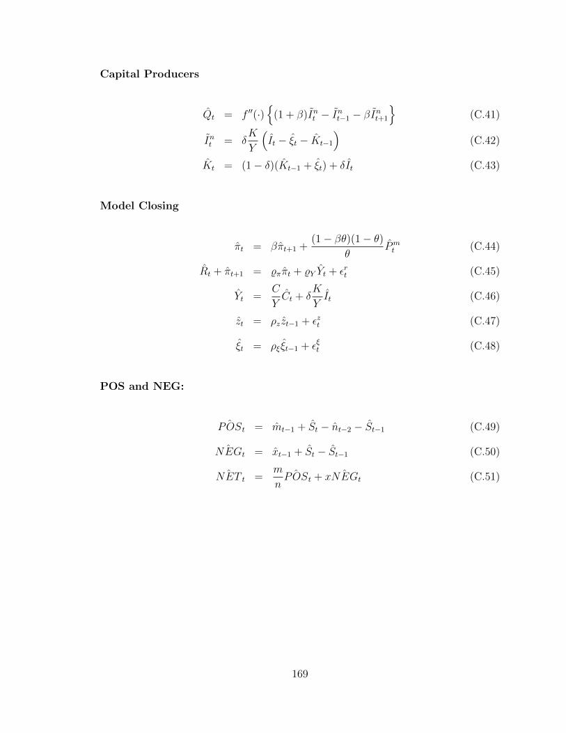
Capital Producers

Qt = f ′′(·){

(1 + β)Int − Int−1 − βInt+1

}(C.41)

Int = δK

Y

(It − ξt − Kt−1

)(C.42)

Kt = (1− δ)(Kt−1 + ξt) + δIt (C.43)

Model Closing

πt = βπt+1 +(1− βθ)(1− θ)

θPmt (C.44)

Rt + πt+1 = %ππt + %Y Yt + εrt (C.45)

Yt =C

YCt + δ

K

YIt (C.46)

zt = ρz zt−1 + εzt (C.47)

ξt = ρξ ξt−1 + εξt (C.48)

POS and NEG:

ˆPOSt = mt−1 + St − nt−2 − St−1 (C.49)

ˆNEGt = xt−1 + St − St−1 (C.50)

ˆNET t =m

nˆPOSt + x ˆNEGt (C.51)

169