Embed Size (px)
Citation preview

Graduate Theses, Dissertations, and Problem Reports
2019
Three Essays on Nonparametric Hypothesis Testing and Three Essays on Nonparametric Hypothesis Testing and
Stochastic Frontier Analysis Stochastic Frontier Analysis
Taining Wang West Virginia University, [email protected]
Follow this and additional works at: https://researchrepository.wvu.edu/etd
Part of the Econometrics Commons
Recommended Citation Recommended Citation Wang, Taining, "Three Essays on Nonparametric Hypothesis Testing and Stochastic Frontier Analysis" (2019). Graduate Theses, Dissertations, and Problem Reports. 3930. https://researchrepository.wvu.edu/etd/3930
This Dissertation is protected by copyright and/or related rights. It has been brought to you by the The Research Repository @ WVU with permission from the rights-holder(s). You are free to use this Dissertation in any way that is permitted by the copyright and related rights legislation that applies to your use. For other uses you must obtain permission from the rights-holder(s) directly, unless additional rights are indicated by a Creative Commons license in the record and/ or on the work itself. This Dissertation has been accepted for inclusion in WVU Graduate Theses, Dissertations, and Problem Reports collection by an authorized administrator of The Research Repository @ WVU. For more information, please contact [email protected].

Three Essays on Nonparametric Hypothesis Testing andStochastic Frontier Analysis
Taining Wang
Dissertation submittedto the John Chambers College of Business and Economics
at West Virginia University
in partial fulfillment of the requirements for the degree of
Doctor of Philosophyin
Economics
Feng Yao, Ph.D., ChairArabinda Basistha, Ph.D.
Jane Ruseski, Ph.D.Xiaoli Etienne, Ph.D.
Department of Economics
Morgantown, West Virginia2019
Keywords: Nonparametric Hypothesis Testing; Semiparametric Models; StochasticFrontier Analysis; Debt Growth; Technical Efficiency
Copyright 2019, Taining Wang

ABSTRACT
Three Essays on Nonparametric Hypothesis Testing andStochastic Frontier Analysis
Taining Wang
The first chapter proposes a nonparametric test of significant variables in the partial derivative of aregression mean function. The test is constructed through a variation based measure of the derivativein the directions of the significant variables, with the derivative estimation through a local polynomialestimator. The test is shown to have the asymptotic null distribution and demonstrated to be consistent.The chapter further proposes a wild-bootstrap test, which exhibits the same null distribution regardlessof whether the null is valid or not. Through Monte Carlo studies, the test shows encouraging finite sampleperformances. Through an empirical application, the test is applied to infer certain aspects of regressionstructures on labor’s earning function.
The second chapter investigates the role of debt in the firm’s production frontier and technical effi-ciency by employing a firm-level dataset over 1998-2007 and 1998-2013. The impact of debt on frontieris decomposed into a stand-alone neutral effect and indirect non-neutral effects, which alter the outputelasticity of production inputs. The effects are estimated through a semiparametric smooth coefficientstochastic frontier model. A nonzero probability for the firms to be fully efficient is allowed, modeledas a function of debt and technical progress. The study shows that an increase in debt significantlyshifts firms’ frontier downward across different ownerships, regions, and industries. Foreign and privatefirms are more efficient, with their full efficiency probability increased by debt and technical progress.By contrast, state-owned enterprises (SOEs) and collective firms are much less efficient and their prob-ability of being fully efficient does not increase with more debt. Furthermore, lower efficiency levels areconcentrated in the central and western regions and in the mining and public utility industries.
The third chapter proposes a semiparametric additive stochastic frontier model for panel data, whereinputs and environment variables can enter the frontier individually and interactively through unknownsmooth functions. The inefficiency has its mean function known up to certain parameters, and influ-enced by its determinants that may or may not appear on the frontier. The model disentangles timeinvariant unobserved heterogeneities from inefficiency, which can be helpful to avoid overestimating theinefficiency level. Different from conventional stochastic frontier models, the proposed model can beidentified without the distribution assumption on the composite error, and consistently estimated with-out suffering from the curse of dimensionality. Thus, a large number of interested variables for frontieror inefficiency determinants can be included, a potentially attractive feature for empirical studies. Thestudy demonstrates the appealing finite-sample performance of the proposed estimator and two relatedhypotheses tests through the Monte Carlo study, and performs a world production frontier analysis with116 countries during 2001-2013.

Acknowledgements
Devoting my time to deeply understanding a subject of my interest has long been a dream since I was
a kid. I consider myself very fortunate to have such a chance to pursue economic research toward the
PhD at West Virginia University. Indeed, this dream becomes true as a result of tremendous help and
supports from the most important people in my life. First of all, it is my genuine pleasure to express
my deep gratitude to my advisor, Dr. Feng Yao, who has consistently provided generous help to my
research. Without the clear guidance and inspiration from Dr. Yao, it is impossible for me to conduct my
initial research in Nonparametric Econometrics. Dr. Yao always possesses enthusiastic attitude towards
research works, which greatly encourages me to face and solve challenging works throughout the research
process. With detailed explanation by Dr. Yao on technical issues, I am able to go deeper in the field of
Econometrics, and see many interesting and promising topics for my future works.
I would like to extend my gratitude to my committee members, Dr. Arabinda Basistha, Dr. Jane
Resuske, and Dr. Xiaoli Etienne, for their constructive feedbacks and advices on my present studies. I
also gratefully thank Dr. Guillermo Franco for his generous help on High Performance Computing, which
significantly facilitates many of my projects.
Last of all, I greatly thank my mother Yihong Zhang for her endless love throughout my life, and my
loving fiance Jinjing Tian for her invaluable support to my PhD life and inspiration for my research. I
also thank my best friend, Tingyu Li, who always have a way to cheer me up when I face obstacles.
iii

Contents
1 A Nonparametric Test of Significant Variables in Gradients 11.1 Introduction . . . . . . . . . . . . . . . . . . . . . . . . . . . . . . . . . . . . . . . . . . . . 11.2 A test for significant variables in gradient . . . . . . . . . . . . . . . . . . . . . . . . . . . 3
1.2.1 Local polynomial gradient estimate . . . . . . . . . . . . . . . . . . . . . . . . . . . 31.2.2 A variation based test . . . . . . . . . . . . . . . . . . . . . . . . . . . . . . . . . . 5
1.3 Asymptotic properties . . . . . . . . . . . . . . . . . . . . . . . . . . . . . . . . . . . . . . 61.3.1 Assumptions . . . . . . . . . . . . . . . . . . . . . . . . . . . . . . . . . . . . . . . 61.3.2 Asymptotic distribution . . . . . . . . . . . . . . . . . . . . . . . . . . . . . . . . . 7
1.4 A bootstrap test . . . . . . . . . . . . . . . . . . . . . . . . . . . . . . . . . . . . . . . . . 81.5 Monte Carlo study . . . . . . . . . . . . . . . . . . . . . . . . . . . . . . . . . . . . . . . . 10
1.5.1 Bivariate Case . . . . . . . . . . . . . . . . . . . . . . . . . . . . . . . . . . . . . . 111.5.2 Trivariate Case . . . . . . . . . . . . . . . . . . . . . . . . . . . . . . . . . . . . . . 121.5.3 A Comparison Study . . . . . . . . . . . . . . . . . . . . . . . . . . . . . . . . . . . 14
1.6 Empirical Application . . . . . . . . . . . . . . . . . . . . . . . . . . . . . . . . . . . . . . 201.7 Conclusion . . . . . . . . . . . . . . . . . . . . . . . . . . . . . . . . . . . . . . . . . . . . 24
2 Does High Leverage Ratio influence Chinese Firm Performance? A SemiparametricStochastic Frontier Approach with Panel Data 12.1 Introduction . . . . . . . . . . . . . . . . . . . . . . . . . . . . . . . . . . . . . . . . . . . . 12.2 Empirical Methodology . . . . . . . . . . . . . . . . . . . . . . . . . . . . . . . . . . . . . 52.3 Data . . . . . . . . . . . . . . . . . . . . . . . . . . . . . . . . . . . . . . . . . . . . . . . . 92.4 Empirical Results . . . . . . . . . . . . . . . . . . . . . . . . . . . . . . . . . . . . . . . . . 13
2.4.1 Whole Sample Analysis: 1998-2007 . . . . . . . . . . . . . . . . . . . . . . . . . . . 132.4.2 Whole Sample Analysis: 1998-2013 . . . . . . . . . . . . . . . . . . . . . . . . . . . 202.4.3 A Robustness Check on Whole Sample Analysis: 1998-2007 . . . . . . . . . . . . . 232.4.4 Analysis across Ownerships . . . . . . . . . . . . . . . . . . . . . . . . . . . . . . . 242.4.5 Analysis across Regions . . . . . . . . . . . . . . . . . . . . . . . . . . . . . . . . . 292.4.6 Analysis across Industries . . . . . . . . . . . . . . . . . . . . . . . . . . . . . . . . 33
2.5 Conclusion . . . . . . . . . . . . . . . . . . . . . . . . . . . . . . . . . . . . . . . . . . . . 36
3 A Fixed Effect Additive Stochastic Frontier Model with Interactions and DistributionFree Inefficiency 33.1 Estimation Procedure and Hypothesis Testing . . . . . . . . . . . . . . . . . . . . . . . . . 6
3.1.1 Semiparametric Estimation . . . . . . . . . . . . . . . . . . . . . . . . . . . . . . . 63.1.2 Hypothesis Testing . . . . . . . . . . . . . . . . . . . . . . . . . . . . . . . . . . . . 9
3.2 Monte Carlo Simulation . . . . . . . . . . . . . . . . . . . . . . . . . . . . . . . . . . . . . 113.3 Empirical Application . . . . . . . . . . . . . . . . . . . . . . . . . . . . . . . . . . . . . . 183.4 Conclusion . . . . . . . . . . . . . . . . . . . . . . . . . . . . . . . . . . . . . . . . . . . . 28
iv

List of Figures
1.1 Power Curve Comparison of Additivity Tests at 5% Rejection Region . . . . . . . . . . . . 191.2 Plot of mw(w) estimates against w . . . . . . . . . . . . . . . . . . . . . . . . . . . . . . . 221.3 Plots of mY (Y ) and m1(Y ) in the Partially Linear Varying Coefficient Model . . . . . . . 231.4 Plots of mY (Y ) and m1(Y ) in the Partially Linear Varying Coefficient Model . . . . . . . 24
2.1 SC-ZISF Estimation from the Whole Sample: 1998-2007 . . . . . . . . . . . . . . . . . . 142.2 Density of Estimated Composite Error and Posterior TE: 1998-2007 . . . . . . . . . . . . 202.3 SC-ZISF Estimation from the Whole Sample: 1998-2013 . . . . . . . . . . . . . . . . . . 212.4 Density of Estimated Composite Error and Posterior TE: 1998-2013 . . . . . . . . . . . . 222.5 SC-ZISF Estimation with Lag of Debt Ratio from the Whole Sample: 1998-2007 . . . . . 232.6 Density of Posterior Probability and Posterior TE across ownerships . . . . . . . . . . . . 262.7 Yearly Averaged Posterior Probability and PTE . . . . . . . . . . . . . . . . . . . . . . . 272.8 Density of Posterior Probability and PTE across Regions . . . . . . . . . . . . . . . . . . 312.9 Density of Posterior Probability and PTE across Industries . . . . . . . . . . . . . . . . . 35
3.1 Simulation Function . . . . . . . . . . . . . . . . . . . . . . . . . . . . . . . . . . . . . . . 123.2 SF-AMIFE: Neutral Functions Comparison . . . . . . . . . . . . . . . . . . . . . . . . . . 213.3 SF-AMIFE: Interaction Functions Comparison . . . . . . . . . . . . . . . . . . . . . . . . 243.4 SF-AMIFE: Interaction Functions Comparison . . . . . . . . . . . . . . . . . . . . . . . . 28
v

List of Tables
1.1 Empirical Size and Power from Bivariate Regression with d = 2 . . . . . . . . . . . . . . . 131.2 Empirical Size and Power from Trivariate Regression with d = 3 . . . . . . . . . . . . . . 151.3 Additivity Test Comparison From A Bivariate Regression . . . . . . . . . . . . . . . . . . 181.4 Descriptive Statistics of the Dataset . . . . . . . . . . . . . . . . . . . . . . . . . . . . . . 211.5 Empirical Results From the Dataset . . . . . . . . . . . . . . . . . . . . . . . . . . . . . . 21
2.1 Data Descriptive Summary Statistics . . . . . . . . . . . . . . . . . . . . . . . . . . . . . . 122.2 The Share of Firms with Different Ownership across Regions and Industries: 1998-2007 . 132.3 SC-ZISF Estimation Results from the Whole Sample . . . . . . . . . . . . . . . . . . . . 162.4 Parametric Models Estimation Results from the Whole Sample . . . . . . . . . . . . . . 172.5 Parameter Estimation Results of Lag of Debt Ratio . . . . . . . . . . . . . . . . . . . . . 242.6 Estimation Results of SC-ZISF Model based on Ownership . . . . . . . . . . . . . . . . . 252.7 Estimation Results of the SC-ZISF Model based on Region . . . . . . . . . . . . . . . . . 302.8 Average of PTE and Posterior Probability across 31 Provinces . . . . . . . . . . . . . . . 322.9 Estimation Results of SC-ZISF Model based on Industry . . . . . . . . . . . . . . . . . . 34
3.1 Simulation Results of Parameters γ in Inefficiency Mean Function . . . . . . . . . . . . . . 143.2 Simulation Results of Function Estimates: A RE model (c0 = 0) . . . . . . . . . . . . . . 153.3 Simulation Results of Function Estimates: A FE model (c0 = 1) . . . . . . . . . . . . . . 163.4 Nonparametric Tests Results (T = 3) . . . . . . . . . . . . . . . . . . . . . . . . . . . . . . 173.5 Data Descriptive Summary Statistics . . . . . . . . . . . . . . . . . . . . . . . . . . . . . . 203.6 OLS FE Estimation Results . . . . . . . . . . . . . . . . . . . . . . . . . . . . . . . . . . . 223.7 Nonparametric Tests Results on Frontier Functional Form and Interactions . . . . . . . . 263.8 Yearly Averaged TE and TEC Ranking 2001-2013 . . . . . . . . . . . . . . . . . . . . . . 27
vi

Chapter 1
A Nonparametric Test of SignificantVariables in Gradients
1.1 Introduction
Nonparametric estimation and hypothesis test gain popularity among practitioners as they are robust to
functional misspecification under less restrictive assumptions (Li and Racine (2007)). The test of signifi-
cant variables has been of interest to many in regression analysis, since it is often used to support/reject
an economic theory or considered for model selection (see Hart (1997) for a review of nonparametric
tests). The test can be performed by the sample analog of a moment condition (Fan et al. (1996), Zheng
(1996), Li and Wang (1998), Li (1999), Lavergne and Vuong (2000), Hsiao et al. (2007), Gu et al. (2007)),
by comparing the difference between sums of squared residuals (Ullah (1985), Dette (1999), Fan and Li
(2002)), by an R2 based statistic (Su and Ullah (2012), Yao and Ullah (2013)), or by the partial deriva-
tive estimate based bootstrap procedure (Racine (1997)). General tests of a parametric model can also
be performed through the integrated squared difference between parametric and nonparametric fit as in
Hardle and Mammen (1993), or likelihood ratio based test (Azzalini and Bowman (1993), Fan and Huang
(2001), Hong and Lee (2009)).
However, relatively little attention has been paid to test significant variables in the partial derivative
of a regression function. Racine (1997) proposes a partial derivative estimate based bootstrap test for
significant variables in the regression function. Sperlich et al. (2002) propose a test based on a cross
derivative for the interaction term in an additive regression model. We are not aware of works in testing
significant variables in the gradients, which can provide valuable insights. First, this test can offer
independent insights into the structure of the gradient functions, regarding whether the partial derivative
depends on all, some, or none of the variables in the regression. For example, in applied nonparametric
estimation, a common practice is to report the partial derivative estimate at the mean value of independent
1

Chapter 1 2
variables, which can be misleading unless the gradient estimate does not change much over the support
of independent variables. In estimating the stochastic frontier to evaluate the productive efficiency, for
example in Yao et al. (2017), one important question arises regarding whether the marginal product of
a regular input depends on computerization, an environment variable. Second, this test further allows
one to infer about the structure of the regression function.1 For instance, in a bivariate regression, if the
gradient of one variable x does not depend on the other variable z, one can infer an additive structure
in the regression. If the gradient of x does not depend on x, one can expect that x enters the model
linearly, with a potential varying coefficient that can depend on the other variable z. If the gradient of
x does not depend on x or z, then not only x enters the model linearly, but also there is no interaction
between x and z variables, i.e., a partially linear model. Finally, as pointed out by Sperlich et al. (2002),
“even though a certain test based on the estimation of a functional form is superior in detecting a general
deviation from the hypothetical one, a single peak or bump can often be better detected by tests based
on the derivatives.”
In this paper, we fill the gap by providing a simple nonparametric test of significant variables in
the partial derivative of a regression function. Recall that a general principle of the nonparametric
tests mentioned above is to compare the difference between the null (parametric or semiparametric) and
alternative (nonparametric) estimates. We note that in the case of testing significant variables in the
derivative, it is not clear to us how to construct the gradient estimate satisfying the null restriction such
that it does not depend on some variables. We overcome this hurdle by proposing a variation based test
using a local polynomial gradient estimate, checking whether the gradients exhibit variations along the
direction of variables that we test in the null.
Facilitated by the local polynomial gradient estimates, we obtain a simple asymptotic null distribution,
whose bias and variance depend only on the error terms in the regression model. We further show that
the test is consistent. Motivated by the simple structure of the null distribution, we propose a wild-
bootstrap test statistic, constructed by only resampling the estimated residuals. We demonstrate that
the bootstrap test statistic exhibits the same asymptotic null distribution, no matter whether the null is
valid or not. This result facilitates greatly in performing the test, since the bootstrap procedure will be
valid across all different types of null hypothesis, and thus there is no need to modify either the procedure
or its asymptotic justification. We further illustrate its encouraging finite sample performances through
a Monte-Carlo study.
Many interesting papers have considered tests for a semiparametric structure in the regression models.
For example, Lewbel (1995) proposes a moment based test of the Slutsky symmetry structure in the
1We assume below that the variables in the regression are significant. Otherwise, one can think of the test of significancethrough whether the partial derivative is zero as a special case of our proposed test.

Chapter 1 3
demand functions, which are estimated with a kernel method. Chen and Fan (1999), Ait-Sahalia et al.
(2001), and Delgado and Manteiga (2001) have considered testing a nonparametric/semiparametric null
model, with the null estimated with a kernel method. Li et al. (2003) propose a series based test for a
semiparametric null model by weighting the unconditional moment. A recent work by Korolev (2018)
proposes a consistent LM type specification test for semiparametric models with an increasing number
of series based unconditional moments. Our test has a different focus, that is, to test for the significant
variables in the gradient function. Like the other omnibus specification tests, our test does not offer a
comprehensive model selection procedure, and remains silent on how to proceed if the null is rejected.
However, our test on the significant variables in the gradient function can be used to infer the structure
of the regression models. In the empirical section, we illustrate with a dataset on estimating the labor
demand that repeated applications of our test can shed light on the search for the refined structure of
the demand.
In what follows, we present the test in section 2, the theoretical properties in section 3, a bootstrap
procedure and its property in section 4, a simulation study in section 5, an empirical illustration in section
6, and conclusion in section 7. All the proofs are relegated to the Appendix in the end.
1.2 A test for significant variables in gradient
Let’s consider a regression model
yi = m(Wi) + εi, i = 1, 2, · · · , n,
based on identically and independently distributed (IID) random variables Wi, yini=1, Wi = (xi, z′i)′ ∈
<d, zi ∈ <d−1, and we define the partial derivative with respect to x as gx(W ) ≡ ∂m(W )∂x . Clearly, here
we can consider x to be any variable in W and we assume that W are all significant in the conditional
mean function, an assumption that can be tested with any of the conditional mean significant variable
tests mentioned above.
1.2.1 Local polynomial gradient estimate
We estimate the gradient with the popular local polynomial estimation (see Fan and Gijbels (1996),
Masry (1996) for discussions on the attractive properties of local polynomials and Su and Ullah (2008)
for applications in simultaneous equation models). We denote the following notation to facilitate the
theoretical representation. Let j = (j1, · · · , jd), j! = j1! × · · · × jd!, |j| =d∑i=1
ji, Wj = W j1
1 × · · · ×Wjdd ,

Chapter 1 4
∑0≤|j|≤p
=p∑i=0
i∑j1=0
· · ·i∑
jd=0
|j|=i
, and (Djm)(W ) = ∂jm(W )
∂Wj11 ···∂W
jdd
. A local polynomial estimator of order p is
obtained from minimizing the multivariate weighted least square criterion
n∑i=1
(yi −∑
0≤|j|≤p
aj(Wi −W )j)2K
(Wi −W
h
), (1.1)
where K(·) is a nonnegative kernel function on <d, and h ≡ h(n) is a scalar bandwidth sequence that
goes to zero as n goes to infinity.
The first order conditions lead to the following set of equations for 0 ≤ |j| ≤ p,
1
nhd
n∑i=1
K
(Wi − w
h
)(Wi −W
h
)j
yi ≡ tn,j(W ) =∑
0≤|k|≤p
akh|k|Sn,j+k(W ), (1.2)
where Sn,j(W ) = 1nhd
n∑i=1
K(Wi−wh
)(Wi−W
h )j. Following Masry (1996), let Ni =
i+ d− 1
d− 1
be the
number of distinct d-tuples j with |j| = i. Arrange these Ni d-tuples as a sequence in lexicographical
order (with the highest priority to the last position or that (0, · · · , 0, i) is the first in the sequence and
(i, 0, · · · , 0) is the last), and let G−1i to denote this one-to-one map. Then the gradient estimate is
gx(W ) = aG1(d), since x appears as the first element in W = (x, z′)′.
The local quadratic estimation is frequently utilized for estimating the first order partial derivative
(Lu (1996), Ruppert and Wand (1994)) and can be sufficient in some empirical situations considered for
testing significant variables of gradient. In this case, the equation (1.1) has a simple format
n∑i=1
(yi −A0 − (Wi −W )′A1 − vech((Wi −W )(Wi −W )′)′A2)2K
(Wi −W
h
), (1.3)
where vech(D) is the half-vectorization for symmetric matrix Dd×d, i.e., the 12d(d+ 1) column vector ob-
tained by vectorizing only the lower triangular part ofD. Define Y = (y1, · · · , yn), K = diagK(Wi−wh
)ni=1,
R =
1 (W1 −W )′ · · · vech′((W1 −W )(W1 −W )′)
......
......
1 (Wn −W )′ · · · vech′((Wn −W )(Wn −W )′)
,
then the gradient estimate is given explicitly as gx(W ) = e′2(R′KR)−1R′KY , where e2 is a (1 + d +
12d(d+ 1))× 1 vector, with its 2nd element being one, and other elements being zeros. The use of local
polynomial estimation offers its generality and convenience in the theoretical consideration, illustrated
more clearly through the requirements on the order of p to reduce the bias (see our Assumption A4(2)

Chapter 1 5
and its discussions below). Hence, we proceed to consider a general p-th order local polynomial gradient
estimation in constructing the test statistics.
1.2.2 A variation based test
We are interested in testing the significance of variables ω in gx(W ), with ω ⊆ W and ω ∈ <d1 , where
1 ≤ d1 ≤ d. Let ωc denote the other d− d1 variables in W and we write ξ(W ) = ξ(ω;ωc) for any generic
function ξ(·), highlighting the d1 variables ω subjected to testing for significance.
We assume that all W variables are significant in m(·), and express our null hypothesis as H0 : ω not
significant in gx(W ), or equivalently, that gx(ω;ωc)’s value does not change with ω. It is not clear to us
how to estimate gx(W ) subject to the null restriction. Denoting the density of random variable W by
f(W ) and the density of ω by fω(ω), we propose to consider the following variation based measure
T =
∫[gx(ωi;ω
ci )−
∫gx(ωj ;ω
ci )fω(ωj)dωj ]
2f(Wi)dWi,
for j 6= i. Thus, it captures the variation of gx(·) in the directions of ω. We note that T measures the
distance between gx(ωi;ωci ) and
∫gx(ωj ;ω
ci )fω(ωj)dωj with a L− 2 norm. Equivalently,
T = E[gx(ωi;ωci )− E(gx(ωj ;ω
ci )|ωci )]2.
In the special case where E[gx(ωi;ωci )−E(gx(ωj ;ω
ci )|ωci )|ωci ] = 0, T = E[E(gx(ωi;ω
ci )−E(gx(ωj ;ω
ci )|ωci )2|ωci )]
= E[V (gx(ωj ;ωci )|ωci )] by Law of Iterated Expectation. Note that the conditional variance V (gx(ωj ;ω
ci )|ωci ) ≥
0, and it is equal to zero only when gx(W ) does not vary with ω under the null hypothesis. So when the
null is not true, T = E[V (gx(ωj ;ωci )|ωci )] > 0. In general, E[gx(ωi;ω
ci ) − E(gx(ωj ;ω
ci )|ωci )|ωci ] 6= 0, so
T does not have the variance interpretation. However, we still have T = 0 under the null, and T > 0
when the null is not true. Thus, this variation based T provides a valid target measure for us to perform
the significance test of the gradient.
We construct an empirical estimate of T to perform the desired test through replacing the unknown
in T by its local polynomial estimates,
T =1
n
n∑i=1
[gx(Wi)−1
(n− 1)
n∑j=1
i6=j
gx(ωj ;ωci )]
2. (1.4)
T estimates its population counterpart T , replacing expectations with sample averages. To simplify
asymptotic analysis, we restrict i 6= j, and rely on the “leave-one-out” local polynomial gradient estimate
gx(Wi), where the data utilized in estimation will not include the evaluation point Wi. T also calls for a

Chapter 1 6
local polynomial gradient estimate gx(ωj ;ωci ), where the estimation of gx will not use the i-th and j-th
observations. Finally, our test statistic is presented as nh2+ d2 T , a scaled version of T .
1.3 Asymptotic properties
We characterize the asymptotic properties of our proposed test nh2+ d2 T under the following assumptions.
Below we denote a generic constant by C, the magnitude of which is inconsequential for the asymptotic
analysis, and can vary from one place to another. Let’s denote a generic function ξ(W ) ∈ Cj if ξ(W )
and all of its partial derivatives of order ≤ j are continuous and uniformly bounded on <d.
1.3.1 Assumptions
A1. (1) yi,Wi, εi is IID, and we denote the density of Wi = (xi, z′i)′ by f(W ); (2) f(W ) ∈ C2 and
0 < infW∈G
f(W ) for a compact subset G of <d. (3) The conditional density of W given ε is fW |ε(W ), and
it is uniformly bounded on <d.
A2. K(W ) : Rd → R is a product kernel K(W ) =∏dj=1K(wj) with symmetric K(wj) : R → R
such that: (1)∣∣K(w)wj
∣∣ ≤ C for all w ∈ R with j = 0, 1, · · · , 2p + 1; (2)∫|wjK(w)|dw ≤ C for
j = 0, 1, · · · , 2p + 1; (3)∫K(w)dw = 1,
∫wK(w)dw = 0; (4) K(w) is continuously differentiable on R
with |wj ddwK(w)| ≤ C for all w ∈ R and j = 0, 1, · · · , 2p+ 1.
A3. (1) E(ε|W ) = 0, E(ε2|W ) = σ2(W ), σ2(W ) ∈ C1 and E(ε4|W ) ∈ C1; (2) m(W ) ∈ Cp+1; (3)
E|gx(ωi;ωcj)|4 < C for all i and j.
A4. (1) nhd+2 →∞ as n→∞; (2) nh2p+ d2 +2 → 0 as n→∞, and p+ 1 > d
4 .
A5. Let µk,j =∫<d ψ
jK(ψ)dψ. Define Si,j to be a Ni × Nj matrix with its (l,m) element being
(Si,j)l,m = µk,Gi(l)+Gj(m). Then S is a positive definite matrix such that S =
S0,0 S0,1 · · · S0,p
S1,0 S1,1 · · · S1,p
......
......
Sp,0 Sp,1 · · · Sp,p
.
Assumption A1 requires that observations are IID across i, a typical assumption applicable to cross-
sectional data. Furthermore, we need the density of W to be smooth and bounded away from zero,
enabling uniform argument on the density estimator component in the local polynomial estimation. The
conditional density fW |ε(W ) is assumed to be uniformly bounded, to obtain the uniform convergence of
the local linear conditional mean estimator for the bootstrap procedure in Theorem 3. A2 gives standard
moment and smoothness conditions on the kernel function to be used in the local polynomial estimation
(see Masry (1996) and Su and Ullah (2008)). A3 requires that the conditional heteroskedasticity function,
the conditional mean function to be smooth, and the fourth moment of the gradient function (only needed

Chapter 1 7
for the alternative asymptotic distribution) to be either smooth or bounded. A4 specifies the bounds on
the speed at which the bandwidth approaches zero as sample sizes increase, which allows a wide range
of choices of bandwidths. Specifically, A4(2) reveals the delicate requirement between the order of local
polynomial and the dimension of W that are needed for the leading bias term to approach zero. We will
discuss the choice of bandwidth which easily satisfies A4 in more detail in the simulation section. Finally,
A5 enables us to state the probability limit of the local polynomial estimation (For example, see A1 in
Su and Ullah (2008)).
1.3.2 Asymptotic distribution
We present the asymptotic null distribution in Theorem 1. Denote the (i, j)th element of matrix A by
Ai,j , note that by the definition of G(·) function, i = G−1|j| (j), and we define
SK(Ψ) =∑
0≤|j|≤p
N|j|∑i=1
S−1
1+d,|j|−1∑i′=0
Ni′+i
K(Ψ)ΨG|j|(i) (1.5)
Theorem 1. Suppose the null H0: ω not significant in gx(W ) holds. Define B1 = (∫σ2(W )dW )(
∫SK2(Ψ)dΨ),
B2 = [∫ σ2(Wt)
f(Wt)f(ωi;ω
ct )f(ωt;ω
cj)f(ωt;ω
cl )dWtdωidω
cjdω
cl ][∫SK(ψ11;ψ12)SK(ψ21;ψ12)dψ11dψ12dψ21] for
i 6= j 6= t 6= l, B3 = [∫σ2(Wi)f(ωi;ω
cl )dWidω
cl ][∫SK(Ψ1)SK(ψ21;ψ12)dΨ1dψ21] for i 6= l, and
Ω = 2(∫σ4(W )dW )[
∫(∫SK(Ψ1 + Ψ)SK(Ψ)dΨ)2dΨ1], then under assumptions A1(1), (2), A2, A3(1),
(2), A4 and A5, as n→∞ we have
nh2+ d2 [T − (
1
nh2+dB1 +
1
nh2+d−d1(B2 − 2B3))(1 + op(1))]
d→ N(0,Ω).
The asymptotic null distribution of T in Theorem 1 provides basis for performing hypothesis test
under H0. Below we briefly sketch the idea used to analyze T , providing insights into its asymptotic
behavior.
We can write
T = 1n
n∑i=1
[gx(Wi)− 1n
n∑l=1
gx(ωl;ωci )]
2 + 1n
n∑i=1
[gx(Wi)− gx(Wi)− 1n
n∑l=1
(gx(ωl;ωci )− gx(ωl;ω
ci ))]
2
+ 2n
n∑i=1
[gx(Wi)− 1n
n∑l=1
gx(ωl;ωci )][gx(Wi)− gx(Wi)− 1
n
n∑l=1
(gx(ωl;ωci )− gx(ωl;ω
ci ))]
= T1n + T2n + T3n.
Under the null hypothesis, T1n and T3n vanish, so we only focus on T2n. It is easy to see that
T2n = 1n
n∑i=1
[gx(Wi)− gx(Wi)]2 + 1
n
n∑i=1
[ 1n
n∑l=1
(gx(ωl;ωci )− gx(ωl;ω
ci ))]
2
− 2n
n∑i=1
[gx(Wi)− gx(Wi)][1n
n∑l=1
(gx(ωl;ωci )− gx(ωl;ω
ci ))]
= T21 + T22 + T23.

Chapter 1 8
Let’s comment here on the asymptotic behavior of T21. We show in the Appendix (Lemma 1) that
uniformly for all Wi ∈ G, a compact subset of <d,
gx(Wi)− gx(Wi) = 1nhd+1f(Wi)
n∑j=1
SK(Wj−Wi
h )(∑
|k|=p+1
hp+1
k! (Dkm)(Wi + λ(Wj −Wi))(Wj−Wi
h )k + εj)(1 +
op(1)). Thus,
T21 = 1n3
n∑i=1
n∑j=1
n∑t=1
i 6=j,i 6=t
1f(Wi)2h2d+2SK(
Wj−Wi
h )SK(Wt−Wi
h )[εjεt
+εj∑
|k|=p+1
hp+1
k! (Dkm)(Wi + λ(Wt −Wi))(Wt−Wi
h )k + εt∑
|k|=p+1
hp+1
k! (Dkm)(Wi + λ(Wj −Wi))(Wj−Wi
h )k
+∑
|k|=p+1
hp+1
k! (Dkm)(Wi + λ(Wt −Wi))(Wt−Wi
h )k∑
|k|=p+1
hp+1
k! (Dkm)(Wi + λ(Wj −Wi))(Wj−Wi
h )k]
= T211 + T212 + T213 + T214.
In the proof of Theorem 1, we demonstrate that the asymptotic behavior of T21 above is totally
determined by T211. Thus, the expressions based on the bias of estimation (Dkm) do not play a role
asymptotically. Specifically, we can show that
nh2+ d2 (T211 − 1
nh2+dB1) = nh2+ d2
n
2
−1
n∑i=1
n∑j=1
i<j
εiεjh2+2d
∫SK(
Wj−Wt
h )SK(Wi−Wt
h ) 1f(Wt)
dWt(1 + op(1))
d→ N(0,Ω).
Thus, the quadratic form of the innovations εi plays the dominating role of determining the asymptotic
distribution (an observation also appears in Hardle and Mammen (1993) and Kress et al. (2008)). Similar
arguments apply to terms T22 and T23, and we can show that T22 +T23 = 1nh2+d−d1 (B2−2B3)(1 + op(1)).
Once again, only the expressions based on ε contribute to the asymptotic bias terms. This observation
greatly simplifies the asymptotic distribution expressions, and further motivates our proposal for the
bootstrap procedure in the next section.
Under the alternative, gx(ω;ωc) varies with ω, thus T1n and T2n do not vanish. We can show that
T1n = E[gx(Wi)−E(gx(ωl;ωci )|ωci )]2+op(1) and T3n = op(1). It leads to our Theorem 2, which establishes
the global consistency of our test nh2+ d2 T .
Theorem 2. Suppose the alternative HA: ω significant in gx(W ) holds. Then under assumptions
A1(1),(2), A2, A3(1)-(3), A4 and A5, we have T = E[gx(Wi) − E(gx(ωl;ωci )|ωci )]2 + op(1). So we have
as n → ∞, P (nh2+ d2 T > cn) → 1 for any positive constant cn = o(nh2+ d
2 ). Thus, the test nh2+ d2 T is
consistent.
1.4 A bootstrap test
The asymptotic distributions of our test nh2+ d2 T obtained in the last section provide guidances to perform
the test. For example, one can construct estimates of the unknowns in the asymptotic distribution,
B1, B2, B3, and Ω, compare the standardized nh2+ d2 T with the critical value from a standard normal

Chapter 1 9
distribution and draw conclusions. However, many papers have revealed that the asymptotic normal
approximation performs poorly in finite sample settings. Specifically, the consistent nonparametric test
often suffers from substantial finite sample size distortions, as the distribution of the nonparametric test
statistic approaches asymptotically the normal distribution at a slow convergence rate (e.g., Hardle and
Mammen (1993), Li and Wang (1998), Fan et al. (2006), Hsiao et al. (2007), Gu et al. (2007)), or the
approximation from the first order asymptotic theory is far too crude to be useful in practice unless the
sample size is tremendously large (Hjellvik et al. (1998)). Therefore, we provide a wild bootstrap test as
a viable alternative for approximating the finite sample null distribution of the test statistic.
Many construct the bootstrap test by imposing the null restriction in the bootstrap sample (i.e., Li
and Wang (1998), Fan et al. (2006), Hsiao et al. (2007), Gu et al. (2007)), such that even when the null
hypothesis is not true, one still obtains the null distribution of the test statistics. This is a strategy that
we could have followed. For example, when ω in gx(ω;ωc) is z, one can infer the additive structure in
m(·). We can estimate m(·) additively, then use the additive m(·) estimate to construct the bootstrap
sample. We note first that our null hypothesis is with regard to significant variables in gx(·). Hence,
placing inferred structural restrictions on m(·), though feasible, is not direct. Second, this strategy needs
to be modified when ω changes, thereby requiring one to change the argument significantly depending on
what appears in ω.
Guided by the analysis of the null distribution of the test nh2+ d2 T , we focus on the terms involving
only the innovations εi mentioned in the last section. They have an unvarying form for all types of
null hypothesis considered in this paper, thus there is no need to modify either the bootstrap procedure
or its argument for its asymptotic validity. As commented before, they play the dominating role of
determining the asymptotic null distribution. We will show that they are asymptotically equivalent to
the test statistics under the null hypothesis. It means that we practically bootstrap from a population
that always reflects the null hypothesis.
We follow Hardle and Mammen (1993) to adopt a wild bootstrap procedure. Let εi = yi − m(Wi),
where a variety of estimates can be used for the conditional mean m(·), and here we focus on the local
linear estimate m(Wi) due to its desirable properties demonstrated in Fan and Gijbels (1996). The
bootstrap test contains the following steps:
Step 1: generate ε∗i as the wild bootstrap error. For example, ε∗i is generated independently from the
two point distribution Fi such that ε∗i = aεi for a = 1−√
52 with probability p =
√5+1
2√
5, and ε∗i = bεi for
b = 1+√
52 with probability 1− p. It is called the wild bootstrap error because we use only single residual
εi to estimate the conditional distribution of εi given Wi by Fi. It does not mimic the iid structure
of Wi, yini=1. Let E∗(·) = E(·|Wi, yini=1) be the expectation under the bootstrap distribution, i.e.,

Chapter 1 10
the conditional distribution given Wi, yini=1. It is easy to verify that E∗(ε∗i ) = 0, E∗(ε∗i )2 = ε2i , and
E∗(ε∗i )3 = ε3i .
Step 2: construct the bootstrap test statistic
T ∗ =1
n
n∑i=1
[g∗x(Wi)−1
(n− 1)
n∑j=1
i6=j
g∗x(ωj ;ωci )]
2,
where g∗x(Wi) and g∗x(ωj ;ωci ) are calculated with the bootstrap sample Wi, ε
∗i ni=1. That is, we use ε∗i as
the bootstrap dependent variable.
Step 3: repeat above two steps B times, with B a large number of choice. Then the B bootstrap test
statistic T ∗ yields the empirical distribution of the bootstrap statistics, which is then used to approximate
the finite sample null distribution of T . The empirical p-value is obtained as the percentage of the number
of times that T ∗ exceeds T in the B repetitions.
Theorem 3 below provides asymptotic justification for the bootstrap procedure above.
Theorem 3. With assumptions A1(1)-(3), A2, A3(1)-(3), A4 and A5, we have as n→∞,
nh2+ d2 [T ∗ − (
1
nh2+dB1 +
1
nh2+d−d1(B2 − 2B3))(1 + op(1))]
d→ (0,Ω),
conditionally on Wi, yini=1, where B1, B2, B3 and Ω are the same as given in Theorem 1.
It indicates that the bootstrap provides an asymptotic valid approximation to the null limiting dis-
tribution of nh2+ d2 T . Theorem 3 holds regardless of whether H0 is true or not. When H0 is true, the
bootstrap procedure will lead asymptotically to the correct size of the test, since nh2+ d2 T ∗ converges in
distribution to the same limiting distribution under H0 as in Theorem 1. When H0 is false, nh2+ d2 T will
converge to infinity as shown in the proof of Theorem 2, but asymptotically the bootstrap critical value
is still finite for any significance level α different from 0. Thus P (nh2+ d2 T > nh2+ d
2 T ∗) → 1, thus the
bootstrap method is consistent.
1.5 Monte Carlo study
We consider three sets of Monte Carlo studies to demonstrate the finite-sample performance of our
bootstrap test statistic T ∗. Before that, we discuss the important issue for the choice of bandwidths,
since the performance of the test depends heavily on the bandwidths. We note that in the kernel based
test for the semiparametric null model, it is common to utilize different bandwidths for the testing and
for the estimation step, i.e., see Gozalo and Linton (2001), Sperlich et al. (2002) and Wang and Carriere

Chapter 1 11
(2011). Different orders of the bandwidths are utilized to derive the asymptotic distribution of the test,
such that the impact of the estimation step can be properly controlled. Sperlich et al. (2002) and Wang
and Carriere (2011) also suggest a double-bandwidth strategy in estimating different components in the
additive part, and it is a key tactic for achieving an increased finite-sample precision of the estimate.
Our test has a different focus to test for significance variables in the gradient, and we only need one set
of bandwidths to implement our test. Our assumptions A4(1) and (2) specify a relatively wide range
of the bandwidths. To be specific, the order of the optimal bandwidth for regression purposes, i.e.,
h = O(n−1
2p+d ), satisfies the assumptions for d < 4. Thus, the estimation based optimal criteria such as
cross-validation can serve as the tuning strategy. For d > 4, a slightly undersmoothed bandwidth should
be utilized.
1.5.1 Bivariate Case
The first study considers a bivariate regression with W = [x, z1]′, and thus d = 2. We consider three
simple null hypotheses that are satisfied by three popular structured regression models. The first null,
denoted by Case 1, is that ω = z1 is insignificant in gx(W ). It is easy to infer that the regression model
is additive, i.e., m(W ) = m1(x) + m2(z1); The second null, Case 2, states that ω = x is insignificant in
gx(W ), so the regression model reveals a varying coefficient structure, i.e., m(W ) = xm1(z1) + m2(z1)
; The third null, Case 3, is that ω = [x, z1]′ is insignificant in gx(W ), which corresponds to a partially
linear model m(W ) = xβ + m1(z1). We consider the following three data-generating processes (DGPs)
for i = 1, · · · , n:
DGP1 : yi = 0.5 + xi + δx2i + z1i + z2
1i + δ1xiz1i + εi
DGP2 : yi = 5 + 2xi − δe1.1xi + z31i + 2δ1xi sin(z1i) + εi
DGP3 : yi = 1 + xi + δx3 + 0.4z21i − δ1xiez1i + εi
where xi and z1i are each IID and drawn independently from a uniform distribution U(−2, 2), and
εi ∼ N(0, 1) is the error term. With a nonzero δ, the three DGPs exhibit nonlinearity in x. With
a nonzero δ1, we introduce an interaction term between x and z1, in which the impact of x is linear
through the three DGPs, and the impact of z1 is linear only in DGP1. DGP2 contains a high frequency
function (sin(z1) in the interaction), and is a modified version from Wang and Carriere (2011) which
tests additivity. DGP3 is adapted from Yang et al. (2006), which test for a constant coefficient against a
varying coefficient model.
We investigate the size and power of our test under Cases 1-3 with different choices of (δ, δ1). For

Chapter 1 12
all three DGPs in Case 1, we investigate the size performance by letting δ1 = 0, i.e., x is not interactive
with z1 in H0. We simply set δ = 1 to allow for nonlinearity in x. In Case 2, we examine the size by
letting δ = 0, i.e., x enters the model linearly in H0. We simply set δ1 = 1 to allow for the presence of
interaction effects. In Case 3, we set (δ, δ1) = (0, 0), i.e., x enters the model linearly with no interaction
with z1 in H0. Different values of δ1, δ and (δ, δ1) other than those chosen above allow us to explore the
power performance. Here, we simply illustrate the empirical power performance by letting δ1 = 1 in Case
1, δ = 1 in Case 2, and (δ, δ1) = (1, 1) in Case 3 to save space.
We perform 500 simulations, and in each we construct the wild bootstrap test based on 299 repetitions.
We utilize the Gaussian kernel function k(v) = 1√2πe−0.5v2 , and choose a rule-of-thumb bandwidth hξ =
Cσξn− 1
2p+d , where C is the scaling factor and σξ is the sample standard deviation of the variable ξ, which
is either x or z1. We set C = 1.0 in our study and consider three sample sizes 50, 100, and 200.
Table 1.1 summarizes the simulation results in terms of the empirical rejection frequency from the
first study, for the significant levels α = (0.10, 0.05, 0.01). For the three cases, the tests are generally
oversized in smaller sample sizes under DGP1 and DGP3, but undersized in DGP2. As the sample size
increases, the size of the test generally improves toward its nominal level across all DGPs and three cases.
For the chosen parameters, the empirical power of the test in Cases 1-3 rises quickly toward unity as the
sample size increases, with that in Case 1 and DGP2 increasing in a moderately slower rate. Across all
Cases and DGPs, the power reaches one when n = 200 , indicating that our test is consistent as claimed
in Theorem 2.
1.5.2 Trivariate Case
The second study explores a multivariate regression with W = [x, Z]′, Z = [z1, z2]′, and thus d = 3.
Similar to the first study, we are interested in testing the null hypothesis that the insignificant variables
in gx(W ) are ω, where ω = Z in Case 1, ω = x in Case 2, and ω = [x, Z ′]′ in Case 3. In addition, the
trivariate regression model allows us to investigate an alternative additive structure by testing the null
that the insignificant variable in gx(W ) is ω = zs which we denote by Case 1.1, and an alternative varying
coefficient structure with ω = [x, zs]′ being insignificant in gx(W ) which we denote by Case 2.1, for s =
1, 2. Correspondingly, the null regression structure is expected to be either m(W ) = m1(x, Z−s)+m2(Z),
an overlapping additive model for Case 1.1, or m(W ) = xm1(Z−s) + m2(Z), an overlapping varying
coefficient model for Case 2.1, with Z−s denoting the variables in Z excluding zs. To accommodate the
nonlinearity of x and its interaction with z1 and z2, we consider the following:

Chapter 1 13
Table 1.1: Empirical Size and Power from Bivariate Regression with d = 2
Case 1 H0: Additive model (δ = 1)DGP1 DGP2 DGP3
δ1 n=50 100 200 n=50 100 200 n=50 100 200
α = 0.10 0.0 0.136 0.088 0.092 0.062 0.068 0.076 0.070 0.078 0.0801.0 0.984 1.000 1.000 0.938 1.000 1.000 0.942 1.000 1.000
α = 0.05 0.0 0.060 0.046 0.050 0.028 0.036 0.042 0.030 0.044 0.0601.0 0.974 1.000 1.000 0.882 0.994 1.000 0.916 1.000 1.000
α = 0.01 0.0 0.018 0.014 0.008 0.007 0.009 0.012 0.005 0.008 0.0121.0 0.908 1.000 1.000 0.798 0.988 1.000 0.838 0.996 1.000
Case 2 H0: Varying coefficient model (δ1 = 1)DGP1 DGP2 DGP3
δ n=50 100 200 n=50 100 200 n=50 100 200
α = 0.10 0.0 0.148 0.114 0.107 0.072 0.084 0.142 0.170 0.102 0.1001.0 1.000 1.000 1.000 0.968 1.000 1.000 1.000 1.000 1.000
α = 0.05 0.0 0.084 0.062 0.054 0.032 0.048 0.054 0.094 0.068 0.0561.0 1.000 1.000 1.000 0.958 1.000 1.000 0.996 1.000 1.000
α = 0.01 0.0 0.038 0.024 0.016 0.006 0.008 0.014 0.018 0.024 0.0131.0 0.998 1.000 1.000 0.936 1.000 1.000 0.986 0.968 1.000
Case 3 H0: Partially linear modelDGP1 DGP2 DGP3
δ = δ1 n=50 100 200 n=50 100 200 n=50 100 200
α = 0.10 0.0 0.168 0.140 0.100 0.122 0.108 0.096 0.154 0.116 0.1041.0 1.000 1.000 1.000 0.982 1.000 1.000 1.000 1.000 1.000
α = 0.05 0.0 0.088 0.062 0.058 0.100 0.044 0.046 0.082 0.076 0.0681.0 1.000 1.000 1.000 0.974 1.000 1.000 1.000 1.000 1.000
α = 0.01 0.0 0.032 0.024 0.011 0.032 0.008 0.008 0.032 0.026 0.0141.0 0.996 1.000 1.000 1.000 1.000 1.000 0.998 1.000 1.000
Note: Empirical size and power are calculated based on 500 simulations with 299 bootstrap repetitions.The rule of thumb bandwidths have a scaling factor C = 1.0, and α is the significant level.

Chapter 1 14
DGP4 : yi = 0.5 + xi + δx2i + δ1xiz1i + δ2xiz2i + z2
1i + z22i + z1iz2i + εi
DGP5 : yi = 5 + 2xi − δe1.1xi + 2δ1xi sin(z1i) + δ2xi cos(−z2i) + z31i + z3
2i + εi
DGP6 : yi = 1 + xi + δx3i − δ1xiez1i + δ2xicos(πz2i) + 0.4(z2
1i + z22i) + εi,
where z2i is IID and generated from U(−2, 2), and all other variables are generated as in the first study.
Note that δ controls for the degree of nonlinearity of x, δ1 for the interaction between x and z1, and δ2
for the interaction between x and z2. Note that zs can be either z1 or z2 in Cases 1.1 and 2.1, and to
save space, we only focus on zs = z1 below for illustrations. Under DGP4−6, we investigate the size by
setting (δ, δ1, δ2) = (1, 0, 0) in Case 1, (δ, δ1, δ2) = (1, 0, 1) in Case 1.1 (ω = z1), (δ, δ1, δ2) = (0, 1, 1) in
Case 2, (δ, δ1, δ2) = (0, 0, 1) in Case 2.1 (ω = [x, z1]′), and (δ, δ1, δ2) = (0, 0, 0) in Case 3. We explore the
power performance by simply setting (δ, δ1, δ2) = (1, 1, 1) in each case.
We implement our bootstrap test in a similar fashion as in the first study, and summarize the simu-
lation results in Table 1.2. Due to the curse of dimensionality, we expect more distorted size and power
performance relative to the first study. Indeed, for the small sample with n = 50 and for Cases 1 and
2, we find that the test in the trivariate DGP4 −DGP6 in Table 2 exhibits smaller empirical power and
its size is farther away from the nominal level, relative to the corresponding bivariate DGPs in Table
1. However, the test for Case 3 seems to be affected less by the curse of dimensionality. Focusing just
on Table 2, we observe that the size throughout the five cases is overestimated with a small sample size
n = 50, except in DGP5 for Case 2.1, but the size improves rapidly towards the nominal level as the
sample size increases. The power approaches one quickly as the sample size increases. The large sample
results are still reasonably satisfactory. For n = 200, the size of the test is fairly close the the target
nominal level and the power is almost one.
1.5.3 A Comparison Study
Since our test statistic T ∗ for the null ω = Z can be used to infer an additive structure in the regression
model, in our last study we compare the performance of T ∗ with two kernel-based tests for additivity in
the literature. Recall that a purely additive model is y = madd(W ) + ε, with W = [W1, . . . ,Wd]′ and
madd(W ) = µ +∑dj=1mj(Wj). The identification conditions are E(mj(Wj)) = 0 for j = 1, · · · , d, so
that µ = E(y).
We first consider a recent additivity test by Wang and Carriere (2011) (WC hereafter) in a cross-
sectional set-up. They recognize that the conventional additivity test in Gozalo and Linton (2001),

Chapter 1 15
Table 1.2: Empirical Size and Power from Trivariate Regression with d = 3
Case 1 H0: Additive model (δ = 1)DGP4 DGP5 DGP6
δ1 = δ2 n=50 100 200 n=50 100 200 n=50 100 200
α = 0.10 0.0 0.160 0.104 0.092 0.160 0.134 0.117 0.198 0.170 0.1461.0 0.966 1.000 1.000 0.818 0.934 1.000 0.902 1.000 1.000
α = 0.05 0.0 0.092 0.088 0.062 0.106 0.076 0.042 0.130 0.098 0.0641.0 0.940 1.000 1.000 0.732 0.900 0.920 0.886 0.998 1.000
α = 0.01 0.0 0.048 0.020 0.012 0.078 0.036 0.006 0.052 0.046 0.0351.0 0.886 0.994 1.000 0.600 0.900 0.944 0.768 0.896 0.970
Case 1.1 H0: Overlapping additive model (δ = δ2 = 1)DGP4 DGP5 DGP6
δ1 n=50 100 200 n=50 100 200 n=50 100 200
α = 0.10 0.0 0.106 0.120 0.110 0.206 0.012 0.080 0.166 0.110 0.0801.0 0.920 1.000 1.000 0.846 0.970 1.000 0.906 1.000 1.000
α = 0.05 0.0 0.042 0.072 0.042 0.112 0.074 0.034 0.106 0.060 0.0421.0 0.850 0.996 1.000 0.782 0.940 0.998 0.862 0.976 1.000
α = 0.01 0.0 0.018 0.022 0.014 0.092 0.074 0.032 0.060 0.020 0.0061.0 0.694 0.986 1.000 0.684 0.940 0.942 0.778 0.898 0.998
Case 2 H0: varying coefficient model (δ1 = δ2 = 1)DGP4 DGP5 DGP6
δ n=50 100 200 n=50 100 200 n=50 100 200
α = 0.10 0.0 0.186 0.152 0.100 0.164 0.074 0.080 0.182 0.146 0.0981.0 1.000 1.000 1.000 0.942 1.000 1.000 0.768 0.894 1.000
α = 0.05 0.0 0.160 0.082 0.048 0.086 0.068 0.044 0.130 0.074 0.0541.0 0.998 1.000 1.000 0.910 1.000 1.000 0.532 0.826 1.000
α = 0.01 0.0 0.046 0.038 0.008 0.036 0.068 0.008 0.082 0.056 0.0101.0 0.982 1.000 1.000 0.742 1.000 1.000 0.412 0.736 0.984
Case 2.1 H0: Overlapping varying coefficient model (δ2 = 1)DGP4 DGP5 DGP6
δ = δ1 n=50 100 200 n=50 100 200 n=50 100 200
α = 0.10 0.0 0.122 0.108 0.104 0.072 0.088 0.094 0.146 0.122 0.1081.0 1.000 1.000 1.000 0.906 1.000 1.000 0.708 1.000 1.000
α = 0.05 0.0 0.058 0.044 0.042 0.038 0.044 0.064 0.076 0.066 0.0501.0 1.000 1.000 1.000 0.846 1.000 1.000 0.664 0.906 0.998
α = 0.01 0.0 0.028 0.018 0.014 0.002 0.004 0.006 0.026 0.018 0.0101.0 0.998 1.000 1.000 0.774 1.000 1.000 0.404 0.786 0.898
Case 3 H0: Partially linear modelDGP4 DGP5 DGP6
δ = δ1 = δ2 n=50 100 200 n=50 100 200 n=50 100 200
α = 0.10 0.0 0.112 0.138 0.104 0.162 0.124 0.096 0.144 0.120 0.1141.0 1.000 1.000 1.000 1.000 1.000 1.000 1.000 1.000 1.000
α = 0.05 0.0 0.068 0.072 0.054 0.082 0.064 0.060 0.070 0.062 0.0541.0 1.000 1.000 1.000 0.998 1.000 1.000 1.000 1.000 1.000
α = 0.01 0.0 0.020 0.026 0.014 0.036 0.020 0.014 0.022 0.020 0.0161.0 1.000 1.000 1.000 0.994 1.000 1.000 0.954 1.000 1.000
Note: Empirical size and power are calculated based on 500 simulations with 299 bootstrap repetitions.The rule of thumb bandwidths have a scaling factor C = 1.0, and α is the significant level.

Chapter 1 16
which directly compares the L-2 norm of m(W ) − madd(W ), the functional difference between the fully
nonparametric and additive estimate, contains a bias from estimating a nonlinear additive function.
Furthermore, the existing choice of optimal bandwidth for regression may not be appropriate for the
additivity test.
Wang and Carriere (2011) propose a different test statistics Twc, which first performs a conditional
smoothing on the residual from an additive estimation, then constructs a L-2 norm of the smoothed
residual.
Twc =
∫RdE(y − madd(W )|W )2dF (W ), (1.6)
where E(·|W ) represents the Nadaraya-Watson estimator, and madd(W ) = µ +∑dj=1 mj(Wj), with
µ = 1n
n∑i=1
yi and mj(Wj) being the Marginal Integration estimate obtained as in Linton and Nielsen
(1995). The test is shown to ameliorate the bias influence from estimating the additive components of
the nonparametric regression, and requires less on the choice of the bandwidth. Specifically, an optimal
bandwidth for regressions can be feasible when the dimension is higher than two.
The second additivity test by Sperlich et al. (2002) (STY hereafter) proposes a derivative-based Tsty
for interactions between two variables in an additive model. One can apply this test to any pair of different
Wk and Wl for k 6= l, and k, l = 1 · · · , d, and this can be regarded as a test for separability/additivity in
the regression model. For example, to test for additivity between Wk and Wl, we can use
Tsty =
∫R2
(m(1,1)(Wk,Wl)
)2
dF (Wk,Wl), (1.7)
where m(1,1)(Wk,Wl) is an estimate for the cross derivative m(1,1)(Wk,Wl) ≡ (∂2m(W )/∂Wk∂Wl). A
vanishing Tsty indicates that the cross derivative is close to zero everywhere, supporting additivity between
Wk and Wl. In practice, for example, Tsty can be implemented by calculating m(1,1)(Wk,Wl) from a
special local quadratic estimator, estimating the directions of Wk and Wl through the local quadratic
estimation, and the other directions with the local constant estimation.
We compare the performance of the three bootstrap tests T ∗, T ∗wc, and T ∗sty with the following three
DGPs adapted from Sperlich et al. (2002),
DGP7 : yi = 0.5 + 2xi + 1.5 sin(−1.5z1i) + δ1m12(xi, z1i) + εi
DGP8 : yi = 0.5 + 1.5 sin(−1.5xi)− z21i + δ1m23(xi, z1i) + εi
DGP9 : yi = 0.5 + 2xi − z21i + δ1m13(xi, z1i) + εi

Chapter 1 17
where xi, z1i and εi are generated as in the first study. For a non-zero value of δ1, the presence of
interaction functions m12(xi, z1i) = xiz1i, m23(xi, z1i) = xiez1i , and m13(xi, z1i) = xi sin(z1i) reflects the
alternative non-additive structure. When δ1 = 0, DGP7 − DGP9 become purely additive. Recall that
when d = 2, our test T ∗ is capable of testing x-z1 separability under the null that ω = z1 is insignificant
in gx(W ) in Case 1. Hence, we choose to construct our test based on Case 1.
To test the null H0 : m(W ) = madd(W ), the bootstrap tests T ∗wc and T ∗sty require estimation of
the additive functions, say, mj(Wj), with j = 1, 2, through a Marginal Integration step that essentially
averages a bivariate estimate of m(·) over the other direction. Following their suggestions, we utilize
two potentially different bandwidths, one for the direction of interest (h1) and the other for the other
direction to be averaged over (h2). Sperlich et al. (2002) and Wang and Carriere (2011) both suggest using
a double-bandwidth strategy that utilizes another set of bandwidths h for the testing step, potentially
different from the bandwidths used in the estimation step. In contrast, our test T ∗ only requires a single
set of bandwidths h.
For a fair comparison, we implement the three test statistics with the same Gaussian kernel function
and carefully choose the bandwidth sequences. Since the optimal bandwidths for regression estimation
are compatible with our assumptions, we start with the rule-of-thumb bandwidth hξ = Cσξn− 1
6 , where
ξ = x or z1. We have used C = 1 in our first two studies, however, the test T ∗sty requires a relatively
large bandwidth (see Assumption A.6 in Sperlich et al. (2002)), so we choose C = 1.5 and call the set
of bandwidths selected as h.2 Though the implementation of both T ∗sty and T ∗wc recommends different
bandwidths, i.e., h1 for the direction of interest in the additive function estimation and h2 for the other
direction to be averaged over, the recommended h1, h2 and h in the simulation of Sperlich et al. (2002) do
not change much in magnitude, thus we use h discussed above to implement T ∗sty. In contrast, WC argue
for the importance of the double bandwidth strategy and utilize h, h1 and h2 of very different magnitudes
in their simulation. To mimic their choice of bandwidths, we use h as above to implement their test,
but for the estimation bandwidths, we set C = 0.5 in hξ = Cσξn− 1
6 and call the resulted bandwidths
h1 for the direction of interest (undersmoothed), and set C = 1 and call the resulted bandwidths h2 for
the other direction to be averaged over (oversmoothed).3 We choose the sample sizes n = (50, 100, 200),
perform 500 simulations with 299 bootstrap repetitions to evaluate the empirical size by setting δ1 = 0,
and power with δ1 = (0.2, 0.4, ..., 1.0), respectively, and we set the significance level α to be 5%.
Table 1.3 presents the size and power under DGP7, DGP8, and DGP9 in Panel A, B, and C, respec-
2We observe from our simulation that an oversmoothing bandwidth h is critical for the power of T ∗sty . For example,
when C is less than 1.3, the power of T ∗sty is small and not changing much with sample sizes, making the comparisons
difficult. Thus, we adopt a larger constant C = 1.5 for all three tests.3For T ∗
wc implementation, we have also set C = (0.4, 1.6), C = (0.3, 1.7) for the constant in the bandwidth of (h1, h2).The conclusion of the tests comparison in terms of size and power does not change qualitatively. Thus we do not reportthese results to save space.
Chapter 1 18
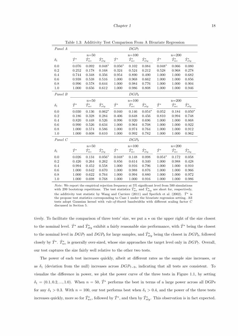
Table 1.3: Additivity Test Comparison From A Bivariate Regression
Panel A DGP7
n=50 n=100 n=200
δ1 T ∗ T ∗wc T ∗
sty T ∗ T ∗wc T ∗
sty T ∗ T ∗wc T ∗
sty
0.0 0.076 0.092 0.048? 0.056? 0.102 0.084 0.048? 0.066 0.0800.2 0.252 0.178 0.168 0.324 0.524 0.212 0.528 0.968 0.2780.4 0.744 0.348 0.356 0.954 0.890 0.490 1.000 1.000 0.6820.6 0.938 0.538 0.516 1.000 0.968 0.662 1.000 1.000 0.8560.8 0.996 0.578 0.644 1.000 0.984 0.776 1.000 1.000 0.9041.0 1.000 0.656 0.612 1.000 0.986 0.808 1.000 1.000 0.946
Panel B DGP8
n=50 n=100 n=200
δ1 T ∗ T ∗wc T ∗
sty T ∗ T ∗wc T ∗
sty T ∗ T ∗wc T ∗
sty
0.0 0.030 0.136 0.062? 0.040 0.146 0.054? 0.052 0.184 0.050?
0.2 0.186 0.328 0.284 0.406 0.648 0.456 0.810 0.994 0.7480.4 0.820 0.448 0.526 0.996 0.920 0.696 1.000 1.000 0.8680.6 0.990 0.526 0.634 1.000 0.964 0.708 1.000 1.000 0.9220.8 1.000 0.574 0.586 1.000 0.974 0.764 1.000 1.000 0.9121.0 1.000 0.608 0.610 1.000 0.992 0.782 1.000 1.000 0.962
Panel C DGP9
n=50 n=100 n=200
δ1 T ∗ T ∗wc T ∗
sty T ∗ T ∗wc T ∗
sty T ∗ T ∗wc T ∗
sty
0.0 0.026 0.134 0.056? 0.048? 0.148 0.098 0.054? 0.172 0.0580.2 0.426 0.264 0.262 0.856 0.614 0.340 1.000 0.988 0.4280.4 0.994 0.452 0.558 1.000 0.916 0.796 1.000 1.000 0.9100.6 1.000 0.642 0.670 1.000 0.988 0.876 1.000 1.000 0.9660.8 1.000 0.622 0.764 1.000 0.994 0.880 1.000 1.000 0.9721.0 1.000 0.698 0.768 1.000 1.000 0.916 1.000 1.000 0.986
Note: We report the empirical rejection frequency at 5% significant level from 500 simulationswith 299 bootstrap repetitions. The test statistics T ∗
wc and T ∗sty are short for, respectively,
the additivity test statistic by Wang and Carriere (2011) and Sperlich et al. (2002). T ∗ isthe propose test statistics corresponding to Case 1 under the bivariate regression setting. Alltests adopt Gaussian kernel with rule-of-thumb bandwidths with different scaling factor Cdiscussed in Section 5.
tively. To facilitate the comparison of three tests’ size, we put a ? on the upper right of the size closest
to the nominal level. T ∗ and T ∗sty exhibit a fairly reasonable size performance, with T ∗ being the closest
to the nominal level in DGP7 and DGP9 for large samples, and T ∗sty being the closest in DGP8, followed
closely by T ∗. T ∗wc is generally over-sized, whose size approaches the target level only in DGP7. Overall,
our test captures the size fairly well relative to the other two tests.
The power of each test increases quickly, albeit at different rates as the sample size increases, or
as δ1 (deviation from the null) increases across DGP7−9, indicating that all tests are consistent. To
visualize the difference in power, we plot the power curve of the three tests in Figure 1.1, by setting
δ1 = (0.1, 0.2, ..., 1.0). When n = 50, T ∗ performs the best in terms of a large power across all DGPs
for any δ1 > 0.3. With n = 100, our test performs best when δ1 > 0.4, and the power of the three tests
increases quickly, more so for T ∗wc, followed by T ∗, and then by T ∗sty. This observation is in fact expected.

Chapter 1 19
Figure 1.1: Power Curve Comparison of Additivity Tests at 5% Rejection RegionDGP7: n=50
δ1
Siz
e/P
ower
0.0 0.2 0.4 0.6 0.8 1.0
0.05
0.20
0.40
0.60
0.80
1.00
T∗
Twc∗
Tsty∗
DGP7: n=100
δ1
Siz
e/P
ower
0.0 0.2 0.4 0.6 0.8 1.0
0.05
0.20
0.40
0.60
0.80
1.00
T∗
Twc∗
Tsty∗
DGP7: n=200
δ1
Siz
e/P
ower
0.0 0.2 0.4 0.6 0.8 1.0
0.05
0.20
0.40
0.60
0.80
1.00
T∗
Twc∗
Tsty∗
DGP8: n=50
δ1
Siz
e/P
ower
0.0 0.2 0.4 0.6 0.8 1.0
0.05
0.20
0.40
0.60
0.80
1.00
T∗
Twc∗
Tsty∗
DGP8: n=100
δ1
Siz
e/P
ower
0.0 0.2 0.4 0.6 0.8 1.0
0.05
0.20
0.40
0.60
0.80
1.00
T∗
Twc∗
Tsty∗
DGP8: n=200
δ1
Siz
e/P
ower
0.0 0.2 0.4 0.6 0.8 1.0
0.05
0.20
0.40
0.60
0.80
1.00
T∗
Twc∗
Tsty∗
DGP9: n=50
δ1
Siz
e/P
ower
0.0 0.2 0.4 0.6 0.8 1.0
0.05
0.20
0.40
0.60
0.80
1.00
T∗
Twc∗
Tsty∗
DGP9: n=100
δ1
Siz
e/P
ower
0.0 0.2 0.4 0.6 0.8 1.0
0.05
0.20
0.40
0.60
0.80
1.00
T∗
Twc∗
Tsty∗
DGP9: n=200
δ1
Siz
e/P
ower
0.0 0.2 0.4 0.6 0.8 1.0
0.05
0.20
0.40
0.60
0.80
1.00
T∗
Twc∗
Tsty∗

Chapter 1 20
When d = 2 the convergence rate of T ∗wc is nh (Theorem 3 in WC), faster than the rate of nh3 in our
test T ∗ and nh5 in T ∗sty (Theorem 9 in STY). With n = 200, our test and T ∗wc all have power one when
the model only moderately deviates from its null (δ1 > 0.4 in DGP7−8 and δ1 > 0.2 in DGP9), while the
power of T ∗sty is increasing but still distinguishably less than one. T ∗sty exhibits the largest power with a
smaller δ1. In all, our test T ∗ exhibits a reasonable performance of size and power, presenting a viable
alternative to the other two additivity tests considered in the simulation study.
1.6 Empirical Application
Revealing the salient semiparametric structure of the regression model can be highly useful. First,
evidence of a correct semiparametric structure can be usefully incorporated into the model, improving
the estimation efficiency and alleviating the curse of dimensionality. Second, the revealed structure
can further be used to test for the validity of the underlying economic hypothesis. Tests for a specific
semiparametric/parametric structure either fail to reject or reject the null hypothesis, and in the case of
rejecting the null, the practitioner is left with only the knowledge of an incorrect null structure, but no
hint regarding where to further search for the feature of the structure, if there is any. One interesting
aspect of our test is that repeated use of our test can further shed light on the structure of the regression
model, since the information on the significant or insignificant variables in the gradient function can
be translated into information regarding the structure of the regression function, as we show in the
simulation section with three popular semiparametric models. We illustrate the empirical applicability
of our proposed test statistic in this section.
We utilize the dataset consisting of 569 Belgian firms in 1996 from Verbeek (2008), regarding the
estimation of a labor demand function. The dataset is available in Labour under R package Ecdat.
Economic theories suggest that the labor demand L is a function of the capital stock (K), output (Y ),
and real labor’s wage (w), however, there is no clear guidance regarding the specific structure or the
functional form of the labor demand function. For example, modeling the labor demand in a simple
linear fashion without interactive effects among its key determinants is likely to be misspecified. We
implement our test to provide statistical evidence on the potential nonlinearity and interactive effects,
illustrating to empirical practitioners a plausible underlying structure of the labor demand.
We start by assuming that the labor demand function is a fully unknown nonparametric function with
an additive error, i.e.,
Li = m(Ki, Yi, wi) + εi, (1.8)
where L (ln labor) is the natural log of total number of workers, depending on capital (K, total fixed assets

Chapter 1 21
Table 1.4: Descriptive Statistics of the Dataset
Variable Index n Mean SD Min Max
ln labor L 481 4.355 1.048 0.000 7.185capital K 481 3.982 5.472 0.002 42.235output Y 481 6.571 7.011 0.026 48.452wage w 481 34.587 7.146 11.734 49.892
Table 1.5: Empirical Results From the Dataset
Panel A Gradient of K
Test ω ωc T ∗ p-value T ∗ (trim) p-value (trim)
1 K,Y,w - 0.0043 0.0725 0.0039 0.08752 K Y ,w 0.0014 0.1200 0.0008 0.18253 Y K,w 0.0235 0.0000 0.0212 0.00024 w K,Y 0.0017 0.2200 0.0019 0.2452
Inferred model structure L = Km1(Y ) +m2(Y,w) + u
Panel B Gradient of Y
Test ω ωc T ∗ p-value T ∗ (trim) p-value (trim)
5 K,Y,w - 0.0282 0.0000 0.0258 0.00006 Y K,w 0.0235 0.0000 0.0203 0.00007 w K,Y 0.0033 0.1700 0.0024 0.1937
Inferred model structure L = Km1(Y ) +mY (Y ) +mw(w) + u
Panel C Gradient of w
Test ω ωc T ∗ p-value T ∗ (trim) p-value (trim)
8 K,Y,w - 0.0007 0.2475 0.0005 0.2898
Inferred model structure L = Km1(Y ) +mY (Y ) + wβ + u
in million euro), output (Y , value added in million euro), and wage (w, total wage costs divided by number
of workers in 1000 euro). To mitigate the impact of extreme outliers, we trim out firms falling in the upper
ten percentiles of each variable. Table 1.4 provides the descriptive statistics for the 481 observations in
the dataset. Before proceeding, a verification that all regressors in (1.8) are significant in m(·) is needed,
as a necessary condition to proceed with our test. We implement a nonparametric R2 test for omitted
variables by Yao and Ullah (2013), to check whether all regressors in (1.8) are significant in m(·). Their
standardized bootstrap test T ∗nG with a rule-of-thumb bandwidth and 399 bootstrap repetitions gives a
p-value of 0.0000, clearly rejecting the null of insignificant K,Y and w in m(·).4
We start the investigation by testing the significance of ω in the gradient function gK(W ), with
W = [K,Y,w]′ and the results are summarized in Panel A of Table 1.5. We begin by specifying ω = W in
the null of Test 1, which is equivalent to testing the structure that K is linear and not interactive with Y
and w. Result of Test 1 from Panel A of Table 1.5 show that the null is rejected at 10% significance level,
4The results are omitted here for brevity and are available upon the request from the second author.

Chapter 1 22
Figure 1.2: Plot of mw(w) estimates against w
Wage (w)
Estim
ates
of m
w(w)
10 20 30 40 50 60
1.5
2.0
2.5
3.0
3.5
4.0
4.5
suggesting that a partially linear model for the labor demand as m(K,Y,w) = Kβ+m(Y,w) is not likely
to be true. Intuitively, the rejection of the null in Test 1 is likely due to the presence of nonlinearity of
K, interaction effects between K and the other variables (Y,w), or both. Hence, we proceed to test the
nonlinearity of K in Test 2 with the null being ω = K, the interaction effect between K and Y in Test
3 with ω = Y , and the interaction effect between K and w in Test 4 with ω = w. Panel A of Table 1.5
indicates that we fail to reject the null in Tests 2 and 4 but reject the null in Test 3 at 1% significant level.
Thus, we conclude that K (capital) enters the labor demand function linearly, whose coefficient varies
significantly with Y (output) but not with w (wage). To summarize, the results in Panel A suggest that
the structure of the labor demand function may be characterized as m(K,Y,w) = Km1(Y ) +m2(Y,w),
a varying coefficient model but with different smoothing variables.
We further explore the structure of m2(Y,w), which is shown from the tests in Panel A to be additively
separable from Km1(Y ), and more detailed structure can surely improve the estimation efficiency. For
illustration purposes, we explore the structure of m2(Y,w) by testing the significance of ω in the gradient
function gY (W ). The p-values in Panel B of Table 1.5 indicate that the effect of Y is significantly
nonlinear (in Tests 5 and 6) but not interactive with w (in Test 7). Thus, given the tests in Panel A, we
expect that m2(·) is additively separable, i.e., m2(Y,w) = mY (Y ) + mw(w). Hence, our labor demand
function structure is pinned down to m(K,Y,w) = Km1(Y ) + mY (Y ) + mw(w), a varying coefficient
additive model.
Finally, one may conjecture that the effect of w is constant, (i.e., mw(w) is linear), since a linear
specification is an empirically popular choice. Based on the revealed varying coefficient additive model

Chapter 1 23
Figure 1.3: Plots of mY (Y ) and m1(Y ) in the Partially Linear Varying Coefficient Model
(a)
Output Y
0 10 20 30 40
2
3
4
5
6
7
8
Neu
tral
func
tion
mY(Y
)
(b)
Output Y
0 10 20 30 40
−0.1
0.0
0.1
0.2
0.3
Non
−ne
utra
l fun
ctio
n m
1(Y
)
structure in Panel B, i.e., m(K,Y,w) = Km1(Y ) + mY (Y ) + mw(w), we consistently estimate mw(·)
through a polynomial B-Spline estimator, with the number of evenly-spaced interior knots chosen with
the generalized cross-validation (see Li and Racine (2007)). We plot the estimates mw(w) against w
with its 95% bootstrap CI superimposed in Figure 1.2, where mw(w) is demonstrated to be a downward
sloping linear line except for the boundary area. Therefore, we further test the null hypothesis that
ω = W is insignificant in gw(W ), corresponding to the structure that w exhibits a constant effect on the
labor demand. The result of Test 8 in Panel C of Table 1.5 supports this conjecture, showing that w
enters the model linearly, with no interactions with either K or Y , consistent with results in Tests 4 and
7. To conclude, the series of our tests reveal that the structure of the labor demand in the dataset is
likely to be m(K,Y,w) = Km1(Y ) +mY (Y ) +wβ, a partially linear varying coefficient model (PLVCM).
We estimate the inferred PLVCM structure for the labor demand, i.e., Li = Kim1(Yi) + mY (Yi) +
wiβ + εi, to illustrate the interaction between Y and K, the nonlinearity of Y , and the constant effect
of w. We follow Fan and Huang (2005) to estimate the neutral function mY (Y ), non-neutral function
m1(Y ), and constant partial effect β through the profile least-square estimator. The estimated neutral
and non-neutral functions mY (Y ) and m1(Y ) are plotted in Panel (a) and (b) of Figure 1.3, respectively,
with the cross validation least square (CVLS) bandwidth implemented. The estimated neutral function
of Y in panel (a) is clearly nonlinear and concave, suggesting a positive yet diminishing effect of the
output on the labor demand. The coefficient function of K on L in panel (b) evidently depends on Y
in a nonlinear fashion, which decreases to a negative level for relatively low level of outputs but steadily

Chapter 1 24
Figure 1.4: Plots of mY (Y ) and m1(Y ) in the Partially Linear Varying Coefficient Model
(a)
Output Y
0 2 4 6 8 10 12 14
3
4
5
6
7
Neu
tral
func
tion
mY(Y
)
(b)
Output Y
0 2 4 6 8 10 12 14
−0.1
0.0
0.1
0.2
0.3
0.4
Non
−ne
utra
l fun
ctio
n m
1(Y
)
increases, and eventually turns positive as the output increases to a high level. This may be intuitively
understood, as higher outputs produced may alter the labor-capital elasticity of substitution, making
capital to be eventually complementary with labor in the production process. Finally, the parameter
estimate is β = −0.0278 with a standard error of 0.0032. It indicates that w (wage) enters the model
linearly and significantly, and one unit increase in the wage decreases the labor demand by about 2.78%.
We further check the sensitiveness of our testing results to the presence of large firms. We trim out
firms with the upper 10% output, and re-preform the testing procedure as above. The results are reported
on the last two columns of Table 1.5. We observe that our implied model structure remain unchanged,
which continues to be a PLVCM. We plot the PLVCM estimates in Figure 1.4, which again reveals
the nonlinearity of both neutral and non-neutral function of output in labor demand. The parametric
estimate is β = −0.029 with a standard error of 0.0037, showing that wage enters the model linearity as
indicated in our previous finding.
1.7 Conclusion
Given a set of significant regressors in conditional mean function, we propose a variation based test for
significant variables in the gradient function. We construct the test by estimating the gradient with a local
polynomial estimator, obtain the asymptotic null distribution of the test, and demonstrate that the test
is consistent. Based on the analysis of the asymptotic null distribution, we propose a wild bootstrap test,

Chapter 1 25
which is easy to implement. We demonstrate the validity of the bootstrap as its asymptotic distribution
is the same as the asymptotic null, no matter whether the null hypothesis is valid or not.
The Monte Carlo studies illustrate encouraging finite sample properties of our test, with the size
being close to the nominal level and the power approaching one quickly as the sample size increases. The
test can be used to infer several well-known semiparametric structures, including the additive model, the
varying coefficient model, and the partially linear model. Through an empirical application on estimating
the labor demand, we illustrate that repeated use of our test can help empirical practitioners to infer the
refined structure for the underlying regression, offering promises for the future work.
Appendix
Lemma 1. Uniformly for all Wi ∈ G, a compact subset of <d,
gx(Wi)− gx(Wi) = 1nhd+1f(Wi)
n∑j=1
SK(Wj−Wi
h )(∑
|k|=p+1
hp+1
k! (Dkm)(Wi + λ(Wj −Wi))(Wj−Wi
h )k + εj)(1 +
op(1)).
Proof. From the first order condition in equation (1.2), let’s arrange the N|j| values of tn,j(W ) in a column
vector τn,|j|(W ), with the k − th element being (τn,|j|)k(W ) = tn,G|j|(k)(W ). For N =p∑i=0
Ni, we define
τn(W ) =
τn,0(W )
τn,1(W )
...
τn,p(W )
. We arrange the distinct values of h|k|ak(W ) for 0 ≤ |k| ≤ p as a N × 1 column
vector αn(W ) =
αn,0(W )
αn,1(W )
...
αn,p(W )
, where (αn,|j|)k(W ) = h|j|an,G|j|(k)(W ). For the true values, α(W ) =
α0(W )
α1(W )
...
αp(W )
, where (α|j|)k(W ) = h|j|aG|j|(k)(W ). Since we arrange W = (x, z′)′ with x being the first
element, gx(W ) = aG1(d)(W ). Next we arrange the possible values of Sn,j+k(W ) by a matrix Sn,|j|,|k|(W )
in a lexicographical order with the (l,m)-th element being (Sn,|j|,|k|)l,m(W ) = Sn,G|j|(l)+G|k|(m)(W ). So

Chapter 1 26
Sn,|j|,|k|(W ) has dimension N|j| ×N|k|. Define Sn(W ) =
Sn,0,0(W ) Sn,0,1(W ) · · · Sn,0,p(W )
Sn,1,0(W ) Sn,1,1(W ) · · · Sn,1,p(W )
...... · · ·
...
Sn,p,0(W ) Sn,p,1(W ) · · · Sn,p,p(W )
.
The set of equations in (1.2) are τn(W ) = Sn(W )αn(W ). Assuming that Sn(W ) is positive definite,
the solution is expressed as αn(W ) = S−1n (W )τn(W ). Specifically, let eN,1+d be a N × 1 vector of zeros,
except one at its (1 + d)th position. Then
hgx(W ) = e′N,1+dS−1n (W )τn(W ).
We note that Sn,G|j|(l)+G|k|(m)(W ) = 1nhd
n∑i=1
K(Wi−wh
)(Wi−W
h )G|j|(l)+G|k|(m). By assumption A3(2),
for W ∗ = λWi + (1− λ)W with λ ∈ (0, 1),
yi = m(Wi) + εi =∑
0≤|k|≤p
1
k!(Dkm)(W )(Wi −W )k +
∑|k|=p+1
1
k!(Dkm)(W ∗)(Wi −W )k + εi.
tn,j(W ) = 1nhd
n∑i=1
K(Wi−wh
)(Wi−W
h )j[∑
0≤|k|≤p
1k! (D
km)(W )(Wi −W )k +∑
|k|=p+1
1k! (D
km)(W ∗)(Wi −W )k + εi]
=∑
0≤|k|≤pakh
|k|Sn,j+k(W ) + 1nhd
n∑i=1
K(Wi−wh
)(Wi−W
h )j[∑
|k|=p+1
1k! (D
km)(W ∗)(Wi −W )k + εi]
=∑
0≤|k|≤pakh
|k|Sn,j+k(W ),
where the last equality is from equation (1.2). Thus,
∑0≤|k|≤p
h|k|(ak(W )−ak(W ))Sn,j+k(W ) =1
nhd
n∑i=1
K
(Wi − w
h
)(Wi −W
h)j[
∑|k|=p+1
1
k!(Dkm)(W ∗)(Wi−W )k+εi].
(1.9)
Then we let κi,|j|(Wi−Wh ) be an N|j| dimensional subvector whose k− th element is [κi,|j|(
Wi−Wh )]k =
K(Wi−wh
)(Wi−W
h )G|j|(k). Furthermore, κi(Wi−Wh ) =
κi,0(Wi−Wh )
κi,1(Wi−Wh )
...
κi,p(Wi−Wh )
.
Thus we express the equations in (1.9) in a matrix format
Sn(W )(αn(W )− α(W )) = 1nhd
n∑i=1
κi(Wi−Wh )[
∑|k|=p+1
1k! (D
km)(W ∗)(Wi −W )k + εi].

Chapter 1 27
So we have
h(gx(W )− gx(W )) = e′N,1+dS−1n (W )
1
nhd
n∑i=1
κi(Wi −W
h)[∑|k|=p+1
1
k!(Dkm)(W ∗)(Wi −W )k + εi]. (1.10)
We note that the element of S are simply multivariate moment of K(·), corresponding to the element
of Sn. Consider a typical element of Sn − f(W )S as
[Sn,i,j − f(W )Si,j ]l,m = Sn,Gi(l)+Gj(m) − ESn,Gi(l)+Gj(m) + ESn,Gi(l)+Gj(m) − µk,Gi(l)+Gj(m)f(W ) =
I1 + I2.
I1 = 1nhd
n∑i=1
K(Wi−wh
)(Wi−W
h )Gi(l)+Gj(m) − E 1nhd
n∑i=1
K(Wi−wh
)(Wi−W
h )Gi(l)+Gj(m). With A1(2), A2
and A4(1), we easily obtain supW∈G |I1| = Op((nhd
lnn )−12 ) (see Lemma 1 in Martins-Filho et al. (2018)).
I2 =∫K(Ψ)ΨGi(l)+Gj(m)(f(W + hΨ) − f(W ))dΨ = h
∫K(Ψ)ΨGi(l)+Gj(m)Ψ′f (1)(W ∗)dΨ = O(h)
uniformly ∀W ∈ G, by A1(2) and A2(2).
So supW∈G |[Sn,i,j−f(W )Si,j ]l,m| = Op(h+ (nhd
lnn )−12 ) = op(1). Furthermore, given A5 and A1(2), we
obtain supW∈G ||Sn−Sf(W )|| = op(1), where ||·|| refers to the Euclidean norm. Since S is positive definite
in A5, the smallest eigenvalue of S is greater than zero, then we have supW∈G ||S−1n − 1
f(W )S−1|| = op(1).
From equation (1.9), we have
h(gx(W )−gx(W )) =1
f(W )[S−1](1+d),·
1
nhd
n∑i=1
κi(Wi −W
h)[∑|k|=p+1
1
k!(Dkm)(W ∗)(Wi−W )k+εi](1+op(1)),
(1.11)
where [S−1](1+d),· refers to the (1 + d)th row of S−1. With the definition of SK(·) in equation (1.5), we
obtain the claimed result.
In our proof, we have made repeated use of the following Lemma 2, which is the same as Theorem 1
in Yao and Martins-Filho (2015). Let Qini=1 be a sequence of independent and identically distributed
(IID) random variables and φn(Q1, · · · , Qk) be a symmetric function with k < n. We call φn(Q1, · · · , Qk)
a kernel function that depends on n and a U-statistic un of degree k is defined as
un =
n
k
−1 ∑
(n,k)
φn(Qi1 , · · · , Qik), (1.12)
where∑
(n,k)
denotes the sum over all subsets 1 ≤ i1 < i2 < · · · < ik ≤ n of 1, 2, · · · , n. Now, let
φcn(q1, · · · , qc) = E(φn(Q1, · · · , Qc, Qc+1, · · · , Qk)|Q1 = q1, Q2 = q2, · · · , Qc = qc), σ2cn = V ar(φcn(Q1, · · · ,

Chapter 1 28
Qc)) and θn = E(φn(Q1, · · · , Qk)). In addition, recursively define h(1)n (q1) = φ1n(q1)−θn, · · · , h(c)
n (q1, · · · ,
qc) = φcn(q1, · · · , qc)−c−1∑j=1
∑(c,j)
h(j)n (qi1 , · · · , qij )−θn for c = 2, · · · , k, where the sum
∑(c,j)
is over all subsets
1 ≤ i1 < · · · < ij ≤ c of 1, · · · , c. By Hoeffding’s H-decomposition we have
un = θn +
n
k
−1
k∑j=1
n− j
k − j
∑(n,j)
h(j)n (Qv1 , · · · , Qvj ) = θn +
k∑j=1
k
j
H(j)n (Qv1 , · · · , Qvj ),
where H(j)n (Qv1 , · · · , Qvj ) =
n
j
−1 ∑
(n,j)
h(j)n (Qv1 , · · · , Qvj ). Since un can be written as a finite sum of
H(j)n , its magnitude can be determined by studying H
(j)n . The following result shows that the magnitude
of H(j)n is determined by n and the leading variance σ2
jn defined above.
Lemma 2. Let Qini=1 be an IID sequence and un be defined as in equation (1.12) such that
un = θn +
k∑j=1
k
j
H(j)n (Qv1 , · · · , Qvj ).
Then,
(a) V ar(H
(j)n
)= O
(n−j
j∑c=1
σ2cn
)= O
(n−jσ2
jn
)and H
(j)n = Op
((n−jσ2
jn)12
);
(b) for 1 ≤ c ≤ c′ ≤ k, we haveσ2cn
c ≤σ2c′nc′ .
Theorem 1.
Proof. Following the arguments after Theorem 1, we show below that
(1) nh2+ d2 (T21 − 1
nh2+dB1)d→ N(0,Ω).
(2) T23 = − 2nh2+d−d1B3(1 + op(1)) + op((nh
2+ d2 )−1).
(3) T22 = 1nh2+d−d1B2(1 + op(1)) + op((nh
2+ d2 )−1).
(1)-(3) give the claimed results.
(1) As stated before, T21 = T211 + · · ·+ T214.
(a) T211 = 1n3
n∑i=1
n∑j=1
n∑t=1
i 6=j,i 6=t
1f(Wi)2h2d+2SK(
Wj−Wi
h )SK(Wt−Wi
h )εjεt = 1n3
n∑i=1
n∑j=1
n∑t=1
i6=j,i 6=t
ψnijt, and notice ψnijt
is symmetric in indices j and t.
(i) Consider the case that i 6= j 6= t. Let φnijt = ψnijt +ψnjit +ψntji, and it is symmetric in all of its
indices, then

Chapter 1 29
T211 = 13n3
n∑i=1
n∑j=1
n∑t=1
i 6=j 6=t
φnijt = 2n3
n∑i=1
n∑j=1
n∑t=1
i<j<t
φnijt = 13 [O(n−4) +
n
3
−1
]n∑i=1
n∑j=1
n∑t=1
i<j<t
φnijt
= 13
n
3
−1
n∑i=1
n∑j=1
n∑t=1
i<j<t
φnijt(1 + op(1))
Note that it is a U-statistic. We apply the H-decomposition result for U-statistic with sample size
dependent kernel in Lemma 2, for φn(Qi, Qj , Qt) ≡ φnijt, to obtain
T211 = 13 [θn +
3∑j=1
3
j
H(j)n (Qv1 , · · · , Qvj )](1 + op(1)), where
H(j)n (Qv1 , · · · , Qvj ) =
n
j
−1 ∑
(n,j)
h(j)n (Qv1 , · · · , Qvj ), Qi = (W ′i , εi)
′. Here, θn = E(φnijt) = 0.
H(1)n (Qv1) =
n
1
−1
n∑i=1
h(1)n (Qi) = 1
n
n∑i=1
[E(φnijt|Qi)− θn] = 0, since E(εi|Wi) = 0.
13
3
2
H(2)n (Qv1 , Qv2) =
n
2
−1
n∑i=1
n∑j=1
i<j
h(2)n (Qi, Qj)
=
n
2
−1
n∑i=1
n∑j=1
i<j
[E(φnijt|Qi, Qj)− h(1)n (Qi)− h(1)
n (Qj)− θn]
=
n
2
−1
n∑i=1
n∑j=1
i<j
E(ψnijt + ψnjit + ψntji|Qi, Qj) =
n
2
−1
n∑i=1
n∑j=1
i<j
E(ψntji|Qi, Qj)
=
n
2
−1
n∑i=1
n∑j=1
i<j
εiεjh2d+2
∫SK(
Wj−Wt
h )SK(Wi−Wt
h ) 1f(Wt)
dWt.
V (H(3)n (Qv1 , Qv2 , Qv3)) = Op(n
−3σ23n), where by A2, A3(1),
σ23n = Eφ2
nijt ≤ CEψ2nijt = C 1
h4d+4E[ 1f4(Wi)
SK2(Wj−Wt
h )SK2(Wi−Wt
h )σ2(Wj)σ2(Wt)] = Op(h
−2d−4).
So V (H(3)n (Qv1 , Qv2 , Qv3)) = Op(n
−3h−2d−4), and
H(3)n (Qv1 , Qv2 , Qv3) = Op(n
− 32h−d−2) = Op(n
−1h−d2−2n−
12h−
d2 ) = op((nh
2+ d2 )−1).
So in all, we obtain for i 6= j 6= t,
T211 ≡ T211e =
n
2
−1
n∑i=1
n∑j=1
i<j
εiεjh2d+2
∫SK(
Wj−Wt
h )SK(Wi−Wt
h ) 1f(Wt)
dWt(1 + op(1)).
(ii) T211e =
n
2
−1
h−2− d2n∑i=1
n∑j=1
i<j
εiεj
h3d2
∫SK(
Wj −Wt
h)SK(
Wi −Wt
h)
1
f(Wt)dWt︸ ︷︷ ︸
φnij
(1 + op(1)).
Note that φnij = φn(Qi, Qj) is symmetric in Qi and Qj . Since E(φnij |Qi) = 0, by Theorem 1 in Hall
(1984), if Eφ2nij <∞, and
EG2n(Qi,Qj)+
1nEφ
4nij
[Eφ2nij ]
2 → 0, then

Chapter 1 30
nh2+ d2 T211e = n
n
2
−1
n∑i=1
n∑j=1
i<j
φnijd→ N(0, 2Eφ2
nij).
Recall the definition of SK(·) in equation (1.5), and let Wi−Wt
h = Ψ,Wj−Wi
h = Ψ1, thenWj−Wt
h =
Ψ1 + Ψ, Wt = Wi − hΨ, and Wj = Wi + hΨ1. Then
2Eφ2nij = 2E[σ2(Wi)σ
2(Wj)1hd
( 1hd
∫SK(
Wj−Wt
h )SK(Wi−Wt
h ) 1f(Wt)
dWt)2]
= 2∫f(Wi)f(Wi + hΨ1)σ2(Wi)σ
2(Wi + hΨ1)[∫ ∑
0≤|j|≤p
N|j|∑l=1
S−1
1+d,|j|−1∑l′=0
Nl′+l
K(Ψ1 + Ψ)(Ψ1 + Ψ)G|j|(l)
∑0≤|j′|≤p
N|j′|∑l′=1
S−1
1+d,|j′|−1∑l′′=0
Nl′′+l′
K(Ψ)ΨG|j′|(l′) 1f(Wi−hΨ)dΨ]2dWidΨ1
→ 2[σ4(Wi)dWi][∫
(∫SK(Ψ1 + Ψ)SK(Ψ)dΨ)2dΨ1] = Ω.
Eφ4nij = h−d
∫E(ε4i |Wi)E(ε4j |Wi+hΨ1)[
∫SK(Ψ1+Ψ)SK(Ψ) 1
f(Wi−hΨ)dΨ]4f(Wi)f(Wi+hΨ1)dWidΨ1,
thus, with A1, A2, and A3(1), 1nEφ
4nij → 0 as nhd →∞.
With similar change of variables, i.e., Ψ = Wi−Wt
h , Ψ1 =Wj−W ′t
h , Ψ2 = Wl−Wi
h , Ψ3 =Wi−Wj
h , we have
EG2n(Qi, Qj) = E[E2(φnliφnlj |Qi, Qj)]
= hdEε2i ε2j [∫σ2(Wl)(
1hd
∫SK(Wi−Wt
h )SK(Wl−Wt
h ) 1f(Wt)
dWt)
( 1hd
∫SK(
Wj−W ′th )SK(
Wl−W ′th ) 1
f(W ′t )dW ′t )f(Wl)dWl]
2
= h4d∫σ2(Wi)σ
2(Wi − hψ3)f(Wi)f(Wi − hψ3)[∫σ2(Wi + hψ2)(
∫SK(Ψ)SK(Ψ2 + Ψ) 1
f(Wi−hΨ)dΨ]
(∫SK(Ψ1)SK(Ψ2 + Ψ1 + Ψ3) 1
f(Wi−hΨ3−hΨ1)dΨ1)f(Wi + hΨ2)dΨ2]2dΨ3dWi
= O(h4d),
so we verify the condition for the asymptotic normality and we have nh2+ d2 T211e
d→ N(0,Ω).
(iii) Since i 6= j and i 6= t, the only other case is for i 6= j = t. In this case, since the kernel is
symmetric,
T211 ≡ T211B = 1n3h2d+2
n∑i=1
n∑j=1
i 6=j
ε2jf2(Wi)
SK2(Wj−Wi
h ) = 12nh2+d
2n2
n∑i=1
n∑j=1
i6=j
ε2jhdf2(Wi)
SK2(Wj −Wi
h)︸ ︷︷ ︸
ψnij
.
Note that 2n2
n∑i=1
n∑j=1
i 6=j
ψnij = [O(n−3) +
n
2
−1
]n∑i=1
n∑j=1
i 6=j
φnij for φnij = ψnij + ψnji. We apply Lemma
2 here again and write
n
2
−1
n∑i=1
n∑j=1
i6=j
φnij = θn +2∑j=1
2
j
H(j)n (Qv1 , · · · , Qvj ).
θn = Eφnij = 2∫
1hdf2(Wi)
SK2(Wj−Wi
h )σ2(Wj)f(Wi)f(Wj)dWidWj → 2∫σ2(Wi)dWi
∫SK2(Ψ)dΨ.
H(2)n (Qv1 , Qv2) = Op(n
−1σ2n) = Op(n−1h−
d2 ), since σ2
2n = Eφ2nij = O(h−d).
H(1)n (Qv1) = Op(n
− 12σ1n) = Op(n
− 12 ), since σ2
1n = E[E2(φnij |Qi)] = E[∫
1f2(Wi)
SK2(Ψ)σ2(Wi +
hΨ)dΨ]2 = O(1).

Chapter 1 31
So in all, T211B = 1nh2+d
∫σ2(Wi)dWi
∫SK2(Ψ)dΨ(1 + op(1)) = 1
nh2+dB1(1 + op(1)).
Combing above (i)-(iii), we obtain that nh2+ d2 (T211 − 1
nh2+dB1)d→ N(0,Ω).
(b)
T212 = 1n3
n∑i=1
n∑j=1
n∑t=1
i 6=j,i 6=t
1f2(Wi)h2d+2SK(
Wj−Wi
h )SK(Wt−Wi
h )εj∑
|k|=p+1
hp+1
k! (Dkm)(Wi + λ(Wt −Wi))(Wt−Wi
h )k
= 1n3
n∑i=1
n∑j=1
n∑t=1
i 6=j,i 6=t
ψnijt.
(i) Consider the case i 6= j 6= t. With φnijt = ψnijtψnitj+ψnjit+ψnjti+ψntij+ψntji, we apply Lemma
2 to obtain T212 = 16
n
3
−1
n∑i=1
n∑j=1
n∑t=1
i<j<t
φnijt(1 + op(1)) = 16 [θn +
3∑j=1
3
j
H(j)n (Qv1 , · · · , Qvj )].
Here θn = 0 as E(εj |Wj) = 0.
H(1)n (Qv1) = n−1
n∑i=1
E(φnijt|Qi)
= 1n
n∑i=1
2εih2d+2
∫1
f2(Wj)SK(
Wi−Wj
h )SK(Wt−Wj
h )∑
|k|=p+1
hp+1
k! (Dkm)(Wj + λ(Wt −Wj))(Wt−Wj
h )k
×f(Wj)f(Wt)dWjdWt
= Op(n− 1
2hp−1),
since (Dkm)(W ) is bounded and uniformly continuous for |k| = p+ 1 as in A3(2).
Given that σ22n = E(φ2
2n(Qi, Qj)), φ2n(Qi, Qj) = E(φnijt|Qi, Qj) = E(ψnijt + ψnjit + ψntij +
ψntji|Qi, Qj),
E(ψnijt|Qi, Qj) =εj
f2(Wi)h2d+2
∫SK(
Wj−Wi
h )SK(Wt−Wi
h )∑
|k|=p+1
hp+1
k! (Dkm)(Wi+λ(Wt−Wi))(Wt−Wi
h )kf(Wt)dWt.
We obtain E[E2(ψnijt|Qi, Qj)] = O(h2p+2−4−d) = O(h2p−d−2). Since similar arguments apply to the
other terms, we have σ22n = O(h2p−d−2). Since V (H
(2)n (Qv1 , Qv2)) = O(n−2σ2
2n), we conclude
H(2)n (Qv1 , Qv2) = Op(n
−1hp−d2−1) = op(n
−1h−d2−2).
σ23n = E(φ2
nijt) = O(h2(p−d)−2), V (H(3)n (Qv1 , Qv2 , Qv3) = Op(n
−3σ23n), and thus since nhd →∞,
H(3)n (Qv1 , Qv2 , Qv3) = Op(n
− 32 ph(p−d)−1) = Op((n
−1h−d2−2)(n−
12h(p− d2 )+1) = op((n
−1h−d2−2).
So T212 = Op(n− 1
2hp−1) + op((n−1h−
d2−2) = op((n
−1h−d2−2) with nh2p+d+2 → 0 as in A4(2).
(ii) When i 6= j = t, then
T212 = 1n3
n∑i=1
n∑j=1
i 6=j
1f2(Wi)h2d+2SK
2(Wj−Wi
h )εj∑
|k|=p+1
hp+1
k! (Dkm)(Wi + λ(Wj −Wi))(Wj−Wi
h )k.
We again apply Lemma to obtain with similar arguments that
T212 = Op(n−2hp−
32d−1)+Op(n
− 32hp−d−1) = Op(n
− 32hp−d−1) = Op(n
−1h−d2−2n−
12hp−
d2 +1) = op(n
−1h−d2−2).
(i)-(ii) above give the results that T212 = op(n−1h−
d2−2).
(c) T213 = op(n−1h−
d2−2) follows from the same arguments in (b) for T212.
(d)

Chapter 1 32
T214 = 1n3
n∑i=1
n∑j=1
n∑t=1
i 6=j,i 6=t
1f2(Wi)h2d+2SK(
Wj−Wi
h )SK(Wt−Wi
h )∑
|k|=p+1
hp+1
k! (Dkm)(Wi + λ(Wj −Wi))(Wj−Wi
h )k
×∑
|k′|=p+1
hp+1
k′! (Dk′m)(Wi + λ(Wt −Wi))(Wt−Wi
h )k′
= 1n3
n∑i=1
n∑j=1
n∑t=1
i 6=j,i 6=t
ψnijt.
(i) i 6= j 6= t. Note that ψnijt is symmetric in j, t. So we let φnijt = ψnijt + ψnjit + ψntji and apply
Lemma 2 to have
T214 = 13
n
3
−1
n∑i=1
n∑j=1
n∑t=1
i 6=j,i 6=t
φnijt(1 + op(1)) = (1 + op(1)) 13 [θn +
3∑j=1
3
j
H(j)n (Qv1 , · · · , Qvj )].
Recall the definition of SK(·) in equation (1.5),
13θn = Eψnijt
= h2p∑
0≤|j|≤p
N|j|∑l=1
∑0≤|j′|≤p
N|j′|∑l′=1
S−1
1+d,|j|−1∑l′=0
Nl′+l
S−1
1+d,|j′|−1∑l′′=0
Nl′′+l′
∫1
f2(Wi)K(Ψ1)
×∑
|k|=p+1
hp+1
k! (Dkm)(Wi + λhΨ1)(Ψ1)k+G|j|(l)K(Ψ2)∑
|k′|=p+1
hp+1
k′! (Dk′m)(Wi + λhΨ2)(Ψ2)k′+G|j′|(l
′)
×f(Wi)f(Wi + hΨ1)f(Wi + hΨ2)dWidΨ1dΨ2
= O(h2p) = o(n−1h−d2−2) since nh
d2 +2h2p → 0 in A4(2).
H(1)n (Qv1) = Op(n
− 12h2p) = op(n
−1h−d2−2) since V (H
(1)n (Qv1)) = O(n−1σ2
1n) and σ21n = O(h4p).
H(2)n (Qv1 , Qv2) = Op(n
−1h2p− d2 ) = op(n−1h−
d2−2) since V (H
(2)n (Qv1 , Qv2)) = O(n−2σ2
2n) and σ22n =
O(h4p−d).
H(3)n (Qv1 , Qv2 , Qv3) = Op(n
− 32h2p−d) = op(n
−1h−d2−2) since V (H
(3)n (Qv1 , Qv2 , Qv3)) = O(n−3σ2
3n)
and σ23n = O(h4p−2d).
So when i 6= j 6= t, T214 = op(n−1h−
d2−2).
(ii) When i 6= j = t,
T214 = 1n3
n∑i=1
n∑j=1
i6=j
1f2(Wi)h2d+2SK
2(Wj−Wi
h )(∑
|k|=p+1
hp+1
k! (Dkm)(Wi + λ(Wj −Wi))(Wj−Wi
h )k)2.
Since E|T214| = O(n−1h2(p+1)−d−2) = O(n−1h2p−d) = op(n−1h−
d2−2h2p− d2 +2) = op(n
−1h−d2−2),
where we need p+ 1 > d4 in A4(2), we obtain that T214 = op(n
−1h−d2−2).
In all, T214 = op(n−1h−
d2−2).
Combining results in (1)(a)-(d), we obtain the claim in (1).
(2) T23 calls for
gx(ωl;ωci )− gx(ωl;ω
ci )
= 1f(ωl;ωci )nhd+1
n∑j=1
SK(ωj−ωlh ;
ωcj−ωci
h )[∑
|k|=p+1
hp+1
k! (Dkm)(ωl + λ(ωj − ωl);ωci + λ(ωcj − ωci ))(ωj−ωlh ;
ωcj−ωci
h )k
+εj ](1 + op(1)),

Chapter 1 33
where we follow equation (1.5) to define
SK(ωj − ωl
h;ωcj − ωci
h) =
∑0≤|k|≤p
N|k|∑m=1
S−1
1+d,|k|−1∑m′=0
Nm′+m
K(ωj − ωl
h;ωcj − ωci
h)(ωj − ωl
h;ωcj − ωci
h)G|k|(m).
(1.13)
Here we write (Wj−Wi
h ) ≡ (ωj−ωlh ;
ωcj−ωci
h ) to denote an equivalent rearrangement, highlighting the vari-
ables ω in W to be tested for significance.
With equations (1.5) and (1.13), we have
T23 = − 2n
n∑i=1
[ 1f(Wi)nhd+1
n∑j=1
SK(Wj−Wi
h )(∑
|k|=p+1
hp+1
k! (Dkm)(Wi + λ(Wj −Wi))(Wj−Wi
h )k + εj)]
× 1n
n∑l=1
1f(ωl;ωci )nhd+1
n∑t=1
SK(ωt−ωlh ;ωct−ω
ci
h )[∑
|k|=p+1
hp+1
k! (Dkm)(ωl + λ(ωt − ωl);ωci + λ(ωct − ωci ))
×(ωt−ωlh ;ωct−ω
ci
h )k + εt]
= − 2n4
n∑i=1
n∑j=1
n∑l=1
n∑t=1
i6=j,t 6=l,t6=i
1h2d+2f(Wi)f(ωl;ωci )
SK(Wj−Wi
h SK(ωt−ωlh ;ωct−ω
ci
h )[εjεt
+εt∑
|k|=p+1
hp+1
k! (Dkm)(Wi + λ(Wj −Wi))(Wj−Wi
h )k
+εj∑
|k|=p+1
hp+1
k! (Dkm)(ωl + λ(ωt − ωl);ωci + λ(ωct − ωci ))(ωt−ωlh ;ωct−ω
ci
h )k
+∑
|k|=p+1
hp+1
k! (Dkm)(Wi + λ(Wj −Wi))(Wj−Wi
h )k
×∑
|k|=p+1
hp+1
k! (Dkm)(ωl + λ(ωt − ωl);ωci + λ(ωct − ωci ))(ωt−ωlh ;ωct−ω
ci
h )k]
= T231 + T232 + T233 + T234.
(a) We claim that
T231 = − 2n4
n∑i=1
n∑j=1
n∑l=1
n∑t=1
i6=j,t 6=l,t6=i
1h2d+2f(Wi)f(ωl;ωci )
SK(Wj−Wi
h )SK(ωt−ωlh ;ωct−ω
ci
h )εjεt = − 2n4
n∑i=1
n∑j=1
n∑l=1
n∑t=1
i 6=j,t 6=l,t6=i
ψnijlt
= − 2nh2+d−d1B3(1 + op(1)). The claim follows from results (i)-(iii) below.
(i) When i 6= j 6= l 6= t, we apply Lemma 2 to have
T231 = − 224
n
4
−1
n∑i=1
n∑j=1
n∑l=1
n∑t=1
i 6=j 6=l 6=t
ψnijlt(1 + op(1)) = − 224
n
4
−1
n∑i=1
n∑j=1
n∑l=1
n∑t=1
i<j<l<t
φnijlt(1 + op(1)),
where
φnijlt = ψnijlt + ψnijtl + ψniltj + ψniljt + ψnitjl + ψnitlj + ψnjilt + ψnjitl + ψnjlti + ψnjlit + ψnjtli + ψnjtil
+ψnlijt + ψnlitj + ψnljti + ψnljit + ψnltji + ψnltij + ψntijl + ψntilj + ψntjli + ψntjil + ψntlij + ψntljipresent a permutation of ψnijlt across the indices, so that φnijlt is symmetric in the indices. Again, we
write
T231 = − 224 [θn +
4∑j=1
4
j
H(j)n (Qv1 , · · · , Qvj )].
V (H(2)n (Qv1 , Qv2)) = O(n−2σ2
2n). σ22n = V (φ2n(Q1, Q2)), φ2n(Qj , Qt) = E(φnijlt|Qj , Qt) = E(ψnijlt+
ψnljit + ψnitlj + ψnltij |Qj , Qt). Since

Chapter 1 34
E(ψnijlt|Qj , Qt) = εtεj∫
1h2d+2f(Wi)f(ωl;ωci )
SK(Wj−Wi
h )SK(ωt−ωlh ;ωct−ω
ci
h )f(Wi)f(Wl)dWidWl,
E[E2(ψnijlt|Qj , Qt)] = O(h−4−(d−d1)). Similar arguments apply to the other terms and we obtain σ22n =
O(h−4−(d−d1)). So H(2)n (Qv1 , Qv2) = Op(n
−1h−2− (d−d1)2 ) = op(n
−1h−2− d2 ), since d1 ≥ 1.
V (H(3)n (Qv1 , Qv2 , Q(v3))) = O(n−3σ2
3n). σ23n = V (φ3n(Q1, Q2, Q3)), φ3n(Qi, Qj , Ql) = E(φnijlt|Qi, Qj , Ql) =
E(ψntjli+ψntjil+ψntlji+ψntlij +ψntijl+ψntilj +ψnijtl+ψnjitl+ψnjlti+ψnljti+ψniltj +ψnlitj |Qj , Qt).
Since
E(ψntjli|Qi, Qj , Ql) = εiεj∫
1h2d+2f(Wt)f(ωl;ωct )
SK(Wj−Wt
h )SK(ωi−ωlh ;ωci−ω
ct
h )f(Wt)dWt,
E[E2(ψntjli|Qi, Qj , Ql)] = O(h−4−d). Similar arguments apply to the other terms and we obtain σ23n =
O(h−4−d). So H(3)n (Qv1 , Qv2 , Qv3) = Op(n
− 32h−2− d2 ) = op(n
−1h−2− d2 ).
V (H(4)n (Qv1 , Qv2 , Qv3 , Qv4)) = O(n−4σ2
4n), σ24n ≤ CEψ2
nijlt = Op(h−4−2d) by A2, A3(1), and A1(2),
so we obtain
H(4)n (Qv1 , Qv2 , Qv3 , Qv4) = Op(n
−2h−2−d) = op(n−1h−2− d2 ).
So in all, T231 = op(n−1h−2− d2 ) when i 6= j 6= l 6= t.
(ii) When i 6= j = l 6= t,
T231 = − 2n4
n∑i=1
n∑j=1
n∑t=1
i 6=j 6=t
1h2d+2f(Wi)f(ωj ;ωci )
SK(Wj−Wi
h )SK(ωt−ωlh ;ωct−ω
ci
h )εtεj = Op(n−1h−2) = op(n
−1h−2− d2 ).
(iii) When i 6= j = t 6= l,
T231 ≡ T231B = − 2(nh2+d−d1 )6
6n3
n∑i=1
n∑j=1
n∑l=1
i 6=j 6=l
1
h2d+2f(Wi)f(ωl;ωci )SK(
Wj −Wi
h)SK(
ωj − ωlh
;ωcj − ωci
h)ε2j︸ ︷︷ ︸
ψnijl
= − 2nh2+d−d1B3(1 + op(1)).
As 6n3
n∑i=1
n∑j=1
n∑l=1
i 6=j 6=l
ψnijl =
n
3
−1
n∑i=1
n∑j=1
n∑l=1
i<j<l
φnijl = θn+3∑j=1
3
j
H(j)n (Qv1 , · · · , Qvj ) for φnijl = ψnijl +
ψnilj + ψnjil + ψnjli + ψnlij + ψnlij . Since
θn = 6Eψnijl → 6∫σ2(Wi)f(ωi;ω
cl )dWidω
cl
∫SK(Ψ1)SK(ψ21;ψ12)dψ1dψ21 = 6B3,
H(1)n (Qv1) = Op(n
− 12σ1n) = Op(n
− 12 ) = op(1),
H(2)n (Qv1 , Qv2) = Op(n
−1σ2n) = Op(n−1h−
d2 ) = op(1),
H(3)n (Qv1 , Qv2 , Qv3) = Op(n
− 32σ3n) = Op(n
− 32h−
d+d12 ) = op(1),
we have 6n3
n∑i=1
n∑j=1
n∑l=1
i 6=j 6=l
ψnijl = 6B3 + op(1) and the claim above.
With similar but lengthy arguments, we show that
(b)T232
= − 2n4
n∑i=1
n∑j=1
n∑l=1
n∑t=1
i6=j,t 6=l,t6=i
1h2d+2f(Wi)f(ωl;ωci )
SK(Wj−Wi
h SK(ωt−ωlh ;ωct−ω
ci
h )εt∑
|k|=p+1
hp+1
k! (Dkm)(Wi + λ(Wj −Wi))
×(Wj−Wi
h )k
= op(n−1h−2− d2 ).

Chapter 1 35
(c)T233
= − 2n4
n∑i=1
n∑j=1
n∑l=1
n∑t=1
i6=j,t 6=l,t6=i
1h2d+2f(Wi)f(ωl;ωci )
SK(Wj−Wi
h SK(ωt−ωlh ;ωct−ω
ci
h )εj
×∑
|k|=p+1
hp+1
k! (Dkm)(ωl + λ(ωt − ωl);ωci + λ(ωct − ωci ))(ωt−ωlh ;ωct−ω
ci
h )k
= op(n−1h−2− d2 ).
(d)T234
= − 2n4
n∑i=1
n∑j=1
n∑l=1
n∑t=1
i6=j,t 6=l,t6=i
1h2d+2f(Wi)f(ωl;ωci )
SK(Wj−Wi
h SK(ωt−ωlh ;ωct−ω
ci
h )∑
|k|=p+1
hp+1
k! (Dkm)(Wi + λ(Wj −Wi))
×(Wj−Wi
h )k∑
|k|=p+1
hp+1
k! (Dkm)(ωl + λ(ωt − ωl);ωci + λ(ωct − ωci ))(ωt−ωlh ;ωct−ω
ci
h )k
= op(n−1h−2− d2 ).
The claim in (2) follows from (2)(a)-(d) above.
(3) Following (2) above, we letDkmtj;ti =∑
|k|=p+1
hp+1
k! (Dkm)(ωj+λ(ωt−ωj);ωci+λ(ωct−ωci ))(ωt−ωjh ;
ωct−ωci
h )k,
and write
T22 = 1n
n∑i=1
[ 1n
n∑j=1
(gx(ωj ;ωci )− gx(ωj ;ω
ci ))]
2
= 1n
n∑i=1
[ 1n
n∑j=1
1f(ωj ;ωci )nhd+1
n∑t=1
SK(ωt−ωjh ;
ωct−ωci
h )[Dkmtj;ti + εt]2
= 1n5
n∑i=1
n∑j=1
n∑t=1
n∑l=1
n∑m=1
t6=j 6=i,m6=l 6=i
1h2d+2f(ωj ;ωci )f(ωl;ωci )
SK(ωt−ωjh ;
ωct−ωci
h )SK(ωm−ωlh ;ωcm−ω
ci
h )[εtεm
+εt∑
|k|=p+1
hp+1Dkmml;mi + εm∑
|k|=p+1
hp+1Dkmtj;ti
+h2(p+1)∑
|k|=p+1
hp+1Dkmtj;ti
∑|k|=p+1
hp+1Dkmml;mi]
= T221 + T222 + T223 + T224.
(a) T221 = 1n5
n∑i=1
n∑j=1
n∑t=1
n∑l=1
n∑m=1
t 6=j 6=i,m6=l 6=i
1
h2d+2f(ωj ;ωci )f(ωl;ωci )SK(
ωt − ωjh
;ωct − ωci
h)SK(
ωm − ωlh
;ωcm − ωci
h)εtεm︸ ︷︷ ︸
ψnijtlm
.
We show below with (i)-(iii) that T221 = 1nh2+d−d1B2(1 + op(1)) + op(n
−1h−2− d2 ).
(i) When i 6= j 6= t 6= l 6= m, we apply Lemma 2 to perform U-statistics decomposition to have
T221 = θn +5∑j=1
5
j
H(j)n (Qv1 , · · · , Qvj ). We can show that θn = 0, H
(1)n (Qv1) = 0, H
(2)n (Qv1 , Qv2) =
Op(n−1σ2n) = Op(n
−1h−2− d2 +d12 ) = op(n
−1h−2− d2 ) since σ22n = O(h−4−(d−d1)), H
(3)n (Qv1 , Qv2 , Qv3) =
Op(n− 3
2σ3n) = Op(n− 3
2 (h−2−(d−d1) + h−2− d2 )) = op(n−1h−2− d2 ) since σ2
3n = O(h−4−(2d−2d1) + h−4−d),
H(4)n (Qv1 , Qv2 , Qv3 , Qv4) = Op(n
−2σ4n) = Op(n−2(h−2− (d+d1)
2 + h−2−d+d12 )) = op(n
−1h−2− d2 ) since
σ24n = O(h−4−(d+d1) + h−4−(2d−d1)), H
(5)n (Qv1 , Qv2 , Qv3 , Qv4 , Qv5) = Op(n
− 52σ5n) = Op(n
− 52 (h−2−d) =
op(n−1h−2− d2 ) since σ2
5n = O(h−4−2d). Thus, T221 = op(n−1h−2− d2 ).
(ii) When i 6= j = l 6= t = m, or i 6= j = m 6= t = l, or i 6= j = l 6= t 6= m, i 6= j = m 6= t 6= l,
i 6= j 6= t = t 6= m, we can show that T221 = op(n−1h−2− d2 ).
Chapter 1 36
(iii) When i 6= j 6= t = m 6= l, we can show that with similar arguments as in T211B and T231B that
T221 = 1n5
n∑i=1
n∑j=1
n∑t=1
n∑l=1
t 6=j 6=it6=l
ε2th2d+2f(ωj ;ωci )f(ωl;ωci )
SK(ωt−ωjh ;
ωct−ωci
h )SK(ωt−ωlh ;ωct−ω
ci
h )
≡ T221B = 1nh2+d−d1B2(1 + op(1)),
(b) T222 = 1n5
n∑i=1
n∑j=1
n∑t=1
n∑l=1
n∑m=1
t6=j 6=i,m6=l 6=i
1h2d+2f(ωj ;ωci )f(ωl;ωci )
SK(ωt−ωjh ;
ωct−ωci
h )SK(ωm−ωlh ;ωcm−ω
ci
h )εt∑
|k|=p+1
hp+1Dkmml;mi.
T223 = 1n5
n∑i=1
n∑j=1
n∑t=1
n∑l=1
n∑m=1
t 6=j 6=i,m6=l 6=i
1h2d+2f(ωj ;ωci )f(ωl;ωci )
SK(ωt−ωjh ;
ωct−ωci
h )SK(ωm−ωlh ;ωcm−ω
ci
h )εm∑
|k|=p+1
hp+1Dkmtj;ti.
T224 = 1n5
n∑i=1
n∑j=1
n∑t=1
n∑l=1
n∑m=1
t 6=j 6=i,m 6=l 6=i
1h2d+2f(ωj ;ωci )f(ωl;ωci )
SK(ωt−ωjh ;
ωct−ωci
h )SK(ωm−ωlh ;ωcm−ω
ci
h )
∑|k|=p+1
hp+1Dkmtj;ti
∑|k|=p+1
hp+1Dkmml;mi.
We show similarly that T22i = op(n−1h−2− d2 ) for i = 2, 3, and 4.
The claim in (3) follows from (3)(a) and (b) above and we conclude the proof for Theorem 1 based
on (1)-(3).
Theorem 2.
Proof. Given that T = T1n + T2n + T3n, and Theorem 1 implies that T2n = op(1), we show below that
(1) T1n = E[gx(Wi)− E(gx(ωl;ωci )|ωci )]2 + op(1).
(2) T3n = op(1).
Since under the alternative HA : gx(ω;ωc) depends on ω, T → E[gx(Wi)−E(gx(ωl;ωci )|ωci )]2 > 0. Then
we have as n → ∞, P (nh2+ d2 T > cn) → 1 for any positive constant cn = o(nh2+ d
2 ). Below we show (1)
and (2).
(1) T1n = 1n
n∑i=1
g2x(ωi;ω
ci )− 2
n2
n∑i=1
n∑l=1
gx(ωi;ωci )g
2x(ωl;ω
ci ) + 1
n
n∑i=1
[ 1n
n∑l=1
gx(ωl;ωci )]
2 = T11 + T12 + T13.
(a) With Eg2x(ωi;ω
ci ) < C in A3(3), we easily have T11
p→ Eg2x(ωi;ω
ci ).
(b) T12 = − 1n2
n∑i=1
n∑l=1
[gx(ωi;ωci )gx(ωl;ω
ci ) + gx(ωl;ω
cl )] = − 1
n2
n∑i=1
n∑l=1
φil.
(i) When i 6= l, we apply Lemma 2 to obtain
T12 = − 2n2
n∑i=1
n∑l=1
i<l
φil = − 2n
n∑i=1
[E(φil|Wi)− Eφil] + Eφil +Op(n−1(Eφ2
il)12 ).
Since Eφ2il ≤ CEg2
x(ωi;ωci )g
2x(ωl;ω
ci ) ≤ C[Eg4
x(ωi;ωci )]
12 [Eg4
x(ωl;ωci )]
12 < C by Cauchy Schwatz In-
equality and A1(3), Op(n−1(Eφ2
il)12 ) = Op(n
−1). Furthermore, 2n
n∑i=1
[E(φil|Wi)−Eφil] = Op(n− 1
2 ), since
E[E(φil|Wi)− Eφil]2 ≤ CEφ2il = O(1). Clearly, φil = 2Egx(ωi;ω
ci )gx(ωl;ω
ci ), thus we obtain
T12 = −2Egx(ωi;ωci )gx(ωl;ω
ci ) + op(1).
(ii) When i = l, T12 = − 2n2
n∑i=1
g2x(ωi;ω
ci ) = Op(n
−1).
So in all, T12 = −2Egx(ωi;ωci )gx(ωl;ω
ci ) + op(1).

Chapter 1 37
(c) T13 = 1n3
n∑i=1
n∑l=1
n∑j=1
gx(ωl;ωci )gx(ωj ;ω
ci ).
(i) When i 6= j 6= l, we apply Lemma 2 to write it as a U-statistics, perform U-Statistics decomposition,
analyze each term and obtain
T13 = Egx(ωl;ωci )gx(ωj ;ω
ci ) + op(1).
(ii) When i = l 6= j, or i = j 6= l, or j = l 6= i, or i = l = j, T13 = O(n−1) since E|T13| = O(n−1).
So in all, we obtain T13 = Egx(ωl;ωci )gx(ωj ;ω
ci ) + op(1).
Combining (1)(a)-(c) above, we obtain
T1n = Eg2x(ωi;ω
ci )− 2Egx(ωi;ω
ci )gx(ωl;ω
ci ) + Egx(ωl;ω
ci )gx(ωj ;ω
ci ) + op(1)
= E[gx(Wi)− E(gx(ωl;ωci )|ωci )]2 + op(1).
(2)T3n = 2n
n∑i=1
[gx(Wi)− 1n
n∑l=1l 6=i
gx(ωl;ωci )][gx(Wi)− gx(Wi)]
− 2n
n∑i=1
[gx(Wi)− 1n
n∑l=1l 6=i
gx(ωl;ωci )]
1n
n∑l=1
[gx(ωl;ωci )− gx(ωl;ω
ci )]
= T31 + T32.
Given that 1n
n∑l=1l 6=i
gx(ωl;ωci ) = E(gx(ωl;ω
ci )|ωci )+op(1) uniformly for ωci , we denoteDkmji ≡ (Dkm)(Wi+
λ(Wj −Wi))(Wj−Wi
h )k. Then
(a)T31 = 2n
n∑i=1
[gx(Wi)− Egx(ωl;ωci )|ωci )][ 1
f(Wi)nhd+1
n∑j=1
j 6=i
SK(Wj−Wi
h )(εj +∑
0≤|k|≤p
hp+1
k! Dkmji](1 + op(1))
= (T311 + T312)(1 + op(1)).
(i) T311 = 2n2
n∑i=1
n∑j=1
j 6=i
[gx(Wi)− Egx(ωl;ωci )|ωci )] 1
f(Wi)hd+1SK(Wj−Wi
h )εj = 2n2
n∑i=1
n∑j=1
j 6=i
ψnij .
We apply Lemma 2 to write φnij = ψnij + ψnji, and
T311 =
n
2
−1
n∑i=1
n∑j=1
i<j
φnij(1 + o(1)) = θn +2∑j=1
2
j
H(j)n (Qv1 , · · · , Qvj ).
θn = 0, H(1)n (Qv1) = Op(n
− 12σ1n) = Op(n
− 12h) since σ2
1n = O(h2), H(2)n (Qv1 , Qv2) = Op(n
−1σ2n) =
Op(n−1h−1− d2 ) since σ2
2n = O(h−2−d). Thus, T311 = Op(n− 1
2h).
(ii) T312 = 2n2
n∑i=1
n∑j=1
i 6=j
[gx(Wi) − Egx(ωl;ωci )|ωci )] 1
f(Wi)hd+1SK(Wj−Wi
h )∑
0≤|k|≤p
hp+1
k! Dkmji(1 + op(1)) =
Op(hp), since E|T312| = O(hp).
So we obtain T31 = Op(n− 1
2h) +Op(hp) = op(1).
(b) With similar arguments, we show that
T32 = 2n
n∑i=1
[gx(Wi)− Egx(ωl;ωci )|ωci )] 1
n
n∑l=1
1f(ωl;ωci )nhd+1
n∑t=1
SK(ωt−ωlh ;ωct−ω
ci
h )[εt
+∑
0≤|k|≤p
hp+1
k! Dkmtl;ti](1 + op(1))
= op(1).
The claim in (2) follows from (2)(a)-(b) above.

Chapter 1 38
Thus, we obtain T3n = op(1) and we conclude the proof of Theorem 2.
Theorem 3.
Proof. Following the arguments in Lemma 1, we define t∗n,j(W ) = 1nhd
n∑i=1
K(Wi−Wh )(Wi−W
h )jε∗j , (τ∗n,|j|)k =
t∗n,G|j|(k), and τ∗n(W ) =
τ∗n,0(W )
τ∗n,1(W )
...
τ∗n,p(W )
, then we obtain from the first order condition in equation (1.2),
hg∗x(W ) = e′N,1+dSn(W )−1τ∗n(W ) =1
f(W )[S−1]1+d,·τ
∗n(W )(1 + op(1)).
From these, we obtain
g∗x(Wi) =1
f(Wi)nhd+1
n∑j=1
j 6=i
SK(Wj −Wi
h)ε∗j (1 + op(1)), and
g∗x(ωl;ωci ) =
1
f(ωl;ωci )nhd+1
n∑j=1
j 6=l,j 6=i
SK(ωj − ωl
h;ωcj − ωci
h)ε∗j (1 + op(1)).
T ∗ = 1n
n∑i=1
(g∗x(Wi))2 + 1
n
n∑i=1
[ 1n
n∑l=1l 6=i
g∗x(ωl;ωci )]
2 − 2n2
n∑i=1
n∑l=1
l 6=i
g∗x(Wi)g∗x(ωl;ω
ci ) = T ∗1 + T ∗2 + T ∗3 .
We show below that conditional on Q(n) = Wi, yini=1,
(1) nh2+ d2 (T ∗1 − 1
nh2+dB1(1 + op(1)))d→ N(0,Ω).
(2) T ∗3 = − 2nh2+d−d1B3(1 + op(1)) + op((nh
2+d)−1).
(3) T ∗2 = 1nh2+d−d1B2(1 + op(1)) + op((nh
2+d)−1).
The claim in Theorem 3 follows from (1)-(3).
(1)T ∗1 = 1n
n∑i=1
[ 1f(Wi)nhd+1
n∑j=1
j 6=i
SK(Wj−Wi
h )ε∗j ]2
= 1n3
n∑i=1
n∑j=1
n∑l=1
i 6=k,i 6=l
1
f2(Wi)nh2(d+1)SK(
Wj −Wi
h)SK(
Wl −Wi
h)ε∗j ε
∗l︸ ︷︷ ︸
ψnijl
(1 + op(1)).
(a) When i 6= j 6= l, we note that the U-statistics results in Lemma 2 can not be applied here as we do
not have the IID assumption conditioning on the data Q(n). We let φnijl = ψnijl + ψnjil + ψnlji, which
is symmetric in i, j, l. We rewrite T ∗1 as

Chapter 1 39
T ∗1 = (1 + op(1)) 13
n
3
−1 n− 2
1
n∑i=1
n∑j=1
i<j
φ2nij + 13
n
3
−1
[n∑i=1
n∑j=1
n∑l=1
i<j<l
φnijl −
n− 2
1
n∑i=1
n∑j=1
i<j
φ2nij ]
= (1 + op(1))T ∗1a + T ∗1b,
where φ2nij =∫ψnijlF (Wl)dWl =
ε∗j ε∗i
h2(d+1)
∫1
f2(Wl)SK(
Wj−Wl
h )SK(Wi−Wl
h )f(Wl)dWl.
(i) Claim: T ∗1b = op(n−1h−2− d2 ).
T ∗1b = 13
n
3
−1
[n∑i=1
n∑j=1
n∑l=1
i<j<l
φnijl − φ2nij − φ2nil − φ2njl] = 13
n
3
−1
n∑i=1
n∑j=1
n∑l=1
i<j<l
Φnijl.
Note that E∗(ε∗i ) ≡ E(ε∗i |Q(n)) = 0, so E(T ∗1b|Q(n)) = 0.
V (T ∗1b|Q(n)) = 19
n
3
−2
n∑i=1
n∑j=1
n∑l=1
i<j<l
n∑i′=1
n∑j′=1
n∑l′=1
i′<j′<l′
E(ΦnijlΦni′j′l′ |Q(n))
= 19
n
3
−2
n∑i=1
n∑j=1
n∑l=1
i<j<l
E(Φ2nijl|Q(n)) + V1b1.
Note that if (i, j, l) are each distinct from (i′, j′, l′), since ε∗i is independent conditioning on Q(n), then
E(ΦnijlΦni′j′l′ |Q(n)) = E(Φnijl|Q(n))E(Φni′j′l′ |Q(n)) = 0. Similarly, if only one index in (i, j, l) is the
same as that in (i′, j′, l′), E(ΦnijlΦni′j′l′ |Q(n)) = 0. So in V1b1, we only consider the case that two of the
indices in (i, j, l) are the same as that in (i′, j′, l′). Due to the symmetry in Φnijl, we can just consider
any two indices.
Consider i = i′ 6= j = j′ 6= l 6= l′, E(ΦnijlΦnijl′ |Q(n)) = E[(ψnlji − φ2nij)(ψnl′ji − φ2nij)|Q(n)]. Thus,
V1b1 = O( 19
n
3
−2
n∑i=1
n∑j=1
n∑l=1
n∑l′=1
i 6=j 6=l 6=l′
E[(ψnlji − φ2nij)(ψnl′ji − φ2nij)|Q(n)]
= O( 19
n
3
−2
n∑i=1
n∑j=1
n∑l=1
n∑l′=1
i 6=j 6=l 6=l′
ε2i ε2j
h4(d+1) [ 1f2(Wl)
SK(Wj−Wl
h )SK(Wi−Wl
h )
−∫
1f2(Wl)
SK(Wj−Wl
h )SK(Wi−Wl
h )f(Wl)dWl]
×[ 1f2(Wl′ )
SK(Wj−Wl′
h )SK(Wi−Wl′h )−
∫1
f2(Wl′ )SK(
Wj−Wl′h )SK(Wi−Wl′
h )f(Wl′)dWl′ ])
= O( 19
n
3
−2
n∑i=1
n∑j=1
n∑l=1
n∑l′=1
i 6=j 6=l 6=l′
ε2i ε2j
h4(d+1) [ 1f2(Wl)
SK(Wj−Wl
h )SK(Wi−Wl
h )
−∫
1f2(Wl)
SK(Wj−Wl
h )SK(Wi−Wl
h )f(Wl)dWl]
×[ 1f2(Wl′ )
SK(Wj−Wl′
h )SK(Wi−Wl′h )−
∫1
f2(Wl′ )SK(
Wj−Wl′h )SK(Wi−Wl′
h )f(Wl′)dWl′ ](1 + op(1)))
= O( 19
n
3
−2
n∑i=1
n∑j=1
n∑l=1
n∑l′=1
i 6=j 6=l 6=l′
ψnvijll′(1 + op(1))) = O(V1b11),
where the third to last equality is from the fact that εi = yi−m(Wi) = εi+(m(Wi)−m(Wi)) = εi+op(1)
uniformly ∀Wi ∈ G.

Chapter 1 40
The claim that supW∈G |m(W )−m(W )| = op(1) follows by applying Lemma 3 of Martins-Filho et al.
(2018). Note that assumption A3(1) implies that E|ε|s < C for some s > 2. This observation, together
with assumptions A1(1)-(3), A2, A3(1), (2) and A4(1), enable us to apply Lemma 3 of Martins-Filho
et al. (2018) to obtain the uniform convergence result. We apply Lemma 2 on V1b11 below. Define
φnvijll′ = ψnvijll′ + ψnvijl′l + ψnviljl′ + ψnvill′j + ψnvil′jl + ψnvil′lj
+ψnvjill′ + ψnvjil′l + ψnvjlil′ + ψnvjll′i + ψnvjl′il + ψnvjl′li
+ψnvlijl′ + ψnvlil′j + ψnvljl′i + ψnvljil′ + ψnvll′ij + ψnvll′ji
+ψnvl′ijl + ψnvl′ilj + ψnvl′jil + ψnvl′jli + ψnvl′lij + ψnvl′lji,
V1b11 = 19
n
3
−2 n
4
n
4
−1
n∑i=1
n∑j=1
n∑l=1
n∑l′=1
i<j<l<l′
φnvijll′ = O(n−2)[θn+4∑j=1
4
j
H(j)n (Qv1 , · · · , Qvj )].
Since∫
[ 1f2(Wl)
SK(Wj−Wl
h )SK(Wi−Wl
h ) −∫
1f2(Wl)
SK(Wj−Wl
h )SK(Wi−Wl
h )f(Wl)dWl]f(Wl)dWl = 0,
θn = 0, andH(1)n (Qv1) = 0. H
(2)n (Qv1 , Qv2) = Op(n
−1σ2n) = Op(n−1h−4− 3d
2 ), since σ22n = E[E2(φnvijll′ |Ql, Ql′)] =
O(h−8−3d). H(3)n (Qv1 , Qv2 , Qv3) = O2
p(n− 3
2σ3n) = Op(n− 3
2h−4−2d), since σ23n = E[E2(φnvijll′ |Qi, Qj , Ql)] =
O(h−8−4d). H(4)n (Qv1 , Qv2 , Qv3 , Qv4) = Op(n
−2σ4n) = Op(n−2h−4− 5
2d), since σ24n = E[φnvijll′ ] =
O(h−8−5d).
So V1b11 = Op(n−2[n−1h−4− 3d
2 +n−32h−4−2d+n−2h−4− 5
2d]) = Op(n−3h−4− 3
2d), and V1b1 = Op(n−3h−4− 3
2d).
Next, we note that by c-r inequality, and since E(φ22nij |Q(n)) is of smaller order, n
3
−2
n∑i=1
n∑j=1
n∑l=1
i<j<l
E(Φ2nijl|Q(n))
≤ C
n
3
−2
n∑i=1
n∑j=1
n∑l=1
i<j<l
[E(φ2nijl|Q(n)) + E(φ2
2nij |Q(n)) + E(φ22nil|Q(n)) + E(φ2
2njl|Q(n))]
= C
n
3
−2
n∑i=1
n∑j=1
n∑l=1
i<j<l
E(φ2nijl|Q(n))(1 + op(1))
= C
n
3
−2
n∑i=1
n∑j=1
n∑l=1
i<j<l
[E(ψ2nijl|Q(n)) + E(ψ2
njil|Q(n)) + E(ψ2nlji|Q(n))](1 + op(1))
= Op(n−3h−4−2d),
where the last equality follows from the observation that

Chapter 1 41
n
3
−2
n∑i=1
n∑j=1
n∑l=1
i<j<l
E(ψ2nijl|Q(n))
=
n
3
−2
n∑i=1
n∑j=1
n∑l=1
i<j<l
ε2j ε2l
f4(Wi)h4(d+1)SK2(Wj−Wi
h )SK2(Wl−Wi
h )
=
n
3
−2
n∑i=1
n∑j=1
n∑l=1
i<j<l
ε2jε2l
f4(Wi)h4(d+1)SK2(Wj−Wi
h )SK2(Wl−Wi
h )(1 + op(1))
= Op(n−3h−4−2d).
So V (T ∗1b|Q(n)) = 19
n
3
−2
n∑i=1
n∑j=1
n∑l=1
i<j<l
E(Φ2nijl|Q(n)) + V1b1 = Op(n
−3h−4−2d) + Op(n−3h−4− 3
2d).
Thus, T ∗1b = Op(n− 3
2h−2−d) = op(n−1h−2− d2 ), as claimed.
(ii) Claim: nh2+ d2 T ∗1a
d→ N(0,Ω).
nh2+ d2 T ∗1a = nh2+ d
213
n
3
−1 n− 2
1
n∑i=1
n∑j=1
i<j
φ2nij
=n∑i=1
n∑j=1
i<j
nh2+ d2
n
2
−1
ε∗i ε∗j
h2(d+1)
∫1
f2(Wl)SK(
Wj−Wl
h )SK(Wi−Wl
h )f(Wl)dWl
=n∑i=1
n∑j=1
i<j
ψn1ij .
Note that ψn1ij is symmetric in i, j, E(ψn1ij |Q(n), ε∗j ) = 0, so conditioning on Q(n), nh
2+ d2 T ∗1a is a
degenerate second order U-statistics. Defining (S∗n)2 ≡ E((n∑i=1
n∑j=1
i<j
ψn1ij)2|Q(n)) = V (T ∗1a|Q(n)), we apply
Proposition 3.2 of de Jong (1987) to obtain
(S∗n)−1nh2+ d2 T ∗1a
d→ N(0, 1),
if GI , GII , GIV are each of order op((S∗n)4), where GI =
n∑i=1
n∑j=1
i<j
E(ψ4n1ij |Q(n)),
GII =n∑i=1
n∑j=1
n∑t=1
i<j<t
[E(ψ2n1ijψ
2n1it|Q(n)) + E(ψ2
n1jiψ2n1jt|Q(n)) + E(ψ2
n1tiψ2n1tj |Q(n))] = GII1 +GII2 +GII3,
GIV =n∑i=1
n∑j=1
n∑t=1
n∑l=1
i<j<t<l
[E(ψn1ijψn1itψn1ljψn1lt|Q(n)) + E(ψn1ijψn1ilψn1tjψn1tl|Q(n)) + E(ψn1itψn1ilψn1jtψn1jl|Q(n))]
= GIV 1 +GIV 2 +GIV 3.
Since E(ε∗i ε∗j ε∗t ε∗m|Q(n)) = ε2i ε
2j when i = t < j = m, and zero in the other cases, we have

Chapter 1 42
(S∗n)2 = n2h4+d
n
2
−2
n∑i=1
n∑j=1
i<j
ε2i ε2j
h4(d+1) [∫
1f2(Wl)
SK(Wj−Wl
h )SK(Wi−Wl
h )f(Wl)dWl]2
= 4(n−1)2
n∑i=1
n∑j=1
i<j
ε2i ε2j
h4(d+1) [∫
1f2(Wl)
SK(Wj−Wl
h )SK(Wi−Wl
h )f(Wl)dWl]2(1 + op(1))
= (1 + op(1))2
n
2
−1
n∑i=1
n∑j=1
i<j
ε2i ε2j
h4(d+1) [∫
1f2(Wl)
SK(Wj−Wl
h )SK(Wi−Wl
h )f(Wl)dWl]2
= (1 + op(1))2
n
2
−1
n∑i=1
n∑j=1
i<j
ψnsij ,
where the second equality follows since n2
n
2
−2
= 4(n−1)2 , and εi = εi + op(1) uniformly. The third
follows since 2(n−1)2 −
n
2
−1
= O(n−3). We then apply Lemma 2 to obtain that
n
2
−1
n∑i=1
n∑j=1
i<j
ψnsij = θn +2∑j=1
2
j
H(j)n (Qv1 , · · · , Qvj ) = Ω
2 +Op(n−1h−
d2 ),
since θn = Eψnsij →∫σ4(Wi)dWi
∫[∫SK(Ψ1 + Ψ)SK(Ψ)dΨ]2dΨ1 = Ω
2 , H(1)n (Qv1) = Op(n
−1), and
H(2)n (Qv1 , Qv2) = Op(n
−1h−d2 ). Thus, (S∗n)2 = Ω + op(1).
GI =n∑i=1
n∑j=1
i<j
h8+2d 16(n−1)4
E((ε∗i ε∗j )4|Q(n))
h8(d+1) [∫
1f2(Wl)
SK(Wj−Wl
h )SK(Wi−Wl
h )f(Wl)dWl]4 = O(n−2h−d) =
op((S∗n)4), since (S∗n)4 = O(1).
GII1 =n∑i=1
n∑j=1
n∑t=1
i<j<t
h8+2d 16(n−1)4h
−8−8dE((ε∗i )4(ε∗j )
2(ε∗t )2|Q(n))[
∫1
f2(Wl)SK(
Wj−Wl
h )SK(Wi−Wl
h )f(Wl)dWl]2
×[∫
1f2(Wl′ )
SK(Wt−Wl′h )SK(Wi−Wl′
h )f(Wl′)dWl′ ]2
= O(n−1).
Similarly, GII2 = O(n−1), GII3 = O(n−1), thus we conclude that GII = O(n−1) = o((S∗n)4).
GIV 1 =n∑i=1
n∑j=1
n∑t=1
n∑l=1
i<j<t<l
16(n−1)4h
−2dE((ε∗i )(ε∗j )
2(ε∗t )2(ε∗l )
2|Q(n))[1hd
∫1
f2(Wl)SK(
Wj−Wl
h )SK(Wi−Wl
h )f(Wl)dWl]
×[ 1hd
∫1
f2(Wl)SK(Wt−Wl
h )SK(Wi−Wl
h )f(Wl)dWl][1hd
∫1
f2(Wl′ )SK(
Wj−Wl′h )SK(Wl−Wl′
h )f(Wl′)dWl′ ]
×[ 1hd
∫1
f2(Wl′ )SK(Wt−Wl′
h )SK(Wl−Wl′h )f(Wl′)dWl′ ](1 + op(1))
= O(hd).
Similarly, GIV 2 = O(hd), and GIV 3 = O(hd), and thus we have GIV = O(hd) = o((S∗n)4).
Since we obtain that (S∗n)2 p→ Ω, we conclude that nh2+ d2 T ∗1a
d→ N(0,Ω).
(b) When i 6= j = l, T ∗1 ≡ T ∗1B = 1nh2+d
1n2
n∑i=1
n∑j=1
i6=j
1f2(Wi)hd
SK2(Wj−Wi
h )(ε∗j )2 = 1
nh2+dT∗1B1.
Claim: T ∗1B = 1nh2+dB1(1 + op(1)).

Chapter 1 43
To this end, we only need to show that T ∗1B1 = B1 + op(1) conditioning on Q(n).
(i) E(T ∗1B1|Q(n)) = 1n2
n∑i=1
n∑j=1
i 6=j
1f2(Wi)hd
SK2(Wj−Wi
h )ε2j = B1(1 + op(1)).
(ii) V (T ∗1B1|Q(n)) = E([T ∗1B1 − E(T ∗1B1|Q(n))]2|Q(n))
= E([ 1n2
n∑i=1
n∑j=1
i 6=j
1f2(Wi)hd
SK2(Wj−Wi
h )((ε∗j )2 − ε2j )]2|Q(n))
= 1n4
n∑i=1
n∑j=1
i 6=j
n∑l=1
n∑m=1
l 6=m
1f2(Wi)f2(Wl)h2dSK
2(Wj−Wi
h )SK2(Wm−Wl
h )E[((ε∗j )2 − ε2j )((ε∗m)2 − ε2m)|Q(n)].
Note first that whenever j 6= m, above is zero. Second, the two point distribution Fi described in
Step 1 of the bootstrap procedure implies that E(ε∗j |Q(n)) = 0, E(|ε∗j ||Q(n)) = 2√5|εj |, E((ε∗j )
2|Q(n)) = ε2j ,
E((ε∗j )3|Q(n)) = 0, E((ε∗j )
4|Q(n)) = 2ε4j .
When i 6= j = m 6= l, as E(((ε∗j )2 − ε2j )2|Q(n)) = ε4j ,
V (T ∗1B1|Q(n))
= 1n4
n∑i=1
n∑j=1
n∑l=1
i 6=j 6=l
1f2(Wi)f2(Wl)h2dSK
2(Wj−Wi
h )SK2(Wj−Wl
h )E(((ε∗j )2 − ε2j )2|Q(n))
= 1n4
n∑i=1
n∑j=1
n∑l=1
i 6=j 6=l
1f2(Wi)f2(Wl)h2dSK
2(Wj−Wi
h )SK2(Wj−Wl
h )ε4j (1 + op(1))
= O(n−1).
When i = l 6= j = m,
V (T ∗1B1|Q(n)) = 1n4
n∑i=1
n∑j=1
i 6=j
1f4(Wi)h2d (SK2(
Wj−Wi
h ))2ε4j = Op(n2h−d) = op(n−1).
So in all, V (T ∗1B1|Q(n)) = Op(n−1).
Combining (i) and (ii) above, we obtain that T ∗1B1 = B1 + op(1) conditioning on Q(n).
Combining (a) and (b) above, we obtain the claim in (1).
(2)T ∗3 = − 2n2
n∑i=1
n∑l=1
l 6=i
1f(Wi)nhd+1
n∑j=1
SK(Wj−Wi
h )ε∗j1
f(ωl;ωci )nhd+1
n∑t=1
SK(ωt−ωlh ;ωct−ω
ci
h )ε∗t (1 + op(1))
= − 2n4
n∑i=1
n∑j=1
n∑l=1
n∑t=1
i 6=j,t 6=l 6=i
1f(Wi)f(ωl;ωci )nh2(d+1)SK(
Wj−Wi
h )SK(ωt−ωlh ;ωct−ω
ci
h )ε∗j ε∗t (1 + op(1))
= − 2n4
n∑i=1
n∑j=1
n∑l=1
n∑t=1
i 6=j,t 6=l 6=i
ψnijlt
(a) When i 6= j 6= l 6= t, E(T ∗3 |Q(n)) = 0 as E(ε∗j |Q(n)) = 0, and
V (T ∗3 |Q(n)) = 4n8
n∑i=1
n∑j=1
n∑l=1
n∑t=1
i 6=j 6=l 6=t
n∑i′=1
n∑j′=1
n∑l′=1
n∑t′=1
i′ 6=j′ 6=l′ 6=t′
E(ψnijltψni′j′l′t′ |Q(n)).
We can show that E(|V (T ∗3 |Q(n))|) = o(n−2h−4−d) with different combinations of indices in the
summation, thus we apply Chebyshev’s inequality to conclude that T ∗3 = op(n−1h−2− d2 ).
(b) When i 6= j = l 6= t,

Chapter 1 44
T ∗3 = − 2n4
n∑i=1
n∑j=1
n∑t=1
i 6=j 6=t
1f(Wi)f(ωj ;ωci )h2(d+1)SK(
Wj−Wi
h )SK(ωt−ωjh ;
ωct−ωci
h )ε∗j ε∗t (1 + op(1)).
Again E(T ∗3 |Q(n)) = 0, and we can show that V (T ∗3 |Q(n)) = Op(n−4h−4−d), and thus T ∗3 = op(n
−1h−2− d2 ).
(c) When i 6= j = t 6= l,
T ∗3 ≡ T ∗3B = − 2n4
n∑i=1
n∑j=1
n∑l=1
i 6=j 6=l
1f(Wi)f(ωl;ωci )h2(d+1)SK(
Wj−Wi
h )SK(ωj−ωlh ;
ωcj−ωci
h )(ε∗j )2(1 + op(1)).
With tedious but similar arguments as in T ∗1B , we can show that
T ∗3B = − 2nh2+(d−d1)B3(1 + op(1)).
The claim in (2) follows from (2)(a)-(2)(c) above.
(3) We perform similar arguments to obtain that
T ∗2 = 1n
n∑i=1
[ 1n
n∑j=1
1f(ωj ;ωci )nhd+1
n∑t=1
SK(ωt−ωjh ;
ωct−ωci
h )ε∗t ][1n
n∑l=1
1f(ωl;ωci )nhd+1
n∑m=1
SK(ωm−ωlh ;ωcm−ω
ci
h )ε∗m](1 + op(1))
= 1n5
n∑i=1
n∑j=1
n∑t=1
n∑l=1
n∑m=1
i 6=j 6=t,i 6=l 6=m
1f(ωj ;ωci )f(ωl;ωci )h2(d+1)SK(
ωt−ωjh ;
ωct−ωci
h )SK(ωm−ωlh ;ωcm−ω
ci
h )ε∗t ε∗m(1 + op(1))
= 1n5
n∑i=1
n∑j=1
n∑t=1
n∑l=1
i6=j 6=t 6=l
1f(ωj ;ωci )f(ωl;ωci )h2(d+1)SK(
ωt−ωjh ;
ωct−ωci
h )SK(ωt−ωlh ;ωct−ω
ci
h )(ε∗t )2 + op(n
−1h−2− d2 )
= T ∗2B + op(n−1h−2− d2 ).
Furthermore, we can show that T ∗2B = 1nh2+d−d1B2(1+op(1)). Thus, we obtain the claim in (3), which
concludes the proof of Theorem 3.

Bibliography
Ait-Sahalia, Y., Bickel, P. J., Stoker, T. M., 2001. Goodness-of-fit tests for kernel regression with anapplication to option implied volatilities. Journal of Econometrics 105, 363–412.
Azzalini, A., Bowman, A. W., 1993. On the Use of Nonparametric Regression for Checking LinearRelationships. Journal of the Royal Statistical Society. Series B ( Methodological ) 55, 549–557.
Chen, X., Fan, Y., 1999. Consistent hypothesis testing in semiparametric and nonparametric models foreconometric time series. Journal of Econometrics 91, 373–401.
de Jong, P., 1987. A central limit theorem for generalized quadratic forms. Probability Theory and RelatedFilelds 75, 261–277.
Delgado, M., Manteiga, W. G., 2001. Significance testing in nonparametric regression based on thebootstrap. The Annals of Statistics 29, 1469–1507.
Dette, H., 1999. A consistent test for the functional form of a regression based on a difference of varianceestimators. Annals of Statistics 27, 1012–1040.
Fan, J., Gijbels, I., 1996. Local polynomial modeling and its applications. Chapman and Hall, London.
Fan, J., Huang, L., 2001. Goodness-of-Fit Tests for Parametric Regression Models. Journal of the Amer-ican Satistical Association 96, 640– 652.
Fan, J., Huang, T., 2005. Profile likelihood inferences on semiparametric varying-coefficient partiallylinear models. Bernoulli 11 (6), 1031–1057.
Fan, Y., Li, Q., 2002. A consistent model specification test based on the kernel sum of squares of residuals.Econometric Reviews 21, 337–352.
Fan, Y., Li, Q., Min, I., 2006. A Nonparametric Bootstrap Test of Conditional Distributions. EconometricTheory 22, 587–613.
Fan, Y., Li, Q., Weersink, A., 1996. Semiparametric estimation of stochastic production frontier models.Journal of Business and Economic Statistics 14, 460–468.
Gozalo, P. L., Linton, O. B., 2001. Testing additivity in generalized nonparametric regression modelswith estimated parameters. Journal of Econometrics 104 (1), 1–48.
Gu, J., Li, D., Liu, D., 2007. Bootstrap non-parametric significance test. Journal of NonparametricStatistics 19, 215–230.
Hall, P., 1984. Central Limit Theorem for Integrated Square Error of Multivariate Nonparametric DensityEstimators. Journal of Multivariate Analysis 14, 1–16.
Hardle, W., Mammen, E., 1993. Comparing nonparametric versus parametric regression fits. Annals ofStatistics 21, 1926–1947.
Hart, J. D., 1997. Nonparametric smoothing and lack-of-fit test. Springer, New York.
45
Chapter 1 46
Hjellvik, V., Yao, Q., Tjostheim, D., 1998. Linearity testing using local polynomial approximation. Jour-nal of Statistical Planning and Inference 68, 295–321.
Hong, Y., Lee, Y.-J., 2009. A loss function approach to model specification testing and its relativeefficiency to the GLR test. Manuscript, Cornell University.
Hsiao, C., Li, Q., Racine, J., 2007. A consistent model specification test with mixed discrete and contin-uous data. Journal of Econometrics 140, 802–826.
Korolev, I., 2018. Consistent LM Type Specification Tests for Semiparametric Models. Working paper.
Kress, J.-P., Neumann, M. H., Yao, Q., 2008. Bootstrap tests for simple structures in nonparametric timeseries regression. Statistics and its interface 1 ((2)), 367–380.
Lavergne, P., Vuong, Q., 2000. Nonparametric significance testing. Econometric Theory 16, 576–601.
Lewbel, A., 1995. Consistent nonparametric hypothesis tests with an application to Slutsky symmetry.Journal of Econometrics 67 (2), 379–401.
Li, Q., 1999. Consistent model specification tests for time series econometric models. Journal of Econo-metrics 92, 101–147.
Li, Q., Hsiao, C., Zinn, J., 2003. Consistent specification tests for semiparametric / nonparametric modelsbased on series estimation methods. Journal of Econometrics 112, 295–325.
Li, Q., Racine, J., 2007. Nonparametric econometrics: theory and practice. Princeton University Press,Princeton, NJ.
Li, Q., Wang, S., 1998. A simple consistent bootstrap test for a parametric regression function. Journalof Econometrics 87, 145–165.
Linton, O. B., Nielsen, J. P., 1995. A kernel method of estimating structured nonparametric regressionbased on marginal integration. Biometrika 82, 93–100.
Lu, Z. Q., 1996. Multivariate locally weighted polynomial fitting and partial derivative estimation. Journalof Multivariate Analysis 59 (2), 187–205.
Martins-Filho, C., Yao, F., Torero, M., 2018. Nonparametric estimation of conditional value-at-risk andexpected shortfall based on extreme value theory. Econometric Theory 34 (1).
Masry, E., 1996. Multivariate local polynomial regression for time series: uniform strong consistency andrates. Journal of Time Series Analysis 17, 571–599.
Racine, J., 1997. Consistent significance testing for nonparametric regression. Journal of Business andEconomic Statistics 15, 369–378.
Ruppert, D., Wand, M. P., 1994. Multivariate locally weighted least squares regression. Annals of Statis-tics 22, 1346–1370.
Sperlich, S., Tjostheim, D., Yang, L., 2002. Nonparametric Estimation and Testing of Interaction inAdditive Models. Econometric Theory 18, 197–251.
Su, L., Ullah, A., 2008. Local polynomial estimation of nonparametric simultaneous equations models.Journal of Econometrics 144, 193–218.
Su, L., Ullah, A., 2012. A nonparametric goodness-of-fit-based test for conditional heteroskedasticity.Forthcoming in Econometric Theory.
Ullah, A., 1985. Specification analysis of econometric models. Journal of Quantitative Economics 1, 187–209.
Verbeek, M., 2008. A guide to modern econometrics. John Wiley & Sons.
Chapter 1 47
Wang, X., Carriere, K. C., 2011. Assessing additivity in nonparametric modelsa kernel-based method.Canadian Journal of Statistics 39 (4), 632–655.
Yang, L., Park, B. U., Xue, L., Hardle, W., 2006. Estimation and testing for varying coefficients in additivemodels with marginal integration. Journal of the American Satistical Association 101, 1212–1227.
Yao, F., Martins-Filho, C., 2015. An Asymptotic Characterization of Finite Degree U-statistics withSample Size-Dependent Kernels: Applications to Nonparametric Estimators and Test Statistics. Com-munications in Statistics - Theory and Methods 44 (15).
Yao, F., Ullah, A., 2013. A nonparametric R-square test for the presence of relevant variables. Journalof Statistical Planning and Inference 143 (9), 1527–1547.
Yao, F., Zhang, F., Kumbhakar, S. C., 2017. Semiparametric smooth coefficient stochastic frontier modelwith panel data. Journal of Business & Economic Statistics. Forthcoming.
Zheng, J. X., 1996. A consistent test of functional form via nonparametric estimation techniques. Journalof Econometrics 75, 263–289.

Chapter 2
Does High Leverage Ratio influenceChinese Firm Performance? ASemiparametric Stochastic FrontierApproach with Panel Data
2.1 Introduction
In the past decades, financial sectors have increased the productivity and efficiency of industrial firms in
China by increasing their access to corporate debt (Lin et al., 2003). Excessive debt growth has been
witnessed in recent years; however, the results of firms’ production overcapacity and financial performance
deterioration have also been observed (Maliszewski et al., 2016). Recent studies have documented that
excessive total debt relative to total assets (i.e., higher debt ratio) significantly hurts firms’ performance
(Lang et al., 1995; Gennaioli et al., 2012; Coricelli et al., 2012).1 A higher debt ratio has also been
observed to negatively affect the total factor productivity (TFP) growth of Chinese industrial firms
(Maliszewski et al., 2016; Jin et al., 2017). Because the change in technical efficiency is a critical part of
productivity growth (Kumbhakar et al., 2000), the excessive debt ratio of Chinese firms may significantly
decrease their productivity through reducing technical efficiency (i.e., the deviation of firms’ output from
its frontier).
The neoclassical theory by Modigliani and Miller (1958) shows that debt financing or, more broadly,
external financing under perfect capital market conditions is irrelevant to firms’ value. Nonetheless, the
financial market in China is far from perfect due to its inability to catch up with fast-paced industry
reforms and the existence of asymmetric information (Allen et al., 2005). Furthermore, firms, particularly
1We note that the measure of firm’s performance varies in the literature. The measures commonly include ROA, ROE,profitability, TFP growth, and technical efficiency. In this paper, we extend the effect of debt to both firm’s frontier(measured by net output values) and technical efficiency (measured by the mean of technical efficiency conditioning on acomposite error).
1

Chapter 2 2
non-state-owned firms, are provided limited access to debt, and incur high financial constraints relevant
to their performance (Curtis, 2013; Pessarossi and Weill, 2013). A few recent studies have explored the
role of debt in firms’ performance measured by technical efficiency. Weill (2008) demonstrates that higher
debt improves firms’ efficiency only in countries with higher institutional quality. Mugera and Nyambane
(2015) observe that the productive efficiency of farms in western Australia is positively associated with
short-term debt. Agostino et al. (2018) document that higher debt ratio in small and medium-sized
enterprises (SMEs) significantly diminishes the positive effect of longer lending relationships on firms’
productive efficiency.
Nonetheless, the role of debt in determining the production frontier has been generally overlooked in
the literature. On one hand, the debt ratio may affect the frontier directly, and we call this a neutral
effect. According to the agency cost theory, debt financing increases financial pressure on managers to
perform, reducing the “free cash-flow” problem (Jensen, 1986) and thus promoting firm’s output through
innovation (Weill, 2008; Giannetti, 2012). This positive impact of debt may be more relevant under a
sound financial market policy and institution (Levine, 1999). However, an excessive level of debt ratio
likely creates the soft budget constraint, inducing risk-taking behavior in firm managers (i.e., a moral
hazard problem) that adversely affects the firms’ output and profitability (Jensen and Meckling, 1976;
Garriga, 2006). Hence, the production frontier of firms may be neutrally shifted by different levels of
debt ratio, and possibly in a nonlinear fashion. On the other hand, debt financing may affect production
frontier indirectly through the output elasticity of physical capital and labor, which we call non-neutral
effects. For instance, a higher level of debt ratio relaxes Chinese firms’ financial constraints, permitting
more resources to be allocated toward R&D investment (Lin et al., 2017). A greater R&D investment
allows for updated technology in production, which can improve a firm’s productivity (Zhang et al.,
2012). Wakelin (2001) and Tsai and Wang (2004) demonstrate that the output elasticity of capital and
labor changes at different levels of R&D. Amoroso (2015) observes that an increase in R&D investment
significantly improves the output elasticity of labor. Hence, we expect that higher debt can affect the
output elasticity of capital and labor in Chinese firms through R&D.
Ignoring the potential dependence of both the neutral and non-neutral effects on debt may misspec-
ify the production frontier model, resulting in misleading technical efficiency measures and ultimately
invalidating the policy implication. In this paper, we fill the gap in the literature by investigating the
impact of the debt ratio of Chinese industrial firms on the production frontier and technical efficiency.
The conventional linear stochastic frontier (SF) model and data envelopment analysis (DEA) have been
widely applied to study China’s technical efficiency in areas that include, but are not limited to, agri-
culture (Bhattacharyya and Parker, 1999; Chen et al., 2009; Kalirajan and Huang, 1996; Ma and Feng,

Chapter 2 3
2013; Mao and Koo, 1997; Monchuk et al., 2010), banking (Chen et al., 2005; Fungacova et al., 2013;
Hsiao et al., 2015; Ariff and Luc, 2008), energy companies (Hu and Wang, 2006; Lin and Wang, 2014),
hospitals (Hu et al., 2012; Yang and Zeng, 2014; Ng, 2011), the insurance industry (Yao et al., 2007),
and the iron and steel industries (Wu, 1995; Movshuk, 2004; Zhou et al., 2011).
In this paper, we investigate a SF framework for three reasons. First, different from the DEA approach,
the SF model allows a random error term. This feature is desirable because, in practice, a part of the
output variation is likely to be unobserved due to randomness (e.g., production shocks, measurement
error), and this randomness is captured by the stochastic noise in the SF model. Second, the SF model
accommodates the stochastic noise as an integral part of the production technology and can further
separate the noise from inefficiency. Therefore, we can obtain a meaningful measure of firm-specific
inefficiency in the presence of the stochastic noise. Finally, the semiparametric specification of our SF
model greatly facilitates our empirical investigation of the neutral and non-neutral effects of debt ratio.
We observe two common problems regarding modeling efficiency using Chinese data. First, many
studies have implemented a two-step approach in the SF model that can lead to biased or inconsistent
estimates. In the first step, generally an estimation of the efficiency score in a standard linear SF model is
performed. In the second step, the efficiency is regressed on a set of explanatory variables to investigate
their impact (Chen et al., 2009; Zhou et al., 2011; Wu et al., 2002). According to the assertion by Battese
and Coelli (1995) and Wang and Schmidt (2002), due to potential omitted variables in the first step,
the two-step approach leads to a biased technical efficiency estimate and an inconsistent estimate in the
second step. The alternative is to use the one-step SF model in Battese and Coelli (1995). However, the
functional form of the frontier must be specified a priori. The restrictions may not reveal the nonlinearity
of output elasticities of inputs, resulting in model misspecification.
Second, none of the studies on China’s technical efficiency using the standard SF model, according
to our review of the literature, can allow for the possibility of fully efficient firms. The reason for this
is that the standard SF model assumes the firm efficiency to be a random variable with a continuous
density function. Hence, the probability of having zero inefficiency is zero. Kumbhakar et al. (2013)
demonstrate that the failure of allowing for the possibility of full efficient firms in an SF model significantly
under-estimates technical efficiency, providing a false signal to regulators regarding the improvements in
efficiency.
Our motivation to allow a nonzero probability of fully efficient firms in China is inspired by the
suggestive evidence from several recent studies. Zhou et al. (2011) use provincial data from 1985-2008
to document that the provinces of Heilongjiang, Hebei, and Fujian, located in the eastern region, exhibit
technical efficiency scores closer to unity. Wu and Zhou (2013) and He et al. (2015) made similar
Chapter 2 4
observations for non-state-owned enterprises (SOEs) in China’s manufacturing firms and textile industry.
However, Zhou et al. (2011) and Wu and Zhou (2013) employ a fully nonparametric regression model
by Henderson and Simar (2005) with a purely two-sided random error, compared with the SF model
that uses a composite error of the inefficiency and the random error. Their estimates are essentially for
a regression mean, instead of the frontier. Furthermore, they measure the technical inefficiency as the
difference between firms’ estimated output level and the highest estimated outputs in the sample. This
implicitly assumes firms with the highest estimated outputs in the sample are fully efficient, which may
not be reasonable. He et al. (2015) implement the DEA approach to compute firms’ efficiency score.
Without the random error, this approach is the deterministic frontier in the literature. Different from
the reviewed studies, we adopt the SF model, specify a flexible frontier, and allow a nonzero probability
for fully efficient firms.
To model the impact of debt ratio on frontier and technical efficiency and allow for the probability of
full efficiency, we adopt a newly developed smooth coefficient SF model by Yao et al. (2018a). We allow
the debt to shift the frontier neutrally, and non-neutrally by altering output elasticities. We model both
effects nonparametrically as smooth functions of debt to capture the nonlinear effects. According to the
discussion in Zhang et al. (2012) and Zhang et al. (2018), the debt variable does not enter the frontier
as a regular input (e.g., capital or labor) in the production function. In this study, we model debt as an
environment variable, with its neutral effect exerting a stand-alone facilitating impact on frontier, and
its non-neutral effects altering the output elasticity of regular inputs. In a conventional SF model, the
debt changes only the efficiency distribution through its conditional mean function, that is, in the second
step. We let debt influence the frontier and the efficiency through a conditional probability for firms to
be fully efficient. Thus, we allow for a more general stochastic relationship between debt and efficiency.2
We also include a linear time trend in the probability function to capture the effect of technical progress.
Therefore, our model generalizes the standard SF model and the empirical version of the neoclassical
production model, where firms are deemed fully inefficient in the former and fully efficient in the latter.
We employ a balanced panel of 8,501 Chinese industrial firms from 1998-2007 from the Chinese Annual
Surveys of Industrial Production, maintained by the National Bureau of Statistics of China (NBSC). Using
the rich firm-level data, we investigate the debt ratio’s effect on production frontier and efficiency from
a micro-level foundation. We further extend our dataset to cover 1998-2013, showing that the effects
of debt ratio remain fairly persistent over recent years. We observe that an increase in the debt ratio
significantly decreases a firm’s frontier regardless of a firm’s ownership, region, and industry. We show
that foreign and private firms are likely to be more efficient, but SOEs and collective firms are much
2See Zhang et al. (2018) for more discussion on the limitation of modeling the determinants of inefficiency through onlyits conditional mean function.

Chapter 2 5
less efficient with higher debt. As a result, regions (central and western provinces) or industries (mining
and public utilities) dominated by SOEs and collectives exhibit clear efficiency loss compared with the
eastern region or the manufacturing industry dominated by foreign and private firms.
From a policy perspective, our results provide insights regarding how the debt ratio should be effec-
tively regulated to improve the production frontier and technical efficiency, particularly for SOEs facing
soft budget constraints. On the other front, the literature (Drehmann and Juselius, 2014; Walter and
Howie, 2012; Pettis, 2013) has highlighted the importance of debt ratio regulation to reduce the future
banking credit risk, to prevent financial crisis and restrain macroeconomic instability. Thus, we expect
that improving firms’ efficiency by effectively controlling the debt ratio would contribute to properly
managing the risks associated with China’s economic development. He Liu, the Vice-Premier of China,
emphasizes that one major task for the Chinese government in the near future is to effectively control
the overall debt ratio (World Economic Forum, 2018).
The remainder of the paper is organized as follows. Section 2 details the methodology in a semipara-
metric SF model specification. Section 3 discusses the data and variables used in our study. Section 4
presents and discusses empirical results, and Section 5 concludes.
2.2 Empirical Methodology
We adopt the SF model framework popularized by Aigner et al. (1977) and Meeusen and van Den Broeck
(1977). A vast body of literature has investigated modeling a production frontier and estimating technical
efficiency by using SF.3 The following two recent developments in the methodology are notable.
Much effort has been made to model the frontier in a flexible fashion, alleviating the risk of misspec-
ification. Fan et al. (1996) first introduce a nonparametric frontier model, and Martins-Filho and Yao
(2015) investigate its asymptotic properties and further propose a profile-likelihood based estimator for
the nonparametric frontier. Kumbhakar et al. (2007) and Park et al. (2015) model all parameters in
the distribution of the composite error and frontier nonparametrically. However, the fully nonparametric
frontier may not be empirically feasible with many input variables due to the well-known curse of dimen-
sionality problem. We are inspired by Yao et al. (2018a) and model the frontier semiparametrically as a
smooth coefficient frontier. We allow the regular inputs to enter the frontier parametrically and model
the impacts of the environment variable, the debt, nonparametrically.
As aforementioned, in the standard SF framework, efficient firms are inefficient because the inefficiency
variable is modeled with a continuous density; thus, the probability of having zero inefficient firms is zero.
3See Parmeter and Kumbhakar (2014) and Kumbhakar et al. (2015) for an comprehensive review of recent developmentin SF models with empirical applications.

Chapter 2 6
Kumbhakar et al. (2013) and Rho and Schmidt (2015) propose a “zero inefficiency stochastic frontier”
(ZISF) to allow for a nonzero probability for firms to be fully efficient, which generalizes the standard
SF model (all firms are inefficient) and the empirical version of the neoclassical production model (all
firms are efficient). This approach is further extended in Tran and Tsionas (2015), with the probability of
being fully efficient modeled as a fully nonparametric function of the environment variable. Kumbhakar
et al. (2013) demonstrate through simulations and empirical applications that the standard SF method
produces a significant upward bias in the technical inefficiency. Chinese firms in eastern regions or non
SOEs have been shown to have high technical efficiency scores (Zhou et al., 2011; Wu and Zhou, 2013;
He et al., 2015). Thus, a SF model with a nonzero probability for fully efficient firms is more appropriate
in our study.
We adopt a semiparametric smooth coefficient stochastic production frontier model (SC-ZISF) by Yao
et al. (2018a) as
Yit = α(Dit) +KitβK(Dit) + LitβL(Dit) + εit (2.1)
where i = 1, ..., n and t = 1, ..., T represent firms and years, respectively; Yit represents the firm’s output;
Kit represents the firm’s physical capital; Lit represents the firm’s labor; and Dit represents the firm’s
debt ratio, which is our environment variable. The smooth coefficient frontier is semiparametric in nature,
and this allows the regular inputs (Kit and Lit) to enter the frontier linearly, and the environment variable
(Dit) affects the frontier nonlinearly through the neutral effect α(·) and the non-neutral effects (βK(·) and
βL(·)); all three are smooth functions of D. Because all smooth functions are univariate, the requirement
of convergence speed on data is much less demanding than the full nonparametric frontier.
We further rewrite (2.1) as
Yit = α(Dit) +XTitβ(Dit) + εit (2.2)
where Xit = [Kit, Lit]T, and β(Dit) = [βK(Dit), βL(Dit)]
T. We follow Kumbhakar et al. (2013) to
assume two regimes for firms to operate. Correspondingly, the composite error εit = vit is used for the
fully efficient regime with probability p(Zit), and εit = vit−uit is for the inefficient regime with probability
1− p(Zit), where the random noise is vit ∼ N(0, σ2v), and the inefficiency term is uit ∼ |N(0, σ2
u)|. p(Z)
can depend on the environment variables Z = [D,R]T, where R is a time trend capturing the effect of
technical progress. We follow Yao et al. (2018a) to use a logistic function for p(·),
p(Zit) =exp(DitγD +RitγR)
1 + exp(DitγD +RitγR)(2.3)

Chapter 2 7
where Rit = t. Notably, we adopt a common frontier for both regimes to be α(Dit) + XTitβ(Dit).
Furthermore, D and R influence the technical efficiency through altering the probability for firms to be
fully efficient.
We adopt the three-step procedures in Yao et al. (2018a) to conduct the estimation. First,
Yit − E(Y |Dit) = (Xit − E(X|Dit))Tβ(Dit) + εit − E(ε|Dit).
Because E(εit|Dit) = 0 for εit = εit − E(ε|Dit), we can estimate β(Dit) in (2.2) provided the unknown
E(Y |D) and E(Xj |D) can be replaced with their local linear estimates πY (D) and πXj (D), respectively.
Thus, using Yit = Yit−πY (Dit) as the dependent variable, and Xj,it = Xj,it−πXj (Dit) as the independent
variable, we follow step 1 (their equation (2)) in Yao et al. (2018a) to obtain a local linear smooth
coefficient estimate β(D) = (βK(D), βL(D))T. Second, because εit = vit − uit(1− I(uit = 0)), we obtain
E(εit|Dit) = −E(uitI(uit > 0)|Dit) = −(1− p(Zit))√
2σ2u
π= −E(uit|Dit) ≡ −µ(Dit; θ0).
With the parameter vector θ0 = (σ2u, σ
2v , γD, γR), we construct εit(θ) = Yit − Xitβ(Dit)− µ(Dit; θ). The
distributional assumptions on v and u allow us to write the conditional density of εi given Xi = XitTt=1
and Zi = [Di, Ri]T as h(εi;Xi, Zi, θ0). With the constructed observations, we then estimate θ by θ through
step 2 (their equation (3)) in Yao et al. (2018a). Finally, given θ, we obtain the estimate µ(Dit; θ), and
Yit = Yit + µ(Dit; θ). Because Yit + µ(Dit; θ0) = (1, XTit)δ(Dit) + εit and E(εit|Xit, Dit) = 0, we follow
step 3 in Yao et al. (2018a) to perform another local linear smooth coefficient estimation of Yit on (1, XTit)
to obtain our final estimates δ(D) = [α(D), βK(D), βL(D)]T. Notably, our estimates, β(D) in step one
and δ(D) in step three, depend on a level of debt ratio D, illustrating the potential heterogeneous effects
of the debt ratio on the frontier.
To implement the estimators, we use a Gaussian kernel function. In the first step, h = σ2D(nT )−
15−δ
is an under-smoothing rule-of-thumb bandwidth, and we use it in the second step to estimate θ, where
δ = 0.03, and σ2D is the sample standard deviation of D. According to the comments in Yao et al.
(2018a), our choice of h ensures that the bias generated in the first step does not affect the θ estimates
asymptotically in the second step. In the third step, we use the bandwidth as hcvls based on a cross-
validation that minimizes the integrated mean squared error:
hcvls = argminh
n∑i=1
n∑t=1
[Yit − α−i(Dit)−XT
itβ−i(Dit)]2
(2.4)

Chapter 2 8
where α−i(Dit) and β−i(Dit) = [βK,−i(Dit), βL,−i(Dit)]T are leave-one-firm-out estimates in step three.4
Because the three-step estimation is in-line with Yao et al. (2018a), we expect that the asymptotic
properties for our SC-ZISF estimators would follow Theorems 1-4 in Yao et al. (2018a).
We compare our SC-ZISF model with four commonly used parametric SF models in the literatures
as benchmarks, where all firms are deemed inefficient (i.e., p(Z) = 0). The first model is a standard
Cobb-Douglas (CD) production function
Yit = α0 + α1Dit + βKKit + βLLit + vit − uit, (2.5)
where the neutral function in (2.5) is linear, that is, α(Dit) = α0+α1Dit, and the output elasticity of each
input is simply estimated by a constant; thus, CD is nested in (2.1). To allow for a nonlinear quadratic
neutral function, that is, α(Dit) = α0 + α1Dit + α2D2it, we consider the extended Cobb-Douglas (ECD)
production function as
Yit = α0 + α1Dit + α2D2it + βKKit + βLLit + vit − uit. (2.6)
Clearly, the ECD in (2.6) remains a special case of SC-ZISF in (2.1). We further consider a translog (TL)
model as our third benchmark model
Yit = α0 + α1Dit + α2D2it + βKKit + βLLit + βDKDitKit + βDLDitLit (2.7)
+ βK2K2it + βL2L
2it + βKLKitLit + vit − uit.
It is not nested in (2.1) due to the cross-product and squared terms of K and L. The last benchmark
model is a restricted translog (RTL) model:
Yit = α0 + α1Dit + α2D2it + βKKit + βLLit + βDKDitKit + βDLDitLit + vit − uit, (2.8)
where the restrictions βK2 = βL2 = βKL = 0 in (2.7) are imposed. RTL is nested in (2.1) because the
output elasticities of inputs are simply linear functions of D. In the benchmark models, uit ∼ |N(µit, σ2u)|.
For the purpose of comparison, we follow Battese and Coelli (1995) to specify µit = DitηD +RitηR; thus,
the conditional mean of u is a linear function of the debt ratio D and the time trend R. All parameters
in the aforementioned benchmark SF models are estimated by MLE, as in Battese and Coelli (1995).
4A typical cross-validation bandwidth selection in cross-section data is to leave-one-observation-out. In panel data, weleave-one-firm-out to follow the argument by Henderson and Parmeter (2015). In this manner, we ensure that a countrywith its observations as outliers can be entirely removed, preventing bandwidth from being too large. This approach alsospeeds up the optimization dramatically in the panel data.
Chapter 2 9
Section 3 discusses the data.
2.3 Data
Our data is obtained from the Chinese Annual Surveys of Industrial Production (ASIP), officially referred
as the “all state-owned and all above-scale non-state owned industrial enterprise database”. Maintained
by the NBSC, the ASIP covers enterprises in 31 provinces and municipalities (i.e., Beijing, Shanghai,
Tianjin, and Chongqing), accounting for more than 90% of the gross industrial output of China. Three
main industries in the dataset are manufacturing, mining, and public. See Appendix 1 for a list of the
2-digit Chinese Industrial Classification Code (CICC) and industry names.
Notably, yearly reports from the ASIP are available from 1998-2013. However, the 1998-2007 sample
provides relatively reliable statistical measures (Cai and Liu, 2009), and has been employed intensively in
recent literature (Hsieh and Klenow, 2009; Song et al., 2011; Berkowitz et al., 2017; Brandt et al., 2017;
Zou et al., 2018). The main reason to exclude the ASIP data after 2008 has been the absence of main
indicators (Zou et al., 2018). Firm’s value added and intermediate inputs, for instance, are officially not
reported after 2008 in the ASIP, the Statistical Yearbook, and the Census Yearbook by the NBSC. As a
result, retrieving value added and intermediate inputs by matching the data from different databases is
infeasible. Another reason to exclude the ASIP data after 2008 is the change in sample selection criterion:
the minimum annual sales of firms in the ASIP increased from RMB 5 million from 1998-2010 to RMB
20 million from 2011-2013. See Brandt et al. (2014) for a thorough discussion on the ASIP dataset.
In our study, we provide empirical evidences on the role of debt ratio on Chinese firm’s frontier and
efficiency with the more reliable ASIP dataset from 1998-2007. Notably, based on recent concerns over
the rapid build-up of debt ratio, extending the samples to cover the recent time period would be desirable;
however, this task would be challenging because of the data limitation. Therefore, we employ two datasets
in the empirical analysis: 1) ASIP 1998-2007, a conventional choice in the literature due to the superior
data quality, and 2) ASIP 1998-2013, a reasonable choice to provide recent empirical evidence.
In both datasets, we measure a firm’s output, Yit, as value added, or a firm’s net output values. Using
value added for the output has become a common choice in the literature (Wu, 1995; Movshuk, 2004;
Fu et al., 2008; Zhang et al., 2012). Using the total output values, instead of value added, does not use
the final product’s market demand as guidances, which may bias the evaluation of SOEs’ performance in
our sample.5 In dataset 1), we obtain the value added directly from the ASIP, computed based on the
5See Fu et al. (2008). In addition, using firm output as a measure of Yit typically requires production inputs to havecapital, labor, and raw materials. In this set-up, the multicollinearity issue appears and affects the convergence of MLEestimation in our second step and the parametric SF models, making the empirical results unreliable. A similar issue is alsopointed out by Movshuk (2004).

Chapter 2 10
production approach:
Value added (production approach) = gross output− intermediate inputs + value-added tax.
In dataset 2), by contrast, value added based on the production approach is unavailable after 2008 and
also cannot be computed because of the unreported intermediate inputs. Thus, we follow the suggestion
by Brandt et al. (2014) and perform an alternative computation of the value added on the basis of the
income approach:
Value added (income approach) = labor compenstation + net indirect taxes
+ firm operating profit + capital depreciation,
where labor compensation = total wage + total labor benefit, and net indirect taxes = sales tax +
managerial tax + value added tax − subsidy income. Notably, total wage and subsidy income are not
reported from 2009-2010, and total benefit is not reported from 2009-2013. We thus approximate all
unreported data by using the average of the previous 2-year observations.
Our environment variable is the debt ratio, Dit, defined as a firm’s total debt divided by its total
assets. Our production inputs include the real capital, Kit, measured by the total fixed physical capital,
and labor, Lit, the number of employees. Yit and Kit are measured in thousands of RMB. Yit, Kit, and Lit
are in natural log; thus, the smooth coefficient functions βK(·) and βL(·) in (1) can be interpreted as the
output elasticity of K and L, respectively, which vary with D. By following Chen and Guariglia (2013),
we further compute the real variables Yit and Kit by using the producer price index from China’s 60-year
statistics yearbook by the NBSC. To alleviate the impact of firm entry and exit, we use a balanced panel
with incumbent firms. To mitigate the effect of outliers, we drop firms within the highest and lowest one
percentile of all variables. We drop observations with obvious measurement error, such as a negative value
on employees or debt ratio. Our final data comprises 8,501 incumbent firms from the ASIP 1998-2007 and
85,010 firm-year observations, and 2,205 incumbent firms from the ASIP 1998-2013 and 35,328 firm-year
observations.6
We further address the potential heterogeneous effect of debt ratio using ASIP 1998-2007 due to its
rich observation and superior data quality. First, the debt ratio may play a different role in frontier
and technical efficiency for firms with different ownership. Recently, several studies have observed that
SOEs with soft budget constraints in China have operated with low technical efficiency compared with
6The smaller sample size in ASIP 1998-2013 is due to the change of firm scale since 2011, when firms with annual salesat or above 20 million RMB could be included.

Chapter 2 11
non-SOEs (Fu et al., 2008; Movshuk, 2004; Wu, 1995; Wu and Zhou, 2013). We follow Guariglia et al.
(2011) and Chen and Guariglia (2013) to classify four ownerships based on firms’ share of paid-in capital.
SOEs and collective enterprises are firms with more than 50% of the firm’s paid-in capital owned by
the state and by urban or rural communities, respectively. Private firms have more than 50% of paid-in
capital controlled by private and legal individuals.7. Finally, foreign ownership is defined as firms with
more than 50% of paid-in capital from Hongkong, Macau, and Taiwan, or foreign countries.
Second, the heterogeneous impact of debt ratio may also exist across different regions. We group
firms into the eastern, central, and the western regions based on the Region Classification Code from the
NBSC. The eastern area includes 11 provinces and accounts for 13.5% of total area of China’s territory.
The plentiful natural resources and coastline have resulted in the eastern provinces becoming the most
developed area of the economy since the outset of the economic reforms. The central area has eight
provinces, accounts for 29.3% of China’s total area, and is known to lead primarily in the development of
heavy industries due to its rich metal and non-metal resources. The western area includes 12 provinces,
accounts for 56.4% of China’s total area, and has slowest economic growth due to limited transportation
and complex terrain. See Appendix 2 for a map of China with the three regions labeled.
Finally, the debt’s impact may be different across industries. For example, firms in a manufacturing
industry, such as the agriculture and food processing industry, typically have higher productive efficiency
than firms in public utility (Wu et al., 2002). Thus, we split firms into manufacturing industry (CICC
13-43), mining industry (CICC 6-11), and public utility industry (CICC 44-46).
The descriptive statistics for the ASIP 1998-2007 are reported in Panel A of Table 2.1. Each variable
is summarized based on the whole sample or sub-samples according to ownership types, regions, and
industries, with their sample sizes in terms of (n, T ) reported in Panel B. Foreign firms exhibit the
highest mean of log value added (3.908), followed by SOEs (3.672) and collective (3.363) and private
(3.332) firms. Foreign, private, and collective firms are more labor-intensive, and the mean of their log
labor is 5.686, 5.441, and 5.33, respectively, higher than that of their log capital at 4.515, 3.699, and
3.763. That SOEs possess the highest average of log labor (5.93) and capital (5.266) is not surprising. On
one hand, SOEs have been characterized as iron-bowl companies and pursue highly secured and excessive
employment due to political pressure on their annual output target (Berkowitz et al., 2017); on the other
hand, the allocation of corporate debt has long been biased toward SOEs (Pessarossi and Weill, 2013).
Facing the soft budget constraint, SOEs have a relatively high debt ratio with an average of 0.517.
The descriptive statistics for ASIP 1998-2013 are also provided in Table 1 and are denoted by Whole
(1998-2013). We observe that the ln value added, computed based on the income approach, has its
7Legal persons are defined as various domestic institutions such as banks and research institutions. Because the goal ofthis ownership is to profit, it is treated as private ownership.
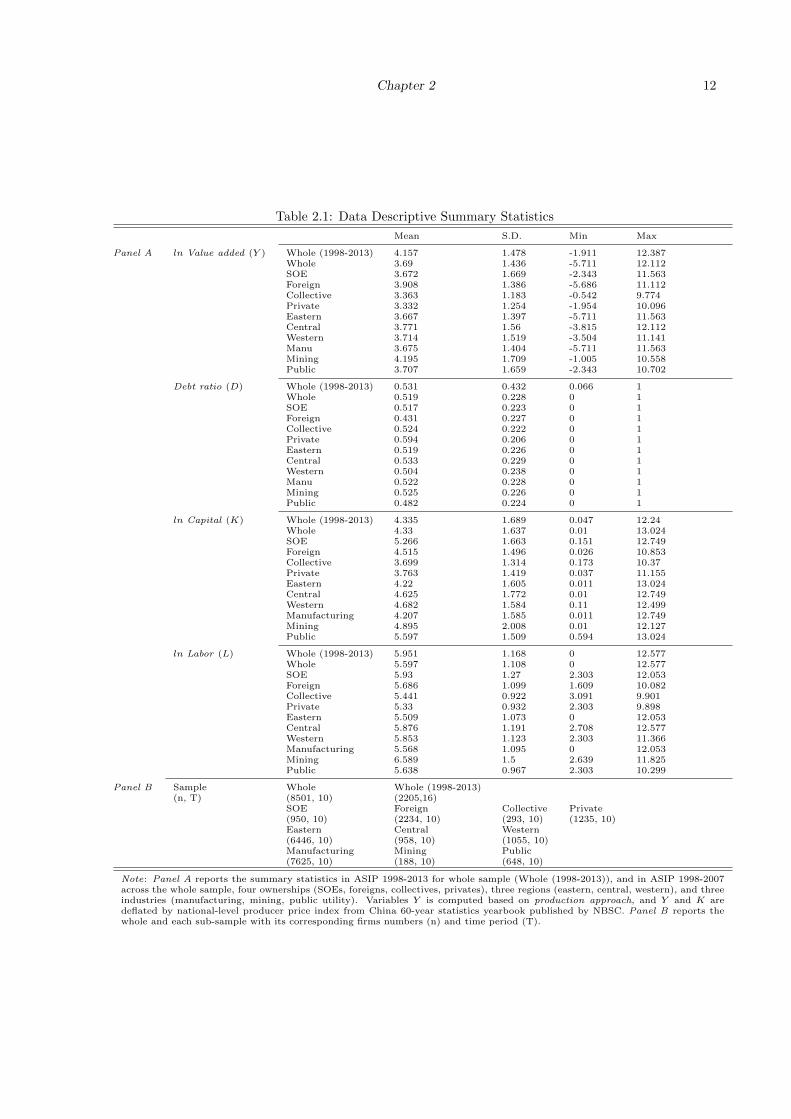
Chapter 2 12
Table 2.1: Data Descriptive Summary Statistics
Mean S.D. Min Max
Panel A ln Value added (Y ) Whole (1998-2013) 4.157 1.478 -1.911 12.387Whole 3.69 1.436 -5.711 12.112SOE 3.672 1.669 -2.343 11.563Foreign 3.908 1.386 -5.686 11.112Collective 3.363 1.183 -0.542 9.774Private 3.332 1.254 -1.954 10.096Eastern 3.667 1.397 -5.711 11.563Central 3.771 1.56 -3.815 12.112Western 3.714 1.519 -3.504 11.141Manu 3.675 1.404 -5.711 11.563Mining 4.195 1.709 -1.005 10.558Public 3.707 1.659 -2.343 10.702
Debt ratio (D) Whole (1998-2013) 0.531 0.432 0.066 1Whole 0.519 0.228 0 1SOE 0.517 0.223 0 1Foreign 0.431 0.227 0 1Collective 0.524 0.222 0 1Private 0.594 0.206 0 1Eastern 0.519 0.226 0 1Central 0.533 0.229 0 1Western 0.504 0.238 0 1Manu 0.522 0.228 0 1Mining 0.525 0.226 0 1Public 0.482 0.224 0 1
ln Capital (K) Whole (1998-2013) 4.335 1.689 0.047 12.24Whole 4.33 1.637 0.01 13.024SOE 5.266 1.663 0.151 12.749Foreign 4.515 1.496 0.026 10.853Collective 3.699 1.314 0.173 10.37Private 3.763 1.419 0.037 11.155Eastern 4.22 1.605 0.011 13.024Central 4.625 1.772 0.01 12.749Western 4.682 1.584 0.11 12.499Manufacturing 4.207 1.585 0.011 12.749Mining 4.895 2.008 0.01 12.127Public 5.597 1.509 0.594 13.024
ln Labor (L) Whole (1998-2013) 5.951 1.168 0 12.577Whole 5.597 1.108 0 12.577SOE 5.93 1.27 2.303 12.053Foreign 5.686 1.099 1.609 10.082Collective 5.441 0.922 3.091 9.901Private 5.33 0.932 2.303 9.898Eastern 5.509 1.073 0 12.053Central 5.876 1.191 2.708 12.577Western 5.853 1.123 2.303 11.366Manufacturing 5.568 1.095 0 12.053Mining 6.589 1.5 2.639 11.825Public 5.638 0.967 2.303 10.299
Panel B Sample Whole Whole (1998-2013)(n, T) (8501, 10) (2205,16)
SOE Foreign Collective Private(950, 10) (2234, 10) (293, 10) (1235, 10)Eastern Central Western(6446, 10) (958, 10) (1055, 10)Manufacturing Mining Public(7625, 10) (188, 10) (648, 10)
Note: Panel A reports the summary statistics in ASIP 1998-2013 for whole sample (Whole (1998-2013)), and in ASIP 1998-2007across the whole sample, four ownerships (SOEs, foreigns, collectives, privates), three regions (eastern, central, western), and threeindustries (manufacturing, mining, public utility). Variables Y is computed based on production approach, and Y and K aredeflated by national-level producer price index from China 60-year statistics yearbook published by NBSC. Panel B reports thewhole and each sub-sample with its corresponding firms numbers (n) and time period (T).

Chapter 2 13
Table 2.2: The Share of Firms with Different Ownership across Regions and Industries: 1998-2007
SOEs Foreign Collective Private
Regions Eastern 11.39% 36.86% 15.24% 36.51%Central 38.9% 9.29% 18.50% 33.31%Western 30.72% 29.78% 12.64% 26.86%
Industry Manufacturing 10.14% 36.39% 13.74% 39.73%Mining 53.36% 0.37% 24.41% 21.86%Public Utility 87.01% 2.78% 3.02% 7.19%
standard deviation and maximum value reasonably close to that based on the production approach
(Table 1 Panel A). The ln value added from 1998-2007, obtained from two different approaches, has
a correlation coefficient of 0.9534, indicating a fairly reasonable measure of value added based on the
income approach. Compared with ASIP 1998-2007, this sample contains larger incumbent firms with at
least 20 million RMB annual sales, with a relatively higher mean and minimum value of ln value added.
Variables debt ratio, ln capital, and ln labor do not exhibit significant difference except for a relatively
higher mean and standard deviation in ASIP 1998-2013.
In Table 2.2, we report the average share of firms with different ownerships across regions and indus-
tries in ASIP 1998-2007. Clearly, SOEs account for the lowest proportion of firms in the east (11.39%),
the highest in the central (38.9%) and western (30.72%) where most heavy industries are located. Foreign
and private firms are more dominant in eastern region, and their average share is 36.86% and 36.51%,
respectively, but less dominant in the central and western areas. SOEs also largely dominate mining
(53.36%) and public utility industries (87.01%). By contrast, the majority of firms in the manufacturing
industry are foreign and private, with a share of 36.39% and 39.73%, respectively, whereas the share of
SOEs is 10.14%. These results correspond to the observation that the highest mean of log capital and
labor in Table 2.1 are observed in regions or industries where SOEs dominate.
2.4 Empirical Results
2.4.1 Whole Sample Analysis: 1998-2007
We begin our analysis on the whole sample from ASIP 1998-2007. We wonder whether a SF model with
zero inefficiency should be implemented. We follow Kumbhakar et al. (2013) to test the null H0: p = 0
through a likelihood ratio (LR) test, where LR = −2(lnL(θSF )− lnL(θZISF )), with L(θSF ) (L(θZISF ))
being the likelihood estimated from a smooth coefficient SF model without (with) zero inefficiency. Rho
and Schmidt (2015) demonstrate that the LR test has the most reasonable size and power in a finite

Chapter 2 14
Figure 2.1: SC-ZISF Estimation from the Whole Sample: 1998-2007
(a)
Debt Ratio (with 95% bounds)
Neu
tral
Effe
ct
0.0 0.1 0.2 0.3 0.4 0.5 0.6 0.7 0.8 0.9 1.0
−1.33
−0.93
−0.53
−0.13
0.27
0.67
SC−ZISFCobb−DouglasExtended Cobb−DouglasR−TranslogTranslog
(b)
Debt Ratio (with 95% bounds)
Out
put E
last
icity
of C
apita
l
0.0 0.1 0.2 0.3 0.4 0.5 0.6 0.7 0.8 0.9 1.0
0.22
0.28
0.34
0.40
0.46
0.52
(c)
Debt Ratio (with 95% bounds)
Out
put E
last
icity
of L
abor
0.0 0.1 0.2 0.3 0.4 0.5 0.6 0.7 0.8 0.9 1.0
0.35
0.40
0.45
0.50
0.55
0.60
0.65
sample study compared with alternative test statistics. Clearly, the rejection of H0 indicates a nonzero
probability of fully efficient firms through p(Z) in (2.3). Under appropriate conditions, Chen and Liang
(2010) show that LRd→ 1
2χ2(0) + 1
2χ2(1), which is a 50:50 mixture χ2 distribution. We compute the critical
values by independently drawing 100,000,000 values from the mixture distribution, which provides 1.6429,
2.7066, and 5.4134 at the 10%, 5%, and 1% significant levels, respectively. Our LR test provides 51.52,
clearly rejecting the SF model without full efficiency at the 1% significance level.
We first report the frontier estimation results from the SC-ZISF model on the left of Panel A of Table
2.3. To illustrate the impact of the debt ratio, we report α(D), βK(D), and βL(D) at the following values
of D (0.1, 0.25, 0.5, 0.75, 0.9), and report the mean of neutral and non-neutral functions at the bottom
of Panel A. Our results show that the frontier is neutrally shifted slightly upward only when the debt
ratio is kept fairly low at approximately .15. As D reaches 0.25, the neutral function turns negative and
becomes -0.096. As D gets larger, the neutral effect continues to decline. The mean of α(D) (-0.4618)
indicates that the neutral effect of D is negative.
To provide a vivid picture, we plot α(D) (solid line) in Panel (a) of Figure 2.1 against the debt ratio,
along with its 95% confident interval (short dash line, constructed with Theorem 4 in Yao et al. (2018a)).
The neutral effect of D is highly nonlinear with an inverted U-shape, increasing the frontier a bit with a
small value of D, and pulling down the frontier with higher level of D (D ≥ 0.15). This nonlinearity is
consistent with the literature. The agency cost theory suggests that the neutral effect of debt ratio on a
firm’s output can be positive, because the “free cash-flow” problem (Jensen, 1986) can be reduced through
the financial pressure of debt, which effectively disciplines mangers’ profit-maximizing behavior (Weill,
2008; Giannetti, 2012). However, the moral hazard theory argues that a higher debt ratio may easily

Chapter 2 15
create a soft budget constraint and can induce firm managers to take risky projects, resulting in minimum
return and adversely affecting the firms’ output and profitability (Jensen and Meckling, 1976; Garriga,
2006). Given that the positive effect of debt ratio is more apparent under sound financial institutions
and regulation (Levine, 1999), our results suggest a much more dominating role of moral hazard behavior
in Chinese industrial firms, causing the output level to decrease sharply as the debt ratio rises.
We report the estimates of the non-neutral function βK(D) at five levels of D in Panel A of Table
2.3. The mean of βK(D) is 0.414, suggesting a positive output elasticity of physical capital. We further
plot βK(D) in Panel (b) of Figure 2.1. As the debt ratio increases before reaching 0.12, output elasticity
of capital is significantly increased from 0.39 to 0.49, or a 25.6% increase. Beyond a level of 0.12 in the
debt ratio, however, βK(D) starts to and continues to decrease. Thus, βK(D) also exhibits an inverted-U
shape. The increasing part of the inverted-U-shape is likely due to R&D investment, which becomes
increasingly available for firms with easier access to debt (Zhang et al., 2012; Lin et al., 2017). With the
R&D investment, firms can adopt better technology in production, which is likely to promote outputs
through the increasing output elasticity of capital. However, in the presence of a cheap capital price, the
excessive debt in recent years has lead Chinese firms to over-accumulate capital, resulting in production
overcapacity (Maliszewski et al., 2016; Berkowitz et al., 2017). Thus, we expect that the excessive use of
debt diminishes its output elasticity, contributing to a declining βK(D).
Different from the first two, βL(D) exhibits an upward trend in general, as shown in Panel (c) of
Figure 2.1. The output elasticity of labor is on average 0.476. βL(D) steadily increases from 0.39 to
0.55 as the debt ratio varies from 0.1 to 0.9 (Panel A of Table 2.3). Similar to the output elasticity of
capital, the increasing βL(D) may be attributed to the relaxation in financial constraint, which allows
firms to invest more in R&D and promote human capital. The investment in knowledge thus promotes
labor specialization, that is, workers gain expertise on a narrower range of tasks. Labor specialization
improves firms’ performance (Rosen, 1983) and may lead to non-diminishing marginal returns of labor.
The empirical findings from Amoroso (2015) support the conjecture. Given the tight connection between
the debt ratio and R&D investment in China, we expect a similar transmission mechanism behind the
increasing pattern of βL(D).
We further compute the total partial effect of debt on frontier (TP(Y )) as ∂α(D)∂D + Kit
∂βK(D)∂D +
Lit∂βL(D)∂D , with their estimates obtained in step 3. Hence, TP(Y ) is a combination of the partial effect on
the neutral function ∂α(D)∂D and on the non-neutral functions weighted by inputs, Kit
∂βK(D)∂D +Lit
∂βL(D)∂D .
The mean of TP(Y ) reported in Panel C of Table 2.3 indicates an overall negative impact of -1.141 from
the debt ratio.
To compare our SC-ZISF and conventional SF estimates, in Figure 2.1 we plot the neutral and non-

Chapter 2 16
Tab
le2.
3:S
C-Z
ISF
Est
imati
on
Res
ult
sfr
om
the
Wh
ole
Sam
ple
ASIP
1998-2
007
ASIP
1998-2
013
Panel
AD
ebt
rati
o(D
)α
(D)
βK
(D)
βL
(D)
Deb
tra
tio
(D)
α(D
)βK
(D)
βL
(D)
0.1
0.2
017*
0.4
972***
0.3
93***
0.1
0.2
044**
0.5
991***
0.3
64***
(0.1
082)
(0.0
156)
(0.0
234)
(0.1
015)
(0.0
141)
(0.0
204)
0.2
5-0
.096***
0.4
612***
0.4
276***
0.2
50.0
48**
0.5
388***
0.3
879***
(0.0
297)
(0.0
109)
(0.0
160)
(0.0
683)
(0.0
102)
(0.0
142)
0.5
-0.5
947***
0.4
37***
0.4
702***
0.5
-0.5
732***
0.4
82***
0.4
662***
(0.0
391)
(0.0
063)
(0.0
092)
(0.0
448)
(0.0
069)
(0.0
098)
0.7
5-0
.7903***
0.3
83***
0.5
071***
0.7
5-1
.0452***
0.3
946***
0.5
592***
(0.0
386)
(0.0
060)
(0.0
089)
(0.0
509)
(0.0
077)
(0.0
111)
0.9
-0.8
974***
0.3
158***
0.5
504***
0.9
-1.3
454***
0.3
188***
0.6
498***
(0.0
573)
(0.0
084)
(0.0
129)
(0.0
832)
(0.0
116)
(0.0
172)
Mea
n-0
.4618
0.4
144
0.4
755
Mea
n-0
.5624
0.4
657
0.4
892
Panel
Bσ2 u
σ2 v
γD
γR
σ2 u
σ2 v
γD
γR
8.4
939***
0.3
646***
4.6
674***
0.1
355***
6.5
585***
0.5
976***
5.6
218***
0.5
095***
(0.5
070)
(0.0
042)
(0.3
952)
(0.0
590)
(0.1
623)
(0.0
049)
(0.4
984)
(0.0
745)
Panel
CM
ean
of
TP
(Y)
-1.1
413
Mea
nof
TP
(Y)
-1.2
605
Mea
nof
TP
(lnPTE
)0.3
534
Mea
nof
TP
(lnPTE
)0.3
686
Mea
nof
TP
-0.7
879
Mea
nof
TP
-0.8
919
Log-l
ikel
ihood
5392.1
Log-l
ikel
ihood
4171.2
Bandw
idthh1:
0.1
035
Bandw
idthh1:
0.1
152
Fir
ms
:8501
Fir
ms
:2208
Tim
eSpan:
10
Tim
eSpan:
16
Tota
lO
bs:
85010
Tota
lO
bs:
35328
No
te:
Dep
end
ent
vari
ab
leis
the
natu
ral
log
of
firm
valu
ead
ded
Y,
com
pu
ted
base
don
pro
du
ctio
nap
pro
ach
.T
he
esti
mate
dn
eutr
al
fun
ctio
nα
(D)
an
dn
on
-neu
tral
fun
ctio
ns
βK
(D)
an
dβL
(D)
are
plo
tted
again
std
ebt
rati
oD
at
0.1
,0.2
5,
0.5
,0.7
5,
0.9
.S
tan
dard
erro
rsare
rep
ort
edb
enea
thth
ees
tim
ate
dco
effici
ents
.***,*
*,*
stand
sfo
rth
est
ati
stic
ally
sign
ifica
nt
level
at
1%
,5%
an
d10%
,re
spec
tivel
y.

Chapter 2 17
Tab
le2.
4:P
aram
etri
cM
od
els
Est
imati
on
Res
ult
sfr
om
the
Wh
ole
Sam
ple
ASIP
1998-2
007
ASIP
1998-2
013
PanelA
vari
able
sC
obb-D
ougla
sE
xte
nded
Cobb-D
ougla
sR
est
ricte
dT
ransl
og
Tra
nsl
og
Cobb-D
ougla
sE
xte
nded
Cobb-D
ougla
sR
est
ricte
dT
ransl
og
Tra
nsl
og
const
ant
-0.2
203***
-0.3
707***
-0.3
079***
0.7
532***
-0.0
922***
-0.0
826***
0.1
383***
1.2
001***
(0.0
175)
(0.0
207)
(0.0
408)
(0.0
613)
0.0
238
0.0
239
0.0
402
0.0
776
D-0
.2768***
0.4
695***
0.3
761***
0.2
504***
-0.1
027***
0.2
546***
0.6
847***
0.6
21***
(0.0
154)
(0.0
567)
(0.0
863)
(0.0
859)
0.0
101
0.0
185
0.0
533
0.0
599
D2
—-0
.7082***
-0.8
216***
-0.8
354***
—-0
.0327***
-0.0
502***
-0.0
53***
—(0
.0533)
(0.0
526)
(0.0
518)
—0.0
027
0.0
028
0.0
03
K0.4
305***
0.4
291***
0.5
353***
0.2
921***
0.4
963***
0.4
93***
0.5
685***
0.4
935***
(0.0
023)
(0.0
024)
(0.0
058)
(0.0
134)
0.0
032
0.0
031
0.0
051
0.0
145
L0.4
641***
0.4
632***
0.3
668***
0.1
921***
0.4
169***
0.4
285***
0.3
367***
0.0
101***
(0.0
036)
(0.0
035)
(0.0
090)
(0.0
238)
0.0
049
0.0
047
0.0
074
0.0
267
D×K
——
-0.2
058***
-0.1
855***
——
-0.1
464***
-0.1
097***
——
(0.0
103)
(0.0
105)
——
0.0
074
0.0
074
D×L
——
0.1
909***
0.2
001***
——
0.1
693***
0.1
25***
——
(0.0
161)
(0.0
160)
——
0.0
116
0.0
118
K2
——
—0.0
555***
——
—0.0
578***
——
—(0
.0012)
——
—0.0
014
L2
——
—0.0
308***
——
—0.0
584***
——
—(0
.0028)
——
—0.0
028
K×L
——
—-0
.0480***
——
—-0
.0804***
——
—(0
.0030)
——
—0.0
03
PanelB
σ2 u
6.6
946***
5.7
927***
5.7
212***
7.8
372***
4.5
532***
4.8
543***
5.3
438***
5.7
639***
(0.4
719)
(0.3
487)
(0.3
559)
(0.5
788)
0.3
321***
(0.3
032)
(0.3
642)
(0.3
931)
σ2 v
0.6
327***
0.6
330***
0.6
317***
0.5
986***
0.5
858***
0.5
781***
0.5
781***
0.5
412***
(0.0
039)
(0.0
053)
(0.0
046)
(0.0
039)
0.0
047
(0.0
049)
(0.0
043)
(0.0
044)
γD
-6.0
662***
-3.7
055***
-4.5
598***
-6.9
043***
-0.4
242***
-3.0
354***
-3.6
237***
-5.0
317***
(0.5
487)
(0.2
063)
(0.2
424)
(0.4
705)
0.0
261
(0.0
148)
(0.0
185)
(0.0
244)
γR
-1.7
806***
-1.5
882***
-1.6
467***
-2.6
961***
-1.0
676***
-0.0
714***
-0.0
707***
-2.0
681***
(0.1
233)
(0.0
953)
(0.1
037)
(0.1
527)
0.0
981
(0.0
014)
(0.0
011)
(0.0
014)
Log-l
ikelihood
11066.3
11057.8
11038.8
10872.2
16068.5
216022.1
116063.4
216919.7
Fir
ms
:8501
8501
8501
8501
2208
2208
2208
2208
Tim
eSpan:
10
10
10
10
16
16
16
16
Tota
lO
bs:
85010
85010
85010
85010
35328
35328
35328
35328

Chapter 2 18
neutral function estimates from SC-ZISF together with four benchmark parametric SF models discussed
in Section 2. The MLE parameter estimates of the benchmark models are provided on the left of Panel
A of Table 2.4. First, Figure 2.1 (a) shows that the neutral impact estimates in the CD model (dotted
line with circle) is a linear downward sloping line with a slope of -0.277, clearly ignoring the nonlinearity.
The ECD (dot-dash line with triangle) and RTL estimates (long dash line with diamond) capture the
inverted-U-shape, but most of them are outside of the 95% confidence interval constructed for the SC-
ZISF estimates, casting doubt on the validity of these two estimates. The turning point on D for the
neutral effect to switch to a decreasing pattern is 0.332 (0.155) in ECD (RTL), which is higher than the
0.123 in SC-ZISF. Surprisingly, the TL estimate (short-long dash line with star) largely deviates from
the other estimates, predicting a positive output level uniformly over the entire range of the debt ratio.
Additionally, the TL’s average output elasticity is three times higher or lower than the other estimates,
making the comparison difficult and unreliable.
Panels (b) and (c) in Figure 2.1 show that CD and ECD provide similar output elasticities, with
(βK ,βL) estimates being (0.431,0.464) and (0.429,0.463), respectively. A fair portion of the RTL elasticity
estimate is inside the 95% CI of our SC-ZISF. All parametric models, however, do not illustrate the
nonlinearity of neutral and non-neutral functions. We do not plot the TL estimates for the elasticities
due to its largely deviation from the rest, making graphical presentation difficult. Our SC-ZISF estimates
show that the capital has a slightly lower average output elasticity than labor, qualitatively similar to
what has reported in Movshuk (2004) and Zhang et al. (2012). Finally, the average of return-to-scale
(RTS) in SC-ZISF is 0.890, and this result is fairly close to the estimates of CD (0.894), ECD (0.892),
and RTL (0.895), but again, highly different from that of TL (1.144).
These results suggest that the benchmark models widely used in the literature cannot describe the
frontier adequately (perhaps less so for TL in the output elasticities), and the potential cause of this
inadequacy is model-misspecification. To test for the validity of a parametric model, we follow Yao et al.
(2018a) to construct a bootstrap version of the standardized test statistic T ∗n to test H0: δ(D) = δ(D;β0),
δ(D) = [α(D), βK(D), βL(D)]T, and δ(D;β0) are parametrically specified functions known up to a vector
of constants β0, including those from CD, ECD, RTL, and TL. We estimate the alternative with our
SC-ZISF approach. Using 299 bootstrap repetitions with a rule-of-thumb bandwidth, the test yields
empirical p-values all smaller than 0.03; hence, we reject the parametric specifications considered at a
significance level of 0.05.
We plot the density of the composite error estimates from SC-ZISF (with a mode of -0.302) and three
parametric models - CD, RTL and TL (with mode average of -0.44, and clearly they are close to each
other) in the left panel of Figure 2.2. We do not include the ECD estimates because they are nearly

Chapter 2 19
identical to the estimates of CD. Clearly, a fair proportion of firms operate with inefficiency. The left of
Panel A in Table 2.4 shows that the estimate of σ2v across the four parametric models is fairly similar and
ranges from 0.60 in the TL model to 0.63 in the other three models. The σ2u estimate in the parametric
models is much higher, with the lowest estimate being 5.72 in RTL and the highest estimate being 7.84
in TL. By contrast, SC-ZISF in Table 2.3 provides a lower σ2v = 0.37, but an even higher σ2
u = 8.49.
Hence, the different models suggest a large magnitude of inefficiency relative to the random noise in the
composite error.
That σ2u is relatively small in all parametric models relative to that of SC-ZISF is expected. We expect
that firms with full efficiency are likely to be present in our sample. Given that all firms are perceived
as inefficient in conventional SF models, the presence of fully efficient firms would drive down the overall
level of inefficiency, leading to an under-estimated σ2u. In our SC-ZISF, we specify the full efficiency
probability p(Z) as a logistic function, with the coefficient estimate of D and R reported in Panel B of
Table 2.3. The debt ratio and R enters p(Z) significantly and positively, suggesting that higher debt
ratio increases the probability of firms to become fully efficient, and a positive role of technical progress
in improving firm efficiency.
Our p(Z) estimates have a mean of 0.88 and range from 0.71 at the 10% percentile to 0.978% at the
90% percentile. Following Kumbhakar et al. (2013), we further estimate the posterior probability of being
fully efficient as
pit =(p(Zit)/σv)φ(εit/σv)
(p(Zit)/σv)φ(εit/σv) + (1− p(Zit)) 2σφ(εit/σ)Φ(− εitλσ )
(2.9)
where λ = σu/σv, σ =√σu
2 + σv2, εit is the estimated composite error in SC-ZISF. Clearly, debt and
technical progress influence pit through p(Z). Relative to p(Z), we observe that pit provides a similar
mean of 0.8617 but with a wider dispersion, ranging from 0.496 at the 10% percentile to 0.996 at the
90% percentile.
We further compute a posterior probability weighted technical efficiency (PTE) score following Kumb-
hakar et al. (2013), where PTEit = exp(−(1− pit)uit), with uit ≡ E(uit|εit) the conditional inefficiency
estimate from Jondrow et al. (1982):
E(uit|εit) =σuσvσ
[φ(εitλ/σ)
Φ(−εitλ/σ)− (εitλ/σ)
](2.10)
Hence, with a nonzero p, as in our case, firms in SC-ZISF should be more efficient than they would be in
the conventional SF models where p = 0. We plot the density estimates of PTE for SC-ZISF and the three
parametric models on the right panel of Figure 2. As expected, SC-ZISF allows the possibility of fully

Chapter 2 20
Figure 2.2: Density of Estimated Composite Error and Posterior TE: 1998-2007
Composite Error
Den
sity
Est
imat
es
−4.0 −3.2 −2.4 −1.6 −0.8 0.0 0.8 1.6 2.4 3.2 4.0
0.0
0.1
0.2
0.3
0.4
0.5
SC−ZISFCobb−DouglasRestriced TranslogTranslog
Posterior Technical Efficiency
Den
sity
Est
imat
es
0.4 0.5 0.6 0.7 0.8 0.9 1.0
0.0
1.5
3.0
4.5
6.0
7.5
9.0
10.5
12.0
13.5SC−ZISFCobb−DouglasRestriced TranslogTranslog
efficient firms, and the density of its PTE estimates hovers to the right of the others with a higher mean
of 0.914. Moreover, SC-ZISF shows that 3,856 firms, representing approximately 45.4% of our whole
sample, have PTE larger than 0.990, and 1,042 firms with PTE greater than 0.995. By contrast, the
densities of PTE estimates from the parametric SF models, resembling each other in a general pattern,
present an average mean of 0.715, that is, 21.8% lower than that from SC-ZISF. More important, only an
average of 11 firms from parametric models have PTE greater than 0.900, and no firms has PTE greater
than 0.920. Therefore, our SC-ZISF model reveals that a large portion of firms are nearly fully efficient,
and clearly masked under the parametric models. This result is also in line with Kumbhakar et al. (2013)
and Yao et al. (2018a), that is, parametric SF models perceive all firms as inefficient and thus largely
underestimate the technical efficiency of firms.
Finally, to provide additional details on the overall effect of debt on frontier and efficiency level, we
compute the total partial effect of debt on the log of PTE as TP(lnPTE) = ∂ lnPTE/∂D, and the total
partial effect of debt on frontier and PTE as TP = TP (Y ) + TP (lnPTE). Both measures are averaged
and reported in Panel C of Table 2.3. Although a higher debt ratio increases firms’ efficiency through
PTE, it significantly reduces the production frontier, resulting in an overall output and efficiency loss.
2.4.2 Whole Sample Analysis: 1998-2013
We now conduct the whole sample analysis with ASIP 1998-2013. Similar to our analysis in ASIP 1998-
2007, we reject the null of a standard SF model with zero probability of full efficiency, with the LR test

Chapter 2 21
Figure 2.3: SC-ZISF Estimation from the Whole Sample: 1998-2013
(a)
Debt Ratio (with 95% bounds)
Neu
tral
Effe
ct
0.0 0.1 0.2 0.3 0.4 0.5 0.6 0.7 0.8 0.9 1.0
−1.71
−1.31
−0.91
−0.51
−0.11
0.29
SC−ZISFCobb−DouglasExtended Cobb−DouglasR−TranslogTranslog
(b)
Debt Ratio (with 95% bounds)
Out
put E
last
icity
of C
apita
l
0.0 0.1 0.2 0.3 0.4 0.5 0.6 0.7 0.8 0.9 1.0
0.28
0.34
0.40
0.46
0.52
0.58
(c)
Debt Ratio (with 95% bounds)
Out
put E
last
icity
of L
abor
0.0 0.1 0.2 0.3 0.4 0.5 0.6 0.7 0.8 0.9 1.0
0.35
0.40
0.45
0.50
0.55
0.60
0.65
0.70
0.75
statistics being 59.28. This supports our usage of the SC-ZISF model in the sample. We report the
SC-ZISF frontier estimation results in the right panel of Table 3, and plot the α(D), βK(D), and βL(D)
estimates in Figure 3. We continue to observe a clear, inverted-U-shape of the neutral effect. Specifically,
a firm’s frontier is significantly increased from -0.29 to 0.24 when D increases to 0.13, but decreases
toward -1.45 as D further increases. Relative to the neutral effect estimates in ASIP 1998-2007, we
further observe that debt ratio exhibits a more negative neutral effect when D > 0.5 with the ASIP 1998-
2013 sample. For example, an increase in D from 0.75 to 0.90 changes the neutral effects from −1.045 to
−1.345, while in the ASIP 1998-2007 sample, the corresponding effects are from −0.790 to −0.897. This
result suggests that the dominating and adverse effect of debt ratio on frontier (moral hazard) is likely
to persist and even intensify over time. The neutral effect of debt ratio average is decreased from -0.4618
(ASIP 1998-2007) to -0.562 (ASIP 1998-2013), a 22% drop, indicating a more detrimental neutral effect
of debt ratio in recent years.
The output elasticity of K (L) remains qualitatively similar compared to the left panel in Table 4
and Figure 1, except with a slightly higher (lower) magnitude in general. Hence, a higher debt ratio
continues to decrease (increase) the return of capital (labor), and this possibly occurs through R&D.
The overall effect of debt ratio, measured by TP(Y ), is -1.2605; again, this result is consistent with our
previous result that a firm’s frontier declines overall because of excessive debt ratio. Nevertheless, the
effects of debt ratio are not well captured by the parametric models, as demonstrated in Figure 3. They
generally overestimate α(D) and βK(D) and underestimate βL(D). The parametric SF frontier estimates
are presented in the right panel in Table 4 and roughly corresponding to those in the left panel of Table
4 for ASIP 1998-2007.

Chapter 2 22
Figure 2.4: Density of Estimated Composite Error and Posterior TE: 1998-2013
Composite Error
Den
sity
Est
imat
es
−4.0 −3.2 −2.4 −1.6 −0.8 0.0 0.8 1.6 2.4 3.2 4.0
0.0
0.1
0.2
0.3
0.4
0.5
SC−ZISFCobb−DouglasRestriced TranslogTranslog
Posterior Technical Efficiency
Den
sity
Est
imat
es
0.4 0.5 0.6 0.7 0.8 0.9 1.0
0.0
1.5
3.0
4.5
6.0
7.5
9.0
10.5
12.0
13.5 SC−ZISFCobb−DouglasRestriced TranslogTranslog
The left panel in Figure 4 plots the density of estimated composite error across different SF models,
which exhibits a fairly similar pattern to Figure 2 and highlights the presence of inefficient firms in the
sample. This is also indicated by the larger estimate σ2u relative to σ2
v in the right panels of Tables 3
and 4, with σ2u being the highest in SC-ZISF, as expected. Consistent with our previous finding, the
probability for firms to be fully efficient estimated in SC-ZISF, is significantly improved by higher debt
ratio and technical progress. In the right panel of Figure 4, the density of the SC-ZISF PTE estimates,
with a mean of 0.924, is to the right of the parametric counterparts, exhibiting a much larger mode
close to one. The densities of all parametric SF PTE estimates, with a mean of 0.806 on average, still
underestimate the technical efficiency. Indeed, in our SC-ZISF estimates, 1,129 firms, accounting for
51.13% of the sample, exhibit PTE larger than 0.990, and 650 firms show PTE greater than 0.995. By
contrast, in the parametric estimates, no firm exhibits PTE greater than 0.900. Finally, the right side
of Panel C in Table 3 shows that the TP is -0.892, and this result, again reflects an overall reduction in
output and technical efficiency due to higher debt ratio.
In summary, our empirical findings are fairly robust and consistent across the two datasets.8 Given
the increasing trend of the debt ratio in recent years, we observe that the significant role of debt on
frontier and technical efficiency of Chinese enterprises is likely to be persistent rather than vanishing
over time. Given the relatively small sample size, concerns with the construction of the dataset in ASIP
1998-2013, and the qualitatively similar conclusion with whole sample using both datasets, we conduct
8We have also constructed dataset that covers 2008-2010, 2008-2013, and 1998-2010. The empirical results all remainqualitatively similar, and we thus omit them for brevity.

Chapter 2 23
Figure 2.5: SC-ZISF Estimation with Lag of Debt Ratio from the Whole Sample: 1998-2007
(a)
Lag Debt Ratio (with 95% bounds)
Neu
tral
Effe
ct
0.0 0.1 0.2 0.3 0.4 0.5 0.6 0.7 0.8 0.9 1.0
0.93
1.33
1.73
SC−ZISFCobb−DouglasExtended Cobb−DouglasR−TranslogTranslog
(b)
Lag Debt Ratio (with 95% bounds)
Out
put E
last
icity
of C
apita
l
0.0 0.1 0.2 0.3 0.4 0.5 0.6 0.7 0.8 0.9 1.0
0.16
0.22
0.28
0.34
0.40
(c)
Lag Debt Ratio (with 95% bounds)
Out
put E
last
icity
of L
abor
0.0 0.1 0.2 0.3 0.4 0.5 0.6 0.7 0.8 0.9 1.0
0.55
0.60
0.65
0.70
sub-sample analyses with ASIP 1998-2007.
2.4.3 A Robustness Check on Whole Sample Analysis: 1998-2007
In the previous two analyses, we explore the contemporary effect of Dit on a firm’s frontier and TE.
However, the effects of debt ratio in one year may not be fully revealed until years after. To investigate
the potential lag effect of D in (2.1), we employ ASIP 1998-2007 by replacing Dit in (2.1) with its 1-year
lag value Di,t−1.9 We continue to reject the null of a standard SF model, with the LR test given by 43.124.
Thus, we proceed by implementing our SC-ZISF model with the sample. To save space, we do not report
the SC-ZISF estimates (α(·), βK(·), βL(·)), but plot them against those obtained from the four parametric
models in panel (a)-(c) of Figure 2.5, respectively. Panel (a) shows that the 1-year lag debt ratio, again,
neutrally shift downward the frontier except when Di,t−1 > 0.8. Thus, we do not find evidence on the
positive neutral effect of debt ratio through its disciplining role after one year. In addition, the lag of
debt ratio’s neutral effect is more positive and higher in magnitude than its counterpart without lag. For
instance, the average of α(·) with the lag of D is 1.143 relative to -0.462 without the lag of D. Thus,
the neutral effect of debt is likely to persist and but vanish a year after. In addition, an increase in the
lag of D introduces the diminishing return of βK(·) with a mean of 0.3307, which remains qualitatively
similar to the estimates in panel (b) of Figure 2.1. A higher lag of D also in general improves the output
elasticity of labor βL(·) with a mean of 0.6331, although the effect of which is less significant relative to
panel (c) of Figure 2.3. The overall marginal impact of the lag of D is negative on the frontier, indicated
by the average of TP (Y ) as −0.827.
9In this case, our total observation reduces to (n, T ) = (8, 501, 9)

Chapter 2 24
Table 2.5: Parameter Estimation Results of Lag of Debt Ratio
SC-ZISF Cobb-Douglas Extended Cobb-Douglas Restricted Translog Translog
σ2u 7.809*** 4.0058*** 4.4414*** 4.2533*** 4.9718***
(0.0397) (0.7086) (0.6057) (0.7133) (1.2007)σ2v 0.4208*** 0.5471*** 0.5444*** 0.5407*** 0.5125***
(0.0090) (0.0041) (0.0050) (0.0038) (0.0031)γD -5.3531*** -3.1037*** -3.2017*** -3.5338*** -3.9901***
(0.9006) (0.0578) (1.0120) (0.6380) (0.5069)γR 0.8049*** 1.2378*** 1.2017 1.2465*** 1.4083***
(0.0827) (0.0875) (0.0820) (0.0741) (0.0158)
Log-likelihood 7459.24 9257.71 9257.71 9250.02 9154.04Firms : 8501 8501 8501 8501 8501Time Span: 9 9 9 9 9Total Obs: 76509 76509 76509 76509 76509
We report the parameter estimates of (σ2u, σ
2v) and (γD, γR) in Table 2.5. Comparing to the corre-
sponding estimates without the lag of D in Panel B of Table 2.3 and 2.4, we observe that debt ratio has
a negative lag effect (γD = −5.353 in SC-ZISF) on firm’s full efficiency probability. This is also confirmed
from TP (lnPTE), with a mean of -0.133. The totally partial effect TP has an average of −0.960, 22%
higher than the TP with D. Thus, our results suggest that the excessive debt ratio is likely to pulls down
the frontier in the current year, and also influence firms to be less efficient in the next year. As a result,
firms have experience a significant drop in both frontier and technical efficiency due to the lag effect of
debt ratio.
2.4.4 Analysis across Ownerships
We analyze the impact of debt on frontier and efficiency across the SOEs, foreign, collective, and private
firms. Panel A of Table 2.6 reports the estimated α(D), βK(D) and βL(L) across the four ownership
types. We fail to reject the null H0: p = 0 only in collective firms in Panel C of Table 2.6, indicating
an absence of fully efficient firms in the collective firms. This result is also hinted at the insignificant
SC-ZISF parameter estimates of γD (debt ratio) and γR (time trend) in Panel B of Table 2.6. Thus, we
follow Yao et al. (2018a) to estimate a smooth coefficient SF model for the collective firms with p = 0
and report its estimated frontiers and parameters (σ2u, σ
2v) in Panel B of Table 2.6.
Focusing on the neutral impact α(D), the frontier of firms of different ownerships is significantly lower
with a higher debt ratio, except perhaps the collective firms. We observe that SOEs’ frontier neutrally
decreases by a magnitude uniformly larger than the other firms. Conditioning on D = 0.25, for instance,
α(D) from SOEs is -1.611, whose absolute value is at least three times larger than the other firms, where
the estimate for foreign, collective, and private firms is -0.220, -0.196, and -0.408, respectively. Not
surprisingly, the average of the neutral effect at the bottom of Panel A is the largest in absolute value
for SOEs (-1.584), followed by private (-0.781), foreign (-0.543), and collective (-0.052) firms. We posit

Chapter 2 25
Tab
le2.
6:E
stim
ati
on
Res
ult
sof
SC
-ZIS
FM
od
elb
ase
don
Ow
ners
hip
SO
Es
Fore
ign
Collecti
ve
Pri
vate
PanelA
Debt
rati
o(D
)α
(D)
βK
(D)
βL
(D)
α(D
)βK
(D)
βL
(D)
α(D
)βK
(D)
βL
(D)
α(D
)βK
(D)
βL
(D)
0.1
-1.3
379***
0.5
189***
0.5
269***
-0.0
045
0.4
769***
0.3
56***
0.0
926
0.3
839***
0.4
100***
-0.0
362
0.4
545***
0.3
867***
(0.2
541)
(0.0
415)
(0.0
661)
(0.1
156)
(0.0
169)
(0.0
229)
(0.4
176)
(0.0
596)
(0.0
888)
(0.5
986)
(0.0
102)
(0.0
320)
0.2
5-1
.6106***
0.5
482***
0.5
202***
-0.2
201**
0.5
044***
0.3
78***
-0.1
621
0.3
009***
0.5
19***
-0.4
083***
0.4
663***
0.4
122***
(0.1
673)
(0.0
307)
(0.0
438)
(0.0
944)
(0.0
141)
(0.0
193)
(0.2
792)
(0.0
448)
(0.0
634)
(0.1
276)
(0.0
035)
(0.0
074)
0.5
-1.6
233***
0.5
391***
0.5
049***
-0.5
555***
0.4
854***
0.4
339***
-0.2
358
0.3
387***
0.4
905***
-0.9
483***
0.4
301***
0.5
102***
(0.1
089)
(0.0
215)
(0.0
275)
(0.0
774)
(0.0
116)
(0.0
158)
(0.1
856)
(0.0
311)
(0.0
425)
(0.0
580)
(0.0
017)
(0.0
036)
0.7
5-1
.6821***
0.4
189***
0.5
981***
-0.7
762***
0.4
319***
0.4
952***
-0.2
294
0.2
95***
0.4
104***
-1.0
66***
0.3
771***
0.5
459***
(0.1
452)
(0.0
274)
(0.0
353)
(0.1
023)
(0.0
142)
(0.0
202)
(0.2
191)
(0.0
313)
(0.0
450)
(0.0
554)
(0.0
013)
(0.0
031)
0.9
-1.6
457***
0.2
844***
0.6
948***
-1.0
306***
0.3
895***
0.5
59***
0.7
369
0.2
549***
0.3
26***
-1.3
466***
0.3
436***
0.6
066***
(0.2
357)
(0.0
363)
(0.0
484)
(0.1
905)
(0.0
253)
(0.0
363)
(0.6
667)
(0.0
454)
(0.0
703)
(0.1
068)
(0.0
024)
(0.0
060)
mean
-1.5
843
0.4
675
0.5
646
-0.5
433
0.4
581
0.4
48
-0.0
519
0.3
16
0.4
393
-0.7
812
0.4
148
0.4
956
PanelB
σ2 u
2.6
665***
(1.0
020)
1.7
975***
(0.1
429)
0.1
347***
(0.0
652)
1.4
230***
(0.3
119)
σ2 v
0.7
278***
(0.0
109)
0.7
111***
(0.0
082)
0.6
949***
(0.0
398)
0.5
681***
(0.0
087)
γD
0.6
854
(1.6
621)
3.5
618***
(0.3
205)
3.6
862
(59.5
857)
9.3
347***
(0.9
184)
γR
3.1
949***
(0.9
977)
0.3
801***
(0.0
357)
3.9
312
(84.6
079)
-0.0
606
(0.0
642)
PanelC
H0:p
=0
Test
39.8
198
447.2
56
0.3
71
136.1
35
p-v
alu
e0.0
000
0.0
000
0.2
71
0.0
000
PanelD
mean
of
TP
(Y)
-0.5
668
-0.2
921
-0.8
422
-0.5
609
mean
of
TP
(lnPTE
)0.1
424
0.3
475
—0.1
051
mean
of
TP
-0.4
243
-0.0
834
-0.4
641
-0.4
558
Bandw
idthh1:
0.1
356
0.1
306
0.1
314
0.1
314
Log
likelihood
1205.4
2916.7
3810.8
21434.4
Fir
ms
:950
2234
293
1235
Tim
eSpan:
10
10
10
10
Tota
lO
bs:
9500
22340
2930
12350

Chapter 2 26
Figure 2.6: Density of Posterior Probability and Posterior TE across ownerships
Posterior Probability
Den
sity
Est
imat
es
0.0 0.1 0.2 0.3 0.4 0.5 0.6 0.7 0.8 0.9 1.0
0
1
2
3
4
5
6
7 SOEsForeignPrivate
Posterior Technical Efficiency
Den
sity
Est
imat
es0.40 0.45 0.50 0.55 0.60 0.65 0.70 0.75 0.80 0.85 0.90 0.95 1.00
0
2
4
6
8
10 SOEsForeignCollectivePrivate
that the moral hazard issue might be present in SOEs.
We observe an invert-U-shape relationship between the debt ratio and output elasticity of capital in
foreign and private firms. For example, βK(D) in foreign (private) firm increases from 0.477 (0.455) to
0.504 (0.466) as D increases from 0.1 to 0.25 but steadily decreases afterward as debt increases. As in the
whole sample, we posit that the result can be due to R&D’s return on capital productivity (with lower
debt) and the diminishing return of capital (with higher debt). We also observe the non-diminishing
return of labor in SOEs, foreign, and private firms, which potentially benefit from the return of R&D
on labor productivity because of the lower financial constraint. Nevertheless, the overall impact of debt
on frontier is negative for all ownerships. The mean of TP(Y) is relatively small (in absolute value) in
the foreign (-0.292) firms, and larger in the private (-0.561) firms, SOEs (-0.567) and collective (-0.842)
firms.
From Panel B of Table 2.6, we observe that the σ2v estimates are all less than one and fairly similar
across different ownership types. However, SOEs have the largest σ2u = 2.667 compared with its counter-
part’s estimates, 1.798, 1.192, and 1.423 for foreign, collective, and private firms, respectively. Thus, the
variation of composite error in SOEs is dominated by the inefficiency term. Furthermore, debt ratio does
not play a role in changing the probability of SOEs to be fully efficient. With the mean of TP (Y ) and
TP (lnPTE) being -0.567 and 0.14 for SOEs, we are not surprised to observe that that excessive debt
largely pulls down SOE’s frontier but does not improve technical efficiency, exerting an overall negative
effect on output (the mean of TP is -0.42). The technical efficiency or p(Z) in collective firms does not
seem to depend on the debt ratio or technical progress. By contrast, the full efficiency probability of

Chapter 2 27
Figure 2.7: Yearly Averaged Posterior Probability and PTE
1998 1999 2000 2001 2002 2003 2004 2005 2006 2007
Year
ly A
vera
ged
Pos
terio
r P
roba
bilit
y
0.4
0.5
0.6
0.7
0.8
0.9
1.0
SOEs Foreign Private
1998 1999 2000 2001 2002 2003 2004 2005 2006 2007Ye
arly
Ave
rage
d P
oste
rior
Tech
nica
l Effi
cien
cy0.4
0.5
0.6
0.7
0.8
0.9
1.0
SOEs Foreign Collective Private
foreign firms is improved with a higher debt ratio (γD = 3.561) and technical progress (γR = 0.381). Pri-
vate firms’ probability is mostly improved by the debt ratios (γD = 9.335), although not by the technical
progress.
To display the difference, in Figure 2.6 we plot the density of posterior probability (left panel) and
PTE (right panel) for the SOEs (solid line), foreign firms (dash line with circle), collective firms (dot
line with triangle), and private firms (dot-dash line with star). We do not plot the posterior probability
density for collective firms because we do not reject the null that p = 0. The p estimate for SOEs has a
mean of 0.597, clearly exhibiting a fat tail on the left. Compared with non-SOEs, a large proportion of
SOEs are far from being fully efficient. This result is in line with our previous finding that the presence
of a higher debt ratio does not improve the probability for SOEs to become efficient. By contrast, the
probability of private firms to be fully efficient is much higher, with a mean of 0.978, 21% higher than
that of the foreign firms (0.809). The density of PTE reveals that the most inefficient firms are SOEs,
with an average PTE of 0.708, lower than that of foreign (0.869) and private firms (0.987). With a mean
PTE at 0.747 and a mode of 0.75, collective firms are less efficient than the other two non-SOEs. The
left panel of Figure 2.7 plots the average of p over years across the three ownerships. Promoted by debt
ratio and technical progress, private firms top the list (with an average consistently close to one from
1998 to 2007), followed by foreign firms, with its mean increasing from 0.768 in 1998 to 0.836 in 2007.
As expected, the full efficiency probability for SOEs is the lowest and is mainly increased by technical
progress, with its average increasing from 0.510 in 1998 to 0.682 in 2007.
The finding that SOEs have the lowest technical efficiency relative to non-SOEs is consistent with
Chapter 2 28
many studies in the literature (Zheng et al., 1998; Shiu, 2002; Fu et al., 2008; He et al., 2015). The overall
relatively low efficiency in SOEs may be attributed to the soft budget constraint problem.10 The managers
of SOEs typically have a strong affiliation with the government, allowing the SOEs’ loans to be borrowed
at a much lower rate compared with a competitive market (Ding et al., 2016). Additionally, the central
and local government in China has intensively intervened in lending during economic reforms, making
considerable funds available for SOEs that are not subject to close monitoring (Riedel et al., 2007).
Hence, we expect that the historical soft budget constraint has induced the existence of a potentially
severe moral hazard problem among SOEs, rather than a discipline effect. This expectation may explain
that the debt shifts down the frontier neutrally by the highest magnitude but plays no role in increasing
the full efficiency probability. By contrast, non-SOEs (foreign, collective, and private firms) are treated
differently in the financial system and pay higher interest rates for funds than SOEs and thus incur
difficult budget constraints (Guariglia et al., 2011). Hence, a higher debt may result in the associated
financial pressure, which disciplines non-SOEs managers to behave as profit maximizers and helps improve
the full efficiency probability.
The right panel of Figure 2.6 also reveals a wide dispersion of PTE for the SOEs. Its PTE estimates
range from the minimum of 0.167 to the maximum of 0.939; thus, a small fraction of SOEs may be
efficient. According to Berkowitz et al. (2017), a particular group of SOEs has tight political connections
and are distinguishable from other SOEs in terms of their remarkable productivity (e.g., as high as foreign
and private firms). These SOEs are known as “top central SOEs,” that is, SOEs with exceptionally high
political position in comparison to “central SOEs,” which are directly supervised by the state-owned
Assets Supervision and Administration Commission of the State Council (SASAC). We posit that the
top central SOEs may display productivity gains through better technical efficiency. As in Berkowitz
et al. (2017), we pursue a conservative measure by identifying an SOE as a top central SOE in any year
if it has more than 10,000 employees and an output level exceeding RMB 1 billion. We identify 24 top
central SOEs in our sample, with most of their PTE in the top 10% percentile in the PTE distribution.
The PTE in the top central SOEs has a mean of 0.8818 compared with 0.7038 in the sample without the
top central SOEs. Hence, the top central SOEs are highly efficient among SOEs and largely contribute
to the right tail of the SOEs PTE distribution.
Nonetheless, the SOEs efficiency may have been significantly improved since 1998. Historically, the
market-oriented economic policy advocated by Deng Xiaoping during his “Southern Tour Speech” induces
10Other issues have been well discussed in explaining SOEs’ low production efficiency. For example, the deviation ofbureaucrats’ political interests (i.e., focusing on annual production target by the central government) from shareholder’sinterests (i.e., profit maximization) reduces the efficiency of SOEs (He et al., 2015). Additionally, the political pressureon SOEs induces SOEs managers to pursue not probability but capital accumulation with a cheap price and securedemployment. As a result, the input can be seriously mis-allocated, causing the efficiency of SOEs to decrease significantly(Berkowitz et al., 2017; Hsieh and Klenow, 2009).

Chapter 2 29
SOEs to dramatically expand firm size and investment. In the early of 1990s; however, a vast amount of
investments were not fully capitalized to increase the output level, causing SOEs to incur huge losses and
budget deficits (Fu et al., 2008). To reverse the situation, a series of loss-reduction economic reforms,
known as “Grasp the Large, Release the Small,” were enacted for SOEs in 1998, resulting in a massive
lay-off of surplus employees. With increasing competition against non-SOEs (mainly privates), Fu et al.
(2008) document that SOEs efficiency on average has improved since 1998. We confirm this observation
by plotting the yearly average of PTE estimates aross different ownerships on the right panel of Figure
2.7. SOEs have steadily caught up with non-SOEs with their PTE increasing from 0.665 in 1998 to 0.752
in 2007.
Overall, we observe that a high debt ratio significantly shifts down the frontier of SOEs and all non-
SOEs but improves the full efficiency probability steadily only for the foreign and private firms. Hence, an
excessive use of debt financing lowers the frontier of SOEs and collective firms without enhancing their full
efficiency probability, impacting the output negatively as an overall effect (i.e., TP). Economic reforms
on SOEs since 1998 have effectively increased SOE’s PTE, displaying an increasing trend across years
and potentially contributed by a small group of top central SOEs having notable productive efficiency.
2.4.5 Analysis across Regions
Zhou et al. (2011) and Zhang et al. (2012) argue that the advanced economic development in eastern
regions is due to higher production efficiency than that in the central and western regions. We illustrate
the potential heterogeneous impact of the debt ratio across the eastern, central, and western regions, by
providing the frontier estimates in Panel A of Table 2.7.
Through the neutral effect α(D), the impact of the debt ratio is negative and heterogeneous across
regions. At a moderate debt ratio of 0.25, for instance, α(D) is -0.386 in the eastern region, -0.673 in the
central region, and -1.21 in the western region. The result may be attributed to the following: 73.37%
of firms in the eastern regions are foreign and private firms, whereas 57.4% (43.36%) firms in the central
(western) regions are SOEs and collective enterprises. As in Table 2.6, the neutral effect of a large debt
on the frontier is more detrimental in SOEs and collective firms. We observe an inverted-U-shape for the
neutral function in the eastern region, with the peak of α(D) reached at a debt ratio of 0.16. However,
we do not observe a similar pattern in the other two regions.
Through the non-neutral effects, the output elasticities of capital estimate, βK(D), decreases across
all regions with a larger debt ratio. For example, with the debt ratio increasing from 0.1 to 0.9, βK(D)
decreases by 30.8%, in eastern region, and βK(D) is reduced by an even larger percentage in central and
western regions. The output elasticities of labor estimate, βL(D), by contrast, is significantly increased

Chapter 2 30
Tab
le2.
7:E
stim
ati
on
Res
ult
sof
the
SC
-ZIS
FM
od
elb
ase
don
Regio
n
East
Centr
al
West
PanelA
Debt
rati
oα
(D)
βK
(D)
βL
(D)
α(D
)βK
(D)
βL
(D)
α(D
)βK
(D)
βL
(D)
0.1
-0.2
737***
0.4
879***
0.4
02***
-0.3
116
0.4
256***
0.4
567***
-0.9
841***
0.5
454***
0.4
017***
(0.0
722)
(0.0
107)
(0.0
157)
(0.2
299)
(0.0
298)
(0.0
518)
(0.1
982)
(0.0
272)
(0.0
405)
0.2
5-0
.3861***
0.4
636***
0.4
298***
-0.6
732***
0.4
213***
0.4
827***
-1.2
095***
0.5
071***
0.4
729***
(0.0
519)
(0.0
080)
(0.0
119)
(0.1
625)
(0.0
248)
(0.0
398)
(0.1
488)
(0.0
231)
(0.0
321)
0.5
-0.7
113***
0.4
29***
0.4
862***
-1.0
92***
0.3
992***
0.5
297***
-1.0
645***
0.4
808***
0.4
576***
(0.0
350)
(0.0
056)
(0.0
082)
(0.1
025)
(0.0
178)
(0.0
251)
(0.1
109)
(0.0
169)
(0.0
242)
0.7
5-0
.8408***
0.3
953***
0.5
118***
-1.2
765***
0.3
348***
0.5
775***
-1.1
538***
0.3
804***
0.5
336***
(0.0
396)
(0.0
060)
(0.0
091)
(0.1
201)
(0.0
195)
(0.0
291)
(0.1
276)
(0.0
188)
(0.0
267)
0.9
-0.9
959***
0.3
375***
0.5
644***
-1.0
781***
0.2
84***
0.5
529***
-1.1
71***
0.3
639***
0.5
428***
(0.0
622)
(0.0
095)
(0.0
142)
(0.1
765)
(0.0
229)
(0.0
382)
(0.1
872)
(0.0
273)
(0.0
372)
mean
-0.6
655
0.4
207
0.4
839
-0.8
878
0.3
769
0.5
17
-1.0
98
0.4
58
0.4
766
PanelB
σ2 u
1.5
125***
(0.0
543)
0.9
838***
(0.1
049)
1.2
14***
(0.1
684)
σ2 v
0.3
506***
(0.0
024)
0.7
542***
(0.0
205)
0.8
58***
(0.0
170)
γD
4.7
465***
(0.1
295)
4.6
732***
(0.6
281)
4.0
148***
(0.5
181)
γR
0.1
476***
(0.0
105)
-0.1
532***
(0.0
425)
0.1
043***
(0.0
501)
PanelC
H0:p
=0
Test
428.2
17
80.7
22
86.7
225
p-v
alu
e0.0
000
0.0
000
0.0
000
PanelD
mean
of
TP
(Y)
-0.5
559
-0.9
585
-0.3
326
mean
of
TP
(lnPTE
)0.2
501
0.2
508
0.3
037
mean
of
TP
-0.3
057
-0.7
078
-0.0
29
Bandw
idthh1:
0.1
246
0.1
365
0.1
373
Log
likelihood
6327.4
1307.3
1352.6
Fir
ms
:6446
958
1055
Tim
eSpan:
10
10
10
Tota
lO
bs:
64460
9580
10550

Chapter 2 31
Figure 2.8: Density of Posterior Probability and PTE across Regions
Posterior Probability
Den
sity
Est
imat
es
0.0 0.2 0.4 0.6 0.8 1.0
0
2
4
6
8EastCentralWest
Posterior Technical Efficiency
Den
sity
Est
imat
es0.75 0.80 0.85 0.90 0.95 1.00
0
3
6
9
12
15
18 EastCentralWest
with a larger debt ratio across all regions, the largest being 40.4% in the eastern region, followed by
35.12% in the western region and 21.06% in the central region. For the eastern region, we observe that
an increasing debt ratio increases βL(D) by a larger percentage than the reduction in βK(D). Because
a lower financial constraint significantly promotes Chinese firm R&D investment (Lin et al., 2017), we
expect that firms in the eastern region with a higher debt ratio may lead to intensive R&D investment,
with output elasticities of inputs improved; in this case, we observe that the improvement is focused on
βL(D).11 Nonetheless, the totally partial effect of the debt ratio on frontier (TP (Y )) remains negative,
with a mean of -0.556, -0.959, and -0.333 in the eastern, central, and western regions, respectively.
Panel B of Table 2.7 indicates that firms in the eastern region have the highest variation in inefficiency
term (1.513) relative to that of the random noise (0.351), and both are significant at a 1% level. By
contrast, the central region has the lowest inefficiency-to-noise ratio, with (σ2u, σ
2v) = (0.9838, 0.7542).
The western region provides (σ2u, σ
2v) = (1.214, 0.858). Furthermore, we observe that a higher debt ratio
significantly increases the firm’s full efficiency probability across all regions. The probability also increases
with time in all but the central region.
As in Panel C, we reject the null that p = 0 for all regions, indicating that allowing for the presence
of fully efficient firms is appropriate. Figure 2.8 plots the density of posterior probability (left) and
PTE (right) across regions. For each region, a fairly large portion of firms possess high full efficiency
probability, with the mean of the posterior probability being 0.8996 in the east (solid line), 0.8862 in the
11Zhang et al. (2012) find that the eastern region in China has a highly intensive R&D inventory compared to centraland western region.

Chapter 2 32
Table 2.8: Average of PTE and Posterior Probability across 31 Provinces
East APTE APP Central APTE APP West APTE APP
1 Hainan 0.891 0.697 Jilin 0.923 0.854 Tibet 0.849 0.7572 Guangdong 0.918 0.819 Hunan 0.928 0.863 Sichuan 0.901 0.8413 Liaoning 0.912 0.803 Jiangxi 0.934 0.875 Inner Mongolia 0.902 0.8484 Fujian 0.921 0.829 Henan 0.936 0.892 Guangxi 0.911 0.8555 Tianjin 0.928 0.835 Anhui 0.937 0.887 Gansu 0.912 0.8376 Beijing 0.933 0.852 Heilongjiang 0.942 0.887 Qinghai 0.913 0.8367 Shanghai 0.938 0.884 Shanxi 0.943 0.899 ShaanXi 0.913 0.8608 Shandong 0.940 0.866 Hubei 0.947 0.904 Yunnan 0.919 0.8749 Hebei 0.941 0.858 Guizhou 0.919 0.86110 Zhejiang 0.952 0.904 Xinjiang 0.923 0.87411 Jiangsu 0.956 0.911 Ningxia 0.924 0.86212 Chongqing 0.928 0.888
mean 0.938 0.842 0.936 0.877 0.909 0.849
central (dash line with circle) and 0.8516 in the west (dot line with star). Due to the similarity of the
posterior probability (p) density across the three regions, we implement a distribution equality test by Li
(1996) to test the null hypothesis that the distribution of p across regions is pair-wisely equal. Our test
with 299 bootstrap repetitions and rule-of-thumb bandwidths provides test statistics T ∗n to be 130.53 (for
the east-central pair), 673.87 (for the east-west pair), and 158.92 (for the central-west pair), with all the
p-values of 0.000. Thus, we conclude that the densities are distinctively different. Compared with the
central and western regions, eastern firms are more likely to become fully efficient. The eastern region is
also more efficient than the other two regions. The mean of PTE in the east is 0.9379, followed by 0.9366
and 0.9081 in the central and west, respectively.
In Table 2.8, we further provide the province-specific average of posterior probability (APP) and of
PTE (APTE). Provinces in the east, central, and west are ranked in ascending order of their APTE
score. In the eastern region, Jiangsu, Zhejiang, and Hebei are the top three provinces, with their APTE
higher than 0.94, and their APP larger than 0.85. Hainan province has the lowest APTE and APP. One
reason for this result might be that Hainan island has an economic development strategy that is highly
focused on tourism rather than an industrial sector and financial market development. These findings are
qualitatively similar to Zhou et al. (2011), that is, Zhejiang and Jiangsu provinces are technical efficient,
and Hainan is less efficient relative to other eastern provinces.12
In the central region, Hubei, Shanxi, and Heilongjiang top the list, with their mean of APTE and
APP higher than 0.94 and 0.88, respectively. The good performance of firms in Heilongjiang is expected.
As the nation’s “industrial base,” most SOEs in the northeastern area (Heilongjiang and Jilin) have
undergone major economic reforms since the early 1990s, with many policies enacted to attract high-tech
12We note that a direct comparison between our results and Zhou et al. (2011) is inappropriate. They measure thetechnical inefficiency as the difference between firms’ estimated output level and the highest outputs estimated in thesample, whereas we measure the inefficiency through its density conditioning on composite error. Their frontier model isdeterministic, thus does not separate inefficiency term from the random noisy. We model the probability of inefficiencyexplicitly in a semiparametric frontier model with the composite error structure.

Chapter 2 33
industries, such as electronic manufacturing. Finally, Chongqing, Ningxia, and Xinjiang in the western
region have the APTE above 0.92 and APP above 0.87. This finding is in line with Fu et al. (2008)
and Zhou et al. (2011), who show that Xinjiang has many SOEs in the oil processing industry and has
performed quite well since 1998. Finally, we are not surprised to observe that Tibet has the lowest
APTE (0.849) and APP (.757), and this result is likely due to its complex geography and historically
under-developed economy.
Overall, our results clearly indicate a significantly higher technical efficiency and full efficiency prob-
ability in the eastern region relative to the central and western regions, and this result is consistent with
many studies (Zheng et al., 1998; Shiu, 2002; Fu et al., 2008; Zhou et al., 2011). We are also aware that
many private and collective firms in the western and central regions were separated from SOEs in the late
1990s. Hence, we are likely to observe heterogeneous productive efficiency and full efficiency probability
even within private and collective firms in each region. We suggest further exploration of this topic as a
direction for further research.
2.4.6 Analysis across Industries
Another notable thread in the literature demonstrates that efficiency differs across industries in China
(Wu et al., 2002; Wu and Zhou, 2013). We classify industries into manufacturing, mining, and public
utility based on their corresponding CICC (Appendix 1). Table 2.9 presents the estimation result from
the SC-ZISF model. We first observe from Panel B that the probability of full efficiency in the mining
industry is not a function of debt and technical progress. Furthermore, the test in Panel C shows that
we fail to reject the null H0: p = 0 in the mining industry. Thus, we estimate a smooth coefficient SF
model with p = 0 as in Yao et al. (2018a), and report the frontier and parameter estimates (σ2u,σ2
v) for
the mining industry in Panel A-B.
We first observe that the neutral effect of debt on the frontier differs across the three industries.
We observe an inverted U shape in the α(D) estimates for the manufacturing industry, where the peak
is reached for D = 0.18, and α(D) steadily declines afterward. The inverted-U-shape is not observed
from the neutral effect in the other two industries. For instance, the frontier in the mining industry is
not significantly and neutrally shifted by the debt ratio. By contrast, the public utility industry’s α(D)
generally increases with a large debt ratio.
For the non-neutral effects, across all industries and for a debt ratio higher than 0.1, an increasing
debt significantly reduces the output elasticity of capital βK(D), with the highest percentage reduction
in the mining industry. In the manufacturing industry, we also observe a slight increase in βK(D) from
0.494 to 0.505 as the debt ratio changes from 0 to 0.07. Additionally, an increase in debt ratio from

Chapter 2 34
Tab
le2.
9:E
stim
ati
on
Res
ult
sof
SC
-ZIS
FM
odel
base
don
Ind
ust
ry
Manufa
ctu
ring
Min
ing
Public
Uti
lity
PanelA
Debt
rati
oα
(D)
βK
(D)
βL
(D)
α(D
)βK
(D)
βL
(D)
α(D
)βK
(D)
βL
(D)
0.1
-0.0
554
0.5
037***
0.3
657***
0.9
736
0.4
941***
0.2
941***
-1.6
567***
0.8
41***
0.2
83***
(0.2
539)
(0.0
415)
(0.0
660)
(0.6
350)
(0.0
634)
(0.1
186)
(0.2
765)
(0.0
504)
(0.0
735)
0.2
5-0
.0682
0.4
808***
0.3
983***
0.2
873
0.4
722***
0.3
904***
-1.4
884***
0.8
448***
0.2
81***
(0.1
671)
(0.0
307)
(0.0
437)
(0.3
600)
(0.0
513)
(0.0
747)
(0.2
215)
(0.0
394)
(0.0
572)
0.5
-0.2
552**
0.4
475***
0.4
492***
0.0
057
0.4
372***
0.4
418***
-1.5
704***
0.7
679***
0.3
985***
(0.1
088)
(0.0
214)
(0.0
275)
(0.2
822)
(0.0
470)
(0.0
646)
(0.2
116)
(0.0
304)
(0.0
467)
0.7
5-0
.4145***
0.3
935***
0.4
969***
-0.4
841
0.3
508***
0.4
105***
-1.4
039***
0.7
007***
0.4
331***
(0.1
453)
(0.0
274)
(0.0
353)
(0.2
705)
(0.0
485)
(0.0
611)
(0.2
716)
(0.0
380)
(0.0
623)
0.9
-0.5
371***
0.3
412***
0.5
379***
-0.5
015
0.2
487***
0.4
488***
-0.6
372***
0.6
198***
0.3
644***
(0.2
359)
(0.0
363)
(0.0
485)
(0.4
774)
(0.0
765)
(0.1
006)
(0.4
112)
(0.0
499)
(0.0
885)
mean
-0.2
76
0.4
328
0.4
52
-0.0
258
0.4
018
0.4
054
-1.3
747
0.7
511
0.3
615
PanelB
σ2 u
1.5
303***
(0.1
253)
1.1
154***
(0.1
963)
3.1
979***
(0.4
070)
σ2 v
0.3
455***
(0.0
707)
0.8
679***
(0.0
304)
0.7
098***
(0.3
019)
γD
0.5
449***
(0.0
615)
0.0
213
(0.0
615)
-4.1
744***
(0.6
933)
γR
0.1
304***
(0.0
478)
0.8
427
(3.6
661)
6.3
94***
(0.5
989)
PanelC
H0:p
=0
Test
428.2
17
0.3
658
86.7
225
p-v
alu
e0.0
000
0.2
728
0.0
000
mean
of
TP
(Y)
-0.3
082
-0.7
827
-0.6
146
mean
of
TP
(lnPTE
)0.2
494
—0.5
607
mean
of
TP
-0.3
323
-0.7
827
-0.2
346
Bandw
idthh1:
0.1
240
0.1
501
0.1
387
Log
likelihood
-7502.4
-2535.1
5-2
557.7
5F
irm
s:
7625
188
648
Tim
eSpan:
10
10
10
Tota
lO
bs:
76250
1880
6480

Chapter 2 35
Figure 2.9: Density of Posterior Probability and PTE across Industries
Posterior Probability
Den
sity
Est
imat
es
0.0 0.2 0.4 0.6 0.8 1.0
0
2
4
6
ManufacturingPublic
Posterior Technical EfficiencyD
ensi
ty E
stim
ates
0.0 0.2 0.4 0.6 0.8 1.0
0.0
0.5
1.0
1.5
2.0
2.5
3.0
3.5
4.0 ManufacturingMiningPublic
0.1 to 0.9 significantly and monotonically increases the output elasticity of labor βL(D). Nonetheless,
the positive partial effect of debt ratio on βL(D) is largely offset by its negative impact on α(D) and
βK(D), resulting in a negative average of TP (Y ) in the manufacturing (-0.326), mining (-0.783), and
public utility industries (-0.615). Thus, an increase in the debt ratio pulls down the frontier across all
types of industries.
From Panel B of Table 2.9, the public utility industry has the highest variation of inefficiency term
relative to the random error, with (σ2u, σ
2v) = (3.1979, 0.7098). σ2
u in the public utility industry is roughly
twice that for the manufacturing and mining industries. This result is partially expected because 87% of
firms in the public utility industry from our sample are SOEs, whose variation of inefficiency term is higher
than other ownership types (Table 2.6). The manufacturing industry has (σ2u, σ
2v) = (1.5303, 0.3455), and
its technical efficiency and the full efficiency probability are significantly improved with a larger debt
(γD = 0.5449) and technical progress (γR = 0.1304). By contrast, the efficiency of firms in the public
industry only improves with technical progress. The mining industry’s efficiency is not impacted by either
D or R, because all firms are suggested to be inefficient. This result is consistent with the following:
almost 78% of firms are either SOEs or collectives, and they are relatively inefficient (Table 2).
Based on the analysis, we expect that the technical efficiency is likely to be higher on average in
the manufacturing industry than in the mining and public utility industries. We plot the density of
posterior probability p on the left panel in Figure 2.9 with the mining industry omitted and PTE in the
right panel. Notably, most firms of public utility are less likely to be fully efficient, with the density
of posterior probability (dot line with star) far to the left, and a mean of 0.39. By contrast, p in the

Chapter 2 36
manufacturing industry (solid line) ranges from 0.124 at the 10 percentile to 0.858 at 90 percentile and has
the highest mean of 0.558 relative to the other industries. As expected, manufacturing firms are typically
more efficient as indicated by the corresponding PTE density plot. The plot is tightly concentrated in
the high efficiency range, with a mean of 0.758. Mining firms are clearly less efficient, with their PTE
density (dash line with circle) largely concentrated around the mean of PTE at 0.503. We observe that
the lower 10% of PTE firms comprise 73% mining companies located in the central and west, and this
result is fairly consistent with the findings in Hu and Wang (2006). Public utility firms are least inefficient
because their PTE density hovers in the low efficiency range with a mean of only 0.39. As indicated by
the negative TP (Y ), a larger debt ratio continues to have an overall detrimental impact on the frontier
of firms across all industries.
Our findings that the manufacturing industry tends to be more efficient are consistent with some
early results. Wu et al. (2002) show that the manufacturing industries of agriculture and food processing
(CICC 13), foodstuff (CICC 14), and transport and communication facilities (CICC 37) were the best
performers in 1995 in terms of technical efficiency. By contrast, electricity firms as a part of public utility
industry were the worst.
2.5 Conclusion
The recent growth of debt ratio increases the concerns of its impact on Chinese firm’s production overca-
pacity and productive efficiency. However, whether and how the firm’s debt ratio affects the production
frontier and technical efficiency has received little attention in the literature.
In this paper, we address this topic by employing a panel of 8,501 Chinese industrial firms from
1998-2007. We further employ a panel of 2,206 firms from 1998-2013 as our second dataset to provide
more recent empirical evidence for the persistent effects of debt over years. We consider the impact
of debt through a semiparametric smooth coefficient SF model by Yao et al. (2018a). Different from
conventional parametric SF models, our model allows the debt to affect the frontier through the neutral
and non-neutral effects. We further model the firm’s full efficiency probability as a function of the debt,
and allow debt to affect firm’s technical efficiency through the probability. Thus, our model generalizes
the standard SF models and empirical version of neoclassical production models. Our model is also more
robust to potential mis-specification, allowing us to investigate the impacts of debt on Chinese firms’
production frontier and efficiency.
Our empirical results remain fairly robust from 1998-2007 and 1998-2013, showing that excessive debt
ratio significantly pulls down the production frontier neutrally and non-neutrally through decreasing the

Chapter 2 37
output elasticity of capital. Additionally, the nonlinear effects are not well captured by the restrictive
model specification in standard SF models. We observe that only firms in the eastern region and in
manufacturing (dominated by foreign and private firms) have the frontier moderately improved neutrally
and non-neutrally when the debt ratio is maintained at a relatively low level (below 12%). However,
a larger debt ratio overall declines in the frontier, and this relationship is consistently displayed across
different ownerships, regions, and industries. We observe that the probability of full efficiency for foreign
and private firms is strengthened by the use of debt. By contrast, SOEs and collectives are not likely to
be fully efficient with higher debt. Hence, an excessive debt decreases both the frontier and efficiency
of SOEs and collectives. Furthermore, we observe that the eastern region has a much higher technical
efficiency relative to the central and western regions. The manufacturing industry exhibits a higher
efficiency level than the mining and public utility industries where SOEs and collectives dominate. These
results are expected because the eastern region and manufacturing industry are dominated by foreign
and private firms.
Based on our results, we call for the Chinese government to implement policies that effectively regulate
debt ratio and, in particular, minimize the moral hazard for the sake of increasing firms’ frontiers and
technical efficiency. Among others, we observe that the soft budget constraint is present in SOEs. The
excessive debt decreases SOEs’ production frontier by a large magnitude without improving technical
efficiency. Since the loss-reduction reforms for SOEs in 1998, we observe that SOEs improve over time in
terms of the average efficiency but continue to be much less efficient relative to foreign and private firms.
Given the dominance of SOEs in many provinces and industries, we expect that policies that promote
the effective use of debt in SOEs may help to shrink the efficiency gap across regions and industries in
China.

Bibliography
Agostino, M., Ruberto, S., Trivieri, F., 2018. Lasting lending relationships and technical efficiency: evi-dence on European SMEs. Journal of Productivity Analysis, 1–16.
Aigner, D., Lovell, C. A.K., Schmidt, P., 1977. Formulation and estimation of stochastic frontiers pro-duction function models. Journal of Econometrics 6 (1), 21–37.
Allen, F., Qian, J., Qian, M., 2005. Law, finance, and economic growth in China. Journal of FinancialEconomics 77 (1), 57–116.
Amoroso, S., 2015. Profits, R&D and labour: breaking the law of diminishing returns to labour. Workingpapers on corporate R&D and innovation, Joint Research Center.
Ariff, M., Luc, C., 2008. Cost and profit efficiency of Chinese banks: a non-parametric analysis. ChinaEconomic Review 19 (2), 260–273.
Battese, G.E., Coelli, T.J., 1995. A model for technical inefficiency effects in a stochastic frontier pro-duction function for panel data. Empirical Economics 20 (2), 325–332.
Berkowitz, D., Ma, H., Nishioka, S., 2017. Recasting the iron rice bowl: the reform of China’s state-ownedenterprises. Review of Economics and Statistics 99 (4), 735–747.
Bhattacharyya, A., Parker, E., 1999. Labor productivity and migration in Chinese agriculture a stochasticfrontier approach. China Economic Review 10 (1), 59–74.
Brandt, L., Loren, Van Biesebroeck, J., Zhang, Y., 2014. Challenges of working with the Chinese NBSfirm-level data. China Economic Review 30, 339–352.
Brandt, L., Loren, Van Biesebroeck, J., Wang, L., Zhang, Yifan, 2017. WTO accession and performanceof Chinese manufacturing firms. American Economic Review 107(9), 2784–2820.
Cai, H., Liu, Q., 2009. Competition and corporate tax avoidance: evidence from Chinese industrial firms.The Economic Journal 119 (537), 764–795.
Cai, Z., Fan, J., Li, R., 2000. Efficient estimation and inferences for varying-coefficient models. Journalof the American Statistical Association 95 (451), 888–902.
Chen, M., Guariglia, A., 2013. Internal financial constraints and firm productivity in China: do liquidityand export behavior make a difference? Journal of Comparative Economics 41 (4), 1123–1140.
Chen, X.G., Michael, S., Kym, B., 2005. Banking efficiency in China: Application of DEA to pre-andpost-deregulation eras: 1993–2000. China Economic Review 16 (3), 229–245.
Chen, Y., Liang, K.-Y., 2010. On the asymptotic behaviour of the pseudolikelihood ratio test statisticwith boundary problems. Biometrika 97 (3), 603–620.
Chen, Z., Huffman, W.E., Rozelle, S., 2009. Farm technology and technical efficiency: evidence from fourregions in China. China Economic Review 20 (2), 153–161.
38

Chapter 2 39
Coricelli, F., Driffield, N., Pal, S., Roland, I., 2012. When does leverage hurt productivity growth? Afirm-level analysis. Journal of International Money and Finance 31 (6), 1674–1694.
Curtis, C.C., 2013. Economic reforms and the evolution of Chinas TFP in the state and the privatesectors. Working paper, University of Richmond.
Ding, S., Knight, J., Zhang, X., 2016. Does china overinvest? Evidence from a panel of Chinese firms.The European Journal of Finance, 1–23.
Drehmann, M., Juselius, M., 2014. Evaluating early warning indicators of banking crises: Satisfyingpolicy requirements. International Journal of Forecasting 30 (3), 759–780.
Fan, Y., Li, Q., Weersink, A., 1996. Semiparametric estimation of stochastic production frontier models.Journal of Business and Economic Statistics 14, 460–468.
Fu, F.C., Vijverberg, C.P.C., Chen, Y.S., 2008. Productivity and efficiency of state-owned enterprises inChina. Journal of Productivity Analysis 29 (3), 249–259.
Fungacova, Z., Pessarossi, P., Weill, L., 2013. Is bank competition detrimental to efficiency? evidencefrom China. China Economic Review 27, 121–134.
Garriga, J.M., 2006. The effect of relationship lending on firm performance. University Autonoma deBarcelona. Department d’Economia de l’Empresa
Gennaioli, N., Shleifer, A., Vishny, R., 2012. Neglected risks, financial innovation, and financial fragility.Journal of Financial Economics 104 (3), 452–468.
Giannetti, C., 2012. Relationship lending and firm innovativeness. Journal of Empirical Finance 19 (5),762–781.
Guariglia, A., Liu, X., Song, L., 2011. Internal finance and growth: microeconometric evidence on Chinesefirms. Journal of Development Economics 96 (1), 79–94.
He, Y., Chiu, Y.H., Zhang, B., 2015. The impact of corporate governance on state-owned and non-state-owned firms efficiency in China. The North American Journal of Economics and Finance 33, 252–277.
Henderson, D.J., Parmeter, C.F., 2015. Applied nonparametric econometrics. Cambridge UniversityPress.
Henderson, D.J., Simar, L., 2005. A fully nonparametric stochastic frontier model for paneldata. Unpublished manuscript. Retrieved from https://sites.uclouvain.be/ISBA-Archives/
ISBApublications/archive/dp2005/dp0525.pdf
Hsiao, C., Yan, S., Wenlong, B., 2015. Evaluating the effectiveness of China’s financial reformthe efficiencyof China’s domestic banks. China Economic Review 35, 70–82.
Hsieh, C.T., Klenow, P.J., 2009. Misallocation and manufacturing TFP in China and India. The QuarterlyJournal of Economics 124 (4), 1403–1448.
Hu, H.H., Qi, Q., Yang, C.H., 2012. Analysis of hospital technical efficiency in China: effect of healthinsurance reform. China Economic Review 23 (4), 865–877.
Hu, J.L., Wang, S.C., 2006. Total-factor energy efficiency of regions in China. Energy Policy 34 (17),3206–3217.
Jensen, M., Meckling, W., 1976. Theory of the firm: managerial behavior, agency costs and ownershipstructure. Journal of Financial Economics 3 (4), 305–360.
Jensen, M.C., 1986. Agency costs of free cash flow, corporate finance, and takeovers. The AmericanEconomic Review 76 (2), 323–329.
Jin, M., Zhao, S., Kumbhakar, S. C., 2017. Financial constraints and firm productivity: evidence fromChinese manufacturing. Working paper.

Chapter 2 40
Jondrow, J., Lovell, C. A.K., Materov, I.S., Schmidt, P., 1982. On the estimation of technical inefficiencyin the stochastic frontier production function model. Journal of Econometrics 19, 233–238.
Kalirajan, K., Huang, Y., 1996. An alternative method of measuring economic efficiency: the case ofgrain production in China. China Economic Review 7 (2), 193–203.
Kumbhakar, S.C., Denny, M., Fuss, M., 2000. Estimation and decomposition of productivity change whenproduction is not efficient: a panel data approach. Econometric Reviews 19 (4), 312–320.
Kumbhakar, S.C., Park, B.U., Simar, L., Tsionas, E., 2007. Nonparametric stochastic frontiers: a localmaximum likelihood approach. Journal of Econometrics 137, 1–27.
Kumbhakar, S.C., Parmeter, C.F., Tsionas, E.G., 2013. A zero inefficiency stochastic frontier model.Journal of Econometrics 172 (1), 66–76.
Kumbhakar, S.C., Wang, H.J., Horncastle, A.P., 2015. A Practitioner’s Guide to Stochastic FrontierAnalysis Using Stata. Cambridge University Press.
Lang, L., Ofek, E., Stulz, R.M., 1995. Leverage, investment, and firm growth. Journal of FinancialEconomics, 40 (1), 3–29.
Levine, R., 1999. Financial development and economic growth: views and agenda. The World Bank.
Li, Q., 1996. Nonparametric testing of closeness between two unknown distribution functions. EconometricReviews 15, 261–274.
Lin, B., Wang, X., 2014. Exploring energy efficiency in China’s iron and steel industry: a stochasticfrontier approach. Energy Policy 72, 87–96.
Lin, J.Y., Cai, F., Li, Z., 2003. The China miracle: development strategy and economic reform. ChineseUniversity Press.
Lin, Z.J., Liu, S., Sun, F., 2017. The impact of financing constraints and agency costs on corporate R&Dinvestment: evidence from China. International Review of Finance 17 (1), 3–42.
Walter, C., Howie, F., 2012. Red capitalism: The fragile financial foundation of China’s extraordinaryrise. Singapore: John Wiley.
Liu H., 2018. Three critical battles China is preparing to fight. Speech in World Economic Forum AnnualMeeting, Davos, 2018.
Lipton, D., 2017. Rebalancing China: International lessons in corporate debt. China Economic Review10.
Ma, S., Feng, H., 2013. Will the decline of efficiency in China’s agriculture come to an end? an analysisbased on opening and convergence. China Economic Review 27, 179–190.
Maliszewski, W., Arslanalp, M.S., Caparusso, J., Garrido, J., Guo, M.S., Kang, J.S., Lam, W.R., Law,D., Liao, W., 2016. Resolving China’s corporate debt problem. International Monetary Fund.
Mao, W., Koo, W.W., 1997. Productivity growth, technological progress, and efficiency change in Chineseagriculture after rural economic reforms: a DEA approach. China Economic Review 8 (2), 157–174.
Martins-Filho, C., Yao, F., 2015. Nonparametric stochastic frontier estimation via profile likelihood.Econometric Reviews 34 (4), 413–451.
Meeusen, W., van Den Broeck, J., 1977. Efficiency estimation from Cobb-Douglas production functionswith composed error. International Economic Review 18, 435–444.
Modigliani, F., Miller, M.H., 1958. The cost of capital, corporation finance, and the theory of investment.The American Economic Review 48 (3), 261–291.
Chapter 2 41
Monchuk, D.C., Chen, Z., Bonaparte, Y., 2010. Explaining production inefficiency in China’s agricultureusing data envelopment analysis and semi-parametric bootstrapping. China Economic Review 21 (2),346–354.
Movshuk, O., 2004. Restructuring, productivity and technical efficiency in Chinas iron and steel industry,1988–2000. Journal of Asian Economics 15 (1), 135–151.
Mugera, A.W., Nyambane, G.G., 2015. Impact of debt structure on production efficiency and financialperformance of broad acre farms in western Australia. Australian Journal of Agricultural and ResourceEconomics 59 (2), 208–224.
Ng, Y.C., 2011. The productive efficiency of Chinese hospitals. China Economic Review 22 (3), 428–439.
Park, B.U., Simar, L., Zelenyuk, V., 2015. Categorical data in local maximum likelihood: theory andapplications to productivity analysis. Journal of Productivity Analysis 43, 199–214.
Parmeter, C.F., Kumbhakar, S.C., 2014. Efficiency Analysis: a primer on recent advances. Foundationsand Trends R© in Econometrics 7 (3-4), 191–385.
Pessarossi, P., Weill, L., 2013. Choice of corporate debt in China: the role of state ownership. ChinaEconomic Review 26, 1–16.
Pettis, M., 2013. Avoiding the fall: China’s economic restructuring. Brookings Institution Press.
Rho, S., Schmidt, P., 2015. Are all firms inefficient? Journal of Productivity Analysis 43 (3), 327–349.
Riedel, J., Jin, J., Gao, J., 2007. How China grows: investment, finance, and reform. Princeton UniversityPress.
Rosen, S., 1983. Specialization and human capital. Journal of Labor Economics 1 (1), 43–49.
Shiu, A., 2002. Efficiency of Chinese enterprises. Journal of Productivity Analysis 18 (3), 255–267.
Song, Z., Storesletten, K., Zilibotti, F., 2011. Growing like China. American Economic Review 101 (1),196–233.
Sun, K., Kumbhakar, S.C., 2013. Semiparametric smooth-coefficient stochastic frontier model. EconomicsLetters 120 (2), 305–309.
Tran, K.C., Tsionas, M.G., 2015. Zero-inefficiency stochastic frontier models with varying mixing pro-portion: a semiparametric approach. European Journal of Operational Research 249 (3), 1113–1123.
Tsai, K.H., Wang, J.C., 2004. R&D productivity and the spillover effects of high-tech industry on thetraditional manufacturing sector: the case of Taiwan. World Economy 27 (10), 1555–1570.
Wakelin, K., 2001. Productivity growth and R&D expenditure in UK manufacturing firms. Researchpolicy 30 (7), 1079–1090.
Wang, H.J., Schmidt, P., 2002. One-step and two-step estimation of the effects of exogenous variables ontechnical efficiency levels. Journal of Productivity Analysis 18 (2), 129–144.
Weill, L., 2008. Leverage and corporate performance: does institutional environment matter? SmallBusiness Economics 30 (3), 251–265.
Wu, Y., 1995. The productive efficiency of Chinese iron and steel firms a stochastic frontier analysis.Resources Policy 21 (3), 215–222.
Wu, Y., Zhou, X., 2013. Technical efficiency in the Chinese textile industry. Frontiers of Economics inChina 8 (1), 146–163.
Wu, Y., et al., 2002. Technical efficiency and its determinants in Chinese manufacturing sector. Workingpaper.

Chapter 2 42
Yang, J., Zeng, W., 2014. The trade-offs between efficiency and quality in the hospital production: someevidence from Shenzhen, China. China Economic Review 31, 166–184.
Yao, S.J., Han, Z.W., Feng, G.F., 2007. On technical efficiency of China’s insurance industry after WTOaccession. China Economic Review 18 (1), 66–86.
Yao, F., Zhang, F., Kumbhakar, S. C., 2018a. Semiparametric smooth coefficient stochastic frontier modelwith panel data. Journal of Business & Economic Statistics, 1–17.
Yao, F., Wang, T., Tian, J., Kumbhakar, S. C., 2018b. Estimation of a smooth coefficient zero-inefficiencypanel stochastic frontier model: a semiparametric approach. Economics Letters 166, 25–30.
Zhang, F., Hall, J., Yao, F., 2018. Does economic freedom affect the production frontier? a semiparametricapproach with panel data. Economic Inquiry 56 (2), 1380–1395.
Zhang, R., Sun, K., Delgado, M. S., Kumbhakar, S. C., 2012. Productivity in China’s high technologyindustry: regional heterogeneity and R&D. Technological Forecasting and Social Change 79 (1), 127–141.
Zheng, J., Liu, X., Bigsten, A., 1998. Ownership structure and determinants of technical efficiency: anapplication of data envelopment analysis to Chinese enterprises (1986–1990). Journal of ComparativeEconomics 26 (3), 465–484.
Zhou, X., Li, K.-W., Li, Q., 2011. An analysis on technical efficiency in post-reform China. ChinaEconomic Review 22 (3), 357–372.
Zou, J., Shen, G., Gong, Y., 2018. The effect of value-added tax on leverage: Evidence from China’svalue-added tax reform. China Economic Review, In press.

Chapter 2 1
Appendix 1 Chinese Industrial Two-Digit Classification Codes
CICC Industry Name
6 Exploration and abstention of coal and char industry7 Exploration of oil and natural gas industry8 Picking of ferrous metal mine industry9 Picking of non-ferrous metal mine industry10 Picking of nonmetal mine industry11 Other mining industry13 Agriculture and food processing industry14 Foodstuff manufacturing industry15 Soft drink manufacturing industry16 Tobacco manufacturing industry17 Textile industry18 Waving costume, shoes and cap manufacturing industry19 Leather, fur and feather manufacturing industry20 Wood working, and wood,bamboo,bush rope,palm,
and straw manufacturing industry21 Furniture manufacturing industry22 Paper making and paper products industry23 Print and copy of record vehicle industry24 Stationary and sporting goods manufacturing industry25 Oil processing, coking and nuclear manufacturing industry26 Chemical material and chemical product manufacturing industry27 Medicine manufacturing industry28 Chemical fiber manufacturing industry29 Rubber product industry30 Plastics product industry31 Nonmetallic mineral product industry32 Ferrous metal refining and calendaring processing industry33 Non-ferrous metal refining and calendaring processing industry34 Metal product industry35 Universal equipment manufacturing industry36 Task equipment manufacturing industry37 Transport and communication facilities manufacturing industry39 Electric machine and fittings manufacturing industry40 Communication apparatus ,computer and other electric
installation manufacturing industry41 Instrument and meter, stationery machine manufacturing industry42 Handicraft and other manufacturing industry43 Removal and processing of obsolete resource and material industry44 Electricity and thermal manufacturing and supplying industry45 Combustion gas manufacturing and supplying industry46 Water manufacturing and supplying industry
Note: CICC refers to two-digit industry classification code based on NBSC. Industries are mainly classified as manufacturing(CICC 13-43), mining (CICC 6-11), and public utility industries (CICC 44-46).

Chapter 2 2
Appendix 2 China Regional Map
Chapter 3
A Fixed Effect Additive StochasticFrontier Model with Interactionsand Distribution Free Inefficiency
The introduction of stochastic frontier (SF) model by Aigner et al. (1977) and Meeusen and van Den
Broeck (1977) has evoked a myriad of studies to model frontier function in the presence of inefficiency.1
One desirable feature of the SF model is its ability to estimate and isolate the inefficiency term from
stochastic noise, which can capture unobserved output variation due to randomness (e.g., production
shocks, measurement error). The SF model also allows the frontier to be properly specified, facilitating
statistical inference on interested economic hypotheses.
In the literature, the SF model has been commonly specified as a parametric frontier function (e.g.,
Cobb-Douglas, Translog), with the inefficiency following a parametric distribution (e.g., Half-normal
(Aigner et al., 1977), Exponential (Meeusen and van Den Broeck, 1977), Truncated normal (Stevenson,
1980), Gamma (Stevenson, 1980; Greene, 1980), or Uniform (Li, 1996)) and the stochastic noise following
a normal distribution. The basic model setup has been further extended to incorporate panel data
structure. Greene (2005a,b) consider a fixed effect SF model (SF-FE) by separating firm’s unobserved
heterogeneity from inefficiency, and estimate it directly with firm-specific dummies. Wang and Ho (2010)
and Chen et al. (2014) estimate the SF-FE by applying within or first-differencing estimator to avoid the
incidental parameter. Colombi et al. (2014) extend the approach in Chen et al. (2014) to propose a random
effect SF model (SF-RE).2 Nonetheless, the identification of the SF models above hinges upon correct
specification on frontier model and the distribution of composite error (i.e., inefficiency and stochastic
noise). Without a clear guidance from economic theories, however, the specifications are restrictive and
1For comprehensive reviews of SF models, see Greene (1993),Kumbhakar and Lovell (2000), Parmeter and Kumbhakar(2014), and Kumbhakar et al. (2018). For the illustration of SF empirical studies, see Kumbhakar et al. (2015). For anextensive review of Data Envelopment Analysis as an alternative approach to SF, see Simar and Wilson (2008).
2In the following discussion, we use the term SF-FE (SF-RE) to represent a generic fixed effect (random effect) SFmodel, regardless of the specification made on the frontier or composite error.
3

Chapter 3 4
may not hold in practice.
Maintaining the parametric specification on the frontier model, many studies have made effort on
eschewing the specification on the composite error distribution. With panel data, Schmidt and Sickles
(1984) consider a time-invariant inefficiency, which can be bundled and eliminated with firm fixed effect.
Cornwell et al. (1990) model the inefficiency as a deterministic function of time trend. Kumbhakar (1990),
Battese and Coelli (1992), Lee and Schmidt (1993), and Kumbhakar and Wang (2005a) specify a time-
invariant inefficiency, scaled by a deterministic function of time with different functional form. With
cross sectional data, Horrace and Parmeter (2011) estimate the unknown distribution of the composite
error through deconvolution. Parmeter et al. (2016) propose a partially linear SF model (SF-PLM) to
estimate the mean function of inefficiency with distribution free composite error. However, their frontier
models require a parametric specification a priori, which may deviate from its true underlying structure.
A correctly specified frontier model is paramount to provide reliable insights on the features of technology
(e.g., return to scale) as well as inefficiency level, thus rendering solid implication for policy makers.
Maintaining the parametric specification on the composite error, a series of studies have improved
the flexibility of modeling the frontier. Fan et al. (1996) first propose a fully nonparametric frontier
model. Martins-Filho and Yao (2015) investigate its asymptotic properties, and propose a refined profile-
likelihood based estimator for the nonparametric frontier. Kumbhakar et al. (2007) model all parameters
in the composite error distribution and frontier nonparametrically with kernel weighted local log-likelihood
approach. Park et al. (2015) further generalize their results to incorporate categorical data. Kneip et al.
(2015) propose to estimate a fully nonparametric frontier model when the stochastic noise is log-normally
distributed with unknown variance.
Given many input variables in applied works, however, the fully nonparametric frontier can be em-
pirically infeasible due to the well-known curse of dimensionality problem. Under the framework of Fan
et al. (1996), Ferrara and Vidoli (2017) consider an additive frontier model (SF-AM) of inputs. Sun and
Kumbhakar (2013) and Yao et al. (2018b) consider a semiparametric smooth coefficient model (SF-SC),
where a set of environment variables can impact frontier as well as the moments of inefficiency. However,
the SF-AM does not models the determinants of inefficiency. Also, both SF-AM and SF-SC cannot allow
interactions among frontier inputs, which can be a common feature in practice due to the possibility of
their substitutable/complementary effect. Furthermore, all non/semiparametric frontier models above
do not separate time-invariant fixed effect from inefficiency. With panel data, the fixed effect may be
embedded in inefficiency, and the level of which can be overestimated and thus misleading.
Hence, the restrictive assumption on composite error distribution or frontier model has been relaxed
on one side at the expense of being maintained on the other side. In this paper, we relax the assumption
Chapter 3 5
on both sides by proposing a fixed effect semiparametric additive frontier model with interactions, which
unifies several appealing features. First, we allow a set of inputs x and environment variables z to shift
the frontier through unknown smooth functions. We further incorporate interactive effects within x,
within z, and between x and z, and model them as smooth functions of their multiplicative value. Hence,
our model captures the potential nonlinearity of x and z, and reveals their interactive effects beyond a
linear fashion. However, SF-SC cannot model the nonlinearity of inputs and the interaction within x.
SF-AM and SF-PLM cannot model the interaction either within or between x and z. In fact, our model
nests additive model, partially linear additive model, and linear model as special cases.
Second, we do not impose distribution assumption on both inefficiency term and stochastic error.
We allow the inefficiency to be influenced by its observed determinants w through its mean function.
Parmeter et al. (2016) estimate the mean function nonparametrically, which is an appealing feature.
As the number of inefficiency determinants rises (see, for example, Iyer et al. (2008)), however, the
nonparametric estimation is subject to the curse of dimensionality. To improve the model’s applicability,
we follow a conventional specification in the literature by assuming the mean function to be known up to
certain parameters. We note that SF-AM assumes the absence of w, SF-SC require w to only include z,
and the SF-PLM precludes w from having any variable in x or z. Here, we provide a more flexibility on
modeling the inefficiency determinants, which can include all, some, or none of variables appearing on the
frontier. As emphasized in (Parmeter and Kumbhakar, 2014), a correct modeling on the dependence of
the inefficiency on w is important to avoid biasing the estimates of both frontier and technical efficiency.
Finally, we adopt a panel data structure, allowing the inefficiency to be disentangled from time-
invariant fixed effect. We allow the fixed effect to be arbitrarily correlated with variables showing up on
both frontier and inefficiency mean function. We note that taking into account the fixed effect is relevant
to providing robust inefficiency level estimates, as well as to meaningfully mitigating the endogeneity
concerns due to potential omitted variables.
We achieve the flexible modeling on the frontier with distribution free composite error through a com-
bined use of B-spline estimator and Nonlinear Least Square estimator (NLS). Utilizing the property of
B-spline estimator, we eliminate the fixed effect through within transformation, and consistently estimate
unknown smooth functions as well as their derivatives. Due to the presence of inefficiency, our frontier
estimates can be expressed as a function of the parameters in the inefficiency mean function, which are
consistently estimated through NLS. Our estimators are free of incidental parameter and the curse of
dimensionality problem, and computationally attractive for massive datasets in empirical application.
We also propose two nonparametric hypothesis tests on the frontier model specification and the pres-
ence of interaction functions. Through simulation studies, we demonstrate the appealing finite sample

Chapter 3 6
performance of our proposed estimators and tests. We apply our model and tests to a world production
frontier application with 116 countries during 2000-2013.
Following the introduction from above, we detail our estimation procedure with two statistical tests
in Section 2, illustrate their finite sample performance through simulation studies in Section 3, illustrate
an empirical application in Section 4, and conclude in Section 5.
3.1 Estimation Procedure and Hypothesis Testing
3.1.1 Semiparametric Estimation
To facilitate our discussion, we adopt a production frontier framework, and consider the following fixed
effect semiparametric additive stochastic frontier model with interactions (SF-AMIFE):
yit = αi +
d∑j=1
mj(xj,it) +
q∑s=1
fs(zs,it) +
m∑k=1
gk(ζk,it) + vit − uit, (3.1)
where i = 1, ..., n and t = 1, ..., T indexes for firm and time, respectively, yit is the production output,
xit ∈ Rd is a random vector of traditional frontier inputs, such as labor and physical capital, and
zit ∈ Rq represents the exogenous environment variables, such as human capital or economic freedom,
having facilitating impacts on the frontier. To capture possible interaction effects, Sperlich et al. (2002)
incorporate smooth bivariate functions of two different regressors in an additive model, estimated via
marginal integration (Linton and Nielsen, 1995). However, the marginal integration estimator is embodied
with the curse of dimensionality, thus impeding its practical use in empirical studies. Here, we allow the
interaction to be captured through a function gk(ζk,it), where ζk,it is a multiplicative value of choice from
xj,it ∗ xj′,it, zs,it ∗ zs′,it, and xj,it ∗ zs,it, for j 6= j′, or s 6= s′. Hence, model (3.1) allows both xit and
zit to shift the frontier individually through mj(·) and fs(·), and interactively through gk(·), all three
functions being unknown and smooth. In other words, our model permits the nonlinearity of x, z, and
their multiplicative interactions, thus alleviating significantly the risk of model misspecification.
To ensure the identification of (3.1), we follow the literature to impose the condition E(mj(·)) =
E(fs(·)) = E(gk(·)) = 0 for all j = 1, ..., d, s = 1, .., q, and k = 1, ...,m. The condition is clearly not a
restriction in our model, which can be easily imposed in practice. Of course, the identification condition
will not affect the derivative estimation of functions, which are of main interests in economic studies.
Notice that when gk(·) is a linear function, (3.1) reduces to partially linear additive model (Li, 2000).
When gk(·) = 0 ,∀k = 1, ...,m, (3.1) becomes purely additive model (Linton and Nielsen, 1995). When
all functions mj(·), fs(·), and gk(·) are linear functions, (3.1) is the conventional linear regression.

Chapter 3 7
The composite error term εit = vit−uit is consisted of the stochastic noise vit capturing the random-
ness, and the one-sided random variable uit representing inefficiency, or the shortfall of production outputs
from its frontier level. We allow the conditional mean function of inefficiency to be influenced by its de-
terminants wit ∈ Rp such that E(uit|wit) = µ(wit; γ), with µ(wit; γ) a non-negative function known up to
a vector of coefficients γ. The vector wit may or may not include x and/or z. Let Ψit = xit, zit, wit, we
assume E(vit|Ψit) = 0, so E(εit|Ψit) = −µ(wit; γ). With the use of NLS estimator illustrated below, we
can eschew the distribution assumptions on both vit and uit for the identification of γ, thus circumvent
the risk of distribution misspecification.
Finally, αi is the fixed effect, reflecting unobserved heterogeneities across firms that does not change
over time. We assume αi is i.i.d. and E(αi) = 0. We separate it from uit, and allow it to be arbitrarily
correlated with xit, zit, and wit, so E(αi|Ψit) 6= 0. If E(αi|Ψit) = 0, model (3.1) reduces to SF-RE. It is
well known, however, that the FE estimator is consistent in both SF-FE and SF-RE, except with some
efficiency loss when the SF-RE model is true. However, SF-RE model is inconsistent if αi is correlated
with regressors, which can commonly occur in empirical studies. Thus, we focus on the SF-FE framework
in our study.
A direct estimation of (3.1) is infeasible since E(εit|Ψit) 6= 0. Instead, we add µ(wit; γ) on both sides
in (3.1) to obtain
yit(γ) = αi +
d∑j=1
mj(xj,it) +
q∑s=1
fs(zs,it) +
m∑k=1
gk(ζk,it) + εit, (3.2)
where yit(γ) = yit+µ(wit; γ) can be known up to γ, and εit = εit+µ(wit; γ) satisfying the E(εit|Ψit) = 0.
Hence, the frontier model in (3.2) can be identified if γ is known. We implement B-spline estimator to
approximate unknown functions in the frontier. For a generic random variable ϕit ∈ Rr with their smooth
functions τl(ϕl,it)rl=1, we place J number of interior knots evenly on the support of ϕl,it, and choose the
B-spline basis function with order ρ+ 1. Denote L = J + ρ, we approximate∑rl=1 τl(ϕl,it) ≈ φρ(ϕit)Tβϕ
fromr∑l=1
τl(ϕl,it) ≈ φρ(ϕit)Tβϕ, (3.3)
where φρ(ϕit) =[φρ(ϕ1,it)
T, ..., φρ(ϕr,it)T]T
is a (1× rL) vector with
φρ(ϕl,it) = [φ1(ϕl,it), ..., φL(ϕl,it)]T, and βϕ = [βT
ϕ1, ..., βT
ϕr ]T is a (rL × 1) coefficient vector with βϕl =
[βϕ1,l, ..., βϕL,l ]
T.3 For each function τl(ϕl), we further obtain the consistent derivative estimates of
τ ′l (ϕl) ≡ ∂∂ϕl
τl(ϕl) from
τ ′l (ϕl) ≈ φ′ρ(ϕl,it)Tβϕl , (3.4)
3Since∑r
l=1 φl(ϕl,it) = 1, we require L = J + ρ instead of L = J + ρ+ 1 due to the multicollinearity issue.

Chapter 3 8
where φ′ρ(ϕl,it) = [φ′1(ϕl,it), ..., φ′L(ϕl,it)]
T is a 1 × L vector, and βϕl is obtained in (3.3). We follow Ai
et al. (2014) to let J →∞ and J/n→ 0 as n→∞ for fixed T . Thus, with the B-spline estimator as in
(3.3), we approximate (3.2) as
yit(γ) = αi + φρ(xit, zit, ζit)Tβ + εit, (3.5)
where φρ(xit, zit, ζit)T = [φρ(xit)
T, φρ(zit)T, φρ(ζit)
T]T and β = [βTx , β
Tz , β
Tζ ]T are defined as in (3.3) with
ϕ replaced correspondingly. To facilitate discussion, let Q = [X,Z, ζ] be a nT × (d+ q+m) matrix with
its itth row given by Qit = [xit, zit, ζit]T. We rewrite (3.5) in matrix form as
Y (γ) = Dα+ Φ(Q)β + ε, (3.6)
where Y (γ) = [y11(γ), ..., ynT (γ)]T, α = [α1, ..., αn]T, ε = [ε11, ..., εnT ]T, Φ(Q) is a nT × L(d + q + m)
matrix with its itth row given by φρ(xit, zit, ζit)T in (3.5). D = In ⊗ ιT , where Ie and ιe represent,
respectively, a e×e identify matrix and a e×1 vector of ones a positive constant e. Define the orthogonal
projection matrix MD = InT −D(DTD)−1DT, we wipe out the fixed effect α by pre-multiplying MD on
both sides of (3.6) to have
MDY (γ) = MDΦ(Q)β +MD ε, (3.7)
which permits the closed form solution of β through OLS:
β(γ) = (Φ(Q)TMDΦ(Q))−1Φ(Q)TMDY (γ). (3.8)
We then obtain the function estimates mj(·), fs(·), and gk(·) with (3.8) correspondingly. In practice,
however, β(γ) is infeasible since γ is unknown. We propose to replace γ by its consistent NLS estimates
γ from
γ = argminγ
[Y (γ)− Φ(Q)β(γ)]TMD[Y (γ)− Φ(Q)β(γ)]. (3.9)
With γ, we update our B-spline estimator β(γ) in (3.8) by β(γ), as well as the estimates of inefficiency
mean function by µ(wit; γ). Finally, we obtain the estimates of the partial effect of xj and z on the
frontier for a fixed i and t, respectively, from
∂y
∂xj= φ′ρ(xj)
Tβxj (γ) +∑j′
φ′ρ(xjx′j)
Tβζjj′ (γ)xj′ +∑s
φ′ρ(xjzs)Tβζjs(γ)zs, (3.10)

Chapter 3 9
and
∂y
∂zs= φ′ρ(zs)
Tβzs(γ) +∑s′
φ′ρ(zsz′s)
Tβζss′ (γ)zs′ +∑j
φ′ρ(xjzs)Tβζjs(γ)xj , (3.11)
where the φ′ρ(·) is define in (3.4).
3.1.2 Hypothesis Testing
We propose two hypothesis tests that are relevant to empirical application. First, it is important to
provide statistical foundation for the functional form of SF-SIMFE in (3.1). Thus, one may interested
in testing whether (3.1) can be correctly specified by parametric functions. If so, a parametric SF model
should be implemented for significant estimation efficiency gain. Denote Λ(Q) =d∑j=1
mj(xj)+q∑s=1
fs(zs)+
m∑k=1
gk(ζk) defined in (3.2). Let Λ(Q; η) =d∑j=1
mj(xj ; ηx) +q∑s=1
fs(zs; ηs) +m∑k=1
gk(ζk; ηζ), where mj(xj ; ηx),
fs(zs; ηs), and gk(ζk; ηζ) be parametric functions known up to a finite vector of η = (ηx, ηz, ηζ). We are
interested in testing the following hypothesis on the parametric specification of the frontier model:
H01 : PrΛ(Q) = Λ(Q; η) = 1, (3.12)
for almost all x, z, and ζ in Q, and some η in a compact subset of Rd+q+m. Assuming that γ0 is the
√n−consistent estimator for γ0 under H01, we observe from (3.2) that
yit(γ0)(1 + op(1))− Λ(Qit; η) = αi + εit. (3.13)
For simplicity without losing generosity, we consider a linear parametric model as a special case of
Λ(Qit; η). Let Λ(Q; η) be the nT × 1 matrix with the itth row equal to Λ(Qit; η), we have Λ(Q; η) ≡
Qη(γ0), where η(γ0) = [QTMDQ]−1QTMDY (γ0). Thus, underH01 we observe in (3.13) thatMD(Y (γ0)−
Qη) = MD ε ≡ e. Inspired by Lin et al. (2014), we focus on a conditional moment test In1 =
E(eE(e|x, z)p(x, z)), with p(x, z) the multivariate density of x and z. Clearly, In1 = 0 under H01 since
E(e|x, z) = 0. We construct the following feasible test statistic of In1 with local constant estimator of
E(e|x, z):
In1 =1
n2hd+q
n∑i=1
n∑t=1
n∑i′ 6=i
T∑t′ 6=t
eitei′t′K
(xit − xi′t′
hx
)K
(zit − zi′t′
hz
), (3.14)
with its standardized version given by
Tn1 =n√hh+q In(1)√
Σn, (3.15)

Chapter 3 10
where Σn = 2n2hd+q
n∑i=1
n∑t=1
∑ni′ 6=i
∑Tt′ 6=t e
2ite
2i′t′K
2(xit−xi′t′
hx
)K2(zit−zi′t′
hz
), and K(·) : Rr → R with r ∈
(d, q) is product kernel function. eit is the itth element of e = MD(Y (γ0) − Qη(γ0)), where η(γ0) =
[QTMDQ]−1QTMDY (γ0). Given the condition γ0− γ0 = op(1/√n), we note that tests Tn1 are the same
as the test in equation (3.5) of Lin et al. (2014). Thus, we expect that Tn1d→ N(0, 1) when H01 is true.
In addition to the functional form test, one may also interested in testing possible interaction effects
between inputs and environment variables of interests. For instance, the output elasticities of capital
and labor can significantly depend on the human capital (Yao et al., 2018b) or economic freedom (Zhang
et al., 2018). Since we capture potential interactive effects through gk(·), providing statistical evidence
on whether gk(·) appears on the frontier model can be very useful to support/refute its related economic
hypotheses. Specifically, we test the following null hypothesis:
H02 : Prgk(ζk) = 0 = 1, (3.16)
for almost all ζk defined in (3.1), and k = 1, ...,m. Inspired by Sperlich et al. (2002), we consider a L-2
norm based test statistic In2 =∫R g
2k(ζ)p(ζ)dζ, with p(ζ) the density of ζ. In2 is a suitable candidate for
testing H02, since In2 = 0 if and only if H02 is true. In practice, we use the sample analogue of In2 to
form a feasible test as:
In2 =1
nT
n∑i=1
n∑t=1
gk(ζk,it)2w(ζk,it), (3.17)
where gk(ζk,it) is obtained correspondingly from (3.8), and w(·) is a trimming function to remove outliers
of ζ due to the possible singularity of the inverse matrix in (3.8).
It is well known that the size and power performance based on the asymptotic null distribution of Tn1
or In2 can be poor in practice unless the sample size can be sufficiently large. Thus, we approximate the
distribution of Tn1 (In2) under H01 (H02) through a wild-bootstrapped procedure as follows:
1) With the original sample Θ = yit, Qitn,Ti=1,t=1, compute Tn1 in (3.15) or In2 in (3.17). Obtain the
residual eit = ˆεit − 1T
n∑t=1
ˆεit, where ˆεit = yit(γ) − Λ(Qit), with Λ(Qit) = φρ(Qit)Tβ(γ) defined in
(3.6).
2) With eitn,Ti=1,t=1, obtain wild-bootstrap residual e∗itn,Ti=1,t=1, where e∗it = [(1−
√5)/2]eit with prob-
ability P = (1 +√
5)/2√
5, and e∗it = [(1 +√
5)/2]eit with probability 1− P .
For testing H01, construct the bootstrap sample Θ∗1 = y∗it, Qitn,Ti=1,t=1, where y∗it = Λ(Qit; γ
∗0)+e∗it,
with Λ(Qit; γ∗0) = QT
itη(γ∗0 ), and η(γ∗0) = [QTMDQ]−1QTMDY∗(γ∗0 ).
For testingH02, construct the bootstrap sample Θ∗2 = y∗it, xit, zit, ζitn,Ti=1,t=1, where y∗it = Λ0(Q−ζk,it)+
e∗it, with Λ0(Q−ζk,it) ≡ φρ(Q−ζk,it)Tβ0(γ0), and Q−ζk,it is the vector with the kth element in ζ re-

Chapter 3 11
moved from Qit.
3) Compute T ∗n1 (I∗n2) similar as in 1), except replacing Θ with Θ∗1 (Θ∗2) for H01 (H02).
4) Repeat step 2)-3) a large number (B) of times to obtain an empirical distribution from T ∗n1,bBb=1
or I∗n2,bBb=1. We reject H01 (H02) if p∗n1(p∗n2) < a, where p∗n1 = 1B
∑Bb=1 1(T ∗n1,b > Tn1) (p∗n2 =
1B
∑Bb=1 1(I∗n2,b > In2)) is the empirical p-value, 1(·) is the indicator function, and a is the significant
level.
In each repetition above, we generate the bootstrapped dependent variable y∗it correspondingly to impose
the null H01 or H02. Hence, the empirical distribution from T ∗n1,bBb=1 (I∗n2,bBb=1) can be used to
approximate the null distribution of Tn1 (In2), regardless of whether H01 (H02) holds or not. For example,
if H01 is true, the bootstrap procedure can asymptotically lead to the correct size of the Tn1. Thus, we
expect that supξ∈R|Pr(T ∗n(1) < ξ|Θ) − Φ(ξ)| = op(1), where Φ(·) is the standard normal c.d.f.. If H01 is
not true, our bootstrap critical value remains asymptotically finite for any a > 0, but Tn1 will converge
to infinity. Thus, we can show that P(Tn1 > T ∗n1|H01 is false) → 1, indicating a consistent bootstrap
test. We expect that the similar argument can be applied to the asymptotic property of In2 and its
standardized version.
3.2 Monte Carlo Simulation
In this section, we investigate the finite sample performance of our estimators of frontier and parameters
in the inefficiency mean function, and of two tests Tn1 and In2 proposed in Section 2. We first explore
the performance of γ in (3.9) and β(γ) in (3.8) under 1) sample size (n, T ) with different combination,
2) SF-RE or SF-FE model, and 3) correlated regressors between inputs and environment variables.
We consider the following Data Generating Process (DGP) for the simulation study:
yit = αi +m1(x1,it) +m2(x2,it) + f(zit) + g1(x1,itx2,it) + g2(x1,itzit) + vit − uit, (3.18)
where for i = 1, .., n and t = 1, ..., T , m1(x1,it) =√x1,it, m2(x2,it) = 3
2x22,it, f(zit) = −z2
it, g1(x1,itx2,it) =
sin(x1,itx2,it), and g2(x1,itzit) = Φ(x1,itzit), with Φ the standard normal c.d.f.. To mimic the possi-
ble correlation across frontier variables, we generate variables from a multivariate normal distribution
x1,it, x2,it, zitn,Ti=1,t=1 ∼ N(µ0,Σ0), where µ0 = [4, 6, 2] is the vector of variables mean, and Σ0 the
covariance matrix with its (i, j)th element Σij = δ|i−j| for i = j = 1, 2, 3. We set δ = 0.5 to allow for
regressors to be fairly correlated, which can be a common feature in economic studies. To facilitate
placing knots, we rescale x1,it, x2,it, zitn,Ti=1,t=1 into a range of [0, 3]. We consider a scaling property

Chapter 3 12
Figure 3.1: Simulation Function
0.0 0.5 1.0 1.5 2.0 2.5 3.0
−1.
0−
0.5
0.0
0.5
(a)
x1
m1(
x 1)
0.0 0.5 1.0 1.5 2.0 2.5 3.0
−4
−2
02
46
8
(b)
x2
m2(
x 2)
0.0 0.5 1.0 1.5 2.0 2.5 3.0
−6
−4
−2
02
(c)
z1
f(z)
0 2 4 6 8
−1.
0−
0.5
0.0
0.5
(d)
x1*x2
g 1(x
1x2)
0 2 4 6 8
−0.
3−
0.2
−0.
10.
00.
1
(e)
x1*z
g 2(x
1z)
in uit such that uit = (√
2σ2u/π)−1u∗iµ(wit; γ), where u∗i ∼ |N(0, σ2
u)| follows a half-normal distribution
such that E(u∗i |wit) =√
2σ2u
π . We draw vit ∼ N(0, σ2v), and fix (σ2
v , σ2u) = (0.5, 1) to reflect a relatively
large variation of inefficiency in the composite error. Since uit ≥ 0 by construction, we impose the
non-negativity constrain by assuming µ(·; γ) be an exponential function. Thus, our inefficiency mean
function gives E(uit|wit) ≡ µ(wit; γ) = exp w1,itγ1 + zitγ2, where w1,it ∼ U(0, 4) represents a determi-
nant of inefficiency not appearing on the frontier, and (γ1, γ2) = (−0.5, 1.5). We construct the fixed effect
αi = 1T
n∑t=1
c0(x1,it + x2,it + zit + w1,it) + ξi, where ξi ∼ N(0, 1) and c0 is a constant. Thus, we set c0 = 0
(c0 = 1) to reflect a SF-RE (SF-FE) model. We also replace αi with (αi− 1n
n∑i=1
αi) due to E(αi) = 0. Fi-
nally, we impose the identification condition in SF-AMIFE by empirically centering all smooth functions
in (3.18). Figure 3.1 plots the simulated functions (m1(·),m2(·), f(·)) in panel (a)-(c), and interaction
functions (g1(·), g2(·)) in panel (d)-(f), respectively. Thus, the DGP displays clear nonlinearities of inputs
and environment variables, with their interactive effects enter the frontier model beyond a simple linear
fashion.
As a common feature in other smoothing estimators, it is important to choose properly the number
of interior knots J . In the simulation study, Wang and Xue (2015) estimate an additive model with
regressor defined in range [0, 1], and choose J as the integer part of (n)1
2ρ+3 , where ρ is the polynomial

Chapter 3 13
order of B-spline basis function in (3.3). To alleviate computational burden, we adopt their knots selection
procedure with some modification. For neutral functions (m1(·), m2(·), f(·)) in (3.18), we choose J as
the three-fold integer part of (nT )1
2ρ+3 , since (x1, x2, z1) are defined in [0, 3]. For interaction functions
(g1(·), g2(·), we choose J be the nine-fold integer part of (nT )1
2ρ+3 , since x1x2 and x1z1 has its support
in [0, 9].
For the simulation study, we follow the literature to employ a cubic B-spline basis function (ρ = 3).
We choose n from (100, 200, 400), T from (3, 4, 5), and perform R = 1000 repetition in our exper-
iment. To evaluate the performance of parameters γ = (γ1, γ2), we report the root mean squared
error ( 1R
∑Rr=1
√(γp,r − γp)2
, or RMSE), the bias ( 1R
∑Rr=1(γp,r − γp), or BIAS), and the standard
deviation (sd(γpRr=1), or STD), for p ∈ (1, 2). To evaluate the performance of function estimates
(m1(·),m2(·), f(·), g1(·), g2(·)), we report for each function, say m1(·), by
1) RAMSE, or the root averaged MSE: 1R
∑Rr=1
[1nT
n∑i=1
n∑t=1
(m1r(x1,it)−m1(x1,it))2
] 12
2) ABIAS, or the averaged bias: 1R
∑Rr=1
[1nT
n∑i=1
n∑t=1
(m1r(x1,it)−m1(x1,it))
], and
3) ASTD, or the averaged standard deviation: 1nT
n∑i=1
n∑t=1
sd(m1r(x1,it), ..., m1R(x1,it)).
We first report the simulation results of γ in Table 3.1, where Panel A displays the results for a
SF-RE model (c0 = 0) , and Panel B a SF-FE model (c0 = 1). For comparison purpose, in each panel we
compare the performance of our estimator in (3.8), denoted as FE, with our pool estimator that ignores
the panel structure, denoted as Pool.4 In each panel, we record the measures for FE and Pool by having
n = (100, 200, 400) with T fixed at 3, 4, or 5. When the true model is SF-RE, we observe that our propose
FE estimates perform fairly well as sample size nT rises, represented by a clear declining trend toward
zero in RMSE, BIAS, and STD. This is true when either n doubles with T fixed or T rises with n fixed
at each level. Thus, our proposed estimator in (3.9) is unbiased and consistent. The Pool estimator is
also consistent with large sample size, but has its statistical measures uniformly higher than that of FE
by a large magnitude. As expected, ignoring the random effect structure can lead to an efficiency loss
in the Pool estimator. When the true model is fixed effect, the performance of FE remains fairly well,
again demonstrating its consistency. In contrast, the Pool estimator is clearly biased and inconsistent as
expected.
We now evaluate the simulation results of function estimates in Table 3.2 for SF-RE, and in Table 3.3
for SF-FE. In each table, we report the results with n = (100, 200, 400) when T = 3 in Panel A, T = 4
in Panel B, and T = 5 in Panel C. We observe that the performance between FE and Pool is similar
to those in Table 3.1. Under both random and fixed effect panel data structure, our FE estimator is
consistent, with RAMSE, ABIAS, and STD significantly lower than its Pool estimator counterparts (see
4In this case, the Pool estimator is obtained by replacing the matrix MDΦ(Q) with Φ(Q) in (3.8) and (3.9).

Chapter 3 14
Table 3.1: Simulation Results of Parameters γ in Inefficiency Mean Function
Panel A n=100 200 400
c0 = 0 (T = 3) FE Pool FE Pool FE Pool
γ1 RMSE 0.3940 1.6169 0.2003 0.8001 0.0646 0.4822ABIAS -0.1174 -0.4438 -0.0315 -0.2477 -0.0101 -0.0701ASD 0.3762 1.5556 0.2004 0.7731 0.0638 0.3759
γ2 RMSE 0.3965 1.6250 0.2048 0.8042 0.0747 0.4890ABIAS -0.1144 -0.4435 -0.0255 -0.4528 -0.0067 -0.0636ASD 0.3794 1.5571 0.2064 0.7817 0.0686 0.3798
(T = 4)
γ1 RMSE 0.2444 1.4181 0.1415 0.6141 0.0511 0.2664ABIAS -0.0495 -0.4182 -0.0195 -0.1389 -0.0060 -0.0430ASD 0.2395 1.2691 0.1402 0.5985 0.0508 0.2630
γ2 RMSE 0.2502 1.3297 0.1476 0.6254 0.0530 0.2682ABIAS -0.0420 -0.3566 -0.0104 -0.1359 0.0029 -0.0316ASD 0.2446 1.3815 0.1481 0.6097 0.0614 0.2746
(T = 5)
γ1 RMSE 0.2039 1.2653 0.0814 0.5202 0.0442 0.2013ABIAS -0.0337 -0.4016 -0.0131 -0.1039 -0.0050 -0.0231ASD 0.2012 0.9387 0.0804 0.5100 0.0440 0.2001
γ2 RMSE 0.2092 0.9660 0.0876 0.5213 0.0440 0.2036ABIAS -0.0280 -0.3954 -0.0075 -0.1023 -0.0013 -0.0180ASD 0.2082 1.0446 0.0825 0.5110 0.0524 0.2042
Panel B n=100 200 400
c0 = 1 (T = 3) FE Pool FE Pool FE Pool
γ1 RMSE 0.3813 1.7057 0.2177 1.7623 0.0820 1.8668ABIAS -0.1040 -0.4835 -0.0414 -0.5190 -0.0091 -0.6881ASD 0.3671 1.6366 0.2138 1.3053 0.0721 1.4544
γ2 RMSE 0.3827 1.7179 0.2271 1.7695 0.0632 1.4681ABIAS -0.0962 -0.4785 -0.0400 -0.4168 -0.0009 -0.4967ASD 0.3696 1.6460 0.2156 1.7423 0.0616 0.9577
(T = 4)
γ1 RMSE 0.2659 1.2639 0.0918 1.6793 0.0529 1.6116ABIAS -0.0571 -0.3444 -0.0113 -0.4722 -0.0063 -0.4748ASD 0.2599 1.2167 0.0911 1.1575 0.0526 1.3069
γ2 RMSE 0.2729 1.2663 0.1000 1.3891 0.0601 1.4617ABIAS -0.0450 -0.3366 -0.0091 -0.3661 -0.0006 -0.4436ASD 0.2634 1.2282 0.0973 1.2654 0.0539 1.2167
(T = 5)
γ1 RMSE 0.2316 1.3015 0.0830 1.5537 0.0449 1.6007ABIAS -0.0451 -0.3035 -0.0093 -0.3524 -0.0054 -0.4937ASD 0.2273 0.9549 0.0724 0.9526 0.0446 1.0994
γ2 RMSE 0.2379 1.0094 0.0744 1.5601 0.0549 1.5096ABIAS -0.0367 -0.2932 -0.0010 -0.3514 -0.0003 -0.3401ASD 0.2395 0.9601 0.0780 0.9707 0.0513 0.9108

Chapter 3 15
Table 3.2: Simulation Results of Function Estimates: A RE model (c0 = 0)
Panel A n = 100 200 400
(T = 3) FE Pool FE Pool FE Pool
m1(x1) RAMSE 0.2860 0.7573 0.1727 0.7572 0.1231 0.7746ABIAS -0.1724 -0.5377 -0.1156 -0.5503 -0.0820 -0.5731ASD 0.5439 0.4450 0.4883 0.4122 0.4481 0.4115
m2(x2) RAMSE 0.2466 0.5111 0.1281 0.4342 0.0910 0.4156ABIAS 0.1371 0.3282 0.0875 0.2888 0.0621 0.2866ASD 0.4060 3.7864 0.4053 3.7679 0.4043 3.7554
f(z) RAMSE 0.9190 13.1011 0.6080 10.2681 0.3834 7.4158ABIAS -0.5474 -8.2243 -0.3502 -6.2666 -0.2324 -4.3472ASD 0.9978 13.6577 0.6887 10.9940 0.4835 8.1376
g1(x1x2) RAMSE 0.3398 0.6901 0.1767 0.5821 0.1273 0.5586ABIAS -0.1911 -0.4619 -0.1217 -0.4172 -0.0867 -0.4190ASD 0.7012 0.8545 0.6399 0.7691 0.6238 0.7450
g2(x1z) RAMSE 0.2603 0.6697 0.1692 0.6149 0.1209 0.5886ABIAS 0.1668 0.4603 0.1167 0.4433 0.0831 0.4454ASD 0.2860 0.7948 0.2207 0.7588 0.2009 0.7423
Panel B n = 100 200 400
(T = 4) FE Pool FE Pool FE Pool
m1(x1) RAMSE 0.2319 0.7555 0.1447 0.7720 0.0968 0.7801ABIAS -0.1422 -0.5441 -0.0964 -0.5659 -0.0648 -0.5793ASD 0.5141 0.4248 0.4737 0.4183 0.4375 0.4133
m2(x2) RAMSE 0.1851 0.4648 0.1075 0.4429 0.0729 0.4177ABIAS 0.1073 0.3021 0.0726 0.3017 0.0500 0.2918ASD 0.4050 3.7728 0.4046 3.7457 0.4034 3.7416
f(z) RAMSE 0.6857 12.1005 0.4977 9.1484 0.3120 6.2823ABIAS -0.3994 -7.5012 -0.2957 -5.5278 -0.1881 -3.6684ASD 0.7576 12.7541 0.5761 9.7940 0.4208 7.0800
g1(x1x2) RAMSE 0.2581 0.6222 0.1483 0.5965 0.1025 0.5632ABIAS -0.1497 -0.4264 -0.1017 -0.4385 -0.0701 -0.4308ASD 0.6645 0.7980 0.6324 0.7718 0.6178 0.7471
g2(x1z) RAMSE 0.2063 0.6410 0.1400 0.5802 0.0970 0.5738ABIAS 0.1393 0.4532 0.0970 0.4267 0.0667 0.4402ASD 0.2441 0.7778 0.1989 0.7284 0.1882 0.7297
Panel C n = 100 200 400
(T = 5) FE Pool FE Pool FE Pool
m1(x1) RAMSE 0.1763 0.7575 0.1247 0.7721 0.0863 0.7841ABIAS -0.1184 -0.5476 -0.0825 -0.5694 -0.0578 -0.5843ASD 0.4871 0.4188 0.4549 0.4127 0.4355 0.4145
m2(x2) RAMSE 0.1345 0.4460 0.0918 0.4190 0.0641 0.4156ABIAS 0.0916 0.2984 0.0626 0.2862 0.0439 0.2948ASD 0.4043 3.7630 0.4038 3.7527 0.4029 3.7374
f(z) RAMSE 0.5945 10.6131 0.3989 8.1730 0.2759 5.6196ABIAS -0.3498 -6.5784 -0.2372 -.8604 -0.1661 -3.3783ASD 0.6654 11.2398 0.5012 8.8696 0.3945 6.3367
g1(x1x2) RAMSE 0.1842 0.6005 0.1264 0.5614 0.0898 0.5609ABIAS 0.1269 0.4230 0.0872 0.4145 0.0618 0.4345ASD 0.6425 0.7791 0.6249 0.7480 0.6157 0.7418
g2(x1z) RAMSE 0.1692 0.6187 0.1256 0.5978 0.0879 0.5711ABIAS 0.1146 0.4403 0.0853 0.4501 0.0603 0.4419ASD 0.2265 0.7592 0.1606 0.7503 0.1044 0.7283

Chapter 3 16
Table 3.3: Simulation Results of Function Estimates: A FE model (c0 = 1)
Panel A n = 100 200 400
(T = 3) FE Pool FE Pool FE Pool
m1(x1) RAMSE 0.2813 0.8884 0.1712 0.8749 0.1205 0.8854ABIAS -0.1727 -0.6011 -0.1145 -0.5987 -0.0804 -0.6127ASD 0.5369 0.6018 0.4822 0.5593 0.4577 0.5559
m2(x2) RAMSE 0.2284 0.5362 0.1253 0.4390 0.0901 0.4058ABIAS 0.1336 0.3437 0.0864 0.2756 0.0614 0.2513ASD 0.4063 3.9534 0.4051 3.9160 0.4043 3.7374
f(z) RAMSE 0.8999 14.5179 0.6086 11.0904 0.3999 8.5688ABIAS -0.5342 -9.4453 -0.3475 -6.7981 -0.2355 -5.1438ASD 0.9666 14.8980 0.6889 11.6298 0.5017 9.2296
g1(x1x2) RAMSE 0.3087 0.9197 0.1713 0.8241 0.1250 0.8159ABIAS -0.1848 -0.6259 -0.1186 -0.5996 -0.0859 -0.6246ASD 0.6909 1.0226 0.6391 0.9337 0.6248 0.9207
g2(x1z) RAMSE 0.2570 0.9655 0.1710 0.8752 0.1201 0.823ABIAS 0.1743 0.6718 0.1172 0.6448 0.0830 0.6311ASD 0.2980 1.0978 0.2286 1.0228 0.1913 0.9781
Panel B n = 100 200 400
(T = 4) FE Pool FE Pool FE Pool
m1(x1) AMSE 0.2109 0.8443 0.1425 0.8549 0.0982 0.8761ABIAS -0.1417 -0.5805 -0.0949 -0.5956 -0.0655 -0.6198ASD 0.5089 0.5361 0.4703 0.5254 0.4400 0.5316
m2(x2) AMSE 0.1566 0.4781 0.1046 0.4202 0.0738 0.4032ABIAS 0.1065 0.3017 0.0719 0.2628 0.0500 0.2538ASD 0.4057 3.8879 0.4045 3.8652 0.4038 3.8452
f(z) RMSE 0.7023 12.5170 0.4681 9.9073 0.3252 7.0054ABIAS -0.4148 -7.8225 -0.2806 -6.0209 -0.1987 -4.2254ASD 0.7769 13.0300 0.5452 10.4745 0.4300 7.7369
g1(x1x2) AMSE 0.2172 0.8161 0.1452 0.7620 0.1024 0.7617ABIAS -0.1483 -0.5753 -0.1006 -0.5672 -0.0701 -0.5899ASD 0.6546 0.9355 0.6290 0.8858 0.6182 0.8784
g2(x1z) AMSE 0.2019 0.8302 0.1388 0.7814 0.0973 0.7742ABIAS 0.1369 0.5877 0.0949 0.5871 0.0670 0.5987ASD 0.2428 0.9690 0.1991 0.9329 0.1849 0.9306
Panel C n = 100 200 400
(T = 5) FE Pool FE Pool FE Pool
m1(x1) RAMSE 0.1801 0.8294 0.1245 0.8363 0.0833 0.8559ABIAS -0.1182 -0.5759 -0.0828 -0.5908 -0.0559 -0.6113ASD 0.4918 0.5097 0.4605 0.4975 0.4289 0.5052
m2(x2) RAMSE 0.1347 0.4437 0.0933 0.4047 0.0634 0.3906ABIAS 0.0920 0.2818 0.0638 0.2555 0.0433 0.2499ASD 0.4050 3.8577 0.4044 3.8443 0.4032 3.8253
f(z) RAMSE 0.6291 12.0171 0.3938 9.2310 0.2778 6.0768ABIAS -0.3676 -7.5230 -0.2346 -5.4599 -0.1661 -3.6358ASD 0.7075 12.6450 0.4873 9.9936 0.3969 6.7136
g1(x1x2) RAMSE 0.1868 0.7438 0.1293 0.7082 0.0887 0.7055ABIAS -0.1284 -0.5317 -0.0888 -0.5318 -0.0606 -0.5494ASD 0.6443 0.8803 0.6257 0.8456 0.6140 0.8371
g2(x1z) RAMSE 0.1759 0.7876 0.1217 0.7496 0.0852 0.7346ABIAS 0.1188 0.5646 0.0836 0.5633 0.0582 0.5733ASD 0.2263 0.9296 0.1932 0.9016 0.1802 0.8926

Chapter 3 17
Table 3.4: Nonparametric Tests Results (T = 3)
Test Tn1 under H01 Test In2 under H02
Empirical Size Empirical Power Empirical Size Empirical Power
a n=100 200 400 n=100 200 400 n=100 200 400 n=100 200 400
c0 = 0 0.01 0.007 0.009 0.011 1 1 1 0.016 0.013 0.008 0.379 0.617 0.8180.05 0.039 0.044 0.048 1 1 1 0.058 0.053 0.048 0.429 0.774 0.9950.1 0.08 0.099 0.101 1 1 1 0.167 0.128 0.104 0.649 0.894 1
c0 = 1 0.01 0.007 0.008 0.011 1 1 1 0.038 0.022 0.016 0.384 0.604 0.8260.05 0.041 0.048 0.051 1 1 1 0.067 0.057 0.054 0.424 0.798 0.9120.1 0.081 0.094 0.102 1 1 1 0.184 0.123 0.106 0.661 0.916 1
c0 = 2 0.01 0.004 0.007 0.009 1 1 1 0.019 0.013 0.007 0.308 0.602 0.8130.05 0.045 0.048 0.050 1 1 1 0.078 0.064 0.055 0.464 0.782 0.9110.1 0.093 0.097 0.101 1 1 1 0.189 0.133 0.092 0.685 0.998 1
f(z)). The Pool estimates are in general consistent under the random effect model, except for m1(x1),
g2(x1z), and g2(x1z) even with a fairly large sample size (see Panel A-C of Table 3.2 when n = 400).
We also observe from Table 3.2 that the Pool estimator converges in a much slower rate than that of
FE estimator. Under a SF-FE model in Table 3.3, however, the Pool estimator is largely biased and
inconsistent. Thus, a comparison of the performance between FE and Pool reveals a considerable gain by
incorporating the fixed effect in a SF model, which can be substantial to improve the reliability of both
frontier and inefficiency estimates. Overall, our FE estimator demonstrates its appealing performance,
which are robust to SF-RE and SF-FE when the regressors are fairly correlated to each other.
Last, we investigate the performance of our proposed test statistics Tn1 and In2 in terms of their
empirical size and power. For Tn1 in (3.15), we test H01: Λ(Qit) = Λ(Qit; η), where Λ(Qit; η) = α+QTitη
from
DGP01 : yit = αi + α0 +QTitη + vit − uit
where α0 = 1 is invariant over i and t, Qit = [x1,it, x2,it, zit, ζTit]
T, ζit = [x1,itx2,it, x1,itzit]T, and η =
[ηx1 , ηx2 , ηz, ηx1x2 , ηx1z]T = [1, 1.5,−1, 2, 0.5]T. We maintain the specification on the inefficiency function
µ(wit; γ), the distribution of variables x1,it, x2,it, zit, w1,itn,Ti=1,t=1, and αi as in (3.18). We estimate
η ≡ η(γ0) as discussed in Section 2.2, and consistently estimate α0 by α0 = 1nT
n∑i=1
n∑t=1
(ˆyit(γ0)−QT
itη(γ0))
.
We use DGP in (3.18) as the alternative of H01. For In2 in (3.17), we test H02: g2(x1z) = 0 in (3.18), so
the null model is given by:
DGP02 : yit = αi +m1(x1,it) +m2(x2,it) + f(zit) + g1(x1,itx2,it) + vit − uit,
We approximate the null distribution of both tests via the wild-bootstrap procedures outlined in
Section 2.2. For Tn1, we adopt a rule of thumb bandwidth h = [hx, hz] in (3.15) from h = cσ(nT )−17 ,
where σ is the empirical standard deviation of x1,it, x2,it, zitn,Ti=1,t=1, and c = 1 is used in our simulation.

Chapter 3 18
For In2, we select J based on the same selection procedure as in (3.18). We obtain the empirical size and
power as the average of rejection frequency from 1000 repetition with B = 399 bootstrap. We further
investigate the impact of fixed effect on the test performance by changing c0 = (0, 1, 2). In each test, we
set the sample size n = (100, 200, 400) with T = 3 for brevity.5
Table 3.4 shows the testing results of Tn1 on the left panel and In2 on the right panel. The empirical
size and power are obtained for significant level a = (0.01, 0.05, 0.10), and reported beneath each size of
n. We observe that the empirical size of Tn1 (In2) is undersized (oversized) when n = 100, but approaches
steadily to its corresponding nominal level as n doubles. The empirical powers of Tn1 are all 1 across
different n, a, and c0. The empirical powers of In2 are moderately lower with small sample size nT = 300,
but increases rapidly toward unity when n reaches 400. Overall, both tests exhibit reasonably well size
and power across both Sf-RE and SF-FE model.
3.3 Empirical Application
We illustrate the empirical applicability of the SF-AMIFE through an application on a world production
SF model. A number of studies have estimated world production model under SF framework, albeit with
model setup. Kumbhakar and Wang (2005a) estimate the world production frontier with panel data for
82 countries during 1960-1987. Their study model the determinants of inefficiency as a function of time
trend, and did not consider the role of environment variables. Pires and Garcia (2012) adopt the SF model
specification as in Kumbhakar and Wang (2005a) with a long panel of 75 countries during 1950-2000.
Employing a pooled estimator, Iyer et al. (2008) estimate the SF model in 20 OECD countries during
1982-2000, which incorporates human capital and R&D as environment variable in the frontier, and
several trade variables, such as trade openness, in the inefficiency mean function. However, all studies
above require a parametric specification a priori on both frontier and composite error distribution.
Recently, Zhang et al. (2018) specify a SF-SC model to investigate the effect of economic freedom, an
environment variable, on the frontier and inefficiency using 110 countries during 1990-2010. Similarly, Yao
et al. (2018a) employ a SF-SC model with human capital as an environment variable using 134 countries
during 1990-2011. However, both SF-SC models only include one and different environment variable at
a time, and do not consider other potential determinants of inefficiency.6 The above SF models also did
not control for country-specific fixed effect.
Therefore, it is interesting to estimate the stochastic world production model by SF-AMIFE to incor-
porate important determinants of both frontier and inefficiency addressed in the literature. We source
5The results with T = 4 and T = 5 remain qualitatively similar. We thus omit them to save space.6Under a SF-SC model, expanding the size of either environment variables or determinants of inefficiency will introduce
the curse of dimensionality.

Chapter 3 19
our aggregate country-level data from version 9.0 of Penn World Table (PWT), and merge it with Eco-
nomic Freedom of the World: 2015 Annual Report (EFW) by Gwartney (2015) for the proxy of economic
freedom. We use the PWT dataset because it provides the most comprehensive country-level panel data
for our variables with reliable measures. The PWT also constructs country’s gross domestic product
(GDP) by its output-side real value in million of 2011 U.S. dollars, which can facilitate the comparison
of economic productivity across countries and time. The EFW has been widely used in the literature,
providing us the economic freedom index (based on a 0-10 scale) with higher score representing higher
degree of economic freedom. Thus, a combination of the two datasets allow us to consider several in-
terested variables in our application. To ensure a relatively large size of our sample in recent years, we
extract a balanced panel of 116 countries during 2000-2013 to estimate the following SF-AMIFE:
Yit = αi+m1(Kit) +m2(Lit) + f1(EFit) + f2(Hit) (3.19)
+g1(KitLit) + g2(KitEFit) + g3(LitEFit)
+g4(KitHit) + g5(LitHit) + g6(EFitHit) + vit − uit,
where for n = 1, ..., 116 and t = 1, ..., 14, Yit is measured by the output-side real GDP, Kit real capital
stock, Lit the millions of persons engaged in employment, Hit the human capital index based on years of
schooling and returns to education (Barro and Lee, 2013), and EFit the chain-linked economic freedom
index for its comparability across time. All Y , K, L, and H are taken natural log, with Y and K measured
in millions of 2011 U.S. dollars. Thus, we allow two traditional production inputs (K,L) to nonlinearly
shift the frontier through (m1(·),m2(·)), possibly in a concave fashion. We also model the two inputs
interaction effect through function g1(·), the slope of which depends on their elasticity of substitution.
Furthermore, we follow Zhang et al. (2018) and Yao et al. (2018a) to model the neutral effect of both
EF and H through (f1(·), f2(·)), which are potentially nonlinear. We also follow them to incorporate
the interaction effects between (K,L) and EF in functions (g2(·), g3(·)), and between (K,L) and H in
functions (g4(·), g5(·)). We reflect the potential interaction of EF and H in g6(·), as the neutral impact
of human capital may be facilitated further in a country with higher economic freedom.
We also include a set of determinants of inefficiency addressed in the literature. First, a higher H can
significantly improve country’s productivity, possibly through enhancing technical efficiency (Miller and
Upadhyay, 2000; Kumbhakar and Lovell, 2000). An increase in H also reduces the relative inefficiency
among OECD countries (Kneller and Stevens, 2006). Second, countries with higher EF can improve its
technical efficiency (Adkins et al., 2002; Klein and Luu, 2003; Zhang et al., 2018). Third, international
trade can influence country’s inefficiency through the effects of exports or imports. On one hand, engaging

Chapter 3 20
Table 3.5: Data Descriptive Summary Statistics
Variables Notation Mean S.D. Min Q25 Q75 Max
ln Real GDP Y 11.694 1.844 7.282 10.169 12.97 16.6ln Capital K 12.737 1.965 7.416 11.249 14.165 17.934ln Labor L 1.657 1.591 -2.528 0.724 2.733 6.676ln Human capital H 0.887 0.287 0.112 0.699 1.12 1.315Economic freedom index EF 6.792 0.984 2.88 6.13 7.52 9.07Export share EX 0.307 0.289 0.013 0.114 0.431 2.086Import share IM 0.35 0.289 0.013 0.154 0.454 2.425
(n, T) (116,14)
in exports leads to international competition, which improves technical efficiency by reducing managerial
inefficiency and resources mis-allocation (Chen and Tang, 1987; Egan and Mody, 1992; Clerides et al.,
1998). On the other hand, import competition may impede the development of domestic firms in infancy
(Shafaeddin, 2005). Countries may also experience higher efficiency over time through technological
progress. We incorporate the above factors as the determinants of inefficiency in inefficiency mean
function µ(wit; γ) from
µ(wit; γ) = expγ0 + EFitγEF +HitγH + EXitγEX + IMitγIM + tγT , (3.20)
where γ0 is a constant, EXit (IMit) is exports (imports) share of GDP, measured by share of merchandise
exports (imports) at current PPPs, and t is the linear time trend to capture the effect of technological
progress. Finally, country-specific unobserved heterogeneity is likely to present in our study and correlated
with our regressors. For instance, countries with coastline or trade-driven economic growth strategy may
be more inclined to engage in trade. We use αi in (3.19) to capture the fixed effect. In our estimation, we
follow the insights from simulation study to select J . Table 3.5 provides the data descriptive summary,
including the first and third quantile (Q25, Q75) of each variables. See Feenstra et al. (2015) and Gwartney
(2015) for a detailed data description.
To be consistent with the literature on the SF model, we further compare our SF-AMIFE in (3.19)
with three popular parametric SF models in the literature. The first model is a Cobb-Douglas SF model
(SF-CD):
Yit = α0 + αi +KitβK + LitβL + EFitβEF +HitβH + vit − uit, (3.21)
where the neutral functions of both inputs and environment variables are linearly without interactions.
The second model considered is a Extended Cobb-Douglas SF model (SF-ECD):
Yit = α0 + αi +KitβK + LitβL + EFitβEF + EF 2itβEF2 +HitβH +H2
itβH2 + vit − uit, (3.22)

Chapter 3 21
Figure 3.2: SF-AMIFE: Neutral Functions Comparison
10 12 14 16
−0.
50.
00.
51.
0
(a)
ln Capital (K)
m1(
K)
estim
ates
SF−AMIFECobb−CouglasExtended Cobb−DouglasTranslog
−2 0 2 4 6
−3
−2
−1
01
23
(b)
ln Labor (L)
m2(
L) e
stim
ates
3 4 5 6 7 8 9
−1
01
23
45
(c)
Economic Freedom (EF)
f1(E
F)
estim
ates
0.2 0.4 0.6 0.8 1.0 1.2
−1.
0−
0.5
0.0
0.5
1.0
(d)
ln Human Capital (H)
f2(H
) es
timat
es
where we allow H and EF to neutrally shift the frontier quadratically, while maintain the linearity of
inputs. The third parametric SF model is a Translog SF model (SF-TL):
Yit = α0 + αi+KitβK +K2itβK2 + LitβL + L2
itβL2 + EFitβEF + EF 2itβEF2 (3.23)
+HitβH +H2itβH2 +KitLitβKL +KitEFitβK,EF
+LitEFitβL,EF +KitHitβK,H + LitHitβL,H + EFitHitβEF,H + vit − uit,
where both inputs and environment variables can impact the frontier through a quadratic function, with
their pair-wise interaction captured by their product values. All three parametric SF models above have
µ(wit; γ) defined in (3.20). Clearly, our SF-AMIFE nests the three parametric SF models as special cases.
We first compare the estimated neutral functions by plotting m1(·), m2(·), f1(·), and f2(·) in Panel

Chapter 3 22
Table 3.6: OLS FE Estimation Results
Panel A variables Cobb-Douglas Extended Cobb-Douglas Translog
β0 5.8439*** 5.2716*** 7.9377***(0.0087) (0.0074) (0.0515)
K 0.4011*** 0.4240*** 0.3896***(0.0093) (0.0099) (0.0091)
K2 — — 0.0283***— — (0.0097)
L 0.5974*** 0.5884*** 0.5547***(0.0102) (0.0108) (0.1399)
L2 — — 0.0551***— — (0.0121)
EF -0.0428*** -0.1893*** -0.2456***(0.0096) (0.0689) (0.1048)
EF 2 — 0.0172*** -0.0688***— 0.0054 (0.0080)
H -1.9316*** 1.1744*** -0.8121*(0.0427) (0.1512) (0.4575)
H2 — -0.5816*** 0.1569— (0.0891) (0.1988)
K ∗ L — — -0.0687***— — (0.0208)
K ∗ EF — — -0.0351***— — (0.0106)
L ∗ EF — — 0.05776***— — (0.0126)
K ∗H — — -0.0468— — (0.0734)
L ∗H — — 0.4723***— — (0.0860)
EF ∗H — — -0.2717***— — (0.0673)
Panel B γEF -0.0859*** -0.6518*** -0.2354***(0.0157) (0.0155) (0.0147)
γH -1.525*** 2.8068*** -1.0618***(0.0422) (0.0435) (0.0614)
γEX -0.8922*** 2.0391*** -0.2201***(0.0357) (0.0357) (0.0372)
γIM 1.1819*** -7.6633*** 0.3331***(0.0211) (0.0214) (0.0134)
γT 0.0037 -0.233*** -0.0033(0.0147) (0.0198) (0.0345)
NLS Score 21.5325 21.1579 19.793FE YES YES YESCountry (n) 116 116 116Time (T) 14 14 14Total Obs: 1624 1624 1624

Chapter 3 23
(a)-(d) of Figure 3.2, respectively, by SF-AMIFE (solid line) with 95% wild-bootstrap CI (thin dash line),
SF-CD (dot line with circle), SF-ECD (short dash-dot line with triangle), and SF-TL (long dash-dot line
with star). Due to the identification condition, our neutral functions need to be centered. For comparison
purpose, we also center the estimated parametric functions, with their corresponding estimates reported
in Panel A of Table 3.6. We also estimate the derivative of each neutral functions in SF-AMIFE. For
brevity, we will summarize the estimated derivatives of SF-AMIFE throughout the discussion below.
In Panel (a)-(b) of Figure 3.2, our SF-AMIFE reveals that both K and L shift upward the frontier
nonlinearly, with its diminishing return clearly observed at the upper boundary. This is consistent with
the economic theory regarding the concavity of the production inputs. In contrast, SF-CD and SF-ECD
slightly overestimate (underestimate) the slope of m1(K) (m2(L)), and SF-TL predicts a convex, rather
than concave, shape of both functions ((βK , βK2) = (0.3896, 0.0283), (βL, βL2) = (0.5547, 0.0551)). Our
SF-AMIFE gives the mean of derivative estimates m′
1(K) (m′
2(L)) by 0.3313 (0.6368), relatively lower
(higher) than the parametric estimates. Panel (c) shows that SF-AMIFE disclose a declining trend
in the neutral function of EF , with its marginal effects also decreased as EF rises. The derivative
estimates f′
1(EF ) reduces from -0.926 to -0.562 as EF increases from its first to third quantile, with an
average of -0.764. Thus, a higher EF exhibits a lower facilitating impact of EF on the frontier. This
is consistent with Yao et al. (2018b), showing that an increase in EF relaxes governmental control of
population, inducing many immigrants to migrate to other countries with higher EF . Thus, the original
country may experience less increase in output. We observe that SF-CD and SF-ECD of f1(EF ) largely
deviate from the semiparametric estimates, and SF-TL gives f1(EF ) with a different curvature. Panel
(d) demonstrates a significant inverted U shape in the neutral function of f2(H) by SF-AMIFE, with the
frontier improved with H < 0.5 but declined afterwards with higher H. The declining part of f2(H) also
in line with Yao et al. (2018a), documenting a diminishing return of H on country’s output through its
neutral function. However, all three parametric estimates largely fall outside of the 95% CI constructed
for SF-AMIFE, thus failing to capture the nonlinearity of human capital neutral function.
We further compare the estimated interaction functions in Figure 3.3. In each panel (a)-(f), we plot
the estimated gk(·), k = 1, ..., 6, by SF-AMIFE against the SF-TL estimates. One clear observation
is that the parametric functions do not capture the majority shape of each interaction function, with
some of them having opposite slope. Based on the SF-AMIFE estimates, panel (a) shows that K and
L jointly increases the frontier through g1(KL) when K ∗ L are kept less than 18. Given the positive
output elasticity of K and L in panel (a)-(b) of Figure 3.2, we observe a complementary effect among
inputs when KL < 18, but a more substitutable effect when 18 < KL < 45. This can be potentially due
to the capital-biased technology, enlarging the capital-labor elasticity of substitution (Blanchard et al.,

Chapter 3 24
Figure 3.3: SF-AMIFE: Interaction Functions Comparison
−20 0 20 40 60 80 100
−2
02
4
(a)
K*L
g1(K
*L)
estim
ates
SF−AMIFETranslog
40 60 80 100 120 140
−10
−5
05
(b)
K*EF
g2(K
*EF
) es
timat
es
−10 0 10 20 30 40
−0.
50.
00.
51.
0
(c)
L*EF
g3(L
*EF
) es
timat
es
5 10 15 20
−1.
0−
0.5
0.0
0.5
1.0
1.5
2.0
(d)
K*H
g4(K
*H)
estim
ates
−2 0 2 4 6
−0.
50.
00.
51.
01.
52.
02.
5
(e)
L*H
g5(L
*H)
estim
ates
2 4 6 8 10
−0.
20.
00.
20.
4
(f)
EF*H
g6(E
F*H
) es
timat
es

Chapter 3 25
1997). Similar to the finding in Zhang et al. (2018) and Yao et al. (2018a), an increasing EF or H rises
the frontier by improving the output elasticity of K through (panel (b), (d)), but decreases the frontier
through lowering the output elasticity of labor (panel (c), (e)) with L ∗EF < 10 and L ∗H < 4.2. Panel
(f) shows that EF and H jointly increases Y through g6(EF ∗H) with a fairly low level of EF ∗H < 3,
followed by steadily declining trend as EF ∗H further rises.
Finally, we evaluate the partial effect of K, L, EF , and H on the frontier. We follow the formula (3.10)
to compute dY/dK and dY/dL, and (3.11) to compute dY/dEF and dY/dH. Since partial effect of each
variables depends all (K,L,EF,H) and derivate estimates, we summarize each measures below based on
their mean value. We observe that output elasticity of K (dY/dK) in SF-SMIFE has a mean of 0.393,
fairly close to its parametric counterparts in SF-CD (0.401), SF-ECD (0.424), and SF-TL (a mean of
0.417). However, the output elasticity of labor (dY/dL) has a mean of 0.768 in SF-AMIFE, much higher
than its mean of 0.674 in SF-TL and both SF-CD (0.597) and SF-ECD (0.589). EconomicfreedomEF
in SF-AMIFE improves the frontier by a marginal impact of 0.204 on average. However, all parametric
models predicts a negative partial effect of EF , with the SF-TL giving the largest estimates of -1.773,
followed by SF-ECD of -0.044 and SF-CD of -0.043. H in SF-SMIFE promotes the frontier marginally
by 0.041 on average, but declines the frontier by a magnitude of more than 1.5 across parametric models.
Hence, our SF-AMIFE provides a more reliable and intuitive measures on the elasticity of inputs and
environment variables.
In sum, our SF-AMIFE reveals significant nonlinear effects of inputs, environment variables, and
their joint effects, all of which are not captured adequately by their parametric SF models. Thus, we
conjecture that the parametric models may suffer from model misspecification. We test the conjecture
by implementing our test Tn1 with 399 bootstrap repetition, with the null model structure being SF-CD,
SF-ECD, or SF-TL. The test results are given in the upper panel of Table 3.4 with the four-digit zero
empirical p-values under each null. Thus, we reject all parametric models at 1%, indicating that the
conventional specification on the frontier can be still restrictive to reveal the complexity of production
frontier model. We further provide evidence on the presence of each interaction function g1−6(·) by testing
H02 : gk(·) = 0 for k = 1, ..., 6. The results are reported in lower panel of Table 3.4. We find a week
evidence on the interaction of K and L, which is significant at 10% level. The joint effect of g2(K ∗EF ),
g2(L ∗ EF ), g2(K ∗ H), g2(K ∗ L) are all highly significant, again in line with Zhang et al. (2018) and
Yao et al. (2018a). The interaction effect between EF and H is also significant at 1% level, highlighting
the importance of modeling them in empirical studies.
Regarding the inefficiency mean function, the SF-AMIFE has the estimates
γ = (γ0, γEF , γH , γEX , γIM , γT ) = (0.1123,−0.1406,−1.4721,−0.5383, 0.7832,−0.0191), with standard

Chapter 3 26
Table 3.7: Nonparametric Tests Results on Frontier Functional Form and Interactions
Model Specification Test H01: OLS FE
OLS Model Tn1 p-value
CD 5.6649 0.0000ECD 4.2147 0.0000TL 5.3948 0.0000
Presence of Interaction Test H02: gk(·) = 0
Interaction In2 p-value
g1(K ∗ L) 0.4810 0.0920g2(K ∗ EF ) 2.9838 0.0175g3(L ∗ EF ) 1.1950 0.0000g4(K ∗H) 1.4821 0.0000g5(L ∗H) 0.2440 0.0125g6(EF ∗H) 1.6269 0.0000
error given by (0.0321, 0.0802, 0.0446, 0.0615, 0.1848, 0.0032). Here, a positive sign indicates a positive
effect on the inefficiency mean, thus a negative effect on the productive efficiency. Consistent with
the finding in the literature, we find that countries endowed with higher human capital and level of
economic freedom tend to be more efficient. Engaging in exports also contributes to lower inefficiency
in a country doe to the international trade competition, although the domestic competition induced
by imports enlarges the inefficiency level. Finally, countries are more efficient over time due to the
technological progress. The parametric estimates of γ in Panel B of Table 3.6 have the sign qualitatively
similar to that of the SF-AMIFE, except some counter-intuitive estimates of γH = 2.807, γEX = 2.039,
and γIM = −7.6633 by SF-ECD.
Our estimates γ also allows us to construct country-specific technical efficiency (TE) level, which can
be of interest to regulators. One popular approach is to compute TE = exp−uit, where uit = E(uit|εit)
is computed based on the convolution density of vit − uit by Jondrow et al. (1982) (JLMS). However,
the JLMS requires the distribution of the composite error to be specified. We propose to construct
TE = exp−µ(wit; γ), where γ is obtained from SF-AMIFE or the parametric models. To provide a
vivid picture of our TE estimates, we plot its density across SF-AMIFE, SF-CD, SF-ECD, and SF-TL
in panel (a) of Figure 3.4. The TE from SF-AMIFE has a mean of 0.8789, clearly revealing a relatively
large fraction of inefficient countries. Comparing with SF-AMIFE, the TE is underestimated by SF-
CD with a mean of 0.8289, but largely overestimated in SF-ECD (0.956) and SF-TL (0.914). Thus, a
misspecified frontier model can lead to a misleading conclusion regarding the level of technical efficiency
across countries. We further calculate the yearly average of TE (ATE) and of the change of TE (ATEC)
during 2001-2013, and report the top and bottom 20 countries in our sample based on the ranking of

Chapter 3 27
Table 3.8: Yearly Averaged TE and TEC Ranking 2001-2013
Country Name ATE ATEC
Top 20 Countries Norway* 0.9518 0.0005United States* 0.9509 -0.0002Switzerland* 0.9499 0.0001Canada* 0.9498 0.0000Australia* 0.9486 -0.0002United Kingdom* 0.9476 0.0000Germany* 0.9468 0.0000Japan* 0.9455 -0.0001New Zealand* 0.9421 -0.0002Denmark* 0.9412 0.0000Ireland* 0.9406 0.0006Czech Republic* 0.9386 0.0001Finland* 0.9382 -0.0003Israel* 0.9377 0.0010Republic of Korea 0.9374 0.0008Sweden* 0.9361 -0.0001Netherlands* 0.9339 0.0000Estonia* 0.9327 0.0000Slovakia* 0.9317 0.0005Austria* 0.9315 -0.0003
Bottom 20 Countries Niger 0.6712 0.0045Burundi 0.6885 0.0073Mali 0.6988 0.0055Senegal 0.7335 0.0037Myanmar 0.7601 0.009Central African Republic 0.7634 0.0035Sierra Leone 0.7664 0.0089Benin 0.7673 0.0051Nepal 0.7776 0.0057D.R. of the Congo 0.7803 0.0054Cte d’Ivoire 0.7829 0.0018Rwanda 0.7907 0.0084Malawi 0.7908 0.0037Madagascar 0.7917 0.0036U.R. of Tanzania: Mainland 0.7969 0.0031Haiti 0.8006 0.0007Morocco 0.8056 0.0033Togo 0.8101 0.0039Pakistan 0.8182 0.0041Nigeria 0.8236 0.0042
Note: Countries with star are OECD countries by 2013.

Chapter 3 28
Figure 3.4: SF-AMIFE: Interaction Functions Comparison
0.70 0.75 0.80 0.85 0.90 0.95 1.00
05
1015
(a)
Technical Efficiency
Den
sity
Est
imat
es
SF−AMIFECobb−CouglasExtended Cobb−DouglasTranslog
TE in Table 3.8. All countries but South Korea are OECD countries (with star) in the Top 20 list, with
Norway, United States, and Switzerland as the top three efficient countries in the world. In contrast,
most countries in the Bottom 20 list are Africa countries, with Niger, Burunidi, and Mali the bottom
three inefficient countries. The average of ATE over the Top 20 countries is 0.942, about 22% higher than
the mean of ATE over the bottom 20 countries (0.771). Similar to the finding in Iyer et al. (2008), ATEC
is moderately lower on the Top 20 than the Bottom 20. This is expected, since high efficient countries
can produce very near to the frontier, thus not likely to experience a further notable improvement (i.e.,
a slow change of TE). However, inefficient countries may catch up with their frontier more quickly by
exploring available opportunities that effectively reduce production inefficiency, such as accumulating
human capital. Overall, our SF-AMIFE provides a fairly reasonable measure on the TE and as well as
its ranking.
3.4 Conclusion
In this paper, we propose a semiparametric additive stochastic frontier model with several features that
adds to the literature. We model the frontier as an additive unknown functions of transitional inputs,
environment variables, as well as their possible interactions, all of which are nonparametrically estimated

Chapter 3 29
to capture the potential nonlinearities of interests. We allow the mean function of inefficiency to be
influenced by a set of its determinants, which may or may not appear on the frontier model. To avoid mis-
measuring the inefficiency level, we adopt a panel data structure by separating out the time-invariant fixed
effect from inefficiency. We estimate the model consistently through B-spline estimator combined with
NLS, which does not require restrictive assumption on the composite error distribution. Our estimator is
computationally attractive, and does not suffer from the curse of dimensionality and incidental parameter
problem. Hence, the environment variables and inefficiency determinants can be of high dimension in our
model with a large panel data.
We demonstrate through simulation studies the finite sample performance of our proposed estimator,
which works reasonably well under either random or fixed effect SF model with fairly correlated regres-
sors. We also construct two nonparametric tests for the frontier functional form specification and the
presence of interaction functions, both exhibiting reliable size and power. To illustrate the practical use
of our model with the proposed tests, we employ 116 countries during 2001–2013 to perform an world
production frontier model estimation. Follow the recent literature, we include economic freedom and hu-
man capital as environment variables that influence the frontier with traditional production inputs, and
also as inefficiency determinants together with trade variables and technological progress. We find that
both inputs significantly rise the frontier with diminishing return, and both environment variables shift
the frontier in a nonlinear fashion. The environment variables also collaborate with the inputs on shifting
the frontier, consistent with the finding in recent studies. We show that the above nonlinear effects are
not captured adequately by conventional parametric SF models, whose specification are all rejected 1%
significant level. We observe that a country’s technical efficiency is improved by human capital, economic
freedom, exports, and technological progress, but lowered by import. Based on the ranking of TE over
years, we see that OECD countries are much more efficient than Africa and Southern Asia countries.

Bibliography
Adkins, L. C., Moomaw, R. L., Savvides, A., 2002. Institutions, freedom, and technical efficiency. South-ern Economic Journal, 92–108.
Ai, C., You, J., Zhou, Y., 2014. Estimation of fixed effects panel data partially linear additive regressionmodels. The Econometrics Journal 17 (1), 83–106.
Aigner, D., Lovell, C. A. K., Schmidt, P., 1977. Formulation and estimation of stochastic frontiers pro-duction function models. Journal of Econometrics 6, 21–37.
Barro, R. J., Lee, J. W., 2013. A new data set of educational attainment in the world, 1950-2010. Journalof Development Economics 104, 184–198.
Battese, G. E., Coelli, T. J., 1992. Frontier production functions, technical efficiency and panel data:with application to paddy farmers in India. Journal of Productivity Analysis 3, 153–169.
Blanchard, O. J., Nordhaus, W. D., Phelps, E. S., 1997. The medium run. Brookings Papers on EconomicActivity 1997 (2), 89–158.
Chen, T., Tang, D., 1987. Comparing technical efficiency between import-substitution-oriented andexport-oriented foreign firms in a developing economy. Journal of Development Economics 26 (2),277–289.
Chen, Y., Schmidt, P., Wang, H., 2014. Consistent estimation of the fixed effects stochastic frontiermodel. Journal of Econometrics 181 (2), 65–76.
Clerides, S. K., Lach, S., Tybout, J. R., 1998. Is learning by exporting important? micro-dynamicevidence from Colombia, Mexico, and Morocco. The Quarterly Journal of Economics 113 (3), 903–947.
Colombi, R., Kumbhakar, S. C., Martini, G., Vittadini, G., 2014. Closed-skew normality in stochasticfrontiers with individual effects and long/short-run efficiency. Journal of Productivity Analysis 42 (2),123–136.
Cornwell, C., Schmidt, P., Sickles, R. C., 1990. Production frontiers with cross-sectional and time-seriesvariation in efficiency levels. Journal of Econometrics 46 (2), 185–200.
Egan, M. L., Mody, A., 1992. Buyer-seller links in export development. World Development 20 (3),321–334.
Fan, Y., Li, Q., Weersink, A., 1996. Semiparametric estimation of stochastic production frontier models.Journal of Business and Economic Statistics 14, 460–468.
Feenstra, R. C., Inklaar, R., Timmer, M. P., 2015. The Next Generation of the Penn World Table.American Economic Review 105, 3150–3182.
Ferrara, G., Vidoli, F., 2017. Semiparametric stochastic frontier models: A generalized additive modelapproach. European Journal of Operational Research 258 (2), 761–777.
30

Chapter 3 31
Greene, W., 2005a. Fixed and random effects in stochastic frontier models. Journal of ProductivityAnalysis 23 (1), 7–32.
Greene, W., 2005b. Reconsidering heterogeneity in panel data estimators of the stochastic frontier model.Journal of Econometrics 126 (2), 269–303.
Greene, W. H., 1980. Maximum likelihood estimation of econometric frontier functions. Journal of Econo-metrics 13 (1), 27–56.
Greene, W. H., 1993. The econometric approach to efficiency analysis. In: H. Fried, C. A. K. Lovell, andS. S. Schmidt, (Eds.), The Measurement of Productive Efficiency. Oxford University Press, Oxford.
Gwartney, J., Lawson, R., Hall. J., 2015. Economic freedom of the world: 2015 annual report. Vancouver,Fraser Institute.
Horrace, W. C., Parmeter, C. F., 2011. Semiparametric deconvolution with unknown error variance.Journal of Productivity Analysis 35 (2), 129–141.
Iyer, K. G., Rambaldi, A. N., Tang, K. K., 2008. Efficiency externalities of trade and alternative formsof foreign investment in OECD countries. Journal of Applied Econometrics 23 (6), 749–766.
Jondrow, J., Lovell, C. A. K., Materov, I. S., Schmidt, P., 1982. On the estimation of technical inefficiencyin the stochastic frontier production function model. Journal of Econometrics 19, 233–238.
Klein, P. G., Luu, H., 2003. Politics and productivity. Economic Inquiry 41 (3), 433–447.
Kneip, A., Simar, L., Van Keilegom, I., 2015. Frontier estimation in the presence of measurement errorwith unknown variance. Journal of Econometrics 184 (2), 379–393.
Kneller, R., Stevens, P. A., 2006. Frontier technology and absorptive capacity: Evidence from oecdmanufacturing industries. Oxford Bulletin of Economics and Statistics 68 (1), 1–21.
Kumbhakar, S. C., 1990. Production frontiers, panel data, and time-varying technical inefficiency. Journalof Econometrics 46 (1-2), 201–211.
Kumbhakar, S. C., Lovell, C. A. K., 2000. Stochastic frontier analysis. Cambridge university Press,Cambridge, UK.
Kumbhakar, S. C., Park, B. U., Simar, L., Tsionas, E., 2007. Nonparametric stochastic frontiers: a localmaximum likelihood approach. Journal of Econometrics 137, 1–27.
Kumbhakar, S. C., Parmeter, C. F., Zelenyuk, V., 2018. Stochastic frontier analysis: Foundations andAdvances. Tech. rep.
Kumbhakar, S. C., Wang, H.-J., 2005a. Estimation of growth convergence using a stochastic productionfrontier approach. Economics Letters 88 (3), 300–305.
Kumbhakar, S. C., Wang, H.-J., Horncastle, A. P., 2015. A Practitioner’s Guide to Stochastic FrontierAnalysis Using STATA. Cambridge University Press.
Lee, Y., Schmidt, P., 1993. A production frontier model with flexible temporal variation in technicalefficiency. In: in L. H. Fried & S. Schmidt, eds, ’The Measurement of Productive Efficiency’. OxfordUniversity Press, Oxford, United Kingdom.
Li, Q., 1996. Estimating a stochastic production frontier when the adjusted error is symmetric. EconomicsLetters 52 (3), 221–228.
Li, Q., 2000. Efficient estimation of additive partially linear models. International Economic Review41 (4), 1073–1092.
Lin, Z., Li, Q., Sun, Y., 2014. A consistent nonparametric test of parametric regression functional formin fixed effects panel data models. Journal of Econometrics 178, 167–179.

Chapter 3 32
Linton, O. B., Nielsen, J. P., 1995. A kernel method of estimating structured nonparametric regressionbased on marginal integration. Biometrika 82, 93–100.
Martins-Filho, C., Yao, F., 2015. Nonparametric stochastic frontier estimation via profile likelihood.Econometric Reviews 34 (4), 413–451.
Meeusen, W., van Den Broeck, J., 1977. Efficiency estimation from Cobb-Douglas production functionswith composed error. International Economic Review 18, 435–444.
Miller, S. M., Upadhyay, M. P., 2000. The effects of openness, trade orientation, and human capital ontotal factor productivity. Journal of Development Economics 63 (2), 399–423.
Park, B. U., Simar, L., Zelenyuk, V., 2015. Categorical data in local maximum likelihood: theory andapplications to productivity analysis. Journal of Productivity Analysis 43, 199–214.
Parmeter, C. F., Kumbhakar, S. C., 2014. Efficiency Analysis: A Primer on Recent Advances. Foundationsand Trends R© in Econometrics 7 (3-4), 191–385.
Parmeter, C. F., Wang, H.-J., Kumbhakar, S. C., 2016. Nonparametric estimation of the determinantsof inefficiency. Journal of Productivity Analysis.
Pires, J. O., Garcia, F., 2012. Productivity of nations: a stochastic frontier approach to TFP decompo-sition. Economics Research International 2012.
Schmidt, P., Sickles, R. C., 1984. Production frontiers and panel data. Journal of Business & EconomicStatistics 2 (2), 367–374.
Shafaeddin, S. M., 2005. Trade policy at the crossroads: The recent experience of developing countries.Palgrave Macmillan.
Simar, L., Wilson, P., 2008. Statistical inference in nonparametric frontier models: recent developmentsand perspectives. In: Fried, H., Lovell, C. A. K., Schmidt, S. S. (Eds.), The Measurement of ProductiveEfficiency. Oxford University Press, Oxford, UK, Ch. Chapter 4.
Sperlich, S., Tjøstheim, D., Yang, L., 2002. Nonparametric estimation and testing of interaction inadditive models. Econometric Theory 18 (2), 197–251.
Stevenson, R. E., 1980. Likelihood functions for generalized stochastic frontier estimation. Journal ofEconometrics 13 (1), 57–66.
Sun, K., Kumbhakar, S. C., 2013. Semiparametric smooth-coefficient stochastic frontier model. EconomicsLetters 120 (2), 305–309.
Vidoli, F., Ferrara, G., 2015. Analyzing Italian citrus sector by semi-nonparametric frontier efficiencymodels. Empirical economics 49 (2), 641–658.
Wang, H.-J., Ho, C.-W., 2010. Estimating fixed-effect panel stochastic frontier models by model trans-formation. Journal of Econometrics 157 (2), 286–296.
Wang, L., Xue, L., 2015. Constrained polynomial spline estimation of monotone additive models. Journalof Statistical Planning and Inference 167, 27–40.
Yao, F., Wang, T., Tian, J., Kumbhakar, S. C., 2018a. Estimation of a smooth coefficient zero-inefficiencypanel stochastic frontier model: A semiparametric approach. Economics Letters 166, 25–30.
Yao, F., Zhang, F., Kumbhakar, S. C., 2018b. Semiparametric smooth coefficient stochastic frontier modelwith panel data. Journal of Business & Economic Statistics, 1–17.
Zhang, F., Hall, J., Yao, F., 2018. Does economic freedom affect the production frontier? a semiparametricapproach with panel data. Economic Inquiry 56 (2), 1380–1395.
Zhang, R., Sun, K., Delgado, M. S., Kumbhakar, S. C., 2012. Productivity in china’s high technologyindustry: Regional heterogeneity and r&d. Technological Forecasting and Social Change 79 (1), 127–141.