Three Essays on International Trade with a Focus on ... · Three Essays on International Trade with a Focus on Intellectual Property Rights ... The answer to the above question varies

University of Colorado, BoulderCU Scholar

Economics Graduate Theses & Dissertations Economics

Spring 2010

Three Essays on International Trade with a Focuson Intellectual Property RightsPo-Lu [email protected]

Follow this and additional works at: http://scholar.colorado.edu/econ_gradetds

Part of the Economics Commons

This Thesis is brought to you for free and open access by Economics at CU Scholar. It has been accepted for inclusion in Economics Graduate Theses &Dissertations by an authorized administrator of CU Scholar. For more information, please contact [email protected].

Recommended CitationChen, Po-Lu, "Three Essays on International Trade with a Focus on Intellectual Property Rights" (2010). Economics Graduate Theses &Dissertations. Paper 6.

http://scholar.colorado.edu?utm_source=scholar.colorado.edu%2Fecon_gradetds%2F6&utm_medium=PDF&utm_campaign=PDFCoverPages

http://scholar.colorado.edu/econ_gradetds?utm_source=scholar.colorado.edu%2Fecon_gradetds%2F6&utm_medium=PDF&utm_campaign=PDFCoverPages

http://scholar.colorado.edu/econ?utm_source=scholar.colorado.edu%2Fecon_gradetds%2F6&utm_medium=PDF&utm_campaign=PDFCoverPages

http://scholar.colorado.edu/econ_gradetds?utm_source=scholar.colorado.edu%2Fecon_gradetds%2F6&utm_medium=PDF&utm_campaign=PDFCoverPages

http://network.bepress.com/hgg/discipline/340?utm_source=scholar.colorado.edu%2Fecon_gradetds%2F6&utm_medium=PDF&utm_campaign=PDFCoverPages

http://scholar.colorado.edu/econ_gradetds/6?utm_source=scholar.colorado.edu%2Fecon_gradetds%2F6&utm_medium=PDF&utm_campaign=PDFCoverPages

mailto:[email protected]

THREE ESSAYS ON INTERNATIONAL TRADE WITH A FOCUS ON

INTELLECTUAL PROPERTY RIGHTS

by

PO-LU CHEN

B.A., National Taiwan University, 2000

M.A., National Tsing Hua University, 2002

A thesis submitted to the

Faculty of the Graduate School of the

University of Colorado in partial fulfillment

of the requirement for the degree of

Doctor of Philosophy

Department of Economics

2010

This thesis entitled:

Three Essays on International Trade with a Focus on Intellectual Property Rights

written by Po-Lu Chen

has been approved for the Department of Economics

_____________________________

Professor Keith Maskus, Chair

_____________________________

Professor Robert McNown

Date

The final copy of this thesis has been examined by the signatories, and we

find that both the content and the form meet acceptable presentation standards

of scholarly work in the above mentioned discipline.

iii

Chen, Po-Lu (Ph.D., Economics)

Three Essays on International Trade with a Focus on Intellectual

Property Rights

Thesis directed by Professor Keith E. Maskus

This thesis discusses three independent topics related to parallel trade and the

nexus between intellectual property rights (IPRs) protection and the mode of foreign

direct investment (FDI). A simple model and a numerical example are demonstrated

in chapter 2 to show that even though parallel imports (PI) may reduce IPR holder’s

incentive in investing in brand marketing due to free rider problem, investment in

service will increase as a response to PI since service is excludable and it helps

mitigate price competition by achieving product differentiation. In chapter 3, I

investigate the impact of software piracy and PI in the video game market. Three

interesting results are obtained. First, the software provider and the hardware

manufacturer could both benefit from software piracy. Second, the hardware

manufacturer may benefit from parallel imports (PI). Third, the consumers in the PI

recipient country are not necessarily better off due to PI. Chapter 4 is an empirical

study that discusses how IPR regime affects multinational firms’ ownership structure

(joint venture or wholly owned subsidiaries) in the foreign market. By analyzing a

firm-level panel data set from Taiwanese manufacturing multinational enterprises for

the period 2003 to 2005, I find that Taiwanese manufacturing multinational firms are

iv

more likely to choose joint ventures if IPR protection in the FDI host country is strong.

The estimation results suggest that one unit increase in IPR protection in the average

country raises the probability of joint ventures by 13.5 percent. I also find that MNEs

prefer wholly owned subsidiaries to joint ventures in host countries with large markets

and high factor price as well as high average income.

v

CONTENTS

CHAPTER I ................................................................................................................... 1

INTRODUCTION ................................................................................................. 1

CHAPTER II .................................................................................................................. 7

PARALLEL IMPORTS, SERVICE AND INVESTMENT INCENTIVES ........... 7

1. Introduction ............................................................................................ 7

2. Literature Review................................................................................. 10

2.1 Price Discrimination and Retail Arbitrage ..................................... 11

2.2 Vertical Price Control ..................................................................... 15

2.3 Parallel Imports and Product Differentiation ................................. 18

2.4 Bundling ......................................................................................... 19

3. The Model ............................................................................................ 20

3.1 The Background ............................................................................. 20

3.2 The Manufacturer and the Parallel Importer .................................. 21

3.3 The Consumers .............................................................................. 22

3.4 The Game Structure ....................................................................... 23

4. Solving the Model ................................................................................ 25

4.1 Solving the Pricing Game in Country A ........................................ 26

4.2 Solving the Entry Game ................................................................. 34

5. Parallel Imports and Investment .......................................................... 35

5.1 Equilibrium Investment when Service Marketing is Considered .. 36

5.2 Equilibrium Investment When Service Marketing

is Not Considered ........................................................................... 37

5.3 A Numerical Example .................................................................... 37

5.4 International Trade Cost ................................................................. 39

6. Conclusions .......................................................................................... 42

CHAPTER III .............................................................................................................. 44

OUTLAW INNOVATION, VIDEO GAME PIRACY AND PARALLEL

IMPORTS ............................................................................................................ 44

1. Introduction .......................................................................................... 44

2. The Model ............................................................................................ 49

2.1 The Benchmark: The Basic Model with No Piracy .................... 50

2.2 Software Piracy When PI is Prohibited ...................................... 52

2.3 Software Piracy When PI is Considered ..................................... 60

3. Welfare Analysis .................................................................................. 72

vi

3.1 Consumer’s welfare change with software piracy

when hardware PI is prohibited. .................................................... 72

3.2 Welfare change due to parallel imports given software piracy ...... 74

4. Region-free Hardware .......................................................................... 85

5. Discussion and Conclusions ................................................................ 87

Appendix ...................................................................................................... 90

CHAPTER IV .............................................................................................................. 94

MODES OF FOREIGN DIRECT INVESTMENT AND INTELLECTUAL

PROPERTY RIGHTS PROTECTION: WHOLLY-OWNED OR JOINT

VENTURE? FIRM-LEVEL EVIDENCE FROM TAIWANESE

MULTINATIONAL MANUFACTURING ENTERPRISES .............................. 94

1. Introduction .......................................................................................... 94

2. Theoretical Consideration .................................................................. 101

3. The Econometric Specification and Data .......................................... 106

4. Econometric Theory ........................................................................... 113

5. Empirical Results ............................................................................... 116

6. Robustness Test .................................................................................. 126

7. Conclusions ........................................................................................ 133

Appendix .................................................................................................... 135

CHAPTER V ............................................................................................................. 137

CONCLUSION .................................................................................................. 137

REFERENCE ............................................................................................................. 139

vii

TABLES

Table 2.1 Consumer’s payoff in country A .................................................. 23

Table 2.2 Firms’ payoff matrix in country A. ( 0 ) .......................... 33

Table 2.3 Profit-maximizing investment in brand marketing

and service marketing .................................................................. 38

Table 3.1 The strategies that are available for the manufacturer to adopt ... 70

Table 3.2 Welfare change due to piracy ....................................................... 82

Table 3.3 Welfare change due to PI ............................................................. 82

Table 4.1 Shares of investors in each industry for the period 2003-2005 .... 99

Table 4.2 Variable definition, basic statistics and data source ................... 112

Table 4.3 Panel binary outcomes estimation results .................................. 118

Table 4.4 Marginal effect (panel probit random effect model) .................. 120

Table 4.5 Definition of industry dummy for foreign subsidiaries ............. 123

Table 4.6 Panel binary outcomes estimation results (SID added) ............. 125

Table 4.7 Two-sided panel tobit regression ............................................... 128

Table 4.8 Estimation results in two-stage probit model with selection ..... 129

Table 4.9 Estimation results in two-stage probit model with

selection for developing host economies ................................... 131

viii

FIGURES

Figure 2.1 Demand curves for the bundle and the product .......................... 28

Figure 2.2 Profit for different offering strategies ......................................... 34

Figure 2.3 Changes in service investment due to PI .................................... 39

Figure 2.4 Investment in brand marketing increases as trade cost rises ...... 41

Figure 2.5 Iinvestment in service marketing decreases as trade cost rises .. 41

Figure 2.6 Total investment decreases as trade cost rises ............................ 42

Figure 3.1 The area where the firms can benefit from piracy ...................... 57

Figure 3.2 The region where the hardware manufacturer

can benefit from permitting PI ................................................... 63


suffers from permitting PI (Empty Set) ..................................... 64


can benefit by accommodating PI .............................................. 69

Figure 3.5 Consumer’s welfare change is positive when

software piracy is present. .......................................................... 74

Figure 3.6 The region where consumers in country A are better off

if the manufacturer accommodates PI for

1 α c δ /2 1/3 t .................................................... 78

Figure 3.7 The region where consumers in country A are worse off

if the manufacturer accommodates PI for

1 α c δ /2 1/3 t .................................................... 79

Figure 3.8 The region where consumers in country A suffer from

accommodating PI for 1 α c δ /2 1/3 .............. 80

Figure 3.9 The region where consumers in country B benefit from

accommodating PI for 1 α c δ /2 1/3 .............. 81

Figure 4.1 The relationship between share of wholly-owned

subsidiaries and IPR protection in China ................................. 100

1

CHAPTER I

INTRODUCTION

Intellectual property rights (IPRs) protection plays an important role in

international trade agreements for recent years. Agreement on Trade-Related Aspects

of Intellectual Property Rights (TRIPS), which sets minimum standards of IPR

protection applied to members of World Trade Organization (WTO) was negotiated at

Uruguay Round of the General Agreement on Tariffs and Trade (GATT) in 1994. With

rapid technological development, more and more intellectual property questions

raised in areas such as computer software, integrated circuits, biotechnology,

entertainment, and publishing industries. In addition, with economic globalization,

countries that produce IPR-intensive goods and services have more concern about IPR

protection in foreign markets and therefore strengthening IPR protection is a key

negotiating issue in international trade agreements.

Intellectual property law awards IPR holder exclusive rights to a variety of

intangible assets, such as rights to produce, distribute, copy and license goods and

technologies within the country. Patents, copyrights, trademarks, industrial design

rights and trade secrets are common types of intellectual property. What optimal level

of IPR protection for a country should be is an interesting political issue. From an ex

ante perspective, strong IPR protection provides incentives to inventors to engage in

2

developing new knowledge; however, from an ex post perspective, the exclusive

rights result in efficiency loss since once the new knowledge is developed, social

optima implies free access to the new knowledge. How to balance these two effects

and find the optimal strength of IPR protection remains an empirical question.

Analysis of IPR protection in an open economy becomes more complicated. A lot of

factors affect the IPR holder’s choice of ways to serve the foreign country and the IPR

protection strength in that country is important one. For example, a firm, the IPR

holder, can choose to serve the foreign country by exports, foreign direct investment

(FDI) or licensing. In an extreme case with absence of IPR protection in the foreign

country, it is possible that IPR holder’s products are easily and fully imitated by

foreign firms. That may drive the IPR holder out of the foreign market. As IPR

protection gets stronger and it becomes profitable to serve the foreign market, exports

may dominate FDI for weak IPR protection since FDI increases the risk of know-how

being copied. With the same idea, for sufficiently strong IPR protection, international

licensing could be more attractive. However, the nexus of IPR and entry mode needs

further empirical investigation.

Another interesting economic issue in open economies arises due to different

rules of exhaustion, which specifies the moment when the IPR holder’s control over

the distribution of protected goods ceases. It generally occurs after first sale. In other

3

words, a IPR holder can no longer control over the distribution of protected goods

after first sale in the national market. However, if the first sale occurs in country A,

does the IPR holder still have the right to control over the distribution of the protected

goods in country B? The answer to the above question varies under different doctrines

of exhaustion- international exhaustion, national exhaustion and regional exhaustion.

The answer is “No” if country B applies the concept of international exhaustion. The

doctrine of international exhaustion indicates that the IPR holder’s rights to control

over the distribution of the protected goods are deemed exhausted at the moment

when the first sale occurs in any country around the world. National exhaustion means

the aforementioned right exhausted within the country after first sale occurred in the

same country. Under national exhaustion in country B, the answer to the question

stated above is “Yes” since the IPR does not exhaust in country B. Regional

exhaustion is a doctrine between national exhaustion and international exhaustion. It

states that IPR exhausts within a region after first sale occurred in the same region. In

our example, if country A and country B locate in the same region, then the IPR

holder does not have the right to control over the distribution of the protected goods

after first sale in country A since the right exhausts if country B adopts the doctrine of

regional exhaustion. On the other hand, if country A and country B reside in different

regions, then the IPR holder still has the right to control over the distribution of the

4

protected goods in country B. When prices vary across countries, international

arbitrage, which is often called parallel trade, occurs if the doctrine of exhaustion

allows the parallel trader to do so. For example, under the system of international

exhaustion, parallel trade is allowed since the IPR holder can no longer control over

further distribution of the goods after its first sale overseas. Parallel trade influences

IPR holder’s pricing behavior and thus it has important welfare implications. Many

theoretical studies investigate the nexus between IPR holder’s profit and parallel trade

but the conclusion on whether parallel trade is harmful for the IPR holder is still

ambiguous. To have a clear picture on recent development in parallel trade analysis,

we will give a short review of related literature in chapter 2.

This dissertation discusses three independent topics related to parallel trade and

the nexus between IPR protection and the mode of FDI. In chapter 2, the relationship

between parallel imports (PI), service and investment is discussed. I develop a simple

model and show that parallel trade does not necessarily lead to uniform pricing across

countries because the IPR holder can respond to PI by engaging in bundling service to

mitigate price competition. Chapter 2 also shows that investment in excludable

service increases when parallel trade is allowed.

Chapter 3 analyzes welfare change in the video game market that faces software

piracy and PI. Rather than just focusing on piracy in a closed economy, this chapter

5

also discusses the impact of PI inspired by the modification chip, which is a device

that allows the user to bypass legal safeguard. I develop a simple model with one

monopolistic hardware manufacturer and one monopolistic software provider (where

the hardware and the software are perfect complements) selling their products in two

countries to show three results that are in contrast to general expectation. First, the

software provider and the hardware manufacturer could both benefit from software

piracy. Second, the hardware manufacturer may benefit from PI. Third, the consumers

in the PI recipient country are not necessarily better off due to PI.

Chapter 4 empirically tests the nexus between mode of FDI (joint venture or

wholly owned subsidiaries) and IPR protection in the host country. By analyzing a

firm-level panel data set from Taiwanese manufacturing multinational enterprises for

the period 2003 to 2005, I find that MNEs are more likely to choose joint ventures if

IPR protection in the FDI host country is strong. The estimation results suggest that

one unit increase in IPR protection in the average country raises the probability of

joint ventures by 13.5 percent. I also find that MNEs prefer wholly owned

subsidiaries to joint ventures in host countries with large markets and high factor price

as well as high average income.

How to set the rules for IPR protection is complicated and should be concerned

case by case. For example, exhaustion policies for patented, copyrighted and

6

trademarked goods can vary to satisfy domestic needs within the same country.

Although it is commonly believed that there are no easy solutions for IPR policy

given theoretical and empirical ambiguity, this dissertation tries to shed some lights

on the effect of IPR reform in open economies for specific markets and is expected to

provide helpful information to policymakers.

7

CHAPTER II

PARALLEL IMPORTS, SERVICE AND INVESTMENT INCENTIVES

1. Introduction

The exhaustion doctrine related to intellectual property rights (IPRs) defines the

territorial rights of IPR holders after the first sale of their protected products. It simply

states that the IPR holder may no longer control distribution of a protected good.

There are three kinds of exhaustion regimes: national exhaustion, international

exhaustion and regional exhaustion. Current exhaustion regimes differ widely among

countries. Under a system of national exhaustion, once the IPR holder sells its

protected product within a country that adopts national exhaustion, this IPR holder

can no longer control its distribution. i.e., the first sale within a country exhausts

original ownership rights. Similarly, international exhaustion indicates that the first

sale in any countries exhausts the IPR holder’s exclusive privilege. For example, if

Australia adopts international exhaustion for music CDs, then anyone can resell a

music CD in Australia no matter where the first sale occurred. Regional exhaustion

states that the original ownership rights are exhausted if the first sale occurs anywhere

within the region.

Parallel imports (PI, sometimes are called gray market goods) are genuine

8

products imported into a country through unauthorized channels. As stated above,

under a system of national exhaustion, an IPR holder can prevent parallel imports of

his or her products from a foreign country. Similarly, parallel imports from any

foreign countries are allowed in a country that adopts international exhaustion

doctrine. Under a system of regional exhaustion, parallel imports cannot be prohibited

only when those protected products are imported from other countries within this

region. The existence of PI raises a lot of interesting political and strategic issues.

Since PI occur when arbitrage opportunities exist, PI will affect the price and welfare

in a country. From the IPR holder’s point of view, parallel imports have effects on his

or her market power and profits. Therefore, the IPR holder may adopt some strategies

as responses to PI.

Generally, parallel imports and authorized goods are treated as homogeneous

products in most studies. However, it is hard to believe that consumers will consider

authorized goods and parallel imports as homogenous. There are at least two reasons

why consumers tend to buy authorized goods if the prices of authorized goods and

parallel imports are identical: signaling and after-sale services. For signaling,

consumers will expect that products sold by the franchised distributor must be

genuine. The effect of signaling is significant for famous-brand bags or clothes such

as Coach, Prada and so on. These products are typically durable goods; therefore

9

warranties are less important for these products. For services, consumers will expect

that buying authorized goods can enjoy better services.

In this study, I am going to focus on the effect of services. Treating PI as

homogeneous goods does not consider one possible strategy that firms may employ to

alleviate the degree of competition: firms can offer services to achieve product

differentiation. In addition, people may argue that the existence of parallel imports

will reduce the authorized distributor’s market development investment in PI recipient

country. However, they do not consider another investment that will not be free ridden

by PI – investment in service. In practice, authorized goods and parallel imports can

be distinguished by a sticker or by the product series number and therefore, authorized

distributors will offer service for authorized products only. Thus, to discuss PI’s

impact on investment, we should separate the investment into brand marketing and

service marketing, where the former can be free ridden by parallel imports but the

latter cannot.

A simple Bertrand competition game is developed and some numerical examples

are given to show the ideas of this chapter. The main results of this chapter are as

follows. First, in equilibrium, the IPR holder will bundle its product and service and

the parallel importer will offer the product only. Thus the price of PI is lower than the

price of authorized goods. Second, the authorized distributors may respond to PI by

10

investing more in service. The intuition behind these results is that authorized

distributors can alleviate price competition by offering service and investing more in

service, because this strategy can make authorized products and parallel imports more

differentiated.

This chapter is organized as follows. Some relevant literatures are reviewed in

section 2. The model of firms’ decision making is developed in section 3. Section 4

analyzes the equilibrium. Section 5 extends the basic model to discuss investment in

PI recipient country. Conclusions presented in section 6.

2. Literature Review

In this section, I will summarize some economic studies that discuss parallel imports.

Those studies can be categorized by three kinds of theoretical settings: (1) retail

arbitrage (or horizontal parallel trade) due to price discrimination, (2) vertical price

control model and (3) free-rider problem. I will not discuss the third category in detail

but give some intuitions behind this argument. Studies in the third category argue that

parallel imports will undermine the incentive of a franchised distributor to invest in

market development because PI will free ride on the investments made by official

distributor.

11

2.1 Price Discrimination and Retail Arbitrage

Intellectual property rights give the title holders market power. Firms with market

power have an incentive to charge consumers different prices. In section 2.1, I will

review some studies that build models based on retail arbitrage due to price

discrimination. In these papers, parallel importation occurs because of differences

between retail prices.

2.1.1 Third-Degree Price discrimination

In third-degree price discrimination, price varies by location or by consumer

segment. With internationally segmented markets, firms may charge different prices

in different countries. The inverse-elasticity rule claims that optimal pricing implies

that the monopolist should charge more in markets with the lower elasticity of

demand (Tirole 1988). Permitting PI will limit the scope for international price

discrimination.

The welfare effect of third-degree price discrimination is ambiguous. Fink (2004)

provides a simple example. Suppose there are one rich country and one poor country.

Permitting PI may reduce the deadweight loss in the rich country because of a lower

price and a higher quantity. On the other hand, if PI are allowed between these two

countries and the firm is forced to charge a uniform price, then it is possible that only

12

the rich country will be served. Therefore, permitting PI has two offsetting effects on

welfare. The positive effect comes from the limitation of market power; the negative

effect may arise in the absence of markets in some countries. This argument indicates

that substantial differences in valuation and price elasticity of demand increase the

risk that permitting PI leaves some markets unserved.

Malueg and Schwartz (1994) consider a monopolist with zero marginal cost. The

monopolist faces a continuum market and linear demands. Each market can be viewed

as a country. They compare the global welfare in uniform pricing, price discrimination

and a mixed regime where prices are different between regions but are identical

within the region. They find that uniform pricing by a monopolist could yield lower

global welfare than third-degree discriminatory pricing if demand dispersion across

markets is sufficiently large. The intuition is that though uniform pricing avoids

output misallocation, too many markets go unserved. Moreover, they also show that

the global welfare can be maximized under a system of regional exhaustion, i.e. price

discrimination is allowed between groups but is not allowed within the group. This is

not surprising because in a mixed system, markets with similar demands are grouped

together. The misallocation due to price differences can be reduced to some extent,

while all markets are still served.

However, we should note that in Malueg and Schwartz (1994), regional

13

exhaustion is socially optimal in global terms. This does not imply that national

welfare is also maximized. Consumers in countries with a lower price under

international price discrimination then under uniform pricing will prefer regulations

on PI; while consumers in countries with a high price under international price

discrimination than under uniform pricing will be better off if parallel importation is

allowed.

Richardson (2002) argues that in recent years many small countries have

liberalized parallel imports. This runs counter to the prediction stated above. To

explain this finding, Richardson (2002) develops a simple price discrimination model

where countries choose their parallel importing regime simultaneously and

non-cooperatively, a global Nash equilibrium involves the permitting of parallel

importing into all relevant foreign markets i.e. global uniform pricing.

2.1.2 Second-Degree Price Discrimination

In second-degree price discrimination, price varies depending on quantity sold.

Firms will provide incentives for the consumers to differentiate themselves according

to preference. Given arbitrage costs, consumers in the high-price market can choose

which market to buy in, and thus there is self-selection among them. Therefore, firms

can choose prices to split consumers endogenously. In this section, I will review some

14

studies where arbitrage could be good for firms with market power. Anderson and

Ginsburg (1999) develop a model with two countries and heterogeneous consumers,

who are different in willingness to pay and arbitrage costs. They show that a firm has

an incentive to open a new market in another country even if there is no local demand

there. The reason for doing so is that by opening a new market, the firm can price

discriminate between consumers at domestic country. The intuition can be explained

by a simple example. Suppose that country 1 has two types of consumers. Type 1

consumers have high valuation for the product and also have a prohibitive arbitrage

cost. Type 2 consumers have low valuation for the product and have a low arbitrage

cost. Assume that there is no local demand in the country 2. Without opening a new

market in country 2, the firm will charge a price equal to type 2 consumers’ marginal

benefit. However, given the spirit of second-degree price discrimination, the firm can

benefit if it can distinguish between these two types of consumers. This can be done

by opening a new market in country 2. The firm can take the arbitrage cost into

account and then charge a higher price in country 1 and a lower price in country 2 so

that both groups of consumers will purchase. It is straightforward that the firm’s profit

will increase as type 2 consumers’ arbitrage cost decreases because the firm can

increase the price in country 2 and thus the profit will increase. Thus, in Anderson and

Ginsburg’s model, firms with market power can benefit from arbitrage.

15

Raff and Schmitt (2007) also provide a model with uncertain demand to

demonstrate that the manufacturer may benefit from parallel trade. Moreover, they

also show that parallel trade is welfare improving. Their results are based on four

conditions. First, retailers must place orders before the state of demand is known.

Second, at the end of the demand period, it is costly to maintain them as inventories.

Third, the states of demand must be different across markets. Finally, different states

of demand affect the quantity demanded rather than consumer’s willingness to pay for

the products. The intuition behind their results is that parallel trade gives retailers an

incentive to place larger orders than they otherwise would.

2.2 Vertical Price Control

In section 2.1, arbitrage is based on differences in retail prices. However,

evidences show that it is common to see parallel trade from countries with high retail

prices to countries with low retail prices. Therefore, the retail or horizontal arbitrage

models seem insufficient to explain this phenomenon. Evidences also show that in

many products PI exist at the wholesale level. In this section, I will review some

studies that focus on wholesale level arbitrage.

Maskus and Chen (2002) develop a theory of parallel imports and vertical price

control. They consider a manufacturer selling its protected product in two countries, A

16

and B. The manufacture sells directly to consumers in country A, where the

manufacturer locates, but sells its products in country B through a franchised

distributor. The manufacturer can’t prevent the distributor from selling its product in

country A as PI; however, if the distributor does so, it incurs a positive trade cost.

The manufacturer charges the distributor by two part tariff and thus the distributor’s

economic profits will be fully extracted. With linear demands in both countries (vary

only by an intercept term), they show that the manufacturer can limit such parallel

imports by raising wholesale prices, but this reduces vertical pricing efficiency.

Parallel imports can thus occur in equilibrium. In this model, they provide a consistent

explanation for two empirical facts. First, parallel imports are procured at the

wholesale level. Second, their model can explain the fact that parallel trade from high

retail price countries to low retail price countries.

Maskus and Chen (2004) and Chen and Maskus (2005) use a similar framework.

In a 2-country and one-way PI model, they assume that the manufacturer sells

products through two distributors A and B. A is the franchised distributor in country 1

and B is the franchised distributor in country 2. The manufacturer charges the

distributors by two part tariff. In this framework, three tradeoffs arise. First, with PI,

there is a pro-competitive effect in the PI-recipient market. Second, if the

manufacturer tries to limit or deter PI by raising the wholesale price in the export

17

market, it will cause double-markup problem there. Third, the trade cost, which is a

waste in resources, will reduce the manufacturer’s profit. Therefore, in this framework,

the manufacturer has two instruments, two wholesale prices, to balance three effects

stated above.

Their conclusions can be summarized as follows. First, starting from zero trade

costs, an increase in trade cost reduces parallel imports. At the same time, the

manufacturer will charge a higher wholesale price in the export market. If the trade

costs are low enough, by raising the wholesale price in the export market, the

pro-competitive effect plus the trade cost effect would dominate the double-markup

effect. As trade costs rise toward the prohibitive level so that markets are segmented,

the manufacturer will reduce the wholesale price toward the efficient vertical level in

the export market to avoid double-markup problem. This implies that the wholesale

price curve is an inverted-V shape in underlying trade costs. Second, they find that the

manufacturer’s profit is U-shape in trade costs. The profit falls with an initial increase

in trade cost because as trade cost rises from zero, even though the volume of PI

decreases, the cost of PI will increase from zero. In addition to this effect, the

double-markup effect caused by an increase in the wholesale price in the export

market will also reduce the manufacturer’s profit. As the trade cost achieves

prohibitive level, the effect of waste in trade cost becomes less important; therefore, it

18

can reduce the wholesale prices to avoid the double-markup problem. Thus, as PI are

deterred, profits start to rise until they achieve their maximum when markets are fully

segmented.

Ganslandt and Maskus (2007) also use this framework and work carefully

through the first-order conditions that capture the pro-competitive effect, the existence

of trade costs and the double-markup effect. They obtain a counterintuitive result: In

some circumstances it may be misleading to think that permitting PI is an

unambiguous force for price integration: for low trade costs, retail prices could

diverge as a result of declining trading costs, even as the volume of PI increases. The

intuition behind this result is that with low trade costs, the manufacturer can set a high

wholesale price in the recipient market to avoid the pro-competitive effect. At the

same time, it can charge a low wholesale price in the export market to avoid the

double-markup problem as long as the trade cost is sufficiently low.

2.3 Parallel Imports and Product Differentiation

Papers that consider PI and product differentiation are very limited. Ahmadi and

Yang (2000), Cosac (2003) and Ganslandt and Maskus (2007) assume that the quality

of PI is exogenously a fraction of the quality of authorized goods. Ahmadi and Yang

(2000) show that parallel imports may actually increase the monopolist’s profits. The

19

intuition behind this is that parallel importation becomes another channel for the

authentic goods and creates a new product version that allows the manufacturer to

price discriminate. Cosac (2003) develops a vertical price control model and assumes

that consumers consider the authorized good to be of higher quality than the parallel

imports, and shows that it is often in the interest of the manufacturer to encourage the

availability of parallel imported goods.

However, their models do not answer why the parallel imports must be inferior

to the authorized goods. In this chapter, as mentioned in introduction, I am going to

provide an economic rationale by developing a simple horizontal parallel trade model

to show that even if the parallel imports and the authorized goods are identical in

products, the IPR holder can alleviate price competition by bundling the product and

service and thus the price of authorized goods (a bundle of product and service) is

higher than the price of PI.

2.4 Bundling

The concept of bundling two different markets has been studied with different

assumptions. Chen (1997) assumes that the first market has duopoly and the second

market has perfect competition. He shows that bundling enables competing firms to

differentiate their products and alleviate price competition. He also shows that pure

20

bundling weakly dominates mixed bundling; however this result builds on the

assumption that both firms have identical marginal cost. The assumption of symmetry

in cost might be inapplicable to PI study. Horn and Shy (1996) and Kameshwaran,

Viswanadham and Vijay Desai (2007) consider the problem of product-service

bundling and pricing. In a symmetric duopoly market, where consumers have

identical preference for the product and heterogeneous willingness to pay for the

service, they show that in equilibrium, one firm will bundle the product and service

while the other will sell the product only. However, Horn and Shy do not consider the

case where service is provided separately. To have a complete analysis, we discuss the

case where the firm has three strategies: offering the product only, selling the product

and service separately and bundling the product and service. This setting is similar to

Kameshwaran, Viswanadham and Vijay Desai (2007) but we extend the idea to a

retail arbitrage PI model with asymmetric firms, which is not considered in

Kameshwaran, Viswanadham and Vijay Desai (2007).

3. The Model

3.1 The Background

Let’s consider one small open economy (A) and the rest of the world (ROW).

The manufacturer (M) sells its products in both A and ROW. If PI is prohibited in

21

country A, M will be the monopolist in this country. If country A allows PI, then there

could be a trader shipping the products from ROW to A as parallel imports. Providing

services is an open strategy for the manufacturer and the parallel importer. However,

we assume that the service provided by a firm can only be utilized for the product sold

by the same firm. This setup can capture the common parallel trade pattern between

Taiwan and Japan. In recent years, many products (such as air conditioners,

automobiles, electronics, etc.) are parallel imported from Japan to Taiwan. For

example, in February 2008, consumers in Taiwan can buy Nikon Coolpix P5100 (a

digital camera) either from authorized channels or from parallel traders. According to

Taiwan Yahoo, the price of authorized good is around USD $430 and the price of PI is

around USD $310. However, buying authorized goods will have 18 months warranties

by Nikon in Taiwan, but buying PI will not. In other words, the franchised distributors

offer services only to consumers who buy the authorized product. That is, Nikon in

Taiwan will not provide any service for PI.

3.2 The Manufacturer and the Parallel Importer

We assume that the manufacturer has a constant marginal cost of production CP.

We assume horizontal parallel trade; therefore, the parallel importer’s cost of

providing a product is equal to the retail price in ROW pR plus international

22

shipping cost. To earn nonnegative profit in ROW, we must have pR CP. For both

manufacturer and parallel importer, the cost of providing service is CS. Both firms

(manufacturer and parallel importer) face the following Stackelberg pricing game. In

stage 1, the parallel importer will decide whether or not to enter country A. If it enters,

in stage 2, the manufacturer picks up one strategy from the set (G, G+S, GS). After

observing manufacturer’s decision, the parallel importer chooses one strategy from (G,

G+S, GS) as well. Strategy G indicates offering goods only. G+S is a strategy that

offers goods and services separately. GS means bundling goods and services. Let P

(j=G, G+S, GS; i=M, PI) be the price charged by firm i with strategy j in country A.

(If the strategy is G+S, then there will be prices PG and PS denoting the price of the

good and the price of service respectively.) After determining the strategy in stage 2,

as Ahmadi and Yang (2000), firms set their prices in the manner of Stackelberg price

competition in stage 3. That is the parallel trader sets its price after observing M’s

pricing decision.

3.3 The Consumers

In both countries, we assume a continuum of consumers with total measure one.

This model assumes that consumers in country A have heterogeneous preference for

the product and service with valuation γ and δ respectively. γ is a random variable that

23

is uniformly distributed on the support [0,γ]. Similarly, δ is also a random variable

that is uniformly distributed on the support [0, ]. We assume that people with high

valuation for the product will also have higher willingness to pay for the service. The

demand for the product and the bundle of product and service can be represented by

the following functions.

P γ δ γ δ Q if service is provided

P γ γQ if service is not provided

Let the price of service be PS. A consumer is assumed to choose the offering that

maximizes his/her payoff. In country A, consumer’s payoff is shown in table 2.1.

Offering Buying from M Buying from PI

G γ PGM γ PG

PI

G+S γ δ PGM PS

M γ δ PGPI PS

PI

GS γ δ PGSM γ δ PGS

PI

Table 2.1 Consumer’s payoff in country A

3.4 The Game Structure

This is a three stage non-cooperative game:

Stage 1: Entering

24

The parallel importer decides whether or not to enter the market in country A. If

not, the manufacturer will be the monopolist in both countries. If the parallel importer

enters, then this game will move to stage 2.

Stage 2: Offering

In stage 2, after observing the parallel importer’s entry, the manufacturer will

choose one strategy in country A from G, G+S and GS. After manufacturer’s move,

the parallel importer will then pick up one strategy from the strategy set (G,G+S,GS).

Once the choice is made, neither can change the offering. Therefore, there will be nine

possible outcomes in this stage.

Stage 3: Pricing

Given the strategy in stage 2, both firms set the price for their respective offering

in a manner of Stackelberg leader-follower pricing game. For the firms to get

non-negative profits and for the consumers to get non-negative payoffs, the prices in

country A should satisfy the following constraints:

(1) CP t PGM γ

(2) pR t PGPI γ

(3) CS PS δ i= M, PI

25

(4) CP CS t PGSM γ δ

(5) pR CS t PGSPI γ δ

(6) δ is sufficiently large. This condition captures the assumption that the upper

bound of consumers’ valuation for service is high enough and thus the profit in

offering service could be significant.

(7) γ pR t If not, no international trade occurs.

In addition to above constraints, we will make one more crucial assumption: the gap

between the retail price in ROW and the manufacturer’s production cost is not too

high. That is, pR CP is sufficiently small. This assumption is related the cost

structures of the two competing firms in country A. If the gap is too high, PI will

never occur, which is not an interesting case. Thus, we make such an assumption in

the following analysis.

4. Solving the Model

The equilibrium in this chapter is Subgame Perfect Nash Equilibrium (SPNE).

Backward induction is employed in solving this game. To solve the equilibrium in

country A, we will first solve the pricing game in 9 subgames and obtain the payoffs

in those 9 subgames. Given the payoffs, firms can pick up the strategy that maximizes

its payoff. Once the SPNE in stage 2 and stage 3 is obtained, the parallel importer will

26

make his decision on entering and thus the Nash equilibrium of the whole game is

solved.

4.1 Solving the Pricing Game in Country A

Let Γ σ , σ be the subgame that the manufacturer chooses σ1 and the parallel

importer chooses σ2 in stage 2. There are nine subgames that should be analyzed.

(1) Γ G, G

The parallel importer’s marginal cost of providing the product is pR t, where t is the

international shipping cost. Similarly, the manufacturer’s marginal cost of providing

the product is CP t. Since CP pR, in a price competition game, the price of the

product will be pR t , where 0 represents the smallest currency unit. The

parallel importer will earn zero profit. Since consumers with γ pR t will buy

the product from M, the manufacturer’s profit is pR CP 1 R assuming that

0 .1

(2) Γ G S, G S

If both firms offer G+S in country A, Bertrand competition in product market implies

1 We will impose this assumption for the following analysis.

27

that PGPI G S, G S pR t and PG

M G S, G S pR t .

Similarly, PSM PS

PI CS. Therefore, the parallel importer’s profit is zero and the

manufacturer’s profit is pR CP 1 R .

(3) Γ GS, GS

In this subgame, price competition leads to the following pricing

result: PGSPI GS, GS pR t CS , PGS

M GS, GS pR t CS . Therefore, the

profit of the parallel importer and the manufacturer will be 0 and

pR CP 1 R CS respectively.

(4) Γ G S, G

In this subgame, the parallel importer will earn zero profit. The manufacturer sells the

product at PGM pR t and charges a price for service PS

M to maximize

πG SM G S, G pR CP 1 R PS

M CSPS

M

2.1

We can easily verify that the optimal service price charged by the manufacturer is

PSM G S, G CS and the manufacturer’s profit is

πG SM G S, G pR CP 1 R CS 2.2

(5) Γ GS, G

28

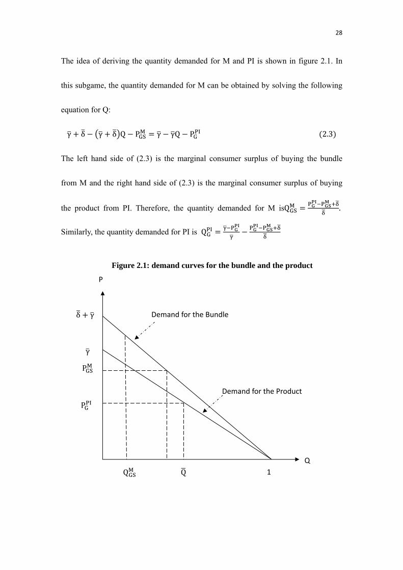
The idea of deriving the quantity demanded for M and PI is shown in figure 2.1. In

this subgame, the quantity demanded for M can be obtained by solving the following

equation for Q:

γ δ γ δ Q PGSM γ γQ PG

PI 2.3

The left hand side of (2.3) is the marginal consumer surplus of buying the bundle

from M and the right hand side of (2.3) is the marginal consumer surplus of buying

the product from PI. Therefore, the quantity demanded for M isQGSM PG

PI PGSM

.

Similarly, the quantity demanded for PI is QGPI PG

PI PGPI PGS

M

Figure 2.1: demand curves for the bundle and the product

P

δ γ Demand for the Bundle

γ

PGSM

Demand for the Product

PGPI

Q

QGSM Q 1

29

Therefore, the parallel importer will face the following optimization problem:

maxPG

PIπG

PI GS, G PGPI pR t

γ PGPI

γPG

PI PGSM δ

δ 2.4

While the manufacturer is solving the following optimization problem:

maxPGS

MπGS

M GS, G PGSM CP t CS

δ PGSM PG

PI

δ 2.5

To solve a Stackelberg pricing game by backward induction, we should solve the

optimal PGPI first. It is easy to verify that

PGPI GS, G

PGSM γ δ γ pR t

2 γ δ 2.6

Substituting (2.6) into (2.5), and find the FOC for PGSM , we can obtain

PGSM GS, G

CP 2δ γ γ pR CS 2t δ 2δ pR 2CS 3t

2 2δ γ 2.7

And thus the profits of these two firms in country A are

πGPI GS, G

γ CP CS pR 4δ pR t δγ 2 CP CS δ γ 3t 5pR

16δγ δ γ 2δ γ2.8

and

πGSM GS, G

2δ CP 2δ γ γ CS pR δ pR 2γ 2CS t

8δ δ γ 2δ γ 2.9

(6) Γ GS, G S

Price competition implies that PGSM PG

PI PSPI pR t CS . In this

30

subgame, there exists some demand for the product from PI. In other words, PI can

choose PGPI to maximize its profit. The quantity demanded for M and PI can be

derived by the same method in subgame (5). Therefore, the parallel trader will face

the following optimization problem:

maxPS

PIπG S

PI PGPI pR t

γ PGPI

γPG

PI PGSM δ

δ

s. t. PGSM pR t CS

We can easily verify that PGPI R R CS , πG S

PI CS R and

πGSM R CP CS R CS

(7) Γ G S, GS

In this subgame, price competition will lead the manufacturer to choose PGM and PS

M

such that PGM PS

M PGSPI. In other words, the parallel importer will earn zero profit in

this subgame. However, the manufacturer can choose an optimal PGM to maximize

profit. From the consumer’s payoff matrix, we know some consumers will buy both

product and service form M and some consumers will only buy the product from M.

Thus, the manufacturer will face the following profit maximization problem:

maxPG

MπG S

M G S, GS

PGM CP t

pR t CS PGM

δ

PGM

γ

pR t CPδ pR t CS PG

M

δ 2.10

31

From the FOC of (2.10), we can easily obtain the optimal price of product PGM G

S, GS CP R CS and thus, the optimal price of service is PSM G

S, GS pR t CSCP R CS .

The manufacturer’s profit can be obtained by substituting the optimal prices in the

profit function. That is πG SM G S, GS CPδ γ CS t 2δγ 2pR pR

γ CS 4pR 2γ 3CS t t δ 4pRγ t 4γ t 2cPδ δ 2γ t

γ 2pR 2γ CS 3t / 4δγ δ γ

(8) Γ G, GS

The idea of solving the NE in this subgame is identical to Γ GS, G . In Γ G, GS , the

manufacturer will face the following profit maximization problem:

maxPG

MπG

M G, GS PGM CP t

γ PGM

γδ PG

M PGSPI

δ 2.11

Similarly, the parallel importer will face the following maximization problem:

maxPGS

PIπGS

PI G, GS PGSPI pR t CS

δ PGSPI PG

M

δ 2.12

A Stackelberg pricing game leads us to the following optimal prices in this subgame:

PGSPI G, GS

12

δ pR PGM CS t 2.13

PGM G, GS

1

4δ2CPδ γ 2δγ 2δt 2.14

By substituting (2.14) into (2.13), (2.11) and (2.12), we can obtain both firms’ profit

in this subgame:

32

πGSPI G, GS

4δ CP 2δ γ γ pR CS δ 4p 3γ 4CS 2t

16δ 2δ γ 2.15

πGM G, GS

CP 2δ γ γ δ pR CS 2δt

8δγ 2δ γ 2.16

(9) Γ G, G S

In this subgame, no consumers will buy product without buying service from PI since

price competition will make the payoff of buying product from PI strictly less than the

payoff of buying product from the manufacturer. Thus, a consumer will choose to buy

G+S from PI or G from M. Price competition will lead PGM G, G S pR t .

Consumers with γ δ PSPI PG

M γ PGM will buy G+S from PI. Therefore, the

parallel importer will face the following profit maximization problem:

maxPS

PIπG S

PI G, G S PSPI CS

δ PSPI

δ 2.17

PSPI G, G S

12

δ CS 2.18

πGM G, G S pR CP

δ CS

2δ

pR tγ

2.19

πG SPI G, G S

1

δ

δ CS

2 2.20

Since the payoff is hard to compare directly, we assign some values for the parameters

to make the payoff comparable. The result in table 2.2 is obtained by assigning

δ, γ, pR, t, CP, CS 1, 2, 1, 0.05, 0.9, 0.5 .

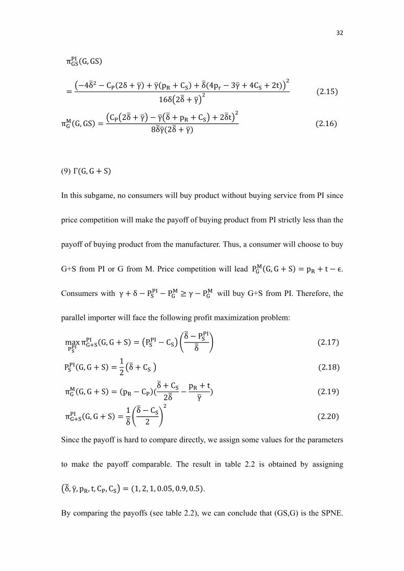
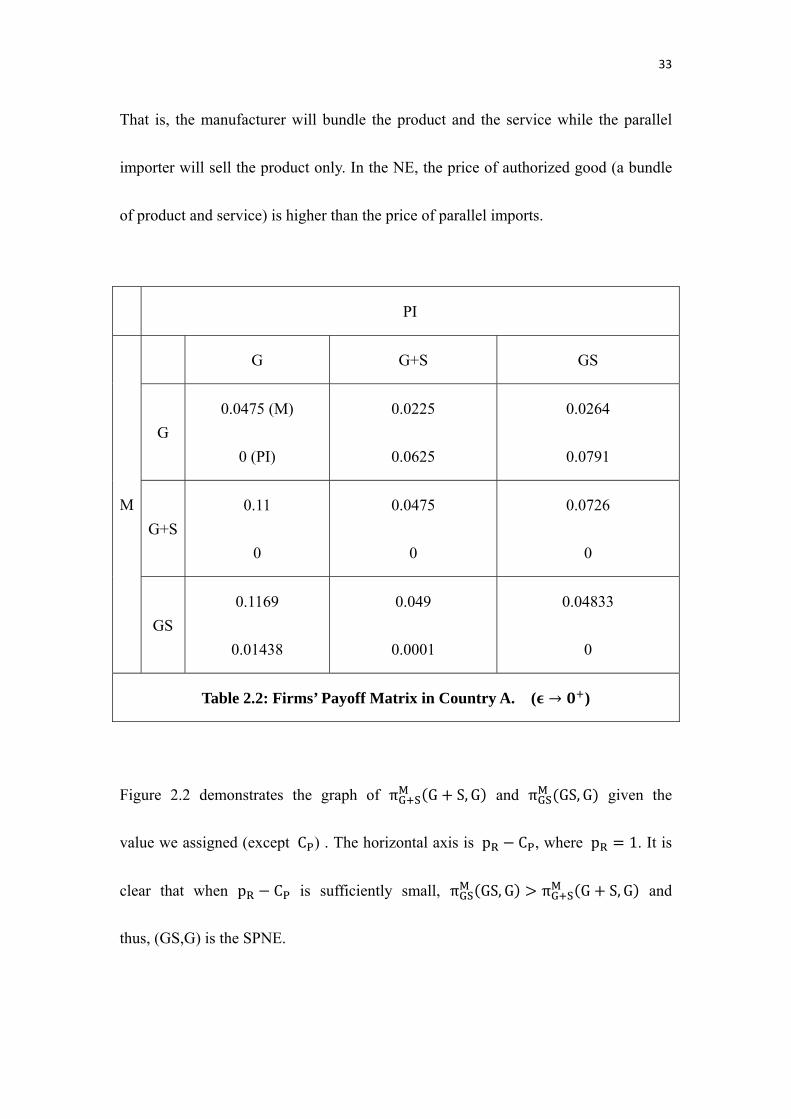
By comparing the payoffs (see table 2.2), we can conclude that (GS,G) is the SPNE.

33

That is, the manufacturer will bundle the product and the service while the parallel

importer will sell the product only. In the NE, the price of authorized good (a bundle

of product and service) is higher than the price of parallel imports.

PI

M

G G+S GS

G

0.0475 (M)

0 (PI)

0.0225

0.0625

0.0264

0.0791

G+S

0.11

0

0.0475

0

0.0726

0

GS

0.1169

0.01438

0.049

0.0001

0.04833

0

Table 2.2: Firms’ Payoff Matrix in Country A. ( )

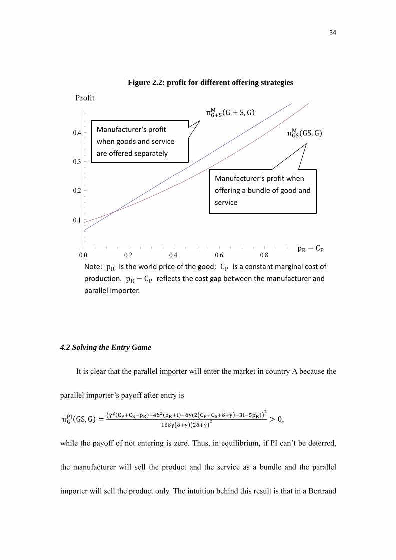
Figure 2.2 demonstrates the graph of πG SM G S, G and πGS

M GS, G given the

value we assigned (except CP) . The horizontal axis is pR CP, where pR 1. It is

clear that when pR CP is sufficiently small, πGSM GS, G πG S

M G S, G and

thus, (GS,G) is the SPNE.

34

4.2 Solving the Entry Game

It is clear that the parallel importer will enter the market in country A because the

parallel importer’s payoff after entry is

πGPI GS, G

CP CS R R CP CS R 0,

while the payoff of not entering is zero. Thus, in equilibrium, if PI can’t be deterred,

the manufacturer will sell the product and the service as a bundle and the parallel

importer will sell the product only. The intuition behind this result is that in a Bertrand

0.0 0.2 0.4 0.6 0.8 1.0

0.1

0.2

0.3

0.4

0.5

Figure 2.2: profit for different offering strategies

Profit

Manufacturer’s profit when

offering a bundle of good and

service

pR CP

Manufacturer’s profit

when goods and service

are offered separately

Note: pR is the world price of the good; CP is a constant marginal cost of

production. pR CP reflects the cost gap between the manufacturer and

parallel importer.

πGSM GS, G

πG SM G S, G

35

competition game, firms have incentives to differentiate their products because the

more similar the offers are, the lower profits firms can earn.

5. Parallel Imports and Investment

In this section, based on the result in section 4, we will discuss the impact of PI

on authorized distributors’ investment incentive. Given certain assumptions, we know

in equilibrium, the authorized distributor will offer product and service as a bundle,

while the parallel importer will sell the product only. In this section, we will consider

the case that the demand can be affected by authorized distributor’s market

development investment. Here, the market development investment is separated into

investment in brand marketing and investment in service marketing. The key

difference between them is that the parallel importer can free ride authorized

distributor’s effort in brand marketing, while the investment in service marketing is

excludable. An investing stage is added in the very beginning of the game structure.

That is, the authorized distributor will decide how much to invest in brand marketing

and service marketing so that the demand functions are determined. And then the

game will be played as stated in section 4.

36

5.1 Equilibrium Investment when Service Marketing is Considered

As stated in section 3.3, the demand functions are still

P γ δ γ δ Q if service is provided

P γ γQ if service is not provided

However, γ and δ are no longer constant. We will assume that

γ γ α eB

δ δ β eS

where γ , δ , α and β are given constants and eB and eS denote the effort in brand

marketing and service marketing respectively.

The cost of investment is assumed to be of a quadratic form. The cost of brand

marketing is eB and the cost of service marketing is µ eS. Similar to section 4, the

authorized distributor’s profit function can be represented by

πM pM CP t CS 1pM pPI

δ β eS

λ2

eBµ2

eS 2.21

The parallel importer’s profit function is

πPI pPI pR tpM pPI

δ β eS

pPI

γ α eB 2.22

From (2.22), we can easily verify that the optimal price charged by PI is

pPI pMγ δ β eS γ pR t α eB pR t pM

2 δ α eB β eS γ 2.23

Substituting (2.23) into (2.21) and deriving the FOC with respect to pM, we can find

the optimal price charged by authorized distributor: pM eB, eS argmax πM

37

And then substituting pM eB, eS and pPI eB, eS into (2.21), we can solve for

optimal effort in brand marketing eB and optimal effort in service marketing eS.

5.2 Equilibrium Investment When Service Marketing is Not Considered

In some studies that PI and authorized products are considered as homogeneous,

such as Palangkaraya and Yong (2006) argue that the existence of parallel imports will

reduce the authorized distributor’s market development investment in PI recipient

country. To compare the optimal investment effort with and without service, we

should also analyze the case when service is not provided.

If service is not considered, authorized goods and parallel imports are homogeneous.

Price competition implies that pM pR t , where 0 . Therefore, the

authorized distributor’s profit becomes

πM pR CP 1pR t

γ α eB

λ2

eB 2.24

Then we may find the optimal effort in brand marketing eB when service is not

provided.

5.3 A Numerical Example

I will provide a numerical example to show that even though PI may reduce the

investment effort in brand marketing, which is non-excludable, the authorized

38

distributor can respond to PI by investing more in service.

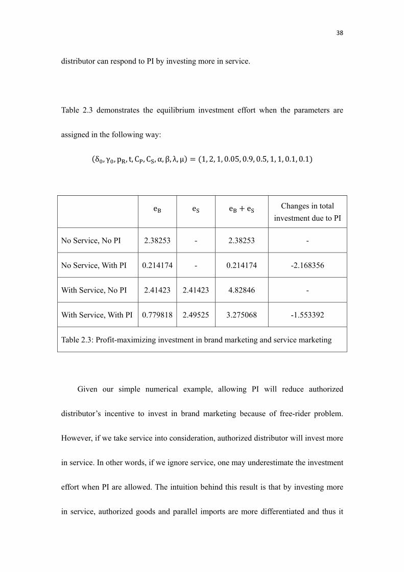
Table 2.3 demonstrates the equilibrium investment effort when the parameters are

assigned in the following way:

δ , γ , pR, t, CP, CS, α, β, λ, µ 1, 2, 1, 0.05, 0.9, 0.5, 1, 1, 0.1, 0.1

eB eS eB eS Changes in total

investment due to PI

No Service, No PI 2.38253 - 2.38253 -

No Service, With PI 0.214174 - 0.214174 -2.168356

With Service, No PI 2.41423 2.41423 4.82846 -

With Service, With PI 0.779818 2.49525 3.275068 -1.553392

Table 2.3: Profit-maximizing investment in brand marketing and service marketing

Given our simple numerical example, allowing PI will reduce authorized

distributor’s incentive to invest in brand marketing because of free-rider problem.

However, if we take service into consideration, authorized distributor will invest more

in service. In other words, if we ignore service, one may underestimate the investment

effort when PI are allowed. The intuition behind this result is that by investing more

in service, authorized goods and parallel imports are more differentiated and thus it

39

can mitigate price competition.

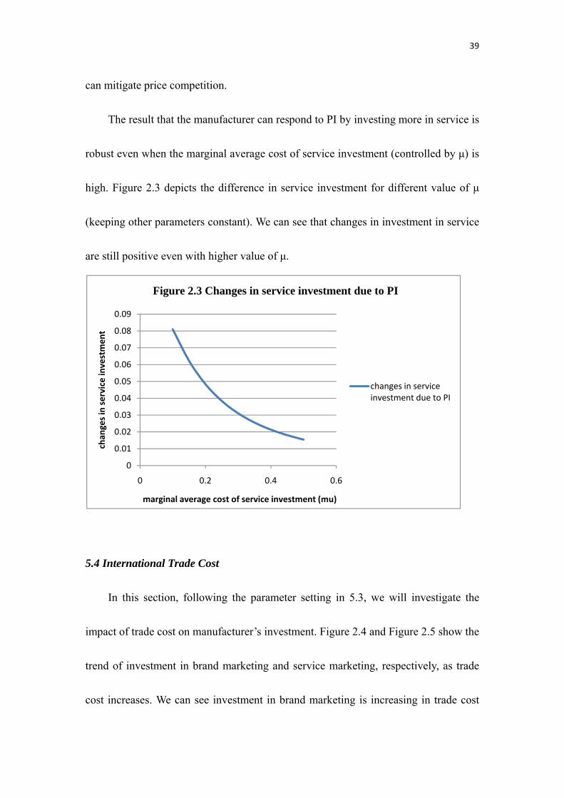
The result that the manufacturer can respond to PI by investing more in service is

robust even when the marginal average cost of service investment (controlled by μ) is

high. Figure 2.3 depicts the difference in service investment for different value of μ

(keeping other parameters constant). We can see that changes in investment in service

are still positive even with higher value of μ.

5.4 International Trade Cost

In this section, following the parameter setting in 5.3, we will investigate the

impact of trade cost on manufacturer’s investment. Figure 2.4 and Figure 2.5 show the

trend of investment in brand marketing and service marketing, respectively, as trade

cost increases. We can see investment in brand marketing is increasing in trade cost

0

0.01

0.02

0.03

0.04

0.05

0.06

0.07

0.08

0.09

0 0.2 0.4 0.6

chan

ges in service investment

marginal average cost of service investment (mu)

changes in service investment due to PI

Figure 2.3 Changes in service investment due to PI

40

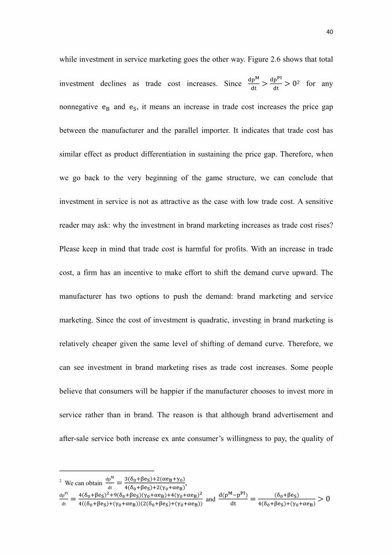
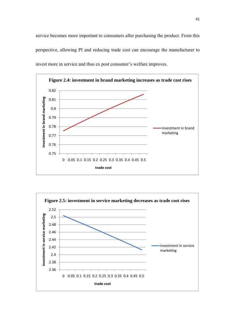
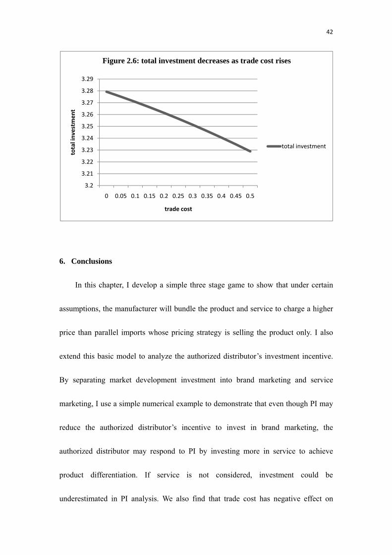
while investment in service marketing goes the other way. Figure 2.6 shows that total

investment declines as trade cost increases. Since M PI

02 for any

nonnegative eB and eS, it means an increase in trade cost increases the price gap

between the manufacturer and the parallel importer. It indicates that trade cost has

similar effect as product differentiation in sustaining the price gap. Therefore, when

we go back to the very beginning of the game structure, we can conclude that

investment in service is not as attractive as the case with low trade cost. A sensitive

reader may ask: why the investment in brand marketing increases as trade cost rises?

Please keep in mind that trade cost is harmful for profits. With an increase in trade

cost, a firm has an incentive to make effort to shift the demand curve upward. The

manufacturer has two options to push the demand: brand marketing and service

marketing. Since the cost of investment is quadratic, investing in brand marketing is

relatively cheaper given the same level of shifting of demand curve. Therefore, we

can see investment in brand marketing rises as trade cost increases. Some people

believe that consumers will be happier if the manufacturer chooses to invest more in

service rather than in brand. The reason is that although brand advertisement and

after-sale service both increase ex ante consumer’s willingness to pay, the quality of

2 We can obtain

dpM

dt

S B

S B,

dpPI

dt

S S B B

S B S B and

M PIS

S B0

41

service becomes more important to consumers after purchasing the product. From this

perspective, allowing PI and reducing trade cost can encourage the manufacturer to

invest more in service and thus ex post consumer’s welfare improves.

0.75

0.76

0.77

0.78

0.79

0.8

0.81

0.82

0 0.05 0.1 0.15 0.2 0.25 0.3 0.35 0.4 0.45 0.5

investment in brand m

arketing

trade cost

investment in brand marketing

investment in brand marketing

2.36

2.38

2.4

2.42

2.44

2.46

2.48

2.5

2.52

0 0.05 0.1 0.15 0.2 0.25 0.3 0.35 0.4 0.45 0.5

investment in service m

arketing

trade cost

investment in service marketing

investment in service marketing

Figure 2.4: investment in brand marketing increases as trade cost rises

Figure 2.5: investment in service marketing decreases as trade cost rises

42

6. Conclusions

In this chapter, I develop a simple three stage game to show that under certain

assumptions, the manufacturer will bundle the product and service to charge a higher

price than parallel imports whose pricing strategy is selling the product only. I also

extend this basic model to analyze the authorized distributor’s investment incentive.

By separating market development investment into brand marketing and service

marketing, I use a simple numerical example to demonstrate that even though PI may

reduce the authorized distributor’s incentive to invest in brand marketing, the

authorized distributor may respond to PI by investing more in service to achieve

product differentiation. If service is not considered, investment could be

underestimated in PI analysis. We also find that trade cost has negative effect on

3.2

3.21

3.22

3.23

3.24

3.25

3.26

3.27

3.28

3.29

0 0.05 0.1 0.15 0.2 0.25 0.3 0.35 0.4 0.45 0.5

total investment

trade cost

total investment

total investment

Figure 2.6: total investment decreases as trade cost rises

43

service investment since given the same quality difference, trade cost reduces the

price gap between authorized products and PI, and thus product differentiation is not

as attractive as the case with low trade cost.

44

CHAPTER III

OUTLAW INNOVATION, VIDEO GAME PIRACY AND PARALLEL IMPORTS

1. Introduction

Innovations not only can be done by manufacturers but also be realized by users.

User innovations aim to add more functions that are not originally provided on the

product or to bypass legal or technical safeguards. In particular, electronic

manufactures often embed security mechanism in order to prevent users from running

unauthorized software or illegally obtained content on their platform. For example,

the region code on a DVD player prevents users from buying parallel imported

multimedia products. The security mechanism on a game console prevents illegally

copied game ROMs from being operated on the platform. Similar examples can also

be found in telecommunication industry. Apple’s iPhone users can only choose AT&T

in United States because of the mechanism that aims to increase firms’ market power.

Mollick (2004) is the first paper that analyzes user innovations that deactivate the

security mechanisms. Extending Mollick’s research, Flowers (2008) introduces the

concept of outlaw innovation and provides case studies of how communities create

and distribute outlaw innovations. As defined by Schulz and Wagner (2008), outlaw

innovations are user modifications of a product to not only gain unauthorized access

45

to the product’s system but to also enable the user to use the system more effectively.

Outlaw innovation is an important issue because it may violate manufacturers’

intellectual property rights and will restrict manufacturers’ market power as well as

pricing behaviors. For example, users of a videogame console can embed a

modification chip (or modchip), which is a device used to play import discs, backup

dvd-r/ dvd-rw, or homebrew game ROMs on the game console to play videogames

without paying any money to game providers by downloading game ROMs from the

internet.

This paper is motivated by the fact that Sony has decided to make its new

generation game console, Playstation 3 (PS3), a region-free game console.3 In other

words, PS3 users can play international version games on the PS3 platform if the

hardware is region-free. A Japanese PS3 hardware owner can run a USA version game

on the Japanese hardware. Similar strategies are also adopted by Microsoft Xbox 360.

As we know, the modification chips encourage video game piracy and parallel

imports (PI). When video game piracy is mentioned, most people expect that the

modification chips will boost sales of game consoles and will reduce the game

providers’ profit. However, in this paper, we show the latter is not necessarily true. In

addition to illegal copy of the software, the modification chips can also undermine

3 See “regional lockout” on Wikipedia: http://en.wikipedia.org/wiki/Regional_lockout

46

manufacturers’ international third degree price discrimination by inspiring parallel

trade. However, our model shows that it is premature to claim that the hardware

manufacturer will suffer from parallel imports. Why did Sony and Microsoft change

their mind to encourage parallel imports? Different model specifications have

different explanations. In the literature of PI, studies can be roughly categorized as

vertical price control model and horizontal retail price arbitrage model. The vertical

price control model of PI, which is first developed by Maskus and Chen (2002, 2004)

and Chen and Maskus (2005), assumes that a manufacturer protected by IPR in two

markets has an independent distributor in each location. The manufacturer offers the

distributors two-part tariff contracts that specify the wholesale prices and a lump-sum

fee in order to induce profit-maximizing retail prices. In the framework of vertical

price control model, Ganslandt and Maskus (2007) develop a model to show that the

manufacturer will prefer to serve a country by PI when trade cost is sufficiently low.

The idea behind their result is that the manufacturer would push the distributor in the

PI recipient country out of the market in order to avoid pro-competitive effect when

trade cost is small.

The other framework, horizontal retail price arbitrage model, assumes that PI

occurs simply due to retail price differences between two markets. In general, retail

price arbitrage prevents the manufacturer from third-degree price discrimination;

47

however, Anderson and Ginsburg (1999) argue that consumers’ arbitrage behaviors

provide the manufacturer a channel to second-degree price discrimination. They

develop a two-country model with heterogeneous consumers to show that a firm with

market power may have an incentive to create a second market in the second country,

even if there is no local demand there. The intuition is that consumer’s arbitrage

between two countries provides the firm a means to price discriminate across

consumers in the first country.

The analysis of the present paper follows the idea of Anderson and Ginsburg

(1999). A consumer who purchases a game console from unauthorized channels has a

strong tendency to play pirated or illegally obtained games.4 This kind of consumer

has lower willingness to pay and thus parallel imports give the manufacturer a lead to

distinguish high-type consumers and low-type consumers; hence second-degree price

discrimination in the PI recipient country becomes feasible.

The idea that parallel imports or pirated goods lead to second degree price

discrimination is not new. Takeyama (1994) develops a model to discuss the impact of

software piracy on software providers in the presence of network externalities. She

finds that with network externality, piracy is an efficient means to expand network

size and thus the copies are sold at one price (zero) while genuine product buyers are

4 One report on 2007.04.30 indicates that more than 80% Taiwanese consumers who purchased parallel imported Wii game consoles asked to modify the hardware to play pirated games. See The Sun, Hong Kong.

48

charged at a higher price. However, her model can’t be applied to video game piracy

because her model does not take the hardware firm into account. Taking the hardware

firm into consideration is important for discussing piracy in the video game market

because the hardware is specific and perfectly complementary to the software. In

other words, both hardware and software firms’ pricing behaviors will be pinned

down by each other and thus we should not ignore hardware firm in the analysis of

video game piracy. In addition, most papers that discuss software piracy only consider

the story in a closed economy. In other words, they ignore the impact of PI on the

hardware manufacturer and the software provider.

To my knowledge, this paper is the first one that integrates software piracy and

parallel imports. It sheds some lights on pricing by software and hardware firms when

they feature complementary products and the hardware can be parallel traded while

the other not. This paper argues that parallel trade in hardware is a channel used to let

consumers reveal their preference for playing video games. Authorized hardware and

PI are homogeneous to pirated software users (low type consumers) because after-sale

service is not available for modified-hardware users. Therefore, the manufacturer can

extract more profits from consumers by serving high type consumers by authorized

products with a higher price and serving low type consumers by cheaper PI. Based on

this idea, in this paper, I develop a simple model with one monopolistic hardware

49

manufacturer and one monopolistic software provider (where the hardware and the

software are perfect complements) selling their products in two countries. Starting

from the assumption that the hardware is protected by a region code which prevents

consumers from using international version software, I show three results that are in

contrast to general expectation. First, the software provider and the hardware

manufacturer could both benefit from software piracy. Second, the hardware

manufacturer may benefit from PI since PI can serve as a channel to second-degree

price discrimination. Third, the consumers in the PI recipient country are not

necessarily better off due to PI since the gains from an open policy might be offset if

the hardware firm chooses to engage in price discrimination. Then to explain why

Sony and Microsoft make their new generation game consoles region-free, I relax the

region code assumption and show that, in equilibrium, imposing a region code on the

hardware is redundant. All results in this study still hold for region-free hardware.

This paper is organized as follows. A simple model is developed in section 2.

Welfare analysis is given in section 3. Section 4 offers a short analysis of a region-free

hardware and section 5 concludes.

2. The Model

In this section, we develop the basic non-cooperative game with a monopolistic

50

hardware manufacturer and one game provider.5 We will discuss two cases. First,

let’s consider the impact of software piracy on the hardware manufacturer and the

software provider respectively when parallel importation is not permitted. Second, we

will discuss the impact of PI on both firms given software piracy.

There are two countries, A and B. We assume that the total number of consumers

in country A and B are normalized to unity. Consumers are heterogeneous in their

value of playing video games. Let v denote a consumer’s gross utility of playing video

games. The distribution of v in both countries is identical and is assumed to be a

uniform distribution with support [0,1]. Here, the hardware is assumed to provide zero

utility if it is not utilized with software.

2.1 The Benchmark: The Basic Model with No Piracy

Let’s consider the benchmark case: no piracy, no PI. The utility functions in both

countries are given by

U p BM p BM if purchasing the system0 if no adoption

A, B 3.1

p BM denotes the price of official software in country i and p BM is the price of

hardware in country i. The subscript BM indicates the variable for the benchmark

case.

5 The assumption of non-cooperative game is briefly discussed in section 5.

51

Without loss of generality, we take country A as the discussing object. A

consumer in country A with v p BMA p BM

A will purchase the system. For

simplicity, we also assume that both hardware and software firms’ marginal cost are

normalized to zero.6 Since each consumer purchases one unit of the product, the

quantity demanded can be calculated by 1dx 1 p BMA p BM

A . Now we can

obtain both firms’ profit earned in country A:

π BMA p BM

A 1 p BMA p BM

A , j h, o 3.2

The optimization of (3.2) with respect to p BMA and p BM

A indicates that

p BMA p BM

A

Identical argument can be applied to country B and we will have

p BMB p BM

B

Therefore, both firms’ profits in this benchmark case are identical and equal to the

sum of profits in both countries given by .

6 This seems a stronger assumption on manufacturer’s marginal cost. Normalizing the marginal cost to zero helps simplify the analysis. The value of the marginal cost does affect values of the variables, such as the profit level, but will not affect the direction of the change in variables due to some scenarios demonstrated in our model since the marginal cost is a common factor in every stage. The main interest of this chapter is to discuss how firms’ profits and consumer’s welfare change and thus it is safe to normalize the marginal cost to zero.

52

2.2 Software Piracy When PI is Prohibited

In this section, we consider the case where pirated software is available in country

A. For simplicity, we assume that consumers in country B are unable to access pirated

software. The utility function in country A now becomes

UAp PN

A p PNA if purchasing official software

1 α p PNA c δ if using illegal software

0 if no adoption 3.3

The subscript PN indicates piracy exists while parallel imports do not. 1 α is a

discount factor to the value v if the consumer modifies the hardware. Assume that by

installing the modification chip on the hardware, users can bypass all security

mechanism including region code. Here, α 0,1 because any unauthorized

modification to the hardware will void warranty. The parameter α can also be

interpreted as the probability that a hardware buyer needs after sale service.7 c 0

refers to a fixed cost of modifying the hardware8. δ 0,1 measures the extra

benefit along with the hardware modification. For example, more powerful

multimedia functions on a modified Microsoft XBOX.9

Let v be the value of one consumer who is indifferent between using official

software and pirated copy. Therefore, v p PNA p PN

A 1 α v p PNA c

7 Some studies such as Takeyama (1994) and Bae and Choi (2006) consider 1 α as a utility discount factor for using pirated software. However, as stated in Peitz and Waelbroeck (2006), for video game piracy, the original and the copy have almost the same quality. Therefore, in this study, we will use 1 α to represent the utility discount factor due to loss of after-sale service. 8 For example, a modification chip or a recordable DVD that is required to make and play a homebrew pirated Wii game. 9 For more detail discussions on XBOX modification, see Schulz and Wagner (2008).

53

δ. A consumer will purchase official software if his valuation v v PNA δ

α.

Thus, the quantity demanded for legitimate software is 1dx 1 PNA δ

α. It is

worthy to note that the quantity demanded for the official software is irrelevant to the

hardware price since the hardware price does not play a role in consumer’s choice

between legitimate software and pirated software.

The software provider maximizes his profit in country A:

maxPN

A π PN

A 1p PN

A c δ

αp PN

A 3.4

FOC indicates that the optimal official software price in country A,

p PNA α δ 0,1 3.5

Both official software buyers and pirated software users need to purchase the

hardware. Let v be the value of a consumer who is indifferent between using the

system and not adoption. Therefore, consumers with v v PNA δ

will buy the

hardware. The hardware manufacturer maximizes its profit in country A:

maxPN

Aπ PN

A 1p PN

A c δ

1p PN

A 3.6

First order condition is 1 PNA δ PN

A

α0. Solving the FOC to find the

optimal hardware price in country A, we will have p PNA α δ 0.

It is natural to assume that v is greater than v . Since α 0,1 , this inequality

54

implies that c .10

Proposition 1. The hardware manufacturer can sell more units when software piracy

exists

<Proof> If piracy is not available, the value v such that one consumer is indifferent

between buying the system and not adoption is equal to . In other words, total

quantity sold by the hardware manufacturer is of the total population. However,

when software piracy is introduced, total hardware quantity sold is 1 v 1

α δδ

1 δ

α for c Q.E.D

The profits that both firms can obtain in country B are identical to the benchmark

case discussed in section 2.1. Total profits of the software provider can be calculated

by substituting p PNA into π PN

A and then plus the profit from country B. π PN, the

profit of the software provider under the situation where software piracy exists while

PI do not, is π PNα δ

α. The combined profit function of the hardware

manufacturer becomes11

10 The derivation of this inequality is demonstrated in the appendix A1. 11 It is easy to verify that 1 v v 0. Any other situations do not hold. When v 0, the market is fully served by the hardware manufacturer. However, v will never be strictly less than zero because the hardware manufacturer has an incentive to increase the hardware price.

55

π PN19

1 α c δ

4 1 α for 1 v v 0 3.7

Now we can compare the profits obtained in section 2.2 to those calculated in the

benchmark case to see the impact of software piracy on the hardware manufacturer

and the software provider. The hardware manufacturer can (weakly) benefit from

software piracy if π PN π BM . Solving this inequality, we have

1 if 12

19

19

7 929

1 9 if 19

0 3.8

Similarly, the software provider can earn a higher profit if π PN π BM . That is

1 9 2 9 1

8 √19 0 3.9

The combination of α, c δ where the hardware manufacturer and the

software provider can benefit from piracy can be described by the dark (light) area in

figure 3.1. The medium dark area is the intersection of dark area and light area, which

indicates the combination of α, c δ where both hardware manufacturer and

software provider benefit from software piracy.

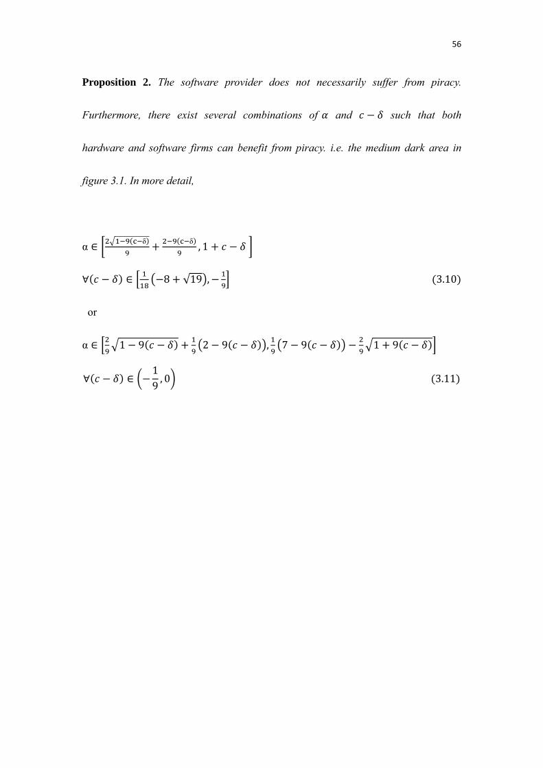
56

Proposition 2. The software provider does not necessarily suffer from piracy.

Furthermore, there exist several combinations of and such that both

hardware and software firms can benefit from piracy. i.e. the medium dark area in

figure 3.1. In more detail,

αδ δ , 1

8 √19 , 3.10

or

α 1 9 2 9 , 7 9 1 9

19

, 0 3.11

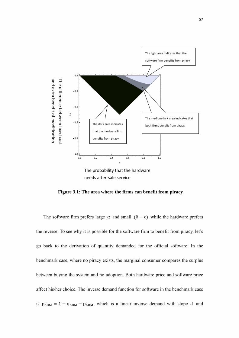
57

The software firm prefers large α and small δ c while the hardware prefers

the reverse. To see why it is possible for the software firm to benefit from piracy, let’s

go back to the derivation of quantity demanded for the official software. In the

benchmark case, where no piracy exists, the marginal consumer compares the surplus

between buying the system and no adoption. Both hardware price and software price

affect his/her choice. The inverse demand function for software in the benchmark case

is p BM 1 q BM p BM, which is a linear inverse demand with slope -1 and

The probability that the hardware

needs after‐sale service The differen

ce betw

een fixe

d co

st

and extra b

enefit o

f modificatio

n

The dark area indicates

that the hardware firm

benefits from piracy.

The light area indicates that the

software firm benefits from piracy

The medium dark area indicates that

both firms benefit from piracy.

Figure 3.1: The area where the firms can benefit from piracy

58

intercept 1 p BM . However, in a model with piracy, hardware price won’t affect

the choice of the marginal consumer who considers whether to buy the legitimate

software or to pirate the software. The inverse demand function for the software in the

case with piracy is p PN α 1 q PN δ c , which is a linear inverse demand

with slope α and intercept α δ c . The parameter α can measure how

elastic the software demand is. Since α 1, the inverse demand function for the

software in the case with piracy is flatter than the benchmark. However, the inverse

demand function is also controlled by the intercept. With a sufficiently small number

of δ c , i.e. δ c is sufficiently closed to zero, such that δ c is smaller

than p BM, the software provider in fact faces a larger market in the case with piracy

than in the benchmark case as long as α is not too small. In other words, comparing

the result in this section to the benchmark case, if the “disadvantage” due to elasticity

(α) can be covered by the gain from consumer’s willingness to pay (larger intercept

captured by small δ c ), the software firm can benefit from piracy.

The existence of piracy enables the hardware manufacturer to sell more units.

When pirated software is available, the hardware manufacturer can set the price

without taking the software provider’s action into consideration because the marginal

consumer who decides whether to buy the hardware or not does not care about the

price of the official software since he/she uses illegal copy of the software. Similarly,

59

the marginal consumer of the legitimate software does not take the hardware price

into consideration because the hardware is required no matter whether the official or

illegal software is chosen. In other words, both firms won’t be pinned down by each

other and thus have higher market power to some extent relative to the benchmark

case where the outcome depends on the pricing behavior of each other. That’s why for

certain parameter sets, both firms can benefit from piracy. However, it is somewhat

surprising that the hardware manufacturer suffers from piracy on the light region of

figure 3.1, where α is sufficiently large and c δ is also sufficiently large (closed

to zero). In proposition 1, we show that the quantity demanded for the hardware will

increase due to piracy; however, it does not guarantee that the hardware

manufacturer’s profit will increase as well. To see this, let’s check the inverse demand

function of the hardware when piracy exists. The inverse demand function of the

hardware is p BM 1 α c δ 1 α q BM. When α is sufficiently large

and c δ is sufficiently closed to zero, the linear inverse demand curve is flat with

a small intercept indicating that consumer’s willingness to pay for the hardware is low.

In addition, a large α means that the degradation cost of modification is high, while

a large c δ means the net benefit along with modification is small. Both indicate

that modification is not attractive suggesting that consumer’s willingness to pay is low.

As a consequence, in extreme circumstances, it is still possible for the hardware

60

manufacturer to suffer from piracy.

2.3 Software Piracy When PI is Considered

In this section, we consider the case such that consumers in country A can choose

to buy the hardware from either country A or country B. The hardware purchased

from country B is called a parallel import. We can imagine that there are many traders

who purchase the hardware from retail markets in country B and sell the product in

country A. Eventually, PI traders earn zero profit with free entry assumption. However,

if a consumer purchases a PI hardware, some modifications to the hardware are

required to bypass the region code safeguard. In addition, because the regulation on

multimedia product is stronger in reality, we assume that the parallel importation of

software is prohibited between two countries.12 Since we assume that the hardware is

protected by a region code, it will be one-way PI from country B to country A because

we assume that the modification chip is not available in country B. Given our model

specification, we would claim that all PI hardware buyers will pirate the software. The

reason is straightforward because if a consumer purchases PI hardware but buys

official software, his utility is 1 α v pB c t δ pA, which is strictly less

than 1 α v pB c t δ, the utility obtained by pirating software. Here, a

12 For example, parallel imports of copyrighted works are considered to be a copyright infringement. See Article 87(4) , Taiwan Copyright Law.

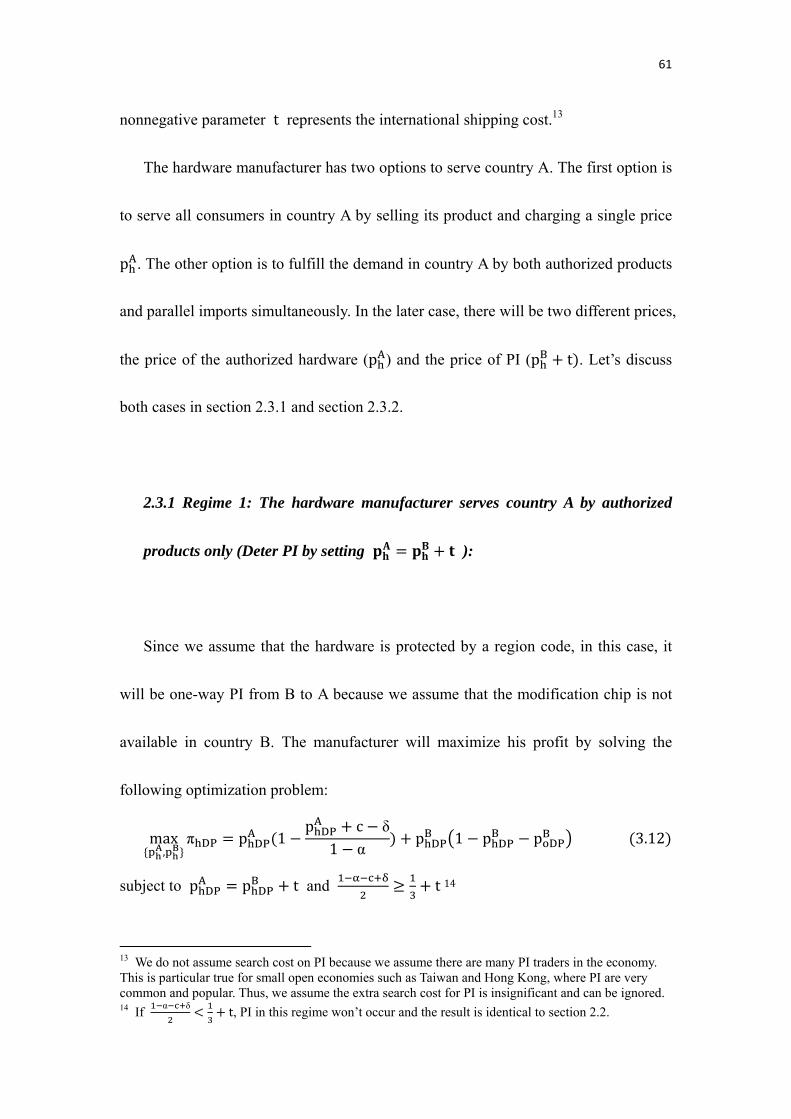
61

nonnegative parameter t represents the international shipping cost.13

The hardware manufacturer has two options to serve country A. The first option is

to serve all consumers in country A by selling its product and charging a single price

pA. The other option is to fulfill the demand in country A by both authorized products

and parallel imports simultaneously. In the later case, there will be two different prices,

the price of the authorized hardware (pA) and the price of PI (pB t . Let’s discuss

both cases in section 2.3.1 and section 2.3.2.

2.3.1 Regime 1: The hardware manufacturer serves country A by authorized

products only (Deter PI by setting ):

Since we assume that the hardware is protected by a region code, in this case, it

will be one-way PI from B to A because we assume that the modification chip is not

available in country B. The manufacturer will maximize his profit by solving the

following optimization problem:

maxA, B

π DP p DPA 1

p DPA c δ

1 αp DP

B 1 p DPB p DP

B 3.12

subject to p DPA p DP

B t and t 14

13 We do not assume search cost on PI because we assume there are many PI traders in the economy. This is particular true for small open economies such as Taiwan and Hong Kong, where PI are very common and popular. Thus, we assume the extra search cost for PI is insignificant and can be ignored. 14 If

α δt, PI in this regime won’t occur and the result is identical to section 2.2.

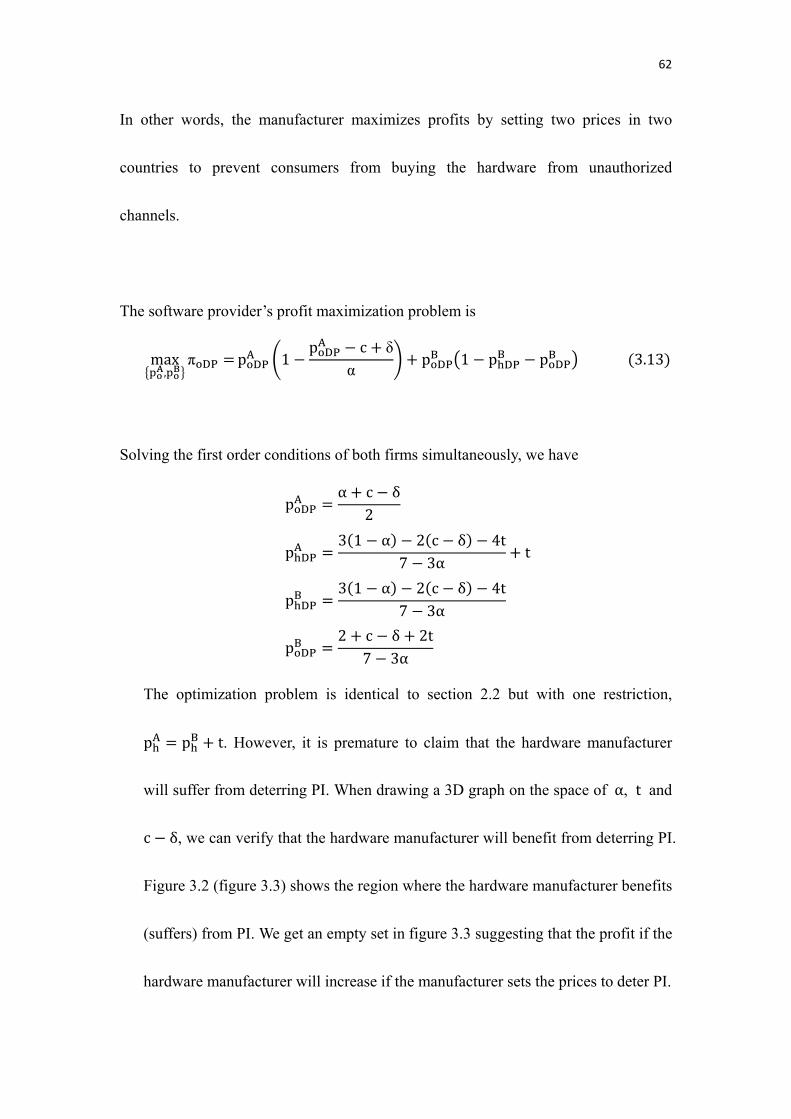
62

In other words, the manufacturer maximizes profits by setting two prices in two

countries to prevent consumers from buying the hardware from unauthorized

channels.

The software provider’s profit maximization problem is

maxA, B

π DP p DPA 1

p DPA c δ

αp DP

B 1 p DPB p DP

B 3.13

Solving the first order conditions of both firms simultaneously, we have

p DPA α c δ

2

p DPA 3 1 α 2 c δ 4t

7 3αt

p DPB 3 1 α 2 c δ 4t

7 3α

p DPB 2 c δ 2t

7 3α

The optimization problem is identical to section 2.2 but with one restriction,

pA pB t. However, it is premature to claim that the hardware manufacturer

will suffer from deterring PI. When drawing a 3D graph on the space of α, t and

c δ, we can verify that the hardware manufacturer will benefit from deterring PI.

Figure 3.2 (figure 3.3) shows the region where the hardware manufacturer benefits

(suffers) from PI. We get an empty set in figure 3.3 suggesting that the profit if the

hardware manufacturer will increase if the manufacturer sets the prices to deter PI.

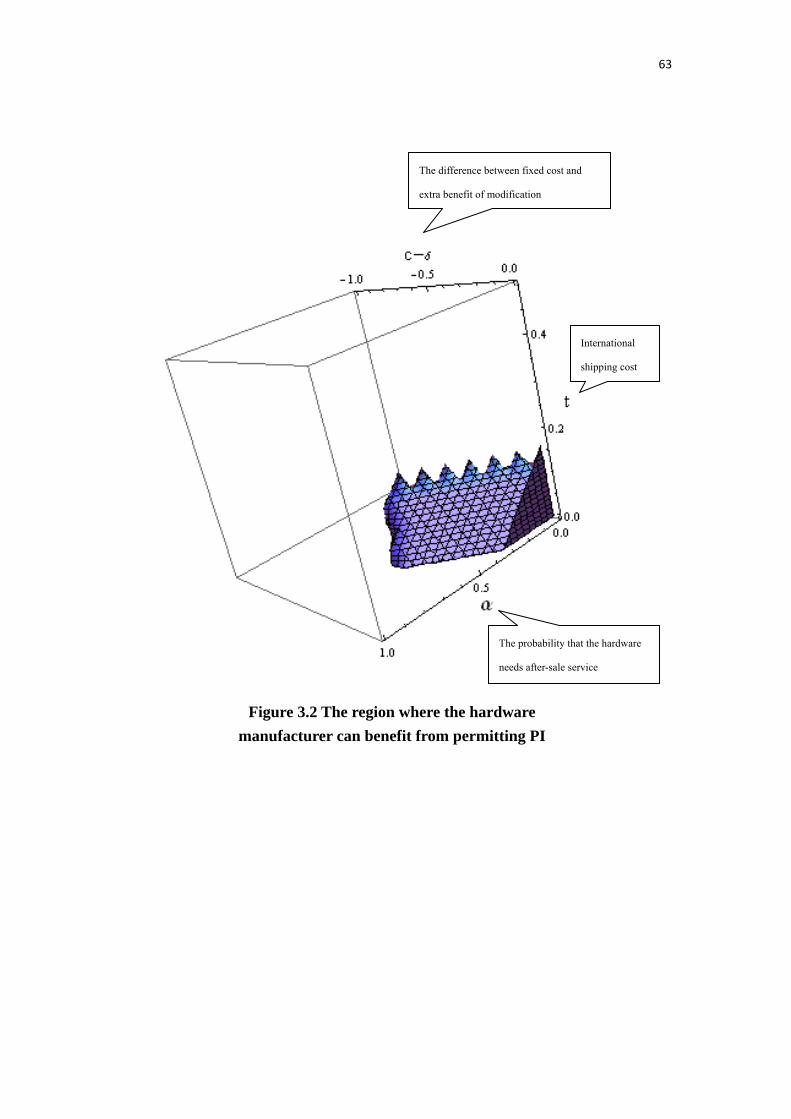
63


needs after-sale service

International

shipping cost

The difference between fixed cost and

extra benefit of modification

Figure 3.2 The region where the hardware

manufacturer can benefit from permitting PI

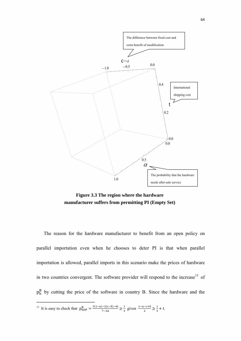
64

The reason for the hardware manufacturer to benefit from an open policy on

parallel importation even when he chooses to deter PI is that when parallel

importation is allowed, parallel imports in this scenario make the prices of hardware

in two countries convergent. The software provider will respond to the increase15 of

pB by cutting the price of the software in country B. Since the hardware and the

15 It is easy to check that p DP

B given t.

0.0

0.5

1.0

a

-1.0 -0.5 0.0c-d

0.0

0.2

0.4

t



International

shipping cost



Figure 3.3 The region where the hardware

manufacturer suffers from permitting PI (Empty Set)

65

software are complements, the decrease in software price will increase the demand for

the hardware. In other words, parallel trade is a commitment device for the hardware

manufacturer to raise the hardware price in country B and thus parallel trade enables

the hardware firm to extract profits from the software provider. In short, even though

the hardware firm suffers in the PI recipient country by deterring PI, the

complementarity between the hardware and the software enables the hardware firm to

benefit in the parallel exporting country. As consequence, the benefit in country B

dominates the loss in country A.

The software provider’s profit in country A will not change. However, given our

parameter restriction, t, the software provider’s profit will decrease in

country B because both price and quantity demanded for the software in country B

decrease.16

2.3.2 Regime 2: The hardware manufacturer serves country A by both

authorized products and PI (Accommodate PI):

If α δ t, in the specification of section 2.3.1, PI won’t occur. However,

parallel importation is still possible in another scenario which is the one we will

16 p DP

B p DPB is greater than (the value in the benchmark case) and p DP

B δ

α (the

price charged by the software firm in the benchmark case) provided that α δ

t

66

discuss in this section. The hardware manufacturer can utilize parallel imports as a

channel to price discrimination. Since illegal software users have to modify the

hardware, after-sale service is not available even if they purchase the hardware from

authorized channels. The only concern that illegal software users have in mind in

choosing the hardware provider is the price of the hardware. If authorized hardware is

cheaper than PI, no consumers will purchase PI, which is either an uninteresting case

or has been discussed in section 2.3.1. Therefore, in this section, we will consider the

case where the hardware price in country A is higher than the price of PI, which is the

hardware price in country B plus shipping cost. The price gap sustains even when

parallel importation exists because PI is now a channel to separating different types of

consumers. In our specification, all illegal software users will buy PI and only those

consumers who purchase official software will buy the authorized hardware.

Consumer’s preference in country A and country B can be described by

UApA pA if purchasing the legitimate system

1 α pB t c δ if using pirated software and PI 0 if no adoption

;

UB pB pB if purchasing the system0 if no adoption

We can now obtain the profit functions of both hardware and software firms.

The hardware manufacturer’s profit maximization problem is

maxAP

A , APB

π AP p APB 1 p AP

B p APB

67

p APB pOAP

A p APA p AP

B t c δ

α

p APB t c δ

1 α

p APA 1

p APA p AP

A p APB t c δ

α 3.14

s.t. 1 APA

APA

APB δ

αAP

B δ

α0 and p AP

A p APB t

The derivation of (3.14) is shown in appendix A2. The first term in the profit function

is the profit obtained in country B where piracy is absent. The second term describes

the profit from PI and the last term in the profit function is the profit from selling

authorized hardware in country A. OAPA

APA

APB δ

αAP

B δ

α captures the

PI volume while 1 APA

APA

APB δ

α describes the quantity demanded for

the authorized hardware in country A. The later inequality comes from the assumption

that the hardware manufacturer serves country A by both authorized products and

parallel imports. If it were violated, the result will be identical to the one of deterring

PI.

Similarly, the software provider maximizes his profit

π AP p APB 1 p AP

B p APB

p APA 1

p APA p AP

A p APB t c δ

α 3.15

First order conditions imply

p APA α c δ t

3

p APB 2 c δ t

7 3α

68

p APA 9 2 3α 1 3

3 7 3

p APB 3 3 2

7 3

subject to17

0 tα c δ

2,7 c δ α 6α 5 1 α c δ

7 α 6α 5

Comparing this set of prices to that in the case of deterring PI, given the

constraints on t, we have the following results: p APA p DP

A , p APB p DP

B ,

p APA p DP

A , and p APB p DP

B . In other words, the manufacturer charges higher

prices while the software provider reduces the prices in both countries if the hardware

manufacturer chooses to accommodate PI. The reason for an increase in hardware

price in country B builds on an increase in demand for country B’s hardware since

consumers who pirate the software will purchase the hardware from country B. One

should note that the extra demand in hardware from country B does not accompany

with an increase in the demand for country B’s official software. Actually, the increase

in demand for country B’s hardware is harmful for the software provider in country B.

Since PI will raise the price of country B’s hardware, fewer consumers in country B

are willing to purchase the system (hardware plus software) and thus the demand for

the software in country B decreases. Therefore, the price of software in country B

17 t

α δ because pA pB t ; t

δ α α α δ

α α because v v .

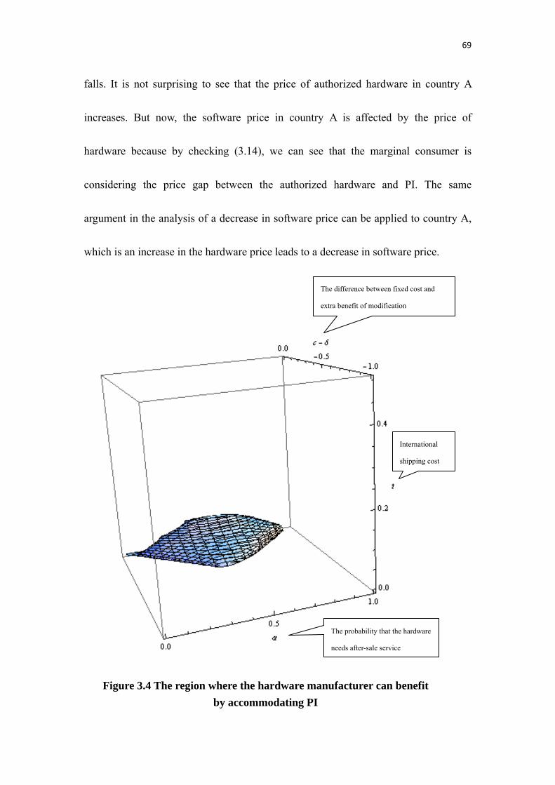
69

falls. It is not surprising to see that the price of authorized hardware in country A

increases. But now, the software price in country A is affected by the price of

hardware because by checking (3.14), we can see that the marginal consumer is

considering the price gap between the authorized hardware and PI. The same

argument in the analysis of a decrease in software price can be applied to country A,

which is an increase in the hardware price leads to a decrease in software price.



International

shipping cost



Figure 3.4 The region where the hardware manufacturer can benefit

by accommodating PI

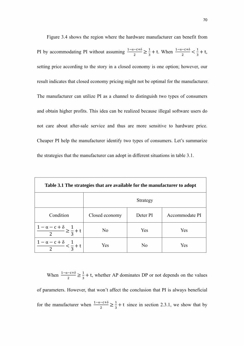
70

Figure 3.4 shows the region where the hardware manufacturer can benefit from

PI by accommodating PI without assuming α δ t. When

α δ t,

setting price according to the story in a closed economy is one option; however, our

result indicates that closed economy pricing might not be optimal for the manufacturer.

The manufacturer can utilize PI as a channel to distinguish two types of consumers

and obtain higher profits. This idea can be realized because illegal software users do

not care about after-sale service and thus are more sensitive to hardware price.

Cheaper PI help the manufacturer identify two types of consumers. Let’s summarize

the strategies that the manufacturer can adopt in different situations in table 3.1.

Table 3.1 The strategies that are available for the manufacturer to adopt

Strategy

Condition Closed economy Deter PI Accommodate PI

1 α c δ

213

t No Yes Yes

1 α c δ

213

t Yes No Yes

When α δ t, whether AP dominates DP or not depends on the values

of parameters. However, that won’t affect the conclusion that PI is always beneficial

for the manufacturer when α δ t since in section 2.3.1, we show that by

71

deterring PI, the manufacturer can always raise the profit. In section 2.3.2, we also

show that when α δ t, in certain circumstances which are demonstrated in

figure 3.4, the manufacturer might earn even higher profit than he could in the closed

economy by encouraging PI. In other words, the manufacturer can adopt a proper

strategy (AP or closed economy pricing) such that his profit is greater or equal to what

he can earn in the closed economy for α δ t . Combining these results

gives proposition 3.

Proposition 3. Parallel imports are never harmful to the hardware manufacturer.

We can then discuss the impact of hardware manufacturer’s second degree price

discrimination behavior on the software provider’s profit. The quantity demanded for

legitimate software in country A is 1 APA

APA

APB δ

α, which is smaller

than the quantity demanded in the closed economy, 1 APA δ

α because

p APA p AP

B 0 in regime 2. In addition, the price of the software in country A also

decreases. The same argument applies to country B. Therefore, the profit of the

software provider will decrease if the hardware manufacturer accommodates PI. This

result is not surprising because the hardware price in regime 2 is higher than that in

regime 1 and thus the software provider’s profit falls given the fact that the hardware

72

and the software are perfect complements.

3. Welfare Analysis

We will first demonstrate a comparison of consumer surplus with and without

software piracy. Then, we will discuss the impact of PI on consumer’s welfare.

3.1 Consumer’s welfare change with software piracy when hardware PI is

prohibited

To compare changes in consumer surplus (CS) due to software piracy, let’s first

calculate the CS in both countries for the benchmark case. i.e. the consumer welfare

when piracy and PI are not available.

CSNNA CSNN

B v13

13

dv1

18 3.16

where the subscript NN denotes “No piracy” and “No PI”.

If there is illegal software copy in country A, the welfare in country A becomes

CSPNA 1 α v p PN

A c δ dv v p PNA p PN

A dv 3.17

where

73

v

α c δ2 c δ

α, v

1 α c δ2 c δ

1 α,

p PNA 1 α c δ

2, p PN

A α c δ

2

where the subscript PN denotes “Piracy” and “No PI”.

Let the consumer’s welfare change in country A be ∆CSPNA CSPN

A CSNNA . We

can verify that the consumer’s surplus will increase by checking figure 3.5. From the

graph, we see ∆CSPNA is always positive on the same domain of figure 3.1 suggesting

that consumers are always better off when software piracy exists. In section 2.2, we

have explained that both firms might be better off due to piracy in certain

circumstances. (i.e. the medium dark area in figure 3.1.) Combining the results in

section 2.2 and the present section, we can say that software piracy could be Pareto

improving. Lemma 1 summarizes this finding.

Lemma 1. If hardware parallel importation is not permitted, the existence of software

piracy might be Pareto improving.

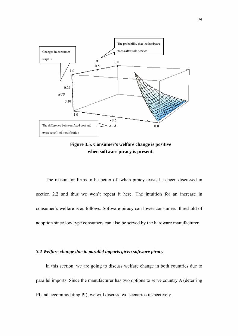
74

The reason for firms to be better off when piracy exists has been discussed in

section 2.2 and thus we won’t repeat it here. The intuition for an increase in

consumer’s welfare is as follows. Software piracy can lower consumers’ threshold of

adoption since low type consumers can also be served by the hardware manufacturer.

3.2 Welfare change due to parallel imports given software piracy

In this section, we are going to discuss welfare change in both countries due to

parallel imports. Since the manufacturer has two options to serve country A (deterring

PI and accommodating PI), we will discuss two scenarios respectively.

Changes in consumer

surplus





Figure 3.5. Consumer’s welfare change is positive

when software piracy is present.

75

Scenario 1: Deterring PI

Let the consumer’s surplus in country A and B when the manufacturer deters PI

be

CSDPA 1 α v p DP

A c δ dvDP

DPv p DP

A p DPA dv

DP 3.18

CSDPB 1 p DP

B p DPB dv

DPB

DPB

3.19

where vDPα δ

δ

α , vDP

α δα

δ

α, p DP

A α δ,

p DPA α δ

αt, p DP

B α δ

α and p DP

B δ

α

The consumer’s welfare change due to PI in country A is now ∆CSDPA CSDP

A

CSPNA . We can conclude that if deterring PI is the manufacturer’s best response,

consumer’s surplus in country A will increase for sure. This result is not surprising. If,

in equilibrium, the manufacturer chooses to deter PI, he needs to cut the hardware

price in the PI recipient country. In addition, the software provider will not change his

pricing behavior because v does not change. In other words, the marginal consumer

who is indifferent between official games and pirated games will not change his/her

decision since for the marginal consumer, playing official games is still as appealing

as playing pirated games even though we have a decrease of the hardware price.

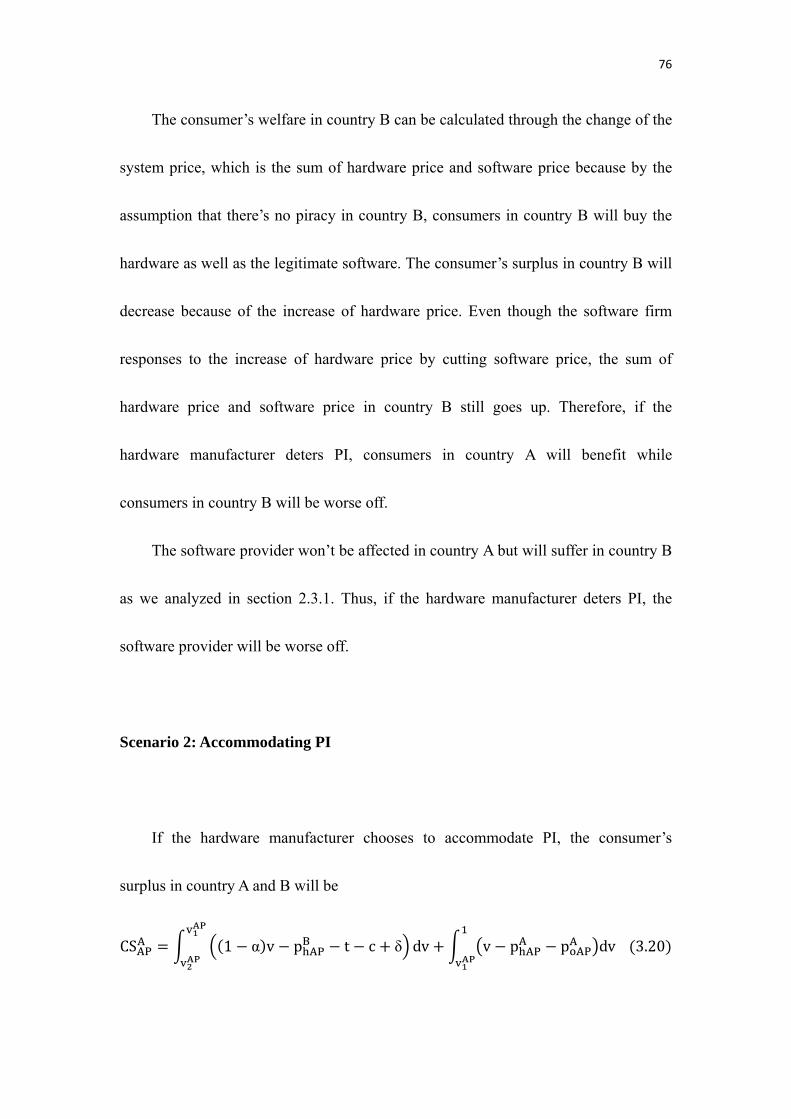
76

The consumer’s welfare in country B can be calculated through the change of the

system price, which is the sum of hardware price and software price because by the

assumption that there’s no piracy in country B, consumers in country B will buy the

hardware as well as the legitimate software. The consumer’s surplus in country B will

decrease because of the increase of hardware price. Even though the software firm

responses to the increase of hardware price by cutting software price, the sum of

hardware price and software price in country B still goes up. Therefore, if the

hardware manufacturer deters PI, consumers in country A will benefit while

consumers in country B will be worse off.

The software provider won’t be affected in country A but will suffer in country B

as we analyzed in section 2.3.1. Thus, if the hardware manufacturer deters PI, the

software provider will be worse off.

Scenario 2: Accommodating PI

If the hardware manufacturer chooses to accommodate PI, the consumer’s

surplus in country A and B will be

CSAPA 1 α v p AP

B t c δ dvAP

APv p AP

A p APA dv

AP 3.20

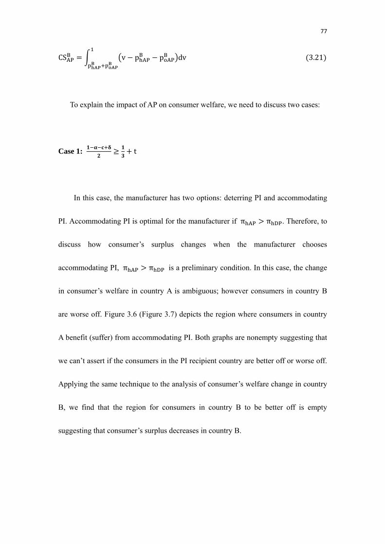
77

CSAPB v p AP

B p APB dv

APB

APB

3.21

To explain the impact of AP on consumer welfare, we need to discuss two cases:

Case 1: t

In this case, the manufacturer has two options: deterring PI and accommodating

PI. Accommodating PI is optimal for the manufacturer if π AP π DP. Therefore, to

discuss how consumer’s surplus changes when the manufacturer chooses

accommodating PI, π AP π DP is a preliminary condition. In this case, the change

in consumer’s welfare in country A is ambiguous; however consumers in country B

are worse off. Figure 3.6 (Figure 3.7) depicts the region where consumers in country

A benefit (suffer) from accommodating PI. Both graphs are nonempty suggesting that

we can’t assert if the consumers in the PI recipient country are better off or worse off.

Applying the same technique to the analysis of consumer’s welfare change in country

B, we find that the region for consumers in country B to be better off is empty

suggesting that consumer’s surplus decreases in country B.

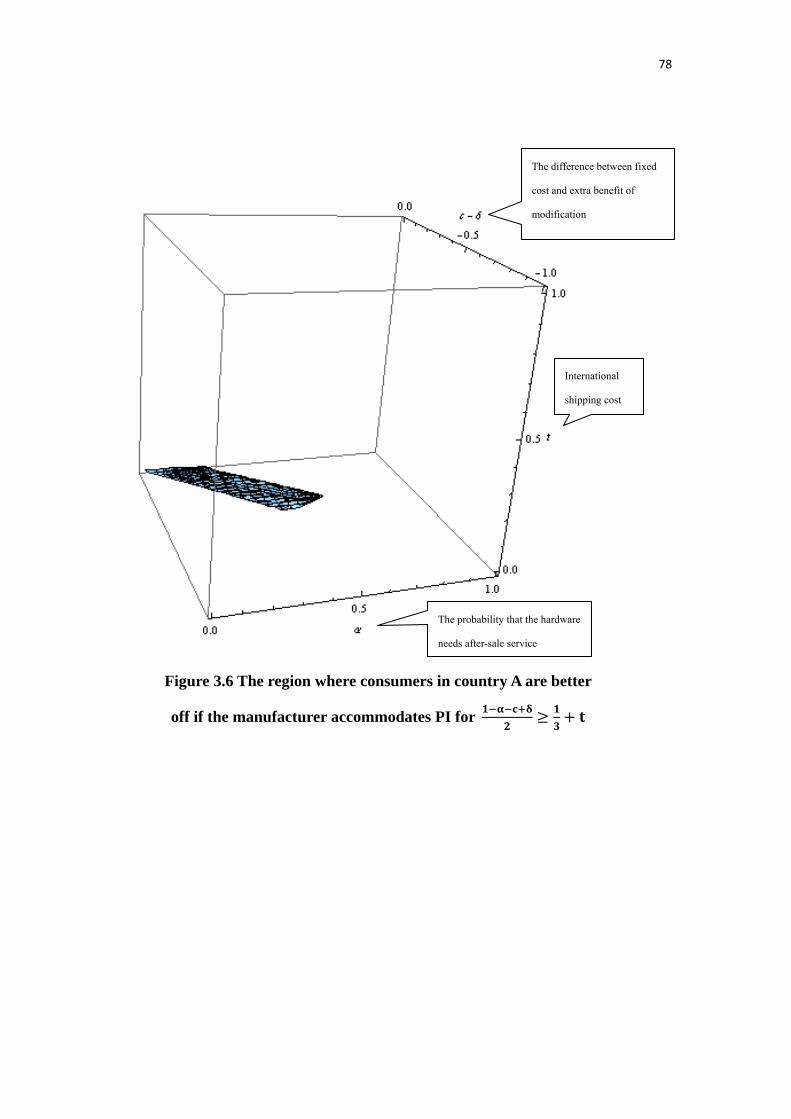
78

The difference between fixed

cost and extra benefit of

modification

International

shipping cost



Figure 3.6 The region where consumers in country A are better

off if the manufacturer accommodates PI for

79

Case 2:

The manufacturer will choose either closed economy pricing or accommodating

PI. If accommodating PI is the manufacturer’s best choice, then the consumers in the

PI recipient country will be worse off since the region where π AP π PN and

International

shipping cost



The difference between

fixed cost and extra benefit of

modification

Figure 3.7 The region where consumers in country A are worse

off if the manufacturer accommodates PI for

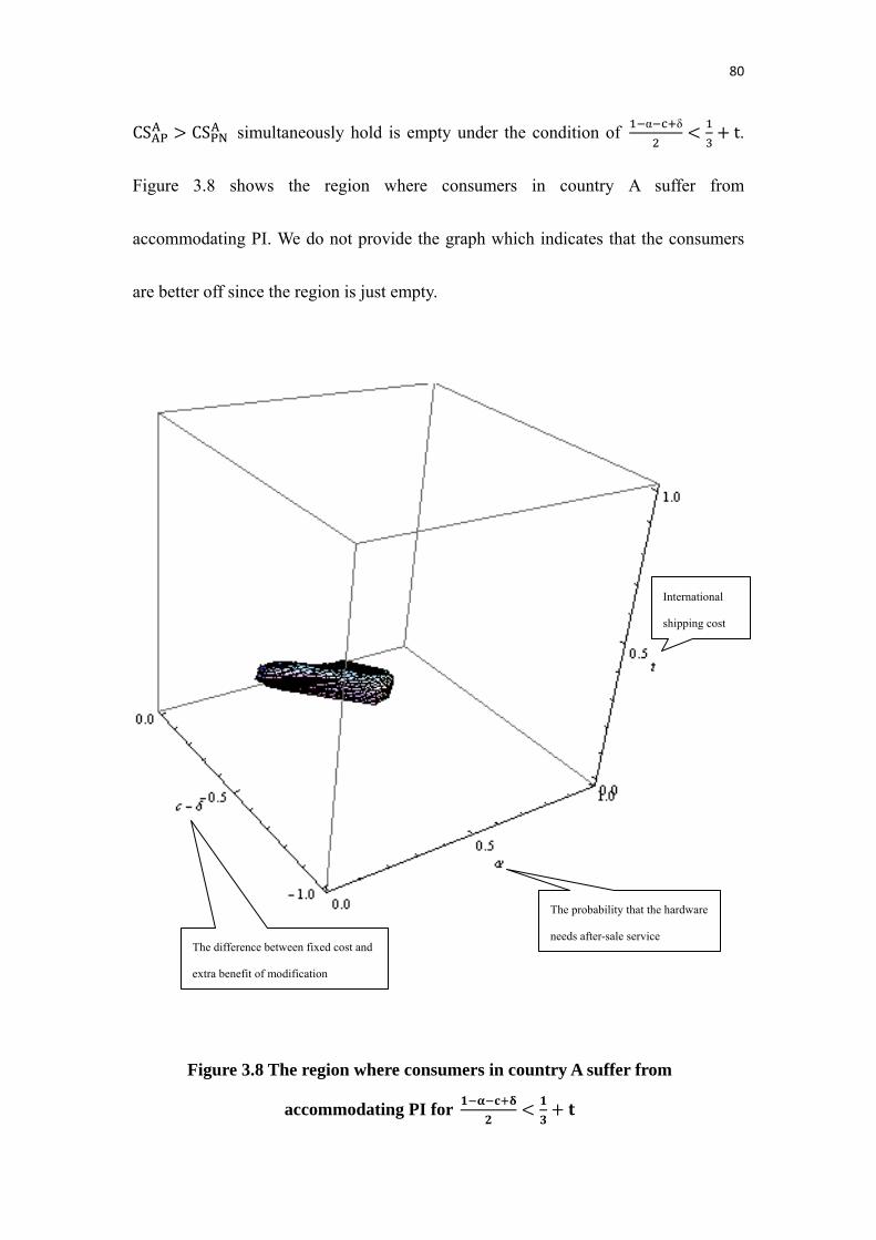
80

CSAPA CSPN

A simultaneously hold is empty under the condition of α δ t.

Figure 3.8 shows the region where consumers in country A suffer from

accommodating PI. We do not provide the graph which indicates that the consumers

are better off since the region is just empty.



International

shipping cost



Figure 3.8 The region where consumers in country A suffer from

accommodating PI for

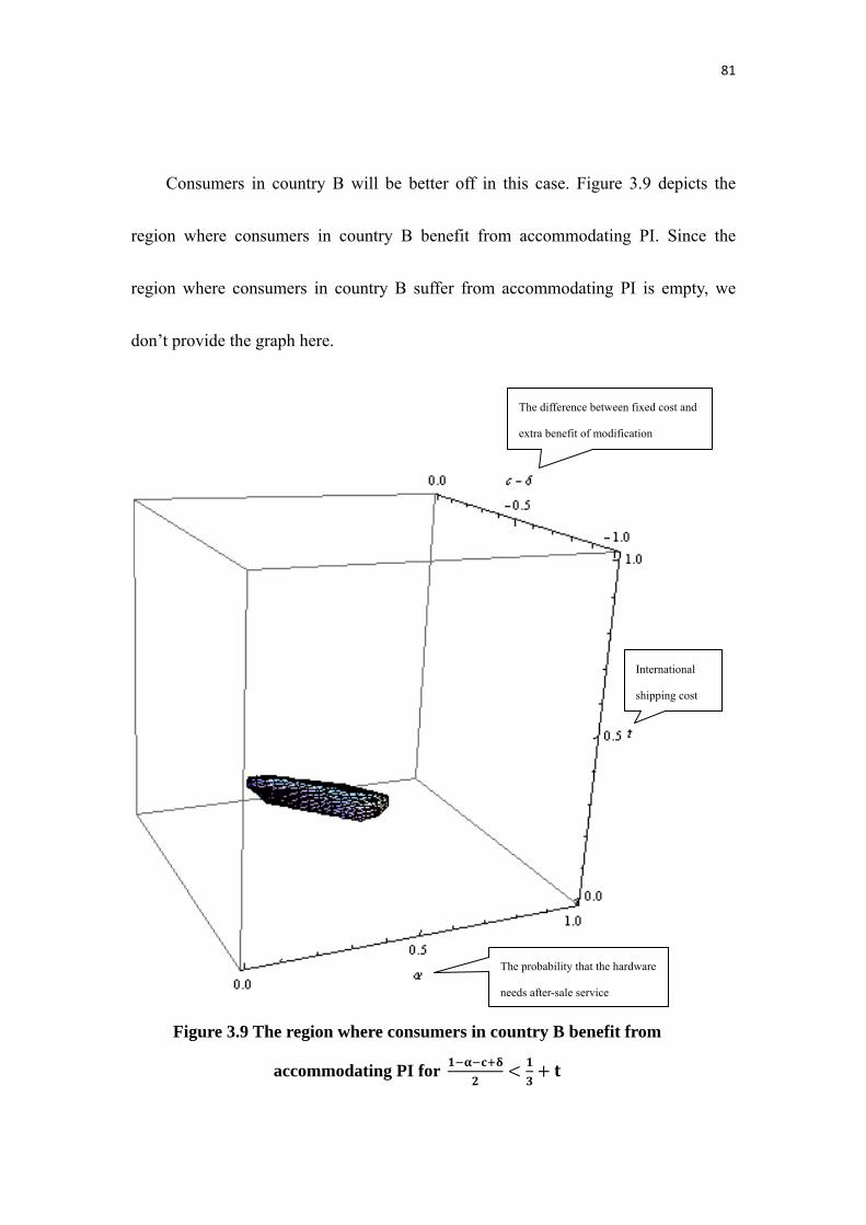
81

Consumers in country B will be better off in this case. Figure 3.9 depicts the

region where consumers in country B benefit from accommodating PI. Since the

region where consumers in country B suffer from accommodating PI is empty, we

don’t provide the graph here.



International

shipping cost



Figure 3.9 The region where consumers in country B benefit from

accommodating PI for

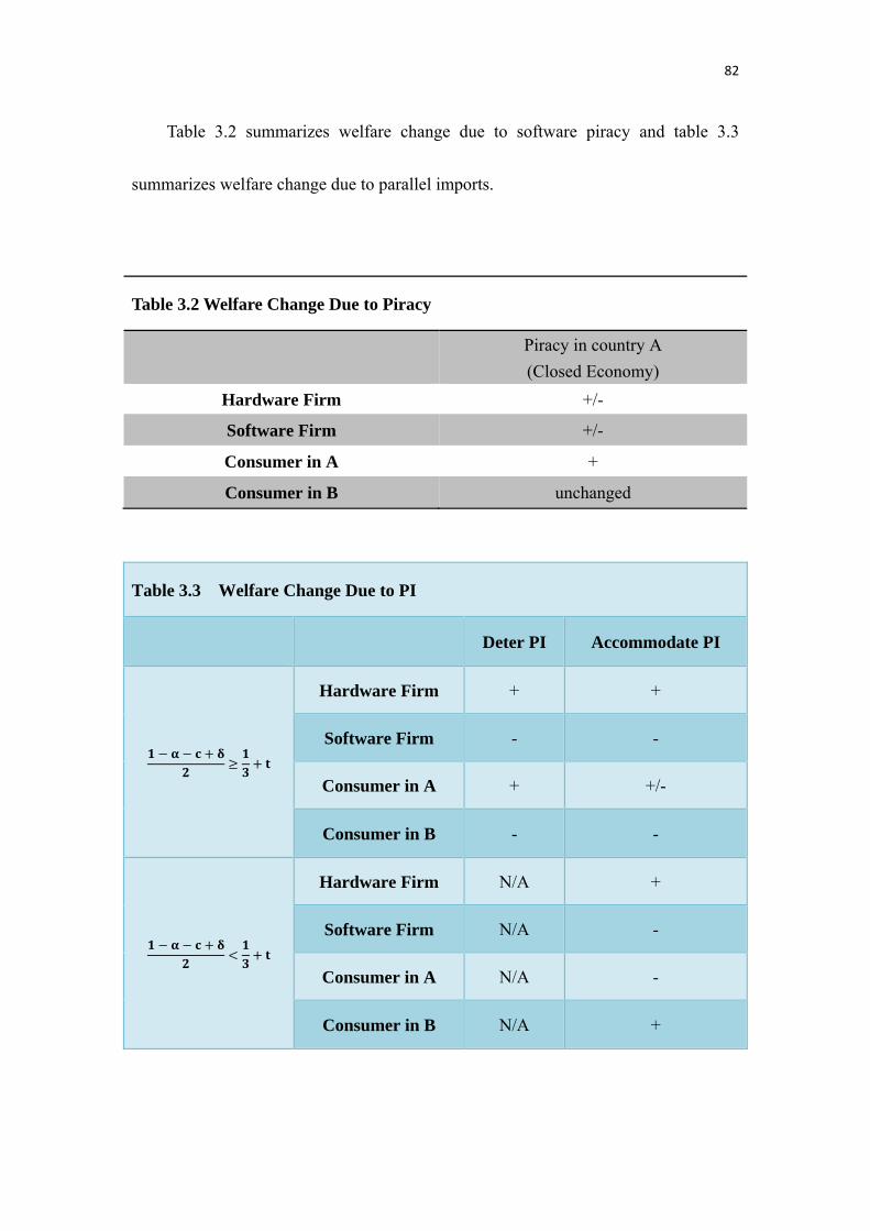
82

Table 3.2 summarizes welfare change due to software piracy and table 3.3

summarizes welfare change due to parallel imports.

Table 3.2 Welfare Change Due to Piracy

Piracy in country A

(Closed Economy)

Hardware Firm +/-

Software Firm +/-

Consumer in A +

Consumer in B unchanged

Table 3.3 Welfare Change Due to PI

Deter PI Accommodate PI

Hardware Firm + +

Software Firm - -

Consumer in A + +/-

Consumer in B - -

Hardware Firm N/A +

Software Firm N/A -

Consumer in A N/A -

Consumer in B N/A +

83

In this section, I demonstrate welfare implication of PI. It should be noted that

unlike piracy which creates extra demand for hardware, the way for the hardware

manufacturer to benefit from PI is to extract profits from the software firm. When

closed-economy hardware price in country A is higher than the sum of retail price in

country B and international shipping cost, the hardware manufacturer can respond to

the price gap either by deterring PI or by accommodating PI. On the other hand,

deterring PI is not applicable for the case where closed-economy hardware price in

country A is lower than the sum of retail price in country B and international shipping

cost. Deterring PI is beneficial for the hardware manufacturer since parallel trade

from country B to country A is now a commitment device for the hardware

manufacturer to raise the price in country B allowing the hardware firm to extract

profits from the software firm in country B. Moreover, the hardware manufacturer can

utilize PI as a channel to distinguish high type and low type consumers to earn even

more profits. In other words, for certain circumstances, the hardware manufacturer

may find it profitable to serve country A by both authorized products and PI.

Authorized product buyers in country A are charged at a higher price while pirated

game players are charged at a lower price. Since the price of authorized hardware

increases in this case, the price of legitimate software in country A must decrease, and

thus the software firm will suffer if the hardware firm chooses to accommodate PI.

84

Consumer’s welfare implication is also intuitive. Deterring PI lowers the hardware

price in country A suggesting that the consumers in country A are better off; while

consumers in the parallel exporting country will be worse off due to price

convergence between two countries as stated in Malueg and Schwartz (1994).

The welfare implication of accommodating PI is as follows. If the hardware

manufacturer accommodates PI to realize second price discrimination, the profits of

the software firm are further extracted by the hardware firm due to an increase in

hardware price in both countries. Hence, accommodating PI is harmful for the

software firm. As for consumer’s welfare, the impact of accommodating PI on

consumer’s welfare depends on the autarky price of the hardware. As stated in the

economic textbook, cēterīs paribus, price discrimination is harmful for consumers.

When the closed-economy hardware price in country A is high, allowing PI is

generally beneficial for consumers in country A; however, the benefits could be

eroded if the hardware firm chooses to utilize PI as the channel to achieve price

discrimination. Therefore, when the autarky hardware price in country A is high, the

impact of accommodating PI on consumer’s welfare in country A is ambiguous. On

the other hand, when the autarky hardware price in country A is low, consumers in

country A can’t obtain any benefits from an open policy but need to bear the welfare

loss due to price discrimination. Hence, consumers in country A are worse off in the

85

case of accommodating PI when the autarky hardware price in country A is low.

We can apply the same argument to explain the consumer’s welfare change in

country B in the case of accommodating PI. It should be noted that when the autarky

hardware price in country A is low, parallel trade will occur only in the form of

accommodating PI. To make PI possible, the hardware manufacturer needs to reduce

the price in country B from 1/3 to a lower level in order to attract low type consumers

in country A. Therefore, if the autarky hardware price in country A is low and

accommodating PI is the equilibrium, consumers in country B will be better off.

4. Region-free Hardware

If the hardware is region-free, the PI recipient country could be country A or

country B. Suppose that country A is the PI recipient country, the claim that all

consumers who purchase PI hardware will pirate the software still holds. The reason

is as follows. Since the manufacturer does not provide after-sale service to a PI buyer,

an official game player who purchases PI hardware has a surplus of 1 α v pB

t pA, which is smaller than 1 α v pB t c δ given the fact that c pA

and δ 0. Therefore, if country A is the PI recipient country, the result won’t change

even though the hardware is region-free.

However, is it possible for country B to be the PI recipient country when the

86

hardware is region-free? Our model shows that country B can’t be the PI recipient

country. First, we will claim that serving country B only by authorized products

(deterring PI) is not feasible by simple steps. Let vB be the valuation of the marginal

consumer who is indifferent between authorized hardware and PI in country B. vB

must satisfy vB pB pB 1 α vB pA t pB and is equal to pB

pA t . Similarly, let vB be the valuation of the marginal consumer who is

indifferent between PI and no adoption. We have vB pA t pB . Since

vB vB , we have pB pA t pA t pB . Solving this inequality

implies pB pA t pB pB . However, deterring PI implies that pB

pA t , which is a contradiction to pB pA t pB pB 0 given

positive prices assumptions.

We have shown that pB pA t does not hold, but on the other hand, in

equilibrium, can we have pB pA t , which is the case that the manufacturer

serves country B by both authorized products and PI simultaneously? Our work in the

appendix A3 proves that this is still infeasible for the manufacturer. In summary, even

though the hardware is region free, it is still a one-way PI outcome from country B to

country A.

This result can explain why Sony and Microsoft make their new game console

region-free. As stated above, embedding a region code on the hardware is redundant

87

since the region code does not play any role. Parallel trade occurs from country B to

country A no matter whether there is region code or not.

5. Discussion and Conclusions

We analyze the impact of outlaw innovations on the video game market. We

obtain three results that are different from general expectation. Firstly, we discuss the

existence of software piracy in a closed economy. Our benchmark model indicates

that the hardware manufacturer may benefit from piracy as expected by most people.

However, we also find that software piracy may also be beneficial to the software

provider. Secondly, we extend our closed-economy model to a two-country model

where the modification chips are available in one country but are unavailable in the

other. We show that the existence of hardware parallel imports is beneficial to the

hardware manufacturer but is harmful to the software provider. Thirdly, our welfare

analysis shows that the consumers in the PI recipient country are not necessarily

better off. If the hardware manufacturer deters PI, consumers in the PI recipient

country will benefit as expected. However, if the hardware provider chooses to serve

the country by both authorized products and parallel imports, PI provide the

manufacturer a key to second-degree price discriminating the consumers in the PI

recipient country. In this case, consumers in the PI recipient country may be worse

88

off.

This paper considers a non-cooperative game; however, some may argue that it is

possible for both software and hardware firms to cooperate and offer a bundle of

hardware and software to prevent piracy. In appendix A4, it is shown that there does

not exist a way to distribute the joint profit such that both firms are willing to join the

coalition. Consequently, bundling won’t be utilized to prevent piracy.

It should be noted that our results base on the assumption that both the hardware

manufacturer and the software provider are monopoly. If there are two or more firms

who produce homogeneous products in the market, price competition leads to zero

profits. If firms are differentiated vertically, it will be difficult to set up consumers’

preference order. For example, if authorized product i is superior to authorized

product j, then whether PI of ith product are inferior to jth authorized products or not

is crucial for the analysis. Unfortunately, we do not have a judgment on preference

order. As the number of firms increases, it becomes too complicated to analyze.

Therefore, we assume one hardware manufacturer and one software provider in the

model. Although this assumption is somewhat strong, it is still acceptable since in the

realistic world, different brands of game consoles or software are reasonably

differentiated in several dimensions, and thus firms have market power even though

the inverse demand will become flatter due to competition. Hence, our analysis may

89

still work for explaining the change in region-code strategy adopted by the hardware

manufacturer.

The result of the model suggests that piracy is welfare improving for consumers.

However, this result could only be true in a static model. In the present model, we

show that piracy could sometimes be beneficial for the software provider; however, it

is more common to see that the software firm suffers from piracy. In a dynamic model,

even though consumers can be better off due to software piracy in the short run,

piracy would be harmful for the software firm’s investment incentive in quality

improvement or development of new software. As a consequence, with software

piracy, the consumer’s welfare would decrease in the long run.

As aforementioned, we adopt horizontal retail price arbitrage framework in our

analysis. Parallel to the case of accommodating PI, applying our idea to vertical price

control framework, we expect that the manufacturer will charge a higher wholesale

price in country A and a lower wholesale price in country B to encourage PI and get

benefits from price discrimination. Although we do not provide vertical price control

model in the present paper, it will be interesting for future analysis. In addition, in this

model, we assume the utility discount factor 1 α to be exogenous. Since α can

be interpreted as the probability that a consumer needs after-sale service for the

hardware, for future research, it would be interesting to endogenize this parameter.

90

Appendix

A1. The derivation of c

v PNA δ

α

α δδ

α and v PN

A δα δ

δ

. Since v v , we have . This inequality is equivalent to

0. Since α 0,1 , the inequality can be reduced to

c δ 1 α α c δ 0, which is the inequality c .

A2. The derivation of (3.14)

UAv pA pA

1 α v pB t c δ0

; UB v pB pB

0

For simplicity, we ignore the subscript AP. A consumer with valuation v in country

A is indifferent between legitimate software and illegal software if v pA pA

1 α v pB t c δ . Solving for v , we can say that consumers with

v v OA A B δ

α will purchase the authorized hardware and official

software. Similarly, A consumer with valuation v in country A will be indifferent

between illegal software and no adoption if 1 α v pB t c δ 0. Thus,

vB δ

α. Consumers with valuation between v and v will purchase the PI

hardware. The quantity demanded for the authorized hardware in country A can be

calculated by 1dx 1 OA A B δ

α, while the quantity demanded for the PI

91

hardware is 1dx OA A B δ

α

B δ

α. Therefore, the profit of the

hardware manufacturer is the sum of profit from authorized channels in both countries

and the profit from PI. The profit from authorized channel in country B is shown in

the benchmark, which is equal to pB 1 pB pB . The profit from authorized

channel in country A ispA 1 OA A B δ

α. The profit generated from PI is

pB OA A B δ

α

B δ

α. Summing these terms up leads to (3.14).

A3. Country B won’t be the PI recipient country.

Suppose that country B is the PI recipient country. The quantity demanded for the

authorized hardware is 1dxB 1B A

. Similarly, the quantity demanded for

the PI hardware can be represented by 1dxB

B

B A A B

. Since all

buyers in country B purchase legitimate software, the quantity demanded for the

software is 1dxB 1A B

.

The manufacturer faces the following profit maximization problem:

maxA B,

πRF pB 1pB pA t

αpA pB pA t

αpA t pB

1 α

pA 1pA c δ

1 α

92

where the superscript RF indicates region free. The first term is the profit from selling

authorized products in country B. The second term is the profit from PI while the third

term is the profit of authorized products in country A. The software provider’s profit

maximization problem is now

maxA, B

πRF pB 1pA t pB

1 α pA 1

pA c δα

The first (second) term is the profit from country B (country A).

Solving 4 first order conditions with respect to pA, pB, pA, and pB implies:

pA , pB , pA , and pB

Substituting pA , pB , pA , and pB into vB and vB and imposing the assumption

that vB vB , we have vBB A

vB

A B

. Since α 0,1 and t 0 , solving the

inequality yields c δ 0 . This contradicts to the result that

c δ 0, which has been proven in A1.

A4. Bundling won’t be utilized to prevent piracy

When both firms cooperate and offer a bundle of hardware and software, the

equilibrium price of the bundle can be derived by solving the following profit

93

maximization problem:

max πBU p p 1 p

The equilibrium price of the bundle is and joint profit is . Let s 0,1 be the

fraction of the joint profit that goes to the hardware manufacturer. When piracy exists,

the hardware manufacturer would prefer to cooperate with the software firm if

α δ

α. Similarly, the software firm would prefer to offer a bundle by

cooperating with the hardware firm if α δ

α. Given α and c δ), if we can

find an s such that both inequalities hold, then cooperation can be the equilibrium. In

other words, by definition of the core of a coalition game, the core is nonempty if

α δ

α and

α δ

α simultaneously hold. Accordingly, the core is

nonempty if α δ

α1 α δ

α. However, this double inequality never

holds since 1 α δ

α

α δ

α

δ

α α0 for α 0,1 , which is a

contradiction to the condition for the core to exist. In other words, with

aforementioned restrictions on parameters, the set α, c δ, s | α δ

α

α δ

α is empty suggesting that it is impossible to find a method to

distribute the joint profit such that both firms agree to join the coalition and thus

bundling won’t be adopted to prevent piracy.

94

CHAPTER IV

MODES OF FOREIGN DIRECT INVESTMENT AND INTELLECTUAL PROPERTY RIGHTS PROTECTION:

WHOLLY-OWNED OR JOINT VENTURE? FIRM-LEVEL EVIDENCE FROM TAIWANESE MULTINATIONAL MANUFACTURING

ENTERPRISES

1. Introduction

Intellectual property rights (IPRs) protection has been considered as an important

factor for international trade and foreign direct investment (FDI). How IPR protection

affects international trade flows is still ambiguous. On one hand, some people believe

that IPR protection can stimulate international trade flows due to the market

expansion hypothesis, which claims that strengthening IPR may reduce imitation in

the importing country and thus will encourage the IPR holder to export more. On the

other hand, IPR protection may have negative effects on trade volume because of the

market power effect and FDI. The market power hypothesis focuses on the IPR

holder’s market power and claims that stronger IPR protection offers the IPR holder

monopoly power and therefore it reduces volume of imports in the importing country.

IPR protection may also be negatively correlated with trade volume because as IPR

protection becomes sufficiently strong, IPR holders are more willing to substitute

exporting by FDI. However, a very strong IPR system may also deter FDI since

licensing would be a good alternative to FDI. Maskus (1998) finds that FDI is

95

sensitive to IPR protection. He uses U.S. annual data from 1989 to 1992 to show that

by holding other things equal, if the extent of patent protection rises by 1 percent in

the FDI recipient country, the stock of U.S. investment in that country increases by

0.45 percent. Nicholson (2007) employs U.S data in 1995 and find evidence to

support that stronger IPR leads to an increase in both FDI and licensing. Smith (2001)

also finds that sales of U.S. affiliates and the strength of IPR protection in the host

country are positively correlated. However, other studies such as Ferrantino (1993),

Mansfield (1993), Maskus and Konan (1994) and Primo Braga and Fink (2000) do not

find statistically significant evidence to support that argument. Thus, the overall

relationship between IPR protection and FDI remains ambiguous.

If we take a closer look at composition of FDI, IPR protection in the FDI host

country plays a significant role for the MNEs on whether to invest in wholly owned

subsidiaries or to enter joint ventures. Exploring the impact of IPR on FDI

composition is interesting because it has important policy implications for developing

countries. It is widely believed that joint ventures result in more technology spillovers

to the host country than wholly owned subsidiaries do. Javorcik (2004a) and Javorcik

and Spatareanu (2008) employ Lithuanian and Romanian data respectively to show

that local participation plays an important role on technology spillovers from foreign

direct investment. Maskus (1998) argues that to prevent its know-how from leakage to

96

a Southern firm, the IPR holder will engage in greenfield FDI if the host country has

weak enforcement on IPR protection. Leahy and Naghavi (2010) develop a theoretical

model to support this argument. They show that joint venture is the equilibrium

market structure when IPR protection is stringent. Lee and Mansfield (1996) provide

evidence from U.S. firms to show that a country’s system of IPR protection influences

the volume and composition of FDI. They use data collected from almost 100 U.S.

firms and conclude that stronger IPR protection in the host country has a positive

effect on FDI volume. As for composition of FDI, they investigate data from 14 major

U.S. chemical firms and find that MNEs tend to invest in wholly-owned subsidiaries

if IPR protection is weaker in the host country. Javorcik (2004b) is another empirical

study related to composition of FDI. She uses a unique data set collected from Eastern

Europe and the former Soviet Union and finds that investors are more likely to engage

in projects focusing on distribution rather than local production if the IPR protection

is weak in the host country. These studies suggest that IPR protection in the host

country is a significant determinant for FDI volume and composition.

The deregulation of developing countries’ policy for inward FDI provides us a

rationale to discuss the impact of IPR regime on MNE’s choice of ownership structure

in the host country. So far, Agreement on Trade-Related Investment Measures (TRIMs)

does not impose any restrictions on local equity requirement. However, since FDI has

97

been considered as an important channel for developing countries to absorb new

technology, many developing countries deregulate their inward FDI restrictions. For

example, Thailand has no restrictions on local equity requirement in principle, except

for certain industries. For these industries, foreign firms still can apply for the

approval by Board of Investment (BOI) to bypass local equity requirement. In

Indonesia, the government imposed two restrictions before 1999. They were: first, the

foreign firm’s equity share is not allowed to exceed 95% in a joint venture with a local

firm. Second, a wholly owned foreign subsidiary must be transferred to a local firm

within 15 years. However, both policies have been cancelled in 1999. The Republic

of Philippines has similar policy with Thailand. The Philippines government allows

foreign firms to hold 100% equity share in principle, except for some specific

industries. In Malaysia, 100% foreign ownership is permitted with some restrictions

according to The Promotion of Investment Act of 1986. In 1998, regulation for

foreign ownership of manufacturing industries is further relaxed. However, certain

industries, such as paper, steel, printing, etc. are still under regulation. For China, let’s

look at the summary provided by The US-China Business Council (USCBC, 2009):

“On Nov. 7, 2007 the PRC National Development and Reform Commission (NDRC)

and Ministry of Commerce (NOFCOM) jointly issued the most recent version of the

Catalogue Guiding Foreign Investment in Industry. The catalogue is long-standing

tool that PRC policymakers have used to manage and direct foreign investment.

98

Similar to the 2002 and 2004 editions, the 2007 catalogue divides industries into

three basic categories: encouraged, restricted and prohibited. Industries not listed in

the catalogue are generally open to foreign investment unless specifically barred in

other PRC regulations. FIEs in encouraged industries are often permitted to establish

wholly foreign-owned enterprises (WFOEs). They are also generally eligible for

investment incentives, although China is currently adjusting many preferential

policies for foreign investment, particularly tax-related policies. Industries in the

restricted category may be limited to equity or contractual joint ventures, in some

cases with the Chinese partner as the majority shareholder. Restricted category

projects are also subject to higher government approvals. Industries in the prohibited

section are closed to foreign investment.”

USCBC also indicates that the number of items listed in the encouraged or

permitted categories is far larger than the number in restricted and prohibited

categories. The relaxing of local equity requirement for most industries in developing

countries provides most Taiwanese MNEs freedom of choosing their ownership

structure. And thus, we can further explore how IPR regime affects the ownership

structure.

Empirical studies that discuss the relationship between IPR protection and

structures of foreign subsidiary ownership are surprisingly sparse. Javorcik and Saggi

(2010) empirically test the relationship between technological asymmetry and entry

mode of foreign investors. They find that foreign investors with more sophisticated

technologies are less likely to choose joint ventures. However, they do not find

evidence of IPR strength affecting the choice of entry mode by investigating the data

from East European countries. Our study is another one that contributes to this topic.

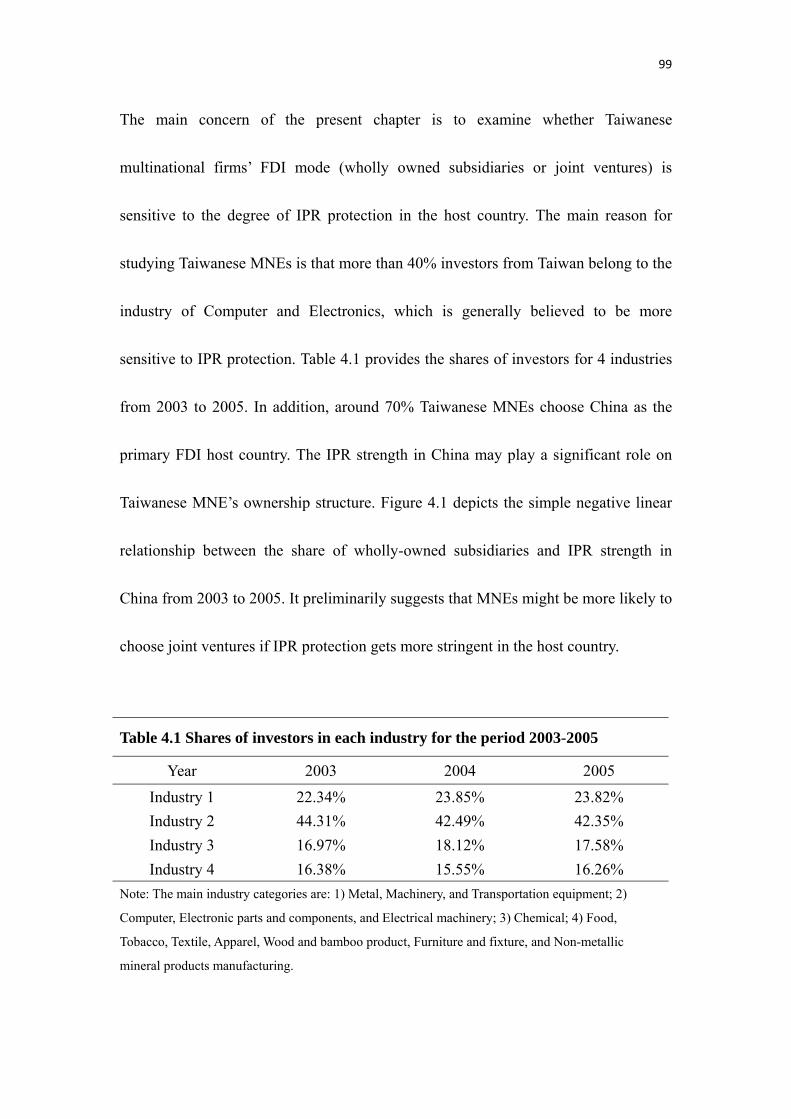
99

The main concern of the present chapter is to examine whether Taiwanese

multinational firms’ FDI mode (wholly owned subsidiaries or joint ventures) is

sensitive to the degree of IPR protection in the host country. The main reason for

studying Taiwanese MNEs is that more than 40% investors from Taiwan belong to the

industry of Computer and Electronics, which is generally believed to be more

sensitive to IPR protection. Table 4.1 provides the shares of investors for 4 industries

from 2003 to 2005. In addition, around 70% Taiwanese MNEs choose China as the

primary FDI host country. The IPR strength in China may play a significant role on

Taiwanese MNE’s ownership structure. Figure 4.1 depicts the simple negative linear

relationship between the share of wholly-owned subsidiaries and IPR strength in

China from 2003 to 2005. It preliminarily suggests that MNEs might be more likely to

choose joint ventures if IPR protection gets more stringent in the host country.

Table 4.1 Shares of investors in each industry for the period 2003-2005

Year 2003 2004 2005

Industry 1 22.34% 23.85% 23.82%

Industry 2 44.31% 42.49% 42.35%

Industry 3 16.97% 18.12% 17.58%

Industry 4 16.38% 15.55% 16.26%

Note: The main industry categories are: 1) Metal, Machinery, and Transportation equipment; 2)

Computer, Electronic parts and components, and Electrical machinery; 3) Chemical; 4) Food,

Tobacco, Textile, Apparel, Wood and bamboo product, Furniture and fixture, and Non-metallic

mineral products manufacturing.

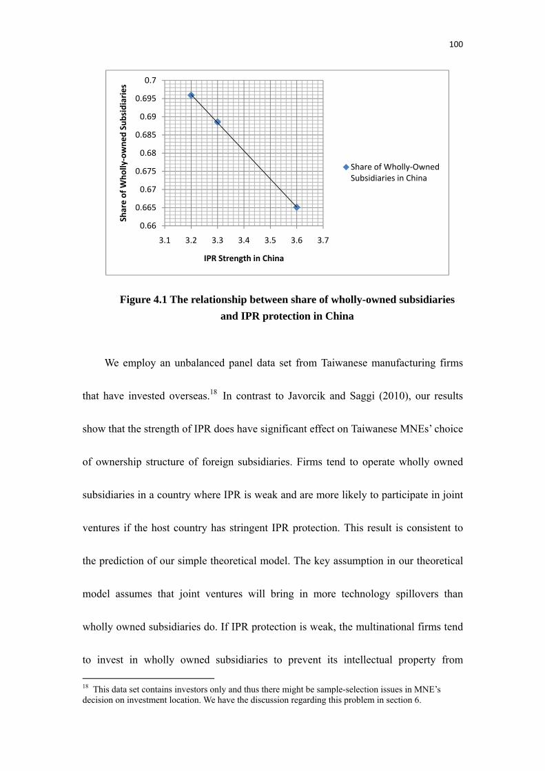
100

We employ an unbalanced panel data set from Taiwanese manufacturing firms

that have invested overseas.18 In contrast to Javorcik and Saggi (2010), our results

show that the strength of IPR does have significant effect on Taiwanese MNEs’ choice

of ownership structure of foreign subsidiaries. Firms tend to operate wholly owned

subsidiaries in a country where IPR is weak and are more likely to participate in joint

ventures if the host country has stringent IPR protection. This result is consistent to

the prediction of our simple theoretical model. The key assumption in our theoretical

model assumes that joint ventures will bring in more technology spillovers than

wholly owned subsidiaries do. If IPR protection is weak, the multinational firms tend

to invest in wholly owned subsidiaries to prevent its intellectual property from

18 This data set contains investors only and thus there might be sample-selection issues in MNE’s decision on investment location. We have the discussion regarding this problem in section 6.

0.66

0.665

0.67

0.675

0.68

0.685

0.69

0.695

0.7

3.1 3.2 3.3 3.4 3.5 3.6 3.7

Share of Wholly‐owned Subsidiaries

IPR Strength in China

Share of Wholly‐Owned Subsidiaries in China

Figure 4.1 The relationship between share of wholly-owned subsidiaries

and IPR protection in China

101

leakage to a local firm. If IPR protection is sufficiently strong, the MNEs are more

likely to participate in joint ventures to take the advantage of avoiding fixed cost for

production in the local market and reducing the degree of competition by cooperating

with a local firm.

This chapter is organized as follows. Section 2 provides the theoretical

consideration of our empirical work. The econometric specification and the data are

described in section 3. Section 4 demonstrates econometric approaches and concerns.

The empirical results are discussed in section 5. Section 6 provides another empirical

test and section 7 concludes.

2. Theoretical Consideration

Let’s consider a model that is similar to the framework in Leahy and Naghavi

(2010). Introducing the theoretical consideration is helpful for understanding which

variables are going to be included in the regression as well as expecting the direction

of effects of the variables. Assume that there are N identical local firms in the host

country competing in quantity with the MNE. The MNE has the same size with the

local firms but with superior technology by engaging in cost-reducing R&D. The

MNE can invest in the host country either by wholly-owned subsidiaries or by joint

ventures. If the MNE invests in wholly-owned subsidiaries, it has to produce products

102

by incurring fixed cost F. On the other hand, the MNE can avoid the fixed cost by

entering a joint venture with an existing local firm19. If the MNE chooses to operate a

wholly-owned subsidiary, its profit is

πW p M, QW, ∑ qN c T, SW μ, ι QW C T, η QW F (4.1)

The MNE’s profit when entering by joint ventures becomes

πJ p M, QJ, ∑ qN c T, SJ μ, ι QJ C T, η QJ δ (4.2)

where the subscript W and J denote wholly-owned subsidiaries and joint ventures

respectively. 20

p is the inverse demand function faced by the MNE and the local firms. Let M be

the market size and Q denote quantity demanded for the MNE in the host country.

q · is the quantity demanded for local firm i. Without loss of generality, we assume

that the Nth local firm is the partner if joint venture is the equilibrium outcome. T

19 There might also exist some fixed cost for joint venture; however, it is generally small and can be ignored. 20 We assume that there are fewer competitors in the market if an MNE chooses joint venture. If an MNE acquires a local firm, the advantage of reducing number of competitors in joint venture might be offset. However, we exclude the possibility of an MNE acquiring a local firm in the theoretical model since from our data, we can only know the ownership structure but do not have any information regarding acquisition. Nevertheless, number of competitors should still be (weakly) smaller in joint ventures.

103

measures the MNE’s technology intensity, which can be approximated by investment

in R&D. The higher T is, the lower marginal cost will be. η denotes the price of

production factors, such as labor cost in the host country. The technology spillover

function S μ, ι 0 which is determined by two factors measures how much

knowledge developed by the MNE unintentionally transfers to the local firms. A

higher S leads to a smaller cost difference between the MNE and local firms since the

marginal cost of the local firm decreases as knowledge leakage goes up. The first

factor μ is local firms’ capability of technology absorption while the second factor ι

represents the strength of intellectual property rights protection in the host country. μ

measures how easy the local firms can learn and manipulate new technologies. In

more specific term, if the local firms have higher μ, then they are more likely to

successfully copy or imitate the sophisticated technology developed by the MNE.

Therefore, it is natural to assume that μ is positively correlated with technology

spillovers. However, on the other hand, stronger IPR protection raises the cost that the

local firms need to pay to access the technology established by the MNE. Therefore,

we will assume S μ,ι

ι0. c T, S 0 defined by the marginal cost of the local

outsider firm minus the marginal cost of the MNE is affected by T and S. For any

given T 0 , we assume that technology spillover reduces the cost gap. i.e.

T,S

S0. In addition, as long as the technology is not fully copied by the local

104

outsider firm, c is strictly increasing in T.

SJ μ, ι SW μ, ι 0 is a key assumption of the present study. This assumption is

empirically supported by Javorcik and Spatareanu (2008). It captures that joint

ventures will result in much higher technology spillovers if IPR protection is not

sufficiently strong. Since the MNE has better control on wholly-owned subsidiaries,

technology spillovers are supposed to be less significant in this case than in joint

ventures.21 Based on this assumption, it is natural to make another assumption that

SJ μ,ι

ι

SW μ,ι

ι0 . This inequality builds on the fact that marginal effect is

decreasing. It is equivalent to saying that technology spillovers are more sensitive to

IPR reform under joint ventures. Therefore, in summary, we have c T, SJ μ, ι

c T, SW μ, ι .

Furthermore, if the MNE enters the host country by joint ventures, it maximizes

joint profits with a fixed share of profits distributing to each partner. Let δ be the

share going to the MNE. If δ is small, joint venture is not attractive for the MNE;

however, if it is too large, the local firm will reject to participate in the joint venture.

Therefore, the joint venture will occur only for medium value of δ. In other words,

joint venture is the equilibrium ownership structure if

21 For simplicity, Leahy and Naghavi (2010) assume that technology spillover won’t occur if the MNE invests in wholly-owned subsidiaries. In our empirical study, this assumption is relaxed.

105

πJ πW subject to

p M, QJ, ∑ qN c T, SJ μ, ι QJ C T, η QJ 1 δ

p M, QW, ∑ qN c T, SW μ, ι qN C T, η c T, SW μ, ι qN (4.3)

The second inequality describes the condition for the local firm to participate in the

joint venture. If it were violated, the local firm would prefer to stay as an outsider.

The necessary and sufficient condition for the MNE to choose wholly owned

subsidiaries is πW πJ. Let the function φ be the difference of πW and πJ. Profit

maximization in Cournot manner implies that φ φ M, T, δ, η, μ, ι, F πW πJ .

Our interest is the sign and magnitude of φ

ι. Since

S μ,ι

ι and

T,S

S are both

negative, we can derive ι

0. It means stronger IPR protection will increase the

marginal cost gap between the insider and the outsider firms and thus it makes the

market less competitive. Given a certain incremental level of IPR protection, since

technology spillovers decrease more under joint ventures than under wholly-owned

subsidiaries, the MNE can benefit more under the former than under the later as IPR

protection becomes stronger. Therefore, joint ventures are more appealing as ι goes

up, and we expect a negative sign for φ

ι. In summary, the MNE is more likely to

invest in joint ventures (wholly-owned subsidiaries) if the IPR protection gets more

106

(less) stringent.

In addition to avoiding the fixed cost F, the joint venture has another benefit for

the MNE. By cooperating with a local firm, the market in the host country becomes

less competitive because there are fewer rivals in the market and that increases the

MNE’s market power. However, if the technology spillover coming along with joint

ventures is too high, the MNE and the local firms are more symmetric in marginal

cost and the market becomes again competitive. Since c is crucial for the MNE to

determine the mode of entry, the technology intensity (T) of the MNE also plays a

significant role. We can expect that joint ventures are less attractive for MNEs with

higher T because the MNE and the local firms are more asymmetric in marginal cost.

The advantage of reducing the number of competitors, which comes from joint

ventures is more significant when the MNE and the local firms are more symmetric in

marginal cost. An increase in c due to an increase in T will make this advantage less

significant to the MNE and thus we expect that φ

T0.

3. The Econometric Specification and Data

The hypothesis we are going to test is whether the MNE is more likely to invest

in wholly owned subsidiaries if the IPRs protection is weak. Let φ be the profit

difference of two investment alternatives, wholly owned subsidiaries and joint

107

ventures, faced by firm i in year t. Obviously, φ is the firm’s private information

which is unobservable. However, if φ 0, the MNE will decide to operate wholly

owned subsidiaries. Otherwise, joint venture will be a best choice for entrance. What

we can actually observe is whether the MNE firm invests in wholly-owned

subsidiaries or in joint ventures22. Therefore, a binary outcome model is appropriate to

test the hypothesis.

Let’s consider the model:

φ1 if and only if φ α x′ β 0

0 if and only if φ α x′ β 0 (4.4)

where x is the vector of independent variables, while α represents the unobserved

individual specific effect. Since φ is not observable, equation 4.4 is also called a

latent variable model.

Therefore, we will estimate the following model

φ β β lnGDP β lnPGDP β lnRDINT β lnEMP

β SS β SS β TA β TR β IPR β LANG (4.5)

β CORR γ ID θ PD

22 We do not consider other choice such as exporting to the country because of the data limitation. The data limitation will be discussed later.

108

We employ an unbalanced panel data set from 2003 to 2005. There are 1880,

1711, and 1667 observations for 2003, 2004 and 2005 respectively. The dependent

variable comes from the annual survey conducted by the Ministry of Economic

Affairs (MOEA) of Taiwan. Each year, a short questionnaire is sent to Taiwanese

manufacturing firms that have invested abroad. Each firm is required to pick up one

foreign country/region where it primarily invested and the structure of ownership of

its subsidiary from the questionnaire. The dependent variable equals unity if the

subsidiary in the FDI host country is wholly owned by the MNE; otherwise, it takes

the value zero.23 However, since the respondents in this survey are limited to firms

that have invested abroad, we can’t take other entry mode such as direct exporting and

licensing into consideration. This data can only reveal the choice of ownership

structure (wholly-owned subsidiaries or joint ventures) in the FDI host country and

thus we will focus our analysis on the mode of FDI rather than mode of entry. There

are 19 countries/regions that can be circled on the questionnaire.24 The measure of

IPR protection in each country/region can be obtained from the Global

Competitiveness Report of the World Economic Forum (WEF). The IPR index of 23 We follow Álvarez (2003) and define the mode of FDI as either wholly-owned subsidiaries or joint ventures. For a partially-owned subsidiary, it is classified as joint ventures. This classification is not harmful for our analysis since similar to the case of joint ventures, knowledge leakage is also higher for partially-owned subsidiaries. 24 The 19 countries/regions include United States, Canada, Mexico, Latin America, West Europe, East Europe, Hong Kong, China, Japan, Malaysia, Singapore, Thailand, Indonesia, Philippines, Vietnam, South Asia, Australia and New Zealand, Africa, and other region not listed.

109

WEF is between 1 (weak or nonexistence) and 7 (equal to the world’s most stringent).

A higher score indicates a stronger level of IPR protection. This index has been

widely used in many studies, such as Yang and Huang (2009), Nunnenkamp and Spatz

(2004), Wu (2009), the annual report of the Economic Freedom of the World Index

conducted by Fraser Institute (FI) and so on. In our study, the IPR index of a region is

calculated by the average of IPR index of each member country in the region. We pick

up values from 101 countries for all years (2004, 2005, and 2006) to make the index

consistent and comparable across years even though there are more countries listed on

some WEF reports25. To measure the market size of the host country, lnGDP,

representing GDP (in billions) in logarithm is adopted. GDP per capita in natural

logarithm, denoted by lnPGDP, is used as a control variable. As stated in Javorcik

(2004b), countries with higher lnPGDP tend to have higher factor price. On the

demand side, it can also stand for average income in the host country. We collect

lnGDP and lnPGDP from World Economic Outlook Database (WEO) developed by

International Monetary Fund (IMF). lnEMP, the number of employees of a firm in

natural logarithm, measures the firm size. lnRDINT represents R&D intensity in

natural logarithm. The data for R&D intensity come from MOEA, which is calculated

by R&D expenditure of a firm divided by the number of employees in that firm. The

25 The Global Competitiveness Report (2004) contains 104 countries; however, Angola and Zambia are dropped in the report of 2005 while Ghana is excluded from the report of 2006. Therefore, we only use the data from 101 countries for the given time span.

110

variable LANG is a dummy variable which equals one if the FDI host country and

Taiwan share the same official language, which is Chinese. Therefore, LANG equals

one for China and Hong Kong26. The coefficient of LANG is expected to be positive

since if language is a barrier (LANG=0), investors tend to find a local partner (ψ=0)

to handle communication in the host country. CORR is a measure for business costs

of corruption. This index obtained from WEF ranges from 1 (impose large costs) to 7

(impose no costs). The higher CORR is, the more transparent the government is. We

will expect that firms are more likely to participate in joint ventures if corruption in

the host country is more serious because a local partner has better understanding

about the local government. Therefore, a positive coefficient of CORR is expected.

ID is a set of dummy variables for 4 industry classifications of the parent enterprises.

The purpose of adding ID in the regression is to control for specific characteristics

of each industry. The bargain power δ is approximated by sales share of the firm

within each industry category since δ ranges between 0 and 1. A firm with higher

sales share is expected to have higher bargain power. There are 4 main industry

classifications and 4 subcategories27. In other words, we have 16 combinations of

industry categories. Thus, SS, the sales share for a particular firm, is calculated by the 26 Taiwan and Hong Kong use traditional Chinese while China uses simplified Chinese. They are slightly different but should not be considered as a language barrier. 27 The main industry categories include: 1) Metal, Machinery, and Transportation equipment; 2) Computer, Electronic parts and components, and Electrical machinery; 3) Chemical; 4) Food, Tobacco, Textile, Apparel, Wood and bamboo product, Furniture and fixture, and Non-metallic mineral products manufacturing. The sub category includes: 1) Resource Light Industry; 2) Processing Light Industry 3) Resource Heavy Industry; and 4) Processing Heavy Industry.

111

sales of the firm divided by total sales of Taiwanese firms in the same industry. That is,

SS∑

, where i is the ith Taiwanese firm in category j. To capture the nonlinear

influence on structure of ownership, we add a square term of SS in the regression. TA

stands for firm-level technology absorption, which measures how aggressive firms in

a particular country absorb new technology. This firm-level index ranging from 1 (not

interested in absorbing new technology) to 7 (aggressive in absorbing new technology)

can be obtained from WEF. Technological readiness (TR) collected from WEF

measures a country’s technological level. It also ranges from 1 (generally lags behind

most other countries) to 7 (among those of the world leaders).

One may argue that the project type of the subsidiary (distribution or production)

could be a significant factor for the MNE to choose its structure of ownership because

local production will generate higher technology spillovers and thus investors are

more likely to engage in greenfield investment to undertake projects focusing on local

production. Therefore, we add a dummy PD that equals 1 if the subsidiary

undertakes production project and 0 if it focuses on distribution to check if IPR is still

robust in our analysis. Table 4.2 provides the descriptive statistics and data sources of

all variables.

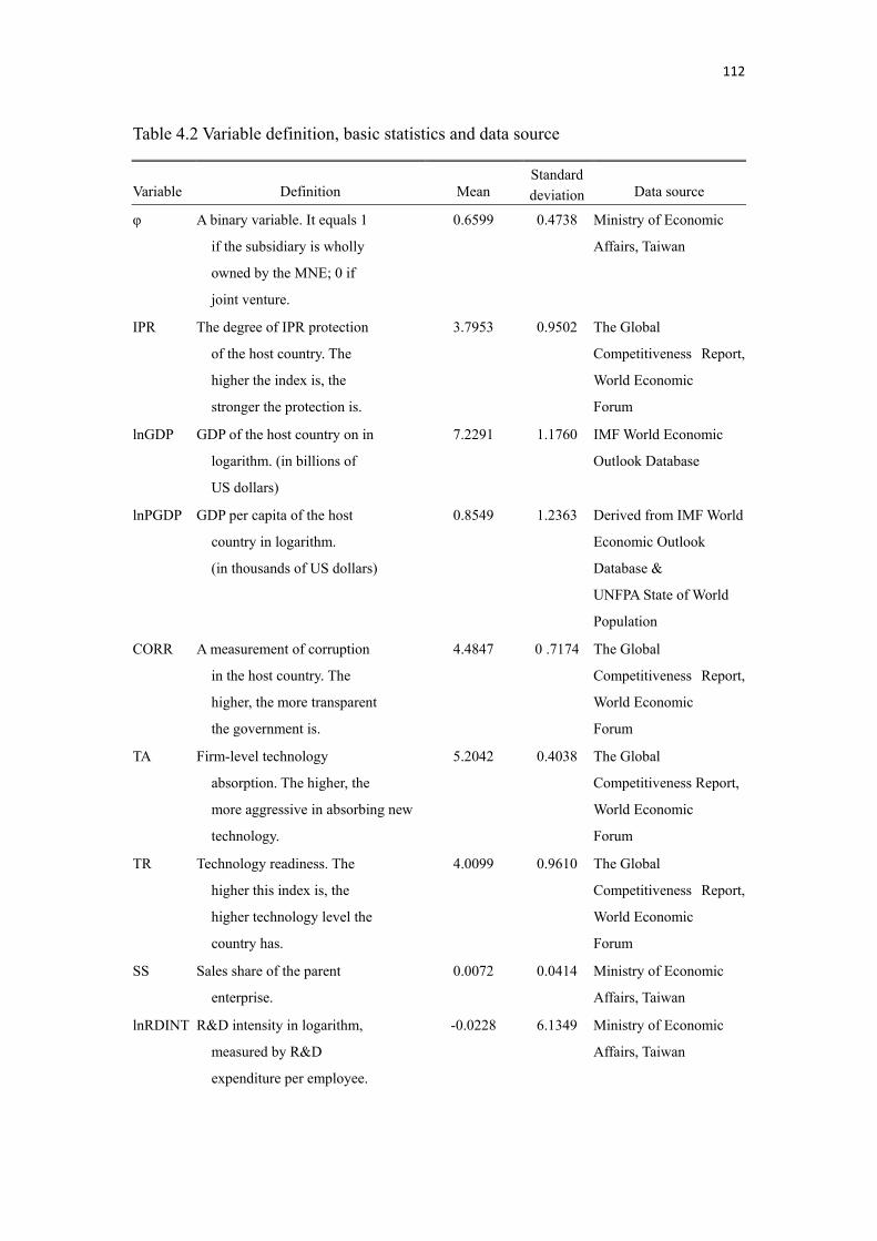
112

Table 4.2 Variable definition, basic statistics and data source

Variable Definition Mean Standard

deviation Data source

φ A binary variable. It equals 1

if the subsidiary is wholly

owned by the MNE; 0 if

joint venture.

0.6599 0.4738 Ministry of Economic

Affairs, Taiwan

IPR The degree of IPR protection

of the host country. The

higher the index is, the

stronger the protection is.

3.7953 0.9502 The Global

Competitiveness Report,

World Economic

Forum

lnGDP GDP of the host country on in

logarithm. (in billions of

US dollars)

7.2291 1.1760 IMF World Economic

Outlook Database

lnPGDP GDP per capita of the host

country in logarithm.

(in thousands of US dollars)

0.8549 1.2363 Derived from IMF World

Economic Outlook

Database &

UNFPA State of World

Population

CORR A measurement of corruption

in the host country. The

higher, the more transparent

the government is.

4.4847 0 .7174 The Global


World Economic

Forum

TA Firm-level technology

absorption. The higher, the

more aggressive in absorbing new

technology.

5.2042 0.4038 The Global


World Economic

Forum

TR Technology readiness. The

higher this index is, the

higher technology level the

country has.

4.0099 0.9610 The Global


World Economic

Forum

SS Sales share of the parent

enterprise.


Affairs, Taiwan

lnRDINT R&D intensity in logarithm,

measured by R&D

expenditure per employee.

-0.0228 6.1349 Ministry of Economic

Affairs, Taiwan

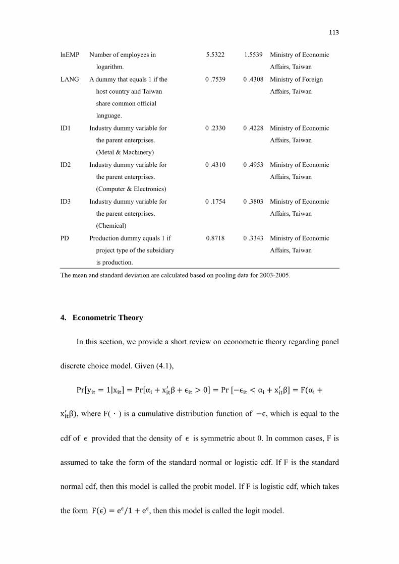
113

lnEMP Number of employees in

logarithm.


Affairs, Taiwan

LANG A dummy that equals 1 if the

host country and Taiwan

share common official

language.

0 .7539 0 .4308 Ministry of Foreign

Affairs, Taiwan

ID1 Industry dummy variable for

the parent enterprises.

(Metal & Machinery)

0 .2330 0 .4228 Ministry of Economic

Affairs, Taiwan



(Computer & Electronics)


Affairs, Taiwan



(Chemical)


Affairs, Taiwan

PD Production dummy equals 1 if

project type of the subsidiary

is production.

0.8718 0 .3343 Ministry of Economic

Affairs, Taiwan

The mean and standard deviation are calculated based on pooling data for 2003-2005.

4. Econometric Theory

In this section, we provide a short review on econometric theory regarding panel

discrete choice model. Given (4.1),

Pr y 1|x Pr α x β 0 Pr α x β F α

x β , where F(．) is a cumulative distribution function of , which is equal to the

cdf of provided that the density of is symmetric about 0. In common cases, F is

assumed to take the form of the standard normal or logistic cdf. If F is the standard

normal cdf, then this model is called the probit model. If F is logistic cdf, which takes

the form F e /1 e , then this model is called the logit model.

114

A pooled regression specifies constant coefficients and thus α α for all units.

However, in a more general model, when individual-specific effects are considered,

each cross-sectional unit is allowed to have a different intercept. In other words, the

intercept term, α varies across the cross-sectional units but is constant across time.

In addition, α may or may not be correlated with x . If α is correlated with x ,

the model is called a fixed effect model; while a random effect model assumes that α

and x are uncorrelated.

Cameron and Trivedi (2005) point out that pool estimation ignores individual

specific effects, and therefore, the estimates in the pooled model are generally

inconsistent. To solve this problem, the fixed effect and random effect models are

adopted instead. However, fixed effect specification is generally not applicable to

nonlinear panel models. Neyman and Scott (1948) argue that maximum likelihood

method fails to estimate the coefficients consistently in nonlinear panel fixed effect

model due to incidental parameters problem, which arises when the length of the

panel is small and fixed. To solve the incidental parameters problem, Neyman and

Scott (1948) propose a general principle to find a consistent estimator of β. They

suggest to find K functions

GN y , … , yN|β , j 1, … , K

that are independent of α and have the property that GN y , … , yN|βP

0 as

115

N ∞. However, it is model-specific and generally difficult to find such functions. In

particular, for fixed effect probit model, there does not exist such functions and thus

we don’t have consistent estimators in fixed effect probit model (Hsiao, 1986).

Similar problem arises in fixed effect logit model. The conditional likelihood

approach suggested by Andersen (1970, 1973) is applied to the binary choice logit

model to obtain consistent estimators for the structural parameter β. However, this

approach discards observations that are time invariant and thus it is less efficient. The

efficiency loss in fixed effect logit model is typically large especially for binary

choice panel data.

Alternatively, in the random effect model, the logit and probit have little

difference between the predicted probabilities except in the tails where probabilities

are closed to 0 or 1 (Cameron and Trivedi, 2005). However, as stated in Maddala

(1987), the logit model is somewhat more restrictive since it is derived from the

multivariate logistic distribution, (which is more restrictive than the normal

distribution), and therefore, the probit model is more popular in the random effect

model. The random effect probit model assumes α ~N 0, σα , ~N 0, σ , and

both of them are mutually independent and are independent of x as well. Given the

property of mutual independence, by conditioning on α , the joint density function

can be decomposed so that the joint probability is simplified and the log-likelihood

116

function only involves a single integration over α . Therefore, the corresponding

estimator becomes computationally feasible by the method of Butler and Moffitt

(1982). For the details, the derivation of the log-likelihood function in random effect

probit model is provided in the appendix.

In short, we will focus our empirical results from random effect probit model for

the following reasons: 1) the pooled estimation is generally inconsistent. 2) the fixed

effect model is inconsistent due to incidental parameters problem. Although a

consistent estimator is available by conditional likelihood approach in a binary fixed

effect logit model, it is less efficient because it may not contain time invariant

variables. 3) in a random effect model, the probit model is less restrictive than the

logit model.

5. Empirical Results

Table 4.3 demonstrates the estimation results. Random effect models for panel

logit and probit model are shown in column 1 and column2 respectively. Column 3

represents the result for fixed effect panel logit model. Please note that the fixed effect

specification for panel probit model is not applicable as we describe in section 4.

Column 4 and column 5 provide the result of pooled model (or population-averaged,

PA) for logit and probit specification respectively. Given our data set, we lost 79.8%

117

of our sample (4194 out of 5258) in fixed effect model since it drops individuals that

do not change over time. In other words, fixed effect logit model has big efficiency

loss. For pooled model, as aforementioned, since this specification ignores individual

specific effects, the estimates in the pooled model are generally inconsistent.

Therefore, even though all specifications reveal that the choice of ownership structure

is significantly affected by strength of IPR protection, our discussion will focus on the

results obtained from random effect probit model, which is shown in column 2.

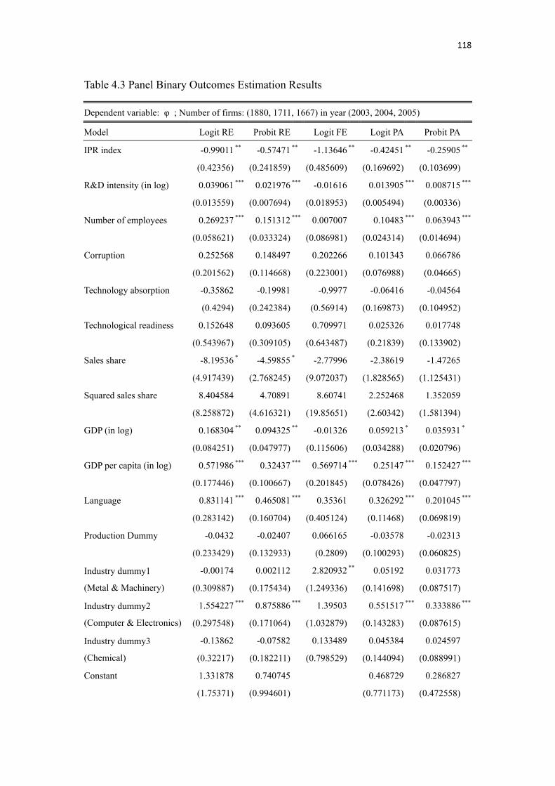
118

Table 4.3 Panel Binary Outcomes Estimation Results

Dependent variable: φ ; Number of firms: (1880, 1711, 1667) in year (2003, 2004, 2005)

Model Logit RE Probit RE Logit FE Logit PA Probit PA

IPR index -0.99011 ** -0.57471 ** -1.13646 ** -0.42451 ** -0.25905 **

(0.42356) (0.241859) (0.485609) (0.169692)

(0.103699)

R&D intensity (in log) 0.039061 *** 0.021976 *** -0.01616 0.013905 *** 0.008715 ***

(0.013559) (0.007694) (0.018953) (0.005494)

(0.00336)

Number of employees 0.269237 *** 0.151312 *** 0.007007 0.10483 *** 0.063943 ***

(0.058621) (0.033324) (0.086981) (0.024314)

(0.014694)

Corruption 0.252568 0.148497 0.202266 0.101343

0.066786

(0.201562) (0.114668) (0.223001) (0.076988) (0.04665)

Technology absorption -0.35862 -0.19981 -0.9977 -0.06416 -0.04564

(0.4294) (0.242384) (0.56914) (0.169873) (0.104952)

Technological readiness 0.152648 0.093605 0.709971 0.025326 0.017748

(0.543967) (0.309105) (0.643487) (0.21839) (0.133902)

Sales share -8.19536 * -4.59855 * -2.77996 -2.38619

-1.47265

(4.917439) (2.768245) (9.072037) (1.828565)

(1.125431)

Squared sales share 8.404584 4.70891 8.60741 2.252468

1.352059

(8.258872) (4.616321) (19.85651) (2.60342)

(1.581394)

GDP (in log) 0.168304 ** 0.094325 ** -0.01326 0.059213 * 0.035931 *

(0.084251) (0.047977) (0.115606) (0.034288)

(0.020796)

GDP per capita (in log) 0.571986 *** 0.32437 *** 0.569714 *** 0.25147 *** 0.152427 ***

(0.177446) (0.100667) (0.201845) (0.078426)

(0.047797)

Language 0.831141 *** 0.465081 *** 0.35361 0.326292 *** 0.201045 ***

(0.283142) (0.160704) (0.405124) (0.11468) (0.069819)

Production Dummy -0.0432 -0.02407 0.066165 -0.03578

-0.02313

(0.233429) (0.132933) (0.2809) (0.100293)

(0.060825)

Industry dummy1

(Metal & Machinery)

-0.00174 0.002112 2.820932 ** 0.05192

0.031773

(0.309887) (0.175434) (1.249336) (0.141698)

(0.087517)

Industry dummy2

(Computer & Electronics)

1.554227 *** 0.875886 *** 1.39503 0.551517 *** 0.333886 ***

(0.297548) (0.171064) (1.032879) (0.143283)

(0.087615)

Industry dummy3

(Chemical)

-0.13862 -0.07582 0.133489 0.045384 0.024597

(0.32217) (0.182211) (0.798529) (0.144094) (0.088991)

Constant 1.331878 0.740745 0.468729 0.286827

(1.75371) (0.994601) (0.771173) (0.472558)

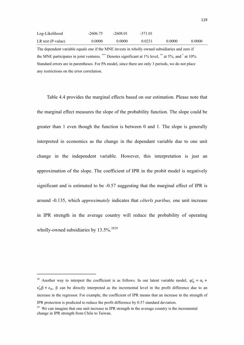
119

Log-Likelihood -2606.75 -2608.01 -371.01

LR test (P-value) 0.0000 0.0000 0.0231 0.0000 0.0000

The dependent variable equals one if the MNE invests in wholly owned subsidiaries and zero if

the MNE participates in joint ventures. *** Denotes significant at 1% level, ** at 5%, and * at 10%.

Standard errors are in parentheses. For PA model, since there are only 3 periods, we do not place

any restrictions on the error correlation.

Table 4.4 provides the marginal effects based on our estimation. Please note that

the marginal effect measures the slope of the probability function. The slope could be

greater than 1 even though the function is between 0 and 1. The slope is generally

interpreted in economics as the change in the dependant variable due to one unit

change in the independent variable. However, this interpretation is just an

approximation of the slope. The coefficient of IPR in the probit model is negatively

significant and is estimated to be -0.57 suggesting that the marginal effect of IPR is

around -0.135, which approximately indicates that cēterīs paribus, one unit increase

in IPR strength in the average country will reduce the probability of operating

wholly-owned subsidiaries by 13.5%.2829

28 Another way to interpret the coefficient is as follows. In our latent variable model, φ α

x β , β can be directly interpreted as the incremental level in the profit difference due to an

increase in the regressor. For example, the coefficient of IPR means that an increase in the strength of

IPR protection is predicted to reduce the profit difference by 0.57 standard deviation. 29 We can imagine that one unit increase in IPR strength in the average country is the incremental change in IPR strength from Chile to Taiwan.

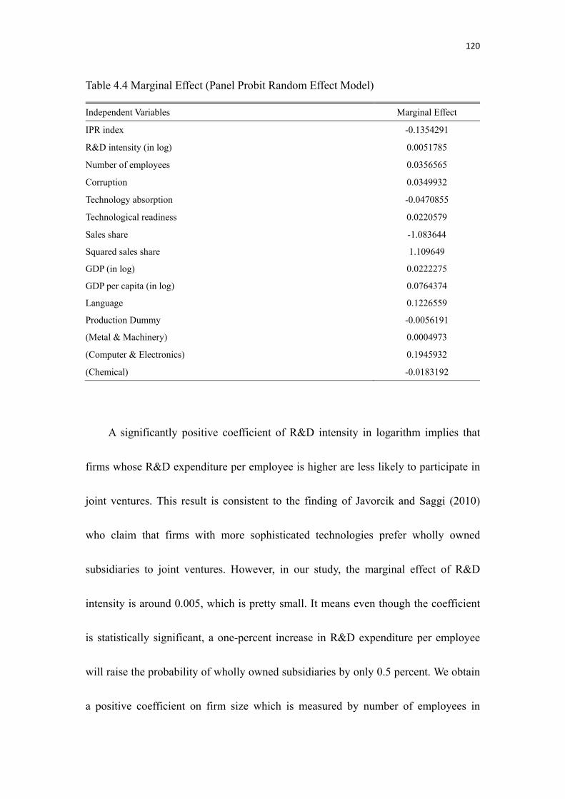
120

Table 4.4 Marginal Effect (Panel Probit Random Effect Model)

Independent Variables Marginal Effect

IPR index -0.1354291

R&D intensity (in log) 0.0051785

Number of employees 0.0356565

Corruption 0.0349932

Technology absorption -0.0470855

Technological readiness 0.0220579

Sales share -1.083644

Squared sales share 1.109649

GDP (in log) 0.0222275

GDP per capita (in log) 0.0764374

Language 0.1226559

Production Dummy -0.0056191

(Metal & Machinery) 0.0004973

(Computer & Electronics) 0.1945932

(Chemical) -0.0183192

A significantly positive coefficient of R&D intensity in logarithm implies that

firms whose R&D expenditure per employee is higher are less likely to participate in

joint ventures. This result is consistent to the finding of Javorcik and Saggi (2010)

who claim that firms with more sophisticated technologies prefer wholly owned

subsidiaries to joint ventures. However, in our study, the marginal effect of R&D

intensity is around 0.005, which is pretty small. It means even though the coefficient

is statistically significant, a one-percent increase in R&D expenditure per employee

will raise the probability of wholly owned subsidiaries by only 0.5 percent. We obtain

a positive coefficient on firm size which is measured by number of employees in

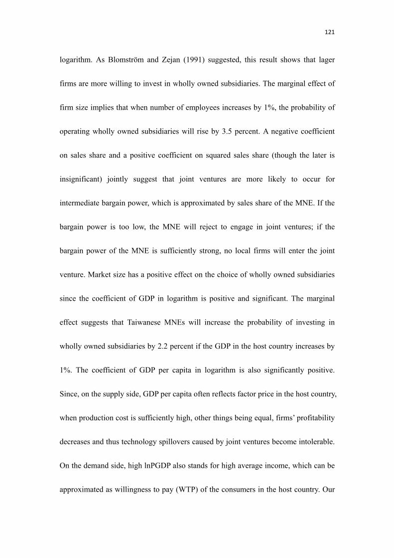
121

logarithm. As Blomström and Zejan (1991) suggested, this result shows that lager

firms are more willing to invest in wholly owned subsidiaries. The marginal effect of

firm size implies that when number of employees increases by 1%, the probability of

operating wholly owned subsidiaries will rise by 3.5 percent. A negative coefficient

on sales share and a positive coefficient on squared sales share (though the later is

insignificant) jointly suggest that joint ventures are more likely to occur for

intermediate bargain power, which is approximated by sales share of the MNE. If the

bargain power is too low, the MNE will reject to engage in joint ventures; if the

bargain power of the MNE is sufficiently strong, no local firms will enter the joint

venture. Market size has a positive effect on the choice of wholly owned subsidiaries

since the coefficient of GDP in logarithm is positive and significant. The marginal

effect suggests that Taiwanese MNEs will increase the probability of investing in

wholly owned subsidiaries by 2.2 percent if the GDP in the host country increases by

1%. The coefficient of GDP per capita in logarithm is also significantly positive.

Since, on the supply side, GDP per capita often reflects factor price in the host country,

when production cost is sufficiently high, other things being equal, firms’ profitability

decreases and thus technology spillovers caused by joint ventures become intolerable.

On the demand side, high lnPGDP also stands for high average income, which can be

approximated as willingness to pay (WTP) of the consumers in the host country. Our

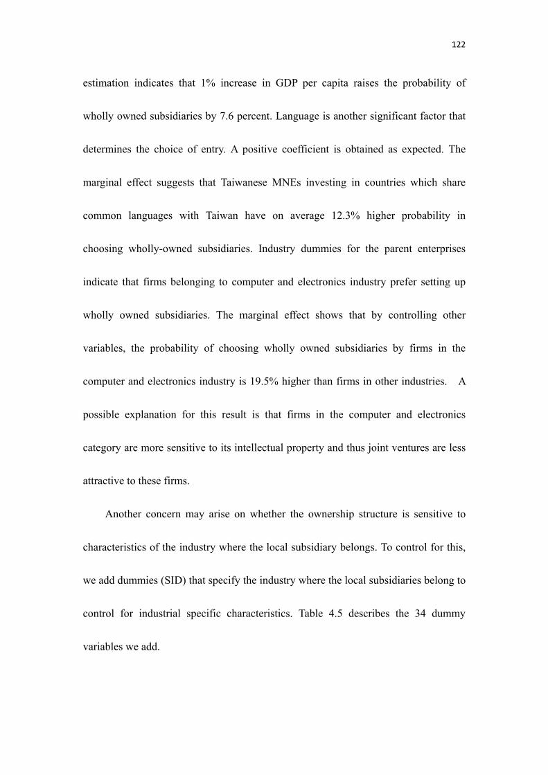
122

estimation indicates that 1% increase in GDP per capita raises the probability of

wholly owned subsidiaries by 7.6 percent. Language is another significant factor that

determines the choice of entry. A positive coefficient is obtained as expected. The

marginal effect suggests that Taiwanese MNEs investing in countries which share

common languages with Taiwan have on average 12.3% higher probability in

choosing wholly-owned subsidiaries. Industry dummies for the parent enterprises

indicate that firms belonging to computer and electronics industry prefer setting up

wholly owned subsidiaries. The marginal effect shows that by controlling other

variables, the probability of choosing wholly owned subsidiaries by firms in the

computer and electronics industry is 19.5% higher than firms in other industries. A

possible explanation for this result is that firms in the computer and electronics

category are more sensitive to its intellectual property and thus joint ventures are less

attractive to these firms.

Another concern may arise on whether the ownership structure is sensitive to

characteristics of the industry where the local subsidiary belongs. To control for this,

we add dummies (SID) that specify the industry where the local subsidiaries belong to

control for industrial specific characteristics. Table 4.5 describes the 34 dummy

variables we add.

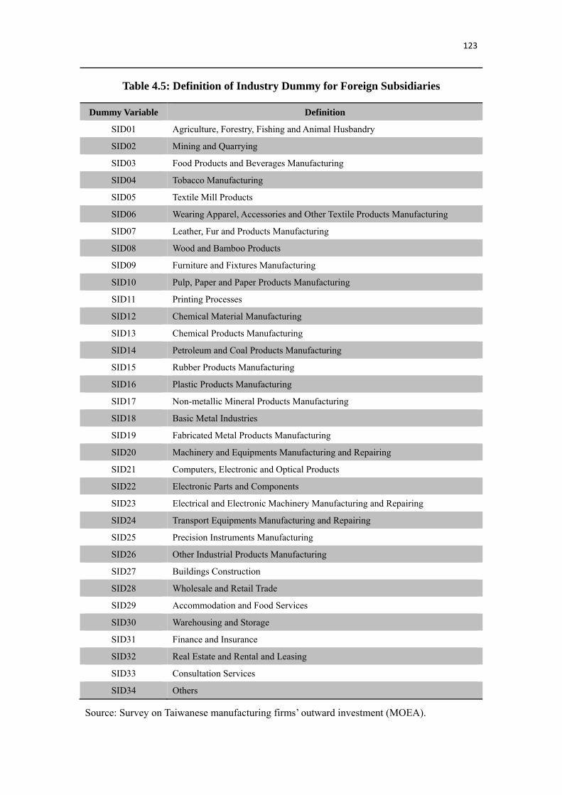
123

Table 4.5: Definition of Industry Dummy for Foreign Subsidiaries

Dummy Variable Definition

SID01 Agriculture, Forestry, Fishing and Animal Husbandry

SID02 Mining and Quarrying

SID03 Food Products and Beverages Manufacturing

SID04 Tobacco Manufacturing

SID05 Textile Mill Products

SID06 Wearing Apparel, Accessories and Other Textile Products Manufacturing

SID07 Leather, Fur and Products Manufacturing

SID08 Wood and Bamboo Products

SID09 Furniture and Fixtures Manufacturing

SID10 Pulp, Paper and Paper Products Manufacturing

SID11 Printing Processes

SID12 Chemical Material Manufacturing

SID13 Chemical Products Manufacturing

SID14 Petroleum and Coal Products Manufacturing

SID15 Rubber Products Manufacturing

SID16 Plastic Products Manufacturing

SID17 Non-metallic Mineral Products Manufacturing

SID18 Basic Metal Industries

SID19 Fabricated Metal Products Manufacturing

SID20 Machinery and Equipments Manufacturing and Repairing

SID21 Computers, Electronic and Optical Products

SID22 Electronic Parts and Components

SID23 Electrical and Electronic Machinery Manufacturing and Repairing

SID24 Transport Equipments Manufacturing and Repairing

SID25 Precision Instruments Manufacturing

SID26 Other Industrial Products Manufacturing

SID27 Buildings Construction

SID28 Wholesale and Retail Trade

SID29 Accommodation and Food Services

SID30 Warehousing and Storage

SID31 Finance and Insurance

SID32 Real Estate and Rental and Leasing

SID33 Consultation Services

SID34 Others

Source: Survey on Taiwanese manufacturing firms’ outward investment (MOEA).

124

The equation we are going to estimate becomes

φ β β lnGDP β lnPGDP β lnRDINT β lnEMP

β SS β SS β TA β TR β IPR β LANG (4.6)

β CORR γ ID θ PD SID

We present the estimation results for different model specifications in table 4.6.

As we stated above, fixed effect for panel probit model is not available and the fixed

effect specification for panel logit model is not appropriate since it results in 79.8%

loss of our sample. IPR is still robust for all model specifications. Among the new

dummy variables we add in this regression, random effect specification shows that

only the coefficient of the dummy that represents paper industry is negatively

significant. All other dummies we add in this section are insignificant. This result

suggests that Taiwanese MNEs tend to participate in joint ventures in paper industry.

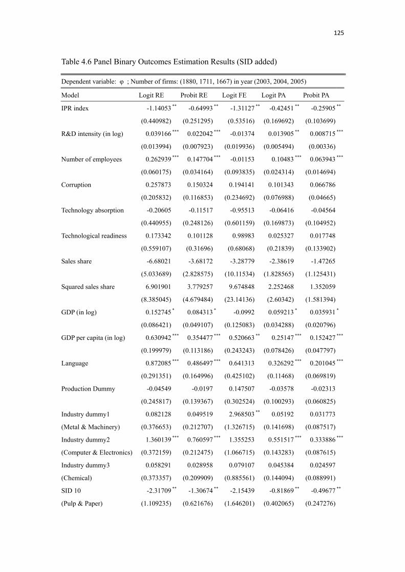
125

Table 4.6 Panel Binary Outcomes Estimation Results (SID added)

Dependent variable: φ ; Number of firms: (1880, 1711, 1667) in year (2003, 2004, 2005)

Model Logit RE Probit RE Logit FE Logit PA Probit PA

IPR index -1.14053 ** -0.64993 ** -1.31127 ** -0.42451 ** -0.25905 **

(0.440982) (0.251295) (0.53516) (0.169692)

(0.103699)

R&D intensity (in log) 0.039166 *** 0.022042 *** -0.01374 0.013905 ** 0.008715 ***

(0.013994) (0.007923) (0.019936) (0.005494)

(0.00336)

Number of employees 0.262939 *** 0.147704 *** -0.01153 0.10483 *** 0.063943 ***

(0.060175) (0.034164) (0.093835) (0.024314) (0.014694)

Corruption 0.257873 0.150324 0.194141 0.101343 0.066786

(0.205832) (0.116853) (0.234692) (0.076988) (0.04665)

Technology absorption -0.20605 -0.11517 -0.95513 -0.06416 -0.04564

(0.440955) (0.248126) (0.601159) (0.169873) (0.104952)

Technological readiness 0.173342 0.101128 0.98983 0.025327 0.017748

(0.559107) (0.31696) (0.68068) (0.21839) (0.133902)

Sales share -6.68021 -3.68172 -3.28779 -2.38619 -1.47265

(5.033689) (2.828575) (10.11534) (1.828565) (1.125431)

Squared sales share 6.901901 3.779257 9.674848 2.252468 1.352059

(8.385045) (4.679484) (23.14136) (2.60342) (1.581394)

GDP (in log) 0.152745 * 0.084313 * -0.0992 0.059213 * 0.035931 *

(0.086421) (0.049107) (0.125083) (0.034288)

(0.020796)

GDP per capita (in log) 0.630942 *** 0.354477 *** 0.520663 ** 0.25147 *** 0.152427 ***

(0.199979) (0.113186) (0.243243) (0.078426)

(0.047797)

Language 0.872085 *** 0.486497 *** 0.641313 0.326292 *** 0.201045 ***

(0.291351) (0.164996) (0.425102) (0.11468) (0.069819)

Production Dummy -0.04549 -0.0197 0.147507 -0.03578

-0.02313

(0.245817) (0.139367) (0.302524) (0.100293)

(0.060825)

Industry dummy1 0.082128 0.049519 2.968503 ** 0.05192

0.031773

(Metal & Machinery) (0.376653) (0.212707) (1.326715) (0.141698)

(0.087517)

Industry dummy2 1.360139 *** 0.760597 *** 1.355253 0.551517 *** 0.333886 ***

(Computer & Electronics) (0.372159) (0.212475) (1.066715) (0.143283)

(0.087615)

Industry dummy3 0.058291 0.028958 0.079107 0.045384

0.024597

(Chemical) (0.373357) (0.209909) (0.885561) (0.144094)

(0.088991)

SID 10 -2.31709 ** -1.30674 ** -2.15439 -0.81869 ** -0.49677 **

(Pulp & Paper) (1.109235) (0.621676) (1.646201) (0.402065)

(0.247276)

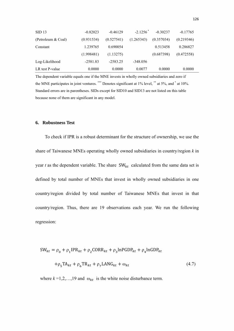
126

SID 13 -0.82023 -0.46129 -2.1256 * -0.30237

-0.17765

(Petroleum & Coal) (0.931534) (0.527541) (1.265343) (0.357034)

(0.219346)

Constant 1.239765 0.690054 0.513458

0.286827

(1.998481) (1.13275) (0.687398)

(0.472558)

Log-Likelihood -2581.83 -2583.25 -348.056

LR test P-value 0.0000 0.0000 0.0077 0.0000 0.0000

The dependent variable equals one if the MNE invests in wholly owned subsidiaries and zero if

the MNE participates in joint ventures. *** Denotes significant at 1% level, ** at 5%, and * at 10%.

Standard errors are in parentheses. SIDs except for SID10 and SID13 are not listed on this table

because none of them are significant in any model.

6. Robustness Test

To check if IPR is a robust determinant for the structure of ownership, we use the

share of Taiwanese MNEs operating wholly owned subsidiaries in country/region k in

year t as the dependent variable. The share SW calculated from the same data set is

defined by total number of MNEs that invest in wholly owned subsidiaries in one

country/region divided by total number of Taiwanese MNEs that invest in that

country/region. Thus, there are 19 observations each year. We run the following

regression:

SW ρ ρ IPR ρ CORR ρ lnPGDP ρ lnGDP

ρ TA ρ TR ρ LANG ω (4.7)

where k =1,2,…,19 and ω is the white noise disturbance term.

127

The independent variables are defined in the previous section. The dependent

variable ranges between 0 and 1; this suggests that a 2-sided panel tobit model is

appropriate for the estimation. The result is summarized in column 1 of table 4.7. The

coefficient of IPR is still negative though it is insignificant. One problem of this

regression may arise when sample sizes are quite asymmetric across regions. If

identical weight is placed on each region, the influence of certain regions with small

sample size will be overestimated.30 To correct this problem, two alternatives are

employed. The first approach is that we use the average number of firms investing in

region k for the period 2003-2005 as the importance weight.31 The second approach

is dropping those regions where SW equals 0 or 1 in any year. The reason for adopting

the second approach is that if SW reaches 0 or 1 for one region, it is because the

sample size in that region is too small.32 Dropping those outliers can correct the

“equal weights problem” stated above. The results for first and second approach are

shown in column 2 and 3 of table 4.7 respectively. The coefficients of IPR in column

2 and 3 are both significantly negative. Both estimates indicate that foreign ownership

structure is sensitive to IPR protection. MNEs are more likely to participate in joint

30 For example, for some regions such as Canada and Mexico, number of investors is pretty small. Both Canada and Mexico have only 2 establishments, while there are 1217 establishments in China in 2005. 31 For example, the numbers of firms investing in United States in 2003, 2004 and 2005 are 174, 131 and 122 respectively. The weight for United States is given by the mean of (174, 131, 122), which is 142.33. 32 Given our data set, the regions that are discarded contain less than 9 observations (for three years). In other words, on average, only 3 or fewer firms invest in the discarded region.

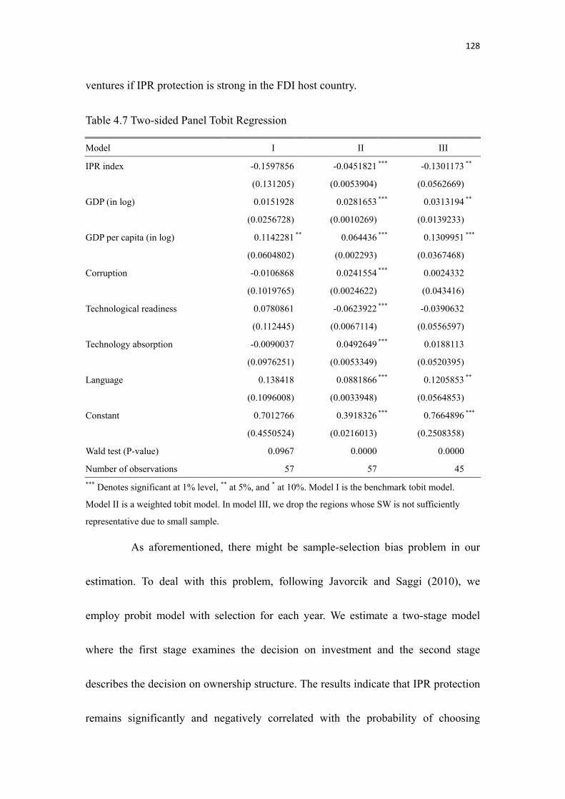
128

ventures if IPR protection is strong in the FDI host country.

Table 4.7 Two-sided Panel Tobit Regression

Model I II III

IPR index -0.1597856 -0.0451821 *** -0.1301173 **

(0.131205) (0.0053904) (0.0562669)

GDP (in log) 0.0151928 0.0281653 *** 0.0313194 **

(0.0256728) (0.0010269) (0.0139233)

GDP per capita (in log) 0.1142281 ** 0.064436 *** 0.1309951 ***

(0.0604802) (0.002293) (0.0367468)

Corruption -0.0106868 0.0241554 *** 0.0024332

(0.1019765) (0.0024622) (0.043416)

Technological readiness 0.0780861 -0.0623922 *** -0.0390632

(0.112445) (0.0067114) (0.0556597)

Technology absorption -0.0090037 0.0492649 *** 0.0188113

(0.0976251) (0.0053349) (0.0520395)

Language 0.138418 0.0881866 *** 0.1205853 **

(0.1096008) (0.0033948) (0.0564853)

Constant 0.7012766 0.3918326 *** 0.7664896 ***

(0.4550524) (0.0216013) (0.2508358)

Wald test (P-value) 0.0967 0.0000 0.0000

Number of observations 57 57 45

*** Denotes significant at 1% level, ** at 5%, and * at 10%. Model I is the benchmark tobit model.

Model II is a weighted tobit model. In model III, we drop the regions whose SW is not sufficiently

representative due to small sample.

As aforementioned, there might be sample-selection bias problem in our

estimation. To deal with this problem, following Javorcik and Saggi (2010), we

employ probit model with selection for each year. We estimate a two-stage model

where the first stage examines the decision on investment and the second stage

describes the decision on ownership structure. The results indicate that IPR protection

remains significantly and negatively correlated with the probability of choosing

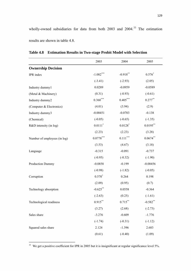
129

wholly-owned subsidiaries for data from both 2003 and 2004.33 The estimation

results are shown in table 4.8.

Table 4.8 Estimation Results in Two-stage Probit Model with Selection

2003 2004 2005

Ownership Decision

IPR index -1.082*** -0.918** 0.576*

(-3.41) (-2.93) (2.05)

Industry dummy1 0.0289 -0.0959 -0.0589

(Metal & Machinery) (0.31) (-0.93) (-0.61)

Industry dummy2 0.360*** 0.405*** 0.277**

(Computer & Electronics) (4.01) (3.94) (2.9)

Industry dummy3 -0.00451 -0.0703 -0.138

(Chemical) (-0.05) (-0.65) (-1.35)

R&D intensity (in log) 0.0111* 0.0128* 0.0195**

(2.23) (2.23) (3.28)

Number of employees (in log) 0.0778*** 0.111*** 0.0674**

(3.53) (4.67) (3.18)

Language -0.315 -0.091 -0.737

(-0.95) (-0.32) (-1.90)

Production Dummy -0.0858 -0.199 -0.00456

(-0.98) (-1.82) (-0.05)

Corruption 0.570* 0.264 0.198

(2.09) (0.95) (0.7)

Technology absorption -0.625** 0.0558 -0.364

(-2.63) (0.25) (-1.61)

Technological readiness 0.915** 0.715** -0.582**

(3.27) (2.68) (-2.73)

Sales share -3.276 -0.609 -1.776

(-1.74) (-0.31) (-1.12)

Squared sales share 2.124 -1.396 2.683

(0.61) (-0.40) (1.09)

33 We get a positive coefficient for IPR in 2005 but it is insignificant at regular significance level 5%.

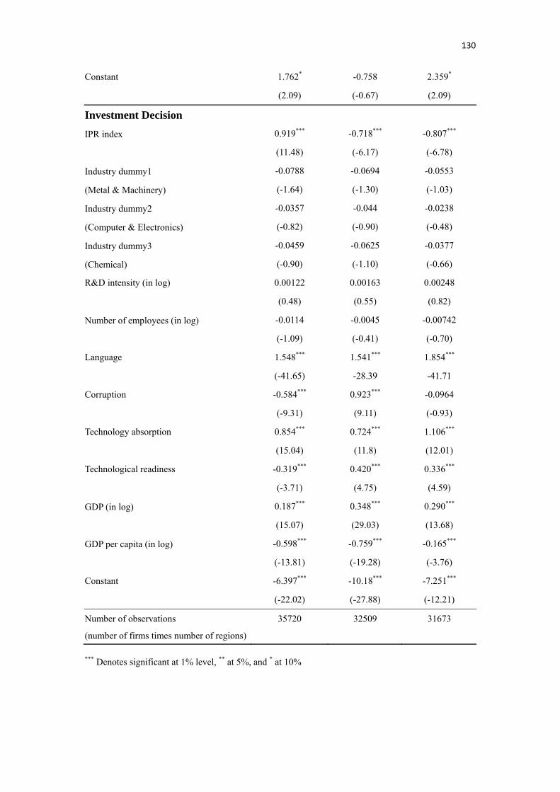
130

Constant 1.762* -0.758 2.359*

(2.09) (-0.67) (2.09)

Investment Decision

IPR index 0.919*** -0.718*** -0.807***

(11.48) (-6.17) (-6.78)

Industry dummy1 -0.0788 -0.0694 -0.0553

(Metal & Machinery) (-1.64) (-1.30) (-1.03)

Industry dummy2 -0.0357 -0.044 -0.0238

(Computer & Electronics) (-0.82) (-0.90) (-0.48)

Industry dummy3 -0.0459 -0.0625 -0.0377

(Chemical) (-0.90) (-1.10) (-0.66)

R&D intensity (in log) 0.00122 0.00163 0.00248

(0.48) (0.55) (0.82)

Number of employees (in log) -0.0114 -0.0045 -0.00742

(-1.09) (-0.41) (-0.70)

Language 1.548*** 1.541*** 1.854***

(-41.65) -28.39 -41.71

Corruption -0.584*** 0.923*** -0.0964

(-9.31) (9.11) (-0.93)

Technology absorption 0.854*** 0.724*** 1.106***

(15.04) (11.8) (12.01)

Technological readiness -0.319*** 0.420*** 0.336***

(-3.71) (4.75) (4.59)

GDP (in log) 0.187*** 0.348*** 0.290***

(15.07) (29.03) (13.68)

GDP per capita (in log) -0.598*** -0.759*** -0.165***

(-13.81) (-19.28) (-3.76)

Constant -6.397*** -10.18*** -7.251***

(-22.02) (-27.88) (-12.21)

Number of observations

(number of firms times number of regions)

35720 32509 31673

*** Denotes significant at 1% level, ** at 5%, and * at 10%

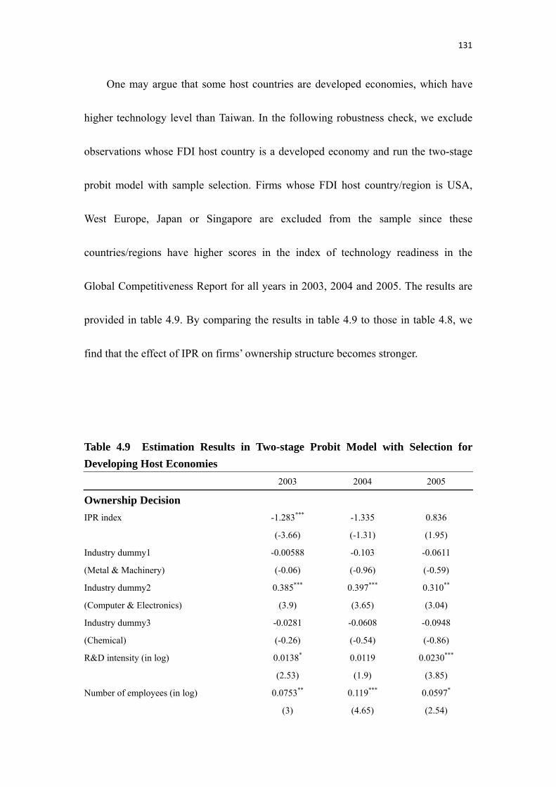
131

One may argue that some host countries are developed economies, which have

higher technology level than Taiwan. In the following robustness check, we exclude

observations whose FDI host country is a developed economy and run the two-stage

probit model with sample selection. Firms whose FDI host country/region is USA,

West Europe, Japan or Singapore are excluded from the sample since these

countries/regions have higher scores in the index of technology readiness in the

Global Competitiveness Report for all years in 2003, 2004 and 2005. The results are

provided in table 4.9. By comparing the results in table 4.9 to those in table 4.8, we

find that the effect of IPR on firms’ ownership structure becomes stronger.

Table 4.9 Estimation Results in Two-stage Probit Model with Selection for

Developing Host Economies

2003 2004 2005

Ownership Decision

IPR index -1.283*** -1.335 0.836

(-3.66) (-1.31) (1.95)

Industry dummy1 -0.00588 -0.103 -0.0611

(Metal & Machinery) (-0.06) (-0.96) (-0.59)

Industry dummy2 0.385*** 0.397*** 0.310**

(Computer & Electronics) (3.9) (3.65) (3.04)

Industry dummy3 -0.0281 -0.0608 -0.0948

(Chemical) (-0.26) (-0.54) (-0.86)

R&D intensity (in log) 0.0138* 0.0119 0.0230***

(2.53) (1.9) (3.85)

Number of employees (in log) 0.0753** 0.119*** 0.0597*

(3) (4.65) (2.54)

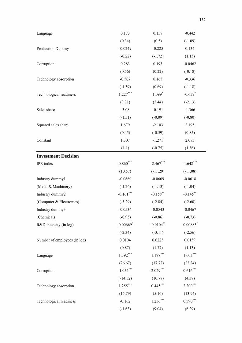
132

Language 0.173 0.157 -0.442

(0.34) (0.5) (-1.09)

Production Dummy -0.0249 -0.225 0.134

(-0.22) (-1.72) (1.13)

Corruption 0.283 0.193 -0.0462

(0.56) (0.22) (-0.18)

Technology absorption -0.507 0.163 -0.336

(-1.39) (0.69) (-1.18)

Technological readiness 1.227*** 1.099* -0.659*

(3.31) (2.44) (-2.13)

Sales share -3.08 -0.191 -1.366

(-1.51) (-0.09) (-0.80)

Squared sales share 1.679 -2.103 2.195

(0.45) (-0.59) (0.85)

Constant 1.307 -1.271 2.073

(1.1) (-0.75) (1.36)

Investment Decision

IPR index 0.860*** -2.467*** -1.648***

(10.57) (-11.29) (-11.08)

Industry dummy1 -0.0669 -0.0669 -0.0618

(Metal & Machinery) (-1.26) (-1.13) (-1.04)

Industry dummy2 -0.161*** -0.158** -0.145**

(Computer & Electronics) (-3.29) (-2.84) (-2.60)

Industry dummy3 -0.0534 -0.0543 -0.0467

(Chemical) (-0.95) (-0.86) (-0.73)

R&D intensity (in log) -0.00669* -0.0104** -0.00883*

(-2.34) (-3.11) (-2.56)

Number of employees (in log) 0.0104 0.0223 0.0139

(0.87) (1.77) (1.13)

Language 1.392*** 1.198*** 1.603***

(26.67) (17.72) (23.24)

Corruption -1.052*** 2.029*** 0.616***

(-14.52) (10.78) (4.38)

Technology absorption 1.255*** 0.445*** 2.200***

(15.79) (5.16) (13.94)

Technological readiness -0.162 1.256*** 0.590***

(-1.63) (9.04) (6.29)

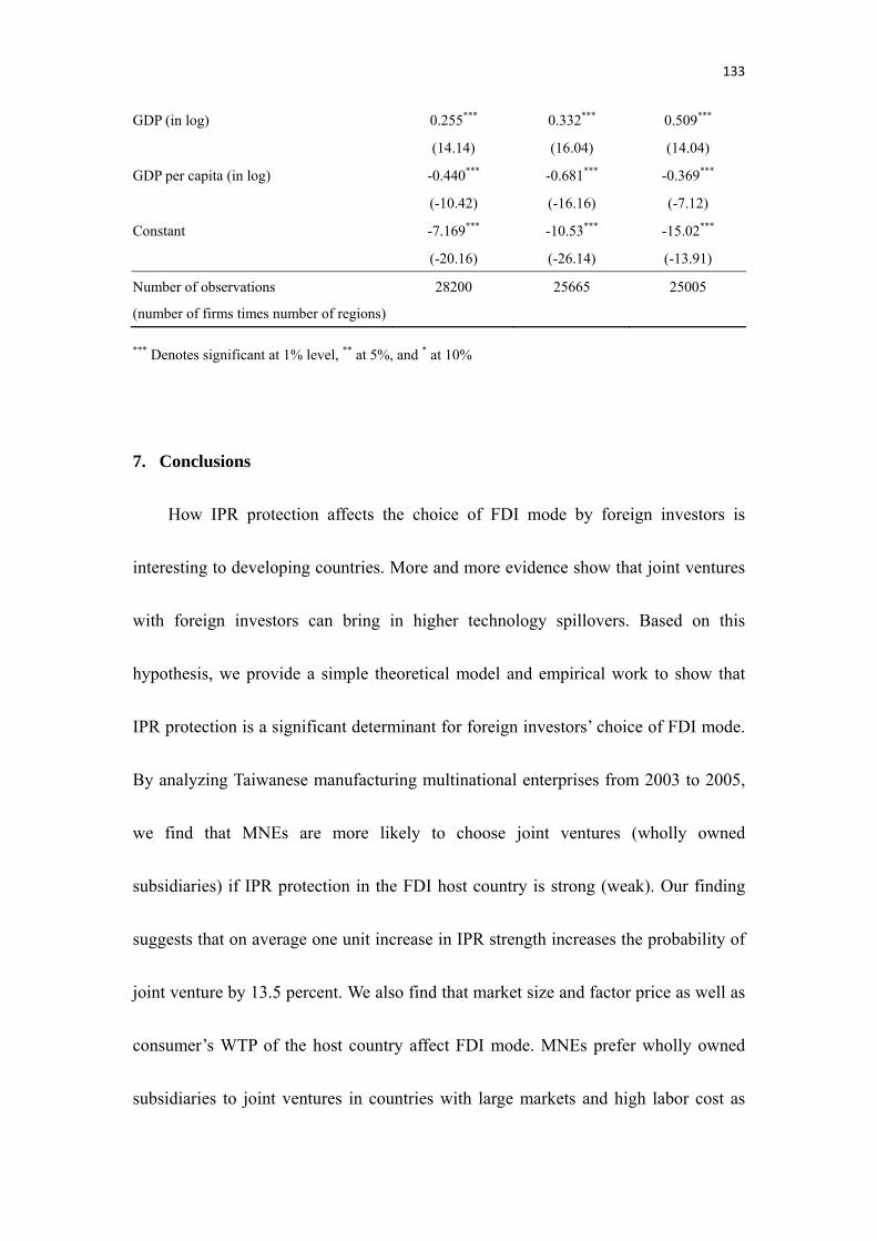
133

GDP (in log) 0.255*** 0.332*** 0.509***

(14.14) (16.04) (14.04)

GDP per capita (in log) -0.440*** -0.681*** -0.369***

(-10.42) (-16.16) (-7.12)

Constant -7.169*** -10.53*** -15.02***

(-20.16) (-26.14) (-13.91)

Number of observations

(number of firms times number of regions)

28200 25665 25005

*** Denotes significant at 1% level, ** at 5%, and * at 10%

7. Conclusions

How IPR protection affects the choice of FDI mode by foreign investors is

interesting to developing countries. More and more evidence show that joint ventures

with foreign investors can bring in higher technology spillovers. Based on this

hypothesis, we provide a simple theoretical model and empirical work to show that

IPR protection is a significant determinant for foreign investors’ choice of FDI mode.

By analyzing Taiwanese manufacturing multinational enterprises from 2003 to 2005,

we find that MNEs are more likely to choose joint ventures (wholly owned

subsidiaries) if IPR protection in the FDI host country is strong (weak). Our finding

suggests that on average one unit increase in IPR strength increases the probability of

joint venture by 13.5 percent. We also find that market size and factor price as well as

consumer’s WTP of the host country affect FDI mode. MNEs prefer wholly owned

subsidiaries to joint ventures in countries with large markets and high labor cost as

134

well as high consumer’s WTP. We also find that R&D intensity is statistical

significant in determining the ownership structure. However, the magnitude is very

small since our results show that 1 percent increase in R&D expenditure per employee

results in 0.5 percent increase in probability of wholly owned subsidiaries.

Our finding has an important policy implication. In order to increase local

participation, the FDI host country may directly impose local equity requirements.

However, this would not be a best choice since the local equity requirements may

reduce foreign investors’ incentive to invest in that country. We can imagine that if

there are two countries that are identical in all aspects except the policy on local

equality requirement, it is not surprising that the MNE will invest in the country

where there is no local equality requirement. Alternatively, the results of this study

suggest that by strengthening IPR protection, developing countries can increase local

participation without imposing regulations that are harmful for encouraging inward

FDI.

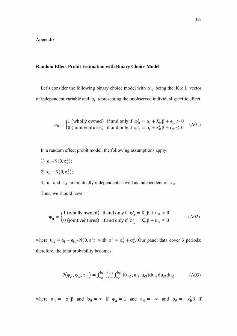
135

Appendix

Random Effect Probit Estimation with Binary Choice Model

Let’s consider the following binary choice model with x being the K 1 vector

of independent variable and α representing the unobserved individual specific effect

φ1 wholly owned if and only if φ α X β 00 joint ventures if and only if φ α X β 0

(A01)

In a random effect probit model, the following assumptions apply:

1) α ~N 0, σα ;

2) ~N 0, σ ;

3) α and are mutually independent as well as independent of x .

Thus, we should have

φ1 wholly owned if and only if φ X′ β u 0

0 joint ventures if and only if φ X′ β u 0 (A02)

where u α ~N 0, σ with σ σα σ . Our panel data cover 3 periods;

therefore, the joint probability becomes:

P φ ,φ ,φ f u , u , u du du du (A03)

where a x′ β and b ∞ if φ 1 and a ∞ and b x′ β if

136

φ 0. Following Butler and Moffitt (1982), since u |α and u |α (t s) are

independent, when conditioning on the random disturbance term α , the joint density

function in (A03) can be rewritten as

f u , u , u f α f u , u , u |α

f α f u |α f u |α f u |α (A04)

Therefore, (A03) becomes

P φ ,φ ,φ

f α∞

∞f u |α du f u |α du f u |α du dα

∏ F b |α F a |α f α∞

∞dα

(A05)

The likelihood function can be obtained by multiplying each individual’s

probability obtained from (A05). Taking logarithm on the likelihood function, the

log-likelihood function is:

ln L ∑ ln ∏ F b |α F a |α f α∞

∞dαN (A06)

137

CHAPTER V

CONCLUSION

This thesis discusses three independent topics regarding intellectual property

rights protection and international trade. In the framework of horizontal arbitrage

model in PI analysis, I show that allowing PI encourages the manufacture to find

other ways such as offering the product as well as better service to mitigate price

competition. The intuition is as follows. In contrast to investment in brand marketing,

which can be freely ridden by parallel importers, investment in service is excludable

and thus the manufacturer has an incentive to invest more in service in order to

achieve product differentiation.

The horizontal arbitrage framework is applied to the analysis of piracy and

parallel imports in the video game market. Three results that are different from

common expectations are developed. First, video game piracy could be beneficial for

both hardware manufacture and software provider since neither of them will be

pinned down by each other with the existence of piracy. Second, allowing PI for

hardware is also beneficial for the hardware manufacturer since piracy and PI provide

the hardware firm a means to distinguish consumers’ type and thus price

discrimination can be sustained. Third, this study shows that consumers are not

necessarily better off due to parallel importation.

138

An essay that discussed the nexus between IPR and mode of FDI is included in

this thesis. By analyzing a firm-level panel data set from Taiwanese multinational

manufacturing firms for the period 2003-2005, I find that MNEs are more likely to

choose joint ventures if IPR protection in the FDI host country is strong. The

estimation results suggest that one unit increase in IPR protection in the average

country raises the probability of joint ventures by 13.5 percent. I also find that MNEs

prefer wholly owned subsidiaries to joint ventures in host countries with large markets

and high factor price as well as high average income.

139

REFERENCE

Álvarez, M., 2003, Wholly-owned subsidiaries versus joint ventures: The determinant

factors in the Catalan multinational manufacturing case, Institut d'Economia de

Barcelona Working Paper: 2003/5.

Ahmadi, R.. and R. Yang, 2000, “Parallel Imports: Challenges from Unauthorized

Distribution Channels,” Marketing Science Vol. 19 No. 3. pp. 279-294

Andersen, E.B. ,1970, “Asymptotic Properties of Conditional Maximum Likelihood

Estimators,” Journal of the Royal Statistical Society, Series B, 32, 283–301.

Andersen, E.B. ,1973, Conditional Inference and Models for Measuring. Köbenhavn:

Mentalhygiejnish Farlag.

Anderson, S.P. and V.A. Ginsburg, 1999, “International Pricing with Costly Consumer

Arbitrage,” Review of International Economics 7: 126-139.

Bae, S.H and J.P. Choi, 2006, “A Model of Piracy,” Information Economics and

Policy, 18: 303–320

Blomström, M., Zejan, M., 1991. Why do multinational firms seek out joint ventures?

Journal of International Development, 3, 53–63.

Butler, J. S. and Moffitt, R. (1982) “A Computationally Efficient Quadrature

Procedure for the One-Factor Multinomial Probit Model”, Econometrica, 50(3),

761-764.

Cameron, A. C., Trivedi, P. K.,2005. Microeconometrics: Method and Applications,

Cambridge University Press.

Chen, Y., 1997, ”Equilibrium Product Bundling,” Journal of Business, Vol. 70, No.1,

pp. 85-103

Chen, Y., and K.E. Maskus, 2005, “Vertical Pricing and Parallel Imports,” Journal of

International Trade and Economic Development 14: 1-18.

140

Cosac, T., 2003, “Vertical Restraints and Parallel Imports with Differentiated

Products,” Canadian Competition Bureau Working Paper

Ferrantino, M.J., 1993. The effect of intellectual property rights on international trade

and investment. Weltwirtschaftliches Archiv 129, 300–331.

Fink, C., 2004, “Entering the Jungle of Intellectual Property Rights Exhaustion and

Parallel Imports,” in Carsten Fink and Keith E. Maskus, eds., Intellectual Property

Rights and Development: Lessons from Recent Economic Research (Oxford: Oxford

University Press).

Flowers, S., 2008, Harnessing the hackers: The emergence and Exploitation of Outlaw

Innovation, Research Policy, 37 (2): 177–193.

Ganslandt, M. and K.E. Maskus, 2007, “Vertical Distribution, Parallel Trade and Price

Divergence in Integrated Markets,” European Economic Review 51: 943-970.

Horn, Henrik and O. Shy, 1996, “Bundling and International Segmentation,”

International Economic Review 37(1): 51-69.

Hsiao, C. (1986) Analysis of Panel Data, Cambridge University Press.

Javorcik, B.S., 2004a. Does foreign direct investment increase the productivity of

domestic firms? In Search of spillovers through backward linkages. American

Economic Review 94 (3), 605–627.

Javorcik, B.S., 2004b. The composition of foreign direct investment and protection of

intellectual property rights: evidence from transition economies. European Economic

Review 48 (1), 39–62.

Javorcik, B.S. and K. Saggi, 2010. Technological Asymmetry among Foreign

Investors and Mode of Entry. Economic Inquiry 48(2), 415-433

Javorcik, B.S. and M. Spatareanu, 2008. To share or not to share: Does local

participation matter for spillovers from foreign direct investment?. Journal of

Development Economics 85, 194–217

Kameshwaran, S. , N. Viswanadham, and V. Desai, 2007, “On Bundling and Pricing

141

of the Service with the Product,” IEEE Conference on Automation Science and

Engineering

Leahy, D., Naghavi, A.,2010. Intellectual Property Rights and Entry into a Foreign

Market: FDI vs. Joint Ventures, Review of International Economics, forthcoming.

Lee, J.-Y., Mansfield, E., 1996. Intellectual property protection and U.S. foreign

direct investment. Review of Economics and Statistics 78, 181–186.

Malueg, D.A. and M. Schwartz, 1994, “Parallel Imports, Demand Dispersion, and

International Price Discrimination,” Journal of International Economics 37: 187-196.

Mansfield, E.. 1993. "Unauthorized Use of Intellectual Property: Effects on

Investment, Technology Transfer, and Innovation," in M. Wallerstein, M. Mogee, and

R. Schoen (eds.), Global Dimensions of Intellectual Property Rights in Science and

Technology. National Academy Press, Washington, D.C.

Maskus, K., 1998. The Role of Intellectual Property Rights in Encouraging Foreign

Direct Investment and Technology Transfer," Duke Journal of Comparative and

International Law 9, 109-61.

Maskus, K.E. and Y. Chen, 2002, "Parallel Imports in a Model of Vertical Distribution:

Theory, Evidence, and Policy," Pacific Economic Review 7: 319-334

Maskus, K.E. and Y. Chen, 2004, "Vertical Price Control and Parallel Imports: Theory

and Evidence," Review of International Economics 12: 551-570.

Maskus, K. and D. Konan, 1994. Trade-related intellectual property rights: Issues and

exploratory results. In: Deardor3, A., Stern, R. (Eds.), Analytical and Negotiating

Issues in the Global Trading System. University of Michigan Press, Ann Arbor, MI,

pp. 401–446.

Mollick, E., 2004, Innovations from the Underground: Towards a Theory of Parasitic

Innovation, unpublished master’s thesis, Cambridge, MA: MIT Library.

Nicholson, M., 2007. The impact of industry characteristics and IPR policy on foreign

direct investment, Review of World Economics 143 (1), 27–54.

142

Nunnenkamp, P., Spatz, J., 2004. Intellectual property rights and foreign direct

investment: A disaggregated analysis. Review of World Economics 140 (3), 393-414

Palangkaraya, A. and J. Yong, 2006, Parallel Imports, Market Size and Investment

Incentive. Intellectual Property Research Institute of Australia Working Paper No.

14/06

Peitz, M. and P. Waelbroeck, 2006, Piracy of Digital Products: A Critical Review of

the Theoretical Literature, Information Economics and Policy, 18 (4), 449-476.

Primo Braga, C., Fink, C., 2000. International transactions in intellectual property and

developing countries. International Journal of Technology Management 19, 35–56.

Raff, H., and N. Schmitt, 2007, “Why Parallel Trade May Raise Producers’ Profits,”

Journal of International Economics 71: 434-447

Richardson, M., 2002, “An Elementary Proposition Concerning Parallel Imports,”

Journal of International Economics 56: 233-245

Schulz, C. & S. Wagner, 2008, Outlaw Community Innovations, International

Journal of Innovation Management, 12 (03), 399-418.

Smith, P.J., 2001. How do foreign patent rights a3ect U.S. exports, affiliate sales and

licenses? Journal of International Economics 55, 411–439.

Takeyama, L.N., 1994, “The Welfare Implications of Unauthorized Reproduction of

Intellectual Property in the Presence of Network Externalities”, Journal of Industrial

Economics 42, 155-166.

The US-China Business Council, 2009. Example of Market Access and Investment

Barriers for US firms in China’s Energy and Environmental Technology Sectors.

Available at USCBC:

http://www.uschina.org/public/documents/2009/10/wto_testimony.pdf

Tirole, J., 1988, The Theory of Industrial Organization (The MIT Press)

Wu, H., 2009. Entry Barriers, Property Rights, and R&D Activities: Evidence from

OECD Countries. Available at SSRN: http://ssrn.com/abstract=1338926

143

Yang, C.H., Huang, Y.J., 2009. Do Intellectual Property Rights Matter to Taiwan’s

Exports? A Dynamic Panel Approach. Pacific Economic Review 14 (4), 555-578

Documents

Three Essays on International Trade with a Focus on ... · Three Essays on International Trade with a Focus on Intellectual Property Rights ... The answer to the above question varies