Embed Size (px)
Citation preview
Department of Economics
Three Essays on International Trade
Davide Sala
Thesis submitted for assessment with a view to obtaining the degree of Doctor of Economics of the European University Institute
Florence, June 2007
EUROPEAN UNIVERSITY INSTITUTE Department of Economics
Three Essays on International Trade
Davide Sala
Thesis submitted for assessment with a view to obtaining the degree of
Doctor of Economics of the European University Institute
Jury Members: Prof. Omar Licandro,EUI, Supervisor Prof. Morten Ravn, EUI Prof. Gianmarco I.P. Ottaviano, University of Bologna Prof. Wilhelm Kohler, Eberhard Karls University Tübingen
© 2007, Davide Sala No part of this thesis may be copied, reproduced or transmitted without prior permission of the author

DEDICATION
To my Father and Mother.
i

ACKNOWLEDGMENTS
I am grateful to my supervisor, prof. Omar Licandro for his support through these years,
to my second advisors Prof. Frank Vella and Prof. Morten Ravn. I am profoundly indebted
to Prof. Robert Staiger for his supervision at the University of Wisconsin - Madison and to
Prof. Gian Marco Ottaviano for his precious suggestions and guidance while at the EUI. A
special thank goes to Antonio Navas for taking the challenge of starting a research project
together. I also would like to thank all the administrative staff at the economic department
for invaluable support and help through out all these years.
I am grateful to all my close friends with whom I shared all my academic and nonacademic
moments and made me feel in Florence often like at home. They certainly have given to
Florence a magic touch. The EUI theatre group experience was certainly a great school of
life and it should be acknowledged.
Finally, I am thankful to my new colleagues and friends at the University of Tuebingen
who have made the transition from Florence to Germany interesting, fun and challenging
and have provided a great support (also technical) in these last months of my thesis writing.
ii
CONTENTS
I Introduction v
II Chapters 1
1 TECHNOLOGY ADOPTION AND THE SELECTION EFFECT OF TRADE 1
1.1 Introduction . . . . . . . . . . . . . . . . . . . . . . . . . . . . . . . . . . . . 1
1.2 The Closed Economy . . . . . . . . . . . . . . . . . . . . . . . . . . . . . . . 4
1.2.1 Equilibrium in a closed economy . . . . . . . . . . . . . . . . . . . . . 10
1.2.2 The Innovation Decision . . . . . . . . . . . . . . . . . . . . . . . . . 13
1.3 The Open Economy . . . . . . . . . . . . . . . . . . . . . . . . . . . . . . . . 14
1.3.1 Selection BW . . . . . . . . . . . . . . . . . . . . . . . . . . . . . . . 17
1.3.2 Selection B . . . . . . . . . . . . . . . . . . . . . . . . . . . . . . . . 23
1.3.3 Final Remarks . . . . . . . . . . . . . . . . . . . . . . . . . . . . . . 24
1.4 Caveats and Further Research . . . . . . . . . . . . . . . . . . . . . . . . . . 25
1.5 Conclusion . . . . . . . . . . . . . . . . . . . . . . . . . . . . . . . . . . . . . 26
1.6 Appendix . . . . . . . . . . . . . . . . . . . . . . . . . . . . . . . . . . . . . 27
1.6.1 Appendix A - Closed Economy . . . . . . . . . . . . . . . . . . . . . 27
1.6.1.1 Aggregation . . . . . . . . . . . . . . . . . . . . . . . . . . . 27
1.6.1.2 Determination of the equilibrium . . . . . . . . . . . . . . . 29
1.6.1.3 Existence and Uniqueness of the equilibrium in the closed
economy . . . . . . . . . . . . . . . . . . . . . . . . . . . . . 30
1.6.1.4 Determination of the number of varieties . . . . . . . . . . . 31
1.6.2 Appendix B - Comparison of our entry cutoff with Melitz’s (2003) in
the closed economy . . . . . . . . . . . . . . . . . . . . . . . . . . . . 32
1.6.3 Appendix C - Open economy - selection BW . . . . . . . . . . . . . . 33
1.6.3.1 Aggregation . . . . . . . . . . . . . . . . . . . . . . . . . . . 33
1.6.3.2 Existence and Uniqueness of the trading equilibrium . . . . 34
1.6.3.3 Comparison of the entry cost-cutoff in autarky and in trade 35
1.6.3.4 Proposition 1.1 - In BW, trade increases the proportion of
firms performing process-innovation . . . . . . . . . . . . . . 35
1.6.3.5 Lemma 1.2 . . . . . . . . . . . . . . . . . . . . . . . . . . . 37
1.6.3.6 Lemma 1.3 . . . . . . . . . . . . . . . . . . . . . . . . . . . 38
iii
CONTENTS iv
2 RTAS FORMATION AND TRADE POLICY 44
2.1 Introduction . . . . . . . . . . . . . . . . . . . . . . . . . . . . . . . . . . . . 44
2.2 The model . . . . . . . . . . . . . . . . . . . . . . . . . . . . . . . . . . . . . 48
2.3 Regional Integration with different trade policies . . . . . . . . . . . . . . . . 55
2.3.1 The small open economy case . . . . . . . . . . . . . . . . . . . . . . 58
2.3.2 The large economy case . . . . . . . . . . . . . . . . . . . . . . . . . 60
2.4 RIAs and VERs . . . . . . . . . . . . . . . . . . . . . . . . . . . . . . . . . . 64
2.5 Comparison of the different strategies to RIAs . . . . . . . . . . . . . . . . . 67
2.6 Conclusion . . . . . . . . . . . . . . . . . . . . . . . . . . . . . . . . . . . . . 69
2.7 Appendix . . . . . . . . . . . . . . . . . . . . . . . . . . . . . . . . . . . . . 72
2.7.1 Appendix A - Derivation of formula (2.13) . . . . . . . . . . . . . . . 72
2.7.2 Appendix B - Proof of terms of trade preservation under reform q . . 74
2.7.3 Appendix C - Reform v reduces epCand has ambiguous effects on epB . 74
2.7.4 Appendix D - Derivation of (2.18) . . . . . . . . . . . . . . . . . . . . 75
2.7.5 Appendix E - Proof of Proposition (2.2) . . . . . . . . . . . . . . . . 76
3 THE GROWTH-EFFECT OF REGIONAL INTEGRATION: A SURVEY 81
3.1 Introduction . . . . . . . . . . . . . . . . . . . . . . . . . . . . . . . . . . . . 81
3.2 The growth-effect of Regional Integration . . . . . . . . . . . . . . . . . . . 83
3.2.1 Theoretical models . . . . . . . . . . . . . . . . . . . . . . . . . . . . 83
3.2.2 Empirical Models . . . . . . . . . . . . . . . . . . . . . . . . . . . . . 89
3.3 The institutional channel . . . . . . . . . . . . . . . . . . . . . . . . . . . . 95
3.3.1 Data and Descriptive Statistics . . . . . . . . . . . . . . . . . . . . . 98
3.3.2 Empirical Results . . . . . . . . . . . . . . . . . . . . . . . . . . . . . 100
3.4 Conclusions and Open Issues . . . . . . . . . . . . . . . . . . . . . . . . . . . 102
APPENDICES
A. Data Appendix . . . . . . . . . . . . . . . . . . . . . . . . . . . . . . . . . . 103

Part I
Introduction
v
vi
International trade and trade liberalization is the logical nexus through this thesis.
Not only trade volumes have largely expanded after World War II, but - perhaps less
known - also the number of developing and underdeveloped countries opening their markets
to international trade has increased sharply in the 80s and the 90s. During the period
1960-1998 the average share of import plus export in total GDP rose from less than 0.55
up to 0.75 and the total volume of merchandise trade rose steadily at a rate of 10.7%. The
greater openness of many developing countries is mirrored by the large membership WTO
has reached - almost 150 countries. While the number of participating countries at the first
round of GATT in 1947 were a bit more than 20, slightly above 100 were sitting in the last
GATT round (the Uruguay round).
The number of foreign markets opened to trade - together with the transportation costs
and the fixed costs associated to trade - are important elements of a firm’s decision to
export. As well established in the literature, declining costs associated to trade will push
firms to greater exporting. However, recent microeconometric evidence shows that trade
liberalization is associated also with productivity increments at the firm level, a fact which
can not be accounted by our theoretical trade models.
The first chapter of this thesis (joint with Antonio Navas) focuses on this innovation
aspect related to trade liberalization. We introduce into a standard trade framework the
possibility of costly process-innovations investments. Firms undertake these investments
with the aim of improving the efficiency of their production stage and lowering their unit
cost of production. More specifically, firms can decide to costly adopt a more productive
available technology than the current in use. Interestingly, we show that trade liberalization
matters for process-innovation at the firm-level. The reduction of both variable and fix cost
of trade as well as the openness of new markets provide firms with the incentives to adopt
the high-productive technology. This, in turn, has positive effects on the productivity level
of the industry where such changes occurs.
The cooperation with Antonio Navas is the convergence of my interests for trade and
its effects on firms’ innovation activities and his interests for the innovation activity as the
engine of growth in open and integrated markets.
There is little disagreement that increased volumes of trade and the growing number of
participating countries into world trade relations can be ascribed among the major success
of multilateral trade liberalization within the GATT/WTO. As a result of subsequent and
awkwardly multilateral negotiations, all countries have put a great effort to reduce their
tariff-protection, so that tariff rates across goods have considerably declined through the

vii
70s and the 80s. However, multilateral liberalization has proceeded parallel to two other
important phenomena. First, as the level of tariffs has fallen, governments have devised
other forms of protection - namely quotas and other non-tariff barriers - for sectors facing
increased foreign competition. This has brought up substantial consensus upon the gradual
but fundamental change in the nature of trade protection from the mid 60s to the mid 80s.
Second, countries have liberalized trade on a preferential basis, rather than on a MFN (Multi-
favored-Nation) basis as permitted by GATT. Starting from the 90s, regional integration has
experienced a spurt and it has represented a major feature of International Relations.
The second chapter aims at reconciling these events looking at the implications that
different trade policies have for the formation of Regional Trade Agreements. In particular,
it ascertains the proliferation of regionalism in the 90s to the change in the nature of trade
protection occurring from the mid 60s to the mid 80s. While the welfare outcome of a
Regional Trade Agreements in presence of tariff restricted trade is ambiguous and difficult
to sign - as well established in the literature - I prove Regionalism Integration yields welfare
gains in presence of quota-restricted trade. This result can provide an explanation for a
renewed policy interest for regionalism in the 90s, when trade had become more quota-
restricted than in the 70s. Especially in the second best world in which policy makers
typically operate, attempting to reduce some distortions while others remaining firmly in
place does not necessarily increase welfare. This result may constitute then a simple rule -
a rule of thumb - telling them "which way is up".
The third chapter looks at the growth implication of Regional Integration. Indeed, the
current regionalism can be distinguished from the regionalism of the 1960s in two impor-
tant respects. First, the regionalism of the 1960s represented an extension of the import-
substitution industrialization strategy from the national to the regional level and was there-
fore inward-looking. The current regionalism is by contrast taking place in an environment
of outward-oriented policies. Second, in the 1960s developing countries pursued regionalism
integration (RI) exclusively with other developing countries. Today these countries have
their eyes on integration with large developed countries. Interestingly, the fastest grow-
ing component of world trade is North-South, and the North-South trade agreements that
have flourished in the recent wave of Regional Integration have presumably contributed to
stimulate such trade flows.
North-South integration has therefore appeared at many policy makers as a growth-
conducive policy. The chapter reviews recent theoretical contributions to emphasize what
it can be learnt from endogenous growth theory applied more specifically to regional inte-
gration. The predictions from these models are then useful to interpret the mixed empirical

viii
evidence on the growth effect of regional integration. From my survey I conclude that we still
know very little about the long run consequences of regional integration and further research
on the topic is desirable. However, the actual knowledge seems to suggest that a successful
growth conducive regional integration should combine trade liberalization with the promo-
tion of good and stable institutions. In this respect, the European integration represents a
unique example and the good economic performance of Ireland, the Mediterranean countries
as well as of the Central and Eastern European countries calls for a better understanding of
the nexus between growth and trade and institutional integration.

Part II
Chapters
1
CHAPTER 1
TECHNOLOGY ADOPTION AND THE SELECTION EFFECT
OF TRADE
(Joint with Antonio Navas)
1.1 Introduction
Longitudinal micro-data has revealed i) the reallocation of output across plants (between
effect) and ii) productivity growth in the individual plants/firms are the two main sources
of productivity growth at the industry level (within effect).1
The first effect is at the heart of the recent literature on heterogenous-firm models pi-
oneered by Melitz (2003) and Bernard et. al. (2003). These models predict heterogenous
responses to reduced trade costs across firms, including entry into exporting by some and
increased failure by others. As a result, when trade costs fall, industry productivity rises
both because low-productive non-exporting firms exit and because high-productive firms are
able to expand through exporting. In these models, it is the reallocation of activity across
firms - not intra-firms productivity growth - that boosts industry productivity.
In contrast, the aim of our paper is to stress the gains via the second microeconomic
channel (ii), focusing on endogenous technology adoption within firms, but still building on
a heterogenous firms modelling setup. We show that plant productivity actually rises in
response to lower trade costs, a result beyond the existing literature and motivated by the
empirical relevance that within-plant productivity improvements play in the productivity
growth of an industry.
For instance, the right shift of the Canadian productivity distribution of manufacturing
firms in 1996 compared to 1988 following the Canada-U.S. FTA documented in Trefler (2005)
can be ascribed to both effects. Low productive firms that either exit or downsize following
trade liberalization shrink the left tail of the distribution in 1996 relative to 1988, while high
productive firms expanding their foreign sales through exporting contribute to the fatter
1See Bartelsman and Doms (2000) for a recent review of the studies using the Longitudinal ResearchDatabase (LRD). See Bernard, Eaton, Jensen and Kortum (2003) for evidence on the degree of heterogeneityacross firms in productivity as well as in innovation activities and export performances in nearly all industriesexamined. Finally the role of trade in the success and failure of firms in developing countries is reviewed byTybout (2000).
1
1.1. INTRODUCTION 2
right tail of the (size weighted) distribution in 1996 (between effect).
This does not exhaust the contribution of trade to aggregate productivity gains at the
industry level. As reported in Trefler (2004), U.S. trade concessions to Canada has led to
increases in productivity at surviving plants, contributing considerably to the thicker right
tail of the distribution in 1996 too (within effect).
This effect is what Foster, Haltiwanger and Krizan (FHK, henceforth, 2001) call the
"within" effect in their decomposition of the aggregate productivity growth and it constitutes
the bulk of overall labour productivity growth in industrial economies. Likewise - as studied
by Bustos (2005) - Argentinian exporters have adopted more innovative technologies after
Argentina’s trade liberalization of the 90s and - as reported by Bernard, Jensen and Schott
(2006) - plant-productivity improvements are associated to declining industry-level trade
costs in the US manufacturing industry.
Moreover, all these studies reveal that within-plant productivity growth was stronger
among the group of exporters and among the most export oriented industries. This suggests
that there is selection on the basis of innovation status and leads us to model firm’s hetero-
geneity in productivity levels, so that the innovation type can be identified and her responses
to trade reforms analyzed. This can not be achieved in the simpler Krugman (1980) setup,
as all firms are equally productive and no firm-selection on the innovation status is possible.
We add a technology-adoption choice into the Melitz (2003)’s framework. After entry
into the industry, all firms have the option to implement a more productive technology at
the expense of higher "implementation" costs or adoption costs.
We think broadly of the adoption of a new technology, including the introduction of a new
management, the re-organization of labour, the qualification and training of employees and
leading to the reduction of the unit-cost of production. Hence, the intra-firm productivity
increase is modeled as a costly investment within the firm to reduce its marginal cost of
production and we shall assume there are no technological spillover across firms, as in Cohen
and Klepper (1996a) and (1996b). This implies that the return of a process innovation due
to a reduction of the variable costs is positively related to the number of internal applications
which depends on the firm’s scale.
Trade liberalization entails an improved and/or new access to product markets as well as
an increased number of competitors. As a result, domestic exporters increase their combined
market share, as they conquer part of the exiting firm’s market as well as they gain a freer
access to foreign markets. Therefore, by raising the scale of production of some exporters,
trade strengthens their incentive for vertical innovation. This leads a group of exporters, who
ex-ante were not productive enough to perform vertical R&D, to raise their productivity.

1.1. INTRODUCTION 3
This is the new and main result of our model and, mostly important, not only holds
true in the transition from autarky to trade (i.e. when a country first opens to trade), but
it also applies when transportation costs - a proxy for trade barriers.- are reduced. Hence,
it applies to incomplete steps of trade liberalization or partial tariff reforms, of which the
Canada-US Free Trade Area (CUSFTA) and Argentinian trade liberalization of the 90s are
two examples. This result allows to relate our model to the available evidence in Bernard
(2006), Trefler (2004) and Bustos (2005).
The model is closely related to Bustos (2005), although our motivation and aim are
different from hers. In common, they have the relation between the engagement of a firm in
trade with the adoption of a more productive technology. Indeed, in both models firms are
confronted with the option of adopting an alternative technology to the current employed,
featuring a lower variable cost, but a higher fixed cost. While in Bustos (2005), the alternative
technology is common to all firms, in our framework the alternative technology is firm-
specific, matching the evidence on site-to-site variations in the success of implementing new
technologies (e.g. Coming (2007) and Bikson et. al. (1987)).
In this respect, our model is similar to Helpam, Melitz and Yeaple (HMY henceforth,
2004) where the proximity-concentration trade-off determines whether a firm opts for FDI or
exporting as a mode to serve a foreign market. In our framework, the trade off being between
efficiency-implementation costs and shaping the firm’s choice between two its alternative
technologies (modes of production).
A second important difference with Bustos (2005) is that we present a general equilibrium
set up rather than resting on a partial equilibrium approach. The new insight is that trade
can both favour or deter technology-adoption as opposed to always favour it as it occurs
in the partial equilibrium analysis. On one hand, trade lowers the cost to benefit ratio of
implementing a more productive technology because it increases the access to foreign markets
and therefore it increases the total demand for a firm’s product. On the other, trade increases
competition on the goods market (i.e. lower the demand for the firm’s product) and it is a
costly activity, putting grater pressure on the scarce input resources. This leads to a higher
real wage and, overall, to a higher cost to benefit ratio of technology implementation. The
latter effect - which is offsetting the former positive effect of trade - is absent in the partial
equilibrium analysis.
We shall show the former can dominate the latter and therefore, when trade costs fall,
productivity can increase at the plant level, in particular among the low-productive exporters.
This is one difference with Yeaple (2005) where all exporters adopt necessarily the more

1.2. THE CLOSED ECONOMY 4
innovative technology and therefore, no selection on the basis of innovation status is possible.
In his model, the reduction of transportation costs can only lead the domestic producers to
adopt an innovative technology.
This model has some feedback for productivity studies, which are hardly related to
trade. Our model suggests that a greater degree of openness in the trading relations can
be partly responsible for the importance of the "within" component for the productivity
growth in industrialized countries, as reported by Bartelsman, Haltiwanger and Scarpetta
(BHS henceforth, 2004).
Finally, Baldwin and Nicoud (2005) have recently questioned that the positive effect of
trade on aggregate productivity derived in a static model of trade maps into a dynamic
growth effect. They highlight a static versus dynamic trade-off in terms of productivity
gains: freer trade raises the aggregate productivity level through the selection effect, but
at the same time it also rises the cost of creating new varieties since the expected survival
probability into the industry is smaller. In turn, productivity growth slows down. Gustafsson
and Segerstrom (2006) have shown that this result crucially depends on the strength of
knowledge spillover assumed in the R&D technology. Our model suggests that were firms
performing vertical innovation, the selection effect could generate productivity growth by
forcing the least efficient firms out of the market and reallocating market shares across the
most productive firms. Indeed, higher market shares incentive process-innovation leading to
productivity growth.
The paper is organized as follows. Section 1.2 presents the model in the closed economy
to be compared with the open economy in Section 1.3. This comparison is illustrative of
the effects of trade on the aggregate productivity growth to be confronted with the available
evidence. Section 1.4 discusses some drawbacks of the model and possible solutions to them.
Finally the last section concludes.
1.2 The Closed Economy
In this section we extend Melitz (2003) to incorporate technology adoption.
Preference
Our economy is populated by a continuum of households of measure L, whose preferences
are given by the standard C.E.S. utility function:

1.2. THE CLOSED ECONOMY 5
U =
∙ Rω∈Ω[q(ω)]ρdω
¸1/ρwhere the measure of the set Ω represents the mass of available goods, 0 < ρ < 1. Each
household is endowed with one unit of labour which is inelastically supplied at the given wage
w.The maximization of utility subject to the total expenditure R = PQ =R
ω∈Ωp(ω)q(ω)dω
(where Q is the aggregate good Q ≡ U) yields the demand function for every single variety
ω:
q(ω) = A [p(ω)]−σ (1.1)
where A represents the demand level which is exogenous from the point of view of the
individual supplier and P is the price index of the economy, given by:
A =RR
ω∈Ω[p(ω)]1−σ dω
=R
P 1−σ
P =
∙ Rω∈Ω
[p(ω)]1−σ dω
¸ 11−σ
whereas
σ = 1/(1− ρ) > 1
is the elasticity of substitution across varieties.2
TechnologyEach variety is produced by a single firm according to a technology for which the only
input is labour. The total amount of labour required to produce the quantity q(ω) of the
final good or service ω is given by
l(ω) = fD + cq(ω) (1.2)
where fD is the fixed labour requirement and c ∈ [0, c] the firm-specific marginal labourrequirement3.
2A is an endogenous variable to be determined in equilibrium, but it is a constant from the point of viewof an individual supplier because of the monopolistic competition assumptions. Indeed, each variety supplierignores that her behavior can affect the price or the quantity index, and therefore it takes A as given whenit maximizes its profits.
3Clearly, this technology exhibits increasing return to scale. fD can be thought as all those activities likemarketing or setting up a sales network which are independent of the scale of production. Then, it can beseen as the fixed cost of serving the domestic market. The inverse of c is a measure of a firm’s productivityin the production process.
1.2. THE CLOSED ECONOMY 6
Entry - ExitTo enter the industry, a firm must make an initial investment, modeled as a fixed cost of
entry fE > 0measured in labour units, which is thereafter sunk. There is a large (unbounded)
pool of prospective entrants into the industry and prior to entry, all firms are identical.
An entrant then draws a labour-per-unit-output coefficient c from a known and exogenous
distribution with cdf G(c) and density function g(c) on the support [0, c]. Upon observing
this draw, a firm has three options. Like in Melitz (2003), it may decide to exit or to produce.
If the firm does not exit and/or produces, it bears the additional fixed overhead labour costs
fD. Additionally to Melitz (2003), it can opt for adopting a more productive technology.
By investing fI units of labour, the firm can produce at a lower cost γc (γ < 1). This
is one time investment and, ultimately, it is a choice among a well established technology
("baseline") - characterized by "implementation" costs fD and variable costs of production
c - and an innovative one - featuring lower variable costs (γc), but higher fixed cost of
adoption (fD + fI). The trade-off being between efficiency-implementation costs, much like
of the proximity-concentration trade off for horizontal FDI in HMY. Indeed, the technology
choice option is formally quite close to the FDI decision in HMY and, therefore, compared
to the Melitz model, we add an extra firm-type in the economy, namely the innovating firm,
the equivalent of the firm performing FDI in HMY.
We are assuming that technological uncertainty and heterogeneity of the Melitz-type
relates to what we have called a "baseline" technology. Having found out about their idio-
syncratic productivity in the variable cost part of this technology, all firms face the option of
adopting an alternative technology, what we have referred to as the "innovative" one. While
the extra fixed cost is the same for each firm, the reduction in variable cost is proportional to
the firm’s idiosyncratic "marginal cost draw" given from its own entry. Since the Melitz-type
entry leads to heterogeneity in variable cost, the technological option is differently attractive
for different firms, relative to their "baseline" technologies. In other words, each firm has
its own distinct alternative technology option. This could be rationalized as differences in
"implementation process" across firms. Adopting a technology requires an active engage-
ment of the adopter - namely a series of investments undertaken by the adopter - beyond
the selection of which technology to adopt. These investments are often label "technology
implementation process" and are empirically the main source of site-to-site variations in
the success of implementing new technologies.4 In turn, better implementation makes new
technologies more productive.
Finally, as in Melitz (2003) every incumbent faces a constant (across productivity levels)4See Comin (2007) and Bikson et. al. (1987).

1.2. THE CLOSED ECONOMY 7
probability δ in every period of a bad shock that would force it to exit.
When entrance is successful, a new variety/service is created and introduced into the
good market - product innovation (or horizontal innovation) On top of this, in our model,
firms can implement more efficient technologies. The consumers may benefit from this form
of innovation in the form of a reduction of good prices. We shall refer sometimes to this
reduction of costs in the production stage with an abuse of terminology as process or vertical
innovation .
Prices and Profits
A producer of variety ω with labour-output coefficient c faces the demand function (1.1)
and charges the profit maximizing price:
p(ω) =σ
σ − 1wc ≡ pD(c) (1.3)
where σσ−1 is the constant markup factor and w is the common wage rate, hereafter taken
as the numeraire (w = 1). A variety ω produced with the innovative technology is sold at
p(ω) = σσ−1γc = γpD(c) ≡ pI(c). As a result, the effective price (1.3) charged to consumers
by non-innovator is higher than the price pI(c) charged by an innovator. Since demand (1.1)
is symmetric and isoelastic, the equilibrium price does not depend on variety-characteristics,
but only on the firms specific marginal cost times a constant markup. Therefore, when (1.3)
is substitute in (1.1):
q(ω) = A
∙σ
σ − 1c¸−σ≡ qD(c) (1.4)
and likewise the output of an innovating firm producing variety ω is qI(c) = γ−σqD(c). It
follows the profit of firm type D and firm type I (D for a producer with a "traditional"
technology, I for an a firm with innovative technology) are:
πD(c) =rD(c)
σ− fD = Bc1−σ − fD (1.5)
πI(c) =rI(c)
σ− fD − δfI = B(γc)1−σ − fD − δfI (1.6)
where rs(c) = ps(c)qs(c), s = D, I is the revenue of firm type s and B = (1/σ)A¡
σσ−1¢1−σ
is
taken as a constant by a single producer and it represents the level of demand in the country
1.2. THE CLOSED ECONOMY 8
since it is only a function of A and σ.5 The innovation cost fI into the profit function is
weighted by the exogenous probability of exiting . Given that the innovation decision occurs
after firms learn about their productivity c and since there is no additional uncertainty
or time discounting other than the exogenous probability of exiting, firms are indifferent
between paying the one time investment cost fI or the per-period amortized cost δfI . We
shall adopt the latter notation for analytical convenience.
Using (1.4) and (1.3), we have the ratio of any two firms’s output and revenues only
depend on the ratio of their productivity levels:
q(c1)
q(c2)=
∙c1c2
¸−σ,
r(c1)
r(c2)=
∙c1c2
¸1−σ(1.7)
(1.7) has some interesting implications. First, dividing numerator and denominator of
the quantity ratio by Q and the numerator and the denominator of the revenue ratio by R,
we can conclude that relative market shares of the firms depends only on the cost ratio and
are independent of aggregate variables. Second, rI(c)/rD(c) > 1, that is rent increases more
than proportionally following the introduction of process innovations.6
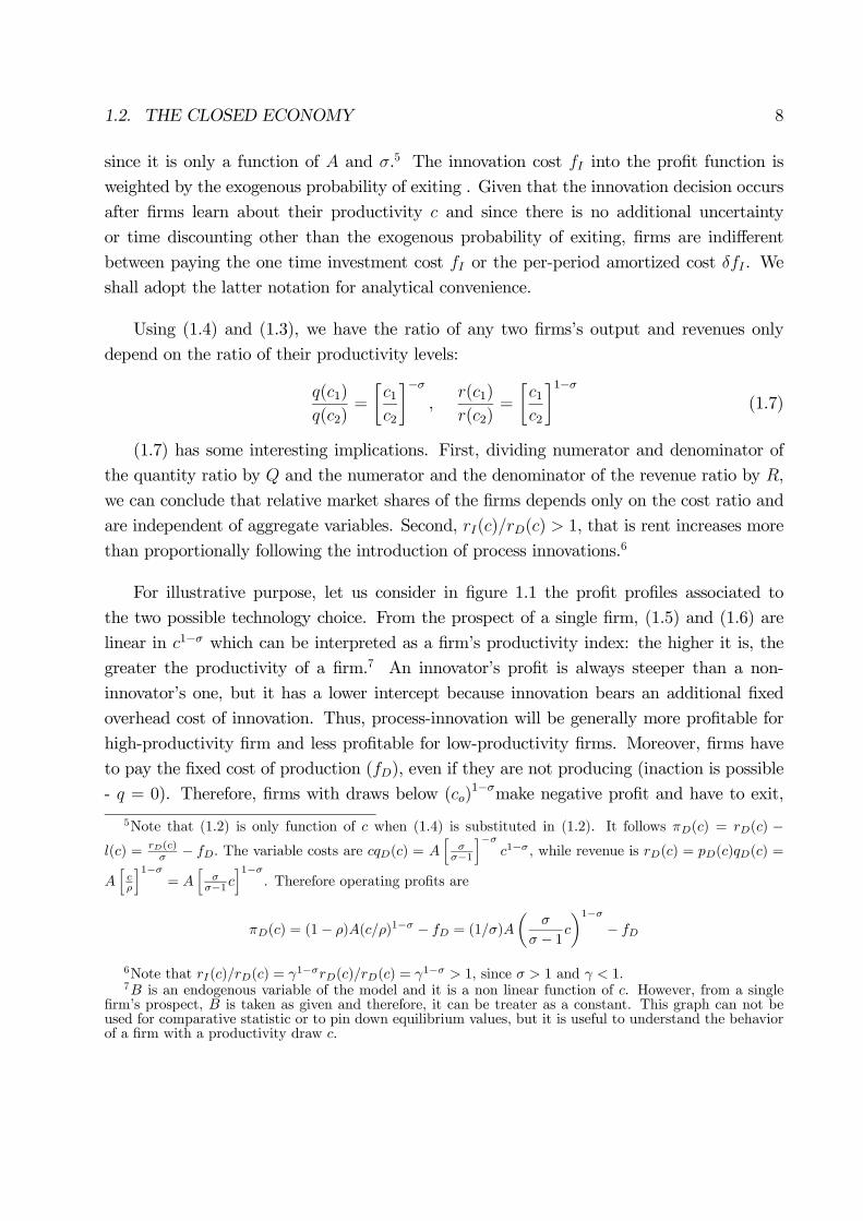
For illustrative purpose, let us consider in figure 1.1 the profit profiles associated to
the two possible technology choice. From the prospect of a single firm, (1.5) and (1.6) are
linear in c1−σ which can be interpreted as a firm’s productivity index: the higher it is, the
greater the productivity of a firm.7 An innovator’s profit is always steeper than a non-
innovator’s one, but it has a lower intercept because innovation bears an additional fixed
overhead cost of innovation. Thus, process-innovation will be generally more profitable for
high-productivity firm and less profitable for low-productivity firms. Moreover, firms have
to pay the fixed cost of production (fD), even if they are not producing (inaction is possible
- q = 0). Therefore, firms with draws below (co)1−σmake negative profit and have to exit,
5Note that (1.2) is only function of c when (1.4) is substituted in (1.2). It follows πD(c) = rD(c) −l(c) = rD(c)
σ − fD. The variable costs are cqD(c) = Ah
σσ−1
i−σc1−σ, while revenue is rD(c) = pD(c)qD(c) =
Ahcρ
i1−σ= A
hσ
σ−1ci1−σ
. Therefore operating profits are
πD(c) = (1− ρ)A(c/ρ)1−σ − fD = (1/σ)A
µσ
σ − 1c¶1−σ
− fD
6Note that rI(c)/rD(c) = γ1−σrD(c)/rD(c) = γ1−σ > 1, since σ > 1 and γ < 1.7B is an endogenous variable of the model and it is a non linear function of c. However, from a single
firm’s prospect, B is taken as given and therefore, it can be treater as a constant. This graph can not beused for comparative statistic or to pin down equilibrium values, but it is useful to understand the behaviorof a firm with a productivity draw c.

1.2. THE CLOSED ECONOMY 9
σ−1cσ−1Ic
σ−1oc
)(cDπ
)(cIπ
0
Df−
)( ID ff δ+−
Figure 1.1: Profits from producing and innovating on the domestic market.
while firms with productivity index above (co)1−σ entry successfully. Only a fraction of these
firms (c1−σ ≥ (cI)1−σ), perform also process-innovation. Denote by MI and MD respectively
the mass of active innovator and domestic (non-innovator) producers, where
MI =G(cI)
G(co)M (1.8)
MD =G(co)−G(cI)
G(co)M (1.9)
andM is the mass of incumbent firms in the economy. G(cI)G(co)
(G(co)−G(cI)G(cI)
) is the ex-ante (prior
to entry) probability of being an innovator (non innovator). In other words, it represents
the probability for a potential entrant to innovate (to entry). By the law of large numbers,
it also represents the fraction of innovating (not-innovating) firms in the economy.
M =MI+MD is also the total mass of available varieties to the consumers in this closed
economy.
1.2. THE CLOSED ECONOMY 10
1.2.1 Equilibrium in a closed economy
We are interested in a stationary equilibrium where the aggregate variables must also
remain constant over time. This requires a mass Me of new entrants in every period, such
that the mass of successful entrants, MeG(co), exactly replaces the mass δM of incumbents
who are hit by the bad shock and exit: MeG(co) = δM .
The equilibrium entry cost-cutoff co and innovation cost-cutoff cI must satisfy8:
πD(co) = 0⇐⇒ B (co)1−σ = fD (1.10)
πI(cI) = πD(cI)⇐⇒ (γ1−σ − 1)B (cI)1−σ = δfI (1.11)
Firms will learn about their productivity only upon becoming operative into the industry.
Therefore, when they take the entry decision their productivity is unrevealed yet and they
will compare the expected profit in the industry with the entry cost, taking into account the
possibility of being hit by a bad shock. Free entry ensures equality between the expected
present discounted value of operating profits of a potential entrant and the entry cost fE:
∞Pt=0
(1− δ)t
"cIR0
πI(c)dG(c) +coRcI
πD(c)dG(c)
#= fE
The term in brackets in the LHS is the expected per-period profit for entering into the
industry, while∞Pt=0
(1 − δ)t is the surviving probability into the market in the future. The
whole expression can be rewritten as the equivalence between the per-period expected profit
from entering and the equivalent amortized per-period entry cost:
cIR0
πI(c)dG(c) +coRcI
πD(c)dG(c) = δfE (1.12)
(1.10) to (1.12) characterize the equilibrium cost-cutoffs co and cI as well as B.
Combining (1.10) with (1.11) we have the relation between the innovation and the entry
cutoff:
(cI)1−σ =
δfIγ1−σ − 1
1
fD(co)
1−σ = Ψ (co)1−σ (1.13)
where δfIγ1−σ−1 is the cost to benefit ratio of innovation. The numerator is the per-period cost
of innovation while the denominator represents the revenue differential of innovation per unit
of revenue initially earned. It is high when either the innovation cost per se is high or the
benefit from innovations are small (γ → 1).
8See also figure 1.1.

1.2. THE CLOSED ECONOMY 11
It follows that a necessary and sufficient condition to have selection into the innova-
tion status is Ψ > 1, which measures the cost of innovation relative to the overhead cost
of production. The greater the relative cost of innovation Ψ, the higher the productivity
threshold for innovating. We shall assume that this condition holds throughout since the
empirical evidence suggests that only a subset of more productive firms undertakes process
innovations9.
To develop a better intuition of (1.12), let us denote by π the average industry profit and
note thatcIR0
πI(c)dG(c) +coRcI
πD(c)dG(c) = G(co)π - in words, the expected average profit in
the industry is the average profit in the industry (π) times the ex-ante probability of entry
(G(co)) (see (1.42) in the appendix), so that (1.12) becomes:
π =δfEG(co)
(1.14)
It states that firms - upon entry - compare the average industry profit with the per-period
cost of entry weighted by the inverse of the probability for a successful entry. The tinier this
probability, the higher the "effective" cost of entry since the smaller the chances of recovering
it in the future. Therefore, when the per-period entry cost δfE rises, firms are willing to
enter if they can expect either a higher per period average profit or greater chances of entry
(higher co).
This can be seen in fig. 1.2 where we show the LHS and the RHS of (1.12).10 Given
(1.13), (1.12) is a function of only co. We show in the appendix (see (1.43)), the LHS of
(1.12) is monotonically increasing from 0 to infinity in c, so that its intersection with the
constant line δfE determines uniquely co. It is also clear from the graph that co has to rise
when the fixed cost of entry increases, for the free entry (FE) condition to hold.
Some important remarks are in order. First, fD, δ, fI affect the innovation cost cutoff
cI through both Ψ and the entry cost-cutoff co. More specifically, a greater fD lowers Ψ,
but it also shifts up the LHS curve in fig. 1.2, so that it reduces the entry cost-cutoff to
c0o.- see(1.43) in the appendix. The intuition is simple and comes from inspecting (1.5) and
(1.6). A larger fD reduces the profits of all firm types in the economy for any given c. It
follows that co and cI have to adjust for (1.12) to hold in a way that the marginal entering
firm can increase its profit and recoup the increased fixed cost of operation. Overall, the
effect of an increase in fD on the innovation productivity cutoff (cI)1−σ is ambiguous since
9See for instance Parisi et. al. (2005) for evidence on Italian firms and Baldwin et al. (2004) for evidenceon Canada.10The curves are dipicted as a parabola for convenience. We do not know the exact shape of them, but
that are monotonically increasing on [o, c].

1.2. THE CLOSED ECONOMY 12
c0
Efδ
c
)( ↑Df
oc'oc
LHS
Figure 1.2: Determination of the equilibrium entry cost cutoff as given by the Free Entry
Condition
Ψ is lower, but (co)1−σ is larger. This ambiguity is a specific-feature of a general equilibrium
model and its source is the entry decision of firms. In absence of an entry decision - like in
Bustos (2005) - the effect of fD would be well determined and would affect the economy only
through Ψ.
Second, this thought experiment in which the fixed costs of operation fD rises (stronger
increasing return to scale) is illustrative of the basic mechanism through which trade openness
will affect vertical innovation in the open economy of the next section. As for fD, trade
will have contrasting effects on the innovation cost cutoff. On the one hand, trade offers
new market opportunities to the exporters. Exporting firms that compensate some market
share loss on the domestic market due to import competition with market shares gains on
foreign markets, will increase their total sales and revenue. Therefore, it will be easier for
them to recoup the fixed cost of innovation and the benefits associated to the cost-reducing
innovations will be spread on a greater output. This means that trade liberalization will lower
the cost to benefit ratio of innovation Ψ. On the other one, more competition from foreigner
exporters will force the least productive domestic firms out of the market - extensive-margin

1.2. THE CLOSED ECONOMY 13
adjustment or selection effect of trade. As described in Melitz (2003) this translates in a
lower entry cost cutoff co.
This ambiguous effect of fD on the innovation cost cutoff carries on to the number of
varieties in the economy, whereas in Melitz (2003) increasing fD unambiguously reduces the
number of firms in the the industry. As shown in the appendix, the number of varieties is:
M =R
r=
L
σ(π + fD +G(cI)G(co)
δfI)(1.15)
so that when fD rises, a larger π and G(co) contribute to reduce the number of varieties11.
However, only when cI rises, the total number of firms unambiguously declines. In the other
case - when cI is reduced - the effect of fD on M remains ambiguous.12
There is an other difference between our economy and the economy in Melitz (2003),
namely the entry productivity cutoff level is higher in this setting.13 The possibility to
innovate allows the most efficient firms that perform process innovation to "steal" market
shares to the least efficient firms for which is harder to survive into the market. Consequently,
our economy is more efficient, because some varieties are produced at a lower cost, but less
varied because some varieties have disappeared. This trade-off has been well emphasized in
the literature (see Peretto (1998)).
1.2.2 The Innovation Decision
Before turning to the open economy we look more closely at the firm’s decision to inno-
vate. Firms will introduce process innovation if the adoption of the innovative technology
yields higher profits than the traditional one, namely whenever (1.6) is greater than (1.5) or:
(γ1−σ − 1)rD(c) > σδfI
where we used rI(c) = γ1−σrD(c). Note that in equilibrium, R = L - that is, the aggregate
revenue coincides with labour income (w = 1) - as shown in the appendix. Dividing the
expression above by R, the firm’s decision to innovate can be evaluated also in terms of its
market share by:
(γ1−σ − 1)s(c) > σδfIL
(1.16)
11Recall that a larger fD entails a lower co. A lower co translates into higher π - by (1.14) - and lowerG(co).12Given that such effect should offset the other negative effects through fD, π and G(cAo ), we think of this
possibility as implausible. Indeed, assuming G(c) as in (1.30), the innovation cost cutoff would increase andthe number of firms decreases when fD is larger.13The proof of this result has been left to the appendix.
1.3. THE OPEN ECONOMY 14
where s(c) = rD(c)/R is the firm’s market share. Accordingly, a firm evaluates the expected
changes in market share when it takes its innovation decision and it will innovate if the
increment in its market share is at least as big as the RHS of (1.16). It is interesting to note
that fD affects the firm’s innovation decision only through R (taken as given by a single firm),
since the fixed cost of production has to be incurred regardless of the technology choice. In
other words, the degree of increasing return to scale (IRS) determines the size of the market
share each single firm can have and, in turn influences the innovation decision. Since the
benefits from innovation are proportional to the firm’s cost level, the innovation decision can
also be related to the firm’s current market share by:
s(c) > σΨfDL
(1.17)
The higher the present market share of a firm, the higher the likelihood for this firm to
be an innovator. The intuition is simple: the greater the market share, the greater the firm’s
sales and its profits from a cost-reduction innovation. The larger the market (L), the greater
the market power (low σ), the lower the relative cost of innovation (Ψ), the more likely is
process-innovation.
1.3 The Open Economy
Let us assume that the economy under study can trade with other n ≥ 1 symmetric
countries. We will assume that trade is not free, but it involves both fixed and variable
costs, since free trade could simply be analyzed by doubling L in the closed economy. One
can think of the fixed cost associated to trade as the cost of customizing its own variety
to the regulations and tastes of foreign countries as well as of creating sale-networks. The
variable trade costs are trade barriers such as transportation costs imposed by distance. We
follow a long tradition in the trade literature and model these variable costs in the iceberg
formulation: τ > 1 units of a good must be shipped in order for 1 unit to arrive at destination.
Finally, the symmetry of countries is required to ensure that factor price equalization
holds and countries have indeed a common wage which can be still taken as the numeraire.
Alternatively, a freely traded homogenous good produced under constant return to scale
could be introduced to pin down its price and thus the wage to unit in all countries. The
symmetry assumptions also ensures that all countries share the same aggregate variables.
Prices,Profits and Firm-TypesThe variable costs of trade are naturally reflected into the price charged by the domestic
exporters into foreign markets. By symmetry, the imported products are more expensive
1.3. THE OPEN ECONOMY 15
than domestically produced goods due to transportation costs. As a result, the effective
consumer price for imported products from any of the n countries is:
pX(c) = τpD(c) (1.18)
while an exporter who has opted for process innovation charges:
pXI(c) = γpX(c) (1.19)
Analogously, the profits of an exporter and an innovator-exporter in a foreign market
are14:
πX(c) = τ1−σBc1−σ − δfX (1.20)
πXI(c) = (γτ)1−σBc1−σ − δfX (1.21)
where δfX is the amortized per-period fixed cost of the overhead fixed cost fX that firms
have to pay (in units of labour) to export to foreign markets.
The following table summarizes the profit function for all possible firm-types with pro-
ductivity c.
type Domestic Producer Exporter
Non Innovator πD(c) πD(c) + nπX(c)
Innovator πI(c) πI(c) + nπXI(c)
No firm will ever export and not also produce for its domestic market. Indeed, any
firm would earn strictly higher profits by also producing for its domestic market since the
associated variable profit rD(c)/σ is always positive and the overhead production cost fDis already incurred. Then, all exporters’ profits can be separated into the portion earned
domestically (πD(c) or πI(c)) and on each of the foreign market (πX(c) or πXI(c)). Moreover,
since the export cost is assumed equal across countries, a firm will either export to all n
countries in every period or never export.
Finally, not all four types can coexist simultaneously in the economy, but which firm
type is active will depend on the kind of selection. The empirical evidence suggests that
14rS(c) = pS(c)qS(c), S = X ,XI . Note that rXI(c) = γ1−σrX(c) = τ1−σrI(c) as well as rX(c) =
τ1−σrD(c). So, πX(c) =rX(c)σ − δfX =
τ1−σrD(c)σ − δfX = τ1−σBc1−σ − δfX and πXI(c) =
rXI(c)σ − δfX =
(γτ)1−σrD(c)σ − δfX = (γτ)
1−σBc1−σ − δfX .Note we account for the entire overhead production cost in the domestic profit (see (1.5) and (1.6)). This
choice is uninfluential for the equilibrium as all firms (domestic producers and exporters) will produce alsofor the domestic market and incur fD upon staying into the industry.
1.3. THE OPEN ECONOMY 16
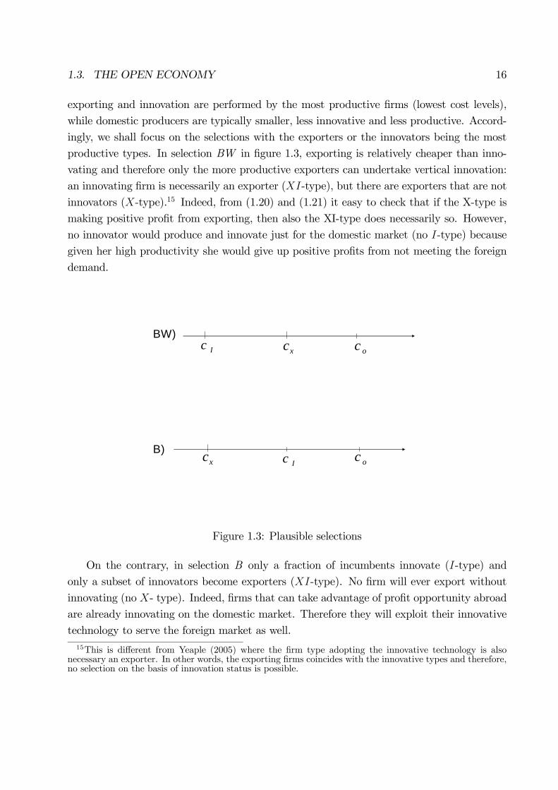
exporting and innovation are performed by the most productive firms (lowest cost levels),
while domestic producers are typically smaller, less innovative and less productive. Accord-
ingly, we shall focus on the selections with the exporters or the innovators being the most
productive types. In selection BW in figure 1.3, exporting is relatively cheaper than inno-
vating and therefore only the more productive exporters can undertake vertical innovation:
an innovating firm is necessarily an exporter (XI-type), but there are exporters that are not
innovators (X-type).15 Indeed, from (1.20) and (1.21) it easy to check that if the X-type is
making positive profit from exporting, then also the XI-type does necessarily so. However,
no innovator would produce and innovate just for the domestic market (no I-type) because
given her high productivity she would give up positive profits from not meeting the foreign
demand.
BW)
B)
xcIc oc
ocIcxc
Figure 1.3: Plausible selections
On the contrary, in selection B only a fraction of incumbents innovate (I-type) and
only a subset of innovators become exporters (XI-type). No firm will ever export without
innovating (no X- type). Indeed, firms that can take advantage of profit opportunity abroad
are already innovating on the domestic market. Therefore they will exploit their innovative
technology to serve the foreign market as well.15This is different from Yeaple (2005) where the firm type adopting the innovative technology is also
necessary an exporter. In other words, the exporting firms coincides with the innovative types and therefore,no selection on the basis of innovation status is possible.

1.3. THE OPEN ECONOMY 17
BW is interesting because the marginal innovating firm is an exporter and trade is
likely going to affect its innovation decision. B represents the other side of the same coin:
the marginal innovating firm is a domestic producer and therefore, innovation is mostly
determined by domestic factors and will less likely respond to trade liberalization.
Given the aim of the paper, we focus closely on selection BW where trade induces within-
plant productivity changes besides allocative effects of market shares. Roughly stated, trade
will have "between" and "within" effects on productivity growth (from here BW ). Then,
we turn to discuss briefly selection B and highlight why trade is not influential on plants’
innovation activity. In this equilibrium, trade affects productivity only through allocative
effects - between effect (form here B).
1.3.1 Selection BW
Let us denote by MD the mass of active incumbent firms with a local dimension only,
by MX the mass of exporting not innovating firms and by MXI the mass of exporting and
innovating firms. The sum of all these firms (MD +MX +MXI = M) gives the mass of
incumbent firms in any country. The mass of non-innovating incumbent firms in any country
isMNI =MD+MX , whileMT =MD+n(MX+MXI) gives the total mass of varieties available
to consumers in any country. Let prD = [G(co)−G(cX)]/G(co), prX = [G(cX)−G(cI)]/G(co),prXI = [G(cI)]/G(co) be the probability of becoming each type conditional on being an
incumbent.
The equilibrium - BWWe are again interested only in a stationary equilibrium where all aggregate variables are
constant over time. The stability condition imposes the entrants into the industry replaces
exactly exiting firms, i.e. δM = MeG(co). Note that the equilibrium value of the aggregate
variable Q, R, and therefore A and B as well as of the entry cutoff co is different in this
equilibrium from the closed economy one. Nevertheless we stick to same notation as they
are defined in the same way.
Cutoffs in equilibrium BW must satisfy the following conditions:
πD(co) = 0⇔rD(co)
σ= B (co)
1−σ = fD (1.22)
πX(cX) = 0⇔rD(cx)
σ= Bc1−σX =
δfXτ 1−σ
(1.23)
πI(cI) + nπXI(cI) = πD(cI) + nπX(cI)⇔rD(cI)
σ= B (cI)
1−σ =δfI
(γ1−σ − 1)(1 + nτ 1−σ)(1.24)
1.3. THE OPEN ECONOMY 18
Thus the parameter restriction that sustains this equilibrium (cI ≤ cX ≤ co) where only
exporters perform process innovation must satisfy:
δfI(γ1−σ − 1)
1
(1 + nτ 1−σ)≥ δfXτ
σ−1 ≥ fD (1.25)
This condition requires that the innovating is relatively more expensive than exporting.
That is, the foreign markets should be fairly accessible, otherwise serving them would result
extremely costly and it could be afforded exclusively by the most productive firms.δfI
(γ1−σ−1) is equivalent to the cutoff for innovation for the closed economy: the same
assumptions that guarantees selection on the basis of innovation status in the closed economy
(i.e., Ψ ≥ 1) ensures that this term is positive and bounded away from zero in the open
economy. Recall that this term represents the cost to benefit ratio of innovation. Importantly,
in the open economy we have an extra term given by 1(1+nτ1−σ) which is unity in the closed
economy (set n = 0 or τ → ∞). The denominator represents precisely the further revenuedifferential associated to innovation on each of the foreign markets that become available
with trade.
We like to think of n as the number of countries into the trading network sharing a
common code of rules as it could be for the WTO membership. Then, it represents a
measure of the world’s openness to trade, as for a low n very few countries have trading
relations. φ = τ 1−σ ∈ [0, 1] is commonly referred in the literature as an index of the freenessof trade with values closer to 1 indexing freer trade.
Clearly, trade liberalization that come in the form of either freer trade (greater φ) or
greater world openness (larger n) can affect process innovation weighing upon the return of
innovation.
(1.22) to (1.24) give a system of 3 equations in 4 unknowns (co,cX ,cI ,B). We can use the
FE condition to close this system and uniquely determine the entry cutoff. The FE condition
ensures the equivalence between expected entry profit and entry cost:coRcX
πD(c)dG(c) +cXRcI
(πD(c) + nπX(c))dG(c) +cIR0
(πI(c) + nπXI(c))dG(c) = δfE (1.26)
Combining appropriately the three conditions for the cutoff points ((1.22) to (1.24)), the
relation between the cutoffs can be written explicitly as:
(cI)1−σ =
δfI(γ1−σ − 1)(1 + nτ 1−σ)
1
fD(co)
1−σ = Ψf (co)1−σ (1.27)
(cI)1−σ =
δfI(γ1−σ − 1)(1 + nτ 1−σ)
1
δfXτσ−1c1−σX = (Ψf
X)c1−σX (1.28)

1.3. THE OPEN ECONOMY 19
c1−σX =δfXτ
σ−1
fD(co)
1−σ (1.29)
Note that Ψ = Ψf(1 + nτ 1−σ) and ΨfX = ΨffD/δfXτ
σ−1. Ψ ≥ Ψf - namely, the cost to
benefit ratio is smaller in the trading equilibrium than in autarky - reflects that trade and
vertical innovation are related: new market opportunities abroad induce exporters to expand
their scale of operation and the benefits of cost-reducing innovation are spread on a greater
number of units sold, while the up-front cost of innovation is unchanged.16 Comparing
(1.27) with (1.13) shows that the distance between the entry productivity index cutoff and
the innovation productivity index cutoff is always smaller in the trading equilibrium than
in autarky (Ψf < Ψ), as trade reduces the relative cost of innovation. Hence, trade (for
positive n and non-prohibitive transportation cost τ) reduces, ceteris paribus,the innovation
productivity cutoff (cI)1−σand therefore it boosts within-plant innovation. This is the partial
equilibrium effect described also in Bustos (2005).17
However, this is not enough for concluding the proportion of incumbents undertaking
productivity innovation will be larger after trade. In general equilibrium, trade affects also
the entry productivity cutoff (co)1−σ which results higher in the trading equilibrium than in
autarky, as it is shown in the appendix. Trade increases competition on the domestic market
and forces the least productive producers out of the market (selection effect). The most hurt
are obviously the domestic firms that produce exclusively for the national market whose
product demand is reduced without being compensated by the expansion of their product
demand on the foreign markets, as it is for some of the exporters.
In this equilibrium, two forces are affecting the innovation cost cutoff when the economy
opens to trade:
i) the selection effect of trade reduces the incentive to perform process innovation because
entry is less likely and survival more difficult in a more competitive environment - lower
co;
ii) conditional on being an incumbent, the benefit of cost-reducing innovation is higher
after trade because the selection effect and the scale effect together increase exporters’
total market shares. Thus, some incumbent will start performing vertical innovation -
Ψf < Ψ.
16Only for prohibitive trade barriers (φ = 0) or a close world (n = 0), Ψ = Ψf .17This situation would describe an industry within the economy which is small enough to affect the
equilibrium price index of the economy, and therefore, real wages and where no entry and exit takes place.
1.3. THE OPEN ECONOMY 20
The overall effect of trade on innovation is ambiguous and depends on the relative
strength of these pushing and deterring factors of process innovation. Although, the pro-
portion of incumbents is reduced (lower co), the proportion of innovating firms among them
will raise (higher cI) if the ii) dominates i), namely if the adjustments through the extensive
margin of innovation dominate those through the extensive margin of trade.
In order to shed some light on which effect dominates, we use a specific parametrization
for G(c). We shall show that the net outcome of these two offsetting forces is a higher
proportion of firms performing process innovation with freer trade.
Assuming that the productivity draws (1/c) are distributed according to a Pareto dis-
tribution with low productivity bound (1/c) and k ≥ 1, the c.d.f of cost draws c is givenby:
G(c) =³cc
´k, k > σ − 1, k > 2. (1.30)
This formulation has been used widely in many extensions of Melitz (2003) because
it allows to derive closed form solutions for the cutoff levels18. k is a shape parameter
indexing the dispersion of cost draws. k = 1, corresponds to the uniform distribution. As k
increases, the distribution is more concentrated at higher cost level and firms’ heterogeneity
is reduced. k > 2 ensures that the second moment of the distribution is well defined, while
k > σ − 1 ensures the first moment of the truncated distribution ((1.33) and (1.34) inthe Appendix) exists and is well defined. With this assumption, we are able to prove the
following proposition on technology adoption.
Proposition 1.1 Denote with cAI (cfI ) the equilibrium innovation cost cutoff in autarky (in
the open economy). If (1.30) and (1.25) hold, then the innovation cost cutoff in the open
economy is larger than in autarky (i.e cAI < cfI )
Proof. See appendix.
An intuition for this result is the following. The market shares of the domestic exiting
firms are reallocated to the more productive surviving incumbents, and thus, also to some
domestic exporters (extensive margin effect or selection effect). This effect adds up to the
intensive-margin effect or scale effect - that following trade liberalization, some exporters
will increase their market share abroad. As a result, their combined market share enlarges.
18See for example Melitz and Ottaviano (2005).

1.3. THE OPEN ECONOMY 21
Since to a larger scale of operation corresponds a greater return from "vertical innovation",
a larger fraction of them finds profitable to introduce "process-innovation". In other words,
trade affects the extensive margin of innovation inducing exporting firms that are not as
productive as former innovators, to introduce more productive technologies.
Interestingly the reallocation of output across plants induced by trade - between effect
- is playing a key role and is related to fX , the fixed cost of trade. In absence of it and
with CES preferences, all firms exports and therefore all firms perfectly compensates for
the loss in the domestic market shares with gains in foreign market shares. Differently
expressed, the increase in each firm’s market size after trade is exactly offset by the rise in
the number of competitors. This can be easily checked inspecting the equilibrium conditions.
(1.22) becomes (1+nτ 1−σ)Bc1−σo = fD which together with (1.24) and (1.26) characterize the
equilibrium with fX = 0, co ≡ cX and π(co) = π(cX). It is easy to show that such equilibrium
is equivalent to the autarky one described by (1.10)-(1.12). In other words, no firms using
the baseline technology opts to implement the innovative technology after engaging in trade.
However, when fX > 0, an increase in the revenue from sales abroad does not map into
a greater profit for all firms, determining selection into exports by a subset of incumbents.
This means that the increase in market size for the exporting firms is not longer exactly
compensated for the augment of competitors. Indeed, some domestic exporter are enjoying
a larger slice of the foreign market (and higher revenues from foreign market) as they are not
facing the competition from their actual domestic producers (previously exporting) and, at
the same time (by symmetry) are confronted with less competitors on the national market
since the number of foreign competitors on the national market has analogously decreased.
This is the basic economic intuition behind ii) it is strictly related to the existence of fixed
trade costs.
Nevertheless, firms willing to engage in trade and incurring fX , exacerbates the compe-
tition for the scarce labour input pushing up the real wage, making survival tougher, and
exporting and innovating more costly (i, above). Still, trade translates into net gains for the
most productive exporting non-innovating firms, inducing them to implement the innovative
technology, as we can conclude from showing that ii is dominating i.
We would expect that the reduction of transportation costs which lead to trade creation
in this model have similar effects on innovation. This is established in the following Lemma.
Lemma 1.2 Assume (1.30) and (1.25) hold, dcI/dτ ≤ 0.Proof. See in the appendix

1.3. THE OPEN ECONOMY 22
Its relevance is that trade liberalization taking the form of partial tariff reform, as often
it is in practice, induce similar positive effect on process innovation. For instance, we can
evaluate the effects of Canada-US FTA (CUSFTA) on within firm performances. τ in (1.27) is
the transportation cost faced by Canadian manufacturing firms exporting to US. The model
predicts US tariff concessions granted to Canada - a reduction of τ - after the FTA would
induce some Canadian exporters to innovate, as they can take advantage of a lower cost to
benefit ratio. This is consistent with the evidence shown in Trefler (2004). The numbers
are quite substantial: "U.S. tariff concessions raised labor productivity by 14 percent or 1.9
percent annually in the most impacted, export-oriented group of industries". Bustos (2005)
find evidence of adoption of innovative technology by Argentinean manufacturing exporting
firms following the substantial trade liberalization of the country in the 90s. Interestingly,
firms adopting the innovative technology are the high productive non-innovating exporters,
so that she concludes that the change in technology spending has an inverted U shape after
trade liberalization. It is highest for firms in the middle range of the productivity distribution,
consistently with the predictions of our model. Indeed, the firms incurring the fixed cost of
innovation after trade liberalization are neither the most productive ones which have already
incurred this cost, nor the least productive ones which have never paid this cost, but rather
firms with productivity in the range between the old and the new innovation cost cutoff.
Only these firms are innovating and therefore, copping with the fixed adaptation cost fI .
Interestingly, Bustos finds also the some exporters keep the "traditional" technology
even after trade liberalization, providing empirical support for the relevance of selection BW
analyzed here.19
Summing up, by increasing the scale of production of some of the exporters, trade in-
creases what Cohen and Klepper (1996) call the "ex ante" output - the firm’s output when
it conducts process innovation. This, in turn, raises firms’ incentive to innovate and triggers
process-innovation, productivity increments and market share growth at firm level (see (1.7)).
This is consistent with Baldwin and Gu (2003) and Trefler (2004) who find that within-firm
productivity increments have occurred mostly among exporters. Moreover, Baldwin (2004)
finds empirical support for such casual link: vertical innovation is a main determinant of
productivity growth and productivity growth induces market share growth20.
19Also in Yeaple (2005), lower transportation costs induce a greater adoption of the innovative technology.However, no exporters retain the old technology as found in Bustos (2005).20Baldwin (2004) finds Canadian process-innovators had productivity growth that was 3.6 percentage
points higher than Canadian non-process innovators (table 9). Moreover, a within-firm productivity incre-ment of 10% relative to the industry average translate into almost 2% gain in the firm’s market share (table12).

1.3. THE OPEN ECONOMY 23
Finally, the reduction of transportation costs has contrasting effect on cX too. A re-
duction of trade barriers have a direct effect and lowers the exporting productivity cutoff
c1−σX (see (1.29)), but also an indirect effect through (co)1−σ which rises this threshold. The
following lemma shows that the direct effect dominates the indirect one.
Lemma 1.3 Assume (1.30) holds, dcX/dτ ≤ 0.Proof. See the appendix
In the context of CUSFTA, this lemma predicts that some Canadian manufacturing firms
which are not as productive as established exporters, will also start to serve the US market
in virtue of the American preferential tariff reform. Interestingly, Baldwin et al. (2003) find
evidence of this.
1.3.2 Selection B
We shall just show that trade in this equilibria can not affect the extensive margin
of innovation as for selection BW. The non-innovating firms are only the D-type, while
the innovating firms are the I-type and the XI-type, but only the latter are present on
international market. There is no X-type.
The cutoff conditions for equilibrium B are:
πD(co) = 0 (1.31)
πI(cI) = πD(cI) (1.32)
πXI(cX) = 0⇔ Bc1−σX = (τγ)σ−1δfX
which imply that the necessary and sufficient condition for cX ≤ cI ≤ co is:
δfXτσ−1 ≥ δfI
(γ1−σ − 1)γ1−σ ≥ fDγ
1−σ
This equilibrium is characterized by a trading cost relatively higher than the innovat-
ing one. High variable and fixed cost of exporting make trading a very expensive activity
performed only by the most productive firms.
Note also that (1.31) and (1.32) imply the same relation among the innovation and
the entry cutoff as in the closed economy given by (1.13). Indeed, the marginal innovating
firm is not an exporter and the transition from autarky to trade leaves the cost to benefit
ratio of innovation unchanged. That is, trade liberalization can not affect and stimulate
firms’ innovation investments because it has no impact on Ψ. In other words, the extensive
margin of innovation responds to lower trade barriers uniquely through the selection effect;
consequently, a raise in c1−σo raises c1−σI as well and depresses vertical innovation.

1.3. THE OPEN ECONOMY 24
1.3.3 Final Remarks
The model has implications on the aggregate productivity level. As in Melitz (2003), the
industry average productivity will be rising in the long run by means of the selection effect
which spells the least efficient firms out of the market - between effect . Moreover, in our
model trade will rise the average industry productivity through a further channel, namely
the within effect (Proposition 1.1 and Lemma 1.2). Following trade liberalization, some of
the exporters opt for implementing a more efficient technology, improving their productivity
level. The right shift of the Canadian productivity distribution of manufacturing firms in
1996 compared to 1988 following the Canada-U.S. FTA documented in Trefler (2005) can be
interpreted as the combination of the between effect and of the within effect. Low productive
firms - below the industry average - that either exit or downsize following trade liberalization
- between component - determine a thinner left tail of the distribution in 1996 relative to
1988. Analogously, the reallocation of market shares favouring high productive firms has
contributed to a fatter right tail of the distribution of 1996.
The exporters who have raised their plant productivity (within component) significantly
determine the increased mass on medium and high productivity levels for the distribution
in 1996 relative to the one in 1988.
Moreover, such liberalization encourages also new Canadian exporters that are less pro-
ductive than old Canadian exporters to enter the US market (Lemma 1.3). This must reduce
the industry average productivity as the expansion in the US market increases the market
share of lower productivity new exporters.
Finally the model suggests that trade liberalization and the geography of a country can
interact each other: the same trade liberalization may induce different innovation outcomes
depending on the location of a country.
Moving from B to BW, the cost of exporting relative to the cost of innovating decreases.
This means that the effect trade has on the process innovation will be differentiated according
to the level of transportation cost. We shall interpret high transportation cost as a proxy for
the remoteness of the Home economy from the main exporting markets or, more generally,
as the level of trade barriers faced by the Home country.
If in the transition from autarky to trade, the country is fairly remote and faces selection
B, then process innovation performed will be reduced, as discussed above. On the contrary, if
the country is close to the exporting markets and selection BW is possible, process innovation
increases.

1.4. CAVEATS AND FURTHER RESEARCH 25
1.4 Caveats and Further Research
We have modeled the process innovation very simply as a binary decision - adopt/not
adopt the new productive technology. The benefit and the cost of innovation are known and
exogenously given. This introduces two major limitations.
First, more innovation in this economy is measured by the changes in the proportion of
firms innovating and therefore is related uniquely to the extensive margin of innovation. In
other words, the intensity of innovation is out of the model as firms do not decide upon their
productivity target.
Second, all innovators improve their productivity in the same proportion. This means
that the mass of firm with cost levels in the range [γcI , cI ] has measure zero and the ex-post
innovation cost distribution of incumbent-firms has a hole.
One way around the latter problem which preserves the innovation decision as exogenous
would be introducing γ as a continuous random variable. Firms would pay the cost of
innovation to draw a γ.
Instead, we are currently working to make the innovation decision endogenous: firms that
opt for vertical innovation, choose optimally their γ balancing the benefits with the costs of
innovation. Not only this avenue would solve the problem of the hole in the distribution,
but it also allows to analyze how both the intensive and the extensive margin of innovation
respond to trade liberalization.
Indeed, trade would affect both who is innovating and how much each firm is innovating.
In equilibrium BW, the within effect would not be comprised of only the new innovators,
but also of the former innovators investing more intensively in productivity increments.
Interestingly, in equilibrium B, trade may continue to be unrelated to the extensive margin
on innovation, but it still could affect the intensive margin inducing some of the innovators
to innovate more. Thus, the dichotomy within and no-within effect proper of equilibrium
BW and B is a specific feature of our setup and would not survive under this modification.
Trade would affect the industry productivity growth through both the within and the between
effect in both equilibrium. However, the degree of importance of the within effect would be
different across the two equilibrium and only in equilibrium BW trade can likely weigh upon
the extensive margin of innovation.
In spite of all these limitations, this set up highlight in a simple way the trade forces
related to the within-firm productivity changes. Moreover, it is able to generate some pre-
dictions that are consistent with the available empirical evidence.
1.5. CONCLUSION 26
1.5 Conclusion
The paper introduces process innovation into the Melitz (2003) framework. As in Melitz
(2003), trade has a selection effect on firms forcing the least productive ones out of the market
and reallocating market shares to the more productive ones. Although this contributes to the
aggregate productivity growth, it is not exhaustive of the effects of trade on productivity.
We showed trade can favour the adoption of an innovative technology, especially among
exporters.
One could think that fiercer competition implied by trade can reduce the incentive for
innovation. This is certainly true for low productive domestic firms whose survival possibil-
ities have decreased together with their market shares. Instead, exporters compensate the
loss of market shares in the domestic market with gains in market shares in foreign markets.
As they expand their scale of production, their incentive for process innovation strengthens
and some of them introduce a more productive technology. Moreover, if the reallocation of
output from exiting firms to incumbents firms is consistent, also relatively low productive
exporters can take advantage of a greater market share and benefit from vertical innovation.
In productivity studies, this is the so called within effect - some of the incumbent firms
update their productivity - and it is a main source of labour productivity growth in indus-
trialized countries. This is the new insight of the model: trade contributes to the industry
productivity growth through the within effect besides through the between effect. More
generally, a greater openness in the trading relations can justify the finding of the great
importance of the within component for the industry productivity growth, as recently doc-
umented.
This seems consistent with some recent micro evidence. For instance, the productivity
distribution of Canadian manufacturing firms has shifted to the right decreasing considerably
the mass on low productivity values (between effect) and at the same time increasing its
mass on the upper-tail of the distribution (within effect) after the US-Canada Free Trade
Agreement was signed. The latter has also brought some new Canadian firms - not quite as
productive as old exporters - into exporting to the US market in virtue of these lower trade
barriers. This is consistent with the prediction of the model that a reduction of transportation
costs leads to an increase of the proportion of firms exporting to foreign markets, as firms
not as productive as well established exporters can also afford to serve some markets abroad.
Furthermore, geography plays an important role. Trade liberalization can depress ver-
tical innovation (equilibrium B) for remote countries, while it can boost process-innovation
(equilibrium BW ) for countries closely located to the core of the exporting markets.

1.6. APPENDIX 27
1.6 Appendix
1.6.1 Appendix A - Closed Economy
We first proceed with the aggregation to define the aggregate variables of the economy
that firms take as given in their decisions (see (1.5) and (1.6)). Then, we turn to the analysis
of the equilibrium and determine the entry cost-cutoff and the number of varieties.
1.6.1.1 Aggregation
Let us denote by µD(c) and µI(c) respectively, the cost distribution of domestic producers
and active innovator prior to innovation. These "ex-ante"-innovation cost distributions are
truncated distribution of g(c):
µD(c) =g(c)
G(co)−G(cI)o
,cI < c < co
otherwise(1.33)
µI(c) =g(c)G(cI)
o,
0 < c < cI
otherwise(1.34)
and will be used repeatedly in the aggregation. They are not affected by the exogenous
productivity δ which affects all firms equally and it is independent of the productivity level.
Finally, in order to derive the aggregated variable, it is useful to introduce some synthetic
measures of the productivity index as the following averages:
fcD1−σ = coZcI
cµD(c)dc (1.35)
ecI1−σ = 1
G(cI)
cIZ0
c1−σµI(c)dc (1.36)
ec1−σ = 1
M
£MI(γ ecI)1−σ +MDfcD1−σ¤ (1.37)
(1.35) is the weighted average productivity index within the subgroup domestic producers,
while (1.36) is the "ex ante"-innovating weighted average productivity index among the sub-
group of inventors21. Given that process innovation is simply modeled as a fixed proportional
reduction in the cost level, the "ex-post" innovation weighted average productivity index will
also be increased proportionally and be (γecI)1−σ. Therefore, (1.37) is the weighted average21Given that domestic (non-innovators) domestic producers do not increment their productivity level, the
ex-ante and ex-post innovation cost distribution of domestic producers coincide.
1.6. APPENDIX 28
productivity index of the economy which is an opportunely weighted average of the averages
prevailing in each subgroup. All these measures are independent of the number of firms. ec isthe most aggregated productivity-index and completely summarizes all aggregate variables
of the model derived below.
Using (1.3) for both a domestic and an innovator producer and the definition of the price
index for CES utility function in footnote ??, it is possible to define the price index for thiseconomy as:
P 1−σ =
cIZ0
MI [pI(c)]1−σµI(c)dc+
coZcI
MD [pD(c)]1−σ µD(c)dc
= (1/ρ)1−σ£MIγ
1−σ ecI1−σ +MDfcD1−σ¤ (1.38)
= M
∙ecρ
¸1−σ=M [pD(ec)]1−σ
Similarly,
R =
cIZ0
MIrI(c)µI(c)dc+
coZcI
MDrD(c)µD(c)dc
= MIrI(ecI) +MNIrD(fcD) (1.39)
= MIγ1−σrD(ecI) +MNIr(fcD)
= M
∙MI
Mγ1−σrD(ecI) + MNI
Mr(fcD)¸ =MrD(ec) =Mr
and
Π =
cIZ0
MIπI(c)µI(c)dc+
coZcI
MDπD(c)µD(c)dc
=1
σ
⎡⎣ cIZ0
MIrI(c)µI(c)dc+
coZcI
MDrD(c)µD(c)dc
⎤⎦−MfD −MIδfI (1.40)
= MrD(ec)σ−MfD −MIδfI =M
∙rD(ec)σ− fD −
MI
MδfI
¸| z
πD(c)
=M
∙r
σ− fD −
MI
MδfI
¸| z
π
where r and π are the average revenue and profit in the economy.
In a proof below, we shall use the average profit in autarky and we shall use the convention
that the variable with superscript A denote the equilibrium variables in the closed economy
1.6. APPENDIX 29
equilibrium. For example the average profit in autarky will be:
πA =rA
σ− fD −
MAI
MAδfI (1.41)
where rA is (1.39) evaluated at the equilibrium cost cutoff cAo and cAI .
Note we can use the first line of (1.40) together with (1.8), (1.9), (1.33) and (1.34) to
rewrite (1.12) as:cAIR0
πI(c)dG(c) +cAoRcAI
πD(c)dG(c) = G(cAo )πA (1.42)
which is (1.14).
1.6.1.2 Determination of the equilibrium
µI(c) and µD(c) are not affected by the simultaneous entry and exit since the successful
entrants and failing incumbents draw their productivity level from a common distribution
and δ is independent of the innovation status. These distributions depend exclusively on the
cutoffs points for entry and innovation.
Using (1.40) together with (1.8) and (1.9), it is possible to express (1.12) as (1.14), which
can be further refined and express in terms of solely co. Insert (1.10) and (1.11) into (1.12),
replace δfI = Ψ(γ1−σ − 1)fD and rearrange terms to get:
δfE = B£γ1−σG(cI)ecI1−σ + (G(co)−G(cI))fcD1−σ¤− fDG(co)− δfIG(cI)
= G(cI)γ1−σ
µ ecIco
¶1−σfD −G(cI)
µfcDco
¶1−σfD −G(cI)Ψ(γ
1−σ − 1)fD +
+G(co)
µfcDco
¶1−σfD −G(co)fD (1.43)
= fD£jD(co) + γ1−σjI(co)
¤where
jD(co) = G(co)
"µfcDco
¶1−σ− 1#−G(cI)
"µfcDco
¶1−σ−Ψ
#(1.44)
jI(co) = G(cI)
"µ ecIco
¶1−σ−Ψ
#(1.45)

1.6. APPENDIX 30
1.6.1.3 Existence and Uniqueness of the equilibrium in the closed economy
Proposition 1.4 Under autarky, the equilibrium exists and is unique.
Proof. We shall prove that the RHS of (1.43) is monotonically increasing in co on the
domain [0, c], so that co is uniquely determined by the intersection of the latter curve with
the flat line δfe in the [0, c] space. Recall that ecI is a function of cI (see (1.36)), which, inturn, is a function of co by (1.13). Let us define Λ = Ψ1/1−σ. Note that (1.13) implies:
∂cI∂co
= Ψ1/1−σ = Λ
and (1.36) implies:
∂
∂co
µ ecI1−σc1−σo
¶=
Ψ1/1−σg(cI)[(cI)1−σ−c1−σI ](co)1−σ
G(cI)− ecI1−σ(1− σ) (co)
−σ
(co)2(1−σ)
= Λg(cI)
G(cI)
"µcIco
¶1−σ−µ ecIco
¶1−σ#− ecI1−σ(1− σ)
(co)1−σ co
= Λg(cI)
G(cI)
"Ψ−
µ ecIco
¶1−σ#−µ ecIco
¶1−σ1− σ
co
It follows:
∂jI(co)
∂co=
∂
∂c
(G(cI)
"µ ecIco
¶1−σ−Ψ
#)(1.46)
= g(cI)(∂cI∂c)
"µ ecIco
¶1−σ−Ψ
#+G(cI)
"∂
∂c
µ ecIco
¶1−σ#
= g(cI)Λ
"µ ecIco
¶1−σ−Ψ
#+G(cI)
(Λg(cI)
G(cI)
"Ψ−
µ ecIco
¶1−σ#−µ ecIco
¶1−σ1− σ
co
)
= −1− σ
coG(cI)
µ ecIco
¶1−σ≥ 0
Using (1.35) and following similar steps we get:
∂
∂c
µfcDco
¶1−σ=
g(co)
G(co)−G(cI)
"1−
µfcDco
¶1−σ#+
g(co)Λ
G(co)−G(cI)
"µfcDco
¶1−σ−Ψ
#−µfcDco
¶1−σ1− σ
co
∂jD(co)
∂co=
∂jD(co)
∂co
(G(co)
"µfcDco
¶1−σ− 1#−G(cI)
"µfcDco
¶1−σ−Ψ
#)(1.47)
= −1− σ
co[G(co)−G(cI)]
µfcDco
¶1−σ≥ 0
1.6. APPENDIX 31
(1.46) and (1.47) ensure that the RHS of (1.43) is an increasing function of co. Furthermore,
limco→c
jI(co) =∞, and limco→c
jD(co) = a <∞, so that limco→c
[jD(co) + γ1−σjI(co)] =∞. In orderto show that the RHS of (1.43) goes to 0 as co goes to 0, I will follow Melitz (2003) and show
that the elasticities of jI(co) and jD(co) are positive and jI(co) is always bounded away from
0.∂jI(co)
∂co
cojI(co)
= −(1− σ)
∙1 +
Λ
jI(co)
¸≥ −(1− σ)
∂jD(co)
∂co
cojD(co)
= −(1− σ)
⎡⎢⎣(G(co)−G(cI))³cDco
´1−σjD(co)
⎤⎥⎦ ≥ 0Therefore the RHS of (1.43) is monotonically increasing in the space (0, c) and it must cross
the horizontal curve δfE only once. The equilibrium co exists and it is unique.
Once the unique co is determined, (1.33) and (1.34) can be determined as well as (1.35) to
(1.37). By (1.13) follows cI , while by (1.14) follows π. However, to determine the aggregate
variables, we have to compute the number of varieties.
1.6.1.4 Determination of the number of varieties
Labour can be employed in three activities: product innovation, process innovation and
production. The labour used for product innovation is the labour used by new entrants
for investment purposes and amounts to Le units. Lp is the labour devoted to produce a
variety or make its productive process more efficient. By full employment L = Le+Lp. The
market clearing condition for product innovation is Le = Mefe, since each of the new Me
entrants pays fe units of labour. Domestic producers and Innovators pay their workers out
of revenues. Thus, the aggregate payment to production workers must match the difference
between aggregate revenue and profit:
wLp = Lp = R−Π
The stability condition MeG(co) = δM together with (1.14) imply:
Le =Mefe =δMfeG(co)
=Mπ = Π
Then, the labour market clearing conditions implies L = Le+Lp = Π+R−Π = R, that is
the aggregate revenue consists of the aggregate consumers’ expenditure and it is exogenously
limited by the country size. Then, from (1.39) follows (1.15), with the understanding that the
1.6. APPENDIX 32
superscript A denotes the autarky equilibrium value of these variables. The cutoffs and the
number of varieties pin down all other aggregate variables and complete the characterization
of the unique stationary equilibrium in the closed economy.
1.6.2 Appendix B - Comparison of our entry cutoff with Melitz’s (2003) in
the closed economy
Proposition 1.5 Let denote c∗M as the cutoff level of marginal cost found in Melitz (2003)
for the closed economy. Then we have that:
c0 < c∗MProof. Since (1.10) and R = L are common to both models, the ratio of the entry
cost-cutoff is given by:
c∗Mc0=
P ∗MP
where
P ∗M =
⎛⎜⎝ cIZ0
(p(c))1−σ g(c)dc+
c∗MZcI
(p(c))1−σ g(c)dc
⎞⎟⎠1
1−σ
P =
⎛⎝ cIZ0
(γp(c))1−σ g(c)dc+
c0ZcI
(p(c))1−σ g(c)dc
⎞⎠ 11−σ
Assume that:
c0 > c∗MThis implies that :
⎛⎜⎝ cIZ0
(p(c))1−σ g(c)dc+
c∗MZcI
(p(c))1−σ g(c)dc
⎞⎟⎠1
1−σ
<
⎛⎝ cIZ0
(γp(c))1−σ g(c)dc+
c0ZcI
(p(c))1−σ g(c)dc.
⎞⎠ 11−σ
and, rearranging terms, we have:
(1− γ1−σ)
cIZ0
(p(c))1−σ g(c)dc >
c0ZcI
(p(c))1−σ g(c)dc.−c∗MZcI
(p(c))1−σ g(c)dc.
which is not possible since, γ < 1, σ > 1, c0 > c∗M .
Q.E.D
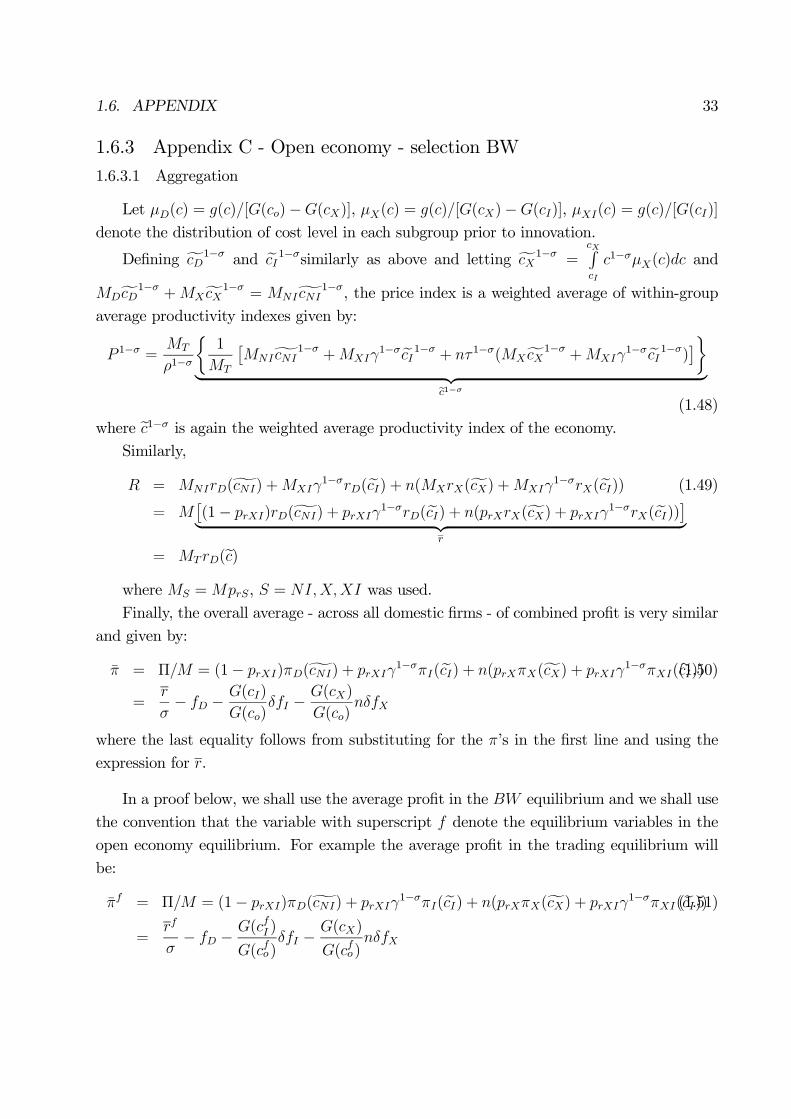
1.6. APPENDIX 33
1.6.3 Appendix C - Open economy - selection BW
1.6.3.1 Aggregation
Let µD(c) = g(c)/[G(co)−G(cX)], µX(c) = g(c)/[G(cX)−G(cI)], µXI(c) = g(c)/[G(cI)]
denote the distribution of cost level in each subgroup prior to innovation.
Defining fcD1−σ and ecI1−σsimilarly as above and letting fcX1−σ = cXRcI
c1−σµX(c)dc and
MDfcD1−σ +MXfcX1−σ = MNIgcNI1−σ, the price index is a weighted average of within-group
average productivity indexes given by:
P 1−σ =MT
ρ1−σ
½1
MT
£MNIgcNI
1−σ +MXIγ1−σ ecI1−σ + nτ 1−σ(MXfcX1−σ +MXIγ
1−σ ecI1−σ)¤¾| z c1−σ
(1.48)
where ec1−σ is again the weighted average productivity index of the economy.Similarly,
R = MNIrD(gcNI) +MXIγ1−σrD(ecI) + n(MXrX(fcX) +MXIγ
1−σrX(ecI)) (1.49)
= M£(1− prXI)rD(gcNI) + prXIγ
1−σrD(ecI) + n(prXrX(fcX) + prXIγ1−σrX(ecI))¤| z
r
= MT rD(ec)where MS =MprS, S = NI,X,XI was used.
Finally, the overall average - across all domestic firms - of combined profit is very similar
and given by:
π = Π/M = (1− prXI)πD(gcNI) + prXIγ1−σπI(ecI) + n(prXπX(fcX) + prXIγ
1−σπXI(ecI))(1.50)
=r
σ− fD −
G(cI)
G(co)δfI −
G(cX)
G(co)nδfX
where the last equality follows from substituting for the π’s in the first line and using the
expression for r.
In a proof below, we shall use the average profit in the BW equilibrium and we shall use
the convention that the variable with superscript f denote the equilibrium variables in the
open economy equilibrium. For example the average profit in the trading equilibrium will
be:
πf = Π/M = (1− prXI)πD(gcNI) + prXIγ1−σπI(ecI) + n(prXπX(fcX) + prXIγ
1−σπXI(ecI))(1.51)
=rf
σ− fD −
G(cfI )
G(cfo)δfI −
G(cX)
G(cfo)nδfX
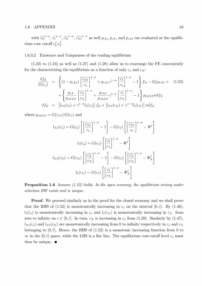
1.6. APPENDIX 34
with fcD1−σ, ecI1−σ, fcX1−σ,gcNI1−σ as well prD, prX , and prXI are evaluated at the equilib-
rium cost cutoff cfo ,cfI .
1.6.3.2 Existence and Uniqueness of the trading equilibrium
(1.22) to (1.24) as well as (1.27) and (1.28) allow us to rearrange the FE conveniently
for the characterizing the equilibrium as a function of only co and cX :
δfEG(co)
=
((1− prXI)
∙gcNI
co
¸1−σ+ prXIγ
1−σ∙ ecIco
¸1−σ− 1)fD − δfIprXI + (1.52)
+
(prX
prEXP
∙fcXcX
¸1−σ+
prXI
prEXPγ1−σ
∙ ecIcX
¸1−σ− 1)prEXPnδfX
δfE =£lNI(co) + γ1−σlI(co)
¤fD +
£lNI(cX) + γ1−σlI(cX)
¤nδfX
where prEXP = G(cX)/G(co) and
lNI(co) = G(co)
"∙gcNI
co
¸1−σ− 1#−G(cI)
"∙gcNI
co
¸1−σ−Ψf
#
lI(co) = G(cI)
"∙ ecIco
¸1−σ−Ψf
#
lNI(cX) = G(cX)
"∙fcXcX
¸1−σ− 1#−G(cI)
"∙fcXcX
¸1−σ−Ψf
X
#
lI(cX) = G(cI)
"∙ ecIcX
¸1−σ−Ψf
X
#
Proposition 1.6 Assume (1.25) holds. In the open economy, the equilibrium arising underselection BW exists and is unique.
Proof. We proceed similarly as in the proof for the closed economy and we shall provethat the RHS of (1.52) is monotonically increasing in co on the interval [0, c]. By (1.46),
lI(co) is monotonically increasing in co and lI(cX) is monotonically increasing in cX from
zero to infinity on c ∈ [0, c]. In turn, cX is increasing in co from (1.29). Similarly by (1.47),
lNI(co) and lNI(cX) are monotonically increasing from 0 to infinity respectively in co and cXbelonging to [0, c]. Hence, the RHS of (1.52) is a monotonic increasing function from 0 to
∞ in the [0, c] space, while the LHS is a flat line. The equilibrium cost-cutoff level co must
then be unique.

1.6. APPENDIX 35
1.6.3.3 Comparison of the entry cost-cutoff in autarky and in trade
To compare the equilibrium entry cost-cutoff of autarky cAo with the one arising in the
BW -equilibrium cfo , it is useful to re-arrange (1.52) in a more convenient way as:
δfE =£jD(c
fo) + γ1−σjI(c
fo)¤fD + Γ (1.53)
where
Γ =
(∙fcXcX
¸1−σ− G(cfI )
G(cX)
∙fcXcX
¸1−σ+ γ1−σ
G(cfI )
G(cX)
∙ ecIcX
¸1−σ− 1)G(cX)nδfX ≥ 0
The first term of the RHS in (1.53) is exactly the same as in the closed economy. If Γ
were 0, (1.43) and (1.53) would yield the same solution, i.e. cfo = cAo . Since Γ is positive
the curve representing the RHS of (1.53) must lie above the curve representing the RHS
of (1.43), implying a lower entry cost-cutoff in the trading equilibrium than in the autarky
equilibrium. That is, cfo ≤ cAo .
1.6.3.4 Proposition 1.1 - In BW, trade increases the proportion of firms performing process-
innovation
Proposition 1.1. If (1.30) and (1.25) hold, then the innovation cutoff in the openeconomy is lower than in autarky (i.e cfI < cAI ).
Proof. First, use the expressions for µD, µX , µXI , prX , prXI to rewrite (1.26) as:
πf =δfE
G(cfo)(1.54)
where πf is (1.51).
Using (1.14) and (1.54) combined with (1.30) it is possible to write the ratio of the
average profit in the trading equilibrium to the average profit in autarky as:
πf
πA=
µcAocfo
¶k
Use (1.13) and (1.27) to get:ÃcAIcfI
!k
= (1 + nτ 1−σ)k
1−σ
µπf
πA
¶Let us make some convenient transformations. Recalling that:
Ψf =δfI
(γ1−σ − 1)(1 + nτ 1−σ)fD(1.55)

1.6. APPENDIX 36
we define Λ = Ψ1
1−σ , Λ∗ = Ψf 11−σ ,and Λ∗ = αβ where:
α =
µτ 1−σfI
(γ1−σ − 1)(1 + nτ 1−σ)fX
¶ 11−σ
β =
µδfXfD
τσ−1¶ 1
1−σ
(1.56)
(1.52) can then be expressed as a function of the parameters of the model:
πf =
∙k
k + 1− σ
£(1− Λk+1−σ) + γ1−σΛk+1−σ¤− 1¸ fD − δfIΛ
k +∙k
k + 1− σ
£(1− αk+1−σ) + γ1−σαk+1−σ¤− 1¸βknδfX
Using the definition of Λ and rearranging terms we get:
πf =k
k + 1− σ
£(γ1−σ − 1)Λk+1−σ¤ fD − δfIΛ
k +σ − 1
k + 1− σfD +
k
k + 1− σ
£(γ1−σ − 1)Λk+1−σ¤βσ−1nδfX + σ − 1
k + 1− σβknδfX
Using (1.56) and the fact that Λ∗ = (1 + nτ 1−σ)1
σ−1Λ:
πf =
∙k
k + 1− σ
£Λ1−σ(γ1−σ − 1)
¤fD − δfI
¸Λ∗k +
σ − 1k + 1− σ
fD (1.57)
+σ − 1
k + 1− σβknδfX
and expanding (1.43):
πA =
∙k
k + 1− σ
£Λ1−σ(γ1−σ − 1)
¤fD − δfI
¸Λk +
σ − 1k + 1− σ
fD
Then, ÃcAIcfI
!k
=(1 + nτ 1−σ)
kσ−1A+B + C
(1 + nτ 1−σ)k
σ−1A+ (1 + nτ 1−σ)k
σ−1B(1.58)
where
A = [k
k + 1− σ
£Λ1−σ(γ1−σ − 1)
¤fD − δfIΛ
k (1.59)
B =σ − 1
k + 1− σfD (1.60)

1.6. APPENDIX 37
C =σ − 1
k + 1− σβknδfX (1.61)
We have to show that :cAIcfI
< 1
which implies:
((1 + nτ 1−σ)k
σ−1 − 1)B > C
Substituting (1.60),(1.61), the inequality becomes:
(1 + nτ 1−σ)k
σ−1 > 1 +
µδfXfD
¶k+1−σ1−σ
τ−kn
To show that this inequality holds true, note that β < 1 implies:µδfXfD
¶k+1−σ1−σ
τ−kn < nτ 1−σ ⇒ 1 +
µδfXfD
¶k+1−σ1−σ
τ−kn < 1 + nτ 1−σ
It follows:
(1 + nτ 1−σ)k
σ−1 > (1 + nτ 1−σ) > 1 +
µδfXfD
¶k+1−σ1−σ
τ−kn
since k > σ − 1 is assumed.
1.6.3.5 Lemma 1.2
Lemma 1.2. Assume (1.30) and (1.25) hold. Trade liberalization will have positiveeffects in innovation, i.e. dcI/dτ ≤ 0.
Proof. Combining (1.27) with (1.30), we get that:
G(cI) = Ψk
1−σG(cfo)
Substitute (1.54) and (1.55) into this expression to get:
(G(cI))−1 = (1 + nτ 1−σ)
k1−σ πfΘ = f
where Θ is a constant independent of τ , so that we shall ignore it because it does not affect
the derivative. Totally differentiating both sides of this expression w.r.t. τ , we obtain the
following:dcIdτ
=dfdτ
d(G(cI))−1
dcI

1.6. APPENDIX 38
Since the denominator is negative, it is enough to show dfdτ
> 0 for dcIdτ
< 0. Use (1.57), (1.59)
to (1.61) and recall Λ∗ = (1 + nτ 1−σ)1
σ−1Λ to expand f in the following way:
f = A+B
(1 + nτ 1−σ)k
σ−1+
C
(1 + nτ 1−σ)k
σ−1
where A,B,C are defined as in (1.59) to (1.61) and A is independent of τ . Using (1.56) and
(1.61), it is convenient to express C = λφk
σ−1 ., with φ ≡ τ1−σ, so that:
df
dφ=
λφk+1−σσ−1 (1 + nφ)
kσ−1 − (1 + nφ)
k+1−σσ−1 φ
kσ−1λn−Bn(1 + nφ)
k+1−σσ−1
(1 + nφ)2kσ−1
Rearranging terms:
df
dφ=
∙λφ
kσ−1 1
φ(1+nφ)−B n
1+nφ
¸(1 + nφ)
kσ−1
Since we are deriving f with respect to φ (instead of τ) and σ > 1, the numerator is negative
(i.e. dfdτ
> 0) iff:
φk+1−σσ−1 <
B
λn
and substituting for the values of B and λ, we get:
φ =fDδfX
and:
τ ≤µδfXfD
¶ 11−σ
which satisfies our parameter restrictions (1.25).
1.6.3.6 Lemma 1.3
Lemma 1.3. Assume (1.30) holds. cx is monotonically decreasing in τ and fx.
Proof. Combining (1.29) with (1.30) gives the following equality:
G(cX) = βkG(co)
Substitute (1.54) and (1.56) into this expression to get:
(G(cX))−1 = ζτkπf = g (1.62)

1.6. APPENDIX 39
where ζ =³δfXfD
´ kσ−1
is constant with respect to tariffs.
Proceeding similarly to the proof above, we take the total differential of both sides of
(1.62) w.r.t. τ , so that the response of the exporting cost cutoff to changes in the trans-
portation costs is given by:
dcXdτ
=dgdτ
d(G(cX))−1
dcX
Since the denominator is negative, we need to prove dgdτ
> 0 for dcXdτ
< 0. Substituting
(1.57),(1.59),(1.60),(1.61) into (1.62), g is a function given by:
g = ζτk(1 + nτ 1−σ)k
σ−1A+ ζτkB + ζτkC
or, substituting for the value of C, g can be conveniently expanded as:
g = ζ(τk(σ−1) + nτ (k−1)(σ−1))k
σ−1A+ ζτkB + Φ
where Φ = (σ−1)nk+1−σ (δfX). It follows
dgdτ
> 0.
To prove that dcX/dfX ≤ 0 we totally differentiate both sides of (1.62) w.r.t. fX and
obtain the following:dcXdfX
=
dgdfX
d(G(cX))−1
dcX
Note that dgdfX
> 0 as dζdfX
> 0, dωdfX
> 0 and A,B are independent of fX . Recalling that
the denominator is negative, it follows that dcXdfX≤ 0 - Q.E.D.
BIBLIOGRAPHY
[1] Baldwin, J.R. (1995) The Dynamics of Industrial Competition. Cambridge: UniversityPress.
[2] Baldwin, John R. and Gu, Wulong. (2003). Participation on Export Markets and Pro-ductivity Performance in Canadian Manufacturing. Canadian Journal of Economics,36(3): 634-657.
[3] Baldwin, John R. and Gu, Wulong. (2004). Innovation, Survival and Performance ofCanadian Manufacturing Plants. Analytical Studies Research Paper Series 11F0027MIEAnalytical Studies Branch Ottawa: Statistics Canada.
[4] Baldwin, Richard, and Nicoud, Frédéric, R. (2005). Trade and Growth with Heteroge-nous Firms. CEPR Discussion Paper No. 4965.
[5] Bartelsman, Eric J., Haltiwanger, John and Scarpetta, Stefano. (2004). MicroeconomicEvidence of Creative Destruction in Industrial and Developing Countries. TinbergenInstitute Discussion Paper 114/3.
[6] Bartelsman, Eric and Doms, Mark. (2000). Understanding Productivity: Lessons fromLongitudinal Microdata. Journal of Economic Literature: 38(3), 569-594.
[7] Bernard, Andrew, Eaton Janathan, Jensen, Bradford and Kortum, Samuel. (2003).Plants and Productivity in International Trade. American Economic Review 93(4):1268-1290.
40
BIBLIOGRAPHY 41
[8] Bernard, Andrew, Jensen, Bradford J. and Schott, Peter K. (2006). Trade costs, firmsand productivity. Journal of Monetary Economics 53: 917-937.
[9] Bernard, Andrew. (2006). Firms in International Trade.NBER Reporter : Research Sum-mary Fall 2006.
[10] Bikson, Tora K., Don Mankin, Barbara A. Gutek. (1987). Implementing ComputerizedProcedures on Office Settings: Influences and Outcome. Rand Report.
[11] Blundell, R.W., Griffith, R. and Van Reenen, J. (1995). Dynamic Count Data Modelsof Technological Innovation. The Economic Journal : 105, 333-344.
[12] Bustos, Paula. (2005). The Impact of Trade on Technology and Skill Upgrading Evidencefrom Argentina. Mimeo, CREI.
[13] Cohen, Wesley and Klepper, Steven. (1996a). Firm Size and the Nature of Innovationwithin Industries: The case of Process and Product R&D. Review of Economics andStatistics: 78, 232-243.
[14] Cohen, Wesley and Klepper, Steven. (1996b). A reprise of size and R&D. EconomicJournal : 106, 925-951.
[15] Comin, Diego and Hobijin, Bart. (2007). Implementing Technology. Mimeo, New YorkUniversity.
[16] Ewers, Hans-Jurgen, Becker, Carsten and Fritsch Michael. (1990). The Nature of Em-ployment Effects of New Technology in Egon Matzner and Michael Wagner (eds.), TheEmployment Impact of New Technology - The Case of West Germany. Aldershot 1990:Avebury/Gower, 23-41.
[17] Fritsch, Michael and Meschede, Monika. (1998). Product Innovation, process innovationand size. Freiberg Working Papers. Freiberger Arbeitspapier. 98/13.

BIBLIOGRAPHY 42
[18] Foster, Lucia, Haltiwanger, John and Krizan C. J. (2001). Aggregate ProductivityGrowth: Lessons from Microeconomic Evidence. In: Edward Dean, Michael Harper andCharles Hulten (eds). New Developments in Productivity Analysis. Chicago: Universityof Chicago Press.
[19] Helpman, Elhanan, Melitz, Marc J., Yeaple, Stephen R. (2004). Export versus FDI withheterogenous firms. American Economic Review, 94(1): 300-316.
[20] Gustafsson, Peter and Segerstrom, Paul. (2006). Trade liberalization and productivitygrowth. Mimeo Stockholm School of Economics.
[21] Martinez-Ros, Ester. (1998). Explaining the decisions to carry out product and processinnovations: the spanish case. WP 98-98. Business Economics Series 22. UniversidadCarlos III de Madrid.
[22] Melitz, Marc J. (2003). The Impact of Trade on Intra-Industry Reallocations and Ag-greate Industry Productivity. Econometrica, 71: 1695-1725.
[23] OECD. (1992).OECD Proposed Guidelines for Collecting and Interpreting TechnologicalInnovation Data. Paris: OECD (General Distribution (92)26).
[24] Melitz, Marc and Ottaviano, Gianmarco. (2005). Market Size, Trade, and Productivity.Mimeo, Harvard University
[25] Parisi, Maria Laura, Schiantarelli, Fabio and Sembenelli, Alessandro. (2006). Produc-tivity, Innovation and R&D: Micro Evidence for Italy. European Economic Review 8
[26] Reinganum, J. (1989). The timing of innovation. In Schmalensee and Willig (eds), TheHandbook of Industrial Organization, Vol. I.
[27] Trefler, Daniel. (2004). The Long and Short of the Canada-U.S. Free Trade Agreement.American Economic Review, 94(4): 870-895.
BIBLIOGRAPHY 43
[28] Trefler, Daniel. (2005). Successful Economies, Failed Economics: What the CAnada-USFree Trade Agreement Teaches Us about International Economics. In The MacdonaldCommission Report 20 Years On edited by David Laidler and Bill Robson. Toronto:C.D. Howe Institute, 2005, pages 111-120.
[29] Tybout, James R. (2000). Manufacturing Firms in Developing Countries: How Well DoThey Do, and Why?. Journal of Economic Literature 38(1): 11-44.
[30] Yeaple, Stephen R. (2005). A simple model of firm heterogeneity, international trade,and wages. Journal of International Economics 65: 1-20.
CHAPTER 2
RTAS FORMATION AND TRADE POLICY
2.1 Introduction
Starting from the 90s, regional integration has experienced a spurt and it has represented
a major feature of International Relations. Starting in 1948, some 200 RIAs have been
notified to GATT/WTO, but about one-half of all notifications have occurred in the last
decade.
This recent proliferation of preferential trade agreements (PTAs) was often attributed to
the unsatisfactory progress of multilateral trade negotiations and therefore, to issues related
to the efficiency of multilateral trade liberalization to achieve free trade.1 This view has
shifted the economic debate from the traditional concern about the welfare implications
of preferential trade per se, to the highly controversial issue on whether regionalism or
multilateralism is the most effective strategy for achieving global free trade.2
A common feature of this literature is that trade policy has been represented mostly
by tariff measures and their reductions, mirroring probably that the major effort of GATT
rounds was the reduction of tariff barriers.3
However, this at odd with the striking empirical observation that numerous other in-
struments of trade policy - such as global and country specific volume quotas, value quotas,
voluntary export restraint (VER), local content schemes - have become more and more pop-
ular throughout out all countries. The relevance of this is that Corden and Falvey (1985) and
Falvey (1988) have shown that these instruments have specific implications - not shared with
tariffs - in the context of piecemeal tariff reform which are likely to be relevant for regional
1See for example Bhagwati (1993). The first wave of regionalism took place in the 1960s, but it failed tospread because the U.S. supported a multilateral approach. But the U.S. changed positions, and — startingwith the 1980s — has favored regional trade agreements. See also Fernandez (1997) for a broad and extensivereview on the "traditional" and "non-traditional" gains of regionalism .
2Some view PTAs as antithetical to the GATT, inevitably leading to a world of warring trade blocs -stumbling blocs in Bhagwati’s definition - while others view them as supplemental, being just one more pathby which global free trade can be approached - building blocs. See Summers (1991), Krugman (1993) andFrankel et. al (1997). For a traditional approach to custom unions (CUs) focusing on its welfare outcome,refer to Viner (1950).
3In this literature, alternative measures to tariff protection such as quota restrictions have been analyzedin terms of their tariff-equivalent. Note that uniform tariff measures are also analytically convenient.
44
2.1. INTRODUCTION 45
integration too, but have not been - to the best of my knowledge - explored so far. Going
back to a more traditional welfare approach, the aim of this paper is to show that, differently
from tariffs, such non tariff barriers have positive implications for the welfare consequence
of a regional integration agreement.
Starting from this standpoint, this paper relates the policy interest in preferential trade
among nations to a well known feature of international trade relations - the gradual but
fundamental change in the nature of trade protection over the past thirty years. As inter-
national negotiation has succeeded in reducing tariffs to low levels, national governments
have resorted to a range of increasingly intricate policies to protect their domestic industries
from foreign competition. As Laird and Yeats (1990) note "while a major effort was made
in multilateral trade negotiations to reduce tariffs, protectionism in the form of NTBs (non
tariff barriers) greatly expanded, and may have even offset or exceeded the effects of liberalized
import duties". Estimates relating to the post WWII period indicate that the average tariff
on manufactures in developed countries was approximately 40 percent, whereas nowadays it
is lower than 5 percent. The declining proportion of imported industrial products that do
not receive duty free treatment in developed countries, and the reduced fraction of imports
into developed countries from all sources facing tariff rates more than 15%, point to the same
evidence of falling tariffs protection over the same period. On the contrary, in 1966 NTBs
affected 25 per cent of developed countries’ imports, while in 1986 this share had increased
to 48 percent, a symptom of an increasing trend of non-tariff trade restrictions.
In spite of GATT prohibitions, these quantitative restriction have been widely used,
partly because GATT rules do permit countries to recourse to instruments such as quota
to protect domestic agriculture as anti-dumping measures and as temporary "safeguard"
actions. Moreover, most developing economies are exonerated from these rules and trade
in textile and apparel and agriculture commodities has been largely exempted from GATT
disciplines for decades. In addition, VER, being voluntary, are negotiated on a bilateral
basis outside the GATT framework.4 The consequence being that such direct quantitative
restrictions (QRs) on international trade have greatly expanded their coverage: from $ 30
billion of imports from OECD countries affected by NTBs in 1966 ($ 100 billion in 1986
prices) to the $356 billion of 1986.
4For instance, The Long-Term Textile Agreement (LTA) and the Multi-Fiber Arrangement (MFA) are aseries of bilateral trade quotas covering textiles and apparel that have been negotiated outside the GATT.Many countries have kept their programs of support for agricultural apart from GATT rules. The USA,for example, have being using import quotas to support domestic farm price, and similarly the EuropeanCommunity supports its farmers with its Common Agricultural Policy which relies on a series of variabletariffs that act very much like quotas.

2.1. INTRODUCTION 46
In the context of regional integration (RI), non tariff barriers have different implications
from tariffs on trade flows and therefore, they lead to a different welfare outcome. Prior to a
regional agreement, it may be presumed that a country had the same tariffs on all countries,
but it purchased from outside the union because that price was lowest. After the union, the
country switches its purchases from the lowest-price to a higher-price country. However, if
imports had been limited by volume quotas, a member-country could still have imported the
good from the lowest cost supplier, as long as the quantity of imports did not exceed the
quota limits. Trade diversion occurs at a less extent under quota restricted trade than under
tariff-restricted trade. In particular, if quotas vis-á-vis countries outside the union result
binding even after the implementation of a RTA, the volumes of trade with the rest of the
world will be clearly preserved - which is the "efficient rule" for welfare-enhancing custom
unions and FTAs as proposed by Kemp andWan (1976) and Krishna and Panagariya (2002).
In other words, the Kemp-Wan and Krishna-Panagariya results have important implications
in the presence of QRs. This is the main result of the paper and suggests welfare gains from
a trade agreement may turn to be more likely under NTBs than under tariff-barriers. In
turn, this may have led government to a renewed policy interest in the formation of RTAs
after 1990.
The intuition for this result is simple: binding quotas, differently from tariffs, succeed to
preserve the trade volumes with the rest of the world. When purchases from the rest of the
world are fixed, countries in a CU and in a FTA move closer to free trade which is welfare
improvement. Indeed, in this specific case the FTA does not reduce trade with the outside
world and expands trade between the partners.
Krishna and Panagariya (2002) do not provide a general existence result for a tariff
vector ensuring that the criterion they propose for welfare enhancing FTA holds - namely,
every FTA member imports and exports the same quantity with the rest of the world as
they did before the FTA. This paper shows that the presence of binding NTBs vis-à-vis non
member countries leads to a FTA formation that naturally implements this "efficiency rule",
whereas the same agreement implemented in presence of tariff restricted trade could not lead
to such outcome. The intuition for the latter result is related to Bagwell and Staiger (2004)
who shows that any bilateral agreement on tariff-reduction can preserve the pre-existing
volumes of trade if only satisfies the principles of reciprocity and Most Favoured Nation
(MFN) treatment, which is necessarily violated by a FTA.5
5This principle states that all countries belonging to GATT should be treated equally. So if Japan reducesits tariffs on goods coming from Europe, it must do the same for those goods coming from any other membercountry of GATT.
2.1. INTRODUCTION 47
Furthermore, Kemp and Wan (1976) and Krishna and Panagariya (2002) allow us to
conclude that welfare improving CUs and FTAs exist, while this paper emphasizes that the
desirability of such reforms has increased through time, by relating the existence of welfare
enhancing FTAs to the systematic change in the type of trade policy instruments adopted by
most countries over the past twenty-five years. As countries have reduced tariff protection in
the fulfilment of GATT regulations and substitute it with non-tariff trade restrictions, policy
maker’s interest for joining into a RTAs has also increased, resulting in a greater formation
of RTAs.
Chang and Winters (2002) have shown that Mercosur has brought significant terms of
trade appreciation for Brazil and loss for the external countries exporting into the area,
including US, Japan, Germany, South Korea and Chile. Interestingly, the model shows that
such effects could be driven by agreements upon the abolition of existing VERs (possibly
arising also in the context of regional integration) and that such agreements may turn to
be welfare-enhancing. This is especially important, given the extensive use of VERs in the
mid-80s for which later on countries have rescinded their requests in the 90s.6
Finally, in their survey De Melo et. al. (1993), they briefly discuss the possibility of a
welfare improving FTA in presence of QRs, but their underline assumption is that partner
countries are small relative to the rest of the world. I consider the large country setting, but
like them, I assess the benefits of RI from the view point of participating countries rather
than the world as a whole.
The basic insights are developed in a three-countries, two-goods general equilibrium trade
model presented in section 2.2. I shall follow closely Bagwell and Staiger (1999), (2002) and
(2004), and extend their framework to include global quotas, country-specific quotas and
VERs besides tariffs, as instruments of trade policy available to countries. Then, the model
is used in section 2.3 to analyze the different welfare consequence of a RTA in presence of
quota-restricted from tariff-restricted trade. The small open economy case is illustrative of
the different adjustment mechanisms implied by NTBs and tariffs after the implementation
of an agreement. Such mechanisms will still be operative in the large economy case, but they
will be either reinforced or offset by terms of trade effects. Given the empirical relevance of
VERs, section 2.4 shows that they can also lead to a favorable welfare outcome of regionalism
Under the principle of reciprocity, negotiations result in tariff adjustments that generate for each partici-pant an equal change in the volume of its imports and exports.
6For example Laird and Yeat (1990) have documented that the incidence of VERs on import volumeshas greatly increased between 1981 and 1986 for all developed economies.
2.2. THE MODEL 48
in spite of the terms of trade effects induced. In section (2.5), I turn to the possibility of
comparing the gains arising from RIAs under two different trade policies, namely quotas and
tariffs. The last section concludes.
2.2 The model
The basic insights for the different outcome of regional integration in presence of two
different instruments of trade policy - namely tariffs and volume quota restrictions - can be
developed in a three country A,B,C, two goods x, y general equilibrium model.7 All
countries share the same preferences over x, y which are normal goods in consumption and
are produced in each country with a non-increasing return to scale technology. All markets
are perfectly competitive.
Trade-Patterns
Trade patterns reflect comparative advantages: without loss of generality, country A
(home country- no *) exports good y to foreign countries ∗B and ∗C and imports good x
from them. For simplicity, suppose further that the two foreign countries do not trade with
one another8. This is the easiest and minimal structure to confront, in the next section, the
home country with the option of a trade agreement with ∗B (e.g. a FTA) when trade is
restricted either by NTBs or by tariff measures.
Trade Policy
The trade policy conducted by each country is exogenously given, as its political de-
termination is beyond the aim of the present paper. Among several types of NTBs, direct
quantitative restrictions on international trade have become particularly widespread. Thus,
I shall restrict my attention here to volume import quotas and VERs. The volume quota
imposed by the home country on imports of x from foreign country i is denoted as mi, and
m∗i is likewise the quantity restriction imposed by foreign country i on imports of good y.
Note that, more broadly, mi may be re-interpreted as the VER imposed (possibly on request
or threat) by foreign country i to A, and likewise, m∗i may be the VER levied by A against
foreign country i.
When trade protection is achieved through tariffs, the ad valorem tariff that the home
government places on imports of x from foreign country i is denoted as ti, and t∗i likewise
denotes the ad valorem tariff levied by the government of foreign country i on imports of y
7This model is developed in greater detail in Bagwell and Staiger (1999), (2002) and (2004).8This is the simplest way to ensure A can set a discriminatory trade policy (e.g. a trade agreement)
against its two foreign trading partners without prohibiting trade with the less favored partner.
2.2. THE MODEL 49
from the home country. When tB = tC, A is implementing a non-discriminatory trade policy
complying with the Most Favoured Nation (MFN) principle of GATT. On the other hand,
tB 6= tC is a descriminatory trade policy. Note that t (t∗i) can also the implicit trade tax
associated with a quantitative restriction mi (m∗i).
Assume that the revenue collected by each country from trade protection is disbursed to
the consumers by costless non-distortionary means. Throughout, I shall assume the market
for import quota licenses is competitive. That is, quota are allocated so as to ensure perfect
competition among quota holders.9
International Transaction, and Terms of Trade
Let p ≡ px/py denotes A’s local relative price and similarly p∗i = p∗ix /p∗iy , the local
relative price in foreign country i. Letting τ i ≡ (1 + ti) and τ ∗i = (1 + t∗i), the local
prices can be represented in terms of world prices and tariffs by p = τ ipwi ≡ p(τ i, pwi)
and p∗i = pwi/τ ∗i ≡ p∗i(τ ∗i, pwi). pwi = p∗ix /py, i = B,C is the "world" (i.e. untaxed)
relative price or, equivalently, the ratio of exporter/producer prices for trade between the
home country and foreign country i. It represents foreign country i’s terms of trade while
its inverse is A’s bilateral terms of trade with each trading partner.10
Foreign country i buys good y internationally from country A at py, but its local price
is p∗iy = τ ∗ipy, whereas the local price of good x coincides with the producer or the exporter
price p∗ix , as no export taxes or subsidies are in place. A has two possible source countries
from which to buy good x at either p∗Bx or p∗Cx . It is natural to assume that consumers in the
home country are indifferent between an homogenous good x coming from the two locations
B and C.11 Due to this perfect substitutability, A will be trading with both partners provided
that consumer prices of goods coming from different locations are equalized:
px = (1 + tB)p∗Bx = (1 + tC)p∗Cx (2.1)
or in terms of relative price:
9This assumption ensures that in equilibrium there will no be unexploited profit opportunities so thateach quota-license holder uses entirely its license.Moreover, as Krueger (1974) notes quota-induced scarcity rents are economically valuable and may push
some firms to engage in some "rent seeking" activities such as lobbying, red-tape, and other resource-usingactivities. I disregard this possibility here and assume that there is no diversion of economic resources fromtheir most efficient use.10The terms of trade of a country is defined as the price of its exports relative to the price of its imports.11This preference could be represented by U(C∗ix , C∗iy ) in foreign country i and U(Cx, Cy) in the home
country with Cx = cxA+cxB+cxC being a linear subutility function. Cx is a quantity index giving the totalamount of good x consumed regardless of its origin. cxk, k = A,B,C is the units of good x manufacturedin country k and consumed in country A. The linearity makes good xk from the different source countriesperfect substitutes, or equivalently, the indifference curves between these locations are linear.
2.2. THE MODEL 50
p = τBpwB = τCpwC (2.2)
which states that world prices are linked across bilateral trading relationships. (2.2)
implies that under MFN tariffs (τB = τC) a single world price pw = pwB = pwC arises,
whereas when A discriminates with its tariff policy (τB 6= τC) - like in the case of a regional
integration agreements - there are different world prices: pwB 6= pwC. (2.1) like (2.2) is the
condition for an interior solution - that is, A trades simultaneously with both its trading
partners. Otherwise A would be just trading with the source-country whose good can be
offered at a cheaper local price, as it is the only good for which demand is positive.
Note that when A is a small country, its volume of trade are too limited to affect p∗Bxand p∗Cx which are taken as given. Assuming C is the lowest cost supplier (p∗Cx < p∗Bx ), (2.1)
can not possibly hold with a MFN tariff, leading only to bilateral trade between the home
country and the cheapest source country.
When A is a large country, p∗Bx and p∗Cx are endogenously determined and depend on
the volume exchanged. In this context, C being the lowest cost supplier just means that it
has a grater comparative advantage relative to B and can therefore supply more quantities
at the same price. A allocates optimally its imports between the two foreign countries so
that the premium per good x (the excess of the tariff-distorted domestic price over the world
price) is the same across locations. If this is not the case (e.g. px − p∗Bx < px − p∗Cx ), the
tariff revenue per unit of good x will be greater from importing additional units of good x
from C and fewer from B. Such reallocation will continue until either the premia is driven
to equality or until all imports come necessarily from a single source.
An MFN tariff further implies that import mix from the two possible sources have to
equalize producer prices.
Production
LetQk = Qk(p) andQ∗ik = Q∗ik (p∗i), k = x, y and i = B,C denote the optimal production
quantities of good k respectively in the home country and in foreign country i.12 The optimal
production quantity in each country is determined by the tangency point on the production
possibility frontier between the marginal rate of transformation between x and y and the
local relative price.
Consumption, Tariff Revenue and GDP12Think of the production quantities as the result of profit maximization of the representative firm in each
sector k. With the assumption of perfect competition, the amounts produced in each industry will maximizethe value of GDP at the local prices. That is, Qk(p) = argmaxQk
pQx(p) +Qy(p) s.t. PPF where PPFis the production possibility frontier. Analogously, Q∗ik (p) = argmaxQk
©Qx(p
∗i) +Qy(p∗i)/p∗i s.t. PPF
ª
2.2. THE MODEL 51
Consumption in each country is a function of the local relative price and income. Given
that the tariff/quota revenue is redistributed back to the consumers, national income for the
home country (foreign country i) will be the sum of the value of domestic production (GDP)
and tariff revenue R (R∗i) expressed in units of the local export good at local prices:13
I(p,R) = pQx(p) +Qy(p) +R (2.3)
I∗i(p∗i, R∗i) = Qx(p∗i) +Qy(p
∗i)/p∗i +R∗i (2.4)
Given that each country’s income is a function of local relative prices and revenue from
protection, consumption of good k can be represented by C∗ik = C∗ik (p∗i, R∗i) for foreign
country i and by Ck = Ck(p,R) for the domestic economy for k = x, y. The tariff revenue
in foreign country i in units of the local export good at local prices is defined implicitly by:
R∗i = (t∗i/pwi)[C∗iy (p∗i, R∗i)−Q∗iy (p
∗i)]
= [1/p∗i − 1/pwi][C∗iy (p∗i, R∗i)−Q∗iy (p∗i)]
≡ R∗i(p∗i, pwi)
Denoting byM∗i(p∗i, pwi) ≡ C∗iy (p∗i, R∗i(p∗i, pwi))−Q∗iy (p∗i) the imports of good y for foreign
country i and, similarly by E∗ix (p∗i, pwi) ≡ Q∗ix (p
∗i)−C∗ix (p∗i, R∗i(p∗i, pwi)) foreign country i’s
exports of good x, the expression for tariff revenue simplifies to:
R∗i = (t∗i/pwi)M∗i(p∗i, pwi) = [1/p∗i − 1/pwi]M∗i(p∗i, pwi) (2.5)
Consumption in the domestic country is affected by R which originates from trading
with both trading partners. Moreover, if A imposes a discriminatory trade policy, its tariff
revenue will depend upon the total volume of x that it imports and the composition of this
volume across the foreign trading partners. Defining bilateral trade shares by:
s∗i =E∗i(p∗i, pwi)P
j∈B,CE∗j(p∗j, pwj)
≡ s∗i(p∗B, p∗C , pwB, pwC) (2.6)
and country A’s multilateral terms of trade as:
13Think of the consumed quantities in each country as derived from the maximizing of the representativeconsumer’s preferences subject to the budget constraint. For instance, the representative consumer of foreigncountry i solves:maxC∗ix ≥0,C∗iy ≥0 U(C
∗ix , C∗iy )
s.t. pxC∗ix + pyC
∗i = pxQ∗ix + pyQ
∗iy +R∗i
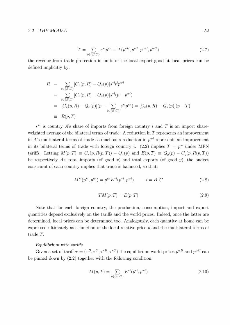
2.2. THE MODEL 52
T =P
i∈B,Cs∗ipwi ≡ T (p∗B, p∗C , pwB, pwC) (2.7)
the revenue from trade protection in units of the local export good at local prices can be
defined implicitly by:
R =P
i∈B,C[Cx(p,R)−Qx(p)]s
∗itipwi
=P
i∈B,C[Cx(p,R)−Qx(p)]s
∗i(p− pwi)
= [Cx(p,R)−Qx(p)](p−P
i∈B,Cs∗ipwi) = [Cx(p,R)−Qx(p)](p− T )
≡ R(p, T )
s∗i is country A’s share of imports from foreign country i and T is an import share-
weighted average of the bilateral terms of trade. A reduction in T represents an improvement
in A’s multilateral terms of trade as much as a reduction in pwi represents an improvement
in its bilateral terms of trade with foreign country i. (2.2) implies T = pw under MFN
tariffs. Letting M(p, T ) ≡ Cx(p,R(p, T )) − Qx(p) and E(p, T ) ≡ Qy(p) − Cy(p,R(p, T ))
be respectively A’s total imports (of good x) and total exports (of good y), the budget
constraint of each country implies that trade is balanced, so that:
M∗i(p∗i, pwi) = pwiE∗i(p∗i, pwi) i = B,C (2.8)
TM(p, T ) = E(p, T ) (2.9)
Note that for each foreign country, the production, consumption, import and export
quantities depend exclusively on the tariffs and the world prices. Indeed, once the latter are
determined, local prices can be determined too. Analogously, each quantity at home can be
expressed ultimately as a function of the local relative price p and the multilateral terms of
trade T .
Equilibrium with tariffs
Given a set of tariff τ = (τB, τC , τ ∗B, τ ∗C) the equilibrium world prices pwB and pwC can
be pinned down by (2.2) together with the following condition:
M(p, T ) =P
i∈B,CE∗i(p∗i, pwi) (2.10)

2.2. THE MODEL 53
(2.10) is the market clearing condition for good x stating that the world demand for
good x is equal to its world supply and recall (2.2) is the condition for an interior solution.
By Walras law, (2.10), (2.8) and (2.9) ensure the market for good y clears as well14. (2.10)
and (2.2) determine the two unknown world prices which together with the tariffs determine
the equilibrium values of all local prices. In turn, all other quantities (domestic consumption
and production, import and export volumes, tariff revenue) and the multilateral terms of
trade can be derived.
Given the general form of the functions assumed, it is possible that anomalous but not
impossible cases - such as the Metzler and the Lerner paradox - arise. The Metzler paradox
comprises a situation in which the domestic price of an imported good fall after a country
levies a tariff on that good. This means that the sector which recieves a greater protection is
worse off after the introduction of the tariff, so that resources move away from the protected
sector since it becomes less profitable. The Lerner paradox refers to the situation in which
the terms of trade moves against the tariff-imposing country. In other words, the shortage of
demand (excess of supply) that a country induces by imposing a tariff on the imported good
does not yield a fall in the international price of that good and consequently an improvement
of the country’s terms of trade. Technically, this cases can arise because the offer curve is not
necessarily well behaved (namely, monotonically increasing and concave to its import axis)
even if we assume underlying well behaved supply and demand schedules.15 I shall restrict
my focus to an equilibrium which lies on the upward-sloping segment of the offer curve - the
so called "elastic" region.16
Therefore, I shall assume i) ∂pwi/∂τ i ≤ 0 ≤ ∂pwi/∂τ ∗i which ensures the terms of trade
are always an increasing function of each country’s own tariffs (no Lerner paradox). In
case of MFN tariffs (τC = τB = τ), these restrictions are simply ∂pw/∂τ ≤ 0 ≤ ∂pw/∂τ ∗i.
14The market clearing condition for market y is E(p, T ) =P
i∈B,CM∗i(p∗i, pwi).
15For instance, an offer curve for foreign country i can be derived solving:maxM∗i,E∗i B(M
∗i, E∗i) s.t. (2.8)whereB(M∗i, E∗i) ≡ maxC∗ix ,C∗iy ,Q∗ix ,Q∗iy
[U(C∗ix , C∗iy ) :M∗i = C∗iy −Q∗iy , E
∗ix = Q∗ix − C∗ix , PPF ]
and PPF is the production possibility frontier.16The "elasticity" terminology comes from the fact that the offer curve has a positive slope if and only
if the home country’s elasticity of demand for imports (with respect to the relative price of the importable)exceeds unity. When the price of a good increases (say because a tariff on this good is levied), it producesthree effects: i) a production effect (resources move in the sector whose good price has increased) ii) asubstitution effect (consumer switch demand toward less expensive goods) iii) an income effect (due to theimproved real income of a country associated to higher terms of trade). Effects i) and ii) both contribute todecrease imports of this good and increase exports of other goods. On the contrary, effect iii) contributesto raise imports of all goods. Restricting to the upward sloping segment of the offer curve means focusingon a situation where the income effect iii) is dominated by i) and ii), so that an increase of the price of theimported good leads to a reduction of its imported quantity.

2.2. THE MODEL 54
Moreover, I shall assume that when other countries raise tariffs on one another, foreign
country i’s terms of trade improve - i.e. ii) ∂pwi/∂τ j ≥ 0 (i 6= j) and iii) ∂pwi/∂τ ∗j ≥ 0(i 6= j). Finally iv) dp/dτ i > 0 and v) dp∗i/dτ ∗i ≤ 0, rule out the Metzler paradox and
imply a restrictive trade policy always raise local prices. Recall that p = τ ipwi, so that the
total differential of this expression yields the change in the domestic price induced by a tariff
change, namely dp/dτ i = pwi + τ idpwi/dτ i. Given that the last term is negative (since an
increase in τ i improves A’s terms of trade), ruling out the Metzler pardox (i.e. dp/dτ i ≥ 0)is equivalent to assume that the terms of trade effect induced by the tariff are not so strong
to offset the increment that a tariff has on the domestic price of the good.
Note that the balanced trade conditions together with the market clearing conditions
allow to rewrite the domestic tariff revenue as:
R =P
i∈B,CtipwiE∗i(p∗i, pwi) =
Pi∈B,C
(p− pwi)E∗i(p∗i, pwi) (2.11)
= (p− T )M(p, T )
where the intuition for the first equality follows from the bilateral nature of the trading
relations which make foreign country i’s exports necessarily the home’s imports from i.
Note R∗i and R are an increasing function of foreign country i’s terms of trade, under our
assumption that goods are normal.
Furthermore, given that tariff revenues are only functions of local relative prices and
world relative prices, also national incomes (2.3) and (2.4) are only functions of local and
world relative prices.
Equilibrium with volume quotas
The bilateral nature of exchanges between A and each foreign country i fixes B’s and
C’s exports of good x at the quantity level set by A’s import quota of mB units of good x
from B and of mC units from C. Thus, the equilibrium world prices are determined by
E∗i(p∗i, pwi) = mi i = B,C. (2.12)
(2.10) becomes a tautology because A’s total imports are necessarily the sum of the two
binding volume quota restrictions. In addition, if foreign country i imposes a volume quota
of m∗i on its imports, world price pwi can be be explicitly determined by (2.8) as the ratio
m∗i/mi.
When the only restrictions in place are A’s import quotas on imports from country C,
E∗C(p∗C , pwC) = mC still determines pwC and (2.10) determines the remaining unknown pwB.

2.3. REGIONAL INTEGRATION WITH DIFFERENT TRADE POLICIES 55
This highlight a specificity of a quota with respect to a tariff which is worth mentioning
as it will play a crucial role in the welfare analysis. If a quantitative restriction on imports
from C remains binding even after a reform that abolishes a formerly existing quota mB
imposed on imports from B, E∗C(p∗C , pwC) = mC will still fix the level of imports from C
and the terms of trade at the pre-reform level. Thus, all the adjustments induced by the
reform affect only the bilateral relations among B and A. On the contrary, a reform that
alters a pre-existing A’s MFN tariffs lowering only the tariff risen on imports from B will
lead to world price adjustments (see (2.2) and i) and ii) above).17 Intuitively, if the home
government taxes more heavily the exports of foreign country C, then the home demand
for exports from C is reduced whereas the home demand for exports from B is increased,
resulting in a terms of trade loss for C and a terms of trade gain for B. In this sense, the
tariff protection is more likely to induce cross market effects than quota protection.
This insight gives the intuition for a potentially more severe trade diversion in tariff
protected than in quota restricted markets. Note, however, it is a feature of country-specific
volume quota. Were A restricting only its total imports of good x to M = mB +mC units
(global quota), the outcome would be similar to the tariff case. Imports from each source
country would be allocated such that the quota premium is equalized across source country
( px − p∗Bx = px − p∗Cx ) or all imports come from the single source that maximizes the quota
premia. Indeed, there are several combinations of import-mixes from the two source countries
that can satisfy (2.10) with M held fixed at M and the one chosen is maximizing the quota
premium. Thus, country-specific direct quantitative restrictions are more restrictive than an
equivalent global quota because they restrict the import mix to a specific one which is not
necessarily the optimal one.18
2.3 Regional Integration with different trade policies
I shall consider now the welfare outcome of a regional integration (RI) policy under
alternative trade policies. Without loss of generality, country A has the option to sign a
trade agreement with B reducing preferentially trade barriers to the member country (B),
but leaving unaltered those raised vis-à-vis non-member countries (C).
The desirability of a RIA has to be evaluated according to some welfare measure and I
17An example would be a reform that lowers τB to 1 and leaves τC unaltered at τ .18Country-specific quotas are widely employed. The United States, for instance, imposes limitations on
imports of sugar on a country-by-country basis, with each specific exporting country having its own quotaallotment of sugar exports. Trade in textiles and apparel is managed in much the same way; importingnations negotiate country-specific import targets with each significant exporter. See Markunsen et. al(1995).

2.3. REGIONAL INTEGRATION WITH DIFFERENT TRADE POLICIES 56
shall assume national governments maximize national income. This choice corresponds to
national governments maximizing the indirect utility function v of the representative con-
sumer. Therefore, V (p, T ) = v(p, I(p, T )) measures A’s welfare and, similarly V ∗i(p∗i, pwi) =
v(p∗i, I∗i(p∗i, pwi)) represents the welfare of foreign country i.19
Countries may trade in two different policy regimes. In the first one, all countries are
making use of tariff measures to protect national industries - as in the 70s. The initial
tariff vector is τ I = (τBI , τ
CI , τ
∗BI , τ ∗CI ), I for initial. Then, A and B join into a FTA which
gives free access to the internal market only to member countries, leaving trade barriers
against non member countries unaltered (reform t hereafter). Thus, the post reform tariff
vector (indexed by t) is τ t = (1, τCI , 1, τ∗CI ). That is, A and B trade freely one another.
Given that C is not part of the agreement and its tariff level is unchanged after the reform,
for simplicity I shall set τ ∗C = 1, meaning it is trading freely before and after the reform.
Therefore, τ I = (τBI , τ
CI , τ
∗BI , 1) and τ t = (1, τ
CI , 1, 1).
Consequently, let me denote as VI the welfare associated to the pre-agreement equilibrium
and likewise, Vt the welfare associated to the post-agreement equilibrium when trade is
restricted by tariffs.
In the second one - as in the 90s -trade is initially restricted by direct quantitative
restrictions and countries A and B undergo through the same kind of piecemeal reform
which liberalizes the internal market to member countries while it leaves unchanged the
quantity restrictions vis-à-vis non-member countries (reform q hereafter). Therefore ms =
(mBs ,m
Cs ,m
∗Bs ,m∗C
s ) (s for start) is the pre-agreement quota vector andmq = (no,mCs , no,m
∗Cs )
is the post-reform quota vector. no in the first element of this vector means that no vol-
ume quota is in place in country A for imports of good x from B. As above, I shall as-
sume for simplicity that C is in a free trade regime. We have, ms = (mBs ,m
Cs ,m
∗Bs , no)
and mq = (no,mCs , no, no). Thus, the volume quota faced by C remains the only restric-
tion in place after the FTA is signed. Obviously, Vs denotes the welfare associated to the
pre-agreement equilibrium and likewise, Vq the welfare associated to the post-agreement
equilibrium when trade is restricted by volume quota.
As well established in the literature, such partial reforms should be evaluated in terms
of terms of trade and efficiency effects. As shown in Grinols and Wong (1991) and Ju
and Krishna (2000a), reform q can ensure Pareto gains (s0, Vq ≥ Vs) through a system of
19Bagwell and Staiger (2002) show that government preferences can be generalized to allow for a widerange of economic and political motivations.

2.3. REGIONAL INTEGRATION WITH DIFFERENT TRADE POLICIES 57
self-financing lump sum transfers provided that the following condition holds:20
(pwBs − pwBq )E∗B(p∗Bs , pwBs ) + (pwCs − pwCq )E∗C(p∗Cs , pwCs )
+(pq − pwBq )[E∗B(p∗Bq , pwBq )− E∗B(p∗Bs , pwBs )] (2.13)
+(pq − pwCq )[E∗C(p∗Cq , pwCq )− E∗C(p∗Cs , pwCs )] ≥ 0
that is, regionalism integration must avoid adverse terms of trade or efficiency effects to
ensure Pareto gains. The first line in (2.13) indicates the impact of the reform on the terms
of trade: if the RTA reduces (increases) the price of imports (exports), it will contribute
positively to raise welfare. The last two lines are the change in tariff revenue evaluated at
the post-reform tariff vector (see (2.11)) and represent efficiency gains.21 Trade diversion
means that A switches the supplier from outside the FTA (where tariff revenue is collected)
to another within the FTA (with no tariff revenue), so that tariff revenue falls. The last two
lines would then be negative. Thus, RTAs should reduce trade diversion as much as possible
to be welfare enhancing. It is worth mentioning that (2.13) is a sufficient condition, so that
its violation does not mean the reform under evaluation is a failure a priori, but it just needs
a careful examination.
It is instructive to consider first the small open economy, first. It allows to abstract from
terms of trade and focus closely only on the different degree of trade diversion implied by
the two different instruments of trade policy. Then, I shall analyze the large country case
where the same mechanisms of trade diversion interact with terms of trade effects, making
the analysis more cumbersome.
Given that the literature on regional integration has found trade diversion theoretically
and empirically relevant, the interesting case is represented by a potential trade diverting
agreement.
Therefore, I shall consider C - the outside union member - as the lowest cost supplier
or the cheapest source country in the small open economy. In the large economy, C has
a comparative advantage in good x relative to B, translating in greater export supply for
20This formula is derived in the appendix. See also Feenstra(2004). The intuition is that the revenue Rcollected after the implementation of the reform can be used to finance a system of lump sum transfers whichcompensates losers and taxes gainers. This redistributive policy aims at equilibrating the uneven benefitdistribution arising with the trade reform and therefore can achieve Pareto gains for all consumers.21See Feenstra (2004). The tariff reflects the difference between domestic and international prices: if
positive, that indicates that marginal costs at home exceed international prices, so it would be more efficientfor the country to import the good. Therefore the term (pq−pwiq )[E∗i(p∗iq , pwiq )−E∗i(p∗is , pwis )] gives a measureof the efficiency gain by attracting imports towards the highest-tariff sectors after the implementation of areform.
2.3. REGIONAL INTEGRATION WITH DIFFERENT TRADE POLICIES 58
any given world price. Note that trade diverting agreements do not need to be necessarily
welfare decremental, but they can be welfare enhancing.22 In particular, I am interested in
whether such agreements are welfare enhancing when trade protection is achieved through
NTBs, so that the formation of RIAs in the 90s can be related to the observed change in the
nature of trade protection.
2.3.1 The small open economy case
The small open economy is illustrative of how a volume quota has different effects from
tariff when a country undergoes a piecemeal tariff reforms.
The assumption of a small open economy ensures that:
• A’s trade policy does not affect the terms of trade with the two possible suppliers, B
and C, but only the relative domestic prices p ≡ px/py. As world prices do not change
in response of a trade reform, I shall denote them as pwB and pwCwithout any subindex
(I, s, t, q).
• B’s and C’s supply is infinitively elastic at the world relative price pwi, i = B,C for
trade with A, with pwC < pwB, as C is assumed to be the lowest cost supplier,. Assume
further that pwC ≤ pwB ≤ τCI pwC = p, that is that B’s terms of trade with A is lower
than the tariff-distorted domestic price of good x coming from C.23
To see how the two types of instruments lead to different adjustment mechanisms when a
RIA is joined, suppose country A is initially protecting its industries by a MFN ad valorem
tariff tI = tBI = tCI . Imports from B would be more expensive than imports from C (by
assumption pwB ≥ pwC), and could be sold domestically only at a higher price (τ IpwB ≥τ Ip
wC) - so that (2.2) is violated and A will be only trading with C. Indeed, given that C
is willing to supply all M(pI , pwCI ) at the world price pwC, all imports of x come from C.24
Thus, in equilibrium there are only bilateral relations among A and C, but the tariff revenue
is positive and given by (2.11).25
22Trade diverting preferential agreement are necessarily welfare reducing under two specific assumptions:i) no substitution in consumption and ii) a linear production possibility frontier. See Markunsen et. al.(1995).23This assumption puts A into the situation of a trade diverting agreement.24In other words, (2.10) is M(pI , pwCI ) = E∗C(p∗CI , pwCI ) and E∗B(p∗BI , pwBI ) = 0. As shown in section
(2.2), (2.2) can not possible hold in the small open economy with MFN tariff. The equilibrium is necessarilya corner solution where A trades only with partner C.25Obviously E∗B(pI , p
wBI ) = 0 in (??), as the equilibrium is in the corner solution where A trades only
with C.
2.3. REGIONAL INTEGRATION WITH DIFFERENT TRADE POLICIES 59
However, when A grants preferential access to its market only to country B and retains
the same tariff on imports from C, the relative domestic price of good x imported from B
becomes pt = pwB, lower than the price τ IpwC at which each unit imported from C could
possibly be sold in A. Given that A’s total import demand at pwB is completely satisfied,
trade is completely diverted from country C to country B. In this case, in equilibrium only
A and B trade each other and the tariff revenue is lost because all imports come from a
union-members to which no tariff is applied.
The outcome differs under the NTBs regime. Suppose that A initially sets a global
quota M s on the total number of units of x imported. Assume that it is binding and, for
expositional simplicity, it is the tariff-equivalent quota (i.e. Ms = E∗C(pwCI )), that is the
implicit ad valorem tariff associated to it is tI .26 Therefore, the initial equilibrium is formally
identical to the the initial tariff-ridden equilibrium with all units imported exclusively from
C and sold domestically at the tariff-distorted domestic price ps = pI = τ IpwC. Therefore,
the tariff revenue collected is the same too.
After A joins into a RIA with B, A will be trading freely with B, but it can also keep
trading with C within the limits imposed by the volume quotaMs, now imposed exclusively
on imports from C. Note that C faces an import restriction as high as it was before the
agreement, while B benefits from the removal of all trade barriers. Since the international
prices at which country A can make international transactions are not affected by this policy,
a quota-license holder can make positive profit by buying x from the lowest cost supplier C
at pwC and re-sell it at the higher domestic price pq = pwB. All license holders will have an
incentive to use entirely their license and the amount of x imported from C is therefore Ms.
This is an equilibrium because C is willing to supply all the M s units at pwC , whereas B
serves the residual import demand (Mq −M s) at pwB.27 All three countries end up trading
simultaneously and therefore some revenue Rq = (pwB − pwC)Ms from industry protection
can be maintained even after the implementation of the agreement. The part of the original
revenue that is given up (pI − pwB)M s reflects exactly the reduced economic value of the
quota which is not as stringent as it was before the integration.28 Indeed, those units of
imports desired by country A in excess of the quota limit that could not be imported before
the agreement, can now be imported from Country B.
Although the partial reform implemented under the two different types of protection has
26The equivalence result between a tariff and a quota due to Bhagwati (1965) holds - in the sense thata tariff rate will produce an import level which, if alternatively set as a quota, will produce an identicaldiscrepancy between foreign and domestic prices.27The binding quota ensures the desired imports of good x necessarily exceed the Ms units after the
agreement is in place.28The pre-agreement quota rent is RI = (pI − pwC)Ms = [(pI − pwB)− (pwB − pwC)]Ms.

2.3. REGIONAL INTEGRATION WITH DIFFERENT TRADE POLICIES 60
identical effects on A’s relative domestic prices (i.e. pq = pt = pwB), the composition of
the volume of trade across the two supplier is rather different as trade diversion does not
occur under quantitative restrictions to trade. With quota protection, A expands its volume
of trade with B (trade creation), but trades with C ex-post as much as it did ex-ante the
agreement, whereas with tariff protection, trade diversion alters the pre-union trade patterns
between A and C. Only the FTA implemented in presence of quota restrictions preserves the
imports and the exports with the rest of the world and results therefore welfare improving
as shown by Krishna and Panagariya (2002). This observation is the essence of the different
welfare consequence of a trade agreement under the two types of trade policy instruments.
This different degree of trade diversion implied by the two types of trade barriers will
extend naturally to the large country case. Therefore I shall defer the formal proof of this
result till later in the more general case of large countries.
Note that such conclusion would still hold if A were initially setting country specific
import restrictions mB and mC . After a RTA that abolishes just mB, but it leaves un-
changed the quota raised on imports from C at mC , A’s post-agreement purchases from C
are unchanged provided that this quota is still binding.
2.3.2 The large economy case
Although a small country always gain from reform q, a large country may not do so if
such reform leads to adverse terms of trade effects. Let pwBs and pwCs the world price in the
pre-agreement equilibrium determined by (2.12). Note that E∗C is an increasing function
of only pwCas C does not protect its imports (i.e. p∗Cs = pwCs ). Supposing mCs keeps be
binding after the reform, (2.12) implies that the terms of trade with C are unchanged (i.e.
pwCq = pwCs ) and, in turn,M∗C(pwCq ) =M∗C(pwCs ) by (2.8). (2.10) implies that also the terms
of trade with B are fixed at their initial value (i.e. pwBq = pwBs ), as proved in the appendix.29
Therefore, after the reform is implemented, A is trading with partner C as much as it was
doing before the reform was approved, importing and exporting the same quantities. This
is the criteria for welfare enhancing Free Trade Areas proposed by Krishna and Panagariya
(2002). The preservation of trade volumes with non-members countries guarantees that their
terms of trade and, in turn, their welfare is preserved (i.e. V ∗Cs = V ∗Cq ) too. To see that it also
29To see this point, note that (2.10) implies that M(pq, Tq) − E∗B(p∗Bq , pwBq ) = E∗C(pwCq ) = mCs =
M(ps, Ts) − E∗B(p∗Bs , pwBs ). Given market x is intially clearing at (pwCs , pwBs ), it necessarily keeps clearingat these world prices after reform q. That is, pwCs = pwCq , pwBs = pwBq . Indeed, the increase in B’s exportsupply matches exactly with A’s greater total import demand (i.e. M(pq, Tq)−M(ps, Ts) = E∗B(p∗Bq , pwBq )−E∗B(p∗Bs , pwBs )), so that market x necessarily clears at the same pre-reform world prices.

2.3. REGIONAL INTEGRATION WITH DIFFERENT TRADE POLICIES 61
improves the welfare of participating government, it is easy to verify that (2.13) is satisfied
being equal to zero. The first line is 0 because the world price vector is unchanged and,
therefore countries in the FTA do not experience terms of trade gains or loss. The second
line is 0 as no quota premium arises from FTA members (p∗Bq − pwBq = 0). Finally, the
last line is 0, as trade diversion does not occur and import volumes with third countries are
preserved (i.e. E∗C(p∗Cq , pwCq ) = mCs = E∗C(p∗Cs , pwCs )). Clearly, this agreement increases B’s
volume of trade, contributing to raise its welfare too - see the appendix (2.7.1).30 Henceforth,
the agreement is mutually favorable. We have the following proposition.
Proposition 2.1 A RIA between the home country and foreign country i that abolishes
volume quota one another leaving unaltered former volume import restrictions vis-á-vis non-
member country j is welfare enhancing, provided that such import restrictions keep being
binding after the agreement is implemented.
A FTA implemented in presence of quota restricted trade does not yield terms of trade
gains, but it also avoids any trade diversion. This is enough to ensure the possibility to
achieve Pareto gains through a system of transfers among consumers and, more importantly,
among countries. The intuition for this result is suggested by the literature on piecemeal tariff
reform.31 Since following reform q, some binding quota are relaxed with others remained fixed
and there are no other distorted markets, the welfare change is positive because the relaxation
in any quota unambiguously enlarges the economy’s consumption set. Importantly, these
gains from consumption are not offset by adverse terms of trade effects.
I think of this proposition as an indication of the desirability of regionalism in presence
of quota-restricted trade. This is known as the "compensation principle" due to Chipman
(1987) - in the sense that if regional integration agreements combined with lump-sum trans-
fers could make everyone better off, then we accept such reform itself as a worthwhile policy,
even when the transfers are not made. Indeed, the knowledge required to implement the
long list of lump sum compensatory payments, some of them international in nature, make
the practical implementation of these transfers very difficult.
Obviously, proposition (2.1) holds for a small country too, as (2.13) is satisfied by the
small country above.30It can be directly verified that (2.24) in the appendix - a formula like (2.13) for foreign country ∗B -
holds. The first term is 0 since reform q has no terms of trade effect. The second term is 0 as no quotais risen on imports from member countries (i.e. the implicit tariff is t∗B = 0). If B had multiple partnerstoo, trade patterns would be symmetric to A, exporting x to both the union country A and a third countryoutside the FTA and importing y from a union country A and the third country outside the union. Thus,the question of whether union formation is welfare improving for each member country could be analyzed inthe same way for both members of the union. Since the FTA results welfare-enhancing for A, it would be sofor B too.31See Vousden (1990), chapter 9 pag pag 217.
2.3. REGIONAL INTEGRATION WITH DIFFERENT TRADE POLICIES 62
On the contrary, reform t is not necessarily welfare improving because the trade diversion
induces terms of trade movements as well. The initial equilibrium world prices pwCI , pwBI solve
(2.10) and (2.2). After the reform t, the elimination of tariff within the FTA reduces the local
price of the imported good in the two member countries, so that [1/τ ∗BI ≤ pwBt /pwBI ≤ τBI ],
whereas by (2.2), C’s terms of trade worsen (pwCt ≤ pwCI ) to preserve competitiveness in the
union market.32 This appreciation of A’s terms of trade against C originates from the trade
diversion of imports formerly coming from the outside member country in favor of intra-union
imports (i.e. E∗C(pwCt ) ≤ E∗C(pwCI )). The elimination of tariff on union trade shifts out both
A’s import demand and B’s export supply. Depending on this relative shifts, B’s terms of
trade may appreciate or depreciates. First, suppose it appreciates (1 ≤ pwBt /pwBI ≤ τBI ) - for
instance because at the initial world price there is an excess demand of good x by A to be
cleared out. Replacing q with t and s with I, (2.13) is not necessarily positive: the second
line is 0 as no tariff is levied on member’s imports, whereas the third line is negative as trade
diversion reduces tariff revenue from non-members countries. Finally, the first term in the
first line is negative while the second term is positive. For welfare to raise, favorable terms
of trade effects against non-member countries have to be strong enough to compensate for
both terms of trade loss vis-à-vis member countries and efficiency loss.
Supposing instead that (pwBt ≤ pwBI ), welfare gains are more likely as A experiences
favorable terms of trade effects with both member and non-member trading partners which
can offset the efficiency loss associated to trade diversion (the negative term in the last line
of (2.13).
Note for the small open economy above, Pareto gains can not be ensured either, since
(2.13) is violated. The first two lines are clearly 0, whereas the last line is negative because
of trade diversion. The intuition is again that trade diversion associated to the preferential
reduction of tariffs may not necessarily translates into the enlargement of the economy’s
consumption set, especially when imports are just diverted from one source to another.
Moreover, adverse terms of trade plausibly associated to trade diversion make imports more
expensive and reduce welfare.
It is worth pointing out a number of interesting features of this result.
First, the desirability of reform t has to be evaluated empirically case by case, as widely
recognized in the literature. For instance, Grinols (1984) finds that Great Britain incurred
in a welfare loss when it joined the European Economic Community in 1973 and (2.13) was
32[1/τ∗BI ≤ pwBt /pwBI ≤ τBI ] follows from pt = pwBt ≤ τBI pwBI = pI and pwBt = p∗Bt ≥ p∗BI = pwBI /τ∗BI .
pwCt ≤ pwCI follows from τCI pwCt = pt ≤ pI = τCI p
wCI . This is fully consistent with price restriction i) and ii).
2.3. REGIONAL INTEGRATION WITH DIFFERENT TRADE POLICIES 63
evaluated to be negative. In contrast, proposition (2.1) suggests a general desirability of
reform q which can provide an explanation for a renewed interest in RIAs policy in the 90s.
Indeed, policy makers are usually working in a second best world, attempting to reduce some
distortions while others remaining firmly in place. As we know from the theory of second
best, such changes do not necessarily increase welfare. However, it would be helpful to have
some simple rules - a rule of thumb - telling them "which way is up". Then, Proposition
(2.1) suggests reform q can be readily understood and implemented by policy makers with
some confidence that a welfare improvement will be the outcome.33
Second, because "the way up" is so clear when all trade barriers consists of quantitative
restrictions, it would appear that the difficulty of identifying welfare-enhancing FTA can be
resolved simply by converting all explicit taxes or subsidies to quotas and then gradually
relaxing the quotas. Such an approach runs counter to the view of reform which is popular
to most policy makers and adopted by the WTO in 1995, that is change quotas to tariffs
and then set about reducing the tariffs - so called "tariffication" process. However, quotas
have many other disadvantages relative to tariffs, particularly in the presence of monopoly
and/or foreign retaliation, and such considerations presumably are what motivate the pop-
ular view.34
Third, the welfare outcome of reform q and reform t is different, though both reforms
leave unaltered former trade barriers against non-member countries. This is the criteria
established by GATT-WTO regulations to permit preferential trade agreements. Article
XXIV of GATT explicitly imposes “the duties (with outside parties) shall not on the whole be
higher or more restrictive than the general incidence of the duties...prior to the formation”.
This criteria naturally implements the efficient rule for welfare-enhancing FTA in case of
NTBs, as it helps to keep purchases from the rest of the world fixed. In contrast, in case of
tariff protection (reform t), it is unable to lead to welfare improving FTA as this principle
does not suffice, on its own, to preserve trade volumes with non-member countries. As
shown by Bagwell and Staiger (2004), the FTA would do so if only complies with two other
principles of GATT-WTO - namely reciprocity and MFN. However a FTA could not possibly
respect MFN as, by definition, it is a legal recognized exception to it.
Fourth, the model suggests that when a RTA is implemented in presence of NTBs, the
terms of trade vis-à-vis non member countries should be preserved. This seems at odd with
the empirical findings by Chang and Winters (2002) of favourable terms of trade effects of
33This has some analogies with the large literature on piecemeal tariff reforms. A number of economistshave looked for simple piecemeal reform rules that could be leading to welfare enhancing outcomes with someconfidence. Examples of such rule of thumb rules are proportional reduction of all trade taxes or reductionof the highest tariff rate first. See Vousden (1990), Chapter 9 for a review.34See Vousden (1990), chapter 4, 5 and 6.

2.4. RIAS AND VERS 64
MERCOSUR for Brazil vis-à-vis US, Japan, Germany, South Korea and Chile, who are all
exporting into the union-area. However, Mercosur entailed also tariff reductions which can
lead to terms of trade effects as predicted by the model (reform t). Moreover, it is important
to note that the preservation of trade volumes with non-member countries is a specificity
of country-specific volume quotas. Consequently, terms of trade effects can also occur in
presence of only quantitative restrictions, when, for instance, a RTA provides that countries
relax a global import volume quota or a formerly employed VERs. Given the empirical
relevance of VERs in trade policies, next section will consider them specifically and show
that, indeed, may lead to favourable terms of trade improvements for member countries and
loss for non member countries as for Brazil after Mercosur.35
2.4 RIAs and VERs
A VER is a quota imposed by an exporting country on its exports to another country
in response to pressure by the importing country. In my framework, the initial VERs vector
mo = (m∗Bs , no,mB
s ,mCs ) where foreign country i imposes a VER of mi
s units of good x,
whereas A restricts its exports to m∗Bs units of good y toward B, mirrors the protection
achieved by the initial import-volume quota vector ms. The equivalent of reform q in terms
of VERs relaxation (hereafter denoted as reform v) implemented by a bilateral agreement
yields the post-reform VER-vector mv = (no, no, no,mCs ). For an exporter in foreign country
i, a unit of the exported good x is more valuable on the international market than on the
domestic market (i.e. px ≥ p∗ix ) due to the artificial scarcity created by a VER. Analogously,
for a home exporter, the international price of the exported good y benefits from such
artificial restrain and results above its domestic price (i.e. p∗iy ≥ py). Then, the untaxed or
"world" relative price at which international transactions are made is given by epi = px/p∗iy
which still represents foreign country i’s terms of trade and the ratio of exporter prices. With
this definition, relative domestic prices are in the same relation with world prices as above
(i.e. p∗i ≤ epi ≤ p) and (2.8) is still foreign country i budget constrain with pwi replaced byepi.35VERs have become most pervasive in the textiles and clothing area, applying to 80% of the world trade
in these industries through the various bilateral agreement which constitutes the Multifibre Arrangement(MFA). They are also particularly in evidence in the steel industry, in which they limit steel exports fromJapan and the EEC to the USA. They were employed in the automobile industry, in which they restrictedexports from Japan to the USA, Germany, France, UK and Italy. For example, after 1981, the JapaneseMinistry of International Trade and Industry (MITI) told each auto manufacturer in Japan how much itcould export to the U.S. In the late 1980s, US and the European countries rescinded their request to Japanfor restricted automobile exports. Later on, they have begun to be applied to a range of electronic consumergoods. As documented by Laird and Yeats (1990), over the period 1981-1986 a major shift has occurred inthe use of VERs on import volumes as opposed to other forms of NTBs.

2.4. RIAS AND VERS 65
One major difference with the import quota case analyzed above, is that both E∗C and
E∗B are vertical at mCs and mB
s when VERs are binding and do not pin down world prices.
These are determined by:
M(po, eTo) = mBs +mC
s (2.14)
M∗B(p∗Bo , epBo ) = m∗Bs (2.15)
with eT =Pi∈B,C esi/epi and esi =M∗i(p∗i, epi)/M∗B(p∗B, epB) +M∗C(p∗C , epC).36 Note that.differently from above, an increase in eT represents an improvement in A’s multilateral termsof trade. (2.15) determines epBo while (2.14) pins down eTo and, in turn, epCo .37 Generally, epiowill result different from the terms of trade pwis because C and B are moving the terms of
trade in their favour by imposing a VER whereas, in the import quota case, was A to benefit
from the terms of trade appreciation with the imposition of a country-specific quota to each
of its trading partners. Moreover, revenue formerly collected with the imposition of such
import quotas, accrues under the VER scheme to foreign country i, implying quite different
lump sum transfers for consumers of country A. In turn, in general equilibrium models,
also relative domestic prices will be generally different in the two situations (ps 6= po and
p∗is 6= p∗io ) because of income effects associated with changes in the terms of trade.
After the implementation of the RTA between A and B, only the VER imposed by C
on its exports is firmly in place and assumed to be binding, which implies that E∗C is still
vertical at mCs . Clearly, the export quantities toward A are preserved, but, differently from
the import quota case, the terms of trade are not necessarily preserved because, under a
binding VER only this quantity is supplied regardless of its price. By (2.8), the terms of
trade would be unchanged if only the quantity imported by C were also unchanged.
The market of good y results free of protection and country A has two potential buyers,
namely B and C. Of course, A would maximize its export revenue by selling to the best
buyer and will allocate to it all its exports unless the price per unit of good exported is
not driven to equality by such allocation (i.e. p∗By = p∗Cy ). Therefore, the post-agreement
equilibrium in which A is trading with both partners is characterized by the following market
x clearing condition and arbitrage condition:
36To develop an intuition it is useful to think of VERs in terms of implicit export taxes. t∗i is the exporttax levied by foreign government i on its exports of good x - so that an exporter receives p∗ix = (1− t∗i)px.tB is the export tax imposed by A on exports directed to B, while tC = 0 - so that an exporter in the homecountry receives py = (1− tB)p∗By when it sells the good in market B and py = p∗Cy when it sells its good inmarket C. Export taxes and import tariffs have qualitatively the same effects because they distort domesticprices in the same manner favouring the import-competitive sector.37Actually epBo can be derived more explicitly and it is epBo = m∗Bs /mB
s .
2.4. RIAS AND VERS 66
M(eTv) = E∗B(epBv ) +mCs (2.16)
epBv = epCv (2.17)
The y market clearing condition E(eTv) =M∗B(epv)+M∗C(p∗Cv , epv) implied by (2.16) and(2.8) provides us with an intuition for the effects of the RTA. Initially, the allocation of A’s
exports to its partners is constrained by the A’s VER of m∗Bs units of good y (see (2.15)).
Following the trade liberalization, A will wish to export more units and its allocation among
its trading partners is driven by revenue maximization. Very likely, such optimal export
mix toward its trading partners is different from the original export mix and leads to terms
of trade movements. In particular, it can be shown (see the appendix) that the effect onepBv is ambiguous, while epCv and M∗C are smaller than initially. The preserved exchanges of
good x between A and C does not longer suffice to preserve the volumes traded of good y
as well as the terms of trade. Therefore, negotiated bilateral agreements for the elimination
of VERs also have favourable terms of trade effects for the the negotiating parties vis-à-vis
third parties.
As shown in the appendix, it is possible to express the sufficient condition for Pareto
gains for the home country as:Pi∈B,C
µ1epiv − 1
pv
¶£M∗i(p∗iv , epiv)−M∗i(p∗io , epio)¤+ (2.18)µ
1epBv − 1epBo¶M∗B(p∗Bo , epBo ) +µ 1epCv − 1epCo
¶M∗C(p∗Co , epCo ) ≥ 0
where the first line is 0 in my framework because A does not employ any VER after
reform v is implemented. Therefore, Pareto gains only depend on terms of trade movements.
In particular, when both epBv ≤ epBo and epCv ≤ epCo , Pareto gains can be ensured, otherwisepossible adverse terms of trade with member countries have to be offset by gains vis-à-vis
non member countries. Most remarkably, Pareto gains for country A under a VER reform
are more likely than under reform t, although both reforms t and v entail similar terms of
trade effects. The reason is that country A had already given up its tariff revenue when it
negotiated a VER protection and regionalism (reform v) has no consequences for the loss of
such revenue in this case. In contrast, (2.13) showed that favourable terms of trade induced
by reform t had in any case to compensate for tariff revenue loss (the negative term in the
third line) to ensure Pareto gains.38
38Note that if A were imposing initially a VER to both its trading partner and leaving its VER unalterated
2.5. COMPARISON OF THE DIFFERENT STRATEGIES TO RIAS 67
2.5 Comparison of the different strategies to RIAs
We have shown that policy makers may be quite confident about pursuing regional
integration policies to rise the well being of countries in a context where trade is restricted
by NTBs, while the outcome of this strategy is quite case-specific and needs more careful
evaluation in a context of tariff restricted trade. However, in many cases, the option for such
preferential reforms may still represent an improvement relative to pre-existent tariff-ridden
trade relations. In spite of a more generalized desirable welfare outcome of RTAs in presence
of NTBs, it would be interesting to be able to compare the size of the gains associated to
piecemeal reforms with either type of instruments. In terms of the notation of my model,
I am interested in comparing gains from a reform q relative to those arising under reform
t (i.e.Vq − Vs vs. Vt − VI). This enables us to construct useful counterfactuals. Would a
country joining into a regional trade agreement in the 70s have gained at least as much had
it signed the same agreement twenty years after at the end of the 80s? Or would a country
recently joining into an agreement in presence of NTBs gained more or less had it enrolled
into this agreement much earlier in the 70s when tariff rather than NTBs were in place?
Therefore, these counterfactual are useful to shed some light on how attractive and valid is
the option for a RTA in the 90s for a country for which it was not worth joining into an
agreement in the 70s.
In such thought experiments, it is important to attribute any change in the welfare only
to the piecemeal tariff/quota reform. Clearly, Vs = VI would ensure A has the same initial
welfare with either trade policy and therefore any welfare change can be attributed to the
different adjustments implied by volume quota liberalization and tariff liberalization in the
process of a RTA reform. The assumption of a competitive market for import quota licenses
ensures the equivalence result between a tariff and a volume quota holds.39 Therefore, the
levels of prices, production, consumption, imports, exports and transfers of rents to the
protected industry prevailing in the pre-reform equilibrium with tariff are identical to those
characterizing the pre-agreement equilibrium with NTBs. It follows the welfare associated
to both equilibrium must coincide, i.e. Vs = VI . Given this equivalence, Vq − Vs ≥ Vt − VI
reduces to study under which conditions A is better off in the q equilibrium as opposed to
the t equilibrium (Vq ≥ Vt) which can still be evaluated similarly to (2.13) by:
against country C after reform v, trade diversion translates into rents loss and gains from regionalism wouldbe less plausible as well.39See Bhagwati (1965).
2.5. COMPARISON OF THE DIFFERENT STRATEGIES TO RIAS 68
(pwBt − pwBq )E∗B(p∗Bt , pwBt ) + (pwCt − pwCq )E∗C(p∗Ct , pwCt ) (2.19)
+(pq − pwBq )[E∗B(p∗Bq , pwBq )− E∗B(p∗Bt , pwBt )]
+(pq − pwCq )[E∗C(p∗Cq , pwCq )− E∗C(p∗Ct , pwCt )] ≥ 0
(2.19) clearly holds for a small country: the first line is necessarily 0 because the terms of
trade are taken as given (pwBt = pwBq = pwB); the second line is also 0 as no quota rents arise
from member countries (i.e. pq = pwBq ). Finally, the third line is positive and it represents
exactly the change in tariff revenue from t to the q equilibrium.40 Therefore, the following
proposition holds true for a small country.
Proposition 2.2 For a small country with a competitive market for import quota licenses,Vq − Vs ≥ Vt − VI.
Proof. See the appendix for a direct proof.
Note that this proposition holds true also when VER-protection is considered, as it is
shown in the appendix. However, this result does not extend to a large country setting
due to possible adverse term of trade effects. Recall that the MFN tariff together with the
equivalence result which is assumed to hold, imply that pwBs = pwBI = pw = pwCI = pwCs .
Moreover, in equilibrium q, pwBq = pwBs and pwCs = pwCq , while in equilibrium t we have
pwBt /pwBI ∈ [1/τ ∗BI , τBI ] and pwCt ≤ pwCI . Like for a small country, the last term in (2.19)
is positive also for a large country because NTBs imply a lower degree of trade diversion
resulting in E∗C(pwCq ) ≥ E∗C(pwCt ).41 Supposing pwBt ≥ pwBq , the first term in the first line
is positive as imports from B are cheaper in the q equilibrium, but the second term on the
same line is negative as trade diversion in equilibrium t is compensated by favorable terms of
trade movements. Unless trade of terms gain vis-à-vis non member countries are so strong
to offset all other forces, (2.19) is likely satisfied for a large country who therefore would
also gain relative more from a regional integration pursued in presence of NTBs. However, if
pwBt ≤ pwBq , the first term turns to be negative and the inequality will less likely be satisfied
since stronger efficiency gains would be needed. In other words, the strongest the terms
of trade gain achieved after the implementation of reform t relative to those attained with
40Recall that for a small country, after reform q is implemented, imports from C are exactly the quotalimit (E∗C(p∗Cq , pwCq ) =Ms) and following reform t, E∗C(p∗Ct , pwCt ) = 0 because of complete trade diversion.41Recall pwCq = pwCs = pwCI and pwCt ≤ pwCI . Given E∗C is an increasing function of world relative price,
E∗C(pwCq ) ≥ E∗C(pwCt ).
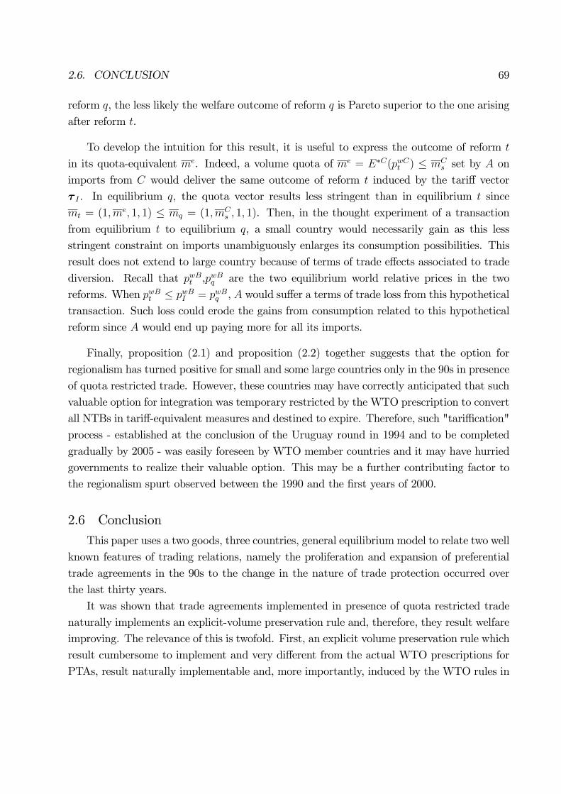
2.6. CONCLUSION 69
reform q, the less likely the welfare outcome of reform q is Pareto superior to the one arising
after reform t.
To develop the intuition for this result, it is useful to express the outcome of reform t
in its quota-equivalent me. Indeed, a volume quota of me = E∗C(pwCt ) ≤ mCs set by A on
imports from C would deliver the same outcome of reform t induced by the tariff vector
τ I . In equilibrium q, the quota vector results less stringent than in equilibrium t since
mt = (1,me, 1, 1) ≤ mq = (1,m
Cs , 1, 1). Then, in the thought experiment of a transaction
from equilibrium t to equilibrium q, a small country would necessarily gain as this less
stringent constraint on imports unambiguously enlarges its consumption possibilities. This
result does not extend to large country because of terms of trade effects associated to trade
diversion. Recall that pwBt ,pwBq are the two equilibrium world relative prices in the two
reforms. When pwBt ≤ pwBI = pwBq , A would suffer a terms of trade loss from this hypothetical
transaction. Such loss could erode the gains from consumption related to this hypothetical
reform since A would end up paying more for all its imports.
Finally, proposition (2.1) and proposition (2.2) together suggests that the option for
regionalism has turned positive for small and some large countries only in the 90s in presence
of quota restricted trade. However, these countries may have correctly anticipated that such
valuable option for integration was temporary restricted by the WTO prescription to convert
all NTBs in tariff-equivalent measures and destined to expire. Therefore, such "tariffication"
process - established at the conclusion of the Uruguay round in 1994 and to be completed
gradually by 2005 - was easily foreseen by WTO member countries and it may have hurried
governments to realize their valuable option. This may be a further contributing factor to
the regionalism spurt observed between the 1990 and the first years of 2000.
2.6 Conclusion
This paper uses a two goods, three countries, general equilibriummodel to relate two well
known features of trading relations, namely the proliferation and expansion of preferential
trade agreements in the 90s to the change in the nature of trade protection occurred over
the last thirty years.
It was shown that trade agreements implemented in presence of quota restricted trade
naturally implements an explicit-volume preservation rule and, therefore, they result welfare
improving. The relevance of this is twofold. First, an explicit volume preservation rule which
result cumbersome to implement and very different from the actual WTO prescriptions for
PTAs, result naturally implementable and, more importantly, induced by the WTO rules in

2.6. CONCLUSION 70
presence of quota restricted trade. Second, for small and some large countries, preferential
trade has become a "positive-dividend" option only in the 90s, when trade was more quota-
restricted than in the past, justifying a renewed policy interest for regionalism in the last
fifteen years. At the basis of this result is the different mechanism with which a tariff and
a quota operate: while a tariff has direct effect on prices, a quota operates on quantities
and affects prices only indirectly. Because a tariff increases the prices of all imports from
non-member countries, it may cause union-member to become artificially the lowest cost
supplier. Trade is then diverted from non-members toward members of a FTA. Under quota
protection this does not occur and a country can still import from the world lowest cost
supplier provided that it does not exceed the quota limit. In turn, the pre-agreement volumes
of trade are preserved.
Most likely, such benefits associated to regional integration would have expired as soon
as countries had complied with the "tariffication" process established by the WTO in 1995
and to be completed in the following ten years. Anticipating such eventuality, governments
may have hurried to sign agreements under negotiation.
While this paper contributes to shed some light on the spurt of regionalism in the 90s, it
can not provide any answer to the types of agreements signed. Trade policy can not explain
whether North-North or South.South or, as more common in the last years, North-South
agreements are signed. These themes are certainly worth to be explored in future research.
Finally, my model does not allow for strategic interaction of countries and, thus, for plausible
retaliation actions. This is because my main interest are the welfare consequences of a trade
agreement for a country that trades multilaterally and may employ different instruments of
trade policy. In this respect, I follow a long tradition in the literature of piecemeal tariff
reform of which regional agreements are just a special kind. This paper shares with this
literature also the limit of analyzing only the two polar situations of trade policy: either
tariff or non-tariff protection, whereas a framework comprising these instruments together
remains in the research agenda. Clearly, the quota case is useful to understand the effects
of RTAs in presence of non-linear tariffs, also defined as a system of tariff-quotas.42
In spite of this limitation, the model correctly predicts that bilateral agreement entailing
tariff-reductions can lead to terms of trade effects consistently with empirical findings. More
interestingly, given the empirical relevance of VERs, it shows that such effects can also be led
by bilateral agreements calling for the elimination of formerly negotiated VERs. Although,
42Alternatively defined also as tariff-rate quotas. The tariff rate is low under an volume-threshold ofimports (on the in-quota quantities), while it is much higher above this threshold (on the out-of-quotaquantities). For example, imported car entering under the tariff-quota (up to x cars) are generally charged10%. Imports entering outside the tariff-quota are charged 80%.

2.6. CONCLUSION 71
the volume preservation outcome is a specificity of country-specific quotas not shared by
VERs, the possibility that a welfare improvement will also be the outcome of such agreements
abolishing VERs is not compromised.

2.7. APPENDIX 72
2.7 Appendix
2.7.1 Appendix A - Derivation of formula (2.13)
In general terms, suppose country A undertakes a piecemeal tariff reform such as for
example a regional integration agreement. Let me index by 0 the level of a variable in the
pre-reform equilibrium and by 1 the level of a variable in the post-reform equilibrium. The
budget constraint of country A in the pre-reform and in the post-reform are the following:
p(0)Cx(0) + Cy(0) ≤ p(0)Qx(0) +Qy(0) +R(0) (2.20)
p(1)Cx(1) + Cy(1) ≤ p(1)Qx(1) +Qy(1) + TR(1) (2.21)
where R(0) is the tariff revenue (quota rents) in units of the local export good (y)
collected in the pre-reform equilibrium and TR(1) are the total transfers in units of the
local export good received in the post-reform equilibrium. The representative consumer of
this economy is better off after the implementation of the reform if her utility is at least as
high as before the reform. By the weak axiom of revealed preferences (WA), it is enough
to show that the old consumption and production bundle are still feasible and affordable
in the post-reform equilibrium. Of course, if the transfer compensates the representative
consumer in such a way that the old consumption-production bundle is still affordable in the
new equilibrium, the WA will hold. Such transfer is the following:
TR(1) = [p(1)− p(0)][Cx(0)−Qx(0)] +R(0) = [p(1)− p(0)]M(0) +R(0) (2.22)
where the consumer receives the old tariff revenue and a subsidy to compensate her for
an eventual increase in the relative domestic price of the imported good. It is easy to check
that the old consumption-production bundle (Cx(0), Cy(0), Qx(0), Qy(0)) is still affordable
in the new equilibrium by substituting (2.22) and ((Cx(0), Cy(0), Qx(0), Qy(0))) in (2.21):
p(1)Cx(0) + Cy(0) ≤ p(1)Qx(0) +Qy(0) + [p(1)− p(0)][Cx(0)−Qx(0)] +R(0)
⇔ p(0)Cx(0) + Cy(0) ≤ p(0)Qx(0) +Qy(0) +R(0)
which is always verified as it is (2.20). Therefore, the consumer is better off. Only it is
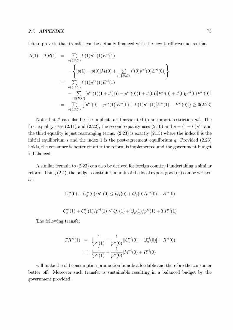
2.7. APPENDIX 73
left to prove is that transfer can be actually financed with the new tariff revenue, so that
R(1)− TR(1) =P
i∈B,Cti(1)pwi(1)E∗i(1)
−([p(1)− p(0)]M(0) +
Pi∈B,C
ti(0)pwi(0)E∗i(0)]
)=
Pi∈B,C
ti(1)pwi(1)E∗i(1)
−P
i∈B,C[pwi(1)(1 + ti(1))− pwi(0)(1 + ti(0))]E∗i(0) + ti(0)pwi(0)E∗i(0)]
=P
i∈B,C
©[pwi(0)− pwi(1)]E∗i(0) + ti(1)pwi(1)[E∗i(1)−E∗i(0)]
ª≥ 0(2.23)
Note that ti can also be the implicit tariff associated to an import restriction mi. The
first equality uses (2.11) and (2.22), the second equality uses (2.10) and p = (1 + ti)pwi and
the third equality is just rearranging terms. (2.23) is exactly (2.13) where the index 0 is the
initial equilibrium s and the index 1 is the post-agreement equilibrium q. Provided (2.23)
holds, the consumer is better off after the reform is implemented and the government budget
is balanced.
A similar formula to (2.23) can also be derived for foreign country i undertaking a similar
reform. Using (2.4), the budget constraint in units of the local export good (x) can be written
as:
C∗ix (0) + C∗iy (0)/p∗i(0) ≤ Qx(0) +Qy(0)/p
∗i(0) +R∗i(0)
C∗ix (1) + C∗iy (1)/p∗i(1) ≤ Qx(1) +Qy(1)/p
∗i(1) + TR∗i(1)
The following transfer
TR∗i(1) = [1
p∗i(1)− 1
p∗i(0)][C∗iy (0)−Q∗iy (0)] +R∗i(0)
= [1
p∗i(1)− 1
p∗i(0)]M∗i(0) +R∗i(0)
will make the old consumption-production bundle affordable and therefore the consumer
better off. Moreover such transfer is sustainable resulting in a balanced budget by the
government provided:
2.7. APPENDIX 74
R∗i(1)− TR∗i(1) = [1
pwi(0)− 1
pwi(1)]M∗i(0) +
t∗i(1)
pwi(1)[M∗i(1)−M∗i(0)] ≥ 0 (2.24)
Whenever the last condition holds, foreign country i will be undoubtedly better off
following the implementation of the reform.
2.7.2 Appendix B - Proof of terms of trade preservation under reform q
I shall prove that pwBq = pwBs .
(2.8), (2.10), (2.9) and E(p, T ) =P
i∈B,CM∗i(p∗i, pwi) (market y clearing condition) have
to hold in both s and q equilibrium.
Using E∗C(pwCq ) = mCs = E∗C(pwCs ) and pwCq = pwCs and (2.8),
M∗C(pwCq ) =M∗C(pwCs ) (2.25)
The market x clearing condition (2.10) implies the following
M(pq, Tq)−E∗B(p∗Bq , pwBq ) = mCs =M(ps, Ts)−mB
s ⇔ (2.26)
M(pq, Tq)−M(ps, Ts) = E∗B(p∗Bq , pwBq )−mBs = k
The market y clearing condition above together implies that:
E(ps, Ts)−m∗Bs = M∗C(pwCs ) = E(pq, Tq)−M∗B(pwBq )⇔ (2.27)
E(pq, Tq)−E(ps, Ts) = M∗B(pwBq )−m∗Bs = H
Using (2.25), (2.27) in (2.8), it follows
m∗Bs +H = pwBq
¡mB
s + k¢⇔
pwBs mBs +H = pwBq
¡mB
s + k¢
⇒ pwBs = pwBq
where the second line uses (2.8) again for equilibrium s. Indeed, when pwBs = pwBq , then
H = pwBs k which is reciprocity!
2.7.3 Appendix C - Reform v reduces epCand has ambiguous effects on epBI shall prove epCv ≤ epCo . Recall (2.8) and (2.14) to (2.17) have to hold.

2.7. APPENDIX 75
In particular, the assumption of a binding VER (mCs ) even after the reform v is imple-
mented together with (2.8) imply:
M∗C(p∗Co , epCo )epCo = mCs =
M∗C(p∗Cv , epCv )epCv⇔ M∗C(p∗Cv , epCv ) = kM∗C(p∗Co , epCo )epCv = kepCo ∀k ≥ 0
Moreover, reform v changes relative domestic prices lowering relative domestic prices at
home because the economic value associated to the artificial scarcity created by a VER is
reduced after the reform is implemented. Therefore,
epCv = pv ≤ po = epCo ⇒ 0 ≤ k ≤ 1
where the equalities between A’s relative domestic price and A’s bilateral terms of trade
with C follows from the fact that A is not restraining its exports of good y to C. Therefore,
the price an exporter receives at home (py) is exactly the price received internationally as
paid by the importer (p∗Cy ).
I shall sketch a proof for epBv R?epBo .By (2.8), epBo = m∗B
s /mBs . Since both VERs are assumed to be binding, both M∗B
and E∗B are greater in the new equilibrium. Depending on the relative magnitude of these
changes, the bilateral terms of trade with B may result appreciated or depreciated.
2.7.4 Appendix D - Derivation of (2.18)
The logic and steps are identical to section 2.7.1 above. I shall use the same notation as
well with the understanding that all variables are now expressed in units of the local import
good (good x) at local prices.
Cx(0) + Cy(0)/p(0) ≤ Qx(0) +Qy(0)/p(0) +R(0)
Cx(1) + Cy(1)/p(1) ≤ Qx(1) +Qy(1)/p(1) + TR(1)
TR(1) = [1/p(1)− 1/p(0)][Cy(0)−Qy(0)] +R(0)
R(0) =P
i[1/epi(0)− 1/p(0)][C∗iy (0)−Q∗iy (0)]
R(1) =P
i[1/epi(1)− 1/p(1)][C∗iy (1)−Q∗iy (1)]
Adding and subtracting (P
i[1/epi(1) − 1/p(1)][C∗iy (0) − Q∗iy (0)]) to R(1) − TR(1) ≥ 0,gives exactly (2.18) where M∗i(0) = C∗iy (0)−Q∗iy (0).
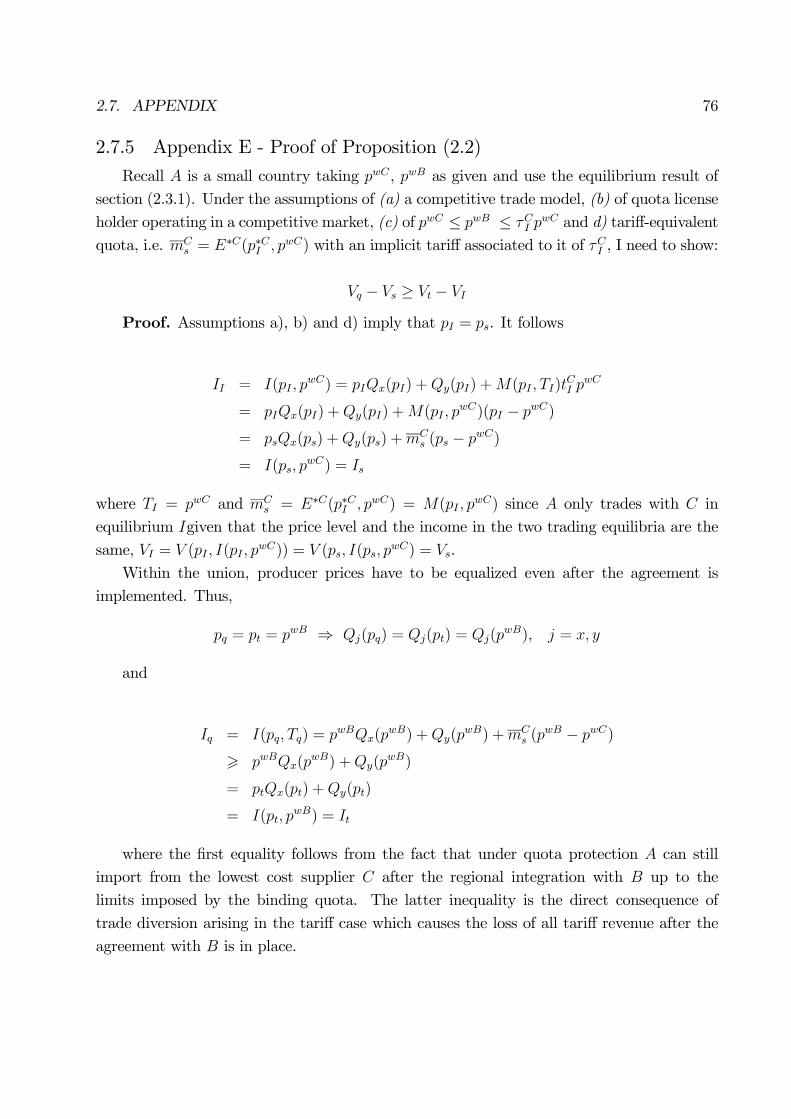
2.7. APPENDIX 76
2.7.5 Appendix E - Proof of Proposition (2.2)
Recall A is a small country taking pwC , pwB as given and use the equilibrium result of
section (2.3.1). Under the assumptions of (a) a competitive trade model, (b) of quota license
holder operating in a competitive market, (c) of pwC ≤ pwB ≤ τCI pwC and d) tariff-equivalent
quota, i.e. mCs = E∗C(p∗CI , pwC) with an implicit tariff associated to it of τCI , I need to show:
Vq − Vs ≥ Vt − VI
Proof. Assumptions a), b) and d) imply that pI = ps. It follows
II = I(pI , pwC) = pIQx(pI) +Qy(pI) +M(pI , TI)t
CI p
wC
= pIQx(pI) +Qy(pI) +M(pI , pwC)(pI − pwC)
= psQx(ps) +Qy(ps) +mCs (ps − pwC)
= I(ps, pwC) = Is
where TI = pwC and mCs = E∗C(p∗CI , pwC) = M(pI , p
wC) since A only trades with C in
equilibrium Igiven that the price level and the income in the two trading equilibria are the
same, VI = V (pI , I(pI , pwC)) = V (ps, I(ps, p
wC) = Vs.
Within the union, producer prices have to be equalized even after the agreement is
implemented. Thus,
pq = pt = pwB ⇒ Qj(pq) = Qj(pt) = Qj(pwB), j = x, y
and
Iq = I(pq, Tq) = pwBQx(pwB) +Qy(p
wB) +mCs (p
wB − pwC)
> pwBQx(pwB) +Qy(p
wB)
= ptQx(pt) +Qy(pt)
= I(pt, pwB) = It
where the first equality follows from the fact that under quota protection A can still
import from the lowest cost supplier C after the regional integration with B up to the
limits imposed by the binding quota. The latter inequality is the direct consequence of
trade diversion arising in the tariff case which causes the loss of all tariff revenue after the
agreement with B is in place.

2.7. APPENDIX 77
By the property of the indirect utility function that is strictly increasing in income, it
follows that
Vq = V (pq, Iq) = V (pwB, I(pq, Tq)) > V ((pwB, I(pt, pwB)) = V (pt, It) = Vt
This result holds true also when VER instead of volume quotas are in place. Terms of
trade are unchanged, domestic relative prices are identical to equilibrium q. Thus, po = ps =
pI and pv = pq = pwB. The only difference is that tariff revenue is accrued by the foreign
country.
Proof.
Iv = pwBQx(pwB) +Qy(p
wB)
= It
Then
Vq = V (pwB, Iv) = V (pwB, It) = Vt
Given
II = pIQx(pI) +Qy(pI) +M(pI , TI)tCpwC
≥ pIQx(pI) +Qy(pI)
= poQx(po) +Qy(po)
= Io
it follows
Vo = V (po, Io) ≤ V (pI , II) = VI
as po = pI . It follows Vv − Vo ≥ Vt − VI .

BIBLIOGRAPHY
[1] Bagwell, Kyle and Staiger, Robert. (1999). An economic theory of GATT. AmericanEconomic review 89, 215— 248.
[2] Bagwell, Kyle and Staiger, Robert. (2002). The economics of the World Trading System.Cambridge: MIT Press.
[3] Bagwell, Kyle and Staiger, Robert. (2004). Multilateral trade negotiations, bilateral op-portunism and the rules of GATT/WTO. Journal of International Economics 63, 1— 29.
[4] Bhagwati, Jagdish N. (1965). On the Equivalence of Tariffs and Quotas. In: Robert E.Baldwin et al. (eds). Trade Growth and the Balance of Payments: Essays in Honor ofGottfried Haberler. Chicago: Rand-McNally, 53-67.
[5] Bhagwati, Jagdish N. (1993). Regionalism andMultilateralism: AnOverview. in DeMelo,Jaime and Arvind Panagariya (eds.), New Dimensions in Regional Integration, Cambridge:Cambridge University Press.
[6] Chang, Won andWinters, Alan L. (2002). HowRegional Blocs Affect Excluded Countries:The Price Effects of MERCOSUR. American Economic Review, forthcoming.
[7] Chipman, John S. (1987). Compensation Principle, in John Eatwell, Murray Milgateand Peter Newman, eds. The New Palgrave: A Dictionary of Economics, vol. 1. London:MacMillan, and New York: Stockton, 524-531.
[8] De Melo, Jaime, Panagariya, Arvind and Rodrik, Dani. (1993). The New Regionalism: A
78

BIBLIOGRAPHY 79
Country Perspective In, J. de Melo and A. Panagariya (eds.), New Dimensions in RegionalIntegration, London, Cambridge University Press for CEPR, 1993.
[9] Feenstra, Robert C. (2004). Advanced International Trade: Theory and Evidence. Prince-ton University Press.
[10] Feenstra, Robert C. and Tracy R. Lewis. (1991b). Negotiated Trade Restrictions withPrivate Political Pressure. Quarterly Journal of Economics, November, 1287-1307.
[11] Fernandez, Raquel. (1997). Returns to Regionalism: An Evaluation of Non-TraditionalGains from RTAs. NBER WP 5970 March.
[12] Fernandez, Raquel. (1997). Returns to regionalism : an evaluation gains from RTAs.CEPR Discussion Paper series 1634.
[13] Frankel, J.A., Stein, E., and Wei, S.-J. (1996). Regional trading arrangements: naturalor supernatural. American Economic Review 86(2), 52-56.
[14] Grinols, Earl L. (1984). The Thorn in the Lion’s Paw: Has Britain Paid Too Much forCommon Market Membership. Journal of International Economics, 16, 271-293.
[15] Grinols, Earl L. and Kar-yiu Wong. (1991). An Exact Measure of Welfare Change.Canadian Journal of Economics, 24(2), 429-449.
[16] Ju, Jiandong and Kala Krishna. (2000a). Evaluating Trade Reform with Many Con-sumers. Canadian Journal of Economics, 33(3), 787-798.
[17] Ju, Jiandong and Kala Krishna. (2000b). Welfare and Market Access Effects of Piece-meal Tariff Reform. Journal of International Economics, 51, 305-316.
[18] Kemp, Murray and HenryWan, Jr. (1976). An Elementary Proposition Concerning theFormation of Customs Unions. In: Marry Kemp. Three Topics in the Theory of Interna-tional Trade: Distribution, Welfare and Uncertainty. Amsterdam: North Holland.
BIBLIOGRAPHY 80
[19] Krishna, Pravin and Panagariya, Arvind. (2002). On Welfare-Enhancing Free TradeAreas. Journal of International Economics, 57: 353-367.
[20] Krueger, Anne O. (1974). The Political Economy of the Rent-Seeking Society. AmericanEconomic Review, 64(3), June, 291-303.
[21] Krugman, Paul. (1993). Regionalism versus multilateralism: analytical notes. In: DeMelo, J., Panagariya, A. (Eds.). New Dimensions in Regional Integration. CambridgeUniversity Press, Cambridge, pp.58—89.
[22] Laird, S. and Yeat, A. (1990). Trends in Nontariff Barriers of Developed Countries.1966-1986. Weltwirtschaftliches Archiv, 126:299-325.
[23] Laird, S. and Yeat, A. (1990). Quantitative Methods for Trade barrier Analysis. London.
[24] Markunsen, James R., Melvin, James R., Kaempfer, William H., Maskus, Keith E.(1995). International Trade. Theory and Evidence. McGraw Hill.
[25] Summers, Lawrence H. (1991). Regionalism and the World Trading System. In PolicyImplications of Trade and Currency Zones, Kansas City: Federal Reserve Bank.
[26] Trefler, Daniel. (2001). The Long and Short of the Canada-U.S. Free Trade Agreement.NBER Working Paper No. 8293.
[27] Viner, J. (1950). The Customs Union Issue. New York: Carnegie Endowment for Inter-national Peace.
[28] Vousden, Neil. (1990). The economics of trade protection. Cambridge University Press.
CHAPTER 3
THE GROWTH-EFFECT OF REGIONAL INTEGRATION: A
SURVEY
3.1 Introduction
Since the beginning of 1990, Regional Integration Agreements (RIAs) have mushroomed
again, after "lying dormant" for two decades. This is quantitatively an important phenom-
enon as it involves virtually almost all countries of the world and a big proportion of trade
volumes are exchanged regionally.
The current regionalism can be distinguished from the regionalism of the 1960s in two
important respects. First, the regionalism of the 1960s represented an extension of the
import-substitution industrialization strategy from the national to the regional level and
was therefore inward-looking. The current regionalism is by contrast taking place in an en-
vironment of outward-oriented policies. Second, in the 1960s developing countries pursued
regionalism integration (RI) exclusively with other developing countries. Today these coun-
tries, especially those in Latin America, have their eyes on integration with large developed
countries.
This has appeared to many policy makers the right premise to be a growth conducive
regional integration. However, from an economic prospect, trade policies eliminating trade
barriers only partially do not need to be welfare improving or growth enhancing. Therefore,
the spread of regional integration agreements (RTAs) has stimulated a large body of theo-
retical literature aiming at discerning the conditions favorable to gains from regionalism, as
well as several empirical studies evaluating actual benefits and costs of integration.
The aim of this paper is reviewing some recent theoretical and empirical literature on
the growth effect of RIAs, as well as to bridge these two sides of the literature. Indeed,
not only theoretical models provide the foundation for empirical work, but they also give
insights how to interpret the mixed empirical findings. And the way around: it is plausible
that different and often contrasting empirical results simply mirror the lack of clear cut
theoretical predictions about the growth outcome of regional integration policies.
Two features characterize this essay from others in the literature. First, it focuses on
81

3.1. INTRODUCTION 82
the long run gains of regional trade agreements, while most of the existing contributions
emphasizes the trade-aspect of the agreements.1 Second, it considers both the theoretical
and the empirical results as the two sides of a single coin.2
Moreover, empirical work has always been confronted with the difficult task of iden-
tifying the causal effect of regionalism, discerning it from other changes occurring in the
economies in the same period. Recently, there has been some advances made in this respect,
certainly facilitated by better data as well as the development of more appropriate econo-
metric techniques. It is then worth reviewing the achievements registered in establishing a
sound framework for causality analysis and discussing its limitations and drawbacks, given
the relevance this framework can have for future empirical research. To the best of my
knowledge, most of the empirical surveys still refer to the early and pioneering empirical
work of the early 90s, while substantial progress has been made in this field.
Once presented where the literature stands, this review points out some interesting di-
rections for future research. In particular, Gancia (2003) shows north-south integration can
be growth conducive if liberalization does not only entail trade barriers reductions, but it
also provides members with improved institutions. I believe Europe offers an unique exam-
ple in this respect. All economic-lagged countries before accession - such as Ireland, Greece,
Spain, Portugal - have started to develop considerably and catch up after their accession to
the European Community (EC). More recently, the newly Eastern and Central European
accessed countries are showing already tendencies of development and catch up. The unique
and distinguishing feature of the negotiation process to join the European Union (EU) is
to provide the potential members with the obligation to adopt the "acquis comunitaire" -
a full and exhaustive agenda of legal, institutional and economic reforms. Therefore, the
multiyear process of negotiating accession becomes for each of them a forceful framework
and road map for their national reform strategies. Overall, this may suggest that an impor-
tant growth effect of north-south integration may be channeled through this institutional
compliance. The "institutional channel" - as I call it - is simply missing in this literature,
in spite of a growing theoretical and empirical literature on the importance of institutions
for economic development3. The literature on regionalism should look with interest at this
new developments in the growth and institutional literature to have a better understanding
1See Panagariya (2000) for a recent theoretical review.2See for instance Walz (1997) for a recent review of theoretical models assessing the growth effects of RTAs.
Deardorff is an exception and considers both theoretical and empirical aspects of regionalism. However, hisanalysis is mostly focused on trade issues.
3See Acemoglu et. al. (2005)

3.2. THE GROWTH-EFFECT OF REGIONAL INTEGRATION 83
of the effects of regional integration on members’ development chances.
The paper is organized as follows. Section 3.2 is divided in two subsection. The first
one presents the main theoretical models which are useful to interpret the impact of regional
integration on growth outcome. While presenting the model’s prediction, I shall also discuss
the evidence supporting those predictions. The second one discusses the empirical method-
ology that different studies have applied to cope with the difficulty of identifying a casual
relation from integration to growth. Section 3.3 discusses the "institutional channel" and
argues that it should be an important part of future research. The last section concludes.
3.2 The growth-effect of Regional Integration
Although there is a much larger literature on the effect of regional integration - dealing
for instance with its impact on trade flows and welfare consequences - my focus here is
restricted to the growth consequences of RI.
3.2.1 Theoretical models
Models of endogenous growth in an open economy setting have constituted the workhorse
to analyze the consequences of trade integration. These models identify three main growth
effects of trade openness, namely, the redundancy effect, the scale effect and the reallocation
effect.4
The redundancy effect refers to the avoidance of duplicative R&D in different countries
after integration. Since international trade makes unprofitable to "discover" an already
existing good for the second time, the overlap in the creation of new goods is eliminated
with the integration of product markets.
The scale effect works thorough the integration of the R&D sectors of the economies in the
presence of increasing returns to scale. Trade integration has two contrasting consequences.
On one hand, it enlarges the product market. On the other one, it makes competition fiercer.
The overall effect on R&D activities depends on the assumptions on the R&D function. In the
lab-equipment formulation, an enlarged product market for innovators leads to a scale effect
in the R&D sector and therefore, it lowers R&D costs. In contrast, in the knowledge-driven
formulation of the R&D function, there is no scale effect with product market regulation.
R&D is rather driven by a "knowledge" spillover effect. Therefore, only if trade and factor
flows are valuable sources of "learning", trade integration contributes to lower R&D costs
4See Walz (1997) for an extensive riview on these models.
3.2. THE GROWTH-EFFECT OF REGIONAL INTEGRATION 84
and enhances economic growth.5
Finally, the reallocation effect describes the change in intra-and intersectoral resource
allocation following trade integration. A reallocation of resources in (out of) the R&D sector
fosters (depress) the rate of knowledge accumulation and henceforth growth.
For identical and innovating countries, Rivera-Batiz and Romer (1991) show that the
growth rate of the two innovating countries is a non monotonic function of the tariff rate.
For small initial tariffs, trade liberalization fosters growth, while if the initial tariffs ex-
ceed a critical threshold, tariff cuts depress growth. Therefore, we can conclude that trade
integration between two industrialized countries (North-North scheme of integration - NN
integration henceforth) is likely to be growth-enhancing, especially if both countries are
levying low tariffs each other.
When countries are more dissimilar - as it is in Free Trade Areas (FTAs) between de-
veloped and developing countries (North-South scheme of integration - NS henceforth) - the
implications of integration are not so clear cut.6
However, these models can not properly deal with the discriminatory nature of preferen-
tial trade liberalization typical of FTA and Custom Unions (CU), because they miss a third
country or an outside world. Indeed, they basically reflect the global integration between
different types of countries. Moreover, deeper scheme of trade integration than simple FTA
or CU - e.g. Common Markets like the European Union (EU) - involve the free circulation
of the factors of production and therefore, call also for the incorporation of regional elements
in the analysis.
Walz (1997) proposes an endogenous growth model with 3 countries and a location deci-
sion for the producers of specialized inputs, to study the effects of NS integration. Country
A is the most advanced country where all R&D is concentrated, while country B is a devel-
oping country producing both an industrial good (Y) which uses the specialized intermediate
inputs coming from A and a traditional good (Z). Finally C plays the role of the ROW and
it is assumed to be completely specialized in the traditional sector.
Ultimately the direction of the growth effect of NS initiatives depends whether the reallo-
cation of resources favors sectors in which the Union as a whole has a comparative advantage
or a comparative disadvantage. The removal of inner-union trade barriers between A and B
on the final goods (Y and Z) diverts consumption of the traditional good in country A from
the ROW to Z-goods produced in country B. Therefore, resources that within the Union5Grossman and Helpman (1991) investigate the implication of trade if knowledge spillovers are a positive
function of trade volume - reflecting that knowledge and goods flows can not be separated from each other.Razin and Yuen (1995) explore the possibility of knowledge spillover via labour migration.
6See for example Grossman and Helpman (1991), Feenstra (1996), Redding (1999).
3.2. THE GROWTH-EFFECT OF REGIONAL INTEGRATION 85
are conveyed into the traditional sector - where the Union as a whole has a comparative
disadvantage - have to be subtracted to the innovating sector (R&D) and to the industrial
sector (Y) - where the Union has a comparative advantage. These inefficient reallocation
of resources inevitably depresses the innovation activity and, consequently growth in all
countries.7
In contrast, the abolition of trade barriers in the intermediate goods sector has growth-
enhancing effects. Trade liberalization in the intermediate-goods sector where no import
competition with the ROW takes place, has a pure trade creation effect yielding production
efficiency gains. Part of this gains are reflected by the expansion of R&D activities in country
A.8
In conclusion, the overall-effect of liberalization of inner-union barriers to trade is am-
biguous: only if the latter effect dominates the former, NS integration can lead to improved
growth performances.
There are two main messages in this result. The first obvious one is that NS integration
does not need to be necessarily growth enhancing. The second one is that for this given
particular trade-specialization pattern, the static notion of trade creation and diversion maps
into dynamic growth enhancing and growth depressing effect.9
This inconclusiveness of theoretical predictions on the dynamic long run effects of in-
tegration is reflected in the mixed evidence of empirical studies. For instance, Vanhoudt
(1999) concluded from a sample of OECD countries that EU membership hardly had a pos-
itive impact on growth compared to developed countries out of the EU. On the contrary,
Henrekson et. al. (1997) found that EC and EFTA membership have increased growth rates
in the order of 0.6-0.8 percentage point per year. Finally, the evidence presented by Crespo
et.al. (2002) seems to suggest the longer a country’s membership in the EU, the higher the
growth-dividend from membership.
Regional integration policies are often implemented in concomitance with broader trade
7As consequence of trade diversion, resources in country B are re-directed from the contracting industrialsector Y toward the expanding traditional sector Z and, in turn, a higher demand for Y in the union has tobe met by A. Resources in country A are then shifted from the R&D sector into the Y-sector. Indeed theupward wage pressure in country A pushes up innovation costs. The incentive to innovate declines and thegrowth rate decreases in both A and B.
8Lower tariffs on intermediate inputs make Y-producers in B more competitive on the world market. TheY sector in country B expands mirrored by its contraction in country A in favor of an expansion of the R&Dactivities.
9The assumption of innovation not taking place in the ROW is certainly an extreme case. However,if innovation takes place also in the ROW, trade liberalization either in the final good sector or in theintermediate good sector, will be accompanied by a trade diversion effect. Therefore the qualitative predictionof the effects of NS integration is not reversed: the dynamic gains associated to the trade creation effect haveto dominate the dynamic losses induced by trade diversion.
3.2. THE GROWTH-EFFECT OF REGIONAL INTEGRATION 86
reforms or multilateral trade liberalization. For example, the European common external
tariff (CET) lowered from more than 15% in the 60s to less than 4% in 2000.10 Only UK,
Ireland and UK were classified as "open" according to the Sachs and Werner openness index
at the time of the first implementation of the European Community, while for the other
members of EC, broad liberalization proceeded in parallel with regional integration.11 The
model above is flexible enough to encompass the case of a CU formation (between A and
B) establishing a common external tariff (CET). The reduction of the latter favors trade
with the rest of the world and therefore the Union prefers to import good Z from C rather
than producing and trading it locally. The reallocation of resources reflects the natural
comparative advantage of the countries and enhances R&D activities in country A. Therefore,
inner-union trade liberalization complemented with outward oriented policies as a bloc is
growth stimulating. Indeed, Vamvakidis (1998) finds that broad trade liberalization promotes
growth even controlling for regional integration and, generally, in all studies openness is
always found an important determinant of growth.12 Clearly, this poses empirical studies
in front of the challenge of disentangling the effects of preferential trade liberalization from
multilateral trade liberalization, as discussed in the next section.
This model could be applied as well to a subsequent enlargement of a NN trading bloc to
a developing country, as the integration of Mediterranean countries or, more recently, Eastern
European countries into the EU or of Mexico into NAFTA. Then, the trading bloc between
A and B would be the new NS integration agreement between a technological advanced
and existing North bloc (A) and a technological-follower developing country (B). The model
would not deliver any clear prediction on the growth outcome of this integration.
An other interesting situation - not considered by Walz (1997) - arises if countries A
and C form an integration bloc. The difference being in the development stage of the new
accessed member. Although C is technologically lagged, such integration would exploit the
comparative advantage of A and C and therefore - I conjecture - it may be trade creating
and growth enhancing.13 It would be then interesting to compare the outcome of these two
extensions of the Walz model with the predictions stemming from Venables (2002) - that is
countries with a comparative advantage between that of their partners and the rest of the10See Badinger (2005).11See Vamvakidis (1998).12See Vamvakidis (1998), tab. 4, column 6 and 7.13A would import relatively more Z-goods from C substituting away from imports of the same good from
B. People dismissed from sector Z in country B have to be re-employed in sector Y, provided that B remainsincompletely specialized. The reduction of wages favors B’s competitiveness of Y-goods on the internationalmarket, leading A to import relatively more Y-goods from B and specializing further in the production andthe exportation of the intermediate inputs. Individual countries’ growth rates as well as the world growthrate should then increase.

3.2. THE GROWTH-EFFECT OF REGIONAL INTEGRATION 87
world (B) do better than countries with an "extreme" comparative advantage (C).
In contrast, Walz (1998) takes a different route to analyze the case of the enlargement of
a NN trading bloc to a developing country. Walz (1997)’s model is slightly modified in that
B is a developed country and, like country A, performs R&D activities besides producing
the industrial good Y and the traditional good Z. Country C is again completed specialized
in the traditional sector Z and represents the South country to be integrated into an existing
NN trade agreement between A and B. After integration, the production of the traditional
good is partially transferred to the accessing country and, therefore, labour in the common
market is released from the traditional sector and reallocated to a the dynamic R&D sector.
Thus, growth results fostered.
Contrary to the two possibilities outlined above, this approach loses the ROW and after
integration the world is perfectly integrated. However, the theoretical prediction is sharper
and indicate NS integrations as a growth promoting policies. The data seems to support
this conclusion. For instance, Crespo et al. (2002) find evidence of catching up of the South
Mediterranean economies with the richer founding members of EU. Moreover, his evidence
seems to suggest that the poorer countries have profited the most from this integration
process. Unfortunately, there is little evidence (no evidence) on the growth effect of other
NS agreements. To my knowledge, Madriaga et al. (2004) constitute the only attempt to
evaluate the consequences of NAFTA for its member’s growth performances. They find some
(weak) evidence of conditional beta-convergence between NAFTA-members. Unfortunately,
it is too early to access any convergence hypothesis for the Eastern European countries
joining the EU, although their economic performances seems encouraging.
Often, many regional agreements are also formed between only developing countries
with the deliberate objective of promoting economic growth to its members - South-South
integration scheme - henceforth SS. MERCOSUR, CAN (Andean Pact), CACM (Central
American Common Market) formed among Latin American countries are just few examples.
This situation is out of the models outlined so far. Lo Turco (2004) fills in this gap building
on Walz (1997). She supposes countries B and C join into a regional trade agreement, while
country A is the industrialized ROW. Following regional integration, B gives up part of the
Z-good production and further specializes in the the industrial sector Y. This expansion
pushes up the demand for intermediate goods and therefore it triggers an expansion of
the R&D sector in country A. The efficiency gains that arise from the redistribution of
resources according to the natural countries’ comparative advantage, materialize in a growth-
promoting trade-union. In a certain sense, B and C import the growth rate as they benefit
from any situation that lead to an expansion of the dynamic sector in A, so that the growth
3.2. THE GROWTH-EFFECT OF REGIONAL INTEGRATION 88
success of a SS integration is more likely if complemented with broad trade liberalization.
This is the main result of the model which provides a possible explanation for the failure of
the regional integration experiences in Latin America in the 70s as a means of promoting
growth through the protection of "infant" industries in the context of a large market. Indeed,
based on the Sachs and Warner’s definition of openness, all Latin American countries that
conducted regional trade agreements (RTAs) in the 1960s and 1970s had high protection.14
However, one of the most prominent feature of the second wave of regionalism in South
America at the beginning of the 90s, is its implementation in the context of outward oriented
macroeconomic policies. As predicted by the model, policy makers have hoped to be a growth
conducive policy. Lo Turco (2005) provides the first empirical assessment of SS agreements in
Latin Americas and she generally finds no beneficial growth effects for its member countries.
In some cases, the evidence seems rather suggesting that if there is any impact, it seems to
be growth detrimental.
Although no firm predictions can be established from this class of models, I believe that
we learn that growth performances are mainly related to the trade pattern specialization
and that, roughly speaking, whether or not a NS-trade-union is trade creating is likely the
main predictor of its success to be growth promoting as well. Moreover, CUs with the
objective of implementing import-substitution policies liberalizing trade only preferentially
to member countries, but isolating the bloc from the ROW are likely to fail as growth
promoting strategies. The cost of such closure in this model is an industrial structure that
does not reflect the natural comparative advantage.
More broadly in the growth literature, leaving aside the case of symmetric countries,
that generally implies that trade liberalization is beneficial to both countries and leads to
convergence in the growth rates, the results on asymmetric countries are some what more
controversial. On the one side, there are models that stress the role of initial conditions,so
that differences across countries can lead to differences in income levels and divergence in
the growth rates (Grossman and Helpman (1991), Feenstra (1996), Redding (1999)). On
the other side, models that rely upon the assumption of global knowledge spillovers predict
that trade liberalization in the context North-South integration will lead to convergence
of growth rates across countries (Grossman and Helpman (1991), Barro and Sala i Martin
(1997), Martin and Ottaviano (1999)). If spillovers are national in scope, we would observe
divergence, implying that trade by itself would not be enough to generate convergence.
14See Vamvakidis (1998).
3.2. THE GROWTH-EFFECT OF REGIONAL INTEGRATION 89
3.2.2 Empirical Models
The major and most problematic task in evaluating the growth effect of regional inte-
gration is disentangling the effect of RIAs from other changes in the economy. No review of
this literature can hope to be exhaustive and I shall mainly focus here on the progress made
by new studies to identify such dynamic effects of regional integration policies.
The first econometric approach typically employed cross-section techniques and rested
on the following simple linear growth equation:
∆yi = α+ βy0i +Diδ +Xiθ + ui i = 1, ...N (3.1)
where ∆y is the average of the annual growth rate of real GDP per capita over a given
period of time, yo is the real GDP per capita at the beginning of this period,Xi is a row-vector
of explanatory variables, Di = [d1i, ..., dKi] represents a row vector of integration-dummy
variables (so that dki = 1 if i ∈ k, indicating country i’s membership in regional integration
agreement k) and u is the error term. Alternatively, in some studies Di could also be a row
vector of proxies for regional integration15. Borrowing from the empirical growth literature,
Xi typically includes also variables that affect a country’s steady state of per capita GDP,
such as proxies for human capital and investments. Once controlled for Xi, β tests the
conditional-convergence hypothesis and should have a negative sign. The interest lies in the
column-vector δ: when the kth-element is positive and statistically significant, it indicates a
positive growth effects of regional integration agreement k. The evidence from these studies
is contrasting. For instance, none of the 6 integration-dummies in De Melo Montenegro
and Panagariya (1992) are ever significant, while Henrekson et. al (1997) find evidence of a
positive long run growth effect of European Community (EC) or EFTA memberships16.
The conclusion from these studies should be taken cautiously since OLS applied to (3.1)
is an inappropriate estimation method resulting in biased and (possibly) inconsistent esti-
mates17. Indeed, there may be important unobservable country-specific characteristics (such
as the political and diplomatic ability of a country, lobbying, political institutions, beliefs,
reputation, credibility) which may determine the participation into a regional agreement.
Such unobservable factors are likely to be correlated with the proxy for regional integration,
causing serious econometric problems. The development of panel data technique has allowed
15For example, a proxy of regional integration that has been extensively used is a country’s intra-bloctrade as a share of its total trade or GDP.16The 6 regional integration agreements (RIAs) considered in De Melo et al. (1992) are EC, EFTA, CACM,
LAFTA,CEAO, SACU. There is one exception: the dummy for SACU turns out to be significant.17Baldwin and Venables (1995) also stress out this point.
3.2. THE GROWTH-EFFECT OF REGIONAL INTEGRATION 90
to introduce explicitly country-heterogeneity as well as an arbitrary correlation between the
unobserved country factors and the observed explanatory variables. The regression equations
that are usually estimated fit into this general formulation:
yit = α+ dstλ+ βyit−τ +Ditδ +Xitθ + ci + uit i = 1, ...N ; t = 1, ...T (3.2)
where y indicates the natural logarithm of real GDP per capita, τ denotes the time-span
of each period (there are T periods), Xi is a vector of time-varying explanatory variables,
Di is the row vector of integration-dummies (indicating country memberships in agreement
k at time t) or integration proxies and the u’s are the idiosyncratic disturbances18. c is
the country unobserved effect, also referred as unobserved heterogeneity in the literature.19
dst= [d2t, ..., dTt] is a row vector of time dummies, so that dst = 1 if s = t.20
Studies evaluating the dynamic growth effects of regional integration mainly differ for
the countries and the number of observation in the sample, for the way regional integration
is measured and for the identification strategy and the estimation method implemented.
Vamvakidis (1999) is one of the few panel data analysis on a large set of countries,
while Henrekson et. al. (1997), Vanhoudt (1999), Crespo et. al (2002), Brodzicki (2003),
Badinger (2005) restrict their focus on the European integration and Lo Turco (2005) consid-
ers integration in Latin America. Besides the variables typically included in the augmented
neoclassical growth regressions, all specifications include:
• time-dummies to control for some major macroeconomic shocks such as oil shocks,currency crisis, the collapse of the Soviet Union.
• measures of trade openness to disentangle the effect of unilateral or multilateral tradeliberalization from preferential trade liberalization achieved through regional integra-
tion.18Note (3.2) is observationally equivalent to
yit − yit−τ = α+ λdst + eβyit−τ + δDit + θXit + ci + uit i = 1, ...N t = 1, ...T
where eβ = β − 1. The time span of each period t denoted with τ is typically 5 years in growth regressions,but sometimes is longer (e.g. 8 years in Crespo et. al (2002) -and sometimes is even annual - as in Lo Turco(2005) -). Therefore if period t is for instance 5 years average 75-80, yit−τ is the logarithm of real GDP percapita in 1975.19The arbitrary correlation between ci and the explanatory variables in Xi is achieved through the choice
of the estimation method. Most studies employ the dummy variable estimator or the fixed effects estimatoror the Arellano and Bond GMM estimator and therefore assume implicitly E(ci|Xi) can be any function ofXi.20Note that α is the intercept for the base time period t = 1 and can not be identified as it can not be
distinguished from ci. However, the λ’s are identified and measure the differences in the time effects relativeto a base period.

3.2. THE GROWTH-EFFECT OF REGIONAL INTEGRATION 91
• policy variables like the inflation rate, the exchange rate volatility, public expenditure,size of government which influence growth directly.
Ultimately, all these variables are possible confounding factors, so that their inclusion
avoid to attribute their effects erroneously to regional integration. For instance, the integra-
tion dummy for the European Community may reflect possible similarities of macroeconomic
policies in the member countries or the improved macroeconomic stability following the im-
plementation of the EMU zone. Therefore, proxies for such variables ought to be included
in the vector X in (3.2).
With the exception of Vanhoudt (1999), Brodzicki (2003) and Lo Turco (2005), all studies
mentioned above typically base their identification strategy uniquely on a good specification
of the empirical model. They hope (assume) that once controlled for observable factors and
unobservable heterogeneity, their measure of integration catches the relevant dynamic effects
of integration. However, they completely miss any reference to the counterfactual situation
- what would have happened to the integrating countries, had they not undergone through
a process of regional integration. Clearly, the growth experience of the same integrating
countries before the implementation of regional integration policy can not simply be repre-
sentative of the counterfactual situation because integration induces profound changes in the
economic environment. Unfortunately, the counterfactual situation is never observable and,
therefore a group of countries - the control group - has to be careful chosen to reasonably
represent what would have happened to the treatment group in absence of the treatment.
It is natural to think of the difference in the average growth performance of the treated
group relative to the control group - the so called average treatment effect on the treated
(ATT) - as the desirable measure of the casual effect of integration on growth. Lo Turco
(2005) explicitly states the conditions needed for interpreting δ in (3.2) as the ATT which
can be summarized in the following way:
i) the only difference between the pre and the post agreement period for the countries
involved in it is represented by the agreement;
ii) the treated group and the control group are subject to the same factors in the same
period;
iii) once controlled for the observable characteristics, the only difference between the two
groups of countries is the participation in the agreement.
3.2. THE GROWTH-EFFECT OF REGIONAL INTEGRATION 92
As a clarifying example, it is instructive to consider the identification strategy sug-
gested in Lo Turco (2005) to analyze the growth effect of four Latin American integration
agreements, namely the original Andean Community of 1969 (d1) and its renewed version
operative since 1991 (d2), the MERCOSUR implemented in 1991 (d3) and finally the Central
American Common Market, also operative from 1991 (d4). d1 to d4 are the four integration
dummies: each one takes value 1 for the member countries in the integration agreement
from the year of implementation onwards. Henceforth, Di = [d1, d2, d3, d4] is the row-vector
of integration dummies and δ its associated parameter column vector. The definition of
time-dummies indicating the starting year of each of the agreements is crucial for the correct
identification of the causal effect of the agreement on the growth rate of the member coun-
tries. More specifically, let ds = [d69, d91] be the vector of these time dummies where dxx
takes value 1 for all countries from year xx onward; λ =
"λ69
λ91
#is its associated parameter
vector. Ignoring X, ci and the lagged income variable for the time being, (3.2) implies α
represents the average real GDP per capita before the agreement for both the treated and
control group; α+ λ91 + δk is the the total average real income per capita for the countries
into agreement k (k = 1, .., 4), while α + λ91 represents the average real GDP per capita
among the control group. Therefore, the latter represents the missing counterfactual of the
growth outcome that the integrated countries would have experienced in absence of regional
integration agreement k. Note that δk (i.e. the integration agreement) is the only difference
between the treated and the control group and the time dummies represent the common
factors to which both the treated and the control group have been exposed over the same
period of time - so that assumption i) and ii) are fulfilled. Finally, the inclusion of country
unobserved heterogeneity (the ci’s) and the time-varying explanatory variables in X as well
as the lagged y make assumption iii) more likely to hold. This clarifies also that a good
specification of the empirical model on which all previous studies have exclusively relied
to correctly identify the ATT is certainly indispensable, but it is not enough on its own.
Assumptions i) and ii) are also needed and are both related to the issue of defining a good
control group, whose growth performances can approximate reasonably well the unobserv-
able per capita-growth rate for the treatment group in the counterfactual situation of no
integration. In this respect, studies not including a time dummy indicating the starting year
for each of the agreement analyzed are failing to correctly identify the ATT.
The are two critical issues to be discussed about this approach. The first one - the self
selection problem - arises from the fact that the assignment into treatment is not random
like in the scientific experiments, but countries rather choose deliberately to join into some
3.2. THE GROWTH-EFFECT OF REGIONAL INTEGRATION 93
integration scheme in the expectation of economic returns. Therefore, if the participation
into regional agreements is affected by unobserved country factors, δ can identify correctly the
ATT only to the extent that such unobservable factors are time-invariant - this is assumption
in Lo Turco (2005). On the contrary, if one believes that time-varying factor are playing
an important role in the participation decision, (3.2) should also be complemented with
a further equation specifying the assignment into treatment and the estimation technique
should properly cope with the "endogenous selection" problem.21
Second, whether the control group emerging from this approach is representative of the
treated group or not should be critically discussed. Continuing the example above, Argentina,
Brazil, Paraguay and Uruguay constitute the treated group of MERCOSUR. However, in the
control group fall also countries belonging to other agreements such as d2 and d4 signed in
the same period. Therefore, countries in the treated group are not subject to d2 or d4 and at
the same time countries in control group are not subject to MERCOSUR (d3), undermining
assumption ii). Only Latin American countries involved in no agreement would constitute a
better control group, so that the quality of the control group as a good image of the treated
group is at least questionable.22 More generally, the fact that most of the countries in the
world are basically integrated in some regional agreement may represent an obstacle to such
analysis.
The interpretation of δ as the ATT is also valid for Vanhoudt (1999) and Brodzicki
(2003) under assumptions i)-iii) which are only implicit in their framework23. Although
they do not use this terminology, they employ similar definitions for the time dummies and
the integration dummy. However, it is worth mentioning that they estimate δ differently
from Lo Turco (2005). While they use the least square dummy variable estimator (LSDV), Lo
Turco (2005) uses Arellano and Bond GMM estimator which is more efficient and certainly
consistent (and therefore preferable) with dynamic panel data - i.e. panel data that contains
a lag-dependent variable among the regressors.
It is curious to notice that δ hardly show any positive growth effect of regional integration
in Vanhoudt (1999) and Brodzicki (2003) and Lo Turco (2005).24 If this may seem a plausible
21See Ichino (2006) and Wooldridge (2002). See for instance Baier and Bergstrand (2003) for an empiricalmodel of economic determinants of Free Trade Areas.22Bad matching between the treated and the control group cause biased (but still consistent) estimates.
The mean selection bias arises from the fact that the control group is not representative of the treated inabsence of the treatment. See Ichino (2006)23In their work, besides integration dummies, they employ also other proxies of regional integration such
as the length of EU membership or scale variables. Such conclusion on the interpretation of δ as the ATTis only valid for the integration dummy.24Also Vamvakidis (1999) and Henrekson et. al. (1997) use an integration dummy and find no evidence
3.2. THE GROWTH-EFFECT OF REGIONAL INTEGRATION 94
outcome for Latin American regional integration, it is at least surprising for the European
Union and it is at odd with the recent positive growth experienced by South Mediterranean
countries as well as by Eastern European countries following their inclusion in the European
Community and/or in the European Union. The theory (see Walz (1998)) would also suggest
that the growth effect may not necessarily be positive for the founding core members, but it
is positive for the new entering members.
One possibility is that the time span usually covered by all these studies is too short -
at best up to 2000 - to catch the recent positive growth performance of the new members.
Yet, in a panel, the growth success of the accessing countries may result mitigated or offset
by the mixed growth performances of the funding members.
Another possibility is that the control group is not properly defined, as the explicit
assumption ii) makes clear. Indeed, Vanhoudt (1999) and Brodzicki (2003) have a sample
of developed OECD countries of which Canada, Switzerland, USA, Japan, Norway are the
only countries outside the European Union. I doubt whether they can constitute a good
control group representative of European integrating countries because it is hard to believe
that they have been subject to the same factors in the same period. Furthermore, after 1991
Canada and US have undergone through regional integration too.
Finally, the same studies or other studies employing proxies for regional integration
different from integration dummies - see Vanhoudt (1999), Crespo et. al (2002), Brodzicki
(2003), Badinger (2005) - find evidence of a positive influence of regional integration on
the growth performance.25 This may suggest that regional integration poses a measurement
issue. Although one takes care of country and time effects, an integration dummy may be a
too crude measure of integration, capturing primarily common country characteristics rather
than effects of integration. Indeed, integration dummies have been supplemented with other
proxies of integration such as the length of EU membership and the size of the enlarged
market, reflecting the view that formal participation into the EU process as well as the
access to a large market are important features of the European integration process and
influence growth positively.
Badinger (2005) takes an innovative route and construct an integration index which
takes into account both preferential trade liberalization within the European Community
and multilateral trade liberalization in the context of GATT/WTO as reflected by the re-
duction of the European common external tariff. On one hand, such an attempt points out
of the growth effects although their δ can not be interpreted as the ATT.25Crespo et. al. (2002) consider only EU members in 2002 and therefore can not employ an integration
dummy for EU. Therefore they center all their analysis on the length of EU membership and in the sensitivityanalysis they also look at a measure of the scale of the market as proxy for integration.

3.3. THE INSTITUTIONAL CHANNEL 95
that better and more comprehensive measures of integration is a pre-requisite to the full
comprehension of the dynamic consequences of regional integration. Measures of integration
should encompass the gradualness and continuity of a regional integration process and in-
tegration dummies certainly fail in this respect. However, in my opinion, his measure does
not allow to disentangle properly the effect of regional integration from broad liberalization
and therefore it could be hardly employed to establish the average treatment effect (ATT)
of regional integration.
3.3 The institutional channel
Recent contributions in the field of economic growth have put an increasing emphasis on
the role of institutions in determining different patterns of economic growth - the fundamental
cause of Long-Run Growth as Rodrik et. al. (2004) and Acemoglu et. al. (2005) refer to
it. At its core, this hypothesis is based on the notion that it is the way that humans
themselves decide to organize their societies that determines whether or not they prosper.
Acemoglu et. al (2005) think of good economic institutions as those that provide security
of property rights and relatively equal access to economic resources to a broad cross-section
of society. Interestingly, Gancia (2003) shows how trade and the protection of intellectual
property rights (IPRs - proxies for good institutions) can jointly affect growth. If a developing
country weakly protects/ does not enforce IPRs, the rent from innovation in the Southern
economy will be eroded, and trade integration will be associated with an increase in the
relative intensity of R&D in the developed country. Gangia shows that such reallocation
of resources does not only depress growth in the South, but it may also reduce growth in
the North, so that the IPRs regulatory policy of each country affects all the integrated
economies. This is an application of the second best principle: any policy that aims at
removing some distortions of the economy (i.e. trade barriers in this case) leaving other
distortions in place (i.e. ineffective IPRs protection) need not to be necessarily welfare
improving (growth enhancing in this case) neither for Southern countries nor for Northen
countries. However, when trade integration is also complemented by the adoption of good
institutions, NS integration is a successful growth policy.
One important implication for NS regional integration is that Northern countries have
strong interests in promoting good market institutions in their Southern partners. The EU
enlargement offers an unique example of such strategy: the obligation to adopt the "acquis
comunitaire" provides each of the accessing members with a full and exhaustive agenda of
legal, institutional and economic reforms. The multiyear process of negotiating accession
becomes for each of them a forceful framework and road map for their national reform

3.3. THE INSTITUTIONAL CHANNEL 96
strategies. In addition, the fact that reform comes embedded in the accession process gives
it a credibility that it could only with great difficulty have on its own. These enhanced
credibility is a valuable asset both internally and externally. Internally, it places the most
important aspects of the reform program in a consensual space, protected from political
and social resistance. Externally, the prospect of accession has also acted as a country’s
commitment to reform, given that its reversal is highly unlikely. Then, the catching up of
Ireland, Spain, Portugal and Greece and, more recently, of the Eastern European economies
- Slovenia, Poland, the Baltic Republics, Romania - following the integration into the EU
does not come at surprise. In light of Gancia (2003), it is the consequence of deep integration
process involving both trade liberalization and institutional arrangements.
Surprisingly, the literature on regional integration has been impermeable - to the best of
my knowledge - to the "institutional view". The studies focusing on the EU growth effects
include at most measures of macroeconomic policies to control for the effects of fiscal policy
discipline - hard budget constraints. Measures of the security of property rights are hardly
included in any regression - not even in the vector of control variables X in (3.2).
This raise the interesting question whether the "institutional channel" of NS integration
has positive growth implications. This question remains largely unexplored and it represents
in my view the challenge of future research.
The main empirical difficulty is related to identify the causal effect of the induced in-
stitutional change on growth. Ideally, one would need a trade agreement displaying similar
patterns of trade liberalization and production to the European Union one, without any
institutional provisions. Unfortunately, EU represents a rather unique case in the history of
regional integration. Moreover, a panel data analysis - as it would be appropriated in this
case - would suffer of data limitations. For instance, one could proxy (even at the cost of
measurement errors) the quality of institutions with some indexes. In particular, the "rule
of law" index - a measure of the quality of contract enforcement - compiled by Kaufmann
(2006) et. al. would seem particularly appropriate to measure institutions as Acemoglu and
Rodrik intend them. However, for each country there are only four observations in time
starting in 1996 - definitely a too short time span respect the much longer typically covered.
As only a purely explorative avenue, I propose here to look empirically at the "institu-
tional channel" of north-south integration with a cross-sectional approach, similarly to the
approach employed in the early studies of regional integration based on (3.1). The aim is just
to assess whether institution-quality is related or not to the growth effect of NS integration.
The motivation is based on recent developments of the empirical growth literature which has

3.3. THE INSTITUTIONAL CHANNEL 97
focused on the effects of geographic factors (nature), trading relations (country openness)
and institutions on growth.26 In all these studies, institutions quality - as measured by "Rule
of law index" - is highly significant and has sizable effect on growth. Moreover, once it is
introduced it nullifies or reduce considerably the significance of proxies for geographic factors
and trade, leading the institution-"advocates" to conclude on "the primacy of institutions
over geography and integration in economic development". If the institutional channel is
so fundamental to promote growth, it is natural to ask whether North-South integration
that has favored the development of good institutions has also been growth conducive. If
so, it is plausible that north-south integrated countries have experienced some additional
growth-benefits through the institutional channel. I shall, therefore, estimate the following
equation:
yi = α+Xiθ +Diδ + Iiγ + ui i = 1, ...N (3.3)
where I is a row vector of interaction terms between some of the covariates Xi = [Gi, Ti, Ri]
and the integration dummy in Di=[NSi, NNi, SSi]. G,T ,R are measures of respectively
geographical factors, trade openness and institutions, whereas NS,NN ,SS are integration
dummies indicating whether a country has joined into a NS, NN , SS scheme of integration.
The interaction term in which I am mostly interested is R×NS: a positive and significant
coefficient associated to it indicates that institutions have an additional impact on growth
for the NS integrated countries, presumably because the process of integration has also
required Southern countries to comply with appropriate institutional reforms. Indeed, one
would hope that if integration has contributed to shape institutions, other things equal,
one would observe higher growth among members. Clearly, such a relation could in no
way be interpreted as causal relation for all problems arising with OLS - reverse causation,
measurement errors, endogenous regressors (T , R), self-selection, unobserved heterogeneity
- discussed at length in the previous section. Albeit not causal, such correlation would
mean that the institutional dimension of an integration process may be beneficial for the
likelihood of growth-enhancing RI. Ultimately, this empirical exploration should be seen as
a first attempt to bridge this empirical growth literature emphasizing institutions as the
fundamental cause of long run prosperity with the role North-South integration can play
to sustain members’ growth through the promotion of good institutions. Its objective is to
26See Acemoglu et. al. (2001), Acemoglu et. al (2002), Rodrik et. al (2004), Acemoglu (2005), Sach(2003), Frankel and Romer (1999), Dollar and Krey (2002). With the exception of the latter, all thesestudies are based on cross section evidence. They regress real GDP per capita on different measures ofgeographic factors, trade and institutions.Dollar and Kray (2002) criticize such an approach and claim it is inadequate to establish the primacy of
institutions on geographical and and integration factors. Instead, they propose a panel approach. However,when they employ the "Rule of law" index, their panel is a cross section analysis because of data limitations.
3.3. THE INSTITUTIONAL CHANNEL 98
provide incentives for looking closer at this "institutional channel" of integration.
Note that Rodrik at. al (2004) run the same regression as in (3.3) without theD and the
I terms. In that context, IV estimation is feasible because the literature has provided some
instruments for R and T and solves the drawbacks posed by Least-square estimation. In my
analysis, the integration dummies raise a serious concern for self selection of countries into
the type of integration deliberately chosen, so that D (and therefore of I) are endogenous
regressors. Unfortunately, the IV strategy results impracticable in this context as it can not
cope successfully with the selectivity issue.
3.3.1 Data and Descriptive Statistics
I use the same data as Rodrik et. al. (2004) - I acknowledge them to provide me with
their data.27 This choice eases the comparison of my results with those obtained in the
empirical growth literature which has inspired my crude empirical exercise.
G is the distance from the equator (proxy for geography), T is the logarithm of openness
defined as the ratio of nominal imports plus exports to nominal GDP averaged over all
available periods (1950-1998) and R is the "Rule of law" index in 2002 (proxy for good
institutions - see Kaufmann et. al. (2006)).28 The dependent variable yi is the level of
GDP per capita in year 1995. The integration dummies NS, NN , SS catch the type of
integration countries have been exposed to. I shall restrict my focus to the trade agreements
covered by the studies surveyed in section 3.2. Table 3.1 presents the agreements and their
classification in detail. The NS integration scheme include the European Community (EC -
at 15 members in 1995) and the North American Free Trade Area (NAFTA). NN integration
include the Closer Trade Relations Trade Agreement (CER) and the European Free Trade
Association (EFTA). Given that the latter have also accessed the EC in 1973, I shall consider
EFTA among NS group in some regressions. Unfortunately, the number of countries that
fall into the NN aggregation is very small (5 countries), making very hard to draw insightful
indication from its coefficient. Indeed, I shall sometimes restrict the analysis only at NS
and SS integration. Finally, the SS integration include the trade agreements signed among
the Latin American countries, the Baltic FTA (BAFTA) and the Central European FTA
(CEFTA). The latter two were signed while some of these Eastern and Central European
countries were negotiating access into the European Union.
Table (3.2) presents descriptive statistics (the sample mean and the standard deviation)
27I am also grateful to Prof. Daron Acemoglu for providing me with the data in Acemoglu et. al. (2001)which contains the settler mortality data (the instrument for institutions).28See the data appendix and Rodrik et. al. (2004) for a better description of the data.
3.3. THE INSTITUTIONAL CHANNEL 99
of the relevant variables. The sample I use (140 countries) is the "large sample" used by
Rodrik et .al. (2004) and include all countries for which they have some instruments for the
endogenous variables T and R. Since I shall not perform IV estimation, my sample could
be extended up to 162 countries, depending on the list of regressors. However, I shall not
do so here and present only the results obtained with 140 countries, since no better insight
emerges from using the largest available sample.
There is almost 5 log-point GDP difference between the richest and the poorest country
which translates in the richest being 107 times richer than the poorest. Such log difference is
reduced to a bit less than 2 points among only NS integrated countries and a bit more than
2 points among SS countries. Interestingly, there is little difference (virtually no difference)
between the average country openness in the SS and NS group, reflecting that integration
in Latin America in the 90s - differently from the first wave of regionalism of the 70s - has
been implemented in a context of outward oriented policies. However, the differences in the
average value for the index of institutions quality is quite substantial between the SS group
and either the NN or NS group, as also reflected by comparing fig.3.1 with fig.3.2. On the
horizontal axis is measured institutional quality and on the vertical one, per capita output.
The fitted regression line is steeper for the NS than for the SS group, while the flat line
indicates the median income in the whole sample. It clearly emerges:
• that all NS countries, but Mexico have a positive value for the institution index (rangingfrom -2.5 to 2.5, higher values indexing better institutions);
• Among the SS countries, the Eastern and Central European countries have betterinstitutions than Latin American countries and they contribute to raise the group
average.
• Only Barbados has an index value for institution quality above 1 (as for the developedcountries), while with the exception of Romania none of the former communist coun-
tries have a negative value for the institutional quality index. Therefore the latter is
ranging from modestly positive to negative for all the Latin American country.
Finally, the NS group consists of 20 countries, the NN group of 5 countries and finally
the SS group of 26 countries. While the first two groups lose basically no observation when
the largest available sample is restricted to Rodrik et. al.’s one of 140 countries, the SS group
squeeze from 37 to 26 - mostly Central American countries and Central Eastern European
countries are lost. The results are not sensitive to the use of these two different samples.
Henceforth, only the results with 140 countries are reported.
3.3. THE INSTITUTIONAL CHANNEL 100
3.3.2 Empirical Results
Table 3.3 presents different OLS specifications. Column 1 exemplifies the regression
estimated by Rodrik et al. (2004) and, similarly by all other related growth studies.29 It
reflects three distinct theories on what types of factor provide fundamental explanations
of comparative growth. The first theory emphasizes the importance of institutions (R), the
second emphasizes geography (G) and finally the third stresses culture and trade (T). Column
2 adds the integration dummies, so that this approach looks very similar to (3.1), except for
the dependent variable which is expressed in level rather than being a growth rate. Therefore,
the integration dummies indicate whether the integrated countries have enjoyed on average
higher per capita output (a level effect of integration). That is, they have an intercept
different from the common one. Finally, the remaining column presents the saturated model
where the covariates T and R have also been interacted with each integration dummy. In
column 4, I add the logarithm of population (lnpop) and the logarithm of a country’s surface
(lnarea) among the regressors, as a proxy for within trade (see Frankel and Romer (1999)). I
also have used alternative measure to the distance from the equator for G - such as a malaria
index, but the results do not change substantially (not reported).
The following results stand out from table 3.3:
• G,T ,R are highly correlated with growth, conformably with the previous findings in
the literature;
• The integration dummies NS and SS are robustly positive and significant (Column2,3,4 below), pointing to a positive correlation between per capita output and north-
south and south-south integration. However, Lo Turco (2005) finds no positive effect of
integration for Latin American countries, while the evidence is mixed for EU integration
in the context of panel data. While the OLS effect of NS integration seems to survive to
the more appropriate methodology of panel data, the SS integration effect completely
vanishes in a sound framework for causality analysis. Likely, OLS tend to overestimate
the growth effect of SS integration.
• SS×T is often negative (column 2,3,4) and significant, meaning that for SS integrated
country trade does not yield in average as much benefits in terms of output per capita
as for other countries. This result goes in the same direction as Lo Turco (2005)’s
29T and R are in all these approaches instrumented. Typically in a cross section, the instruments for Tis the constructed trade share based only on geographical factors (see Frankel and Romer (1999)), while theinstrument for R is typical the settler mortality (see Acemoglu et. al. (2001) or the fraction of the populationspeaking English and/or one of the major languages of Western Europe (see Hall and Jones (1999).
3.3. THE INSTITUTIONAL CHANNEL 101
findings and fits the trade diversion story of Lo Turco (2004). Trade leads to growth
depressing effects if the trade agreement between the two southern countries (B and C)
result overall trade diverting. Interestingly Chang and Winters (2002) find evidence
of trade diversion for Mercosur. However, the same model - Lo Turco (2004) - shows
the paradoxical, although unlikely, situation that the SS trade agreement proves to
be growth detrimental when B and C lowers their external protection.30 It would
then be natural to associate this outcome to a RI in Latin America taking place in
an environment of outward oriented policies. Nevertheless, I would not push forward
this interpretation, if not as a clear indication for the need of further theoretical and
empirical research in this field.
• NS×R is rarely significant (only in column 3), indicating no additional effect of insti-
tutional quality through North-South integration. This may reflect that the estimates
can not catch the recent successful enlargement of European Union where the institu-
tional implications have been more intensive. It also partly reflects that the "control
group" defined by the saturated model is totally inadequate, as I already discussed
above for Lo Turco (2005) and the other studies. However, it may also suggests that
North-South integration is just the means - a vehicle - to adopt credibly and effectively
good institutions. Once implemented successfully, there is no reason why they should
have a differentiated or stronger effect in north-south integrated countries than they
have in average for other countries adopting good and sound economic institutions.
Anyway, this conclusion does not contradict the "institutional hypothesis", as some
countries could implement better institutions only by means of north-south integra-
tion.
One may suspect from fig. 3.1 that Mexico - the only country with a negative "rule of
law" index among the NS group - may be an influential point for the latter result. Omitting
Mexico from the NS group does not change any of the results. Likewise, considering only
the NS and SS integration dummies and leaving out the NN dummy which has only 5
observations, does not affect these conclusions either.
30When B and C lower their external tariffs, they can benefit from cheaper imports of good Y fromA. Therefore, the demand for Y imports from A raise inside the trade union. Consequently, in countryA resources move out from the R&D sector to convey in sector Y. Growth results then depressed by thecontraction of the innovative sector. However, Lo Turco also shows that this equilibrium depends on a veryspecific parameter specification of the model and the degree of freedom for changing the external protectionare very limited.

3.4. CONCLUSIONS AND OPEN ISSUES 102
3.4 Conclusions and Open Issues
The sharpest conclusion from this literature review is that no clear cut prediction on the
growth effects of RIAs emerge from endogenous growth models and we should envisage it as
an application of the "second best" principle. In turn, this is mirrored by a mixed evidence on
the growth effect of regional integration. While no growth effect (or if anything a negative
one) it is found for integration characterizing the South America area, mixed evidence it
is found for a positive effect of integration in Europe. European Community constitutes a
unique exception in the panorama of regional integration as far the deepness of the integration
process is concerned. In particular, assessing the EU requires the credible adoption of the
"acquis comunitaire", so that all members in the union share common economic as well
as political institutions. The success of EU to promote growth and development to the
"Southern" members can be seen as the consequence of a regional integration process that
has brought trade liberalization together with the implementation of sound and growth-
friendly institutions.
Therefore, the "the institutional channel" of regionalism - its ability to promote growth
through institutional changes - should be carefully considered in the future research agenda
and it represents, in my view, the missing aspect in the regionalism literature. Recent con-
tributions have started to develop an institutional framework to study both the determinant
of institutional change and their effect on economic development. Therefore, this emerg-
ing literature can constitute a fruitful source for analyzing the consequences of institutional
changes within the context of regional integration.
Finally, I presented recent empirical work which have successfully come up with a con-
vincing causality framework for analyzing the growth effect of a trade agreement. In my
opinion, this should be the building framework for further empirical investigation in this
field. Indeed, we are lacking better measures of integration which are able to take into ac-
count trade liberalization (within-union and extra-union trade barriers reduction), as well as
the institutional reforms entailed in RI. Indeed, a dummy variable seems to be a too crude
and unsuccessful way of capturing the effects of integration.

APPENDICES
A. Data Appendix
(y) lcgdp95 = Natural logarithm of per capita GDP in Purchasing-Power-Parity US dollars(PPP GDP) in 1995. Source: Penn World Tables, Mark 6.
Geographic factors
(G) Disteq = Distance from the equator of capital city measured in absolute Latitude.
Source: World Bank (2002)31.
malfal94 = Malaria index, year 1994. Source: Gallup and Sachs (1998).
lnarea = Land area in thousands square meters. Source: Frankel and Romer (1999).
lnpop = Natural logarithm of population. Source: World Bank (2002).
Integration Dummies
NS = dummy variables taking value one if a country belongs to a North-South type of
integration. See table (3.3) for a list of agreements classified as North-South RTAs.
NN = dummy variable taking value one if a country belongs to a North-North integration.
See table (3.3) for a list of agreements classified as North-North RTAs.
NN = dummy variable taking value one if a country belongs to a South-South integration.
See table (3.3) for a list of agreements classified as South-South RTAs.
Institution quality
31It was kindly provided by Rodrik, Subramanian, and Trebbi together with many of the variableslisted here. They refer to the data set used in Dollar and Kraay which is the one available fromWorld Bank.
103
A.. DATA APPENDIX 104
(R) Rule = Rule of law index. It is one of the six clusters with which Kaufmann, Kraayand Zoido-Lobaton (2006) have measured institutions quality through the 1990s. Source:
Kaufmann, Kraay and Zoido-Lobaton (2006).
SM = Natural logarithm of estimated European settlers’ mortality rate. It is measured as
the deaths per thousand of European solders (with each death replaced with a new soldier)
during the early 19th Century. Replacement implies that mortality rate estimates can greater
than one thousand. Source: Acemoglu, Johnson, Robinson (2001)32.
engfrac = fraction of the population speaking English. Source: Hall and Jones (1999)
eurfrac= fraction of the population speaking one of the major languages of Western Europe:English, French, German, Portoguese, or Spanish. Source: Hall and Jones (1999)
NS x R=NS x rule. Interaction between ns dummy and rule. Source: Author’s calculation.
NN x R = NN x rule. Interaction between nn dummy and rule. Source: Author’s calcula-
tion.
SS x R = SS x rule. Interaction between ss dummy and rule. Source: Author’s calculation.
Integration
(T) lnopen= Natural logarithm the trade share measured as the ratio of (nominal) importsplus exports to nominal GDP in US dollars. Source: Penn World Tables, Mark 6. Average
over all 1950-1998.
FR_constructed trade=Natural logarithm of the predicted trade share as it is computedin Frankel Romer (1999) from a bilateral gravity model with pure geography variables.
Source: Frankel and Romer (1999).
NS x T = ns x lnopen. Interaction variable between ns dummy and trade. Source: Author’scalculation.
NN x T = nn x lnopen. Interaction variable between nn dummy and trade. Source:
Author’s calculation.
SS x T = ss x lnopen. Interaction variable between ss dummy and trade. Source: Author’scalculation.
32The data has been kindly provided by Acemoglu Johnson and Robinson.
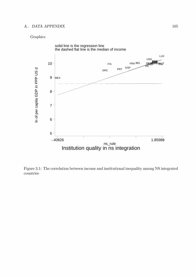
A.. DATA APPENDIX 105
Graphics
solid line is the regression linethe dashed flat line is the median of income
ln o
f per
cap
ita G
DP
in P
PP
US
d
Institution quality in ns integrationns_rule
-.40826 1.85988
5
6
7
8
9
10 AUTBEL CANDEU DNK
ESPFINFRA GBR
GRC
IRLISLITA
LUX
MEX
NLDNOR
PRT
SWEUSA
Figure 3.1: The correlation between income and institutional inequality among NS integratedcountries
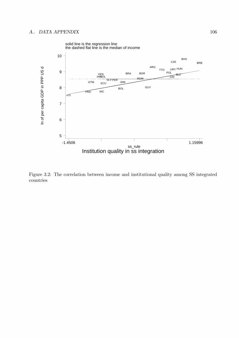
A.. DATA APPENDIX 106
solid line is the regression linethe dashed flat line is the median of income
ln o
f per
cap
ita G
DP
in P
PP
US
d
Institution quality in ss integrationss_rule
-1.4506 1.15996
5
6
7
8
9
10
ARG
BGR
BHS
BLZ
BOL
BRA
BRB
COL CRI
CZE
ECUGTM
GUYHND
HTI
HUN
JAM
NIC
PER
POLPRY ROMSLV
TTO URY
VEN
Figure 3.2: The correlation between income and institutional quality among SS integratedcountries
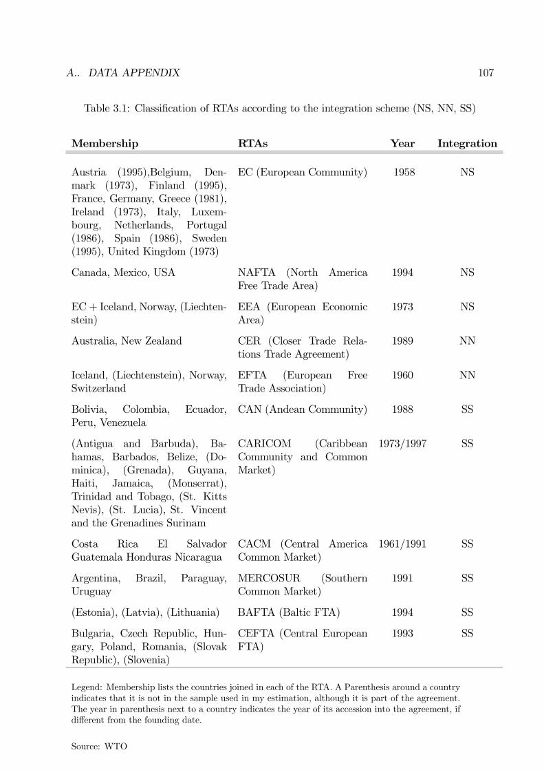
A.. DATA APPENDIX 107
Table 3.1: Classification of RTAs according to the integration scheme (NS, NN, SS)
Membership RTAs Year Integration
Austria (1995),Belgium, Den-mark (1973), Finland (1995),France, Germany, Greece (1981),Ireland (1973), Italy, Luxem-bourg, Netherlands, Portugal(1986), Spain (1986), Sweden(1995), United Kingdom (1973)
EC (European Community) 1958 NS
Canada, Mexico, USA NAFTA (North AmericaFree Trade Area)
1994 NS
EC+ Iceland, Norway, (Liechten-stein)
EEA (European EconomicArea)
1973 NS
Australia, New Zealand CER (Closer Trade Rela-tions Trade Agreement)
1989 NN
Iceland, (Liechtenstein), Norway,Switzerland
EFTA (European FreeTrade Association)
1960 NN
Bolivia, Colombia, Ecuador,Peru, Venezuela
CAN (Andean Community) 1988 SS
(Antigua and Barbuda), Ba-hamas, Barbados, Belize, (Do-minica), (Grenada), Guyana,Haiti, Jamaica, (Monserrat),Trinidad and Tobago, (St. KittsNevis), (St. Lucia), St. Vincentand the Grenadines Surinam
CARICOM (CaribbeanCommunity and CommonMarket)
1973/1997 SS
Costa Rica El SalvadorGuatemala Honduras Nicaragua
CACM (Central AmericaCommon Market)
1961/1991 SS
Argentina, Brazil, Paraguay,Uruguay
MERCOSUR (SouthernCommon Market)
1991 SS
(Estonia), (Latvia), (Lithuania) BAFTA (Baltic FTA) 1994 SS
Bulgaria, Czech Republic, Hun-gary, Poland, Romania, (SlovakRepublic), (Slovenia)
CEFTA (Central EuropeanFTA)
1993 SS
Legend: Membership lists the countries joined in each of the RTA. A Parenthesis around a countryindicates that it is not in the sample used in my estimation, although it is part of the agreement.The year in parenthesis next to a country indicates the year of its accession into the agreement, ifdifferent from the founding date.
Source: WTO
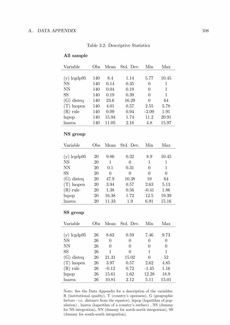
A.. DATA APPENDIX 108
Table 3.2: Descriptive Statistics
All sample
Variable Obs Mean Std. Dev. Min Max
(y) lcgdp95 140 8.4 1.14 5.77 10.45NS 140 0.14 0.35 0 1NN 140 0.04 0.19 0 1SS 140 0.19 0.39 0 1(G) disteq 140 23.6 16.29 0 64(T) lnopen 140 4.01 0.57 2.55 5.78(R) rule 140 0.09 0.94 -2.09 1.91lnpop 140 15.94 1.74 11.2 20.91lnarea 140 11.05 2.18 4.8 15.97
NS group
Variable Obs Mean Std. Dev. Min Max
(y) lcgdp95 20 9.86 0.32 8.9 10.45NS 20 1 0 1 1NN 20 0.1 0.31 0 1SS 20 0 0 0 0(G) disteq 20 47.9 10.38 19 64(T) lnopen 20 3.94 0.57 2.63 5.13(R) rule 20 1.38 0.56 -0.41 1.86lnpop 20 16.38 1.72 12.5 19.39lnarea 20 11.33 1.9 6.91 15.16
SS group
Variable Obs Mean Std. Dev. Min Max
(y) lcgdp95 26 8.62 0.59 7.46 9.73NS 26 0 0 0 0NN 26 0 0 0 0SS 26 1 0 1 1(G) disteq 26 21.31 15.02 0 52(T) lnopen 26 3.97 0.57 2.62 4.85(R) rule 26 -0.12 0.72 -1.45 1.16lnpop 26 15.61 1.62 12.28 18.9lnarea 26 10.81 2.12 5.11 15.01
Note: See the Data Appendix for a description of the variables.R (institutional quality), T (country’s openness), G (geographicfactors - i.e. distance from the equator), lnpop (logarithm of pop-ulation) , lnarea (logarithm of a country’s surface) , NS (dummyfor NS integration), NN (dummy for north-north integration), SS(dummy for south-south integration).
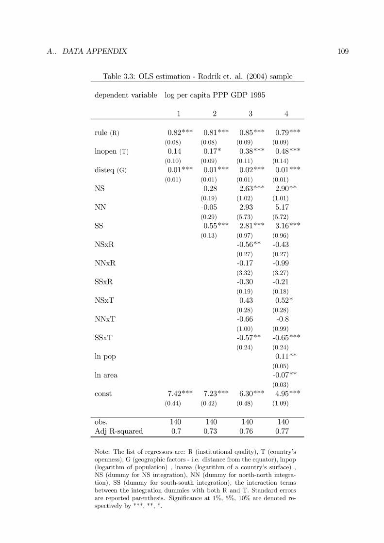
A.. DATA APPENDIX 109
Table 3.3: OLS estimation - Rodrik et. al. (2004) sample
dependent variable log per capita PPP GDP 1995
1 2 3 4
rule (R) 0.82*** 0.81*** 0.85*** 0.79***(0.08) (0.08) (0.09) (0.09)
lnopen (T) 0.14 0.17* 0.38*** 0.48***(0.10) (0.09) (0.11) (0.14)
disteq (G) 0.01*** 0.01*** 0.02*** 0.01***(0.01) (0.01) (0.01) (0.01)
NS 0.28 2.63*** 2.90**(0.19) (1.02) (1.01)
NN -0.05 2.93 5.17(0.29) (5.73) (5.72)
SS 0.55*** 2.81*** 3.16***(0.13) (0.97) (0.96)
NSxR -0.56** -0.43(0.27) (0.27)
NNxR -0.17 -0.99(3.32) (3.27)
SSxR -0.30 -0.21(0.19) (0.18)
NSxT 0.43 0.52*(0.28) (0.28)
NNxT -0.66 -0.8(1.00) (0.99)
SSxT -0.57** -0.65***(0.24) (0.24)
ln pop 0.11**(0.05)
ln area -0.07**(0.03)
const 7.42*** 7.23*** 6.30*** 4.95***(0.44) (0.42) (0.48) (1.09)
obs. 140 140 140 140Adj R-squared 0.7 0.73 0.76 0.77
Note: The list of regressors are: R (institutional quality), T (country’sopenness), G (geographic factors - i.e. distance from the equator), lnpop(logarithm of population) , lnarea (logarithm of a country’s surface) ,NS (dummy for NS integration), NN (dummy for north-north integra-tion), SS (dummy for south-south integration), the interaction termsbetween the integration dummies with both R and T. Standard errorsare reported parenthesis. Significance at 1%, 5%, 10% are denoted re-spectively by ***, **, *.
BIBLIOGRAPHY
[1] Acemoglu, Daron, Johnson, Simon and Robinson, James A. (2001). The Colonial Origins ofComparative Development: An Empirical Investigation. American Economic Review, 91(5):1369-1401.
[2] Acemoglu, Daron, Johnson, Simon and Robinson, James A. (2002). Reversal of Fortune: Ge-ography and Institutions in the Making of the Modern World Income Distribution, QuarterlyJournal of Economics, 118, 1231-1294.
[3] Acemoglu, Daron, Johnson, Simon and Robinson, James. (2005). Institutions as the Funda-mental Cause of Long Run Growth. Handbook of economic growth. Edited by Philippe Aghionand Steven N. Durlauf, North Holland.
[4] Baier, Scott L. and Bergstrand, Jeffrey H. (2003). Economic Determinants of Free Trade Agree-ments. Journal of International Economics: 64(1), 29-63.
[5] Baldwin, Richard E. and Venables, Anthony J. (1995). Regional Economic Integration. Hand-book of International Economics, vol. III. Edited by G. Grossman and K. Rogoff.
[6] Badinger, Harald. (2005). Growth Effects of Economic Integration: Evidence from the EUMember States. Review of World Economics: 141(1), 50-78.
[7] Barro, R. and Sala i Martin, X. (1997). Technological Diffusion, Convergence and Growth,Journal of Economic Growth: 2, 1-27.
[8] Brodzicki, Tomasz. (2003). In search for accumalative effects of European Integration. Paperpresented at the the Second Annual Conference of the European Economic and Finance Society"European Integration: Real and Financial Aspects" Bologna, 14-16 May 2003.
110
BIBLIOGRAPHY 111
[9] Chang, Won and Winters, Alan L. (2002). How Regional Blocs Affect Excluded Countries: ThePrice Effects of MERCOSUR. American Economic Review, 92(4): 889-904.
[10] Crespo-Cuaresma, Jesus, Dimitz Maria Antoinette, Ritzberger-Gruenwald, Doris. (2002).Growth, convergence and EU membership. Working Paper Series 62 Oesterreichische National-Bank.
[11] Deardorff, Alan and Stern, Robert M. (2002). EU Expansion and EU Growth. The Universityof Michigan, Ann Arbor - mimeo
[12] De Melo, Jaime, Montenegro, Claudio and Panagariya Arvind. (1992) Regional IntegrationOld and New: Issues and Evidence. World Bank - mimeo.
[13] De Melo, Jaime, Panagariya, Arvind and Rodrik, Dani. (1993). The New Regionalism: ACountry Perspective In, J. de Melo and A. Panagariya (eds.), New Dimensions in RegionalIntegration, London, Cambridge University Press for CEPR, 1993.
[14] De Menil, Georges. (2003). History, Policy, and Performance in Two Transition Economies:Poland and Romania. In, Rodrik, D. (eds.), Search of Prosperity: Analytic Narratives on Eco-nomic Growth, Princeton University Press.
[15] Dollar, David and Kraay, Aart. (2003). Institutions, trade, and growth: revisiting the evidence.Policy Research Working Paper Series 3004, The World Bank.
[16] Feenstra, Robert. (1996). Trade and Uneven Growth. Journal of Development Economics, 49:229-256.
[17] Frankel, Jeffrey A. and Romer, David. (1999). Does Trade Cause Growth, American EconomicReview, 89(3): 379-399.
[18] Gallup, John L., Sachs, Jeffrey D., and Mellinger, Andrew D. (1998). Geography and EconomicDevelopment. NBER WP 6849.
BIBLIOGRAPHY 112
[19] Gancia, Gino. (2003). Globalization, Divergence, and Stagnation, IIES Working Papers #720.
[20] Grossman, Gene M. and Helpman E. (1991). Innovation and Growth in the Global Economy.The MIT Press.
[21] Hall, Robert E. and Charles I. Jones. (1999). Why Do Some Countries Produce so much moreOutput per Worker than Others?. Quarterly Journal of Economics, 114, 83-116.
[22] Henrekson, Magnus, Torstensson, Johan and Torstensson, Rasha. (1997). Growth effects ofEuropean Integration. European Economic Review, 41: 1537-1557.
[23] Lo Turco, Alessia. (2004). Integrazione regionale Sud-Sud e crescita economica: valutazionedegli accordi di comercio in America Latina. Tesi di dottorato, Dipartimento di Economia, Uni-versità Politecnica delle Marche.
[24] Lo Turco, Alessia. (2005). Are South-South Trade Agreements Growth Enhancing? The Caseof Latin American Agreements. Applied Econometrics and International Development, 5(2),April-June.
[25] Ichino, Andrea. (2006). The Problem of Causality in the Analysis of Educational Choices andLabor Market Outcomes - Slides for Lectures. Available at http://www2.dse.unibo.it/ichino/
[26] Madriaga, Nicole, Montout, Sylvie and Ollivand, Patrice. (2004). Regional Convergence, TradeLiberalization and the agglomeration of activities: an analysis of NAFTA and MERCOSURcases. Cahiers de la Maison des Sciences Economique, bla04069, Université Paris1 Panthéon-Sorbonne.
[27] Martin, P. and Ottaviano, G.I.P. (1999). Growing Locations: Industry Location in a Model ofEndogenous Growth. European Economic Review, 43: 281-302.
[28] Panagariya, Arvind. (2000). Preferential Trade Liberalization: The Traditional Theory andNew Developments. Journal of Economic Literature, 38(2): 287-331.
BIBLIOGRAPHY 113
[29] Redding, S. (1999). Dynamic Comparative Advantages and the Welfare Effects of Trade.Oxford Economic Papers, 51: 15-39.
[30] Rodrik, Dani, Subramanian A. and Trebbi, F. (2004). Institutions Rule: The Primacy ofInstitutions over Geography and Integration in Economic Development. Journal of EconomicGrowth, 9(2).
[31] Sach, Jeffrey D. (2003) Institutions don’t Rule: Direct Effects of Geography on per capitaIncome, NBER WP 9490.
[32] Vamvakidis, Athanasios. (1998). Regional Trade Agreements Versus Borad Liberalization:Which Path Leads to Faster Growth? Time-Series Evidence. IMF WP/98/40.
[33] Vanhoudt, P. (1999). Did the European Unification Induce Economic Growth? In Search ofScale Effects and Persistent Changes. Review of World Economics, 135 (2): 193—220.
[34] Venables, Anthony. (2003). Winners and losers from regional integration agreements, Eco-nomic Journal, 113, 747-761.
[35] Walz, Uwe. (1997). Growth and Deeper Regional Integration in a Three-Country Model. Re-view of International Economics, 5(4) 492-507.
[36] Walz, Uwe. (1997). Dynamic Effects of Economic Integration: A Survey. Open economiesreview, 8 (3), 309-326.
[37] Walz, Uwe. (1998). Does an enlargement of a common market stimulate growth and conver-gence?. Journal of International Economics, 45, 297-321.
[38] Wooldridge, Jeffrey M. (2002). Econometric Analysis of Cross Section and Panel Data. TheMit Press.