Three essays on finance - Home | Nanyang Technological

This document is downloaded from DR‑NTU (https://dr.ntu.edu.sg)Nanyang Technological University, Singapore.

Three essays on finance

Yang, Chuyi

2020

Yang, C. (2020). Three essays on finance. Doctoral thesis, Nanyang TechnologicalUniversity, Singapore.

https://hdl.handle.net/10356/138123

https://doi.org/10.32657/10356/138123

This work is licensed under a Creative Commons Attribution‑NonCommercial 4.0International License (CC BY‑NC 4.0).

Downloaded on 25 Jan 2022 02:40:26 SGT

THREE ESSAYS ON FINANCE

YANG CHUYI

NANYANG BUSINESS SCHOOL

2020

THREE ESSAYS ON FINANCE

YANG CHUYI

Nanyang Business School

A thesis submitted to the Nanyang Technological University

in partial fulfilment of the requirement for the degree of

Doctor of Philosophy

2020

Statement of Originality

I hereby certify that the work embodied in this thesis is the result of original

research, is free of plagiarised materials, and has not been submitted for a higher

degree to any other University or Institution.

[Date] [Signature]

. . . . March 16h, 2020. . . . . . . . . . . . Yang Chuyi. . . . . . . . .

Date Name

Supervisor Declaration Statement

I have reviewed the content and presentation style of this thesis and declare it is free

of plagiarism and of sufficient grammatical clarity to be examined. To the best of

my knowledge, the research and writing are those of the candidate except as

acknowledged in the Author Attribution Statement. I confirm that the investigations

were conducted in accord with the ethics policies and integrity standards of

Nanyang Technological University and that the research data are presented honestly

and without prejudice.

Authorship Attribution Statement

Please select one of the following; *delete as appropriate:

*(B) This thesis contains material from 2 papers published in the following peer-reviewed

journal(s) / from papers accepted at conferences in which I am listed as an author.

Chapter 1

The contributions of the co-authors are as follows:

I discovered the findings that the Monday effect is affected by the jackpot sizes on

the preceding Saturday

Prof Chuan Yang Hwang provided project direction

I developed the hypothesis, collected jackpot data, conducted data analysis and

prepared the manuscript under the supervision of Prof Chuan Yang Hwang

Prof Chuan Yang Hwang revised the manuscript

Chapter 2 is presented at Nanyang Business School Seminar (Singapore, October 2017),

2017 Singapore Scholar Symposium (Singapore, November 2017), Sichuan University

Department of Economics (Chengdu, December 2017), 6th East Lake International Forum

for Outstanding Overseas Young Scholars (Wuhan, December 2017), Asian Finance

Association Conference (Tokyo, June 2018)


Assoc Prof Lei Zhang and Asst Prof Chongwu Xia provided project direction

I developed the hypothesis, conducted data analysis and prepared the manuscript

under the supervision of Assoc Prof Lei Zhang

Asst Prof Chongwu Xia revised the manuscript

Chapter 3 is presented at 2017 Asia FMA PhD Consortium (Taipei, May 2017), 2017 Asian

Meeting of the Econometric Society (Hong Kong, June 2017), 2017 Singapore Economic

Review Conference (Singapore, August 2017), Jiangxi University of Finance and

Economics (Nanchang, October 2018)


Assoc Prof Lei Zhang provided securities class action lawsuit data and provided

project direction

I developed the hypothesis, conducted data analysis and prepared the manuscript

under the supervision of Assoc Prof Lei Zhang

Assoc Prof Barry Oliver revised the manuscript

[Date] [Signature]

. . . . March 16h, 2020. . . . . . . . . . . . Yang Chuyi. . . . . . . . .

Date Name

Acknowledgements

First and foremost, I would like to thank my supervisor Prof Hwang Chuan Yang and co-supervisor

Prof Zhang Lei for their excellent expertise on finance research, as well as their detailed guidance,

great patience and continuous encouragement. Without Prof Hwang and Prof Zhang’s tremendous

help and guidance, my thesis would be impossible. I am also inspired from their enthusiasm, hard-

working and attitude towards rigorous research and their influence has set good examples for my

future academic career. Prof Zhang has lead me into the world of research from data collection,

hypothesis development to programming efficiency. I am very grateful for all his advice, patience

in answering questions, and generosity in sharing of his proprietary data to me. My ideas of

applying behavioral finance concepts in empirical asset pricing research has developed during Prof

Hwang’s interesting and inspiring classes. I deeply appreciate his inspiration and time to help me

develop research ideas, refine hypothesis and improve methodology. I am motivated by his hard-

working and care for students, as I will always receive his advice in time during the weekends, and

when he is travelling. He encourages me to overcome all the difficulties when pursing topics that

I am passionate about.

I am very grateful for my committee members, Prof Kang Jun-Koo, Prof Luo Jiang, and Prof He

Tai-Sen for their insightful and constructive advice on my thesis development. I would like to

thank Prof Chen Zhanhui, for his detailed guidance on our collaborating paper, patience in

answering questions and inspiring discussions. I am also grateful for Prof Zhu Qifei for valuable

advice on my thesis. I would also like to thank Prof Angie Low, Prof Byeong-Je An, Prof Chang

Xin, Prof Chen Guojun, Prof Chen Tao, Prof Hyunsoo Doh, Prof Hoonsuk Park, Prof Ru Hong,

Prof Sie Ting Lau, Prof Stephen Dimmock, Prof Wang Xin, Prof Wu Yuan, Prof Zhang Huai and

all the other faculty members for their advices.

The PhD journey is more meaningful with the companion of friends in the NBS family. I would

like to thank my peers for all the discussions and support for each other. It is great to have friends

around so that I am not alone on this journey. I would like to thank Xia Chongwu, Wang Yuxi,

Yang Endong, Zhang Li, Phua Jing Wen Kenny, Xie Wenjun, Yang Bowen, Zhang Jin, Li

Lingwei, Chen Yuzi, Lou Pingyi, Lee Min Suk, Choi Changhwan, Li Wei, Yang Yanjia, Kim

Hyemin, Kim Baek-Chun, and Qu Chengyuan for their kind help and encouragement. I will always

remember the fruitful time we spent together in our PhD office. I want to thank Quek Bee Hua,

Karen Barlaan, Amarnisha Mohd, Ada Ong Ke Jia, Cher Mui Luang Florence, and all the other

management staffs for their help and strong support.

Most importantly, I would like to thank my families for their unconditional love, who always

support my decisions and my pursuit of dreams wholeheartedly. My beloved grandmother, who is

a great mathematics teacher, not only teaches me mathematics and takes very good care of me, but

also influences me to be a kind, positive and helpful person. I am aspiring to be a good teacher as

her since my childhood and throughout my life.

Table of Contents

Summary ................................................................................................................... 1

Chapter 1 Lottery Jackpots and the Monday Effect ............................................ 2

I. Introduction ......................................................................................................................5

II. Hypothesis Development ...............................................................................................10

III. Data ................................................................................................................................12

IV. Results ............................................................................................................................13

i. Summary Statistics .....................................................................................................13

ii. The Monday Effect a Weekend Jackpot Effect? .......................................................14

iii. Friday Earnings News, Friday Return and the Monday Effect .................................17

iv. The Monday Effect of Anomalies ..............................................................................19

V. Return Co-movement and Saturday Jackpots ................................................................21

VI. Trading Activity and Saturday Jackpots ........................................................................23

VII. Weekend Jackpot vs. Weekday Jackpot ........................................................................25

VIII. Sports Events, Friday Return and the Monday Effect: Evidence from 1967 .................27

IX. Conclusion ......................................................................................................................31

X. Reference ........................................................................................................................33

XI. Tables .............................................................................................................................40

Chapter 2 Foreign Exchange Hedging and Corporate Innovation ................... 79

I. Introduction ...................................................................................................................82

II. Sample and Data ............................................................................................................89

III. Main Results ..................................................................................................................93

i. Pooled OLS Baseline Regression ..............................................................................93

ii. Potential Benefit of FX hedge ....................................................................................95

iii. Robustness Checks ....................................................................................................97

IV. Endogeneity Concerns ..................................................................................................98

i. Change Level Regression ..........................................................................................98

ii. Difference-in-Differences Analysis ............................................................................99

iii. Instrumental Variable Approach ..............................................................................100

iv. Reverse Causality .............................................................................................................. 102

V. Economic Channels .....................................................................................................103

i. Information Asymmetry ..........................................................................................103

ii. Myopic Behaviors ....................................................................................................105

VI. Additional Analyses ....................................................................................................107

i. Accounting Conservatism ........................................................................................107

ii. Innovation Efficiency ...............................................................................................108

iii. Alternative explanation: Cost of Capital ........................................................................ 110

VII. Conclusions .................................................................................................................111

VIII. Reference ......................................................................................................................113

IX. Tables ...........................................................................................................................122

Chapter 3 Do Law Firms Matter for Securities Class Action Lawsuits? ...... 162

I. Introduction ..................................................................................................................164

II. Hypothesis Development .............................................................................................171

III. Data and Variables .......................................................................................................172

i. Data ..........................................................................................................................172

ii. Main Variables .........................................................................................................172

i. Control Variables......................................................................................................176

IV. Results ..........................................................................................................................178

i. Predicting Litigation Outcome .................................................................................179

ii. Cumulative Abnormal Return ..................................................................................180

ii. Settlement Amount ...................................................................................................181

iii. Unitization Rate ........................................................................................................182

iv. Case Length ..............................................................................................................183

v. Market Share ............................................................................................................184

vi. CEO Turnover ..........................................................................................................184

V. Robustness ....................................................................................................................186

VI. Conclusion ....................................................................................................................188

VII. Reference ......................................................................................................................190

VIII. Tables ...........................................................................................................................194

Summary

In Chapter 1, using large lottery jackpots on Saturday as repeated exogenous shocks to investor

attention, we find that the Monday effect of market return and the Monday effect of anomalies

only exist on Mondays with a large jackpot on the preceding Saturday. For example, the Monday

effect of high idiosyncratic volatility stocks is a striking - 64 bps when there was a large Saturday

jackpot but is negligible otherwise. This is consistent with the hypothesis that individual investors

allocate the weekends to process information and decide on trading strategies. Large jackpots

during the weekends distract individual investors’ attention from the stock market, resulting in less

buying relative to selling, lower return and larger stock co-movement on the following Monday.

The jackpot effect is larger among stocks preferred by individual investors. Interestingly, we do

not find similar jackpot effect on weekday drawings.

In Chapter 2, we study the real effects of foreign exchange hedging on corporate innovation. Under

the information asymmetry hypothesis, corporate hedging reduces firm’s information asymmetry,

and alleviates manager’s career concern from undervaluation and helps investors to better monitor

the manager, which in turn increases innovation. Under the market pressure hypothesis, hedging

imposes more short-term earnings pressure on managers because of mark-to-market hedge

accounting, hence leads to lower innovation. Our results support the information asymmetry

hypothesis. Hedged firms invest more heavily in innovative projects, generate more patents and

have more patent citations. To address endogeneity concerns, we employ both difference-in-

differences and instrumental variables regressions, and test for reverse causality explicitly.

In Chapter 3, we document a measure of law firm expertise that could predict the outcomes of

future lawsuits conducted by the law firm, using securities class action lawsuits from 1996 to 2013.

We use prior Dismissed Ratio as law firm expertise measure on a rolling basis, defined as ratio of

number of dismissed cases to number of total cases conducted by the law firm in the past 5 years.

It is found that law firms with lower prior Dismissed Ratio are more likely to be skilled law firms

with less agency problem. Cases conducted by skilled law firms with less agency problem are

more likely to be settled, have more negative cumulative abnormal return during the filing date,

win larger settlement amount, result in larger probability of CEO turnover and are associated with

larger short interest one week prior to the filing event. Skilled law firms contribute to better

outcomes by exerting more effort in the litigation process, as evident by the longer Case Length

from filing date to status date. In addition, market share of law firms increases after performing as

skilled law firms and skilled law firms are less likely to disappear from the market in the future.

Overall, predictive power and persistence of law firm expertise suggest law firm fixed effect in

securities class action lawsuits. Robustness tests suggest existence of law firm expertise beyond

case selection.

2

Chapter 1

3

Lottery Jackpots and the Monday Effect

Chuan Yang Hwang

[email protected]

Division of Banking and Finance


Nanyang Technological University

Singapore 639798

Chuyi Yang

[email protected]




Singapore 639798

4

Lottery Jackpots and the Monday Effect

Abstract

Using large lottery jackpots on Saturday as repeated exogenous shocks to investor attention, we

find that the Monday effect of market return and the Monday effect of anomalies only exist on

Mondays with a large jackpot on the preceding Saturday. For example, the Monday effect of high

idiosyncratic volatility stocks is a striking - 64 bps when there was a large Saturday jackpot but is

negligible otherwise. This is consistent with the hypothesis that individual investors allocate the

weekends to process information and decide on trading strategies. Large jackpots during the

weekends distract individual investors’ attention from the stock market, resulting in less buying

relative to selling, lower return and larger stock co-movement on the following Monday. The

jackpot effect is larger among stocks preferred by individual investors. Interestingly, we do not

find similar jackpot effect on weekday drawings.

JEL Classification: G41, G12, G11

Keywords: Investor Attention, Monday Effect, Stock Market Anomalies

5

I. Introduction

The Monday effect, equity market return on Monday is lower than other days of the week and on

average negative, has remained an intriguing anomaly for a long time in the U.S. and international

markets1. The most consistent and widely accepted explanation2 is that the Monday effect is related

to investors’ trading behavior. As it takes time to process information, individual investors will

process information during the weekends and trade on Monday for liquidity needs or rebalancing

reasons (Osborne (1962), Miller (1988), Lakonishok and Maberly (1990), Abraham and Ikenberry

(1994)). In contrast, institutional investors usually allocate Monday as strategic planning day

(Osborne (1962)) and refrain from trading on Monday (Jain and Joh (1988), Lakonishok and

Maberly (1990), Venezia and Shapira (2007), Ülkü and Rogers (2018)).

These papers also suggest that individual investors are more likely to sell (or less likely to buy)

on Monday and depress prices3. However, the static proxies for individual investors’ and

institutional investors’ trading activity based on trader-type classifications become less accurate in

the recent period with electronic trading and order divisibility (Hvidkjaer (2008), Campbell,

1 The Monday effect also exists in other asset class: treasury bill returns (Gibbons and Hess (1981)), federal funds

rates (Griffiths and Winters (1995)), bonds return (Jordan and Jordan (1991)), gold price (Ball, Torous, and Tschoegl

(1985)), and currency exchange rate (Coats (1981), McFarland, Pettit, and Sung (1982)). International evidence on

the Monday effect is documented in Chang, Pinegar, and Ravichandran (1993), Dubois and Louvet (1996) and Jaffe

and Westerfield (1985).

2 Other explanations for the Monday effect lie in several areas: Monday effect as statistical errors (Sullivan,

Timmermann, and White (2001)), settlement and clearing delays (Lakonishok and Levi (1982)), information flows of

both macro (Chang, Pinegar, and Ravichandran (1998)) and firm-specific announcements (French (1980), Damodaran

(1989)), and Monday blue (Rystrom and Benson (1989)).

3 There are mixed evidences of individual investors’ trading behavior on Monday. For example, Ülkü and Rogers

(2018) find increase in net buying from individual investors and decrease in net buying from institutional investors on

Monday, using daily trading data from Korea Stock Exchange, Taiwan Stock Exchange and Stock Exchange of

Thailand.

6

Ramodorai, Schwartz (2009)).To overcome this difficulty, we take advantage of the following

insight. If the Monday effect is indeed driven by individual investors’ trading pattern and if there

are exogenous events that distract their attention to learning trading strategies during the weekends,

then we would expect Monday return and trading activity to vary with distraction events. In this

paper, we identify large Powerball jackpots4, as series of attention distraction events during the

weekends; and show that they cause lower return on the following Mondays.

Attention is a scarce resource and paying attention requires effort (Kahneman (1973)). Limited

investor attention will influence investor perceptions, resulting in neglect of information and

under-reaction to news (Hirshleifer and Teoh (2003), Peng (2005), Peng and Xiong (2006),

Hirshleifer, Lim and Teoh (2009)). Thus, limited attention is expected to have impact on both stock

valuations and trading interest. In our setting, a large jackpot attracts attention through its large

prize as well as widespread media coverage (Clotfelter and Cook (1989)), causing investors to pay

less attention to the stock market in general. The major advantage of utilizing large jackpots as

attention distracting events is that they are largely independent of the economic factors that may

systematically affect our tests. This is because jackpots accumulate when there is no winners for a

consecutive period and thus their occurrences can be treated as random events.

Gao and Lin (2015) are the first to recognize large jackpots as series of natural experiments of

shocks to investor attention, and find that individual investors’ trading activity decreases during

large jackpot days in Taiwan. Using the same data, Huang, Huang and Lin (2019) further argue

that investors will pay less attention to stocks listed on the Taiwan Stock Exchange during these

days. Limited attention forces them to allocate relatively more attention to market information,

4 Jackpot size larger than or equal to the 70 percentile of our sample period, 114 million US dollars.

7

which, in turn, results in larger return co-movement as hypothesized in Peng and Xiong (2006),

Veldkamp (2006) and Veldkamp and Wolfers (2007). In the U.S equity markets, Dorn, Dorn, and

Sengmueller (2015) find less small trade participation when the combined future jackpot size of

the multi-state lotteries (Powerball and Mega Millions) increases. Despite of these convincing

evidence of the lottery impact on the trading activity of individual investors, none of the papers in

the literature has been able to show that lottery jackpots have any impact on stocks returns so far.

In this paper, we connect the Monday effect literature with a seemingly unrelated literature on

stock trading as gambling, and provide new perspectives to both strands of literature. Unlike earlier

papers, we find that lottery jackpots significantly affect stock returns. In particular, we find return

predictability in U.S. equal-weighted and value-weighted market return based on Powerball

jackpot size on Saturday. More importantly, we discover that the Monday effect only exists when

there was a large Saturday jackpot.5 The lottery impacts on Monday effect are significant, both

economically and statistically. While the Monday return of the equal-weighted market is - 4 bps

in our sample period, it is -21 (3) bps with (without) a large jackpot on the preceding Saturday.

According to the best of our knowledge, we are the first paper to document investor inattention

as causal explanation behind the Monday effect. We propose the investor inattention hypothesis

to explain these findings. Our hypothesis posits that a large Saturday jackpot would distract

investors from learning trading strategies, as individual investors usually reserve the weekends to

decide trading strategies and positions. Since buying requires more attention than selling,

distraction effect from large jackpots will have asymmetric effect on buying and selling behavior

5 We define large jackpots as those with jackpot size larger than or equal to the 70 percentile of our sample period.

We also use alternative definition for large jackpots, including above 50 percentile, above 75 percentile, and above 80

percentile of Saturday jackpot size. Our results remain qualitatively the same and economic significance increases

with larger thresholds.

8

(Barber and Odean (2008)). Consistent with the hypothesis, we find less buying than selling from

individual investors, lower market return and larger return co-movement on Monday following a

large Saturday jackpot. Furthermore, the effects are stronger for liquid stocks, which is consistent

with models of limits to arbitrage literature (Shleifer and Summers (1990), Shleifer and Vishny

(1997), Delong, Shleifer, Summers, and Waldman (1990a), (1990b)). According to these models,

greater liquidity reflects intense trading activity of noise traders, who tend to be individual

investors. In addition, we reveal the distraction effect of jackpots to be larger with bad news or

negative return on Friday, as bad news and negative return on Friday further discourage the trading

interest and the attention paid to the stock market over the weekends. This is consistent with

“ostrich effect” that investors monitor investments less frequently in non-rising markets than rising

markets (Karlsson, Loewenstein, and Seppi (2009)).

Our paper is similar to Gao and Lin (2015) and Huang, Huang and Lin (2019) in many aspects,

but there are major differences. First, we extend their studies from the Taiwanese stock and lottery

markets to the more established and much larger U.S. markets, thus our sample covers more firms

with larger market capitalization, and over a much longer period. Second, unlike their papers, we

show that there is a lottery jackpot impact on stocks returns, which, in turn, allows us to extend

the study from market returns to return anomalies as discussed below. Third, and more importantly,

we show that the lottery jackpot effect in the U.S. has a day-of-the-week pattern, which enables us

to contribute to the Monday effect literature.

Our paper is also closely related to Birru (2018), who shows a surprising and strong day-of-

the-week pattern on return anomalies. In particular, Birru (2018) uncovers the Monday effect of

anomalies --- anomalies associated with speculative or hard-to-value stocks such as the abnormally

low returns of stocks with high idiosyncratic volatility or distress risk concentrate on Monday.

9

Birru (2018) explains these results as investors’ bad mood on Monday lowering the valuation of

speculative stocks. We complement Birru (2018) by showing that investor inattention caused by

large jackpots plays an important role in his findings. Since speculative stocks are harder to value

and require more attention to study and learn, the inattention effect caused by Saturday jackpot

drawings would be much stronger for these stocks. Indeed, we find that the Monday effect of

several prominent anomalies is stronger than the Monday effect of market returns. Furthermore, it

exists only when there was a large jackpot on the preceding Saturday. For example, the Monday

effect of high idiosyncratic volatility stocks and high distress risk stocks are strikingly large (more

than - 60 bps) when there was a large Saturday jackpot. In contrast, the Monday effect of the same

stocks are insignificant and negligible when there was not. These results, together with investor

inattention hypothesis, contribute significantly to the literature by showing that investor inattention

plays an important role in the formation of major stock return anomalies.

Besides Powerball drawings on Saturday, there are other lottery drawings on weekdays:

Powerball drawings on Wednesday, and Mega Millions drawings on Tuesday and Friday.

Interestingly, we find there is no jackpot effect associated with the weekday drawings as we found

with Saturday drawings. This asymmetry between weekend jackpots and weekday jackpots

suggests that unlike over the weekend, individual investors usually don’t have time to learn and

study trading strategies and positions during the weekdays. Thus, distraction from large jackpots

on weekdays have minimal impact on investors’ trading behavior.

In addition to lottery jackpots, negative Friday return and sports events over the weekends also

distract investors from learning trading strategies during the weekends. We study the joint effect

of negative Friday return and two popular sports events, Super Bowl and Kentucky Derby, on

Monday return in the United States from 1967 to 2002. We find lower Monday return following

10

both negative Friday return and sports events, which explains most of the Monday effect in earlier

period. This extends our investor inattention hypothesis to other investor attention distraction

events in a much earlier sample period, further corroborating the causal evidence that investor

inattention is the driving force behind the Monday effect.

The rest of the paper is organized as follows: Section II develops hypothesis. Section III

describes sample and data in detail. Section IV presents the main results on the Monday effect.

Section V explores the return co-movement and Section VI explores trading activity. Section VII

studies weekday drawings. Section VIII studies sports events and the Monday effect in earlier

sample periods. Section IX concludes.

II. Hypothesis Development

In this paper, we propose investor inattention hypothesis to explain the Monday effect. Osborne

(1962), Miller (1988), Lakonishok and Maberly (1990), Abraham and Ikenberry (1994) highlight

the role of individual investors’ trading pattern in explaining the Monday effect. As it takes time

to process information, individual investors will process information during the weekends and

trade on Monday. Due to limited attention (Kahneman (1973)), a large jackpot drawing will

distract individual investors from learning trading strategies during the weekends. In addition, we

expect the jackpot effect to be larger among stocks with intense trading from noise traders, who

tend to be individual investors and have a preference for lottery-like stocks such as those with high

idiosyncratic volatility or positive skewness (Barberis and Huang (2008), Kumar (2009), Bali,

Cakici, and Whitelaw (2011), Green and Hwang (2012)). According to limits to arbitrage literature

(Shleifer and Summers (1990), Shleifer and Vishny (1997)), liquidity is provided by noise traders

who often possess wrong beliefs or are overconfident about their information. Consistent with this,

Hwang, Titman and Yi (2019) show that lottery-related anomalies are much stronger in liquid

11

stocks. Thus, in this paper we choose liquidity to proxy for the trading intensity of noise traders

and hence of individual investors.

We are also motivated by Gao and Lin (2015), and Huang, Huang, and Lin (2019) from the

investor attention literature. Gao and Lin (2015) document lower individual trading activity during

large jackpot days in Taiwan. They argue that both trading and gambling are fun and exciting

activities, and thus investors would be distracted from stock market and allocate more attention to

lottery gambling on those days. Huang, Huang, and Lin (2019) further find that such distractions

have resulted in a larger return co-movement of Taiwanese stocks on large jackpot days. This is

because given limited attention, investors will pay more attention to aggregate (i.e., market) shocks

instead of firm specific shocks (Peng and Xiong (2006), Veldkamp (2006) and Veldkamp and

Wolfers (2007)).

According to Barber and Odean (2008), attention affects buying and selling behavior of

individual investors asymmetrically. Investors choose from thousands of stocks when buying

stocks, whereas they sell from a few stocks that they already owned and seldom short sell. We

hence hypothesize that a large jackpot during the weekend distracts investors from learning trading

strategies, which will result in relative less buying than selling on the following Monday, as buying

requires more attention.

Accordingly, we propose the investor inattention hypothesis formally as below.

Investor Inattention Hypothesis: Individual investors get distracted by lottery drawings with large

jackpot pool on Saturday, and spend less time studying trading strategies during the weekends. As

buying requires more attention than selling, investors will buy less relative to sell on the following

Monday, resulting in lower market return. Furthermore, when attention is limited, investors would

12

pay relatively more attention to market information than individual stock information, which

would increase the co-movement in the stock market. This hypothesis generates four testable

implications:

1. Both the Monday effect of market return and the Monday effect of anomalies are much

stronger following a large jackpot on Saturday.

2. Return co-movement on Monday would be higher following a large jackpot on the

preceding Saturday.

3. The jackpot effects predicted above are stronger in liquid stocks preferred by individual

investors.

4. Trading activity, particularly buying, on Monday would be lower following a large jackpot

on the preceding Saturday.

III. Data

Powerball is one of the most popular multi-state lotteries in the United States6. We have collected

a daily history of jackpots and national-level sales for each drawing of Powerball game and Mega

Millions game7 from January 2003 to December 2018. Powerball drawings happen at 10:59 p.m.

Eastern Time on Wednesday and Saturday, including holidays. Mega Millions drawings happen

6 Lottery games are widely played in the United States. According to Gallup Survey in June 2016, 49% of U.S. adults

reported buying lottery tickets and 64% reported gambling in any forms in the past year of the survey, which makes

lottery tickets the most popular form of gambling in the United States. In addition, 53% of high income group (above

$90,000), 40% of low income group (under $36,000), 56% of middle income group (between $36,000 and $89,999)

have reported buying lottery in the past year of the survey. As of the fiscal year of 2014, the total spending on lottery

tickets is over $70 billion, which is larger than the combined spending on books, video games, movie tickets and

sporting events tickets. Source: Derek Thompson, Lotteries: America's $70 Billion Shame, THE ATLANTIC (May

11, 2015), https://www.theatlantic.com/business/archive/2015/05/lotteries-americas-70-billion-shame/392870/

7 An agreement to cross-sell Mega Millions and Powerball in American lottery jurisdictions was reached by The Mega

Millions consortium and Multi-State Lottery Association (MUSL) on October 13, 2009. The expansion was effective

on January 31, 2010, after which 23 existing Powerball member states began selling Mega Millions tickets and 10

existing Mega Millions member states began selling Powerball tickets.

https://www.theatlantic.com/business/archive/2015/05/lotteries-americas-70-billion-shame/392870/

13

at 11 p.m. Eastern Time on Tuesday and Friday, including holidays. The news media will announce

the jackpot each morning following the previous drawing. Therefore, people would know the

advertised jackpot amount on jackpot drawing day t when they trade on day t (Dorn, Dorn, and

Sengmueller (2015)), if day t is a trading day and a jackpot drawing day.

Jackpot sizes of Powerball and Mega Millions should be time-series uncorrelated with each

other, since the hit of a jackpot is a random event and large jackpots arise due to a series of no-hit

events. We define jackpot size based on jackpot size of both Mega Millions and Powerball: jackpot

size equals to the Mega Millions jackpot size on Tuesday and Friday, and equals to the Powerball

jackpot size on Wednesday and Saturday. Large Jackpot Dummy on Tuesday or Friday equals to

1 if jackpot size of Mega Millions on Tuesday or Friday is larger than or equal to 70 percentile of

Mega Millions jackpot size in our sample period. Large Jackpot Dummy on Wednesday or

Saturday equals to 1 if jackpot size of Powerball is larger than or equal to 70 percentile of

Powerball jackpot size in our sample period.

We adopt CRSP daily market indexes, equal-weighted market return index and value-weighted

market return index, as proxy for market return. We calculate daily Close-to-Close, Open-to-Close

and Close-to-Open return from S&P 500 prices. Individual investors’ trading behavior is identified

through TAQ data.

IV. Results

i. Summary Statistics

We tabulate summary statistics of equal-weighted market index return and value-weighted market

index return by days of the week in Panel A of Table 1. Our sample period is from January 2003

to December 2018, consistent with availability of lottery jackpot data. For Mondays from January

14

2003 to December 2018, the average equal-weighted market return is -4 bps and average value-

weighted market return is -1 bps. In contrast to negative average return on Monday, average equal-

weighted market return and value-weighted market return are positive for Tuesday, Wednesday,

Thursday and Friday. We also provide summary statistics of total trading volume as sum of trading

volume of all stocks and total dollar trading volume as sum of dollar trading volume of all stocks

by days of the week. On average, total trading volume on Monday is 3830 millions of shares

traded, and total dollar volume on Monday is 122,000 million US dollars.

In Panel B, we tabulate summary statistics of jackpot size by days of the week and Large/Non-

large Jackpot Dummy. Large Jackpot Dummy on Tuesday or Friday equals to 1 if jackpot size on

Tuesday or Friday is larger than or equal to 70 percentile of Mega Millions jackpot amount ($89

million). Large Jackpot Dummy on Wednesday or Saturday equals to 1 if jackpot size on

Wednesday or Saturday is larger than or equal to 70 percentile of Powerball jackpot amount ($114

million). Non-large Jackpot Dummy equals to 1 when Large Jackpot Dummy equals to 0. The

largest jackpot on Saturday during the sample period reaches $947.9 million.

[Insert Table 1 Here]

ii. The Monday Effect a Weekend Jackpot Effect?

In Table 2, we confirm the existence of the Monday effect in our sample. In Column (1) and (2),

we regress equal-weighted return and value-weighted market return on Monday, Tuesday,

Thursday and Friday dummy, with Wednesday as benchmark. We control for Before holiday

dummy and After holiday dummy, as individual investors increase trades before or after holidays

and weekends (Lakonishok and Maberly (1990), Dorn, Dorn, and Sengmueller (2015)). We

estimate Newey-West standard errors, allowing maximum lags up to 5 lags. The significantly

15

negative coefficient of the Monday dummy in Column (1) and the insignificant coefficient in

Column (2) indicate that the Monday effect exists in the equal-weighted return index but not in

value-weighted return index during our sample period. This is consistent with prior literature that

smaller stocks have more significant Monday effect while the Monday effect of larger stocks

decrease over the years (Kamara (1997)).


Table 3 reports the baseline results of this paper where we perform the same regressions as in

Table 2 except that we do it separately on Large Saturday Jackpot and Non-large Saturday Jackpot

subsamples. For every trading day in week w, we classify it into Large Saturday Jackpot and Non-

large Saturday Jackpot subsample based on whether there was a large Saturday Jackpot in week

w-1. A Powerball jackpot on Saturday is deemed as Large if it ranks among the top 70 percentile

of all Powerball jackpots in our sample period, and Non-large otherwise. The results of equal-

weighted market return are reported in Column (1) and (2) and those of value-weighted market

return are in Column (3) and Column (4). Strikingly, we find the Monday effect only exists in the

subsample of Large Saturday Jackpot8. Relative to benchmark (Wednesday), equal-weighted

market return is 30 bps lower and value-weighted market return is 27 bps lower on Monday in the

Large Saturday Jackpot subsample. In contrast, Monday return is not statistically different from

other days of the week in the Non-large Saturday Jackpot subsample.

As Monday return is affected by the non-trading period during the weekends, Rogalski (1984)

decomposes S&P500 and Dow Jones Industrial Average close-to-close return into trading day

8 We use alternative cut-off thresholds for Large Jackpot Dummy, such as top 50, 75 and 80 percentile. Our results

remain qualitatively the same, and is not driven by the thresholds for Large Jackpot definition.

16

returns and non-trading day returns, and shows that negative Monday returns are concentrated in

non-trading period from Friday close to Monday open. Similar to Rogalski (1984), we also

decompose S&P500 close-to-close return into non-trading period (close-to-open) return and

trading period (open-to-close), except that we perform the analyses separately on Large Saturday

Jackpot and Non-large Saturday Jackpot subsamples. These results are reported in Panel B of Table

3. We observe that the Monday effect only exists in Large Saturday Jackpot subsample, when

market return is calculated from S&P500 prices. Furthermore, the effect is mainly restricted in the

trading period as indicated by the significant coefficients of Monday dummy in Column (5) Open-

to-Close return and insignificant coefficients of Monday dummy in Column (3) Close-to-Open

respectively, opposite to the findings of Rogalski (1984).

We further test the heterogeneous jackpot effect among different liquidity groups in panel C.

We focus on the test of the third prediction of the investor inattention hypothesis – the jackpot

effect is larger among liquid stocks dominated by noise traders (Shleifer and Summers (1990),

Shleifer and Vishny (1997)). We separate stocks based on daily share turnover ratio in the previous

quarter end, and classify stocks as liquid (illiquid) stocks if share turnover ratio is larger (smaller)

than or equal to 70th (30th) percentile threshold. Consistent with our hypothesis, we observe the

jackpot effect to be largest among liquid stocks and there is monotonic increase of jackpot effect

when liquidity measure increases. Equal-weighted return of stocks on Monday in the liquid group,

middle group, and illiquid group is 42 bps, 29 bps and 23 bps lower than other days of the week

respectively. In contrast, the Monday effect is absent in neither groups when there were absent of

large Saturday jackpots.


17

In sum, the results in Table 3 indicate that Monday effect is essentially a Saturday (weekend)

jackpot effect postulated in the investor inattention hypothesis, and its effect concentrates in

Monday trading hours. In addition to attention distract from large Saturday jackpots, bad earnings

news may adversely affect the trading interest and the attention paid to stock market by individual

investors, which may in turn amplify the jackpot effect described in the Table 3. We therefore

study the effect of Saturday jackpots on Monday return when there was negative return and bad

earnings announcement news on the preceding Friday.

iii. Friday Earnings News, Friday Return and the Monday Effect

Information release on Friday and over the weekend has been proposed to explain the Monday

effect. Gennotte and Trueman (1996) show that managers have the incentive to release bad news

after trading hours, which is also consistent the findings of DellaVigna and Pollet (2009) that

earnings announcement on Friday has lower immediate response and higher delayed response due

to less investor attention on Friday. To make sure our baseline results are not driven by the delayed

response to news releases on Friday and over the weekend, we do the following analyses. We first

compute standardized unexpected earnings (SUE) surprises for each earnings announcement,

based on IBES reported analyst forecasts and actuals as in Livnat and Mendenhall (2006). For each

combined period of Friday and the following weekend, we first count the total number of firms

with positive SUE and the total number of firms with negative SUE for earning news announced

during that particular period. For each combined period, we calculate the bad news to total news

ratio and classify it as Bad news period if the ratio is above the sample mean, and good news period

otherwise. Finally, we modify the regressions in Panel A of Table 3 by further separating the

Monday dummy into Monday dummy that follows bad news Friday period (Monday_Bad News

Friday) and that follows good news Friday period (Monday_Good News Friday). Column (1) of

18

Table 4 reveals that Monday with large Saturday jackpots has 37 (26) bps lower equal-weighted

return when there are more bad (good) news on the preceding Friday and the weekend, suggesting

that bad news on Friday exacerbates the effect of weekend jackpots on Monday return but doesn’t

drive the Monday effect. Furthermore, Column (2) indicates that in the absence of large Saturday

jackpots, there is no Monday effect even for Monday that follows a bad news Friday period.

Column (3) and Column (4) deliver the same message when we examine the value-weighted

market return. Our finding lends support to Damodaran (1989) that small proportion of around

3.4% of the Monday effect could be explained by earnings announcement and dividend

announcement on Friday.


Abraham and Ikenberry (1994) find that negative Monday return is driven by Friday’s return,

as Monday’s return is on average -0.61% when Friday’s return is negative, while Monday’s return

is on average 0.11% when Friday’s return is positive during their sample period. They further

document that following a positive Friday, early morning trading of Monday does not have large

price decline. Hence, we perform similar analyses as in Table 4, except that we replace bad (good)

news Friday with negative (positive) return Friday in Table 5. The results in Table 5 are similar to

Table 4 in that Negative Friday return exacerbates but does not drive the Monday effect as there

is no significant Monday effect in the absence of Saturday jackpot even when there was negative

Friday return as shown in Column (2) and Column (4). The Monday return following a large

Saturday jackpot and a negative Friday return is noteworthy in magnitude. It is lower than other

weekdays by 58 bps, which is striking considering the average equally-weighted daily market

return on Monday is -4 bps during our sample period, and suggesting a profitable trading strategy.

It is also consistent with investor inattention hypothesis and suggests that the effect of the

19

distraction from large Saturday jackpots is more severe when investors’ trading interest and

attention paid to stock market are already low due to bad news and negative return on Friday. This

is consistent with “ostrich effect” that investors monitor investments less frequently in non-rising

markets than rising markets (Karlsson, Loewenstein, and Seppi (2009)).


iv. The Monday Effect of Anomalies

According to our investor inattention hypothesis, if individual investors’ inattention during the

weekends are driving the Monday effect, then we shall expect the effect of Saturday jackpots to

be stronger among stocks that are hard to value and are preferred by individual investors. Birru

(2018) documents a striking day-of-the-week effect in many prominent anomalies. In particular,

he shows that profits derived from the long leg of these anomaly-based long-short trading

strategies concentrate on Friday, but he also shows a much larger profit derived by taking a short

position in speculative and hard-to-value stocks concreates on Monday, a phenomenon we call the

Monday effect of anomalies. Birru (2018) attributes the low returns associated with these

speculative and hard-to-value stocks to the low valuations caused by bad mood on Monday

(Wright and Bower (1992)). Having shown that a large Saturday jackpot plays a critical role in

explaining the Monday effect of market return, we are interested in learning if a large Saturday

jackpot has similar effect on the Monday effect of anomalies. We first validate findings in Birru

(2018) using two anomalies (IVOL and distress risk) that have the strongest Monday effect in our

sample period. Both high IVOL and high distress risk are associated with hard-to-value and

speculative firms.

Following Kumar (2009), IVOL at the end of month t is the residual from fitting Carhart four-

factor model using daily return of the previous 6 months, from t-6 to t-1. A stock is classified as

20

high (low) IVOL for trading days in month t+1, if its IVOL ranks in the top (bottom) quintile at

the end of month t. We also use the 12-month logit regression coefficients from Table IV in

Campbell, Hilscher, Szilagy (2008) to calculate the distress probability at the end of December in

each year t. A stock is classified as high (low) Distress risk stocks for trading days in year t+1, if

distressed probability of the stock is in the top (bottom) quintile of distressed probability in the

December of year t.

In Table 6 Panel A, we report value-weighted excess return and alpha for high IVOL and high

Distress stocks adjusted by CAPM, Fama-French three-factor model and Carhart four-factor model

respectively. We calculate the return and alphas separately on Monday and non-Monday (rest of

the days). Consistent with Birru (2018), we find that short-leg return of both anomalies is profitable

on Monday but not on the rest of the days. In Panel B, we further separate Monday studied in Panel

A into Monday with Large Saturday jackpot and Monday with Non-large Saturday Jackpot

subsamples. And we find that the Monday effect of anomalies exist only in the subgroup of

Monday with Large Saturday Jackpot 9. In particular, the excess return of high IVOL and high

Distress risk are on average -44 bps and -43 bps respectively on Monday with Large Saturday

jackpot but are insignificant on Monday with Non-Large Saturday jackpot.

Assuming the risk of a stock does not vary systematically within the day of the week, a more

powerful test to detect the Monday effect of anomalies is to avoid risk-adjustment and run value-

weighted excess regressions of high IVOL and high Distress risk portfolios on the day-of-the-week

dummies as shown in Panel C of Table 6, similar to the regression as in Table 2. Form these

9 In Birru (2018), long-short portfolio of IVOL earns on average 22.6 bps on Monday from July 1963 to December

2013. During our sample period, long-short portfolio of IVOL and Distress earns on average 29 bps on Monday with

large jackpots, compared with insignificant 9 bps on Monday with non-large jackpots.

21

regressions, we observe a clear Monday effect for high IVOL stocks and high Distress risk stocks.

When we run the same regression separately on Large Saturday Jackpot and Non-large Saturday

Jackpot subsamples in Panel D, the Monday effect for both anomalies becomes stronger in the

Large Saturday Jackpot subsample. Furthermore, the Monday effect of anomalies only exists in

this subsample and absent in Non-large Saturday Jackpot subsample10. The magnitude of the

Monday effect for high IVOL and high distress risk stocks are strikingly large, in excess of 60 bps,

suggesting a profitable trading strategy. In sum, these results are not only consistent with the first

testable implication of investor inattention hypothesis that the Monday effect is larger among

stocks that are hard to value in nature and require more investor attention, but also suggest Monday

effect of anomalies, like the Monday effect of market return, could be a manifestation of weekend

jackpot effect.


V. Return Co-movement and Saturday Jackpots

In this section, we test the second prediction of investor inattention hypothesis that there would be

an increase in return co-movement in the stock market on Monday following a large jackpot on

the preceding Saturday.

For each stock in our sample, we calculate its return co-movement by the day-of-the-week and

Large Saturday Jackpot dummies. Consistent with our prior definition, Large Saturday Jackpot

dummy equals to 1 if Powerball’s jackpot on Saturday is larger than or equal to the 70 percentile

of Powerball jackpot. Non-large Saturday Jackpot dummy equals to 1 when Large Saturday

10 In unreported results, we also find that low future return of stocks with high maximum daily return over the past

month (Bali, Cakici, and Whitelaw (2011)), low price (Birru and Wang (2016)), young age (Ritter (1991)) and far

from 52-week high (George and Hwang (2004)) only exits on Monday following a large Saturday jackpot.

22

Jackpot dummy equals to 0. For trading days in week w, we classify into Large Saturday Jackpot

and Non-large Saturday Jackpot groups based on Large Saturday Jackpot dummy and Non-large

Saturday Jackpot dummy on the Saturday of week w-1. Return co-movement is calculated as the

adjusted R-square from the market model regression (Barberis, Shleifer and Wurgler (2005)), and

as time series Pearson correlation of stock excess returns and market excess returns (Peng and

Xiong (2006), Antón and Polk (2014)). For each stock in the portfolios defined by Large Saturday

Jackpot dummy and day-of-the-week dummy, we require at least 20 observations for the

regression and correlation estimation. The mean and median estimate in each portfolios are

reported in Panel A of Table 7. Compared with Mondays without large Saturday jackpots,

Mondays with large Saturday jackpots have significantly larger return co-movement. This is

consistent with our second prediction of investor inattention hypothesis that return co-movement

on Monday, would be higher following a large jackpot on the preceding Saturday. In addition, we

observe the co-movement increase due to large Saturday jackpot is larger on Monday than on other

weekdays.

As explained earlier in the section of hypothesis development, we use high liquidity to proxy

for the trading intensity of nosier traders and individual investors. We separate stocks based on

share turnover ratio in the previous quarter end, and classify stocks as liquid (illiquid) stocks if

share turnover ratio is larger (smaller) than or equal to 70th (30th) percentile threshold. We repeat

our tests in Panel A but separately for liquid and illiquid stocks and report the results in Panel B

and Panel C respectively. We can clearly see that the jackpot effect on the co-movement is much

larger on Monday than other weekdays, and the effect is larger liquid stocks, consistent with the

third prediction of the investor inattention hypothesis. For example, the average increase in

adjusted R-square of Monday return is 0.0695 for liquid stocks, compared with 0.0367 for that of

23

other weekday returns. The difference 0.0328 is significant at 1% level. The corresponding figures

for the illiquid stocks are 0.0298, 0.0135, and 0.0163 respectively.


VI. Trading Activity and Saturday Jackpots

In this section, we focus on the test of the fourth prediction of the investor inattention hypothesis

-- distraction from large Saturday jackpots would reduce the trading activity, particularly buying

of individual investors. We use odd-lot trades (trades of fewer than 100 shares) as proxy for

individual investors’ trading behavior (Ritter (1988), Lakonishok and Maberly (1990)). For the

sample period from 2003– 2012, we follow Lee and Ready (1991) to sign trades as buyer or seller

initiated using TAQ Trade and Quote data. With the rise of algorithm trading, trade-size partition

becomes less accurate in the recent period. From 2013 to 2018, we follow Boehmer, Jones, Zhang,

and Zhang (2019) to classify marketable odd-lot retail trades as either buy or sell using TAQ

Millisecond Trade and Quote data. For each trading day t from 2003-2018, we aggregate daily buy

volume for each stock i traded on NYSE/AMEX/NASDAQ, as Odd-Lot Buy Volume on day t.

Similarly, we aggregate daily sell volume for each stock i traded on NYSE/AMEX/NASDAQ, as

Odd-Lot Sell Volume on day t. We calculate daily measures of odd-lot order imbalance using buy

and sell volume, as proxy for asymmetric buying and selling activities of individual investors.

O’Hara, Yao, and Ye (2014) suggest using volume-based or dollar-volume-based measures for

order imbalance to reduce bias arising from missing odd lots in TAQ data.

𝑂𝑟𝑑𝑒𝑟 𝐼𝑚𝑏𝑎𝑙𝑎𝑛𝑐𝑒𝑡 = ∑ 𝑂𝑑𝑑 − 𝐿𝑜𝑡 𝐵𝑢𝑦 𝑉𝑜𝑙𝑢𝑚𝑒𝑖,𝑡𝑖 − ∑ 𝑂𝑑𝑑 − 𝐿𝑜𝑡 𝑆𝑒𝑙𝑙 𝑉𝑜𝑙𝑢𝑚𝑒𝑖,𝑡𝑖

∑ 𝑂𝑑𝑑 − 𝐿𝑜𝑡 𝐵𝑢𝑦 𝑉𝑜𝑙𝑢𝑚𝑒𝑖,𝑡𝑖 + ∑ 𝑂𝑑𝑑 − 𝐿𝑜𝑡 𝑆𝑒𝑙𝑙 𝑉𝑜𝑙𝑢𝑚𝑒𝑖,𝑡𝑖

24

In Table 8 Column (1), we run the order imbalance regressions on weekday dummies and an

interactive term of Monday dummy and Large Saturday jackpot dummy so that the coefficient of

the interactive term, Monday_Large Saturday Jackpot, captures the effect of large Saturday

jackpots on order imbalance of the following Monday. We also control for yearly time dummies

for the time-varying transaction cost in all trading activity regressions (Choe and Hansch (2005)).

The significantly negative coefficient on Monday indicates that individual investors tend to buy

less relative to sell on Mondays following large Saturday jackpots. Interestingly, we do not observe

significant asymmetric buying and selling behavior on Mondays without large Saturday jackpots,

which is consistent with our main return result that the Monday effect only exists following large

Saturday jackpots. This is consistent with the fourth prediction of investor inattention hypothesis

that a large Saturday jackpot distracts individual investors’ attention over the weekends when

investors normally spend time and attention studying trading strategies. As buying require more

attention than selling (Barber and Odean (2008)), a large Saturday jackpot asymmetrically affects

buying and selling behavior of individual investors, resulting in further lower buying than selling

on the following Monday. Furthermore, as negative Friday return is likely to trigger selling

behavior of individual investors, we further study the interaction effect of large Saturday jackpot

with negative Friday return in Column (2). We create Negative Friday Return dummy and Positive

Friday Return dummy for week w, based on whether the return of respective market index on the

preceding Friday is negative or positive in week w-1. We interact Negative Friday Return dummy

with Monday dummy and Large Saturday Jackpot dummy as Monday_Negative Friday

Return_Large Saturday Jackpot. However, we do not observe any additional order imbalance

arising from negative Friday return, as shown by the insignificant coefficient of Monday_Negative

Friday Return_Large Saturday Jackpot. In Column (3), we separately study the interaction effect

25

of Positive/Negative Friday return dummy with Large/Non-Large Saturday Jackpot dummy.

Compared with other days of the week, there is relative less buying than less on Mondays with

Large Jackpots, and the magnitude is largest (0.038) when there was negative Friday return and

large Saturday jackpot among the four groups. Therefore, we provide individual investors’

reduction in buying relative to selling as the link between large Saturday jackpots and lower

Monday return.


VII. Weekend Jackpot vs. Weekday Jackpot

As investor inattention hypothesis is designed to explain the Monday effect, we have so far focus

on the distraction and inattention caused by the weekend (Saturday) jackpot. In this section, we

investigate if there is a similar effect caused by the weekday jackpots. For drawings on Tuesday,

Wednesday and Friday, we study the effect of jackpots on market indexes on the same trading day

and exclude any holidays. For drawings on Saturday, we study the effect on market return and

trading activity on the following Monday. Large Jackpots are events where the jackpot size of

Tuesday or Friday Mega Millions or the jackpot size of Wednesday or Saturday Powerball are

above the 70 percentiles of the respective Mega Millions and Powerball jackpot size in our sample.

In Table 9, we modify the specification of the trading activity regressions in Table 8 to test if there

is weekday jackpot effect on return. Specifically, we regress equal-weighted market return and

value-weighted market return on interaction of Monday dummy with Large Saturday Jackpot

dummy, interaction of Tuesday/Wednesday/Friday dummy with Large

Tuesday/Wednesday/Friday Jackpot dummy, day-of-the-week dummies, Before holiday and After

holiday dummies. We find that weekday jackpots, including Wednesday Powerball, have no effect

on the contemporaneous weekday return as indicated by the insignificant coefficients on various

26

interaction terms between weekday dummies and large weekday jackpot dummies. In contrast, the

Monday effect caused by the large Saturday jackpots we have observed earlier in Table 3 remains

strong in Table 9. This asymmetry in effects between weekend and weekday jackpots does not

reflect the difference in the type of jackpot, where Mega Millions are exclusively weekday

jackpots. Instead, it reflects the significant effect of Saturday Powerball that falls on the weekends,

and the insignificant weekday jackpots that also includes the Wednesday Powerball. The lack of

effect from weekday jackpots is also consistent with the investor inattention hypothesis. While

investors normally reserve weekends for studying stocks’ trading strategies, they need to work and

cannot afford to do so during weekdays. As a result, even though individual investors may also be

distracted by large jackpots on weekdays, such distraction may not affect the attention nor the

effort that they spend on studying stocks’ trading strategies, as they rarely do so on weekdays even

without distraction.

In addition, the asymmetric effect could help us separate gambling sentiment and mood change

explanation from investor attention explanation. Chen, Kumar and Zhang (2018) find that

gambling sentiment proxied by Internet search volume predicts abnormal return of lottery-like

stocks positively in the short-run due to increased investor demand. Edmans, Garcia, and Norli

(2007) link sport sentiment to stock return. Soccer outcomes could trigger sudden changes in

investor mood, and market declines after losses in the soccer outcomes. The effect is stronger in

smaller stocks and robust in other sports events, such as cricket, rugby, and basketball games. In

our setting, if change in gambling sentiment or mood is induced by disappointment of most

investors for not winning the large jackpot, we should observe the jackpot effect on return for both

27

weekend jackpots and weekday jackpots. The fact that we only observe aggregate return

predictability from Saturday jackpots lends further support to investor inattention hypothesis.11


VIII. Sports Events, Friday Return and the Monday Effect: Evidence from 1967

The earliest studies of the Monday effect in the equity stock market include French (1980) who

studies S&P 500 index from January 1953 to December 1977, and Gibbons and Hess (1981) who

study both S&P 500 index and CRSP market indexes from July 1962 to December 1978. Keim

and Stambaugh (1984) discover negative Monday return for S&P composite back to 1928 and rule

out measurement errors as explanation.

We further test investor inattention hypothesis using negative Friday return and sports events

over the weekends in the earlier period before lottery jackpot data is available. Negative Friday

return will in the first place distract investors from the stock market. According to “ostrich effect”,

investors monitor investments less frequently in non-rising markets than rising markets (Karlsson,

Loewenstein, and Seppi (2009)). Therefore, we examine whether Friday negative return is enough

to explain the Monday effects in the earlier period from 1967 to 2002. We define Negative Friday

Return dummy for week w, which equals to 1 if the return of respective market index on the

preceding Friday is negative in week w-1. We first validate the existence of Monday effect in

earlier sample period in Column (1) and (4) of Table 10 for equal-weighted and value-weighted

market return respectively. Compared with the Monday effect from 2003 to 2018 (11 bps lower)

11 In unreported results, we also find the co-movement increase associated with large jackpot is much larger on

Monday than on other weekdays. These results are inconsistent with mood change explanation as the mood change

and valuation change alone should not cause co-movement to change, let alone causing the change to display the

week-of-the-day pattern.

28

in Table 2, the magnitude of the Monday effect from 1967 to 2002 (24 bps lower) is twice as large

for equal-weighed market return, which is possibly due to a greater influence of individual

investors in the earlier period as there has been a steady increase in the institutional investors over

the years. In Column (2) and (5) of Table 10, we regress equal-weighted and value-weighted

market return on Monday dummy with Negative Friday return, Monday dummy and other days-

of-the-week dummies. The difference in equal-weighted market return between Monday with

negative Friday return and other Mondays is as large as 69 bps. Equal-weighted market return on

Monday is 73 bps and 4.1 bps lower than other days of the week when the previous Friday return

is negative and non-negative respectively. In addition, Monday effect for value-weighted market

return only exists with negative Friday return, which is 46 bps lower than other days. Consistent

with Abraham and Ikenberry (1994), we find that negative Monday return is largely driven by

Friday’s return in our sample period from 1967 to 2002. Abraham and Ikenberry (1994) argue that

lower Monday return arises from individual investors’ selling behavior following bad news on

Friday. Different from Abraham and Ikenberry (1994), our results suggest that lower Monday

return following negative Friday return is also contributed by less buying from individual investors

who are distracted from the stock market. This is consistent with “ostrich effect” that investors

monitor the market less frequently following negative Friday return, which results in less trading

on Monday. Similar to negative Friday return as distraction events, large Saturday jackpots will

also distract individual investors from learning the stock market and result in decline in trading

volume dominated by noise traders as shown in Table 8.

As further support for investor inattention explanation, additional distraction such as sports

events further reduce attention that investors spend on researching on the stock market, which in

turn further lower the Monday return on market. We therefore study the effect of popular sports

29

events during the weekends on the Monday effect to corroborate our investor inattention

hypothesis. If investor inattention caused by large Powerball jackpots on Saturday is driving the

Monday effect, then sports events during the weekends that also distract investor attention will

impact market return on the following Monday. Due to unavailability of the jackpot data from

1967 to 2002, we validate our investor inattention hypothesis using two popular sports events

(Super Bowl and Kentucky Derby) in the United States from 1967 to 2002. The Super Bowl is an

annual championship game of the National Football League (NFL) held on Sunday between mid-

January and early February, starting from 1967. The Kentucky Derby is an annual horse race event

held on the first Saturday of May, starting from 1875. We collect each event date of Super Bowl

and Kentucky Derby from January 1967 to December 2002, and define a Sports Event dummy

based on the dates of both events. Sports Event dummy equals to 1 on the Monday of week w if

there was a sports event (Super Bowl or Kentucky Derby) over the weekends of week w-1.

In Column (3) and (6), we jointly study the investor attention distraction effect from negative

Friday return and sports events. We interact Sports Event dummy with Negative Friday Return

dummy and Monday dummy as Monday_Negative Friday Return_Sports Event dummy to study

the interaction effect. In Column (3), we regress equal-weighted market return on Monday dummy

with Negative Friday return and Sports Event, Monday dummy with Negative Friday Return,

Monday dummy and other days-of-the-week dummies. Consistent with results in Column (2),

lower Monday return concentrates on Mondays following negative Friday return. Furthermore,

with the presence of sports events and negative Friday return, the Monday return is 34 bps further

lower than Monday with negative Friday return and without sports events. For Monday following

sports events and negative Friday return, the equal-weighted return is a strikingly 105.6

(67.6+33.9) bps lower than other days of the week. Similarly, for value-weighted market return in

30

Column (6), Monday effect only exists following negative Friday return. Therefore, results of

sports events further corroborate our investor inattention hypothesis that similar to large jackpot

drawings, sports events over the weekends will also distract individual investors from learning

trading strategies, resulting in lower Monday return.


We directly examine the impact of negative Friday return and sports events on investor

attention by measuring return co-movement. Based on existence of sports events and the sign of

Friday return in week w-1, we classify Monday in week w into following groups: Monday with

Negative Friday Return and Sports Event, Monday with Negative Friday Return and all Monday.

We calculate firm-level co-movement by each of the group. We require at least 20 observations

for each firm in each group to reduce effects of outliers. Comparing Monday with negative Friday

return to all Monday, we observe an increase in return co-movement with negative Friday return.

Mean co-movement measured using adjusted R-square (correlation) is 0.0577 (0.1906) on Monday

and 0.0748 (0.2206) on Monday with negative Friday return. This is consistent with our hypothesis

that negative Friday return distract investors from learning the stock market, resulting in more

attention allocated to market information instead of firm-specific information. Furthermore,

conditional on negative Friday return, return co-movement on Monday with sports events is

significantly larger than other Monday. Return co-movement is largest in the group with sports

events and negative Friday return: mean co-movement measured using adjusted R-square is 0.115

and mean co-movement measured using correlation is 0.3197. This suggests that both negative

Friday return and sports events distract investor attention from the stock market, consequently,

investors will allocate more attention to market information instead of firm-specific information.

A sports event over the weekends following negative Friday return will have additional distraction

31

effect, which is consistent with the results in Table 10 that Monday return is the lowest in this

scenario. Therefore, we provide robust evidence of investor inattention as driving force behind the

Monday effect using negative Friday return and sports events from 1967 to 2002, when our lottery

jackpot data is not available.


IX. Conclusion

We use the setting of large jackpots on Saturday that distract investor attention to provide causal

evidence on the Monday effect, the puzzling phenomenon that Monday has lower return than other

days. We find that the Monday effect exists only when there was a large jackpot on the preceding

Saturday. We propose investor inattention hypothesis to explain this finding--- individual investors

normally reserve weekends for learning trading strategies and information processing, a large

jackpot drawing on Saturday will distract them from the stock market, resulting in less buying than

selling activities and return decline on Monday. Other evidences such as increase in return co-

movement on Monday following large Saturday jackpots, with stronger effect for liquids stocks,

are also consist with investor inattention hypothesis.

We also find investor inattention is closely related to the Monday effect of anomalies, first

discovered by Birru (2018) who find that anomalies associated with speculative or hard-to-value

stocks such as the low future returns of stocks with high idiosyncratic volatility or distress risk

only occur on Monday. We show that these anomalies, just like the Monday effect of market

returns, also exist only on Monday following large Saturday jackpots. These results suggest that

investor inattention is likely the key driver behind many major return anomalies in the literature.

32

To the best of our knowledge, we are the first paper to document aggregate market return

predictability of lottery jackpots in the literature. We owe this success to separating the weekend

jackpot from weekday jackpot. We also extend distraction effect of lottery jackpots to sports events

and negative Friday return, further corroborating our investor inattention hypothesis in earlier

sample period. Whether this applies to stocks return and jackpots in other countries remains

interesting future research.

33

References:

Abraham, Abraham, and David L Ikenberry, 1994, The individual investor and the weekend

effect, Journal of Financial and Quantitative Analysis 29, 263-277.

Amihud, Yakov, 2002, Illiquidity and stock returns: Cross-section and time-series effects,

Journal of Financial Markets 5, 31-56.

Antón, Miguel, and Christopher Polk, 2014, Connected stocks, The Journal of Finance 69, 1099-

1127.

Baker, Malcolm, and Jeffrey Wurgler, 2006, Investor sentiment and the cross‐section of stock

returns, The Journal of Finance 61, 1645-1680.

Bali, Turan G., Nusret Cakici, and Robert F. Whitelaw, 2011, Maxing out: Stocks as lotteries and

the cross-section of expected returns, Journal of Financial Economics 99, 427-446.

Ball, Clifford A, Walter N Torous, and Adrian E Tschoegl, 1985, The degree of price resolution:

The case of the gold market, Journal of Futures Markets 5, 29-43.

Barber, Brad M, and Terrance Odean, 2008, All that glitters: The effect of attention and news on

the buying behavior of individual and institutional investors, The Review of Financial

Studies 21, 785-818.

Barberis, Nicholas, and Ming Huang, 2008, Stocks as lotteries: The implications of probability

weighting for security prices, American Economic Review 98, 2066-2100.

Barberis, Nicholas, Andrei Shleifer, and Jeffrey Wurgler, 2005, Comovement, Journal of

Financial Economics 75, 283-317.

Birru, Justin, 2018, Day of the week and the cross-section of returns, Journal of Financial

Economics 130, 182-214.

Birru, Justin, and Baolian Wang, 2016, Nominal price illusion, Journal of Financial Economics

119, 578-598.

Boehmer, Ekkehart, Charles M Jones, Xiaoyan Zhang, and Xinran Zhang, 2019, Tracking retail

investor activity, Available at SSRN 2822105.

Campbell, John Y, Jens Hilscher, and Jan Szilagyi, 2008, In search of distress risk, The Journal

of Finance 63, 2899-2939.

Campbell, John Y, Tarun Ramadorai, and Allie Schwartz, 2009, Caught on tape: Institutional

trading, stock returns, and earnings announcements, Journal of Financial Economics 92,

66-91.

Cha, Heung-Joo, and Bong-Soo Lee, 2001, The market demand curve for common stocks:

Evidence from equity mutual fund flows, Journal of Financial and Quantitative Analysis

36, 195-220.

Chang, Eric C, J Michael Pinegar, and R Ravichandran, 1998, Us day-of-the-week effects and

asymmetric responses to macroeconomic news, Journal of Banking & Finance 22, 513-

534.

Chang, Eric C, J Michael Pinegar, and Ravi Ravichandran, 1993, International evidence on the

robustness of the day-of-the-week effect, Journal of Financial and Quantitative Analysis

28, 497-513.

Chen, Yao, Alok Kumar, and Chendi Zhang, 2018, Searching for gambles: Gambling sentiment

and stock market outcomes, Available at SSRN 2635572.

Choe, Hyuk, and Oliver Hansch, 2005, Which trades move stock prices in the internet age?, in

Pennsylvania state university working paper.

Chordia, Tarun, Richard Roll, and Avanidhar Subrahmanyam, 2001, Market liquidity and trading

activity, The Journal of Finance 56, 501-530.

34

Clotfelter, Charles T, and Philip J Cook, 1989, The demand for lottery products, (National

Bureau of Economic Research Cambridge, Mass., USA).

Coats Jr, Warren L, 1981, The weekend eurodollar game, The Journal of Finance 36, 649-659.

Coval, Joshua D, and Tobias J Moskowitz, 1999, Home bias at home: Local equity preference in

domestic portfolios, The Journal of Finance 54, 2045-2073.

Damodaran, Aswath, 1989, The weekend effect in information releases: A study of earnings and

dividend announcements, The Review of Financial Studies 2, 607-623.

DellaVigna, Stefano, and Joshua M Pollet, 2009, Investor inattention and friday earnings

announcements, The Journal of Finance 64, 709-749.

De Long, J Bradford, Andrei Shleifer, Lawrence H Summers, and Robert J Waldmann, 1990a,

Positive feedback investment strategies and destabilizing rational speculation, The

Journal of Finance 45, 379-395.

De Long, J Bradford, Andrei Shleifer, Lawrence H Summers, and Robert J Waldmann, 1990b,

Noise trader risk in financial markets, Journal of Political Economy 98, 703-738.

Dorn, Anne Jones, Daniel Dorn, and Paul Sengmueller, 2015, Trading as gambling, Management

Science 61, 2376-2393.

Dubois, Michel, and Pascal Louvet, 1996, The day-of-the-week effect: The international

evidence, Journal of Banking & Finance 20, 1463-1484.

Edmans, Alex, Diego Garcia, and Øyvind Norli, 2007, Sports sentiment and stock returns, The


French, Kenneth R, 1980, Stock returns and the weekend effect, Journal of Financial Economics

8, 55-69.

Gao, Xiaohui, and Tse-Chun Lin, 2015, Do individual investors treat trading as a fun and

exciting gambling activity? Evidence from repeated natural experiments, The Review of

Financial Studies 28, 2128-2166.

Gennotte, Gerard, and Brett Trueman, 1996, The strategic timing of corporate disclosures, The

Review of Financial Studies 9, 665-690.

George, Thomas J, and Chuan‐Yang Hwang, 2004, The 52‐week high and momentum investing,

The Journal of Finance 59, 2145-2176.

Gibbons, Michael R, and Patrick Hess, 1981, Day of the week effects and asset returns, Journal

of Business 579-596.

Green, T Clifton, and Byoung-Hyoun Hwang, 2012, Initial public offerings as lotteries:

Skewness preference and first-day returns, Management Science 58, 432-444.

Griffiths, Mark D, and Drew B Winters, 1995, Day-of-the-week effects in federal funds rates:

Further empirical findings, Journal of Banking & Finance 19, 1265-1284.

Grinblatt, Mark, and Matti Keloharju, 2000, The investment behavior and performance of

various investor types: A study of finland's unique data set, Journal of financial

economics 55, 43-67.

Harris, Lawrence, and Eitan Gurel, 1986, Price and volume effects associated with changes in

the s&p 500 list: New evidence for the existence of price pressures, The Journal of

Finance 41, 815-829.

Hess, Alan C, and Peter A Frost, 1982, Tests for price effects of new issues of seasoned

securities, The Journal of Finance 37, 11-25.

Hirshleifer, David, and Siew Hong Teoh, 2003, Limited attention, information disclosure, and

financial reporting, Journal of Accounting and Economics 36, 337-386.

35

Hirshleifer, David, Sonya Seongyeon Lim, and Siew Hong Teoh, 2009, Driven to distraction:

Extraneous events and underreaction to earnings news, The Journal of Finance 64, 2289-

2325.

Hong, Harrison, Jeffrey D Kubik, and Jeremy C Stein, 2008, The only game in town: Stock-price

consequences of local bias, Journal of Financial Economics 90, 20-37.

Huang, Shiyang, Yulin Huang, and Tse-Chun Lin, 2019, Attention allocation and return co-

movement: Evidence from repeated natural experiments, Journal of Financial Economics

132, 369-383.

Huberman, Gur, 2001, Familiarity breeds investment, The Review of Financial Studies 14, 659-

680.

Hvidkjaer, Soeren, 2008, Small trades and the cross-section of stock returns, The Review of

Financial Studies 21, 1123-1151.

Hwang, Chuan-Yang, Sheridan Titman, and Long Yi, 2019, Distress Risk, Liquidity and the

Cross Section of Stock Returns, working paper.

Jaffe, Jeffrey, and Randolph Westerfield, 1985, The week‐end effect in common stock returns:

The international evidence, The Journal of Finance 40, 433-454.

Jain, Prem C, and Gun-Ho Joh, 1988, The dependence between hourly prices and trading

volume, Journal of Financial and Quantitative Analysis 23, 269-283.

Jordan, Susan D, and Bradford D Jordan, 1991, Seasonality in daily bond returns, Journal of

Financial and Quantitative Analysis 26, 269-285.

Kahneman, Daniel, 1973. Attention and effort (Citeseer).

Kamara, Avraham, 1997, New evidence on the monday seasonal in stock returns, Journal of

Business 63-84.

Karlsson, Niklas, George Loewenstein, and Duane Seppi, 2009, The ostrich effect: Selective

attention to information, Journal of Risk and uncertainty 38, 95-115.

Keim, Donald B, and Robert F Stambaugh, 1984, A further investigation of the weekend effect

in stock returns, The Journal of Finance 39, 819-835.

Kumar, Alok, 2009, Who gambles in the stock market?, The Journal of Finance 64, 1889-1933.

Lakonishok, Josef, and Maurice Levi, 1982, Weekend effects on stock returns: A note, The


Lakonishok, Josef, and Edwin Maberly, 1990, The weekend effect: Trading patterns of

individual and institutional investors, The Journal of Finance 45, 231-243.

Livnat, Joshua, and Richard R Mendenhall, 2006, Comparing the post–earnings announcement

drift for surprises calculated from analyst and time series forecasts, Journal of

Accounting Research 44, 177-205.

McFarland, James W, R Richardson Pettit, and Sam K Sung, 1982, The distribution of foreign

exchange price changes: Trading day effects and risk measurement, The Journal of

Finance 37, 693-715.

Miller, Edward M, 1988, Why a weekend effect?, Journal of Portfolio Management 14, 43.

O'hara, Maureen, Chen Yao, and Mao Ye, 2014, What's not there: Odd lots and market data, The


Osborne, Maury FM, 1962, Periodic structure in the brownian motion of stock prices,

Operations Research 10, 345-379.

Peng, Lin, 2005, Learning with information capacity constraints, Journal of Financial and

Quantitative Analysis 40, 307-329.

36

Peng, Lin, and Wei Xiong, 2006, Investor attention, overconfidence and category learning,

Journal of Financial Economics 80, 563-602.

Petajisto, Antti, 2009, Why do demand curves for stocks slope down?, Journal of Financial and

Quantitative Analysis 44, 1013-1044.

Ritter, Jay R, 1991, The long‐run performance of initial public offerings, The Journal of Finance

46, 3-27.

Ritter, Jay R, 1988, The buying and selling behavior of individual investors at the turn of the

year, The Journal of Finance 43, 701-717.

Rogalski, Richard J, 1984, New findings regarding day‐of‐the‐week returns over trading and

non‐trading periods: A note, The Journal of Finance 39, 1603-1614.

Rystrom, David S, and Earl D Benson, 1989, Investor psychology and the day-of-the-week

effect, Financial Analysts Journal 45, 75-78.

Shleifer, Andrei, 1986, Do demand curves for stocks slope down?, The Journal of Finance 41,

579-590.

Shleifer, Andrei, and Lawrence H Summers, 1990, The noise trader approach to finance, Journal

of Economic Perspectives 4, 19-33.

Shleifer, Andrei, and Robert W Vishny, 1997, The limits of arbitrage, The Journal of Finance

52, 35-55.

Sullivan, Ryan, Allan Timmermann, and Halbert White, 2001, Dangers of data mining: The case

of calendar effects in stock returns, Journal of Econometrics 105, 249-286.

Ülkü, Numan, and Madeline Rogers, 2018, Who drives the monday effect?, Journal of Economic

Behavior & Organization 148, 46-65.

Veldkamp, Laura, 2006, Information markets and the comovement of asset prices, The Review of

Economic Studies 73, 823-845.

Veldkamp, Laura, and Justin Wolfers, 2007, Aggregate shocks or aggregate information? Costly

information and business cycle comovement, Journal of Monetary Economics 54, 37-55.

Venezia, Itzhak, and Zur Shapira, 2007, On the behavioral differences between professional and

amateur investors after the weekend, Journal of Banking & Finance 31, 1417-1426.

Wright, William F, and Gordon H Bower, 1992, Mood effects on subjective probability

assessment, Organizational behavior and human decision processes 52, 276-291.

40

Table 1 Summary Statistics

In this table, we report summary statistics of market return and market trading activity by days of the week from January 2003 to December 2018 in Panel A. We

report mean, median, standard deviation, minimum and maximum of market indexes return, total trading volume, and total dollar trading volume, by days of the

week in Panel A. Equal-Weighted Market Return is the equal-weighted return including dividends. Value-Weighted Market Return is the value-weighted return

including dividends. Total trading volume is the sum of trading volume of all stocks. Total dollar volume is the sum of dollar trading volume of all stocks. Return

is reported in percentage, total trading volume is reported in millions of shares traded and total dollar volume is reported in millions of dollar. In Panel B, we

tabulate the summary statistics of jackpot size by days of the week and Large Jackpot Dummy for trading days from January 2003 to December 2018. Large Jackpot

Dummy on Tuesday or Friday equals to 1 if jackpot size on Tuesday or Friday is larger than or equal to 70 percentile of Mega Millions jackpot amount ($89

million). Large Jackpot Dummy on Wednesday or Saturday equals to 1 if jackpot size is larger than or equal to 70 percentile of Powerball jackpot amount ($114

million). Non-large Jackpot Dummy equals to 1 when Large Jackpot Dummy equals to 0.

41

Panel A Market Return, Total Trading Volume, and Total Dollar Volume by Days of the Week

Obs Mean Median Std.Dev. Min Max

Monday

Equal-Weighted Market Return (in Percentage) 755 -0.035 0.043 1.23 -7.824 10.742

Value-Weighted Market Return (in Percentage) 755 -0.014 0.014 1.3 -8.937 11.488

Total Trading Volume (in Millions of Shares Traded) 755 3830 3520 1180 1420 10900

Total Dollar Volume (in Million) 755 122000 122000 35500 42700 298000

Tuesday

Equal-Weighted Market Return (in Percentage) 825 0.082 0.088 1.02 -5.151 6.263

Value-Weighted Market Return (in Percentage) 825 0.091 0.098 1.16 -5.792 9.526



Wednesday





Thursday





Friday





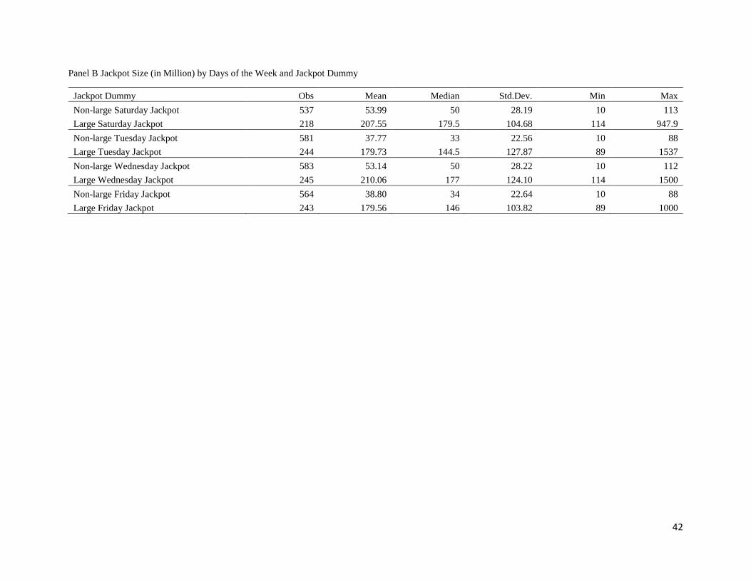
42

Panel B Jackpot Size (in Million) by Days of the Week and Jackpot Dummy

Jackpot Dummy Obs Mean Median Std.Dev. Min Max

Non-large Saturday Jackpot 537 53.99 50 28.19 10 113

Large Saturday Jackpot 218 207.55 179.5 104.68 114 947.9

Non-large Tuesday Jackpot 581 37.77 33 22.56 10 88

Large Tuesday Jackpot 244 179.73 144.5 127.87 89 1537

Non-large Wednesday Jackpot 583 53.14 50 28.22 10 112

Large Wednesday Jackpot 245 210.06 177 124.10 114 1500

Non-large Friday Jackpot 564 38.80 34 22.64 10 88

Large Friday Jackpot 243 179.56 146 103.82 89 1000

43

Table 2 The Monday Effect

In Panel A, we verify the long-existing Monday effect (where Monday return is on average lower than other days of the week) using market return indexes from

2003 January to 2018 December. The dependent variables are market return indexes in CRSP. In Column (1), Equal-Weighted Market Return is the equal-weighted

return including dividends. In Column (2), Value-Weighted Market Return is the value-weighted return including dividends. In Column (1) and (2), we regress

return of market indexes on Monday, Tuesday, Thursday and Friday dummy, with Wednesday as benchmark. We control for Before holiday and After holiday

dummies. We estimate Newey-West standard errors, allowing maximum lags up to 5 lags. ***, ** and * represent significance levels at 1%, 5% and 10%

respectively with t-statistics given in parentheses.

(1) (2)

Equal-Weighted Market Return Value-Weighted Market Return

Monday -0.113** -0.066

(-2.00) (-1.07)

Tuesday -0.002 0.032

(-0.05) (0.56)

Thursday -0.025 -0.010

(-0.50) (-0.18)

Friday 0.001 -0.033

(0.02) (-0.63)

Before holiday 0.220*** 0.119

(2.76) (1.47)

After holiday 0.127 0.103

(1.31) (1.00)

Constant 0.071* 0.048

(1.95) (1.21)

Observations 4,027 4,027

44

Table 3 The Monday Effect a Weekend Jackpot Effect?

This table studies the effect of Saturday jackpots on Monday return in the subsample of Large and Non-large Saturday Jackpot respectively. Large Saturday Jackpot

dummy equals to 1 if Powerball’s jackpot on Saturday is larger than or equal to the 70 percentile of Powerball jackpot. Non-large Saturday Jackpot dummy equals

to 1 when Large Saturday Jackpot dummy equals to 0. For trading days in week w, we classify into Large Saturday Jackpot and Non-large Saturday Jackpot groups

based on Large Saturday Jackpot dummy and Non-large Saturday Jackpot dummy on the Saturday of week w-1.

In Panel A, we perform subsample analysis on equal-weighted and value-weighted market return. Large Saturday jackpot subsample is in Column (1) and (3).

Non-large Saturday Jackpot subsample is in Column (2) and (4). The dependent variables are market return indexes in CRSP. In Column (1) and (2), Equal-

Weighted Market Return is the equal-weighted return including dividends. In Column (3) and (4), Value-Weighted Market Return is the value-weighted return

including dividends.

In Panel B, we use alternative measure of stock market return. In Column (1) and (2), we calculate close-to-close return from S&P 500 stock prices. In Column (3)

and (4), we calculate close-to-open return from S&P 500 stock prices. In Column (5) and (6), we calculate open-to-close return from S&P 500 stock prices.

In Panel C, we study the effect of jackpots on return of stocks within different liquidity groups. We separate stocks based on share turnover ratio in the previous

quarter end, and classify stocks as liquid (illiquid) stocks if share turnover ratio is larger (smaller) than or equal to 70 th (30th) percentile threshold. We calculate

equal-weighted return for liquid, middle group and illiquid stocks respectively. We regress the return of stocks in each liquidity group on Monday dummy and day-

of-the-week dummies, when there was a large Saturday jackpot in Column (1)-(3). Similarly, we perform similar analyses in Column (4)-(6) when there was a non-

large Saturday jackpot.

For all regressions in this table, we control for Before holiday, After holiday dummies. We estimate Newey-West standard errors, allowing maximum lags up to 5

lags. ***, ** and * represent significance levels at 1%, 5% and 10% respectively with t-statistics given in parentheses.

45

Panel A Subsample Analysis on Equal-Weighted and Value-Weighted Market Return

(1) (2) (3) (4)

Equal-Weighted Market Return

Value-Weighted Market Return

Large

Saturday

Jackpot

Non-large

Saturday

Jackpot

Large

Saturday

Jackpot

Non-large

Saturday

Jackpot

Monday -0.303*** -0.034 -0.273** 0.019

(-3.18) (-0.49) (-2.57) (0.26)

Tuesday -0.037 0.014 0.026 0.038

(-0.40) (0.25) (0.24) (0.55)

Thursday -0.058 -0.015 -0.053 0.002

(-0.61) (-0.26) (-0.50) (0.04)

Friday -0.049 0.021 -0.085 -0.011

(-0.55) (0.38) (-0.87) (-0.18)

Before holiday 0.321** 0.176* 0.178 0.092

(2.12) (1.89) (1.09) (1.00)

After holiday 0.134 0.099 0.129 0.056

(0.59) (0.97) (0.50) (0.54)

Constant 0.093 0.062 0.082 0.034

(1.49) (1.40) (1.20) (0.70)

Observations 1,178 2,847 1,178 2,847

46

Panel B Subsample Analysis on S&P Close-to-Close, Close-to-Open and Open-to-Close Return

(1) (2) (3) (4) (5) (6)

Close-to-Close Close-to-Open Open-to-Close

Large

Saturday

Jackpot

Non-large

Saturday

Jackpot

Large

Saturday

Jackpot

Non-large

Saturday

Jackpot

Large

Saturday

Jackpot

Non-large

Saturday

Jackpot

Monday -0.237** 0.045 0.012 0.013 -0.249** 0.031

(-2.22) (0.60) (0.58) (1.27) (-2.49) (0.44)

Tuesday 0.049 0.048 0.002 0.003 0.048 0.044

(0.45) (0.68) (0.08) (0.35) (0.45) (0.65)

Thursday -0.040 0.012 -0.013 -0.002 -0.027 0.015

(-0.37) (0.18) (-0.66) (-0.25) (-0.27) (0.22)

Friday -0.079 -0.014 -0.005 0.003 -0.074 -0.017

(-0.82) (-0.22) (-0.22) (0.30) (-0.83) (-0.27)

Before holiday 0.129 0.068 -0.015 -0.002 0.144 0.071

(0.77) (0.74) (-0.44) (-0.19) (0.96) (0.79)

After holiday 0.143 0.053 -0.024 -0.001 0.165 0.054

(0.55) (0.51) (-0.66) (-0.07) (0.68) (0.57)

Constant 0.061 0.017 0.011 -0.001 0.049 0.018

(0.88) (0.36) (0.99) (-0.18) (0.74) (0.39)

Observations 1,178 2,846 1,178 2,846 1,178 2,846

47

Panel C Subsample Analysis by Different Liquidity Groups

(1) (2) (3) (4) (5) (6)

Large Saturday Jackpot Non-large Saturday Jackpot

Illiquid Middle Liquid Illiquid Middle Liquid

Monday -0.229*** -0.289** -0.420*** -0.052 -0.025 -0.056

(-3.08) (-2.57) (-3.05) (-1.16) (-0.30) (-0.57)

Tuesday -0.032 -0.008 -0.036 -0.006 0.043 0.017

(-0.44) (-0.06) (-0.25) (-0.14) (0.59) (0.19)

Thursday 0.015 -0.010 -0.070 -0.008 -0.009 -0.030

(0.21) (-0.08) (-0.50) (-0.19) (-0.12) (-0.33)

Friday 0.038 -0.053 -0.124 0.053 0.019 -0.037

(0.55) (-0.48) (-0.96) (1.40) (0.27) (-0.44)

Before holiday 0.283** 0.273 0.448** 0.215*** 0.153 0.198

(2.36) (1.44) (2.00) (2.92) (1.28) (1.46)

After holiday 0.011 0.167 0.220 0.066 0.065 0.104

(0.07) (0.56) (0.62) (0.76) (0.55) (0.71)

Constant 0.074 0.078 0.117 0.078** 0.068 0.074

(1.47) (0.98) (1.25) (2.54) (1.25) (1.13)

Observations 1,178 1,178 1,178 2,847 2,847 2,847

48

Table 4 Friday Earnings News and the Monday Effect

In this table, we study interaction effect between Saturday jackpot and earnings announcement on Friday and weekends in the subsample of Large and Non-large

Saturday Jackpot. We compute standardized unexpected earnings (SUE) surprises for each earnings announcement, based on IBES reported analyst forecasts and

actuals as in Livnat and Mendenhall (2006). For each earnings announcement day that falls on Friday, Saturday or Sunday, we count the total number of firms with

SUE larger than 0 as number of good news and count the total number of firms with SUE smaller than 0 as number of bad news. We then calculate percentage of

bad news as number of bad news/(number of good news + number of bad news). If the percentage of bad news on Friday and weekends is larger than or equal to

mean, then we classify the following Monday as a day with bad news and define Bad News dummy = 1; otherwise, it is a day with good news and define Good

News dummy = 1. For each Monday, we interact Bad News dummy/Good News dummy with Monday dummy to study the interaction effect. For trading days in

week w, we classify into Large Saturday Jackpot and Non-large Saturday Jackpot groups based on Large Saturday Jackpot dummy and Non-large Saturday Jackpot

dummy on the Saturday of week w-1. Large Saturday jackpot subsample is in Column (1) and (3). Non-large Saturday Jackpot subsample is in Column (2) and

(4). In Column (1) and (2), Equal-Weighted Market Return is the equal-weighted return including dividends. In Column (3) and (4), Value-Weighted Market Return

is the value-weighted return including dividends. We control for Before holiday and After holiday dummies. We estimate Newey-West standard errors, allowing

maximum lags up to 5 lags. ***, ** and * represent significance levels at 1%, 5% and 10% respectively with t-statistics given in parentheses.

(1) (2) (3) (4)


Large

Saturday

Jackpot

Non-large

Saturday

Jackpot

Large

Saturday

Jackpot

Non-large

Saturday

Jackpot

Monday_ Bed News Friday -0.365** 0.098 -0.388** 0.160

(-2.28) (1.04) (-2.15) (1.57)

Monday_ Good News Friday -0.259** -0.120 -0.191* -0.072

(-2.53) (-1.52) (-1.74) (-0.85)

Tuesday -0.037 0.014 0.026 0.038

(-0.40) (0.25) (0.24) (0.55)

Thursday -0.058 -0.015 -0.053 0.002

(-0.61) (-0.26) (-0.50) (0.04)

Friday -0.049 0.021 -0.085 -0.011

(-0.55) (0.38) (-0.87) (-0.17)

Before holiday 0.320** 0.173* 0.176 0.089

(2.10) (1.86) (1.07) (0.97)

After holiday 0.137 0.099 0.134 0.055

(0.60) (0.96) (0.52) (0.53)

Constant 0.093 0.062 0.082 0.034

(1.49) (1.41) (1.20) (0.71)

Observations 1,178 2,847 1,178 2,847

49

Table 5 Friday Return and the Monday Effect

Negative Friday return is an explanation for the Monday effect (Abraham and Ikenberry, 1994). In this table, we separately study the effect of Saturday jackpot on

Monday return when the return of respective market index on the preceding Friday is positive or negative. We interact Positive/Negative Friday Return dummy

with Monday dummy in the subsample of Large and Non-large Saturday jackpot respectively. For trading days in week w, we classify into Large Saturday Jackpot

and Non-large Saturday Jackpot groups based on Large Saturday Jackpot dummy and Non-large Saturday Jackpot dummy on the Saturday of week w-1 respectively.

Large Saturday Jackpot subsample is in Column (1) and (3). Non-large Saturday Jackpot subsample is in Column (2) and (4). In Column (1) and (2), Equal-

Weighted Market Return is the equal-weighted return including dividends. In Column (3) and (4), Value-Weighted Market Return is the value-weighted return

including dividends. We control for Before holiday and After holiday dummies. We estimate Newey-West standard errors, allowing maximum lags up to 5 lags.

***, ** and * represent significance levels at 1%, 5% and 10% respectively with t-statistics given in parentheses.

(1) (2) (3) (4)


Large

Saturday

Jackpot

Non-Large

Saturday

Jackpot

Large

Saturday

Jackpot

Non-Large

Saturday

Jackpot

Monday_ Negative Friday Return -0.579*** -0.172 -0.369** 0.062

(-3.45) (-1.60) (-2.10) (0.55)

Monday_ Positive Friday Return -0.098 0.051 -0.190* -0.011

(-1.06) (0.69) (-1.85) (-0.14)

Tuesday -0.037 0.015 0.026 0.038

(-0.39) (0.25) (0.24) (0.55)

Thursday -0.058 -0.015 -0.053 0.002

(-0.61) (-0.26) (-0.50) (0.04)

Friday -0.049 0.021 -0.085 -0.011

(-0.56) (0.38) (-0.88) (-0.18)

Before holiday 0.328** 0.177* 0.181 0.093

(2.19) (1.90) (1.11) (1.01)

After holiday 0.133 0.096 0.133 0.056

(0.57) (0.94) (0.51) (0.54)

Constant 0.093 0.062 0.082 0.034

(1.49) (1.40) (1.20) (0.70)

Observations 1,178 2,847 1,178 2,847

50

Table 6 The Monday Effect of Anomalies

In this table, we focus on the stocks that are difficult to value and therefore require more investor attention. We use stocks with high idiosyncratic volatility (Ivol)

and high distressed risk probability (Distress) as examples of hard-to-value stocks. Consistent with Kumar (2009), idiosyncratic volatility at the end of month t is

the residual from fitting four-factor model using daily return of the previous 6 months, from t-6 to t-1. Stocks are classified as high (low) Ivol stocks for trading

day d in month t+1, if Ivol of the stock is in the top (bottom) quintile of idiosyncratic volatility. Distressed risk probability is measured following Campbell,

Hilscher, Szilagy (2008) Table IV predictive return for 12 months. We calculate distressed risk at the end of December in each year t. Stocks are classified as high

(low) Distress stocks for trading day d in year t+1, if distressed probability of the stock is in the top (bottom) quintile of distressed probability in the December of

year t.

In Panel A, we calculate excess return and alphas of short legs of the anomalies, adjusted by CAPM, Fama-French three-factor model, Carhart four-factor model,

on Monday and other days of the week separately. In Panel B, we calculate excess return and alphas of short legs of the anomalies, adjusted by CAPM, Fama-

French three-factor model, Carhart four-factor model, on Monday with Large Saturday Jackpot and Non-large Saturday Jackpot respectively.

In Panel C, we validate findings in Birru (2018) that profits of the anomalies with short leg as speculative leg concentrate on Monday. We regress time-series of

value-weighted excess return of the short legs on day-of-the-week dummies. In Panel D, we study the joint effect of large jackpots and day-of-the-week dummies.

We regress time-series of value-weighted excess return of the short leg on days of the week dummy in the subsample of Large Saturday Jackpot and Non-large

Saturday jackpot respectively. For trading days in week w, we classify into Large Saturday Jackpot and Non-large Saturday Jackpot groups based on Large Saturday

Jackpot dummy and Non-large Saturday Jackpot dummy on the Saturday of week w-1. Large Saturday jackpot subsample is in Column (1) and (3).Non-large

Saturday jackpot subsample is in Column (2) and (4).

We estimate Newey-West standard errors, allowing maximum lags up to 5 lags. ***, ** and * represent significance levels at 1%, 5% and 10% respectively with

t-statistics given in parentheses.

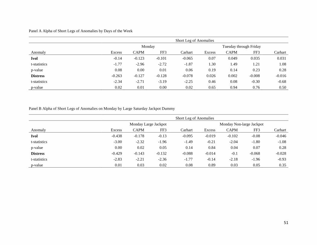
51

Panel A Alpha of Short Legs of Anomalies by Days of the Week

Short Leg of Anomalies

Monday Tuesday through Friday

Anomaly Excess CAPM FF3 Carhart Excess CAPM FF3 Carhart

Ivol -0.14 -0.123 -0.101 -0.065 0.07 0.049 0.035 0.031

t-statistics -1.77 -2.96 -2.72 -1.87 1.30 1.49 1.21 1.08

p-value 0.08 0.00 0.01 0.06 0.19 0.14 0.23 0.28

Distress -0.263 -0.127 -0.128 -0.078 0.026 0.002 -0.008 -0.016

t-statistics -2.34 -2.71 -3.19 -2.25 0.46 0.08 -0.30 -0.68

p-value 0.02 0.01 0.00 0.02 0.65 0.94 0.76 0.50

Panel B Alpha of Short Legs of Anomalies on Monday by Large Saturday Jackpot Dummy


Monday Large Jackpot Monday Non-large Jackpot

Anomaly Excess CAPM FF3 Carhart Excess CAPM FF3 Carhart

Ivol -0.438 -0.178 -0.13 -0.095 -0.019 -0.102 -0.08 -0.046

t-statistics -3.00 -2.32 -1.96 -1.49 -0.21 -2.04 -1.80 -1.08

p-value 0.00 0.02 0.05 0.14 0.84 0.04 0.07 0.28

Distress -0.429 -0.143 -0.132 -0.088 -0.014 -0.1 -0.068 -0.028

t-statistics -2.83 -2.21 -2.36 -1.77 -0.14 -2.18 -1.96 -0.93

p-value 0.01 0.03 0.02 0.08 0.89 0.03 0.05 0.35

52

Panel C Regression of Short Legs of Anomalies on Days of the Week

(1) (2)


High Ivol High Distress

Monday -0.217** -0.223**

(-2.20) (-2.25)

Tuesday -0.034 0.019

(-0.36) (0.20)

Thursday -0.053 -0.034

(-0.57) (-0.36)

Friday -0.037 -0.086

(-0.45) (-1.01)

Before Holiday 0.376*** 0.274*

(2.93) (1.69)

After Holiday 0.307* 0.149

(1.65) (0.81)

Constant 0.062 0.085

(0.94) (1.32)


53

Panel D Regression of Short Legs of Anomalies on Days of the Week and Jackpot Dummy

(1) (2) (3) (4)


High Ivol High Distress

Large

Saturday

Jackpot

Non-large

Saturday

Jackpot

Large

Saturday

Jackpot

Non-large

Saturday

Jackpot

Monday -0.636*** -0.044 -0.609*** -0.063

(-3.62) (-0.37) (-3.35) (-0.54)

Tuesday -0.098 -0.001 0.008 0.033

(-0.56) (-0.01) (0.04) (0.29)

Thursday -0.162 -0.017 -0.102 -0.015

(-0.88) (-0.16) (-0.53) (-0.15)

Friday -0.192 0.026 -0.198 -0.041

(-1.27) (0.26) (-1.19) (-0.41)

Before holiday 0.610** 0.278** 0.580 0.144

(2.00) (2.18) (1.36) (1.02)

After holiday 0.230 0.274 -0.066 0.161

(0.51) (1.44) (-0.15) (0.85)

Constant 0.189 0.010 0.183 0.046

(1.60) (0.12) (1.62) (0.59)

Observations 1,178 2,847 1,178 2,847

54

Table 7 Return Co-movement and Saturday Jackpots

In this table, we study the effect of large jackpots on market attention by measuring co-movement of all stocks, liquid stocks and illiquid stocks. We separate stocks

based on share turnover ratio in the previous quarter end, and classify stocks as liquid (illiquid) stocks if share turnover ratio is larger (smaller) than or equal to 70th

(30th) percentile threshold. Following Barberis, Shleifer and Wurgler (2005), we measure co-movement as the adjusted R-Square from the market model regressions.

Following Peng and Xiong (2006) and Antón and Polk (2014), we measure co-movement as the time series Pearson correlation of stock excess returns and market

excess returns. Large Saturday Jackpot dummy equals to 1 if Powerball’s jackpot on Saturday is larger than or equal to the 70 percentile of Powerball jackpot.

Non-large Saturday Jackpot dummy equals to 1 when Large Saturday Jackpot dummy equals to 0. For trading days in week w, we classify into Large Saturday

Jackpot and Non-large Saturday Jackpot groups based on Large Saturday Jackpot dummy and Non-large Saturday Jackpot dummy on the Saturday of week w-1.

We calculate firm-level co-movement by Large Saturday Jackpot dummy and day-of-the-week dummy. We require at least 20 observations for each firm in each

portfolio defined by Large Saturday Jackpot dummy and day-of-the-week dummy to reduce effects of outliers. In Panel A, we calculate mean and median co-

movement of all stocks by Large Saturday Jackpot dummy on Monday and other weekday. In Panel B, we calculate mean and median co-movement of liquid

stocks by Large Saturday Jackpot dummy on Monday and other weekday. In Panel C, we calculate mean and median co-movement of illiquid stocks by Large

Saturday Jackpot dummy on Monday and other weekday. We further test the difference between mean and median co-movement between Large Saturday Jackpot

subsample and Non-Large Saturday Jackpot subsample in all panels.

Panel A Co-movement of All Stocks on Monday and Other Weekdays

adjusted R-Square

Monday Return Large Saturday Jackpot Non-Large Saturday Jackpot Difference (p value)

Mean 0.2255 0.1884 0.0371 <.0001

Median 0.1977 0.152 0.0457 <.0001

Other Weekday Return Large Saturday Jackpot Non-Large Saturday Jackpot Difference (p value)

Mean 0.1551 0.1421 0.013 <.0001

Median 0.1275 0.1094 0.0181 0.0004

Correlation

Monday Return Large Saturday Jackpot Non-Large Saturday Jackpot Difference (p value)

Mean 0.4081 0.3595 0.0486 <.0001

Median 0.4404 0.3685 0.0719 <.0001

Other Weekday Return Large Saturday Jackpot Non-Large Saturday Jackpot Difference (p value)

Mean 0.3287 0.3062 0.0225 <.0001

Median 0.3456 0.3084 0.0372 <.0001

55

Panel B Co-movement of Liquid Stocks on Monday and Other Weekdays

adjusted R-Square

Monday Return Liquid Stocks Large Saturday Jackpot Non-Large Saturday Jackpot Difference (p value)

Mean 0.3026 0.2331 0.0695 <.0001

Median 0.2822 0.1991 0.0831 <.0001

Other Weekday Return Liquid Stocks Large Saturday Jackpot Non-Large Saturday Jackpot Difference (p value)

Mean 0.2006 0.1639 0.0367 <.0001

Median 0.1755 0.1368 0.0387 <.0001

Correlation

Monday Return Liquid Stocks Large Saturday Jackpot Non-Large Saturday Jackpot Difference (p value)

Mean 0.5008 0.4255 0.0753 <0.0001

Median 0.529 0.439 0.09 <0.0001

Other Weekday Return Liquid Stocks Large Saturday Jackpot Non-Large Saturday Jackpot Difference (p value)

Mean 0.3959 0.3451 0.0508 <.0001

Median 0.4111 0.3508 0.0603 <.0001

Panel C Co-movement of Illiquid Stocks on Monday and Other Weekdays

adjusted R-Square

Monday Return Illiquid Stocks Large Saturday Jackpot Non-Large Saturday Jackpot Difference (p value)

Mean 0.1376 0.1078 0.0298 <.0001

Median 0.0834 0.0401 0.0433 <.0001

Other Weekday Return Illiquid Stocks Large Saturday Jackpot Non-Large Saturday Jackpot Difference (p value)

Mean 0.0988 0.1123 0.0135 <.0001

Median 0.0436 0.0367 0.0069 0.4465

Correlation

Monday Return Illiquid Stocks Large Saturday Jackpot Non-Large Saturday Jackpot Difference (p value)

Mean 0.2987 0.2454 0.0533 <0.0001

Median 0.2916 0.2014 0.0902 <0.0001

Other Weekday Return Illiquid Stocks Large Saturday Jackpot Non-Large Saturday Jackpot Difference (p value)

Mean 0.2563 0.2366 0.0197 <.0001

Median 0.2102 0.1809 0.0293 <.0001

56

Table 8 Trading Activity and Saturday Jackpots

In this table, we study the effect of Saturday jackpots on individual investors’ trading activity proxied by odd-lot order imbalance. We calculate odd-lot order

imbalance as (aggregate daily odd-lot buy volume – aggregate daily odd-lot sell volume) / (aggregate daily odd-lot buy volume + aggregate daily odd-lot sell

volume). For the sample period from 2003– 2012, we follow Lee and Ready (1991) to sign trades as buyer or seller initiated using TAQ Trade and Quote data.

With the rise of algorithm trading, trade-size partition becomes less accurate in the recent period. From 2013 to 2018, we follow Boehmer, Jones, Zhang, and Zhang

(2019) to classify marketable odd-lot retail trades as either buy or sell using TAQ Millisecond Trade and Quote data.

We create Negative Friday Return dummy and Positive Friday Return dummy for week w, based on whether the return of respective market index on the preceding

Friday is negative or positive in week w-1. We interact Negative Friday Return dummy with Monday dummy and Large Saturday Jackpot dummy as Monday_

Negative Friday Return_Large Saturday Jackpot. We interact Positive Friday Return dummy with Monday dummy and Large Saturday Jackpot dummy as Monday_

Positive Friday Return_Large Saturday Jackpot. We interact Negative Friday Return dummy with Monday dummy and Non-Large Saturday Jackpot dummy as

Monday_ Negative Friday Return_Non-Large Saturday Jackpot. We interact Positive Friday Return dummy with Monday dummy and Non-Large Saturday Jackpot

dummy as Monday_ Positive Friday Return_Non-Large Saturday Jackpot.

In Column (1), we regress odd-lot order imbalance on Monday with Large Saturday Jackpot dummy, Monday dummy, and other days-of-the-week dummies. In

Column (2), we regress odd-lot order imbalance on Monday with Large Saturday Jackpot dummy, Monday with Negative Friday return and Large Saturday Jackpot

dummy, Monday dummy, and other days-of-the-week dummies. In Column (3), we regress odd-lot order imbalance on Monday with Negative Friday return and

Large Saturday Jackpot dummy, Monday with Positive Friday return and Large Saturday Jackpot dummy, Monday with Negative Friday Return and Non-Large

Saturday Jackpot dummy, Monday with Positive Friday Return and Non-Large Saturday Jackpot dummy and other days-of-the-week dummies.

We control for Before holiday, After holiday dummies. We additionally control for year fixed effect to control for time-varying transaction costs. We estimate

Newey-West standard errors, allowing maximum lags up to 5 lags in return regressions. ***, ** and * represent significance levels at 1%, 5% and 10% respectively

with t-statistics given in parentheses.

57

(1) (2) (3)

Odd-lot Order Imbalance

Monday_Large Saturday Jackpot -0.031*** -0.027**

(-3.01) (-2.12)

Monday_ Negative Friday Return_Large Saturday Jackpot -0.009 -0.038***

(-0.57) (-2.93)

Monday_ Positive Friday Return _Large Saturday Jackpot -0.029**

(-2.47)

Monday_ Negative Friday Return_Non-Large Saturday Jackpot -0.018*

(-1.69)

Monday_ Positive Friday Return _Non-Large Saturday Jackpot 0.008

(0.93)

Monday -0.002 -0.002

(-0.22) (-0.22)

Tuesday 0.005 0.005 0.005

(0.72) (0.72) (0.72)

Thursday -0.002 -0.002 -0.002

(-0.29) (-0.29) (-0.29)

Friday 0.010 0.010 0.010

(1.44) (1.44) (1.44)

Before holiday 0.003 0.003 0.003

(0.29) (0.29) (0.30)

After holiday 0.002 0.002 0.002

(0.18) (0.18) (0.16)

Constant -0.013 -0.013 0.027***

(-1.37) (-1.38) (5.50)

Observations 4,025 4,025 4,025

58

Table 9 Weekend Jackpots vs. Weekday Jackpots

We study the effect of Saturday jackpot and weekday jackpot on market return. Large Jackpot Dummy on Tuesday or Friday equals to 1 if jackpot size on Tuesday

or Friday is larger than or equal to 70 percentile of Mega Millions jackpot amount. Large Jackpot Dummy on Wednesday or Saturday equals to 1 if jackpot size is

larger than or equal to 70 percentile of Powerball jackpot amount. We regress equal-weighted and value-weighted return on interaction of Monday dummy with

Large Saturday Jackpot dummy, interaction of Tuesday/Wednesday/Friday dummy with Large Tuesday/Wednesday/Friday Jackpot dummy. We control for Before

holiday and After holiday dummies. We estimate Newey-West standard errors, allowing maximum lags up to 5 lags. ***, ** and * represent significance levels

at 1%, 5% and 10% respectively with t-statistics given in parentheses.

(1) (2)


Monday_Large Saturday Jackpot -0.236** -0.241**

(-2.43) (-2.30)

Tuesday_Large Tuesday Jackpot -0.041 -0.092

(-0.54) (-1.11)

Wednesday_Large Wednesday Jackpot -0.043 -0.033

(-0.56) (-0.40)

Friday_Large Friday Jackpot 0.053 0.084

(0.84) (1.17)

Monday -0.019 0.014

(-0.29) (0.20)

Tuesday 0.036 0.070

(0.64) (1.10)

Wednesday 0.038 0.020

(0.67) (0.31)

Friday 0.011 -0.047

(0.21) (-0.80)

Before holiday 0.218*** 0.117

(2.76) (1.46)

After holiday 0.122 0.099

(1.26) (0.95)

Constant 0.046 0.037

(1.21) (0.92)


59

Table 10 Friday Return, Sports Events and the Monday Effect

This table studies the effect of Friday return and weekend sports events, Super Bowl and Kentucky Derby, on Monday return from January 1967 to December

2002. We define a Sports Event dummy, which equals to 1 on the Monday of week w if there was a sports event (Super Bowl or Kentucky Derby) over the

weekends of week w-1. We create Negative Friday Return dummy and Positive Friday Return dummy for week w, based on whether the return of respective market

index on the preceding Friday is negative or positive in week w-1. We interact Negative Friday Return dummy with Monday dummy as Monday_ Negative Friday

Return. We interact Negative Friday Return dummy with Monday dummy and Sports Event dummy as Monday_ Negative Friday Return_Sports Event. In Column

(1), we regress equal-weighted market return on Monday dummy, and other days-of-the-week dummies. In Column (2), we regress equal-weighted market return

on Monday with Negative Friday return dummy, Monday dummy, and other days-of-the-week dummies. In Column (3), we regress equal-weighted market return

on Monday with Negative Friday return and Sports Event dummy, Monday with Negative Friday Return dummy, Monday dummy and other days-of-the-week

dummies. In Column (4) - (6), we study value-weighted market return. We estimate Newey-West standard errors, allowing maximum lags up to 5 lags. ***, **

and * represent significance levels at 1%, 5% and 10% respectively with t-statistics given in parentheses.

(1) (2) (3) (4) (5) (6)


Monday_ Negative Friday Return_Sports Event -0.339** -0.082

(-2.30) (-0.44)

Monday_ Negative Friday Return -0.689*** -0.676*** -0.460*** -0.456***

(-13.22) (-12.64) (-8.51) (-8.28)

Monday -0.239*** -0.041* -0.041* -0.161*** 0.035 0.035

(-9.33) (-1.74) (-1.74) (-4.80) (1.06) (1.06)

Tuesday -0.139*** -0.139*** -0.139*** -0.071** -0.071** -0.071**

(-6.59) (-6.59) (-6.58) (-2.50) (-2.50) (-2.50)

Thursday 0.008 0.008 0.008 -0.050* -0.050* -0.050*

(0.38) (0.38) (0.38) (-1.78) (-1.78) (-1.78)

Friday 0.113*** 0.113*** 0.113*** -0.016 -0.016 -0.016

(5.13) (5.13) (5.13) (-0.54) (-0.54) (-0.54)

Constant 0.133*** 0.133*** 0.133*** 0.102*** 0.102*** 0.102***

(7.78) (7.78) (7.78) (4.92) (4.92) (4.92)

Observations 9,061 9,061 9,061 9,061 9,061 9,061

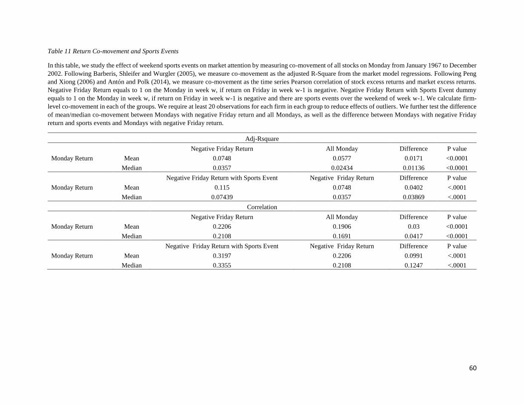
60

Table 11 Return Co-movement and Sports Events

In this table, we study the effect of weekend sports events on market attention by measuring co-movement of all stocks on Monday from January 1967 to December

2002. Following Barberis, Shleifer and Wurgler (2005), we measure co-movement as the adjusted R-Square from the market model regressions. Following Peng

and Xiong (2006) and Antón and Polk (2014), we measure co-movement as the time series Pearson correlation of stock excess returns and market excess returns.

Negative Friday Return equals to 1 on the Monday in week w, if return on Friday in week w-1 is negative. Negative Friday Return with Sports Event dummy

equals to 1 on the Monday in week w, if return on Friday in week w-1 is negative and there are sports events over the weekend of week w-1. We calculate firm-

level co-movement in each of the groups. We require at least 20 observations for each firm in each group to reduce effects of outliers. We further test the difference

of mean/median co-movement between Mondays with negative Friday return and all Mondays, as well as the difference between Mondays with negative Friday

return and sports events and Mondays with negative Friday return.

Adj-Rsquare

Negative Friday Return All Monday Difference P value

Monday Return Mean 0.0748 0.0577 0.0171 <0.0001

Median 0.0357 0.02434 0.01136 <0.0001

Negative Friday Return with Sports Event Negative Friday Return Difference P value

Monday Return Mean 0.115 0.0748 0.0402 <.0001

Median 0.07439 0.0357 0.03869 <.0001

Correlation

Negative Friday Return All Monday Difference P value

Monday Return Mean 0.2206 0.1906 0.03 <0.0001

Median 0.2108 0.1691 0.0417 <0.0001

Negative Friday Return with Sports Event Negative Friday Return Difference P value

Monday Return Mean 0.3197 0.2206 0.0991 <.0001

Median 0.3355 0.2108 0.1247 <.0001

79

Chapter 2

80

Foreign Exchange Hedging and Corporate Innovation

Chongwu Xia

[email protected]

Institute for Financial and Accounting Studies

Xiamen University

Chuyi Yang

[email protected]




Singapore 639798

Lei Zhang

[email protected]

UQ business school

University of Queensland

39 Blair drive, Queensland 4072, Australia

81

Abstract

We study the real effects of foreign exchange hedging on corporate innovation. Under the

information asymmetry hypothesis, corporate hedging reduces firm’s information asymmetry, and

alleviates manager’s career concern from undervaluation and helps investors to better monitor the

manager, which in turn increases innovation. Under the market pressure hypothesis, hedging

imposes more short-term earnings pressure on managers because of mark-to-market hedge

accounting, hence leads to lower innovation. Our results support the information asymmetry

hypothesis. Hedged firms invest more heavily in innovative projects, generate more patents and

have more patent citations. To address endogeneity concerns, we employ both difference-in-

differences and instrumental variables regressions, and test for reverse causality explicitly.

82

1. Introduction

According to Bank for International Settlements (2017), notional amount of outstanding foreign

exchange derivatives arrives at $77 trillion as of June 2017. Dominating the currency derivative

usage is corporate hedging (DeMarzo and Duffie, 1995). However, in the frictionless world of

Modigliani and Miller (1958), hedging should be irrelevant, as shareholders possess the requisite

tools and information to create their desired risk profile. This contradiction leads to the long-

debated question: Does corporate hedging matter? Existing literature provides various

explanations on why firms hedge. These explanations include managerial risk aversion (Stulz,

1984), information asymmetry (DeMarzo and Duffie, 1991, 1995; Breeden and Viswanathan,

2015), tax convexity (Mayers and Smith, 1982; Smith and Stulz, 1985), financial distress and debt

capacity (Nance, Smith, and Smithson,1993), and underinvestment problem (Shapiro and Titman,

1986; Stulz, 1990; Froot, Scharfstein, and Stein,1993).

Empirically, existing studies have largely focused on capital market implications of corporate

hedging. For example, Carter, Rogers, and Simkins (2006), Allayannis and Weston (2001), Perez-

Gonzalez and Yun (2013), and Gilje and Taillard (2017) find that corporate hedging increases firm

value. Graham and Rogers (2002) and Campello, Lin, Ma, and Zhou (2011) document that

corporate hedging improves debt capacity. On the contrary, Tufano (1996) and Jin and Jorin (2006)

test the relationship between hedging and firm value within specific industries, and fail to find

significant results. In this paper, we take one step further and examines whether corporate hedging

affects firms’ real activities. In particular, we study how foreign exchange (FX) hedging affects

corporate innovation.12

12 We acknowledge that there are other types of financial uncertainty such as interest rate risk. We focus on FX hedging

because the usage of currency derivatives is mainly for hedging purpose against FX risk (Allayannis and Weston,

83

Ex-ante, it is unclear whether corporate hedging increases or decreases firms’ innovation

activities. On one hand, corporate hedging is shown to reduce the information asymmetry between

the firms and the outside investors. When firms have proprietary information that could not be

shared with investors, investors could neither hedge the risk nor do they know how to hedge

(DeMarzo and Duffie, 1991). In this case, firms could hedge on investors’ behalf so that investors

are less concerned with information asymmetry. DeMarzo and Duffie (1995) further show that

hedging could help to signal managerial ability and enhance the informational content of corporate

earnings. Similarly, Breeden and Viswanathan (2015) argue that hedging can be a strategy used to

enhance learning process about managerial ability. Consistent with the theoretical works, DaDalt,

Gay, and Nam (2002) empirically validate the role of hedging in reducing noise from

macroeconomic factors and hence information uncertainty. Moreover, Manconi, Massa, and

Zhang (2017) show that corporate hedging reduces information asymmetry and increases stock

price informativeness, by documenting the eroded information advantage of informed traders after

hedging. The role of corporate hedging on reducing information asymmetry has two implications

for firm innovation.

First, innovation is a long-term process with significant uncertainty, and requires information

privacy due to its strategic importance (Hall, Jaffe and Trajtenberg, 2005; Caggese, 2012). The

lack of full disclosure on innovation investments hinders effective communication between

managers and outside investors, and increases information asymmetry (Bhattacharya and Ritter,

1983; Anton and Yao, 2002). Therefore, innovative firms tend to be undervalued by investors

(Diamond and Verrecchia, 1991). The undervaluation leads to higher take-over threat to the firms

and higher career concern to the managers, managers are consequently induced to be more myopic

2001; Brown, 2001), while interest rate derivatives usage have been found to be more likely for the purpose of

speculation and earnings management (Faulkender, 2005; Chernenko and Faulkender, 2011).

84

and tend to reduce innovation activities (Stein, 1988, 1989). In short, reduction of information

asymmetry between the firm and investors alleviates manager’s career concern from

undervaluation, and allows manager to better allocate resources to long term value enhancing

activities such as innovation. Second, reduction of information asymmetry allows the market to

play a more active role in monitoring managers when they pursue innovation activities that are

informationally opaque in nature (e.g., Holmstrom and Tirole, 1993; Faure-Grimaud and Gromb,

2004). In addition, higher stock price informativeness may also facilitate managers to better learn

about the value of their growth opportunities and engage in more value-increasing innovation

activities (Foucault and Gehrig, 2008). This will increase the firm’s innovation efficiency.13

Therefore, given that information environment is key to corporate innovation, and corporate

hedging reduces a firm’s information asymmetry, we hypothesize that hedging boosts innovation.

We term this argument the information asymmetry hypothesis.14

On the other hand, innovation process is subject to capital market pressure which might lead

to managerial myopia and long-term value sacrifice (Bhojraj and Libby, 2005; He and Tian, 2013).

The survey by Graham, Harvey, and Rajgopal (2005) finds that due to market pressure, CFOs tend

to sacrifice long-term value by means like cutting R&D expenditure to meet short-term profit

targets. Corporate hedging can increase firms’ short-term earnings pressure as a result of mark-to-

market requirement for hedge accounting. In this case, firms have to recognize the loss from

derivatives hedging position immediately, but may not be able to recognize the gain from the

underlying asset due to accounting conservatism requirement. Therefore, hedging increases short-

13 Similar arguments have been used by Blanco and Wehrheim (2017) to develop the hypothesis that options trading

affect firm innovation.

14 Alternatively, hedging can spur innovation through its role in lower cost of capital. However, this alternative

argument cannot explain our findings that hedging also improves innovation efficiency. We discuss this issue in detail

in Section 6.3

85

term earnings pressure. As a result, hedging reduces firms’ long-term investment and hinders

corporate innovation. We term this alternative argument the market pressure hypothesis.

Corporate hedging can be negatively associated with innovation for other reasons. First, the

purpose of financial derivatives usage could be for speculation (Faulkender, 2005). In this

scenario, hedging is a signal of managerial myopia and therefore correlated with lower level of

innovation. Second, hedging as a mean of risk management, can also be a signal of managerial

risk aversion (Stulz, 1984) and leads to lower innovation. Third, the accounting literature has some

findings that hedging can increase firm’s financial reporting opacity (Campbell, 2015; Donohoe,

2015; Chang, Donohoe, and Sougiannis, 2016; Campbell, D’Adduzio, Downes, and Utke, 2017),

which predicts lower innovation.

To test the relationship between corporate hedging and innovation, we focus on the usage of

foreign exchange derivatives (FX hedge) to measure corporate hedging activities, because the

usage of currency derivatives is mainly for hedging purpose against FX risk (Allayannis and

Weston, 2001; Brown, 2001). We rely on the number of patents and forward citation of patents at

firm level to measure innovation outputs. We find that FX hedging leads to higher innovation

investments and outputs in the baseline regression, supporting the information asymmetry

hypothesis. While our identification strategy relies on the dummy variable FX hedge, we conduct

a battery of analyses to examine how the extent of FX hedge’s potential benefit affects firm’s

innovation. We show that the effect of FX hedge are stronger for firms facing higher FX hedging

needs (as measured by FX risk exposure, international competition, and FX volatility). Our results

are robust to negative binomial regression, and subsample regressions accounting for the patent

data truncation bias and accounting rule change.

86

Endogeneity is a major concern to our findings. It is possible that our results are driven by

some firm unobservable characteristics that simultaneously affect firm’s hedging decision and

innovation. For example, firms with higher opacity and volatility may have higher propensity to

utilize FX hedging, while these characteristics are also associated with higher innovation activities.

It is also possible that the causality between hedging and innovation goes the opposite direction.

For example, higher innovation outputs might be related to higher innovation inputs and risk,

leading to stronger incentive to hedge. To address the endogeneity problem, we first conduct a

change regression to rule out the effect of time invariant unobservable variables. We also perform

propensity score matching (PSM) to find a control firm for each firm that initiates FX hedge, and

conduct a difference-in-differences (DiD) analysis. The results show that relative to the control

firms, the treatment firms (those initiate FX hedge) are associated with higher innovation outputs

after the initiation. Next, we take advantage of the institutional feature of corporate tax code in

U.S. firms and use tax convexity as an instrumental variable (IV) to FX hedging. The results from

two-stage IV Heckman treatment regression holds qualitatively similar with baseline results.

Moreover, we explicitly address the reserve causality concern by categorizing each firm-year into

four types: remain-unhedged firms, quit-hedging firms, start-hedging firms, and continue-hedging

firms, and test whether innovation affects hedging decisions. Empirically, there is no evidence to

reject the hypotheses that decision to begin/quit hedging is unaffected by innovation, at

conventional levels of significance.

To provide further support to the information asymmetry hypothesis, we conduct moderation

analyses using analyst forecast dispersion, breadth of ownership, and PIN to measure information

asymmetry. Consistent with the information asymmetry hypothesis, we find that the effect of FX

hedge is stronger for firms with higher information asymmetry. Next, we conduct a battery of

87

analyses to examine how FX hedge affects firm’s myopic behavior. Specifically, we find that FX

hedge increases firm’s long term investment, and curbs manager’s real earnings management. We

also find that effect of FX hedge is stronger when managers have higher career concern (or are

more likely to be myopic facing information asymmetry).

In the additional analyses, we first we address the competing market pressure hypothesis.

Though we find that the market pressure hypothesis plays a role in affecting corporate innovation,

the effect is dominated by information asymmetry hypothesis. Next we find that FX hedge

increases innovation efficiency, which is consistent with our information asymmetry hypothesis,

and inconsistent with the alternative explanation of cost of capital channel. Finally, we further

investigate the cost of capital channel. We show that though FX hedge decreases firm’s cost of

capital which in turn increases innovation outputs, the channel only explains a marginal portion of

the effect of FX hedge on innovation.

Our paper contributes to the literature in three ways. First, we contribute to the strand of

literature on corporate hedging. Froot, Scharfstein, and Stein (1993) argue that one benefit of

hedging is alleviating underinvestment problem. DeMarzo and Duffie (1995) provide a theoretical

basis for the information asymmetry reduction role of corporate hedging, by arguing that hedging

allows investors to learn better about the management ability and project quality from firm’s

earnings. Empirically, some findings support that corporate hedging increases firm value (Carter

et al., 2006; Allayannis and Weston, 2001; Perez-Gonzalez and Yun, 2013; Gilje and Taillard,

2017). Related to firm innovation, Géczy, Minton, and Schrand (1997) document a positive

relation between currency hedging and growth opportunity in Fortune 500 firms. Petersen and

Thiagarajan (2000) show that the choice of hedging is influenced by abilities to adjust operating

costs, requirement of investment capital as well as managerial incentives and compensation.

88

Campello et al. (2011) show that hedging allows firm to enjoy lower borrowing cost and less

investment restrictions. By focusing on innovation, we can not only separate the short-term and

long-term investment, but also examine the outcome of investment. We hence contribute to the

fundamental question of whether hedging matters, by documenting a real effect of hedging on firm

innovation outputs and efficiency.

Second, we contribute to the literature on motivating firm innovation, especially on the

information environment side. Manso (2011) argues that motivating innovation requires tolerance

of short-term failure and reward for long-term success, which provides the theoretical basis of how

information environment can shape innovation. He and Tian (2013) reveal the negative effect of

analyst coverage on firm innovation, as a result of reduced tolerance for failure and exacerbated

managerial myopia. Dai, Shen, and Zhang (2017) find that innovation is impeded by media

coverage. Similarly, Agarwal, Vashishtha and Venkatachalam (2018) find that mutual fund

transparency exacerbates managerial myopia and leads to a decline in innovation. Blanco and

Wehrheim (2017), on the other hand, find that options trading can enhance price efficiency and

therefore boost innovation. We add to this line of research by showing that hedging reduces firm’s

information asymmetry, hence alleviates manager’s career concern from undervaluation, and helps

investors to better monitor the manager, leading to higher innovation.

Third, we contribute to the debate on whether the purpose of derivatives usage by non-

financial firms is for hedging against risks or for speculating of underlying asset’s movements.

Innovation provides an ideal setting as it is a long-term process that should be differently affected

by derivatives usage according to its purpose. Allayannis and Weston (2001) find that the purpose

of using currency derivatives is generally to reduce FX risk exposure instead of speculation.

Faulkender (2005) and Chernenko and Faulkender (2011) argue that interest rate derivatives usage

89

is more likely for speculating on interest rate movements and facilitating earnings management.

Consistently, DaDalt et al. (2002) find that the informational role of hedging is primarily driven

by currency derivatives and weakly extends to interest rate derivatives. We document that firms

with FX hedging are associated with more innovations, which supports the view that the usage of

FX derivatives is generally for hedging purposes.

The rest of the paper is organized as follows: Section 2 describes sample and data in details.

Section 3 presents the main results. Section 4 addresses endogeneity concern. Section 5 explores

the economic channel. Section 6 provides additional analyses. Section 7 concludes.

2. Sample and Data

We start our sample with all non-financial firms in the Compustat and CRSP merged database with

available hedging information. We hand collect the hedging information for these firms based on

their 10-K and 10-Q filings as in Manconi et al. (2017). Next, we compute firm characteristics

from Compustat, CRSP and Thomson Reuter’s 13F databases, and exclude firms with missing

values.

To gauge the innovation outputs, we construct measures from the patent database by Kogan,

Papanikolaou, Seru, and Stoffman (2017), which covers all U.S. patent documents from Google

Patents and NBER database up to 2010. We use application year as time placer and end the

innovation output data until 2006, since excluding 3 to 4 years is necessary to minimize patent

data truncation bias (Dass, Nanda, and Xiao, 2017)15. The similar database has been widely used

15 Our results are qualitatively similar if we extend our sample to year 2007 or 2008.

90

in previous innovation studies (Moser and Voena, 2012; Moser, Voena, and Waldinger, 2014;

Bernstein, 2015; Dong, Hirshleifer, and Teoh, 2016).

Specifically, two measures of innovation outputs are used for a given firm in each year:

number of patents (LnPatent), and forward citation (LnCitation) adjusted using fixed effect

approach as in Hall, Jaffe, and Trajtenberg (2001). Consistent with innovation literature, we take

the natural logarithm of innovation outputs (Hall et al., 2001; Kogan et al., 2017). LnPatent is the

natural logarithm of (1 + Patent Number), where Patent Number is the number of patents finally

granted. LnCitation is the natural logarithm of (1 + Citation), where Citation is the sum of adjusted

citation for all patents applied in a given firm-year. For each patent citation, we scale the raw

citation by the mean citation of the same technological class and application year. LnCitation

gauges the importance of patents with forward patent citation, and indicates the scientific value of

patent quality. The citation of patents is an important complement to the patent number measure

(Griliches, Pakes, and Hall, 1987; Trajtenberg, 1990; Hall et al., 2001). Following literature (Tian

and Wang, 2011; Atanassov, 2013; Hsu, Tian and Xu, 2014), we take a two-year gap between

innovation output measures and independent variables due to the long-term nature of innovative

activities.

Following literature (Nance et al., 1993; Allayannis and Weston, 2001; Purnanandam, 2008;

Campello et al., 2011), we focus on firm’s usage of relevant derivatives to measure corporate

hedging activities.16 To measure FX hedging, we search firms’ 10-K and 10-Q filings using

keywords provided by Manconi et al. (2017).17 For those filings containing the keywords, we

16 The Financial Accounting Standards Board (FASB) (1998) Statement of Financial Accounting Standards (SFAS)

133 (effective on 2000), requires all derivatives to be carried at fair value, instead of notional value. For this reason,

Graham and Rogers (2002) note that the fair value information reported under SFAS 133 is limited and warn against

using the fair value information to study corporate hedging. 17 Specifically, we search for the following keywords: “foreign exchange forward”, “forward foreign exchange”,

“foreign exchange rate forward”, “currency forward”, “currency rate forward”, “foreign exchange option”, “currency

91

manually check the filings to eliminate misclassifications. The FX hedge is then defined to be 1 if

the firm uses FX hedging in year t, and 0 otherwise.

We also include several control variables in our test. Size is firm’s size measured by logged

total asset and we expect larger firms to have more innovation outputs (Hall and Ziedonis, 2001).

We use net property, plant, and equipment scaled by prior fiscal year’s total asset (PPE) to control

for capital intensity, as capital intensity will influence firm’s innovation activities (Hall and

Ziedonis, 2001). M/B is firm’s market to book ratio, a proxy for firm’s growth opportunities. In

addition, we also control for sales growth (Sales Growth). We control for the firm age (Age)

measured by the number of years since its initial appearance in CRSP database, as firm in the

different life cycle might have different innovation capacity. Institutional ownership (Institutional

ownership) is controlled for its influence on firm innovation (Aghion, Van Reenen, and Zingales,

2013). Other controls include firm’s return on asset (ROA), leverage (Leverage), cash holding

(Cash Holding), stock return (Return), Amihud’s illiquidity (Illiquidity), stock volatility (Return

Volatility), Herfindahl index (HHI), and square of Herfindahl index (HHI_sq). Foreign Income is

firm’s foreign income exposure, and is included to control for firms’ propensity to utilize foreign

exchange rate hedge (Manconi et al., 2017). The variable definitions are listed in Appendix 1.

Finally, we recognize that there are firms that do not conduct FX hedging because they don’t

face significant ex ante FX exposure, such firms are not proper counterfactuals in our tests. We

therefore follow Graham and Rogers (2002) and Campello et al. (2011), to exclude firms without

ex ante FX risk exposures using the following procedures:

option”, “foreign exchange rate option”, “currency rate option”, “foreign exchange future”, “currency rate future”,

“foreign exchange swap”, “currency swap”, “foreign exchange rate swap”, “currency rate swap”, “foreign exchange

cap”, “currency cap”, “foreign exchange rate cap”, “currency rate cap”, “foreign exchange collar”, “currency collar”,

“foreign exchange rate collar”, “currency rate collar”, “foreign exchange floor”, “currency floor”, “foreign exchange

rate floor” and “currency rate floor”. We also filter out filings containing phrases such as “we (the company) do not

(does not) have (utilize, enter) any foreign exchange derivatives.”

92

First, similar with Campello et al. (2011), we check whether firms explicitly discuss FX risks

in their 10-K and10-Q filings based on keywords. The list of keywords includes “currency risk”,

“currency rate risk”, “exchange risk”, “exchange rate risk”, “foreign exchange risk”, and “foreign

exchange rate risk”.

Second, we follow Graham and Rogers (2002) and Campello et al. (2011), and check whether

firms disclose positive values of foreign currency adjustment, exchange rate effect, foreign income

taxes, or deferred foreign taxes in their annual Compustat files, or disclose foreign assets, sales, or

income in the Compustat Geographic segment files.

Last, we follow Aggarwal and Harper (2010) and Jorion (1991) to calculate FX risk

exposures. For each firm in each year, we pool firm-month observations for the past five years and

we regress stock returns on changes in exchange rate between US dollar against currencies of

major US trading partners (the Trade Weighted US dollar index TWEXB from the Federal Reserve

Bank at St Louis), and market return. The regression coefficient on exchange rate changes is taken

as a proxy for FX risk exposure. The coefficients are replaced with zero if not significant at 10%

significance level.

Following these procedures, we end up deleting 3,766 observations that 1) have no discussion

on FX risks; 2) do not have positive foreign related items; 3) do not have statistically significant

measures of ex-ante FX risk exposure. The final sample consists of 32,194 firm-year observations

from 1998 to 2006 (or from 1994 to 2004 in terms of independent variables).

Table 1 Panel A provides the summary statistics for the variables used in our main analysis.

In our sample, 13.7% of the firm-year observations use FX hedging, which is consistent with

Campello et al. (2011) and Manconi et al. (2017). On average, 27.1% of the firms have nonzero

number of patents, consistent with innovation literature that majority of the firms report zero

93

innovation outputs (e.g., Tian and Wang, 2011; He and Tian, 2013). The distribution of control

variables are all consistent with previous studies.

[Table 1 about here]

Table 1 Panel B and C provide the distribution of hedging firms across industries18 and years.

The “Chemicals and Allied Products” industry has the highest proportion of hedging firms, while

the “Wholesale, Retail Services” industry has the lowest proportion. On the time dimension, there

is a trend of increase in the proportion of firms that engage in FX Hedging.

3. Main Results

3.1. Pooled OLS Baseline Regression

We start by testing whether FX hedge cause managers to increase investment on innovation

using the following regression:

R&D/Assetsi,t+1/i,t+2=α0+α1FX_hedgei,t

+ ∑αk Controlsi,t+εi,t+2 (1)

R&D/Assets is the ratio of R&D expenditures divided by lagged total assets. If the R&D

expenditure is missing, we follow Hirshleifer, Low, and Teoh (2012), He and Tian (2013), and

Blanco and Wehrheim (2017), and replace the missing values with zero.19 FX hedge is a dummy

variable that equals to 1 if the firm hedges against FX risk and 0 otherwise. We control for various

firms characteristics that are likely to influence innovation input and FX hedging decision. We

also include year fixed effect to control for the time trend at aggregate level and industry fixed

effects to account for the heterogeneous innovative nature of different industries. The hedging

18 The industry classification we use here is Fama-French 12 industry, for the simplicity of illustration. In our

regressions, we employ 2-digit SIC code for industry classification.

19 In the internet appendix, we restrict our sample to nonmissing R&D observations, and find qualitatively similar

results.

94

literature (Allayannis and Ofek, 2001; Manconi et al., 2017) generally includes industry fixed

effects instead of firm fixed effects, as firm’s hedging activities do not vary much across years.20

To address the concern that our results are driven by unobservable firm characteristics, we include

lagged R&D/Assets as additional control variables.21 The results are reported in Table 2 Panel A.

In columns (1) and (2), we use the R&D/Asset measured at year t+1, while in columns (3) and (4),

we use the R&D/Asset measured at year t+2.


The coefficients of FX hedge are all positive and statistically significant at 1% significance

level. Compared with the non-hedgers, firms that hedge against FX risk invest 0.004 to 0.011 more

in R&D depending on model specifications. Compared with the mean level of R&D/Assets (0.061),

the effect is also economically significant.

Since missing R&D expenditures doesn’t necessarily imply the firm lacks innovation

activities (Koh and Reeb, 2015), and innovation output is more relevant to our research question,

we therefore focus on innovation outputs. To test the relationship between FX hedging and

innovation outcomes, we run the following OLS regression:

Innovation_Outputi,t+2

=α0+α1FX_hedgei,t

+ ∑αk Controlsi,t+εi,t+2 (2)

where the innovation output is measured by two variables at firm-year level: LnPatent (natural

logarithm of (1+ number of patents)), and LnCitation (natural logarithm of (1+ forward adjusted

citation)). To address the concern that our results are driven by unobservable firm characteristics,

20 In fact, the results from firm fixed effect model will be unreliable if the regressor doesn’t have much time series

variation (Zhou, 2001). 21 There are also innovation studies that do not include firm fixed effects when the variables of interest do not have

much time series variation (Hall et al., 2005; Hirshleifer, Low, and Teoh, 2012). In particular, Blundell, Griffith, and

Van Reenen (1999) and Blanco and Wehrheim (2017) control for the pre-sample mean of innovation outputs to control

for unobservable firm characteristics. In unreported results, we use the similar approach and find robust results.

95

we control for lagged LnPatent or LnCitation correspondingly. The results are reported in Table 2

Panel B.

Consistent with previous findings, our results show that innovation output increases with size

(He and Tian, 2013), market-to-book ratio (Dong et al., 2016), cash holding, illiquidity (He and

Tian, 2013), and volatility. Innovation output is found to be negatively associated with leverage

(Tian and Wang, 2014), sales growth and prior stock return.

More importantly, Table 2 Panel B shows that FX hedging boosts innovation output in both

measures in all specifications. The coefficients of FX hedge are all significantly positive at 1%

significance level. Compared with the non-hedgers, firms that hedge against FX risk generate

10.2% - 14.8% more patents, receive 11.5% -16.2% more adjusted citations depending on model

specifications.

3.2. Potential Benefit of FX hedge

A drawback of our identification strategy is that we reply on a dummy variable to measure FX

hedging, and can’t provide information about how the extent of FX hedging affects firm’s

innovation outputs. Due to data limitation,22 it’s difficult to construct a measure for the extent of

FX hedging. We therefore indirectly examine how the extent of FX hedge’s potential benefit

affects firm’s innovation. Specifically, we proxy firm’s FX hedging needs by FX exposure,

International competition, and FX volatility. Presumably, firms with higher FX hedging needs

potentially benefit more from FX hedge. In Table 3, we test whether the effect of FX hedge is

stronger for firms with higher hedging needs.

22 It’s difficult to quantify both the dollar amount of firms’ FX exposures due to the lack of theoretical background.

It’s also difficult to measure the notional amount of FX derivatives that firms use to hedge FX risk, since the SFAS

133 requires derivatives to be carried at fair value, as opposed to notional value.

96


In Table 3 Panel A, we use FX exposure to measure FX hedging needs. FX exposure is

computed as defined in Section 2. The coefficients of the interaction term between FX hedge and

High FX exposure (a dummy variable that equals to 1 if FX exposure is higher than the median

level, and 0 otherwise) are positive and statistically significant in all specifications. Compared to

firms with low FX exposure, the effect of FX hedge is 0.080 to 0.115 stronger in firms with high

FX exposure.

In Table 3 Panel B, we use International competition to measure FX hedging needs. For each

4-digit SIC industry, international competition is measured as the fraction of non-US sales

(measured in US dollars) among total sales. We obtain sales data of international companies from

the Compustat Global database. The coefficients of the interaction term between FX hedge and

High international competition (a dummy variable that equals to 1 if International competition is

higher than the median level, and 0 otherwise) are positive and statistically significant in all

specifications. Compared to firms with low International competition, the effect of FX hedge is

0.109 to 0.158 stronger in firms with high International competition.

In Table 3 Panel C, we use FX volatility to measure FX hedging needs. For each year, FX

volatility is computed as the standard deviation of monthly TWEXB (the exchange rate of US

dollar against currencies of major US trading partners). The coefficients of the interaction term

between FX hedge and High FX volatility (a dummy variable that equals to 1 if FX volatility is

higher than the median level, and 0 otherwise) are positive and statistically significant in all

specifications. Compared to years of low FX volatility, the effect of FX hedge is 0.030 to 0.060

stronger in years of high FX volatility.

97

Taken together, the results all consistently show that the effect of FX hedge is stronger when

the potential benefit of FX hedge is larger.

3.3. Robustness Checks

In our main specification, we employ OLS regressions with logged innovation outputs as

dependent variables. In this subsection, we use the negative binomial regression with the unlogged

Patent and Citation as dependent variables, to check whether our findings are robust to the

alternative model specification. The results are reported in Table 4 Panel A. The coefficients of

FX hedge are positive and statistically significant in columns (1)-(4), suggesting that our results

are robust to alternative model specification.


In addition, the lag between patent application and patent grant leads to truncation bias (Dass

et al., 2017). In the main specification, we cut off our sample four years before 2010 to minimize

truncation bias. In the subsection, we further cut off our sample to 1998-2004 to check whether

our results still hold. The results are reported in Table 4 Panel B. The coefficients of FX hedge are

positive and statistically significant in columns (1)-(4), suggesting that our results are robust to

truncation bias.

Last, during the sample period of our study, there is a regime switch in hedge accounting. In

2000, the FASB Statement of Financial Accounting Standards (SFAS) 133 became effective.

SFAS 133 requires all derivatives to be carried at fair value, instead of notional amount. As a

result, the hedging information reported under SFAS 133 is limited (Graham and Rogers, 2002).

In turn, this change in hedging accounting could potentially lower the effect of hedging on

innovation. In this subsection, we examine whether the effect of hedging still exists after SFAS133.

98

In Table 4 Panel C, we restrain the sample period to post SFAS133 period, and test whether

hedging affects innovation. The coefficients of FX hedge are positive and statistically significant

in columns (1)-(4). Though the economic magnitudes of the effects are lower than in Table 2 Panel

B (where the whole sample is used), they are still economically significant. Compared with the

firms that do not hedge, the hedging firms have 9.0% - 9.1% (9.2% - 9.4%) higher patents

(citations).

3. Endogeneity Concerns

While the above findings support our argument that FX hedging leads to more innovation outputs,

it is possible that our results are driven by some unobservable firm characteristics that

simultaneously affect firm’s hedging decision and innovation. For example, firms with higher

opacity and volatility may have higher propensity to utilize FX hedging, while these characteristics

are also associated with higher innovation activities. It is also possible that the causality between

hedging and innovation goes the opposite direction. For example, higher innovation outputs might

be related to higher innovation inputs and risk, leading to stronger incentive to hedge. In this

section, we address the above concerns using several tests.

4.1. Change Level Regression

In this subsection, we conduct a change level regression to control for the potential time-invariant

omitted variables. Specifically, we compute the change of innovation outputs from year t+2 to

t+1, and the change of independent variables from year t to t-1, so that the time-invariant portion

is cancelled. We then run the following regression:

99

∆Innovation_Outputi,t+2

=α0+α1∆FX_hedgei,t

+ ∑αk ∆Controlsi,t+εi,t+2 (3)

where ∆𝐼𝑛𝑛𝑜𝑣𝑎𝑡𝑖𝑜𝑛 is measured by ∆𝐿𝑛𝑃𝑎𝑡𝑒𝑛𝑡 and ∆𝐿𝑛𝐶𝑖𝑡𝑎𝑡𝑖𝑜𝑛. Here we don’t include the

lagged innovation outputs, as the specification has already cancelled the time invariant firm

variables. The results are reported in Table 5.


The coefficients of ΔFX hedge are positive and statistically significant at 5% or lower

significance levels, suggesting that our results are robust to the endogeneity concern related to time

invariant omitted variables.

4.2. Difference-in-Differences Analysis

Following Guay (1999) and Chang et al. (2016), we take advantage of firms’ initiation of FX

hedging and conduct a difference-in-differences analysis. Specifically, we identify firms that

initiate FX hedging in the sample period. For each of the first-time users, we match it with a similar

firm that never uses FX hedging throughout the sample period, with a caliber of 0.05. We are able

to identify 298 pairs of firms. By constructing a control group that is otherwise similar to the

hedging firms, we can draw causal inferences in the non-experimental settings (Rosenbaum and

Rubin, 1983).

Specifically, we regress the following model to obtain propensity scores:

Pr(Initiationi,t) =θ0+ ∑θ

KY

i,t+ε

i,t (4)

where the control variables includes firm size, market-to-book, foreign income, leverage,

institutional ownership, cash holding, sales growth, prior return, stock illiquidity, return volatility,

Herfindahl index and its square. We also include year and industry fixed effects.

100

We first check the covariate balance in Table 6 Panel A. No significant difference in control

variables is found between the treatment and control groups. Based on the paired firms, we then

run the following regression using two years window around the initiation:

Innovation_Outputsi,t+1

= ψ0+ψ1Initiation+ ψ2Post+ψ3Initionation×Post+ γXi,t +εi,t

(5)

where Initiation is an indicator that equals to 1 for first-time users (i.e., the treatment group) and

0 otherwise. Post is an indicator that equals to 1 if the observation is the year of initiation, and 0

otherwise. We are interested in the interaction term between Initiation and Post, which captures

the innovation differences between first-time users and non-users. The results are reported in Table

6 Panel B. In columns (1) and (3), we include year and industry fixed effects. Since in the DiD

regression, we are more interested in the interaction term Initiation × Post, we drop the Initiation

dummy, and include year and firm fixed effects to control for the time invariant firm characteristics

in columns (2) and (4),. We find that the coefficients of Initiation × Post are significantly positive

in all the columns, further confirming the causal effect of FX hedging on innovation.


4.3. Instrumental Variable Approach

Though the above methods help to address endogeneity concerns related to time-invariant

unobservable omitted variables, it is still possible that there exist time-variant omitted variables

that affect both hedging decisions and innovation outcomes. To mitigate this concern, we conduct

101

a two-stage residual inclusion (Hausman, 1978) analysis in this subsection.23 Specifically,

following existing studies (Smith and Stulz, 1985; Campello et al., 2011; Manconi et al., 2017),

we use corporate income tax convexity as an instrumental variable. Corporate income tax

convexity is a result of institutional feature of the U.S. corporate tax code, and is weakly associated

with firm innovation.24 Hedging, however, can reduce the firm’s expected tax liability through

lowering taxable income variability, and is directly related to tax convexity.

Following Campello et al (2011) and Manconi et al (2017), we use the following equation to

define effective tax convexity:

Convexityit=4.88+0.019TIVolit-5.5TICorrit-1.28DITCit+3.29DNOLit+7.15DSmallNeg

it

+1.60DSmallPosit-4.77DNOLit×DSmallNegit-1.93DNOLit×DSmallPosit (6)

The tax convexity measure is essentially the expected average tax savings from 5% reduction in

taxable income volatility (Graham and Smith, 1999)25. TIVol denotes the volatility of taxable

income, calculated on a rolling basis using all available historical annual data up to the year t.

TICorr denotes taxable income’s serial correlation, calculated on a rolling basis using all available

historical annual data up to the year t. DITC is a dummy variable indicating investment tax credits.

DNOL is a dummy variable indicating net operating losses. DSmallNeg/DSmallPos is a dummy

variable indicating small negative/positive taxable income.

Following the two-stage residual inclusion regression (Hausman, 1978), we first estimate a

Logit model using FX hedge as dependent variable and Convexity as independent variable with all

23 Our results are robust if we use treatment regression model.

24 One exception is Gentry & Hubbard (2004), who show that the household tax convexity deters people from

entrepreneurial activities. If the similar effect exists in corporate innovation, it will only introduce downward bias to

our findings, i.e., our findings would otherwise be stronger.

25 The tax savings include tax-loss carrybacks, carryforwards, investment tax credits (ITCs), and the alternative

minimum tax (AMT).

102

controls used in the baseline regressions. From the Logit regression, we compute the residual and

include the residual as additional controls and then re-estimate our baseline regressions. The two-

stage residual inclusion has been used by various studies to address endogeneity (e.g., Terza, Basu,

and Rahouz, 2008; Chen, Hong, Jiang, and Kubik, 2012). We present the results in Table 7.


Colums (1) and (2) in Table 7 Panel A report the first stage of IV regression. Consistent with

previous literature (Dionne and Garand, 2003; Campello et al., 2011; Manconi et al., 2017), the

results show that tax convexity positively influences firm’s hedging decision. Columns (3) and (4)

report the second stage results. We find that the coefficients of FX hedge are positive and highly

significant, which lends strong support to the information asymmetry hypothesis.

We then re-run the same regression in Table 7 Panel B with different definitions of tax

convexity. Specifically, we exclude taxable income volatility from convexity calculation to avoid

the potential correlation between income volatility and innovation. Our results remain robust.

Finally, to further alleviate the concern that the firm’s tax convexity is related to innovation

activities per se, we employ the state level tax convexity as an IV. The state level tax convexity is

hard to manipulate by the firm, and serves as a valid IV. The results are reported in Table 7 Panel

C. We find that the state level tax convexity is significantly related to firm’s hedging activities,

and our results that FX hedge boosts innovation are robust.

4.4. Reverse Causality

It is possible that firms hedge to mitigate the potential high earnings volatility caused by innovation

activities. In this case, the causality between hedging and innovation goes the opposite to our

hypothesis. To address the concern, we analyze the effect of prior innovation in year t on FX

103

hedging policy change (from year t to year t+1). Specifically, we create two dummy variables:

Begin Hedging is a dummy variable that equals to 1 if firm does not hedge in year t but starts

hedging in year t+1, and 0 otherwise; Quit Hedging is a dummy variable that equals to 1 if firm

hedges in year t but does not hedge in year t+1, and 0 otherwise. The results are reported in Table

8.


In columns (1) and (2), we test whether innovation affects firm’s decision to begin FX

hedging, using LnPatent and LnCitation respectively. In columns (3) and (4), we test whether

innovation affects firm’s decision to quit FX hedging, using LnPatent and LnCitation respectively.

In all specifications, none of the coefficients of innovation measures are significant. Therefore, we

provide evidence that reverse causality could not explain the positive effect of FX hedging on

innovation outputs.

5. Economic Channels

5.1. Information Asymmetry

Our information asymmetry hypothesis hinges on the information asymmetry reduction role of FX

hedging, hence we expect the effects between hedging and innovation to be stronger for firms with

higher information asymmetry. In this subsection, we conduct cross sectional analyses based on

information asymmetry. Specifically, we use analyst forecast dispersion (Diether, Malloy, and

Scherbina, 2002), breadth of investor ownership (Chen et al., 2002) and probability of informed

trading PIN (Easley, Hvidkjaer, and O’Hara, 2002) to measure information asymmetry. For each

variable, we define a dummy variable that equals to 1 if it is greater than the median level, and 0

104

otherwise. We then interact the dummy variables with FX hedge to test how the effect of FX hedge

varies. The results are reported in Table 9.


In Table 9 Panel A, we use analyst forecast dispersion to measure information asymmetry.

Analyst forecast dispersion is defined as the standard deviation of analyst EPS forecasts, divided

by previous-month stock price. Larger analyst forecast dispersion indicates higher information

asymmetry. In Table 9 Panel A, the coefficients of the interaction FX hedge × High dispersion are

positive and statistically significant at 5% significance level in all the columns, suggesting that the

effect of FX hedging on innovation is stronger for firms with larger analyst forecast dispersion. In

terms of economic significance, compared with firms with lower analyst forecast dispersion, firms

with higher dispersion enjoy 9.7 % - 10.8% more increase in patent number, and 3.0% - 5.2 %

more increase in patent citation after FX hedging.

In Table 9 Panel B we use ownership breadth to measure information asymmetry. Chen et al.

(2002) argue that breadth of ownership measures the number of institutional investors that are

willing to hold a particular stock and implies lower disagreement in valuation among investors. As

a result, higher ownership breadth is associated with less information asymmetry. In Table 9 Panel

B, the coefficients of the interaction FX hedge × High breadth are negative and statistically

significant at 5% or lower significance levels in all the columns, suggesting that the effect of FX

hedging on innovation is stronger for firms with lower breadth of ownership, or higher information

asymmetry. In terms of economic significance, compared with firms with lower breadth of

ownership, firms with higher breadth have 10.2 % - 12.3% less increase in patent number, and

11.5% - 13.4 % less increase in patent citation after FX hedging.

105

In Table 9 Panel C we use the PIN to measure information asymmetry. Higher PIN indicates

higher information asymmetry. The coefficients of the interaction FX hedge × High PIN are

positive and statistically significant at 1% significance level in all the columns, suggesting that the

effect of FX hedging on innovation is stronger for firms with higher PIN. In terms of economic

significance, compared with firms with lower PIN, firms with higher PIN have 11.6 % - 14.4%

more increase in patent number, and 17.6% - 20.5 % more increase in patent citation after FX

hedging.

Taken together, we find consistent results that the effect of FX hedging on innovation is

stronger for firms facing higher information asymmetry, lending further support to our information

asymmetry hypothesis.

5.2. Myopic Behaviors

An important part of the information asymmetry hypothesis is that hedging alleviates manager’s

career concern from undervaluation, and helps the investors to better monitor manager in long

term investment. In this subsection, we investigate whether the above argument is true.

Specifically, we first test whether hedging increases firm’s long term investment. The long-term

investment is defined as the R&D expenditures divided by the sum of R&D expenditures and

capital expenditure. We regress the long-term investment on FX hedge and report the results in

Table 10 Panel A. In columns (1) and (2), we use the long term investment at year t+1 as dependent

variables, while in columns (3) and (4), we use the long term investment at year t+2.


The coefficients of FX hedge are positive and significant at 1% significance level in all the

columns, suggesting that FX hedging increases long-term investment.

106

To provide further evidence on the effect of hedging on manager’s myopic behavior, we

examine manager’s real earnings management behavior. In Table 10 Panel B, we test how FX

hedge affects firm’s propensity of cutting R&D expense to manipulate earnings. According to

Bushee (1998), managers tend to cut R&D for earnings management purpose, which is a myopic

behavior and have real damage to the firm’s long-term value. Following Bushee (1998), we define

an indicator variable SD dummy, which equals to 1 if the firm’s earning is lower than last year by

an amount manageable through cutting R&D, and 0 otherwise. SD dummy essentially measures

the feasibility of achieving desirable earnings target through cutting R&D. Distance from earnings

goal relative to last year’s R&D (Distance) is defined as the ratio of change in pre-tax and pre-

R&D earnings to previous year’s R&D expense. Distance reflects the portion of R&D expense

that needs to be cut to generate an increase in earnings. Dependent variable (CUT RD) is an

indicator that equals to 1 if a firm cuts R&D expense relative to last year, and 0 otherwise. We

interact FX hedge and SD dummy to examine how FX hedging affects manager’s decision to

manipulate earnings. The results are reported in Table 10 Panel B. The coefficients of FX hedge

× SD dummy are negative and significant at 1% significance level, suggesting that hedging firms

are less likely to engage in real earnings manipulation than those without hedging. The results are

consistent with the argument that FX hedging alleviates manager’s career concern from

undervaluation, and reduces manger’s myopic behaviors.

Next, we follow Blanco and Wehrheim (2017), and use Market competition and CEO

entrenchment to measure manager’s career concern. If FX hedging boosts innovation through the

reduction of career concern from undervaluation, we should observe the effect of hedging to be

stronger in firms with more concerned managers. In Table 10 Panel C, we use the HHI to measure

the market competition firms facing. High market competition is a dummy variable that equals to

107

1 if the HHI is lower than the median level, and 0 otherwise. Higher market competition indicates

higher career concern to the managers, because competition reduces the probability of success and

increases reputation risk (Blanco and Wehrheim, 2017). We find that the coefficients of the

interaction FX hedge × High market competition are positive and significant in all the columns,

suggesting that the effect of FX hedging on innovation is stronger for firms facing higher market

competition. In Table 10 Panel D, we use the G-index (Gompers, Ishii, and Metrick, 2003) to

measure CEO’s entrenchment. Higher G-index indicates more restrictions on shareholder rights

(higher CEO entrenchment), or lower career concern to the CEO. High CEO entrenchment is a

dummy variable that equals to 1 if the G-index is higher than the median level, and 0 otherwise.

We find that the coefficients of the interaction FX hedge × High CEO entrenchment are negative

and significant in all the columns, suggesting that the effect of FX hedging on innovation is

stronger for firms with less entrenched CEOs. Taken together, the results are consistent with the

expectation that the effect of FX hedging is stronger when managers have higher career concern.

6. Additional Analyses

6.1.Accounting Conservatism

Our alternative market pressure hypothesis argues that mark-to-market hedge accounting requires

firms to recognize the loss from derivative hedging position immediately, but firms may not be

able to recognize the gain from the underlying asset immediately because of accounting

conservatism practices. Therefore, the mark-to-market requirement of hedge accounting can

increase hedging firms’ short-term earnings pressure and dampens innovation. In this subsection,

we test whether accounting conservatism influences the effect of hedging on innovation.

108

In Table 11, we define a dummy variable High conservatism that equals to 1 if the accounting

conservatism is higher than the median level, and 0 otherwise. Accounting conservatism is defined

as the C_Score following Khan and Watts (2009). We find that the coefficients of the interaction

FX hedge × High conservatism are negative and significant at 1% significance level in all the

columns, indicating that the market pressure hypothesis plays a role. However, if we sum the

coefficients of FX hedge and FX hedge × High conservatism, they all appear to be positive,

suggesting that the information asymmetry hypothesis dominates the market pressure hypothesis

even for the high accounting conservatism firms.


6.2. Innovation Efficiency

So far, we have found that FX hedge increases the innovation outputs. However, since Table

2 shows that FX hedge also increases firm’s R&D expenditures, we do not know whether the

effect of FX hedge on innovation comes from the increased investment in innovation or

improvement on innovation efficiency. The question is important in our setting because our

information asymmetry hypothesis implies that FX hedge should also increase firm’s

innovation efficiency, in addition to innovation outputs. First, if FX hedging reduces the

information asymmetry of the firm and alleviates the manager’s career concern of

undervaluation, the manager should be able to pursue projects that are riskier but with higher

NPV. Second, if the reduction of information asymmetry helps investors to better monitor the

manager, it should also help the manager to better allocate the resources and improve

innovation efficiency (Blanco and Wehrheim, 2017).

109

In this subsection, we examine whether FX hedge improves innovation efficiency. First, we

follow Hirshleifer et al. (2012), and add the lagged R&D/Assets as an additional control in our

regression,26 so that we can interpret the coefficient of FX hedge as the effect on innovation

efficiency. The results are reported in Table 12 Panel A. The coefficients of FX hedge are positive

and statistically significant at 1% significance level in all the columns, suggesting that FX hedging

increases firm’s innovation efficiency. In addition, the magnitudes of coefficients are slightly

lower than those in Table 2 Panel B. suggesting that the effect of FX hedging on innovation outputs

are mainly from the improved innovation efficiency, instead of increased R&D expenditures.


To further test the relation between FX hedging and innovation efficiency, we employ a set

of innovation efficiency measures. First, we test the effect of FX hedging on Generality and

Originality of patents, following Trajtenberg, Henderson, and Jaffe (1997) and Hall et al. (2001).

Generality reflects the range of fields for citations received by a patent, and Originality reflects

the range of fields for citations made by a patent. Both Generality and Originality are measures of

the fundamental importance of innovation (Lerner and Seru, 2015). In Table 12 Panel B, we

present the results with Generality as dependent variable in column (1) and Originality in column

(2). For each regression, we also include the corresponding lagged efficiency measure, to control

for unobservable firm characteristics. The results show that FX hedging increases Generality and

Originality at 5% or lower significance levels. These results suggest that hedging improves the

fundamental importance of innovation activities.

Next, in column (3) of Table 13 Panel B, we reply on Citation per Patent to test the effect of

FX hedging on innovation efficiency. In column (4) of Table 13 Panel B, we reports the results

26 The results are qualitatively similar if we use the contemporary R&D/Assets.

110

on economic value of innovation (Economic Value). Economic Value is based on filtered stock

price reaction to patents two days after the patent issuance day, and captures the private economic

value of patent (Kogan et al., 2017). In column (5) of Table 13 Panel B, we use Research Quotient

as a measure of innovation efficiency. Research Quotient is defined as the firm-specific output

elasticity of R&D and provides complementary information on the efficiency of R&D investment

(Knott, 2008).27 In all the specifications, the coefficients of FX hedge are positive and statistically

significant at conventional significance levels, consistent with the argument that FX hedging

improves innovation efficiency.

6.3.Alternative explanation: Cost of Capital

An alternative explanation to our findings is that FX hedging reduces firm’s cost of capital, and in

turn increases firm’s long term investment such as R&D expenditures. While most of our findings

so far can be explained by this argument, it cannot explain our findings on innovation efficiency.

On the contrary, the cost of capital argument may even imply a negative effect of FX hedging on

innovation efficiency. This is because a lower cost of capital allows firms to invest in innovation

projects that otherwise would have negative NPV. Nonetheless, in this subsection, we explicitly

discuss the cost of capital channel.

First, we test whether FX hedging decreases firm’s cost of capital. Following Li and

Mohanram (2014), we measure the implied cost of capital (ICC) as the predicted earnings divided

by the stock price using Gordon and Gordon (1997) model. The results are reported in Table 13

Panel A. In columns (1) and (2) we use the ICC at year t+1 as the dependent variable, while in

27 Research quotients are estimated from firm’s production function, holding inputs and elasticities constant. It

reflects the percentage increase in revenues with a 1% increase in R&D investment.

111

columns (3) and (4) we use the ICC at year t+2. The results show that FX hedging in general

reduces implied cost of capital one year and two years after FX hedging.


Since FX hedging indeed lowers firm’s cost of capital, we next test whether our findings can

be explained by the reduction in the cost of capital. In Panel B of Table 13, we add ICC as an

additional control to test the relation between FX hedge and innovation outputs. We find that the

coefficients of FX hedge are still positive and statistically significant at 1% significance level in

all the columns. Compared with the results in Table 2 Panel B, the magnitudes of the coefficients

are slightly lower, but are still economically significant. FX hedging increases firm’s patent by

9.0% - 13.6%, and citation by 9.1% to 13.5%. Therefore, the cost of capital argument can at most

explain a marginal part of our findings.

7. Conclusions

In this study, we study the real effects of FX hedging on corporate innovation. We test two

competing hypotheses. Under the information asymmetry hypothesis, FX hedging reduces firm’s

information asymmetry, which alleviates manager’s career concern from undervaluation and helps

investors to better monitor the manager, in turn, FX hedging increases innovation. Under the

market pressure hypothesis, hedging imposes higher short-term earnings pressure on managers

because of mark-to-market hedge accounting, hence leads to lower innovation.

Our results support the information asymmetry hypothesis. We establish a positive causal

effect between FX hedging and corporate innovation. Further, we find that the effect is stronger

for firms with larger hedging needs or higher potential benefits from FX hedging. Our results are

112

robust to different model specification, and different sample periods accounting for patent data

truncation bias and hedge accounting rule change. We also carefully address the endogeneity

concerns by employing change regression, DiD regression and IV regression. We also explicitly

test for reverse causality. Consistent with the information asymmetry hypothesis, we find that

hedging effect is stronger for firms with higher information asymmetry. We also show that FX

hedging effectively curbs manager’s myopic behavior and focus more on long term investment.

Our paper contributes to the hedging literature by documenting an unexplored real impact of

FX hedging. We also add to the literature on the relation between information environment and

innovation. Finally, we provide additional insight to the debate on whether firm trading currency

derivatives for speculative or hedging purpose in the ideal setting of innovation.

113

References

Agarwal, V., Vashishtha, R., Venkatachalam, M., 2017. Mutual fund transparency and corporate

myopia. Rev. Financ. Stud. 31, 1966–2003. https://doi.org/10.1093/rfs/hhx125

Aggarwal, R., Harper, J.T., 2010. Foreign exchange exposure of “domestic” corporations. J. Int.

Money Financ. 29, 1619-1636. https://doi.org/10.1016/j.jimonfin.2010.05.003

Aghion, P., Van Reenen, J., Zingales, L., 2013. Innovation and institutional ownership. Am.

Econ. Rev. 103, 277-304. https://doi.org/10.1257/aer.103.1.277

Allayannis, G., Ofek, E., 2001. Exchange rate exposure, hedging, and the use of foreign currency

derivatives. J. Int. Money Financ. 20, 273–296. https://doi.org/10.1016/S0261-5606(00)00050-4

Allayannis,G. & Weston, J., 2001. The use of foreign exchange derivatives and firm market

value. Rev. Financ. Stud. 14, 243-276. https://doi.org/10.1093/rfs/14.1.243

Amihud, Y., 2002. Illiquidity and stock returns: Cross-section and time-series effects. J. Financ.

Mark. 5, 31-56. https://doi.org/10.1016/S1386-4181(01)00024-6

Anton, J.J., Yao, D.A., 2002. The sale of ideas: strategic disclosure, property rights, and

contracting. Rev. Econ. Stud. 69, 513–531. https://doi.org/10.1111/1467-937X.t01-1-00020

Atanassov, J., 2013. Do hostile takeovers stifle innovation? evidence from antitakeover

legislation and corporate patenting. J. Finance. 68, 1097-1131. https://doi.org/10.1111/jofi.12019

Bank for International Settlements (BIS). Statistical release: OTC Derivatives Statistics at End-

June-2017. Report, (2017), https://www.bis.org/publ/otc_hy1711.pdf.

Bernstein, S., 2015. Does going public affect innovation? J. Finance. 70, 1365-

1403.https://doi.org/10.1111/jofi.12275

Bhattacharya, S., Ritter, J.R., 1983. Innovation and communication: signalling with partial

disclosure. Rev. Econ. Stud. 50, 331-346. https://doi.org/10.2307/2297419

Bhojraj, S., Libby, R., 2005. Capital market pressure, disclosure frequency-induced

earnings/cash flow conflict, and managerial myopia. Account. Rev. 80, 1-20.

https://doi.org/10.2308/accr.2005.80.1.1

Blanco, I., Wehrheim, D., 2017. The bright side of financial derivatives: Options trading and

firm innovation. J. Financ. Econ. 125, 99–119. https://doi.org/10.1016/j.jfineco.2017.04.004

Breeden, D.T., Viswanathan, S., 2015. Why do firms hedge? An asymmetric information model.

J. Fixed Income. 25, 7-25. https://doi.org/10.3905/jfi.2016.25.3.007

Brown, G.W., 2001. Managing foreign exchange risk with derivatives. J. Financ. Econ. 60, 401-

448. https://doi.org/10.1016/S0304-405X(01)00049-6

Bushee, B.J., 1998. The influence of institutional investors on myopic R&D investment

behavior. Account. Rev. 73, 305-333. https://doi.org/10.2307/248542

Caggese, A., 2012. Entrepreneurial risk, investment, and innovation. J. Financ. Econ. 106, 287-

307.https://doi.org/10.1016/j.jfineco.2012.05.009

114

Campbell, J.L., 2015. The fair value of cash flow hedges, future profitability, and stock returns.

Contemp. Account. Res. 32, 243-279. https://doi.org/10.1111/1911-3846.12069

Campbell, J.L., Feagin, J., Utke, S., 2017. Do investors adjust for balance sheet risk that should

be “Off Balance Sheet”? evidence from cash flow hedges. SSRN Electron. J.

https://doi.org/10.2139/ssrn.2898184

Campello, M., Lin, C., Ma, Y., Zou, H., 2011. The real and financial implications of corporate

hedging. J. Finance. 66, 1615-1647. https://doi.org/10.1111/j.1540-6261.2011.01683.x

Cao, Y., Myers, L.A., Tsang, A., Yang, Y.G., 2017. Management forecasts and the cost of equity

capital: international evidence. Rev. Account. Stud. 22, 791–838.

https://doi.org/10.1007/s11142-017-9391-5

Carter, D.A., Rogers, D.A., Simkins, B.J., 2006. Does hedging affect firm value? Evidence from

the US airline industry. Financ. Manag. 35, 53-87. https://doi.org/10.1111/j.1755-

053X.2006.tb00131.x

Chang, H.S., Donohoe, M., Sougiannis, T., 2016. Do analysts understand the economic and

reporting complexities of derivatives? J. Account. Econ. 61, 584–604.

https://doi.org/10.1016/j.jacceco.2015.07.005

Chen, J., Hong, H., Jiang, W., Kubik, J.D., 2013. Outsourcing mutual fund management: firm

boundaries, incentives, and performance. J. Finance. 68, 523-558.

https://doi.org/10.1111/jofi.12006

Chen, J., Hong, H., Stein, J.C., 2002. Breadth of ownership and stock returns. J. Financ. Econ.

66, 171–205. https://doi.org/10.1016/S0304-405X(02)00223-4

Chernenko, S., Faulkender, M., 2011. The two sides of derivatives usage: Hedging and

speculating with interest rate swaps. J. Financ. Quant. Anal. 46, 1727-1754.

https://doi.org/10.1017/S0022109011000391

Dadalt, P., Gay, G.D., Nam, J., 2002. Asymmetric information and corporate derivatives Use. J.

Futur. Mark. 22, 241-267. https://doi.org/10.1002/fut.2216

Dai, L., Shen, R., Zhang, B., 2017. Does the media spotlight burn or spur innovation? SSRN

Electron. J. https://doi.org/10.2139/ssrn.3037838

Dass, N., Nanda, V., Xiao, S.C., 2017. Truncation bias corrections in patent data: Implications

for recent research on innovation. J. Corp. Financ. 44, 353-374.

https://doi.org/10.1016/j.jcorpfin.2017.03.010

DeMarzo, P.M., Duffie, D., 1991. Corporate financial hedging with proprietary information. J.

Econ. Theory 53, 261–286. https://doi.org/10.1016/0022-0531(91)90156-X

DeMarzo, P.M., Duffie, D., 2002. Corporate incentives for hedging and hedge accounting. Rev.

Financ. Stud. 8, 743-771. https://doi.org/10.1093/rfs/8.3.743

Diamond, D.W., Verrecchia, R.E., 1991. Disclosure, liquidity, and the cost of capital. J. Finance.

46, 1325-1359. https://doi.org/10.1111/j.1540-6261.1991.tb04620.x

115

Diether, K.B., Malloy, C.J., Scherbina, A., 2002. Differences of opinion and the cross section of

stock returns. J. Finance. , 57, 2113-2141. https://doi.org/10.1111/0022-1082.00490

Dionne, G., Garand, M., 2003. Risk management determinants affecting firms’ values in the gold

mining industry: New empirical results. Econ. Lett. 79, 43–52. https://doi.org/10.1016/S0165-

1765(02)00286-0

Dong, M., Hirshleifer, D.A., Teoh, S.H., 2018. Stock Market Overvaluation, Moon Shots, and

Corporate Innovation. SSRN Electron. J. https://doi.org/10.2139/ssrn.3094381

Donohoe, M.P., 2015. The economic effects of financial derivatives on corporate tax avoidance.

J. Account. Econ. 59, 1–24. https://doi.org/10.1016/j.jacceco.2014.11.001

Easley, D., Hvidkjaer, S., O’Hara, M., 2002. Is information risk a determinant of asset returns? J.

Finance. 57, 2185–2221. https://doi.org/10.1111/1540-6261.00493

Faulkender, M., 2005. Hedging or market timing? selecting the interest rate exposure of

corporate debt. J. Finance. 60, 931-962. https://doi.org/10.1111/j.1540-6261.2005.00751.x

Faure-Grimaud, A., Gromb, D., 2004. Public trading and private incentives. Rev. Financ. Stud.

17, 985–1014. https://doi.org/10.1093/rfs/hhh002

Foucault, T., Gehrig, T., 2008. Stock price informativeness, cross-listings, and investment

decisions. J. Financ. Econ. 88, 146-168. https://doi.org/10.1016/j.jfineco.2007.05.007

FROOT, K.A., SCHARFSTEIN, D.S., STEIN, J.C., 1993. Risk management: coordinating

corporate investment and financing policies. J. Finance. 48, 1629-1658.

https://doi.org/10.1111/j.1540-6261.1993.tb05123.x

Geczy, C., Minton, B.A., Schrand, C., 1997. Why firms use currency derivatives. J. Finance 52,

1323-1354. https://doi.org/10.2307/2329438

Gentry, W.M., Hubbard, R.G., 2004. Entrepreneurship and household saving. Adv. Econ. Anal.

Policy. 4 (1),1053-1053. https://doi.org/10.2202/1538-0637.1053

Gilje, E.P., Taillard, J.P., 2017. Does hedging affect firm value? evidence from a natural

experiment. Rev. Financ. Stud. 30, 4083–4132. https://doi.org/10.1093/rfs/hhx069

Gompers, P., Ishii, J., Metrick, A., 2003. Corporate governance and equity prices. Q. J. Econ.

118, 107–156. https://doi.org/10.1162/00335530360535162

Graham, J.R., Harvey, C.R., Rajgopal, S., 2005. The economic implications of corporate

financial reporting. J. Account. Econ. 40, 3-73. https://doi.org/10.1016/j.jacceco.2005.01.002

Graham, J.R., Rogers, D.A., 2002. Do firms hedge in response to tax incentives? J. Finance. 57,

815-839. https://doi.org/10.1111/1540-6261.00443

Graham, J.R., Smith, C.W., 1999. Tax incentives to hedge. J. Finance 54, 2241–2262.

https://doi.org/10.1111/0022-1082.00187

Griliches, Z., A. Pakes, and B. H. Hall. Economic Policy and Technological Performance.

Cambridge University Press, (1987).

116

Guay, W.R., 1999. The impact of derivatives on firm risk: An empirical examination of new

derivative users. J. Account. Econ. 26, 319–351. https://doi.org/10.1016/S0165-4101(98)00032-9

Hall, B.H., Ziedonis, R.H., 2001. The patent paradox revisited: an empirical study of patenting in

the U.S. semiconductor industry, 1979-1995. RAND J. Econ. 32, 101-128.

https://doi.org/10.2307/2696400

Hall, B., Jaffe, A., Trajtenberg, M., 2001. The NBER patent citation data file: lessons, insights

and methodological tools. https://doi.org/10.3386/w8498

Hall, B.H., Jaffe, A., Trajtenberg, M., 2005. Market value and patent citations. RAND J. Econ.

36, 16–38. https://doi.org/10.2307/1593752

Hausman, J. A., 1987. "Specification Tests in Econometrics." Econometrica.46, 1251-1271.

https://doi.org/10.2307/1913827

He, J. (Jack), Tian, X., 2013. The dark side of analyst coverage: the case of innovation. J. Financ.

Econ. 109, 856–878. https://doi.org/10.1016/j.jfineco.2013.04.001

Hirshleifer, D., Low, A., Teoh, S.H., 2012. Are overconfident CEOs better innovators? J.

Finance. 67, 1457-1498. https://doi.org/10.1111/j.1540-6261.2012.01753.x

Holmström, B., Tirole, J., 2002. Market liquidity and performance monitoring. J. Polit. Econ.

101, 678-709. https://doi.org/10.1086/261893

Hsu, P.H., Tian, X., Xu, Y., 2014. Financial development and innovation: Cross-country

evidence. J. Financ. Econ. 112, 116-135. https://doi.org/10.1016/j.jfineco.2013.12.002

Jin, Y., Jorion, P., 2006. Firm value and hedging: Evidence from U.S. oil and gas producers. J.

Finance 61, 893–919. https://doi.org/10.1111/j.1540-6261.2006.00858.x

Jorion, P., 1991. The pricing of exchange rate risk in the stock market. J. Financ. Quant. Anal.

26, 363-376. https://doi.org/10.2307/2331212

Khan, M., Watts, R.L., 2009. Estimation and empirical properties of a firm-year measure of

accounting conservatism. J. Account. Econ. 48, 132-150.


Knott, A.M., 2008. R&D/Returns causality: absorptive capacity or organizational IQ. Manage.

Sci. 54, 2054-2067. https://doi.org/10.1287/mnsc.1080.0933

Kogan, L., Papanikolaou, D., Seru, A., Stoffman, N., 2017. Technological innovation, resource

allocation, and growth. Q. J. Econ. 132, 665-712. https://doi.org/10.1093/qje/qjw040

Koh, P.S., Reeb, D.M., 2015. Missing R and D. J. Account. Econ. 60, 73-94.


Lerner, J., Seru, A., 2015. The use and misuse of patent data: Issues for corporate finance and

beyond. Working Paper, Booth/Harvard Business School.

Li, K.K., Mohanram, P., 2014. Evaluating cross-sectional forecasting models for implied cost of

capital. Rev. Account. Stud. 19, 1152-1185. https://doi.org/10.1007/s11142-014-9282-y

117

Manconi, A., Massa, M., Zhang, L., 2017. The Informational Role of Corporate Hedging.

Manage. Sci. 64, 3843–3867. https://doi.org/10.1287/mnsc.2016.2717

Manso, G., 2011. Motivating Innovation. J. Finance. 66, 1823–1860.

https://doi.org/10.1111/j.1540-6261.2011.01688.x

Modigliani, F., Miller, M.H., 1958. The cost of capital, corporation finance and the theory of

investment. Am. Econ. Rev. 48, 261-297. https://doi.org/10.2307/1809766

Mayers, D., C., W., Smith, Jr.,1990. On the corporate demand for insurance: evidence from the

reinsurance market. 55, 281-296 J. Bus. http://dx.doi.org/10.1086/296481

Moser, P., Voena, A., 2012. Compulsory licensing: evidence from the trading with the enemy

act. Am. Econ. Rev. 102, 396-427. https://doi.org/10.2307/41408779

Moser, P., Voena, A., Waldinger, F., 2014. German jewish Émigrés and US invention. Am.

Econ. Rev. 104, 3222-3255. https://doi.org/10.2307/43495318

Nance, D.R., Smith, C.W., Smithson, C.W., 1993. On the Determinants of Corporate Hedging. J.

Finance. 48, 267-284. https://doi.org/10.1111/j.1540-6261.1993.tb04709.x

Pérez-González, F., Yun, H., 2013. Risk management and firm value: evidence from weather

derivatives. J. Finance. 68, 2143–2176. https://doi.org/10.1111/jofi.12061

Petersen, M.A., Thiagarajan, S.R., 2007. Risk measurement and hedging: with and without

derivatives. Financ. Manag. 29, 5-29. https://doi.org/10.2307/3666367

Purnanandam, A., 2008. Financial distress and corporate risk management: theory and evidence.

J. Financ. Econ. 87, 706–739. https://doi.org/10.1016/j.jfineco.2007.04.003

Rubin, D.B., Rosenbaum, P.R., 1983. The central role of the propensity studies for causal effects.

Biometrika. 70, 41-55. https://doi.org/10.1093/biomet/70.1.41

Shapiro, A.C., Titman, S., 2005. An integrated approach to corporate risk management. The

Revolution in Corporate Finance. 3, 251-265.

Smith, C.W., Stulz, R.M., 1985. The Determinants of firms’ hedging policies. J. Financ. Quant.

Anal. 20, 391-405. https://doi.org/10.2307/2330757

Stein, J.C., 1988. Takeover threats and managerial myopia. J. Polit. Econ. 96, 61-80.

https://doi.org/10.1086/261524

Stein, J.C., 1989. Efficient capital markets, inefficient firms: a model of myopic corporate

behavior. Q. J. Econ. 104, 655-669. https://doi.org/10.2307/2937861

Stulz, R.M., 1984. Optimal hedging policies. J. Financ. Quant. Anal. 19, 127-140.

https://doi.org/10.2307/2330894

Stulz, R.M., 1990. Managerial discretion and optimal financing policies. J. Financ. Econ. 26, 3-

27. https://doi.org/10.1016/0304-405X(90)90011-N

118

Terza, J. V., Basu, A., Rathouz, P.J., 2008. Two-stage residual inclusion estimation: addressing

endogeneity in health econometric modeling. J. Health Econ. 27, 531-543.

https://doi.org/10.1016/j.jhealeco.2007.09.009

Tian, X., Wang, T.Y., 2014. Tolerance for failure and corporate innovation. Rev. Financ. Stud.

27, 211-255. https://doi.org/10.1093/rfs/hhr130

Trajtenberg, M., 1990. A penny for your quotes: patent citations and the value of innovations.

RAND J. Econ. 21, 172–187. https://doi.org/10.2307/2555502

Trajtenberg, M., Henderson, R., Jaffe, A., 1997. University versus corporate patents: a window

on the basicness of invention. Econ. Innov. New Technol. 5, 19-50.

https://doi.org/10.1080/10438599700000006

Tufano, P., 1996. Who manages risk? An empirical examination of risk management practices in

the gold mining industry. J. Finance. 51, 1097-1137. https://doi.org/10.1111/j.1540-

6261.1996.tb04064.x

119

Appendix: Variable Definitions

FX hedge: Indicator variable that equals to 1 if a given firm engages in foreign exchange hedging

in a given year. Corporate hedging information is obtained from 10-K and 10-Q filings by hand-

collection. Hand-collection process is following the keyword search procedure, following

Manconi, Massa and Zhang (2017).

Firm Innovation Measures: Using patent database from Kogan et al. (2017), we construct firm-

level innovation measure for each year with application date as time placer. Two measures of

innovation outputs are used for a given firm in each year: number of patents (Patent), and adjusted

citation (Citation) using fixed effect approach as in Hall et al. (2001). We take the natural logarithm

of (1+ innovation output measures) due to the right skewness of these variables (Hall et al. (2001);

Kogan et al. (2017)). Patent Number is the number of patents applied in a firm-year and finally

granted, which denotes the firm’s success in obtaining patents. For each patent citation, we adjust

by scaling the mean citation of the same technological class and application year. Citation for each

firm-year observation is the sum of adjusted citation for all patents applied in the firm-year. The

citation of patents is an important complement to the patent number measure (Griliches et al.

(1987), Trajtenberg (1990), Hall et al. (2001)).

Patent Generality/Originality: Following Trajtenberg et al. (1997) and Hall et al. (2001) and

using 2011 version patent data of Kogan et al. (2017), generality of a patent is measured as one

minus the Herfindahl concentration index for citation received by the patent in technological

classes. A larger value of generality indicates that the patent will more likely to have a broader

impact in a various fields. Originality of a patent is measured as one minus the Herfindahl

concentration index for citation made by the patent in technological classes. A larger value of

originality implies that the patent cites previous patents with a wind range of fields.

Citation per Patent: For each firm-year observation, we construct citation per patent as total

adjusted citation divided by total number of patent number.

Economic Value of Patent: Following Kogan et al. (2017), stock-market based value of patents

for a given firm in a given year, calculated based on stock price reaction of a three-day

announcement window [t,t+2] around issuance date of a patent. Forward patent citations measure

the scientific value of innovation whereas stock-market based value of patents reflect the patent’s

private economic value.

R&D: Research and Development Expense, defined as Compustat Item (XRD) from Income

Statement/ lag book assets (AT).

CAPEX: Capital expenditure, defined as Compustat Item (CAPX) Capital Expenditures/ lag book

assets (AT)

Size: natural logarithm of Compustat Item book assets (AT).

M/B: Market to book ratio, defined as market value of assets/book assets, book assets is Compustat

item (AT), where the market value of assets is calculated as: stock price (PRCC_F) * shares

outstanding (CSHO) + short term debt (DLC) + long term debt (DLTT) + preferred stock

liquidation value (PSTKL) – deferred taxes and investment tax credits (TXDITC).

120

Leverage: total debt/book assets (AT), where the total debt is Compustat Item long term debt

(DLTT) + Compustat Item short term debt (DLC).

Cash: cash holding, defined as cash and short-term investments (CHE)/book assets (AT)

Growth: sales growth, defined as (current year sales (SALE) - prior year sales) /prior year sales

Foreign Income: Pretax Income Foreign (PIFO) / lag book assets (AT)

Age: Number of years since firm’s initial appearance in the CRSP database

ROA: Operating Income Before Depreciation (OIBDP)/lag book assets (AT)

PPE: Property, Plant and Equipment - Total (Net) (PPENT)/ lag book assets (AT)

Tax convexity: Tax convexity index of a firm is defined following Graham and Smith ((1999))

and Campello, Lin, Ma and Zou (2011)

Convexityit=4.88+0.019TIVolit-5.50TICorrit-1.28DITCit+3.29DNOLit+7.15

DSmallNegit+1.60DSmallPosit-4.77DNOLit×DSmallNeg

it-1.93 DNOLit×DSmallPosit

Where 𝑇𝐼𝑉𝑜𝑙 denotes volatility of taxable income, calculated on a rolling basis using all available

historical annual data up to the year of interest. Taxable income = operating income after

depreciation(OIADP) + nonoperating income (UNOPINC) - interest and related expense (XINT)

- [income taxes - deferred (TXDI)/top income tax rate] + [extraordinary items and discontinued

operations (XIDO)/(1 - top income tax rate)] + special items (SPI)

𝑇𝐼𝐶𝑜𝑟𝑟 denotes taxable income’s serial correlation, calculated on a rolling basis using all available

historical annual data up to the year of interest.

𝐷𝐼𝑇𝐶 is a dummy variable describing investment tax credits.

𝐷𝑁𝑂𝐿 is a dummy variable describing net operating losses.

𝐷𝑆𝑚𝑎𝑙𝑙𝑁𝑒𝑔/𝐷𝑆𝑚𝑎𝑙𝑙𝑃𝑜𝑠 is a dummy variable describing small negative/positive taxable income.

𝐷𝑆𝑚𝑎𝑙𝑙𝑁𝑒𝑔/𝐷𝑆𝑚𝑎𝑙𝑙𝑃𝑜𝑠 = 1 if table income is between -$500,000 and $0/$0 and $500,000.

Return: prior return, defined as cumulative raw return over the previous 12 months.

Illiquidity: Amihud illiquidity, average of the daily ratio of absolute stock return to dollar volume.

Volatility: return volatility, defined as the standard deviation of monthly stock returns in a year.

Inst: institutional ownership, defined as number of shares held by all of the institutional investors

divided by the total number of shares outstanding, from Thompson Reuters 13F database.

Implied cost of capital: We follow the Li and Mohanram (2014) residual income model to

estimate the implied cost of equity. It is the discount rate used to compute the present stock price

from the expected future cash flows. To avoid the data availability issue with analysts’ earnings

forecasts, we follow the cross-sectional regression method to estimate the expected earnings, based

on the residual income valuation. Specifically, following Li and Mohanram (2014), we estimate

one-year ahead earnings as follows:

121

Et+1=x0+x1NegEt+x2Et+x3NegE×E

t+x4Bt+x5TACCt+ε,

where 𝐸𝑡+1is the earnings in year t, 𝑁𝑒𝑔𝐸 is a dummy indicator for negative earnings, 𝐵𝑡is the

book value of equity, and 𝑇𝐴𝐶𝐶𝑡 is the total accruals. Earnings are computed as the earnings

before special and extraordinary items per share ((IB-SPI)/CSHO). 𝑁𝑒𝑔𝐸 equals 1 for firms with

negative earnings and 0 otherwise. Book value of equity is computed as the book value of common

stocks divided by the number of shares outstanding (CEQ/CSHO). Total accruals are computed as

in Richardson et al. (2005), i.e., the sum of the change in non-cash working capital (WC=(ACT-

CHE)-(LCT-DLC), divided by CSHO), the change in net non-current operating assets (NCO=

(AT-ACT-IVAO)-(LT-LCT-DLTT), divided by CSHO) and the change in net financial assets

(FIN=(IVST+IVAO)-(DLTT+DLC+PSTK), divided by CSHO). To minimize the survivorship

bias, we use the previous 5 years data to run pool regressions to estimate the coefficients and then

compute the predicted earnings one-year ahead. Next, we use the Gordon and Gordon (1997)

model to estimate the implied cost of equity as the predicted earnings divided by the stock price.

We assume a 3-month reporting lag. That is, we match the stock price at the end of June of

year t with the predicted earnings computed from firms with fiscal year ending between April of

year t-1 and March of year t. We set negative estimates to missing.

Breadth of ownership: Following Chen et al. (2002), breadth of ownership is the number of

mutual funds holding the stock in a firm-quarter, divided by the total number of mutual funds in

that quarter. Firm-year definition is the yearly average across four quarters. Mutual fund ownership

is obtained from the Thomson Reuters 13F database and only active U.S. domestic equity mutual

funds are considered.

Analyst forecast dispersion: In a firm-month, standard deviation of analyst one-year EPS

forecasts/stock price at the end of previous month. Firm-year analyst forecast dispersion is the

average of monthly value, weighted by analyst coverage. Analyst forecasts are from I/B/E/S

database.

SA index: Financial constraint measure based on firm size and age, following Hadlock and Pierce

(2010).

Distance: The ratio of change in pre-tax and pre-R&D earnings to previous year’s R&D expense,

which reflects the portion of R&D expense that needs to be cut in order to manage a positive

change in earnings, as in Bushee (1998).

Research quotient: Data item blup_lxrd from WRDS Research Quotient database, representing

the firm-specific output elasticity of R&D investment (Knott (2008)).

HHI: Herfindahl index based on four-digit SIC code.

122

Table 1 Summary Statistics

This table presents the summary statistics of main variables used in our analyses. Using patent database from Kogan

et al. (2017), we construct firm-level innovation measure for each year with application date as time placer. Patent

Number is the number of patents applied in a firm-year and finally granted, which denotes the firm’s success in

obtaining patents. For each patent citation, we adjust by scaling the mean citation of the same technological class and

application year. Citation for each firm-year observation is the sum of adjusted citation for all patents applied in the

firm-year. Citation per patent is measured as total adjusted citation divided by total number of patent number. We take

the natural logarithm of (1+ innovation output measures) due to the right skewness of these variables. FX hedge is an

indicator variable that equals to 1 if a given firm engages in foreign exchange hedging in a given year, obtained from

10-K and 10-Q filings by hand-collection. The detailed definitions of control variables are provided in the appendix.

The innovation variables are measured from 1998 to 2006, while the independent and control variables are lagged by

two years, i.e., from 1996 to 2004. Panel A summarizes the main variables used in our analyses, Panel B and C describe

the distributions of FX hedging across industries and years respectively.

Panel A: Summary Statistics of Main Variables

Variable N Mean Median Std

LnPatent 32,194 0.525 0.000 1.076

LnCitation 32,194 0.454 0.000 1.083

Patent 32,194 9.254 0.000 90.738

Citation 32,194 9.610 0.000 92.485

R&D/Assets 32,194 0.061 0.000 0.185

FX hedge 32,194 0.137 0.000 0.344

Size 32,194 5.214 5.064 1.934

M/B 32,194 1.887 1.212 1.961

Foreign income 32,194 0.086 0.000 0.306

Leverage 32,194 0.220 0.178 0.215

PPE 32,194 3.633 3.443 1.340

ROA 32,194 0.044 0.112 0.320

Age 32,194 23.388 18.000 14.755

Cash 32,194 0.197 0.093 0.232

CAPEX 32,194 0.077 0.045 0.104

Growth 32,194 0.282 0.096 0.888

Inst 32,194 0.376 0.341 0.274

Return 32,194 0.144 0.016 0.725

Illiquidity 32,194 0.517 0.230 0.652

Volatility 32,194 0.040 0.035 0.023

HHI 32,194 0.184 0.077 0.266

HHI_sq 32,194 0.104 0.006 0.259

123

Panel B: FX Hedging of Firms by Industry

Fama-French 12 Industry Classification Hedger Non-hedger Total

Consumer NonDurables 382 1703 2085

Consumer Durables 197 749 946

Manufacturing 936 3191 4127

Oil, Gas, and Coal Extraction and Production 102 1192 1294

Chemicals and Allied Products 243 520 763

Business Equipment 1336 6876 8212

Telephone and Television Transmission 111 949 1060

Utilities 80 676 756

Wholesale, Retail Services 272 3519 3791

Healthcare, Medical Equipment, and Drug 387 3613 4000

Other -- Mines, Construction, etc. 373 4787 5160

Panel C: FX Hedging of Firms by Year

Year Hedger Non-hedger Total

1996 256 2983 3239

1997 351 3078 3429

1998 446 3117 3563

1999 479 3539 4018

2000 520 3520 4040

2001 563 3142 3705

2002 590 2961 3551

2003 596 2732 3328

2004 618 2703 3321

124

Table 2 Baseline Regression

This table presents the baseline OLS regressions of innovation on FX hedging and the sample consists of firms with

available FX hedging information from 1996 to 2006 and innovation data from 1998 to 2008. In Panel A, the

dependent variable is R&D/Assets, computed as the ratio of R&D expenses divided by lagged total asset. The missing

value of R&D expense is replaced by zero. In columns (1) and (2) we use the R&D/Asset measured at year t+1, while

in columns (3) and (4), we use the R&D/Asset measured at year t+2. Columns (1) and (3) include year fixed effect,

and columns (2) and (4) include year and industry fixed effects. In Panel B, two measures of innovation outputs are

used for a given firm in each year: number of patents (Patent), and adjusted citation (Citation) using fixed effect

approach as in Hall et al. (2001). Patent Number is the number of patents applied in a firm-year and finally granted,

which denotes the firm’s success in obtaining patents. For each patent citation, we adjust by scaling the mean citation

of the same technological class and application year. Citation for each firm-year observation is the sum of adjusted

citation for all patents applied in the firm-year. We take the natural logarithm of (1+ innovation output measures) due

to the right skewness of these variables. Columns (1) and (2) test the effect of FX hedging on LnPatent, while columns

(3) and (4) test on LnCitation. FX hedge is an indicator variable that equals to 1 if a given firm engages in foreign

exchange hedging in a given year, obtained from 10-K and 10-Q filings by hand-collection, and zero otherwise. All

specifications include year fixed effects, while columns (2) and (4) also include industry fixed effects (2-digit SIC

code). We cluster the standard errors at the firm level. ***, ** and * represent significance levels at 1%, 5% and 10%

respectively with t-statistics given in brackets.

Panel A: R&D Expenditures

R&D/Assestst+1 R&D/Assestst+2

(1) (2) (3) (4)

FX hedget 0.011*** 0.006*** 0.008*** 0.004***

[6.74] [3.81] [4.94] [2.82]

Sizet -0.008*** -0.007*** -0.006*** -0.004***

[-11.26] [-9.27] [-6.97] [-5.48]

M/Bt 0.010*** 0.009*** 0.010*** 0.009***

[11.12] [10.49] [9.63] [9.06]

Foreign incomet 0.002 -0.001 0.002 -0.001

[1.53] [-0.86] [1.35] [-0.45]

Leveraget -0.000 -0.001 0.003 0.001

[-0.04] [-0.13] [0.51] [0.23]

PPEt 0.004*** 0.004*** 0.003*** 0.003***

[5.05] [4.11] [4.87] [3.30]

ROAt -0.077*** -0.074*** -0.048*** -0.046***

[-14.52] [-14.15] [-8.72] [-8.27]

Aget 0.000** -0.000 0.000* -0.000

[2.39] [-0.17] [1.78] [-0.51]

Casht 0.086*** 0.074*** 0.067*** 0.058***

[11.71] [10.54] [7.44] [6.75]

CAPEXt -0.115*** -0.085*** -0.090*** -0.066***

[-12.55] [-9.91] [-8.49] [-6.13]

Growtht -0.005*** -0.005*** -0.003** -0.004**

[-4.08] [-4.19] [-2.11] [-2.14]

Instt 0.015*** 0.010*** 0.010*** 0.006

[4.15] [2.75] [2.59] [1.49]

Returnt -0.000 0.001 0.003** 0.003**

[-0.02] [0.58] [2.07] [2.39]

Illiquidityt -0.013*** -0.012*** -0.006** -0.005**

[-6.29] [-5.78] [-2.57] [-2.33]

125

Return volatilityt 0.049 0.076 -0.010 0.022

[0.85] [1.31] [-0.17] [0.36]

HHIt -0.119*** -0.102*** -0.089*** -0.083***

[-11.88] [-8.61] [-8.95] [-7.02]

HHI_sqt 0.094*** 0.081*** 0.072*** 0.068***

[10.51] [7.93] [8.15] [6.58]

R&D/Assestst 0.284*** 0.272*** 0.475*** 0.464***

[9.39] [9.00] [12.09] [11.77]

Constant 0.059*** 0.059*** 0.031*** 0.031***

[11.51] [11.32] [5.67] [5.41]

Observations 32,194 32,194 32,194 32,194

Adjusted R2 0.464 0.476 0.509 0.514

Industry FE NO YES NO YES

Year FE YES YES YES YES

126

Panel B: Innovation Outputs

LnPatentt+2 LnCitationt+2

(1) (2) (3) (4)

FX hedget 0.148*** 0.102*** 0.162*** 0.115***

[5.76] [4.09] [5.43] [3.93]

Sizet 0.087*** 0.111*** 0.102*** 0.123***

[10.44] [12.80] [11.02] [12.77]

M/Bt 0.035*** 0.038*** 0.042*** 0.045***

[8.69] [9.67] [8.85] [9.73]

Foreign incomet 0.024 0.009 0.026 0.008

[1.14] [0.42] [1.08] [0.33]

Leveraget -0.266*** -0.236*** -0.307*** -0.271***

[-8.83] [-7.90] [-8.69] [-7.72]

PPEt 0.006 0.027*** 0.000 0.024***

[1.52] [5.00] [0.10] [3.78]

ROAt 0.069*** 0.055*** 0.112*** 0.091***

[3.35] [2.84] [4.82] [4.10]

Aget -0.007*** -0.007*** -0.006*** -0.006***

[-10.83] [-10.78] [-8.03] [-7.88]

Casht 0.221*** 0.239*** 0.182*** 0.201***

[6.39] [7.09] [4.54] [5.17]

CAPEXt -0.021 0.090** 0.018 0.094*

[-0.48] [2.02] [0.38] [1.86]

Growtht -0.002 0.002 -0.001 0.004

[-0.43] [0.39] [-0.12] [0.70]

Instt -0.050 -0.072** -0.080* -0.100**

[-1.40] [-2.06] [-1.96] [-2.47]

Returnt -0.001 0.002 -0.005 -0.002

[-0.32] [0.36] [-0.99] [-0.40]

Illiquidityt 0.028*** 0.051*** 0.054*** 0.077***

[2.61] [4.70] [4.61] [6.47]

Return volatilityt 1.108*** 0.973*** 1.256*** 0.961***

[3.91] [3.56] [3.89] [3.04]

HHIt -0.319*** -0.293*** -0.241*** -0.151

[-4.06] [-3.16] [-2.72] [-1.42]

HHI_sqt 0.259*** 0.244*** 0.185** 0.120

[3.48] [2.91] [2.19] [1.25]

Patent Measuret 1.080*** 1.026*** 0.909*** 0.863***

[72.68] [67.69] [51.34] [48.02]

Constant -0.227*** -0.461*** -0.357*** -0.590***

[-5.40] [-10.15] [-7.40] [-11.27]

Observations 32,194 32,194 32,194 32,194

Adjusted R2 0.711 0.726 0.585 0.601



127

Table 3 Necessities of FX Hedging

WThis table examines how the FX hedging necessities affect the relation between FX hedge and innovation outputs.

In Panels A to C, we employ FX exposure, International competition, and FX volatility respectively. LnPatent is the

natural logarithm of (1+Patent Number), and LnCitation is the natural logarithm of (1+Citation). Columns (1) and (2)

test the effect of hedging on LnPatent, while columns (3) and (4) test the effect on LnCitation. Columns (1) and (3)

include year fixed effect, and columns (2) and (4) include year and 2-digit SIC industry fixed effects. We cluster the

standard errors at the firm level. ***, ** and * represent significance levels at 1%, 5% and 10% respectively with t-

statistics given in brackets.

Panel A: FX Exposure


(1) (2) (3) (4)

FX hedget 0.097*** 0.062** 0.120*** 0.084**

[3.19] [2.09] [3.35] [2.42]

High FX exposuret 0.013 0.011 0.014 0.009

[1.51] [1.34] [1.37] [0.86]

FX hedget×High FX exposuret 0.115*** 0.092** 0.096** 0.080*

[2.90] [2.38] [2.00] [1.70]

Sizet 0.088*** 0.111*** 0.103*** 0.115***

[10.48] [12.83] [11.07] [12.32]

M/Bt 0.035*** 0.038*** 0.042*** 0.043***

[8.73] [9.69] [8.88] [9.46]

Foreign incomet 0.026 0.010 0.028 0.006

[1.23] [0.49] [1.18] [0.27]

Leveraget -0.267*** -0.237*** -0.308*** -0.251***

[-8.85] [-7.94] [-8.73] [-7.36]

PPEt 0.006 0.027*** 0.001 0.023***

[1.56] [5.00] [0.15] [3.70]

ROAt 0.064*** 0.052*** 0.108*** 0.091***

[3.15] [2.66] [4.68] [4.13]

Aget -0.007*** -0.007*** -0.006*** -0.006***

[-10.54] [-10.54] [-7.82] [-7.82]

Casht 0.215*** 0.235*** 0.177*** 0.144***

[6.23] [6.98] [4.43] [3.62]

CAPEXt -0.021 0.090** 0.017 0.080

[-0.49] [2.01] [0.36] [1.63]

Growtht -0.002 0.002 -0.001 0.002

[-0.36] [0.44] [-0.10] [0.45]

Instt -0.048 -0.070** -0.078* -0.075*

[-1.35] [-2.01] [-1.91] [-1.87]

Returnt -0.003 0.001 -0.007 -0.006

[-0.59] [0.13] [-1.21] [-1.21]

Illiquidityt 0.030*** 0.052*** 0.057*** 0.086***

[2.83] [4.82] [4.82] [7.60]


[3.61] [3.31] [3.62] [3.05]

HHIt -0.307*** -0.284*** -0.232*** -0.159*

[-3.92] [-3.05] [-2.62] [-1.71]

HHI_sqt 0.249*** 0.236*** 0.178** 0.123

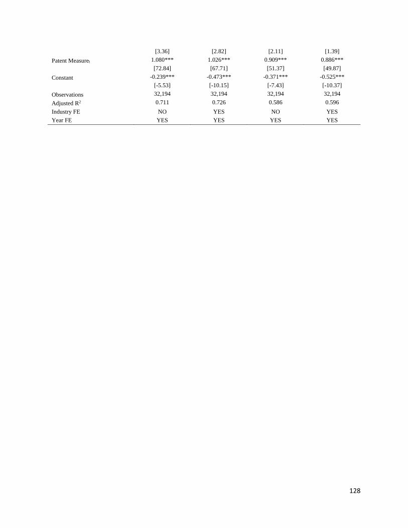
128

[3.36] [2.82] [2.11] [1.39]

Patent Measuret 1.080*** 1.026*** 0.909*** 0.886***

[72.84] [67.71] [51.37] [49.87]

Constant -0.239*** -0.473*** -0.371*** -0.525***

[-5.53] [-10.15] [-7.43] [-10.37]

Observations 32,194 32,194 32,194 32,194

Adjusted R2 0.711 0.726 0.586 0.596



129

Panel B: International Competition


(1) (2) (3) (4)

FX hedget 0.091*** 0.053* 0.091** 0.048

[2.94] [1.75] [2.48] [1.35]

High international competitiont -0.023** -0.002 -0.018 -0.008

[-2.20] [-0.14] [-1.53] [-0.61]

FX hedget×High international

competitiont

0.126*** 0.109*** 0.158*** 0.148***

[2.92] [2.58] [3.09] [2.94]

Sizet 0.087*** 0.111*** 0.103*** 0.123***

[10.47] [12.82] [11.02] [12.77]

M/Bt 0.035*** 0.038*** 0.042*** 0.045***

[8.71] [9.70] [8.87] [9.75]

Foreign incomet 0.025 0.010 0.027 0.009

[1.19] [0.48] [1.14] [0.39]

Leveraget -0.267*** -0.236*** -0.307*** -0.271***

[-8.87] [-7.91] [-8.72] [-7.73]

PPEt 0.006 0.028*** 0.001 0.025***

[1.55] [5.13] [0.17] [3.90]

ROAt 0.069*** 0.054*** 0.111*** 0.090***

[3.39] [2.80] [4.82] [4.07]

Aget -0.007*** -0.007*** -0.006*** -0.006***

[-10.77] [-10.74] [-7.94] [-7.80]

Casht 0.219*** 0.238*** 0.180*** 0.199***

[6.37] [7.06] [4.53] [5.13]

CAPEXt -0.013 0.090** 0.023 0.095*

[-0.30] [2.02] [0.47] [1.86]

Growtht -0.002 0.002 -0.000 0.004

[-0.39] [0.43] [-0.08] [0.75]

Instt -0.051 -0.073** -0.082** -0.102**

[-1.44] [-2.10] [-2.01] [-2.52]

Returnt -0.001 0.002 -0.005 -0.002

[-0.32] [0.38] [-0.99] [-0.38]

Illiquidityt 0.027** 0.050*** 0.054*** 0.076***

[2.57] [4.69] [4.58] [6.45]


[4.02] [3.59] [3.97] [3.08]

HHIt -0.315*** -0.283*** -0.228** -0.138

[-3.99] [-3.05] [-2.54] [-1.30]

HHI_sqt 0.256*** 0.236*** 0.175** 0.110

[3.42] [2.83] [2.06] [1.15]

Lag_Patent Measure 1.079*** 1.026*** 0.908*** 0.863***

[72.65] [67.78] [51.29] [48.03]

Constant -0.219*** -0.463*** -0.353*** -0.590***

[-5.18] [-10.21] [-7.25] [-11.25]

Observations 32,194 32,194 32,194 32,194

Adjusted R2 0.711 0.726 0.586 0.602



130

Panel C: FX Volatility


(1) (2) (3) (4)

FX hedget 0.135*** 0.089*** 0.136*** 0.089***

[5.20] [3.52] [4.51] [3.01]

High FX volatilityt -0.004 -0.008 -0.008 -0.010

[-0.31] [-0.61] [-0.53] [-0.61]

FX hedget×High FX volatilityt 0.030* 0.030* 0.060*** 0.059***

[1.72] [1.80] [2.82] [2.84]

Sizet 0.087*** 0.111*** 0.103*** 0.123***

[10.45] [12.81] [11.04] [12.78]

M/Bt 0.035*** 0.038*** 0.042*** 0.045***

[8.70] [9.68] [8.87] [9.75]

Foreign incomet 0.024 0.009 0.026 0.008

[1.15] [0.43] [1.09] [0.34]

Leveraget -0.267*** -0.236*** -0.308*** -0.271***

[-8.84] [-7.91] [-8.71] [-7.74]

PPEt 0.006 0.028*** 0.001 0.024***

[1.52] [5.01] [0.11] [3.80]

ROAt 0.069*** 0.055*** 0.112*** 0.091***

[3.35] [2.84] [4.82] [4.10]

Aget -0.007*** -0.007*** -0.006*** -0.006***

[-10.83] [-10.78] [-8.04] [-7.88]

Casht 0.221*** 0.240*** 0.182*** 0.201***

[6.39] [7.09] [4.55] [5.17]

CAPEXt -0.021 0.090** 0.018 0.094*

[-0.49] [2.02] [0.37] [1.85]

Growtht -0.002 0.002 -0.001 0.004

[-0.43] [0.39] [-0.12] [0.70]

Instt -0.049 -0.072** -0.080* -0.100**

[-1.40] [-2.05] [-1.95] [-2.46]

Returnt -0.001 0.002 -0.005 -0.002

[-0.29] [0.39] [-0.95] [-0.35]

Illiquidityt 0.028*** 0.051*** 0.055*** 0.078***

[2.66] [4.74] [4.70] [6.54]


[3.90] [3.54] [3.88] [3.02]

HHIt -0.319*** -0.293*** -0.241*** -0.151

[-4.06] [-3.16] [-2.72] [-1.42]

HHI_sqt 0.259*** 0.244*** 0.185** 0.120

[3.48] [2.91] [2.19] [1.25]

Patent Measuret 1.080*** 1.026*** 0.909*** 0.863***

[72.68] [67.68] [51.35] [48.02]

Constant -0.253*** -0.456*** -0.386*** -0.585***

[-6.10] [-10.00] [-8.04] [-11.11]

Observations 32,194 32,194 32,194 32,194

Adjusted R2 0.711 0.726 0.586 0.602



131

Table 4 Robustness Checks

In this table, we conduct a battery of robustness checks on our main results. In Panel A, we employ the negative

binomial regression to test the relation between FX hedge and innovation outputs. In Panel B, we restrict the sample

to before year 2004. In Panel C, we restrict the sample to after SFAS 133, i.e., after year 2002. LnPatent is the natural

logarithm of (1+Patent Number), and LnCitation is the natural logarithm of (1+Citation). Columns (1) and (2) test the

effect of hedging on Patent/LnPatent, while columns (3) and (4) test the effect on Citation/LnCitation. Columns (1)

and (3) include year fixed effect, and columns (2) and (4) include year and 2-digit SIC industry fixed effects. We

cluster the standard errors at the firm level. ***, ** and * represent significance levels at 1%, 5% and 10% respectively

with t-statistics given in brackets.

Panel A: Count Model

Patentt+2 Citationt+2

(1) (2) (3) (4)

FX hedget 0.460*** 0.240*** 0.422*** 0.211***

[5.82] [3.50] [5.00] [2.81]

Sizet 0.335*** 0.445*** 0.291*** 0.378***

[8.09] [11.89] [6.63] [8.83]

M/Bt 0.057*** 0.059*** 0.063*** 0.070***

[3.45] [4.43] [4.02] [5.23]

Foreign incomet 0.102 0.046 0.075 0.009

[1.62] [0.88] [1.11] [0.16]

Leveraget -0.783*** -0.602*** -0.997*** -0.689***

[-3.36] [-2.79] [-4.04] [-2.94]

PPEt -0.035 0.049 -0.028 0.055

[-1.06] [0.82] [-0.80] [0.87]

ROAt 0.055 -0.054 0.064 -0.042

[0.53] [-0.57] [0.54] [-0.37]

Aget -0.004* -0.004* -0.003 -0.004*

[-1.76] [-1.68] [-1.53] [-1.90]

Casht 1.065*** 0.811*** 0.959*** 0.731***

[5.44] [4.48] [5.02] [3.95]

CAPEXt -0.863** -0.338 -0.673* -0.205

[-2.35] [-0.98] [-1.81] [-0.54]

Growtht -0.053* -0.026 -0.031 -0.005

[-1.72] [-0.99] [-0.87] [-0.15]

Instt 0.652*** 0.425** 0.572*** 0.324

[3.30] [2.35] [2.66] [1.61]

Returnt 0.067*** 0.082*** 0.076*** 0.088***

[2.70] [3.70] [3.13] [3.74]

Illiquidityt -1.831*** -1.509*** -2.248*** -1.964***

[-6.57] [-5.80] [-6.38] [-5.86]

Return volatilityt 8.312*** 4.216 9.414*** 3.963

[2.95] [1.49] [3.04] [1.23]

HHIt -0.941** -0.879** -0.631 -0.398

[-2.09] [-2.15] [-1.31] [-0.89]

HHI_sqt 0.868* 0.743* 0.618 0.379

[1.89] [1.80] [1.23] [0.82]

Patent measuret 0.050*** 0.032*** 0.047*** 0.033***

[16.78] [10.38] [18.59] [12.18]

Constant -1.242*** -1.546*** -0.890** -0.998**

132

[-3.56] [-4.43] [-2.35] [-2.57]

Observations 32,194 32,194 32,194 32,194

Pseudo R2 0.564 0.564 0.564 0.564



133

Panel B: Before Year 2004


(1) (2) (3) (4)

FX hedget 0.116*** 0.111*** 0.139*** 0.134***

[4.49] [4.31] [4.56] [4.42]

Sizet 0.107*** 0.102*** 0.120*** 0.114***

[13.00] [12.24] [12.92] [12.22]

M/Bt 0.036*** 0.036*** 0.043*** 0.043***

[9.00] [9.07] [9.24] [9.26]

Foreign incomet 0.014 0.016 0.014 0.016

[0.70] [0.76] [0.57] [0.65]

Leveraget -0.242*** -0.230*** -0.275*** -0.264***

[-8.10] [-7.75] [-7.80] [-7.51]

PPEt 0.026*** 0.023*** 0.022*** 0.020***

[4.83] [4.31] [3.55] [3.13]

ROAt 0.054*** 0.064*** 0.092*** 0.100***

[2.76] [3.22] [4.02] [4.35]

Aget -0.007*** -0.007*** -0.006*** -0.006***

[-10.47] [-9.96] [-7.31] [-6.96]

Casht 0.225*** 0.210*** 0.193*** 0.181***

[6.55] [6.15] [4.80] [4.55]

CAPEXt 0.076* 0.116** 0.086 0.120**

[1.66] [2.48] [1.64] [2.25]

Growtht 0.002 0.003 0.004 0.005

[0.39] [0.65] [0.70] [0.82]

Instt -0.063* -0.083** -0.090** -0.106**

[-1.75] [-2.31] [-2.16] [-2.51]

Returnt -0.002 0.001 -0.005 -0.003

[-0.40] [0.28] [-0.85] [-0.51]

Illiquidityt 0.048*** 0.033*** 0.070*** 0.059***

[5.00] [3.21] [6.45] [5.08]


[5.12] [4.51] [4.89] [3.83]

HHIt -0.196** -0.227** -0.101 -0.137

[-2.14] [-2.48] [-0.95] [-1.28]

HHI_sqt 0.162* 0.184** 0.082 0.108

[1.94] [2.20] [0.85] [1.11]

Patent measuret 1.042*** 1.046*** 0.882*** 0.885***

[68.13] [68.26] [48.45] [48.66]

Constant -0.434*** -0.422*** -0.562*** -0.549***

[-9.79] [-9.45] [-10.82] [-10.47]

Observations 25,545 25,545 25,545 25,545

Adjusted R2 0.742 0.742 0.622 0.623



134

Panel C: After SFAS 133 (Year 2000)


(1) (2) (3) (4)

FX hedget 0.090*** 0.091*** 0.092*** 0.094***

[2.94] [2.98] [2.61] [2.66]

Sizet 0.141*** 0.138*** 0.155*** 0.151***

[12.74] [12.42] [12.33] [12.01]

M/Bt 0.048*** 0.048*** 0.053*** 0.053***

[8.71] [8.69] [8.25] [8.16]

Foreign incomet 0.009 0.011 0.012 0.014

[0.35] [0.40] [0.41] [0.48]

Leveraget -0.286*** -0.283*** -0.307*** -0.305***

[-6.96] [-6.89] [-6.27] [-6.23]

PPEt 0.035*** 0.034*** 0.033*** 0.033***

[4.64] [4.61] [3.78] [3.84]

ROAt 0.047* 0.040 0.074** 0.062**

[1.69] [1.43] [2.40] [1.98]

Aget -0.008*** -0.008*** -0.007*** -0.007***

[-10.65] [-10.69] [-7.97] [-8.13]

Casht 0.308*** 0.306*** 0.249*** 0.251***

[6.93] [6.89] [4.85] [4.90]

CAPEXt 0.145** 0.136* 0.154** 0.122

[2.11] [1.94] [1.98] [1.54]

Growtht 0.005 0.006 0.009 0.009

[0.76] [0.89] [1.11] [1.05]

Instt -0.121*** -0.116*** -0.160*** -0.149***

[-2.74] [-2.61] [-3.14] [-2.89]

Returnt -0.009 -0.003 -0.012* -0.003

[-1.64] [-0.54] [-1.66] [-0.42]

Illiquidityt 0.066*** 0.060*** 0.085*** 0.084***

[5.38] [4.63] [6.16] [5.82]

Return volatilityt 0.943*** 0.577 1.118*** 0.463

[2.84] [1.54] [2.91] [1.08]

HHIt -0.425*** -0.425*** -0.195 -0.197

[-3.29] [-3.29] [-1.34] [-1.35]

HHI_sqt 0.356*** 0.356*** 0.145 0.147

[3.09] [3.09] [1.13] [1.14]

Patent measuret 0.985*** 0.984*** 0.831*** 0.830***

[53.28] [53.14] [37.73] [37.59]

Constant -0.571*** -0.584*** -0.716*** -0.723***

[-9.67] [-9.86] [-10.54] [-10.59]

Observations 17,945 17,945 17,945 17,945

Adjusted R2 0.679 0.680 0.559 0.559



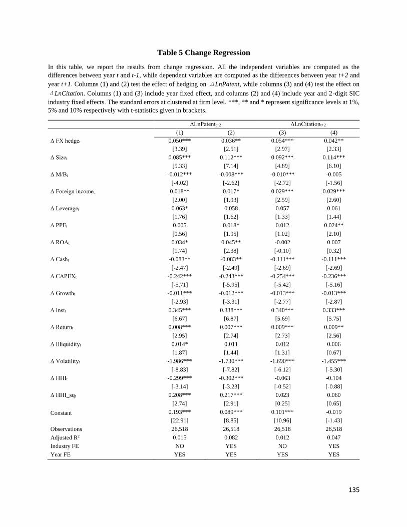
135

Table 5 Change Regression

In this table, we report the results from change regression. All the independent variables are computed as the

differences between year t and t-1, while dependent variables are computed as the differences between year t+2 and

year t+1. Columns (1) and (2) test the effect of hedging on ΔLnPatent, while columns (3) and (4) test the effect on

ΔLnCitation. Columns (1) and (3) include year fixed effect, and columns (2) and (4) include year and 2-digit SIC

industry fixed effects. The standard errors at clustered at firm level. ***, ** and * represent significance levels at 1%,

5% and 10% respectively with t-statistics given in brackets.

ΔLnPatentt+2

ΔLnCitationt+2

(1) (2) (3) (4)

Δ FX hedget 0.050*** 0.036** 0.054*** 0.042**

[3.39] [2.51] [2.97] [2.33]

Δ Sizet 0.085*** 0.112*** 0.092*** 0.114***

[5.33] [7.14] [4.89] [6.10]

Δ M/Bt -0.012*** -0.008*** -0.010*** -0.005

[-4.02] [-2.62] [-2.72] [-1.56]

Δ Foreign incomet 0.018** 0.017* 0.029*** 0.029***

[2.00] [1.93] [2.59] [2.60]

Δ Leveraget 0.063* 0.058 0.057 0.061

[1.76] [1.62] [1.33] [1.44]

Δ PPEt 0.005 0.018* 0.012 0.024**

[0.56] [1.95] [1.02] [2.10]

Δ ROAt 0.034* 0.045** -0.002 0.007

[1.74] [2.38] [-0.10] [0.32]

Δ Casht -0.083** -0.083** -0.111*** -0.111***

[-2.47] [-2.49] [-2.69] [-2.69]

Δ CAPEXt -0.242*** -0.243*** -0.254*** -0.236***

[-5.71] [-5.95] [-5.42] [-5.16]

Δ Growtht -0.011*** -0.012*** -0.013*** -0.013***

[-2.93] [-3.31] [-2.77] [-2.87]

Δ Instt 0.345*** 0.338*** 0.340*** 0.333***

[6.67] [6.87] [5.69] [5.75]

Δ Returnt 0.008*** 0.007*** 0.009*** 0.009**

[2.95] [2.74] [2.73] [2.56]

Δ Illiquidityt 0.014* 0.011 0.012 0.006

[1.87] [1.44] [1.31] [0.67]

Δ Volatilityt -1.986*** -1.730*** -1.690*** -1.455***

[-8.83] [-7.82] [-6.12] [-5.30]

Δ HHIt -0.299*** -0.302*** -0.063 -0.104

[-3.14] [-3.23] [-0.52] [-0.88]

Δ HHI_sqt 0.208*** 0.217*** 0.023 0.060

[2.74] [2.91] [0.25] [0.65]

Constant 0.193*** 0.089*** 0.101*** -0.019

[22.91] [8.85] [10.96] [-1.43]

Observations 26,518 26,518 26,518 26,518

Adjusted R2 0.015 0.082 0.012 0.047



136

Table 6 Difference-in-Differences Regression

In this table, we conduct a difference-in-differences analysis based on FX hedging initiation. We construct the matched

sample based on all control variables in the baseline regression. In Panel A, we report the covariate balance for the

matched sample. In Panel B, we run a difference-in-differences regression using the paired firms. Columns (1) and

(2) test the effect of hedging on LnPatent, while columns (3) and (4) test the effect on LnCitation. Columns (1) and

(3) include year and 2 digit industry fixed effects, and columns (2) and (4) include year and firm fixed effects. We

cluster the standard errors at firm level. ***, ** and * represent significance levels at 1%, 5% and 10% respectively

with t-statistics given in brackets

Panel A: Covariate Balance

Variable Treat Control Treat-Control p value

Size 6.096 5.96 0.136 0.298

M/B 1.424 1.531 -0.107 0.291

Foreign income 0.127 0.106 0.021 0.448

Leverage 0.241 0.224 0.017 0.254

PPE 3.768 3.768 0.000 0.999

ROA 0.12 0.127 -0.007 0.558

Age 24.223 23.067 1.156 0.327

Cash 0.145 0.148 -0.003 0.872

CAPEX 0.07 0.065 0.005 0.413

Growth 0.228 0.271 -0.043 0.441

Inst 0.511 0.499 0.012 0.544

Return 0.144 0.179 -0.035 0.522

Illiquidity 0.309 0.289 0.020 0.589

Volatility 0.031 0.032 -0.001 0.681

HHI 0.217 0.216 0.001 0.985

HHI_sq 0.119 0.121 -0.002 0.935

137

Panel B Difference-in-Differences Regression

LnPatentt+2 LnPatentt+2 LnCitationt+2 LnCitationt+2

(1) (2) (3) (4)

Initiationt -0.046 -0.009

[-1.45] [-0.24]

Postt -0.057*** -0.076*** -0.021 -0.042 [-3.09] [-3.17] [-0.79] [-1.24]

Initiationt×Postt 0.119*** 0.135*** 0.077* 0.081* [4.50] [4.17] [1.96] [1.67]

Sizet 0.031* 0.025 0.026 0.014 [1.91] [0.44] [1.63] [0.12]

M/Bt 0.020 0.017 0.015 -0.004 [1.34] [0.87] [0.82] [-0.12]

Foreign incomet 0.031 -0.041 0.007 -0.109 [0.79] [-0.78] [0.15] [-1.42]

Leveraget -0.109 -0.403** -0.103 -0.207 [-1.32] [-2.04] [-0.83] [-0.62]

PPEt -0.005 -0.098 0.013 -0.152 [-0.29] [-1.34] [0.62] [-1.32]

ROAt 0.055 0.051 -0.022 0.052 [0.59] [0.43] [-0.22] [0.27]

Aget -0.002** -0.051*** -0.001 0.007 [-2.28] [-5.61] [-1.17] [1.15]

Casht 0.070 -0.323 0.180 -0.067 [0.61] [-1.23] [1.09] [-0.11]

CAPEXt -0.098 -0.117 0.033 -0.004 [-0.70] [-0.65] [0.21] [-0.02]

Growtht -0.011 -0.011 -0.038 -0.024 [-0.63] [-0.32] [-1.48] [-0.46]

Instt -0.007 -0.060 0.039 0.217 [-0.07] [-0.36] [0.38] [0.73]

Returnt -0.009 -0.012 -0.009 -0.041 [-0.46] [-0.44] [-0.38] [-0.90]

Illiquidityt -0.059 0.033 -0.072 -0.026 [-1.43] [0.63] [-1.59] [-0.31]

Return volatilityt 3.750*** 2.089 2.972** 1.726 [3.02] [1.34] [2.16] [0.74]

HHIt -0.011 -0.034 0.225 -0.202 [-0.05] [-0.11] [0.84] [-0.48]

HHI_sqt 0.038 0.084 -0.169 0.277 [0.19] [0.34] [-0.73] [0.65]

Patent measuret 1.128*** 0.833*** 0.895*** 0.548*** [17.25] [9.04] [12.02] [3.91]

Constant -0.136 1.617*** -0.247* 0.389 [-1.03] [3.74] [-1.69] [0.54]

Observations 1,192 1,192 1,192 1,192

Adjusted R2 0.681 0.903 0.515 0.757

Industry FE YES No YES No

Firm FE No YES No YES


138

Table 7 Instrumental Variable Regression

This table presents the results of two-stage residual inclusion regression by Hausman (1978), using tax convexity as

an IV. The first stage is a Logit regression with dependent variable being the FX hedge and instrumental variable as

tax convexity. The second stage is an OLS regression controlling for variables as in main regression and residual from

first stage Logit regression. In Panel A, we follow the definition of tax convexity in literature (Smith and Stulz (1985),

Campello et al. (2011), Manconi et al. (2017)). In Panel B, we exclude TIVOL (volatility of taxable income) from tax

convexity calculation. In Panel C, we use the state tax convexity as IV. Colums (1) and (2) report the first stage results.

Columns (3) and (4) report the results of second stage regression. Year and 2-digit SIC industry fixed effects are

included. We cluster the standard errors at firm level. ***, ** and * represent significance levels at 1%, 5% and 10%

respectively using robust standard errors with t-statistics given in brackets.

Panel A: Normal Definition of Convexity

FX hedget FX hedget LnPatentt+2 LnCitationt+2

(1) (2) (3) (4)

Convexityt 0.055*** 0.055***

[3.00] [3.04]

FX hedget 0.087*** 0.078***

[3.36] [2.59]

Sizet 0.354*** 0.360*** 0.066*** 0.041***

[9.31] [9.46] [6.73] [3.76]

M/Bt 0.009 0.007 0.036*** 0.039***

[0.35] [0.27] [7.28] [6.67]

Foreign incomet 0.832*** 0.849*** -0.125*** -0.233***

[9.73] [9.96] [-4.71] [-7.31]

Leveraget -0.922*** -0.929*** -0.139*** -0.089**

[-4.38] [-4.42] [-4.18] [-2.26]

PPEt -0.036 -0.037 0.027*** 0.031***

[-1.04] [-1.08] [4.46] [4.32]

ROAt 0.806*** 0.815*** 0.082*** 0.107***

[3.11] [3.10] [2.97] [3.30]

Aget 0.001 0.001 -0.007*** -0.007***

[0.16] [0.29] [-9.75] [-8.27]

Casht 0.012 -0.005 0.209*** 0.201***

[0.06] [-0.02] [5.49] [4.54]

CAPEXt -3.221*** -3.248*** 0.266*** 0.423***

[-4.92] [-4.96] [4.28] [5.50]

Growtht -0.188*** -0.195*** 0.005 0.010

[-2.99] [-3.03] [0.91] [1.46]

Instt 0.652*** 0.633*** -0.122*** -0.213***

[3.24] [3.15] [-3.13] [-4.63]

Returnt -0.052 -0.050 0.007 0.011*

[-1.57] [-1.51] [1.35] [1.80]

Illiquidityt -0.139 -0.130 0.045*** 0.061***

[-1.27] [-1.18] [4.14] [5.15]

Return volatilityt 1.145 0.867 0.361 -0.153

[0.41] [0.31] [1.16] [-0.42]

HHIt 0.261 0.310 -0.389*** -0.306***

[0.55] [0.65] [-3.85] [-2.63]

HHI_sqt -0.061 -0.103 0.312*** 0.232**

139

[-0.13] [-0.22] [3.44] [2.22]

Patent measuret 0.409*** 0.383*** 0.955*** 0.744***

[8.81] [8.95] [48.80] [32.88]

First stage residualst -0.917*** -1.764***

[-5.89] [-9.19]

Constant -4.852*** -4.864*** 0.698*** 1.579***

[-16.19] [-16.25] [3.83] [7.06]

Observations 24,236 24,236 24,236 24,236

Pseudo/Adjusted R2 0.202 0.202 0.772 0.655

Industry FE YES YES YES YES


Panel B: Excluding Taxable Income Volatility in Convexity Calculation

FX hedge FX hedge LnPatent LnCitation (1) (2) (3) (4)

Convexity 0.055*** 0.056***

[2.94] [2.98]

FX hedge 0.087*** 0.078***

[3.36] [2.60]

Controls YES YES 0.087*** 0.078***

Observations 24,236 24,236 24,236 24,236




Panel C: State tax convexity

FX hedge FX hedge LnPatent LnCitation (1) (2) (3) (4)

Convexity 0.206** 0.198**

[2.29] [2.20]

FX hedge 0.094*** 0.094***

[3.61] [3.08]

Controls YES YES YES YES

Observations 24,236 24,236 24,236 24,236




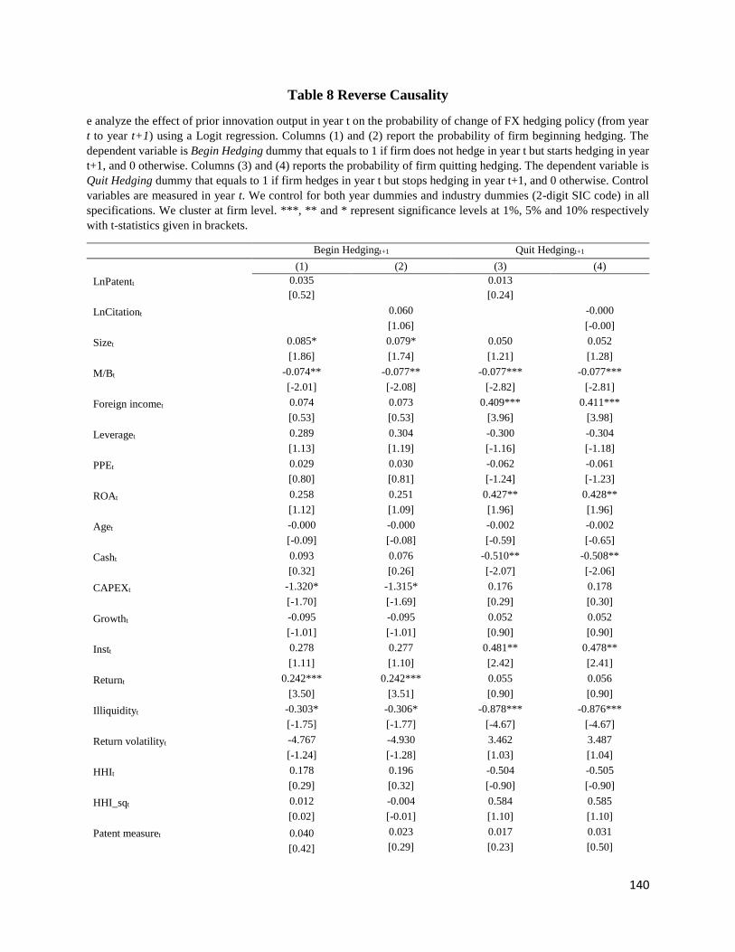
140

Table 8 Reverse Causality

e analyze the effect of prior innovation output in year t on the probability of change of FX hedging policy (from year

t to year t+1) using a Logit regression. Columns (1) and (2) report the probability of firm beginning hedging. The

dependent variable is Begin Hedging dummy that equals to 1 if firm does not hedge in year t but starts hedging in year

t+1, and 0 otherwise. Columns (3) and (4) reports the probability of firm quitting hedging. The dependent variable is

Quit Hedging dummy that equals to 1 if firm hedges in year t but stops hedging in year t+1, and 0 otherwise. Control

variables are measured in year t. We control for both year dummies and industry dummies (2-digit SIC code) in all

specifications. We cluster at firm level. ***, ** and * represent significance levels at 1%, 5% and 10% respectively

with t-statistics given in brackets.

Begin Hedgingt+1

Begin Hedging

Quit Hedgingt+1

Quit Hedging (1) (2) (3) (4)

LnPatentt 0.035

0.013

[0.52]

[0.24]

LnCitationt 0.060

-0.000

[1.06]

[-0.00]

Sizet 0.085* 0.079* 0.050 0.052

[1.86] [1.74] [1.21] [1.28]

M/Bt -0.074** -0.077** -0.077*** -0.077***

[-2.01] [-2.08] [-2.82] [-2.81]

Foreign incomet 0.074 0.073 0.409*** 0.411***

[0.53] [0.53] [3.96] [3.98]

Leveraget 0.289 0.304 -0.300 -0.304

[1.13] [1.19] [-1.16] [-1.18]

PPEt 0.029 0.030 -0.062 -0.061

[0.80] [0.81] [-1.24] [-1.23]

ROAt 0.258 0.251 0.427** 0.428**

[1.12] [1.09] [1.96] [1.96]

Aget -0.000 -0.000 -0.002 -0.002

[-0.09] [-0.08] [-0.59] [-0.65]

Casht 0.093 0.076 -0.510** -0.508**

[0.32] [0.26] [-2.07] [-2.06]

CAPEXt -1.320* -1.315* 0.176 0.178

[-1.70] [-1.69] [0.29] [0.30]

Growtht -0.095 -0.095 0.052 0.052

[-1.01] [-1.01] [0.90] [0.90]

Instt 0.278 0.277 0.481** 0.478**

[1.11] [1.10] [2.42] [2.41]

Returnt 0.242*** 0.242*** 0.055 0.056

[3.50] [3.51] [0.90] [0.90]

Illiquidityt -0.303* -0.306* -0.878*** -0.876***

[-1.75] [-1.77] [-4.67] [-4.67]

Return volatilityt -4.767 -4.930 3.462 3.487

[-1.24] [-1.28] [1.03] [1.04]

HHIt 0.178 0.196 -0.504 -0.505

[0.29] [0.32] [-0.90] [-0.90]

HHI_sqt 0.012 -0.004 0.584 0.585

[0.02] [-0.01] [1.10] [1.10]

Patent measuret 0.040 0.023 0.017 0.031

[0.42] [0.29] [0.23] [0.50]

141

Constant -5.039*** -5.006*** -12.636*** -12.649***

[-12.18] [-12.07] [-11.51] [-11.39]

Observations 22,780 22,780 22,780 22,780

Pseudo R2 0.035 0.035 0.035 0.035



142

Table 9 Information Asymmetry

This table examines how information asymmetry affects the relation between FX hedge and innovation outputs. In

Panels A to C, we employ Analyst forecast dispersion, Breadth of ownership, and PIN respectively. LnPatent is the

natural logarithm of (1+Patent Number), and LnCitation is the natural logarithm of (1+Citation). Columns (1) and (2)

test the effect of hedging on LnPatent, while columns (3) and (4) test the effect on LnCitation. Columns (1) and (3)

include year fixed effect, and columns (2) and (4) include year and 2-digit SIC industry fixed effects. We cluster the

standard errors at firm level. ***, ** and * represent significance levels at 1%, 5% and 10% respectively with t-

statistics given in brackets.

Panel A: Analyst Forecast Dispersion


(1) (2) (3) (4)

FX hedget 0.102*** 0.036 0.107** 0.039

[2.84] [1.05] [2.53] [0.96]

High dispersiont 0.036** 0.018 0.052*** 0.030*

[2.34] [1.23] [2.94] [1.76]

FX hedget×High dispersiont 0.108** 0.097** 0.130** 0.121**

[2.33] [2.19] [2.38] [2.33]

Sizet 0.114*** 0.149*** 0.136*** 0.166***

[8.95] [11.46] [9.80] [11.65]

M/Bt 0.035*** 0.042*** 0.042*** 0.050***

[5.69] [7.12] [5.96] [7.39]

Foreign incomet 0.030 0.004 0.022 -0.007

[1.05] [0.14] [0.68] [-0.21]

Leveraget -0.345*** -0.273*** -0.381*** -0.297***

[-6.74] [-5.37] [-6.37] [-4.94]

PPEt 0.014* 0.045*** 0.005 0.040***

[1.88] [4.36] [0.62] [3.32]

ROAt 0.111*** 0.071** 0.184*** 0.131***

[3.23] [2.20] [4.83] [3.59]

Aget -0.009*** -0.008*** -0.008*** -0.007***

[-9.21] [-8.53] [-7.15] [-6.56]

Casht 0.345*** 0.336*** 0.321*** 0.310***

[6.16] [6.11] [4.97] [4.89]

CAPEXt -0.110* 0.062 -0.040 0.090

[-1.67] [0.88] [-0.54] [1.12]

Growtht -0.010 -0.004 -0.009 -0.001

[-1.14] [-0.51] [-0.83] [-0.15]

Instt -0.077 -0.103** -0.097* -0.123**

[-1.62] [-2.21] [-1.77] [-2.27]

Returnt 0.010 0.015** 0.015 0.019**

[1.36] [2.06] [1.62] [2.13]

Illiquidityt -0.020 0.048 0.035 0.104**

[-0.53] [1.31] [0.83] [2.47]

Return volatilityt 3.040*** 1.648** 3.135*** 1.308

[4.12] [2.35] [3.76] [1.60]

HHIt -0.452*** -0.477*** -0.341** -0.273

[-3.56] [-3.23] [-2.37] [-1.60]

HHI_sqt 0.375*** 0.404*** 0.267* 0.220

143

[3.07] [3.01] [1.93] [1.43]

Patent Measuret 1.099*** 1.013*** 0.938*** 0.864***

[67.25] [57.74] [49.16] [42.56]

Constant -0.441*** -0.752*** -0.642*** -0.948***

[-5.45] [-9.40] [-7.04] [-10.40]

Observations 18,157 18,157 18,157 18,157

Adjusted R2 0.711 0.734 0.595 0.620



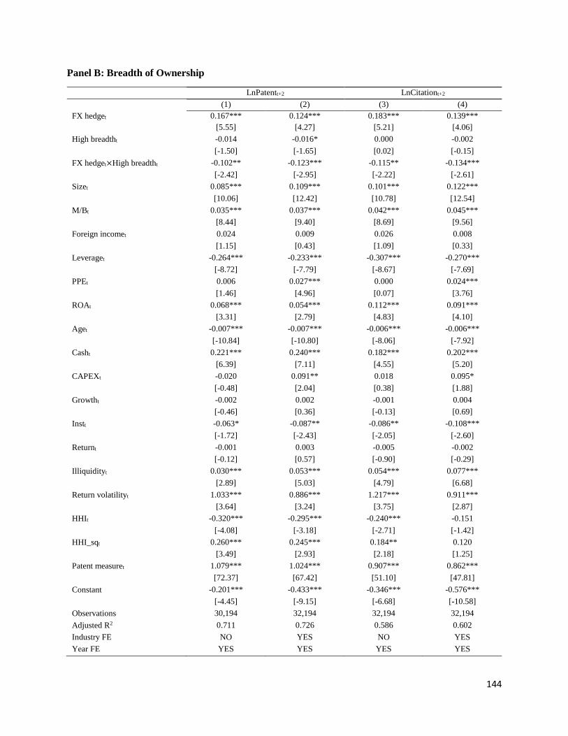
144

Panel B: Breadth of Ownership


(1) (2) (3) (4)

FX hedget 0.167*** 0.124*** 0.183*** 0.139***

[5.55] [4.27] [5.21] [4.06]

High breadtht -0.014 -0.016* 0.000 -0.002

[-1.50] [-1.65] [0.02] [-0.15]

FX hedget×High breadtht -0.102** -0.123*** -0.115** -0.134***

[-2.42] [-2.95] [-2.22] [-2.61]

Sizet 0.085*** 0.109*** 0.101*** 0.122***

[10.06] [12.42] [10.78] [12.54]

M/Bt 0.035*** 0.037*** 0.042*** 0.045***

[8.44] [9.40] [8.69] [9.56]

Foreign incomet 0.024 0.009 0.026 0.008

[1.15] [0.43] [1.09] [0.33]

Leveraget -0.264*** -0.233*** -0.307*** -0.270***

[-8.72] [-7.79] [-8.67] [-7.69]

PPEt 0.006 0.027*** 0.000 0.024***

[1.46] [4.96] [0.07] [3.76]

ROAt 0.068*** 0.054*** 0.112*** 0.091***

[3.31] [2.79] [4.83] [4.10]

Aget -0.007*** -0.007*** -0.006*** -0.006***

[-10.84] [-10.80] [-8.06] [-7.92]

Casht 0.221*** 0.240*** 0.182*** 0.202***

[6.39] [7.11] [4.55] [5.20]

CAPEXt -0.020 0.091** 0.018 0.095*

[-0.48] [2.04] [0.38] [1.88]

Growtht -0.002 0.002 -0.001 0.004

[-0.46] [0.36] [-0.13] [0.69]

Instt -0.063* -0.087** -0.086** -0.108***

[-1.72] [-2.43] [-2.05] [-2.60]

Returnt -0.001 0.003 -0.005 -0.002

[-0.12] [0.57] [-0.90] [-0.29]

Illiquidityt 0.030*** 0.053*** 0.054*** 0.077***

[2.89] [5.03] [4.79] [6.68]


[3.64] [3.24] [3.75] [2.87]

HHIt -0.320*** -0.295*** -0.240*** -0.151

[-4.08] [-3.18] [-2.71] [-1.42]

HHI_sqt 0.260*** 0.245*** 0.184** 0.120

[3.49] [2.93] [2.18] [1.25]

Patent measuret 1.079*** 1.024*** 0.907*** 0.862***

[72.37] [67.42] [51.10] [47.81]

Constant -0.201*** -0.433*** -0.346*** -0.576***

[-4.45] [-9.15] [-6.68] [-10.58]

Observations 30,194 32,194 32,194 32,194

Adjusted R2 0.711 0.726 0.586 0.602



145

Panel C: PIN


(1) (2) (3) (4)

FX hedget 0.074** 0.005 0.045 -0.027

[2.57] [0.16] [1.34] [-0.77]

High PINt 0.054*** 0.053*** 0.069*** 0.069***

[4.58] [4.65] [4.87] [5.01]

FX hedget×High PINt 0.116*** 0.144*** 0.176*** 0.205***

[2.72] [3.45] [3.48] [4.12]

Sizet 0.088*** 0.114*** 0.102*** 0.125***

[9.52] [12.02] [9.84] [11.70]

M/Bt 0.033*** 0.036*** 0.039*** 0.043***

[7.63] [8.69] [7.77] [8.71]

Foreign incomet 0.025 0.009 0.026 0.006

[1.13] [0.42] [1.02] [0.24]

Leveraget -0.286*** -0.249*** -0.334*** -0.290***

[-8.30] [-7.28] [-8.26] [-7.23]

PPEt 0.007 0.032*** 0.001 0.029***

[1.51] [5.16] [0.15] [3.96]

ROAt 0.069*** 0.054** 0.120*** 0.097***

[3.01] [2.52] [4.62] [3.93]

Aget -0.008*** -0.008*** -0.007*** -0.006***

[-10.74] [-10.61] [-8.07] [-7.88]

Casht 0.238*** 0.258*** 0.199*** 0.222***

[6.29] [7.01] [4.55] [5.22]

CAPEXt -0.021 0.111** 0.019 0.113**

[-0.45] [2.28] [0.35] [2.05]

Growtht -0.003 0.001 -0.001 0.004

[-0.61] [0.17] [-0.18] [0.62]

Instt -0.075* -0.102*** -0.114** -0.139***

[-1.95] [-2.69] [-2.56] [-3.16]

Returnt -0.006 -0.001 -0.009 -0.005

[-1.23] [-0.32] [-1.56] [-0.80]

Illiquidityt 0.035*** 0.062*** 0.067*** 0.093***

[3.08] [5.21] [5.18] [7.03]

Return volatilityt 1.265*** 1.020*** 1.196*** 0.775**

[3.75] [3.14] [3.11] [2.05]

HHIt -0.330*** -0.302*** -0.242** -0.149

[-3.85] [-2.99] [-2.50] [-1.29]

HHI_sqt 0.268*** 0.250*** 0.186** 0.117

[3.30] [2.75] [2.02] [1.13]

Patent measuret 1.066*** 1.002*** 0.893*** 0.840***

[70.51] [63.83] [49.33] [45.06]

Constant -0.227*** -0.489*** -0.350*** -0.609***

[-4.79] [-9.63] [-6.40] [-10.39]

Observations 29,158 29,158 29,158 29,158

Adjusted R2 0.707 0.724 0.581 0.599



146

Table 10 FX Hedging and Investment Horizon

In this table, we test whether FX hedging affects firm’s investment horizon. Panel A tests the effect of FX hedge on

Long term investment. The Long term investment is computed as R&D expense scaled by sum of capital expenditure

and R&D expense. Columns (1) and (2) employ the Long term investment at year t+1, and Columns (3) and (4) employ

the Long term investment at year t+2. Columns (1) and (3) include year fixed effect, and columns (2) and (4) include

year and 2-digit SIC industry fixed effects. In Panel B, we test how FX hedge affect the relation between cutting R&D

expense (CUT RD) and small earnings decrease dummy (SD dummy). We include year and 2-digit SIC industry fixed

effects. In Panels C and D, we employ Market competition and CEO entrenchment respectively, to examine how

market pressure affects the relation between FX hedge and innovation outputs. LnPatent is the natural logarithm of

(1+Patent Number), and LnCitation is the natural logarithm of (1+Citation). Columns (1) and (2) test the effect of

hedging on LnPatent, while columns (3) and (4) test the effect on LnCitation. Columns (1) and (3) include year fixed

effect, and columns (2) and (4) include year and 2-digit SIC industry fixed effects. We cluster the standard errors at

the firm level. ***, ** and * represent significance levels at 1%, 5% and 10% respectively with t-statistics given in

brackets.

Panel A: FX Hedging and Long Term Investment

Long Term Investmentt+1 Long Term Investmentt+2

(1) (2) (3) (4)

FX hedget 0.010*** 0.006*** 0.009*** 0.004***

[6.67] [3.64] [5.60] [2.73]

Sizet -0.003*** -0.003*** -0.000 0.001

[-5.62] [-4.66] [-0.48] [0.89]

M/Bt -0.000 -0.001 0.002*** 0.002***

[-0.31] [-1.13] [4.36] [3.80]

Foreign incomet 0.004** 0.002 0.005*** 0.002

[2.28] [0.91] [2.79] [1.21]

Leveraget -0.012*** -0.010*** -0.017*** -0.016***

[-3.74] [-2.86] [-4.67] [-4.01]

PPEt 0.001** 0.006*** -0.002*** 0.000

[2.29] [8.02] [-3.83] [0.23]

ROAt -0.013*** -0.016*** -0.000 -0.004

[-3.98] [-4.76] [-0.11] [-1.03]

Aget 0.000*** 0.000*** 0.000*** 0.000

[3.58] [2.91] [2.69] [1.08]

Casht 0.031*** 0.034*** 0.040*** 0.045***

[7.06] [7.39] [8.23] [8.88]

CAPEXt 0.073*** 0.082*** 0.044*** 0.058***

[8.90] [9.59] [5.39] [6.53]

Growtht -0.002 -0.002 0.001 0.001

[-1.33] [-1.50] [0.59] [0.47]

Instt 0.001 -0.002 0.001 -0.001

[0.44] [-0.53] [0.31] [-0.37]

Returnt -0.017*** -0.016*** 0.000 0.000

[-14.81] [-13.98] [0.19] [0.29]

Illiquidityt -0.014*** -0.013*** -0.004** -0.004*

[-7.90] [-7.38] [-2.12] [-1.92]

Return volatilityt 0.257*** 0.243*** 0.089 0.106*

[5.02] [4.57] [1.57] [1.79]

HHIt -0.050*** -0.051*** -0.064*** -0.065***

[-6.42] [-5.44] [-7.51] [-6.56]

147

HHI_sqt 0.042*** 0.043*** 0.055*** 0.057***

[5.66] [5.12] [6.81] [6.25]

Long term investmentt 0.946*** 0.915*** 0.941*** 0.911***

[312.81] [227.90] [297.38] [214.45]

Constant 0.029*** 0.015*** 0.021*** 0.015***

[5.97] [2.85] [3.91] [2.66]

Observations 29,552 29,552 27,070 27,070

R-squared 0.914 0.915 0.916 0.917



148

Panel B: Real Earnings Management

CUT R&Dt+1

(1) (2)

FX hedget -0.099** -0.096**

[-2.14] [-2.08]

SD dummyt 0.269*** 0.267***

[9.58] [9.43]

FX hedget×SD dummyt -0.190*** -0.179***

[-3.06] [-2.86]

Distancet -0.004 -0.005

[-0.28] [-0.36]

Sizet -0.009 -0.007

[-1.43] [-1.02]

M/Bt 0.011 0.021

[0.29] [0.56]

Foreign incomet -0.056 -0.058

[-0.68] [-0.69]

Leveraget 0.008 0.016

[0.46] [0.85]

PPEt -0.125*** -0.138***

[-2.60] [-2.85]

ROAt 0.001 0.001

[0.50] [0.68]

Aget 0.071 0.068

[0.99] [0.92]

Casht -0.091 -0.121

[-0.50] [-0.65]

CAPEXt 0.007 0.012

[0.46] [0.81]

Growtht 0.023 -0.001

[0.28] [-0.01]

Instt -0.045** -0.047**

[-2.48] [-2.54]

Returnt 0.053 0.065*

[1.39] [1.69]

Illiquidityt 2.391** 2.071**

[2.35] [2.01]

Return volatilityt -0.106 -0.408*

[-0.53] [-1.82]

HHIt 0.183 0.424**

[0.91] [1.98]

HHI_sqt -0.004 -0.005

[-0.28] [-0.36]

Constant -0.319*** -0.710***

[-2.99] [-5.81]


Pseudo R2 0.050 0.050

Industry FE NO YES

Year FE YES YES

149

Panel C: Market Competition


(1) (2) (3) (4)

FX hedget 0.091*** 0.044 0.110*** 0.060*

[3.31] [1.64] [3.41] [1.92]

High market competitiont 0.031* 0.038** 0.015 0.012

[1.85] [2.01] [0.73] [0.56]

FX hedget×High market

competitiont

0.194*** 0.198*** 0.178** 0.185***

[3.19] [3.41] [2.54] [2.73]

Sizet 0.087*** 0.111*** 0.102*** 0.123***

[10.45] [12.85] [10.96] [12.75]

M/Bt 0.035*** 0.038*** 0.042*** 0.045***

[8.65] [9.69] [8.81] [9.72]

Foreign incomet 0.026 0.011 0.027 0.010

[1.21] [0.55] [1.15] [0.41]

Leveraget -0.261*** -0.232*** -0.303*** -0.268***

[-8.72] [-7.83] [-8.59] [-7.66]

PPEt 0.006 0.026*** 0.000 0.023***

[1.43] [4.76] [0.05] [3.66]

ROAt 0.062*** 0.049** 0.106*** 0.086***

[3.04] [2.56] [4.60] [3.88]

Aget -0.007*** -0.007*** -0.006*** -0.006***

[-10.49] [-10.48] [-7.73] [-7.61]

Casht 0.205*** 0.225*** 0.171*** 0.194***

[6.00] [6.75] [4.31] [4.98]

CAPEXt -0.025 0.093** 0.016 0.096*

[-0.58] [2.09] [0.33] [1.90]

Growtht -0.002 0.002 -0.000 0.004

[-0.35] [0.44] [-0.06] [0.75]

Instt -0.049 -0.071** -0.079* -0.099**

[-1.40] [-2.03] [-1.94] [-2.44]

Returnt -0.001 0.001 -0.005 -0.002

[-0.29] [0.30] [-0.99] [-0.44]

Illiquidityt 0.028*** 0.050*** 0.053*** 0.075***

[2.64] [4.75] [4.59] [6.43]


[3.75] [3.45] [3.84] [3.04]

HHIt -0.128 -0.103 -0.114 -0.038

[-1.40] [-1.04] [-1.10] [-0.34]

HHI_sqt 0.100 0.086 0.080 0.027

[1.21] [0.98] [0.85] [0.27]

Patent measuret 1.078*** 1.024*** 0.907*** 0.862***

[72.44] [67.49] [51.15] [47.85]

Constant -0.282*** -0.488*** -0.405*** -0.602***

[-6.27] [-10.34] [-7.84] [-11.07]

Observations 32,194 32,194 32,194 32,194

Adjusted R2 0.712 0.727 0.586 0.602



150

Panel D: CEO Entrenchment


(1) (2) (3) (4)

FX hedget 0.200*** 0.107*** 0.190*** 0.085*

[4.12] [2.64] [3.35] [1.83]

High CEO entrenchmentt 0.060** 0.039* 0.067** 0.042

[2.28] [1.77] [2.21] [1.46]

FX hedget×High CEO

entrenchmentt

-0.129** -0.086* -0.146** -0.094*

[-2.06] [-1.73] [-2.03] [-1.71]

Sizet 0.115*** 0.154*** 0.135*** 0.172***

[7.02] [7.97] [7.64] [8.36]

M/Bt 0.046*** 0.063*** 0.052*** 0.075***

[3.70] [7.64] [3.62] [6.39]

Foreign incomet 0.008 -0.020 0.006 -0.028

[0.26] [-0.60] [0.17] [-0.67]

Leveraget -0.292*** -0.257*** -0.285*** -0.224**

[-3.99] [-3.44] [-3.42] [-2.47]

PPEt -0.009 0.029 -0.020* 0.028

[-0.83] [1.26] [-1.72] [1.10]

ROAt 0.298*** 0.194*** 0.376*** 0.256***

[3.11] [2.62] [3.33] [3.09]

Aget -0.008*** -0.007*** -0.007*** -0.007***

[-7.51] [-6.44] [-6.34] [-5.10]

Casht 0.492*** 0.346*** 0.467*** 0.297**

[5.22] [3.95] [4.46] [2.30]

CAPEXt -0.532*** -0.205 -0.436*** -0.228

[-3.83] [-1.02] [-2.66] [-1.04]

Growtht -0.008 0.002 -0.012 0.002

[-0.32] [0.13] [-0.43] [0.07]

Instt -0.135* -0.144** -0.153* -0.187***

[-1.81] [-2.38] [-1.77] [-2.75]

Returnt 0.008 0.014 0.002 0.003

[0.67] [1.03] [0.14] [0.22]

Illiquidityt -0.196*** -0.133* -0.111 -0.052

[-2.71] [-1.87] [-1.39] [-0.73]

Return volatilityt 4.447*** 2.895** 3.523** 1.684

[3.64] [2.17] [2.48] [0.99]

HHIt -0.642*** -0.607*** -0.543*** -0.387

[-3.99] [-2.62] [-2.98] [-1.62]

HHI_sqt 0.579*** 0.525*** 0.485*** 0.343

[3.85] [2.68] [2.83] [1.64]

Patent measuret 1.050*** 0.966*** 0.919*** 0.841***

[56.98] [54.94] [44.83] [38.10]

Constant -0.406*** -0.683*** -0.566*** -0.904***

[-3.43] [-4.92] [-4.20] [-5.32]

Observations 9,443 9,443 9,443 9,443

Adjusted R2 0.762 0.784 0.645 0.671



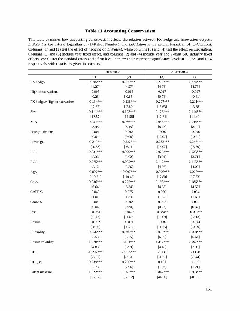
151

Table 11 Accounting Conservatism

This table examines how accounting conservatism affects the relation between FX hedge and innovation outputs.

LnPatent is the natural logarithm of (1+Patent Number), and LnCitation is the natural logarithm of (1+Citation).

Columns (1) and (2) test the effect of hedging on LnPatent, while columns (3) and (4) test the effect on LnCitation.

Columns (1) and (3) include year fixed effect, and columns (2) and (4) include year and 2-digit SIC industry fixed

effects. We cluster the standard errors at the firm level. ***, ** and * represent significance levels at 1%, 5% and 10%

respectively with t-statistics given in brackets.


(1) (2) (3) (4)

FX hedget 0.205*** 0.206*** 0.272*** 0.274***

[4.27] [4.27] [4.73] [4.73]

High conservatismt 0.005 -0.016 0.017 -0.007

[0.28] [-0.85] [0.74] [-0.31]

FX hedget×High conservatismt -0.134*** -0.138*** -0.207*** -0.211***

[-2.82] [-2.89] [-3.63] [-3.68]

Sizet 0.111*** 0.103*** 0.123*** 0.114***

[12.57] [11.58] [12.31] [11.40]

M/Bt 0.037*** 0.036*** 0.046*** 0.044***

[8.43] [8.15] [8.45] [8.10]

Foreign incomet 0.001 0.002 -0.002 -0.000

[0.04] [0.08] [-0.07] [-0.01]

Leveraget -0.240*** -0.222*** -0.262*** -0.246***

[-6.58] [-6.11] [-6.07] [-5.69]

PPEt 0.031*** 0.029*** 0.026*** 0.025***

[5.36] [5.02] [3.94] [3.71]

ROAt 0.075*** 0.082*** 0.112*** 0.115***

[3.12] [3.36] [4.07] [4.09]

Aget -0.007*** -0.007*** -0.006*** -0.006***

[-10.81] [-10.46] [-7.80] [-7.63]

Casht 0.236*** 0.225*** 0.193*** 0.186***

[6.64] [6.34] [4.66] [4.52]

CAPEXt 0.049 0.075 0.080 0.094

[1.01] [1.53] [1.39] [1.60]

Growtht 0.000 0.002 0.002 0.002

[0.04] [0.34] [0.26] [0.37]

Instt -0.053 -0.062* -0.088** -0.091**

[-1.47] [-1.69] [-2.09] [-2.13]

Returnt -0.002 -0.001 -0.007 -0.004

[-0.50] [-0.25] [-1.25] [-0.69]

Illiquidityt 0.056*** 0.040*** 0.079*** 0.068***

[5.58] [3.75] [6.95] [5.64]


[4.88] [3.99] [4.40] [2.95]

HHIt -0.292*** -0.315*** -0.131 -0.158

[-3.07] [-3.31] [-1.21] [-1.44]

HHI_sqt 0.239*** 0.256*** 0.101 0.119

[2.78] [2.96] [1.03] [1.21]

Patent measuret 1.022*** 1.023*** 0.862*** 0.863***

[65.17] [65.12] [46.56] [46.55]

152

Constant -0.461*** -0.412*** -0.599*** -0.543***

[-9.19] [-7.99] [-10.03] [-8.84]

Observations 29,330 29,330 29,330 29,330

Adjusted R2 0.741 0.741 0.618 0.619



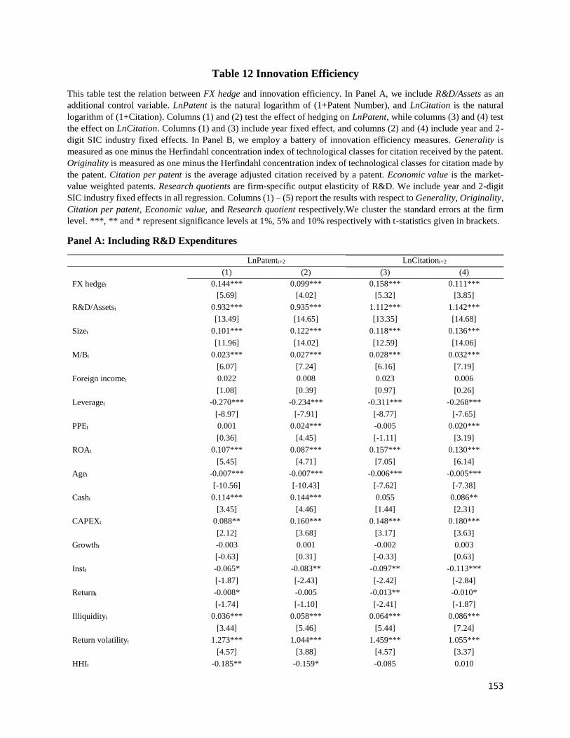
153

Table 12 Innovation Efficiency

This table test the relation between FX hedge and innovation efficiency. In Panel A, we include R&D/Assets as an

additional control variable. LnPatent is the natural logarithm of (1+Patent Number), and LnCitation is the natural

logarithm of (1+Citation). Columns (1) and (2) test the effect of hedging on LnPatent, while columns (3) and (4) test

the effect on LnCitation. Columns (1) and (3) include year fixed effect, and columns (2) and (4) include year and 2-

digit SIC industry fixed effects. In Panel B, we employ a battery of innovation efficiency measures. Generality is

measured as one minus the Herfindahl concentration index of technological classes for citation received by the patent.

Originality is measured as one minus the Herfindahl concentration index of technological classes for citation made by

the patent. Citation per patent is the average adjusted citation received by a patent. Economic value is the market-

value weighted patents. Research quotients are firm-specific output elasticity of R&D. We include year and 2-digit

SIC industry fixed effects in all regression. Columns (1) – (5) report the results with respect to Generality, Originality,

Citation per patent, Economic value, and Research quotient respectively.We cluster the standard errors at the firm

level. ***, ** and * represent significance levels at 1%, 5% and 10% respectively with t-statistics given in brackets.

Panel A: Including R&D Expenditures


(1) (2) (3) (4)

FX hedget 0.144*** 0.099*** 0.158*** 0.111***

[5.69] [4.02] [5.32] [3.85]

R&D/Assetst 0.932*** 0.935*** 1.112*** 1.142***

[13.49] [14.65] [13.35] [14.68]

Sizet 0.101*** 0.122*** 0.118*** 0.136***

[11.96] [14.02] [12.59] [14.06]

M/Bt 0.023*** 0.027*** 0.028*** 0.032***

[6.07] [7.24] [6.16] [7.19]

Foreign incomet 0.022 0.008 0.023 0.006

[1.08] [0.39] [0.97] [0.26]

Leveraget -0.270*** -0.234*** -0.311*** -0.268***

[-8.97] [-7.91] [-8.77] [-7.65]

PPEt 0.001 0.024*** -0.005 0.020***

[0.36] [4.45] [-1.11] [3.19]

ROAt 0.107*** 0.087*** 0.157*** 0.130***

[5.45] [4.71] [7.05] [6.14]

Aget -0.007*** -0.007*** -0.006*** -0.005***

[-10.56] [-10.43] [-7.62] [-7.38]

Casht 0.114*** 0.144*** 0.055 0.086**

[3.45] [4.46] [1.44] [2.31]

CAPEXt 0.088** 0.160*** 0.148*** 0.180***

[2.12] [3.68] [3.17] [3.63]

Growtht -0.003 0.001 -0.002 0.003

[-0.63] [0.31] [-0.33] [0.63]

Instt -0.065* -0.083** -0.097** -0.113***

[-1.87] [-2.43] [-2.42] [-2.84]

Returnt -0.008* -0.005 -0.013** -0.010*

[-1.74] [-1.10] [-2.41] [-1.87]

Illiquidityt 0.036*** 0.058*** 0.064*** 0.086***

[3.44] [5.46] [5.44] [7.24]


[4.57] [3.88] [4.57] [3.37]

HHIt -0.185** -0.159* -0.085 0.010

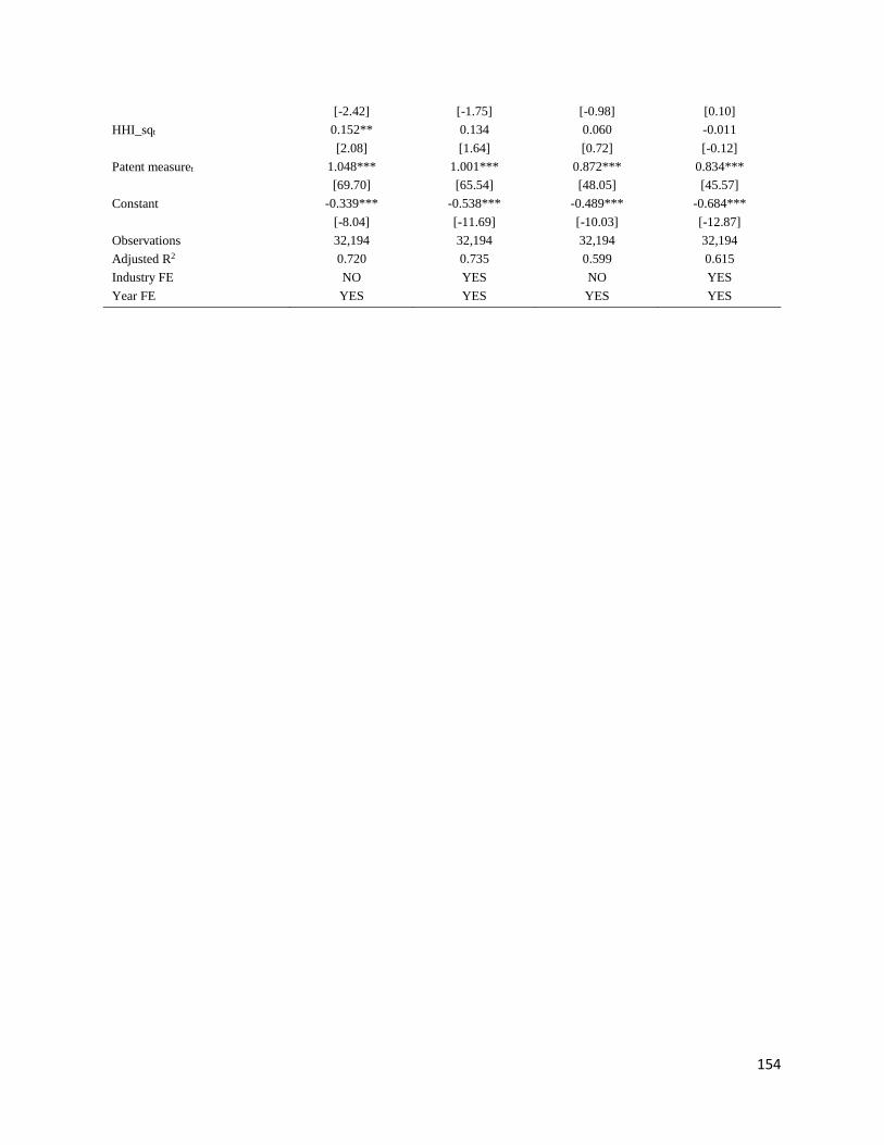
154

[-2.42] [-1.75] [-0.98] [0.10]

HHI_sqt 0.152** 0.134 0.060 -0.011

[2.08] [1.64] [0.72] [-0.12]

Patent measuret 1.048*** 1.001*** 0.872*** 0.834***

[69.70] [65.54] [48.05] [45.57]

Constant -0.339*** -0.538*** -0.489*** -0.684***

[-8.04] [-11.69] [-10.03] [-12.87]

Observations 32,194 32,194 32,194 32,194

Adjusted R2 0.720 0.735 0.599 0.615



155

Panel B: Effectiveness Measures

Generalityt+2 Originalityt+2 Citation per

Patentt+2

Economic

Valuet+2

Research

Quotientt+2

(1) (2) (3) (4) (5)

FX hedget 0.015*** 0.006** 0.015** 0.109*** 0.006*** [3.19] [2.06] [2.01] [4.79] [4.83]

Sizet 0.016*** 0.011*** 0.019*** 0.178*** 0.000 [11.52] [12.30] [8.20] [19.93] [0.42]

M/Bt 0.007*** 0.005*** 0.011*** 0.055*** 0.001*** [7.52] [7.36] [7.58] [13.57] [3.00]

Foreign incomet 0.005 0.000 0.001 0.071*** 0.004*** [1.11] [0.05] [0.24] [3.77] [3.39]

Leveraget -0.039*** -0.029*** -0.057*** -0.263*** -0.011*** [-5.84] [-6.57] [-5.57] [-9.47] [-3.78]

PPEt 0.005*** 0.003*** 0.009*** 0.020*** 0.001* [3.84] [3.29] [4.37] [3.64] [1.76]

ROAt 0.011** 0.009** 0.015* 0.028 0.007** [2.14] [2.33] [1.89] [1.54] [2.30]

Aget 0.001*** 0.000*** -0.001*** 0.004*** -0.000 [4.44] [3.80] [-5.01] [5.65] [-0.72]

Casht 0.035*** 0.020*** 0.086*** 0.260*** 0.002 [4.69] [3.84] [6.79] [9.66] [0.40]

CAPEXt 0.014 0.011 -0.000 0.113** -0.018*** [1.08] [1.22] [-0.02] [2.28] [-3.43]

Growtht -0.001 0.000 0.004** 0.006 0.002 [-0.49] [0.09] [2.22] [1.08] [1.58]

Instt -0.000 -0.006 -0.003 -0.187*** 0.001 [-0.02] [-1.41] [-0.26] [-6.35] [0.59]

Returnt 0.005** 0.004** 0.000 -0.019*** -0.000 [2.33] [2.49] [0.06] [-2.87] [-0.05]

Illiquidityt -0.007** 0.003* -0.002 0.117*** -0.003** [-2.47] [1.74] [-0.53] [10.85] [-2.12]

Return volatilityt -0.023 -0.037 0.129 1.082*** 0.037 [-0.30] [-0.74] [1.24] [4.28] [0.95]

HHIt -0.021 -0.008 0.028 0.019 -0.003 [-1.10] [-0.63] [0.88] [0.23] [-0.47]

HHI_sqt 0.028 0.012 -0.020 0.025 0.003 [1.55] [1.02] [-0.70] [0.33] [0.62]

Efficiency measuret 0.596*** 0.555*** 0.535*** 0.760*** 0.825***

[74.38] [66.99] [42.72] [101.37] [58.72]

Constant -0.090*** -0.050*** -0.093*** -0.545*** 0.006*

[-7.70] [-6.01] [-6.07] [-10.37] [1.74]

Observations 32,194 32,194 32,194 32,194 32,194

Adjusted R2 0.536 0.522 0.410 0.744 0.638

Industry FE YES YES YES YES YES

Year FE YES YES YES YES YES

156

Table 13 Cost of Capital

n this table, we examine the alternative explanation: cost of capital channel. In Panel A, we test the effect of FX hedge

on cost of capital. In columns (1) and (2), we use the implied cost of capital (ICC) at year t+1, while in columns (3)

and (4), we use ICC at year t+2. Columns (1) and (3) include year fixed effect, and columns (2) and (4) include year

and 2-digit SIC industry fixed effects. In Panel B, we add ICC as an additional control variable to the regression of

innovation outputs on FX hedge. Columns (1) and (2) test the effect of hedging on LnPatent, while columns (3) and

(4) test the effect on LnCitation. Columns (1) and (3) include year fixed effect, and columns (2) and (4) include year

and 2-digit SIC industry fixed effects. We cluster the standard errors at the firm level. ***, ** and * represent

significance levels at 1%, 5% and 10% respectively with t-statistics given in brackets.

Panel A: FX Hedging and Implied Cost of Capital ICCt+1 ICCt+2

(1) (2) (3) (4)

FX hedget -0.004*** -0.003*** -0.003*** -0.002

[-4.85] [-3.40] [-2.67] [-1.43]

Betat -0.007 -0.008* -0.006 -0.007

[-1.58] [-1.67] [-1.01] [-1.19]

Idiosyncratic Riskt 0.002 0.003 0.019* 0.018*

[0.18] [0.38] [1.71] [1.71]

Sizet -0.001* -0.001*** 0.000 -0.000

[-1.78] [-3.15] [0.30] [-0.71]

M/Bt -0.004*** -0.004*** -0.004*** -0.003***

[-15.22] [-14.37] [-11.83] [-10.59]

Foreign incomet 0.002* 0.003*** -0.002 -0.001

[1.70] [2.87] [-1.40] [-0.41]

Leveraget 0.008*** 0.006** 0.029*** 0.028***

[2.78] [1.98] [8.24] [7.83]

PPEt 0.002*** 0.001*** 0.001** 0.000

[4.73] [2.73] [2.08] [0.53]

ROAt 0.060*** 0.062*** 0.018*** 0.019***

[11.82] [11.95] [3.75] [3.85]

Aget 0.000*** 0.000*** 0.000*** 0.000***

[2.91] [2.79] [2.75] [2.79]

Casht 0.013*** 0.014*** 0.009** 0.011***

[4.46] [4.81] [2.51] [3.06]

CAPEXt -0.018*** -0.018*** -0.015** -0.020***

[-3.58] [-3.12] [-2.47] [-2.94]

Growtht 0.003*** 0.003*** 0.004*** 0.004***

[3.88] [3.52] [3.38] [3.18]

Instt 0.000 0.002 0.004* 0.004*

[0.17] [1.09] [1.79] [1.83]

Returnt -0.002*** -0.003*** 0.001 0.001

[-4.10] [-4.53] [1.34] [0.90]

Illiquidityt 0.015*** 0.014*** 0.016*** 0.015***

[7.75] [7.47] [7.47] [7.13]

Return volatilityt -0.438*** -0.419*** -0.110 -0.105

[-6.72] [-6.27] [-1.40] [-1.30]

HHIt 0.027*** 0.018*** 0.016*** 0.003

[5.28] [3.10] [2.74] [0.48]

HHI_sqt -0.021*** -0.015*** -0.008 0.001

157

[-4.33] [-2.75] [-1.41] [0.19]

ICCt 0.422*** 0.410*** 0.326*** 0.316***

[25.81] [25.32] [20.65] [19.88]

Constant 0.025*** 0.028*** 0.022*** 0.024***

[6.58] [7.30] [4.79] [5.25]

Observations 16,228 16,228 16,228 16,228

Adjusted R2 0.374 0.379 0.249 0.257



158

Panel B: Including Implied Cost of Capital LnPatentt+2 LnCitationt+2

(1) (2) (3) (4)

FX hedget 0.136*** 0.090*** 0.135*** 0.091***

[4.65] [3.15] [4.06] [2.78]

ICCt -0.137** -0.180*** -0.142** -0.178**

[-2.06] [-2.71] [-2.01] [-2.49]

Sizet 0.090*** 0.119*** 0.103*** 0.131***

[8.12] [10.49] [8.62] [10.74]

M/Bt 0.046*** 0.048*** 0.052*** 0.056***

[6.44] [6.98] [6.32] [6.94]

Foreign incomet 0.058* 0.040 0.059* 0.038

[1.96] [1.44] [1.79] [1.22]

Leveraget -0.234*** -0.248*** -0.251*** -0.263***

[-4.95] [-5.21] [-4.82] [-5.01]

PPEt 0.009 0.029*** 0.003 0.026***

[1.58] [3.54] [0.51] [2.82]

ROAt 0.088 0.087 0.113* 0.108*

[1.56] [1.59] [1.73] [1.71]

Aget -0.007*** -0.007*** -0.007*** -0.006***

[-8.64] [-8.68] [-7.31] [-7.32]

Casht 0.324*** 0.279*** 0.309*** 0.256***

[5.79] [5.05] [4.80] [4.02]

CAPEXt -0.101 0.115* -0.034 0.152*

[-1.62] [1.66] [-0.49] [1.94]

Growtht -0.002 -0.002 -0.005 -0.004

[-0.19] [-0.14] [-0.38] [-0.28]

Instt -0.055 -0.064 -0.084* -0.098**

[-1.25] [-1.48] [-1.70] [-2.02]

Returnt -0.005 0.001 0.000 0.004

[-0.70] [0.09] [0.02] [0.52]

Illiquidityt 0.053*** 0.089*** 0.086*** 0.124***

[3.04] [4.96] [4.58] [6.36]

Return volatilityt 2.083*** 1.964*** 1.746*** 1.515**

[3.91] [3.68] [2.93] [2.49]

HHIt -0.333*** -0.333*** -0.266** -0.237*

[-3.28] [-2.84] [-2.36] [-1.79]

HHI_sqt 0.296*** 0.297*** 0.217** 0.197*

[3.08] [2.81] [2.02] [1.65]

Patent measuret 1.101*** 1.039*** 0.970*** 0.915***

[63.66] [57.37] [50.61] [45.55]

Constant -0.334*** -0.578*** -0.441*** -0.699***

[-5.62] [-9.03] [-6.61] [-9.76]

Observations 18,301 18,301 18,301 18,301

Adjusted R2 0.762 0.776 0.661 0.676



159

Internet Appendix: Nonzero Innovation and Nonmissing R&D Subsamples

This table tests whether our findings are robust to the subsamples of nonzero innovation and nonmissing R&D

expenditures. In Panel A, we use the nonzero innovation subsample, while in in Panel B, we use the nonmissing R&D

subsample. Columns (1) and (2) test the effect of hedging on LnPatent, while columns (3) and (4) test the effect on

LnCitation. Columns (1) and (3) include year fixed effect, and columns (2) and (4) include year and 2-digit SIC

industry fixed effects.

Panel A: Nonzero Innovation Subsample

R&D/Assetst+2 LnPatentt+2 LnCitationt+2

(1) (2) (3) (4) (5) (6)

FX hedget 0.007** 0.006** 0.204*** 0.170*** 0.213*** 0.170*** [2.51] [2.14] [4.37] [3.86] [3.57] [2.97]

Sizet -0.010*** -0.009*** 0.314*** 0.360*** 0.325*** 0.360*** [-5.58] [-4.37] [17.39] [20.53] [14.61] [16.26]

M/Bt 0.012*** 0.011*** 0.056*** 0.066*** 0.072*** 0.083*** [5.94] [5.66] [8.22] [10.13] [7.68] [8.99]

Foreign incomet 0.002 0.001 -0.023 -0.038 -0.046 -0.068 [0.86] [0.41] [-0.58] [-1.04] [-0.88] [-1.34]

Leveraget 0.020 0.008 -0.566*** -0.491*** -0.760*** -0.659*** [1.40] [0.59] [-6.31] [-5.38] [-6.56] [-5.68]

PPEt 0.010*** 0.005** -0.054** 0.033 -0.074*** 0.037 [4.16] [1.99] [-2.54] [1.51] [-2.74] [1.28]

ROAt -0.074*** -0.066*** 0.153*** 0.054 0.285*** 0.153** [-5.55] [-4.87] [3.13] [1.19] [4.20] [2.36]

Aget 0.000 0.000 -0.013*** -0.009*** -0.013*** -0.010*** [1.52] [0.56] [-7.34] [-5.65] [-6.33] [-5.17]

Casht 0.093*** 0.082*** 0.182** 0.298*** 0.196* 0.362*** [4.47] [4.09] [2.42] [4.10] [1.91] [3.67]

CAPEXt -0.168*** -0.128*** 0.512*** 0.301** 0.580*** 0.299 [-3.94] [-2.89] [3.36] [2.04] [2.86] [1.46]

Growtht 0.001 0.001 -0.015 -0.005 -0.006 0.010 [0.28] [0.18] [-1.30] [-0.42] [-0.40] [0.64]

Instt 0.002 0.002 -0.162* -0.225*** -0.171 -0.250** [0.21] [0.20] [-1.84] [-2.72] [-1.44] [-2.23]

Returnt 0.004 0.005 0.008 0.010 0.004 0.008 [1.43] [1.59] [0.66] [0.79] [0.22] [0.43]

Illiquidityt -0.004 -0.004 0.074* 0.134*** 0.068 0.126** [-0.52] [-0.46] [1.96] [3.55] [1.32] [2.47]

Return volatilityt 0.110 0.269 6.118*** 5.167*** 5.728*** 4.308*** [0.54] [1.36] [5.50] [4.78] [3.79] [2.86]

HHIt -0.116*** -0.118*** -0.564** -0.319 -0.368 0.065 [-4.61] [-3.85] [-2.31] [-1.26] [-1.20] [0.20]

HHI_sqt 0.089*** 0.092*** 0.387 0.223 0.215 -0.087 [3.92] [3.44] [1.62] [0.93] [0.71] [-0.29]

Innovation

measuret

0.402*** 0.393*** 0.614*** 0.520*** 0.579*** 0.516***

[9.91] [9.80] [25.56] [20.40] [21.13] [18.09]

Constant 0.051*** 0.068*** -0.390*** -0.982*** -0.637*** -1.327*** [3.30] [4.03] [-3.33] [-8.43] [-4.17] [-8.64]

Observations 8,735 8,735 8,735 8,735 8,735 8,735

160

Adjusted R2 0.475 0.477 0.532 0.571 0.389 0.427

Industry FE NO YES NO YES NO YES

Year FE YES YES YES YES YES YES

161

Panel B: Nonmissing R&D Subsample

R&D/Assetst+2 LnPatentt+2 LnCitationt+2

(1) (2) (3) (4) (5) (6)

FX hedget 0.007*** 0.006** 0.186*** 0.118*** 0.212*** 0.136***

[2.98] [2.48] [4.70] [3.11] [4.59] [3.07]

Sizet -0.005*** -0.005*** 0.173*** 0.211*** 0.208*** 0.242***

[-3.71] [-3.15] [10.92] [13.16] [11.93] [13.74]

M/Bt 0.011*** 0.010*** 0.042*** 0.048*** 0.051*** 0.057***

[7.54] [7.24] [7.37] [8.90] [7.69] [9.12]

Foreign incomet 0.003 0.001 0.050 0.012 0.045 -0.001

[1.39] [0.52] [1.46] [0.37] [1.15] [-0.02]

Leveraget 0.001 -0.005 -0.403*** -0.313*** -0.493*** -0.385***

[0.05] [-0.47] [-6.71] [-5.26] [-6.94] [-5.51]

PPEt 0.008*** 0.004* 0.064*** 0.066*** 0.055*** 0.064***

[4.29] [1.91] [5.12] [5.11] [3.91] [4.22]

ROAt -0.071*** -0.067*** 0.083** 0.053* 0.124*** 0.085**

[-7.78] [-7.38] [2.39] [1.66] [3.16] [2.30]

Aget 0.000 -0.000 -0.011*** -0.011*** -0.010*** -0.010***

[0.99] [-0.68] [-8.45] [-9.03] [-6.90] [-7.30]

Casht 0.068*** 0.057*** 0.288*** 0.328*** 0.262*** 0.314***

[4.63] [4.08] [5.13] [5.97] [3.96] [4.91]

CAPEXt -0.137*** -0.104*** 0.071 0.276*** 0.088 0.261**

[-5.39] [-3.81] [0.70] [2.77] [0.77] [2.23]

Growtht -0.001 -0.002 0.001 0.006 0.009 0.015

[-0.50] [-0.66] [0.08] [0.73] [0.86] [1.50]

Instt 0.016** 0.016** -0.146** -0.164** -0.206*** -0.216***

[2.09] [2.02] [-2.13] [-2.54] [-2.60] [-2.88]

Returnt 0.005* 0.005* -0.000 0.001 -0.003 -0.001

[1.95] [1.92] [-0.02] [0.17] [-0.28] [-0.09]

Illiquidityt -0.002 -0.002 0.062*** 0.105*** 0.100*** 0.148***

[-0.48] [-0.38] [2.96] [5.07] [4.34] [6.47]

Return volatilityt 0.059 0.119 2.312*** 1.817*** 2.510*** 1.657**

[0.44] [0.90] [3.91] [3.21] [3.68] [2.48]

HHIt -0.113*** -0.106*** -0.744*** -0.634*** -0.622*** -0.361*

[-6.10] [-4.79] [-4.55] [-3.45] [-3.41] [-1.76]

HHI_sqt 0.094*** 0.090*** 0.589*** 0.498*** 0.490*** 0.272

[5.61] [4.59] [3.70] [2.89] [2.78] [1.43]

Innovation

measuret

0.454*** 0.446*** 1.006*** 0.946*** 0.883*** 0.834***

[10.43] [10.20] [52.65] [49.11] [41.01] [38.92]

Constant 0.020* 0.036*** -0.641*** -0.878*** -0.847*** -1.067***

[1.91] [2.97] [-7.54] [-10.22] [-8.91] [-11.01]

Observations 14,683 14,683 14,683 14,683 14,683 14,683

Adjusted R2 0.535 0.537 0.712 0.734 0.621 0.646

Industry FE NO YES NO YES NO YES

Year FE YES YES YES YES YES YES

162

Chapter 3

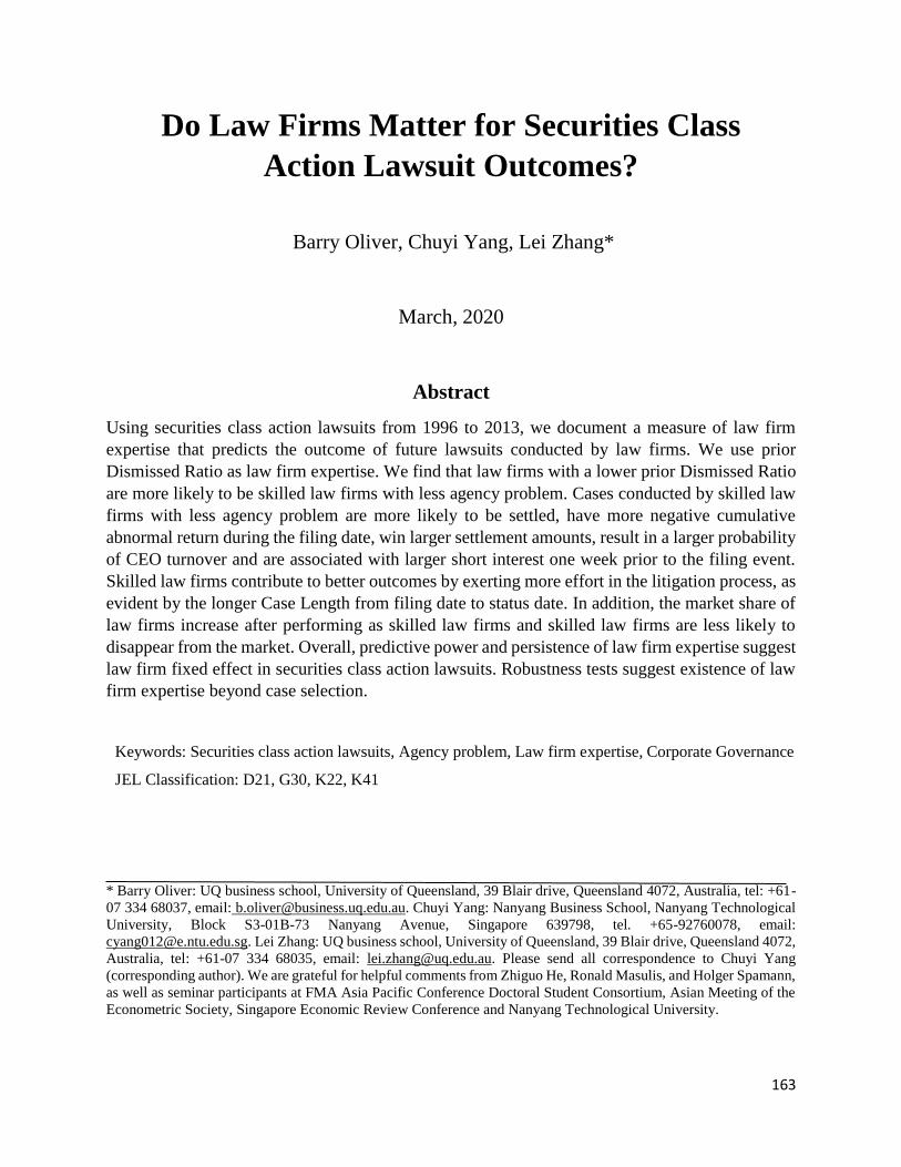
163

Do Law Firms Matter for Securities Class

Action Lawsuit Outcomes?

Barry Oliver, Chuyi Yang, Lei Zhang*

March, 2020

Abstract

Using securities class action lawsuits from 1996 to 2013, we document a measure of law firm

expertise that predicts the outcome of future lawsuits conducted by law firms. We use prior

Dismissed Ratio as law firm expertise. We find that law firms with a lower prior Dismissed Ratio

are more likely to be skilled law firms with less agency problem. Cases conducted by skilled law

firms with less agency problem are more likely to be settled, have more negative cumulative

abnormal return during the filing date, win larger settlement amounts, result in a larger probability

of CEO turnover and are associated with larger short interest one week prior to the filing event.

Skilled law firms contribute to better outcomes by exerting more effort in the litigation process, as

evident by the longer Case Length from filing date to status date. In addition, the market share of

law firms increase after performing as skilled law firms and skilled law firms are less likely to

disappear from the market. Overall, predictive power and persistence of law firm expertise suggest

law firm fixed effect in securities class action lawsuits. Robustness tests suggest existence of law

firm expertise beyond case selection.

Keywords: Securities class action lawsuits, Agency problem, Law firm expertise, Corporate Governance

JEL Classification: D21, G30, K22, K41

* Barry Oliver: UQ business school, University of Queensland, 39 Blair drive, Queensland 4072, Australia, tel: +61-

07 334 68037, email: [email protected]. Chuyi Yang: Nanyang Business School, Nanyang Technological

University, Block S3-01B-73 Nanyang Avenue, Singapore 639798, tel. +65-92760078, email:

[email protected]. Lei Zhang: UQ business school, University of Queensland, 39 Blair drive, Queensland 4072,

Australia, tel: +61-07 334 68035, email: [email protected]. Please send all correspondence to Chuyi Yang

(corresponding author). We are grateful for helpful comments from Zhiguo He, Ronald Masulis, and Holger Spamann,

as well as seminar participants at FMA Asia Pacific Conference Doctoral Student Consortium, Asian Meeting of the

Econometric Society, Singapore Economic Review Conference and Nanyang Technological University.

mailto:[email protected]

164

I. Introduction

Plaintiff law firms are at centre stage of securities class action lawsuits28. Traditionally, law firms

are viewed as an agent of the client and advise as independent professionals. However, in the

scenario of class actions, dispersed and disorganized shareholders, as plaintiffs, do not have the

incentives nor ability to effectively monitor the law firms. In “large-scale, small-claim” litigation,

agency costs of law firms arise when the individual interest of the class is small and the overall

liability is large (Macey and Miller, 1991). There has been long-time debate on whether securities

class action lawsuits is of merit due to the expertise and agency problem of law firms. The

enforcement system and incentive structure implies that risk-averse law firms prefer to settle

(Coffee, 1986), because the attorney fee comes from the recovery for the class members

(Alexander, 1991; Coffee, 1986; Macey and Miller, 1991). Therefore, it leads to excessive

settlement rates or extremely low settlement amounts (Starkman, 1997; Niehaus and Roth, 1999;

Perino, 2012). Consequently, law firms derive private interests that diverge from shareholders,

bear the litigation risk, and “exercise plenary control over nearly all important decisions in the

lawsuit” (Macey and Miller, 1991).

Given the controversial and complex features of securities class actions as inferred above, it is

interesting to quantify the existence of law firm expertise and agency problem. If heterogeneous

law firm expertise lead to different outcomes, then it implies that law firms play an important role

in shaping the results of securities class actions. If law firms indeed provide expertise in the

litigation process, cases conducted by law firms with higher quality and less agency problem would

28 Securities class action litigation under Securities and Exchange Commission Rule 10b-5 is filed on firms where

there is allegation of omission of material facts or misrepresentation of information that inflates the market price of

the firm’s stocks.

165

achieve more favorable outcomes. In contrast, if law firms exhibit pure rent seeking behavior and

litigate only for the purpose of earning attorney fees, law firm expertise could not predict litigation

outcomes. The existence of law firm expertise remains an unexplored empirical question. In

different settings, performance of investment banks (Ban and Edmans, 2011), auditors (Cai et al.,

2016) and legal advisors29 (Beatty and Welch, 1996; Krishnan and Masulis 2013) have been widely

studied in the M&A and IPO literature. In contrast to performance persistence documented in

investment banks, auditors, and legal advisors, existence of skilled mutual fund managers is not

found (Carhart (1997)). In the paper, we propose a quantitative measure for law firm expertise and

agency problem in securities class actions. Particularly, we use Dismissed Ratio (DR) as the proxy

for both expertise and agency problem, which is calculated in a rolling window of 5 years30 prior

to filing date of the case. As law firms have the opportunistic behavior of excessive settlement due

to the contingency attorney fee, settling the case might not indicate that the case is of merit. In

contrast, dismissing the case provides a clear evidence that the case is of less merit. Since law

firms will not be reimbursed following unsuccessful action, they must conduct cost benefit analysis

in advance to determine whether to undertake the action (Coffee, 2006). Law firms will therefore

advance the expense of the action and estimate the expected fee award. Most importantly, the law

firms are the principal enforcer of securities law liabilities, and are indifferent to the source of the

29 Beatty and Welch (1996) adopts prior market shares to identify top law firms in the context of IPO and studies the

reputation effect of advisers. Using market share measure, the effect of legal advisor expertise has been studied in the

context of mergers and acquisitions in Krishnan and Masulis (2013). It is found that bidder law firms with top market

share are associated with higher offer completion rates, whereas top target law firms are associated with higher offer

withdrawal rates.

30 Our results remain robust using rolling window of 3 years or 4 years.

166

settlement. According to Weiss and Beckerman (1995), class counsel usually prefer a quick

settlement and conduct the litigation in an aggressive manner.

Hence, at the law firm level, dismissing more cases proportional to all cases taken previously

is a signal of relative lower expertise and larger agency problem. We further document DR to be

a significant predictor for litigation outcomes: cases conducted by skilled law firms are more likely

to be settled, have more negative cumulative abnormal returns during the filing dates, win larger

settlement amounts, and are associated with larger short interest in the filing months.

In addition to outcome predictability, we further examine the corporate governance outcomes

of cases conducted by skilled law firms. This is because lawsuits by shareholders are filed after

the break down of other mechanisms. Indeed, we found that cases conducted by skilled law firms

will result in larger probability of CEO turnover. By linking law firm expertise and agency problem

measure to CEO turnover, we contribute to the literature on shareholders rights and litigation

risk31. Law firms could contribute to better corporate governance outcomes through litigating cases

that are of merit. We therefore supplement the study on the monitoring role of institutions32 in the

lawsuits.

31 Lowry and Shu (2002) study litigation risk related to IPO underpricing; Skinner (1994, 1997) study financial

reporting and accounting disclosure; Crane (2011) studies leverage effects; Seetharaman, Gul, and Lynn (2002) study

audit fees; Arena and Julio (2015) study corporate savings and investment policy.

32 Cheng et al. (2010) study the function of institutional monitoring and conclude that institutional lead plaintiffs will

lead to less likelihood of dismissal and larger monetary settlements. In addition, subsequent governance improvements

in the long term demonstrates the effectiveness of institution monitoring. In Wei and Zhang (2016), a firm-level

measure of litigation risk is created for firms sharing the same institutional shareholders. They find that this

shareholder linkage predicts short interest and cash holdings, reflecting weak governance and poor monitoring by

institutional shareholders.

167

Besides DR, we identify two other measures of law firms that are related to efforts and market

share respectively. For law firms that possess better expertise and less agency problem, they are

more likely to devote themselves in the cases. We therefore use Case Length (CL)33 as a proxy for

law firm efforts. Indeed, we find that skilled law firms pay more efforts and conduct due diligence

during the litigation process, and is associated with longer CL. In addition, the Market Share

(MS)34 of a law firm increases after performing as a skilled law firm and skilled law firms are less

likely to disappear from the market. This suggests that clients do recognize the expertise of law

firms and skilled law firms will have increasing market share after better performance. Therefore,

we document the existence of law firm fixed effects in securities class action lawsuits and provides

implications for the traceable evidence for law firm expertise.

We address the case selection versus law firm expertise issue by focusing on the cases where

case selection is minimized. If prior results are driven by systematic selection of cases with certain

characteristics by law firms, then it is more likely that law firms select cases in the same industry.

Therefore, we create a Dismissed Ratio excluding cases in the same industry for the focal case,

and it remains a significant predictor for litigation outcomes. Hence, our results are not entirely

driven by case selection.

Identifying expertise and agency problems of plaintiff law firms has been difficult. Firstly,

plaintiff law firms seek a viable strategy to file frivolous lawsuits to conduct discovery and to find

claims that were not alleged in the complaint. Moreover, this opportunistic behavior of law firms

33 Case Length (CL) is the number of days between filing dates and status dates, scaled by 365 days.

34 Market Share (MS) is defined as number of cases conducted by a law firm divided by number of all cases in year

t.

168

is often confounded by the unobservable reason of large stock price declines following optimistic

statements for outside investors: whether it is due to fraud, risk, market movement, or simple bad

luck (Pritchard and Ferris, 2001). Prior to 1995, law firms opportunistically attempted to profit

from stock price falls and would approach and persuade the plaintiff shareholders to file for class

action lawsuits35. Nevertheless, not all significant price declines at the disclosure will lead to class

actions. The opportunistic behavior of plaintiff law firms has led to the enactment of 1995 Private

Securities Litigation Reform Act (PSLRA)36, which is intended to curtail frivolous securities

lawsuits and prevent professional advisors from abusive class action litigation. The nature of

securities fraud changes over time. In recent times, lawsuits have been filed when there are serious

declines in the fortune of the firm.

In spite of the important role of law firms in all the stages of securities class action lawsuits,

there is scant research that has identified which dimensions of law firms really matter for the

litigation outcome. A closely related paper written by Badawi and Webber (2015) gauges the

quality of law firms in deal litigation by using the settlements published by RiskMetrics and annual

rankings of Securities Class Action Services (SCAS). Their main focus is the case selection ability

of law firms and their sample only includes law firms that appear on the SCAS top 10 list at least

once during 2003 to 2008. Another study by Krishnan, Solomon and Thomas (2016) identifies the

35 Alexander (1991) and Jones and Weingram (1996) contend large and sudden stock price declines during information

releases as a measure of ex ante litigation risk. Kellogg (1984) have documented the price declines that have triggered

the securities class litigation are larger than 10% of firm market capitalizations. Beck and Bhagat (1997) adopt two

criteria to jointly access unusual negative share-price performance. These are a combination of cumulative quarterly

raw returns less than -0.1 and cumulative abnormal returns less than -0.2.

36 Particularly, there are three mechanisms in the PSLRA, all of which are targeted at the law firms’ incentives and

behaviors. The three mechanisms are summarized in Choi and Thompson (2006) as “raising the bar as to what

constitutes securities fraud, empowering lead plaintiffs to rein in their lawyers in class actions, and requiring judges

to sanction securities lawyers for frivolous litigation”.

169

top 5 law firms in merger litigation only and gauges the effectiveness of law firms based on the

number of lead or co-lead counsel and the ability to obtain attorney fees. They find that top law

firms are less likely to dismiss cases and they obtain higher settlement amounts. In addition, they

also find that top law firms submit more filings and more docket entries, which is consistent with

our results that skilled law firms spend more efforts during the litigation process.

Different from prior literature, our paper gauges both law firm expertise and agency problems

quantitatively in a unifying manner. Furthermore, we do not rely on existing rankings to identify

top law firms. Instead, we gauge law firm expertise and agency problems by utilizing past lawsuit

information, as dismissing the case is a definite signal of lower law firm expertise and larger

agency problem. Our aim is to examine whether law firm characteristics is a determinant of

litigation outcomes, from the perspectives of both law firm expertise and agency problems.

Particularly, we shed light on whether law firm expertise is an omitted variable in the current

models of securities class action outcomes.

We also add to the debate on the merit of securities class action lawsuits. According to Griffin,

Grundfest and Perino (2004), proponents contend the rife of securities fraud among public

companies and support litigation as supplement to the anti-fraud enforcement program of SEC.

Opponents hold the view that the litigation process creates incentives for law firms to benefit from

the merit of plaintiffs’ claims37. There are also criticisms of filing frivolous or low-probability

37 For example, Macey and Miller (1991) has criticized the regulatory system and advocated a reform to reduce agency

costs when law firms control the litigation. Macey and Miller (1991) further point out the fundamental error of

regulatory shortfalls as failure to recognize the difference between “entrepreneurial litigation nature of class action”

and “traditional litigation”. Romano (1991) questions the efficacy of shareholder litigation as a governance mechanism

since the cost of bringing a lawsuit exceeds the “pro rata benefit of shareholder-plaintiff”. Principal-agent problem

arises from the misalignment between law firms’ incentives and shareholders’ interest. Romano (1991) argues that

law firms, instead of shareholders are the principal beneficiaries of cash payouts in lawsuits. Grundfest (1994) argues

that lawsuits will be of no merit if law firms expect the defendants to settle and attorney fee is larger than law firms’

litigation cost. Judges, practitioners, and academics have been increasingly criticized that plaintiff law firms take

170

lawsuits for the purpose of coercing settlements (Coffee, 2006). Furthermore, Beck and Bhagat

(1997) identifies another criticism as the stack of allegations. The actual proof of the allegation is

unknown since the case is not adjudicated but simply settled. By identifying a measure of law firm

quality, we would be able to imply the case outcomes and merit from the law firms involved in the

case.

Last but not least, our law firm expertise measure sheds light on the effectiveness of PSLRA.

Since the enactment of PSLRA in 1995, a strand of literature has studied the market reaction38 to

the PSLRA and assesses the effectiveness of the regulation. Choi and Thompson (2006) examined

the effectiveness of the focus of PSLRA in regulating lawyers’ behavior in the first decade after

the enactment. They find that institutional lead plaintiffs tend to repeat relationships with certain

top law firms after the PSLRA. Despite the increasing cost in filing lawsuits after PSLRA, plaintiff

law firms could still approach individual shareholders as “group of persons” with the largest

financial stake, according to Berger, Coffey, and Silk (2001). Nevertheless, in our findings, law

firms have a higher probability of existing after performing as low quality law firms, as measured

by high DR ratio. This suggests the effectiveness of PSLRA that clients could imply the quality of

law firms and low quality law firms would therefore have decreasing market share.

advantage of the litigation system by settling too cheaply instead of raising stronger claims (Thomas and Thompson,

2012). Macey and Miller (1991) further point out the fundamental error of regulatory shortfalls as failure to recognize

the difference between “entrepreneurial litigation nature of class action” and “traditional litigation”.

38 Johnson, Kasznik and Nelson (2000) studied the reaction of stock price to PSLRA using high-technology firms,

showing that PSLRA is less beneficial for firms for which lawsuits are meritorious but wealth-increasing for firms

with greater risk of class actions. Spiess and Tkac (1997) confirmed the dominance of the positive effects of the act

over the inability to bring meritorious suits using four industries: biotechnology, computers, electronics, and retailing.

171

The paper is structured as follows. Section II develops hypothesis. Section III describes data

and variables. Section IV presents results. Section V provides robustness test. Section VI

concludes.

II. Hypothesis Development

We developed three testable hypothesis related to plaintiff law firms’ expertise and agency

problems in the securities class action lawsuits. The first hypothesis is the law firm skill hypothesis.

This hypothesis argues that law firm skill matters in the likelihood of a case being dismissed. The

second hypothesis is the predictive outcome hypothesis. This argues that skilled law firms will

achieve more favorable litigation outcomes. The third hypothesis is the law firm effort hypothesis.

This argues whether skilled law firms will exert more effort and provide better outcomes. The

fourth hypothesis is the market share hypothesis. This tests the predictive power of market share

and whether clients chase past performance. These hypotheses are stated as follows:

H1: Law firms with lower prior Dismissed Ratios are skilled law firm with less agency problems.

H2: Law firms with lower prior Dismissed Ratios are more likely to conduct cases with meritorious

outcomes. Skilled law firms will have higher probability of settling the case in the future, and more

negative market reaction at the filing event date, achieve higher settlement amount and are

associated with greater short interest of the sued company prior to the filing date.

H3: Law firms with lower prior Dismissed Ratios will put more effort into the litigation process

and it takes longer time for the results of the case to be revealed.

H4: Law firms with lower prior Dismissed Ratios will have increasing market share in the future.

Law firms with higher prior Dismissed Ratios will more likely disappear from the market.

172

III. Data and Variables

i. Data

Security class action information is obtained from the Stanford Law School Securitas Class Action

Clearinghouse http://securities.stanford.edu/index.html. Sample period of the lawsuits ranges from

1996 to 2013. The lawsuits with ongoing status as of May 1st, 2016 are excluded from the sample.

Since it takes 5 years to compute the Dismissed Ratio for year 2001, lawsuits from 1996 to 2000

are used to compute initial independent variables and are therefore excluded from dependent

variables. Due to the availability of control variables, 1420 lawsuits filed between 2001 and 2013

are included for the analysis. Stock returns and accounting data are from CRSP and

COMPUSTAT. Institutional holdings data are from Thomason CDA/Spectrum 13F database.

Settlement amounts are from RiskMetrics.

ii. Main Variables

a. Class Period Start Date, Class Period End Date, Filing Date, Status Date

The fact that several distinct and sequential events characterize the litigation process

aggravates the complexity of the litigation. Upon a serious price decline, plaintiff’ counsel analyses

the events for corrective disclosure and facts that might lead to the filing. The truth is revealed to

the market at the class period end date. Therefore, the Beginning of the Class Period (BCP) marks

the beginning of the fraud on the market. The Class Period End Date (CPED) is the date of a

corrective disclosure. The class period starts from the date where the defendant committed the

alleged misconduct and ends on the date of the revelation of the event. The CP is the period

between BCP and CPED. Niehaus and Roth (1999) indicates that corporate insiders are usually

the net sellers during the Class Period (CP), though average selling behavior is not abnormal. After

the end of CPED, filing of the complaint happens on the Filing Date (FD). Since filing action is

http://securities.stanford.edu/index.html

173

regarded as a foregone conclusion by the market, market reaction on the FD manifests the residual

uncertainty since the CPED (Griffin, Grundfest and Perino, 2004).

The events studied in this paper are consistent with Griffin, Grundfest and Perino (2004),

which analyze stock price responses to news at class period start dates, class period end dates and

filing dates. They find that the market interprets these three events in a sequential and conditional

way. They further find no price momentum beyond announcement dates, suggesting the efficiency

of markets. Using a different time period of cases, it takes close to two years on average from filing

to settlement for class actions in Klausner and Hegland (2010). Gande and Lewis (2009) reveals

the partial anticipation of lawsuits by shareholders through other firms in the same industry and

the capitalization of losses prior to lawsuit filing dates. Therefore, using filing dates alone will

understate the magnitude of shareholder losses.

A typical timeline for a securities class action lawsuit is as follows:

Class Period Start Date Class Period End Date Filing Date Status Date

1) Class Period Length = Class Period End Date – Class Period Start Date

2) Filing Period Length = Filing Date – Class Period End Date

3) Case Length = Status Date – Filing Date

b. Dismissed Ratio (DR)

The Dismissed Ratio (DR) is calculated in a rolling window of 5 years prior to filing date of the

case, which is intended to minimize look-ahead bias. DR for law firm j at time t is defined as the

number of dismissed cases divided by the total number of cases conducted by law firm j from year

t-5 to year t-1. Aggregated at the case level, DR for lawsuit i is defined as the average of DR of all

174

law firms j engaging in case i. Following Bao and Edmans (2011) and Krishnan, Solomon and

Thomas (2016), each law firm is given full credit for each lawsuit it is engaged. Therefore, each

measure at the case level is the equal weighted average of all law firms engaging in the case.

We used the past 5 years to calculate DR since the mean number of years for the results of the

cases to be known is between 4 and 5 years. Considering the economic meaning of DR, we drop

the observations when law firms conduct less than 5 cases within the prior five years. In unreported

results, using the prior 3 or 4 years suggests qualitatively similar conclusions. Consistent with prior

literature, Cheng et al. (2010) considers the lower likelihood of dismissal as a meritorious outcome.

Krishnan, Solomon and Thomas (2016) argue that top law firms file cases that are less likely to be

dismissed.

c. Case Length (CL)

Case Length (CL) is the number of days between filing dates and status dates, scaled by 365 days.

CL is a measure of law firm efforts and an implicit indicator of agency problems. The possibility

of using time length for the test is made possible due to the clear identification of different stages

in securities class action data. Since only investors who bought or sold a company’s securities

within a specific period of time (class period) file for the litigation, the timeline for the class action

is trackable and is available in the filing files. After controlling for case characteristics, time length

of different stage of the case partially reveals the effort of law firms, and less efforts further

suggests larger agency problems. If the law firm is skilled or does not file for frivolous cases for

quick settlement, then the settling period will more likely to be longer.

A longer CL is consistent with findings in Krishnan, Solomon and Thomas (2016) that top law

firms might “file for more documents and bring injunction motions to enjoin a transaction”. A

175

longer class period is likely to be related to larger investor damages and also to prove the scienter

of the defendant, as documented in Cheng et al. (2010). In Cheng et al. (2010), they provided

evidence that institutional lead plaintiffs will influence the settlement time on behalf of investors.

However, they do not conclude whether a longer or shorter period is beneficial. In this paper, a

detailed look into CL will help refine the answer. Weiss and White (2004) also reveals the negative

side of law firms as “file early, then free ride”, since law firms are there to settle cases instead of

litigating. Consistent with our third hypothesis, Bajaj, Mazumdar and Sarin (2002) compare the

average speed of settlements before and after the reform. The average speed of settlements are 4

and 5 years in pre and after reform period respectively. Their results partially support our

hypothesis that law firms with less agency problems tend to have longer Case Length and file for

less frivolous lawsuits, which is in line with the trend of less frivolous lawsuits after the PSLRA.

Moreover, Case Length is related to the area of behavioral law and economics. In Daniel

Kahneman’s book “Thinking, fast and slow”, two systems of thinking are proposed: the intuitive

and quick “system 1” and the deliberate and slow “system 2”. Olazabal (2012) shows that the

speed of thinking is related to scienter and psychological illusion not only exists in individual but

also in organizations. A slower organizational thinking will help to reduce recklessness and

prevent securities fraud. In a similar manner, a slower thinking process for law firms will curb the

frivolous lawsuits and reduce agency costs of the law firms. The comparable notion of “system 2”

thinking applied to law firms would translate into a longer Case Length.

d. Market Share (MS)

In Beatty and Welch (1996) and Krishnan and Masulis (2013), market share of law firms is used

as proxy for law firm expertise. In this paper, Market Share (MS) of law firm j in year t is defined

as the number of cases conducted by law firm j in year t, divided by the total number of cases in

176

year t. If the law firm has lower DR in the past, then the market share of the law firm will increase

in the future. Consistent with prior literature, Choi and Thompson (2006) use pre-PSLRA market

share as a proxy for expertise and examine whether law firms with higher pre-PSLRA market share

will increase in the post-PSLRA period. In addition, we also test whether the DR or the MS have

any predictive power for the survival of law firms.

e. Prior Average CAR

Bao and Edmans (2011) show that the existence of investment bank fixed effects implies the

persistence of bank average CARs in M&A events. Similarly, in this paper we use alternative law

firm fixed effects measured by law firm Prior Average CAR as robustness. For each case i, we

average the prior 5 years of Cumulative Abnormal Returns of the cases conducted by law firms

engaged in the case i. If the dependent variable is CAR (-1,1), then prior average CAR is the prior

5 years of average CAR (-1,1). If the dependent variable is CAR (-10,1) or CAR (-30,1), then the

prior average CAR is measured based on (-10,1) or (-30,1) correspondingly.

iii. Control Variables

Firm-level controls include size, Market to Book ratio, book leverage, profitability, cash holdings,

Amihud illiquidity measure (Amihud, 2002), industry classification and stock return volatility.

Since size is likely to be correlated with the limits for insurance policies and the undisclosed policy

limits are highly correlated with settlement amounts, firm size is likely to be a determinant of

lawsuit outcomes. Market to Book ratio controls for the growth opportunity of firms, since rapid

growth firms will tend to misstate financial statements to present a stable growth picture

(Loebbecke et al., 1989; Beasley, 1996). According to Coffee (2006), there are three factors that

might principally determine the probability of a firm being sued: stock price volatility, industry

177

classification and firm size. Kim and Skinner (2012) have identified measure of firm

characteristics including size, growth and stock volatility as predictive measure of litigation risk,

in addition to previous documented industry membership. Kim and Skinner (2012) further argue

that corporate governance quality proxy and managerial opportunism do not provide additional

predictive power for litigation risk, these variables are therefore not included as control variables

in this paper.

Following Cheng et al. (2010), two dummy variables are used to control for the allegation type.

IPO dummy is equal to 1 if the case is related to IPO violations. GAAP dummy is equal to 1 if the

lawsuit involves violations of Generally Accepted Accounting Principles (GAAP). A pension

dummy is added to consider for pension fund participation, due to the importance of institution

types in the lawsuit. According to Murphy and Van Nuys (1994) and Woidtke (2002), public

pension fund managers are more likely to lead securities class litigation due to political or

reputational reasons. It is also shown that public pension funds are more effective in shareholder

activism (Gillan and Starks, 2000). Industry dummy is equal to 1 if the industry is biotechnology,

computer, and retail (Francis, Philbrick, and Schipper (1994a, 1994b). Biotech: SIC codes 2833-

2838 8731-8734; Computer: SIC codes 3570-3577, 7370-7374; Electronics: SIC codes 3600-

3674; Retail: SIC codes 5200-5961.

These set of variables control for the firms’ prior performance and are measured one year

before the lawsuit. This is to avoid the effect of stock price falls that triggers the lawsuit. Year

fixed effects are included to control for time-varying macroeconomic trends. Standard errors are

clustered at the law firm level in the regressions. Summary statistics of main variables and control

variables are in Table I.

[Insert Table I Here]

178

From Table I, the average CAR around the announcement date (-1,1) is -3.93%. Strikingly,

average CAR for the period 10 days before the announcement is -10.1% and for the period 30 days

prior to the announcement is as large as -15.3%. The average settlement amount is $98.19 million

with a maximum of $7,241 million and minimum of just over $400,000. The mean whole period

length is 5.6 years, with a mean class period length of 1.23 years. The mean case length is around

4 years.

IV. Results

We tabulate the ranking of law firms by the number of cases conducted in our sample period, and

report law firms that conducted more than 100 cases in Table II. We give full credit to each law

firm if multiple law firms are involved in one case. As shown in Table II, Milberg Weiss Bershad

Hynes & Lerach LLP conducted over 1,000 cases and represented approximately 10% of the total

number of cases. The Dismissed Ratio for this firm is 0.23. This means that 23% of the total

number of cases conducted by this firm in the past 5 years were dismissed. Among the firms

tabulated in Table II, Robbins, Geller Rudman and Dowd LLP has the highest Dismissed Ratio,

implying that 55% of their cases in the past 5 years were dismissed.

[Insert Table II Here]

i. Predicting Litigation Outcome

We test the second implication of our hypothesis that cases conducted by skilled law firms are

more likely to be settled. A probit model is used to examine the relation between law firm expertise

proxy (Dismissed Ratio) and the probability of settling. This model is shown below:

Litigation Status Dummyi,t = α + λ × Dismissed Ratioi,t−1 + γ × Xi,t−1 + εi.t (1)

179

where Litigation Status Dummy is 1 if the case is settled and 0 if the case is dismissed. In Column

(1), we study the effect of Dismissed Ratio on Litigation Status Dummy. In Column (2), we add

characteristics of the firm involved in the securities class action lawsuits. The vector of control are

as previously defined in the control variables session. We additionally control for year fixed effect

in column (3) and (4). In Column (4), we further include the type of the case and industry dummies.

Following Cheng et al. (2010), two dummy variables are used to control for the allegation type.

IPO dummy is equal to 1 if the case is related to IPO violations. GAAP dummy is equal to 1 if the

lawsuit involves violations of Generally Accepted Accounting Principles (GAAP). A pension

dummy is added to consider for pension fund participation, due to the importance of institution

types in the lawsuit. As shown in Table III, we find a significantly negative relation between the

DR and the litigation dummy across four different specifications of Model 1. This provides

preliminary evidence that skilled law firms (lower prior Dismissed Ratio) are more likely to settle

cases in the future. The status of settlement is associated with more favorable litigation outcomes.

On average, firm characteristics such as size, illiquidity and institutional ownership are

significantly related to case outcomes.

[Insert Table III Here]

ii. Cumulative Abnormal Return

We next focus on the cumulative abnormal return (CAR (-1,1), CAR(-10,1), CAR (-30,1)) around

the filing date. Stock prices are expected to decline during the filing of the lawsuit, since securities

class action lawsuits usually involve disclosure of bad news. According to Gande and Lewis

(2009), there are two components related to the expected losses. The first aspect is the response to

the information that triggers the lawsuit and the second aspect is the deadweight loss born by the

180

impaired shareholders. The cumulative abnormal return around the filing date is calculated using

market model with -300 to -46 days before the filing date as the estimation period.

The dependent variable of column (1) CAR (-1,1) is the 3-day CAR around the filing date,

from one day before the filing date to one day after the filing date. In Column (2), the dependent

variable CAR(-10,1) is 12-day CAR around the filing date, from ten days before the filing date to

one day after the filing date. In Column (3), dependent variable CAR (-30,1) is 32-day CAR around

the filing date, from thirty days before the filing date to one day after the filing date. Across all

three specifications, the Dismissed Ratio is positive and significant. This means that lower quality

law firms are correlated with higher (less negative) CARs, and similarly higher quality firms

conduct cases with lower CARs. More negative market reaction further supports the hypothesis

that skilled law firms with less agency problems will file for less frivolous lawsuits, which is

related to release of negative information and therefore more negative market reaction.

In addition, we find larger market reactions during the longer event horizon CAR (-30, 1) and

CAR (-10, 1), which is consistent with the corporate disclosure policies of firms at risk of litigation.

Upon the filing of a lawsuit by the skilled law firm, there is additional negative market reaction

relative to the filing effect (Badawi and Webber (2015)). Skinner (1994) has documented the

preemptive disclosure behavior of firms to reduce the risk of being sued. Romano (1991)

interpreted the negative stock price effect before filing as the expectation that lawsuits will

adversely affect firm future cash flows. In a stock price reaction event study by Pritchard and Ferris

(2001), there is a large and significant negative reaction to revelation of potential fraud, a smaller

but significant reaction to filing and no significant reaction to the dismissal of a lawsuit.

[Insert Table IV Here]

181

iii. Settlement Amount

In the securities class action lawsuits, law firms obtain their attorney fee contingent on the total

settlement amount. Eisenberg and Miller (2004) report an average attorney fee of 21.9 percent of

the total recovery for lawsuits from 1993 to 2002, and conclude the amount of client recovery as

the key determinant of the attorney fee, providing a better explanatory power than the lodestar

calculation (product of hours and hourly rate) by the court. An earlier study by Martin, Juneja,

Foster, and Dunbar (1999) estimate the fee to be between 30 and 33 percent of the settlement

amount. Kritzer (2002) undermines the myths of contingency fees and makes an argument that

“contingency fee lawyers and their clients are routinely in conflict”. Hence, the contingency

attorney fee leads to a statement that securities class actions are frivolous and only benefit the law

firms, casting doubt on whether the fees awarded by courts follow the reasonableness checking

against the lodestar calculation. Therefore, settlement amount is a key indicator of whether the

lawsuits are of merit. In Table V Column (1), we calculate settlement amounts scaled by the market

capitalization of firms one year prior to the beginning of the class period action. In Column (2),

we exclude all cases with zero settlement amount. In Column (1), it is shown that law firms with

a lower Dismissed Ratio will settle the case with large settlement amount. Our result remains

robust when we exclude cases with a zero settlement amount in Column (2). Higher settlement

amounts could be translated into better law firm skills and less agency problems, since the class

will get a larger recovery. In addition, attorney fees are contingent on the amount of settlement

recovery in U.S., and therefore skilled law firms will perform due diligence to achieve higher

settlement amounts.

[Insert Table V Here]

182

iv. Utilization Rate

Since information about future stock price movements are contained in the short selling activity

(Miller, 1977; Diamond and Verrecchia, 1987; Diether, Lee, and Werner, 2009), utilization rate in

the month of filing date is another relevant test for law firm expertise. We measure utilization rate

as the ratio of number of shares borrowed to the number of shares willing to be lent by institutional

investors. Following Blau and Tew (2001), Gande and Lewis (2009), and Wei and Zhang (2016),

we test whether markets anticipate the litigation risk. Blau and Tew (2001) investigated the

hypothesis that lawyers might leak information about filing dates to short sellers on purpose. High

return predictability of short selling and increases in short selling activities are documented during

the pre-filing period. Gande and Lewis (2009) document negative market reaction to peer firms

generated by lawsuits. It is likely that short sellers infer the information from the law firm expertise

to exploit litigation risk.

In Table VI, a lower Dismissed Ratio predicts a higher short interest in the one week prior to

the filing event. The coefficient is not significant in the week of the filing nor one week after the

filing. The utilization rate results are consistent with results in Table IV that a lower Dismissed

Ratio predict more negative market reaction in the cases conducted by the law firms.

[Insert Table VI Here]

v. Case Length

Case Length (CL) is the number of days between filing dates and status dates, scaled by 365 days.

CL is a measure of law firm efforts and an implicit indicator of agency problems. According to

Krishnan, Solomon and Thomas (2016), top law firms might “file for more documents and bring

injunction motions to enjoin a transaction”. Completion time is also studied in other contexts such

183

as mergers and acquisitions (M&A), where investment banks might have a different interest

compared with their principal, either bidder or target. However, the agency problem of investment

banks could not be measured, since a deal is only known at announcement and the effort of

investment banks is before the announcement. Hence, there is no available data on either the time

length of effort or amount of effort by the investment bank. Investment banks with less agency

problem could either complete the deal quickly or slowly, as the time length is only measurable

upon announcement before which a lot of effort of investment bank have been invested. Therefore,

although completion time of M&As is used to study legal advisor expertise in Krishnan and

Masulis (2013), they did not interpret completion time as a measure of agency problem. In Deng,

Kang and Low (2013), completion time is regarded as the ex-post obstacle to complete the deal

from stakeholders. Deng, Kang and Low (2013) show that acquirers conducting more corporate

social responsibilities take less time to complete the M&A deal.

In Table VII, we study whether Dismissed Ratio is a predictor of Case Length conducted by

the law firms in the future. We control for year fixed effect in Column (2) and (3), and additional

firm characteristics in Column (3). In all specifications, skilled law firms will put more effort in

the litigation process, as evident by longer case length. In Panel B, we further separately study the

Case Length effect in the subsample of settled case and dismissed case respectively. The law firm

expertise measure remains significant after controlling for the outcome of the case. This effect is

significant in the settled subsample but not in the dismissed subsample, suggesting that the result

is not driven by the shorter length of dismissed case compared with the settled case. For the cases

that ultimately settle, law firms also put more effort into the litigation process. Therefore, we might

interpret agency problems of law firms from the time length.

[Insert Table VII Here]

184

vi. Market Share

In Beatty and Welch (1996) and Krishnan and Masulis (2013), market share of law firms is used

as proxy for law firm expertise. In this paper, Market Share (MS) of law firm j in year t is defined

as the number of cases conducted by law firm j in year t, divided by the total number of cases in

year t. If the law firm has lower DR in the past, then the market share of the law firm will increase

in the future. Whether law firm skill has an impact on the market share of law firms provides

answer to whether clients chase performance.

In Table VIII Panel A, we find that a lower Dismissed Ratio predicts an increase in the market

share in the future, suggesting that law firm skill matters and is recognized by the market. In Panel

B, we study whether larger Dismissed Ratio, proxy for lower quality of law firms, could predict

disappearance of the law firm in the future. We define a Disappear Dummy for law firm j in year

t+K, which equals to 1 if law firm has zero market share in the year t + k and nonzero market share

in the year t; equals to 0 otherwise. K equals to 3, 4, or 5 years. A larger Dismissed Ratio will

increase the likelihood of law firms disappearing from the market after 3, 4, or 5 years.

[Insert Table VIII Here]

vii. CEO turnover

Shareholders exercise their rights through dividends, voting, selling stocks and suing in the event

of material misstatement or omission of fact. Lawsuits by shareholders are filed after the break

down of other mechanisms. According to Shleifer and Vishny (1997), class actions play an

important role as a corporate governance mechanism. After the settlement of lawsuits, top

management can face adverse consequences as a result of lawsuits. CEO turnover represents a real

consequence of the lawsuits on the corporate governance of the defendant firm. If lawsuits result

185

in CEO turnover after the class period, then it could shed light on the debate on whether lawsuits

have merit, and whether lawsuits are pure settlement seeking behavior of law firms. Niehaus and

Roth (1999) document larger probability of CEO turnover rates in the defendant firms that settle,

compared with a match sample with large stock price falls. They also find that CEO turnover is

related to insider sales during the class period and the settlement amount of the lawsuit. Livingston

(1996) also documents abnormally high management turnover for firms that are filed lawsuits by

the SEC. Strahan (1998) finds that firms more subject to agency problems are more likely to be

filed for class actions and CEO turnover increases significantly after the filings for these firms.

In Table IX, we relate our measure of law firm expertise, the Dismissed Ratio, to both CEO

turnover and forced turnover in the year of filing event. If lawsuits are of merit and the law firms

indeed play a role in achieving meritorious outcomes in lawsuits, then we would expect law firms

with smaller dismissed ratio, who are more likely to file for meritorious cases in the past, predict

larger likelihood of CEO turnover. In Table IX, we use the Dismissed Ratio to predict the

probability of CEO turnover in column (1) and forced CEO turnover in column (2). Consistent

with our hypothesis, law firms with smaller Dismissed Ratios are related to larger CEO turnover

and forced turnover, after controlling for case characteristics. In addition to supporting the merit

of securities class actions, CEO turnover also provides deterrent effects and could foster the release

of information. Despite the majority of settlements coming from insurance and indemnification

agreements (Martin, Juneja, Foster, and Dunbar, 1999, and Arlen and Carney, 1992), potential

CEO turnover suggests that top managers could be disciplined by the corporate governance

mechanism by shareholders and in the market for corporate control. Thus, our results not only

reinforce prior results on the meritorious nature of securities class action litigation, but also pioneer

work in relating law firm expertise to real consequences of lawsuits.

186

[Insert Table IX Here]

V. Robustness

Though our proxy for law firm expertise, the Dismissed Ratio could predict the lawsuit outcomes

well, whether it represents law firm’s selection into cases or law firm’s ability to shape the

outcomes remains unclear. Therefore, we conduct several robustness tests to partially address the

selection versus ability issue. First, we split the sample by the case count of each law firm and

define a law firm to be large law firm if the number of cases conducted by the law firm is above

the 25 percentile of law firms in our sample. We define a law firm to be small law firm if the

number of cases conducted by the law firm is below the 75 percentile of law firms in our sample.

When calculating the Dismissed Ratio, only large law firms or small law firms are used separately

for each case. The cut off points are selected to remove the effect of extremely large or small law

firms and to ensure we have sufficient observations for the Dismissed Ratio and regression

analysis. We report the main tests of case outcomes and cumulative abnormal returns for large and

small law firms separately in Table X. Panel A1 and A2 document large law firms and Panel B1

and B2 document results of small law firms.

Our main results show cases conducted by law firms with lower Dismissed Ratio have a larger

probability of settlement, are associated with a more negative market reaction, which holds for

large and small firms separately. To the extent that small firms are less likely to select the cases,

the qualitatively similar results in the small firm sample suggest the role of law firm ability is a

factor in the outcomes.

[Insert Table X Here]

187

As a further attempt to separate selection from ability, we exclude cases of the same industry

sector when calculating the Dismissed Ratio of the focal case. If prior results are driven by

systematic selection of cases with certain characteristics by law firms, then it is more likely that

law firms select cases in the same industry. When calculating the Dismissed Ratio for case i, we

exclude cases in the same industry as case i during the calculation. The industry sector is defined

for each case on the Stanford Law School Securitas Class Action Clearinghouse website and

includes: Basic Materials, Capital Goods, Conglomerates, Consumer Cyclical, Consumer Non-

Cyclical, Energy, Financial, Healthcare, Services, Technology, Transportation, and Utilities. We

perform our main regressions using the Dismissed Ratio calculated by excluding the same

industry. If law firms are more likely to select cases within the same industry, then the

predictability of the Dismissed Ratio calculated using cases in other industries suggest the presence

of law firm expertise beyond case selection.

We present the results in Table XI panel A for case outcomes and panel B for cumulative

abnormal returns (CAR). The results remain qualitatively the same with our regression results in

Table III and IV when all cases are included. In addition, the effect of the Dismissed Ratio on the

CARs is slightly stronger when same industry cases are excluded in the calculation of the

Dismissed Ratio. Though we cannot fully rule out selection from ability and case selection as not

entirely independent from prior records of law firms, the robustness tests on size and industry

suggests the presence of law firm ability beyond selection in shaping the litigation outcomes.

[Insert Table XI Here]

As an alternative measure of law firm expertise, we use another measure based on past CAR

of cases conducted by all law firms engaging in the focal case. The past 5 year average of CAR is

188

measured in a similar way to the Dismissed Ratio, except that we use the CAR instead of the

percentage of dismissed cases by the law firms.

In Table XII, we use the past CAR measures to predict the CAR of the focal case with three

windows. For each case i, we average the prior 5 years of Cumulative Abnormal Returns of the

cases conducted by law firms engaged in the case i. For the regression with the dependent variable

of CAR (-1,1), the Prior Average CAR is measured using the prior CAR (-1,1). Similarly, for the

regressions with the dependent variables of CAR (-10,1) and CAR (-30,1), the Prior Average CAR

is measured using the prior CAR (-10,1) and CAR (-30,1), respectively. Other studies that use

persistence of CAR to study performance persistence include Bao and Edmans (2011) who study

investment bank fixed effects. We find a highly persistent law firm performance from the measure

of past average CAR, further confirming law firm fixed effects in the securities class action

lawsuits.

[Insert Table XII Here]

VI. Conclusions

Performance persistence and expertise of financial intermediaries or professional advisors are

often obscure and difficult to measure. Securities class action lawsuits provide a unique and ideal

playground to test the agency problem of law firms. This paper provides novel evidence in

interpreting the agency problem and law firm expertise from the Dismissed Ratio. The Dismissed

Ratio could predict various dimensions of lawsuit outcomes such as status, CAR and settlement

amounts. Particularly, Case Length is a traceable indicator of law firm effort and agency problems,

since abundant literature on law firms documented agency problems, such as settling quickly for

189

small settlements. A longer Case Length suggests that law firms conduct due diligence in

investigating the truth and fight for justice.

The contributions of the research are as follows. First, this paper contributes to the law firm

fixed effects literature by identifying law firm characteristics that have predictive power for future

lawsuit results. Second, this paper contributes to the strand of literature on litigation risk. This

paper hinges on components of risk arising from the agency problem of law firms, since they are

the group that approach shareholders for initiation of litigation after calculating their expected

attorney fees. Last but not least, this paper adds to the debate on whether securities class action is

of merit from the perspective of law firm expertise. The paper provides policy implication for the

regulation of securities class actions and the attorney fees. Competent law firms might be rewarded

higher due to the different source of settlements, instead of the aggregate amounts. The testable

measure of law firm competency would be an indicator of law firm agency problems, and partially

a determinant of the attorney fee in the settlements. This paper also partially sheds light on the

effectiveness of PSLRA after two decades by a direct examination of plaintiff law firms’

behaviors.

In addition to agency problem and expertise of plaintiff’s law firms, director & officer (D&O)

insurance adds another layers of agency problem by insiders which remains an interesting future

topic. It remain an interesting topic to explore the interaction effect of agency problem of both

plaintiff’s law firms and directors with D&O insurance.

190

References

Alexander, J.C., 1991, Do the merits matter? A study of settlements in securities class

actions, Stanford Law Review, 497-598.

Amihud, Y., 2002, Illiquidity and stock returns: Cross-section and time series effects, Journal of

Financial Markets, 5, 31–56.

Arena, M. and Julio, B., 2015, The Effects of Securities Class Action Litigation on Corporate

Liquidity and Investment Policy, Journal of Financial and Quantitative Analysis, 50(1-2), 251–

275. doi: 10.1017/S0022109015000010.

Arlen, J. H., and Carney, W. J., 1992, Vicarious Liability for Fraud on Securities Markets: Theory

and Evidence. U. Ill. L. Rev., 691.

Badawi, A.B. and Webber, D.H., 2015, Does the Quality of Plaintiffs' Law Firm Matter in Deal

Litigation. J. Corp. L., 41, 359.

Bajaj, M., Mazumdar, S.C. and Sarin, A., 2002, Securities class action settlements, Santa Clara L.

Rev., 43, 1001.

Bao, Jack, and Alex Edmans., 2011, Do Investment Banks Matter for M&A Returns?, Review of

Financial Studies, 24, 2286–2315.

Beasley, M.S., 1996, An empirical analysis of the relation between the board of director

composition and financial statement fraud, Accounting Review, 443-465.

Beatty, Randolph P., and Ivo Welch., 1996, Issuer Expenses and Legal Liability in Initial Public

Offerings, Journal of Law and Economics, 39, 545–602.

Beck, J.D. and Bhagat, S., 1997, Shareholder Litigation: Share price movements, news releases,

and settlement amounts, Managerial and Decision Economics, 563-586.

Berger, M., Coffey, J., Silk, G., 2001, A Forward-looking Statement: Institutional Investors as

Lead Plaintiffs: Is There a New and Changing Landscape? St. John’s Law Review, 75, 31–46.

Blau, B.M. and Tew, P.L., 2011, Short Sales, Class-Action Lawsuits, and Potential Information

Leakages. Class-Action Lawsuits, and Potential Information Leakages, January 6,

Cai, Y., Kim, Y., Park, J.C. and White, H.D., 2016, Common auditors in M&A transactions.

Journal of Accounting and Economics, 61(1), pp.77-99.

Carhart, M. M. ,1997, On persistence in mutual fund performance. The Journal of finance, 52(1),

57-82.

Cheng, C. A., Huang, H. H., Li, Y., & Lobo, G. ,2010, Institutional monitoring through shareholder

litigation. Journal of Financial Economics, 95(3), 356-383.

Choi, S.J. and Thompson, R.B., 2006, Securities Litigation and its Lawyers: Changes During the

First Decade after the PSLRA, Columbia Law Review, 1489-1533.

Crane, A.D., 2011, The Litigation Environment of a Firm and its Impact on Financial Policy,

191

working paper, Rice University.

Coffee, J.C., 1986, Understanding the Plaintiff's Attorney: The implications of economic theory

for private enforcement of law through class and derivative actions, Columbia Law Review, 86(4),

669-727.

Coffee, J.C., 2006, Reforming the Securities Class Action: An Essay on Deterrence and Its

Implementation, Columbia Law Review, 106(7), 1534-1586.

Diamond, D. and Verrecchia, R., 1987, Constraints on Short Selling and Asset Price Adjustment

to Private Information. Journal of Financial Economics, 18, 277-312.

Deng, X., Kang, J.K. and Low, B.S., 2013, Corporate Social Responsibility and Stakeholder Value

Maximization: Evidence from Mergers, Journal of Financial Economics, 110(1), 87-109.

Diether, K., Lee, K and Werner, I., 2009, Short-Sale Strategies and Return Predictability. Review

of Financial Studies 22, 575-607.

Eisenberg, T. and Miller, G.P., 2004, Attorney Fees in Class Action Settlements: An empirical

study, Journal of Empirical Legal Studies, 1(1), 27-78.

Gande, A., Lewis, C., 2009, Shareholder Initiated Class Action Lawsuits, Shareholder Wealth

Effects and Industry Spillovers, Journal of Financial and Quantitative Analysis, 44, 823-850.

Gillan, S., Starks, L., 2000, Corporate Governance Proposals and Shareholder Activism: The Role

of Institutional Investors, Journal of Financial Economics 57, 275–305.

Griffin, P. A., Grundfest, J. A. and Perino, M. A., 2004, Stock Price Response to News of

Securities Fraud Litigation: An Analysis of Sequential and Conditional Information, Abacus, 40,

21–48. doi:10.1111/j.1467-6281.2004.00149.x

Grundfest, J.A., 1994, Why disimply. Harv. L. Rev, 108, 727.

Francis, J., Philbrick, D., Schipper, K., 1994a, Shareholder Litigation and Corporate Disclosures,

Journal of Accounting Research, 32, 137–164.

Francis, J., Philbrick, D., Schipper, K., 1994b. Determinants and Outcomes in Class Action

Securities Litigation, Working Paper, University of Chicago.

Johnson, M.F., Kasznik, R. and Nelson, K.K., 2000, Shareholder Wealth Effects of the Private

Securities Litigation Reform Act of 1995, Review of Accounting Studies, 5(3), 217-233.

Jones, C.L. and Weingram, S.E., 1996, The Determinants of 10b-5 Litigation Risk. Available at

SSRN 2684.

Kahneman, D., 2011, Thinking, fast and slow. Macmillan.

Kellogg, R. L., 1984, Accounting Activities, Security Prices, and Class Action Lawsuits, Journal

of Accounting and Economics, 6(3).

192

Kim, I. and Skinner, D.J., 2012, Measuring Securities Litigation Risk, Journal of Accounting and

Economics, 53(1), 290-310.

Klausner, M. and Hegland, J., 2010, When are Securities Class Actions Dismissed, When do

they Settle, and for How Much?, Part II, Professional Liability Underwriting Society Journal

23, 1–5.

Kritzer, H.M., 2002, Seven Dogged Myths Concerning Contingency Fees, Wash. ULQ, 80, 739.

Krishnan, C.N.V. and Masulis, R.W., 2013, Law Firm Expertise and Merger and Acquisition

Outcomes, Journal of Law and Economics, 56(1), 189-226.

Krishnan, C.N.V., Solomon, S.D. and Thomas, R.S., 2016, Who are the Top Law Firms? Assessing

the Value of Plaintiffs' Law Firms in Merger Litigation, American Law and Economics Review,

18(1), 122-154.

Livingston , J., 1996, Management-Borne Costs of Fraudulent and Misleading Financial Reporting

Available at SSRN: https://ssrn.com/abstract=2815.

Loebbecke, J.K., Eining, M.M. and Willingham, J.J., 1989, Auditors Experience with Material

Irregularities-Frequency, Nature, and Detectability, auditing- A Journal of Practice and Theory,

9(1), 1-28.

Lowry, M. and Shu, S., 2002, Litigation Risk and IPO Underpricing, Journal of Financial

Economics, 309–336.

Macey, J. and Miller, G., 1991, The Plaintiffs’ Attorney’s Role in Class Action and Derivative

Litigation: Economic Analysis and Recommendations for Reform. University of Chicago Law

Review, 58, 1–118.

Martin, D.N., Juneja, V.M., Foster, T.S. and Dunbar, F.C., 1999, Recent trends IV: What Explains

Filings and Settlements in Shareholder Class Actions, Stan. JL Bus. & Fin., 5, 121.

Miller, E.M., 1977, Risk, Uncertainty, and Divergence of Opinion, Journal of Finance 32, 1151-

1168.

Murphy, K., Van Nuys, K., 1994, State Pension Funds and Shareholder Inactivism, Unpublished

working paper, Harvard University, Cambridge, MA.

Niehaus, G. and Roth, G., 1999, Insider Trading, Equity Issues and CEO Turnover in Firms

Subject to Securities Class Action, Financial Management, 52-72.

Olazábal, A.M., 2012, Behavioral Science and Scienter in Class Action Securities Fraud

Litigation, Loy. U. Chi. LJ, 44, 1423.

Perino, M., 2012, Institutional activism through litigation: An empirical analysis of public pension

fund participation in securities class actions. Journal of Empirical Legal Studies, 9(2), pp.368-392.

https://ssrn.com/abstract=2815

193

Pritchard, A.C. and Ferris, S.P., 2001, Stock Price Reactions to Securities Fraud Class Actions

Under the Private Securities Litigation Reform Act, Michigan Law and Economics Research

Paper, (01-009).

Romano, R., 1991, The Shareholder Suit: Litigation without Foundation?, Journal of Law,

Economics, & Organization, 7(1), 55-87.

Seetharaman, A., Gul, F., Lynn, S., 2002, Litigation Risk and Audit Fees: Evidence from UK

Firms Cross-Listed on US Markets, Journal of Accounting and Economics, 33, 1–115.

Shleifer, A., & Vishny, R. W., 1997, A Survey of Corporate Governance, The Journal of Finance,

52(2), 737-783.

Skinner, D.J., 1994, Why Firms Voluntarily Disclose Bad News?, Journal of Accounting

Research, 32, 38–60.

Skinner, D.J., 1997, Earnings Disclosures and Stockholder Lawsuits, Journal of Accounting

and Economics, 23, 249–282.

Spiess, D.K. and Tkac, P.A., 1997, The Private Securities Litigation Reform Act of 1995: The

Stock Market Casts Its Vote, Managerial and Decision Economics, 545-561.

Starkman, D., l997, Fraud—Suit Plaintiffs, Lawyers Draw Fire, Wall Street Journal (October 28).

BIZ.

Strahan, Philip E., 1998, Securities Class Actions, Corporate Governance and Managerial Agency

Problems, Available at SSRN: https://ssrn.com/abstract=104356 or

http://dx.doi.org/10.2139/ssrn.104356.

Thomas, R.S. and Thompson, R.B., 2012, Theory of Representative Shareholder Suits and Its

Application to Multijurisdictional Litigation, A. Nw. UL Rev., 106, 1753.

Wei, C. and Zhang, L., 2016, Identifying Ineffective Monitors From Securities Class Action

Lawsuits. Available at SSRN: https://ssrn.com/abstract=2809016.

Weiss, E., Beckerman, J., 1995, Let the Money do the Monitoring: How Institutional Investors

Can Reduce Agency Costs in Securities Class Actions, Yale Law Journal, 104, 2053–2128.

Weiss, E.J. and White, L.J., 2004, File Early, then Free Ride: How Delaware Law (Mis) Shapes

Shareholder Class Actions, V and. L. Rev., 57, 1797.

Woidtke, T., 2002, Agents Watching Agents?: Evidence from Pension Fund Ownership and Firm

Value, Journal of Financial Economics, 63, 99–131.

194

Table I Summary Statistics

This table reports summary statistics of the sample of cases. It documents the number of observations, mean, standard

deviation, minimum and maximum values for the variables.

(1) (2) (3) (4) (5)

VARIABLES Number of

Observations

Mean Standard

Deviation

Minimum Maximum

CAR (-1,1) 1,209 -0.0393 0.152 -1.062 1.001

CAR (-10,1) 1,211 -0.101 0.275 -1.308 1.961

CAR (-30,1) 1,211 -0.153 0.393 -1.601 1.916

Status Dummy 1,420 0.648 0.478 0 1

Settlement (US$millions) 387 98.19 451.4 0.406 7,241

Dismissed Ratio 1,189 0.456 0.140 0 1

Utilization Rate 642 26.51 29.02 0 97.87

Whole Period Length (yrs) 1,417 5.616 2.964 0.255 16.26

Class Period Length (yrs) 1,417 1.233 1.081 0 7.501

Filing Period Length (yrs) 1,417 0.386 0.512 0 4.863

Case Length (yrs) 1,420 4.001 2.577 0.175 11.84

Profit (US$millions) 1,212 -0.0112 0.267 -3.422 0.427

Cash Holding (US$millions) 1,212 0.302 0.273 0 0.997

Yearly Return (%) 1,212 -0.0703 0.821 -0.890 2.988

Illiquidity 1,211 0.116 0.201 0.004 2.955

Volatility 1,201 0.0416 0.0243 0.006 0.148

Institution Ownership 1,202 0.495 0.292 0.000 1

GAAPdummy 1,212 0.408 0.492 0 1

IPOdummy 1,212 0.272 0.445 0 1

PensionDummy 1,212 0.259 0.438 0 1

Market Share (%) 384 0.0173 0.0261 0.000384 0.153

195

Table II Top 20 Law Firm Cases

This table reports summary statistics of law firm case frequencies, percentage of total cases, and average Dismissed

Ratio from 1996 to 2013. The top 20 law firms ranked by number of cases are listed.

Law Firm

Number

of Cases

Percent (%) of

Total Cases

Dismissed

Ratio

Milberg Weiss Bershad Hynes & Lerach LLP 1,023 9.92 0.23

Schiffrin & Barroway LLP 612 5.93 0.21

Stull, Stull & Brody 509 4.93 0.19

Wolf Haldenstein Adler Freeman & Herz LLP 506 4.9 0.16

Bernstein Liebhard & Lifshitz, LLP 420 4.07 0.17

Lerach Coughlin Stoia Geller Rudman & Robbins LLP 394 3.82 0.35

Milberg Weiss Bershad & Schulman LLP 357 3.46 0.21

Sirota & Sirota LLP 314 3.04 0.01

Bernstein Litowitz Berger & Grossmann LLP 192 1.86 0.15

Labaton Sucharow & Rudoff LLP 191 1.85 0.29

Berger & Montague PC 171 1.66 0.27

Coughlin Stoia Geller Rudman & Robbins LLP 169 1.64 0.51

Robbins Geller Rudman & Dowd LLP 159 1.54 0.55

Weiss & Yourman 154 1.49 0.36

Cohen Milstein Hausfeld & Toll PLLC 151 1.46 0.29

Glancy Binkow & Goldberg LLP 130 1.26 0.45

Berman DeValerio Pease Tabacco Burt & Pucillo 109 1.06 0.21

Kaplan Fox & Kilsheimer, LLP 107 1.04 0.21

Barrack, Rodos & Bacine 105 1.02 0.33

196

Table III Predicting Future Litigation Result

This table shows whether our proxy for law firm expertise could predict the probability of settling the case

conducted by the law firm. Specifically, we estimate the following probit model:

Litigation Status Dummyi,t = α + λ × Dismissed Ratioi,t−1 + γ × Xi,t−1 + εi.t (1)

Where the dependent variable is a dummy variable that equals to 1 if the case being sued in year t is ultimately settled

and 0 being dismissed. The main variables of interest are Dismissed Ratioi,t−1, defined as the equal-weighted

Dismissed Ratio (number of dismissed case/number of total case) for each law firm j engaging in the lawsuit i from

year t-5 to year t-1. In Column (1), we study the effect of Dismissed Ratio on Litigation Status Dummy. In Column

(2), we add characteristics of the firm involved in the securities class action lawsuits. The vector of control are defined

in the control variables session. We additionally control for year fixed effect in column (3) and (4). In Column (4), we

further include the type of the case and industry dummies. Robust standard errors with z-statistics are given in

parentheses. ***, ** and * represent significance levels at 1%, 5%, and 10%, respectively.

(1.1) (1.2) (1.3) (1.4)

Litigation Status Dummy

Dismissed Ratio -0.646*** -0.520*** -0.366*** -0.369***

(-6.29) (-5.12) (-3.42) (-3.52)

Size -0.025*** -0.029*** -0.030***

(-2.71) (-3.07) (-3.35)

Market to Book -0.003 -0.009* -0.007

(-0.71) (-1.81) (-1.34)

Leverage 0.076 0.077 0.100

(1.06) (1.11) (1.45)

Profitability 0.009 -0.058 -0.076

(0.13) (-0.77) (-1.02)

Cash Holding -0.068 -0.067 -0.101

(-0.98) (-0.96) (-1.41)

Return -0.048** -0.033 -0.024

(-2.56) (-1.54) (-1.13)

Illiquidity -0.358*** -0.253** -0.191*

(-3.16) (-2.34) (-1.92)

Volatility 4.061*** 1.092 -0.479

(3.86) (0.83) (-0.36)

Institutional Ownership -0.172*** -0.106* -0.102*

(-2.96) (-1.81) (-1.74)

Industry Dummy -0.015

(-0.48)

GAAP Dummy 0.056**

(1.99)

IPO Dummy 0.259***

(5.05)

Pension Dummy 0.016

(0.48)

Year FE No No Yes Yes

Observations 1,189 1,169 1,169 1,169

197

Table IV Cumulative Abnormal Return (CAR) of Litigation

In this table, we present the relation between law firm expertise proxies and CAR of different event windows. The

cumulative abnormal return around the filing date is calculated using market model with -300 to -46 days before the

filing date as the estimation period.

The dependent variable of column (1) is the 3-day CAR around the filing date, from one day before the filing date to

one day after the filing date. In Column (2), the dependent variable is 12-day CAR around the filing date, from ten

days before the filing date to one day after the filing date. In Column (3), dependent variable is 32-day CAR around

the filing date, from thirty days before the filing date to one day after the filing date.

Main independent variables are the Dismissed Ratio. We control for firm characteristics, year fixed effect, industry

dummies, and the type of the case in all columns.

𝐶𝐴𝑅 (−1,1)𝑖,𝑡 = 𝛼 + 𝛽 × Dismissed Ratio𝑖,𝑡−1 + 𝛾 × 𝑋𝑖,𝑡−1 + 𝜀𝑖.𝑡 (2.1)



Robust standard errors with t-statistics are given in parentheses. ***, ** and * represent significance levels at 1%, 5%,

and 10%, respectively.

198

(2.1) (2.2) (2.3)

CAR (-1,1) CAR (-10,1) CAR (-30,1)

Dismissed Ratio 0.090** 0.116* 0.230***

(2.20) (1.76) (2.68)

Size 0.002 0.008 0.020***

(0.78) (1.60) (2.95)

Market to Book -0.002* -0.005 -0.007

(-1.68) (-1.62) (-1.47)

Leverage -0.008 -0.038 -0.067

(-0.40) (-0.90) (-1.06)

Profitability -0.007 0.014 0.051

(-0.29) (0.30) (0.75)

Cash Holding 0.011 -0.071* -0.038

(0.47) (-1.66) (-0.67)

Return -0.013 -0.035** -0.071***

(-1.42) (-2.15) (-3.55)

Illiquidity -0.052 0.022 0.076

(-1.37) (0.18) (0.53)

Volatility 0.338 1.034 2.408**

(0.85) (1.35) (2.03)

Institutional Ownership 0.004 0.010 0.050

(0.21) (0.28) (1.12)

Industry Dummy 0.005 0.008 0.029

(0.54) (0.48) (1.23)

GAAP Dummy -0.011 -0.026 -0.024

(-1.18) (-1.44) (-0.92)

IPO Dummy 0.006 0.093*** 0.130***

(0.42) (3.38) (2.77)

Pension Dummy 0.007 0.007 0.025

(0.74) (0.39) (1.01)

Constant -0.105*** -0.241*** -0.533***

(-2.66) (-3.21) (-5.29)

Year FE Yes Yes Yes


R-squared 0.033 0.071 0.101

r2_a 0.011 0.050 0.080

199

Table V Settlement Amount

In this table, we document the relation between the settlement amount and the Dismissed Ratio. The dependent

variable in both columns are settlement amount, scaled by the total market capitalization of the firm one year prior to

the beginning of the securities class litigation. The first column contains all available settlement dollar data. The

second column excludes zero settlement dollar data.

𝑆𝑒𝑡𝑡𝑙𝑒𝑚𝑒𝑛𝑡_𝑆𝑐𝑎𝑙𝑒𝑑𝑖,𝑡 = 𝛼 + 𝛽 × 𝐷𝑖𝑠𝑚𝑖𝑠𝑠𝑒𝑑 𝑅𝑎𝑡𝑖𝑜𝑖,𝑡−1 + 𝛾 × 𝑋𝑖,𝑡−1 + 𝜀𝑖.𝑡 (3)

We control for firm characteristics, year fixed effect, industry dummies, and the type of the case in all columns.

Robust standard errors with t-statistics are given in parentheses. ***, ** and * represent significance levels at 1%, 5%,

and 10%, respectively.

(3.1) (3.2)

Scaled Settlement Dollars Scaled Settlement Dollars

Exclude 0 Settlement

Dismissed Ratio -68.640** -91.890**

(-2.54) (-2.40)

Size -2.874** -4.032*

(-2.06) (-1.86)

Market to Book -1.843 -2.529

(-1.13) (-1.19)

Leverage 9.535 22.56

(0.78) (0.94)

Profitability 44.900* 66.650**

(1.85) (2.16)

Cash Holding 14.700 19.940

(0.82) (0.89)

Return 1.472 2.216

(0.31) (0.36)

Illiquidity 29.350 25.450

(0.75) (0.56)

Volatility 996.900*** 1,126.000**

(2.68) (2.56)

Institutional Ownership -27.910* -43.610*

(-1.72) (-1.91)

Industry Dummy -9.977 -10.930

(-1.35) (-1.11)

GAAP Dummy 2.647 0.640

(0.49) (0.07)

IPO Dummy 18.220 17.410

(0.74) (0.60)

Pension Dummy -1.711 -4.618

(-0.29) (-0.52)

Constant 62.860** 94.510**

(2.51) (2.35)

Year FE Yes Yes

Observations 598 373

R-squared 0.154 0.182

r2_a 0.115 0.123

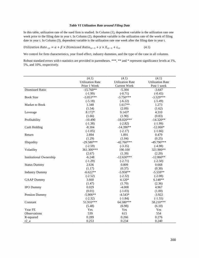
200

Table VI Utilization Rate around Filing Date

In this table, utilization rate of the sued firm is studied. In Column (1), dependent variable is the utilization rate one

week prior to the filing date in year t. In Column (2), dependent variable is the utilization rate of the week of filing

date in year t. In Column (3), dependent variable is the utilization rate one week after the filing date in year t.

𝑈𝑡𝑖𝑙𝑖𝑧𝑎𝑡𝑖𝑜𝑛 𝑅𝑎𝑡𝑒 𝑖,𝑡 = 𝛼 + 𝛽 × 𝐷𝑖𝑠𝑚𝑖𝑠𝑠𝑒𝑑 𝑅𝑎𝑡𝑖𝑜𝑖,𝑡−1 + 𝛾 × 𝑋𝑖,𝑡−1 + 𝜀𝑖.𝑡 (4.1)

We control for firm characteristics, year fixed effect, industry dummies, and the type of the case in all columns.

Robust standard errors with t-statistics are provided in parentheses. ***, ** and * represent significance levels at 1%,

5%, and 10%, respectively.

(4.1) (4.1) (4.1)

Utilization Rate

Prior 1 Week

Utilization Rate

Current Week

Utilization Rate

Post 1 week

Dismissed Ratio -15.760** -5.304 -3.647

(-1.99) (-0.71) (-0.45)

Book Size -3.053*** -3.750*** -3.529***

(-5.18) (-6.22) (-5.49)

Market to Book 1.348 1.617** 1.273

(1.54) (2.09) (1.62)

Leverage 8.172* 9.143* 4.310

(1.66) (1.90) (0.83)

Profitability -10.490 -18.020*** -14.320**

(-1.38) (-2.82) (-1.99)

Cash Holding -8.304 -14.390** -12.060*

(-1.05) (-2.17) (-1.66)

Return 2.894 1.891 0.479

(1.29) (1.04) (0.25)

Illiquidity -29.580*** -42.760*** -49.790***

(-2.59) (-3.35) (-4.98)

Volatility 361.300*** 190.100 321.900**

(2.67) (1.39) (2.20)

Institutional Ownership -6.248 -12.630*** -12.860**

(-1.29) (-2.71) (-2.50)

Status Dummy 2.636 0.809 0.668

(1.17) (0.37) (0.30)

Industry Dummy -6.622** -5.958** -5.559**

(-2.52) (-2.32) (-2.08)

GAAP Dummy 3.660 4.120* 6.148**

(1.47) (1.70) (2.36)

IPO Dummy 0.029 -4.008 4.967

(0.01) (-1.03) (1.00)

Pension Dummy -5.906** -4.543* -3.922

(-2.32) (-1.84) (-1.55)

Constant 51.910*** 64.580*** 58.210***

(5.48) (6.98) (6.10)

Year FE Yes Yes Yes

Observations 539 615 554

R-squared 0.289 0.266 0.276

r2_a 0.253 0.234 0.240

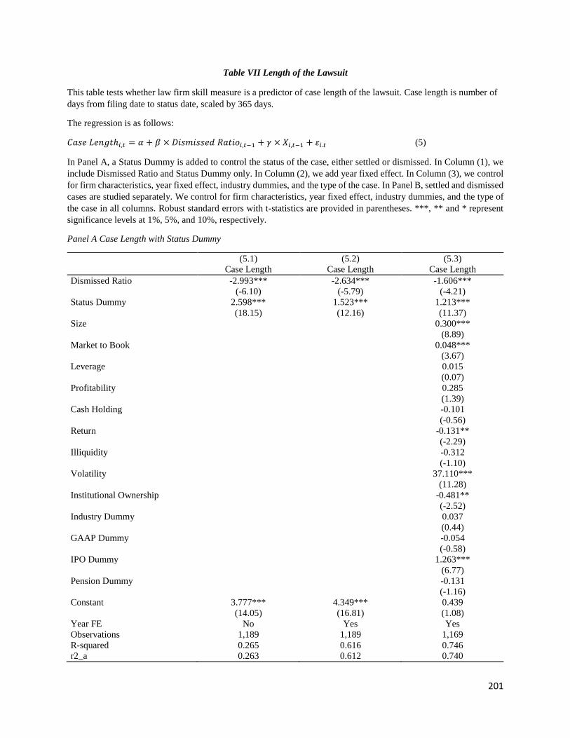
201

Table VII Length of the Lawsuit

This table tests whether law firm skill measure is a predictor of case length of the lawsuit. Case length is number of

days from filing date to status date, scaled by 365 days.

The regression is as follows:

𝐶𝑎𝑠𝑒 𝐿𝑒𝑛𝑔𝑡ℎ𝑖,𝑡 = 𝛼 + 𝛽 × 𝐷𝑖𝑠𝑚𝑖𝑠𝑠𝑒𝑑 𝑅𝑎𝑡𝑖𝑜𝑖,𝑡−1 + 𝛾 × 𝑋𝑖,𝑡−1 + 𝜀𝑖.𝑡 (5)

In Panel A, a Status Dummy is added to control the status of the case, either settled or dismissed. In Column (1), we

include Dismissed Ratio and Status Dummy only. In Column (2), we add year fixed effect. In Column (3), we control

for firm characteristics, year fixed effect, industry dummies, and the type of the case. In Panel B, settled and dismissed

cases are studied separately. We control for firm characteristics, year fixed effect, industry dummies, and the type of

the case in all columns. Robust standard errors with t-statistics are provided in parentheses. ***, ** and * represent

significance levels at 1%, 5%, and 10%, respectively.

Panel A Case Length with Status Dummy

(5.1) (5.2) (5.3)

Case Length Case Length Case Length

Dismissed Ratio -2.993*** -2.634*** -1.606***

(-6.10) (-5.79) (-4.21)

Status Dummy 2.598*** 1.523*** 1.213***

(18.15) (12.16) (11.37)

Size 0.300***

(8.89)

Market to Book 0.048***

(3.67)

Leverage 0.015

(0.07)

Profitability 0.285

(1.39)

Cash Holding -0.101

(-0.56)

Return -0.131**

(-2.29)

Illiquidity -0.312

(-1.10)

Volatility 37.110***

(11.28)

Institutional Ownership -0.481**

(-2.52)

Industry Dummy 0.037

(0.44)

GAAP Dummy -0.054

(-0.58)

IPO Dummy 1.263***

(6.77)

Pension Dummy -0.131

(-1.16)

Constant 3.777*** 4.349*** 0.439

(14.05) (16.81) (1.08)

Year FE No Yes Yes


R-squared 0.265 0.616 0.746

r2_a 0.263 0.612 0.740

202

Panel B Subsample Analysis for Case Length

(5.3) (5.3)

Case Length

Settled Subsample

Case Length

Dismissed Subsample

Dismissed Ratio -1.886*** -0.754

(-3.74) (-1.43)

Size 0.300*** 0.295***

(7.26) (4.81)

Market to Book 0.0452*** 0.0635

(3.34) (1.25)

Leverage 0.198 -0.535

(0.73) (-1.53)

Profitability 0.166 -0.039

(0.60) (-0.14)

Cash Holding 0.183 -0.846**

(0.94) (-2.50)

Return -0.164** -0.004

(-2.04) (-0.06)

Illiquidity -0.609 -0.024

(-1.39) (-0.07)

Volatility 33.610*** 35.890***

(8.42) (5.83)

Institutional Ownership -0.480** -0.483

(-2.08) (-1.57)

Industry Dummy 0.081 0.009

(0.78) (0.07)

GAAP Dummy -0.028 -0.114

(-0.24) (-0.76)

IPO Dummy 1.367*** -0.042

(5.90) (-0.15)

Pension Dummy -0.101 -0.080

(-0.71) (-0.48)

Constant 1.972*** -0.034

(3.88) (-0.05)

Year FE Yes Yes

Observations 801 368

R-squared 0.753 0.308

r2_a 0.745 0.255

203

Table VIII Predicting Market Share

In this table, we examine whether law firm expertise has predictive power for market share of law firms in Panel A

and the probability of law firms’ disappearing from the market in Panel B. The main independent variable is the

Dismissed Ratio at law firm level, controlling for the market share of law firm j in the past year. 𝐷𝑖𝑠𝑚𝑖𝑠𝑠𝑒𝑑 𝑅𝑎𝑡𝑖𝑜𝑗,𝑡−1,

defined as the equal-weighted Dismissed Ratio (number of dismissed case/number of total case) for law firm j from

year t-5 to year t-1.

In Panel A, dependent variable is the market share of law firm j in year t. We run the regression as follows:

𝑀𝑎𝑟𝑘𝑒𝑡 𝑆ℎ𝑎𝑟𝑒𝑗,𝑡 = 𝛼 + 𝛽 × 𝐷𝑖𝑠𝑚𝑖𝑠𝑠𝑒𝑑 𝑅𝑎𝑡𝑖𝑜𝑗,𝑡−1 + 𝛾 × 𝑀𝑎𝑟𝑘𝑒𝑡 𝑆ℎ𝑎𝑟𝑒𝑗,𝑡−1 + 𝜀𝑗.𝑡 (6.1)

In Panel B, we define 𝐷𝑖𝑠𝑎𝑝𝑝𝑒𝑎𝑟 𝐷𝑢𝑚𝑚𝑦𝑗,𝑡+𝑘 , which equals to 1 if law firm has zero market share in the year t + k

and nonzero market share in the year t; equals to 0 otherwise. K equals to 3, 4, or 5 years.

We run probit regression as follows:

𝐷𝑖𝑠𝑎𝑝𝑝𝑒𝑎𝑟 𝐷𝑢𝑚𝑚𝑦𝑗,𝑡+𝑘 = 𝛼 + 𝛽 × 𝐷𝑖𝑠𝑚𝑖𝑠𝑠𝑒𝑑 𝑅𝑎𝑡𝑖𝑜𝑗,𝑡−1 + 𝛾 × 𝑀𝑎𝑟𝑘𝑒𝑡 𝑆ℎ𝑎𝑟𝑒𝑗,𝑡−1 + 𝜀𝑗.𝑡 (6.2)

We control for lagged market share in both panels, and year fixed effect in panel B. Errors are clustered at the law

firm level in all specifications. Robust standard errors with t-statistics are given in parentheses. ***, ** and * represent


Panel A Dismissed Ratio and Market Share

(6.1)

Market Share

Market Share Lagged 0.459***

(8.55)

Dismissed Ratio -0.008*

(-1.92)

Constant 0.012***

(4.92)

Observations 255

R-squared 0.541

r2_a 0.516

Panel B Dismissed Ratio and Probability of Disappearance

(6.2) (6.2) (6.2)

Disappear Dummy

After 3 years

Disappear Dummy

After 4 years

Disappear Dummy

After 5 years

Dismissed Ratio 0.410** 0.725*** 0.729***

(2.26) (3.40) (3.11)

Market Share Lagged -3.167 -1.758 -2.460

(-1.62) (-0.93) (-1.21)

Year FE

Cluster

Yes

Firm

Yes

Firm

Yes

Firm


204

Table IX Effect on CEO Turnover

We relate CEO turnover and forced turnover to the year of the case’s filing date, and examine the effect of the prior

Dismissed Ratio on the probability of turnover or forced turnover. We study the probability of turnover in Column (1)

and forced turnover in Column (2). We control for firm characteristics, year fixed effect, industry dummies, and the

type of the case in all columns. Robust standard errors with t-statistics are given in parentheses. ***, ** and * represent


(1) (2)

Turnover Forced Turnover

Dismissed Ratio -0.068** -0.047*

(-2.05) (-1.75)

Size 0.009*** 0.007***

(2.93) (2.99)

Market to Book -0.001 -0.001

(-0.70) (-0.66)

Leverage 0.027 0.030**

(1.39) (1.96)

Profitability -0.030 -0.020

(-0.97) (-0.82)

Cash Holding -0.036 -0.011

(-1.18) (-0.60)

Return 0.001 0.004

(0.18) (0.71)

Illiquidity -0.106 -0.0525

(-1.01) (-0.66)

Volatility 0.181 0.307

(0.49) (1.01)

Institutional Ownership 0.035 0.046**

(1.60) (2.47)

Industry Dummy 0.007 -0.001

(0.63) (-0.02)

GAAP Dummy 0.018* 0.015*

(1.81) (1.82)

IPO Dummy -0.005 -0.005

(-0.32) (-0.37)

Pension Dummy 0.020 0.024**

(1.60) (2.23)


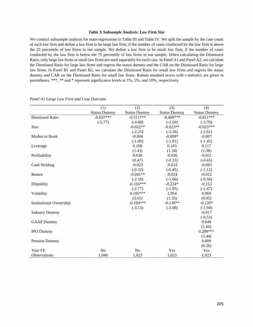
205

Table X Subsample Analysis: Law Firm Size

We conduct subsample analysis for main regressions in Table III and Table IV. We split the sample by the case count

of each law firm and define a law firm to be large law firm, if the number of cases conducted by the law firm is above

the 25 percentile of law firms in our sample. We define a law firm to be small law firm, if the number of cases

conducted by the law firm is below the 75 percentile of law firms in our sample. When calculating the Dismissed

Ratio, only large law firms or small law firms are used separately for each case. In Panel A1 and Panel A2, we calculate

the Dismissed Ratio for large law firms and regress the status dummy and the CAR on the Dismissed Ratio for large

law firms. In Panel B1 and Panel B2, we calculate the Dismissed Ratio for small law firms and regress the status

dummy and CAR on the Dismissed Ratio for small law firms. Robust standard errors with t-statistics are given in

parentheses. ***, ** and * represent significance levels at 1%, 5%, and 10%, respectively.

Panel A1 Large Law Firm and Case Outcome

(1) (2) (3) (4)

Status Dummy Status Dummy Status Dummy Status Dummy

Dismissed Ratio -0.637*** -0.511*** -0.400*** -0.411***

(-5.77) (-4.68) (-3.50) (-3.70)

Size -0.022** -0.023** -0.025***

(-2.25) (-2.36) (-2.61)

Market to Book -0.004 -0.009* -0.007

(-1.00) (-1.81) (-1.45)

Leverage 0.108 0.103 0.117

(1.43) (1.34) (1.58)

Profitability 0.038 -0.026 -0.051

(0.47) (-0.33) (-0.65)

Cash Holding -0.023 -0.033 -0.083

(-0.32) (-0.45) (-1.12)

Return -0.041** -0.024 -0.012

(-2.10) (-1.06) (-0.56)

Illiquidity -0.316*** -0.224* -0.153

(-2.77) (-1.95) (-1.47)

Volatility 4.195*** 1.954 0.069

(3.65) (1.35) (0.05)

Institutional Ownership -0.194*** -0.130** -0.120*

(-3.13) (-2.08) (-1.94)


(-0.53)

GAAP Dummy 0.049

(1.60)

IPO Dummy 0.289***

(5.44)

Pension Dummy 0.009

(0.26)


Observations 1,040 1,023 1,023 1,023

206

Panel A2 Large Law Firm and Cumulative Abnormal Return

(1) (2) (3)

CAR (-1,1) CAR (-10,1) CAR (-30,1)

Dismissed Ratio 0.097** 0.132* 0.230**

(2.23) (1.83) (2.44)

Size 0.002 0.006 0.019***

(0.71) (1.23) (2.61)

Market to Book -0.002 -0.002 -0.006

(-1.17) (-0.86) (-1.16)

Leverage -0.006 -0.018 -0.056

(-0.26) (-0.40) (-0.77)

Profitability -0.008 0.001 0.035

(-0.31) (0.01) (0.47)

Cash Holding 0.010 -0.073 -0.050

(0.40) (-1.61) (-0.81)

Return -0.016* -0.044** -0.083***

(-1.70) (-2.51) (-3.87)

Illiquidity -0.046 0.063 0.130

(-1.12) (0.46) (0.87)

Volatility 0.289 0.706 1.905

(0.74) (0.85) (1.46)


(0.32) (0.42) (1.11)


(0.28) (0.09) (0.87)

GAAP Dummy -0.008 -0.031 -0.034

(-0.82) (-1.60) (-1.20)

IPO Dummy 0.005 0.098*** 0.163***

(0.32) (3.30) (3.21)

Pension Dummy 0.006 0.010 0.029

(0.54) (0.49) (1.07)

Constant -0.111*** -0.239*** -0.522***

(-2.61) (-2.95) (-4.74)

Year FE Yes Yes Yes


R-squared 0.036 0.072 0.105

r2_a 0.010 0.048 0.081

207

Panel B1 Small Law Firm and Case Outcome

(1) (2) (3) (4)


Dismissed Ratio -0.697*** -0.550*** -0.455*** -0.441***

(-7.11) (-5.33) (-4.07) (-4.02)

Size -0.021** -0.020* -0.022**

(-1.99) (-1.89) (-2.08)

Market to Book -0.005 -0.009 -0.008

(-0.86) (-1.45) (-1.17)

Leverage 0.082 0.068 0.088

(0.98) (0.80) (1.07)

Profitability 0.001 -0.052 -0.079

(0.00) (-0.59) (-0.89)

Cash Holding -0.115 -0.128 -0.169**

(-1.41) (-1.54) (-1.97)

Return -0.023 -0.006 0.002

(-1.03) (-0.26) (0.09)

Illiquidity -0.277** -0.208* -0.162

(-2.27) (-1.65) (-1.37)

Volatility 4.375*** 3.125** 1.598

(3.63) (2.03) (1.06)

Institutional Ownership -0.159** -0.112 -0.098

(-2.32) (-1.60) (-1.41)


(-1.43)

GAAP Dummy 0.060*

(1.72)

IPO Dummy 0.316***

(5.19)

Pension Dummy 0.007

(0.19)


Observations 870 855 855 855

208

Panel B2 Small Law Firm and Cumulative Abnormal Return

(1) (2) (3)

CAR (-1,1) CAR (-10,1) CAR (-30,1)

Dismissed Ratio 0.087** 0.143** 0.177**

(2.17) (2.13) (2.01)

Size 0.002 0.007 0.019**

(0.63) (1.32) (2.55)

Market to Book -0.001 0.001 0.002

(-0.50) (0.04) (0.44)

Leverage 0.008 -0.038 -0.066

(0.31) (-0.73) (-1.04)

Profitability -0.017 -0.001 0.048

(-0.55) (-0.02) (0.61)

Cash Holding 0.008 -0.087* -0.065

(0.27) (-1.66) (-0.98)

Return -0.017 -0.044** -0.095***

(-1.55) (-2.33) (-4.13)

Illiquidity -0.049 0.091 0.146

(-1.05) (0.58) (0.87)

Volatility 0.075 0.640 1.491

(0.16) (0.66) (1.24)


(0.47) (0.94) (1.30)

Industry Dummy 0.001 -0.008 0.016

(0.13) (-0.38) (0.60)

GAAP Dummy -0.015 -0.040* -0.026

(-1.27) (-1.84) (-0.91)

IPO Dummy 0.010 0.088*** 0.120**

(0.54) (2.73) (2.18)

Pension Dummy 0.003 -0.005 -0.001

(0.27) (-0.26) (-0.03)

Constant -0.100** -0.246*** -0.475***

(-2.17) (-2.78) (-4.54)

Year FE Yes Yes Yes


R-squared 0.034 0.064 0.096

r2_a 0.003 0.034 0.067

209

Table XI Law Firm Selection versus Expertise

We perform robustness test regarding law firm selection issues. If prior results are driven by systematic selection of

cases with certain characteristics by law firms, then it is more likely that law firms select cases in the same industry.

Therefore, we create a Dismissed Ratio excluding cases in the same industry for the focal case. When calculating the

Dismissed Ratio for case i, we exclude cases in the same industry as case i during the calculation. Panel A reports

main analysis as in Table III and Panel B reports analysis as in Table IV, except that the Dismissed Ratio is calculated

after excluding same industry cases. Robust standard errors with t-statistics are given in parentheses. ***, ** and *

represent significance levels at 1%, 5%, and 10%, respectively.

Panel A Case Outcome

(1) (2) (3) (4)


Dismissed Ratio -0.650*** -0.503*** -0.373*** -0.393***

(-6.00) (-4.74) (-3.32) (-3.59)

Size -0.022** -0.025** -0.027***

(-2.23) (-2.51) (-2.76)

Market to Book -0.003 -0.008 -0.006

(-0.59) (-1.52) (-1.05)

Leverage 0.096 0.097 0.113

(1.29) (1.27) (1.52)

Profitability 0.011 -0.059 -0.081

(0.13) (-0.72) (-1.01)

Cash Holding -0.057 -0.055 -0.100

(-0.78) (-0.75) (-1.35)

Return -0.042** -0.026 -0.016

(-2.08) (-1.16) (-0.75)

Illiquidity -0.306*** -0.213* -0.146

(-2.71) (-1.87) (-1.40)

Volatility 4.106*** 1.467 -0.364

(3.56) (1.01) (-0.25)

Institutional Ownership -0.227*** -0.165*** -0.155**

(-3.59) (-2.59) (-2.45)


(-0.75)

GAAP Dummy 0.053*

(1.68)

IPO Dummy 0.292***

(5.48)

Pension Dummy 0.011

(0.32)


Observations 1,029 1,011 1,011 1,011

210

Panel B Cumulative Abnormal Return

(1) (2) (3)

CAR (-1,1) CAR (-10,1) CAR (-30,1)

Dismissed Ratio 0.104** 0.170** 0.250***

(2.38) (2.37) (2.67)

Size 0.003 0.009* 0.020***

(1.13) (1.72) (2.71)

Market to Book -0.002 -0.001 -0.006

(-1.18) (-0.59) (-1.24)

Leverage -0.009 -0.038 -0.058

(-0.38) (-0.81) (-0.78)

Profitability -0.006 -0.004 0.057

(-0.22) (-0.09) (0.77)

Cash Holding 0.013 -0.081* -0.040

(0.55) (-1.81) (-0.65)

Return -0.012 -0.038** -0.084***

(-1.31) (-2.17) (-3.88)

Illiquidity -0.025 0.089 0.125

(-0.63) (0.65) (0.83)

Volatility 0.299 0.857 1.906

(0.78) (1.04) (1.63)


(0.54) (0.34) (0.47)

Industry Dummy 0.002 -0.001 0.023

(0.19) (-0.05) (0.92)

GAAP Dummy -0.009 -0.031 -0.035

(-0.87) (-1.58) (-1.25)

IPO Dummy 0.005 0.104*** 0.155***

(0.32) (3.52) (3.02)

Pension Dummy 0.007 0.010 0.020

(0.62) (0.53) (0.78)

Constant -0.129*** -0.283*** -0.521***

(-3.03) (-3.41) (-4.92)

Year FE Yes Yes Yes


R-squared 0.034 0.079 0.112

r2_a 0.008 0.055 0.088

211

Table XII Alternative Measure of Law Firm Expertise: Persistence of CAR

In this table, we provide another measure of law firm expertise as a robustness test and in a similar manner as the

investment bank fixed effect in Bao and Edmans (2011). For each case i, we average the prior 5 years of Cumulative

Abnormal Returns of the cases conducted by law firms engaged in the case i. If the dependent variable is CAR (-1,1),

then prior average CAR is the prior 5 years of average CAR (-1,1). If the dependent variable is CAR (-10,1) or CAR

(-30,1), then the prior average CAR is measured based on (-10,1) or (-30,1) correspondingly. We study persistence of

CAR (-1,1) in Column (1), CAR (-10,1) in Column (2), and CAR (-30,1) in Column (3). We control for firm

characteristics, year fixed effect, industry dummies, and the type of the case in all columns. Robust standard errors

with t-statistics are given in parentheses. ***, ** and * represent significance levels at 1%, 5%, and 10%, respectively.

(1) (2) (3)

CAR(-1,1) CAR(-10,1) CAR(-30,1)

Prior Average CAR 1.224*** 1.203*** 1.118***

(9.31) (15.64) (13.61)

Size 0.001 0.003 0.012**

(0.44) (0.79) (2.01)

Market to Book -0.002 -0.003 -0.007

(-1.54) (-1.09) (-1.57)

Leverage 0.006 0.019 -0.037

(0.33) (0.57) (-0.61)

Profitability 0.008 0.022 0.140**

(0.46) (0.63) (2.19)

Cash Holding -0.001 -0.063* -0.002

(-0.09) (-1.73) (-0.04)

Return -0.007 -0.028** -0.059***

(-1.02) (-2.08) (-3.38)

Illiquidity -0.054 -0.006 0.047

(-1.64) (-0.05) (0.33)

Volatility 0.308 0.663 2.179*

(0.88) (0.99) (1.95)

Institutional Ownership -0.006 -0.016 0.012

(-0.34) (-0.50) (0.30)


(1.22) (1.44) (0.95)

GAAP Dummy -0.001 -0.006 -0.006

(-0.05) (-0.38) (-0.28)

IPO Dummy -0.011 0.055** 0.073

(-0.87) (2.19) (1.63)

Pension Dummy -0.009 -0.005 -0.001

(-0.96) (-0.33) (-0.07)

Constant 0.005 -0.020 -0.175*

(0.19) (-0.36) (-1.96)

Year FE Yes Yes Yes


R-squared 0.242 0.236 0.217

r2_a 0.225 0.219 0.200

Documents

Three essays on finance - Home | Nanyang Technological