Embed Size (px)
Citation preview
THREE ESSAYS IN NATURAL RESOURCE AND
ENVIRONMENTAL ECONOMICS
Olli-Pekka Kuusela
Dissertation submitted to the faculty of the Virginia Polytechnic Institute and State University in
partial fulfillment of the requirements for the degree of
Doctor of Philosophy
In
Forestry
Gregory S. Amacher, Chair
Janaki Alavalapati
Bradley J. Sullivan
Klaus Moeltner
Kwok Ping Tsang
January 18, 2013
Blacksburg, VA
Keywords: Tropical deforestation; Timber concessions; Performance bonds; Permit markets;
Macroeconomic uncertainty
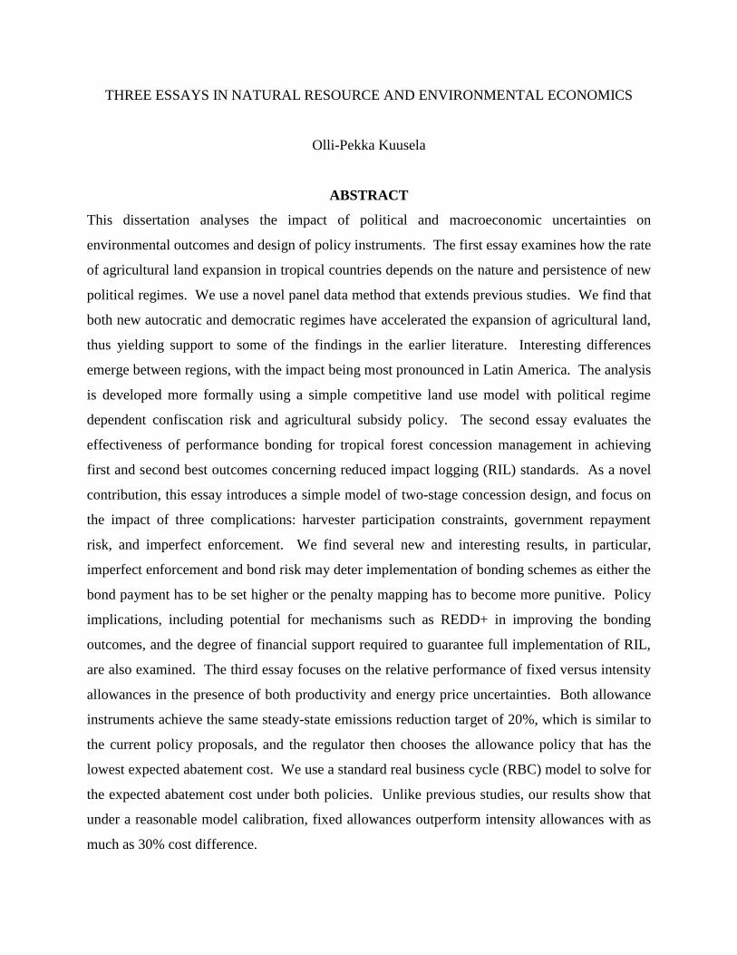
THREE ESSAYS IN NATURAL RESOURCE AND ENVIRONMENTAL ECONOMICS
Olli-Pekka Kuusela
ABSTRACT
This dissertation analyses the impact of political and macroeconomic uncertainties on
environmental outcomes and design of policy instruments. The first essay examines how the rate
of agricultural land expansion in tropical countries depends on the nature and persistence of new
political regimes. We use a novel panel data method that extends previous studies. We find that
both new autocratic and democratic regimes have accelerated the expansion of agricultural land,
thus yielding support to some of the findings in the earlier literature. Interesting differences
emerge between regions, with the impact being most pronounced in Latin America. The analysis
is developed more formally using a simple competitive land use model with political regime
dependent confiscation risk and agricultural subsidy policy. The second essay evaluates the
effectiveness of performance bonding for tropical forest concession management in achieving
first and second best outcomes concerning reduced impact logging (RIL) standards. As a novel
contribution, this essay introduces a simple model of two-stage concession design, and focus on
the impact of three complications: harvester participation constraints, government repayment
risk, and imperfect enforcement. We find several new and interesting results, in particular,
imperfect enforcement and bond risk may deter implementation of bonding schemes as either the
bond payment has to be set higher or the penalty mapping has to become more punitive. Policy
implications, including potential for mechanisms such as REDD+ in improving the bonding
outcomes, and the degree of financial support required to guarantee full implementation of RIL,
are also examined. The third essay focuses on the relative performance of fixed versus intensity
allowances in the presence of both productivity and energy price uncertainties. Both allowance
instruments achieve the same steady-state emissions reduction target of 20%, which is similar to
the current policy proposals, and the regulator then chooses the allowance policy that has the
lowest expected abatement cost. We use a standard real business cycle (RBC) model to solve for
the expected abatement cost under both policies. Unlike previous studies, our results show that
under a reasonable model calibration, fixed allowances outperform intensity allowances with as
much as 30% cost difference.

iii
To my mother
iv
ACKNOWLEDGEMENTS
I would like to start by expressing my deepest gratitude to my academic advisor and committee
chair Dr. Gregory S. Amacher for all the support and help he has provided during the challenging
but rewarding years of dissertation work and graduate courses. Anyone who has once embarked
on the often solitary journey of Ph.D. studies knows how important it is to have someone who
provides guidance, and occasionally, steers off the many dangers lurking along the way. Dr.
Amacher’s expertise, kind understanding, and dedication made my journey possible, and
provided inspiration for my own professional development, and beyond. In retrospect, it was
truly a remarkable coincidence that I enrolled to his environmental economics class as an
unsuspecting exchange student in 2007. That seemingly minor choice proved to be a momentous
decision in regard to my professional career and ambitions.
I would also like to thank each of my committee members for the significant
contributions they have made on their part to my intellectual and professional growth. Their
dedication and intellectual integrity continues to inspire me. I am also grateful for the great
many opportunities I have had to interact with and learn from other professors and researchers
during my time as a graduate student. I would like to thank Sue Snow and the rest of the staff at
the Department of Forest Resources and Environmental Conservation for all the kindness and
assistance they have provided. The department and our great university have both offered a
stimulating environment to learn, conduct research, and aspire to excellence.
Finally, I’m forever grateful for the continued support and love of my family and friends.
My parents and my sister have always been there for me, whether to share the blessings in my
life, or to see through the occasional hardships. Weekly Skype calls, on every Sunday, with my
mother and father gave me strength and confidence to push forward. My new life-long friends
have made my stay here in Blacksburg, Virginia an unforgettable experience. I am forever
indebted for their generosity and unconditional kindness, and without these relationships, my
time here would have not been complete and meaningful.
v
TABLE OF CONTENTS 1 INTRODUCTION ................................................................................................................... 1
2 CHANGING POLITICAL REGIMES AND TROPICAL DEFORESTATION .................... 4
2.1 ABSTRACT ..................................................................................................................... 4
2.2 INTRODUCTION ............................................................................................................ 4
2.3 MODEL OF COMPETITIVE LAND USE ..................................................................... 8
2.3.1 AGRICULTURAL MARGIN ................................................................................ 11
2.3.2 NATIVE FOREST MARGIN................................................................................. 13
2.4 ECONOMETRIC MODEL ............................................................................................ 14
2.4.1 ESTIMATION ........................................................................................................ 16
2.5 DATA ............................................................................................................................. 17
2.6 RESULTS AND DISCUSSION .................................................................................... 19
2.7 CONCLUSIONS ............................................................................................................ 22
3 PERFORMANCE BONDS IN TIMBER CONCESSIONS ................................................. 29
3.1 ABSTRACT ................................................................................................................... 29
3.2 INTRODUCTION .......................................................................................................... 29
3.3 CONCESSIONS AND PERFORMANCE BONDING ................................................. 32
3.3.1 BOND PARTICIPATION CONSTRAINT ............................................................ 38
3.4 BOND REPAYMENT RISK ......................................................................................... 40
3.4.1 BOND PARTICIPATION CONSTRAINT ............................................................ 44
3.4.2 CRITICAL LEVEL OF REPAYMENT RISK ....................................................... 46
3.5 IMPERFECT ENFORCEMENT ................................................................................... 47
3.5.1 PARTICIPATION CONSTRAINT ........................................................................ 50
3.6 BOND SIMULATIONS ................................................................................................ 52
3.7 CONCLUSIONS ............................................................................................................ 55
4 FIXED VERSUS INTENSITY PERMIT ALLOWANCES ................................................. 64
4.1 ABSTRACT ................................................................................................................... 64
4.2 INTRODUCTION .......................................................................................................... 64
4.3 INTENSITY TARGETS ................................................................................................ 67
4.4 REAL BUSINESS CYCLE MODEL ............................................................................ 69
4.5 ABATEMENT COST COMPARISON ......................................................................... 74
vi
4.5.1 NO POLICY SCENARIO (BAU) .......................................................................... 75
4.5.2 ABATEMENT COST UNDER PERMIT ALLOWANCES .................................. 76
4.5.3 COST COMPARISON ........................................................................................... 77
4.6 MODEL SPECIFICATION ........................................................................................... 78
4.7 RESULTS AND DISCUSSION .................................................................................... 78
4.7.1 CRITICAL VALUES ............................................................................................. 82
4.8 CONCLUSIONS ............................................................................................................ 83
5 CONCLUSIONS ................................................................................................................... 93
6 REFERENCES ...................................................................................................................... 96
APPENDIX A: COMPARATIVE STATICS ............................................................................. 103
APPENDIX B: BOND PROOFS................................................................................................ 106
APPENDIX C: FIRST ORDER CONDITIONS AND STEADY STATES .............................. 110
APPENDIX D: PERMIT PRICE EXAMPLE ............................................................................ 113

vii
LIST OF FIGURES
Figure 2.1: Agricultural margin and native forest margin ............................................................ 24
Figure 2.2: New regime effect (first five years) on agricultural land expansion .......................... 25
Figure 3.1: Timing of events ......................................................................................................... 35
Figure 3.2: Timing of Events ........................................................................................................ 41
Figure 3.3: Full compliance .......................................................................................................... 57
Figure 3.4: Repayment risk ........................................................................................................... 57
Figure 3.5: Second-best bond scheme .......................................................................................... 58
Figure 3.6: Bond scheme with repayment risk ............................................................................. 59
Figure 3.7: An example of bond failure in the presence of repayment risk .................................. 60
Figure 3.8: Critical risk ................................................................................................................. 61
Figure 3.9: Bond scheme with imperfect enforcement ................................................................. 62
Figure 3.10: Bond failure in presence of imperfect enforcement ................................................ 63
Figure 4.1: Ex-ante abatement cost curve ..................................................................................... 84
Figure 4.2: Ex-post abatement cost curve ..................................................................................... 84
Figure 4.3: Permit price simulation .............................................................................................. 85
Figure 4.4: Abatement cost difference, energy price shock standard deviation ........................... 86
Figure 4.5: Abatement cost difference, energy price AR(1) persistence term .............................. 87
Figure 4.6: Abatement cost difference, energy price MA(1) persistence term ............................. 88
Figure 4.7: Abatement cost difference, productivity AR(1) persistence term .............................. 89
Figure 4.8: Abatement cost difference, productivity shock standard deviation ........................... 90
viii
LIST OF TABLES
Table 2.1: Variable definitions ..................................................................................................... 26
Table 2.2: List of countries ........................................................................................................... 26
Table 2.3: Descriptive statistics .................................................................................................... 27
Table 2.4: Within estimator results ............................................................................................... 28
Table 3.1: Parameter values .......................................................................................................... 58
Table 4.1: Baseline calibration ..................................................................................................... 91
Table 4.2: Steady state values in levels ........................................................................................ 91
Table 4.3: Equations of motion .................................................................................................... 91
Table 4.4: Baseline results in logs ................................................................................................ 92
Table 4.5: Baseline results in levels .............................................................................................. 92

1
1 INTRODUCTION
Political and macroeconomic uncertainties are prone to exacerbate both market and policy
failures that threaten the quality of our ambient environment and sustainability of our renewable
resource base. Macroeconomic instability can be a leading indicator for political and social
unrest, and it can also encourage myopic resource extraction. Political risks and institutional
unpredictability enforce the vicious cycle of market failures that lead to overexploitation and
degradation of natural resource stocks such as tropical forests and ocean fisheries. Institutional
failures, such as omnipresent corruption, further feed into this tragedy, but also gain strength
from the instability itself. This is evident in the experiences of many tropical countries, and
manifested in the alarming rate of tropical deforestation and loss of biodiversity. The need for
both national and global action remains stronger than ever.
The same uncertainties that contribute to environmental degradation, directly or indirectly,
are also hindering the effectiveness of policy instruments designed to correct market failures.
This can be seen, for example, in the frustratingly slow progress made in the sustainable
management of tropical timber concessions. Elsewhere, macroeconomic uncertainties stemming
from business cycles and fluctuating energy prices have already put in test the viability of
greenhouse gas emissions permit markets, most notably the European Union Emissions Trading
Scheme (EU ETS). Incorporating institutional realities in the policy design and choosing policy
instruments that perform the best in an unpredictable environment may be the key factors
contributing to the ultimate success of national and global policy responses. Even if the
institutional context enables us to achieve only a second-best policy outcome, it is still better
than the alternative of total policy failure.
The three essays in this dissertation each contribute and extend the past research that
analyzes the effects of uncertainty and risk on environmental outcomes and policy instrument
design. The first essay examines the effect of political regime turnovers on tropical deforestation
by first developing a formal land use model and then applying a novel empirical approach to
identify these effects. The second essay analyses the design of performance bonds in tropical
timber concessions where government’s repayment ability may be of concern and detection of
contract violations is imperfect. The third essay compares the abatement cost outcomes under
two alternative permit policies, intensity and fixed allowances, in an economy that is subject to
both productivity and energy price uncertainty.

2
Agricultural land expansion has been identified as the single most important factor
driving tropical deforestation. There are a variety of underlying factors that in turn drive
agricultural land expansion, but active government policies in form of subsidies and land reforms
are certainly a significant catalyst for land conversion. The first essay of this dissertation begins
from the observation that most of the tropical countries have undergone recurring political
regime changes during the past decades. These regime changes have frequently been
accompanied with policies that include land reforms, land confiscations, and push to settle the
frontier lands to ease population pressures. These policies have in turn deteriorated property
rights and favored land conversion to agriculture, thus resulting in accelerating deforestation.
The above argument is formally modeled using a simple competitive land use model. The
predictions from the model are then tested using a novel empirical approach. We find a
significant and persistent effect from new political regimes on agricultural land expansion, from
both autocratic and democratic. Increasing level of income, on the other hand, has tended to
reduce the rate of tropical deforestation in Latin America and Asia.
Unsustainable concession management practices and myopic extraction have
significantly contributed to forest degradation and deforestation in the tropics. To guarantee
future economic and environmental value of tropical forests, the application of reduced impact
logging (RIL) techniques is deemed as a necessary condition for achieving sustainable forest
management. The second essay of this dissertation analyzes the use of performance bonds in
enforcing RIL in tropical timber concessions. We build a simple two-stage model of concession
design that incorporates the risk of moral hazard in the form government’s repayment ability and
imperfect enforcement environment which is a widespread problem in most tropical concessions.
It is also common that concession harvesters face financial constraints that may hinder them
from posting a high enough bond payment. We propose a bonding scheme that leads to full
implementation of RIL, or in the presence of binding participation constraint, a second-best RIL
level. Bond simulations provide a realistic assessment of the severity of repayment risk and
imperfect enforcement on the successful implementation of performance bonds, and the required
bond level to achieve full RIL under such circumstances. Our results suggest that the needed
REDD+ funding for performance bond schemes may be much higher than anticipated, depending
on degree of institutional challenges.
3
Cap-and-trade policies have been and continue to be at the forefront of policy options in
the reduction of anthropocentric greenhouse gas emissions (GHG). These schemes fix the
quantity of total emissions through permit issuance, and then enable trading among permit
holders with the goal of achieving the least overall cost of abatement. Most notably, the EU ETS
launched its first phase in 2005 and is currently entering its third phase in 2013, while many
other countries are currently in the process of including similar policies in their respective
climate change legislation. Fixing the amount of emissions years in advance, however, leads to
uncertainty about the ultimate cost of abatement. The third, and the final, essay compares the
uncertain abatement cost outcomes under two competing permit allowance policies: intensity and
fixed allowances. The attraction of intensity based emissions targeting derives from its ability to
reduce abatement cost uncertainties that are mainly due to unanticipated short-run changes in
economic activity. Following previous literature, we use a real business cycle (RBC) model to
simulate policy outcomes under the two policies with an emissions reduction target of 20% from
the business as usual (BAU) steady state. In our model, the abatement cost uncertainty stems
from both stochastic business cycles and energy prices. Our results suggest that with reasonable
model parameterization, fixed allowances outperform intensity allowances in terms of the
expected cost of abatement. This difference in cost outcomes crucially depends on the
approximation method applied when linearizing the RBC model. We also simulate policy
outcomes under differing model parameterizations to find critical values for energy price and
productivity processes that determine when intensity allowances gain advantage over fixed
allowances.
The plan of the dissertation is as follows. The second section presents the essay
“Changing Political Regimes and Tropical Deforestation”. The third section consists of the
essay “Performance Bonds in Timber Concessions”. The fourth section presents the essay
“Fixed vs. Intensity Permit Allowances”, while the last section offers concluding remarks.
4
2 CHANGING POLITICAL REGIMES AND TROPICAL
DEFORESTATION
2.1 ABSTRACT
Expansion of agriculture is a main cause of tropical deforestation. Government policies
and weak property rights contribute to this process by encouraging landowners and landless to
accelerate land clearing. Using panel data common to previous studies, we add the dimension of
new political regimes, democratic and non-democratic, and investigate how the rate of
agricultural land expansion in tropical countries depends on the nature and persistence of each
regime. We find that both new autocratic and democratic regimes have accelerated the
expansion of agricultural land, thus yielding support to some of the findings in the earlier
literature. Interesting differences emerge between regions, with the impact being most
pronounced in Latin America. We interpret these results mainly in the context of increasing
tenure and ownership insecurity, which in turn is driven by the tendency of new regimes to
implement land reforms as a form of social and economic policy or voter payback. The
argument is developed more formally using a simple competitive land use model with political
regime dependent confiscation risk and agricultural subsidy policy.
2.2 INTRODUCTION
Tropical deforestation and its underlying causes have been an area of active research at
least for the past three decades. It is widely agreed that the main driver of forest loss has been
the rapid expansion of agricultural land. Other significant causes are road building, illegal
logging, industrial harvesting through concessions, and fuelwood collection by local
communities (Pfaff et al. 2010). Population pressures and economic development have also been
commonly identified as important overall drivers. In many instances, however, the actions and
policies of the governments, in addition to institutional characteristics of the countries, certainly
work to magnify the extent of deforestation. Insecure property rights and subsidies for
agriculture favor clearing land over keeping native or plantation forests. Political instability,
perceived through quick turnover of regimes, and accompanying ownership uncertainty further
reduce the profitability of long term investments, such as forestry, favoring instead some form of
extensive agriculture (Bohn and Deacon 2000).
5
A considerable number of tropical forest countries have gone through some degree of
political upheaval, such as revolutions and military coups, during the past half century. For
example, the first part of 1990’s witnessed multiple democratization processes in Africa alone,
and the Latin American countries have been oscillating between autocratic and democratic
regimes since the Second World War. The ownership of productive land has frequently been at
the core of the controversial issues surrounding postcolonial countries, and thus unsurprisingly,
has provided a spark for many political conflicts leading to regime changes (Prosterman and
Riedinger 1987). To consolidate their power, or to preserve old privileges, new political regimes
have recurrently enacted policies to redistribute land, commonly including provisions granting
land ownership to migrants who clear forests.1 The effects of these land reforms on tropical
deforestation in turn may depend on the success and persistence of each new regime in power.
The purpose of this chapter is to highlight the impact of the political economy on tropical
deforestation from a perspective that extends past work (Bohn and Deacon 2000; Edward
Barbier 2001; Lopez and Galinato 2005; Buitenzorgy and Mol 2010). Using panel data and
robust estimation methods, we examine how changes in political regime type affect the rates of
tropical deforestation through agricultural land expansion. We propose a simple competitive
land use model similar to Amacher et al. (2008) that captures the main effects of a new political
regime on the economy's land allocation decision. New regimes may cause changes in the
agricultural margin either through regime dependent land confiscation risk or through changes in
agricultural subsidies, or both. This model and its predictions form the theoretical basis for our
empirical investigation that in turn is closely related to Barbier (2001) and Rodrik and Wacziarg
(2005).
Most recently, Buitenzorgy and Mol (2010) examine the causal relationship between
democratization and deforestation in cross-sectional setting using regime data compiled by Polity
IV Project.2 We too make use of the Polity IV project to encode a set of regime transition
indicator variables in a panel data context. This allows us to derive more reliable coefficient
estimates and distinguish between new and established regimes. The same empirical strategy
1 These reforms have been varying in their scale and scope, and in underlying intentions. Some have included direct
expropriation and redistribution of private land, whereas others have aimed at encouraging peasants to colonize
frontier lands. Adams (1995) observes that many historical land reforms in tropical countries have been purely
opportunistic in their motives. 2 Bohn and Deacon (2000) also employ a similar type of an approach to identify the political factors influencing the
investment environment. Their data on political attributes, however, come from a different source and the results
with respect to deforestation are based on a limited cross-section study.
6
was recently applied by Rodrik and Wacziarg (2005) to identify the impact of democratization
on economic growth. Buitenzorgy and Mol (2010) combined forest cover data for the developed
and developing world, but our work instead concentrates on explaining the expansion of
agricultural land in tropical forest countries, and we go beyond cross sectional data by using a
panel spanning 70 tropical countries from 1961 to 2008.3
Our main finding is that both new democratic and autocratic regimes are statistically and
quantitatively significant causes of higher rates of agricultural land expansion in tropical
countries. The expansion of agriculture in turn drives tropical deforestation at the agricultural
margin. In terms of our analytical model, relative rents from agriculture become higher after a
regime change, thus expanding the agricultural margin at the expense of forests. Our results give
support to the findings in Barbier (2001) where political instability was shown to be a significant
and positive cause of agricultural land expansion. Our approach, however, enables us to identify
the effects of both autocratic and democratic regime changes and their persistence on agricultural
land expansion. We also make a contribution to the recent literature on the effect of
democratization vs. economic growth on environmental outcomes (e.g., Midlarsky 1998;
Buitenzorgy and Mol 2010). We find that new democratic regimes accelerate the expansion of
agricultural land whereas established democracies do not. We furthermore find that higher
income levels as measured by GDP translate to decreased agricultural land expansion in Latin
America but the opposite holds in Africa. Finally, corruption control plays an interesting role
through its interaction with the level of income, and its effect differs across regions.
In the context of our theory model, we can interpret our main empirical findings through
the hypothesis of reduced ownership security, which itself is caused by political instability and
government policies that encourage land conversion.4 The same underlying cause of
deforestation has been discussed extensively in the past literature (e.g., Deacon 1994;
Mendelsohn 1994; Deacon 1995; Deacon 1999; Bohn and Deacon 2000; Amacher et al. 2008).
For example, Mendelsohn (1994) demonstrates that even a small increase in the probability of
3 Barbier (2001) and Barbier and Burgess (2002) recommend using agriculture land data because of problems with
the reliability of existing forest cover data. Remote sensing data have recently become more readily available for
some tropical countries, but these data are still too limited for the purpose of this study. 4 Alston et al. (2000) explain how Brazilian land policies incentivize both landowners and squatters to clear the
rainforests for pasture. They find that land reform programs have been responsible for 30 percent of deforestation,
or approximately 15 million hectares, between 1964 and 1997.
7
confiscation leads squatters to favor more “destructive” forms of agriculture.5 It is also possible
that new regimes invest in road building at the agricultural margin and provide direct subsidies
for farmers, thus accelerating the deforestation process by lowering land access costs.
Although new regimes may enact land reforms for various reasons, some common
threads have been pointed out in the literature. For example, a new autocratic regime may
implement a land reform in order to appease the poor majority and thus prevent the possibility of
a future revolution (Acemoglu and Robinson 2001).6 Similarly, Grossman (1994) models land
reforms as an optimal response on behalf of the landowning class that faces a “threat of
extralegal appropriation of land rents”.7 On the other hand, redistribution of wealth is also in the
interest of democratic regimes since they need to consolidate support among the poor and also
cater to the ambitions of the majority (Midlarsky 1998). As in the case of autocracies, the most
obvious way to redistribute wealth is to enact a land reform or to give out public land. Landless
people can then claim an ownership stake on underdeveloped land by converting it to more
productive uses like agriculture (Mendelsohn 1994).8
Alternatively, cultivation driven deforestation may occur through development policies
aimed at improving the efficiency of the country’s resource use. For example, new regimes
might want to increase the output of the domestic agricultural sector. The skewed distribution of
ownership, however, has led to a situation where large tracts of productive land lie idle, while
sustenance farmers are forced to find living on marginal, and often environmentally fragile, lands
(Deininger and Binswanger 1999). Thus land clearing subsidies or direct expropriation, where
previously underused land areas are given to landless poor, potentially leads to a higher
5 Deacon (1994) identifies cronyism and the inability of the government to enforce property rights as the two main
factors feeding political uncertainty, which in turn deteriorates the profitability of long term investments. Bohn and
Deacon (2000) provide evidence that political instability decreases investment share of total output, thus implying a
reduction in forest capital as well. 6 These mostly modest land reforms have been carried out with the support of the landowning class in the hopes of
preventing subsequent more severe infringement of their land holdings (Adams 1995). 7 Pfaff (1999) describes how in Brazil the military regime’s push to colonize the Amazonian Basin in the 1970’s was
related to their effort to reduce pressures for social unrest due to growing population. 8 Binswanger (1991) and Alston et al. (2000) provide evidence that such land policies in Brazil have contributed to
deforestation through conflicting interests and land clearing incentives. The landowners expelled tenants and
embarked on expanding extensive ranching activities after learning about land reform plans (Deininger and
Binswanger 1999). In Cameroon the expectations of the 1974 land reform, where the government was planning to
confiscate parts of the community forests for commercial exploitation, led villagers to rapidly expand croplands in
order to establish ownership claim (Karsenty 2010b).
8
utilization rate of the land.9 Redistribution of land can thus lead to land clearing in the form of
slash-and-burn agriculture, where areas previously deemed as unprofitable for agriculture are
now converted to crop production by the new users.10
For example, Barbier (2010) makes the
observation that the expansion of agriculture to environmentally fragile areas seems to be driven
by growing number of rural poor.
The structure of this paper is as follows. In the second section, we present a simple
model of competitive land uses and show under what conditions increasing ownership
uncertainty, specifically impinging on the forest resources, induces expansion of agricultural
land. In the third section, we outline our empirical strategy and the econometric model. The
fourth section describes the data and the fifth presents the results with a discussion, while the last
section concludes.
2.3 MODEL OF COMPETITIVE LAND USE
In this section, we present a simple model of competitive land use that captures the effect
of a new political regime on deforestation process. The goal here is to build a parsimonious
analytical framework that can then be used to motivate our econometric model, and to interpret
the empirical results in the subsequent sections. The model extends land rent based approaches
to include the regime dependent risk of expropriation of land rents and agricultural subsidies.
Change in political regime can be captured via a binary variable where
means status quo and means new regime. There are two variables that are directly dependent
on the political regime: agricultural access subsidy variable, , and forest rent confiscation
probability, . Regime change, autocratic or democratic, will change the value of both of
these two variables. We do not know the direction of these changes a priori. It is likely however
that new regimes provide more agricultural access subsidies to encourage land conversion, and
that the confiscation risk of forestry rents becomes relatively higher.
Land is assumed to be of heterogeneous quality, and the quality of each parcel can be
ranked with a scalar variable q, 0 ≤ q ≤ 1 (Lichtenberg 1989). This variable captures factors such
as distance to markets, tree species, and soil productivity. Each unit parcel is of uniform quality.
9 International development and loan institutions have also encouraged land conversion to agricultural on their part
as a condition for development aid. Democratization has furthermore been an essential requirement for the
eligibility to receive external funding from international lending institutions. 10
The goal of the land reforms in countries like Brazil, Bolivia, and Colombia has been to realign the highly skewed
distribution of wealth (Deininger and Binswanger 1999). In many cases, land reform policies are designed so as to
penalize owners who keep their land “underdeveloped”.
9
Let denote the cumulative distribution function of q, i.e., the set of parcels having at most
the quality level q. The total amount of land in a country is then given by:
(1)
where is the density function of the cumulative distribution function .11 There are two
possible land uses for each parcel in the economy: agriculture and forest production.12
Both
agriculture and forestry produce land rents, and these rents are increasing in land quality. The
economy allocates each parcel of land to its most profitable use.13
Any parcel that has negative
land rents from both agriculture and forestry is left undisturbed as virgin forest.
Any parcel of quality that is allocated to forestry produces timber at time given by a
production function where denotes forestry labor input.14
Timber production is
increasing in both labor and land quality, and there is an exogenous timber price, . Accessing
a forest parcel and transporting timber to the market place is costly and requires roads. This cost
is captured by function where is the road variable. We assume that access and
transportation costs are decreasing in both and . The latter property captures the fact that
parcels with higher land quality are also located closer to the markets. Political risk adjusted per
parcel present value returns from forestry can be written as
(2)
where is the discount rate and denotes wages. Notice that confiscation probability
now depends also on the land quality. This allows for certain parcels to face higher political risk,
for example, forests closer to agricultural margin.
11
Although we are assuming that is a continuous variable here, we still refer to individual parcels as having a
certain level of quality. 12
This assumption undoubtedly simplifies the complex and region specific process of deforestation, but we can
justify it on two grounds. First, it enables us to focus on our main argument that new regimes have a more active
stance vis-à-vis land reforms, which in turn has an impact on the expansion of agricultural frontier in the tropics.
Secondly, our specification does allow our goal of capturing the impact of political regime across different countries
with varying land-uses, such as intensive agriculture, shifting cultivation, cattle ranching, plantation forestry, and
timber concessions, while controlling for those variables known to be important to deforestation from previous
work. 13
This is a common assumption made in the economic analysis of land-use decisions. The same approach has been
used extensively in the past work on tropical deforestation (e.g. Mendelsohn 1994; Deacon 1994; Chomitz and Gray
1996; Pfaff 1999; Angelsen 2007; Amacher et al. 2008). 14
Later, we make a distinction between concession (extractive) forestry rents and plantation (productive) forest
rents.

10
Agricultural production on any given parcel of quality of yields output at time given
by a production function where denotes agricultural labor input. The production
function is increasing in both arguments, and there is a global agricultural price index . As in
the case of forestry, accessing the parcel and transporting agricultural products to the market
place is costly. This cost is captured by a function which is decreasing in both
arguments. Per parcel present value returns from agriculture can be written as
(3)
where we have assumed that the wage index is the same as in the case of forestry production.15
We define the total forest land in a country as the total sum of parcels allocated to
undisturbed virgin forests and parcels allocated to forestry production.16
Let denote the land
quality where forestry rents are zero, . This point determines the undisturbed virgin
forest margin. Notice that is a function of the exogenous variables.17
The following
assumptions ensure that unique interior solutions for the land use switching points exist:
for
for (4)
where the net present values for each parcel have been maximized with respect to the labor input
variables.18
Agricultural production is more profitable on higher quality parcels and forestry is
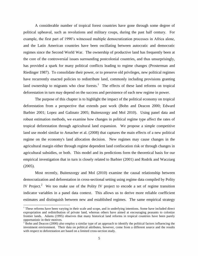
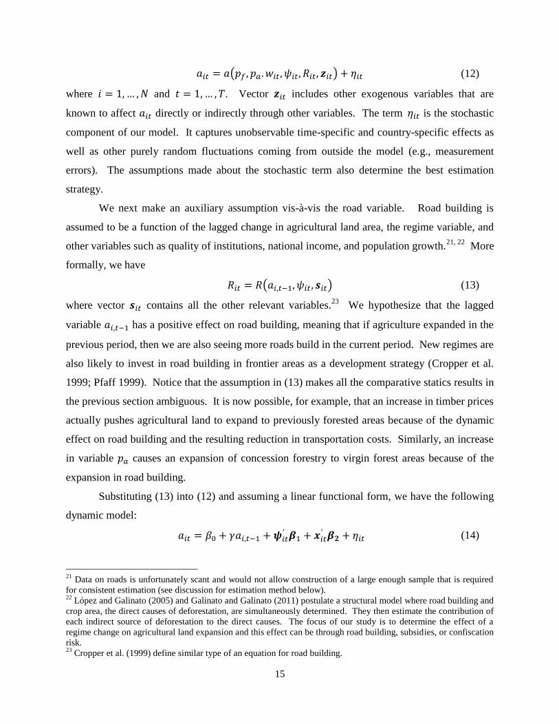
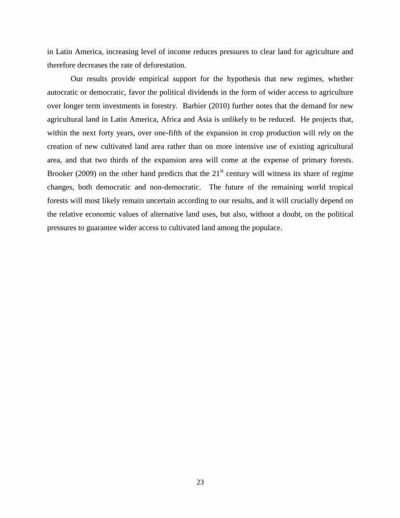
more profitable on lower quality parcels. Parcels with are left undisturbed. Figure 2.1
illustrates the meaning of the above assumption by plotting the maximized rents, and , as a
function of land quality, q. The point where the curves intersect defines the agricultural margin,
. Any shift in the margin to the left that is due to changes in exogenous variables is interpreted
as deforestation.
To formalize the allocation decision depicted in Figure 2.1, denote the portion of each
land parcel allocated to forestry production as , and the portion of each parcel allocated to
15
Agricultural land may also be subject to expropriation risk when a new regime comes to power. We have not,
however, incorporated this risk in our theory model as it would not change the main tenet of our analysis.
Additionally, the confiscation risk impinging on forest land can be thought of as the relative risk of land use. 16
Forest parcels allocated to harvesting activities can be also thought of as the frontier land or as degraded forests.
Deforestation occurs when agriculture takes over these parcels. We discuss this in more detail below. 17
We derive comparative statics results below. 18
We assume that the objective functions are well behaved and have a unique maximum for each land quality.
11
agriculture as . The economy then allocates each parcel with quality
between the two land uses based on the following maximization problem:
(5)
where and are the maximized values of land rents for each parcel. The optimal labor
input decisions, and
, are the corresponding solutions to the per parcel maximization
problem.
The first-order condition for the problem in (5) can be written as
(6)
This implicitly defines the switching point, , called the agricultural margin, that divides the
whole land area into two compact subsets of forestry and agriculture uses. Formally, the total
areas allocated to forestry and agriculture can then be defined as
(7)
Condition holds, where denotes the fixed total amount of land, is the area
under agriculture, and is the area under forestry. Notice that any change in either area leads to
an equivalent but opposite change in the other area.
2.3.1 AGRICULTURAL MARGIN
The comparative statics results of this model inform our empirical expectations with
respect to key variables. They determine how exogenous forces affect the agricultural margin,
, and thus the land allocation decision. If the agricultural margin shifts to the left in Figure 2.1,
we take this to mean deforestation. If the margin shifts to the right, we take this to mean
expansion of plantation forestry.19
19
Plantation forests are not necessarily a substitute for native forests or even for degraded forest stands. The real
definition of deforestation is therefore more nuanced and contested than the one we apply here. Notice, however,
that our main goal is to assess the impact of new regimes on agricultural expansion.
12
Define a parameter vector for the continuous variables, , and
differentiate the second expression in (7) with respect to the parameter vector to get
(8)
The partial derivative on the right hand side of equation (8) can be derived by implicitly
differentiating the first order condition in equation (6). The effect of regime change on
agricultural margin is derived using discreet methods. We then arrive at the following
predictions (see Appendix A for derivation):
(9)
We discuss each of these results individually and their relation to the regime dependent risk.
Agricultural Produce Price Index
The sign of the effect of on agricultural expansion is unambiguously positive: higher prices
translate to more land clearing for agriculture, and thus to deforestation at the margin.
Timber Price
Higher timber prices translate to expansion of forestry to previously cultivated land areas. This
can be interpreted as expansion of plantation forestry. The magnitude of this effect depends on
the political regime risk, and the higher the risk of confiscation, the smaller the change at the
margin, .
Labor Unit Price
Since a change in has an effect on both plantation forestry and agricultural land rents, the
overall effect on the agricultural margin is ambiguous. The political regime variable affects the
magnitude of this effect and may decide the direction as well. For example, suppose that labor
costs decrease because of rapid population growth. Then, if the confiscation risk facing
plantation forestry is sufficiently high, the agricultural margin will expand at the cost of forests.
Regime Variable
The effect of a regime change is ambiguous and depends on the sign of the following expression
(see Appendix A):
Case 1:

13
Agricultural rents are now higher than forest rents at the old margin , thus leading to an
expansion of agricultural area until the economy reaches a new point where holds
again. This outcome occurs if the new regime favors agriculture over forest production. The
new regime may subsidize encroachment of agriculture to areas previously under concession
harvesting: . It may also directly confiscate forest areas at the margin through
land reforms and allocate them to farmers who then convert the land to cultivation:
.
Case 2:
Now plantation forestry expands to previously cultivated areas until the economy reaches a new
point where holds again. This outcome occurs if the new regime either reduces
agricultural subsidies, , or reduces the risk of forest confiscation,
.
Roads Variable
Expansion of roads has an ambiguous effect on the agricultural margin since it reduces
transportation and access costs for both plantation forestry and agriculture. However, the higher
the political regime risk facing plantation forestry, the more likely it is that road building benefits
agriculture more, thus leading to an expansion agriculture and deforestation at the margin.
2.3.2 NATIVE FOREST MARGIN
Next, we derive the comparative static results with respect to the virgin forest land area.20
A decrease in this land area is assumed to mean expansion of concession forestry. The forest
land area left as undisturbed is defined as
The comparative statics are then (see Appendix A for derivation):
(10)
We again discuss each of these cases individually and their relation to the regime variable.
Agricultural Produce Price Index
20
Changes at this margin are not the focus of our econometric study, but we derive these results for the sake of
completeness and as guidelines for future research.
14
Variable has no effect on virgin forest area since in our model, agricultural land expands on
areas where concession harvesting is practiced, that is, at the margin .
Timber Price
Changes in timber prices have an unambiguous effect on virgin forests. Higher timber prices
attract more timber firms and result in expansion of concession harvesting at the margin. If the
regime risk is high, the expansion will be smaller as the concession firms may risk losing their
land rents.
Labor Unit Price
Variable also has an unambiguous effect on the virgin forests. For example, suppose that
wages decrease due to population growth. This results in expansion of concession forestry as
labor costs are reduced.
Regime Variable
The effect of a regime change is ambiguous. It depends on the sign of forest rents
evaluated at the old margin . If , concession harvesting expands on virgin forest
areas, whereas if , virgin forests overtake areas previously allocated to concession
harvesting. The first outcome occurs when new regimes actually reduce riskiness of concession
harvesting. The second outcome occurs when new regimes increase risks associated with
concessions, leading harvesters to abandon old areas due to uncertainty.
Roads Variable
Road building has an unambiguous effect on virgin forest land: more roads reduce the
transportation and access costs, thus making expansion of concession harvesting more attractive.
2.4 ECONOMETRIC MODEL
Our goal in this section is to postulate an econometric model that captures the effect of the
political regime variable, , on the agricultural land margin, , and thus whether new regimes
induce higher or lower rate of deforestation at this margin. Define the percentage change in
agricultural area in country at time as
(11)
Based on our theory model, we can then write in a reduced form as a function of exogenous
variables and a random disturbance term:
15
(12)
where and . Vector includes other exogenous variables that are
known to affect directly or indirectly through other variables. The term is the stochastic
component of our model. It captures unobservable time-specific and country-specific effects as
well as other purely random fluctuations coming from outside the model (e.g., measurement
errors). The assumptions made about the stochastic term also determine the best estimation
strategy.
We next make an auxiliary assumption vis-à-vis the road variable. Road building is
assumed to be a function of the lagged change in agricultural land area, the regime variable, and
other variables such as quality of institutions, national income, and population growth.21, 22
More
formally, we have
(13)
where vector contains all the other relevant variables.23
We hypothesize that the lagged
variable has a positive effect on road building, meaning that if agriculture expanded in the
previous period, then we are also seeing more roads build in the current period. New regimes are
also likely to invest in road building in frontier areas as a development strategy (Cropper et al.
1999; Pfaff 1999). Notice that the assumption in (13) makes all the comparative statics results in
the previous section ambiguous. It is now possible, for example, that an increase in timber prices
actually pushes agricultural land to expand to previously forested areas because of the dynamic
effect on road building and the resulting reduction in transportation costs. Similarly, an increase
in variable causes an expansion of concession forestry to virgin forest areas because of the
expansion in road building.
Substituting (13) into (12) and assuming a linear functional form, we have the following
dynamic model:
(14)
21
Data on roads is unfortunately scant and would not allow construction of a large enough sample that is required
for consistent estimation (see discussion for estimation method below). 22
López and Galinato (2005) and Galinato and Galinato (2011) postulate a structural model where road building and
crop area, the direct causes of deforestation, are simultaneously determined. They then estimate the contribution of
each indirect source of deforestation to the direct causes. The focus of our study is to determine the effect of a
regime change on agricultural land expansion and this effect can be through road building, subsidies, or confiscation
risk. 23
Cropper et al. (1999) define similar type of an equation for road building.
16
Vector contains the set of control variables including proxy variables for some of the
variables in (12). Control variables include, for example, the level of national income as
measured by GDP and its square. This allows us to test for the Environmental Kuznets Curve
hypothesis, the existence of a turning point for deforestation-income relationship. Other control
variables are described in the data section in more detail. The stochastic term takes the following
general form:
(15)
Following the standard approach in panel data analysis, we allow for both unobservable
individual effects, , and unobservable time-wise effects, . The individual effects may
exhibit correlation with the independent variables in equation (12), i.e. a fixed effects model
(FE), or alternatively, they can be viewed as random draws from an i.i.d. distribution with zero
mean and common variance, i.e., a random effects model (RE). Usually FE model is preferred in
country level settings such as ours, but this hypothesis is testable.24
2.4.1 ESTIMATION
A dynamic FE model with a lagged dependent variable yields inconsistent parameter
estimates when using a within or first-difference (FD) estimator. This inconsistency, however,
disappears in the case of a within estimator as (Nickell 1981). Alternatively, one can
apply an instrumental variable method proposed by Anderson and Hsiao (1982), or a GMM-
estimator proposed by Arellano and Bond (1991) to get consistent estimates. Both of these
methods, however, rely on FD transformation. This is not innocuous in the context of our study
since we use constant binary variables to capture the effect of a regime change on the agricultural
margin. Laporte and Windmeijer (2005) show that in cases like these, FD estimator performs
poorly if the actual treatment effect is not constant in time. Within estimator, on the other hand,
tends to be considerably more robust to this type of specification error. Hence, we use a within
estimator and rely on asymptotics. Inconsistency of the within estimator may also result from
unobserved or omitted time-varying variables that are correlated with the control variables or the
regime change variable. For example, there is a possibility that and some of the right-hand
side variables in (14) are simultaneously determined (e.g. López and Galinato 2005). Using
exclusion restrictions and a Hausman test, we assess whether contemporaneous correlation
24
The advantage of fixed effects model is that we are able to control for unobserved individual effects that may bias
coefficient estimates in cross-sectional studies if they correlated with independent variables.
17
between the idiosyncratic error, , and a subset of covariates raises concerns over consistency
of our estimates.
2.5 DATA
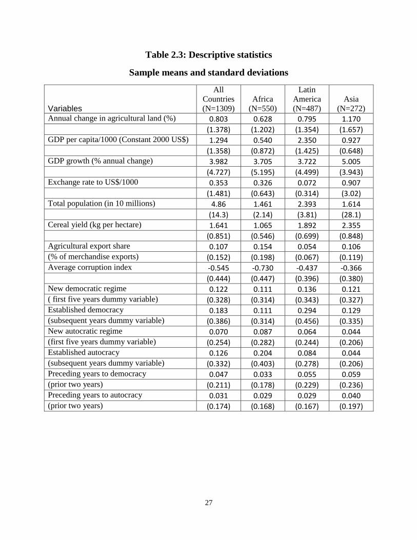
We follow Barbier (2001) and use country level data on annual changes in agricultural area
as the dependent variable.25
Reliability of such data is always a concern, and ideally, we would
like to use observations based on more accurate methods such as remote sensing. This is not,
however, feasible in the context of our study since to achieve consistent estimates requires a
large sample of countries observed over a long time period. Our data come from the following
sources: the World Bank’s WDI and WGI databases, Penn Tables, and the Polity IV Project.
Tropical countries are defined as the countries that have the majority of their land mass located
between the tropics (Barbier and Burgess 1997; Barbier 2001). Our final sample is an
unbalanced panel dataset including 66 countries and spanning years from 1961-2007.26
Table
2.1 provides variable descriptions and Table 2.3 presents sample descriptive statistics.
Two shortcomings with our dataset are the lack of price and wage data. These are some
of the main components implied by our theory model as well.27
This information is
unfortunately scant, or in many cases, nonexistent. Assuming global timber and agricultural
prices we are, however, able to capture their effects through time specific error component that is
common to all countries at time . Variables for cereal yield and agricultural export share also
serve as good proxies to the value of agricultural products in different countries. Level of real
GDP and GDP growth rate on the other hand provide good proxies for changes in real wages. In
order to control for institutional differences, we include a corruption index variable in our
dataset. Corruption is frequently found to be an important explanation for unsustainable forest
management (e.g., Ferreira and Vincent 2010). The index scores countries on a scale between -
2.5 and 2.5, where smaller values mean higher level of perceived corruption. We use a time-
averaged index value for each country and then interact this average index with other control
variables of interest (Galinato and Galinato 2011).
25
We have removed observations with zero values since we are mainly interested in cases where there actually have
been changes in the expansion rate. To check for potential selection problem, we estimate a Heckman selection
model and cannot reject random selection. Thus removing zero observations should not be of concern. We have
also removed observations that have exceptionally large values (the lower and upper 1st percentiles).
26 See Table 2.2 for the list of countries.
27 Information on road building is also an important missing element (López and Galinato 2005). Data on roads is
limited and would not allow construction of a large enough sample.
18
Next we describe the set of political regime variables that are new to our empirical
approach. Using Rodrik and Wacziarg (2005) we have recreated their set of indicators that serve
to identify a change in each country’s political regime. They use information reported by the
Polity IV Project (2002) to encode political regime transitions, whereas we use a newer version
(2009) of the same source. Dummy variables “new democratic regime” and “new autocratic
regime” take on values 1 starting from the year of a major regime change depending, of course,
on the direction of the change. Note that the definition of a major regime change is given by the
Polity IV Project (Marshall et al. 2009). These dummy variables continue having value 1 for the
subsequent five years unless the regime is disrupted during that period. If the new regime
survives the first five years, then the dummy variables “established democratic regime” and
“established autocratic regime” take on values 1 thereafter until they are possibly again disrupted
by a new major regime change. We also augment the original set of dummy variables in Rodrik
and Wacziarg (2005) to include two indicator variables that capture the preceding two years prior
to a democratic and autocratic regime change, recognizing that there may be some preemptive
policy shifts before a new regime formally takes over.28
This complete set of indicators enables us to investigate the impact of different phases of
a new political regime in more detail. For example, the average life-span of a military regime is
five years (Brooker 2009). These types of regimes are usually concentrated on getting a few
specific objectives completed before stepping down. It is interesting therefore to see whether the
first years of a new regime have distinct impact on the expansion rate of agriculture as the level
of uncertainty on land rents might be at its highest. Notice that the baseline case here is “no
regime changes of any kind” during the sample period. Thus the dummy variables capture the
effect of a regime change compared to status quo, whether that is a democratic or autocratic
regime. Also, it is important to note that transitions from one regime to another are not clear cut
or instantaneous necessarily which somewhat complicates the identification of the year of a
regime change.29
28
We assume here that the preceding two years are enough to capture the expectations of a regime change and any
uncertainty caused by a prospective land reform. 29
For example, a revolution could sweep in during one year or it could require a prolonged civil war before any
clear outcome is perceivable. In many cases, the outcome is actually muddled where the new regime lies
somewhere in between the two regime types. In encoding the indicator variables, we have followed the definitions
provided by Polity IV in a consistent manner in order reduce ambiguities.
19
2.6 RESULTS AND DISCUSSION
The estimation results from our empirical model are presented in Table 2.4. The estimated
model includes fixed country specific and time specific effects. Robust standard errors are
reported in the parentheses below the coefficient estimates. We have interacted the political
regime variables and GDP variables with region specific dummy variables.30
This enables us to
determine whether coefficients differ between regions. These region specific interaction terms
are presented in the second (Africa) and the third (Asia) columns, whereas the first column
represents the baseline estimates which are for Latin America. Additionally, we have added
interaction terms for GDP and corruption index. Corruption index itself is time invariant and
therefore included in the country specific effects. Notice that our final specification does not
include squared GDP term as it was deemed statistically insignificant.
The political regime coefficient estimates provide interesting clarification to the
ambiguities in our theory model’s predictions. The effects of regime changes seem to be region
dependent for the most part. Starting with new democratic regime variable, it is significant at
5% level for Latin America, but there is no statistically significant difference between the
regions. Established democracy variable is not significant implying that once democratic regime
has survived the first five years it has no tendency to accelerate expansion of agriculture. New
autocratic regime variable is significant and positive for Latin America but negative and
significant for Africa. This means that in Africa new autocracies have not had a major impact on
agricultural land expansion. Established autocracy variable has the same pattern but now also
the interaction term with Asia has a positive and significant coefficient. This implies that in Asia
established autocracies have accelerated agricultural expansion even more than in Latin America.
Preceding years to autocracy have not had statistically significant effect on the dependent
variable, whereas preceding years to democracy have had a positive and significant effect in
Latin America but negative and significant effect in Africa.
The lagged dependent variable is statistically significant but the coefficient is small,
implying low persistence.31
GDP growth rate has a positive effect on the dependent variable,
whereas increases in cereal yield lead to decreases in the rate of expansion of agricultural land.
Weaker exchange rate of the local currency in relation to US$ has a positive effect on the
dependent variable. Higher population has a positive effect as well. The coefficient for GDP per
30
We also tried including interaction terms with other control variables but these were not important. 31
Dynamic IV and GMM estimates for the lagged dependent variable did not differ much from the within estimate.
20
capita is negative and significant in the case of Latin America, but the interaction term with
Africa is positive and significant. This means that higher income level has reduced or reversed
agricultural expansion in Latin America, whereas in Africa the opposite holds. Also the
corruption interaction term has differing effects across regions. In Latin America, better control
of corruption makes GDP to have even more pronounced negative effect on agricultural land
expansion. This could mean, for example, that improved corruption control together with
income growth implies better property rights enforcement. In Africa and Asia, however, the
opposite holds. In these two regions, higher income levels result in higher rate of agricultural
expansion when control of corruption is also improving.
GDP and GDP growth variables may potentially violate exogeneity assumption. We use
the U.S. real GDP deviations from linear time trend line interacted with trade openness as an
instrument to test the exogeneity assumption.32
This instrument captures the effect of global
economic conditions and these effects presumably differ depending on the openness of the
economy, hence the interaction form. Moreover, after controlling for agricultural export share,
these changes in global economy do not affect the rate of agricultural land expansion. This
constitutes as our exclusion restriction. Based on a Hausman test (e.g., Wooldridge 2002), we
cannot reject exogeneity at 10% level for either GDP or GDP growth, and therefore, we do not
proceed to use instrumental variables estimation methods.
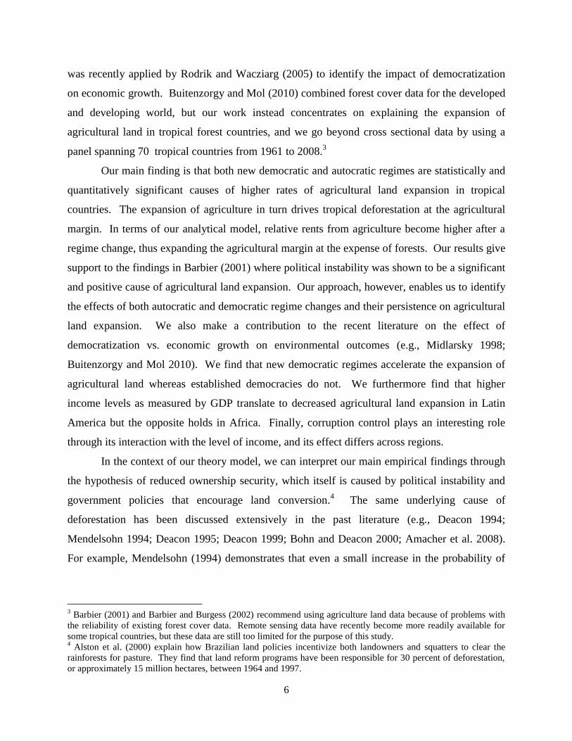
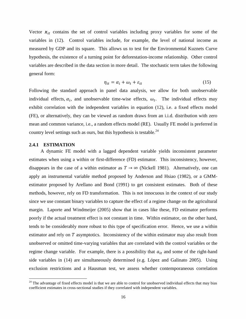
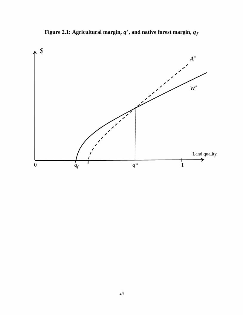
Figure 2.2 presents regional examples of the effects of the first five years of new regimes
on the rate of agricultural land expansion. At year zero (not shown in the figure), both Latin
America and Africa have their respective steady state agricultural expansion rates, which we
assume to be the average values found in Table 2.3. In year one, there is a regime switch and the
new regime persists for five years. After that, we assume that both regions return back to their
steady state values. Notice that we are not including the effects from the preceding years or the
effects from the new regimes becoming established regimes after the first five years. As can be
seen from the graph, the effect is most pronounced in Latin America in the case of a new
autocratic regime. The rate of expansion is more than doubled. Also new democratic regime in
Latin America has a significant effect on the rate of expansion. In Africa, new autocratic
regimes have much smaller effect. Notice that since the coefficient estimates for new democratic
32
Trade openness is defined as the sum of imports and exports divided by GDP.
21
regime are not statistically different between the regions, the graphs for Asia and Africa would
resemble the one for Latin America.
There are some clear interpretations for our collective results. Starting with Latin
America, it is well known that this region has witnessed multiple attempts to reform
landownership during our sample period, and in some countries, like Mexico, the drive to reform
was initiated even earlier. Powerful landlord classes have historically controlled vast tracts of
land in many of these countries, and the inequality of ownership has been high. Large estates
called “haciendas” and owned by landlords have continued to play a significant role in the
political and socio-economic setting. This explains why ownership of land still continues to be a
controversial issue and also the cause of land reform and settlement policies under both new
autocratic and new democratic regimes. These results are also supported by empirical findings
in Barbier (2001). He finds that a general political stability indicator variable is a significant and
positive predictor of agricultural land expansion in Latin America. Our interpretation goes
further in showing that political regime is important, and as such the results for Latin American
countries are best in line with our theoretical predictions. New regimes have a more active
stance concerning land use policies exactly because land ownership has been and continues to be
at the core of the social and economic issues causing political instability.
Our estimation results for Africa call for an alternative interpretation. Referring to Table
2.3, the descriptive statistics show that new autocracies in this region have been relatively more
long-lived than elsewhere. This could imply that the leaders of these autocratic regimes are less
worried about being overthrown and thus less inclined to embark on reformist policies. They
might also have become more reliant on the rents from other types of natural resources such as
oil and minerals. This means that they have not needed to take into consideration the needs of
the general population, or the landless, to the same extent as in other circumstances. In Africa,
tribal and family hierarchies have furthermore been the traditional and dominant form of societal
organization. The impact of new regimes may therefore be smaller than elsewhere as tribal
chiefs and other communal leaders have acted as filters between the central power and the tribes’
land use decisions. Our results showing that agricultural expansion is reduced during the two
years prior to a new democratic regime may capture the effect of prolonged civil wars and chaos.
In many Asian countries, similar to the experiences in Latin America, landlord classes
have historically controlled large tracts of land, which have then been cultivated through tenancy
22
and sharecropper arrangements. Such institutions have been less common in Africa (Daley and
Hobley 2005), and this additionally can help in explaining the similarities in results between
Asia and Latin America, on the one hand, and differences between Africa and the two other
regions on the other. There are some anecdotal examples of authoritarian leaders who have used
redistribution of land as a political weapon in Asia. For example, Ferdinand Marcos, the
authoritarian leader of Philippines from 1965 to 1986, redistributed private land to small farmers
under his program “Operation Land Transfer.”33
2.7 CONCLUSIONS
We began our analysis by proposing a simple land allocation model with regime dependent
confiscation risk and agricultural subsidy policy. The theory model provides ambiguous
predictions with respect to the effects of new political regimes on the agricultural margin. The
purpose of the empirical part is to clarify these theoretical ambiguities, and we make some
interesting findings with respect to the region specific differences in these effects. We find that
in Latin America and Asia both new democratic and new autocratic regimes have increased the
expansion of agricultural land. In Africa, however, new autocracies have not had similar kind of
effect on the agricultural margin and new democratic regimes have similarly had weaker positive
effect. Our results show that autocratic regimes that have survived the first five years have a
tendency to further accelerate agricultural land expansion in both Latin America and Asia. In
Africa, this effect has been again considerably smaller. Established democratic regimes have
had no statistically significant effect.
Bohn and Deacon (2000) conclude their work with an optimistic note. They deem that
the recent “trend toward democracy and reduced political instability worldwide” provides a good
prospect for the future of global forests. The main findings of this chapter are not as optimistic,
at least with respect to tropical forests in some regions. Once we include new politically
constructed data on regime implementation and persistence and success, we find that
democratization should not be viewed automatically as a panacea that leads to reduced pressures
on the exploitation of tropical forest resources. New democratic regimes might simply favor the
socio-economic and political stability implications of wider access to agricultural land over the
other land use alternatives (Midlarsky 1998). On the other hand, our empirical results show that 33
This policy is cited as responsible for gaining wide support of the population for the ruling regime. Land
expropriations, however, targeted mainly Marcos’s political enemies such as the communist movement (Borras Jr.
2001).
23
in Latin America, increasing level of income reduces pressures to clear land for agriculture and
therefore decreases the rate of deforestation.
Our results provide empirical support for the hypothesis that new regimes, whether
autocratic or democratic, favor the political dividends in the form of wider access to agriculture
over longer term investments in forestry. Barbier (2010) further notes that the demand for new
agricultural land in Latin America, Africa and Asia is unlikely to be reduced. He projects that,
within the next forty years, over one-fifth of the expansion in crop production will rely on the
creation of new cultivated land area rather than on more intensive use of existing agricultural
area, and that two thirds of the expansion area will come at the expense of primary forests.
Brooker (2009) on the other hand predicts that the 21st century will witness its share of regime
changes, both democratic and non-democratic. The future of the remaining world tropical
forests will most likely remain uncertain according to our results, and it will crucially depend on
the relative economic values of alternative land uses, but also, without a doubt, on the political
pressures to guarantee wider access to cultivated land among the populace.
24
Figure 2.1: Agricultural margin, , and native forest margin,
Land quality
0 qf q* 1
A*
W*
$
25
Figure 2.2: New regime effect (first five years) on agricultural land expansion
1 2 3 4 5 6 7 8 9 10
0.8
1
1.2
1.4
1.6
1.8
2%
change in a
g.
are
a
years
Africa: New autocracy
Latin America: New autocracy
Latin America: New democracy
26
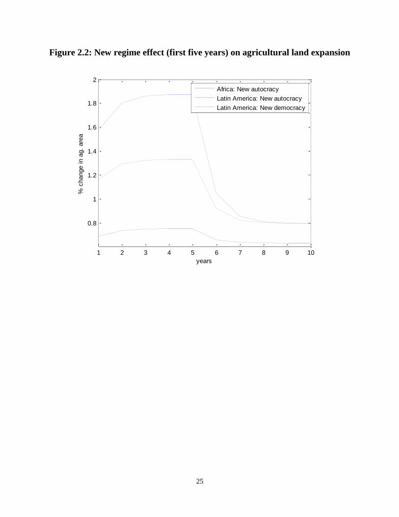
Table 2.1: Variable definitions
Dependent variable: Percentage change in agricultural area from last year’s value. Agricultural land is defined as the land area that is arable, under permanent crops, and under permanent pastures (WDI, FAO).
Control variables: Cereal yield (kg per hectare) Agricultural export share of total merchandise exports (%) GDP per capita (Constant 2000 US$) GDP growth (% annual change)
Exchange rate to US$
Total population
Corruption index variable, time averaged over period 1996-2007 (World Bank WGI)
Regime change: New Democratic Regime (first five years, or if interrupted
during that period, then the years prior to the interruption) New Autocratic Regime (first five years, or if interrupted
during that period, then the years prior to the interruption) Established Democracy (subsequent years or until a new
interruption) Established Autocracy (subsequent years or until a new
regime interruption) Preceding two years prior to a democratic regime change Preceding two years prior to a autocratic regime change
Table 2.2: List of countries
Angola, Belize, Benin, Bolivia, Botswana, Brazil, Burkina Faso, Burundi, Cambodia, Cameroon,
Central African Republic, Chad, Colombia, Comoros, Dem. Rep. Congo, Rep. Congo, Costa
Rica, Cote d'Ivoire, Djibouti, Dominican Republic, Ecuador, El Salvador, Ethiopia, Fiji, Gabon,
Gambia, Ghana, Guatemala, Guinea, Guyana, Haiti, Honduras, India, Indonesia, Jamaica,
Kenya, Liberia, Madagascar, Malawi, Malaysia, Mali, Mauritania, Mauritius, Mexico,
Mozambique, Nicaragua, Niger, Nigeria, Panama, Papua New Guinea, Peru, Philippines,
Rwanda, Senegal, Sierra Leone, Sri Lanka, Sudan, Tanzania, Thailand, Togo, Uganda,
Venezuela, Vietnam, Rep. Yemen, Zambia, Zimbabwe.
27
Table 2.3: Descriptive statistics
Sample means and standard deviations
Variables
All
Countries
(N=1309)
Africa
(N=550)
Latin
America
(N=487)
Asia
(N=272)
Annual change in agricultural land (%) 0.803 0.628 0.795 1.170 (1.378) (1.202) (1.354) (1.657) GDP per capita/1000 (Constant 2000 US$) 1.294 0.540 2.350 0.927 (1.358) (0.872) (1.425) (0.648) GDP growth (% annual change) 3.982 3.705 3.722 5.005 (4.727) (5.195) (4.499) (3.943) Exchange rate to US$/1000 0.353 0.326 0.072 0.907 (1.481) (0.643) (0.314) (3.02) Total population (in 10 millions) 4.86 1.461 2.393 1.614 (14.3) (2.14) (3.81) (28.1) Cereal yield (kg per hectare) 1.641 1.065 1.892 2.355 (0.851) (0.546) (0.699) (0.848) Agricultural export share 0.107 0.154 0.054 0.106 (% of merchandise exports) (0.152) (0.198) (0.067) (0.119) Average corruption index -0.545 -0.730 -0.437 -0.366 (0.444) (0.447) (0.396) (0.380) New democratic regime 0.122 0.111 0.136 0.121 ( first five years dummy variable) (0.328) (0.314) (0.343) (0.327) Established democracy 0.183 0.111 0.294 0.129 (subsequent years dummy variable) (0.386) (0.314) (0.456) (0.335) New autocratic regime 0.070 0.087 0.064 0.044 (first five years dummy variable) (0.254) (0.282) (0.244) (0.206) Established autocracy 0.126 0.204 0.084 0.044 (subsequent years dummy variable) (0.332) (0.403) (0.278) (0.206) Preceding years to democracy 0.047 0.033 0.055 0.059 (prior two years) (0.211) (0.178) (0.229) (0.236) Preceding years to autocracy 0.031 0.029 0.029 0.040 (prior two years) (0.174) (0.168) (0.167) (0.197)
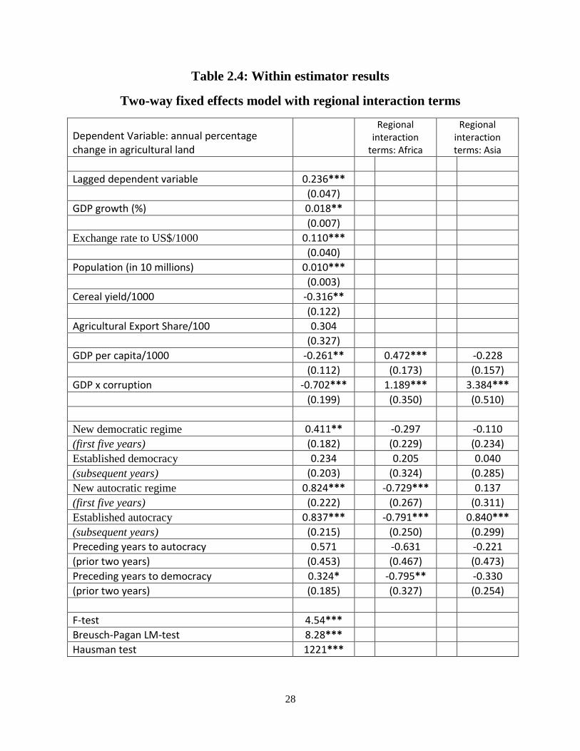
28
Table 2.4: Within estimator results
Two-way fixed effects model with regional interaction terms
Dependent Variable: annual percentage change in agricultural land
Regional interaction
terms: Africa
Regional interaction terms: Asia
Lagged dependent variable 0.236***
(0.047)
GDP growth (%) 0.018**
(0.007)
Exchange rate to US$/1000 0.110***
(0.040)
Population (in 10 millions) 0.010***
(0.003)
Cereal yield/1000 -0.316**
(0.122)
Agricultural Export Share/100 0.304
(0.327)
GDP per capita/1000 -0.261**
0.472***
-0.228
(0.112)
(0.173)
(0.157)
GDP x corruption -0.702***
1.189***
3.384***
(0.199)
(0.350)
(0.510)
New democratic regime 0.411**
-0.297
-0.110
(first five years) (0.182)
(0.229)
(0.234)
Established democracy 0.234
0.205
0.040
(subsequent years) (0.203)
(0.324)
(0.285)
New autocratic regime 0.824***
-0.729***
0.137
(first five years) (0.222)
(0.267)
(0.311)
Established autocracy 0.837***
-0.791***
0.840***
(subsequent years) (0.215)
(0.250)
(0.299)
Preceding years to autocracy 0.571
-0.631
-0.221
(prior two years) (0.453)
(0.467)
(0.473)
Preceding years to democracy 0.324*
-0.795**
-0.330
(prior two years) (0.185)
(0.327)
(0.254)
F-test 4.54*** Breusch-Pagan LM-test 8.28*** Hausman test 1221***
29
3 PERFORMANCE BONDS IN TIMBER CONCESSIONS
3.1 ABSTRACT
We evaluate effectiveness of performance bonding for tropical forest concession
management in achieving first and second best outcomes concerning reduced impact logging
(RIL) standards. As a novel contribution, we introduce a simple model of two-stage concession
design, and focus on the impact of three complications: harvester participation constraints,
government repayment risk, and imperfect enforcement. We find several new and interesting
results, in particular, imperfect enforcement and bond risk may deter implementation of bonding
schemes as either the bond payment has to be set higher or the penalty mapping has to become
more punitive. Policy implications, including potential for mechanisms such as REDD+ in
improving the bonding outcomes, and the degree of financial support required to guarantee full
implementation of RIL, are examined. We find that the necessary REDD+ finances required to
support performance bonding schemes may be much higher than expected.
3.2 INTRODUCTION
Poor design and harvesting practices in industrial timber concessions are commonly
identified as significant, albeit indirect, causes of tropical deforestation. High grading, illegal
logging, and collateral stand damages have led to forest degradation, whereas roads have
provided access routes to slash-and-burn agriculture with ensuing deforestation. The standard
way governments have regulated these actions is via direct restrictions and limitations but also
through taxes, or royalties, for harvesting either based on volume or area, with the idea of
seeking a first-best Pigouvian solution. Sole reliance on these instruments has, however,
received criticism due to their apparent failures in encouraging sustainable forest management
practices. Many, including Ruzicka (2010) recently, have argued for a better evaluation of the
obstacles hindering the use of non-tax market alternatives such as bonding in concession design.
Environmental performance bonds have received some attention in the literature as a
promising complement to royalties for governments seeking to both capture rents and ensure
harvesters follow concessions rules (e.g., Paris et al. 1994; Boscolo and Vincent 2000; Leruth et
al. 2001; Macpherson et al. 2010; Ruzicka 2010). The idea is that performance bonds create a
stronger incentive for harvesters to comply with concession rules and at the same time provide
30
the government with critical funds to compensate for environmental damages when they do
occur.34
Bonds have not, however, gained much traction in practice for a wide variety of
reasons. At the most basic level, setting “the right” bond payment has been difficult. In many
developing countries, bond repayment risk and concessionaires’ liquidity constraints also raise
concerns about the practicability of bonding schemes. Performance bonds nevertheless possess
properties that can make them attractive in forest concessions, if designed well.35
The purpose of this chapter is to analytically examine the properties of bonding schemes
and to identify their potential shortcomings in the context of Reduced Impact Logging (RIL)
standards for forest concessions. Previously, Boscolo and Vincent (2000) and Macpherson et al.
(2010) have examined the effectiveness of bonds in enforcing RIL standards, whereas Boltz et al.
(2003) conclude that the harvesters may not fully implement RIL techniques without additional
incentives. Our novel contribution is to concentrate on three well-identified complications:
liquidity (credit) constraints on the part of the harvester, imperfect enforcement, and repayment
risk stemming from the government’s potential inability to pay back the bond at the end of the
concession.
The first of these complications is caused by “thin” financial markets, a condition
prevalent in many tropical countries, that prevents smaller scale concessionaires from sufficient
collateral needed to obtain credit in the first place (Simula et al. 2002; Canby and Raditz 2005;
Pescott et al. 2010; Grossheim 2011). Imperfect enforcement has been frequently identified as
one of the most problematic features of tropical timber concessions. Obstacles to enforcement
can be multifold, such as poor monitoring capabilities, inadequate judicial systems and corrupt
governments. Vast concession areas moreover create an environment conducive to low
enforcement, contract violations and illegal logging (Callister 1999; Hardner and Rice 2000;
Contreras-Hermosilla 2002; Amacher et al. 2012). The third complication stems partly from
unpredictable institutional arrangements typical of many of the tropical countries. Governments
34
Mathis and Baker (2002) track the fundamental concept of “assurance” schemes to “materials-use fees”
originating from Solow (1971) and Mills (1972). Other examples come from refundable deposit schemes in
beverage industry (Sterner 2003), and mine reclamation in the U.S. and Australia (Sullivan and Amacher 2009).
Leruth et al. (2001) advocate the use of performance bonding arguing that they reduce public monitoring costs by
relying mainly on a final inspection. 35
Having guaranteed access to funds needed to mitigate potential contract violations is especially relevant in
institutional settings where ex-post financial retribution for damages may be uncertain and costly to attain (Boyd
2001). Furthermore, environmental bonds can be used to reveal the true market value of the forest resource when it
is combined with competitive bidding procedures (Leruth et al., 2001).

31
may not be able honor promises to repay the bond at the end of the concession contract, or
bureaucratic red tape may make repayment time unreasonably long.36
Our analysis represents the first theoretical assessment of performance bonding for
tropical concessions under the assumption that there is moral hazard, i.e., the government forest
owner may not be able to ensure paying the bond back with probability one, and additionally the
harvester may face liquidity constraints. We take a simple static approach that illustrates clearly
many of the important issues and results that would still be present in a more complicated model.
We will derive the necessary and sufficient conditions that guarantee full RIL implementation by
a cost minimizing harvester and discuss when this can and cannot be expected and what its
implications are for successful bond design, detailing various second-best outcomes that result
when the first-best solution is not attainable. We find, not surprisingly, an important role for
supranational parties that provides another important context for REDD+ mechanisms.37
Using
model simulations, our approach allows us to compute the necessary REDD+ transfer that still
guarantees full RIL implementation when government repayment risk and imperfect enforcement
are present. We also find the critical level of repayment risk that determines whether full RIL
realization is possible to achieve given the harvester’s participation constraint.
The plan of the chapter is as follows. The next section reviews the issues surrounding the
recommendations and debate over environmental bonds for concessions. We proceed by
presenting a model of concessions design and bonding in a perfect institutional setting and
introduce participation constraint. Section 3 analyses the impact of repayment risk on the
harvester’s compliance decision and participation ability. Section 4 examines the repercussions
of imperfect enforcement on the bond design. Section 5 uses model simulations to assess the
practical impact of the various complications analyzed in the previous sections. Finally, the last
section offers concluding remarks and policy implications.
36
Institutional uncertainty causes skepticism especially with respect to the transparency and fairness of the final
assessment method. Credit constraints are further exacerbated by the presence of such concerns since creditors may
require a higher risk premium, or they will simply refuse to extend credit. 37
Reducing emissions from deforestation and forest degradation (REDD) is one of the main focuses of the ongoing
UNFCCC climate change treaty negotiations. REDD+ is a comprehensive policy concept that incorporates variety
of approaches and financial incentives that aim at enhancing the forest carbon stocks in developing countries, and
encouraging conservation and sustainable forest management practices (Nasi et al. 2011; Pfaff et al. 2010; Karsenty
2012).

32
3.3 CONCESSIONS AND PERFORMANCE BONDING
This section develops the most basic concession bond model with perfect enforcement and
no government repayment risk. The subsequent sections extend this model to incorporate more
realistic features that are prevalent in many tropical timber concessions. Before elaborating a
model of a bond issuing government and bond paying firm, some background concerning the
problem is needed. Forest concessions typically involve the government allocating the forest use
rights to a private concessionaire or contracting with a firm for forest management services, all
of which require firms to fulfill a wide range of contract clauses (Gray 2002; Karsenty et al.
2008). The main challenge facing the government is how to guarantee concessionaires’
adherence to contract rules in an institutional setting characterized by imperfect enforcement and
omnipresent corruption, all of which impede tropical developing governments from managing
concession design (Amacher et al. 2007).
In the context of industrial logging concessions, performance bonds have been actively
discussed for the past two decades as an alternative to poorly designed royalty systems that are
not effective at capturing rents or creating incentives for sustainable harvesting, at least since
Paris et al. (1994).38
While there have been some actual experiments with forest concession
performance bonds in the Philippines and Malaysia during the 1990’s, the policy outcomes were
disappointing. Too low of an initial bond payment has been faulted as the main cause for policy
failure (Coria and Sterner 2011). Ruzicka (2010), however, argues that performance bonding
schemes have never really been tried properly and calls for further investigation of their potential
for concessions. Most recently, Nasi et al. (2011) also suggest that performance bonding
schemes have potential to enforce environmental goals in concession design. Similar in spirit to
what a bond might represent, Amacher et al. (2012) show that the size of a penalty levied against
environmental damages that must be mitigated after a concession is completed can be used to
control for high grading.
Boscolo and Vincent (2000) and more recently Macpherson et al. (2010) investigate the
effectiveness of performance bonding schemes and renewability audits in industrial forest
concessions using simulation studies which link their analytical model to practical data. Both
38
See for example Karsenty (2010), Leruth et al. (2001), Macpherson et al. (2010), Merry and Amacher (2005).
Particularly relevant for our study, Leruth et al. (2001) show that royalty rates may fail to encourage the adoption of
environmentally less harmful logging practices pointing out that the negative externality is only weakly related to
the quantity harvested, thus rendering the classical Pigouvian solution ineffective. Instead of improving the harvest
method, the concessionaire may simply cut costs by adopting an even more harmful harvest technology.

33
studies find that performance bonding schemes can be successfully used to enforce reduced
impact logging practices in forest management. Based on their simulation analysis, Macpherson
et al. (2012) conjecture that although RIL is found to be superior in comparison to conventional
logging methods in net present value terms, concession loggers may still choose to only partially
adopt RIL and instead use harvest practices that directly improve profitability. For example,
Putz et al. (2008) observe that logging companies employ few forest engineers and few foresters
and thus have insufficient competency in RIL techniques.
Despite the promise of these studies, they do not investigate the institutional
imperfections common in many tropical countries that could undermine the effectiveness and
feasibility of concessions bonding schemes. For example, Merry and Amacher (2005) predict
that Brazilian loggers would be highly suspicious of bonding schemes due to distrust of public
institutions. Shogren et al. (1993) list moral hazard, liquidity constraints, and legal restrictions
on contracts as potential disadvantages associated with performance bonds in environmental
regulation.39
Determining the correct bond payment in the presence of such complications
becomes another vexing issue. If the bond is set too low, then it may fail to deliver expected
compliance with terms of the concessions contract, whereas too high of a bond might burden the
industry up to a point where the entry costs become prohibitive.40
Liquidity or credit constraints
that may either prevent government repayment of bonds to harvesters, or prevent harvesters from
posting an initial bond for a concession, naturally also become more severe as the potential for
major environmental damages increases.41
In an imperfect institutional environment, the firms
may also expend more resources on legal actions that aim at challenging any losses on the
principal payment (Shogren et al., 1993). All the above issues are certainly relevant in the
context of tropical logging.
39
The issue of moral hazard affects the behavior of both the principal and the agent. For example, the principal
(government) may choose to confiscate the bond even if the agent (firm) has performed according to the rules, and
thus the firms, having realized that they will lose the bond, will simply ignore all costly precautionary measures. 40
Mathis and Baker (2002) provide a useful comparison of the views how the bond payment should be set. These
views were originally discussed in Costanza and Perrings (1990) and in Shogren et al. (1993), but there is
disagreement. The former proposes that a bond payment should be set so that it can cover for the “worst probable”
environmental damages, whereas the latter requires the bond to be set to equal the level at which it can induce the
agent to comply with regulation. Mathis and Baker (2002) call the first view as a form of social insurance aimed at
“indemnifying the society” against potential environmental damages, whereas the second resembles more of a
deposit-refund system that simply encourages the agent to adopt an environmentally less harmful technology. 41
Public authorities may also use high bond payments as an instrument to skim financially the strongest (or best
connected) participants and thus discriminate against smaller candidates.
34
In order to accommodate these many observations and realities, we proceed by modeling
a situation where the government owns a forest stand,42
the concessionaire is a large privately-
owned firm,43
henceforth called the concession harvester, and there are reduced impact logging
(RIL) standards within the concession contract that specify a list of preharvest procedures and
harvesting techniques required from the harvester.44
The goal of the government is to achieve
the highest possible level of application of RIL standards in the concession operation, as this
offers the highest protection for the forest.45
Following Boscolo and Vincent (2000) and
Macpherson et al. (2010), we define a continuous index variable that represents the
exact extent of RIL methods used by the harvester. The lower bound, , means no
application (business as usual), and the upper bound, , means full RIL application.46
Hence, the index variable can be thought of as the percentage of RIL procedures that were
actually applied during the harvesting.47
Conversely, denotes the percentage of RIL
procedures that were not applied.
The harvester’s convex RIL cost function is defined as which is increasing and
continuously differentiable over a convex and closed set . Private RIL costs include capital
and labor related costs as well as any other related opportunity cost (these may include forgone
profits from not engaging in illegal activity).48
We assume that holds, although this is
not critical. The interpretation for the convex cost function is that the final RIL activities, such
as retaining some of the most valuable species standing in the forest, are much costlier to the
42
The concession stand can be of heterogeneous structure consisting of multiple different species and diameter
classes. This assumption is not however crucial for our analysis. 43
Most of the firms bidding for concession contracts are large harvesting companies with potential to invest in RIL.
Many harvesters also have international connections. There are some local harvesters with limited capital
equipment that are unlikely to possess resources to adopt RIL. Our analysis here pertains to the larger harvesters. 44
Putz et al. (2008) define reduced impact logging as “intensively planned and carefully controlled timber
harvesting conducted by trained workers in ways that minimize the deleterious impacts of logging.” 45
We do not explicitly model environmental damages in the following discussion. We simply assume that full
application of RIL procedures is socially optimal and hence “first best”. 46
Blas and Perez (2008) provide the following list defining RIL requirements: the delimitation of protected forests
within concessions; the determination and use of minimum tree diameter at breast height (dbh); the development of
a management plan and a logging inventory; minimizing the width and density of the logging roads network;
planning of logging roads; setting a maximum ceiling on number of trees felled by hectare; use of directional felling;
optimizing timber transport roads network; and planning of timber yards. 47
Alternatively, the index variable can represent the proportion of trees that have been treated and harvested
according to the RIL standards. Or the index variable can also denote the share of total forest area under RIL
management. 48
Although the literature provides mixed evidence on the relative profitability of RIL over conventional logging
practices (Medjibe and Putz 2012), our analysis will take it as given that switching to RIL methods means real costs
for the harvester, in one form or another. Boltz et al. (2003) and Medjibe and Putz (2012) find that RIL techniques
may incur much higher opportunity costs than conventional logging.

35
harvester than initial site preparation work such as road building and mapping.49
Finally, we
assume the information on the shape of the cost function, , is symmetric knowledge (e.g.,
Amacher and Malik 1996). This assumption is realistic as RIL requirements are usually
designed by NGOs, are typically known and common knowledge, and the information on the
costs of compliance is often readily accessible and part of extension activities in tropical
concession countries.50
Government sets the
bond, , and designs
a bond function
Harvester chooses level
of compliance with RIL
rules.
Government deducts
possible penalties for
noncompliance.
Figure 3.1: Timing of events
To enforce RIL standards, the government requires a bond deposit, , from the
concession harvester at the beginning of the contract. To make the bond payment operational,
the government devises a bond penalty function that maps the harvester’s level of
compliance to corresponding penalties. This function may in principle take any monotone
decreasing form, although we rule out “all-or-nothing” bonds.51
Figure 3.1 illustrates the timing
of events in our concession model.52
First, the harvester pays the initial bond payment, , and
then takes this entry decision and the penalty mapping, , as given when deciding the
level of RIL compliance. Based on the harvester’s RIL decision, the government proceeds to
49
A convex cost function can be also interpreted as implying that the harvester first fulfills those RIL requirements
that have a low marginal cost, and as the level of compliance increases (as we get closer to ), the harvester has
to comply with rules that have higher marginal costs in terms of x. 50
We retain the simplification of known costs to focus on other features of the performance bond schemes that
would only be reinforced with asymmetrical knowledge of compliance costs or with cost uncertainty. 51
“All-or-nothing” bonds have been successfully applied in other contexts such as reforestation and mine closure
compliance enforcement. In those cases, the regulator releases the bond once the level of compliance has been
deemed adequate. In case of RIL standards, all-or-nothing bonds may not, however, be as appropriate for at least
three reasons: RIL includes multiple steps that have to be performed during and before the harvesting activity and
not as a final procedure; if the harvester fails to comply, the regulator cannot go back and reapply RIL after trees
have been harvested; and the harvesters may distrust any bond scheme where the bond release would depend on the
last inspection in an otherwise cumulative compliance process. These reasons lend support for using a bond
function which explicitly maps bond penalties based on the percentage of compliance. 52
In a more dynamic setting, reputational effects may become an important consideration (Costello and Kaffine
2008). We leave this for future research.
36
deduct any penalties from the bond as dictated by the penalty mapping. Hence, we assume that
the government is fully able to commit to the bond penalty rule.53
For any ex-ante target RIL level set by the government, where means
the full RIL target level, we require the penalty function to satisfy two compliance based
conditions: and .54
In other words, fully complying with the government's
RIL target level, , results in no penalties and zero compliance results in complete initial bond
confiscation.55
The harvester receives back any amount that is left over from the original bond
deposit after deducting for penalties. We can therefore think of the bond penalty function
explicitly laying out the liability rules imposed on the harvester for all possible concession
outcomes.56
Unlike this chapter, Boscolo and Vincent (2000) and Macpherson et al (2010) both
define a linear bond function , or simply . This type of
bond function, however, uses only the bond payment as an instrument but does not utilize the
information about the harvester's cost structure. We expand on this latter point in what follows.
We postulate that the harvester’s problem is one of compliance cost minimization as a
function of RIL intensity:
(16)
The sum inside the curly brackets denotes the harvester’s total cost of RIL compliance under the
bond scheme. It has two components: the private cost of compliance, , which is increasing
and convex in x, and the bond penalty function, , which is decreasing in x. We have
written explicitly as a parameter of the bond function to make it clear that the properties of
the bond function depend on the bond payment.
53
See Amacher and Malik (1996) for a discussion on the role of commitment in environmental regulation. 54
The government may have to aim at a less than full RIL target level if it knows ex-ante that the maximum bond
payment the harvester is able to pay due to capital constraints is not sufficient to guarantee the full RIL target
. In the absence of such capital constraints the government would naturally always choose as its ex-
ante target level and then adjust the bond payment, however high, to guarantee this outcome. The impact of a
binding participation constraint is explained in the next subsection. 55
Alternatively, we could use a setup where the government's target RIL level is always at and let the
harvester's compliance level vary given the bond payment. We instead use a setting where the government decides
the target level given the bond payment and then aims at full compliance with the prescribed target level. The
two approaches are equivalent. 56
A monotone and decreasing bond function makes it somewhat difficult to consider situations where we would like
to punish different RIL violations more or less severely. This would add only complexity without additional
insights to our analysis. So we assume here that the “ordering” of violations does not matter. Only the extent of
deviation from the target compliance matters.
37
The government designs the bond function given its knowledge of the
harvester's problem in equation (16) and the properties of . This leads to the following
proposition:
Proposition 1
Let and for some RIL target level of . Then
is the unique solution to the harvester's problem in equation (16) if and only if the
condition
(17)
holds for any other RIL level given a bond payment that satisfies
.
Proof:
The harvester chooses a unique if and only if holds for
all . Since by assumption, the proposition follows.
Corollary 1: Full RIL target ( )
For a unique solution at , the condition has to hold for
all given a bond payment that satisfies .
Proposition 1 provides bounds for the level and the curvature properties of the bond
function given the harvester's cost structure and target RIL level. It simply means that in order to
guarantee full compliance with the target level the harvester must face a higher total cost for
choosing any other alternative. The right-hand side of condition (17) stands for the cost savings
from not complying, and the bond penalty has to be greater than this to discourage non-
compliance. Moreover, the right hand side of (17) is a strictly decreasing and concave function
for values since we have assumed a strictly convex cost function. Hence from now on,
we focus solely on bond functions that are strictly concave in the range .57
It is worth
pointing out here that the presence of participation constraints, which we will discuss more
below, forms the distinguishing feature of any bonding scheme in comparison to a pure penalty
scheme where no ex-ante bond payment is required.
57
Although not necessary, we restrict our focus on strictly concave bond functions for mathematical convenience.
38
Proposition 2
Given the target level of RIL , the simplest continuous and non-negative bond
function that still satisfies the condition in Proposition 1 is given by
(18)
where and . This function is decreasing, as required, since the
condition
holds for all RIL compliance levels , and
it is constant elsewhere.
Corollary 2: Full RIL target ( )
Given the full RIL target, the candidate bond function becomes
. Any bond payment with achieves full RIL
implementation.
Proposition 2, which is proved in Appendix B, provides a candidate bonding scheme that
satisfies the conditions in Proposition 1. Hence, this function guarantees a unique cost
minimizing point at . We restrict it to be non-negative since negative values would in effect
mean that the government pays a subsidy for the harvester’s compliance.58
Figure 3.3 illustrates
a bonding scheme that satisfies the conditions in Corollary 2, hence achieving full RIL
implementation. Notice that the bond function in Proposition 2 is characterized by two
underlying parameters: and . The government in effect chooses these values given the
harvester's participation constraint. We discuss the role of bond participation cost next.
3.3.1 BOND PARTICIPATION CONSTRAINT
Entering a bond scheme is costly for the harvester. This is captured by a convex bond
cost function that is increasing in the level of required bond deposit, B. This function
captures the harvester's borrowing costs, including transaction costs related to liquidity
58
This may, however, provide a way for REDD+ type of funding to move the concession outcome to full RIL
application. We develop this in more detail in what follows.
39
constraints, or alternatively the opportunity cost of using its own capital.59
For example, as is the
case in many tropical countries, concessionaires must resort to external funding for the bond
payment as they lack sufficient funds prior to the concession.60
The bigger the bond the more
expensive it is to borrow funds, that is, holds (e.g., interest payments are increasing in B).
Most importantly, when the harvester enters the concession contract, the bond cost is sunk and
does not enter the harvester's cost minimization problem in equation (16). Later, we introduce
the effect of repayment risk on the bond cost function.
The harvester participates as long as bond costs do not exceed some threshold level,
defined here as . That is, the harvester enters the concession bond scheme if and only if
. We assume that this parameter is exogenously given, but conceivably, it could be
a function of such things as timber prices, availability of competing investment opportunities,
and the harvester’s liquidity in financial markets. Naturally, bigger concession harvesters have
better access to capital than smaller ones, which means that is likely to be higher for big,
multinational firms than for local harvesters. The maximum bond payment, denoted by , is
given by the inverse mapping of the participation cost function: . This simply
means that when access to funds or availability of capital is better, the harvester is able to post a
larger bond at the limit as is higher.
If the highest possible bond payment satisfies the condition , then Corollary 1
and Corollary 2 hold and achieving full RIL compliance target level is feasible. We call
such cases as the "first-best" bond schemes. Notice that in principle the government can set the
bond payment anywhere between and , or more precisely, .61 If the
condition for the first-best is not satisfied, then the government has to design a bond scheme
where the target RIL level is such that . We call such cases as the "second-best" bond
schemes. Since the government's goal is to achieve the highest possible RIL target level, then
choosing the highest possible bond payment to achieve this goal makes sense. This leads to
the following proposition which modifies Proposition 2 to include the second-best scenario and
is proven in Appendix B:
59
Even if the government offered to pay interest on the bond payment during the holding period, it is very unlikely
that this interest rate would coincide with the harvester's private discount rate that may potentially be much higher. 60
In case of a functioning surety market, the function captures the premium the harvester has to pay to a surety
company in order to receive bond guarantees. 61
We do not model how the government may choose the first best bond payment. Potentially, the public's demand
for environmental insurance may guide this decision.
40
Proposition 3
Given a target RIL level , where and denotes the inverse
mapping of the cost function, the simplest continuous and non-negative bond function
that is feasible under the binding participation constraint is given by
(19)
where and .
In the second-best case, the government's problem has become one of simply choosing
some target RIL level since the maximum bond payment is exogenously given. The
harvester when faced with a bond scheme that satisfies Proposition 3 chooses the unique cost
minimizing point .62
The government does not have an incentive to ask for any smaller bond
payment as the harvester's participation decision would be unchanged and smaller bond
payments would decrease the upper bound .63 Note in this case that by providing a subsidy the
government could potentially improve the concession outcome. We compute the required
subsidy to move the concession outcome to first-best in the simulation section.
3.4 BOND REPAYMENT RISK
We now allow for the possibility that the harvester loses the entire bond – it is never paid
back - with probability r, regardless of the level of compliance with the RIL rules. This
probability captures, for instance, the risk of fiscal crisis or political turbulence in the country of
the concession, or other factors that have an impact on the risk that the government will default
on the bond repayment. The harvester may also expect there to be some degree of turnover in
the government’s payrolls which may increase the uncertainty over the ultimate bond release
criteria and timetable. Figure 3.2 shows the timing of the events in our extended model. The
main difference in comparison to our earlier baseline case is that we introduce repayment risk in
62
A linear bond function of the form is suboptimal given a binding participation constraint. In
this case harvester always chooses a point which is implicitly given by the first order condition . This point may not coincide with the government’s target level . 63
If the government values environmental insurance more than the harvester’s borrowing costs, then in the second
best case, it should always demand for the highest possible bond payment as this provides the highest
indemnification for the society in the case of a contract violation.
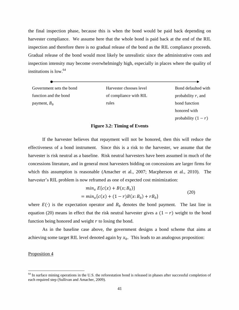
41
the final inspection phase, because this is when the bond would be paid back depending on
harvester compliance. We assume here that the whole bond is paid back at the end of the RIL
inspection and therefore there is no gradual release of the bond as the RIL compliance proceeds.
Gradual release of the bond would most likely be unrealistic since the administrative costs and
inspection intensity may become overwhelmingly high, especially in places where the quality of
institutions is low.64
Figure 3.2: Timing of Events
Government sets the bond
function and the bond
payment,
Harvester chooses level
of compliance with RIL
rules
Bond defaulted with
probability , and
bond function
honored with
probability
If the harvester believes that repayment will not be honored, then this will reduce the
effectiveness of a bond instrument. Since this is a risk to the harvester, we assume that the
harvester is risk neutral as a baseline. Risk neutral harvesters have been assumed in much of the
concessions literature, and in general most harvesters bidding on concessions are larger firms for
which this assumption is reasonable (Amacher et al., 2007; Macpherson et al., 2010). The
harvester’s RIL problem is now reframed as one of expected cost minimization:
(20)
where is the expectation operator and denotes the bond payment. The last line in
equation (20) means in effect that the risk neutral harvester gives a weight to the bond
function being honored and weight to losing the bond.
As in the baseline case above, the government designs a bond scheme that aims at
achieving some target RIL level denoted again by . This leads to an analogous proposition:
Proposition 4
64
In surface mining operations in the U.S. the reforestation bond is released in phases after successful completion of
each required step (Sullivan and Amacher, 2009).
42
Let and . To guarantee a unique RIL solution at
, the government has to design a bond scheme such that the condition
(21)
holds for any other RIL compliance level given a bond payment that satisfies
.
Proof:
The harvester chooses a unique if and only if
holds for all . The left-hand side captures the harvester’s costs at the compliance level
and the right-hand side captures the cost of choosing any other RIL alternative. Since
by assumption, the proposition follows.
Corollary 3: Full RIL target ( )
For a unique RIL solution at , the condition
has to hold for all .
Proposition 4 means that, in order to still guarantee a unique solution at , the presence
of repayment risk forces the lower bound for the bond function to be at a strictly higher
level than in Proposition 1 given the same RIL target . This can be seen clearly from
comparing the two propositions: in Proposition 4 the term in the denominator is less than one and
therefore the expression in the right hand side is larger than the one given in Proposition 1.
When , the condition becomes the same as in Proposition 1, and when , the right-
hand side approaches infinity, and thus no bond scheme can achieve compliance. The RHS in
Proposition 4 is therefore an adjustment to the difference in costs of complying and not
complying by the probability of losing the bond, which increases this expected cost difference.
At the limit, when the government confiscates the bond with certainty, the bond function
has no leverage on the harvester’s compliance decision.
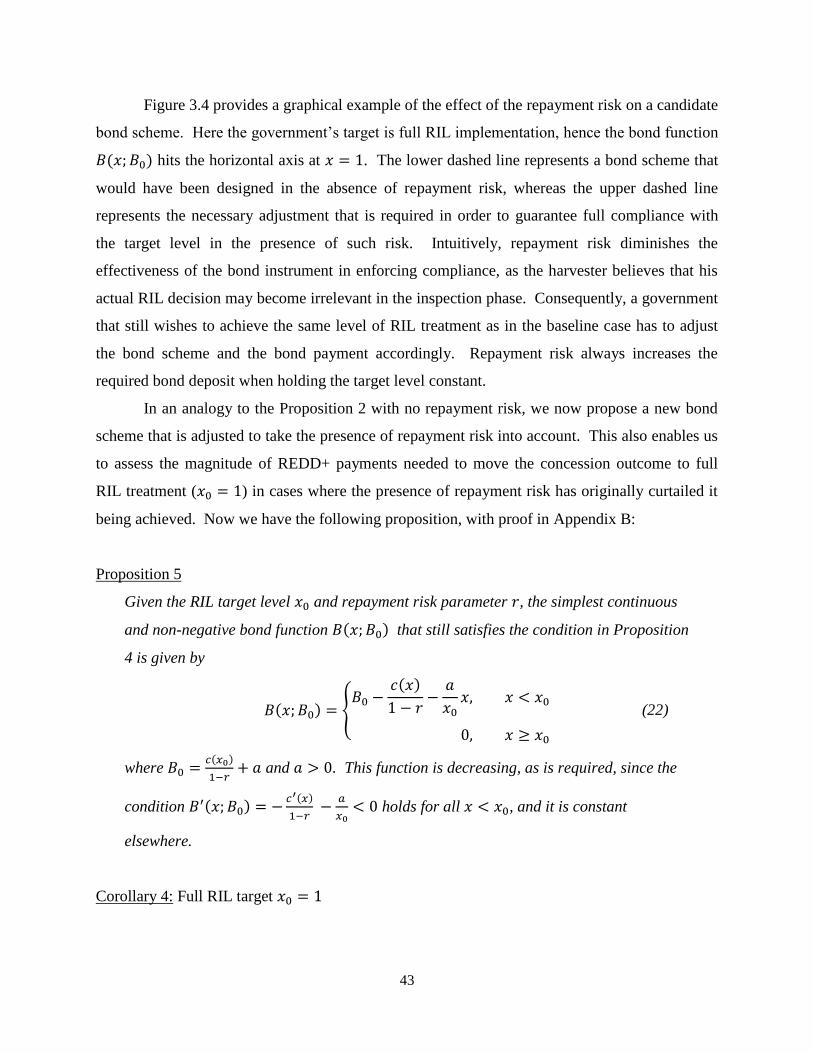
43
Figure 3.4 provides a graphical example of the effect of the repayment risk on a candidate
bond scheme. Here the government’s target is full RIL implementation, hence the bond function
hits the horizontal axis at . The lower dashed line represents a bond scheme that
would have been designed in the absence of repayment risk, whereas the upper dashed line
represents the necessary adjustment that is required in order to guarantee full compliance with
the target level in the presence of such risk. Intuitively, repayment risk diminishes the
effectiveness of the bond instrument in enforcing compliance, as the harvester believes that his
actual RIL decision may become irrelevant in the inspection phase. Consequently, a government
that still wishes to achieve the same level of RIL treatment as in the baseline case has to adjust
the bond scheme and the bond payment accordingly. Repayment risk always increases the
required bond deposit when holding the target level constant.
In an analogy to the Proposition 2 with no repayment risk, we now propose a new bond
scheme that is adjusted to take the presence of repayment risk into account. This also enables us
to assess the magnitude of REDD+ payments needed to move the concession outcome to full
RIL treatment ( ) in cases where the presence of repayment risk has originally curtailed it
being achieved. Now we have the following proposition, with proof in Appendix B:
Proposition 5
Given the RIL target level and repayment risk parameter , the simplest continuous
and non-negative bond function that still satisfies the condition in Proposition
4 is given by
(22)
where
and . This function is decreasing, as is required, since the
condition
holds for all , and it is constant
elsewhere.
Corollary 4: Full RIL target
44
When , the bond function proposal becomes
. Any
bond payment
with achieves full compliance. When , we get
the same result as in the baseline case without repayment risk. As riskiness increases,
the required bond payment also increases and therefore achieving full RIL target level
becomes harder when the harvester faces a binding participation constraint.
When comparing Proposition 2 and Proposition 5, it can be seen that repayment risk has a
twofold effect on the bond function: first, the bond payment has to be set higher than in the
baseline case, and second, the slope of the bond function has to be set steeper, or more
“punitive”. These results are in line with our discussion relating to Proposition 4. Intuitively,
the government has to adjust the bond scheme to account for the diminished effectiveness of the
bond instrument. Consequently, when repayment risk is present, the government may not be
able to achieve the same RIL treatment level as in the baseline scenario if using identical bond
payments. Notice, however, that these differences become relevant only when the harvester
faces binding participation constraints.65
In the simulation section we provide an example of
how even a moderate repayment risk may lead to total noncompliance when the bond scheme is
not adjusted to take this effect into account. These results provide further insights into why
previous experiments with bond in concession management may have failed.
3.4.1 BOND PARTICIPATION CONSTRAINT
When repayment risk exists, the harvester now faces a bond cost function
that is increasing in the level of required bond deposit, B, as was the case in the earlier section,
but also increasing in the parameter, r. The latter captures the perceived riskiness of the
performance bond relative to safer investment. For example, this could simply mean that the
harvester has to pay a higher interest rate if the government's ability to repay the bond has been
rated lower.66
More formally, the bond cost function is increasing in risk, i.e., holds. We
also assume that condition holds, meaning that the marginal borrowing cost is
65
In the absence of participation constraints, the government can always ask for a higher bond payment to neutralize
the impact of repayment risk. 66
In case of surety bonds, the surety company may suspect that the government has a moral hazard problem and
therefore may partially confiscate the bond. This makes the surety company to increase its premium.
45
increasing in risk as well. Intuitively, bigger bond payments become increasingly costly under
repayment risk.
If the harvester's participation constraint is such that the maximum bond payment
satisfies
, where , then achieving the first-best is feasible. In this case,
any bond payment such that
is possible. The parameter in Proposition 5 is
then defined as
. If, however,
then the government chooses as the
second-best bond. This guarantees the highest possible RIL treatment target that is feasible
given the harvester’s participation constraint. The following proposition modifies Proposition 3
to incorporate repayment risk:
Proposition 6
Suppose that
and therefore, , where is the inverse of
the cost function and defines the upper bound for RIL compliance. Given a target
level , the simplest continuous and non-negative bond function that is
feasible under the binding participation constraint is given by
(23)
where and
and where denotes the inverse of the
participation cost function.
Proof: The result follows from adjusting the proofs for Propositions 3 and 5, and by making the
substitution .
When comparing Proposition 3 and 6, the effect of repayment risk on the second-best
bonding scheme becomes clear. First, the maximum bond payment is lower given the same
participation constraint . This occurs because the repayment risk increases the harvester’s bond
costs. With a lower bond payment the government can achieve a lower RIL treatment outcome.
Secondly, repayment risk diminishes the effectiveness of the bond payment, and therefore, the
upper bound is unambiguously lower than in Proposition 3. This means that with a given bond
46
payment the government cannot achieve as high of a treatment target as was the case in the
absence of repayment risk. This result follows from the fact that the bond function has to be
designed steeper to punish the harvester more for marginal noncompliance in order to counteract
the effect of repayment risk. Since the government cannot increase the bond payment, , to
adjust for the steeper bond function, the resulting outcome is that the bond function will
necessarily hit the horizontal axis at a lower level of RIL treatment than in Proposition 3.
3.4.2 CRITICAL LEVEL OF REPAYMENT RISK
As suggested in the above discussion, whether or not the government is able to design a
bond scheme that guarantees full RIL target level depends on the participation constraint
and the repayment risk. In this section, we derive the critical risk level, , below which the
government is still able achieve full RIL target given the values for all the other variables. The
following proposition captures the main result:
Proposition 7
Let
denote the lower bound for the first-best bond payment, and let
hold for some critical risk level . The critical risk level is then
implicitly given by the condition
(24)
By applying the implicit function theorem, we conclude that:
The critical risk level is increasing in the harvester’s participation constraint, that is, a harvester
with better access to capital can handle a higher level of repayment risk. The critical level of risk
is decreasing in the cost of RIL compliance, that is, when compliance becomes more costly,
achieving full RIL treatment becomes infeasible with lower and lower levels of risk. In the
simulation section, we compute the critical risk level given our functional form assumptions and
parameterization.
47
3.5 IMPERFECT ENFORCEMENT
In this subsection, we consider a more realistic enforcement environment with which the
government is forced to operate. The timing is the same as in Figure 3.1, but now the
government uses imperfect detection technology to detect the harvester’s RIL compliance level.
The quality of the government’s enforcement technology is captured by the parameter e. The
harvester takes its value as given at the beginning of the concession, as in most of the
enforcement literature (e.g. Amacher and Malik, 1996). There is an endogenous RIL compliance
detection probability given by that is a function of enforcement quality, e, and also of
harvester’s compliance decision (Amacher et al., 2012; Macpherson et al., 2010). The
probability of detection is increasing in enforcement quality, e, and decreasing in RIL
compliance, x. More formally, the conditions and hold. The former assumption
is intuitive; the latter on the other hand means that the bigger the deviation from the prescribed
target level the more likely is detection.67
It also means that when the ex-ante target RIL level is
low to begin with, detecting noncompliance is easier as there are fewer requirements to be
fulfilled and subsequently detected. As the government aims at a higher level of RIL treatment,
it also needs to improve enforcement by hiring experts and other personnel to assess harvester’s
performance. Therefore with the same level of enforcement quality, e, detecting noncompliance
becomes harder the higher the target level is set.68
Assuming a strictly positive level for the enforcement quality, the detection function has
the following bounds:
(25)
The first bound means that the government is able to detect total noncompliance with certainty.
The second condition means that when the harvester is fully complying with RIL target level of
, then the probability for detecting noncompliance, that is, a slight deviation from , is
defined as some lower bound that depends on level of enforcement quality. If
67
As an example, assume that the harvester has chosen . The government then detects the resulting
noncompliance with probability and finds full compliance with probability . 68
Alternatively, this detection probability can also represent the degree of corruption among the inspectors. If, for
example, the inspectors are susceptible to industry capture, the harvester can in effect discount the threat of bond
penalties since it knows that the inspectors are likely to forgo reporting violations. We do not, however, explicitly
include the possibility of corrupt inspectors and bargaining in our analysis.
48
noncompliance goes undetected, then the harvester receives the entire bond back regardless of
the actual outcome.69
Assuming again risk neutrality, the harvester’s problem becomes one of expected cost
minimization given the quality of the government’s enforcement technology:
(26)
where we have used the condition to eliminate the last term from the second line.
Knowing the harvester’s behavior given in (11), the government’s goal is to again design a bond
scheme that achieves some target level of RIL compliance denoted by . This leads to the
following proposition proven in Appendix B:
Proposition 8
Let and . To guarantee a unique RIL solution at
, the condition
(27)
has to hold for any other RIL compliance level given a bond payment such
that . This condition, however, does not guarantee a decreasing bond
function because now is not sufficient for a decreasing function.70
We
examine this feature in more detail below.
Proposition 8 provides the necessary and sufficient conditions that the bond function has
to satisfy in order to for the harvester to choose full compliance with the RIL target . The
condition in equation (27) resembles the condition (21) in Proposition 4 except now the
denominator is also a function of RIL compliance. The intuition remains the same: the
government has to make sure that the bond penalty for noncompliance is always greater than the
69
It is easy to think of a situation where the government instead receives a noisy signal from the actual outcome, for
example, as a draw from a probability distribution that includes the actual outcome (say the actual outcome is the
mode of the distribution). As an example of such a modeling choice, if the harvester chooses value , then
the government might receive a signal that gives . The government would then deduct a penalty from the
bond based on the information given by this signal. 70
If the bond function is increasing and has values that are larger than the initial bond payment defined as , then the government would in effect need to wield an extra penalty.

49
harvester’s cost savings from not fully complying. Since imperfect enforcement reduces the
effectiveness of the bond function similarly as was the case with repayment risk, the government
needs to take this into account when designing the bond scheme, hence the adjustment in the
denominator.
The main difference in comparison with our earlier analyses is, however, that a bond
function that satisfies the condition in Proposition 8 may not be decreasing. This can be seen
clearly by taking the derivative of the right-hand side of the expression in equation (27) with
respect to :
Since by assumption, the above expression may take positive values for some
compliance levels. This means that, given some bond payment , it may be necessary
for the bond function to become increasing for some , and possibly even
holding for some in order for it to satisfy Proposition 8. We next propose a bond scheme
(proof in Appendix B) that satisfies the condition in Proposition 8 and is also decreasing over the
whole range:
Proposition 9
Given the RIL target level of and the detection probability function , the
simplest continuous and non-negative bond function that still satisfies the
condition in Proposition 7 and is decreasing over the whole interval is given by
(28)
where and . To guarantee a decreasing bond function for all
, we furthermore require that the following “slope condition” is satisfied:
(29)
for all and where denotes the derivative of with respect to . This
means in effect that, as in the case of repayment risk, imperfect enforcement may cause
the required bond payment to be higher than in the baseline case.
50
Corollary 5: Full RIL target ( )
Given the target level , the bond function becomes
(30)
Any bond payment such that and where parameter satisfies
(31)
for all achieves full compliance with the target level.
Proposition 9 is analogous to Propositions 2 and 5 with one important exception being the
slope condition. Given the condition in Proposition 8 it may be possible that the bond function is
at a higher level than the bond payment, . Since this would in effect mean that the government
designs a penalty-bond hybrid, we rule this possibility out by requiring that and are adjusted
to guarantee a decreasing bond function, hence the slope condition. Effectively, this means that
the government would first increase the parameter , that is ask for a higher bond payment, and
if this would not be enough to satisfy the slope condition, then the government would have to
decrease the level of required RIL treatment, . Notice that when the constraint on the
parameter is binding due to the participation constraint , that is, when it is not possible to ask
for a bigger bond payment, then the government has to resort to decreasing the target level .
Imperfect enforcement may therefore reduce the level of RIL that is feasible. In the simulation
section, we demonstrate using numerical examples how the above results may have a significant
impact on the real world concession bond design, and also compute the required subsidy to move
a second-best bond scheme to the first-best using the conditions in Corollary 5.
3.5.1 PARTICIPATION CONSTRAINT
The bond cost function, , has the same properties as in the baseline case in section
3.3 and the constraint continues to hold. If the maximum bond payment
is such that , where satisfies the slope condition in Corollary 5, then
achieving full RIL treatment is feasible. In this case, any bond payment such that
is possible. If for the smallest value of that still satisfies the
condition in Corollary 5, then the government chooses as the second-best bond. This
51
guarantees the highest RIL treatment that is feasible given the harvester’s participation
constraint. However, if the slope condition in Proposition 9 is still not satisfied, then the
government has to adjust the level of RIL target downwards until the condition is satisfied. In
such cases, the parameter is given by . By substituting this into the expression
in equation (29), the slope condition in Proposition 9 becomes:
(32)
The government adjusts until the above condition is satisfied for all . We summarize
these results in the following proposition:
Proposition 10
Let . Suppose that either holds, that is, achieving full RIL is not
possible due to the participation constraint, or that holds for all such
values of the parameter that satisfy the following slope condition:
for all . Then the government chooses a second-best target , where
and a bond function such that
(33)
for all and
(34)
where .
Proof:
Both expressions can be derived from Proposition 9 using and and
modifying the proof for Propositions 3.
Here we see that the presence of repayment risk and imperfect enforcement jointly lead to
very similar concession outcomes. Both reduce the highest level of RIL treatment that is feasible
52
when the harvester’s participation constraint is binding. If the government designs a bond
scheme that does not factor in these two features, then achieving the desired target level is not
possible as it is most likely set too high. Since imperfect enforcement, corruption and repayment
risk are all persistent features of many tropical timber concessions, achieving full RIL
application with bond instrument is hard to envision without institutional improvements. To
assess the severity of these factors on the success of performance bond schemes, we next turn to
model simulations.
3.6 BOND SIMULATIONS
To gain better understanding of how performance bonds work in practice, we use
simulations built on the analytical framework laid out in the previous sections. We start by
defining the functional forms for the RIL cost function , participation cost function ,
risk adjusted participation cost function , and the detection probability function .
There have been various attempts to quantify the cost of RIL in the literature (Medjibe and Putz,
2012). Holmes et al. (2001) list RIL related costs by each component and each task has a
differing cost. Opportunity cost of RIL compliance may become even higher than the actual
technical costs. To keep the analysis tractable, we propose the following functional forms for the
RIL cost function and the harvester’s participation cost function:
(35)
where are parameters that we choose to calibrate the model to fit real world data. The
RIL cost function takes a simple quadratic form to capture the increasing costs of
implementation, and the participation cost function is simply a linear function in bond size.
Parameters and can be thought of as the interest rate and fixed borrowing cost,
respectively.
To examine the impact of repayment risk, we use a risk adjusted participation cost
function:
(36)
Notice that when , is the same as in (35), and when , we have .
This means that the harvester cannot enter a bond scheme where the government confiscates the
whole bond with certainty. In other words, the harvester is unable to borrow funds from the

53
financial markets to pay for such a bond. To study the effect of imperfect enforcement, we
suppose that the detection function takes the following form:
(37)
where . The above form for the detection function means that the probability of
detection is a linear function of compliance level and increasing in the level of enforcement
quality, .71
As , the government detects all deviations with certainty. The boundary
condition for the detection probability becomes
. When examining the effect
of imperfect enforcement we use the participation cost function given in (35).
Concession literature provides mixed evidence on the relative cost of fully implementing
RIL. Some studies have found that RIL is more profitable than conventional logging but these
studies do not usually account for the various opportunity costs related to sustainable forestry. In
our simulations, we assume that fully implementing RIL costs an additional $100 per hectare,
and use this value to pin down parameter k with condition from our cost function
specification.72
The interest rate at which the harvester is able to borrow funds is assumed to be
15% and the fixed borrowing cost is specified as $5 per hectare. We use two participation
constraint values: $15 and $25 per hectare. Table 3.1 summarizes the parameter values used in
our simulation study.
Figure 3.5 presents the simplest second-best RIL scenario. We set the participation
constraint, , at $15. Consequently, the maximum target level and maximum bond payment are
and , respectively. For expositional reasons, we assume that the government
sets the RIL target level at . The government then uses this information to design a
bond scheme following the conditions given in Proposition 3. Both the RIL target and the bond
payment are shown in Figure 3.5. The harvester fully complies with the target as it is the point
that minimizes the total cost of compliance, . It is also easy to calculate the minimum per
hectare subsidy required to move the concession outcome to the first-best:
.
71
Notice that for any two compliance levels such that , condition holds. This also
means that any deviation from a higher target level is harder to detect than when the target is set lower (see the
discussion in the first paragraph of the previous section). 72
For example, Macpherson et al. (2010) find that approximately $200 bond payment per hectare is needed to
guarantee full RIL implementation. Given that we do not really know the harvester’s participation constraint, the
exact number used here does not change the insights gleaned from the simulation study.
54
Figure 3.6 shows a concession outcome with repayment risk 0.3 and a participation
constraint of $25 per hectare. The bond is set at per hectare which is the highest possible
bond the harvester can pay given the risk adjusted participation constraint (36). The government
therefore has to aim at a second-best outcome, that is, due to the repayment risk, the government
cannot target full RIL treatment. Given this bond payment, the maximum target level is
. We assume that the government sets a target . The dashed curve with a kink
point captures the expected total cost of compliance, , and it attains its minimum value at
the target level . Hence the harvester fully complies. To move this bond outcome to the first-
best, a minimum subsidy of per hectare would have to be available. This follows from
computing the lower bound for the first-best bond payment using the formula ,
which becomes per hectare using our simulation parameterization.
Figure 3.7 shows a situation where the government designs a bond function in a way that
does not incorporate the presence of repayment risk. The government may think, for example,
that the participation constraint, , is simply caused by thin financial markets, and tries
to form a second-best bonding scheme following Proposition 3. The target level is set at
but the harvester ends up choosing as this is the point that minimizes the total
expected cost. With the same parameter values as in Figure 3.6, the concession outcome is now
zero compliance. The government failed to design the bond scheme in such a way to penalize
the harvester sufficiently for noncompliance. Also the initial bond payment, , was not high
enough to justify the higher level of RIL targeting, .
Given the parameter values and , the critical risk level is 0.12.
This means that if the repayment risk exceeds this threshold, then achieving full RIL treatment is
not possible. Figure 3.8 illustrates how critical risk level varies as we change the values of the
participation constraint and the full RIL cost per hectare. In the upper graph, we let take
different values while holding the full implementation cost at $100, and in the lower graph, we
let vary while holding the participation constraint at $25. These graphs confirm the
analytical results in Proposition 7. Notice that when the cost of full implementation exceeds the
threshold of $133 per hectare, the critical risk level becomes zero and therefore the presence of
even a small repayment risk precludes full RIL targeting. On the other hand, when participation
constraint is below $20, full implementation becomes infeasible in the presence of repayment
risk. In both cases, these thresholds correspond to the second-best limits.
55
In the case of imperfect enforcement, Figures 3.9 and 3.10 present a successful and
unsuccessful bond schemes, respectively, given . In Figure 3.9, the government has
designed a bond scheme following Proposition 10, thus leading to a higher bond and lower level
of RIL treatment than what would be the case under Propositions 2 and 3. Now the government
targets the maximum level of RIL, , using the maximum feasible bond payment given
by . This example illustrates how the government has to adjust both parameters and
since the participation constraint has become binding because of imperfect detection. In
Figure 3.10, the government is now following Corollary 2, thus targeting full RIL, and using a
bond payment of $110 per hectare. But the harvester chooses as this is the point that
minimizes the total expected cost. This is well below the target RIL level of . To move
this concession outcome to the first-best, a subsidy of $50 per hectare would be required. This
can be computed as the difference between the bond that satisfies the slope condition defined in
Corollary 5 and the maximum feasible bond (see Appendix B). If the participation
constraint were $15 per hectare, the subsidy would need to be at least $117 per hectare.
3.7 CONCLUSIONS
Our theoretical analysis and the simulation examples explore the ways in which repayment
risk and imperfect enforcement together with a binding participation constraint can undermine
the effectiveness of bonding schemes in inducing RIL compliance, and propose conditions that
need to be satisfied in order to reach the desired RIL treatment target in timber concessions. We
present several new and important findings. We show that both imperfect enforcement and
repayment risk increase the required level of bond payment and may force the government to
aim at a lower RIL target level when the participation constraint is binding. We define and
quantify the concept of critical risk and derive the “slope condition” that has to be satisfied by a
decreasing bond function in the presence of imperfect enforcement. These findings collectively
shed some new light on the question why performance bonding schemes in concession design
have not been successful and how they may be improved.
The main policy implication stemming from our above analysis and the simulation results
is that the necessary REDD+ finances required to support performance bonding schemes can be
much higher than what anticipated. Our results show that these sums can be quite significant
when repayment risk and imperfect enforcement are present, thus emphasizing the need for a
comprehensive approach that focuses on capacity building and transparency in concession
56
management and administration. Careful assessment of the institutional and enforcement
realities in each concession setting is needed to estimate the limitations of bond instruments in
attaining full RIL treatment outcome. Failure to do so can lead to gross errors as highlighted in
our simulations examples. REDD+ related finances may, however, carry the extra benefit of
reducing repayment riskiness directly as international entities are more likely to have a lower
default risk. In this case, it may also be worthwhile to consider establishing credit lines for
financial institutions specializing in surety markets.
As we have stressed throughout the chapter, the distinguishing feature of a bonding
scheme is the presence of a participation constraint. This provides a natural route for REDD+
finances to lift the concession outcome to the first-best. In practice, a bond-subsidy scheme
would entail a promise to pay the harvester any subsidy after the completion of the required RIL
procedures. Such a hybrid scheme would still entail the harvester having to post a bond, thus
guaranteeing the government access to funds that at least partially compensate for potential
contract violations. Bond-subsidy schemes also carry the additional benefit of introducing a
third party element, such as a surety entity, to ascertain that the harvester fully complies with the
RIL target and receives the subsidy at the end of the concession harvesting, potentially its own
compensation depending on that. Therefore, bonding schemes continue to possess attractive
properties which can be utilized to move tropical timber concessions on a more sustainable basis
given an appropriate bond design and sufficient financial support.
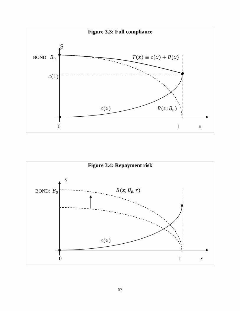
57
Figure 3.3: Full compliance
$
BOND:
0 1 x
Figure 3.4: Repayment risk
$
BOND:
0 1 x
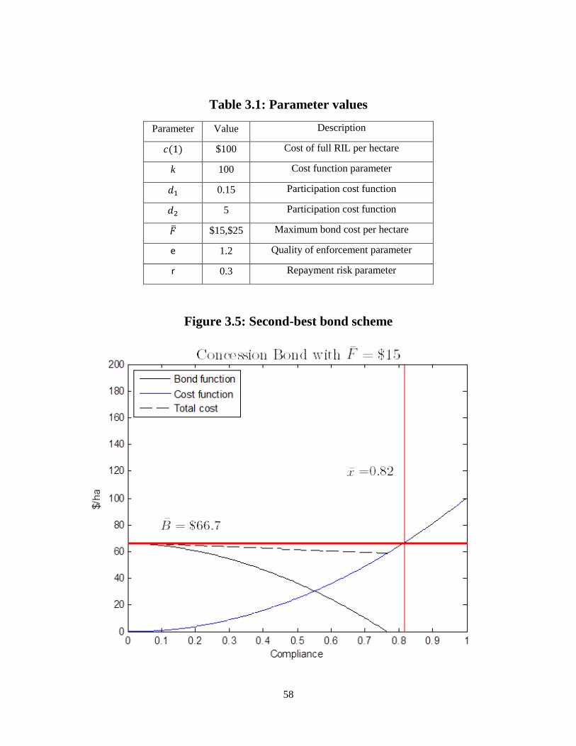
58
Table 3.1: Parameter values
Parameter Value Description
$100 Cost of full RIL per hectare
k 100 Cost function parameter
0.15 Participation cost function
5 Participation cost function
$15,$25 Maximum bond cost per hectare
e 1.2 Quality of enforcement parameter
r 0.3 Repayment risk parameter
Figure 3.5: Second-best bond scheme
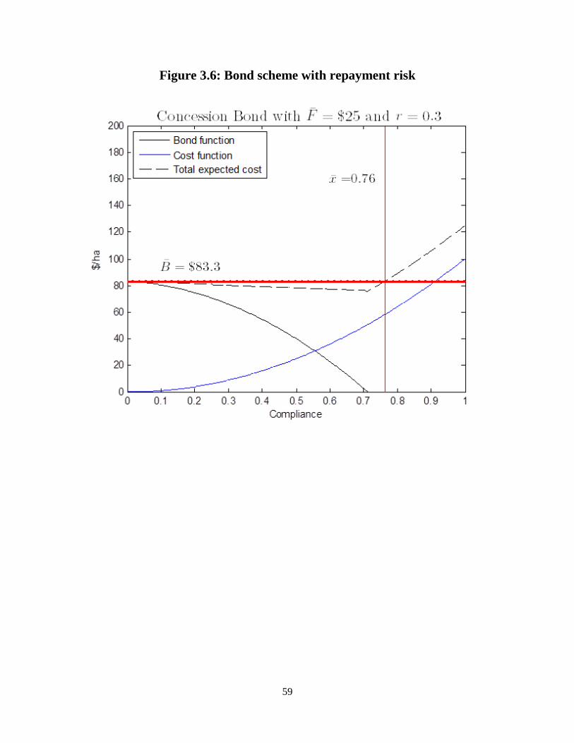
59
Figure 3.6: Bond scheme with repayment risk
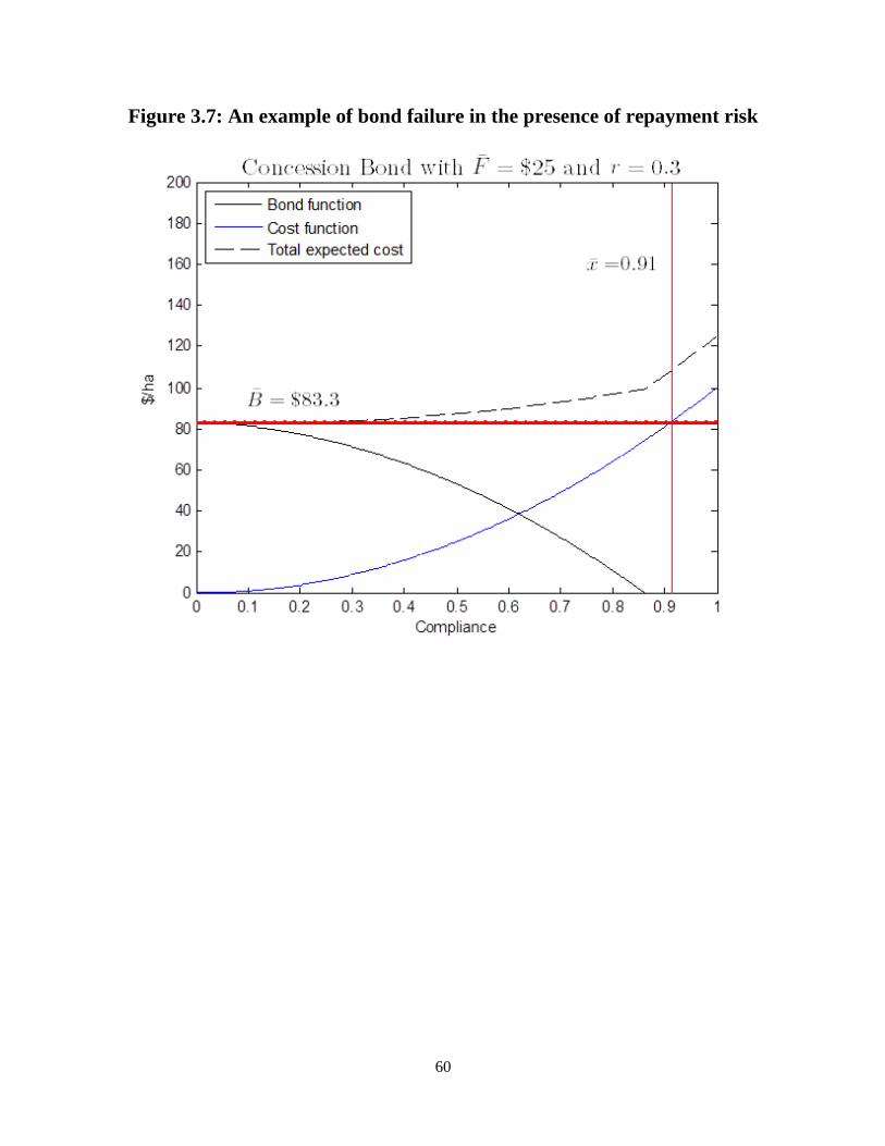
60
Figure 3.7: An example of bond failure in the presence of repayment risk
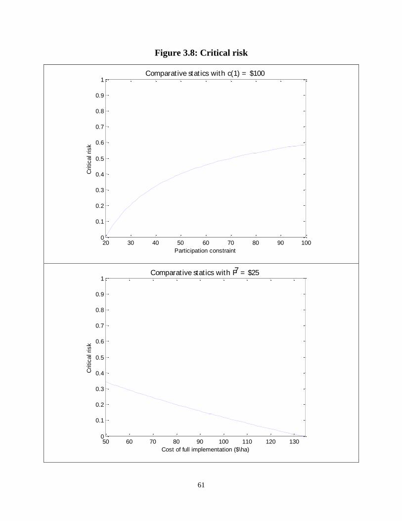
61
Figure 3.8: Critical risk
20 30 40 50 60 70 80 90 1000
0.1
0.2
0.3
0.4
0.5
0.6
0.7
0.8
0.9
1Comparat ive stat ics with c(1) = $100
Critical risk
Participation constraint
50 60 70 80 90 100 110 120 1300
0.1
0.2
0.3
0.4
0.5
0.6
0.7
0.8
0.9
1Comparat ive stat ics with 7F = $25
Critical risk
Cost of full implementation ($\ha)
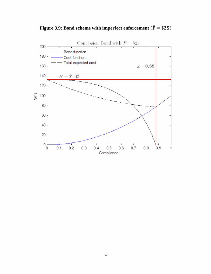
62
Figure 3.9: Bond scheme with imperfect enforcement
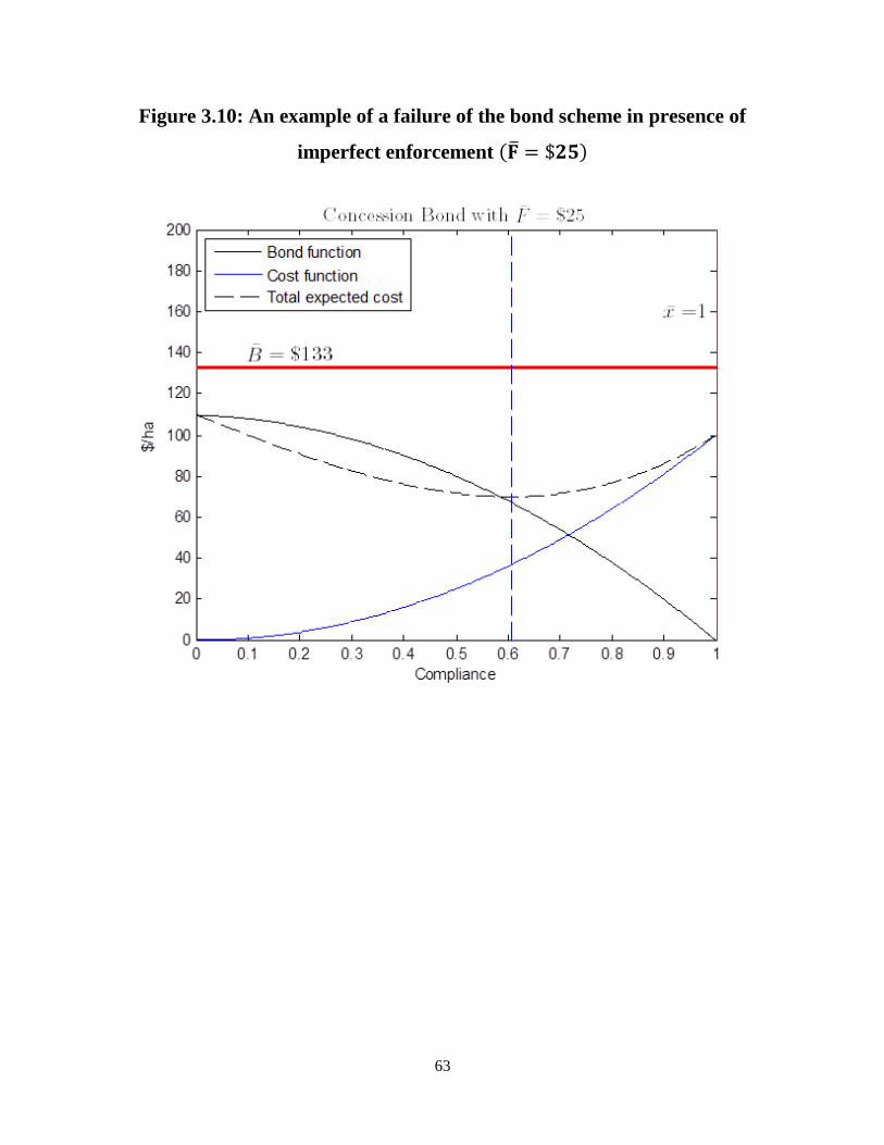
63
Figure 3.10: An example of a failure of the bond scheme in presence of
imperfect enforcement
64
4 FIXED VERSUS INTENSITY PERMIT ALLOWANCES
4.1 ABSTRACT
Tradable permit markets for carbon dioxide (C02) emissions respond to short run
fluctuations in economic activity as showcased by the recent experiences in the European Union
Emissions Trading Scheme (EU ETS). To provide stability in future permit systems, both price
and quantity interventions have been proposed. Our research focuses on the relative
performance of fixed versus intensity allowances in the presence of both productivity and energy
price uncertainty. Both allowance instruments achieve the same steady-state emissions reduction
target of 20%, which similar to the current policy proposals, and the regulator then chooses the
allowance policy that has the lowest expected abatement cost. We use a standard real business
cycle (RBC) model to solve for the expected abatement cost under both policies. We compare
the expected cost outcomes using data from the US economy as the baseline scenario, and
simulate policy outcomes under differing model parameterizations to determine the critical
values after which intensity allowances begin to dominate fixed allowances. Unlike previous
studies, our results show that under a reasonable model calibration, fixed allowances outperform
intensity allowances by as much as 30% cost difference.
4.2 INTRODUCTION
Cap-and-trade schemes have been at the forefront of policy options in the reduction of
greenhouses gas (GHG) emissions. These schemes fix the quantity of total emissions through
permit issuance, and then enable trading among permit holders with the goal of achieving the
least overall cost of abatement. Most notably, the European Union Emissions Trading Scheme
(EU ETS) launched its first phase in 2005 and is currently entering its third phase in 2013.
Fixing the amount of emissions years in advance, however, leads to uncertainty about the
ultimate cost of abatement. During a period of economic expansion the cost of abatement may
become higher than expected, whereas recessions reduce the demand for polluting goods which
in turn means lower than expected cost of abatement.73
73
The most recent economic downturn provides a case in point: the functioning of the EU ETS has been highly
criticized, with emission allowances trading well below their intended price. This type of wide variability in permit
prices can undermine the credibility of the permit system, and may also discourage investment in cleaner
technologies and hinder cost efficiency (Zhao 2003; Baldursson and von der Fehr 2004). Additionally, uncertainty

65
To contain the range of ex-post abatement costs, some countries have adopted intensity
based targeting, with the most popular target being GDP. In this case, rather than fixing the
quantity of emissions, the regulator fixes the GDP share of emissions, that is, the emissions
intensity in the economy.74
The idea is to allow the quantity of emissions to move together with
GDP changes, thus relaxing the constraint when the economy is growing and tightening when
slowing down. In the context of a cap-and-trade scheme, emissions intensity targeting would
essentially mean adjusting the permit allowance periodically based on the level of economic
activity, therefore resulting in more predictability in the permit price signal.75
A measure of economic activity such as GDP does not, however, carry all the relevant
information related to the firms’ cost of abatement. There are other factors and variables that can
directly influence the ex-post abatement cost, one example being the price of energy inputs.
Consequently, intensity targeting based GDP indexation will not fully remove all the uncertainty
vis-à-vis the cost of abatement. The question then becomes, under what circumstances will
intensity based permit allowance dominate fixed allowances, or will they always dominate.
The purpose of this chapter is to compare the expected cost of abatement between two
alternative policy scenarios: fixed permit allowance versus intensity based permit allowance.
We evaluate how energy price and productivity uncertainties affect the relative performance of
these two policy instruments. Following Fischer and Springborn (2011) and Heutel (2012), we
use a simple real business cycle (RBC) model to simulate fluctuations in economic activity and
policy outcomes, but we add stochastic energy prices as a new element. In contrast to their
work, our main focus is on the first two moments of the endogenous permit price variable, which
in the RBC model is captured by the shadow price of the emission constraint. We then introduce
a simple decision framework where the regulator prefers the policy instrument that has the
lowest expected abatement cost.76
The difference between the abatement costs under the
alternative policies is fully conveyed in the first two moments of the permit price variable.
stemming from the EU Commission’s “backloading” plan has furthermore exacerbated concerns over the system’s
overall credibility (Grubb 2012; Kossoy and Guigon 2012). 74
For example, Bush administration targeted an emission intensity of 20%. 75
In practice, this would entail market interventions reminiscent of actions of a central bank that, in the case of
emission allowances, would follow a mechanical rule based on intensity targeting. Commitment and credibility may
become issues in such a policy design. 76
Environmental damages are assumed to be the same under both policies since we are framing the emissions
reduction target in terms of steady state reduction. Under intensity targeting, the amount of CO2 emissions does
fluctuate in the short-run, but since CO2 is a long-lived stock pollutant these short-term variations do not matter.

66
As in Fischer and Springborn (2011), we impose an exogenous 20% emission reduction
target from the policy-free steady state.77
Both policy instruments, therefore, achieve the same
long-run emissions reduction goal. Intensity targeting, however, entails more stringent emissions
intensity in the steady state than what is the case under a fixed quantity target. The reason is
that, with an intensity target, there is an incentive to produce more in order to gain more permits
and relax the constraint. Consequently, the expected value of the permit price will be higher
under intensity targeting but its variance will be lower than under a fixed allowance.
The comparison between fixing the periodic quantity of emissions versus fixing the
periodic emissions intensity boils down to the relative magnitude of the mean and variance of the
permit price variable, which itself is the carrier of information about the relative cost of
abatement. We start with a baseline model calibration and evaluate which policy dominates in
the baseline scenario in terms of expected abatement cost. We then proceed to find the critical
levels for persistence and variance of the energy and productivity processes after which intensity
allowance begins to dominate fixed allowances. We use both first order and second order
approximations when linearizing the model around its steady state since the approximation
method has an impact on the magnitudes of the first two moments of the permit price variable.78
Our results extend the analysis in Fischer and Springborn (2011) and provide further
insight into the comparison between the policy instruments. Unlike their study, we find that
fixed allowances may actually outperform intensity allowances in term of expected abatement
cost, and the approximation method matters.79
When using second order approximation, the
energy price and productivity uncertainties also influence the expected permit price level. Our
results show that this has a more pronounced impact on the expected abatement cost under
intensity allowances.
Allowing for less-than-perfect correlation between the index of choice, here GDP, and
abatement costs has been studied before in Jotzo and Pezzey (2007). They derive a country
specific optimal indexation rule using a static model of global permit trading and endogenous
emissions reduction target. Our novel contribution is to identify energy price volatility as the
main source of exogenous noise that reduces the contemporaneous correlation between GDP and
77
The 20% reduction resembles the EU reduction target and the target level proposed in Waxman-Markey and
Kerry-Lieberman Bills (Fischer and Springborn 2011). 78
When using first order approximation, certainty equivalence holds. 79
Fischer and Springborn (2011) use standard welfare metrics to compare policy outcomes, and their analysis is
based on first order approximation.
67
abatement costs, and then use RBC modeling framework to find the critical levels of persistence
and shock variance in the productivity and energy processes.80
These critical values can then be
compared to the historical values found in different countries.
The recent experiences in the EU ETS shed some light on how energy prices changes
transmit to permit markets. In general, energy prices tend to have a greater impact on energy
intensive industries (Grubb 2012). Periods of high energy prices curb demand for fuels and
electricity, and as a result, demand for permits also decreases, thus lowering the price of permits.
On the other hand, “coal-gas price differential” has had a clear impact on the permit prices in the
EU ETS. Increases in oil prices have a tendency to drive natural gas prices higher. This in turn
increases the marginal cost of abatement as switching to natural gas becomes more expensive.
Hence, permit price response can be positive to increases in oil prices. In our RBC model setup,
higher energy prices always reduce demand for permits. We introduce an exogenous energy
price process following the specification and estimation results in Kim and Loungani (1992) and
Dhawan and Jeske (2005).
The plan of the chapter is as follows. The next section provides a short literature review
over the ongoing debate about the relative merits of fixed vs. intensity targets. Section 4.4 lays
out the real business cycle model that we use to derive the moments of the permit price process.
Section 4.5 presents the derivation of expected abatement cost which the regulator uses when
choosing between policy instruments. Section 4.6 defines the functional forms and parameter
values used in the baseline case. Section 4.7 presents the results, while the last section offers
concluding remarks and policy recommendations.
4.3 INTENSITY TARGETS
During the past decade, there has been a growing interest concerning the relative merits of
intensity based regulation versus more traditional price instruments and fixed quotas.81
Proponents of intensity targeting are in favor of flexibility and reduction of abatement cost
uncertainties which may in turn spur investments in cleaner technology. Critics worry about the
ensuing uncertainty over emissions reduction targets as the cap is allowed to vary, for example,
80
For example, Hamilton (1983) finds that an increase in oil prices typically lead by 3-4 quarters a period of slower
output growth. Rotemberg and Woodford (1996) estimate that a 10 percent exogenous increase in the price of oil
has been followed by an output decline of 2.5 percent 5-6 quarters after the price shock. 81
Intensity targeting as a potential greenhouse gas (GHG) mitigation policy began receiving more attention in the
academic and policy circles in the aftermath of Kyoto Protocol ratification. For a review, see Peterson (2008).

68
with ups and downs in GDP. For example, Pizer (2005) contends that intensity targets make
sense in the context of framing reduction goals for developing countries, but that intensity targets
with annual adjustments to emissions cap should not be viewed as a solution to abatement cost
uncertainty. Kolstad (2005) on the other hand reasons that intensity-based flexible caps can have
potential in reducing abatement cost uncertainty. This in turn may have the beneficial effect of
making international agreements in multilateral emission reductions more likely.82
The cost advantage of emissions indexation hinges on the premise that GDP and
emissions levels are correlated. Jotzo (2006) and Heutel (2012) provide empirical evidence
supporting this assumption. Jotzo and Pezzey (2007) and Sue Wing et al. (2009) ask the
question whether current cap-and-trade schemes can be improved upon in a way to reduce the
inherent abatement cost uncertainties.83
Their studies find that indexation can deliver
improvements in abatement outcomes both in terms of cost uncertainty and emissions levels.
Correspondingly, Quirion (2005) and Newell and Pizer (2008) set out to determine the
conditions under which intensity targeting ought to be preferred over fixed targets, or vice versa,
by choosing the policy that maximizes the expected net benefits from abatement. Following the
analytical framework in Weitzman (1974), they find that indexed quantities are likely to perform
better when there is stronger positive correlation between the index and abatement cost
uncertainty and also relatively small index variance. Furthermore, in the case of GHG
reductions, they find that countries with strong correlation between output and emissions
combined with relatively low output variance may prefer indexation over fixed quantities.
Fischer and Springborn (2011) and Heutel (2012) are the first studies to compare the
performance of different emissions regulation instruments using a RBC model that simulates
random economic fluctuations. Whereas the former imposes an exogenous 20% emissions
reduction target from a no-policy steady state scenario, the latter focuses on analyzing the
optimal policy under endogenous reduction targets. In both papers, the source of business cycle
uncertainty stems from serially correlated productivity shocks. Heutel (2012) finds that optimal 82
Permit banking has been discussed in the literature as a way to reduce abatement cost uncertainty. See for
example Newell and Pizer (2003) and Newell et al. (2005). Also setting permit price floors and ceilings to reduce
cost uncertainty has received wide attention. 83
Jotzo and Pezzey (2007) use a single-period, stochastic, globally integrated partial equilibrium model to analyze
the advantage of more flexible intensity targeting over fixed targets. Their model allows for varying degrees of
indexation and endogenously determined target levels. Sue Wing et al. (2009) apply two criteria to compare the
comparative performance of fixed and intensity based emissions targets: First, how well each instrument preserves
the initial expectations of the amount of emissions reductions and costs involved, and second, how well each
instrument minimizes the volatility of the same variables due to uncertainty about GDP and emissions.
69
policy allows for relaxation of the cap during economic expansion, and conversely, tightening of
the cap during downturns. He also finds that indexing emissions to GDP replicates the optimal
policy with a good approximation. Fischer and Springborn (2011), on the other hand, show that
fixed caps lead to the lowest level of variability in all variables, except in the shadow price of the
constraint, i.e., the permit price. Under intensity targeting, the magnitudes of variance terms do
not differ from the no-policy baseline scenario (business-as-usual). Since intensity targeting
absorbs the impact of productivity shocks on the emissions constraint, the resulting permit price
remains constant in their model. They also find that intensity targets outperform fixed caps when
comparing steady state values using standard welfare based metrics.84
Overall, however, these
differences are small and the authors conclude that when deciding between policy instruments,
the regulator may want to focus on other metrics instead.85
4.4 REAL BUSINESS CYCLE MODEL
The basic RBC model presented in this section follows closely the presentation in Fischer
and Springborn (2011). The representative consumer derives utility from consumption, , and
leisure, , given by a standard utility function , and sells labor input, , to a firm in a
competitive labor market.86
By normalizing the total time endowment to one, we can write labor
allocation as . The representative firm uses capital, , labor, , and an
intermediate polluting energy input, , to produce output, . The economy’s total output
(GDP) is defined as
(38)
It is a product of a stochastic productivity term, , which follows a stationary process with
, and a deterministic production function .87
Notice that we are
abstracting from economic growth in our model.88
84
But the ordering is reversed when they account for the transition phase with elevated level of consumption under
fixed caps. 85
Instead of a welfare comparison, we compare the expected cost of abatement. 86
We could add environmental benefits from the emissions regulation in the consumer’s utility function as an
additively separable term. In this case, the utility would only depend on the steady state reduction in emissions and
would not be affected by short-run fluctuations. Hence policies that achieve the same steady state reduction in
emissions would entail the same amount of utility from environmental benefits. This is a reasonable assumption in
the context of CO2 emissions since they are a long-lived stock pollutant, and short-run fluctuations do not
considerably alter their climatic impact. 87
We have specific functional forms in the calibration section. 88
It is also possible that accumulation of emissions has an effect on the productivity of the economy, hence making
the production function time dependent. We do not model emissions accumulation here since we are assuming that
70
Capital accumulates according to the equation
(39)
where the parameter is the rate of capital depreciation, and denotes investment. Following
Kim and Loungani (1992) and Finn (2000), we assume that the firm takes the price of the
polluting energy input as given. The economy’s resource constraint can therefore be written as
(40)
where is a stationary energy price process with . The way the energy input enters
the resource constraint in equation (40) can be interpreted to mean that the economy imports all
of its energy input from the world market and hence is small enough to have no influence on the
price (Kim and Loungani 1992).
Emissions, , are proportional to the use of energy inputs and to minimize notation the
units of emissions are chosen so that one unit of energy input emits one unit of emissions.
Henceforth, variable denotes both energy use and emissions. To reduce the amount of
emissions in the economy, the regulator imposes an emissions constraint:
(41)
where is called the allowance function that take different forms under different policies.89
We focus on two cap-and-trade policies: 1) intensity targeting with an adjustable allowance, and
2) fixed allowance. With fixed emissions allowance, , the allowance function is simply
(42)
With intensity targeting, the regulator adjusts the amount of available permits based on the
realized output in the current period. The emissions allowance function is hence defined as
(43)
where s denotes the allowed output share of emissions, or the emissions intensity.90
The
regulator chooses and , depending on the policy, to achieve any given emissions reduction
target.91
only the steady state emissions level matter in the case of CO2, and hence the effects would be identical under
policies that achieve the same steady state reduction. 89
The only way to reduce emissions here is through the reduction of polluting energy input used in the economy.
This feature neglects the possibility of improving energy efficiency and abatement technology. Our model does,
however, allow for substitution between the energy input and labor and capital. Notice that these inputs are not
perfect substitutes. 90
We could also have alternative specifications for the intensity based allowance function. For instance, the
regulator could choose the current period’s permit allowance in the previous period given his expectation of the
level of output: .
71
Assuming competitive labor and capital markets, the social planner solves the following
infinite horizon utility maximization problem:
(44)
subject to the resource constraint (40) and the constraint on emissions (41). The parameter is
the discount factor defined as where is the discount rate, and denotes the
expectation operator given the information available at time . Define where is
the Lagrangian multiplier of constraint (41), and of constraint (40). The system of first order
conditions for the social planner’s problem can then be written as (see Appendix C):
(45)
where functions with subscripts denote the derivative of the function with respect to the variable
in the subscript. The above system of nonlinear equations characterizes the equilibrium
relationships that have to hold in optimum in every period, . Assuming the existence of a steady
state in the system (45), it is implicitly defined for each variable by the following system:
(46)
where all the variables take steady state values (e.g., .92 Notice that the only
difference between the system in (45) and the corresponding conditions in Springborn and
91
This target level is also related to the environmental damages since the use of polluting input incurs damages. In
this chapter, we use an exogenous target of 20% reduction in steady state emissions. 92
By specifying functional forms for and , we can explicitly solve for each steady state value.
We do this in our simulation section.

72
Fischer (2011) is the introduction of random energy prices, . Since the expected value of is
one, the steady state conditions are identical with their study.
For the purpose of this study, the properties of variable , the shadow value of the
emissions constraint, are of primary interest. This variable is the equilibrium permit price in a
competitive permit market.93
Notice that it has been written in terms of output, that is, it is the
real price of a permit. Our next goal is to log-linearize the above system (45) around its steady
state given in (46), and to solve for the equations of motion that characterize the movement of
the endogenous and state variables in the proximity of that steady state (e.g., Uhlig, 1995). For
example, the logarithm of the permit price variable, , is written as a linear function of the
exogenous variables and , and the predetermined variable .
To log-linearize the system in (45), we start by writing each variable in terms of its
percentage deviation from the steady state.94
Using variable as an example, we make the
following two definitions:
(47)
where denotes (approximately) the percentage deviation from its steady state, .95
After
substituting for each variable in (45) with its corresponding expression written in terms of
percentage deviation from the steady state, e.g., , we linearize the resulting system
using first or second order Taylor approximation.96
Define the following vectors:
and
where collects the endogenous variables (jump
variables) and the exogenous variables. Notice that the variables in vector are now written
in terms of percentage deviations from the steady states, denoted by a small case letter or tilde.
Also variables in are by definition percentage deviations around zero.
Suppose now that we apply the first order Taylor approximation. We can write the
resulting system of linear rational expectation equations in the following generic form (see
Appendix C):
(48)
93
In reality, the permit markets may not be competitive since some market participants may have market power.
Since market structure is assumed to be the same under both policies, this may not have an effect on our abatement
cost comparisons. We leave the determination the effect of the market structure for future research. 94
The presentation here follows Uhlig (1995) and McCandless (2008). 95
This can be seen from noting that where . 96
In the model simulation section, we use both approximations.

73
where we have separated equations that include expectations from those that do not. The matrix
coefficients, , are all known from the log-linearization step, and is a vector
with mean zero stochastic elements.97
Given the linear system in (48) our goal is to find
equations of motion:
(49)
where matrix coefficients, , are all unknown and can be solved, for example, by using
the method of undetermined coefficients. In particular, we want to find the equation of motion
for .98
It will take the following generic form:
(50)
where coefficients are solutions from solving (49), and , where is
the steady state permit price. We use the expression in (50) to derive the expected value and
variance of , which, as we show later, convey the information about the expected cost of
abatement.
To give an example, suppose that both the energy price process, , and the technology
process, , take the following AR(1) forms:
(51)
where and are independent white noise disturbances with mean zero and variance terms
and , respectively. In the case of first order Taylor approximation, certainty equivalence
holds:
(52)
where denotes the steady state value. The variance of the permit price process is given by:
97
We will assume standard linear functional forms for both energy price (ARMA) and productivity processes (AR)
with mean zero stochastic terms and respectively. 98
When we log-linearize the equilibrium conditions, we are implicitly restricting the permit price to take strictly
positive values. We return to this important point in a subsequent section.

74
(53)
where coefficients are solutions to the permit price and capital equations of
motion (see Appendix D). From (53) we can see that as the variance terms, and
, increase
the variance of the permit price increases as well. Similarly, if either of the persistence terms,
and , increases, the permit price variance increases as well.
The purpose of the above example is to show how the properties of the productivity and
energy price processes are transmitted to the permit price process. This mechanism is described
by the equations (52) and (53). Notice that due to certainty equivalence, persistence and
variance terms do not have an effect on the expected permit price given in (52). If we used
second order Taylor approximation instead, these terms would also enter (52). To determine
how much permit price variability responds under the competing policies, we would need to
solve for the coefficients for both policies since they will differ in general.
The first order and steady state conditions under fixed and intensity targets are detailed in
Appendix C.
Before solving the above RBC model under the two allowance policies, we need to
answer the question how the regulator determines which permit system is better. To do this, we
build a decision framework based on abatement cost minimization problem.99
As we will see,
information about the difference in abatement cost between the two policies is captured by the
first two moments of the permit price variable, .
4.5 ABATEMENT COST COMPARISON
Suppose that the regulator’s goal is to achieve a given emissions reduction target with the
smallest expected abatement cost which is measured as the cost of deviating from the business-
as-usual (BAU) scenario.100
The reduction target is exogenously given, for example, as a result
99
We could use the above RBC modeling framework to compare the welfare difference in terms of consumption
between the two policies. The welfare differences are, however, small (Fischer and Springborn, 2011). It is more
likely that the regulator is interested to know the abatement cost difference rather than the welfare difference. 100
We define this in more detail below.
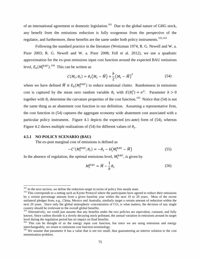
75
of an international agreement or domestic legislation.101
Due to the global nature of GHG stock,
any benefit from the emissions reduction is fully exogenous from the perspective of the
regulator, and furthermore, these benefits are the same under both policy instruments.102,103
Following the standard practice in the literature (Weitzman 1974; R. G. Newell and W. a.
Pizer 2003; R. G. Newell and W. a. Pizer 2008; Fell et al. 2012), we use a quadratic
approximation for the ex-post emissions input cost function around the expected BAU emissions
level, .104
This can be written as
(54)
where we have defined to reduce notational clutter. Randomness in emissions
cost is captured by the mean zero random variable with . Parameter
together with determine the curvature properties of the cost function.105
Notice that (54) is not
the same thing as an abatement cost function in our definition. Assuming a representative firm,
the cost function in (54) captures the aggregate economy wide abatement cost associated with a
particular policy instrument. Figure 4.1 depicts the expected (ex-ante) form of (54), whereas
Figure 4.2 shows multiple realizations of (54) for different values of .
4.5.1 NO POLICY SCENARIO (BAU)
The ex-post marginal cost of emissions is defined as
(55)
In the absence of regulation, the optimal emissions level, , is given by
(56)
101
In the next section, we define the reduction target in terms of policy free steady state. 102
This corresponds to a setting such as Kyoto Protocol where the participants have agreed to reduce their emissions
by a certain percentage amount from a given baseline year within the next 10 to 20 years. Most of the recent
unilateral pledges from, e.g., China, Mexico and Australia, similarly target a certain amount of reduction within the
next 20 years. Since only the global atmospheric concentration of CO2 is what matters, the decision of any single
country should be irrelevant to the overall global benefits. 103
Alternatively, we could just assume that any benefits under the two policies are equivalent, constant, and fully
known. Since carbon dioxide is a slowly decaying stock pollutant, the annual variation in emissions around its target
level during the regulation period has no impact on final benefits. 104
This can be thought of as the energy input cost function, but since we are using emissions and energy
interchangeably, we retain to emissions cost function terminology. 105
We assume that parameter has a value that is not too small, thus guaranteeing an interior solution to the cost
minimization problem.

76
where we have used the first order condition – to derive (56). In Figure 4.2, the
points where the ex-post cost curves attain their minima correspond to for different
realizations of . Any deviation from point would be suboptimal. We define the cost of
abatement as the inefficiency cost resulting from choosing some emissions level such that
. The abatement cost can be written as
(57)
Here, the BAU level, , acts as the reference level.
4.5.2 ABATEMENT COST UNDER PERMIT ALLOWANCES
Any allowance policy put in place will in general make the ex-post emissions level, ,
deviate from the cost minimizing outcome: . Notice that under fixed allowance,
, whereas can fluctuate periodically, but under intensity allowances, both and
fluctuate periodically. Suppose now that the regulator uses emissions allowances to
restrict the amount of emissions in the economy, , and enables permit trading
between firms. Assuming that the permit market is competitive and efficient, the representative
firm chooses its level of emissions to equate the marginal cost of emissions to the market permit
price, :
(58)
Using (58), we can find the optimal emissions level, under either allowance scheme:
(59)
The ex-post amount of abatement is defined as
(60)
Notice that this amount is always positive as long as the permit price is positive as well. We
restrict to only take positive values in our RBC model.106
Using (60), we can now rewrite the
abatement cost function in (57) as
(61)
The expected cost of abatement then becomes
106
Positive permit price values can be justified by the notion of option value. Since in the steady state the amount of
emissions reduction is always below the BAU level, the permit prices retain positive value in the short run.

77
(62)
The above expression is written only in terms of the expectation and the variance of the permit
market price, , and parameter b.
From (62), we can see that the regulator prefers the allowance policy that has the smallest
sum of the permit price variance and the squared mean permit price. One interpretation for this
rule is that the regulator chooses the instrument that minimizes the mean squared error of
abatement cost. This “error” can be thought of arising from having an emissions reduction target
put in place. In the absence of emissions regulation, the permit price would naturally be
invariantly zero under both policies, and therefore, mean squared error would be at minimum.
But because of the reduction target, the regulator chooses the instrument that yields the smallest
mean squared error.107
As we will see, the expected permit price under intensity allowance is
always higher than with fixed allowance, but the variance is lower under intensity allowance.
Hence, what matters is the relative magnitude of the first two moments of the permit variable
under each policy.
4.5.3 COST COMPARISON
The difference in the expected abatement cost between intensity and fixed allowances is
defined as
(63)
where subscript stands for intensity allowance and subscript for fixed allowance.
Substituting (62) into (63) and assuming that all the model parameters are invariant between
different policies, that is, only the amount of abatement may differ, we finally have
(64)
If the expression in (64) is positive, then intensity allowance is preferred, whereas if the
expression negative, then fixed allowance is preferred. To empirically assess which policy is
superior, we would need to have estimates for the mean and the variance of the permit price of
under both policies. Since there are no data on intensity allowances, we resort to solving for
these moments using the above RBC model.108
107
Quadratic utility function yields a decision rule that minimizes mean squared error. 108
Notice that we do not model the transitioning phase between the policy free steady state and the resulting new
steady state. We focus on comparing the expected costs when the policies are fully in place.
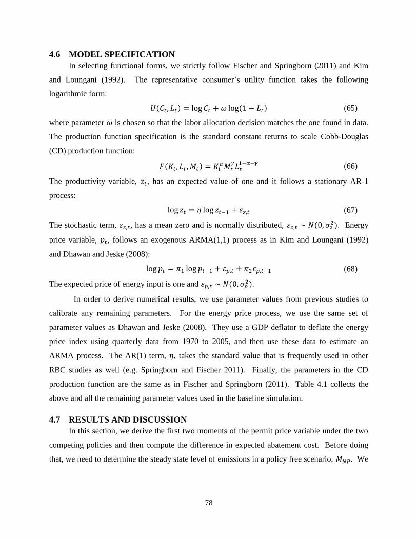
78
4.6 MODEL SPECIFICATION
In selecting functional forms, we strictly follow Fischer and Springborn (2011) and Kim
and Loungani (1992). The representative consumer’s utility function takes the following
logarithmic form:
(65)
where parameter is chosen so that the labor allocation decision matches the one found in data.
The production function specification is the standard constant returns to scale Cobb-Douglas
(CD) production function:
(66)
The productivity variable, , has an expected value of one and it follows a stationary AR-1
process:
(67)
The stochastic term, , has a mean zero and is normally distributed, . Energy
price variable, , follows an exogenous ARMA(1,1) process as in Kim and Loungani (1992)
and Dhawan and Jeske (2008):
(68)
The expected price of energy input is one and .
In order to derive numerical results, we use parameter values from previous studies to
calibrate any remaining parameters. For the energy price process, we use the same set of
parameter values as Dhawan and Jeske (2008). They use a GDP deflator to deflate the energy
price index using quarterly data from 1970 to 2005, and then use these data to estimate an
ARMA process. The AR(1) term, , takes the standard value that is frequently used in other
RBC studies as well (e.g. Springborn and Fischer 2011). Finally, the parameters in the CD
production function are the same as in Fischer and Springborn (2011). Table 4.1 collects the
above and all the remaining parameter values used in the baseline simulation.
4.7 RESULTS AND DISCUSSION
In this section, we derive the first two moments of the permit price variable under the two
competing policies and then compute the difference in expected abatement cost. Before doing
that, we need to determine the steady state level of emissions in a policy free scenario, . We
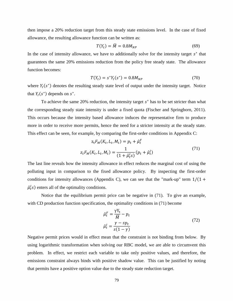
79
then impose a 20% reduction target from this steady state emissions level. In the case of fixed
allowance, the resulting allowance function can be written as:
(69)
In the case of intensity allowance, we have to additionally solve for the intensity target that
guarantees the same 20% emissions reduction from the policy free steady state. The allowance
function becomes:
(70)
where denotes the resulting steady state level of output under the intensity target. Notice
that depends on .
To achieve the same 20% reduction, the intensity target has to be set stricter than what
the corresponding steady state intensity is under a fixed quota (Fischer and Springborn, 2011).
This occurs because the intensity based allowance induces the representative firm to produce
more in order to receive more permits, hence the need for a stricter intensity at the steady state.
This effect can be seen, for example, by comparing the first-order conditions in Appendix C:
(71)
The last line reveals how the intensity allowance in effect reduces the marginal cost of using the
polluting input in comparison to the fixed allowance policy. By inspecting the first-order
conditions for intensity allowances (Appendix C), we can see that the "mark-up" term
enters all of the optimality conditions.
Notice that the equilibrium permit price can be negative in (71). To give an example,
with CD production function specification, the optimality conditions in (71) become
(72)
Negative permit prices would in effect mean that the constraint is not binding from below. By
using logarithmic transformation when solving our RBC model, we are able to circumvent this
problem. In effect, we restrict each variable to take only positive values, and therefore, the
emissions constraint always binds with positive shadow value. This can be justified by noting
that permits have a positive option value due to the steady state reduction target.
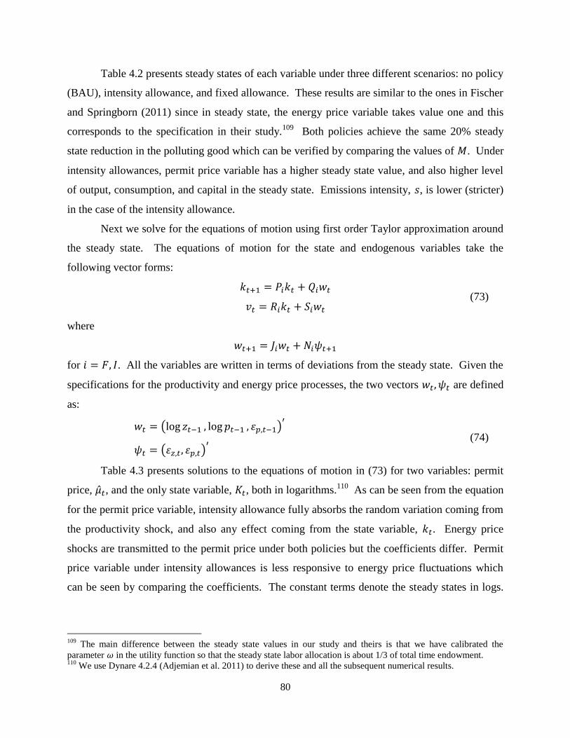
80
Table 4.2 presents steady states of each variable under three different scenarios: no policy
(BAU), intensity allowance, and fixed allowance. These results are similar to the ones in Fischer
and Springborn (2011) since in steady state, the energy price variable takes value one and this
corresponds to the specification in their study.109
Both policies achieve the same 20% steady
state reduction in the polluting good which can be verified by comparing the values of . Under
intensity allowances, permit price variable has a higher steady state value, and also higher level
of output, consumption, and capital in the steady state. Emissions intensity, , is lower (stricter)
in the case of the intensity allowance.
Next we solve for the equations of motion using first order Taylor approximation around
the steady state. The equations of motion for the state and endogenous variables take the
following vector forms:
(73)
where
for . All the variables are written in terms of deviations from the steady state. Given the
specifications for the productivity and energy price processes, the two vectors are defined
as:
(74)
Table 4.3 presents solutions to the equations of motion in (73) for two variables: permit
price, , and the only state variable, , both in logarithms.110
As can be seen from the equation
for the permit price variable, intensity allowance fully absorbs the random variation coming from
the productivity shock, and also any effect coming from the state variable, . Energy price
shocks are transmitted to the permit price under both policies but the coefficients differ. Permit
price variable under intensity allowances is less responsive to energy price fluctuations which
can be seen by comparing the coefficients. The constant terms denote the steady states in logs.
109
The main difference between the steady state values in our study and theirs is that we have calibrated the
parameter in the utility function so that the steady state labor allocation is about 1/3 of total time endowment. 110
We use Dynare 4.2.4 (Adjemian et al. 2011) to derive these and all the subsequent numerical results.

81
In Figure 4.3, we graph an example of a permit price process realization using the equations of
motion in Table 4.3.
To gain further insight, the equation of motion for the permit price variable can be
written as
(75)
where the coefficients correspond to the solutions in Table 4.3. Notice that all the variables on
the right-hand side are normally distributed. Hence, has a normal distribution with its
mean at the steady state value, .111
Consequently, has a log-normal distribution. Once we
solve for the first two moments of using equation (75), we can then derive the
corresponding moments in levels using the following relationships:
(76)
Tables 4.4 and 4.5 present the means and variances of the permit price variables under
the two policy instruments. We use both the first and the second order Taylor approximation
around the steady state. Table 4.4 reports these values in logarithmic scale, and Table 4.5 reports
the values in levels after applying the mappings in (76). We furthermore compute the difference
in expected abatement cost in percentage terms, hence cancelling out the parameter in (64):
(77)
We use equation (77) to compare the allowance policies and make policy recommendations.
Negative percentage value in (77) means that fixed allowance entails lower abatement cost by
the corresponding percentage amount, and positive value means that intensity allowance is more
cost efficient again by that percentage amount. In Table 4.4, we have not computed (77) since
when squaring a negative log value, the ranking is reversed and thus the abatement cost
comparison becomes meaningless. As Table 4.4 shows, the second order approximation method
yields smaller mean value for both policy instruments. Variance terms are, however, the same
with both approximation methods.
Based on the results in Table 4.5, we conclude that fixed allowances dominate the
intensity based allowance system. Fixed allowance has 8.76% lower expected abatement cost
111
The mean coincides with the steady state only when using first order Taylor approximation.
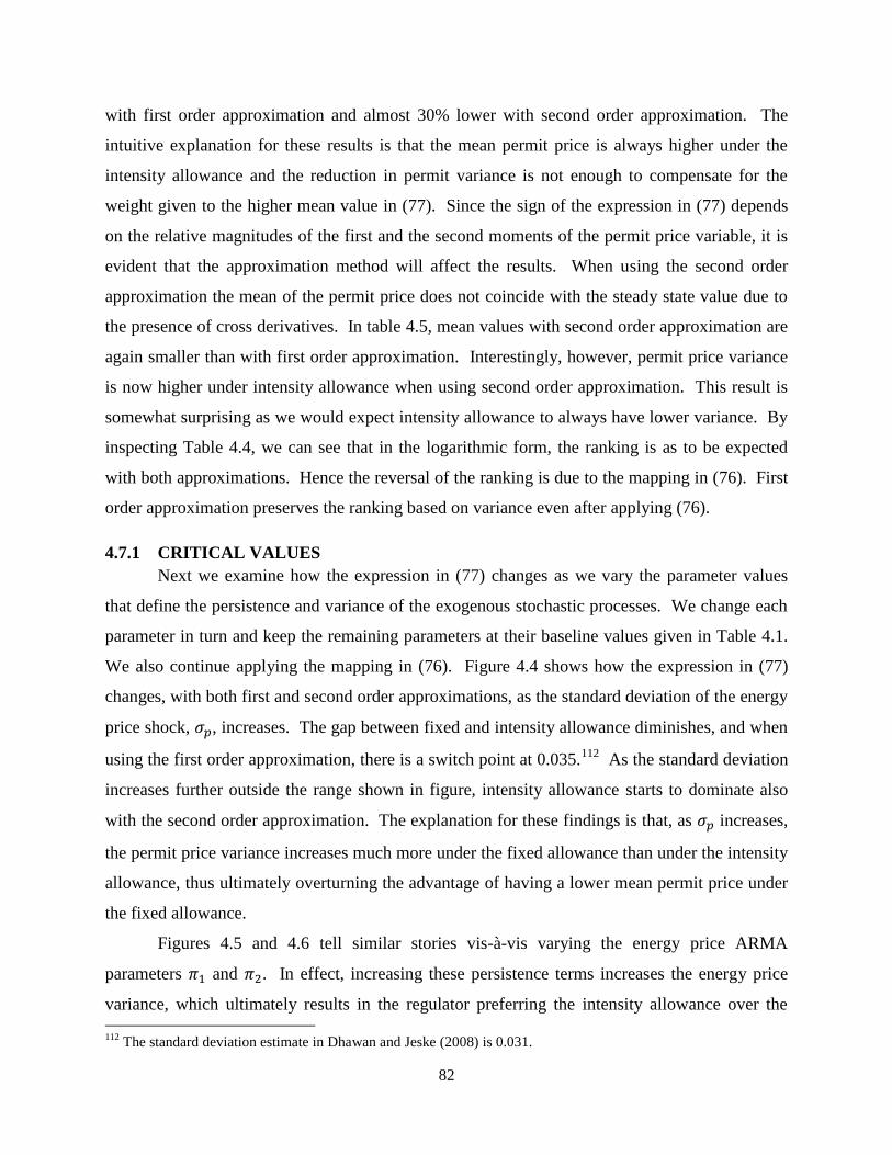
82
with first order approximation and almost 30% lower with second order approximation. The
intuitive explanation for these results is that the mean permit price is always higher under the
intensity allowance and the reduction in permit variance is not enough to compensate for the
weight given to the higher mean value in (77). Since the sign of the expression in (77) depends
on the relative magnitudes of the first and the second moments of the permit price variable, it is
evident that the approximation method will affect the results. When using the second order
approximation the mean of the permit price does not coincide with the steady state value due to
the presence of cross derivatives. In table 4.5, mean values with second order approximation are
again smaller than with first order approximation. Interestingly, however, permit price variance
is now higher under intensity allowance when using second order approximation. This result is
somewhat surprising as we would expect intensity allowance to always have lower variance. By
inspecting Table 4.4, we can see that in the logarithmic form, the ranking is as to be expected
with both approximations. Hence the reversal of the ranking is due to the mapping in (76). First
order approximation preserves the ranking based on variance even after applying (76).
4.7.1 CRITICAL VALUES
Next we examine how the expression in (77) changes as we vary the parameter values
that define the persistence and variance of the exogenous stochastic processes. We change each
parameter in turn and keep the remaining parameters at their baseline values given in Table 4.1.
We also continue applying the mapping in (76). Figure 4.4 shows how the expression in (77)
changes, with both first and second order approximations, as the standard deviation of the energy
price shock, , increases. The gap between fixed and intensity allowance diminishes, and when
using the first order approximation, there is a switch point at 0.035.112
As the standard deviation
increases further outside the range shown in figure, intensity allowance starts to dominate also
with the second order approximation. The explanation for these findings is that, as increases,
the permit price variance increases much more under the fixed allowance than under the intensity
allowance, thus ultimately overturning the advantage of having a lower mean permit price under
the fixed allowance.
Figures 4.5 and 4.6 tell similar stories vis-à-vis varying the energy price ARMA
parameters and . In effect, increasing these persistence terms increases the energy price
variance, which ultimately results in the regulator preferring the intensity allowance over the 112
The standard deviation estimate in Dhawan and Jeske (2008) is 0.031.

83
fixed allowance. In Figures 4.5 and 4.6, the cutoff points, when using the first order
approximation, are slightly above 0.98 for the AR part, , and around 0.64 for the MA part, .
Figures 4.7 and 4.8 show the effect of changing the parameter values defining the productivity
process. Higher standard deviation, , and persistence, , reduce the gap between the policies,
and the closer we get to the productivity process being a pure random walk the more preferred
the intensity allowance becomes. The cutoff point for is around 0.01, and for around 0.975
when using the first order approximation.
4.8 CONCLUSIONS
The recent studies comparing intensity based emissions targeting and fixed emissions
quotas have usually come out in favor of the former. It is true that flexibility in allowance
allocation does reduce abatement cost uncertainty, but this comes at the cost of more stringent
intensity level to achieve the same reduction target. Our analysis weighs both of these aspects to
determine which allowance policy is preferred. The above results show that when using a
reasonable model calibration, fixed allowances outperform intensity allowances. Depending on
the approximation method, the cost difference in percentage terms can be quite significant. We
find that with second order approximation the abatement cost difference is 30% in favor of fixed
allowances. With first order approximation, this gap is almost 9% in favor of fixed allowances.
Our simulation results also show that as the economic environment becomes more uncertain,
intensity allowances begin to dominate fixed allowances. Hence, in some cases where the
country faces extreme energy price and productivity uncertainties, intensity allowances may
ultimately become the preferred policy option. Interesting future research includes determining
an optimal intensity indexation rule that achieves the lowest expected abatement cost.
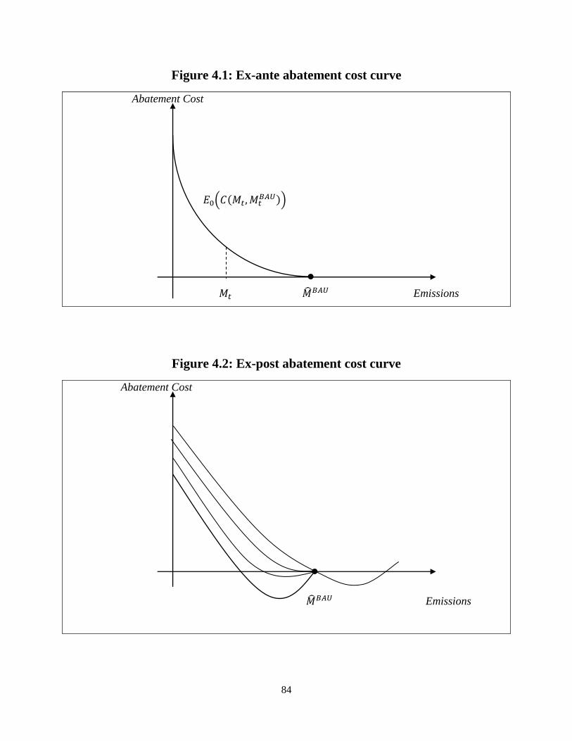
84
Figure 4.1: Ex-ante abatement cost curve
Abatement Cost
Emissions
Figure 4.2: Ex-post abatement cost curve
Abatement Cost
Emissions
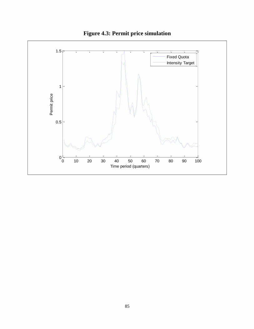
85
Figure 4.3: Permit price simulation
0 10 20 30 40 50 60 70 80 90 1000
0.5
1
1.5P
erm
it p
rice
Time period (quarters)
Fixed Quota
Intensity Target

86
Figure 4.4: Abatement cost difference, energy price shock standard deviation
x-axis: standard deviation,
y-axis: %-difference between fixed and intensity based allowance. Negative value means that
fixed allowances are preferred.
0.005 0.01 0.015 0.02 0.025 0.03 0.035 0.04 0.045 0.05-40
-20
0
20
401ST ORDER TAYLOR APPROXIMATION
%
standard deviation
0.005 0.01 0.015 0.02 0.025 0.03 0.035 0.04 0.045 0.05-50
-40
-30
-20
-10
02ND ORDER TAYLOR APPROXIMATION
%
standard deviation
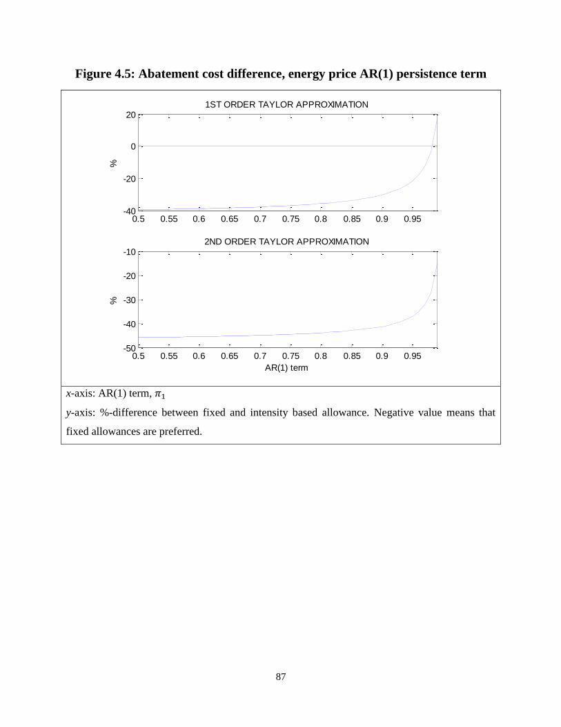
87
Figure 4.5: Abatement cost difference, energy price AR(1) persistence term
x-axis: AR(1) term,
y-axis: %-difference between fixed and intensity based allowance. Negative value means that
fixed allowances are preferred.
0.5 0.55 0.6 0.65 0.7 0.75 0.8 0.85 0.9 0.95-40
-20
0
201ST ORDER TAYLOR APPROXIMATION
%
0.5 0.55 0.6 0.65 0.7 0.75 0.8 0.85 0.9 0.95-50
-40
-30
-20
-102ND ORDER TAYLOR APPROXIMATION
%
AR(1) term
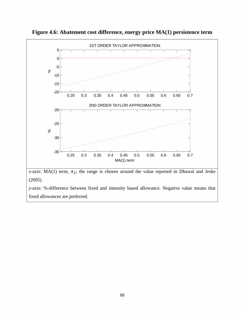
88
Figure 4.6: Abatement cost difference, energy price MA(1) persistence term
x-axis: MA(1) term, ; the range is chosen around the value reported in Dhawal and Jeske
(2005)
y-axis: %-difference between fixed and intensity based allowance. Negative value means that
fixed allowances are preferred.
0.25 0.3 0.35 0.4 0.45 0.5 0.55 0.6 0.65 0.7-20
-15
-10
-5
0
51ST ORDER TAYLOR APPROXIMATION
%
0.25 0.3 0.35 0.4 0.45 0.5 0.55 0.6 0.65 0.7-35
-30
-25
-202ND ORDER TAYLOR APPROXIMATION
%
MA(1) term
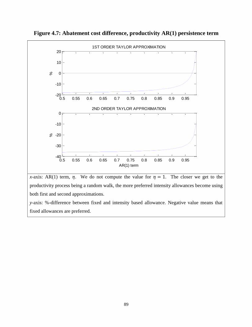
89
Figure 4.7: Abatement cost difference, productivity AR(1) persistence term
x-axis: AR(1) term, . We do not compute the value for . The closer we get to the
productivity process being a random walk, the more preferred intensity allowances become using
both first and second approximations.
y-axis: %-difference between fixed and intensity based allowance. Negative value means that
fixed allowances are preferred.
0.5 0.55 0.6 0.65 0.7 0.75 0.8 0.85 0.9 0.95-20
-10
0
10
201ST ORDER TAYLOR APPROXIMATION
%
0.5 0.55 0.6 0.65 0.7 0.75 0.8 0.85 0.9 0.95-40
-30
-20
-10
02ND ORDER TAYLOR APPROXIMATION
%
AR(1) term
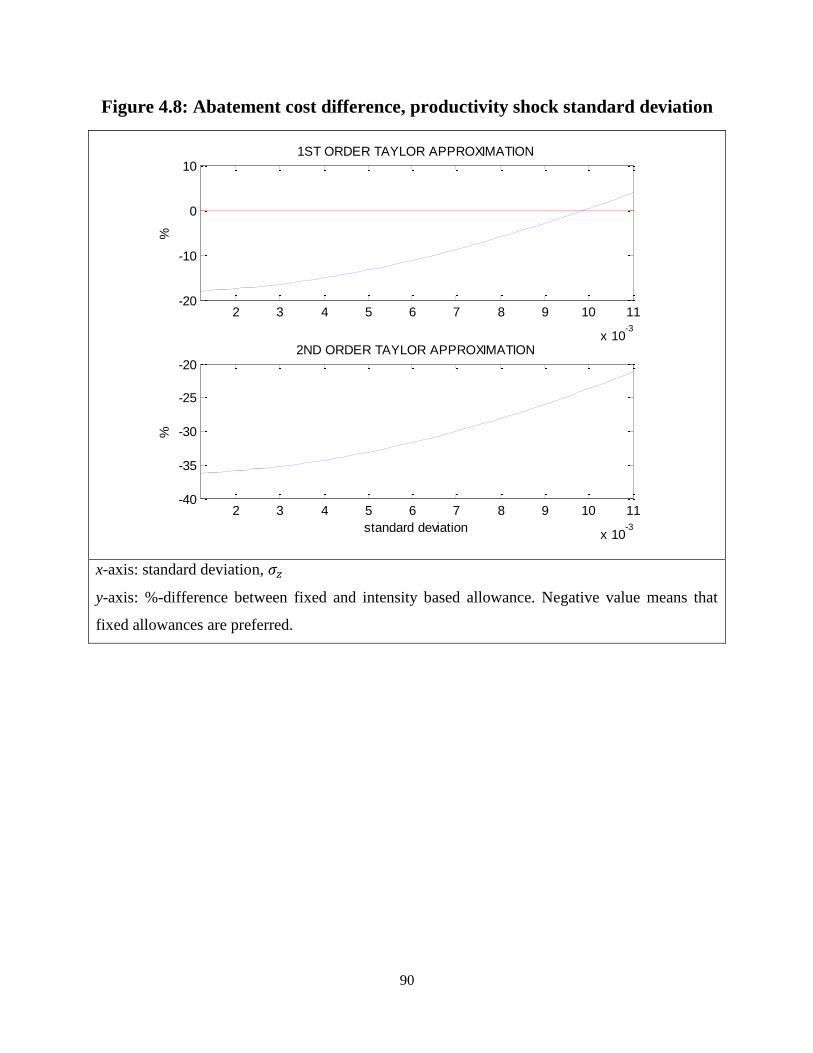
90
Figure 4.8: Abatement cost difference, productivity shock standard deviation
x-axis: standard deviation,
y-axis: %-difference between fixed and intensity based allowance. Negative value means that
fixed allowances are preferred.
2 3 4 5 6 7 8 9 10 11
x 10-3
-20
-10
0
101ST ORDER TAYLOR APPROXIMATION
%
2 3 4 5 6 7 8 9 10 11
x 10-3
-40
-35
-30
-25
-202ND ORDER TAYLOR APPROXIMATION
%
standard deviation

91
Table 4.1: Baseline calibration
0.990 0.025 1.72 0.950 0.975 0.422
0.090 0.330 0.580
Table 4.2: Steady state values in levels
No Policy, BAU 0 7.714 0.554 0.074 0.333 0.821 0.090
Fixed Allowance 0.198 7.392 0.542 0.059 0.328 0.786 0.075
Intensity Allowance 0.246 7.689 0.552 0.059 0.333 0.803 0.074
Table 4.3: Equations of motion
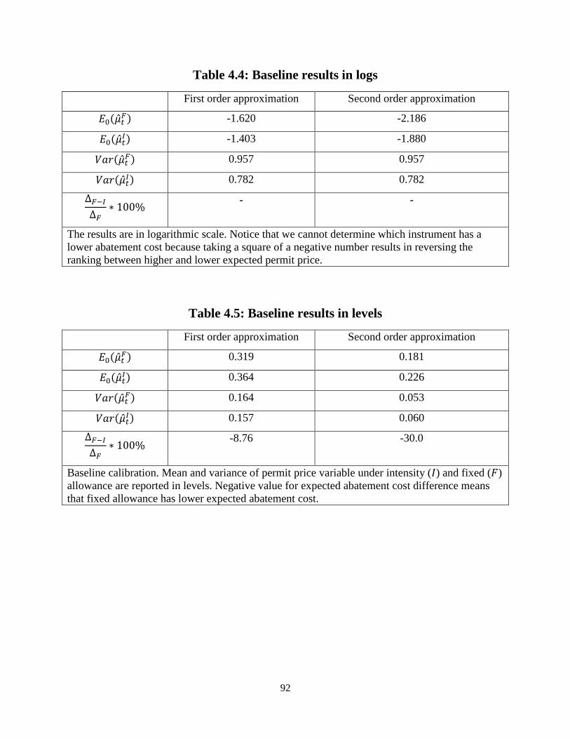
92
Table 4.4: Baseline results in logs
First order approximation Second order approximation
-1.620 -2.186
-1.403 -1.880
0.957 0.957
0.782 0.782
- -
The results are in logarithmic scale. Notice that we cannot determine which instrument has a
lower abatement cost because taking a square of a negative number results in reversing the
ranking between higher and lower expected permit price.
Table 4.5: Baseline results in levels
First order approximation Second order approximation
0.319 0.181
0.364 0.226
0.164 0.053
0.157 0.060
-8.76 -30.0
Baseline calibration. Mean and variance of permit price variable under intensity ( ) and fixed ( )
allowance are reported in levels. Negative value for expected abatement cost difference means
that fixed allowance has lower expected abatement cost.
93
5 CONCLUSIONS
The future impact of climate change on human lives and societies remain uncertain, but the
prospective scenarios seem deeply disconcerting to any prudent observer. The long-term
survival of many ecosystems with fragile wildlife habitats is under an increasing threat, and no
doubt add to the urgency of decisive action. National and global policy responses to these
environmental challenges are inevitably the defining monuments of our next century. The goal
of this dissertation is to analyze the impact of political and macroeconomic uncertainty on
environmental outcomes and policy instruments. Our results and new methods contribute to the
existing literature in natural resource and environmental economics, and provide guidance to the
policymakers when formulating responses to the environmental challenges today and in the
future.
Tropical deforestation and accompanying land use changes have been significant
contributors to anthropocentric GHG emissions. Agricultural land expansion and road building
have been deemed as the main direct drivers of this process. The first essay of this dissertation
finds that new political regimes tend to increase the rate of agricultural land expansion in tropical
countries. This land conversion comes at the expense of previously forested lands, and both
democratic and autocratic regimes have contributed to this process. The magnitude of this effect
can be significant and persistent as past agricultural land expansion stimulates more road
building, and therefore, better access routes for future land conversion. We find that the impact
of new regimes is more pronounced in Latin America and Asia, whereas in Africa to a smaller
extent. These differences can be mainly explained in terms of differing historical forms of land
ownership and colonial legacy. We also find that increasing level of income has reduced the rate
of agricultural land expansion in Latin America, but the opposite holds in Africa. The role of
corruption furthermore differs across regions. Our collective results suggest that future political
instability and heightened demand for agricultural land continue to present a significant threat to
tropical forests, and that democratization does not seem to be a sufficient condition for better
environmental outcomes. Future research should develop a dynamic theory model and a more
flexible regime dummy variable specification. Also country or region specific micro studies
with richer dataset would enhance our understanding of how political economy affects
deforestation.
94
Performance bonds have been suggested as a promising new policy instrument to regulate
environmental outcomes in tropical timber concessions. They have not, however, gained much
traction for variety of reasons. The second chapter of this dissertation identifies repayment risk
and imperfect enforcement together with binding participation constraint as important factors
hindering the successful implementation of bonding schemes. We show that both imperfect
enforcement and repayment risk increase the required level of bond payment and may force the
government to aim at a lower RIL target level when the harvester’s participation constraint is
binding. We define and quantify the concept of critical risk and derive the “slope condition” that
has to be satisfied by a decreasing bond function when enforcement is imperfect. These findings
collectively shed some new light on the question why performance bonding schemes have not
been successful in concession design and how they may be improved. Our simulation results
give support to the potentially important role of supranational entities such as REDD+ in lifting
bond outcomes to the first-best level. REDD+ finances have the potential of reducing repayment
uncertainty and improving the quality of concession enforcement. These improvements enhance
the future effectiveness of bonding schemes for any given initial bond payment. Future research
in performance bonds should look into dynamic consideration such as reputational effects, and
how an optimal subsidy policy should be designed.
A well-functioning and reasonably predictable permit market alleviates the abatement cost
uncertainty and also encourages investments in cleaner forms of production. Intensity targeting
indexes the number of emissions allowances to GDP, and therefore, it potentially reduces the
cost uncertainty in achieving overall emissions reduction target. The third chapter of this
dissertation compares the performance of fixed versus intensity allowances when the economy is
subject to both energy and productivity uncertainties. We find that the reduction in abatement
cost variance under intensity allowances may not be enough to offset the more stringent intensity
target level required to achieve the same steady state emissions reduction target. It is true that
ultimately intensity allowances begin to dominate fixed allowances as we increase the variance
and persistence of the energy and productivity processes, but the corresponding critical points are
higher than the historical values found in the U.S. Using the baseline calibration, the abatement
cost difference can be as high as 30% in favor of fixed allowances. The magnitude of the cost
difference depends on the approximation methods applied when solving the RBC model. With
the second order approximation, the degree of uncertainty over the price of energy input and the

95
economy’s productivity additionally affects the expected level of permit price which further
reduces the attractiveness of intensity allowances for any given level of permit variance. Future
research should determine the optimal indexation rule that achieves the lowest expected
abatement cost.
96
6 REFERENCES
Acemoglu, D. and Robinson, J.A., 2001. A Theory of Political Transitions. The American
Economic Review, 91(4), pp.938–963.
Adams, M., 1995. Land Reform: New Seeds on Old Ground? ODI Natural Resource
Perspectives, 6.
Adjemian, S. et al., 2011. Dynare: Reference Manual.
Alston, L.J., Libecap, G.D. and Mueller, B., 2000. Land Reform Policies, the Sources of Violent
Conflict, and Implications for Deforestation in the Brazilian Amazon. Journal of
Environmental Economics and Management, 39(2), pp.162–188.
Amacher, G.S., Koskela, E. and Ollikainen, M., 2008. Deforestation and Land Use under
Insecure Property Rights. Environment and Development Economics, 14, pp.281–303.
Amacher, G.S., Koskela, E. and Ollikainen, M., 2007. Royalty Reform and Illegal Reporting of
Harvest Volumes under Alternative Penalty Schemes. Environmental and Resource
Economics, 38, pp.189–211.
Amacher, G.S. and Malik, A.S., 1996. Bargaining in Environmental Regulation and the Ideal
Regulator. … of Environmental Economics and Management, 30, pp.233–253.
Amacher, G.S., Ollikainen, M. and Koskela, E., 2012. Corruption and Forest Concessions.
Journal of Environmental Economics and Management, 63(1), pp.92–104.
Anderson, T.W. and Hsiao, C., 1982. Formulation and Estimation of Dynamic Models Using
Panel Data. Journal of Econometrics, 18, pp.47–82.
Angelsen, A., 2007. Forest Cover Change in Space and Time: Combining the von Thünen and
Forest Transition Theories. World Bank Policy Research Working Paper.
Arellano, M. and Bond, S., 1991. Some Tests of Specification for Panel Data: Monte Carlo
Evidence and an Application to Employment Equations. The Review of Economic Studies,
58(2), pp.277–297.
Baldursson, F.M. and Von der Fehr, N.-H.M., 2004. Price Volatility and Risk Exposure: on
Market-Based Environmental Policy Instruments. Journal of Environmental Economics and
Management, 48(1), pp.682–704.
Barbier, E.B., 2010. Scarcity and Frontiers: How Economies Have Developed through Natural
Resource Exploitation, Cambridge University Press.
97
Barbier, E.B., 2001. The Economics of Tropical Deforestation and Land Use: An Introduction to
the Special Issue Use. Land Economics, 77(2), pp.155–171.
Barbier, E.B. and Burgess, J.C., 2002. The Economics of Tropical Deforestation. Journal of
Economic Surveys, 15(3), pp.413–433.
Barbier, E.B. and Burgess, J.C., 1997. The Economics of Tropical Forest Land Use Options.
Land Economics, 73(2), pp.174–195.
Binswanger, H.P., 1991. Brazilian Policies that Encourage Deforestation in the Amazon. World
Development, 19(7), pp.821–829.
Blas, D.E. De and Perez, M.R., 2008. Prospects for Reduced Impact Logging in Central African
logging concessions. Forest Ecology and Management, 256, pp.1509–1516.
Bohn, H. and Deacon, R.T., 2000. Ownership Risk, Investment, and the Use of Natural
Resources. The American Economic Review, 90(3), pp.526–549.
Boltz, F., Holmes, T.P. and Carter, D.R., 2003. Economic and Environmental Impacts of
Conventional and Reduced-Impact Logging in Tropical South America: A Comparative
Review. Forest Policy and Economics, 5, pp.69–81.
Borras Jr., S.M., 2001. State-Society Relations in Land Reform Implementation in the
Philippines. Development and Change, 32, pp.545–575.
Boscolo, M. and Vincent, J.R., 2000. Better Logging Practices in Promoting Analysis of Tropical
Forests: A Simulation Alternative Regulations. Land Economics, 76(1), pp.1–14.
Boyd, J., 2001. Financial Responsibility for Environmental Obligations: Are Bonding and
Assurance Rules Fulfilling Their Promise? RFF Discussion Paper, 01-42.
Brooker, P., 2009. Non-Democratic Regimes, Palgrave Macmillan.
Buitenzorgy, M. and Mol, A.P.J., 2010. Does Democracy Lead to a Better Environment?
Deforestation and the Democratic Transition Peak. Environmental and Resource
Economics, 48(1), pp.59–70.
Callister, D.J., 1999. Corrupt and Illegal Activities in the Forestry Sector: Current
Understandings and Implications for World Bank Forest Policy. World Bank Working
Paper.
Canby, K. and Raditz, C., 2005. Opportunities and Constraints to Investment: Natural Tropical
Forest Industries, Forest Trends, ITTO.
Chomitz, K.M. and Gray, D. a., 1996. Roads, Land Use, and Deforestation: A Spatial Model
Applied to Belize. The World Bank Economic Review, 10(3), pp.487–512.
98
Contreras-Hermosilla, A., 2002. Underlying Causes of Forest Decline. CIFOR Occasional
Paper, 30.
Coria, J. and Sterner, Thomas, 2011. Natural Resource Management: Challenges and Policy
Options. Annual Review of Resource Economics, 3(1), pp.203–230.
Costanza, R. and Perrings, C., 1990. A Flexible Assurance Bonding Environmental Management
System for Improved. Ecological Economics, 2, pp.57–75.
Costello, C.J. and Kaffine, D., 2008. Natural Resource Use with Limited-Tenure Property
Rights. Journal of Environmental Economics and Management, 55(1), pp.20–36.
Cropper, M., Griffiths, C. and Mani, M., 1999. Roads, Population Pressures, and Deforestation in
Thailand, 1976-1989. Land Economics, 75(1), pp.58–73.
Daley, E. and Hobley, M., 2005. Land: Changing Contexts, Changing Relationships, Changing
Rights. Urban-Rural Change Team, DFID.
Deacon, R.T., 1995. Assessing the Relationship between Government Policy and Deforestation.
Journal of Environmental Economics and Management, 28, pp.1–18.
Deacon, R.T., 1999. Deforestation and Ownership : Evidence from Historical Accounts and
Contemporary Data. Land Economics, 75(3), pp.341–359.
Deacon, R.T., 1994. Deforestation and the Rule of Law in a Cross-Section of Countries. Land
Economics, 70(4), pp.414–430.
Deininger, K. and Binswanger, H., 1999. The Evolution of the World Bank ’ s Land Policy:
Principles, Experience, and Future Challenges. The World Bank Research Observer, 14(2),
pp.247–276.
Dhawan, R. and Jeske, K., 2008. Energy Price Shocks and the Macroeconomy: The Role of
Consumer Durables. Journal of Money, Credit and Banking, 40(7), pp.1357–1377.
Fell, H., MacKenzie, I. a. and Pizer, W. a., 2012. Prices versus Quantities versus Bankable
Quantities. NBER Working Paper Series.
Ferreira, S. and Vincent, J.R., 2010. Governance and Timber Harvests. Environmental and
Resource Economics, 47(2), pp.241–260.
Finn, M.G., 2000. Perfect Competition and the Effects of Energy Price Increases on Economic
Activity. Journal of Money, Credit and Banking, 32(3), pp.400–416.
Fischer, C. and Springborn, M., 2011. Emissions Targets and the Real Business Cycle: Intensity
Targets versus Caps or Taxes. Journal of Environmental Economics and Management,
62(3), pp.352–366.
99
Galinato, G.I. and Galinato, S.P., 2011. The Effects of Corruption Control, Political Stability and
Economic Growth on Deforestation-Induced Carbon Dioxide Emissions. Environment and
Development Economics, 17(01), pp.67–90.
Gray, J.A., 2002. Forest Concession Policies and Revenue Systems: Country Experience and
Policy Changes for Sustainable Tropical Forestry. World Bank Technical Paper, Forest
Series.
Grossheim, C., 2011. Forest Concessions in Peru. In S. M. Weber, B. Stimm, and R. Mosandi,
eds. Silviculture in the Tropics. Tropical Forestry 8, pp. 53–60.
Grossman, H.I., 1994. Production, Appropriation, and Land Reform. The American Economic
Review, 84(3), pp.705–712.
Grubb, M., 2012. Strengthening the EU ETS: Creating a Stable Platform for EU Energy Sector
Investment. Climate Strategies.
Hamilton, J.D., 1983. Oil and the Macroeconomy since World War II. Journal of Political
Economy, 91(2), pp.228–248.
Hardner, J. and Rice, R., 2000. Rethinking Forest Use Contracts in Latin America.
Environmental Division Working Paper, Inter-American Development Bank, Washington
DC.
Heutel, G., 2012. How Should Environmental Policy Respond to Business Cycles? Optimal
Policy under Persistent Productivity Shocks. Review of Economic Dynamics, 15(2), pp.244–
264.
Holmes, T.P. et al., 2001. Financial and Ecological Indicators of Reduced Impact Logging
Performance in the Eastern Amazon. Forest Ecology and Management, 5583, pp.1–18.
Jotzo, F., 2006. Quantifying Uncertainties for Emissions Targets. Economics and Environment
Network Working Paper.
Jotzo, F. and Pezzey, J.C. V., 2007. Optimal Intensity Targets for Greenhouse Gas Emissions
Trading under Uncertainty. Environmental and Resource Economics, 38(2), pp.259–284.
Karsenty, A., 2012. Financing Options to Support REDD+ Activities. Cirad.
Karsenty, A., 2010a. Forest Taxation Regime for Tropical Forests: Lessons from Central Africa.
International Forestry Review, 12(2), pp.121–129.
Karsenty, A., 2010b. Large-Scale Acquisition of Rights on Forest Lands in Africa. The Rights
and Resources Initiative, Cirad, Washington DC.
100
Karsenty, A. et al., 2008. Regulating Industrial Forest Concessions in Central Africa and South
America. Forest Ecology and Management, 256, pp.1498–1508.
Kim, I.-M. and Loungani, P., 1992. The Role of Energy in Real Business Cycle Models. Journal
of Monetary Economics, 29(2), pp.173–189.
Kolstad, C.D., 2005. The Simple Analytics of Greenhouse Gas Emission Intensity Reduction
Targets. Energy Policy, 33(17), pp.2231–2236.
Kossoy, A. and Guigon, P., 2012. State and Trends of the Carbon Market 2012, World Bank,
Washington DC.
Laporte, A. and Windmeijer, F., 2005. Estimation of Panel Data Models with Binary Indicators
when Treatment Effects Are Not Constant over Time. Economics Letters, 88(3), pp.389–
396.
Leruth, L., Paris, Remi and Ruzicka, Ivan, 2001. Complier Pays Principle: the Limits of Fiscal
Approaches toward Sustainable Forest Management. IMF Staff Papers, 48(2).
Lichtenberg, E., 1989. Land Quality, Irrigation Development, and Cropping Patterns in the
Northern High Plains. American Journal of Agricultural Economics, 71(1), pp.187–194.
Lopez, R. and Galinato, G.I., 2005. Trade Policies, Economic Growth, and the Direct Causes of
Deforestation. Land Economics, 81(2), pp.145–169.
Macpherson, A.J. et al., 2010. Following the Rules : Brazilian Logging Concessions under
Imperfect Enforcement and Royalties. Land Economics, 86(3), pp.493–513.
Macpherson, A.J. et al., 2012. The Sustainability of Timber Production from Eastern Amazonian
Forests. Land Use Policy, 29, pp.339–350.
Marshall, M.G., Gurr, T.R. and Jaggers, K., 2009. POLITYTM
IV PROJECT.
Mathis, M.L. and Baker, P.B., 2002. Assurance Bonds: A Tool for Managing Environmental
Costs in Aquaculture. Aquaculture Economics and Management, 6(1-2), pp.1–17.
McCandless, G.T., 2008. The ABCs of RBCs: An Introduction to Dynamic Macroeconomic
Models, Harvard University Press.
Medjibe, V.P. and Putz, F.E, 2012. Cost Comparisons of Reduced-Impact and Conventional
Logging in the Tropics. Journal of Forest Economics, 18(3), pp.242–256.
Mendelsohn, R., 1994. Property Rights and Tropical Deforestation. Oxford Economic Papers,
46, pp.750–756.

101
Merry, F.D. and Amacher, G.S., 2005. Forest Taxes, Timber Concessions, and Policy Choices in
the Amazon. Journal of Sustainable Forestry, 20(2), pp.15–44.
Midlarsky, M.I., 1998. Democracy and the Environment: An Empirical Assessment. Journal of
Peace Research, 35(3), pp.341–361.
Mills, E.S., 1972. Urban Economics, Scott, Foresman and Company, Glenview, Illinois.
Nasi, R. et al., 2011. Sustainable Forest Management and Carbon in Tropical Latin America: The
Case for REDD+. Forests, 2, pp.200–217.
Newell, R., Pizer, W. and Zhang, J., 2005. Managing Permit Markets to Stabilize Prices.
Environmental and Resource Economics, 31(2), pp.133–157.
Newell, R.G. and Pizer, W. a., 2008. Indexed Regulation. Journal of Environmental Economics
and Management, 56(3), pp.221–233.
Newell, R.G. and Pizer, W. a., 2003. Regulating Stock Externalities under Uncertainty. Journal
of Environmental Economics and Management, 45(2), pp.416–432.
Nickell, S., 1981. Biases in Dynamic Models with Fixed Effects. Econometrica, 49(6), pp.1417–
1426.
Paris, R, Ruzicka, I and Speechly, H., 1994. Performance Guarantee Bonds for Commercial
Management of Natural Forests - Early Experience from the Philippines. Commonwealth
Forestry Review, 73(2), pp.106–112.
Pescott, M., Durst, P.B. and Leslie, R.N., 2010. Growing Green Assets : Removing Constraints
to Private Sector Investment in Forestry in Asia and the Pacific, Bangkok: RAP Publication
18, FAO.
Peterson, S., 2008. Intensity Targets: Implications for the Economic Uncertainties of Emissions
Trading. In Economics and Management of Climate Change, Part II. pp. 97–110.
Pfaff, A. et al., 2010. Policy Impacts on Deforestation: Lessons Learned from Past Experiences
to Inform New Initiatives. Nicholas Institute Report, Duke Nicholas Institute.
Pfaff, A.S.P., 1999. What Drives Deforestation in the Brazilian Amazon? Journal of
Environmental Economics and Management, 37(1), pp.26–43.
Pizer, W., 2005. The Case for Intensity Targets. Climate Policy, 5(4), pp.455–462.
Prosterman, R.L. and Riedinger, J.M., 1987. Land reform and Democratic Development, Johns
Hopkins University Press.
102
Putz, F.E. et al., 2008. Reduced-Impact Logging: Challenges and Opportunities. Forest Ecology
and Management, 256(7), pp.1427–1433.
Quirion, P., 2005. Does Uncertainty Justify Intensity Emission Caps? Resource and Energy
Economics, 27(4), pp.343–353.
Rodrik, D. and Wacziarg, R., 2005. Do Democratic Transitions Produce Bad Economic
Outcomes? The American Economic Review, 95(2), pp.50–55.
Rotemberg, J.J. and Woodford, M., 1996. Imperfect Competition and the Effects of Energy Price
Increases on Economic Activity. Journal of Money, Credit and Banking, 28(4), pp.549–577.
Ruzicka, Ivan, 2010. Taxation of Tropical Forests: Search for Generalizations After Half a
Century of trying. International Forestry Review, 12(2), pp.181–186.
Shogren, J.F., Herriges, J. a. and Govindasamy, R., 1993. Limits to Environmental Bonds.
Ecological Economics, 8(2), pp.109–133.
Simula, M., Salmi, J. and Puustajarvi, E., 2002. Forest Financing in Latin America: The Role of
the Inter-American Development Bank. Inter-American Development Bank, Washington
DC.
Solow, R.M., 1971. The Economist’s Approach to Pollution and Its Control. Science, 173, p.502.
Sterner, T., 2003. Policy Instruments for Environmental and Natural Resource Management,
RFF Press, Washington DC.
Sullivan, J. and Amacher, G.S., 2009. The Social Costs of Mineland Restoration. Land
Economics, 85(4), pp.712–726.
Uhlig, H., 1995. A Toolkit for Analyzing Nonlinear Stochastic Models Easily. Institute for
Empirical Macroeconomics, Federal Reserve Bank of Minneapolis, 101.
Weitzman, M.L., 1974. Prices vs. Quantities. The Review of Economic Studies, 41(4), pp.477–
491.
Wing, I.S. et al., 2009. Absolute vs . Intensity Limits for CO2 Emission Control: Performance
Under Uncertainty R. Tulkens, H. Guesnerie, ed., MIT Press, Cambridge, MA.
Wooldridge, J.M., 2002. Econometric Analysis of Cross Section and Panel Data, MIT Press,
Cambridge, MA.
Zhao, J., 2003. Irreversible Abatement Investment under Cost Uncertainties: Tradable Emission
Permits and Emissions Charges. Journal of Public Economics, 87(12), pp.2765–2789.

103
APPENDIX A: COMPARATIVE STATICS
Agricultural land area:
Agricultural Produce Price Index:
This can be established by noting that and
. By assumption (4),
, and the overall effect is therefore positive.
Timber Price:
Note that and
. By assumption (4),
,
and the overall effect is therefore negative.
Labor Unit Price:
Note that
and
, and therefore the sign is
ambiguous.
Regime Variable:
Define the following two expressions evaluated at :
where stands for the presence of a new regime, and for the presence of status quo regime.
The direction of the change in the agricultural margin depends on the sign of difference of the
above two expressions:

104
Since before the regime change the optimality condition was defined as
we have
The sign of determines whether the agricultural margin expands (+) or shrinks (-).
Roads Variable:
Since the and are both decreasing in road building, we have
and therefore the sign is ambiguous.
Virgin forest land area:
Agricultural Produce Price Index:
since .
Timber Price:
since
and .
Labor Unit Price:

105
since
and .
Regime Variable:
Define . Since both terms on the right-hand side are evaluated at , we
have . If , then new regime leads to expansion of concession forestry until we
reach a new point where . Similarly, if , then virgin forests expand until
the point where .
Roads Variable:
since
and .
106
APPENDIX B: BOND PROOFS
Proof of Proposition 2:
Let where and . This function satisfies the
condition in Proposition 1 and in effect generates a linear total cost of compliance function
. This can be seen clearly by substituting the proposed bond function into
the definition for which then becomes . Our goal is to choose all
the parameters in such a way to guarantee that then minimizes .
Using the condition we have
Using we get
Combining the above two conditions with , we get the
expression in (3) for . For any RIL compliance level such that , we simply
set the bond function to take value zero.
Proposition 3: We first prove two lemmas that establish the upper bound for feasible .
Lemma 1:
If RIL compliance is a unique solution to the harvester’s cost minimization problem,
then the bond payment satisfies . Conversely, if , then cannot be a
solution to the harvester's cost minimization problem.
Lemma 2:
The second-best bond, , can achieve any unique RIL compliance level where
and denotes the inverse mapping of the cost function. In other words, denotes the
upper bound for RIL compliance that can be achieved with the second-best bond.

107
Proof of Lemma 1 and Lemma 2:
Let . For Lemma 1, then assume that the harvester chooses RIL level , that is,
total noncompliance. At this point, the harvester’s costs are , and since
by assumption, cannot minimize costs. For Lemma 2, notice that the case where
is ruled out by Lemma 1. Now suppose that . Then we can write the condition in
Proposition 1 as
which holds for any . Since this becomes
Now evaluating this at we have
which cannot be true as the left hand side also equals . Therefore is not a unique
solution. Finally, suppose that . Then by applying Proposition 2, we can always devise a
bond function that guarantees a unique solution at .
Proof of Proposition 3: Given the conditions in Lemma 1 and Lemma 2, the result follows from
Proposition 2 by making the substitution .
Proof of Proposition 5:
Let
where and . This function satisfies the condition in
Proposition 4. Using the condition we have
since . Using , it follows that
Combining the above to conditions, we have the expression in Proposition 5.

108
Proof of Proposition 8:
Proposition 8 follows from the requirement that
for all and where . The left-hand side represents the expected cost of
choosing any other RIL intensity, and the right-hand side captures the expected cost from
choosing the target RIL level.
Proof of Proposition 9:
Let
where and . This function satisfies the condition in
Proposition 8. Using the conditions and , we have
Using , it follows that
The additional requirements on the parameters and can be derived by taking the derivative
of the bond function in the subset with respect to :
(78)
This expression has to be negative for all to guarantee a decreasing bond function.
Combining the above to conditions, we get all the expressions in Proposition 8.
Simulations: Imperfect Enforcement
From Corollary 5, the first-best bond is given by where parameter has to satisfy
the following slope condition:
for all . Given the functional forms in our simulations, it can be shown that the right hand
side in the above condition has a maximum point at on the interval and for
. Therefore, using the assumed functional forms, the parameter has to satisfy

109
Plugging in and , we get . Hence the minimum bond payment that
guarantees full RIL target is given by .

110
APPENDIX C: FIRST ORDER CONDITIONS AND STEADY STATES
The Lagrangian of the constrained utility maximization problem can be written as
(79)
The first order conditions are
where , and functions with subscripts denote the derivative of the function with
respect to the variable in the subscript. We can use the condition in the first line to substitute for
and reduce the above system to the one in (45).
Fixed Permit Quota
With fixed quota, we have and . The necessary conditions in (45) become
(80)
The steady state relationships in (46) can be written as
(81)
111
where all the variables are in a steady state.
Intensity Targeting
With intensity target, the permit allowance is adjusted periodically given the intensity target, ,
and based on the rule . Therefore, , and the first-order conditions become
(82)
The steady state relationships are now:
(83)
Log-linearization
For any variable, , the following definitions hold
(84)
where denotes the steady state in levels. Assuming the functional forms in (65) and (66), the
log-linearized equations under fixed allowances are
(85)
112
where Similarly, the log-linearized equations under intensity allowances are
(86)
Define the following vectors: and
where collects the
endogenous variables (jump variables) and the exogenous variables. Collecting all the
coefficients in their respective matrices, we can write (85) or (86) as
(87)

113
APPENDIX D: PERMIT PRICE EXAMPLE
Let the energy price process, , and the technology process, , both take the following AR-1
forms:
(88)
where and are independent white noise disturbances with mean zero and variance terms
and
, respectively. Let the equation of motion for capital be given by
(89)
where is defined as the log deviation from steady state and coefficients are known
solutions to the log-linearized system. By applying recursive substitution, we can write (89) as a
function of past shocks only:
(90)
Let the equation of motion for the permit price process, , is given by
(91)
where coefficient are all known from the solution to the log-linearized system and
. Using the following expressions for the stochastic processes written in
terms of lagged disturbances:
(92)
and (90) lagged by one period, we can rewrite (91) as
(93)
This expression can furthermore be written as

114
(94)
From (94), we can derive the expected value:
(95)
Since the and and independent processes, we can write the variance of the permit price
process as
(96)