Three Essays in International Finance and Macroeconomics€¦ · des points de retournement (« turning points ») dans l’évolution de l’économie canadienne. Un cadre d’analyse

Three Essays in International Finance andMacroeconomics

Thèse

Simplice Aimé Nono

Doctorat en économiquePhilosophiæ doctor (Ph.D.)

Québec, Canada

© Simplice Aimé Nono, 2017

Three Essays in International Finance andMacroeconomics

Thèse

Simplice Aimé Nono

Sous la direction de:

Kévin Moran, directeur de recherche

Résumé

Cette thèse examine l’effet de l’information sur la prévision macroéconomique. De façon spéci-fique, l’emphase est d’abord mise sur l’impact des frictions d’information en économie ouvertesur la prévision du taux de change bilatéral et ensuite sur le rôle de l’information issue desdonnées d’enquêtes de conjoncture dans la prévision de l’activité économique réelle. Issu duparadigme de la nouvelle macroéconomie ouverte (NOEM), le premier essai intègre des fric-tions d’informations et des rigidités nominales dans un modèle d’équilibre général dynamiquestochastique (DSGE) en économie ouverte. Il présente ensuite une analyse comparative desrésultats de la prévision du taux de change obtenu en utilisant le modèle avec et sans cesfrictions d’information. Tandis que le premier essai développe un modèle macroéconomiquestructurel de type DSGE pour analyser l’effet de la transmission des choc en informationincomplète sur la dynamique du taux de change entre deux économies, le deuxième et troi-sième essais utilisent les modèles factorielles dynamiques avec ciblage pour mettre en exerguela contribution de l’information contenu dans les données d’enquêtes de confiance (soit auniveau de l’économie nationale que internationale) sur la prévision conjoncturelle de l’activitééconomique réelle.

« The Forward Premium Puzzle : a Learning-based Explanation » (Essai 1) est une contribu-tion à la littérature sur la prévision du taux de change. Cet essai a comme point de départ lerésultat théorique selon lequel lorsque les taux d’intérêt sont plus élevés localement qu’ils lesont à l’étranger, cela annonce une dépréciation future de la monnaie locale. Cependant, lesrésultats empiriques obtenus sont généralement en contradiction avec cette intuition et cettecontradiction a été baptisée l’énigme de la parité des taux d’intérêt non-couverte ou encore «énigme de la prime des contrats à terme ». L’essai propose une explication de cette énigmebasée sur le mécanisme d’apprentissage des agents économiques. Sous l’hypothèse que leschocs de politique monétaire et de technologie peuvent être soit de type persistant et soit detype transitoire, le problème d’information survient lorsque les agents économiques ne sont pasen mesure d’observer directement le type de choc et doivent plutôt utiliser un mécanisme defiltrage de l’information pour inférer la nature du choc. Nous simulons le modèle en présencede ces frictions informationnelles, et ensuite en les éliminant, et nous vérifions si les donnéesartificielles générées par les simulations présentent les symptômes de l’énigme de la prime descontrats à terme. Notre explication à l’énigme est validée si et seulement si seules les données

iii

générées par le modèle avec les frictions informationnelles répliquent l’énigme.

« Using Confidence Data to Forecast the Canadian Business Cycle » (Essai 2) s’appuie surl’observation selon laquelle la confiance des agents économiques figure désormais parmi lesprincipaux indicateurs de la dynamique conjoncturelle. Cet essai analyse la qualité et laquantité d’information contenu dans les données d’enquêtes mesurant la confiance des agentséconomiques. A cet effet, il évalue la contribution des données de confiance dans la prévisiondes points de retournement (« turning points ») dans l’évolution de l’économie canadienne.Un cadre d’analyse avec des modèles de type probit à facteurs est spécifié et appliqué àun indicateur de l’état du cycle économique canadien produit par l’OCDE. Les variablesexplicatives comprennent toutes les données canadiennes disponibles sur la confiance des agents(qui proviennent de quatre enquêtes différentes) ainsi que diverses données macroéconomiqueset financières. Le modèle est estimé par le maximum de vraisemblance et les données deconfiance sont introduites dans les différents modèles sous la forme de variables individuelles,de moyennes simples (des « indices de confiance ») et de « facteurs de confiance » extraitsd’un ensemble de données plus grand dans lequel toutes les données de confiance disponiblesont été regroupées via la méthode des composantes principales,. Nos résultats indiquent que leplein potentiel des données sur la confiance pour la prévision des cycles économiques canadiensest obtenu lorsque toutes les données sont utilisées et que les modèles factoriels sont utilisés.

« Forecasting with Many Predictors: How Useful are National and International ConfidenceData? » (Essai 3) est basé sur le fait que dans un environnement où les sources de données sontmultiples, l’information est susceptible de devenir redondante d’une variable à l’autre et qu’unesélection serrée devient nécessaire pour identifier les principaux déterminants de la prévision.Cet essai analyse les conditions selon lesquelles les données de confiance constituent un desdéterminants majeurs de la prévision de l’activité économique dans un tel environnement.La modélisation factorielle dynamique ciblée est utilisé pour évaluer le pouvoir prédictif desdonnées des enquêtes nationales et internationales sur la confiance dans la prévision de lacroissance du PIB Canadien. Nous considérons les données d’enquêtes de confiance désagrégéesdans un environnement riche en données (c’est-à-dire contenant plus d’un millier de sériesmacro-économiques et financières) et évaluons leur contenu informatif au-delà de celui contenudans les variables macroéconomiques et financières. De bout en bout, nous étudions le pouvoirprédictif des données de confiance en produisant des prévisions du PIB avec des modèlesà facteurs dynamiques où les facteurs sont dérivés avec et sans données de confiance. Lesrésultats montrent que la capacité de prévision est améliorée de façon robuste lorsqu’on prenden compte l’information contenue dans les données nationales sur la confiance. En revanche,les données internationales de confiance ne sont utiles que lorsqu’elles sont combinées dans lemême ensemble avec celles issues des enquêtes nationales. En outre, les gains les plus pertinentsdans l’amelioration des prévisions sont obtenus à court terme (jusqu’à trois trimestres enavant).

iv

Abstract

This thesis examines the effect of information on macroeconomic forecasting. Specifically,the emphasis is firstly on the impact of information frictions in open economy in forecast-ing the bilateral exchange rate and then on the role of information from confidence surveydata in forecasting real economic activity. Based on the new open-economy macroeconomicsparadigm (NOEM), the first chapter incorporates information frictions and nominal rigiditiesin a stochastic dynamic general equilibrium (DSGE) model in open economy. Then, it presentsa comparative analysis of the results of the exchange rate forecast obtained using the modelwith and without these information frictions. While the first chapter develops a structuralmacroeconomic model of DSGE type to analyze the effect of shock transmission in incompleteinformation on exchange rate dynamics between two economies, the second and third chaptersuse static and dynamic factor models with targeting to highlight the contribution of informa-tion contained in confidence-based survey data (either at the national or international level)in forecasting real economic activity.

The first chapter is entitled The Forward Premium Puzzle: a Learning-based Explanation andis a contribution to the exchange rate forecasting literature. When interest rates are higher inone’s home country than abroad, economic intuition suggests this signals the home currencywill depreciate in the future. However, empirical evidence has been found to be at odds withthis intuition: this is the "forward premium puzzle." I propose a learning-based explanationfor this puzzle. To do so, I embed an information problem in a two-country open-economymodel with nominal rigidities. The information friction arises because economic agents do notdirectly observe whether shocks are transitory or permanent and must infer their nature usinga filtering mechanism each period. We simulate the model with and without this informationalfriction and test whether the generated artificial data exhibits the symptoms of the forwardpremium puzzle. Our leaning-based explanation is validated as only the data generated withthe active informational friction replicates the puzzle.

The second chapter uses dynamic factor models to highlight the contribution of the infor-mation contained in Canadian confidence survey data for forecasting the Canadian businesscycle: Using Confidence Data to Forecast the Canadian Business Cycle is based on the factthat confidence (or sentiment) is one key indicators of economic momentum. The chapter

v

assesses the contribution of confidence -or sentiment-data in predicting Canadian economicslowdowns. A probit framework is applied to an indicator on the status of the Canadianbusiness cycle produced by the OECD. Explanatory variables include all available Canadiandata on sentiment (which arise from four different surveys) as well as various macroeconomicand financial data. Sentiment data are introduced either as individual variables, as simpleaverages (such as confidence indices) and as confidence factors extracted, via principal com-ponents’ decomposition, from a larger dataset in which all available sentiment data have beencollected. Our findings indicate that the full potential of sentiment data for forecasting futurebusiness cycles in Canada is attained when all data are used through the use of factor models.

The third chapter uses dynamic factor models to highlight the contribution of the informationcontained in confidence survey data (either in Canadian or International surveys) for forecast-ing the Canadian economic activity. This chapter entitled Forecasting with Many Predictors:How Useful are National and International Confidence Data? is based on the fact that ina data-rich environment, information may become redundant so that a selection of forecast-ing determinants based on the quality of information is required. The chapter investigateswhether in such an environment; confidence data can constitute a major determinant of eco-nomic activity forecasting. To do so, a targeted dynamic factor model is used to evaluate theperformance of national and international confidence survey data in predicting Canadian GDPgrowth. We first examine the relationship between Canadian GDP and confidence and assesswhether Canadian and international (US) improve forecasting accuracy after controlling forclassical predictors. We next consider dis-aggregated confidence survey data in a data-richenvironment (i.e. containing more than a thousand macroeconomic and financial series) andassess their information content in excess of that contained in macroeconomic and financialvariables. Throughout, we investigate the predictive power of confidence data by producingGDP forecasts with dynamic factor models where the factors are derived with and withoutconfidence data. We find that forecasting ability is consistently improved by considering infor-mation from national confidence data; by contrast, the international counterpart are helpfulonly when combined in the same set with national confidence. Moreover most relevant gainsin the forecast performance come in short-horizon (up to three-quarters-ahead).

vi

Contents

Résumé iii

Abstract v

Contents viii

List of Tables xi

List of Figures xii

List of Abbreviations xiii

Remerciements xviii

Avant-propos xxii

1 The Forward Premium Puzzle: a Learning-based Explanation 11.1 Introduction . . . . . . . . . . . . . . . . . . . . . . . . . . . . . . . . . . . . 21.2 Review of literature . . . . . . . . . . . . . . . . . . . . . . . . . . . . . . . 31.3 The model economy . . . . . . . . . . . . . . . . . . . . . . . . . . . . . . . 5

1.3.1 Preferences . . . . . . . . . . . . . . . . . . . . . . . . . . . . . . . . 51.3.2 Assets market and budget constraint . . . . . . . . . . . . . . . . . . 61.3.3 Firms . . . . . . . . . . . . . . . . . . . . . . . . . . . . . . . . . . . 7

1.3.3.1 Domestic final goods . . . . . . . . . . . . . . . . . . . . . . 71.3.3.2 Domestic composite goods . . . . . . . . . . . . . . . . . . 71.3.3.3 Domestic basic goods . . . . . . . . . . . . . . . . . . . . . 8

1.3.4 Monetary policy . . . . . . . . . . . . . . . . . . . . . . . . . . . . . 91.4 Information frictions and filtering mechanism . . . . . . . . . . . . . . . . . 9

1.4.1 Technology shocks . . . . . . . . . . . . . . . . . . . . . . . . . . . . 101.4.2 Monetary policy shocks . . . . . . . . . . . . . . . . . . . . . . . . . 101.4.3 Incomplete information and Kalman filter . . . . . . . . . . . . . . . 11

1.5 Results . . . . . . . . . . . . . . . . . . . . . . . . . . . . . . . . . . . . . . . 121.5.1 Parameter calibration . . . . . . . . . . . . . . . . . . . . . . . . . . 121.5.2 Impulse response functions: Complete information . . . . . . . . . . 131.5.3 Impulse response functions: Complete versus incomplete information 171.5.4 Unbiasedness regression and the UIP . . . . . . . . . . . . . . . . . 19

1.5.4.1 UIP with monetary policy regime shifts . . . . . . . . . . . 20

viii

1.5.4.2 UIP with monetary policy regime shifts for various samplesizes . . . . . . . . . . . . . . . . . . . . . . . . . . . . . . . 21

1.5.4.3 UIP with other shocks . . . . . . . . . . . . . . . . . . . . . 231.5.5 Sensitivity analysis . . . . . . . . . . . . . . . . . . . . . . . . . . . . 25

1.6 Concluding Remarks . . . . . . . . . . . . . . . . . . . . . . . . . . . . . . . 26

2 Using Confidence Data to Forecast the Canadian Business Cycle 522.1 Introduction . . . . . . . . . . . . . . . . . . . . . . . . . . . . . . . . . . . . 532.2 Related Literature . . . . . . . . . . . . . . . . . . . . . . . . . . . . . . . . 542.3 Model . . . . . . . . . . . . . . . . . . . . . . . . . . . . . . . . . . . . . . . 572.4 Data . . . . . . . . . . . . . . . . . . . . . . . . . . . . . . . . . . . . . . . . 58

2.4.1 Canadian Business Cycles . . . . . . . . . . . . . . . . . . . . . . . . 582.4.2 Explanatory Variables . . . . . . . . . . . . . . . . . . . . . . . . . . 60

2.5 Results . . . . . . . . . . . . . . . . . . . . . . . . . . . . . . . . . . . . . . . 622.5.1 Single-predictor models . . . . . . . . . . . . . . . . . . . . . . . . . 622.5.2 Multiple-predictor models . . . . . . . . . . . . . . . . . . . . . . . . 652.5.3 Robustness . . . . . . . . . . . . . . . . . . . . . . . . . . . . . . . . 68


3 Forecasting with Many Predictors: How Useful are National and In-ternational Confidence Data? 793.1 Introduction . . . . . . . . . . . . . . . . . . . . . . . . . . . . . . . . . . . . 803.2 Framework . . . . . . . . . . . . . . . . . . . . . . . . . . . . . . . . . . . . 81

3.2.1 Forecasting Models . . . . . . . . . . . . . . . . . . . . . . . . . . . . 823.2.2 Factor Estimation . . . . . . . . . . . . . . . . . . . . . . . . . . . . 833.2.3 Factor and Predictor targeting . . . . . . . . . . . . . . . . . . . . . 843.2.4 Forecast Evaluation Measures . . . . . . . . . . . . . . . . . . . . . . 86

3.3 Data . . . . . . . . . . . . . . . . . . . . . . . . . . . . . . . . . . . . . . . . 873.3.1 Confidence Variables . . . . . . . . . . . . . . . . . . . . . . . . . . . 873.3.2 Macroeconomic and Financial variables . . . . . . . . . . . . . . . . 92

3.4 Empirical Analysis . . . . . . . . . . . . . . . . . . . . . . . . . . . . . . . . 923.4.1 Targeting procedure . . . . . . . . . . . . . . . . . . . . . . . . . . . 923.4.2 Forecasting procedure . . . . . . . . . . . . . . . . . . . . . . . . . . 933.4.3 Comparison exercise . . . . . . . . . . . . . . . . . . . . . . . . . . . 95

3.5 Results . . . . . . . . . . . . . . . . . . . . . . . . . . . . . . . . . . . . . . . 953.5.1 Forecasting Performance with no Targeting . . . . . . . . . . . . . . 953.5.2 Forecasting Performance with Predictor Hard Thresholding . . . . . 973.5.3 Forecasting Performance with Predictor Soft Thresholding . . . . . 983.5.4 Forecasting Performance with Factor Targeting . . . . . . . . . . . . 98


Conclusion 106

A Survey Data on Sentiment 109A.1 Conference Board Consumer Confidence survey . . . . . . . . . . . . . . . . 109A.2 Conference Board Business Confidence Survey . . . . . . . . . . . . . . . . . 110A.3 Bank of Canada Business Outlook Survey . . . . . . . . . . . . . . . . . . . 113A.4 Bank of Canada Senior Loan Officer Survey . . . . . . . . . . . . . . . . . . 115

ix

B 116B.1 Canadian Business Cycles according to the OECD . . . . . . . . . . . . . . 116B.2 Variables in the macroeconomic and financial database . . . . . . . . . . . . 117

Bibliography 121

x

List of Tables

1.1 Baseline estimates for the UIP regression under Complete information . . . . . 191.2 Baseline estimates for the UIP regression under Incomplete information . . . . 191.3 Nominal UIP regression estimates under Complete information . . . . . . . . . 211.4 Nominal UIP regression estimates Incomplete information . . . . . . . . . . . . 211.5 Real UIP regression estimates - Complete information . . . . . . . . . . . . . . 221.6 Real UIP regression estimates - Incomplete information . . . . . . . . . . . . . 221.7 Fisher effect test . . . . . . . . . . . . . . . . . . . . . . . . . . . . . . . . . . . 231.8 Nominal UIP regression estimates with variation of φ1 . . . . . . . . . . . . . . 251.9 Real UIP regression estimates with variation of φ1 . . . . . . . . . . . . . . . . 25

2.1 Single-predictor Probit: Classical predictors and Confidence indices . . . . . . . 712.2 Single-predictor Probit: Individual Sentiment Variables . . . . . . . . . . . . . 722.3 Single-predictor Probit: Factors . . . . . . . . . . . . . . . . . . . . . . . . . . . 732.4 Probit with Multiple predictors: In-Sample Results . . . . . . . . . . . . . . . . 742.5 Probit with Multiple Predictors: Longer Forecasting Horizons . . . . . . . . . . 752.6 Probit with Multiple Predictors: Earlier Sample (2002Q3 - 2010Q1) . . . . . . 762.7 An Out-of-Sample Experiment (2010Q2 to 2014Q1) . . . . . . . . . . . . . . . . 77

3.1 Different subsets of national and international data . . . . . . . . . . . . . . . . 933.2 The Forecasting Experiment (2010Q1 - 2015Q4) . . . . . . . . . . . . . . . . . 933.3 Forecasting Performance with no targeting . . . . . . . . . . . . . . . . . . . . . 1003.4 Forecasting Performance with Targeting I: Hard-Thresholding with t? = 1.28 . 1013.5 Forecasting Performance with Targeting II: Hard-Thresholding with t? = 1.65 . 1013.6 Forecasting Performance with Targeting I: Hard-Thresholding with t? = 2.58 . 1023.7 Forecasting Performance with Predictor Soft-thresholding . . . . . . . . . . . . 1033.8 Forecasting Performance with Factor Targeting . . . . . . . . . . . . . . . . . . 104

B.1 Chronology of the Canadian Business Cycle Since 1961 . . . . . . . . . . . . . . 116B.2 Variable Names . . . . . . . . . . . . . . . . . . . . . . . . . . . . . . . . . . . . 117

xi

List of Figures

1.1 Responses to a transitory monetary policy shock I . . . . . . . . . . . . . . . . 271.2 Responses to a transitory monetary policy shock II . . . . . . . . . . . . . . . . 281.3 Responses to a transitory monetary policy shock III . . . . . . . . . . . . . . . 291.4 Responses to a persistent technological shock I . . . . . . . . . . . . . . . . . . 301.5 Responses to a persistent technological shock II . . . . . . . . . . . . . . . . . . 311.6 Responses to a persistent technological shock III . . . . . . . . . . . . . . . . . 321.7 Responses to a monetary policy shift I . . . . . . . . . . . . . . . . . . . . . . . 331.8 Responses to a monetary policy shift II . . . . . . . . . . . . . . . . . . . . . . 341.9 Responses to a monetary policy shift III . . . . . . . . . . . . . . . . . . . . . . 351.10 Monetary policy shift: Complete vs Incomplete Information I . . . . . . . . . . 361.11 Monetary policy shift: Complete vs Incomplete Information II . . . . . . . . . . 371.12 Monetary policy shift: Complete vs Incomplete Information III . . . . . . . . . 381.13 Monetary policy shift: Complete vs Incomplete Information IV . . . . . . . . . 391.14 UIP test with monetary policy regime shifts: Complete Information . . . . . . . 401.15 UIP test with monetary policy regime shifts: Incomplete Information . . . . . . 411.16 UIP test with monetary policy shifts and shocks: Complete Information . . . . 421.17 UIP test with monetary policy shifts and shocks: Incomplete Information . . . 431.18 UIP test with frequent monetary policy regime shifts: Complete Information . 441.19 UIP test with frequent monetary policy regime shifts: Incomplete Information . 451.20 UIP test with persistent and transitory technology shocks: Complete Information 461.21 UIP test with persistent and transitory technology shocks: Incomplete Infor-

mation . . . . . . . . . . . . . . . . . . . . . . . . . . . . . . . . . . . . . . . . . 471.22 Monetary policy shift: Incomplete Information-φ1 = 0.95 vs φ1 = 0.75 . . . . . 481.23 Monetary policy shift: Incomplete Information-φ1 = 0.95 vs φ1 = 0.75 . . . . . 491.24 Monetary policy shift: Incomplete Information-φ1 = 0.95 vs φ1 = 0.75 . . . . . 50

2.1 Canadian Recessions: OECD and C.D. Howe . . . . . . . . . . . . . . . . . . . 592.2 Estimated Probability of Slowdown: Confidence Indices and Confidence Factors 67

3.1 Confidence data and GDP growth: Conference Board Data . . . . . . . . . . . 883.2 Confidence data and GDP growth: Bank of Canada Data . . . . . . . . . . . . 903.3 US confidence data and Canadian GDP growth . . . . . . . . . . . . . . . . . . 913.4 Stages of the forecasting exercise . . . . . . . . . . . . . . . . . . . . . . . . . . 94

xii

List of Abbreviations

AIC Akaike Information CriterionBCI Business Confidence IndexBIC Bayesian Information CriterionBOS Business Outlook SurveyC.D. Howe Clarence Decatur Howe InstituteCCI Consumer Confidence IndexCEA Canadian Economic AssociationCIP Covered interest rate parityCML Cost-weighted Misclassification LossesCPI consumer price indexCRS constant returns to scaleCSI Canada’s Short-Term IndicatorDM Diebold and Mariano (1995) testDSGE Dynamic Stochastic General Equilibrium ModelFRED-MD Federal Reserve Economic Data - Monthly DatabaseGDP Gross Domestic ProductGW Giacomini and White (2006) testICE Index of Consumer ExpectationICS Index of Consumer SentimentISM Institute of Supply ManagementKPSS Kwiatkowski-Phillips-Schmidt-Shin testsLARS-EN Least Angle Regression Selection with Elastic NetMSFE Mean Squared Forecast ErrorNBER National Bureau of Economic ResearchNIPA National Income and Product AccountsNOEM New-Open Economy MacroeconomicsOECD Organisation for Economic Co-operation and DevelopmentPC Principal ComponentPCA Principal Component AnalysisPMI Purchasing Managers’ Indexes

xiii

QPS Quadratic Probability ScoreSCSE Société Canadienne de Sciences ÉconomiquesSLO Senior Loan OfficersSP/TSX Standard and Poor’s/Toronto Stock Exchange indexSPF Survey of Professional ForecastersUIP Uncovered Interest ParityUK United-KingdomUS United-StatesVAR Vector Autoregressive

xiv

To the loving memory of mygrandmother Jouego Luise.

xvi

Economics has then as itspurpose firstly to acquireknowledge for its own sake, andsecondly to throw light onpractical issues.

Alfred Marshall 1920, p. 33

xvii

Acknowledgments

I owe a debt of gratitude to several people for the realization of this thesis, but first of all, Iam grateful to the Almighty God for giving me the opportunity to pursue my doctoral studiesand for providing me with health and the needed resources to complete this thesis. I wouldlike to extend my deepest gratitude to all individuals and organizations that have providedme help and support throughout the whole period of my doctoral studies.

I express my gratitude first and foremost to my thesis advisor Prof. Kevin Moran for mentoringme over the course of my thesis. He provided me with essential tools in macroeconomicmodeling and gave a clear direction to my research when leaving me a full autonomy. Hisprofessional breadth throughout this research guided me to improve its technical aspects andhis experience led to this original proposal that analyzes a topical issue of social sciences in amore innovative way.

I also thank Dr. Imad Rherrad who accepted to act as my supervisor during my three yearsat the Quebec Ministry of Finance as a PhD research fellow. He patiently guided me withhis precious comments and suggestions. His insight in economic research and analysis shapedthis document; may he find in these words my gratitude for all I have learned from him andfor his continuous support.

I would additionally like to thank Prof. Benoît Carmichael who has taught me in my doctoralcoursework in Macroeconomics and Prof. Stephen Gordon who has taught me in my doctoralcoursework in Econometrics and both accepted to be part of my thesis committee. I alsothank Prof. John W. Galbraith from McGill University who accepted to serve as the externalreviewer of this thesis. Their cogent comments and suggestions have improved the quality ofthis document.

I would also like to thank the Department of Economics of Université Laval and all its facultymembers for the quality of training I have received and for their availability and assistance overthe course of my studies. In particular, I thank Prof. Sylvain Dessy, who, as Chair of GraduateStudies in 2011, accepted my application to the PhD program and for his continuous support,encouragement and discussions over the last five years. His mentorship has been crucial in myacademic success and my journey in the program.

xviii

I also thank The Honourable Prof. Jean-Yves Duclos, who, as Chair of the Department ofEconomics offer me my first contract as lecturer and after him, Prof. Guy Lacroix for givingme the same trust and support for the same job. I also thank Prof. Philippe Barla andProf. Stephen Gordon, who, as chair of Graduate Studies successively, provided me timelinesssupport and assistance in renewing my immigration documents. I am grateful to Prof. CarlosOrdas Criado, who has taught me in my doctoral coursework in Econometrics, for his supportand advice.

I am also grateful to all the professors of the Department of Economics, who helped improvedthe quality of my work with their comments and guidance on how to communicate and writeefficiently a scientific document by attending my presentations at the Department. I am alsograteful to all the administrative staff of the Department of Economics and its research centerCIRPÉE for their kind collaboration and support.

I would like to thank conference participants at Laval University, Canadian Economics As-sociation Conference, Congrès annuel de la société canadienne de science économique, anddiscussants of my work at conferences. I am also grateful to all my macroeconomist colleaguesat the Ministry of Finance of Quebec for their advice and assistance, a special thanks to DanielFloréa and Raymond Fournier.

I would like to thank all the professors of the Department of Statistics at Padua University andthe Department of Mathematics at the University of Yaoundé I, where I obtained my Bachelorand Master’s degrees. These undergraduate years in discovering Economics and learningquantitative tools were decisive in my PhD journey. A special thanks to Prof. MassimilianoCaporin, Prof. Nunzio Cappuccio, Prof. Efrem Castelnuovo, Prof. Guglielmo Weber, Prof.Ottorino Chillemi and Prof. Giovanni Battista Di Masi.

I would also like to express my appreciation to my colleagues of the Department of Economicsfor their (and non-) academic discussions, patience, assistance and friendship over the last fiveyears. In particular, I am grateful to André-Marie Taptué for his time and support. I alsoexpress my gratitude to my elders Legrand Kana, Bouba Housseini, Alexendre Kopoin, HabibSome, Jerome Gagnon-April, Aboudrahim Savadogo and Rokaya Ndiaye for their advice.

I also thank my close friends and colleagues for their crucial support and continuous encour-agement throughout the whole period of my PhD studies. Many thanks to Gilles Koumou,Jean-Armand, Ali, Setou, Isaora, Mbea, Abdhalla, Elfried, Marie-Albertine, Bodel, Carollefor giving me crucial support and assistance.

I also extend my deepest gratitude to my family, in particular, to my late grandmother Louise,who set the path for all possible knowledge in my life. To my mother and siblings, my friendsin Quebec, Italy and Cameroon and all the persons who have always been there for me,physically or in thoughts. For their love, encouragement and continuous guidance to pursue

xix

my PhD studies, may all of these persons find in these words my deepest gratitude.

Finally, I gratefully acknowledge logistical and financial support from: the Department ofeconomics of Université Laval; the Faculty of Social Sciences of Université Laval, the CentreInteruniversitaire sur le Risque, les Politiques Économiques et l’Emploi (CIRPÉE) and theQuebec Ministry of Finance. I would also like to thank them for their logistical and financialsupport, including the sponsoring of my participation to various academic conferences andinternship. These activities have hugely boosted my research skills and interest in the areasof macroeconomic modeling, economic analysis and forecasting.

xx

Avant-propos

Cette thèse s’articule autour de trois chapitres indépendants qui s’inscrivent dans les champs dela macroéconomie, de la finance internationale et de prévision économique. Les trois chapitresconstituent des articles soumis ou à soumettre à des revues scientifiques avec comité de lecture.Je suis le principal auteur de chacun de ces trois articles.

Le premier chapitre est un article réalisé avec mon directeur de thèse, Kevin Moran. Il faitl’objet de quelques révisions pour être soumis à une revue scientifique avec comité de lecture.

Le deuxième chapitre est un article réalisé avec mon directeur de thèse, Kevin Moran, et monco-auteur, Imad Rherrad. Cet article, dont je suis le principal auteur, a été soumis pourpublication à une revue scientifique avec comité de lecture.

Le troisième chapitre est un article réalisé sous la direction de mon directeur de thèse, KevinMoran, et avec la collaboration de mon co-auteur Imad Rherrad. Cet article a été soumis pourpublication à une revue scientifique avec comité de lecture.

xxii

Chapter 1

The Forward Premium Puzzle: aLearning-based Explanation

Abstract

When interest rates are higher in one’s home country than they are abroad, standard arbi-trage arguments suggest this signals that the home currency will depreciate in the future.However, empirical evidence has regularly been found to be strongly at odds with thisintuition. This is the “forward premium puzzle”. This paper proposes a learning-basedexplanation for this puzzle. We embed an information problem in the two-country New-Open Economy Macroeconomics (NOEM) model with nominal rigidities. The informationfriction arises because the shocks affecting the model economy can be of either persistentor transitory types and economic agents do not directly observe the shocks’ types; insteadthey must infer their nature using a filtering mechanism. We simulate the model with andwithout this informational friction and test whether the generated artificial data exhibitsthe symptoms of the forward premium puzzle. Our leaning-based explanation is validatedif only the data generated with the active informational friction replicates the puzzle.

Keywords: monetary policy, learning, exchange rate, forward premium puzzle, open-economy,UIP, DSGE.

1

1.1 Introduction

Research in international finance has documented the presence of several empirical regularitiesthat pose significant challenges to standard open-economy models and arguments. Theseregularities, often described as “anomalies” or “puzzles”, are the subject of much active research.One important such anomaly is the forward premium puzzle. This puzzle arises becausesimple theories of international finance suggest that observing a premium between the domesticinterest rate and its foreign counterpart signals that the home currency will depreciate in thefuture. However, data on interest rates and realized exchange rate depreciations have stronglyand consistently refuted the implication of these theories.1

This paper proposes a learning-based explanation for the forward premium puzzle. To do so,we first embed an information friction in the New-Open Economy Macroeconomics (NOEMhenceforth) model with nominal rigidities.2 Specifically, we assume that monetary policy andtechnology shocks can each either be of a persistent or a transitory type, but that economicagents do not observe the type directly and must instead infer its nature using a filteringmechanism. We then simulate the model repeatedly, with and without this informationalfriction, and assess the generated artificial data to see if they exhibit the signs of the forwardpremium puzzle. Validation for our leaning-based explanation for the puzzle arises in the eventthat only the data generated with the active informational friction can replicate the puzzle.

The simulations undertaken with our model lead to these findings: the forward premiumpuzzle arises in an environment where investors face an information bias about the relevantnature of each shock hitting the economy. As the time-horizon increases the puzzle lessensand subsequently disappears in the medium-term of about two or three years. Only underincomplete information, we document a strong consistency with the regularities emerging frommost empirical studies in literature, namely the negative correlation between the interest ratedifferential and the foreign exchange rate changes overtime (the negative slope coefficient inthe Fama [1984] regression).

The rest of this paper is organized as follows. Section 2 presents a short literature review thatdiscusses the forward premium puzzle and the literature that analyses it and attempts to ra-tionalize it. Section 3 presents our model economy. Section 4 describe the information frictionthat we embed in the NOEM model and the filtering mechanism used to distinguish betweenpersistent and transitory shocks. Section 5 presents our simulation results and discusses them,while Section 6 concludes.

1The existence of this puzzle was documented in early contributions such as Hansen and Hodrick [1980]and Fama [1984] and confirmed since by several subsequent studies [Froot and Thaler, 1990, Gourinchas andTornell, 2004, Engel, 2014].

2The NOEM framework originates from Obstfeld and Rogoff [1995] and is an open-economy extension ofthe New Keynesian model. See Lane [2001] and Corsetti [2008] for surveys on the NOEM and Corsetti et al.[2010] for an analysis of optimal monetary policy within the model.

2

1.2 Review of literature

According to the efficient-market hypothesis, prices integrate all the information availableto market participants and there is no possibility for a trader to earn excess returns. Oneimplication of this hypothesis is that in foreign exchange markets, the covered interest rateparity condition (CIP) holds:

ft − et = it − i∗t , (1.1)

where it and i∗t are the returns on comparable domestic and foreign assets, respectively, be-tween time t and t + 1, ft denotes the logarithm of the forward exchange rate (the rate forforeign exchange delivered next period) and et is the spot exchange rate (the price of foreigncurrency in units of domestic currency). Equation (1.1) represents a no-arbitrage conditionbecause all the variables are known at time t. Several empirical analyses have confirmed thevalidity of the CIP condition using a large variety of currencies.3

The empirical evidence has not been as supportive of the uncovered interest parity condition,however. This condition arises by taking (1.1), assuming further that agents are risk neutralso that no risk premium is required by an agent choosing between a risky and a risk-free asset,that they have rational expectations and that forward rates equal expected future rates, sothat

Et(et+1 − et) ≈ it − i∗t , (1.2)

where Et(et+1) is the rational expectation of the future spot exchange rate et+1. Since bydefinition et+1 = Et(et+1) + ξt+1 with ξt+1 ∼ i.i.d N(0, σ), condition (1.2) can be rewritten as

et+1 − et = it − i∗t + ξt+1. (1.3)

The empirical validity of this condition is usually assessed by running the following regressionin nominal terms:

et+1 − et = α0 + α1 (it − i∗t ) + ξt+1, (1.4)

or in real terms:st+1 − st = α0 + α1 (rt − r∗t ) + ξt+1, (1.5)

where the real rate st = et ∗ Pt/P ∗t and testing the unbiasedness hypothesis H0 : α0 =

0 , α1 = 1. Under this null hypothesis, realized changes in the spot exchange rates shouldtherefore have a one to one correlation with the interest rate differential. However, resultsfrom the literature reject H0 decisively, with estimates α0 6= 0, α1 � 1 and many instances ofnegative estimates for α1.4 Such frequent rejection of H0 is referred to as the forward premium

3See Sarno and Taylor [2002], Chap. 2, for a detailed description and analysis of the CIP.4As indicated above, several authors report such evidence; among them, Froot and Thaler [1990], Backus

et al. [1993], Lewis [1995], Bansal and Dahlquist [2000], Moore and Roche [2002, 2008], Gourinchas and Tornell[2004] or Engel [2014].

3

puzzle. Froot and Thaler [1990], for example, survey more than 70 empirical contributionsthat analyse the puzzle and report that the average estimate of α1 is −0.88.

A large literature has proposed various explanations to rationalize the forward premium puzzle,among them, Bacchetta and Van Wincoop [2006], Kearns [2007], Benigno and Benigno [2008],Chakraborty and Evans [2008], Burnside et al. [2007], Evans [2010], Snaith et al. [2013], Hallet al. [2011], Martin [2011], Ilut [2012], Coudert and Mignon [2013], Yu [2013], Djeutem [2014]and Londono and Zhou [2015]. This literature and contributions have proposed two mainapproaches to explain the puzzle.

The first such approach originates in Fama [1984] and focuses on the existence of a riskpremium. This premium, when introduced either in capital asset pricing, portfolio balance, ifboth highly volatile and positively correlated with the interest rate differential it − i∗t couldaffect the estimation of (1.4) and help induce a small or even negative estimate for α1. Macklem[1991], Engel [1992] and Bekaert [1994] show that such class of models can indeed generate arisk premium, but that the quantitative magnitude of this premium is not sufficient to accountfor the high volatility in the data. This occurs because the implied variability in the inter-temporal marginal rate of substitution of the agents is too low. Using a general equilibrium,open-economy model similar to the one used here but with incomplete markets, Leduc [2002]shows that it can generate at best a degree volatility in the risk premium that is 30% of whatwould be necessary to rationalize the findings in the empirical literature.

Alternatively, Froot and Frankel [1989] propose to decompose the predictable excess returns(a fact closely associated to the presence of the foward premium puzzle) into currency riskpremium and expectation error components, using survey data to measure expectations. Theyshow that the forward premium puzzle is mostly associated with the expectation error com-ponent. Accordingly, the conclude that models based on risk premia may have less potentialto provide an explanation to the puzzle.

The second general approach thus relies on expectation errors. Froot and Frankel [1989], Lewis[1988, 1993], De Long et al. [1990] and Gourinchas and Tornell [1996] argue that the puzzlemay be due to systematic expectational errors on the part of investors. In addition, theypoint out that the presence of market speculators create informational heterogeneity betweentraders, which can lead to inefficient expectation errors, of that rational expectation errorsmay emerge from regime shifts and so called peso problems.5

The present paper contributes to this literature by investigates whether a general equilibrium,two-country model with rational and risk-averse agents can explain the forward premium puz-zle, in the information environment is such that agents cannot directly observe the persistence

5Yet another line of inquiry into the forward premium puzzle involves assuming and showing that sub-stantial non-linearities affect the regression (1.4). Mark and Moh [2002] illustrate that transaction costs andcentral bank interventions can indeed lead to a non-linear variance of the innovation term in (1.4). See alsoBaldwin [1990] and McCallum [1994].

4

of a given shock but must instead use a filtering mechanism to ascertain that persistence.Our methodological approach thus follows Lewis [1988, 1995] and Andolfatto et al. [2008] andrepeatedly simulates the economy with and without the information friction and then runningthe classic econometric tests of coefficients in the Fama (1984) regression, reporting the valueof each coefficient and the frequency at which the null hypothesis of unbiasedness is rejected.

1.3 The model economy

This section describes our two-country model economy. The model is part of the New Open-Economy Macroeconomics (NOEM) literature exemplified by Corsetti [2008] and Corsettiet al. [2010]. As indicated above, this model is drawn from the New Keynesian paradigmnwith monopolistic competition and nominal rigidities, extended to a two-country world. Theworld economy consists of two countries of equal size, denotedH(Home) and F (Foreign). Eachcountry specializes in one type of traded good produced in a number of varieties (or brands)defined over a continuum of unit mass. Brands of tradable goods are indexed by h ∈ [0, 1]

in the Home country and f ∈ [0, 1] in the Foreign country. Firms producing the goods aremonopolistic suppliers of one brand only and use labor as the only input to production. Thesefirms set nominal prices in local currency units and in staggered fashion, à la Calvo [1983].Finally, international asset markets are complete.6

1.3.1 Preferences

We describe the structure of the Home country, with the understanding that similar expressionscharacterize the Foreign country economy with obvious notational changes. We consider acashless economy in which the representative household (or Home agent) maximizes expectedlifetime utility :

W0 = E0

∞∑t=0

βtU [Ct, Lt], (1.6)

where instantaneous utility U is a function of the consumption index Ct and of leisure (1−Lt),as follows:

U [Ct, Lt] =C1−σt

1− σ+ κ

(1− Lt)1+η

1 + η, σ > 0. (1.7)

Households consume both domestically-produced and imported goods, aggregated in the bas-kets CH,t and CF,t respectively. We define Ct(h) as Home’s consumption of Home good h,and similarly, Ct(f) as Home’s consumption of imported Foreign good f . Each good h (or f)is an imperfect substitute for other varieties so that the baskets CH,t and CF,t are:

CH,t ≡[∫ 1

0Ct(h)

θθ−1dh

], CF,t ≡

[∫ 1

0Ct(f)

θθ−1df

], (1.8)

6Corsetti et al. [2010] also analyse a model version with incomplete asset markets.

5

with the constant elasticity of substitution θ > 1 common across baskets. The full consump-tion basket Ct aggregates both domestic and foreign baskets according to the following CESfunction:

Ct ≡[a

1/φH C

φ−1φ

H,t + a1/φF C

φ−1φ

F,t

] φφ−1

, φ > 0, (1.9)

where aH and aF are the weights of home and foreign goods in total Home consumption,respectively, and φ is the elasticity of substitution between CH,t and CF,t. As in Corsettiet al. [2010], the utility-based CPI associated with the consumption basket Ct is the resultminimizing total expenses in order to purchase one unit of Ct and entails

Pt =[aHP

1−θH,t + aFP

1−θF,t

] 11−θ

, (1.10)

where sub-indices PH,t and PF,t of home and foreign composites are

PH,t =

[∫ 1

0Pt(h)1−θdh

] 11−θ

; PF,t =

[∫ 1

0Pt(f)1−θdf

] 11−θ

. (1.11)

1.3.2 Assets market and budget constraint

In each time period t, Home households purchase Bt+1 units of contingent claims at the pricepbt,t+1. These assets represent a promise to pay one unit of local currency the next period foreach possible realization of the state of nature. Domestic households also derive income fromwork, WtLt, from their ownership of domestic firms, Π(h), with h ∈ [0, 1] and from bondsholdings Bt. Home’s disposable income is used to consume both home and foreign producedgoods or invested to transfer wealth in the next period. The budget constraint for the Home’sis therefore

PH,tCH,t + PF,tCF,t +

∫spbt,t+1Bt+1 ≤WtLt +Bt +

∫ 1

0Π(h) dh. (1.12)

Home household’s optimization problem can therefore be explicitly defined as

maxE0

∞∑t=0

βt[C1−σt

1− σ+ k

(1− Lt)1+η

1 + η

],

subject to (1.12).

Foreign households face a similar maximization problem, as in

maxE0

∞∑t=0

βt[C∗1−σt

1− σ+ k

(1− L∗t )1+η

1 + η

],

subject to

P ∗H,tC∗H,t + P ∗F,tC

∗F,t +

∫sp∗bt,t+1B

∗t+1 ≤W ∗t L∗t +B∗t +

∫ 1

0Π(f) df,

where P ∗H,t, C∗H,t, P

∗F,t, C

∗F,t are defined in analogous fashion to their domestic counterparts.

6

1.3.3 Firms

Three different types of firms are present in the home and foreign country, each producing aspecific type of good.

1.3.3.1 Domestic final goods

Domestic final good assemblers operate in a perfectly competitive environment and use thefollowing CRS production function:

Dt =

[a

1φ

HDφ−1φ

H,t + a1φ

FDφ−1φ

F,t

] φφ−1

,

where DH,t represents inputs of home-produced goods and DF,t inputs of foreign-producedgoods, respectively, with φ the elasticity of substitution between home and foreing goods inproduction. Profit maximisation for these firms entails

maxDH,t;DF,t

[PtDt − PH,tDH,t − PF,tDF,t] ,

with the optimality conditions leading to input-demand functions DH,t = Dt

(PH,tPt

)and

DF,t = Dt

(PF,tPt

). Further, imposing the zero-profit condition leads to equation (1.10).

1.3.3.2 Domestic composite goods

Domestic composite good assemblers operate under perfect competition, using the followingCRS technology:

DH,t =

[∫ 1

0Dt(h)

θ−1θ dh

] θθ−1

,

where Dt(h) represents their input demand for each of the differentiated domestic goods h.Their profit maximization problem is therefore as such:

maxDt(h)

[PH,tDH,t −

∫ 1

0Pt(h)Dt(h) dh

].

and from the optimality conditions and the zero-profit condition, one can derive

Dt(h) = DH,t

(Pt(h)

PH,t

)(1.13)

and

PH,t =

[∫ 1

0Pt(h)1−θdh

] 11−θ

. (1.14)

For assemblers of the foreign composite good, similar expressions obtain:

maxDt(f)

[PF,tDF,t −

∫ 1

0Pt(f)Dt(f) df

]s.t. DF,t =

[∫ 1

0Dt(f)

θ−1θ df

] θθ−1

,

7

withDt(f) = DF,t

(Pt(f)

PF,t

), (1.15)

and

PF,t =

[∫ 1

0Pt(f)1−θdf

] 11−θ

.

1.3.3.3 Domestic basic goods

Domestic producers of basic goods operate under monopolistic competition and employ do-mestic labor to produce a differentiated good h using the following linear production function:

Yt(h) = ZtLt(h), (1.16)

where Lt(h) is the demand for labor by the producer of good h and Zt is a technology shockcommon to all producers in the domestic country, which follows a statistical process to bespecified below.

For a typical such producer, output satisfies a domestic and a foreign demand in that:

Yt(h) = Dt(h) +D∗t (h) (1.17)

where Dt(h) is the domestic demand for the good, expressed above in equation (1.14) andD∗t (h) is the foreign demand for the same good. Total real revenues for this firm are therefore:

Pt(h)Dt(h) + EtP ∗t (h)D∗t (h)

Pt,

where Et is the nominal exchange rate i.e. the price of the domestic currency in terms of theforeign one (increases in Et thus represent domestic depreciations). Firms are subject to nom-inal rigidities a la Calvo. Every period t, some firms receive a signal indicating they can seta new price. Each firm receiving this signal chooses its domestic and foreign-currency pricesPt(h) and P ∗t (h) knowing the same prices continue to apply in future periods with proba-bility α, while their real production cost will be mct (Dt(h) +D∗t (h)). 7 The intertemporalmaximization problem is then:

maxP (h),P ∗(h)

Et

{ ∞∑k=0

(αβ)kµt+kµt

(1

Pt+k

[Pt(h)Dt+k(h) + EtP ∗t (h)D∗t+k(h)

]−

MCt+kPt+k

[Dt+k(h) +D∗t+k(h)

] )} (1.18)

where µt+1

µtis the firm’s stochastic nominal discount factor between t and t + k.8 By the

first order condition of the producer’s problem, the optimal price Pt(h) in domestic currencycharged to domestic customers is:

Pt(h) =θ

θ − 1

Et∑∞

k=0(αβ)kµt+kmct+kPθH,t+kCH,t+k

Et∑∞

k=0(αβ)kµt+kPθH,t+k

CH,t+kPt+k

, (1.19)

7This specification of the production assumes that when firms update their prices, they do so simultaneouslyin the Home and in the Foreign market and in the respective currencies.

8µt is the Lagrange multiplicator in the Home’s firm maximisation problem

8

similarly, the optimal price P ∗t (h) in domestic currency charged to foreign customers is:

P ∗t (h) =θ

θ − 1

Et∑∞

k=0(αβ)kµ∗t+kmc∗t+kP

∗θH,t+kC

∗H,t+k

Et∑∞

k=0(αβ)kµ∗t+kP∗θH,t+k

C∗H,t+kP ∗t+k

.

Since all the producers allowed to set new prices in period t make the same choices Pt(h) = Pt,we obtain the following equation for PH,t and P ∗H,t:

P 1−θH,t = αP 1−θ

H,t−1 + (1− α)Pt(h)1−θ,

P ∗1−θH,t = αP ∗1−θH,t−1 + (1− α)P ∗t (h)1−θ,(1.20)

and we note that similar relations is applicable for the Foreign firms f .

For the goods market clearing condition in the Home economy, it follows that :

Dt = Ct , DH,t = CH,t , DF,t = CF,t.

We obtain dual relations in the Foreign economy.

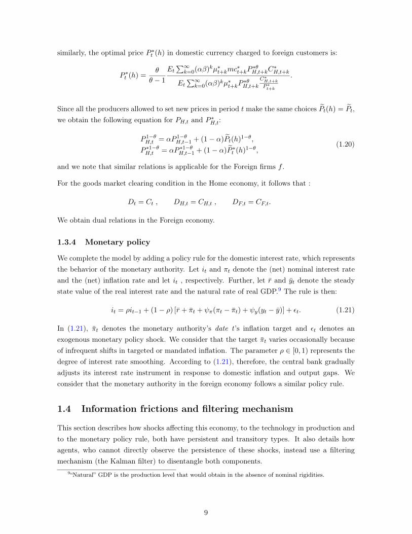
1.3.4 Monetary policy

We complete the model by adding a policy rule for the domestic interest rate, which representsthe behavior of the monetary authority. Let it and πt denote the (net) nominal interest rateand the (net) inflation rate and let it , respectively. Further, let r and yt denote the steadystate value of the real interest rate and the natural rate of real GDP.9 The rule is then:

it = ρit−1 + (1− ρ) [r + πt + ψπ(πt − πt) + ψy(yt − y)] + εt. (1.21)

In (1.21), πt denotes the monetary authority’s date t ’s inflation target and εt denotes anexogenous monetary policy shock. We consider that the target πt varies occasionally becauseof infrequent shifts in targeted or mandated inflation. The parameter ρ ∈ [0, 1) represents thedegree of interest rate smoothing. According to (1.21), therefore, the central bank graduallyadjusts its interest rate instrument in response to domestic inflation and output gaps. Weconsider that the monetary authority in the foreign economy follows a similar policy rule.

1.4 Information frictions and filtering mechanism

This section describes how shocks affecting this economy, to the technology in production andto the monetary policy rule, both have persistent and transitory types. It also details howagents, who cannot directly observe the persistence of these shocks, instead use a filteringmechanism (the Kalman filter) to disentangle both components.

9“Natural” GDP is the production level that would obtain in the absence of nominal rigidities.

9

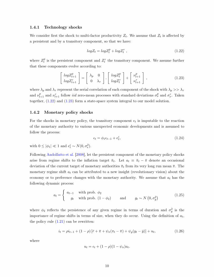
1.4.1 Technology shocks

We consider first the shock to multi-factor productivity Zt. We assume that Zt is affected bya persistent and by a transitory component, so that we have:

logZt = logZpt + logZτt , (1.22)

where Zpt is the persistent component and Zτt the transitory component. We assume furtherthat these components evolve according to:[

logZpt+1

logZτt+1

]=

[λp 0

0 λτ

].

[logZptlogZτt

]+

[νpt+1

ντt+1

], (1.23)

where λp and λτ represent the serial correlation of each component of the shock with λp >> λτ

and νpt+1 and ντt+1 follow iid zero-mean processes with standard deviations σpν and στν . Takentogether, (1.22) and (1.23) form a state-space system integral to our model solution.

1.4.2 Monetary policy shocks

For the shocks in monetary policy, the transitory component εt is imputable to the reactionof the monetary authority to various unexpected economic developments and is assumed tofollow the process:

εt = φ1εt−1 + eεt, (1.24)

with 0 ≤ |φ1| � 1 and eεt ∼ N(0, σ2e).

Following Andolfatto et al. [2008], let the persistent component of the monetary policy shocksarise from regime shifts to the inflation target πt. Let at ≡ πt − π denote an occasionaldeviation of the current target of monetary authorities πt from its very long run mean π. Themonetary regime shift at can be attributed to a new insight (revolutionary vision) about theeconomy or to preference changes with the monetary authority. We assume that at has thefollowing dynamic process:

at =

{at−1 with prob. φ2

gt with prob. (1− φ2) and gt ∼ N(0, σ2

g

) (1.25)

where φ2 reflects the persistence of any given regime in terms of duration and σ2g is the

importance of regime shifts in terms of size, when they do occur. Using the definition of at,the policy rule (1.21) can be rewritten:

it = ρit−1 + (1− ρ) [r + π + ψπ(πt − π) + ψy(yt − y)] + ut, (1.26)

whereut = εt + (1− ρ)(1− ψπ)at.

10

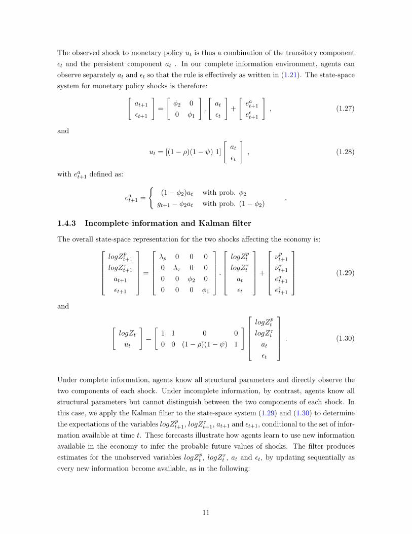
The observed shock to monetary policy ut is thus a combination of the transitory componentεt and the persistent component at . In our complete information environment, agents canobserve separately at and εt so that the rule is effectively as written in (1.21). The state-spacesystem for monetary policy shocks is therefore:[

at+1

εt+1

]=

[φ2 0

0 φ1

].

[at

εt

]+

[eat+1

eεt+1

], (1.27)

and

ut = [(1− ρ)(1− ψ) 1]

[at

εt

], (1.28)

with eat+1 defined as:

eat+1 =

{(1− φ2)at with prob. φ2

gt+1 − φ2at with prob. (1− φ2).

1.4.3 Incomplete information and Kalman filter

The overall state-space representation for the two shocks affecting the economy is:logZpt+1

logZτt+1

at+1

εt+1

=

λp 0 0 0

0 λτ 0 0

0 0 φ2 0

0 0 0 φ1

.logZptlogZτt

at

εt

+

νpt+1

ντt+1

eat+1

eεt+1

(1.29)

and

[logZt

ut

]=

[1 1 0 0

0 0 (1− ρ)(1− ψ) 1

]logZptlogZτt

at

εt

. (1.30)

Under complete information, agents know all structural parameters and directly observe thetwo components of each shock. Under incomplete information, by contrast, agents know allstructural parameters but cannot distinguish between the two components of each shock. Inthis case, we apply the Kalman filter to the state-space system (1.29) and (1.30) to determinethe expectations of the variables logZpt+1, logZ

τt+1, at+1 and εt+1, conditional to the set of infor-

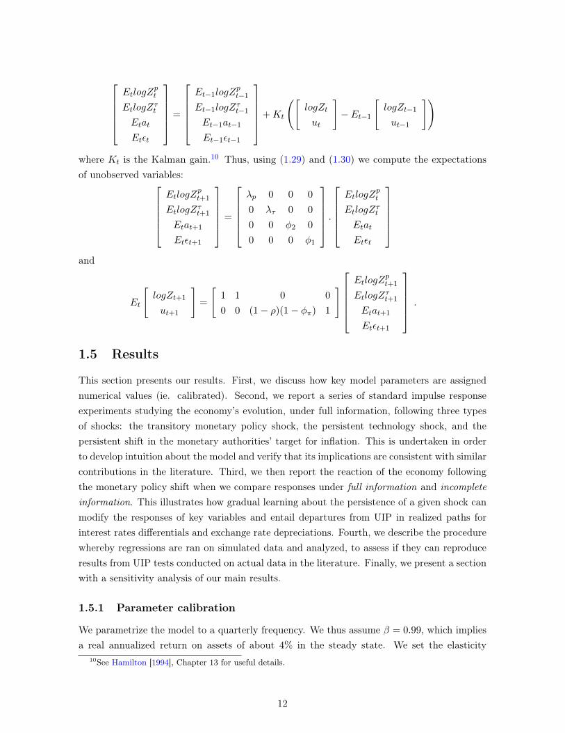
mation available at time t. These forecasts illustrate how agents learn to use new informationavailable in the economy to infer the probable future values of shocks. The filter producesestimates for the unobserved variables logZpt , logZτt , at and εt, by updating sequentially asevery new information become available, as in the following:

11

EtlogZ

pt

EtlogZτt

Etat

Etεt

=

Et−1logZ

pt−1

Et−1logZτt−1

Et−1at−1

Et−1εt−1

+Kt

([logZt

ut

]− Et−1

[logZt−1

ut−1

])

where Kt is the Kalman gain.10 Thus, using (1.29) and (1.30) we compute the expectationsof unobserved variables:

EtlogZpt+1

EtlogZτt+1

Etat+1

Etεt+1

=

λp 0 0 0

0 λτ 0 0

0 0 φ2 0

0 0 0 φ1

.EtlogZ

pt

EtlogZτt

Etat

Etεt

and

Et

[logZt+1

ut+1

]=

[1 1 0 0

0 0 (1− ρ)(1− φπ) 1

]EtlogZ

pt+1

EtlogZτt+1

Etat+1

Etεt+1

.

1.5 Results

This section presents our results. First, we discuss how key model parameters are assignednumerical values (ie. calibrated). Second, we report a series of standard impulse responseexperiments studying the economy’s evolution, under full information, following three typesof shocks: the transitory monetary policy shock, the persistent technology shock, and thepersistent shift in the monetary authorities’ target for inflation. This is undertaken in orderto develop intuition about the model and verify that its implications are consistent with similarcontributions in the literature. Third, we then report the reaction of the economy followingthe monetary policy shift when we compare responses under full information and incompleteinformation. This illustrates how gradual learning about the persistence of a given shock canmodify the responses of key variables and entail departures from UIP in realized paths forinterest rates differentials and exchange rate depreciations. Fourth, we describe the procedurewhereby regressions are ran on simulated data and analyzed, to assess if they can reproduceresults from UIP tests conducted on actual data in the literature. Finally, we present a sectionwith a sensitivity analysis of our main results.

1.5.1 Parameter calibration

We parametrize the model to a quarterly frequency. We thus assume β = 0.99, which impliesa real annualized return on assets of about 4% in the steady state. We set the elasticity

10See Hamilton [1994], Chapter 13 for useful details.

12

of substitution between the brands, θ, to be 6, which implies a markup over the marginalcost equal to 20% at the steady state. The parameter α, governing the frequency of pricechanges, is equal to 0.75, which implies an average of four periods (one year) between twoprice adjustments. We set the parameter governing the curvature on labor disutility η, tobe equal to 1.5 and the parameter κ such that the hours worked are 1/3 of available timeat the steady state. Finally we assume an import share in consumption equal to aF = 0.4,corresponding to the import/GDP ratio in Canada.11

The calibration of the monetary policy rule (1.21) is adapted from Andolfatto et al. [2008].First, we set the coefficient governing the response to inflation deviations from target, ψπ,to 1.8 and the coefficient governing the inertia in interest rate, ρ, to 0.1. The calibration ofthe shock processes, which play a decisive role in the model, is next. To this end, note thatφ2 characterizes the mean duration of a given regime shift in monetary authorities’ inflationtarget and σg the standard deviation of the distribution governing the magnitude of suchregime shifts when they do occur. Following Andolfatto et al. [2008], we set φ1 = 0.0 andφ2 = 0.975, σg = 0.01 and σε = 0.005; these values entail Kalman filter gains that are similar tothose used by Erceg and Levin [2003] and Schorfheide [2005]. Note that these parameter valuesimply that monetary policy shifts occur infrequently (on average once every 40 quarters, or 10

years) and that when they do occur their magnitude is relatively high, changing the inflationtarget by a typical 4 points of percentage on an annualized basis (0.01·4). For the technologicalshocks, we similarly set λτ = 0.0 and λp = 0.95, as well as στ = 0.005 and σp = 0.0025. Weuse a similar calibration for the foreign economy’s monetary policy.

1.5.2 Impulse response functions: Complete information

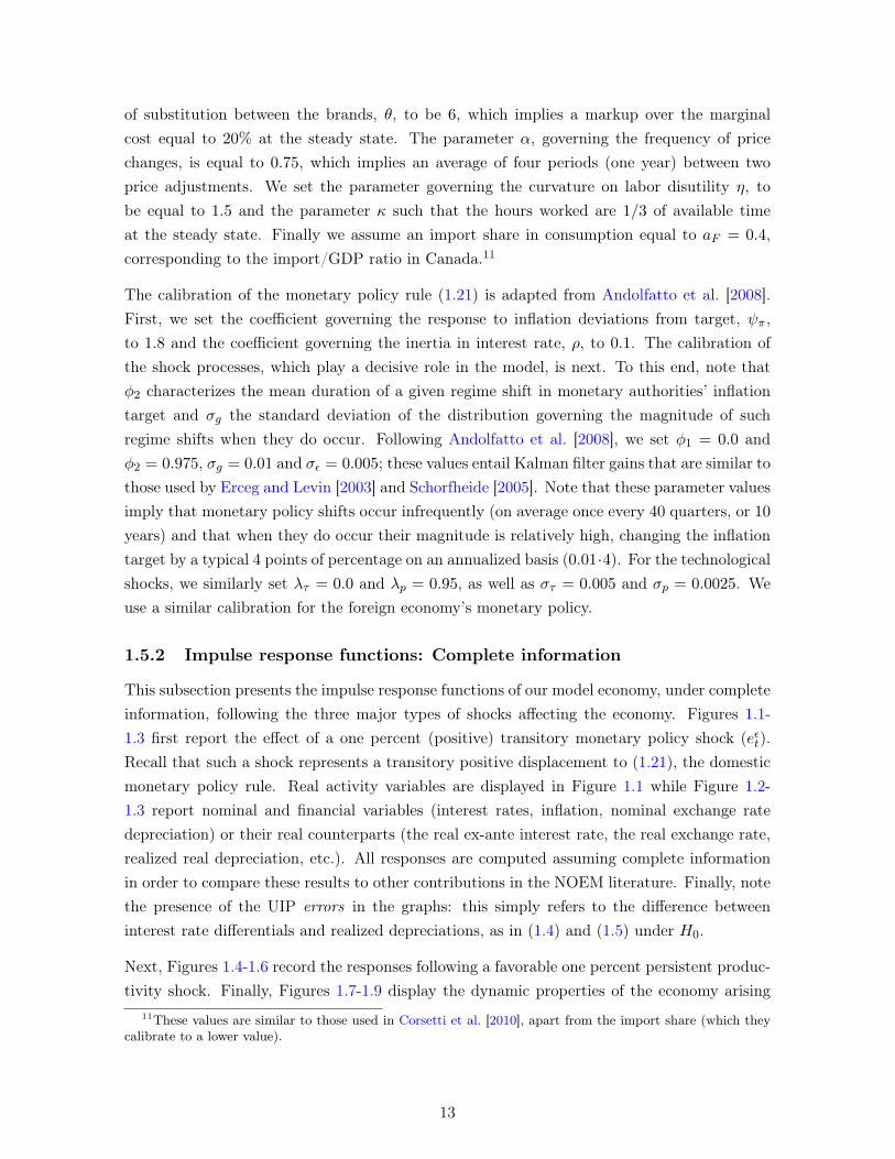
This subsection presents the impulse response functions of our model economy, under completeinformation, following the three major types of shocks affecting the economy. Figures 1.1-1.3 first report the effect of a one percent (positive) transitory monetary policy shock (eεt).Recall that such a shock represents a transitory positive displacement to (1.21), the domesticmonetary policy rule. Real activity variables are displayed in Figure 1.1 while Figure 1.2-1.3 report nominal and financial variables (interest rates, inflation, nominal exchange ratedepreciation) or their real counterparts (the real ex-ante interest rate, the real exchange rate,realized real depreciation, etc.). All responses are computed assuming complete informationin order to compare these results to other contributions in the NOEM literature. Finally, notethe presence of the UIP errors in the graphs: this simply refers to the difference betweeninterest rate differentials and realized depreciations, as in (1.4) and (1.5) under H0.

Next, Figures 1.4-1.6 record the responses following a favorable one percent persistent produc-tivity shock. Finally, Figures 1.7-1.9 display the dynamic properties of the economy arising

11These values are similar to those used in Corsetti et al. [2010], apart from the import share (which theycalibrate to a lower value).

13

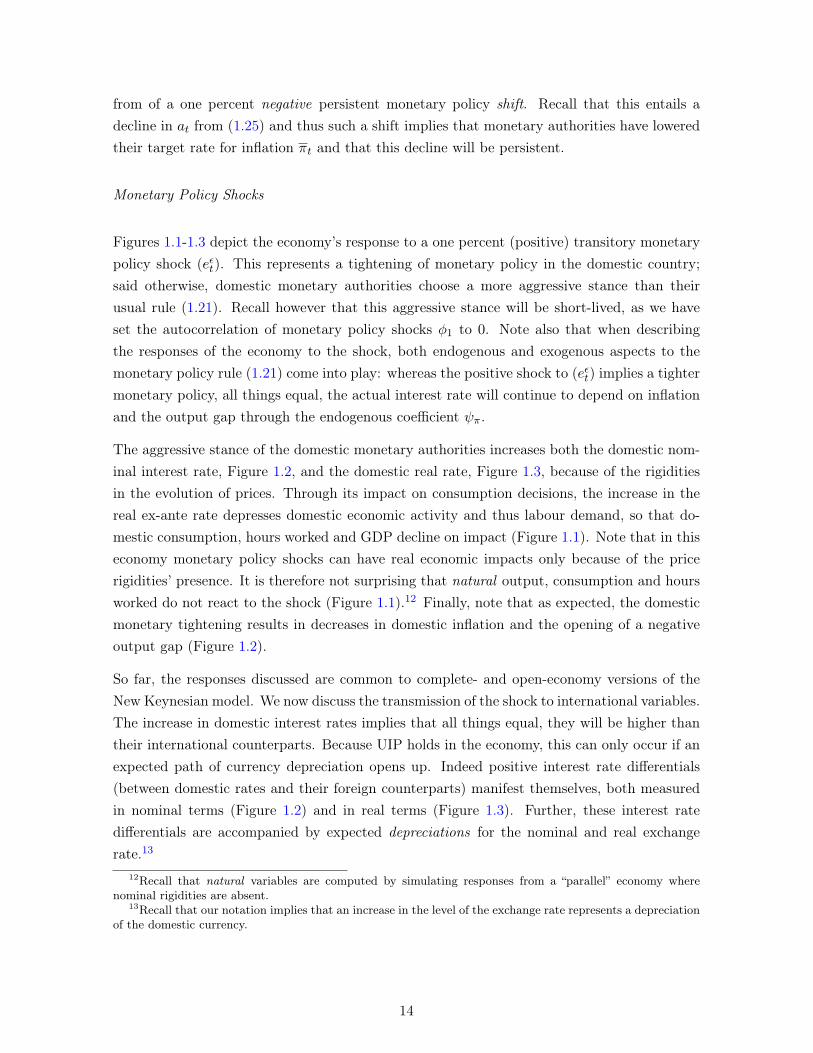
from of a one percent negative persistent monetary policy shift. Recall that this entails adecline in at from (1.25) and thus such a shift implies that monetary authorities have loweredtheir target rate for inflation πt and that this decline will be persistent.

Monetary Policy Shocks

Figures 1.1-1.3 depict the economy’s response to a one percent (positive) transitory monetarypolicy shock (eεt). This represents a tightening of monetary policy in the domestic country;said otherwise, domestic monetary authorities choose a more aggressive stance than theirusual rule (1.21). Recall however that this aggressive stance will be short-lived, as we haveset the autocorrelation of monetary policy shocks φ1 to 0. Note also that when describingthe responses of the economy to the shock, both endogenous and exogenous aspects to themonetary policy rule (1.21) come into play: whereas the positive shock to (eεt) implies a tightermonetary policy, all things equal, the actual interest rate will continue to depend on inflationand the output gap through the endogenous coefficient ψπ.

The aggressive stance of the domestic monetary authorities increases both the domestic nom-inal interest rate, Figure 1.2, and the domestic real rate, Figure 1.3, because of the rigiditiesin the evolution of prices. Through its impact on consumption decisions, the increase in thereal ex-ante rate depresses domestic economic activity and thus labour demand, so that do-mestic consumption, hours worked and GDP decline on impact (Figure 1.1). Note that in thiseconomy monetary policy shocks can have real economic impacts only because of the pricerigidities’ presence. It is therefore not surprising that natural output, consumption and hoursworked do not react to the shock (Figure 1.1).12 Finally, note that as expected, the domesticmonetary tightening results in decreases in domestic inflation and the opening of a negativeoutput gap (Figure 1.2).

So far, the responses discussed are common to complete- and open-economy versions of theNew Keynesian model. We now discuss the transmission of the shock to international variables.The increase in domestic interest rates implies that all things equal, they will be higher thantheir international counterparts. Because UIP holds in the economy, this can only occur if anexpected path of currency depreciation opens up. Indeed positive interest rate differentials(between domestic rates and their foreign counterparts) manifest themselves, both measuredin nominal terms (Figure 1.2) and in real terms (Figure 1.3). Further, these interest ratedifferentials are accompanied by expected depreciations for the nominal and real exchangerate.13

12Recall that natural variables are computed by simulating responses from a “parallel” economy wherenominal rigidities are absent.

13Recall that our notation implies that an increase in the level of the exchange rate represents a depreciationof the domestic currency.

14

Because our open economy is relatively highly-integrated (recall our calibration of aF = 0.4)the shock also has important negative impacts on the foreign economy: Foreign GDP, hoursworked, and inflation all decline and a negative output gap also opens in the foreign econ-omy. Considering that the interest rate rule followed by the foreign monetary authority isof the same form as (1.21), the foreign interest rate responds to these depressed conditionswith a small decline. Finally, note that the real exchange rate appreciates on impact: thisoccurs because perfect risk sharing commands that this rate equal the ratio of domestic toforeign consumption, and domestic consumption has declined importantly. Said otherwise,the model rationalizes the fall in the foreign to domestic consumption ratio by increasing therelative price of domestic goods, ie. by appreciating the real exchange rate. As discussedabove, this contemporaneous, real appreciation is expected to undo itself in future periodsand the currency is thus expected to experience future depreciations. This pattern, whereby acontemporaneous real exchange rate appreciation is associated with future depreciations, realor nominal, is consistent with the classic Dornbush overshooting hypothesis and is discussedat length in Eichenbaum et al. [2017]. It will play a key role below when we discuss depar-tures from UIP under incomplete information. Here, under complete information, UIP holdsexactly however so that the positive interest rate differentials are exactly matched with thesubsequent depreciations and UIP errors are nil (Figure 1.2-Figure 1.3).

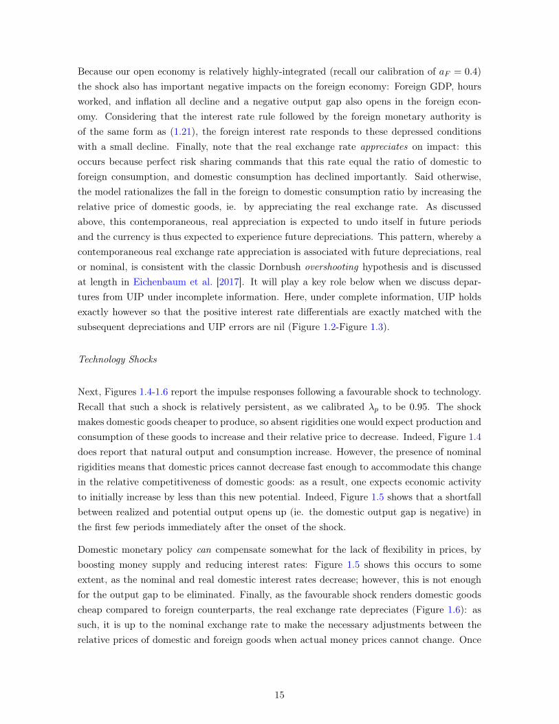
Technology Shocks

Next, Figures 1.4-1.6 report the impulse responses following a favourable shock to technology.Recall that such a shock is relatively persistent, as we calibrated λp to be 0.95. The shockmakes domestic goods cheaper to produce, so absent rigidities one would expect production andconsumption of these goods to increase and their relative price to decrease. Indeed, Figure 1.4does report that natural output and consumption increase. However, the presence of nominalrigidities means that domestic prices cannot decrease fast enough to accommodate this changein the relative competitiveness of domestic goods: as a result, one expects economic activityto initially increase by less than this new potential. Indeed, Figure 1.5 shows that a shortfallbetween realized and potential output opens up (ie. the domestic output gap is negative) inthe first few periods immediately after the onset of the shock.

Domestic monetary policy can compensate somewhat for the lack of flexibility in prices, byboosting money supply and reducing interest rates: Figure 1.5 shows this occurs to someextent, as the nominal and real domestic interest rates decrease; however, this is not enoughfor the output gap to be eliminated. Finally, as the favourable shock renders domestic goodscheap compared to foreign counterparts, the real exchange rate depreciates (Figure 1.6): assuch, it is up to the nominal exchange rate to make the necessary adjustments between therelative prices of domestic and foreign goods when actual money prices cannot change. Once

15

more, note that UIP continues to hold exactly: the negative differentials in interest rates areexactly matched by expected and realized depreciations and the UIP errors (Figure 1.5 - 1.6)are nil. Said otherwise, the contemporaneous real depreciation is associated with an expectedpath of future appreciations, a key negative correlation that is consistent with data [Burnsideet al., 2007] and that will imply departures from UIP under incomplete information, below.

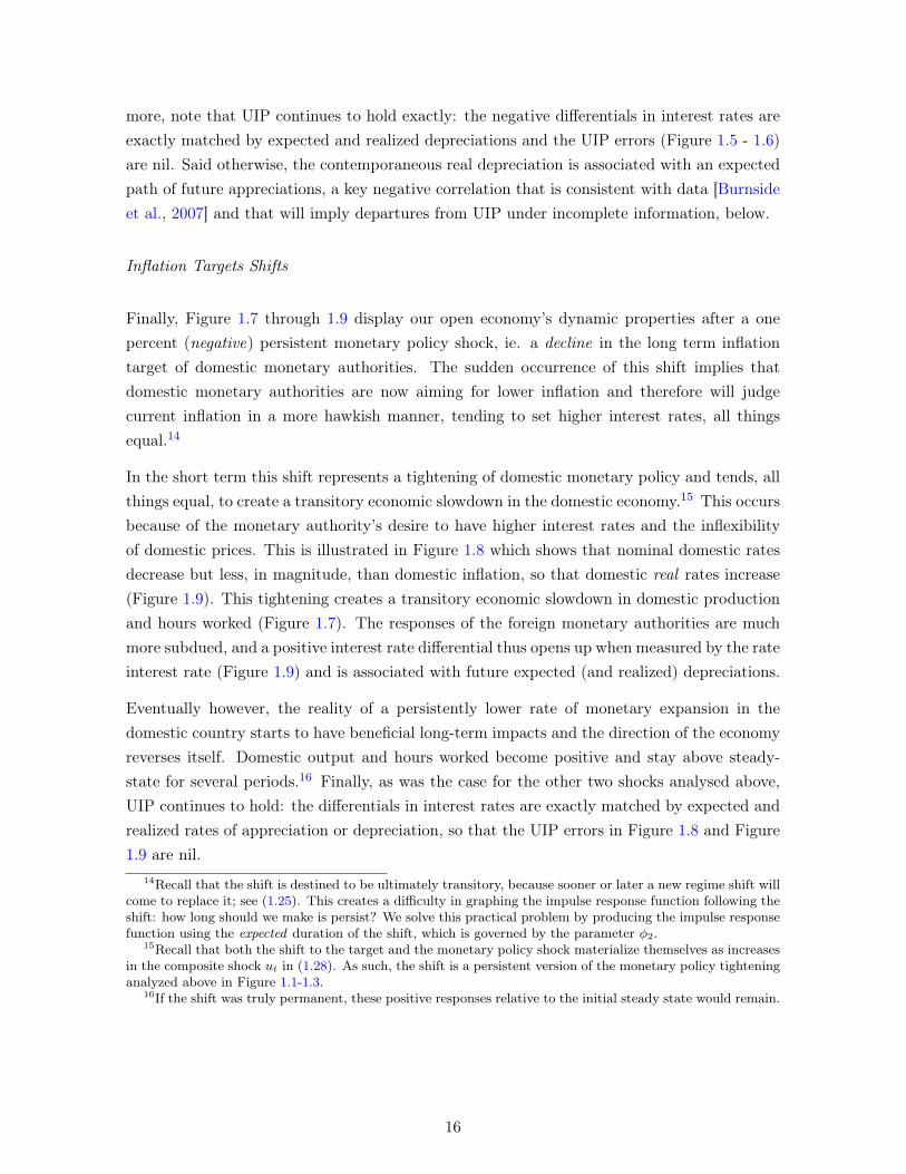
Inflation Targets Shifts

Finally, Figure 1.7 through 1.9 display our open economy’s dynamic properties after a onepercent (negative) persistent monetary policy shock, ie. a decline in the long term inflationtarget of domestic monetary authorities. The sudden occurrence of this shift implies thatdomestic monetary authorities are now aiming for lower inflation and therefore will judgecurrent inflation in a more hawkish manner, tending to set higher interest rates, all thingsequal.14

In the short term this shift represents a tightening of domestic monetary policy and tends, allthings equal, to create a transitory economic slowdown in the domestic economy.15 This occursbecause of the monetary authority’s desire to have higher interest rates and the inflexibilityof domestic prices. This is illustrated in Figure 1.8 which shows that nominal domestic ratesdecrease but less, in magnitude, than domestic inflation, so that domestic real rates increase(Figure 1.9). This tightening creates a transitory economic slowdown in domestic productionand hours worked (Figure 1.7). The responses of the foreign monetary authorities are muchmore subdued, and a positive interest rate differential thus opens up when measured by the rateinterest rate (Figure 1.9) and is associated with future expected (and realized) depreciations.

Eventually however, the reality of a persistently lower rate of monetary expansion in thedomestic country starts to have beneficial long-term impacts and the direction of the economyreverses itself. Domestic output and hours worked become positive and stay above steady-state for several periods.16 Finally, as was the case for the other two shocks analysed above,UIP continues to hold: the differentials in interest rates are exactly matched by expected andrealized rates of appreciation or depreciation, so that the UIP errors in Figure 1.8 and Figure1.9 are nil.

14Recall that the shift is destined to be ultimately transitory, because sooner or later a new regime shift willcome to replace it; see (1.25). This creates a difficulty in graphing the impulse response function following theshift: how long should we make is persist? We solve this practical problem by producing the impulse responsefunction using the expected duration of the shift, which is governed by the parameter φ2.

15Recall that both the shift to the target and the monetary policy shock materialize themselves as increasesin the composite shock ut in (1.28). As such, the shift is a persistent version of the monetary policy tighteninganalyzed above in Figure 1.1-1.3.

16If the shift was truly permanent, these positive responses relative to the initial steady state would remain.

16

1.5.3 Impulse response functions: Complete versus incompleteinformation

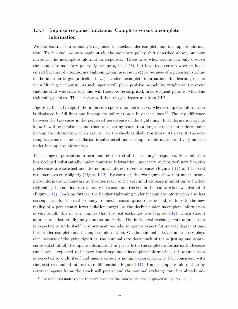
We now contrast our economy’s responses to shocks under complete and incomplete informa-tion. To this end, we once again study the monetary policy shift described above, but nowintroduce the incomplete information responses. These arise when agents can only observethe composite monetary policy tightening ut in (1.28), but have to ascertain whether it oc-curred because of a temporary tightening (an increase in eεt) or because of a persistent declinein the inflation target (a decline in at). Under incomplete information, this learning occursvia a filtering mechanism; as such, agents will place positive probability weights on the eventthat the shift was transitory and will therefore be surprised, in subsequent periods, when thetightening persists. This surprise will then trigger departures from UIP.

Figure 1.10 - 1.12 report the impulse responses for both cases, where complete informationis displayed in full lines and incomplete information is in dashed lines.17 The key differencebetween the two cases is the perceived persistence of the tightening: full-information agentsknow it will be persistent, and thus price-setting reacts to a larger extent than it does underincomplete information, when agents view the shock as likely transitory. As a result, the con-temporaneous decline in inflation is substantial under complete information and very modestunder incomplete information.

This change of perception in turn modifies the rest of the economy’s responses. Since inflationhas declined substantially under complete information, monetary authorities’ new hawkishpreferences are satisfied and the nominal interest rates decreases (Figure 1.11) and the realrate increases only slightly (Figure 1.12). By contrast, the two figures show that under incom-plete information, monetary authorities react to the very mild decrease in inflation by furthertightening: the nominal rate actually increases, and the rise in the real rate is now substantial(Figure 1.12). Looking further, the harsher tightening under incomplete information also hasconsequences for the real economy: domestic consumption does not adjust fully to the newreality of a persistently lower inflation target, so the decline under incomplete informationis very small; this in turn implies that the real exchange rate (Figure 1.12), which shouldappreciate substantially, only does so modestly. The initial real exchange rate appreciationis expected to undo itself in subsequent periods, so agents expect future real depreciations,both under complete and incomplete information. On the nominal side, a similar story playsout: because of the price rigidities, the nominal rate does much of the adjusting and appre-ciates substantially (complete information) or just a little (incomplete information). Becausethe shock is expected to be very transitory under incomplete information, this appreciationis expected to undo itself and agents expect a nominal depreciation (a fact consistent withthe positive nominal interest rate differential - Figure 1.11). Under complete information bycontrast, agents know the shock will persist and the nominal exchange rate has already ad-

17The responses under complete information are the same as the ones displayed in Figures 1.4-1.6.

17

justed by a significant margin; as a consequence, they expect it to actually appreciate a littlein future periods, which is congruent with the negative interest rate differential in Figure 1.11.

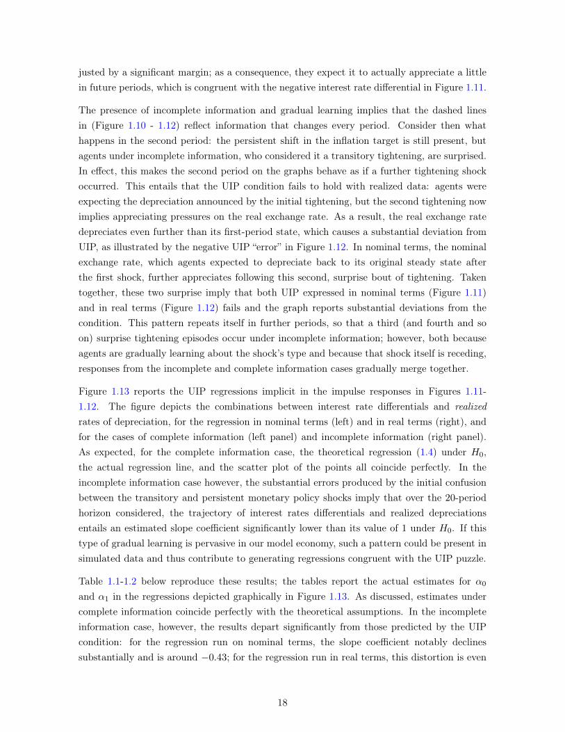
The presence of incomplete information and gradual learning implies that the dashed linesin (Figure 1.10 - 1.12) reflect information that changes every period. Consider then whathappens in the second period: the persistent shift in the inflation target is still present, butagents under incomplete information, who considered it a transitory tightening, are surprised.In effect, this makes the second period on the graphs behave as if a further tightening shockoccurred. This entails that the UIP condition fails to hold with realized data: agents wereexpecting the depreciation announced by the initial tightening, but the second tightening nowimplies appreciating pressures on the real exchange rate. As a result, the real exchange ratedepreciates even further than its first-period state, which causes a substantial deviation fromUIP, as illustrated by the negative UIP “error” in Figure 1.12. In nominal terms, the nominalexchange rate, which agents expected to depreciate back to its original steady state afterthe first shock, further appreciates following this second, surprise bout of tightening. Takentogether, these two surprise imply that both UIP expressed in nominal terms (Figure 1.11)and in real terms (Figure 1.12) fails and the graph reports substantial deviations from thecondition. This pattern repeats itself in further periods, so that a third (and fourth and soon) surprise tightening episodes occur under incomplete information; however, both becauseagents are gradually learning about the shock’s type and because that shock itself is receding,responses from the incomplete and complete information cases gradually merge together.

Figure 1.13 reports the UIP regressions implicit in the impulse responses in Figures 1.11-1.12. The figure depicts the combinations between interest rate differentials and realizedrates of depreciation, for the regression in nominal terms (left) and in real terms (right), andfor the cases of complete information (left panel) and incomplete information (right panel).As expected, for the complete information case, the theoretical regression (1.4) under H0,the actual regression line, and the scatter plot of the points all coincide perfectly. In theincomplete information case however, the substantial errors produced by the initial confusionbetween the transitory and persistent monetary policy shocks imply that over the 20-periodhorizon considered, the trajectory of interest rates differentials and realized depreciationsentails an estimated slope coefficient significantly lower than its value of 1 under H0. If thistype of gradual learning is pervasive in our model economy, such a pattern could be present insimulated data and thus contribute to generating regressions congruent with the UIP puzzle.

Table 1.1-1.2 below reproduce these results; the tables report the actual estimates for α0

and α1 in the regressions depicted graphically in Figure 1.13. As discussed, estimates undercomplete information coincide perfectly with the theoretical assumptions. In the incompleteinformation case, however, the results depart significantly from those predicted by the UIPcondition: for the regression run on nominal terms, the slope coefficient notably declinessubstantially and is around −0.43; for the regression run in real terms, this distortion is even

18

worse and the slope coefficient is close to −1.0.

Table 1.1: Baseline estimates for the UIP regression under Complete information

Estimates α0 α1

Nominal terms: Regressing (et+1 − et) on (it − it∗)Persistent shock 0 1Transitory shock 0 1

Real terms: Regressing (st+1 − st) on (rt − rt∗)Persistent shock 0 1Transitory shock 0 1

Table 1.2: Baseline estimates for the UIP regression under Incomplete information

Estimates α0 α1

Nominal terms: Regressing (et+1 − et) on (it − it∗)Persistent shock -0.5831 -0.4302Transitory shock 0.1483 1.4830

Real terms: Regressing (st+1 − st) on (rt − rt∗)Persistent shock 0.2684 -1.0223Transitory shock 0.1132 1.5850

Note however that Tables 1.1-1.2 also present the regression results following one transitoryshock to monetary policy. This shock was already studied above in Figures 1.1-1.3 undercomplete information only. Again, in that case, the regression estimates implicit in thosefigures implied that UIP held perfectly; this is now reflected in Table 1.1-1.2, with the estimatesfor α0 and α1 exactly equal to 0 and 1, respectively. However, under incomplete information,another set of results emerge. Now, when the initial shock occurs, economic agents mightbe expecting it to be long-lasting, but it fact it will be purely transitory. As a result, theexpected depreciations, nominal or real, inherent to the UIP condition might be acceleratedunder incomplete information when in subsequent periods, agents realize the shock has recededcompletely. This situation leads to instances where the slope coefficient α1, notably, might bebigger than 1. Indeed Tables 1.1-1.2 show that when one transitory monetary policy shockaffects the economy, incomplete information entails departures from UIP that look like themirror image from those following the persistent shift. The question as to which effect willdominate in repeated simulations of the model is taken on below.

1.5.4 Unbiasedness regression and the UIP

We now use the economic model to generate (simulate) data and assess the Fama [1984]regression using these data. We first consider a baseline case where only the persistent shiftsto monetary policy are present. We then consider a more complete model accounting for other

19

types of shocks. Throughout, we study the properties of the estimates α0 and α1 both for thenominal UIP equation (1.4) and its counterpart expressed in real terms (1.5), as well as theF -tests assessing H0 : α0 = 0, α1 = 1.

1.5.4.1 UIP with monetary policy regime shifts

In this baseline test, we present results obtained from an economic environment subjected onlyto the persistent monetary policy disturbances. To this end, we use the model to generate2000 simulations, each containing a 200-periods-sample for all the economy’s variables, undereach information structure. This thus corresponds to a 50-year sample of data, which might beon the high end for tests assessing UIP on actual time series. Then, we run the unbiasednessregression on each sample, for the nominal and the real UIP regression, and under eachinformation structure: we thus have 4 sets of 2000 values each for the parameters (α0, α1)and for the test statistic for H0.

The results are presented in Figures 1.14-1.15. These figures display the histograms of all2000 estimates for α0, α1, and the test statistic for H0 : α0 = 0, α1 = 1, under completeinformation (Figure 1.14) and incomplete information (Figure 1.15). Results for the nominalversion of the UIP regression are on the left-hand side panel of each figure, and those related toits real counterpart are on the right-hand side panel. Figure 1.14 reveals that under completeinformation the point estimates are distributed relatively tightly around the hypothesizedvalues under H0, although the slope estimates for the nominal regression (median estimatearound 0.89) is somewhat surprisingly away from 1. The test statistics have median valuesof 2.35 and 1.52 for the nominal and real regression, respectively, and these lead to rejectionof H0 in around 20% of cases. While this is higher than the 5% theoretical size of the test,it is probably linked to the non-standard shape of the persistent monetary policy shock, amixture of Bernouilli and unit root processes, which might entail non-normal behaviour insmall samples.

By contrast, under incomplete information, Figure 1.15 shows that the empirical estimates ofthe two parameters are distributed wildly, with the slope estimate α1 notably being distributedsubstantially away from 1, particularly for the regression in real terms. As a result, the teststatistic almost invariably leads to rejections of H0, in 90% (nominal regression) and 99.9%

(real regression) of cases, respectively.

In synthesis, model simulations shows that if the persistent monetary policy shifts were theonly shocks affecting our model economy, complete information would entail no rejections ofthe UIP hypothesis beyond the normal low probability related to test size, whereas incompleteinformation would imply that in almost all simulated cases, an econometrician studying thedata would have concluded that UIP does not hold.

20

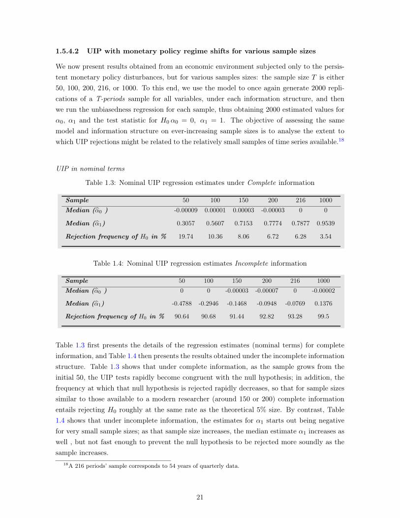
1.5.4.2 UIP with monetary policy regime shifts for various sample sizes

We now present results obtained from an economic environment subjected only to the persis-tent monetary policy disturbances, but for various samples sizes: the sample size T is either50, 100, 200, 216, or 1000. To this end, we use the model to once again generate 2000 repli-cations of a T-periods sample for all variables, under each information structure, and thenwe run the unbiasedness regression for each sample, thus obtaining 2000 estimated values forα0, α1 and the test statistic for H0 α0 = 0, α1 = 1. The objective of assessing the samemodel and information structure on ever-increasing sample sizes is to analyse the extent towhich UIP rejections might be related to the relatively small samples of time series available.18

UIP in nominal terms

Table 1.3: Nominal UIP regression estimates under Complete information

Sample 50 100 150 200 216 1000Median (α0 ) -0.00009 0.00001 0.00003 -0.00003 0 0

Median (α1) 0.3057 0.5607 0.7153 0.7774 0.7877 0.9539

Rejection frequency of H0 in % 19.74 10.36 8.06 6.72 6.28 3.54

Table 1.4: Nominal UIP regression estimates Incomplete information

Sample 50 100 150 200 216 1000Median (α0 ) 0 0 -0.00003 -0.00007 0 -0.00002

Median (α1) -0.4788 -0.2946 -0.1468 -0.0948 -0.0769 0.1376


Table 1.3 first presents the details of the regression estimates (nominal terms) for completeinformation, and Table 1.4 then presents the results obtained under the incomplete informationstructure. Table 1.3 shows that under complete information, as the sample grows from theinitial 50, the UIP tests rapidly become congruent with the null hypothesis; in addition, thefrequency at which that null hypothesis is rejected rapidly decreases, so that for sample sizessimilar to those available to a modern researcher (around 150 or 200) complete informationentails rejecting H0 roughly at the same rate as the theoretical 5% size. By contrast, Table1.4 shows that under incomplete information, the estimates for α1 starts out being negativefor very small sample sizes; as that sample size increases, the median estimate α1 increases aswell , but not fast enough to prevent the null hypothesis to be rejected more soundly as thesample increases.

18A 216 periods’ sample corresponds to 54 years of quarterly data.

21

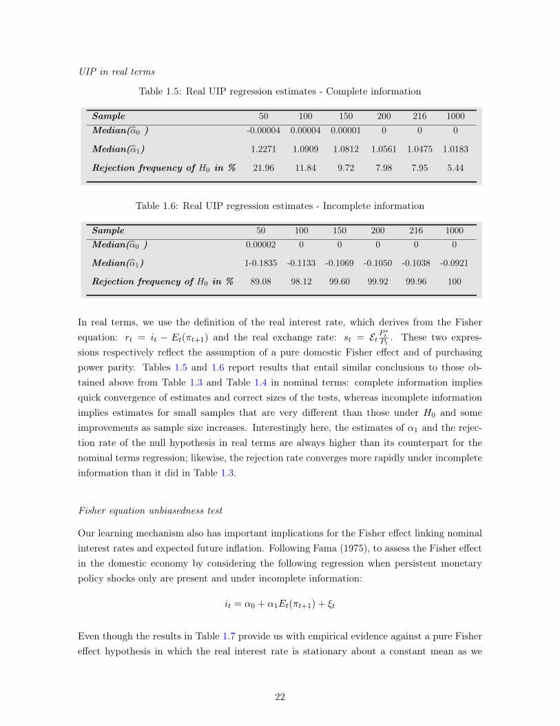
UIP in real terms

Table 1.5: Real UIP regression estimates - Complete information

Sample 50 100 150 200 216 1000Median(α0 ) -0.00004 0.00004 0.00001 0 0 0

Median(α1) 1.2271 1.0909 1.0812 1.0561 1.0475 1.0183


Table 1.6: Real UIP regression estimates - Incomplete information

Sample 50 100 150 200 216 1000Median(α0 ) 0.00002 0 0 0 0 0

Median(α1) 1-0.1835 -0.1133 -0.1069 -0.1050 -0.1038 -0.0921

Rejection frequency of H0 in % 89.08 98.12 99.60 99.92 99.96 100

In real terms, we use the definition of the real interest rate, which derives from the Fisherequation: rt = it − Et(πt+1) and the real exchange rate: st = Et P

∗tPt

. These two expres-sions respectively reflect the assumption of a pure domestic Fisher effect and of purchasingpower parity. Tables 1.5 and 1.6 report results that entail similar conclusions to those ob-tained above from Table 1.3 and Table 1.4 in nominal terms: complete information impliesquick convergence of estimates and correct sizes of the tests, whereas incomplete informationimplies estimates for small samples that are very different than those under H0 and someimprovements as sample size increases. Interestingly here, the estimates of α1 and the rejec-tion rate of the null hypothesis in real terms are always higher than its counterpart for thenominal terms regression; likewise, the rejection rate converges more rapidly under incompleteinformation than it did in Table 1.3.

Fisher equation unbiasedness test

Our learning mechanism also has important implications for the Fisher effect linking nominalinterest rates and expected future inflation. Following Fama (1975), to assess the Fisher effectin the domestic economy by considering the following regression when persistent monetarypolicy shocks only are present and under incomplete information:

it = α0 + α1Et(πt+1) + ξt

Even though the results in Table 1.7 provide us with empirical evidence against a pure Fishereffect hypothesis in which the real interest rate is stationary about a constant mean as we

22

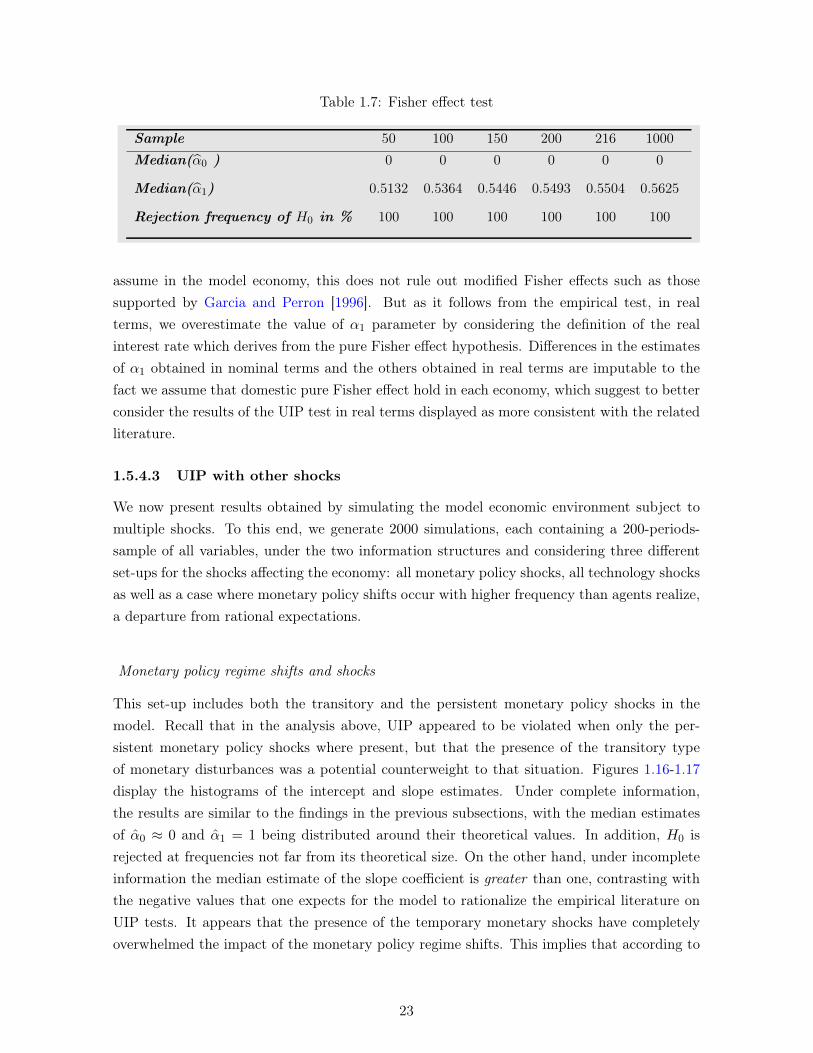
Table 1.7: Fisher effect test

Sample 50 100 150 200 216 1000Median(α0 ) 0 0 0 0 0 0

Median(α1) 0.5132 0.5364 0.5446 0.5493 0.5504 0.5625

Rejection frequency of H0 in % 100 100 100 100 100 100

assume in the model economy, this does not rule out modified Fisher effects such as thosesupported by Garcia and Perron [1996]. But as it follows from the empirical test, in realterms, we overestimate the value of α1 parameter by considering the definition of the realinterest rate which derives from the pure Fisher effect hypothesis. Differences in the estimatesof α1 obtained in nominal terms and the others obtained in real terms are imputable to thefact we assume that domestic pure Fisher effect hold in each economy, which suggest to betterconsider the results of the UIP test in real terms displayed as more consistent with the relatedliterature.

1.5.4.3 UIP with other shocks

We now present results obtained by simulating the model economic environment subject tomultiple shocks. To this end, we generate 2000 simulations, each containing a 200-periods-sample of all variables, under the two information structures and considering three differentset-ups for the shocks affecting the economy: all monetary policy shocks, all technology shocksas well as a case where monetary policy shifts occur with higher frequency than agents realize,a departure from rational expectations.

Monetary policy regime shifts and shocks

This set-up includes both the transitory and the persistent monetary policy shocks in themodel. Recall that in the analysis above, UIP appeared to be violated when only the per-sistent monetary policy shocks where present, but that the presence of the transitory typeof monetary disturbances was a potential counterweight to that situation. Figures 1.16-1.17display the histograms of the intercept and slope estimates. Under complete information,the results are similar to the findings in the previous subsections, with the median estimatesof α0 ≈ 0 and α1 = 1 being distributed around their theoretical values. In addition, H0 isrejected at frequencies not far from its theoretical size. On the other hand, under incompleteinformation the median estimate of the slope coefficient is greater than one, contrasting withthe negative values that one expects for the model to rationalize the empirical literature onUIP tests. It appears that the presence of the temporary monetary shocks have completelyoverwhelmed the impact of the monetary policy regime shifts. This implies that according to

23

our simulated model economy and if monetary disturbances are the main drivers of economicfluctuations, the learning mechanism present in our model has difficulty replicating the em-pirical Evidence about UIP.

Frequent monetary policy shifts

Let us now consider an alternative scenario regarding monetary policy shocks. Imagine a worldwhere the persistent monetary policy shifts occur with more frequency that economic agentsrealize. This implies that the impact of these shifts on UIP will receive more weight and thatlearning about them will be non-optimal, because agents have relatively faulty informationabout the general data generating process for the shocks. This set-up can be interpreted as aworld where within the limited time actual data on exchange rates has been available, thesetypes of shifts have been more frequent than they would be in very long samples. This isakin to a assumption that agents are not fully rational or have not had the chance to receivesufficient information about these shifts.

Figures 1.18-1.19 report results related to this case and they show that departures from UIPbecome prevailing again. As always, the overall picture shows coherent results to the previouscases under complete information. Under incomplete information however, results are nowmore coherent with the empirical literature about the UIP hypothesis: the decrease in agentrationality induces declines in the median slope estimates around α1 = 0.6 and then close to0 in the nominal and real regressions, respectively. Accordingly the frequency at which H0 isrejected increases dramatically.

Transitory and persistent technology shocks

Finally, Figures 1.20-1.21 present the results obtained when technology shocks are the mainsource of economic fluctuations. To this end the model economy is simulated with both thepersistent and transitory disturbances in the technology, as calibrated above. The figures showthat in this world, simulated data seem to rationalize departures from UIP. All the results arecoherent with the previous findings as we obtain a negative value for the slope estimate underincomplete information in real terms and a slope estimate near zero in nominal terms. Theimportant conclusion we can draw from this analysis is that indeed incomplete informationdoes matter in explaining UIP, and it does matter most in an environment with technologyshocks where monetary policy regime shifts are more frequent with less interference withtransitory monetary policy shocks.

24

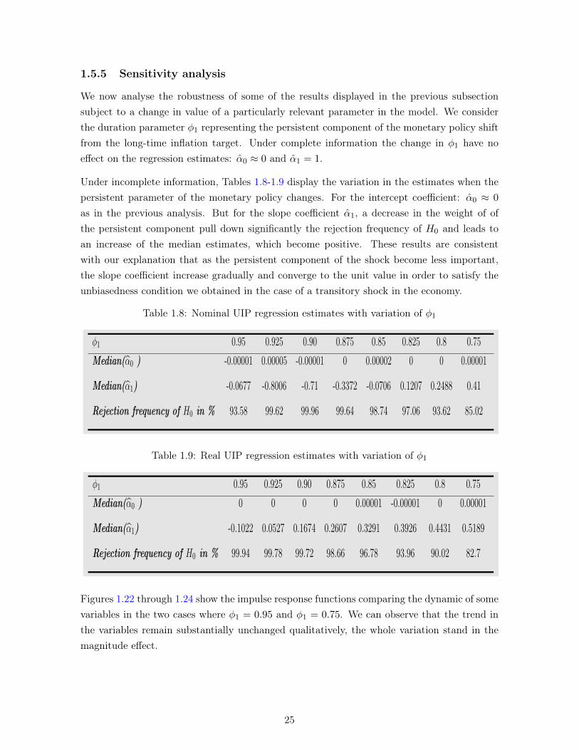
1.5.5 Sensitivity analysis

We now analyse the robustness of some of the results displayed in the previous subsectionsubject to a change in value of a particularly relevant parameter in the model. We considerthe duration parameter φ1 representing the persistent component of the monetary policy shiftfrom the long-time inflation target. Under complete information the change in φ1 have noeffect on the regression estimates: α0 ≈ 0 and α1 = 1.

Under incomplete information, Tables 1.8-1.9 display the variation in the estimates when thepersistent parameter of the monetary policy changes. For the intercept coefficient: α0 ≈ 0

as in the previous analysis. But for the slope coefficient α1, a decrease in the weight of ofthe persistent component pull down significantly the rejection frequency of H0 and leads toan increase of the median estimates, which become positive. These results are consistentwith our explanation that as the persistent component of the shock become less important,the slope coefficient increase gradually and converge to the unit value in order to satisfy theunbiasedness condition we obtained in the case of a transitory shock in the economy.

Table 1.8: Nominal UIP regression estimates with variation of φ1

φ1 0.95 0.925 0.90 0.875 0.85 0.825 0.8 0.75Median(α0 ) -0.00001 0.00005 -0.00001 0 0.00002 0 0 0.00001

Median(α1) -0.0677 -0.8006 -0.71 -0.3372 -0.0706 0.1207 0.2488 0.41

Rejection frequency of H0 in % 93.58 99.62 99.96 99.64 98.74 97.06 93.62 85.02

Table 1.9: Real UIP regression estimates with variation of φ1

φ1 0.95 0.925 0.90 0.875 0.85 0.825 0.8 0.75Median(α0 ) 0 0 0 0 0.00001 -0.00001 0 0.00001

Median(α1) -0.1022 0.0527 0.1674 0.2607 0.3291 0.3926 0.4431 0.5189

Rejection frequency of H0 in % 99.94 99.78 99.72 98.66 96.78 93.96 90.02 82.7

Figures 1.22 through 1.24 show the impulse response functions comparing the dynamic of somevariables in the two cases where φ1 = 0.95 and φ1 = 0.75. We can observe that the trend inthe variables remain substantially unchanged qualitatively, the whole variation stand in themagnitude effect.

25

1.6 Concluding Remarks

This research proposes an open-economy environment in which gradual learning about thepersistence of shocks may imply departures from UIP. The model is repeatedly simulated,with and without this information constraint, and the generate data is assessed to verify ifit replicates observed departures from UIP in the data. We report that in our simulateddata, the dynamics of realized depreciations in nominal and real exchange rates are perfectlycoherent with UIP under complete information, but may be in stark departure from it underour assumed incomplete-information structure, depending on the shocks that are responsiblefor economic fluctuations. Such evidence is not incoherent with the rational expectationhypothesis if one assumes that the underlying shocks are inherently undistinguishable, or notcredibly communicated.

26

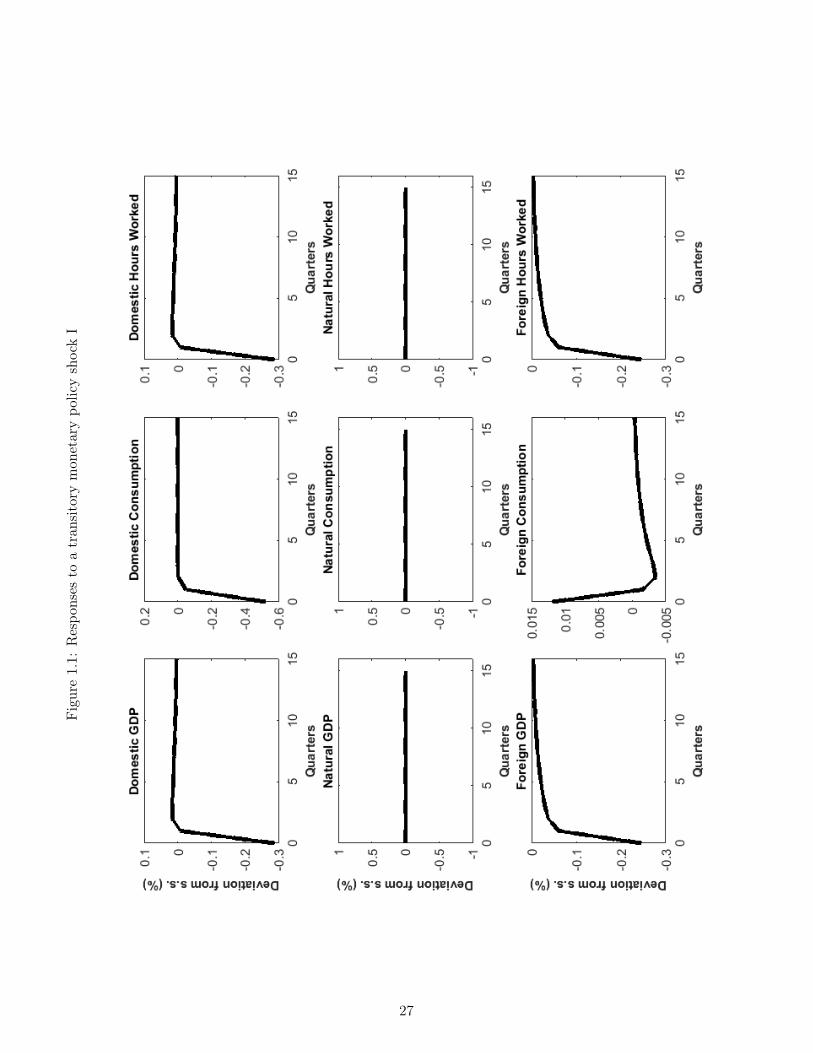
Figure1.1:

Respo

nses

toatran

sitory

mon

etarypo

licyshockI

27

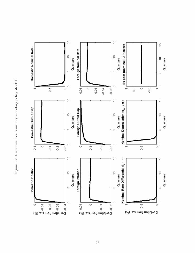
Figure1.2:

Respo

nses

toatran

sitory

mon

etarypo

licyshockII

28

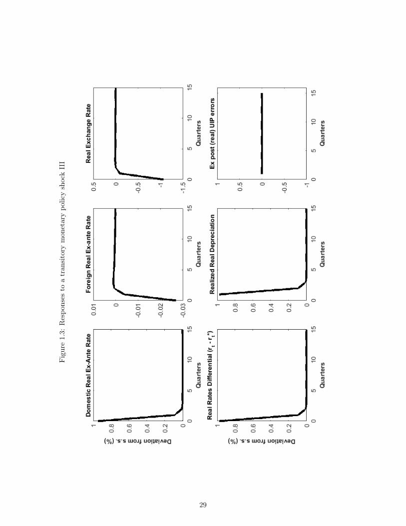
Figure1.3:

Respo

nses

toatran

sitory

mon

etarypo

licyshockIII

29

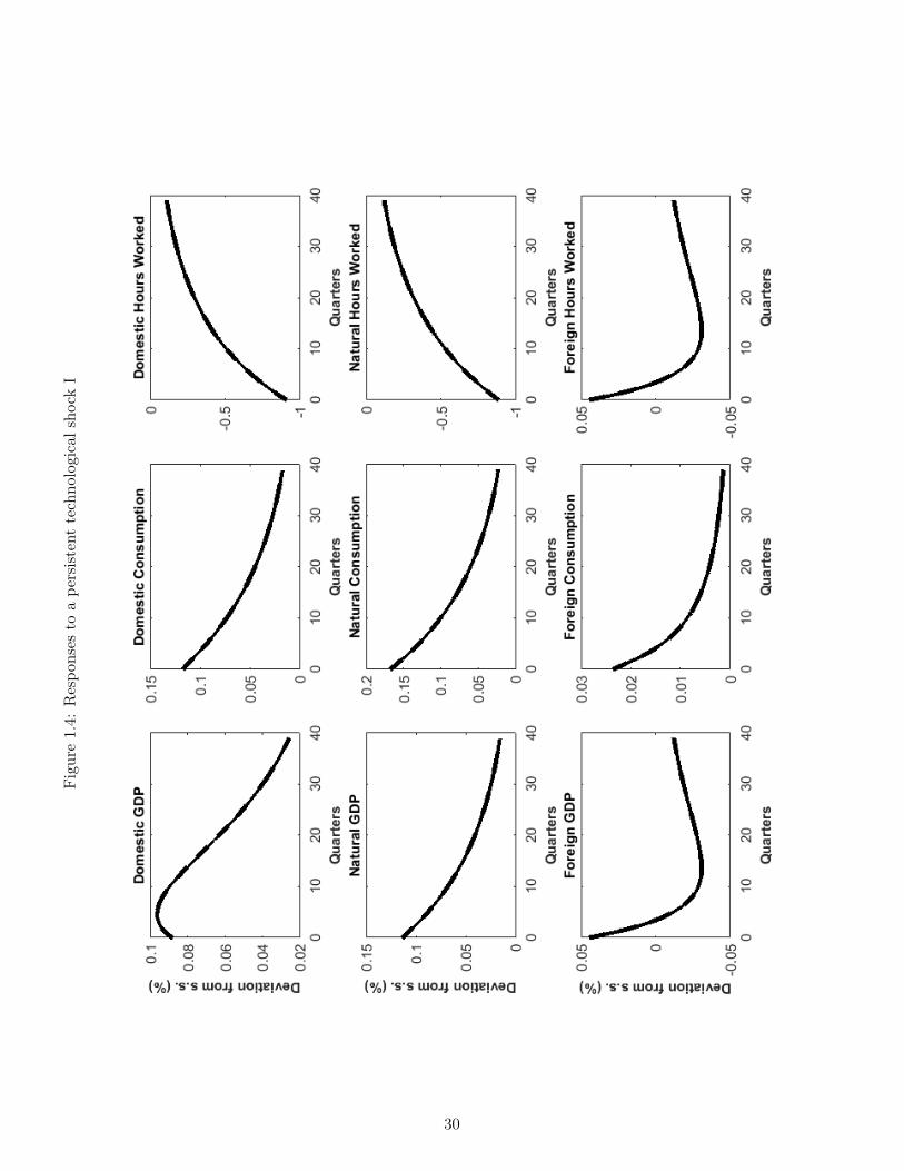
Figure1.4:

Respo

nses

toape

rsistent

techno

logicals

hock

I

30

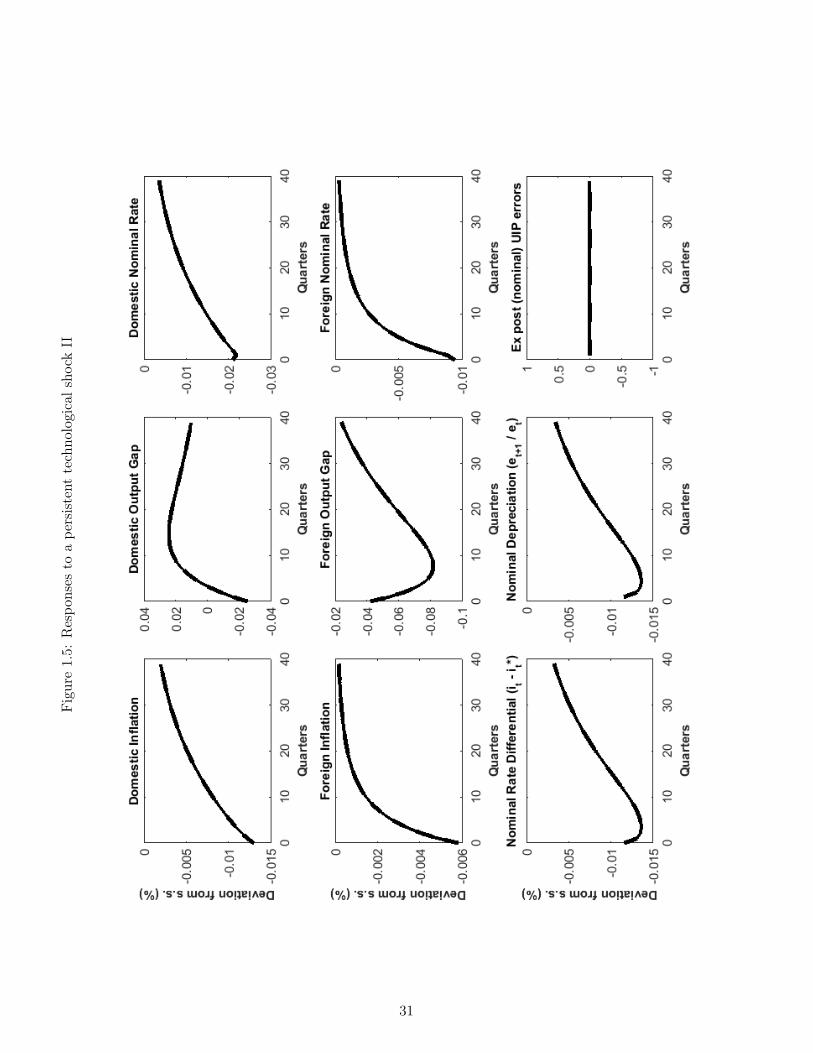
Figure1.5:

Respo

nses

toape

rsistent

techno

logicals

hock

II

31

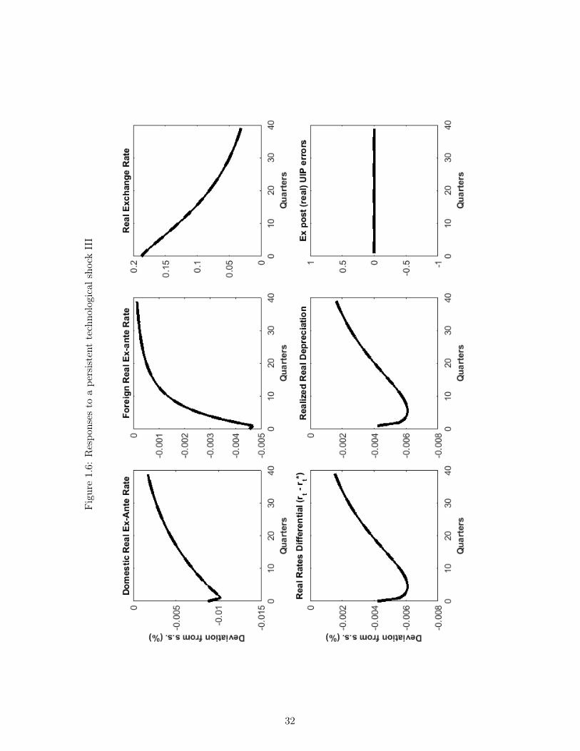
Figure1.6:

Respo

nses

toape

rsistent

techno

logicals

hock

III

32

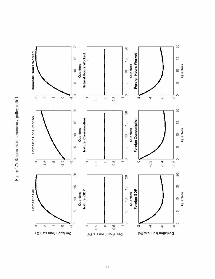
Figure1.7:

Respo

nses

toamon

etarypo

licyshift

I

33

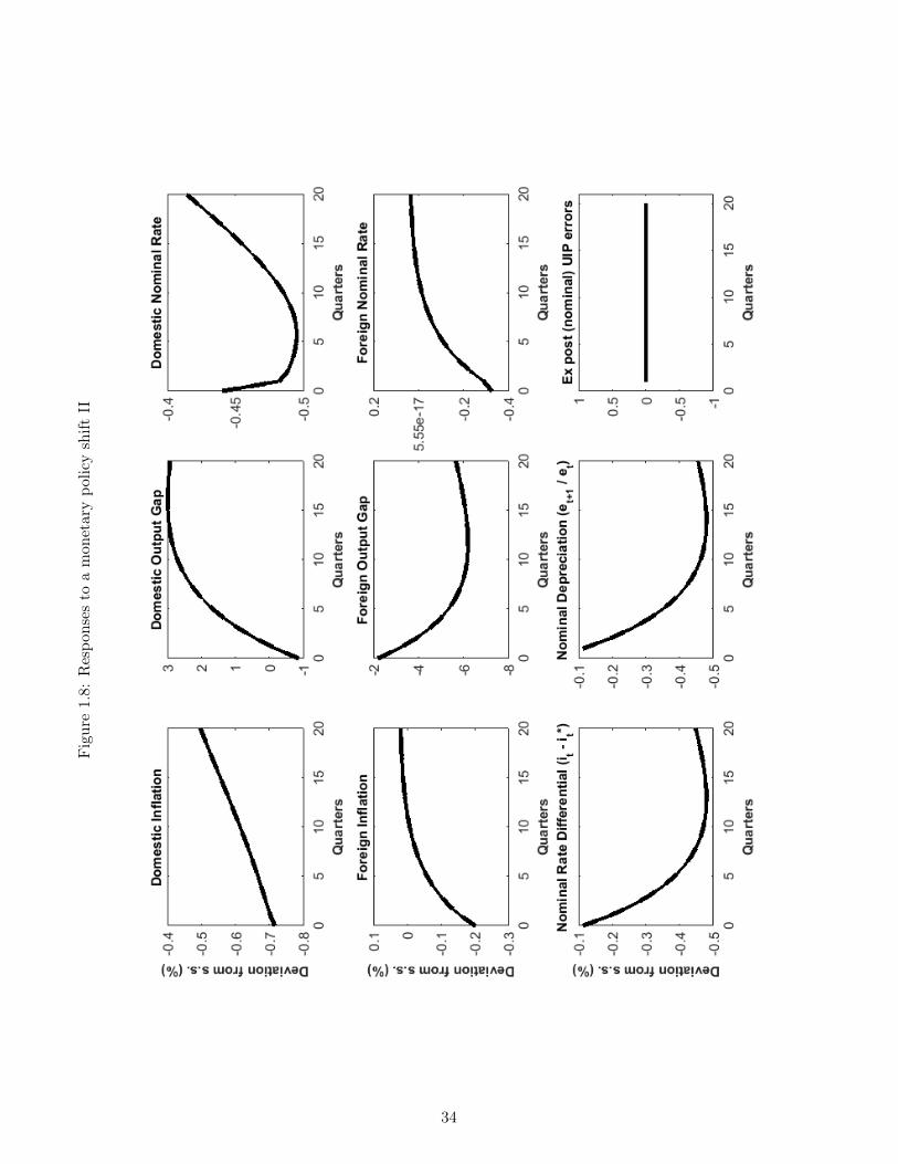
Figure1.8:

Respo

nses

toamon

etarypo

licyshift

II

34

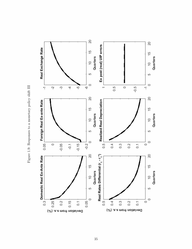
Figure1.9:

Respo

nses

toamon

etarypo

licyshift

III

35

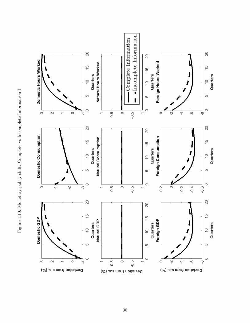
Figure1.10

:Mon

etarypo

licyshift:Com

pletevs

IncompleteInform

ationI

36

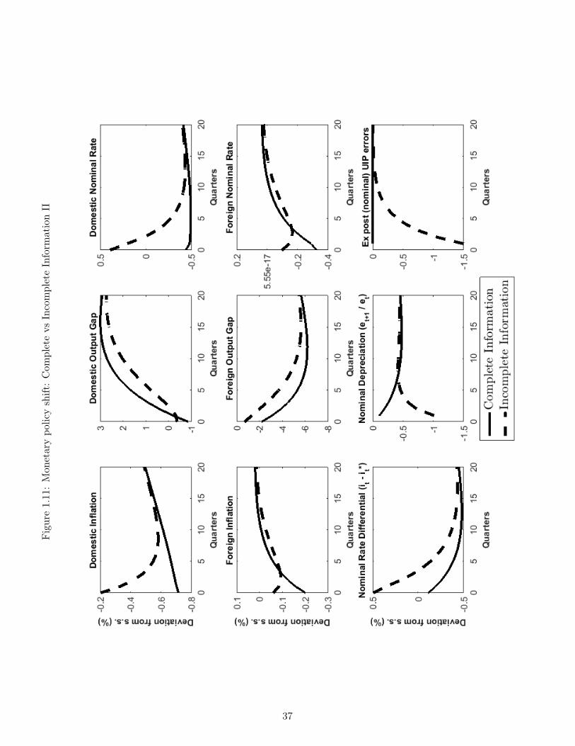
Figure1.11

:Mon

etarypo

licyshift:Com

pletevs

IncompleteInform

ationII

37

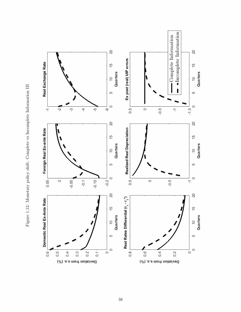
Figure1.12

:Mon

etarypo

licyshift:Com

pletevs

IncompleteInform

ationIII

38

Figure1.13

:Mon

etarypo

licyshift:Com

pletevs

IncompleteInform

ationIV

39

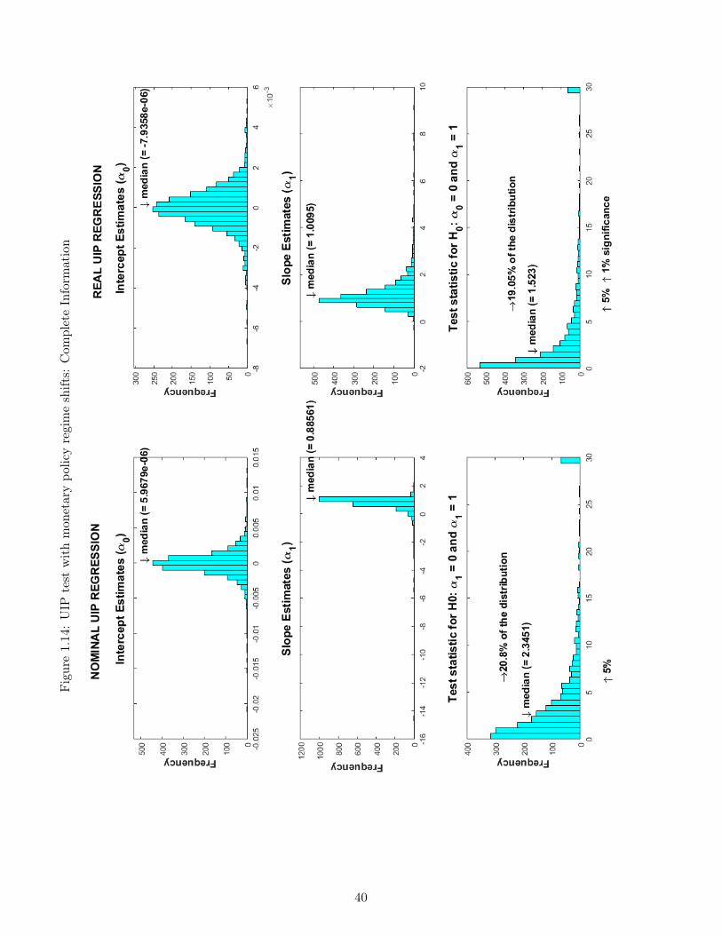
Figure1.14

:UIP

test

withmon

etarypo

licyregimeshifts:

Com

pleteInform

ation

40

Figure1.15

:UIP

test

withmon

etarypo

licyregimeshifts:

IncompleteInform

ation

41

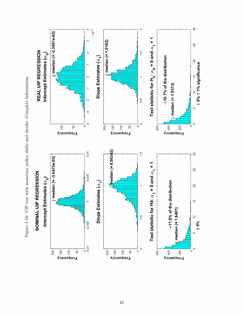
Figure1.16

:UIP

test

withmon

etarypo

licyshiftsan

dshocks:Com

pleteInform

ation

42

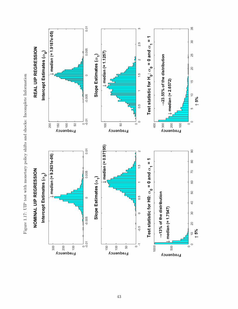
Figure1.17

:UIP

test

withmon

etarypo

licyshiftsan

dshocks:IncompleteInform

ation

43

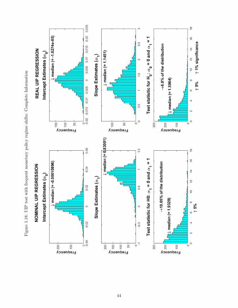
Figure1.18

:UIP

test

withfreque

ntmon

etarypo

licyregimeshifts:

Com

pleteInform

ation

44

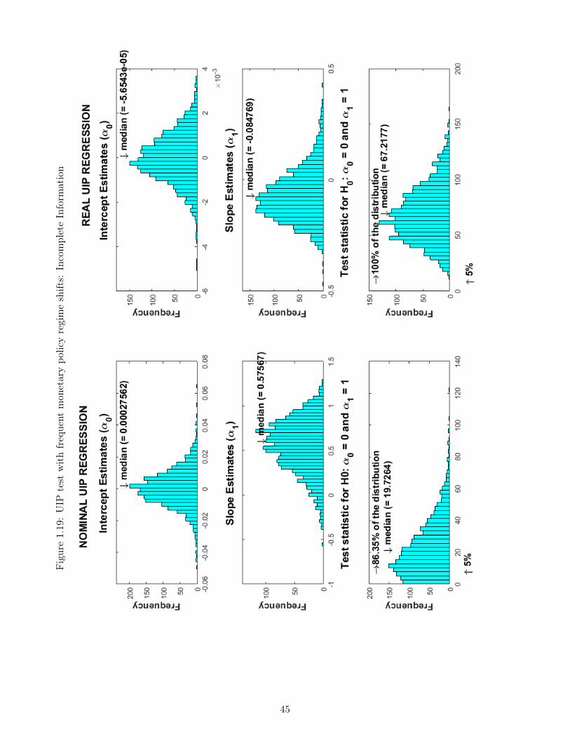
Figure1.19

:UIP

test

withfreque

ntmon

etarypo

licyregimeshifts:

IncompleteInform

ation

45

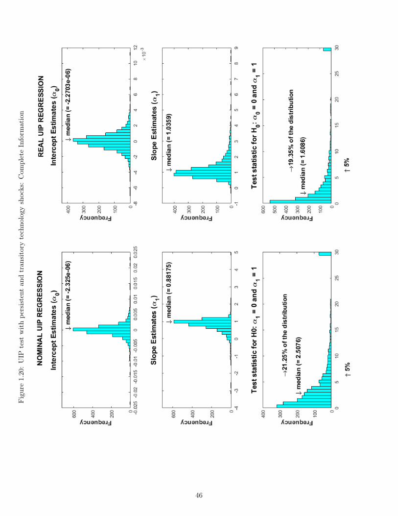
Figure1.20

:UIP

test

withpe

rsistent

andtran

sitory

techno

logy

shocks:Com

pleteInform

ation

46

Figure1.21

:UIP

test

withpe

rsistent

andtran

sitory

techno

logy

shocks:IncompleteInform

ation

47

Figure1.22

:Mon

etarypo

licyshift:IncompleteInform

ation-φ

1=

0.95

vsφ

1=

0.75

48

Figure1.23

:Mon

etarypo


ation-φ

1=

0.95

vsφ

1=

0.75

49

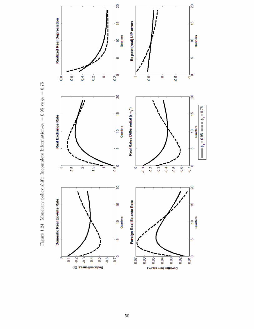
Figure1.24

:Mon

etarypo


ation-φ

1=

0.95

vsφ

1=

0.75

50

Chapter 2

Using Confidence Data to Forecast theCanadian Business Cycle

Abstract

This paper assesses the contribution of confidence –or sentiment– data for predictingCanadian economic slowdowns. A probit framework is applied to an indicator on the sta-tus of the Canadian business cycle produced by the OECD. Explanatory variables includeall available Canadian data on sentiment (from four distinct surveys) as well as macroe-conomic and financial data. Sentiment data are introduced either as individual variables,as simple averages (such as confidence indices) and as confidence factors extracted fromlarger datasets containing all available sentiment data. Results indicate that the full po-tential of confidence data for forecasting Canadian business cycles obtains when factormodels are used and all confidence data are utilized.

Keywords: Business Cycles; Leading Indicators; Probability Forecasting; Turning Points; Con-fidence Surveys.

52

2.1 Introduction

Survey data on consumer and business confidence – or sentiment– play important roles inthe decision processes of monetary and government policy makers worldwide.1 Interest forthis type of data arises because of their timeliness and the fact that they are seldom revised.In addition, it reflects the belief that these data provide signals about current and futureeconomic developments that complements the information embodied in standard time-seriesfrom financial markets or national accounts.2

The growing interest for such data has manifested itself in the establishment of several dif-ferent surveys. In Canada, four major separate surveys regularly examine various aspects ofconsumer and business sentiment. First, the Business Confidence Survey, established in 1977

by the Conference Board, is a quarterly survey that queries managers of Canada’s businessorganizations. Second, the Consumer Confidence Survey, originated by the same ConferenceBoard in 1979, scrutinizes consumers’ attitudes and optimism about their current and futureeconomic prospects. Next, the more recently (1997) established Business Outlook Survey, or-ganized and managed by the Bank of Canada’s regional offices, is a quarterly consultationwith businesses across Canada that covers topics related to demand conditions, productivecapacity, prices and inflation. Finally, the Bank of Canada’s Senior Loan Officers Survey,quarterly and established in 1999, analyzes the business-lending practices of major Canadianfinancial institutions.

This expanding diversity in the available data on business and consumer sentiment holdsthe potential to improve forecasts of future Canadian economic developments and thus lead tobetter decision making. However, it calls into question the most efficient use of al these variousdata. Should forecasters focus on individual, particularly promising survey questions to obtaina parsimonious forecasting equation? Or should they instead use all available information, evenat the risk of overfitting their models?

This paper provides an analysis of this question. To this end, we test several specifications ofprobit forecasting equations for Canada’s future business cycle turning points. Throughout ouranalysis, the variable to forecast is the status of Canada’s business cycle, as measured by theOECD.3 The explanatory variables drawn from sentiment data include individual time-series

1Throughout the paper we refer to ‘confidence’ and ‘sentiment’ data interchangeably. See Murray [2013]for a general overview of the decision process at the Bank of Canada and how sentiment data contribute tothat process.

2Sentiment data might be able to signal future economic developments because they reflect informationabout future fundamental shocks that is not contained in other time-series; alternatively it may be thatconfidence and its evolution has a causal impact on future economic developments. See Barsky and Sims[2012] for a discussion.

3This measures stems from a growth-cycle framework for understanding business cycles [Zarnowitz andOzyldirim, 2006]. We use this measure because the alternative, the recession dates established by the C.D.Howe Institute for Canada, include only one recession in the last 25 years (since the early 1990s). Accordingly,we refer to slowdowns in the Canadian economy instead of recessions when discussing our models and our

53

resulting from some specific survey questions, simple aggregates of these time-series (such asIndex of Consumer Confidence produced by the Conference Board of Canada) and estimatedfactors extracted from all survey data available for Canada. We assess the forecasting abilityof these models by comparing them to those using the ‘classical predictors’ popularized in theliterature on predicting recessions4 as well as information extracted from a large, 144-variablesdataset of Canadian macroeconomic, financial and national accounts data.

Our results indicate that sentiment data has substantial forecasting power for future status ofthe Canadian business cycle. Specifically, we first show that within the class of single-predictorprobits, models using sentiment data produce results comparable to the best performancesobtained using the classical predictors popularized by Estrella and Mishkin [1998]. Next, wereport strong evidence in favor of using multiple-predictors frameworks with confidence ‘fac-tors’ extracted from all available sentiment; this happens because such factors are orthogonalone to the other and including additional such factors can only improve the fit of the model,but will not necessarily improve the performance of coursIndeed, we find that the statisticalsignificance of each factor used remains high in these multiple-predictors models and that mea-sures of model performance increase relative to cases where only individual variables are used.We show that these findings are robust to varying the forecasting horizon and the sample usedand that they are strengthened in an out-of-sample experiment. Overall, our result indicatethat the full potential of sentiment data for forecasting business cycles is likely to be attainedwhen all such data are used and amalgamated through factor models.

The rest of the paper is organised as follows. Section 2 discusses the related literature usingsentiment data for forecasting or analysing economic fluctuations. Next, Section 3 discussesour probit forecasting framework and Section 4 provides a detailed description of all data used.Section 5 describes our results and Section 6 concludes by suggesting likely avenues for futureresearch.

2.2 Related Literature

The expanding availability of survey data on sentiment has generated a growing empiricalliterature, which has tended to fall under two general themes; we review them in turn.

Forecasting with Confidence Data

The first major direction along which this literature has progressed assesses the ability of sen-timent data to forecast future economic developments. Christiansen et al. [2014] is a recent,

results. See Section 4 for a complete description of all data used in the present study.4The term spread and the return on stock markets are two such classical predictors [Estrella and Mishkin,

1998].

54

representative contribution to this research agenda. In that paper, the authors examine theforecasting ability of the Consumer Confidence Index and of the Purchasing Managers’ In-dex for US recessions.5 They use the probit framework popularized by Estrella and Mishkin[1998], which aims to forecast a binary ‘recession’ variable indicating whether the economy isexperiencing a downturn or an expansion.6 Christiansen et al. [2014] report that sentimentvariables have substantial power to predict the occurrence of future downturns, both in-sampleand out-of-sample. Specifically, sentiment variables, when taken individually, predict futuredownturns better than the ‘classical’ recession predictors identified by Estrella and Mishkin[1998] (the term spread and stock market indices). In addition, when sentiment variablesare combined with other explanatory variables (including estimated factors extracted froma large dataset of macroeconomic variables) the model attains a superior forecasting perfor-mance. Taylor and McNabb [2007] present a similar analysis, applied to data from the UK,the Netherlands, France and Italy. They also report that sentiment, particularly data drawnfrom business surveys, can contribute significantly to forecasting economic downturns.

Researchers have provided evidence about the substantial forecasting ability of sentiment vari-ables in other contexts. For example, recent work by Ollivaud et al. [2016] shows that smallforecasting models for various OECD countries that include sentiment data among a very lim-ited list of explanatory variables have the capacity to predict future economic developmentsas well as larger models drawing their information from multiple explanatory variables. In arelated way, Hansson et al. [2005] use a VAR framework to show that survey data from theSwedish Business Tendency Survey can help forecast the growth of Swedish GDP, particularlywhen all sentiment data are aggregated via a dynamic factor model and forecasting is under-taken using the estimated factors. Their results are confirmed and extended to the case of theNorwegian business cycle by Martinsen et al. [2014b]. Additionally, Bodo et al. [2000] showthat forecasting Industrial Production in the Euro area using an error-correction system thatincludes a business confidence index produces good results and Batchelor and Dua [1998] re-port that the Blue Chip Consensus forecast could have better predicted the 1991 US recessionif the information contained in the Conference Board’s Consumer Confidence index had beentaken into account.

As described above, a rich variety of survey data exists in Canada, with four major surveysassessing the sentiment of businesses, consumers, and financial institutions. However, theability of these data to help forecast Canadian economic developments has been the subjectof only limited analysis. This analysis includes Pichette [2012], who studies how the Bank

5The Consumer Confidence Index is constructed from answers to the University of Michigan Survey ques-tions. The Purchasing Managers’ Index is produced by the Institute of Supply Management by aggregatingsurvey answers from managers and purchasers at important manufacturing companies in the US. Christiansenet al. [2014] use the NBER dates to measure U.S. recessions.

6The Estrella and Mishkin [1998] strategy of identifying predictors of future recessions has been extendedby various authors [Kauppi and Saikkonen, 2008, Nyberg, 2010, Chen et al., 2011, Fornaro, 2016, Kotchoniand Stevanovic, 2016].

55

of Canada’s Business Outlook Survey (BOS) data is correlated with future values of output,investment and consumption growth. The author reports that the BOS data helps predictfuture output and investment growth, but that results for consumption are weaker. Morerecent work on the same lines includes Pichette and Robitaille [2016], which again shows thatthe BOS data has important explanatory power in real-time forecasting exercises where thedata vintages used reproduce the information known at the time, before the data revisions,which can be sizeable for GDP. The analysis in Pichette [2012] and Pichette and Robitaille[2016] is limited to the BOS survey however, and pertains to the growth rate of variables. Asindicated above, we provide a generalization of that analysis by examining all the informationcontained in the four available surveys; in addition, our focus is on the prediction of a binaryvariable indicating whether the economy is experiencing a slowdown or an expansion. Otherwork includes Binette and Chang [2013a], who analyse the performance of Canada’s Short-Term Indicator Model (CSI ) a forecasting framework for future Canadian GDP growth; themodel includes some of the BOS Survey data among its explanatory variables. As indicatedabove, our paper provides a novel contribution to the literature, by showing how using allCanadian data on sentiment and organising it within a factor model provides a very promisingavenue for predicting future Canadian economic developments.

Structural Impact of Confidence Shocks

A second major thrust of the research using survey data concerns its structural interpretation.This literature originated in the work of Matsusaka and Sbordone [1995] and is represented byrecent contributions from Leduc and Sill [2013], Barsky and Sims [2012] and Lambertini et al.[2013]. Using VAR frameworks that include sentiment variables, these authors first identifyshocks to the sentiment variable (thus assigning a structural interpretation to its innovations)and then estimate the macroeconomic impact of those shocks.

In that context, Leduc and Sill [2013] report that declines in expected future unemploymentrates (as measured by answers to the relevant question in the Livingstone and SPF surveys)have a positive and contemporaneous impact on economic activity, reducing current unem-ployment and increasing current inflation. In addition, they show that these declines trigger atightening process of monetary policy, a result coherent with a worldview whereby monetarypolicy exerts a stabilizing influence on economic fluctuations, gradually tightening interestrates when the economy is affected by positive waves of optimism about future economic con-ditions. Lambertini et al. [2013] extend the findings in Leduc and Sill [2013] and documentthat positive confidence shocks also have positive impacts on real estate and housing prices. Ina related contribution, Barsky and Sims [2012] show that shocks to the forward-looking ques-tions in the Michigan Consumer Survey are associated with gradual and long-lasting rises inconsumption and output in the US. They also argue that such effects are compatible with the

56

view that these shocks represent signals about future fundamental innovations to technology.

The relative abundance of Canadian data on sentiment suggests that exercises where a struc-tural identification is assigned to shocks in Canadian confidence data and the macroeconomicimpact of such shocks is estimated would represent a fruitful avenue for future research. Inaddition, the extent to which US confidence data affect their Canadian counterparts, and howthey then jointly affect overall Canadian economic fluctuations, are important open questions.

2.3 Model

We adopt the framework popularized by Estrella and Mishkin [1998] and used by much ofthe literature on forecasting recessions or economic slowdowns.7 Denote by yt+h the binaryvariable indicating whether economic activity at time t+h experiences a slowdown (yt+h = 1)or an expansion (yt+h = 0). Our aim is to forecast P (yt+h = 1) on the basis of informationavailable at time t.

To this end, consider the following Probit model:

y∗t+h = β′Xt − εt, εt ∼ N(0, σ); (2.1)

yt+h = 1(y∗t+h ≥ 0); (2.2)

where the unobserved variable y∗t+h is a function of the vector of explanatory variables Xt,yt+h is the indicator variable signalling the state of the business cycle at time t + h andP (yt+h = 1) = P (εt ≤ β′Xt) is the model’s probability of a slowdown at time t+h. The time-series of realized values for the indicator variable yt+h, together with the vector of explanatoryvariables Xt, can then be used to maximize the sample’s likelihood

LogL =∑t

[yt+hlogΦ(β′Xt) + (1− yt+h)log(1− Φ(β′Xt))

], (2.3)

where Φ(·) is the standard normal cumulative distribution function.

Following Christiansen et al. [2014], we posit that three general types of variables are includedin the explanatory bloc Xt. First, we include specific, individual variables, such as the termspread or stock market returns, which have been identified elsewhere as valuable predictors

7See for example, Taylor and McNabb [2007], Kauppi and Saikkonen [2008], Nyberg [2010] and Christiansenet al. [2014]. These authors motivate their interest in forecasting a binary variable –whether the economy isexperiencing a slowdown or an expansion– in two ways. First, there exists legitimate interest from policymakers or market participants for this question. Second, a large empirical literature has documented the factthat time-series processes with regimes fit the evolution of economic activity well; in that context, interest foran underlying binary variable indicating the status of the business cycle is natural. See Ferrara and van Dijk[2014] for a recent discussion about the interest in forecasting binary variables indicating the business cyclestatus.

57

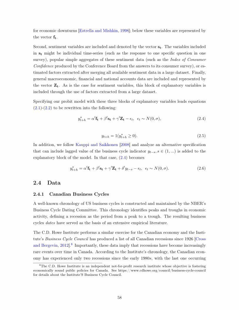
for economic downturns [Estrella and Mishkin, 1998]; below these variables are represented bythe vector ft.

Second, sentiment variables are included and denoted by the vector st. The variables includedin st might be individual time-series (such as the response to one specific question in onesurvey), popular simple aggregates of these sentiment data (such as the Index of ConsumerConfidence produced by the Conference Board from the answers to its consumer survey), or es-timated factors extracted after merging all available sentiment data in a large dataset. Finally,general macroeconomic, financial and national accounts data are included and represented bythe vector Zt. As is the case for sentiment variables, this block of explanatory variables isincluded through the use of factors extracted from a large dataset.

Specifying our probit model with these three blocks of explanatory variables leads equations(2.1)-(2.2) to be rewritten into the following:

y∗t+h = α′ft + β′st + γ′Zt − εt, εt ∼ N(0, σ), (2.4)

yt+h = 1(y∗t+h ≥ 0). (2.5)

In addition, we follow Kauppi and Saikkonen [2008] and analyze an alternative specificationthat can include lagged value of the business cycle indicator yt−s, s ∈ (1, ...) is added to theexplanatory block of the model. In that case, (2.4) becomes

y∗t+h = α′ft + β′st + γ′Zt + δ′yt−s − εt, εt ∼ N(0, σ). (2.6)

2.4 Data

2.4.1 Canadian Business Cycles

A well-known chronology of US business cycles is constructed and maintained by the NBER’sBusiness Cycle Dating Committee. This chronology identifies peaks and troughs in economicactivity, defining a recession as the period from a peak to a trough. The resulting businesscycles dates have served as the basis of an extensive empirical literature.

The C.D. Howe Institute performs a similar exercise for the Canadian economy and the Insti-tute’s Business Cycle Council has produced a list of all Canadian recessions since 1926 [Crossand Bergevin, 2012].8 Importantly, these data imply that recessions have become increasinglyrare events over time in Canada. According to the Institute’s chronology, the Canadian econ-omy has experienced only two recessions since the early 1980s, with the last one occurring

8The C.D. Howe Institute is an independent not-for-profit research institute whose objective is fosteringeconomically sound public policies for Canada. See https://www.cdhowe.org/council/business-cycle-councilfor details about the Institute’S Business Cycle Council.

58

during the 2008 − 2009 Great recession.9 One practical implication from this feature of theC.D. Howe data is that empirical work using explanatory variables for which limited historicaldata are available will likely include only one recession (in 2008-2009), severely reducing thepotential power of any econometric method.

Both the NBER and the C.D. Howe Institute interpret recessions as declines in the level ofgeneral economic activity. However, other conceptual frameworks view recessions as periodswhere economic activity, even if it is growing, is doing so at a rate below its long-term potential.Notably, the OECD uses a growth cycle framework to compute troughs and peaks, ie. turningpoints in these growth cycles, for all member countries.10 Figure 2.1 below illustrates theimplication of these two differing views of what constitutes an economic downturn. In thefigure, the dark-shaded episodes are the C.D. Howe recessions dates for Canada while thelight-shaded periods are the growth slowdowns for Canada as identified by the OECD growth-cycle methodology. Although both chronologies overlap to a considerable extent, notice thatthe OECD has identified several low-growth episodes since the 1991 recession, while the C.D.Howe methodology has only identified one recession, in 2008− 2009.11

Figure 2.1: Canadian Recessions: OECD and C.D. Howe

9This is contrast to the US economy, which was affected by an additional recession in 2001, according tothe NBER dates.

10See Zarnowitz and Ozyldirim [2006] for a discussion of growth cycles and a description of estimated growthcycles for the US. In addition, see Anderson and Vahid [2001] for an analysis where an alternative metric isused to defined recessions.

11Table B.1 in Appendix provides a detailed list of all peaks and troughs in the Canadian business cycleidentified by the OECD methodology.

59

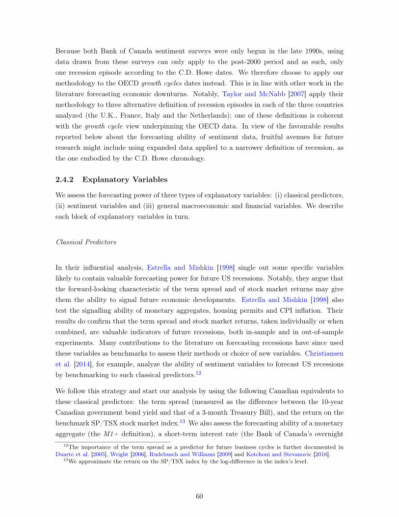
Because both Bank of Canada sentiment surveys were only begun in the late 1990s, usingdata drawn from these surveys can only apply to the post-2000 period and as such, onlyone recession episode according to the C.D. Howe dates. We therefore choose to apply ourmethodology to the OECD growth cycles dates instead. This is in line with other work in theliterature forecasting economic downturns. Notably, Taylor and McNabb [2007] apply theirmethodology to three alternative definition of recession episodes in each of the three countriesanalyzed (the U.K., France, Italy and the Netherlands); one of these definitions is coherentwith the growth cycle view underpinning the OECD data. In view of the favourable resultsreported below about the forecasting ability of sentiment data, fruitful avenues for futureresearch might include using expanded data applied to a narrower definition of recession, asthe one embodied by the C.D. Howe chronology.

2.4.2 Explanatory Variables

We assess the forecasting power of three types of explanatory variables: (i) classical predictors,(ii) sentiment variables and (iii) general macroeconomic and financial variables. We describeeach block of explanatory variables in turn.

Classical Predictors

In their influential analysis, Estrella and Mishkin [1998] single out some specific variableslikely to contain valuable forecasting power for future US recessions. Notably, they argue thatthe forward-looking characteristic of the term spread and of stock market returns may givethem the ability to signal future economic developments. Estrella and Mishkin [1998] alsotest the signalling ability of monetary aggregates, housing permits and CPI inflation. Theirresults do confirm that the term spread and stock market returns, taken individually or whencombined, are valuable indicators of future recessions, both in-sample and in out-of-sampleexperiments. Many contributions to the literature on forecasting recessions have since usedthese variables as benchmarks to assess their methods or choice of new variables. Christiansenet al. [2014], for example, analyze the ability of sentiment variables to forecast US recessionsby benchmarking to such classical predictors.12

We follow this strategy and start our analysis by using the following Canadian equivalents tothese classical predictors: the term spread (measured as the difference between the 10-yearCanadian government bond yield and that of a 3-month Treasury Bill), and the return on thebenchmark SP/TSX stock market index.13 We also assess the forecasting ability of a monetaryaggregate (the M1+ definition), a short-term interest rate (the Bank of Canada’s overnight

12The importance of the term spread as a predictor for future business cycles is further documented inDuarte et al. [2005], Wright [2006], Rudebusch and Williams [2009] and Kotchoni and Stevanovic [2016].

13We approximate the return on the SP/TSX index by the log-difference in the index’s level.

60

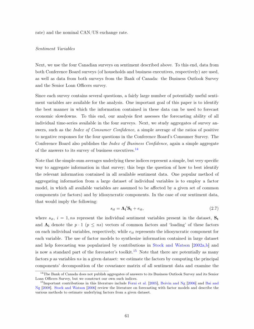
rate) and the nominal CAN/US exchange rate.

Sentiment Variables

Next, we use the four Canadian surveys on sentiment described above. To this end, data fromboth Conference Board surveys (of households and business executives, respectively) are used,as well as data from both surveys from the Bank of Canada: the Business Outlook Surveyand the Senior Loan Officers survey.

Since each survey contains several questions, a fairly large number of potentially useful senti-ment variables are available for the analysis. One important goal of this paper is to identifythe best manner in which the information contained in these data can be used to forecasteconomic slowdowns. To this end, our analysis first assesses the forecasting ability of allindividual time-series available in the four surveys. Next, we study aggregates of survey an-swers, such as the Index of Consumer Confidence, a simple average of the ratios of positiveto negative responses for the four questions in the Conference Board’s Consumer Survey. TheConference Board also publishes the Index of Business Confidence, again a simple aggregateof the answers to its survey of business executives.14

Note that the simple-sum averages underlying these indices represent a simple, but very specificway to aggregate information in that survey; this begs the question of how to best identifythe relevant information contained in all available sentiment data. One popular method ofaggregating information from a large dataset of individual variables is to employ a factormodel, in which all available variables are assumed to be affected by a given set of commoncomponents (or factors) and by idiosyncratic components. In the case of our sentiment data,that would imply the following:

sit = Λi′St + eit, (2.7)

where sit, i = 1, ns represent the individual sentiment variables present in the dataset, St

and Λi denote the p · 1 (p ≤ ns) vectors of common factors and ‘loading’ of these factorson each individual variables, respectively, while eit represents the idiosyncratic component foreach variable. The use of factor models to synthesize information contained in large datasetand help forecasting was popularized by contributions in Stock and Watson [2002a,b] andis now a standard part of the forecaster’s toolkit.15 Note that there are potentially as manyfactors p as variables ns in a given dataset: we estimate the factors by computing the principalcomponents’ decomposition of the covariance matrix of all sentiment data and examine the

14The Bank of Canada does not publish aggregates of answers to its Business Outlook Survey and its SeniorLoan Officers Survey, but we construct our own such indices.

15Important contributions in this literature include Forni et al. [2005], Boivin and Ng [2006] and Bai andNg [2008]. Stock and Watson [2006] review the literature on forecasting with factor models and describe thevarious methods to estimate underlying factors from a given dataset.

61

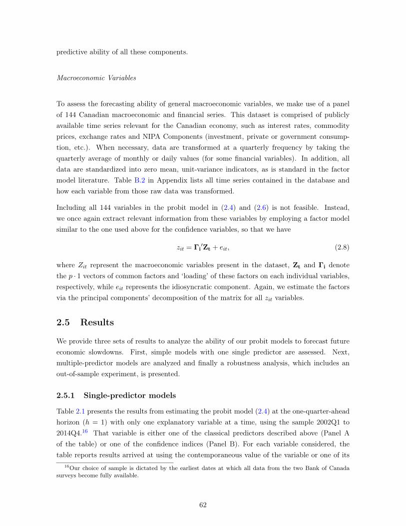
predictive ability of all these components.

Macroeconomic Variables

To assess the forecasting ability of general macroeconomic variables, we make use of a panelof 144 Canadian macroeconomic and financial series. This dataset is comprised of publiclyavailable time series relevant for the Canadian economy, such as interest rates, commodityprices, exchange rates and NIPA Components (investment, private or government consump-tion, etc.). When necessary, data are transformed at a quarterly frequency by taking thequarterly average of monthly or daily values (for some financial variables). In addition, alldata are standardized into zero mean, unit-variance indicators, as is standard in the factormodel literature. Table B.2 in Appendix lists all time series contained in the database andhow each variable from those raw data was transformed.

Including all 144 variables in the probit model in (2.4) and (2.6) is not feasible. Instead,we once again extract relevant information from these variables by employing a factor modelsimilar to the one used above for the confidence variables, so that we have

zit = Γi′Zt + eit, (2.8)

where Zit represent the macroeconomic variables present in the dataset, Zt and Γi denotethe p · 1 vectors of common factors and ‘loading’ of these factors on each individual variables,respectively, while eit represents the idiosyncratic component. Again, we estimate the factorsvia the principal components’ decomposition of the matrix for all zit variables.

2.5 Results

We provide three sets of results to analyze the ability of our probit models to forecast futureeconomic slowdowns. First, simple models with one single predictor are assessed. Next,multiple-predictor models are analyzed and finally a robustness analysis, which includes anout-of-sample experiment, is presented.

2.5.1 Single-predictor models

Table 2.1 presents the results from estimating the probit model (2.4) at the one-quarter-aheadhorizon (h = 1) with only one explanatory variable at a time, using the sample 2002Q1 to2014Q4.16 That variable is either one of the classical predictors described above (Panel Aof the table) or one of the confidence indices (Panel B). For each variable considered, thetable reports results arrived at using the contemporaneous value of the variable or one of its

16Our choice of sample is dictated by the earliest dates at which all data from the two Bank of Canadasurveys become fully available.

62

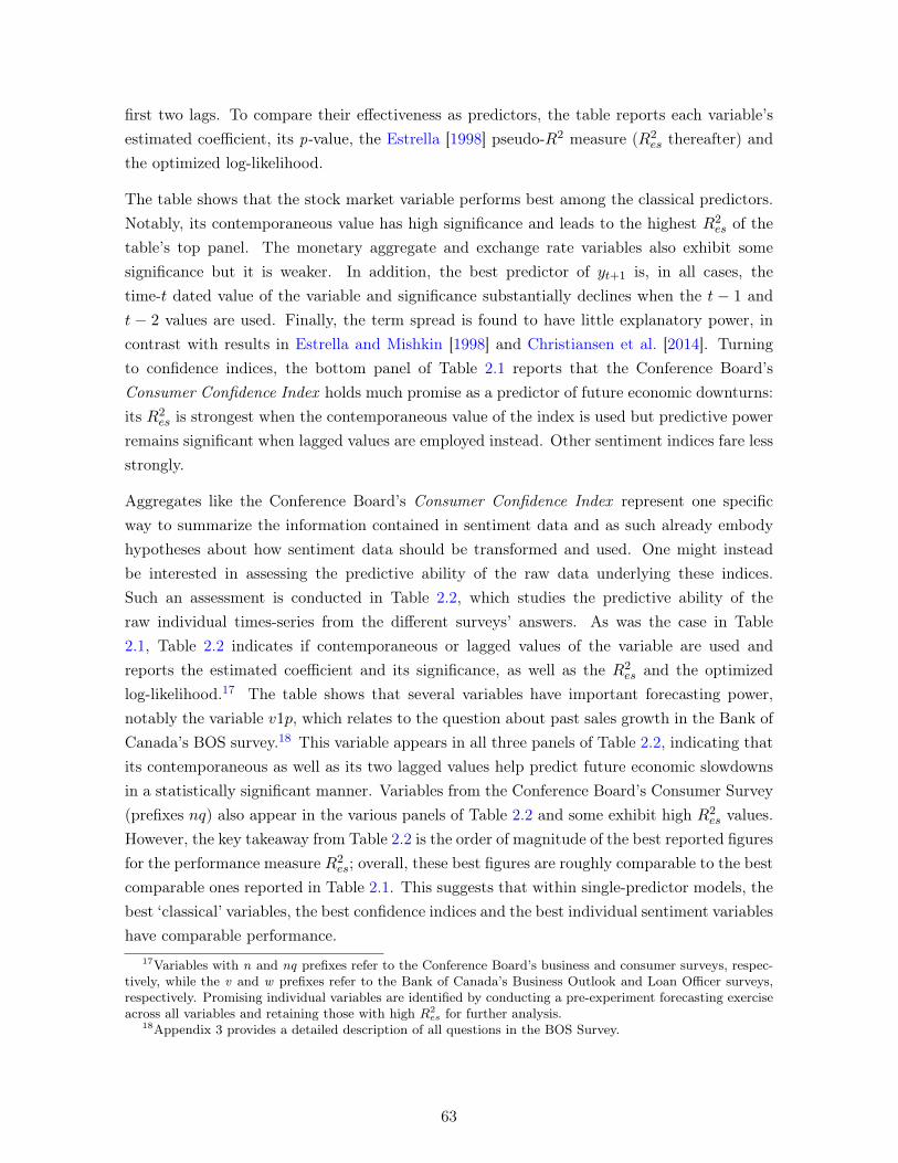
first two lags. To compare their effectiveness as predictors, the table reports each variable’sestimated coefficient, its p-value, the Estrella [1998] pseudo-R2 measure (R2

es thereafter) andthe optimized log-likelihood.

The table shows that the stock market variable performs best among the classical predictors.Notably, its contemporaneous value has high significance and leads to the highest R2

es of thetable’s top panel. The monetary aggregate and exchange rate variables also exhibit somesignificance but it is weaker. In addition, the best predictor of yt+1 is, in all cases, thetime-t dated value of the variable and significance substantially declines when the t − 1 andt − 2 values are used. Finally, the term spread is found to have little explanatory power, incontrast with results in Estrella and Mishkin [1998] and Christiansen et al. [2014]. Turningto confidence indices, the bottom panel of Table 2.1 reports that the Conference Board’sConsumer Confidence Index holds much promise as a predictor of future economic downturns:its R2

es is strongest when the contemporaneous value of the index is used but predictive powerremains significant when lagged values are employed instead. Other sentiment indices fare lessstrongly.

Aggregates like the Conference Board’s Consumer Confidence Index represent one specificway to summarize the information contained in sentiment data and as such already embodyhypotheses about how sentiment data should be transformed and used. One might insteadbe interested in assessing the predictive ability of the raw data underlying these indices.Such an assessment is conducted in Table 2.2, which studies the predictive ability of theraw individual times-series from the different surveys’ answers. As was the case in Table2.1, Table 2.2 indicates if contemporaneous or lagged values of the variable are used andreports the estimated coefficient and its significance, as well as the R2

es and the optimizedlog-likelihood.17 The table shows that several variables have important forecasting power,notably the variable v1p, which relates to the question about past sales growth in the Bank ofCanada’s BOS survey.18 This variable appears in all three panels of Table 2.2, indicating thatits contemporaneous as well as its two lagged values help predict future economic slowdownsin a statistically significant manner. Variables from the Conference Board’s Consumer Survey(prefixes nq) also appear in the various panels of Table 2.2 and some exhibit high R2

es values.However, the key takeaway from Table 2.2 is the order of magnitude of the best reported figuresfor the performance measure R2

es; overall, these best figures are roughly comparable to the bestcomparable ones reported in Table 2.1. This suggests that within single-predictor models, thebest ‘classical’ variables, the best confidence indices and the best individual sentiment variableshave comparable performance.

17Variables with n and nq prefixes refer to the Conference Board’s business and consumer surveys, respec-tively, while the v and w prefixes refer to the Bank of Canada’s Business Outlook and Loan Officer surveys,respectively. Promising individual variables are identified by conducting a pre-experiment forecasting exerciseacross all variables and retaining those with high R2

es for further analysis.18Appendix 3 provides a detailed description of all questions in the BOS Survey.

63

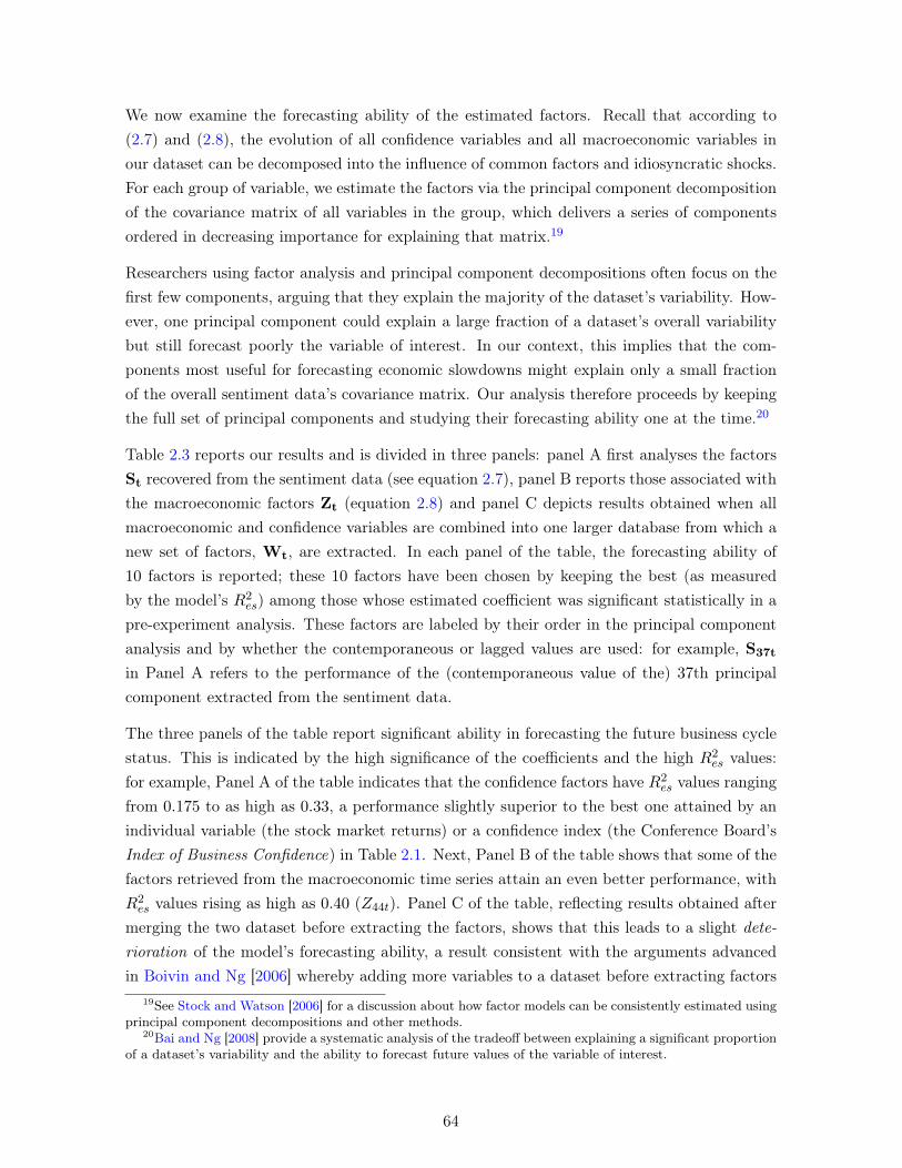
We now examine the forecasting ability of the estimated factors. Recall that according to(2.7) and (2.8), the evolution of all confidence variables and all macroeconomic variables inour dataset can be decomposed into the influence of common factors and idiosyncratic shocks.For each group of variable, we estimate the factors via the principal component decompositionof the covariance matrix of all variables in the group, which delivers a series of componentsordered in decreasing importance for explaining that matrix.19

Researchers using factor analysis and principal component decompositions often focus on thefirst few components, arguing that they explain the majority of the dataset’s variability. How-ever, one principal component could explain a large fraction of a dataset’s overall variabilitybut still forecast poorly the variable of interest. In our context, this implies that the com-ponents most useful for forecasting economic slowdowns might explain only a small fractionof the overall sentiment data’s covariance matrix. Our analysis therefore proceeds by keepingthe full set of principal components and studying their forecasting ability one at the time.20

Table 2.3 reports our results and is divided in three panels: panel A first analyses the factorsSt recovered from the sentiment data (see equation 2.7), panel B reports those associated withthe macroeconomic factors Zt (equation 2.8) and panel C depicts results obtained when allmacroeconomic and confidence variables are combined into one larger database from which anew set of factors, Wt, are extracted. In each panel of the table, the forecasting ability of10 factors is reported; these 10 factors have been chosen by keeping the best (as measuredby the model’s R2

es) among those whose estimated coefficient was significant statistically in apre-experiment analysis. These factors are labeled by their order in the principal componentanalysis and by whether the contemporaneous or lagged values are used: for example, S37t

in Panel A refers to the performance of the (contemporaneous value of the) 37th principalcomponent extracted from the sentiment data.

The three panels of the table report significant ability in forecasting the future business cyclestatus. This is indicated by the high significance of the coefficients and the high R2

es values:for example, Panel A of the table indicates that the confidence factors have R2

es values rangingfrom 0.175 to as high as 0.33, a performance slightly superior to the best one attained by anindividual variable (the stock market returns) or a confidence index (the Conference Board’sIndex of Business Confidence) in Table 2.1. Next, Panel B of the table shows that some of thefactors retrieved from the macroeconomic time series attain an even better performance, withR2es values rising as high as 0.40 (Z44t). Panel C of the table, reflecting results obtained after

merging the two dataset before extracting the factors, shows that this leads to a slight dete-rioration of the model’s forecasting ability, a result consistent with the arguments advancedin Boivin and Ng [2006] whereby adding more variables to a dataset before extracting factors

19See Stock and Watson [2006] for a discussion about how factor models can be consistently estimated usingprincipal component decompositions and other methods.

20Bai and Ng [2008] provide a systematic analysis of the tradeoff between explaining a significant proportionof a dataset’s variability and the ability to forecast future values of the variable of interest.

64

does not necessarily always lead to improvements in forecasting ability.

2.5.2 Multiple-predictor models

Results in Table 2.3 might appear to suggest that aggregating information using the factormodels (2.7) or (2.8) provides little or no improvement in forecasting ability, when comparedto results obtained by using individual variables, as in Table 2.1 and Table 2.2. Indeed, thebest R2

es were found to be roughly of the same order of magnitude in all tables analyzed so far:factor-based prediction models may sometimes exhibit slightly higher R2

es in Table 2.3, butthis small improvement might not be enough to arbitrage the challenges these models pose,notably with respect to communication of results. Taken together, therefore, results depictedin Table 2.1, Table 2.2 and Table 2.3 might be interpreted as suggesting that sentiment data,although incorporating valuable predictive power, do not appear to deliver a clear increase insuch predictive power relative to classical predictors.

However, multiple-predictor probit models have the potential to modify this assessment. Be-cause our estimated factors are orthogonal to each other, the predictive ability of each newadded factor should always increase the overall performance of a given model; by contrast, nosuch assurance is present when specific individual variables are added to a model since anyadditional variable would not be orthogonal to those already in use.

To test this conjecture, Table 2.4 reports estimation results using several predictors at the sametime. The table is divided in two panels: the standard model is assessed on the left-hand sidewhile a model that includes the lagged value of the dependent variable, as in (2.6), is analyzedon the right-hand side. For each estimation, between four and six variables from each blockconsidered so far are used: the blocks are the classical predictors (heading “M1 ” in the table),confidence indices (“M2 ”), factors drawn from our macroeconomic dataset (“M3 ”), from thesentiment data (“M4 ”) and from the amalgamated database (“M5 ”). For each column, onlyestimated coefficients significant at the 10% level are reported: for example, the column M1on the left-hand side panel of the table only reports the estimated coefficient for the stockmarket return variable since it is the only one statistically significant.21

As expected, the first two columns of the table’s left-hand side (headings M1 and M2 ) depictresults very similar to those from Table 2.1: in each column, only one individual variable isstatistically significant (the return to stock markets and the Conference Board’s ConsumerConfidence Index ) and the R2

es are very similar to those in Table 2.1.22 These columns thusconfirm that the addition of specific, additional variables to the probit does not significantlyimprove performance.

21We identify the best model in each of columns M3 to M5 as follows: all factors significant at the 10%level in a single-predictor model are first identified (this usually selects around 10 potential predictors). Thesefactors are then included in a multiple-predictor probit in all possible permutations to select the best model.

22Results are not exactly the same because the presence of other variables influences the estimation processeven if not all coefficient estimates are depicted.

65

The next three columns (headings M3, M4 and M5 ) paint a different picture. Here, thedifferent factors included in the multiple-predictor probit appear to all add to the model’sperformance. Indeed, all factors are statistically significant and model performance is improvedsubstantially: the R2

es reported at the bottom of the three columns are significantly higherthan those in Table 2.3 and attain a high mark of 0.956 (for the model using factors extractedfrom confidence variables, M4 ). The AIC and QPS scores concur with this result and alsoshow big declines relative to the first two columns of the table.

Recall that one important goal of the present paper is to identify the best way by whichsentiment data can help forecast business cycle turning points. In that regard, the tableshows that using all available data on sentiment, through the factor model (2.7), significantlyincreases performance relative to using summary variables like the Conference Board’s Con-sumer Confidence Index. This is apparent when comparing columns M2 and M4 : the R2

es

measure is significantly higher in the latter column, and both AIC and QPS scores are muchlower. In synthesis, the left-hand side panel of the table has two key findings: (i) using severalorthogonal factors significantly improves the predicting ability of our probit framework andin particular (ii) including sentiment data through the factor model (2.7) provides substantialimprovements relative to more straightforward summary measures of sentiment. This lastfinding is illustrated graphically in Figure 2.2 below, which shows the estimated probabilitiesfor the best model arising from confidence indices (dashed lines) and from confidence factors(full lines): the predictions based on confidence factors have visibly better forward-indicatorcapabilities and have much more contrasted probability regions.

The right-hand side of Table 2.4 next analyzes a model similar to (2.6), where the lagged valuesof the dependent variable yt−1 is added to the estimation. As expected, the lagged status ofthe business cycle is very informative and its estimated coefficients are very-highly significantand positive –which implies positive auto-correlation in the business cycle– in all columns.Interestingly, the presence of yt−1 also significantly modifies which variable performs well andhow much they do so. For example, the stock market return variable is now absent from thetable (column M1 ), suggesting that this variable does not help predict future business cyclestatus once the current status is included; instead the money growth rate appears significantly.Similarly, the Conference Board’s Consumer Confidence Index is now also absent (columnM2 )and is replaced by the Bank of Canada’s Senior Loan Officers (SLO) survey data. This suggeststhat once yt−1 is included, a different type of information is emphasized by the estimation.In addition, the table shows that including yt−1 in the probit significantly increases the R2

es

performance of models M1 and M2, relative to what was reported in the left-hand side panelof the table.

The columns reporting results using factors (M3 to M5 ) deliver a slightly different message.On the one hand, the estimated coefficient on yt−1 does remain highly significant and thenumber of other predictors statistically significant is lower that it was before. On the other

66

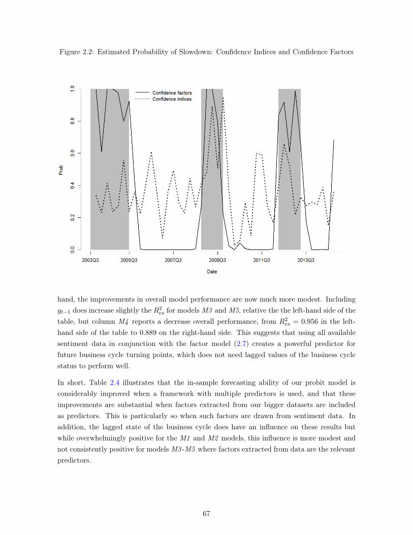
Figure 2.2: Estimated Probability of Slowdown: Confidence Indices and Confidence Factors

hand, the improvements in overall model performance are now much more modest. Includingyt−1 does increase slightly the R2

es for models M3 and M5, relative the the left-hand side of thetable, but column M4 reports a decrease overall performance, from R2

es = 0.956 in the left-hand side of the table to 0.889 on the right-hand side. This suggests that using all availablesentiment data in conjunction with the factor model (2.7) creates a powerful predictor forfuture business cycle turning points, which does not need lagged values of the business cyclestatus to perform well.

In short, Table 2.4 illustrates that the in-sample forecasting ability of our probit model isconsiderably improved when a framework with multiple predictors is used, and that theseimprovements are substantial when factors extracted from our bigger datasets are includedas predictors. This is particularly so when such factors are drawn from sentiment data. Inaddition, the lagged state of the business cycle does have an influence on these results butwhile overwhelmingly positive for the M1 and M2 models, this influence is more modest andnot consistently positive for models M3 -M5 where factors extracted from data are the relevantpredictors.

67

2.5.3 Robustness

We now assess the robustness of our results. We first evaluate our framework’s performanceover longer forecasting horizons. Next, we reestimate our model over a different sample andfinally, we conduct an out-of-sample experiment.

Longer Forecasting Horizons

Until now, our analysis has concentrated on the task of predicting the occurrence of economicslowdowns one-quarter ahead, ie the case h = 1 in our basic model (2.1). Table 2.5 nextassesses the ability of our framework to forecast at longer horizons.

Accordingly, the table has four panels, one for each value of h. In each panel, several perfor-mance measures are reported for the best model in each block of predictor variables.23 Thesemeasures, in addition to the usual AIC and QPS criteria, include the CML (which measuresthe aggregate of a model’s mistakes) as well as the proportion of correctly predicted downturns(shots+) and the proportion of missed expansions (shots−).24

The results depicted in Table 2.5 largely accord with those discussed above. First, the tableshows that using factors, extracted from either sentiment or macroeconomic variables, providessubstantial improvement to the forecasting ability of the probit. To see this, compare the AICor QPS metrics for the first two lines (classical predictors and confidences indices) with thosein the last three. For each horizon h = 1, 2, 3, 4, these figures are, for the most part, noticeablysmaller when factors are the main predictors. Further, the proportion of correctly predicteddownturns (shots+) is also (almost) uniformly better when such factors used. In addition, thetable strongly suggests that the full potential of sentiment data for forecasting future businesscycles is likely to be attained when all such data is used, and is amalgamated through a factormodel like (2.7). This is evident when comparing the Confidence indices and Confidencesfactors lines in the table: in most cases and for most performance measures, the latter modelperforms best.

Note that one interesting caveat to this assessment occurs for the CML measure, especially atlonger horizons: in such cases, predicting with confidence factors appears to result in inferiorperformance. For example the CML at h = 4 for Confidence indices is 0.360 while it ishigher (0.588) for Confidence factors. At the same time, the measure shots+ (the proportion

23The best model for each block of variables is identified using the procedure described above in the contextof the results from Table 2.3.

24The CML is discussed in Buja et al. [2005]. It aggregates the model’s mistakes by summing the false posi-tives (predicting an economic downturn that does not occur) and the false negatives (failing to predict a reces-sion that actually occurs). It is computed as CML = 1

T

∑Tt=1

[(1− q)yt(1− 1(pt≥0.5)) + q(1− yt)(1(pt≥0.5))

],

where 1() is 1 if its argument is true and 0 otherwise and q is the relative cost of the two different types ofmistakes. We use q = 1/3, which penalizes false positives more heavily.

68

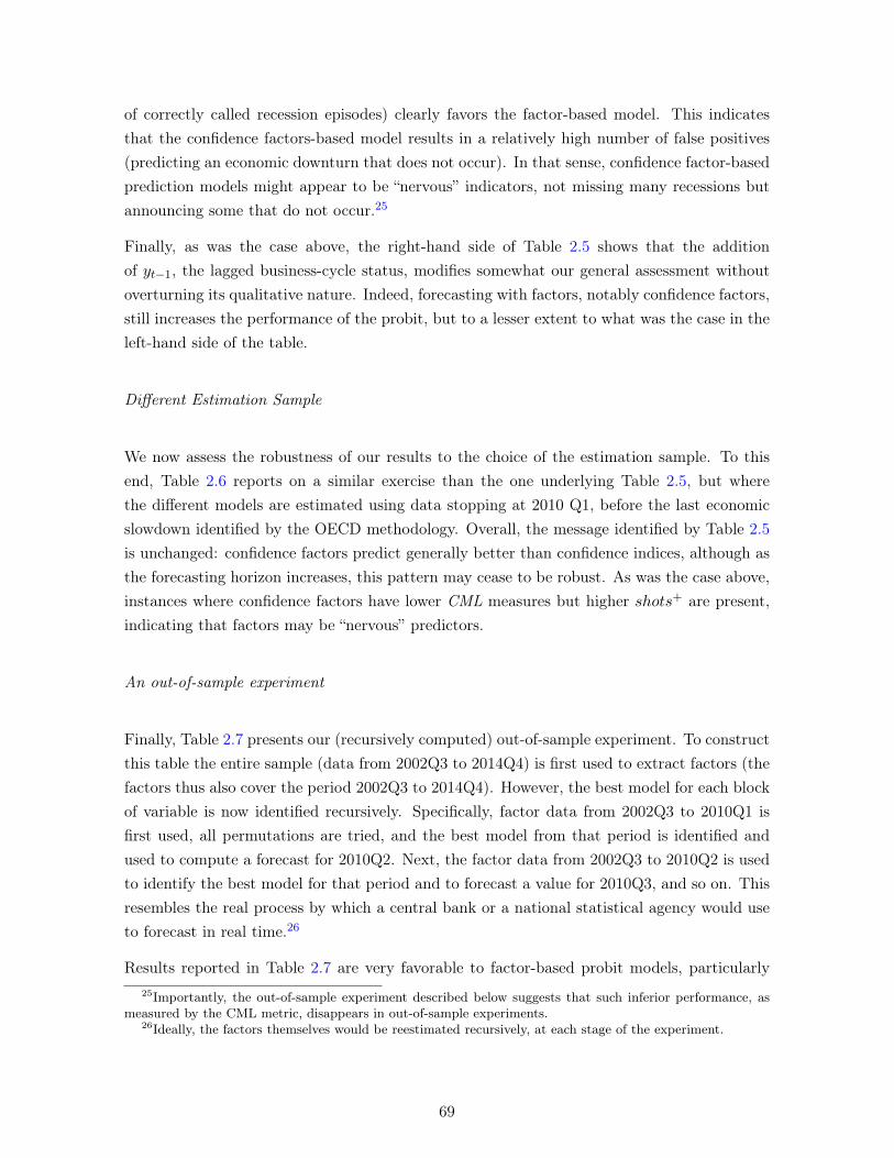
of correctly called recession episodes) clearly favors the factor-based model. This indicatesthat the confidence factors-based model results in a relatively high number of false positives(predicting an economic downturn that does not occur). In that sense, confidence factor-basedprediction models might appear to be “nervous” indicators, not missing many recessions butannouncing some that do not occur.25

Finally, as was the case above, the right-hand side of Table 2.5 shows that the additionof yt−1, the lagged business-cycle status, modifies somewhat our general assessment withoutoverturning its qualitative nature. Indeed, forecasting with factors, notably confidence factors,still increases the performance of the probit, but to a lesser extent to what was the case in theleft-hand side of the table.

Different Estimation Sample

We now assess the robustness of our results to the choice of the estimation sample. To thisend, Table 2.6 reports on a similar exercise than the one underlying Table 2.5, but wherethe different models are estimated using data stopping at 2010 Q1, before the last economicslowdown identified by the OECD methodology. Overall, the message identified by Table 2.5is unchanged: confidence factors predict generally better than confidence indices, although asthe forecasting horizon increases, this pattern may cease to be robust. As was the case above,instances where confidence factors have lower CML measures but higher shots+ are present,indicating that factors may be “nervous” predictors.

An out-of-sample experiment

Finally, Table 2.7 presents our (recursively computed) out-of-sample experiment. To constructthis table the entire sample (data from 2002Q3 to 2014Q4) is first used to extract factors (thefactors thus also cover the period 2002Q3 to 2014Q4). However, the best model for each blockof variable is now identified recursively. Specifically, factor data from 2002Q3 to 2010Q1 isfirst used, all permutations are tried, and the best model from that period is identified andused to compute a forecast for 2010Q2. Next, the factor data from 2002Q3 to 2010Q2 is usedto identify the best model for that period and to forecast a value for 2010Q3, and so on. Thisresembles the real process by which a central bank or a national statistical agency would useto forecast in real time.26

Results reported in Table 2.7 are very favorable to factor-based probit models, particularly25Importantly, the out-of-sample experiment described below suggests that such inferior performance, as

measured by the CML metric, disappears in out-of-sample experiments.26Ideally, the factors themselves would be reestimated recursively, at each stage of the experiment.

69

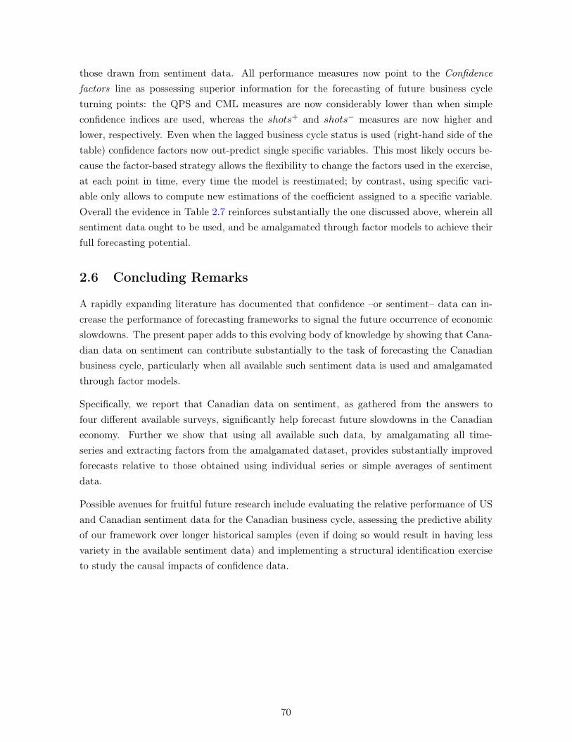
those drawn from sentiment data. All performance measures now point to the Confidencefactors line as possessing superior information for the forecasting of future business cycleturning points: the QPS and CML measures are now considerably lower than when simpleconfidence indices are used, whereas the shots+ and shots− measures are now higher andlower, respectively. Even when the lagged business cycle status is used (right-hand side of thetable) confidence factors now out-predict single specific variables. This most likely occurs be-cause the factor-based strategy allows the flexibility to change the factors used in the exercise,at each point in time, every time the model is reestimated; by contrast, using specific vari-able only allows to compute new estimations of the coefficient assigned to a specific variable.Overall the evidence in Table 2.7 reinforces substantially the one discussed above, wherein allsentiment data ought to be used, and be amalgamated through factor models to achieve theirfull forecasting potential.


A rapidly expanding literature has documented that confidence –or sentiment– data can in-crease the performance of forecasting frameworks to signal the future occurrence of economicslowdowns. The present paper adds to this evolving body of knowledge by showing that Cana-dian data on sentiment can contribute substantially to the task of forecasting the Canadianbusiness cycle, particularly when all available such sentiment data is used and amalgamatedthrough factor models.

Specifically, we report that Canadian data on sentiment, as gathered from the answers tofour different available surveys, significantly help forecast future slowdowns in the Canadianeconomy. Further we show that using all available such data, by amalgamating all time-series and extracting factors from the amalgamated dataset, provides substantially improvedforecasts relative to those obtained using individual series or simple averages of sentimentdata.

Possible avenues for fruitful future research include evaluating the relative performance of USand Canadian sentiment data for the Canadian business cycle, assessing the predictive abilityof our framework over longer historical samples (even if doing so would result in having lessvariety in the available sentiment data) and implementing a structural identification exerciseto study the causal impacts of confidence data.

70

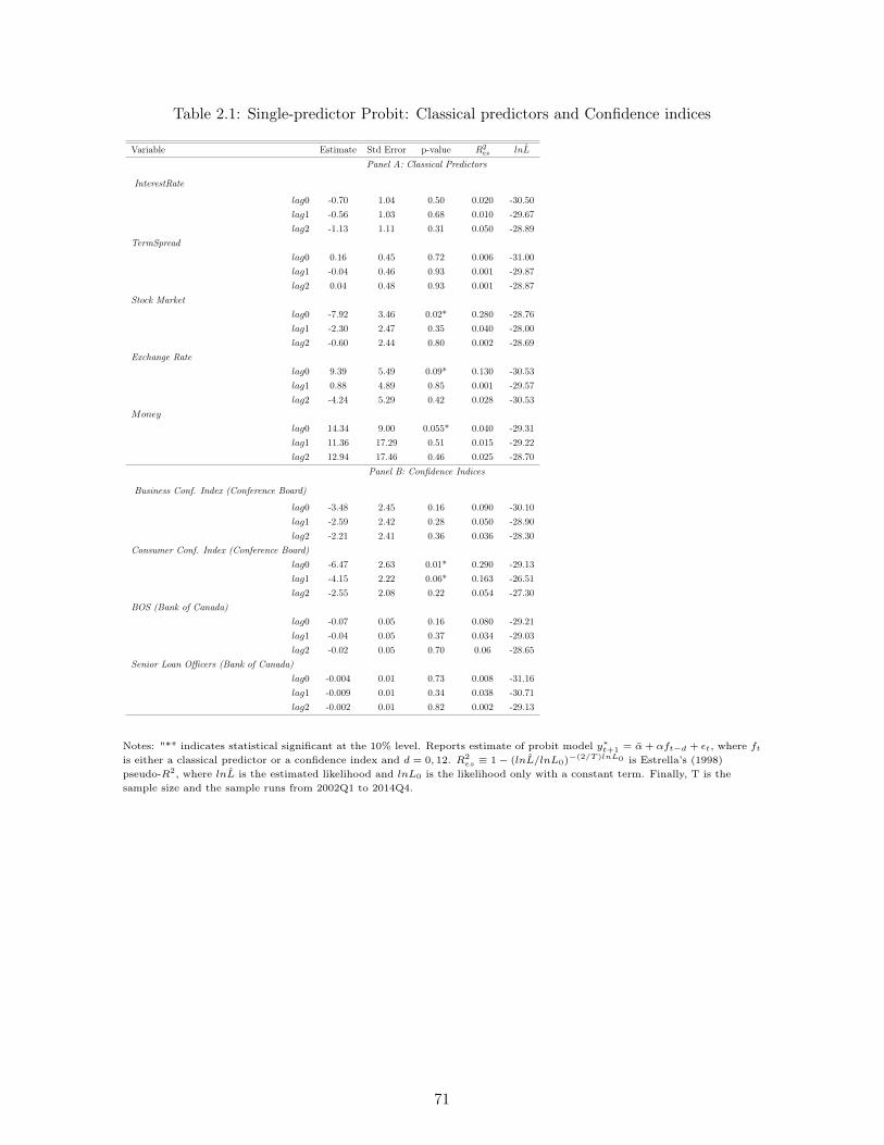
Table 2.1: Single-predictor Probit: Classical predictors and Confidence indices

Variable Estimate Std Error p-value R2es lnL

Panel A: Classical Predictors

InterestRate

lag0 -0.70 1.04 0.50 0.020 -30.50lag1 -0.56 1.03 0.68 0.010 -29.67lag2 -1.13 1.11 0.31 0.050 -28.89

TermSpreadlag0 0.16 0.45 0.72 0.006 -31.00lag1 -0.04 0.46 0.93 0.001 -29.87lag2 0.04 0.48 0.93 0.001 -28.87

Stock Marketlag0 -7.92 3.46 0.02* 0.280 -28.76lag1 -2.30 2.47 0.35 0.040 -28.00lag2 -0.60 2.44 0.80 0.002 -28.69

Exchange Ratelag0 9.39 5.49 0.09* 0.130 -30.53lag1 0.88 4.89 0.85 0.001 -29.57lag2 -4.24 5.29 0.42 0.028 -30.53

Money

lag0 14.34 9.00 0.055* 0.040 -29.31lag1 11.36 17.29 0.51 0.015 -29.22lag2 12.94 17.46 0.46 0.025 -28.70

Panel B: Confidence Indices

Business Conf. Index (Conference Board)

lag0 -3.48 2.45 0.16 0.090 -30.10lag1 -2.59 2.42 0.28 0.050 -28.90lag2 -2.21 2.41 0.36 0.036 -28.30

Consumer Conf. Index (Conference Board)lag0 -6.47 2.63 0.01* 0.290 -29.13lag1 -4.15 2.22 0.06* 0.163 -26.51lag2 -2.55 2.08 0.22 0.054 -27.30

BOS (Bank of Canada)lag0 -0.07 0.05 0.16 0.080 -29.21lag1 -0.04 0.05 0.37 0.034 -29.03lag2 -0.02 0.05 0.70 0.06 -28.65

Senior Loan Officers (Bank of Canada)lag0 -0.004 0.01 0.73 0.008 -31.16lag1 -0.009 0.01 0.34 0.038 -30.71lag2 -0.002 0.01 0.82 0.002 -29.13

Notes: "*" indicates statistical significant at the 10% level. Reports estimate of probit model y∗t+1 = α+ αft−d + εt, where ftis either a classical predictor or a confidence index and d = 0, 12. R2

es ≡ 1 − (lnL/lnL0)−(2/T )lnL0 is Estrella’s (1998)pseudo-R2, where lnL is the estimated likelihood and lnL0 is the likelihood only with a constant term. Finally, T is thesample size and the sample runs from 2002Q1 to 2014Q4.

71

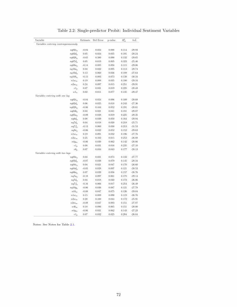
Table 2.2: Single-predictor Probit: Individual Sentiment Variables

Variable Estimate Std Error p-value R2es lnL

Variables entering contemporaneously

nq02cq -0.04 0.024 0.088 0.114 -29.93nq02dq 0.05 0.024 0.035 0.191 -28.24nq02hq -0.65 0.380 0.090 0.132 -29.65nq07dq 0.05 0.019 0.005 0.323 -25.46nq08aq -0.14 0.085 0.094 0.115 -29.06nq10aq 0.04 0.022 0.095 0.113 -29.74nq10dq 0.13 0.060 0.036 0.189 -27.64nq10hq -0.15 0.083 0.073 0.139 -30.34n1wm 0.19 0.088 0.035 0.180 -29.34n2wm 0.24 0.097 0.015 0.251 -29.91v1p 0.07 0.031 0.019 0.225 -28.43w1n 0.02 0.011 0.077 0.135 -29.47

Variables entering with one lagnq02cq -0.04 0.024 0.096 0.109 -28.68nq02dq 0.06 0.025 0.018 0.243 -27.36nq02hq -0.86 0.444 0.052 0.191 -28.61nq04bq 0.04 0.021 0.041 0.181 -29.87nq05aq -0.09 0.038 0.019 0.225 -29.35nq6dq 0.08 0.039 0.050 0.164 -29.94nq7dq 0.04 0.018 0.020 0.218 -25.71nq7fq -0.13 0.060 0.030 0.213 -31.53nq9cq -0.06 0.032 0.052 0.152 -29.63n1wm 0.19 0.091 0.032 0.186 -27.76n2wm 0.25 0.102 0.015 0.252 -26.88n4gm -0.06 0.030 0.062 0.142 -28.86v1p 0.08 0.031 0.016 0.235 -27.10v6p 0.07 0.034 0.043 0.177 -28.13

Variables entering with two lagsnq03cq 0.04 0.021 0.074 0.132 -27.77nq03dq -0.07 0.038 0.079 0.145 -28.34nq04cq 0.04 0.021 0.047 0.170 -26.60nq04dq -0.05 0.028 0.097 0.121 -28.53nq06aq 0.07 0.039 0.056 0.157 -26.76nq7aq -0.18 0.097 0.061 0.175 -29.14nq7dq 0.04 0.018 0.040 0.173 -26.06nq7fq -0.16 0.066 0.017 0.254 -26.49nq10gq -0.06 0.036 0.087 0.121 -27.78n1bm -0.08 0.047 0.075 0.126 -29.04n1wm 0.15 0.089 0.090 0.119 -26.76n2wm 0.20 0.100 0.044 0.172 -25.91n3mm -0.08 0.047 0.093 0.151 -27.87n4bm 0.18 0.096 0.065 0.151 -28.00n4gm -0.06 0.031 0.062 0.143 -27.23v1p 0.07 0.032 0.025 0.204 -26.04

Notes: See Notes for Table 2.1.

72

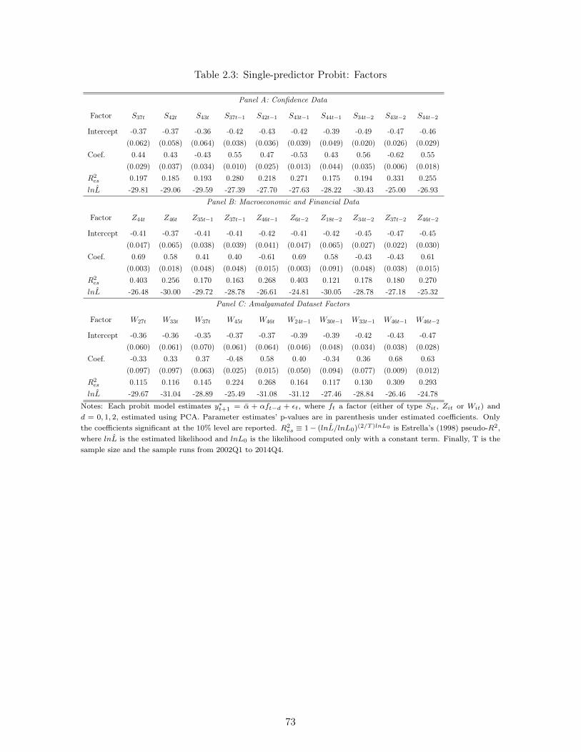
Table 2.3: Single-predictor Probit: Factors

Panel A: Confidence Data

Factor S37t S42t S43t S37t−1 S42t−1 S43t−1 S44t−1 S34t−2 S43t−2 S44t−2

Intercept -0.37 -0.37 -0.36 -0.42 -0.43 -0.42 -0.39 -0.49 -0.47 -0.46(0.062) (0.058) (0.064) (0.038) (0.036) (0.039) (0.049) (0.020) (0.026) (0.029)

Coef. 0.44 0.43 -0.43 0.55 0.47 -0.53 0.43 0.56 -0.62 0.55(0.029) (0.037) (0.034) (0.010) (0.025) (0.013) (0.044) (0.035) (0.006) (0.018)

R2es 0.197 0.185 0.193 0.280 0.218 0.271 0.175 0.194 0.331 0.255

lnL -29.81 -29.06 -29.59 -27.39 -27.70 -27.63 -28.22 -30.43 -25.00 -26.93Panel B: Macroeconomic and Financial Data

Factor Z44t Z46t Z35t−1 Z37t−1 Z46t−1 Z6t−2 Z18t−2 Z34t−2 Z37t−2 Z46t−2

Intercept -0.41 -0.37 -0.41 -0.41 -0.42 -0.41 -0.42 -0.45 -0.47 -0.45(0.047) (0.065) (0.038) (0.039) (0.041) (0.047) (0.065) (0.027) (0.022) (0.030)

Coef. 0.69 0.58 0.41 0.40 -0.61 0.69 0.58 -0.43 -0.43 0.61(0.003) (0.018) (0.048) (0.048) (0.015) (0.003) (0.091) (0.048) (0.038) (0.015)

R2es 0.403 0.256 0.170 0.163 0.268 0.403 0.121 0.178 0.180 0.270

lnL -26.48 -30.00 -29.72 -28.78 -26.61 -24.81 -30.05 -28.78 -27.18 -25.32Panel C: Amalgamated Dataset Factors

Factor W27t W33t W37t W45t W46t W24t−1 W30t−1 W33t−1 W46t−1 W46t−2

Intercept -0.36 -0.36 -0.35 -0.37 -0.37 -0.39 -0.39 -0.42 -0.43 -0.47(0.060) (0.061) (0.070) (0.061) (0.064) (0.046) (0.048) (0.034) (0.038) (0.028)

Coef. -0.33 0.33 0.37 -0.48 0.58 0.40 -0.34 0.36 0.68 0.63(0.097) (0.097) (0.063) (0.025) (0.015) (0.050) (0.094) (0.077) (0.009) (0.012)

R2es 0.115 0.116 0.145 0.224 0.268 0.164 0.117 0.130 0.309 0.293

lnL -29.67 -31.04 -28.89 -25.49 -31.08 -31.12 -27.46 -28.84 -26.46 -24.78Notes: Each probit model estimates y∗t+1 = α + αft−d + εt, where ft a factor (either of type Sit, Zit or Wit) andd = 0, 1, 2, estimated using PCA. Parameter estimates’ p-values are in parenthesis under estimated coefficients. Onlythe coefficients significant at the 10% level are reported. R2

es ≡ 1− (lnL/lnL0)(2/T )lnL0 is Estrella’s (1998) pseudo-R2,where lnL is the estimated likelihood and lnL0 is the likelihood computed only with a constant term. Finally, T is thesample size and the sample runs from 2002Q1 to 2014Q4.

73

Table 2.4: Probit with Multiple predictors: In-Sample Results

Panel A: Standard Model Panel B: Dynamic ModelVariables M1 M2 M3 M4 M5 Variables M1 M2 M3 M4 M5

Intercept -0.20 -0.41 -0.85 -2.08 -1.61 Intercept -1.86 -1.83 -1.76 -1.82 -1.97(0.350) (0.047) (0.008) (0.028) (0.020) (0.000) (0.000) (0.001) (0.000) (0.001)

yt−1 yt−1 3.11 2.91 2.33 2.96 3.37(0.000) (0.000) (0.000) (0.000) (0.001)

InterestRatet - InterestRatet -(-) (-)

Termspreadt - Termspreadt -(-) (-)

StockMarkett -8.90 StockMarkett -(0.051) (-)

Ex.Ratet - Ex.Ratet -(-) (-)

Moneyt - Moneyt 65.21(-) (0.028)

BCIt - BCIt -(-) (-)

CCIt -6.22 CCIt -(0.030) (-)

BOSt - BOSt -(-) (-)

SLOt - SLOt -0.03(-) (0.054)

Z44t 0.95 Z44t 0.70(0.005) (0.050)

Z37t−1 -0.76 Z37t−1 -(0.029) ()

Z46t−1 1.05 Z46t−1 -(0.006) (-)

Z34t−2 -0.65 Z34t−2 -0.64(0.013) (0.040)

S37t 1.48 S37t -(0.029) (-)

S43t -1.46 S43t -(0.027) (-)

S42t−1 2.48 S42t−1 -(0.016) (-)

S44t−1 1.77 S34t−2 1.10(0.031) (0.023)

S37t−2 1.68 S37t−2 -(0.017) (-)

W33t 0.84 W33t -(0.026) (-)

W37t 1.42 W37t -(0.014) (-)

W46t 1.17 W46t 0.72(0.037) (0.044)

W24t−1 1.13 W30t−1 -0.98(0.038) (0.045)

W33t−1 1.35 W33t−1 -(0.010) (-)

W46t−2 1.76 W46t−2 -(0.022) (-)

R2es 0.341 0.292 0.844 0.956 0.936 R2

es 0.903 0.872 0.901 0.889 0.940AIC 56.69 57.00 36.03 27.37 32.04 AIC 30.54 31.70 29.53 28.64 26.91QPS 0.450 0.454 0.311 0.282 0.324 QPS 0.060 0.053 0.077 0.075 0.099

Notes: The left panel presents results from the standard probit while the right panel analyzes its dynamic version,both estimated on 2002Q1 to 2014Q4. Variables considered are: M1 = Classical predictors, M2 = Confidence indices,M3 = Macroeconomic factors, M4 = Confidence factors, M5 = Amalgamated-dataset factors. Coefficients’ p-valuesare in parenthesis under estimates. R2

es ≡ 1− (lnL/lnL0)−(2/T )lnL0 is Estrella’s (1998) pseudo-R2, where lnL is theestimated likelihood and lnL0 is the likelihood only with a constant term. Other reported performance measuresinclude Akaike’s asymptotic information criterion AIC and the quadratic probability score QPS.

74

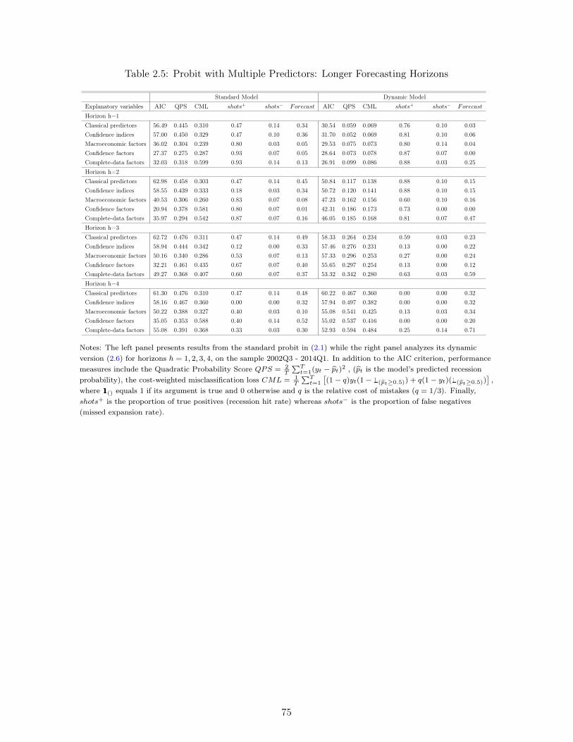
Table 2.5: Probit with Multiple Predictors: Longer Forecasting Horizons

Standard Model Dynamic ModelExplanatory variables AIC QPS CML shots+ shots− Forecast AIC QPS CML shots+ shots− Forecast

Horizon h=1Classical predictors 56.49 0.445 0.310 0.47 0.14 0.34 30.54 0.059 0.069 0.76 0.10 0.03Confidence indices 57.00 0.450 0.329 0.47 0.10 0.36 31.70 0.052 0.069 0.81 0.10 0.06Macroeconomic factors 36.02 0.304 0.239 0.80 0.03 0.05 29.53 0.075 0.073 0.80 0.14 0.04Confidence factors 27.37 0.275 0.287 0.93 0.07 0.05 28.64 0.073 0.078 0.87 0.07 0.00Complete-data factors 32.03 0.318 0.599 0.93 0.14 0.13 26.91 0.099 0.086 0.88 0.03 0.25Horizon h=2Classical predictors 62.98 0.458 0.303 0.47 0.14 0.45 50.84 0.117 0.138 0.88 0.10 0.15Confidence indices 58.55 0.439 0.333 0.18 0.03 0.34 50.72 0.120 0.141 0.88 0.10 0.15Macroeconomic factors 40.53 0.306 0.260 0.83 0.07 0.08 47.23 0.162 0.156 0.60 0.10 0.16Confidence factors 20.94 0.378 0.581 0.80 0.07 0.01 42.31 0.186 0.173 0.73 0.00 0.00Complete-data factors 35.97 0.294 0.542 0.87 0.07 0.16 46.05 0.185 0.168 0.81 0.07 0.47Horizon h=3Classical predictors 62.72 0.476 0.311 0.47 0.14 0.49 58.33 0.264 0.234 0.59 0.03 0.23Confidence indices 58.94 0.444 0.342 0.12 0.00 0.33 57.46 0.276 0.231 0.13 0.00 0.22Macroeconomic factors 50.16 0.340 0.286 0.53 0.07 0.13 57.33 0.296 0.253 0.27 0.00 0.24Confidence factors 32.21 0.461 0.435 0.67 0.07 0.40 55.65 0.297 0.254 0.13 0.00 0.12Complete-data factors 49.27 0.368 0.407 0.60 0.07 0.37 53.32 0.342 0.280 0.63 0.03 0.59Horizon h=4Classical predictors 61.30 0.476 0.310 0.47 0.14 0.48 60.22 0.467 0.360 0.00 0.00 0.32Confidence indices 58.16 0.467 0.360 0.00 0.00 0.32 57.94 0.497 0.382 0.00 0.00 0.32Macroeconomic factors 50.22 0.388 0.327 0.40 0.03 0.10 55.08 0.541 0.425 0.13 0.03 0.34Confidence factors 35.05 0.353 0.588 0.40 0.14 0.52 55.02 0.537 0.416 0.00 0.00 0.20Complete-data factors 55.08 0.391 0.368 0.33 0.03 0.30 52.93 0.594 0.484 0.25 0.14 0.71

Notes: The left panel presents results from the standard probit in (2.1) while the right panel analyzes its dynamicversion (2.6) for horizons h = 1, 2, 3, 4, on the sample 2002Q3 - 2014Q1. In addition to the AIC criterion, performancemeasures include the Quadratic Probability Score QPS = 2

T

∑Tt=1(yt − pt)2 , (pt is the model’s predicted recession

probability), the cost-weighted misclassification loss CML = 1T

∑Tt=1

[(1− q)yt(1− 1(pt≥0.5)) + q(1− yt)(1(pt≥0.5))

],

where 1() equals 1 if its argument is true and 0 otherwise and q is the relative cost of mistakes (q = 1/3). Finally,shots+ is the proportion of true positives (recession hit rate) whereas shots− is the proportion of false negatives(missed expansion rate).

75

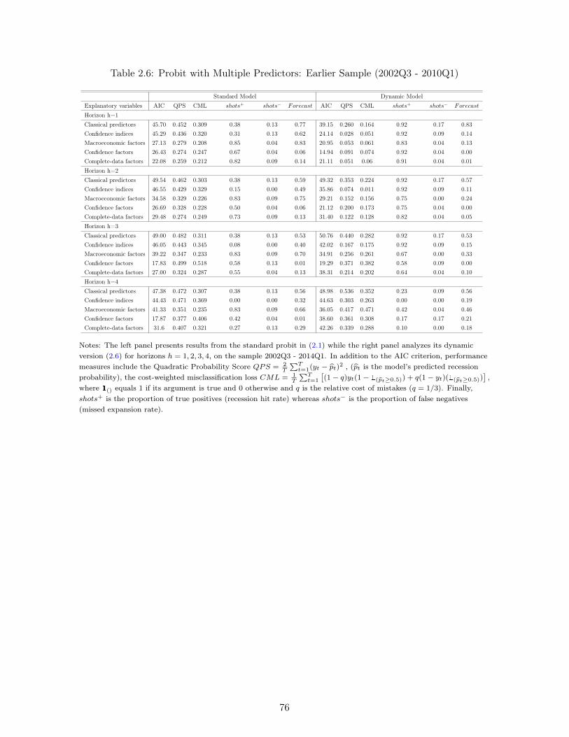
Table 2.6: Probit with Multiple Predictors: Earlier Sample (2002Q3 - 2010Q1)

Standard Model Dynamic ModelExplanatory variables AIC QPS CML shots+ shots− Forecast AIC QPS CML shots+ shots− Forecast

Horizon h=1Classical predictors 45.70 0.452 0.309 0.38 0.13 0.77 39.15 0.260 0.164 0.92 0.17 0.83Confidence indices 45.29 0.436 0.320 0.31 0.13 0.62 24.14 0.028 0.051 0.92 0.09 0.14Macroeconomic factors 27.13 0.279 0.208 0.85 0.04 0.83 20.95 0.053 0.061 0.83 0.04 0.13Confidence factors 26.43 0.274 0.247 0.67 0.04 0.06 14.94 0.091 0.074 0.92 0.04 0.00Complete-data factors 22.08 0.259 0.212 0.82 0.09 0.14 21.11 0.051 0.06 0.91 0.04 0.01Horizon h=2Classical predictors 49.54 0.462 0.303 0.38 0.13 0.59 49.32 0.353 0.224 0.92 0.17 0.57Confidence indices 46.55 0.429 0.329 0.15 0.00 0.49 35.86 0.074 0.011 0.92 0.09 0.11Macroeconomic factors 34.58 0.329 0.226 0.83 0.09 0.75 29.21 0.152 0.156 0.75 0.00 0.24Confidence factors 26.69 0.328 0.228 0.50 0.04 0.06 21.12 0.200 0.173 0.75 0.04 0.00Complete-data factors 29.48 0.274 0.249 0.73 0.09 0.13 31.40 0.122 0.128 0.82 0.04 0.05Horizon h=3Classical predictors 49.00 0.482 0.311 0.38 0.13 0.53 50.76 0.440 0.282 0.92 0.17 0.53Confidence indices 46.05 0.443 0.345 0.08 0.00 0.40 42.02 0.167 0.175 0.92 0.09 0.15Macroeconomic factors 39.22 0.347 0.233 0.83 0.09 0.70 34.91 0.256 0.261 0.67 0.00 0.33Confidence factors 17.83 0.499 0.518 0.58 0.13 0.01 19.29 0.371 0.382 0.58 0.09 0.00Complete-data factors 27.00 0.324 0.287 0.55 0.04 0.13 38.31 0.214 0.202 0.64 0.04 0.10Horizon h=4Classical predictors 47.38 0.472 0.307 0.38 0.13 0.56 48.98 0.536 0.352 0.23 0.09 0.56Confidence indices 44.43 0.471 0.369 0.00 0.00 0.32 44.63 0.303 0.263 0.00 0.00 0.19Macroeconomic factors 41.33 0.351 0.235 0.83 0.09 0.66 36.05 0.417 0.471 0.42 0.04 0.46Confidence factors 17.87 0.377 0.406 0.42 0.04 0.01 38.60 0.361 0.308 0.17 0.17 0.21Complete-data factors 31.6 0.407 0.321 0.27 0.13 0.29 42.26 0.339 0.288 0.10 0.00 0.18


T



∑Tt=1

[(1− q)yt(1− 1(pt≥0.5)) + q(1− yt)(1(pt≥0.5))

],


76

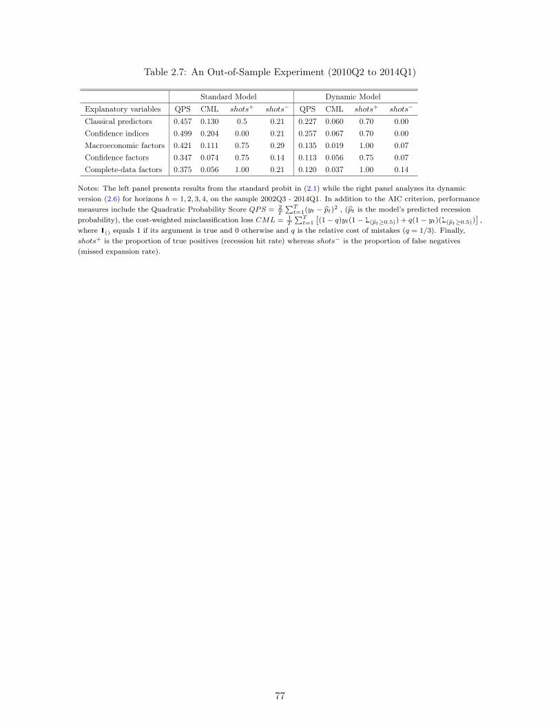
Table 2.7: An Out-of-Sample Experiment (2010Q2 to 2014Q1)

Standard Model Dynamic ModelExplanatory variables QPS CML shots+ shots− QPS CML shots+ shots−

Classical predictors 0.457 0.130 0.5 0.21 0.227 0.060 0.70 0.00Confidence indices 0.499 0.204 0.00 0.21 0.257 0.067 0.70 0.00Macroeconomic factors 0.421 0.111 0.75 0.29 0.135 0.019 1.00 0.07Confidence factors 0.347 0.074 0.75 0.14 0.113 0.056 0.75 0.07Complete-data factors 0.375 0.056 1.00 0.21 0.120 0.037 1.00 0.14


T



∑Tt=1

[(1− q)yt(1− 1(pt≥0.5)) + q(1− yt)(1(pt≥0.5))

],


77

Chapter 3

Forecasting with Many Predictors:How Useful are National andInternational Confidence Data?

Abstract

This paper assesses the contribution of Canadian and International (US) confidence data,drawn from consumer and business sentiment surveys, for forecasting Canadian GDPgrowth. The targeting approaches of Bai and Ng [2008] and Bai and Ng [2009] areemployed to extract promising predictors from large databases each containing betweenseveral dozen and several hundred time series. The databases are categorised betweenthose containing macroeconomic (Canadian and US) and confidence (Canadian and US)data, allowing us to assess formally the value added of international and confidence data.We find that forecasting ability is consistently improved by considering information fromnational confidence data; by contrast, their US counterparts appear to be helpful onlywhen combined with national time-series. Overall, most relevant gains in forecastingperformance are observed for short-term (up to three-quarters-ahead) horizons, perhapsreflecting the timing advantage in the releases of sentiment data.

Keywords: forecasting, data-rich models, confidence, GDP, Real Economic Activity, Canada,US, survey data.

79

3.1 Introduction

Over the last decade, the use of survey data on business, consumer and investor confidence - orsentiment1 - has become an important tool for policy makers worldwide. Surveys on sentimentare carried out on a very timely manner (on a monthly or quarterly basis) in order to elicitearly signals for future economic developments and these data are not subject to revision. Bycontrast, information on the current state of the economy, while crucial to economic-policy-analysis and forecasting, is released after substantial delays and is likely to be subjected toimportant revisions in future vintages of data releases. This timing discrepancy and theabsence of revisions represent key potential advantages for sentiment data when forecastingfuture economic activity [Lahiri and Monokroussos, 2013, Lahiri et al., 2016].

The present paper assesses the extent to which this advantage is present when Canadianas well as International (ie US) confidence data are employed to forecast Canadian GDPgrowth. To provide this assessment, we use four distinct databases, where the first two containstandard macroeconomic and NIPA data from Canada and the US, respectively, while thelatter two incorporate sentiment data from each of these two countries. A targeted approachadapted from Bai and Ng [2008] and Bai and Ng [2009] is employed to identify promisingpredictors for each of the databases: since these contains between several dozens and severalhundred variables each, such an approach is necessary to reduce the dimensionality of theforecasting equation and efficiently use the information present in these data. We then testthe forecasting ability of our different databases via an out-of-sample experiment based on arolling window and formally compare the resulting forecasts. Finally, we repeat the analysisby progressively merging the four databases into larger ones arranged by theme (all Canadiandata, all confidence data, etc) until we have one larger database using all our 1300 time series.

We find that forecasting ability is consistently improved by considering information fromnational confidence data; by contrast, their US counterparts appear to be helpful only whencombined with national time-series. Overall, most relevant gains in forecasting performanceare observed for short-term (up to three-quarters-ahead) horizons, perhaps reflecting the timerelease advantage of sentiment data.

Our results contribute to two distinct research programs. First, our findings about the fore-casting ability of sentiment data extend the body of evidence documenting how such data canimprove forecasts for real activity variables such as GDP growth or the likelihood of economicdownturns. This contribution of sentiment data is analyzed in several contributions, such asMatsusaka and Sbordone [1995], Santero and Westerlund [1996], Bodo et al. [2000], Hanssonet al. [2005], or Taylor and McNabb [2007]. This literature has recently expanded and nowuses factor targeting models as the benchmark of analysis, as in Chen et al. [2011], Lahiri andMonokroussos [2013], Christiansen et al. [2014], Martinsen et al. [2014a], Moran et al. [2016]

1In this paper, the terms sentiment and confidence are used interchangeably.

80

and Lahiri et al. [2016]. Evidence specifically related to the Canadian case is more scarce,despite the existence of at least four distinct surveys on sentiment in Canada. The forecast-ing framework presented in Binette and Chang [2013b], Ferrara et al. [2015] and Chernis andSekkel [2017] does include confidence data but does not identify its specific contribution, whilerecent work by Pichette and Robitaille [2017] analyzes how Canadian survey evidence mayhelp produce better forecasts, by focusing on the Business Outlook Survey data produced bythe Bank of Canada. By using all available Canadian data on confidence and using targetingapproaches organized by database, our work has the potential to both generalize these findingsand identify the specific contribution of sentiment data.

Second, our paper also adds to a literature that assesses the extent to which internationalvariables are important to provide accurate forecasts for national variables of interest: Cheungand Demers [2007], Schumacher [2010], Eickmeier and Ng [2011] or Kopoin et al. [2013] arerepresentative contributions to this literature. Interestingly, this research program has showedthat while international variables can help forecast better, this advantage is not present for allcases and at all forecasting horizons; sometimes, the efficient use of national variables mightbe sufficient to forecast accurately [Kopoin et al., 2013]. Such a finding accords well withthose, documented in the present paper, whereby US confidence data might not be needed toprovide the best forecasts possible and the databases with the larger number of time seriesmay not produce the better forecasts.

Throughout the paper, we apply targeting methods designed to efficiently extract informationcontained in large databases. These methods reflect the fact, documented in Boivin and Ng[2006], that applying factor modeling to larger databases does not invariably lead to betterforecasting equations, but that instead identifying variables or factors likely to contain goodinformation in advance of the factor extracting and forecasting exercise may produce superiorresults [Bai and Ng, 2008, 2009].

The rest of the paper is organized as follows. Section 2 describes our forecasting model andtargeting approaches. Section 3 describes the data used and the rich variety of sentiment datawe employ. Section 4 presents the empirical analysis. Section 5 reports our results, whileSection 6 concludes by offering some suggestions for future research.

3.2 Framework

This section describes our theoretical framework. In the first subsection, we revisit the factormodels discussed in a number of key papers in the forecasting literature. The second sub-section describes the principal component technique used to compute common factors. Thethird subsection presents the variable and factor selection processes used to identify promisingpredictors. Finally the fourth subsection specifies the evaluation measures used to comparethe forecasting performance of the different models.

81

3.2.1 Forecasting Models

Our goal is to forecast the time series {yτ+h}T∗

τ=T−h+1 conditional on Fτ , the informationset available at time τ , which contains the previous values of y up to τ and a large numberof potential predictors observed at time τ . The first step in our approach is to estimate abaseline model in which changes in real economic activity only depend on past realizations,i.e. assuming that yt follows an autoregressive (AR) process of order p:

yt+h = αh +

p∑d=1

λhdyt−d+1 + εt+h, (3.1)

where yt is a measure of economic activity (here the growth rate of real GDP), d the numberof lags used, t ≤ T − h+ 1 the length of the estimation sample, h the forecasting horizon andεt an i.i.d normal error term: εt ∼ i.i.d. N(0, 1). Given the information set, the h-step-aheadforecast of yτ with T − h+ 1 ≤ τ ≤ T ∗ is derived as:2

yτ+h/τ = αh +

p∑d=1

λhdyτ−d+1.

Next, suppose that Xt = (X1t, X2t, ..., XNt) = [Xit]i=1,...,N ;t=1,...,T represents a N-dimensionalvector of time series of potential predictors for yt+h. An extension of the baseline model is toaccount for current and lagged values of other explanatory variables in the regressors, as in:{

yt+h = αh +∑p

d=1 λhdyt−d+1 +

∑qd=1 β

hdXt−d+1 + εt+h,

yτ+h/τ = αh +∑p

d=1 λhdyτ−d+1 +

∑qd=1 β

hdXτ−d+1.

(3.2)

In a data-rich environment, dozens of time series may be available as predictive regressorsfor the variable of interest and thus as candidates to include in the vector Xt. In such anenvironment, the use of factor models can help reduce the dimension of the problem [Stock andWatson, 2002a,b]. These models combine the information content of many different variablesinto a few representative factors that are then used to forecast the variable of interest usinglinear regression models. Following Stock and Watson [2002a,b], we thus assume that eachpotential predictor Xit in (3.2) has a factor structure whereby

Xit = α′iFt + eit, i = 1, ..., N , t = 1, ..., T, (3.3)

where Ft is a r × 1 vector of factors common to all Xit, αi a r × 1 vector of factor loadingscollecting the influence of each factor on Xit, eit ∼ i.i.d. N(0, 1) is an idiosyncratic componentand εt+h is the prediction error. The r common factors (r << N) are estimated by performinga principal component decomposition to the normalized data Xt and estimated factors Ft arethen used in forecasting yt+h by computing the regression:{

yt+h = αh +∑p

d=1 λhdyt−d+1 +

∑qd=1 γ

hd Ft−d+1 + εt+h,

yτ+h/τ = αh +∑p

d=1 λhdyτ−d+1 +

∑qd=1 γ

hd Fτ−d+1,

(3.4)

2Note that when h > d, we consider dynamic forecasts where yt+d+1,· · · , yt+h−1 are used to forecastyt+h/τ .

82

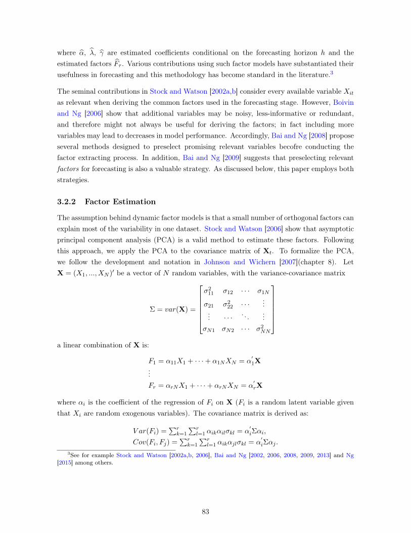
where α, λ, γ are estimated coefficients conditional on the forecasting horizon h and theestimated factors Fτ . Various contributions using such factor models have substantiated theirusefulness in forecasting and this methodology has become standard in the literature.3

The seminal contributions in Stock and Watson [2002a,b] consider every available variable Xit

as relevant when deriving the common factors used in the forecasting stage. However, Boivinand Ng [2006] show that additional variables may be noisy, less-informative or redundant,and therefore might not always be useful for deriving the factors; in fact including morevariables may lead to decreases in model performance. Accordingly, Bai and Ng [2008] proposeseveral methods designed to preselect promising relevant variables becofre conducting thefactor extracting process. In addition, Bai and Ng [2009] suggests that preselecting relevantfactors for forecasting is also a valuable strategy. As discussed below, this paper employs bothstrategies.

3.2.2 Factor Estimation

The assumption behind dynamic factor models is that a small number of orthogonal factors canexplain most of the variability in one dataset. Stock and Watson [2006] show that asymptoticprincipal component analysis (PCA) is a valid method to estimate these factors. Followingthis approach, we apply the PCA to the covariance matrix of Xt. To formalize the PCA,we follow the development and notation in Johnson and Wichern [2007](chapter 8). LetX = (X1, ..., XN )′ be a vector of N random variables, with the variance-covariance matrix

Σ = var(X) =

σ2

11 σ12 · · · σ1N

σ21 σ222 · · ·

...... · · · . . .

...σN1 σN2 · · · σ2

NN

a linear combination of X is:

F1 = α11X1 + · · ·+ α1NXN = α′1X

...Fr = αrNX1 + · · ·+ αrNXN = α

′rX

where αi is the coefficient of the regression of Fi on X (Fi is a random latent variable giventhat Xi are random exogenous variables). The covariance matrix is derived as:

V ar(Fi) =∑r

k=1

∑rl=1 αikαilσkl = α

′iΣαi,

Cov(Fi, Fj) =∑r

k=1

∑rl=1 αikαjlσkl = α

′iΣαj .

3See for example Stock and Watson [2002a,b, 2006], Bai and Ng [2002, 2006, 2008, 2009, 2013] and Ng[2015] among others.

83

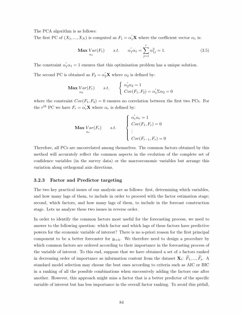
The PCA algorithm is as follows:The first PC of (X1, ..., XN ) is computed as F1 = α

′1X where the coefficient vector α1 is:

Max V ar(F1)α1

s.t. α′1α1 =

r∑j=1

α21j = 1. (3.5)

The constraint α′1α1 = 1 ensures that this optimisation problem has a unique solution.

The second PC is obtained as F2 = α′2X where α2 is defined by:

Max V ar(Fr)α2

s.t.

{α′2α2 = 1

Cov(F1, F2) = α′1Σα2 = 0

where the constraint Cov(F1, F2) = 0 ensures no correlation between the first two PCs. Forthe rth PC we have Fr = α

′rX where αr is defined by:

Max V ar(Fr)αr

s.t.

α′rαr = 1

Cov(F1, Fr) = 0...Cov(Fr−1, Fr) = 0

Therefore, all PCs are uncorrelated among themselves. The common factors obtained by thismethod will accurately reflect the common aspects in the evolution of the complete set ofconfidence variables (in the survey data) or the macroeconomic variables but arrange thisvariation along orthogonal axis directions.

3.2.3 Factor and Predictor targeting

The two key practical issues of our analysis are as follows: first, determining which variables,and how many lags of them, to include in order to proceed with the factor estimation stage;second, which factors, and how many lags of them, to include in the forecast constructionstage. Lets us analyze these two issues in reverse order.

In order to identify the common factors most useful for the forecasting process, we need toanswer to the following question: which factor and which lags of these factors have predictivepowers for the economic variable of interest? There is no a-priori reason for the first principalcomponent to be a better forecaster for yt+h. We therefore need to design a procedure bywhich common factors are ordered according to their importance in the forecasting process ofthe variable of interest. To this end, suppose that we have obtained a set of s factors rankedin decreasing order of importance as information content from the dataset Xt: F1, ..., Fs. Astandard model selection may choose the best ones according to criteria such as AIC or BICin a ranking of all the possible combinations when successively adding the factors one afteranother. However, this approach might miss a factor that is a better predictor of the specificvariable of interest but has less importance in the overall factor ranking. To avoid this pitfall,

84

we instead use a hard-thresholding method on the common factors, as in Bai and Ng [2009].This method assesses if a candidate principal component shows good forecasting power beforeit is selected by the procedure, and requires investigating the predictive power of each factorindividually before choosing the relevant ones as those significant in single-predictor regressionmodels whereby

yt+h = αh + βhidFi,t−d+1 + εt+h, i = 1, ..., s , d = 1, ..., q

and keeping Fi,t−d+1 if βhid is greater than our threshold.

Note that the strategy considered so far treats all the predictors in the set Xt as equallypromising in terms of forecasting, and thus includes them all when extracting the factors.However, as Boivin and Ng [2006] point out, it may occur that valuable information about thetarget variable to forecast is included timeseries that are less relevant for explaining the overallvariability in Xt and thus less important for factor estimation. In response, Bai and Ng [2008]propose selection methods by which only variables with good potential as predictors will beincluded in the factor estimation stage. One such method, hard-thresholding, investigates thepredictive power of each variable individually and chooses those to keep via the single-predictorregression model

yt+h = αh +

p∑d=1

λhdyt−d+1 +

q∑d=1

βhidXi,t−d+1 + εt+h, i = 1, ..., N , d = 1, ..., q

and keeping Xi,t (which now denotes one single variable) for the factor extraction stage onlyif βhid is statistically significant at some given threshold.

Soft-thresholding is another possible targeting method. It analyses all potential predictorssimultaneously, within a multiple-predictor regression, to reduce the possibility that the pre-dictors selected by hard-thresholding contain essentially the same information. The soft-thresholding approach thus considers

yt+h = αh +

p∑d=1

λhdyt−d+1 +

N∑i=1

q∑d=1

βhidXi,t−d+1 + εt+h,

ie. includes all available potential predictors and then estimates βh as in Zou and Hastie[2005], by solving

minβh

RSS + κ1

∑i,d

|βhid|+ κ2

∑i,d

βhid2

where κ1 and κ2 are parameters to be specified by the user. The calibration of the twoparameters allows to shrink the number of coefficients to be estimated and to determine theregressors to consider in the factor derivation process.

85

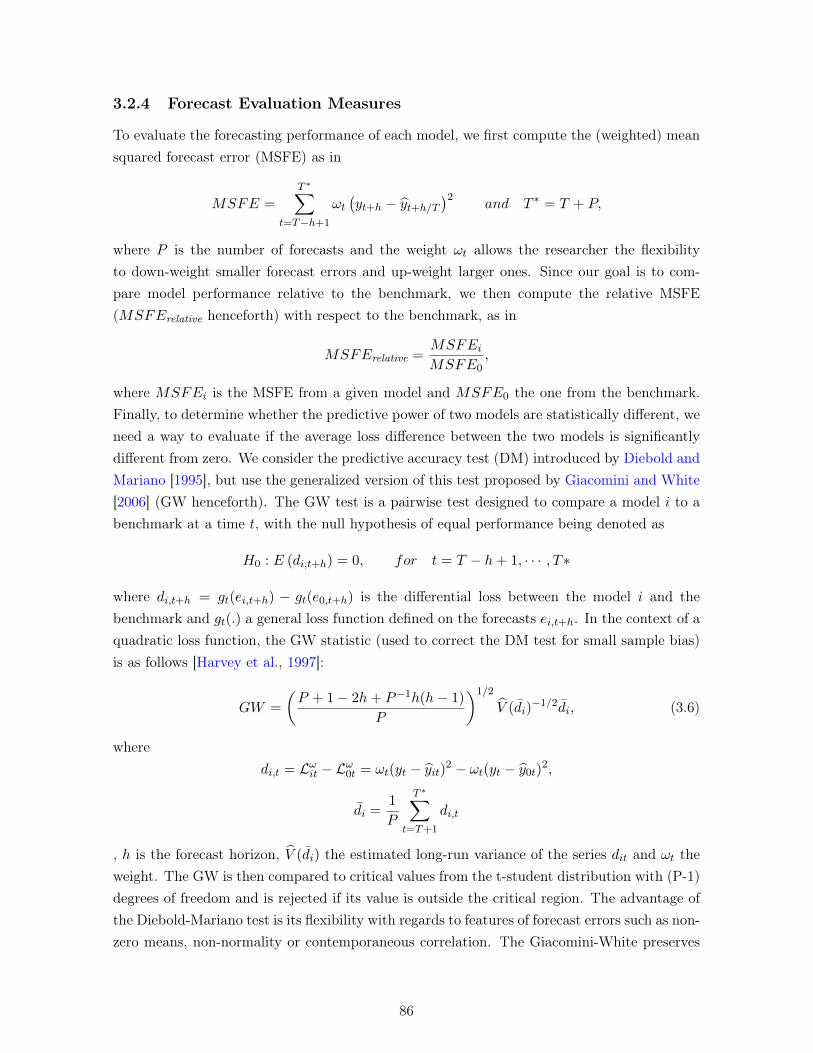
3.2.4 Forecast Evaluation Measures

To evaluate the forecasting performance of each model, we first compute the (weighted) meansquared forecast error (MSFE) as in

MSFE =T ∗∑

t=T−h+1

ωt(yt+h − yt+h/T

)2and T ∗ = T + P,

where P is the number of forecasts and the weight ωt allows the researcher the flexibilityto down-weight smaller forecast errors and up-weight larger ones. Since our goal is to com-pare model performance relative to the benchmark, we then compute the relative MSFE(MSFErelative henceforth) with respect to the benchmark, as in

MSFErelative =MSFEiMSFE0

,

where MSFEi is the MSFE from a given model and MSFE0 the one from the benchmark.Finally, to determine whether the predictive power of two models are statistically different, weneed a way to evaluate if the average loss difference between the two models is significantlydifferent from zero. We consider the predictive accuracy test (DM) introduced by Diebold andMariano [1995], but use the generalized version of this test proposed by Giacomini and White[2006] (GW henceforth). The GW test is a pairwise test designed to compare a model i to abenchmark at a time t, with the null hypothesis of equal performance being denoted as

H0 : E (di,t+h) = 0, for t = T − h+ 1, · · · , T∗

where di,t+h = gt(ei,t+h) − gt(e0,t+h) is the differential loss between the model i and thebenchmark and gt(.) a general loss function defined on the forecasts ei,t+h. In the context of aquadratic loss function, the GW statistic (used to correct the DM test for small sample bias)is as follows [Harvey et al., 1997]:

GW =

(P + 1− 2h+ P−1h(h− 1)

P

)1/2

V (di)−1/2di, (3.6)

wheredi,t = Lωit − Lω0t = ωt(yt − yit)2 − ωt(yt − y0t)

2,

di =1

P

T ∗∑t=T+1

di,t

, h is the forecast horizon, V (di) the estimated long-run variance of the series dit and ωt theweight. The GW is then compared to critical values from the t-student distribution with (P-1)degrees of freedom and is rejected if its value is outside the critical region. The advantage ofthe Diebold-Mariano test is its flexibility with regards to features of forecast errors such as non-zero means, non-normality or contemporaneous correlation. The Giacomini-White preserves

86

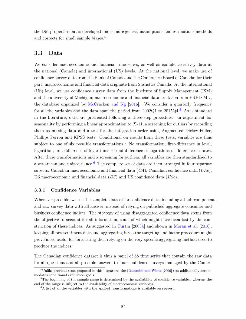
the DM properties but is developed under more general assumptions and estimations methodsand corrects for small sample biases.4

3.3 Data

We consider macroeconomic and financial time series, as well as confidence survey data atthe national (Canada) and international (US) levels. At the national level, we make use ofconfidence survey data from the Bank of Canada and the Conference Board of Canada; for theirpart, macroeconomic and financial data originate from Statistics Canada. At the international(US) level, we use confidence survey data from the Institute of Supply Management (ISM)and the university of Michigan; macroeconomic and financial data are taken from FRED-MD,the database organized by McCracken and Ng [2016]. We consider a quarterly frequencyfor all the variables and the data span the period from 2002Q1 to 2015Q4.5 As is standardin the literature, data are pretreated following a three-step procedure: an adjustment forseasonality by performing a linear approximation to X-11, a screening for outliers by recordingthem as missing data and a test for the integration order using Augmented Dickey-Fuller,Phillips Perron and KPSS tests. Conditional on results from these tests, variables are thussubject to one of six possible transformations : No transformation, first-difference in level,logarithm, first-difference of logarithms second-difference of logarithms or difference in rates.After these transformations and a screening for outliers, all variables are then standardized toa zero-mean and unit-variance.6 The complete set of data are then arranged in four separatesubsets: Canadian macroeconomic and financial data (CA), Canadian confidence data (CAc),US macroeconomic and financial data (US ) and US confidence data (USc).

3.3.1 Confidence Variables

Whenever possible, we use the complete dataset for confidence data, including all sub-componentsand raw survey data with all answer, instead of relying on published aggregate consumer andbusiness confidence indices. The strategy of using disaggregated confidence data stems fromthe objective to account for all information, some of which might have been lost by the con-struction of these indices. As suggested in Curtin [2003a] and shown in Moran et al. [2016],keeping all raw sentiment data and aggregating it via the targeting and factor procedure mightprove more useful for forecasting then relying on the very specific aggregating method used toproduce the indices.

The Canadian confidence dataset is thus a panel of 88 time series that contain the raw datafor all questions and all possible answers to four confidence surveys managed by the Confer-

4Unlike previous tests proposed in this literature, the Giacomini and White [2006] test additionally accom-modates conditional evaluation goals.

5The beginning of the sample range is determined by the availability of confidence variables, whereas theend of the range is subject to the availability of macroeconomic variables.

6A list of all the variables with the applied transformations is available on request.

87

ence Board of Canada and the Bank of Canada. The Conference Board manages two of thesesurveys: the consumer and business confidence surveys. The Consumer Confidence survey wasestablished in 1979 to sample 2000 Canadian households at a monthly frequency and querytheir views about their current and future economic conditions. The survey contains fourquestions and two response options (good, bad): respondents are asked to give their viewsabout their current and expected financial positions, their short-term employment outlookand their opinions about choosing the current moment for a major purchase such as houses orcars. The data therefore define 8 variables, in terms of percentage of good or bad responses foreach question.7 We transform the data to a quarterly frequency by simple averages. Note thatthe Conference Board of Canada uses data from this survey to produce its Consumer Confi-dence Index (CCIt), an average of the balance of opinion on the survey’s four questions. Asmentioned above, we analyse the CCI to test if relevant information is lost in the aggregatingprocess.

Figure 3.1: Confidence data and GDP growth: Conference Board Data

The second survey managed by the Conference Board is the quarterly Business Confidencesurvey, which exist since 1977. It interviews the Chief Executive Officers and Chief Finan-cial Officers of major Canadian business organizations, in order to measure perceptions aboutcurrent and future economic conditions and the investment intentions of businesses country-wide. The survey consists of ten descriptive questions, with eight of them focusing on theeconomic environment, financial conditions, inflation, profit, future investments, productionlevel, capacity utilization, geographical expansion perspectives, employment level and speedof supplier deliveries. Questions may have multiple response options and data are providedin terms of the percentages of respondents choosing each option of response, giving a total of

7Appendix A describes in details the questions and possible answers for the four surveys.

88

58 variables as potential predictors. These raw data are aggregated by the Conference Boardof Canada to compute and publish at a quarterly frequency the Business Confidence Index(BCIt). The data become available during the first month of each quarter.

Figure 3.1 above illustrates the evolution of the Conference Board of Canada’s confidenceindexes and GDP growth8 for the sample of interest. The two indexes appear to have leadingindicator properties. Since 2002, the indexes have decreased before each slowdown period,most notably in the months preceding the Great Recession of 2008-2009, and appear to havegone again nearly two quarters before growth resumed. To the best of our knowledge, theforecasting ability of the confidence data from the Conference Board of Canada has neverbeen analysed systematically. We assess this forecasting ability, when both the aggregateindices and the raw data are used. The Bank of Canada also conducts two confidence surveys:the Business Outlook Survey and the Senior Loan Officer Survey. The Bank of Canada beganthe Business Outlook Survey in 1997. The survey is conducted at a quarterly frequency by theBank’s regional offices and gathers information from firms about their sentiment on businessdevelopments and economic conditions. The senior management of 100 firms is interviewed onselected topics: survey respondents are asked to answer eleven attitudinal questions on topicsregarding past and future sales growth, investment in machinery, ability to meet the demand,labour shortages, intensity of labour shortages, input and output price inflation, inflationexpectations and credit conditions.9 Most questions have three response options (greater, thesame, lower) but the question about the expected inflation rate asks participants’ views inmore quantitative terms: (four options: above 3%, between 2 and 3%, between 1 and 2%,less than 1%). The responses to nine of the questions are available in the form of balance ofopinions (the difference in percentages between the opposite options of each question), exceptfor the responses on labour shortages (one variable), ability to meet the demand (arranged intwo variables) and inflation expectations (arranged in four variables which are in percentages).Therefore, the data represent all together a set of 15 variables and are available during thefirst month of the current quarter by the Bank of Canada. Since the Bank of Canada does notpropose an overall aggregate index, we produce the BOSt index as an equal-weighted averageof the eleven balances of opinion from the survey. We transform the inflation expectationsresponses in a two option-responses (above 2%, less than 2%). Again, our interest in simpleaverages such as the BOS is to verify whether they entail a loss of relevant information forforecasting.

8GDP growth is computed as yt = log (Yt/Yt−4)), where Yt is quarterly Canadian real GDP.9Details about the survey are provided in Martin (2004). All questions and answer choices are detailed in

Appendix A.

89

Figure 3.2: Confidence data and GDP growth: Bank of Canada Data

Finally, the Senior Loan Officer survey is a quarterly survey of the business-lending practicesof the 11 major Canadian financial institutions and is implemented and managed by theBank of Canada since 1999.10 Survey participants are asked to provide their informativeopinion on changes in both the price and non-price terms of business lending over the currentquarter. Moreover, the respondents are surveyed about their views on how changing economicor financial conditions are affecting business lending. The survey is conducted during thetwo-weeks-period before the end of each quarter and summarized in percentages of surveyedfinancial institutions reporting tightened credit conditions and those reporting eased creditconditions. Data are provided in terms of balance of opinion of the respondents. Data areavailable in two variables during the earliest week of each quarter through the Bank of Canadaweb site. The Bank of Canada provides an aggregate balance of opinions for the overallbusiness lending conditions that we denote the SLOt composite index. Figure 3.2 illustratesthe relationship between the two Bank of Canada confidence indexes and GDP growth for thesample of interest. The figure depicts the negative value of SLOt, which fits better with theGDP growth dynamics. Again, the two indexes seem to display leading indicator properties,as the relevant changes in the GDP growth follow the ups and downs in the indicators.

Let us now turn to US confidence data. The US confidence dataset is a panel of 299 timeseries containing data from two confidence surveys held by the University of Michigan andthe Institute of Supply Management. First, the University of Michigan has been running theconsumer confidence survey since the 1940s. Nowadays, the survey is conducted on a monthlybasis but we use a quarterly frequency by averaging the monthly data. Each month, at least500 households are interviewed by phone all over the US in order to gather information and sen-timent about their own current and expected financial situations; broader economic conditions

10See Faruqui et al. [2008] for more details on this survey.

90

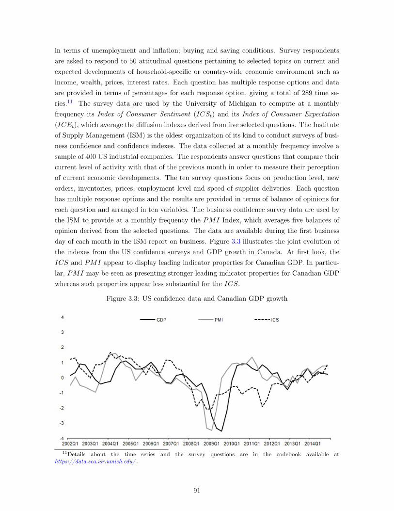
in terms of unemployment and inflation; buying and saving conditions. Survey respondentsare asked to respond to 50 attitudinal questions pertaining to selected topics on current andexpected developments of household-specific or country-wide economic environment such asincome, wealth, prices, interest rates. Each question has multiple response options and dataare provided in terms of percentages for each response option, giving a total of 289 time se-ries.11 The survey data are used by the University of Michigan to compute at a monthlyfrequency its Index of Consumer Sentiment (ICSt) and its Index of Consumer Expectation(ICEt), which average the diffusion indexes derived from five selected questions. The Instituteof Supply Management (ISM) is the oldest organization of its kind to conduct surveys of busi-ness confidence and confidence indexes. The data collected at a monthly frequency involve asample of 400 US industrial companies. The respondents answer questions that compare theircurrent level of activity with that of the previous month in order to measure their perceptionof current economic developments. The ten survey questions focus on production level, neworders, inventories, prices, employment level and speed of supplier deliveries. Each questionhas multiple response options and the results are provided in terms of balance of opinions foreach question and arranged in ten variables. The business confidence survey data are used bythe ISM to provide at a monthly frequency the PMI Index, which averages five balances ofopinion derived from the selected questions. The data are available during the first businessday of each month in the ISM report on business. Figure 3.3 illustrates the joint evolution ofthe indexes from the US confidence surveys and GDP growth in Canada. At first look, theICS and PMI appear to display leading indicator properties for Canadian GDP. In particu-lar, PMI may be seen as presenting stronger leading indicator properties for Canadian GDPwhereas such properties appear less substantial for the ICS.

Figure 3.3: US confidence data and Canadian GDP growth

11Details about the time series and the survey questions are in the codebook available athttps://data.sca.isr.umich.edu/ .

91

https://data.sca.isr.umich.edu/fetchdoc.php?docid=45121

3.3.2 Macroeconomic and Financial variables

We use balanced panels of macroeconomic and financial variables arranged in two datasetscontaining 764 and 128 time series for Canada and the US, respectively. The panels reflect thefollowing broadly-defined categories of economic data: National income and product accounts,industrial production, investment and consumption, employment and unemployment, housing,inventories, orders and sales, prices, hours worked and earnings, interest rates, money andcredit, exchange rates, stock markets.12

3.4 Empirical Analysis

3.4.1 Targeting procedure

We use the four original datasets (CA, CAc, US, USc) and natural amalgamations of them(All Canadian data, All Confidence data, All data). Such amalgamation provides a qualitativeselection criterion to identify promising variables for forecasting. Table 3.1 presents each subsetwith the number of variables candidate to the targeting process. Next, for each dataset used,we apply the Bai and Ng [2008] and Bai and Ng [2009] targeting methods to identify promisingindividual variables and factors. Specifically, the targeting procedure consists of the followingsteps:

1. Following Bai and Ng [2008], we apply a hard thresholding method to select the pre-dictors likely to be useful in the factor derivation process of our analysis. This methodconsists of preselecting the variables that remain in the pool from which factors areextracted by looking at their forecasting performance within a set of regressions runwith only one predictor at time. The predictive power of each individual variable isevaluated by comparing the Student t-statistic with a given threshold t∗ (we considert∗ = 0, 1.28, 1.65, 2.58, which respectively correspond to no threshold, 10%, 5% and 1%critical values for two-tailed t-tests).

2. As in Bai and Ng [2009] we compute the Principal Component decomposition of thematrix of selected variables in the pool and so derive the common factors. We thenapply a hard thresholding method to select promising factors. This method comprisesin a selection of useful factors by looking at their forecasting performance in a set ofregressions with only one factor as predictor.

3. In the spirit of Bai and Ng [2008], we experiment with an alternative, soft-thresholdingmethod to preselect useful predictors: this works by applying the least-angle regressionwith elastic net (LARS-EN). Its selects the useful variables for the factor derivation

12Further details about these data are available in Cheung and Demers [2007] and Moran et al. [2016] forthe Canadian database and in McCracken and Ng [2016] for US database.

92

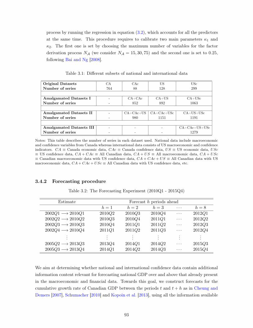
process by running the regression in equation (3.2), which accounts for all the predictorsat the same time. This procedure requires to calibrate two main parameters κ1 andκ2. The first one is set by choosing the maximum number of variables for the factorderivation process NA (we consider NA = 15, 30, 75) and the second one is set to 0.25,following Bai and Ng [2008].

Table 3.1: Different subsets of national and international data

Original Datasets US+CA+USc CAc US UScNumber of series 764 88 128 299

Amalgamated Datasets I - CA+CAc CA+US CA+UScNumber of series - 852 892 1063

Amalgamated Datasets II - CA+CAc+US CA+CAc+USc CA+US+UScNumber of series - 980 1151 1191

Amalgamated Datasets III - - - CA+CAc+US+UScNumber of series - - - 1279

Notes: This table describes the number of series in each dataset used. National data include macroeconomicand confidence variables from Canada whereas international data consists of US macroeconomic and confidenceindicators. CA ≡ Canada economic data, CAc ≡ Canada confidence data, US ≡ US economic data, USc≡ US confidence data, CA + CAc ≡ All Canadian data, CA + US ≡ All macroeconomic data, CA + USc≡ Canadian macroeconomic data with US confidence data, CA + CAc + US ≡ All Canadian data with USmacroeconomic data, CA+ CAc+ USc ≡ All Canadian data with US confidence data, etc.

3.4.2 Forecasting procedure

Table 3.2: The Forecasting Experiment (2010Q1 - 2015Q4)

Estimate Forecast h periods aheadh = 1 h = 2 h = 3 · · · h = 8

2002Q1 −→ 2010Q1 2010Q2 2010Q3 2010Q4 · · · 2012Q12002Q2 −→ 2010Q2 2010Q3 2010Q4 2011Q1 · · · 2012Q22002Q3 −→ 2010Q3 2010Q4 2011Q1 2011Q2 · · · 2012Q32002Q4 −→ 2010Q4 2011Q1 2011Q2 2011Q3 · · · 2012Q4

......

......

......

2005Q2 −→ 2013Q3 2013Q4 2014Q1 2014Q2 · · · 2015Q32005Q3 −→ 2013Q4 2014Q1 2014Q2 2014Q3 · · · 2015Q4

We aim at determining whether national and international confidence data contain additionalinformation content relevant for forecasting national GDP over and above that already presentin the macroeconomic and financial data. Towards this goal, we construct forecasts for thecumulative growth rate of Canadian GDP between the periods t and t+ h as in Cheung andDemers [2007], Schumacher [2010] and Kopoin et al. [2013], using all the information available

93

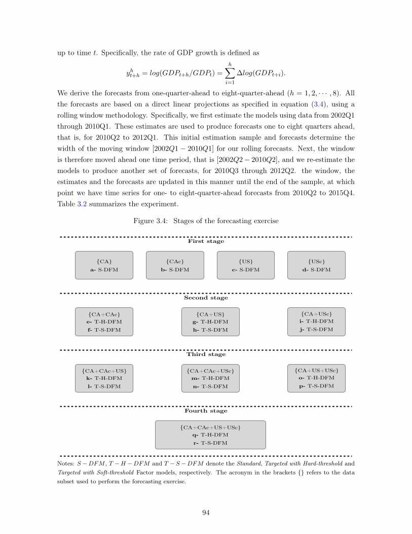
up to time t. Specifically, the rate of GDP growth is defined as

yht+h = log(GDPt+h/GDPt) =h∑i=1

∆log(GDPt+i).

We derive the forecasts from one-quarter-ahead to eight-quarter-ahead (h = 1, 2, · · · , 8). Allthe forecasts are based on a direct linear projections as specified in equation (3.4), using arolling window methodology. Specifically, we first estimate the models using data from 2002Q1through 2010Q1. These estimates are used to produce forecasts one to eight quarters ahead,that is, for 2010Q2 to 2012Q1. This initial estimation sample and forecasts determine thewidth of the moving window [2002Q1 − 2010Q1] for our rolling forecasts. Next, the windowis therefore moved ahead one time period, that is [2002Q2− 2010Q2], and we re-estimate themodels to produce another set of forecasts, for 2010Q3 through 2012Q2. the window, theestimates and the forecasts are updated in this manner until the end of the sample, at whichpoint we have time series for one- to eight-quarter-ahead forecasts from 2010Q2 to 2015Q4.Table 3.2 summarizes the experiment.

Figure 3.4: Stages of the forecasting exercise

First stage

{CA}a- S-DFM

{CAc}b- S-DFM

{US}c- S-DFM

{USc}d- S-DFM

Second stage

{CA+CAc}e- T-H-DFM

f- T-S-DFM

{CA+US}g- T-H-DFM

h- T-S-DFM

{CA+USc}i- T-H-DFM

j- T-S-DFM

Third stage

{CA+CAc+US}k- T-H-DFM

l- T-S-DFM

{CA+CAc+USc}m- T-H-DFM

n- T-S-DFM

{CA+US+USc}o- T-H-DFM

p- T-S-DFM

Fourth stage

{CA+CAc+US+USc}q- T-H-DFM

r- T-S-DFM

Notes: S −DFM , T −H −DFM and T − S −DFM denote the Standard, Targeted with Hard-threshold andTargeted with Soft-threshold Factor models, respectively. The acronym in the brackets {} refers to the datasubset used to perform the forecasting exercise.

94

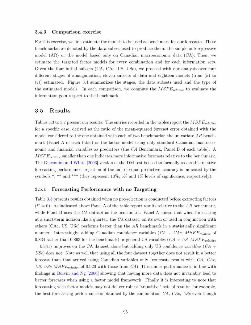
3.4.3 Comparison exercise

For this exercise, we first estimate the models to be used as benchmark for our forecasts. Thesebenchmarks are denoted by the data subset used to produce them: the simple autoregressivemodel (AR) or the model based only on Canadian macroeconomic data (CA). Then, weestimate the targeted factor models for every combination and for each information sets.Given the four initial subsets (CA, CAc, US, USc), we proceed with our analysis over fourdifferent stages of amalgamation, eleven subsets of data and eighteen models (from (a) to(r)) estimated. Figure 3.4 summarizes the stages, the data subsets used and the type ofthe estimated models. In each comparison, we compute the MSFErelative to evaluate theinformation gain respect to the benchmark.

3.5 Results

Tables 3.3 to 3.7 present our results. The entries recorded in the tables report theMSFErelative

for a specific case, derived as the ratio of the mean-squared forecast error obtained with themodel considered to the one obtained with each of two benchmarks: the univariate AR bench-mark (Panel A of each table) or the factor model using only standard Canadian macroeco-nomic and financial variables as predictors (the CA Benchmark, Panel B of each table). AMSFErelative smaller than one indicates more informative forecasts relative to the benchmark.The Giacomini and White [2006] version of the DM test is used to formally assess this relativeforecasting performance: rejection of the null of equal predictive accuracy is indicated by thesymbols *, ** and *** (they represent 10%, 5% and 1% levels of significance, respectively).

3.5.1 Forecasting Performance with no Targeting

Table 3.3 presents results obtained when no pre-selection is conducted before extracting factors(t∗ = 0). As indicated above Panel A of the table report results relative to the AR benchmark,while Panel B uses the CA dataset as the benchmark. Panel A shows that when forecastingat a short-term horizon like a quarter, the CA dataset, on its own or used in conjunction withothers (CAc, US, USc) performs better than the AR benchmark in a statistically significantmanner. Interestingly, adding Canadian confidence variables (CA + CAc, MSFErelative of0.834 rather than 0.863 for the benchmark) or general US variables (CA + US, MSFErelative

= 0.841) improves on the CA dataset alone but adding only US confidence variables (CA +USc) does not. Note as well that using all the four dataset together does not result in a betterforecast than that arrived using Canadian variables only (contrasts results with CA, CAc,US, USc MSFErelative of 0.920 with those from CA). This under-performance is in line withfindings in Boivin and Ng [2006] showing that having more data does not invariably lead tobetter forecasts when using a factor model framework. Finally it is interesting to note thatforecasting with factor models may not deliver robust “transitive" sets of results: for example,the best forecasting performance is obtained by the combination CA, CAc, USc even though

95

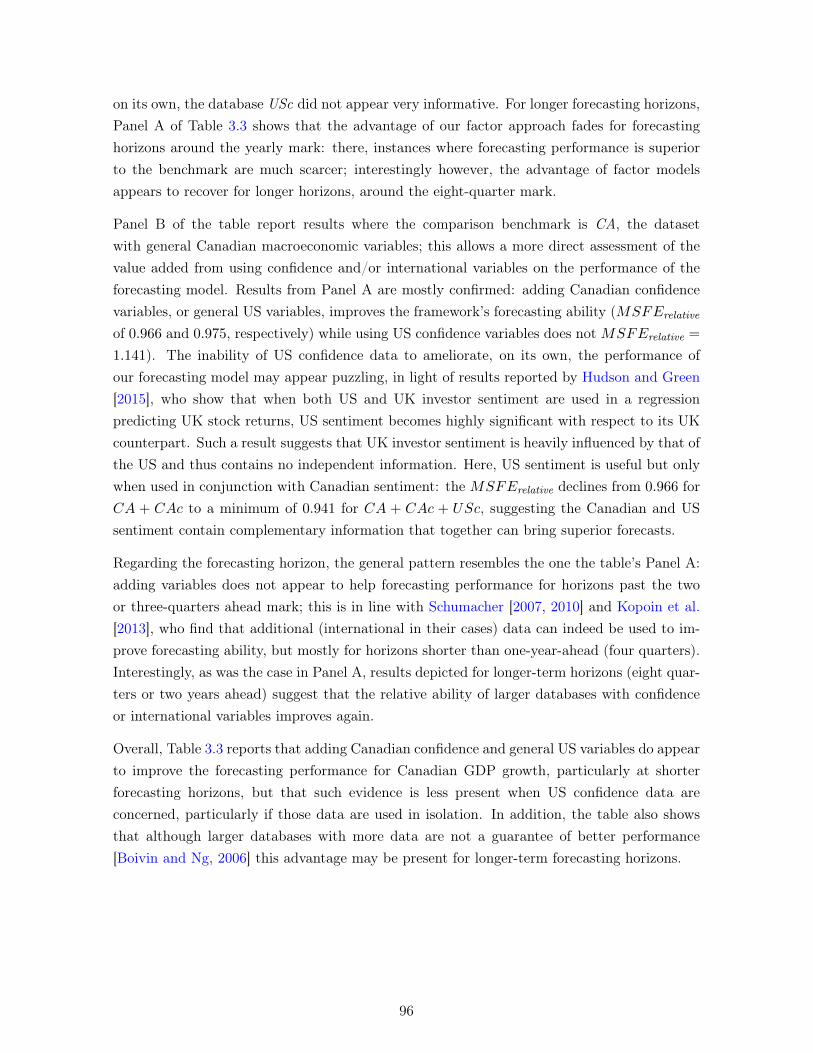
on its own, the database USc did not appear very informative. For longer forecasting horizons,Panel A of Table 3.3 shows that the advantage of our factor approach fades for forecastinghorizons around the yearly mark: there, instances where forecasting performance is superiorto the benchmark are much scarcer; interestingly however, the advantage of factor modelsappears to recover for longer horizons, around the eight-quarter mark.

Panel B of the table report results where the comparison benchmark is CA, the datasetwith general Canadian macroeconomic variables; this allows a more direct assessment of thevalue added from using confidence and/or international variables on the performance of theforecasting model. Results from Panel A are mostly confirmed: adding Canadian confidencevariables, or general US variables, improves the framework’s forecasting ability (MSFErelative

of 0.966 and 0.975, respectively) while using US confidence variables does not MSFErelative =

1.141). The inability of US confidence data to ameliorate, on its own, the performance ofour forecasting model may appear puzzling, in light of results reported by Hudson and Green[2015], who show that when both US and UK investor sentiment are used in a regressionpredicting UK stock returns, US sentiment becomes highly significant with respect to its UKcounterpart. Such a result suggests that UK investor sentiment is heavily influenced by that ofthe US and thus contains no independent information. Here, US sentiment is useful but onlywhen used in conjunction with Canadian sentiment: the MSFErelative declines from 0.966 forCA + CAc to a minimum of 0.941 for CA + CAc + USc, suggesting the Canadian and USsentiment contain complementary information that together can bring superior forecasts.

Regarding the forecasting horizon, the general pattern resembles the one the table’s Panel A:adding variables does not appear to help forecasting performance for horizons past the twoor three-quarters ahead mark; this is in line with Schumacher [2007, 2010] and Kopoin et al.[2013], who find that additional (international in their cases) data can indeed be used to im-prove forecasting ability, but mostly for horizons shorter than one-year-ahead (four quarters).Interestingly, as was the case in Panel A, results depicted for longer-term horizons (eight quar-ters or two years ahead) suggest that the relative ability of larger databases with confidenceor international variables improves again.

Overall, Table 3.3 reports that adding Canadian confidence and general US variables do appearto improve the forecasting performance for Canadian GDP growth, particularly at shorterforecasting horizons, but that such evidence is less present when US confidence data areconcerned, particularly if those data are used in isolation. In addition, the table also showsthat although larger databases with more data are not a guarantee of better performance[Boivin and Ng, 2006] this advantage may be present for longer-term forecasting horizons.

96

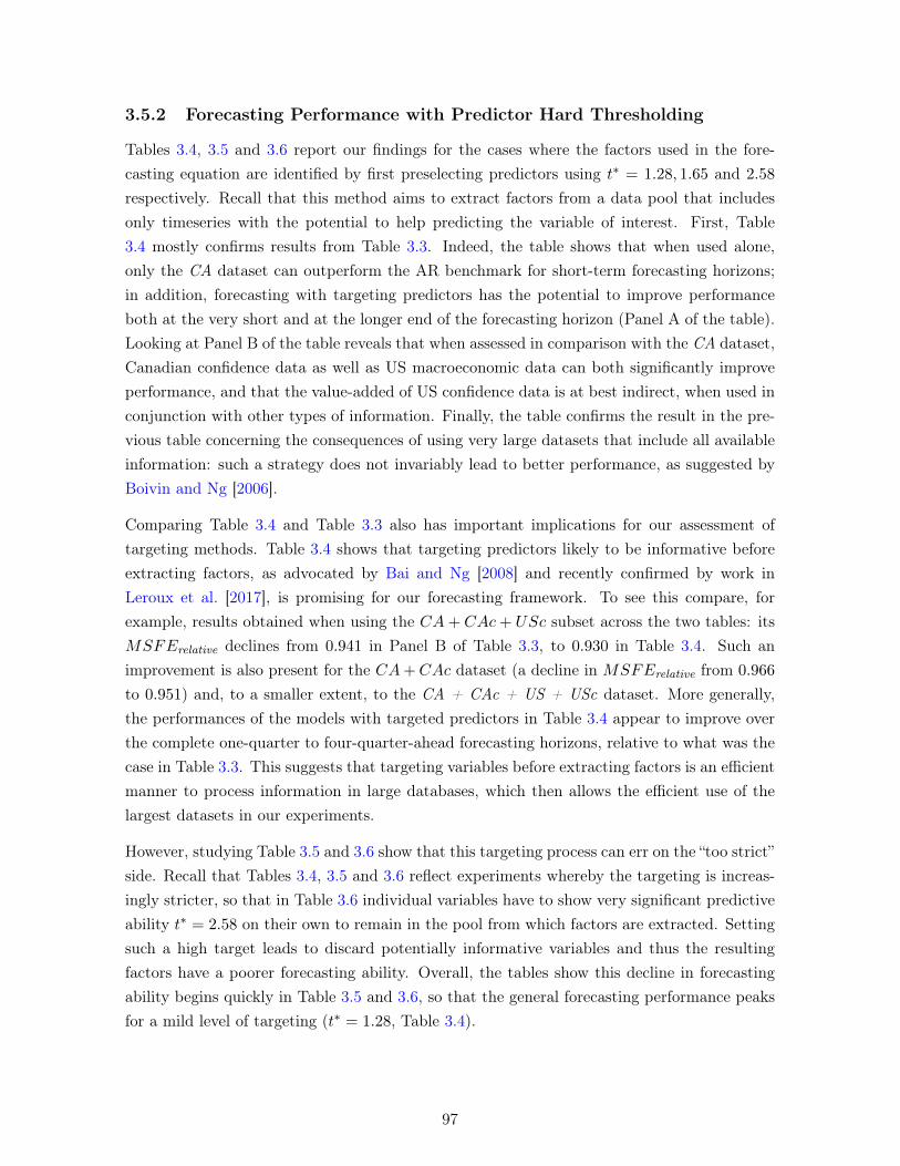
3.5.2 Forecasting Performance with Predictor Hard Thresholding

Tables 3.4, 3.5 and 3.6 report our findings for the cases where the factors used in the fore-casting equation are identified by first preselecting predictors using t∗ = 1.28, 1.65 and 2.58

respectively. Recall that this method aims to extract factors from a data pool that includesonly timeseries with the potential to help predicting the variable of interest. First, Table3.4 mostly confirms results from Table 3.3. Indeed, the table shows that when used alone,only the CA dataset can outperform the AR benchmark for short-term forecasting horizons;in addition, forecasting with targeting predictors has the potential to improve performanceboth at the very short and at the longer end of the forecasting horizon (Panel A of the table).Looking at Panel B of the table reveals that when assessed in comparison with the CA dataset,Canadian confidence data as well as US macroeconomic data can both significantly improveperformance, and that the value-added of US confidence data is at best indirect, when used inconjunction with other types of information. Finally, the table confirms the result in the pre-vious table concerning the consequences of using very large datasets that include all availableinformation: such a strategy does not invariably lead to better performance, as suggested byBoivin and Ng [2006].

Comparing Table 3.4 and Table 3.3 also has important implications for our assessment oftargeting methods. Table 3.4 shows that targeting predictors likely to be informative beforeextracting factors, as advocated by Bai and Ng [2008] and recently confirmed by work inLeroux et al. [2017], is promising for our forecasting framework. To see this compare, forexample, results obtained when using the CA+ CAc+ USc subset across the two tables: itsMSFErelative declines from 0.941 in Panel B of Table 3.3, to 0.930 in Table 3.4. Such animprovement is also present for the CA+CAc dataset (a decline in MSFErelative from 0.966

to 0.951) and, to a smaller extent, to the CA + CAc + US + USc dataset. More generally,the performances of the models with targeted predictors in Table 3.4 appear to improve overthe complete one-quarter to four-quarter-ahead forecasting horizons, relative to what was thecase in Table 3.3. This suggests that targeting variables before extracting factors is an efficientmanner to process information in large databases, which then allows the efficient use of thelargest datasets in our experiments.

However, studying Table 3.5 and 3.6 show that this targeting process can err on the “too strict”side. Recall that Tables 3.4, 3.5 and 3.6 reflect experiments whereby the targeting is increas-ingly stricter, so that in Table 3.6 individual variables have to show very significant predictiveability t∗ = 2.58 on their own to remain in the pool from which factors are extracted. Settingsuch a high target leads to discard potentially informative variables and thus the resultingfactors have a poorer forecasting ability. Overall, the tables show this decline in forecastingability begins quickly in Table 3.5 and 3.6, so that the general forecasting performance peaksfor a mild level of targeting (t∗ = 1.28, Table 3.4).

97

3.5.3 Forecasting Performance with Predictor Soft Thresholding

Table 3.7 contains the results based on Bai and Ng [2008] LARS-EN variable pre-selection.Recall that this targeting method identifies the variables to keep in the pool used to extractfactors in a manner that simultaneously assesses the forecasting ability of all other potentialvariables. Each panel of the table presents the MSFErelative with respect to the CA bench-mark for a given maximum number (NA) of variables in the pool of variables used to derivethe common factors. The results show strong evidence in favour of the relevance of nationaland international confidence data. The overall performance in coherent with the main resultsobtained in the previous subsection: the use of national and international confidence help toimprove consistently the forecasting performance and the derived forecasts are most infor-mative and statistically significant at the one-quarter-ahead horizon. Moreover, although atargeting approach with LARS-EN allow to broadly improve the forecasting ability, a closerlook at the detailed results let observe that they are noticeably sensitive to the choose of NA.Selecting up to NA = 75 allow the results to vary over the forecast horizon, but for NA ≥ 75

there are no other changes in the computedMSFErelative, results become stable over the fore-cast horizon, consistent with the results in Schumacher [2010]. The best forecast performanceis obtained in panel B, for the combination of datasets CA+CAc+USc when NA = 30. Theadvantages derived from the use of confidence data (both national and international) are morepronounced with the use of a soft thresholding approach (employing LARS-EN to preselectvariables) which allow results in table 3.7 to outperform those depicted in tables 3.3 to 3.6.Results in line with the findings obtained by Bai and Ng [2008] that with a soft thresholdingapproach, the factor derivation process becomes more efficient.

3.5.4 Forecasting Performance with Factor Targeting

Table 3.8 presents results obtained with factor targeting à la Bai and Ng [2009], a selectionbetween of factors derived with the use of the full datasets and no pre-selection of variables.Results are broadly similar to those in previous subsections using variable hard- and soft-thresholding. Indeed, accounting for both national and international confidence in the allows tosubstantially improve forecasting accuracy. Not surprisingly, forecasting ability does vary withtargeting threshold and results become more stable, according to the Giacomini and White[2006] test, over the horizon when the threshold increases. The best forecasting performanceis obtained in Panel B of the table with the target t∗ = 1.65 in the factor hard-thresholdingprocess. In the this case, the same combination of dataset CA + CAc + USc also displaysthe best predictive performance. This is in line with the findings in Bai and Ng [2009] asusing a factor targeting contributes to boost the predictive ability of every data combinationand allows the results to outperform those derived before with a variable hard-threhsoldingmethod.

98


Over the last decade, confidence surveys have received increasing attention and diffusionthroughout media as well as among economic practitioners. This paper provides evidenceto support the view that national (Canada) and international (US) confidence data are use-fully contribute to the objective of forecasting Canadian economic activity. More specifically,we use data from various investor, business and consumer surveys in Canada and US andinvestigate the marginal contribution they can have within large datasets of Canadian and In-ternational general macroeconomic variables. We find that Canadian confidence data containespecially valuable additional information, over and above information contained in bench-mark macroeconomic variables. Our methodology employs the Bai and Ng [2008] and Bai andNg [2009] targeting methods whereby variables are preselected according to different criteriabefore entering the pool of variables from which the factors used in the forecasting equationwill be extracted. Doing so, we direct our attention to individual, non aggregated confidencedata, instead of using the available, aggregated confidence indices

Our findings reveal that confidence variables (both national and international) possess relevantpredictive ability for future Canadian economic activity. For some forecasting horizons, theinformation contained in confidence allows it outperform any combination of datasets thatabstract from confidence variables. The best forecasting performance is obtained by combiningCanadian and US confidence with Canadian macroeconomic and financial variables in a largedataset to derive factors. The overall results suggest that disaggregated confidence survey dataon investor, business and consumer both at national and international level are informative inthe forecasting of national real economic activity.

A promising avenue for future research would be to evaluate the potential contribution ofconfidence data when producing distribution rather than mean forecasts; recent research hashighlighted the interest of using density forecast to measure uncertainty around future macroe-conomic outcomes and confidence data can potentially make this literature progress.

99

Table 3.3: Forecasting Performance with no targeting

Targeting method: None

Dataset h = 1 h = 2 h = 3 h = 4 h = 5 h = 6 h = 7 h = 8

Panel A: MSFErelative with respect to the AR model

CA 0.863*** 1.027* 1.038** 0.914*** 0.995 0.982 0.985 0.989

CAc 1.172*** 1.040** 1.040** 0.976 1.013 0.994 0.944*** 0.949**US 1.042*** 1.073*** 1.122*** 1.026* 1.078*** 1.025* 0.964** 0.961**USc 1.181* 1.051** 1.056* 1.191*** 1.035 1.053** 0.992*** 0.989*CA+ CAc 0.834*** 1.025* 1.040** 0.915*** 0.994 0.985 0.989 0.969**CA+ US 0.841*** 1.017 1.021 0.941*** 0.994 0.983 0.986 0.973*CA+ USc 0.985* 1.021** 1.016* 1.091*** 1.005 1.023** 0.962*** 0.959*CA+ CAc+ US 0.823*** 1.016 1.025* 0.939*** 0.995 0.986 0.989 0.972*CA+ CAc+ USc 0.812*** 1.030 1.073*** 0.927*** 0.991 1.004 0.991 0.983CA+ US + USc 0.891*** 1.002 1.014 1.013 0.988 0.987 0.966*** 0.957*CA+ CAc+ US + USc 0.920*** 1.017* 1.049*** 1.017* 0.981* 0.994 0.978** 0.970*

Panel B: MSFErelative with respect to the CA model

CA+ CAc 0.966*** 0.998* 1.002** 1.001*** 0.999 1.003 1.004 0.980**

CA+ US 0.975*** 0.990 0.984 1.030*** 0.999 1.001 1.001 0.984*CA+ USc 1.141* 0.994** 0.979* 1.194*** 1.010 1.042** 0.977*** 0.970*CA+ CAc+ US 0.954*** 0.989 0.987* 1.027*** 0.999 1.004 1.004 0.983*CA+ CAc+ USc 0.941*** 1.003 1.034*** 1.014*** 0.996 1.022 1.006 0.994CA+ US + USc 1.032*** 0.976 0.977 1.108 0.993 1.005 0.981*** 0.968*CA+ CAc+ US + USc 1.006*** 0.990* 1.011*** 1.113* 0.986* 1.012 0.993** 0.981**

Notes: Results from forecasting Canadian GDP growth using four separate datasets: the ones labelled CAand US contain standard Canadian and US macroeconomic and financial variables, respectively, while CAcand USc incorporate Canadian and US confidence data. Factors are extracted as indicated in the test and theforecasting equation are estimated and forecasts computed separately for each horizon, using a rolling window.Each table entry is the relative mean squared forecast error (MSFErelative) ie. the ratio of the mean squaredforecast error from the factor model to that obtained with the AR benchmark using only lags of the dependentvariable as predictors (Panel A) or with the CA model, which uses only standard Canadian macroeconomicvariables as predictors (Panel B). Entries under 1 suggests that the factor model displays better forecastingperformance than the benchmark. The quotes *, ** and *** indicate that the null hypothesis of equal predictiveaccuracy is rejected at the 10%, 5% and 1% level, respectively according to the Giacomini and White [2006] test.

100

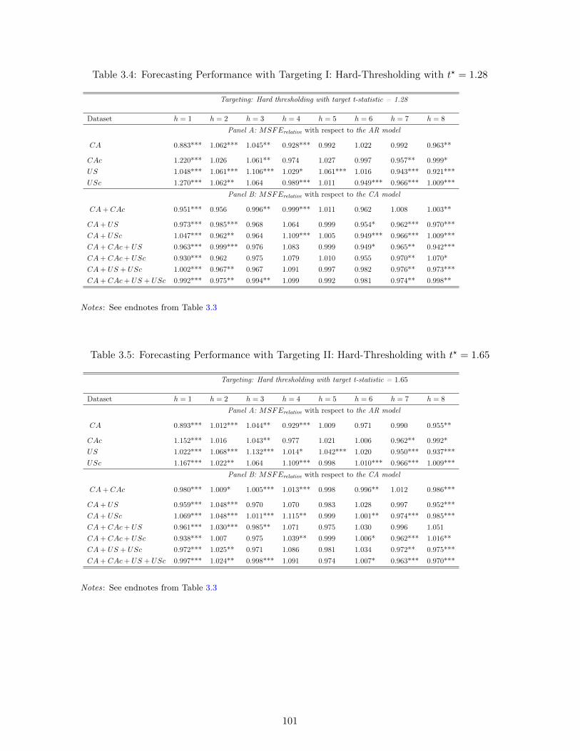
Table 3.4: Forecasting Performance with Targeting I: Hard-Thresholding with t? = 1.28

Targeting: Hard thresholding with target t-statistic = 1.28



CA 0.883*** 1.062*** 1.045** 0.928*** 0.992 1.022 0.992 0.963**

CAc 1.220*** 1.026 1.061** 0.974 1.027 0.997 0.957** 0.999*US 1.048*** 1.061*** 1.106*** 1.029* 1.061*** 1.016 0.943*** 0.921***USc 1.270*** 1.062** 1.064 0.989*** 1.011 0.949*** 0.966*** 1.009***


CA+ CAc 0.951*** 0.956 0.996** 0.999*** 1.011 0.962 1.008 1.003**

CA+ US 0.973*** 0.985*** 0.968 1.064 0.999 0.954* 0.962*** 0.970***CA+ USc 1.047*** 0.962** 0.964 1.109*** 1.005 0.949*** 0.966*** 1.009***CA+ CAc+ US 0.963*** 0.999*** 0.976 1.083 0.999 0.949* 0.965** 0.942***CA+ CAc+ USc 0.930*** 0.962 0.975 1.079 1.010 0.955 0.970** 1.070*CA+ US + USc 1.002*** 0.967** 0.967 1.091 0.997 0.982 0.976** 0.973***CA+ CAc+ US + USc 0.992*** 0.975** 0.994** 1.099 0.992 0.981 0.974** 0.998**

Notes: See endnotes from Table 3.3

Table 3.5: Forecasting Performance with Targeting II: Hard-Thresholding with t? = 1.65

Targeting: Hard thresholding with target t-statistic = 1.65



CA 0.893*** 1.012*** 1.044** 0.929*** 1.009 0.971 0.990 0.955**

CAc 1.152*** 1.016 1.043** 0.977 1.021 1.006 0.962** 0.992*US 1.022*** 1.068*** 1.132*** 1.014* 1.042*** 1.020 0.950*** 0.937***USc 1.167*** 1.022** 1.064 1.109*** 0.998 1.010*** 0.966*** 1.009***


CA+ CAc 0.980*** 1.009* 1.005*** 1.013*** 0.998 0.996** 1.012 0.986***

CA+ US 0.959*** 1.048*** 0.970 1.070 0.983 1.028 0.997 0.952***CA+ USc 1.069*** 1.048*** 1.011*** 1.115** 0.999 1.001** 0.974*** 0.985***CA+ CAc+ US 0.961*** 1.030*** 0.985** 1.071 0.975 1.030 0.996 1.051CA+ CAc+ USc 0.938*** 1.007 0.975 1.039** 0.999 1.006* 0.962*** 1.016**CA+ US + USc 0.972*** 1.025** 0.971 1.086 0.981 1.034 0.972** 0.975***CA+ CAc+ US + USc 0.997*** 1.024** 0.998*** 1.091 0.974 1.007* 0.963*** 0.970***


101

Table 3.6: Forecasting Performance with Targeting I: Hard-Thresholding with t? = 2.58

Targeting method: Hard thresholding with target tstatistic = 2.58



CA 0.811*** 0.999 1.024 0.887*** 0.988 0.980 0.984 0.954**

CAc 1.148*** 1.016 1.065*** 0.980 1.044*** 1.009 0.988 1.006US 1.048*** 1.051*** 1.133*** 1.030** 1.049*** 1.016 0.948*** 0.954***USc 1.133*** 1.049** 1.091 1.073** 1.060 1.025 1.004 1.024


CA+ CAc 1.017*** 1.002 0.993 1.041*** 1.001 0.996* 0.992* 0.996***

CA+ US 1.033*** 1.035** 0.963 1.063*** 1.003 1.008 0.974*** 0.968***CA+ USc 1.033*** 1.049** 0.991 1.073** 1.020 1.025 1.034 1.024CA+ CAc+ US 1.064*** 1.035** 0.965 1.066*** 1.003 1.025 0.976** 0.969***CA+ CAc+ USc 1.012*** 0.999 0.992 1.060*** 1.006 1.011 0.983** 1.018*CA+ US + USc 1.074*** 1.044*** 0.964 1.081*** 1.006 1.020 0.975*** 0.966***CA+ CAc+ US + USc 1.079*** 1.045*** 0.974 1.057*** 1.006 1.024 0.973*** 0.971***


102

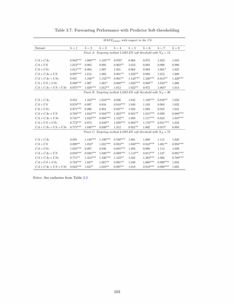
Table 3.7: Forecasting Performance with Predictor Soft-thresholding

MSFErelative with respect to the CA


Panel A: Targeting method LARS-EN soft threshold with NA = 15

CA+ CAc 0.982*** 1.080*** 1.183*** 0.976* 0.968 0.973 1.023 1.010CA+ US 1.013*** 0.982 0.995 0.962** 1.013 0.982 0.999 0.996CA+ USc 1.011*** 0.994 1.007 1.021 0.964 0.983 1.001* 1.025CA+ CAc+ US 0.997*** 1.012 1.003 0.981** 1.022** 0.989 1.012 1.009CA+ CAc+ USc 0.837 1.106** 1.152*** 0.901** 1.143*** 1.230*** 0.913** 1.429***CA+ US + USc 0.898*** 1.007 1.001* 0.980*** 1.022*** 0.968** 1.010** 1.006CA+ CAc+ US + USc 0.975*** 1.038*** 1.012** 1.012 1.022** 0.972 1.005* 1.014

Panel B: Targeting method LARS-EN soft threshold with NA = 30

CA+ CAc 0.852 1.162*** 1.016*** 0.936 1.042 1.188*** 0.858** 1.050CA+ US 0.970*** 0.997 0.816 0.918*** 1.040 1.103 0.903 1.033CA+ USc 0.971*** 0.996 0.804 0.927** 1.034 1.093 0.910 1.041CA+ CAc+ US 0.703*** 1.034*** 0.924*** 1.263*** 0.931** 1.015*** 0.929 0.988***CA+ CAc+ USc 0.745** 1.042*** 0.888*** 1.132** 1.080 1.117*** 0.823 1.047***CA+ US + USc 0.772*** 0.973 0.849** 1.039*** 0.983** 1.176*** 0.851*** 1.033CA+ CAc+ US + USc 0.775*** 1.048*** 0.939** 1.312 0.921** 1.002 0.915* 0.993

Panel C: Targeting method LARS-EN soft threshold with NA = 75

CA+ CAc 0.895 1.130*** 1.190*** 0.780*** 1.091 1.009 1.115 1.020CA+ US 0.899** 1.024* 1.031*** 0.924** 1.030*** 0.942*** 1.081** 0.994***CA+ USc 1.035*** 0.997 0.946 0.885*** 1.083 0.990 1.114 1.039CA+ CAc+ US 0.959*** 0.936*** 1.026*** 0.889*** 1.113** 0.914*** 1.127 0.991***CA+ CAc+ USc 0.771** 1.454*** 1.336*** 1.123** 1.022 1.282*** 1.086 0.780***CA+ US + USc 0.784*** 1.037* 1.001** 0.991** 1.049 1.060*** 0.998*** 1.050CA+ CAc+ US + USc 0.923*** 1.047* 1.010** 0.997** 1.019 0.910*** 0.998*** 1.005


103

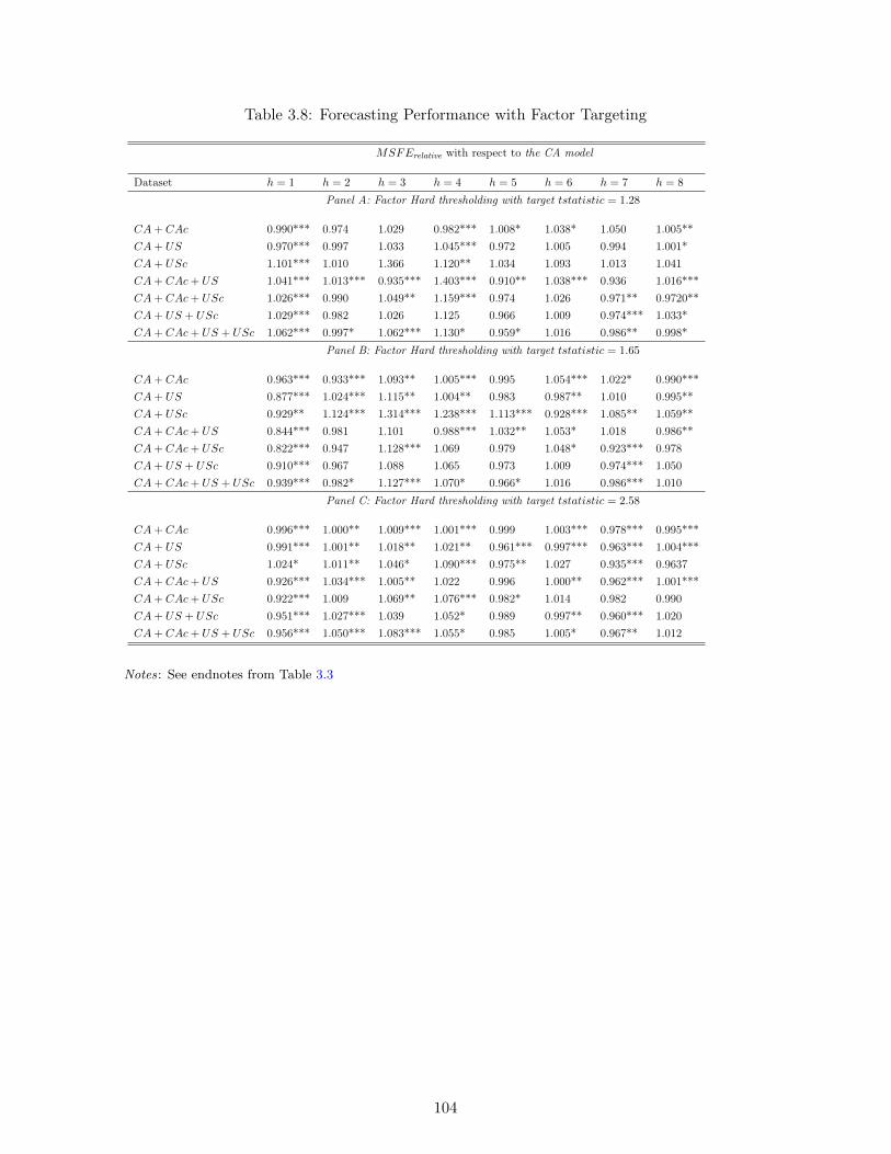
Table 3.8: Forecasting Performance with Factor Targeting

MSFErelative with respect to the CA model


Panel A: Factor Hard thresholding with target tstatistic = 1.28

CA+ CAc 0.990*** 0.974 1.029 0.982*** 1.008* 1.038* 1.050 1.005**CA+ US 0.970*** 0.997 1.033 1.045*** 0.972 1.005 0.994 1.001*CA+ USc 1.101*** 1.010 1.366 1.120** 1.034 1.093 1.013 1.041CA+ CAc+ US 1.041*** 1.013*** 0.935*** 1.403*** 0.910** 1.038*** 0.936 1.016***CA+ CAc+ USc 1.026*** 0.990 1.049** 1.159*** 0.974 1.026 0.971** 0.9720**CA+ US + USc 1.029*** 0.982 1.026 1.125 0.966 1.009 0.974*** 1.033*CA+ CAc+ US + USc 1.062*** 0.997* 1.062*** 1.130* 0.959* 1.016 0.986** 0.998*

Panel B: Factor Hard thresholding with target tstatistic = 1.65

CA+ CAc 0.963*** 0.933*** 1.093** 1.005*** 0.995 1.054*** 1.022* 0.990***CA+ US 0.877*** 1.024*** 1.115** 1.004** 0.983 0.987** 1.010 0.995**CA+ USc 0.929** 1.124*** 1.314*** 1.238*** 1.113*** 0.928*** 1.085** 1.059**CA+ CAc+ US 0.844*** 0.981 1.101 0.988*** 1.032** 1.053* 1.018 0.986**CA+ CAc+ USc 0.822*** 0.947 1.128*** 1.069 0.979 1.048* 0.923*** 0.978CA+ US + USc 0.910*** 0.967 1.088 1.065 0.973 1.009 0.974*** 1.050CA+ CAc+ US + USc 0.939*** 0.982* 1.127*** 1.070* 0.966* 1.016 0.986*** 1.010

Panel C: Factor Hard thresholding with target tstatistic = 2.58

CA+ CAc 0.996*** 1.000** 1.009*** 1.001*** 0.999 1.003*** 0.978*** 0.995***CA+ US 0.991*** 1.001** 1.018** 1.021** 0.961*** 0.997*** 0.963*** 1.004***CA+ USc 1.024* 1.011** 1.046* 1.090*** 0.975** 1.027 0.935*** 0.9637CA+ CAc+ US 0.926*** 1.034*** 1.005** 1.022 0.996 1.000** 0.962*** 1.001***CA+ CAc+ USc 0.922*** 1.009 1.069** 1.076*** 0.982* 1.014 0.982 0.990CA+ US + USc 0.951*** 1.027*** 1.039 1.052* 0.989 0.997** 0.960*** 1.020CA+ CAc+ US + USc 0.956*** 1.050*** 1.083*** 1.055* 0.985 1.005* 0.967** 1.012


104

Conclusion

This thesis investigated the effect of information on macroeconomic forecasting. Firstly, wefocus on the impact of information frictions in open economy in forecasting the bilateral ex-change rate. Specifically, the forward premium puzzle is a well-documented strand of researchin the international finance but no consensus has emerged from the literature for its explana-tion so far. We contribute to this research agenda by proposing a learning-based explanation.Secondly, we analyse the role of information from confidence -or sentimentdata in forecast-ing real economic activity. Precisely, survey data on confidence has become more popularamong researchers and economic agents but from the literature there is lack of evidence abouttheir usefulness in macroeconomic forecasting. We contribute to this growing literature onsentiment data by investigating the role of information contained in confidence-based surveydata (either at the national or international level) in forecasting real economic activity in theCanadian context.

In the first chapter, based on the new open-economy macroeconomics paradigm (NOEM),we incorporate information frictions and nominal rigidities in a stochastic dynamic generalequilibrium (DSGE) model in open economy. Then, we present a comparative analysis of theresults of the exchange rate forecast obtained using the model with and without these infor-mation frictions. We find that the developments of the realized depreciation of exchange ratesas observed in foreign exchange markets are coherent with the learning behavior of agentsabout the transitory or permanent features of the shocks as the simulated data under incom-plete information replicate the puzzle. The forward premium puzzle could emerge becauseof the existence of information frictions and the learning dynamics. Such evidences are notincoherent with the rational expectation hypothesis because the learning process implementedby the agent in the economy could explain the alteration of the predictions. Possible avenuesfor fruitful future research include either using other filters for the signal extraction problemor allow a risk structure in a model with stochastic volatility.

In the second chapter, we assess the contribution of confidence -or sentimentdata in predictingCanadian economic slowdowns. A probit framework is applied to an indicator on the status ofthe Canadian business cycle produced by the OECD and using among explanatory variablesthe factors derived from amalgamated confidence and macroeconomic data. We report that

106

Canadian data on sentiment, as gathered from the answers to four different available surveys,significantly help forecast future slowdowns in the Canadian economy. Further we show thatusing all available such data, by amalgamating all time-series and extracting factors fromthe amalgamated dataset, provides substantially improved forecasts relative to those obtainedusing individual series or simple averages of sentiment data.

In the third chapter, we use dynamic factor models with targeting to highlight the contributionof information contained in confidence-based survey data (either at the national or interna-tional level) in forecasting Canadian real GDP. We find that Canadian data on sentimentcan contribute substantially to the task of forecasting the Canadian business cycle, partic-ularly when all available such sentiment. The results show that confidence variables (bothnational and international) contain relevant predictive ability for Canadian real economic ac-tivity when combined with other datasets. Confidence data displays quality-extra informationcontent which allows outperforming any combination of datasets without confidence variables.The best forecasting performance is obtained by combining Canadian and US confidence withCanadian macroeconomic and financial variables in a large dataset to derive factors. Furtherthe overall results suggest that disaggregated confidence survey data on investor, business andconsumer both at national and international level are informative in the forecasting of nationalreal economic activity.

A promising avenue for future research includes evaluating the dispersion of out-of-samplepoint forecasts as a measure of uncertainty in forecasting with confidence data. Furthermore,recent research highlights the interest of using density forecast to measure uncertainty aroundmacroeconomic forecasting outcomes. Another important avenue for future research includesevaluating the success of density forecasting when dealing with data-rich models and confidencedata.

107

Appendix A

Survey Data on Sentiment

A.1 Conference Board Consumer Confidence survey

The Conference Board of Canada has been operating a monthly survey of Canadian households since1979, to measure levels of optimism regarding current and future economic conditions. Surveyedhouseholds are asked to give their views about their current and expected financial positions andemployment outlook. In addition, they are also asked to assess whether now is a good time or a badtime to make a major purchase such as a house, car or other big-ticket items. Specifically, the fourquestions comprising the survey are as follows:

1. Considering everything, would you say that your family is better or worse off financially thansix months ago?

2. Again, considering everything, do you think that your family will be better off, the same orworse off financially six months from now?

3. How do you feel the job situation and overall employment will be in this community six monthsfrom now?

4. Do you think that right now is a good or bad time for the average person to make a majoroutlay for items such as a home, car or other major item?

Each question is answered positively or negatively; for example, a surveyed household answering thathis family is better off financially than six months ago (first question) will be labelled as havingresponded positively.

The Conference Board then aggregates answers by calculating the ratio of positive responses for eachquestion and taking the simple average across the four questions to create the publicly available Indexof Consumer Confidence. As such, this index represents one specific way to aggregate informationcontained in the survey. As indicated in the text, the present paper assesses whether more flexibleaggregation methods arising from factor models can improve on the signaling ability of these data.

109

A.2 Conference Board Business Confidence Survey

The Conference Board of Canada has been operating a quarterly survey of Canadian business execu-tives since 1977. The survey is meant to measure perceptions of the current economic environment andthe investment intentions of business. The questions comprising the survey, as well as all categoriesfor the answers, are detailed below. As was the case for the Consumer survey, the Conference Boardconstructs an aggregate of survey answers, the Index of Business Confidences by summing the netratio of positive answers to the third, fifth and eight questions below.

List of questions in the Business Confidence Survey

1. Do you expect overall economic conditions in Canada six months from now to be:

• Better,

• Worse,

• The same.

2. Do you expect prices, in general, in Canada to increase over the next six months at an annual rate of:(data since 1987Q3)

• < 1%

• 1%

• 2%

• 3%

• 4%

• 5%

• 6%

• 7%

• 8%

• > 8%

3. Over the next six months, do you expect your firm’s financial position to:

• Improve,

• Worsen,

• Remain the same.

4. Over the next six months, do you expect your firm’s profitability to:

• Improve,

• Worsen,

• Remain the same.

5. Would you say the present is a good or a bad time to undertake expenditures to expand your plant oradd to your stock of machinery and equipment?

• Good,

110

• Bad,

• Not sure.

6. What change in the level of your capital investment expenditures do you expect over the next 6 months?

• Up 20%

• Up 10% to 19%

• Up 1% to 9%

• No change,

• Down 1% to 9%

• Down 10% to 19%

• Down 20% or more.

7. In which region(s) of the country do you expect the bulk of your planned investment expenditures forthe next six months to take place? (data since 1987Q3)

• Atlantic Provinces,

• Quebec,

• Ontario,

• Prairie Provinces,

• British Columbia,

• United States, (data since 1994Q4)

• International. (data since 1994Q4)

8. How do you assess your current level of operations relative to optimal capacity?

• Above capacity,

• At or close to capacity,

• At, close to, or above, capacity

• Slightly below capacity,

• Substantially below capacity.

9. Compared with six months ago, what is your current rate of return to invested capital?

• Better than expected,

• As expected,

• Worse than expected.

10. What factors, if any, are currently adversely affecting the level of your planned expenditures in Canada?

• Excess productive capacity,

• Weak market demand,

• Foreign competition,

• Rising cost of capital goods,

• Rising labour costs,

• Overall corporate liquidity,

111

• High interest rates,

• Weak commodity prices,

• Shortage of qualified staff,

• Government policies,

• Taxes,

• More attractive opportunities outside Canada,

• Appreciation of the Canadian dollar,

• Depreciation of the Canadian dollar.

112

A.3 Bank of Canada Business Outlook Survey

The Business Outlook Survey is a quarterly survey of the senior management of 100 Canadian busi-nesses that are selected with a view to produce a representative selection of Canada’s gross domesticproduct. The survey’s was initiated in the Fall of 1997 and its purpose is to “gather the perspectives ofthese businesses on topics of interest to the Bank of Canada (such as demand and capacity pressures)and their forward-looking views on economic activity” and is conducted by the staff of the regionaloffices of the Bank. It was created to extend and formalize the informal discussion that the Bank asalways conducted with relevant Canadian economic actors.

Each question elicits a categorical response from a surveyed firm (see below for the list of all questionsand answer categories) and the Bank of Canada makes the percentage of firms answering each answercategory publicly available. In addition, the Bank emphasizes a “balance of opinion” synthesis foreach question, which is constructed by substracting the percentage of negative responses from thepercentage of positive ones (balance of opinion can thus vary between −100 and 100). The completelist of all questions and answer categories is as follows:

List of questions in the Business Outlook Survey

1. (PAST SALES GROWTH) Over the past 12 months, the rate of increase in your firm’s sales volume(compared with the previous 12 months) was. . .

• Greater,

• Less,

• The same.

2. (FUTURE SALES GROWTH) Over the next 12 months, the rate of increase in your firm’s sales volume(compared with the past 12 months) is expected to be. . .

• Greater,

• Less,

• The same.

3. (FUTURE SALES GROWTH) Compared with 12 months ago, have your recent indicators (order books,advanced bookings, sales inquiries, etc.)... (Data since 2003Q3)

• Improved,

• Deteriorated.

4. (INVESTMENT IN MACHINERY AND EQUIPMENT) Over the next 12 months, your firm’s invest-ment spending on M & E (compared with the past 12 months) is expected to be. . .

• Higher,

• Lower,

• The same.

5. (FUTURE EMPLOYMENT LEVEL) Over the next 12 months, your firm’s level of employment isexpected to be. . .

• Higher,

113

• Lower,

• The same.

6. (ABILITY TO MEET DEMAND) How would you rate the current ability of your firm to meet anunexpected increase in demand? (Data since 1999Q3)

• Some difficulty,

• Significant difficulty.

7. (LABOUR SHORTAGES) Does your firm face any shortages of labour that restrict your ability to meetdemand?

• Yes,

• No.

8. (INTENSITY OF LABOUR SHORTAGES) Compared with 12 months ago, are labour shortages gen-erally...(Data since 2001Q1)

• More intense,

• Less intense.

9. (INPUT PRICE INFLATION) Over the next 12 months, are prices of products/services purchasedexpected to increase at a greater, lesser, or the same rate as over the past year?

• Greater,

• Less,

• The same.

10. (OUTPUT PRICE INFLATION) Over the next 12 months, are prices of products/services sold expectedto increase at a greater, lesser, or the same rate as over the past year?

• Greater,

• Less,

• The same.

11. (INFLATION EXPECTATIONS) Over the next two years, what do you expect the annual rate ofinflation to be, based on the consumer price index? (Data since 2001Q2)

• Above 3%,

• 2% to 3%,

• 1% to 2%,

• Below 1%.

12. (CREDIT CONDITIONS) Over the past 3 months, how have the terms and conditions for obtainingfinancing changed (compared with the previous 3 months)? (Data since 2001Q4)

• Tightened,

• Eased.

114

A.4 Bank of Canada Senior Loan Officer Survey

The bank of Canada has been conducting the Senior Loan Officer Survey since 1999. This quar-terly survey assesses the business-lending practices of major Canadian financial institutions, gatheringinformation both on price but also non-price terms of business lending.

Specifically, the survey asks the Senior Loan Officer of participating institutions the following question:How have your institution’s general standards (i.e. your appetite for risk) and terms for approvingcredit changed in the past three months?

• Tightened,

• Eased,

• Remain unchanged.

Surveyed institutions condition their answer on the evolution of business lending conditions by takinginto account each of the following conditions:

1. Pricing of credit (spreads over base rates, fees),

2. General standards,

3. Limit of capital allocation,

4. Terms of credit (collateral, covenants, etc.),

so that a given institution could, in principle, report tightening conditions on pricing of credit buteasing them with respect to general standards, limits or terms of credit. Two balance of opinion timesseries are made publicly available by the Bank of Canada: the balance of opinion to the pricing ofcredit, as well as a non-price aggregate to the remaining three categories (a “tightening" is coded if theinstitution reports tightening either general standards, limits of capital allocation or terms of credit).1

1The questions are further detailed as to whether they pertain to loans provided to corporate, commercialand small business firms; responses for commercial and small business firms are further provided for five regions:British Columbia, the Prairies, Ontario, Quebec, and the Atlantic provinces.

115

Appendix B

B.1 Canadian Business Cycles according to the OECD

The OECD maintains a database of the status of the business cycles for each member country. Theclassification follows a growth-cycle methodology and the following dates of peaks and troughs areobtained for Canada:

Table B.1: Chronology of the Canadian Business Cycle Since 1961

Monthly Trough Monthly Peak1961 M3 1962 M21963 M6 1966 M41968 M1 1968 M121971 M2 1974 M11975 M5 1976 M61977 M7 1979 M111982 M11 1985 M111986 M11 1989 M51992 M5 1994 M121996 M8 2000 M62001 M10 2002 M72003 M10 2007 M82009 M7 2011 M112012 M11 2014 M10

Note: Source: OECD. http://www.oecd.org/std/leading-indicators/CLI-components-and-turning-points.pdf.

116

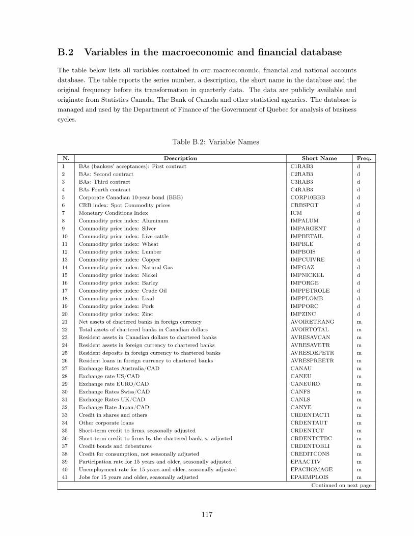
B.2 Variables in the macroeconomic and financial database

The table below lists all variables contained in our macroeconomic, financial and national accountsdatabase. The table reports the series number, a description, the short name in the database and theoriginal frequency before its transformation in quarterly data. The data are publicly available andoriginate from Statistics Canada, The Bank of Canada and other statistical agencies. The database ismanaged and used by the Department of Finance of the Government of Quebec for analysis of businesscycles.

Table B.2: Variable Names

N. Description Short Name Freq.1 BAs (bankers’ acceptances): First contract C1RAB3 d2 BAs: Second contract C2RAB3 d3 BAs: Third contract C3RAB3 d4 BAs Fourth contract C4RAB3 d5 Corporate Canadian 10-year bond (BBB) CORP10BBB d6 CRB index: Spot Commodity prices CRBSPOT d7 Monetary Conditions Index ICM d8 Commodity price index: Aluminum IMPALUM d9 Commodity price index: Silver IMPARGENT d10 Commodity price index: Live cattle IMPBETAIL d11 Commodity price index: Wheat IMPBLE d12 Commodity price index: Lumber IMPBOIS d13 Commodity price index: Copper IMPCUIVRE d14 Commodity price index: Natural Gas IMPGAZ d15 Commodity price index: Nickel IMPNICKEL d16 Commodity price index: Barley IMPORGE d17 Commodity price index: Crude Oil IMPPETROLE d18 Commodity price index: Lead IMPPLOMB d19 Commodity price index: Pork IMPPORC d20 Commodity price index: Zinc IMPZINC d21 Net assets of chartered banks in foreign currency AVOIRETRANG m22 Total assets of chartered banks in Canadian dollars AVOIRTOTAL m23 Resident assets in Canadian dollars to chartered banks AVRESAVCAN m24 Resident assets in foreign currency to chartered banks AVRESAVETR m25 Resident deposits in foreign currency to chartered banks AVRESDEPETR m26 Resident loans in foreign currency to chartered banks AVRESPREETR m27 Exchange Rates Australia/CAD CANAU m28 Exchange rate US/CAD CANEU m29 Exchange rate EURO/CAD CANEURO m30 Exchange Rates Swiss/CAD CANFS m31 Exchange Rates UK/CAD CANLS m32 Exchange Rate Japan/CAD CANYE m33 Credit in shares and others CRDENTACTI m34 Other corporate loans CRDENTAUT m35 Short-term credit to firms, seasonally adjusted CRDENTCT m36 Short-term credit to firms by the chartered bank, s. adjusted CRDENTCTBC m37 Credit bonds and debentures CRDENTOBLI m38 Credit for consumption, not seasonally adjusted CREDITCONS m39 Participation rate for 15 years and older, seasonally adjusted EPAACTIV m40 Unemployment rate for 15 years and older, seasonally adjusted EPACHOMAGE m41 Jobs for 15 years and older, seasonally adjusted EPAEMPLOIS m

Continued on next page

117

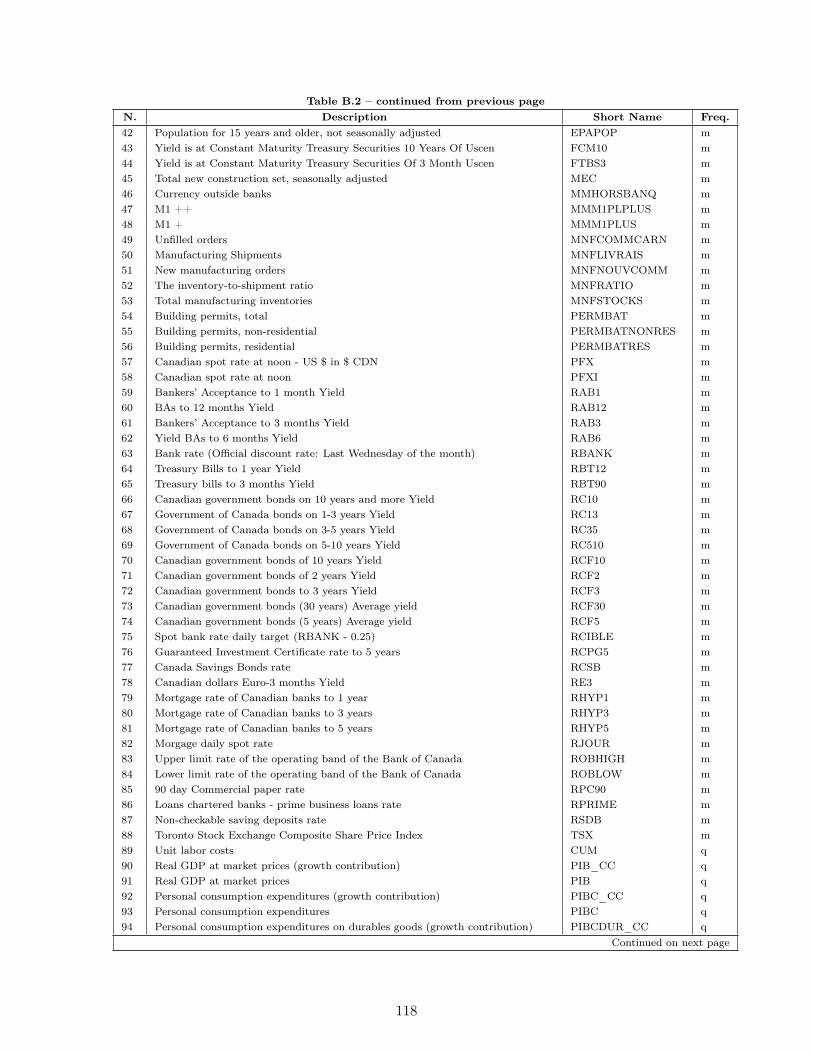
Table B.2 – continued from previous pageN. Description Short Name Freq.42 Population for 15 years and older, not seasonally adjusted EPAPOP m43 Yield is at Constant Maturity Treasury Securities 10 Years Of Uscen FCM10 m44 Yield is at Constant Maturity Treasury Securities Of 3 Month Uscen FTBS3 m45 Total new construction set, seasonally adjusted MEC m46 Currency outside banks MMHORSBANQ m47 M1 ++ MMM1PLPLUS m48 M1 + MMM1PLUS m49 Unfilled orders MNFCOMMCARN m50 Manufacturing Shipments MNFLIVRAIS m51 New manufacturing orders MNFNOUVCOMM m52 The inventory-to-shipment ratio MNFRATIO m53 Total manufacturing inventories MNFSTOCKS m54 Building permits, total PERMBAT m55 Building permits, non-residential PERMBATNONRES m56 Building permits, residential PERMBATRES m57 Canadian spot rate at noon - US $ in $ CDN PFX m58 Canadian spot rate at noon PFXI m59 Bankers’ Acceptance to 1 month Yield RAB1 m60 BAs to 12 months Yield RAB12 m61 Bankers’ Acceptance to 3 months Yield RAB3 m62 Yield BAs to 6 months Yield RAB6 m63 Bank rate (Official discount rate: Last Wednesday of the month) RBANK m64 Treasury Bills to 1 year Yield RBT12 m65 Treasury bills to 3 months Yield RBT90 m66 Canadian government bonds on 10 years and more Yield RC10 m67 Government of Canada bonds on 1-3 years Yield RC13 m68 Government of Canada bonds on 3-5 years Yield RC35 m69 Government of Canada bonds on 5-10 years Yield RC510 m70 Canadian government bonds of 10 years Yield RCF10 m71 Canadian government bonds of 2 years Yield RCF2 m72 Canadian government bonds to 3 years Yield RCF3 m73 Canadian government bonds (30 years) Average yield RCF30 m74 Canadian government bonds (5 years) Average yield RCF5 m75 Spot bank rate daily target (RBANK - 0.25) RCIBLE m76 Guaranteed Investment Certificate rate to 5 years RCPG5 m77 Canada Savings Bonds rate RCSB m78 Canadian dollars Euro-3 months Yield RE3 m79 Mortgage rate of Canadian banks to 1 year RHYP1 m80 Mortgage rate of Canadian banks to 3 years RHYP3 m81 Mortgage rate of Canadian banks to 5 years RHYP5 m82 Morgage daily spot rate RJOUR m83 Upper limit rate of the operating band of the Bank of Canada ROBHIGH m84 Lower limit rate of the operating band of the Bank of Canada ROBLOW m85 90 day Commercial paper rate RPC90 m86 Loans chartered banks - prime business loans rate RPRIME m87 Non-checkable saving deposits rate RSDB m88 Toronto Stock Exchange Composite Share Price Index TSX m89 Unit labor costs CUM q90 Real GDP at market prices (growth contribution) PIB_CC q91 Real GDP at market prices PIB q92 Personal consumption expenditures (growth contribution) PIBC_CC q93 Personal consumption expenditures PIBC q94 Personal consumption expenditures on durables goods (growth contribution) PIBCDUR_CC q

Continued on next page

118

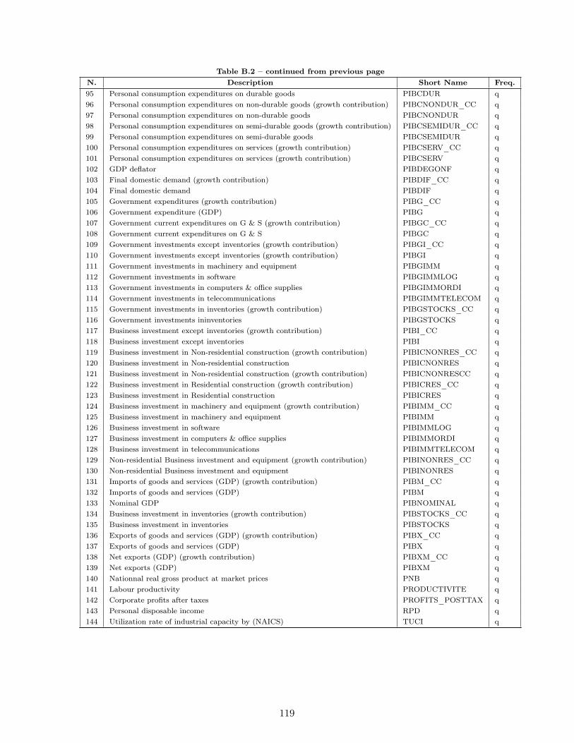
Table B.2 – continued from previous pageN. Description Short Name Freq.95 Personal consumption expenditures on durable goods PIBCDUR q96 Personal consumption expenditures on non-durable goods (growth contribution) PIBCNONDUR_CC q97 Personal consumption expenditures on non-durable goods PIBCNONDUR q98 Personal consumption expenditures on semi-durable goods (growth contribution) PIBCSEMIDUR_CC q99 Personal consumption expenditures on semi-durable goods PIBCSEMIDUR q100 Personal consumption expenditures on services (growth contribution) PIBCSERV_CC q101 Personal consumption expenditures on services (growth contribution) PIBCSERV q102 GDP deflator PIBDEGONF q103 Final domestic demand (growth contribution) PIBDIF_CC q104 Final domestic demand PIBDIF q105 Government expenditures (growth contribution) PIBG_CC q106 Government expenditure (GDP) PIBG q107 Government current expenditures on G & S (growth contribution) PIBGC_CC q108 Government current expenditures on G & S PIBGC q109 Government investments except inventories (growth contribution) PIBGI_CC q110 Government investments except inventories (growth contribution) PIBGI q111 Government investments in machinery and equipment PIBGIMM q112 Government investments in software PIBGIMMLOG q113 Government investments in computers & office supplies PIBGIMMORDI q114 Government investments in telecommunications PIBGIMMTELECOM q115 Government investments in inventories (growth contribution) PIBGSTOCKS_CC q116 Government investments ininventories PIBGSTOCKS q117 Business investment except inventories (growth contribution) PIBI_CC q118 Business investment except inventories PIBI q119 Business investment in Non-residential construction (growth contribution) PIBICNONRES_CC q120 Business investment in Non-residential construction PIBICNONRES q121 Business investment in Non-residential construction (growth contribution) PIBICNONRESCC q122 Business investment in Residential construction (growth contribution) PIBICRES_CC q123 Business investment in Residential construction PIBICRES q124 Business investment in machinery and equipment (growth contribution) PIBIMM_CC q125 Business investment in machinery and equipment PIBIMM q126 Business investment in software PIBIMMLOG q127 Business investment in computers & office supplies PIBIMMORDI q128 Business investment in telecommunications PIBIMMTELECOM q129 Non-residential Business investment and equipment (growth contribution) PIBINONRES_CC q130 Non-residential Business investment and equipment PIBINONRES q131 Imports of goods and services (GDP) (growth contribution) PIBM_CC q132 Imports of goods and services (GDP) PIBM q133 Nominal GDP PIBNOMINAL q134 Business investment in inventories (growth contribution) PIBSTOCKS_CC q135 Business investment in inventories PIBSTOCKS q136 Exports of goods and services (GDP) (growth contribution) PIBX_CC q137 Exports of goods and services (GDP) PIBX q138 Net exports (GDP) (growth contribution) PIBXM_CC q139 Net exports (GDP) PIBXM q140 Nationnal real gross product at market prices PNB q141 Labour productivity PRODUCTIVITE q142 Corporate profits after taxes PROFITS_POSTTAX q143 Personal disposable income RPD q144 Utilization rate of industrial capacity by (NAICS) TUCI q

119

Bibliography

K. A. Aastveit, A. Carriero, T. Clark, and M. Marcellino. Have standard vars remained stablesince the crisis? 2014.

G. A. Akerlof and R. J. Shiller. Animal spirits: How human psychology drives the economy,and why it matters for global capitalism. Princeton University Press, 2010.

R. Albuquerque. The forward premium puzzle in a model of imperfect information. Economicsletters, 99(3):461–464, 2008.

H. M. Anderson and F. Vahid. Predicting the probability of a recession with nonlinear au-toregressive leading-indicator models. Macroeconomic Dynamics, 5(4):482–505, 2001.

D. Andolfatto and P. Gomme. Monetary policy regimes and beliefs. International EconomicReview, 44(1):1–30, 2003.

D. Andolfatto, S. Hendry, and K. Moran. Are inflation expectations rational? Journal ofMonetary Economics, 55(2):406–422, 2008.

P. Bacchetta and E. Van Wincoop. Can information heterogeneity explain the exchange ratedetermination puzzle? The American Economic Review, 96(3):552–576, 2006.

P. Bacchetta and E. Van Wincoop. Infrequent portfolio decisions: A solution to the forwarddiscount puzzle. The American Economic Review, 100(3):870–904, 2010.

P. Bacchetta and E. Van Wincoop. On the unstable relationship between exchange rates andmacroeconomic fundamentals. Journal of International Economics, 91(1):18–26, 2013.

P. Bacchetta, E. van Wincoop, et al. Modeling exchange rates with incomplete information.DEEP, 2011.

D. Backus, P. J. Kehoe, and F. E. Kydland. International business cycles: Theory andevidence. NBER Working Paper Series, (w4493), 1993.

D. K. Backus, S. Foresi, and C. I. Telmer. Affine term structure models and the forwardpremium anomaly. The Journal of Finance, 56(1):279–304, 2001.

121

D. K. Backus, F. Gavazzoni, C. Telmer, and S. E. Zin. Monetary policy and the uncoveredinterest parity puzzle. NBER Working Paper Series, (w16218), 2010.

J. Bai. Inferential theory for factor models of large dimensions. Econometrica, 71(1):135–171,2003.

J. Bai and S. Ng. Determining the number of factors in approximate factor models.Econometrica, 70(1):191–221, 2002.

J. Bai and S. Ng. Confidence intervals for diffusion index forecasts and inference for factor-augmented regressions. Econometrica, 74(4):1133–1150, 2006.

J. Bai and S. Ng. Forecasting economic time series using targeted predictors. Journal ofEconometrics, 146(2):304–317, 2008.

J. Bai and S. Ng. Boosting diffusion indices. Journal of Applied Econometrics, 24(4):607–629,2009.

J. Bai and S. Ng. Principal components estimation and identification of static factors. Journalof Econometrics, 176(1):18–29, 2013.

R. E. Baldwin. Re-interpreting the failure of foreign exchange market efficiency tests: Smalltransaction costs, big hysteresis bands. NBER Working Paper 3319, 1990.

R. Bansal and M. Dahlquist. The forward premium puzzle: different tales from developed andemerging economies. Journal of International Economics, 51(1):115–144, 2000.

R. B. Barsky and E. R. Sims. Information, animal spirits, and the meaning of innovations inconsumer confidence. Technical report, National Bureau of Economic Research, 2009.

R. B. Barsky and E. R. Sims. Information, animal spirits, and the meaning of innovations inconsumer confidence. The American Economic Review, 102:1343–1377, 2012.

R. Batchelor and P. Dua. Improving macro-economic forecasts: The role of consumer confi-dence. International Journal of Forecasting, 14(1):71–81, 1998.

P. Beaudry and F. Portier. Stock prices, news and economic fluctuations. Technical report,National Bureau of Economic Research, 2004.

P. Beaudry and F. Portier. Stock prices, news, and economic fluctuations. The AmericanEconomic Review, 96(4):1293–1307, 2006.

G. Bekaert. Exchange rate volatility and deviations from unbiasedness in a cash-in-advancemodel. Journal of International Economics, 36(1):29–52, 1994.

G. Bekaert and R. J. Hodrick. Expectations hypotheses tests. The journal of finance, 56(4):1357–1394, 2001.

122

G. Benigno and P. Benigno. Exchange rate determination under interest rate rules. Journalof International Money and Finance, 27(6):971–993, 2008.

G. Benigno, P. Benigno, and S. Nisticò. Risk, monetary policy and the exchange rate. NBERWorking Paper Series, (w17133), 2011.

B. Bernanke. Stabilizing the financial markets and the economy. speech made at the EconomicClub of New York, New York, New York, 15, 2008.

A. Binette and J. Chang. CSI: A model for tracking short-term growth in Canadian realGDP. Bank of Canada Review, Summer 2013a.

A. Binette and J. Chang. CSI: A model for tracking short-term growth in Canadian real GDP.Bank of Canada Review, 2013(Summer):3–12, 2013b.

C. R. Birchenhall, H. Jessen, D. R. Osborn, and P. Simpson. Predicting us business-cycleregimes. Journal of Business & Economic Statistics, 17(3):313–323, 1999.

G. Bodo, R. Golinelli, and G. Parigi. Forecasting industrial production in the Euro area.Empirical economics, 25(4):541–561, 2000.

J. Boivin and S. Ng. Are more data always better for factor analysis? Journal of Econometrics,132(1):169–194, 2006.

J. Boudoukh, M. Richardson, and R. F. Whitelaw. A new look at the forward premium puzzle.Stern School of Business, Manuscript, 2012.

G. W. Brier. Verification of forecasts expressed in terms of probability. Monthly weatherreview, 78(1):1–3, 1950.

M. Brisson, B. Campbell, and J. W. Galbraith. Forecasting some low-predictability time seriesusing diffusion indices. Journal of Forecasting, 22(6-7):515–531, 2003.

A. Buja, W. Stuetzle, and Y. Shen. Loss functions for binary class probability estimation andclassification: Structure and applications. Working draft, November, 2005.

C. Burnside, M. Eichenbaum, and S. Rebelo. Understanding the forward premium puzzle: Amicrostructure approach. NBER Working Paper Series, (w13278), 2007.

G. A. Calvo. Staggered prices in a utility-maximizing framework. Journal of MonetaryEconomics, 12(3):383–398, 1983.

J. Y. Campbell and J. H. Cochrane. By force of habit: A consumption-based explanation ofaggregate stock market behavior. NBER Working Paper Series, (w4995), 1995.

P. Carnazza and G. Parigi. Tentative business confidence indicators for the italian economy.Journal of Forecasting, 22(8):587–602, 2003.

123

A. Chakraborty and G. W. Evans. Can perpetual learning explain the forward-premiumpuzzle? Journal of Monetary Economics, 55(3):477–490, 2008.

M. Chauvet. An econometric characterization of business cycle dynamics with factor structureand regime switching. International economic review, pages 969–996, 1998.

M. Chauvet and J. D. Hamilton. Dating business cycle turning points. Contributions toEconomic Analysis, 276:1–54, 2006.

M. Chauvet and J. Piger. A comparison of the real-time performance of business cycle datingmethods. Journal of Business & Economic Statistics, 26(1):42–49, 2008.

M. Chauvet and S. Potter. Forecasting recessions using the yield curve. Journal of Forecasting,24(2):77–103, 2005.

M. Chauvet and S. Potter. Business cycle monitoring with structural changes. InternationalJournal of Forecasting, 26(4):777–793, 2010.

L. Chen. Forecasting Canadian Recessions Using Qual VAR Model. PhD thesis, Universityof Ottawa, 2014.

Z. Chen, A. Iqbal, and H. Lai. Forecasting the probability of US recessions: a probit anddynamic factor modelling approach. Canadian Journal of Economics/Revue canadienned’économique, 44(2):651–672, 2011.

T. Chernis and R. Sekkel. A dynamic factor model for nowcasting Canadian GDP growth.Technical report, February 2017. Bank of Canada Staff Working Paper 2017-02.

C. Cheung and F. Demers. Evaluating forecasts from factor models for Canadian GDP growthand core inflation. Bank of Canada Working Paper, 2007(8), 2007.

M. Chinn and J. Frankel. Survey data on exchange-rate expectations. Monetary Policy,Capital Flows and Exchange Rates: Essays in Memory of Maxwell Fry, 13:145, 2002.

M. Chinn, J. A. Frankel, et al. More Survey Data on Exchange Rate Expectations: MoreCurrencies, More Horizons, More Tests. Citeseer, 1994.

C. Christiansen, J. N. Eriksen, and S. V. Møller. Forecasting US recessions: The role ofsentiment. Journal of Banking & Finance, 49:459–468, 2014.

T. E. Clark and M. W. McCracken. Evaluating the accuracy of forecasts from vector autore-gressions. VAR Models in Macroeconomics–New Developments and Applications: Essaysin Honor of Christopher A. Sims (Advances in Econometrics, Volume 32) Emerald GroupPublishing Limited, 32:117–168, 2013.

G. Corsetti. New open economy macroeconomics. CEPR Discussion Paper, (DP6578), 2007.

124

G. Corsetti. New open economy macroeconomics. In S. N. Durlauf and L. E. Blume, editors,The New Palgrave Dictionary of Economics, Second Edition. Palgrave Macmillan, 2008.

G. Corsetti, L. Dedola, and S. Leduc. Optimal monetary policy in open economies. InB. Friedman and M. Woodford, editors, The Handbook of Monetary Economics vol III.Elsevier, 2010.

J. A. Cotsomitis and A. C. Kwan. Can consumer confidence forecast household spending?evidence from the european commission business and consumer surveys. Southern EconomicJournal, pages 597–610, 2006.

V. Coudert and V. Mignon. The forward premium puzzle and the sovereign default risk.Journal of International Money and Finance, 32:491–511, 2013.

J. S. Cramer. Predictive performance of the binary logit model in unbalanced samples. Journalof the Royal Statistical Society: Series D (The Statistician), 48(1):85–94, 1999.

P. Cross and P. Bergevin. Turning points: Business cycles in Canada since 1926. C. D. HoweInstitute Commentary No. 366, October 2012.

R. Curtin. What recession? what recovery? the arrival of the 21st century consumer: consumerambiguity is likely to be a feature of the us economy for some time to come. BusinessEconomics, 38(2):25–33, 2003a.

R. T. Curtin. Unemployment expectations: The impact of private information on incomeuncertainty. Review of Income and Wealth, 49(4):539–554, 2003b.

A. D’Agostino and C. Mendicino. Expectation-driven cycles: time-varying effects. 2015.

J. B. De Long, A. Shleifer, L. H. Summers, and R. J. Waldmann. Noise trader risk in financialmarkets. Journal of Political Economy, pages 703–738, 1990.

M. Del Negro and F. Schorfheide. Inflation dynamics in a small open-economy model underinflation targeting: some evidence from Chile. FRB of New York Staff Report, (329), 2008.

F. Dias, M. Pinheiro, and A. Rua. Forecasting using targeted diffusion indexes. Journal ofForecasting, 29(3):341–352, 2010.

F. X. Diebold and R. S. Mariano. Comparing predictive accuracy. Journal of Business &Economic Statistics, 13(3):253–263, 1995.

F. X. Diebold and G. D. Rudebusch. Scoring the leading indicators. Journal of Business,pages 369–391, 1989.

E. Djeutem. Model uncertainty and the forward premium puzzle. Journal of InternationalMoney and Finance, 46:16–40, 2014.

125

E. Djeutem and K. Kasa. Robustness and exchange rate volatility. Journal of InternationalEconomics, 91(1):27–39, 2013.

T. Doan, R. Litterman, and C. Sims. Forecasting and conditional projection using realisticprior distributions. Econometric reviews, 3(1):1–100, 1984.

R. Dornbusch. Expectations and exchange rate dynamics. The journal of political economy,pages 1161–1176, 1976.

A. Duarte, I. A. Venetis, and I. Paya. Predicting real growth and the probability of recessionin the Euro area using the yield spread. International Journal of Forecasting, 21:261–277,2005.

M. Dueker. Dynamic forecasts of qualitative variables: a qual var model of us recessions.Journal of Business & Economic Statistics, 23(1):96–104, 2005.

M. Dueker and K. Assenmacher-Wesche. Forecasting macro variables with a qual var businesscycle turning point index. Applied Economics, 42(23):2909–2920, 2010.

M. J. Dueker et al. Strengthening the case for the yield curve as a predictor of us recessions.Federal Reserve Bank of St. Louis Review, (Mar):41–51, 1997.

J. V. e Azevedo and A. Pereira. Approximating and forecasting macroeconomic signals inreal-time. International Journal of Forecasting, 29(3):479–492, 2013.

M. Eichenbaum, B. Johannsen, and S. Rebelo. Monetary policy and the predictability ofnominal exchange rates. Manuscript, January 2017.

S. Eickmeier and T. Ng. Forecasting national activity using lots of international predictors:An application to New Zealand. International Journal of Forecasting, 27(2):496–511, 2011.

C. Engel. On the foreign exchange risk premium in a general equilibrium model. Journal ofInternational Economics, 32(3):305–319, 1992.

C. Engel. Exchange rates and interest parity. NBER Working Paper Series, (w19336), 2013.

C. Engel. Exchange rates and interest parity. In G. Gopinath and E. Helpman, editors, TheHandbook of International Economics. North-Holland, 2014.

C. Engel. Exchange rates, interest rates, and the risk premium. American Economic Review,106(2):436–319, 2016.

C. J. Erceg and A. T. Levin. Imperfect credibility and inflation persistence. Journal ofMonetary Economics, 50(4):915–944, 2003.

C. J. Erceg, D. W. Henderson, and A. T. Levin. Optimal monetary policy with staggeredwage and price contracts. Journal of Monetary Economics, 46(2):281–313, 2000.

126

C. J. Erceg, C. Gust, and D. López-Salido. The transmission of domestic shocks in the openeconomy. NBER Working Paper Series, (w13613), 2007.

A. Estrella. A new measure of fit for equations with dichotomous dependent variables. Journalof Business & Economic Statistics, 16(2):198–205, 1998.

A. Estrella and F. S. Mishkin. Predicting US recessions: Financial variables as leading indi-cators. Review of Economics and Statistics, 80(1):45–61, 1998.

A. Estrella and M. Trubin. The yield curve as a leading indicator: Some practical issues.Current Issues in Economics and Finance, 12(5), 2006.

M. D. Evans. Order flows and the exchange rate disconnect puzzle. Journal of InternationalEconomics, 80(1):58–71, 2010.

R. C. Fair. Estimating event probabilities from macroeconometric models using stochasticsimulation. In Business Cycles, Indicators and Forecasting, pages 157–178. University ofChicago Press, 1993.

E. F. Fama. Short-term interest rates as predictors of inflation. The American EconomicReview, 65(3):269–282, 1975.

E. F. Fama. Forward and spot exchange rates. Journal of Monetary Economics, 14(3):319–338,1984.

U. Faruqui, P. Gilbert, W. Kei, et al. The bank of canada’s senior loan officer survey. Bankof Canada Review, 2008(Autumn):57–64, 2008.

L. Ferrara and D. van Dijk. Forecasting the business cycle. International Journal ofForecasting, 30:517–519, 2014.

L. Ferrara, M. Marcellino, and M. Mogliani. Macroeconomic forecasting during the greatrecession: The return of non-linearity? International Journal of Forecasting, 31(3):664–679,2015.

P. Fornaro. Forecasting US recessions with a large set of predictors. Journal of Forecasting,2016.

M. Forni, M. Hallin, M. Lippi, and L. Reichlin. The generalized dynamic factor model: Onesided estimation and forecasting. Journal of the American Statistical Association, 100:830–840, 2005.

S. Fossati. Forecasting us recessions with macro factors. Applied Economics, 47(53):5726–5738,2015.

127

K. A. Froot and J. A. Frankel. Forward discount bias: Is it an exchange risk premium? TheQuarterly Journal of Economics, 104(1):139–161, 1989.

K. A. Froot and K. Rogoff. Perspectives on PPP and long-run real exchange rates. Handbookof international economics, 3:1647–1688, 1995.

K. A. Froot and R. H. Thaler. Anomalies: foreign exchange. The Journal of EconomicPerspectives, 4(3):179–192, 1990.

J. Gali and T. Monacelli. Monetary policy and exchange rate volatility in a small openeconomy. The Review of Economic Studies, 72(3):707–734, 2005.

R. Garcia and P. Perron. An analysis of the real interest rate under regime shifts. The Reviewof Economics and Statistics, pages 111–125, 1996.

R. Giacomini and H. White. Tests of conditional predictive ability. Econometrica, 74(6):1545–1578, 2006.

D. Giannone, L. Reichlin, and S. Simonelli. Nowcasting Euro area economic activity in realtime: the role of confidence indicators. National Institute Economic Review, 210(1):90–97,2009.

D. Giannone, M. Lenza, D. Momferatou, and L. Onorante. Short-term inflation projections: Abayesian vector autoregressive approach. International journal of forecasting, 30(3):635–644,2014.

N. Gospodinov. A new look at the forward premium puzzle. Journal of Financial Econometrics,page nbp002, 2009.

P.-O. Gourinchas and A. Tornell. Exchange rate dynamics and learning. NBER WorkingPaper Series, (w5530), 1996.

P.-O. Gourinchas and A. Tornell. Exchange rate puzzles and distorted beliefs. Journal ofInternational Economics, 64(2):303–333, 2004.

S. Grover, M. W. McCracken, et al. Factor-based prediction of industry-wide bank stress.Federal Reserve Bank of St. Louis Review, 96(2):173–194, 2014.

S. G. Hall, P. Swamy, G. S. Tavlas, and A. Kenjegaliev. The forward rate premium puzzle: Aresolution. Dept. of Economics, University of Leicester, Working paper, (11/23), 2011.

J. D. Hamilton. Time Series Analysis. Princeton University Press, Princeton, 1994.

J. D. Hamilton. Calling recessions in real time. International Journal of Forecasting, 27(4):1006–1026, 2011.

128

L. P. Hansen and R. J. Hodrick. Forward exchange rates as optimal predictors of future spotrates. Journal of Political Economy, 88(5):829–65, 1980.

P. R. Hansen. In-sample fit and out-of-sample fit: Their joint distribution and its implicationsfor model selection. preliminary version April, 23:2009, 2009.

J. Hansson, P. Jansson, and M. Löf. Business survey data: do they help in forecasting GDPgrowth? International Journal of Forecasting, 21:377–389, 2005.

W. Härdle and L. Simar. Applied multivariate statistical analysis, volume 22007. Springer,2007.

D. Harvey, S. Leybourne, and P. Newbold. Testing the equality of prediction mean squarederrors. International Journal of Forecasting, 13(2):281–291, 1997.

R. Horvath. Do confidence indicators help predict economic activity? the case of the czechrepublic*. Finance a Uver, 62(5):398, 2012.

Y. Hudson and C. J. Green. Is investor sentiment contagious? International sentiment andUK equity returns. Journal of Behavioral and Experimental Finance, 5:46–59, 2015.

C. Ilut. Ambiguity aversion: Implications for the uncovered interest rate parity puzzle.American Economics Journal: Macroeconomics, 4(3):33–65, 2012.

J. V. Issler and F. Vahid. The missing link: using the nber recession indicator to constructcoincident and leading indices of economic activity. Journal of Econometrics, 132(1):281–303, 2006.

R. Johnson and D. Wichern. Applied multivariate statistical analysis.: Pearson prentice hall.Upper Saddle River, NJ, 2007.

I. Jolliffe. Principal component analysis. Wiley Online Library, 2002.

K. Jurado, S. C. Ludvigson, and S. Ng. Measuring uncertainty. Technical report, NationalBureau of Economic Research, 2013.

H. Kauppi and P. Saikkonen. Predicting US recessions with dynamic binary response models.The Review of Economics and Statistics, 90(4):777–791, 2008.

J. Kearns. Commodity currencies: why are exchange rate futures biased if commodity futuresare not? Economic Record, 83(260):60–73, 2007.

J. Kearns and R. Rigobon. Identifying the efficacy of central bank interventions: evidencefrom Australia and Japan. Journal of International Economics, 66(1):31–48, 2005.

P. Kennedy. A guide to econometrics. MIT press, 2003.

129

J. M. Keynes. The general theory of employment, interest and money. The General Theoryof Employment, Interest and Money. London,, 1936.

J. M. Keynes. General theory of employment, interest and money. Atlantic Publishers & Dist,2006.

K. M. Kiani and T. L. Kastens. Using macro-financial variables to forecast recessions: Ananalysis of canada, 1957-2002. Applied Econometrics and International Development, 6(3),2006.

T. B. King, A. T. Levin, and R. Perli. Financial market perceptions of recession risk. 2007.

A. Kopoin, K. Moran, and J.-P. Paré. Forecasting regional GDP with factor models: Howuseful are national and international data? Economics Letters, 121(2):267–270, 2013.

R. Kotchoni and D. Stevanovic. Probability and severity of recessions. CIRANO-ScientificPublication, (2013s-43), 2013.

R. Kotchoni and D. Stevanovic. Forecasting U.S. recessions and economic activity. August2016.

M. Kuzmanovic and P. Sanfey. Can consumer confidence data predict real variables? evidencefrom croatia. Croatian Economic Survey, (15):5–24, 2013.

A. C. Kwan and J. A. Cotsomitis. Can consumer attitudes forecast household spending in theunited states? further evidence from the michigan survey of consumers. Southern EconomicJournal, pages 136–144, 2004.

J. A. Lafuente, R. Pérez, and J. Ruiz. Monetary policy regimes and the forward bias forforeign exchange. Journal of Economics and Business, 85:13–28, 2016.

K. Lahiri and G. Monokroussos. Nowcasting US GDP: The role of ISM business surveys.International Journal of Forecasting, 29(4):644–658, 2013.

K. Lahiri, G. Monokroussos, and Y. Zhao. Forecasting consumption: The role of consumerconfidence in real time with many predictors. Journal of Applied Econometrics, 31:1254–1275, 2016.

L. Lambertini, C. Mendicino, and M. T. Punzi. Expectation-driven cycles in the housingmarket: Evidence from survey data. Journal of Financial Stability, 9(4):518–529, 2013.

P. R. Lane. The new open economy macroeconomics: a survey. Journal of InternationalEconomics, 54(2):235–266, 2001.

S. Leduc. Incomplete markets, borrowing constraints, and the foreign exchange risk premium.Journal of International Money and Finance, 21(7):957–980, 2002.

130

S. Leduc and K. Sill. Expectations and economic fluctuations: an analysis using survey data.Review of Economics and Statistics, 95(4):1352–1367, 2013.

S. Leduc, K. Moran, and R. Vigfusson. Learning about future oil prices. 2013.

R. Lehmann and K. Wohlrabe. Forecasting GDP at the regional level with many predictors.German Economic Review, 16(2):226–254, 2015.

M. Leroux, R. Kotchoni, and D. Stevanovic. Forecasting economic activity in data-rich envi-ronment. CIRANO Scientific Series, 2017(s-05), 2017.

K. K. Lewis. The persistence of the peso problem when policy is noisy. Journal of InternationalMoney and Finance, 7(1):5–21, 1988.

K. K. Lewis. Are foreign exchange intervention and monetary policy related and does it reallymatter? NBER Working Paper Series, (w4377), 1993.

K. K. Lewis. Puzzles in international financial markets. Handbook of International Economics,3:1913–1971, 1995.

M. Li and A. Tornell. Exchange rates under robustness: An account of the forward premiumpuzzle. SSRN, 1300608, 2008.

L.-G. LLOSA and V. Tuesta. Determinacy and learnability of monetary policy rules in smallopen economies. Journal of Money, Credit and Banking, 40(5):1033–1063, 2008.

J. M. Londono and H. Zhou. Variance risk premiums and the forward premium puzzle. SSRN,2133569, 2015.

T. A. Lubik and F. Schorfheide. Do central banks respond to exchange rate movements? astructural investigation. Journal of Monetary Economics, 54(4):1069–1087, 2007.

R. E. Lucas. Interest rates and currency prices in a two-country world. Journal of MonetaryEconomics, 10(3):335–359, 1982.

S. C. Ludvigson and S. Ng. Macro factors in bond risk premia. Review of Financial Studies,22(12):5027–5067, 2009.

R. MacDonald. Expectations formation and risk in three financial markets: Surveying whatthe surveys say. Journal of Economic Surveys, 14(1):69–100, 2000.

R. MacDonald and M. P. Taylor. Exchange rate economics: a survey. Staff Papers, 39(1):1–57, 1992.

T. Macklem. Forward exchange rates and risk premiums in artificial economies. Journal ofInternational Money and Finance, 10(3):365–391, 1991.

131

M. Marcellino, J. H. Stock, and M. W. Watson. A dynamic factor analysis of the EMU.manuscript, http://www. igier. uni-bocconi. it/whos. php, 2000.

M. Marcellino, J. H. Stock, and M. W. Watson. Macroeconomic forecasting in the Euro area:Country specific versus area-wide information. European Economic Review, 47(1):1–18,2003.

N. C. Mark and Y.-K. Moh. Continuous-time market dynamics, ARCH effects, and the forwardpremium anomaly. Ohio State University Working Paper, 2002.

I. Martin. The forward premium puzzle in a two-country world. NBER Working Paper Series,(w17564), 2011.

M. Martin, C. Papile, et al. The Bank of Canada’s business outlook survey: an assessment.Bank of Canada, 2004.

K. Martinsen, F. Ravazzolo, and F. Wulfsberg. Forecasting macroeconomic variables usingdisaggregate survey data. International Journal of Forecasting, 30(1):65–77, 2014a.

K. Martinsen, F. Ravazzolo, and R. Wulfsberg. Forecasting macroeconomic variables usingdisaggregate survey data. International Journal of Forecasting, 30:65–77, 2014b.

J. G. Matsusaka and A. M. Sbordone. Consumer confidence and economic fluctuations.Economic Inquiry, 33(2):296–318, 1995.

B. T. McCallum. A reconsideration of the uncovered interest parity relationship. Journal ofMonetary Economics, 33(1):105–132, 1994.

M. W. McCracken and S. Ng. FRED-MD: A monthly database for macroeconomic research.Journal of Business & Economic Statistics, 34(4):574–589, 2016.

D. McFadden. On conditional logit model of qualitative choice behaviour. Frontiers inEconometrics, 1974.

D. McFadden et al. Conditional logit analysis of qualitative choice behavior. 1973.

C. Mendicino, M. T. Punzi, et al. Confidence and economic activity: the case of portugal.Economic Bulletin and Financial Stability Report Articles, 2013.

B. Meyer and S. Zaman. It’s not just for inflation: The usefulness of the median cpi in bvarforecasting. 2013.

C. Milas, P. Rothman, and D. Van Dijk. Nonlinear time series analysis of business cycles,volume 276. Emerald Group Publishing, 2006.

F. Moneta. Does the yield spread predict recessions in the Euro area? International Finance,8(2):263–301, 2005.

132

M. J. Moore and M. J. Roche. Less of a puzzle: a new look at the forward forex market.Journal of International Economics, 58(2):387–411, 2002.

M. J. Moore and M. J. Roche. Volatile and persistent real exchange rates with or withoutsticky prices. Journal of Monetary Economics, 55(2):423–433, 2008.

M. J. Moore and M. J. Roche. Solving exchange rate puzzles with neither sticky prices nortrade costs. Journal of International Money and Finance, 29(6):1151–1170, 2010.

K. Moran, S. A. Nono, and I. Rherrad. Using confidence data to forecast the Canadian businesscycle. CRREP Working paper, 2016(06), 2016.

J. Murray. Monetary policy decision making at the Bank of Canada. Bank of Canada Review,pages 1–9, 2013. Autumn.

S. Ng. Viewpoint: boosting recessions. Canadian Journal of Economics/Revue canadienned’économique, 47(1):1–34, 2014.

S. Ng. Constructing common factors from continuous and categorical data. EconometricReviews, 34(6-10):1141–1171, 2015.

S. Ng and J. H. Wright. Facts and challenges from the great recession for forecasting andmacroeconomic modeling. Technical report, National Bureau of Economic Research, 2013.

H. Nyberg. Dynamic probit models and financial variables in recession forecasting. Journalof Forecasting, 29(1-2):215–230, 2010.

M. Obstfeld and K. Rogoff. The six major puzzles in international macroeconomics: is there acommon cause? In NBER Macroeconomics Annual 2000, Volume 15, pages 339–412. MITpress, 2001.

M. Obstfeld and K. S. Rogoff. Exchange rate dynamics redux. Journal of Political Economy,103(3):624–660, 1995.

M. Obstfeld and K. S. Rogoff. Global current account imbalances and exchange rate adjust-ments. Brookings papers on economic activity, 2005(1):67–146, 2005.

P. Ollivaud, P. A. Pionnier, E. Rusticelli, C. Schwellnus, and S. H. Koh. A contest betweensmall-scale bridge and large-scale dynamic factor models. OECD Economics DepartmentWorking Papers No. 1313, July 2016.

G. K. Pasricha et al. Survey of literature on covered and uncovered interest parities. Technicalreport, University Library of Munich, Germany, 2006.

W. M. Persons and A. Pigou. Pigou, industrial fluctuations, 1928.

133

L. Pichette. Extracting information from the Business Outlook Survey using statistical ap-proaches. Bank of Canada Discussion paper No. 2012-8, December 2012.

L. Pichette and M. N. Robitaille. Assessing the Business Outlook Survey underlying indicatorusing real-time data. Bank of Canada Discussion Paper, 2016.

L. Pichette and M. N. Robitaille. Assessing the Business Outlook Survey underlying indicatorusing real-time data. Bank of Canada Discussion Paper, 2017.

L. Pichette, L. Rennison, et al. Extracting information from the Business Outlook Survey : Aprincipal-component approach. Bank of Canada Review, 2011(Autumn):21–28, 2011.

A. C. Pigou. Industrial fluctuations. Macmillan, 1929.

S. Richards and M. Verstraete. Understanding firms’ inflation expectations using the bank ofcanada’s business outlook survey. Technical report, Bank of Canada, 2016.

G. D. Rudebusch and J. C. Williams. Forecasting recessions: the puzzle of the enduring powerof the yield curve. Journal of Business & Economic Statistics, 27:492–503, 2009.

G. D. Rudebusch and J. C. Williams. Forecasting recessions: the puzzle of the enduring powerof the yield curve. Journal of Business & Economic Statistics, 2012.

T. Santero and N. Westerlund. Confidence indicators and their relationship to changes ineconomic activity. 1996.

L. Sarno. Viewpoint: Towards a solution to the puzzles in exchange rate economics: wheredo we stand? Canadian Journal of Economics/Revue canadienne d’économique, 38(3):673–708, 2005.

L. Sarno and M. P. Taylor. The economics of exchange rates. Cambridge University Press,2002.

L. Sarno, G. Valente, and M. E. Wohar. Monetary fundamentals and exchange rate dynamicsunder different nominal regimes. Economic Inquiry, 42(2):179–193, 2004.

L. Sarno, G. Valente, and H. Leon. Nonlinearity in deviations from uncovered interest parity:an explanation of the forward bias puzzle. Review of Finance, 10(3):443–482, 2006.

F. Schorfheide. Learning and monetary policy shifts. Review of Economic dynamics, 8(2):392–419, 2005.

F. Schorfheide and D. Song. Real-time forecasting with a mixed-frequency var. Journal ofBusiness & Economic Statistics, 33(3):366–380, 2015.

C. Schumacher. Forecasting German GDP using alternative factor models based on largedatasets. Journal of Forecasting, 26(4):271–302, 2007.

134

C. Schumacher. Factor forecasting using international targeted predictors: the case of GermanGDP. Economics Letters, 107(2):95–98, 2010.

C. A. Sims, S. M. Goldfeld, and J. D. Sachs. Policy analysis with econometric models.Brookings Papers on Economic Activity, 1982(1):107–164, 1982.

S. Snaith, J. Coakley, and N. Kellard. Does the forward premium puzzle disappear over thehorizon? Journal of Banking & Finance, 37(9):3681–3693, 2013.

J. H. Stock and M. W. Watson. New indexes of coincident and leading economic indicators.In NBER Macroeconomics Annual 1989, Volume 4, pages 351–409. MIT press, 1989.

J. H. Stock and M. W. Watson. Forecasting using principal components from a large numberof predictors. Journal of the American Statistical Association, 97(460):1167–1179, 2002a.

J. H. Stock and M. W. Watson. Macroeconomic forecasting using diffusion indexes. Journalof Business & Economic Statistics, 20(2):147–162, 2002b.

J. H. Stock and M. W. Watson. Forecasting with many predictors. Handbook of EconomicForecasting, 1:515–554, 2006.

J. H. Stock and M. W. Watson. Indicators for dating business cycles: Cross-history selectionand comparisons. The American Economic Review, 100(2):16–19, 2010.

J. H. Stock and M. W. Watson. Disentangling the channels of the 2007-2009 recession. Tech-nical report, National Bureau of Economic Research, 2012.

J. H. Stock and M. W. Watson. Estimating turning points using large data sets. Journal ofEconometrics, 178:368–381, 2014.

J. B. Taylor. Discretion versus policy rules in practice. In Carnegie-Rochester conference serieson public policy, volume 39, pages 195–214. Elsevier, 1993.

J. B. Taylor. A historical analysis of monetary policy rules. In Monetary policy rules, pages319–348. University of Chicago Press, 1999.

K. Taylor and R. McNabb. Business cycles and the role of confidence: Evidence for Europe.Oxford Bulletin of Economics and Statistics, 69(2):185–208, 2007.

A. Utaka. Confidence and the real economy-the japanese case. Applied Economics, 35(3):337–342, 2003.

J. Valle e Azevedo and I. Gonçalves. Macroeconomic forecasting starting from survey nowcasts.Technical report, Banco de Portugal, Economics and Research Department, 2015.

J. H. Wright. The yield curve and predicting recessions. 2006.

135

J. Yu. A sentiment-based explanation of the forward premium puzzle. Journal of MonetaryEconomics, 60(4):474–491, 2013.

V. Zarnowitz and A. Ozyldirim. Time series decomposition and measurement of businesscycles, trends, and growth cycles. Journal of Monetary Economics, 53:1717–1739, 2006.

J. Závacká. Constructing business cycle regime switching model for czech economy. InProceedings of the 30th International Conference Mathematical Methods in Economics,pages 1016–1020, 2012.

H. Zou and T. Hastie. Regularization and variable selection via the elastic net. Journal of theRoyal Statistical Society: Series B (Statistical Methodology), 67(2):301–320, 2005.

136

Documents

Three Essays in International Finance and Macroeconomics€¦ · des points de retournement (« turning points ») dans l’évolution de l’économie canadienne. Un cadre d’analyse