THREE ESSAYS IN CORPORATE FINANCE

BY

PING LIU

DISSERTATION

Submitted in partial fulfillment of the requirements

for the degree of Doctor of Philosophy in Finance

in the Graduate College of the

University of Illinois at Urbana-Champaign, 2017

Urbana, Illinois

Doctoral Committee:

Professor Heitor Almeida, Chair, Director of Research

Professor Timothy Johnson, Co-Chair

Associate Professor Alexei Tchistyi

Associate Professor Yuhai Xuan

ii

ABSTRACT

This thesis consists of three essays that examine theoretical and empirical questions in

corporate finance. The first essay develops a unified general equilibrium framework examining

the joint relationships between firm capital structure choice and labor market outcomes in an

economy featuring two-sided labor market search frictions. I nest a canonical asset pricing and

capital structure model in the spirit of Leland (1994) into a competitive searching and bargaining

environment in the spirit of Diamond-Mortensen-Pissarides. I obtain highly tractable solutions

for optimal capital structure choices and equilibrium labor market outcomes in the presence of

wage bargaining, capital structure posting and labor market search frictions. In particular, an

increase in labor market search efficiency provokes the employers to adjust their leverage

upward, which relieves the labor market congestions on the workers’ side. This capital structure

choice provides an important channel through which labor market search efficiency influences

various aspects of labor market outcomes. For example, in the presence of optimal leverage

choices, labor market search efficiency affects the wage of the new hires in a modest and non-

monotonic way. Additionally, the endogenous capital structure choices by the employers are

shown to influence the relationships between workers’ bargaining power and labor market

outcomes. Moreover, economic volatility influences the firms’ optimal capital structure choices

and labor market outcomes: most prominently, both firm leverage and the labor force

participation rate climb up during turbulent economic times.

The second essay examines the consequences of leveraged buyout (LBO) transactions

through the lens of subsequently withdrawn transactions. Using the reason for LBO withdrawal

and the unfavorable credit market movements during the period when the deal is in play to

address the endogenous withdrawal decision, I create a sample of LBOs withdrawn for reasons

not related to target firm fundamentals. This paper documents the following facts. First, target

firms of failed LBO transactions experience upward revaluation by the stock market. Such

results are stronger for target firms with more information asymmetry problems. The evidence in

my paper indicates that private equity investors are able to identify undervalued firms in the

stock market. Second, I document improvements in operating performance of firms after LBO

transactions compared to target firms that fail to go through the LBO process. Third, private

equity investors adjust the capital structure of target firms to exploit the tax benefit of interest

iii

deductions. Fourth, private equity investors also tend to reshuffle the management of target firms

shortly after the LBO transactions. Overall, the evidence suggests that private equity creates

value by exploiting the undervaluation of target firms, and also by improving their operational

performance and financial structure.

The third essay investigates how executive employment contracts influence corporate

financial policies during the final year of the contract term. We find that the impending

expiration of fixed-term employment contracts creates incentives for CEOs to engage in strategic

window-dressing activities, including managing earnings aggressively and withholding negative

firm news. At the same time, acquisitions announced during the contract renegotiation year yield

higher abnormal returns than during other periods, suggesting that the upcoming contract

renewal can also have disciplinary effects on potential value-destroying behaviors of CEOs.

CEOs who engage in manipulation during contract renewal obtain better employment terms in

their new contracts.

iv

To my parents

v

ACKNOWLEDGEMENTS

Many people contribute to my Ph.D. life. First, I would like to extend my sincere

appreciation to my dissertation chairs, Heitor Almeida and Timothy Johnson, for their

continuous encouragements and extensive discussions. They are always helpful and patient

during the course of my Ph.D. life. Their wisdom, excitement about academic research sparkle

my academic life and fortify my determination to be pursue their career path after graduation. I

am very fortunate to have two masterminds that guide me through the academic research. I am

also deeply indebted to Yuhai Xuan, for his unconditional support and unbounded willingness to

listen to my ideas and give critical yet constructive comments. I cannot remember how many

times Yuhai had motivated me at critical moments in my Ph.D. years. Special thanks to Alexei

Tchistyi for his timely arrival and tireless guidance that navigates me through the most

complicated field in finance academia. To me, the whiteboard in his office is also the whetstone

that sharpens my theoretical skills. His succinct yet insightful comments tremendously improve

my theoretical work. Other faculty members, Mao Ye, Yufeng Wu and Rustom Irani also

deserve my deep gratitude for their kindly supports at some critical moments in my Ph.D. life. I

also express my deep gratitude to Denise Madden, for emancipating me from logistics and

administrative burdens.

Getting a Ph.D. is a long journey and can be exciting and stressful now and then. I thank

my former and current colleagues, Tolga Caskurlu, Igor Cunha, Fabricio D’Almeida, Ruidi

Huang, Shuoyuan He, Spyridon Lagaras, Mo Liang, for turning this journey into a smooth and

pleasant trip. Your intelligence, humor and kindness have etched deeply in my heart. I feel

blessed to have our paths crossed at this little college town.

Lastly, I am deeply indebted to my fiancée, Selina Han, for her unconditional love and

dedication. Her home cooking is the lifeblood that sustains me through the most demanding

years in my life. My life at Urbana could never be such a lovely and fruitful experience were she

not around.

vi

TABLE OF CONTENTS

CHAPTER 1: A GENERAL EQUILIBRIUM MODEL OF CAPITAL STRUCTURE UNDER

LABOR MARKET SEARCH .................................................................................1

CHAPTER 2: HORSE PICKER OR RIGHT JOCKEY? AN EXAMINATION OF PRIVATE

EQUITY VALUE CREATION THROUGH THE LENS OF WITHDRAWN

LEVERAGED BUYOUTS ....................................................................................44

CHAPTER 3: THE CONTRACT YEAR PHENOMENON IN THE CORNER OFFICE:

AN ANALYSIS OF FIRM BEHAVIOR DURING CEO CONTRACT

RENEWALS ..........................................................................................................68

FIGURES AND TABLES .............................................................................................................88

REFERENCES ............................................................................................................................121

APPENDIX A: DETERMINISTIC AND PUBLICLY OBSERVABLE PRODUCTIVITY .....128

APPENDIX B: BAYESIAN LEARNING ABOUT THE UNKNOWN MATCH QUALITY ..138

APPENDIX C: ASYMMETRIC INFORMATION ABOUT FIRM PRODUCTIVITY ............147

1

CHAPTER 1: A GENERAL EQUILIBRIUM MODEL OF CAPITAL STRUCTURE

UNDER LABOR MARKET SEARCH

1.1 Introduction

It is widely acknowledged that the labor market outcomes and firms’ capital structure

decisions are interdependent. A large volume of empirical research focuses on the joint

relationship between labor market dynamics and corporate finance dynamics1. However, economic

theories traditionally examine labor market dynamics and capital structure dynamics in isolated

models2. This paper bridges the gap between empirical and theoretical research on joint dynamics

of labor market outcomes and firms’ capital structure choices. Specifically, I develop a general

equilibrium framework answering the following questions: How do employers optimally choose

their capital structures facing the frictional search in the labor market? How do the capital structure

choices by the individual firms collectively feed back to the labor market and affect the labor

market outcomes in the economy?

In this paper, I nest a standard dynamic asset pricing and capital structure model (Leland,

1994) to an equilibrium frictional labor market searching and matching framework in the spirit of

Diamond-Mortensen-Pissarides (DMP hereafter), and examine how a firm in a frictional labor

market designs its capital structure, and how these individual capital structure decisions

collectively affect labor market outcomes in the economy. The framework captures two common

themes in labor market models — wage bargaining and frictional search. The resulting model is

highly tractable, featuring closed-form expressions of labor market outcomes. A simple numerical

exercise generates novel and empirically testable implications regarding the influence of labor

market characteristics, namely, workers’ bargaining power and job market search efficiency, on

employers’ capital structure choices. One novel prediction is that an increase in labor market

search efficiency provokes the employers to choose higher leverages, which relieves the

1 One strand of empirical literature documents that employers’ capital structure decisions influence the employment

and wage dynamics (e.g., Hanka, 1998; Chemmanur, Cheng and Zhang, 2013). Meanwhile, firms’ costly search for

workers and workers’ collective bargaining powers in wage negotiations affect the capital structure decisions on the

firm side (e.g., Bronars and Deere, 1991; Cavanaugh and Garen, 1997; Klasa, Maxwell and Ortiz-Molina, 2009; Matsa,

2010; Bae, Kang and Wang, 2011; Agrawal and Matsa, 2013; Brown and Matsa, 2016). 2 There are a few scholarly works that put labor market and capital structure under the same umbrella. However, this

strand of research focuses on either frictionless labor market (e.g, Berk, Stanton Zechner, 2010), or simple debt

instruments in a random matching framework (e.g., Monacelli, Quadrini and Trigari, 2011; Chugh, 2013; Petrosky-

Nadeau, 2014).

2

congestions among searching workers. This capital structure decision provides an important

channel through which labor market search efficiency influences various aspects of labor market

outcomes. For example, in the presence of this capital structure choice, labor market search

efficiency affects the wages of the new hires in a modest and non-monotonic way. This contrasts

to the situation without consideration of firms’ endogenous capital structure choices, in which the

wages of new hires monotonically increase with the labor market search efficiency for obvious

reasons: higher search efficiency increases the searching workers’ outside option value, thereby

increasing the required surplus they demand from a matching relationship. Moreover, the

endogenous capital structure choices by the employers are shown to influence the relationships

between workers’ bargaining power and labor market outcomes. What is more, employers’

endogenous capital structure choices in the frictional labor market provide a novel explanation for

the empirically confirmed positive co-movement between economic volatility, aggregate leverages

and labor market outcomes: both firm leverage and the labor force participation rate climb up

during turbulent economic times. The baseline model is shown to be easily extended to two

empirically prevalent environments: the environment featuring Bayesian learning about the

matching quality and the environment with asymmetric information problem regarding the

matching quality.

The model is motivated by two empirical observations in the relationship between capital

structure choice and labor market characteristics. Firstly, several papers highlight the role of debt

in strategic bargaining between firms and workers. Firms respond to higher bargaining power on

the workers’ side by employing a higher leverage (e.g., Bronars and Deere, 1991; Matsa, 2010).

A more important conundrum comes from the second empirical observation: firms care about their

employees’ welfare. They are more conservative in debt usage when their employees are faced

with higher unemployment risk or incur enormous loss upon unemployed (Agrawal and Matsa,

2013; Chemmanur, Cheng and Zhang, 2013). This is inconsistent with canonical view that a firm’s

sole objective is to maximize shareholder value3. To examine theoretically the role of debt in a

strategic bargaining environment, as motivated by the first strand of empirical literature, I assume

3 Recent empirical researches reveal the tip of the economic force behind the second empirical regularities. Brown

and Matsa (2016) uses a proprietary data from a job matching platform and finds that job seekers have precise

information about the employers’ financial conditions for job vacancies they apply for. Moreover, they utilize such

information and avoid applying for jobs posted by employers with higher leverage.

3

that the firm and the worker split the matching surplus induced by the labor market search friction,

according to a generalized Nash bargaining rule based on the current state of the cash flow. I

further assume that firms are able to issue debt to reduce the “size of the pie” shared with the

workers. Specifically, firms issue debt against future cash flows from the match and the pay out

the proceeds to the shareholders, immediately after the match is formed4. To examine theoretically

the role of debt in the hiring practice, as motivated by the second strand of empirical literature, I

develop a novel equilibrium concept — competitive search equilibrium with capital structure

choice. Under this equilibrium concept, the firms compete for workers by posting the job vacancies

and the associated debt level they intend to use. The firms commit to their posted capital structures.

Job seekers observe all the job vacancies and have information regarding the leverage of each job

vacancy. Job seekers apply for the jobs that give them the highest expected value of active

searching. There are “congestions” on both the employer side and worker side of the labor market,

preventing instantaneous matches between vacancies and workers5. In the equilibrium, the firm

chooses the capital structure that maximizes the expected value of its job vacancy, subject to the

constraint that it must provide the searching workers with the expected value comparable to other

searching firms, in order to attract searching workers to apply for its job vacancy. As a result, two

countervailing forces come into play in determining optimal leverage: a higher leverage enhances

the shareholder value after the match, by expropriating a larger share of post-match cash flow in

the form of debt issuance proceeds. Meanwhile, since workers have information regarding the

leverage associated with each job vacancy, higher leverage choice leads to fewer job applications,

thereby reducing the hiring rate. In the model, the former benefit is summarized by the elasticity

of expected post-match shareholder value with respect to leverage choice, and the latter cost is

captured by the elasticity of the expected hiring rate with respect to leverage choice. Individual

firm optimally chooses its capital structure that balances the benefit and the cost associated with

leverage. Mathematically, it equalizes the absolute value of the two elasticities. The expected

4 The extant literature (e.g., Monacelli, Quadrini and Trigari, 2011) makes the same timing assumption regarding the

payout of proceeds from debt issuance in the presence of wage bargaining. 5 The searching friction demarcates my labor market from most of the competitive markets. For example, in a standard

retail product market where the consumers search for the best price and suppliers post their prices, suppliers are able

to satisfy any demand and consumers always visit the suppliers who announce the lowest price. Notice that in the

absence of search frictions, my economy resembles the retail market economy, and the optimal leverage ratio is always

zero.

4

value of a searching worker is pinned down by the free-entry condition of the firms. The labor

market tightness is then determined by the searching worker’s value function.

Once I characterize the optimal leverage, expected value of a searching worker, and labor

market tightness, other labor market outcomes can be solved in closed forms. I first solve for the

optimal separation threshold of a matching relationship6. The individual firm’s optimal choice of

capital structure, together with the optimal separation threshold characterize the expected matching

durations in the economy. The two optimal policies also characterize the stationary cross-sectional

distribution of the wage rate, among the matches in the steady-state economy7. The steady-state

cross-sectional distribution in turn gives rise to the equilibrium unemployment rate of the

economy8.

A simple numerical exercise, based on empirically confirmed matching function

specifications and model parameters, generates rich and novel predictions regarding the

comparative statics of optimal capital structure choice. Consistent with existing empirical research,

the optimal debt level increases with the workers’ bargaining power (e.g., Bronars and Deere, 1991;

Matsa, 2010). Novel to the literature, the model is able to generate a positive relationship between

the labor market search efficiency and firms’ optimal leverage choices. The underlying logic is as

follows: on one hand, the marginal benefit of a higher leverage on post-match shareholder value

scales up with the labor market search efficiency. On the other hand, the negative impact of a

higher leverage on the hiring rate is dampened when labor market search is more efficient. This is

consistent with the recent literatures that document a negative relationship between unemployment

risk of the workers and employers’ debt usage (e.g., Agrawal and Matsa, 2013; Chemmanur,

Cheng and Zhang, 2013). Another interesting fact is that the leverage increases as economic

volatility increases. This is consistent with findings from other research on the relationship

between leverage and aggregate volatility (e.g., Johnson, 2016). However, I provide a novel

6 The worker and firm in a matching relationship optimally choose the identical cash flow threshold to leave the

matching relations, by the virtue of generalized Nash bargaining sharing rule. 7 This stationary cross-sectional distribution can be conveniently characterized by an analytically solvable Fokker-

Planck equation with proper boundary conditions. The resulting density function follows a Double Pareto form, which

is similar to the literature on power laws in the stochastic growth models featuring population births and deaths (e.g.,

Gabaix, 2009). Refer to subsection 1.3.5 for details. 8 The equilibrium unemployment rate is represented by a probability mass of the density function of the stationary

cross-sectional distribution.

5

mechanism originated from labor market frictions 9 . To my best knowledge, this is the first

theoretical research that tackles the positive leverage-volatility co-movement puzzle from a

frictional labor market perspective. Lastly, the optimal leverage decreases with the cost of

bankruptcy, which is again consistent with most of the extant corporate finance research (e.g.,

Leland, 1994).

The numerical exercise of the model also provides a rich set of empirically testable

predictions regarding the impacts of the labor market search friction, workers’ bargaining power

and economic volatility on labor market consequences, through a novel channel of endogenous

capital structure choice. One novel prediction is that in the presence of endogenous leverage

decisions, labor market search efficiency affects the wage of the new hires in a modest and non-

monotonic way: More efficient labor market search even suppresses the wage rate for a certain

range of search efficiency levels, because of the higher leverage policy by the firms facing more

efficient labor market. Moreover, the workers’ bargaining power and labor market search frictions

affect various other aspects of labor market outcomes, through the endogenous capital structure

choice channel. For example, a lower workers’ bargaining power or a lower search efficiency

generates a fatter left tail of stationary cross-sectional cash flow distribution, thus wage distribution,

in the economy. Unemployment rate increases with workers’ bargaining power and decreases with

the labor market search efficiency. Moreover, more efficient matching technology induces the

workers to exert more job searching effort, in order to capitalize a more “productive” matching

process. Lastly, the model opens up a novel explanation for the observed relationship between

volatility and labor market outcomes. One prominent result is that a higher economic volatility

elicits more searching effort by the workers. This finding is in line with the empirical regularities

that the transition rate from out-of-labor-force to unemployment pool is countercyclical, ramping

up during the recessions (e.g., Elsby, Hobijn and Sahin, 2015; Krueger, 2016). Although the

economic recessions are characterized by both lower productivity and higher uncertainty, I have

shown that the volatility certainly contributes to the observed countercyclical behavior of labor

force participation, which is, to my best knowledge, novel to the literature.

9 Johnson (2016) resorts to a deposit insurance mechanism to explain the positive leverage-volatility co-movement

puzzle.

6

I go on to extend the baseline model using alternative assumptions about the information

structure of the productivities of the matches in the economy. First, I extend the model to an

unobservable matching-specific productivity and Bayesian learning framework. The same set of

equilibrium solutions goes through. Secondly, I assume that only the employer knows about its

own productivity and it cannot credibly commit to a particular leverage choice. A High-

productivity firm suffers from an asymmetric information and capital market undervaluation.

Consequently, it has incentive to signal quality to the capital market through excessive debt

issuance compared with the full-information first best scenario. I show a separating equilibrium

always exists. Under the separating equilibrium, the high-productivity firm may issue more debt

compared with its first best capital structure choice under symmetric information. In this case, the

post-match shareholder value of a high-productivity firm is reduced by the asymmetric information

problem. Therefore, high-productivity firms post fewer vacancies and the labor market is less tight.

I also demonstrate that under certain restrictions on the model parameters, there also exist two

types of pooling equilibria. This part of analysis takes the first step toward an understanding about

the joint movement of capital market misvaluation and its impact on employment dynamics.

This paper contributes to several strands of literature. First of all, the modeling choice of

this paper, i.e., bringing together the Leland-type capital structure model and the DMP labor

market searching and matching model adds to the burgeoning macroeconomic literature that

studies the relationship between financial market conditions and labor market conditions (e.g.,

Wasmer and Weill, 2004; Monacelli, Quadrini and Trigari, 2011; Chugh, 2013; Petrosky-Nadeau,

2014). The underlying mechanisms through which the labor market and financial market are

interrelated demarcate this paper from most of extant literature (e.g., Chugh, 2013; Petrosky-

Nadeau, 2014). The mechanism proposed in Chugh (2013) and Petrosky-Nadeau (2014) is the

traditional credit channel where firms could be financially constrained and the financing cost of

vacancy creations plays a central role in the transmission of shocks10. In this sense these papers

share similar features to models proposed by Bernanke and Gertler (1989) and Kiyotaki and Moore

(1997), which document the amplification of productivity shocks through financial constraints and

depressed asset prices. In my model the wage bargaining between firms and workers and the

10 Similar channels also play a central role in Wasmer and Weil (2004), which considers an environment where

bargaining is between entrepreneurs and financiers. In their model, financiers are needed to finance the cost of posting

a vacancy and the surplus extracted by financiers is similar to the cost of financing investments.

7

impact of debt on hiring rate jointly determine the optimal leverage choice11. A salient feature of

my paper is the equilibrium concept, in which the firms internalize the effect of the leverage on

the welfare of searching workers when choosing their capital structures, which is absent in the

extent models12,13. From a methodological point of view, the continuous time approach enables

me to characterize the various aspects of labor market outcomes in closed forms. The optimal

leverage, expected value of being unemployed, and labor market tightness are characterized by a

simple system of equations.

Moreover, this paper also complements to the micro-economic level analyses on human

capital and capital structure choices (Berk, Stanton and Zechner, 2010). In Berk, Stanton and

Zechner (2010), firms compete for scarce labor force in a frictionless labor market. They only

focus on the firm’s optimal capital structure choice and do not consider the collective impact of

individual firms’ optimal capital structure choices on the aggregate labor market outcomes. On the

contrary, my paper nests a dynamic capital structure model into a frictional labor market and is

able to generate the individual firm’s optimal capital structure choice in a frictional labor market

searching and bargaining environment. More distinctively, my model is able to demonstrate the

impact of the labor market search friction, workers’ bargaining power and economic volatility on

a rich set of aggregate labor market outcomes. Employers’ optimal leverage decisions play a

crucial role in determining such influences. More generally, several microeconomic analyses build

models on the capital structure and debt maturity structure of firms facing frictional credit markets

(e.g., He and Milbradt, 2014; Hugonnier, Malamund and Morellec, 2015). A common theme is

that the imperfect credit market, featuring searching for financiers, can dramatically alter the firms’

security issuance behaviors and default choices. My paper extends the literature by considering an

alternative market friction, labor market friction, and its impact on firms’ capital structure choices.

11 In Monacelli, Quardrini Trigari (2011), wage bargaining between firms and workers also plays a central role in

determining the optimal leverage choice, but they do not consider the hiring role of debt. 12 In most of the extent models (e.g., Monacelli, Quadrini and Trigari, 2011) the leverage is chosen to maximize the

matching surplus only, since the leverage choice is determined only after the match is formed. This is similar to my

last part of analysis, where the firms lack commitment power and are unable to credibly inform workers their capital

structure choices early in workers’ job hunting stage. 13 My modelling of debt instrument is consistent with the classic dynamic corporate finance literature, in which debt

is typically modeled as a perpetual coupon-bearing bond with endogenous bankruptcy threshold. My paper also

embraces much richer features about the productivity shocks, default decisions, and information structure.

8

A unique feature of my paper is the feedback from individual firms’ optimal capital structure

choices to the labor market consequences at macroeconomic level.

Lastly, the findings of this paper generate novel and empirically testable implications and

call for a thorough welfare analysis of government labor market polices. For example, battling

against the recent financial crisis, many countries from Europe, to name a few, UK, Germany and

Ireland, expand current vocational training program and initiate new programs to reduce the labor

market mismatches (Heyes, 2012). These active labor market programs that improve the labor

market search efficiency are argued to swiftly increase the national welfare in the short run (Brown

and Koettl, 2015). However, one subtlety is that employers might take advantage of these job

creation programs by increasing their leverages. As a result, the employment rate might rise at a

cost of lower wage. A complete welfare implication of these programs might yield more complex

results than the original expectations.

The paper is organized as follows. The next section lays out some common structures of

the model environment used throughout the paper. Section 1.3 considers the core model in which

firms post their capital structures to job seekers under perfect information about matching

productivity and gives a numerical example. Section 1.4 relaxes the assumption about the perfect

information, and solves the model in the context of Bayesian learning about matching quality

through cash flow performance. The next section considers the no-commitment case in which no

capital structure posting is allowed. The first subsection deals with the perfect information case,

followed by the subsection that concentrates on asymmetric information case and the resulting

capital market signaling. Section 1.6 concludes the paper with some possible directions of future

research.

1.2 Model environment

1.2.1 Labor market participants

Time is continuous. The labor market consists of a continuum of workers and a continuum

of firms. The measure of workers is normalized to one. The measure of job vacancies is

endogenously determined to ensure free entry on the firm side14. In the core model, the productivity

14 I assume that each firm can only post one vacancy in the job market. However, this assumption only facilitates the

expressions and has no material consequences.

9

of a match, 𝜃, is deterministic and public knowledge. Firms post vacancies and the associated

capital structure to the potential job seekers. A firm incurs a flow cost 𝜅 to keep the vacancy open.

I assume that the labor market is so large and workers can only select a subset of job vacancies to

apply for. The important assumption here is:

Assumption 1 Workers have perfect information about the leverage of each job vacancy

prior to their search, or at least at an early stage in the job search process.

Whether the workers’ knowledge is perfect or with small noises is not crucial. For the

expositional purpose, I assume that workers possess perfect knowledge on the leverage associated

with each posted job vacancy they apply for. Both workers and firms are risk-neutral. They

optimize and discount future cash flows at rate 𝑟 > 0. The workers are ex-ante identical. All the

benefits15 accrued to an unemployed worker are summarized by a flow value 𝑏. I assume that 𝑏 is

small so that no matches are rejected by the workers and all the matches are socially efficient.

1.2.2 Production upon matching

The production starts immediately after the match is made, capital structure is set up, and

the wage bargaining outcome is accepted by both parties. The matching-specific cash flow of a

match 𝑖 at time 𝑡 is equal to 𝜃𝑋𝑖𝑡 − 𝑓. 𝑓 > 0 represents a constant flow of operating costs16. In the

remaining parts of the paper, except Section 1.4, the cash flow of the match is subject to two

orthogonal sources of idiosyncratic noises. First of all, for each successful match 𝑖, 𝑋𝑖𝑡 starts at

𝑋0, and evolves according to a geometric Brownian motion process:

𝑑𝑋𝑖𝑡

𝑋𝑖𝑡= 𝜇𝑑𝑡 + 𝜎𝑑𝑍𝑖𝑡 𝜃𝑋0 > 𝑓

where 0 < 𝜇 < 𝑟 and 𝜎 > 0. Moreover, there exists a Poisson process that governs the

exogenous destruction rate of the matching relationship, with intensity17 𝑠. Upon exogenous match

15 The benefits include, but not limited to, unemployment allowance, leisure, social welfare, and income from self-

employment. 16 My model implications are qualitatively unchanged if I assume that a fixed investment amount 𝐼 is required to start

the production after a match is formed, and the firm designs optimal capital structure to finance the fixed investment. 17 The exogenous separation of a match is standard in literature (e.g., Pissarides, 2009; Moen and Rosen, 2011). This

could reflect the risk of technological obsolescence, natural disasters and worker relocations, etc.

10

destruction, the salvage values for all financial claims are zero. I emphasize here that both sources

of idiosyncratic noises are independent across matches.

1.2.3 Job search and match

Both the job search process and the labor hiring process are frictional. Specifically, the

flow of new worker-firm matches is captured by the homogeneous-of-degree-one concave

matching function 𝑚(𝑢, 𝑣) . 𝑢 and 𝑣 denotes the unemployment rate and vacancy rate in the

economy, respectively. Let 𝑔 denote the matching rate of workers, representing the rate at which

an unemployed worker meets a vacancy. Let ℎ denote the matching rate of firms, representing the

rate at which an idle firm meets an unemployed worker. Obviously, 𝑔 ≔𝑚(𝑢,𝑣)

𝑢= 𝑚(1, 𝜖) ≔

𝑔(𝜖) and ℎ ≔𝑚(𝑢,𝑣)

𝑣= 𝑚(

1

𝜖, 1) ≔ ℎ(𝜖)18, where 𝜖 =

𝑣

𝑢 stands for the labor market tightness. I

assume that lim→0𝑔(𝜖) = lim

𝜖→∞ℎ(𝜖) = 0 and lim

→∞𝑔(𝜖) = lim

𝜖→0ℎ(𝜖) = ∞. Sometimes it is useful to

introduce the following expression: ℎ = ℎ(𝜖) = ℎ(𝑔−1(𝑔)) = ℎ(𝑔), where ℎ′(𝑔) < 0.

1.2.4 Debt contract

Consistent with Leland (1994), debt contract in this paper is represented by a consol bond

with a constant coupon rate 𝑐. Consistent with Monacelli, Quadrini and Trigari (2011), a crucial

assumption regarding the timing of the debt issuance and payment of proceeds to shareholders is:

Assumption 2 The proceeds of debt issuance are immediately distributed to shareholders,

before the wage bargaining takes place.

Firms may declare bankruptcy at any time. If a bankruptcy occurs, a fraction 0 < 𝛼 ≤ 1 of

net present value will be lost to the bankruptcy costs, leaving creditors with abandonment value

net of bankruptcy costs, and shareholder with nothing. Upon bankruptcy, the match ends.

1.2.5 Wage bargaining

I assume that neither firms nor the workers have the commitment power to enter into long-

term employment contracts. Either party can leave the match at any time and return to search. This

18 Following conventions in mathematics, throughout the paper, " = " means “equal to”, and " ≔ " means “denoted

as”

11

reflect the fact that in the United States, most of the employment relationships are “at will”. A

consequence of lack of commitment power is that the wage during a particular matching

relationship is determined by continuous bilateral bargaining between the firm and the worker.

Following the literature, unless otherwise specified, I take an axiomatic approach and use

continuous generalized Nash bargaining solutions to characterize the bargaining outcome,

conditional on cash flow at time 𝑡. 𝛽 stands for the bargaining power of the workers, and 1 − 𝛽

stands for the bargaining power of the firms.

1.2.6 Discussion

The key assumption is that searching workers have perfect information about the firm’s

intentional capital structure choice of each job vacancy. This assumption may be extreme at the

first sight. However, this assumption has found empirical support recently (e.g., Brown and Matsa,

2016). With the help of newly available survey data from an online job search platform, Brown

and Matsa (2016) finds that the job seekers’ information on employers’ financial conditions are

consistent with employers’ true financial conditions, such as indicated by their CDS prices.

Moreover, job seekers act upon their information and are reluctant to apply job vacancies posted

by firms with poor financial conditions and high leverages. Their findings corroborate my

assumption here that workers have precise information about the leverages associated with job

vacancies in the job market when searching for jobs. Another piece of evidence for predictable

capital structure is that most of public firms often stick to particular capital structures over the

course of many years (Lemmon, Roberts and Zender, 2008). Assumption 1 is harmless even if one

has strong prior that workers’ information collection takes time. Consider the following thought

experiment: Firms build up their reputation for leverage usage in the labor market through repeated

matching and financing choices. Workers learn about each firm’s reputation for leverage usage

through observations. My analysis focuses on the economy at the steady state. Without loss of

generality, I may still assume that workers have perfect knowledge about the firms’ leverage

choices and firms do not have incentives to deviate from their long-term leverage targets. Lastly,

I conjecture that the insights from this paper will be qualitatively unaffected as long as the workers

can glean some information regarding the capital structure choices by the potential employers in

the labor market.

1.3 Baseline model — Perfect knowledge about deterministic 𝜽

12

In the baseline model, the match productivity 𝜃 is deterministic and both the firms and the

workers have the perfect knowledge about it. I begin with derivation of post-match values of debt

𝐷(𝑋), equity 𝐸(𝑋), worker’s compensation 𝑊(𝑋). Then I define submarket in the economy, after

which I present the asset values of unemployed workers, 𝑈, and asset values of idle vacancies, 𝑉.

Equation for 𝑈 plays a central role in individual firm’s equilibrium expectation about the unique

relationship between the leverage choice and the probability of matching with workers. I continue

to introduce and the key definition of this section: the competitive search rational expectation

equilibrium. This section culminates with characterization of equilibrium leverage, separation

threshold and stationary cross-sectional distribution of cash flow states. I use matching surplus

𝑆(𝑋) to obtain solutions.

1.3.1 post-match Asset values

It is convenient to introduce the following notations. Let the de facto discount rate, 𝛿 =

𝑟 + 𝑠, the present value of operating cost, 𝐹 ≔ ∫ 𝑒−𝛿𝑡𝑓𝑑𝑡 =𝑓

𝛿

∞

0, and the expected present value

of a perpetual streams of value 𝑋 starting at 𝑋0 = 𝑥:

𝛱(𝑥) ≔ 𝐸[∫ 𝑒−𝛿𝑡𝑋𝑡𝑑𝑡|𝑋0 = 𝑥] =𝑥

𝛿 − 𝜇

∞

0

1.3.1.1 Debt

For a given coupon rate 𝑐 and unemployment value 𝑈, the debt value 𝐷(𝑋) of a matched

firm-worker pair satisfies the following Hamilton-Jacobi-Bellman (HJB hereafter) equation

𝑟𝐷(𝑋) = 𝑐 + 𝜇𝑋𝐷′(𝑋) +1

2𝜎2𝑋2𝐷″(𝑋) − 𝑠𝐷(𝑋) (1.1)

The boundary condition are standard value-matching conditions19:

𝐷(𝑋) = 𝐷𝐵 = (1 − 𝛼) (𝜃𝛱(𝑋) − 𝐹 −𝑟𝑈

𝛿 ) ; 𝑙𝑖𝑚

𝑋→∞𝐷(𝑋) =

𝑐

𝛿 (1.2)

19 According to the specification of abandonment value, the abandonment value drops to zero following exogenous

separation, while equal to the abandonment value of the firm net of default costs in case of endogenous default by the

firms. This specification reflects the fact that exogenous separation, for example, a natural disaster, often wipes out

the entire equipment and premise of the firms, rendering zero recovery value of the firm. Monacelli, Quadrini and

Trigari (2011) has used the same specification.

13

By standard results from dynamic capital structure literature (e.g., Goldstein, Ju and Leland, 2001).

The solution of the above boundary value problem is

𝐷(𝑋) =𝑐

𝛿− (

𝑐

𝛿− (1 − 𝛼) (𝜃𝛱(𝑋) − 𝐹 −

𝑟𝑈

𝛿))(

𝑋

𝑋)

𝜈

(1.3)

where 𝜈 is the negative root of the equation 𝜈(𝜈 − 1) +2𝜇

𝜎2𝜈 −

2𝛿

𝜎2= 0.

𝜈 = (1

2−𝜇

𝜎2) − √(

1

2−𝜇

𝜎2)2

+2𝛿

𝜎2(1.4)

1.3.1.2 Equity

Similarly, for a given coupon rate 𝑐, wage rate 𝑤, and vacancy value 𝑉, the equity value

obeys the following HJB equation

𝑟𝐸(𝑋) = 𝜃𝑋 − 𝑓 − 𝑐 − 𝑤 + 𝜇𝑋𝐸′(𝑋) +1

2𝜎2𝑋2𝐸″(𝑋) − 𝑠(𝐸(𝑋) − 𝑉) (1.5)

The boundary conditions are:

𝐸(𝑋𝐸) = 𝑉(𝑣𝑎𝑙𝑢𝑒 𝑚𝑎𝑡𝑐ℎ𝑖𝑛𝑔);

𝐸′(𝑋)| 𝑋=𝑋𝐸 = 0 (𝑠𝑚𝑜𝑜𝑡ℎ 𝑝𝑎𝑠𝑡𝑖𝑛𝑔); 𝑙𝑖𝑚𝑋→∞(𝐸

𝑋) < ∞ (𝑛𝑜 𝑏𝑢𝑏𝑏𝑙𝑒) (1.6)

𝑋𝐸 denotes the optimal bankruptcy threshold 𝑋 for the firm.

1.3.1.3 Employed worker

For a given wage rate 𝑤 and unemployment value 𝑈, an employed worker’s value 𝑊(𝑋)

satisfies the following HJB equation:

𝑟𝑊(𝑋) = 𝑤 + 𝜇𝑋𝑊′(𝑋) +1

2𝜎2𝑋2𝑊″(𝑋) − 𝑠(𝑊(𝑋) − 𝑈) (1.7)

The boundary conditions are:

𝑊(𝑋𝑊) = 𝑈(𝑣𝑎𝑙𝑢𝑒 𝑚𝑎𝑡𝑐ℎ𝑖𝑛𝑔);

𝑊′(𝑋)| 𝑋=𝑋𝑊 = 0(𝑠𝑚𝑜𝑜𝑡ℎ 𝑝𝑎𝑠𝑡𝑖𝑛𝑔); 𝑙𝑖𝑚𝑋→∞

(𝑊

𝑋) < ∞(𝑛𝑜 𝑏𝑢𝑏𝑏𝑙𝑒) (1.8)

�̲�𝑊 denotes the optimal separation threshold 𝑋 for the worker.

14

The optimal separation threshold for a matched firm-worker pair merits some additional

explanation. Unlike the standard dynamic capital structure models, like Leland (1994), the no-

commitment assumption on both sides of the match enables both parties of the matched pair to

walk away at any time at his/her will. Therefore, the match lasts until 𝑋 hits max {�̲�𝐸 , �̲�𝑊}. The

party with higher valuation of the match might be tempted to make side payments to the other

party after 𝑋 hits the other party’s separation threshold, only to hope that the other party stay in

the matching relationship for a longer time. Such considerations significantly complicate the

optimal stopping problem. Fortunately, as will be shown below, under generalized Nash

bargaining, the worker and the firm always agree with each other on the separation threshold.

To facilitate the intuition behind my equilibrium concept, I first introduce a notion of

submarket in the labor market20:

Definition 1.1 (Submarket) A submarket with coupon 𝑐𝑖 , which I call it submarket 𝑖 ,

consists all firms posting job vacancies with coupon 𝑐𝑖 and all the workers applying for the job

vacancies with this coupon.

1.3.2 Unemployed worker

I focus on a searching worker’s behavior in the steady state labor market with 𝐼 nonempty

submarkets indexed by 𝑖 ∈ {1,2, … , 𝐼}. Each submarket 𝑖 is characterized by a coupon choice 𝑐𝑖,

posted by a measure of 𝑚𝑖 firms.

Let 𝑈𝑖 denote the value of being unemployed, in other words, the value of active searching

for jobs in submarket 𝑖, the HJB equation for an actively searching worker in submarket 𝑖 with

coupon choice 𝑐𝑖 is:

𝑟𝑈𝑖 = 𝑏 + 𝑔(𝜖𝑖)[𝑊𝑖(𝑋0) − 𝑈𝑖] (1.9)

Since workers are ex-ante identical, and they have perfect information regarding the leverage

associated with all the job vacancies in the labor market. They will enter the submarket that provide

them with the highest expected value of active job search. All the submarkets with nonempty job

applicants must grant the same level of expected value to the unemployed workers, which I denote

20 This is similar to submarket concept in Moen (1995) on wage posting in labor market.

15

this value as 𝑈. Bringing 𝑈 into (1.9), the value of an unemployed worker satisfies the following

HJB equation:

𝑟𝑈 = 𝑏 + 𝑔(𝜖𝑖)[𝑊𝑖(𝑋0) − 𝑈] (1.10)

Simple algebraic manipulation gives:

𝑔(𝜖𝑖) =𝑟𝑈 − 𝑏

𝑊𝑖(𝑋0) − 𝑈(1.11)

For a given 𝑈, (1.11) defines a unique relationship between the coupon rate 𝑐 and the labor market

tightness 𝜖 in each submarket 𝑖. In other words, 𝜖 is a function, specified by (1.11), of 𝑈 and 𝑐.

Note that 𝑈 only depends on the aggregate debt level in the labor market. Since in the

baseline model, all the firms have the same productivity and face the same optimization problem

for coupon rate, all the firms choose the same coupon 𝑐 in equilibrium. There is only one

submarket.

1.3.3 Idle vacancies

Denote 𝑉(𝑐; 𝑈) as the expected value of a vacancy for which the firm chooses coupon rate

𝑐, given unemployment value 𝑈. Then 𝑉(𝑐; 𝑈) obeys the following HJB equation:

𝑟𝑉(𝑐; 𝑈) = −𝜅 + ℎ𝑒(𝜖(𝑐; 𝑈))[𝐸(𝑋0) + 𝐷(𝑋0) − 𝑉] (1.12)

where ℎ𝑒(𝜖(𝑐; 𝑈)) is a firm’s belief about relationship between the announced coupon choice

𝑐 and the arrival rate of workers, given 𝑈. In equilibrium, the firm’s expectation is always equal

to the true relationship between announced capital structure and the arrival rate of workers, with

𝜖(𝑐; 𝑈) is an implicit function of 𝑐 given by (1.11). This identity holds even for off-equilibrium

coupon announcements21. By free-entry condition, in equilibrium, 𝑉(𝑐; 𝑈) = 0.

1.3.4 Competitive search rational expectation equilibrium

Now I am ready to introduce the definition of competitive search rational expectation

equilibrium (CSREE).

21 Moen (1995) has shown that such belief restriction is also consistent with a stable equilibrium concept first

introduced by Gale (1992), in which impact of deviating coupon choices associated with a subset of job vacancies on

the equilibrium converges to zero as the measure of deviating job vacancies approaches to zero.

16

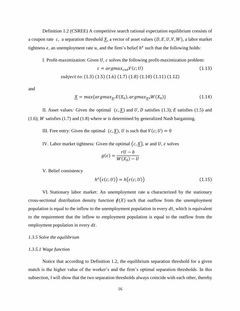
Definition 1.2 (CSREE) A competitive search rational expectation equilibrium consists of

a coupon rate 𝑐, a separation threshold 𝑋, a vector of asset values (𝐷, 𝐸, 𝑈, 𝑉,𝑊), a labor market

tightness 𝜖, an unemployment rate 𝑢, and the firm’s belief ℎ𝑒 such that the following holds:

I. Profit-maximization: Given 𝑈, 𝑐 solves the following profit-maximization problem:

𝑐 = 𝑎𝑟𝑔𝑚𝑎𝑥𝑐≥0𝑉(𝑐; 𝑈) (1.13)

𝑠𝑢𝑏𝑗𝑒𝑐𝑡 𝑡𝑜: (1.3) (1.5) (1.6) (1.7) (1.8) (1.10) (1.11) (1.12)

and

𝑋 = 𝑚𝑎𝑥 {𝑎𝑟𝑔𝑚𝑎𝑥𝑋′𝐸(𝑋0), 𝑎𝑟𝑔𝑚𝑎𝑥𝑋″𝑊(𝑋0)} (1.14)

II. Asset values: Given the optimal (𝑐, 𝑋) and 𝑈, 𝐷 satisfies (1.3); 𝐸 satisfies (1.5) and

(1.6); 𝑊 satisfies (1.7) and (1.8) where 𝑤 is determined by generalized Nash bargaining.

III. Free entry: Given the optimal (𝑐, 𝑋), 𝑈 is such that 𝑉(𝑐; 𝑈) = 0

IV. Labor market tightness: Given the optimal (𝑐, 𝑋), 𝑤 and 𝑈, 𝜖 solves

𝑔(𝜖) =𝑟𝑈 − 𝑏

𝑊(𝑋0) − 𝑈

V. Belief consistency

ℎ𝑒(𝜖(𝑐; 𝑈)) = ℎ(𝜖(𝑐; 𝑈)) (1.15)

VI. Stationary labor market: An unemployment rate 𝑢 characterized by the stationary

cross-sectional distribution density function 𝒻(𝑋) such that outflow from the unemployment

population is equal to the inflow to the unemployment population in every 𝑑𝑡, which is equivalent

to the requirement that the inflow to employment population is equal to the outflow from the

employment population in every 𝑑𝑡.

1.3.5 Solve the equilibrium

1.3.5.1 Wage function

Notice that according to Definition 1.2, the equilibrium separation threshold for a given

match is the higher value of the worker’s and the firm’s optimal separation thresholds. In this

subsection, I will show that the two separation thresholds always coincide with each other, thereby

17

greatly simplifying my subsequent analyses. As a byproduct, I also present a wage function linear

in current cash flow state 𝑋.

After a match is created and the debt is issued, the worker and the firm split the remaining

matching surplus through continuous bilateral bargaining according to a generalized Nash

bargaining rule. The generalized Nash bargaining selects the wage:

𝑤(𝑋) ∈ argmax𝑤

[𝑊(𝑋) − 𝑈]𝛽[𝐸(𝑋) − 𝑉]1−𝛽

As repeated shown in labor market search literature, this maximization yields as a

necessary and sufficient first-order condition:

𝛽[𝐸(𝑋) − 𝑉] = (1 − 𝛽)[𝑊(𝑋) − 𝑈]

In equilibrium, 𝑉 = 0. The worker’s outside option value is 𝑈. Therefore, I have

𝛽𝐸(𝑋) = (1 − 𝛽)[𝑊(𝑋) − 𝑈] (1.16)

Taking derivatives of both sides of (1.16) with respect to 𝑋. I have:

𝛽𝐸′(𝑋) = (1 − 𝛽)𝑊′(𝑋) (1.17)

and

𝛽𝐸″(𝑋) = (1 − 𝛽)𝑊″(𝑋) (1.18)

One direct consequence of equation (1.17) is that the matched firm and worker agree to

separate the matching relationship and return to search when 𝑋 hits the same threshold, i.e., 𝑋𝐸 =

𝑋𝑊 ≔ 𝑋. Therefore, the asset values in the economy have similar expressions as in Leland (1994),

which greatly simplifies my analyses. I also obtain the following lemma with regard to the wage

function, which is linear in current cash flow state 𝑋.

Lemma 1.1 (Wage function) In equilibrium, under generalized Nash bargaining, the wage

function is linear in 𝑋

𝑤(𝑋) = 𝛽(𝜃𝑋 − 𝑓 − 𝑐) + (1 − 𝛽)𝑏 + 𝛽𝑔(𝜖)𝐸(𝑋0)

= 𝛽(𝜃𝑋 − 𝑓 − 𝑐) + (1 − 𝛽)𝑏 + (1 − 𝛽)𝑔(𝜖)[𝑊(𝑋0) − 𝑈] (1.19)

Proof: Appendix A.

1.3.5.2 Matching surplus

18

It is easier to work with the matching surplus than to derive the expected discounted values

of equity and wage. First, I define matching surplus as 𝑆 ≔ 𝐸 +𝑊 − 𝑉 − 𝑈. Then by generalized

Nash bargaining:

𝐸 − 𝑉 = (1 − 𝛽)𝑆

and

𝑊 −𝑈 = 𝛽𝑆

Denote 𝐷0 ≔ 𝐷(𝑋0) , 𝑆0 ≔ 𝑆(𝑋0), 𝑔 ≔ 𝑔(𝜖), 𝑎𝑛𝑑 ℎ ≔ ℎ(𝜖) . The value function of being

unemployed (1.10) can be expressed in terms of 𝑆:

𝑟𝑈 = 𝑏 + 𝑔𝛽𝑆0 (1.20)

Similarly, the value function of an idled vacancy becomes

𝑟𝑉 = −𝜅 + ℎ[(1 − 𝛽)𝑆0 + 𝐷0] (1.21)

By the definition of 𝑆, the HJB equation for 𝑆 is as follows:

𝛿𝑆(𝑋) = 𝜃𝑋 − 𝑓 − 𝑐 − 𝑏 + 𝜅 − [𝑔𝛽 + ℎ(1 − 𝛽)]𝑆0 − ℎ𝐷0 + 𝜇𝑋𝑆′(𝑋) +1

2𝜎2𝑋2𝑆″(𝑋) (1.22)

Using (1.20) and (1.21),

𝛿𝑆(𝑋) = 𝜃𝑋 − 𝑓 − 𝑐 − 𝑟𝑈 − 𝑟𝑉 + 𝜇𝑋𝑆′(𝑋) +1

2𝜎2𝑋2𝑆″(𝑋) (1.23)

with boundary conditions:

𝑆(𝑋) = 0 (𝑣𝑎𝑙𝑢𝑒 𝑚𝑎𝑡𝑐ℎ𝑖𝑛𝑔);

𝑆′(𝑋)|𝑋=𝑋 = 0(𝑠𝑚𝑜𝑜𝑡ℎ 𝑝𝑎𝑠𝑡𝑖𝑛𝑔); 𝑙𝑖𝑚𝑋→∞

(𝑆

𝑋) < ∞(𝑛𝑜 𝑏𝑢𝑏𝑏𝑙𝑒) (1.24)

In the Appendix A, I obtain a closed-form solution of the boundary problem (1.22), (1.23)

and (1.24). Taking derivative of 𝑆(𝑋) with respect to 𝑋 and setting this expression equal to zero

at 𝑋 = 𝑋, I achieve Proposition 1.1 regarding the optimal separation threshold:

Proposition 1.1 (Optimal separation threshold) Given 𝑈 and 𝑐, the matching surplus 𝑆(𝑋)

is given by

19

𝑆(𝑋) = 𝜃𝛱(𝑋) − 𝐹 −𝑐 + 𝑏 − 𝜅 + [𝑔𝛽 + ℎ(1 − 𝛽)]𝑆0 + ℎ𝐷0

𝛿−

[𝜃𝛱(𝑋) − 𝐹 −𝑐 + 𝑏 − 𝜅 + [𝑔𝛽 + ℎ(1 − 𝛽)]𝑆0 + ℎ𝐷0

𝛿] (𝑋

𝑋)

𝜈

= 𝜃𝛱(𝑋) − 𝐹 −𝑐 + 𝑟𝑈 + 𝑟𝑉

𝛿− [𝜃𝛱(𝑋) − 𝐹 −

𝑐 + 𝑟𝑈 + 𝑟𝑉

𝛿] (𝑋

𝑋)

𝜈

(1.25)

The optimal separation threshold 𝑋 is

𝑋 =−𝜈

1 − 𝜈

𝛿 − 𝜇

𝜃 [𝐹 +

𝑐 + 𝑏 − 𝜅 + [𝑔𝛽 + ℎ(1 − 𝛽)]𝑆0 + ℎ𝐷0

𝛿]

=−𝜈

1 − 𝜈

𝛿 − 𝜇

𝜃 [𝐹 +

𝑐 + 𝑟𝑈 + 𝑟𝑉

𝛿] (1.26)

In equilibrium, the matching surplus becomes

𝑆(𝑋) = 𝜃𝛱(𝑋) − 𝐹 −𝑐 + 𝑟𝑈

𝛿− [𝜃𝛱(𝑋) − 𝐹 −

𝑐 + 𝑟𝑈

𝛿](𝑋

𝑋)

𝜈

(1.27)

The equilibrium optimal separation threshold 𝑋 is

𝑋 =−𝜈

1 − 𝜈

𝛿 − 𝜇

𝜃 [𝐹 +

𝑐 + 𝑟𝑈

𝛿] (1.28)

The optimal separation threshold 𝑋 is decreasing in productivity 𝜃, and is increasing in 𝑐 and 𝑈.

Proof: Appendix A.

The fact that the optimal separation threshold is increasing in 𝑐 echoes the finding from

risky debt and capital structure literature, for example, Leland (1994). The optimal separation

threshold and 𝑈 move in the same direction is new to the literature. The separation threshold can

be triggered by either party of the firm-worker match. Therefore, the optimal separation threshold

incorporates the worker’s outside option value 𝑈.

1.3.5.3 Optimal coupon 𝑐∗

The optimal coupon rate 𝑐∗ solves the following constrained maximization problem:

𝑟𝑉∗(𝑈) = 𝑚𝑎𝑥𝑐≥0

−𝜅 + ℎ[(1 − 𝛽)𝑆0 + 𝐷0] (1.29)

20

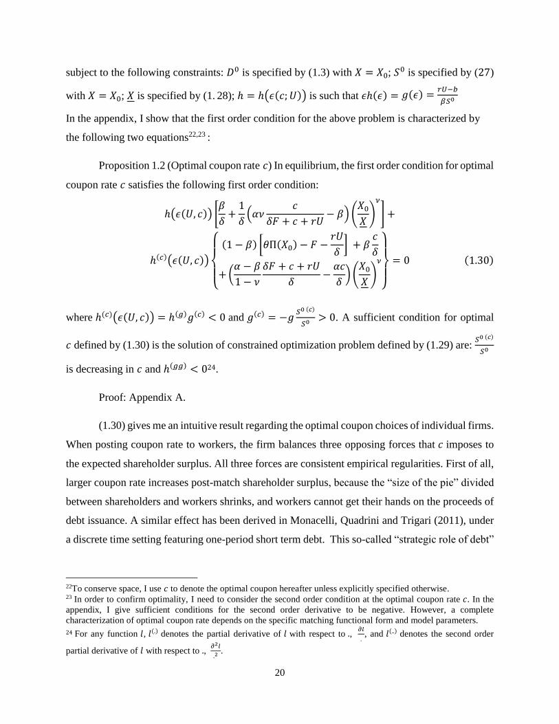
subject to the following constraints: 𝐷0 is specified by (1.3) with 𝑋 = 𝑋0; 𝑆0 is specified by (27)

with 𝑋 = 𝑋0; 𝑋 is specified by (1. 28); ℎ = ℎ(𝜖(𝑐; 𝑈)) is such that 𝜖ℎ(𝜖) = 𝑔(𝜖) =𝑟𝑈−𝑏

𝛽𝑆0

In the appendix, I show that the first order condition for the above problem is characterized by

the following two equations22,23 :

Proposition 1.2 (Optimal coupon rate 𝑐) In equilibrium, the first order condition for optimal

coupon rate 𝑐 satisfies the following first order condition:

ℎ(𝜖(𝑈, 𝑐)) [𝛽

𝛿+1

𝛿(𝛼𝜈

𝑐

𝛿𝐹 + 𝑐 + 𝑟𝑈− 𝛽)(

𝑋0𝑋)

𝜈

] +

ℎ(𝑐)(𝜖(𝑈, 𝑐))

{

(1 − 𝛽) [𝜃Π(𝑋0) − 𝐹 −

𝑟𝑈

𝛿] + 𝛽

𝑐

𝛿

+(𝛼 − 𝛽

1 − 𝜈

𝛿𝐹 + 𝑐 + 𝑟𝑈

𝛿−𝛼𝑐

𝛿) (𝑋0𝑋)

𝜈

}

= 0 (1.30)

where ℎ(𝑐)(𝜖(𝑈, 𝑐)) = ℎ(𝑔)𝑔(𝑐) < 0 and 𝑔(𝑐) = −𝑔𝑆0 (𝑐)

𝑆0> 0. A sufficient condition for optimal

𝑐 defined by (1.30) is the solution of constrained optimization problem defined by (1.29) are: 𝑆0 (𝑐)

𝑆0

is decreasing in 𝑐 and ℎ(𝑔𝑔) < 024.

Proof: Appendix A.

(1.30) gives me an intuitive result regarding the optimal coupon choices of individual firms.

When posting coupon rate to workers, the firm balances three opposing forces that 𝑐 imposes to

the expected shareholder surplus. All three forces are consistent empirical regularities. First of all,

larger coupon rate increases post-match shareholder surplus, because the “size of the pie” divided

between shareholders and workers shrinks, and workers cannot get their hands on the proceeds of

debt issuance. A similar effect has been derived in Monacelli, Quadrini and Trigari (2011), under

a discrete time setting featuring one-period short term debt. This so-called “strategic role of debt”

22To conserve space, I use 𝑐 to denote the optimal coupon hereafter unless explicitly specified otherwise. 23 In order to confirm optimality, I need to consider the second order condition at the optimal coupon rate 𝑐. In the

appendix, I give sufficient conditions for the second order derivative to be negative. However, a complete

characterization of optimal coupon rate depends on the specific matching functional form and model parameters.

24 For any function 𝑙, 𝑙(.) denotes the partial derivative of 𝑙 with respect to ., 𝜕𝑙

., and 𝑙(..) denotes the second order

partial derivative of 𝑙 with respect to ., 𝜕2𝑙

.2.

21

is empirically proved by, for example, Matsa (2010), which finds that firms respond to stronger

pro-union state laws by using higher leverage. The second effect is the classic cost of financial

distress. Since higher debt issuance triggers bankruptcy earlier and bankruptcy is costly by the

model assumption, a higher 𝑐 reduces the equity value by forcing premature separation of a firm-

worker match. This effect is absent in the traditional labor economics literature, since most

scholarly works focus on all-equity financed firms. The cost of financial distress associated with

high leverage is widely documented in the tradeoff theory of capital structure with risky debt, for

example, Leland (1994). The last effect, which is novel to the theoretical literature on labor market

search, is that a higher coupon rate 𝑐 reduces the arrival rate of the applicants to the posted job

vacancy, thus reduces the probability of the matching formation in the first place. This effect has

met great empirical success recently. For example, Brown and Matsa (2016) uses newly available

data from an online job search platform and finds that job vacancies posted by firms with poor

financial conditions and higher leverage result in fewer applicants. In equilibrium, individual firm

optimally chooses its coupon rate, that balances the benefit of leverage, the strategic role of debt,

and two costs of leverage, the cost of financial distress and the hiring role of debt. Mathematically,

the firm chooses optimal 𝑐 that equalizes the following two absolute values of elasticities with

respect to 𝑐: the elasticity of expected post-match shareholder surplus, (1 − 𝛽)𝑆0 + 𝐷0, and the

elasticity of before-match hiring rate, ℎ(𝜖(𝑈, 𝑐)).

|𝜂𝑐[(1 − 𝛽)𝑆0 + 𝐷0]|= |𝜂𝑐[ℎ(𝜖(𝑈, 𝑐))]| (1.31)

where |𝜂𝑐(. )| stands for the absolute value of respective elasticity with respect to 𝑐.

1.3.5.4 Expected job tenure

My model settings allow me to derive a closed-form representation of the expected

remaining job tenure, i.e., the expected match duration, when current cash flow state is 𝑋 .

Specifically, 𝑇(𝑋) stands for the expected remaining duration of a match when current cash flow

state is 𝑋. Standard results from stochastic process literature (e.g., Karlin and Taylor, 1981, 15.3)

shows that 𝑇(𝑋) solves the following boundary value ODE problem.

𝜇𝑋𝑇′(𝑋) +1

2𝜎2𝑋2𝑇″(𝑋) − 𝑠𝑇(𝑋) = −1 (1.32)

The boundary conditions are:

22

𝑇(𝑋) = 0 𝑎𝑛𝑑 𝑙𝑖𝑚𝑋→∞

𝑇(𝑋) =1

𝑠(1.33)

Heuristically, the remaining tenure is zero if 𝑋 hits the separation threshold, 𝑋. Meanwhile, if 𝑋

is very large, only event that could end the match is the exogenous match destruction event, with

arrival intensity 𝑠 . Solving explicitly the boundary value problem (1.32) and (1.33) for the

expression of 𝑇(𝑋), we have the following proposition:

Proposition 1.3 (Expected tenure) Given the expected value of a searching worker 𝑈 and

optimal coupon rate 𝑐, the expected job tenure in equilibrium is

𝑇(𝑋) =1

𝑠[1 − (

𝑋

𝑋)

𝜌

] (1.34)

where 𝜌 = (1

2−

𝜇

𝜎2) − √(

1

2−

𝜇

𝜎2)2

+2𝑠

𝜎2. 𝑇(𝑋) is decreasing in coupon rate 𝑐 and is increasing in

the current cash flow state 𝑋 and vacancy productivity 𝜃.

Proof: Appendix A.

Recall that wage is also increasing in the current cash flow state 𝑋, therefore I obtain a

positive relationship between job tenure and wage. Many empirical labor economists find a robust

positive relationship between seniority and wage, in both the United States (e.g., Topel, 1991) and

Europe (e.g., Dustmann and Meghir, 2005).

1.3.5.5 Stationary distributions of cash flow state 𝑋

In this section, I characterize the stationary cross-sectional distribution of the cash flow

state 𝑋 in the economy. This exercise serves two purposes. First of all, the steady-state

unemployment rate 𝑢 is expressed in terms of stationary cross-sectional distribution density

function, since the total mass of workers is one. Moreover, as seen from Lemma 1.1 and

Proposition 1.3, wages and expected job tenures are deterministic function of cash flow state 𝑋.

By deriving the stationary cross-sectional distribution of 𝑋, I am able to pin down the stationary

cross-sectional distribution of wages and expected job tenure in the economy.

23

My economy is a stochastic growth economy featuring matching pair deaths and births25,

with labor market search being the only friction. The stochastic process governing the dynamic

evolution of the cash flow state 𝑋, by assumption, is a geometric Brownian process with drift.

Obviously, 𝑋 belongs a class of Kolmogorov-Feller diffusion process 26 . Let 𝒻(𝑋; 𝑋0) be the

transition probability density function for 𝑋 in the economy with the starting value 𝑋0. From the

classic treatment (e.g., Karatzas and Shreve, 1991, Chapter 5, Section 1), the dynamics of 𝒻(𝑋)

follows a Fokker-Planck equation, also known as Kolmogorov forward equation of the process 𝑋,

∀ X ∈ [X, ∞] \{X0},

𝑑𝒻(𝑋)

𝑑𝑡= −

𝑑

𝑑𝑋[𝜇𝑋𝒻(𝑋)] +

1

2

𝑑2

𝑑𝑋2[𝜎2𝑋2𝒻(𝑋)] − 𝑠𝒻(𝑋) (1.35)

Let 𝒻(𝑋) denote the stationary 𝒻(𝑋), I have the following boundary value problems governing

𝒻(𝑋):

−𝑑

𝑑𝑋[𝜇𝑋𝒻(𝑋)] +

1

2

𝑑2

𝑑𝑋2[𝜎2𝑋2𝒻(𝑋)] − 𝑠𝒻(𝑋) = 0 (1.36)

with boundary conditions27:

𝒻(𝑋 +) = 0 (1.37)

1

2𝜎2𝑋0

2[𝒻′(𝑋0 −) − 𝒻′(𝑋0 +)] = 𝑠∫ 𝒻(𝑋)𝑑𝑋 +

1

2𝜎2𝑋2𝒻′(𝑋 +)

∞

𝑋

(1.38)

𝑔 [1 − ∫ 𝒻(𝑋)𝑑𝑋∞

𝑋

] = 𝑠∫ 𝒻(𝑋)𝑑𝑋 +1

2𝜎2𝑋2𝒻′(𝑋 +)

∞

𝑋

(1.39)

The boundary conditions, despite their complexities, are intuitive under scrutiny. First,

once the post-match performance is poor and the cash flow state 𝑋 reaches the equilibrium

endogenous default threshold, 𝑋, separation occurs immediately. In other words, 𝑋 spends no time

at 𝑋28. Mathematically, this requires 1

2𝜎2𝑋2𝒻(𝑋 +) = 0 , since

1

2𝜎2𝑋2 ≠ 0 , I have (1.37).

25 For the application of power laws to city and population growth, refer to Gabaix (2009). 26 For the definition of Kolmogorov-Feller diffusion process, please consult to Karatzas and Shreve (1991), Chapter

5, Definition 1.1.1. 27 𝑋+∶= lim

𝑋′↓𝑋𝑋′ and 𝑋−∶= lim

𝑋′↑𝑋𝑋′

28 Mathematically, 𝑋 is an attainable boundary that can be hit by the process in finite time period with positive

probability. Moreover, attainable boundaries are either absorbing or reflecting. In my case, it is absorbing.

24

Secondly, (1.38) has an economic meaning as follows: at steady state, the total flows into the

employment must commensurate the total flows out of the employment. The left hand side is the

total flows into the employment. The density 𝒻(𝑋) is not differentiable at 𝑋0, corresponding to the

inflow of workers to the employment and all new matches starting at 𝑋0. The right hand side is the

total flows out of the employment. The first term is intuitive. For the last term, the flow of matching

separation at 𝑋 is given by 1

2𝜎2𝑋2𝒻′(𝑋 +). Intuitively, over a small enough interval of time Δ, the

diffusion term in 𝑑𝑋𝑡 = 𝜇𝑋𝑡𝑑𝑡 + 𝜎𝑋𝑡𝑑𝑍𝑡 dominates, and half of the measure 29 of 𝒻(𝑋 +

𝜎𝑋√Δ) × 𝜎𝑋√Δ matched firm-worker pairs near the boundary 𝑋 will exit the production. Finally,

(1.39) is the standard restriction in labor market search models (e.g., Mortensen and Pissarides,

1994), which yields the Beveridge curve. The left hand side is the outflow from the unemployment

population, and the right hand is the inflow to the unemployment population, which, by definition,

is also the outflow from the employment population.

The solution technique of the boundary problem (1.36) subject to (1.37) — (1. 39) is similar

to those continuous time cases in the power law literature (e.g., Gabaix, 2009; Achdou, Han, Lasry,

Lions and Moll, 2015). For 𝑋 ∈ [𝑋,∞] \{𝑋0} , the following proposition characterizes the

stationary cross-sectional distribution density function of 𝑋, in the equilibrium:

Proposition 1.4 (Stationary cross-sectional distribution of 𝑋), Given 𝑈, 𝑔 and 𝑐, for 𝑋 ∈

[𝑋, ∞] \{𝑋0}, the stationary cross-sectional distribution density function of 𝑋 in equilibrium is:

𝒻(𝑋) = {

𝜁𝑋−𝑚1−1 , 𝑋 > 𝑋0

𝜁𝑋−𝑚0−1 [1 − (𝑋

𝑋)𝑚1−𝑚0

], 𝑋 ≤ 𝑋 < 𝑋0(1.40)

where 𝑚0 = (1

2−

𝜇

𝜎2) − √(

1

2−

𝜇

𝜎2)2

+2𝑠

𝜎2 and 𝑚1 = (

1

2−

𝜇

𝜎2) + √(

1

2−

𝜇

𝜎2)2

+2𝑠

𝜎2; 𝜁 and 𝜁 are

positive and uniquely determined by boundary conditions (1.38) and (1.39).

Proof: Appendix A.

29 This expression is derived by using Taylor expansion at 𝑋 = 𝑋.

25

The expression of the stationary cross-sectional distribution density function 𝒻(𝑋) of cash

flow state 𝑋 takes the form of Double-Pareto distribution density, as repeatedly shown in the

stochastic growth literature (e.g., Gabaix, 2009; Achdou, Han, Lasry, Lions and Moll, 2015).

We thus complete the solution of a Competitive Search Rational Expectation Equilibrium

defined in Definition 1.2. The solutions for optimal coupon rate 𝑐, unemployment value 𝑈, and

labor market tightness 𝜖 , are characterized by a system algebraic equations. The separation

threshold 𝑋 and the labor market aggregates: the wage function 𝑤, expected job tenure 𝑇, and the

stationary cross-sectional distribution of cash flow state in the economy 𝒻, are all in analytical

forms.

1.3.6 Labor force participation rate

The labor force participation rate (LFPR hereafter) is counter-cyclical. The empirical

consensus is that the transition from out of labor force to unemployment goes up when the

economy is sliding into recession (Elsby, Hobijn and Sahin, 2015; Krueger, 2016). In this

subsection, I try to extend the model to allow for workers’ job searching intensity decisions. Higher

job searching intensity indicates more active labor force participation.

Theoretically, a rigorous treatment of labor force participation decisions requires three

states of workers— unemployed, employed and out of the labor force, and three value functions

for workers, one for each state. However, my model only offers two-state value functions for

workers. I bypass the modeling difficulties by incorporating an endogenous job searching effort

variable to my baseline model, and shed some light on the role of capital structure choice in

affecting the worker’s labor force participation choice, which is the job searching effort he/she

optimally expends.

Specifically, let 𝑒𝑗 denote the job searching effort an unemployed worker 𝑗 exerts in the

labor market. Without loss of generality, I restrict 𝑒𝑗 ∈ [0, �̅�], �̅� < ∞. Higher 𝑒𝑗 denotes for more

active labor force participation, with 𝑒𝑗 = �̅� standing for full labor force participation. The cost of

labor searching effort is 𝑙(𝑒𝑗), with the usual convex assumptions: 𝑙′(𝑒𝑗) > 0 and 𝑙″(𝑒𝑗) > 0.

26

The matching rate for searching worker 𝑗 is 𝑔(𝑒𝑗, 𝜖) ≔𝑚(𝑒𝑗𝑢,𝜈)

𝑢= 𝑚(𝑒𝑗, 𝜖). Again, 𝑢, 𝜈 and 𝜖

denotes the unemployment rate, vacancy rate and labor market tightness in the economy,

respectively. Similarly, the matching rate for the firm is ∫ 𝑚(𝑒𝑗,𝜖)𝑑𝑗𝑢0

𝜈.

The value function of an unemployed worker becomes30

𝑟𝑈(𝑒𝑗) = 𝑏 + 𝑔(𝑒𝑗 , 𝜖)𝛽𝑆0 − 𝑙(𝑒𝑗) (1.41)

and the first order condition for the optimal effort 𝑒𝑗 is31

𝑔(𝑒𝑗)(𝑒𝑗, 𝜖)𝛽𝑆0 − 𝑙′(𝑒𝑗) = 0 (1.42)

In the equilibrium, since workers are ex-ante identical, they face the same job searching effort

optimization problem and choose the same optimal amount of effort, denoted as 𝑒, and they obtain

the same value of being unemployed. I omit the subscripts of worker indices. (1.41) and (1.42)

become:

𝑟𝑈 = 𝑏 + 𝑔(𝑒, 𝜖)𝛽𝑆0 − 𝑙(𝑒) (1.43)

and

𝑔(𝑒)(𝑒, 𝜖)𝛽𝑆0 − 𝑙′(𝑒) = 0 (1.44)

The value function for an idle vacancy is:

𝑟𝑉 = −𝜅 + ℎ(𝑒, 𝑔)[(1 − 𝛽)𝑆0 + 𝐷0] (1.45)

which is similar to (1.29), except that the matching rate ℎ now depends on the job searching effort

in the economy, 𝑒, in addition to the labor market tightness.

The first order condition for optimal coupon rate 𝑐 is similar to (1.30), except that

ℎ(𝑐)(𝑒, 𝑔) = ℎ(𝑒)𝑒(𝑐) + ℎ(𝑔)𝑔(𝑐), in the Appendix A, I show the explicit expressions of 𝑒(𝑐) and

𝑔(𝑐) . The following proposition characterizes the optimal coupon rate 𝑐 in the presence of

endogenous searching effort.

30 Note that as in the baseline case, a searching worker 𝑗’s 𝑈 does not depend on the individual coupon choice. Meanwhile, 𝑈 does depend on the individual 𝑗’s searching effort. 31 Note that the internal solution always exists because (1.41) is concave in 𝑒.

27

Proposition 1.5 (Optimal coupon rate 𝑐 in the presence of job searching effort 𝑒 ) In

equilibrium with optimal searching effort 𝑒, the optimal coupon rate 𝑐 satisfies the following first

order condition:

ℎ(𝑒(𝑈, 𝑐), 𝑔(𝑈, 𝑐)) [𝛽

𝛿+1

𝛿(𝛼𝜈

𝑐

𝛿𝐹 + 𝑐 + 𝑟𝑈− 𝛽)(

𝑋0𝑋)

𝜈

] +

ℎ(𝑐)(𝑒(𝑈, 𝑐), 𝑔(𝑈, 𝑐))

{

(1 − 𝛽) [𝜃𝛱(𝑋0) − 𝐹 −

𝑟𝑈

𝛿] + 𝛽

𝑐

𝛿

+(𝛼 − 𝛽

1 − 𝜈

𝛿𝐹 + 𝑐 + 𝑟𝑈

𝛿−𝛼𝑐

𝛿) (𝑋0𝑋)

𝜈

}

= 0 (1.46)

where ℎ(𝑐)(𝑒(𝑈, 𝑐), 𝑔(𝑈, 𝑐)) = ℎ(𝑒)𝑒(𝑐)+ ℎ

(𝑔)𝑔(𝑐) . 𝑔(𝑐) and 𝑒(𝑐) is defined in (A.35) and (A.36),

respectively. A sufficient condition for optimal 𝑐 defined by (1. 46) is the solution of constrained

optimization problem defined by (1.45) is ℎ(𝑐𝑐)(𝑒, 𝑔) < 0.

Proof: Appendix A.

The solutions of expected duration of a matching relationship in the economy and

stationary cross-sectional distribution of the cash flow states 𝑋 are similar to the baseline case,

which I omit here.

1.3.7 A numerical example

In this section, I demonstrate the model implications for joint relationship between optimal

leverage choices and labor market dynamics for different model parameters. Specifically, I focus

on three sets of model parameters: the workers’ bargaining power, 𝛽, the matching efficiency, 𝐴,

and indicators of economic downturns, 𝛼 and 𝜎 . Consistent with the empirical findings on

functional form of the labor market matching technology, I use a constant-return-to-scale, Cobb-

Douglas matching function 32 𝑚(𝑢, 𝜈) = 𝐴𝑢𝜄𝜈1−𝜄 (Petrongolo and Pissarides, 2001). The

benchmark parameter values are presented in Table 1.1 and are in line with extant research on

aggregate labor market dynamics.

1.3.7.1 Optimal leverage

32 In the presence of job searching effort, the matching function becomes: 𝑚(𝑒𝑢, 𝜈) = 𝐴(𝑒𝑢)𝜄𝜈1−𝜄 , in which 𝑒 is

searching worker’s job searching effort.

28

In this subsection, I examine the impacts of model parameters on firms’ optimal leverage

choices. The results are illustrated in Figure 1.1. Several robust patterns are revealed. First of all,

debt level 𝑐 is increasing in workers’ bargaining power, 𝛽, as illustrated in Figure 1.1. This is

consistent with recent empirical and theoretical findings that firms utilize higher leverage to

discourage the workers’ stronger wage demand (e.g., Matsa, 2010; Monacelli, Quadrini and Trigari,

2011). More interesting facts about the leverage choice is that it increases with the labor market

search efficiency parameter, 𝐴, for an empirical plausible range of estimates33. The underlying

logic is as follows: on one hand, the marginal benefit of a higher leverage on post-match

shareholder value scales up with the labor market search efficiency. On the other hand, recall that

the marginal cost of posting a larger 𝑐 for the firm is lowering the labor market matching

probability. As labor market search becomes more efficient, this marginal cost of 𝑐 is decreasing.

The two forces induce the firm to lever up34 as labor market search efficiency improves. This

relationship is supported by recent empirical literature, which finds that firms choose lower

leverage when their workers face greater unemployment risk (e.g., Agrawal and Matsa, 2013;

Chemmanur, Cheng and Zhang, 2013). Another interesting fact is that the leverage increases as

economic volatility mounts up. This is consistent with findings from other research on the

relationship between leverage and aggregate volatility (e.g., Johnson, 2016). However, the

underlying mechanism is different. Johnson (2016) resorts to a deposit insurance mechanism. I

provide an alternative mechanism originated from labor market search frictions. I further

decompose the marginal benefits and marginal cost to various levels of 𝑐, at high and low volatility

levels. The result confirms that marginal cost of choosing a higher coupon rate 𝑐 decreases rapidly

with the volatility. Notice that the productivity does not change in the core model. Therefore, as

volatility increases, the value of a match deteriorates35. Consequently, the marginal cost of a higher

leverage 𝑐 decreases. This is because as the value of a successful match to the firm is lower,

33 Most of the labor economics papers estimate 𝐴 between 4 and 5. 34 The relationship between 𝑐 and 𝐴 is not monotonic. A further examination reveals that as 𝐴 becomes very large, the

optimal leverage jumps down to zero. Notice that the labor market matching process becomes almost frictionless as

𝐴 becomes very large. The labor market is analogues to a retail market, in which firms provide homogeneous

product—job vacancies to workers, and workers always go to the highest valued vacancies, i.e., vacancies with zero

leverage. The searching workers’ choices arise from the fact that as 𝐴 becomes very large, the firms can

instantaneously fulfill any amounts of searching workers’ job demands. 35 This is because bankruptcy is costly and the matching relationship has higher chance to hit the bankruptcy boundary.

29

increasing matching probability through lower 𝑐 becomes less desirable36. Therefore, the firm

responds to a higher economic volatility by employing a higher leverage policy. To my best

knowledge, this is the first theoretical research that tackles the positive leverage-volatility co-

movement puzzle from a frictional labor market perspective. Lastly, as seen from Figure 1.1, the

optimal coupon rate decreases with the cost of bankruptcy 𝛼. This finding is consistent with most

of the extant corporate finance research (e.g., Leland, 1994).

1.3.7.2 Expected tenure

Notice that from (34) of Proposition 1.3, the expected matching duration decreases with

the separation threshold, which in turn, increases with the optimal debt usage by the firm.

Consistent with findings regarding the comparative statics of optimal leverage in Figure 1.1, the

expected job tenure in the economy is decreasing in the worker’s bargaining power, the labor

market search efficiency and the cash flow volatility. It increases with the bankruptcy cost

parameter.

1.3.7.3 Stationary cross-sectional density function of 𝑋

I compare the stationary cross-sectional density function of the cash flow state 𝑋, between

high and low values of workers’ bargaining power, and high and low values of labor market search

efficiency. As shown in Figure 1.3, lower value of workers’ bargaining power generates a fatter

left tail of stationary cash flow distribution among matches, so does a lower value of search

efficiency parameter. These results are intuitive. Since the separation threshold increases with the

worker’s bargaining power and the search efficiency37, matches are endogenously destroyed at

higher cash flow level. Therefore, the stationary cross-sectional cash flow distributions in the

economy with lower workers’ bargaining power and lower matching efficiency are more dispersed,

compared with an otherwise identical economy characterized by higher workers’ bargaining power

and higher search efficiency. Since wage is a linear function of cash flow state 𝑋, as shown in

36 Volatility also affects the marginal benefit of 𝑐. Notice that as volatility increases, the firm has higher chance to

generate large cash flow. By Nash bargaining, the worker will take a larger share of the cash flow under this high

profitability scenario. Therefore, the firm has more incentive to use debt to reduce the worker’s wage demand. 37 Two forces contribute to this. First of all, the optimal leverage increases with worker’s bargaining power and

matching efficiency, which elevates the separation threshold. A second and subtler force is as follows: increases in

worker’s bargaining power and search efficiency elevate the expected value of a searching worker, thereby raising the

required cash flow threshold to keep the matching relationship valuable to both parties.

30

(1.19) of Lemma 1.1, the wage distribution in the former economy also has a fatter left tail,

compared with that of the latter economy. As far as I am concerned, this is the first research relating

the wage bargaining and labor market search efficiency to the dispersion of the wage and cash

flows in the economy, through an endogenous capital structure choice channel on the employer

side.

1.3.7.4 Unemployment rate 𝑢

In this subsection, I examine how the wage bargaining, the labor market search efficiency

and the economy-wide volatility affect the steady-state unemployment rate 𝑢. This practice differs

from traditional labor market search models because an important underlying channel is the

optimal capital structure choice by the employers in the economy. First of all, as shown in Figure

1.4, the unemployment rate increases with the workers’ bargaining power. Intuitively, a higher

bargaining power induces the termination of the matching relationship at a higher cash flow level,

as firms employ higher leverages to prevent workers from scooping large share of matching

surplus. As a result, more workers go back to unemployment pool during each time period.

Regarding the labor market search efficiency, despite higher leverage choice as a response to a

higher search efficiency, the unemployment rate drops as the search efficiency improves, as shown

in Figure 1.4. Regarding the effect of bankruptcy cost, a higher bankruptcy cost constrains the

firm’s ability to grab a larger share of matching surplus by levering up, thereby reducing its

incentive to post a vacancy. Moreover, the more conservative leverage policy as a response to a

higher bankruptcy cost elicits more job applicants, thereby further reducing the matching

probability of the individual worker. The two effects collectively drive up the unemployment rate.

This is consistent with the empirical findings that unemployment rate is higher during collateral

crisis. One counterintuitive result is the negative relationship between economic volatility and

unemployment rate. Unemployment rate is well known as a countercyclical variable while higher

economic volatility is often accompanied by an economic recession. However, one equally widely

known fact about unemployment rate is that unemployment rate is less volatile than the gross

domestic product, so called “Okun’s law”. A common explanation is that a large component of

unemployment rate is unrelated with business cycles (Hall, 2005; Hall, 2016). My model sheds

new light to this old conundrum. In my economy, the productivity is constant over time. Therefore,

I could isolate the effect of volatility change on unemployment rate from the overall business cycle

31

effect. The result highlights one silver lining of higher leverage choice during more volatile times:

Higher leverage choices reduce the “congestion effect” among the searching workers. In other

words, the higher leverage policy unintendedly creates a positive externality on the workers’ job

searching process. This “congestion reduction” effect dominates “surplus reduction” effect during

turbulent times, thereby leading to a negative relationship between economic volatility and

unemployment rate38. This positive externality of high leverage choice in reducing the “congestion”

on workers’ job searching is overlooked by the previous literature.

1.3.7.5 Initial wage 𝑤0

In this subsection, I fix the cash flow state at 𝑋0, and examine how the wage bargaining,

the labor market search efficiency, and the economy-wide volatility affect the initial wage 𝑤0.

Several patterns emerge. First and foremost, as seen from Figure 1.5, labor market search

efficiency affects the wage of the new hires in a modest and non-monotonic way. From un-

tabulated analyses, for very inefficient matching technology, an increase in search efficiency

rapidly boosts the expected value of an unemployed worker, thereby elevating the wage for the

new hires. However, as the search efficiency continue to improve, the positive effect of search

efficiency on unemployment value dwindles. The firm’s higher optimal leverage policy as a

response of improved search efficiency dominates and wears down the starting wage of a matching

relationship. This contrasts to traditional labor market search models without consideration of

employers’ leverage choices, in which the wage of new hires monotonically increases with the

search efficiency for obvious reasons: higher search efficiency increases the workers’ expected

value of searching, thereby increasing the required surplus they demand from a matching

relationship. Moreover, this non-monotonic and modest relationship between search efficiency and

wage dynamics calls for a thorough cost-benefit analysis of government policies aimed at

promoting labor market search efficiency. For example, battling against the recent financial crisis,

many countries from Europe, to name a few, UK, Germany and Ireland, expand current vocational

training program and initiate new programs to reduce the labor market mismatches (Heyes, 2012).

These active labor market programs that improve the labor market search efficiency are argued to

swiftly increase the national welfare in the short run (Brown and Koettl, 2015). However, one

38 Of course, allowing for a multi-state Markov process of productivity 𝜃 will reduce both the debt and the surplus

values of the matching, which, in turn, overturns the positive relationship between economic volatility and leverage.

32

subtlety is that employers might take advantage of these job creation programs by adjusting

upward their leverage ratios. As a result, the new employments might arise at a cost of lower wages.

A complete welfare implication of these programs might yield more complex results than the

original expectations. Lastly, as seen from Figure 1.5, the optimal capital structure choice as

responses to the worker’s bargaining power and macroeconomic condition plays a dominant role

in determining the initial wages of a matching relationship. Specifically, higher bargaining power

on the worker side and more volatile economy elicit higher leverage choices by the firms, which

in turn cuts back the initial wages. An opposite effect of higher bankruptcy cost on wage holds

analogously. An important empirical implication drawn from Figure 1.5 is that collateral crisis and

volatility spikes might alter wages in opposite directions, even if they are often concomitant with

each other during economic recessions.

1.3.7.6 Labor force participation 𝑒

As shown in Subsection 1.3.6, I interpret workers’ labor force participation rate as workers’

job search intensity. Two model parameters come into play when I examine the comparative statics

of LFPR. First of all, as shown in Figure 1.6, a more efficient matching technology induces the

workers to exert more job searching effort, in order to capitalize a more “productive” matching

process. It is intuitive because by the matching function specified in Subsection 1.3.6, an additional

searching effort yields a larger increase in matching probability when search efficiency is higher.

Another important model parameter is the economic volatility. A higher economic volatility elicits

more job searching effort by the workers. This is because the positive externality of higher leverage

in reducing the congestion among searching workers. As a result, workers have higher incentives

to participate in the labor market, because the return of such effort, in terms of job matching

probability, is higher. This finding is in line with the empirical regularities that the transition rate

from out-of-labor-force to the unemployment pool is countercyclical, ramping up during the

recessions (e.g., Elsby, Hobijn and Sahin, 2015; Krueger, 2016). Although the economic

recessions are characterized by both lower productivity and higher uncertainty, I have shown that

the volatility certainly contributes to the observed counter-cyclical behavior of labor force

participation, which is, to my best knowledge, novel to the literature.

1.4 Learning the random 𝝁

33

In this section, I relax the model assumption about the deterministic and publicly

observable match-specific quality. I assume that the match-specific productivity can be either high

or low and is unobservable to both parties of the match. Such a setting meets with great empirical

success 39 . I begin this section by specifying the modified environment of the model. The

characterization of the competitive search rational expectation equilibrium is very similar to that

derived in Section 1.3. Therefore, I delegate the details to Appendix B.

1.4.1 Searching and learning environment

The environment is the same as Section 1.2, except for the following changes. I change the

cash flow specification to maintain the model’s tractability. Specifically, the match-specific

cumulative cash flow process evolves according to a standard Brownian motion with unknown

drifts. For a match 𝑖,

𝑑𝑋𝑖𝑡 = 𝜇𝑖𝑑𝑡 + 𝜎𝑑𝑍𝑖𝑡 , 𝑤ℎ𝑒𝑟𝑒 𝜇𝑖 = {𝜇𝐻 , 𝑝0𝜇𝐿 , 1 − 𝑝0

(1.47)

𝜇 is a match-specific quality measure, and 𝑝0 represents the common prior belief that the matching

quality is high. I assume that all the agents have the same prior beliefs regarding the matching

quality. Furthermore, I also assume that 𝑏 ∈ [𝜇𝐿 , 𝑝0𝜇𝐻 + (1 − 𝑝0)𝜇𝐿]. In other words, learning is

nontrivial in my economy. It is socially inefficient to keep a match with productivity 𝜇𝐿.

According to classic treatment on optimal nonlinear filtering (e.g., Liptser and Shiryaev,

2001, Chapter 9), the steady-state posterior 𝑝𝑡 about the matching quality evolves according to:

𝑑𝑝𝑡 = 𝑝𝑡(1 − 𝑝𝑡)𝜙𝑑�̅�𝑡 (1.48)

𝜙 ≔𝜇𝐻−𝜇𝐿

𝜎 is the signal-to-noise ratio, which measures the informativeness of the cumulative cash

flow process regarding the unobserved matching quality. 𝑑�̅�𝑡 =1

𝜎 [𝑑𝑋𝑡 − 𝑝𝑡𝜇𝐻𝑑𝑡 − (1 −

𝑝𝑡)𝜇𝐿𝑑𝑡] is a Brownian motion process with respect to the filtration {ℱ𝑡𝑋}. Intuitively, 𝑑�̅�𝑡 is an

innovation process from the perspectives of both parties of a match. In Appendix B, I follow the

same procedure as Section 1.3, to characterize the asset values, optimal separation threshold and

39 Inspired by the influential work by Jovanovic (1979), micro-labor economics models treat the firm-worker match

as an experienced good, whose quality is initially unknown and is gradually revealed through a noisy cash flow process.

For details, please refer to an excellent survey by Lazear and Oyer (2009).

34

coupon rate, in terms of 𝑝𝑡. The stationary cross-sectional distribution of posterior belief 𝑝𝑡 again

takes the Double-Pareto form.

1.5 No coupon-posting

In this section, I relax two important assumptions of the baseline model in Section 1.3.

First, I relax the assumption of credible capital structure posting. There is no reliable way that

firms could credibly signal their intentional capital structure choice to potential job applicants40.

Furthermore, I introduce heterogeneity in job productivity types. More specifically, there are two

large measures of firms, different in the productivities of the job vacancies they post. Each measure

is determined endogenously through free-entry conditions for both types of the firms. Workers are

agnostic about the employers’ productivity types during job search. The above model

environments are consistent with real-world labor market observations. For majority of non-

publicly listed firms, it is generally impossible to find out reliable information about their capital

structure choices. Empiricists have shown that there exist considerable productivity discrepancies

across firms within the same industry, and across industries 41 . I begin this section with a

formalization of the aforementioned two relaxations. Then I consider two cases regarding the

information structure about firm-specific productivity: the case in which the worker, the firm and

the capital provider know the firm-specific productivity after the match is formed, and the other

case in which only the firm is savvy about its own productivity after the match is formed.

1.5.1 Model environment

The cash flow process and flow operating cost are the same as in Section 1.3, except that

𝜃 ∈ {𝜃𝐻 , 𝜃𝐿}. The financial contract space is the same as in Section 1.3. A Firm chooses its capital

structure by issuing perpetual debt after the match is formed, but before the wage negotiation

begins. Proceeds of debt issuance are distributed to shareholders immediately. Let 𝑝 denote the

common prior belief that productivity of the job vacancy is high, which is endogenously

determined in equilibrium. Furthermore, I assume that job vacancies of both productivity levels

are accepted by the workers. This occurs if the difference between 𝜃𝐻 and 𝜃𝐿 is not large, or the

40 I could equivalently keep the credible capital structure posting assumption, but instead assume that the firm is always

attempted to deviate from the pre-committed capital structure to an ex-post optimal one after a match is formed. 41 For a survey regarding the determinants and cross-sectional distributions of firm productivity in U.S. economy,

please refer to Syverson (2011).

35

“efficiency” of labor market matching function 𝑚(𝑢, 𝑣) is sufficiently low42. Throughout the

section, I use subscript 𝑘 ∈ {𝐻, 𝐿} to denote respective quantities for firms of a certain type, either

high or low productivity.

1.5.2 Full information about 𝜃

On one hand, the HJB equations and boundary conditions for 𝐷𝑘(𝑋) and 𝑆𝑘(𝑋) remain the

same as corresponding equations in Section 1.3, expect one expression for each type. Therefore,

the expressions for debt value 𝐷𝑘(𝑋), match surplus 𝑆𝑘(𝑋), and optimal separation threshold 𝑋𝑘

are analogous to the respective asset value equations in Section 1.343. On the other hand, the

unemployment value satisfies the following HJB equation:

𝑟𝑈 = 𝑏 + 𝑔(𝜖)[𝑝𝑊𝐻0 + (1 − 𝑝)𝑊𝐿

0] = 𝑏 + 𝑔(𝜖)𝛽[𝑝𝑆𝐻0 + (1 − 𝑝)𝑆𝐿

0] (1.49)

Under the case that firms choose debt issuance only after the matches are formed. The

optimal coupon 𝑐𝑘 solves the optimization problem:

𝑚𝑎𝑥𝑐𝑘′(1 − 𝛽)𝑆𝑘

0 + 𝐷𝑘0 (1.50)

The first order condition for 𝑐𝑘 is:

𝛽

𝛿−𝛽 − 𝛼𝜈

𝛿 (𝑋0𝑋𝑘)

𝜈

= 0

After simplifying, the optimal coupon 𝑐𝑘 for the firms with productivity type 𝜃𝑘 under symmetric

information is

𝑐𝑘 = 𝛿 [1 − 𝜈

−𝜈 (

𝛽

𝛽 − 𝛼𝜈)−1𝜈𝜃𝑘𝛱(𝑋0) − 𝐹] − 𝑟𝑈 (1.51)

Bringing (1.51) to (1.28), the optimal separation threshold 𝑋𝑘 is

𝑋𝑘 = (𝛽

𝛽 − 𝛼𝜈)−1𝜈𝑋0 (1.52)

42 For example, if 𝑚(𝑢, 𝑣): = 𝐴𝑢𝜄𝑣1−𝜄, then 𝐴 is sufficiently small. 43 I modify the default value of the firm to 𝐷(𝑋) = 𝐷𝐵 = (1 − 𝛼)𝜃𝛱(𝑋) − 𝐹 −

𝑟𝑈

𝛿 to make the calculation less cumbersome.

It is not crucial and does not change any model predictions in the section.

36

Notice that the optimal separation threshold is independent of the productivity parameter

𝜃𝑘. On one hand, ceteris paribus, both parties of a match are willing to separate at a later time

when the productivity of the match is higher; on the other hand, more productive firms optimally

choose larger coupon rate 𝑐𝑘, which leads to earlier defaults. In equilibrium, the two effects exactly

offset each other.

Equipped with the optimal coupon rate 𝑐𝑘 and optimal default threshold 𝑋𝑘, I am ready to

simplify the debt value and matching surplus, 𝐷𝑘(𝑋) and 𝑆𝑘(𝑋). Similar to steps in Section 1.3, I

have:

𝑆𝑘(𝑋) = 𝜃𝑘𝛱(𝑋) + (𝛽

𝛽 − 𝛼𝜈)−1𝜈𝜃𝑘𝛱(𝑋0) [

1 − 𝜈

𝜈−1

𝜈

𝛽

𝛽 − 𝛼𝜈(𝑋

𝑋0)𝜈

] (1.53)

At the start of the match, 𝑋 = 𝑋0,

𝑆𝑘(𝑋0) = 𝜃𝑘𝛱(𝑋0) + (𝛽

𝛽 − 𝛼𝜈)−1𝜈𝜃𝑘𝛱(𝑋0) (

1 − 𝜈

𝜈−1

𝜈

𝛽

𝛽 − 𝛼𝜈) (1.54)

The debt value is

𝐷𝑘(𝑋) =1 − 𝜈

−𝜈 (

𝛽

𝛽 − 𝛼𝜈)−1𝜈𝜃𝑘𝛱(𝑋0) [1 − (1 + (1 − 𝛼)

𝜈

1 − 𝜈)

𝛽

𝛽 − 𝛼𝜈(𝑋

𝑋0)𝜈

] − 𝐹 −𝑟𝑈

𝛿(1.55)

At the start of the match, 𝑋 = 𝑋0,

𝐷𝑘(𝑋0) =1 − 𝜈

−𝜈 (

𝛽

𝛽 − 𝛼𝜈)−1𝜈𝜃𝑘𝛱(𝑋0) [1 − (1 + (1 − 𝛼)

𝜈

1 − 𝜈)

𝛽

𝛽 − 𝛼𝜈] − 𝐹 −

𝑟𝑈

𝛿(1.56)

Since the matches of high and low productivities have the same separation threshold, the stationary

cross-sectional distribution density function 𝒻(𝑋) is defined similarly to Proposition 1.4.

1.5.3 Asymmetric information about 𝜃

In this subsection, I consider the cases in which the productivity 𝜃 is only observable by

the firm. To make it more interesting, I assume that the firm cares about market value of its

securities, as well as the intrinsic values. Specifically, I define that a firm’s objective function after

the match is formed as:

37

𝑚𝑎𝑥𝑐𝜔[𝑀0(𝑐; 𝜃𝑚)] + (1 − 𝜔)[(1 − 𝛽)𝑆

0(𝑐; 𝜃𝑘) + 𝐷0(𝑐; 𝜃𝑘)] (1.57)

where𝑀0(𝑐; 𝜃𝑚) = ∑ 𝑝𝑘[(1 − 𝛽)𝑆0(𝑐; 𝜃𝑘) + 𝐷

0(𝑐; 𝜃𝑘)]𝑘=𝐿,𝐻 , where 𝑝𝑘 ≔ Pr[𝜃 = 𝜃𝑘] for 𝑘 ∈

{𝐿, 𝐻}. In other words, 𝑀0(𝑐; 𝜃𝑚) is the market valuation of the firm’s financial claims, including

debt and equity, when the current cash flow state is 𝑋0, the coupon rate is 𝑐, and the market belief

about the firm’s productivity type is 𝜃𝑚.

The specification of (1.57) is consistent with the “capital-market driven” corporate finance

models (e.g., Baker, 2009; Baker and Wurgler, 2011), in which the firm cares about the intrinsic

value of its marketable securities, but at the same time is well aware of any misvaluation. The

objective function is also consistent with the fact that a firm has to sell financial claims against

future cash flows to investors, and become a sole custodian of the firm’s productive assets44.

Informed capital providers are often capital-constrained. Therefore, the firm is forced to go to

arm’s-length capital market agnostic as to the firm’s type. 𝜃𝑚 is the market belief about the firm’s

productivity type, and 𝜃𝑘 is the firm’s true type. 𝜔 measures the firm’s dependence to arm’s-length

capital market. If the firms of both productivity types in the arm’s-length market issue the same

amount of debt, then the market’s belief about 𝜃 is simply 𝑝𝑘 = 𝑝, where 𝑝 is the common prior

belief that the productivity of the job vacancy is high. In this case, a firm of high productivity

suffers from undervaluation in capital market while a firm of low productivity enjoy

overvaluation45. Therefore, I face a situation of capital market signaling through debt issuance46.

To make the model recursively stable, I assume that the amount and valuation of security issuance,

as well as the wage bargaining are private information among the firm, the current employed

worker and the current capital provider. I also assume that capital market is atomless so that it is

impossible for the firm to meet the same capital provider more than once. I begin by considering

the separating equilibrium, followed by two categories of pooling equilibria.

44 There are numerous reasons for the selling of securities, for example, liquidity reasons (e.g., DeMarzo and Duffie,

1999). 45 It is straightforward from (1.54) and (1.56) that both debt and equity value increase in 𝜃. 46 There is a notable uniqueness in my setting. The asymmetric information between the firm and the worker renders

the generalized Nash bargaining solution inappropriate. However, since wage bargaining occurs after the security

issuance and the issuing amount is observable to the matched worker by assumption. The worker is able to infer the

firm quality from its security issuance outcome, and make her wage demand accordingly. As I show later, worker’s

inference gives rise to two types of pooling equilibria.

38

1.5.3.1 Separating equilibrium

In this section, I first prove the existence of a separating equilibrium, in which the more

productive firm deviates from its full-information optimal coupon choice, in order to differentiate

itself from the less productive firm, who always chooses its full-information optimal coupon rate.

Having observed the debt issuance, the matched worker can perfectly infer the employer’s

productivity type from its debt issuance choice. The ensued wage bargaining outcome is the same

as full-information case and is dictated by the generalized Nash bargaining solution.

First, I show a sufficient condition for the existence of a separating equilibrium47. As

repeatedly shown in the signaling game literature, a sufficient condition for the existence of a

separating equilibrium in a two-player signaling game is the “single-crossing” condition (e.g.,

Sobel, 2007). Specifically, I have the following proposition.

Proposition 1.6 (Single-crossing condition)

𝜕

𝜕𝜃𝑘(𝜕𝑀

𝜕𝑐) < 0 (1.58)

Thus a separating equilibrium always exists.

Proof: Appendix C.

Intuitively, signaling through excessive debt issuance is costly, which requires additional

reward from capital providers by assigning higher valuations of the firm’s financial securities, in

order for the firm to remain on the same indifference curve. However, the high-type firm requires

less increase in capital market valuation than the low-type firm to stay on the same indifference

curve. Therefore, there always exists a debt level that the low-type firm would rather issue its full-

information debt amount and enjoy a utility level corresponding to its full-information first best

level.

47 Throughout this section, I focus on the case that high-type firms signal their qualities via additional debt issuance

compared with their full-information first-best levels. This assumption greatly simplifies my analysis on the existence

and characteristics of the separating equilibrium, and is consistent with capital market signaling and security design

literature (e.g., Noe, 1988; Nachman and Noe, 1994; DeMarzo and Duffie, 1999).

39

I am ready to characterize the separating equilibrium. First, I present the incentive

compatibility for the low-productivity firm. Let 𝑐𝑠 be the debt level chosen by high-productivity

firm in the separating equilibrium, then 𝑐𝑠 must satisfies:

(𝐼𝐶. 𝐿) 𝜔[(1 − 𝛽)𝑆0(𝑐𝑠; 𝜃𝐻) + 𝐷0(𝑐𝑠; 𝜃𝐻)] + (1 − 𝜔)[(1 − 𝛽)𝑆

0(𝑐𝑠; 𝜃𝐿) + 𝐷0(𝑐𝑠; 𝜃𝐿)] ≤

(1 − 𝛽)𝑆0(𝑐𝐿; 𝜃𝐿) + 𝐷0(𝑐𝐿; 𝜃𝐿) (1.59)

Intuitively, the (IC.L) (1.59) requires that the utility for the low-type firm from mimicking

the coupon choice of the high-type firm is lower than that for the low-type firm from sticking with

its full-information first best coupon choice. Let 𝑐𝑠∗ the coupon rate such that the left hand side of

(1.59) is equal to the right hand side. In the Appendix C, I show that such 𝑐𝑠∗ always exists. Let 𝑐̅

be some large but finite coupon rate that is never optimal for both type of the firms48. Then any

value of 𝑐𝑠 ∈ [𝑐𝑠∗, 𝑐̅] satisfies the incentive compatibility condition for the low-type firm (1. 59).

I have the following lemma.

Lemma 1.2 (Incentive compatibility for low-productivity firms) There always exists a

finite 𝑐𝑠∗ such that (1.59) holds with identity. any value of 𝑐𝑠 ∈ [𝑐𝑠∗, 𝑐̅] satisfies the incentive

compatibility for the low-productivity firm, (1. 59).

Proof: Appendix C.

Next, I characterize the incentive compatibility constraints for the high-type firm, which is:

(𝐼𝐶. 𝐻) (1 − 𝛽)𝑆0(𝑐𝑠; 𝜃𝐻) + 𝐷0(𝑐𝑠; 𝜃𝐻) ≥

𝜔[(1 − 𝛽)𝑆0(𝑐𝐿; 𝜃𝐿) + 𝐷0(𝑐𝐿; 𝜃𝐿)] + (1 − 𝜔)[(1 − 𝛽)𝑆

0(𝑐𝐿; 𝜃𝐻) + 𝐷0(𝑐𝐿; 𝜃𝐻)] (1.60)

Intuitively, in order for a separating equilibrium to exist, the utility for the high-type firm

from signaling its type must be higher than the utility for the high-type firm from pooling with the

low-type firm in its coupon choice. Let 𝑐𝑠∗∗ be the coupon rate such that the left hand side of (1.60)

is equal to the right hand side. In the Appendix C, I show that such 𝑐𝑠∗∗ always exists and 𝑐𝑠∗∗ >

𝑐𝑠∗. In sum, I have the following lemma.

48 One candidate 𝑐̅ = 𝛿 [

1−𝜈

−𝜈𝜃𝐻Π(𝑋0) − 𝐹] − 𝑟𝑈 ,i.e., 𝑋𝐻 = 𝑋0. Immediate default occurs. I assume that default cost

is such that (1 − 𝛼)𝜃𝐻 < 𝜃𝐿. Under such assumption, the left hand side of (1.59) is strictly smaller than the right hand

side.

40

Lemma 1.3 (Incentive compatibility for high-productivity firms) There always exists a

finite 𝑐𝑠∗∗ such that (1.60) holds with identity. Any value of 𝑐𝑠 ∈ [𝑐𝐻, 𝑐𝑠∗∗] satisfies the incentive

compatibility condition for the high-productivity firm.

Proof: Appendix C.

Therefore, I have the following proposition regarding the characterization of 𝑐𝑠 that

enforces a separating equilibrium.

Proposition 1.7 (𝑐𝑠in separating equilibrium) Any 𝑐𝑠 ∈ [𝑐𝑠∗, 𝑐𝑠∗∗] enforces a separating

equilibrium.

Proof: from Lemma 1.2 and Lemma 1.3.

In equilibrium, whenever 𝑐𝑠∗ > 𝑐𝐻, the values accrued to the high-productivity firms upon

matches are smaller compared with the full-information first best case, because the high-

productivity firms have to issue additional debt to signal their types. As a consequence, the high-

productivity firms post fewer job vacancies and the economy suffers from lower employment

compared with the full-information case. The stationary cross-sectional distribution density

function 𝒻(𝑋) can be derived similarly to Proposition 1.4, and is omitted here.

1.5.3.2. Pooling equilibrium

Under pooling equilibrium, firms of high and low productivities issue the same amount of

debt in the arm’s length capital market. Matched worker cannot infer his/her employer’s

productivity type from its capital structure choice. Like any other signaling games, the equilibrium

suffers from multiplicity. By assuming that all firms use one particular coupon rate regardless of

their productivity levels, and that the capital market punishes all other coupon choices with the

least attractive valuation upon observing deviating coupon choices, I could have infinite number

of pooling equilibria. However, according to the equilibrium refinement in Maskin and Tirole

(1992), in the game in which an informed principal (the firm in my case) offers contracts to outside

agents (arm’s length capital market in my case), the pooling equilibria that survives from the

refinement are those at least weakly Pareto-dominate the least-cost separating equilibrium, which

corresponds to the equilibrium characterized by the coupon choice (𝑐𝑠,𝐿𝐶 , 𝑐𝐿) in my capital-raising

game, where 𝑐𝑠,𝐿𝐶 = max (𝑐𝑠∗, 𝑐𝐻). Meanwhile, a unique feature of my signaling game is that

41

under asymmetric information about matching surplus, I cannot apply generalized Nash bargaining

solution to characterize the wage negotiation outcome 49 . Fortunately, Myerson (1984) has

characterized the so-called neutral bargaining solutions for two-person bargaining game that can

be applied to the cases in which the bargaining parties have incomplete information about value-

relevant parameters. This bargaining solution can be implemented by a random-dictator

mechanism50. In my case, the wage bargaining takes place at the beginning of the match, after the

firm’s capital raising, but before the production begins. With probability 𝛽, the worker makes a

wage demand, and firm could choose to accept the demand and starts the production, or could

choose to reject it and dissolves the match. In case that the match is dissolved, both parties return

to search. With probability 1 − 𝛽, the firm makes a wage offer, and if the worker accepts, the

production begins; if she/he rejects it, the match dissolves and both parties return to search.

Obviously, if it is the firm’s turn to make wage offers, regardless of its productivity type, it will

offer the worker a compensation package with expected value equal to the worker’s outside option,

i.e., the value of being unemployed, 𝑈. Meanwhile, if the worker gets the chance to make a wage

demand, she/he has two choices: Firstly, the worker could demand a compensation with expected

value equal to the high productivity matching surplus, which I term as “screening demand”,

exposing herself/himself to the risk of matching dissolution from the rejection by the low-

productivity firms. The probability of the match continuation is equal to the proportion of highly

productive job vacancies in the economy. Meanwhile, the worker could demand a compensation

with expected value equal to the low productivity matching surplus, which I term as “pooling

demand”, leaving the high-productivity firm an information rent with the amount equal to the

difference in expected matching surplus value between the high and low productivity firms. I

examine the two types of wage demands in turn in the next two subsections51,52.

1.5.3.2.1 “Screening demand”

49 The three axioms that generalized Nash bargaining solution satisfies are silent about the bargaining outcomes under

the scenario in which there exists asymmetric information between bargaining parties about the surplus value. 50 Kennan (2010) applies neutral bargaining solution in a classic DMP labor market match model. However, that paper

only focuses on the pooling wage demand by the worker, without considering the screening wage demand by the

worker. 51 Notice that under “screening demand” case, the neutral bargaining solution coincides with generalized Nash

bargaining solution. 52 A complete characterization of the conditions for the existence of each type of pooling equilibrium is analytically

impossible. They can only be full characterized via numerical methods, which I leave for future research.

42

This case arises if the expected value to the worker from making a screening wage demand

is higher than that from making a pooling wage demand, i.e., 𝑝𝑆0(𝑐𝑝, 𝜃𝐻) > 𝑆0(𝑐𝑝, 𝜃𝐿), where 𝑐𝑝

denotes the coupon rate in the pooling equilibrium. In the Appendix C, I demonstrate the incentive

compatibility conditions for both types of firms to pool their capital structure choices in the capital

market, and show that the pooling equilibrium exists under certain parameter restrictions.

Moreover, let 𝑐1𝑝∗

be the optimal pooling coupon rate for high-type firms under “screening

demand”. Then 𝑐1𝑝∗ < 𝑐𝐻, where 𝑐𝐻 is the full-information first best coupon choice for the high-

productivity firm.

1.5.3.2.2 “Pooling demand”

This case arises if the expected value to the worker from making a screening wage demand

is lower than that from making a pooling wage demand, i.e., 𝑝𝑆0(𝑐𝑝, 𝜃𝐻) < 𝑆0(𝑐𝑝, 𝜃𝐿), where 𝑐𝑝

denotes the coupon rate in the pooling equilibrium. In the Appendix C, I demonstrate the incentive

compatibility conditions for both types of firms to pool their capital structure choices in the capital

market, and show that the pooling equilibrium exists under certain parameter restrictions.

Moreover, let 𝑐2𝑝∗

be the optimal pooling coupon rate for high-type firm under “pooling demand”,

I have 𝑐𝐿 < 𝑐2𝑝∗ < 𝑐𝐻 , between the full-information first best coupon choices for the low-

productivity and high-productivity firms.

1.6 Conclusion

This paper outlines a highly tractable labor market search model, which encompasses the

capital structure choice on the firm side �̀� 𝑙𝑎 Leland (1994). Novel to the literature, this paper has

shown that under competitive search rational expectation equilibrium, individual firms optimally

choose their capital structures that equalize the absolute value of the elasticity of expected post-

match shareholder value with respect to capital structure choice, to the absolute value of the

elasticity of ex-ante hiring rate with respect to the capital structure choice. Aggregate outcomes in

labor markets can be conveniently expressed as functions of firms’ optimal capital structure

choices. A simple numerical illustration of the baseline model generates rich and empirically

testable predictions regarding the impact of labor market search frictions, workers’ bargaining

power, and aggregate economic performance on firms’ optimal capital structure choices and labor

market outcomes, such as wage dispersions and unemployment rate. It calls for a thorough welfare

43

analysis on the government policies aimed to reduce the labor market frictions. Specifically, any

careful cost-benefit analysis of these programs should take into consideration the employers’

optimal capital structure adjustments in response to the changes in labor market conditions. The

equilibrium solution is similar to those from the burgeoning continuous time macroeconomic

models on heterogeneous agents (e.g., Brunnermeier and Sannikov, 2014; Achdou, Han, Lasry,

Lions and Moll, 2015). The continuous time approach delivers a more tractable framework

compared with discrete time modelling choice.

To keep the tractability, the paper overlooks some potentially interesting modelling choice.

Firstly, this paper assumes that in a given match, the firm only has one opportunity to choose its

capital structure, at the beginning of the matching relationship. Starting from Goldstein, Ju and

Leland (2001), and recently addressed in Hugonnier, Malamund and Morellec (2015), allowing

the firm to repeatedly tap capital market greatly alters its capital structure choice. A direct

extension would be to examine how the model fares if the employer is allowed to adjust the capital

structure over the course of matching relationship. Moreover, a drastic assumption in this paper is

that the searching worker has perfect information about the capital structure associated with every

posted job vacancy. A more realistic assumption would be that a firm’s past capital structure

choices have a reputational effect on the worker’s perception about the firm’s future capital

structure choice. With the continuous-time approach on reputation game (e.g., Faingold and

Sannikov, 2011) at my toolbox, I could incorporate reputational effects in my model. I leave the

aforementioned and other interesting extensions for the future research.

44

CHAPTER 2: HORSE PICKER OR RIGHT JOCKEY? AN EXAMINATION OF

PRIVATE EQUITY VALUE CREATION THROUGH THE LENS OF WITHDRAWN

LEVERAGED BUYOUTS

2.1 Introduction

The last 30 years have revealed exponential growth in the private equity industry despite

some cyclical setbacks53. The prominence of private equity industry in capital markets is justified

by its track record of strong performance. Recent studies have found that private equity funds

outperform their public equity counterparts, even after accounting for fees and other expenses (see,

e.g., Higson and Strucke, 2012; Harris, Jenkinson and Kaplan, 2014; Robinson and Sensoy,

2013)54.

The superior performance of the private equity industry raises a natural and important

question: What is the propelling force behind such strong performance? One view, referred to as

“cherry-picking channel”, is that private equity funds consist of savvy investors that “cherry-pick”

undervalued target firms, load them with high debt level, and sell them for capital gains, either

through secondary buyout or through public offering (DeAngelo, DeAngelo and Rice, 1984;

Kaplan Stromberg, 2009; Dittmar, Li and Nain, 2012). A second view, which has been confirmed

by the literature, is that private equity firms create economic value by improving operating

performance of target firms. This can be achieved by operational engineering, in which private

equity funds help the firm cut operating costs (Kaplan, 1989b), and allocate labor and capital to

more efficiently (Smith, 1990; Davis, Haltiwanger, Jarmin, Lerner and Miranda, 2014).

Differentiating between private equity investors’ ability to identify undervalued target

firms from the private equity investors’ capabilities in improving the target firms’ performance is

an empirically challenging task. For example, the market reaction to a private equity buyout could

reflect both the undervaluation as well as the expected economic value of the target firm created

53 As of 2012, the global private equity industry has grown to reveal influential financial clout, with 4,800 active

private equity firms with 1 trillion dollar dry powders in the pockets. Source: Bain and Company global private equity

report, 2013. 54 Specifically, Harris, Jenkinson and Kaplan (2014) document a sizable outperformance of 20% to 27% in higher

returns as compared to the S&P 500 Index stocks through a fund’s life, or more than 3% annually. On the deal level,

Guo, Hotchkiss and Song (2011) document a hefty increase in firm value from pre-buyout level to the exit of the

private equity firm.

45

by the private equity investor if the deal goes through. Even a simple examination of the stock

returns of target firms during the period the deal is in play for unsuccessful buyouts may present

problems in correct interpretation, in that the reason for the withdrawal of the deal in itself could

contain information that could simultaneously affect the fundamentals of the target firms. On the

other hand, uncovering the change in operating performance and corporate governance practices

depends crucially on the control group for comparison purposes, since a recent study has shown

that the target firms of financial acquirers are different from those of other firms (Gorbenko

Malenko, 2014).

This paper overcomes the above-mentioned empirical difficulties by collecting a sample

of unsuccessful LBO transactions sponsored by private equity investors and by using the sample

to examine the cherry-picking hypothesis. The sample is also used as a baseline to check whether

the firms that go through LBOs enjoy operating performance improvements compared to firms

that failed in the LBO process. One drawback of this approach, seen in previous studies as well, is

that the reason for the failure in the deal going through could simultaneously depress the stock

price and undermine the future operating performance of the target. For example, new negative

information about the target firm’s prospects could be uncovered during the due diligence process.

Moreover, firm performance could fall below the private equity forecast on which the bid valuation

is based. I use two empirical strategies to show that private equity bids for target firms result in

increases in the value of their stock as well as improvements in their operation. In the first approach,

I search through LexisNexis for the reasons behind each unsuccessful LBO and create an

“exogenously withdrawn” sample by carefully excluding cases in which the failure of the deal is

due to disagreement over the bid price; to new information uncovered regarding firm fundamentals;

or to the evolution in the conditions of the firm, all of which could affect target firm value55. To

reduce subjectivity in this process, and to address the concern that some targets or acquirers might

lie about the reason that the deal failed56, I use an objective measure that classifies an unsuccessful

LBO as a “LBO failure due to unfavorable credit market movement” if the change in high-yield

bond market index since the deal announcement falls within the bottom quarter of that of all the

leveraged buyouts announced during the same year.

55 I also exclude cases in which the private equity investors withdraw from the deal because another acquirer offered

a higher bid. As in these cases, the stock price also incorporates the value premium of the competing bid. 56 I thank Joshua Pollet for pointing out this possibility.

46

Overall, I find that, on average, the target stock experiences an 11.9% market-adjusted buy-

and-hold return, and a 10.6% buy-and-hold abnormal return against a benchmark portfolio

matching on Fama-French industry, capitalization and book-to-market ratio, from a period starting

from 25 trading days before the deal announcement to 25 trading days after the deal withdrawal

(“deal active period”). Similar buy-and-hold abnormal returns are present for the “exogenously

withdrawn” sample and for “LBO failures due to unfavorable credit market movement”. For

example, during the same holding period as the full sample, the target firms, on average, yield a

13.4% cumulative abnormal return against market portfolio and a 16.5% cumulative abnormal

return against the matching portfolio for the “exogenously withdrawn” sample. Since each deal

has a different length of time from announcement to failure, I also report an average standardized

daily buy-and-hold abnormal return to gauge the economic significance of the abnormal returns.

The resulting daily buy-and-hold abnormal return is economically significant. For example, for

deals that fail due to unfavorable credit market movements, the target stock, on average, generates

a 15 basis points daily buy-and-hold return against the market portfolio, and a 16 basis points daily

buy-and-hold abnormal return compared to the matching portfolio. Similar results hold for all the

withdrawn deals, whether or not they are withdrawn for reasons unrelated to target stock price.

Overall, the evidence so far suggests that private equity funds are capable of identifying

undervalued companies, and that the stock market recognizes their abilities. As a result, even if

the leveraged transaction does not eventually go through, the stock price is still higher than at the

pre-announcement level, reflecting a market revaluation of target firms.

A natural follow-up question would be: What makes private equity firms savvy about

valuation? To explore potential channels through which private equity firms identify the

undervalued targets, first I split the sample into two halves according to the information asymmetry.

Using three measures for information asymmetry common in the literature—number of analysts

that cover the firm, analyst forecast dispersion, and analyst forecast accuracy—I found that the

abnormal returns during the period when the deal was in play was concentrated within target firms

suffering from greater information asymmetry, both statistically and economically. This is

47

consistent with the hypothesis that private equity firms have more and better information than

average investors, information they rely on to help cherry-pick the targets57,58.

In what follows, I examine the second view regarding the value created by private equity

investors—that is, whether they improve the operating performance by overhauling the investment

as well as the financial policies of the firms in their portfolio. The empirical results confirm the

positive effect of private equity buyouts on the operating performance of the target firms after the

LBO transactions. For example, firms that fail LBOs do not display any improvement in earnings

and operating cash flow, while firms that are successfully bought by private equity firms through

LBO transactions enjoy increases in both earnings and operating cash flow by 0.031 and 0.035 of

the value of their assets, respectively.

Moreover, I use two empirical strategies to address the concern that the withdrawal of the

deal might be associated with information that are detrimental to the performance of the target

firms after the LBO transaction. First, I compare the evolution of the operating performance of the

target firms following both successful and unsuccessful LBO transactions due to reasons

exogenous to target fundamentals. Again, I found similar results. While the successful LBOs

always enjoy improvements in earnings and operating cash flow—measured against their assets—

by an economically significant amount of 0.031 and 0.035, respectively. The target firms in failed

LBO samples, on the other hand, do not show any meaningful change in their operating measures.

In the following analysis, instead of using actual failed LBO transactions, I use, as explanatory

variable, a predicted withdrawn probability for each LBO transaction from a linear probability

regression that forecasts deal withdrawal probability based on deal characteristics, target pre-

announcement financial conditions, as well as the change in high yield bond market index since

announcement 59 . This empirical strategy yields similar results as mentioned above: After

57 However, in un-tabulated analysis, for the period the deal was in play, I failed to find any difference in abnormal

returns between unsuccessful LBO transactions with management participation and unsuccessful LBO transactions

without management participation. Moreover, I failed to find any robust difference in abnormal returns between failed

deals that occurred before and after the enactment of “Regulation FD”. All these pieces of evidence point to the fact

that the information advantage possessed by private equity firms does not mainly come from target management

insiders or the board of directors of the target firms. 58 Recent anecdotal evidence shows that top private equity firms now hire former industry professionals, in addition

to dealmakers with financial background. For example, former GE CEO Jack Welch joined Clayton, Dubilier & Rice

and Lou Gerstner, once at the helm of RJR Nabisco and IBM, is affiliated with Carlyle (Kaplan and Stromberg, 2009).

It would be interesting to see if those industry professionals help private equity firms choose the right targets.

59 The results are similar if I use Probit model instead of the linear probability model.

48

controlling for deal characteristics, pre-deal financial conditions, and the industry fixed effects, the

target firms with higher probability of LBO success display higher earnings following the closure

of the transaction.

Overall, I was able to confirm that private equity firms are not just financial alchemists but

also operational experts, in that they create economic value for the target firms by improving their

operating performance. A further analysis reveals that the improvement in operating performance

is not due to cuts in investment spending after the LBO transaction, since both completed and

withdrawn LBO targets exhibit similar changes in capital expenditures after the LBO transactions.

Lastly, I examine the change in capital structure following the LBO transactions. As expected, the

results hold for all different samples of withdrawn transaction in my study: Successful LBO targets

show higher levels of debt in their balance sheets. More interestingly, the unsuccessful targets also

indicate an increase in leverage ratio of 8% to 15% after the LBO attempts.

The last two parts of the paper explore other ways that private equity firm could create

value for the firms in their portfolios. Extant research state that the economic value creation

through private equity LBOs can also be achieved by increasing tax benefits of interest expense

(Kaplan, 1989a), and reforming corporate governance practices by offering, for example, more

powerful managerial incentives and enhanced board monitoring (Acharya, Gottschalg, Hahn and

Kohoe, 2013)60. Correspondingly, the next part of this paper examines whether the private equity

firms adjust the capital structure of their target firms in a way that increases tax benefit of interest

expense. In particular, I compare the change in probability that a firm’s marginal tax rate (MTR)

after interest expense lies on the downward sloping part of interest deduction-MTR graph

(“Graham’s Kink”, Graham, 2000), between completed LBO target firms and withdrawn LBO

target firms. If private equity investors exploit tax deductions in interest, I should be able to observe

interest expenses of more successful LBO target firms exceed those inferred by “Graham’s Kink”

after the LBO transaction, compared to that of unsuccessful LBO targets. The empirical results

confirm my hypothesis and are economically significant. For instance, in the three-year period

after the completion of the LBO transaction, 23% more target firms maintain their leverage ratios,

to the point where the MTR after interest expense starts to decrease. At the same time, for the

60 A recent study on private equity investments in the restaurant industry reveals that private equity firms create value

through instituting better management practices, such as better food quality, more sanitary environment, and more

reasonable menu prices (Bernstein and Sheen, 2013). However, this channel is beyond the scope of this study.

49

unsuccessful LBO target firms, the probabilities do not show any meaningful statistical or

economic change. In general, the results of the paper confirm that tax benefits associated with

optimized capital structure is one way that private equity investors create value through LBO

transactions.

The last part of the analysis examines the change in corporate governance following LBO

transactions. In particular, I focus on one important channel that is well documented in the

corporate governance literature: the probability of CEO replacements following LBO transactions.

Previous literature documents an increase in CEO turnovers following successful LBOs by private

equity investors (e.g., Acharya, Gottschalg, Hahn and Kehoe, 2013). Consistent with extant studies,

I find that, compared to unsuccessful LBO targets, the target firms that actually go through the

LBO transactions have a 18% to 30% higher probability of replacing their CEOs during the one-

year period after the completion of the deal. This result holds when I use the change in the high

yield bond market index to instrument the potentially endogenous LBO withdrawal decision and

conduct a two-stage least square regression. Interestingly, the unsuccessful LBO targets exhibit

stronger turnover-performance sensitivity compared to successful LBO targets, which is consistent

with recent literature that show that private equity firms use private information to evaluate the

CEO performance of target firms over a longer period of time relative to their publically traded

counterparts (Cornelli and Karakas, 2013).

Overall, I find that private equity firms are savvy investors in stock market, in that they are

able to identify undervalued target firms (“horse picker”). At the same time, the findings in this

paper challenge accusations in the literature that claim that private equity firms adhere to a “buy-

strip-flip” strategy and privilege short-term profits over long-term value61. Under the management

of private equity firms, the target firms—as compared to those that failed the LBO processes

(“right jockey”)—exhibit improvements in operations, optimization in capital structure, and

positive organizational changes.

This paper contributes to several strands of the literature in the field. First of all, the

empirical findings of this paper confirm the superior performance of private equity industry

documented in the literature (e.g., Higson and Strucke, 2012; Harris, Jenkinson and Kaplan, 2014;

61 For example, Buy it, Strip it then Flip it. Bloomberg BusinessWeek Magazine, August 6, 2006.

50

Robinson and Sensoy, 2013). Specifically, by comparing the LBO target firms against carefully

designed control firms—i.e., target firms that failed LBO transactions for exogenous reasons—

this paper provides clean empirical evidence that private equity managers create value for their

limited partners by carefully picking undervalued target firms, and reengineering them through

operational, tax, and organizational lenses. Extant evidence in the literature on private equity firms’

cherry-picking abilities is limited and indirect. For example, Dittmar, Li and Nain (2002) find that

strategic acquirers purchasing target firms by competing with financial buyers earn an 8.80%

higher CAR during -20 to +180 window compared with corporate buyers competing against other

corporate buyers. The authors conclude that financial buyers are able to identify target firms with

higher potential for value improvement that are also valuable to other acquirers. This paper

employs a different empirical strategy and confirms the cherry-picking ability of private equity

investors through stock market reaction during the period in which the deal is in play of

unsuccessful LBOs. Moreover, I further document the operational engineering of private equity

firms, which they do through a turnaround in the operating performance of target firms. I document

as well not only the financial engineering conducted by private equity firms through capital

structure optimization, but also the governance engineering performed by reshuffling the corporate

management of target firms.

Moreover, this paper contributes to the literature on the driving forces behind value

improvement in target firms following buyout transactions in general. There are two hypotheses

that can explain the observed improvement in operating performance after LBO transactions. The

first—the organizational change hypothesis—states that organizational changes following buyouts

enhance operating performance of target firms. These changes include providing more incentives

to management, promoting better monitoring by corporate boards, as well as mitigating agency

cost of free cash flows via high leverage and more interest expenses (Jensen, 1989). The other

popular hypothesis is private information hypothesis, which states that buyout acquirers identify

undervalued targets that have great economic potential. Thus the improvement in operating

performance could occur even without the LBO transaction. Empirical evidence on the latter

hypothesis focus on management buyouts of their own firms. Studies providing such evidence are

generally based on small samples and offer mixed conclusions. DeAngelo, DeAngelo and Rice

(1984) document that, for a sample of 20 unsuccessful private transactions, the target stock has,

on average, a 25% market-adjusted abnormal return for the period from 40 trading days before the

51

announcement of the deal to 40 trading days after the withdrawal of the deal. Those studies

acknowledge that without knowing the reason behind the failure of the deal, it is impossible to

distinguish between target undervaluation and the future takeover probability that drive the

observed returns. Marais, Schipper and Smith (1989) find a much smaller rate of return for a

sample of 15 buyout transactions. Smith (1990) cites no change in operating performance

following LBO proposals that were either rejected by target firms or withdrawn by the acquirers

as evidence against private information hypothesis. However, as mentioned above, change in

operating performance is not the only source of economic value creation. Moreover, reasons for

withdrawal of LBOs are not specified for more than half of her sample deals. This confounds the

causality since, more often than not, the reason behind the deal being withdrawn might contain

useful information about firm fundamentals that simultaneously affects the future performance of

the target firms. More recently, Lee (1992) and Ofek (1994) use a larger sample of management

buyouts and find that for unsuccessful buyouts without subsequent takeover proposals, the stock

prices of target firms fall back to pre-buyout level. They also fail to find any improvement in

operating performance following failed management buyout attempts. The authors claim that the

empirical findings reject the private information hypothesis. This paper uses a comprehensive

sample of all LBO transactions sponsored by private equity firms from 1979 to 2012 and uses

news sources as well as change in LBO funding environment to address the endogeneity problems

that confound the conclusions of previous literature. I document a robust positive revaluation of

target stocks following failed LBO attempts. Moreover, I also examine channels other than

operational improvement, such as tax benefits and organizational change, as potential sources of

economic value creation by private equity firms.

Lastly, this paper also contributes to the empirical literature on the value implications of

merger and acquisitions. For example, Malmendier, Opp and Saidi (2016) find that much of the

market reaction to merger announcement are attributable to the revaluation of target firms if the

acquisition is paid in cash. This paper adds to this strand of literature by showing that a part of

value gains from private equity buyouts comes from the undervaluation of firms targeted by private

equity firms.

The rest of the paper is organized as follows. The following section, Section 2.2, presents

sample and data information. Section 2.3 expounds on the empirical results, which comprise of

52

three subsections. Subsection 2.3.1 focuses on the examination of the abilities of private equity

firms to explore undervaluation in stock markets. Subsection 2.3.2 compares operating

performance and policy changes of LBO target firms following successful LBOs against failed

LBO attempts. Subsections 2.3.3 and 2.3.4 test other channels that private equity investors employ

in value creation, using failed LBO target firms as baseline. This includes tax benefits of higher

leverage, as well as the reshuffling of management of the target firms. The paper concludes with

directions for future research.

2.2 Sample and Data

2.2.1 Sample construction

My starting point of sample collection is all the merger and acquisition transactions termed

as “Leveraged buyouts” in SDC Platinum. SDC covers 10,042 leveraged buyout deals from 1979

to 2012. Then I use the following criteria to screen the sample. Firstly, I require the target firms

have public equity outstanding before the announcement of the LBO transactions and will become

privately owned firms if the deal goes through. Secondly, I require that the target firms do not

receive any leveraged buyout bids during three-year period before the current transaction. Thirdly,

I drop deals that are classified as “Rumors” or “Pending”. Moreover, I exclude transactions in

which the acquiring parties acquire less than 50% of shares. Finally, I erase deals in which the

acquiring parties acquire “remaining assets” of the target firms. This yield a LBO sample of 1,159

deals. In the following step, I search for each deal in LexisNexis and SEC filings surrounding the

deal announcement and ending dates to verify the acquirer identities, the eventual outcome of the

deal, and the announcement as well as the ending dates 62 . Similar to Lerner, Sorenson and

Stromberg (2011), I exclude buyouts that do not involve a financial sponsor (i.e., private equity

firms). Those deals are typically buyout transactions by target managements using their own

resources and bank debt, which are not the focus of this study63. The final sample consists of 610

LBOs sponsored by private equities from 1979 to 2012, of which 126 deals fail, and 484 deals

62 I eliminate deals in which I could not verify the deal closing dates. 63 Similar to Lerner, Sorenson and Stromberg (2011), I also erase the buyout transactions that are done by traditional

early-stage venture capital funds. Those deals are typically venture capital investments and have much lower leverage

in buyout capital structure.

53

eventually succeed. Table 2.1 present the distribution of deal cohorts according to their

announcement years.

2.2.2 Withdrawn reasons

The main goal of this paper is to examine the four channels through which private equity

funds could generate investment returns for their limited partners: undervaluation channel,

operational engineering, tax engineering and governance engineering. The announcement of a

leveraged buyout is concomitant with large market reaction64, which reflects market assessment

of the undervaluation channel, the probability of deal success, as well as the target firm value

enhancement via the three other channels, which are conditional on deal success. In order to

disentangle the undervaluation channel from the other channels, I look at the stock market reaction

during the period when the deal is in play, which is 25 trading days before the deal announcement

and 25 trading days after the withdrawal of the deal. The choice of 25 trading days is consistent

with previous findings concerning stock price run-up occurrences before deal announcements

(Schwert, 1996; Malmendier, Opp and Saidi, 2016). The basic logic is as follows: since the deal

does not eventually go through, the stock price after the deal withdrawal does not reflect

operational engineering, tax engineering and governance engineering and all other value creation

channels which are conditional on deal success. Any remaining abnormal returns reflect the

undervaluation of targets before the private equity bids and the consequent market revaluation.

I also examine the operating performance change for the sample of successful LBO targets

using a sample of unsuccessful LBO targets as the control group. Previous studies show that

mergers and acquisitions market is segmented and targets of financial acquirers are special. Thus,

a comparison of operating performance and firm policies between successful and unsuccessful

LBO firms will shed light on whether or not private equity funds add value to their portfolio firms

through tax engineering, operational engineering, and governance engineering.

Unfortunately, not all of the withdrawn samples are eligible for inclusion in this analysis.

An essential criterion for a valid unconsummated LBO is that the reason for a LBO failure is not

related to the target firm’s valuation as well as the target firm’s operating performance and policies

64 The average three-day announcement returns are 19% for both deals that eventually succeed and deals that are

eventually snapped.

54

in the future. For example, if the private equity investors walk away due to material adverse

changes in the target firms after the deal announcement, then the stock price of the target will

plummet and the operating performance will deteriorate afterwards even if the proposed LBO

transaction never occurs. This is by no means a theoretical possibility. In order to address the

endogeneity problem mentioned above, I check the LexisNexis and target SEC filings surrounding

the deal withdrawal date. This was done in order to determine the reasons behind each

unconsummated deal. I carefully screen out all of the LBO transactions which are withdrawn for

explicit reasons that have the potential to affect the target firm’s valuation and future operating

performance, and the remainder is deemed to be an “exogenously withdrawn” sample65. Table 2.2

presents the detailed withdrawal reasons for the sample LBOs in this study.

In order to reduce subjectivity in the determination process of “exogenously withdrawn”

samples, and to address the concern that some targets or acquirers might misrepresent the reasons

why the deal is called off, I use another objective approach to analyze deals which are withdrawn

for reasons other than fundamentals of target firms. Previous literature has documented that the

junk bond market affect LBO pricing, capital structure and deal volume. For example, Axelson,

Jenkinson, Stromberg, Weisbach (2013) document that “mezzanine debt” and “junior bonds”

account for 19.2% capital of an average LBO deal, and that the high yield bond market conditions

dominate target characteristics in determining buyout capital structure. Kaplan and Stein (1993)

also find that “demand push” in the junk bond market leads to aggressive pricing of LBOs, higher

leverage in LBO capital structures, and high LBO volume. Motivated by these studies, I use the

change in the average logarithm Merrill-Lynch high yield bond market index between the quarter

period before the deal announcement and the period from deal announcement to deal ending, as

an instrument for the possibility of deal failure. The logic is that while an individual LBO

transaction is unlikely to affect the change in the high yield bond market condition, the turbulences

in the high yield bond market elevate the estimated financing costs of an individual LBO, thereby

increasing the possibility that the private equity investors will walk away from the targets. I classify

65 Some people might be concerned because the announced withdrawal reasons are not the underlying reasons behind

the deal failure. For example, a stated reason of “deal withdrawal because of the target management’s resistance”

might cloud the underlying fact that the target management might possess some positive information about the

prospects of target firms, which propels them to retain control. My assumption is that published news articles about

the deal reflect all of the public information that is available regarding the deal. Therefore, any other private

information is not incorporated into stock prices and does not confound my analysis in a systematic manner.

55

a withdrawn deal as a “LBO failure due to unfavorable credit market movement” if the difference

in average logarithm Merrill-Lynch high yield bond market index between the quarterly period

before the deal announcement and the period from the deal announcement to the deal ending falls

within the bottom quarter of the universe of leverage buyout transactions66 announced during the

same year.

2.2.3 Detecting abnormal stock performance

I use two benchmarks to detect abnormal stock performance. Firstly, I use a simple CRSP

value-weighted market portfolio the same nature as Fama and French use to calculate market

excess returns. Moreover, in a manner similar to Barber and Lyon (1997) and Savor and Lu (2009),

I use a matching portfolio strategy. More specifically, I first identified all of the firms that operate

in the same Fama-French 49 industry and have market values of equity between 50% and 150%

of the market equity of the failed LBO target firm. I then pick the firm with the book-to-market

ratio closest to the ratio of the failed LBO target. The selection processes are repeated 3 times in

order to generate 3 control firms. The matching portfolio is an equally weighted portfolio

consisting of these 3 control firms. If there are fewer than 3 matching firms for the LBO target in

question (because there is an insufficient number of firms in the same industry that satisfy the size

criterion), the matching portfolio contains fewer than 3 control firms. If one control firm disappears

from CRSP before the end of the holding period, it is replaced by the next-best match67. The market

value of equity is calculated as of the market close 30 trading days before the deal announcement.

The book value of equity of the most recent fiscal year before the date used to calculate the market

value of equity, which is defined following Cohen, Polk and Vuolteenaho (2003) and Savor and

Lu (2009). The detailed procedure is outlined on page 613 of Cohen, Polk and Vuolteenaho (2003)

and omitted here for the sake of brevity. Buy-and-hold abnormal return (BHAR), cumulative

abnormal return (CAR) and standardized daily buy-and-hold abnormal return (DBHAR) over the

holding period t is defined as follows:

66 The universe of LBO transactions includes all of the leveraged buyout transactions of U.S. public firms, private

firms and subsidiaries. 67 My results are qualitatively similar if I use a matching portfolio consisting of 1 control firm or 5 control firms.

56

𝐵𝐻𝐴𝑅𝑖,𝑡 =∏(1 + 𝑟𝑒𝑡𝑖,𝑗) −∏(1 + 𝑟𝑒𝑡𝑝,𝑗)

𝑡

𝑗=1

𝑡

𝑗=1

(2.1)

𝐶𝐴𝑅𝑖,𝑡 =∑(𝑟𝑒𝑡𝑖,𝑗 − 𝑟𝑒𝑡𝑝,𝑗)

𝑡

𝑗=1

(2.2)

𝐷𝐵𝐻𝐴𝑅𝑖,𝑡 = √∏(1 + 𝑟𝑒𝑡𝑖,𝑗)

𝑡

𝑗=1

𝑡

− √∏(1 + 𝑟𝑒𝑡𝑝,𝑗)

𝑡

𝑗=1

𝑡

(2.3)

where 𝑟𝑒𝑡𝑖,𝑗 and 𝑟𝑒𝑡𝑝,𝑗 denote firm i's stock return and the benchmark portfolio return at

day j, respectively.

2.2.4 Operating performance and firm policy

Target firms in LBO transactions become private firms after the deals are consummated,

and are often no longer required to file financial reports with the Security and Exchange

Commission (SEC). I am thus only able to retrieve measures of operating performance and firm

policies for successful LBO targets should those targets continue to file public reports with SEC.

Those LBO targets typically have public debts outstanding, or have filed for public offerings again

after the buyout, and must disclose accounting information for the three years prior to the public

offering filing. I use COMPUSTAT and Capital IQ to retrieve accounting information concerning

LBO targets whenever such are available. I employ two measures for operating performance:

profitability and operating cash flow. Profitability is defined as earnings before interest,

depreciation and amortization (EBITDA) over total assets, whereas operating cash flow is defined

as the difference between EBITDA minus capital expenditures over total assets. Investment policy

is measured as follows: capital expenditures over total assets. Financial leverage is measured as

the sum of debts in current liabilities and long-term debt over total assets68. Marginal tax rates both

68 One problem is that the asset value of successful LBO targets inflates exponentially at the end of the fiscal year

during which the LBO occurs and afterwards. This is the case because existing accounting rules require acquired

assets and liabilities to be recorded in terms of fair market value, which is typically much higher than the book value

recorded beforehand since target firms are bought using large premiums in LBO transactions (Custódio, 2014).

Therefore, following Cohn, Mills and Towery (2014), I use total assets for the fiscal year during which the LBO is

57

before and after interest expenses are derived from Blouin, Core and Guay (2010). Those tax rates

are based on forecasted 22 years’ taxable income and take into consideration the carryforwards

and carrybacks. The tax rates measure the expected additional taxes a firm must pay during current

years as well as future years as a result of one-dollar increase in taxable income69.

2.2.5 Other control variables

In this paper, I use the following variables to control for deal characteristics, financial

conditions of target firms, and stock performance of target firms, in different sections of the

analyses. The financial conditions of the target firms are obtained from COMPUSTAT annual

tapes for the most recent fiscal year ending before the deal announcement. Target cash flow is

defined as the sum of COMPUSTAT Item IB and Item DP over Item AT. Target financial leverage

is defined as the sum of Item DLTT and Item DLC over Item AT. Target Q is defined as the market

value of assets over the book value of assets, where the market value of the assets is equal to Item

AT plus the market value of equity minus Item TXDB minus Item CEQ. The market value of

equity is Item PRCC multiplied by Item CSHO. Target cash holdings is defined as Item CHE over

Item AT. Target stock performance is defined as the abnormal buy-and-hold return against the

market portfolio for a one-year period ending 11 days before the deal announcement. I obtain deal

characteristics from SDC Platinum database. Log (deal value) is the logarithm of deal value.

Hostile deal is equal to one if the LBO is classified as being hostile. LBO duration is the logarithm

of the number of days between the deal announcement and the deal ending. LBO announcement

return is defined as the three-day cumulative abnormal return surrounding the LBO announcement

dates. Competing deals is equal to one if there are multiple bidders for the target. Table 2.3 reports

the summary of the deal and the target characteristics of successful deals, withdrawn deals and

“exogenously withdrawn” deals. Compared with successful deals, withdrawn deals are smaller,

and are more likely to involve competing bidders.

2.3 Empirical results

This section presents the empirical results of this paper. Firstly, I answer the question of

whether private equity investors are able to identify undervalued targets in the market by

completed as the scale factor for all of the years prior to the LBO completion year. This method accounts for any

accounting adjustments that are related to the LBO transaction. 69 I thank the authors for sharing the data via Wharton Research Data Services.

58

examining the stock returns during the deal active period for the unsuccessful LBO sample. The

following section examines whether private equity investors improve the operating performance

of their portfolio firms using failed LBO targets as a control group. The last two parts of the

analyses deal with the channels through which private equity investors ameliorate operating

performance. More specifically, I investigate the tax benefits channel and corporate governance

engineering.

2.3.1 Does the private equity identify undervalued targets?

This section examines the target stock performance of target firms during the deal active

period, which is 25 trading days before the deal announcement up through 25 trading days after

the deal withdrawal. The logic behind this empirical strategy is as follows: Assuming the stock

market is at least semi-efficient, then the stock price at the time of the announcement of LBO

transactions should incorporate market revaluation of the previously undervalued target (if any),

the probability of deal success, and the value enhancement of the target firm brought about by the

private equity investors, which is conditional on the deal’s success. After the deal failure, the stock

price should drop compared to the announcement level since the value creation associated with the

transaction has not been realized. However, if the stock price remains above the pre-deal level,

that indicates that the stock market has revalued the target stock’s value. The stock market

revaluation thus provides evidence that the target was undervalued before, and the buyout proposal

and the bid from private equity signals to the stock market what the target’s fair value actually is.

Empirically speaking, any abnormal returns during the deal active period for withdrawn LBOs

reflect the undervaluation of targets before the private equity bids and the consequent market

revaluation.

More specifically, I analyze the stock market reaction during the deal active period, which

is 25 trading days before the deal announcement and 25 trading days after the deal withdrawal70.

The choice of 25 trading days is consistent with previous findings concerning target stock price

70 The abnormal stock returns continue to hold for the “exogenously withdrawn” sample if I examine a longer period

after a deal failure, say, 100 trading days after a deal withdrawal. The abnormal buy-and-hold return against market

portfolio and matching portfolio for the “exogenously withdrawn deals” are economically and statistically significant,

and are more than 9% and 11% on average, respectively. The abnormal stock buy-and-hold return against market

portfolio and matching portfolio for the failed LBOs is due to unfavorable credit market movement continue

economically large, 11% and 8%, respectively, but cease to be statistically significant due to explosive standard errors

brought about by small sample size.

59

run-up starts from about one month before deal announcements (Schwert, 1996). Figure 2.1

present some graphic evidence. I plot the cumulative abnormal return against the market portfolios

for withdrawn LBO targets starting 25 days before the deal announcement through 25 days after

the deal withdrawal. I standardize deal length in the same manner as Malmendier, Opp and Saidi

(2016). There is a large jump in stock prices upon deal announcements. At the time of the deal

withdrawal announcement, the stock price nosedives. However, the stock price remains higher

than its pre-LBO level. Table 2.4 presents the empirical results. For each panel, I report the buy-

and-hold abnormal return, the cumulative abnormal return and the standardized daily abnormal

return against market portfolios and the three-firm portfolio matched on industry, size and book-

to-market ratio. The first panel, from top to bottom, of Table 2.4 reports the stock returns for the

full sample of withdrawn LBOs. During the deal active period, the target firms for withdrawn LBO

transactions yield an average 11.9% buy-and-hold abnormal return against the CRSP value-

weighted market return, and a 10.6% buy-and-hold abnormal return against the matching portfolio.

Both results are statistically significant below the 5% two-tail significance level. In order to gauge

the economic significance of the buy-and-hold abnormal returns, I standardized the buy-and-hold

abnormal returns for each deal according to equation (2.3). On average, the target firms involved

in withdrawn LBO transactions generate 8 basis points of abnormal buy-and-hold returns per day

against the matching portfolio, and there are similar results for returns against market portfolios.

Both standardized daily abnormal buy-and-hold returns are statistically significant below the 1%

significance level.

One concern is that some LBOs are unconsummated for reasons that might simultaneously

affect the targets’ stock returns. For example, about 30% of the withdrawn LBOs fail because the

private equity acquirers are outbid by another strategic acquirer. In this case, the stock price after

the deal is withdrawn by the private equity investors incorporates the future takeover and value

premium associated with the new offer. In order to address these endogeneity issues, I include only

deals that are “exogenously withdrawn”, i.e., deals that fail for reasons not directly related to target

firm fundamentals. Detailed criteria for the construction the “exogenously withdrawn” sample are

presented in Table 2.2. The results are tabulated in the second panel of Table 2.4. Again, the

abnormal returns for target firms during the deal active period are both statistically and

economically significant. For example, over the deal active period, the target firms of LBO

transactions that are terminated exogenously generate on average abnormal buy-and-hold returns

60

of 9.9% and 13.4% against the market portfolio and matching portfolio, respectively, which is

statistically significant below the 10% significance level. Similar results hold for standardized

abnormal returns.

It is inevitable that the construction of “exogenously withdrawn” samples depends on some

form of subjective judgment. Moreover, targets and acquirers might misrepresent the identity of

the culprit behind the deal failures. In order to address these issues, I use an objective criterion to

construct a withdrawn sample for which the reasons are largely unrelated to an individual target’s

or acquirer’s characteristics. More specifically, I use change in the average logarithm Merrill-

Lynch high yield bond market index between the quarter before the deal announcement and the

period from the deal announcement to the deal ending, as an instrument for the possibility of deal

failure. Previous research shows that high-yield bond market conditions play vital roles in buyout

activities, e.g., capital structure (Axelson, Jenkinson, Stromberg and Weisbach, 2013) and deal

pricing (Kaplan and Stein, 1993). An unsuccessful deal is classified as a “LBO failure due to

unfavorable credit market movement” if the difference in the average logarithm Merrill-Lynch

high yield bond market index between the quarter before the deal announcement and the period

from the deal announcement to the deal ending falls within the bottom quarter of the universe of

leverage buyout transactions announced during the same year. The argument is that if the high-

yield credit market index deteriorates, private equity investors become more likely to walk away

from the targets due to the heightened financing costs. More importantly, those deals are

withdrawn as a result of the systematic downturn in the credit market, which is unlikely to be

affected by any individual LBO transaction. The third panel of Table 2.4 presents the results. Again,

the results are both quantitatively and qualitatively similar to the results exhibited in the first panel

and the second panel of Table 2.4. For example, in the case of deals that are withdrawn due to

unfavorable credit market movements, the buy-and-hold abnormal return is 18% and 20.3%

against the market portfolio and matching portfolio, respectively. Another challenge to the

empirical findings so far is that the higher stock price compared with the pre-deal level might

reflect a higher future takeover probability that the target may face. In order to rule out this

possibility, I repeat the analyses using a set of unsuccessful LBO transactions in which the target

firms do not receive takeover bids for a period of at least one year after the deal withdrawal. The

results exhibited in the fourth panel of Table 2.4, are qualitatively similar to the unrestricted sample

and the two “exogenously withdrawn samples”.

61

Overall, I find that private equity investors are savvy about undervaluation in the stock

market. The stock market recognizes private equity investors’ “serendipity” and revalues firms

targeted by private equity investors. Other information leakage during the deal active period and

future takeover probability do not undermine my empirical findings.

A natural follow-up question would concern the extent to which the information advantage

possessed by private equity investors facilitates their ability to identify undervalued targets. In

order to address this issue, I split the sample into halves according to the information asymmetry

of target firms. I follow existing literature by using three measures of information asymmetry (e.g.,

Duchin, Matsusaka and Ozbas, 2010; He and Tian, 2013): the number of analyst who cover the

firm, analyst forecast dispersion scaled by firm assets, and analyst forecast accuracy, which is

measured by the absolute difference between the consensus forecasted EPS and actual EPS scaled

by stock price. Table 2.5 presents the results. I find that the abnormal returns during the deal active

period are concentrated in target firms suffering from greater information asymmetry, both

statistically and economically. For example, exogenously withdrawn LBO targets with analyst

forecast errors above the sample median display buy-and-hold abnormal returns of 20.5% and 16.4%

against the market portfolio and matching portfolio, respectively. On the contrary, exogenously

withdrawn LBO targets with analyst forecast errors below the sample median do not display any

abnormal returns during the deal active periods. Similar results are found when using the other two

measures of information asymmetry. The empirical findings in Table 2.5 provide indirect evidence

of the information advantage possessed by private equity investors. This information advantage is

more noticeable when public equity investors of target firms suffer additional information

asymmetry problems. However, in un-tabulated analysis, I fail to find differences in abnormal

returns between LBO transactions with and without management participation. Moreover, I fail to

find robust differences in abnormal returns between deals that occurred before and after the

enactment of “Regulation FD”. All of these pieces of evidence point out that the information

advantages possessed by private equity investors do not primarily come from target insiders.

Target insiders are not the only potential source from which private equity investors could glean

information that is typically not available to ordinary public equity investors. Recent anecdotal

evidence shows that the top private equity firms now hire former industry professionals in addition

to dealmakers with financial backgrounds. For example, former GE CEO Jack Welch joined

Clayton, Dubilier & Rice, and Lou Gerstner, formerly the head of RJR Nabisco and IBM, is

62

affiliated with Carlyle (Kaplan and Stromberg, 2009). It would be interesting to examine the

relationship between the backgrounds of general partners and the ability of private equity funds to

identify undervaluation, and determine whether the ability to identify undervalued firms is most

pronounced in industries in which the investment personnel in private equity firms have substantial

industrial experience. This is beyond the scope of this study due to the issue of data availability.

2.3.2 Does LBO improve operating performance?

This section examines whether private equity investors have operational engineering

capacities. Given that the data on the day-to-day operations of private companies are limited, I

gauge operational engineering by comparing changes in the operating performance of successful

LBO targets against changes in respective measure of failed LBO targets, during the three years

before and after LBOs end. Most of my sample of successful LBO targets cease public trading

status after the transaction and no longer file financial reports with the SEC. Meanwhile, Table 2.2

shows that about one third of my sample of unsuccessful transactions are unconsummated because

the private equity firms are overbid and the targets are often bought out by another acquirer after

the private equity investors pulled out from the deal. As a result, only a subset of my LBO sample

has at least one year of financial data during both the three-year periods before and after the LBO

transaction. I end up with 115 completed LBOs, and 68 unconsummated LBOs, 25 of which are

classified as LBOs withdrawn for “exogenous reasons”. I employ standard difference-in-difference

analyses in Table 2.6 and Table 2.7, and multivariate regression analyses in Table 2.8.

Table 2.6 presents the results using the full sample of withdrawn LBOs as the control group.

The results show that successful LBO transactions drastically increase the profitability of target

firms compared with firms that fail in LBO transactions. For example, the first panel and the third

panel, from top to bottom, of Table 2.6 indicate that, firms which experienced failed LBOs do not

exhibit any improvements in earnings and the operating cash flow, while the firms going through

LBOs enjoy earnings and operating cash flow increases of 0.031 and 0.035 of their asset values,

respectively. The differences in changes of operational earnings and cash flows between successful

and unsuccessful LBO targets are significant below 1% significance level and are economically

noticeable. Similar operation improvements are documented when I compare the respective

63

operating measure against the industry median, as indicated in the second panel and the fourth

panel of Table 2.6. Previous research has found that private equity investors increase the operating

performance of target firms through cost cutting, streamlining capital expenditures and sales of

assets (Kaplan, 1989; Lichtenberg and Siegel, 1990). Correspondingly, I examine capital

expenditure changes in target firms after successful and failed LBO transactions. I do not find any

evidence that private equity firms pump up short-term profits by disposing assets or slowing down

capital expenditures. The fifth panel and the sixth panel of Table 2.6 show that both successful

LBO targets and failed LBO targets do not exhibit economically and statistically differences in

capital spending before and after LBO transactions. My results cast doubt on previous claims that

private equity ownership is associated with asset disposals. the seventh panel and the eighth panel

of Table 2.6 show that, as expected, successful LBO targets experience large hikes in their leverage

ratios after deal completions, compared with those of unsuccessful LBO targets. Interestingly, the

failed LBO targets also increase their leverage ratio by 0.077 after failed LBO transactions.

One concern, similar to that raised in Section 2.3.1, is that deal withdrawals might be

concomitant with changes in targets’ fundamentals that could affect target firms’ performance

afterwards. I again compare the evolution of operating performance following successful LBO

transactions and unsuccessful LBO transactions for reasons exogenous to target quality. I find

similar results which are exhibited in Table 2.7. Successful LBOs always enjoy improvements in

earnings and operating cash flow scaled by assets, by economically significant amount of 0.031

and 0.035, respectively. However, the targets in failed LBO samples do not exhibit any meaningful

changes in their operating performance measures. The results are qualitatively similar to the results

reported Table 2.6 for capital expenditure and leverages71.

In the analysis below, instead of using actual deal failures, I use as an explanatory variable

a predicted withdrawn probability from a linear probability regression which forecast the deal

withdrawal probability using deal characteristics, target pre-announcement financial conditions,

industry fixed effects, and changes in the high yield bond market index since deal announcement.

Table 2.8 shows the results. Column (1) and Column (2) of second panel, from top to

bottom, show that the change in the average logarithm Merrill-Lynch high yield bond market index

71 My results in Table 2.6 and Table 2.7 remain qualitatively similar if I use the same model specifications as those

used in Table 2.8.

64

between the one quarter period before the deal announcement and the period from the deal

announcement to the deal ending is negatively correlated with deal success probability. One

standard deviation drops in the high-yield bond market index reduces the deal success rate by 2%

and 3%, depending on which alternative estimation model is used. Moreover, using predicted

withdrawal probabilities instead of actual withdrawal cases yields similar results for difference in

the operational changes between successful and failed LBO targets before and after the LBO

transactions. The target firms with higher deal success probabilities exhibit improvements in

earnings after controlling for deal characteristics, pre-LBO target financial conditions, and the

industry fixed effects. Similar results are found for firm investment policy and capital structure

changes. Overall, the empirical results show that private equity investors are able to increase target

firms’ operating performance. The improvements in operating performance are not driven by

changes in the targets’ fundamentals, since exogenously failed LBO targets do not exhibit similar

operational improvements. In addition, the improvements do not appear to be driven by cost

cutting and asset disposals. Interestingly, the withdrawn LBO targets appear to emulate post-LBO

capital structures by adding more debt on their balance sheets72.

2.3.3 Does LBO transactions lower the target firms’ marginal tax rate?

One debatable consequence of LBO transactions is that LBO transactions transfer

government income to post-LBO equity owners and debt holders. For example, Kaplan (1989b)

estimate that reduced tax payments increase firm value by 4% to 40% among target firms. The

lower boundary assumes that LBO debt is paid off within eight years and personal taxes on interest

income offset the corporate debt benefits from interest expenses. The upper boundary assumes that

the debt is permanent and that there is no offset from personal debt. Empirically an accurate

estimate of the tax benefit of LBO transactions is difficult (Kaplan and Stromberg, 2009), given

that marginal tax rates of one-dollar additional income depends on current income and forecasted

future incomes, as well as carryforwards and carrybacks (Graham, 2000; Blouin, Core and Guay,

2010). This section does not attempt to estimate the value implications of tax reductions, instead

72 One concern is that because I only observe the operating performance of targets after the LBO transactions that

have available SEC filings, and those firms might be of better quality since they have public debts outstanding, or

return to public stock markets, my results for changes in operating performance of successful LBO targets might not

represent the universe of LBO target firms. Unfortunately, I could not address this problem due to data availability

problems. For more discussion on this issue, please refer to Cohn, Mills and Towery (2013).

65

I offer empirical evidence concerning whether the target firms are more inclined to efficiently

adjust their capital structures from the tax benefits perspective.

Table 2.9 reports the results. The dependent variable is equal to one if the target firm’s

marginal tax rate after interest expenses is at least 50 basis points lower than the marginal tax rate

before interest expenses, zero otherwise. The first panel of Table 2.9, from top to bottom, uses the

entire withdrawn sample as the control group. After LBO transactions, target firms are 23.1% more

likely to employ a capital structure that enables the marginal tax rate after interest expenses to be

at least 50 basis points lower than the marginal tax rate before interest expenses, which indicates

that private equity, after LBO transactions, is more likely to employ a capital structure that enables

the target firm to aggressively exploit the tax benefits of debt. As regards the sample of withdrawn

LBO targets, I do not observe a similar pattern. The second panel of Table 2.9 uses “exogenously

withdrawn” LBOs as control group and yields similar conclusions. Overall, I find that private

equity investors take more consideration of the tax benefits brought about by interest payments

when designing the capital structures of their portfolio firms73.

2.3.4 CEO turnovers after the LBO transaction

Another potential effect brought about by private equity investors is that drastic changes in

the ownership structures of target firms facilitates the reshuffling of management teams. However,

recent evidence has shown that private equity investors tend to preserve the management teams of

target firms, and CEO turnover is less sensitive to target performance (Cornelli and Karakas, 2013).

In this part, I examine the CEO turnover rate of target firms during the one-year period after the

LBO transaction, using failed LBO targets as a control group. The results are presented in Table

2.10. In the first two columns, I use Probit model to link the CEO turnover probability with deal

outcomes. Withdrawn LBO targets are 17.8% less likely to change their CEOs after deal

withdrawals, compared with successful LBO targets. Using “exogenously withdrawn” LBOs as

the control group, as shown in column (2), does not change the results. In the following two

73 One question would be whether or not the documented tax benefit results are concentrated in the initial year after

the buyout completion when there is large LBO debt on the balance sheet. Over the time, the difference in tax benefits

between completed and withdrawn LBO targets diminishes as the completed LBO targets pay down the buyout debt.

I address this issue by comparing the probability that target firms’ marginal tax rates after interest expenses is at least

50 basis points lower than the marginal tax rates before interest expenses during the third year after the buyout

transactions and the three-year period before transactions, across successful and unconsummated LBO targets. I still

find economically and statistically significant differences between completed and withdrawn LBO targets.

66

columns, I use a two-stage-least-square estimation approach, in which the first step uses the change

in the average logarithm Merrill-Lynch high yield bond market index between the one quarter

period before the deal announcement and the period from the deal announcement to the deal ending,

as an instrument for deal withdrawal. The F-statistic in the first step is above 10, as shown in

column (3), which indicates the strong power of the instrument. Again, the results are qualitatively

similar. The effects of the other control variables are as expected. For example, target CEOs are

more likely to step down if the target stock performance before the LBO announcement is worse

and the LBO is hostile. The last column examines differences in CEO turnover sensitivity to firm

performance by comparing successful and failed LBO targets. Consistent with recent literature

(Cornelli and Karakas, 2013), the CEO turnover in target firms for successful LBOs is less

sensitive to stock performance compared with unconsummated LBO transactions, as indicated by

the negative coefficient on the interactive term between the deal withdrawal and the target firm

performance, which is -0.353 and statistically significant below the 5% significance level. Overall,

I find that LBO transactions facilitates the reshuffling of top management teams of target firms.

Nevertheless, private equity firms rely more on private information over long horizon to evaluate

the performance of target CEOs.

2.4 Conclusion

This paper examines the economic consequences of LBO transactions sponsored by private

equity investors. Firstly, I find that the stock market revaluates target firms that have been

subjected to unsuccessful LBOs by private equity firms. This result is not driven by new

information releases or fundamental firm changes during LBO withdrawals, and are concentrated

in target firms that suffer from greater information asymmetry problems. Overall, the empirical

finding is consistent with the view that private equity firms are savvy investors in public equity

markets that are able to identify undervalued companies. Moreover, using withdrawn LBO targets

as a benchmark group, this paper documents increases in profitability and the operating cash flow

of firms that experienced successful LBO transactions. The operational improvements remain

similar when using “exogenously withdrawn” LBO targets as the control group, and when using

predicted withdrawn probability due to the adverse movements of the high yield bond market

instead of the actual deal withdrawals. These tests rule out the possibility that the reasons behind

deal failures drive the observed operational improvements. I further demonstrate that private equity

67

firms leverage up the target firms after the LBO transactions, compared with target firms that are

not bought out by private equities. Private equities adjust the capital structures of targets in a

manner consistent with the tax benefits of leverage, and ownership changes in target firms facilitate

the reshuffling of management teams based on private information about mangers’ quality. As a

result, the turnover sensitivity to performance decreases for successful LBO target firms, compared

with unconsummated LBO target firms.

The findings of this paper pave the way for further studies of the economic consequences

of private equity investments. Firstly, detailed examinations of the channels through which the

private equity identify undervalued targets would be beneficial. In un-tabulated results, I do not

find the targets’ abnormal returns to be systematically different between deals with and without

management participation. Moreover, the abnormal returns do not reflect any difference between

deals announced before or after the enactment of Regulation FD. Insider information does not

appear to play a vital role in private equity investors’ target identification processes. Recent

anecdotal evidence shows that top private equity firms now hire former industry professionals in

addition to dealmakers with financial backgrounds. For example, former GE CEO Jack Welch

joined Clayton, Dubilier & Rice and Lou Gerstner, once at the helm of RJR Nabisco and IBM, is

affiliated with Carlyle (Kaplan and Stromberg, 2009).

One promising way to examine the target identification process used by private equity

investors would be to link the general partners’ backgrounds with the investment choices and

investment performance of private equity transactions. The paper offers some preliminary

evidence that target firms from withdrawn LBOs emulate LBO capital structures by leverage-up

themselves. A detailed examination of the financial and real policy changes following LBO

failures would provide useful guidance for the top managements of corporate America.

68

CHAPTER 3: THE CONTRACT YEAR PHENOMENON IN THE CORNER OFFICE:

AN ANALYSIS OF FIRM BEHAVIOR DURING CEO CONTRACT RENEWALS

3.1 Introduction

The modern firm can be characterized as a nexus of contracts (Jensen and Meckling,

1976), and in reality, these contracts are typically incomplete. In a principal-agent framework,

because it is either impossible or prohibitively costly to fully observe individual actions, the

contractual agreements designed to guide appropriate actions from the agents are generally

contracted upon imperfect information, thereby creating opportunities for the agents to “game

the system” (Prendergast, 1999). The agents’ incentives to engage in strategic behavior to

influence the evaluation process can be particularly strong during contract renewal, when their

performance is being assessed and their contracts are being renegotiated and subject to

termination. In professional sports such as the Major League Baseball (MLB) and the National

Basketball Association (NBA), this behavior manifests itself in increased performance by the

players in the final year of their current contracts (the “contract year”) in hopes of securing new

contracts with lavish terms, and is well documented and commonly referred to as the contract

year phenomenon. Like athletes in the MLB and NBA, many CEOs are employed under fixed-

term contracts, yet, by contrast, little is known about how CEOs respond to impending contract

expirations and in turn influence the behaviors and outcomes of the firms under their control

during contract renewal. In this paper, we aim to fill this gap by examining CEO behavior and

the resulting corporate financial policy changes in the final year of CEO employment contracts.

Both theoretical and empirical work in the agency literature suggests that while under

performance evaluation, agents may engage in “inefficient behavioral responses” that are

designed to game the assessment system and influence the assessment outcome to their own

benefit, but that are of less value to the organization than some other activity that they could

carry out (Prendergast, 1999).74 Employment contract expiration creates an opportunity for a

CEO to renegotiate and improve contract terms in the new agreement but at the same time

exposes the CEO to the heightened risk of job termination.75 Consequently, the CEO, as the

74 See Prendergast (1999) for a comprehensive review of the literature on agents and incentives. 75 Xu (2011) shows that CEO dismissal rates are the highest close to or at contract expiration.

69

agent of his firm, may have particularly strong incentives to engage in strategic behavior during

contract renewal times to impress and influence the board of directors and shareholders in the

performance evaluation process, in order to get his tenure renewed and contract terms improved

in the new employment agreement. Such behavior can take two different forms.

On the one hand, the CEO may be inclined to employ window-dressing strategies, such

as managing up earnings or controlling negative firm news release, during the contract renewal

period, especially if the board of directors put more weight on the recent performance in their

evaluation of the CEO’s overall performance. Indeed, Fudenberg and Tirole (1995) argue that

recent performance observations can be viewed by the firm as being more informative than older

ones and thus serve as a more important factor in the performance evaluation of managers. This

“information decay” forms a key building block for a theory of earnings management based on

managers’ concern about keeping their positions (Fudenberg and Tirole, 1995). The bias of

favoring recent information in review processes is also related to the cognitive heuristic of

representativeness (Tversky and Kahneman, 1974), as the most recent performance of the CEO

can be the most salient in the evaluation and thus get emphasized and extrapolated (Shleifer,

2000). Moreover, even if corporate boards and investors are rational in the sense that they

anticipate the short-term window-dressing behavior by the CEO during contract renegotiation,

the opportunistic behavior could still exist as an equilibrium outcome (Stein, 1989). Stein (1989)

models myopic corporate behavior as the Nash equilibrium outcome of a noncooperative game:

in a situation analogous to the prisoner’s dilemma, managers faced with short-term pressure

engage in myopic behavior to boost earnings up even though the market correctly conjectures

myopia and the resulting earnings inflation and takes them into account in making its predictions.

Overall, the CEO has strong incentives during contract renewal to employ window-dressing

strategies to manipulate performance signals, such as earnings management and news release

timing, if the CEO believes that superior recent performance can increase his bargaining power

in the contract renegotiation process.

On the other hand, the desire to show good performance and the job uncertainty created

by the impending contract expiration can also have disciplinary effects on potential value-

destroying behaviors of the CEO. Existing research shows that corporate boards use possible

turnovers as a threatening device to discipline self-serving managers (Weisbach, 1988; Morck,

70

Shleifer and Vishny, 1989) and that the probability of CEO dismissal is heightened at contract

expiration (Xu, 2011). Therefore, the CEO whose contract is up for renewal may be particularly

cautious in choosing projects during the contract renegotiation period so as to avoid making

decisions that detract from his performance or are perceived as salient mistakes by the market.

As a result, certain aspects of corporate performance and outcomes can be superior during CEO

contract renewal times as compared to other periods.

Using a new, hand-collected sample of fixed-term employment agreements for CEOs of

the S&P 500 firms from 2001 to 2010, we find strong evidence of the contract year phenomenon

exhibited by firms whose CEOs are in the final year of their current employment contracts. Our

analysis shows that, compared to normal periods, CEOs manipulate earnings more aggressively

when they are in the process of contract renegotiations. In the one-year period leading up to the

contract ending, the average quarterly abnormal accruals (scaled by total assets) of a sample firm

are 0.014 higher than those of the same firm during the one-year period before or after its CEO’s

contract year. This difference is significant not only statistically but also economically,

representing an almost three-fold increase in earnings management intensity in the contract year

over the sample average abnormal accruals of 0.005. Correspondingly, during CEO contract

renewal times, firms are more likely to report earnings that meet or narrowly beat analyst

consensus forecasts. For example, the likelihood for firms to just beat (by one cent) analyst

consensus earnings estimates is 7.8 percentage points higher in the four quarters during the

contract year than in the four quarters before or after the contract year, which is a substantial

increase given that the sample average propensity to just beat consensus estimates is 9.0%. In

addition to manipulating earnings, CEOs also strategically control the amount of negative firm

news disseminated during their contract year. We show that the average number of negative

news pieces disclosed by a sample firm through SEC filings and press releases decreases sharply

in its CEO’s contract year. For example, the amount of downsizing and layoff news drops by

more than 40% compared to non-contract years. Overall, these results indicate that CEOs faced

with the pressure from contract renewal actively engage in gaming strategies to manipulate both

the quantitative (earnings) and the qualitative (news) signals that may benefit their performance

evaluation.

71

At the same time, we also find support for the disciplinary effects of the impending

contract renewal in the contract year. Our analysis focuses on CEOs’ acquisition decisions.

Mergers and acquisitions are important corporate events that generally have substantial impacts

on shareholder wealth, yet these transactions are often conducted for CEOs’ private benefit at the

tremendous cost of shareholder value (e.g., Morck, Shleifer and Vishny, 1990). As a result,

CEOs’ performance evaluations typically place an emphasis on acquisition performance, and

CEOs who conduct value-destroying deals are more likely to be dismissed (Lehn and Zhao,

2006). Moreover, the market’s reaction to firms’ acquisition decisions is highly visible and

immediately available upon deal announcement, providing a strong and timely signal on

performance. Therefore, CEOs may be particularly cautious in their acquisition decisions in the

contract year to ensure performance and avoid value destruction. Indeed, we find that

acquisitions announced during a CEO’s contract year receive significantly better reactions from

the market compared to acquisitions conducted by the same CEO in the year before or after his

contract year. Everything else equal, the average three-day cumulative abnormal return (CAR)

for acquisitions announced in the contract year is 1.3 percentage points higher, a difference that

is significant both statistically and economically.

Figure 3.1 summarizes and depicts our findings on the four aspects of firm behavior that

we examine—earnings management, the propensity to just beat consensus earnings estimates,

negative news release, and acquirer announcement return—contrasting the contract year against

the surrounding years. Each date on a graph represents a quarter (year) relative to the contract

ending quarter (year), which is denoted by 0. The contract year clearly stands out in its high

earnings management intensity (the first panel, from top to bottom), high likelihood to just beat

earnings estimates (the second panel), high acquirer CARs upon acquisition announcement (the

fourth panel), and low number of negative news releases (the third panel). Together, these graphs

illustrate a clear pattern of distinctly different firm behavior in a CEO’s contract year as

compared to in non-contract renewal years.

Our empirical methodology to identify the CEO contract year phenomenon relies on a

comparison of firm behavior during a CEO’s contract ending year and during the surrounding

years under the same CEO’s control. The identification is relatively clean because contract

ending years are predetermined at the time when the contracts are signed, often several years

72

prior. Moreover, our tests in the full specification include firm-level fixed effects, which allow us

to examine changes in financial policies within the same firm under the same CEO during

contract renewal times while controlling for a full range of unobservable firm characteristics. In

addition, we also study firm behavior under CEOs who are not subject to contract renewal

pressure, including CEOs who are scheduled or expected to leave their posts upon contract

expiration as well as a sample of CEOs who are matched to the main sample by industry, tenure,

and year. CEOs who know that they will step down after their current employment contracts

expire should not have as strong an incentive to engage in strategic behaviors during the contract

ending year. Indeed, we observe no behavioral changes for such CEOs in the final year of their

contracts: their firms do not intensify earnings manipulation and have similar propensity to meet

or just beat analyst earnings estimates and similar acquisition performance as in non-contract

ending years. Similarly, there is no significant change in any aspect of firm behavior around

“pseudo” contract years for the sample of matching CEOs. Furthermore, a difference-in-

differences examination of corporate behavior changes around the (actual and pseudo) contract

ending year indicates that CEOs whose contracts are under review for renewal change their

behavior significantly in the contract year as compared to CEOs who are bound to leave office

upon contract expiration and to matching CEOs in the pseudo contract year. These analyses

further confirm that it is the upcoming contract renewal and the associated incentives to

influence the evaluation process and renewal outcome, rather than the contract ending per se or

other industry- or tenure-related factors, that drive CEOs’ behavior changes in the contract year.

We complete our analysis by assessing the benefits accrued to CEOs from their

manipulative behaviors during contract renewal. Using the incremental earnings management

intensity in the contract year over the surrounding years as a proxy for the extent of CEOs’

opportunistic behavior, we find that CEOs who more actively engage in manipulation in the final

year of their contracts obtain greater contract lengths, more generous severance packages, and

higher salaries and bonuses in their new employment agreements. CEOs’ behavior change in the

contract year is thus rationalized: their strategic behaviors during contract renewal are associated

with overall more favorable employment terms in the new contracts.

Taken together, our results indicate that job uncertainty created by expiring employment

contracts induces incentives to game the evaluation procedure and influence the evaluation

73

outcome, resulting in changes in managerial behaviors that have significant impacts on firm

financial activities and outcomes. These findings complement the classic literature on agency,

incentives, and contracts. In particular, a set of theoretical work focuses on inefficient behavioral

responses that arise in performance evaluation and contracting situations, such as multi-tasking

(e.g., Holmstrom and Milgrom, 1991) and rent-seeking (e.g., Milgrom, 1988; Tirole, 1992).

These theories emphasize that incentive schemes and contracts often have unintended

consequences caused by agents changing their activities to their benefit in attempts to influence

the evaluation process and outcome. Focusing on corporate earnings, Stein (1989) and

Fudenberg and Tirole (1995) model earnings management as an equilibrium response from

managers who are concerned about keeping their position to manipulate signals used by the

market and the firm in forecasts and evaluations. Despite the multiplicity of theoretical models,

relevant empirical evidence is relatively limited due to data availability constraints and problems

of identification.76 This paper presents a study of agents’ strategic behavioral responses in a

relatively clean empirical setting and illustrates clear patterns of CEOs’ behavioral changes

during their employment contract renewal that significantly impact firm financial policies. The

paper also contributes to the small but burgeoning literature on CEO employment contracts

(Gillan, Hartzell, and Parrino, 2009; Xu, 2011). By documenting the countervailing effects of job

uncertainty created by the expiration of fixed-term contracts, this paper enriches the

understanding of CEOs’ varying behavior and incentives at various points in the contract cycle

as well as during contract renegotiation and provides useful insights for designing optimal

managerial contracts.77

The remainder of this paper is organized as follows. Section 2 discusses the data and the

construction of the variables. Section 3 presents the empirical analysis of the CEO contract year

76 For example, Healy (1985) shows that managers strategically report earnings when their compensation is a

nonlinear function of earnings, i.e., they underreport when actual earnings are in a region where it is unlikely that

they earn additional reward (e.g., when earnings are above the reward ceiling specified in the compensation scheme

or far below the floor). Oyer (1998) studies how salespeople’s contracts based on performance over the fiscal year

induce these agents to manipulate prices and influence the timing of customer purchases. Huther, Robinson, Sievers,

and Hartmann-Wendels (2015) examine limited partnership agreements in the private equity industry and find that

management contracts change general partners’ investment behavior. 77 This paper is also broadly related to the literature that studies CEOs’ behavior at various points in their career. For

example, Weisbach (1995) examines divestitures of recently acquired divisions by newly appointed CEOs; Xuan

(2009) examines new CEO’s internal capital allocation decisions in multi-segment firms; Pan, Wang, and Weisbach

(2015) examine corporate investment over the CEO cycle.

74

phenomenon, focusing on firm earnings management activities, propensity to meet or just beat

analyst earnings estimates, release of negative news, and acquisition performance, as well as

examining the behavior of CEOs who are not subject to contract renewal pressure and the

benefits accrued to manipulative CEOs in their new employment contracts. Section 4 concludes.

3.2 Data and variables

This section describes the sample construction process and discusses the data sources as

well as the variables used in the empirical analysis. The summary statistics for the variables are

provided in Table 3.1.

3.2.1 CEO employment contracts

We start building our sample by hand-collecting employment contracts for the CEOs of

all firms included in the Standard & Poor’s (S&P) 500 index from 2001 to 2010. Our sample

coverage reflects a balance between sample representativeness and a manageable workload of

data collection. Information on CEO employment agreements is publicly available through

corporate filings with the U.S. Securities and Exchange Commission (SEC). Regulation S-K

specifies that CEO employment agreements are considered material contracts, which require

public disclosure in Form 8-K (filed under Item 1.01, Entry into a Material Definitive

Agreement) and Form 10-K or 10-Q (filed as Exhibit 10, Material Contracts).78 Therefore, we

manually search through all relevant SEC filings to identify and retrieve CEO employment

contracts.79 To be retained in our sample, a CEO’s employment agreement must be fixed-term,

with an exact ending date. Furthermore, to compare firm policies during the CEO’s contract year

with those in the years before and after the contract renewal, we require that the contract length

be at least two years, that the CEO remain in office for at least two years after the contract is

renewed, and that firm financial data be non-missing for the years surrounding the contract

renewal (one year before and one year after). Our final sample of CEO contracts consists of 159

78 See http://www.sec.gov/divisions/corpfin/form8kfaq.htm and http://www.sec.gov/investor/pubs/ edgarguide.htm. 79 The original contract in its entirety is normally included in one of the filings. Other filings may provide a brief

description of the employment agreement and then reference the filing that contains the detailed information. For

example, in Exhibit 10.ii of the 2002 Form 10-K filed on March 21, 2003, MEMC Electronic Materials Inc.

indicates that the employment agreement for its CEO, Nabeel Gareeb, was first filed in Exhibit 10.ii of the firm’s

Form 10-Q for the quarter ending on March 31, 2002. We then locate the Form 10-Q filed on August 14, 2002 for

the quarter ending on March 31, 2002 to retrieve the CEO employment agreement.

75

employment agreements that cover 130 firms and 138 CEOs, with an average contract length of

3.2 years.

3.2.2 Earnings management

We use Compustat quarterly data to compute the measure for earnings management.

Following Dechow, Sloan, and Sweeney (1995), we estimate abnormal accruals as a proxy for

the intensity of earnings management activities using the modified Jones model. The basic idea

of the model is to purge non-discretionary accruals, which can occur in the normal course of

business even in the absence of any earnings manipulation, from total accruals to arrive at an

estimate for discretionary accruals, which reflect management choice and earnings quality.

Specifically, for each quarter, we estimate the Jones (1991) accruals regressions for all firms in

each two-digit Standard Industrial Classification (SIC) industry, in which the dependent variable

is total accruals, defined as the difference between net income before extraordinary items and net

cash flow from operating activities scaled by total assets, and the independent variables include

the change in net sales, gross property, plant and equipment, and a constant term, all scaled by

total assets.80 Estimates from these regressions are then used to generate fitted values for each

firm in each quarter, which approximate the firm’s non-discretionary accruals (scaled by

assets).81 The measure of abnormal accruals (scaled by assets) is calculated as the difference

between total accruals and non-discretionary accruals.

3.2.3 Analyst consensus earnings forecasts

We use the I/B/E/S database to construct the variables for estimating a firm’s propensity

to meet or narrowly beat analyst consensus earnings estimates. From I/B/E/S, we obtain reported

quarterly earnings per share (EPS) and consensus EPS forecast numbers. For each quarter, we

compare a firm’s actual EPS with the latest analyst consensus (median) EPS before the end of

the quarter and construct two dummy variables indicating whether the firm’s earnings meet or

narrowly beat market expectations. The first dummy variable is equal to one if the quarterly EPS

number either exactly equals the analyst consensus forecast or exceeds the consensus by just one

80 For each regression, we require that at least six firms with available data exist in the industry-quarter cluster. 81 The modified Jones model (Dechow, Sloan, and Sweeney, 1995) adjusts changes in net sales by changes in

accounts receivable to account for the discretion made on the realization of revenues from sales on credit and uses

the adjusted change in net sales in the prediction stage.

76

cent and zero otherwise. The second dummy variable is equal to one if the quarterly EPS number

exceeds the analyst consensus forecast by just one cent and zero otherwise.

3.2.4 Firm news releases

We use two data sources for analyzing firm new releases. The first is the Key

Development Database provided by Capital IQ. This database collects all the key events of

public firms from various third party news sources, corporate press releases, as well as corporate

filings to the SEC. For each piece of news, the database provides the announcement date and

time, the headline, and the content of the news. More importantly, it reports the news category

into which Capital IQ classifies each news article. The major categories with most news stories

include “Client Announcements”, “Product-related Announcements”, “Strategic Alliances”,

“Discontinued operations/Downsizings”, etc. To examine the release of negative firm news, we

count for each firm the number of news articles classified as “Discontinued

operations/Downsizings”, “Corporate Guidance – Lowered”, or “Dividend Decrease” in the one-

year period leading to the contract ending date as well as in the one-year periods before and after

the contract year. Since about 80% of the negative news comes from the “Discontinued

operations/Downsizings” category, we also examine the number of downsizing and layoff news

articles separately.

Our second news data source is compiled from the 8-K filings of our sample firms. Major

downsizings and layoffs constitute material events that require the filing of Form 8-K. We first

parse all 8-K filings of our sample firms and search for the keywords “workforce reduction”,

“layoff”, “downsize”, “discontinued operation”, “shutdown”, “disposal activities”, and their

variations. Next, we manually read the content of each Form 8-K that contains one or more of

the keywords and retain only those filings that include news related to major downsizing or

layoff events. For each firm, we then count the number of layoff or downsizing news releases

filed through 8-K filings during the CEO contract year and its surrounding years.

3.2.5 Acquisitions

We obtain acquisition data for the sample firms from the Securities Data Company

(SDC) U.S. Mergers and Acquisitions Database, including the acquisition announcement date,

the target type, the value of the transaction, and the percentage of cash and stock used in the

77

financing. We manually search corporate filings and news reports to fill in any missing values,

when possible. We require that the acquisition be completed and that the acquirer own less than

50% of target shares at the announcement date and acquire 100% of target shares after the

transaction. To study the market’s reaction to the acquisition announcement, we calculate for

each transaction the three-day cumulative abnormal return (CAR) surrounding the deal

announcement date. Daily abnormal returns are calculated as differences between the actual

daily returns and the predicted values using a market model estimated in the period from days -

205 to -6 relative to the announcement date (Brown and Warner, 1985). Daily abnormal returns

are then cumulated over the three-day event window to arrive at the cumulative abnormal

returns. Our final acquisition sample consists of 264 transactions conducted by the sample firms

in a CEO contract year and its surrounding years.

3.3 Empirical results

Our empirical strategy to analyze how CEOs act differently during contract renewal times

relies on a comparison of firm behavior during the contract year versus during the surrounding

years. Specifically, we estimate the following empirical model:

𝐹𝑖𝑟𝑚 𝑏𝑒ℎ𝑎𝑣𝑖𝑜𝑟 = 𝑓(𝐶𝑜𝑛𝑡𝑟𝑎𝑐𝑡 𝑦𝑒𝑎𝑟, 𝐹𝑖𝑟𝑚 𝑐𝑜𝑛𝑡𝑟𝑜𝑙𝑠, 𝑌𝑒𝑎𝑟 𝐹𝐸, 𝐹𝑖𝑟𝑚 𝐹𝐸) (3.1)

In (3.1), the dependent variable is an aspect of firm behavior that we examine: earnings

management, the propensity to meet or narrowly beat consensus earnings estimates, negative

news release, or acquirer announcement return. The key independent variable of interest is

Contract year, a dummy variable that equals one if the observation occurs in the contract ending

year and zero if the observation occurs in the year before or the year after the contract ending

year. Other independent variables include firm controls such as firm size, Q, leverage, and

operating performance as well as year and firm fixed effects.82 The identification is relatively

clean because contract ending years are predetermined at the time when the contracts are signed,

often several years apart. Moreover, including firm fixed effects in our model allows us to

82 Firm size is measured by log total assets. Q is calculated as total assets plus market equity minus book equity and

deferred taxes all over total assets. Leverage is calculated as the sum of debt in current liabilities and long-term debt,

divided by total assets. Operating performance is defined as operating income before depreciation divided by total

assets.

78

compare corporate policies of the same firm under the same CEO during contract renewal times

versus during normal times while controlling for a full range of unobservable firm characteristics.

3.3.1 Earnings management

We first examine earnings management activities around CEO contract renewal.

Corporate earnings are a highly visible signal commonly used by the market and the firm in

forecasts and evaluations and are thus prone to strategic manipulation by management, especially

when performance assessment and contract renegotiation are under way (e.g., Healy 1985; Stein,

1989; Fudenberg and Tirole, 1995; Healy and Wahlen, 1999). Table 3.2 presents the ordinary

least squares (OLS) regression results contrasting earnings management activities in the CEO

contract year versus in the surrounding years.

For each sample firm, we include in the regressions 12 quarterly observations, the four

quarters leading up to the contract ending and the eight surrounding quarters (four before and

four after). The dependent variable is the quarterly abnormal accruals (scaled by assets) as a

proxy for earnings management intensity, estimated from quarterly income and financial data

using the modified Jones model (Jones, 1991; Dechow, Sloan, and Sweeney, 1995). The key

independent variable of interest, Contract year, is a dummy variable that takes the value one for

the four quarters leading up to the contract ending and zero for the four quarters before and four

quarters after the contract year. We run four regression specifications. The first includes the

Contract year dummy only on the right hand side. The second adds firm controls, and the third

further adds year fixed effects. The fourth is the full specification with firm fixed effects added.

Across all specifications, we see that the coefficient on the Contract year dummy is

significantly positive. Everything else equal, the average quarterly abnormal accruals of a sample

firm are 0.014 higher in the CEO contract year than those of the same firm during the one-year

period before or after. This difference is highly significant both statistically and economically,

representing a nearly three-fold increase in earnings management intensity in the contract year

over the sample average abnormal accruals of 0.005. The sharp increase in earnings management

activities during the contract year is consistent with the hypothesis that the heightened pressure

of job uncertainty associated with contract renewal induces CEOs to engage in strategic

manipulation in the hopes of increasing their bargaining power in the negotiation process.

79

3.3.2 Propensity to meet or narrowly beat analyst consensus earnings estimates

We next examine how a firm’s likelihood to meet or marginally beat analyst consensus

earnings estimates changes in the CEO contract year. Matching or beating earnings consensus

number is one of the most commonly used yardstick by investors and directors for assessing

corporate performance. Firms that miss consensus forecasts are penalized by the market while

firms that meet and especially those that beat the consensus estimates experience price run-ups

after earnings announcements (e.g., Richardson, Teoh, and Wysocki, 2004; Bhojraj, Hribar,

Picconi, and McInnis, 2009). Therefore, managers use analyst consensus earnings forecasts as a

benchmark in earnings management, and as a result, a disproportionately higher number of firms

meet or narrowly beat (by one cent) consensus estimates than would be expected by chance

alone (e.g., Degeorge, Patel, and Zeckhauser, 1999). Indeed, most managers acknowledge that

they are willing to manipulate earnings so that their reported quarterly earnings number does not

fall short of the current quarter consensus estimate according to a survey conducted by Graham,

Harvey, and Rajgopal (2005). A firm’s propensity to meet, and especially to just beat, the analyst

consensus earnings forecast is thus a useful proxy for earnings management activities

encompassing manipulation through accruals as well as real activities (e.g., Roychowdhury,

2006; Bhojraj, Hribar, Picconi, and McInnis, 2009).

In Table 3.3, we present the results of our analysis of this propensity in the contract year

versus during the surrounding years using Probit regressions (with marginal effects reported).

For each sample firm, we include in the regressions 12 quarterly observations, four quarters

before, four quarters during, and four quarters after the contract year. In Columns 1 through 4,

the dependent variable is a dummy variable that equals one if the quarterly EPS number either

equals the analyst consensus forecast or exceeds the consensus by just one cent and zero

otherwise. In Columns 5 through 8, we examine separately the likelihood to narrowly beat

consensus forecast using a dependent variable that is a dummy variable equal to one if the

quarterly EPS number exceeds the analyst consensus forecast by just one cent and zero otherwise.

As before, the key independent variable, Contract year, is a dummy variable that takes the value

one for the four quarters leading up to the contract ending and zero for the four quarters before

and four quarters after the contract year.

80

The consistently positive and significant estimates on Contract year across all columns in

Table 3.3 indicate that firms are more likely to report earnings that meet or narrowly beat analyst

consensus forecasts when the CEO is going through the employment contract renewal. Using the

estimates from Column 4 with firm and year fixed effects, for example, the propensity for a firm

to meet or just beat the consensus earnings forecast is 9.3 percentage points higher in the four

quarters during the contract year than in the four quarters before or after the contract year. This is

a substantial increase in likelihood given that the sample average propensity to meet or just beat

consensus estimates is 19.4%. Similarly, estimates from Column 8 show that the likelihood for a

firm to marginally beat the consensus forecast by just one cent is 7.8 percentage points higher in

the contract year, representing an 87% jump over the sample average propensity to just beat

consensus forecasts (9.0%). Using the likelihood to meet or narrowly beat analyst earnings

consensus as an all-encompassing measure for earnings manipulation activities, these results

corroborate our findings on accruals management and suggest that CEOs strategically

manipulate earnings during their contract renewal times to deliver window-dressed earnings that

appeal to the shareholders and directors.

3.3.3 Release of negative firm news

In addition to manipulating earnings, CEOs can also strategically control the amount of

negative firm news disseminated during their contract year. Existing studies show that corporate

news releases, especially negative ones, affect asset prices (e.g., Tetlock, 2007). Accordingly,

managers, realizing the potential impact of news, often strategically control the timing of

negative news or delay the release of bad news in order to manipulate investor perceptions and

influence market responses (e.g., Dellavigna and Pollet, 2009; Kothari, Shu, and Wysocki, 2009;

Ahern and Sosyura, 2014). In this subsection, we therefore examine the pattern of negative firm

news releases around the CEO contract year.

Table 3.4 presents the OLS regression results from this investigation. For each sample

firm, we include in the regressions three annual observations for the contract year and its

neighboring years. The dependent variable in Columns 1 through 4 is the total number of

negative news articles reported in the Capital IQ database. In Columns 5 through 8, our

dependent variable focuses on the number of downsizing and layoff news articles separately

since this is the major news category that contains approximately 80% of the negative news

81

compiled by Capital IQ. The dependent variable in Columns 9 to 12 is the number of layoff or

downsizing news releases filed through 8-K filings. These are major downsizings and layoffs

that constitute material events that require the filing of Form 8-K. The key independent variable,

Contract year, is a dummy variable that equals one for the one-year period leading to the contract

ending date and zero for the one-year period before or after.

The results are consistent across different specifications and different definitions of

negative news. The negative and significant coefficients on Contract year indicate that the

average number of negative news pieces disclosed by a sample firm through SEC filings and

press releases decreases sharply in its CEO’s contract year. The economic magnitude is also

significant. Relative to sample means, the amount of all negative news released, the amount of

downsizing and layoff news released, and the amount of major downsizing and layoff news

released drop by 35%, 41%, and 74%, respectively, during the contract year. These results

suggest that in addition to manipulating quantitative signals through window-dressed earnings,

CEOs faced with the pressure from contract renewal also actively control the more qualitative

signals (such as news) that may impact the evaluation and renegotiation process.

3.3.4 Acquisition performance

So far we have shown that the expiration of fixed-term employment contracts creates

incentives for CEOs to engage in strategic behavior in the final year of the contracts to “game”

the evaluation and renewal process. However, the desire to show good performance in the

contract renewal period and the job uncertainty created by the impending contract expiration can

also have disciplinary effects on potential value-destroying behaviors of CEOs. At contract

expiration, the probability of CEO dismissal increases, and the threat of possible turnovers can

restrain CEOs’ self-serving behaviors that may not be in the best interest of the shareholders (e.g.,

Weisbach, 1988; Morck, Shleifer and Vishny, 1989; Xu, 2011). As a result, CEOs may be

particularly cautious during the contract renegotiation period and refrain from making decisions

that detract from performance or are perceived as salient mistakes by the market.

In this subsection, we focus on CEOs’ acquisition decisions. Mergers and acquisitions are

important corporate events that generally have large impacts on shareholder wealth yet are often

conducted for CEOs’ private benefits (e.g., Morck, Shleifer and Vishny, 1990). Acquisition

82

performance is an important aspect of CEOs’ performance evaluation, and CEOs who conduct

value-destroying transactions are more likely to be dismissed (Lehn and Zhao, 2006). Moreover,

the market’s reaction to firms’ acquisition decisions is highly visible and immediately observable

upon deal announcement, providing a strong and timely signal on performance. Therefore, CEOs

may exercise particular caution in their acquisition decisions during contract renewal to ensure

performance and avoid value destruction.

We examine the acquisition announcement returns of all acquisitions conducted by

sample firms around CEO contract renewals in Table 3.5 using OLS regressions. The dependent

variable is the three-day cumulative abnormal returns (CAR[-1, +1]) for the acquirer. The key

independent variable, Contract year, is a dummy variable that equals one if the acquisition takes

place in the one-year period leading up to the contract ending date and zero if the acquisition

takes place in the one-year period before or after. In addition to acquirer characteristics, we also

control for deal characteristics including the relative size of the transaction, whether the

acquisition is financed 100% with equity, whether the acquirer and the target are in related

industries, and whether the target is a public firm.83

The results in Table 3.5 show that the market reacts more favorably to acquisitions

announced in the CEO contract year than to those announced in surrounding years. The

coefficient on Contract year is positive and highly significant across all specifications. Based on

the estimates from Column 4 with the addition of both year and firm fixed effects, for example,

the average three-day CAR for acquisitions announced in the contract year is 1.3 percentage

points higher, a difference that is significant not only statistically but also economically. This

pattern of acquisition announcement returns around CEO contract renewal times is consistent

with the disciplinary effect of the impending contract expiration on CEO behavior during the

contract year.

3.3.5 Behavior of CEOs who are not subject to contract renewal pressure

To confirm that CEOs’ behavioral changes in the contract year are induced by pressures

and uncertainties associated with the evaluations and renegotiations involved in the contract

83 Relative transaction value is defined as the transaction value divided by acquirer market capitalization. A deal is

classified as related if the acquirer and the target have the same two-digit SIC code.

83

renewal process, we also examine firm behavior under CEOs who are not subject to contract

renewal pressure. Specifically, we study the behavior of CEOs who are bound to leave office

upon contract expiration as well as the behavior of a sample of CEOs who are matched to our

main sample by industry, tenure, and year around “pseudo” contract years.

We first focus on CEOs who are scheduled or expected to leave their posts upon contract

expiration. If it is the impending contract renewal that brings about the changes in CEO behavior,

the CEOs who know that they will step down after the expiration of their current employment

contracts should not have as strong an incentive to engage in strategic or manipulative activities

during the contract ending year.

From the data we collected, we thus construct a sample of CEOs who are bound to leave

office upon contract expiration. This sample consists of 24 CEOs who work under fixed-term

employment contracts of at least two years’ length, are aware before or in the contract year that

their contracts will not be renewed upon expiration, and leave office after their contracts expire.

In Table 3.6, we compare the changes in firm behavior around contract expiration for this group

of “departing CEOs” against our main sample of CEOs using the difference-in-differences

analysis.

The first, the second and the third panel, top to bottom, of Table 3.6 focus on earnings

management (abnormal accruals), the propensity to meet or narrowly beat consensus EPS

forecasts, and acquirer announcement returns, respectively.84 For departing CEOs, non-contract

year is the year before the contract year. For CEOs in our main sample, non-contract year

denotes the year before and the year after the contract year. The first column in each panel shows

that firms with departing CEOs and firms with CEOs renewing their contracts are similar in their

earnings management activities, likelihood to meet or just beat EPS consensus, and acquisition

performance. None of the differences between the two groups in the first column is statistically

significant. In the contract year, however, the two groups of CEOs behave very differently.

While firms under CEOs seeking contract renewal increase earnings management, become more

likely to meet or narrowly beat earnings consensus, and have better acquisition performance in

84 Negative news release is not included in the difference-in-differences analysis because all firms in the departing

CEO sample have zero negative news release before or during the contract year.

84

the contract year, we observe no significant changes in any of these aspects of firm behavior in

the final year of their contracts as compared to non-contract years for the departing CEOs.

Furthermore, the difference-in-differences estimates compare corporate behavior changes around

contract expiration for the two groups and show that CEOs whose contracts are under review for

renewal change their behavior during the contract year in a way that is significantly different

from CEOs who are bound to leave office upon contract expiration.

We also examine the behavior of a sample of CEOs who are matched to the main sample

by industry, tenure, and year around pseudo contract years. The matching CEOs and the pseudo

contract years are chosen in the following manner. For each CEO in our main sample, we

calculate the length of his CEO tenure at his firm as of the actual contract year and then identify

all CEOs in other S&P 500 firms in the same 3-digit SIC industry as potential matches. For each

potential match, the associated pseudo contract year is the year in which the length of CEO

tenure for the potential match equals the actual tenure length of the main sample CEO. To be

further considered as a matching candidate, we require that the pseudo contract year be indeed

pseudo, i.e., it is not an actual contract ending year for the potential match, to make sure that the

matching CEO is not subject to contract renewal pressure in the pseudo contract year. We also

require that the potential match preside over his firm as CEO in the three years around the

pseudo contract year. From the qualified matching candidates, we then choose the matching

CEO as the potential match whose pseudo contract year is the closest in time to the actual

contract year for the main sample CEO. In essence, matched by industry, tenure, and year, the

matching sample provides a set of pseudo contract years for CEOs with the same length of tenure

in the same industry as our main sample CEOs.

Table 3.7 reports estimates from the difference-in-differences analysis that compares firm

policy changes for the sample of matching CEOs around the pseudo contract year and CEOs in

our main sample around the actual contract year. non-contract year denotes the year before and

the year after the (actual or pseudo) contract year. The results in Table 3.7 show that, for the

sample of matching CEOs, there is no significant change in any firm behavior around pseudo

contract years, in terms of earnings manipulation (the first panel, top to bottom), likelihood to

meet or just beat earnings forecasts (the second panel), negative news release (the third panel), or

acquisition performance (the fourth panel). The difference-in-differences estimates are

85

statistically significant in all four panels, indicating that the changes in firm behavior around

actual CEO contract ending years are significantly different from any changes (if at all) around

pseudo contract years.

Overall, the results from these analyses support that it is the impending contract renewal

and the associated incentives to influence the evaluation and renegotiation process, rather than

the contract ending per se or other industry- or tenure-related factors, that drive the changes in

CEO behavior during the contract year.

3.3.6 Benefits accrued to CEOs from manipulation during contract renewal

In this subsection, we examine whether CEOs’ strategic behaviors in the contract year

strengthen their bargaining position in the contract renewal process and bring them any benefits

as reflected in their new contracts. To assess this, we use the incremental earnings management

intensity in the contract year as a proxy for the extent of CEOs’ manipulative behavior and

explore its link to improvements in the contract terms of their new employment agreements after

renewal. Table 3.8 presents the results from this investigation.

We examine changes in three contract terms: contract length, severance, and salary and

bonus. In Columns 1 through 3, we run Probit regressions (with marginal effects reported) in

which the dependent variable is a dummy variable that equals one if the contract length is

improved in the new employment agreement and zero otherwise. The contract length is

considered improved if the new contract length is greater than the old one or if the new

employment contract switches from a fixed-term contract to a contract with indefinite term. In

Columns 4 through 6, we run Probit regressions (with marginal effects reported) in which the

dependent variable is a dummy variable that equals one if the CEO’s severance package

improves in the new contract and zero otherwise. Severance is considered improved if the

amount of severance pay specified in the new contract is greater than that in the old contract or if

the circumstances under which the CEO can receive severance pay upon leaving post become

broader. In Columns 7 through 9, we run OLS regressions in which the dependent variable is the

difference between the sum of salary and bonus specified in the new contract versus the sum of

salary and bonus the CEO earns in the last year of the current contract, scaled by the sum of

salary and bonus in the last year of the current contract. The key independent variable,

86

Incremental earnings management intensity in the contract year, is defined as the difference

between the average abnormal accruals in the contract year and the non-contract years, scaled by

the average abnormal accruals in the non-contract years, and serves as a proxy for the extent of

manipulative activities by the CEO.

The estimates in Table 3.8 indicate that the extent of the CEO’s opportunistic behavior is

positively and significantly associated with the likelihood that the new employment agreement

has greater contract length and more generous severance benefits as well as the change in salary

and bonus. This relationship is robust across all specifications. CEOs who more actively engage

in window-dressing activities in the contract year benefit from their “gaming” behaviors: they

tend to end up with overall more favorable employment terms in their new contracts.

3.4 Conclusion

The aim of this paper has been to investigate how CEO employment contracts influence

CEO behavior and firm financial policies during the final year of the contract term. We

document the contract year phenomenon in the corner officer: CEOs faced with the pressure and

uncertainty associated with the impending contract expiration engage in strategic behaviors in

the contract ending year in order to increase their bargaining power in the evaluation and

renegotiation process and influence the renewal outcome. We find that CEOs employ window-

dressing strategies in the contract year by managing up earnings and controlling the release of

negative firm news. Firms have higher abnormal accruals, are more likely to meet or just beat

analyst earnings consensus estimates, and release less negative news in their CEOs’ contract year

compared to during normal periods. At the same time, we find that the upcoming contract

renewal and the associated evaluation and possibility of termination have disciplinary effects on

CEOs’ potential value-destroying behaviors. Acquisitions conducted in the CEO contract year

have significantly higher abnormal returns upon announcement than those conducted during

normal times. In addition, we show that firms under CEOs who are not subject to contract

renewal pressure do not exhibit the same pattern of changes in behavior and that CEOs who

engage in manipulation during contract renewal obtain better employment terms in their new

contracts, in terms of contract length, severance benefits, and salary and bonus.

87

Overall, our results suggest that job uncertainty created by expiring employment

contracts induces changes in managerial behaviors that have significant impacts on firm financial

activities and outcomes. The countervailing forces associated with contract renewal uncovered in

this paper, namely the gaming incentives versus the disciplinary effects, enrich our

understanding of CEO incentives and behaviors and provide useful insights towards the design

of optimal managerial contracts.

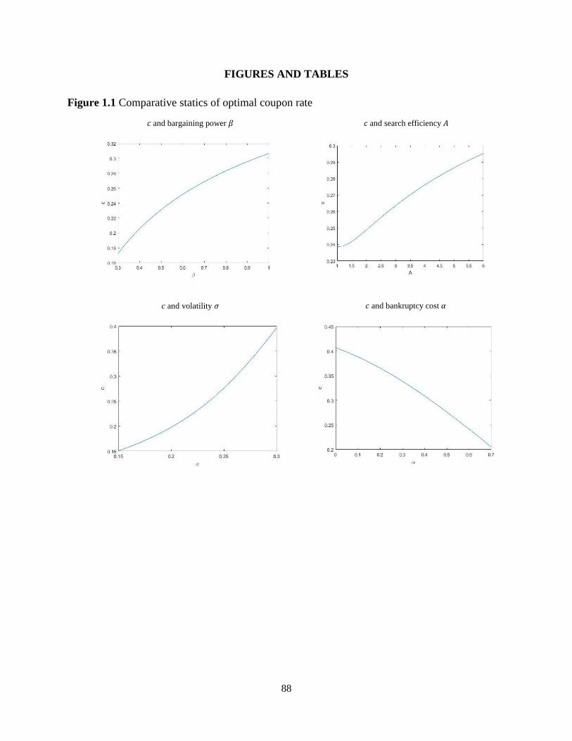
88

FIGURES AND TABLES

Figure 1.1 Comparative statics of optimal coupon rate

𝑐 and bankruptcy cost 𝛼

𝑐 and bargaining power 𝛽 𝑐 and search efficiency 𝐴

c and volatility 𝜎

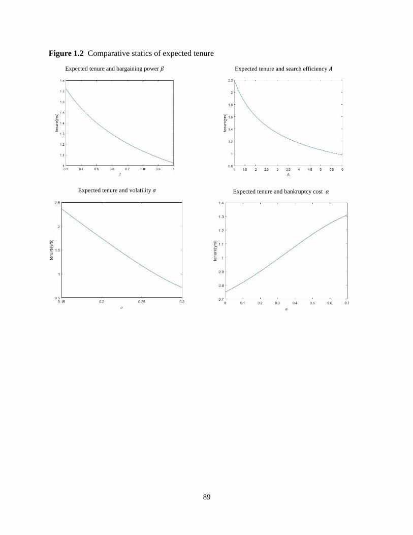
89

Figure 1.2 Comparative statics of expected tenure

Expected tenure and search efficiency 𝐴 Expected tenure and bargaining power 𝛽

Expected tenure and bankruptcy cost 𝛼 Expected tenure and volatility 𝜎

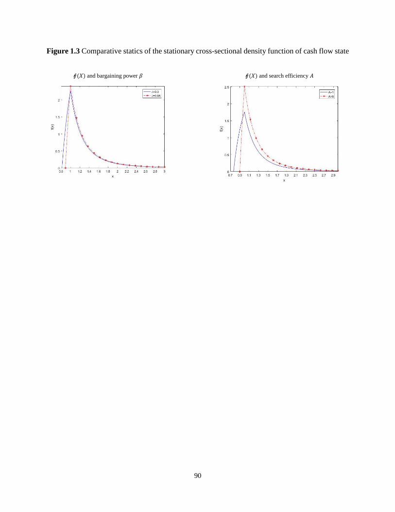
90

Figure 1.3 Comparative statics of the stationary cross-sectional density function of cash flow state

𝒻(𝑋) and bargaining power 𝛽 𝒻(𝑋) and search efficiency 𝐴

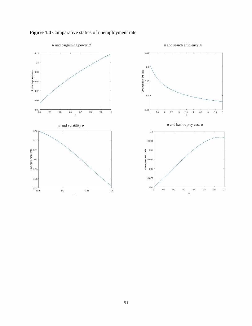
91

Figure 1.4 Comparative statics of unemployment rate

𝑢 and search efficiency 𝐴 𝑢 and bargaining power 𝛽

𝑢 and bankruptcy cost 𝛼 𝑢 and volatility 𝜎

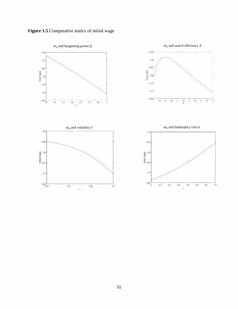
92

Figure 1.5 Comparative statics of initial wage

𝑤0 and search efficiency 𝐴 𝑤0 and bargaining power 𝛽

𝑤0 and bankruptcy cost 𝛼 𝑤0 and volatility 𝜎

93

Figure 1.6 Comparative statics of labor force participation

𝑒 and search efficiency 𝐴 𝑒 and volatility 𝜎

94

Figure 2.1 Cumulative abnormal returns for withdrawn LBOs

Cumulative abnormal returns for all withdrawn deals

Cumulative abnormal returns for exogenously withdrawn deals

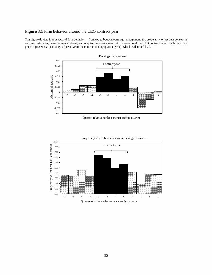
95

Figure 3.1 Firm behavior around the CEO contract year This figure depicts four aspects of firm behavior— from top to bottom, earnings management, the propensity to just beat consensus

earnings estimates, negative news release, and acquirer announcement returns — around the CEO contract year. Each date on a

graph represents a quarter (year) relative to the contract ending quarter (year), which is denoted by 0.

-0.02

-0.015

-0.01

-0.005

0

0.005

0.01

0.015

0.02

0.025

0.03

-7 -6 -5 -4 -3 -2 -1 0 1 2 3 4

Ab

no

rmal

acc

rual

s

Quarter relative to the contract ending quarter

Earnings management

Contract year

0%

2%

4%

6%

8%

10%

12%

14%

16%

18%

20%

-7 -6 -5 -4 -3 -2 -1 0 1 2 3 4

Pro

pen

sity

to

ju

st b

eat

EP

S c

on

sen

sus

Quarter relative to the contract ending quarter

Propensity to just beat consensus earnings estimates

Contract year

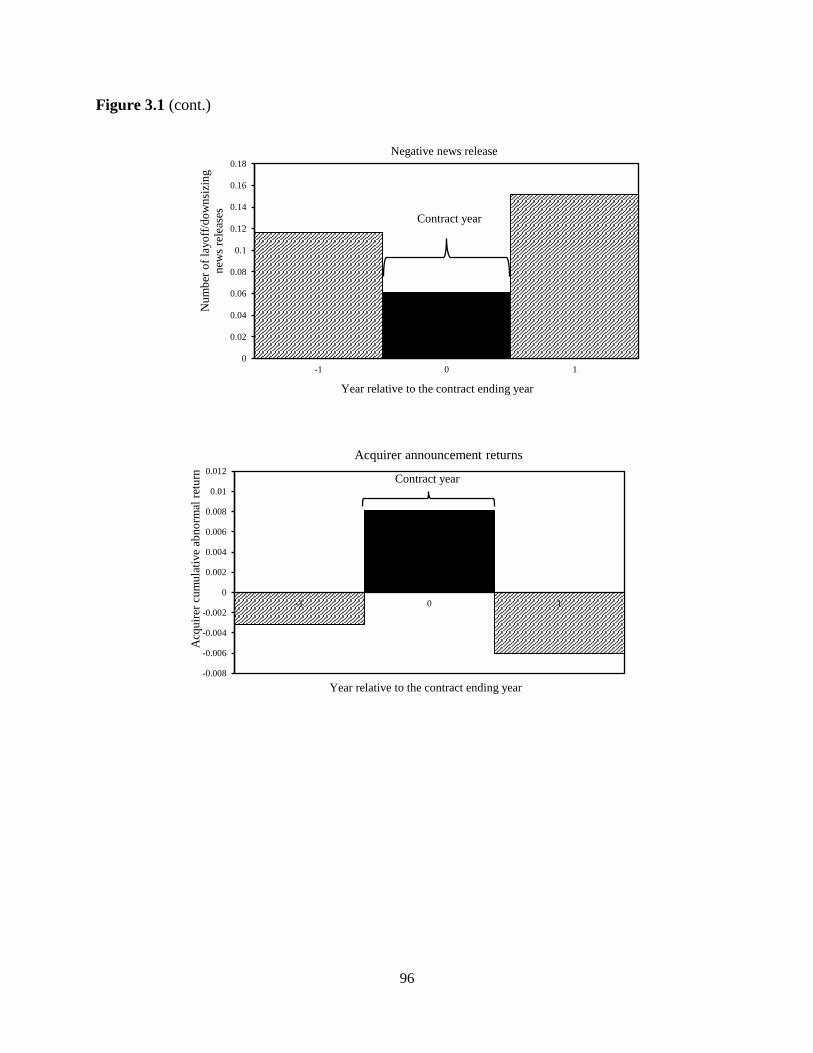
96

Figure 3.1 (cont.)

0

0.02

0.04

0.06

0.08

0.1

0.12

0.14

0.16

0.18

-1 0 1

Nu

mb

er o

f la

yo

ff/d

ow

nsi

zin

g

new

s re

leas

es

Year relative to the contract ending year

Negative news release

Contract year

-0.008

-0.006

-0.004

-0.002

0

0.002

0.004

0.006

0.008

0.01

0.012

-1 0 1

Acq

uir

er c

um

ula

tive

abn

orm

al r

etu

rn

Year relative to the contract ending year

Acquirer announcement returns

Contract year

97

Table 1.1 Model parameters for baseline calibration

Parameters Interpretation Values Reference

𝛽 Worker’s bargaining power 0.75 Shimer (2005)

𝛼 Bankruptcy cost 0.5 Leland (1994)

𝑏 Unemployment benefit 0.4 Shimer (2005)

𝑠 Exogenous separation rate 0.15 Monacelli, Quadrini and Trigari (2011)

𝜅 Cost of maintaining a vacancy 0.4 Moen and Rosen (2011)

𝑋0 Initial cash flow state 1

𝜃 Productivity 1

𝑟 Interest rate 0.05 Brunnermeier Sannikov (2014)

𝜇 Drift −0.022 He and Milbradt (2014)

𝜎 Volatility 0.25 He and Milbradt (2014)

𝑓 Flow operational cost 0

𝐹 Present value of 𝑓 0

𝜄 Matching elasticity on 𝑢 0.3 Petrongolo and Pissarides (2001)

𝐴 Matching efficiency 4 Mortensen and Pissarides (1994)

98

Table 2.1 Annual distribution of leveraged buyouts with private equity participation

Table 2.1 reports the annual distribution of number of total LBOs with private equity participation, as well as number of the

successful deals and withdrawn deals according to deal announcement year.

Announcement year Total LBOs Successful LBOs Withdrawn LBOs

1979 1 0 1

1984 9 4 5

1985 22 12 10

1986 25 22 3

1987 26 18 8

1988 53 41 12

1989 15 9 6

1990 4 4 0

1991 2 1 1

1992 3 1 2

1993 4 4 0

1994 5 4 1

1995 5 4 1

1996 10 9 1

1997 17 14 3

1998 17 13 4

1999 36 28 8

2000 33 28 5

2001 9 9 0

2002 12 9 3

2003 12 9 3

2004 23 18 5

2005 39 33 6

2006 64 55 9

2007 64 50 14

2008 21 14 7

2009 19 13 6

2010 37 35 2

2011 23 23 0

Total 610 484 126

99

Table 2.2 Distribution of deal withdrawn reasons

Table 2.2 presents the reason behind each withdrawn deal. I search for news articles around deal withdrawal dates from LexisNexis

for withdrawal reasons. The 40 deals withdrawn for reasons specified in bold letters are the ones withdrawn without disclosing any

information with regard to target performance or target stock price during the deal outstanding period (“exogenously withdrawn”

sample thereafter).

Withdrawal reason # cases

Adverse change in capital market and economic conditions 7

Favorable change in public equity market 1

Lack of finance 5

Target's high leverage 1

Negotiation failed due to price disagreement 19

Negotiation failed due to reasons other than bid price issue, target news or target performance 24

Negative target news (material adverse change of the target) /poor performance 17

Outbid by another acquirer 37

Positive target news/strong performance 3

Rejected by regulatory government agency 3

Withdrawn reason not specified 9

Total cases 126

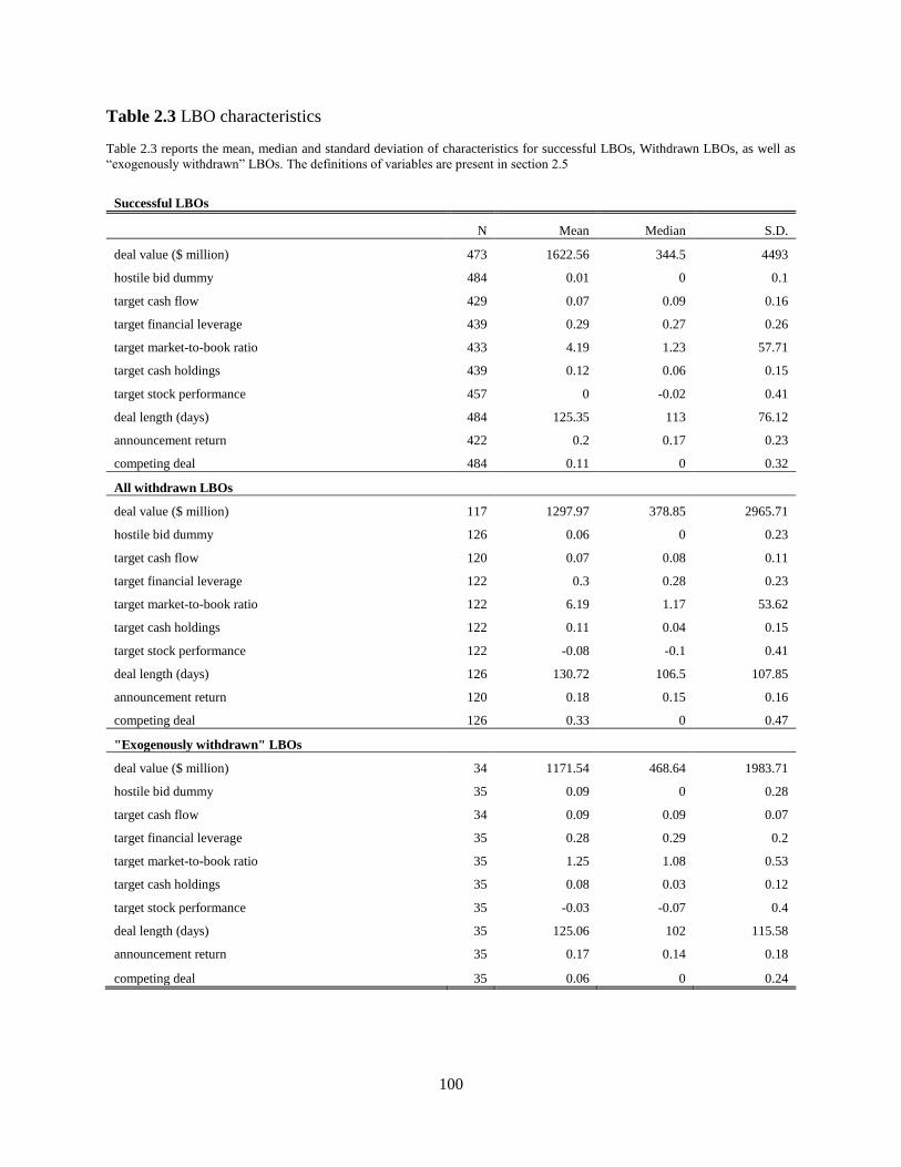
100

Table 2.3 LBO characteristics

Table 2.3 reports the mean, median and standard deviation of characteristics for successful LBOs, Withdrawn LBOs, as well as

“exogenously withdrawn” LBOs. The definitions of variables are present in section 2.5

Successful LBOs

N Mean Median S.D.

deal value ($ million) 473 1622.56 344.5 4493

hostile bid dummy 484 0.01 0 0.1

target cash flow 429 0.07 0.09 0.16

target financial leverage 439 0.29 0.27 0.26

target market-to-book ratio 433 4.19 1.23 57.71

target cash holdings 439 0.12 0.06 0.15

target stock performance 457 0 -0.02 0.41

deal length (days) 484 125.35 113 76.12

announcement return 422 0.2 0.17 0.23

competing deal 484 0.11 0 0.32

All withdrawn LBOs

deal value ($ million) 117 1297.97 378.85 2965.71

hostile bid dummy 126 0.06 0 0.23

target cash flow 120 0.07 0.08 0.11

target financial leverage 122 0.3 0.28 0.23

target market-to-book ratio 122 6.19 1.17 53.62

target cash holdings 122 0.11 0.04 0.15

target stock performance 122 -0.08 -0.1 0.41

deal length (days) 126 130.72 106.5 107.85

announcement return 120 0.18 0.15 0.16

competing deal 126 0.33 0 0.47

"Exogenously withdrawn" LBOs

deal value ($ million) 34 1171.54 468.64 1983.71

hostile bid dummy 35 0.09 0 0.28

target cash flow 34 0.09 0.09 0.07

target financial leverage 35 0.28 0.29 0.2

target market-to-book ratio 35 1.25 1.08 0.53

target cash holdings 35 0.08 0.03 0.12

target stock performance 35 -0.03 -0.07 0.4

deal length (days) 35 125.06 102 115.58

announcement return 35 0.17 0.14 0.18

competing deal 35 0.06 0 0.24

101

Table 2.4 Stock returns for withdrawn leveraged buyouts

For each LBO deal, I calculate the abnormal buy-and-hold return, cumulative abnormal return, and standardized daily abnormal

return for the target stock in question, from 25 trading days before the deal announcement date till 25 trading days after the deal

withdrawn date. The benchmark portfolios are value-weighted market portfolio for “Market portfolio” column and a three-firm

portfolio matching on Fama-French 49 industry, size and book-to-market ratio, similar to Barber and Lyon (1997), in the “Matching

portfolio” column. LBOs withdrawn for exogenous reasons are defined in Table 2.2. I classify LBOs withdrawn due to adverse

change in high-yield bond market since announcement if the change in average log high-yield bond market index between one

quarter before the announcement and the LBO period are among the worst 25% among all LBOs announced during that year.

Withdrawn LBOs without subsequent bids are withdrawn deals without any subsequent acquisition bids at least one year thereafter.

T-statistics are in parenthesis. ***, **, * denotes statistically significant below 1%, 5%, 10% level, respectively.

All withdrawn LBOs

Market portfolio Matching portfolio

105 cases

Raw buy-and-hold return 0.173***

(4.212)

Raw cumulative return 0.203***

(5.833)

Abnormal buy-and-hold return 0.119*** 0.106**

(2.987) (2.385)

Cumulative abnormal return 0.149*** 0.135***

(4.434) (3.640)

Standardized daily abnormal buy-and-hold return 0.0011*** 0.0008*** 0.0008***

(4.071) (3.122) (2.922)

LBOs withdrawn for "exogenous" reasons

Market portfolio Matching portfolio

35 cases

Raw buy-and-hold return 0.145**

(2.692)

Raw cumulative return 0.181***

(3.794)

Abnormal buy-and-hold return 0.099* 0.134***

(1.980) (3.086)

Cumulative abnormal return 0.134*** 0.165***

(3.040) (3.960)

Standardized daily abnormal buy-and-hold return 0.0011** 0.0009** 0.0012***

(2.317) (2.267) (2.968)

Withdrawn LBOs with adverse change in high-yield bond market since announcements

Market portfolio Matching portfolio

21 cases

Raw buy-and-hold return 0.105

(1.219)

Raw cumulative return 0.161*

(1.986)

Abnormal buy-and-hold return 0.180** 0.203***

(2.251) (3.078)

Cumulative abnormal return 0.227*** 0.253***

102

Table 2.4 (Cont.)

(2.993) (4.038)

Standardized daily abnormal buy-and-hold return 0.0008 0.0015** 0.0016***

(1.171) (2.678) (3.099)

Withdrawn LBOs without subsequent bids one year thereafter

Abnormal buy-and-hold return Market portfolio Matching portfolio

Full sample 79 cases

0.179*** 0.145**

(3.620) (2.526)

LBOs withdrawn for "exogenous" reasons 23 cases

0.174** 0.202***

(2.759) (4.052)

LBOs withdrawn due to adverse change in high-yield bond market

14 cases

0.281** 0.281***

(2.740) (3.255)

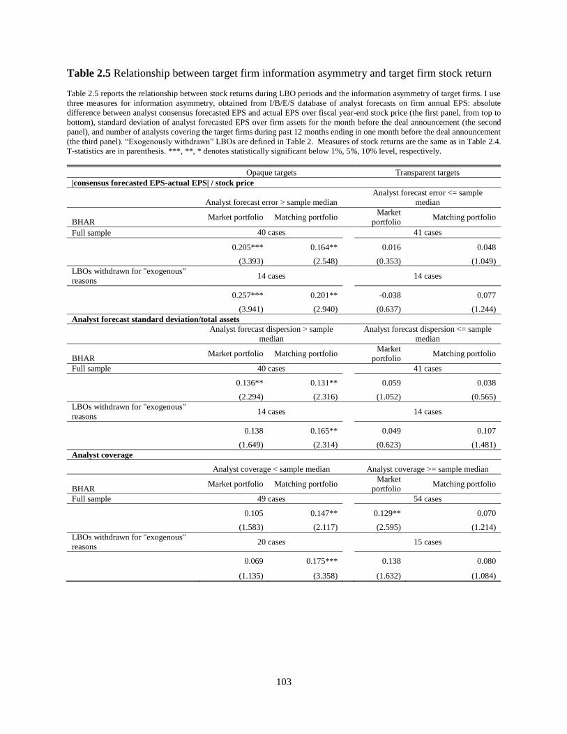
103

Table 2.5 Relationship between target firm information asymmetry and target firm stock return

Table 2.5 reports the relationship between stock returns during LBO periods and the information asymmetry of target firms. I use

three measures for information asymmetry, obtained from I/B/E/S database of analyst forecasts on firm annual EPS: absolute

difference between analyst consensus forecasted EPS and actual EPS over fiscal year-end stock price (the first panel, from top to

bottom), standard deviation of analyst forecasted EPS over firm assets for the month before the deal announcement (the second

panel), and number of analysts covering the target firms during past 12 months ending in one month before the deal announcement

(the third panel). “Exogenously withdrawn” LBOs are defined in Table 2. Measures of stock returns are the same as in Table 2.4.

T-statistics are in parenthesis. ***, **, * denotes statistically significant below 1%, 5%, 10% level, respectively.

Opaque targets Transparent targets

|consensus forecasted EPS-actual EPS| / stock price

Analyst forecast error > sample median

Analyst forecast error <= sample

median

BHAR Market portfolio Matching portfolio

Market

portfolio Matching portfolio

Full sample 40 cases 41 cases

0.205*** 0.164** 0.016 0.048

(3.393) (2.548) (0.353) (1.049)

LBOs withdrawn for "exogenous"

reasons 14 cases 14 cases

0.257*** 0.201** -0.038 0.077

(3.941) (2.940) (0.637) (1.244)

Analyst forecast standard deviation/total assets

Analyst forecast dispersion > sample

median

Analyst forecast dispersion <= sample

median

BHAR Market portfolio Matching portfolio

Market

portfolio Matching portfolio

Full sample 40 cases 41 cases

0.136** 0.131** 0.059 0.038

(2.294) (2.316) (1.052) (0.565)

LBOs withdrawn for "exogenous"

reasons 14 cases 14 cases

0.138 0.165** 0.049 0.107

(1.649) (2.314) (0.623) (1.481)

Analyst coverage

Analyst coverage < sample median Analyst coverage >= sample median

BHAR Market portfolio Matching portfolio

Market

portfolio Matching portfolio

Full sample 49 cases 54 cases

0.105 0.147** 0.129** 0.070

(1.583) (2.117) (2.595) (1.214)

LBOs withdrawn for "exogenous"

reasons 20 cases 15 cases

0.069 0.175*** 0.138 0.080

(1.135) (3.358) (1.632) (1.084)

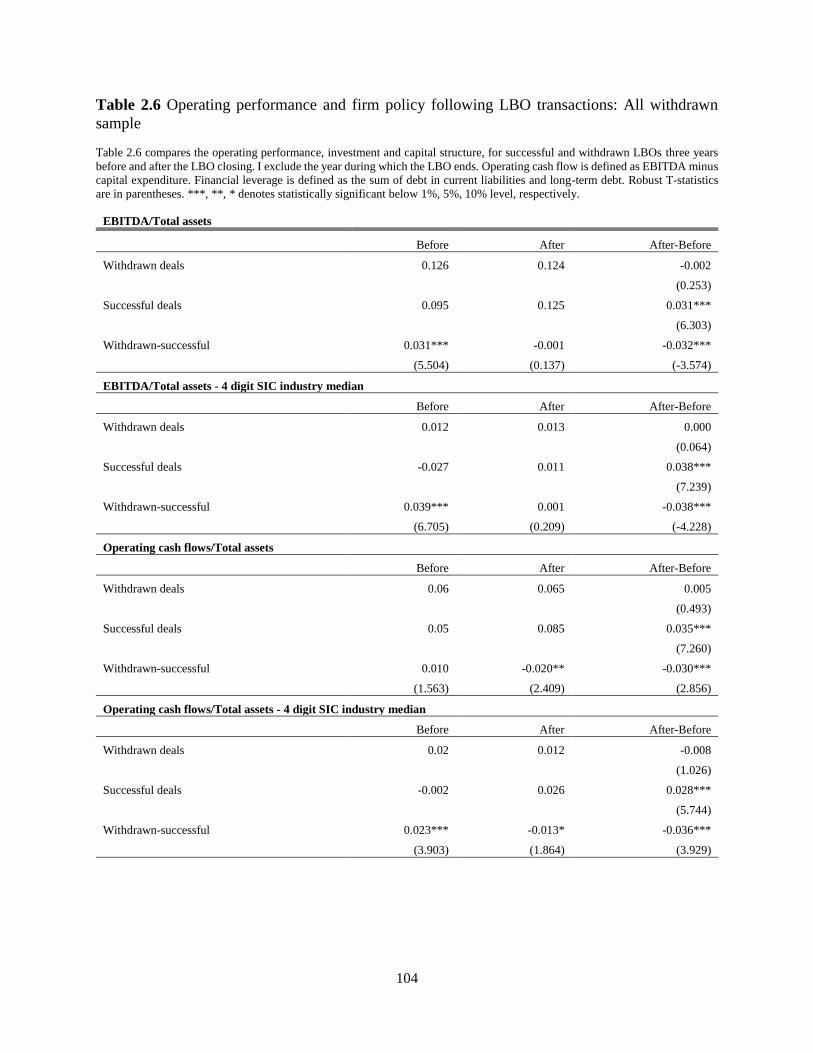
104

Table 2.6 Operating performance and firm policy following LBO transactions: All withdrawn

sample

Table 2.6 compares the operating performance, investment and capital structure, for successful and withdrawn LBOs three years

before and after the LBO closing. I exclude the year during which the LBO ends. Operating cash flow is defined as EBITDA minus

capital expenditure. Financial leverage is defined as the sum of debt in current liabilities and long-term debt. Robust T-statistics

are in parentheses. ***, **, * denotes statistically significant below 1%, 5%, 10% level, respectively.

EBITDA/Total assets

Before After After-Before

Withdrawn deals 0.126 0.124 -0.002

(0.253)

Successful deals 0.095 0.125 0.031***

(6.303)

Withdrawn-successful 0.031*** -0.001 -0.032***

(5.504) (0.137) (-3.574)

EBITDA/Total assets - 4 digit SIC industry median

Before After After-Before

Withdrawn deals 0.012 0.013 0.000

(0.064)

Successful deals -0.027 0.011 0.038***

(7.239)

Withdrawn-successful 0.039*** 0.001 -0.038***

(6.705) (0.209) (-4.228)

Operating cash flows/Total assets

Before After After-Before

Withdrawn deals 0.06 0.065 0.005

(0.493)

Successful deals 0.05 0.085 0.035***

(7.260)

Withdrawn-successful 0.010 -0.020** -0.030***

(1.563) (2.409) (2.856)

Operating cash flows/Total assets - 4 digit SIC industry median

Before After After-Before

Withdrawn deals 0.02 0.012 -0.008

(1.026)

Successful deals -0.002 0.026 0.028***

(5.744)

Withdrawn-successful 0.023*** -0.013* -0.036***

(3.903) (1.864) (3.929)

105

Table 2.6 (cont.)

CAPEX/Total assets

Before After After-Before

Withdrawn deals 0.066 0.057 -0.009

(1.473)

Successful deals 0.045*** 0.040 -0.005

(-1.472)

Withdrawn-successful 0.021*** 0.017*** -0.004

(4.475) (3.559) (0.598)

CAPEX/Total assets - 4 digit SIC industry median

Before After After-Before

Withdrawn deals 0.000 0.008 0.007

(1.640)

Successful deals -0.015 -0.008 0.008***

(2.700)

Withdrawn-successful 0.016*** 0.015*** -0.000

(4.381) (3.895) (0.047)

Financial leverage/Total assets

Before After After-Before

Withdrawn deals 0.319 0.396 0.077***

(2.646)

Successful deals 0.222 0.686 0.464***

(22.216)

Withdrawn-successful 0.097*** -0.290*** -0.387***

(5.330) (9.361) (10.771)

Financial leverage/Total assets - 4 digit SIC industry median

Before After After-Before

Withdrawn deals 0.039 0.142 0.103***

(4.083)

Successful deals -0.036 0.376 0.412***

(21.580)

Withdrawn-successful 0.075*** -0.234*** -0.309***

(4.989) (8.383) (9.747)

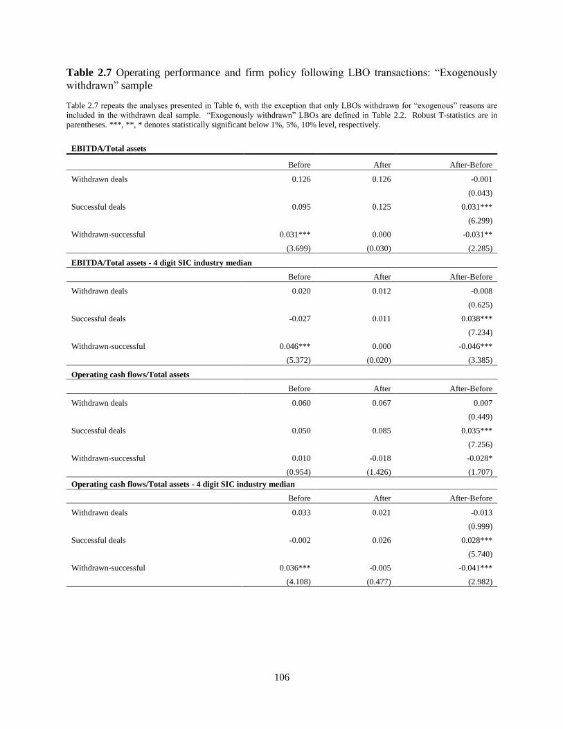
106

Table 2.7 Operating performance and firm policy following LBO transactions: “Exogenously

withdrawn” sample

Table 2.7 repeats the analyses presented in Table 6, with the exception that only LBOs withdrawn for “exogenous” reasons are

included in the withdrawn deal sample. “Exogenously withdrawn” LBOs are defined in Table 2.2. Robust T-statistics are in

parentheses. ***, **, * denotes statistically significant below 1%, 5%, 10% level, respectively.

EBITDA/Total assets

Before After After-Before

Withdrawn deals 0.126 0.126 -0.001

(0.043)

Successful deals 0.095 0.125 0.031***

(6.299)

Withdrawn-successful 0.031*** 0.000 -0.031**

(3.699) (0.030) (2.285)

EBITDA/Total assets - 4 digit SIC industry median

Before After After-Before

Withdrawn deals 0.020 0.012 -0.008

(0.625)

Successful deals -0.027 0.011 0.038***

(7.234)

Withdrawn-successful 0.046*** 0.000 -0.046***

(5.372) (0.020) (3.385)

Operating cash flows/Total assets

Before After After-Before

Withdrawn deals 0.060 0.067 0.007

(0.449)

Successful deals 0.050 0.085 0.035***

(7.256)

Withdrawn-successful 0.010 -0.018 -0.028*

(0.954) (1.426) (1.707)

Operating cash flows/Total assets - 4 digit SIC industry median

Before After After-Before

Withdrawn deals 0.033 0.021 -0.013

(0.999)

Successful deals -0.002 0.026 0.028***

(5.740)

Withdrawn-successful 0.036*** -0.005 -0.041***

(4.108) (0.477) (2.982)

107

Table 2.7 (cont.)

CAPEX/Total assets

Before After After-Before

Withdrawn deals 0.067 0.054 -0.012

-1.217

Successful deals 0.045 0.040 -0.005

-1.471

Withdrawn-successful 0.022*** 0.014** -0.008

(2.757) (2.023) (0.722)

CAPEX/Total assets - 4 digit SIC industry median

Before After After-Before

Withdrawn deals -0.006 -0.003 0.003

(0.353)

Successful deals -0.015 -0.008 0.008***

(2.698)

Withdrawn-successful 0.009 0.004 -0.005

(1.402) (0.714) (0.514)

Financial leverage/Total assets

Before After After-Before

Withdrawn deals 0.287 0.434 0.148***

(2.735)

Successful deals 0.222 0.686 0.464***

(22.202)

Withdrawn-successful 0.065** -0.252*** -0.317***

(2.558) (4.836) (5.468)

Financial leverage/Total assets - 4 digit SIC industry median

Before After After-Before

Withdrawn deals 0.031 0.180 0.149***

(3.061)

Successful deals -0.036 0.376 0.412***

(21.566)

Withdrawn-successful 0.068*** -0.196*** -0.264***

(3.085) (4.132) (5.047)

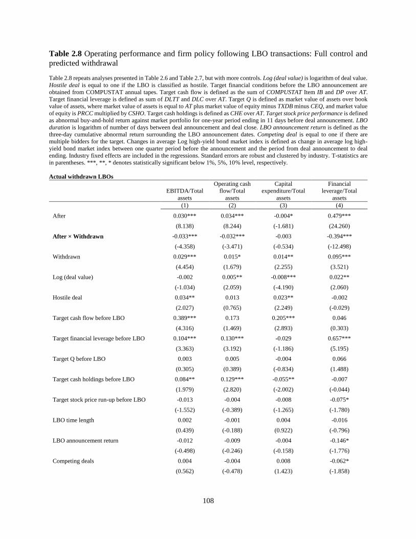
108

Table 2.8 Operating performance and firm policy following LBO transactions: Full control and

predicted withdrawal

Table 2.8 repeats analyses presented in Table 2.6 and Table 2.7, but with more controls. Log (deal value) is logarithm of deal value.

Hostile deal is equal to one if the LBO is classified as hostile. Target financial conditions before the LBO announcement are

obtained from COMPUSTAT annual tapes. Target cash flow is defined as the sum of COMPUSTAT Item IB and DP over AT.

Target financial leverage is defined as sum of DLTT and DLC over AT. Target Q is defined as market value of assets over book

value of assets, where market value of assets is equal to AT plus market value of equity minus TXDB minus CEQ, and market value

of equity is PRCC multiplied by CSHO. Target cash holdings is defined as CHE over AT. Target stock price performance is defined

as abnormal buy-and-hold return against market portfolio for one-year period ending in 11 days before deal announcement. LBO

duration is logarithm of number of days between deal announcement and deal close. LBO announcement return is defined as the

three-day cumulative abnormal return surrounding the LBO announcement dates. Competing deal is equal to one if there are

multiple bidders for the target. Changes in average Log high-yield bond market index is defined as change in average log high-

yield bond market index between one quarter period before the announcement and the period from deal announcement to deal

ending. Industry fixed effects are included in the regressions. Standard errors are robust and clustered by industry. T-statistics are

in parentheses. ***, **, * denotes statistically significant below 1%, 5%, 10% level, respectively.

Actual withdrawn LBOs

EBITDA/Total

assets

Operating cash

flow/Total

assets

Capital

expenditure/Total

assets

Financial

leverage/Total

assets

(1) (2) (3) (4)

After 0.030*** 0.034*** -0.004* 0.479***

(8.138) (8.244) (-1.681) (24.260)

After × Withdrawn -0.033*** -0.032*** -0.003 -0.394***

(-4.358) (-3.471) (-0.534) (-12.498)

Withdrawn 0.029*** 0.015* 0.014** 0.095***

(4.454) (1.679) (2.255) (3.521)

Log (deal value) -0.002 0.005** -0.008*** 0.022**

(-1.034) (2.059) (-4.190) (2.060)

Hostile deal 0.034** 0.013 0.023** -0.002

(2.027) (0.765) (2.249) (-0.029)

Target cash flow before LBO 0.389*** 0.173 0.205*** 0.046

(4.316) (1.469) (2.893) (0.303)

Target financial leverage before LBO 0.104*** 0.130*** -0.029 0.657***

(3.363) (3.192) (-1.186) (5.195)

Target Q before LBO 0.003 0.005 -0.004 0.066

(0.305) (0.389) (-0.834) (1.488)

Target cash holdings before LBO 0.084** 0.129*** -0.055** -0.007

(1.979) (2.820) (-2.002) (-0.044)

Target stock price run-up before LBO -0.013 -0.004 -0.008 -0.075*

(-1.552) (-0.389) (-1.265) (-1.780)

LBO time length 0.002 -0.001 0.004 -0.016

(0.439) (-0.188) (0.922) (-0.796)

LBO announcement return -0.012 -0.009 -0.004 -0.146*

(-0.498) (-0.246) (-0.158) (-1.776)

Competing deals 0.004 -0.004 0.008 -0.062*

(0.562) (-0.478) (1.423) (-1.858)

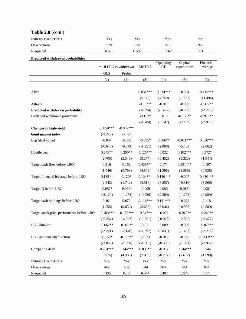
109

Table 2.8 (cont.)

Industry fixed effects Yes Yes Yes Yes

Observations 929 929 929 929

R-squared 0.555 0.502 0.562 0.631

Predicted withdrawal probabilities

=1 if LBO is withdrawn EBITDA

Operating

CF

Capital

expenditure

Financial

leverage

OLS Probit

(1) (2) (3) (4) (5) (6)

After 0.031*** 0.034*** -0.004 0.415***

(5.140) (4.759) (-1.182) (11.496)

After × -0.052** -0.046 -0.008 -0.372**

Predicted withdrawn probability (-1.994) (-1.477) (-0.530) (-2.260)

Predicted withdrawn probability -0.152* 0.017 -0.160** -0.916**

(-1.784) (0.147) (-2.139) (-2.085)

Changes in high-yield -0.850*** -0.902***

bond market index (-3.242) (-3.821)

Log (deal value) -0.007 -0.006 -0.005* 0.006** -0.011*** 0.030***

(-0.645) (-0.579) (-1.951) (2.008) (-5.488) (2.662)

Hostile deal 0.375** 0.390** 0.125*** 0.022 0.102*** 0.372*

(2.705) (2.548) (3.274) (0.452) (3.323) (1.944)

Target cash flow before LBO 0.216 0.162 0.439*** 0.174 0.251*** 0.197

(1.046) (0.793) (4.509) (1.395) (3.556) (0.928)

Target financial leverage before LBO 0.135** 0.120* 0.134*** 0.136*** -0.007 0.930***

(2.243) (1.742) (4.516) (3.857) (-0.316) (5.566)

Target Q before LBO -0.057* -0.060* -0.009 0.003 -0.015* 0.051

(-2.129) (-1.753) (-0.736) (0.200) (-1.793) (0.989)

Target cash holdings before LBO 0.101 0.070 0.116*** 0.131*** -0.026 0.118

(1.095) (0.630) (2.685) (3.044) (-0.985) (0.589)

Target stock price performance before LBO -0.183*** -0.183*** -0.047** -0.002 -0.042** -0.249**

(-5.264) (-4.302) (-2.251) (-0.078) (-2.396) (-2.477)

LBO duration -0.062** -0.049** -0.011 0.000 -0.009 -0.076**

(-2.221) (-2.146) (-1.397) (0.031) (-1.483) (-2.252)

LBO announcement return -0.153* -0.173** -0.033 -0.012 -0.020 -0.339***

(-2.056) (-2.090) (-1.361) (-0.399) (-1.021) (-2.867)

Competing deals 0.234*** 0.244*** 0.038** -0.007 0.044*** 0.144

(3.975) (4.333) (2.030) (-0.287) (2.672) (1.599)

Industry fixed effects Yes Yes Yes Yes Yes Yes

Observations 469 469 844 844 844 844

R-squared 0.135 0.13 0.544 0.497 0.574 0.571

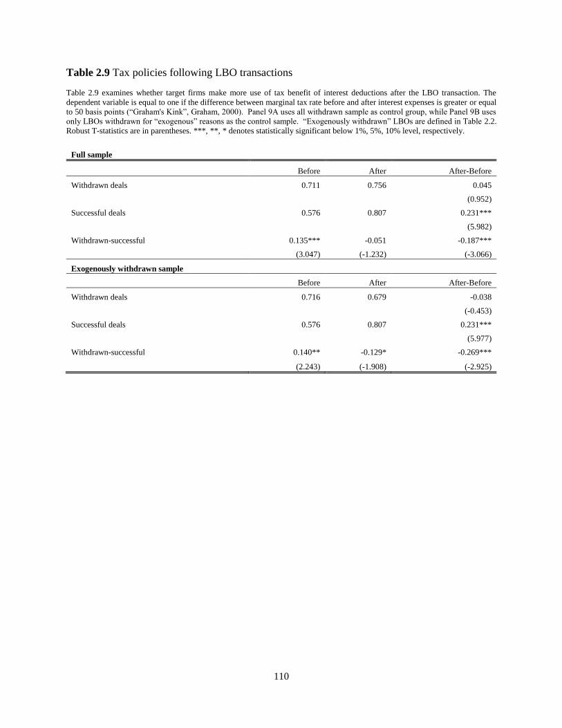
110

Table 2.9 Tax policies following LBO transactions

Table 2.9 examines whether target firms make more use of tax benefit of interest deductions after the LBO transaction. The

dependent variable is equal to one if the difference between marginal tax rate before and after interest expenses is greater or equal

to 50 basis points (“Graham's Kink”, Graham, 2000). Panel 9A uses all withdrawn sample as control group, while Panel 9B uses

only LBOs withdrawn for “exogenous” reasons as the control sample. “Exogenously withdrawn” LBOs are defined in Table 2.2.

Robust T-statistics are in parentheses. ***, **, * denotes statistically significant below 1%, 5%, 10% level, respectively.

Full sample

Before After After-Before

Withdrawn deals 0.711 0.756 0.045

(0.952)

Successful deals 0.576 0.807 0.231***

(5.982)

Withdrawn-successful 0.135*** -0.051 -0.187***

(3.047) (-1.232) (-3.066)

Exogenously withdrawn sample

Before After After-Before

Withdrawn deals 0.716 0.679 -0.038

(-0.453)

Successful deals 0.576 0.807 0.231***

(5.977)

Withdrawn-successful 0.140** -0.129* -0.269***

(2.243) (-1.908) (-2.925)

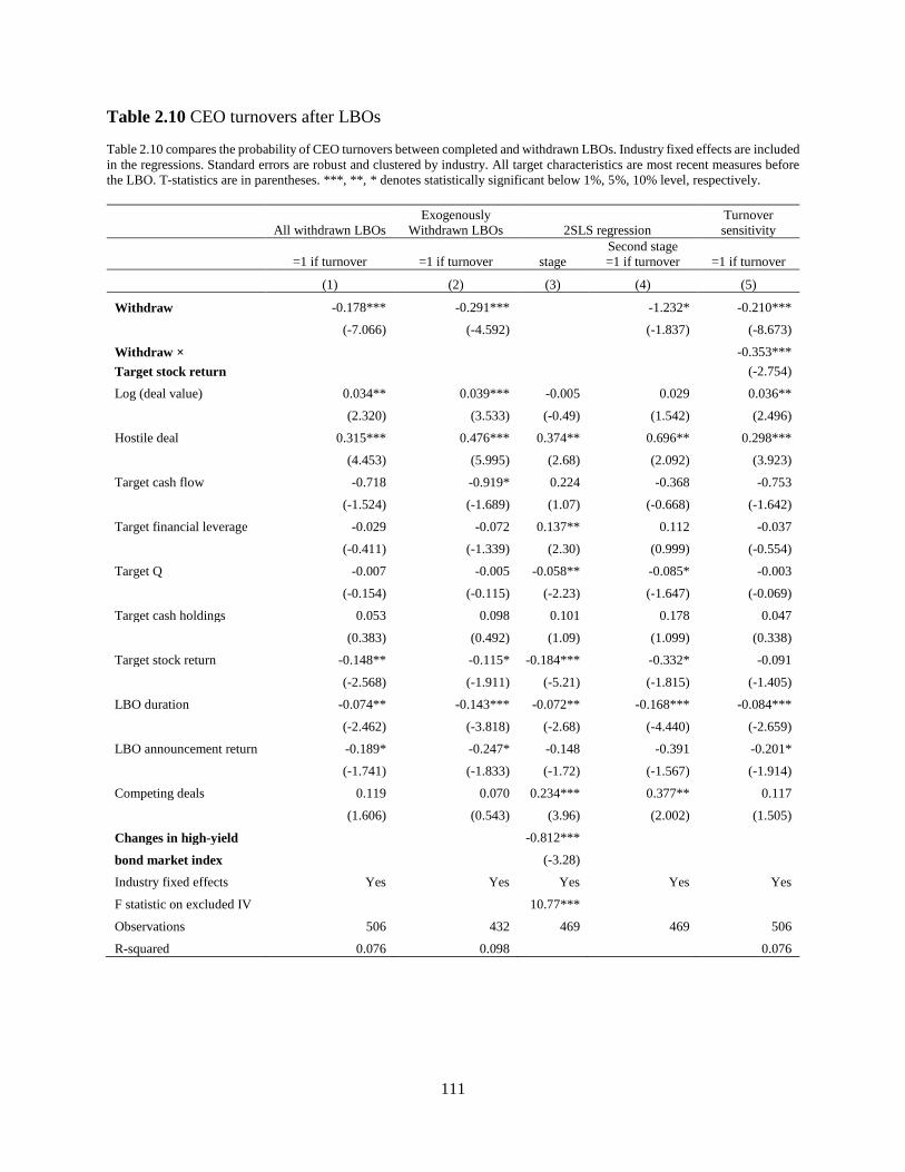
111

Table 2.10 CEO turnovers after LBOs

Table 2.10 compares the probability of CEO turnovers between completed and withdrawn LBOs. Industry fixed effects are included

in the regressions. Standard errors are robust and clustered by industry. All target characteristics are most recent measures before

the LBO. T-statistics are in parentheses. ***, **, * denotes statistically significant below 1%, 5%, 10% level, respectively.

All withdrawn LBOs

Exogenously

Withdrawn LBOs 2SLS regression

Turnover

sensitivity

=1 if turnover =1 if turnover stage

Second stage

=1 if turnover =1 if turnover

(1) (2) (3) (4) (5)

Withdraw -0.178*** -0.291*** -1.232* -0.210***

(-7.066) (-4.592) (-1.837) (-8.673)

Withdraw × -0.353***

Target stock return (-2.754)

Log (deal value) 0.034** 0.039*** -0.005 0.029 0.036**

(2.320) (3.533) (-0.49) (1.542) (2.496)

Hostile deal 0.315*** 0.476*** 0.374** 0.696** 0.298***

(4.453) (5.995) (2.68) (2.092) (3.923)

Target cash flow -0.718 -0.919* 0.224 -0.368 -0.753

(-1.524) (-1.689) (1.07) (-0.668) (-1.642)

Target financial leverage -0.029 -0.072 0.137** 0.112 -0.037

(-0.411) (-1.339) (2.30) (0.999) (-0.554)

Target Q -0.007 -0.005 -0.058** -0.085* -0.003

(-0.154) (-0.115) (-2.23) (-1.647) (-0.069)

Target cash holdings 0.053 0.098 0.101 0.178 0.047

(0.383) (0.492) (1.09) (1.099) (0.338)

Target stock return -0.148** -0.115* -0.184*** -0.332* -0.091

(-2.568) (-1.911) (-5.21) (-1.815) (-1.405)

LBO duration -0.074** -0.143*** -0.072** -0.168*** -0.084***

(-2.462) (-3.818) (-2.68) (-4.440) (-2.659)

LBO announcement return -0.189* -0.247* -0.148 -0.391 -0.201*

(-1.741) (-1.833) (-1.72) (-1.567) (-1.914)

Competing deals 0.119 0.070 0.234*** 0.377** 0.117

(1.606) (0.543) (3.96) (2.002) (1.505)

Changes in high-yield -0.812***

bond market index (-3.28)

Industry fixed effects Yes Yes Yes Yes Yes

F statistic on excluded IV 10.77***

Observations 506 432 469 469 506

R-squared 0.076 0.098 0.076

112

Table 3.1 Summary statistics

This table presents the mean, standard deviation, and number of observations (N) for the variables used in the paper.

Variable name Mean Standard deviation N

Total assets (in million $) 15,492.56 23,436.05 1,132

Q 1.840 0.853 1,132

Financial leverage 0.272 0.168 1,132

Operating performance 0.039 0.022 1,132

Earnings management

Abnormal accruals 0.005 0.086 1,132

Propensity to meet or just beat consensus forecasts

Meet or just beat consensus EPS forecast? 0.194 0.396 1,551

Just beat consensus EPS forecast? 0.090 0.286 1,551

Negative news release

Number of negative news releases from Capital IQ 0.964 2.012 439

Number of layoff/downsizing news releases from Capital IQ 0.781 1.894 439

Number of major layoff/downsizing news releases from 8-K 0.109 0.455 439

Acquisitions

Cumulative abnormal return (CAR [-1, +1]) -0.037% 0.036 264

Relative transaction value 0.073 0.154 264

Pure stock deal? 0.042 0.200 264

Related deal? 0.470 0.500 264

Public target? 0.197 0.398 264

113

Table 3.2 Earnings management

This table presents the OLS regression results for earnings management around the CEO contract year. For each sample firm, 12

quarterly observations are included in the regressions including the four quarters before, four quarters during, and four quarters

after the contract year. The dependent variable is the quarterly abnormal accruals (scaled by assets) estimated from quarterly

income and financial data using the modified Jones model (Dechow, Sloan, and Sweeney, 1995). Contract year is a dummy variable

that takes the value one for the four quarters leading up to the contract ending and zero for the four quarters before and four quarters

after the contract year. Control variables include firm size, Q, leverage, and operating performance. Robust standard errors

clustered by firm are in parentheses. Asterisks denote statistical significance at the 1% (***), 5% (**), or 10% (*) level.

Abnormal accruals

Independent variable (1) (2) (3) (4)

Contract year? 0.015*** 0.015*** 0.015** 0.014**

(0.006) (0.006) (0.006) (0.006)

Log assets 0.004 0.006* -0.020

(0.003) (0.003) (0.016)

Q 0.008* 0.012** 0.016

(0.004) (0.004) (0.011)

Financial leverage -0.006 -0.010 -0.013

(0.021) (0.023) (0.043)

Operating performance -0.210 -0.289 -0.248

(0.200) (0.199) (0.352)

Year fixed effects No No Yes Yes

Firm fixed effects No No No Yes

Number of observations 1,132 1,132 1,132 1,132

R-squared 0.007 0.011 0.023 0.150

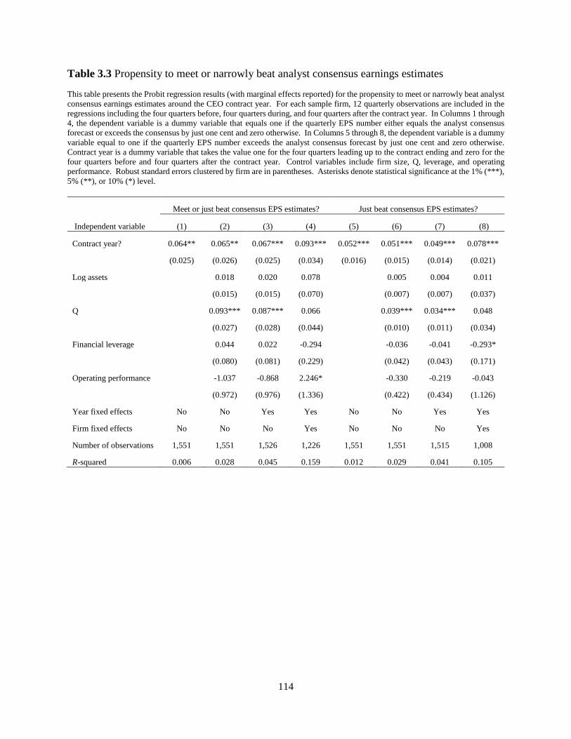
114

Table 3.3 Propensity to meet or narrowly beat analyst consensus earnings estimates

This table presents the Probit regression results (with marginal effects reported) for the propensity to meet or narrowly beat analyst

consensus earnings estimates around the CEO contract year. For each sample firm, 12 quarterly observations are included in the

regressions including the four quarters before, four quarters during, and four quarters after the contract year. In Columns 1 through

4, the dependent variable is a dummy variable that equals one if the quarterly EPS number either equals the analyst consensus

forecast or exceeds the consensus by just one cent and zero otherwise. In Columns 5 through 8, the dependent variable is a dummy

variable equal to one if the quarterly EPS number exceeds the analyst consensus forecast by just one cent and zero otherwise.

Contract year is a dummy variable that takes the value one for the four quarters leading up to the contract ending and zero for the

four quarters before and four quarters after the contract year. Control variables include firm size, Q, leverage, and operating

performance. Robust standard errors clustered by firm are in parentheses. Asterisks denote statistical significance at the 1% (***),

5% (**), or 10% (*) level.

Meet or just beat consensus EPS estimates? Just beat consensus EPS estimates?

Independent variable (1) (2) (3) (4) (5) (6) (7) (8)

Contract year? 0.064** 0.065** 0.067*** 0.093*** 0.052*** 0.051*** 0.049*** 0.078***

(0.025) (0.026) (0.025) (0.034) (0.016) (0.015) (0.014) (0.021)

Log assets 0.018 0.020 0.078 0.005 0.004 0.011

(0.015) (0.015) (0.070) (0.007) (0.007) (0.037)

Q 0.093*** 0.087*** 0.066 0.039*** 0.034*** 0.048

(0.027) (0.028) (0.044) (0.010) (0.011) (0.034)

Financial leverage 0.044 0.022 -0.294 -0.036 -0.041 -0.293*

(0.080) (0.081) (0.229) (0.042) (0.043) (0.171)

Operating performance -1.037 -0.868 2.246* -0.330 -0.219 -0.043

(0.972) (0.976) (1.336) (0.422) (0.434) (1.126)

Year fixed effects No No Yes Yes No No Yes Yes

Firm fixed effects No No No Yes No No No Yes

Number of observations 1,551 1,551 1,526 1,226 1,551 1,551 1,515 1,008

R-squared 0.006 0.028 0.045 0.159 0.012 0.029 0.041 0.105

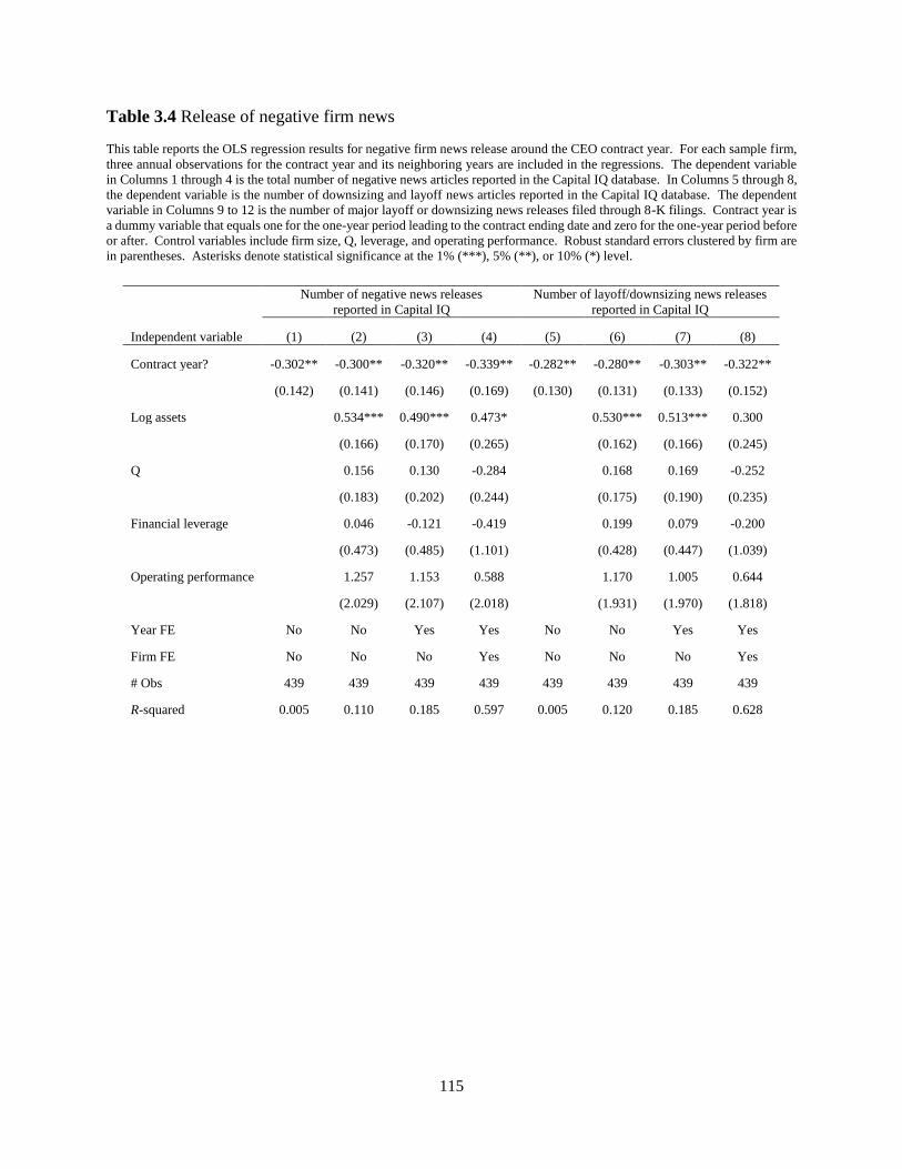
115

Table 3.4 Release of negative firm news

This table reports the OLS regression results for negative firm news release around the CEO contract year. For each sample firm,

three annual observations for the contract year and its neighboring years are included in the regressions. The dependent variable

in Columns 1 through 4 is the total number of negative news articles reported in the Capital IQ database. In Columns 5 through 8,

the dependent variable is the number of downsizing and layoff news articles reported in the Capital IQ database. The dependent

variable in Columns 9 to 12 is the number of major layoff or downsizing news releases filed through 8-K filings. Contract year is

a dummy variable that equals one for the one-year period leading to the contract ending date and zero for the one-year period before

or after. Control variables include firm size, Q, leverage, and operating performance. Robust standard errors clustered by firm are

in parentheses. Asterisks denote statistical significance at the 1% (***), 5% (**), or 10% (*) level.

Number of negative news releases

reported in Capital IQ

Number of layoff/downsizing news releases

reported in Capital IQ

Independent variable (1) (2) (3) (4) (5) (6) (7) (8)

Contract year? -0.302** -0.300** -0.320** -0.339** -0.282** -0.280** -0.303** -0.322**

(0.142) (0.141) (0.146) (0.169) (0.130) (0.131) (0.133) (0.152)

Log assets 0.534*** 0.490*** 0.473* 0.530*** 0.513*** 0.300

(0.166) (0.170) (0.265) (0.162) (0.166) (0.245)

Q 0.156 0.130 -0.284 0.168 0.169 -0.252

(0.183) (0.202) (0.244) (0.175) (0.190) (0.235)

Financial leverage 0.046 -0.121 -0.419 0.199 0.079 -0.200

(0.473) (0.485) (1.101) (0.428) (0.447) (1.039)

Operating performance 1.257 1.153 0.588 1.170 1.005 0.644

(2.029) (2.107) (2.018) (1.931) (1.970) (1.818)

Year FE No No Yes Yes No No Yes Yes

Firm FE No No No Yes No No No Yes

# Obs 439 439 439 439 439 439 439 439

R-squared 0.005 0.110 0.185 0.597 0.005 0.120 0.185 0.628

116

Table 3.4 (cont.)

Number of major layoff/downsizing news

filed in 8-K

(9) (10) (11) (12)

Contract year? -0.073** -0.075** -0.079** -0.081**

(0.028) (0.029) (0.031) (0.037)

Log assets -0.025 -0.042 -0.042

(0.027) (0.033) (0.160)

Q -0.001 -0.015 -0.100

(0.053) (0.046) (0.144)

Financial leverage -0.069 -0.139 -0.653

(0.116) (0.134) (0.658)

Operating performance -0.414 -0.412 -0.091

(0.412) (0.386) (1.034)

Year FE No No Yes Yes

Firm FE No No No Yes

# Obs 439 439 439 439

R-squared 0.006 0.013 0.056 0.376

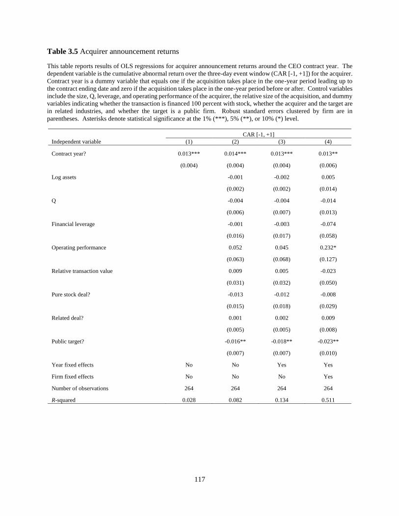
117

Table 3.5 Acquirer announcement returns

This table reports results of OLS regressions for acquirer announcement returns around the CEO contract year. The

dependent variable is the cumulative abnormal return over the three-day event window (CAR [-1, +1]) for the acquirer.

Contract year is a dummy variable that equals one if the acquisition takes place in the one-year period leading up to

the contract ending date and zero if the acquisition takes place in the one-year period before or after. Control variables

include the size, Q, leverage, and operating performance of the acquirer, the relative size of the acquisition, and dummy

variables indicating whether the transaction is financed 100 percent with stock, whether the acquirer and the target are

in related industries, and whether the target is a public firm. Robust standard errors clustered by firm are in

parentheses. Asterisks denote statistical significance at the 1% (***), 5% (**), or 10% (*) level.

CAR [-1, +1]

Independent variable (1) (2) (3) (4)

Contract year? 0.013*** 0.014*** 0.013*** 0.013**

(0.004) (0.004) (0.004) (0.006)

Log assets -0.001 -0.002 0.005

(0.002) (0.002) (0.014)

Q -0.004 -0.004 -0.014

(0.006) (0.007) (0.013)

Financial leverage -0.001 -0.003 -0.074

(0.016) (0.017) (0.058)

Operating performance 0.052 0.045 0.232*

(0.063) (0.068) (0.127)

Relative transaction value 0.009 0.005 -0.023

(0.031) (0.032) (0.050)

Pure stock deal? -0.013 -0.012 -0.008

(0.015) (0.018) (0.029)

Related deal? 0.001 0.002 0.009

(0.005) (0.005) (0.008)

Public target? -0.016** -0.018** -0.023**

(0.007) (0.007) (0.010)

Year fixed effects No No Yes Yes

Firm fixed effects No No No Yes

Number of observations 264 264 264 264

R-squared 0.028 0.082 0.134 0.511

118

Table 3.6 Behavior of CEOs that are bound to leave office upon contract expiration

This table reports estimates from the difference-in-differences analysis that compares firm policy changes around the contract year

for CEOs who are bound to leave office upon contract expiration (“departing CEOs”) and CEOs in our main sample. Panels A, B,

and C focus on earnings management (abnormal accruals), the propensity to meet or narrowly beat consensus EPS forecasts, and

acquirer announcement returns, respectively. For departing CEOs, Non-contract year is the year before the contract year. For

CEOs in our main sample, Non-contract year denotes the year before and the year after the contract year. Robust standard errors

clustered by firm are in parentheses. Asterisks denote statistical significance at the 1% (***), 5% (**), or 10% (*) level.

Earnings management

Non-contract year Contract year Difference

(1) (2) (3) = (2) - (1)

Departing CEOs 0.009 0.000 -0.009

(N=142) (0.009) (0.004) (0.009)

Main sample CEOs 0.002 0.015*** 0.013***

(N=1,225) (0.003) (0.004) (0.005)

Difference Difference-in-Differences

Departing CEOs - Main sample CEOs 0.007 -0.015*** -0.022**

(0.009) (0.005) (0.010)

Propensity to meet or narrowly beat consensus EPS forecasts

Non-contract year Contract year Difference

(1) (2) (3) = (2) - (1)

Departing CEOs 0.195*** 0.122*** -0.073

(N=164) (0.038) (0.034) (0.044)

Main sample CEOs 0.169*** 0.223*** 0.054**

(N=1,714) (0.016) (0.025) (0.024)

Difference Difference-in-Differences

Departing CEOs - Main sample CEOs 0.026 -0.101** -0.127**

(0.040) (0.042) (0.049)

Acquirer announcement returns

Non-contract year Contract year Difference

(1) (2) (3) = (2) - (1)

Departing CEOs 0.001 -0.005 -0.005

(N=24) (0.008) (0.003) (0.008)

Main sample CEOs -0.005* 0.008** 0.013***

(N=275) (0.003) (0.003) (0.004)

Difference Difference-in-Differences

Departing CEOs - Main sample CEOs 0.006 -0.013*** -0.018**

(0.008) (0.004) (0.009)

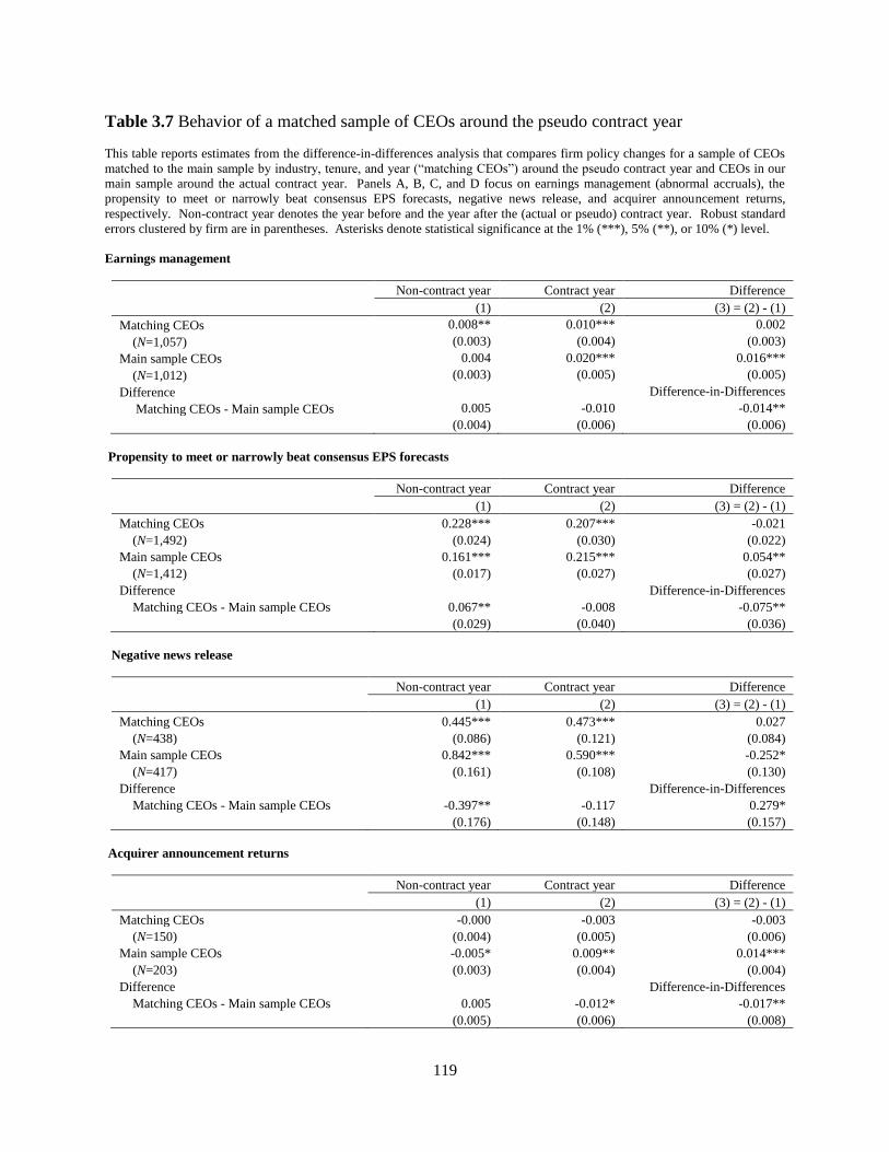
119

Table 3.7 Behavior of a matched sample of CEOs around the pseudo contract year

This table reports estimates from the difference-in-differences analysis that compares firm policy changes for a sample of CEOs

matched to the main sample by industry, tenure, and year (“matching CEOs”) around the pseudo contract year and CEOs in our

main sample around the actual contract year. Panels A, B, C, and D focus on earnings management (abnormal accruals), the

propensity to meet or narrowly beat consensus EPS forecasts, negative news release, and acquirer announcement returns,

respectively. Non-contract year denotes the year before and the year after the (actual or pseudo) contract year. Robust standard

errors clustered by firm are in parentheses. Asterisks denote statistical significance at the 1% (***), 5% (**), or 10% (*) level.

Earnings management

Non-contract year Contract year Difference

(1) (2) (3) = (2) - (1)

Matching CEOs 0.008** 0.010*** 0.002

(N=1,057) (0.003) (0.004) (0.003)

Main sample CEOs 0.004 0.020*** 0.016***

(N=1,012) (0.003) (0.005) (0.005)

Difference Difference-in-Differences

Matching CEOs - Main sample CEOs 0.005 -0.010 -0.014**

(0.004) (0.006) (0.006)

Propensity to meet or narrowly beat consensus EPS forecasts

Non-contract year Contract year Difference

(1) (2) (3) = (2) - (1)

Matching CEOs 0.228*** 0.207*** -0.021

(N=1,492) (0.024) (0.030) (0.022)

Main sample CEOs 0.161*** 0.215*** 0.054**

(N=1,412) (0.017) (0.027) (0.027)

Difference Difference-in-Differences

Matching CEOs - Main sample CEOs 0.067** -0.008 -0.075**

(0.029) (0.040) (0.036)

Negative news release

Non-contract year Contract year Difference

(1) (2) (3) = (2) - (1)

Matching CEOs 0.445*** 0.473*** 0.027

(N=438) (0.086) (0.121) (0.084)

Main sample CEOs 0.842*** 0.590*** -0.252*

(N=417) (0.161) (0.108) (0.130)

Difference Difference-in-Differences

Matching CEOs - Main sample CEOs -0.397** -0.117 0.279*

(0.176) (0.148) (0.157)

Acquirer announcement returns

Non-contract year Contract year Difference

(1) (2) (3) = (2) - (1)

Matching CEOs -0.000 -0.003 -0.003

(N=150) (0.004) (0.005) (0.006)

Main sample CEOs -0.005* 0.009** 0.014***

(N=203) (0.003) (0.004) (0.004)

Difference Difference-in-Differences

Matching CEOs - Main sample CEOs 0.005 -0.012* -0.017**

(0.005) (0.006) (0.008)

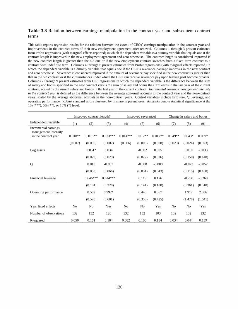
120

Table 3.8 Relation between earnings manipulation in the contract year and subsequent contract

terms

This table reports regression results for the relation between the extent of CEOs’ earnings manipulation in the contract year and

improvements in the contract terms of their new employment agreement after renewal. Columns 1 through 3 present estimates

from Probit regressions (with marginal effects reported) in which the dependent variable is a dummy variable that equals one if the

contract length is improved in the new employment agreement and zero otherwise. The contract length is considered improved if

the new contract length is greater than the old one or if the new employment contract switches from a fixed-term contract to a

contract with indefinite term. Columns 4 through 6 present estimates from Probit regressions (with marginal effects reported) in

which the dependent variable is a dummy variable that equals one if the CEO’s severance package improves in the new contract

and zero otherwise. Severance is considered improved if the amount of severance pay specified in the new contract is greater than

that in the old contract or if the circumstances under which the CEO can receive severance pay upon leaving post become broader.

Columns 7 through 9 present estimates from OLS regressions in which the dependent variable is the difference between the sum

of salary and bonus specified in the new contract versus the sum of salary and bonus the CEO earns in the last year of the current

contract, scaled by the sum of salary and bonus in the last year of the current contract. Incremental earnings management intensity

in the contract year is defined as the difference between the average abnormal accruals in the contract year and the non-contract

years, scaled by the average abnormal accruals in the non-contract years. Control variables include firm size, Q, leverage, and

operating performance. Robust standard errors clustered by firm are in parentheses. Asterisks denote statistical significance at the

1% (***), 5% (**), or 10% (*) level.

Improved contract length? Improved severance? Change in salary and bonus

Independent variable (1) (2) (3) (4) (5) (6) (7) (8) (9)

Incremental earnings

management intensity

in the contract year 0.018** 0.015** 0.023*** 0.014*** 0.012** 0.017** 0.049** 0.043* 0.039*

(0.007) (0.006) (0.007) (0.006) (0.005) (0.008) (0.023) (0.024) (0.023)

Log assets 0.051* 0.034 -0.002 0.005 0.010 -0.033

(0.029) (0.029) (0.022) (0.026) (0.150) (0.148)

Q 0.010 -0.037 -0.008 -0.008 -0.072 -0.052

(0.058) (0.066) (0.031) (0.043) (0.115) (0.160)

Financial leverage 0.646*** 0.614*** 0.119 0.176 -0.280 -0.260

(0.184) (0.220) (0.141) (0.180) (0.361) (0.510)

Operating performance 0.589 0.992* 0.446 0.567 1.917 2.386

(0.570) (0.601) (0.353) (0.425) (1.478) (1.641)

Year fixed effects No No Yes No No Yes No No Yes

Number of observations 132 132 120 132 132 103 132 132 132

R-squared 0.050 0.161 0.184 0.082 0.100 0.184 0.034 0.044 0.139

121

REFERENCES

Acharya, V., Gottschalg, O., Hahn, M., Kehoe, C., 2013. Corporate governance and value creation:

Evidence from private equity. Review of Financial Studies 26, 368-402.

Achdou, Y., Han, J., Lasry, J., Lions, P, Moll, B., 2015. Heterogeneous agent models in continuous

time. Working paper, Princeton University.

Agrawal, A., Matsa, D., 2013. Labor unemployment risk and corporate financing decisions.

Journal of Financial Economics 108, 449–470.

Ahern, K., Sosyura, D., 2014. Who writes the news? Corporate press releases during merger

negotiations. Journal of Finance 69, 241–291.

Axelson, U., Jenkinson, T., Stromberg, P., Weisbach, M., 2013. Borrow cheap, buy high? The

determinants of leverage and pricing in buyouts. The Journal of Finance, forthcoming.

Bae, K., Kang, J., Wang, J., 2011. Employee treatment and firm leverage: A test of the stakeholder

theory of capital structure. Journal of Financial Economics 100, 130–153.

Bain and Company, 2013. Global private equity report 2013.

Baker, M., 2009. Capital market-driven corporate finance. Annual Review of Financial Economics

1, 181–205.

Baker, M., Wurgler, J., 2011. Behavioral corporate finance: An updated survey. In: Constantinides,

George, Milton Harris and Rene Stulz (Eds.), Handbook of the Economics of Finance. Newnes,

Boston, pp. 357-424.

Barber, B., Lyon, J., 1997. Detecting long-run abnormal stock returns: The empirical power and

specification of test statistics. Journal of Financial Economics 43, 341-372.

Berk, J.,Stanton, J., Zechner, J., 2010. Human capital, bankruptcy, and capital structure. The

Journal of Finance 65, 891-926.

Bernstein, S., Sheen, A., 2016. The operational consequences of private equity buyouts Evidence

from the restaurant industry. Review of Financial Studies 29, 2387-2418.

Bhojraj, S., Hribar, P., Picconi, M., McInnis, J., 2009. Making sense of cents: an examination of

firms that marginally miss or beat analyst forecasts. Journal of Finance 64, 2361–2388.

Bloomberg BusinessWeek Magazine, 2006. Buy it, strip it then flip it.

Blouin, J., Core, J., Guay, W., 2010. Have the tax benefits of debt been overestimated? Journal of

Financial Economics 98, 195-213.

Bronars, S., Deere, D., 1991. The threat of unionization, the use of debt, and the preservation of

shareholder wealth. The Quarterly Journal of Economics 106, 231-254.

Brown, A., Koettl, J., 2015. Active labor market programs – employment gain or fiscal drain? IZA

Journal of Labor Economics 4:12.

122

Brown, J., Matsa, D., 2016. Boarding a sinking ship? An investigation of job applications to

distressed firms. The Journal of Finance 71, 507-550.

Brown, S., Warner, J., 1985. Using daily stock returns: the case of event studies. Journal of

Financial Economics 14, 3–31.

Brunnermeier, M., Sannikov, Y., 2014. A macroeconomic model with a financial sector. The

American Economic Review 104, 379-421.

Cavanaugh, J., Garen, J., 1997. Asset specificity, unionization and the firm's use of debt.

Managerial and Decision Economics 18, 255-269.

Chemmanur, T., Cheng, Y., Zhang, T., 2013. Human capital, capital structure, and employee pay:

An empirical analysis. Journal of Financial Economics 110, 478–502.

Chugh, S., 2013. Costly external finance and labor market dynamics. Journal of Economic

Dynamics & Control 37, 2882–2912.

Cohen, R., Polk, C., Vuolteenaho, T., 2003. The value spread. The Journal of Finance 58, 609-642.

Cohn, J., Mills, L., Towery, E., 2014. The evolution of capital structure and operating performance

after leveraged buyouts. Journal of Financial Economics, 111, 469-494.

Cornelli, F., Karakas, O., 2013. CEO turnover in LBOs: The role of boards. Working paper.

Custódio, C., 2014. Mergers and acquisitions accounting and the diversification discount. The

Journal of Finance 69, 219-240.

Davis, S., Haltiwanger, J., Handley, K., Jarmin, R., Lerner, J., Miranda, J., 2014. Private equity,

jobs and productivity. The American Economic Review 104, 3956-3990.

DeAngelo, H., DeAngelo, L., Rice, E., 1984. Going private: Minority freeze outs and stockholders’

wealth. Journal of Law and Economics 27, 367-401.

Dechow, P., Sloan, R., Sweeney, A., 1995. Detecting earnings management. Accounting Review

70, 193–225.

Degeorge, F., Patel, J., Zeckhauser, R., 1999. Earnings management to exceed thresholds. Journal

of Business 72, 1–33.

Dellavigna, S., Pollet, J., 2009. Investor inattention and Friday earnings announcements. Journal

of Finance 64, 709–749.

DeMarzo, P., Duffie, D., 1999. A liquidity-based model of security design. Econometrica 67, 65-

99.

Dittmar, A., Li, D., Nain, A., 2012. It pays to follow the leader: Acquiring targets picked by private

equity. Journal of Financial and Quantitative Analysis 47, 901-931.

Duchin, R., Matsusaka J., Ozbas, O., 2010. When are outside directors effective? Journal of

Financial Economics 96, 195-214.

123

Dustmann, C. Meghir, C., 2005. Wages, experience and seniority. Review of Economic Studies

72, 77–108.

Elsby, M., Hobijn, B., Şahin, A., 2015. On the importance of the participation margin for labor

Market fluctuations. Journal of Monetary Economics 72, 64-82.

Faingold, E., Sannikov, Y., 2011. Reputation in continuous-time games. Econometrica 79, 773-

876.

Fudenberg, D., Tirole, J., 1995. A theory of income and dividend smoothing based on incumbency

rents. Journal of Political Economy 103, 75–93.

Gabaix, X., 2009. Power laws in economics and finance. Annual Review of Economics 1, 255-

294.

Gale, D., 1992. A Walrasian theory of markets with adverse selection. Review of Economic

Studies 59, 229-255.

Gillan, S., Hartzell, J., Parrino, R., 2009. Explicit versus implicit contracts: evidence from CEO

employment agreements. Journal of Finance 64, 1629–1655.

Goldstein, R., Ju, N., Leland, H., 2001. An EBIT-based model of dynamic capital structure. The

Journal of Business 74, 483-512.

Gorbenko, A., Malenko, A., 2014. Strategic and financial bidders in takeover auctions. The Journal

of Finance 69, 2513-2555.

Graham, J., 2000. How big are the tax benefits of debt? The Journal of Finance 55, 1901-1941.

Graham, J., Harvey, C., Rajgopal, S., 2005. The economic implications of corporate financial

reporting. Journal of Accounting and Economics 40, 3–73.

Guo, S., Hotchkiss, E., Song, W., 2011. Do buyouts (still) create value? The Journal of Finance

66, 479-517.

Hall, R., 2005. Employment fluctuations with equilibrium wage stickiness. American Economic

Review 95, 50-65.

Hall, R., 2016. Why has the unemployment rate fared better than GDP growth? Stanford

University and NBER working paper.

Hanka, G., 1998. Debt and the terms of employment. Journal of Financial Economics 48, 245-282.

Harris, R., Jenkinson, T., Kaplan, S., 2014. Private equity performance: What do we know? The

Journal of Finance 69, 1851-1882.

Hayes, J., 2012. Vocational training, employability and the post-2008 jobs crisis: Responses in the

European Union. Economic and Industrial Democracy 34, 291-311.

He, J., Tian, X., 2013. The dark side of analyst coverage: The case of innovation. Journal of

Financial Economics 109, 856-878.

124

He, Z., Milbradt, K., 2014. Endogenous liquidity and defaultable bonds. Econometrica 82, 1443-

1508.

Healy, P., 1985. The effect of bonus schemes on accounting decisions. Journal of Accounting and

Economics 7, 85–107.

Healy, P., Wahlen, J., 1999. A review of the earnings management literature and its implications

for standard setting. Accounting Horizons 13, 365–383.

Higson, C., Stucke, R., 2012. The performance of private equity. Working paper.

Holmstrom, B., Milgrom, P., 1991. Multitask principal-agent analyses: incentive contracts, asset

ownership, and job design. Journal of Law, Economics and Organization 7, 24–52.

Hugonnier, J., Malamud, S., Morellec, E., 2015. Credit market frictions and capital structure

dynamics. Journal of Economic Theory 157, 1130-1158.

Huther, N., Robinson, D., Sievers, S., Hartmann-Wendels, T., 2015. Paying for performance in

private equity: evidence from management contracts. Working paper, Duke University.

Jensen, M., 1989. Eclipse of the public corporation. Harvard Business Review 67, 61–74.

Jensen, M., Meckling, W., 1976. Theory of the firm: managerial behavior, agency costs, and

ownership structure. Journal of Financial Economics 3, 305–360.

Johnson, T., 2016. Economic uncertainty, aggregate debt, and the real effects of corporate finance.

University of Illinois working paper.

Jones, J., 1991. Earnings management during relief investigations. Journal of Accounting Research

29, 193–228.

Jovanovic, B., 1979. Job matching and the theory of turnover. Journal of Political Economy 87,

972-990.

Kaplan, S., 1989a. Management buyouts: Evidence on taxes as a source of value. The Journal of

Finance 44, 611-632.

Kaplan, S., 1989b. The effects of management buyouts on operating performance and value.

Journal of Financial Economics 24, 217-254.

Kaplan, S., Stein, J., 1993. The evolution of buyout pricing and financial structure in the 1980s.

The Quarterly Journal of Economics 108, 313-357.

Kaplan, S., Stromberg, P., 2009. Leveraged buyouts and private equity. Journal of Economic

Perspectives 23, 121-146.

Karatzas, I., Shreve, S., 1991. Brownian motion and stochastic calculus. Springer, Berlin.

Karlin, S., Taylor, H., 1981. A second course in stochastic processes. Academic press, San Diego,

California.

125

Klasa, S., Maxwell, W., Ortiz-Molina, H., 2009. The strategic use of corporate cash holdings in

collective bargaining with labor unions. Journal of Financial Economics 92, 421-442.

Kothari, S.P., Shu, S., Wysocki, P., 2009. Do managers withhold bad news? Journal of Accounting

Research 47, 475–679.

Krueger, A., 2016. Where have all the workers gone? Princeton and NBER working paper.

Lazear, E., Oyer, P., 2012. Personnel Economics. In: Gibbons, Robert and John Roberts (Eds.),

Handbook of Organizational Economics. Princeton University Press, Princeton, New Jersey, pp.

479-519.

Lee, S., 1992. Management buyout proposals and inside information. The Journal of Finance 47,

1061-1079.

Lehn, K., Zhao, M., 2006. CEO turnover after acquisitions: are bad bidders fired? Journal of

Finance 61, 1759–1811.

Leland, H., 1994. Corporate debt value, bond covenants, and optimal capital structure. The Journal

of Finance 49, 1213-1252.

Lemmon, M., Roberts M., Zender, J., 2008. Back to the beginning: Persistence and the cross-

section of corporate capital structure. The Journal of Finance 63, 1575-1608.

Lichtenberg, F., Siegel, D., 1990. The effects of leveraged buyouts on productivity and related

aspects of firm behavior. Journal of Financial Economics 27, 165-194.

Liptser, R., Shiryaev, A., 2001. Statistics of random processes I: General theory. Springer, Berlin.

Malmendier, U., Opp, M., Saidi, F., 2016. Target revaluation after failed takeover attempts: Cash

versus stock. Journal of Financial Economics 119, 92-106.

Marais, L., Schipper, K., Smith, A., 1989. Wealth effects of going private for senior securities.

Journal of Financial Economics 23, 155-191.

Maskin, E., Tirole, J., 1992. The principal-agent relationship with an informed principal, II:

Common values. Econometrica 60, 1-42.

Milgrom, P., 1988. Employment contracts, influence activities and efficient organization design.

Journal of Political Economy 96, 42–60.

Moen, E., 1995. Essays on matching models of the labor market.

Moen, E., Rosen, A., 2011. Incentives in competitive search equilibrium. Review of Economic

Studies 78, 733-761.

Monacelli, T., Quadrini V., Trigari, A., 2011. Financial markets and unemployment. NBER

working paper.

Morck, R., Shleifer, A., Vishny, R., 1989. Alternative mechanisms for corporate control. American

Economic Review 89, 842–852.

126

Morck, R., Shleifer, A., Vishny, R., 1990. Do managerial objectives drive bad acquisitions?

Journal of Finance 65, 31–48.

Mortensen, D., Pissarides, C., 1994. Job creation and job destruction in the theory of

unemployment. Review of Economic Studies 61, 397-415.

Myerson, R., 1984. Two-person bargaining problems with incomplete information. Econometrica

52, 461-487.

Ofek, E., 1994. Efficiency gains in unsuccessful management buyouts. The Journal of Finance 49,

637-654.

Oyer, P., 1998. Fiscal year ends and nonlinear incentive contracts: the effect of business

seasonality. Quarterly Journal of Economics 113, 149–185.

Pan, Y., Wang T., Weisbach, M., 2015. CEO investment cycles. Review of Financial Studies,

forthcoming.

Petrongolo, B., Pissarides, C., 2001. Looking into the black box: A survey of the matching function.

Journal of Economic literature 39, 390-431.

Petrosky-Nadeau, 2014. Credit, vacancies and unemployment fluctuations. Review of Economic

Dynamics 17, 191-205.

Pissarides, C., 2009. The unemployment volatility puzzle: Is wage stickiness the answer?

Econometrica 77, 1339-1369.

Prendergast, C., 1999. The provision of incentives in firms. Journal of Economic Literature 37, 7–

63.

Richardson, S., Teoh, S.H., Wysocki, P., 2004. The walk-down to beatable analyst forecasts: the

role of equity issuance and insider trading incentives. Contemporary Accounting Research 21,

885–894.

Robinson, D., Sensoy, B., 2013. Do private equity fund managers earn their fees? Compensation,

ownership, and cash flow performance. Review of Financial Studies 26, 2760-2797.

Roychowdhury, S., 2006. Earnings management through real activities manipulation. Journal of

Accounting and Economics 42, 335–370.

Savor, P., Lu, Q., 2009. Do stock mergers create value for acquirers? The Journal of Finance 64,

1061-1097.

Schwert, W., 1996. Markup pricing in mergers and acquisitions. Journal of Financial Economics

41, 153-192.

Shleifer, A., 2000. Inefficient Markets: An Introduction to Behavioral Finance. Oxford University

Press, USA.

Smith, A., 1990. Corporate ownership structure and performance: The case of management

buyouts. Journal of Financial Economics 27, 143-164.

127

Sobel, J., 2007. Signaling games. Lecture notes. University of California, San Diego.

Stein, J., 1989. Efficient capital markets, inefficient firms: a model of myopic corporate behavior.

Quarterly Journal of Economics 104, 655–669.

Syverson, C., 2011. What determines productivity? Journal of Economic literature 49, 326-365.

Tetlock, P., 2007. Giving content to investor sentiment: the role of media in the stock market.

Journal of Finance 62, 1139–1168.

Tirole, J., 1992. Collusion and the theory of organizations. In: Laffont, J. (Ed.), Advances in

Economic Theory: Sixth World Congress, Vol. 2. Cambridge University Press, Cambridge,

England.

Topel, R., 1991. Specific capital, mobility, and wages: Wages rise with job seniority. Journal of

Political Economy 99, 145-176.

Tversky, A., Kahneman, D., 1974. Judgment under uncertainty: heuristics and biases. Science 185,

1124–1131.

Wasmer, E., Weil, P., 2004. The macroeconomics of labor and credit market imperfections. The

American Economic Review 94, 944-963.

Weisbach, M., 1988. Outside directors and CEO turnover. Journal of Financial Economics 20,

431–460.

Weisbach, M., 1995. CEO turnover and the firm’s investment decisions. Journal of Financial

Economics 37, 159–188.

Xu, M., 2011. The costs and benefits of long-term CEO contracts. Working paper, London School

of Economics and Political Science.

Xuan, Y., 2009. Empire-building or bridge-building? Evidence from new CEOs’ internal capital

allocation decisions. Review of Financial Studies 22, 4919–4948.

Zaitsev, V., Polyanin, A., 2002. Handbook of exact solutions for ordinary differential equations.

CRC Press, Boca Raton, Florida.

128

APPENDIX A: DETERMINISTIC AND PUBLICLY OBSERVABLE PRODUCTIVITY

A1 Proof of Lemma 1.1

I speculate 𝑤(𝑋) is linear in 𝑋. Notice that 𝑈 and 𝑉 are independent of 𝑋. From the HJB

equations in (1.5), (1.7), (1.10) and free-entry condition, multiply both sides of (1.5) by 𝛽.

𝛽𝑟𝐸(𝑋) = 𝛽 [(𝜃𝑋 − 𝑓 − 𝑐 − 𝑤) + 𝜇𝑋𝐸′(𝑋) +1

2𝜎2𝐸″(𝑋) − 𝑠𝐸(𝑋)] (𝐴. 1)

and multiply the difference between (1.7) and (1.10) by 1 − 𝛽.

(1 − 𝛽)𝑟[𝑊(𝑋) − 𝑈] = (1 − 𝛽) {𝑤 + 𝜇𝑋𝑊′(𝑋) +

1

2𝜎2𝑋2𝑊′′(𝑋) − 𝑠[𝑊(𝑋) − 𝑈] −

𝑏 − 𝑔(𝜖)[𝑊(𝑋0) − 𝑈]} (𝐴. 2)

By (1.16), (A.1) is equal to (A.2), and using (1.17) and (1.18) in the main text and simplifying, I

have proved (1.19). ||

A2 Proof of Proposition 1.1

Notice that the homogeneous part of (1. 22) and (1. 23) is a Cauchy-Euler equation, and the

general solution takes the form:

𝑆𝐻𝐺(𝑋) = 𝐴𝑋𝜈 + �̃�𝑋�̃�

where 𝜈 𝑎𝑛𝑑 �̃� are negative and positive solutions of the equation 𝜈(𝜈 − 1) +2𝜇

𝜎2 𝜈 −2𝛿

𝜎2 = 0.

The general solution of (1.22) and (1.23) takes the form85:

𝑆(𝑋) = 𝜃𝛱(𝑋) − 𝐹 −𝑐 + 𝑏 − 𝜅 + [𝑔𝛽 + ℎ(1 − 𝛽)]𝑆0 + ℎ𝐷0

𝛿+ 𝐴𝑋𝜈

= 𝜃𝛱(𝑋) − 𝐹 −𝑐 + 𝑟𝑈 + 𝑟𝑉

𝛿+ 𝐴𝑋𝜈 (𝐴. 3)

By “value-matching” condition:

−𝐴𝑋𝜈 = 𝜃𝛱(𝑋) − 𝐹 −𝑐 + 𝑟𝑈 + 𝑟𝑉

𝛿

85 Notice that �̃� = 0 by “no-bubble” condition.

129

𝐴 = −𝑋−𝜈 [𝜃𝛱(𝑋) − 𝐹 −𝑐 + 𝑟𝑈 + 𝑟𝑉

𝛿] (𝐴. 4)

Bringing (A.4) to (A.3), I have obtained (1.25) in Proposition 1.1.

𝑆′(𝑋)|𝑋=𝑋 = 0

From (1.25), taking derivatives with respect to 𝑋 and by “smooth-pasting” condition, I

have

𝜃

𝛿 − 𝜇− [𝜃𝛱(𝑋) − 𝐹 −

𝑐 + 𝑏 − 𝜅 + [𝑔𝛽 + ℎ(1 − 𝛽)]𝑆0 + ℎ𝐷0

𝛿] (

𝜈

𝑋) = 0

(1 − 𝜈)𝜃𝛱(𝑋) = −𝜈 [𝐹 +𝑐 + 𝑏 − 𝜅 + [𝑔𝛽 + ℎ(1 − 𝛽)]𝑆0 + ℎ𝐷0

𝛿]

𝑋 =−𝜈

1 − 𝜈

𝛿 − 𝜇

𝜃[𝐹 +

𝑐 + 𝑏 − 𝜅 + [𝑔𝛽 + ℎ(1 − 𝛽)]𝑆0 + ℎ𝐷0

𝛿]

=−𝜈

1 − 𝜈

𝛿 − 𝜇

𝜃 [𝐹 +

𝑐 + 𝑟𝑈 + 𝑟𝑉

𝛿] (𝐴. 5)

The last line gives (1.26) in Proposition 1.1. In equilibrium, by free-entry condition of the firms,

𝑉 = 0, bringing the free-entry condition to (1.25) and (1.26) yields (1.27) and (1.28) in Proposition

1.1. ||

A3 Proof of Proposition 1.2

A3.1 First order condition

The optimal coupon rate 𝑐 solves the constrained maximization problem defined by (1.29).

First, I solve several quantities that will facilitate the calculation of the first order condition. The

derivative of 𝑋 with respect to 𝑐, 𝑋(𝑐), from (1.28), is

𝑋(𝑐) =−𝜈

1 − 𝜈

𝛿 − 𝜇

𝜃

1

𝛿(𝐴. 6)

It is convenient to calculate some quantities that I use repeatedly in this appendix. From (1.28),

𝜃𝛱(𝑋) = 𝜃𝑋

𝛿 − 𝜇=

𝜃

𝛿 − 𝜇

−𝜈

1 − 𝜈

𝛿 − 𝜇

𝜃

𝛿𝐹 + 𝑐 + 𝑟𝑈

𝛿=

−𝜈

1 − 𝜈

𝛿𝐹 + 𝑐 + 𝑟𝑈

𝛿(𝐴. 7)

𝜃𝛱(𝑋) −𝛿𝐹 + 𝑐 + 𝑟𝑈

𝛿=

−𝜈

1 − 𝜈

𝛿𝐹 + 𝑐 + 𝑟𝑈

𝛿−

𝛿𝐹 + 𝑐 + 𝑟𝑈

𝛿= −

𝛿𝐹 + 𝑐 + 𝑟𝑈

(1 − 𝜈)𝛿(𝐴. 8)

130

From (1.28) and (𝐴. 6),

𝜕

𝜕𝑐 (

𝑋

𝑋)

𝜈

= (𝑋

𝑋)

𝜈

(−𝜈)1 − 𝜈

−𝜈

𝜃

𝛿 − 𝜇

𝛿

𝛿𝐹 + 𝑐 + 𝑟𝑈

−𝜈

1 − 𝜈 𝛿 − 𝜇

𝜃

1

𝛿= (

𝑋

𝑋)

𝜈−𝜈

𝛿𝐹 + 𝑐 + 𝑟𝑈(A. 9)

From (1.27) and (A.8), the matching surplus function 𝑆(𝑋) becomes

𝑆(𝑋) = 𝜃𝛱(𝑋) − 𝐹 −𝑐 + 𝑟𝑈

𝛿+

𝛿𝐹 + 𝑐 + 𝑟𝑈

(1 − 𝜈)𝛿(

𝑋

𝑋)

𝜈

(𝐴. 10)

and from (A.9) and (A.10), in equilibrium, its derivative with respect to 𝑐 is

𝑆(𝑐)(𝑋) = −1

𝛿+

𝛿𝐹 + 𝑐 + 𝑟𝑈

(1 − 𝜈)𝛿(

𝑋

𝑋)

𝜈−𝜈

𝛿𝐹 + 𝑐 + 𝑟𝑈+

1

(1 − 𝜈)𝛿 (

𝑋

𝑋)

𝜈

= −1

𝛿+

1

𝛿(

𝑋

𝑋)

𝜈

= −1

𝛿(1 − (

𝑋

𝑋)

𝜈

) (𝐴. 11)

From (1.3) and (A.8), the value of debt contract 𝐷(𝑋) is

𝐷(𝑋) =𝑐

𝛿− (

𝑐

𝛿− (1 − 𝛼) (𝜃𝛱(𝑋) − 𝐹 −

𝑟𝑈

𝛿)) (

𝑋

𝑋)

𝜈

=𝑐

𝛿− (

𝛼𝑐

𝛿− (1 − 𝛼) (𝜃𝛱(𝑋) −

𝛿𝐹 + 𝑐 + 𝑟𝑈

𝛿)) (

𝑋

𝑋)

𝜈

=𝑐

𝛿− (

𝛼𝑐

𝛿+ (1 − 𝛼)

𝛿𝐹 + 𝑐 + 𝑟𝑈

(1 − 𝜈)𝛿) (

𝑋

𝑋)

𝜈

(𝐴. 12)

Bringing (A.9) into (A.12), the derivative of 𝐷𝑘(𝑋) with respect to 𝑐𝑘, 𝐷𝑘(𝑐)(𝑋), is

𝐷(𝑐)(𝑋) =1

𝛿− (

𝛼

𝛿+

1 − 𝛼

(1 − 𝜈)𝛿) (

𝑋

𝑋)

𝜈

− (𝛼𝑐

𝛿+ (1 − 𝛼)

𝛿𝐹 + 𝑐 + 𝑟𝑈

(1 − 𝜈)𝛿)

−𝜈

𝛿𝐹 + 𝑐 + 𝑟𝑈(

𝑋

𝑋)

𝜈

=1

𝛿−

1

𝛿(𝛼 +

1 − 𝛼

1 − 𝜈−

𝜈(1 − 𝛼)

1 − 𝜈) (

𝑋

𝑋)

𝜈

+𝛼𝜈

𝛿

𝑐

𝛿𝐹 + 𝑐 + 𝑟𝑈(

𝑋

𝑋)

𝜈

=1

𝛿−

1

𝛿(

𝑋

𝑋)

𝜈

+ 𝛼𝜈

𝛿

𝑐

𝛿𝐹 + 𝑐 + 𝑟𝑈(

𝑋

𝑋)

𝜈

=1

𝛿[1 − (1 − 𝛼𝜈

𝑐

𝛿𝐹 + 𝑐 + 𝑟𝑈) (

𝑋

𝑋)

𝜈

] (𝐴. 13)

From (1.29), the first order condition of the maximization problem (1.29) with respect to 𝑐 is

ℎ(𝜖(𝑈, 𝑐))[(1 − 𝛽)𝑆0 (𝑐) + 𝐷0 (𝑐)] + ℎ(𝑐)(𝜖(𝑈, 𝑐))[(1 − 𝛽)𝑆0 + 𝐷0 ] = 0 (𝐴. 14)

131

where 𝑆0, 𝐷0, 𝑆0(𝑐) and 𝐷0(𝑐) is specified by (A.10), (A.12), (A.11), and (A.13), respectively,

with 𝑋 = 𝑋0, and ℎ(𝜖(𝑈, 𝑐)) is such that 𝜖ℎ(𝜖) = 𝑔(𝜖) =𝑟𝑈−𝑏

𝛽𝑆0 . Simple algebraic manipulation

gives (1. 30).

From Section 1.2.3, ℎ = ℎ(𝜖) = ℎ(𝑔−1(𝑔)) = ℎ(𝑔), where ℎ′(𝑔) < 0 . Differentiating

(1.10) with respect to 𝑐 on both sides86, I have

𝑔(𝑐)𝛽𝑆0 + 𝑔𝛽𝑆0 (𝑐) = 0 (𝐴. 15)

thereby proving the first order condition in Proposition 1.2. ||

A3.2 The second order condition for optimal coupon rate 𝑐

It is obvious that the objective function in (1.29) is continuously differentiable, and the set

of viable coupon rate 𝑐 is a closed interval in 𝑅+, i.e., 𝑐 ∈ [0, 𝑐̅], which is closed and bounded.

Obviously, one candidate of 𝑐̅ is value of 𝑐 such that 𝑋 = 𝑋0 . In other words, default occurs

immediately after matching. Therefore, the maximization problem is well defined and a maximizer

𝑐 exists.

The second order derivative on the left hand side of (1.30) with respect to 𝑐 at the optimal

𝑐 is

ℎ [1

𝛿(𝛼𝜈

𝛿𝐹 + 𝑟𝑈 − 𝜈𝑐

(𝛿𝐹 + 𝑐 + 𝑟𝑈)2+ 𝛽

𝜈

𝛿𝐹 + 𝑐 + 𝑟𝑈) (

𝑋0

𝑋)

𝜈

]

+2ℎ(𝑔)𝑔(𝑐) [𝛽

𝛿+

1

𝛿(𝛼𝜈

𝑐

𝛿𝐹 + 𝑐 + 𝑟𝑈− 𝛽) (

𝑋0

𝑋)

𝜈

]

+ [ℎ(𝑔)𝑔(𝑐𝑐) + ℎ(𝑔𝑔)(𝑔(𝑐))2

] [(1 − 𝛽)𝑆0 + 𝐷0] (A. 16)

Notice that the first two terms of (A.16) are obviously negative. Take the second-order

derivative of 𝑔(𝜖(𝑐, 𝑈)) with respect to 𝑐:

𝑔(𝑐𝑐) = −𝑔(𝑐) 𝑆0 (𝑐)

𝑆0− 𝑔

𝑆0 (𝑐𝑐)𝑆0 − (𝑆0(𝑐))2

(𝑆0)2

86 Notice that in equilibrium, 𝑈 only depends on the aggregate debt level.

132

The first term of 𝑔(𝑐𝑐) is greater than zero. In order to have 𝑔(𝑐𝑐) > 0, the second term must be

smaller than zero87, i.e., 𝑆0 (𝑐)

𝑆0 is decreasing in 𝑐. To ensure ℎ(𝑔𝑔)(𝑔(𝑐))2 < 0, I need ℎ(𝑔𝑔) < 0. In

sum, I have proved Proposition 1.2. ||

A4 Proof of Proposition 1.3

Again, the homogenous part of ODE (1.32) is a Cauchy-Euler equation, which admits a

general form of solution:

𝑇𝐻𝐺(𝑋) = 𝐻𝑋𝜌 + �̃�𝑋�̃�

where 𝜌 and �̃� is negative and positive solution to 1

2𝜎2�̅�(�̅� − 1) + 𝜇�̅� − 𝑠 = 0, respectively.

𝜌 = (1

2−

𝜇

𝜎2) − √(1

2−

𝜇

𝜎2)2

+2𝑠

𝜎2 and �̃� = (1

2−

𝜇

𝜎2) + √(1

2−

𝜇

𝜎2)2

+2𝑠

𝜎2

Therefore, the general solution of the boundary problem (1.32) and (1.33) takes the form

𝑇(𝑋) = 𝐻𝑋𝜌 + �̃�𝑋�̃� +1

𝑠(𝐴. 17)

Since 𝑙𝑖𝑚𝑋→∞

𝑇(𝑋) =1

𝑠< ∞, I have �̃� = 0. 𝐻 can be determined by another boundary condition

𝑇(𝑋) = 0.

𝐻𝑋𝜌 +1

𝑠= 0 ⇒ 𝐻 = −

1

𝑠 𝑋−𝜌 (𝐴. 18)

Bringing (A.18) to (A.17) leads to (1.34). ||

A5 Proof of Proposition 1.4

From Gabaix (2009), the general solution of (1. 36) is

𝒻𝑖(𝑋) = 𝜁−𝑖 𝑋−𝑚0−1 + 𝜁+

𝑖 𝑋−𝑚1−1 𝑋 ≠ 𝑋0 (𝐴. 19)

where 𝑖 ∈ {0,1}, in which 𝒻0(𝑋) represents the probability density function for 𝑋 ∈ [𝑋, 𝑋0) and

𝒻1(𝑋) represents the probability density function for 𝑋 ∈ (𝑋0, ∞] . In (A.19), 𝑚0 and 𝑚1 is

87 Notice that ℎ(𝑔) < 0 by assumption.

133

negative and positive root for the equation 𝜎2

2𝑚(𝑚 − 1) + 𝜇𝑚 − 𝑠 = 0, respectively, from which

I get the expressions for 𝑚0 and 𝑚1 in Proposition 1.4.

By the definition of probability density function, the expression ∫ 𝒻(𝑋)𝑑𝑋∞

𝑋 must be

integrable. From which, I have:

∫ 𝒻(𝑋)𝑑𝑋∞

𝑋

= 𝒻(𝑋0) + ∫ 𝒻0(𝑋)𝑑𝑋𝑋0

𝑋

+ ∫ 𝒻1(𝑋)𝑑𝑋∞

𝑋0

< ∞ (𝐴. 20)

From (A.19), I have 𝜁−1 = 0, otherwise ∫ 𝒻1(𝑋)𝑑𝑋

∞

𝑋0 explodes as 𝑋 → ∞88.

From (1.37), I have 𝜁−0𝑋−𝑚0−1 + 𝜁+

0𝑋−𝑚1−1 = 0, i.e.,

𝜁+0 = −𝜁−

0𝑋−𝑚0−1𝑋𝑚1+1

= −𝜁−0𝑋𝑚1−𝑚0

The two remaining unknown coefficients 𝜁+1 and 𝜁−

0 are determined by (1.38) and (1.39). Letting

𝜁 ≔ 𝜁+1 and 𝜁 ≔ 𝜁−

0, we have (1.40) in Proposition 1.4. In what following, I will solve 𝜁 and 𝜁

explicitly. The solution procedure consists of several steps.

Firstly, using (1.40), I obtain the left and right derivatives of 𝑓(𝑋) with respected to 𝑋 at

𝑋 = 𝑋0.

𝑓′(𝑋0 −) = −𝜁(𝑚0 + 1)𝑋0−𝑚0−2

+ 𝜁(𝑚1 + 1)𝑋0−𝑚0−2

(𝑋

𝑋0)

𝑚1−𝑚0

(𝐴. 21)

𝑓′(𝑋0 +) = −𝜁(𝑚1 + 1)𝑋0−𝑚1−2 (𝐴. 22)

Secondly, using (1.40), I obtain the integral of 𝑓(𝑋) over the domain of viable 𝑋.

88 ∫ 𝒻1(𝑋)𝑑𝑋 = −

𝜁−1

𝑚−𝑋−𝑚− |𝑋0

∞ ∞

𝑋0−

𝜁+1

𝑚+𝑋−𝑚+ |𝑋0

∞ , from which I could see that if 𝜁−1 ≠ 0, the first term explodes as

𝑋 → ∞.

134

∫ 𝑓(𝑋)𝑑𝑋𝑋0

𝑋

= ∫ (𝜁𝑋−𝑚0−1 − 𝜁𝑋𝑚1−𝑚0𝑋−𝑚1−1)𝑑𝑋𝑋0

𝑋

= 𝜁 (−1

𝑚0𝑋−𝑚0 + 𝑋𝑚1−𝑚0

1

𝑚1𝑋−𝑚1) |𝑋

𝑋0

= 𝜁 [1

𝑚1𝑋−𝑚0 ((

𝑋

𝑋0)

𝑚1

− 1) +1

𝑚0(𝑋−𝑚0 − 𝑋0

−𝑚0)] (𝐴. 23)

Similarly,

∫ 𝑓(𝑋)𝑑𝑋∞

𝑋0

= ∫ 𝜁𝑋−𝑚1−1𝑑𝑋∞

𝑋0

= 𝜁 (−1

𝑚1) 𝑋−𝑚1|𝑋0

∞ =𝜁

𝑚1𝑋0

−𝑚1 (𝐴. 24)

Thirdly, I obtain the right derivatives of 𝑓(𝑋) with respected to 𝑋 at 𝑋 = 𝑋.

𝑓′(𝑋 +) = 𝜁(𝑚1 − 𝑚0)𝑋−𝑚0−2 (𝐴. 25)

Fourthly, I express boundary conditions (1.38) and (1.39) from (A.21) — (A.25). (1.38)

becomes

𝜁𝛬1 − 𝜁𝛬2 = 𝑠𝜁𝛬3 + 𝑠𝜁𝛬4 + 𝜁𝛬5

⇔ (𝛬1 − 𝑠𝛬3 − 𝛬5)𝜁 − (𝛬2 + 𝑠𝛬4)𝜁 = 0 (𝐴. 26)

and (1.39) becomes

𝑔 − 𝑔(𝜁𝛬3 + 𝜁𝛬4) = 𝑠𝜁𝛬3 + 𝑠𝜁𝛬4 + 𝜁𝛬5

⇔ [(𝑔 + 𝑠)𝛬3 + 𝛬5]𝜁 + (𝑔 + 𝑠)𝛬4𝜁 = 𝑔 (𝐴. 27)

The parameters 𝛬𝑖, 𝑖 = {1, 2, 3, 4, 5} are defined as follows:

𝛬1 =1

2𝜎2 [−(𝑚0 + 1) + (𝑚1 + 1) (

𝑋

𝑋0)

𝑚1−𝑚0

] 𝑋0−𝑚0 (𝐴. 28)

𝛬2 = −1

2𝜎2(𝑚1 + 1)𝑋0

−𝑚1 (𝐴. 29)

𝛬3 = ∫ 𝑋−𝑚0−1 [1 − (𝑋

𝑋)

𝑚1−𝑚0

] 𝑑𝑋𝑋0

𝑋

=1

𝑚1𝑋−𝑚0 ((

𝑋

𝑋0)

𝑚1

− 1) +1

𝑚0(𝑋−𝑚0 − 𝑋0

−𝑚0)(𝐴. 30)

𝛬4 = ∫ 𝑋−𝑚1−1𝑑𝑋∞

𝑋0

=1

𝑚1𝑋0

−𝑚1 (𝐴. 31)

135

𝛬5 =𝜎2

2(𝑚1 − 𝑚0)𝑋−𝑚0 (𝐴. 32)

(A.26) and (A.27) pin down 𝜁 and 𝜁. It can be shown that 𝑓(𝑋0 +) = 𝑓(𝑋0−), in other

words, 𝑓(𝑋) is continuous at 𝑋0. Therefore, 𝜁 and 𝜁 are positive and unique. ||

A6 Proof of Proposition 1.5

A6.1 First order condition

The proof of the first order condition (1.46) is the same as the proof of first order condition

(1.30) in the baseline case. Therefore, I focus on the solutions of 𝑔(𝑐) and 𝑒(𝑐) in this appendix

section.

Taking the derivative with respect to 𝑐 on both sides of (1.43), notice that 𝑈 only depends

on 𝑐 through 𝑒, by the envelope theorem

𝑔𝛽𝑆0(𝑐) + 𝑔(𝑐)𝛽𝑆0 − 𝑙′(𝑒)𝑒(𝑐) = 0 (𝐴. 33)

Taking the derivative with respect to 𝑐 on both sides of (1.44),

𝑔(𝑒)𝛽𝑆0(𝑐) + (𝑔(𝑒𝑒)𝑒(𝑐) + 𝑔(𝑒𝑔)𝑔(𝑐))𝛽𝑆0 − 𝑙″(𝑒)𝑒(𝑐) = 0

Collecting terms yields

𝑔(𝑒)𝛽𝑆0(𝑐) + 𝑔(𝑒𝑔)𝛽𝑆0𝑔(𝑐) + (𝑔(𝑒𝑒)𝛽𝑆0 − 𝑙″(𝑒)) 𝑒(𝑐) = 0 (𝐴. 34)

Solving 𝑔(𝑐) and 𝑒(𝑐) from (A.33) and (A.34) we have

𝑔(𝑐) =𝛤3𝛤5 − 𝛤2𝛤6

𝛤1𝛤5 − 𝛤2𝛤4

(𝐴. 35)

and

𝑒(𝑐) =𝛤1𝛤6 − 𝛤3𝛤4

𝛤1𝛤5 − 𝛤2𝛤4

(𝐴. 36)

where 𝛤1 = 𝛽𝑆0 , 𝛤2 = −𝑙′(𝑒), 𝛤3 = −𝑔𝛽𝑆0(𝑐) , 𝛤4 = 𝑔(𝑒𝑔)𝛽𝑆0 , 𝛤5 = 𝑔(𝑒𝑒)𝛽𝑆0 − 𝑙″(𝑒) and 𝛤6 =

−𝑔(𝑒)𝛽𝑆0(𝑐). ||

A6.2 Second order condition

136

The first term of the second order condition is similar to that of (A.16), except for the fact

that ℎ now also depends on 𝑒 in additional to 𝑔. The second term of the second order condition is

similar to that of (A.16) except that ℎ(𝑔)𝑔(𝑐) is replaced by ℎ(𝑒)𝑒(𝑐) + ℎ(𝑔)𝑔(𝑐). The first two terms

are smaller than zero. The third term of the second order condition is the same as that of (A.16)

except that ℎ(𝑔)𝑔(𝑐𝑐) + ℎ(𝑔𝑔)(𝑔(𝑐))2 is replaced by

ℎ(𝑐𝑐)(𝑒, 𝑔) = ℎ(𝑒𝑒)(𝑒(𝑐))2

+ ℎ(𝑒𝑔)𝑔(𝑐)𝑒(𝑐) + ℎ(𝑒)𝑒(𝑐𝑐) + ℎ(𝑔𝑔)(𝑔(𝑐))2

+ ℎ(𝑔𝑒)𝑒(𝑐)𝑔(𝑐) + ℎ(𝑔)𝑔(𝑐𝑐)

= ℎ(𝑒𝑒)(𝑒(𝑐))2

+ ℎ(𝑔𝑔)(𝑔(𝑐))2

+ 2ℎ(𝑒𝑔)𝑒(𝑐)𝑔(𝑐) + ℎ(𝑒)𝑒(𝑐𝑐) + ℎ(𝑔)𝑔(𝑐𝑐) (𝐴. 37)

The third term is smaller than zero if ℎ(𝑐𝑐)(𝑒, 𝑔) < 0 . The remaining part of this subsection

calculates 𝑔(𝑐𝑐) and 𝑒(𝑐𝑐).

Take derivative with respect to 𝑐 on both sides of (A.33)

𝑔(𝑐)𝛽𝑆0(𝑐) + 𝑔𝛽𝑆0(𝑐𝑐) + 𝑔(𝑐𝑐)𝛽𝑆0 + 𝑔(𝑐)𝛽𝑆0(𝑐) − 𝑙″(𝑒)(𝑒(𝑐))2

− 𝑙′(𝑒)𝑒(𝑐𝑐) = 0

Collecting terms yields

−𝛽𝑆0𝑔(𝑐𝑐) + 𝑙′(𝑒)𝑒(𝑐𝑐) = 𝑔𝛽𝑆0(𝑐𝑐) + 2𝑔(𝑐)𝛽𝑆0(𝑐) − 𝑙″(𝑒)(𝑒(𝑐))2

(𝐴. 38)

Take derivative with respect to 𝑐 on both sides of (A.34)

𝑔(𝑒)𝛽𝑆0(𝑐𝑐) + (𝑔(𝑒𝑒)𝑒(𝑐) + 𝑔(𝑒𝑔)𝑔(𝑐))𝛽𝑆0(𝑐) + 𝑔(𝑒𝑔)𝑔(𝑐)𝛽𝑆0(𝑐) + 𝑔(𝑒𝑔)𝑔(𝑐𝑐)𝛽𝑆0 +

(𝑔(𝑒𝑔𝑒)𝑒(𝑐) + 𝑔(𝑒𝑔𝑔)𝑔(𝑐))𝛽𝑆0𝑔(𝑐) +

(𝑔(𝑒𝑒𝑒)𝑒(𝑐)𝛽𝑆0 + 𝑔(𝑒𝑒𝑔)𝑔(𝑐)𝛽𝑆0 + 𝑔(𝑒𝑒)𝛽𝑆0(𝑐) − 𝑙‴(𝑒)𝑒(𝑐))𝑒(𝑐) +

(𝑔(𝑒𝑒)𝛽𝑆0 − 𝑙″(𝑒)) 𝑒(𝑐𝑐) = 0

Collecting terms yields

−𝑔(𝑒𝑔)𝛽𝑆0𝑔(𝑐𝑐) + (𝑙″(𝑒) − 𝑔(𝑒𝑒)𝛽𝑆0)𝑒(𝑐𝑐) =

𝑔(𝑒)𝛽𝑆0(𝑐𝑐) + 2(𝑔(𝑒𝑒)𝑒(𝑐) + 𝑔(𝑒𝑔)𝑔(𝑐))𝛽𝑆0(𝑐) + (𝑔(𝑒𝑔𝑒)𝑒(𝑐) + 𝑔(𝑒𝑔𝑔)𝑔(𝑐))𝛽𝑆0𝑔(𝑐) +

(𝑔(𝑒𝑒𝑒)𝑒(𝑐)𝛽𝑆0 + 𝑔(𝑒𝑒𝑔)𝑔(𝑐)𝛽𝑆0 − 𝑙‴(𝑒)𝑒(𝑐))𝑒(𝑐) (𝐴. 39)

Solving 𝑔(𝑐𝑐) and 𝑒(𝑐𝑐) from (A.38) and (A.39) we have

𝑔(𝑐𝑐) =𝛥3𝛥5 − 𝛥2𝛥6

𝛥1𝛥5 − 𝛥2𝛥4

(𝐴. 40)

𝑒(𝑐𝑐) =𝛥1𝛥6 − 𝛥3𝛥4

𝛥1𝛥5 − 𝛥2𝛥4

(𝐴. 41)

137

where Δ1 = −𝛽𝑆0 , Δ2 = 𝑙′(𝑒), Δ3 = 𝑅𝐻𝑆 𝑜𝑓 (A. 38) , Δ4 = −𝑔(𝑒𝑔)𝛽𝑆0 , Δ5 = 𝑙″(𝑒) − 𝑔(𝑒𝑒)𝛽𝑆0

and Δ6 = 𝑅𝐻𝑆 𝑜𝑓 (A. 39). ||

A7 Numerical example

In Table 1, I present model parameters for baseline calibration.

A7.1 An illustration of solution procedure

Firstly, the optimal coupon rate 𝑐, value of being unemployed 𝑈 and matching rate of

workers 𝑔 are jointly determined by the worker’s and firm’s value function (1.20) and (1.21),

respectively and the first order condition for firm’s optimal coupon choice (1.30). After checking

the second order condition for the optimality of coupon choice obtained from the first step, the

expected tenure is derived according to (1.34) of Proposition 1.3. The stationary cross-sectional

density function of cash flow state 𝑋, 𝒻(𝑋), is derived according to (1.40) of Proposition 1.4. The

unemployment rate 𝑢 = 1 − ∫ 𝒻(𝑋)𝑑𝑥∞

𝑋.

138

APPENDIX B: BAYESIAN LEARNING ABOUT THE UNKNOWN MATCH QUALITY

B1 Asset values and Wage function

Let Σ(𝑝) ≔1

2𝑝2(1 − 𝑝)2𝜙2 and �̅�(𝑝) ≔ 𝑝𝜇𝐻 + (1 − 𝑝)𝜇𝐿. Throughout Section 1.4 and

Appendix B, I assume that the flow operating cost 𝑓 = 089.

B1.1 Debt

Given a coupon rate 𝑐 and value of being unemployed 𝑈, the bellman equation for a debt

contract is:

𝑟𝐷(𝑝) = 𝑐 + 𝛴(𝑝)𝐷′′(𝑝) − 𝑠𝐷(𝑝) (𝐵. 1)

subject to the boundary conditions90:

𝐷 (𝑝) = 𝐷𝐵 = (1 − 𝛼)�̅� (𝑝)

𝛿−

𝑟𝑈

𝛿 𝑎𝑛𝑑 𝑙𝑖𝑚

𝑝→1𝐷(𝑝) <

𝜇𝐻

𝛿< ∞ (𝐵. 2)

From Polyanin and Zaitsev (2003, 2.1.7 — 6, equation 216), the homogeneous part of (B.1)

has a general solution of the form:

𝛾1𝑝�̂�1(1 − 𝑝)�̂�2 + 𝛾2𝑝�̂�2(1 − 𝑝)�̂�1

where �̂�1 and �̂�2 is negative and positive root of the equation �̂�(�̂� − 1) −2𝛿

𝜙2 = 0.

�̂�1 =1

2− √

1

4+

2𝛿

𝜙2 𝑎𝑛𝑑 �̂�2 =1

2+ √

1

4+

2𝛿

𝜙2(𝐵. 3)

The general solution for (B.1) is

𝐷(𝑝) =𝑐

𝛿+ 𝛾1𝑝�̂�1(1 − 𝑝)�̂�2 + 𝛾2𝑝�̂�2(1 − 𝑝)�̂�1

Since 𝑙𝑖𝑚𝑝→1

𝐷(𝑝) <𝜇𝐻

𝛿< ∞, I have 𝛾2 = 0. Let 𝛾 ≔ 𝛾1. Using 𝐷 (𝑝) = 𝐷𝐵 = (1 − 𝛼)

�̅�(𝑝)

𝛿−

𝑟𝑈

𝛿, I

have 𝛾 =(1−𝛼)�̅�(𝑝)−𝑟𝑈−𝑐

𝛿𝑝�̂�1(1−𝑝)�̂�2

. Then the debt value 𝐷(𝑝) is given by

89 This assumption is innocuous. 90 The bankruptcy cost definition is slight different from the benchmark case to make the calculation less cumbersome.

It is not crucial.

139

𝐷(𝑝) =𝑐

𝛿−

𝑐 − (1 − 𝛼)�̅� (𝑝) + 𝑟𝑈

𝛿 (

𝑝

𝑝)

�̂�1

(1 − 𝑝

1 − 𝑝)

�̂�2

(B. 4)

||

B1.2 Other asset values, wage function and match surplus

The equity value follows the HJB equation

𝑟𝐸(𝑝) = �̅�(𝑝) − 𝑐 − 𝑤 + 𝛴(𝑝)𝐸′′(𝑝) − 𝑠(𝐸(𝑝) − 𝑉) (𝐵. 5)

subject to boundary conditions

𝐸 (𝑝) = 𝑉; 𝐸′(𝑝)|𝑝=𝑝 = 0; 𝑙𝑖𝑚𝑝→1

𝐸(𝑝) < ∞ (𝐵. 6)

Similarly, the value of being employed satisfies the HJB equation

𝑟𝑊(𝑝) = 𝑤 + 𝛴(𝑝)𝑊′′(𝑝) − 𝑠(𝑊(𝑝) − 𝑈) (𝐵. 7)

subject to boundary conditions

𝑊 (𝑝) = 𝑈; 𝑊′(𝑝)|𝑝=𝑝 = 0; 𝑙𝑖𝑚𝑝→1

𝑊(𝑝) < ∞ (𝐵. 8)

The value of being unemployed satisfies the HJB equation

𝑟𝑈 = 𝑏 + 𝑔(𝜖)[𝑊(𝑝0) − 𝑈] (𝐵. 9)

The value of an idle vacancy obeys the HJB equation

𝑟𝑉 = −𝜅 + ℎ(𝜖)[𝐸(𝑝0) + 𝐷(𝑝0) − 𝑉] (𝐵. 10)

Before I move on to calculate the matching surplus 𝑆(𝑝), I derive a wage function that is linear in

posterior belief 𝑝. Specifically, I have the following lemma.

Lemma B.1 In equilibrium, under generalized Nash bargaining, the wage function is linear

in X

𝑤(𝑝) = 𝛽(�̅�(𝑝) − 𝑐) + (1 − 𝛽)𝑏 + 𝛽𝑔(𝜖)𝐸(𝑝0)

= 𝛽(�̅�(𝑝) − 𝑐) + (1 − 𝛽)𝑏 + (1 − 𝛽)𝑔(𝜖)[𝑊(𝑝0) − 𝑈] (𝐵. 11)

Proof: Similar to Lemma 1.1. ||

By the virtue of continuous generalized Nash bargaining solution, I have

𝛽𝐸(𝑝) = (1 − 𝛽)[𝑊(𝑝) − 𝑈] (𝐵. 12)

140

Taking derivatives of both sides of (B.12) with respect to 𝑝. I have:

𝛽𝐸′(𝑝) = (1 − 𝛽)𝑊′(𝑝) (𝐵. 13)

and

𝛽𝐸′′(𝑝) = (1 − 𝛽)𝑊′′(𝑝) (𝐵. 14)

Again I have proved that the worker and the firm of a given matching pair agree to separate the

matching relationship and return to search when 𝑝 hits the same threshold, i.e., 𝑝𝐸 = 𝑝𝑊: = 𝑝. ||

B1.3 Solve for the matching surplus 𝑆(𝑝), 𝑝 and 𝑐

Similar to Section 1.3, I define matching surplus 𝑆 ≔ 𝐸 + 𝑊 − 𝑉 − 𝑈. Then by Nash

bargaining:

𝐸 − 𝑉 = (1 − 𝛽)𝑆

and

𝑊 − 𝑈 = 𝛽𝑆

Denote 𝐷0 ≔ 𝐷(𝑝0) , 𝑆0 ≔ 𝑆(𝑝0) , 𝑔 ≔ 𝑔(𝜖) and ℎ ≔ ℎ(𝜖) . The value function of being

unemployed (B.9) can be expressed in terms of 𝑆:

𝑟𝑈 = 𝑏 + 𝑔𝛽𝑆0 (𝐵. 15)

Similarly, the value function of an idled vacancy becomes

𝑟𝑉 = −𝜅 + ℎ[(1 − 𝛽)𝑆0 + 𝐷0] (𝐵. 16)

By the definition of 𝑆, the HJB equation for 𝑆 is as follows:

𝛿𝑆(𝑝) = �̅�(𝑝) − 𝑐 − 𝑏 + 𝜅 − [𝑔𝛽 + ℎ(1 − 𝛽)]𝑆0 − ℎ𝐷0 + 𝛴(𝑝)𝑆′′(𝑝) (𝐵. 17)

with boundary conditions:

𝑆 (𝑝) = 0; 𝑆′(𝑝)| 𝑝=𝑝 = 0; 𝑙𝑖𝑚𝑝→1

𝑆(𝑝) < ∞ (𝐵. 18)

Similar to derivation of debt value function, I have

141

𝑆(𝑝) =�̅�(𝑝) − 𝑐 − 𝑏 + 𝜅 − (𝑔𝛽 + ℎ(1 − 𝛽))𝑆0 − ℎ𝐷0

𝛿−

�̅� (𝑝) − 𝑐 − 𝑏 + 𝜅 − (𝑔𝛽 + ℎ(1 − 𝛽))𝑆0 − ℎ𝐷0

𝛿(

𝑝

𝑝)

�̂�1

(1 − 𝑝

1 − 𝑝)

�̂�2

(𝐵. 19)

where �̂�1 and �̂�2 are the same as those in (B.3).

The optimal separation threshold 𝑝 is determined by smooth-pasting condition:

𝑆′(𝑝)| 𝑝=𝑝 = 0

𝜇𝐻 − 𝜇𝐿

𝛿−

�̅� (𝑝) − 𝑐 − 𝑏 + 𝜅 − (𝑔𝛽 + ℎ(1 − 𝛽))𝑆0 − ℎ𝐷0

𝛿(

�̂�1

𝑝−

�̂�2

1 − 𝑝) = 0 (𝐵. 20)

Using the fact that �̂�1 + �̂�2 = 1 and denoting Δ ≔ 𝑐 + 𝑏 − 𝜅 + (𝑔𝛽 + ℎ(1 − 𝛽))𝑆0 + ℎ𝐷0 give

rise to the expression for optimal separation threshold 𝑝.

𝑝 =(𝜇𝐿 − 𝛥)�̂�1

�̂�2𝜇𝐻 + �̂�1𝜇𝐿 − 𝛥(𝐵. 21)

In equilibrium, by free entry, 𝑉 = 0, then

𝑆(𝑝) =�̅�(𝑝) − 𝑐 − 𝑟𝑈

𝛿−

�̅� (𝑝) − 𝑐 − 𝑟𝑈

𝛿(

𝑝

𝑝)

�̂�1

(1 − 𝑝

1 − 𝑝)

�̂�2

(𝐵. 22)

and the optimal separation threshold 𝑝 is

𝑝 =(𝜇𝐿 − 𝑐 − 𝑟𝑈)�̂�1

�̂�2𝜇𝐻 + �̂�1𝜇𝐿 − 𝑐 − 𝑟𝑈(𝐵. 23)

𝑝(𝑐) =−�̂�1�̂�2(𝜇𝐻 − 𝜇𝐿)

(�̂�2𝜇𝐻 + �̂�1𝜇𝐿 − 𝑐 − 𝑟𝑈)2> 0 (𝐵. 24)

(1 − 𝛽)𝑆0 + 𝐷0 =

(1 − 𝛽)�̅�(𝑝0) − 𝑟𝑈

𝛿+

𝛽𝑐

𝛿−

(𝛼 − 𝛽)�̅� (𝑝) + 𝛽(𝑐 + 𝑟𝑈)

𝛿(

𝑝0

𝑝)

�̂�1

(1 − 𝑝0

1 − 𝑝)

�̂�2

(𝐵. 25)

142

𝜕

𝜕𝑐[(1 − 𝛽)𝑆0 + 𝐷0] =

𝛽

𝛿−

𝛽 + (𝛼 − 𝛽)(𝜇𝐻 − 𝜇𝐿)𝑝(𝑐)

𝛿 (

𝑝0

𝑝)

�̂�1

(1 − 𝑝0

1 − 𝑝)

�̂�2

−

(𝛼 − 𝛽)�̅� (𝑝) + 𝛽(𝑐 + 𝑟𝑈)

𝛿(

𝑝0

𝑝)

�̂�1

(1 − 𝑝0

1 − 𝑝)

�̂�2

(�̂�2

1 − 𝑝−

�̂�1

𝑝) 𝑝(𝑐) (𝐵. 26)

The first-order condition of the optimal 𝑐 is

ℎ(𝜖(𝑈, 𝑐))[(1 − 𝛽)𝑆0 (𝑐) + 𝐷0 (𝑐)] + ℎ(𝑐)(𝜖(𝑈, 𝑐))[(1 − 𝛽)𝑆0 + 𝐷0 ] = 0 (𝐵. 27)

where the (1 − 𝛽)𝑆0 (𝑐) + 𝐷0 (𝑐) is defined in (B.26), and (1 − 𝛽)𝑆0 + 𝐷0 is defined in (B.25),

and

ℎ(𝑐)(𝜖(𝑈, 𝑐)) = ℎ(𝑔)𝑔(𝑐) < 0 𝑤ℎ𝑒𝑟𝑒 𝑔(𝑐) = −𝑔𝑆0 (𝑐)

𝑆0> 0 (𝐵. 28)

||

B2 Expected job tenure

Extending the baseline model to allow for Bayesian learning about the matching quality

does not compromise the closed-form representation of the expected job tenure, i.e., the expected

match duration.

Specifically, let �̂�(𝑝) be the expected remaining duration of a match when current posterior

about matching quality is 𝑝. �̂�(𝑝) solves the following boundary value problem:

𝛴(𝑝)�̂�′′(𝑝) − 𝑠�̂�(𝑝) = −1 (𝐵. 29)

The boundary conditions are:

�̂� (𝑝) = 0 𝑎𝑛𝑑 𝑙𝑖𝑚𝑝→1

�̂�(𝑝) =1

𝑠(𝐵. 30)

Intuitively, the remaining tenure is zero if 𝑝 hits the separation threshold, 𝑝. Meanwhile,

as both parties are certain that the match quality is high, only event that could end the match is the

exogenous matching destruction event, with arrival intensity 𝑠.

Again, the homogenous part of (B.29) admits a general form of solution:

𝛾1𝑝𝜏1(1 − 𝑝)𝜏2 + 𝛾2𝑝𝜏2(1 − 𝑝)𝜏1 (𝐵. 31)

143

where 𝜏1 and 𝜏2 is negative and positive root of the equation 𝜏(𝜏 − 1) −2𝑠

𝜙2= 0, respectively.

𝜏1 =1

2− √

1

4+

2𝑠

𝜙2 𝑎𝑛𝑑 𝜏2 =

1

2+ √

1

4+

2𝑠

𝜙2(𝐵. 32)

Therefore, the general solution of the boundary problem (B.29) and (B.30) takes the form

�̂�(𝑝) = 𝛾1𝑝𝜏1(1 − 𝑝)𝜏2 + 𝛾2𝑝𝜏2(1 − 𝑝)𝜏1 +1

𝑠(𝐵. 33)

Since 𝑙𝑖𝑚𝑋→1

�̂�(𝑝) =1

𝑠< ∞, I have 𝛾2 = 0. 𝛾1 can be determined by another boundary condition

�̂�(𝑝) = 0.

𝛾1𝑝𝜏1 (1 − 𝑝)𝜏2

+1

𝑠= 0 ⇒ 𝛾1 = −

1

𝑠𝑝𝜏1 (1 − 𝑝)𝜏2

(𝐵. 34)

Bringing (B.34) to (B.33) leads to

�̂�(𝑝) =1

𝑠[1 − (

𝑝

𝑝)

𝜏1

(1 − 𝑝

1 − 𝑝)

𝜏2

] (𝐵. 35)

where 𝜏1 and 𝜏2 are given in (B.32). It is straightforward that the expect tenure of a job decreases

in coupon rate 𝑐 and increases in the current posterior 𝑝. Recall that wage also increases in the

current cash flow state 𝑝. Again I obtain a positive relationship between job tenure and wage.

B3 Derive the stationary cross-sectional probability density function of 𝑝

To close the equilibrium, in this section, I characterize the stationary cross-sectional

distribution of the posterior on match-specific quality 𝑝 in the economy. The stochastic process

governing the evolution of the posterior 𝑝, is a Brownian motion with respect to the filtration {ℱ𝑡𝑋}.

Obviously, 𝑝 is a Kolmogorov-Feller diffusion process. Let 𝒻(𝑝) be the transition probability

density function for 𝑝 in the economy. Similar to Section 1.3.5.5, the Fokker-Planck equation, also

known as Kolmogorov forward equation of the posterior 𝑝, governs the dynamics of 𝒻(𝑝).

𝑑𝒻(𝑝)

𝑑𝑡=

𝑑2

𝑑𝑝2[𝛴(𝑝)𝒻(𝑝)] − 𝑠𝒻(𝑝) (𝐵. 36)

144

Let 𝒻(𝑝) denote the stationary 𝒻(𝑝) , I have the following boundary value problems

governing the dynamics of 𝒻(𝑝):

𝑑2

𝑑𝑝2[𝛴(𝑝)𝒻(𝑝)] − 𝑠𝒻(𝑝) = 0 (𝐵. 37)

with boundary conditions91:

𝒻 (𝑝 +) = 0 (𝐵. 38)

𝛴(𝑝0)[𝒻′(𝑝0 −) − 𝒻′(𝑝0 +)] = 𝑠 ∫ 𝒻(𝑝)𝑑𝑝 + 𝛴 (𝑝) 𝒻′ (𝑝 +)1

𝑝

(𝐵. 39)

𝑔 [1 − ∫ 𝒻(𝑝)𝑑𝑝1

𝑝

] = 𝑠 ∫ 𝒻(𝑝)𝑑𝑝 + 𝛴 (𝑝) 𝒻′ (𝑝 +)1

𝑝

(𝐵. 40)

As in Appendix A5, define 𝒻𝑖(𝑝), 𝑖 ∈ {0,1}, in which 𝒻0(𝑝) represents the probability

density function for 𝑝 ∈ [𝑝, 𝑝0) and 𝒻1(𝑝) represents the probability density function for 𝑝 ∈

(𝑝0, 1]. The solution procedure of the boundary problem (B.37) and (B.38) — (B.40) is more

complicated than the geometric Brownian motion case, due to the fact that a general solution of

the homogeneous part of (B.37) is difficult to obtain directly. I resort to the following change-of-

variable technique.

Specifically, define 𝜂𝑖(𝑝) ≔ 𝑝2(1 − 𝑝)2𝒻𝑖(𝑝) , multiplying both sides of (B.37) by

𝑝2(1 − 𝑝)2, and dividing both sides using 𝜙2

2 . (B.37) becomes:

𝑝2(1 − 𝑝)2𝜂′′(𝑝) −2𝑠

𝜙2𝜂(𝑝) = 0 (𝐵. 41)

Again from Polyanin and Zaitsev (2003, 2.1.7 — 6, equation 216), a general solution of

(B.37) takes the form of

𝜂𝑖(𝑝) = 𝜉1𝑖 𝑝�̃�1(1 − 𝑝)�̃�2 + 𝜉2

𝑖 𝑝�̃�2(1 − 𝑝)�̃�1 𝑝 ≠ 𝑝0 (𝐵. 42)

where �̃�1 and �̃�2 is negative and positive root for the equation 𝜙2

2�̃�(�̃� − 1) − 𝑠 = 0.

91 𝑝+∶= lim

𝑝′↓𝑝𝑝′ and 𝑝−∶= lim

𝑝′↑𝑝𝑝′

145

�̃�1 =1

2− √

1

4+

2𝑠

𝜙2 𝑎𝑛𝑑 �̃�2 =

1

2+ √

1

4+

2𝑠

𝜙2 (𝐵. 43)

Then, inverting 𝒻𝑖(𝑝) from 𝜂𝑖(𝑝),

𝒻𝑖(𝑝) = 𝜂𝑖(𝑝)𝑝−2(1 − 𝑝)−2

= 𝜉1𝑖 𝑝�̃�1−2(1 − 𝑝)�̃�2−2 + 𝜉2

𝑖 𝑝�̃�2−2(1 − 𝑝)�̃�1−2

= 𝜉1𝑖 𝑝�̃�1−2(1 − 𝑝)−�̃�1−1 + 𝜉2

𝑖 𝑝−�̃�1−1(1 − 𝑝)�̃�1−2 (𝐵. 44)

The last equality comes from the fact that �̃�1 + �̃�2 = 1. The expression ∫ 𝒻(𝑝)𝑑𝑝1

𝑝 must be

integrable, i.e.,

∫ 𝒻(𝑝)𝑑𝑝1

𝑝

= 𝒻(𝑝0) + ∫ 𝒻0(𝑝)𝑑𝑝𝑝0

𝑝

+ ∫ 𝒻1(𝑝)𝑑𝑝1

𝑝0

< ∞ (𝐵. 45)

Notice that

∫ 𝒻1(𝑝)𝑑𝑝1

𝑝0

= ∫ 𝜉11𝑝�̃�1−2(1 − 𝑝)−�̃�1−1𝑑𝑝 + ∫ 𝜉2

1𝑝−�̃�1−1(1 − 𝑝)�̃�1−2𝑑𝑝1

𝑝0

1

𝑝0

Let 𝜄 ̂ = 𝑚𝑖𝑛 (1, 𝑝0−�̃�1−1

), then I have

∫ 𝜉21𝑝−�̃�1−1(1 − 𝑝)�̃�1−2𝑑𝑝

1

𝑝0

> 𝜉21𝜄 ̂ ∫ (1 − 𝑝)�̃�1−2𝑑𝑝 = 𝜉2

1𝜄 ̂ (1 − 𝑝)�̃�1−1

�̃�1 − 1|𝑝01 → ∞

1

𝑝0

as 𝑝 → 1 , since �̃�1 < 0 thus �̃�1 − 1 < −1 . ∫ 𝒻1(𝑝)𝑑𝑝1

𝑝0< ∞ , therefore 𝜉2

1 = 0 , otherwise

∫ 𝒻1(𝑝)𝑑𝑝1

𝑝0 explodes as 𝑝 → 1.

On the other hand,

∫ 𝜉11𝑝�̃�1−2(1 − 𝑝)−�̃�1−1𝑑𝑝 >

1

𝑝0

𝜉11 ∫ (1 − 𝑝)−�̃�1−1𝑑𝑝 = 𝜉1

1(1 − 𝑝)−�̃�1

−�̃�1|𝑝01 < ∞

1

𝑝0

because �̃�1 < 0. Therefore 𝜉11 can be nonzero.

At 𝑝 = 𝑝, by boundary condition 𝒻 (𝑝 +) = 0, I have

𝜉10𝑝�̃�1−2 (1 − 𝑝)

−�̃�1−1

+ 𝜉20𝑝−�̃�1−1 (1 − 𝑝)

�̃�1−2

= 0

146

𝜉20 = −𝜉1

0 (𝑝

1 − 𝑝)

2�̃�1−1

The two remaining unknown coefficients 𝜉10 and 𝜉1

1 are determined by (B39) and (B40).

Now I present the stationary cross-sectional distribution density function for 𝑝 ∈

[𝑝, 1] \{𝑝0} in equilibrium:

𝒻(𝑝) = {

𝜉11𝑝�̃�1−2(1 − 𝑝)−�̃�1−1 , 𝑝0 < 𝑝 ≤ 1

𝜉10𝑝�̃�1−2(1 − 𝑝)−�̃�1−1[1 − (

𝑝

1 − 𝑝

1 − 𝑝

𝑝)

2�̃�1−1

] , 𝑝 ≤ 𝑝 < 𝑝0

(𝐵. 46)

where �̃�1 =1

2− √

1

4+

2𝑠

𝜙2 .

The expression of the stationary cross-sectional density function 𝒻(𝑝) of posterior 𝑝 takes

the Double-Pareto distribution form, as shown in the stochastic growth literature (e.g., Gabaix,

2009; Achdou, Han, Lasry, Lions and Moll, 2015).

147

APPENDIX C: ASYMMETRIC INFORMATION ABOUT FIRM PRODUCTIVITY

C1 Separating equilibrium

C1.1 Proof of Proposition 1.6

Let 𝐼𝑉 ≔ (1 − 𝛽)𝑆0(𝑐; 𝜃𝑘) + 𝐷0(𝑐; 𝜃𝑘) be the intrinsic value of financial claims. Along

any iso-value curve, I have:

𝜔𝜕𝑀

𝜕𝑐+ (1 − 𝜔)

𝜕𝐼𝑉

𝜕𝑐= 0

⇒𝜕𝑀

𝜕𝑐= −

1 − 𝜔

𝜔

𝜕𝐼𝑉

𝜕𝑐= −

1 − 𝜔

𝜔[𝛽

𝛿−

𝛽 − 𝛼𝜈

𝛿(

𝑋0

𝑋𝑘)

𝜈

] (𝐶. 1)

where the last equality follows from the fact that Nash bargaining outcome holds for separating

equilibrium. Taking the derivative with respect to 𝜃𝑘 on both sides of (C.1), I have:

𝜕

𝜕𝜃𝑘(

𝜕𝑀

𝜕𝑐) = −

1 − 𝜔

𝜔[−

𝛽 − 𝛼𝜈

𝛿(

𝑋0

𝑋𝑘)

𝜈

(−𝜈)1 − 𝜈

−𝜈

𝜃𝑘

𝛿 − 𝜇

𝛿

𝛿𝐹 + 𝑐 + 𝑟𝑈

−𝜈

1 − 𝜈

𝛿 − 𝜇

−𝜃𝑘2

𝛿𝐹 + 𝑐 + 𝑟𝑈

𝛿]

=1 − 𝜔

𝜔 𝛽 − 𝛼𝜈

𝛿(

𝑋0

𝑋𝑘)

𝜈𝜈

𝜃𝑘< 0 (𝐶. 2)

since 𝜈 < 0. ||

C1.2 Proof of Lemma 1.2

Notice that the difference between left hand side and right hand side of (IC.L) (1.59) is

continuous in 𝑐𝑠. Consider 𝑐𝑠 = 𝑐𝐿, i.e., the separating coupon rate is equal to the full-information

first best coupon choice of the low-type firms. Under this case, it is obvious that left hand side of

(IC.L) (1.59) is greater than the right-hand side, since the first term on the left hand side is greater

than the second term, which is equal to a proportion 1 − 𝜔 of the right hand side of (IC.L) (1.59).

At 𝑐̅ specified in footnote 48, under the parameter restriction, left hand side of (IC.L) (1.59) is

strictly smaller than the right hand side. By continuity, there exists a 𝑐𝑠∗ ∈ (𝑐𝐿 , 𝑐̅) such that the left

hand side of (IC.L) (1.59) is equal to the right hand side.

Notice that at 𝑐𝐿, the left hand side of (IC.L) (1.59) is strictly increasing in 𝑐, because the

derivative of the first term on the left hand side with respect to 𝑐 at 𝑐 = 𝑐𝐿 is greater than zero,

whereas the derivative of the second term with respect to 𝑐 at 𝑐 = 𝑐𝐿 is equal to zero, by the

148

optimality of 𝑐𝐿 and optimal 𝑐𝐻 > 𝑐𝐿. Moreover, the left hand side of (IC.L) (1.59) is concave

since it is a linear combination of two concave shareholder value functions. Thus the left hand side

of (IC.L) (1.59) admits a unique maximizing coupon rate, denoted as 𝑐𝑚. Since at 𝑐𝑠∗, the left

hand side of (IC.L) (1.59) is equal to the right hand side, I must have 𝑐𝑠∗ > 𝑐𝑚. Using the fact that

the left hand side of (IC.L) (1.59) decreases in 𝑐 for 𝑐 > 𝑐𝑚, I have that (IC.L) (1.59) holds for

∀𝑐𝑠 ∈ [𝑐𝑠∗, 𝑐̅]. ||

C1.3 Proof of Lemma 1.3

I focus on case in which 𝑐𝑠∗ > 𝑐𝐻, since in this case, the separating equilibrium creates

under-employment problem. Notice that the difference between left hand side and right hand side

of (IC.H) (1.60) is continuous in 𝑐𝑠. Consider 𝑐𝑠 = 𝑐𝐻, i.e., the separating coupon rate is equal to

the full-information first best coupon choice of the high-type firm. Under this circumstance, it is

obvious that left hand side of (IC.H) (1.60) is greater than the right-hand side, since the high-type

firm cannot fare better than its full-information first best scenario. At 𝑐̅ specified in footnote 48,

left hand side of (IC.H) (1.60) is strictly smaller than the right hand side. By continuity, there exists

a 𝑐𝑠∗∗ ∈ (𝑐𝐻, 𝑐̅) such that the left hand side of (IC.H) (1.60) is equal to the right hand side. Notice

that the left hand side of (IC.H) (1.60) is strictly decreasing in 𝑐𝑠 for 𝑐𝑠 ∈ (𝑐𝐻, 𝑐̅). Therefore, I

have that (IC.H) (1.60) holds for ∀𝑐𝑠 ∈ [𝑐𝐻, 𝑐𝑠∗∗].

In order to show that the separating equilibrium exits, I must show that 𝑐𝑠∗ < 𝑐𝑠∗∗. I prove

this inequality by demonstrating that 𝑐𝑠∗∗ satisfies the (IC.L) (1.59). Notice that at 𝑐𝑠∗∗, (IC.H)

(1.60) holds with equality by definition. Therefore (IC.L) (1.59) at 𝑐𝑠∗∗ is equivalent to:

𝜔[(1 − 𝛽)𝑆0(𝑐𝐿; 𝜃𝐿) + 𝐷0(𝑐𝐿; 𝜃𝐿)] + (1 − 𝜔)[(1 − 𝛽)𝑆0(𝑐𝐿; 𝜃𝐻) + 𝐷0(𝑐𝐿; 𝜃𝐻)]

−(1 − 𝜔)[(1 − 𝛽)𝑆0(𝑐𝑠∗∗; 𝜃𝐻) + 𝐷0(𝑐𝑠∗∗; 𝜃𝐻)] +

(1 − 𝜔)[(1 − 𝛽)𝑆0(𝑐𝑠∗∗; 𝜃𝐿) + 𝐷0(𝑐𝑠∗∗; 𝜃𝐿)] <

(1 − 𝛽)𝑆0(𝑐𝐿; 𝜃𝐿) + 𝐷0(𝑐𝐿; 𝜃𝐿) (𝐶. 3)

⇔

(1 − 𝜔)[(1 − 𝛽)𝑆0(𝑐𝑠∗∗; 𝜃𝐻) + 𝐷0(𝑐𝑠∗∗; 𝜃𝐻)] −

(1 − 𝜔)[(1 − 𝛽)𝑆0(𝑐𝑠∗∗; 𝜃𝐿) + 𝐷0(𝑐𝑠∗∗; 𝜃𝐿)] >

(1 − 𝜔)[(1 − 𝛽)𝑆0(𝑐𝐿; 𝜃𝐻) + 𝐷0(𝑐𝐿; 𝜃𝐻)] − (1 − 𝜔)[(1 − 𝛽)𝑆0(𝑐𝐿; 𝜃𝐿) + 𝐷0(𝑐𝐿; 𝜃𝐿)] (𝐶. 4)

I prove (C.4) holds by showing that the function

149

[(1 − 𝛽)𝑆0(𝑐; 𝜃𝐻) + 𝐷0(𝑐; 𝜃𝐻)] − [(1 − 𝛽)𝑆0(𝑐; 𝜃𝐿) + 𝐷0(𝑐; 𝜃𝐿)] (𝐶. 5)

increases in 𝑐. (C.5) is equal to92

(1 − 𝛽)(𝜃𝐻 − 𝜃𝐿)𝛱(𝑋0) +𝛼𝜈 − 𝛽

1 − 𝜈

𝛿𝐹 + 𝑐 + 𝑟𝑈

𝛿[(

𝑋0

𝑋𝐻𝑐 )

𝜈

− (𝑋0

𝑋𝐿𝑐)

𝜈

] (𝐶. 6)

Taking the derivative of (C.6) with respect to 𝑐 gives:

𝛼𝜈 − 𝛽

1 − 𝜈

1

𝛿[(

𝑋0

𝑋𝐻𝑐 )

𝜈

− (𝑋0

𝑋𝐿𝑐)

𝜈

] +𝛼𝜈 − 𝛽

1 − 𝜈(−𝜈)

1

𝛿[(

𝑋0

𝑋𝐻𝑐 )

𝜈

− (𝑋0

𝑋𝐿𝑐)

𝜈

] > 0 (𝐶. 7)

I have proved that 𝑐𝑠∗ < 𝑐𝑠∗∗ . Therefore, there exists a 𝑐𝑠 that enforces a separating

equilibrium and 𝑐𝑠 ∈ [𝑐𝑠∗, 𝑐𝑠∗∗]. ||

C2. Pooling equilibrium

C2.1 “Screening demand”

As mentioned in Section 1.5.3.2, I compare the value accrued to the firm from pooling in

the capital market, to that from the least-cost separating equilibrium outcome, characterized by

coupon choices by the high and low productivity firms, (𝑐𝑠,𝐿𝐶 , 𝑐𝐿). The incentive compatibility

constraint for the low-type firms is:

(𝐼𝐶𝑝𝑜𝑜𝑙. 𝐿) 𝜔 {𝑝[(1 − 𝛽)𝑆0(𝑐𝑝; 𝜃𝐻) + 𝐷0(𝑐𝑝; 𝜃𝐻)] +

(1 − 𝑝)(1 − 𝛽)[𝑆0(𝑐𝑝; 𝜃𝐿) + 𝐷0(𝑐𝑝; 𝜃𝐿)]} +

(1 − 𝜔)(1 − 𝛽)[𝑆0(𝑐𝑝; 𝜃𝐿) + 𝐷0(𝑐𝑝; 𝜃𝐿)] ≥

(1 − 𝛽)𝑆0(𝑐𝐿; 𝜃𝐿) + 𝐷0(𝑐𝐿; 𝜃𝐿) (𝐶. 8)

The second term of the left hand side of (C.8) reflects the fact that if the wage demand is

rejected by the firm, with probability 𝛽, the match dissolves and all financial claims against future

cash flows from the match are worthless.

Next, I consider the incentive constraint for the high-productivity firm, which is:

92 𝑋𝑘

𝑐 is the optimal separation threshold of the firm with productivity type 𝑘 ∈ {𝐿, 𝐻} for a particular coupon rate 𝑐,

as in (1.28).

150

(𝐼𝐶𝑝𝑜𝑜𝑙. 𝐻) 𝜔 {𝑝[(1 − 𝛽)𝑆0(𝑐𝑝; 𝜃𝐻) + 𝐷0(𝑐𝑝; 𝜃𝐻)] +

(1 − 𝑝)(1 − 𝛽)[𝑆0(𝑐𝑝; 𝜃𝐿) + 𝐷0(𝑐𝑝; 𝜃𝐿)]} +

(1 − 𝜔)[(1 − 𝛽)𝑆0(𝑐𝑝; 𝜃𝐻) + 𝐷0(𝑐𝑝; 𝜃𝐻)] ≥

(1 − 𝛽)𝑆0(𝑐𝑠∗; 𝜃𝐻) + 𝐷0(𝑐𝑠∗; 𝜃𝐻) (𝐶. 9)

First, notice that whenever 𝑐𝑠∗ < 𝑐𝐻, no pooling equilibrium could survive the equilibrium

refinement in Maskin and Tirole (1992). Under this case, the least-cost separating equilibrium is

characterized by (𝑐𝐻, 𝑐𝐿). In other words, the high-productivity firm separates itself from low-

productivity firm at its full-information first best coupon rate. It cannot not do any better than the

full-information first best scenario. Therefore, in order for the existence of a pooling equilibrium

in “screening offer” case, I must have 𝑐𝑠∗ > 𝑐𝐻. Moreover, if 𝜔 is too small, the (ICpool.L) (C.8)

cannot hold.

Let me compare the two incentive constraints, (ICpool.L) (C.8) and (ICpool.H) (C.9), notice

that the first terms in the braces are the same for (ICpool.L) (C.8) and (ICpool.H) (C.9). Take the

difference in differences between the second term of the left hand side and the term on the right

hand side, for both (ICpool.L) (C.8) and (ICpool.H) (C.9).

(1 − 𝜔)[(1 − 𝛽)𝑆0(𝑐𝑝; 𝜃𝐻) + 𝐷0(𝑐𝑝; 𝜃𝐻)] − [(1 − 𝛽)𝑆0(𝑐𝑠∗; 𝜃𝐻) + 𝐷0(𝑐𝑠∗; 𝜃𝐻)] −

(1 − 𝜔)(1 − 𝛽)[𝑆0(𝑐𝑝; 𝜃𝐿) + 𝐷0(𝑐𝑝; 𝜃𝐿)] + (1 − 𝛽)𝑆0(𝑐𝐿; 𝜃𝐿) + 𝐷0(𝑐𝐿; 𝜃𝐿) (𝐶. 10)

Taking derivative of (C.10) with respect to 𝜔, I get

−[(1 − 𝛽)𝑆0(𝑐𝑝; 𝜃𝐻) + 𝐷0(𝑐𝑝; 𝜃𝐻)] + (1 − 𝛽)[𝑆0(𝑐𝑝; 𝜃𝐿) + 𝐷0(𝑐𝑝; 𝜃𝐿)] < 0 (𝐶. 11)

At 𝜔 = 1, (C.10) is smaller than zero. Therefore, I must have a 𝜔 such that whenever 𝜔 >

𝜔, (ICpool.H) (C.9) implies (ICpool.L) (C.8), which is the case I focus on.

Notice that the left hand side of (ICpool.H) (C.9) admits a unique maximizing 𝑐𝑝. This is

because the left hand side of (ICpool.H) (C.9) is a linear combination of nonnegative concave

functions, thus is concave, and the choice set of 𝑐𝑝 is a compact set. The first order condition for

the maximization problem is93:

93 𝑋𝑘

𝑝 denotes the optimal separation threshold for firms with productivity type 𝑘 ∈ {𝐿, 𝐻}, when coupon rate is 𝑐𝑝

151

(1 − 𝜔 + 𝜔𝑝) [𝛽

𝛿−

𝛽 − 𝛼𝜈

𝛿(

𝑋0

𝑋𝐻𝑝)

𝜈

] + 𝜔(1 − 𝑝)(1 − 𝛽)𝛼𝜈

𝛿(

𝑋0

𝑋𝐿𝑝)

𝜈

(𝐶. 12)

Denote the maximizing coupon rate is 𝑐1𝑝∗

, I need restrictions on model parameters so that

(ICpool.H) (C.9) holds for 𝑐𝑝∗. Notice that 𝑐1𝑝∗ < 𝑐𝐻, because the second term inside the braces of

the left hand side of (C.9) decreases in 𝑐𝑝. ||

C2.2 “Pooling demand”

As mentioned in Section 1.5.3.2, I compare the value accrued to the firm from pooling in

the capital market, to that from the least-cost separating equilibrium outcome, characterized by

coupon choice, (𝑐𝑠,𝐿𝐶 , 𝑐𝐿).94 The incentive compatibility constraint for the low-type firms is:

(𝐼𝐶𝑝𝑜𝑜𝑙. 𝐿) 𝜔 {𝑝[𝑆0(𝑐𝑝; 𝜃𝐻) − 𝛽𝑆0(𝑐𝑝, 𝜃𝐿) + 𝐷0(𝑐𝑝; 𝜃𝐻)] +

(1 − 𝑝)[(1 − 𝛽)𝑆0(𝑐𝑝; 𝜃𝐿) + 𝐷0(𝑐𝑝; 𝜃𝐿)]} +

(1 − 𝜔)[(1 − 𝛽)𝑆0(𝑐𝑝; 𝜃𝐿) + 𝐷0(𝑐𝑝; 𝜃𝐿)] ≥ (1 − 𝛽)𝑆0(𝑐𝐿; 𝜃𝐿) + 𝐷0(𝑐𝐿; 𝜃𝐿) (𝐶. 13)

Next, I consider the incentive constraint for the high-productivity firm, which is:

(𝐼𝐶𝑝𝑜𝑜𝑙. 𝐻)𝜔 {𝑝[𝑆0(𝑐𝑝; 𝜃𝐻) − 𝛽𝑆0(𝑐𝑝, 𝜃𝐿) + 𝐷0(𝑐𝑝; 𝜃𝐻)] +

(1 − 𝑝)[(1 − 𝛽)𝑆0(𝑐𝑝; 𝜃𝐿) + 𝐷0(𝑐𝑝; 𝜃𝐿)]} +

(1 − 𝜔)[𝑆0(𝑐𝑝; 𝜃𝐻) − 𝛽𝑆0(𝑐𝑝, 𝜃𝐿) + 𝐷0(𝑐𝑝; 𝜃𝐻)] ≥ (1 − 𝛽)𝑆0(𝑐𝑠∗; 𝜃𝐻) + 𝐷0(𝑐𝑠∗; 𝜃𝐻) (𝐶. 14)

The term 𝑆0(𝑐𝑝; 𝜃𝐻) − 𝛽𝑆0(𝑐𝑝, 𝜃𝐿) + 𝐷0(𝑐𝑝; 𝜃𝐻) reflects the fact that the high-

productivity firm enjoys an information rent with the amount equal to the difference in expected

matching surplus values between the high and low productivity firms, when the worker makes a

pooling wage demand. Similar to “screening demand” case, if 𝜔 is too small, the (ICpool.L) (C.13)

does not hold.

Let me compare the two incentive constraints, (ICpool.L) (C.13) and (ICpool.H) (C.14),

notice that the first term under the braces is the same for (ICpool.L) (C.13) and (ICpool.H) (C.14).

Take the expression similar to (C.10),

94 One subtlety is that if the worker makes a pooling demand, he might leave the match when cash flow state 𝑋 hits

the separation threshold for the low-productivity firm. I assume that the high-productivity firm can always make a

flow of side-payments equal to 𝑟𝑈, to keep the worker until 𝑋 hits the separation threshold for the high-productivity

firm.

152

(1 − 𝜔)[𝑆0(𝑐𝑝; 𝜃𝐻) − 𝛽𝑆0(𝑐𝑝; 𝜃𝐿) + 𝐷0(𝑐𝑝; 𝜃𝐻)] −

[(1 − 𝛽)𝑆0(𝑐𝑠∗; 𝜃𝐻) + 𝐷0(𝑐𝑠∗; 𝜃𝐻)] −

(1 − 𝜔)[(1 − 𝛽)𝑆0(𝑐𝑝; 𝜃𝐿) + 𝐷0(𝑐𝑝; 𝜃𝐿)] + (1 − 𝛽)𝑆0(𝑐𝐿; 𝜃𝐿) + 𝐷0(𝑐𝐿; 𝜃𝐿) (𝐶. 15)

Taking derivative of (C.15) with respect to 𝜔, I get

−[𝑆0(𝑐𝑝; 𝜃𝐻) − 𝛽𝑆0(𝑐𝑝; 𝜃𝐿) + 𝐷0(𝑐𝑝; 𝜃𝐻)] + [(1 − 𝛽)𝑆0(𝑐𝑝; 𝜃𝐿) + 𝐷0(𝑐𝑝; 𝜃𝐿)] < 0 (𝐶. 16)

At 𝜔 = 1, (C.15) is smaller than zero. Therefore, I must have a 𝜔 such that whenever 𝜔 > 𝜔,

(ICpool.H) (C.14) implies (ICpool.L) (C.13), which is the case I focus on.

Notice that the left hand side of (ICpool.H) (C.14) admits a unique maximizing 𝑐𝑝. This is

because the left hand side of (ICpool.H) (C.14) is a linear combination of nonnegative concave

functions, thus is concave, and the choice set of 𝑐𝑝 is a compact set. To further clarify this

observation, rewrite the left hand side of (ICpool.H) (C14) as

(1 − 𝜔 + 𝜔𝑝)[(1 − 𝛽)𝑆0(𝑐𝑝; 𝜃𝐻) + 𝐷0(𝑐𝑝; 𝜃𝐻)] + 𝜔(1 − 𝑝)[(1 − 𝛽)𝑆0(𝑐𝑝; 𝜃𝐿) + 𝐷0(𝑐𝑝; 𝜃𝐿)]

+ (1 − 𝜔 + 𝜔𝑝)𝛽[𝑆0(𝑐𝑝; 𝜃𝐻) − 𝑆0(𝑐𝑝, 𝜃𝐿)]

The first two terms are obviously concave. The sign of the second order derivative of the

last term with respect to 𝑐𝑝 is determined by that of the term in the brackets, whose second order

derivative with respect to 𝑐𝑝 is −𝜈

𝛿

1

𝛿𝐹+𝑐+𝑟𝑈[(

𝑋0

𝑋𝐻𝑝)

𝜈

− (𝑋0

𝑋𝐿𝑝)

𝜈

] < 0.

The first order condition for the maximization problem is:

(1 − 𝜔 + 𝜔𝑝) [𝛽

𝛿−

𝛽 − 𝛼𝜈

𝛿(

𝑋0

𝑋𝐻𝑝)

𝜈

] + 𝜔(1 − 𝑝) [𝛽

𝛿−

𝛽 − 𝛼𝜈

𝛿(

𝑋0

𝑋𝐿𝑝)

𝜈

] +

(1 − 𝜔 + 𝜔𝑝)𝛽

𝛿[(

𝑋0

𝑋𝐻𝑝)

𝜈

− (𝑋0

𝑋𝐿𝑝)

𝜈

] = 0 (𝐶. 17)

Simplifying,

𝛽

𝛿+ (1 − 𝜔 + 𝜔𝑝)

𝛼𝜈

𝛿(

𝑋0

𝑋𝐻𝑝)

𝜈

−𝛽 − 𝜔(1 − 𝑝)𝛼𝜈

𝛿(

𝑋0

𝑋𝐿𝑝)

𝜈

= 0 (𝐶. 18)

153

Recall that at 𝑐𝐿, the full-information optimal coupon rate for the low-productivity firm,

the first order condition of the asset value for low-productivity firm is such that 𝛽

𝛿−

𝛽−𝛼𝜈

𝛿(

𝑋0

𝑋𝐿𝑝)

𝜈

=

0. Therefore, at 𝑐𝑝 = 𝑐𝐿, the second term of (C.17) is equal to zero, and (C.17) becomes:

(1 − 𝜔 + 𝜔𝑝) [𝛽

𝛿+

𝛼𝜈

𝛿(

𝑋0

𝑋𝐻𝑝)

𝜈

−𝛽

𝛿(

𝑋0

𝑋𝐿𝑝)

𝜈

] > (1 − 𝜔 + 𝜔𝑝) [𝛽

𝛿−

𝛽 − 𝛼𝜈

𝛿(

𝑋0

𝑋𝐿𝑝)

𝜈

] (𝐶. 19)

The inequality comes from the fact that 𝑋𝐿𝑃 > 𝑋𝐻

𝑃 and 𝜈 < 0. Therefore, at 𝑐𝐿, the left hand

side of (C.17) is greater than zero. Therefore, I have 𝑐2𝑝∗

> 𝑐𝐿, by the concavity of (ICpool.H) (C.14).

It is obvious that 𝑐2𝑝∗

< 𝑐𝐻. If the parameter restrictions are such that (ICpool.H) (C.14) holds at 𝑐2𝑝∗

,

then 𝑐2𝑝∗ ∈ (𝑐𝐿, 𝑐𝐻), between the full-information first best coupon choices of the low-productivity

and high-productivity firms. ||