Embed Size (px)
Citation preview

University of Kentucky University of Kentucky
UKnowledge UKnowledge
Theses and Dissertations--Economics Economics
2012
THREE ESSAYS CONCERNING THE RELATIONSHIP BETWEEN THREE ESSAYS CONCERNING THE RELATIONSHIP BETWEEN
EXPORTS, MACROECONOMIC POLICY, AND ECONOMIC GROWTH EXPORTS, MACROECONOMIC POLICY, AND ECONOMIC GROWTH
Brandon James Sheridan University of Kentucky, [email protected]
Right click to open a feedback form in a new tab to let us know how this document benefits you. Right click to open a feedback form in a new tab to let us know how this document benefits you.
Recommended Citation Recommended Citation Sheridan, Brandon James, "THREE ESSAYS CONCERNING THE RELATIONSHIP BETWEEN EXPORTS, MACROECONOMIC POLICY, AND ECONOMIC GROWTH" (2012). Theses and Dissertations--Economics. 7. https://uknowledge.uky.edu/economics_etds/7
This Doctoral Dissertation is brought to you for free and open access by the Economics at UKnowledge. It has been accepted for inclusion in Theses and Dissertations--Economics by an authorized administrator of UKnowledge. For more information, please contact [email protected].

STUDENT AGREEMENT: STUDENT AGREEMENT:
I represent that my thesis or dissertation and abstract are my original work. Proper attribution
has been given to all outside sources. I understand that I am solely responsible for obtaining
any needed copyright permissions. I have obtained and attached hereto needed written
permission statements(s) from the owner(s) of each third-party copyrighted matter to be
included in my work, allowing electronic distribution (if such use is not permitted by the fair use
doctrine).
I hereby grant to The University of Kentucky and its agents the non-exclusive license to archive
and make accessible my work in whole or in part in all forms of media, now or hereafter known.
I agree that the document mentioned above may be made available immediately for worldwide
access unless a preapproved embargo applies.
I retain all other ownership rights to the copyright of my work. I also retain the right to use in
future works (such as articles or books) all or part of my work. I understand that I am free to
register the copyright to my work.
REVIEW, APPROVAL AND ACCEPTANCE REVIEW, APPROVAL AND ACCEPTANCE
The document mentioned above has been reviewed and accepted by the student’s advisor, on
behalf of the advisory committee, and by the Director of Graduate Studies (DGS), on behalf of
the program; we verify that this is the final, approved version of the student’s dissertation
including all changes required by the advisory committee. The undersigned agree to abide by
the statements above.
Brandon James Sheridan, Student
Dr. Jenny Minier, Major Professor
Dr. Aaron Yelowitz, Director of Graduate Studies

University of KentuckyUKnowledge
Theses and Dissertations--Economics Economics
2012
THREE ESSAYS CONCERNING THERELATIONSHIP BETWEEN EXPORTS,MACROECONOMIC POLICY, ANDECONOMIC GROWTHBrandon James SheridanUniversity of Kentucky, [email protected]
This Doctoral Dissertation is brought to you for free and open access by the Economics at UKnowledge. It has been accepted for inclusion in Thesesand Dissertations--Economics by an authorized administrator of UKnowledge. For more information, please contact [email protected].
Recommended CitationSheridan, Brandon James, "THREE ESSAYS CONCERNING THE RELATIONSHIP BETWEEN EXPORTS,MACROECONOMIC POLICY, AND ECONOMIC GROWTH" (2012). Theses and Dissertations--Economics. Paper 7.http://uknowledge.uky.edu/economics_etds/7

STUDENT AGREEMENT:
I represent that my thesis or dissertation and abstract are my original work. Proper attribution has beengiven to all outside sources. I understand that I am solely responsible for obtaining any needed copyrightpermissions. I have obtained and attached hereto needed written permission statements(s) from theowner(s) of each third‐party copyrighted matter to be included in my work, allowing electronicdistribution (if such use is not permitted by the fair use doctrine).
I hereby grant to The University of Kentucky and its agents the non-exclusive license to archive and makeaccessible my work in whole or in part in all forms of media, now or hereafter known. I agree that thedocument mentioned above may be made available immediately for worldwide access unless apreapproved embargo applies.
I retain all other ownership rights to the copyright of my work. I also retain the right to use in futureworks (such as articles or books) all or part of my work. I understand that I am free to register thecopyright to my work.
REVIEW, APPROVAL AND ACCEPTANCE
The document mentioned above has been reviewed and accepted by the student’s advisor, on behalf ofthe advisory committee, and by the Director of Graduate Studies (DGS), on behalf of the program; weverify that this is the final, approved version of the student’s dissertation including all changes requiredby the advisory committee. The undersigned agree to abide by the statements above.
Brandon James Sheridan, Student
Dr. Jenny Minier, Major Professor
Dr. Aaron Yelowitz, Director of Graduate Studies

THREE ESSAYS CONCERNING THE RELATIONSHIP BETWEEN EXPORTS,
MACROECONOMIC POLICY, AND ECONOMIC GROWTH
____________________________
DISSERTATION ___________________________
A dissertation submitted in partial fulfillment of the requirements for the degree of Doctor of Philosophy in the
College of Business and Economics at the University of Kentucky
By
BrandonJames Sheridan
Lexington, Kentucky
Director: Dr. Jenny Minier, Professor of Economics
Lexington, Kentucky
2012
Copyright © BrandonJames Sheridan 2012

ABSTRACT OF DISSERTATION
THREE ESSAYS CONCERNING THE RELATIONSHIP BETWEEN EXPORTS,
MACROECONOMIC POLICY, AND ECONOMIC GROWTH
This dissertation consists of three essays that collectively investigate the relationship between exports, macroeconomic policy and economic growth. The first essay investigates the relationship between disaggregated exports and growthto address why many developing countries rely on primary goods as their main source of export income when evidence suggests they could earn higher returns by exporting manufactured goods.Using regression tree analysis, I find that although increasing manufacturing exports is important for sustained economic growth, this relationship only holds once a threshold level of development is reached. The results imply that a country needs a minimum level of education before it is beneficial to transition from a reliance on primary exports to manufacturing exports. Thesecond essay explores the impact of fiscal episodes on the extensive and intensive margins of exports for a sample of OECD countries. In general, a fiscal stimulus in an exporting country is associated with a substantial decrease in each margin. However, a fiscal consolidation in an exporting country is associated with a large increase in the extensive margin, yielding a positive net effect on total exports. This positive effect of a consolidation disappears when an importing country simultaneously experiences a fiscal episode. Overall, the effect of fiscal episodes on total exports and the export margins yield important ramifications for policy-makers. The third essay takes a broad perspective in characterizing the relationship between disaggregated exports, macroeconomic policy, and economic growth. Few studies consider that macroeconomic policy may influence growth, at least partly, through the export channel and none consider that this impact may differ for primary and manufacturing exports. I first explore the determinants of disaggregated exports to empirically test whether macroeconomic policy influences the size of the export sector in a country. Second, I use simultaneous equations methods to identify the impact of macroeconomic policy and exports on economic growth. Indeed, there appears to be some evidence that macroeconomic policy may affect the level of exports.Moreover, exports appear to exert an influence on growth, but the role of macroeconomic policy in the growth process seems to be only through its influence on other variables.

KEY WORDS: exports, economic growth, fiscal policy, export margins, developing countries
__Brandon J. Sheridan__
___July 16, 2012________

THREE ESSAYS CONCERNING THE RELATIONSHIP BETWEEN EXPORTS,
MACROECONOMIC POLICY, AND ECONOMIC GROWTH
By
Brandon J. Sheridan
____Jenny Minier, Ph.D._____ Director of Dissertation
___Aaron Yelowitz, Ph.D.____ Director of Graduate Studies
____ __July 16, 2012______

Acknowledgments
I am sincerely grateful to my advisor, Jenny Minier, whose encouragement, advice,
and patience helped me complete this dissertation in a timely manner. Her insight and
wisdom throughout the dissertation process was invaluable. I also greatly benefited
from discussions with the members of my dissertation committee: Chris Bollinger,
Josh Ederington, Mike Reed, and Paul Shea. In addition, I thank my outside ex-
aminer, Nancy Johnson, and the seminar participants at the University of Kentucky
and the Southern Economic Association for their insightful feedback. I am a bet-
ter economist as a direct result of the guidance and acuity of the aforementioned
individuals.
I owe many thanks to my wife, McKinzie, who provided on-going support through-
out the dissertation process. I thank my parents, who instilled in me from a young
age the desire, motivation, and dedication necessary to succeed. I also thank the rest
of my family and friends for their support and encouragement. Without the com-
bined effort of these individuals, none of this would be possible. Finally, I thank the
University of Kentucky, for providing crucial financial support for the duration of my
time in Lexington.
iii

Table of Contents
Page
Acknowledgments iii
Table of contents iv
List of Tables vi
List of Figures vii
1 Introduction 11.1 Essay 1: Manufacturing Exports and Growth . . . . . . . . . . . . . . 11.2 Essay 2: Fiscal Episodes and Export Margins . . . . . . . . . . . . . 21.3 Essay 3: Macroeconomic Policy, Exports, and Economic Growth . . . 3
2 Manufacturing Exports and Growth: When is a Developing Country Readyto Transition from Primary Exports to Manufacturing Exports? 52.1 Introduction . . . . . . . . . . . . . . . . . . . . . . . . . . . . . . . . 52.2 Background . . . . . . . . . . . . . . . . . . . . . . . . . . . . . . . . 6
2.2.1 Exports and Economic Growth . . . . . . . . . . . . . . . . . 62.2.2 Disaggregated Exports and Economic Growth . . . . . . . . . 82.2.3 Exports, Thresholds, and Economic Growth . . . . . . . . . . 10
2.3 Methodology . . . . . . . . . . . . . . . . . . . . . . . . . . . . . . . 122.3.1 Regression Tree Analysis . . . . . . . . . . . . . . . . . . . . . 192.3.2 Threshold Variables . . . . . . . . . . . . . . . . . . . . . . . . 202.3.3 Regression Tree Results . . . . . . . . . . . . . . . . . . . . . 222.3.4 Sensitivity Analysis . . . . . . . . . . . . . . . . . . . . . . . . 25
2.4 Concluding Remarks . . . . . . . . . . . . . . . . . . . . . . . . . . . 26
3 The Effect of Fiscal Episodes on the Extensive and Intensive Margins ofExports 293.1 Introduction . . . . . . . . . . . . . . . . . . . . . . . . . . . . . . . . 293.2 Background . . . . . . . . . . . . . . . . . . . . . . . . . . . . . . . . 30
3.2.1 Empirical support for the the extensive margin . . . . . . . . 303.2.2 Empirical support for the intensive margin . . . . . . . . . . . 333.2.3 Fiscal Episodes . . . . . . . . . . . . . . . . . . . . . . . . . . 35
3.3 Methodology, Data, and Results . . . . . . . . . . . . . . . . . . . . . 363.3.1 Methodology and Data . . . . . . . . . . . . . . . . . . . . . . 363.3.2 Results . . . . . . . . . . . . . . . . . . . . . . . . . . . . . . . 403.3.3 Impact on Total Exports . . . . . . . . . . . . . . . . . . . . . 423.3.4 Impact on the Extensive Margin . . . . . . . . . . . . . . . . . 453.3.5 Impact on the Intensive Margin . . . . . . . . . . . . . . . . . 463.3.6 Successful Fiscal Consolidations . . . . . . . . . . . . . . . . . 483.3.7 Comparison Using IMF Definition of Fiscal Consolidation . . . 48
iv

3.4 Discussion . . . . . . . . . . . . . . . . . . . . . . . . . . . . . . . . . 50
4 Macroeconomic Policy, Disaggregated Exports, and Economic Growth: ASimultaneous Equations Approach 544.1 Introduction . . . . . . . . . . . . . . . . . . . . . . . . . . . . . . . . 544.2 Background . . . . . . . . . . . . . . . . . . . . . . . . . . . . . . . . 55
4.2.1 Macroeconomic policy and economic growth . . . . . . . . . . 554.2.2 Macroeconomic policy and exports . . . . . . . . . . . . . . . 57
4.3 Theory and Methodology . . . . . . . . . . . . . . . . . . . . . . . . . 594.3.1 Theory . . . . . . . . . . . . . . . . . . . . . . . . . . . . . . . 594.3.2 Methodology . . . . . . . . . . . . . . . . . . . . . . . . . . . 61
4.4 Data and Results . . . . . . . . . . . . . . . . . . . . . . . . . . . . . 624.4.1 Data . . . . . . . . . . . . . . . . . . . . . . . . . . . . . . . . 624.4.2 Baseline Results . . . . . . . . . . . . . . . . . . . . . . . . . . 644.4.3 Macroeconomic Policy Indicator Results . . . . . . . . . . . . 664.4.4 IV-GMM Estimation Results . . . . . . . . . . . . . . . . . . 694.4.5 High Manufacturing Exports vs. Low Manufacturing Exports 74
4.5 Concluding Remarks . . . . . . . . . . . . . . . . . . . . . . . . . . . 79
Appendix 1: Essay 1 80
Appendix 2: Essay 2 85
Appendix 3: Essay 3 94
References 101
Vita 105
v

List of Tables
Table 2.1 Panel Results . . . . . . . . . . . . . . . . . . . . . . . . . . . . 14Table 2.2 Cross-section Results . . . . . . . . . . . . . . . . . . . . . . . 18Table 2.3 Threshold Variable Correlation Matrix . . . . . . . . . . . . . . 21Table 2.4 Regression Tree Results (Pruned Tree) . . . . . . . . . . . . . . 23Table 2.5 Marginal Effects of Interacting Education with all other variables 26Table 3.1 Summary of Fiscal Episodes . . . . . . . . . . . . . . . . . . . 40Table 3.2 Gravity Results for Control Variables Only . . . . . . . . . . . 41Table 3.3 Conditional Effects of Fiscal Episodes on Total Exports . . . . 43Table 3.4 Marginal Effects of Fiscal Episodes Occurring Simultaneously in
Each Country (Total Exports) . . . . . . . . . . . . . . . . . . . . . . 44Table 3.5 Conditional Effects of Fiscal Episodes on the Extensive Margin 45Table 3.6 Marginal Effects of Fiscal Episodes Occurring Simultaneously in
Each Country (Extensive Margin) . . . . . . . . . . . . . . . . . . . . 46Table 3.7 Conditional Effects of Fiscal Episodes on the Intensive Margin 47Table 3.8 Marginal Effects of Fiscal Episodes Occurring Simultaneously in
Each Country (Intensive Margin) . . . . . . . . . . . . . . . . . . . . 47Table 3.9 Conditional Effects of Successful Fiscal Consolidation . . . . . 49Table 3.10 Summary of Fiscal Episodes (IMF Definition) . . . . . . . . . . 50Table 3.11 Conditional Effects of Fiscal Consolidation (IMF Definition) . . 51Table 4.1 Determinants of Exports (Cross-section) . . . . . . . . . . . . . 65Table 4.2 Determinants of Exports (Panel) . . . . . . . . . . . . . . . . . 66Table 4.3 Conditional Effects of Policy Indicators on Exports (Cross-section) 67Table 4.4 Conditional Effects of Policy Indicators on Exports (Panel) . . 69Table 4.5 Complete Results (Cross-Section) . . . . . . . . . . . . . . . . . 70Table 4.6 Complete Results (Panel) . . . . . . . . . . . . . . . . . . . . . 71Table 4.7 IV-GMM Growth Equation Results . . . . . . . . . . . . . . . 72Table 4.8 IV-GMM Conditional Effects of Policy Indicators on GDP per
cap. growth (Cross-section) . . . . . . . . . . . . . . . . . . . . . . . 73Table 4.9 IV-GMM Conditional Effects of Policy Indicators on GDP per
cap. growth (Panel) . . . . . . . . . . . . . . . . . . . . . . . . . . . . 74Table 4.10 Conditional Effects of Policy Indicators on Exports (Cross-section) 75Table 4.11 Conditional Effects of Policy Indicators on Exports (Panel) . . 76Table 4.12 IV-GMM Conditional Effects of Policy Indicators on GDP per
cap. growth (Cross-section) . . . . . . . . . . . . . . . . . . . . . . . 77Table 4.13 IV-GMM Conditional Effects of Policy Indicators on GDP per
cap. growth (Panel) . . . . . . . . . . . . . . . . . . . . . . . . . . . . 78
vi

List of Figures
Figure 2.1 Pruned Regression Tree . . . . . . . . . . . . . . . . . . . . . 22Figure 2.2 Manufacturing Exports and GDP Per Capita Growth . . . . . 24
vii

1 Introduction
As our society becomes increasingly globalized, the economic growth path of any one
particular country relies more and more on the success or failure of other countries,
particularly that of trading partners. As such, this dissertation is comprised of three
independent essays with a common theme – exports. The first essay explores poten-
tial nonlinearities in the relationship between disaggregated exports (manufacturing
and primary) and economic growth. The second essay measures the response of the
extensive and intensive margins of exports following a fiscal consolidation or fiscal
stimulus in a given country. The third essay investigates the relationship between
macroeconomic policy, exports, and economic growth.
1.1 Essay 1: Manufacturing Exports and Growth
The first essay specifically considers the relationship between disaggregated exports
and growth, with the intent of addressing the following question: why do many devel-
oping countries still rely on primary goods as their main source of export income when
evidence from previous studies suggests they could earn higher returns by exporting
manufactured goods? In this context, primary products generally refer to that class
of goods which undergo minimal processing before being exported. Examples include
oil, minerals, and agricultural products such as cocoa and coffee. Manufacturing
exports consists of goods with a much higher level of processing and technological
content, such as electronics. Intuitively, countries that export, particularly those that
export manufactured goods, are likely to benefit from positive externalities such as
knowledge spillovers and economies of scale. Thus, participating in the international
market allows a country to grow at a higher rate than would otherwise be possible.
However, a country may need to be relatively developed before they are able to benefit
from these positive externalities. Traditionally, a developed country is characterized
as such based on its per capita income level. However, since development is multi-
1

faceted, I allow for several measures of development: income, investment, education,
primary exports, and manufacturing exports. I use an endogenous sample-splitting
technique known as regression tree analysis to allow the data to determine the appro-
priate measure of development and the location of the threshold. I find that although
increasing manufacturing exports is important for sustained economic growth, this
relationship only holds once a threshold level of development is reached. The results
imply that a country needs to achieve a minimum level of human capital before it is
beneficial to transition from a reliance on primary exports to manufacturing exports.
1.2 Essay 2: Fiscal Episodes and Export Margins
This essay explores the impact of fiscal episodes on the extensive and intensive margins
of exports for a sample of OECD countries. Much of the existing literature on fiscal
episodes examines the impact on economic growth of changes in tax rates versus
changes in government spending, as in Alesina & Ardagna (2009). Differentiating
between the various sources of fiscal stimuli or consolidations is outside the scope of
the current paper. Instead, we use the fiscal episodes identified by Alesina & Ardagna
(2009) and focus on how these episodes affect the margins of exports. The extensive
margin is defined as the total number of products country h exports to country i
and the intensive margin is the average volume per product of the exports from h
to i. There are essentially two types of scenarios that are relevant from a policy
standpoint, the first of which is much more common in the current dataset: 1) When
a fiscal episode occurs in an exporting country, and, 2) When a fiscal episode occurs
in both countries of a country-pair simultaneously. A consolidation in an exporting
country results in a large increase in the extensive margin of over 16%, which yields a
net increase in the total volume of exports of nearly 7%. For large fiscal consolidations,
known as “successful” fiscal consolidations in this study, the increase in total exports
is approximately 14.5% and is driven entirely by changes in the extensive margin.
2

Leigh et al. (2010) show that a decrease in interest rates usually follows a fiscal
consolidation, meaning that countries may use a fiscal consolidation as a time to
invest and expand their product lines. This is consistent with the finding in this
essay of an increase in the extensive margin following a consolidation. Conversely,
a fiscal stimulus in an exporting country results in a decline in the extensive and
intensive margins, yielding a decrease in total exports of over 21%. If an importing
country also undergoes an episode, the impact is fairly minimal on the cumulative
effect of the export margins and total exports. The results do not shed light on
the specific mechanism that is causing the change in exports, or which type of fiscal
policy prompts a specific episode. However, since many governments are currently
considering fiscal policy measures, these results should be taken into account when
formulating those policies.
1.3 Essay 3: Macroeconomic Policy, Exports, and Economic Growth
Recent empirical studies offer mixed results on the impact of exports and macroe-
conomic policy – monetary policy and fiscal policy – on economic growth. This
essay takes a relatively broad perspective in characterizing the relationship between
exports, macroeconomic policy, and economic growth. Many existing studies look
at the impact of exports on growth or the impact of certain macroeconomic poli-
cies on growth, but few consider that macroeconomic policy may influence growth,
at least partly, through the export channel. Furthermore, none consider that this
effect may differ for primary and manufacturing exports. Since exports are vitally
important to a country’s growth performance, I first explore the determinants of dis-
aggregated exports to empirically test whether macroeconomic policy influences the
size of the export sector in a given country. Second, I use IV-GMM, a simultane-
ous equations method, to identify the impact of macroeconomic policy and exports
on economic growth. This serves not only to more accurately measure the marginal
3

effect of exports on growth, but also to determine the relative importance of various
macroeconomic policy indicators. Indeed, there appears to be some evidence that
macroeconomic policy may affect the level of exports. Furthermore, this relationship
is stronger when using panel data as opposed to cross-section data, implying that
the variation in macroeconomic policy over time within a country may matter more
for exports and, additionally, that these effects tend to dissipate in the long run.
When the two-step estimation is employed, the results show a positive relationship
between manufacturing exports and growth, confirming conventional wisdom that
countries that emphasize manufacturing exports experience higher economic growth,
on average. However, there appears to be no statistical relationship between macroe-
conomic policy and economic growth, suggesting that policies influence growth, if at
all, through their impact on other variables, such as disaggregated exports.
4

2 Manufacturing Exports and Growth: When is a Developing Country Ready to
Transition from Primary Exports to Manufacturing Exports?
2.1 Introduction
Many developing countries are heavily dependent on primary products as their main
source of export income.1 However, several studies argue that countries that em-
phasize manufacturing exports will grow faster than those that emphasize exports
of primary products (Hausmann, Hwang & Rodrik, 2007; Jarreau & Poncet, 2012;
Crespo-Cuaresma & Worz, 2005). The idea is that countries that export, particularly
those that export products with a relatively high technological content, benefit from
positive externalities that help their economies grow in ways that would otherwise not
take place. The main sources of these positive externalities are likely to be knowledge
spillovers and economies of scale. For example, a country may learn more efficient
production techniques or benefit from increased specialization. Why, then, have more
developing countries not grown their manufactured goods export sector? One possi-
ble explanation is that a country needs to be relatively developed before it can fully
reap the benefits from increasing its manufactured exports. By its very nature, devel-
opment is multifaceted and, thus, encompasses various aspects of an economy, such
as income, education, investment, and trade. As in Azariadis & Drazen (1990), a
critical mass of any combination of these variables may be necessary for a country
to break out of an undesirable steady state. For example, a critical mass of skilled
workers or a certain level of infrastructure may be necessary before a country is able
to attract the business necessary to help it move from a point of relative stagnation to
one of sustained growth. Many studies consider the possibility that a country needs
a certain amount of income before it begins to see high rates of sustained growth, but
1Here, primary products generally refer to that class of goods which undergo minimal processingbefore being exported. Examples include oil, minerals, and agricultural products such as cocoa andcoffee.
5

few explore other development thresholds.2 An innovation of this paper is to examine
the growth effects of disaggregated exports and allow for endogenously-determined
thresholds based not only on income, but also on investment, education, primary ex-
ports, and manufacturing exports. Identifying thresholds in the relationship between
exports and economic growth may have important policy ramifications for developing
countries. Since the data determine the threshold variable and the location of the
split(s), it may be possible for countries to better prioritize their development goals,
so as to maximize long-run economic growth. Although numerous studies investigate
the growth effects of export composition, none (to this author’s knowledge) identifies
thresholds in the relationship between disaggregated exports and economic growth.
This paper aims to fill that gap.
The remainder of the paper is organized as follows. Section 2 discusses the rele-
vant literature. Section 3 presents the methodology and examines the corresponding
results. Section 4 concludes and discusses possible extensions and areas of future
research.
2.2 Background
2.2.1 Exports and Economic Growth
A casual review of the relationship between exports and GDP would lead one to
infer that the correlation between the two is positive (see Michaely (1977), Feder
(1983), and Greenaway et al. (1999), among others). Intuitively, since exports are
a component of GDP, increasing exports necessarily increases GDP, ceteris paribus.
However, in addition, there are potential positive externalities created by exporting.
A seminal study by Emery (1967) outlines three general ways these spillovers are
realized: an increase in available foreign exchange, an increase in factor productivity,
2Durlauf & Johnson (1995), Papageorgiou (2002), Foster (2006), and Minier (1998, 2003) are notableexceptions. In addition to income, these authors also consider thresholds based on literacy rates,trade volume, export levels and export growth, democracy, and financial development, respectively.
6

and economies of scale. Grossman & Helpman (1991) claim that an emphasis on
exports will lead to positive externalities for the non-export sector in the form of
knowledge spillovers. Moreover, Edwards (1993) explains that these spillovers could
take the form of more efficient management and better production techniques, for the
export sector as well as the non-export sector. This, in turn, may lead to innovation
and production expansion in each sector, consequently raising incomes and propelling
economic growth. Exports also provide the foreign exchange needed to purchase im-
ports, which provides further beneficial effects on economic growth (Thirlwall, 2000).
Crespo-Cuaresma & Worz (2005) argue that significant positive externalities accrue
to the exporting country as a result of competition in international markets, includ-
ing increasing returns to scale, learning spillovers, increased innovation, and other
efficiency gains, all of which can increase the rate of economic growth.
Perhaps unsurprisingly, most empirical studies find a positive relationship between
exports and economic growth.3 Tyler (1981) utilizes a production function framework
for a sample of 55 countries and generally corroborates earlier results that there exists
a positive relationship between export growth and economic growth. In contrast, I
include more countries and cover a longer time period. Additionally, I focus on the
level of exports as opposed to export growth, following a simple model developed in
the next section. Feder (1983) also employs a production function framework, but
formally derives the externality effect of exports and finds that the export sector is
more productive than the non-export sector. Furthermore, Feder shows this result is
driven by positive production externalities that accrue to the export sector and, as
such, countries that emphasize exports will grow faster than those that do not. As
further evidence, Greenaway et al. (1999) use GMM on a panel of 69 countries over the
period 1975-1993 and find that export growth propels economic growth. Recent work
tends to focus more on specific case studies, such as Rangasamy (2009), which uses
3See Edwards (1993) and Crespo-Cuaresma & Worz (2005) for a more thorough review of thisliterature.
7

quarterly data from 1960-2007 for South Africa and finds evidence of uni-directional
Granger causality running from exports to GDP.
2.2.2 Disaggregated Exports and Economic Growth
Although many studies find a positive relationship between total exports and eco-
nomic growth, it is reasonable to question whether this relationship holds for both
primary exports and manufacturing exports. The main argument for a differing im-
pact, according to Fosu (1996), is that primary exports are usually raw and unpro-
cessed whereas manufactured goods are more technologically intensive, and therefore
more likely to create positive spillovers. Thus, I expect manufacturing exports to be
more positively correlated with economic growth than primary exports.
However, empirical evidence on the relationship between disaggregated exports
and economic growth is somewhat mixed. Xu (2000) describes primary exports as
creating a “vent for surplus” in which resources that were previously unused (or per-
haps underused) are employed to increase production of primary products, which are
then exported. Consider, for example, a country that produces and sells corn domesti-
cally. The country can only consume so much corn on its own, so that exporting allows
previously unused/underused land and labor to be utilized. In so doing, primary ex-
ports exert positive externalities on the non-export economy through an increase in
demand for services and resources, which leads to increased economic growth for the
economy as a whole. Indeed, Xu (2000) finds empirical support for the hypothesis
that primary exports positively affect economic growth. Xu uses a VAR approach
for a sample of 74 countries over the period 1965-1992 and finds that 55 of the 74
countries demonstrate positive effects of primary export growth on long-term GDP
growth.
In contrast, Syron & Walsh (1968) use data on 50 countries over the period 1953-
1963, then divide their sample into countries with low, medium, and high food content
8

in exports. They find that increasing exports may be beneficial for all countries, as
long as the less developed countries are not dependent on exporting food, which is
a common form of primary good. The Prebisch-Singer hypothesis (Prebisch, 1950;
Singer, 1950) states that the relative price of primary products, as compared to
manufactured goods, deteriorates over time. Singer (1950) explains that technological
progress will benefit either producers in the form of profits or consumers in the form
of lower prices. In the case of primary products, more technological progress usually
means that less raw materials and labor will be utilized per unit of output. In turn,
prices for these products fall, which leads to layoffs and lower wages for workers in the
exporting country. Since workers are making less money, they must spend less and
save less, which impedes economic growth. The problem perpetuates in the following
manner:
Good prices for their primary commodities, specially if coupled with arise in quantities sold, as they are in a boom, give to the underdevelopedcountries the necessary means for importing capital goods and financingtheir own industrial development; yet at the same time they take awaythe incentive to do so, and investment, both foreign and domestic, isdirected into an expansion of primary commodity production, thus leavingno room for the domestic investment which is the required complement ofany import of capital goods.4
This issue is particularly pronounced in developing countries, in which a large share of
total exports are derived from primary products. The unc (2005) states that 75% of
exports from Africa are primary products and 39 of 48 African developing countries
have a range of primary products as their main source of exports (defined as 50%
or more of total exports). Furthermore, 14 out of 20 Latin American developing
countries also have primary products as their main source of exports. An exception is
East and South Asia, where only 3 of 19 developing countries rely on primary products
as their main export source. The mixed empirical results on the relationship between
4Singer (1950), pg. 482. This turns out to be an early explanation of Dutch Disease.
9

primary exports and economic growth lead to an ambiguous expectation about the
sign of the coefficient estimate.
Developing a strong manufacturing export sector is often thought to be vital for
any developing country. Bigsten et al. (2004) explain that the domestic market for
manufactured goods is typically small in developing countries. Since these economies
are characterized by low incomes per capita, they must focus on international mar-
kets if they plan to grow their manufacturing sector. Greenaway et al. (1999) use
data on 66 countries over the period 1980-1990 and find that countries that export
manufacturing goods benefit more from export expansion than countries that focus
on exporting primary products. Crespo-Cuaresma & Worz (2005) use a panel of 45
countries over the period 1981-1997 and find that exporting goods with high technol-
ogy content is more beneficial for growth than exporting goods with low technology
content. Based on this evidence, they conclude that countries should promote high-
technology industries over low-technology and agricultural industries. Hausmann
et al. (2007) also find that exporting goods with higher levels of productivity, such as
manufactured goods, leads to higher rates of economic growth.
2.2.3 Exports, Thresholds, and Economic Growth
While most studies show that increasing exports is positively related to economic
growth, there is less consensus over the exact nature of this relationship. For exam-
ple, the aforementioned study by Michaely (1977) divides a sample of 41 developing
countries into least developed and most developed countries over the period 1950-1973
and finds a positive relationship between export growth and economic growth for the
most developed countries, but not for those which are least developed. Michaely ar-
gues this is evidence that countries need to reach a threshold level of development
before they can fully reap the benefits from increasing exports. However, Michaely’s
study is limited in that it arbitrarily defines development and the corresponding
10

threshold. In contrast, I let the data endogenously determine the appropriate mea-
sure(s) of development and the proper threshold(s). Tyler (1981) extends Michaely’s
study by modifying the measure of export growth and covering 55 countries over the
time period 1960-1977, finding a positive relationship between export growth and
economic growth. However, the study omits the poorest countries from the sample,
claiming “...some basic level of development is necessary for a country to most benefit
from export oriented growth, particularly involving manufactured exports,” although
Tyler does not test this claim directly.5 Other studies find evidence of diminishing
marginal returns to increasing exports. For example, Kohli & Singh (1989) analyze
a sample of 41 developing countries over two time periods, 1960-1970 and 1970-1981,
in which exports are more important for economic growth in the earlier sample than
the latter. Average economic growth rates are similar in each period, as are export
shares, yet the export variables of interest are insignificant in the later period. As
such, they infer that the returns to exporting diminish over time. More recent work by
Foster (2006) also finds diminishing returns to export growth, but finds no evidence
that a country needs to be relatively developed before it can benefit from increas-
ing its exports. An advantage of Foster’s approach is that he allows for the data
to endogenously split the sample, using the technique of Hansen (2000).6 However,
Foster (2006) only analyzes aggregate exports in a sample of African countries. In
contrast, my study includes a wider variety of countries and considers the impact of
disaggregated exports in addition to total exports.
The extant literature clearly shows that exports play an important role in the eco-
nomic growth process of a country. However, many empirical studies only consider the
growth of total exports. The few studies that investigate disaggregated exports do not
consider, to my knowledge, that a country may need to meet some sort of development
5Tyler (1981), p. 124.6A disadvantage of the Hansen method is that it only allows for one threshold for each thresholdvariable. The regression tree technique discussed later imposes no such restrictions.
11

threshold before it can benefit from exporting manufactured goods. Furthermore, it’s
possible that the level of exports is more relevant than export growth for capturing
the positive externality effects. I explore this possibility in the next section.
2.3 Methodology
In modeling economic growth, I begin by following the contributions of Solow (1956)
and Mankiw, Romer & Weil (1992) and assume the following Cobb-Douglas produc-
tion function:
Yi,t = Ai,tKαi,tH
βi,tL
γi,t (1)
for country i during period t, in which Y is total output, K is physical capital, H is
human capital, and L is labor. In neoclassical growth models such as Solow (1956),
A grows at an exogenous rate, which is usually referred to as technological progress.
However, Azariadis & Drazen (1990), among others, argue that this technological
progress may depend on myriad social inputs that are realized at the aggregate level,
rather than only at the individual firm level. Tyler (1981) hypothesizes that part of
the technological progress or social input captured by the growth of A is the result of
positive spillovers from the export sector. Ait is defined as in Mankiw et al. (1992),
among others:
Ai,t = A0egi,t (2)
in which A0 is the initial level of technology in a country that grows at rate g. I
assume technological progress, g, depends in part on the level of exports in a country,
so that:
gi,t = η + θXi,t (3)
Generally, the only factors considered to be direct inputs into the production pro-
cess are physical capital, human capital, and labor. However, Tyler (1981), Feder
(1983), and Fosu (1990), among others, argue that although exports are not direct
12

inputs into the production process they contribute to total output through positive
spillover effects from the export sector to aggregate production. Therefore, I hypoth-
esize that exporting countries have higher levels of economic growth than they would
under autarky and this effect is due to more than just selling to a larger market. As
mentioned previously, these spillovers may be realized through the economies of scale
that result from international competition, including improved resource allocation,
increased specialization, higher worker productivity, and better management prac-
tices. Inefficiencies may also be reduced in the non-export sector due to competition
from the export sector.
To explore the relationship between disaggregated exports and economic growth
empirically, as well as possible nonlinearities in that relationship, I first consider both
panel data and cross-sectional data. Using Equations (2) and (3), and after a log
transformation of Equation (1), I obtain the following equation for the panel data
analysis, which can be estimated using the fixed effects methodology7:
yi,t − yi,0 = η + ψyi,0 + θxi,t−1 + αki,t + βhi,t + γli,t + εi,t (4)
in which lowercase values indicate the variables are in logs and εi,t = δi + ωt + ui,t.
The dependent variable is GDP per capita growth during period t. Country-fixed
effects and time effects are captured by δi and ωt, respectively. Data are averaged
over 5-year time intervals for the period 1960-2009. As such, yi,0 is GDP per capita at
the beginning of each period t. This measure of initial GDP per capita is commonly
included to control for the convergence effect, whereby it is often observed that poor
countries grow faster than rich countries.8 Data on GDP are from the Penn World
Tables mark 7.0 (Heston, Summers & Aten, 2011). Human capital, h, is measured as
7A Hausman test yields χ2 = 104.11, soundly rejecting the null hypothesis, implying fixed effectsare preferred to random effects.
8See Solow (1956), Mankiw et al. (1992), and Barro (1991), among others, for a more detailedexposition.
13

the percentage of secondary schooling attained by the population aged 15 years and
older, as taken from Barro & Lee (2010).9 Remaining data are from the World Bank’s
World Development Indicators 2010 database. The capital stock, k, is measured as
the investment to GDP ratio, and l is measured as the average annual population
growth rate. The export variables of interest, x, are lagged one period to allow time
for spillovers to take effect and reduce endogeneity concerns. These variables are
measured as the ratio of total exports to GDP, the ratio of manufacturing exports
to GDP, and the ratio of primary exports to GDP. As such, Equation (4) is esti-
mated twice, once with total exports and once with exports disaggregated into its
manufacturing and primary components.
Table 2.1: Panel Results
(1) (2) (3) (4)
Full Full GDP≤ $5, 381 GDP> $5, 381
INIT GDP -0.196*** -0.206*** -0.205*** -0.292***(0.025) (0.023) (0.042) (0.044)
EDUC -0.039* -0.035 -0.029 0.006(0.020) (0.022) (0.046) (0.018)
INV 0.159*** 0.124*** 0.147*** 0.073**(0.023) (0.023) (0.032) (0.029)
POPGR 0.001 -0.022 0.009 -0.010(0.062) (0.063) (0.125) (0.062)
TOTEXPlag 0.002(0.016)
MNFGlag 0.026*** 0.038*** 0.001(0.008) (0.012) (0.014)
PRIMlag -0.000 -0.013 0.025(0.013) (0.018) (0.023)
Constant 1.307*** 1.526*** 1.221*** 2.502***(0.265) (0.228) (0.375) (0.411)
R2 0.292 0.284 0.267 0.370Observations 882 756 378 378No. of countries 117 115 71 61
Note: Time dummies are omitted for space considerations. Robust standard er-rors are in parentheses. *** p<0.01, ** p<0.05, * p<0.1
9These schooling data are not a perfect measure of human capital, as this does not account forcross-country differences in quality of schooling (Wood & Mayer, 2001).
14

I begin by using a panel of 117 countries over the period 1960-2009.10 Many earlier
studies make use of cross-sectional data; however, panel data allows for variation over
time within countries, rather than strictly looking at variation between countries,
which may potentially yield more accurate results. Column (1) of Table 2.1 shows
that the coefficient estimate on total exports has the expected sign but is statistically
indistinguishable from zero, suggesting that exports may not be beneficial for growth.
This result is surprisingly inconsistent with earlier studies, such as Michaely (1977).
However, there are several potential explanations for this. First, I use a much larger
sample of countries, which include developing and developed countries, for a longer
time period. Second, Michaely (1977) and other early studies look at bivariate re-
lationships, whereas the current study controls for many other factors. Finally, the
measurement of the variables is different, in that many earlier studies focus on export
growth whereas the current study is concerned with the level of exports, as discussed
previously. It is possible that the relationship between exports and growth is masked
by aggregation. To address this, I disaggregate total exports into manufacturing and
primary exports in column (2). As expected, the coefficient estimate on manufactur-
ing exports is positive and statistically significant. Furthermore, the magnitude of the
coefficient suggests that a country that increases its share of manufacturing exports
in GDP by ten percentage points would see a corresponding increase in economic
growth in the following period by nearly 0.3 percentage points.11 Although primary
exports do not enter significantly, they are of the correct anticipated sign.
Since the purpose of this paper is to investigate the existence of development
thresholds, I consider this possibility in columns (3) and (4) of Table 2.1. A common
test for nonlinearity in the literature is to split the sample based on the median level
of development, for which income is typically used as a proxy. As such, I split the
10OPEC countries are omitted from all samples; the results are robust to their inclusion. Theseresults are available from the author upon request.
11A one standard deviation (3.45 percentage point) increase in (lagged) manufacturing exportsresults in a 0.09 percentage point increase in growth.
15

sample based on the median of $5, 381 per capita, which is approximately the size
of South Africa in 1995.12 For countries below the median level of initial GDP per
capita, manufacturing exports appear to be highly beneficial for economic growth.
Specifically, countries which are in the low-income subsample seem to benefit signif-
icantly from emphasizing manufacturing exports, whereas primary exports have no
discernible impact on their growth process. In this case, the magnitude is approxi-
mately 50% greater than in the full sample case in column (2). As countries become
wealthier, manufacturing exports appear to matter less, suggesting the existence of
diminishing marginal returns to exporting manufactures. Overall, these results are
consistent with previous findings that manufacturing exports are more beneficial for
growth than primary exports and also lend some support to Kohli & Singh (1989),
who find diminishing returns to exports. These results, however, are not indicative
of a development threshold requirement before the beneficial effects from exporting
manufactured goods are realized. On the contrary, it appears that a country may ben-
efit more by emphasizing manufacturing exports during earlier stages of the growth
process.
While using a panel is informative, it may be the case that it takes much longer
for the spillovers from exporting to have a discernible influence on growth than is
allowed for in the panel context. To consider the long-run relationship, I use data for
92 countries over the period 1970-2009 and estimate the following equation:13
yi,2009 − yi,1970 = η + ψyi,70 + αki,7079 + βhi,70 + γli,7079 + θxi,7079 + εi (5)
for country i, in which the dependent variable is the total growth of GDP per capita
12A partial F-test fails to reject the null hypothesis that the two equations are the same (F-statistic= 1.33 p-value= 0.196).
13The number of countries varies between the panel and cross-section estimates because severalcountries do not report export data until after 1980. Thus, these countries appear in the panel,but not the cross-section.
16

over the period 1970-2009 and y0 is initial GDP per capita.14 The remaining variables
are defined analogously as above. However, the initial value (1970) of human capital,
h, is used. Furthermore, ten-year averages over the period 1970-1979 are used for
physical capital (k), labor (l), and exports (x).
Equation (5) is estimated twice, once with the total exports/GDP ratio and again
using the manufacturing exports/GDP ratio and the primary exports/GDP ratio.
The estimates in columns (1) and (2) of Table 2.2 assume there is a linear relationship
between GDP per capita growth and the explanatory variables. The results again
indicate there is no statistically significant relationship between total exports and
GDP per capita growth. I again disaggregate exports into its manufacturing and
primary components in column (2). First, notice that the coefficient estimate on
education becomes highly significant and positive when compared to the results from
Table 2.1, suggesting that the returns to education may take time before the gains
are fully realized. The same story holds for investment; the gains, whether direct or
indirect, take time to materialize. The coefficient estimate on manufacturing exports
remains positive and highly significant. As such, the long-term impact appears to be
larger than the short-term impact.
I split the sample in columns (3) and (4) of Table 2.2, again based on the median
level of initial GDP per capita.15 The results are similar to the fixed effects results,
in which manufacturing exports are more important for low-income countries than
high-income countries, and are more closely related to growth than primary exports.16
Furthermore, the direction of change in coefficient estimates between Columns (3) and
(4) in Tables 2.1 and 2.2 are similar.
Thus far it appears that, at a minimum, manufacturing exports are more posi-
14The year 1970 is chosen as the starting point instead of 1960 so as to maximize the sample size.15Since all values for initial GDP per capita are from 1970, it is no surprise that the median value
is lower in this case than in the earlier panel case.16However, a partial F-test could not be rejected in this case; F-statistic = 1.17;Prob > F = 0.333.
17

Table 2.2: Cross-section Results
(1) (2) (3) (4)
Full Full GDP≤ $3, 041 GDP> $3, 041
INIT GDP70 -0.229** -0.295*** -0.005 -0.454**(0.097) (0.082) (0.232) (0.153)
EDUC70 0.246*** 0.279*** 0.210* 0.256**(0.083) (0.071) (0.109) (0.117)
INV7079 0.658*** 0.336* -0.024 0.821**(0.219) (0.179) (0.266) (0.329)
POPGR7079 -0.428* -0.399* -0.753* -0.324(0.249) (0.220) (0.420) (0.306)
TOT EXP7079 -0.047(0.079)
MNFG7079 0.108** 0.189* 0.066(0.048) (0.098) (0.056)
PRIM7079 -0.034 -0.015 -0.068(0.053) (0.079) (0.070)
Constant -0.497 1.920** 1.537 1.928*(0.833) (0.757) (1.428) (1.133)
R2 0.306 0.380 0.446 0.354No. of Countries 92 86 43 43
Note: Robust standard errors are in parentheses. *** p<0.01, ** p<0.05, * p<0.1
tively correlated with growth than primary exports, which produces an interesting
question: If an emphasis on manufacturing exports yields better growth prospects,
then why do so many developing countries still rely heavily on exporting primary
products? A reasonable answer is that a country must be relatively developed before
it can benefit from exporting manufactured goods and, furthermore, the appropriate
development metric may not be income. Thus, the production function for a country
may vary between different regimes, implying that performing OLS on the full sam-
ple of countries may produce inaccurate results. In particular, it may be incorrect
to assume a linear relationship between manufacturing exports and GDP per capita
growth because the true relationship may, indeed, be nonlinear. I explored one way
to test this hypothesis in the preceding section. While these results may appear to
be evidence against the hypothesis that a country needs to be relatively developed
before it can benefit from increasing manufacturing exports, keep in mind that the
18

level of development and thresholds used thus far are arbitrary, which can lead to
inaccurate results. To allow the production function to differ between regimes while
avoiding an arbitrary sample split, I employ regression tree analysis in the following
section, an endogenous sample-splitting technique whereby the data determine the
threshold variable and value of the best sample split(s).
2.3.1 Regression Tree Analysis
I employ regression tree analysis, following the contributions of Breiman, Friedman,
Olshen & Stone (1984) and Hardle (1990).17 The idea is that the positive relationship
between manufacturing exports and growth may depend on some threshold measure
of development, above and below which the production function for countries varies.
To determine the appropriate threshold variable and value, the data are indexed by
each potential threshold variable and all possible two-way sample splits are consid-
ered. It is possible that no splits of the data will occur, in which the full sample is
endogenously selected as the best specification. There is no limit to the number of
threshold variables that may be considered, and testing additional variables does not
affect the procedure in any way (other than computational time). Regressions are
run on the subsamples of each possible split and the one which minimizes the sum of
squared residuals is chosen as the first split. The process is then repeated to identify
additional splits, with each potential threshold variable being considered each time.
To avoid unnecessary splits (i.e. over-parameterization), a cost function is introduced
that penalizes splits which result in extremely small decreases in the error variance,
also known as “pruning the tree.” A common form of this cost function is as follows:
Ψ = SSR + κ(#(N)− 1) (6)
17Early applications of this technique in economics include Durlauf & Johnson (1995) and Minier(1998), among others.
19
where SSR is the sum of squared residuals and #(N) is the number of terminal
nodes, which cannot be split any further. Enlarging the value of κ increases the
cost of splitting the sample, where κ = 0 represents all possible sample splits and
κ = ∞ is equivalent to the full sample with no splits. The “leave-one-out” method
of cross-validation is then used on the pruned trees to select the final appropriate
specification, which is the one that minimizes the cross-validated SSR.18
2.3.2 Threshold Variables
Before proceeding with the threshold analysis, some discussion is in order on the
potential threshold variables: initial GDP per capita, physical capital investment,
human capital investment, primary exports and manufacturing exports. First, within
the threshold literature, initial GDP per capita is commonly considered as a potential
threshold variable and as a proxy for the level of development of a country, not least
because these data are plentiful and readily available.19 In fact, Tyler (1981) uses a
sample that omits the poorest countries because of the perceived need for a minimum
level of income before the beneficial effects of exports can be realized.
Two additional variables I consider are physical capital investment and human
capital investment. Intuitively, some minimal level of physical infrastructure is likely
needed before a country can adequately address export demand and, thus, before
expanding the manufacturing exports sector is beneficial. While it is true that in-
frastructure is also required for the export of primary goods, there is also more of
a domestic market for primary goods relative to manufactured goods in developing
countries. Moreover, manufactured goods are commonly more capital-intensive than
primary goods (Hausmann et al., 2007). I include the percentage of secondary school-
18In the “leave-one-out” method of cross-validation, the ith observation is omitted and the SSRis calculated over the remaining observations in the subsample. This is repeated for each i andthe resulting residuals are summed over each subsample. The tree which produces the smallestcross-validated SSR converges in mean-squared error to the best nonlinear predictor (Breiman,Friedman, Olshen & Stone, 1984).
19See Durlauf & Johnson (1995) and Minier (2003), among others.
20

ing attained by the population as a proxy for a country’s human capital. In many
studies, such as Calderon, Chong & Zanforlin (2001), a skilled labor force is necessary
to produce manufacturing goods, which have a relatively high technological content.
Therefore, a critical mass of skilled workers may be necessary before a beneficial effect
of manufacturing exports on economic growth is observed.
Finally, the ratio of primary exports/GDP and manufacturing exports/GDP are
each considered as potential threshold variables, as a critical mass of either of these
variables may be necessary before a beneficial impact from manufacturing exports is
realized. Xu (2000) suggests that building up to a certain level of primary exports
supplies the foreign exchange needed to purchase imports, particularly the advanced
technology and capital needed to enhance the productivity of the manufacturing
sector. Achieving a particular level of manufacturing exports may be necessary before
the efficiencies of economies of scale are realized, thus making it necessary to reach
a threshold level of manufacturing exports before a positive spillover to aggregate
production takes place.
Table 2.3: Threshold Variable Correlation Matrix
GDP70 EDUC70 INV7079 MNFG7079 PRIM7079
GDP70 1.000
EDUC70 0.747 1.000
INV7079 0.610 0.504 1.000
MNFG7079 0.625 0.496 0.562 1.000
PRIM7079 -0.304 -0.116 -0.079 -0.182 1.000
The correlation matrix in Table 2.3 below shows the relationship between the
potential threshold variables. Perhaps unsurprisingly, education, investment, and the
level of manufacturing exports are all positively related to income. This is important
because even though the variables are correlated, the regression tree procedure chooses
the variable most appropriate to split the sample (if a split is necessary).
21

2.3.3 Regression Tree Results
In proceeding with the regression tree procedure, the first sample split chosen by
the data is based on the initial percentage of the population that has attained some
secondary education, implying that the average production function for countries be-
low this threshold is statistically different from the average production function of
countries above the threshold. Moreover, this human capital measure is chosen over
splits based on any of the of other potential threshold variables, including income.
Although the low-education subsample is also characterized by low income (relative
to the high-education subsample), the regression tree procedure still determined the
education split was preferred to a split based on income. The split occurs at 12.37%
Figure 2.1: Pruned Regression Tree
(of the population that has achieved some secondary education), approximately the
level of Spain in 1970, with 48 countries above this level and 38 countries below it.20
This split occurs approximately at the full-sample mean ratio of the population that
has attained some secondary education of 12.42% (see Table A.5 in the Appendix) but
below the median of 16.88%. The regression tree technique splits the sample further,
but these additional splits were deemed insignificant by the cross-validation proce-
20As a robustness check, education data from Cohen & Soto (2007) are also used; the correlationbetween datasets is 0.88. The regression tree results are qualitatively consistent.
22

dure. The procedure also chooses this split over the full sample, implying that a linear
specification for the full sample is inappropriate. Figure 2.1 shows the final pruned
tree.21 Each terminal node contains a sample of countries that behave similarly ac-
cording to the regression tree technique. Thus, the typical problem of heterogeneity
is mitigated by the regression tree technique, albeit not completely resolved. The
following results should be interpreted with caution, as asymptotic theory to test the
significance of the splits does not yet exist.
Table 2.4: Regression Tree Results (Pruned Tree)
Node: Full 1L 1R
EDUC≤ 12.37% EDUC> 12.37%
INIT GDP70 -0.295 -0.299 -0.332(0.082) (0.126) (0.098)
EDUC70 0.279 0.504 0.179(0.071) (0.135) (0.106)
INV7079 0.336 0.326 0.481(0.189) (0.257) (0.267)
POPGR7079 -0.399 -1.726 -0.175(0.220) (0.610) (0.202)
MNFG7079 0.108 -0.153 0.181(0.048) (0.083) (0.047)
PRIM7079 -0.034 -0.086 0.032(0.053) (0.079) (0.062)
Constant 1.920 4.171 1.562(0.757) (1.619) (0.926)
R2 0.380 0.433 0.455No. of Countries 86 38 48
Note: Robust standard errors are in parentheses.
The regression results from each terminal node are in Table 2.4 and there are sev-
eral interesting points to observe. First, manufacturing exports are negatively related
to GDP per capita growth in the low-education subsample (node 1L) and positively
related to growth in the high-education subsample (node 1R). This relationship is
also clearly demonstrated in Figure 2.2. Moreover, the difference between the two
coefficients is substantial. This supports the hypothesis that a minimum level of
21See Figure A.1 in the Appendix for the full tree before pruning.
23

skilled workers is necessary before the beneficial effects of manufacturing exports are
realized.
Figure 2.2: Manufacturing Exports and GDP Per Capita Growth
Second, the coefficient on education decreases by nearly 65% from the low-education
subsample to the high-education subsample, suggesting that there are diminishing
returns to increased education. To ensure the results are not driven by the highly-
educated “Asian tiger” countries, who also have large manufacturing exports/GDP
ratios, I omit them from the sample; the results remain virtually unchanged.22 Third,
the coefficient on investment is higher in the high-education subsample, suggesting
that more educated countries invest more efficiently. Consider a country that builds
a new factory with the hopes of enticing new investors, yet is unable to do so be-
cause it does not possess the necessary skilled workforce to complement the factory
investment.
Overall, the average proportion of the population with some secondary education
in the low-education subsample is approximately 4.5% compared to 27.5% in the high-
education subsample (see Table A.5). Moreover, the average growth rate in the high-
education subsample is nearly double that of the low-education subsample (85.5%
to 43.2%). The high-education subsample is also characterized by a higher average
22These results are available from the author upon request.
24

investment/GDP ratio, a higher average share of manufacturing exports/GDP ratio,
lower average population growth, and a lower average share of primary exports/GDP
ratio. Although largely consistent with the existing literature, the results also suggest
that achieving a basic level of education and skilled workers is vital for countries to
benefit from expanding their manufacturing exports sector and achieve sustained long-
run growth. Furthermore, this development threshold is deemed more appropriate
than thresholds based on the other measures of development that are tested.
2.3.4 Sensitivity Analysis
The aforementioned caveat about the lack of asymptotic theory in regression tree
analysis may raise questions about the true impact of the explanatory variables in
each regime (i.e. low-education and high-education). Since the regression tree pro-
cedure identifies “education” as the best variable upon which to split the sample, it
is informative to interact education with all other variables in the original regression
to ascertain a more accurate estimate of the magnitude of each coefficient. In doing
so, I can evaluate the marginal effect of the explanatory variables at various levels
of education. This serves several purposes. First, it helps to assess the qualitative
consistency of the regression tree results. Second, it allows for a discussion of the
statistical significance of the corresponding results. Finally, it informs the discussion
on which variables may be driving the results.
The qualitative interpretation from the regression tree results is largely in agree-
ment with the results in Table 2.5 below, with the exception of the education variable.
The evidence of diminishing returns to education seems to disappear when the ex-
planatory variables are directly conditioned on education. However, the case for the
other results is strengthened. For example, the coefficient estimate on investment is
only statistically significant at higher levels of education, suggesting that countries
with more education tend to invest more efficiently than their low-education coun-
25
terparts. A similar story is true of manufacturing exports, as the coefficient estimate
is statistically indistinguishable from zero at extremely low levels of education but is
positive and highly statistically significant at high levels of education. This provides
further evidence in favor of the hypothesis that a country needs a minimum level of
skilled workers before the benefits of manufacturing exports on economic growth are
realized.
Table 2.5: Marginal Effects of Interacting Education with all othervariables
Percentileof Education: 10th 25th 50th 75th 90th
Marginal Effect of:
INIT GDP70 -0.090 -0.192* -0.307*** -0.370*** -0.412***(0.163) (0.108) (0.076) (0.087) (0.104)
EDUC70 0.332* 0.347*** 0.364*** 0.373** 0.379**(0.186) (0.101) (0.095) (0.142) (0.180)
INV7079 0.129 0.304 0.501** 0.611*** 0.683**(0.260) (0.187) (0.204) (0.254) (0.296)
POPGR7079 -1.625*** -1.050*** -0.403* -0.044 0.195(0.587) (0.377) (0.228) (0.255) (0.314)
MNFG7079 -0.087 0.002 0.102** 0.157*** 0.194***(0.088) (0.058) (0.039) (0.043) (0.051)
PRIM7079 -0.097 -0.062 -0.022 >-0.0005 0.014(0.119) (0.077) (0.049) (0.055) (0.068)
Note: The coefficient point estimates of the explanatory variables (including the inter-action terms) and constant term are omitted for space considerations and brevity, butare available from the author upon request. Robust standard errors are in parentheses.Asterisks denote significance at the following levels: *** p<0.01, ** p<0.05, * p<0.1
2.4 Concluding Remarks
Past studies exploring the relationship between exports and economic growth have
been limited by arbitrary definitions of development, including the point at which a
country is considered “developed.” In this paper, I use an endogenous sample-splitting
technique to allow the data to determine not only the threshold level of development
that separates countries into different regimes, but also determines which measures
26

of development are most important. Using the regression tree technique, I find the
best way to split the sample is based on educational attainment. Countries with the
lowest levels of human capital do not appear to benefit from exporting; in particular,
the correlation between manufacturing exports and economic growth is negative and
relatively large. However, once a country develops a critical level of skilled workers,
the return to exporting manufactured goods greatly increases, as does the return on
physical capital investment.
So, when is a developing country ready to transition from a reliance on primary
exports to manufacturing exports? The evidence in this study suggests the answer is
once the populace attains a certain level of education. While the lack of asymptotic
theory invites caution when making inferences based on the results, there are still
several policy implications that may be gleaned from this study. First, investing
heavily in the manufacturing sector in a country without the necessary skilled workers
is likely to be an inefficient use of resources. Second, when exporting, manufacturing
exports are more highly correlated with growth than primary exports, conditional on
a country having attained a threshold level of human capital. Third, it appears that
education yields the highest return where it has the lowest initial value, although this
particular result is not robust.
Crespo-Cuaresma & Worz (2005) show that higher value-added manufacturing
exports are better for growth. Future research should focus on further disaggregating
exports as more detailed data become available. Exports of services, for example,
are not included in this study due to limited data availability. Initial evidence from
Peneder (2003) suggests that the export of services may not be conducive to the long-
run growth prospects of a country. However, this relationship needs to be explored
further as more data become available. While beyond the scope of the current study,
another useful exercise may be to consider the relationship between disaggregated
exports, trading partners, and economic growth. That is, does a country’s trading
27

partner(s) matter for economic growth within the current context? Addressing this
question may better equip countries to select trading partners and formulate related
policies.
28

3 The Effect of Fiscal Episodes on the Extensive and Intensive Margins of Exports
3.1 Introduction
The recent worldwide financial crisis, coupled with the plight of European economies
such as Greece and Spain, has strengthened interest in the effects of changes in a
government’s fiscal policy stance. Much of the existing literature examines the impact
on economic growth of changes in tax rates versus changes in government spending,
as in Alesina & Ardagna (2009). Differentiating between the various sources of fiscal
stimuli or consolidation is outside the scope of the current paper. Instead, we use
the fiscal episodes identified by Alesina & Ardagna (2009) and focus on how these
episodes affect the margins of trade. Utilizing bilateral export data for 20 OECD
countries, we examine the effect of a fiscal stimulus and/or consolidation on the
extensive and intensive margins of exports. The extensive margin is defined as the
total number of products country h exports to country i and the intensive margin is
the average volume per product of the exports from h to i. In general, we find that a
fiscal stimulus in an exporting country is associated with a substantial decrease in the
extensive margin, ranging between 10% and 13.6%, which results in a decrease in total
exports of between 21.3% and 27.3%. However, a fiscal consolidation in an exporting
country is associated with an increase in the extensive margin of approximately 16%
and a decrease in the intensive margin of nearly 8%, leading to a net increase in total
exports. Overall, it appears that fiscal episodes have a significant influence on exports
and trade margins, particularly when the episode occurs in the exporting country.
The paper proceeds as follows. Section 2 explores the existing literature on the
extensive and intensive margins of exports, and also considers the relevant literature
on fiscal episodes. Section 3 presents the methodology, data, and results. Section 4
concludes.
29

3.2 Background
The recent focus of the trade literature is on highly disaggregated, firm-level analysis
of the extensive and intensive margins of exports (Bernard, Jensen, Redding & Schott,
2007). Most of these studies seek to address which margin contributes the most to
overall export growth and the results are somewhat mixed. This is primarily due
to the different definitions of each margin, which vary depending on the level of
data aggregation and scope of the study. Since the current paper is concerned with
outcomes along each margin after a fiscal episode, we choose to focus on country-level
data, as changes in fiscal policy are more likely to materialize in country aggregates
than firm-level data. However, an understanding of the issues involved in measuring
each margin and how they contribute to export growth is generalizable to the country-
level, so that a review of the existing literature on the extensive and intensive margins
of exports is illustrative; this follows in the next section.
3.2.1 Empirical support for the the extensive margin
A recent study by Hummels & Klenow (2005) seeks to address the issue of how large
economies are able to export so much more than smaller economies. Specifically, the
authors examine the importance of the extensive and intensive margins of exports
relative to export growth, in which they compare their results to those from more
traditional trade models, particularly the seminal contributions of Armington (1969)
and Krugman (1981). Hummels & Klenow (2005) use export data from 1995 for 126
countries, to 59 importers, across 5,017 six-digit product categories, for which they
decompose exports into the extensive and intensive margins. The extensive margin
is defined as a weighted count of the categories in which a country exports relative to
the categories exported by the rest of the world. The intensive margin is defined as
the nominal exports from a country, say h, relative to the nominal exports from the
rest of the world in the categories that h also exports. Thus, the extensive margin is
30

essentially a measure of diversification and the intensive margin is a measure of trade
volume, which is similar to the current study. OLS is employed on a simple bivariate
model that considers the relationship between each margin and the ratio of GDP in
the exporting country relative to world GDP.23 In general, the results suggest the
extensive margin is the most important component of exports, accounting for 62% of
the larger volume of exports from large economies. Additionally, the authors find that
wealthier countries export more goods at modestly higher prices, implying that they
are exporting higher-quality products. This evidence is contrary to the Armington
(1969) model, which does not allow for an extensive margin or quality differences,
and to the Krugman (1981) model, which allows for an extensive margin but does
not account for the fact that firms may not export at all, or may only export to
a small subset of markets. Thus, Hummels & Klenow (2005) stress the need for a
model that incorporates both an extensive and intensive margin, but one that also
takes into account product differentiation and export-market entry costs. We are
able to address this, in part, with the use of a gravity model for estimation and SITC
four-digit level data.
Kehoe & Ruhl (2009) analyze changes in the extensive margin as a result of trade
liberalization, structural changes, and cyclical changes. Previous studies defining the
extensive margin have typically focused on the switch from zero, or extremely small,
trade flows to positive trade flows. To define the cutoff of what are considered small
trade flows, past studies have imposed a country-invariant threshold value of trade
(e.g. $50, 000). The Kehoe & Ruhl (2009) study is unique in that the threshold
which divides products into least-traded and most-traded is specific to each country,
defined as products which cumulatively make up only one-tenth of total export value.
Thus, changes in the extensive margin show up as changes in the total trade share
23The authors also consider a trivariate framework, where the explanatory variables are GDP perworker and overall employment. The results are similar, so the bivariate results are emphasizedhere for parsimony.
31

of the least-traded products over time. The data cover several country pairs over
an 11-year time period encompassing the year of one of the aforementioned events
(i.e. trade liberalization, structural change, or cyclical change) with 5 years of data
before and after each event. Products are defined by the SITC (revision 2) four-digit
code. The results show significant evidence of extensive margin growth after a trade
liberalization or structural change, but no significant growth as a result of changes in
the business cycle. When considering NAFTA as an example of a trade liberalization,
the data show an increase in the extensive margin between Mexico and Canada, for
which the 10% of least traded goods in 1989 constitute 31% of exports by 1999.24
The study shows a similar impact for structural changes, such as China’s transition
from a command economy to a market-oriented economy. During this transition, the
set of goods that made up the 10% of least traded goods from China to the U.S. in
1995, increased to nearly 25% of exports to the U.S. from China by 2005. However,
this study is limited by not controlling for confounding factors. The current study
addresses this by using a gravity model of trade and a much larger dataset.
These studies demonstrate that fixed costs are likely a crucial factor in determining
the extensive margin of exports. It appears that lowering fixed costs may have a
particularly large impact on a country’s incentive to diversify their exports. The
lower fixed costs may take the form of a trade liberalization or structural change of
the economy, as in Kehoe & Ruhl (2009). It may also be the case that fixed costs
are simply not a limiting factor for large economies, relative to smaller economies,
allowing for firms to collectively export in more categories and subsequently have a
larger extensive margin (Hummels & Klenow, 2005). The fiscal episodes investigated
in this paper also have the potential to increase or decrease the fixed costs of exporting
by inducing changes in interest rates.
24NAFTA was instituted in 1994. When the time period is widened, the extensive margin increasesfurther.
32

3.2.2 Empirical support for the intensive margin
Helpman, Melitz & Rubinstein (2008) examine data for 158 countries for 1986 by
first developing a theoretical model, from which they derive a gravity estimating
equation.25 One of the main innovations of their theoretical model is that it allows
for zero trade flows and firm heterogeneity, but does not require firm-level data for
estimation.26 Incorporating zero trade flows between countries is important, as nearly
half of the country pairs in the sample do not trade with each other. The extensive
margin is defined as the number of exporting firms and the intensive margin is defined
as trade volume per firm. This is similar to the current paper, except we define the
extensive margin as the number of products exported and the intensive margin as
trade volume per product. In their initial data analysis, Helpman et al. (2008) find
that the majority of the growth in trade since 1970 occurs between countries that have
an existing trade relationship, implying the intensive margin is the most important
component of export growth. However, upon deriving an estimating equation and
empirically testing this observation in the data, the authors find evidence suggestive
of a complementary relationship between the intensive and extensive margins. First,
a probit estimation determines the probability of positive trade flows, then non-linear
least squares is used to assess the importance of various explanatory variables. The
results show that lower trade barriers are not the only factor driving increased trade
volumes. In addition, a greater proportion of exporters to a specific country, i.e. the
extensive margin, also predicts higher trade volumes. So, while the intensive margin
seems to comprise the majority of export growth, this is driven, at least in part, by
the extensive margin.
Felbermayr & Kohler (2006) use the extensive and intensive margins of trade to
25The authors explain that their results are not particular to 1986, as they repeat empirical tests forall of the 1980s and find similar results. The year 1986 was chosen for convenience, as the paperis primarily methodological.
26See Helpman et al. (2008) for a detailed explanation.
33

investigate the “distance puzzle,” for which past empirical evidence shows that trade
volumes have become more sensitive to the geographic distance between countries
over time. This is puzzling, of course, given the recent advances in transportation
technology and subsequent decreases in transportation costs. As in Helpman et al.
(2008), an important part of the authors’ analysis is constructing a dataset that
includes country pairs with zero trade flows. Since this type of data is not explicitly
available, all missing observations are treated as zero trade flows, which the authors
claim is justified on the grounds that approximately 80% of missing observations are
found to actually be zeros when compared across data sources. Thus, the extensive
margin is defined as variation in the number of active trading relationships that
occur due to the formation of new trading relationships or the destruction of old
relationships, or the trade in new products between countries that have a preexisting
trading relationship. The intensive margin is defined as changes in the trade volumes
of existing trading relationships. The focus lies on the period 1970-1990, for which the
results show that the importance of distance diminishes over time when the extensive
and intensive margins are measured appropriately, thus providing an explanation
for the distance puzzle. Furthermore, the intensive margin explains the majority of
export growth for the period, suggesting the extensive margin has an opportunity to
play a larger role in future export growth.
Amurgo-Pacheco & Pierola (2008) also find that export growth is primarily de-
termined along the intensive margin, especially for developed countries. They use a
cross-section sample of 24 developed and developing countries over the period 1990-
2005.27 The authors follow the theoretical framework provided by Melitz (2003) and
estimate bilateral trade flows using a gravity equation. The intensive margin is de-
fined as changes in the volume of trade for existing trading relationships and the
extensive margin is defined as establishing a new trading partner or exporting a new
27Amurgo-Pacheco & Pierola (2008) include four countries which are also considered in this paper:Australia, Canada, Japan, and the United States.
34

product to an existing trading partner, which are similar to the definitions used in
this paper. Using Tobit estimation, the results show that the larger and closer the
destination market, the higher is the growth in the volume of exports and the higher
is the probability of an increase in the extensive margin of exports, with the former
effect having the largest magnitude.
Besedes & Prusa (2010) add a new dimension to the literature by considering the
dynamics of trading relationships over time, in contrast to previous models that look
at one point in time or perform static comparisons of points in time. The study exam-
ines manufacturing exports for 46 countries over the period 1975-2003. The extensive
margin is defined as establishing new trading partners and new export markets, and
the intensive margin is defined as having existing trading relationships persist and/or
deepen. A relationship is considered to persist if positive trade flows exist from one
year to the next. “Deepening” is defined as an increase in the trade volume of exist-
ing relationships. Furthermore, any trading relationship that persists past one year
is reclassified from the extensive margin to the intensive margin. The authors extend
the model from Melitz (2003) and estimate hazard rates for trade relationships, and
also decompose export growth into its respective margins.28 The results show that
the survival of trading relationships is most important for long-run export growth,
implying that the majority of export growth occurs at the intensive margin, rather
than the extensive margin. Moreover, there is much less export persistence in devel-
oping countries relative to developed countries, implying a critical part of improved
export growth for developing countries may be focusing on existing relationships.
3.2.3 Fiscal Episodes
This paper draws largely on two sources from the fiscal episode literature, Alesina &
Ardagna (2009) and Leigh et al. (2010). In Alesina & Ardagna (2009), the authors
28See Besedes & Prusa (2010) for more information concerning the estimation of hazard rates.
35

main focus is distinguishing between the growth effects of tax increases and spending
cuts. Although such an exercise is outside the scope of the current study, the authors
do identify episodes of fiscal consolidation and stimulus for 20 OECD countries, which
are employed here to examine trade margins. Leigh et al. (2010) research a similar
question, but use a different methodology to identify fiscal episodes, citing certain
limitations in the methodology of Alesina & Ardagna (2009). As such, the authors
develop a separate set of fiscal episodes, which are used as a robustness check in the
current paper. In addition, they offer a brief discussion about exports, in which they
show that net exports actually increase after a consolidation due to exchange rate
depreciation and falling interest rates. Our study offers support for this result, but
we go one step further in looking at the extensive and intensive margins.
Although the country coverage in the current paper is somewhat limited, the
primary purpose is to gauge the response of the extensive and intensive margins
of trade to fiscal episodes. This requires us to focus on countries for which fiscal
episode data are available. However, we are able to extend the time coverage to 1970-
2010, which is beyond that of previous studies. We use parsimonious definitions of
the extensive and intensive margins of exports, consistent with earlier studies, and
estimate a simple gravity model described in the next section.
3.3 Methodology, Data, and Results
3.3.1 Methodology and Data
As is common in the literature, OLS is employed on the following gravity model of
trade:
lnXh,i,t = α0 +α1Fh,i,t+βZh,i,t+∑
α2EXPh+∑
α3IMPi+∑
α4Y Rt+εh,i,t (7)
36

in which h is the exporter and i is the importer at time t. F represents the fiscal
episode(s) under consideration. Z is a vector of control variables including distance
between countries h and i, GDP per capita of the exporting and importing country,
population of each country in a country-pair, the natural log of the product of the
land area of each country in a country-pair, and the number of islands in the pair
of countries (maximum of 2). In addition, dummy variables for whether the pair of
countries were ever in a colonial relationship, share a common border, share a com-
mon language, are in a strict currency union, or are in a regional trade agreement are
also included as controls. EXP , IMP , and Y R are dummy variables for exporters,
importers, and time, respectively. The time dummy variables control for time-specific
unobservables that are similar across countries, such as business cycle effects. The
exporter and importer dummy variables capture unobserved time-invariant hetero-
geneity that is specific to each country. As a robustness check, the following equation
is also estimated:
lnXh,i,t = α0 + α1Fh,i,t +∑
α2CPh,i +∑
α4Y Rt + βZh,i,t + εh,i,t (8)
whereby CP is a dummy variable for each country-pair, which replaces the exporter
and importer dummy variables from Equation (7). This is to capture unobserved
characteristics of each country-pair that may influence their trading relationship (e.g.
geography, political relationships, etc.). Other time-invariant variables are encom-
passed by these dummies, meaning that coefficient estimates for characteristics such
as sharing a common border or language cannot be estimated when these dummies
are included. However, since this study considers primarily industrialized economies,
unobserved factors relating to each country may be more important than unobserved
common traits shared by a country-pair (Baller, 2007). Therefore, Equation (7), with
exporter and importer fixed effects, is preferred in this context. The results from
37

estimating Equation (8), with country-pair dummies, are available in the Appendix.
The dependent variable, X, is a vector of the export variables of interest: total
export volume, the extensive margin, and the intensive margin. Total exports are
calculated as the log of the total volume of exports (in current US dollars), V , between
an exporter and importer, and can be decomposed into the extensive and intensive
margins of exports as follows:
lnVh,i,t = lnNh,i,t + lnVh,i,tNh,i,t
(9)
The extensive margin is defined as the log of the number of products that a country
exports, N . The intensive margin is the log of the average volume of exports per
product from country h to i, and is calculated by dividing the total volume of exports
by the total number of products exported. Bernard et al. (2007), Amurgo-Pacheco &
Pierola (2008), and Helpman et al. (2008), among others, define the margins similarly,
although they are more interested in firm-level exports, as opposed to the country
aggregates explored here.
The analysis covers the period 1970-2010 for the 20 OECD countries from the
Alesina & Ardagna (2009) study. Bilateral export data are classified at the four-
digit level of SITC revision 2, collected from the World Integrated Trade Solutions
(WITS) database. Data for the control variables are taken from Andrew Rose’s
website.29 Data for fiscal episodes are from Alesina & Ardagna (2009). Generally, a
fiscal stimulus is an event during which the exporter’s budget deficit increases in an
attempt to stimulate aggregate demand. Fiscal consolidation is defined analogously,
with policy aimed at decreasing the budget deficit in an attempt to reduce the overall
debt level of an economy. The specific definition of these episodes is as follows: “A
period of fiscal adjustment (stimulus) is a year in which the cyclically adjusted primary
29For more information, see: http://faculty.haas.berkeley.edu/arose/.
38

balance improves (deteriorates) by at least 1.5 percent of GDP.”30 For purposes of
this paper, the fiscal stimuli and consolidation variables are constructed as dummy
variables that take on a value of 1 during an episode and 0 otherwise. For example,
if a fiscal stimulus occurs in 1980, then the corresponding dummy variable for period
t will take on the value of 1 in 1980 and zero in all other years. For period t+ 1, the
dummy variable takes on a value of 1 in 1981, but zero in all other years, indicating
that a stimulus occurred in the prior year. The definition is analogous if the episode
lasts multiple years. For example, if a stimulus takes place in 1982 and 1983 in a
given country, then the stimulus dummy variable for time period t equals one in both
1982 and 1983, but zero in all other years. In period t+ 1, the fiscal stimulus variable
will equal one in 1984, while it will equal zero in all other years, and so forth. This
allows the marginal effect of the episode lasting an additional year to be calculated,
while adding up the coefficient estimates from each time period allows for the total
effect to be calculated.
Table 3.1 lists the number of occurrences of each type of episode, including in-
stances when episodes happen simultaneously in an exporting and importing coun-
try.31 Consider that there are 1,874 observations of a fiscal consolidation during the
initial year of an exporter consolidation.32 Given the nature of bilateral export data,
a consolidation that occurs in, say, Australia in 1987 shows up as one observation
when Australia trades with Canada in 1987 and again when Australia trades with
the United States in 1987. Thus, a single episode in any given year in a country
actually leads to many fiscal episode observations because of multiple trading part-
ners. Columns 2-4 show that fiscal episode observations decrease in periods after the
initial episode. There are a couple of factors that are driving this phenomenon. First,
30Alesina & Ardagna (2009), page 8. The authors use fiscal consolidation and fiscal adjustmentinterchangeably.
31Statistics for “Successful” fiscal episodes are also listed, but are discussed in greater detail inSection 3.3.6.
32There are 14,441 observations in our dataset. See Table B.1 for more information.
39

episodes that last consecutive years are identified as contemporaneously experiencing
the episode for each of those years: for example, a fiscal episode during 1984-85 is
treated as two current episodes (1984 and 1985). However, since t+1 refers to the year
after an episode ends, the fiscal consolidation dummy variable only equals one during
1986 in this case, not 1985 and 1986, to avoid overlap between current episodes and
episodes that have ended. Second, there are missing data for some control variables
in subsequent years, which causes some observations to be omitted.
Table 3.1: Summary of Fiscal Episodes
Type of Episode t t+1 t+2 t+3
Exp. Consolidation 1,874 1,459 1,446 1,471with Imp. Consolidation 395 222 216 222with Imp. Stimulus 154 89 89 89
Imp. Consolidation 1,889 1,454 1,457 1,467with Exp. Stimulus 156 89 89 89
Exp. Stimulus 1,607 1,228 1,228 1,228with Imp. Stimulus 303 180 180 180
Imp. Stimulus 1,621 1,225 1,228 1,223Successful Exp. Consolidation 383 312 294 314Successful Imp. Consolidation 382 312 311 313Successful Both Consolidation 8 6 5 6
3.3.2 Results
The results in Table 3.2 show the control variables that are included in each regression
throughout the paper. These control variables are commonly included in gravity
models in the trade literature (Rose & Spiegel, 2011, among others). As shown in
Equation (9), the coefficient estimates of the extensive and intensive margins add up
to equal total exports.33 They are mostly all statistically significant and of the correct
expected sign. For example, distance is negatively associated with both the extensive
and intensive margins of trade, indicating that total trade decreases as the distance
between trading partners increases. As the population of trading partners increases,
33There are instances when the extensive and intensive margins coefficients do not appear to sumto total exports, but this is solely due to rounding.
40

Table 3.2: Gravity Results for Control Variables Only
Total Exports Extensive Intensive
Distance -1.158*** -0.375*** -0.783***(0.069) (0.035) (0.056)
Populationh 0.621* 1.747*** -1.126***(0.328) (0.169) (0.337)
Populationi 1.216*** 0.520*** 0.696**(0.282) (0.154) (0.295)
Real GDP per capitah 1.043*** 0.252*** 0.791***(0.088) (0.036) (0.085)
Real GDP per capitai 0.637*** 0.220*** 0.417***(0.072) (0.042) (0.079)
Strict Currency Union 0.155*** 0.001 0.154***(0.057) (0.025) (0.056)
Common Language 0.207** 0.152*** 0.055(0.099) (0.044) (0.084)
Regional Trade Agreement 0.336*** 0.069*** 0.268***(0.054) (0.024) (0.054)
Common Border -0.104 -0.282*** 0.177(0.121) (0.066) (0.111)
No. of Islands -0.476 3.755*** -4.231***(0.857) (0.407) (0.885)
Log Product of Land Area 0.094 -0.869*** 0.963***(0.188) (0.096) (0.190)
Colony 0.616*** 0.179** 0.437***(0.155) (0.086) (0.108)
Constant -23.726*** -11.144*** -12.582**(5.015) (2.835) (5.370)
R2 0.919 0.833 0.881Observations 14,441 14,441 14,441Year Effects Yes Yes YesExp. and Imp. Effects Yes Yes YesCountry-pair Effects No No No
Note: Robust standard errors are in parentheses. Significance is denoted asfollows: *** p<0.01, ** p<0.05, * p<0.1
so does the trade between two countries, with the curious exception of the intensive
margin in the exporting country. An increase in income is positively associated with
each trade margin and, thus, total exports. Having a strict currency union appears
to be positively associated with total exports, although this is entirely driven by
the intensive margin. Sharing a common language or being a member of a regional
trade agreement are traits that predict higher volumes of trade between countries.
41
Somewhat surprisingly, sharing a common border is negatively correlated with the
extensive margin and statistically insignificant for the intensive margin and total
exports. Increasing the number of islands in a country-pair is positively associated
with the extensive margin and negatively associated with the intensive margin, while
the opposite is true for the natural log of the product of the land area of the country-
pair. Trade is predicted to be larger between countries that were once in a colonial
relationship, with the intensive margin being the largest contributor to total exports
in this instance.
3.3.3 Impact on Total Exports
Table 3.3 shows the effect of various fiscal episodes on the total export volume between
two countries. The findings in the first four columns (i.e. time t to t + 3) are from
a single regression – the table is arranged in multiple rows and columns to show
the marginal effect of the episodes over time. The estimates in the last column are
formulated by summing across each row, then testing the null hypothesis that this
sum of the coefficient estimates is equal to zero. The first column shows the immediate
impact on total exports of a fiscal episode in one country of a country-pair. When
an exporter experiences a consolidation, there is no statistically discernible effect on
total exports in the year of the episode. However, one year and two years after the
consolidation, total exports increase by 4.4% and 2.6%, respectively.34 Three years
after the end of a consolidation, the total volume of exports from country h to country
i cumulatively increases 7%. While this is an economically large effect, an exporter
that undergoes a fiscal stimulus experiences substantially larger effects, albeit in the
opposite direction. The impact is the strongest in the year of the stimulus, during
which total exports decline 7.4%. The cumulative decrease three years after the
stimulus ends is 20.9%. When an importing country experiences a fiscal episode, the
34These are calculated as follows: [exp(0.043)-1]*100 and [exp(0.026)-1]*100, respectively. The fiscalepisode results in remainder of the paper are interpreted identically.
42

impact on total exports is negative, although this is only statistically significant in
the year of the episode. The magnitude of the total effect is relatively large, as in
the case of an exporter episode, but is statistically insignificant. The magnitudes are
also similar whether the importer has a consolidation or stimulus. From these results,
it appears that fiscal episodes have a greater impact on the total volume of exports
when the exporter experiences the episode. In general, a consolidation increases
total exports, with most of this increase occurring in the first two years after the
consolidation has taken place. This is consistent with Leigh et al. (2010), who show
that a decrease in interest rates and exchange rate depreciation accompany a fiscal
consolidation, prompting an increase in exports. Although Leigh et al. (2010) do not
address fiscal stimuli in their study, it logically follows that exchange rate appreciation
and an increase in interest rates likely occurs as a result of a fiscal stimulus, leading
to a decrease in total exports which the current results corroborate.
Table 3.3: Conditional Effects of Fiscal Episodes on Total Exports
t t+1 t+2 t+3 Total
Exp. Cons. 0.003 0.043*** 0.026** -0.004 0.068*(0.011) (0.011) (0.011) (0.011) (0.037)
Exp. Stim. -0.077*** -0.051*** -0.053*** -0.054*** -0.235***(0.012) (0.013) (0.013) (0.012) (0.044)
Imp. Cons. -0.026** -0.013 -0.015 -0.016 -0.071(0.012) (0.013) (0.012) (0.012) (0.043)
Imp. Stim. -0.032** -0.020 -0.019 -0.008 -0.079(0.014) (0.014) (0.014) (0.013) (0.050)
R2 0.919Observations 14,441Year Effects YesExp. and Imp. Effects YesCountry-pair Effects No
Note: These are the estimated marginal effects when the indicated fiscal episode occurs inperiod t. The results are from a single regression, but are presented in multiple columns forreadability. In addition, the control variables from Table 3.2 are included in the regression,but the coefficient estimates are omitted here for space considerations. Robust standard er-rors are in parentheses. Significance is denoted as follows: *** p<0.01, ** p<0.05, * p<0.1
43

Table 3.4: Marginal Effects of Fiscal Episodes Occurring Simultaneouslyin Each Country (Total Exports)
t t+1 t+2 t+3 Total
Exp. and Imp. Cons. -0.023 0.030 0.011 -0.021 -0.003(0.016) (0.018) (0.018) (0.017) (0.061)
Exp. and Imp. Stim. -0.109*** -0.072*** -0.072*** -0.062*** -0.315***(0.019) (0.019) (0.019) (0.018) (0.068)
Exp. Cons. and Imp. Stim. -0.029 0.023 0.007 -0.012 -0.011(0.018) (0.018) (0.018) (0.017) (0.064)
Exp. Stim. and Imp. Cons. -0.102*** -0.065*** -0.068*** -0.071*** -0.306***(0.017) (0.018) (0.017) (0.017) (0.062)
Note: Robust standard errors are in parentheses. Significance is denoted as follows: *** p<0.01,** p<0.05, * p<0.1
Leigh et al. (2010) argue that episodes occurring simultaneously in many coun-
tries are an increasingly important consideration, given the current economic climate.
Furthermore, Table 3.1 shows that this is a relatively common occurrence in the data.
Thus, Table 3.4 shows the effect of both countries in a country-pair experiencing a
fiscal episode simultaneously. When both countries have a fiscal consolidation, the
signs and magnitudes of the coefficient estimates are mixed but statistically insignifi-
cant. The same is true when an exporter undergoes a consolidation and an importer
undergoes a stimulus. However, when an exporting country has a fiscal stimulus, the
impact on total exports is negative and large. The effect is similar whether the im-
porting country has a consolidation or a stimulus, and the effects are strongest in the
year of the fiscal episode. This evidence again demonstrates the large and negative
impact of fiscal stimuli, which seems to become more pronounced when an importing
country experiences a fiscal episode of either type. However, the positive effects of
fiscal consolidation disappear, in both magnitude and statistical significance, when
an importing country also has a fiscal episode. In the following sections, total exports
are decomposed into the extensive and intensive margins to elucidate differences in
how each margin contributes to the change in total exports and responds to fiscal
episodes.
44

3.3.4 Impact on the Extensive Margin
Table 3.5 presents the results for the extensive margin of exports. As with total ex-
ports, a fiscal consolidation is associated with an increase in the extensive margin.
The effect appears to strengthen in the periods after the initial episode, with a cu-
mulative increase of 16.3%. Recall that the extensive margin refers to the number
of products being exported. The average number of products exported by a given
country in this sample is 360, meaning a fiscal consolidation is associated with nearly
59 new products being exported, cumulatively, three years after the consolidation. A
fiscal stimulus in an exporting country prompts a large initial decrease in the exten-
sive margin of 4.5%, with the impact weakening over time. The cumulative decrease
is quite strong, with a total decline of 12.5%. Interestingly, episodes in importing
countries do not significantly affect the extensive margin.
Table 3.5: Conditional Effects of Fiscal Episodes on the ExtensiveMargin
t t+1 t+2 t+3 Total
Exp. Cons. 0.013** 0.050*** 0.053*** 0.035*** 0.151***(0.006) (0.005) (0.006) (0.005) (0.018)
Exp. Stim. -0.046*** -0.042*** -0.025*** -0.023*** -0.134***(0.006) (0.006) (0.006) (0.006) (0.021)
Imp. Cons. 0.005 0.009 0.008 0.009 0.031(0.006) (0.007) (0.007) (0.007) (0.023)
Imp. Stim. -0.011 -0.004 -0.001 0.003 -0.012(0.007) (0.007) (0.007) (0.007) (0.025)
R2 0.833Observations 14,441Year Effects YesExp. and Imp. Effects YesCountry-pair Effects No
Note: These are the estimated marginal effects when the indicated fiscal episode occurs inperiod t. The results are from a single regression, but are presented in multiple columns forreadability. In addition, the control variables from Table 3.2 are included in the regression,but the coefficient estimates are omitted here for space considerations. Robust standard er-rors are in parentheses. Significance is denoted as follows: *** p<0.01, ** p<0.05, * p<0.1
Considering episodes occurring simultaneously in both countries of a country-pair,
in Table 3.6, yields similar results. When an exporting country undergoes a fiscal
45
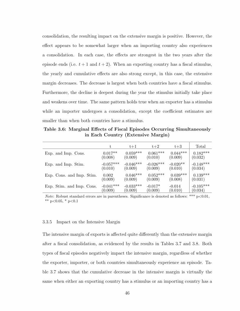
consolidation, the resulting impact on the extensive margin is positive. However, the
effect appears to be somewhat larger when an importing country also experiences
a consolidation. In each case, the effects are strongest in the two years after the
episode ends (i.e. t+ 1 and t+ 2). When an exporting country has a fiscal stimulus,
the yearly and cumulative effects are also strong except, in this case, the extensive
margin decreases. The decrease is largest when both countries have a fiscal stimulus.
Furthermore, the decline is deepest during the year the stimulus initially take place
and weakens over time. The same pattern holds true when an exporter has a stimulus
while an importer undergoes a consolidation, except the coefficient estimates are
smaller than when both countries have a stimulus.
Table 3.6: Marginal Effects of Fiscal Episodes Occurring Simultaneouslyin Each Country (Extensive Margin)
t t+1 t+2 t+3 Total
Exp. and Imp. Cons. 0.017** 0.059*** 0.061*** 0.044*** 0.182***(0.008) (0.009) (0.010) (0.009) (0.032)
Exp. and Imp. Stim. -0.057*** -0.046*** -0.026*** -0.020** -0.148***(0.010) (0.009) (0.009) (0.010) (0.034)
Exp. Cons. and Imp. Stim. 0.002 0.046*** 0.052*** 0.039*** 0.139***(0.009) (0.009) (0.009) (0.008) (0.031)
Exp. Stim. and Imp. Cons. -0.041*** -0.033*** -0.017* -0.014 -0.105***(0.009) (0.009) (0.009) (0.010) (0.034)
Note: Robust standard errors are in parentheses. Significance is denoted as follows: *** p<0.01,** p<0.05, * p<0.1
3.3.5 Impact on the Intensive Margin
The intensive margin of exports is affected quite differently than the extensive margin
after a fiscal consolidation, as evidenced by the results in Tables 3.7 and 3.8. Both
types of fiscal episodes negatively impact the intensive margin, regardless of whether
the exporter, importer, or both countries simultaneously experience an episode. Ta-
ble 3.7 shows that the cumulative decrease in the intensive margin is virtually the
same when either an exporting country has a stimulus or an importing country has a
46

consolidation, with declines of 9.6% and 9.5%, respectively. A consolidation in an ex-
porting country results in a decline of the intensive margin by a total of 8%, whereas
a stimulus in an importing country has no statistically significant effect.
Table 3.7: Conditional Effects of Fiscal Episodes on the IntensiveMargin
t t+1 t+2 t+3 Total
Exp. Cons. -0.010 -0.007 -0.026** -0.040*** -0.083**(0.010) (0.011) (0.010) (0.010) (0.036)
Exp. Stim. -0.031*** -0.009 -0.028** -0.031*** -0.101**(0.011) (0.012) (0.012) (0.011) (0.040)
Imp. Cons. -0.031*** -0.022* -0.023** -0.025** -0.100**(0.011) (0.012) (0.011) (0.011) (0.039)
Imp. Stim. -0.021 -0.017 -0.018 -0.011 -0.067(0.013) (0.013) (0.013) (0.013) (0.048)
R2 0.881Observations 14,441Year Effects YesExp. and Imp. Effects YesCountry-pair Effects No
Note: These are the estimated marginal effects when the indicated fiscal episode oc-curs in period t. The results are from a single regression, but are presented in multiplecolumns for readability. In addition, the control variables from Table 3.2 are includedin the regression, but the coefficient estimates are omitted here for space considera-tions. Robust standard errors are in parentheses. Significance is denoted as follows:*** p<0.01, ** p<0.05, * p<0.1
Table 3.8: Marginal Effects of Fiscal Episodes OccurringSimultaneously in Each Country (Intensive Margin)
t t+1 t+2 t+3 Total
Exp. and Imp. Cons. -0.041*** -0.030* -0.049*** -0.065*** -0.184***(0.015) (0.017) (0.016) (0.016) (0.057)
Exp. and Imp. Stim. -0.052*** -0.026 -0.046*** -0.042** -0.167**(0.018) (0.019) (0.018) (0.017) (0.065)
Exp. Cons. and Imp. Stim. -0.031* -0.024 -0.045*** -0.051*** -0.150**(0.017) (0.017) (0.017) (0.016) (0.061)
Exp. Stim. and Imp. Cons. -0.062*** -0.032* -0.051*** -0.057*** -0.201***(0.017) (0.017) (0.016) (0.016) (0.058)
Note: Robust standard errors are in parentheses. Significance is denoted as follows: ***p<0.01, ** p<0.05, * p<0.1
When countries experience episodes simultaneously, the largest decreases in the
47

intensive margin occur when an importing country has a fiscal consolidation. When
an importer undergoes a stimulus and an exporting country also experiences a fiscal
episode, the decline in the intensive margin is also statistically significant, although
not as severe as when the importer has a consolidation.
3.3.6 Successful Fiscal Consolidations
Alesina & Ardagna (2009) also consider the effects of what they deem “successful”
fiscal consolidations, in which “the cumulative reduction of the debt to GDP ratio
three years after the beginning of a fiscal adjustment is greater than 4.5 percentage
points.”35 Referring back to Table 3.1, notice that successful fiscal consolidations are
a small subset of total fiscal consolidations. It is interesting to see that the percentage
increase in total exports after a successful fiscal consolidation is twice that in Table 3.3
(14% compared to 7%), but that the increase in total exports is again entirely driven
by the increase in the extensive margin of exports. The intensive margin appears to
play a very limited role in this scenario. Although results are also reported here for
when an exporting and importing country undergo a successful fiscal consolidation
simultaneously, these cases are so rare that they should be interpreted with caution.
3.3.7 Comparison Using IMF Definition of Fiscal Consolidation
Thus far, the fiscal episodes in this paper have been based on the definitions put forth
by Alesina & Ardagna (2009). However, as discussed previously in Section 3.2.3, Leigh
et al. (2010) develop a new definition of fiscal consolidation, citing concerns with lim-
itations of previous definitions. Specifically, the authors argue that their definition
of fiscal consolidation is more accurate because it is based on policy actions, rather
than budget outcomes. A narrative approach is used to identify cases of fiscal con-
solidation, in which the authors consult numerous sources to determine what policy
35Alesina & Ardagna (2009), pages 8-9.
48

Table 3.9: Conditional Effects of Successful Fiscal Consolidation
t t+1 t+2 t+3 Total
Total Exports:
Exp. Cons. 0.014 0.070*** 0.060*** -0.013 0.131*(0.024) (0.022) (0.022) (0.020) (0.077)
Imp. Cons. 0.005 0.012 -0.004 -0.036* -0.023(0.020) (0.021) (0.022) (0.020) (0.072)
Exp. and Imp. Cons. 0.018 0.082** 0.056* -0.049 0.108(0.032) (0.033) (0.033) (0.030) (0.113)
Extensive Margin:
Exp. Cons. 0.030*** 0.039*** 0.070*** -0.003 0.136***(0.009) (0.009) (0.011) (0.008) (0.031)
Imp. Cons. 0.008 0.009 0.003 -0.002 0.017(0.011) (0.011) (0.012) (0.012) (0.040)
Exp. and Imp. Cons. 0.038** 0.047*** 0.073*** -0.005 0.153***(0.015) (0.015) (0.017) (0.016) (0.055)
Intensive Margin:
Exp. Cons. -0.016 0.031* -0.010 -0.010 -0.005(0.020) (0.018) (0.020) (0.018) (0.066)
Imp. Cons. -0.003 0.003 -0.007 -0.033* -0.040(0.019) (0.019) (0.019) (0.017) (0.064)
Exp. and Imp. Cons. -0.019 0.035 -0.017 -0.044 -0.045(0.027) (0.028) (0.030) (0.026) (0.098)
Observations 14,441Year Effects YesExp. and Imp. Effects YesCountry-pair Effects No
Note: Separate regressions are run for Total Exports, the Extensive Margin, and theIntensive Margin, in which dummy variables are included for exporter and importer con-solidations in t through t + 3. These are the estimated marginal effects when the indi-cated fiscal episode occurs in period t. In addition, the control variables from Table 3.2are included in each regression, but the coefficient estimates are omitted here for spaceconsiderations. Robust standard errors are in parentheses. Significance is denoted asfollows: *** p<0.01, ** p<0.05, * p<0.1
actions countries actually take. As is evident in Table 3.10 by the fewer instances of
consolidation, their sample is much smaller than that of Alesina & Ardagna (2009),
with only 15 OECD countries for the period 1980-2009.
They also do not consider fiscal stimuli, but the episodes they identify serve as
a good robustness check for the case of fiscal consolidation. Indeed, the results in
49

Table 3.10: Summary of Fiscal Episodes (IMF Definition)
Type of Episode t t+1 t+2 t+3
Exp. Consolidation 431 263 254 254Imp. Consolidation 429 262 254 254Both Consolidation 58 28 28 28
Table 3.11 show that a consolidation in an exporting country is associated with a
relatively large increase in total exports, as in our previous results. However, in this
case the intensive margin also contributes to the increase in total exports. In fact, it
is hard to determine which trade margin plays the biggest role in the increase of total
exports, as an exporter consolidation leads to an increase in the extensive margin in
periods t+ 1 and t+ 2, and an increase in the intensive margin in periods t and t+ 1.
The magnitudes are slightly larger for the intensive margin, but the total impact
is statistically insignificant for each margin. Episodes in importing countries are
statistically insignificant with coefficient estimates near zero, consistent with earlier
results. Overall, the results using the IMF definition of fiscal consolidation compare
favorably to the earlier results. However, the much smaller sample size invites caution
when comparing the two sets of results.
3.4 Discussion
This paper demonstrates the importance of fiscal episodes to the extensive and in-
tensive margins of trade, as well as the overall volume of exports. Large changes in
the fiscal stance of a country are shown to have a substantial impact on their trading
relationships. There are essentially two types of scenarios that are relevant from a
policy standpoint, the first of which is much more common in the current dataset: 1)
When a fiscal episode occurs in an exporting country, and, 2) When a fiscal episode
occurs in both countries of a country-pair simultaneously. A consolidation in an ex-
porting country results in an increase in the extensive margin of over 16% and an
increase in the total volume of exports by nearly 7%. For large fiscal consolidations,
50

Table 3.11: Conditional Effects of Fiscal Consolidation (IMFDefinition)
t t+1 t+2 t+3 Total
Total Exports:
Exp. Cons. 0.059* 0.094*** 0.028 -0.019 0.162*(0.032) (0.034) (0.021) (0.020) (0.095)
Imp. Cons. 0.003 -0.037 -0.023 -0.028 -0.085(0.029) (0.025) (0.021) (0.021) (0.083)
Exp. and Imp. Cons. 0.062 0.057 0.005 -0.046 0.078(0.044) (0.041) (0.030) (0.030) (0.123)
Extensive Margin:
Exp. Cons. 0.007 0.049** 0.026** -0.012 0.069(0.017) (0.024) (0.012) (0.009) (0.059)
Imp. Cons. 0.004 0.003 -0.002 -0.004 0.001(0.013) (0.011) (0.011) (0.011) (0.039)
Exp. and Imp. Cons. 0.011 0.052* 0.024 -0.016 0.071(0.021) (0.027) (0.017) (0.015) (0.074)
Intensive Margin:
Exp. Cons. 0.052* 0.045** 0.002 -0.006 0.093(0.028) (0.022) (0.016) (0.016) (0.071)
Imp. Cons. -0.001 -0.040* -0.021 -0.024 -0.086(0.026) (0.021) (0.016) (0.017) (0.067)
Exp. and Imp. Cons. 0.051 0.004 -0.019 -0.030 0.007(0.041) (0.031) (0.023) (0.024) (0.101)
Observations 5,965Year Effects YesExp. and Imp. Effects YesCountry-pair Effects No
Note: Separate regressions are run for Total Exports, the Extensive Margin, andthe Intensive Margin, in which dummy variables are included for exporter and im-porter consolidations in t through t+ 3. These are the estimated marginal effectswhen the indicated fiscal episode occurs in period t. In addition, the control vari-ables from Table 3.2 are included in the regression, but the coefficient estimatesare omitted here for space considerations. Robust standard errors are in paren-theses. Significance is denoted as follows: *** p<0.01, ** p<0.05, * p<0.1
known as “successful” fiscal consolidations in this study, the increase in total exports
is approximately 14.5% and is driven entirely by changes in the extensive margin.
Leigh et al. (2010) show that a decrease in interest rates usually follows a fiscal con-
solidation, meaning that countries may use a fiscal consolidation as a time to invest
and expand their product lines, which is consistent with an increase in the extensive
51
margin. These results are robust to using the IMF definition of fiscal consolidation,
which shows an increase in total exports of over 17.5%. However, a fiscal stimulus
in an exporting country results in a decline in the extensive and intensive margin,
yielding a decrease in total exports of over 21%. Although these results do not shed
light on the type of fiscal policy used to prompt the fiscal episode, or the exact mech-
anism that is causing the change in exports, the implication is that policy-makers
should take these potential consequences into account when considering changes in
fiscal policy.
When an exporting and importing country simultaneously experience an episode,
total exports are only significantly affected by a stimulus in the exporting country.
In this case, the decline in total exports is approximately 27%, regardless of whether
the importing country has a stimulus or consolidation. Thus, the decline in exports
following a fiscal stimulus in an exporting country appears to be deeper if the import-
ing country also experiences a fiscal episode. Although the extensive and intensive
margins each contribute to the decline in total exports, the intensive margin declines
relatively more in the case of a stimulus. When an exporting country undergoes a
fiscal consolidation and an importing country also has a fiscal episode, the positive
effects of the extensive margin are offset by the negative effects of the intensive margin
so that the impact on total exports is close to zero and statistically insignficant. This
is especially relevant in today’s policy arena as many governments are considering
fiscal consolidation measures. The results suggest that an increase in total exports
should not be expected if a country’s trading partner has recently experienced a fiscal
consolidation.
Although we are unable to identify the exact mechanism that is causing the change
in exports following a fiscal episode, there are recent studies that shed light on some
possibilities. For example, Leigh et al. (2010) show that a country typically experi-
ences an exchange rate depreciation as well as a decrease in interest rates following
52

a fiscal consolidation, which tends to increase exports. The current study confirms
this and makes sense intuitively, as firms may use the drop in interest rates and ex-
change rate depreciation brought about by fiscal consolidation as an opportunity to
expand their product line. Leigh et al. (2010) do not address fiscal stimuli, but it
naturally follows that if a consolidation is associated with an increase in exports due
to decreases in interest rates and the exchange rate, then a fiscal stimulus is likely to
be associated with a decrease in exports due to an increase in interest rates and the
exchange rate. Indeed, our results support this possibility.
The current paper is focused specifically on gauging the response of exports to
various fiscal episodes in bilateral trading relationships. However, there are natural
extensions worth further research. For example, it may be interesting to measure
the extensive margin in a more detailed way. That is, rather than simply counting
the number of categories in which a country exports, construct a weighted measure
of the extensive margin, whereby goods that compose a larger percentage of total
trade are weighted higher than those that are a smaller proportion of total trade.
This would also allow for a more specific measurement of the intensive margin, by
giving more weight to those products that make up a larger share of total exports.
Adding more countries to the study and doing a comparison with developing countries
may also be fruitful. From a policy perspective, it may be worthwhile to consider
the potential asymmetric impact of tax changes versus changes in spending as the
source of the fiscal episode. Moreover, determining the exact mechanism responsible
for the change in total exports and the respective trade margins, be it changes in
interest rates, exchange rates, or something else entirely, may be useful for future
policy prescriptions.
53

4 Macroeconomic Policy, Disaggregated Exports, and Economic Growth: A Simul-
taneous Equations Approach
4.1 Introduction
Given the increasingly global nature of the economy, any analysis of the efficacy of
various macroeconomic policies on economic growth should also incorporate the in-
creasing role of exports into the framework. Recent empirical studies offer mixed
results on the impact of exports and macroeconomic policy – monetary policy and
fiscal policy – on economic growth. The extant literature takes a rather fragmented
approach to measuring these policies, using various indices, proxies, and econometric
techniques. Furthermore, given the importance of the impact of trade on growth, rel-
atively little attention is paid to the possible indirect effect of macroeconomic policy
on economic growth through the export channel. Thus, the contributions of this pa-
per are twofold. First, I explore the determinants of disaggregated exports – primary
and manufacturing exports – to empirically test whether macroeconomic policy does
indeed influence the size of the export sector in a given country. Second, I use simulta-
neous equations methods to identify the impact of macroeconomic policy and exports
on economic growth. The results offer support for the idea that macroeconomic pol-
icy directly affects export levels and also demonstrate that exports affect economic
growth. However, the evidence demonstrating a direct link between macroeconomic
policy and growth is much weaker.
The paper proceeds as follows. Section 2 explores the relevant literature on the
relationship between macroeconomic policy, exports, and economic growth. Section
3 discusses the theory and methodology. Section 4 presents the data and results.
Section 5 concludes.
54

4.2 Background
4.2.1 Macroeconomic policy and economic growth
Since price stability is a principal goal of macroeconomic policy, early studies focus
heavily on the relationship between inflation and economic growth. Bleaney (1996)
finds no relationship between inflation and growth. However, he truncates the maxi-
mum inflation rate at 100% to avoid “outliers,” which, according to Bruno & Easterly
(1998), are the source of the negative relationship between inflation and economic
growth. Indeed, Bruno & Easterly (1998) provide evidence that high-inflation crises
are particularly harmful to growth, as they find a negative relationship between in-
flation and growth only during periods when inflation is above a threshold level of
40% per year. Fischer (1991, 1993) demonstrates that countries with low levels of
inflation grow much faster than those with high levels of inflation, and that high infla-
tion also impedes growth by discouraging physical capital investment. Barro (1996)
finds, on average, that a 10 percentage point increase in inflation is associated with
a decrease in the GDP growth rate of 0.24 percentage points. Upon further inves-
tigation, he finds that the negative relationship between inflation and growth only
holds for those countries with inflation rates above 20% per year. Durlauf, Kourtel-
los & Tan (2008) use Bayesian Model Averaging to test the robustness of various
growth theories, including a theory that macroeconomic policy variables are impor-
tant determinants of a country’s growth process. They use panel data covering three
time periods, 1965-74, 1975-84, and 1985-94 for 53, 54, and 57 countries, respectively.
Their results show that growth rates are positively correlated with improvements in
macroeconomic policy variables, specifically inflation and government consumption.
A theme that emerges from the literature, as noted by Bruno & Easterly (1998), is
that extremely high rates of inflation tend to be significantly negatively associated
with long-run growth and that the inflation-economic growth relationship weakens as
55

data frequency decreases.
While certainly important, inflation is not the only available macroeconomic pol-
icy indicator. Bleaney (1996) analyzes a cross-section of 41 developing countries for
the period 1980-90, and a smaller sample of countries over the period 1972-90, and
finds that changes in growth rates are positively correlated with improvements in
macroeconomic policies, for a given level of investment. Macroeconomic policies are
evaluated using five different measures of debt, inflation, and exchange rates, in which
the fiscal balance and exchange rate volatility are found to be the most highly cor-
related with economic growth. Bleaney posits that including exchange rate volatility
in the same regression as the inflation rate, which are highly positively correlated,
may partially explain why inflation does not enter significantly – perhaps because it
has proxied for exchange rate volatility in prior work. Combined with the previous
studies he cites, Bleaney explains this evidence “suggests that variability of the real
exchange rate is an important aspect of policy-induced macroeconomic instability
that adversely affects performance.”36 Rodrik (2008) examines data on 188 countries
over the time period 1950-2004 to investigate the relationship between the real ex-
change rate and economic growth. Using several measures of under/over-valuation
of the real exchange rate and various estimation techniques, he concludes that un-
dervaluation prompts economic growth. Moreover, he finds that when a country’s
currency is significantly overvalued their export sector suffers much more than the
non-export sector. My analysis takes this idea one step further and allows for het-
erogeneity across exports by disaggregating the export sector into its manufacturing
and primary components.
Other studies, such as Montiel & Serven (2006), find no discernible evidence that
improving macroeconomic policy is beneficial to a country’s growth process. They
analyze data from 1960-2003 and explain that developing countries have generally
36Bleaney (1996), p. 466.
56

improved their macroeconomic policies over time, yet have not seen the anticipated
growth advantages from doing so. Bigsten et al. (1999) attempt to model the quality
of macroeconomic policy through a measure of country openness known as the Dollar
index, which is a measure of how much domestic prices are above/below international
prices.37 Although they find no significant impact on exports from changes in the
level of openness, they only analyze firm-level data for four countries covering the
time period 1991-95 and therefore recommend using caution when interpreting their
results. Hausmann, Pritchett & Rodrik (2005) examine growth accelerations, defined
as an increase in GDP per capita growth of 2 percentage points that is sustained
for at least 8 years, in which the post-acceleration annual growth rate is at least
3.5 percent. They look at 110 countries over the period 1957-92 and find that these
accelerations are not usually preceded by changes in economic policies, implying that
macroeconomic policy may have little or no impact on sustained economic growth.
Thus, evidence is mixed concerning the relationship between macroeconomic pol-
icy and growth. The extent to which these policies may affect growth appears to
depend, at least in part, on how the policies are defined as well as the countries
and time period selected for study. I attempt to address this by using a variety
of macroeconomic policy indicators, a long time period, and numerous countries.
Equally important in the present study is the role of exports, which is explored in
more detail in the next section.
4.2.2 Macroeconomic policy and exports
In theory when the exchange rate in a given country appreciates, exports from that
country become more expensive relative to non-export products. Thus, one would
expect exports, on average, to decrease under such circumstances. Moreover, Collier &
Gunning (1999) cite the presence of a “Dutch disease” effect, whereby exporting large
37See Bigsten et al. (1999), or the appendix of Sirimaneetham & Temple (2009) for a more detailedexposition of the Dollar Index.
57

quantities of natural resources, as is typically the case in developing countries, can
lead to an appreciation of the exchange rate, hurting the manufacturing export sector
much more than the primary export sector. Whereas some countries in East Asia
and Latin America have promoted their manufacturing export sector over the past
few decades, this is not true of all developing countries, particularly those in Africa.
In addition to a reliance on primary exports, it is not uncommon for developing
countries to have overvalued exchange rates, tariffs, and taxes that are unfavorable to
exporting. As Collier & Gunning (1999) point out, these types of policies are much
more harmful to “transaction-intensive” sectors like manufacturing. Furthermore,
such policies make the black market an attractive alternative for selling products.
The informal nature of the agriculture sector, in addition to typically being less
capital-intensive, makes it a less risky venture than the manufacturing sector, thus
providing for an easier transition to the black market when prompted by unfavorable
macroeconomic policies. This stifles production in the manufacturing sector and the
positive spillovers that would arise from it, thereby contributing to the slow economic
growth of many developing countries over the past few decades.
The literature clearly shows that exports and macroeconomic policies play an im-
portant role in the economic growth process of a country. However, much of the
current empirical work implicitly assumes that only direct effects exists from macroe-
conomic policies and/or exports to economic growth. I take an alternative approach
in the next section by considering the effects of policy variables on exports and the
indirect effect of policy variables on economic growth through the use of simultaneous
equations methods.
58
4.3 Theory and Methodology
4.3.1 Theory
Past empirical research suggests that the macroeconomic stability of a country may
directly influence its volume of exports and economic growth rate. However, since
exports are also vitally important to a country’s growth performance, macroeconomic
policy may also exert an indirect effect on growth through its influence on exports.
Therefore, in thinking of the importance of macroeconomic policy and exports in
the growth process, it is perhaps more appropriate to model them separately, in a
system of equations, rather than with a single estimating equation. This serves not
only to more accurately measure the marginal effect of exports on growth, but also
to determine the relative importance of macroeconomic policy indicators.
Esfahani (1991) argues that a simultaneous equations approach is necessary be-
cause although GDP growth is a function of exports, export growth is also a function
of GDP growth. Estimating a single equation with exports as an explanatory variable
may overstate the importance of exports to economic growth. Thus, it is optimal to
have an export equation in addition to an economic growth equation. However, Esfa-
hani (1991) only considers GDP per capita, population, and their respective growth
rates as determinants of the level of exports. Price measures that may indicate the
relative competitiveness of the export sector are not considered; human capital is
not considered in either the exports or economic growth equations. Sprout & Weaver
(1993) do include a price competitiveness measure as a potential exports determinant,
in addition to the rate of economic growth, the growth of a country’s main trading
partners, and a measure of export composition and concentration. Sprout & Weaver
(1993) construct their export composition measure by adding the share of primary
products in total exports and the share of the two largest export commodities in
total exports, then dividing by two. I take a similar approach, except I disaggregate
59

exports into its manufacturing and primary components for use as the dependent vari-
ables in the export equations and the explanatory variables in the economic growth
equation. Greenaway & Sapsford (1994) investigate the importance of liberalization
policies to exports and growth, yet find little support for the idea that a country that
undergoes a trade policy liberalization will experience higher export and economic
growth. While highlighting the potentially important role government policy may
play in determining export and economic growth, the study is limited by the narrow
scope of policies considered. I take a broader approach by looking at changes in vari-
ous macroeconomic policies to see if the dynamics are different between the short run
and long run, rather than looking at strict “episodes” of liberalization.
The exports and economic growth equations in the following section are based on a
production function approach, in which Y = A∗f(K,H,L) andX = g(Y,K,H,L, P,M).
Y is total output, A is technology, K is physical capital, H is human capital, L is
labor, P is price competitiveness, and M is macroeconomic policy indicators. Us-
ing a Cobb-Douglas functional form and following the contributions of Solow (1956),
Mankiw, Romer & Weil (1992), and Tyler (1981), output is modeled as follows:
Yi,t = Ai,tKαi,tH
βi,tL
γi,t (10)
for country i during period t. Ait depends on the initial level of technology in a
country, macroeconomic policy, and the rate of technological progress, similar to
Mankiw et al. (1992), among others:
Ai,t = A0egi,tMi,t (11)
Technological progress, g, depends in part on the level of exports, so that:
gi,t = η + θXi,t (12)
60

The level of exports is determined similarly, with physical capital, human capital,
and labor growth playing an important role. In addition, it is important to control
for economic growth, the relative competitiveness of the export sector, and macroe-
conomic policy, as these also influence the overall level of exports (Sprout & Weaver,
1993; Greenaway & Sapsford, 1994).
4.3.2 Methodology
Thus, I estimate the following system of reduced-form equations:
xit = ηi1 + µt1 + α1ki,t−1 + β1hi,t−1 + γ1li,t−1 + δ1ti,t−1 + ϕ1ri,t−1 + κ1mi,t−1
+ θ7yi,t−1 + εit1 (13)
yit = ηi2 + µt2 + α2ki,t−1 + β2hi,t−1 + γ2li,t−1 + θ1xi,t + κ2mi,t−1 + εit2 (14)
for country i over time period t, in which x is a vector of the export variables of inter-
est, including total merchandise exports as a share of GDP, manufacturing exports
as a share of GDP, and primary exports as a share of GDP.38 y is GDP per capita
growth, and η and µ control for country-fixed effects and time effects, respectively.
Traditional control variables are included, wherein k is physical capital investment, h
is human capital investment, and l is the growth rate of labor (see Levine & Renelt,
1992, among many others). The tariff rate, t, and the volatility of the real effective
exchange rate index, r, are only included in the export equation, in an effort to control
for the openness of a country and the stability of the exchange rate. These additional
variables in the export equation also make the system over-identified, which is an
important factor in determining an estimation method. m is a vector of the macroe-
conomic policy indicators of interest, which are discussed in more detail in the next
section.
38Detailed variable definitions are available in the Appendix.
61
Equation (13) is estimated first, in both the cross-section and panel context, us-
ing ordinary least squares (OLS) in an effort to identify the effect of macroeconomic
policy on the level of exports in a country. This is done using total exports, man-
ufacturing exports, and primary exports as dependent variables. Then, I consider
possible indirect effects of macroeconomic policy on growth through the export chan-
nel, using the two-step IV-GMM estimation technique, again in a cross-section and
panel context. These results are discussed in the following section.
4.4 Data and Results
4.4.1 Data
The majority of the data are collected from the World Bank’s 2010 World Develop-
ment Indicators database over the sample period 1990-2009.39 The education data
are from Barro & Lee (2010) and government debt data are from Jaimovich & Panizza
(2010). Equation (13) is estimated below, using both cross-section and panel estima-
tion techniques to check for the robustness of relationships between the explanatory
variables and exports over the short run and long run. The dependent variables are
total merchandise exports, manufacturing exports, and primary exports, respectively;
each export variable is scaled by GDP and logged. In the cross-sectional case, the
export variables are averaged over the entire sample period and the explanatory vari-
ables are ten-year averages, from 1990-1999, to mitigate endogeneity concerns. In the
panel case, all data are in five-year averages and all explanatory variables are lagged
one period.40
Some discussion is warranted on the macroeconomic policy indicators of interest.
In general, perceived improvements in macroeconomic policy indicators are subjective
and this should be kept in mind when interpreting the results. There are six vari-
39Data from previous periods are too sparse and unreliable to allow for more comprehensive timecoverage.
40Detailed variable descriptions are available in the Appendix.
62

ables included here, chosen on the basis of data availability and their use in previous
studies. For some, the reason for inclusion is quite obvious. Inflation, for exam-
ple, has been widely used in past empirical studies (Fischer, 1991, 1993; Bruno &
Easterly, 1998), in which high inflation is usually associated with low or diminished
growth. Moreover, many countries set inflation targets, making inflation a sufficient
indicator of macroeconomic policy. However, inflation volatility is also included be-
cause while extremely high rates of inflation are found to be detrimental to economic
growth in previous studies, the volatility of inflation may be equally important. Since
exports are an important part of economic activity, inflation volatility is expected
to be negatively associated with the level of exports. For others, such as the ratio
of government debt to GDP, the argument for inclusion may be less apparent. For
example, a country that is highly indebted may inadvertently discourage investment
due to higher interest rates or fears of increased tax liabilities in the future. In turn,
it becomes more difficult and less likely that the export sector will expand, meaning
the country will not experience the positive externalities resulting from exporting.
The adverse impact of an indebted government will likely affect the manufactured
goods export sector more than the primary goods export sector because of the higher
returns and possibility of positive externalities associated with the former. Alterna-
tively, a country may be indebted because it has spent large sums of money investing
in infrastructure or human capital. In this case, exports, particularly of manufactured
goods, would be expected to subsequently increase. Similar arguments can be made
for government consumption expenditures. A significant amount of spending may
be the result of investment in infrastructure or stimulus for the economy, in which
case exports could potentially increase. However, it may also be the case that high
government expenditures are a sign of instability or weakness in the economy, which
may adversely affect consumer confidence, leading to a decrease in exports. An in-
crease in the money supply, M2, may signify more activity in the economy, in which
63

case manufacturing and total exports will likely increase, whereas primary exports
may decrease as resources are shifted toward more profitable outlets. Conversely, it
may be the case that an increase in M2 is the result of economic uncertainty and
people may just be holding more money, rather than using it to expand output, in
which case there may be a negative relationship with exports. Finally, a low real in-
terest rate may incentivize businesses to open or expand their operations, which may
subsequently increase exports, whereas high interest rates discourage investment and
business expansion, which in turn may discourage exports, especially of manufactured
goods.
4.4.2 Baseline Results
The cross-sectional results are reported in Table 4.1, in which OLS is applied to
Equation (13) while omitting the indicators of macroeconomic policy to first give
baseline estimates. Notice that the coefficient estimate on investment is positive and
highly statistically significant in the total exports equation. Moreover, the magnitude
is economically significant, suggesting that increasing the investment to GDP ratio
by one percentage point increases total exports by nearly 0.72 percentage points.
Perhaps even more striking are the coefficient estimates on the education variable.
The coefficient estimate is positive and highly statistically significant in the case of
manufacturing exports. The magnitude is also economically large, suggesting that a
one percentage point increase in the population that has some secondary education
leads to nearly a 0.5 percentage point increase in manufacturing exports as a share
of GDP. However, in the primary exports equation, the coefficient estimate is nega-
tive and statistically significant with an even larger magnitude. Thus, these results
suggest that increasing the secondary education level in a country leads people to
utilize their skills in the more productive manufacturing export sector, which in turn
diverts resources away from the primary export sector. Last, notice the negative and
64

statistically significant coefficient estimate on the volatility of the real effective ex-
change rate (REER) index. This suggests that the volatility of a country’s exchange
rate is more harmful to the manufacturing export sector than the primary or total
export sector. This is somewhat unsurprising since the manufacturing export sector
is typically more transaction-intensive than other sectors (Collier & Gunning, 1999).
Table 4.1: Determinants of Exports (Cross-section)
Total Exp. Manuf. Exp. Prim. Exp.
Ann. Avg. GDP per cap. growth rate 0.005 0.049 0.002(0.019) (0.036) (0.064)
Working-age population growth rate 0.065 -0.271** -0.006(0.071) (0.112) (0.201)
Investment 0.718** 0.573 -0.147(0.305) (0.554) (0.782)
Education -0.022 0.462* -0.821**(0.155) (0.241) (0.388)
Tariff rate -0.221 -0.111 -0.398(0.157) (0.220) (0.366)
REER Index Volatility -0.010 -0.028** -0.008(0.006) (0.013) (0.023)
Constant 1.895* -0.194 5.583**(1.080) (1.889) (2.757)
R2 0.207 0.442 0.086No. of Countries 68 68 68
Note: The dependent variable is the level of exports, averaged over the entire sampleperiod. All explanatory variables are 10-year averages. Robust standard errors are inparentheses. Significance is denoted as follows: *** p<0.01, ** p<0.05, * p<0.1
Table 4.2 presents the results from a fixed effects estimation and provides some
support for the cross-sectional results. For example, the coefficient estimate on in-
vestment is positive for the total and manufacturing export sectors, although it is
only significant in the case of manufacturing exports. The coefficient estimate on
investment for the primary exports equation is again negative, albeit insignificant.
While the results are qualitatively similar, the only other variable that is statistically
significant is the negative coefficient estimate on the tariff rate in the manufacturing
exports equation. It implies that increasing the tariff rate by one percentage point
65
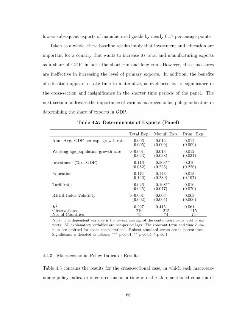
lowers subsequent exports of manufactured goods by nearly 0.17 percentage points.
Taken as a whole, these baseline results imply that investment and education are
important for a country that wants to increase its total and manufacturing exports
as a share of GDP, in both the short run and long run. However, these measures
are ineffective in increasing the level of primary exports. In addition, the benefits
of education appear to take time to materialize, as evidenced by its significance in
the cross-section and insignificance in the shorter time periods of the panel. The
next section addresses the importance of various macroeconomic policy indicators in
determining the share of exports in GDP.
Table 4.2: Determinants of Exports (Panel)
Total Exp. Manuf. Exp. Prim. Exp.
Ann. Avg. GDP per cap. growth rate -0.006 -0.012 -0.012(0.005) (0.009) (0.009)
Working-age population growth rate >-0.001 0.013 0.012(0.023) (0.038) (0.034)
Investment (% of GDP) 0.116 0.503** -0.210(0.082) (0.225) (0.226)
Education 0.174 0.143 0.013(0.146) (0.289) (0.197)
Tariff rate -0.026 -0.168** 0.016(0.025) (0.077) (0.070)
REER Index Volatility >-0.001 -0.003 0.003(0.002) (0.005) (0.006)
R2 0.297 0.415 0.061Observations 219 215 215No. of Countries 75 74 74
Note: The dependent variable is the 5-year average of the contemporaneous level of ex-ports. All explanatory variables are one-period lags. The constant term and time dum-mies are omitted for space considerations. Robust standard errors are in parentheses.Significance is denoted as follows: *** p<0.01, ** p<0.05, * p<0.1
4.4.3 Macroeconomic Policy Indicator Results
Table 4.3 contains the results for the cross-sectional case, in which each macroeco-
nomic policy indicator is entered one at a time into the aforementioned equation of
66

control variables from Table 4.1. Note that more of the policy indicators have a sig-
nificant effect on manufacturing exports than total or primary exports. For example,
consider the real interest rate, whose coefficient estimate is positive and statistically
significant in the case of primary exports, but negative and statistically significant
in the case of manufacturing exports. An increase in the real interest rate drives up
the cost of capital and the manufacturing export sector typically uses capital more
intensively than the primary export sector. The results lend support to this idea and
the magnitudes imply that a one percentage point increase in the real interest rate
decreases manufacturing exports by nearly as much as it increases primary exports.
M2 is positively related to manufacturing exports, and is also statistically significant,
consistent with the predictions in Section 4.4.1. Moreover, M2 is negatively, albeit in-
significantly, related to primary exports, suggesting that an economy which increases
its money supply subsequently directs resources away from the primary exports sector.
Table 4.3: Conditional Effects of Policy Indicators on Exports(Cross-section)
Total Exp. Manuf. Exp. Prim. Exp. # of Countries
Gov. Debt -0.019 -0.052 -0.045 65(0.134) (0.139) (0.188)
Gov. Consum. 0.220 0.222 -0.384 68(0.191) (0.356) (0.457)
Real Int. Rate -0.001 -0.024** 0.026* 64(0.005) (0.010) (0.013)
M2 (% of GDP) 0.030 0.577* -0.530 55(0.163) (0.330) (0.352)
Inflation -0.060 -0.059 -0.079 68(0.052) (0.090) (0.111)
Inflation Vol. >-0.001 >-0.001 <0.001 68(0.000) (0.000) (0.000)
Note: Control variables for each policy indicator include annual average GDPgrowth, labor growth, the investment rate, the percentage of the population withsome secondary education, and the tariff rate. For space considerations, the coeffi-cients of these variables, along with the constant, are omitted. Due to sample sizerestrictions, the policy indicators were entered into the equation one at a time, withno two indicators being included in the same equation. Robust standard errors arein parentheses. Significance is denoted as follows: *** p<0.01, ** p<0.05, * p<0.1
67
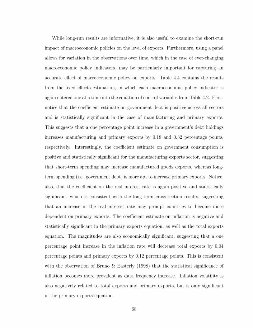
While long-run results are informative, it is also useful to examine the short-run
impact of macroeconomic policies on the level of exports. Furthermore, using a panel
allows for variation in the observations over time, which in the case of ever-changing
macroeconomic policy indicators, may be particularly important for capturing an
accurate effect of macroeconomic policy on exports. Table 4.4 contains the results
from the fixed effects estimation, in which each macroeconomic policy indicator is
again entered one at a time into the equation of control variables from Table 4.2. First,
notice that the coefficient estimate on government debt is positive across all sectors
and is statistically significant in the case of manufacturing and primary exports.
This suggests that a one percentage point increase in a government’s debt holdings
increases manufacturing and primary exports by 0.18 and 0.32 percentage points,
respectively. Interestingly, the coefficient estimate on government consumption is
positive and statistically significant for the manufacturing exports sector, suggesting
that short-term spending may increase manufactured goods exports, whereas long-
term spending (i.e. government debt) is more apt to increase primary exports. Notice,
also, that the coefficient on the real interest rate is again positive and statistically
significant, which is consistent with the long-term cross-section results, suggesting
that an increase in the real interest rate may prompt countries to become more
dependent on primary exports. The coefficient estimate on inflation is negative and
statistically significant in the primary exports equation, as well as the total exports
equation. The magnitudes are also economically significant, suggesting that a one
percentage point increase in the inflation rate will decrease total exports by 0.04
percentage points and primary exports by 0.12 percentage points. This is consistent
with the observation of Bruno & Easterly (1998) that the statistical significance of
inflation becomes more prevalent as data frequency increase. Inflation volatility is
also negatively related to total exports and primary exports, but is only significant
in the primary exports equation.
68

Table 4.4: Conditional Effects of Policy Indicators on Exports (Panel)
Total Exp. Manuf. Exp. Prim. Exp. # of Countries # of Obs
Gov. Debt 0.013 0.178** 0.318*** 68 194(0.044) (0.073) (0.084)
Gov. Consum. 0.182 0.482** -0.147 74 215(0.125) (0.211) (0.247)
Real Int. Rate 0.001 0.004 0.006** 70 197(0.002) (0.005) (0.003)
M2 (% of GDP) -0.009 0.085 0.299 73 179(0.071) (0.183) (0.219)
Inflation -0.044** -0.044 -0.119*** 74 210(0.018) (0.035) (0.035)
Inflation Vol. >-0.001 0.001 >-0.001*** 74 215(0.000) (0.000) (0.000)
Note: Control variables for each policy indicator include annual average GDP growth, laborgrowth, the investment rate, the percentage of the population with some secondary education,and the tariff rate. For space considerations, the coefficients of these variables, along with theconstant, are omitted. Due to sample size restrictions, the policy indicators were entered into theequation one at a time, with no two indicators being included in the same equation. Robust stan-dard errors are in parentheses. Significance is denoted as follows: *** p<0.01, ** p<0.05, * p<0.1
Ideally, all macroeconomic policy indicators would be included in the same re-
gression, as opposed to entering them one at a time. However, doing so drastically
reduces the sample size, which in turn jeopardizes the consistency and efficiency of
the estimation. These results are presented below, but caution is warranted when
trying to interpret the results.
4.4.4 IV-GMM Estimation Results
As discussed previously, the literature shows that exports and macroeconomic policy
each directly affect growth. However, as demonstrated thus far, macroeconomic policy
also directly affects the level of exports, implying that macroeconomic policy may
affect economic growth indirectly through its impact on exports. One way to explore
this issue is through the use of simultaneous equations methods. While two-stage
least squares (2SLS) is a popular estimator it can be shown that IV-GMM, which is
69
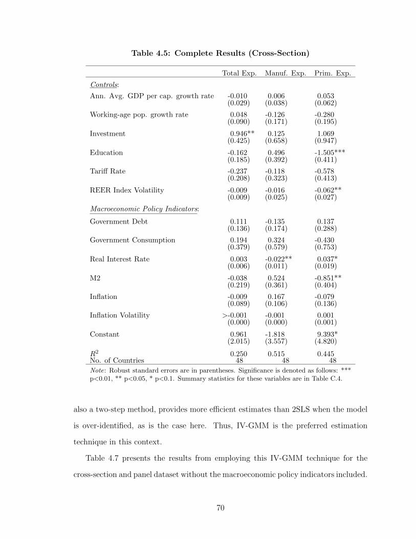
Table 4.5: Complete Results (Cross-Section)
Total Exp. Manuf. Exp. Prim. Exp.
Controls:
Ann. Avg. GDP per cap. growth rate -0.010 0.006 0.053(0.029) (0.038) (0.062)
Working-age pop. growth rate 0.048 -0.126 -0.280(0.090) (0.171) (0.195)
Investment 0.946** 0.125 1.069(0.425) (0.658) (0.947)
Education -0.162 0.496 -1.505***(0.185) (0.392) (0.411)
Tariff Rate -0.237 -0.118 -0.578(0.208) (0.323) (0.413)
REER Index Volatility -0.009 -0.016 -0.062**(0.009) (0.025) (0.027)
Macroeconomic Policy Indicators:
Government Debt 0.111 -0.135 0.137(0.136) (0.174) (0.288)
Government Consumption 0.194 0.324 -0.430(0.379) (0.579) (0.753)
Real Interest Rate 0.003 -0.022** 0.037*(0.006) (0.011) (0.019)
M2 -0.038 0.524 -0.851**(0.219) (0.361) (0.404)
Inflation -0.009 0.167 -0.079(0.089) (0.106) (0.136)
Inflation Volatility >-0.001 -0.001 0.001(0.000) (0.000) (0.001)
Constant 0.961 -1.818 9.393*(2.015) (3.557) (4.820)
R2 0.250 0.515 0.445No. of Countries 48 48 48
Note: Robust standard errors are in parentheses. Significance is denoted as follows: ***p<0.01, ** p<0.05, * p<0.1. Summary statistics for these variables are in Table C.4.
also a two-step method, provides more efficient estimates than 2SLS when the model
is over-identified, as is the case here. Thus, IV-GMM is the preferred estimation
technique in this context.
Table 4.7 presents the results from employing this IV-GMM technique for the
cross-section and panel dataset without the macroeconomic policy indicators included.
70

Table 4.6: Complete Results (Panel)
Total Exp. Manuf. Exp. Prim. Exp.
Controls:
Ann. Avg. GDP per cap. growth rate -0.011* -0.002 -0.021(0.007) (0.011) (0.013)
Working-age pop. growth rate 0.018 0.092 0.158***(0.033) (0.059) (0.056)
Investment 0.166 0.822*** -0.083(0.114) (0.301) (0.274)
Education 0.144 0.169 0.016(0.087) (0.217) (0.186)
Tariff rate -0.063 -0.359*** -0.009(0.046) (0.089) (0.102)
REER Index Volatility -0.002 -0.001 0.004(0.003) (0.006) (0.007)
Macroeconomic Policy Indicators:
Government Debt -0.023 0.097 0.315***(0.045) (0.089) (0.116)
Government Consumption 0.127 0.619* -0.549(0.149) (0.318) (0.465)
Real Interest Rate -0.002 -0.001 <0.001(0.003) (0.004) (0.004)
M2 -0.071 0.001 0.291(0.066) (0.195) (0.227)
Inflation -0.126*** -0.199*** -0.171***(0.030) (0.060) (0.062)
Inflation Volatility 0.001*** 0.003*** <0.001(0.000) (0.001) (0.001)
R2 0.808 0.741 0.845No. of countries 61 61 61No. of Obs. 141 140 140
Note: Robust standard errors are in parentheses. Significance is denoted as follows: ***p<0.01, ** p<0.05, * p<0.1. Summary statistics for these variables are in Table C.5.
The first column presents the results from the cross-section regression, in which man-
ufacturing exports and labor force growth are positively and statistically significantly
related to economic growth. While the coefficient estimate on initial GDP per capita
is of the correct expected sign, it is statistically insignificant. The coefficient estimates
on investment and education are insignificant as well, but are also of the opposite ex-
pected sign. Notice that when using panel data in column two that manufacturing
71
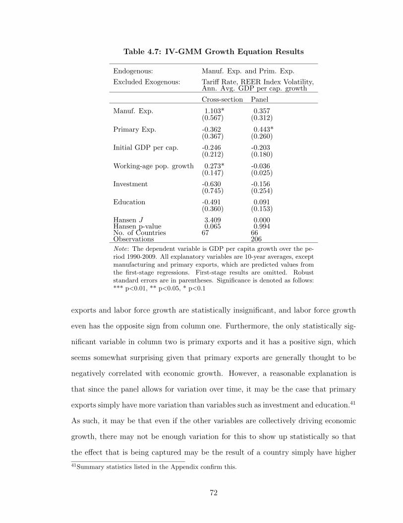
Table 4.7: IV-GMM Growth Equation Results
Endogenous: Manuf. Exp. and Prim. Exp.
Excluded Exogenous: Tariff Rate, REER Index Volatility,Ann. Avg. GDP per cap. growth
Cross-section Panel
Manuf. Exp. 1.103* 0.357(0.567) (0.312)
Primary Exp. -0.362 0.443*(0.367) (0.260)
Initial GDP per cap. -0.246 -0.203(0.212) (0.180)
Working-age pop. growth 0.273* -0.036(0.147) (0.025)
Investment -0.630 -0.156(0.745) (0.254)
Education -0.491 0.091(0.360) (0.153)
Hansen J 3.409 0.000Hansen p-value 0.065 0.994No. of Countries 67 66Observations 206
Note: The dependent variable is GDP per capita growth over the pe-riod 1990-2009. All explanatory variables are 10-year averages, exceptmanufacturing and primary exports, which are predicted values fromthe first-stage regressions. First-stage results are omitted. Robuststandard errors are in parentheses. Significance is denoted as follows:*** p<0.01, ** p<0.05, * p<0.1
exports and labor force growth are statistically insignificant, and labor force growth
even has the opposite sign from column one. Furthermore, the only statistically sig-
nificant variable in column two is primary exports and it has a positive sign, which
seems somewhat surprising given that primary exports are generally thought to be
negatively correlated with economic growth. However, a reasonable explanation is
that since the panel allows for variation over time, it may be the case that primary
exports simply have more variation than variables such as investment and education.41
As such, it may be that even if the other variables are collectively driving economic
growth, there may not be enough variation for this to show up statistically so that
the effect that is being captured may be the result of a country simply have higher
41Summary statistics listed in the Appendix confirm this.
72

growth at a time when primary exports are also relatively higher, even if they are not
actually the driver of the growth. However, caution is warranted when interpreting
the results, as the Hansen J test suggests the instruments may not be valid in the
cross-section case.
Table 4.8: IV-GMM Conditional Effects of Policy Indicatorson GDP per cap. growth (Cross-section)
Endogenous: Manuf. Exp. and Prim. Exp.
Excluded Exogenous: Tariff Rate, REER Index Volatility,Ann. Avg. GDP per cap. growth
Coeff. Obs. Hansen J Hansen p-value
Government Debt -0.029 64 7.571 0.006(0.112)
Government Consumption -0.390 67 3.109 0.078(0.375)
Real Interest Rate 0.046 63 0.547 0.459(0.028)
M2 1.939 54 0.175 0.676(3.596)
Inflation 0.014 67 2.847 0.092(0.127)
Inflation Volatility <0.001 67 3.450 0.063(0.000)
Note: The variables from Table 4.7 are included as controls. For space consid-erations, the coefficients of these variables, along with the constant terms, areomitted. Due to sample size restrictions, the policy indicators were entered intothe equation one at a time, with no two policy indicators being included in thesame equation. First-stage results are omitted. Robust standard errors are inparentheses. Significance is denoted as follows: *** p<0.01, ** p<0.05, * p<0.1
Macroeconomic policy indicators are entered sequentially in Tables 4.8 and 4.9,
but none of the policies are statistically significantly related to economic growth. One
plausible explanation for this is that the macroeconomic policy indicators considered
simply do not directly affect growth. Thus, beyond their impact on exports, macroe-
conomic policy does not matter for economic growth. Caution is warranted when
interpreting these results, though, as the Hansen J Statistic yields mixed results as
to the orthogonality of the over-identifying restrictions. This could indicate poor
73

Table 4.9: IV-GMM Conditional Effects of Policy Indicators on GDPper cap. growth (Panel)
Endogenous: Manuf. Exp. and Prim. Exp.
Excluded Exogenous: Tariff Rate, REER Index Volatility,Ann. Avg. GDP per cap. growth
Coeff. Countries Obs. Hansen J Hansen p-value
Government Debt -0.159 61 186 0.010 0.919(0.131)
Government Consumption 0.029 66 206 0.000 0.992(0.172)
Real Interest Rate >-0.001 60 186 0.001 0.977(0.004)
M2 -0.142 54 159 0.015 0.903(0.154)
Inflation 0.019 66 202 0.008 0.930(0.021)
Inflation Volatility 0.001 66 206 0.001 0.978(0.001)
Note: The variables from Table 4.7 are included as controls. For space considerations, the co-efficients of these variables are omitted. Due to sample size restrictions, the policy indicatorswere entered into the equation one at a time, with no two indicators being included in the sameequation. First-stage results are omitted. Robust standard errors are in parentheses. Signifi-cance is denoted as follows: *** p<0.01, ** p<0.05, * p<0.1
instruments and/or a misspecified model.
4.4.5 High Manufacturing Exports vs. Low Manufacturing Exports
Previous studies have shown that certain policy changes may affect capital- and
transaction-intensive industries, such as those that export manufactures, more so
than those that export less capital- and transaction-intensive goods, such as primary
products (Collier & Gunning, 1999). In this section, I explore the possibility that
countries with different export profiles may react differently to changing macroeco-
nomic conditions by creating a dummy variable equal to one if the manufacturing
exports of a country are in the top 25th percentile. I then create an interaction term
between this dummy variable and each macroeconomic policy variable and repeat the
previous exercises from the paper.
74

Table 4.10: Conditional Effects of Policy Indicators on Exports(Cross-section)
Total Exp. Manuf. Exp. Prim. Exp. # of Countries
High-Manufacturing Export Countries:
Government Debt -0.114 -0.008 0.144 65(0.153) (0.089) (0.230)
Government Consum. 0.188 -0.397 0.273 68(0.354) (0.340) (0.576)
Real Interest Rate -0.011 -0.033* -0.018 64(0.015) (0.018) (0.035)
M2 (% of GDP) 0.081 0.255 -0.323 55(0.171) (0.244) (0.390)
Inflation -0.084 0.037 -0.237* 68(0.066) (0.085) (0.132)
Inflation Volatility <0.001 <0.001 <0.001 68(0.000) (0.000) (0.001)
Low-Manufacturing Export Countries:
Government Debt 0.103 -0.039 -0.265 65(0.160) (0.162) (0.304)
Government Consum. 0.102 -0.008 -0.618 68(0.216) (0.413) (0.630)
Real Interest Rate 0.007 -0.003 0.032** 64(0.006) (0.011) (0.016)
M2 (% of GDP) -0.053 0.375 -0.497 55(0.197) (0.256) (0.429)
Inflation -0.040 -0.045 -0.034 68(0.064) (0.076) (0.114)
Inflation Volatility >-0.001* >-0.001 <0.001 68(0.000) (0.000) (0.000)
Note: The variables from Table 4.7 are included as controls. For space considerations, thecoefficients of these variables, along with the constant, are omitted. Due to sample sizerestrictions, the policy indicators were entered into the equation one at a time, with notwo indicators being included in the same equation. Robust standard errors are in paren-theses. Significance is denoted as follows: *** p<0.01, ** p<0.05, * p<0.1
The cross-sectional results are presented in Table 4.10. First, notice the negative
and statistically significant coefficient estimate on the real interest rate in the second
column for the case of countries with a high level of manufacturing exports. This
implies that a one percentage point increase in the real interest rate drives down
manufacturing exports 3.3%. Countries with a high content of manufactured goods
also see a negative correlation between inflation and primary exports. Specifically,
75

increasing inflation ten percent is associated with a decrease in primary exports of
2.4%. In countries with relatively less manufacturing exports, notice that an increase
in the real interest rate is associated with an increase in primary exports, perhaps
due to a shift toward less capital-intensive exports.
Table 4.11: Conditional Effects of Policy Indicators on Exports (Panel)
Total Exp. Manuf. Exp. Prim. Exp. # of Countries # of Obs
High-manufacturing export countries:
Gov. Debt 0.070 0.204** 0.375*** 68 194(0.066) (0.100) (0.123)
Gov. Consum. 0.206 0.379 0.009 74 215(0.196) (0.251) (0.272)
Real Int. Rate 0.003 0.014*** 0.003 70 197(0.004) (0.005) (0.007)
M2 (% of GDP) 0.094 0.048 0.201 73 179(0.096) (0.119) (0.132)
Inflation -0.059** -0.068 -0.077** 74 210(0.026) (0.043) (0.029)
Inflation Vol. >-0.001 <0.001 -0.001*** 74 215(0.000) (0.000) (0.000)
Low-manufacturing export countries:
Gov. Debt -0.020 0.156* 0.216* 68 194(0.058) (0.088) (0.110)
Gov. Consum. 0.296** 0.543** -0.321 74 215(0.130) (0.251) (0.301)
Real Int. Rate -0.001 0.003 0.007** 70 197(0.003) (0.005) (0.003)
M2 (% of GDP) 0.155 0.114 0.113 73 179(0.094) (0.202) (0.197)
Inflation -0.100*** 0.002 -0.053 74 210(0.032) (0.060) (0.051)
Inflation Vol. -0.003 0.006 -0.003 74 215(0.003) (0.004) (0.007)
Note: The variables from Table 4.7 are included as controls. For space considerations, the coef-ficients of these variables, along with the constant, are omitted. Due to sample size restrictions,the policy indicators were entered into the equation one at a time, with no two indicators beingincluded in the same equation. Robust standard errors are in parentheses. Significance is denotedas follows: *** p<0.01, ** p<0.05, * p<0.1
When turning to panel data in Table 4.11, notice there are many striking results.
Beginning first with the high-manufacturing-exports countries, it is interesting that
76

Table 4.12: IV-GMM Conditional Effects of Policy Indicators onGDP per cap. growth (Cross-section)
Endogenous: Manuf. Exp. and Prim. Exp.
Excluded Exogenous: Tariff Rate, REER Index Volatility,Ann. Avg. GDP per cap. growth
High-Mfg Low-Mfg Obs. Hansen J Hansen p-value
Gov. Debt 0.007 0.026 64 5.788 0.016(0.092) (0.082)
Gov. Cons. -0.055 -0.140 67 5.448 0.020(0.192) (0.139)
Real Int. Rate 0.035** -0.008 63 6.011 0.014(0.198) (0.006)
M2 0.133 0.198 54 8.649 0.003(0.198) (0.210)
Inflation -0.014 0.028 67 7.247 0.007(0.064) (0.041)
Inflation Vol. -0.001*** >-0.001 67 4.310 0.038(0.000) (0.000)
Note: The variables from Table 4.7 are included as controls. For space considerations, thecoefficients of these variables, along with the constant terms, are omitted. Due to samplesize restrictions, the policy indicators were entered into the equation one at a time, withno two policy indicators being included in the same equation. First-stage results are omit-ted. Robust standard errors are in parentheses. Significance is denoted as follows: ***p<0.01, ** p<0.05, * p<0.1
an increase in government debt is associated with both an increase in manufacturing
exports and an increase in primary exports. Inflation and inflation volatility are
negatively correlated with exports across the board, but particularly with primary
exports, as in Table 4.10. Surprisingly, the coefficient estimate on the real interest
rate implies that an increase in the real interest rate actually increases manufacturing
exports.
Now, looking at the results for low-manufacturing-export countries, note that an
increase in government debt is still positively correlated with both manufacturing
and primary exports. Inflation is also still negatively related to exports, but is only
statistically significant in the case of total exports. As in Table 4.10, the statisti-
cally significant coefficient estimate on the real interest rate in the primary exports
equation suggests that countries move toward less capital-intensive products as the
77

Table 4.13: IV-GMM Conditional Effects of Policy Indicators on GDP percap. growth (Panel)
Endogenous: Manuf. Exp. and Prim. Exp.
Excluded Exogenous: Tariff Rate, REER Index Volatility,Ann. Avg. GDP per cap. growth
High-Mfg Low-Mfg Countries Obs. Hansen J Hansen p-value
Gov. Debt -0.306 -0.148 61 186 0.103 0.748(0.191) (0.168)
Gov. Cons. -0.136 -0.068 66 206 0.000 0.990(0.263) (0.345)
Real Int. Rate -0.001 -0.003 60 186 0.167 0.682(0.011) (0.006)
M2 -0.115 -0.059 54 159 0.036 0.849(0.173) (0.222)
Inflation 0.033 -0.008 66 202 0.000 0.997(0.029) (0.032)
Inflation Vol. 0.001 0.003 66 206 0.000 0.997(0.001) (0.006)
Note: The variables from Table 4.7 are included as controls. For space considerations, the coefficients ofthese variables, along with the constant terms, are omitted. Due to sample size restrictions, the policyindicators were entered into the equation one at a time, with no two policy indicators being includedin the same equation. First-stage results are omitted. Robust standard errors are in parentheses. Sig-nificance is denoted as follows: *** p<0.01, ** p<0.05, * p<0.1
interest rate rises. Government consumption expenditure remains positive, as with
the high-manufacturing-export countries, but in this case the coefficient estimates
are statistically significant. This suggests that a one percent increase in government
spending leads to 0.3% more total exports and over 0.5% more manufacturing exports.
Thus, it appears that macroeconomic policy does exert an influence on exports
and that this influence is slightly different for countries with different export profiles.
In Table 4.12, there is some evidence that macroeconomic policy matters more for
economic growth in countries with a high content of manufacturing exports, although
the results are somewhat puzzling. It seems as though an increase in the real interest
rate is associated with an increase in economic growth over the 20-year period under
consideration. Inflation volatility, however, is negatively related to economic growth,
suggesting that inflation stability may increase growth in high-manufacturing-export
countries. Turning to Table 4.13, notice that none of the macroeconomic policy
78

variables are statistically significant, consistent with the earlier panel results. Overall,
the results from Tables 4.12 and 4.13 suggest that, at best, macroeconomic policy
only has an influence on economic growth over a long time period and for countries
with a relatively high content of manufacturing exports, such as more industrialized
countries. However, caution is again warranted, as the Hansen J test suggests the
instruments are invalid in the cross-section context.
4.5 Concluding Remarks
This paper takes a relatively broad perspective in characterizing the relationship
between exports, macroeconomic policy, and economic growth. There appears to be
some evidence in favor of macroeconomic policy exerting a direct impact on the level
of a country’s exports, but evidence supporting a direct link between macroeconomic
policy and growth is sparse. The results show that macroeconomic policy is more
strongly correlated with the level of exports when using panel data, rather than
with cross-sectional data. This suggests that the variation in macroeconomic policy
over time may matter more for exports and, additionally, that these effects tend to
dissipate in the long run. When the two-step estimation is employed, the results
show a positive relationship between manufacturing exports and growth, confirming
conventional wisdom that countries that emphasize manufacturing exports experience
higher economic growth, on average.
Overall, macroeconomic policy appears to play a limited role in terms of its impact
on economic growth and the level of exports within a country. However, caution is
warranted when making inferences from these results, as country coverage is relatively
constricted and the data quality for the macroeconomic policy indicators of interest
are imperfect. Looking forward, a more comprehensive dataset, with more direct
measures of macroeconomic policy would greatly benefit this study.
79
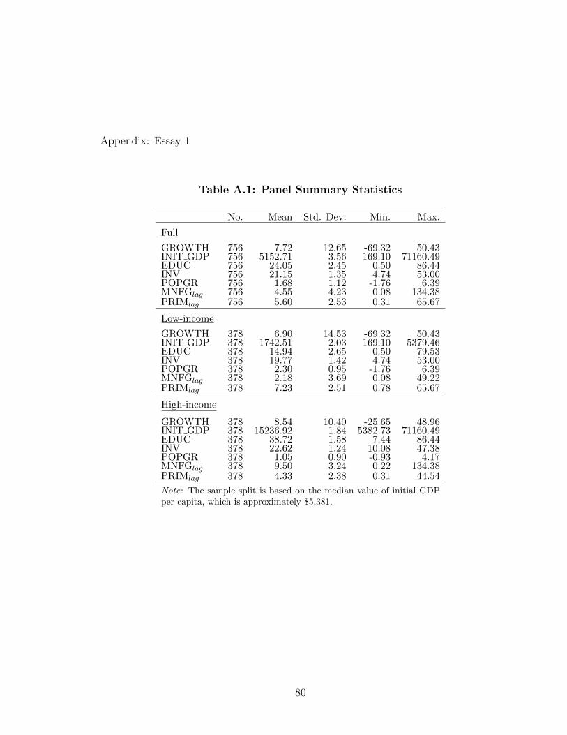
Appendix: Essay 1
Table A.1: Panel Summary Statistics
No. Mean Std. Dev. Min. Max.
Full
GROWTH 756 7.72 12.65 -69.32 50.43INIT GDP 756 5152.71 3.56 169.10 71160.49EDUC 756 24.05 2.45 0.50 86.44INV 756 21.15 1.35 4.74 53.00POPGR 756 1.68 1.12 -1.76 6.39MNFGlag 756 4.55 4.23 0.08 134.38PRIMlag 756 5.60 2.53 0.31 65.67
Low-income
GROWTH 378 6.90 14.53 -69.32 50.43INIT GDP 378 1742.51 2.03 169.10 5379.46EDUC 378 14.94 2.65 0.50 79.53INV 378 19.77 1.42 4.74 53.00POPGR 378 2.30 0.95 -1.76 6.39MNFGlag 378 2.18 3.69 0.08 49.22PRIMlag 378 7.23 2.51 0.78 65.67
High-income
GROWTH 378 8.54 10.40 -25.65 48.96INIT GDP 378 15236.92 1.84 5382.73 71160.49EDUC 378 38.72 1.58 7.44 86.44INV 378 22.62 1.24 10.08 47.38POPGR 378 1.05 0.90 -0.93 4.17MNFGlag 378 9.50 3.24 0.22 134.38PRIMlag 378 4.33 2.38 0.31 44.54
Note: The sample split is based on the median value of initial GDPper capita, which is approximately $5,381.
80

Table A.2: Cross-section Summary Statistics
No. Mean Std. Dev. Min. Max.
Full
GROWTH 86 66.82 50.27 -52.36 211.53INIT GDP70 86 3547.20 3.07 351.41 25963.03EDUC70 86 12.42 2.99 0.50 73.42INV7079 86 21.44 1.41 7.25 40.33POPGR7079 86 1.93 1.09 -0.36 4.88MNFG7079 86 2.96 3.93 0.09 61.64PRIM7079 86 6.66 2.53 0.52 32.09
Low-income
GROWTH 43 58.44 58.53 -52.36 211.53INIT GDP70 43 1335.51 1.65 351.41 3018.41EDUC70 43 6.65 3.01 0.50 49.99INV7079 43 18.67 1.48 7.25 35.35POPGR7079 43 2.52 0.94 -0.36 4.88MNFG7079 43 1.43 3.10 0.09 16.54PRIM7079 43 8.46 2.42 1.36 32.09
High-income
GROWTH 43 75.20 39.31 -51.55 193.99INIT GDP70 43 9421.65 1.80 3064.73 25963.03EDUC70 43 23.20 1.90 5.48 73.42INV7079 43 24.63 1.23 16.64 40.33POPGR7079 43 1.34 0.90 0.05 3.10MNFG7079 43 6.15 3.29 0.25 61.64PRIM7079 43 5.24 2.51 0.52 30.18
Note: The sample split is based on the median value of initial GDPper capita, which is approximately $3, 041.
81

Table A.3: Variable Definitions
Variable Definition
GROWTH Growth of GDP per capita, calculated as the log difference between thebeginning (1970) and end of the period (2009)a
INIT GDP70 1970 GDP per capita (PPP, 2005 international $)a
EDUC70 Percentage of secondary schooling attained in 1970 by the populationaged 15 years and olderb
INV7079 Investment as a share of GDP, averaged over the period 1970-79; consistsof outlays on additions to the fixed assets of the economy plus netchanges in the level of inventories
POPGR7079 Average annual population growth rate over the period 1970-79
MNFG7079 Manufacturing exports as a share of GDP, averaged over the period1970-79; Manufactures comprise commodities in SITC sections 5 (chemicals),6 (basic manufactures), 7 (machinery and transport equipment), and 8(miscellaneous manufactured goods), excluding division 68 (non-ferrousmetals)
PRIM7079 Agricultural and food exports as a share of GDP, averaged over the period1970-79; agricultural exports comprise SITC section 2 (crude materialsexcept fuels) excluding divisions 22, 27 (crude fertilizers and mineralsexcluding coal, petroleum, and precious stones), and 28 metalliferous oresand scrap); Food exports comprise the commodities in SITC sections 0 (foodand live animals), 1 (beverages and tobacco), and 4 (animal and vegetableoils and fats) and SITC division 22 (oil seeds, oil nuts, and oil kernels)
TOT EXP7079 Total merchandise exports, as a percentage of GDP, averaged over theperiod 1970-79
Note: All explanatory variables are in logs. Data are from the World Development Indicators2010 Database, with the exception of:a Data are from Penn World Tables, version 7.0 Heston et al. (2011).b Data are from Barro & Lee (2010).
82

Table A.4: Disaggregated Exports - Countries (by Terminal Node)
1L 1R
Afghanistan Mauritania Argentina IsraelBangladesh Mexico Australia ItalyBenin Morocco Austria JapanBurundi Nepal Barbados JordanCameroon Nicaragua Bolivia Korea, Rep. ofCentral African Republic Niger Brazil MalaysiaCongo, Republic of Pakistan Cambodia MaltaCosta Rica Papua New Guinea Canada MauritiusCote d’Ivoire Portugal Chile NetherlandsEgypt Senegal Colombia New ZealandEl Salvador Spain Cuba NorwayGambia, The Sudan Denmark ParaguayGuatemala Syria Dom. Republic PeruHonduras Thailand Fiji PhilippinesIndia Togo Finland SingaporeJamaica Tunisia France South AfricaKenya Turkey Germany Sri LankaMalawi Uganda Ghana SwedenMali Zambia Greece Switzerland
Guyana TongaHong Kong Trinidad & TobagoHungary United KingdomIceland United StatesIreland Uruguay
Table A.5: Regression Tree Summary Statistics
No. Mean Std. Dev. Min. Max.
Full
GROWTH 86 66.82 50.27 -52.36 211.53INIT GDP70 86 3547.20 3.07 351.41 25963.03EDUC70 86 12.42 2.99 0.50 73.42INV7079 86 21.44 1.41 7.25 40.33POPGR7079 86 1.93 1.09 -0.36 4.88MNFG7079 86 2.96 3.93 0.09 61.64PRIM7079 86 6.66 2.53 0.52 31.09
1L
GROWTH 38 43.21 50.32 -52.36 159.85INIT GDP70 38 1635.41 2.29 351.41 11980.73EDUC70 38 4.55 2.24 0.50 12.37INV7079 38 18.20 1.45 7.25 29.40POPGR7079 38 2.65 0.77 0.74 4.88MNFG7079 38 1.77 3.00 0.10 13.70PRIM7079 38 7.33 2.36 1.36 32.09
1R
GROWTH 48 85.51 42.07 27.75 211.53INIT GDP70 48 6547.75 2.54 938.89 25963.03EDUC70 48 27.53 1.56 12.40 73.42INV7079 48 24.42 1.29 9.68 40.33POPGR7079 48 1.35 0.96 -0.36 3.74MNFG7079 48 4.45 4.19 0.09 61.64PRIM7079 48 6.17 2.67 0.52 30.78
Note: The sample split is chosen by the regression tree technique tobe approximately the average percent of the population with somesecondary education, or 12.37%.
83

Figure A.1: Full Regression Tree (No pruning)
84
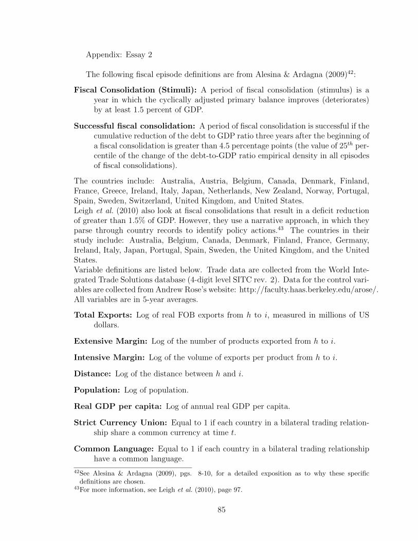
Appendix: Essay 2
The following fiscal episode definitions are from Alesina & Ardagna (2009)42:
Fiscal Consolidation (Stimuli): A period of fiscal consolidation (stimulus) is ayear in which the cyclically adjusted primary balance improves (deteriorates)by at least 1.5 percent of GDP.
Successful fiscal consolidation: A period of fiscal consolidation is successful if thecumulative reduction of the debt to GDP ratio three years after the beginning ofa fiscal consolidation is greater than 4.5 percentage points (the value of 25th per-centile of the change of the debt-to-GDP ratio empirical density in all episodesof fiscal consolidations).
The countries include: Australia, Austria, Belgium, Canada, Denmark, Finland,France, Greece, Ireland, Italy, Japan, Netherlands, New Zealand, Norway, Portugal,Spain, Sweden, Switzerland, United Kingdom, and United States.Leigh et al. (2010) also look at fiscal consolidations that result in a deficit reductionof greater than 1.5% of GDP. However, they use a narrative approach, in which theyparse through country records to identify policy actions.43 The countries in theirstudy include: Australia, Belgium, Canada, Denmark, Finland, France, Germany,Ireland, Italy, Japan, Portugal, Spain, Sweden, the United Kingdom, and the UnitedStates.Variable definitions are listed below. Trade data are collected from the World Inte-grated Trade Solutions database (4-digit level SITC rev. 2). Data for the control vari-ables are collected from Andrew Rose’s website: http://faculty.haas.berkeley.edu/arose/.All variables are in 5-year averages.
Total Exports: Log of real FOB exports from h to i, measured in millions of USdollars.
Extensive Margin: Log of the number of products exported from h to i.
Intensive Margin: Log of the volume of exports per product from h to i.
Distance: Log of the distance between h and i.
Population: Log of population.
Real GDP per capita: Log of annual real GDP per capita.
Strict Currency Union: Equal to 1 if each country in a bilateral trading relation-ship share a common currency at time t.
Common Language: Equal to 1 if each country in a bilateral trading relationshiphave a common language.
42See Alesina & Ardagna (2009), pgs. 8-10, for a detailed exposition as to why these specificdefinitions are chosen.
43For more information, see Leigh et al. (2010), page 97.
85

Regional Trade Agreement: Equal to 1 if each country in a bilateral trading re-lationship have a RTA at time t.
Common Border: Equal to 1 if each country in a bilateral trading relationshipshare a border.
No. of Islands: Equal to the number of islands in a country-pair (maximum valueof 2).
Log Product of Land Area: Log of the product of the land area of h and i.
Colony: Equal to 1 if each country in a bilateral trading relationship were ever in acolonial relationship.
86

Table B.1: Summary Statistics
Variable Obs Mean Std.Dev. Min Max
Extensive Margin 14,441 360.39 2.03 6.00 1478.00Intensive Margin 14,441 16.02 4.42 0.10 1947.83Total Exports 14,441 5,775.10 7.63 1.40 1,433,600.97Exp. Fis. Stim.t 14,441 0.11 0.31 0.00 1.00Exp. Fis. Cons.t 14,441 0.13 0.34 0.00 1.00Exp. Fis. Stim.t+1 14,441 0.09 0.28 0.00 1.00Exp. Fis. Cons.t+1 14,441 0.10 0.30 0.00 1.00Exp. Fis. Stim.t+2 14,441 0.09 0.28 0.00 1.00Exp. Fis. Cons.t+2 14,441 0.10 0.30 0.00 1.00Exp. Fis. Stim.t+3 14,441 0.09 0.28 0.00 1.00Exp. Fis. Cons.t+3 14,441 0.10 0.30 0.00 1.00Imp. Fis. Stim.t 14,441 0.11 0.32 0.00 1.00Imp. Fis. Cons.t 14,441 0.13 0.34 0.00 1.00Imp. Fis. Stim.t+1 14,441 0.09 0.28 0.00 1.00Imp. Fis. Cons.t+1 14,441 0.10 0.30 0.00 1.00Imp. Fis. Stim.t+2 14,441 0.09 0.28 0.00 1.00Imp. Fis. Cons.t+2 14,441 0.10 0.30 0.00 1.00Imp. Fis. Stim.t+3 14,441 0.09 0.28 0.00 1.00Imp. Fis. Cons.t+3 14,441 0.10 0.30 0.00 1.00Distance 14,441 2,079.33 3.12 137.23 12,294.42Populationh 14,441 18,402,186.00 3.51 2,820,007.00 309,051,967.00Populationi 14,441 18,349,998.00 3.50 2,820,007.00 309,051,967.00Real GDP per cap.h 14,441 12,360.57 160.36 2,372.72 44,212.03Real GDP per cap.i 14,441 12,357.09 160.41 2,372.72 44,212.03Strict Currency Union 14,441 0.09 0.29 0.00 1.00Common Language 14,441 0.14 0.35 0.00 1.00Reg. Trade Agreement 14,441 0.39 0.49 0.00 1.00Common Border 14,441 0.08 0.27 0.00 1.00Number of Islands 14,441 0.31 0.50 0.00 2.00Log Prod. of Land Area 14,441 25.50 2.23 20.96 32.20Colony 14,441 0.04 0.20 0.00 1.00
87

Table B.2: Summary Statistics for IMF data
Variable Obs Mean Std.Dev. Min Max
Extensive Margin 5,965 480.47 1.56 36.00 1,478.00Intensive Margin 5,965 27.77 4.06 0.23 1,947.83Total Exports 5,965 13,341.32 5.74 13.25 1,433,600.97Exp. Cons.t 5,965 0.07 0.26 0.00 1.00Exp. Cons.t+1 5,965 0.04 0.21 0.00 1.00Exp. Cons.t+2 5,965 0.04 0.20 0.00 1.00Exp. Cons.t+3 5,965 0.04 0.20 0.00 1.00Imp. Cons.t 5,965 0.07 0.26 0.00 1.00Imp. Cons.t+1 5,965 0.04 0.20 0.00 1.00Imp. Cons.t+2 5,965 0.04 0.20 0.00 1.00Imp. Cons.t+3 5,965 0.04 0.20 0.00 1.00Distance 5,965 2,085.46 2.86 214.97 10,032.20Populationh 5,965 26,228,836.68 3.53 3,400,999.78 309,051,967.40Populationi 5,965 26,169,103.05 3.52 3,400,999.78 309,051,967.40Real GDP per cap.h 5,965 138.97 1.50 23.95 288.70Real GDP per cap.i 5,965 138.74 1.51 23.95 288.70Strict Currency Union 5,965 0.11 0.32 0.00 1.00Common Language 5,965 0.18 0.39 0.00 1.00Reg. Trade Agreement 5,965 0.42 0.49 0.00 1.00Common Border 5,965 0.09 0.29 0.00 1.00Number of Islands 5,965 0.28 0.47 0.00 2.00Log Prod. of Land Area 5,965 26.14 2.33 21.00 32.20Colony 5,965 0.04 0.20 0.00 1.00
Table B.3: Conditional Effects of Fiscal Episodes on Total Exports
t t+1 t+2 t+3 Total
Exp. Cons. <0.001 0.041*** 0.025** -0.004 0.062*(0.010) (0.011) (0.011) (0.011) (0.037)
Exp. Stim. -0.076*** -0.052*** -0.054*** -0.056*** -0.238***(0.012) (0.012) (0.013) (0.012) (0.044)
Imp. Cons. -0.026** -0.014 -0.016 -0.016 -0.072*(0.012) (0.013) (0.012) (0.012) (0.043)
Imp. Stim. -0.029** -0.019 -0.016 -0.005 -0.070(0.014) (0.014) (0.014) (0.013) (0.050)
R2 0.919Observations 14,441Year Effects YesExp. and Imp. Effects NoCountry-pair Effects Yes
Note: These are the estimated marginal effects when the indicated fiscal episode occurs inperiod t. The results are from a single regression, but are presented in multiple columns forreadability. In addition, the control variables from Table 3.2 are included in the regression,but the coefficient estimates are omitted here for space considerations. Robust standard er-rors are in parentheses. Significance is denoted as follows: *** p<0.01, ** p<0.05, * p<0.1
88

Table B.4: Marginal Effects of Fiscal Episodes Occurring Simultaneouslyin Each Country (Total Exports)
t t+1 t+2 t+3 Total
Exp. and Imp. Cons. -0.025 0.027 0.009 -0.020 -0.009(0.016) (0.018) (0.018) (0.017) (0.061)
Exp. and Imp. Stim. -0.105*** -0.071*** -0.070*** -0.061*** -0.308***(0.018) (0.019) (0.019) (0.018) (0.067)
Exp. Cons. and Imp. Stim. -0.029 0.022 0.008 -0.009 -0.008(0.018) (0.018) (0.018) (0.017) (0.063)
Exp. Stim. and Imp. Cons. -0.102*** -0.067*** -0.069*** -0.072*** -0.310***(0.017) (0.018) (0.017) (0.017) (0.061)
Note: Robust standard errors are in parentheses. Significance is denoted as follows: *** p<0.01,** p<0.05, * p<0.1
Table B.5: Conditional Effects of Fiscal Episodes on the ExtensiveMargin
t t+1 t+2 t+3 Total
Exp. Cons. 0.011* 0.049*** 0.052*** 0.035*** 0.147***(0.006) (0.005) (0.006) (0.005) (0.018)
Exp. Stim. -0.045*** -0.041*** -0.025*** -0.022*** -0.134***(0.006) (0.006) (0.005) (0.006) (0.021)
Imp. Cons. 0.004 0.008 0.007 0.008 0.027(0.006) (0.007) (0.007) (0.007) (0.023)
Imp. Stim. -0.010 -0.004 -0.001 0.002 -0.012(0.007) (0.007) (0.007) (0.007) (0.025)
R2 0.833Observations 14,441Year Effects YesExp. and Imp. Effects NoCountry-pair Effects Yes
Note: These are the estimated marginal effects when the indicated fiscal episode occurs inperiod t. The results are from a single regression, but are presented in multiple columns forreadability. In addition, the control variables from Table 3.2 are included in the regression,but the coefficient estimates are omitted here for space considerations. Robust standard er-rors are in parentheses. Significance is denoted as follows: *** p<0.01, ** p<0.05, * p<0.1
89

Table B.6: Marginal Effects of Fiscal Episodes Occurring Simultaneouslyin Each Country (Extensive Margin)
t t+1 t+2 t+3 Total
Exp. and Imp. Cons. 0.015* 0.057*** 0.059*** 0.043*** 0.174***(0.008) (0.009) (0.010) (0.009) (0.032)
Exp. and Imp. Stim. -0.055*** -0.045*** -0.025*** -0.020** -0.146***(0.010) (0.009) (0.009) (0.010) (0.034)
Exp. Cons. and Imp. Stim. 0.001 0.045*** 0.051*** 0.038*** 0.135***(0.009) (0.009) (0.009) (0.009) (0.031)
Exp. Stim. and Imp. Cons. -0.041*** -0.033*** -0.018* -0.015 -0.107***(0.009) (0.009) (0.009) (0.010) (0.034)
Note: Robust standard errors are in parentheses. Significance is denoted as follows: *** p<0.01,** p<0.05, * p<0.1
Table B.7: Conditional Effects of Fiscal Episodes on the IntensiveMargin
t t+1 t+2 t+3 Total
Exp. Cons. -0.011 -0.008 -0.027** -0.039*** -0.085**(0.010) (0.011) (0.010) (0.010) (0.036)
Exp. Stim. -0.030*** -0.011 -0.029** -0.033*** -0.099**(0.011) (0.011) (0.011) (0.011) (0.041)
Imp. Cons. -0.030*** -0.023* -0.022** -0.024** -0.104***(0.011) (0.012) (0.011) (0.011) (0.039)
Imp. Stim. -0.019 -0.015 -0.016 -0.008 -0.058(0.013) (0.013) (0.013) (0.013) (0.048)
R2 0.881Observations 14,441Year Effects YesExp. and Imp. Effects NoCountry-pair Effects Yes
Note: These are the estimated marginal effects when the indicated fiscal episode oc-curs in period t. The results are from a single regression, but are presented in multiplecolumns for readability. In addition, the control variables from Table 3.2 are includedin the regression, but the coefficient estimates are omitted here for space considera-tions. Robust standard errors are in parentheses. Significance is denoted as follows:*** p<0.01, ** p<0.05, * p<0.1
90

Table B.8: Marginal Effects of Fiscal Episodes OccurringSimultaneously in Each Country (Intensive Margin)
t t+1 t+2 t+3 Total
Exp. and Imp. Cons. -0.041*** -0.030* -0.050*** -0.063*** -0.184***(0.015) (0.017) (0.016) (0.016) (0.057)
Exp. and Imp. Stim. -0.049*** -0.026 -0.045*** -0.041** -0.162**(0.018) (0.019) (0.017) (0.017) (0.064)
Exp. Cons. and Imp. Stim. -0.030* -0.023 -0.043** -0.047*** -0.143**(0.017) (0.017) (0.017) (0.017) (0.061)
Exp. Stim. and Imp. Cons. -0.060*** -0.034** -0.052*** -0.057*** -0.203***(0.017) (0.017) (0.016) (0.015) (0.057)
Note: Robust standard errors are in parentheses. Significance is denoted as follows: *** p<0.01,** p<0.05, * p<0.1
91

Table B.9: Conditional Effects of Successful Fiscal Consolidation
t t+1 t+2 t+3 Total
Total Exports:
Exp. Cons. 0.012 0.069*** 0.060*** -0.010 0.131*(0.023) (0.021) (0.021) (0.019) (0.074)
Imp. Cons. -0.001 0.006 -0.009 -0.033 -0.037(0.020) (0.021) (0.021) (0.020) (0.071)
Exp. and Imp. Cons. 0.011 0.075** 0.052 -0.043 0.095(0.031) (0.032) (0.032) (0.030) (0.110)
Extensive Margin:
Exp. Cons. 0.029*** 0.037*** 0.069*** -0.002 0.133***(0.009) (0.008) (0.011) (0.009) (0.031)
Imp. Cons. 0.007 0.005 <0.001 -0.003 0.009(0.011) (0.011) (0.012) (0.012) (0.040)
Exp. and Imp. Cons. 0.036** 0.043*** 0.069*** -0.005 0.142***(0.015) (0.015) (0.017) (0.016) (0.054)
Intensive Margin:
Exp. Cons. -0.017 0.032* -0.009 -0.008 -0.002(0.020) (0.018) (0.019) (0.018) (0.064)
Imp. Cons. -0.008 0.001 -0.009 -0.030* -0.046(0.018) (0.019) (0.018) (0.017) (0.064)
Exp. and Imp. Cons. -0.025 0.032 -0.017 -0.038 -0.048(0.027) (0.028) (0.029) (0.026) (0.096)
Observations 14,441Year Effects YesExp. and Imp. Effects NoCountry-pair Effects Yes
Note: Separate regressions are run for Total Exports, the Extensive Margin, and the In-tensive Margin, in which dummy variables are included for exporter and importer consol-idations in t through t + 3. These are the estimated marginal effects when the indicatedfiscal episode occurs in period t. In addition, the control variables from Table 3.2 areincluded in the regression, but the coefficient estimates are omitted here for space consid-erations. Robust standard errors are in parentheses. Significance is denoted as follows:*** p<0.01, ** p<0.05, * p<0.1
92

Table B.10: Conditional Effects of Fiscal Consolidation (IMFDefinition)
t t+1 t+2 t+3 Total
Total Exports:
Exp. Cons. 0.057* 0.096*** 0.037* -0.013 0.177*(0.031) (0.033) (0.020) (0.020) (0.093)
Imp. Cons. 0.007 -0.035 -0.017 -0.022 -0.067(0.029) (0.024) (0.021) (0.021) (0.082)
Exp. and Imp. Cons. 0.064 0.060 0.020 -0.035 0.109(0.043) (0.039) (0.029) (0.030) (0.120)
Extensive Margin:
Exp. Cons. 0.006 0.047** 0.026** -0.013 0.065(0.017) (0.024) (0.012) (0.010) (0.060)
Imp. Cons. 0.004 0.001 -0.001 -0.003 0.001(0.013) (0.012) (0.011) (0.011) (0.040)
Exp. and Imp. Cons. 0.010 0.048* 0.024 -0.016 0.066(0.022) (0.028) (0.018) (0.016) (0.075)
Intensive Margin:
Exp. Cons. 0.051* 0.049** 0.011 <0.001 0.111(0.027) (0.020) (0.016) (0.016) (0.069)
Imp. Cons. 0.003 -0.037* -0.016 -0.019 -0.069(0.025) (0.021) (0.016) (0.017) (0.065)
Exp. and Imp. Cons. 0.054 0.012 -0.004 -0.019 0.042(0.040) (0.029) (0.023) (0.024) (0.097)
Observations 5,965Year Effects YesExp. and Imp. Effects NoCountry-pair Effects Yes
Note: Separate regressions are run for Total Exports, the Extensive Margin, andthe Intensive Margin, in which dummy variables are included for exporter and im-porter consolidations in t through t + 3. These are the estimated marginal effectswhen the indicated fiscal episode occurs in period t. In addition, the control vari-ables from Table 3.2 are included in the regression, but the coefficient estimates areomitted here for space considerations. Robust standard errors are in parentheses.Significance is denoted as follows: *** p<0.01, ** p<0.05, * p<0.1
93

Appendix: Essay 3
Variable Definitions are listed below. All variables are in logs, with the exception ofthe GDP per capita growth rates, the real interest rate, and the volatility measures.All data are collected from the World Bank’s 2010 World Development Indicatorsdatabase, with the exception of the education variable, which is collected from Barro& Lee (2010). In the cross-section context, variables are averaged over the period1990-1999. In the panel context, variables are averaged over 5-year time periods.
Total Exports: Total exports of goods and services, as a percentage of GDP.
Manufacturing Exports: Manufacturing exports as a share of GDP; Manufacturescomprise commodities in SITC sections 5 (chemicals), 6 (basic manufactures),7 (machinery and transport equipment), and 8 (miscellaneous manufacturedgoods), excluding division 68 (non-ferrous metals).
Primary Exports: Agricultural and food exports as a share of GDP; agriculturalexports comprise SITC section 2 (crude materials except fuels) excluding di-visions 22, 27 (crude fertilizers and minerals excluding coal, petroleum, andprecious stones), and 28 metalliferous ores and scrap); Food exports comprisethe commodities in SITC sections 0 (food and live animals), 1 (beverages andtobacco), and 4 (animal and vegetable oils and fats) and SITC division 22 (oilseeds, oil nuts, and oil kernels).
Annual Average GDP per capita growth rate: Growth rate of GDP per capita,calculated as an annual average rate.
Working-age population growth rate: Annual average growth rate of the working-age (15-64) population.
Investment: Investment as a share of GDP; consists of outlays on additions to thefixed assets of the economy plus net changes in the level of inventories.
Education: Percentage of the population (aged 15 years and older) with some sec-ondary schooling
Tariff Rate: Weighted mean applied tariff is the average of effectively applied ratesweighted by the product import shares corresponding to each partner country.
REER Index Volatility: The real effective exchange rate index is the nominal ef-fective exchange rate divided by an index of costs (2005=100).
Government Debt: Debt data refer to gross central (as opposed as to general)government debt, as in Jaimovich & Panizza (2010).
Government Consumption: General government final consumption expenditure(formerly general government consumption) includes all government currentexpenditures for purchases of goods and services (including compensation of
94

employees). It also includes most expenditures on national defense and security,but excludes government military expenditures that are part of governmentcapital formation.
Real Interest Rate: Real interest rate is the lending interest rate adjusted for in-flation as measured by the GDP deflator.
M2: Money and quasi money comprise the sum of currency outside banks, demanddeposits other than those of the central government, and the time, savings, andforeign currency deposits of resident sectors other than the central government.
Inflation: Inflation as measured by the annual growth rate of the GDP implicitdeflator shows the rate of price change in the economy as a whole. The GDPimplicit deflator is the ratio of GDP in current local currency to GDP in constantlocal currency.
Inflation Volatility: The standard deviation of the inflation rate.
95

Table C.1: Summary Statistics for Baseline Sample (Cross-section)
Variable # of Co. Mean Std. Dev. Min Max
Total Exports 68 35.971 1.672 10.642 133.598
Manufacturing Exports 68 9.938 2.901 0.763 66.912
Primary Exports 68 3.825 3.132 0.116 39.872
Ann. Avg. GDP per cap. growth 68 1.255 2.880 -10.913 9.447
Working-age pop. growth 68 1.608 1.207 -0.495 3.522
Investment 68 21.496 1.259 11.307 39.054
Education 68 34.109 1.641 5.620 70.418
Tariff Rate 68 7.579 1.979 1.890 41.600
REER Index Volatility 68 10.644 8.308 1.677 34.919
Table C.2: Summary Statistics for Baseline Sample (Panel)
Variable # of Co. Obs Mean Std. Dev. Min Max
Total Exports 75 219 37.358 1.771 9.663 223.311
Manufacturing Exports 74 215 10.957 3.046 0.615 136.430
Primary Exports 74 215 3.423 3.148 0.077 45.468
Ann. Avg. GDP per cap. growth 75 219 1.926 2.674 -5.767 11.920
Working-age pop. growth 75 219 1.501 1.305 -2.252 5.494
Investment 75 219 21.238 1.282 7.821 32.283
Education 75 219 37.362 1.609 5.600 77.800
Tariff Rate 75 219 7.060 1.964 1.000 54.754
REER Index Volatility 75 219 7.617 9.878 0.458 117.820
96

Table C.3: Cross-Section Full Country List
Algeria Gabon Papua New GuineaAustralia Germany ParaguayAustria Ghana PhilippinesBahrain Greece PolandBelgium Guyana PortugalBelize Hungary RomaniaBolivia Iceland RussiaBulgaria Ireland Saudi ArabiaCameroon Israel SlovakiaCanada Italy South AfricaCentral African Republic Japan SpainChile Luxembourg SwedenChina Malawi SwitzerlandColombia Malaysia Trinidad and TobagoCosta Rica Malta TunisiaCote d’Ivoire Mexico UgandaCyprus Moldova UkraineCzech Republic Morocco United KingdomDenmark Netherlands United StatesDominican Republic New Zealand UruguayEcuador Nicaragua VenezuelaFinland Norway ZambiaFrance Pakistan
Table C.4: Summary Statistics from Complete Results (Cross-section)
Variable # of Co. Mean Std. Dev. Min Max
Total Exp. 48 36.296 1.657 10.642 100.843
Manufacturing Exports 48 8.148 3.007 0.763 64.397
Primary Exports 48 4.291 3.430 0.116 39.872
Ann. Avg. GDP per cap. growth 48 0.993 3.235 -10.913 9.447
Working-age pop. growth 48 1.787 1.176 -0.495 3.522
Investment 48 21.839 1.282 11.307 39.054
Education 48 33.105 1.676 5.620 68.153
Tariff Rate 48 8.108 1.961 1.890 31.375
REER Index Volatility 48 11.643 8.182 1.677 34.919
Government Debt 48 52.079 2.174 11.073 446.416
Real Interest Rate 48 8.187 10.604 -19.161 40.327
M2 48 39.673 1.950 10.451 205.098
Inflation 48 10.433 5.614 0.154 972.202
Inflation Volatility 48 97.256 333.926 0.491 2,005.591
Government Consumption 48 15.975 1.334 9.208 28.284
97

Table C.5: Summary Statistics from Complete Results (Panel)
Variable # of Co. Obs Mean Std. Dev. Min Max
Total Exports 61 141 36.837 1.738 9.663 223.311
Manufacturing Exports 61 140 9.744 3.168 0.615 136.430
Primary Exports 61 140 3.532 3.209 0.077 45.468
Ann. Avg. GDP per cap. growth 61 141 1.824 2.727 -5.767 11.244
Working-age pop. growth 61 141 1.618 1.225 -1.195 4.562
Investment 61 141 21.484 1.280 8.543 39.283
Education 61 141 37.559 1.640 5.600 77.800
Tariff Rate 61 141 7.064 1.963 1.022 46.440
REER Index Volatility 61 141 7.736 6.279 1.182 37.462
Government Debt 61 141 47.924 1.979 8.820 286.092
Real Interest Rate 61 141 7.646 8.655 -26.753 45.081
M2 61 141 46.894 1.92 8.187 190.124
Inflation 61 141 6.402 3.019 0.340 236.169
Inflation Volatility 61 141 9.958 38.415 0.068 421.256
Government Consumption 61 141 16.151 1.361 7.215 37.743
Table C.6: Summary Statistics from High-Manufacturing-Exports Countries(Cross-section)
Variable # of Co. Mean Std. Dev. Min Max
Total Exports 26 46.785 1.551 24.498 133.598
Manufacturing Exports 26 28.258 1.492 16.452 66.912
Primary Exports 26 3.221 1.983 1.054 11.633
Initial GDP 26 7,025.959 3.462 391.653 33,470.844
Ann. Avg. GDP per cap. growth 26 1.586 3.163 -8.984 9.447
Working-age pop. growth 26 0.984 1.136 -0.495 3.366
Investment 26 23.276 1.221 16.230 39.054
Education 26 44.719 1.289 22.306 70.418
Tariff Rate 26 5.385 1.706 3.378 26.230
Exchange Rate Volatility 26 9.015 7.134 1.677 30.250
Government Debt 25 43.300 2.352 2.840 124.760
Government Consumption 26 18.217 1.326 10.132 28.284
Real Interest Rate 25 4.503 5.297 -17.312 8.599
M2 18 49.540 1.818 13.073 122.589
Inflation 26 7.294 4.788 1.644 670.092
Inflation Volatility 26 60.420 219.397 0.557 1,096.949
98

Table C.7: Summary Statistics from Low-Manufacturing-Exports Countries(Cross-section)
Variable # of Co. Mean Std. Dev. Min Max
Total Exports 42 30.569 1.639 10.642 98.032
Manufacturing Exports 42 5.204 2.219 0.763 16.407
Primary Exports 42 4.254 3.845 0.116 39.872
Initial GDP 42 2,728.870 4.632 132.506 33,595.251
Ann. Avg. GDP per cap. growth 42 1.586 3.163 -8.984 9.447
Working-age pop. growth 42 0.984 1.136 -0.495 3.366
Investment 42 20.464 1.267 11.307 4.441
Education 42 28.844 1.708 5.620 68.153
Tariff Rate 42 9.366 1.981 1.890 41.600
Exchange Rate Volatility 42 9.015 7.134 1.677 30.250
Government Debt 40 58.338 2.086 15.220 446.416
Government Consumption 42 5.002 1.358 5.022 27.257
Real Interest Rate 39 10.038 10.796 -19.161 40.327
M2 37 33.510 1.895 10.451 205.098
Inflation 42 9.108 5.069 0.154 972.202
Inflation Volatility 42 77.859 318.138 0.491 2,005.591
Table C.8: Summary Statistics from High-Manufacturing-Exports Countries(Panel)
Variable # of Co. Mean Std. Dev. Min Max
Total Exports 112 46.961 1.684 15.650 223.311
Manufacturing Exports 112 26.615 1.681 12.818 136.430
Primary Exports 112 3.321 2.204 0.156 45.468
Initial GDP per capita 112 7,694.476 3.344 277.273 46,457.816
Ann. Avg. GDP per cap. growth 112 2.365 2.742 -5.196 11.244
Working-age pop. growth 112 1.012 1.181 -2.252 4.042
Investment 112 22.807 1.218 13.910 39.283
Education 112 44.936 1.335 18.400 77.800
Tariff Rate 112 5.484 1.790 1.000 31.130
Exchange Rate Volatility 112 5.904 5.335 0.458 43.390
Government Debt 101 45.563 2.126 1.940 286.092
Government Consumption 112 17.501 1.368 5.964 37.743
Real Interest Rate 103 5.364 4.297 -20.317 17.962
M2 81 60.839 1.881 11.814 605.675
Inflation 110 4.423 3.174 0.340 236.169
Inflation Volatility 112 60.420 219.397 0.557 1,096.949
99

Summary Statistics from Low-Manufacturing-Exports Countries (Panel)
Variable # of Co. Mean Std. Dev. Min Max
Total Exports 102 28.279 1.636 9.663 85.512
Manufacturing Exports 102 4.158 2.037 0.615 12.616
Primary Exports 102 3.586 4.230 0.077 31.468
Initial GDP 102 2,743.717 4.992 111.237 37,472.777
Ann. Avg. GDP per cap. growth 102 1.406 2.491 -5.767 11.920
Working-age pop. growth 102 2.040 1.234 -1.195 5.494
Investment 102 19.870 1.307 7.821 34.648
Education 102 30.673 1.740 5.600 75.000
Tariff Rate 102 9.370 1.949 1.870 54.754
Exchange Rate Volatility 102 8.559 7.358 0.614 37.462
Government Debt 92 54.632 2.018 9.020 204.649
Government Consumption 102 14.707 1.351 7.215 28.871
Real Interest Rate 93 10.040 11.040 -26.753 47.696
M2 97 36.906 1.942 8.187 220.074
Inflation 99 7.217 3.037 0.237 114.729
Inflation Volatility 102 7.173 8.711 0.370 52.789
100

References
(2005). United Nations Conference on Trade and Development (UNCTAD): Geneva.
Alesina, A. & Ardagna, S. (2009). Large changes in fiscal policy: Taxes versusspending. NBER Working Paper , No. 15438, 1–37.
Amurgo-Pacheco, A. & Pierola, M.D. (2008). Patterns of export diversificationin developing countries. World Bank Policy Research Working Paper 4473 , 1–32.
Armington, P.S. (1969). A theory of demand for products distinguished by placeof production. International Monetary Fund Staff Papers , 16, 159–178.
Azariadis, C. & Drazen, A. (1990). Threshold externalities in economic develop-ment. Quarterly Journal of Economics , 105, 501–526.
Baller, S. (2007). Trade Effects of Regional Standards Liberalization: A Heteroge-neous Firms Approach. SSRN eLibrary .
Barro, R. (1996). Inflation and growth. Review , Federal Reserve Bank of St. Louis,May/June.
Barro, R. & Lee, J.W. (2010). A new data set of educational attainment. NBERWorking Paper No. 15902 .
Barro, R.J. (1991). Economic growth in a cross-section of countries. QuarterlyJournal of Economics , 106, 407–443.
Bernard, A., Jensen, B., Redding, S. & Schott, P. (2007). Firms in inter-national trade. The Journal of Economic Perspectives , 21, 105–130.
Besedes, T. & Prusa, T. (2010). The role of extensive and intensive margins andexport growth. Journal of Development Economics , forthcoming, 1–16.
Bigsten, A., Collier, P., Dercon, S., Fafchamps, M., Gauthier, B., Gun-ning, J.W., Habarurema, J., Isaksson, A., Oduro, A., Oostendorp, R.,Pattillo, C., Soderbom, M., Teal, F. & Zeufack, A. (1999). Exports ofafrican manufactures: macro policy and firm behaviour. The Journal of Interna-tional Trade and Economic Development , 8, 53–71.
Bigsten, A., Collier, P., Dercon, S., Fafchamps, M., Gauthier, B., Gun-ning, J.W., Oduro, A., Oostendorp, R., Pattillo, C., Soderbom, M.,Teal, F. & Zeufack, A. (2004). Do african manufacturing firms learn fromexporting? The Journal of Development Studies , 40, 115–141.
Bleaney, M. (1996). Macroeconomic stability, investment, and growth in developingcountries. Journal of Development Economics , 48, 461–477.
Breiman, L., Friedman, J., Olshen, R. & Stone, C. (1984). Classification andRegression Trees . Wadsworth, Belmont, CA.
101
Bruno, M. & Easterly, W. (1998). Inflation crises and long-run growth. Journalof Monetary Economics , 41, 3–26.
Calderon, C., Chong, A. & Zanforlin, L. (2001). On non-linearities betweenexports of manufactures and economic growth. Journal of Applied Economics , 4,279–311.
Cohen, D. & Soto, M. (2007). Growth and human capital: good data, goodresults. Journal of Economic Growth, 12, 51–76.
Collier, P. & Gunning, J.W. (1999). Why has africa grown slowly? The Journalof Economic Perspectives , 13, 3–22.
Crespo-Cuaresma, J. & Worz, J. (2005). On export composition and growth.Weltwirtschaftliches Archiv , 141, 33–49.
Durlauf, S., Kourtellos, A. & Tan, C.M. (2008). Are any growth theoriesrobust? The Economic Journal , 119, 329–346.
Durlauf, S.N. & Johnson, P.A. (1995). Multiple regimes and cross-countrygrowth behavior. Journal of Applied Econometrics , 10, 365–384.
Edwards, S. (1993). Openness, trade liberalization, and growth in developing coun-tries. Journal of Economic Literature, 31, 1358–1393.
Emery, R.F. (1967). The relation of exports and economic growth. Kyklos , 20,470–486.
Esfahani, H.S. (1991). Exports, imports, and economic growth in semi-industrialized countries. Journal of Development Economics , 35, 93–116.
Feder, G. (1983). On exports and economic growth. Journal of Development Eco-nomics , 12, 59–73.
Felbermayr, G. & Kohler, W. (2006). Exploring the extensive and intensivemargins of world trade. Review of World Economics , 142, 642–674.
Fischer, S. (1991). Growth, macroeconomics, and development. NBER Macroeco-nomics Annual , 6, 329–364.
Fischer, S. (1993). The role of macroeconomic factors in growth. Journal of Mon-etary Economics , 32, 485–512.
Foster, N. (2006). Exports, growth and threshold effects in africa. Journal of De-velopment Studies , 42, 1056–1074.
Fosu, A. (1990). Exports and economic growth: The african case. World Develop-ment , 18, 831–835.
102
Fosu, A. (1996). Primary exports and economic growth in developing countries.World Economy , 19, 465–475.
Greenaway, D. & Sapsford, D. (1994). What does liberalisation do for exportsand growth? Weltwirtschaftliches , 130, 152–174.
Greenaway, D., Morgan, W. & Wright, P. (1999). Exports, export composi-tion and growth. The Journal of International Trade and Economic Development ,8, 41–51.
Grossman, G.M. & Helpman, E. (1991). Innovation and Growth in the GlobalEconomy . Cambridge: The MIT Press.
Hansen, B. (2000). Sample splitting and threshold estimation. Econometrica, 68,575–603.
Hardle, W. (1990). Applied Nonparametric Regression. Cambridge: CambridgeUniversity Press.
Hausmann, R., Pritchett, L. & Rodrik, D. (2005). Growth accelerations. Jour-nal of Economic Growth, 10, 303–329.
Hausmann, R., Hwang, J. & Rodrik, D. (2007). What you export matters.Journal of Economic Growth, 12, 1–25.
Helpman, E., Melitz, M. & Rubinstein, Y. (2008). Estimating trade flows:Trading partners and trading volumes. Quarterly Journal of Economics , 123, 441–487.
Heston, A., Summers, R. & Aten, B. (2011). Penn world table version 7.0.Center for International Comparisons of Production, Income, and Prices at theUniversity of Pennsylvania.
Hummels, D. & Klenow, P.J. (2005). The variety and quality of a nation’s ex-ports. American Economic Review , 95, 704–723.
Jaimovich, D. & Panizza, U. (2010). Public debt around the world: a new datasetof central government debt. Applied Economics Letters , 17, 19–24.
Jarreau, J. & Poncet, S. (2012). Export sophistication and economic growth:Evidence from china. Journal of Development Economics , 97, 281–292.
Kehoe, T.J. & Ruhl, K.J. (2009). How important is the new goods margin ininternational trade? Federal Reserve Bank of Minneapolis , 1–36.
Kohli, I. & Singh, N. (1989). Exports and growth: Critical minimum effort anddiminishing returns. Journal of Development Economics , 30, 391–400.
Krugman, P.R. (1981). Intraindustry specialization and the gains from trade. Jour-nal of Political Economy , 89, 959–973.
103

Leigh, D., Devries, P., Freedman, C., Guajardo, J., Laxton, D. & Pesca-tori, A. (2010). Will It Hurt? Macroeconomic Effects of Fiscal Consolidation.World Economic Outlook: Recovery, Risk, and Rebalancing , 93–124.
Levine, R. & Renelt, D. (1992). A sensitivity analysis of cross-country growthregressions. American Economic Review , 82, 942–963.
Mankiw, G., Romer, D. & Weil, D.N. (1992). A contribution to the empiricsof economic growth. Quarterly Journal of Economics , 107, 407–437.
Melitz, M. (2003). The impact of trade on intra-industry reallocations and aggre-grate industry productivity. Econometrica, 71, 1695–1725.
Michaely, M. (1977). Exports and growth. Journal of Development Economics , 4,49–53.
Minier, J. (1998). Democracy and growth: Alternative approaches. Journal of Eco-nomic Growth, 3, 241–266.
Minier, J. (2003). Are small stock markets different? Journal of Monetary Eco-nomics , 50, 1593–1602.
Montiel, P. & Serven, L. (2006). Macroeconomic stability in developing coun-tries: How much is enough. World Bank Research Observer , 21, 151–178.
Papageorgiou, C. (2002). Trade as a threshold variable for multiple regimes. Eco-nomics Letters , 77, 85–91.
Peneder, M. (2003). Industrial structure and aggregate growth. Structural Changeand Economic Dynamics , 14, 427–448.
Rangasamy, L. (2009). Exports and economic growth: The case of south africa.Journal of International Development , 21, 603–617.
Rodrik, D. (2008). The real exchange rate and economic growth. Brookings Paperson Economic Activity , 365–412.
Rose, A.K. & Spiegel, M.M. (2011). The Olympic Effect. The Economic Journal ,121, 652–677.
Singer, H.W. (1950). The distribution of gains between investing and borrowingcountries. The American Economic Review , 40, 473–485.
Sirimaneetham, V. & Temple, J.R.W. (2009). Macroeconomic stability and thedistribution of growth rates. The World Bank Economic Review , 23, 443–479.
Solow, R. (1956). A contribution to the theory of economic growth. QuarterlyJournal of Economics , 70, 65–94.
104

Sprout, R.V.A. & Weaver, J.H. (1993). Exports and economic growth in asimultaneous equations model. The Journal of Developing Areas , 27, 281–292.
Syron, R.F. & Walsh, B.M. (1968). The relation of exports and economic growth:A note. Kyklos , 21, 541–545.
Thirlwall, A.P. (2000). Trade, trade liberalisation and economic growth: Theoryand evidence. African Development Bank: Economic Research Papers , 1–30.
Tyler, W.G. (1981). Growth and export expansion in developing countries. Journalof Development Economics , 9, 121–130.
Wood, A. & Mayer, J. (2001). Africa’s export structure in a comparative per-spective. Cambridge Journal of Economics , 25, 427–448.
Xu, Z. (2000). Effects of primary exports on industrial exports and gdp: Empiricalevidence. Review of Development Economics , 4, 307–325.
105

CURRICULUM VITAE
BRANDON J. SHERIDAN
Date and Place of Birth June 18, 1984, Henderson, KY
Education
• M.S. in Economics, University of Kentucky (December 2009)
• B.S. in Economics and Government, Centre College (May 2006)
Professional Experience Instructor of Record, University of Kentucky, 2009-2011
• Introduction to the Economics of Business (MBA), Summer 2011
• Introductory Macroeconomics, University of Kentucky (2 sections), Spring 2011
• Introductory Microeconomics, University of Kentucky (3 sections), Summer-Fall2010
• Economic & Business Statistics, University of Kentucky (3 sections), Summer2009 - Spring 2010
Awards and Honors
• Outstanding Teacher Award for Teaching Assistants, University of Kentucky,2011
• Kentucky Opportunity Fellowship, University of Kentucky, 2011-2012
106