UNIVERSITY OF SHEFFIELD

T HREE D I M E N S I O N A L U L T I M A T E S T R E N G T H A N A L Y S I S

OF B E A M - C O L U M N S

BY

M O H A M E D A . E L - K H E N F A S

B.Sc. (LIBYA) 1974

M-Sc. USC (U.S A-) 1980

T h e s i s s u b m i t t e d

for the

d e g r e e o f D o c t o r o f P h i l o s o p h y

at t h e U n i v e r s i t y o f S h e f f i e l d

S e p t e m b e r 19 87

LIBRARYH

SIll'B

IMAGING SERVICES NORTHBoston Spa, Wetherby

West Yorkshire, LS23 7BQ.

www.bl.uk

BEST COPY AVAILABLE.

VARIABLE PRINT QUALITY

DEDICATED TO MY FAMILY

Summary

A rigorous formulation for the structural response o f thin-

walled members o f arbitrary open cross-section acted upon by a general

system o f loads is developed based on energy principles and v irtua l

work concepts. Full account is taken o f three dimensional behaviour,

including sectoria l warping e f fe c ts . The analysis incorporates the

e f fe c t o f in i t ia l geometrical deflections. Different patterns o f

residual stress, non-coincidence o f the shear centre and centroid, a

complete absence o f symmetry in the section and the influence o f higher

order terms in the strain-displacement relationships including products

o f the derivatives o f axial displacements are also incorporated.

A computer program based on f in i t e element analysis suitable

for application in both the e lastic and inelastic ranges is developed.

This is used to solve the d i f fe r en t ia l equations governing the ultimate

strength o f beam-columns in space.

The program , is written in the Fortran 77 Language. The main

function o f the program is to fo llow the loss o f s t i f fn ess due to

spread o f y ie ld and hence to trace the fu l l load-deflection response up

to collapse. It may be used in a wide variety o f ways.

Three types o f analysis have been conducted in th is study.

These are: Linear, Partial Non-linear and Full Non-linear. The Linear

involves only the small deflection theory. Partia l Non-linear analysis

uses non-linear strains while the Full Non-linear analysis incorporates

both non-linear strains and nonlinear s t i f fn ess matrices. Several

i l lu s t ra t iv e examples, previously investigated either theoretica lly or

experimentally, have been chosen to check the v a l id ity o f both the

- i -

analytical approach and the computer program. These examples cover

flexura l, f lexura l-tors iona l, b iax ia l bending, and bending and

torsional behaviour in the e lastic and inelastic ranges. They contain a

wide range o f parameters e .g . d if fe ren t cross-section shapes, loading,

boundary conditions and in i t ia l imperfections. F inally the program has

been used to study the ultimate strength o f s tee l members subjected to

compression, bending and torsion in a more rigorous fashion than has

previously been possible.

i i

Acknowledgement

The work presented in th is thesis has been supported by

Scholarships made available by University o f Al-Fateh, T r ip o l i , Libya

(S .P .L .A .J ).

The Author would like to express his sincere gratitude to Dr.

D.A. Nethercot for his supervision, valuable guidance, encouragement

and general interest throughout this study. The candidate also wishes

to thank Professor T.H. Hanna (Head o f the Department) and a l l his

academic s ta f f for their support.

The candidate is gratefu l for the f a c i l i t i e s made available

by the Department o f C iv il and Structural Engineering and the Computer

Centre at the University o f Sheffie ld .

F ina lly , the candidate wishes to express his deepest

appreciation to his family for their support, encouragement and

understanding throughout the course o f his work. In particular, the

candidate’ s parents have been a continued source o f financial and moral

support, understanding and patience through his many years o f academic

study.

i i i -

L i s t o f P u b lic a t io n s

1. El-Khenfas, M.A. and Nethercoth, D.A., (1987 0 , "Ultimate Strength

Analysis o f Steel Beam-Columns Subjected to Biaxial Bending and

Torsion", Applied Solid Mechanics -2 Conference, University o f

Strathclyde, Glasgow, U.K., April 7/8.

2. El-Khenfas, M.A., and Nethercot, D.A., (19'8?a>, " A General

Formulation for Three Dimensional Analysis o f Beam-columns",

International Journal o f Mechanical Sciences, (submitted for

publication).

3. El-Khenfas, M.A. and Nethercot, D.A., (1987b), "E lastic Analysis

o f Beam-Columns in Space", International Journal o f Mechanical

Sciences, (submitted for publication).

4. El-Khenfas, M.A. and Nethercot, D.A., (1987c)"Inelastic Analysis

of Beam-Columns in Space", International Journal of Mechanical

Sciences, (submitted for publication).

5. Wang, Y.C., El-Khenfas, M.A., And Nethercot, D. A. (1987),

"La te ra l- Torsional Buckling o f Ren-Restrained Beams", Journal o f

Construction Steel Research, (in press).

6. El-Khenfas, M.A., (1987a), "TDFE-Computer Program for Analysis o f

Beams in Space in the Elastic and Inelastic ranges", Report, No.

1CE, C iv i l and Structural Engineering Department, Sheffie ld

University.

7. El-Khenfas, M.A., (1987b), "E lastic Analysis o f Beam-Columns in

Space", Report, No. 2CE, C iv i l and Structural engineering

department, Sheffie ld University.

8. El-Khenfas, M.A., (1987c), " In e las t ic Analysis o f Beam-Column in

3-Dimensions", Report, No. 3CE, C iv il and Structural Engineering

Department, Sheffie ld University.

— i i i 1

CONTENTS

Page No.Summary iAcknowledgments i i iL is t o f Publications i i i 'Contents ivL is t o f Tables x i iL is t o f Figures xivNotation

CHAPTER 1 General Introduction1.1 Introduction. 11.2 Domain o f the Study 21.3 Outline o f the Thesis 3

CHAPTER 2 Review o f Previous Work2.1 Introduction 62.2 Review o f Previous Work 6

2.2.1 Historical & General 62.2.2 Elastic Behaviour 13

2.2.2.1 Flexural & Lateral-Torsional Buckling 132. 2.2. 2 Biaxial Bending 152.2.2.3 Bending and Torsion 15

2.2.3 Ine lastic Behaviour 172.2.3. 1 Flexural & Lateral-Torsional Buckling 17 2. 2. 3. 2 Biaxial Bending 202. 2. 3.3 Bending and Torsion 21

2.2.4 Experimental Development 212.2.5 F in ite Element Development 22

CHAPTER 3 General Foraulation o f Beaa-Coltnn Analysis in Three Dimensions

3.1 Introduction 343.2 Assumptions 353. 3 Theoretical Analysis 35

3.3.1 Kinematics o f the Cross-Section 363.3.2 Stress-Strain Relationships 383.3.3 Strain-Displacement Relationships 393.3.4 Method o f Analysis 45

3. 3.4.1 Principle o f Virtual Work 453.3.4.2 Total Potential Energy 47

3.4 Imperfections 483.5 Equilibrium Equations 53

3.5.1 Virtual Work . 533.5.2 Potential Energy 58

3.6 Comparison with Previous Formulations 723.7 Conclusions 74

CHAPTER 4 Derivation o f S t iffn e ss Matrices4. TIntroduction 824.2 Interpolation Functions 834.3 S t iffness Matrices 85

4.3.1 Principle o f Virtual Work 864.3.1.1 Linear Tangential S tiffness Matrix 86

— IV

<1.3. 1.2 Linear Geometrical S tiffness Matrix 874.3.1.3 Nonlinear Tangential Stiffness Matrix 884.3.1.4 Nonlinear Geometrical Matrix 89

4.3.2 By Total Potential Energy 914.3.2.1 Linear Tangential S tiffness Matrix 974.3.2.2 Linear Geometrical Stiffness Matrix 974.3.2.3 Nonlinear Tangent S tiffness Matrix 984.3.2.4 Nonlinear Geometrical Stiffness Matrix 984.3.2.5 In i t ia l S tiffness Matrix 984.3.2.6 Assembly 98'

4.4 Transformation Matrix 984.5 Strain Displacement Matrix 100

4.5.1 Linear Strain Matrix 1014.5.2 Nonlinear Strain Matrix 104

4.6 Conclusions 106

CHAPTER 5 A nalytica l Procedure and Computer Program Structure5.1 Introduction 1205.2 F in ite Element Method 120

5.2.1 Number o f Elements 1215.2.2 Number o f Segments in the Cross-Section 1215.2.3 Section and Sectorial Properties 1225.2.4 Internal Forces 127

5.3 Assembly o f S tiffness Matrices 1285.4 Method o f Solution 1305.5 Convergence Criter ia 131

5.5.1 Out o f balance force 1335.5.2 I te ra t iv e Process 134

5.6 Computer Program Description 1355.6.1 Computer Program Structure 136

5.7 Computational Steps 1375.8 Conclusions 142

CHAPTER 6- E lastic Analysis o f Bea»-Columns in Thee-Dimensional6.1 Introduction 1516.2 Analysis 1526.3 Numerical Solutions 154

6.3.1 Linear Bending and Torsion 1546.3.2 Flexural and Flexural Torsional Buckling 1556.3.3 Biaxial Bending 1576.3.4 Nonlinear Bending and Torsion 1586.3.5 Biaxial Bending and Torsion 159

6.4 Conclusions 161

CHAPTER 7 In e la s t ic Analysis o f Be »-Colum n in Space7.1 Introduction 1757.2 Assumptions 1767.3 Numerical Results 177

7.3.1 Column with In i t ia l Deflections 1787.3.2 Flexural and Flexural-Torsional Buckling 1787.3.3 Biaxial Bending 180

7.4 Conclusions 181

CHAPTER 8 Ultimate Strength o f Beams under Bending and Torsion8.1 Introduction 1918.2 Analysis 192

8.3 Numerical Results 1938.3.1 Comparison With Previous Analysis 1948.3.2 Elastic Analysis 196

8.3.2.1 Biaxial Bending and Torsion 1968.3.3 Ine lastic Analysis 198

8.3.3.1 Torsional Moment Applied atMid-Span 198

8.3*3.2 Bending and Torsion 1988. 3.3.3 Non-Uniform Bending Moment and Torsion 2008.3.3.3 Biaxial Bending and Torsion 201

8.4 Examination o f the Failure State o f Membersunder Bending and Torsion 2028.4.1 S ta b i l i ty o f I-Section under Flexural and

Torsional Loading 2058.4.1.1 S tab il i ty o f Beam-Column o f I-Section

under Bending and Torsion Based on Pastor and DeWolf (1979) Suggestions 207

8.4.1.2 S tab il i ty o f Beam-Column o f ThinWalled Section Subjected to Combined Bending and Torsion Based on Author Suggestions 209

8.4.1.3 S tab il i ty o f Beam-Column under Biaxial Bending and Torsion 211

8.5 Prediction o f S tab i l i ty o f Beam-Column under FlexuralBending and Torsion using a Regression Analysis 212

8.6 General Features o f the Analysis 2148.7 Conclusions 215

CHAPTER 9 Conclusions and Further Work9.1 Introduction 2449.2 General Formulation 2449.3 Derivation o f S tiffness Matrices 2459.4 Analysis Type Options 2469.5 Development o f Computer Program (TDCP) 2469.6 Comparison with Previous Work 2469.7 Ultimate Strength Behaviour o f Members under

Bending and Torsion 2479.8 Future Work 248

REFERENCES

APPENDICES

L IS T OF TABLES

TABLE NO. TITLE PAGE

Table 3.1 Comparison Between the Author's Formulation and

Previous Studies 75

Table 3.2 Comparison o f AuthoVs Assumptions against Those

o f Chen & Atsuta (1977), Rajaskaran (1970), and

Rajaskaran & Murray (1973) 76

Table «1.1 Linear Tangential Stiffness Matrix 108

Table 4.2 Linear Geometrical Stiffness Matrix 109

Table 4.3 Non-Linear Tangential Stiffness Matrix 110

Table 4.4 Non-Linear Geometrical Stiffness Matrix 111

Table 4.5 Linear Tangential Stiffness Matrix 112

Table 4.6 Linear Geometrical S tiffness Matrix 113

Table 4.7 Non-Linear Tangential Stiffness Matrix 114

Table 4.8 Non-Linear Geometrical Stiffness Matrix 115

Table 4.9 In i t ia l Geometrical Matrix 116

Table 4.10 Linear strain matrix 117

Table 4.11 Non-Linear strain matrix 118

Table 6.1 Examples Selected for Study 163

Table 6.2 Comparison Between Author's Results and Those

by BSCA (1970) 164

Table 6.3 Comparison o f Calculated Results with Anderson

and Trahair (1972) for S tab il i ty o f Doubly

Symmetric Beams 165

Table 6.4 Comparison o f Author's with Those o f Anderson

and Trahair (1972) for S tab il ity o f

Monosymmetric Beams 166

Table 6.5 Comparison o f Calculated Results with Exact

Solution o f Culver (1966a), for Biaxial

Loading, no In i t ia l Deflection 167

Table 6.6 Comparison o f Calculated Results with Exact

Solution o f Culver (1966a) for Beam-Column

under Biaxial Bending, no In i t ia l Deflection 167

Table 6.7 Comparison o f Calculated Results with Exact

Solution o f Culver (1966b) for Beam-Column

Subjected to Biaxial Bending, In i t ia l

Deflection Included 168

Table 6.8 Comparison o f Calculated Results with Exact

Solution o f Culver (1966b) for Beam-Column

Subjected to Biaxial Bending, In i t ia l Deflection

Included 168

Table 6.9 Comparison o f Author’s Results with Moore

(1986) Analysis and Tests for Beams o f

Z-Sections Subjected to Bending and Torsion 169

Table 7.1 Problems Chosen for Study 181

Table 7.2 Comparison Between Author’s Results and Those

Obtained by Fujita and Yoshida (1972) for

Compressive Column with In i t ia l Deflection 182

Table 7.3 Data for Problems Chosen for Purpose o f

Comparison with Lindner (1981) 183

Table 7.4 Comparison o f Selected Tests and Analysis

Conducted by Lindner (1981) Against Those

Obtained by Author 184

Table 7.5 Data for Problems Chosen for Comparison,

— v»|

185

Table 7.6 Comparison o f Author’s Results with Experimental

Data o f Anslijn (1983) 186

Table 7.7 Comparison o f Author’s results with Solution o f

Matthey (1984) 187

Table 8.1 Comparison o f Author's Result against Those

Obtained by Pastor & DeWolf (1979), for a Beam

Subjected to Constant Torsional Moment and

Equal End Moments (cy=50 ksi,W 12x14) 216

Table 8.2 Results Obtained for Three Analyses o f

Beam-Column under Bending and Torsional Moment

at Mid-span 217

Table 8.3 Presentation o f Calculation o f Streses Caused

by Bending and Torsion o f Case A 218

Table 8.4 Presentation o f Calculation o f Streses Caused

by Bending and Torsion o f Case B 219

Table 8.5 Presentation o f Calculation o f Streses Caused

by Bending and Torsion o f Case C 220

Table 8.6 Presentation o f Calculation o f Streses Caused

by Bending and Torsion o f Case A 221

Table 8.7 Presentation o f Calculation o f Streses Caused

by Bending and Torsion o f Case B 222

Table 8.8 Presentation o f Calculation o f Streses Caused

by Bending and Torsion o f Case C 223

Table 8.9 Inetraction o f Stresses o f the Three cases

(A, B, and C) 224

Table 8.10 Ultimate Strength o f Beam-column under Biaxial

Bending and Torsion 225

A n slijn (1983)

ix —

L IS T OF FIGURES

FIGURE No. TITLE PAGE

Figure 1.1 Relations Between Squash Load (P^ ), E u ler ',

Load and Failure Load o f Imperfect Comlumns 5

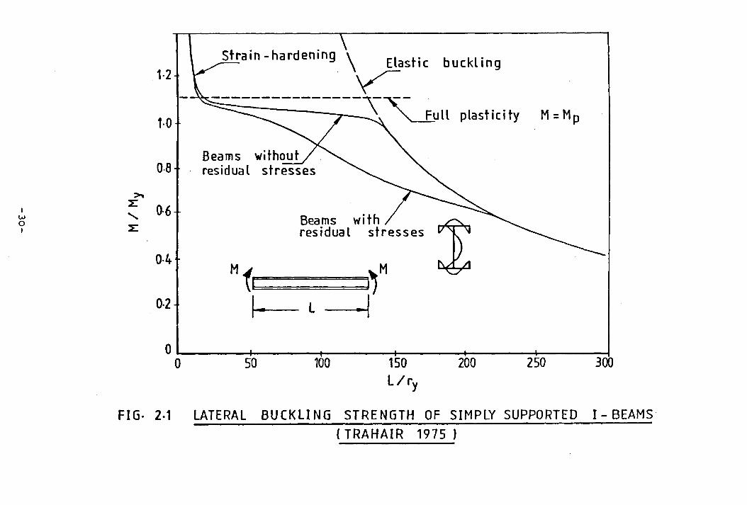
Figure 2.1 Lateral Buckling Strength o f Simply Supported

I-Beam (Trahair, 1975) 30

Figure 2.2 Beam-Column Subjected to Biaxial Bending about axes 31

Figure 2.3a Isolated H-Column under Biaxial Bending 32

Figure 2.3b Decomposition o f a Axial Loading (Perkoz and

Winter 1966) 32

Figure 2 .4a Idealization o f Beams with Geometrical

Imperfections (Yoshida and Maegawa 1984) 33

Figure 2.4b Residual stress Distributions (Yoshida and

Maegawa 1984) 33

Figure 3.1 Definition o f Problem 77

Figure 3.2 Stress-Strain Relationship 78

Figure 3.3 Deformed and Undeformed Body 79

Figure 3.4 Sectoria l Coordinates o f Thin-Walled Section 80

Figure 3.5 General Three Dimensional Body 80

Figure 3.6 Typical Patterns o f Residual Stress Adjusted to

Ensure Full 3-D Equilibrium 81

Figure 4.1 Transformation o f Beam Element 119

Figure 5.1 Location o f Nodes at Discontinuties 144

Figure 5.2 Number o f Elements and Segments in the

Cross-Section 144

X

145

146

147

148

149

170

171

172

173

174

188

189

Cross-Section I l lu s tra t in g the Process o f

Evaluating Section Properties

Sectorial Coordinates o f Thin-Walled Section

Newton-Raphson Method

Example Showing Number o f Elements and Internal

and External Forces

Flow Char o f TDCP (El-Khenfas 1987a)

Comparison Between Author's Results and Roberts

and Azizian (1983a) for I-Sections Subjected to

Axial Load and Vertical Deflection

Comparison Between the Results Obtained by The

Author and Those o f Roberts and Azizian (1983b)

Comparison o f Authors Results with Analysis o f

Moore(1986) and Test data, Lateral Load Applied

Through Shear Centre

Comparison o f Author's Results with Moore (1986)

and Vlasov (1961)

Load - Deflection Curve for Three Types o f

Analyses o f a Simply Supported I-Beam Subjected

to Biaxial Bending and Constant Torsion at

Mid-Span

Adjusted Residual Stress Distribution Presented

by Fukumoto et a l. (1972)

Comparison Between Author's Results and

Experimental o f A n s i i j n ( 1983 ) on Beam-Column

under Biaxial Bending

Comparison o f Authors Results with Anslijn

(1983) Tests - in-Plane and out-of-Plane

XI

190Displacements Test 48

Figure 8.1 Comparison Between the Bending and Warping

Stresses Obtained by Pastor & DeWolf (1979)

Against Those By Author’ s Approach 226

Figure 8.2 Comparison Between Total Stress and Rotation o f

I-Beam under Constant Torsional Moment at Mid-Span

and Equal end Moments to Those obtained by

Author and Pastor and DeWolf (1979) 227

Figure 8.3 Interaction Curves o f Three Analyses Obtained

by Elastic Analysis 228

Figure 8.4 Comparison Between Three Analyses o f a Beam-

Column under Biaxial Bending and In i t ia l

Deflection (L/1000) 229

Figure 8.5 Interaction Curves o f Rotations and Loads o f

Beam-Column Subjected to Biaxial Bending and

Constant Torsion at Mid-Span 230

Figure 8.6 Comparison Between the Three Analyses o f a

Beam-Column under Biaxial Bending and Constant

Torsional Moment at Mid-Span 231

Figure 8.7 Load Rotation Curve o f I-Beam Under Torsional

Moment at Mid-Span, with or without inclusion

o f residual stress 132

Figure 8.8 Spread o f Yield for Linear and Nonlinear

Analysis o f Beam-Column Subjected to Bending

and Torsion 233

Figure 8.9 Interaction Curves o f Equal End Moments and

Concentrated Torsion Applied at Mid-span 234

Figure 8.10 Interaction Between Bending and Torsion for a

x i i —

Beam-Column Subjected to Uniform or Nonuniform

End Moments and Concentrated Torsion 235

Figure 8.11 Typical Spread o f Yield at Mid-span o f

Beam-Column under Unequal end Moments and

Torsion, No Residaul Stress Included 236

Figure 8.12 Typical Spread o f Yield (Mid-span) o f Beam-

Column Subjected to Equal Constant End Moments

and Torsional Moment at Mid-Span 237

Figure 8.13 Comparison o f Authors Results for Linear and

Full Non-Linear Analysis o f Beam-Column

Subjected to Compressive Load with Eccentricity

and Constant Torsion at Mid-Span 238

Figure 8.14 Spread o f Yield for Example o f Fig. 8. 13 239

Figure 8.15 Comparison Between Linear and Full Non-Linear

Analysis o f Beam-Column Under Biaxial Bending

and Constant Torsion at Mid-Span 240

Figure 8.16 Typical Spread o f Yield o f Beam-Column under

Biaxial Bending and Torsion 241

Figure 8.17 Torque Diagrams for Pin-Ended Beam (Salmon and

Johnson, 1980) 242

Figure 8.18 Interaction Curves for Beam-Column o f I-Beam

Section (W12x14) under Flexural Bending and

Torsion at Mid-Span 243

— x i i {— ■

Notation

A Cross-sectional area

Af y My/Myy+HZ/MyZ+Mt /My(j)

%

AA p/P , + M /M 4M /M 4Mt /M pi y py z pz t pu

a ,a y ’ z Distance o f transverse load (concentrated

or d istributed) below or above shear centre

B Flange width (I-sec t ion )

C centroid o f the section

C1My 2 M 2 \ 2

( — ) • + (— ) + (— ), M M M M yy yz yw

c 2 C-Z-)2 . <_5_>2 „ ( _ L ? ^ py pz pu>

D Beam depth

E Elastic modulus.

Esh Strain hardening modulus

Et

ey* ez

Tangent modulus

Eccentric ities o f axial load

- xiv -

Fi Concentrated force

FX Internal axial load

f s Surface traction force

f b Body force

G Elastic shear modulus

Gsh Strain hardening shear modulus

Gt Tangent shear modulus

H D- Tf

: o Polar moment o f inertia

I y * Moment o f inertia about Y and Z axes

I y zProduct moment o f inertia about Y and

Z axes

I , Iyu' zu Warping product moment o f inertia

about Y and Z axes

IOJ

Warping moment o f inertia .

K Torsional constant

L Beam length

1 Beam segment length

Mcr

n ._______I n2EI

rKGN 1- u g k

MP

Plastic moment

MP

^ crp2dA

My

c Zy

XV -

Mx l ' My i ’ Mz i

Applied constant torsional moment

Internal moments to the l e f t o f node

i about X, Y, and Z axes

mr , mrx i ’ y i z i Internal moments to the right o f node

i about X, Y, and Z axes

rnx i ’ " y i * mx i Applied moments to node i about

X, Y, and Z axes

MK. , mrwi* wi Internal moments to the r ight o f node

to the r ight o f node i

NEL Number o f elements

NELS Number o f elements in the cross-section

P Internal axial load

Pt Total force array

Py 0 /

Qy ’ Qz Shear resultant

Qx* ^y» 9Z Transverse loads applied about X,

Y, and Z axes

R Total displacements array

rE Element displacement

r , rP

Projection o f p ' on the

tangent and perpendicular to the tangent

at point A on the contour, F ig. 3.2a

r y* r zRadius o f gyration about Y and Z axes

Sc shear centre coordinate

- X V I -

V sz Plastic section tnodulii about

Y and Z axes

T f Flange thickness

10) Web thickness

u. V, w Displacements in the X, Y, and Z d irections

u . V * o ’ o ’ ° In i t ia l displacements

u - *yz~3yaz

Partia l d if fe ren t ia t ion o f U

with respect to y and z

u Strain energy

V., Potential energy due to applied load

Y , Z F irs t moment o f area about Y and Z axes

Y , Zs ’ s Coordinates o f point s

z , z y * z ELastic section modulii about

Y and Z axes

a Angle between the tangent at the

contour and ve r t ica l axis. Fig. 3.2a

e 8 by ’ z ' “

Properties o f cross-section defined below

8y

t 1 2 J Y(Y + Z )dA - 2 Z S

A

8z

\ 2 2X .J Z(Y + Z )dA — 2Yg

A

3GQ

/ “ (Y2 + Z2)dA

A

- xv iI -

Properties o f cross-section defined below

j - f Y(Y2 + Z?)dA

*A

J - S ZCY2 + Z2 )dA

2 A

^-/o,(Y2 + Z2)dA

“ A

Tolérance error

Axial strain

Residual strain

Yield strain

Linear strain

Nonlinear strain

Slope o f U and V with respect X axis

Bending stress about y and Z axes

Flange t ip residual stress

Flange-web junction residual stress

Residual stress

Total stress

Yield stressy

aa)a

P

T Txz* yz

« «Y » Z

4>0)

$

$f .e.

orn_ i

<>

U

[ ]

[ ]

[k d ]

[kJj], [k£l ]

[Kq ] , [k{Ìl ]

Warping residual stress

Web residual stress

Distance between a point on the cross

-section and shear centre, F ig. 3.2a

Shear stresses.

Major and minor curvatures.

Warping curvature.

Twisting calculated according to

equation 8.7

Twisting calculated according to

f in i t e element analysis

Normal izedwarPin8'fuction *

Total potential energy

Virtual displacements

Virtual work

Row

Column

Matrix

Transpose matrix

Diagonal matrix

Linear and nonlinear tangential matrix

Linear and nonlinear gemetrical matrix

[Ko3

[ Kt ]

[Kww3

[Kuu 3

[Kvv 3

[K ] uv

[K ] wv

[K ] wu

I n i t i a l geometrical s t if fness matrix

Coeffic ien t matrices as

equation *4.7

Total s t i f fn ess matrix

Axial s t if fn ess matrix.

Transverse s t i f fn ess matrix about Z-

Transverse s t i f fn ess matrix about Y-

Coupling s t if fness matrix about Z-Y

Coupling st if fness matrix about W-Y

Coupling s t if fness matrix about W-Z

defined

Z

Y

Chapter 1

Introduction

1.1 General

The order o f complexity o f the response o f a structural

member in three-dimensions depends on a number o f factors. These

include the nature o f the loading, material properties, and the kind o f

assumptions made in deriving the governing equations. The most general

type o f member, which combines both axial and flexural loading, is

generally termed a ’ beam-column'.

The behaviour o f beam-columns depends on their slenderness

and the load conditions as shown in Fig. 1.1. Failure can occur in

either the e lastic or inelastic range, in the form o f flexural or

flexura l-tors ional buckling, or, more generally, b iax ia l bending. When

a member is bent about its weaker principal axis, or when i t is

prevented from de flec t ing la te ra l ly while being bent about its stronger

principal axis, then only an in-plane flexural response is possible.

Flexural-torsional buckling occurs when a member is bent about its

stronger axis but is not restrained la te ra l ly so that i t may buckle out

o f the plane o f bending by de flect ing la te ra l ly and tw isting. I f the

member is bent about both axes and twisted i t w i l l respond in a fu l l

three dimensional manner.

1

1.2 A la o f th e study

The purpose o f th is study is to provide a general formulation

suitable for many kinds o f cross section such as channel, tee, L, Z, U,

I , (mono or doubly symmetric), etc . for structural members acted upon

by any form o f loading and provided with very general support

conditions. The va l id ity and accuracy o f this approach is demonstrated

by several i l lu s tra t iv e examples, the results o f which are compared

with those obtained previously from either theoretical or experimental

investigations.

The domain o f this study is summarized in the following:

1- Developing a theoretica l analysis for a beam-column having an

arbitrary open cross section, which is applicable to both

e las t ic and ine lastic analysis.

2- Derivation o f l inear and nonlinear tangential and geometrical

s t i f fn ess matrices and strain-displacement matrices for a

beam-column in space suitable fo r many kinds o f cross-section

subjected to a wide range o f loading.

3- Developing a general computer program based on f in i t e element

analysis. This program is capable o f implementing the

formulation to provide numerical solutions.

H- Checking the va l id ity and accuracy o f both the derived

equations and the computer program by comparing the results

against those previously obtained by experimental and

theoretica l considerations.

5- Investigating problems o f bending and torsion not previously

fu l ly solved in both the e lastic and the inelastic ranges.

- 2 -

1.3 O u t - l in e o f th e t h e s is

This thesis contains nine chapters setting out the

formulation and implementation o f an ultimate strength study o f the

behaviour o f steel beam-columns.

Chapter 1 provides a general introduction to the problem to

be investigated. This is followed in Chapter 2 by a se lec t ive review o f

the previous work (theoretica l and experimental), within the general

area o f the structural response o f beam-columns.

Chapter 3 presents a pair o f general three dimensional

formulations, based on the concept o f v irtual work or the use o f energy

principles, in which the influence o f higher order terms, the e f fe c t o f

in i t ia l imperfections (such as residual stresses, in i t ia l crockedness,

e tc . ) have been included. Comparison between previous more restricted

formulations and this general one are explained in d e ta i l . Chapter 4

presents the fu l l s t i f fn ess matrices (linear/ nonlinear tangent and

geometric s t if fnesses and linear/ nonlinear strain matrix together with

the interpolation functions and the transformation matrix) required for

the implementation o f th is approach.

Chapter 5 describes both the analytical procedure and the

computer program structure. The analytical process is used to generate

the section and sectoria l properties, internal forces, curvatures,

tracing spread o f y ie ld through the entire cross-section, etc. The

program TDCP (Three Dimensional Computer Program) is based on f in i t e

element computer concepts, is written in the Fortran-77 Language,

contains a wide variety o f options, (in-plane ,out o f plane, uniform

loads »distributed loads, in i t ia l geometrical imperfections, d if fe ren t

boundary conditions, e tc . ) and may be used to investigate the e las t ic

and inelastic behaviour o f members o f thin-walled open cross-section,

- 3 -

under d if feren t load and support arrangements.

Chapters 6 and 7 contain comparisons between the results o f

this program and those derived previously by other techniques. These

i l lu s tra te the advantage o f both the modified formulation and the more

advanced computer program which is capable o f correctly accounting for

factors such as, absence o f symmetry, any form o f loading, any pattern

o f residual stress, any set o f in i t ia l deformations as well as varying

degrees o f sophistication in the assumed strain-displacement relations

and general geometrical aspects o f the problem.

In chapter 8, new problems involving the determination o f

ultimate strength under bending and torsion are presented in both the

e lastic and ine lastic ranges for beam-columns o f I-section .

Chapter 9, presents general conclusions and makes some

suggestions for further work.

4

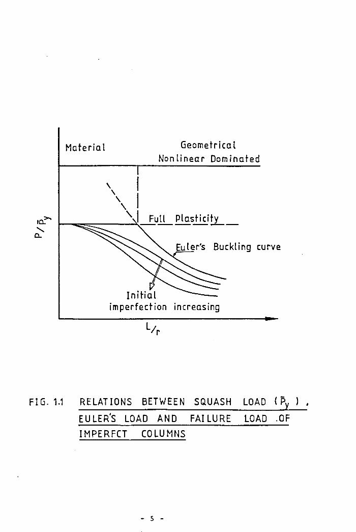
FIG. 1.1 RELATIONS BETWEEN SQUASH LOAD ( Py ) ,

EULER'S LOAD AND FAILURE LOAD -OF

IMPERFCT COLUMNS

5

C hapter 2

Review o f Previous Work

2.1 Introduction

The behaviour o f thin-walled beams and beam-columns o f open

cross-section is a subject o f importance to those concerned with the

design o f metallic structures. This was in i t i a l l y due to the growth o f

their use in a irc ra ft followed by increases in their use as members in

c i v i l engineering structures. A great deal o f research -both

theoretica l and experimental- has been carried out to provide

comprehensive data on which safe and economical designs can be based.

In this thesis a general three-dimensional formulation for

the structural response o f stee l beam-columns having an arbitrary open

cross-section is derived taking into account almost a l l the known

factors a ffec t ing their behaviour, such as in i t i a l crockedness,

d if fe ren t patterns o f residual stresses, and a wide varie ty o f loads

and boundary conditions. The ultimate strength behaviour o f beam-

columns in both the e las t ic and in e las t ic ranges has been investigated

by using a computer program based on the resulting f in i t e element

analysis. Before undertaking th is contribution a review o f previous

work was conducted.

2.2 Review o f Previous Work

2.2.1 H is to r ic a l & General

The behaviour o f a beam-column depends pr inc ipa lly on its

- 6 -

slenderness ra t io . Failure o f slender members is often governed by

buckling in the e las t ic range, for which the e f fe c ts o f small geometric

imperfections are comparatively unimportant, and the presence o f

residual stress irre levan t. Thus e las t ic c r i t i c a l loads may be used to

approximate the ultimate strength. However, members o f intermediate

slenderness normally f a i l by in e lastic buckling, for which the residual

stresses are important because they cause early y ie ld ing within the

cross-section, resulting in a reduction in the e f fe c t iv e s t i f fn ess o f

the member, and a lowering o f the resistance to buckling. Stocky beam-

columns may attain loads determined la rge ly from material strength

considerations. F ig . 2.1 represents a typica l moment-slenderness

relationship for beams. I t re la tes to both idealised members with no

in i t ia l deflections or residual strains, and a real member for which

the e f fe c ts o f these imperfections have been incorporated; fa i lu re may

be either e las t ic or in e las t ic .

A great deal o f research work (experimental and theoretica l)

has been conducted into the behaviour o f stee l members o f thin-walled

cross-section subjected to a var ie ty o f loading conditions. Some o f

these studies have Included the e f fe c ts o f in i t i a l geometrical

imperfections. Investigations have covered both the e las t ic and the

in e las t ic ranges and have considered both two and three dimensional

response.

When a la te ra l ly unsupported member is subjected to b iaxia l

bending, i t w i l l usually d e f le c t in both principal planes and twist at

any load le ve l as i l lu s tra ted in F ig. 2.2. The importance o f twisting

l i e s in the fact that the ultimate load carrying capacity o f an open

cross-section, fo r which the torsional r i g id i t y is small, w i l l be

cruc ia lly a ffected by the torsional aspect o f the deformations.

The review given below covers only a selection o f

contributions to the general subject area, concentrating on some o f the

more s ign ifican t developments.

Timoshenko (1910) developed the fundamental d i f fe ren t ia l

equations for flexure and torsion o f doubly symmetric simply supported

I-beams. He solved them for the e las t ic c r i t i c a l loads by using energy

theorems. A particular study was made o f the e f fe c t o f the point o f

load application when i t was remote from the shear centre axis. Wagner

(1929) studied the torsional buckling o f a thin-walled column; Kappus

(1937) modified Wagner's equation and generalized i t to deal with any

thin-walled open cross section. Bleich (193 3* 193 6) derived an

equilibrium equation for a member subjected to axial compression and

equal end moments having an I-cross section; in his study the c r i t ic a l

loads for flexura l-tors ional buckling were determined.

A number o f investigations have been carried out to determine

the c r i t i c a l loads for I-beams subjected to a va r ie ty o f d if fe ren t load

cases. Tabulated results are given by Clark and H il l (1960), Timoshenko

and Gere (1961), Vlasov (1961), Galambos (1968), Nethercot and Rockey

(1971), and Nethercot (1972). Winter (19^1) derived an approximate

formula to determine the buckling loads o f monosymmetric I-sections

under equal end moments. Other load cases have been considered by

Petterson (1952), Vlasov (1961), and Anderson and Trahair (1972).

General design methods based on the extensive research on the

e las t ic f le xu ra l- to rs ion a l. buckling o f beams have been proposed by

Clark and H il l (I960), Trahair (1966), Nethercot and Rockey (1971), and

SSRC (1976).

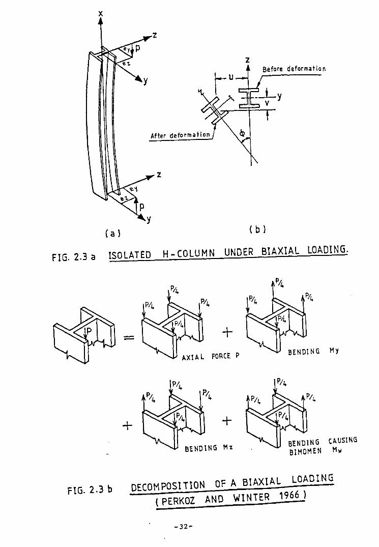
Pekoz and Winter (1966) have noted that the twisting o f a

beam-column subjected to axial load with e ccen tr ic it ie s e and e , cany z ■

- 8 -

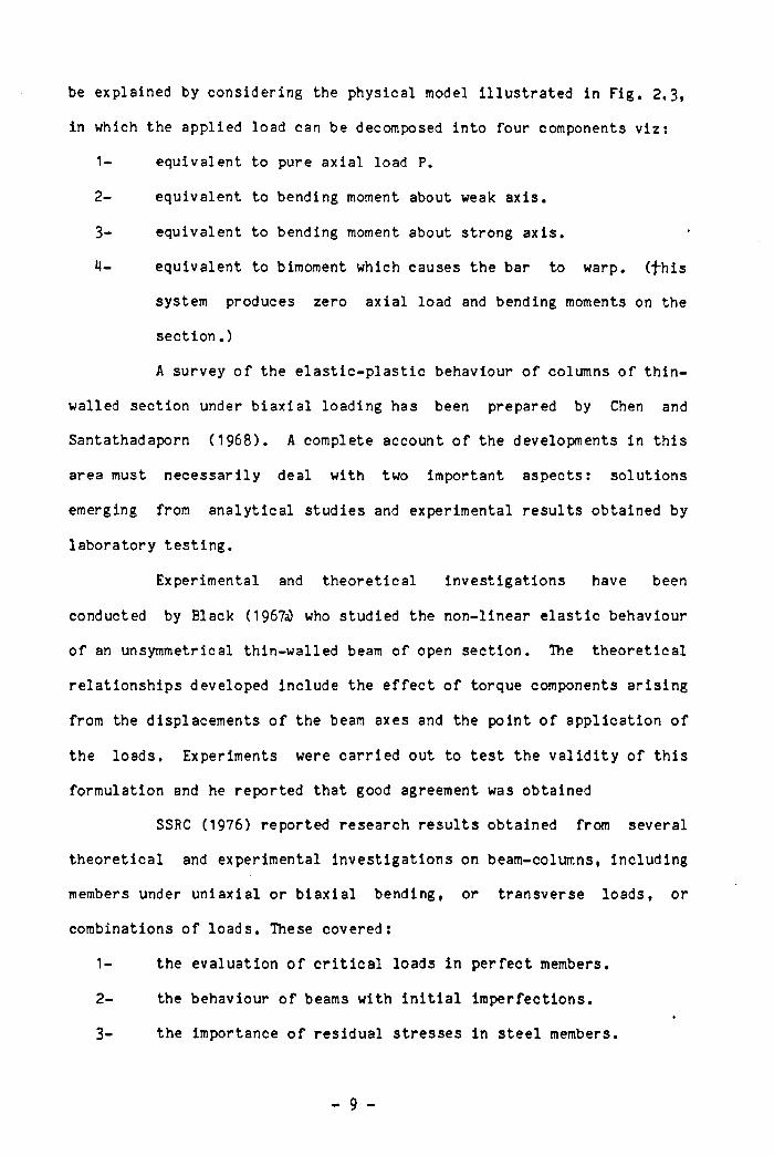
be explained by considering the physical model il lustra ted in Fig. 2.3,

in which the applied load can be decomposed into four components v iz :

1- equivalent to pure axial load P.

2- equivalent to bending moment about weak axis.

3- equivalent to bending moment about strong axis.

4- equivalent to bimoment which causes the bar to warp, (-f-his

system produces zero axial load and bending moments on the

section .)

A survey o f the e la s t ic -p la s t ic behaviour o f columns o f thin-

walled section under b iax ia l loading has been prepared by Chen and

Santathadaporn (1968). A complete account o f the developments in this

area must necessarily deal with two important aspects: solutions

emerging from analytical studies and experimental results obtained by

laboratory testing.

Experimental and theoretical investigations have been

conducted by Black (1967a) who studied the non-linear e las t ic behaviour

o f an unsymmetrical thin-walled beam o f open section. The theoretical

relationships developed include the e f fe c t o f torque components arising

from the displacements o f the beam axes and the point o f application o f

the loads. Experiments were carried out to test the v a l id i ty o f this

formulation and he reported that good agreement was obtained

SSRC (1976) reported research results obtained from several

theoretical and experimental investigations on beam-columns, including

members under uniaxial or b iax ia l bending, or transverse loads, or

combinations o f loads. These covered:

1- the evaluation o f c r i t i c a l loads in perfect members.

2- the behaviour o f beams with in i t i a l imperfections.

3- the importance o f residual stresses in s tee l members.

- 9 -

4- developments re la t ing the strain hardening modulus o f steel

to in e las t ic buckling behaviour.

5- studies o f the combination o f the e f fe c ts o f a ) in i t ia l

residual stress, b) geometrical shape imperfections and/ or

uncertainties o f load location.

A fu l l review o f research on beam-columns in stee l structures

conducted during the las t fo r ty years was carried out by Massonnet

(1976). This covers the behaviour o f beams and beam-columns in the

e las t ic and in e lastic range subjected to d i f fe ren t load patterns. Since

that date extensive additional studies (theoretica l and experimental)

on the behaviour and design o f beam-column have been made. In

(1976,1977) Chen and Atsuta provided a two volume text on the behaviour

o f beam-columns in two and three dimensions; Volume 1 helps the reader

to develop an understanding o f in-plane behaviour, while the second

volume provides a comprehensive source o f information on b iax ia l ly

loaded beam-columns as well as an explanation o f their space behaviour

under various load conditions. The two volumes taken together comprise

the f i r s t single reference book to discuss the complete theory o f beam-

columns systematically from the most elementary to the most advanced

stage o f development. They also covered some publications which provide

background and design rules for beam-columns, sp e c i f ic a l ly :

1- "Guide to S tab ility Design Criteria for Metal Structures", by

SSRC,

2- "S ta b i l i ty o f Steel Structures" by ECCS,

3- "Handbook o f Structural S tab il i ty " by CRC o f Japan,

Chen (1977) has provided a review o f the theory and design

rules for beam-columns under d i f fe ren t load patterns and boundary

conditions. The basic theoretical princip les and methods o f analysis in

10 -

two and three dimensions in the e las t ic and ine lastic ranges have been

included together with an assessment o f the v a l id i ty o f the proposed

interaction approach to the design o f b ia x ia l ly loaded members.

Vinnakota (1977) has derived governing d i f fe r en t ia l equations for an

arbitrary open cross-section, without making use o f the notions o f

centre o f g rav ity , principal axes and shear centre. The f in ite

d ifference method has been used to solve these equations for a number

o f problems having d i f fe ren t load conditions.

Chen and Cheong-Siat-Moy (1980) have presented a review o f

the philosophy behind the various interaction formulas for a beam-

column that have been proposed and are under consideration by various

specification writing bodies such as the American Institu te o f Steel

Constriction. The general v a l id i ty o f these proposed interaction

formulas has been demonstrated by comparison o f computed loads with

test results.

„ A survey o f recent achievements in the analysis (experimental

and numerical solutions) and design o f s tee l members in the USA has

been produced by Chen (1981), who investigated the behaviour o f an

isolated beam-column under the influence o f the in i t ia l de flections,

residual stresses, and various loading and boundary conditions. His

proposed interaction formulas have been checked against both computed

loads and the available test resu lts .

Kennedy and Madugula (1982) made a comprehensive review of

both theoretical and experimental work on the buckling o f angles,

covering single or built-up angles, equal-leg or unequal-leg angles

subjected to axial (e ither concentric or eccentric ) load, transverse

load, or a combination o f loads. Through their study they found that,

depending upon the cross-section, e f fe c t iv e length and applied load

11 -

configuration, members comprising o f angle shapes can f a i l by any o f

the following :

1- Flexural buckling about the minor axis.

2- Torsional buckling about the shear centre.

3- Torsional-flexural buckling.

Local plate buckling.

5- Combination o f tors iona l-flexura l buckling and local buckling.

Cescotto et a l. (1983) developed design rules for determining

the buckling strength o f beam-columns o f monosymmetric sections (Tee

and Triangle ). The ultimate buckling loads obtained from experiments

gave quite sa tis factory agreement with numerical simulations for both

cases. The suggested design rules appear as a useful complement to the

E.C.C.S. Recommendations. Numerical and experimental analyses have been

considered by Nakashima, et al.(1983) to investigate the buckling and

post buckling behaviour o f stee l beams having an H-shape, subjected to

a constant axial thrust and monotonically increasing end moments.

Interaction equations o f beam-columns in the design

specification o f Western Europe have been investigated by Nethercot

(1983). He presented some quantitative evaluation o f these proposals.

He also provided a tabulated comparison o f these interaction formulae.

His investigation covered the following aspects:

1- "Uniaxial bending leading to in-plane fa i lu re " .

2- "Uniaxial bending producing la tera l-to rs iona l buckling".

3- "B iaxia l bending".

A fu l l review covering the theoretica l and experimental

analysis in -both the e la s t ic and in e lastic ranges for columns, beams,

and beam-columns covering the years 1744 to 1984 has been presented by

Cuk (1984). Nethercot (1986) reviewed comprehensively the la tera l

- 12 -

buckling o f beams dealing with theoretica l approaches in both the

e las t ic and in e lastic ranges. I t was found that the original

theoretica l developments could be traced through to the most recent

ultimate strength approaches.

This introductory review is intended to provide an indication

o f both the h is to r ica l development o f the subject and the wide range o f

research already conducted. In the remainder o f this chapter attention

w i l l be focussed on spec if ic aspects o f the subject.

2.2.2 E lastic Behaviour

2.2.2.1 Flexural & Lateral Torsional Buckling

The e las t ic flexural and la tera l- to rs iona l buckling o f beams

o f d if fe ren t cross-section subjected to a wide varie ty o f loads and

boundary conditions have been studied by many investigators.

Anderson and Trahair (1972) presented tabulated results for

simply supported monosymmetric I-beams and cantilevers with

concentrated and distributed loads, and investigated the influence o f

load height on the e las t ic buckling moment. Their results compared very

well with tes t data.

Epstein and Murray (1976) developed a three-dimensional large

deflection theory for the analysis o f thin walled beams. Numerical

examples are presented to i l lu s tra te the application o f their theory to

the solution o f e la s t ic torsional post buckling behaviour o f I-beams.

They reported that their solutions compared well with results obtained

from experiments.

Kitipornchai and Trahair (1980) developed a simple method for

determining section properties for a wide range o f monosymmetric

- 13 -

I-beams, including sections with lipped flanges and also they presented

a method to calculate the e las t ic c r i t i c a l loads o f monosymmetric

beams. Their rule for the calculated e las t ic c r i t i c a l load for both

monosymmetric and doubly symmetric I-beams has been compared with AS

1250, BS 449, and the AISC spec if ica tion . More accurate and consistent

results were obtained.

A second order d i f fe r e n t ia l equation has been derived by

Warnick and Walston (1980) using a coordinate system whose orientation

remains fixed in space for symmetrical members under d i f fe ren t loading

conditions. Several examples were examined to investigate the la te ra l

buckling o f I-beams. Results o f the ir method were comparable with test

data.

The behaviour o f nonprismatic structural members (simply

supported or cantilever) under transverse concentrated loads has been

studied by Brown (1981) using the f in i t e d ifference method to determine

the c r i t i c a l loads o f simply supported and cantilever beams. He found

that the e f fe c t o f loads placed either below or above the centroid was

s ign ifican t in a l l types o f beams but leads to an increase, with

decreasing free end depth for the cantilever.

Cuk (1984) investigated th eore t ica lly isolated/ continuous

beam-columns subjected to transverse loads and end moments to determine

the e las t ic f lexura l-tors ional buckling. He reported that his results

compared favourably with those obtained experimentally.

Kitipornchai et ■ al (1985) proposed an alternative

approximation formula to evaluate the e la s t ic la te ra l buckling o f

simply supported monosymmetric I-beams under moment gradient. They

found three factors a ffec t ing the buckling o f monosymmetric sections,

which were

14 -

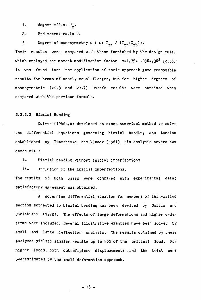
1- Wagner e f f e c t B^.

2- End moment ra tio B.

3- Degree o f monosymmetry P ( P = I ^ / ( I ^ + 1 ^ ) ) .Their results were compared with those furnished by the design rule,

which employed the moment modification factor m=1,75+1.03B+.3B2 ^2.56.'

I t was found that the application o f the ir approach gave reasonable

results for beams o f nearly equal flanges, but for higher degrees o f

monosymmetric (P<.3 and P>.7) unsafe results were obtained when

compared with the previous formula.

2.2 .2 .2 B iax ia l Bending

Culver (1966a,b) developed an exact numerical method to solve

the d i f fe r e n t ia l equations governing b iax ia l bending and torsion

established by Timoshenko and Vlasov (1961). His analysis covers two

cases v iz :

i - Biaxial bending without in i t i a l imperfections

i i - Inclusion o f the in i t i a l imperfections.

The results o f both cases were compared with experimental data;

satis factory agreement was obtained.

A governing d i f fe r en t ia l equation for members o f thin-walled

section subjected to b iax ia l bending has been derived by So lt is and

Christiano (1972). The e f fe c ts o f large deformations and higher order

terms were included. Several i l lu s t ra t iv e examples have been solved by

small and large deflection analysis. The results obtained by these

analyses yielded sim ilar results up to 80X o f the c r i t i c a l load. For

higher loads . both out-of-plane displacements and the tw ist were

overestimated by the small deformation approach.

15 -

A two-volume trea t ise on the behaviour o f beams and girders

subjected to transverse loading causing torsion has been prepared by

BCSA (1968,1970). The f i r s t o f these presents general theory and

formulae together with graphs used to display solutions, while the

la t te r presents worked examples (beams and griders subjected to bending

and torsion) to calculate stresses (normal stress, bending stresses

about Y and Z axes, warping stress, and shearing stresses) and

deflections at any point along the member and around the cross-section.

A theoretica l approach has been developed by Kitipornchai and

Trahair (1975) to study the strength behaviour o f tapered monosymmetric

I-beams o f constant depth subjected to bending and torsion. Also they

carried out experiments on small-scale aluminium I-beams to confirm the

v a l id i ty o f their theory. They reported that excellent agreement

between the two analyses was obtained.

Pastor and DeWolf (1979) investigated theore t ica lly the

behaviour o f wide-flange beams under equal end moments and a constant

torque applied at mid-span. They considered only small deflections and

ignored the coupling e f fe c ts . The results obtained for three beams

having sections W12x120, W12x36, and W 12x14 respective ly under Mcr /

100 at mid-span and monotonically increasing end moments were

tabulated. They suggested the design o f members subjected to flexural

bending and torsion should involve two checks:

1- The to ta l stress should be compared with the y ie ld stress".

2- The applied moments should be compared with c r i t i c a l moments

based on la te ra l- to rs iona l buckling, with safety

considerations.

2 .2 .2 .3 Bend ing and T o rs io n

16 -

2 .2 .3 I n e l a s t i c

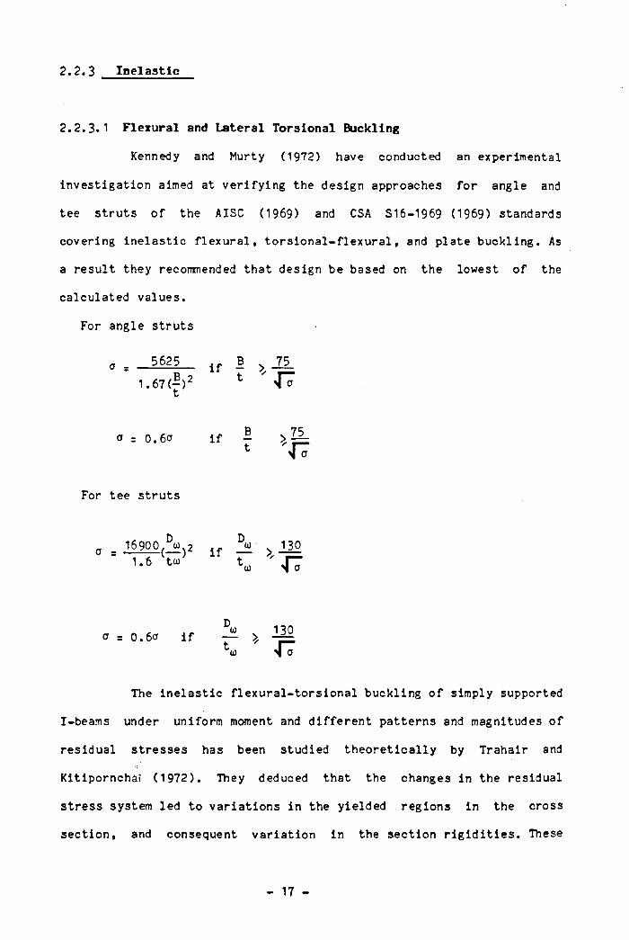
2.2.3.1 Flexural and Lateral Torsional Buckling

Kennedy and Murty 0972) have conducted an experimental

investigation aimed at ver ify ing the design approaches for angle and

tee struts o f the AISC 0 969) and CSA S16-1969 0969) standards

covering ine lastic f lexura l, to rs iona l- f lexu ra l, and plate buckling. As

a result they recommended that design be based on the lowest o f the

calculated values.

For angle struts

a . - 5 « 5 „ ! , i l1 . 6 7 ( f ) 2 1

a = 0.6a i f £Ho

For tee struts

16900. V 2 u . 130a = v lf tM > ^

a = 0.6a i f jo s 11°

The ine lastic f lexura l-tors ional buckling o f simply supported

I-beams under uniform moment and d if fe ren t patterns and magnitudes o f

residual stresses has been studied th eore t ica lly by Trahair and

Kitipornchai 0 972). They deduced that the changes in the residual

stress system led to variations in the yielded regions in the cross

section, and consequent variation in the section r ig id i t i e s . These

17 -

variations cause very s ign if ican t changes in the in e las t ic c r i t ic a l

moment.

Abdel-Sayed and Aglan (1973) studied the la te ra l torsional

buckling o f wide flange beam-columns subjected to axial force and equal

end moments about the major axis. In i t ia l imperfections were considered

together with strain hardening e f fe c ts . They come out with these

general conclusions; the la te ra l torsional buckling reduces the

strength o f beam-column in the in e la s t ic range, while the residual

stresses have neg lig ib le e f fe c t on the buckling in the e las t ic range

but a s ign if ican t e f fe c t in the in e las t ic range.

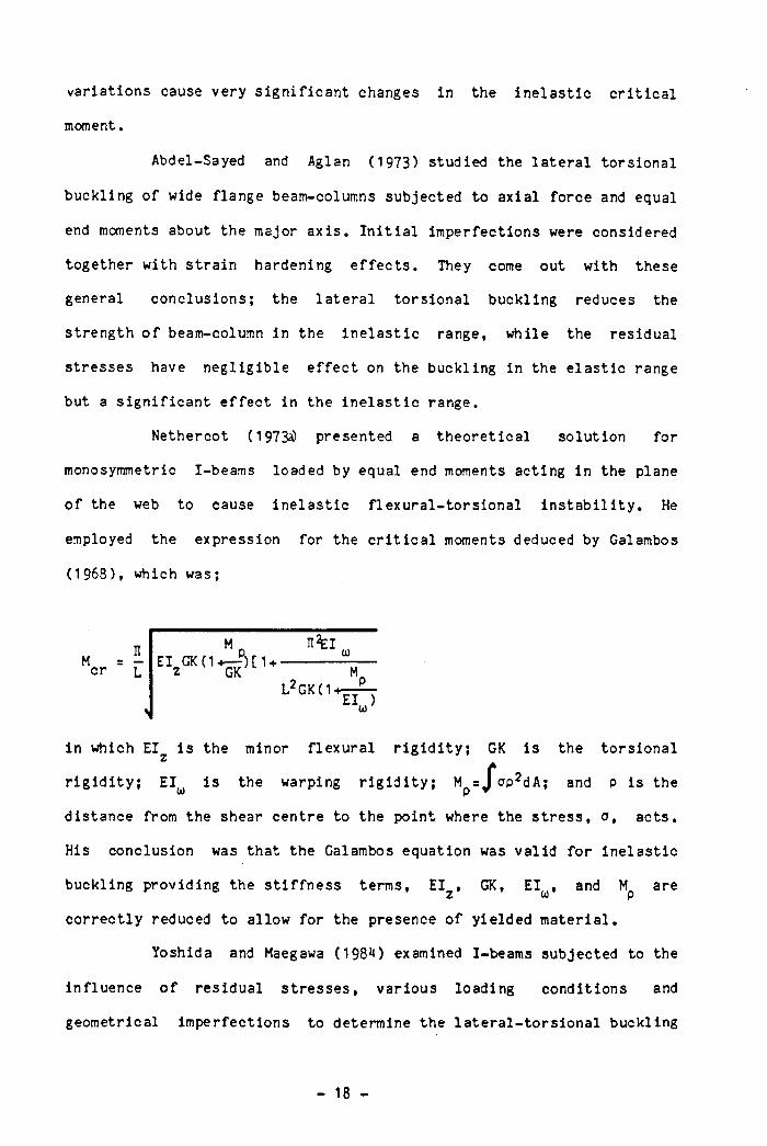
Nethercot (19733) presented a theoretical solution for

monosymmetric I-beams loaded by equal end moments acting in the plane

o f the web to cause in e lastic flexural-tors ional in s ta b i l i ty . He

employed the expression for the c r i t i c a l moments deduced by Galambos

(1968), which was;

cr

n%iEI GK (1 +—-j [ 1 •

z GKL2GK(1-p

EV

in which EIz is the minor flexural r i g id i t y ; GK is the torsional

r ig id i t y ; E I ^ is the warping r ig id i t y ; Mp = a p 2 d A ; and P is the

distance from the shear centre to the point where the stress, o, acts.

His conclusion was that the Galambos equation was valid for ine lastic

buckling providing the s t i f fn ess terms, EIz , GK, EI^, and Mp are

correctly reduced to allow for the presence o f yielded material.

Yoshida and Maegawa (198^) examined I-beams subjected to the

influence o f residual stresses, various loading conditions and

geometrical imperfections to determine the la tera l- to rs iona l buckling

- 18 -

strength, the load-deformation behaviour and the spread o f yielded

portions in the beam. They also examined the re la tion between the

ultimate strength and the buckling strength for the four theoretical

models o f Fig. 2.4, which are:

Model-I A beam with out-of-plane de flec t ion .

Hodel-II Straight beam subjected to a concentrated load at the top

flange with eccen tr ic ity ey ( eyis the distance from centre

line o f web to the loading point on the top flange).

M odel-Ill Beam subjected to a ve r t ica l concentrated load P o n

the top flange and P applied horizontally at the samePy

point, where the ratio — is kept constant.z

Model-IV A beam with out-of-plane displacement under

eccentric loading.

Matthey (1984) studied the ultimate strength behaviour o f

beam-columns o f I-section subjected to axial force, and bending moments

about the x and y axes. Residual stresses and in i t i a l deflections were

included. Those variables were arranged in a systematic fashion to form

the framework for a study o f more than 2500 cases. For each case the

compressive load was applied up to a predetermined lim it followed by

end moment loading to fa i lu re . He used these results to calculate the

Performance Factor which is defined as the ratio between the ultimate

load for every case obtained from his calculations and that given by

the design rules o f EC3 (1983)t SIA (1979), SIAC (1961), and Chen

(1979).

Kitipornchai and Lee (1986a) investigated th eore t ica lly the

ine lastic flexural and flexura l-tors ional buckling o f single-angle, tee

and double-angle cross-sections used as simply supported columns

subjected to axial load. They found that the flexural buckling mode is

- 19 -

the dominant fa i lu re mode for most shapes, except for single unequal

rvangles, for tees, and for double angles whose rad ii o f gyration give —rz

greater than 1.0. These theoretica l results were checked against other

analyses and were in reasonable agreement.

2.2.2.3 Biaxial Bending

An approximate formulation has been provided by Syal and

Sharma (1971) for the solution o f the generalized problem o f b iax ia l ly

loaded columns with equal or unequal load eccen tr ic it ie s . The e ffec ts

o f the residual stresses, cross-section shape B/D, and warping at the

ends being either permitted or restrained have been included. They

reported that the ir results match those previously obtained. Linder

(1972) conducted a theoretica l investigation to determine the ultimate

load o f columns o f bisymmetrical section under b iax ia l loading. He

employed polynomial expressions for the displacements (U, V, and i ) in

order to obtain a general solution. He provided examples to demonstrate

his approach, which incorporates d if fe ren t slenderness, e ccen tr ic it ie s ,

and residual stress.

Epstein et a l . (1978) extended the work developed by Epstein

and Murray (1976) to deal with nontriv ia l ine lastic s ta b i l i t y problems

for the prediction o f the maximum load-carrying capacity o f thin-walled

beam-columns o f open cross-section under b iax ia l bending. Results for

ine lastic b iax ia l bending and for in s ta b i l i ty o f la te ra l ly unsupported

beams were compared with the experimental results obtained by B irnstie l

(1968) and Lee and Galambos (1963) respective ly and satisfactory

agreement was obtained.

- 20 -

Bending and Torsion

Theoretical studies on b ia x ia l ly loaded thin-walled beam-

columns o f open cross-section with and without incorporating torsional

e ffec ts have been investigated by Razzaq (1971*). He undertook some

experimental work to v e r i fy the v a l id i ty o f the theoretica l predictions

o f his analysis. Twenty beam specimens were tested up to collapse at

two d if fe ren t slenderness ratios for the following loading conditions:

1- Subjected to equal end moments about a principal axis.

2- Subjected f i r s t to concentrated torque at midspan, and

subsequently to equal end-moments about minor axis.

3- Reverse o f case 2 .

I t was found that good agreement was obtained between theory and

experiment.

Kollbrunner, et a l . (1978) have examined theoretica lly the

ultimate strength behaviour o f a cantilever member o f I-section

subjected to bending and warping torsion. They reported that the

comparison' o f the analytical results with those obtained from

experiments was good. Kollbrunner, et a l . (1979) have carried out

theoretical investigations on the e la s t ic -p la s t ic behaviour o f thin-

walled fixed ended I-beams under bending and torsion. The results

compared well with those obtained from experiments in terms o f ultimate

loads, internal forces, and twisting angles.

2.2.3 Experimental Studies

The behaviour o f la te ra l ly unsupported angles o f equal and

unequal leg .lengths for a varie ty o f — have been investigatedt

experimentally by Thomas et a l . (1972). Uniform moments were applied

about an axis para lle l to an angle le g . Their conclusion was that the

- 21

angle of twist ($ ) causes a reduction in the maximum section stress and

has a s ign ifican t influence on the maximum loads.

Kitipornchai and Trahair (1975) have conducted an

experimental investigation o f in e las t ic flexura l-tors ional buckling o f

fu l l-sca le simply supported I-beams under concentrated loads. The end

supports allow for rotation about both minor and major axes, transverse

displacements and twisting about the longitudinal axis were restrained,

but warping was free . The beams were loaded to fa ilu re and a l l but one

fa ilu re was in e la s t ic . They found that the e ffe c ts o f residual stresses

was not important, and they confirmed that by theoretica l predictions,

while the geometrical imperfections were more s ign ifican t in reducing

the strength o f beams below their theoretica l buckling loads. They also

reported that the ir results were consistent when compared against

theoretical and tes t data together with the Australian Code for the

e las t ic and ine lastic ranges.

82 experiments have been conduct in Leige (1983) on beam-

columns o f I-cross-section (HEA200 and stee l grade Fe 360), subjected

to b ia x ia l ly eccentric loading. The following variables were accounted

f o r :

1-

2-

3-

U-

The slenderness ra t io in both planes (— and — ) .ry rz

The bending moments applied in both planes.

The axial load applied.

The moment gradient in both planes.

An extensive survey o f the experimental investigations

preformed at various institu tions on beams and girders which fa iled by

la tera l in s ta b i l i ty has been prepared by Fukumoto and Kubo (1977). A

to ta l o f 275 tests have been included in the ir review; 159 for beams

and 119 for welded beams and girders. They employed s ta t is t ic a l

- 22 -

characteristics (Mean values (m) and mean minus twice standard

deviation) in order to have a comparison between test results and those

obtained from recommended design formulae.

The variation o f in e las t ic beam capacity with changing moment

gradient o f simply supported la te ra l ly continuous I-beams has been

investigated experimentally by Dux and Kitipornchai (1983). Beam

slendernesses were chosen such that buckling should occur in the

loading range between the f i r s t y ie ld ing and the attainment o f the

p lastic moment. The points o f load application were prevented from

moving la te ra l ly and tw isting. The tes t results were compared with

theoretical predictions. An experimental investigation to determine the

ine lastic flexura l-tors ional buckling o f continuous beams o f I-section

in a sub-assemblage o f a three dimensional structural framework has

been carried out by Cuk (1984). He reported good agreement with the

results obtained from his para lle l theoretica l study.

A series o f experiments on tees and angles in compression has

been conducted by Wilhoite et a l . (^SHa.b) to study the ir behavior and

strength. The tested bars were made o f high strength, low-alloy stee l

with improved formability to match the requirements o f ASTM-A-718-81,

grade 60. They reported that the results obtained for both sections

match fa i r ly well the theoretica l predictions.

Kitipornchai and Lee (1986b) investigated experimentally the

ine lastic flexural and flexura l-tors ional buckling o f single-angle, tee

and double-angle cross-sections subjected to axial load. They found

that flexural buckling is the dominant fa i lu re mode for most shapes,

except for single unequal angles, for tees, and double angles whosery

radii o f gyration give — greater than 1.0. Their experimental resultsrz

were carried out on 51* struts with modified slendernesses ranging from

- 23 -

0.33 to 1.08 for simply supported members prevented from twisting about

their longitudinal axis. These experimental results are in reasonable

agreement with theoretica l predictions.

2.2.4 F in ite Element Development

Based on the f in i t e element concept much research has been

carried out to obtain formulations for beams and beam-columns in three

dimensions, using the equilibrium condition, the v irtua l work principle

or energy princip les. Some o f these have considered only uniform

torsion, whilst others have studied both uniform and nonuniform torsion

where the loads applied may be ax ia l, f lexura l (uniaxial & b iax ia l ) or

combinations.

The designation ’ f in i t e element concepts', as employed by

Barsoum and Gallagher (1970) ,was intended to characterize the

formulation o f a relationship between the forces and displacements o f a

single member via simplified assumptions as to the behaviour o f the

element in terms o f stress or displacements. Energy theorems were used

to develop the governing d i f fe r en t ia l equation to study the torsion and

combined flexura l-tors ional in s ta b i l i ty o f one dimensional members o f a

constant cross-section in the e las t ic range. Their s t i f fn ess equations

gave excellent agreement (as the number o f elements was increased) with

existing theory when compared with the following cases:

1- Torsional buckling (pure to rs ion ).

2- Lateral buckling o f simply supported beam under applied

moments.

3- Lateral buckling o f a cantilever beam acted upon by

concentrated load at the shear centre.

Rajasekaran (1971) presented a f in i t e element analysis, based

- 24 -

on the princ ip le o f v irtua l work, fo r thin-walled members o f open

section made from material having a t r i l in ea r stress-stra in curve. The

e f fe c ts o f in i t i a l imperfections, residual stresses and d if feren t

patterns o f loads have been included . The v a l id i t y o f th is formulation

has been demonstrated by Rajasekaran and Murray ( 1973) for several

problems in both the e la s t ic and the in e las t ic ranges by comparison

with ex isting resu lts.

Nethercot (1973b) presented solutions for the in e lastic

la te ra l buckling o f I-beams loaded with either uniform or nonuniform

moments, with or without the inclusion o f the e f f e c t o f residual

stresses obtained by the f in i t e element method. His analysis was

applied to several i l lu s t ra t iv e examples and the results compared with

ex is t ing theoretica l and experimental data, good agreement being

obtained.

Epstein and Murray (1976) developed a formulation for the

analysis o f thin -walled beams o f arbitrary open cross-section

subjected to arbitrary large displacements in three-dimensions based on

a set o f kinematic assumptions. They reported that numerical solutions

obtained for e la s t ic la tera l-to rs iona l buckling for several problems

employing th e ir model were consistent with experimental resu lts. The

approach opened the way fo r predicting the real behaviour o f structural

elements in the large deflection range.

Roberts and Azizian (1981) derived expressions for the second

order strains in a thin walled bar o f open cross section subjected to

f lexu ra l, torsional and axi a l di splacements based on energy methods.

These expressions could be used for nonlinear analysis. Such analysis

would be d i f f i c u l t so i t was necessary to employ numerical solution

techniques. Roberts and Azizian (1983a) used these expressions to derive

- 25 -

the equilibrium d if fe ren t ia l equations by assuming linear e lastic

material behaviour. They supported their theory by providing several

i l lu s tra t iv e examples.

Chaudhary (1982) used the d i f fe r e n t ia l equation derived by

Vlasov (1961) to develop a general s t if fn ess matrix fo r a structural

member (monosymmetric) o f thin walled open cross section subjected to a

concentric axial force. The analysis bu ilt upon the hypothesis that the

presence o f bimoment leads to coupling o f rotational displacements. He

found that bimoment has an important e f fe c t with a reduction in wall

thickness o f the cross section o f the structure. A three-dimensional

formulation for beams o f an arb itrary open section based on large

deflection assumptions has been derived by Ramm and Osterrieder (1983).

Several i l lu s t ra t iv e examples are compared with previous work.

Opperman (1983) presented a mathematical model to study the

spatial behaviour o f thin walled open cross-sections using the f in i t e

element method. He reported that good agreement had been achieved

through comparisons with experimental results for several load cases.

Attard (1985) presented a nonlinear theory o f nonuniform

torsion for straight prismatic bars having an open section under

conservative loads, where the nonlinear e f fe c ts o f changes in the

geometry are ignored in the linear e la s t ic theory o f nonuniform

torsion. Yeong Bin -Yang and Mc-guire (1985) adopted the equilibrium (

equations o f thin-walled beams based on the princip le o f v irtual

displacements and an updated Lagrangian procedure.

Hasegawa, et a l . (1985) presented an analysis scheme for the

problem o f out-of-plane in s ta b i l i ty o f thin-walled beams and frames.

Based on the second order strain-displacement relationships, and the

theorem o f v ir tua l work, they derived the general s t i f fn ess equation o f

- 26 -

linearized f in i t e displacements for a thin-walled member. Numerical

examples, which covered the out-of-plane in s ta b i l i ty for both straight

and curved beams, were compared with existing resu lts. Their conclusion

was that the results obtained by them were accurate, e f f ic ie n t and

versa t i le for wide applications. Nishida and Fukumoto (1985) derived an'

exact expression for the fundamental equations o f a member with in i t ia l

imperfections subjected to the action o f bending and torsional moments,

and also to investigate the strength o f a beam under various load and

support conditions.

Wekezer ( 1985) developed an analysis for the nonlinear

torsion o f bars o f variable cross-section. The s t i f fn ess matrix is

expressed as a function o f the coordinates o f a d iscrete set o f points

selected from the mid-surface o f the bar. The geometrical description

o f the mid-surface o f a bar and i t s strain were considered. Stresses

were obtained from the linear stress-strain re la t ions . He reported good

agreement with previously obtained results, either theoretica l or

experimental.

An incremental equilibrium equation has been derived by

Sakimoto, et a l . (1985) for a beam-column with arbitrary open cross-

section. Features provided in the analysis are:

i - Ine lastic warping torsion o f a member.

i i - Y ield o f the material is judged as a b i-ax ia l stress problem

associated with both normal and shear stresses.

i i i - The stress distribution development o f the p lastic zones in

the cross-section can be eas ily displayed at each incremental

load step.

- 27 -

v i - The e f fe c t o f a rb it ra r i ly distributed residual stresses can be

considered.

They reported that their approach shows good agreement when compared

with available theoretica l and experimental results.

Attard (1986) developed two f in i t e element formulations, the

f i r s t one ignores in i t i a l bending curvature and the second takes into

consideration the f i r s t order in i t i a l curvature. The la te ra l buckling

loads for straight e la s t ic prismatic beams o f thin-walled section under

conservative loads were investigated. Close agreement was obtained with

experimental data.

Ohga and Hara (1986) developed a f in i t e element-transfer

matrix method that can be applied to linear and nonlinear problems o f

thin-walled members under various loading conditions. They employed the

Newton-Raphson method to achieve convergence o f each iteration step.

The section was divided into small layers in order to trace the spread

o f y ie ld . The von-Mises y ie ld cr iter ion was used. The accuracy o f the ir

method was demonstrated by the results obtained by experimental

evidence.

Kanok-Nukulchai et a l . (1986) presented a formulation for the

large deflection o f members using a Lagrangian mode o f description for

the structural elements. Their assumptions were based on

1- Appropriate selection o f element geometry, nodes as well as

nodal variables

2- Implementation o f an element shape function which incorporate

a l l the kinematic characteristics o f the applied class o f

structure.

- 28 -

3- Reduction o f the three dimensional model into a suitable form.

To establish an element model, several problems have been solved which

were found to be in close agreement with experimental resu lts.

Total potential energy has been used by Chan and Kitipornchaj

( 1986) to provide a formulation for a general thin walled beam-column

incorporating member geometrical nonlinearity. The proposed f in i te

element formulations were demonstrated on a number o f buckling problems

, including flexura l-tors ional buckling o f rectangular beams, tee beams

under moment gradient and angle beam-columns. Good agreement has been

achieved when compared with independent numerical solutions. The

e f f ic ien cy o f his method has been compared with the experimental

results obtained by Fukumoto and Nishida (1981).

- 29 -

M/

M

FIG- 2-1 LATERAL BUCKLING STRENGTH OF SIMPLY SUPPORTED I-BEAMS(TRAHAIR 1975}

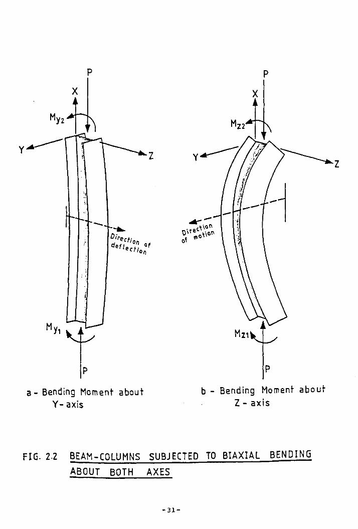
FIG- 12 BEAM-COLUMNS SUBJECTED TO BIAXIAL BENDING

ABOUT BOTH AXES

- 31 -

X

FIG. 2.3 bd e c o m p o s it io n of a b i a x i a l l o a d i n g

- pERK0Z AND WINTER J966J

- 32 -

FIG.24a IDEALIZATION OF BEAMS WITH GEOMETRICAL IMPERFECTIONS[ YOSHIDA AND MAEGAWA 1984]

FIG- 2.4b RESIDUAL STRESS DISTRIBUTIONS

[YOSHIDA AND MAEGAWA 1984]

- 33 -

Chapter 3

G en era l F orm u la tion o f Beam-Column A n a ly s is in Th ree Dim ensions

3.1 Introduction

Much previous research has been conducted to obtain the

governing d i f fe r en t ia l equations for beams and beam-columns in three

dimensions based on considerations o f equilibrium, v irtua l work, or

to ta l potential energy. Some studies considered only uniform torsion,

whilst others studied both uniform and non-uniform torsion.

A to ta l potential energy approach has been used by many

researchers. In 1970 Barsoum and Gallagher developed a s t i f fn ess

equation for torsional and combined flexura l-tors ional e las t ic

in s tab i l i ty o f one-dimensional members o f uniform cross section o f

doubly syrrmetric shape for which the shear centre and centroid

coincide. Rajasekaran and Murray (1973) derived the d i f fe r en t ia l

equations for an arbitrary cross section including in e las t ic material

behaviour, as well as the e f fe c t o f in i t i a l imperfections such as

residual stresses. Roberts and Azizian (1981) derived expressions for

the second order strains o f thin-walled bars o f open cross section

subjected to f lexura l, torsional and axial displacements. Roberts and

Azizian (1983^ used these expressions to derive the equilibrium

d i f fe r en t ia l equations by assuming linear e la s t ic material behaviour,

Attard (19*86) presented a nonlinear theory o f non-uniform torsion for

straight prismatic bars having an open section under the action o f

conservative loads and, Chan and Kitipornchai (1986) applied i t to

obtain a general formulation for thin walled beam-columns,

incorporating member geometrical nonlinearity. The proposed f in i t e

element formulations were applied to a number o f buckling problems,

including flexura l-tors ional buckling o f rectangular beams, la tera l

buckling o f tee beams under moment gradient and angle section beam-

columns .

Nishida and Fukumoto (1985) derived an exact expression for

the fundamental equations o f a member with in i t i a l imperfections

subjected to the action o f bending and torsional moments using the

principle o f v irtua l work. The same approach with the second order

strain displacement relationships has been considered by Hasegawa et

a l. ( 1985) to develop the equilibrium equation for a member having an

open cross-section under f lexural loading. Yang and McGuire (1986)

employed the equilibrium equations o f a thin walled beam based on the

principle o f v ir tua l displacements and an updated Lagrangian procedure

to derive the s t i f fn e ss matrices.

A complete formulation o f the equilibrium o f a thin walled

member o f arbitrary cross section in space is presented herein. The

equilibrium equations have been derived by two methods, the f i r s t is

based on the principle o f v ir tua l work, whilst the second is based on

the energy theorems. Imperfections are included in both formulations.

The v a l id ity and accuracy o f th is formulation has been tested on a

number o f e la s t ic (chapter 6 ) and ine lastic (chapter 7 ) applications.

3.2 Assumptions

The following assumptions have been used in the analysis: -

I - The beam-column has a general open cross-section.

- 35 -

I I - Transverse displacements are much larger than the

longitudinal ones.

I I I - The member length is assumed very large compared with its

cross-sectional dimensions.

IV- No distortion o f the cross-section occurs apart from warping,

(Vlasov 1961).

V- The shearing strain in the middle surface for open cross-

sections and in the planes normal to the individual plate

elements may be e ither neglected or included.

VI- Yielding is governed by normal stresses only.

V II- Applied loads are conservative.

3.3 Theoretical Analysis

The development o f the equilibrium equations for a three-

dimensional beam-column o f thin walled open cross-section requires that

attention be given to :

3-3.1- Kinematics o f a Section.

3-3-2- Stress-Strain Relationship.

3-3-3- Strain-Displacement Relationship.

3 - 3 - Anal ysi s Methods.

3.3.4.1- Virtual work.

3.3-^-2- Total Potential Energy.

3.3-1 Kinematics o f the Section

A thin walled open cross-section is shown in Fig. 3-1 having

Cartesian coordinates X, Y, and, Z, curvilinear coordinates n and s,

where s is measured along the centre l in e o f the section, n is

perpendicular to s, and t ( s ) is the thickness o f the cross-section at a

- 36 -

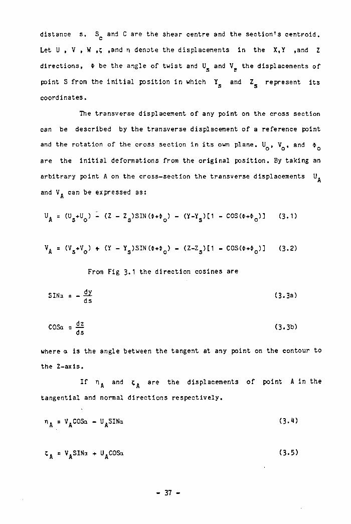
distance s. S and C are the shear centre and the section ’ s centroid, c

Let U , V , W ,5 ,and n denote the displacements in the X,Y ,and Z

directions, 4> be the angle o f tw ist and U and V the displacements o fs spoint S from the in i t i a l position in which Y and Z represent itss scoordinates.

The transverse displacement o f any point on the cross section

can be described by the transverse displacement o f a reference point

and the rotation o f the cross section in i t s own plane. U , V , and $o o o

are the in i t i a l deformations from the orig ina l position. By taking an

arbitrary point A on the cross-section the transverse displacements

and VA can be expressed as:

U. = (U .+U ) 1 (Z - Z )SIN ($+$ ) - (Y-Y ) [1 - COS(*+* ) ] (3.1)A S O S O S 0

VA = (V V * (Y " V SIN($+V " (Z-Zs)[1 " COS(*+ V ] (3.2)

From Fig 3.1 the direction cosines are

SINa = - ^ (3.3a)ds

COSa = — (3.3b)ds

where a is the angle between the tangent at any point on the contour to

the Z-axis.

I f nA and cA are the displacements o f point A in the

tangential and normal directions respective ly .

riA = VACOSa - UASINa (3 .1*)

; A = VASINa + UACOSa (3 .5 )

- 37 -

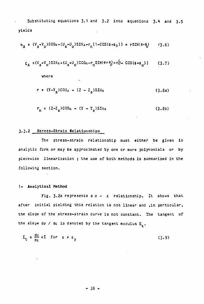
Substituting equations 3.1 and 3.2 into equations 3.4 and 3.5

yields

n * = (V +V )COSa-(U ♦U )SINa-r {1-COS($-*-i0) } + rSIN (MJ (3 . 6)A 5 w s o n oCA a(Vs*Vo )SIMa + (Us+Uo )C0Sa-rnSIN(?t<y-r6- COS(*+iQ) ) ( 3 . 7 )

where

r = (Y-Y)COS., ♦ (Z - Z )SINa5 S (3.8a)

r = (Z-Z)COSa - (Y - Y )SIna n s s (3.8b)

3.3.2 Stress-Strain Relationships

The stress-stra in relationship must e ither be given in

analytic form or may be approximated by one or more polynomials or by

piecewise l in ear iza tion ; the use o f both methods is summarized in the

following section.

1- Analytica l Method

Fig. 3*2a represents a 0 - c re lationship. I t shows that

a fte r in i t i a l y ie ld ing this re la tion is not linear and ,in particular,

the slope o f the stress-stra in curve is not constant. The tangent o f

the slope do / de is denoted by the tangent modulus E .

Et ■ £ <E fo r E » Ey (3 .9 )

- 38 -

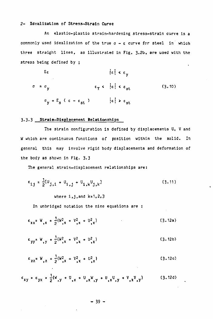
2- Idea lizat ion o f S tress -Stra in Curve

An e la s t ic -p la s t ic strain-hardening stress-stra in curve is a

commonly used idealization o f the true o - e curve for stee l in which

three straight l in es , as il lustra ted in Fig. 3.2b, are used with the

stress being defined by ;

Ee M < ey

Ey <I If e ! < t st (3 .10)

°y + Es ( £ est > !£ ! ” est

3.3.3 Strain—Displacement Relationships

The strain configuration is defined by displacements U, V and

W which are continuous functions o f position within the so lid . In

general this may involve r ig id body displacements and deformation o f

the body as shown in Fig. 3*3

The general strain-displacement relationships are:

£u ■ H i * ui . j * ui.kuj ,k’ (3.11)

where i , j ,an d k=1,2,3

In unbridged notation the nine equations are :

: = W + -{W2 + V2 ♦ U2 }xx ,x 2 *x »x i x

( 3 . 12a)

e = W + -{W2 + V2 + U2 }yy , y 2 . x . x

( 3 . 12b)

e = W + -{W2 + V2 + U2 }zz ,z 2 .x .x .X

( 3 . 12c)

'yx + u + U W + U U + V V ) . X ,x ,y + tx ,y \ x , y J (3 .12d)

- 39 -

e = e = - {W + V + W W + U U + V V }xz zx 2 »z »x ,x ,z ,x ,z ,x ,z (3.12e)

e = e = - { U + V + W W + U U + V V }zy yz 2 .z ,y ,y ,z ,y ,z ,y ,z (3.121)

in which subscripts x, y, z denote d if fe ren t ia t ion with

respect to that parameter.

Equation 3.12 allows for shear deformation due to St. Venant

torsion based on the hypothesis that the twisting o f any cross-section

w i l l produce only shear stresses. This shear stress varies from zero at

the centre o f the section to i t s maximum value at an external surface.

I t is assumed that twisting o f such sections does not produce any

longitudinal stresses (Zbirohowski-Koscia 1967).

Using assumption V leads to

e = e s e = 0. yy zz yz (3.13)

so equation 3*12 can be reduced to

e = W + ^ w2v ♦ V2 + U2 } xx ,x -2 .x ,x (3. I^a)

eyx = exy - I {W,y + U,x * W,x \ y + U,xU,y * V.x\y> ( 3 . I^b)

e = c = —{W _ + V + W W + U U + V „ V „ } Z X X Z 2 * Z ,x ,x ,z ,x ,z ,x ,z ( 3 . 1^0

Equation 3.11 can be written in matrix form by using equations 3.13 and

3.1« as

- «0 -

(3.15)[e

1■ e £ 1XX yx

XQ>II 0 0IE¡_Xz

0 0

i z

The curvil inear shear strain can be obtained from equation 3.12 using

assumption 2 .

1 = 2esx sx

Y = 2e nx nx

CL *■4 > dW dU.A ^ A dVA dVAdx ds ds dx ds dx

d A dW dU,A dUA dVA CL < >

dx dn dn dx dn dx

i 5 to equation 3.16.

(3.16)

(3.17)

^ A + + + b 0dx ds ds dx ds dx

Substituting equations 3.1» 3.2, and 3.7

— = - ^ [ V SIN(4+4 ) +, U COS($+4 ) ] ds ds *x o ,x o

(3.18)

in equation 3.18 yie lds

- — [V COS(4+4 ) - U SIN (4+4 ) 3 - r 4 v (3.19)ds *x o ,x o ,x

Integrating equation 3.19 as

W = W - Y[V SIN(4+4 ) + U COS(4+4 ) ]C | X 0 f X o

- Z[V COS(4+4 ) - U SIN(4+4 ) ] - f { r 4 „Ids , X 0 ,X 0 J ,x

s

( 3 . 2 0 )

where

W = W. + Y.[V SIN(4+4 ) f U COS(4+4 ) ] c A A , x o , x 0

SHEFFIELD | UNIVERSITY i

(3.21)- Z,[V COS($+t> ) . U SIN ($+$ ) ]A ,x o ,x o

where the subscript A is the integral l imits e .g . Y at Y=Y^ and Z= Z^.

The last term o f equation 3.20 may be determined from the

sectional coordinates o f a beam having a cross section with a curved

outline asgiven in Fig. 3.** and is calculated by integration o f this

equation.

6o}n„ = 5Si x rDSJS2 1 S1 s2

( 3 . 22a)

where DsjS2 is equal to the incremental area, r g^g equal

to the distance o f pole D to a l ine passing through points Si and S2

and dS^ is the distance between Si and S2 . Integrating the above

equation between 0 and Sr (the length o f the centerline o f a segment o f

the section measured from point 0) y ie lds.

Sn

“ DOS * J r ( s >ds 0

( 3. 22b)

Further deta i ls are given in Zbirohowski-Koscia (1967). Denoting the

normalized function by ion

un (3.23)

Substituting equation 3.22b into equation 3.20 yie lds

W = Vi - Y[V SIN($+$ ) + U COS ( * + * ) ]C | X 0 f X o- Z[V C0S($+$ ) - U SIN($+4> ) ] * w * „ ,x o ,x 0 n ,x (3.24)

- 42 -

Equation 3.1 in terms of stress-displacements can be rewritten as:

a = E? [W + - {V 2 + U2 + W2 } ] + ax x , x 2 . x . x , x r (3.25a)

f = + U + W W + U U + V V ]xy 2 .y .X ,x ,y ,x ,y ,x , y J (3.25b)

xz 2 .z * V v + W vw „ ♦ U U + V V ]x ,z ,x ,z ,x ,z ' (3.25c)

Substituting equations 3.1, 3.2 and 3.20 into equation 3.25a yie lds a

longitudinal strain which can be written as .

■xx [W + - {U2 + V2 + p2$2 } ]. x 2 . X , x , x J J-Y {U - V * - U — + V * ♦ U * * 1.xx ,xx ,xx 2 ,xx o ,x ,x o ’

$2-Z {V - V ----- U »,xx ,xx 2 .xx - U 4 > + V 4 > 4 > \, X X O , X , X OJ

" V x { v X - u y$ } + J U + V W * ] + Sr ( 3 . 2 6 )O y A f A y A . 5 yX yX yX H y X X I

Equation 3.26 may be written in another form as

e = en ” - 4>,,Z ♦ * to + e_u z y a) n r ( 3 . 2 7 )

where e , 4> , 4> and $ are the representative axialo ,x ,y a)

strain , b iax ia l curvatures about the y , and Z axes and warping

curvature respect ively . They are given by

e0 = W +—{U2 + V2 + p2$ 2 }0 .x 2 .x ,x w * , x J

- Y * { v - IJ * } + Z ♦ y {U ♦ V • )i » X yX | A S yX yX yX

+ e r (3.28)

v

- M3 -

A = V — V ^— — U $ — U $ t-V $ $Ty ,xx ,xx 2 .xx ,xx o ,x ,x o (3 .2 9 a )

$2i> = U - U ----- V i + V 4> - U «> 4>Z , X X , X X 2 . X X , X X O , X , X 0 (3.29b)

4> = <t>w ,xx (3.29c)

Equation 3.27 can be written in matrix form as

a =E [1 - Z - Y - w )n

eo

%z

*w

(3.30)

The stress resultants for a thin-walled member in space are

so dAXX (3.31a)

A

* J \ y dA

A

Qz ■ / » » t dA

A

My * J V Z dA

A

M. * J \ x 1 dA

A

W = T a IJdA id j xx n

A

(3.31b)

(3.31c)

(3.31d)

(3.31e)

(3 .3 l f )

M -

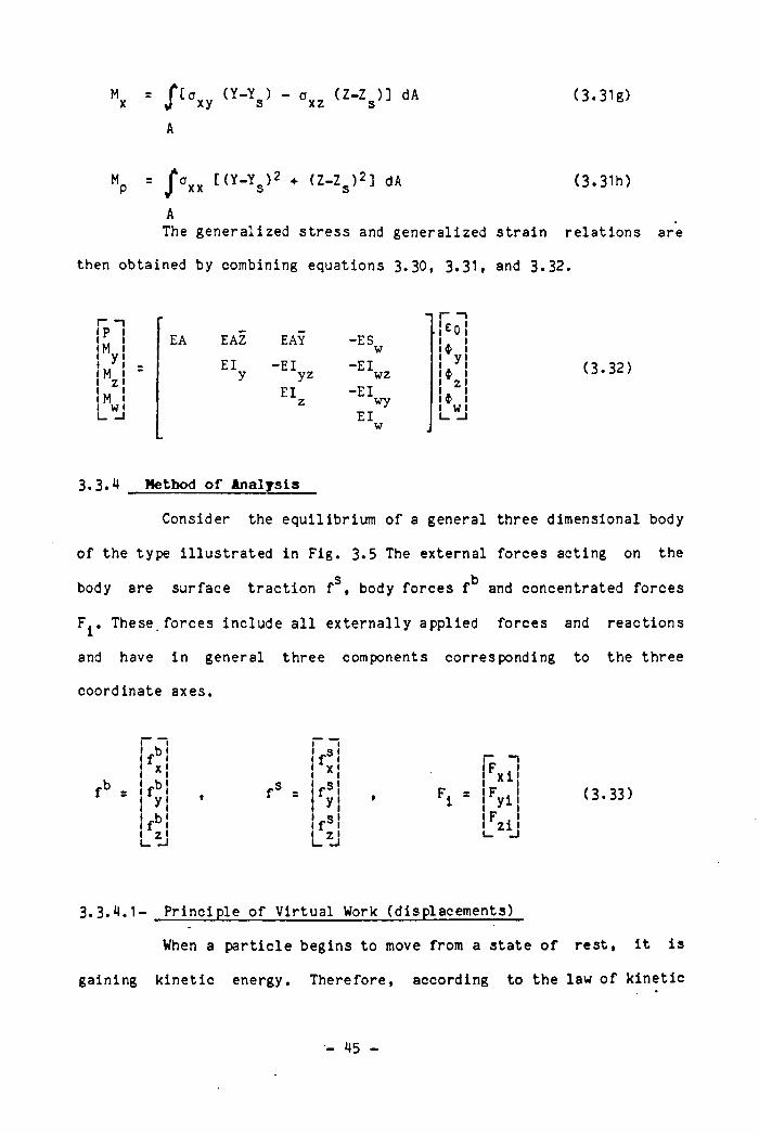
<3.31g)"x = / ‘ »x , ( Ï - V - °xz dA

A

M? = J*0XX t(Y-Ys )2 + (Z-Zs ) 2] dA (3.31h)

AThe generalized stress and generalized strain relations are

then obtained by combining equations 3. 30, 3. 3 1 , and 3 . 32.

r ni p i !u 1 EA EAZ EAŸ -ESM! y j . El -El

w-El

! Mz ! y yz wzI i iM ! L w_j

El z -El wyElw

(3.32)

3.3.4 Method o f Analysis

Consider the equilibrium o f a general three dimensional body

o f the type i l lustrated in Fig. 3.5 The external forces acting on the

s bbody are surface traction f , body forces f and concentrated forces

F T h e s e . f o r c e s include a l l externally applied forces and reactions

and have in general three components corresponding to the three

coordinate axes.

f sx

f sy

x i

"yi

Fz i i

(3.33)

3.3.4.1- Principle o f Virtual Work (displacements)

When a part ic le begins to move from a state o f rest , i t is

gaining kinetic energy. Therefore, according to the law o f kinetic

- 45 -

energy, the forces which act on the part ic le are performing net

positive work. Hence, the part ic le does not move unless i t can undergo

some arbitrary small displacement, say 6r^ (v ir tua l displacement), for

which the corresponding increment o f work 6w (v ir tua l work) o f forces

is posit ive .

that express the equilibrium o f the body is through the use o f the

principle o f v ir tual displacements. This principle states that for the

body to be in equilibrium for any compatible set o f "small" v irtual

displacements imposed on the body the to ta l internal v ir tual work must

be equal to the tota l external v ir tual work i . e .

An equivalent approach which may be used to obtain equations

V V

(3.3*1)

s s

The external work w i l l be given by the product o f the actual

b sforces f , f ,and acting through the v ir tual displacements 6r ,

where

r = [ U V W ] (3.35)

The internal v ir tual work is equal to the actual stresses

acting through the v ir tua l strains corresponding to the imposed

vir tual displacements.

(3.36)

- *16 -

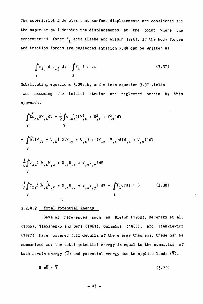
The superscript S denotes that surface displacements are considered and

the superscript i denotes the displacements at the point where the

concentrated force acts (Bathe and Wilson 1976). I f the body forces

and traction forces are neglected equation 3.34 can be written as

/ ai j 6 e i j dv= r ds (3.37)

V s

Substituting equations 3.25a,b, and c into equation 3.37 yields

and assuming the in i t i a l strains are neglected herein by this

approach.

/ ES x 5W,xdv ♦ i / \ x x S[w2,x * u2x * v!x>dv

V V

fc'nw ♦ U } 6{W + u ) + {W +V ) 5 {W „ ♦ V ¥}]dvj »y »* »y »x ,z ,x ,z ,x

F / dxxS1“ ,xW,z * U,xU,z * V. x \ z > dV

i / dxy5< « .x « .y

V

U,xd.y * V,xV,y 1 dV - x F^6rds = 0 (3.38)

3.3.4.2 Total Potentia l Energy

Several references such as Bleich (1952), Kerensky et al.

(1956), Timoshenko and Gere (1961), Galambos (1968), and Zienkiewicz

( 1977) have covered fu l l -details o f the energy theorems, these can be

sumnarized as: the tota l potential energy is equal to the summation o f

both strain energy (U) and potential energy due to applied loads (V ) .

n :U + v (3.39)

- 47 -

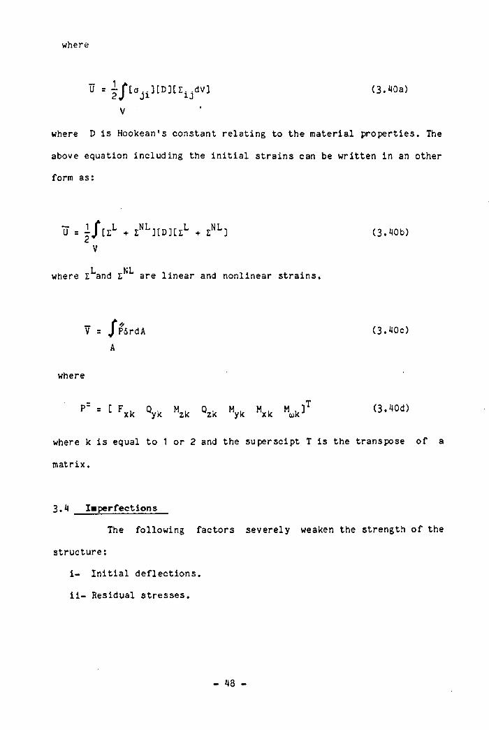
where

U = j/ tO j iJ L D H l j jd V ] (3.40a)

V

where D is Hookean’ s constant relat ing to the material properties. The

above equation including the in i t i a l strains can be written in an other

form as:

U = j / [ Z L + I NL] [D ] [LL + ZNL]

V

L NLwhere Z and Z are l inear and nonlinear strains.

(3.40b)

T . / PSrdA (3.40c)

where

P * [ Fxk °yk Hzk °zk ",k Mxk t k 1 <3 .Wd>

where k is equal to 1 or 2 and the superscipt T is the transpose o f a

matrix.

3.4 ! ■ perfections

The following factors severely weaken the strength o f the

structure:

i - In i t i a l de f lect ions.

i i - Residual stresses.

- 48 -

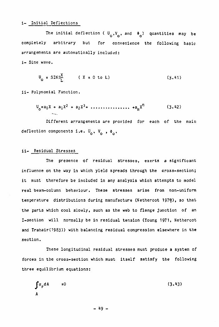
i - In i t ia l Deflections

The in i t i a l def lection ( Uo ,Vq , and i Q) quantities may be

completely arbitrary but for convenience the following basic

arrangements are automatically included:

i - Sine wave.

Uq = SINIljj ( X : 0 to L) (3.41)

i i - Polynomial Function.

Uo=a0X + ajX2 + a2X3+ ............................. +anXn (3.42)

Different arrangements are provided for each o f the main

def lection components i . e . Uo , VQ , 4>o .

i i - Residual Stresses

The presence o f residual stresses, exerts a s ignif icant

influence on the way in which yie ld spreads through the cross-section;

i t must therefore be included in any analysis which attempts to model

real beam-column behaviour. These stresses arise from non-uniform

temperature distr ibutions during manufacture (Nethercot 197^), so that

the parts which cool slowly, such as the web to flange junction o f an

I-section w i l l normally be in residual tension (Young 1971, Nethercot

and Trahair(1983)) with balancing residual compression elsewhere in the

section.

These longitudinal residual stresses must produce a system o f

forces in the cross-section which must i t s e l f sa t is fy the following

three equilibrium equations:

J a rdA =0 (3.43>

A

- *19 -

=0 (3.44)/ ° r YdA

A

j \ Z d A =0 ( 3.^5 )

AI f the measured residual stress distr ibutions do not satisfy

the above conditions, then these stresses must be adjusted until the

necessary balance i s obtained. For I and H sections this can best be

achieved by modifying the maximum web residual stress until equilibrium

resu lts .

Several d i f fe rent forms o f standard residual stress

distribution have been proposed for use in analytical work (O'conner

(1955), Young 1975, Nethercot (1974), Nethercot and Trahair (1983)#

Kitipornchai and Wang-Chung (1985)). Some o f these distributions are

considered herein although because the present study addresses the fu l l

3-dimensional response o f a beam-column some limitations in the

proposals not identi f ied in the context o f 2-dimensional behaviour have

been corrected.

1- Lehigh distr ibution.

2- Parabolic distr ibution.

3- Triangle distr ibution.

1- Lehigh Pattern

Fig. 3.6a i l lu s t ra tes the residual stress distr ibutions used

in much o f the work conducted at Lehigh University. A l inear function

is chosen to represent the var iations o f the stresses along the web and

the flanges, i t can be written as:

- 50 -

o = a o X + a i (3 .^6)

Application o f the boundary conditions to the above equation yie lds

i ) - For the flange

at x = 0 ° fw = a! (3.47a)

at X = B of = a0B + afw

from equation 3.47a and 3.47b, we obtain

(3.47b)

a0° f - g fw

B(3.48)

Substituting equations 3.47a and 3.48 into equation 3.46 yields

equation 3.49, which can be used to evaluate the residual stress at any

point along the flanges.

a1 + afw (3.49)

i i ) - for the web

The residual stress is assumed constant. So equation 3.47

after applying the boundary condition becomes

o = aw (3.50)

where

Oj. is the flange t i p residual stress.

o is the web residual stress w

o^w is the web to f lange junction residual stress

- 51

2- Parabolic Distribution

Recent measurements have suggested that the Lehigh model is

too simple to accurately model the true patterns found in many shapes.

An improvement results i f simple parabolic functions are assumed to

represent the residual stress distr ibutions for both web and flange at

any point along the flange or the web. I t can be written as:

c v= a0X2 + ax (3.51)

Where ao.andaj are arbitrary constants to be determined from boundary

conditions for the web and flanges,

i ) - For the web

at X=0 ow = ai (3.52a)

at afw = a° f * aw (3.52b)

a0a . -a fw w

(3.53)

Substituting equations 3.52a and 3.53 into equation 3.51

yie ld a general equation which represents distributions o f the residual

stresses at any point along the web.

o afw-°

<l>2- x 2 + a (3.54)

i i ) - For the flange

Equation 3.55 can be obtained similar to equation 3.54, by

substituting for the boundary conditions in equation 3.51

- 52

(3.55)o=cr - a- L ^ S x ^

( f ,+ 0f

This distribution is i l lustrated in Fig. 3.6b

3- Triangular Distribution

This is an a lternative simple distr ibution i l lustrated in

Fig. 2c. Equation 3.^7 can be implemented to calculate the residual

stresses at any point along the web or the flange noting the change

in boundary condition required. More sophisticated models (El-Khenfas

and Nethercot 1987a), including any arbitrary pattern which sa t i s f i e s

equations 3. **3, 3. ^ , and 3.^5, may readily be incorporated.

3.5 E q u ilib r ia « Equations * 1 2

Two methods are employed herein in order to obtain general

equilibrium equations for d i f fe rent kinds o f open thin-walled sections

under a variety o f loading and boundary conditions, which are:

1- Virtual Work

2- Total Potential Energy

3.5.1 By Virtual Work

Using Appendix A, assuming the terms containing the products

o f W in the shear strain i . e . W W and W W , to have significant |X tx fy • x z

magnitude so that they cannot be assumed equal to zero, in equation

3.38 the general equilibrium equation o f an arbitrary thin-walled open

cross-section can be written as:

- 53 -

L

; ÌEA[{W ♦ -(U 2 + V2 + p2$2 )' ,x 2 ,x ,x M ,x

O L.

- Y(V $ + U ) - ZCV -U *),xx' ,xx‘ ,xx ,xx

ES- Y * U + Z V Í - — ^ } 6W ]s ,x ,x s i x ,x EA , X ,x

- EAy /w 6(V $+U ) + —(U2 + V2 )L ,x ,xx ,xx 2 .x ,x

+ V , x \ x - V , x U,x )}6U ,x x j

* “ V ' V , * ) * * zt > * V U

- EAr[,,.x5 i ï ,xx-U.xx*> ♦< F<“ îx * v ix>

+ Y $ V - Z 4> U }5V ]s ,x ,x s ,x ,x , X X J- E#W,xt (u ,x ‘ , x ) * 5E#lYI * 2l 1‘ % 5V,xx

+ El ÿ 64> + EI [V 5(V -U $ )a) ,xx ,xx y ,xx ,xx ,x ,x

- 6 CU V # ) - Z $2 ÔV ] ,xx ,xx s ,x ,xx

+ El [U Ô(U +V $ ) - 6(U V i ) - Y $2 6U ]z , x x , x x , x , x v , x x , x x s , x , x x+EI [ 6(U „V - u *U „ + V 4>V ....yz ,xx ,xx ,xx ,xx XXXX

■ u « ( * U ) - $2 (Z 6U vv + Y.ôV vv) ]y X X y X y X y X S y X X s ,xx

El [ SU (V * * U „ „> } ♦ ♦ „ „ 6($my ,xx -, X X , x x ,xx ,x

♦ El [ ô{4> ¥¥(V ¥¥ -U ¥¥$)} - » ¥¥ô(* ¥u ) - zV j î .xx]UlZ i X X i XX y X X i XX |X |X 5 f X

-ES [W + ^ (U- + V* ) + Y í V - Z 4> Uü> , x 2 . x , x , x s , x , x s , x , x

- 54 -

+ ^ ( Y * ♦ z 2 ) J 6 $ , x x 2 s 0

* * V l * % U.xx> * e25“ % v ,xx> * KG\ x 5* .x

piv 6V + U 6U + Z 6{4 (V 4 + U „ ) }9 A ) A | A I A 0 I A I A I A

Yc6{4> v (V y - U * ) } ]S | X f A f A

M 4 64 Y + M 6{4 (V -U ¥4)} - M 6{4 v (V * ♦ U ¥ )}P 9 A f A ¿ . y a f A 9 A y | A f A 9 A

4 - W (V 4 + u v ) )» 9 X 9 X , X

(U 4+U 4 ) + V (V,xx ,x ,x *x

► W (V ,x ,x + U 4) )t X

+ y 6tv (v 4 + v * ) + u (u 4 +v 4 ) } ]s ,x ,xx ,x ,x ,x ,xx ,x ,x ,x

M 6 tv (V • + U „ ) ♦ U (U ® ♦ U 4 )x ,xx ,x ,x ,x ,x ,xx

- V (V 4 ♦ V 4 > - U ¥¥(U 4 + V >} + LF.]{ r } jdx (3.56)9 A 9 a a 9 A 9 A 9 A A 9 A 9 A A ^

I f tne h igher order terms such as V U 4 , V V * ,9 X 9 X X 9 X 9 X 9 X X 9 X

W U 4 ,etc. are neglected from the above equation, then i t can be ,x ,x ,x

written as:

L _

/ES

¡EA{W YU - ZVj , X , x x , x x E A » x xO L_

) 6W „ ]

E W ,xi U ,xx - EA2* , x 6V,xx * E I z U,xx6U»xx + EV , x x 5V,xx

+EI « 54 +EI 6U V + E l 6* U + E l 5(4 V )u ,xx ,xx yz ,xx ,xx uy ,xx ,xx u>zu ,xx ,xx'

-E S W 54 »xx + KG4 v54 vCO 9 X 9 X 9 X

+ Ptv 6V + U 5U ♦ Z 6(4 u ) - Y 5(4 V ) ] , x u , x , x , x s T , x , x s v , x , x- 55 -

(3.57)

M i 6$ „ + M 6( 4 „V ) - M ,6(4 U ) + Q ,6(V 4)P »x »x x ,x y ,x ,x 'y ,x

Q 6(U 4) + M 5(V U „ - U V ) + LF.Jtr} idxx ,xx ,x ,xx ,x 1 !

For a doubly symmetric section, tne above equation reduces to

J jEA(W 6W ) + El U 6U + El V 6V + El 4 64v ,x ,x z ,xx ,xx y ,xx ,xx u> ,xx ,xx

+ KG* 64 + p[V 6V + U 6U ],x ,x ,x ,x ,x ,x

+ H 4 64 + M 6(4 v ) - M 6(4 u ) + Q 6(V 4>)P ,x ,x z ,x ,x ' y ,x ,x ' y , x '* V ' “ , « * ' * Mx6( , ,xxU.x - “ ,x .V,<> * [F iHrJjdx (3 . 58)

The general equation obtained from Appendix B ,where tne

product terms in tne shear strains i . e . ( W W and W W ) arenotf X ty »x »z

included can be written as:-

L

/ | e a LW + ±(U2 + V2 + p242 )! tA •A tA

- Y (V 4 + U ) - Z(V -U 4),xx ,xx ,xx ,xx

ES- Y V 4 + Z U 4 -----^4 } 6W ]s ,x ,x s ,x ,x E p x . X J

- EAYtW + { 1(U2 + V2 > - Y 4 V „• A C # A f A O f A # A

* V , x U.x - b n * z i > * % 3{ u ,x x

- EAZ‘ V l I l u Z x * v(x > - V . x v .x

t Z 5 t , X U , X > - J I > - i ( i I W 2 S 1‘ 2. X ) i i V . X X- 56 -

XX+ El $ 6$ - El iu $-V -Z } fiVu) , x x , x x y , x x f , x x s 2 ,$2

$2+ El (V *+U -Y — } 6U z l , x x * , x x s 2 i X X-El HU - V + Z 4>U2 } 6U yz ,xx ,xx s ,x ,xx

- {V * + U „ + Y j 2 j 6 V „ 1,xx X X S , X , X X '♦ E l , [ ( $ - Y $ 2 ) 6 U w + (V v v * «• u > 6 *uoy ,, x x s , x , x x , X X , XX♦ E l „ [ ( * - Z * 2 V )5V - c u ♦ - V )S*0)Z ,, x x s , x , x x , X X , x x

- E S LW + - { U 2 + V2 } - Y * J „ + Z * , x UU) , x 2 » X . X S f X «X s 9

p n + zv * 2, xi * * ' * *

e i 2 6$ +B 5( i 2 u ) + B 6( i 2 v ) + GK$ 6<J>to ,x ,xx y ,x ,xx Mz ,x ,xx ,x ,x

+ P[V 5V + U 6U + Z f i i * Y ( v * + U ¥) }f A f A | A ) A O f A | A 9 A

- Y 5t$ (V +U $ ) } ] + M 6( U t> + V — ) s ,x ,x ,x y ,xx ,xx 2

*2+ M # 6* + M 5 IV * - U — + F , ( r } jd x

p | X | X L | X X | X X 2 1 I (3.59)

Neglecting the higher order terms ( U V * , ^ U w vV2 ,

e tc . ) in the above equation, then i t can be written as:

L _

/ES

EALW - YU - ZV 36W,x ,xx ,xx EA »xx »x

EAYvJ 6U - EAZtf 6V + El $ 6$ - El V 6V,x ,xx ,xu ,xx 0) ,xx ,xx y ,xx ,xx

El U 6U +E1 (V 6U + U 6V ) z ,xx ,xx yz ,xx ,xx ,xxu ,xx'

- 57 -

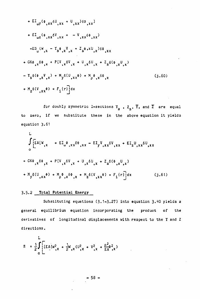
+ El U ¿U + U ) 6$ 3U>y |XX , x x , x x , xx+ El (# 6V + - V Si )U)Z ,xx ,xx ,xx ,xx

-ES (W - Y i V + Z i ,xU )$$0) • X s ,x ,x s ’ ,x ,xx

+ GKi Si + P[V 6V + U 6U + Z S( i U ) ,X ,x ,x ,x ,x ,x s ,x ,x

- Y 6<i v ) + M S ( U i ) + M i Sid | A f A jr f A A P | A ) A

(3.60)

+ M 6( V i ) + F i r } jd xZ i X X X |

for doubly symmetric I-sections Y , Z , Y, and Z are equals s

to zero, i f we substitute these in the above equation i t yields

equation 3.61

/ • EAtW El i 6$ u ,xx XX - EV . x * s\ XX El U 5U Z ,XX , x x+ GKi Si + P[V SV + U SU + Z 6( i U ),x ,x X ,x ,x , x .X ,x

+ M S ( U i ) + M $ S i + M S ( V i ) + F . { r } | d xy ,xx p ,x ,x z ,xx (3.61)

3.5.2 Total Potential Energy

Substituting equations (3.1-3.27) into equation 3 .HO yie lds a

general equilibrium equation incorporating the product o f the

derivatives o f longitudinal displacements with respect to the Y and Z

d irect ions.

n = • [EA{w2v ♦ h y (l)2v + V2y + 1^2 )j* :• ,x 2 t X ' " , x ,x EA' ,X'O L.

- 58 -

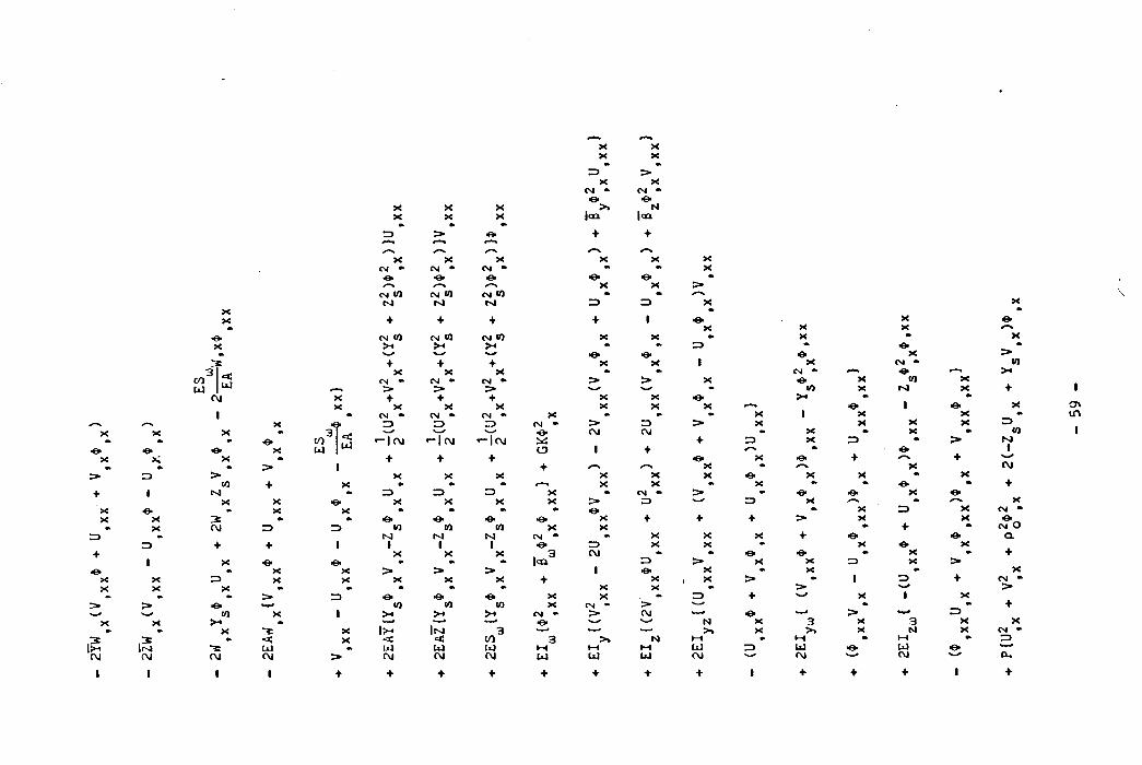
XX«kzd

XCM •dX X X , >*X X X |oa•k •k »zz> s* d +✓—N «""«k ✓ -n

X X X XCM • CM * CM • ••di d *0i d/-> XCM CO CM *0 CM W •kpsj M INI ZDXX + + + +

•e* CM (0 CM (0 CM 10 XX X X X *•k •k_ «ta/ d: + ♦ ♦ X3 X X X •

CO *5« CM • CM *• CM * >UJ U} > > >CVJ X + + ♦ XX X X X X

1 • CM • CM » CM * X »x—v X d ZD ZD ZD CM • >X X X • 3 T 'W' N-/ *0i (M•k • •e* CO 5 *— 1 CVJ •— 1 CM *“ 1 CMd d d X LU 1w O 1X K X «k + + +•k «k • > 1 + y—N

P» ZD > X X X X(0 + X • •k •> r-k X+ 1 M •k zz> ZD ZD X «X X e* X X X X >•X d * X X •* » •k •k dX X 3 «k » d d d d X•k X CVJ ZD ZD (0 CO CO X X

zd « M M M CM • •kzd + + » 1 1 d ZD

+ X X X . 3 CM1 X d d « •k •• |ca

d •k X X > > > 1X X ZD X X X X X +X X X « •k • • » X•k •k •k zd d •e* >e> X XD* > O kW (0 (0 CO X CM •*(0 X I X CM • >X X X a. -y* «-*«* OX X \ x Im 3 W-».ne •> < X <c < CO 3 >»\ x |rs| UJ •k LU UJ UJ M »-»CM CM CM CM > CM CM CM UJ LU1 1 1 1 + + + ♦ + +

XX>XOl » d N|qû+

X X•k Xd •kX» ¿»—kk

ZD X•k1 diX XX » X•» ZD •

di dX 1 X•k CM -> X d X•k «0 XX d >-• •X X *1 d•k •k X 1 XZD > X XCM » X »

+ ZD X ZD+ •k

d X d +/«-N X •kX X d X XX •k X •• •

CM • z> • d dZD •k—* ZD X y""V•k X+ + + X»X X X + dX X » X» •> d d *ZD >► X X ZDd X •• XX , X > • 1X •k >«k ZD + »W» X> •k—* »

CM kW d >s_<* M X 3 Xw* >» X >> XN l-H « M «kM UJ ZD UJ dU1 CM CM w+ + 1 + +

V.X•k

X dX «»-s» Xd »X >

CM *• 10d r—k X

CO XN X + 1

•k1 d X o>X «k mX X ZD 1X « CO

•k > Md t/N + s»-*

X CM•k Xd +X d« «k X

ZD X CM •X d+ » CM Od Q .d XX » +X >

m XZD + CM •

> •1 X

« +w * ZD3 X XM X CM *l-H •k ZDU J d w *CM Ou

♦ 1 +

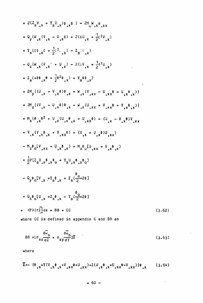
+ 2 (Z V + Y U )* * } - 2M W t>S , X S , X , X * U ,x ,xx

+ Q (W (V - U » ) + 2 (tU + -!<-2v )y . X ,x ,x ,x 2 . X+ Y (4$ i + - : 2 , ) - Z M }s ,x 2 ,x s t x J

- Q (W (V * + U ) - 2(vV + )

+ Z ( -1$ 4> + - U 2$ ) - Y §} } s ,x 2 .x s ,x

+ 2M { (U - V * ) * „ - w (Vy .x 1t X f X 1>x , XX

♦ 2M { (V v - u v* ) * v - w (U +z ,x 1i X | X 1.x , XX

+ M {$ i 2 + u (U 4> + u .*> -x ,x 1 X X X , XX

V t + V * ) }, x x ,x ,x

, x ,x ,xx

- V (V 4> + V $) + (V - U 4>)U }, x v , X , X , X X , X , x , x x '- H H Y - U 4 ) + H t [u + V 4> )z o ,xx ,x ,x z o ,xx ,X ,x

+ 2P [ Z s V, x $ , x 4o + V . x* . x* o3

- V c [ v , x + V , x + V f * 2 * 3+ V o t U ,X +Z3* ,X - V i r 24]

+ <P>tr}Jdx + BB + CC

where CC i s defined in appendix C and BB as

doj du>BB =L a — - + a — -]X

xz dZ xydY

where

X=- {* +Y(V * +V *+U )+Z(U * +U i - V )}4>,x ,x ,x , x x , x x ' ,x ,x , x x , x x ' ,x

C3.62)

(3 .63 )

(3 .6 4 )

- 60 -

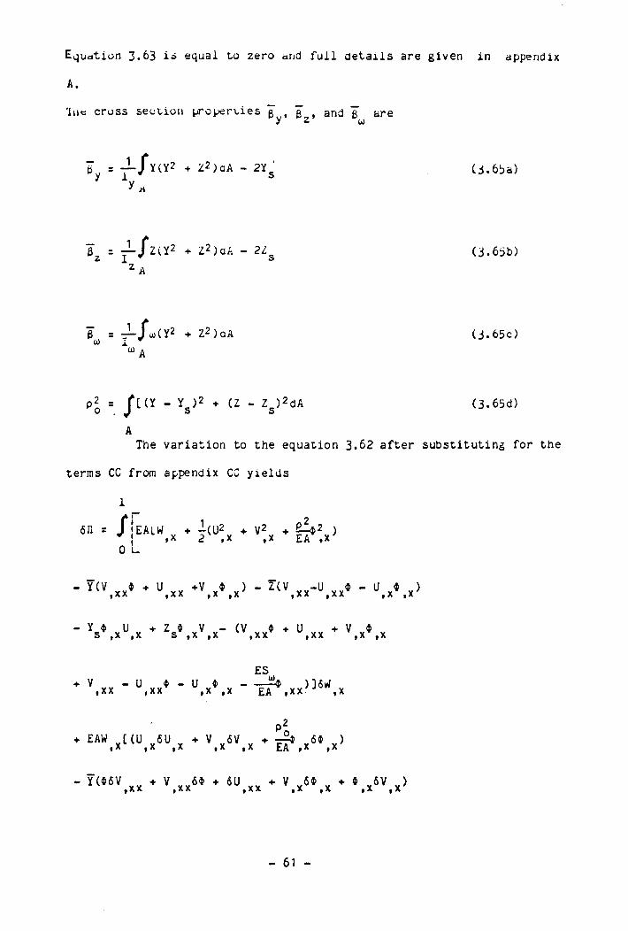
Equation 3.63 io equal to zero arid fu l l deta i ls are given in appendix

A.

Tuc cross section properties g , « and "ft arey 2 uj

is = — J y (Y2 + Z2 ) aA - 2Yy 1 y Sy A ( 3 .65a)

0 z j - / z ( Y 22 A Z2) dA - 2Z5 (3.65b)

0 = 4-Ju)(Y2 + Z2)aAi<\ t ▼U) 1 ( 3 . 65c)

= f [ ( Y - Y )2 + (Z - Z ) 2dA J s s ( 3 .65d)

The variation to the equation 3.62 a f ter substituting for the

terms CC from appendix CC y ie lds

1

6II = J jEALW w + 4(U2 + V2 + 2 )»x

0 L-2 ,x ,x EA »X

- Y(V 4 + U v +V 4 ) - Z(V . . U ..„4,xx ,xx ,x ,x' ,xx ,xx

- Y j u * Z t V - (V 4 + U + Vs ,x ,x s ,x ,x ,xx ,xx

ESV - u 4 - U 4 ----- ^4 )]5W, x x , x x , x , x E A , x x ' J , x

♦ EAW [(U 6U + V 6V ¥ «• -=$ 64 y )|X |X tx • x ix EA $x yx

- I ( tSU ,x« * \ x x 4* * 4u,xx * v .x4\ x * ‘ ,x4\x>

- 61

- 29 “

xx* ,x* x* x* x4 X X 4 X X *A9{( * n+ * A) - <4 n - A ) } ] 13 ♦

X* „X* , ,x* , „ x 4 Xxx* „ X X * X„x4 xxro XX* „XX* m*9 4>J0+ { ( *9 * 42+ 49 z 4) _|+ 49 4} 13 +

V * V * O S Y * Y * Y * Y * Y Y 1

{ 49 4 ( | z + J « + A9 A ♦ 09 tl} 4 +

x x , 4 9 { x ‘34 c| z - ? a ) * x ; a - Xzn}| +

. X ' X 4 X X * ^ x ' . x ' X X ' X X * . „ X * . X * s„( 09 t 4 + 49 (1 4 + 49 4 fl) Z -

/X*inx‘ xx* x* x4 xx* xx4 x4 x4 s T.c> . ( A9 4 4 + 49 A 4 + 49 4 A) I ] S3 *

r ,X* x‘ S S„x X* „X*. x* x* xx* „[ { 49 4 ( j Z + zìi) + A9 A + f l9 fl} A ♦

xx , a9(x ; « ? z* i » * x ; a * x; n)f *

, x ‘ x4 xx4 X ' * ' X X ' , X X * . „ X * Xx4 s „( n s 4 A + 49 n A + A9 4 n ) z -

, X * X* XX* X 4 X 4 XX* XX* „x* x* s ,( A9 4 A + 49 A A + A9 4 A) A l ZV3 ♦

. . x ' „ x ‘ , s „ X* „ x ‘ X* X* X X *[ { 49 4( j Z + j A ) + AS A + fl9 fl} fl

XX*__ X* . , s _ s .n9{"z4(jZ + Z*> + *zA + X2n) f +

,X* X4 XX* X‘ „X4 XX4 XX4 x4 x ‘ „ s( ns 4 n + 4 9 n n + n s 4 n ) z -

,X4 X4 XX4 X4 X4 XX4 XX4 X4 X4 s , „ _( A9 4 n + 49 A n + ns 4 A) A]AV3 +

,xx4.„V3 x4 „ x ‘ , X4 „ X 4 .XX4 XX' XX449^—* - " n s « - 49 n - 49 n - ns4 - a 9 ♦

S3

X* X4 X4 „X4 XX4 „ „XX4 XX4AS 4 + 4? A+ nS + 49 A + A94)

, X * X* X 4 „ X 4 . S , X 4 l n X 4 X 4 x 4 s( 49 A + AS 4) z + ( 49 n nJ 4 ) J

,X* X4, X4 nX4 XX4 . . , .xx ‘ XX4.n>„( n9 4 - 4 9 n - n94 - 4 9 n - a 9 ) z

- £9 -

, xx‘ . xx* X X * X X * . . ,zm _( A9 * + $9 A)] 13 +

r , x x ‘ n , X ‘ X* V . , X ' X ‘ - . X X ‘ , X ‘ . x ' x x ' x * X*,XX*[ { 49( fl“ A) ♦ ( ns- A9) 4} 4 + 49( * fl ” A 4) ♦

X* X* fi X* X* X* X* XX* XX* XX*[ { *9 * Ä2- A9 4“ *9 A- A94 ♦ *9 A} 4 ♦

xx‘ . « / x ‘ *s t x* x* . x x V .J m 49( z4 A “ 4 A “ 4 A)] 13 ♦

,xx* xx* xx‘ xx* N,Aoo ( n9 4 + 49 n)] 13 ♦

xx‘ « « / x , -x‘ - x‘ x‘ . .xx*n9c 4 n ♦ 4 a + 4 n) -

r , x * X * X* X * x * X *[ ( n 9 4 + 49 n + A9 4

X ‘ X * x x '49 A + ft94 ♦ 49"" Í1)"" fl +

, X* X* X* x‘ x‘ x*( 0 9 4 - 49 O “ A9 4 +

X * X ' X X *49 A + A94 + 49"" A)"" A *

xx‘ ,x* x‘ x‘ x‘ xx* ,zA _A9( 4 A + 4 fl “ 4 A)] 13 +

,xx* xx* XX* xx* zA _( n 9 A + A9 n) 13 +

X* x* xx* xx* x* ,z x* x* x* .X*[ { ( 49 4 AS + A9 24) j? + ( f!9 4 “ 49 fl "

X* . . X* X* X* XX* X X * ____. X X 1,A9 4 49 A + 49 A + A94) fl ♦

xx‘ n9{(xV ‘ n - xV ‘ a) ♦ ( xx*n - 4xx‘ a) } ] zi 3

r X* X* , X X * X X * „ X ‘ . v A „[ J9 4 (1Ü + 09 z4) j? +

, , X * X * X* X* X* X* X* „x* xx*( ( 09 4 + 49 n ■*■ 49 A + A9 4) A ”

( XX 094 + 49A~ n ) }A" A “XX* , xx*

♦ EI [ (-U 4 - U 4 - Z 42 )64», x x * , x \ x s , x ' , x x4 {U 64 + 46U +U 64 +4 6U - 2Z 4 4 64» } ]t x x , x x , x x , x , x , x , x s , x x , x , x(4 U + V 4 )64 - 4 {4 (6U + 6V ) + (V +U )64 } ]

, XX , X « X , x x , x , x , x x , x , x , x , x , x x JP tu £ U + V 6V + p24 64, x , x , x , x F o , x , x

* l 2 s U , x - V , x ) M , x * » . « ‘ W W '♦ « #CZ 6V ♦ ï 6U , )I A & I A d I A

+ (Z V +Y U )4 64 + (Z V +y U v )464 „ ]s , x , s f x , x s , x ' s , x+ v“ $U y )ÔW *+W y (6V v-U v0i- $SU v>¿ y Ia tA fA Ia »a |A

♦2(46U +U 64+V 464+^426V )|X iX » X 2 fX

♦ Z (^4264 + 4 464-244 v64-4264 v )5 2 » X t* »x

- Y (464 v ♦ 4 64)]5 » X » X

- ^Q_[(U +4V ) 6W +ki ( 6U Y+V 64+46V )¿ Z Ia Ia Ia Ia I a f A I a

- 2(46U +U 64+U 464+^42öU )|X j x t x 2 fX

+ Ze( i t 264 „ + 4 464-244 64-4264 )5 ¿ | X » X » X f X- Y (454 + 4 64 ) ]

5 • X t X

♦ M [U 64 +4 6U -V 4 v64-V v464 v-44 v6V YJr i a J A i A i A i A y A f A f A | A f A

- (V - U 4 - U 4 )6W, x x , x x , x , x ' , x- W { 6V - U 64 - 461) - U 64 - 4 6U } ], x , x x , x x , x x , x , x , x , X , J

- 64 -

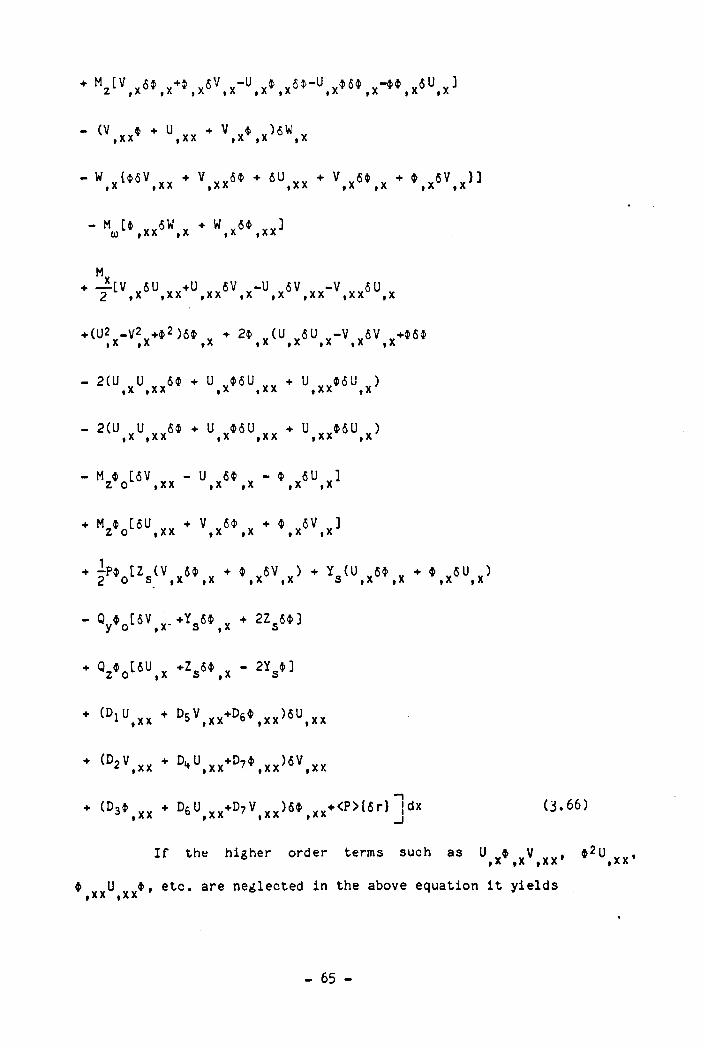
M_[V 6$ Y+i 5V -U * 5*-U ¥$6$ ¥-** ¥6U ]¿m y A | A | a | A | A | A | A | A | A f A

- (V * + U vv ♦ V * )<$W,xx X X ,x ,x ,x

W ii>5V + V 54> + 6U + V 6$ + 9 6V } ]I A | A A | A A | A A | A y A y A | A

M [* yySW + W 6* ](|) | X X | X | X | A A

Mx— tv 5U +U 6V -U 5V -V 5 U2 ,x ,xx ,xx ,x ,x ,xx ,xx ,x

+ UJ2 -V2 +$2 )S4> v ♦ 2* V(U 6U -V 5V v+*5*y X y X y X y X 1 X y X y X y X- 2(U,xU,xx6* + U,x$6U,xx + U,xxtSU,x )

- 2CU U 54> ♦ U 4>5U + U 4>5U ),x ,xx fx ,xx ,xx ,x

- m,M 5 V ¥¥ - U y6$ y - $ SU ]Z 0 y X X y X y X y X y X* M n [6U n + V ¥{$ x + 4 x6V * ]¿ 0 I XX yX yX y X yA

* j W V * . « * * . x sv .x> * W \ x * » . x ^ x 5

- V o tSV. x - * V * . x * 2Zs5tl

* V . “ » , x * z, s t ,x - 2V ]

* lD>u,xx * D5v ,xx'fD6*,xx )5U,xx

* <D2 V , X X * ft.u, „ * M , x x ) « * , „

♦ (D3* . „ * D6u,xx*D2Vixx)«»,xx*<p> l«r) j d x (3. 66)

I f the higher order terms such as U 9 V , $2U v v ,y X | X | X X f X XU 9, etc . are neglected in the above equation i t y ie ldsI X X y X X

- 65 -

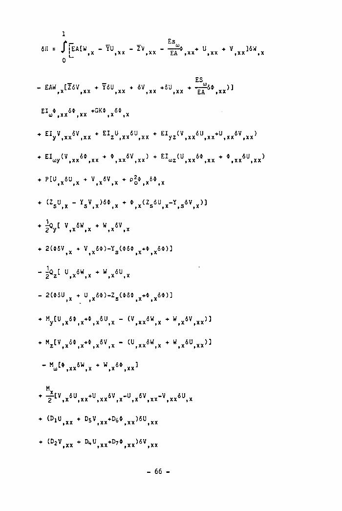
■ X Es611 = J !EA[W - YU „„ - ZV + U + V ] 6WXX ,xx EA *xx ,xx fxx ,x

ES- EAW [Z6V + Y6U + 6V +6U + — ^6* ) ],xx ,xx XX ,xx EA »XX

El 4 64 +GK4 64U) »XX »XX »X »X

♦ EI V ÔV + El U ÔU + EI (V ¿U +U 6V ) y ,xx ,xx z ,xx ,xx yz ,xx ,xx ,xx ,xx

+ EI (V 64 + 4 6V ) + El (U 64 + 4 6U )ojy ,xx ,xx ,xx ,xx u>z ,xx ,xx ,xx ,xx

PLU 6U + V 6V + p24 64,x ,x ,x ,x ,x ,x

+ (Z U - Y V )64 + 4 (Z 6U -Y ÔV ) ]S »X S »X »X ,x ' S ,X ,S »X J

♦ -¿G [ V 6W + W 6V 2 yL »X ,x ,x ,x

♦ 2(46V + V 64)-Y (464 +4 64)3I A y A i A i A

- ¿ V ü,x5\ x * “ ,xSU,x

- 2 (45U + U 64)-Z (464 +4 64)3I X i X 5 i X i X

+ M [U 64 +4 ÔU - (V ÔW + W ÔV ) ]y ,x ,x ,x ,x ,xx ,x ,x , x x 'J

* " z ‘ W \ x 5V,x - ^ . x x ^ . x ♦ “ ,x {U,xx>J

- M [4 6W + W 64 ]u ,xx ,x ,x ,xx

♦ — (V 6U +U 6V -U 6V -V 6U 2 ,x ,xx ,xx ,x ,x ,xx ,xx ,x

* lD‘ U,xx * DSv, , x * D6 * , ,„ > Sü. „

* (Dî * . « ‘ D" Utxx*D’ * , x x )SV.xx

- 66 -

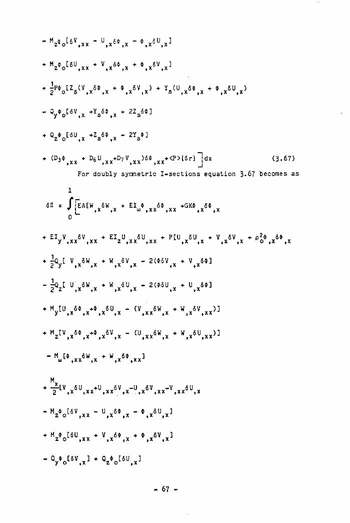
- Mz*o[«V, x * - U, x « * , x - » . x « U,xl

M $ [ 6u + V d$ + * 6V ] z o ,xx ,x ,x ,x , X J♦ —P$ [Z (V 6t + } 5V ) + y (U { » + 4> 6U )2 o s ,x ,x ,x ,x ' s ,x ,x ,x ,x '

- +Y 64> y + 21 ,6*]y O | A d | A O

♦ V » w , x * zs4« , x - 2Ys » ]

♦ « 3« ^ * D6u,xx*’D7V,xx )S t ,xx*<P>l5rl !dx (3.67)

For doubly symmetric I-sections equation 3.67 becomes as

1

<511 = J |EA[W 6W + El » 6» +GK4> 6$* , X , X 00 , X X , X X , X , X

+ El V 6V + El U 6U + P[U 6U + V 6V p2* 6*y ,xx ,xx z ,xx ,xx ,x ,x ,x ,x Ko ,x ,x

k 1 W + W

K [ U.x5u.x + W

M [U 6$ +4> 6 Uy fX .X ,x

M „[V V 64> +$ W5Vz ,x f x f ^■ M [t 6W

id ,xx ,x + W

,x ,x

, x x , x , x , x x

Mx+ — tV 6 U +U 6V -U 6V -V2 , x , x x , x x , x . , x , x x- H 1 [ 6V - U 64» - * 6U „ ]Z 0 , x x , x , x , x , X J♦ W SU.xx * \ x { \ x ♦ * ¥6V ]i * i *

- 67 -

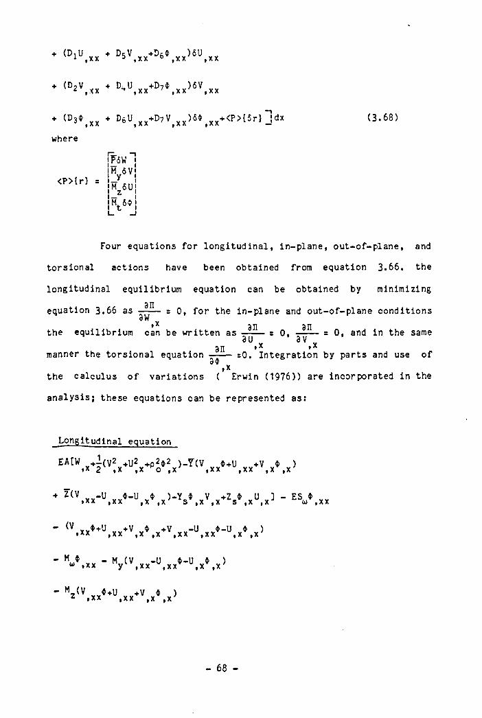
+ (D,U + DtV +Dfi4> )6U 1 , x x 5 , x x 6 , x x ' , x x* <D J V , x x * * D' U , x x * I)’ » . x x > 5 V , x x* <” 3 \ „ * °6U X-»I>7V )6«iXX»CP>[Sr) Jd x

where

( 3 . 6 8 )

¡P5W

¡ V v<p>{r) r t-y 1 1 ¡ M 511 _ z

}M 6*

Four equations for longitudinal, in-plane, out-of-plane, and

torsional actions have been obtained from equation 3. 66. the

longitudinal equilibrium equation can be obtained by minimizing

anequation 3.66 as ------ = 0, for the in-plane and out-of-plane conditions

o W»X an anthe equilibrium can be written as ------ = 0, ------ = 0, and in the same

3U 3V3n »x |X

manner the torsional equation ------ s0. Integration by parts and use o f3$

.xthe calculus o f variations ( Erwin (1976)) are incorporated in the

analysis; these equations can be represented as:

Longitudinal equation

EA[W -4 (V2 +U2 +p2* 2¥ >-7 (V *+U +V * )t X 2 t X f X 0 f X f X X f X X | X | X* Z(V,xx-u ,xx‘ - u . x » , x > - V , x W . x u,x:i - Esu*.xx

- (V 4+u +v * +V -u *-u * )» X X , x x , X , X , X X , X X , x , x '- H { - M (V -U ft—U ft i“ . X X V . x x u , x x * , x , x ;- Mz (V.xx**u ,xx->V,x * ,x )

- 68 -

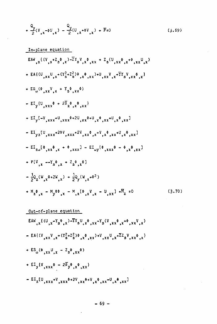
(¿.69)Q Q _

♦ - f (V -fU ) - -£(U +*V ) + P=02 ?x tx » x »x

In-plane equation

EAW {(V +Z i )-ZY V $ + Z (U $ +i U ),x ,x s ,x s ,x ,xx s ,xx ,x ,xx ,x

♦ EA{ (U U + (Y2+Z2 )4> * )+U V +YY V * },xx ,x s s ,x ,xx ,xx ,x s ,xx ,x

+ ES (4> V + Y i 4) O) ,xx ,x s ,xx

- El {U 4 + 26 * * }y ,xxx z ,x ,xx

+ El [-V +U 4+2U 4+U * +U * ]y L ,xxx ,xxx ,xx ,x ,xx ,x ,xx

- E I y z t U , x Xx * 2', V , x x » * 2V, x x \ x * V . x , , x x * u , x » , x x )

- E l, , [* * , , J - El t* # - ♦ « ]Zu) | XX |X f XXX u>y 9 XXX IX } X X+ P [ V — Y 4 + Z t 4],x s ,x s ,x J

- ^3 (W 4+2W ) + ¿Q (W +42)2*z ,x ,x ' 2 y ,X

♦ H ♦ - M i * - M [4 V - U ] +H =0 z ,x y ,x ,x ,x ,x ,xx z (3.70)

Out-of-plane equation

EAW, x l < U , x - V . x > - T l s U, x \ x x - V v , x x \ x * ‘ . x x \ x >

E A I < \ x x \ x * « I * Zl > \ x ‘ , x x > * V , x x V I Z s V, x , ' t ,x>

+ ES (4 U - Z * 4)U) ,xx ,x s ,xx

+ El (V * - 2F * 4 }y 1 ,xxx y ,x ,xx

- El [U +V 4+2V 4+V 4 -U * ]z ,xxx ,xxx ,xx ,x ,xx ,x ,xxJ

- 69 -

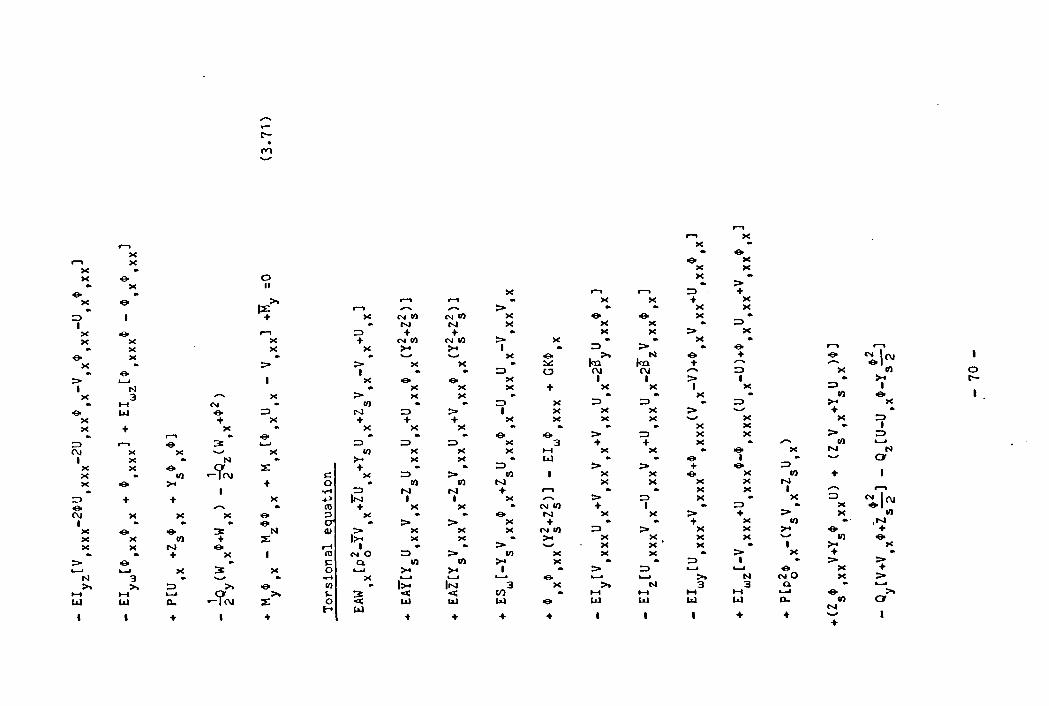
Xr—i X

X •>X •e* o•» X II

•»X ■e* , > » r—»•k r—i y*>k

r> 1 + X cg COa »X •©- n rD +X X X + cg (0

X X X > ««9* X • *

X •> > > X« 9 •

> U l 1 X «©•1 N «• XX 3 X > X•» M cg • CO »

■e* U l ZD INI ZDX + X + +X + X •> X X

•k •k «k •r - » •& U—1 =>

X X U i X CO X1 X •k N •k > « XXX

Xco - 7 « ,

3 :c

♦X rD

X 9 > * + o « CO»rH r> M

r> + + X fly** «k CD ♦ X

CVJ X X X o X •1 » «k e e r «k >X o « N a> > XX X CO + s : l>? XX X M *©• rH »«k •k + X i CD cg O :r>

> e> •k C Q. 10t—i L -l X X o U i

M 3 «k •H X t—1> » X zd > » ■e CO » l> *

H »-H U i e r > » u <W U ) Ou •~T<m s : o *< w

H U4« 1 ♦ 1 ♦ ♦

X

♦

EAZ

[Y

V V

-ZV

U

+V

* (Y

2+Z2

) ]

r*

V V

x»

e

V

V

w

w V

»#

'

e

b ’

•

- E

M

...

»OK

*

(3.72)

♦ M ru -v $+w u -v » ]y ,x ,xv ,x ,x ,xx*

+ M [V -U *-W V -U * ] Z ,x ,x ,x ,x ,xx

[U2 +V2 - î>2-4 * ] + M. =02 ,x ,x .x

Neglecting higher order terms U $ ,V V , U U ,i X X | X | X X fX f X X f Xfrom equations 3.70 3.71» 3.72 yie lds the following equations

Longitudinal equation

EAN + P =0 (3.73)

In-plane equation

+ El U - El V - El U - El *z ,xxx y ,xxx yz ,xxx z u i ,xxx

* P [V,X — V . x 1 - V . X * V . X

+ M $ +• M U +M =0z ,x ,x ,xx z (3.7*0

Out-of-plane equation

♦ El U - El U - El V - El *z ,xxx y ,xxx yz ,xxx yu> ,xxx

♦ P[0 + Z t ] - Q W + Q W,x s ,x z ,x y ,x

+ M * + M U +M =0z ,x ,x ,xx z (3.75)

Torsional equation

- 71 -

etc.

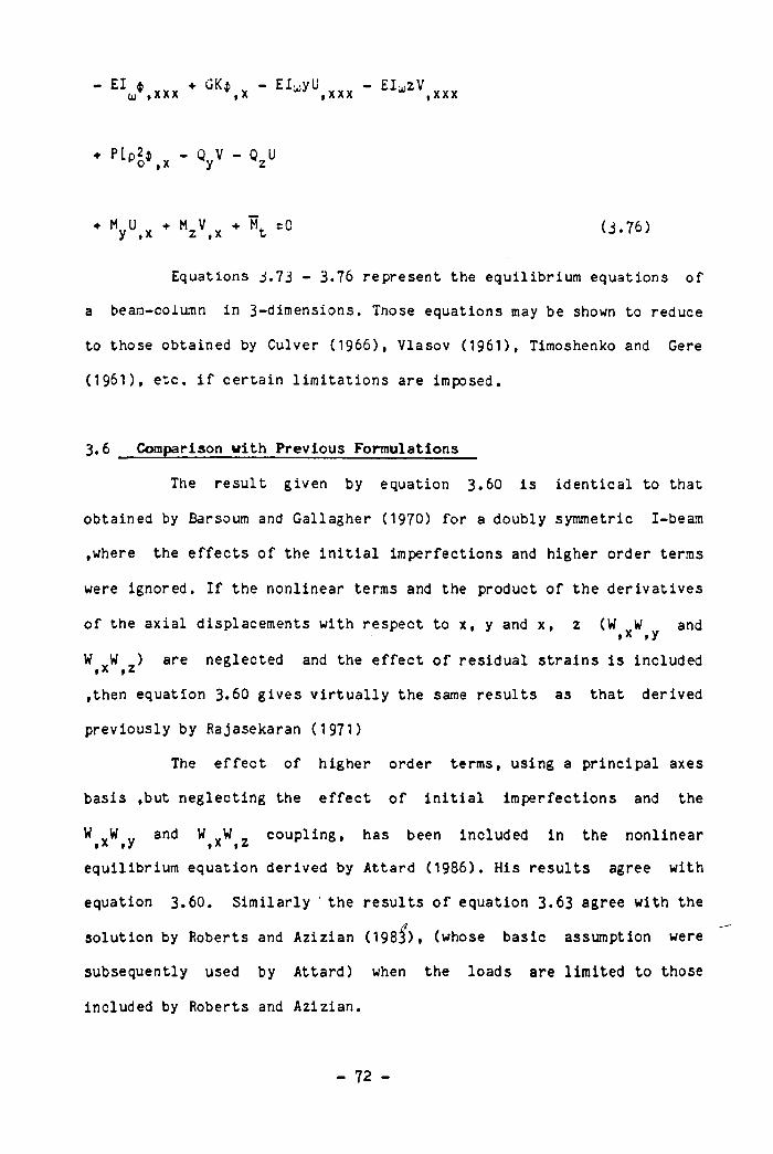
- El « vvv + GK$ - El^yU vvv - EI^zV0)' ,xxx ,xxx ,xxx

♦ Plp2i - Q V - Q U ko*,x y z

MU +y ,x

M_ V Mt =0 (3.76)

Equations ¿.73 - 3.76 represent the equilibrium equations o f

a beam-column in 3-dimensions. Those equations may be shown to reduce

to those obtained by Culver (1966), Vlasov (1961), Timoshenko and Gere

(1961), etc . i f certain l imitations are imposed.

3.6 Comparison with Previous Formulations

The result given by equation 3.60 is identical to that

obtained by Barsoum and Gallagher (1970) for a doubly symmetric I-beam

»where the e f fe c ts o f the i n i t i a l imperfections and higher order terms

were ignored. I f the nonlinear terms and the product o f the derivatives

o f the axial displacements with respect to x, y and x, z (W W andi x ? y

W W ) are neglected and the e f f e c t o f residual strains is includedf X f z

,then equation 3.60 gives v i r tua l ly the same results as that derived

previously by Rajasekaran (1971)

The e f f e c t o f higher order terms, using a principal axes

basis ,but neglecting the e f f e c t o f i n i t i a l imperfections and the

W W and W W coupling, has been included in the nonlinear

equilibrium equation derived by Attard (1986). His results agree with

equation 3.60. Similarly ' the results o f equation 3.63 agree with the

solution by Roberts and Azizian 098^), (whose basic assumption were

subsequently used by Attard) when the loads are l imited to those

included by Roberts and Azizian.

- 72 -

The s t i f fness matrices obtained by Yang and McGuire (1986)

for symmetric sections, using the principal axes, neglecting higher

order terms and residual stresses and including the products o f

derivatives o f the axial displacements with respect to x, y and x, z

respectively i . e (W W and W W not equal to zero) are similar to

equation 3.57 when the higher order terms such as (4>2 U , V ** ,fX | X X | X X | X Xe tc . ) are assumed equal to zero.

The present formulation enables the l imitations o f ea r l ie r

studies (Barsoum and Gallagher (1970), Rajasekaran (1971). Rajasekaran

and Murray (1973). Vinnakota (1977), Nishida and Fukumoto (1985), and

Attard (1986)) to be ident i f ied . Table 3.1 summarises the findings.

Table 3.2 presents a comparison between the assumptions that have

employed by the Author and those used previously [Rajasekaran (1971),

Rajasekaran and Murray (1973), and Chen and Atsuta (1976)] to develop a

formulation for beam-columns in space. Complete derivations o f the

l inear and nonlinear tangential, geometrical, and strain-displacements

matrices are presented in Chapter 4. In this context i t is particularly

important to note that further use o f these formulations as the basis

for ine last ic analysis o f b iaxia l bending leads to e f f e c t i v e cross-

sections for which several assumptions that might have been valid

within the e las t ic range e .g . doubly symmetric, shear centre and

centroid coincide e tc . , are no longer correct . The importance o f not

resorting to such s impli f ications i s c lea r ly i l lustrated by the use o f

the present formulation in a var iety o f example problems (El-Khenfas

and Nethercot (1987b,c), and chapters 6 and 7 respect ive ly . Specific

l imitations in previous studies include:

- 73 -

1- Neglect o f higher order terms and/ or the e f fe c ts o f residual

stress

2- Using the principal axes for an arbitrary cross-section and

neglecting the sh i f t o f the shear centre and the centroid even

in the e last ic range.

3.7- Conclusions

A method has been used to derive the general equilibrium

condition for thin walled beams o f arbitrary cross-section under

general loading. The e f f e c ts o f higher order terms and in i t i a l

imperfections have been included. The method is based on the principle

o f v ir tual work, where the product o f the der ivat ives o f axial

displacements with respect to x, y and x, z (W W and W W ) are,x ,y ,x ,z

accounted for in equation 3.60 or a l ternat ive ly are neglected in

equation 3.57. An a lternative derivation i s also possible, based on the

use o f energy theorems leading to equation 3.63.

Both methods compare very well with the available theories

.permitting their simpli f ications and l imitat ions to be c lear ly

ident i f ied . The va l id i t y and accuracy o f this theory has been

demonstrated in several applications (El-Khenfas and Nethercot

(1987b,c)) and Chapters 6/ 7 respect ive ly , ,which cover both e las t ic

and inelast ic analysis.

- 7 4 -

Table 3.1 Comparison between the author's formulation and previous studies

I<~n

Method o f a n a ly s is

An a lys istype

Im p erfec tion s Axissystem

H.O.T. o f s t r a in d isp , r e la t io n s

Producto fW,xW( ytW(XW<2

N on -lin ea r

Author kg *Z o fs tra in s

Notes

1970 Barsoum and G allagher En E N P r in c ip a l N N N N N 1

1971 Rajasckaran V.W. E, I Y General N N N N N 2

1983 Roberts and A z iz ia n En E Y P r in c ip a l Y N - - - 3

1986 A tta rd En E - P r in c ip a l Y Y N N N 4

1977 Vinnokota F in ite o f d i f fe r e n c e

E, I Y General N N N N N -

1985 Pukumoto t N ish ida V.W. E, I Y General N N N N N -

1986 Yang and McGuir V.W. E, I Y P r in c ip a l N Y N N N -

- Authors* form ulation V.W. ,En • E, I Y General Y Y Y Y Y 5

1. Barsoum and G a lla gh e r* « work 1 » in clu ded s in ce i t i s regarded as the f i r s t coverage o f t o r s io n a l- f le x u r a l e f f e c t s by the f i n i t e elem ent method.

2 . Mote d e ta i ls are g iven in Tab le 3-23. Th is work was performed fo r g en e ra l types o f c r o s s - s e c t io n « , but the Wagner e f f e c t was not included ; i t i s not c le a r e x a c t ly how

n on -lin ea r s tra in s were in co rp ora ted .4. Im perfec tion s were ignored (n o t m entioned ).5. Even fo r e la s t i c a n a ly s is in c lu s io n o f h igh er o rd e r terms in the s o lu tio n has a s ig n i f ic a n t e f f e c t on the r e s u lts , see C h a p t e r 6

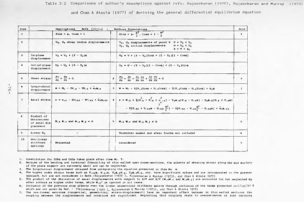
Table 3 2 Comparisons of author's assumptions against refs. Rajasekaran (1970), Rajasekaran and Murray and Chan & Atsuta (1977) of deriving the general differential equilibrium equation

Item D escrip tions R efs , ( a b o v e ) Authors form ulations Note

1 Sin<$ - $, Cos<f - l <♦>3 <t>2Sintt> - <j>- - , Coa$ - 1 - - 1

2 _______________ V3, U9 shear cen tre displacements Vs . us displacem ents o f p o in t S V » v a 4 V0 V „, u0 i n i t i a l d isp lacem ents U - U, + UQ

* “ ♦ + «0

3 In-p lanedisplacem ent

v * - V , ♦ <Y - Y0 ) « V* - V + ( Y — Ys )S ln « + (Z - Z , ) [ l - Cos«.]

|4 O ut-o f-p lane

displacem entU, - U, 4 (Z - Z , >« j u* - U - (Y - Ya )[1 - C os «] + (Z - Z5 )S in «

5 Shear s tra in *3 + *2 - od x as 2 ar) + dw + au du + av dv _ o

d x as as ax as ax 2

6 Longitudinaldisplacement W - Wc - ZV.x - YU,x + w „ ,.x 3

—

w - Wc - Y [V , xSin$ + U,xCos<t) - Z (V ,xCos$ - U,xSin<t>) + wn<|> 3

7 A x ia l s tra in e - V, x - ZV,XX - YU, XX ♦ wn<J>,xx 4. 2 2 2

« - “ .X + lifU.X + V ,x ♦ P .xJ - Ys« .x < V .x - u ,x « ) - Z3« ,x f0 , x + v ,x * ) o

“ YfO.xx + V ,x x * - 0 ,xx |-J - Z [V ,xx - V ,xx|---- U ,x x * ] +

8 Product o f d e r iv a t iv e s o f a x ia l d is placement

W.x w, Y and M,x w .z - o 5 H.x W , Y and W,x w ,z " 0 5

9 L inear K q - T o rs io n a l moment and shear fo rc e s are included S

10 N on-lin ear s t i ffn ess m atrices

Neglected Considered 7

1. Substitu tion fo r SIN<$ and COS$ takes p lace a f t e r item No. 7.2. Because o f the bending and to rs io n a l f l e x i b i l i t y o f th in w a lled open c ro s s -s e c t io n s , the e f f e c t s o f shearing s tra in along the mid su rface

o f the p la te segment are extrem ely small and can be n eg lec ted .3. The lon g itu d in a l d isplacem ent obtained from in te g ra t in g the equation presented in item No. 4.4 . The h igher o rder s tra in terms such as V , U , x x $ , Y 3* , x V ,x, Z34 ,xU ,x , e tc . have s ig n i f ic a n t values and are incorporated in the present

approach, but are not considered in R e fs . ( R a j a s e k a r a n ( 1 9 7 0 ) , R a j a s e k a r a n & M u r r a y ( 1 9 7 3 ) , and Chen & A t s u t a 1977 )5. 'Hie product o f the d e r iv a t iv e o f a x ia l displacem ents w ith respect to X/Y and X/Z (W.xW.y and W,*W,7 ) are accounted fo r but n eg lec ted by

oth er authors as h igher order terms, w h ile is ignored in a l l cases.6. In c lus ion o f the previous step a f fe c t s even the l in e a r q eom etn ca l s t i f fn e s s m atrix through in c lu s ion o f the terms presented in C h a p t e r 4

which are not g iven by R ef. • ( R a j a s e k a r a n ( 1 9 7 0 ) , R a j a s e k a r a n & M u r r a y ( 1 9 7 3 ) , and Chen & Atsuta 1977)7. The n on -lin ear m atrices (ta n g e n t ia l, geom etrica l, s tra in -d isp la cem en t) have an important e f f e c t because in th in -w a lled sec tion s the

coupling between the displacem ents and ro ta tion s are s ig n i f ic a n t . N eg le c t in g th is coupling leads to overestim ates o f load c a rry in g

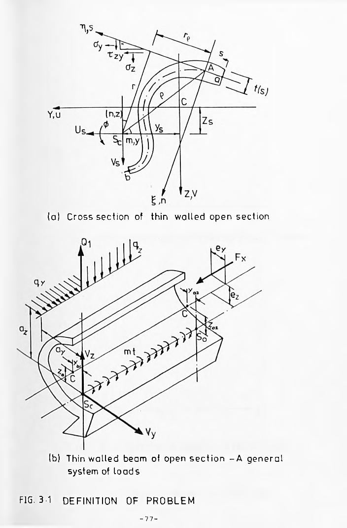
(a) Cross section of thin walled open section

lb) Thin walled beam of open section -A general system of loads

FIG. 3-1 DEFINITION OF PROBLEM

-77-

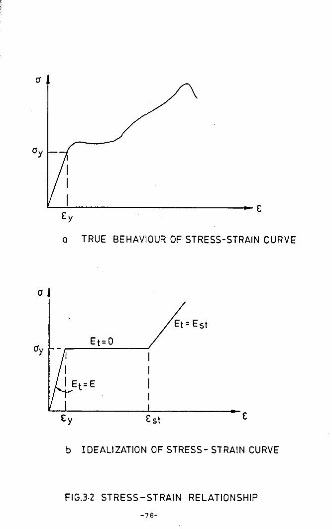
a TRUE BEHAVIOUR OF STRESS-STRAIN CURVE

b IDEALIZATION OF STRESS- STRAIN CURVE

FIG-32 STRESS-STRA IN RELATIONSHIP

- 7 8 -

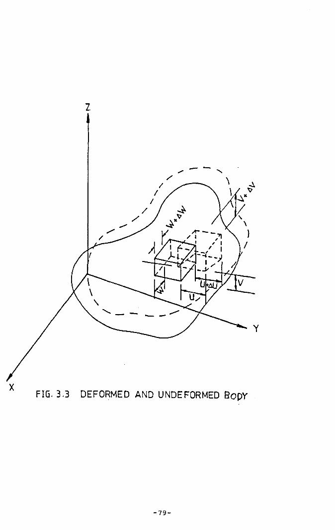
Z

- 7 9 -

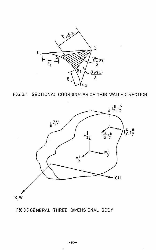
FIG. 3.4 SECTIONAL COORDINATES OF THIN WALLED SECTION

FIG.3.5 GENERAL THREE DIMENSIONAL BODY

- 8 0 -

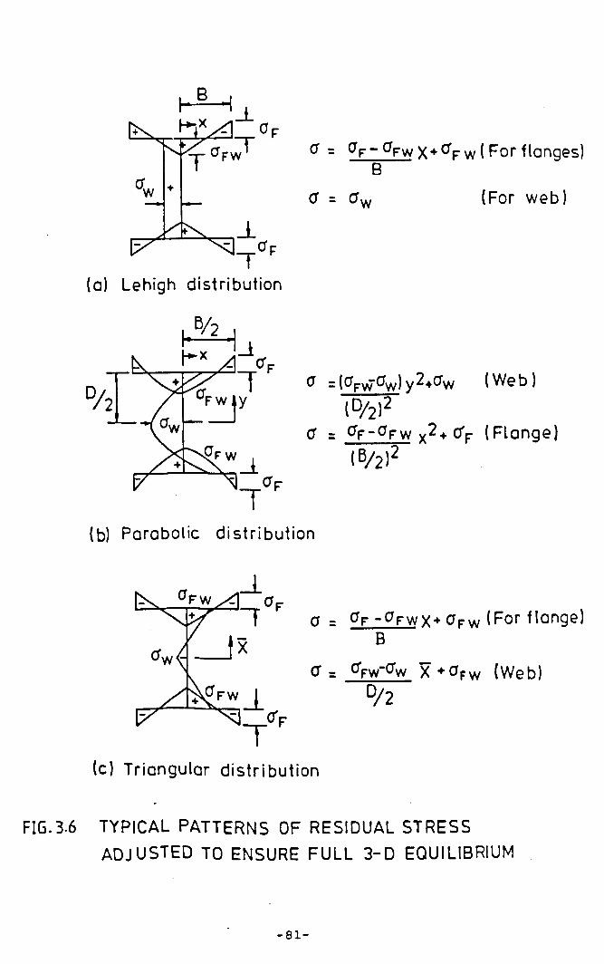
FIG. 3.

[ x a F

+

' y 0 F W 1

_ L

(a) Lehigh distribution

<7= <y- ^fw X + °V w (For flanges) B

cr = crw (For web)

0 = (CpVyC7w ) y 2 +o’ (W e b )

( ° /2)2O' _ <Tf-a r w y 2 + c y ( F la n g e )

( b/ 2)2

(b) Parabolic distribution

a = cy -cyw x+ Qrw (For flange) B

a = o>w'°w x + aFW (Web)

° /2

(c) Triangular distribution

6 TYPICAL PATTERNS OF RESIDUAL STRESS ADJUSTED TO ENSURE FULL 3-D EQUILIBRIUM

- 8 1 -

Chapter 4

Derivation o f St i f fness Matrices

4.1 Introduction

The most important feature o f the matrix s t i f fness analysis

o f structures is the formulation o f the s t i f fness matrix for a discrete

element. This is required in order that the real structure may be

represented by a system with a f in i t e number o f degrees o f freedom upon

which the actual analysis can be performed.

These s t i f fness matrices are usually formulated by assuming

that the displacements within an element vary in a suitable fashion;

normally polynomials, whose coe f f ic ien ts are equal to the number o f

element nodal point displacements, are selected. I t is then necessary

to introduce these interpolation functions to the equilibrium equations

in order to evaluate the element s t i f fness matrices.

Many previous invest igators have derived s t i f fness matrices

for a beam-column element in three dimensions in the form o f a 12x12

s t i f fness matrix for a member having 6 degrees o f freedom at each node.

Tecan and Mahapatra (1969), produced a tangent s t i f fness matrix for a

space frame member using a Taylor expansion ( s e r ie s ) . Przemieniecki

(1968) gave two methods to obtain the l inear tangential and geometrical

st i f fnesses. The f i r s t was based on the displacement method, while the

second employed the force method. Based on considerations o f nonlinear

displacements and the second variation o f the strains, Roberts and

Azizian (1983^ developed both the geometrical ■ and the tangential

s t i f fnesses .

- 82 -

A 14x14 element s t i f fness matrix for a beam-column has been

developed by Tebedge and Tal l (1973). Barsoum and Gallagher (1970),

Rajasekaran and Murry (1973), Yang and Mcguire (1986), and Kitiporncahi

and Chan (1987) by using the strain displacement relationships. The

element nodal displacements were taken to be adequately represented by

a l inear polynomial for the axial displacements, by a cubic polynomial

for la tera l displacements and twists, and by a quadratic polynomial for

the rotations and warping.

4.2 - Interpolation Function

In the f in i t e element approach the displacements are

approximated by forming shape functions. The functions chosen to

represent the solution within the element are most commonly taken as

polynomial series for the following reasons :

a- I t is straightforward to perform d i f ferent ia t ion or integration

and to computerise the processes.

b- I t is straightforward to increase the accuracy o f the results by

increasing the order o f the function.

The approximate function chosen for the displacement model

must be capable o f reproducing certain features o f the true

displacements i f convergence to the true solution is to be obtained

Zienkiewicz (1977), Bathe and Wilson (1976), Richards (1977), Rao

(1982). I t must be continuous within the element and there must be

compatibil ity between adjacent elements . In general the number o f

terms in the chosen series must be d irec t ly related to the to ta l number4

o f degrees o f freedom for the element.

In a one dimensional situation (extensional or f lexural

behaviour o f bars), the required functions for the longitudinal and

- 83 -

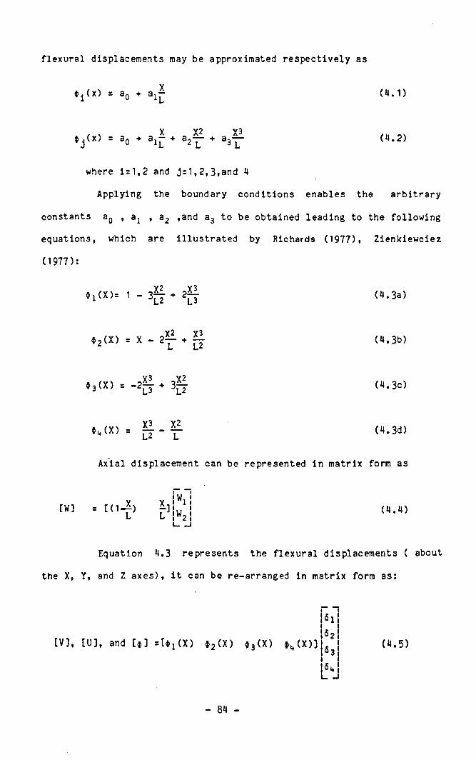
f lexural displacements may be approximated respective ly as

* i (x) = a0 + ai^ (4.1)

, . X X2 X3 * j ( x ) = a0 ♦ a j - + a2— + a3—

where i=1,2 and j=1,2,3,and 4

(4.2 )

Applying the boundary conditions enables the arbitrary

constants aQ , , a2 ,and a3 to be obtained leading to the following

equations, which are i l lustrated by Richards (1977),

(1977):

Zienkiewciez

* ! « > ■ ’ - £ * £ (4.3a)

• 2 « ) = x - 2r * e?(4.3b)

(4 .3 0

(4.3d)

Axial displacement can be represented in matrix form as

[w] = [ < i - i ) h \ l l \L L ¡w2 !

(4.4 )

Equation 4.3 represents the flexural displacements ( about

the X, Y, and Z axes), i t can be re-arranged in matrix form as:

i----1! 51 j i j

[V] , [U], and [ * ] s [ * j (X ) * 2(X) * 3(X) * „ ( X ) ] j g ¡!I Mi___i

(4.5)

- 84 -

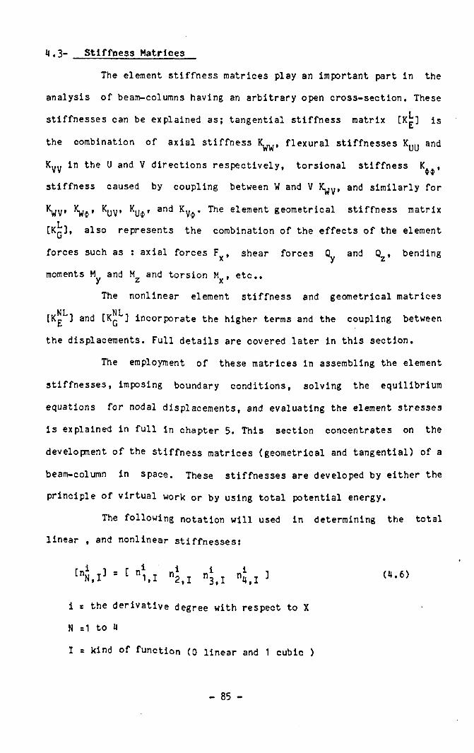
4. 3- St i f fpess Matrices

The element s t i f fness matrices play an important part in the

analysis o f beam-columns having an arbitrary open cross-section. These

st if fnesses can be explained as; tangential s t i f fness matrix [Kg] is

the combination o f axial s t i f fness K ^ , f lexural s t i f fnesses KULJ and

Kyy in the U and V directions respect ive ly , torsional s t i f fness K ,

s t i f fness caused by coupling between W and V K^y, and similarly for

^WV’ ^UV’ an<* Ky$ * el ement geometrical s t i f fness matrix

[Kq ] , also represents the combination o f the e f fe c ts o f the element

forces such as : axial forces Fx , shear forces Qy and Qz , bending

moments M and M and torsion M , e tc . , y z x

The nonlinear element s t i f fness and geometrical matrices

NL NL[K^ ] and [K^ ] incorporate the higher terms and the coupling between

the displacements. Full de ta i ls are covered la ter in this section.

The employment o f these matrices in assembling the element

s t i f fnesses, imposing boundary conditions, solving the equilibrium

equations for nodal displacements, and evaluating the element stresses

i s explained in fu l l in chapter 5. This section concentrates on the

development o f the s t i f fness matrices (geometrical and tangential) o f a

beam-column in space. These st i f fnesses are developed by either the

principle o f v ir tual work or by using tota l potential energy.

The following notation w i l l used in determining the total

l inear , and nonlinear st i f fnesses ;

[niN, I

3 = C ni1.1 ni

2,1 ni4,1 ]

i r the der ivat ive degree with respect to X

N si to 4

I = kind o f function (0 l inear and 1 cubic )

( 4 . 6 )

- 85 -

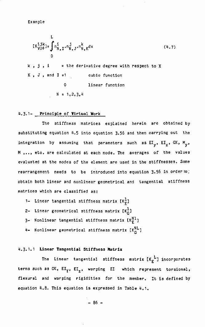
Example

L

■.„ijk. r i J k . [KVU$] ' J nN,I*nN, J*nN,Kdx

0

(4.7)

k , j , i = the der ivat ive degree with respect to X

K , J , and I =1 cubic function

0 l inear function

N = 1,2,3,4

4.3.1- Principle o f Virtual Work

The s t i f fness matrices explained herein are obtained by

substituting equation 4.5 into equation 3.56 and then carrying out the

integration by assuming that parameters such as El , El , GK, M ,y z y

M etc . are calculated at each node. The averages o f the values

evaluated at the nodes o f the element are used in the st i f fnesses. Some

rearrangement needs to be introduced into equation 3.56 in order to;

obtain both linear and nonlinear geometrical and tangential s t i f fness

matrices which are c lass i f ied as:

1- Linear tangential s t i f fness matrix [K*]

2- Linear geometrical s t i f fness matrix [K*]

3- Nonlinear tangential s t i f fness matrix [K^1]

NL4- Nonlinear geometrical s t i f fness matrix [Ju ]G

4.3.1.1 Linear Tangential S t i f fness Matrix

The Linear tangential s t i f fness matrix [ K ^ ] incorporates

terms such as GK, Ely, EIZ, warping El which represent torsional,

f lexural and warping r i g i d i t i e s for the member. I t i s defined by

equation 4.8. This equation is expressed in Table 4.1.

- 86 -

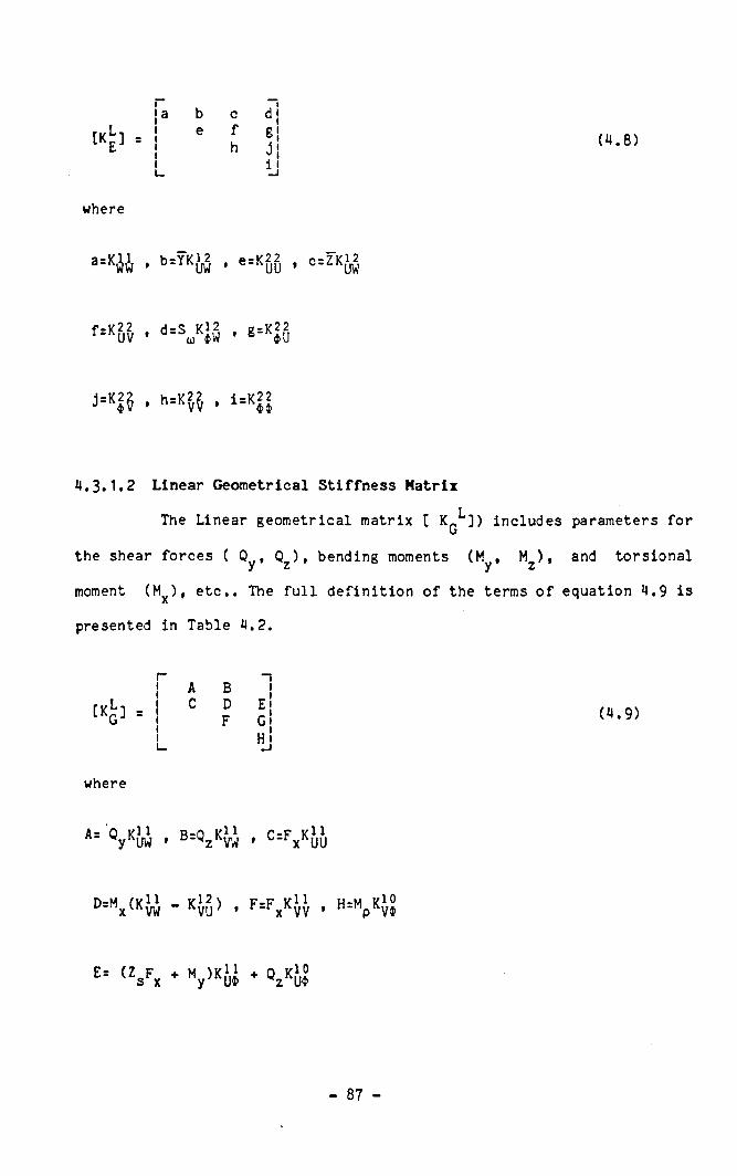
[k£]

be

c djf g|h Jj

(4.8)

where

a=Kii i • b=YKb5 • e=K2u§ • " ZKM

r=K5v • 0-s„ KiS • s=Kiu

J=K|^ • h=KvV * i=K$$

4.3.1.2 Linear Geometrical Sti f fness Matrix

The Linear geometrical matrix [ K_^]) includes parameters forU

the shear forces ( Q , Q ) , bending moments (M , M ) , and torsionaly z y z

moment (Mx) , e t c . . The fu l l def in it ion o f the terms o f equation 4.9 is

presented in Table 4.2.

[ kL]AC

BDF = !

G !H!

(4.9)

where

* * V l w • B=cl* Kvw • C=FxKuJ

D= V Kvw - "vu1 • F =F xKVV • H=MPKV*

E= ( V x * Hy,KU* * °xKU»

- 87 -

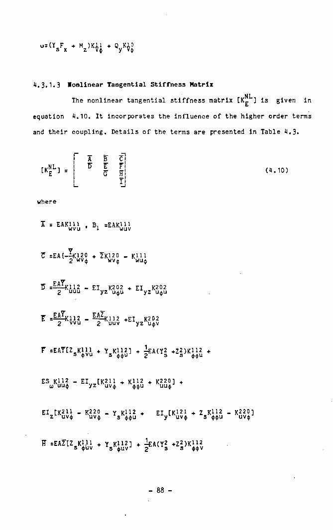
“ = < V , * V H J * y j {

4. 3.1.3 lonlinear Tangential Sti f fness Matrix

NLThe nonlinear tangential s t i f fness matrix [K£ ] is given in

equation 4 . 1 0 . I t incorporates the influence o f the higher order terms

and their coupling. Details o f the terms are presented in Table 4,3.

[KNLE ] =

A B cjTS E r

G H I

where

I = EAK1U wvu B, sEAKHI 1 wuv

Z =EA{—-K120 2 wv4>

ZK120 _ R in WV( J ) w u ^ .

,ea^ i 12 _2 uuu El, K202 yz u$u El K202 yz u$u

+EI K202 yz u a v

( 4 . 1 0 )

F =EAT[Z K i l l ♦ Y K112] + l£A(Y| +Z2)Kll2 ♦ s <pvu s 2 s s

ES KH2 _0 J U U ( J )

El [K2H yz l *uv<j>

KH24>4>u

K220 ] UUij) +

EI,[K2!1 - K220 _ y KH2 + El [Kl21 + Z KH2 _ k220] z L uvij> uv$ As 4>$u y uv$ s uv$

F =EAl[Z K in + Y K112] + ^£A(Y2 +Z2)K112 s <j>uv s $uv 2 s 3

- 88 -

ES K112 _UJ VV$ EIy X U ZSK

112 V

K220 l K u v < T

+ EIJK 211vu<t>

«•220vu4> Y Kl l23 s 9$ v El [K21i y vu<t>

7 «112 «220VU<J>

]

Z =EA=X112 - 2 vvv EIyK2vU El K202 yz v<t>v

T - ES TY «1^2 _ 7 «112 . J.fv2 . 72\«202i ui YsK4>v<i> Zs <J>u<t> 2 s ^s

+ El r«220 . «211 . v «112i

+ El r«220 . «211 . 7112 1 u)ZL *$u<i> %U<}> J

4.3.1.4 Monlinear Geometrical Sti f fhess Matrix

The nonlinear geometrical s t i f fness matrix [K^*] includes the

fu l l higher order terms which are described in equation 4.11. The

expressions for the terms o f equation 4.11 are fu l ly explained in Table

4.4.

[KjL]

r~t111 Ai Bi“1

C1 |11 Dl El F1 i111 Gi H1,111l_ * l j

where

A> — • B1 - 0 yKi5l • Cl - 0 ^ }

(4.11)

Dl --0 Z [«102 —yy S LI\]<j>u«211'Siifru « 1 0 1 1Ku<(>uJ

- 89 -

-Q Y {K i l l + K211} z s u$u u$u' M { K- 01 + K120 _ k i l l } x u^u u^u u$uJ

Ci =-Q Y [K102 + K211 + K101] 1 ^ s 1 v$v + N ^v J

v211 ]k'v4>vj M {K201 nx l v<j>v

+ k120 „ R111} v$v kv4>v '

_ Q 7 K 21 1 _vy*sRu*v 0 Y K211

=[p i s . M IK101 QzYs^KiSJ

—Q 7 i K12 1y V ^ u v *

v-121uu^ k2H 1

K U V $ JM (If210 'V^UU*

_ *,120*uu<t>

Kl l l\K U U ( J ) )

H =[PZS . H 1K>;>y 4><t> v Qz V Klv $ +K1211N u$J

-Q 1 IK121 ■*• K121 - Kl20) + M (K210 - *12° + Kl 111 y ^ tNvu$ vu4> ^uv^ Mx'*vv4> kw 4> k v v <i>

The subassemblage o f the element st i f fnesses stated in

equations 4.8 - 4.11 is the tota l s t i f fness matrix which is employed in

the analysis o f beam-columns under d i f fe ren t load patterns together

with various boundary conditions in the e las t ic and inelast ic ranges as

presented in equation 4.12.

[Kt ] = [Kg] + [Kq ] + [ KJl ] + [ k£L ] (4 .12 )

Further de ta i ls o f the assembly o f the fu l l geometrical

l inear and nonlinear s t i f fness matrices and the element tangent

st if fnesses are explained in chapter 5 and the va l id i t y o f their

implementation in the analysis is demonstrated in chapters 6 and 7

respect ively.

- 90 -

U .3.2 T o t a l P o t e n t i a l Energy

Recall equation 3.62 from chapter 3 which represents the

equilibrium equation o f a beam-column o f thin-walled open cross-section

in three dimensions. Substituting equations 4.5 and 4.7 into 3.62, and

carrying out the integrations the equilibrium condition can be obtained

as a stationary point o f the to ta l potential energy as:

5n = W dw * W dU + T 5 « 9 (14* 13)

or

611 = |3. (4.14)3r

where

r = [Wj Ui eu1 Vi e v1 x i w2 U2 eu2 V2 e v2 * 2 X2 ] T

After some rearrangement the general form o f the equation can be

written as:

1

611 = S f [ E A [ < W > ( K ^ ] _ T « V > [ K 2 0 1 i] + < U > [K 2 1 ] + < V > [ K ^ 1 ] )

0 ^

♦ 5 « v > ( [ k>>>]

- T(<V>tK2J1] .

* <U> " 0 *

ES«JXK ’ S ÎW tW K l 'J , ] ) -

- <u>tCKJJ1.1-tKg 1 3* rK 1 Ji,l ) - MU<,>[K2>

- " , « ï> t x 2v‘ ] - <U>tKjJl] - <U>[K>“ ])

- 91 -

M2 «U>[K21] + <V>[K201 ]V( J ) W

<V>tKlll])v$w

f « v > [Ki¿1 - - t <<u> [kj ì 1 * * F, { w)

E A < W > U K ¿ n ] - Y ( [ K ¿ } ; ] ♦ [ K H I ] )

TtK¿5’ ♦ z s 'Ki ; j ] - ' " ¿ P - V K¿ U ’ * « ¿ 5 ”

E » Y l ï s < g > ( [ K j n ♦ [ K 2 1 1 ] ) )

EA{ZYe<V>([Kll2 + [k 211]) > Z <U>[Kll2] s v$v v4>v s u$v

— (<U>[K112] + <V>[Kll2]2 uuv vvv

* E S J W t K j H ] ♦ <t>[K|l>])

E I y I < V > [K “ ] - < U > [ K 2 p - <U> [K > > $ ]

<v>tKiJ î1 - <v>IKn ì ] )

e i 2« u >[k j ;;] * <u>[Kjn) * V * > [ K J > 2 ] )

E l y ^ ^ X K ^ l * < V > [K 2 » ; i - <U>CK>>$]

< V > [ K U 5 ] * <V>tlCE«;] ♦ < V > [ K 2 n i ♦ <U>[E” } ] )

Ei«y < »> i tKi5ei - “ u j i * [ ku í ”

EI»z<* >" K*v’ * « n t 11

P<V>([K1J] - T,<*>tlC>‘ ] ♦ Zs<»>[K¿OJ]>

£ly«W>lK¿>] * 2«*>[K»5>] * 5VW>U¿°i]

» yKW>[K¿$] ♦ <®>tKgllJ)

M {Cin i« : ! ! ] - <W>[K102] _ <W>[KH1]} z * $v w$v w$v

■ 1 {<U>[K21] - <U>[K12] + 2 < 0 [K i11] 2 X uv uv 4>vv

♦ 2«V> IK102 ] + <V>[K201])]]iv}

+ EA<W>{[Klll ]_Z([Kl02] + [K111] )wuu w <t>u 1 w$u

- y O - V O - ' O - V O * O 1

* EAI(-Zs<V>([K5>¿ ♦ [K j ¿ ¡ ] ) )

- EAT(Z.^XCK,1' 2, * tK2>>]) - 1 <V>[K*'2]S U$U U$U S V<J)U

» 5 « u > t O * <v>«“ S3 « I » z l ’ <*>n!” 53))

♦ <U>[K12111„11} + ES f -Z ,<*>[k2“ ] + <4»>TK2 111} uuu co s 4>$u (fiuu

+ EI { <U>[K22] -<V>rK2°2] + <V>[K1i 2]Z UU V$U V<t>U

* « M O * «MK»2])

- EIy l<V>tK*0*1 * <V>tK2H ] - By<*>tK” 2] )

* EIy2( <V>0 * <V>[K2v» 21 - < IM K ^ 2]

- <u > t O - < ï> [ K v { u 5 - <V> tO * <U>tK5 l i 11

* E IU2< ,> lt K |* 51 * O - [ K ' lJ ] )

* - ' O

♦ P<VMtKlJl * ZS<*>[K*1] <■ ï s« > [ K > » i l )

* - 2 «»> tK j;;i -<*>tK«j3)l - |0y<W>tK»5J,l

- 93 -

- M,{<W>[K12] ♦ <4>>CKO 111}z wu 4>u

♦ - <W>[K102 + <W>[K1H]}y 4>u w,j>u w<j>u

♦ -Vi {<V>[K21] - <V>[K12] + 2<i»>[Kll l] 2 X vu vu <j)uu

2«U>CK1023 + <V>[K201] ) } ] { U }

EA<W>{-Y ( [K120]_[K111]) + Z ( [ k 1 2 0 ] . [ K111]) W V $ WVi } > W U l W U f

Y [K11*] + 1 [ K i l l ] - [K H I ] - [Km J s wu 4> s wv<(> wuij> wv<j)

- ' O * O * Z- k KlV '

♦ ES l<WXZ_[K>>j1 - Y_tK>>>])]ü3 S WU<p S WV<p

■K EAY{Y-<U>[k2¿1-Z <U>tK211] + (Y2+Z®)<U>[K211]} s uv$ s uu$> s s

+ EAZ{Ye<U>[K24 - Z <V>[K21Î ] + (Y2+ZS)<V>[K2} 1 ] } s vv<t) s vu$ s s v4>4>

* EW <V>tKU*] * <»>[KX>)> - Z5«U>[K11J] * <»>tK2H])

2 s s $$<}> s s

♦ * GK<»>tü 3 J

♦ EIz t < V > ( [ K « } ] * CKjl l ] * [ kZ H ] , „ J6y<U>[K jn ] )

♦ EIy « U > ( [ K » 0 ] . [KJU] * [ , n i , ) . 2 Ïy< V > [K » l ] )

* EV <U>([K”U* ’ * t K ^ ] > ♦ < V X tK «® ï * tKZl l ]

* EV <U>![Ku î ] - K » i ] )

- 9« -

* < V X tK $ « ] - [ K ^ J * « > $ } ] ) .¿<V>IK>1J]>

* * tK»°] - 2ïstK21>] ♦ [KH2])}

‘ EIuz«V>([K24] * I K » '] )

- <0>«K2»23 ♦ [KJIJ] -

- « X V ^ U J l * ‘ K2*SS’ * “ » « Î J J 3 *

* V ’ X ' U 1 * p , z s<u>tKi * 1 - V V>tKU ’

* Zs<v> ' KU ° ’ * V u>[K i l “ ] * Zs< v > [K i , U 1 * YS<U>tKÌ H ]

* ¿ V <-2<V>tK‘ } l - <W>tK“ } l - 2<V>([K»0]

* z , < »x - ^ [ kj; > ) ♦ n i ls? ] ♦ s tE j i j ]S O a)a)(p ffi (J) a)

- y * x c * » i * tKi î ]»

- Í 3 2 I ( - 2 < u > n c ¡ , } ) . <W>tK>J» ) * 2 < U X [ K ¡ , ; » ]

* - 2tKU ° ]

- Zs<»XtK»>] * « > » ] ) )

* y<">K1J -

- <V>tlC‘ JJ] * <W>CK¿2 0] ♦ <W>K¿¿>)1

- MzKV>[kX - <U>tK¡,‘ °]

- * <w>[ti í }3 - <w >K ÍU ] >

- V ' O f ' Í * 1 * 2 t<U>[Kì ì * ] - « > « 1 1 * 1

- 95 -

♦ <i>tK001] + 2<$>[K100] _ 2<U>[K120] + 2<V>[K120]}]{6*}<$>(£(£ t y t UUm VV m

- M * [ { v " } - <U>[K11]{$}- <$> [K l l ] {U } ] y o u<j> <fu

+ M » u u " } + <V> [K in {$ }+ < *> tK l l ] {V } ]Z O 4>v

i f * „ [ Z e( <v>[K l l ] { $ } + <*> [K lJ ] {V } ) ]2 o s v$

+ i 5* [YB( <U>[ K l l ] { $ } + <*>tK“ ] {U } ) ]2 o s u$ $u

- Qy4>0I iV* > +Ys i$ ’ ) + 2Zg { * }

» * i+ {u } +Ye {4> } + 2Y {4>} jdxZ 0 S S I

where Dj, D2 , . . . . , D7 were defined in Appendix C

Equation 4.16 can be written in a simple form as:

1

♦ X'r ’[D i<U>[K22]+D5<V>tK22]+D6<$>[K22]]{6Ul

0

+ [D2<V>tK22]+D4<U>[K22]+D7<$>[K22]]{5V}VD UV <pV

—?+ [D3<V>[K22]+D5<U>[K22]+D7<$>[k2 2 ] ] {6* } j dx (4.16)

6H = <r>[KT2) { r } ] + {P} + { r 0P} (4.17)

where

are the in i t ia l deflections.

M..„]T (4.19)

- 96 -

(«.20)[Kt j ] . k \ * * t*L * KNgL * K01

Carry out the integration o f equation «.16 by assuming the

terms Ely, EIz » 7, My, M , e tc . to vary l inear ly in the form

n y . Eiyl . ( n y2-E i y , ) | (1.20a)

or

My = My1 ♦ (My2-My , ) T (1.20b)

where 1 and 2 are nodal member numbers o f the element

The terms o f equation «.20 can be described as:

1- Linear tangential s t i f fness matrix [Kp]L

2- Linear geometrical s t i f fness matrix [K^]

N13- Nonlinear tangential s t i f fness matrix [K . ]

NL« - Nonlinear geometrical s t i f fness matrix [K^ ]

5- In i t i a l s t i f fness matrix [ K ]o

« .3 .2 .1 Linear Tangential S t i f fness Matrix

The l inear tangential s t i f fness matrix [ K^] contains terms

such as Ely, ES , El^y, e tc . These expressions are fu l l y presented in

Table « .5 .

« .3 .2 .2 Linear Geometrical S t i f fness Matrix

Table «.6 gives the terms o f the l inear geometrical s t i f fness

matrix [K^]. The Wagner e f f e c t together with internal forces such as

M , Q , etc are included.y *•

- 97 -

^.3-2.3 Nonlinear Tangential Sti f fness Matrix

The higher order terms such as El , V , El i V . arey ,x ,xx ’ oiy ,x ,xx

accounted for,and are given Table 4.7. These expressions are detailed

in Appendices G and J.

4.3.2.4 Nonlinear Geometrical S t i f fness Matrix

NTThe nonlinear geometrical s t i f fness matrix [K2 ] for a beam-u

element in three dimensions is presented in Table 4.8. The terms o f

that Table are given in fu l l detai l in Appendices H and J.

4.3.2.5 In i t i a l Sti f fness Matrix

The inclusion o f the in i t i a l deflect ions in the st i f fness

matrix i s explained in Table 4.9.

4.3.2.6 Assembly

The assembly o f the submatrices presented in Tables 4.5 to

4.9 corresponding to the l inear geometrical and tangential s t i f fness

matrix and the nonlinear terms together with the in i t i a l s t i f fness

matrix i s demonstrated by several i l lu s t ra t i v e examples in Chapters 6 &

7 respectively.

4.4- Transformation Matrix

The transformation matrix has been explained in many

references such as Weaver (1967), Poresi and Lynn (1977), and Chen and

Atsuta (1977). The transformation presented herein is based on using

vector notation. The element displacements with respect to the local

coordinates can be related to those in the global coordinate system by

the transformation [ T ] .

- 98 -

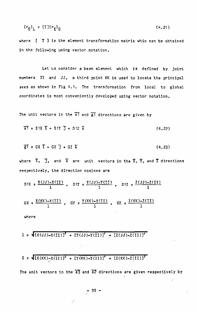
( 4 . 2 1 )i r E} L [T]{rE }G

where [ T ] is the element transformation matrix whic can be obtained

in the following using vector notation.

Let us consider a beam element which i s defined by jo int

numbers I I and JJ, a third point KK is used to locate the principal

axes as shown in Fig 4.1. The transformation from local to global

coordinates is most conveniently developed using vector notation.

The unit vectors in the s1 and g1 directions are given by

¥T = S1X I + S1Y 3 + S1Z k (4.22)

g1 = GX T + GY j + GZ k (4.23)

where T, 3* and k are unit vectors in the 7, Y, and 7 directions

respect ively , the direction cosines are

S1X X (JJ )-X ( I I )1

S1Y Y( JJ ) - Y ( I I ) 1

S1Z z ( j j ) - z d i )l

GX XOOO-X(II)1

GY Y(KK)-Y(TI)1

GZ z o o o - z d i )1

where

1 = >|[X (JJ)-X(I I ) ] ' + [Y ( JJ )-Y ( I I )]* + [Z (JJ ) -Z ( I I )32

G s >|[X(KK)-X(II ) ) 2 + [Y (K K ) -Y ( I I ) ] z + [Z (K K ) -Z ( I I ) ]2

The unit vectors in the ¥3 and ¥5 directions are given respect ive ly by

- 99 -

( U. 24)s3I s3<I w J I = S3X i + S3Y j ♦ S3Z k

s2 = s3xs1 = S2X i + S2Y j + S2Z k (4.25)

Equation 4.22, 3.24, and 4.25 can be written in matrix form as:

!®4!!i|!! s3'

i i»tsA]| 3i

! k!(4.26)

where

J SIX S1Y S1Zj[S ] = ¡S2X S2Y S2Z j (4.27)

3 3 ¡S3X S3Y S3ZJ

The transformation matrix o f a beam-column having 7 degrees

o f free dom at each node can be written as:

[S]tsA]

(4.28)

The assembly o f the tota l transformation matrix in

3-dimensions for a beam element is performed in equation 4.29, the

diagonal terms corresponding to the warping are set to unity. So the

transformation s t i f fness to a beam element can be written as:

CT3 = ! [s] (S3 j (4.29)

4.5 Strain Displacement Matrices

In this section a fu l l explanation o f the expressions for the

strain displacement matrices are presented. The l inear and higher order

- 100 -

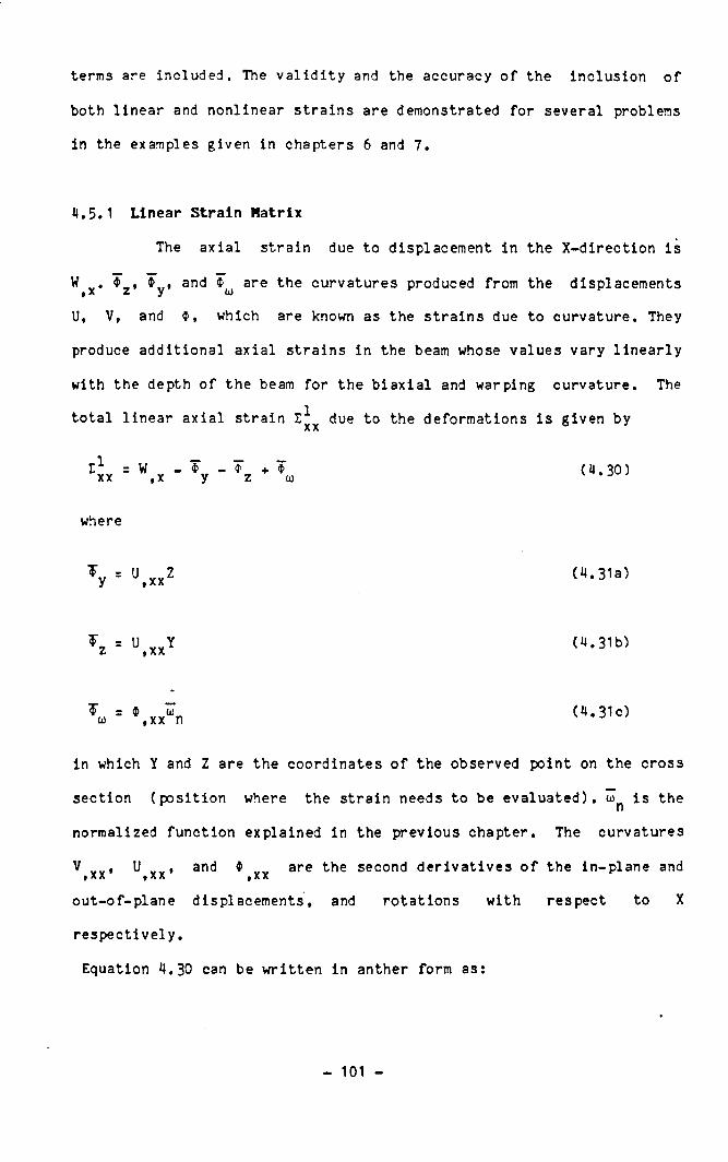
terms are included. The va l id i t y and the accuracy o f the inclusion o f

both linear and nonlinear strains are demonstrated for several problems

in the examples given in chapters 6 and 7.

«.5.1 Linear Strain Matrix

The axial strain due to displacement in the X-direction is

W v* *•»* and ® . are the curvatures produced from the displacements fX z y (jl)

U, V, and $, which are known as the strains due to curvature. They

produce additional axial strains in the beam whose values vary l inear ly

with the depth o f the beam for the b iaxia l and warping curvature. The

tota l l inear axial strain due to the deformations is given by

I 1xx * + *Z OJ ( « .30 )

where

Vy "

( « .31a)

Vz U Y ,xx («.31b)

V s *01 U)xx n ( « . 31c)

in which Y and Z are the coordinates o f the observed point on the cross

section (posit ion where the strain needs to be evaluated), u>n is the

normalized function explained in the previous chapter. The curvatures

V vv* U vv* and * are the second derivat ives o f the in-plane and

out-of-plane displacements, and rotations with respect to X

respectively.

Equation «.30 can be written in anther form as:

- 101

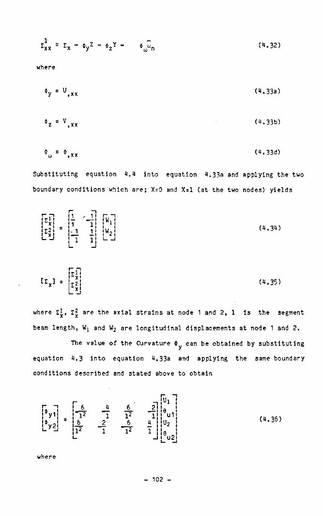
(n.32>rxx = Ex " ®yZ “ $zY 4> to­ol n

where

*„ = U xx (4.33a)

$ = V (4.33b)

C = 4> V VU) f X X (4.33d)

Substituting equation 4.4 into equation 4.33a and applying the two

boundary conditions which are; X=0 and X=1 (at the two nodes) yields

r nr ~ j 1 - i

' 1 !i— i

1 y 1 1 1 ^ X l j 1 ij I w , <

i i ii i

! E 2 • ' t x ! li ! w 2 !L _ _ ! j”T l ! i__i

(4.34)

rI r 1 I I ‘‘ X •i t; 2 ii x i i_ l i

(4.35)

where E*, I * are the axial strains at node 1 and 2, 1 is the segment

beam length, and W2 are longitudinal displacements at node 1 and 2.

The value o f the Curvature 4>y can be obtained by substituting

equation 4.3 into equation 4.33a and applying the same boundary

conditions described and stated above to obtain

r ni a ir*i ^ L J4 6 ' j i

! * y 1 { . ! i 2 1 12 1|

¡*y 2 !L. ’ -i ' \ ± _2 6 4 j

¡ l 2L.1 “1* 1 |

_i

V9u1U2

6u2

where

(4.36)

- 102 -

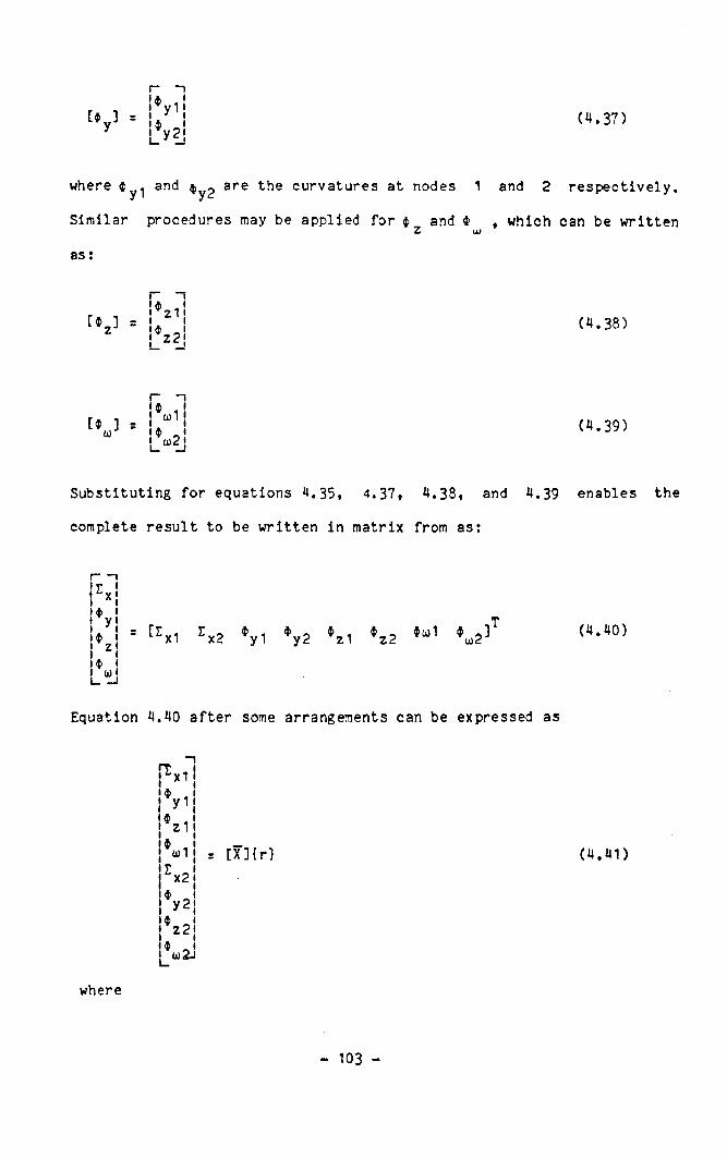
(4.37)IA .I

[$ ] = ! y1l y ¡ V

L . y t l

where and $y^ are the curvatures at nodes 1 and 2 respectively.

Similar procedures may be applied for $ and 4> , which can be writtenZ u)

as:

r —»z,i

^2!(4.38)

[ i ]OJ

(“ I ( i! “ 1!|*U2i

(4.39)

Substituting for equations 4.35, 4.37, 4.38, and 4.39 enables the

complete result to be written in matrix from as:

I r I ‘•y I *I $i yi t>i zi___i

= fZx1 Zx2 *y1 *y2 *z1 *z2 *o>2 (4.40)

Equation 4.40 a f ter some arrangements can be expressed as

p x l

¡%1I A

I 21|*a)1

! Ex2 j y2I» ^L 22| ü)2i

= [X] { r } (4.41)

where

- 103 -

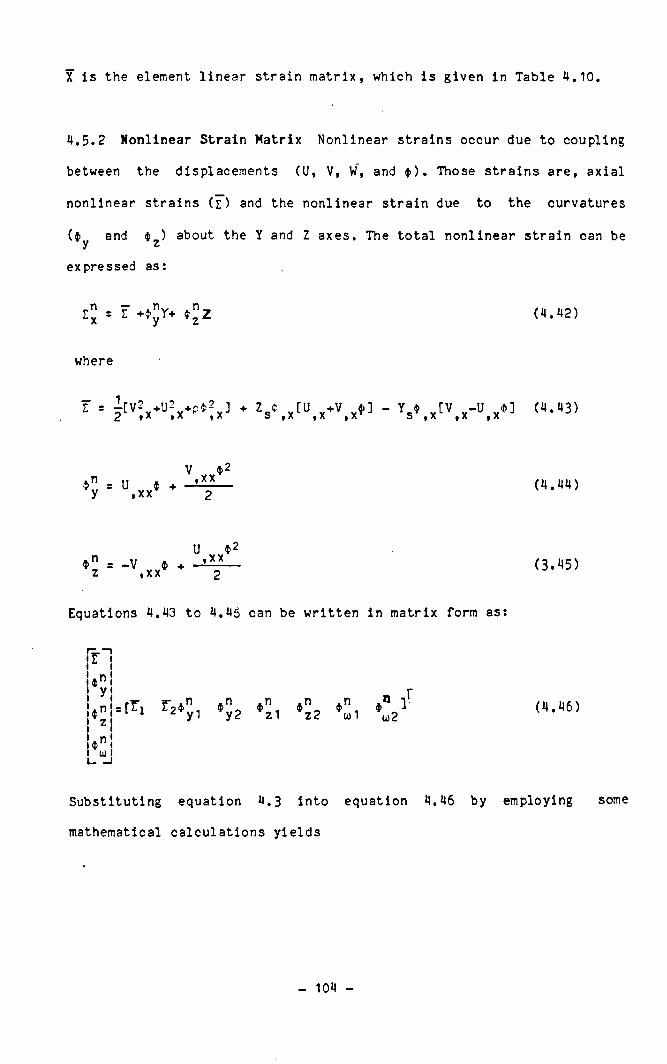
X is the element linear strain matrix, which is given in Table 4.10.

4.5.2 Nonlinear Strain Matrix Nonlinear strains occur due to coupling

between the displacements (U, V, W, and $>). Those strains are, axial

nonlinear strains ( e ) and the nonlinear strain due to the curvatures

($> and $ ) about the Y and Z axes. The total nonlinear strain can bey *expressed as:

z j = Z t * Z (4.42)

where

E ■ ¿ ^ x ^ x * ^ « 1 * V , x tu,x*T .x *J - V [V -u <t>] , x L ,x ,x («.«13)

ny u $,xx (4.44)

u $2= -v vvt + o . ^ )L y X X 2

Equations 4.43 to 4.45 can be written in matrix form as:

r- f .n= [£ i Z2«>yi y 2 z 1 Pz2 0) 1 *'y0)2(4.46)

Substituting equation 4.3 into equation ^. M6 by employing some

mathematical calculations yie lds

104 -

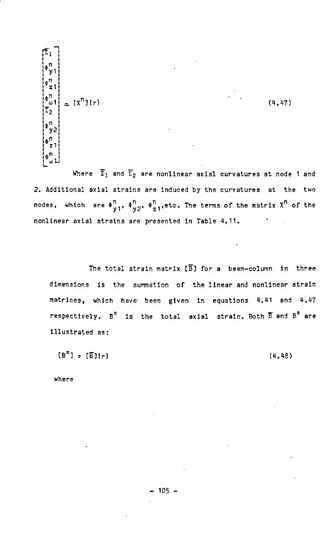
IT

*

*

*

nyinz 1nu1 = [Xn] { r }

4>

*

4>

ny2 j n j 2 1 J n j 0) l-i

(4.47)

Where and I 2 are nonlinear axial curvatures at node 1 and

2. Additional axial strains are induced by the curvatures at the two

nodes, which are * ^ ^ i ^ . e t c . The terms o f the matrix Xn o f the

nonlinear axial strains are presented in Table 4.11.

The tota l strain matrix [B] for a beam-column in three

dimensions is the summation o f the l inear and nonlinear strain

matrices, which have been given in equations 4.41 and 4.47

respectively . B" is the tota l axial strain. Both E and B" are

i l lustrated as:

[B=] = [B] { r } (4.48)

where

- 105 -

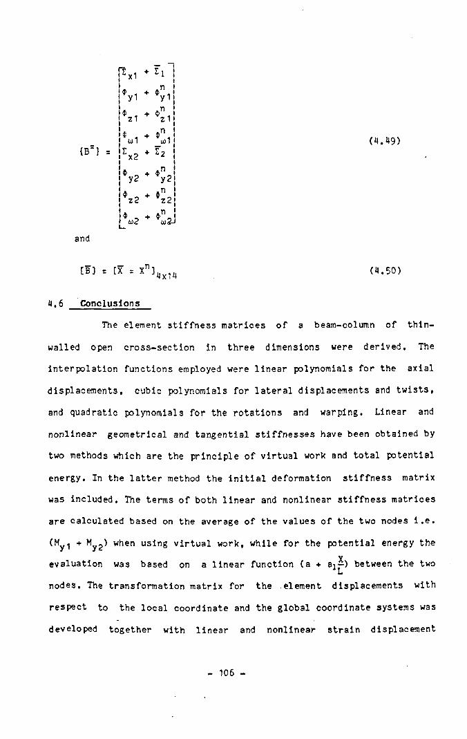
{B- } =

fx1 +Zl I

j%1 + *yi'|U , z1

+ •Mz 1

|*w1 + *n ! $U>1 1

iZx2 + Z2 1$

j y2 + *n iy 2 1!» _j z2 + *n iz 2 j

U o <d2-I

(H.H9)

and

[B] = [X = Xn] 4x14 (4.50)

4.6 Conclusions

The element s t i f fness matrices o f a beam-column o f thin-

walled open cross-section in three dimensions were derived. The

interpolation functions employed were l inear polynomials for the axial

displacements, cubic polynomials for la te ra l displacements and twists,

and quadratic polynomials for the rotations and warping. Linear and

nonlinear geometrical and tangential st i f fnesses have been obtained by

two methods which are the principle o f v ir tual work and tota l potential

energy. In the la t t e r method the i n i t i a l deformation s t i f fness matrix

was included. The terms o f both l inear and nonlinear s t i f fness matrices

are calculated based on the average o f the values o f the two nodes i . e .

(Myi + when using v irtual work, while for the potential energy theY

evaluation was based on a l inear function (a + aj—) between the twoU

nodes. The transformation matrix for the element displacements with

respect to the local coordinate and the global coordinate systems was

developed together with l inear and nonlinear strain displacement

106 -

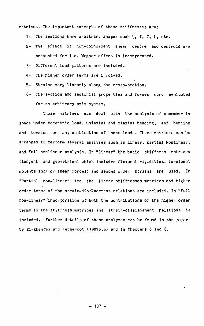
matrices. The important concepts o f these st i f fnesses are:

1- The sections have arbitrary shapes such [ , I , T, L, etc.

2- The e f f e c t o f non-coincident shear centre and centroid are

accounted for i . e . Wagner e f f e c t is incorporated.

3- Dif ferent load patterns are included.

U- The higher order terms are involved.

5- Strains vary l inear ly along the cross-section.

6- The section and sectoria l properties and forces were evaluated

for an arbitrary axis system.

Those matrices can deal with the analysis o f a member in

space under eccentric load, uniaxial and biaxia l bending, and bending

and torsion or any combination o f these loads. These matrices can be

arranged to perform several analyses such as Linear, part ia l Nonlinear,

and Full nonlinear analysis. In "Linear" the basic s t i f fness matrices

(tangent and geometrical which includes flexural r i g i d i t i e s , torsional

moments and/ or shear forces) and second order strains are used. In

"Partial non-linear" the the l inear st i f fnesses matrices and higher

order terms o f the strain-displacement relations are included. In "Full

non-linear" ' incorporation o f both the contributions o f the higher order

terms to the s t i f fness matrices and strain-displacement relations is

included. Further de ta i ls o f these analyses can be found in the papers

by El-Khenfas and Nethercot (1987b,c) and in Chapters 6 and 8.

107 -

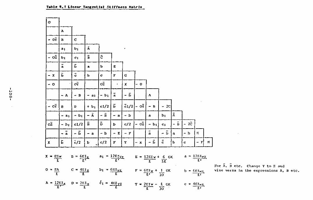
108

Table < « t Linear Tangential S t i f fn e s s M airi»

o

A

- OY B C

at bj À 1

- OZ b i C| B C

a b a b E

- X b c b c F G

- 0 OY OZ • X - O

- A - B - a i - b i a - b A

- OY B D + b| cl/2 b cl/2 - OY - B - 2C

- a i - b l - À - B - a - b a bi

OZ - b , cl/2 B 5 b c/2 - OZ - b] C| - B - 2C

- a - b - a - b - E - F a - b a - b E

X b c/2 b c/2 F T - X - b c b c - F M

X = ES.w B = H I z. a! = 12ErVz V

E = 12EI'rf + 6 GK a = 12EIwZl V l 51

bl = CEIyj^For A, B etc. Change Y to Z and

0 = EA C = 4EIZ F = 6EIW + 1 GK b = G1? 1 \ t7 i vise versa in the expressions A, B etcSL l l " T 2 IO v~~

A = 12EIZ D = 2EIZ c 1 = 4Elyz T = 2EIw - 1 GK c = 4EIwzl IL l 30 £2

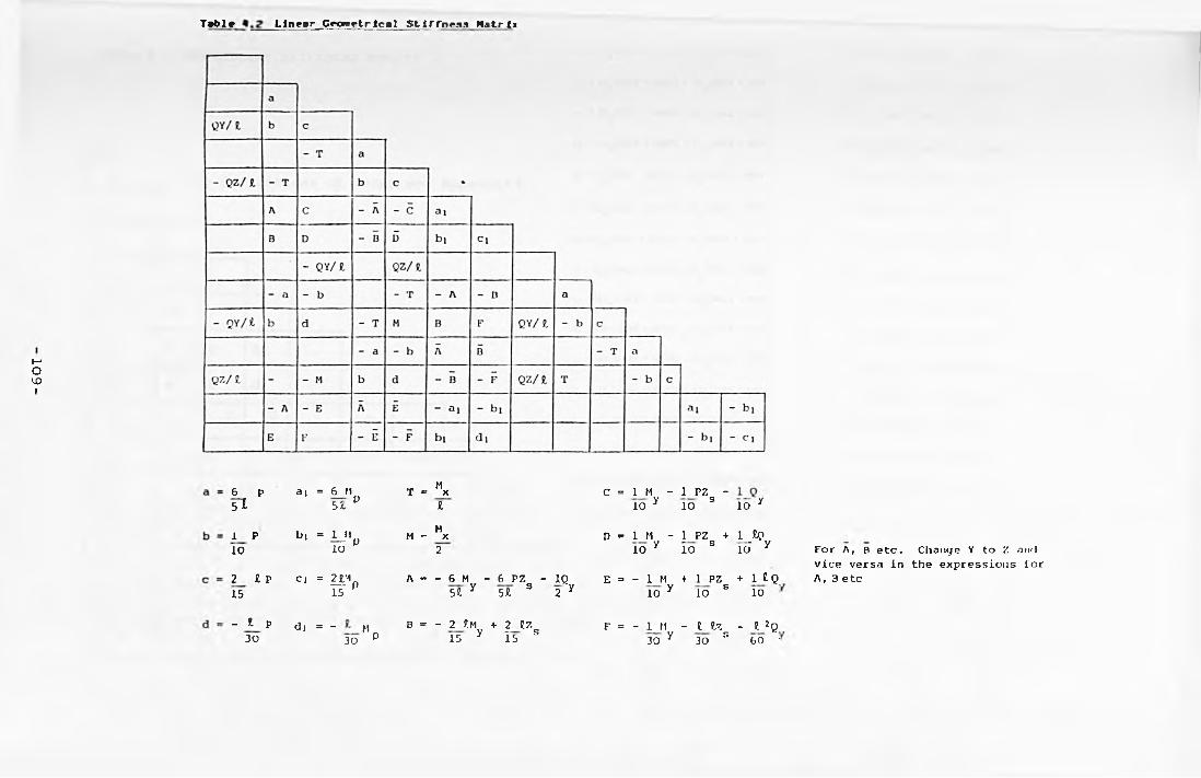
10

9-

Table Llnwr Cwetrlcil Stlffnf.n W.itrli

6 P

5 i

a i = 6 M

5 Z P

T =M

X

l

C = 1 M -

i o y

1 P Z -

l o s 1 0 Y

i p b , = 1 _M M =M

X D = 1 H - 1 P Z + 1 S o

1 0 l o p 2 l o y l o s l o " y

2 l P c * = 1 A 1 n A = - 6 H ■- 6 P Z - 1 Q „ E = - 1 M + 1 P Z + 1 i Q

1 5 I s p 5 1 V 5 P S 2 y i o y 1 0 s 1 0 :

- *■ P

3 0

d i = - h

3 0 P

B = - 2 P.M

1 5 y

+ 2 P z

I s 5

F = - 1 M

w y

- 1 i z

3 0 5

- i 2 q

6 0 :

For A, B e tc . Change Y to Z anrl vice versa in the expressions fo r A, 3 etc

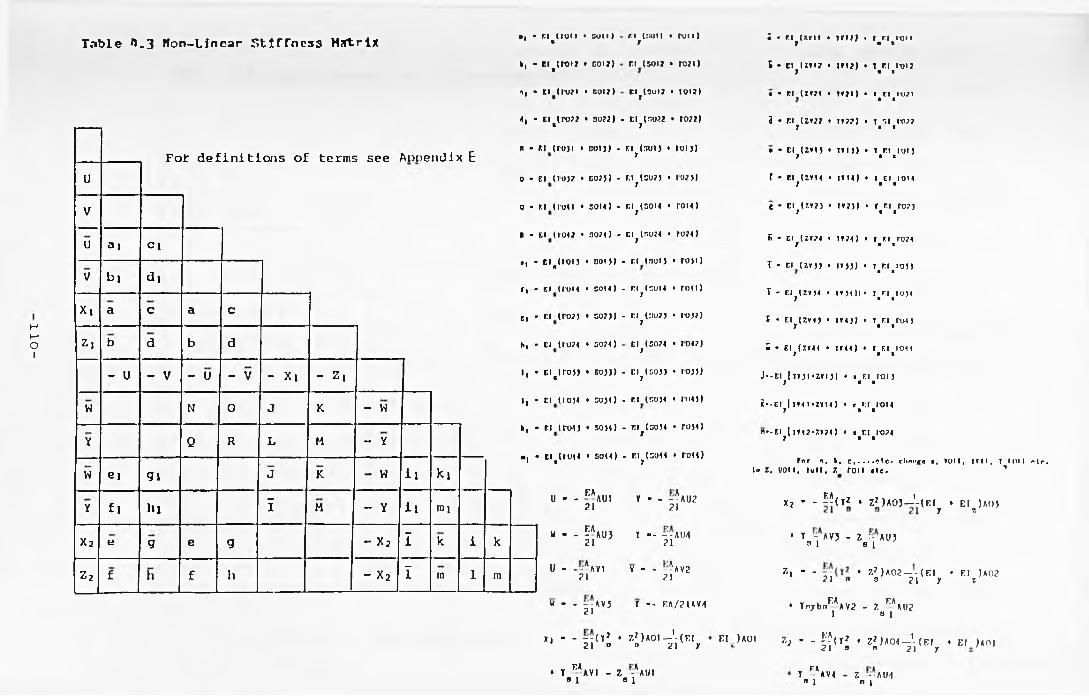
11

0-

Table A.3 Non-Linear Stiffness Hartrlx

F o t d e f in it ion s o f terms see Appendix Eu

V

u a l ci

V t>l di

Xi a c a c

Z| b d b d

- U - V - U - V - Xi - z,

w N 0 J K - W

Y Q R L M - Y

W ei gi J K - W i l ki

Y f l hi I M - Y i l rai

x2 e g e g - x? I k i k

z? f h f h - X2 I m i m

k, • ci^iroi? • coi?)

i i - c i ( ru? i • bo i? )

■ii • ciyro?? • 30??)

n • r.i (ro )i • boij) -

o • El ( lo )? • go? ) ) -

o • ci (ro il • son ) -

II - El (l'04? • 30?() -

t , • E I J I O I ) • O O I J )

r, - ci iron • son )

ci * cM ro? ) • oo?j)

h, - Cl (IO?4 • S0?4)

i, • c i t (ro ) ) • so)) )

l, • Cl (10)4 • 00)1)

k, • Cl (1-04) • 50)4)

a, - Cl_(1044 • S014)

•i • ci'lion • sun) n (cull « r u n ) >

r.i (sol? • ro?i)

e i j l s u i ? • i o i ?)

- ci^tso?? • ro?2)

£1 (301) • 101))

El (SO?) • 10?)) 7

r.i (son • ron ) j

El^( S024 • 1024)

- EMnou • ro ) i )

. n (son • ro4i) i- EI (DO?) • TO)?)

El (SO?4 • 1042) 1- El (S O )) • 1 0 ) ) ) 7- cl (SOM • In4))

- Cl (00)4 • ro)4) 7

- EIJ(3044 * ro l l )

u * - eaau . 21

V - - - AAU2 21

w - - -EAAU3 21

l • - --AIM 21

u - - - AAV121

V - - -*AY2 21

w - - - -AVJ 21

Y — EA/21AV4

*1 - - - - ( T J • Z ^ A O I—'- (E I 21 o o 21 y

i - c i j U f i i • m i ) . f r i i o n9 •

t - C l ( H I ? • I I I ? ) > T E l r o i ?7 ■ »

• - E M Z I 2 I • l l ? l ) . T C l l t ) ? l • •

i - E l ( Z * ? ? • 1 1 2 ? ) . I '*.1 I T )> ?1 B 8

• - E y t Z I I ) • I I I ) ) 4 T E l I t J l ) # *

f * E l ( Z I I 4 • 1 1 1 4 ) • T C l I O M7 B t

e * e i ( z i ? ) • n ? ) ) • t n r o ? 5j B 8

C • C l ( Z I 7 4 • 1 1 7 4 ) • i e i r o ? i7 8 t

T - c l ( z i ) ) 4 i * j j ) . I E l IO J J8 B

T - C I J ( Z » ) 4 • 1 1 ) 4 ) 1 • I r . i i o nB 8

F * E I ^ I Z i p • 1 1 4 ) ) 4 i e i m m )B 8

S * E l (7 .14 4 • 1 1 4 4 ) • 1 E l 1X34 47 • •J--EI I TIJI'ZVIJ) • t El roi J7 • *¡•-El^| IV11 • ZV 14 ) • rB»;l#lt)l4

H--EI (lM2*ZV?4) • s El lt)?4 7 • ■

f o r n, b, c , . . . . r t c . clmt'ge >, l u l l , I l l l , T H i l l lo Z. UOI I. lu l l , 7 roi I t ie . ’

EA 1** . - - ( T * . Z>)AOJ — (E Iy 4 E !7 )A0)

* Tay*vJ - V r AU5

z l * - * Z? )A02—— ( El * El )A0221 n o 21 y z

♦ YoybnE*AY2 - Z E%U21 3 1

El )A0! Z t . - ^ ( r ? . z i ) A « J - ( E I •& 21 a a 21 y

♦ T F*AVI - Z -*AUI ■ 1 "1

FAT - AV4 ■ 1 Z --AIM " 1

" I r .

E l ) A 0 1

Ill

Table fl.*) Non-Linear Geometrical Stiffness Matrix

u

AA

W

W

- U - V

- A

- B - AA

- U

- C

- D

- V

- E

- F

m

m 0

- W

- Y

- W

- Y

0 0U—:-VIOI v ^ i in ?

1 1

Q 0,w-—?voj Y— W04

1 1

For u. v,, W -lnd Y

In th" cxpr"3»ion fo r

M H—- X011 B- - - X012 C2 2

M H~ X014 E- — X023 F2 2

14 MXO)3 II- —* X034 I-

2 2

X072

HX

2

- G

- I

For definitions of terms see Appendix F

• • - n ie l l i • »O il) • - ’ «OH •

b - - » ^ 0 X 2 1 • SOI?) • - 1 0 1 2 • .10 ( b j - b | ) 2 •

nc - - » ^ ( « 1 2 • BOI2 ) • -*XUI? - .10g(W , - ¥ , )

h

t - - »^1 Cl?? • »07? ] * ~ 1 U ? 2

« . 1• - - h [ c u t • n o i ) )

I• • - XU 13 • -0 / ! ( ¥ , - ¥ ,

2 2 •

nr • - » I c m • » o n )

j• -Jr* u u - . » o ( w , - w , :

? «

*■ - - » ?( CIJ? • P0?) ] • ~ x u ? ) ♦ . i o t ( v , - w , ;

*• - f I U 7 4 ------- 0 ( « » - « I

? f.0. ■ 7 1

\ ! ° r

h - -H ^ ( CM? • »074 )

1 - - H j ) CX ) ) • »0 1 ) ) • --f lU33 -

HJ C M ) • »0 )4 ) . —?XU34 - .10 (V , -V .

? •

nk C I )4 • »0 )4 ) • -*XU )4 - . 1 0 ^ » , - » ,

111 [ CI44 • »044 )

J• - - XU44

2

\ | ° ,a CXI) • » 0 1 ) ) * i , u ” - ¿

h

n - -n^t CXI 4 • »014 ) • XU 14 - .10t (W , .¥ ,

Mn . - » ^ l CX?) • » 07 ) ) • ~ * U 2 3 - . lQ e ( v 2 -¥|

P • - » I cx?4 • »01? | 1

• —' IUI? • .10 (W , -¥ , ? * 7 1

Tor n,T» ntc rhnnn* y to ■ nnd vlcn Inti|*r*aniofl for n, b, ate.

112

Table 4.5 Linear Tangential Stiffness Matrix

a.1

B, A1 z

C, B c1 z Z

b. A B A1 yz yz y

C, B c B c1 yz yz y y

A B A B m1 wy wy wz WZ

f, B c B c n 01 wy wy wz wz

- a . -b , -C, -5 , - c. - f, f,i 1 1 1 1 i 1

-b . -A -B -A -B -A -B b, A1 z z yz yz wy wy 1 z

-4 , F D F D ♦ F -D ♦ d -F E1 z z yz yz wy wy 1 z z

-6 , -A -B -A -B -A -B b, A -F Al yz yz y y z wz 1 yz yz y

-d . F D F D r -D d, -F E -F1 yz yz y y WZ wz 1 zy yz y

- e . -A -B -A -B -m -n e. A -F Ai wy wy wz wz 1 wy wy wz

2, F D F D 0 n -R. -F F. -Fwy wy wz wz 1 wy wy WZ

T • T, - T, A ■ EAj — EAj T. ■ T«2 " Tst

*, • ".2 - E,z1 ». EI-2 • “ «I * « ‘ *** ' “ *

E5w ■ Eei2 - ES.1

EM■ T * a

E» ,

b| • - i f ( T - Tg )

EMo, . ~-p-|T,t - Ti> <*i * * ~ (T«r7l) * l ' V 7>

ESwm • - Lr

ES .

f| ■ — gl * 1E\l E5-

For the t e r n s S| , E , , « I . •na 3 I oh ’ n« " T to Z o r v i c e v e r s s .

F

-0

«z

Cz

7z-I . r*

E l , » E I i » ,■ ” T T ♦ * ¡ 1 ®I ■ 6i r * V

•

Az♦ —i

E , zDz • 2 i r *

\1

E I A E I t A_ F

■ " ~ r * ’ f F z ■ 6T T • V

Change the au b a o r lp t o f th e

r z and E I x1# At to J , 7 * . T“ *

. . . . . e n d E I y j , Bn<*

f o l lo w in g t e n t s i T t> Bj t ? t , 5 . .

• nd a t r e s p e c t i v e l y I n the f o r * o f

ET

0 ■ AE I .! m1- + a 2

1 w * Ì 5

" « 1Aw . J L

1 T 30

.GK EI ,n . « “1A

♦ 2-? ♦ ——01C | 106 r n . 6 2 V

)AGK o ■ o r' 2

1

1 A

* '¡7♦ J-GK| 10

■«EIw1N > *---- «1

A- ‘ » W .30

1 .To CE

)0 c,(

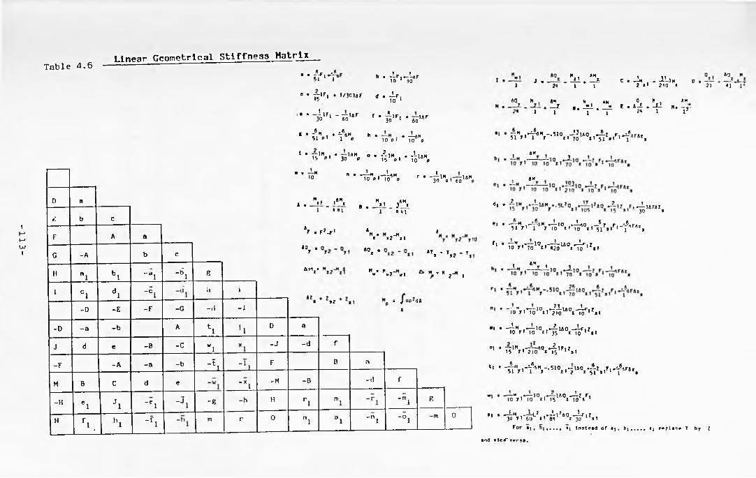
11

3-

Table 4.6Linear Geometrical Stiffness Matrix

I

-6- r . 6 « «■ ■5 1 l *~ P b * “ r i - ~ * F

1 0 1 1 0

0 ■ “ 1 F | 15 ‘

♦ 1 / 3 0 1 A Fd ■ foF>

• a ■— t i f ,3 0 1

- T ~ lA F 6 0 f ’ 3 0 I F * * 6 0 1 4 F

I » -®-M5 1 » '

. 6♦ — -AM

1 Ph * ♦ — AH

10 P ' 10 P

i a — IN 15 P '

♦ 1 AM3 0 P o ■ - ¿ l M ♦ J - U M

15 P 1 10 P

■ a M10 n . —I n —Lam

10 P 1 10 P r * ' ¿ 1K H "30 P1 60

D a MA a _ i . .4M, B . M" j 4M,

¿ b c« «1 1 QUI

F A a*F a F’ - f 1 A

M a I .2^ ,1

AM

G -A b c*0r a A0t a A T aS Ts2 - Ta

H\ b l “ a' l - 6 1 R

AMj* M a pw w? If I H - N2~* 1

1C 1 d l - E1

¡1 iAZ

-D - E -F -G -.1 -X9? Si o w * 'JV J"

A

-D - a -b A*1 ■l

D a

J d e -B -CW1

- J -d r

-F -A -a -b - _tl - T ,F B a

M B C d e- * i

-M -B -d f

-HC1 J 1 ' " I - J i - g -h II

r i " l - " i R

Nf l . h l " f l

m r 0n l a l - " I " 5 i

-m 0

J aM , AM- H ♦ — i C a - L m , - - I 1—'M D 11 ------ 4

AO___ t

1 2U 1 1 2 «1 2 1 0 * 21 «1

AQy H , AM M AM 0 H . AM

2 * 1— X

1- « 1 « N a ------ » ----- -

1 1t . J - i .

21 f « - V -

--M5 i y *

♦ ^ A M • 1 J - 5 l 0 . 1 - ^ 1 4 0 x . ^ . . F i * f 4 r * S

1 AM

. AM

d' *5 . - .6

■ •—uraz3o >

*■ ’ "mV T 4Hr*li10«.*iV0«i'nl..r< ' f F*S

fl * m‘V™ l0iriÌ5U0,‘T >z,i

1 AM 1

^ o ._V ,z .' ~Tò"r '*To10t i*?iol40i"7or| z*i

" * -^Hr'*T3,0. i ^ uox-^>z.,

01 * 7i"'rnT?',T -i'r' t„

" ’ -H,,ri-f#V -5loii*?U0.*5ÌI..r«*f ‘ri*.

-H » -3 -1 0 . -IflO —1 ? F ,io r ' io xi is x io s

il * »J.1ÌA0 _JLf 1?x 30 1 »1F o r a t . i ( I n s t e a d o f «| , t»i , ____ tj r a p i a t e T by l

It . —U --M.Z .»-LlXio ' 3 0 T I 6 0 X l 05

and e1cd" »a rsa .

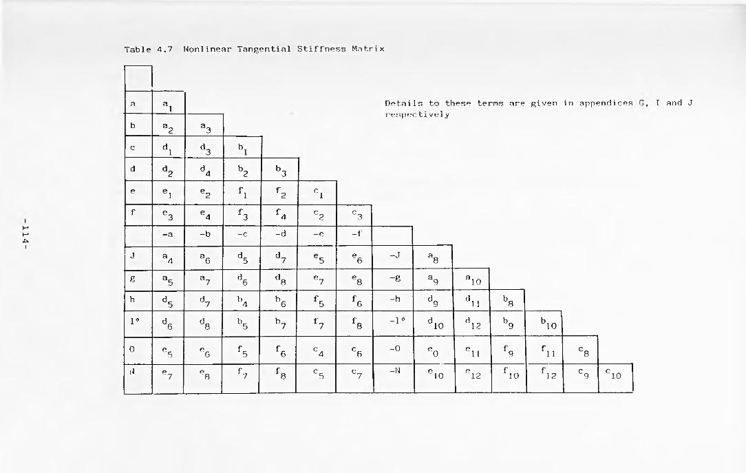
114-

Table 4.7 Nonlinear Tangential Stiffness Matrix

a ai Details to these terms are given in appendices

b a2 a3r e s p e v ; l i v e i y

c dl d3 blcl d2 d4 b2 b3e 61 e2 fl f2 cif e3 e4 f3 f 4 C2 C3

-a -b -c -d -e -f

j a4 a6 d5 d7 e5 e6 -J a8g a5 a7 d6 d8 e7 e8 -g a9 aioh d5 d7 b4 b6 f5 f6 -h d9 dll b81° d6 a

CO b5 b7 f7 f8 -i ° dio d12 b9 b!0

0 e5 e6 f5 f6 C4 C6 - 0 eo ell f9 fll C8W e7 P8 f7 f8 C5 C7 -N eio ei2 fio f12 C9 C 1 0

I and J

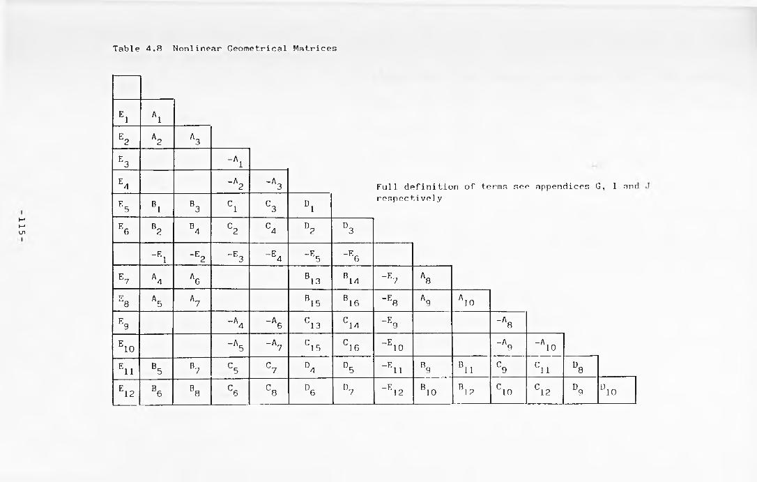
11

5

Table 4.8 Nonlinear Geometrical Matrices

E1 A1

E2 A2 A3

E3 -A1

E4 -A2 -A3 Full definition of terms see appendices G, I am

E5 B1 B3 C1 C3 °1respectively

E6 B2 B4 C2 C4 D2 °3

-E1 -E2 -E3 -E4 -E5 -E6

E7 A4 ag B13 B14 -E7 A8TT~8 A5 A7 B15 B16 -E8 A9 Aio

E9 -A4 -A6 C13 C14 -E9 -A8

e io -A5 -A7 C15 C16 -e io "A9 " Aio

E11 B5 B7 C5 C7 °4 °5 - E n B9 B11 C9 C11 °8

E12 B6 B8 C6 C8 °6 °7 _ E , 2 b io B ,2 c io C12 °9 ü i o

116

Table 4.9 Initial Stiffness MatrixA. = ♦ P,ZS> * f <AMy ♦ APMs )J*o1 A6 = ♦ P,ZS) - ~ ( AMy ♦ APAZ,)]*,,

1 1 ï r*2 = ♦ PiZ3) ♦ ^(AMy * APAZ3) ] Xo1 A7 = t - ( M y1 ♦ P.Z,) ♦ ~(AHy ♦ APAZ,)]»^

A3 = t - > y1 ♦ p , zs ) ♦ ¿ ( ahv ♦ apaz ) ] t . A8 = [ - > . + P,Z oixoP

fl - r l/M . D 7 \ . 1 / « m .n .f \1 . r. •, « 1 -^ - 15'"y i - ■ * s 7 - 30^ ny * '’™ V - ’ xo1 8 - L"îo y 1 + r » s jto2

A1 A 2 Al A2 * 5 = C (Hyi + P>Z30]*o1 *io 1 ff ? (Myi + " ' " s 5 + ^ (AMy + APAZs )])<oi

A3 A4 A3 % A,, r [— (M , + P,Z ) - — (AM ♦ APAZ ) ] * , 11 io y 1 1 s io y s oi

A| 2 = [ -— (M . + P.Z ) - -—( AM + APAZ ) ] t .l£ 30 yi 1 s 6o y s oi

A9 A11For Aj, A2 . Aj, etc. instead of Aj, A? .

' a i o A12vice versa, etc. replace y by z and

A 9 *11

A10 *12

A5 A 0-A

'A7 A8 *13 a m

A7 A8 hÂ6 A9 A10 A] 5 A16

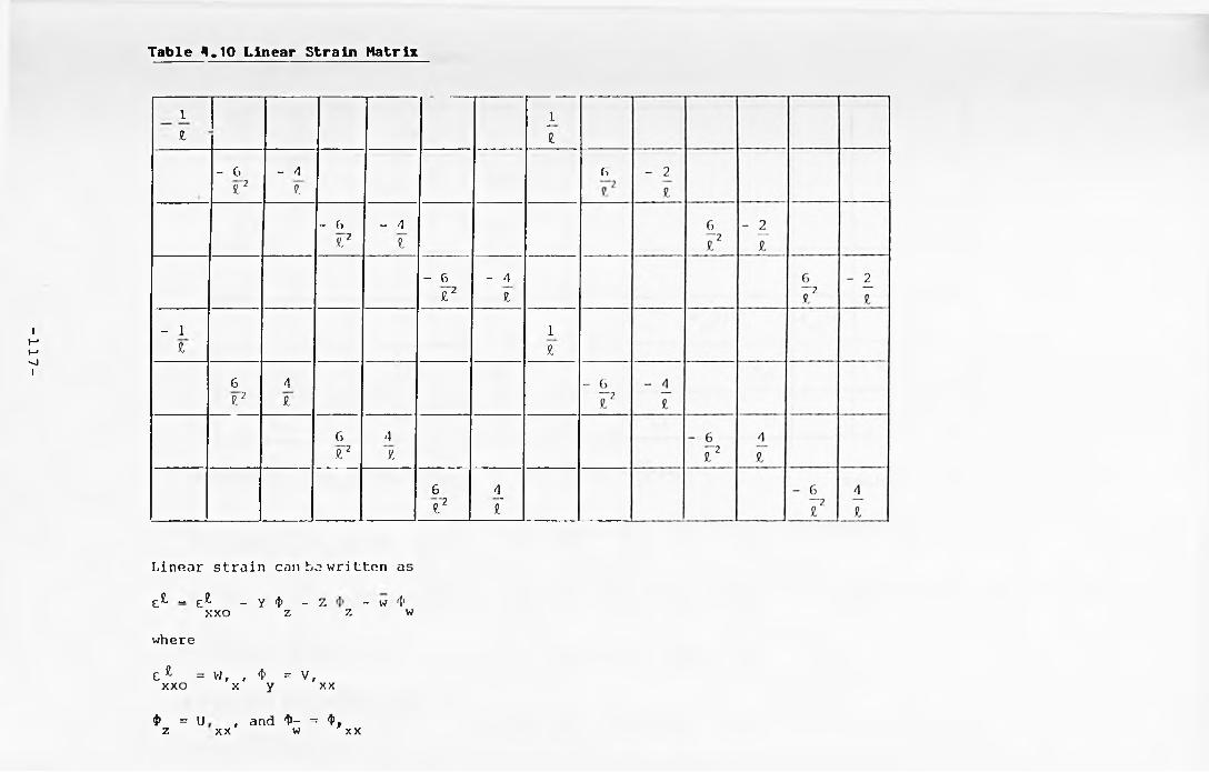
-¿IT

T a b le * .1 0 L in e a r S t r a in M a tr ix

i

1£

- 6 £2

- 4£

- 6£2

- 4£

- 6 £ 2

- 4£

- 1£

6£2

4£

6£2

4£

6£2

4_£

_L£

1£

Linear strain can ba written as

c £ _ £ £ - Y <f — z - w 41xxo z z wwhere

e £ = w, , <t> = v,xxo x y xx

4> =z , and 1>- = Q, wUX X X X

il

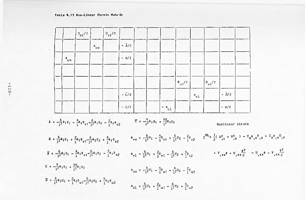
Table <.11 Non-Linear Strain Matrix

0 / 2 u r

0 . / 2 v l

aVO

- A/2

auo - A /2

B -/ 2\i2

0 J 2v2

- C /2a v l

- n/2

- C /2 " *ul - D/2

£*'*■ - Y*l8v,*p*]V! - f*iet, C ■ -T^lU* * li4'"2 nonlinear strain

* ]> 2 \ 2

• ^ iO v, ^ i v a - f * l » ,a

avo 1 - F V> - l°vl * 2 - f \ 2

vl = V Vl * l vl - F V2 + I Bv2

HL 1= M U* * V? > - Y 2 ,x ,x

+ V $ + u, xx ,xx 2

* iv2uo - > - I°U1 - > - I®u2

_ 6 2„ 6 'I«aul * + I*u1 - 1 ^ 2 ♦ - \ 2

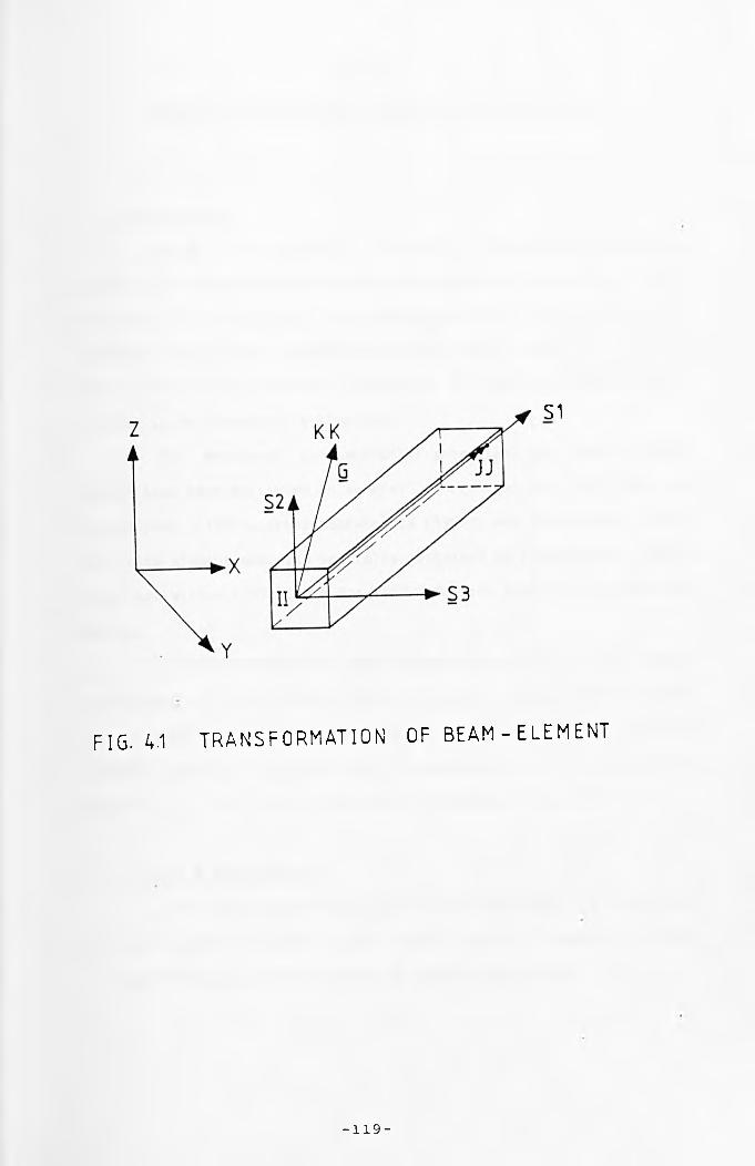
S1

FIG. 4.1 TRANSFORMATION OF BEAM-ELEMENT

-119-

Chapter 5

Analytical Procedure and Computer Program Structure

5.1 Introduction

Using f in i t e element concepts a comprehensive analytical

procedure and computer implementation o f the general formulation for a

beam-column o f thin-walled open cross-section in space is presented.

The program TDA (Three Dimensional Analysis) can be used in both the

e last ic and ine last ic resulting analytical processes are systematically

arranged in for numerical evaluation.

The sectional and sectoria l properties for I-seetion beam-

columns have been mentioned in several references such as Chan and

Kitipornchai (1987), Zhibrroski-Koscia (1967), and Zienkiewicz (1977).

The f in i t e element concepts are fu l l y explained by Zienkiewicz (1977),

Bathe and Wilson (1976), and Rao (1982) for the analysis o f structural

members.

A fu l l coverage o f the analytical procedure and general

descriptions for the program TDCP is presented herein. Details o f the

results obtained by applying TDCP to selected problems covering

d i f ferent aspects o f e last ic and ine last ic behaviour are contained in

chapters 6, 7, and 8 and in references (El-Khenfas 1987c,b)

5.2 Finite Element Method

The f i r s t step in the f in i t e element analysis i s equivalent

to replacing the domain having an in f in i t e number o f degrees o f freedom

by a system having a f in i t e number o f degrees o f freedom.

- 120 -

5 .2 .1 Nuaber o f Elements (MEL)

I f the beam has no change in geometry, material properties

and external conditions ( l ike applied loads ) , then i t can be divided

into equal lengths as shown in Fig. 5.1a. I f discontinuit ies are

present Figs (5.1b and 5.1c) , nodes have to be introduced at these

discontinuities. The number o f elements to be chosen for idealization

is related to the accuracy desired with an increase in the number o f

elements generally providing more accurate results, but at the cost o f

greater computation.

5.2.2 lumber o f Segments over the Cross-Section (NELS)

In order to evaluate the cross-sectional properties appearing

in the various element s t i f fness matrices (El-Khenfas and Nethercot

1987a), i t is convenient to div ide each plate element o f the cross-

section into a number o f small segments. The s ize o f these segments

must be chosen with care for both the e las t ic and inelast ic analysis.

The number required for reasonable accuracy depends on the pattern o f

applied loads (which a f fec ts the type o f response) and the residual

stress patterns (which a f fec ts the spread o f y i e ld ) . Any strain

distribution over the cross-section leading to a mix o f e las t ic and

yielded regions may be conveniently allowed for by considering the

member's cross-section to be divided as shown in Fig. 5.2a. The flanges

and the web are divided into NY segments along each plate length and NZ

through i t s thickness. AA, . is the segment area, where i=1,NY andi f J

j=1,NZ and i t s centroidal coordinate are Y. * and Z. . as given in Fig.1 » J * » J

5.2b.

For e last ic analysis the number o f segments over the cross-

section can simply r e f l e c t the natural div is ion i . e . web, half flange

- 121

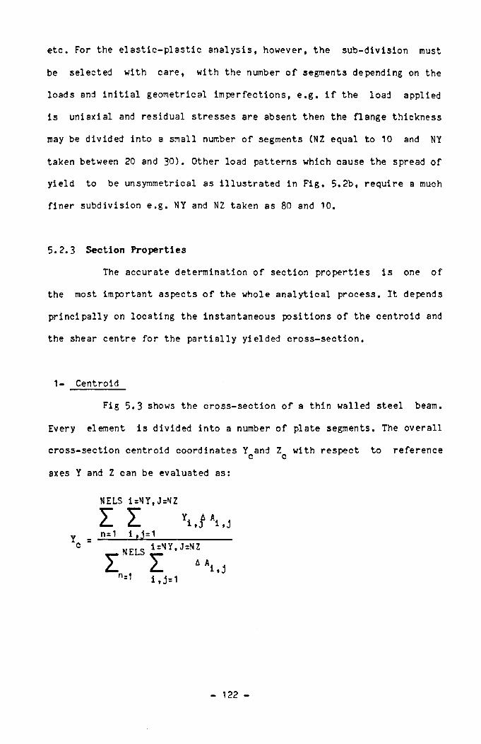
etc. For the e las t ic -p las t ic analysis, however, the sub-division must

be selected with care, with the number o f segments depending on the

loads and in i t i a l geometrical imperfections, e .g . i f the load applied

is uniaxial and residual stresses are absent then the flange thickness

may be divided into a small number o f segments (NZ equal to 10 and NY

taken between 20 and 30). Other load patterns which cause the spread of

yie ld to be unsymmetrical as i l lustrated in Fig. 5.2b, require a much

finer subdivision e.g . NY and NZ taken as 80 and 10.

5.2.3 Section Properties

The accurate determination o f section properties i s one o f

the most important aspects o f the whole analytical process. I t depends

principal ly on locating the instantaneous positions o f the centroid and

the shear centre for the part ia l ly yielded cross-section.

1- Centroid

f i g 5.3 shows the cross-section o f a thin walled steel beam.

Every element i s divided into a number o f plate segments. The overall

cross-section centroid coordinates Y and Z with respect to referencec c

axes Y and Z can be evaluated as:

Yc

NELS i=NY,J=NZ

I I Ai . j

^ NELS

n=1

i=NY, J=NZ

I “i , j =1

- 122 -

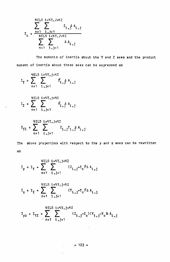
NELS i =N Y, J =N Z

Z Z hj\ . i2 . n=1 i , j =1________________c " NELS i=NY, J=NZ

Z Z ^n=1 i , j =1

The moments o f inert ia about the Y and Z axes and the product

moment o f inert ia about these axes can be expressed as

NELS irNY,j=NZ

'j = Z Zn=1 i,j=1

NELS i=NY,jrNZ

h = Z Z *i,iAi,jn=1 i,j=1

NELS i=NY,j=NZ

l n = Z Z Zi , j Yi , i Ai , jn=1 i , j =1

The above properties with respect to the y and z axes can be rewritten

NELS i=NY,j=NZ

W^Z Z <2i.rzc #i.3ns1 i,j=1

NELS i=NY, j=NZ

Wx*Z Zn=1 i , j =1

NELS i=NY,j=NZ

* n=1 i , j =1

- 123 -

TAN6 r

where 6 is the incl inat ion o f the principal axes ( n and 5)

to the y and z axes and is posit ive i f anticlockwise from the y-axis ) .

The principal moments o f inert ia about nand £ can be written as:

I_ = I COS26 + I SIN26 - I SIN26 Z y z yz

I = I COS26 + I SIN26 - I SIN28 n z y yz

i i - Shear Centre

Sectorial coordinates (a¡) o f points sj and S2 can be written

as uDg , where D denotes the ' pole ’ , si and S2 are points o f

intersection o f the radius, dsi2 i s the distance between the two

points, and h g ^ i s the distance o f pole D from a l ine passing through

points si and S2 . To determine the sectoria l coordinates o f a beam

having an arbitrary thin-walled open cross-section as i l lustrated in

Fig. 5.4, by def in it ion is equal to the algebraic sum o f twiceDSj S26ojDsiS2 The increment o f this value is equal to the product o f

Ds is2 Sds^xhs is2

i f 6uDsis2 is equal to 6<u, and 6dsi2i s equal to ds. Substituting for

these in the above equation and integrating from 0 to sn

(jj = fh dsJ S1 S2

o-

where sn is the length o f the path between Sj and S2 for any

- 124 -

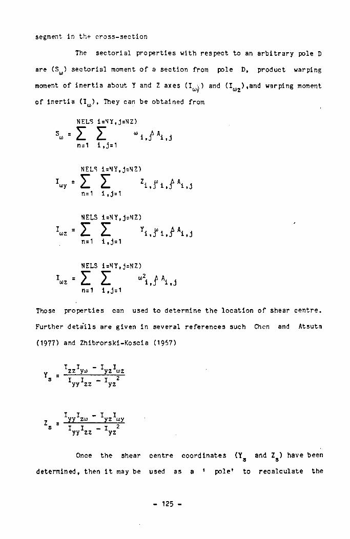
segment in the cross-section

The sectorial properties with respect to an arbitrary pole D

are (S^) sectorial moment o f a section from pole D, product warping

moment o f inert ia about Y and Z axes ( 1 ^ ) and ( I U2),and warping moment

o f inert ia (1^). They can be obtained from

NELS i=NY,j=NZ)

S = Y * 5 ” to A ato i ,J i , jn=1 i , j =1

NELS i=NY,j=NZ)

! toy = ¿E Z ! Zi , f i , ; f Ai , jn=1 i , j =1

NELS i=NY,j=NZ)

I = V T * Y. to. A A. .toz i , j i , J i , jn=1 i , j =1

NELS i=NY,j=NZ)

z = Z! ¿L “ i,/ Ai,jn=1 i , j =1

Those properties can used to determine the location o f shear centre.

Further deta'ils are given in several references such Chen and Atsuta

(1977) and Zhibrorski-Koscia (1957)

v ^zz^yu) ~ ^yz^toz s = i i - I 2

yy zz yz

centre coordinates (Y and Z ) have beens s

used as a ' pole' to recalculate the

_ yy*zto ~ ^yz uys = i i _ i 2

yy zz yz

Once the shear

determined, then i t may be

- 125 -

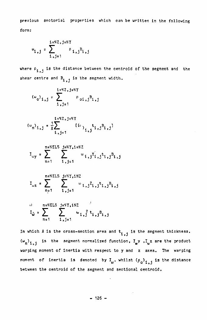
previous sectoria l properties which can be written in the following

form:

i=NZ,j=NY" i , ■ zi , j =1

where pj j is the distance between the centroid o f the segment and the

shear centre and B. . is the segment width.1 f J

' V u • I

i=NZ, j=NYzi , j = 1

P Oi , j Bi , j

(a)n^i . j = a 2 -

isNZ, j=NY

i , j =1

n=NELS j=WY,i=NZ

coy ■ z zn=1 i , j =1

n=NELS j=NY,iNZ■ z zn=1 i , j =1

W i »j Zi » j fci * j Bi * j

n=NELS j=NY,iNZ

= Z Z - i J ' - i . j h , :n=1 i , j = 1

In which A is the cross-section area and t^ j is the segment thickness.

(w . is the segment normalized function, I y ,1 z are the product

warping moment o f inert ia with respect to y and z axes. The warping

moment o f iner t ia is denoted by I . whilst Cp ) . . is the distancew r o 1 , j

between the centroid o f the segment and sectional centroid.

126 -

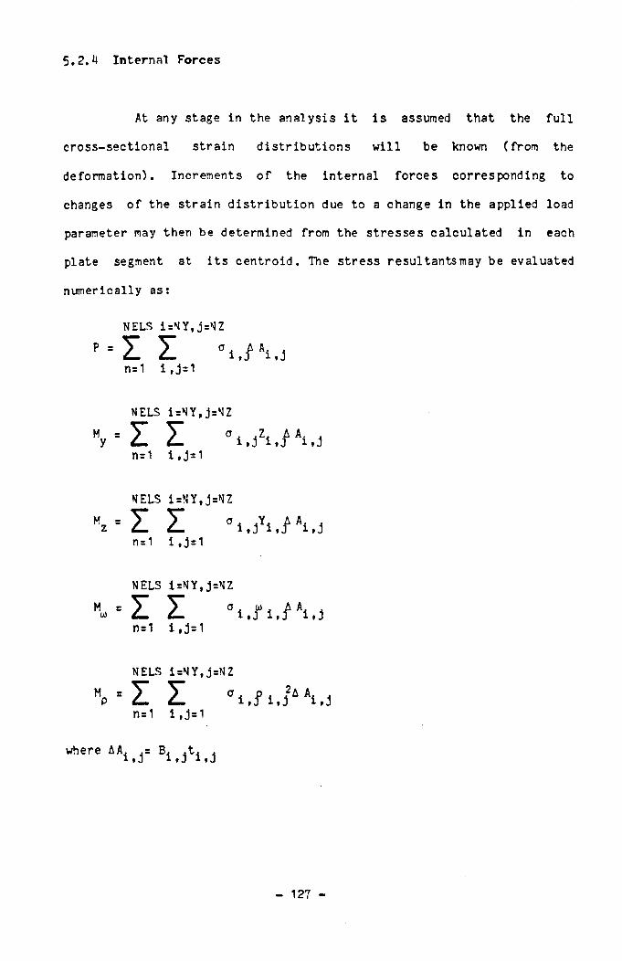
5 . 2 . 1* In t e r n a l F o rces

At any stage in the analysis i t is assumed that the full

cross-sectional strain distributions w i l l be known (from the

deformation). Increments o f the internal forces corresponding to

changes o f the strain distribution due to a change in the applied load

parameter may then be determined from the stresses calculated in each

plate segment at i ts centroid. The stress resultants may be evaluated

numerically as:

NELS i=NY,j=NZ

- I In= 1 i , j = 1

NELS i=NY, j=NZ

V i In=1 i,j=1

NELS i=NY,j=NZ

v l I " i . j i i . n . jn=1 i,j=1

NELS i=NY,j=NZ

M» ‘ I I " t . f i . A ' i . jn=1 i,j=1

NELS i=NY,j=NZ"p = z In=1 i,j=1

where AAi fJ « B ^ t ^

- 127 -

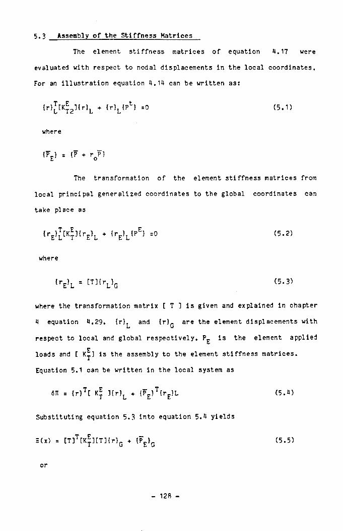
5 .3 Assembly o f th e S t i f f n e s s M a t r ic e s

The element s t i f fness matrices o f equation 4.17 were

evaluated with respect to nodal displacements in the local coordinates.

For an i l lustra t ion equation 4.14 can be written as:

{r}JrK^2 l i r ) L + { r ) L {Pt } =0 (5.1)

where

{P£} = {P ♦ rQP}

The transformation o f the element s t i f fness matrices from

local principal generalized coordinates to the global coordinates can

take place as

( r E) i t4 1 I r E1L ♦ , 'E , L tpE> =° <5-2)

where

{ r E} L = tT3irL}G (5.3)

where the transformation matrix [ T ] i s given and explained in chapter

H equation 4.29. { r } . and { r }_ are the element displacements withL G

respect to local and global respect ive ly . P£ is the element applied

loads and [ K .] is the assembly to the element s t i f fness matrices.

Equation 5.1 can be written in the local system as

fill s { r ) T[ ] { r ) L + {PE} T { r E}L (5 . « )

Substituting equation 5.3 into equation 5.4 yields

E(x) = [T )T [K ^ ] [ T ) { r )G ♦ { P ^ (5.5)

or

128 -

(5.6)' K? ’G] I r ) G * ' V = °

For equilibrium equation 5.6 equals zero as

(5.7)

I f the beam is divided into a number o f elements then the

assembly o f these members can be presented in the following form

where { R} , {P } , and [K,p] are the assembly to the elements

displacements, applied loads, and to the s t i f fness matrices

(tangential, geometrical l inear and nonlinear and in i t i a l displacement

matrix respect ive ly ) . Their assembly arrangement are given in equations

5.9 to 5.11.

[Kt ] {R} + {P} =0 (5.8)

(5.9)

L_

{ R} ( 5 . 1 0 )

r

PE(PI = 5.11)

P

129 -

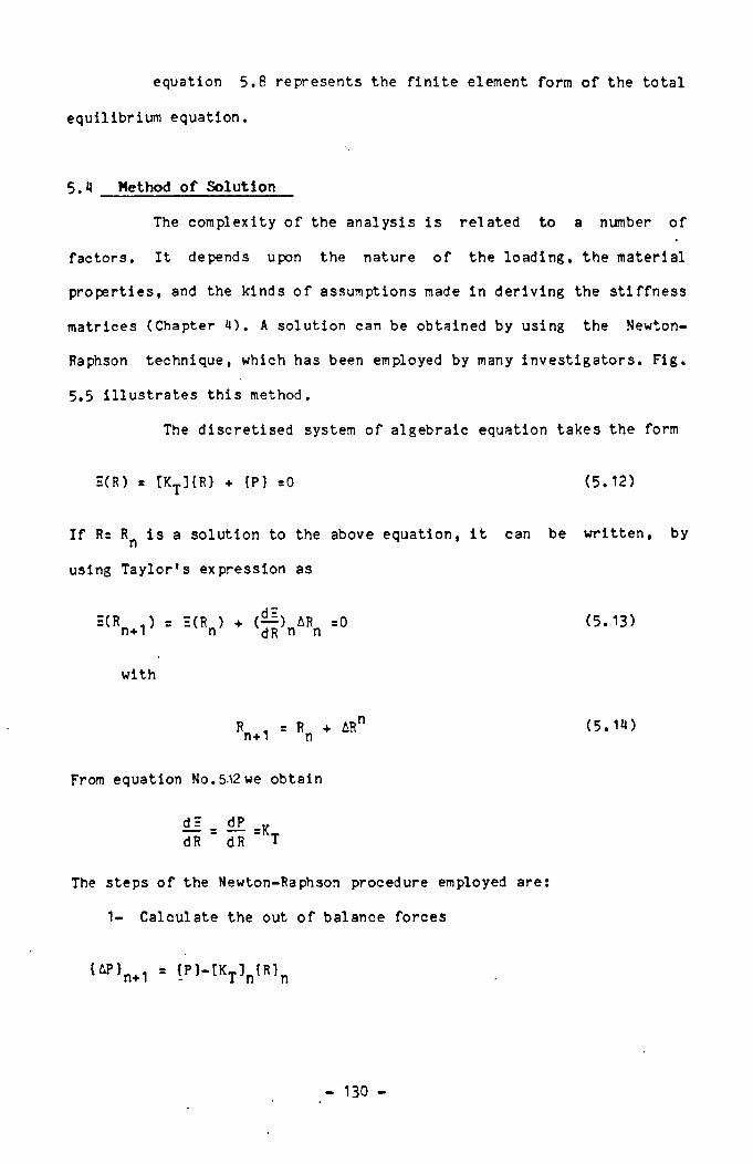
equation 5.8 represents the fin ite element form of the total

equilibrium equation.

5.H Method o f Solution

The complexity o f the analysis is related to a number o f

factors. I t depends upon the nature o f the loading, the material

properties, and the kinds o f assumptions made in deriving the st i f fness

matrices (Chapter H). A solution can be obtained by using the Newton-

Raphson technique, which has been employed by many investigators. Fig.

5.5 i l lus tra tes th is method.

I f R= Rn is a solution to the above equation, i t can be written, by

using Taylor's expression as

The discretised system o f algebraic equation takes the form

=(R) = [Kt ] {R } ♦ {P } =0 (5. 12)

S(R ) = S(R ) + (; î f ) ÛR„ =0 n+i n hr n ndR n n(5.13)

with

n (5 .1 « )

From equation No.512we obtain

d= . dP _K dR ' dR " T

The Steps o f the Newton-Raphson procedure employed are

1- Calculate the out o f balance forces

<ÛP}n+1 = < P > - t KT V R î n

- 130 -

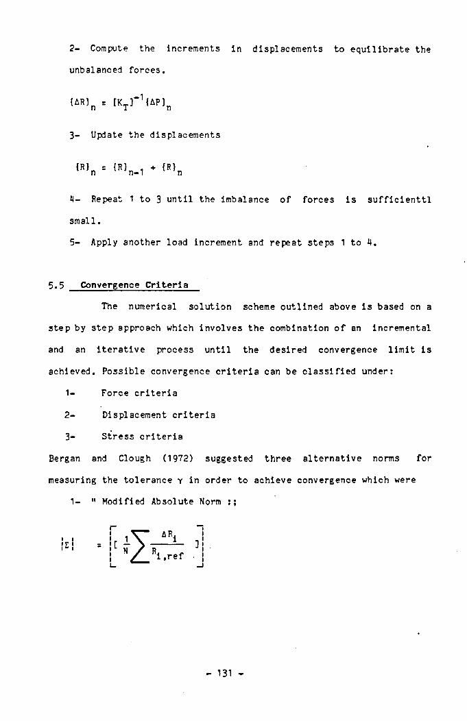
2- Compute the increments in displacements to equil ibrate the

unbalanced forces.

{AH)n = [KTr 1 {ÄP}n

3- Update the displacements

{R} = {R} . + {R}n n- 1 n

4- Repeat 1 to 3 until the imbalance o f forces i s su f f i c ien t t l

small.

5- Apply another load increment and repeat steps 1 to U.

5.5 Convergence Criter ia

The numerical solution scheme outlined above i s based on a

step by step approach which involves the combination o f an incremental

and an i t e ra t i v e process until the desired convergence l im it is

achieved. Possible convergence c r i t e r ia can be c lass i f ied under:

1- Force c r i t e r ia

2- Displacement c r i t e r ia

3- Stress c r i t e r ia

Bergan and Clough (1972) suggested three alternative norms for

measuring the tolerance y in order to achieve convergence which were

1- " Modified Absolute Norm

131 -

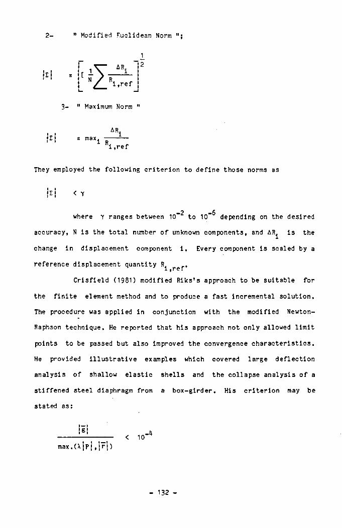
2 - ” Modified Euclidean Norm

i_ i!s !

i_2

3- " Maximum Norm "

Jz ii iAR

= max ii Ri , r e f

They employed the following cr i ter ion to define those norms as

\l\ < 1

where y ranges between 10“ to 10“ depending on the desired

accuracy, N is the tota l number o f unknown components, and AR is the

change in displacement component i . Every component is scaled by a

reference displacement quantity R r e j..

Cr is f ie ld (1981) modified Riks’ s approach to be suitable for

the f in i t e element method and to produce a fast incremental solution.

The procedure was applied in conjunction with the modified Newton-

Raphson technique. He reported that his approach not only allowed l imit

points to be passed but also improved the convergence characterist ics.

He provided i l lu s t ra t i v e examples which covered large def lect ion

shells and the collapse analysis o f a

a box-girder. His cr i ter ion may be

analysis o f shallow e last ic

sti f fened steel diaphragm from

stated as:

max. ( X S P !, S r|)

- 132 -

¡g| =JIv7

Where jgj is proposed by Pearto and Riceioni (1978). g is the

out-of-balance force, P the total applied force, r the reaction vector

and Kp is a diagonal matrix containing the leading diagonal elements o f

the tangent s t i f fness matrix.

To ensure convergence to the correct result certain simple

requirements have to be sa t is f ied , the most obvious o f which i s c lear ly

that the displacement function should be able to represent the

displacement distr ibution as c lose ly as possible. In general the larger

and more complex the numerical problem the more d i f f i c u l t i t w i l l be to

achieve sat is factory convergence.

In the present analysis two methods were applied together to

meet the necessary convergence l im i t ; these can be explained as;

i - Out o f balance forces

i i - I tera t ive process

5.5.1 Out o f Balance Forces

I f the sum o f the total forces at each node i s not in

equilibrium i . e . the summation o f the internal forces does not balance

the external forces, the di f ference between them is termed the out o f

balance force. These residual forces should be re-applied until both

balance each other. To explain this phenomenon, the i l lu s t ra t iv e

example o f Fig. 5.6 shows the load position, beam segment length, and

support conditions. The out-of-balance forces are

- 133 -

AQyi

HU 1 - " i *1' i +1

] - Q

n * * <M»i - H'i - t

L R R Rwhere M ./ M . and M ./ M . are the bending moments about the yi yi u>i oil °

Y-axis and bimoment at node i from l e f t and right. A Q sub i and A

are out-of-balance forces for the shear and bimoment respect ive ly ,

is the element segment length, and the subscript i varies from 1 to

NJ (NJ= number o f j o in t s ) . I f the residual forces {AP^} obtained from

the equilibrium o f node i do not have small values. {AP^} should be re­

applied as an increment o f force and this process repeated until a

balance is achieved. A fu l l description is given in Fig. 5.6.

where

<4P1 > * [ " l 4«y i 4° z l SMzi 40i 4" t l 4V ]

where {AP^} is an array to the out-of-balanee forces at node i .

5.5.2 I t e ra t iv e Process

In this method both the unbalanced or residual forces within

the structure nodes and the increment o f displacements are implemented

at the same time. The out o f balance force and the variat ion o f the

deformations are described as:

i - Out o f balance force

- 134 -

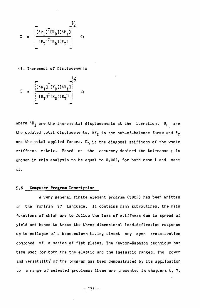
y>

z =[APjl'CKplCAPj]

EPt 3 CKdDCpt ]<Y

i i - Increment o f Displacements

1/2

Z z[AR j ]1 CKd] [ ari ]

[Rt ]T[Kd ] [Rt7<Y

where AR are the incremental displacements at the i te ra t ion , R. are

the updated tota l displacements, AP is the out-of-balance force and

are the tota l applied forces. is the diagonal s t i f fness o f the whole

st i f fness matrix. Based on the accuracy desired the tolerance y i s

chosen in this analysis to be equal to 0. 001, for both case i and case

i i .

5.6 Computer Program Description

A very general f in i t e element program (TDCP) has been written

in the Fortran 77 Language. I t contains many subroutines, the main

functions o f which are to fo llow the loss o f s t i f fness due to spread o f

yield and hence to trace the three dimensional load-def lect ion response

up to collapse o f a beam-column having almost any open cross-section

composed o f a series o f f l a t plates. The Newton-Raphson technique has

been used for both the the e las t ic and the ine last ic ranges. The power

and v e r sa t i l i t y o f the program has been demonstrated by i t s application

to a range o f selected problems; these are presented in chapters 6, 7 »

- 135 -

and 8 respectively

5.6.1 Program Structure

The fu l l TDCP deta i ls together with i t s l i s t in g are given in

re f . ( El-Khenfas 198"fe). This program uses many subroutines to provide

a solution for the e last ic and ine last ic response o f beam-columns. The

more important routines and their functions are b r i e f l y detailed below.

MAIN Reads the input data, controls the ca l l ing sequences.

OUT 1,2, 3 Presents the output o f loading, displacements,

stresses, internal forces, etc .

STIFF 1,2 Forms the l inear and nonlinear tangential s t i f fness

matrices.

GE0MET1,2 Forms the l inear and nonlinear geometrical s t i f fness

matrices.

TRANS Transforms the elements s t i f fness and loads,and

displacements from local to global, (or to the

references ax is ) .

ASSEM Controls the assembly o f the tota l s t i f fness matrices

or the applied loads.

ITLOAD Controls the load or displacement increments.

STRAN 1,2 Evaluates l inear and nonlinear curvatures

BOUND Modifies the to ta l s t i f fness matrix o f the structure

according to the boundary conditions.

PROPER Calls subroutines to calculate the section and

sectoria l properties, trace spread o f y ie ld , and

internal forces.

- 136 -

ELASPL Perform the e la s t ic -p la s t ic analysis using Newton-

Raphson technique.

RESD Calls several routines to generate d i f fe ren t residual

stress d istributions.

INDEF Forms the in i t ia l crookedness by sinusoidal or

polynomial functions.

GAUSS Used to solve the equilibrium equation by Gauss

elim ination.

START Restart f a c i l i t y from a previous equilibrium solution.

STORE Store the whole o f the information obtained from the

previous ite ra t ion .

A basic flow chart is given in Fig. 5.7.

5.7 Computational Steps

The computational processes o f TDCP can be explained in the

following steps

STEP 0 In it ia liz a t io n

In this step in it ia l is a t io n s has to be made to the whole

arrays

STEP 1 Input Data

a) Beam Details

NJ number o f nodes

NEL number o f elements

NDF number o f degree o f freedom

- 137 -

SLENDSLEND slenderness ra t io (— )r y

b) ( Cross-Section Details

NES number o f elements in the cross-section

NJS number o f jo in ts in the section

T(M) plate thickness

NOSI(M) node I number

NOSJ(M) node J number

SEYKM) coordinates o f node 1 with respect to Y-axis

SEY2(M) coordinates o f node 2 with respect to Y-axis

SEZKM) coordinates o f node 1 with respect to Z-axis

SEZ2(M) coordinates o f node 2 with respect to Z-axis

M is the number o f elements in the section

c) Applied Loads

ECY, ECZ, ECR load eccen tr ic it ies

APL(7xN-6) Axial load (Fx1)

APL(7xN-5) Shear force Q„,

APL(7xN-4) Bending moment M

APL(7xN-3) Shear force Qy1

APL(7xN-2) Bending moment M ^

APL (7xN-1) Torsion M^

APL(7xN) Bimoment M ,CO 1

APL(7xN+1) Axial load ( F ^ )

APL(7xN+2) Shear force 0 >Z2

APL(7xN+3) Bending moment M ^

APL(7xN+H) Shear force Qy1

- 138 -

APL(7xN+5) Bending moment M ^

APL(7xN+6) Torsion M ^

APL(7xN+7) Bimoment M ,ii)1

N Number o f elements ( 1 , 2 , . . . ,NEL)

IN CL Type o f load increment

1 Axial load

2 Bending moment about Y-axis

3 Bending moment about Z-axis

12 Axial + Bending about Y-axis

13 Axial + Bending about z-axis

123 Biaxial bending

Different combination can be performed

d) In i t ia l Deflection (R ) —■ ■ ■ ■ ■ ■' 0

INDEF 0 No in i t i a l deflection

1 In i t ia l deflection present

U0 . VQi 4>0 Out-of-plane and in-plane deflections and twisting

IN DEFT

respective ly (they are given in TDCP by ACY, ACZ,

ACR with respect to L)

0 Sine wave

INDEFT 1 polynomial ( you have to insert to the program

the wanted function)

e) Type o f Analysis

IANAL 0 Elastic

IANAL 1 Ine lastic

Analysis options

INC 1 Linear

- 139 -

2 Non-linear3 Full non-linear

f ) Stresses

IRES 0 No residual stress

H Residual stress present

KiND 1 Leigh d istribution

2 Parabolic distribution

3 Triangular Distribution

M ~ 6 Other types

cf Flange t ip residual stress

afw Web-flange junction residual stress

aw Web residual stress

NMAT Number o f material type

ESHD Strain hardening (values)

E Young’ s modulus

G Shear Modulus

g) Boundary Conditions (B.C.)

IRR Number o f restrained nodes (B.C)

KKM 0 Degree o f freedom restrained

1 Degree o f freedom unrestrained

JJM Number o f the degree o f freedom restrained

STEP 2 Load Increment

PAX = AP1 + AFX1

Where PAX is the to ta l load, AP1 is the load increment

(usually given as ra tio e .g . with respect the squash load or Euler load

in the case o f a compressive column load ), and AFX1 is equal to the

1U0 -

value of the internal load of the previous step

PAMY.Z = AP1Y.Z + PAMY3

Where PAMY or Z is the to ta l bending moment, AP1Y and AP1Z

are e ither the increment o f bending moment about the Y or Z-axis,and

PAMY3 is the internal moment o f the previous step.

STEP 3 Displacements

Displacements have to be updated a fte r each load increment as

R = R + AR

STEP 4 S tra ins

Strains have to be calculated at each load increment ,and

then used to calculated the internal forces o f to check spread o f

y ie ld .

STEP 5 Section and S ecto ria l Properties

Section and sectoria l properties have to be calculated each

time o f calculating curvatures ( * 2, ZQ) .

STEP 6 Store

The complete results obtained have to be saved by storing

them

STEP 7 Start

In this step the program can be restarted from where i t

stopped

Step 8 Control Cards

IYYY 0 Start th program from the beginning

1 Restart from where i t stopped

MAXIT Number o f cycles o f loading required

ISTEP=ISTEP+1 Number o f steps required

ISTEP=MAXIT When the number o f steps (ISTEP) is equal to number

o f cycles o f loading required, the program store

the complete data and stop executions.

For other cycles o f loads repeat step 2 up to step 8 again

and again until fa ilu re (collapse occured).

5.8 Conclusions

A very general TDCP (Three Dimensional Computer Program)

based on f in i t e element concepts has been developed. I t was written in

the Fortran 77 Language. The main function o f i t s subroutines is to

follow the loss o f s t i f fn ess due to spread o f y ie ld and hence to trace

the fu l l load -de flec t ion response o f beam-column o f an arbitrary open

thin-walled cross-section subjected to d i f fe ren t loading and boundary

conditions up to collapse. This program can deal with three types o f

analysis which are Linear, Partia l non-linear, or Full non-linear.

These methods are fu l ly explained in Chapter M.

The section and sectoria l properties were evaluated at each

load increment together with the internal forces based o f the strains

which in turn depend upon the type o f analysis required. The

convergence to the correct resu lt employed two methods at the same

time. The f i r s t one used the Out-of-balance forces which represent the

differences between the applied loads and the internal loads, while the

second is based on the increments o f the displacements with respect to

the tota l displacements.

142 -

The main points drawn from this study may be summarised as:

1- A TDCP has been developed for the ultimate strength analysis o f

members to incorporating several types o f open thin-walled

sections ( ] , T, L, I , e t c . ) .

2- The linear and non-linear strains are used to generate the

stress-resu lts and to trace the spread o f y ie ld .

3- The section and sectoria l properties can be evaluated in the

e las t ic and in e las t ic ranges with respect to instantaneous shear

centre and centroid.

4- The convergence to a correct result i s based on the incremental

displacements and the out-of-balance forces.

- 143 -

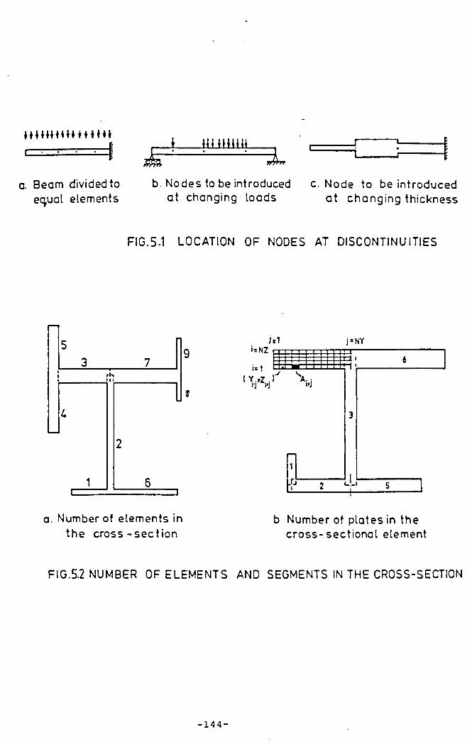
H iH IH U H iH i

a. Beam divided to equal elements

r r r y r f

i___ imiiiiiL> h »

b. Nodes to be introduced at changing loads

c. Node to be introduced a t changing thickness

FIG.5.1 LOCATION OF NODES AT DISCONTINUITIES

Js1 j = NY

a. Number of elements in the c ro ss -se c tio n

b Number of plates in the cross-sectiona l element

FIG.5.2 NUMBER OF ELEMENTS AND SEGMENTS IN THE CROSS-SECTION

- 1 4 4 -

© __________________

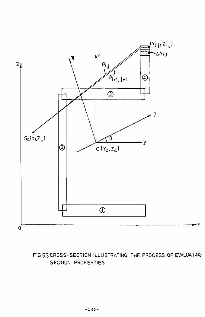
-------------------------------------------------------------------* - Y

FIG.5.3 CROSS-SECTION ILLUSTRATING THE PROCESS OF EVALUATING

SECTION PROPERTIES

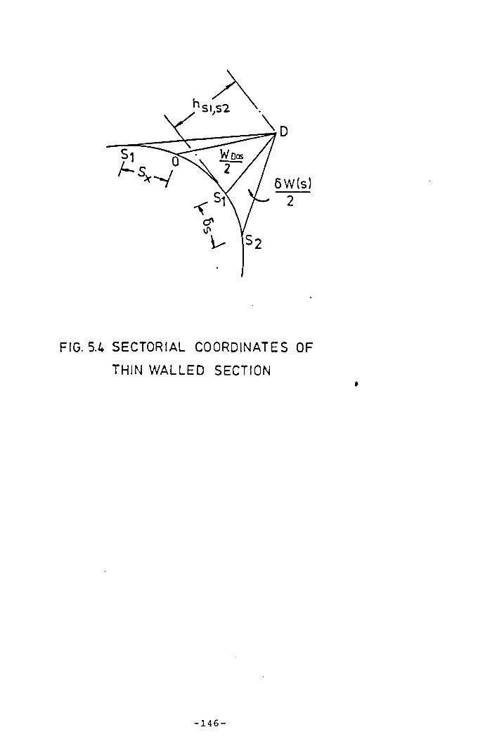
FIG. 5.4 SECTORIAL COORDINATES OF

THIN WALLED SECTION♦

- 1 4 6 -

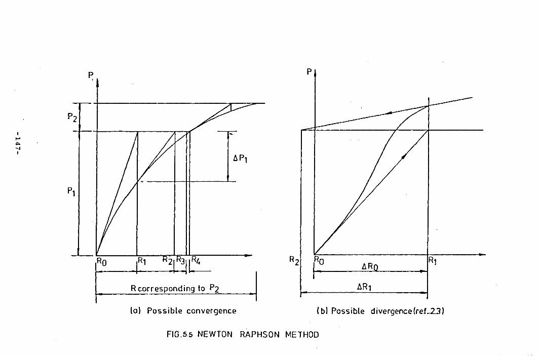
147

FIG.55 NEWTON RAPHSON METHOD

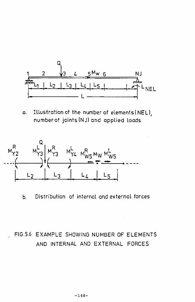
2

Q

1 2DOfl7777771

¿3 ^ 5Mw 6» = =

L1 l l 2 I l 3 I k l l 5

NJy>A//

NEL

a. Illustration of the number of elements(NEL), numberof joints (NJ) and applied loads

QR L

MY2

(

MY3)

\ J

m L, m H. ..R13 " Y i MW5MW M ^ 5

l 2 l 3

b. Distribution of internal and external forces

FIG.5-6 EXAMPLE SHOWING NUMBER OF ELEMENTS

AND INTERNAL AND EXTERNAL FORCES

- 1 4 8 -

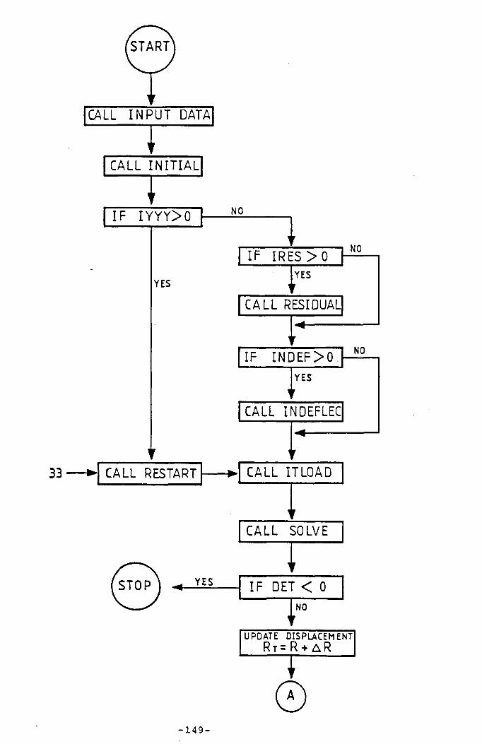
START

33

®- 1 4 9

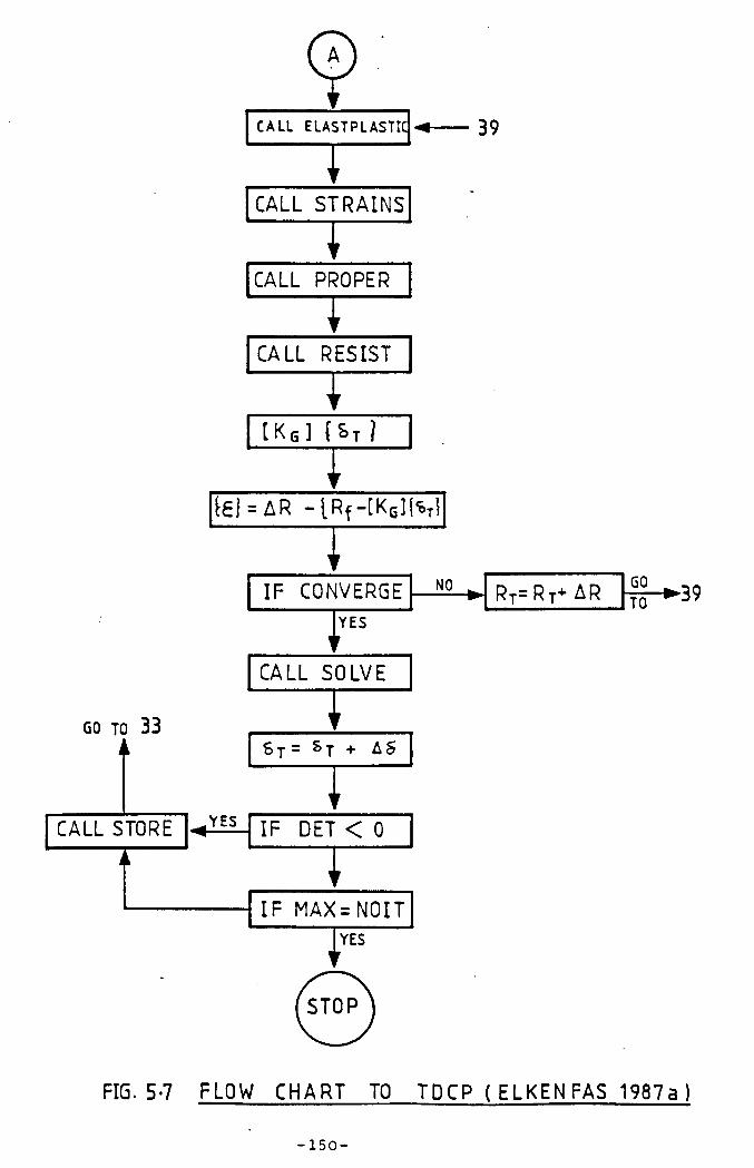
FIG. 5-7 FLOW CHART TO TDCP ( ELKEN FAS 1987a )

- 1 5 0 -

Chapter 6

E la s t ic Analysis o f Bea»-ColinBn in Three-D iaensional

6.1- Introduction

Beam-columns are defined as structural members which are

subjected to combined axia l compression and bending. The bending may

result from eccentric loading, transverse loads, applied moments, or

combinations o f loads.

The c lass ica l l inear buckling theories for e la s t ic beams and

columns were investigated by Bleich(1933) who considered I-beams with

unequal flanges subjected to axial load and equal and opposite end

moments, then he applied his theory to the problem o f beams o f

I-section with the tension flange restrained against la te ra l

displacements. Johnston (19*11), Massonnet (19*17), Horne (195*1) and

Salvadori (1955,195£) studied doubly symmmetric sections under combined

axial thrusts and equal end moments.

D if fe ren t ia l equations governing the flexural torsional

buckling o f thin-walled member subjected to eccentric thrusts have been

used by Goodier (19*12), Timoshenko and Gere (1961) and Vlasov (1961).

Their results were confirmed by tests done by H il l and Clark (1951a,b).

Goodier (19*12, 1956 ) examined the s ta b i l i t y o f a general open section

under axial load and end moments; Anderson and Trahair (1972)

concentrated on la te ra l torsional buckling o f monosymmetric sections.

F lexural-torsional behaviour has been studied by, Vlasov

(1961), and Trahair (1966,1969). They investigated the e f f e c t o f

e las t ic end restra in ts , while the e f f e c t o f continuous diaphram

_ 151 _

restrained has been considered by Hancock and Trahair (1978,1979). A

BSCA publication (1968,1970) investigated members o f d i f fe ren t cross

sections such as (Tee, Channel, Z, L, e tc . sections) under bending and

torsion. Moore (1986) used the f in i t e d ifference method to solve his

developed d i f fe ren t ia l equation in order to study nonuniform torsional

buckling o f Z-sections under la te ra l loads.

The behaviour o f beam-columns depends principally on: the ir

slenderness, the shape and dimensions o f the cross-section, the exact

form o f the applied loading, and the conditions o f support provided.

These w i l l control not only the load carrying capacity but also the

form o f structural response e .g . in-plane flexure, b iax ia l bending etc .

(Chen and Atsuta(1977)). For slender members e las t ic analysis w i l l

provide a close approximation to their true behaviour; more stocky

members, however, fa i l in g by in e las t ic action, w i l l need to be analysed

in a manner which accounts for the gradual development o f p la s t ic i ty .

Even for such cases the basis for an adequate analytical approach must

be developed from an e las t ic treatment o f the problem. Such a

formulation has been presented in chapter 3. In th is chapter the

application o f this approach to a series o f e la s t ic problems, which

cover a range o f structural phenomena, is reported.

6.2 Analysis

The analysis used herein employs the set o f assumptions

normally associated with analytical studies o f the behaviour o f thin-

walled beam-columns in the e las t ic range. These are:

152

1 - The member may have any arbitrary open cross-section with

each plate element having a thickness s ign if ican t ly less than

i t s width.

2- The member’ s cross-section is constant along the span.

3- Both shear deformation and distortion o f the cross-section

(apart from warping) are ignored.

4- D ifferent patterns o f i n i t i a l de flections (Uo , Vo,and * q) ,

may be present.

Full d e ta ils o f the problem formulation, leading to a series

o f s t i f fn ess matrices for use in a nonlinear f in i t e element approach,

are available in chapter 3. A feature o f th is formulation is the

inclusion o f several le v e ls o f so-called higher order terms in the

geometric strain-displacement relationships resulting in a hierarchy o f

s t if fn ess matrices. This permits d if fe ren t types o f combined bending

and torsion problem to be treated with d i f fe ren t le ve ls o f

sophistication. A computer program based on the material o f chapter 3

has been prepared (El-Khenfas 1987a)- using a Newton Raphson solution

scheme.

The numerical solution scheme is based on a step by step

approach which involves the combination o f incremental and i te ra t iv e

processes until the desired convergence is achieved; deta ils were given

in chapter 5. Some judgement is necessary when deciding on;

i - Number o f elements along member length

I f the beam has no change in the geometry, material

properties and external load and restra int conditions, then i t can be

divided into equal lengths. I f d iscontinuities are present, nodes have

153 "

to be introduced at these points

i i - Number o f segments in the cross-section.

The cross-section is divided into a number o f plate elements,

each element containing several small segments. These segments are then

used to evaluate the cross-sectional and sectoria l properties such as «

A, Iy , I^» K, e tc . . Both the number o f plate elements and the

number o f segments used w i l l a f fe c t the accuracy with an increase

generally providing more accurate resu lts , but at the cost o f greater

computation.

6.3 Numerical Results

Several cases have been chosen to cover the range o f problem

types outlined in the Introduction; these are l is ted in Table 6.1

6.3.1 Linear Bending and Torsion

The f i r s t class o f problem considered is the linear

combination o f bending and torsion o f the type covered in design guides

by Terrington (1968,1970). Because d irec t comparison is made against

the results o f Terrington, which are themselves based on the solution

o f the governing d i f fe r e n t ia l equations, the example is quoted in the

orig inal imperial system o f units.

A simply supported beam o f 30 f t . span subjected to la te ra l

loads Q =1 ton and Q =0.1xQ applied at midspan on the top o f a z y z

compound section, consisting o f a 18x7jx 1501b RSJ with a 10x3x19 lb

channel welded to the top flange has been selected. Table 6.2 compares

longitudinal stresses due to ve r t ica l and horizontal bending with those

given by Terrington. In determining these values the contributions to

_ 154 _

the member s t if fn ess matrices arising from the nonlinear strains

included in the formulation (chapter 3) have been suppressed. I t is

clear from the results o f Table 6.2 that the analysis is capable o f

dealing adequately with th is type o f behaviour, the stress values

obtained being almost indistinguishable from those o f Terrington 1970.

6.3.2 F lexural and F lexu ra l-T o rsiona l Buckling

The analysis may also be applied to bifurcation type

problems, involving the determination o f e la s t ic c r i t i c a l loads. In

this case a s l igh t ly d i f fe ren t solution technique, in which the lowest

eigenvalue o f the s t i f fn ess matrix including destab ilis ing e f fe c ts is

determined, must be employed.

The example selected for study is a simply supported beam o f

monosymmetric I-section previously analysed by Anderson and Trahair

(1972). This type o f problem is inherently more complex than the more

usual doubly symmetrical section due to the need to include the Wagner

e f fe c t in the torsional aspects o f the behaviour, a feature that is

accentuated i f loading is applied remote from the shear centre axis.

Anderson and Trahair(197Z) checked their theory against

experimental evidence, and they confirmed that the Wagner e f fe c t

results in either an increase or decrease in the e f fe c t iv e torsional

s t if fn ess for monosymmetric open cross sections. Because the smaller

flange is further from the shear centre, the stresses in th is flange

have a greater lever arm and predominate in the Wagner e f f e c t . Thus

when the smaller flange is in tension the Wagner e f fe c t provides an

increase in torsional s t i f fn ess o f the beam. The reverse is true when

the smaller flange is in compression.

Two examples i l lu s tra t in g the accuracy o f the author's

_155

approach have been selected for comparison. For both central load

(cases A). and distributed load (Cases B) „ the transverse

loads were applied at distances o f up to 7 .6 (—) above or below the2shear centre axis.

Tables 6.3 and 6.4 compare the results obtained by

calculation for both doubly symmetrical and monosyimietric I-sections

with those o f Anderson and Trahair. Generally good agreement has been

achieved with the largest d ifferences being associated with loads

applied below the le v e l o f the bottom flange. These are thought to be a

result o f the approximate form for displacements used by Anderson and

Trahair; the present study makes no prior assumptions about the buckled

shape.

A general equilibrium equation has been developed by Roberts

and Azizian (1983a) governing the geometrically nonlinear behaviour o f

thin-walled open cross-sections by assuming small displacements and

linear e las t ic material behaviour. The solution to th is equation, when

applied to beam-columns under equal end moments and axial load in the

presence o f in-plane in i t i a l d e flec t ion , has been checked against

existing test data.

A simply supported I-section column subjected to a

compressive load, possessing an in i t i a l deflection in the form o f a

h a lf sine wave o f maximum amplitude Uq at mid-height has been chosen

for comparison. Boundary conditions for in-plane and out-of-plane

bending and twisting are fu l ly restrained at both ends, while warping

is permitted at both ends. ( I t should be pointed out, however, that

since a pure in-plane response was expected the out-of-plane and

torsional conditions w i l l have no d irect e f f e c t on the r e s u l t . ) .

Numerical results have been obtained, which allow fo r the e f fe c t o f in­

- 1 5 6

plane deflection on flexural buckling. These require suppression o f

some aspects o f the fu l l analysis corresponding to the equilibrium

equation stated in chapter 3 in order to match Az iz ian 's assumptions.

Fig. 6.1 i l lu s tra tes the load-deflection behaviour obtained from both

analyses in which the d ifference between the fa i lu re loads given by the

two analyses is approximately 1 per cent. A further comparison is

presented in Fig. 6.2, which deals with the la te ra l- torsional response

o f an in i t i a l l y curved and twisted beam. In th is case a fu l l three-

dimensional response is obtained as the in-plane moments act through

the in i t ia l out-of-plane deformations. Failure loads for the three

leve ls o f imperfection considered d i f f e r from those o f Roberts and

Azizian by a maximum o f 4 per cent, the percentage d ifferences being 4,

2.5, and 0.5 for the three cases respective ly .

Results for the e la s t ic c r i t i c a l moment o f a simply supported

T-section under equal end moments applied about the strong axis have

been compared against those reported by Roberts and Azizian (1983b).

For the case when the flange is in tension the d ifferences between the

two results are not more than 3%, while when the flange is in

compression large d ifferences between the two solutions were obtained.

This case was therefore checked against the separate solution given by

Kitipornchai and Chan (1987) which agreed with the authors to within 1

percent. They previously iden tif ied an error in certain aspects o f the

work o f Robert and Azizian.

6.3.3 Biaxial bending

Tables 6.5, 6.6, 6.7, and 6.8 compare results fo r the b iax ia l

bending o f doubly symmetrical I-sections with the 'exact* theoretica l

solution o f Culver (1966a,b). In both cases the member is assumed free

- 157 -

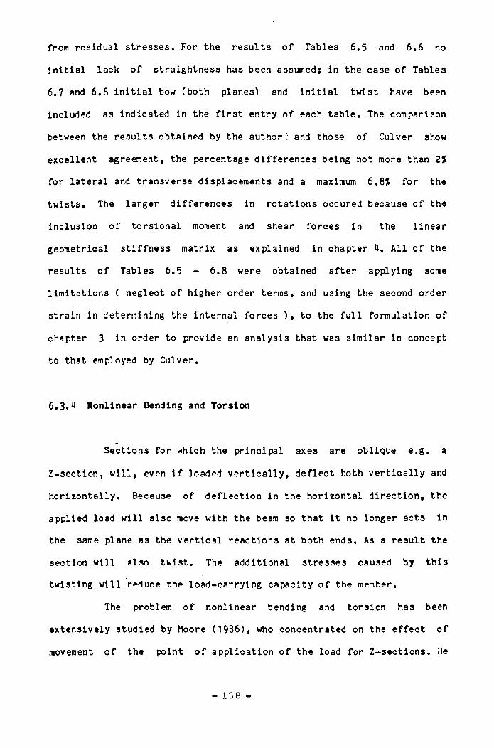
from residual stresses. For the results o f Tables 6.5 and 6.6 no

in i t ia l lack o f straightness has been assumed; in the case o f Tables

6.7 and 6.8 in i t i a l bow (both planes) and in i t i a l tw ist have been

included as indicated in the f i r s t entry o f each table. The comparison

between the results obtained by the author ': and those o f Culver show

excellent agreement, the percentage d ifferences being not more than 2%

for la tera l and transverse displacements and a maximum 6.8X for the

twists. The larger d ifferences in rotations occured because o f the

inclusion o f torsional moment and shear forces in the linear

geometrical s t i f fn ess matrix as explained in chapter 4. A ll o f the

results o f Tables 6.5 - 6.8 were obtained a fte r applying some

lim itations ( neglect o f higher order terms, and using the second order

strain in determining the internal forces ) , to the fu l l formulation o f

chapter 3 in order to provide an analysis that was similar in concept

to that employed by Culver.

6.3.4 Nonlinear Bending and Torsion

Sections for which the principal axes are oblique e .g . a

Z-section, w i l l , even i f loaded v e r t ic a l ly , d e f le c t both v e r t ic a l ly and

horizontally. Because o f de flec t ion in the horizontal d irection , the

applied load w i l l also move with the beam so that i t no longer acts in

the same plane as the v e r t ica l reactions at both ends. As a result the

section w i l l also tw is t. The additional stresses caused by this

twisting w i l l reduce the load-carrying capacity o f the member.

The problem o f nonlinear bending and torsion has been

extensively studied by Moore (1986), who concentrated on the e f fe c t o f

movement o f the point o f application o f the load for Z-sections. He

- 158

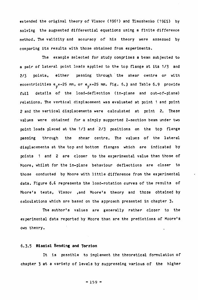
extended the or ig ina l theory o f Vlasov (1961) and Timoshenko (19£5) by

solving the augmented d i f fe r e n t ia l equations using a f in i t e d ifference

method. The v a l id i t y and accuracy o f his theory were assessed by

comparing i t s results with those obtained from experiments.

The example selected for study comprises a beam subjected to

a pair o f la te ra l point loads applied to the top flange at i t s 1/3 and

2/3 points, e ither passing through the shear centre or with

eccen tr ic it ies ey=-25 mm, or ey=+25 mm. Fig. 6.3 and Table 6.9 provide

fu l l d e ta ils o f the load-deflection (in-plane and out-of-plane)

re lations. The v e r t ica l displacement was evaluated at point 1 and point

2 and the v e r t ic a l displacements were calculated at point 2. These

values were obtained for a simply supported Z-section beam under two

point loads placed at the 1/3 and 2/3 positions on the top flange

passing through the shear centre. The values o f the la te ra l

displacements at the top and bottom flanges which are indicated by

points 1 and 2 are c loser to the experimental value than those o f

Moore, whilst for the in-plane behaviour deflections are closer to

those conducted by Moore with l i t t l e d ifference from the experimental

data. Figure 6.$ represents the load-rotation curves o f the results o f

Moore's tests , Vlasov ,and Moore's theory and those obtained by

calculations which are based on the approach presented in chapter 3*

The author's values are generally rather closer to the

experimental data reported by Moore than are the predictions o f Moore's

own theory.

6.3.5 B ia x ia l Bending and Torsion

I t is possible to implement the theoretica l formulation o f

chapter 3 at a va r ie ty o f le v e ls by suppressing various o f the higher

- 159

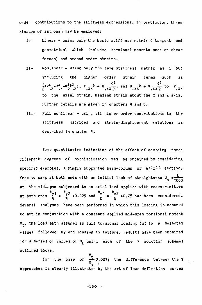
order contributions to the s t i f fn ess expressions. In particu lar, three

classes o f approach may be employed:

i - Linear - using only the basic s t i f fn ess matrix ( tangent and

geometrical which includes torsional moments and/ or shear

forces) and second order strains.

i i - Nonlinear - using only the same s t i f fn ess matrix as i but

including the higher order strain terms such as

-(V* +U1 «-P2* 2 ) , V * +$2

U — , and U$2

* + V — to V2 ix , x o ,x ,xx ,xx 2 »xx ,xx 2 »xx

to the axial stra in , bending strain about the Y and Z axis.

Further d e ta ils are given in chapters H and 5.

i i i - Full nonlinear - using a l l higher order contributions to the

s t i f fn ess matrices and strain-displacement re lations as

described in chapter U.

Some quantitative indication o f the e f fe c t o f adopting these

d if fe ren t degrees o f sophistication may be obtained by considering

spec ific examples. A simply supported beam-column o f W12xl4 section,

free to warp at both ends with an in i t i a l lack o f straightness U =— —o 1000

at the mid-span subjected to an axial load applied with eccen tr ic it ies e 1 e - e . e 0

at both ends — =0. 025 and — = --— =0.25 has been considered. B B D D

Several analyses have been performed in which th is loading is assumed

to act in conjunction with a constant applied mid-span torsional moment

Mfc. The load path assumed is fu l l torsional loading (up to a selected

value) followed by end loading to fa i lu re . Results have been obtained

for a series o f values o f using each o f the 3 solution schemes

outlined above.

MtFor the case o f — =0.023; the d ifference between the 3My

approaches is c lea r ly i l lu s tra ted by the set o f load de flec t ion curves

- 160

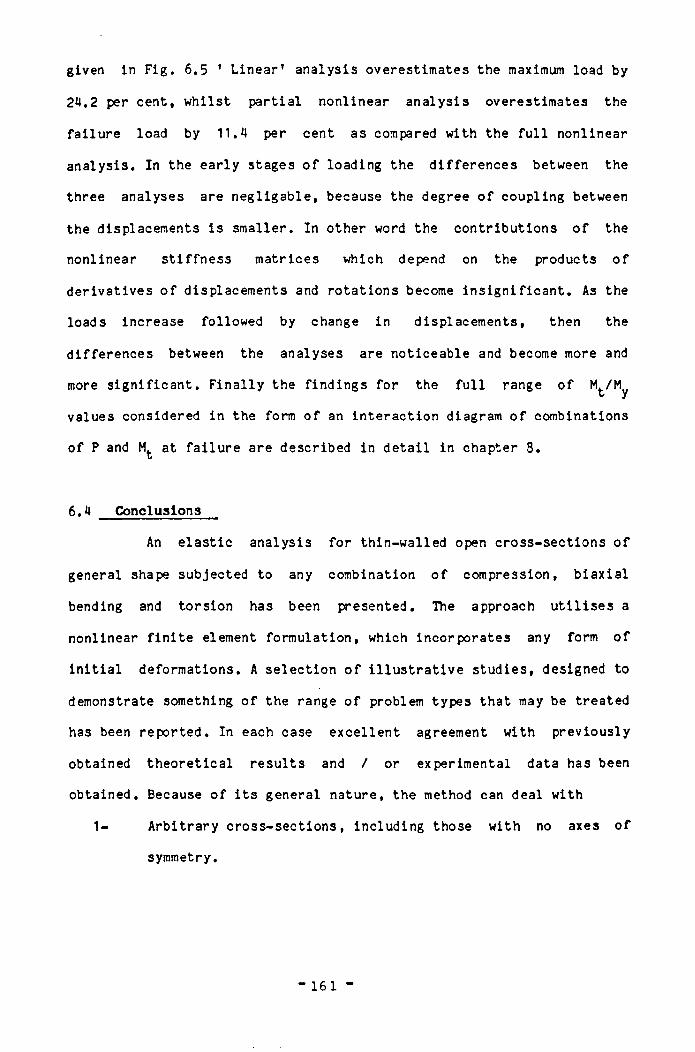
given in F ig. 6.5 ' Linear' analysis overestimates the maximum load by

24.2 per cent, whilst partia l nonlinear analysis overestimates the

fa ilu re load by 11.4 per cent as compared with the fu l l nonlinear

analysis. In the early stages o f loading the d ifferences between the

three analyses are negligable, because the degree o f coupling between

the displacements is smaller. In other word the contributions o f the

nonlinear s t i f fn ess matrices which depend on the products o f

derivatives o f displacements and rotations become ins ign if ican t. As the

loads increase followed by change in displacements, then the

differences between the analyses are noticeable and become more and

more s ign if ican t. F ina lly the findings for the fu l l range o f M./M y

values considered in the form o f an interaction diagram o f combinations

o f P and at fa i lu re are described in de ta il in chapter 8.

6.4 Conclusions

An e la s t ic analysis for thin-walled open cross-sections o f

general shape subjected to any combination o f compression, b iax ia l

bending and torsion has been presented. The approach u t i l is e s a

nonlinear f in i t e element formulation, which incorporates any form o f

in i t ia l deformations. A selection o f i l lu s t r a t iv e studies, designed to

demonstrate something o f the range o f problem types that may be treated

has been reported. In each case excellent agreement with previously

obtained theoretica l results and / or experimental data has been

obtained. Because o f i t s general nature, the method can deal with

1- Arbitrary cross-sections, including those with no axes o f

symmetry.

161

2 - Any arbitrary set o f applied loads.

3- Any arrangement o f flexural and torsional support conditions.

I t therefore represents a powerful - too l for studying the

response o f beam-columns in a very general manner.

- 162 -

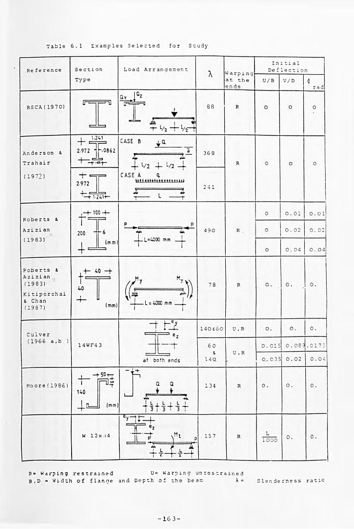
T a b l e 6 . 1 Examp l e s S e l e c t e d f o r St udy

P= W a r p i n g r e s t r a i n e d U= W a r p i n g u n r e s t r a i n e dB , D = W i d t h o f f l a n g e and D e p t h o f t he b e a n S l e n d e r n e s s r a t i c

- 1 6 3 -

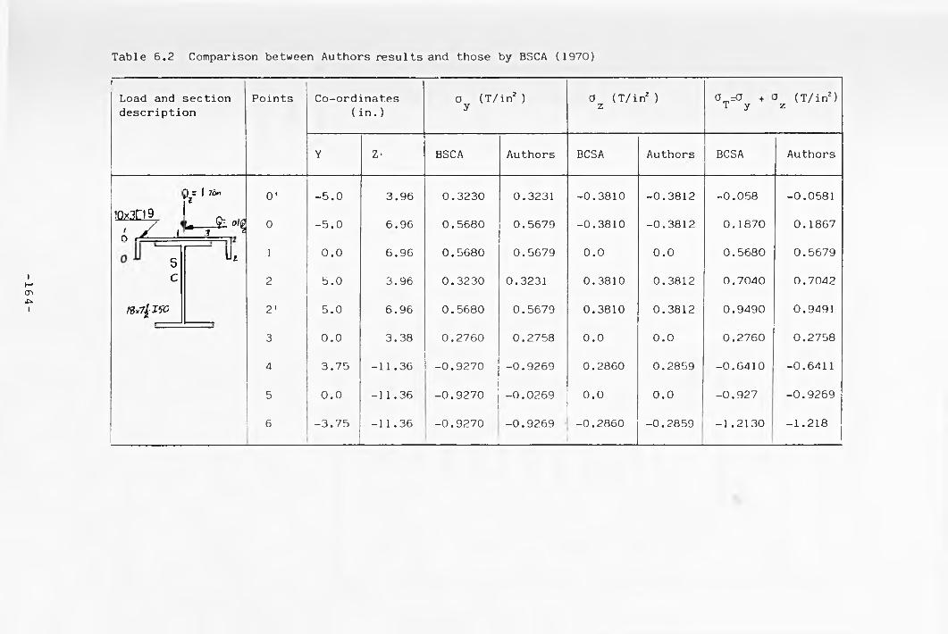
-164-

Table 6.2 Comparison between Authors results and those by BSCA (1970)rLoad and section description

Points Co-ordinates ( in. )

Oy (T/in? ) 0 (T/i z nJ ) 0 = 0 + T y î (T/inJ) z

Y Z- BSCA Authors BCSA Authors BCSA Authors

10*3D9

¿ r¿--- L

j>«=1 r~ 0 ’ -5.0 3.96 0.3230 0.3231 -0.3810 -0.3812 -0.058 -0.0581

L-r*»'? o -5.0 6.96 0.5680 0.5679 -0.3810 -0.3812 0.1870 0.1867

s u, 1 0.0 6.96 0.5680 0.5679 0.0 0.0 0.5680 0.5679C 2 5.0 3.96 0.3230 0.3231 0.3810 0.3812 0.7040 0.7042

/0.7/J5C 2’ 5.0 6.96 0.5680 0.5679 0.3810 0.3812 0.9490 0.9491

3 0.0 3.38 0.2760 0.2758 0.0 0.0 0.2760 0.2758

4 3.75 -11.36 -0.9270 -0.9269 0.2860 0.2859 -0.6410 -0.6411

5 0.0 -11.36 -0.9270 -0.0269 0.0 0.0 -0.927 -0.9269

6 -3.75 -11.36 -0.9270 -0.9269 -0.2860 -0.2859 -1.2130 -1.218

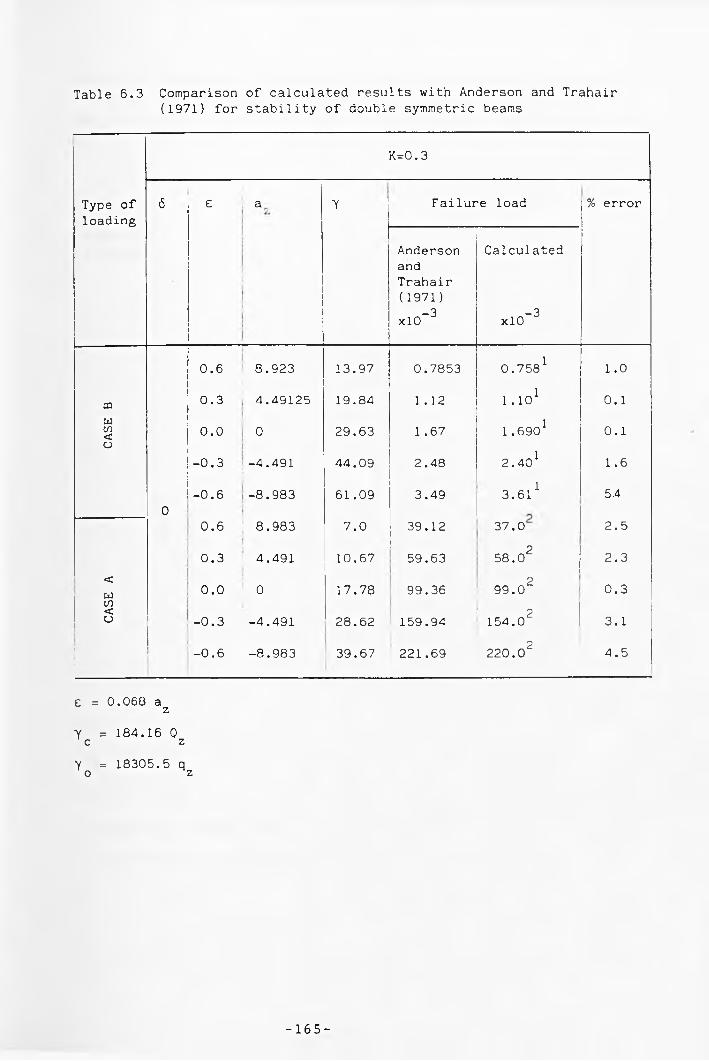
Table 6.3 Comparison of calculated results with Anderson and Trahair(1971) for stability of double symmetric beams

K=0.3

Type of 6 E a Y Failure load % errorloading

AndersonandTrahair(1971)

Calculated

xlO-3 xlO-3

0.6 8.923 13.97 0.7853 0.7581 1.0

CQ 0.3 4.49125 19.84 1.12 1.101 0.1W cn < 0.0 0 29.63 1.67 1.6901 0.1o

-0.3 -4.491 44.09 2.48 2.401 1.6

-0.6 -8.983 61.09 3.49 3.611 5.40

0.6 8.983 7.0 39.12 37.0 2.5

0.3 4.491 10.67 59.63 58.02 2.3<w 0.0 0 17.78 99.36 299.0 0.3m<o -0.3 -4.491 28.62 159.94 154.02 3.1

-0.6 -8.983 39.67 221.69 220.02 4.5

e = 0.060 azY = 184.16 0c zY = 18305.5 qo z

-165-

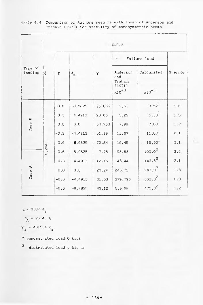
Table 6.4 Comparison of Authors results with those of Anderson andTrahair (1971) for stability of monosymmetric beams

COoII

Failure load

Type of loading 5 e a Y Anderson Calculated % error

andTrahair( 1971)

-3 -3xlO xlO

0.6 8.9825 15.855 3.61 3.571 1.8

0.3 4.4913 23.06 5.25 5.101 1.5CQ

<DW 0.0 0.0 34.763 7.92 7.801 1.2CCo -0.3 -4.4913 51.19 11.67 11.881 2.1

-0.6 -8.9825 70.84 16.45 16.501 3.1oC\J 2

•o 0.6 8.9825 7.78 93.63 1 0 0 . 0 2.8

0.3 4.4913 12.16 146.44 143.52 2.1< 2<D 0.0 0.0 20.24 243.72 243.0 1.3WCCCJ -0.3 -4.4913 31.53 379.796 363.02 6.0

i1

-0.6 -8.9825 43.12 519.28 475.02 7.2

e = 0.07 azv, = 76.46 Q A

03

= 4015.4 qz

l concentrated load Q kips2 distributed load q kip in

166-

Table 6.5 Comparison of calculated results with exact solution ofCulver (1966a), for biaxial loading, no initial deflection

—■ = 0.625, = 0.366 14WF43 Warping unrestrained

F_P

y

U/B

C\J1o•—tX V/D x 10 " Í- Rotation (rad) -3x 10 J

Culver Calculated Culver Calculated Culver Calculated

0.0 0.0 0.01

0.0 0.0 0.0 0.0

0.048 1.515 1.590 0.092 0.092 0.05 I 0.058

0.096 3.093 3.095 0.184 0.184 0.20 0.22

0.144 4.738 4.993 0.276 0.276 0.40 i 0.48

0.194 6.454 6.466 0.368 0.368i

0.80 0.87

0.246___

8.273 8.248 0.461 0.460 1.30 1.39

Table 6.6 Comparison of calculated results with exact solution ofCulver (1966a) for initial deflection

beam-column under biaxial bending, no

r- = 140 r

y

eyB

e= 0.0625, ^ = 0.366 14WF43 Warping unrestrained

pp

y

U/B -2x 10 V/D xl0~3 <J) -Rotation (rad)-2 1 xlO i ___________________ ___

Culver Calculated Culver Calculated Culver Calculated

0.0 0.0 0.0 0.0 0.0 0.0 0.0

0.048 9.06 9.06 5.03 5.03 0.12 0.12

0.096 20.68 20.66 10.15 1 10.15 0.57 0.57

0.144 36.11 36.04 15.27 15.30 1.50 1.55

0.194 57.80 57.33 20.33 20.40 3.43 3.25

0.246 1________

89.73 90.63 25.04 25.25,

6.96 6.48

-167-

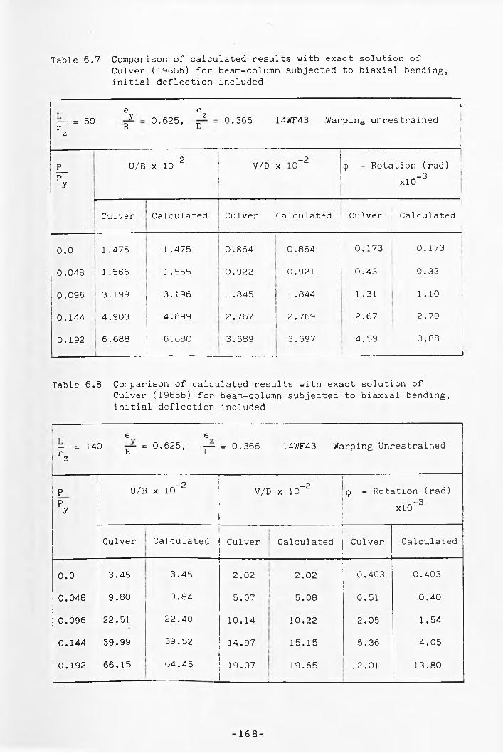
Table 6.7 Comparison of calculated results with exact solution ofCulver (1966b) for beam-column subjected to biaxial bending, initial deflection included

i i

— = 60 rz

eyB 0 .625,

ezD 0.366 14WF43 Warping unrestrained

I1

i >■ 0,10.

U/B X io -2 V/D

CO1oX (J) - Rotation (rad) | xlO-3

Culver Calculated Culver Calculated Culver Calculated

0.0 1 .475 1 .475 0.864 0.864 0.173 0.173

0.048 1.566 1.565 0.922 0.921 0.43 0.33 10.096 3.199 3.196 1.845 1.844 1.31 1.10

0.144 4.903 4.899 2.767 2.769 2.67 2.70

0.192 6.688 6.680 3.689 3.697________

4.59 3.88t

Table 6.8 Comparison of calculated results with exact solution ofCulver (1966b) for beam-column subjected to biaxial bending, initial deflection included

| e e! — = 140 = 0.625, — = 0.366 14WF43 Warping Unrestrainedi r 8 DI z

PP

y

U/B x 10“2 _2V/D x 10 (j> - Rotation (rad) xlO-3

Culver Calculated Culver Calculated Culver Calculated

0.0 3.45 3.45 2.02 2.02 0.403 0.403

0.048 9.80 9.84 5.07 5.08 0.51 0.40

0.096 22.51 22.40 10.14 10.22 2.05 1.54

0.144 39.99 39.52 14.97 15.15 5.36 4.05

0.192 66.15 64.45 19.07 —......................................

19.65 12.01 13.80

- 1 6 8 -

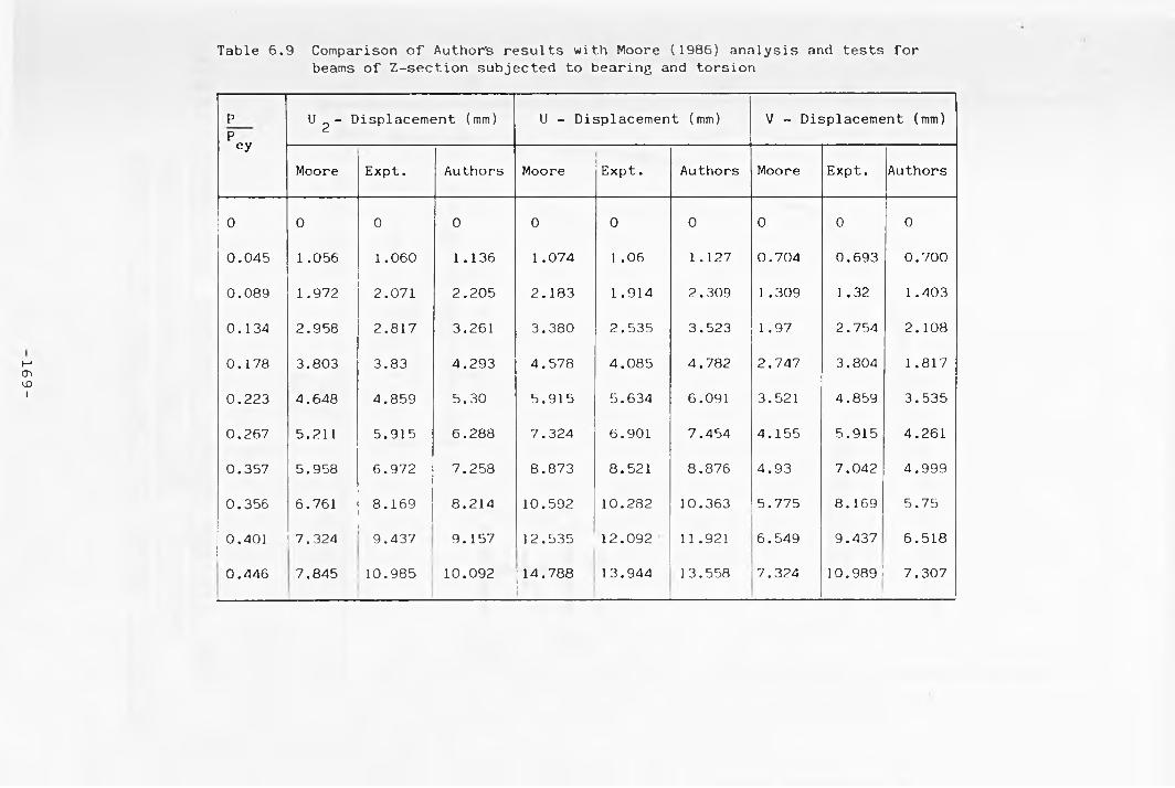
169-

Table 6.9 Comparison of Author’s results with Moore (1986) analysis and tests for beams of Z-section subjected to bearing and torsion

pp

U 2 — Displacement (mm) U - Displacement (mm) V - Displacement (mm)ey

Moore Expt. Authors Moore Expt. Authors Moore Expt. Authors

0 0 0 0 0 0 0 0 0 0

0.045 1 .056 1.060 1.136 1.074 1 .06 1.127 0.704 0.693 0.700

0.089 1.972 2.071 2.205 2.183 1.914 2.309 1 .309 1.32 1.403

0.134 2.958 2.817 3.261 3.380 2.535 3.523 1.97 2.754 2.108

0.178 3.803 3.83 4.293 4.578 4.085 4.782 2.747 3.804 1 .817

0.223 4.648 4.859 5.30 5.915 5.634 6.091 3.521 4.859 3.535

0.267 5.211 5.915 6.288 7.324 6.901 7.454 4.155 5.915 4.261

0.357 5.958 6.972 7.258 8.873 8.521 8.876 4.93 7.042 4.999

0.356 6.761 8.169 8.214 10.592 10.282 10.363 5.775 8.169 5.75

0.401 7.324 9.437 9.157 12.535 12.092 11.921 6.549 9.437 6.518

0.446 7.845 10.985 10.092 14.788 13.944 13.558 7.324 10.989 !1

7.307

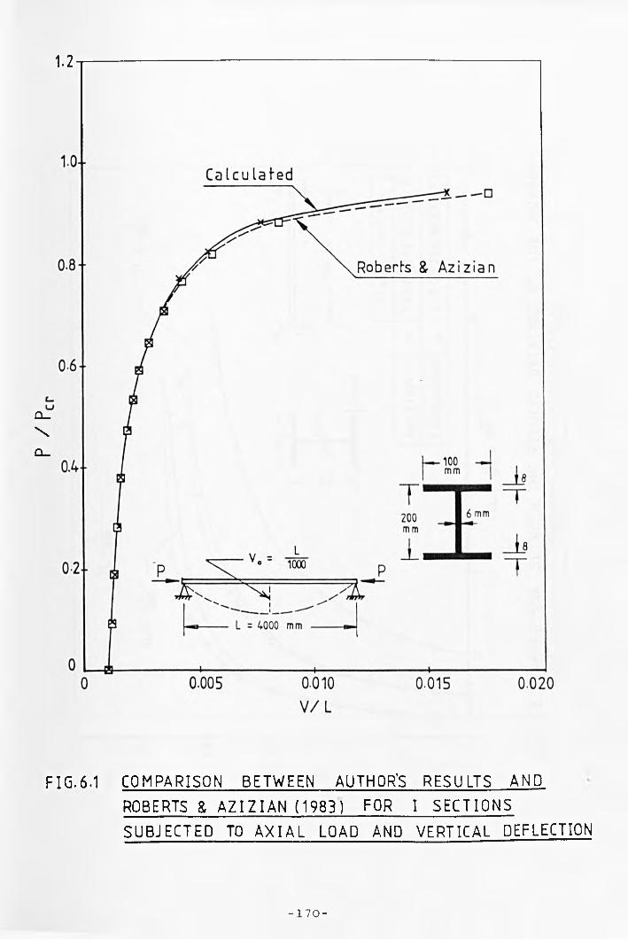
p /p

1.2

FIG.6.1 COMPARISON BETWEEN AUTHOR’S RESULTS AND

ROBERTS & AZIZ IAN (1983) FOR I SECTIONS

SUBJECTED TO AXIAL LOAD AND VERTICAL DEFLECTION

-170-

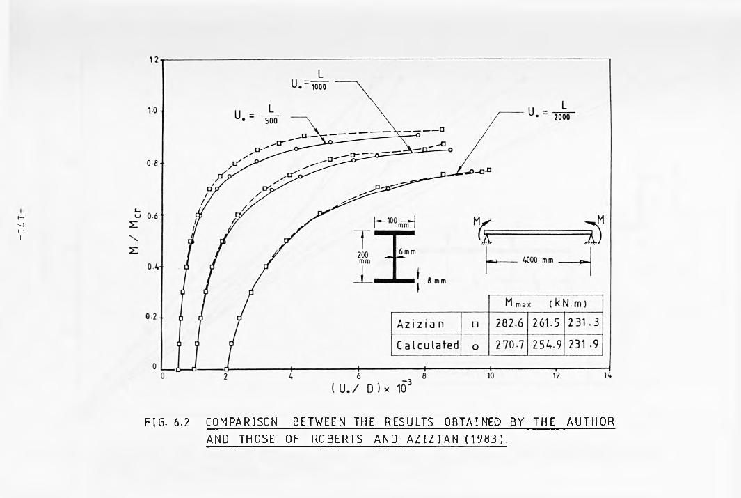
171-

FIG. 6.2 COMPARISON BETWEEN THE RESULTS OBTAINED BY THE AUTHORAND THOSE OF ROBERTS AND AZIZIAN (1983).

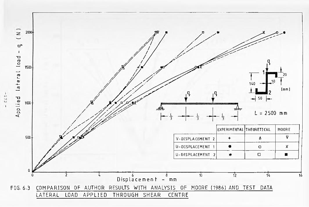
Ap

pli

ed

la

tera

l lo

ad

cAi

1500-

1000 -

L = 2500 mm

6 8 Displa ce men t - mm

10 12 14

FIG. 6.3 COMPARISON OF AUTHOR RESULTS WITH ANALYSIS OF MOORE (1986) AND TEST DATA LATERAL LOAD APPLIED THROUGH SHEAR CENTRE ~

EXPERIMENTAL THEORETICAL MOORE

V-DISPLACEMENT 2 + A V

U- DISPLACEMENT 1 • O X

U-DISPLACEMENT 2 * □ ■

16

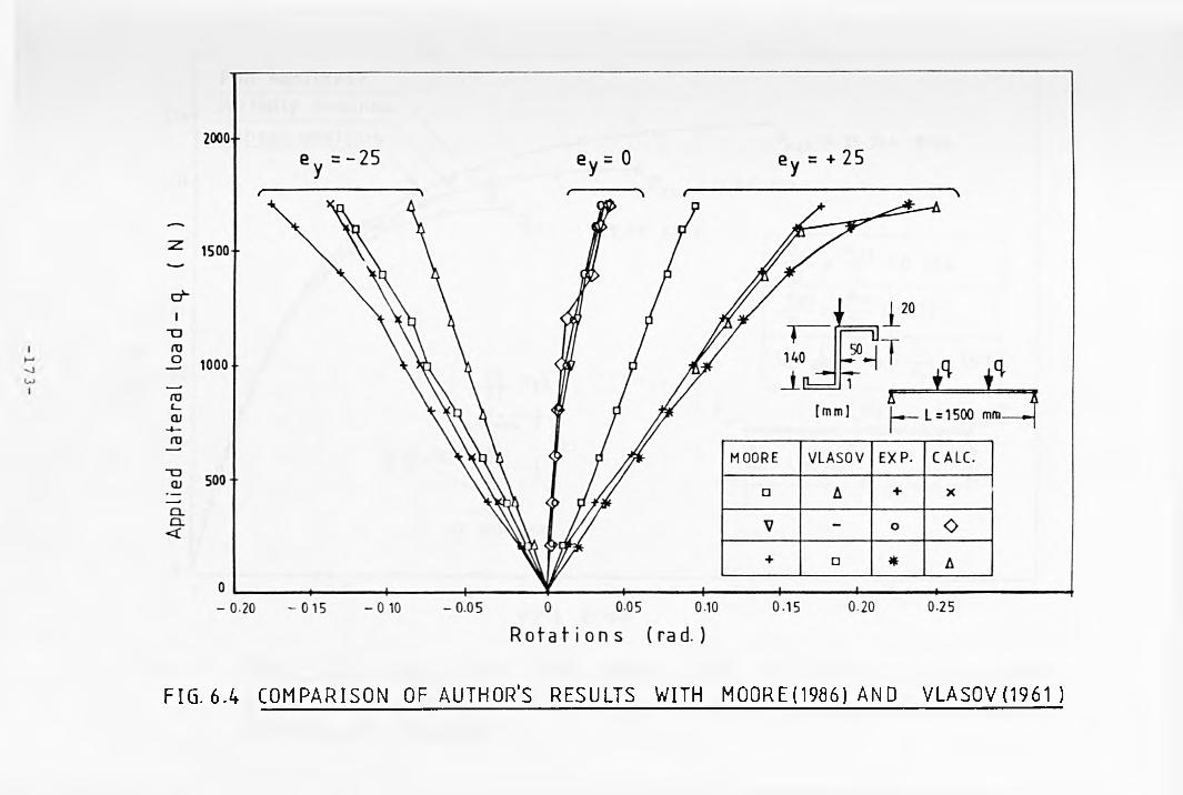
FIG. 6.4 COMPARISON OF AUTHOR'S RESULTS WITH MOORE(1986) AND VLASOV (1961 )

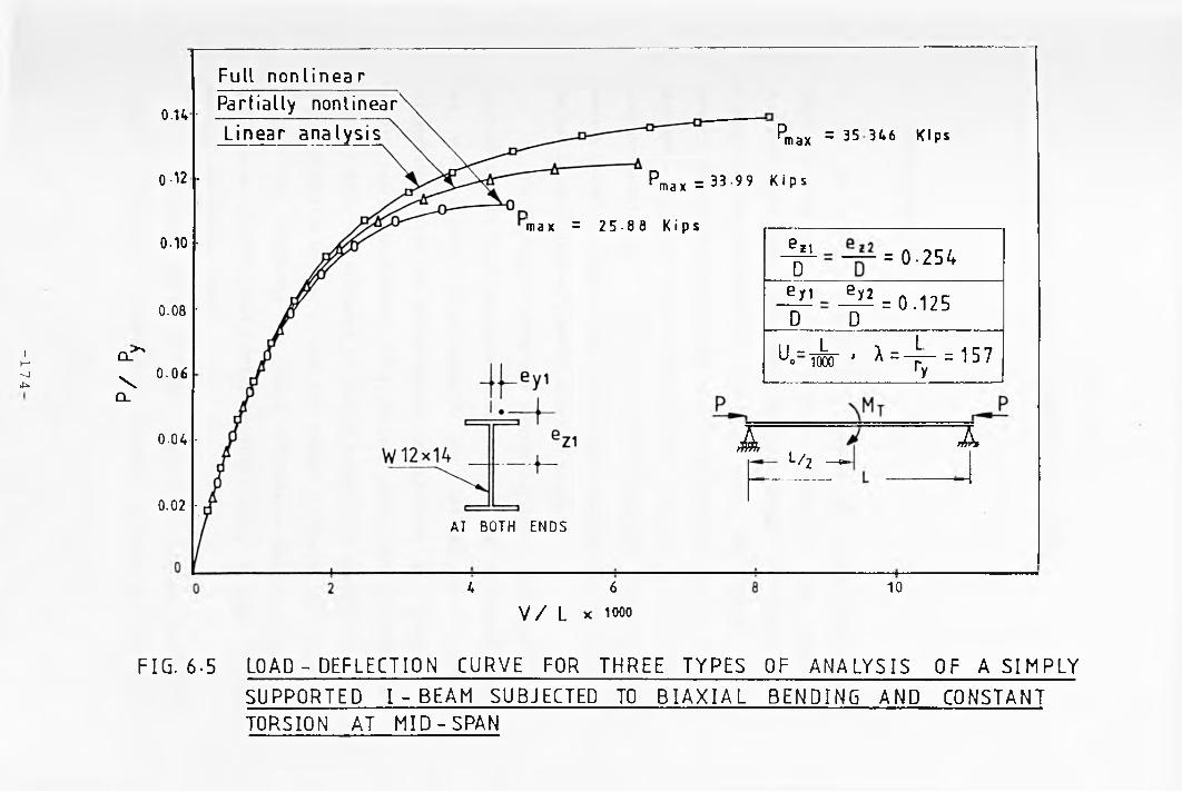
174

I o r "

\CL

o.u-

0-12 -

0-10 •

0.08 ■

0.06

0-04 -

0.02 -

Full nonlinear Partially nonlinear Linear analysis

max = 25-88 K i ps

Pmax = 35 346 Kips

P max =33-99 K i p s

W 12x14

AT BOTH ENDS

4 6

V / L x 1000

eziD — = 0-254

e y i6y2 = 0.125

D DU - Lu° 1000 - X = T - = 157

r y

Al/2 —

lx

10

FIG. 6-5 LOAD - DEFLECTION CURVE FOR THREE TYPES OF ANALYSIS OF A S IMPLY

SUPPORTED I - B E A M SUBJECTED TO B I AX I AL BENDING AND CONSTANT TORSION AT MID-SPAN

C h a p te r 7

In e la s t ic Analysis o f Beat-Column in Space

7.1 Introduction

In order to study the response o f a beam-column in the

ine lastic range i t is necessary to allow correc t ly for the losses in

s t if fness that occur due to spread o f y ie ld through the cross-section,

with due account being taken o f variations along the length o f the

member. The presence o f in i t i a l geometrical imperfections and residual

stresses w i l l a f fe c t both the in it ia t io n and propagation o f y ie ld ing .

Accurate monitoring o f the fu l l three-dimensional response o f such

members therefore requires that very careful consideration be given to

the way in which gradual p la s t i f ica t ion is treated.

The in e las t ic behaviour o f beam-columns o f thin-walled open

cross-section in three dimensions under various types o f applied loads

has been studied experimentally and ana ly t ica lly by several

investigators such as Nethercot ( 19 73 a , b),Trahair and Kitipornchai

(1972), Fujita and Yoshida (1972), Matthey (1984), Anslijn (1983), and

Lindner (1981). The influence o f in i t i a l geometrical imperfections has

been incorporated by some o f them and ignored by others. Reviews o f the

subject are available in many references such as Chen and

Santathadaporn (1968), Chen (1977), Johnston (1976), Massonet (1976),

and Chen and Atsuta (1977)

The application o f the general f in i t e element formulation

presented in chapter 3 to assess the in e las t ic behaviour o f thin-walled

_ 175 _

steel members deforming in space is described herein. This approach is

applicable to various types o f open cross-section, including those with

no degree o f symmetry.

In th is chapter the accuracy and v e r s a t i l i t y o f the

theoretical approach which has been presented in chapter 3 is

demonstrated by application to a wide range o f selected problems

covering flexura l, f lexura l-tors iona l buckling, and bending and

torsion.

7.2 Assumptions

In addition to the basic assumptions o f Vlasov(196l) and

those presented in chapter 3, the following- are taken into

consideration:

I - The distribution o f e la s t ic and yielded regions within the

cross section is determined from the strain distribution and

the material stress-strain curve.

I I - The moduli o f the material are E and G in the e las t ic regions

while in the yielded regions Efc and Gfc are used, with Efc and

Gfc being dependant on the type o f stress-strain curve

employed. Any monotonically increasing curve may be assumed.

I I I - Any reasonable pattern o f residual stresses and v ir tu a l ly any

d istribution o f in i t i a l crookedness may be included.

IV- Control o f the nonlinear numerical solution is as described

in section 4.6 o f chapter 4 with accuracy being based on a

combined displacement change/ out o f balance load check.

V- Yield is controlled by normal stresses only ( although the

inclusion o f more sophisticated y ie ld c r i t e r ia is possible,

with l i t t l e extra work).

176

VI- The sectional and sectoria l properties were evaluated a fter

each load increment in the in e las t ic range.

Various possible load types are given in Table 7 .1 ., which

l i s t s the example problems considered herein. In the case o f transverse

loads, these may be e ither distributed or concentrated and may be

applied at any eccen tr ic ity to the shear centre axis. Allowance for the

e f fe c t o f spread o f yield in any region on cross-sectional properties

makes no assumptions concerning the location o f the shear centre,

existence o f symmetry e tc . . Equilibrium o f internal and external forces

is maintained at a l l stages o f the solution, see section 5.5 o f chapter

5.

The sectoria l properties such as warping moment o f inert ia

(1^ ), warping second moments o f in ert ia ( I and ( I zaj) , aid normalized

function (w ) are not taken as the e las t ic values in the in e las t ic

range as was the case in most previous work (Rajasekaran and Murray

(1973)» Yang and McGuire (1986), and Kitipornchai and Trahair (1975))

but are evaluated accounting for the loss o f s t i f fn ess due to spread o f

yield in a similar fashion to the other sectional properties such as

I y ’ ^ z ’ etc*

7.3 Numerical Results

Several i l lu s t r a t iv e examples have been selected for study.

D ifferent aspects o f behaviour such as flexural buckling, f lexu ra l-

torsional buckling, and b iax ia l bending are covered by these cases. The

influence o f i n i t i a l de flection and residual stresses are incorporated.

The particular features o f each type o f problem are l is ted in Table

7.1.

- 1 7 7 _

In each case the number of elements and the number of plate

segments within the cross-section were chosen so as to achieve accurate

solutions without increasing the computational e f fe c t unnecessarily as

described in Chapter 5. The convergence c r ite r ion o f section 5.5 was

employed.

7.3.1 Coluun with In i t i a l Deflections

A simply supported I-section under axial load assuming

various values o f i n i t i a l deformations, and including the e f f e c t o f

material strain-hardening (Egh = E/10) has been considered. The in i t i a l

crookedness is represented by a sinusoidal function with i t s maximum

value at midspan. Residual stress was not included so as to permit

comparison with the previous solution o f Fujita and Yoshida (1972).

chapter 3 in order to achieve comparable resu lts ; these are the

influence o f the higher order terms o f the strain-displacement

relationship and the nonlinear tangential and geometrical s t i f fn ess

matrices which incorporate the der iva tive o f the displacements such as

chosen from those studied both th eo re t ica lly and experimentally by

Fujita and Yoshida (1972) and the results obtained are given in Table

7.2. The percentage d ifferences between the present solution and the

ea r l ie r results is in no case greater than 4 per cent.

7.3.2 Flexural & Flexural Torsional Buckling

F ig . 7.1 shows a monosymmetric I - section together with the

residual stresses produced by welding; these have adjusted so as to

meet the equilibrium condition o f equations 3.^3* 3.44, and 3.45. This

Some lim itations are imposed on the suggested formulation o f

178

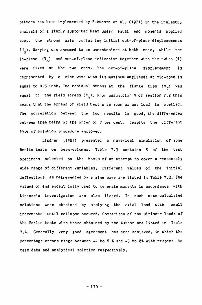
pattern has been implemented by Fukuomto et a l . (1971) in the in e lastic

analysis o f a simply supported beam under equal end moments applied

about the strong axis containing in i t ia l out-of-plane displacements

(Uq) . Warping was assumed to be unrestrained at both ends, while the

in-plane (VQ) and out-of-plane de flect ion together with the twist ( * )

were fixed at the two ends. The out-of-plane displacement is

represented by a sine wave with i t s maximum amplitude at mid-span is

equal to 0.5 inch. The residual stress at the flange tips (o^) was

equal to the y ie ld stress (a^ ). From assumption V o f section 7.2 th is

means that the spread o f y ie ld begins as soon as any load is applied.

The correlation between the two results is good, the d ifferences

between them being o f the order o f 7 per cent, despite the d i f fe ren t

type o f solution procedure employed.

Lindner (1981) presented a numerical simulation o f some

Berlin tests on beam-columns. Table 7.3 contains 5 o f the test

specimens selected on the basis o f an attempt to cover a reasonably

wide range o f d i f fe ren t variab les. D ifferent values o f the in i t i a l

deflections as represented by a sine wave are l is ted in Table 7.3. The

values o f end eccen tr ic ity used to generate moments in accordance with

Lindner's investigation are also l is ted . In each case calculated

solutions were obtained by applying the axial load with small

increments until collapse occured. Comparison o f the ultimate loads o f

the Berlin tests with those obtained by the Author are l is ted in Table

7.4. Generally very good agreement has been achieved, in which the

percentage errors range between -4 to 6 t and -3 to 8% with respect to

test data and analytical solution respec t ive ly .

- 179 -

7.3.3 B iaxial Bending

Several comparisons have been made with the tests on

I-sections subjected to b ia x ia l ly eccentric compression conducted by

Anslijn (1983). Table 7.5 presents the input data, for four tests chosen

for the purposes o f comparison, whilst Table 7.6 compares the

calculated ultimate loads with the experimental values. Differences o f

less than 5% were obtained in each case. The tes t displacements were

measured at the t ips o f the two flanges for v e r t ic a l de flections and

the top and the bottom o f the web for horizontal de flec t ions , the

average being taken for both the in-plane V and out-of-plane U

displacements. A typ ica l comparison between these average values and

those calculated by the program is given in Figs 7.2 and 7.3 for tes t

No. 75 and No. 48. This shows excellent agreement for both in-plane and

out-of-plane deflections. The d ifferences found in the la t te r stages is

thought to be due to cross-sectional d is to rt ion , leading to changes in

flange t ip movement that occur near the collapse.

Many cases from the comprehensive parametric study o f

b iax ia l ly loaded I-section beam-columns presented by Matthey (1984)

have been selected for examination. For each analysis axial load was

applied up to a predetermined l im it followed by end moment loading to

fa i lu re . Thus the actual discrepancies between the two solution given

in Table 7.7 are o f course, smaller than the numerical values would

suggest since they re la te to only a part o f the applied loading.

Nonetheless agreement is considered excellent with the 3 examples

selected representing very d i f fe ren t sets o f parameters.

- 180

7.1» C onc lu s ions

The ine las t ic three-dimensional behaviour o f beam-columns

under d i f fe ren t loading conditions has been studied. The presence o f

in i t ia l imperfections such as residual stresses and in i t i a l de flections

together with the e f fe c ts o f strain hardening were incorporated in the

analysis. Results from several previous theoretica l and experimental

studies were used to check the Author’ s formulation and computer

program which is capable o f dealing with such problems. The v a l id i ty

and the accuracy o f both the approach and the computer program shows an

excellent agreement with those problems previously investigated,

thereby confirming that the analysis represents a powerful tool for the

study o f this class o f problem.

181

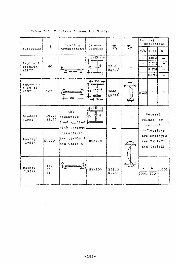
Tab l e 7.1 Problems Chosen f o r Study

Re fe renceloadin g

Ar ran gemen tCros s- Se ct i on V T

I n i t i a lDe f l ec t ion

V/L v /L

Fu j i t a & Yashi da (1972)

60 V.100 0.0067

100 - 28.6Kg/mnf

0.0112

0.0152

0.0215

Fukumoto & et al (1971) 103

< C = ^4— wo _4-

-f - 150O nr r r

-43C04— r~!Qr _(. 100 f .

3666 t

kN/®»

\0-00125

Lindne r ( 1981)

Ans l i jn (1993)

150

19,28 42,52

60,90

The

eccent r i c

load app l i ed

with var ious

e ccen t r i c i t -

i es .Table 3

and Table 5

r - q150 “ 8

HEA200

Mathey(1984)

141, 47 , 94

s S

Se ve r a l

values o f

i n i t i a l

de f l e c t i on s

are employed

see Table7'5

and Ta b l e 3.7

HFA200 235.0N/irnn1 1000 100

. OOl

- 1 8 2 -

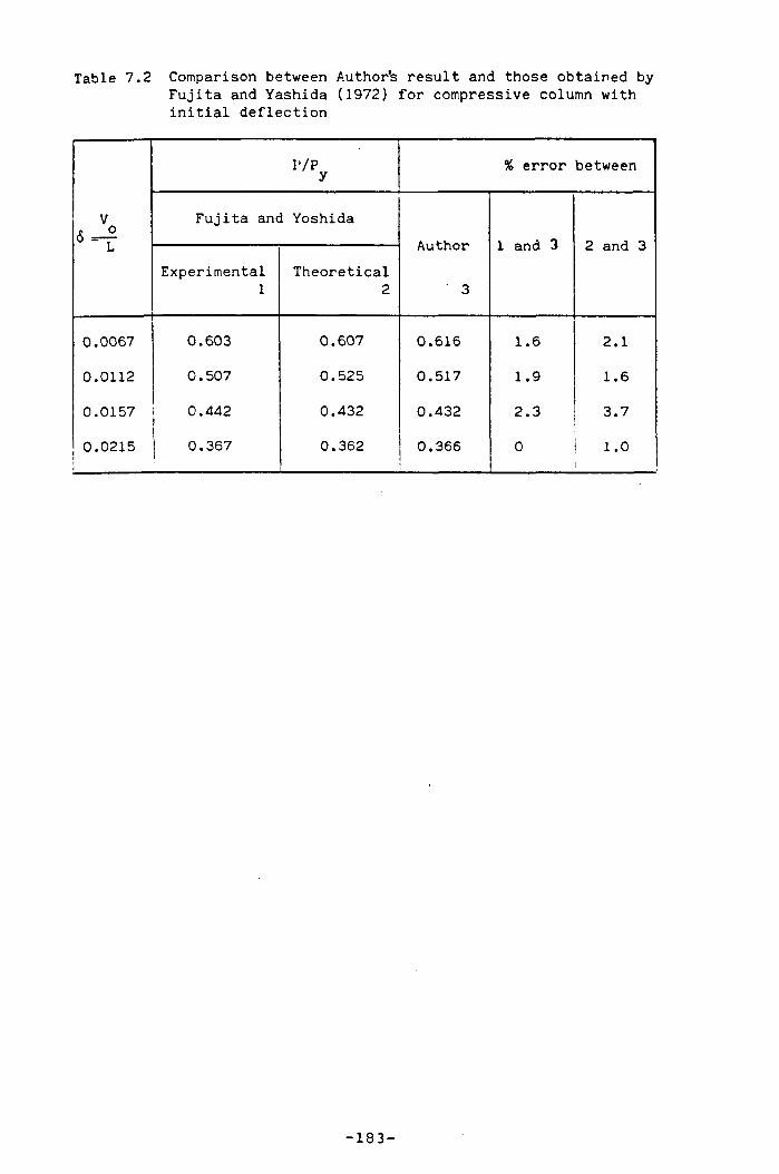
Table 7.2 Comparison between Author’s result and those obtained by Fujita and Yashida (1972) for compressive column with in it ia l deflection

V

IVPy

% error between

Fujita and Yoshida

Author

3

1 and 3 2 and 3Experimental

1Theoretical

2

0.0067 0.603 0.607 0.616 1.6 2.1

0.0112 0.507 0.525 0.517 1.9 1.6

0.0157 0.442 0.432 0.432 2.3 3.7

0.0215 | 0.367 0.362 0.366 0 1.0

- 1 8 3 -

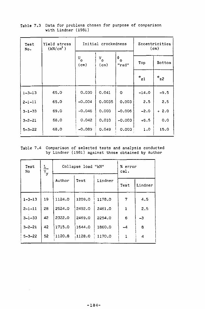
Table 7.3 Data for problems chosen for purpose of comparisonwith Lindner (1981)

TestNo.

Yield stress (kN/cm2 )

In it ia l crockedness Eccentricities(cm)

Uo(cm)

V0(cm)

<i>0"rad" Top Bottom

ezl ez2

1-3-13 65.0 0.030 0.041 0 -14.0 -9.5

2-1-11 65.0 -0.004 0.0035 0.003 2.5 2.5

3-1-33 69.0 -0.046 0.003 -0.006 -2.0 + 2.0

3-2-21 68.0 0.042 0.010 -0.003 +6.5 0.0

5-3-22i

68.0 -0.089 0.049 0.003 1.0 15.0

Table 7.4 Comparison o f selected tests and analysis conducted by Lindner (1981) against those obtained by Author

TestNo

L

Yv

Collapse load "kN" % error c a l.

y

Author Test LindnerTest Lindner

1-3-13 19 1124.0 1209.0 1178.0 7 4.5

2-1-11 28 2524.0 2492.0 2461.0 1 2.5

3-1-33 42 2322.0 2469.0 2254.0 6 -3

3-2-21 42 1715.0 1644.0 1860.0 -41 8

! 5-3-22 52 1120.8i

¡1128.0!

1170.01

1 4

- 1 8 4 -

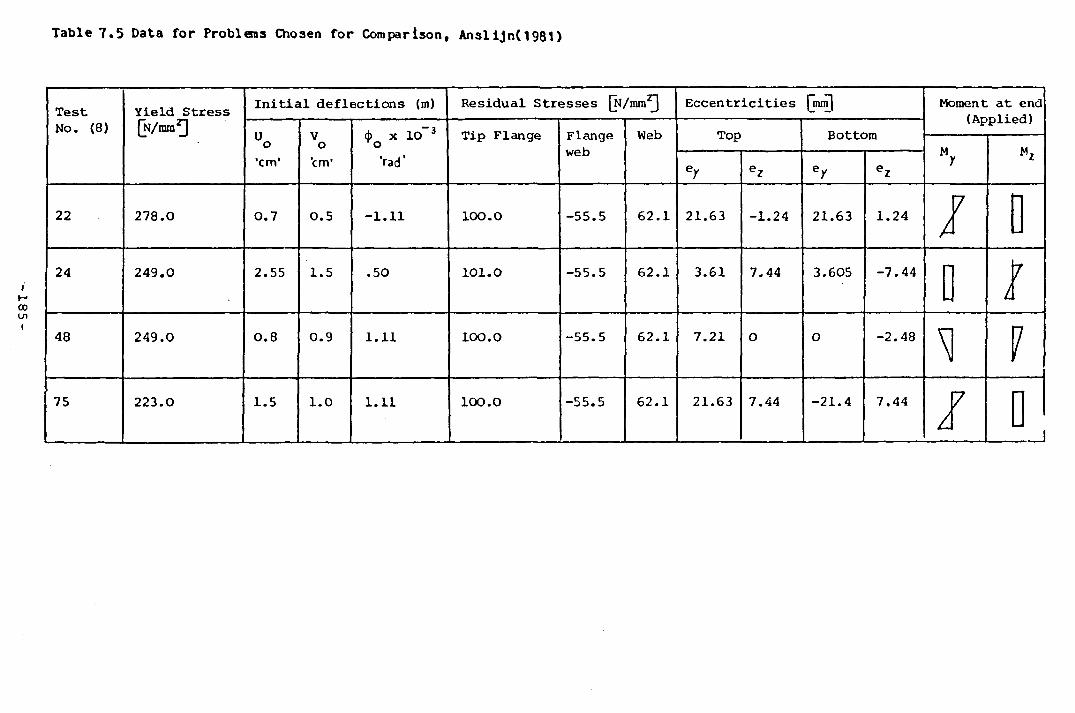
185

T a b le 7 . 5 Data f o r P ro b len s Chosen f o r Com parison, A n s i i j n ( 1981)

Test No. (8)

Y ield Stress [N/mm ]

In it ia l deflections (m) Residual Stresses Qj/mm2] Eccentricities [mm] Moment at end (Applied)

Uo’em ’

Vo'em’

<j> x 10-3 To’rad’

Tip Flange Flangeweb

Web Top Bottom

My Mz

e Y e z e r e z

22 278.0 0.7 0.5 -1.11 100.0 -55.5 62.1 21.63 -1.24 21.63 1.24 I 024 249.0 2.55 1.5 .50 101.0 -55.5 62.1 3.61 7.44 3.605 -7.44 D /48 249.0 0.8 0.9 1.11 100.0 -55.5 62.1 7.21 O O -2.48 F75 223.0 1.5 1.0 1.11 100.0 -55.5 62.1 21.63 7.44 -21.4 7.44 / D

__________i

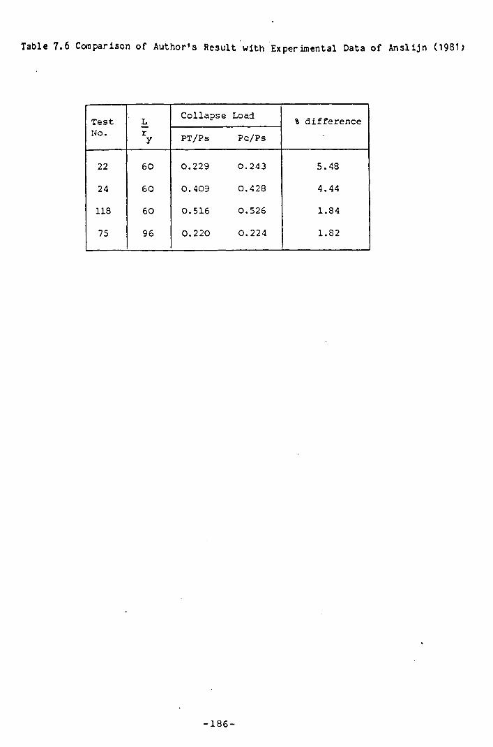
Table 7.6 Comparison of Author’ s Result with Experimental Data of Anslijn (1981)

TestNO.

Lry

Collapse Load % difference

PT/Ps Pc/Ps

22 60 0.229 0.243 5.48

24 60 0.409 0.428 4.44

118 60 0.516 0.526 1.84

75 96 0.220 0.224 1.82

- 1 8 6 -

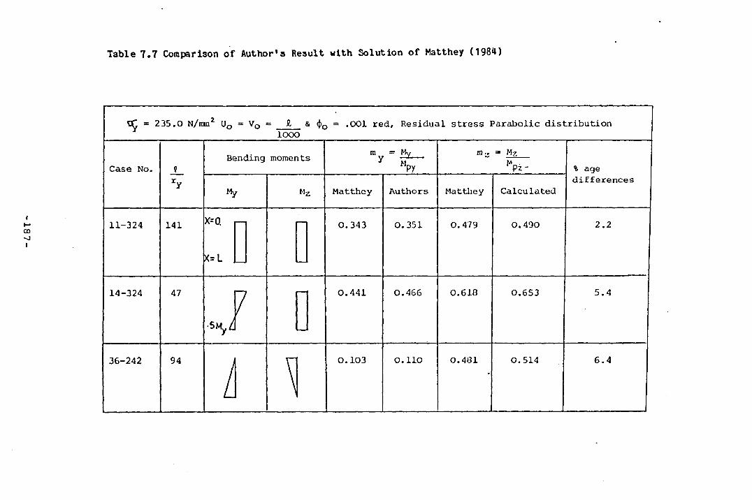
18

7-

T a b le 7 .7 Comparison o f A u th o r 's R e su lt w i th S o lu t io n o f M atthey (19 84 )

tÇ = 235.0 N/tnn2 U0 = Vn = Ü & <J>0 = .OOl red, Residual stress Parabolic d istributionlOOO

Case No. t

ry

Bending moments m = Mvy — X -----

Mpy

m., = MzM .

PZ" % age

My Mz Matthey Authors Matthey Calculateddifferences

11-324 141 X=0.

X= L

0.343 0.351 0.479 0.490 2.2

14-324 47

•SMy^1

0.441 0.466 0.618 0.653 5.4

36-242 94

i

0.103 0.110 0.481 0.514 6.4

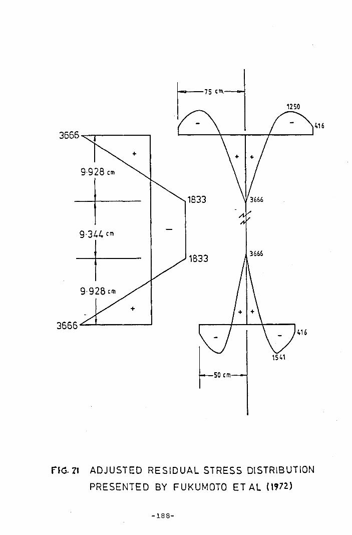
FK3-7I a d j u s t e d r e s i d u a l s t r e s s d i s t r i b u t i o n

PRESENTED BY FUKUMOTO ET AL l»?72)

- 1 8 8 -

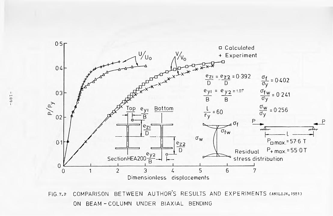
189

Dimensionless displacements

FIG.7.2 COMPARISON B ET W EEN AUTHOR 'S RESULTS AND E X P E R IM E N T S ( a n s l ij n , 1981)

ON B E A M - C O L U M N UNDER B IAX IAL BENDING

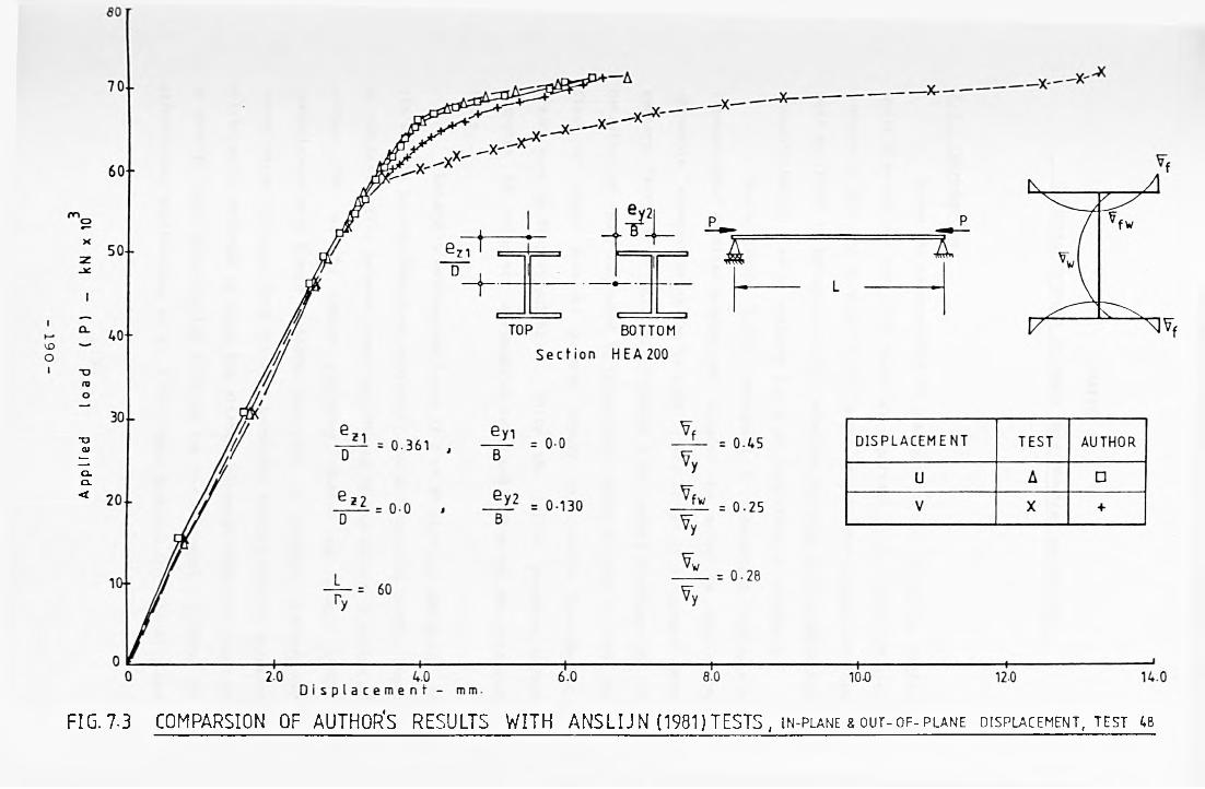
A p

pll

ed

FIG. 7 3 COMPARSION OF AUTHOR'S RESULTS WITH A N SLIJ N (1981) TESTS , in-plane & our-of-plane displacement, test ;b

CHAPTER 8

Ultimate Strength o f Beams under Bending and Torsion

8.1 Introduction

Beams and beam-columns o f various types o f cross section

under flexural and torsional loads are important in the design o f steel

members in both the e las t ic and ine las t ic ranges. Many researchers have

made an e f fo r t to investigate th is behaviour although most studies have

concentrated on e las t ic analysis based on simplified calculations.

Sourochnikoff (1951) presented a theoretica l analysis o f

I-beams under combined bending and torsion in order to obtain the

allowable stresses which can be used in the design o f structural steel

members. Terrington (1968,1970) provided a two-volume trea t ise on the

behaviour o f beams subjected to transverse loading causing torsion. The

f i r s t o f these presents general theory and formulae together with

graphs used to display solutions, while the la t te r presents worked

examples to calculate stresses in beams under flexural and torsional

loads.

La tera lly unsupported beams o f I or WF sections subjected to

bending and torsion have been studied by Chu and Johnston (197*0. Based

on the interaction between these two e f fe c ts they presented a series o f

curves for use by design engineers. Pastor and DeWolf (1979)

investigated wide flange I-beams subjected to uniform flexure and

concentrated torsion. They provided tabulated results for the stresses

which can be employed to check the ultimate strength behaviour based on

an e las t ic l im it condition but allowing for the in teract ive e f fe c ts o f

deformation. Kollbrunner, et a l . (1979) have examined th eore t ica lly and

_ 191 _

experimentally the e la s t ic -p la s t ic behaviour o f thin-walled fixed ended

I-beams under bending and torsion.

The design o f beams having W-shapes under combined bending

and torsion has been investgated by Johnston '(1982). He presented

charts to permit rapid design checks fo r a va r ie ty o f load types and

end conditions. These graphs were based on solutions tabulated by Heins

and Seaburg (1963). Moore (1986) studied the s ta b i l i t y o f Z-sections

subjected to bending and torsion. A ll the above studies were in the

e lastic range. Not much work has been done towards bending and torsion

in the in e las t ic range.

The aim o f th is study is to provide an analysis in the

e las t ic and ine las t ic ranges for beams o f thin walled open cross

section subjected to b iax ia l bending together with concentrated torsion

applied at mid span, and also to use the results in a preliminary study

o f possible simplified in teract ive approaches to design.

8.2 Analysis

The formulation presented in chapter 3 and used as the basis

for the in e lastic ultimate strength analysis procedure described in

chapters U and 5 has been applied to a series o f problems involving

various combinations o f compression, bending about the principal axes

and d irect torsional loading. Problems o f th is type, involving the

interaction o f f lexura l-tors iona l buckling e f fe c ts and applied torsion

in the in e las t ic range, have not, to the author's ’ s knowledge,

previously been studied. In making these studies some attention has

been given to the d i f fe ren t p o s s ib i l i t ie s - in terms o f degree o f

nonlinearity included - presented by the formulation o f chapter 3.

1- Linear analysis

- 192 -

In th is analysis the usual linear s t i f fn ess matrices

(tangential [K^] and geometrical [K^]) and the second order strain-

displacement re lations (E = W - U Z - V Y + i o>) are used.

2- Nonlinear Analysis

The higher order terms o f axia l strain ( —(U2 +V2 +p2*2 ) , and2 * x »x o ,x

*2the bending strains about the Y and Z axes (U $-V — and

,xx ,xx 2$2

V *+U — ) are added to the second order strain as:,xx ,xx 2

E = W v 4 (U2y+V2y + P$? ’Xt * 2 t * tx /

-(U +V *-U j - ) l - (V +U *+V - )Y - * I*),xx ,xx ,xx2 »xx ,xx ,xx2 .xx n

and the same s t i f fn ess matrices stated in 1 are employed.

3- Full nonlinear analysis

Both the nonlinear strains described in 2 and the nonlinear

geometrical and nonlinear tangential s t i f fn ess matrices are

employed. Further d e ta ils are given in Chapter 4.

The d ifferences between these three types o f analyses are

demonstrated by several examples for both the e las t ic and the in e lastic

ranges.

8. 3 Wtwerlcal Results

Numerical results fo r a simply supported beam o f W12x14

section subjected to b iax ia l bending and torsion in the form o f equal

or unequal end moments about the strong axis together with a

concentrated torque at midspan are presented. The boundary conditionsn

are U= V= $ =0 at both ends with warping permitted. The e f fe c ts o f

193

residual stress and in i t ia l de flections are not considered in the

e lastic analysis, although these imperfections are considered in the

ine lastic cases.

Several examples are presented in th is study, including some

comparisons with results obtained previously by other workers.

8.3.1 Cowparison with Previous Analysis

Pastor and DeWolf (1979) presented an e las t ic analysis for

T-beams under equal end moments and constant torsion . Based on a small

deflection theory, so that the terms other than those o f f i r s t order

were neglected, they employed the following d i f fe r en t ia l equations for

a beam under bending and torsion:

EIyV" = My - MxU?

El u" s M $ - M / z y x

GK/ - El / = M - M u 'to x y •

in which E is the modulus o f e la s t ic i t y , I and I are the moments o fy *inertia about the major and minor axes. G is the e las t ic shear modulus,

H2K is the torsion constant, (GK is the torsional r ig id i t y ) and I =1 — .Ill z it

They provided general solutions (complementary and

particular) to the above equations in terms o f Their study was

directed at evaluating the bending (a y and a^) and warping (o^)

stresses and the torsional rotations at mid-span. They considered

Mcrseveral slenderness ra t ios with the torsional moment M. equal to — ru 100

fixed whilst the end moments were varied in steps o f Mp/17. Tabulated

194 “

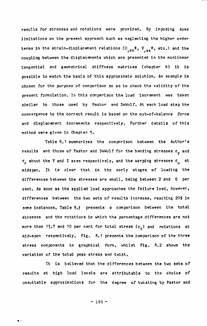
results for stresses and rotations were provided. By imposing some

lim itations on the present approach such as neglecting the higher order

terms in the strain-displacement re lations (U #, V ♦ , e tc . ) and thet XX | XXcoupling between the displacements which are presented in the nonlinear

tangential and geometrical s t i f fn ess matrices (chapter 4) i t is

possible to match the basis o f th is approximate solution. An example is

chosen for the purpose o f comparison so as to check the v a l id i t y o f the

present formulation. In th is comparison the load increment was taken

similar to those used by Pastor and DeWolf. At each load step the

convergence to the correct result i s based on the out-of-balance force

and displacement increments respective ly . Further d e ta ils o f th is

method were given in Chapter 5.

Table 8.1 summarizes the comparison between the Author’ s

results and those o f Pastor and DeWolf fo r the bending stresses cry and

a about the Y and Z axes respective ly , and the warping stresses at

midspan. I t is clear that in the early stages o f loading the

differences between the stresses are small, being between 2 and 6 per

cent. As soon as the applied load approaches the fa i lu re load, however,

d ifferences between the two sets o f results increase, reaching 20% in

some instances. Table 8.J presents a comparison between the to ta l

stresses and the rotations in which the percentage d ifferences are not

more than 13.7 and 10 per cent fo r to ta l stress (o fc) and rotations at

mid-span respective ly . Fig. 8.1 presents the comparison o f the three

stress components in graphical form, whilst F ig . 8.2 shows the

variation o f the to ta l peak stress and tw ist.

I t is believed that the d ifferences between the two sets o f

results at high load le v e ls are attributable to the choice o f

unsuitable approximations for the degree o f twisting by Pastor and

- 195 -

* •

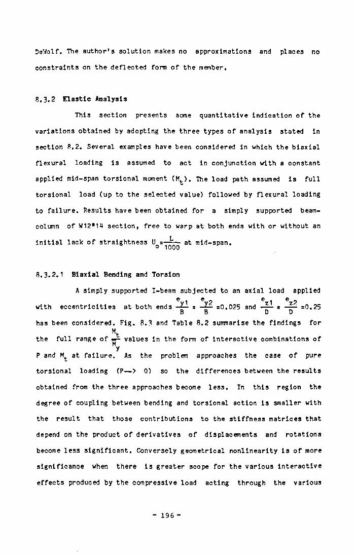
DeWolf. The author’ s solution makes no approximations and places no

constraints on the deflected form o f the member.

8.3 .2 E la s t ic Analysis

This section presents some quantitative indication o f the

variations obtained by adopting the three types o f analysis stated in

section 8.2. Several examples have been considered in which the b iax ia l

flexural loading is assumed to act in conjunction with a constant

applied mid-span torsional moment (Mfc) . The load path assumed is fu l l

torsional load (up to the selected value) followed by flexural loading

to fa i lu re . Results have been obtained for a simply supported beam-

column o f W12*14 section, free to warp at both ends with or without an

in i t ia l lack o f straightness U =—-— at mid-span.° 1000

8.3.2.1 Biaxial Bending and Torsion

A simply supported I-beam subjected to an axial load appliede 1 e _ e . e .

with eccen tr ic it ies at both ends — =0.025 and —2— = =0.25B B D O

has been considered. Fig. 8.3 and Table 8.2 summarise the findings for

Mtthe fu l l range o f ■«- values in the form o f in terac t ive combinations o fMy

P and M at fa i lu re . As the problem approaches the case o f pure

torsional loading (P— > 0) so the d ifferences between the results

obtained from the three approaches become less . In th is region the

degree o f coupling between bending and torsional action is smaller with

the result that those contributions to the s t i f fn ess matrices that

depend on the product o f der iva tives o f displacements and rotations

become less s ign if ican t. Conversely geometrical nonlinearity i s o f more

significance when there is greater scope for the various in teractive

e ffec ts produced by the compressive load acting through the various

- 196 -

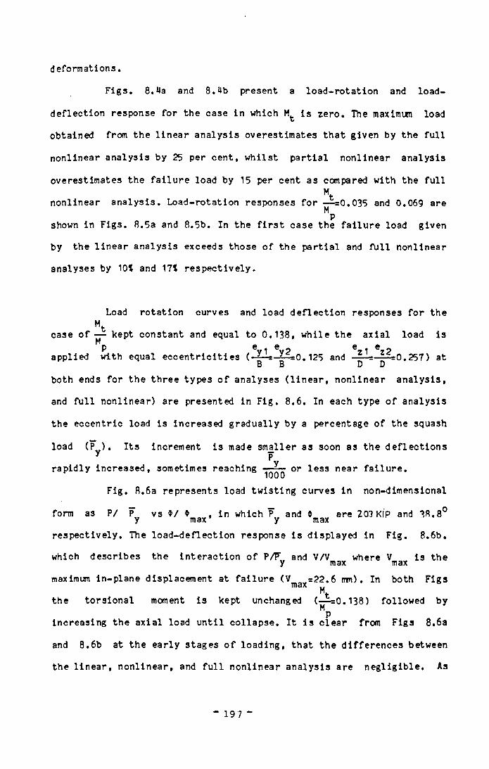
deformations.

Figs. 8.Ma and 8.Ub present a load-rotation and load-

deflection response for the case in which Mfc is zero. The maximum load

obtained from the l in ear analysis overestimates that given by the fu l l

nonlinear analysis by 25 per cent, whilst partia l nonlinear analysis

overestimates the fa i lu re load by 15 per cent as compared with the fu l l

Mtnonlinear analysis. Load-rotation responses fo r — =0.035 and 0.069 areM

Pshown in Figs. 8.5a and 8.5b. In the f i r s t case the fa i lu re load given

by the linear analysis exceeds those o f the partia l and fu l l nonlinear

analyses by 10t and 171 respective ly .

Load rotation curves and load deflection responses for the

Mtcase o f — kept constant and equal to 0.138, while the axia l load is MP 6 6 6 6

applied with equal eccen tr ic it ies ( . X-ls y ?=0.125 and z1= Z?=0.257) atB B D D

both ends for the three types o f analyses ( l in ea r , nonlinear analysis,

and fu l l nonlinear) are presented in Fig. 8.6. In each type o f analysis

the eccentric load is increased gradually by a percentage o f the squash

load (Pv ) . I ts increment is made stnaller as soon as the deflections

pyrapidly increased, sometimes reaching or less near fa i lu re .

Fig. 8.6a represents load tw isting curves in non-dimensional

form as P/ P vs $/ *max» in which P^ and *max are 203 KIP and 38.8°

respectively. The load-deflection response is displayed in Fig. 8.6b.

which describes the interaction o f P/F and V/V where V is they max max

maximum in-plane displacement at fa i lu re (V =22.6 mm). In both Figsmax ..

the torsional moment is kept unchanged (— =0.138) followed byM

Pincreasing the axial load until collapse. I t i s c lear from Figs 8.6a

and 8.6b at the early stages o f loading, that the d ifferences between

the l in ear , nonlinear, and fu l l nonlinear analysis are n eg lig ib le . As

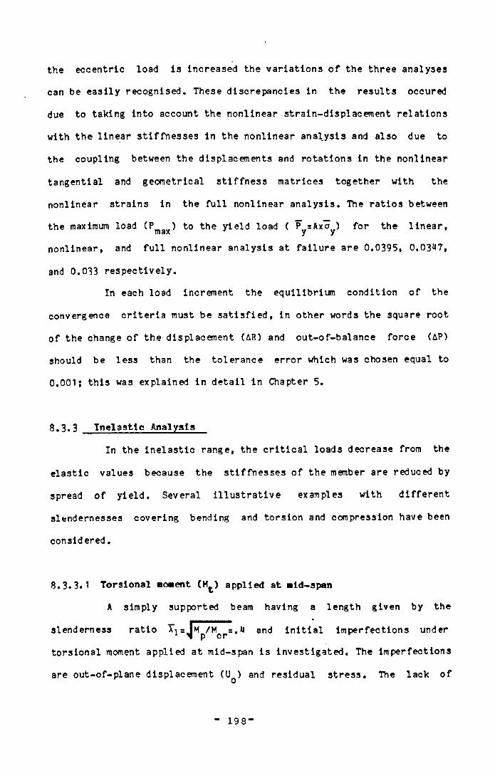
the eccentric load is increased the variations o f the three analyses

can be eas ily recognised. These discrepancies in the results oceured

due to taking into account the nonlinear strain-displacement relations

with the linear s t if fnesses in the nonlinear analysis and also due to

the coupling between the displacements and rotations in the nonlinear

tangential and geometrical s t i f fn ess matrices together with the

nonlinear strains in the fu l l nonlinear analysis. The ratios between

the maximum load (Pmax) to the y ie ld load ( Py=Axoy) for the l in ea r ,

nonlinear, and fu l l nonlinear analysis at fa i lu re are 0.0395, 0.0347,

and 0.033 respective ly .

In each load increment the equilibrium condition o f the

convergence c r i t e r ia must be sa t is f ied , in other words the square root

o f the change o f the displacement (AR) and out-of-balance force (AP)

should be less than the tolerance error which was chosen equal to

0.001; this was explained in d e ta il in Chapter 5.

8.3.3 In e las t ic Analysis

In the in e las t ic range, the c r i t i c a l loads decrease from the

e las t ic values because the s t if fn esses o f the member are reduced by

spread o f y ie ld . Several i l lu s t r a t iv e examples with d if fe ren t

slendernesses covering bending and torsion and compression have been

considered.

8.3.3.1 Torsional «oaent (M^) applied at aid-span

A simply supported beam having a length given by the

slenderness ra t io T1=J m /M =.H and in i t i a l imperfections under'I p cr

torsional moment applied at mid-span is investigated. The imperfections

are out-of-plane displacement (UQ) and residual stress. The lack o f

198

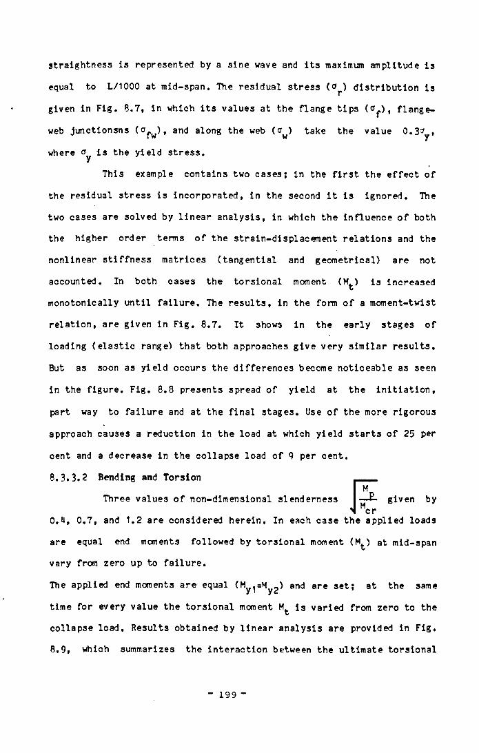
straightness is represented by a sine wave and its maximum amplitude is

equal to L/1000 at mid-span. The residual stress (o ) d istribution isr

given in F ig . 8.7, in which i t s values at the flange t ips (<^ ), flange-

web junctionsns ( CTfw) t and along the web (o^) take the value 0.3<Jy ,

where is the y ie ld stress.

This example contains two cases; in the f i r s t the e f fe c t o f

the residual stress is incorporated, in the second i t is ignored. The

two cases are solved by l in ear analysis, in which the influence o f both

the higher order terms o f the strain-displacement re lations and the

nonlinear s t i f fn ess matrices (tangential and geometrical) are not

accounted. In both cases the torsional moment (M^) is increased

monotonically until fa i lu re . The resu lts, in the form o f a moment-twist

re la tion , are given in Fig. 8.7. I t shows in the early stages o f

loading (e la s t ic range) that both approaches g ive very s im ilar results.

But as soon as y ie ld occurs the d ifferences become noticeable as seen

in the figure. Fig. 8.8 presents spread o f y ie ld at the in i t ia t io n ,

part way to fa i lu re and at the f ina l stages. Use o f the more rigorous

approach causes a reduction in the load at which yie ld starts o f 25 per

cent and a decrease in the collapse load o f 9 per cent.

8.3.3.2 Bending and Torsion' M

given byS Mcr

Three values o f non-dimensional slenderness

O.U, 0.7, and 1.2 are considered herein. In each case the applied loads

are equal end moments followed by torsional moment (M^) at mid-span

vary from zero up to fa i lu re .

The applied end moments are equal ( My 1 =N1y2 and are set; at same

time for every value the torsional moment is varied from zero to the

collapse load. Results obtained by l in ea r analysis are provided in Fig.

8.9, which summarizes the interaction between the ultimate torsional

199 ~

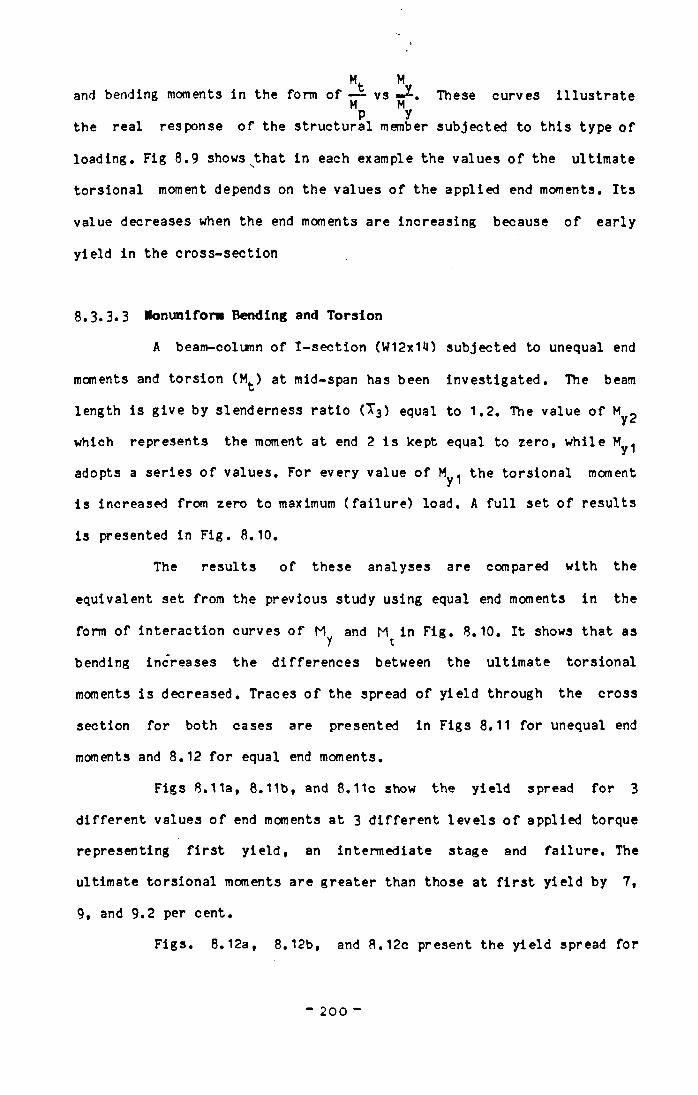
and bending moments in the form o fMP

These curves i l lu s t ra te

the real response o f the structural member subjected to th is type o f

loading. Fig 8.9 shows that in each example the values o f the ultimate

torsional moment depends on the values o f the applied end moments. I ts

value decreases when the end moments are increasing because o f early

yield in the cross-section

8.3 .3 .3 lonun ifon i Bending and Torsion

A beam-column o f I-sec t ion (W12x14) subjected to unequal end

moments and torsion (M^) at mid-span has been investigated. The beam

length is g ive by slenderness ra t io (X3) equal to 1 . 2. The value o f

which represents the moment at end 2 is kept equal to zero, while My1

adopts a series o f values. For every value o f My1 the torsional moment

is increased from zero to maximum ( fa i lu r e ) load. A fu l l set o f results

is presented in F ig. 8.10.

The results o f these analyses are compared with the

equivalent set from the previous study using equal end moments in the

form o f interaction curves o f and Mt in F ig . 8.10. I t shows that as

bending increases the d ifferences between the ultimate torsional

moments is decreased. Traces o f the spread o f y ie ld through the cross

section for both eases are presented in Figs 8.11 for unequal end

moments and 8.12 fo r equal end moments.

Figs 8.11a, 8.11b, and 8.11c show the y ie ld spread for 3

d if fe ren t values o f end moments at 3 d i f fe ren t le v e ls o f applied torque

representing f i r s t y ie ld , an intermediate stage and fa i lu re . The

ultimate torsional moments are greater than those at f i r s t y ie ld by 7,

9, and 9.2 per cent.

F igs. 8.12a, 8.12b, and 8.12c present the y ie ld spread for

- 2 0 0 “

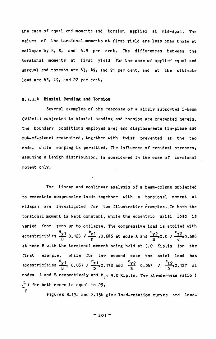
the case o f equal end moments and torsion applied at mid-span. The

values o f the torsional moments at f i r s t y ie ld are less than those at

collapse by 8, 8, and 6.4 per cent. The d ifferences between the

torsional moments at f i r s t yie ld for the case o f applied equal and

unequal end moments are 63, 49, and 21 per cent, and at the ultimate

load are 63, 9, and 22 per cent.

8.3. 3 .1* B iax ia l Bending and Torsion

Several examples o f the response o f a simply supported I-Beam

(W12x14) subjected to b iax ia l bending and torsion are presented herein.

The boundary conditions employed are; end displacements (in-plane and

out-of-plane) restrained, together with tw ist prevented at the two

ends, while warping is permitted. The influence o f residual stresses,

assuming a Lehigh d istr ibu tion , is considered in the ease o f torsional

moment only.

The linear and nonlinear analysis o f a beam-column subjected

to eccentric compressive loads together with a torsional moment at

midspan are investigated for two i l lu s t r a t iv e examples. In both the

torsional moment is kept constant, while the eccentric axial load is

varied from zero up to co llapse. The compressive load is applied withg g g

eccen tr ic it ies -^1=0.125 / — =0.686 at node A and -^ = 0 .0 / B D B

,686

at node B with the torsional moment being held at 3.0 Kip.in for the

f i r s t example, while fo r the second case the axial load has®y 1 ®,1

eccen tr ic it ies -¿-= 0.063 / ---- =0.172 andB D .063

ez 2/ —— =0.127 D

at

nodes A and B respective ly and Ms 9.0 K ip .in . The slenderness ra t io (

~ ) for both cases is equal to 25.r y

Figures 8.13a and 8.13b g ive load-rotation curves and load-

201

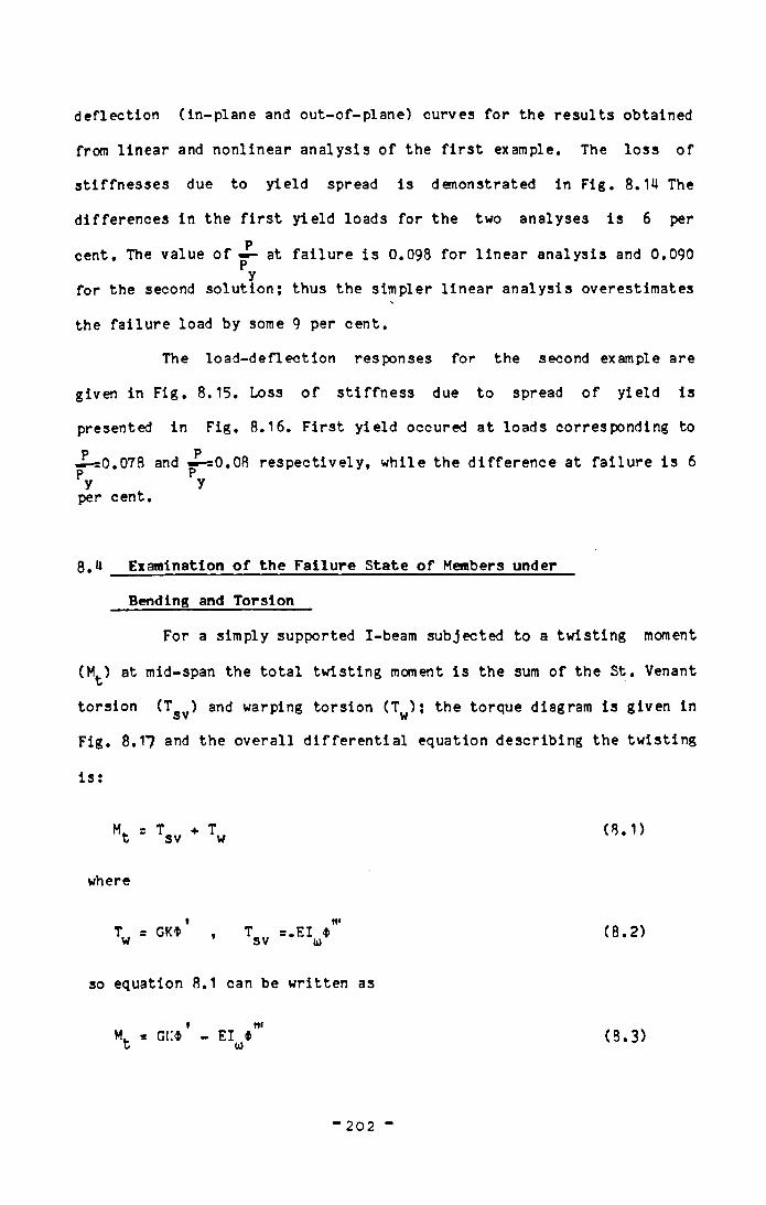
deflection (in-plane and out-of-plane) curves fo r the results obtained

from linear and nonlinear analysis o f the f i r s t example. The loss o f

s t if fnesses due to y ie ld spread is demonstrated in F ig. 8. 1U The

differences in the f i r s t yie ld loads for the two analyses is 6 perP

cent. The value o f —- at fa i lu re is 0.098 for linear analysis and 0.090y

for the second solution; thus the simpler linear analysis overestimates

the fa ilu re load by some 9 per cent.

The load-deflection responses for the second example are

given in F ig. 8.15. Loss o f s t i f fn ess due to spread o f y ie ld is

presented in Fig. 8.16. F irst y ie ld oceured at loads corresponding to

P P---=0.078 and —-=0.08 respective ly , while the d if fe rence at fa i lu re is 6 P P

y yper cent.

8.U Examination o f the Failure State o f Members under

Bending and Torsion * I

For a simply supported I-beam subjected to a tw isting moment

(Mfc) at mid-span the to ta l twisting moment is the sum o f the St. Venant

torsion (Tsv) and warping torsion (Ty ) ; the torque diagram is given in

Fig. 8.17 and the overa ll d i f fe r e n t ia l equation describing the twisting

i s :

M. = T + T t sv w

where

I wT = GK$ , T =.EI $ w ’ SV u)

so equation 8.1 can be written as

» niM. = gi:* - EI * t u

(8. 1)

(8 . 2 )

(8.3)

202

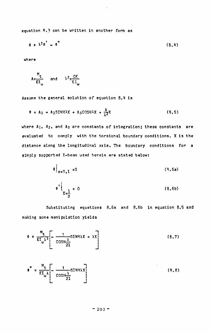
equation B.3 can be written in another form as

A, * n

: A2* - * (8.U)

where

A=-El.

and A 2 ÆEIu>

Assume the general solution o f equation 8.4 is

# = Ai + A2SINHXX + A3COSHXX + yyX (8 .5 )

where Ai, A2 , and A3 are constants o f in tegration ; these constants are

evaluated to comply with the torsional boundary conditions. X is the

distance along the longitudinal axis. The boundary conditions for a

simply supported I-beam used herein are stated below:

$ x=0, l =0 ( 8. 6a)

*$ ( 8. 6b)

Substituting equations 8. 6a and 8. 6b in equation 8.5 and

making some manipulation y ie lds

El X3tii---- !----SINHXX + XXCOSH- -

21

(8 .7 )

If$

Mt r 1 1- r ~ \ ---------- -— SINHXX1FT 1 * \ t

w ' cosh— 'I 21 i

( 8 . 8 )

“ 203

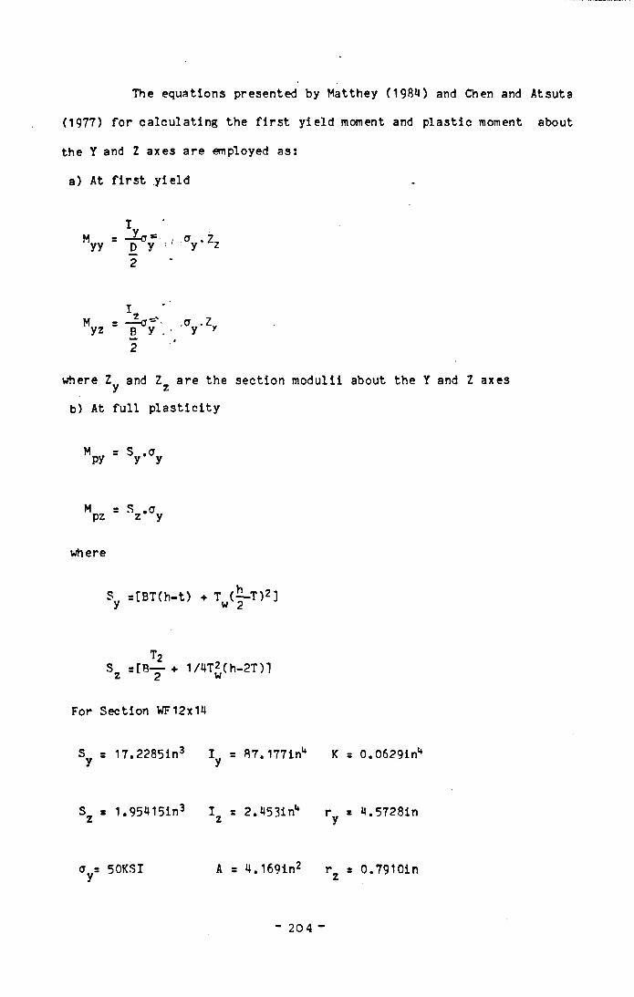
The equations presented by Matthey (198*0 and Chen and Atsuta

(1977) for calculating the f i r s t y ie ld moment and p lastic moment about

the Y and Z axes are employed as:

a) At f i r s t y ie ld

Myy

zz

Myz2 - v

£ V 2

V z'

where Z , and Z are the section modulii about the Y and Z axesy z

b) At fu l l p la s t ic ity

M s S .0py y y

Mpz Sz 0y

where

Sy =[BT(h-t) + Tw(^ -T )2]

Sz =rBT + 1 /l,TJ(h- 2T)l

For Section WF12x14

Sy = 17.2285in3 I = 87. 1771^ K = 0.0629inu

S = 1 . 95*l15in3 I = 2. U53in** r = H.5728inz z y

o = 50KSI A = U.169in2 r . = 0.7910iny z

204 -

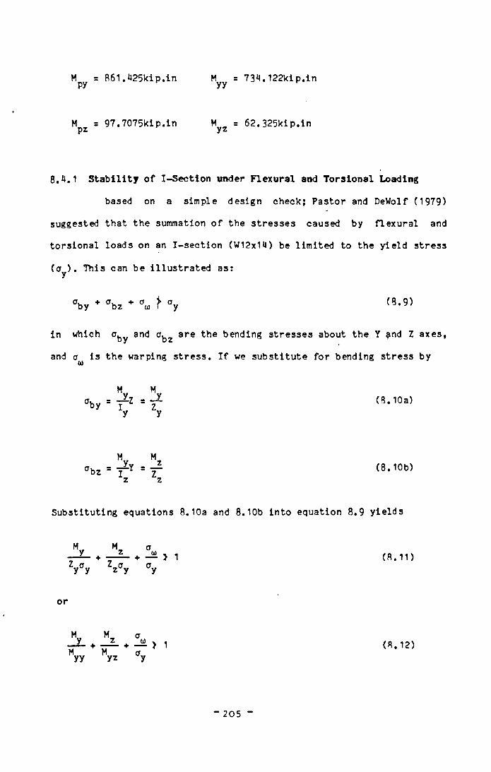
M = 86l.425kip.inpy

Myy = 73ii.122kip.in

M = 97.7075kip.in M = 62.325kip.inpz yz

8.4.1 S ta b i l i t y o f I -Section under Flexural and Torsional Loading

based on a simple design check; Pastor and DeWolf (1979)

suggested that the summation o f the stresses caused by flexural and

torsional loads on an I-section (W12x14) be limited to the y ie ld stress

(Oy). This can be i l lu s tra ted as:

aby + abz + au> f ay (8 *9)

in which a^y and cfez are the bending stresses about the Y ?nd Z axes,

and is the warping stress. I f we substitute for bending stress by

aby = ( 8. 10a)

ffbz = ( 8. 10b)

Substituting equations 8.10a and 8.10b into equation 8.9 y ie lds

M.

Z ay y

l a z y

> 1 (8 . 11)

or

a0) > 1 ( 8 . 12)

" 205

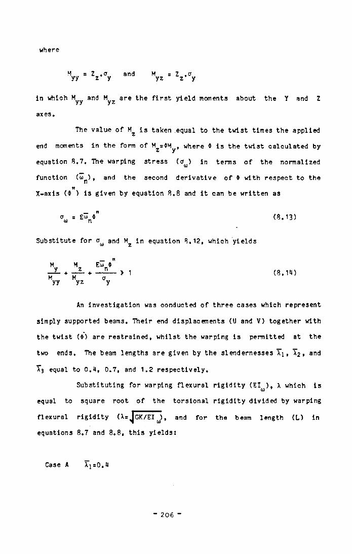
where

M = Z .o and M = Z ,cr yy z y yz z y

in which and Myz are the f i r s t y ie ld moments about the Y and Z

axes.

The value o f i s taken equal to the tw ist times the applied

end moments in the form o f M =$M , where 9 is the tw ist calculated byz y *

equation 8.7. The warping stress (o^) in terms o f the normalized

function (u^ ), and the second der iva t ive o f * with respect to theM

X-axis ($ ) is given by equation 8.8 and i t can be written as

_ na : Em fa) n (8.13)

Substitute for and Mz in equation 8.12, which y ie lds

M M Euj __y_ __z_ nM + M + o

yy yz y

> 1 (8.m)

An investigation was conducted o f three cases which represent

simply supported beams. Their end displacements (U and V) together with

the tw ist (4>) are restrained, whilst the warping is permitted at the

two ends. The beam lengths are given by the slendernesses X j , X2 , and

X3 equal to O.U, 0.7, and 1 .2 respective ly .

Substituting for warping flexural r ig id i t y (El ) , X which is(jj

equal to square root o f the torsional r i g id i t y divided by warping

flexural r ig id i t y (X=^GK/EI J , and for the beam length (L ) in

equations 8.7 and 8. 8, th is y ie lds :

Case A Ai=0.iJ

206

(8.15a)* = 0.0001799 Mfc

*" = 0.2753;ix10_5Mt (8.15b)

Case B ^ 1=0.7

* = 0.0010132 Mfc (8.16a)

*" =0.U80x10“ 6Mt (8.16b)

Case C ^ 1=1 .2

* =0.0046412 Mfc (8.17a)

*" =0.74493l»x10- 5Mt (8.17b)

8.4.1.1 S ta b i l i t y o f Bea»-Colunn o f I-Section under Bending and

Torsion Based on Pastor and DeWolf (1979) Suggestions

Stresses caused by flexural and torsional loads based on the

Author's fu l l f in i t e element ( f . e . ) analysis and the use o f the

equations 8.15 to 8.17 to calculate the interaction stresses are

presented in Tables 8.3, 8.4, and 8.5 for each load combination in each

case. The end moments are applied f i r s t incrementally to a set l im it

followed by incrementing the torsional moment (M^) to fa i lu re . For zero

torsional moment the end moments are simply increased to collapse and a

similar procedure is used when the uniform moments are zero. The

interaction between torsion and bending at the ultimate condition has

been discussed in fu l l in section 8.3 .3 .2. Equation 8.14 is used to

calculate the stresses at f i r s t y ie ld . The ultimate values o f the

207

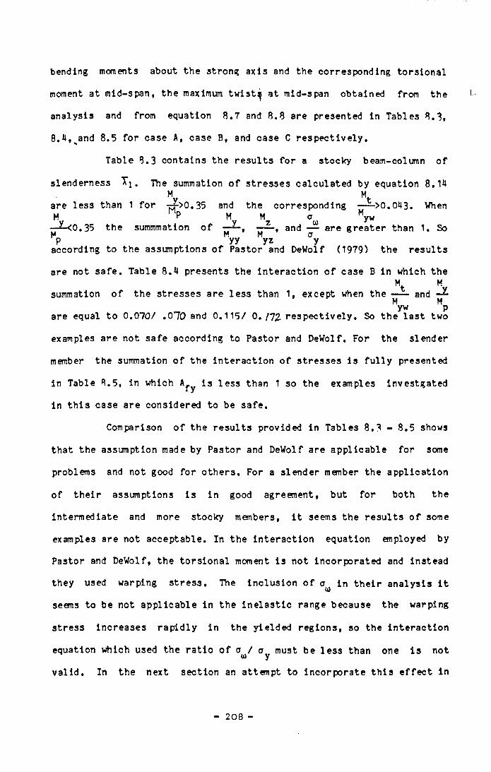
bending moments about the strong axis and the corresponding torsional

moment at mid-span, the maximum tw isty at mid-span obtained from the

analysis and from equation 8.7 and 8.8 are presented in Tables 8.3,

8.4,^and 8.5 for case A, case B, and case C respective ly .

Table 8.3 contains the results fo r a stocky beam-column o f

slenderness The summation o f stresses calculated by equation 8.14M M.V tare less than 1 fo r -tt->0.35 and the corresponding ---- >0.043. When

M P M M O ^yw—^-<0.35 the summmation o f ——, —— , and — are greater than 1. So M M M O’

p yy yz yaccording to the assumptions o f Pastor and DeWoif (1979) the results

are not safe. Table 8.4 presents the interaction o f case B in which theM M

summation o f the stresses are less than 1 , except when the ---- and —M Myw p

are equal to 0.070/ .070 and 0.115/ 0 . /72 respective ly . So the la s t two

examples are not safe according to Pastor and DeWoif. For the slender

member the summation o f the interaction o f stresses is fu l ly presented

in Table 8.5, in which is less than 1 so the examples investgated

in th is case are considered to be safe.

Comparison o f the results provided in Tables 8.3 - 8.5 shows

that the assumption made by Pastor and DeWoif are applicable for some

problems and not good for others. For a slender member the application

o f the ir assumptions is in good agreement, but for both the

intermediate and more stocky members, i t seems the results o f some

examples are not acceptable. In the interaction equation employed by

Pastor and DeWoif, the torsional moment is not incorporated and instead

they used warping stress. The inclusion o f a in the ir analysis i tll)

seems to be not applicable in the in e las t ic range because the warping

stress increases rapid ly in the yielded regions, so the interaction

equation which used the ra t io o f o / a must be less than one is nota) y

va lid . In the next section an attempt to incorporate th is e f fe c t in

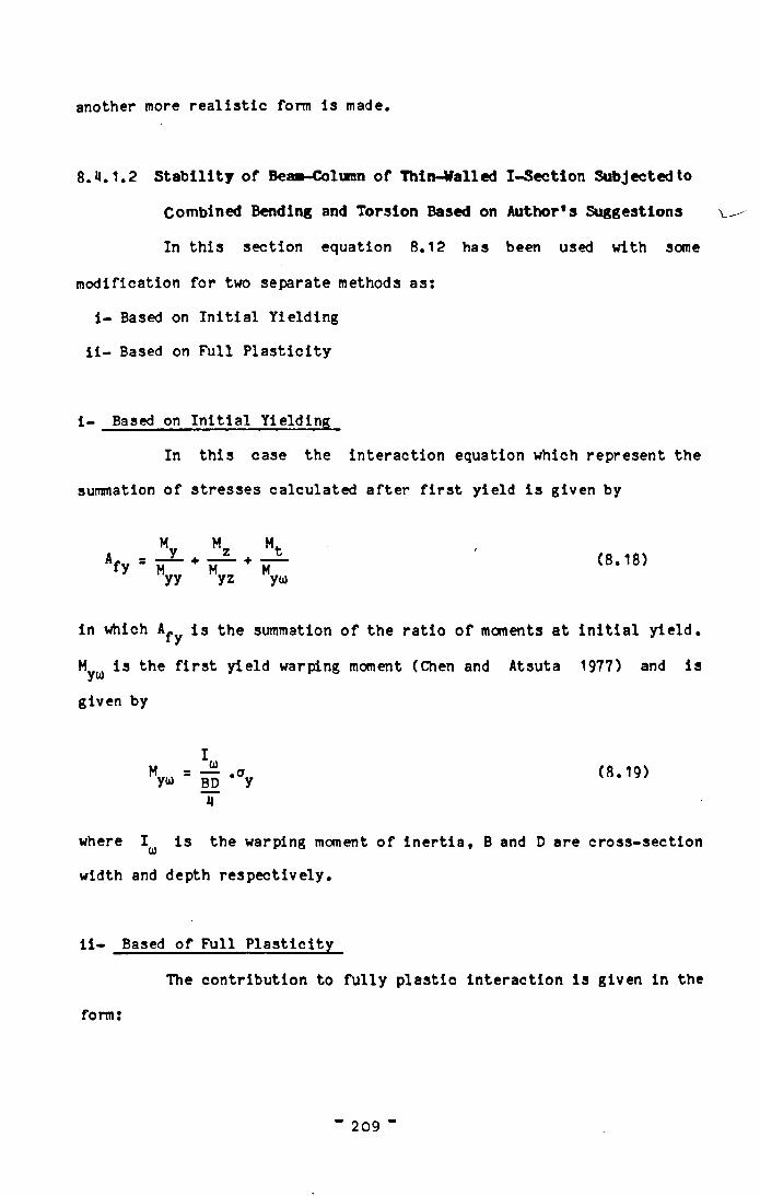
another more r e a l is t ic form is made

8.0 .1 .2 S t a b i l i t y o f Beaa-Colunn o f Thin-Walled I -Sect ion Subjected to

Combined Bending and Torsion Based on Author 's Suggestions v

In th is section equation 8.12 has been used with some

modification for two separate methods as:

i - Based on I n i t i a l Y ield ing

i i - Based on Full P la s t ic i t y

i - Based on In i t i a l Y ield ing

In th is case the interaction equation which represent the

summation o f stresses calculated a f te r f i r s t y ie ld i s given by

M.

f y s hyy

M.

yz yu(8 .18 )

in which i s the summation o f the ra t io o f moments at i n i t i a l y ie ld .

Myu i s the f i r s t y ie ld warping moment (Chen and Atsuta 1977) and i s

given by

IM = — .a

y<*> BD yH

(8 .19 )

where I i s the warping moment o f in e r t ia , B and D are cross-sectionU) 9

width and depth respective ly .

i i - Based o f Full P la s t ic i t y

The contribution to fu l l y p la s t ic interaction i s given in the

form:

" 2 0 9 "

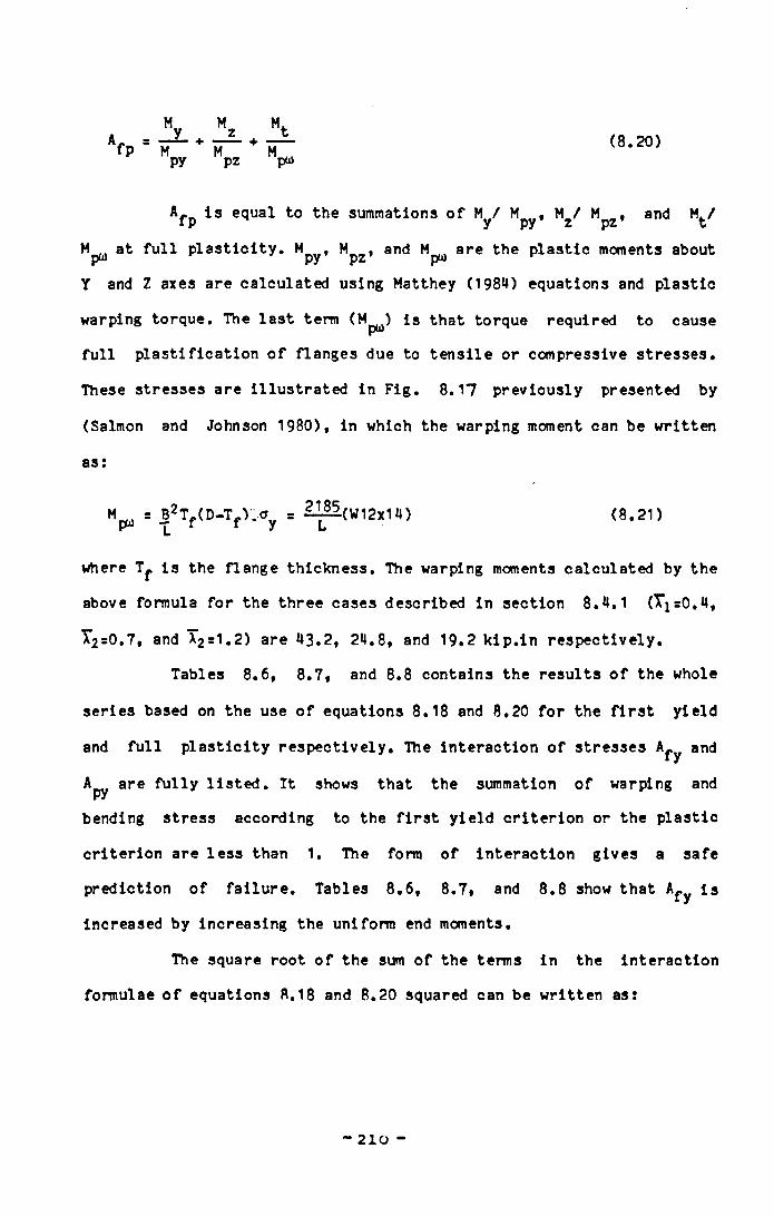
(8 . 20)M

fP " Mpy M.pz Mpu

A. i s equal to the summations o f M / M , M / M , and M. / fp y py* z pz* t

M at f u l l p la s t ic i t y . M , M , and M are the p la s t ic moments aboutp py p* p***

Y and Z axes are ca lcu lated using Matthey (1984) equations and p la st ic

warping torque. The l a s t term (M ) i s that torque required to causepw

f u l l p la s t i f ic a t io n o f flanges due to t e n s i le or compressive s tre sses .

These stresses are i l lu s t ra te d in F ig . 8.17 previously presented by

(Salmon and Johnson 1980), in which the warping moment can be written

as:

Mpw B2Tf (D-Tf ) , o L 1 1 y

£1^(W12x1U)I.

(8. 21)

where T . i s the flange thickness. The warping moments ca lcu lated by the

above formula fo r the three cases described in section 8 .4 .1 (T i=0 .4 ,

\2 =0 .7, and X2 =1.2) are 43 .2 , 24 .8 , and 19.2 k ip . in respect ive ly .

Tables 8.6, 8 .7, and 8.8 contains the re su lts o f the whole

ser ies based on the use o f equations 8.18 and 8.20 fo r the f i r s t y ie ld

and f u l l p la s t ic i t y respec t ive ly . The interaction o f s tresses A » and

Apy are fu l ly l i s t e d . I t shows that the summation o f warping and

bending stress according to the f i r s t y ie ld c r i te r io n or the p la s t ic

c r ite r ion are le s s than 1. The form o f in teract ion g ives a sa fe

prediction o f f a i lu r e . Tables 8 .6 , 8 .7 f and 8.8 show that A .y i s

increased by increasing the uniform end moments.

The square root o f the sum o f the terms in the in teraction

formulae o f equations 8.18 and 8.20 squared can be written as:

210

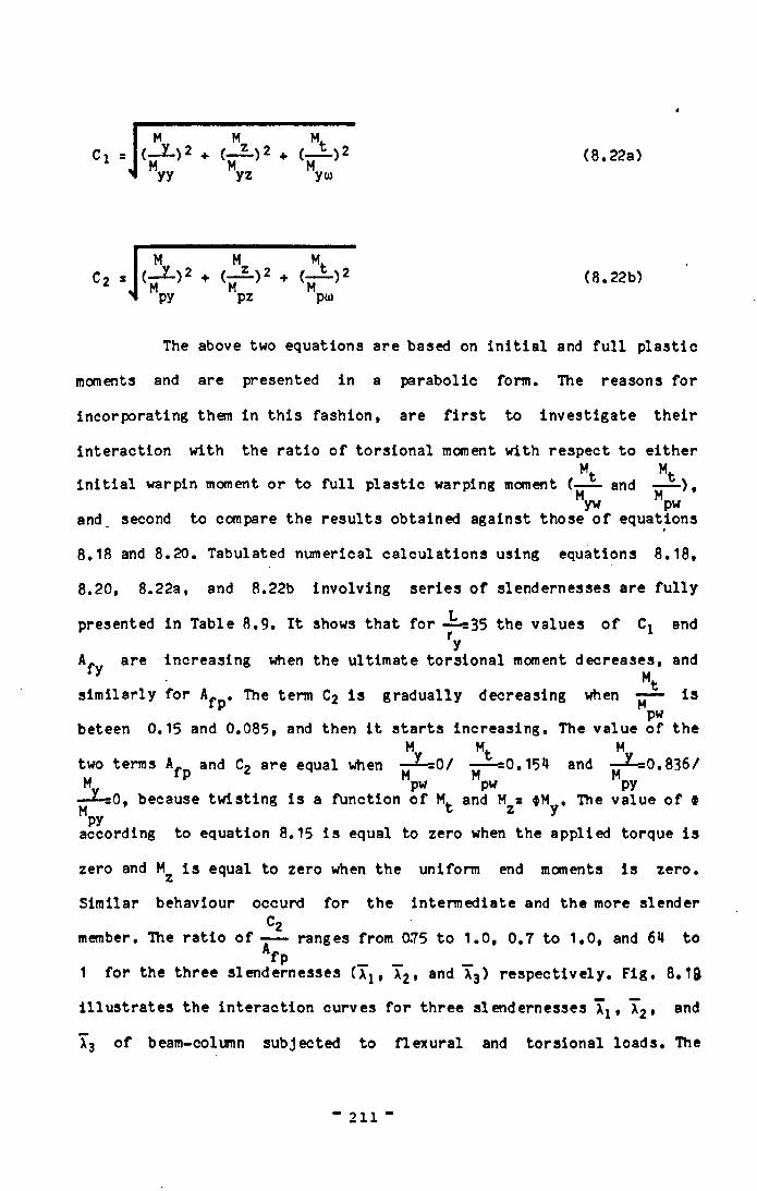
( 8. 22a)C, =M M K

(-J L )2 + (_ Z .)2 + ( _ L )2MyuMyy M.yz

M M M,( ^ - ) 2 + ( t r 2- ) 2 + ( “ T " )Mpo)M

pyM

( 8. 22b)pz

The above two equations are based on in i t i a l and fu l l p las t ic

moments and are presented in a parabolic form. The reasons fo r

incorporating them in th is fashion, are f i r s t to in ves t iga te th e ir

interaction with the ra t io o f torsional moment with respect to e ither

Mt MtIn i t i a l warpin moment or to fu l l p lastic warping moment (—— and ——) ,M Myw pw

and second to compare the resu lts obtained against those o f equations

8.18 and 8.20. Tabulated numerical calculations using equations 8.18,

8. 20, 8. 22a, and 8. 22b involving series o f slendernesses are fu l ly

presented in Table 8.9. I t shows that fo r -^-s35 the values o f C, andry

Af are increasing when the ultimate torsional moment decreases, and

Mts im ila r ly fo r A_ . The term C2 i s gradually decreasing when —— ispw

beteen 0.15 and 0.085, and then i t s tarts increasing. The value o f theM M. M

two terms A_ and C2 are equal when —^-=0/ —^-=0.159 and —^-=0.836/M i P M M M ..pw pw py

*0, because tw isting is a function o f M. and M s *M . The value o f *Mpyaccording to equation 8.15 i s equal to zero when the applied torque is

zero and Mz i s equal to zero when the uniform end moments is zero.

Similar behaviour occurd for the intermediate and the more slenderC2

member. The ra t io o f -— ranges from 0.75 to 1.0, 0.7 to 1.0, and 69 tofp _ _

1 fo r the three slendernesses (x 1# X2, and x3> respec t ive ly . F ig . 8.1&

i l lu s tra te s the in teraction curves fo r three slendernesses Xj, T2, and

T3 o f beam-column subjected to flexura l and torsional loads. The

211

uniform end moments are applied about the strong axis and at the same

time as the tors ional moment at the mid-span. Details o f load

incrementation have been given in section 8.4 .1 .1 . These curves

indicate that i t is possible to provide a practica l prediction formula

which can then be used to determine the ultimate loads. Further

explanations w i l l be provided in section 8. 5 .

8.4.1.3 S ta b i l i t y o f Beaa-Colwn under B iaxia l Bending and Torsion

In th is case selected values o f the mid-span tors ional momentey 1

O O are applied followed by an axia l load with e c c en tr ic i t ie s ,w De . c . c.p-¿■£=0.167 and — --, — £=0.257 about both ends. At every value o f M. the

D B B t

end load is increased up to fa i lu re . The in teraction o f the compressive

force P and torsional moment Mp is given in Table 8.8 where i t i s

compared with the resu lts generated from the fo llow ing equation.

_ M. M MAA - p t y z

P M M Mpl up pyl pzl

where Ppl = cy .A, and Mt , My , Mz , Mupf Mp y l, and Mpzl are defined in

section 8.4.2. The resu lts o f the above equation shows that the term AA

is less than 1 .

8.5 Prediction o f S ta b i l i t y o f Beaw-Coluan under Flexural

Bending and Torsion Using a Regression Analysis

The ultimate bending and torsion values presented in Table

8.9 and i l lu s tra ted in the in teraction curves o f F ig. 8.19 have been

used herein to develop a practica l formula based on the results

previously discussed concerning beams subjected to combined bending and

torsion . Three equations are developed based on:

" 2 1 2 “

1- Interaction o f M./M and A,t pw fy

2- Interaction o f M./M and Cit pw 1

3 - Combination o f 1 and 2

where A ^ and Cj have been defined in equations 8.18 and 8.22a

respective ly .

The development o f these equations are based on the

application o f regression techniques (Draper and Smith,1961, N ev il le

and Kennedy ,1964) A s t a t i s t i c a l package SPSS-X21, a v a i la b le at USCC

(Un iversity o f She ff ie ld Computer Centre ), i s employed to ca lcu la te

d if fe ren t parameters such as , mean va lue , maximum/ minimum values,

standard dev iat ion , co r re la t io n , mean square, res idual standard e rro rs ,

etc . and then these v a r ia b le s are used in deriv ing regression

equations. The equations conducted fo r the three slendernesses X jsO.4,

X2=0.7, and X3=1.2 are summarized in the fo llow ing three cases:

function o f Afy and LCase i M./M t pw

Case ii M./M t pw

Case iii M./Mt pw

in which Af , C j, and L can represent any values o f moments andm 1 ypw

slendernesses. In other words the equations can be applied to any case

previously explained.

The prediction equation o f case i in which

be written as:

i r * F (V u ca"pw

Mt— ! - = 0.167937 - 0.1217A. - 0.001037L Mpw y

(8 .23 )

the other equation which based on ease i i i s

- 213 -

(8.24)Mt— = 0.164857 - 0 .119876Ci - 0.001118LMpw

The la s t equation which employs ------ as a function o f A. , C i, L can beMpw y

written as:

0.164835 - 0.083002Ci 0.03828Afy - 0.001094L (8.25)

Equations 8.23 - 8.25 can be used to determine the ultimate

moment for any set l im it o f torsion or v ice versa. They can also be

used for slendernesses between 0.4 ^1.2. These equations can play an

important part in the design o f members having thin-walled open cross-

section in the design o f s tee l structures and leads the way fo r further

work in th is area.

8.6 General Features o f the Analysis

D ifferen t cases o f loading and slenderness have been

addressed to provide some idea o f the interaction o f these var iab le on

the fa i lu re condition. Before a fu l ly va lida te ultimate strength

approach to the design o f slender members under any form o f combined

torsional/ flexural/ compressive loading can be produced a considerable

amount o f further work i s required. This should cover:

1- D ifferen t slenderness ra t io .

2- D ifferen t loading conditions.

3- D iffe ren t boundary conditions.

4- Variable compressive load eccen tr ic i t ie s .

- 214 -

5- Including in i t i a l imperfections ( such as residual stress and

in i t i a l d e f le c t io n s ) .

6 Interaction equation on the form

i 1 i . < .

Ppl + % + Mpyl + V l '

MOTE An extension to some o f th is work i s now in progress and the

results are encouraging.

8.7 Conclusions

The e la s t ic and in e la s t ic 3-dimensional behaviour o f beam-

columns under bending and tors ional loading .has been studied. The

presence o f i n i t i a l imperfections such as residual stresses and in i t i a l

de flect ions together with monitoring o f the y ie ld spread through the

cross-section have been eonsidered-Several example problems, which have

not been previously solved, have been investigated .

The solutions fo r these examples were obtained by three types

o f analysis; ’ L in ear ', 'Non linear ', and Full Nonlinear. The results

show the importance o f including o f the so c a l l 'h igher order terms' o f

the strain displacement re la t ions and the nonlinear geometrical and

tangential s t i f fn ess matrices in the analysis. From these problems,

several important observations are possibles

1- The a b i l i t y o f the formulation presented in chapter 3 to cover

the fu l l range o f analysis o f beam-columns in 3-dimensions.

2- The need to include higher order terms in the stra in-

displacement re la t ions and s t i f fn e s s matrices in order to avoid

overestimates o f load carrying capacity.

- 215 -

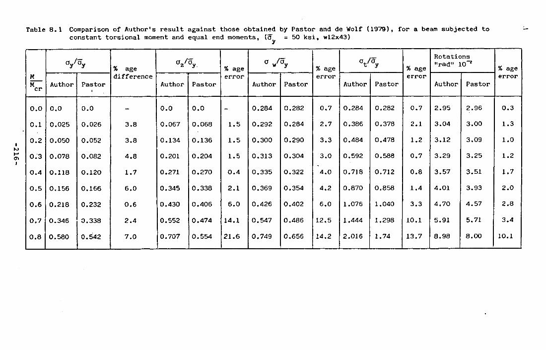
-21

6

Table 8.1 Comparison o f Author's result against those obtained by Pastor and de Wolf (1979), for a beam subjected to constant torsional moment and equal end moments, (o^ = 50 ksi, wl2x43)

MMcr

ay/oy % age difference

°z /oy. % age error

a /a w y% age error

V 0,% age error

Rotations "rad" 10”*

% age

Author Pastor1

Author Pastor Author Pastor Author Pastor Author Pastorerror

0.0 0.0 0.0 - 0.0 0.0 - 0.284 0.282 0.7 0.284 0.282 0.7 2.95 2.96 0.3

0.1 0.025 0.026 3.8 0.067 0.068 1.5 0.292 0.284 2.7 0.386 0.378 2.1 3.04 3.00 1.3

0.2 0.050 0.052 3.8 0.134 0.136 1.5 0.300 0.290 3.3 0.484 0.478 1.2 3.12 3.09 1.0

0.3 0.078 0.082 4.8 0.201 0.204 1.5 0.313 0.304 3.0 0.592 0.588 0.7 3.29 3.25 1.2

0.4 0.118 0.120 1.7 0.271 0.270 0.4 0.335 0.322 4.0 0.718 0.712 0.8 3.57 3.51 1.7

0.5 0.156 0.166 6.0 0.345 0.338 2.1 0.369 0.354 4.2 0.870 0.858 1.4 4.01 3.93 2.0

0.6 0.218 0.232 0.6 0.430 0.406 6.0 0.426 0.402 6.0 1.076 1.040 3.3 4.70 4.57 2.8

0.7 0.346 0.338 2.4 0.552 0.474 14.1 0.547 0.486 12.5 1.444 1.298 10.1 5.91 5.71 3.4

0.8 0.580 0.542 7.0 0.707 0.554 21.6 0.749 0.656 14.2 2.016 1.74 13.7 8.98 8.00 10.1

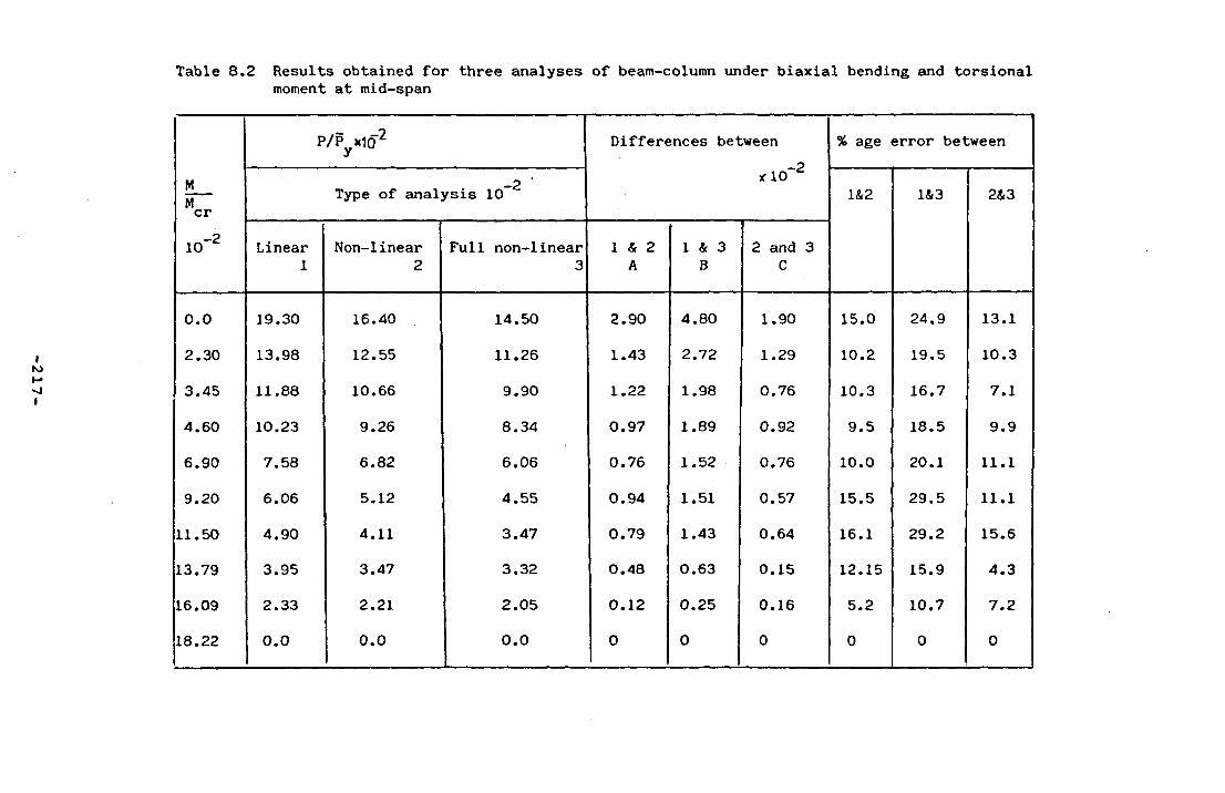
Table 8.2 Results obtained fo r three analyses o f beam-column under b iaxial bending and torsional moment at mid-span

MMcr

io -2

P/Py*102 Differences between

-2*10

% age error between

-2 'Type o f analysis 10 1&2 1&3 2&3

Linear1

Non-linear2

Full non-linear 3

1 & 2 A

1 & 3 B

2 and 3 C

0.0 19.30 16.40 14.50 2.90 4.80 1.90 15.0 24.9 13.1

2.30 13.98 12.55 11.26 1.43 2.72 1.29 10.2 19.5 10.3

3.45 11.88 10.66 9.90 1.22 1.98 0.76 10.3 16.7 7.1

4.60 10.23 9.26 8.34 0.97 1.89 0.92 9.5 18.5 9.9

6.90 7.58 6.82 6.06 0.76 1.52 0.76 10.0 20.1 11.1

9.20 6.06 5.12 4.55 0.94 1.51 0.57 15.5 29.5 11.1

11.50 4.90 4.11 3.47 0.79 1.43 0.64 16.1 29.2 15.6

13.79 3.95 3.47 3.32 0.48 0.63 0.15 12.15 15.9 4.3

16.09 2.33 2.21 2.05 0.12 0.25 0.16 5.2 10.7 7.2

18.22 0.0 0.0 0.0 0 0 0 0 0 0

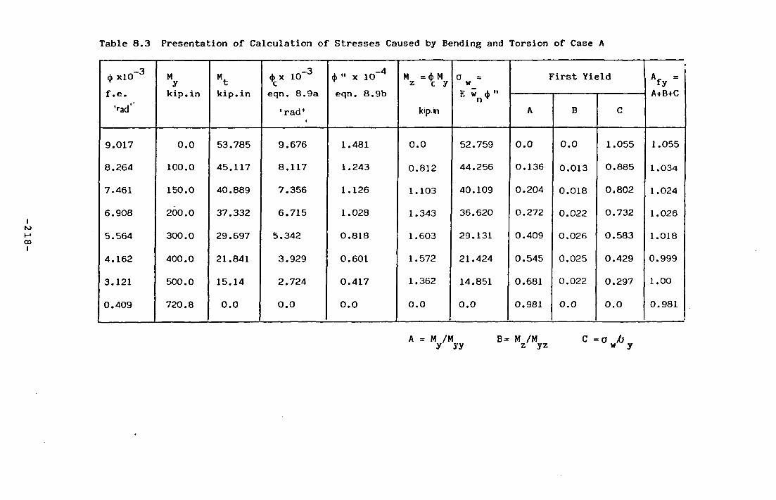
-2

18

-

Table 8.3 Presentation o f Calculation o f Stresses Caused by Bending and Torsion of Case A

(j> xlO“ 3

f .e .Tad ''

My

kip.in\kip.in

d> x 10-3 c

eqn. 8.9a

’ rad’«

<J> " x 10-4

eqn. 8.9b

M = <j> M z t y

kip.in

0 wE w * n n Y

F irst Y ield A_ =f y

A+B+C

A B C

9.017 0.0 53.785 9.676 1.481 0.0 52.759 0.0 0.0 1.055 1.055

8.264 100.0 45.117 8.117 1.243 0.812 44.256 0.136 0.013 0.885 1.034

7-461 150.0 40.889 7.356 1.126 1.103 40.109 0.204 0.018 0.802 1.024

6.908 200.0 37.332 6.715 1.028 1.343 36.620 0.272 0.022 0.732 1.026

5.564 300.0 29.697 5.342 0.818 1.603 29.131 0.409 0.026 0.583 1.018

4.162 400.0 21.841 3.929 0.601 1.572 21.424 0.545 0.025 0.429 0.999

3.121 500.0 15.14 2.724 0.417 1.362 14.851 0.681 0.022 0.297 1.00

0.409 720.8 0.0 0.0 0.0 0.0 0.0 0.981 0.0 0.0 0.981

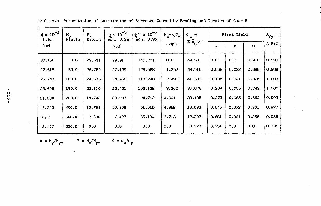
219

i

Table 8.4 Presentation of Calculation o f Stresses»Caused by Bending and Torsion o f Case B

ip x 10 f .e .

Mkip.In Mtkip.in

<J>cx 10 eqn. 8.9a

<J>c" x 10 6 eqn. 8.9b

M =<J> M z c z a =wE w <j> " n

F irst Yield ii£<

’rad’ Vad’ kip.in A B C A+B+C

30.166 0.0 29.521 29.91 141.701 0.0 49.50 0.0 0.0 0.990 0.990

27.615 50.0 26.789 27.139 128.568 1.357 44.915 0.068 0.022 0.898 0.989

25.743 100.0 24.635 24.960 118.248 2.496 41.309 0.136 0.041 0.826 1.003

23.625 150.0 22.110 22.401 106.128 3.360 37.076 0.204 0.055 0.742 1.002

21.294 200.0 19.742 20.003 94.762 4.001 33.105 0.273 0.065 0.662 0.999

13.240 400.0 10.754 10.896 51.619 4.358 18.033 0.545 0.072 0.361 0.977

10.19 500.0 7.330 7.427 35.184 3.713 12.292 0.681 0.061 0.256 0.988

3.147 630.0 0.0 0.0 0.0 0.0 0.778 0.731 0.0 0.0 0.731

A = M /My yy B = M /M z yz c = o /aw y

Table 8.5 Presentation o f Calculation o f Stresses Caused by Bending and Torsion o f Case C

IOto01

<J> x 10 f .e .

My

kip.in\kip.in

(|> x 10 ceqn. 8.9a

x 10-5

eqn. 8.9b

M = <J> M z \ y 0 wE w <f> " n

F irst Yield A_ =fy

A+B+C‘rad’ kip-in A B C

9.381 0.0 19.30 8.962 14.377 0.0 37.415 0.0 0.0 0.748 0.748

7.018 100.0 13.96 6.479 10.399 6.479 36.329 0.136 0.106 0.727 0.969

6.199 150.0 11.64 5.400 8.696 8.100 30.380 0.204 0.132 0.608 0.944

5.450 200.0 9.55 4.43 7.114 8.860 24.853 0.273 0.145 0.497 0.914

4.866 250.0 7.77 3.606 5.788 9.015 20.220 0.341 0.147 0.404 0.892

4.318 300.0 6.19 2.873 4.615 8.619 16.109 0.409 0.141 0.322 0.871

3.835 350.0 4.70 2.181 3.501 7.635 12.231 0.477 0.125 0.245 0.846

1.779 562.0 0.0 0.0 0.0 0.0 0.0 0.766 0.0 0.0 0.766

A = M /My yy B = M /M z yz C =o /ow y

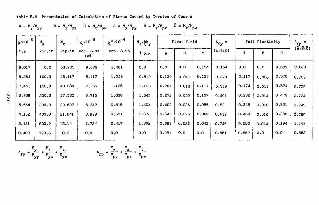
22

1-

Table 8.6 Presentation of Calculation of Stress Caused by Torsion of Case A

i

A = M /My yy

B = M /Mz yz C = M./Mt pw A = M /My py

B = M /Mz pz C = M./Mt pw

<j> xlO 3 My Mt d> xlO-3

cA"xlO-4X

M =d)M z t y F irst Yield A =fy

Full P la s tic ity A<- = fp(A+B+C)

f .e. k ip .in kip.in. eqn. 8.9a rad

eqn. 8.9bkip.in A B C (A+B+C) A B C

9.017 0.0 53.785 9.676 1.481 0.0 0.0 0.0 0.154 0.154 0.0 0.0 0.689 0.689

8.264 100.0 45.117 8.117 1.243 0.812 0.136 0.013 0.129 0.278 0.117 0.008 0.578 6.703

7.461 150.0 40.889 7.356 1.126 1.103 0.204 0.018 0.117 0.339 0.174 0.011 0.524 0.709

6.908 200.0 37.332 6.715 1.028 1.343 0.272 0.022 0.107 0.401 0.232 0.014 0.478 0.724

5.564 300.0 29.697 5.342 0.818 1.603 0.409 0.026 0.085 0.52 0.348 0.016 0.381 0.745

4.162 400.0 21.841 3.929 0.601 1.572 0.545 0.025 0.062 0.632 0.464 0.016 0.280 0.760

3.121 500.0 15.14 2.724 0.417 1.362 0.681 0.022 0.043 0.746 0.580 0.014 0.194 0.783

0.409 720.8 0.0 0.0 0.0 0.0 0.981 0.0 0.0 0.981 0.882 0.0 0.0 0.882

M M Ma - y z tfy M + M + Myy yz yw

M M M.A _ _y_ + +fp “ M M Mpy pz pw

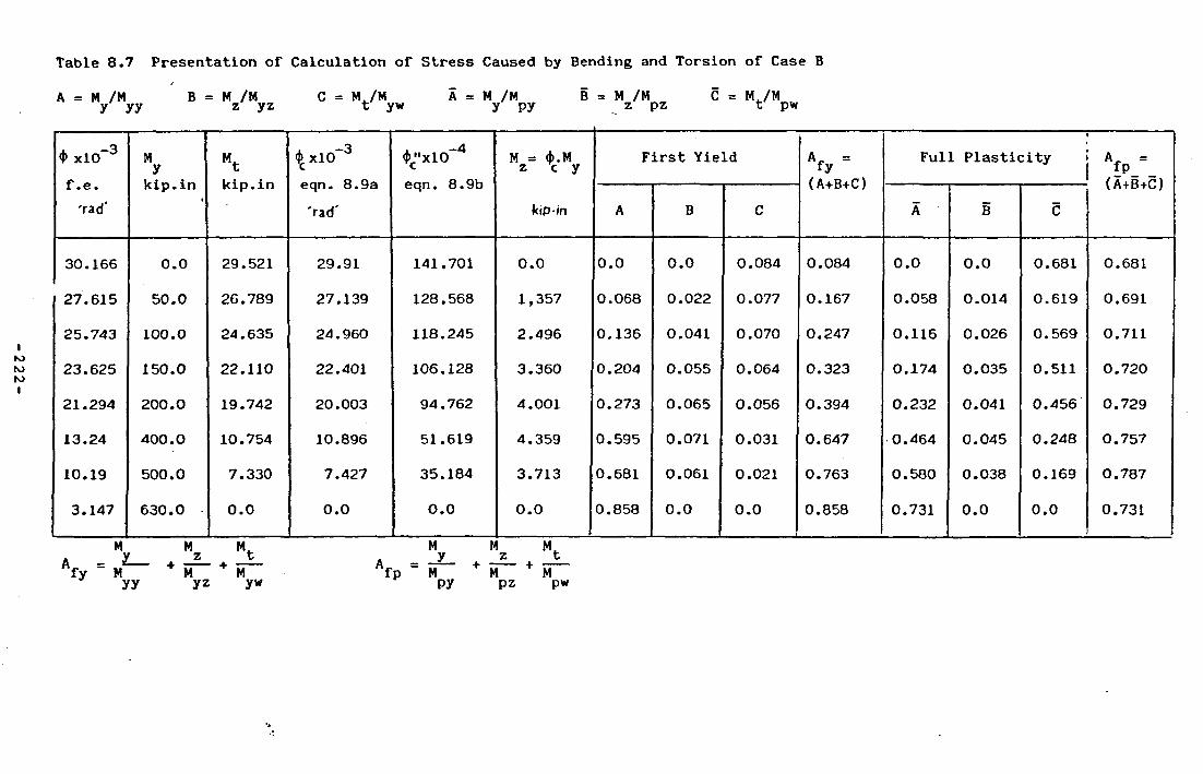
22

2

Table 8.7 Presentation o f Calculation o f Stress Caused by Bending and Torsion o f Case B

i

A = M /My yy

B = M /Mz yz C = M./Mt yw A = M /My py

B = M /Mz pz C = M/Mt pw

$ xlO-3

f .e .'rad'

My

kip.inMtkip.in

xlO-3

eqn. 8.9a

'rad'

<J>c"xl0~4

eqn. 8.9b

M = <t>.M z c y

kip-in

F irst Yield A. =fy(A+B+C)

Full P la s tic ity A =£p_ _

(A+B+C)

A B C A B C

30.166 0.0 29.521 29.91 141.701 0.0 0.0 0.0 0.084 0.084 0.0 0.0 0.681 0.681

27.615 50.0 26.789 27.139 128.568 1,357 0.068 0.022 0.077 0.167 0.058 0.014 0.619 0.691

25.743 100.0 24.635 24.960 118.245 2.496 0.136 0.041 0.070 0.247 0.116 0.026 0.569 0.711

23.625 150.0 22.110 22.401 106.128 3.360 0.204 0.055 0.064 0.323 0.174 0.035 0.511 0.720

21.294 200.0 19.742 20.003 94.762 4.001 0.273 0.065 0.056 0.394 0.232 0.041 0.456 0.729

13.24 400.0 10.754 10.896 51.619 4.359 0.595 0.071 0.031 0.647 0.464 0.045 0.248 0.757

10.19 500.0 7.330 7.427 35.184 3.713 0.681 0.061 0.021 0.763 0.580 0.038 0.169 0.787

3.147 630.0 0.0 0.0 0.0 0.0 0.858 0.0 0.0 0.858 0.731 0.0 0.0 0.731

fy

M M M,y z t

M + M + Myy yz yw

M M M.y z t

M M Mpy pz pw

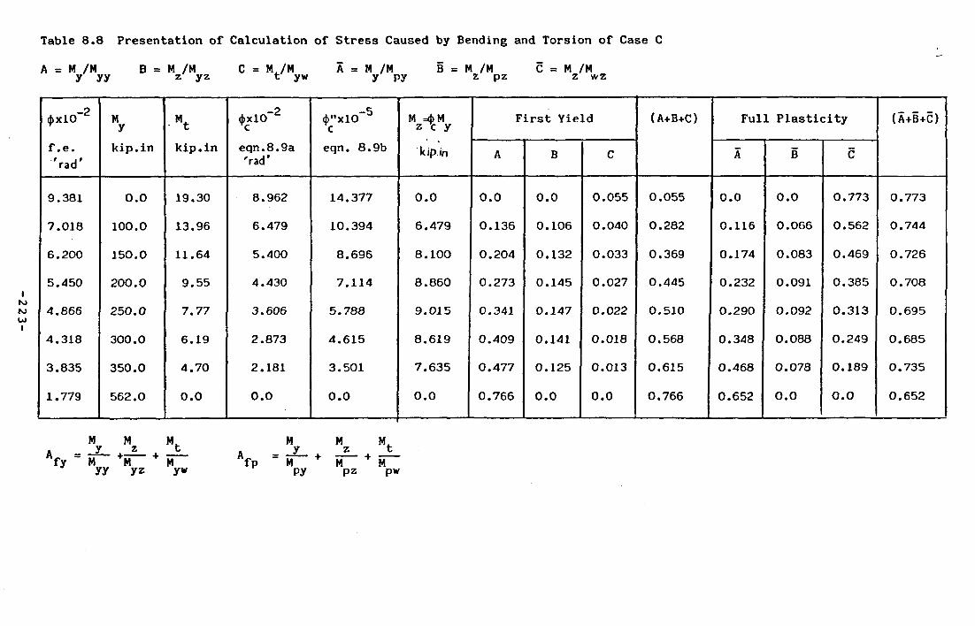
-22

3-

Table 8.8 Presentation o f Calculation o f Stress Caused by Bending and Torsion o f Case C

A = M/M B = M/M C = M/M A = M/M B = M/M C = M/My yy z yz t yw y py z pz z wz

<f>xlO~2 My 4>c*io"2 (j>"xlO-5

CM =4>M z c y F irs t Yield (A+B+C) Full P la s tic ity (A+B+C)

f .e .'rad'

kip.in kip .in eqn.8.9a'rad'

eqn. 8.9b ki pin A B C A B C

9.381 0.0 19.30 8.962 14.377 0.0 0.0 0.0 0.055 0.055 0.0 0.0 0.773 0.773

7.018 100.0 13.96 6.479 10.394 6.479 0.136 0.106 0.040 0.282 0.116 0.066 0.562 0.744

6.200 150.0 11.64 5.400 8.696 8.100 0.204 0.132 0.033 0.369 0.174 0.083 0.469 0.726

5.450 200.0 9.55 4.430 7.114 8.860 0.273 0.145 0.027 0.445 0.232 0.091 0.385 0.708

4.866 250.0 7.77 3.606 5.788 9.015 0.341 0.147 0.022 0.510 0.290 0.092 0.313 0.695

4.318 300.0 6.19 2.873 4.615 8.619 0.409 0.141 0.018 0.568 0.348 0.088 0.249 0.685

3.835 350.0 4.70 2.181 3.501 7.635 0.477 0.125 0.013 0.615 0.468 0.078 0.189 0.735

1.779 562.0 0.0 0.0 0.0 0.0 0.766 0.0 0.0 0.766 0.652 0.0 0.0 0.652

M M M, M M M._X_ Z _ t_ a _ _y_ . z tM M M Afp ■ M M + Myy yz yw py pz pw

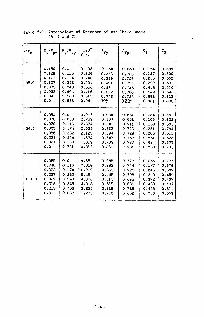
Table 8.9 Interaction o f Stresses o f the Three Cases (A, B and C)

L/rz M /M t pw M /My py

-2xlO f .e.

A_fy

>T> C1 C2

0.154 0.0 0.902 0.154 0.689 0.154 0.6890.129 0.116 0.826 0.278 0.703 0.187 0.5900.117 0.174 0.746 0.339 0.709 0.235 0.552

35.0 0.107 0.232 0.691 0.401 0.724 0.292 0.5310.085 0.348 0.556 0.42 0.745 0.418 0.5160.062 0.464 0.416 0.632 0.760 0.549 0.5420.043 0.580 0.312 0.746 0.783 0.683 0.6120.0 0.836 0.041 0981 0.881 0.981 0.882

0.084 0.0 3.017 0.084 0.681 0.084 0.6810.076 0.058 2.762 0.167 0.691 0.105 0.6220.070 0.116 2.574 0.247 0.711 0.158 0.581

64.0 0.063 0.174 2.363 0.323 0.720 0.221 0.7940.056 0.232 2.129 0.394 0.729 0.286 0.5130.031 0.464 1.324 0.647 0.757 0.551 0.5280.021 0.580 1.019 0.763 0.787 0.684 0.6050.0 0.731 0.315 0.858 0.731 0.858 0.731

0.055 0.0 9.381 0.055 0.773 0.055 0.7730.040 0.116 7.018 0.282 0.744 0.177 0.5780.033 0.174 6.200 0.369 0.726 0.245 0.5070.027 0.232 5.45 0.445 0.708 0.310 0.459

111.0 0.022 0.290 4.866 0.510 0.695 0.372 0.4370.018 0.348 4.318 0.568 0.685 0.433 0.4370.013 0.406 3.835 0.615 0.735 0.493 0.5110.0 0.652 1.779 0.766 0.652 0.766 0.652

224

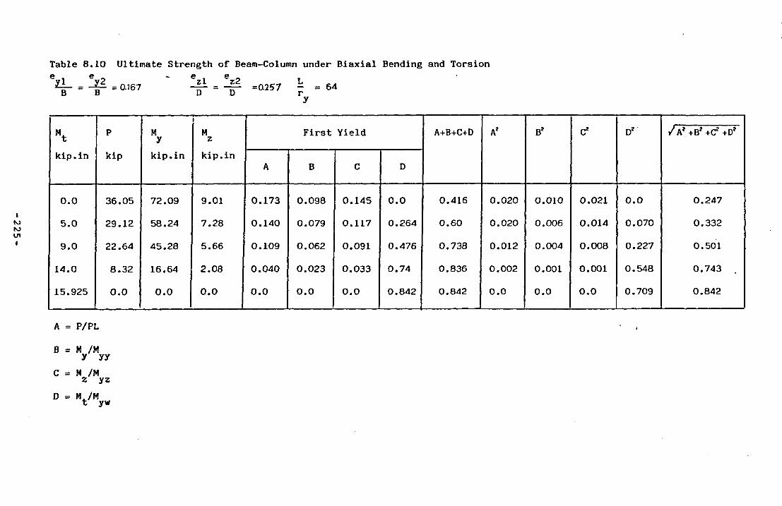
-22

5

i

Table 8.10 e , eZ l_____ i 1

B B

Ultimate Strength o f Beam-Column under Biaxial Bending and Torsion e e

= 0.167 ~ =0257 - * 64D D ry

Mt P My

Mz F irst Yield A+B+C+D A* B2 C2 D2 / A2 +B2 +C2 +D2

kip.in kip kip.in kip.inA B C D

0.0 36.05 72.09 9.01 0.173 0.098 0.145 0.0 0.416 0.020 0.010 0.021 0.0 0.247

5.0 29.12 58.24 7.28 0.140 0.079 0.117 0.264 0.60 0.020 0.006 0.014 0.070 0.332

9.0 22.64 45.28 5.66 0.109 0.062 0.091 0.476 0.738 0.012 0.004 0.008 0.227 0.501

14.0 8.32 16.64 2.08 0.040 0.023 0.033 0.74 0.836 0.002 0.001 0.001 0.548 0.743

15.925 0.0 0.0 0.0 0.0 0.0 0.0 0.842 0.842 0.0 0.0 0.0 0.709 0.842

A = P/PL

B = M /My yy

C = M /M z yz

D = M /Mt yw

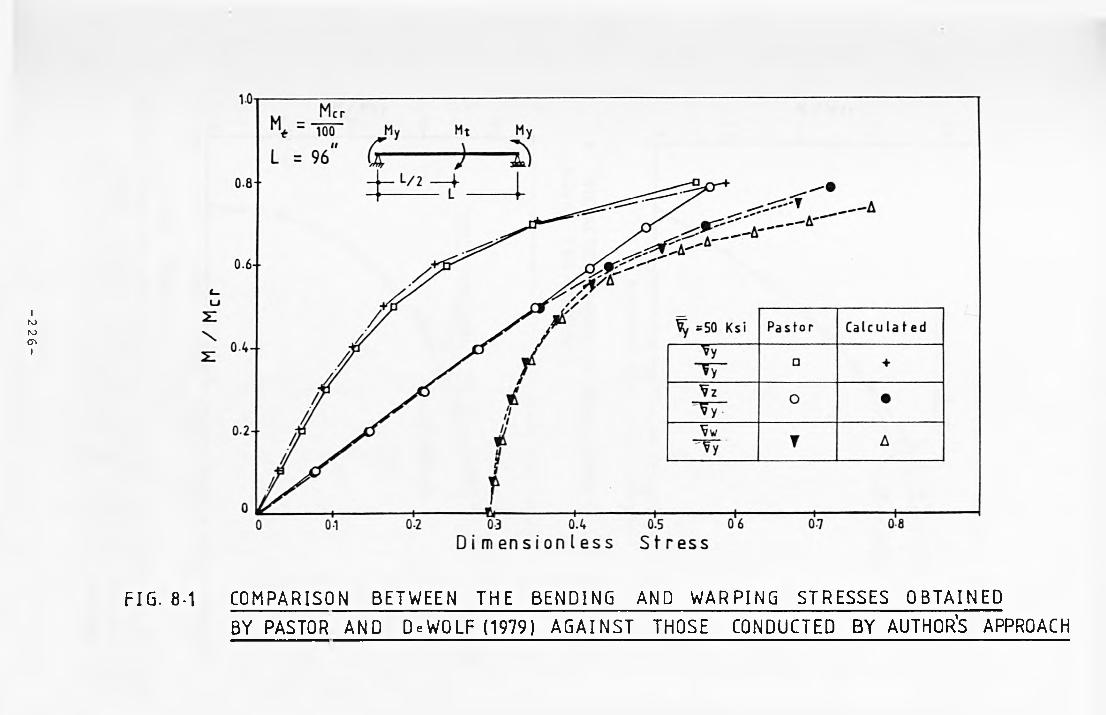
-2

26

-

COMPARISON BETWEEN THE BENDING AND WARPING STRESSES OBTAINED BY PASTOR AND DeWOLF (1979) AGAINST THOSE CONDUCTED BY AUTHOR'S APPROACH

FIG. 8-1

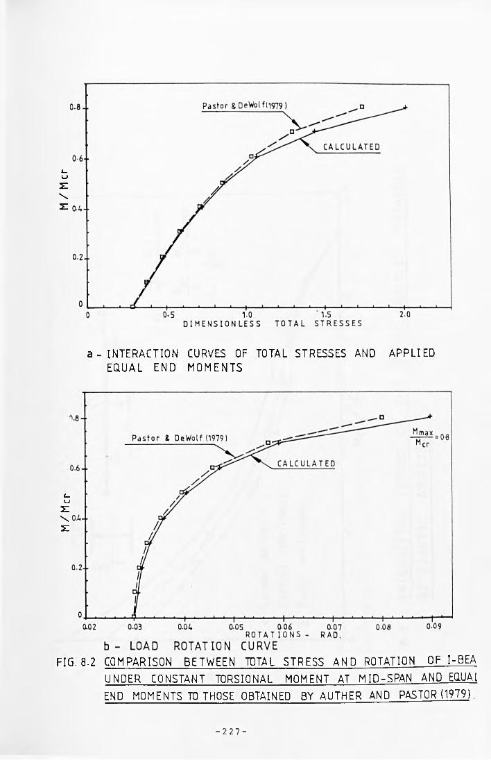
M/M

cr

M/M

cr

a - INTERACTION CURVES OF TOTAL STRESSES AND APPLIED EQUAL END MOMENTS

FIG. 8.2 COMPARISON BETWEEN TOTAL STRESS AND ROTATION OF I-BEA UNDER CONSTANT TORSIONAL MOMENT AT MID-SPAN AND EQUA1 END MOMENTS TO THOSE OBTAINED BY AUTHER AND PASTOR (1979).

- 2 2 7 -

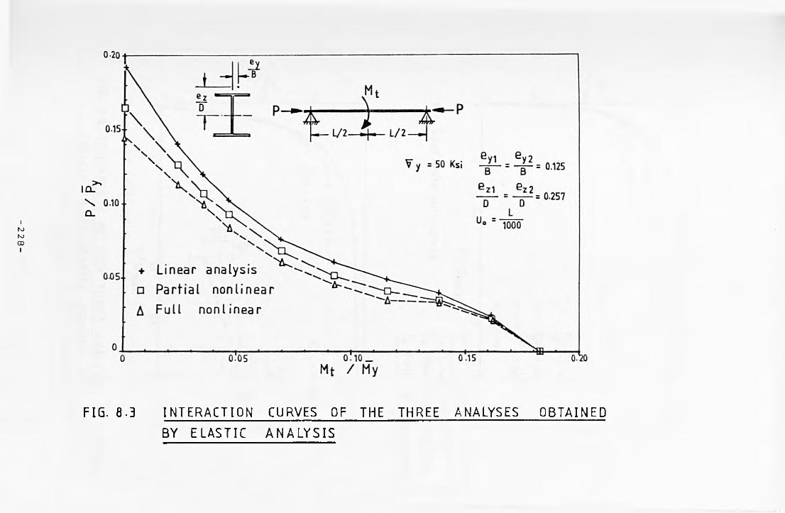
-228-

FIG. 8.3 INTERACTION CURVES OF THE THREE ANALYSES OBTAINEDBY ELASTIC ANALYSIS

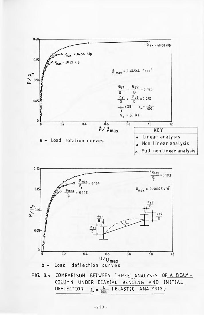
FIG. 8.4 COMPARISON BETWEEN THREE ANALYSES OF A BEAM- COLUMN UNDER BIAXIAL BENDING AND INITIAL DEFLECTION y. = -«L- ( ELASTIC ANALYSIS)

- 2 2 9 -

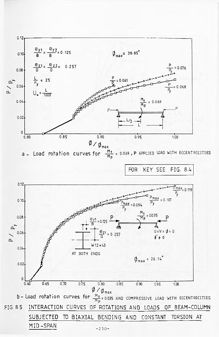
0.12-

FOR KEY SEE FIG. 8A

FIG. 8-5 INTERACTION CURVES OF ROTATIONS AND LOADS OF BEAM-COLUMN

SUBJECTED TO BIAXIAL BENDING AND CONSTANT TORSION AT MID-SPAN

- 2 3 0 -

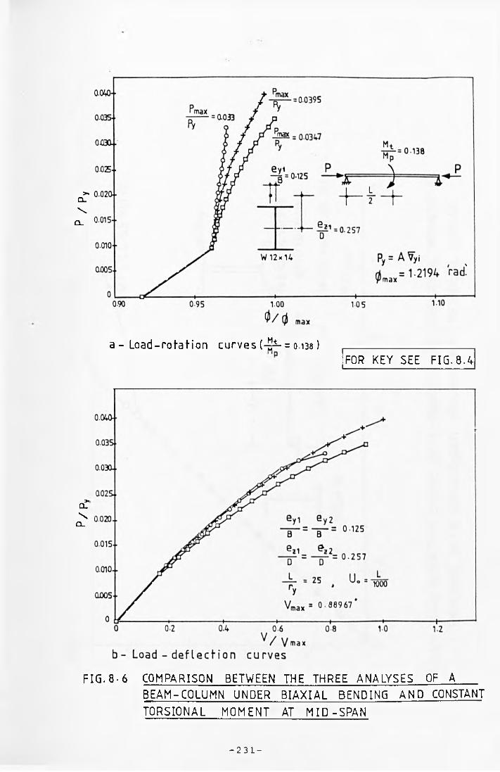
P/P

, P

/P

a - Load-rotation curves (-£*- = 0.13a)FOR KEY SEE FIG. 8.4-

FIG. 8 • 6 COMPARISON BETWEEN THE THREE ANALYSES OF ABEAM-COLUMN UNDER BIAXIAL BENDING AND CONSTANT TORSIONAL MOMENT AT MID-SPAN

- 2 3 1 -

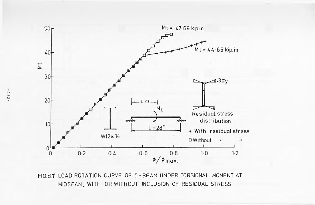
2 3

2-

FIG.8.7 LOAD ROTATION CURVE OF I-BEAM UNDER TORSIONAL MOMENT AT MIDSPAN, WITH OR WITHOUT INCLUSION OF RESIDUAL STRESS

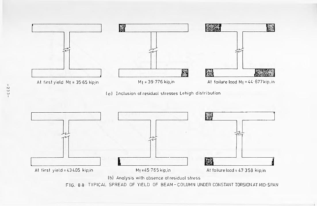
23 3

-

At first yield Mt = 35 65 kip,in Mt = 39 776 kip,in At failure load M{ = ^^ 677kip,in

(a) Inclusion of residual stresses Lehigh distribution

1At first yield = ¿3 ¿0 5 kip,in M{ =¿5-765 kip,in At failure load = ¿7-358 kip,in

(b) Analysis with absence of residual stress

FIG. 8 8 TYPICAL SPREAD OF YIELD OF BEAM -CO LU M N UNDER CONSTANT TORSION AT MID-SPAN

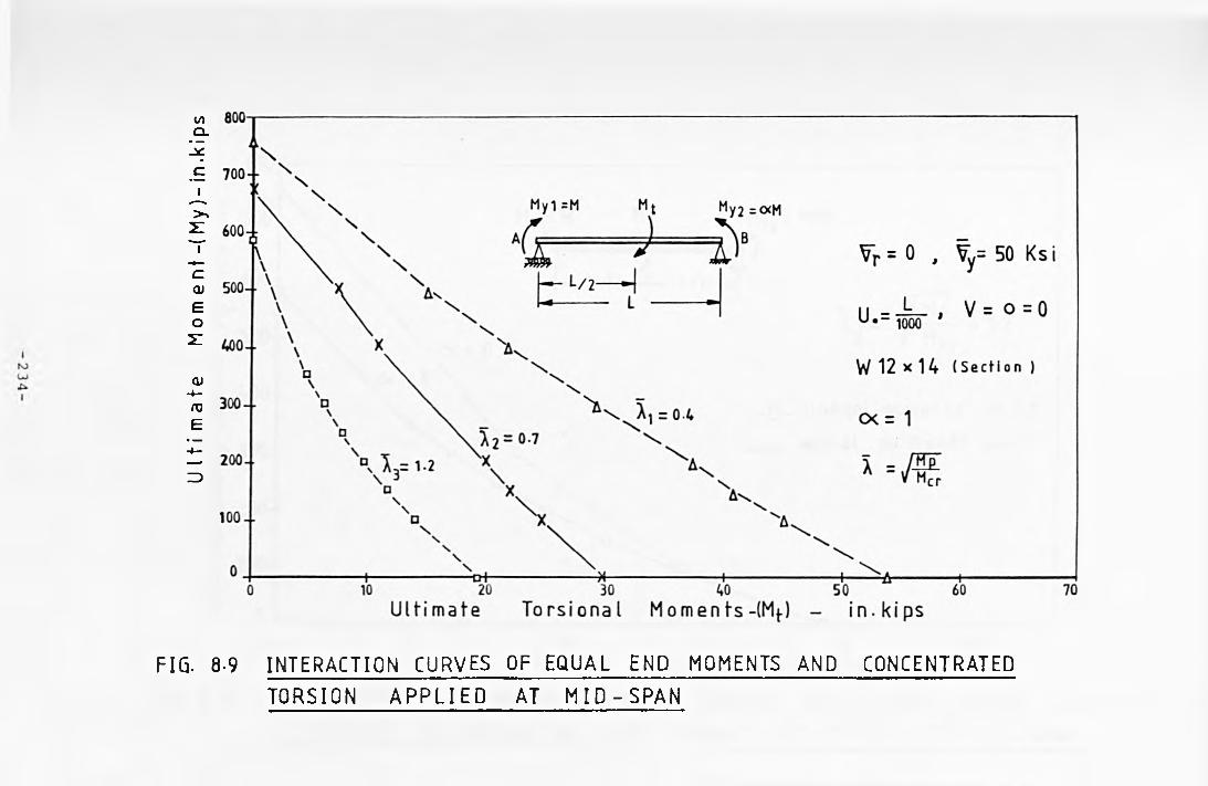
Ult

ima

te

M o

m e

nt

-(M

y)-

in.k

ips

FIG. 8-9 INTERACTION CURVES OF EQUAL END MOMENTS AND CONCENTRATED

TORSION A P P L IE D AT M I D - S P A N

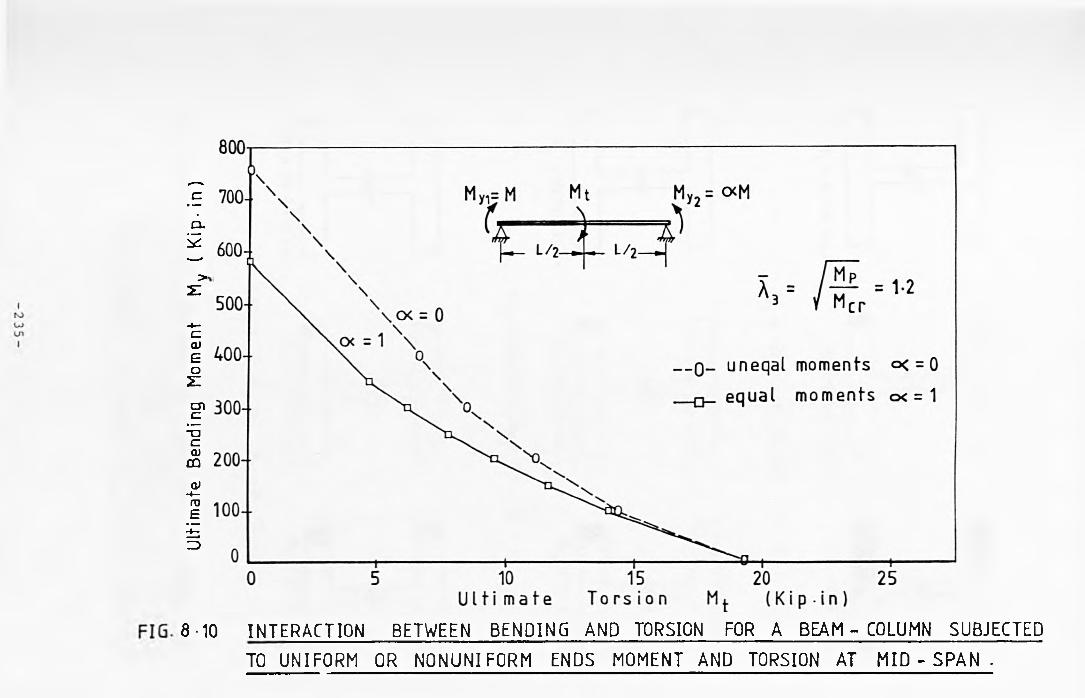
Ult

imat

e Be

ndin

g M

omen

t M

v (K

ip-i

n)

8-10 INTERACTION BETWEEN BENDING AND TORSION FOR A BEAM - COLUMN SUBJECTED

TO UNIFORM OR NONUNIFORM ENDS MOMENT AND TORSION AT MID - SPAN .

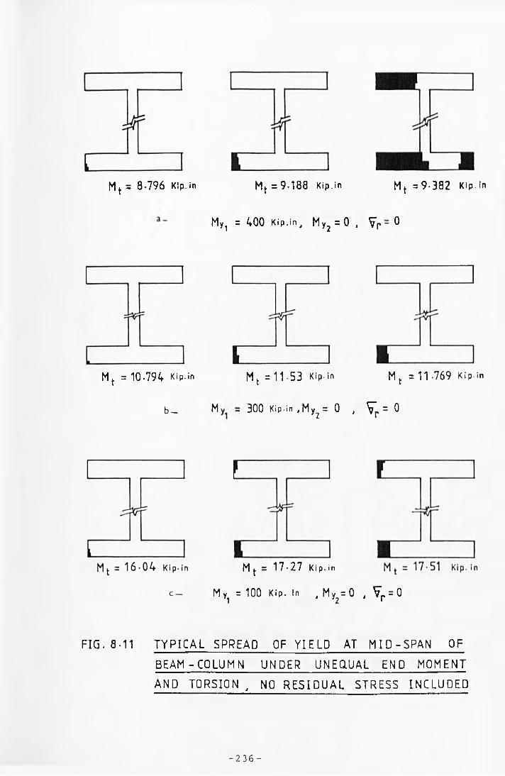
Mf = 8-796 Kip.in Mt =9-188 Kip.in Mf =9-382 K ip . in

Myi = 400 Kip.in , My2 = 0 , Vp - 0

Mt = 10-794 Kip.in M t = 1 1 - 5 3 Kip- in

b _ M — 300 Kip -in , My = 0 , V"p = 0

M t = 11-769 Kip.in

M t = 17-27 Kip. in

Myi =100 Kip. In JMy2=0 , Vp = 0

FIG. 8-11 TYPICAL SPREAD OF YIELD AT M ID-SPAN OF

BEAM -COLUMN UNDER UNEQUAL END MOMENT

AND TORSION , NO RESIDUAL STRESS INCLUDED

-2 36 -

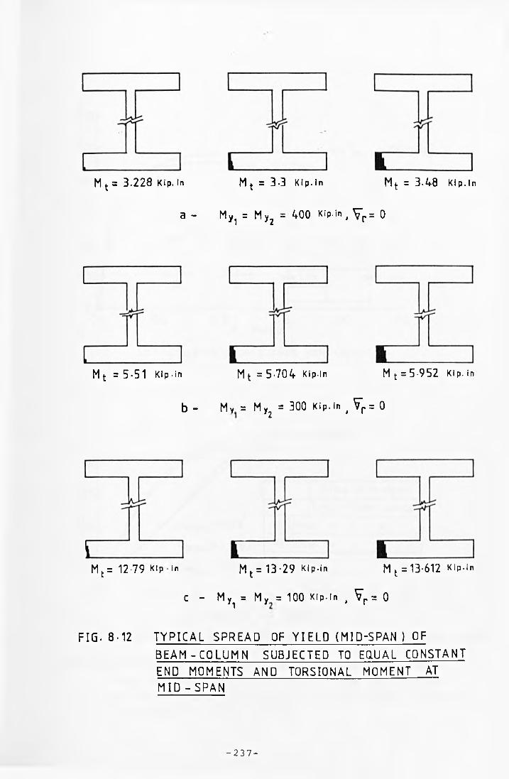
M t = 3-228 Kip.in M t = 3-3 Kip. In Mt = 3-48 Kip.In

a - MYl = My2 = 400 Kip.in , V r= 0

Mt = 5-51 Kip.in M t = 5-704 Kip.in M t = 5-952 Kip.In

b - My = My = 300 Kip. in V r = 0 ’2 ‘ 1

M t = 12-79 Kip in M t = 13-29 Kip.in M t = 13-612 Kip.in

C - M y = My = 100 Kip.in , V p = 0

FIG. 8-12 TYPICAL SPREAD OF YI ELD (MID-SPAN ) OFBEAM-COLUMN SUBJECTED TO ECLUAL CONSTANT END MOMENTS AND TORSIONAL MOMENT AT MID -SPAN

-237-

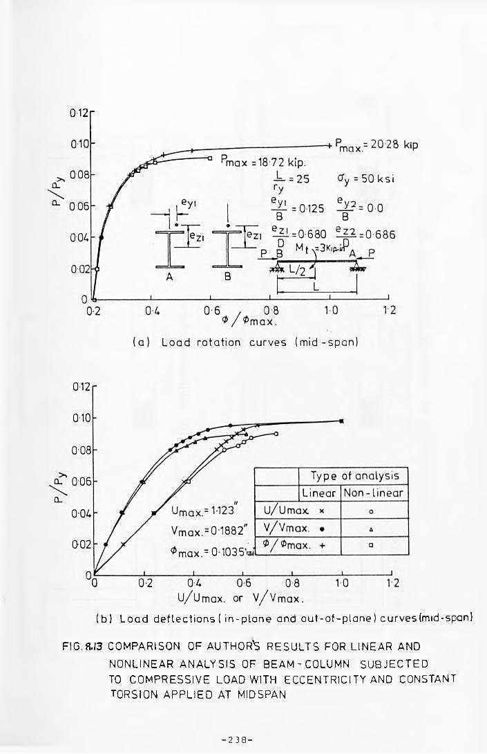
o 12 r

(b) Loa d deflections ( in -p lane and out-of-p lane) c u r v e s (mid-span)

FIG.8.13 COMPARISON OF AUTHOR'S R E S U L T S FOR L IN E A R AND

NO NLINEAR A N A L Y S IS OF B E A M -C O L U M N S U B J E C T E D

TO C O M P R E S S IV E LOAD WITH ECC EN TR IC ITY AND CONSTANT

TORSION A P P L IE D AT M IDSPAN

-2 38 -

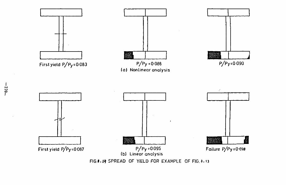
First yield P /Py = 0 083

First yield P/Py=0087

n IP/Py =0 088

(a) Nonlinear analysis

i——lt

□rP/Py=0 090

fjl . 1

P /P y=0095 Failure P/Py = 0 098(bj Linear analysis

FIG.«.!* SPREAD OF YIELD FOR EXAMPLE OF FIG. 8 . 1 3

Pmax. =22-69 kipPpnax. 2 ¿-13 kip

^max.= ^'^28

V max = 0-208

0 max.= 0-206 Tad’

Analysis typeLinear Non -linear

U/Umax. a X

V/Vmax. a ©

0/0max. • +

1-0 1-10-6 0-7 0-8 0 90/0

FIG8J5 COMPARISON BETW EEN LINEAR AND NON-LINEAR ANALYSIS OF B E A M -

COLUMN UNDER B IAX IA L BENDING ANDCONSTANT TORSION AT MIDSPAN

- 2 4 0 -

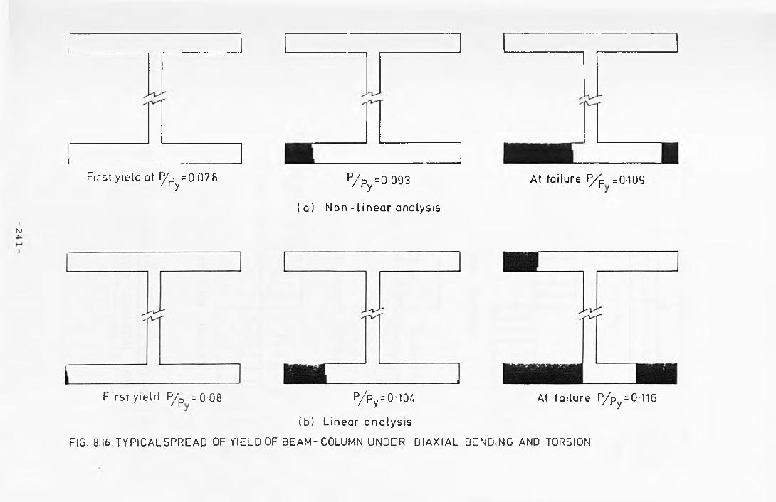
(a) Non - linear analysisI

fsj

First yield at P/ p^ 0 078 P/ Py = 0 093 At failure f^p =0-109

First yield P/p = 0-08 P/py = 0-104 At failure P/Py = 0-116

(b) Linear ana ly s is

FIG. 816 TYP ICALSPREAD OF YIELD OF BEAM-COLUMN UNDER B IAX IAL BENDING AND TORSION

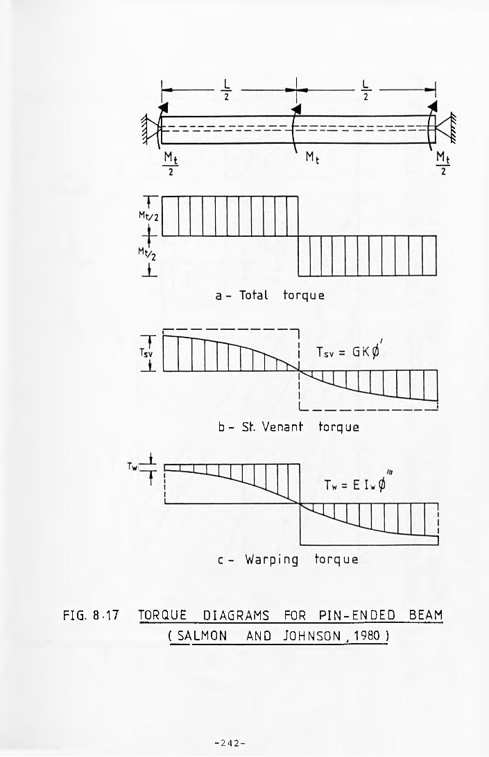
b - St. Venant torque

FIG. 8-17 TORQUE DIAGRAMS FOR P IN -ENDED BEAM

(SALMON AND JOHNSON , 1980 )

- 2 4 2 -

)>//>

/>/

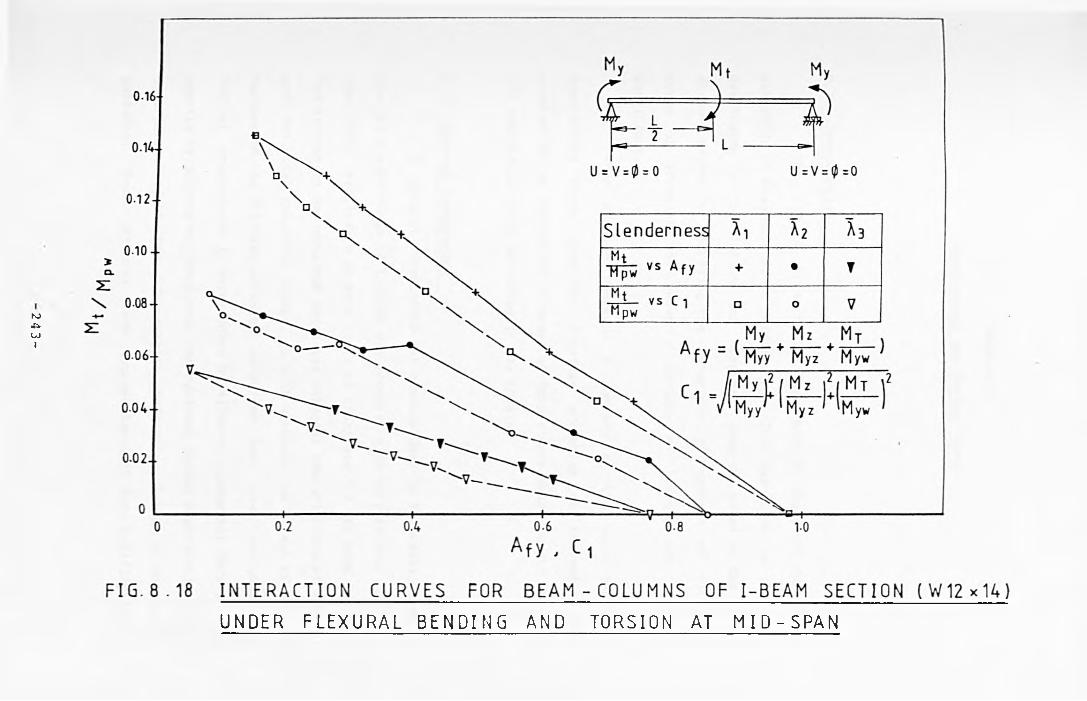
24 3

-

UNDER FLEXURAL BEND I NG AND TORSION AT M I D - S P A N

C h ap ter $

Conclusions and Further Work

9.1 Introductton

The aim o f th is thesis has been to study the fu l l range

behaviour o f beam-columns in 3-dimensions. This has been achieved by

developing a formulation and computer program based on the f in i t e

element method fo r analysing the behaviour o f members o f d if fe re n t

types o f cross-section under a va r ie ty o f loading and boundary

cond i t ions.

This chapter contains a summary o f - the more important

conclusions drawn from the findings presented at the end o f each

chapter and an indication o f areas o f future work which would augment

the ana lytica l study presented in the th es is .

9.2 General Formulation

A general formulation fo r beam-columns in 3-dimensions acted

upon by a wide range o f loading and provided with very general support

conditions app licab le to many kinds o f cross-section has been derived .

The derivation was obtained using two methods: the p rin c ip le o f v ir tu a l

work and to ta l potentia l energy. In both methods, the e f fe c t o f several

factors on the ultimate strength behaviour have been included. The

in it ia l crookedness is represented by e ith er a sinusoidal form or more

exactly by polynomial functions. The residual stress d istribu tions were

incorporated in the form o f parabolic, tr ian gu la r, Lehigh or anj o th »r

patterns. These patterns were implemented with some m odification in

- 244 -

order to s a t is fy the equilibrium conditions fo r three-dimensional

response.

The main reason fo r formulating the governing equations by

two separate methods was to provide a check on the la rge number o f

complicated terms which resulted due to coupling between the

displacements and ro ta tions.

9.3 PerlTatton o f S t if fn e s s M atrices

The element s t if fn e s s matrices and the strain-displacement

matrices fo r a beam-column o f th in-walled open cross-section in

3-dimensions were derived . The lin ea r and nonlinear tangentia l and

geometrical s t if fn e s s matrices correspond to.- an element with 14

D.O.F.(seven degrees o f freedom at each nodes a x ia l, in-plane, and out-

of-p lane displacements, three rotations about X, Y, and Z axes and

warping). The in terpolation functions employed were lin ea r polynomials

for the ax ia l displacements, cubic polynomial fo r la te ra l displacements

and tw is ts , and quadratic polynomial fo r rotations and warping.

The terms in both the lin ea r and nonlinear s t if fn e s s matrices

were calculated by two d iffe re n t methods. The f i r s t is based on the

average o f the values o f the sectoria l/ sectional properties and

internal forces fo r the two nodes, while the second uses a lin ea r

function to evaluate these values between the two nodes. The

transformation matrix fo r the element displacements with respect to

loca l coordinate and the global coordinate systems was developed in a

sophisticated yet straightforward fashion.

245

9 .U Analysis Type Options

The inclusion o f the higher terms in the formulations have

been arranged to form at le a s t three types o f analyses; 'L in ear ' uses

the lin ear tangentia l and geometrical s tiffn esses together with lin ea r

stra ins, 'Nonlinear' employs lin ea r tangentia l and geom etrical

s t iffn e ss matrices and the higher order strain-displacement

re la tionsh ips, and ' Full Nonlinear" which incorporates the

contributions o f both higher order stra in terms and nonlinear s t if fn e s s

matrices.

9.5 Pevelopeent o f Computer Program (TDCP)

A three dimensional computer program (TDCP) which implements

the formulation has been developed. TDCP is based on f in i t e element

techniques and is w ritten in the Fortran 77 Language. The program

contains many subroutines, the functions o f which can be summarized as:

1- Calculating the sectional and sec to r ia l properties in the

e la s tic and in e la s tic ranges fo r complex cross-sections.

2- Calculating the internal strains and stress resu ltan ts.

3- Controlling convergence to the correct resu lt based on the

incremental displacements and out-of-balance forces .

4- Tracing the fu l l load -de flec tion response and loss o f

s t if fn e s s due to y ie ld spread.

9.6 Comparison with Previous Work

The v a l id it y and v e r s a t i l i t y o f both the rigorous formulation

and TDCP have been tested against previously obtained experimental and

th eoretica l resu lts . Several examples covering flexu re , f le x u ra l-

torsional action , b ia x ia l bending, and bending and torsion have been

- 246 -

checked in the e la s t ic and in e la s tic ranges. They contain a wide range

o f parameters e .g . d if fe r e n t types o f cross-section , loading, boundary

conditions and in i t ia l geometrical im perfections. In a l l eases

excellen t agreement has been achieved when some lim ita tion s were

imposed on the present formulation in order to match the more

restric ted approaches used elsewhere.

9.7 U ltim ate Strength Behaviour o f Meibers under Bending and Torsion

Prelim inary resu lts from a new in vestiga tion o f the ultim ate

strength behaviour o f beam-columns subjected to b ia x ia l bending and

torsion have been reported, problems in which d ire c t tors iona l loading

is present have received l i t t l e attention previously.

Several problems o f bending and torsion have been solved . The

solutions were obtained by three types o f analyses; ’ L inear’ ,

’ Nonlinear’ , and Full Nonlinear. The resu lts show the s ign ifican ce o f

the inclusion o f the so ca lled ’ higher order terms' in the s tra in -

displacement re la tion s and the nonlinear geometrical and tangential

s t iffn e ss matrices in the analysis.

Several important observations are possib le:

1- The a b i l i t y o f the formulation presented to cover the fu l l range

o f analysis o f beam-columns in 3-dimensions.

2- The need to include higher order terms in the s tra in -

displacement re la tion s and s t if fn e s s matrices in order to avoid

overestimates o f load carrying capacity .

3- This analysis represents a powerful too l fo r the further study

o f problems in each o f the classes previously id en tified .

- 247 -

9.8 Future Work

The work undertaken in th is thesis has established a general

formulation and a program TDCP which can be used fo r determining the

ultimate strength o f beam-columns. This work can be ea s ily extended to

incorporate many aspects such as:

1- Semi-Rigid Connections

This work is now under investiga tion and the prelim inary

resu lts are encouraging (Wang et a l . 1987).

2- Other types o f material such as Aluminium can be included. In

such case the ch aracter is tic o f the m aterial is nonlinear; th is

extension is also in progress.

3- Analysis o f Frames in Three-dimensions; with r ig id and semi­

r ig id connections

M- Considerations o f requirements fo r members deforming in space to

permit more ra tiona l strength/ s t if fn e s s requirements to be

determined.

- 248 -

References

1. Abedel-Sayed, G. and Aglan, A.A. 0 9 7 3 ). " In e la s t ic Lateral

Torsional Buckling o f Beam-Columns", Publications, IABSE, Vol. 23-

I I , pp. 1-16.

2. A nslijn , R. 0 983), "Tests on Steel 1-Beam-Columns Subjected to

Thrust and B iaxia l Bending", Report MT 157, Centre de Recherches

Sc ien tifiqu es et Techniques de L 'in du strie des Fabrications

M etalliques, Bruxelles, August.

3. Anderson, J.M., and Trahair, N .S ., 0 9 7 2 ), "S ta b il ity o f

Monosymmetric Beams and C an tilevers ," Journal o f the Structural

d iv is ion , ASCE, Vol. 98, No. ST1, Proc. Paper 88U6, Jan. pp. 269-

286.

4. Attard, M.M., 0 985) "Latera l Buckling Analysis o f Beams by the

FEM", Computer and Structures Vol. 23, No. 2, Pergamon Press Ltd.

Printed in U.K., A p r il.

5. Attard, M.M. (1986), "Nonlinear Theory o f Non-uniform Torsion o f

Thin-Walled Beams", International Journal o f Thin-Walled

Structures, Vol. 4, No. 2, pp. 101-13*1.

6. Barsoum, R .S ., and Gaullgher, R.H. 0 9 7 0 ), "F in ite Element

Analysis o f Torsional and Tors iona l-flexu ra l S ta b ility Problems",

In ternational Journal o f Numerical Method in Engineering, Vol. 2,

No. 1, pp. 335-352.

7. Bathe, K. J ., and Wilson, E. L . , 0 976), "Numerical Methods in

F in ite Element Analysis", P rentice-H all, In c ., Englewood C l i f f s ,

New Jersey.

8. Bergan, G.P. and Clough, W.R., 0 9 7 2 ), "Convergence C rite r ia for

- 249 -

I te ra t iv e Processes", AIAA Journal, Vol. 10, No. 8, pp. 1107-1108.

9. B irn s tie l, C. (1968), "Experiments on H-Columns under B iaxia l

Bending", Journal o f the Structural D ivision , ASCE, Vol. 94, No.

ST 10, Proc. Paper 6186, O ct., pp. 2429-2449.

10. Black, M.M., (1967a) "Nonlinear Behaviour o f Thin-Walled

Unsymmetrical Beam-Sections Subjected to Bending and Torsion", In.

Thin-Walled Structures, Chatto and Winds, London.

11. Black, M.M. (1967b), "Nonlinear Behaviour o f Thin-Walled

Unsymmetrical Beam-Sections Subjected to Bending and Torsion",

Thin-Walled Structures a C ollection o f Papers on the S ta b ility and

Strength o f Thin- a iled Structural Members and Frames, Chalto &

Windus Ltd ., London, U.K.

12. B leich, F. (1933), "Stahlhochbouten", Vol. I I , Julius Springer,

Berlin , P. 925.

13. Bleich, F. and B leich, H. (1936), "Bending Torsion and Buckling o f

Bars Composed o f Thin-Walls", Preliminary Publication, 2nd

Congress, IABSE, English ed ition , B erlin , P. 871.

14. Bleich, F ., (1952), "Bucking Strength o f Metal Structures ,"

McGraw-Hill Book Co. In c ., N6w YORK, N.Y.

15. Boresi,P. and Lynn, P .P ., (1974), "E la s t ic ity in Engineering

Mechanics", Pren tice-H all, In c ., Englewood C l i f f s , New Jersey,

USA.

16. Brown, T.G., (1981) " la te ra l Torsional Buckling o f Tapered

I-beams," J. o f the Strutrural d iv is ion , ASCE, Vol. 107, No. ST4,

Proc. Paper 16211, A p r il, pp. 689-697.

17. Cescotto, S .,G ilson , S., Plumir, A ., and Rondal, J. (1983), "

Etudedeu Du Fiambement Plan De Poutres Colonnes en Aciek a Section

Nonsymetrique", J. o f CRSTIFM, MT153, Bruxelles, May.

- 250 -

18. Chaudhary, A.B., (1982), "Generalized S tiffn ess Matrix fo r Thin

Walled Beams " , Journal o f the Strutural D ivision , ASCE, VOL. 108,

No. ST3, Proc. Paper 16938 , March.

19. Chan, S.L. and K itipornchai, S. (1986), "Geometric Nonlinear Thin-

Walled Members", Research Report No. CE67» Dept. C iv il Eng. Univ.

o f Queensland Austra lia , July.

20. Chen, W.F., (1977), "Theory o f Beam-Columns - The S ta te-o f-A rt

Review", Proceedings, In ternational Colloquium on S ta b ility o f

Structures Under S ta tic and Dynamic Loads", SSRC/ ASCE, Washington

D.C., March 17-19» pp. 631-648.

21. Chen, W.F., (1979), "In fluence o f End-Restrained Column

S ta b ility " , C iv il Engineering, Report No. CE - STr - 79-2, Purdue

U niversity, West La fayette , In c ., August, (P rep rin t, ASCE Atlanta

Convention, Oct., 22-26,1979).

22. Chen, W.F., (1981), "Recent Advances on Analysis and Design o f

s tee l Beam-Columns in USA", In e la s tic In s ta b ility o f S teel

Strutrures and Strustural Elements, U. S. Japan, Seminar, Tokyo,

edited by Fu jita , Y. and Galambos, T .V ., pp. 224-292.

23. Chen, W.F. and Atsuta, T. (1976), "Theory o f Beam-Columns- Volume

I : "In-Plane Behaviour and Design", McGraw-Hill, N.Y.

24. Chen, W.F., and Atsusta ,T. (1977), "Theory o f Beam-Column",

Volume 2 Space Behaviour and Design", Me Graw-hill, N.Y.

25. Chen, W.F. and Cheong-Siat-Moy, F. (1980), "L im it States Design o f

Steel Beam-Columns - A s ta te -o f-A rt Review", Journal o f Solid

Mechanics Archives, Noordhoff, Leyden, The Netherlands, March.

26. Chen, A.M. and Santathadaporn, S. (1968), "Review o f Column

Behaviour under B iaxial Loading", Journal o f the Structural

D ivision , ASCE, Proc. Paper 6316, Voi. 94, No ST12, Dec., pp.

- 251

2999-3017.

27. Chu, K. and Johnston R.B (1971), "Torsion in Beams with Open

Sections", Journal o f the Structural D ivision , ASCE, Vol. 105, No.

St 11, pp. 2163-2185.

28. Clark, J.W. and H i l l , H.N. (1960), "La tera l Buckling o f Beams",

Journal o f the Structural D ivis ion , ASCE, Vol. 86, No. ST7, Proc.

Paper 2559, July, pp. 175-196.

29. C r is f ie ld , (1981), "A Fast Incremental/ I t e r a t iv e Solution

Procedure that Handless Snap-Through", Journal o f Computer &

Structures, Vol. 13, Pergamon Press L td ., U.K., pp. 55-65.

30. Cuk, P.E ., (1984), "F lexural-Torsional Buckling in Frame

S tructu tres", Phd Thesis Submitted fo r F u llfillm en t o f Degree o f

Doctor o f Philosophy, University o f Syedney, School o f C iv i l and

Mining Engineering, Sydney, Feb.

31. Culver, C.G. (1966a), "Exact Solution o f The B iax ia lly Bending

Equations", Journal o f the Structural D ivis ion , ASCE, Vol. 92, No.

ST2, Proc. Paper 4772, A p ril, pp. 63-83.

32. Culver. C.G (1966b), " In i t ia l Imperfection in B iaxial Bending",

Journal o f the Structural D ivision , ASCE, Vol. 92, NO. ST3, Proc.

Paper 4846, June, pp. 119-135.

33. Dinno.K.S. and Merchant, W. (1965), " A Procedure fo r Calculating

the P lastic Collapse o f I-Sections under Bending and Torsion", The

Structural Engineer, Vol. 43, No. 7, pp. 219-221.

34. Draper and Smith (1967), "Applied Regression Techniques", John

Wily and Son 2nd, Ed., London.

35. Dux ,P .F ., and Kitipornchai, B.E. (1983)» " Ine lastic Beam Buckling

Experiments", Journal of Constructional steel Research, Vol. 3»

No. 1, pp. 3-9.

- 252

36. El-Khenfas, M.A., (1987a), "TDFE-Computer Program fo r Analysis o f

Beams in Space in the E lastic and In e la s tic Ranges", Report, No.

1CE, C iv il and Structural Engineering Department, S h e ffie ld

University.

37. El-Khenfas, M.A., (1987b), "E la s tic Analysis o f Beam-Columns in

Space", Report, No. 2CE, C iv il and Structural Engineering

department, S h e ffie ld U n iversity .

38. El-Khenfas, M.A., (1987c), " In e la s t ic Analysis o f Beam-Column in

3-Dimensions", Report, No. 3CE, C iv il and Structural Engineering

Department, S h effie ld U n iversity.

39. El-Khenfas, M.A., and Nethercot, D .A., (1987a), " A General

Formulation for Three Dimensional Analysis o f Beam-columns",

(submitted fo r pu b lica tion ).

40. El-Khenfas, M.A. and Nethercot, D.A., (1987b), "E la s tic Analysis

o f Beam-Columns in Space", (submitted fo r pu b lica tion ).

41. El-Khenfas, M.A. and Nethercot, D.A., (1987c)"Inelastic Analysis

o f Beam-Columns in Space", (submitted fo r pub lica tion ).

42. Epstein, M. and Murray, D.W., (1976), "Three Dimensional Large

Deformation Analysis o f Thin-Walled Beams", In t. Journal o f Solids

Structures, Vol. 12 ,Pregamon Press, Printed in U. K.

43. Epstein, M. , Nixon, D., and Murray, D. W., (1978), "Large

Displacements In e la s tic Analysis o f Beam-Columns", Journal o f the

Strutural d iv is ion , ASCE, Vol 104, No. ST5, Proc. Paper 13768,

May, pp. 841-853.

44. Erwin, K. (1976), "Advanced Engineering Mathemathics", John Wiley

& Sons, F ifth Edition, N.Y. (Printed in USA).

45. Fu jita ,Y and Yoshida, K. (1972), "Compressive Strength o f Columns

with In i t ia l D eflections", International Colloquium on Columns

- 253 -

Strength, Paris, France, 23-24, November, pp. 108- 120.

46. Fukumoto, Y. and Kubo, M., (1977)» "An Experimental Review o f

Lateral Buckling o f Beams and G irders", Proceeding o f the

In ternational Colloquium on S ta b ility o f Structure under S ta tic

and Dynamic Loads, SSRC- ASCE, Washington, D.C., Macrh, pp. 541-

562.47. Fukumoto, Y ., Kubo, M. and Yokoyama, A ., (1971)» " In e la s t ic

Lateral Buckling Strength o f Monosymmetric I-Beams", P rep rin t,,

Annual Meeting o f JSCE, October, (in Japanese), pp. 161-162.

48. Fukumoto, Y. and Nishida ,S ., (1981), "Ultimate Load Behaviour o f

Curved I-bearas", Journal o f Engineerimg Mechanics D ivision , ASCE

, Vol. 107, A p r il, pp. 367-385.

49. Galambos, T .V ., (1963) " In e la s t ic Buckling o f Beams", Journal o f

the Structural Duvision, Vol. 89, No. ST5, ASCE, Proc. Paper 3683,

Oct., pp. 217-292.

50. Galambos, T .V ., (1968), "Structural Members and Frames", P ren tice-

Hall In c ., England C l i f f s , New Jersey.

51. Goodier, J.N ., (1942), "Torsional and Flexural Buckling o f Bars o f

Thin Walled Open Section Under Compressive and Bending Loads",

Journal o f AppliedMechanics, Transactions, ASME, Vol. 64, Sept.,

pp. A-103.

52. Goodier, J .N ., (1956),"F lexural-Torsional Buckling o f Bars o f Open

-Section Under Compressive and Bending Loads", Journal o f Applied

Mechanics, Transaction, ASCE, Vol. 64, Sept.

53. Hancock, K.J. (1983), "The Behaviour and Design Cold Formed

Channels in Compression", Journal o f the Australian Instute o f

te e l construction, Vol. 17 No. 3, A tiss in 004-2205.

54. Hancock, G.J. and Trahair. N. S .(1978), "F in ite Element Analysis

- 254 -

o f the Lateral Buckling o f Continously Restrained Beam-Column",

C iv il Engineering Transactions, In titu tion o f Engineers,

Austra lia , Vol. 20 ,No. 2, pp. 120-127.

55. Hancock, G.J. and Trahair, N .S .0 979), "La tera l Buckling o f Roof

Purlins with Diaphram R estra in ts", C iv il Engineering Transaction

In stitu tion o f Engineerrs, Austra lia , Vol. CE21, No. 1, pp. 10-15.

56. Hasegawa, A ., Liyanage, K ., Ikeda, T ., and Nishino, F. (1985), "A

Concise and E xp lic it Formulation o f Out-Of-Plane In s ta b ility o f

Thin-Walled Members", Proc. o f Japan Society o f C iv il Engineers,

Div. o f Structural Engineering/ Earthquake Engineering, Vol. 2,

No. 1, A p r il, pp.. 81-89.

57. Heins, C.P. and Seaburg, P.A. (1963), " Torsional Analysis o f

Rolled Steel Sections", Bethlehem Steel Corporation, Bethlehem,

Pennsylivania.

58. H i l l , H.N. and Clark, J.W. (1951a), "La tera l Buckling o f

Eccentrica lly Loaded I-Section Columns", Transaction, ASCE, Vol.

116, pp. 1179-1191.

59. H il l , H.N. and Clark, J.W. (1951b), "La tera l Buckling o f

E ccen trica lly Loaded I and H-Sections columns " , Proceedings ,1st

U.S, National Congress o f Applied Mechanics, pp. 407-413.

60. Horne , M .R.,( 1954), "The Flexural-Torsion Buckling o f Members o f

Symmetrical I-S ect ion Under Combined Thrust and Unequal Terminal

Moments",Quarterly Journal o f Mechanics and Applined Mathematics,

Vol. 7, Part 4, pp. 410-426.

61. Johnston , B.G., (1941), "La tera l Buckling o f I-Section Columns

with Eccentric End Loads in the Plane o f the Web", Transactions,

ASME, Vol. 63 .P.A-176.

62. Johnston, B.G. (e d . ) , (1976), "Guide to Design C rite r ia fo r

- 255 -

Structures", 3rd. edn., Strutural S ta b ility Research Council, John

Wiley and Sons, In c ., New Yourk, N .Y., 1976.

63. Johnston, B.G., (1982), " Design o f W-shapes fo r Combined Bending

and Torsion", Engineering Journal o f the AISC, Vol. 19, 2nd

quarter, pp. 65-85.

64. Johnston, B.G., Lin, F ., and Galambos, T.V. (1980), "Basic S teel

Design", P r in tice -H a ll, Englewood C l i f f s , New Jersy.

65. Kappus, R. (1937), "D rillhnicken Zentrisch Gedruckter Stabe mit

offenem P r o f i le in Elastischen Bereich"»Luftfahrt-Forschung, Vol.

14, No. 9, Translated in NACA Technical Memoir No. 851, 1938.

66. Kanok-Nukulchai, W. Hasegawa, A. and Nishino, F. (1986), "Generic

Formulation Procedure fo r Large Deformation Analysis o f Structural

Elements", Structural Eng./ Earthquake Eng., Proc. JSCE, No. 368/

1-5, Vol. 3., No. 1, A p r il, pp. 65-73.

67. Kennedy, J.B. and Madugula, M.K.S., (1982), "Buckling o f Angles:

State o f A rte", Journal o f the Structural D iv., ASCE, Proc. Paper

17323, Vol. 108, No. ST9, Sept., pp. 1967-1980.

68. Kennedy. J.B. and Murty, M.K.S., (1972), "Buckling o f S teel Angle

and Tee S tru ts", Journal o f the Strutural D iv., ACSE, Proc. Paper

9348, Vol. 98, No. St1, November, pp. 2507-2521.

69. Kerensky, A .O ., F lin t , A.R., and Brown, W.C. (1956), "The Basis

for Design o f Beams and P late Girders in the Revised B ritish

Standard 153", Proceedings, ICE, Part 3, Vol. 5, Aug. pp. 396-444.

70. K itipornchai, S. and Chan, S .L ., (1987), "Non-Linear F in ite

ELement Analysis o f Angles and Tee Beam-Columns", Journal o f the

Structural Engineering, ASCE, Vol. 113, No. 4, Proc. Paper 21416,

A p r il, 1987., pp. 721-739.

71. K itipornchai, S ., E.,and Lee, H.W.,(1984), " In e la s t ic Buckling o f

- 256 -

Singe Angle, Tee, and Double Angle S tru ts", Research Report No.

CE55, Univ. o f Queensland, C iv il Engineering Dept.,Sept.

72. K itipornchai, B., E. ,and Lee, H.W. (1986a) , " In e la s t ic Buckling

o f Singe Angle, Tee, and Double Angle S trc t ." , Journal o f

Constructional SteeL Reseach, June, pp. 1-18.

73. K itipornchai, S. and Lee, H.W., (1986b )»"In e lastic Experiments on

Angles and Tee Struts, Double-Angle S tru ts", Journal o f

Constructional S teel Research,6, pp. 219-235.

74. K itipornchi, S. and Trahair, N .S., (1975), " In e la s t ic Buckling o f

Simply Supported Steel I-Beams", Journal o f the Structural

Engineering, ASCE Vol. 101, No. ST7, Proc. Paper. 11419, July. pp.

133-1347.

75. K itipornch i, S. and Trahair, N .S., (1980), "Buckling Problems o f

Monosymmetric I-Beams " , Journal o f the Structural D ivision , Vol.

106, NO.ST5, ASCE, Proc. Paper No. 15406, May.

76. K itipornchi, S. and Wang-Chung, M. (1985), "S ta b il ity o f

Monosymmetric C an tilevers", Research Report, Department o f C iv il

Engineering, University o f Queensland, No. C65, Dec.

77. K itipornchai, S.E, Wang, C.M, and Trahair, N.S. (1985), "Buckling

o f Monosymmetric I-Beams under Moment Gradient", University o f

Queensland, Dept, o f C iv il Engineering, Research Report No. CE67,

October.

78. Kollbrunner, C .F., Hajdin, N., and B ran islavc,C ., (1978),

"E la s t ic -P la s t ic Thin-Walled I-sec tion Beam Subjected to Bending

and Warping Torsion ," In s titu te for Engineering Research, Report

43, Zurich, May.

79. Kollbrunner, C .F., Hajdin, N ., and Obradovic, P, (1979), "E la s t ic -

P lastic Fixed Ended Beams o f I-S ect ion Subjected to Bending and

- 257 -

Warping Torsion ", In s titu te fo r Engineering Research, Report 46,

Zurich, December.

80. Lay, M.G. and Ward, R.F. (1969), "Residual stresses in Steel

Structures", Australian In s titu te o f Steel Construction, Vol. 3,

pp. 2-21.

81. Lee, G.C. and Galambos, T.V. (1962), "The Post-Buckling Strength

o f Wide-Flange Beams", Journal o f the Engineering Mechanics

D ivision , ASCE, Vol. 88, No. EM1, Proc. Paper 3059, Feb., pp. 59-

75.

82. Lindner, J . , (1972), "Theoretica l Investigation o f Columns under

Biaxial Bending", IABSE - CRC - ECCS, Colloquium on Column

Strength, November.

83. Lindner, J ., (1981), "BIEGEDRILLKNICKEN HOCHFESTER STAHLE",

Technische U niversität B erlin , In s titu t fur Baukoustruktionen und

F estigk e it, Bericht Nr. VR 2025, Sept.

84. Love, A.E.H., (1944), "A trea tise on the Mathematical Theory o f

T la s t ic ty " , 4th ed. Dover Publications, New York.

85. Massonnet, C ., (1947) "Le Flamblage des Barres a Section Ouverte

et a Parios Minces ” , Hommage Fac. SCI .Appl. a L ' Assoc, des

Ingeniews Sortis de L ’ Ecole de Liege »L iege , pp. 35-146.

86. Massonet, C.E. (1976) »"Forty Years o f Research on Beam-Columns in

Steel ",SM Archives, Vol. 1, Issue 1, Noordhoff In ternational -

leyden, pp. 27-157.

87. Matthey, P. (1984), "Simulation Numérique du Comportement des

Poutres-Columnnes M étalliques", Rapport ICOM137, Ecole

Polytechnique Federal de Lausanne, Department de Genie C iv i l ,

November.

88. Medwodowski, S .J . , (1985), "Warping Moment D istribu tion ", J. o f the

- 258 -

Struc. Eng., Vol. 111, No. 2, ASCE, Proc. Paper No. 19507,

Februray.

89. Moore , D.B, (1986) "A Nonlinear Theory fo r the Behaviour o f Thin-

Walled Sections Subjected to Combined Bending and Torsion",

Journal od Thin-Walled Strudtures, Vol. 4, No. 6, U.K., pp. 449-

466.

90. NaKasheima, M., Nakumura, T. and Wakabayashi, M., (1983), "P os t-

Buckling In s ta b ility o f Steel Beam-Columns", Journal o f the

Structural D ivision , ASCE, Vol. 109, No. ST6, Proc. Paper 18068,

pp. 1414-1430.

91. Nethercot, D.A. (1972), "The E ffec t o f Load Position on the

Lateral S ta b ility o f Beams", Proceedings, Conference on F in ite

Element Methods in C iv il Engineering In s titu te o f Canada,

Monteral, June, p. 347.

92. Nethercot, D.A. (1973a), " In e la s t ic Buckling o f Monosymmetric

I-Beams", Journal o f the Structural D ivision , ASCE, Vol. 99, No.

ST 7, Technical Note, July, pp. 1696-1701.

93. Nethercot, D.A. (1973b), "The Solution o f the In e la s tic Latera l

S ta b ility Problems by F in ite Element Methods", Proceedings , 4th

Australian Conference on Mechanics o f Structures and M aterials,

Brisbane, Austra lia , pp. 183-190.

94. Nethercot, D.A., (1974), "Residual Stresses and Their In fluence

Upon the Lateral Buckling o f Rolled Steel Beams", The Structural

• Engineer, Vol. 52, No. 3, March, pp. 89-96.

95. Nethercot, D.A. (1983), "Evaluation o f In teraction fo r use in

Design Spec ifica tion in Western Europe", Proceedings 3rd.

International Colloquiuri on S ta b ility o f Metal Structures, Canada,

pp. 293-314.

- 259 -

96. Nethercot, D .A., (1986), "La tera l Buckling", 2nd Regional

Colloquium on S ta b ility o f Steel Structures, Hungary, Sept. 25-26,

pp. 99-117.

97. Nethercot, D.A. and Rockey, K.C. (1971), "F in ite Element Solution

fo r the Buckling o f Columns and Beams", In ternational Journal o f

Mechanical Sciences, Voi. 13, pp. 9^5—949.

98. Nethercot. D.A. and Trahair, N .S., (1983), "Design o f L a tte ra lly

unspported Beams", Beams and Beam-Columns, S ta b ility and Strength,

edited by R. Narayanan, Applied Science Publishers, London, pp.

71-94.

99. N e v ille , A.M. and Kennedy, J .B .0 964), "Basic S ta t is t ic a l Methods

for Engineers and S c ien tis ts ", Scranton, International Textbook

Co., London, U.K.

100. Nishida, S. and Fukumoto , Y . , (1985), "U ltim ate load Behaviour o f

Beams with In i t ia l Im perfection", Journal o f Structural

Engineering, ASCE, Voi. 111, No. 6, Proc. Paper 19811, June, pp.

1288-1305.

101. Nylander, H. (1949), "Torsional and Lateral Buckling o f

Eccentrica lly Compressed I and T columns", Transactions, Royal

In s titu te o f Technology, Stockholm, Sweden.

102. O'Connor, C. (1964), "The Buckling o f A Monosynmetric Beam Loaded

in the Plane o f Symmetry", Australian Journal o f Applied Science,

East Melbourne, Australia , Voi. 15, No. 4, Dec., pp 191-203.

103. Ohga, M. and Hara,T. (1986) ."Analysis o f Thin-Walled Members by

F in ite Element-Transfer Matrix Method," Structural Engineering/

Earthquake Eng. Voi. 3, No. 1, Japan Society o f C iv il Eng., Proc.

o f JSCE No. 368/ 1-5 .A p r il.

104. Opperman, G. H. P , , (1983) "Refined Beam-Column Analysis",

- 260 -

Proceedings, 3rd. In ternational Colloquium on S ta b ility o f Metal

Structures, Paris, Nov, pp. 39-47.

105. Pastor, P.T. and DeWolf, T.J, (1979), "Beams with Torsional and

Flexural Loads", Journal o f the Structural D ivis ion , ASCE, Vol.

105, No. ST 3» Proc. paper 14461, March, pp. 527-535.

106. Peano and R iccion i, R. (1978), "Automated Q iscerisa tion Error

Control in F in ite Element Ana lysis in the Corarical Environment",

Edited by J. Robinson, Robinson & Verwood, England, pp. 368-387.

107. Pekoz, T. and Winter, G. (1966), "Torsional Flexural Buckling o f

Thin-Walled Open Sections under Eccentric Axial Loading", Paper

Submitted to ASCE Annual Meetimg and Trans-porttation Engineering

Conference, Philadelphi, Pennsylvania.

108. Petterrsson, 0. (1952), "Combined Bending and Torsion o f I-Beams

o f Monosyirmetical Cross-section", Bu lletin No. 10, D ivision o f

Building S tatics and Structural Engineering, Royal In s titu te o f

Technology, Stockholm.

109. Premieniecki, J.S. (1968), "Theory o f Matrix Structural Analysis",

McGraw-Hill, N.Y.

110. Sakimoto, T . , Yamo, T . , Kikuchi, R. and Sakata, T . , (1985),

"Nonlinear Analysis o f Thin-Walled Frames and Members with

A rb itrary Open Cross-Section", Structural Engineering/ Earthquake

Engineering, Vol. 2, No. 2, PP 139-147.

111. Salmon, C.G. and Johnson, J.E ., (1980), "S tee l Structures" 2nd

ed ition , Harper and Row, Publishers, N.Y. 946 p.

112. Salvadorl, M.G., (1955), "La tera l Buckling o f I-Beams",

Transaction ASCE, Vol. 120, Paper 2773.

113. Salvador!, M.G., (1956), "La tera l Buckling o f E ccen trica lly Loaded

I-Columns", Transactions, ASCE, Vol. 121, Paper 2836, pp. 1163—

- 261

1178

114. S o lt is , A.L. and Christiano, P. (1972), "F in ite Deformation o f

B iax ia lly Loaded Columns", Journal o f the Structural D ivis ion ,

ASCE, Proc. Paper 9407, Vol. 98, No. ST12, Dec., pp. 2647-2661.

115. "S tee l Structures for Buildings", CSA Standard S16, Canadian

Standards Association, Rexdale, Ontario, Canada, 1969«

116. "S pec ifica tion fo r the Design, and Fabrication and Erection o f

Strutural S te l l fo r Build ings", American In s titu te o f Steel

Constrction, New Yourk, N. Y ., 1969.

117. Sourchnikoff, B. (1951), "Strength o f I-Beams in Combined Bending

and Torsion", ASCE, Transactions, Vol. 116, pp. 1319-1342.L

118. Syal, C .I. and Sharma, S .S ., (1971), "B ia x ia lly Loaded Beam-Column

Analysis", Journal o f the Structural D ivision , ASCE, Proc. paper.

8384, Vol. 97., No. ST 9, Sept., pp. 2245-2259.

119. Rajasekaran , S. (1971) »"F in ite Element Analysis o f Thin Walled

Members o f Open Sections," Structural Engineering Report No.34,

Department o f C iv il Engineering »U n iversity o f Alberta Edmonton,

A lberta, Canada, Sept.

120. Rajasekaran, S. and Murray ,D.W. (1973), "F in ite Element Solution

o f In e la ss tic Beam Equations", Journal o f the Structural Divison,

ASCE, Vol. 99, No. ST6, Proc. paper 9773, June, pp. 1024-1042.

121. Ramm, E. and O sterrieder, P. (1983), "U ltim ate Load Analysis o f

Three- Dimensional Beam Structures with Thin-Walled Cross-Section

Using F in ite Elements", S ta b ility o f Metal Structures, Paris 16-17

Nov., primaray report.

122. Rao, S .S ., (1982), "The F in ite Element Method in Engineering",

Pergamon Press Ltd. U.K.

123. Razzaq, Z. (1974), "Theoretica l and Experimental Study o f

- 262 -

B iax ia lly Loaded Thin-Walled Beams o f Open Section with and

without Torsion", A D issertation Presented to the Sever In s itu te

o f Wasington Univ. In pa rtia l F u llfillraen t o f D. Sc..

124. Razzaq, Z. and Galambos, T.V. (1979), " B iaxia l Bending Tests with

or without Torsion", Journal o f the Structural D ivis ion , ASCE,

Vol. 105, No. St 11, pp. 2163-2185.

125. Richards, T.H. (1977), "Energy Methods in Stress Analysis", E l l is

Horwood lim ited , c o l l House, Westergate, Chichester, Sussex,

England.

126. Roberts, T.M. (1981), "Second Order Strains and In s ta b lity o f Thin

-Walled Bars o f Open Cross-Section", In t. Journal Mech, Sciences,

Vol. 23, pp 297-306.

127. Roberts, T.M., and Azizian , Z .G ., (1983a), "Nonlinear Analysis o f

Thin-Walled Bars", International Journal o f Mechanical Sciences,

Vol. 25, No. 8, pp. 543-612.

128. Roberts, T.M. and Azizian , Z.G., (1983b), "In fluence o f Pre-

Buckling Displacements on the E lastic C r it ic a l Loads o f Thin-

Walled Bars o f Open C ross-section", In ternational Journal o f

Mechanical Sciences, Vol. 25, No. 2, pp. 93-104.

129. Tebedge, N. and T a ll, L. (1973), "L inear S ta b ility Analysis o f

Beam-Columns", Journal o f the Structural D ivision , ASCE, Vol. 99,

No. ST 12, Proc. paper 10232, Dec., pp. 2439-2457.

130. Tezcan, S.S. and Mahapatra, B.C., (1969), "Tangent S tiffn ess

Matrix fo r Space Frame Mebers", Journal o f the Structural

D ivision , ASCE, Vol. 95, No. ST6, Proc. Paper. 6627, pp. 1257-

1270.

131. Terrington, J .S ., (1968) »"Comined Bending and Torsion o f Beams",

BCSA Publication No. 31, (F ir s t pa rt).

- 263 -

132. Terrington, J .S ., (1970), "Corained Bending and Torsion o f Beams",

BCSA Publication No. 31» ( Second part ) .

133. Thomas, F .B ., Lehigh, and Lay, G.M., (1972), "The Behaviour o f

La tera lly Unsupported Angles", The In stitu tion o f Engineers, C iv i l

Engineering Transaction, Austra lia , pp. 103-110.

134. Timoshenko, S.P. (1910), "E in ige S ta b ilita ts - Probleme der

E la s t ic ita ts Theories", Z e it s c r i f t fur Mathematic und Physik, Vol.

58, pp. 337-385,. Also in "C o llected papers o f Stephen P.

Timoshenko", McGraw-Hill, N.Y. 1953.

135. Timoshenko, S ., (1945), "Theory o f Bending o f Torsion and Buckling

o f Thin Walled o f Open Cross Section ," Journal »Franklin In s t .,

Philadelphia, March, A p r il, May.

136. Timoshenko, S.P. (1983). "H istory o f Strength o f M ateria ls", Dover

Publications, New York. , 452 p.

137. Timoshenko, S.P. and Gere, J.M. (1961), "Theory o f E lastic

S ta b ility " , 2nd ed., McGraw-Hill, New York.

138. Trahair, N .S ., (1961), "The Ultimate Load Carrying Capacity o f

Slender Stanchions Bent About the Major Axis", Proceedings, ICE,

Vol. 19. August, pp. 479-507.

139. Trahair, N .S., (1966), "E la s tic S ta b ility o f I-Beam Elements in

Rigid Jointed Structures", Journal o f the In s titu tion o f

Engineers, Austra lia , Vol. 38, No. 7-8, July- Aug., pp. 171-180.

140. Trahair, N.S., (1969), "Restrained E lastic Beam-Column", Journal

o f Structural D ivis ion , ASCE, Vol. 95, No. ST 12,7Dec., pp. 2641-

2664.

141. Trahair, S.N. and K itipornchai, S. (1972), "Buckling o f In e la s tio

I-beams under Uniform Moment", Journal o f the Structural D ivis ion ,

ASCE, Vol. 98, No. ST11, Proc. Paper 9339, November, pp. 2551-

- 264 -

2565

142. Vinnakota, N. S. (1977a), " In e la s t ic S ta b i l i ty o f La tera lly

Unsupported I-Beams", Computer and Structures, Vol. 7, No. 3,

June, pp. 377-389.

143. Vinnakota , S ., (1977b), "F in ite Difference Method for P las t ic

Beam-Column", Theory o f Beam Column in Space Behaviour and Design,

Theory o f Beam-Columns,Vol. 2, Chap. 10, W.F., Chen and T .,Atsuta.

eds, McGraw-hill, N .Y ..

144. Vlasov, V. Z ., (1961), "Thin Walled E lastic Beams", 2nd Ed.,

National Science Foundation Washington, D.C.

145. Ugural, A.C. and Fensher, S.K., (1979), "Advanced Strength and

Applied E la s t ic i ty " , E lsevier North Holland Publishing Co., New

York, 433. pp.

146. Wagner, H. (1929), "Verarehung und Knickung von offenen P ro f i len " ,

25th. Anniversary Publication, Technische Hochschule, Danzig,

1904-1929. Translated in N.A.C.A., Technical Memoir, No. 807,

1936.

147. Wang, Y .C ., El-Khenfas, M.A., And Nethercot, D.A. (1987),

"La te ra l- Torsional Buckling o f Ren-Restrained Beams", Journal o f

Construction Steel Research, ( in press).

148. Warnick, W.L. and Walston, W.H. Jr. (1980), "Secondary Deflections

and Lateral S ta b i l i ty o f Beams", Journal o f the Engineering

Mechanics Division, Proceedings o f the American Society o f C iv i l

Engineering, Vol. 106, No. EM6, Proc. paper 15927» December, pp.

1307 -1325.

149. Weaver, W., J r ., (1967), " Computer Programs fo r Structural

Analysis", D. Van Nostrand Company, In c ., Canada.

150. Wekezer, J.W., (1985), "Nonlinear Torsion o f Thin-walled Bars o f

- 265 -

Variable Cross-section " , In t . J. Mech., Sci Vol. 27» No. 10,

Printed in Great Brita in , pp. 631-641.

151. W ilhoite, G., Zandonini, R ., and Zavelalani, A. (1984a), "Behavior

and Strength o f Angkes in Can press ion: An Experimental '

Inevestiga tion ", ASCE Annuaal Convention and Structures Congress,

San Franc is ico , U.S.f October.

152. W ilhoite, G ., Zandonini, R ., and Zavelalani, A. (1984b), n

Behavior and Strength o f T-Shapes in Compression: An Experimental

Inevestiga tion ", ASCE Annuaal Convention and Structures Congress,

San Francisico, U.S., October.

153. Winter, G., (1941), "Latera l S ta b i l i ty o f Unsymmetrical I-Beams

and Trusses in bending", Proceedings, ASCE, Vol. 67, No. 10, Dec.,

pp 1851-1864.

154. Yang Y.B., and Me Guire, W., (1986), "S t i f fn ess Matrix fo r

Geometric Nonlinear Analysis", Journal o f Structural Engineering,

ASCE, Vol. 112, No. 4, Proc. Paper No. 20561, Apr il , pp. 853-877.

155. Young, B.W., (1975) " Residual Stress in Hot-Rolled Section",

Proceedings, International Colloquium on Column Strength, IABSE,

Vol. 23, pp. 25-38.

156. Young, B. W., (1971), " Residual Stresses in Hot-rolled Sections",

Department o f Engineering, University o f Cambridge, CUED/C-Struct.

/TR. 8.

157. Yoshida, H. and Maegawa, K ., (1984), "Latera l In s ta b i l i t y o f

I-Beams with Imperfections", Journal o f Structural Engineering,

Vol. 110, No. 8, ASCE, Proc. Paper 19073, August.

158. Zbirohowski-koscia, K.(1967) , " Thin Walled Beams from Theory to

Practice ", Crosby Lockwood & Son LTD, U. K.

159. Zienkiewciez, 0. C. (1977) ," The f in i t e Element Method " , Third

Ed., McGraw-Hill Book Company, U. K.

- 266 -

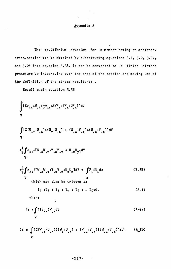
Appendix A

The equilibrium equation for a member having an arb itrary

cross-section can be obtained by substituting equations 3. 1 . 3. 2, 3. 2U,

and 3.25 into equation 3.38. I t can be converted to a f in i t e element

procedure by in tegrating over the area o f the section and making use o f

the de fin it ion o f the stress resultants .

Recall again equation 3.38

V

V

(3.38)

V swhich can also be written asI I +1? + I 3 + Ii* + I 5 + - I 6 s0 ( A-1 )

where

(A -2a)

V

-267-

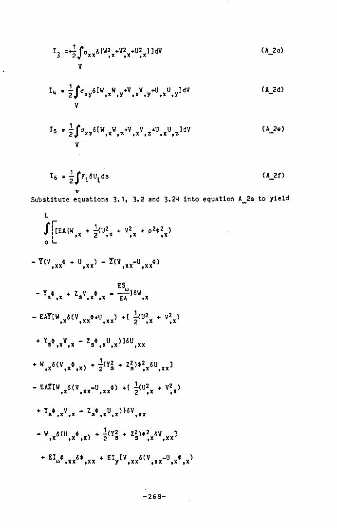
(A 2c)h 4 / ' I x x « (W U?x” dV

! 5 = ¿ / ° x z SIW,x \ z * ' ' , x V,z *U,xU. z ldV

Fi 6Ui ds

Substitute equations 3.1$ 3.2 and 3.24 into equation A_2a

L

/ ' i [EAtw,x + 2 (U% + V-x + P2®2Y>

- Y (V ,xx* + U ,xx> “ Z (V ,xx-Uf xx4)

ES- Y * + Z V * - — }6Ws ,x s ,x ,x ea tX

- EA7[W 5(V *+U ) + { ^(U2 + V2 )9x fXX txx 2 9x

* V , x \ x - z s \ x U.x ,15U.xx

* W.x{ <V. x * , x ) * ? ( i I * Zl > » i,x5U,xx1

- E#rt>' . , S<V,xx-', ,xx»> ♦< 5 <u% * V%>

Y * V - z * U ) } 6 VS ,X , X S ,X , x " ,XXW 6 (u * v ♦ - ( Y 2 + Z 2 ) * 2 5 V ]

,x ,x ,x) 2 s s ,x f xx

+ E l * 5* + E l [V 6 ( V -U * )o> ,xx ,xx yL ,xx ,xx ,x ,x

(A_2d)

(A_2e)

(A_2 f )

to y ie ld

-268-

s(u,xxv ,xx»)- V ? x i V ,xx3E l [U 6(U +V ♦ ) - 6(U V « ) - Y * 2 6U ]z ,xx ,xx ,x ,x ,xx ,xx s ,x ,xx

+EI [ 5 ( U V - U *U + V *V ) yz ,xx ,xx ,xx ,xx ,xx ,xx

♦ V « ( * V ) ,xx ,x ,x

U 6 ( * U ) - i 2 ( Z 6U + Y 6V ) ] ,xx ,x ,x ,x s ,xx s ,xx

E I |IVC 6 { * YY (V * + U ) } wy fXx 9 x x f x x

$ vV - Y * 2 6$ ,XX]f A A I a A 9 f A

* EI»xt s l l >xx(v, x x - u ,xx* )1- * »»«<« »u »> - Z .« 2v 5»,x x ]

f X A 9 X 9 X 5 9 X

- K » ™ . X * i tui . * v%> * V . x \ x - V ' xU,x

♦ ¿ ( Y | + z | ) ] « * f xx

♦HM* 2Y5* yy +H 6( i 2 U yy) + H 6(*2 V YY) + * s* Yjdx a) 9x 9xx y fx fxx z 9x 9xx 9x 9xj

where

P2 . ( Y - Y s ) 2 +CZ-Zg ) 2

Hy s | / Y (Y 2 + z 2 )d A

Hz s j / z ( Y 2+Z2 )d A

(A 3)

(A Ha)

( A Mb)

( A He)

-269-

H = - J Yo)(Y2+Z2)dA y 2 J

A(A Hd)

which may be written as:

I 2 = J Gk$ x6*,xdx (A 5)

K= J [CZ-Zo)2+ (Y-Yd) 2-2(Y-Y ▼ s s>3a>

s 3Z

-2(Z-Z s 3y 3y 3z(AJ )

in which K has been defined (Love 191*1* and Nishida 4 Fukumoto 1985) as

the torsional r i g id i t y

1I 3 = f F Y[U y6U ¥+V 6V + p 2$ 69

J A f A | A | A | A | X | A

0

1

+ f [Z _ 6 {* v ( *V v+U j ) - v (V v -U v * > ^ dXJ 9 f A 9 A | X 9 | X | X | X

0

1“ f[M v6{ * Y(V Y*+U v ) } +M 6{ i (V -*U ) }]dxJ y . X ,x ,x z ,x ,x ,x

(A 7)

In the same manner Ii* + I 5 can be written as

1I«*+l5» fQvC6{V *-w v (V i+U v )]dx

J J f A 9 X | X f A

fQj6(U *+W v (V V+*U ) }dx]dxJ 1 t * f * » A 9 X

-270-

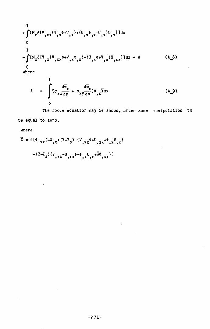
(A 8)

♦ frMf iCV (V * +U W(U * -U V)U } ]dxI A f A A | A f A | A I A I A I X

0

1„ (V „„$+V „* J + (U „$+V JU „ J ]d x ♦ AX ,X ,XX ,X ,X ,X , X ,xx

0where

id to du)

[a — - + o — ]* xzdy xy dy • :

Xdx (A 9)The above equation may be shown, a fte r some manipulation to

be equal to zero,

where

J S fit* (-W + (Y-Y ) {V $+U +$ V },xx ,x s ,xx ,xx ,x ,x

+ (Z -ZJ {V -U * - * U +uTi } ] s ,xx ,xx ,x ,x ,xx

- 2 7 1 -

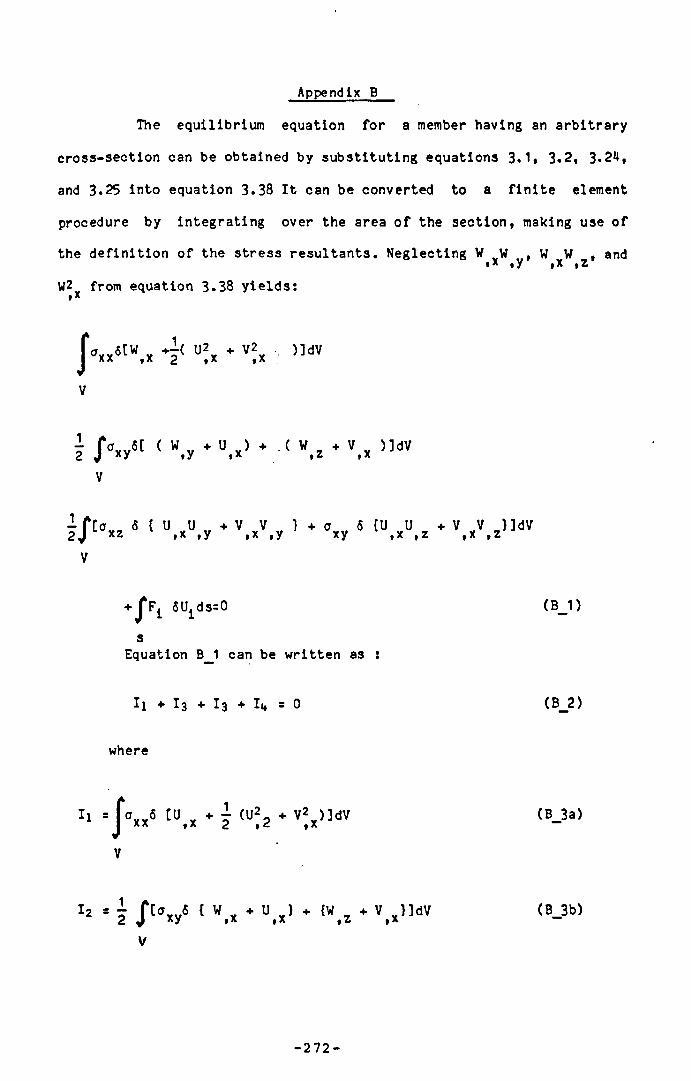
Appendix B

The equilibrium equation fo r a member having an arb itrary

cross-section can be obtained by substituting equations 3. 1 » 3. 2 , 3*24,

and 3.25 into equation 3.38 I t can be converted to a f in i t e element

procedure by integrating over the area o f the section, making use o f

the de fin it ion o f the stress resu ltants. Neglecting W W , W W , and* * #y tX , z

Vf2 from equation 3.38 y ie ld s :• X

v

v

V

(B 1)

sEquation B 1 can be written as

II ♦ I 3 + I 3 + It* = 0 (B 2)

where

(B 3a)

V

(B 3b)

V

-272-

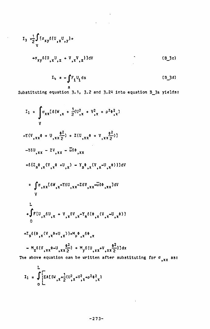
(B 30

I r—J r 0 6 {U U } +3 2*' xy ,x ,y

+( TX V 6 { U v U , + V v V z ” d v *y t x tz tx fZ

- - J V i ds (B 3d)

Substituting equation 3.1. 3.2 and 3*24 in to equation B__3a y ie ld s :

= i 0” ...... >x 2 " ’ x " * x ' ' >xI I s |cwv[ 6{W „ + ^(U2„ + V2„ + p2#2„ )

V

-i ( V ,xx* * U,xxT> * Z<U.xx* * v , x x f >]-Y5U - ZV - 0)5#,xx ,xx ,xx

+5{Z * y (V y4> +U v ) - Y # v (V -U # ) }]dV3 f a 9 X 9 X 8 | X | X | X

fa yy [ 6W -Y6U -Z5V yy-u)5* yy]dVA f X X f X X f X X f X X

+ JF[U X5U + V 5V -Y 5{# (V y-U * ) }T * a f X 9 X | X S 9X | X f x+Z 5 {* (V y#+U ) }+M # 6# wS » X | X #X P f X 9X- M 5{V #-U — ) + M 5{U +V — )]dx

z ,xx ,xx 2 y ,xx , x x 2 iJ

The above equation can be written a fte r substituting for a „ „ as:f X XL

I I = /¡EA[{W y-4(U2y+V2y+p2*2 > i . * 2 »x »* »x

0 L.

-273-

- E A i (V , x x » * U, x x , * EAZ(U. x x * - V , x x )

- Ys“ \ x V,x * Z5* , xU,x- EV , x1sW,x

- t E i 7 « x 4 (U? * * V% ) - V , x V V , x U. x ” 5 U ,x x

- [EAl,W,X<i <Uix*V% ) ‘ V , X V,X*ZX*,XU,Xn ! V IXX

- ‘ EV ^ x 4 ' U% * Vy - V , x v ,x *Z2t .xU,x , I5 \ x x

* E I z< V , x x * * U . x x > SU, x x * E I y ' U, x x ‘ * V . x x , 5 V . x x

+EI * S* + El { * 6U + (V *+U ) 6* }w ,xx ,xx uy ,xx ,xx ,xx ,xx' ,xx+ El {$ 5V +(U *+V )$* }OJZ1 ,xx ,xx ,xx ,xx ,xx

-E l [{U $-V }5U - {V *+U }5V ]yz f xx ,xxJ ,xx ,xx ,xx' ,xxJ

.[EAHy+EA|(Z| * i I > - i sEIz -ZsEIy I ]*Zx5UiXX

*[EAHx*EA|tZ| * i i > - l i3EIy2-ZsEIy ] * Zx«V iXX

ES+ [EAH ^ { Z 2 + Y | } - Y _ E I -Z El ]*2 6* „ „ ti) 2 s s s yu s z(a) | x |XX

FtU 6U Y+V 6V - Y 5{$ (V -U * ) }f A | A | A | A 9 | A | A | A

z_«t* ¥(v Y$+U ) } ]+M ♦ 6# Y s ,x , x , x p , x ,x

- Hx S' V .x x » - U, x x T ’ * V ,U.xx‘ * \ x x T ,] dX (B 5)

Substituting equations 3.1 and 3.2 in equation B_3c y ie lds

the following

-274-

* J V 1V. x ‘ - U. x f ,<lx - f Q_5 { u * ♦ v Y^ ) d x2 |A t x 2

f { a IZ (Y -ys ) - V z- V , { t » . x T )dx

V

/ l " x z ' Z- ZS> * ' , y < lt- V > « V > (1’'V

| V \ < T )dv (B 6)

Substituting equations 3.1 & 3.2 and equation 3.2H into

equation. B_3b y ie ld s :

I 2 =• i 1V V - “ . X T ’ * W - v , x f ndX

- / [ IV Z- ZS> - " x z " - 1' . » * . ,V

- ’ V 2- 2. 1 - ‘, . x ( I -Ts >,* iXMTJ]dTt

1- J Hx5(f d . x ,dx (B- 7)0

Adding equations B__6 and B-7 yie lds :

I2 + I3 = KG* 6* v (B 8)» A t A —

-275-

The las t equation has previously been derived by several

authors e .g . Vlasov (1961), Bleich (1952), Timoshenko and Gere (1961),

and Rajasekaran (1971). The general equilibrium condition can be

written as;

I j +Iji + 1 3 + I 4 =0 (B_9)

-276-

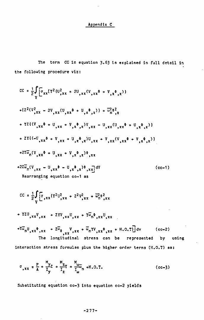
Appendix C

The

the following

term CC in equation 3.63 i s explained in fu l l d e ta i l in

procedure v i z :

CC* ? J T ° « x » 2 <U?xx * 2 u ,xx< v , x x 4 * v . . * - . > »! xx

V,x ,x

+(Z2(V2 - 2V (U * + U * ) } + Û2«2,xx ‘ ' . x x ' ,xx ,x , x ' J n ,xÏZ I < V .x x » * “ .XX * V , X )V.XX - U. x x « , x x * * “ , x ‘ .x>>

Z ï((-U _xx» . ViXX ♦ UiX« fX)UiXX . ViXX(V tXX« ♦ V » iX) }

+2Yu) (V * + U + V * )#nv ,xx ,xx ,x , x v ,xx

♦2Zu) (V - U * - U * )$ “ !dVnv ,xx ,xx ,x ,x ' ,xxj

Rearranging equation cc-1 as

(c c - 1 )

CC S j i ¡0 ,{Y2U2 v + Z2V2 + T2* 2

V{_ »xx , XX txx n ,xx

+ YZU V + ZYV „„U XX + Yu * U9 XX 1 X X »xx , n ,xx , XX

+ Y 7 u n . X X

« 9XX ♦ ZS V ,,xx *XX+ ÜT YV

n ,xx*

,xx ♦ H .O .T}]dv (c c -2 )

The lo n g itu d in a l s t r e s s can be represented by

interaction stress formulae plus the higher order terms (H.O.T) as:

M M M p y , z „ nu>- a xx = 7 + t Z + T "Y + 7-^n +H.0.T.•* 1 h \ "

(cc-3 )

Substituting equation cc-3 in to equation cc-2 y ie lds

-277-

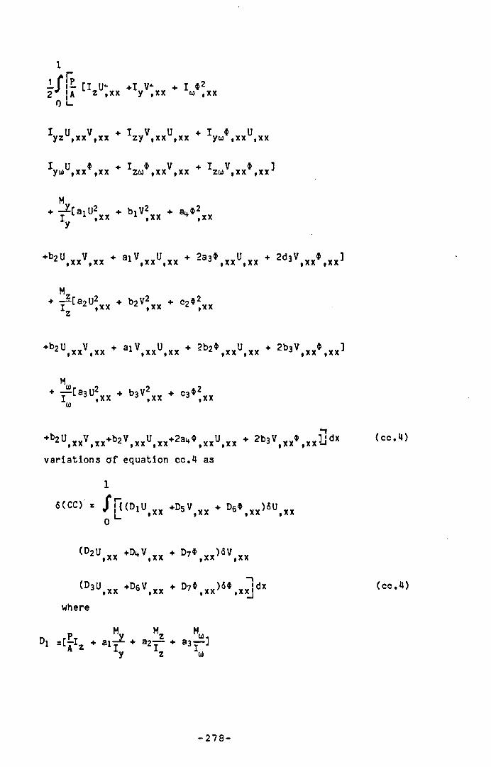
i r i - a u- + i v‘ + 1 * 22 '* A z »XX y . X X 0) , x x

o L

i u v + i v u + i ♦ uyz ,x x f xx z y , x x , x x yu> ,x x ,x x

I U * + I * V + I V * ] yu ,x x ,x x zu ,x x ,x x zu , x x , x x J

* ^ t a l U* x x * b ‘ V* x x * a* * j x x

* b2 " . x x \ x x * a l v , x x “ , x x * 2 a 3 * , x x u , x x * ^ . x x ’ . x x 1

♦ -r -[a2U2 + b2v2Y* + C2#21 •AA » AA tXX+t>2U, x x ^ , x x + a i V , x x U,x x + ~t>2* , x x U,x x + ^b3V , x x * , x x ^

M ,♦ — [a?U2 + b3V2 + C3 ^ 2I 3 ,xx J ,xx 3 ,xx0)

* b2 U, x x v , x x * b2v , x x u , x x * 2a '*4 , x x u .x x * i b 3v , Xx \ x x U dxv a r ia t io n s erf equation cc.H as

6(CC) = / [ { (D iU ¥¥ +D5V ¥¥ ♦ D6* . ¥¥)«UXX 3 ,x x , x x ' ,x x

(D3U,xx *D* v , xx * d3 * ,xx>5v , xx

(D 3“ , x x * DaV, x x ♦ ^ . x x ’ 54 »xx jwhere

„ M M MD1 sCfI 2 ♦ al / + a2T~ ♦ a3 ^

A 2 Jy l z ^

(c c .iO

(cc.U )

- 2 7 8 -

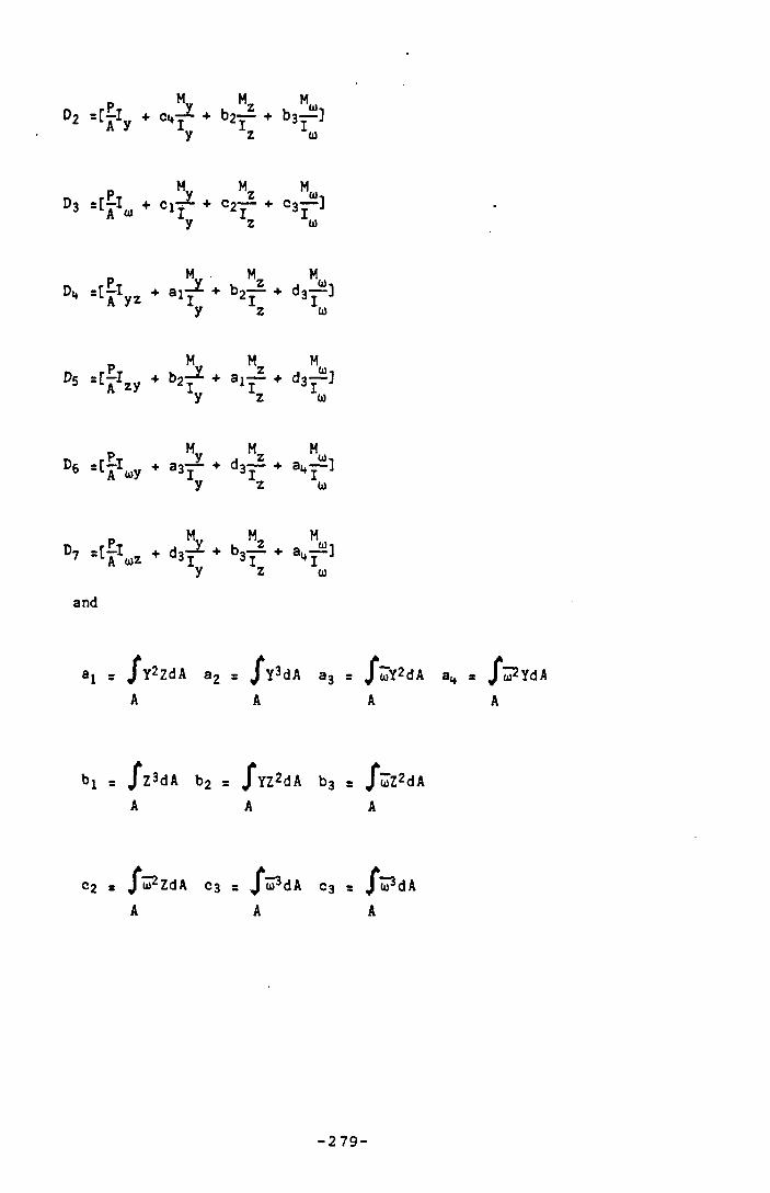
M„ M M°* =c f ly * O .J - * K 2 ° 2~ + b3-=—]

y Z 0)

M, M M»3 ■ £ . *

yc i r 2- +

„ z c2— +

Ü1,c37~]

y z U)

M M M

D* = [ X Ty zy

+ ait+ b2—

2I. Ü),+ d3— ]

y z ü

M, M M»5

+ b2€ ♦ • > r+ d3—■]

y z i»

M„ M M

B‘ « Z *_ y

+ 3î :. z+ do— 3I

- to-. ♦ aH— ]y z u

M„ M

+ d<+ b3—

3I ♦y z to

and

»! = J Y2ZdA a2 = / ï 3dA a3 = /wY2dA aH = f a Yd A

t>i = J*Z3dA b2 = / Y Z 2dA b3 = /wZ2dA

c2 = ^w^ZdA C3 = ^(¡^dA C3 s ^ ¡PdA

A A A

-279-

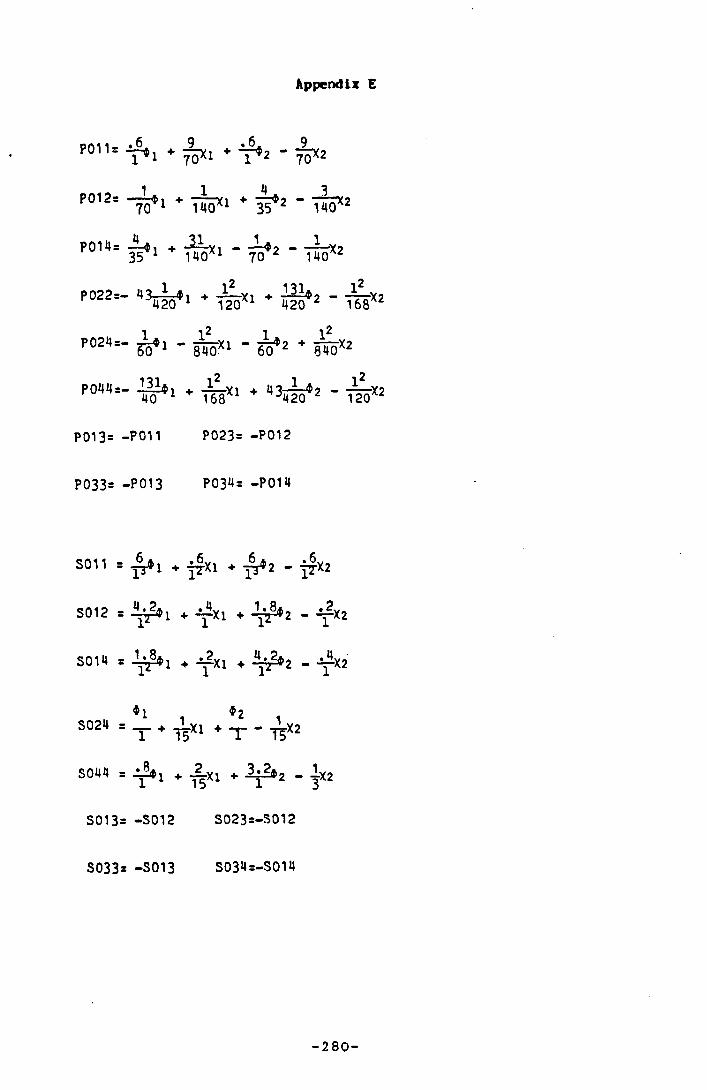
Appendix E

P01U

P012=

P014 =

P022=-

P024=-

P044=-

P013= ■

P033= •

5011 =

5012 =

S014 =

S024 =

S044 =

S013=

S033=

. 6 , 9 . 6 9+ 70*1 + T * 2 ‘ TO*2

170 1740*

4 . 3+ 3? 2 " 14^2

B *1 * W * 1 ‘ TO*2 ' HÓ*2

■ 437 r ^ i ♦131,

420'1 T 120Xl + 420T2 “ 168X2

60*1 “ 840Xl “ 6Ò*2 + 840X2

■ -HI* 40 1 + 168X1 + 1<3420t2 " 120

P011 P023= -P012

-POI 3 P034= -P014

• -jfxi + - ^7X2

¥ * 1 + -yXl + 4j^*2 - -y X2

+ -yXl + 4 ^ *2 - -yX2

*1 - *2 .- + i r xi + - r - i5 X2

• y * l + j^Xl + - ^ * 2 - -|X2

-S012 S023=-S012

-S013 S034=-S014

X2

-280-

YU 11 II If + 4 .20

17" ui "■ + 1 4 e 01 T u2

YU12 * " ^ 1 + -4 ) , A1 u1 h -jfu2 ♦ 1 u2

YU 13 * P ° 1 *1 . 8a“ír® u i ‘" ♦

iUifl7 2 ^ 2

YU14 * - ^ 1 _ .1 u1 ► # 2 -.4nT ^ u 2

YU21 . l i l e+ 1 ni4.2„ - -ÿ *J 2 + I®u2

YU 22■ T “ ! 1• ^ u l - T “2 * ^ U 2

YU23 - 1 « 8,,■ " Ï T “1

_.8n+ 7 * u i

1 . 8..- ^ 2^2 * Î ° u 2

YU24 S — 115 u1 - f 2 2 - 1 a‘ 15 u2

n u i l « t y h ♦ £ u1 - A j r «2 * T « u 2

w « * T “ ! * iV u 1 - - f “ * * ^ u 2

ÏU «3 = - ¡ ^ U l * ÿ u1 - ^ 2 * ^ „ 2

Ï U « = - J u , - £ ul - ^ U 2 * ^<>u2

YU31= -YU11 YU32= -YU12

YU33= -YU13 YU34= -YU14

z m ' * - T ^ u 1 ♦ ¥ * » 2

ZU 12 = ♦ ^ e u l . -j|U 2 ♦ ^ > u 2

Z U M = ^ . J î u l * ^ | u 2 . ^ 6 u 2

Z U 2 2 = - J u i ♦ i e u 1 » J U 2 - ^ « u 2

- 2 8 1 -

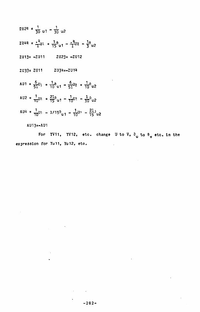
- 3 5 »1 - j s u2

i m = * ^ ul - ^ U 2 - }9 u2

ZU 13= -ZU11 ZU23= -ZU12

ZU33= ZU11 ZU34=-ZU14

AU1 = JUh + J_0 4 _ J la.51 1 10 u1 5 i

AU2 = J j n + 219 J tj? _ 1 oT i r 1 + J S u1 T ÎT W u2

AIW = ^ u , . 1/159u , . S o , . 2 1 ) ,Ter 15 u2

AU13=-AU1

For YV11, YV12, e tc . change U to V, 3u to 9y e tc . In the

expression for Yu11, Yu 12, etc.

-282-

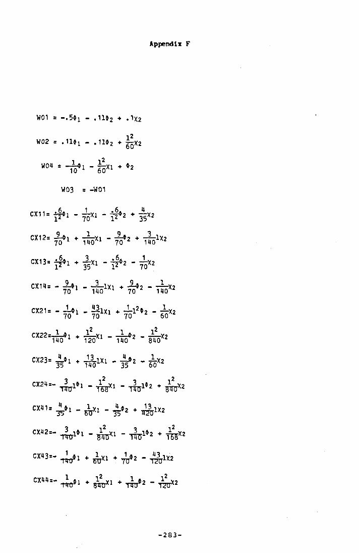
Appendix F

Vi01 a — . 5 * i - . 11 * 2 + * ^ X 212

W02 = . 1 1 * ! - . 1 l i 2 + ^ X 2

* M * - M X1 * *2

W03 a -W01

C X 1 1 = ^ , - ^ x i < - £ x 2

cx’ 2= £ * 1 * i i o Xl - & * w 1«

CX13. ^ ♦ ¿XI - * | » 2 - ¿X 2CX1,,= ' - l f e 1X1 * - i f e X2

CX21‘ - 7^‘ * H 1X1 * & 1**2 - £ X2

CX22.^*1 + — Xl - Y^q* 2 - P o X2

cx23’ j 5 l ♦ m m - b * 2 - ¿ X2

2 2cx24=” W 1* 1 " W ° “ W 1* 2 + bW X2

cx41 = p , - ¿ X l - ¿ # 2 ♦ ^ 1 X 2

CX42=- T O 1*1 - M J *1 - T O 1*2 + m X2

cx43=~ t im 51 + ¿ r x l + j u * 2 ~ T ztr1X2

0X44■“ T t t? 1 + iPTO 1 + TW *2 " T7UX2

-283-

CX31 = -CX11 CX32=-Cx12

CX33 = -CX13 CX34=CX14

B011 = ^ * 1 + * 4 * 2 - TO*2

B012= zl-b i + 7TT 1 W Xl + ¿ * 2 “ W X2

B014 = J U i j.w 1 * 1401X1 + TO*2 ~ T40X2

B022 = 431«1 w - 11*

+ ^ 1 X 12

+ i ^ 1* 2 ■ w X2

B024 =ro 1»* " 8401X1 “ 60*2 " 840X2

B044 =to1* 1 + ’reF1Xl + TJ^1* 2 “ T20*2

B013= - B011 B023= - B012 B033= - B013 B034 = - B014

XU11 1.542858,, — 1 ^ — Ul - — 9 1 351 u1♦

1.542858,,. ---- -7^— u2 _§_e ,

351 u2

XU 12

XU 14

XU 22

XU 24

XU 44

- — Ui _ -2-9 , + — —U2 +-— 9 «3 5 T 1 35 ul + 351 70 u2

—i-ui- + JLe , + _ i -u 2 + -12-9 -351 1 70 U1 351 735 u2

=* ♦ § 9u1 ♦ * i f e Su2

= 7TJ01 “ T ^ 9u1 " 7^2 + T ^ 9u2

” Tncr®i

XU 13= - XU11 XU23= - XU 12 XU33= XU 11 XU34* - XU14

For XV11, XV12, e tc . change u i , 0u1 e tc . to be e ither v i , 6yl

e tc . In the expression for XU 11, XU12, e tc . , or x i

expression for X011, X012, etc .

-284-

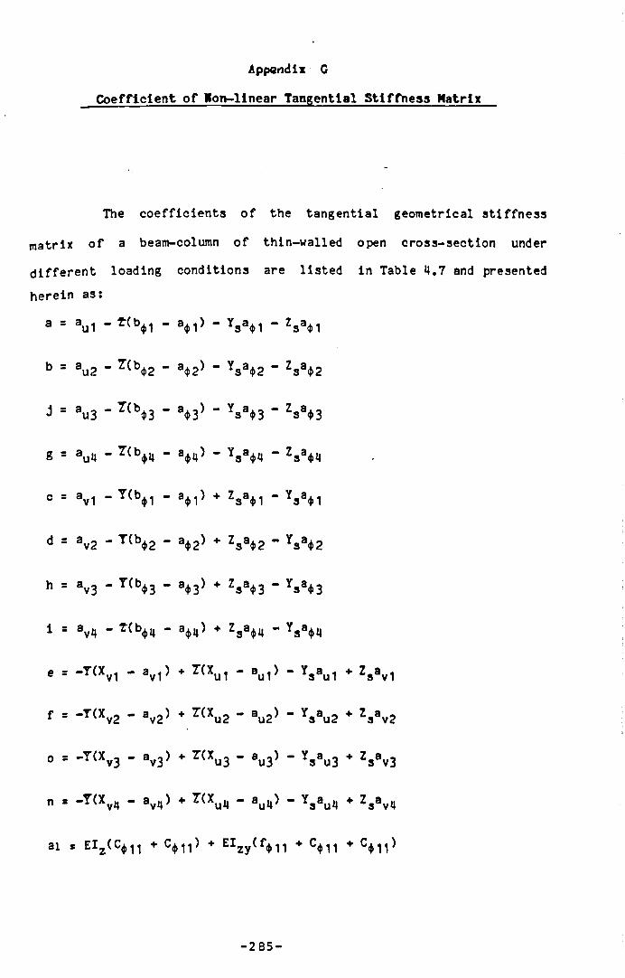
C oe ff ic ien t o f Won-linear Tangential S t i f fn ess Matrix

Append ix G

The co e f f ic ien ts o f the tangentia l geometrical s t i f fn ess

matrix o f a beam-column o f thin-walled open cross-section under

d i f fe r e n t loading conditions are l is ted in Table 4.7 and presented

herein as:

a = au1 - 't (b^1 - a ^ ) - Yaa^1 - Zsa<()1

b = au2 - 7 (b$2 " a*2* " Ysa<j)2 “ Zsa$2

J * au3 " ^ b*^ “ ad> “ V * , “ Zsa*3 “ <l>3 s (j»3 s 4>3

g = auij - - 3«j,n) - Ysa<j,4 “ z sa4>4

= — Y (bA1 — aA1) + Z.a^! — Y„a$1 - 3 ♦ 1

d = av2 “ T (b$2 " a*25 + Zsa$2 " Ysa<fr2

h = a v 3 - - a^3) + Zsa^3 - Y ^ ^

1 s av4 " * {b*4 “ * W + Zsa$4 “ Ysa$4

e = -Y (Xyl - ay1) + T(Xul - au1) - Ysau1 ♦ Zsay1

f = -Y (X v2 - ay2) + Y(Xu 2 - au2) - Y s a u 2 ♦ Z3 v2

o = -Y (Xv3 - av3) ♦ Z-(Xu3 - au3) - Ysau3 ♦ Zaay3

n = -T (X vi| - ay4) + 7(Xu4 - au4) - Yaaul| ♦ Zaav„

a i * S V 0* ! ! + S n * + E I z y ^ f ♦ 11 + C $11 + c * 1 1 *

-285-

- 9 8 3 -

♦ ^♦ o ♦ ‘tI J ) XZI3 + i( h 0 + !El,*D)XI3 - = 6q

« ♦ D + ^ * J ) XZI3 + (££4>3 + ££*D>XI3“ s 8q

+ ti34>3 + *,2<’j ) Âzi3 + (^2♦a + 2tl<t>0 )XI3 - = ¿q

(£2*0 + 2 ^ 0 + £24>J )XZI3 + ( £2*0 - 2 0) XI3” = 9q

(tol O + ^♦ o ♦ h 4,J)ÂZI3 + ( ^ ^ 3 + ln<lD)XI3 - = sq

(^^0 + 1^3 ♦ £ l *J )XZI3 + ( £ l *3 + l£ *0 )XI3“ = ♦’q

(224*3 + 22*0 + 22 )XZI3 ♦ (22*0 ♦ 22*D)XI3 - = £q

(Zl$3 ♦ 12$q + 2 ^ j )XzI3 + (12*0 + 21<|)0 )XI3 - = 3q

( U *0 + l^ D ♦ l U J )XZI3 + ( U *D + l U D)XI3 - 5: Iq

(fihi'Q + tin + ntl<f,J )Xzl3 + (*»>»*3 + hn*3 )XI3- = Ole

(£ti^0 ♦ * * 0 ♦ ^ ♦ j ) Xzl3 + (<i£*3 + ^**^D)ZI3 *= 6e

C«*D + ££*3 + ££4>J )XzI3 ♦ (££4>3 ♦ £^ D ) ZI3 *= 8e

¿ * * 0 ♦ M *o + tl2<l>J )XZI 3 + (*2*3 ♦ 2t,^0)ZI3 = le

( £24>0 ♦ # *3 + Í Z ^J)Az I2 ♦ C£2^ + 2£4»3)zi3 = 9b

( n l*D ♦ 1^3 + nt >ÂZI3 + (H4>3 + lh<i>0 )ZI3 - Se

( £ l *0 ♦ 16*d + £i 4>J )XzI3 + (Ct*3 + l ^^0)ZI3 s «ie

(22*3, ♦ 22t3i + 224*j )^zX3 + (224*3I + 224i3)zi3 = Se

<21*:» - l2*:1 + 2 1 ) ^Z!3[ - <l2*C) + 2t*3) zI3 = ze

bio = - EI yC ♦ C^m,) + E I zy( + <^44 + C^ !,)

°1 = E*u>^w(c<J>11 ♦ 2 0 ^ ) + Eltoyie,,^ 1+CV11 - Y gC ^ i - ¿ Y g C ^ )

“ E I U)Z< ” e u11 + c u11 ♦ z s S l 1 + 2z s C'M 1 5c 2 = E I u> ui( c «t>21 + 2C^ 2 * * E I wy( e v12+Cv21 ” Y s C$21 “ 2Ys C*1 2 *“ EW - e u21 + Cu21 + Z s C*21 + 2Z s C* 1 2 )c 3 s E I wF ü)( c $22 * 2C^ 2 2 ) + E I u y ^ e v224‘C v22 " Y s C*2 2 " 2Ys C<fr22)" E I u>z< " e u22 + Cu22 + Z s C$22 + 2 Zs C^ 2 2 )*»♦ s E I < A ( c <j>31 + + E I u y ( e v31+Cv31 " Y s C<fr31 ” 2Ya C* 1 3 )“ E W " e u31 + c u31 + Z s C<t>31 + 2 Z s S l 3 >c 5 = E I< A > (C<|,41 + + E I u>y( e v41+Cv41 “ Y s C$U1 “ 2Ys C*1 4 *" E I0)Z( " e uM1 + CuU1 + Z S C4>U1 +c 5 s E I uV C + 3 2 ♦ 2 C^ 23) * E I ü>y( e v23+Cv32 ~ Y s C* 3 2 " 2 Y s C^ 2 3 ) “ E W “ e u32 + CU32 + Z s C$32 + 2 Z S C* 3 2 )C 7 S + 2 0 ^ 2 4 ) + E l t t y ( e v , 2 * C v « 2 “ Y 3 C ^ 2 “ 2 Y s C $ 2 * P

“ EW ” e u i*2 + CuU2 + Z s C|t 1i2 + 21 ac^ 2^

c8 * ElÜJ5'ü,(C(j)33 ♦ 2( ^ 33) •*■ EIo>y( e v33+Cv 33 “ YaC*33 ” 2Ysc*33*

“ EW ” e u11 + c u33 + Z s C+33 + 2Zs c *3 3 *°9 * E ï ^ t e ^ j j s + 20^ 3 4 ) ♦ E IMy ( e v , 3 * c vil3 ” Y * C4> 3 " 2 Y s c ^ 3 1*'

-287-

- 8 8 Z -

+ 12a9jXi3 + ^2L4>j + 214»q ) 0^i3_ - za

< “ ♦ * . t u ^ «. U ^ j M j a «. ( U A 0 -+ l t n a ) * X i a +

( “ V j z ♦ u n o+l lA o ♦ ( “ ♦i * “ ♦ a ) mXi 3 - = la

t,n* o ) 2Xi a - ( tilrt3 . " « V i a - ( M * 0 + ^ ♦ j ) XI 3 - ■ Z Ip

♦ ^ ♦ o ) zXi 3 - (El. »3 - " e V i 3 - ( « ♦ a ♦ Up

« ♦ j ♦ etl* 0 ) Z* I 3 - . (HE*3 . »£ V i a - ( El»*0 + h£ V i s - « 0 Ip

( « ♦ j ♦ ^ ♦ o ) z AI3 - ( £ £ * a •. E E ^ ’ n .- (EE^a ■* £ £ Í J ) XI 3 - s 6p

♦ 2to*a)zXi a - ( K * a - * J * J ) ZI 3 - ( 2tr*D ♦ tf2 + j ) * i a - = ®P

m CM ♦ 2 ^ ^ 0 ) zXI 3 - ( « « a - £ e * 3 ) ZI 3 - (2E$a + ^ * J ) XI 3 - s ¿p

c " ‘ * j + U4'0 ) z XI 3 - ( " ‘ ♦a - * l * J > * I 3 - ( ito^a ■♦ ftL* J ) XI 3 - = 9P

( E U j ♦ l £ * 3 ) 2XI 3 - < ^ 3 - £ l * J ) ZI 3 - ( i e * a ♦ i l W n - = SP

( « ♦ j ♦ 2^ D ) 2XI 3 - <«2 *o - « V i a - ( 2 2 * a + 2 2 ) ^ i 3 - = «P

0 ^ 3 ♦ 2l4,D)zXI 3 - ( l 2 *0 - s ‘ V l 3 - C^*Q + 2 l * j ) Ai a - = Ep

( « ♦ j ♦ 2 2 ^ 0 ) z XI 3 - <‘ J *o - Zl , , J ) ZI 3 - ( « ♦ a + 2 l * j / i a - * Zp

CU *J ♦ u 4>0 ) 2XI 3 - c “ *o - “ V i a - ( U * a + u 4,J ) XI 3 - * TP

( t i t i * 0 S Z2 + ft,T*D S Z ♦ tlt,nD + ft,7ns - ) zmi 3 -

(titi*0SA2 - ' " o h - M A3+MAa )Xmi3 + (M*ag + ^ D î V ’lS = Oto

(^ t,l DSZ2 + ^t,^0Sz + ktlnQ + £ftna- ) zinj3 -

+ EIyz (e u12 + cv12* + EIüj2^f 4> 12 + 12 " %12}

e3 = - EIyu)(D«|,12 + f *12) + EIy ( e v21 + Cv12+Cu12 + ^ y 0* ^

+ E I y z ( e u21 + Cv 1 2 ) + E I o)Z( f <t> 12 + 5 ^ 2 1 " e 4>21)

e*» s - E I yoj(D <|.22 + f ij)22^ + E I y ( e v22 + Cv 2 2 +Cu22 + 2* y C* 2 2 *

* E I y z ( e u22 + Cv 2 2 ) + E I ioz( f $ 2 2 + ^ * 2 2 “ e* 2 2 5

e5 = - E I yco<D<H3 + + E I y ( e v31 + Cv 1 3 +Cu13 + ^ y 0* ^ '

+ E I y z ( e u31 + Cv 1 3 5 + E I u z ( f (j>13 + 2° +31 " e<J>315

e6 = -E Iya)(D(>23 + f (|.23) + E I y <ev32 + Cv 2 3 +Cu23 + 2*VC*32)

+ E I y z ( e u32 + C 23) * E I a>z( f $23 + 2 ° * 3 2 “ e*32)

e7 s " E I yüi(D«t>m + f * l 4 * + E I y ( e vU1 + Cv 1 4 +Cu14 + 2^ y C$ 1 4 *

+ E I y z ( e u41 + + E I « z ( f * 1 4 + 2e * 41 " e* 4 1 )

e8 ■ - E I ya,(D4>24 + f * 2 4 * + E I y ( e v42 + Cv 2 4 +Cu24 + 2* y C* 2 4 *

+ E I yz(e u42 + Cv24) + E I£u zCf 4>24 + 2°$42 “ e*4 2 )

e9 s - E I ya»(Dd>33 + f *3 3 5 + E I y (e v33 + Cv33+Cu33 * ^ y 0^ 5

+ E I yz(e u33 + Cv33) + EW f *33 + 5e* 33 “ e^>33)

eio = - E I yM(D^ 4 3 + f^ 3 n> + E I y<ev34 + Cv43+Cu43 + 2^yCH 3 '

+ E I y z (eu43 + Cv 345 + EW f *34 + 5e* 43 “ e*43*

e u = - E I yu(D^34 + f^ 4 3> ♦ E I y ( ev43 + C /34+Cu34 + 2B’yC*3 4 )

-289-

+ E I y z ( e u34 + Cv ‘<3) + E I u>z( f 4>H3 +

e l l = “ E I y U(D (}iHM + f <t)44 + E I y ( e vHH + CvHH+CuHU + 2 * y C $ H l P + E I y z ( e u4'4 + Cv W + E I u z ( f 4>4H + ^ I J U " e $ i| ip

f l = “E I yu3CD4> 11 + {'$‘\‘\) + E I y (e v11 + Cv11+Cu11 + 2^ yC<t> 115

+ E I y z ie u11 + Cv11> + E IüJZ( f <j>11 “ ^ * 1 1 + e<M15

f 2 = - E I yuj(D(t> 12 + f $125 + E I y (e v21 + Cv12+Cu21 + 2* y C$12*

+ E I y z ( e u12 + c v 1 2 ) + E I u>z( f $12 ” 12 + e* 1 2 )

f 3 = ” E I yu)(D<t>12 + f 4> 12^ + E I y ( e v21 + Cv 1 2 +Cu12 + 2By C* 1 2 *

+ E I y z ( e u21 + Cv 1 2 ) + E I ioz( f * 1 2 “ ¿ ^ 2 1 + e* 2 1 }

^ = “ EIyu(D4>22 + f $22* + EIy ( e v22 + Cv22+Cu22 + 2* y C* 22*

■* EIyz (e u22 * Cv22 + EW f 4>22 “ 5e*22 + e4»22

f 5 « “ EIya)(D<il3 + f *135 + EIy ( e v31 + Cv13+Cu13 + 2V ^ 1 3 *

+ EIyz (e u31 + Cv13) + EIo)z( f * l 3 “ ^ $ 3 1 ♦ ®*3 1>

f 6 = - EI yüJ(D^23 + ^ 23) + EIy <ev32 + Cv23+Cu23 * 2* y C*32*

+ EIyz (e u32 + Cv23) + EIioz( f $23 ” 5°$32 + e$32)

f 7 = - EIya)(D«nK + ^ i n 5 + EIy (e vU1 + cv 1U+Cu1U * 2l yC<t> 1U

+ EIyz (e uU1 + Cv 1H) + EIa)z( f (M2< “ jjfyui + * M 1 *

f 8 = —EIya)iD4> 24 + f (J> 24 + EIy ( e vU2 + Cv24+Cu24 * 2BryCi)i24)

-290-

+ E I y z ( e uiJ2 + Cv 2 4 ) EV f $2i| - iC2 ^ 2 * e*M2>

f9 =

+ El yz

f io =

+ El yz

i ' l l =

" E Iytü(Dí 3 3 + f * 3 3 * + E I y (e v33 + Cv33+Cu33 * (e u33 + Cv33) + EV f $33 “ 2 ^ 3 3 * e$33)

~E Iyw(D<H3 + * * 3 4 5 + E I y (e v34 + Cv43+Cu43

(euH3 + Cv31<) + E Iu)z( f 4>34 “ i° H 3 + e**»3^

" E I yiD(D<J>34 + f ((.H3) + E I y C ev43 + Cv3^+Cu34

2V * 3 3 >

+ 2V m 3

+ 2V ^ 3 4

)

)

+ E I y z ( e u34 + C v ^ 3 ) + E I u)z( f H 3 “ ¿ S 3 1* + e 4>3 1* >

e i 2 = - EIyuj(D$i4U + + EIy ( e vHU + cvJm+CuH4 + 2^ y C4>1»1<)

+ E I y z ( e uiJ4 + Cv 4 4 ) + E I u>zí f <t>W " +

-291-

Appendix H

Nonlinear Geometrical S tiffness Matrix

The co e f f ic ien ts o f the nonlinear geometrical s t i f fn ess

matrix given in Table H.8 are explained in d e ta i l as:

#1 = 4 V v * 1, »2 * - i Mx 'V*12 * V*21>

A* * - i « x (V*22 * W #“ * - X (Vt13 * \ 3 1 >

A s * * V ^ 1 ) # f * - i V \ 3 2 * % 2 3 >

#7 * 4 V V« * * V a ’ ‘ 8 * - j V % 3 3 * W

A* ■ - i M«iV *38 * V*1 3 ) A‘ » = ' I W l * W

Bl 8 FYs (n<M1+m(|>1 l ) " Q2U<M1 4Mr <n* n +mi l 1 >* 2Mx (w* i r T* 1 1 >

B2 s FYs (n$21+m<M2)-Qz U$21 +Mz (n$2 1+m$12 )+2Mx (W<H2“T* 2 1 )

B3 = FYs (n4,l2+m«tl21) " QzU«|)12 +Mz (n(|>2l'*‘m(iil2)+2Mx (W«n2“T()>21)

** = FYs (n$22+m$22>“ Qz U<fr22 '^ z * n* 22+,n$22 )+2Mx{W* 22“T* 22)

b5 = +Mz (n^13+m 31) ','2Mx (W l3 "T4>31)

B7 = FYs (n<|132+m(ji23) " Qz U<i.32 +Mz (n<l>234'm<l'32) ',2Mx (W 23“T4'32)

B8 = FYs (n$42+m<t>2^"Qz U4>il2 +Mz Cn4»2U m4>U2>'*'2MxiW 24“ T4>U2

B9 = FYs (n$33+m4>33)_QzU<l>33 +Mz(n*33+m*33î+5Mx % 3 3 “T*33î

Bi0= F Y a ^ + n ^ l l ^ z ^ n +Mz (n*11+m*11),*,2Mx % i r T*11)

-292-

B i i 8 F V % 3 1»+,V » 3 ) “ Qz U* 3 1» +Mz ( V » 3 +m$ 3 l»>' '2 Mx <W$i»3"T * 3 1»)

B12 = FYs (n4,M4+%4M)" QzU<t>M4 +Mz ( n<t,4H+m<i144 j^ x (W$mrT$*»U5

fii3 = FYs (n<|>13+m<t>31) " Qz Uitl13 n*3 ,r*'m* l3 J,*^Mx

B11+ s FYs (n(|)23+m(t)32)-QzU^23 n(j)32^rn(t>23>*2Mx (W 32"T^23)Bis = FYs (n<|)iu+m41m )“ l5zu4>m +Mz {n^m+m i«»)+2Mx<wí í i r T* i 4 >

b16 = FYs^n<j>24+m<j>42^zU4>24 +^z^n4>42+m<|)24 ',’2^x 24^

cl = FZs (n(|>11+m<t>11)" QyU4l11 _My(n<}.1 1 +ni<t.1 1 )“ 2Mx (W(|>irT<t.1 1 >

C2 = FZs (n<j>21+m(|>12) " QyU<f>21 " My (n<j>21+m<M2)"2Mx (W<i>12"T<|i21)

C3 = FZs<n<j,12+m<j>21)" QyU<í>12 “ííy íní21+m*12í“ 2Mx ^ 1 2 “ T*21^

^ = FZs (n4>22+m«í>22)”QyU<t>22 _My( n<í>2 2 +rn<í)2 2 í_ 2Mx ÍW<*>22~T<t>22

c5 * FZs (n^3l+in$13) " QyUi3 l “My (n^l3+,n* 3 l ) “ 2Mx % l 3 “T* 3 l i

C? 8 FZs (n^32+m 23)_QyU<f32 “My(n^23+ni*32>"2Mx{W^23“T^32)

C8 = FZs (n<|>42+m4>24) '"QyU<|>42 ”My(n )24+m<|>U2)~ iMx (W<|>24”T<|>42)

°9 s FZs (n^33+m 33>" QyU 33 ■My<n*33+,n*33>“2Mx (w*33"T*33)

Cio= P V ^ n + ^ n ^ y ^ i i “My in* i i +m* i i ,“ 2Mx<w* i r T^ i i )

cl l = FZS (n4«3V*'m<t>43 -'QyU4)3U “My ^ 4 3 +ni$34^"2Mx iW$43“T4>34*

Ci2 = FZs tn$i|i|+nV44) ” QyUH 4 ” My (n$44+m$ 4 4 * ^ x ^ W<ti4Il"’T,t>1<1

Ci3 = FZs (n<f>l3+m<t>31 “ QyU(M3 ” My^n$31+m<M3>“ 2MxiW<i>3' r T4>'l3^

-293-

- V 6 Z -

= »a

[ 2 * » n f * 2 * n ] V t 2 * ♦ae»2 " V " 2 * n f - ] V o f -

[ 2l,*H3+2l,*n+h2*r>!-]sz*ö^*- = ¿a

t u ^ i p “ V w * £ l,' W ,' V ' l * n f - j V o f -

[“ W V ^ n f - l V c f * * ’ a

[ « ♦ „ p S V w ^ W S V ^ i i f - l V o f -

t eE *BZ*eE *n-Ce+ o f - ] * z * 0 ^ • sa

[ £ l ^ > p £ * n ] V [ l £ * a z * l £ V £ l * n f l V c f

[ l £ * a z * l £ * n * £ l * n ^ - ] s z i 0 ^ = M

cl l ^ 22V w n 2ZW 2V 2*n?-]Vef-

C2 2 * a z . 2 2 V 2 2 * r t f - ] V ¡ f = 5a

C2 ‘ * n p 2 * n ] V t 12* a z » 12 V 21 * 0 ! - ] V e f

c l 2 W 2 V 2 ‘ * n f - ] V e f * H

[ “ ♦ n p l * n i V c u * a s » u * n * u * - 2 1 S TAz J Lf r i -

[ l l ^a2+ U ( *)n * l U ! f ] s z la

xf < " 2 * n V SZJ = *'o

( H *i- ‘ ■ f < * u n V Sz i »

(£2*I--2£‘ «> X 2 , Wf“ ( ^ v ^ * u ) V £ 2 * n * & - 2£^u,+E2^u ) Sz i = ♦a 3

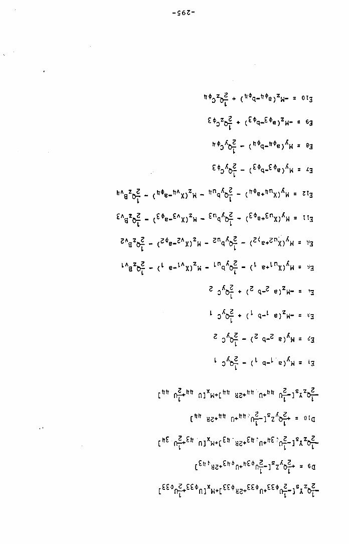
- S 6 Z "

* V e f * ( ti4>q_ti4>8 )z H_ = 0I3

£V o f * (^ q -^^e )ZW“ = 63

» V f t f - ( ^ q - ^ e / w = 03

£V o f - (M q -M . ) AH = l 2

" V o f - ( " . . ' V * - " V o f - ( " ♦ . ♦ * nx )XH * ” 3

£V t > f - ( £*e -£AX)ZW - £V » f - ( £* ^ £nX)i W ■ ” 3

JV c f -¿n X.2

- Q &j- - ( 2<e+2nx )XW = y3

l V t f - = - lAx ) " «Ln_ ^- q &j- - ( l e+inX)XW = *3

2 3*0 + ( 2 q -2 e)zw- = '■13

1 0^ + ( 1 q - L e ) ZN- = f 3

2 DXô | - ( 2 Q-2 e)XW = ¿3 1 DX&| - ( L q - L s / w = l3

[

C

c

n,T n p * m V c ™ H2^tI V nn n f - ] V o f -

[^ti a2+t7t7 n + ^ ' n p ^ t p = 01Q

bt pZ+tb n ]xw+[£to ‘ a2+£t7 ?n+t?s rn j - ] sAz&^-

[ £* = *a

£ £ $ 2 Ç £ à „ X C T A £ £ è £ £ é Z , S zJZfv^- n ] w n n+fctŸi > p ] i O p

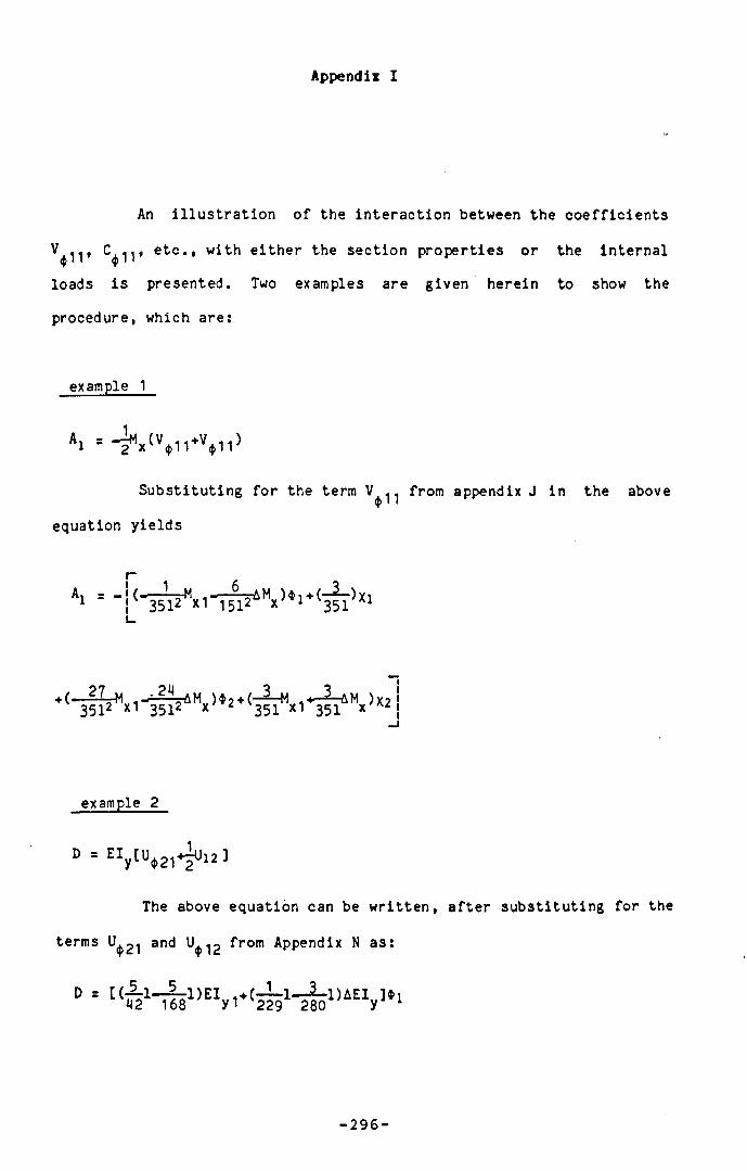
Append ix I

An i l lu s tra t io n o f the in teraction between the coe f f ic ien ts

%11* e tc , t with e ither the section properties or the internal

loads is presented. Two examples are given herein to show the

procedure, which are:

example 1

a i * - K (v * i i * v i >

Substituting fo r the term from appendix J in the above

equation y ie lds

Ai r — j ( —— M . —< ■ ^ ■„ A M ) 1 ^ ) y i 1 3512 1 5 1 2 351 X1

27

3 512 x1 3512 x ) $ 2 + (— M » A H )x ?351 *1 351 x 2

example 2

D ' EIy [ ^ 2 1 - iUl21

The above equation can be written , a fte r substituting for the

terms U ^ i and from Appendix N as:

D = [(— 1—— 1)EI ,+ (-1 -1 — 2_1)AEI ]$i 42 168 V' 229 280 y J 1

-296-

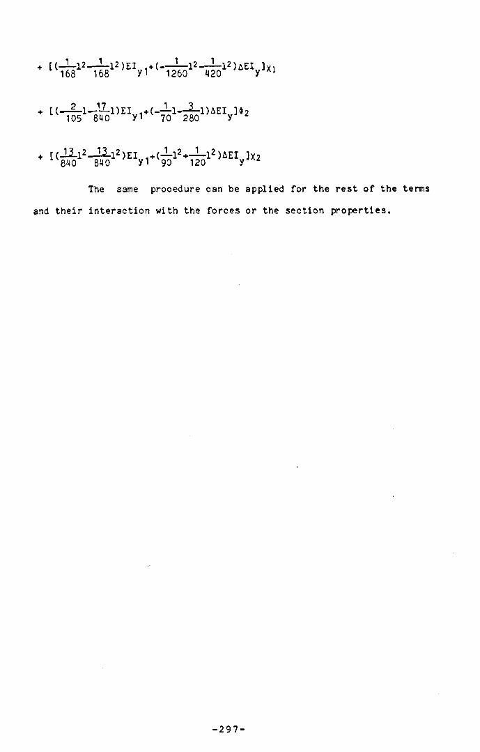
168 168 y1 1260 420 y X1

+ [ ( — — 1 - - — 1 )E l 1— 1) AEI ] $ 2105 840 y1 70 280 y £

+ [ ( -L 2 - l2 _ -L 2 - l2 )E I + ( J - i 2 +_ L i 2 ) AEI ] X840 840 yi qo 120 y £90 120

The same procedure can be applied for the rest o f the terms

and their interaction with the forces or the section properties.

-297-

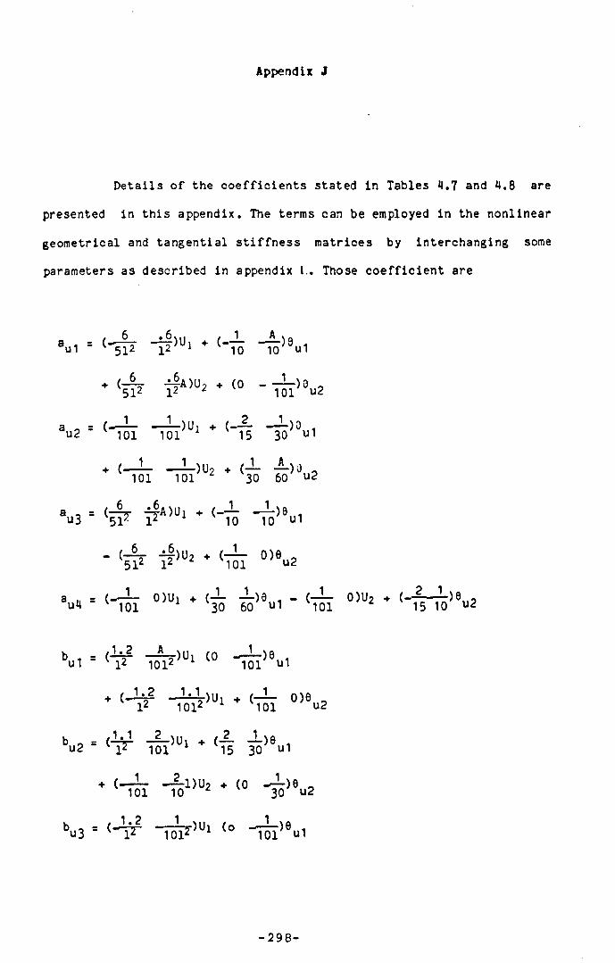
Append ix J

Details o f the coe ffic ien ts stated in Tables *1.7 and M.8 are

presented in this appendix. The terms can be employed in the nonlinear

geometrical and tangential s tiffn ess matrices by interchanging some

parameters as described in appendix I.. Those coe ffic ien t are

6512 - i4 > u> * CD

( - £ -b l 2

^|A)U2 o+ 1101

1 1au2 s ( 101 10l )Ul + ( _ 15 30) 0u 1

+ i _ 10l _ 101)U2 + (30 60)J u2

au3 - < iF F a)u‘ * ( - F - F )e »1

- * (T o i 0,eu2

auU * ‘ - i f e ° )u' * % ¿ >9ui - 0,U2 * ( - F - F )9u2

bu i ■ < ■ ¥ F F ) U ‘ co - T S I ) 9 u i

* ( - ¥ - F F )U‘ * < F I 0,9u2

bu2 = (“p ' T o T >Ul * *1 5 3o " u1

* - F 1 ,u * * <° 1 3 )9 U2bu3 ■ ( J F - F F )U ‘ <° “ F I ) 9 U1

-298-

♦ ( 1-2 ■ 12 1012)U2 ( 101 ° )0u2

(-— — ^-)u, + (—1- —L)e l 101 1 30 30 ui

* ‘ - ¥ T > “ 2 * ^ T6>e»2Change au1 ’ au2’ au3’ auV u V U2 » 6u2

>v2* ®v3* \ V ^2» 0V 3 11 3i>ii 3Â, i 8j'v l 'v2 V 4> 2 * <t> 3* ‘V » *

respectively. A sim ilar procedure can be done for buV

into either a ^ ,

*1 t Xl I *2 » X2

etc » «

m ( n 18 in j. ( ^*2 1.286.«11 s ( ° 35ÎJ> 1 (“1 T — Ï2“ u1

+ (o — _)u2 + (-4 —~-)e 93 5 1 3 l 2 3 512 u 2

,-1.2 1.286N1I . , 4 1c“21 * <15-------- i r - )ui ♦ <TS I 3 i î ,e ui

* < "? 1 ^ ,U2 - 10 l i l )euJ

cu31 . <o . < - ÿ

* (0 * <35? W » » *

■ ( i $ W >u‘ - (0 m )0u', 12 + (---- T— 1212 v„ ,.U 5

351* 3517 )U 2 + ( 1 2 8 1 )9 u 2

CU12 = (“TJ1.2l 2 351

^j-)U i + ( - — ■ -¿00 ,1 0 1 71 u 1

+ (-4^ + (— — !— )6 -l 2 3512 1 351 u2

cu22 = ( ^ ~ — )Ui ♦ ( - - — 2 - A ) Q t . 1 101 71 3 205 u1

+ (-101 351

1 )U2 + ( 1 ■A)0.30 205 u2

/m i / 1. 2 12 \ n / 2 1 \ n

2 3 = ( l 2 3512 1 " 101 T I 5 u1

- 2 9 9 -

cu2li =

C U ! 3 =

cu23 =

C U 33

cu*3

cum

cu2i4

cu3l+

/1.2 12 v„ ,4 5 v.12 3512 U2 (i 351 ôu2

( - y - -6/35DU], + (-| )e.30 205 ul

(— — )U2 + (— — )0 0 1 351 2 15 35 u2

18 1.2 1.286(0 W )Ul + ^ )e U1

* (0 5 ï F )u* * ( i r 3 i f î )eJ1551

.1.2 1.286

u2

( ^ f - ^ > » 1 * «-Î5T l i î )6ui

{î ? 3 ,Ü2 * (0 m )02

(0 t t t tJU! + ( f |* r A v )8.

(0

: (

3513

18

12 3512 u1

)U2 + ( - 12 123512 3512 u23513

P 351?>Ul * ( ° i ï ï ” »1

)9.

( 12 , 12 , 5 xn35l 2 35l 2 2 “ 1 281 9u2

/1 .2 6 x„ , 1.4 1 .1428\n" î2" 7Ï 2 Ul + (- n ~ — r " )9u1

{ ^ • 2 6 \ 11 / • 2 6 \ a(i r 7 i r )u2 - <t - ¡ i ï )eu2

()u ‘ * ( -T7 l A <

-1 .4 1.142861 1

.4 8 x„ ^ , J _ 11 y.101 351 U2 ( ~30 210 9u2

1 « 2 6 \n / M 8 \qT T _ ï ï r,Ul * ( " i ô î " i 5 í )0xi

f (1*2 6 m, / • 2 . 6 \a• j r - ^ > < > 2 ♦ <T * 3^ )% ; ,

(■¿ t .1

6 )Ui + ( - 111

351 > e .30 210 u1

300-

/ * 2 6_x.. * 1 11 \ _* T *3 5 1 U2 * 3 3 5 >e^ >

Change cullt cu12, Ulf 0u1, etc. to the form cvllt

cv12* •••» v i» 0y1» etc. • Same procedure for the term:; such as xi*

,4.2 4

- (

6,

6 l i .

eu1 1 = ( i 3 + 3 5 i 3 )Ul + ( X 2 4 7 l 2 )e ui

13 js^ “ 2 * ‘7 # * 7 ^ >e“ 2

eu13 * <fs ♦ <^# 4^1857)6u 1

- ^ ) 0 U,

.6 .2> u w ■ < - F - ? Î Î ) U 1 * ( f " i t l ) 9 u l

11* < i ! * ^ ,U 2 * < m ” 3 5 1 ' - “ 2

) 0.

A f ü l l J L m i t i l l 11 Nfleu21 = ( i 2 +Y2 )U i + ( i ' 3 5 i ) 0u 1

+ (

'u22

'u23

«.2T ï ^ 2 * (I

4-2-)® ,351 u2

« - Î5 Ï -B T ,U> * <-9.666 -7.9236)0

1 — )U2 + (— 1 )0 o101 351 * 15 105 u2

,1.8( 12

+-^-)0 351 u1

u 1

- ♦ 4 *£>e,

.2

l 2

4

11 351 u2

e 24 + ( -— — =-)Ui + ( - — —^ - ) 0 , u 1 351 1 15 35 u1

+ (— +-ÍÍ-)Ul ♦ ‘- )0 ,1 351 1 15 35 u2

e - r_4- - u31 “ C i3 3 5 i 3^ * « l i * ^ > * u ,

( f * # I > U» * (w”i T - ¡ H * ” « *

- 3 0 1 -

e _ t i â _ _ cu32 ' 1 2 3

+ + 4 .',9

( - 1 - 4 1 ) 6101 351 1

¿ 2

‘ 1 l 5 Î )6u2

e

u33 i 3 l 3 l 2 l 2 u1

, ,6 ,5.057.,, ,4 .2 .3.6285.«* (F * ^ 1 ~ > U2 - < - ¡r p — ) eul

'u3“l * (F * n r>Ul * ' " f * 3 5 Ì )e u1

- ^ * < 4 * ! Ì T >9U2

eu «i 5 (T ^ ^ )Ul * (T * i l i )9ui

- 4 ^ r ^ r ) U , ♦ ( 4 ♦^■>9u21.8 , 1 3 .„ ,.8 2

i r w )U2 * T T i

eu"2 * (f ^ )u> * <1¿ * ¿ - > e ,1 351 Ul

- < f i k ^ * {Jh *8— +— >0 0

15 105 u2

r .4.2 ,3.6285.,, .1 32 »neuH3 * (1 T *^15— )ui * <1 * £ y )9u1

,4.2 ,3.6285.« ,3.2 2.714»«- (-JT 4 T ~ )U2 ♦ ( 1 +“ t ~ )9u2

V * = (_ 101 _351)Ul + ( ”Ï5 ~35)eu1

♦ ( 4 - ^11J L 4 1 )U 2 ♦ (-1 4 - )0 ,101 351 2 3 35 u2

Change e ^ , eu12 » ul * ®u i t0 evvj* ev12’ ^ * ®v1 t0

12t *1» XI etc.

**♦11 5 ( "3 + (— 1 — l )x i420 1 42 229

(4 1"420**2 + ( 422 2291)X2

*♦11»

-302-

^1% 2 1 s% 1 2 5 (_84

—2-1) a, + (— 1 2 --- — 12)y,mo 1 168 1260 Xl

— L 1 ? )X2 252 * 2* ‘ m 1 * (- w 12

N a - ' - » 1’ -5T5l2 ) t > * ' 0

k 2 * k l 2 ) i ’- ' c- i k 13 i k s l 2 ) K

R*32=R*23 = *“420* - 1 U01 H ‘ * í“ l 681 “ 2 5 2 1 ^X1▼ mf*~ Y*--¿ I Mw IUO c:

* <5 io 1 * í í 0 1)t2 * <_28Ö1 ~126Q1 1x2

» m * * » * » ■ ^ ♦ & , « i ♦ ‘ j f e 1* *iT5 l3)Xl

è l 2 ) < 2 * ( - 4 13 - t4 i 3 ) X 2♦ ( _ ü i *

420 60

* ♦ 3 3 = 4 W 1>x‘

♦ < î * & » * * < ■ & ï k l ) "

W « « ■ ‘ m 1 * & » * ‘ * ( 5 » 12 4 i l2 )x i

* < - l ? i -12)X284* 1401)Î2 + ” 1681 149'

1 ï ï l2)*> * < 4 4 4 ?*♦44 = W =315 ^ l3)x>

♦ (- — l 2 +—-—12) î>2 + (0 +—-—1 )X2840 315 2520 “

Change R^ 1, R ^ ........... * i , X l, *2 and X2

Ryi2' •••* 2 » an ®u2 or « v i l* Rv12’ • , * , ^

0V2 respectively.

\11 4 •i ü )V l * ' - M 1 - 4 1>e

i V Vx♦ (-S2-1

8409

140 1 )9 V2

Ru11*

, and

-303-

v12 = (“4 - 7 ^ 1 )v i + C-1 /8M1 2 - - 7 - I 2) e,84 140 210 av1

(—12-1 -420

-2 -1 ) V 2 + (777-1 2 140 1 420 65l2 )6vì

v i3 s ( _ 6—L )Vl + (--32-1

12 1 420 - r f e 1>e

47 w ,23, 27 IX n420 ^ 2 841 1401 )6v2

53UV » ■ ‘& 1 4 W ‘ * (ì i 12 * ¿ l2 )e .1

+ ( ^ 1 - ~ - i ) v 2 + (— ì 2 — i 2)e84 140 ¿ 840 315 v2

Uv21 1 ‘ Ä 1 — l)V i + ( - 7- I 2 229 168

1 -12)0 , 1260 v1

+ (— ^-1 —4 ) V 2 + ( - ^ - l 2 — 12)0 _105 72 840 90 v2

"v22 ■ ( 4 12i 2)V i + (o - - r — i 3)e

+ (■168

- l2

1260 ' ' * " 2520' ' v1

— 12)V2 + (— l 3 — 13)0 ,>qn ¿ ?in 3 1 5 v21250

U - . = (“t4 * - ¿ D V i + (-1/16812 v23 105 72 2520 v1

♦ (-2 1 *210 - ^ - l )V 2 + (— l 2 —— 12)0

167 2 280 138 v2

u - ( -3 -2 —1 2 . /— 3— 1 3 _ J — ^ 3 ) 0Uv24 ■ ^840i 901 1 210^ 315

+ ( - 3 2 - 1 2 — 1 2 ) v 2 + (— 2 _ i 3 — 3— 1 3 ) e280 138 2 280 135 v2

U - (-12- Uv41 " 1 210 4281)V 1 + ( - “ - l 2 ~ 1 2) 6

840 252 v 1

♦ ( - 2 - 1 — — 1 ) V 2 + ( — l 2 — 1 2 ) 0105 194 840 315 v

= (-~12 —ì-l2)Vi + (-4-13v42 ' 840" 252" ’ * ' '4 2 0 T560l3 ,0v1

♦ ( — 3 - 1 2280

— ~ i 2 )v 2 + ( - — ì 31260 ¿ 420 12601 )e v2

-304-

UvU3 = ("1051— 1)7, + (-— 1219- 1 280 126Ol2)0v1

♦ (-5-1M2

-^5-i)v2 + (-— l 2 218 2 168 149

l 2) 0v2

vMM * '8M0* 315* ' 1 " ' M20* 1260" " v l

168

= (tt i 2 - ¿ D V i + ( - r ^ i 3

— 13)0+ (-TTT l2 - —7—l 2 )V2 + (0149 2520 v2

Uv 11=_Uv 11 Uv32=Uv 12 Uv33s-Uv13 Uv3M=" UvM1

Change terms such as Uu l l , Uu12, Ui, and 6 to either

U4,12* * 1 » and *1 or to Uv 11 • Uv12’ V l ’ atld 6v1 *

u1 (" 12h 2 1 Ml ,1 .1— )Ui + (—1 0 1

— )0 , 101 u1

♦ (■ 1.2l 2" 1 0 12)Uz + ( 101

>9101 u2

Xu2 ■ (7 o I0 >U|. + (— —3-)0 ,1 15 30 u1

+ 0)U2 ♦ ( - 30 3 0 ) 9u2

u3

+ ( 1.2

, h l ( 12

111012)u x +

lToI2

101

11■>u2 + (

11 __2_■>e 01012 101 701 u2

x _ = ( - 5 - -L -U j + (_-3- o )e .u3 101 101 30 u1

♦ (• — — i-)U 2 + (-— — )0 - 101 101 30 30 U2Change X ^ , Xy2 to X^ and Xy2, sim ilar procedure for X

X^2 by changing V i, 0y l , * 1 , xi instead o f Ui and 0u respectively

♦ n *

and

-305-

Bu1 = ( - 5 ■12)0, + ( - L i 70 1 10 210 ) 9 U1

+ ( - . 5 J i ) U 2 + (-¿-1 70 z 10J _ L ) 0U 20; U2

Bu 2 = ¿ - l ) U i + ( - . 5 1 702 — 12-12 ) 6

105

♦ ( - ± 1 10 * & T 4 0 1 )e u2

Bu 3 = ( * 5 — >Ui + ( — 135 10 i f 5 1 )e u i

+ ( - . 5 J I ) U 2 + ( - — 135 10

. ^ - > 0 , 210 u2

u1

3u « = < - ^ - ¿ 12)9U1

( -1-110 5TS1,9u2

Change Bu l, Bu2 to Bv1t Bv2’ B<t»2 and at the Same time

replace Uj, 0ul by either V i, 9y1 or by * i , xul respective ly.

'u1 70-2 -i ) 0 . 70 Ul

— )U2 35 " H >9u2

cu2 ■ h o 1 -5T^1)U‘ * ( - 512 - m l2 )9u.

♦ ( - — 1 10

Cu3 = ( *5

¿ 1>9u2

— )Ui + ( -— 1 70 1 10 —2-1)0 , 70 ul

+ ( - . 5

CuH ■ Q

£ > * » 2

■ ^ 1,Ul * ^ W l2 )e ul

1^ ito1>eu2Change Bu1# Bu2 to By l , By2, B ^ , B^2 and at the same time

-306-

replace Ult eu -| by e ither V1( ev1 or by $lt Xul respect ive ly ,

V - (-— •—V I " 1 35124 . ( ■* 0 )yi

10512 1 ¿51 Xl

♦ (

V

27

♦ 12 =

, 5 _ _22_,‘71 351 '

%21 = (

j ) ♦ 2 + ( ^L2 351

— )X2351 X2

351 1 35-1/I0)xi

♦ ( - i -35 35 )X2

— )®i + ( -351 7

-2-) vi 70 X1

(— — 2 - ) *2 + ( - — 351 351 35

♦14 = ( 141 141* 1 + tJh T O 1

(J L - 2 L ) * 2 + ( J L71 351 35

--2 -)X 2 70 * 2

, 16 1 u ♦22 = “ 35 "3 0 1

( - L i -35

( — 2- - )^2 + ( — —170 30 210 42 0 1)X2

mol )x i

>24 = (4^ -12-)* ! + (— 1 — l )X l' o c "51 a * ' i f t r o n ' ' A35 210 105 84

+ (-2- -^-)$2 + (--1 —-1)X235 210 2 3 60 2

v - (-2-♦ 44 " > 0 i f e » * 1 * < 2101 4201)Xl

♦ ( l i i l35 210 )*2 + ( - ¿ 135

V --V> 1 3 ' >11

V --V >21 >23 V 23=“ %33

VH 1="%43 V^13=" V 34 %34=“%14

Change V ^ , to Vy l 1 , Vy l 2 , Vu 1 l , Vu 1 2 , and at the same

time replace * l t xu1 by e ithe r V i , 0y1 or U i , 0u1 respective ly

-307-

mu11 - ( l 701)Ul 70 35) 6u1

^ - ) u 2 + (--2-1 - — 1)0 .m i * 70 14 u2

IICM-©-H ■ 2 ) u i + 140 1

( — 1 -2 - i) 0 l 14 7 0 ' U1

* 4— )u2 ( - - 2 - 1140 2 140

— 1-1 )0 ^ 70 u2

m4>14 = ‘H * <- 2 -1 — 1 )0 140 140 u1

* H s-2 -D o ?

4 u2

\22 ~ ‘li^ 1 — 1)U] 840 1

+ (— l 2 — 12 ) 0 , 120 488 U1

4> 24

-±1 -1 )U 2 + ( - — l 2840 2 169 280

— 12)0

( - & 1 ^ 1)Ul + ( " 8 ^ 12

u2

0)9 u1

■—2-1)U2 + (— l 2 — 12)0 .840 2 840 840 u2

mAUll = (— 1♦44 v420 M01,Ul * <_ L _ 1 2 —?—l 2 >0 168 420 u 1

• (-^-1 + ( - — l 2 130 8 2 12012 )0 .

168 u2

u13=-rnu11 mu12=“ mu21 mu21=" mu23 mu 3 1 s” mu13

u33=“ mu31 mu 32=“ n,u12 mu 3 4 =“ mu14 mu 4 1 = mu14

u42= mu24 mu 43= “ u34Change n>u11, mul2 t 0 mv 1 1 ’ Vv 1 2 ’ mt i r m<t> 12

time replace \}\9 6yl by either V*, 0v1 or * i , xu1 respectively

"♦11 { 1 701 1 1 70 140 X1

same

-308-

- 6 0 C -

. on8 09X ( IT T ” xT _ )

gv, t 021» t 891 + 2X( ZI — g l— ) + « . « S i i -OtiL

T _r

*X (0 2T ~ - ) ♦ T , O H O ftlvT_r )

« « * ? x ^ > ♦ » « 2 -ss * "

< * a 2 f - x° 5 . ■) + T« ( X $

■) ♦

) +

Z Y / T 0 t í 8 T 0 t 7 9 N X 7 / t ° ¿ZX( 2I— gl“ ) + 2* ( I—.O tri I - ? - ) ♦

' * < 1 ^g T ^ - ) T 0 frl/ £ -) = n2*u

JX” T T^ 7 , 0 H » ' « - ¡ r

’X< C ^ T , ° H

7Y/ „ 0 ti8 . ^ , , Otri 3X(o 2I — - ) + 2« ( t — -

_ £2<t>u

r S « - ) *

CSI »- 1 OT-

CVJ

%»✓ +

t* ( I t

• I ^ i - > + Z * ( Ì L *

< * « 2 - T Z»11

« ( 2 -7 .T O H Zi ( — -----

I9 *

. Otri S£. _ , m, X ( t T T T >

I t r l -L ) = M9 * '

7V/Tt» oni . 7 ni o¿xZX (I^- I— - ) + 3* (— -5-) +

0¿t T t t ->

2x ( £ £v ti

i9 ■

81>X2

> 4 4

+ (

1140

-2d » , + (— l 2840

— 1 140

l l ) $ 2+ (-4

— I2 120

n4>31 =” n<(> 11 n<t> 32=—n<t> 12 n<l>33=—n4> 13 n4,34=“ n«j,14

Change n ^ , n^12 to nv l1 , ny12, nu11, nu12, and at the same

time replace t l f xu-| by either V i, 0y1 or Ui, 0u1 respectively

.6 6f ,, s (-T- - ^ t )Ui + (Su 11 V 35l 3 1 l 2 3 5 l2 ) 0u1

, 6 5 .0 5 7 \ 11 , . 6 3 «+ (p - 1 T " ) U 2 + ( " 1 2 n 2 ) 0 u 2

f u12 - < !2 tF >u‘* (-1

101-U -)0 1

351 u1

col♦ 1 .42857\,, , .2l2 >u2‘ ‘- r

4351 )0u2

f u13.1.8

= < X2 35l5')Ul* (_j_21

-2-)e , 351 u1

♦ (JL2l l2

3.628573,, , .4 ^ 2 --- )u2+(-x

_ 11 351 )0u2

f - 1 u22 ” ' i

11 \ii ,1 8 vn351 Ul+ 3 105 u1

♦ ( .8

u24

351

- )U 2 + ( - — 1 * 15

—i - )0 235 2

( i + < ^1 351 15

■)U2. ( - f - ^ - ) 0 2 35 2

:>9 .

f u33 * < f T 5 l3' ) ',1 * (7 W ' 9 u1

♦ < f 5^57 )U2t(^ 6 ^ . , 8 1

1 ui2 -

u2

)0 1351 ui

-310-

12^ 6 2 8 1 7 ) , ( .4

12 2 1 i k H U2

f u44 = — )U 1 + (— 1 71 1 15 T 0 5 )0 u 1

* ‘¥- S - ) 0 235

f u21= fu12 f u31= fu13 f u41= fu14 f u23= _ fu12

f u32= fu23 f u42= fu24 f u43= fu34 f u32s fu23

Change f f , , , .... U>’ V1, . . to either

Vi . ®V1 » ‘ * *<t> 1 2 ' * * ’ * * 1’ xv 1 , , e t c *

W . r l Æ l _ 2 I _ )V l+ ( . - 6 - — 2_)0.v 1 1 ' ( i2 3 5 i 2 ; 1 ( 351 7o i ; ]

+ ( I ^ L i ^ 7 _ ) v 2 + ( . - ^ — ) e 2l 2 3512 351 2101 1

Wv12 = ( - 35i—i- )V 1 + (-2- — L)0701 1 35 28 v1

+ ( 351 701)V2+ (70 140)9 v2

Wv13 = (- ^1,543

l 2 351^ t )Vi + ( ^ 7 — 7 ) 6 1

351 701

+ (• 1.543 ^ -> V 2 + (-^351

-3 -)0 2351 301

Wv 14 = ( '351-—2—>Vi + (— — -90 ,2101 1 35 70 vi

+ (— - 2 - ) v 2 + ( --2 - — 2-)0 ,351 701 35 20 v2

Wv22 = ( _ 35 28>V l+ (351

+(4- ¿ ^ ì + C - r t 1

1- 1 ) 9 .280 vi

35 28 105— 1)9 , 840 v1

Wv23 = ( 351 701- ^ - ) V i + ( - ^ - — ) 9 ,

1 35 28 v1

^v12* * * *'

- 3 1 1 -

------ — 2 - )v 2+ (-— — !- ) e351 701 2 70 140 v2

Wv24 = ( 35 m o ^ ^ i o s 1 8UOl ) 0 v1

" i - oî—)Vi + (-—î—1 --2 -1 )0 ,

UO 105 840 v1

W 1.543v33 = (— p * V v l + ( - *

1.543 ___ ^1* 3512+ (— T?

351

27 )V2 + (_ 6 _ ¿ 351

351 701

3

)9i

701 )02

Wv34 = ( 351 701)V l+ ( _ 70 70)9v 1

351— 2-)V2 + (-^- — )6 -,701 35 20 v2

Wv44= (--2- — L )v 1 + ( . - Í _ i

35 20 1 105—2-1)0 - 840 v1

+ (-2- — )v1+(— i - ^ - 1)0 35 20 35 840 vl

Wv21=Wv12 Wv31=Wv13 Wv32sWv23

Wv41=Wv 14 Wv42=Wv24 Wv43=Wv34

Change Wy l l , Wv l 2 , Vi, 0v1, . . . to e ither Wn11,

U i , 0U or s im ila r ly fo r WA11teto4> 11 '

u i r

D-.. = (o t t t tJüi + ( 1*212

'u11

+ (0

35P

18

■ )0 .

351

1.2 1.286

l 2 3512 ul

1.2 6 . )0y)U2 + — -, -,T z 7 l2 u 2

>u12 = ( - T T - <777 "TT)®2_ __1

101 7 l ' " u1

. / 1 . 2 1 .2 8 6 , , , , 1 .4 1 .1 4 2 8 ,«♦ ( - j r - p - ) u 2 ♦ ( - J - — — :>9u2

.6 12 .4- ) 9 .Dl 4 = ( - A A —y )U1 + .

1 1/ 3512 1 351 u1

.2 6.6 123 5 Î?

* (~5" T777")U2 + (• 1 "351>0u2

2 » . . . »

- 3 1 2 -

2* / 24 1 M) / 1 2Du22 = < 101 351)Ul + ~3 20'

^ k

3 2O5)0« 1

101 351'

. 6 9

• \ 0 15 21 u2

Du23 * (Í ? * <-T§T1 00.■------ i V 4351 u1

l 2 3 5 I 2 2 + ( 101 351 9 u 2

+ (0

—7—>Ui ♦ ( - L2

141 30 205

—7—) U2 ♦ ( - i11

141 30 210

■)0i

•)6l

1.2 12

+ (0

°33 = co * c - ^ -3 ifr> 9ui

18 A , 1.2I s F 2 ( l 2 “ ñ 2) u2

031* = ( - ^ 5- zOUi + (— — )03 3512 3 5 1 2 1 1 351 U1

,1.2+{ 35I2 71 351

)U2 +

Di+i+ = < -i- - | - ) U i + _4_.101 281 15 35

+ Í ■« — |~)U2 + (1 11101 281 3 35

Du13sDu11 Du21=Du12 Du3V

Du41 =Du14 Du42=Du24 Du43

r) 0 u2

06.

D..,.=D

Change the terms u i, 6u1, U2 . 0u2 with Du1l, Du12, e tc . to

V ¡, 9v1, V2 . 0y2 * Dv i i » e tc * Similar procedure for D^n* etc .

Tu 11 = (w351261 O U i ♦ ( - 2 1 - — >0' * ' 1 * i r i ' 1

IO 5 1 2 1 '3 5 1 351 °1

, 1 61 m, , 4 U .+ (------ 5- ---------¡r)Ui + ( - - — )03 5 l 2 1 0 5 l 2 351 71 u1

- 3 1 3 -

+ ( — 2 - o )u 2 + ( - — —3_)e _351 35 70 u2T 12 = (-3- 0)U, + (- -2-) 01« 351 1 7 70 1

Tu13 - (w3512 3512 Ul + (351 351♦ (—2Zj. 351^ -S L -ÎU i + (--2 1 ^ 1 ) 9 , 3512 351 351 u1T 14 = ( -2 - u ‘ 351 -2 _)U ! + (-— —1 )9 1 351 35 70 1+ (——2—351 — 2- ) u2 + (- 1)0 .351 2 7 7 u2

) 9 .

T 21 = (-— —2—)UX + (-— u 71 351 1 35+ (— — 2_)u +71 351 2 35 11

30

■)e.

)9i

3 5 l '~2 T ' 35 210 u2

T - l u22 - ( “ 35 70)Ul *■

— I -D O420

7Ô)Uu 2 + ( - 351 - > 6U2

T 23 = ( - —uc:> 7i— 2_)u +

141 1 70— 1)0 !

30 1

* *-2 _ )U 2 + ( -1 1 - 141 2 35

1 9 1ô 105 6u 2

Tu 24 = ^ 35)Ul + i 2?Ô1— 1)0 , 424 u1

♦ ( - 170 ~35)Uu2 + ^TÔ?1

— 1)9 420 0iv ¿J - - iwj

T , 1 1 y. . , 31 8Tu 31 = ( 351S 10512 1 * ( 351 35

+ ( - — ^ V > ui + (3512 10512

Tu3i * <-35T 0)U* * ( * 7 - ^ >e‘+ ( - 2 - o )u 2 + ( — -2-)0 „

351 2 35 70 u2

^ 1351 —2_>e 351 u14351 -1)971 u1

- 3 1 4 -

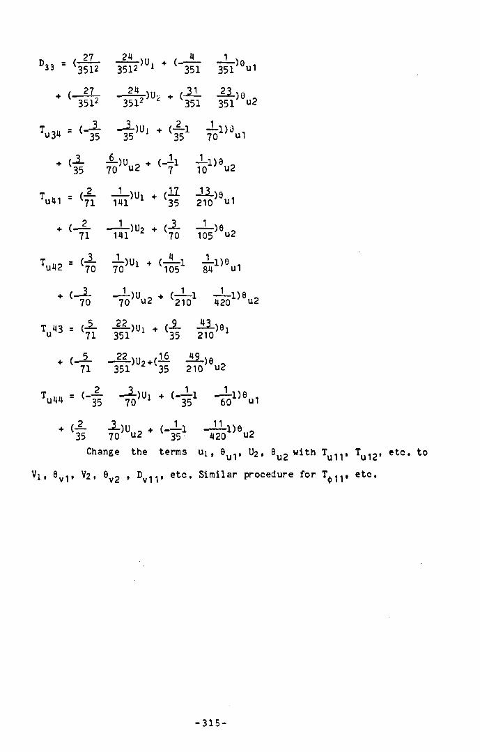
D33 = (3512 3512>U1 + ( 351 35l)0u1

( _ U L 24oc i 2■)U2 + { - ÿ - ^ r )0 .

Tu34 = - á )u* + 70l)0u1

♦ ( i35 70>Uu2 + ‘ "71 & > '. *

*u41 " l7i ^ )Ul * -Ü-Î9 ,35 210 u1

♦ ' - è t ï ï )U2 + (70 T05>0u2

*u42 " 70 * TÖ?1 841)6u1

♦ ( - Ì70 "70)Uu2 “ 5B1 ^ 1)0U2

V 3 * ♦351

■ (-2- JU-)8l35 210 1

-^-)U2+( 351 ¿l i J i je ,35 210 u2

Tu44 = —2-)Ui 70 ‘ ' - à 1 -Ïïïl,6u1

♦ (-2-35 ^ )Uu2 * _42O1)0u2Change the terms u i, 8u1, U2 , 0u2 with Tu11, Tu 2 » • to

V i . e v l . v2 , 0v2 * Dv11» e tc * Similar procedure for T ^ , etc .

-315-