Three-Dimensional Motion Tracking using ClusteringAndrew Zastovnik and Ryan Shiroma

Dec 11, 2015

Abstract

Tracking the position of an object in three dimensional space is a fascinating problem with many realworld applications. With applications ranging anywhere from tracking the positions of people on securitycameras to finding the distance and relative velocities of stars. In this paper we will be discussing a methodof three dimensional motion tracking which uses clustering. The two clustering algorithms we will be usingare K-means and spectral clustering. We will then discuss how this information is used in position tracking.Finally, we will discuss our results and ideas for future work.

1 IntroductionOur motivation for this project idea was to identifysome of the advantages and disadvantages of cluster-ing techniques to real world applications. Theoreti-cally we assumed it was possible to generate 3D pro-jections from image segmentation results but whetherwe’d get practical results was unknown. While other,faster, non-clustering motion tracking methods exist,we wanted to check the feasibility of using clusteringmethods from class to image segment and generate3D projections from our clustering results. In this pa-per we explore two different clustering methods andthe problems we faced in each.

2 DatasetThe two datasets we will be using are videos of usmoving our hands around in three dimensions. Inboth videos the background is a solid color and freeof noise to simplify our methods. Another thing tonote is that our hands are in high contrast with therest of the image. We did this to ensure we would beable to use our clustering techniques to segment theimage correctly.

(a) Dataset 1 (b) Dataset 2

Figure 1: Our two homemade datasets

3 Clustering MethodsBefore we can calculate 3D projections, we’ll firstneed to image segment the object to track. For thepurposes of this paper we only attempt to segmentone object within the frame. Given that assump-tion, we tried two clustering methods, k-means andspectral clustering, each of which has their own ad-vantages and disadvantages. Which method to ulti-mately use depends on the needs of the application.

3.1 K-MeansWe’ll first start with the k-means style clustering. K-means in this particular application has two clusters,one object and one background. With just two clus-ters, k-means reduces to simple thresholding on theintensity values of the image. The value of the thresh-old is effectively set using k-means on these pixel in-tensities.

Figure 2: Intensities by pixel location

We would expect to see the object segmented quiteeasily as long as the object and the background are

1

3 CLUSTERING METHODS 2

homogeneous but of different respective intensities.To run k-means on the image we’ll just need to col-lect each pixel’s intensity with each being its ownobservation in Z1 (its pixel intensity between 1-255).

Figure 3: k-means (k=2) → simple thresholding

This can be extended to color images by using allthree color values and running k-means on data inZ3(red, green, and blue intensities).The main advantages of this method are its speed andits simplicity. We can run k-means on a 100 × 100resolution image in a fraction of a second.

Figure 4: k-means Clustering Results

3.2 Spectral ClusteringSpectral clustering offers more flexibility in imagesegmentation at the expense of computational timeand having to set parameters. Instead of requiringthat clusters be homogeneous in pixel intensity, wejust require a contrast in pixel intensity at the edgesof a given cluster.

3.2.1 Image Spectral Clustering Issues

Since large images contain an enormous amount oftotal pixels (observations), using spectral techniquesbecome increasingly computationally expensive. Ifwe go from an image size n×m to 2n×2n, the number

of pixels increases from nm to 4nm. Thus a similar-ity matrix between all pixels increases from nm×nmto 4nm×4nm. The computational complexity of cal-culating eigenvalues/vectors in MATLAB will be atleast O(n2), where n = 4nm. As you can imagine,computational time(and memory required) increasesfaster than what is practical. Due to this dimension-ality problem, we’ve added a preliminary step to re-duce the dimensionality of the image before the spec-tral clustering step.

3.2.2 Algorithm

One way to reduce the number of “observations” priorto the spectral clustering step is to generate super-pixels using the SLIC algorithm [1]. An image suit-able for clustering is by nature full of adjacent pixelswith similar intensity values. This redundancy allowsus to collapse similarly colored areas into individual“super-pixels”. The SLIC method essentially runs k-means on the image where k clusters are initially po-sitioned in a regular grid interval. It uses intensityas well as pixel location. Since k-means is generallylinear in computational complexity, the issue of di-mensionality has been reduced considerably.

Figure 5: super-pixel locations

Once we have k super-pixels, we now need to com-pute similarities between each super-pixel. Since wecan assume that a cluster will always be contiguouswe only need to compute similarities between adja-cent super-pixels.

S(pi, pj) =

{e−

(DB2σ2

)pi and pj are adjacent

0 else

We also know that each super-pixel is made up ofa sample of pixels with a range of intensities. So one

3 CLUSTERING METHODS 3

way to compare similarity is to compute the similar-ity between the distributions of the pixel intensities.One measure suggested by Tung is to use the Bhat-tacharyya distance [2].

DB(p, q) = −ln( ∑

x∈X

√p(x)q(x)

)

where p(x) is the discrete probability distributionof super-pixel p, and q(x) is the discrete probabilitydistribution of super-pixel q.

Figure 6: each super-pixel is only “similar” to adja-cent super-pixels

When the distributions closely overlap this dis-tance will approach 1, while nonoverlapping distribu-tions will approach 0. With intensity values rangingbetween 1 and 255, it may be hard to achieve a goodidea of the shape of the distribution unless we have alarge number of pixels in every super-pixel. To solvethis issue we bin the samples into 16 equally spacedbins.

Figure 7: distribution for a “background” super-pixel(before binning)

Figure 8: distribution for a “hand” super-pixel (be-fore binning)

We can now create a k × k affinity matrix whichwe can pass on to a spectral clustering function, inthis case we used normalized cuts [3]. The resultingimage segmentation is very clean but takes slightlylonger to run than the k-means segmentation.

(a) Original (b) Segmented

Figure 9: Super-Pixel Spectral Clustering Results

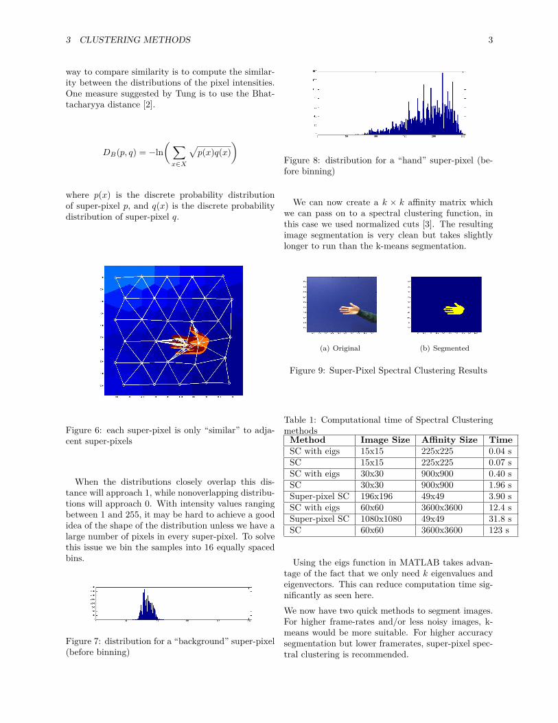
Table 1: Computational time of Spectral Clusteringmethods

Method Image Size Affinity Size TimeSC with eigs 15x15 225x225 0.04 sSC 15x15 225x225 0.07 sSC with eigs 30x30 900x900 0.40 sSC 30x30 900x900 1.96 sSuper-pixel SC 196x196 49x49 3.90 sSC with eigs 60x60 3600x3600 12.4 sSuper-pixel SC 1080x1080 49x49 31.8 sSC 60x60 3600x3600 123 s

Using the eigs function in MATLAB takes advan-tage of the fact that we only need k eigenvalues andeigenvectors. This can reduce computation time sig-nificantly as seen here.We now have two quick methods to segment images.For higher frame-rates and/or less noisy images, k-means would be more suitable. For higher accuracysegmentation but lower framerates, super-pixel spec-tral clustering is recommended.

4 3-D PROJECTION 4

4 3-D ProjectionNow that we have our clusters, how can we use thisinformation to find the three dimensional position ofout object? First let’s recap what we information wehave at this point. The first thing we know is the fieldof view of our camera because we are able to look itup online. Another thing we know from our camera isthe total number of pixels in the image (n×m pixels).The next parameter we need is a little strange. Ifwe are interested in returning real measurements weneed to know the radius of a circle with the samesurface area as our object. Otherwise we can putany number into this parameter and track relativeposition changes. The final parameter is the numberof pixels that out object in occluding in our imagewhich we found out in our clustering step. After weknow all these parameters we can plug them into ourprojection function which we will discuss next.

Figure 10: An object obstructing the field of view

The first coordinate we want to find is the z co-ordinate which is the distance from our camera tothe object. We will be using trigonometry to relatethe four parameters we discussed previously to the zcoordinate.

(# pixels in cluster)n×m

=πd2

πD2√(# pixels in cluster)

n×m=

d

D

sin(θ1) =d

z, sin(θ2) =

D

z

where θ1 is the angle of the object’s obstructionand θ2 is the angle of the FOV of the camera. d issupplied by the user as an estimated initial wifth ofthe object (in inches, cm, etc.).

θ1 = arcsin(sin(θ2)d

D

z = d · tan(θ1)

The formulas for the x and y coordinates followsimilarly.

Figure 11: projection in the x direction(similarly inthe y axis)

θx1 = arcsin( d

D/2θx2)

x = z · sin(θx1)

where D is now defined to be D = n (width of theimage in pixels)The y position will be calculated the same way butwith D = m (height of the image in pixels)

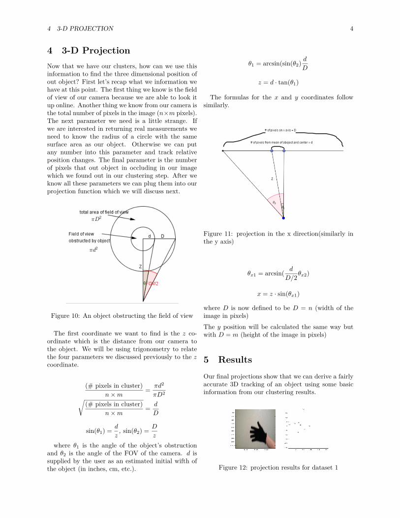
5 ResultsOur final projections show that we can derive a fairlyaccurate 3D tracking of an object using some basicinformation from our clustering results.

Figure 12: projection results for dataset 1

6 FUTURE WORK 5

Figure 13: projection results for dataset 2

Figure 14: 3D view of the final tracking

6 Future WorkThere are many ideas we had in order to improve ourmodel but we unfortunately didn’t have time to im-plement them all. If we had access to actual 3D datapoints of the object we are trying to track we couldoptimize our model further. We would also like tobe able to detect the number of objects in our videoautomatically as well as track multiple objects. An-other important problem to be solved is correctingfor a noisy background so that we can track objectsin the real world by creating a more robust clusteringmodel for this type of application. Finally, we wouldlike to use a filter of some kind to account for noisein our position estimates. Lastly, we would like touse these tracking points to predict future object lo-cations within the image frame. If we could predicta future location, we could possibly reduce the clus-tering phase down to a subimage where the object islikely to be.

References[1] Radhakrishna Achanta. Slic superpixels. Techni-

cal report, EPFL Technical Report, June 2010.

[2] D. Clausi F. Tung, A. Wong. Enabling scalablespectral clustering for image segmentation. Pat-tern Recognition, 43:4069–4076, 2010.

[3] J. Shi and J. Malik. Normalized cuts and imagesegmentation. PAMI, 22(8):888–905, 2000.