Three-Dimensional Modeling and Control of aTethered UAV-Buoy SystemAhmad Kourani ( ahk42@mail.aub.edu )

American University of Beirut https://orcid.org/0000-0002-2626-8545Naseem Daher

American University of Beirut https://orcid.org/0000-0002-3292-0261

Research Article

Keywords: Marine Robotics, Tethered UAVs, Motion Control, Floating Object Manipulation.

Posted Date: December 1st, 2021

DOI: https://doi.org/10.21203/rs.3.rs-1100475/v1

License: This work is licensed under a Creative Commons Attribution 4.0 International License. Read Full License

Springer Nature 2021 LATEX template

Three-Dimensional Modeling and Control of a Tethered

UAV−Buoy System

Ahmad Kourani1 and Naseem Daher2*

1Department of Mechanical Engineering, American University of Beirut, Riad El-Solh, Beirut,

1107 2020, Beirut, Lebanon, ORCID: 0000-0002-2626-8545.2*Department of Electrical and Computer Engineering, American University of Beirut, Riad

El-Solh, Beirut, 1107 2020, Beirut, Lebanon, ORCID: 0000-0002-3292-0261.

*Corresponding author(s). E-mail(s): nd38@aub.edu.lb;

Contributing authors: ahk42@mail.aub.edu;

Abstract

This work presents the nonlinear dynamical model and motion controller of a system consisting of an unmanned

aerial vehicle (UAV) that is tethered to a floating buoy in the three-dimensional (3D) space. Detailed models of

the UAV, buoy, and the coupled tethered system dynamics are presented in a marine environment that includes

surface-water currents and oscillating gravity waves, in addition to wind gusts. This work extends the previously

modeled planar (vertical) motion of this novel robotic system to allow its free motion in all three dimensions.

Furthermore, a Directional Surge Velocity Control System (DSVCS) is proposed to allow both the free movement

of the UAV around the buoy when the cable is slack, and the manipulation of the buoy’s surge velocity when

the cable is taut. Using a spherical coordinates system centered at the buoy, the control system commands the

UAV to apply forces on the buoy at specific azimuth and elevation angles via the tether, which yields a more

appropriate realization of the control problem as compared to the Cartesian coordinates, where the traditional x-,

y-, and z-coordinates do not intuitively describe the tether’s tension and orientation. The proposed robotic system

and controller offer a new method of interaction and collaboration between UAVs and marine systems from a

locomotion perspective. The system is validated in a virtual high-fidelity simulation environment, which was

specifically developed for this work, while considering various settings, operating conditions, and wave scenarios.

Keywords: Marine Robotics, Tethered UAVs, Motion Control, Floating Object Manipulation.

1 Introduction

Teams of unmanned aerial vehicles (UAVs) and un-

manned surface vehicles (USVs) harness the advan-

tages of each vehicle to form a superior robotic

system. To face challenges brought by flood disas-

ters [29], marine oil spill events [10, 22], search and

rescue [4, 21], monitoring and patrol [9], and water

surface cleanup [11], amongst others, heterogeneous

UAV-USV systems have been employed.

The advantages of combining UAVs and USVs

have been explored in literature [14, 29] based on

their complementary abilities. UAVs are advantageous

given their wide field of vision and bird’s-eye view,

higher maneuverability, flexibility, and ease of deploy-

ment; on the other hand, USVs are advantageous in

their durability, extended running time, and large load-

carrying capacity. For instance, to deal with flooding

disasters, the advantage of a UAV’s wide-angle view

of the environment, including the visual horizon, was

1

Springer Nature 2021 LATEX template

combined with the long cruising ability of a USV to

overcome their individual shortcomings, thus allow-

ing the creation of a system with higher efficiency

and lower risk in Search and Rescue (SAR) operations

[29].

UAVs and USVs can form a dexterous robotic

team in the marine environment, as evidenced by the

various applications considered in the literature. A

heterogeneous robotic swarm was considered in [21],

where UAVs are used to generate and transmit path-

planning information in addition to full area maps

for USV agents to perform rescue missions. Further

cooperation between the two vehicle systems can be

achieved via additional sensing and control schemes,

among which is the aerial visual tracking of the USV.

One control solution for robust visual tracking was

proposed in [9], and going further, even visual pose es-

timation of the USV is made possible using the UAV’s

on-board camera as proposed in [4]. If they get within

close proximity, UAVs can perform coordinated tra-

jectory tracking of USVs as in [26], and they can

target-track them to prioritize the camera tilt over the

UAV’s motion while maintaining continuous monitor-

ing of the USV [17]. Physical interaction is another

aspect of the heterogeneous UAV-USV system. For in-

stance, the USV can serve as a landing platform for

the UAV [23], power transmission from a USV to a

UAV can be achieved through an umbilical power ca-

ble [24], and even floating object manipulation can be

made through a tethered UAV system [14].

In addition to using robotic manipulators, a UAV

can interact with its environment via a tether [19, 20],

as it is flexible, extendable, light-weight, and can

transmit tensile forces. Recently, there have been sev-

eral advances and studies on the tethered UAV prob-

lem. A tethered power system for UAVs was proposed

in [2] and is now commercially available [7]. Such

a system can be optimized to suit the special case

of a continuously oscillating marine power station as

studied in [24]. A tethered UAV is also useful in in-

formation transmission. For instance, it plays a keys

role in the emergency marine communication network

proposed in [28], where it takes off from the communi-

cation support ship to secure a wide network coverage,

while being fed with bandwidth and power to sus-

tain its location. To address the challenge presented

by wind gusts in the open marine environment, which

can affect the stability of tethered systems, few works

can be found on the effect of wind disturbances on the

tether and the UAV’s stability [19], and on the tether

vibration [27]. To simplify the analysis of the tether

dynamics, the system was modeled as a multi-element

body in [3].

Beyond the use of a tether for power or infor-

mation transmission, it can transmit tensile forces

whereby a UAV can control the magnitude and di-

rection of the link/tether force, which was proven to

be a set of differentially flat outputs of tethered UAV

systems in [25]. A practical example of force trans-

mission is found in [18], where the transportation of a

payload is cooperative performed by a team of UAVs,

which was made possible through calculation of the

required wrench set. The clever use of a tether even al-

lowed a single UAV to lift a heavy object after hooking

itself at high ground then activating its on-board winch

[12]. Furthermore, a UAV was employed in [14] to

manipulate a floating object’s surge velocity by means

of tether in a 2D space (vertical plane), even in the

presence of waves and water currents.

Amongst the various applications on a force-

transmitting tethered UAV, the emerging marine lo-

comotive tethered UAV−buoy system introduced in

[14] offers a new type of interaction between a UAV

and floating objects including USVs, which provides

a force interconnection between the elements of the

system in addition to power and information transmis-

sion. The potential of this marine robotic system is yet

to be fully discovered, and features a wide range of ap-

plications such as search and rescue, floating sensors

manipulation, water surface cleanup, and building and

inspecting marine structure, to only name a few.

The 2D-planar model of the tethered UAV−buoy

system that was proposed in [14] presented a thorough

analysis of the system’s motivation, its potential ap-

plication, the subsystem’s dynamics and the systems’

stability, the effect of waves, the proposed working

bounds, steady-state values of the system states, and

several practical considerations for implementing the

system. However, the 2D tethered UAV−buoy model

does not capture the complete dynamics of the real

system. For instance, the 2D model has limited rep-

resentations of the Euler angles of both the UAV and

the buoy, it does not encompass composite waves and

currents with varying directions, and it does not al-

low the system to follow trajectories that are in the

3D space. In addition, the orientation of the buoy is

not captured in the 2D-planar model, which can de-

viate from the actual direction of the tether. Finally,

the designed Surge Velocity Control System (SVCS)

in [14] does not include the tether’s azimuth angle

within its controlled state variables, thus the controller

is unable to provide directional manipulation of the

Springer Nature 2021 LATEX template

itle 3

buoy in the horizontal plane if deployed on a 3D

model. Therefore, for real world application, it is nec-

essary to extend the 2D planar model of the tethered

UAV−buoy system to the 3D space, so that it includes

all position and orientation states of the UAV, the buoy,

and the tether, as well as the surface water model.

The contributions of this paper are presented next.

First, we extend the model of the 2D-planar teth-

ered UAV−buoy system dynamics to the 3D space

by incorporating the full six degrees-of-freedom (6-

DOF) rigid-body model for each of the UAV and buoy,

and a 2-DOF model of the tether, to arrive at a 11-

DOF dynamical model that allows for a more realistic

representation of the system’s physics. Second, the

ocean/sea environment is modeled to include not only

the surface water current, but also the full effect of

oscillating gravity waves, even in the vertical direc-

tion. Third, a rigorous mathematical derivation of the

composite system is presented through the Lagrangian

formulation, while defining the required conditions

and constraints to regulate the system’s motion. Forth,

a spherical coordinates-based dual controller is de-

signed to allow the free movement of the UAV around

the buoy while the tether is slack, and to manipulate

the buoy’s surge velocity while the tether is taut. This

controller allows the UAV to apply directional tension

through the tether on the buoy so that it can trigger

motion in all directions of the water surface.

The remainder of this paper is organized as fol-

lows. Section 2 presents a multi-physics description

of the 3D tethered UAV−buoy system components

and the water environment. Section 3 introduces the

control system design for controlling the relative

UAV−buoy position and the buoy’s surge velocity.

Comprehensive numerical co-simulation results of the

derived system model and designed control system are

presented in Section 4. Section 5 closes the paper with

with a conclusion and identifies future development

tracks.

2 Tethered UAV−Buoy System

Dynamical Model

The heterogeneous marine robotic system of a teth-

ered UAV−buoy system has multi-physics elements,

which must be integrated with a proper definition

of the marine environment that it operates in. This

section defines the system components and their in-

terconnection including the water environment, the

USV/buoy, the tether, and the UAV, and it finally

Wave profile

z

xw

Io

y

r

lrGH,b

rGB

ob

φ

FB

mbg

Db

ru

br

'w

α

Rτ

fR

T gmu

ou

T

rGH,u

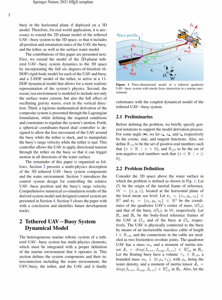
Figure 1 Three-dimensional model of a tethered quadrotor

UAV−buoy system with tensile force interaction in a marine envi-

ronment.

culminates with the coupled dynamical model of the

tethered UAV−buoy system.

2.1 Preliminaries

Before defining the problem, we briefly specify gen-

eral notations to support the model derivation process.

For some angle (•), we let c•, s•, and t• respectively

be the cosine, sine, and tangent functions. Also, we

define R>0 to be the set of positive-real numbers such

that x ∈ R | x > 0, and R≥0 to be the set of

non-negative real numbers such that x ∈ R | x ≥0.

2.2 Problem Definition

Consider the 3D space above the water surface in

which the problem is defined as shown in Fig. 1. Let

OI be the origin of the inertial frame of reference,

W = x, y, z, located at the horizontal plane of

the local mean sea level. Let ru = xu, yu, zu ∈R

3 and rb = xb, yb, zb ∈ R3 be the coordi-

nates of the quadrotor UAV’s center of mass, (Ou),

and that of the buoy, (Ob), in W , respectively. Let

Bu and Bb be the body-fixed reference frames of

the UAV at Ou, and of the buoy at Ob, respec-

tively. The UAV is physically connected to the buoy

by means of an inextensible massless cable of length

l ∈ R>0, and the connections to the cable are mod-

eled as two frictionless revolute joints. The quadrotor

UAV has a mass mu and a moment of inertia ten-

sor Ju = diag(Ju,xx, Ju,yy, Ju,zz) ∈ R3>0 in Bu.

Let the floating buoy have a volume gb ∈ R>0, a

bounded mass mb ∈ (0, ρwgb), with ρw being the

water density, and a moment of inertia tensor Jb =diag(Jb,xx, Jb,yy, Jb,zz) ∈ R

3>0 in Bb. Also, let the

Springer Nature 2021 LATEX template

orientation of Bu and Bb with respect to W be de-

scribed by the Euler angles Ξu = [φu, θu, ψu]⊺ and

Ξb = [φb, θb, ψb]⊺ ∈ (−π, π]3, respectively. Let

Vu = [uu, vu, wu]⊺ ∈ R

3 and Ωu = [pu, qu, ru]⊺ ∈

R3 be the UAV’s linear and angular velocities in Bu,

respectively; and let Vb = [ub, vb, wb]⊺ ∈ R

3 and

Ωb = [pb, qb, rb]⊺ ∈ R

3 be the buoy’s linear and an-

gular velocities in Bb, respectively. Furthermore, let

the translational velocity transformation matrix from

any body frame, B•, to W be described as:

R1,• =

cθ•cψ•− sφ•

sθ•sψ•−cφ•

sψ•sθ•cψ•

+ sφ•cθ•sψ•

cθ•sψ•+ sφ•

sθ•cψ•cφ•

cψ•sθ•sψ•

− sφ•cθ•cψ•

−cφ•sθ• sφ•

cφ•cθ•

,

(1)

and the rotational velocity transformation matrix from

W to any body frame be described as:

R2,• =

cθ• 0 −cφ•sθ•

0 1 sφ•

sθ• 0 cφ•cθ•

. (2)

We also define the rotation matrix about the vertical

z-axis only (yaw) from one body frame, B•, to W as:

Rz• =

cψ•−sψ•

0sψ•

cψ•0

0 0 1

. (3)

Both the UAV and the buoy are subject to cable

tension, T ∈ R≥0, and to gravitational acceleration,

g. The tensile force is applied on the tether hinge in

each platform located at distances, rGH,u and rGH,b,

for the UAV and the buoy, measured in their individ-

ual body frames, respectively. Moreover, the UAV’s

propulsion is described by the input vector uu =[u1, u2, u3, u4]

⊺ ∈ R4 including the thrust force vector

fu = [0, 0, u1]⊺ ∈ R

3≥0, and three torques that induce

a rotational motion about each of the body frame axes

such that τu = [u2, u3, u4]⊺ ∈ R

3. The dynamics of

the UAV actuators (motor propellers) are neglected in

the modeling given that their response time is consid-

erably smaller than that of the UAV (> 10X). Finally,

the buoy is subjected to hydrodynamic and hydrostatic

forces that are subsequently described.

w'

z

x

y

o'r

φ

α

αe

r

φe

e

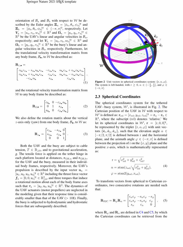
Figure 2 Unit vectors in spherical coordinates system: r, α, ϕ.

The system is left-handed, with r ≥ 0, α ∈ (−π

2, π

2], and ϕ ∈

(−π, π].

2.3 Spherical Coordinates

The spherical coordinates system for the tethered

UAV−buoy system, W ′, is illustrated in Fig. 2. The

Cartesian position of the UAV in W with respect to

W ′ is defined as: rrel = [xrel, yrel, zrel]⊺ = ru − rb ∈

R3, where the subscript (rel) denotes ‘relative.’ We

let its spherical coordinates in W ′, r = [r, 0, 0]⊺,

be represented by the triplet r, α, ϕ with unit vec-

tors er, eα, eϕ, such that the elevation angle α ∈[−π/2, π/2] is defined between r and the horizontal

plane, and the azimuth angle ϕ ∈ (−π, π] is defined

between the projection of r on the x, y plane and the

positive x-axis, which is mathematically represented

as:

r =√

x2rel + y2rel + z2rel,

α = atan(zrel/√

x2rel + y2rel),

ϕ = atan2(yrel, xrel).

(4)

To transform vectors from spherical to Cartesian co-

ordinates, two consecutive rotations are needed such

that:

RS2C = RϕRα =

cαcϕ −sαcϕ −sϕcαsϕ −sαsϕ cϕsα cα 0

, (5)

where Rϕ and Rα are defined in C4 and C5, by which

the Cartesian coordinates can be retrieved from the

Springer Nature 2021 LATEX template

itle 5

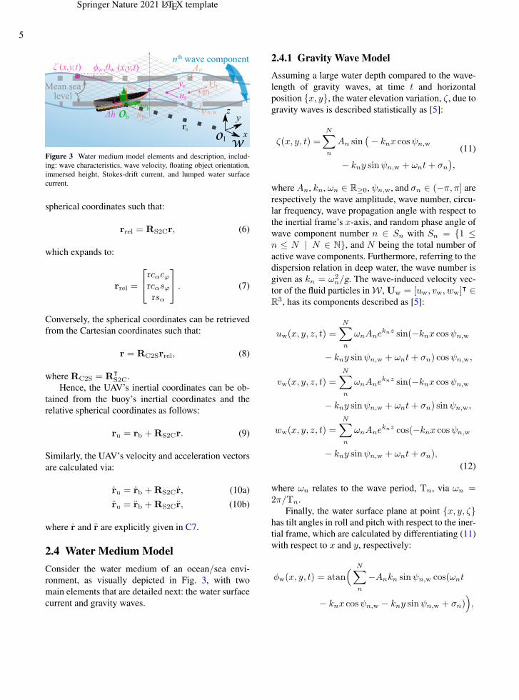
n wave componentth

z

xw

Io

y

Mean sealevel

ob

br

wwvw

uw

Ulψl

Anζ (x,y,t) ϕ ,θ (x,y,t)w w

vs

us

ψn,wψb

Δh

Figure 3 Water medium model elements and description, includ-

ing: wave characteristics, wave velocity, floating object orientation,

immersed height, Stokes-drift current, and lumped water surface

current.

spherical coordinates such that:

rrel = RS2Cr, (6)

which expands to:

rrel =

rcαcϕrcαsϕrsα

. (7)

Conversely, the spherical coordinates can be retrieved

from the Cartesian coordinates such that:

r = RC2Srrel, (8)

where RC2S = R⊺

S2C.

Hence, the UAV’s inertial coordinates can be ob-

tained from the buoy’s inertial coordinates and the

relative spherical coordinates as follows:

ru = rb +RS2Cr. (9)

Similarly, the UAV’s velocity and acceleration vectors

are calculated via:

ru = rb +RS2Cr, (10a)

ru = rb +RS2Cr, (10b)

where r and r are explicitly given in C7.

2.4 Water Medium Model

Consider the water medium of an ocean/sea envi-

ronment, as visually depicted in Fig. 3, with two

main elements that are detailed next: the water surface

current and gravity waves.

2.4.1 Gravity Wave Model

Assuming a large water depth compared to the wave-

length of gravity waves, at time t and horizontal

position x, y, the water elevation variation, ζ, due to

gravity waves is described statistically as [5]:

ζ(x, y, t) =

N∑

n

An sin(

− knx cosψn,w

− kny sinψn,w + ωnt+ σn)

,

(11)

whereAn, kn, ωn ∈ R≥0, ψn,w, and σn ∈ (−π, π] are

respectively the wave amplitude, wave number, circu-

lar frequency, wave propagation angle with respect to

the inertial frame’s x-axis, and random phase angle of

wave component number n ∈ Sn with Sn = 1 ≤n ≤ N | N ∈ N, and N being the total number of

active wave components. Furthermore, referring to the

dispersion relation in deep water, the wave number is

given as kn = ω2n/g. The wave-induced velocity vec-

tor of the fluid particles in W , Uw = [uw, vw, ww]⊺ ∈

R3, has its components described as [5]:

uw(x, y, z, t) =

N∑

n

ωnAneknz sin(−knx cosψn,w

− kny sinψn,w + ωnt+ σn) cosψn,w,

vw(x, y, z, t) =

N∑

n

ωnAneknz sin(−knx cosψn,w

− kny sinψn,w + ωnt+ σn) sinψn,w,

ww(x, y, z, t) =

N∑

n

ωnAneknz cos(−knx cosψn,w

− kny sinψn,w + ωnt+ σn),

(12)

where ωn relates to the wave period, Tn, via ωn =2π/Tn.

Finally, the water surface plane at point x, y, ζhas tilt angles in roll and pitch with respect to the iner-

tial frame, which are calculated by differentiating (11)

with respect to x and y, respectively:

φw(x, y, t) = atan(

N∑

n

−Ankn sinψn,w cos(ωnt

− knx cosψn,w − kny sinψn,w + σn))

,

Springer Nature 2021 LATEX template

θw(x, y, t) = atan(

N∑

n

−Ankn cosψn,w cos(ωnt

− knx cosψn,w − kny sinψn,w + σn))

.

(13)

2.4.2 Water Current

The water surface current acts in the x, y (horizon-

tal) plane of W , such that Uc = [uc, vc, 0]⊺ ∈ R

3, and

is given as:

Uc = Us +Ul, (14)

where Us = [us, vs, 0]⊺ ∈ R

3 is generated from

Stokes drift [6], with its components in the inertial

frame, W , defined as:

us(z) =

N∑

n

cosψn,wA2nωnkne

2knz,

vs(z) =

N∑

n

sinψn,wA2nωnkne

2knz,

(15)

and Ul = [ul, vl, 0]⊺ ∈ R

3 is the resulting sum

of other water current components, determined as

follows:

ul = Ul cosψl,

vl = Ul sinψl,(16)

where Ul and ψl are the average velocity and direction

of the current in W , respectively.

2.5 Buoy’s Dynamic Model

Various types of forces affect the buoy’s motion, with

a major contribution from restoration, damping, and

radiation forces. These forces substantially depend on

the immersed volume of the buoy, gim ∈ [0,gb],which is a function of the buoy’s elevation, defined

as ∆h = ζ(xb, yb, t) − zb. Let the vector from the

buoy’s center of gravity to its center of buoyancy in

W be defined as rGB = [xGB, yGB, zGB]⊺ ∈ R

3,

where the buoyancy force is applied such that FB =[0; 0; ρwggim]. Additionally, let the tether hinge lo-

cation with respect to the buoy’s center of gravity be

defined in Bb as rGH,b = [xGH,b, yGH,b, zGH,b]⊺ ∈

R3, as seen in Fig. 1, where the cable tension is applied

to the buoy in W ′, such that T ′b = [T, 0, 0]⊺.

Assumption 1 The water-buoy friction dominates the air-

buoy friction, thus we neglect the air drag on the buoy.

Consider the buoy dynamics in Bb, and let its state

vector be νb = [ν1,b; ν2,b], where ν1,b = Vb and

ν2,b = ωb. Applying Newton’s second law of motion

gives:

M′bνb +C

′bνb +D

′bνb +G

′b = τ ′

b, (17)

where M′b, D

′b, and C

′b ∈ R

6×6 are respectively

the buoy’s inertia, damping, and Coriolis matrices

expressed in Bb; νb = [ν1,b; ν2,b] is the rela-

tive velocity vector, with ν1,b = ν1,b − (Uw +R

⊺

ψwUs + R

⊺

ψlUl), and ν2,b = ν2,b; the gravi-

tational forces and moments vector are included in

G′b ∈ R

6; and the external forces and moments are

captured in τ ′b ∈ R

6. The inertia matrix expands as

M′b = [M′

1,b,O3; O3,M′2,b], where O3 ∈ R

3×3

is the null matrix, M′1,b = mbdiag(1, 1, 1) + a1,b,

M′2,b = Jb + a2,b, with a1,b = diag(a11, a22, a33)

and a2,b = diag(a44, a55, a66) ∈ R3×3 being the

generalized added mass matrices. The Coriolis ma-

trix, which depends on M′b, is calculated as C

′b =

[O3,C′12,b; C

′21,b,C

′2,b], where:

C′12,b = C

′21,b =

0 (mb + a33)wb −(mb + a22)vb−(mb + a33)wb 0 (mb + a11)ub(mb + a22)vb −(mb + a11)ub 0

C′2,b =

0 (Jzz,b)rb −(Jyy,b)qb−(Jzz,b)rb 0 (Jxx,b)pb(Jyy,b)qb −(Jxx,b)pb 0

.

(18)

The buoy’s total damping in Bb is expressed as:

D′b = DS +DP +DW, (19)

where the generalized radiation-induced po-

tential damping matrix is expanded as DP =[b1,b,O3; O3,b1,b] ∈ R

6×6, with b1,b =diag(b11, b22, b33) and b2,b = diag(b44, b55, b66),and DS = diag(DS,1, ..., DS,6) ∈ R

6×6 is the skin

friction matrix, calculated as:

DS,i = CS,iAwt1

2ρw

∣

∣ν1,b,i

∣

∣ , i = 1, 2, 3, (20)

where CS,i ∈ R>0 is the drag coefficient, Awt ∈ R≥0

is the wetted area of the buoy, and DS,4−6 ∈ R≥0 can

be approximated by considering the moments effect

of DS,1−3 over the buoy’s surface. The effect of the

Springer Nature 2021 LATEX template

itle 7

wave drift damping matrix, DW ∈ R3×3, is already

included in the Stokes drift velocity in (15), thus it will

be dropped from (19).

The buoy dynamics in (17) are expressed in Wwith the state vector, ηb = [η1,b; η2,b] where η1,b =rb and η2,b = Ξb, as:

Mbηb +Cbηb +Db˜ηb +Gb = τb, (21)

where Mb, Db, and Cb ∈ R6×6 are the buoy’s in-

ertia, damping, and Coriolis matrices, respectively,

expressed in W; ˜ηb = [˜η1,b;˜η2,b] is the relative ve-

locity vector, with ˜η1,b := [˜xb, ˜yb, ˜zb]⊺ = η1,b −

(Uw+Uc); Gb and τb are respectively the vectors of

the gravitational and external forces and moments on

the buoy in W given by:

Gb = [0, 0,mbg, 0, 0, 0]⊺,

τb = [τ1,b; τ2,b],

τ1,b = RS2CT′b + FB

= [Tcαcφ, T cαsφ, T sα + ρwggim]⊺,

τ2,b = rGB × FB + (R1,brGH,b)× (RS2CT′b).

(22)

We also define:

Mb = RbM′bR

−1b ,

Db = RbD′bR

−1b ,

Cbηb :=1

2Mbηb,

(23)

where Rb = [R1,b,O3; O3,R−12,b], Mb =

η⊺

b(∂Mb/∂ηb) [6]. Finally, we let Mb,ij , Cb,ij , and

Db,ij , i, j = 1, ..., 6 be elements of Mb, Cb, and

Db, respectively.

2.6 UAV’s Dynamic Model

We let the UAV’s thrust vector in the Cartesian frame,

fu,C = [ux, uy, uz]⊺, be calculated as:

fu,C = R1,ufu, (24)

with its elements being explicitly represented as:

ux = u1(sθucψu+ sφu

cθusψu),

uy = u1(sθusψu− sφu

cθucψu),

uz = u1(cφucθu).

(25)

In the spherical frame, the UAV’s thrust vector, fu,S =[ur, uα, uϕ]

⊺, is expressed as:

fu,S = RC2Sfu,C, (26)

with the element ur, uα, and uϕ being explicitly

represented in C8.

The tether’s tension on the UAV expressed in W ′,

T ′u = [−T, 0, 0]⊺, is applied at location rGH,u =

[xGH,u, yGH,u, zGH,u]⊺ ∈ R

3 in Bu, representing

the distance from the UAV’s center of gravity to its

tether hinge. Finally, the local wind speed that dis-

turbs the UAV’s motion is defined in W as Uwd =[uwd, vwd, 0]

⊺ .

The quadrotor UAV system dynamics in W are ob-

tained from Newton’s second law of motion with the

state vector ηu = [η1,u; η2,u], where η1,u = ru and

η2,u = Ξu, yields:

M1,uη1,u +C1,uη1,u +D1,u˜η1,u +G1,u = τ1,u + δ1,u,

M2,uη2,u +C2,uη2,u +D2,u˜η2,u +G2,u = τ2,u + δ2,u,

(27)

where:

M1,u = mudiag(1, 1, 1), D1,u = R1,uD′1,uR

⊺

1,u,

C1,uη1,u := O3, G1,u = [0, 0,mug]⊺,

and

M2,u = JuR2,u, D2,u = D′2,uR2,u, G2,u = [0, 0, 0]⊺,

C2,uηu := Ωu × (JuΩu) + Ju

(

∂R2,u

∂φu

φu +∂R2,u

∂θuθu

)

η2,u.

D′1,u = diag(Du,1, Du,2, Du,3) and D

′2,u =

diag(Du,4, Du,5, Du,6) ∈ R3×3≥0 are the UAV’s trans-

lational and rotational damping friction matrices, re-

spectively. The relative velocity vectors of the UAV

are ˜η1,u := [˜xu, ˜yu, ˜zu]⊺ = η1,u −Uwd in translation

and ˜η2,u := [˜φu,

˜θu,

˜ψu]

⊺ = η2,u in rotation. τ1,u and

τ2,u ∈ R3 are vectors of other external forces in W

and moments in Bu of the UAV, respectively, and they

include the rotors’ thrust and tether tension effects,

expressed as:

τ1,u = fu,C +RS2CT′u

=

ux − Tcαcϕuy − Tcαsϕuz − Tsα

,

Springer Nature 2021 LATEX template

τ2,u = τu + (rGH,u)× (R⊺

1,uRS2CT′u). (28)

The damping matrix elements,Du,i, i ∈ 1, ..., 3, are

approximated as:

Du,i = Cu,iAucs,i

1

2ρa

∣

∣

∣

˜νu,i

∣

∣

∣, (29)

whereCu,i ∈ R>0 is a drag coefficient, Aucs,i ∈ R≥0 is

the UAV’s cross-sectional area in the respective plane,

ρa is the air density and ˜νu,i is the UAV-wind rela-

tive velocity in the respective body frame axis. The

adopted model captures the major elements required

to represent the quadrotor in a tethered UAV−buoy

system with slow-to-moderate dynamics, thus acro-

batic maneuvers and their influence on the system

dynamics are not considered. For more details on the

quadrotor UAV model, readers can refer to [30].

2.7 System Constraints

In this section, we generalise the system’s 2D con-

straints presented in [14] to the 3D space. These

constraints help establish the bounds and operating

conditions for when the coupled model of the tethered

UAV−buoy system is applicable.

2.7.1 Taut-Cable Constraint

Since the cable is assumed inextensible, it remains

under tension (taut) at time t if r(t) = l, which is

equivalent to:

T > 0. (30)

We label the tethered UAV−buoy system as ‘coupled’

when (30) is satisfied, and ‘decoupled’ otherwise.

2.7.2 No Buoy-Hanging Constraint

To keep the buoy floating on top of the water surface,

the vertical tension component transmitted from the

UAV through the tether must not exceed the weight

of the buoy, otherwise it will be lifted into the air and

the system will reduce to a UAV with a slung payload.

This is prescribed by:

T < mbg/sα, (31)

as deduced from (21) and (22) at steady-state.

2.7.3 No ‘Fly-Over’ Constraint

‘Fly-over’ occurs when the buoy starts hopping over

wave crests [8]. This phenomenon is avoided if:

gim > 0, (32)

which means that the buoy remains partially immersed

at all times. The ‘fly-over’ phenomenon is related to

the total surface velocity of the buoy, described as:

V =√

u2b + v2b,

ψV = arctan(vb/ub),(33)

where V and ψV are its magnitude and direction

in the horizontal plane, respectively. Next, we de-

fine the wave encounter frequency for the nth wave

component, ωe,n, as [5]:

ωe,n = ωn −ω2nV

gcψw,n−ψV

, n ∈ Sn. (34)

The excitation of the buoy’s heave dynamics at ωe,n

induces ‘fly-over’ if it approaches the heave’s natural

frequency, as interpreted in [14].

2.8 The Tethered UAV−Buoy System

Model

In a coupled form, the tethered UAV−buoy system

dynamics can be formulated by referring to the Euler-

Lagrange formulation, which leverages the results in

Sections 2.3, 2.5, 2.6, and 2.7. First, we define the

Lagrangian function as L(q, q) = K(q, q) − U(q),where K(q, q) ∈ R≥0 and U(q) ∈ R are the ki-

netic and potential energies of the system, with q =[xb, yb, zb, α, ϕ, φu, θu, ψu, φb, θb, ψb]

⊺ ∈ R11 being

the generalized coordinates vector. The equations of

motion of the UAV−buoy system are obtained via:

d

dt

(∂L

∂q

)

−∂L

∂q+∂P

∂q= τ , (35)

where τ ∈ R11 is the external forces and moments

vector. Per Assumption 1, let D be the global damp-

ing matrix formulated based on (23) without including

a wind-induced component, and the dissipative forces

are captured by the power function, P ∈ R, such that∂P∂q

:= D˜q. ˜q is defined as:

˜q = q − [uc + uw, vc + vw, ww,

0, 0, 0, 0, 0, 0, 0, 0]⊺

= [xb − uc − uw, yb − vc− vw, zb − ww,

α, ϕ, φu, θu,ψu, φb, θb, ψb]⊺.

(36)

Springer Nature 2021 LATEX template

itle 9

If tether is assumed to have a negligible mass, the

coupled system’s kinetic energy is obtained as the sum

of the individual energies of the UAV and the buoy as

follows:

K =1

2q⊺

Mq :=1

2η⊺

uMuηu +1

2η⊺

bMbηb, (37)

where the global inertia matrix of the UAV−buoy sys-

tem, M, is formulated by using the elements of Mu

and Mb, as described in (C11). Next, the potential en-

ergy of the system can be formulated by referring to

(22) and (2.6) as:

U = mbg zb +mug(zb + lsα). (38)

The details of the Euler-Lagrange formulation in (35)

are detailed in Appendix D, which finally leads to the

following equations of motion:

Mq +Cq +D˜q +G = τ , (39)

where C represents the global Coriolis matrix, and G

is the global vector of gravity forces and moments.

Assumption 2 The design of a stable buoy is beyond the

scope of this work, and only buoys with inherited stability

are considered. Thus, we assume that the buoy’s center of

buoyancy always lies above its center of gravity, and that the

roll and pitch dynamics of the buoy are damped and stable,

which indicates that Db,44 > 0 and Db,55 > 0. Thus, we

assume that the buoy remains tangent to the water surface.

With Assumption 2 and the dominance of waves

with relatively long periods and moderate heights, the

time derivatives of the buoy’s roll and pitch angles,

φb and θb, are small and thus their effects can be

neglected in M.

Since the tether joints are considered revolute and

frictionless, there is no coupling between the tether’s

rotational motion and the UAV and buoy’s rotational

dynamics, whereas their translational dynamics are

coupled through (9). Additionally, as can be deduced

by inspecting the elements of (35), the UAV and

buoy’s rotational dynamics are independent of each

other, and can still be described by the dynamic mod-

els of their individual systems in (27) and (21), respec-

tively. This is further elaborated in Appendix D. Given

this, the tethered UAV−buoy system coupled dynam-

ics can be represented by the first fives states: xb, yb,

zb, α, and ϕ, which are independent of other rigid

body orientation states that concern either the UAV’s

or the buoy’s dynamics alone. Hereafter, we limit the

representation of the coupled system to the first five

state variables mentioned above, while the UAV and

buoy’s rotational dynamics can still be described by

η2,u in (27) and η2,b in (21), respectively. The inertia

matrix for the coupled system is explicitly represented

as M1−5 = [M1; M2; M3; M4; M5], where:

M1 = [Mb,11 +mu Mb,12 Mb,13

−mulsαcϕ −mulcαsϕ],

M2 = [Mb,21 Mb,22 +mu Mb,23

−mulsαsϕ mulcαcϕ],

M3 = [Mb,31 Mb,32 Mb,33 +mu mulcα 0] ,

M4 =[

−mulsαcϕ −mulsαsϕ mulcα mul2 0

]

,

M5 =[

−mulcαsϕ mulcαcϕ 0 0 mul2c2α

]

.

(40)

The Coriolis matrix is explicitly represented as:

C1−5 =

mul

0 0 0 −cαcϕα+ 2sαsϕϕ −cαcϕϕ0 0 0 −cαsϕα− 2sαcϕϕ −cαsϕϕ0 0 0 −sαα 00 0 0 0 lsαcαϕ0 0 0 −2lsαcαϕ 0

,(41)

and the damping matrix is explicitly represented as:

D1−5 =

Db,11 Db,12 Db,13 0 0Db,21 Db,22 Db,23 0 0Db,31 Db,32 Db,33 0 00 0 0 0 00 0 0 0 0

. (42)

Additionally, the gravitation force vector and external

forces and torques vector are explicitly represented as:

G1−5 = [0, 0, (mb +mu)g,mu g lcα, 0]⊺, (43)

and

τ1−5 = [ux, uy, uz, luα, luϕ]⊺, (44)

respectively. If constraints (30) and (32) are satisfied,

the coupled form of the dynamic model equations is

Springer Nature 2021 LATEX template

given by:

(Mb,11 +mu)xb +Mb,12yb +Mb,13zb

+Db,11˜xb + Db,12

˜xb + Db,13˜zb

−mul(

cαcϕα2 − 2sαsϕαϕ+ cαcϕϕ

2

+ sαcϕα+ cαsϕϕ)

= ux,

(45a)

Mb,21xb + (Mb,22 +mu)yb +Mb,23zb

+Db,21˜xb + Db,22

˜yb + Db,23˜zb

−mul(

cαsϕα2 + 2sαcϕαϕ+ cαsϕϕ

2

+ sαsϕα− cαcϕϕ)

= uy,

(45b)

Mb,31xb +Mb,32yb + (Mb,33 +mu)zb

+Db,31˜xb +Db,32

˜yb +Db,33˜zb

−mul(sαα2 − cαα) + (mu +mb − ρwgim)g = uz,

(45c)

mul(−sαcϕxb − sαsϕyb + cαzb + lsαcαϕ2)

+mul2α+mug(lcα) = luα,

(45d)

mul(−cαsϕxb + cαcϕyb − lsαcααϕ)

+mul2c2αϕ+mug(lcα) = luϕ.

(45e)

After solving the above differential equations, the

UAV’s position and velocity vectors can then be com-

puted from (C9) and (C11), respectively. We note that

if the tether’s weight is to be considered, the tethered

system’s model should be updated as per [15].

3 Control System Design

The control system design problem is defined as ma-

nipulating the surge velocity of the buoy, ub, to track a

desired reference, while orienting the cable in the de-

sired elevation angle, α, and azimuth angle, ϕ. This

allows for applying a tension force in any required

direction, while tracking the desired surge velocity.

As an extension to the Surge Velocity Control Sys-

tem (SVCS) presented in [14], which was designed to

only control ub and α, the herein controller will be

dubbed as Directional Surge Velocity Control System

(DSVCS), given that it adds the pulling force direction

(azimuth angle, ϕ) to its controlled states.

We note that solely controlling these states via set-

point tracking does not yield inertial velocity tracking.

For example, external forces that result in sway mo-

tion (in the direction of the buoy’s body-fixed y-axis)

are not rejected by the controller. That said, the con-

troller with the reduced states can be equipped with

a path planner, which can apply lateral tension by

choosing a specific azimuth angle to counter the exter-

nal forces in the sway direction. Such an architecture

would give the system the ability to track reference

trajectories in the inertial frame, but this is beyond the

scope of this work, thus we stick with the design of the

DSVCS.

3.1 Operational Modes and State

Machine

To complement the surge velocity controller, a

UAV−buoy relative position controller is required to

control the radial distance of the UAV in W ′, r, instead

of ub. Both controllers are part of the DSVCS. In [16],

a state machine was proposed to allow the system to

switch between the coupled and decoupled states by

alternating between the two controllers. In addition,

the state machine can trigger a change in the position-

ing of the UAV with respect to the buoy between front

and rear to change the pulling direction. Contrarily,

in the 3D problem of this work, we only consider the

forward motion of the buoy, while the velocity vec-

tor steering will be handled by changing the cable’s

azimuth angle. The purpose of the state machine is

to allow the system to smoothly couple and decouple

when requested by the controller, which will be suffi-

cient to achieve the goals of the controller in this work.

For that, we adopt the same state-machine of [16],

with the exclusion of the ‘repositioning’ maneuver

trigger part.

3.2 Controller Design

With the inner-loop/outer-loop cascaded structure

shown in Fig. 4, the DSVCS allows tracking of the

states ub, α, and ϕ by orienting and scaling the

UAV’s thrust vector. The setpoint for the controller

is (ub0, zu0, ϕ0) in the buoy’s surge velocity control

mode, and (r0, zu0, ϕ0) in the UAV’s relative position

mode. A prepocessing unit then generates the resulting

α based on zu0, and a smoothed signal for the track-

ing setpoints ub0, r0, and ϕ0. When the control mode

changes, a fast and smooth transition function handles

the switching between the two control laws [14].

The resulting force vector with its three compo-

nents along er, eα, and eϕ is transformed to the

Springer Nature 2021 LATEX template

itle 11

inertial frame to determine the desired UAV’s thrust

vector magnitude and orientation. At this point, the

problem reverts to a basic UAV thrust decoupling

problem, where the resulting thrust vector magnitude

and tilt angles can be easily computed, as shown later,

while the yaw angle remains free to set. Since the UAV

is expected to maintain visual tracking of the buoy,

the controller sets the desired yaw angle to equal the

tether’s azimuth angle.

In summary, and as shown in Fig. 5, the pro-

posed DSVCS can control three main variables: 1)

the relative position between the UAV and the buoy

(outer-loop), 2) the buoy’s surge velocity (outer-loop),

and 3) the UAV’s attitude (inner-loop). A state ma-

chine selects which of the two outer-loop controllers

to activate based on the coupling between the UAV

and buoy.

3.2.1 Reference Signals and Velocity Setpoint

The UAV’s desired motion during a buoy manipula-

tion task is limited to a horizontal plane of constant

elevation (zu0), which reduces the UAV’s power con-

sumption [1] and results in safer and more predictable

paths. This can be achieved by computing the result-

ing reference elevation angle, α, based on the desire

reference elevation, zu, as:

α = asin(

(zu − zb)/r)

. (46)

The azimuth angle is chosen to set the pulling direc-

tion, and the UAV’s yaw angle can be independently

manipulated without affecting the other states; here,

we set it equal to azimuth angle in order to keep the

UAV directed forward while an onboard camera can

still point towards the buoy at all times:

ψu = ϕ. (47)

Note that the steady-state velocity vector of the

buoy in the horizontal plane of W , ψV , does not neces-

sarily point in the same direction as ϕ, since the buoy

is free to slide sideways, such that:

ψV = ϕ+ ǫψ, (48)

where ǫψ is an error angle that is related to the sideslip

angle of the buoy, βu. Finally, the radial position,

r0, and the velocity setpoint, ub0, are smoothed by

low-pass filters of fourth- and second-order, respec-

tively, which results in a smoother performance due to

respecting the system dynamics [25].

3.2.2 UAV−Buoy Relative Position Control

Law (Outer-Loop)

To design the relative position control law, we must

refer to the UAV dynamics in W ′ where the states of

interest are explicitly expressed. If we reorder the re-

alization of ru in (10b) and multiply both sides bymu,

we get:

mur = RC2S(muru)−mu(RC2Srb). (49)

The first right-hand side term of (49) can be seen as

the mapping of the translational terms of (27) into

W ′ (kinetics), and the second one can be seen as the

mapping of the buoy’s linear accelerations into W ′

(kinematics). Expanding (49) yields:

mu(r− rα2 − rc2αϕ2) = ur − T

−mugsα −mu(cαcϕxb+ cαsϕyb + sαzb),

mu(r2α+ 2rrα+ r2sαcαϕ

2) = ruα

−mugrcα −mur(−sαcϕxb− sαsϕyb + cαzb),

mu(r2cαϕ+ 2rcαrϕ− 2r2sααϕ) = ruϕ

−mur(−sϕxb + cϕyb).

(50)

Consider the case of nonzero tension for the rela-

tive position dynamics of the UAV−buoy system’s in

(50), with states vectors X1 = [r, α, ϕ]⊺ and X2 =[r, α, ϕ]⊺, control input vector U = [ur, uα, uϕ]

⊺,

subject to unknown external disturbances including

water currents, gravity waves, and wind gusts. The

equations of motion in the kinetic form are expressed

as:

MdcXdc = ΦdcΘdc +Hdc + bdcU + δdc, (51)

where the subscript (dc) refers to the decoupled dy-

namics, Xdc = X1, the inertia matrix Mdc =mudiag(1, r

2, r2cα), the parameter vector Θdc = T ,

the regressor vector Φdc = [−1; 0; 0], and bdc =diag(1, r, r). δdc represents the vector of lumped mod-

eling errors and disturbances, and the vector Hdc =[Hdc,1; Hdc,2; Hdc,3] represents all of the nonlinear

Euler, Coriolis, centrifugal, and gravitational forces

and moments, and is given by:

Hdc,1 = mu(rα2 + rc2αϕ

2 − cαcϕxb − cαsϕyb

− sαzb − gsα),

Hdc,2 = mur(−2rα− rsαcαϕ2 + sαcϕxb + sαsϕyb

Springer Nature 2021 LATEX template

DSVCS

Preprocessing

Setpoint

r ub

State machine

Outer-loop

UAV-buoy

relative position

Buoy's surge

velocity

Tethered UAV-buoy

Inner-loop(UAV attitude)

u,c

Decoupling

θu,c1,cu,cτ

Measurements

u,cϕ

α,α,r, r, φ,φ,

η2,u 2,uη,

position / velocity control

Outputs:

Outputs:

Outputs:

>> zu0 ub0r0φ

>>

>>

α Tφψu,c

ub b, v u, z , zu,1,bη,bψ

>>

>> α, φ, uψ

>>

,,>>>>

u

, ,

,,,,

,

r

φα

φα

ub

Water medium

effect

Wind effect

Springer Nature 2021 LATEX template

itle 13

which results in V2 = −e⊺

1k1e1 − e⊺

2k2e2. Via Barbalat’s

lemma with Assumption 4, the asymptotic convergence of

V2 to zero is guaranteed. Note that if Assumption 4 is vio-

lated by the presence of strong wave disturbances or wind

gusts, stability and finite tracking error are still achieved by

increasing the controller gains, such that they overcome the

disturbances mismatch effect on V2. Finally, the control law

in the PID-like form in (53) is obtained by substituting e2and Υ in (54), then setting eI1 := δ(γk1)

−1.

3.2.3 Buoy Surge Velocity Control Law

(Outer-Loop)

If the cable is taut, its length becomes constant and rand r can be set to zero. Substituting l for r in (50)

yields the UAV’s motion equations in W ′ in spherical

coordinates notation:

mu(−rα2 − rc2αϕ2) = −mugsα + ur − T

−mu(cαcϕxb + cαsϕyb + sαzb),

mu(r2α+ r2sαcαϕ

2) = −mugrcα + ruα

−mur(−sαcϕxb − sαsϕyb + cαzb),

mu(r2cαϕ− 2r2sααϕ) = ruϕ

−mur(−sϕxb + cϕyb),

(55)

In order to control the buoy’s surge velocity, ub, it

must be explicitly expressed in (55). The buoy’s ac-

celeration in the body frame is described as: ν1,b =R

⊺

1,bη1,b. When waves with relatively long periods

and moderate heights are dominant, the resulting

buoy’s roll and pitch angles are small and cannot be

used by the controller unless a proper measurement

technique is available for the UAV. On the other hand,

the USV/buoy heading can be visually estimated with

good accuracy as was demonstrated in [4]. For this

reason, we limit the transformation of R1,b to yaw

only, such that ν1,b ≈ R⊺

zbη1,b. Hence, xb and yb in

(55) can be transformed into ub and vb accordingly.

Consider the UAV dynamics in W ′ in the coupled

case, while following the spherical coordinates nota-

tion as presented in (55). By choosing the state vector

X ′1 = [ub, α, ϕ]

⊺, we can rewrite (55) in the kinetic

form as:

McpXcp = ΦcpΘcp +Hcp + bcpU′ + δcp, (56)

where the subscript (cp) refers to the coupled dy-

namics, Xcp = X ′1, the control vector U ′ = U ,

the parameter vector Θcp = T , the regressor vec-

tor Φcp = [−1; 0; 0], and bcp = diag(1, r, r). δcp

represents the vector of lumped modeling errors and

disturbances, the inertia matrix is expressed as:

Mcp = mu

cα(cϕcψb+ sϕsψb

) 0 0−rsα(cϕcψb

+ sϕsψb) r2 0

−r(sϕcψb− cϕsψb

) 0 r2cα

,

and the vector Hcp = [Hcp,1; Hcp,2; Hcp,3] repre-

sents all of the nonlinear Euler, Coriolis, centrifugal,

and gravitational forces and moments, with:

Hcp,1 = mu

(

rα2 + rc2αϕ2 − sαzb − gsα

+ cα(cϕsψb− sϕcψb

)vb)

,

Hcp,2 = mur(

− rsαcαϕ2 − cαzb − gcα

− sα(cϕsψb− sϕcψb

)vb)

,

Hcp,3 = mur(

2rαϕsα − (sϕsψb+ cϕcψb

)vb)

.

The state-space model in (56) is formulated as a time-

varying second-order nonlinear system as:

X ′1 = X ′

2,

X ′2 = Φ

′Θ

′ +H ′ + b′U ′ + δ′,(57)

where

b′ = M−1cp bcp, Φ

′ = M−1cp Φcp, Θ

′ = Θcp,

δ′ = M−1cp δcp, H

′ = M−1cp Hcp.

The outer-loop velocity controller manipulates the

state vector X ′1, and a control law for the surge veloc-

ity can be designed in a similar fashion as described

in Section 3.2.2, with a difference that only one step is

required in the backstepping process for the state ub.

Let X ′1 = [ub, α, ϕ]

⊺ be the reference state vector and

e′1 = X ′1 − X ′

1 be the respective state vector error.

The control law is defined as:

U ′ = b′−1[

− k′Pe

′1 − k′

IeI′

1 − k′De

′1

+ ¨X ′∗1 −Φ

′Θ

′ −H ′]

,

eI′

1 = e′1,

(58)

where ¨X ′∗1 = [ ˙ub, ¨α, ¨ϕ]; k′

P = diag(0, 1 +k′1,αk

′2,α + γ′α, 1 + k′1,ϕk

′2,ϕ + γ′ϕ), k′

I =diag(γub

, γαk1,α, γϕk1,ϕ), k′D = k′

1 + k′2, with

k′1 = diag(0, k′1,α, k

′1,ϕ), k

′1,α and k′1,ϕ ∈ R>0,

k′2 ∈ R

3×3>0 , and γ′ = diag(γ′ub

, γ′α, γ′ϕ) ∈ R

3×3>0 , are

controller gains that are defined next; and Θ′ is the

estimate of Θ′.

Springer Nature 2021 LATEX template

Theorem 2 Consider the state-space representation in (57)

of the UAV−buoy’s relative position dynamics in (55) when

the system is coupled. If Assumption 3 holds true, the control

law in (58) generates the thrust vector elements in the spher-

ical reference frame ur, uα, and uϕ, that can stabilize the

outer-loop dynamics of the system, and reduce the tracking

error to a small region neighboring the origin in finite time

for a set of gains k′1, k′

2, and γ′ ∈ R3×3≥0 , defined in a sim-

ilar way to their counterparts in Theorem 1. Additionally, if

Assumption 4 holds, the tracking error is reduced to zero in

finite time.

Proof We employ the backstepping control design, which

involves one step for the ub state, and two steps for the α

and ϕ states. To keep a compact representation of the proof

in vector form, the buoy velocity states are tackled in the

second step. First, the Lyapunov function V ′1 = 1

2e2α + 1

2e2ϕ

is proposed, and let its derivative be expressed as V ′1 =

eαeα + eϕeϕ. We proceed to a second step in the control

design process for the states’ rates given that eα and eϕ do

not include an explicit control input. To stabilize e1, we de-

fine a virtual control input as: Υ′ = ˙X ′∗1 − k′

1e′1, where

k′1 = diag(0, k′1,α, k

′1,ϕ) and ˙X ′∗

1 = [ub, ˙α, ˙ϕ]⊺. Next,

we define the rates error as: e′2 = X ′1 − Υ

′. Note that

the rates error of the buoy velocity’s x-component simply

reduces to e′2,1 = ub − ub.

Here, we define a second Lyapunov function as:

V ′2 =

1

2e2α +

1

2e2ϕ +

1

2e′⊺2 e

′2 +

1

2δ′⊺γ′−1

δ′,

with δ′ = δ′ − δ′, then we differentiate to have:

V ′2 = eαeα + eϕeϕ + e

′⊺2 e

′2 + δ

′⊺γ′−1 ˙

δ′

= eα(e′2,2 − k

′1,αeα) + eϕ(e

′2,3 − k

′1,ϕeϕ)

+ e′⊺2 (b′U ′ +Φ

′Θ

′ +H′ + δ

′ − Υ′) + δ

′⊺γ′−1 ˙

δ′.

Finally, the control inputs vector and the update rates of

the lumped disturbances and modeling errors are chosen to

satisfy the negative semi-definiteness of V ′2, as:

U′ = b

′−1(−Φ′Θ

′ −H′ − δ

′ + Υ′ − e

′∗1 − k2e

′2

)

,

˙δ′ = γ

′e′2, e

′∗1 = [0, eα, eϕ]

⊺,

(59)

where the tuning gain k′2 ∈ R

3×3 is a diagonal matrix, and

we get V ′2 = −k′1,αe

2α − k′1,ϕe

2ϕ − e

′⊺2 k′

2e′2.

3.2.4 UAV’s Attitude Controller (Inner-Loop)

Let φu,c and θu,c be the desired roll and pitch angles

of the UAV, respectively, which can be obtained from

the outputs of the outer-loop controller along with the

UAV’s total thrust command, u1,c. The transforma-

tion from thrust components in spherical coordinates

to the UAV’s thrust and tilt angles is performed by

referring to (25) and (26) in two steps. We let the com-

mand thrust vector in the world frame, W ′, be UC,c =[ux,c, uy,c, uz,c]

⊺ = Ru,1[0, 0, u1,c]⊺, and in the spher-

ical frame, W ′, be US,c = [ur,c, uα,c, uϕ,c]⊺ =

RC2SUC,c.

In the first step, given the force commands in the

spherical frame generated from the outer-loop con-

troller, US,c, we calculate UC,c = RS2CUS,c, which

expands to:

ux,c = cαcϕur,c − sαcϕuα,c − sϕuϕ,c,

uy,c = cαsϕur,c − sαsϕuα,c + cϕuϕ,c,

uz,c = sαur,c + cαuα,c.

(60)

In the second step, we calculate φu,c and θu,c given

that UC,c = Ru,1[0, 0, u1,c]⊺, which expands to:

ux,c = u1,c(sθu,ccψu,c+ sφu,c

cθu,csψu,c),

uy,c = u1,c(sθu,csψu,c− sφu,c

cθu,ccψu,c),

uz,c = u1,c(cφu,ccθu,c).

(61)

With mathematical manipulation, we get the following

relationships:

u1,c =√

u2x,c + u2y,c + u2z,c,

φu,c = arctan(ux,csψu− uy,ccψu

)/uz,c,

θu,c = arcsin(ux,ccψu+ uy,csψu

)/u1,c.

(62)

Let φ′u,c = φu,m tanh(

φu,c/φu,m)

and θ′u,c =

θu,m tanh(

θu,c/θu,m)

be smooth and bounded ver-

sions of φu,c and θu,c, where φu,m and θu,m ∈ (0, π2 )are the absolute upper limits of the UAV’s roll and

pitch angles, respectively. The UAV’s yaw dynam-

ics can be be controlled independently of the buoy’s

manipulation.

Consider the UAV’s rotational dynamics in (27)

with state vectors X ′′1 = [φu, θu, ψu]

⊺ and X ′′2 =

[φu, θu, ψu]⊺, and control input vector U ′′ =

[u2, u3, u4]⊺, subject to unknown external distur-

bances like wind gusts. The equations of motion in the

kinetic form is expressed as:

MurXur = ΦurΘur +Hur + burU′′ + δur, (63)

where the subscript (ur) refers to the UAV’s rotational

dynamics, Xur = X ′′1 , the inertia matrix Mur =

M2,u, the parameter vector Θur = T , the regressor

vector Φur = (rGH,u) × (R⊺

1,uRS2C[−1; 0; 0]),

Springer Nature 2021 LATEX template

itle 15

and bur = diag(1, 1, 1). δur represents the vec-

tor of lumped modeling errors and disturbances, and

Hur = −C2,uη2,u −D2,u˜η2,u represents all the non-

linear Coriolis, centrifugal, and damping moments.

The state-space model in (63) is formulated as the fol-

lowing time-varying second-order nonlinear system:

X ′′1 = X ′′

2 ,

X ′′2 = Φ

′′Θ

′′ +H ′′ + b′′U ′′ + δ′′,(64)

where

b′′ = M−1ur bur, Φ

′′ = M−1ur Φur, Θ

′′ = Θur,

δ′′ = M−1ur δur, H

′′ = M−1ur Hur.

Let X ′′1 = [φu, θu, ψu]

⊺ be the reference state

vector, and e′′1 = X1 − X ′′1 be the respective state er-

ror vector. The proposed control law that stabilizes the

UAV’s rotational dynamics is defined as:

U ′′ = b′′−1[

− k′′Pe

′′1 − k′′

I e′′I1 − k′′

De′′1

+ ¨X ′′1 −Φ

′′Θ

′′ −H ′′]

,

e′′I1 = e′′1 ,

(65)

where k′′P , k′′

I , and k′′D ∈ R

3×3>0 are controller gains,

and Θ′′ is the estimate of Θ

′′. Equivalent outcomes

of Theorem 1 are applicable for the UAV’s inner-loop

controller, and can be proved by replicating the pro-

cedure of Theorem 1’s proof, which is omitted for

brevity.

3.3 Parameter Estimation

If the taut-cable condition in (30) holds, the following

realization of the cable tension is given:

T =

(

(mb + a11)ub +D′b,11ub

)

/(

cψbcαcϕ + sψb

cαsϕ)

,∣

∣α− π2

∣

∣ > ǫα,(

muwu +mug(cφucθu)− u1

)

/(

cψucαcϕ + sψu

cαsϕ)

,∣

∣α− π2

∣

∣ ≤ ǫα,

(66)

where ǫα ∈ R≥0 is a constant that prevents singular-

ity in a small region near α = π2 . The cable tension

expression in (66) can be determined from the sum

of the first and second rows of the buoy dynamics in

(21), which shows a direct link with ub for the first

case. The singularity near the vertical cable configu-

ration (α = π/2) is handled by the UAV dynamics in

(27) to compute the actual cable tension, T , as in the

second case of (66). To get an estimate T of T , as re-

quired by the control laws of the DSVCS, (66) should

be used. Here, we note that even if T is inaccurate, the

controller is able to compensate for the tension effect

based on its integral term action.

4 Simulations

This section presents numerical simulations for val-

idating the 3D tethered UAV−buoy robotic system

model, and for evaluating the performance of the

proposed control system in allowing the UAV to ma-

nipulate the buoy in the horizontal plane as well as

the tether’s elevation and azimuth angles. We validate

the system in realistic environmental and operating

conditions including wind, waves, and water current.

To increase the model’s fidelity, the UAV model in-

cludes the motor and propeller dynamics, and the

controller uses non-exact feedback signals (e.g. noise

and bias), which simulate measured outputs based on

state-of-the-art navigation sensors [14].

4.1 Simulation Settings

The validation of the proposed system is carried in the

MATLAB Simulink ® simulation environment. The

system includes a medium-sized quadrotor UAV teth-

ered to a small buoy having a boat-like shape to enable

self-alignment along the pulling direction. The param-

eters of the system are included in Table 1. The UAV’s

thrust-to-weight ratio is considered about 2.5, which

gives a maximum thrust of about 120N. The motor’s

model is considered a low-pass filter of the first-

order with a time constant τm = 0.05 s. The buoy’s

immersed volume, wetted area, and skin friction co-

efficients are calculated as per [14]. Additionally, the

added mass and damping are calculated based on

the strip theory for surface vessels at low oscillating

frequencies with their values presented in Table 1 [6].

We note that a Cartesian-based PID controller was

tested in [14] to check whether it can control the teth-

ered system, however, it resulted in unsatisfactory per-

formance relative to instability. Hence, in this work,

only the DSVCS is implemented and validated. The

controller gains are set to kP = diag(45, 9.6, 9.6),kI = diag(9, 5.6, 5.6), kD = diag(19.5, 1.6, 1.6),k′P = diag(25, 9.6, 9.6), k′

I = diag(12, 5.6, 5.6),k′D = diag(0, 1.6, 1.6), k′′

P = diag(10, 10, 30),k′′I = diag(0.2, 0.2, 0.6), k′′

D = diag(5, 5, 15).

Springer Nature 2021 LATEX template

State vector:

UAV-buoy relative position controller Buoy's surge velocity controller UAV's attitude controller

UAV's translational dynamics in (decoupled case):

'w UAV's translational dynamics in (coupled case):

'w UAV's rotational dynamics in :w

State vector:State vector:

State-space:

Control law:Control law:

State-space:

Control law:

62 63

State-space:

64

65

67

5752

53

55 59

2

3

4

Commandto UAV

>>ψu,c

58

Figure 5 Detailed control map of the DSVCS for the tethered UAV−buoy system showing the two outer-loop (position/velocity) controllers

and the inner-loop (attitude) controller.

Table 1 Three-dimensional tethered UAV−buoy system model parameters

Parameter Value Unit Parameter Value Unit

lb 0.8 m mu 5.0 kghb 0.25 m Ju diag(0.16, 0.16, 0.22) kgm2

mb 12.5 kg φu,m π/4 radJb diag(0.07, 0.21, 0.21) kgm2 θu,m π/4 rada1 diag(0.625, 19.6, 12.5) kg l 7 ma2 diag(0.065, 0.068, 0.105) kg Cu [0.2, 0.2, 0.2] -

b1 diag(0, 0, 27.5) Ns/m Aucs [0.08, 0.08, 0.1] m2

b2 diag(0, 0, 0) Ns/m ρw 1000 kg/m3

g 9.81 m/s2 ρa 1.22 kg/m3

rGH,b [0.4; 0; 0] m rGH,u [0; 0; 0] m

The controller is fed with conditioned virtual mea-

surements of the required feedback signals. We as-

sume that the UAV is equipped with a Global Position-

ing System / Inertial Navigation System (GPS/INS)

system and a stereo camera, which enable measur-

ing the UAV’s pose and its position in the spherical

frame. Before being used by the controller in simu-

lation, we apply sensor characteristics (bias, linearity,

resolution, and accuracy, noise), on the actual sig-

nals that correspond to typical state-of-the-art sensing

technologies. For an entity (•), we denote the mean

absolute value of its estimation error by mav(•),and we set mav(φu) = mav(θu) = mav(ψu) =0.5°, mav(xu) = mav(yu) = mav(zu) = 0.02m,

mav(ψb) = 5°, mav(α) = mav(ϕ) = 0.16°, and

mav(r) = 0.02m. Subsequently, we use (9) and (10)

to obtain the buoy’s translational states.

4.2 Simulation Scenarios

The designed controller’s performance and the fidelity

of the derived system model are validated with differ-

ent simulation scenarios. We first simulate two cases

that include constant water current, wind gust, and

moderate waves. To further validate the system in

additional conditions, we offer extended simulation

scenarios (in Section 4.4) by varying the water current

direction, the wave components in the water environ-

ment, and other system parameters such as buoy size

and cable length.

The first two cases, C1 and C2, both include a

wind gust of Uwd = [−5, 0, 0]m s−1 and a water cur-

rent component with Ul = 1ms−1 and ψl = π. The

two scenarios include:• C1: water current and wind gust only.• C2: water current, wind gust, and moderate

waves with one wave components (N = 1), such

Springer Nature 2021 LATEX template

itle 17

that: A1 = 0.75m, ψ1,w = 0, T1 = 5.7 s, and

σ1 = π.

In both cases, the UAV is initially hovering around

the buoy, it then positions itself in a location that is

suitable to start pulling the buoy at mean elevation, zu,

of 5.0m, which corresponds to a mean elevation angle

of α0 = 45. In the first stage, the UAV pulls the buoy

until it reaches a surge velocity of ub = 5ms−1. In

the second stage, the UAV gradually steers the buoy by

commanding an azimuth angle ϕ that increases from 0to 360°, thus completing a full rotation. The resulting

profile is shown in Fig. 7.

The buoy has an initial velocity that matches its

surrounding water as calculated via (12) and (14); by

referring to Assumption 2, we assume that buoy stays

tangent to the water surface, such that:

φb = φw,

θb = θw,(67)

while its yaw dynamics are governed by (17).

4.3 Simulation Results and Discussion

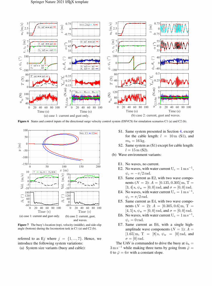
The simulation results for C1 and C2 are shown in

Fig. 6a (left) and Fig. 6b (right), respectively. Sta-

ble and accurate performance is noticed in both cases,

where the UAV is able to successfully drive the buoy

at the desired velocity (ub), while maintaining good

tracking of the reference elevation (α) and azimuth

(ϕ) angles. As seen in the (r) subplot, the UAV first

positions itself near the pulling location, it then en-

ters the pulling state by making the cable taut during

the entire duration of the buoy’s manipulation be-

tween [12, 100] s. Since there are no ambient waves

in C1, there is no apparent fluctuation in the buoy’s

vertical position (zb), immersed volume (gb), and

elevation angle (α); contrarily, the waves in C2 in-

duce fluctuations in these three states. It is noted that

the UAV keeps a level flight in both cases, as seen

in the (zu) subplot in Fig. 6a-b. The UAV is com-

manded to remain oriented forward during the entire

maneuver, which induces large pitch angles (θu) to

counteract disturbances, the roll angle (φu) remains

near-constant, and the yaw angle (ψu) smoothly fol-

lows the azimuth angle of the cable (ϕ) in order to

complete a full rotation during the course of the mo-

tion trajectory. The full rotation in azimuth (ϕ) causes

the buoy to encounter the waves in different direc-

tions, where the frequency of encounter is low during

the initial phase ([20, 40] s) due to following seas, and

when the buoy turns around ([50, 60] s) the encounter

frequency becomes high due to head seas. The cable

tension, seen in the (T ) subplot, increases with ve-

locity when the frequency of encounter with waves is

high, and when the rate of change of the azimuth an-

gle is high. Finally, we note that the thrust and torques

inputs (u(1,2,3,4)c) are bounded and stable.

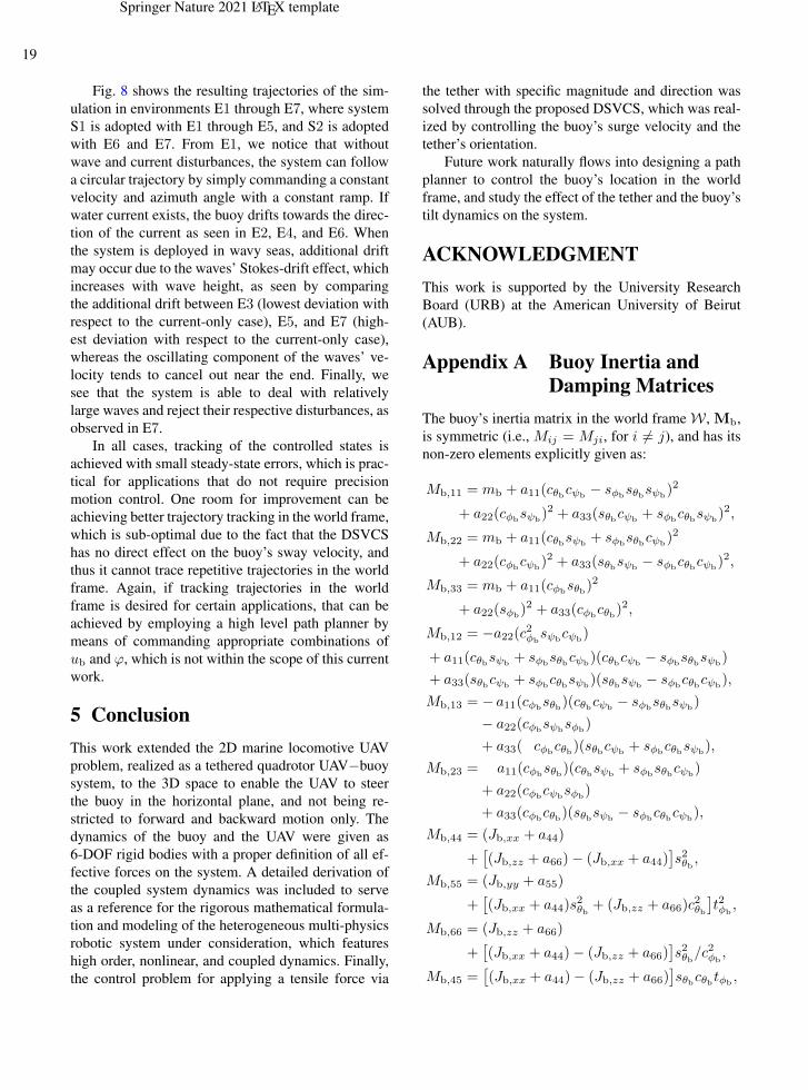
Even though the DSVCS achieves good tracking

of the desired surge and azimuth states, it does not nec-

essarily translate into identical trajectories in the world

frame. This is demonstrated in Fig. 7, which shows the

planar trajectory of the buoy for cases C1 and C2. It

is seen that the two trajectories do not coincide, even

though the results of Fig. 6 showed good tracking with

no steady-state errors. It is it also noticed that the fi-

nal direction of the trajectory is not exactly at zero as

seen in the ‘xy’ subplot of Fig. 7, even though the fi-

nal azimuth angle is zero. This can be understood by

observing the non-zero sway velocity, vb, in the ‘Vel.’

subplot of Fig. 7. We also notice that the sway velocity

of the buoy, vb, can be as large as its surge velocity, ub,

which results in a larger absolute surface velocity of

the buoy, V . Finally, we note that the buoy is prone to

having a nonzero side-slip angle, βb, as seen in Fig. 7,

given that it does not have any constraint on its planar

dynamics. At the start of the simulation (< 17s) when

the cable is slack, the side-slip angle points to a back-

ward motion (βb = 180°) since ub ≈ −1m s−1 and

vb ≈ 0m s−1 due to the initial water current velocity.

As mentioned in Section 3, the above demonstra-

tion motivates the need for a higher level path planner

in the event that the buoy is required to track trajec-

tories in the inertial frame. That said, the obtained

simulation results demonstrate the effectiveness of the

DSVCS in controlling the buoy’s surge velocity, ub,

and the direction of the pulling force by manipulating

the azimuth (ϕ) and elevation (α) angles. This pro-

vides the system with the ability to move forward and

steer as a locomotive, which also lays the foundation

for designing a path planner in the inertial frame.

4.4 Extended Simulations

To further validate the system performance in differ-

ent conditions, we offer additional simulation scenar-

ios by varying the water current direction, the wave

components in the water environment, and well as

changing the system parameters (buoy size and tether

length). The physical system index is referred to as

Si where i = 1, 2, and the environment index is

Springer Nature 2021 LATEX template

0

2.5

5

-0.75

0

0.75

3

5

7

-180

0

180

35

45

55

(°)

-40

0

40

0

40

80

0.15

0.25

0.35

0 20 40 60 80 100

Time (s)

(a) case 1: current and gust only.

40

70

100

1c

(N)

0 20 40 60 80 100

Time (s)

-5

0

5

(2,3

,4)c

(N.m

)

0

2.5

5

-0.75

0

0.75

3

5

7

-180

0

180

35

45

55

(°)

-40

0

40

0

40

80

0

0.25

0.5

0 20 40 60 80 100

Time (s)

(b) case 2: current, gust and waves.

40

80

120

1c

(N)

0 20 40 60 80 100

Time (s)

-5

0

5

(2,3

,4)c

(N.m

)

: ref act

:

° °

ζ (x )b zbSVCS:

: ref act

: actref

: est act

: ref act

: ref actact: ref

: ref actact:

2c 3c 4c

Figure 6 States and control inputs of the directional surge velocity control system (DSVCS) for simulation scenarios C1 (a) and C2 (b).

0 50 100 150 200-150

-100

-50

0

50

100

-10-505

10

-10-505

10

(b) case 2: current, gust,

and waves.

(a) case 1: current and gust only.

:buoy C2C1

0 20 40 60 80 100-60

060

120180

0 20 40 60 80 100-60

060

120180

Figure 7 The buoy’s location (top), velocity (middle), and side-slip

angle (bottom) during the locomotion task in C1 (a) and C2 (b).

referred to as Ej where j = 1, ..., 7. Hence, we

introduce the following system variations:

(a) System size variants (buoy and cable):

S1. Same system presented in Section 4, except

for the cable length: l = 10m (S1), and

mb = 16 kg.

S2. Same system as (S1) except for cable length:

l = 15m (S2).

(b) Wave environment variants:

E1. No waves, no current.

E2. No waves, with water current Uc = 1ms−1,

ψc = −π/2 rad.

E3. Same current as E2, with two wave compo-

nents (N = 2): A = [0.135, 0.305]m, T =[3, 4] s, ψw = [0, 0] rad, and σ = [0, 0] rad.

E4. No waves, with water current Uc = 1ms−1,

ψc = π/2 rad.

E5. Same current as E4, with two wave compo-

nents (N = 2): A = [0.305, 0.6]m, T =[4, 5] s, ψw = [0, 0] rad, and σ = [0, 0] rad.

E6. No waves, with water current Uc = 1ms−1,

ψc = 0 rad.

E7. Same current as E6, with a single high-

amplitude wave components (N = 1): A =[1.65]m, T = [8] s, ψw = [0] rad, and

σ = [0] rad.

The UAV is commanded to drive the buoy at ub =3ms−1 while making three turns by going from ϕ =0 to ϕ = 6π with a constant slope.

Springer Nature 2021 LATEX template

itle 19

Fig. 8 shows the resulting trajectories of the sim-

ulation in environments E1 through E7, where system

S1 is adopted with E1 through E5, and S2 is adopted

with E6 and E7. From E1, we notice that without

wave and current disturbances, the system can follow

a circular trajectory by simply commanding a constant

velocity and azimuth angle with a constant ramp. If

water current exists, the buoy drifts towards the direc-

tion of the current as seen in E2, E4, and E6. When

the system is deployed in wavy seas, additional drift

may occur due to the waves’ Stokes-drift effect, which

increases with wave height, as seen by comparing

the additional drift between E3 (lowest deviation with

respect to the current-only case), E5, and E7 (high-

est deviation with respect to the current-only case),

whereas the oscillating component of the waves’ ve-

locity tends to cancel out near the end. Finally, we

see that the system is able to deal with relatively

large waves and reject their respective disturbances, as

observed in E7.

In all cases, tracking of the controlled states is

achieved with small steady-state errors, which is prac-

tical for applications that do not require precision

motion control. One room for improvement can be

achieving better trajectory tracking in the world frame,

which is sub-optimal due to the fact that the DSVCS

has no direct effect on the buoy’s sway velocity, and

thus it cannot trace repetitive trajectories in the world

frame. Again, if tracking trajectories in the world

frame is desired for certain applications, that can be

achieved by employing a high level path planner by

means of commanding appropriate combinations of

ub and ϕ, which is not within the scope of this current

work.

5 Conclusion

This work extended the 2D marine locomotive UAV

problem, realized as a tethered quadrotor UAV−buoy

system, to the 3D space to enable the UAV to steer

the buoy in the horizontal plane, and not being re-

stricted to forward and backward motion only. The

dynamics of the buoy and the UAV were given as

6-DOF rigid bodies with a proper definition of all ef-

fective forces on the system. A detailed derivation of

the coupled system dynamics was included to serve

as a reference for the rigorous mathematical formula-

tion and modeling of the heterogeneous multi-physics

robotic system under consideration, which features

high order, nonlinear, and coupled dynamics. Finally,

the control problem for applying a tensile force via

the tether with specific magnitude and direction was

solved through the proposed DSVCS, which was real-

ized by controlling the buoy’s surge velocity and the

tether’s orientation.

Future work naturally flows into designing a path

planner to control the buoy’s location in the world

frame, and study the effect of the tether and the buoy’s

tilt dynamics on the system.

ACKNOWLEDGMENT

This work is supported by the University Research

Board (URB) at the American University of Beirut

(AUB).

Appendix A Buoy Inertia and

Damping Matrices

The buoy’s inertia matrix in the world frame W , Mb,

is symmetric (i.e., Mij = Mji, for i 6= j), and has its

non-zero elements explicitly given as:

Mb,11 = mb + a11(cθbcψb− sφb

sθbsψb)2

+ a22(cφbsψb

)2 + a33(sθbcψb+ sφb

cθbsψb)2,

Mb,22 = mb + a11(cθbsψb+ sφb

sθbcψb)2

+ a22(cφbcψb

)2 + a33(sθbsψb− sφb

cθbcψb)2,

Mb,33 = mb + a11(cφbsθb)

2

+ a22(sφb)2 + a33(cφb

cθb)2,

Mb,12 = −a22(c2φbsψb

cψb)

+ a11(cθbsψb+ sφb

sθbcψb)(cθbcψb

− sφbsθbsψb

)

+ a33(sθbcψb+ sφb

cθbsψb)(sθbsψb

− sφbcθbcψb

),

Mb,13 = − a11(cφbsθb)(cθbcψb

− sφbsθbsψb

)

− a22(cφbsψb

sφb)

+ a33( cφbcθb)(sθbcψb

+ sφbcθbsψb

),

Mb,23 = a11(cφbsθb)(cθbsψb

+ sφbsθbcψb

)

+ a22(cφbcψb

sφb)

+ a33(cφbcθb)(sθbsψb

− sφbcθbcψb

),

Mb,44 = (Jb,xx + a44)

+[

(Jb,zz + a66)− (Jb,xx + a44)]

s2θb ,

Mb,55 = (Jb,yy + a55)

+[

(Jb,xx + a44)s2θb

+ (Jb,zz + a66)c2θb

]

t2φb,

Mb,66 = (Jb,zz + a66)

+[

(Jb,xx + a44)− (Jb,zz + a66)]

s2θb/c2φb,

Mb,45 =[

(Jb,xx + a44)− (Jb,zz + a66)]

sθbcθbtφb,

Springer Nature 2021 LATEX template

(a) E1. (b) E2-E3. (c) E4-E5. (d) E6-E7.

Current Waves

0 m/s

Waves A

0.135 m

0.305 m

Current

1 m/s

Current Waves A

0.305 m

0.6 m1 m/s

Current Waves A

1.65 m1 m/s

0 75 150-150-75

075

150

-10-505

10

-180

0

180

0 50 100 150 200

Time (s)

35

45

55

(°)

: ref actact:

: ref act

: ref act

°.

0 75 150-150-75

075

150

-10-505

10

-180

0

180

0 50 100 150 200

Time (s)

35

45

55

(°)

:buoy E3E2

°.

0 75 150-150-75

075

150

-10-505

10

-180

0

180

0 50 100 150 200

Time (s)

35

45

55

(°)

:buoy E5E4

°.

0 75 150-150-75

075

150

-10-505

10

-180

0

180

0 50 100 150 200

Time (s)

35

45

55

(°)

:buoy E7E6

°.

A

0 m

E3 only E5 only E7 only

Figure 8 Trajectory and main states tracking for variants of the tethered UAV−buoy system in different environments: (a) E1, (b) E2 and E3,

(c) E4 and E5, (d) E6 and E7. In all case, l = 10m except in E6 and E7 where l = 15m.

Mb,46 =[

(Jb,zz + a66)− (Jb,xx + a44)]

sθbcθb/cφb,

Mb,56 = −[

(Jb,xx + a44)s2θb

+ (Jb,zz + a66)c2θb

]

tφb/cφb

. (A1)

Similarly, its damping matrix in W , Db, is symmet-

ric (i.e., Dij = Dji, for i 6= j), and has its non-zero

elements explicitly given as:

Db,11 = b11(cθbcψb− sφb

sθbsψb)2 + b22(cφb

sψb)2

+ b33(sθbcψb+ sφb

cθbsψb)2,

Db,22 = b11(cθbsψb+ sφb

sθbcψb)2 + b22(cφb

cψb)2

+ b33(sθbsψb− sφb

cθbcψb)2,

Db,33 = b11(cφbsθb)

2 + b22(sφb)2 + b33(cφb

cθb)2,

Db,12 = b22(−c2φbsψb

cψb)

+ b11(cθbsψb+ sφb

sθbcψb)(cθbcψb

− sφbsθbsψb

)

+ b33(sθbcψb+ sφb

cθbsψb)(sθbsψb

− sφbcθbcψb

),

Db,13 = b22(−cφbsψb

sφb)

+ b11(−cφbsθb)(cθbcψb

− sφbsθbsψb

)

+ b33( cφbcθb)(sθbcψb

+ sφbcθbsψb

),

Db,23 = b22(cφbcψb

sφb)

+ b11(cφbsθb)(cθbsψb

+ sφbsθbcψb

)

+ b33(cφbcθb)(sθbsψb

− sφbcθbcψb

),

Db,44 = b44 +[

b66 − b44]

s2θb ,

Db,55 = b55 +[

b44s2θb

+ b66c2θb

]

t2φb,

Db,66 = b66 +[

b44 − b66]

s2θb/c2φb,

Db,45 =[

b44 − b66]

sθbcθbtφb,

Db,46 =[

b66 − b44]

sθbcθb/cφb,

Db,56 = −[

b44s2θb

+ b66c2θb

]

tφb/cφb

. (A2)

Appendix B UAV Inertia Matrix

The UAV’s inertial matrix in W is symmetric, with

elements explicitly expressed as:

Mu,11 = mu, Mu,22 = mu, Mu,33 = mu,

Mu,12 = 0, Mu,13 = 0, Mu,23 = 0,

Mu,44 = Ju,xx +[

Ju,zz − Ju,xx]

s2θu ,

Mu,55 = Ju,yy +[

Ju,xxs2θu

+ Ju,zzc2θu

]

t2φu,

Mu,66 = Ju,zz +[

Ju,xx − Ju,zz]

s2θu/c2φu,

Mu,45 =[

Ju,xx − Ju,zz]

sθucθutφu,

Mu,46 =[

Ju,zz − Ju,xx]

sθucθu/cφu,

Mu,56 = −[

Ju,xxs2θu

+ Ju,zzc2θu

]

tφu/cφu

. (B3)

Springer Nature 2021 LATEX template

itle 21

Appendix C Spherical

Coordinates Details

The spherical coordinates transformation to Cartesian

coordinates, RS2C, is made by two ordered rotations,

Rα then Rϕ, where:

Rα =

cα −sα 00 0 1sα cα 0

, (C4)

and:

Rϕ =

cϕ −sϕ 0sϕ cϕ 00 0 1

. (C5)

By differentiating r with respect to time, we find

the derivatives of the spherical unit vectors to be:

˙er = αeα + cαϕeϕ,

˙eα = −αer − sαϕeϕ,

˙eϕ = −cαϕer + sαϕeα,

(C6)

From the definition of the spherical coordinates sys-

tem and from (C6), the position, velocity, and acceler-

ation vectors of Ou are given by:

r = rer, (C7a)

r = rer + rαeα + rcαϕeϕ, (C7b)

r = (r− rα2 − rc2αϕ2)er

+ (rα+ 2rα+ rsαcαϕ2)eα

+ (rϕcα + 2rϕcα − 2rαϕsα)eϕ.

(C7c)

The components of the UAV’s thrust vector in the

spherical frame are explicitly realized from (26) as:

ur = u1

[

cαcϕ(sθucψu+ sφu

cθusψu)

+ cαsϕ(sθusψu− sφu

cθucψu) + sα(cφu

cθu)]

,

uα = u1

[

− sαcϕ(sθucψu+ sφu

cθusψu)

− sαsϕ(sθusψu− sφu

cθucψu) + cα(cφu

cθu)]

,

uϕ = u1

[

− sϕ(sθucψu+ sφu

cθusψu)

+ cϕ(sθusψu− sφu

cθucψu)]

.

(C8)

With the taut-cable condition in (30), we have

r = l, and the spherical coordinates of the UAV with

respect to the buoy’s center of mass, Ob, reduced to:

ru = rb +RS2C[l, 0, 0]⊺, (C9)

which expands to:

xu = xb + lcαcϕ,

yu = yb + lcαsϕ,

zu = zb + lsα,

(C10)

and similarly, its velocity can be obtained as:

ru = rb +RS2Cr, (C11)

which expands to:

xu = xb + (−lsαcϕ)α+ (−lcαsϕ)ϕ,

yu = yb + (−lsαsϕ)α+ (lcαcϕ)ϕ,

zu = zb + (lcα)α.

(C12)

Appendix D Euler-Lagrange

Formulation

The Kinetic energy of the tethered UAV−buoy sys-

tem, K, includes the rotational and translational ener-

gies of the UAV and that of the buoy while neglecting

the cable’s energy, and is explicitly described as:

K =1

2

xb(Mb,11xb +Mb,12yb +Mb,13zb)

+ yb(Mb,21xb +Mb,22yb +Mb,23zb)

+ zb(Mb,31xb +Mb,32yb +Mb,33zb)

+ φb(Mb,44φb +Mb,45θb +Mb,46ψb)

+ θb(Mb,54φb +Mb,55θb +Mb,56ψb)

+ ψb(Mb,64φb +Mb,65θb +Mb,66ψb)

+mu(x2u + y2u + z2u)

+ φu(Mu,44φu +Mu,45θu +Mu,46ψu)

+ θu(Mu,54φu +Mu,55θu +Mu,56ψu)

+ ψu(Mu,64φu +Mu,65θu +Mu,66ψu)

,

=1

2

xb[

(Mb,11 +mu)xb +Mb,12yb +Mb,13zb]

+ yb[

Mb,21xb + (Mb,22 +mu)yb +Mb,23zb]

+ zb[

Mb,31xb +Mb,32yb + (Mb,33 +mu)zb]

+mu

[

(lα)2 + (lcαϕ)2

− 2(lsαcϕαxb)− 2(lcαsϕϕxb)

− 2(lsαsϕαyb) + 2(lcαcϕϕyb) + 2(lcααzb)]

+ φb(Mb,44φb +Mb,45θb +Mb,46ψb)

Springer Nature 2021 LATEX template

+ θb(Mb,54φb +Mb,55θb +Mb,56ψb)

+ ψb(Mb,64φb +Mb,65θb +Mb,66ψb)

+ φu(Mu,44φu +Mu,45θu +Mu,46ψu)

+ θu(Mu,54φu +Mu,55θu +Mu,56ψu)

+ ψu(Mu,64φu +Mu,65θu +Mu,66ψu)

. (D13)

The kinetic energy is differentiated with respect to

each state rate then with respect to time. Only the

buoy’s translational states and tether’s orientation

states are of interest, since the UAV and the buoy’s ro-

tational states feature no dependencies on other states,

which can be seen by inspection of the expanded K.

Their corresponding results are expressed as:

d

dt

( ∂K

∂xb

)

= (Mb,11 +mu)xb +Mb,12yb +Mb,13zb

+mul(−sαcϕα− cαcϕα2 − cαsϕϕ

− cαcϕϕ2 + 2sαsϕαϕ),

d

dt

( ∂K

∂yb

)

= Mb,21xb + (Mb,22 +mu)yb +Mb,23zb

+mul(−sαsϕα− cαsϕα2 + cαcϕϕ

− cαsϕϕ2 − 2sαcϕαϕ),

d

dt

( ∂K

∂zb

)

= Mb,31xb +Mb,32yb + (Mb,33 +mu)zb

+mul(cαα− sαα2),

d

dt

(∂K

∂α

)

= mu

[

l2α− lsα(cϕxb + sϕyb) + lcαzb

+ l(−cαcϕαxb + sαsϕϕxb − cαsϕαyb

− sαcϕϕyb − sααzb)]

,

d

dt

(∂K

∂ϕ

)

=

mu

[

l2(c2αϕ− 2sαcααϕ) + lcα(−sϕxb + cϕyb)

+ l(sαsϕαxb − cαcϕϕxb − sαcϕαyb − cαsϕϕyb)]

.

(D14)

The differentiation results of the UAV and buoy’s

rotational states are omitted as they result in sim-

ilar components to the rotational dynamics already

introduced in (27) and (21).

The kinetic energy of the system is differentiated

with respect to the states, (∂K∂η

), where the resulting

nonzero elements are obtained as:

∂K

∂α= mul(−lsαcαϕ

2 − cαcϕαxb + sαsϕϕxb

− cαsϕαyb − sαcϕϕyb − sααzb),

∂K

∂ϕ= mul(sαsϕαxb − cαcϕϕxb − sαcϕαyb

− cαsϕϕyb).

(D15)

Notice that most elements of ∂K∂η

cancels out with

elements of ddt

(

∂K∂η

)

.

The system’s potential energy was given in (38),

and its external forces and moments vector can be

formulated based on (22) and (2.6) as:

τ1 = u1(sθucψu+ sφu

cθusψu),

τ2 = u1(sθusψu− sφu

cθucψu),

τ3 = u1cφucθu + ρwggim,

τ4 = u1l[

− sαcϕ(sθucψu+ sφu

cθusψu)

− sαsϕ(sθusψu− sφu

cθucψu) + cα(cφu

cθu)]

,

τ5 = u1l[

− sϕ(sθucψu+ sφu

cθusψu)

+ cϕ(sθusψu− sφu

cθucψu)]

,

(D16)

Additionally, we have: τ6−8 = τ2,u and τ9−11 =τ2,b. The potential energy’s derivative with respect the

states rates then to time is obtained as:

d

dt

(∂U

∂η

)

= [0, 0, 0, 0, 0, 0, 0, 0, 0, 0, 0]⊺, (D17)

and its first derivative with respect to states is obtained

as:

∂U

∂η= [0, 0, (mb +mu)g,muglcα, 0, 0, 0, 0, 0, 0, 0]

⊺.

(D18)

References

[1] Abeywickrama HV, Jayawickrama BA, He Y,

et al (2018) Comprehensive energy consump-

tion model for unmanned aerial vehicles, based

on empirical studies of battery performance.

IEEE Access 6:58,383–58,394. https://doi.org/

10.1109/ACCESS.2018.2875040

Springer Nature 2021 LATEX template

itle 23

[2] Choi SY, Choi BH, Jeong SY, et al (2014) Teth-

ered aerial robots using contactless power sys-

tems for extended mission time and range. In:

2014 IEEE Energy Conversion Congress and Ex-

position (ECCE), IEEE, pp 912–916, https://doi.

org/10.1109/ECCE.2014.6953495

[3] Dicembrini E, Scanavino M, Dabbene F,

et al (2020) Modelling and simulation

of a tethered UAS. In: 2020 Interna-

tional Conference on Unmanned Aircraft

Systems (ICUAS), pp 1801–1808, https:

//doi.org/10.1109/ICUAS48674.2020.9214006

[4] Dufek J, Murphy R (2016) Visual pose estima-

tion of usv from uav to assist drowning victims

recovery. In: 2016 IEEE International Sympo-

sium on Safety, Security, and Rescue Robotics

(SSRR), pp 147–153, https://doi.org/10.1109/

SSRR.2016.7784291

[5] Faltinsen OM (1990) Sea Loads on Ships and

Offshore Structures. Cambridge University Press

[6] Fossen TI (1995) Guidance and Control of

Ocean Vehicles. WILEY

[7] Foxtech (2020) FOXTECH T3500 Plus Tethered

Power System. https://www.foxtechfpv.com/

foxtech-t3500-plus-tethered-power-system.

html, [Online; accessed 14-May-2021]

[8] Fridsma G (1969) A systematic study of the

rough-water performance of planing boats. Tech.

rep., Davidson Laboratory Report 1275, Stevens

Institute of Technology, URL https://apps.dtic.

mil/sti/citations/AD0708694

[9] Gonzalez-Garcia A, Miranda-Moya A, Cas-

tañeda H (2021) Robust visual tracking con-

trol based on adaptive sliding mode strategy:

Quadrotor UAV - catamaran USV heterogeneous

system. In: 2021 International Conference on

Unmanned Aircraft Systems (ICUAS), pp 666–

672, https://doi.org/10.1109/ICUAS51884.2021.

9476707

[10] Han Y, Ma W (2021) Automatic monitoring

of water pollution based on the combination

of UAV and USV. In: 2021 IEEE 4th Inter-

national Conference on Electronic Information

and Communication Technology (ICEICT), pp

420–424, https://doi.org/10.1109/ICEICT53123.

2021.9531204

[11] Jung S, Cho H, Kim D, et al (2017) Devel-

opment of algal bloom removal system using

unmanned aerial vehicle and surface vehicle.

IEEE Access 5:22,166–22,176. https://doi.org/

10.1109/ACCESS.2017.2764328

[12] Kominami T, Paul H, Miyazaki R, et al (2021)

Active tethered hook: Heavy load movement us-

ing hooks that move actively with micro UAVs

and winch system. In: 2021 IEEE/ASME In-

ternational Conference on Advanced Intelligent

Mechatronics (AIM), pp 264–269, https://doi.

org/10.1109/AIM46487.2021.9517518

[13] Kourani A, Daher N (2021) Leveraging PID

gain selection towards adaptive backstepping

control for a class of second-order sys-

tems. In: 2021 American Control Conference

(ACC), pp 1174–1179, https://doi.org/10.23919/

ACC50511.2021.9483159

[14] Kourani A, Daher N (2021) Marine locomo-

tion: A tethered UAV-buoy system with surge

velocity control. Robotics and Autonomous

Systems 145:103,858. https://doi.org/doi.org/10.

1016/j.robot.2021.103858

[15] Kourani A, Daher N (2021) A tethered quadro-

tor UAV-buoy system for marine locomo-

tion. In: 2021 IEEE International Confer-

ence on Robotics and Automation (ICRA),

pp 59–65, https://doi.org/10.1109/ICRA48506.

2021.9560878

[16] Kourani A, Daher N (2021, accepted.) Bidirec-

tional manipulation of a buoy with a tethered

quadrotor UAV. In: 2021 IEEE 3rd International

Multidisciplinary Conference on Engineering

Technology (IMCET)

[17] Krishna CGL, Cao M, Murphy RR (2017) Au-

tonomous observation of multiple USVs from

UAV while prioritizing camera tilt and yaw over

uav motion. In: 2017 IEEE International Sym-

posium on Safety, Security and Rescue Robotics

(SSRR), pp 141–146, https://doi.org/10.1109/

SSRR.2017.8088154

Springer Nature 2021 LATEX template

[18] Liu Y, Zhang F, Huang P, et al (2021) Analysis,

planning and control for cooperative transporta-

tion of tethered multi-rotor UAVs. Aerospace

Science and Technology 113:106,673. https://

doi.org/doi.org/10.1016/j.ast.2021.106673

[19] Lupashin S, D’Andrea R (2013) Stabilization of

a flying vehicle on a taut tether using inertial

sensing. In: 2013 IEEE/RSJ International Con-

ference on Intelligent Robots and Systems, pp

2432–2438, https://doi.org/10.1109/IROS.2013.

6696698

[20] Nicotra MM, Naldi R, Garone E (2014) Taut ca-

ble control of a tethered UAV. IFAC Proceedings

Volumes 47(3):3190 – 3195. https://doi.org/10.

3182/20140824-6-ZA-1003.02581

[21] Ozkan MF, Carrillo LRG, King SA (2019) Res-

cue boat path planning in flooded urban envi-

ronments. In: 2019 IEEE International Sympo-

sium on Measurement and Control in Robotics

(ISMCR), pp 221–229, https://doi.org/10.1109/

ISMCR47492.2019.8955663

[22] Saleh M, Oueidat G, Elhajj IH, et al (2019) In

situ measurement of oil slick thickness. IEEE

Transactions on Instrumentation and Measure-

ment 68(7):2635–2647. https://doi.org/10.1109/

TIM.2018.2866745

[23] Shao G, Ma Y, Malekian R, et al (2019) A

novel cooperative platform design for coupled

USV–UAV systems. IEEE Transactions on In-

dustrial Informatics 15(9):4913–4922. https://

doi.org/10.1109/TII.2019.2912024

[24] Talke KA, De Oliveira M, Bewley T (2018)

Catenary tether shape analysis for a UAV -

USV team. In: 2018 IEEE/RSJ International

Conference on Intelligent Robots and Systems

(IROS), pp 7803–7809, https://doi.org/10.1109/

IROS.2018.8594280

[25] Tognon M, Franchi A (2017) Dynamics, con-

trol, and estimation for aerial robots teth-

ered by cables or bars. IEEE Transactions

on Robotics 33(4):834–845. https://doi.org/10.

1109/TRO.2017.2677915

[26] Wang N, Ahn CK (2021) Coordinated trajec-

tory tracking control of a marine aerial-surface

heterogeneous system. IEEE/ASME Transac-

tions on Mechatronics pp 1–1. https://doi.org/10.

1109/TMECH.2021.3055450

[27] Xing L, Liu X, Zhang S (2021) The vibration

characteristics analysis of the tethered UAV sys-

tem. Yingyong Lixue Xuebao/Chinese Journal of

Applied Mechanics 38(1):106–112. https://doi.

org/10.11776/cjam.38.01.C075

[28] Xu Z (2021) Application research of teth-

ered UAV platform in marine emergency com-

munication network. Journal of Web Engi-

neering 20(2):491–512. https://doi.org/doi.org/

10.13052/jwe1540-9589.20212

[29] Zhang J, Xiong J, Zhang G, et al (2016) Flood-

ing disaster oriented USV amp; UAV system

development amp; demonstration. In: OCEANS

2016 - Shanghai, pp 1–4, https://doi.org/10.

1109/OCEANSAP.2016.7485676

[30] Zhang J, Gu D, Ren Z, et al (2019) Robust trajec-

tory tracking controller for quadrotor helicopter

based on a novel composite control scheme.

Aerospace Science and Technology 85:199–215.

https://doi.org/10.1016/j.ast.2018.12.013

Statements and Declarations

Funding

This work is supported by the University Research

Board (URB) at the American University of Beirut

(AUB).

Competing Interests

The authors have no relevant financial or non-financial

interests to disclose.

Author Contributions

All authors contributed to the study’s conception

and design. Material preparation and data collection

were performed by Ahmad Kourani, analysis was per-

formed by Ahmad Kourani and Naseem Daher. The

first draft of the manuscript was written by Ahmad

Kourani and all authors commented on subsequent

versions of the manuscript. All authors read and ap-

proved the final manuscript.

Springer Nature 2021 LATEX template

itle 25

Data Availability

The datasets generated and/or analysed dur-

ing the current study are available in the

Github repository: github.com/AUBVRL/3D-

Tethered-UAV-buoy, along with the sim-

ulation environment that is available as a

MATLAB/Simulink® project.