THREE-DIMENSIONAL INVERSE DESIGN OF AXIAL … · A. GIASSI, V. PEDIRODA, C. POLONI* and A. CLARICH Dipartimento di Energetica, University of Trieste, Italy (Received 23 August 2002;

Inverse Problems in Engng, 200?, Vol. 00, No. 0, pp. 1–14

THREE-DIMENSIONAL INVERSE DESIGN

OF AXIAL COMPRESSOR STATOR BLADE

USING NEURAL-NETWORKS AND DIRECT

NAVIER–STOKES SOLVER

A. GIASSI, V. PEDIRODA, C. POLONI* and A. CLARICH

Dipartimento di Energetica, University of Trieste, Italy

(Received 23 August 2002; In final form 22 April 2003)

In this article we describe a new method for the aerodynamic optimisation and inverse design problemresolution. This method is based on the coupling of a classical optimiser with a neural-network. A Navier–Stokes flow solver is used for an accurate computation of the objective function. At first, the neural-network,which has been trained by an initial small database, is used to obtain, by the interpolation of the designsensitivities, a new design point, which is then computed by the Navier–Stokes solver in order to updatethe neural-network training database for further iterative step. Since the neural-network provides the optimi-ser with the derivatives, the objective function has to be evaluated only once at every step. By this method, thecomputational effort is significantly reduced with respect to the classical optimisation methods based on thedesign sensitivities, that are computed directly by the flow solver. The method proposed has been positivelytested on the inverse design of a three-dimensional axial compressor blade, and a summary of the resultsis provided.

Keywords: Neural network; Inverse design; Design sensitivities; Navier–Stokes; Axial compressor blade

1. INTRODUCTION

An inverse design problem consists of the design of an aerodynamic shape with givenperformances. To perform the design, it is usually required to minimise some objectivefunctions. At present, with reference to fluid dynamic problems, it is possible to distin-guish two different approaches. The first one [1] combines the optimisation algorithmwith a direct solver. This method is usually flexible, because the optimiser and the solverare independent, and the user has the freedom to choose the best available solver for theproblem at hand. Nevertheless the computational effort can be very large: in fact theresearch of the function minimum is iterative and, at every step, the number of analysesis close to or even greater than the number of variables.

*Corresponding author. Tel.: 39 (40) 676-3808. Fax:þ 39 (40) 676-3812. E-mail: [email protected]

+ [4.6.2003–9:09pm] FIRST PROOFS {GandB}Gipe/GIPE-31028.3d Inverse Problems in Engng (GIPE) Paper: GIPE-31028 Keyword

ISSN 1068-2767 print: ISSN 1029-0281 online � 200? Taylor & Francis Ltd

DOI: 10.1080/1068276031000147545

The second approach [2] is based on a dedicated flow solver, that at every globaliteration, after each computation of the flow field, provides the sensitivity derivativeswith respect to the design parameters using the adjoint method [3]; by these derivativesit is possible to update the design variables at each iteration. However, this method lacksin adaptability, since it is not possible to integrate an arbitrary, possibly commercialCFD code, and any new application would need a re-building of the code.

A new class of optimisation algorithms is based on the link between response surfaceand stochastic algorithms [9,12]: the main idea is to reduce the computing cost of theoptimisation phase by using interpolated values of the objective function.

In this article a new methodology, related to the last one, based on the interpolationof the design sensitivities by a neural-network, is shown. This feature allows aremarkable reduction in the number of flow simulations. Another interesting featureof this method is the independence from the kind of problem, it means that we cansolve a different optimisation problem using the same algorithm and the same routines,by simply changing the objective function. In fact, the classical methods based on theanalytical derivatives need to adapt the algorithm which calculates the design sensitivi-ties to the current objective function, while our method interpolates the derivatives bythe neural-network, that is independent from the objective function. To test thismethod, we have chosen a turbomachinery inverse design problem.

2. PROBLEM DESCRIPTION

The objective of this inverse design problem is to find a corresponding stator bladegeometry that yields a prescribed target pressure distribution, starting by an arbitrarygeometry. The target pressure distribution corresponds to a stator blade of an axialcompressor that has been previously designed [8] modifying the geometry of a singlestage compressor built in 1992 in our department.

The choice of an inverse design is due to the fact that it is more reliable to test themethodology efficiency, since the comparison of the target distribution with theobtained one is direct.

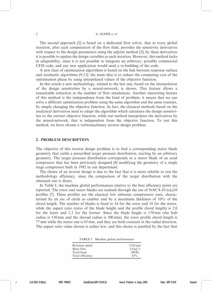
In Table I, the machine global performances relative to the best efficiency point arereported. The rotor and stator blades are realised through the use of NACA 65-(cl0)10profiles [7]. These profiles are the classical low subsonic compressors ones, charac-terised by an arc of circle as camber and by a maximum thickness of 10% of thechord length. The number of blades is fixed to 16 for the rotor and 18 for the stator,while the aspect ratio (ratio of the blade height and the profile chord length) is 2.0for the latter and 2.2 for the former. Since the blade height is 170mm (the hubradius is 130mm and the shroud radius is 300mm), the rotor profile chord length is77mm while the stator one is 85mm, and they are both constant in the radial direction.The aspect ratio value chosen is rather low, and this choice is justified by the fact that

TABLE I Machine global performances

Rotation speed 1210 rpmMass flow 3.6 kg3/sTotal head 300PaTotal efficiency 85%

2 A. GIASSI et al.


the compressor is a single-stage machine, and thus it requires a higher pressure load.A low aspect ratio, in fact, usually gives higher load, higher efficiency, and higherstall pressure.

3. ALGORITHM DESCRIPTION

The first task is the geometrical parameterisation of the stator blade shape and therealisation of a three-dimensional mesh. Then an initial modified configuration ischosen as the starting point of the inverse design. Further, an appropriate number ofdesign points close to the initial configuration (see Section 3.5) are chosen and theirobjective function values are used to define the neural-network initial training set.Once the network is trained, the algorithm may be provided by the interpolated deriva-tives to find the new design point. In a further step the network training set is updatedby the objective function of the new design point calculated by the flow solver. Thesearch continues iteratively until the convergence criterion is satisfied.

3.1. Parameterisation and Numerical Simulation

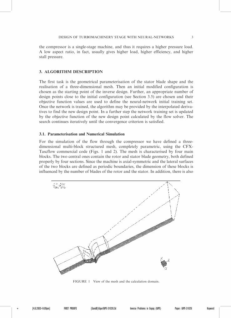
For the simulation of the flow through the compressor we have defined a three-dimensional multi-block structured mesh, completely parametric, using the CFX-Tascflow commercial code (Figs. 1 and 2). The mesh is characterised by four mainblocks. The two central ones contain the rotor and stator blade geometry, both definedproperly by four sections. Since the machine is axial-symmetric and the lateral surfacesof the two blocks are defined as periodic boundaries, the dimension of these blocks isinfluenced by the number of blades of the rotor and the stator. In addition, there is also

FIGURE 1 View of the mesh and the calculation domain.

DESIGN OF TURBOMACHINERY STAGE WITH NEURAL-NETWORKS 3


an inlet block, that drives the flow towards the rotor, and an outlet block, whose func-tion is to give the flow a freedom to expand. For these reasons we apply a boundarycondition of mass flow fixed in correspondence of the inlet (3.6 kg/s as defined byour design conditions) and a static pressure boundary in correspondence of theoutlet, fixed to the atmospheric value. The numerical code applies the equation relativeto the inertial body forces due to the rotation in the region defined by the rotor block,and thus it is necessary to define the interfaces between that block and the two conti-guous ones as a stage. At the interface between the rotating impeller outlet and thestator inlet, the stage averaging option has been used. This means that circumferentialaveraging occurs as the flow crosses across the interface, assuming a complete mixingof the upstream velocity profile.

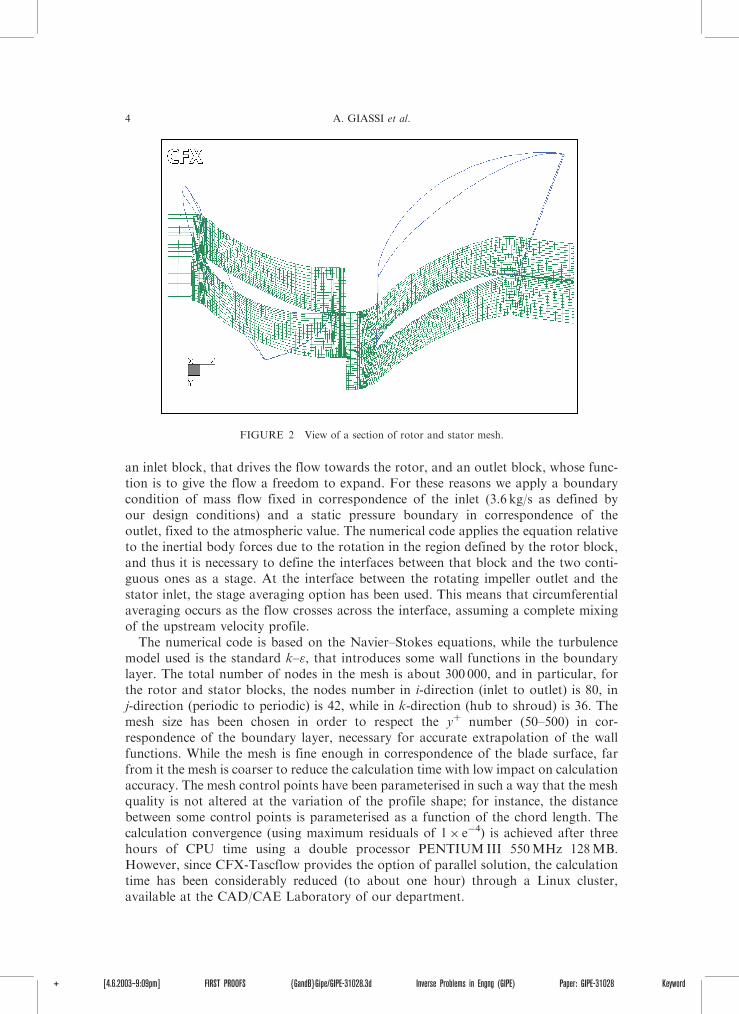
The numerical code is based on the Navier–Stokes equations, while the turbulencemodel used is the standard k–", that introduces some wall functions in the boundarylayer. The total number of nodes in the mesh is about 300 000, and in particular, forthe rotor and stator blocks, the nodes number in i-direction (inlet to outlet) is 80, inj-direction (periodic to periodic) is 42, while in k-direction (hub to shroud) is 36. Themesh size has been chosen in order to respect the yþ number (50–500) in cor-respondence of the boundary layer, necessary for accurate extrapolation of the wallfunctions. While the mesh is fine enough in correspondence of the blade surface, farfrom it the mesh is coarser to reduce the calculation time with low impact on calculationaccuracy. The mesh control points have been parameterised in such a way that the meshquality is not altered at the variation of the profile shape; for instance, the distancebetween some control points is parameterised as a function of the chord length. Thecalculation convergence (using maximum residuals of 1� e�4) is achieved after threehours of CPU time using a double processor PENTIUMIII 550MHz 128MB.However, since CFX-Tascflow provides the option of parallel solution, the calculationtime has been considerably reduced (to about one hour) through a Linux cluster,available at the CAD/CAE Laboratory of our department.

FIGURE 2 View of a section of rotor and stator mesh.

4 A. GIASSI et al.


3.2. Geometric Parameterisation

With reference to the stator shape definition, we have chosen 15 variables, which aredescribed in Table II. These variables reflect the common procedure of blade designaccording to the NACA profile theory [10].

From the initial geometry of the profile NACA 65-10-10, defined by a standardcamber and thickness, both dimensionless with respect to the chord length, we have usedthese variables to change the blade geometry and to define four sections of the stator.

The variable Ar, or aspect ratio, defines the ratio between the blade height, which isfixed to 170mm, and the chord length. The original stator was characterised by an Arvalue of 2.0, and we have chosen a range of variation around that value. Defined in thatway the chord length, the camber of the NACA profile is modified by adding to it pointby point a third order Bezier curve, which is defined by four control points. The Beziercurve is a regular and continuous function, whose tangents on the extremities aredefined by the straight lines passing through the first two and the last two controlpoints. The initial and last control points are fixed in correspondence of the leadingand trailing edge of the profile, while the abscissas and ordinates of the two centralpoints, free to change their position, are defined in order of the fourvariables, Bezier1–Bezier4.

The NACA profile thickness is also changed, multiplying the original value by thevariable Thick, which changes from 0.5 to 1.2. A geometric control has been addedto avoid too low thickness along the blade profiles: if the distance from the upperside to the lower one is less than a minimum value (1% of the chord length) in somepoints of the blade profile, it is kept constant. The new profile so defined is rotatedby different angles in the four sections placed at radius equal to 130, 186, 243, and300mm, respectively, and this angle is controlled by the variables Psi1–Psi4.

The variables Cl1–Cl4 define how the curvature of the four profiles change withrespect to the original one. Known the coefficient Cl of a section, it is possible to multi-ply the camber ordinates by it, obtaining a higher or lower curvature.

The variable Stagg defines the value of the stagger in the tangential direction. Inother words, the barycentre of the stator sections is not placed on the same radialline, but on a line which is shifted by a certain angle in the tangential direction. Thetangent of this angle is defined by the ratio between the variable Stagg and theshroud radius (300mm).

TABLE II Fifteen initial variables and their range of variation

Aspect ratio Ar (1.5, 2,5) [/]Blade thickness Thick (0.5, 1.2) [/]Stagger Stagg (�50, 50) [�]Parameter Bezier1 Bezier1 (0, 1) [/]Parameter Bezier2 Bezier2 (�0.25, 0.25) [/]Parameter Bezier3 Bezier3 (0,1) [/]Parameter Bezier4 Bezier4 (�0.25, 0.25) [/]Coefficient Cl, section 1 Cl1 (�0.4, 0.4) [/]Blade angle, section 1 Psi1 (�5, 5) [�]Coefficient Cl, section 2 Cl2 (0.1, 0.5) [/]Blade angle, section 2 Psi2 (1, 3) [�]Coefficient Cl, section 3 Cl3 (0.1, 0.5) [/]Blade angle, section 3 Psi3 (1, 3) [�]Coefficient Cl, section 4 Cl4 (0.1, 0.5) [/]Blade angle, section 4 Psi4 (1, 3) [�]



3.3. Objective Function

In this inverse problem, the blade pressure distributions along the surface, p(z,var),should minimise the differences with the target pressure distribution, ptarget(z), wherez is the dimensionless axial co-ordinate with respect to the chord length and var isthe vector of the design parameters. The choice of a dimensionless co-ordinate is dueto the fact that the objective function should be independent from the chord length,which is a variable.

Since every two-dimensional section is subdivided into Ntot(¼ 90) nodes and thewhole blade is subdivided into Nk(¼ 36) planar sections, the inverse problem objectivefunction, which should be minimised, is given by the following equation SumP:

SumP ¼XNK

k¼1

XNtot

i¼1

�pi, k�� ðziþ1, k � zi, kÞ ð1Þ

where

�pi, k ¼1

2ð pðziþi, k, varÞ þ p ðzi, k, varÞÞ �

1

2ð ptargetðziþ1, kÞ þ ptargetðzi, kÞÞ ð2Þ

and where zi,k is the co-ordinate z of the node i of section k.Usually, in a common inverse design problem, a quadratic objective function is used,

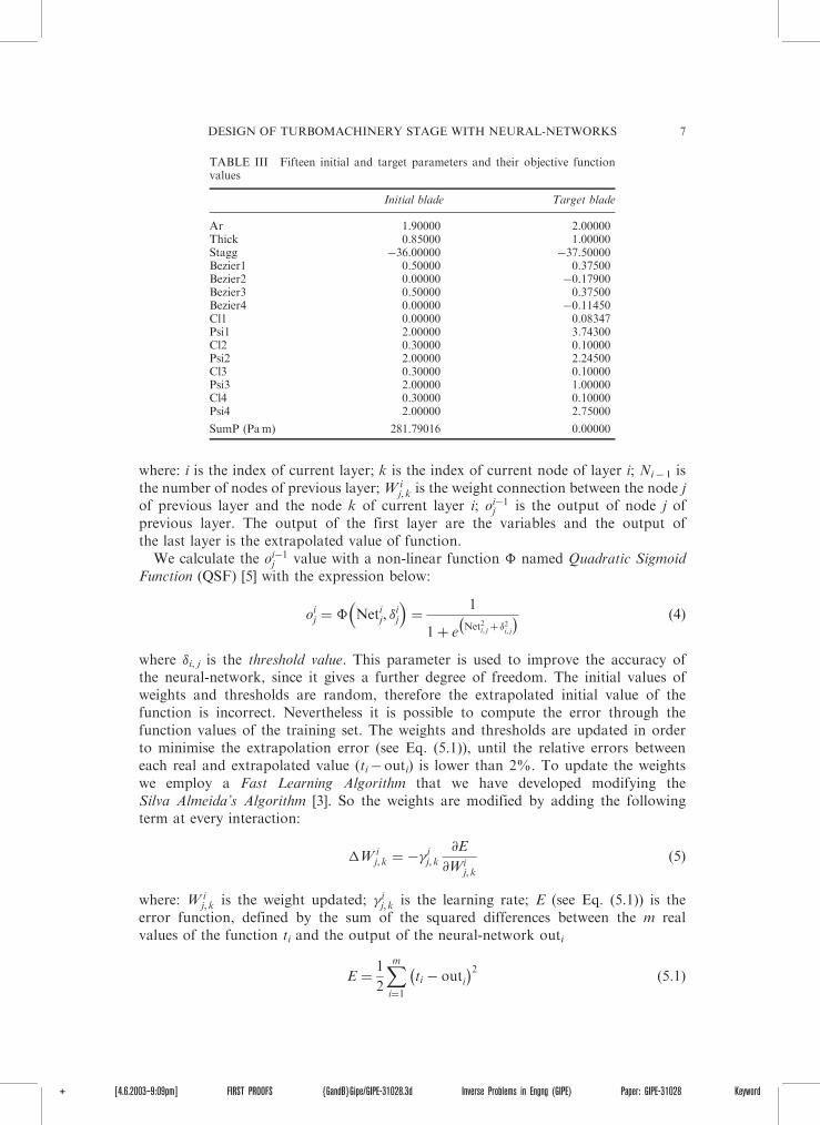
but in this work we have considered a ‘‘flat’’ function (absolute value instead ofsquared), which is more suitable for our neural-network. In fact, in the case of pressuredistributions close to the target, the infinitesimal order of the error function (Eq. (1)) issmaller than a quadratic function, thus the neural-network can appreciate a greaterdifference and can be trained in a better way. In Table III we may find the parametersand the objective function of the initial and target blade shapes.

3.4. Neural-Network

The neural-network model is a non-linear function that allows the extrapolation of amulti-variable function. The net, imitating the human learning process, associates aset of inputs, the variables, to their output, the objective function. Through this process,called training, the neural-network ‘‘learns’’ the function and can extrapolate its valuein an unknown design point.

A multi-layer feed-forward [4] neural-network is chosen because, according to ourtests [11], this is the most appropriate architecture for this kind of problem, becauseit may give efficient results in adequately reduced calculation time. The nodes, whichare the basic unity of neural-networks, are distributed on more layers and each nodecommunicates only with the nodes of the following layer.

The first layer gets the input data, whereas the internal layers, also called hiddenlayers, and the last one get the following values:

Netik ¼XNi�1

j¼1

Wij, k � o

i�1j ð3Þ

6 A. GIASSI et al.


where: i is the index of current layer; k is the index of current node of layer i; Ni� 1 isthe number of nodes of previous layer; Wi

j, k is the weight connection between the node jof previous layer and the node k of current layer i; oi�1

j is the output of node j ofprevious layer. The output of the first layer are the variables and the output ofthe last layer is the extrapolated value of function.

We calculate the oi�1j value with a non-linear function � named Quadratic Sigmoid

Function (QSF) [5] with the expression below:

oij ¼ � Netij, �ij

� �¼

1

1þ e Net2i, j þ �2i, j

� � ð4Þ

where �i, j is the threshold value. This parameter is used to improve the accuracy ofthe neural-network, since it gives a further degree of freedom. The initial values ofweights and thresholds are random, therefore the extrapolated initial value of thefunction is incorrect. Nevertheless it is possible to compute the error through thefunction values of the training set. The weights and thresholds are updated in orderto minimise the extrapolation error (see Eq. (5.1)), until the relative errors betweeneach real and extrapolated value (ti� outi) is lower than 2%. To update the weightswe employ a Fast Learning Algorithm that we have developed modifying theSilva Almeida’s Algorithm [3]. So the weights are modified by adding the followingterm at every interaction:

�Wij, k ¼ �� i

j, k

@E

@Wij, k

ð5Þ

where: Wij, k is the weight updated; � ij, k is the learning rate; E (see Eq. (5.1)) is the

error function, defined by the sum of the squared differences between the m realvalues of the function ti and the output of the neural-network outi

E ¼1

2

Xmi¼1

ti � outi� �2

ð5:1Þ

TABLE III Fifteen initial and target parameters and their objective functionvalues

Initial blade Target blade

Ar 1.90000 2.00000Thick 0.85000 1.00000Stagg �36.00000 �37.50000Bezier1 0.50000 0.37500Bezier2 0.00000 �0.17900Bezier3 0.50000 0.37500Bezier4 0.00000 �0.11450Cl1 0.00000 0.08347Psi1 2.00000 3.74300Cl2 0.30000 0.10000Psi2 2.00000 2.24500Cl3 0.30000 0.10000Psi3 2.00000 1.00000Cl4 0.30000 0.10000Psi4 2.00000 2.75000

SumP (Pam) 281.79016 0.00000



To improve the convergence velocity, an adaptive method to minimise iteratively theerror function has been used (Eq. (6)). The learning rate is local [4], so that it is possibleto employ a different � j,k for each direction in weight space. In this way, these valuesincrease if the gradient direction maintains its sign as constant. In formulas:

�ðnþ1Þj, k ¼

�ðnÞj, k � u if rj, kEðnÞ � rj, kE

ðn�1Þ � 0

�ðnÞj, k � d if rj, kEðnÞ � rj, kE

ðn�1Þ < 0

8<: ð6Þ

where n is the number of the iteration, u is a constant with value >1 whereas d is<1.

3.5. Search of the Minimum

The minimisation of the objective function is obtained by a gradient-based method. Thischoice may seem naı̈ve, but in this way we show unquestionably that the neural-network could extrapolate accurately the gradient function without additionalcomputational cost.

The search of the minimum is iterative and every step corresponds to an update of thedesign variables:

varðnÞi ¼ var

ðn�1Þi �molt grad

ðnÞi �

@SumP=@vari

@SumP=@vari�� þMOM ��var

ðn�1Þi ð7Þ

where: varðnÞi is the i component of variables vector at the iteration n; molt_grad is the

variation step of the input parameters,

molt gradðnÞi ¼

molt gradðn�1Þi � ug if riSumPðnÞ

� riSumPðn�1Þ� 0

molt gradðn�1Þi � dg if riSumPðnÞ

� riSumPðn�1Þ < 0

(ð8Þ

where ug and dg are other constants, >1 and <1 respectively. @ Sump/@vari is thefirst derivative of objective function; MOM is the momentum term; �var

ðn�1Þi is

the i component of the previous step. Therefore the design sensitivity is used onlyfor the sign evaluation, and the lengths of the steps are obtained by the molt_gradterms.

To avoid an excessive acceleration or deceleration, a minimum value for the steplength, mgmin,i, and a maximum value, mgmax,i, are enforced. The algorithm covers allthe design space with an nvar-dimensional grid of side mgmin,i and an nvar-dimensionalgrid of side length mgmax,i. The individual one-dimensional steps can move on allpossible intermediate grids.

Usually we define the start step as follows:

molt gradð0Þi ¼ 0:5 � ðmgmax , i þmgmin , iÞ: ð9Þ

When the minimum of the function lies in a narrow ‘‘valley’’, if the gradient directionis taken, it may produce wide oscillations of the search process. To avoid this problem,we have introduced a momentum term (MOM), that is a weighted average of the current

8 A. GIASSI et al.


step and the previous correction. The introduction of the momentum rate allowsthe attenuation of the oscillations, nevertheless, when we are close to the minimum,the gradient method shows its own limits and the oscillations are inevitable.

The first derivatives of the objective function are evaluated with forward difference asfollows:

@SumP

@vari¼

SumPðvari, . . . , vari þ�i, . . . , varn, varÞ � SumPðvar1, . . . , varn, varÞ

�ið10Þ

where, the second term of the numerator is the function on the current point calculatedby the flow solver, whereas the first one is evaluated by the neural-network in a fewseconds.

When the new design point is found by the derivative (Eq. (7)), its objective functionvalue is evaluated by the flow solver. Then the training set of the neural-network isupdated by adding the new design point and deleting the point which is even furtherfrom the new one. Therefore the training set keeps always the same dimensionn_max. Usually, this parameter is close to the variables number nvar, and is fixed,since the neural-network is initialised by the starting training set. In our algorithm,the starting training set is given from scratch by a DOE (Design of Experiment) algo-rithm. The variables range is centred in the initial design and fixed to 20% of the globalrange of variation (Table II).

We face a problem when we are close to the minimum, as there is an excessive densityof data. Then the noise of the objective function can influence the training process. Thisproblem may be avoided, by initialising the weight of neural-network at every step, sothe learning process is strictly local and the net does not preserve the memory of thepoints that have been previously deleted.

4. RESULTS

The technique described above has been tested by performing the inverse design of thethree-dimensional compressor blade previously described, in subsonic flow conditions.We will show that our method reaches the minimum objective function requiring smallnumber of design evaluations. We assign the following values to the parameters of ouralgorithm (Table IV). The value of mgmax,i is set in order to reach the upper bound ofthe i variable in at least 20 steps if the gradient is constant. The minimum step allowed,mgmin,i, is one-hundredth of the i variable range; this choice avoids too small oscilla-tions in a narrow valley. The other parameters are almost standard, in fact a lot ofsimilar problems have been previously studied using the same values [11].

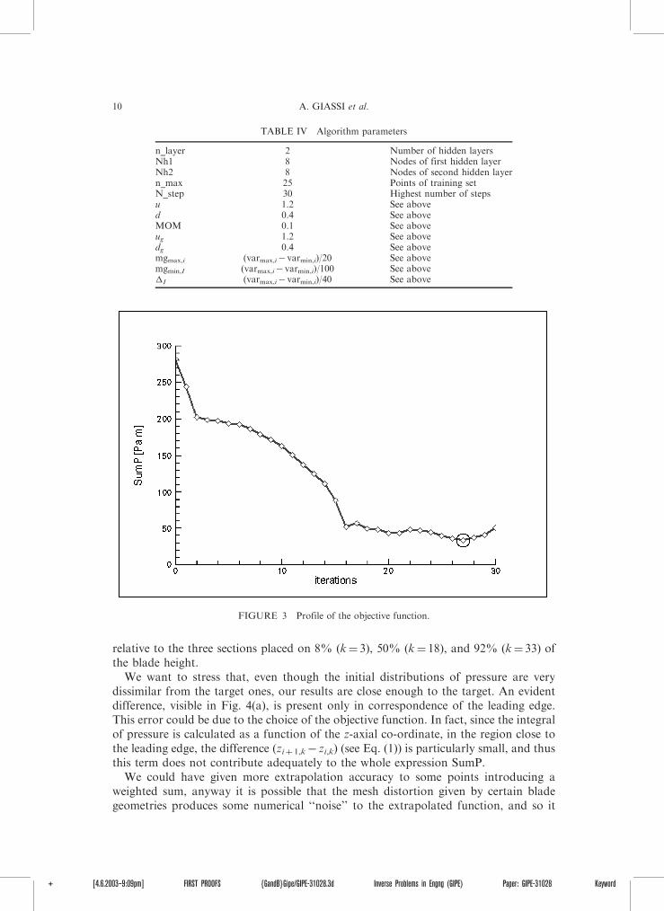
It is possible to observe in Fig. 3 the down course of the objective function: on theminimum zone, we may notice some uncertainties, but an interesting result (33 Pam)is reached in just 27 steps, that is, by 27 flow analyses. So the calculation effort islow. As the function SumP is characterised by some numerical noise due to error tole-rance in the neural-network training (see Eq. (5.1)), and this noise may be approxi-mately estimated to �15 (Pam), we may conclude that the result is close to the target.

In Fig. 4 we show the comparison between the pressure distribution on the statorblade surface of the initial, optimised, and target configuration. The comparison is



relative to the three sections placed on 8% (k¼ 3), 50% (k¼ 18), and 92% (k¼ 33) ofthe blade height.

We want to stress that, even though the initial distributions of pressure are verydissimilar from the target ones, our results are close enough to the target. An evidentdifference, visible in Fig. 4(a), is present only in correspondence of the leading edge.This error could be due to the choice of the objective function. In fact, since the integralof pressure is calculated as a function of the z-axial co-ordinate, in the region close tothe leading edge, the difference (ziþ 1,k� zi,k) (see Eq. (1)) is particularly small, and thusthis term does not contribute adequately to the whole expression SumP.

We could have given more extrapolation accuracy to some points introducing aweighted sum, anyway it is possible that the mesh distortion given by certain bladegeometries produces some numerical ‘‘noise’’ to the extrapolated function, and so it

FIGURE 3 Profile of the objective function.

TABLE IV Algorithm parameters

n_layer 2 Number of hidden layersNh1 8 Nodes of first hidden layerNh2 8 Nodes of second hidden layern_max 25 Points of training setN_step 30 Highest number of stepsu 1.2 See aboved 0.4 See aboveMOM 0.1 See aboveug 1.2 See abovedg 0.4 See abovemgmax,i (varmax,i� varmin,i)/20 See abovemgmin,I (varmax,i� varmin,i)/100 See above�I (varmax,i� varmin,i)/40 See above

10 A. GIASSI et al.


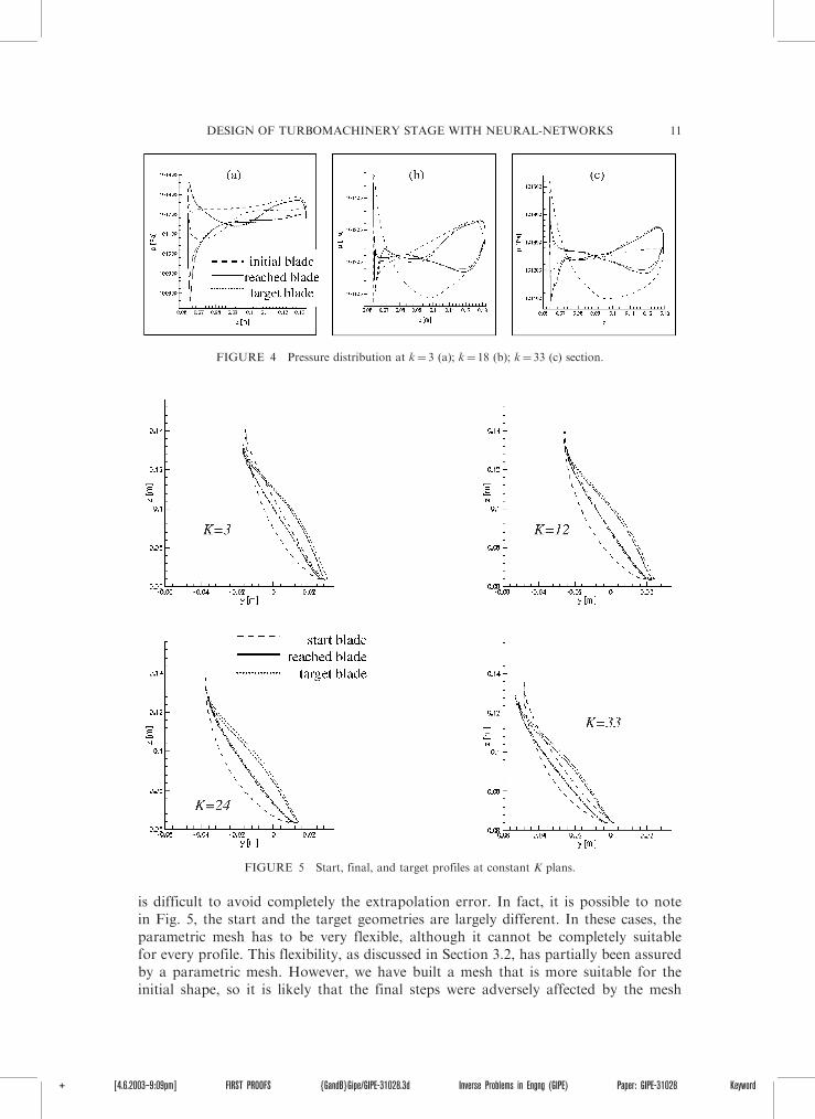
is difficult to avoid completely the extrapolation error. In fact, it is possible to notein Fig. 5, the start and the target geometries are largely different. In these cases, theparametric mesh has to be very flexible, although it cannot be completely suitablefor every profile. This flexibility, as discussed in Section 3.2, has partially been assuredby a parametric mesh. However, we have built a mesh that is more suitable for theinitial shape, so it is likely that the final steps were adversely affected by the mesh

FIGURE 5 Start, final, and target profiles at constant K plans.

FIGURE 4 Pressure distribution at k¼ 3 (a); k¼ 18 (b); k¼ 33 (c) section.



noise. This happens in particular after the sixteenth algorithm step (Fig. 3), after whichthe convergence descent is slowed down.

The global accuracy of the results is however also proved by the comparison betweenthe blade shapes on four different sections (Fig. 5), in which it is possible to note asatisfactory reconstruction of the target geometry except for the leading edge of theroot section (k¼ 3), according to the pressure distribution in Fig. 4(a).

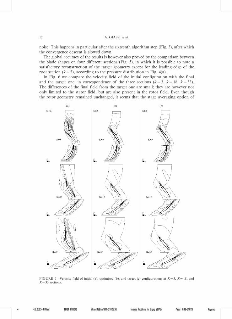
In Fig. 6 we compare the velocity field of the initial configuration with the finaland the target one, in correspondence of the three sections (k¼ 3, k¼ 18, k¼ 33).The differences of the final field from the target one are small; they are however notonly limited to the stator field, but are also present in the rotor field. Even thoughthe rotor geometry remained unchanged, it seems that the stage averaging option of

FIGURE 6 Velocity field of initial (a); optimized (b); and target (c) configurations at K¼ 3, K¼ 18, andK¼ 33 sections.

12 A. GIASSI et al.


CFX code (Section 3.1) influences both the two regions, since it introduces a mixing ofthe upstream velocity profile with the downstream one.

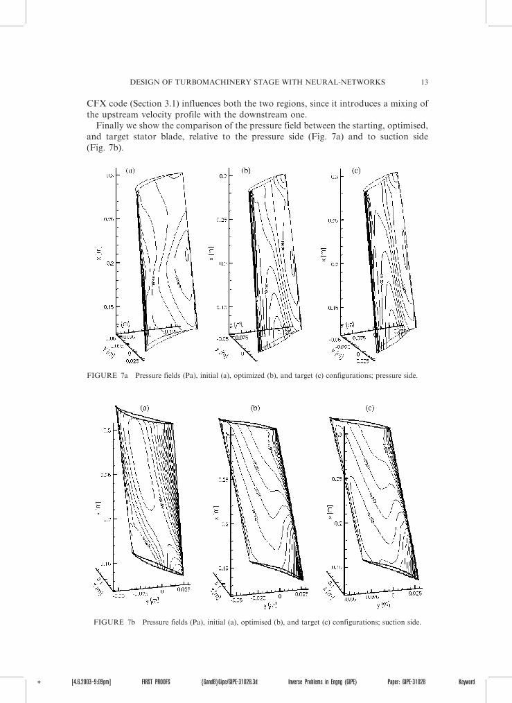
Finally we show the comparison of the pressure field between the starting, optimised,and target stator blade, relative to the pressure side (Fig. 7a) and to suction side(Fig. 7b).

FIGURE 7b Pressure fields (Pa), initial (a), optimised (b), and target (c) configurations; suction side.

FIGURE 7a Pressure fields (Pa), initial (a), optimized (b), and target (c) configurations; pressure side.



5. CONCLUSIONS

In this article we have described a new optimisation methodology, based on the integra-tion of a neural-network with a classic algorithm based on the objective function deriv-atives, and its application in the solution of a complex three-dimensional inverse designproblem. This method makes possible a remarkable reduction of the flow simulationsnecessary to minimise the objective function, and every commercial flow solver maybe integrated, without any change, within the algorithm. Therefore our methodcombines a low computational effort with an accurate and flexible flow computation.

Furthermore, this method is independent from the kind of problem, i.e. we can solvea different optimisation problem, using the same algorithm and the same routines, justchanging the objective function. To test the method, we have chosen an inverse design,because it is particularly useful to demonstrate the efficiency of the technology with adirect comparison between the target geometry and the reached one, but of course anydirect optimisation problem could be solved applying this methodology.

Acknowledgements

We wish to thank the ESTECO Ltd. for the use of modeFrontier� code in the previousprocedure of optimisation, and AEA Technology for the use of CFX-Tascflow�.

References

[1] G.N. Vanderplaats (1984). Numerical Optimization Techniques for Engineering Design: With Applications.McGraw-Hill Inc, New York.

[2] L.A. Catalano and A. Dadone (2001). Progressive Optimisation for the Efficient Design of 3d Cascades,AIAA paper 2001–2578. 15th AIAA CFD Conference, June 11–14. Anaheim, California, USA.

[3] G. Kuruvila, S. Ta’asan and M.D. Salas (1994 November). Airfoil optimization by the one shot method.Agard Report, 803, 7.13–7.21.

[4] Raul Rojas (1996). Neural Networks. Springer Verlag, Heidelberg.[5] C. Poloni, A. Giurgevich, L. Onesti and V. Pediroda (2000). Hybridization of a Multi-objective Genetic

Algorithm, a Neural Network and a Classical Optimiser for a Complex Design Problem in FluidDynamic, Vol. 186, pp. 403–420. CMAME, Computer Methods in Applied Mechanics and Engineering.

[6] CFX-Tascflow-Version 2.8 User Documentation (1998). AEA Technology Engineering Software Ltd.[7] National Advisory Commitee for Aeronautics – Report 1368 (1958).[8] A. Clarich, G. Mosetti, V. Pediroda and C. Poloni (2002). Application of Evolutive Algorithms and

Statistical Analysis in the Numerical Optimisation of an Axial Compressor. The 9th InternationalSymposium on Transport Phenomena and Dynamics of Rotating Machinery, February 10–14,Honolulu, Hawaii.

[9] K.C. Giannakoglou, A. Giotis and M.K. Karakasis (2001). Low-cost genetic optimization based oninexact pre-evaluations and the sensitivity analysis of design parameters. Inverse Problems inEngineering, 9(4).

[10] R. Eppler (1990). Airfoil Design and Data. Springer-Verlag.[11] C. Poloni and V. Pediroda (1998). GA couplet with computationally expensive simulations: tools to

improve efficiency. Genetic Algorithms and Evolution Strategies in Engineering and Computer Science,pp. 267–288. Wiley.

[12] S. Pierret (1997). Turbomachinery blade design using a Navier-Stokes solver and artificial neuralnetwork. VKI Lecture Series, 5.

14 A. GIASSI et al.


proofreader

2

proofreader

1

AUTHOR QUERIES

JOURNAL ID: GIPE – 31028 QUERY NUMBER

QUERY

1 Reference [6] not cited in the text, but listed in the References. 2 Please provide location of the publisher for References [10, 11].

Documents

THREE-DIMENSIONAL INVERSE DESIGN OF AXIAL … · A. GIASSI, V. PEDIRODA, C. POLONI* and A. CLARICH Dipartimento di Energetica, University of Trieste, Italy (Received 23 August 2002;