1

Three-Dimensional Graphics

Enrico Gobbetti and Riccardo Scateni

CRS4, Center for Advanced Studies, Research, and Development in Sardinia

Via Nazario Sauro 10

09123 Cagliari, Italy

E-mail: { Enrico.Gobbetti|Riccardo.Scateni} @crs4.it

2

Three-dimensional graphics is the area of computer graphics that deals with producing two-

dimensional representations, or images, of three-dimensional synthetic scenes, as seen from a

given viewing configuration. The level of sophistication of these images may vary from

simple wire-frame representations, where objects are depicted as a set of segment lines, with

no data on surfaces and volumes (figure 1), to photorealistic rendering, where illumination

effects are computed using the physical laws of light propagation.

Figure 1. Wire-frame representation of a simple scene.

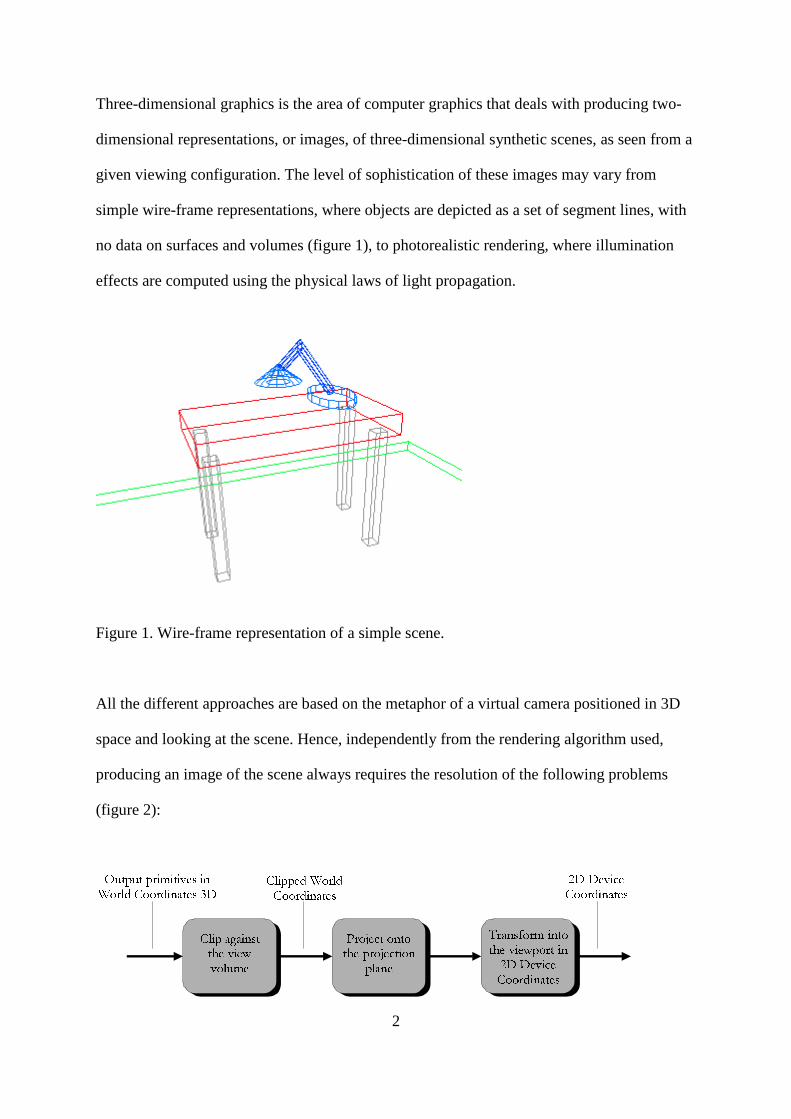
All the different approaches are based on the metaphor of a virtual camera positioned in 3D

space and looking at the scene. Hence, independently from the rendering algorithm used,

producing an image of the scene always requires the resolution of the following problems

(figure 2):

� � � � � � � � � � � � � � � � � � � � �� � � � � � � �� � � � � � � � � �� � � � � � � � � � � � � � � � � � �� � � � �

� � � � � � � �� � � � � � � � � �� � � � � � � � � � � �� � � � � � � � � �� � � � � � � � � � � � � � �� � � � � � � � � � � � � � � � �� � � � � � � � � � � � � � � � � � � �

3

Figure 2. Three-dimensional viewing pipeline.

1. ��� � !#"%$'&)(*(+!#� ,-!#.%/0$'12/3!#"'4 .%$'� &)576 $ 8+594 ,:� &)(*5;1#!#&<!2� =?>@!)1#.A5 , and in particular efficiently

representing the situation in 3D space of objects and virtual cameras;

2. BDC E%E'F%G)HJI G K*L#E'F M MNF'G)H , i.e. efficiently determining which objects are visible from the

virtual camera;

3. ODP0Q?R@S#T)U'V'W)X visible objects on the film plane of the virtual camera in order to render

them.

References (1 - 4) provide excellent overviews of the field of three-dimensional graphics.

This chapter provides an introduction to the field by presenting the standard approaches for

solving the aforementioned problems.

Three-Dimensional Scene Description

Three-dimensional scenes are typically composed of many objects, each of which may be in

turn composed of simpler parts. In order to efficiently model this situation, the collection of

objects that comprise the model handled in a three-dimensional graphics application is

typically arranged in a hierarchical fashion. This kind of hierarchical structure, known as a

Y7Z#[#\ [^]+_3`baNc)d has been introduced by Sutherland (5) and later used in most graphics systems

to support information sharing (6).

In the most common case, a transformation hierarchy defines the position, orientation, and

scaling of a set of reference frames that coordinatize the space in which graphical objects are

defined. Geometrical objects in a scene graph are thus always represented in their own

reference frame, and geometric transformations define the mapping from a coordinate system

4

to another one. This makes it possible to always perform numerical computation using the

most appropriate coordinate systems.

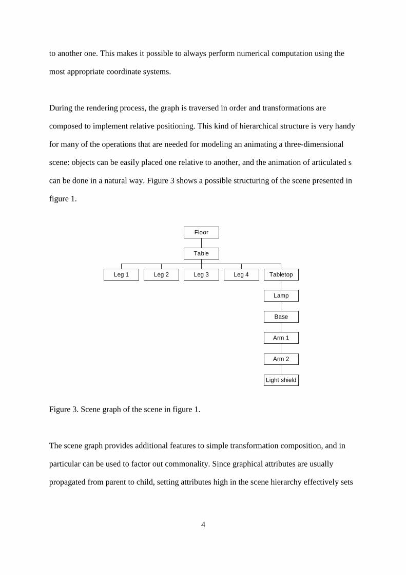
During the rendering process, the graph is traversed in order and transformations are

composed to implement relative positioning. This kind of hierarchical structure is very handy

for many of the operations that are needed for modeling an animating a three-dimensional

scene: objects can be easily placed one relative to another, and the animation of articulated s

can be done in a natural way. Figure 3 shows a possible structuring of the scene presented in

figure 1.

Figure 3. Scene graph of the scene in figure 1.

The scene graph provides additional features to simple transformation composition, and in

particular can be used to factor out commonality. Since graphical attributes are usually

propagated from parent to child, setting attributes high in the scene hierarchy effectively sets

Leg 1 Leg 2 Leg 3 Leg 4

Light shield

Arm 2

Arm 1

Base

Lamp

Tabletop

Table

Floor

5

the attributes for the entire subgraph. As an example, setting to red the color of the root object

of the scene graph defines red as the default color of all objects in the scene.

Most modern three-dimensional graphics systems implement some form of scene graph (e.g.,

OpenInventor (7), VRML (8)). A few system, e.g. PHIGS and PHIGS+ (9), provide multiple

hierarchies, allowing different graphs to specify different attributes.

Geometric Transformations

Geometric transformations describe the mathematical relationship between coordinates in

two different reference frames. In order to efficiently support transformation composition,

three-dimensional graphics systems impose restrictions on the type of transformations used in

a scene graph, typically limiting them to be linear ones.

eNf%g h#i jlk%j0i g)mon@p j3q:i k%f'p g)m have the remarkable property that, since line segments are always

mapped to line segments, it is not necessary to compute the transformation of all points of an

object but only of a few characteristic ones which obviously reduces the computational

burden with respect to supporting arbitrary transformations. For instance, only the vertices of

a polygonal object need to be transformed to obtain the image of the original object.

Furthermore, each elementary linear transformation can be represented mathematically using

linear equations for each of the coordinates of a point, which remains true for transformation

sequences. It is thus possible to perform complex transformations with the same cost

associated to performing elementary ones.

Using 3D Cartesian coordinates does not permit the representation of all types of

transformations in matrix form (e.g. 3D translations cannot be represented as 3x3 matrices),

6

which is desirable to efficiently support transformation composition. For this reason, three-

dimensional graphics systems usually represent geometric entities using r s t:s)uwv#x v)s y)z{ s s |0} ~'x � �%v�z .

Homogeneous Coordinates

Ferdinand Möbius introduced the concept of homogeneous coordinates in the XIX century as

a method for mathematically representing the position P of the center of gravity of three

masses lying onto a plane (10). Once the three masses are arbitrarily placed, the �D�#���+� �A� of

the masses define the placement of P, and a variation in one of the weights reflects on a

variation of P. We have, thus, a coordinate system where three coordinates define a point on

the plane, inside the triangle identified by the three masses. Forgetting the physics and using

negative masses we can represent any point on the plane even if it is outside the triangle. An

interesting property of such a system is given by the fact that scaling the three weights by the

same scale factor does not change the position of the center of gravity: this implies that the

coordinates of a point are not unique.

A slightly different formulation of this concept, due to Plücker, defines the coordinates of the

point P on the Cartesian plane in terms of the distances from the edges of a fixed triangle

(11). A particular case consists in placing one of the edges of the triangle at infinity; under

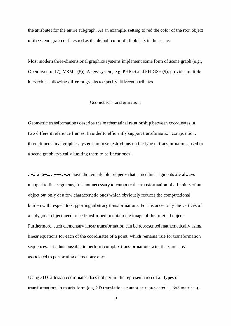
this assumption the relation between the Cartesian coordinates of a point ),(P ��= and its

homogeneous coordinates T),,( ��� will be:

.0;; ≠== �����

��

7

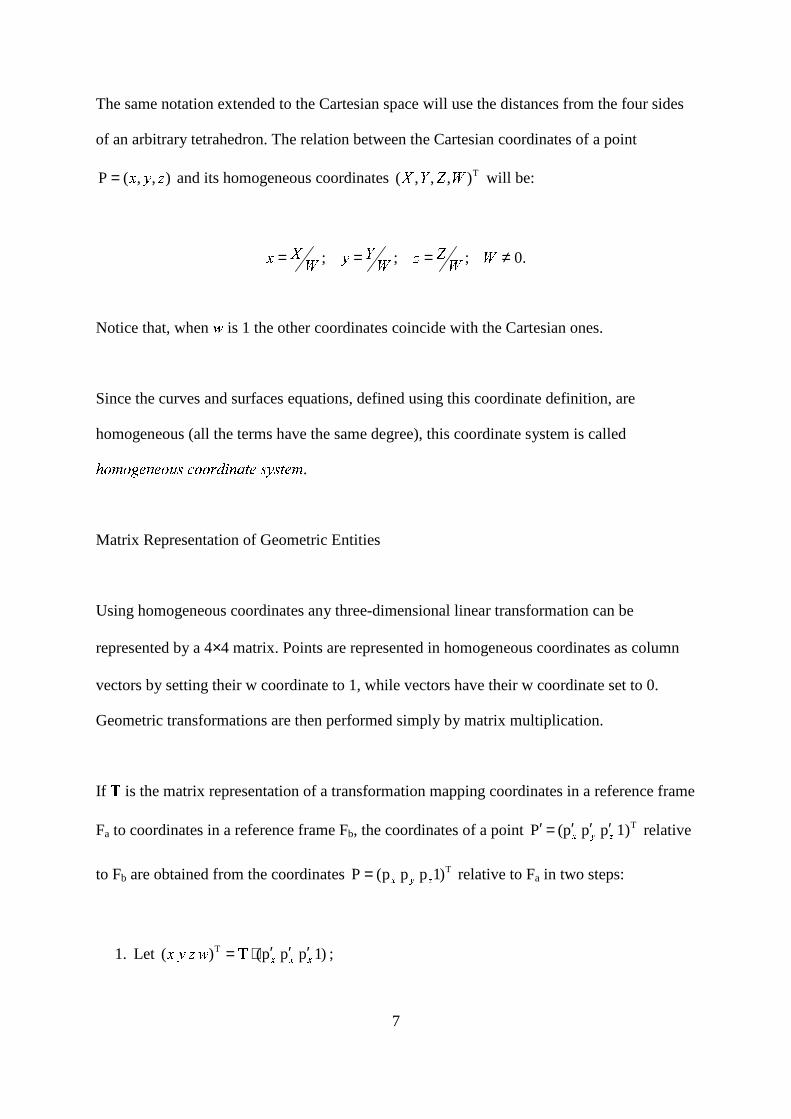
The same notation extended to the Cartesian space will use the distances from the four sides

of an arbitrary tetrahedron. The relation between the Cartesian coordinates of a point

),,(P ���= and its homogeneous coordinates T),,,( ���� will be:

.0;;; ≠=== �����

��� ¡

Notice that, when ¢ is 1 the other coordinates coincide with the Cartesian ones.

Since the curves and surfaces equations, defined using this coordinate definition, are

homogeneous (all the terms have the same degree), this coordinate system is called

£ ¤ ¥:¤)¦+§#¨ §)¤ ©)ª9«#¤ ¤ ¬0­ ®%¨ ¯ °'§^ª²±<ª;°'§#¥.

Matrix Representation of Geometric Entities

Using homogeneous coordinates any three-dimensional linear transformation can be

represented by a 4×4 matrix. Points are represented in homogeneous coordinates as column

vectors by setting their w coordinate to 1, while vectors have their w coordinate set to 0.

Geometric transformations are then performed simply by matrix multiplication.

If ³ is the matrix representation of a transformation mapping coordinates in a reference frame

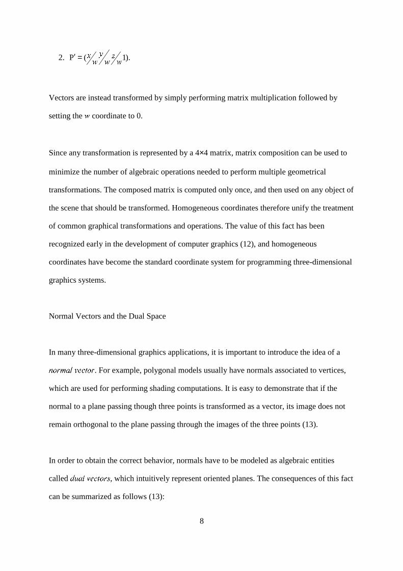
Fa to coordinates in a reference frame Fb, the coordinates of a point T1) p p p( P ´µ¶ ′′′=′ relative

to Fb are obtained from the coordinates T)1p p p(P ·¸¹= relative to Fa in two steps:

1. Let )1p p p()( T ººº»¼½¾ ′′′⋅= ¿ ;

8

2. ).1(P ÀÁÀÂÀÃ=′

Vectors are instead transformed by simply performing matrix multiplication followed by

setting the Ä coordinate to 0.

Since any transformation is represented by a 4×4 matrix, matrix composition can be used to

minimize the number of algebraic operations needed to perform multiple geometrical

transformations. The composed matrix is computed only once, and then used on any object of

the scene that should be transformed. Homogeneous coordinates therefore unify the treatment

of common graphical transformations and operations. The value of this fact has been

recognized early in the development of computer graphics (12), and homogeneous

coordinates have become the standard coordinate system for programming three-dimensional

graphics systems.

Normal Vectors and the Dual Space

In many three-dimensional graphics applications, it is important to introduce the idea of a

Å Æ Ç0È:É ÊÌË#Í#Î#Ï%Æ Ç . For example, polygonal models usually have normals associated to vertices,

which are used for performing shading computations. It is easy to demonstrate that if the

normal to a plane passing though three points is transformed as a vector, its image does not

remain orthogonal to the plane passing through the images of the three points (13).

In order to obtain the correct behavior, normals have to be modeled as algebraic entities

called Ð Ñ Ò ÓÕÔ)Ö;×#Ø'Ù ÚÜÛ , which intuitively represent oriented planes. The consequences of this fact

can be summarized as follows (13):

9

1. Dual vectors are represented as row vectors;

2. If Ý is the matrix representation of a geometric transformation, then dual vectors are

transformed by multiplying them by the inverse transpose of Þ , followed by setting the

last component to 0.

Matrix Representation of Primitive Linear Transformations

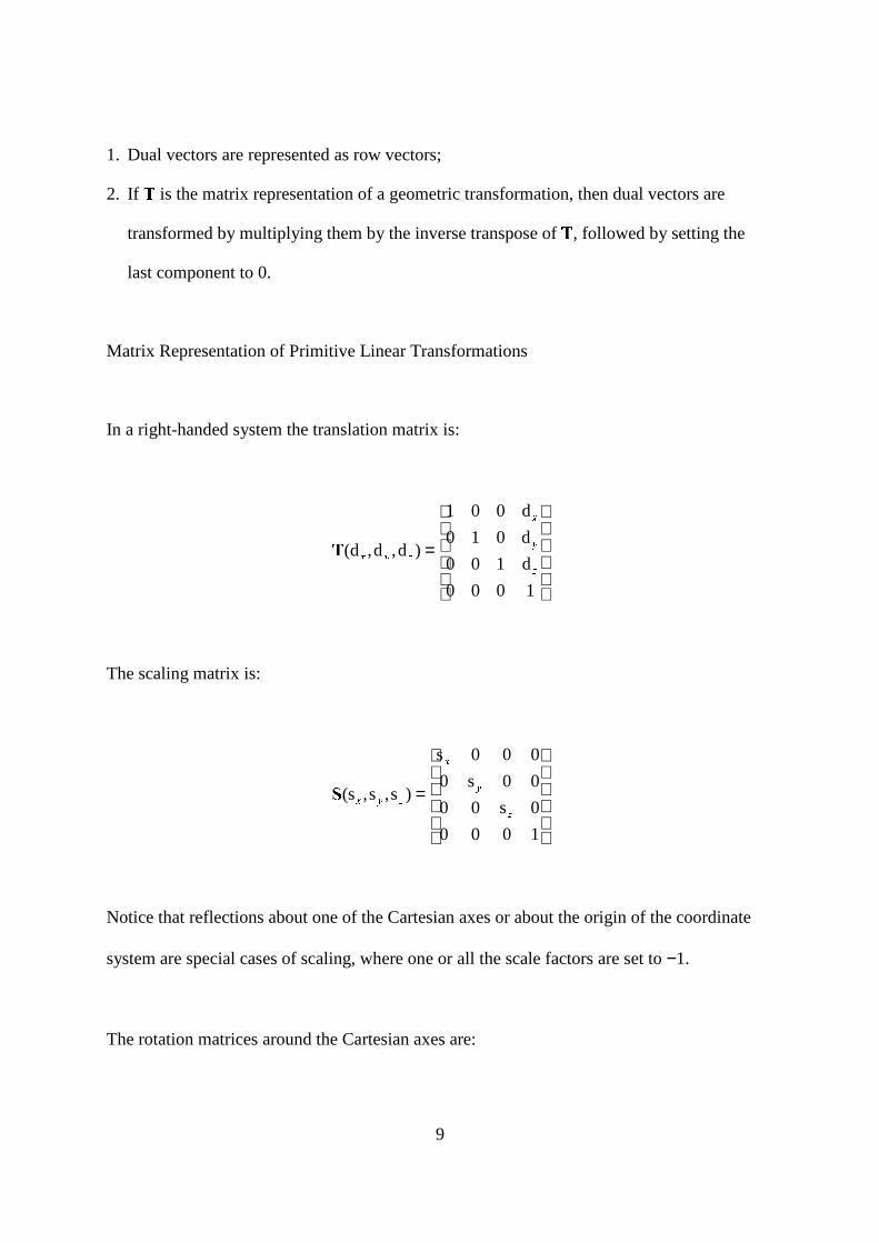
In a right-handed system the translation matrix is:

=

1000

d100

d010

d001

)d,d,d( ßàá

ßàáâ

The scaling matrix is:

=

1000

0s00

00s0

000s

)s,s,s( ãäå

ãäåæ

Notice that reflections about one of the Cartesian axes or about the origin of the coordinate

system are special cases of scaling, where one or all the scale factors are set to −1.

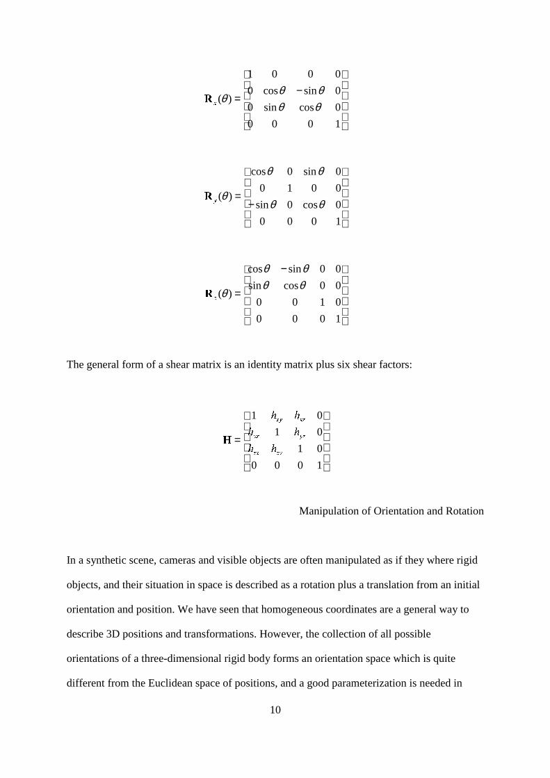
The rotation matrices around the Cartesian axes are:

10

−

=

1000

0cossin0

0sincos0

0001

)(θθθθ

θçè

−=

1000

0cos0sin

0010

0sin0cos

)(θθ

θθ

θéê

−

=

1000

0100

00cossin

00sincos

)(θθθθ

θëì

The general form of a shear matrix is an identity matrix plus six shear factors:

=

1000

01

01

01

íïîíñðî'íî%ðð%íðòî

óóóóóó

ô

Manipulation of Orientation and Rotation

In a synthetic scene, cameras and visible objects are often manipulated as if they where rigid

objects, and their situation in space is described as a rotation plus a translation from an initial

orientation and position. We have seen that homogeneous coordinates are a general way to

describe 3D positions and transformations. However, the collection of all possible

orientations of a three-dimensional rigid body forms an orientation space which is quite

different from the Euclidean space of positions, and a good parameterization is needed in

11

order to easily perform meaningful operations. Representing orientations and rotations as

matrices is sufficient for applications which require only transformation composition, but

does not support transformation interpolation, a required feature for applications such as õ#ö?÷ùøú@û0ü ý-þ'ÿ��

. In particular, interpolation of rotation matrices does not produce orientation

interpolation, but introduces unwanted shearing effects as the matrix deviates from being

orthogonal.

It can be demonstrated that four parameters are needed to coordinatize the orientation space

without singularities (14). Common three-value systems such as Euler angles (i.e. sequences

of rotations about the Cartesian axes) are therefore not appropriate solutions����������� ������������� , invented by Hamilton in 1843 (14) and introduced to the computer graphics

community by Schoemake (15), have proven to be the most natural parameterization for

orientation and rotation.

Quaternion Arithmetic for 3D Graphics

A quaternion ],[ �� �= consists of a scalar part, the real number � , and an imaginary part,

the 3D vector � . It can be interpreted as a point in 4-space, with coordinates ],,,[ ���� ,

equivalent to homogeneous coordinates for a point in projective 3-space� Quaternion

arithmetic is defined as the usual 4D vector arithmetic, augmented with a multiplication

operation defined as follows:

)](),[(],][,[ 212111 � �� � � !!!!!!!!"" ×++•−== ######

12

A rotation of angle θ and axis aligned with a unit vector $ is represented in quaternion form

by the unit quaternion ]2sin,2[cos %& θθ= .

With this convention, composition of rotations is obtained by quaternion multiplication, and

linear interpolation of orientations is obtained by linearly interpolating quaternion

components. The formula for spherical linear interpolation from ')( to *,+ , with parameter -moving from 0 to 1 is the following:

././ 0000θθ

θθ

sin

sin

sin

)1sin(),,slerp(

111 +−=

where

θcos=• 23544

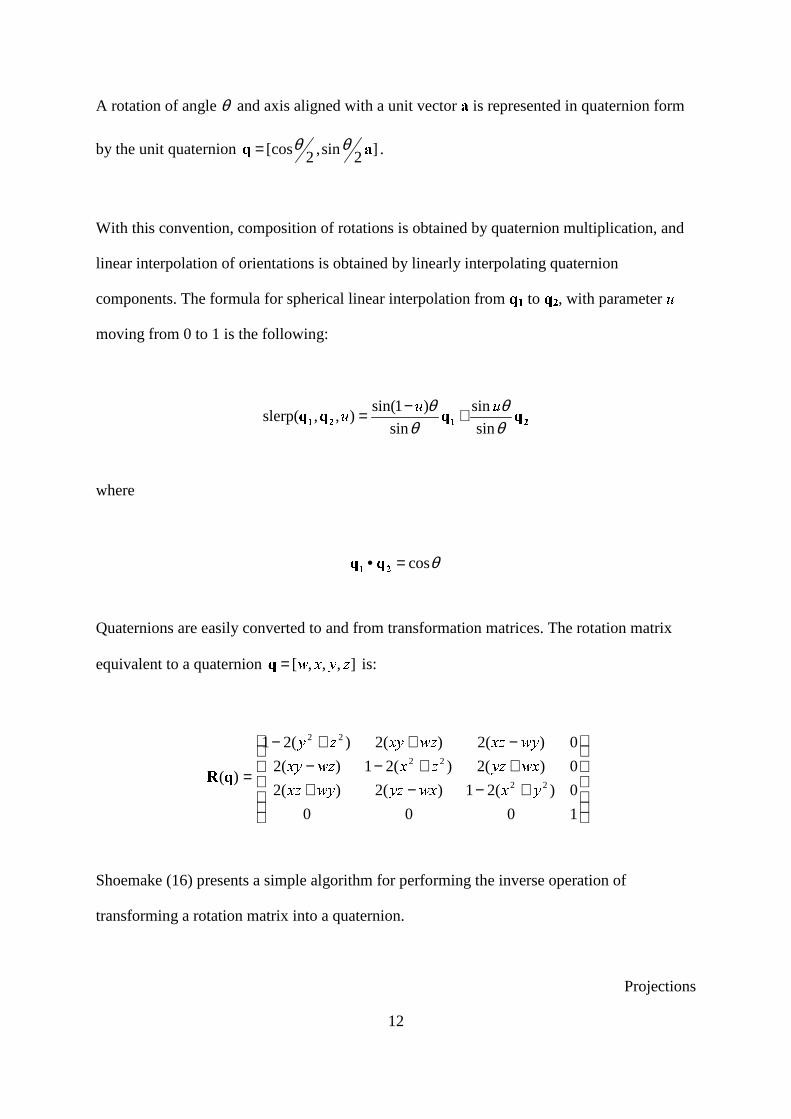
Quaternions are easily converted to and from transformation matrices. The rotation matrix

equivalent to a quaternion ],,,[ 6789=: is:

+−−+++−−−++−

=

1000

0)(21)(2)(2

0)(2)(21)(2

0)(2)(2)(21

)(22

22

22

;<=><;@?=A;<�?=><;@??<=B?<C;=D;<�?=B?<C;?;

EF

Shoemake (16) presents a simple algorithm for performing the inverse operation of

transforming a rotation matrix into a quaternion.

Projections

13

A GIH�JLKNM�O�P�QJ�R is a geometrical transformation from a domain of dimension S to a co-domain of

dimension T −1 (or less). When producing images of three-dimensional scenes, we are

interested in projections from three to two dimensions.

The process of projecting 3D object on a planar surface is performed casting straight rays

from a single point, possibly at infinity, trough each of the points forming the object, and

computing the intersections of the rays with the projection plane. Projecting all the points

forming a segment is equivalent to project its end-points and then connect them on the

projection plane. The projection process can be then reduced to project only the vertices of

the objects forming the scene. This particular class of projections is the class of UIV�W�X�W�YZ�[�\�]^[�_ Y�`�abUIY \Lcd[ a _ ` \ X�e .

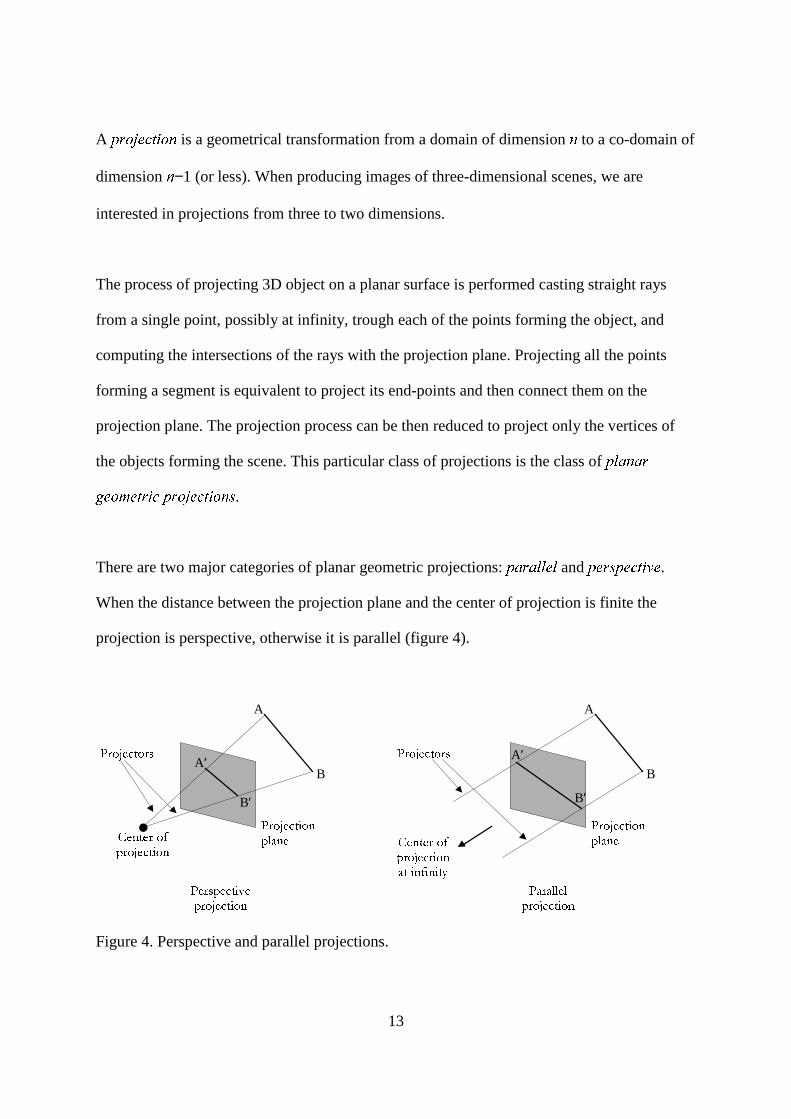
There are two major categories of planar geometric projections: fIg�h�g�ii�j�i and kIl�monokIl�p�qrstl .When the distance between the projection plane and the center of projection is finite the

projection is perspective, otherwise it is parallel (figure 4).

B′

A′B

A

udv�wyx{z}|}~�w�v�

ud��v����{��z��� vw�x{z�|}~ ��w��

udz}v� � z}|}~ �{��z� vw�x{z}|}~ ��wy�

� z}��~�z}v�wy�� vw�x{z�|}~ ��w��

uNvw�x{z}|�~ ��wy�� ������z

B′

A′B

A

�D�}�y���������� ���y�{�}�}� ������ �����y�����}��� �

� ���y�{�}�}� ������}� � �y�

� ����{�}�����y�� 

Figure 4. Perspective and parallel projections.

14

A perspective projection is typically used to simulate a realistic view of the scene, while a

parallel one is more suited for technical purposes.

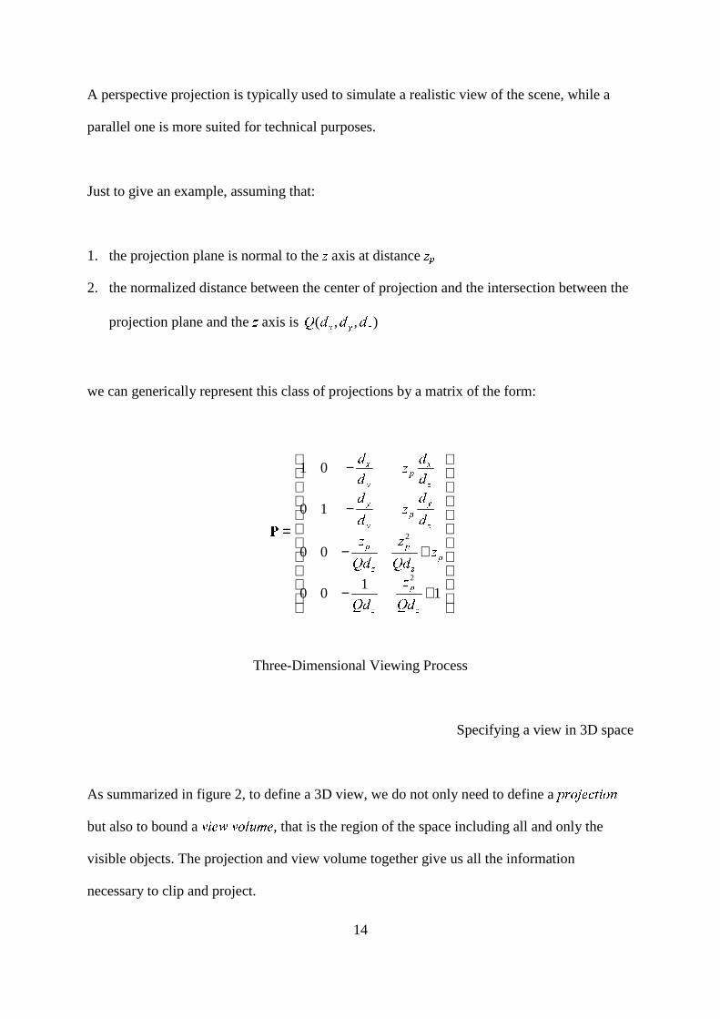
Just to give an example, assuming that:

1. the projection plane is normal to the ¡ axis at distance ¢�£2. the normalized distance between the center of projection and the intersection between the

projection plane and the ¤ axis is ),,( ¥¦§ ¨¨¨©

we can generically represent this class of projections by a matrix of the form:

+−

+−

−

−

=

11

00

00

10

01

2

2

ª«

ª

«ª«

ª«

ª¬«¬

¬ª­«¬

­

®°¯±

®^¯

±®^¯±

®^¯±

¯¯

±¯¯

¯¯±¯

¯

²

Three-Dimensional Viewing Process

Specifying a view in 3D space

As summarized in figure 2, to define a 3D view, we do not only need to define a ³I´�µL¶N·t¸�¹º�µ�»but also to bound a ¼�½¾�¿À¼�Á�ÂÃ�Ä°¾ , that is the region of the space including all and only the

visible objects. The projection and view volume together give us all the information

necessary to clip and project.

15

While this process could be totally described using the mathematics seen before, it is much

more natural to describe the entire transformation process using the so-called Å�Æ�Ç^È�É�ÆÇ^È�Ê�Æ�ËIÌ�Í�É . Setting the parameter of a synthetic view is analogous to taking a photograph with

a camera. We can schematize the process of taking a picture in the following steps:

1. Place the camera and point it to the scene;

2. Arrange the objects in the scene;

3. Choose the lens or adjust the zoom;

4. Decide the size of the final picture.

Generating a view of a synthetic scene on a computer, this four actions correspond to define,

respectively, the following four transformations:

1. Î�ÏÐ�ÑÒÏÓ�ÔÖÕ�×�Ø�Ó�ÙÛÚNÜ�×�Ý^Ø�Õ�ÏÜ�Ó2. Þ^ß�à�á�â�ãä�åÖæ�ç�è�ä�éÛêdß�çëÞ^è�æ�ãß�ä3. ìIí�îLïdð�ñ�òóî�ôõò�í�ö�ô�÷ÛøNî�í�ù^ö�ò�óî�ô4. ú�ûü�ýAþIÿ�� ��� �������Nÿ������ � ûÿ��

The modeling transformation is, typically, a way to define objects in the scene in a

convenient coordinate system, and then transform them in a single, general, coordinate

system called ������������������������������ �!�"����# . The meaning of other three is explained in detail in

the following.

Viewing transformation

16

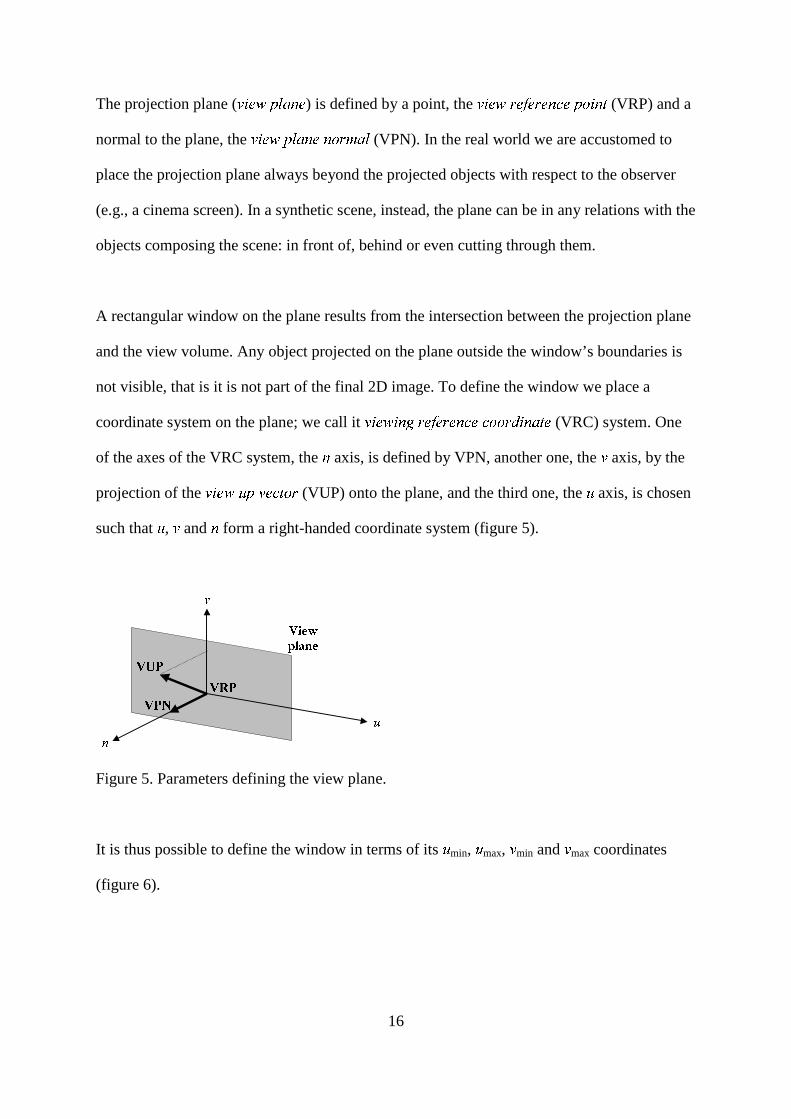
The projection plane ( $�%�&�')(+*�,�-�& ) is defined by a point, the .�/�0�132406570�240�8!9�0;:+<�/�8�= (VRP) and a

normal to the plane, the >�?A@�B)C+D�E�F�@GF�H�I�J�E�D (VPN). In the real world we are accustomed to

place the projection plane always beyond the projected objects with respect to the observer

(e.g., a cinema screen). In a synthetic scene, instead, the plane can be in any relations with the

objects composing the scene: in front of, behind or even cutting through them.

A rectangular window on the plane results from the intersection between the projection plane

and the view volume. Any object projected on the plane outside the window’s boundaries is

not visible, that is it is not part of the final 2D image. To define the window we place a

coordinate system on the plane; we call it K�L�M�NOL�P�QSR�M6TUM�R�M�P�V"MGV�W�W�R�X�L�P�Y�Z�M (VRC) system. One

of the axes of the VRC system, the [ axis, is defined by VPN, another one, the \ axis, by the

projection of the ]�^A_�`badce]�_�f�g�h�i (VUP) onto the plane, and the third one, the j axis, is chosen

such that k , l and m form a right-handed coordinate system (figure 5).

n

o

p

q+rtsvuw x y z s

{}|}~

{}~��{}�}~

Figure 5. Parameters defining the view plane.

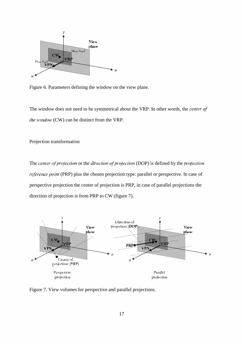
It is thus possible to define the window in terms of its � min, � max, � min and � max coordinates

(figure 6).

17

�

( � min, � min)

( � max, � max)

�

�

�+�t�v�� � � � �

�}����}� �}�}�

Figure 6. Parameters defining the window on the view plane.

The window does not need to be symmetrical about the VRP. In other words, the �����������¡ £¢��¤��G¥�¦���§� �¥ (CW) can be distinct from the VRP.

Projection transformation

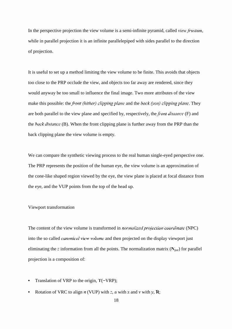
The ̈�©�ª�«�©�¬¡­£®}¯+¬�­£°U±"²�³�´�­�µ or the ¶�·�¸�¹�º�»�·�¼�½�¼£¾}¿+¸�¼£ÀU¹�º�»�·�¼�½ (DOP) is defined by the Á+Â�ãÄ7Å"Æ�Ç�È�Ã�ÉÂ�Å6Ê7Å�Â�Å�É�Æ"Å;Á+Ã�È�É�Ç (PRP) plus the chosen projection type: parallel or perspective. In case of

perspective projection the center of projection is PRP, in case of parallel projections the

direction of projection is from PRP to CW (figure 7).

Ë

Ì

Í

Î�Ï Ð�ÏÒÑÓÑÔ�ÑÕ Ð×ÖÙØÔÙÚÜÛ ÝÒÖßÞ

ÎàÔÙÐ�á Õ ÔÜÚÙÛ Ý â"ÔÕ Ð�ÖvØÔÜÚvÛ Ý×ÖßÞ

ã ÔÜÞßÛtÔÜÐUÖßäÕ Ð Ö Ø Ô Ú Û Ý Ö Þ å æ ç æ è

é}êtëíìî ï ð ñ ë

òôóöõ÷ùø òùúùó

û

ü

ý

þ}ÿ����� � � � �

��� ���� ����

����������� �������� ! � � " � � � � � � # $ % & '

Figure 7. View volumes for perspective and parallel projections.

18

In the perspective projection the view volume is a semi-infinite pyramid, called (*),+.-0/�132*465,287 ,

while in parallel projection it is an infinite parallelepiped with sides parallel to the direction

of projection.

It is useful to set up a method limiting the view volume to be finite. This avoids that objects

too close to the PRP occlude the view, and objects too far away are rendered, since they

would anyway be too small to influence the final image. Two more attributes of the view

make this possible: the 9�:3;8<8=?>�@8AB=,@8C.:�DFE.GBA H8HIA,<*JKHIGBL8<8C and the M8NPO.QFRTS�U8VXWYO.Z,[ \8\I[,V*]K\IZ,N8V8^ . They

are both parallel to the view plane and specified by, respectively, the _�`3a8b8c?d8egfhcBi8b8j.k (F) and

the l8m8n.oKp8qgrhsBm8t8n.u (B). When the front clipping plane is further away from the PRP than the

back clipping plane the view volume is empty.

We can compare the synthetic viewing process to the real human single-eyed perspective one.

The PRP represents the position of the human eye, the view volume is an approximation of

the cone-like shaped region viewed by the eye, the view plane is placed at focal distance from

the eye, and the VUP points from the top of the head up.

Viewport transformation

The content of the view volume is transformed in v8w8x3y0z8{,|~}h�.���Ix3w����.�.�B|,w8v��.w8w8x3�8|Bv8z8�,� (NPC)

into the so called �.�8�8�8�8�,�.�8�?�.�,�*���.�8�B�8��� and then projected on the display viewport just

eliminating the � information from all the points. The normalization matrix (� par) for parallel

projection is a composition of:

• Translation of VRP to the origin, � (−VRP);

• Rotation of VRC to align � (VUP) with � , � with � and � with � , � ;

19

• Shearing to make the direction of projection parallel to the � axis,   par;

• Translation and scaling to the parallel canonical volume, a parallelepiped, defined by the

equations 0;1;1;1;1;1 =−==−==−= ¡¡¢¢££ , ¤ par and ¥ par.

In formula:

)VRP(parparparpar −⋅⋅⋅⋅= ¦§¨¦©ª «

For a perspective projection the normalization matrix (¬ per) is a composition of:

• Translation of VRP to the origin;

• Rotation of VRC to align ­ (VUP) with ® , ̄ with ° and ± with ² ;

• Translation of PRP to the origin;

• Shearing to make the center line of the view volume being the ³ axis;

• Scaling to the perspective canonical volume, a truncated pyramid, defined by the

equations .1;;;;; min −=−=−==−== ´´´´µ´µ´¶´¶

In formula:

)VRP()PRP(perperper −⋅⋅−⋅⋅= ·¸·¹º» ¼

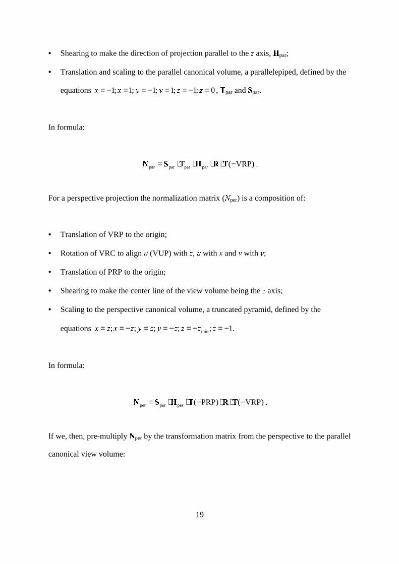
If we, then, pre-multiply ½ per by the transformation matrix from the perspective to the parallel

canonical view volume:

20

1,

010011

100

0010

0001

min

min

min

min

parper −≠

−+

−+

=→ ¾¾¾

¾¿

we obtain:

)VRP()PRP(perperperparperper −⋅⋅−⋅⋅=⋅=′ → ÀÁÀÂÃÄÅÄ

that is the matrix transforming the object in the scene to the canonical parallepided defined

before.

Using Æ ′per and Ç par we are thus able to perform the clipping operation against the same

volume using a single procedure.

Culling and Clipping

The clipping operation consists in determining which parts of an object are visible from the

camera and need to be projected on the screen for rendering. This operation is performed on

each graphical and is composed of two different steps. First, during culling, objects

completely outside of the view volume are eliminated. Then, partially visible objects are cut

against the view volume to obtain only totally visible primitives.

Culling of Points

At the end of the projection stage all the visible points describing the scene are inside the

volume defined by the equations:

21

0;1;1;1;1;1 =−==−==−= ÈÈÉÉÊÊ Ë

The points satisfying the inequalities:

01,11,11 ≤≤−≤≤−≤≤− ÌÍÎ

are visible, all the others have to be clipped out.

The same inequalities, expressed in homogeneous coordinates are:

01,11,11 ≤≤−≤≤−≤≤− ÏÐÏÑÏÒ

corresponding to the plane equations:

.0;;;;; =−==−==−= ÓÔÓÔÕÔÕÔÖÔÖ

Clipping of Line Segments

The most popular line segments clipping algorithm, and perhaps the most used, is the Cohen-

Sutherland algorithm. Since it is a straightforward extension of the two-dimensional clipping

algorithm, we illustrate this one first for sake of simplicity of explanation.

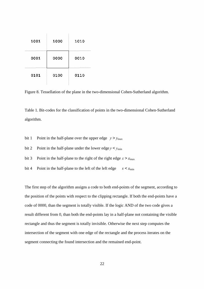
When clipping a line against a two-dimensional rectangle, the plane is tessellated in nine

regions (figure 8); each one identified by a four-bit code, where each bit is associated with an

edge of the rectangle. Each bit is set to 1 or 0 when the conditions listed in table 1 are,

respectively, true or false.

22

×ÙØÙ×ÙØ

ØÙØÙ×ÙØ

ØÙ×Ù×ÙØØÙ×ÙØÙØØÙ×ÙØÙ×

ØÙØÙØÙ×

×ÙØÙØÙ× ×ÙØÙØÙØ

ØÙØÙØÙØ

Figure 8. Tessellation of the plane in the two-dimensional Cohen-Sutherland algorithm.

Table 1. Bit-codes for the classification of points in the two-dimensional Cohen-Sutherland

algorithm.

bit 1 Point in the half-plane over the upper edge Ú > Û max

bit 2 Point in the half-plane under the lower edgeÜ < Ý min

bit 3 Point in the half-plane to the right of the right edge Þ > ß max

bit 4 Point in the half-plane to the left of the left edge à < á min

The first step of the algorithm assigns a code to both end-points of the segment, according to

the position of the points with respect to the clipping rectangle. If both the end-points have a

code of 0000, than the segment is totally visible. If the logic AND of the two code gives a

result different from 0, than both the end-points lay in a half-plane not containing the visible

rectangle and thus the segment is totally invisible. Otherwise the next step computes the

intersection of the segment with one edge of the rectangle and the process iterates on the

segment connecting the found intersection and the remained end-point.

23

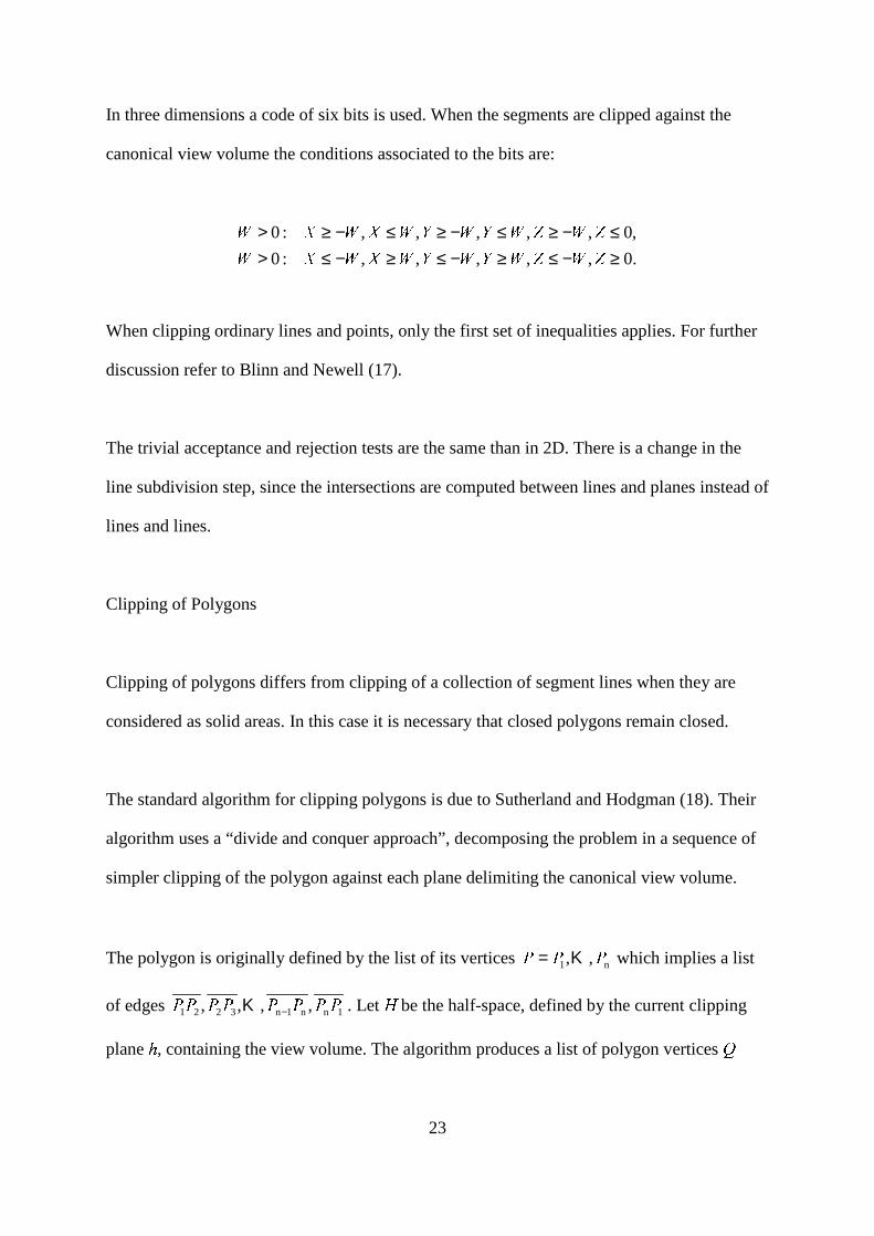
In three dimensions a code of six bits is used. When the segments are clipped against the

canonical view volume the conditions associated to the bits are:

.0,,,,,:0

,0,,,,,:0

≥−≤≥−≤≥−≤>≤−≥≤−≥≤−≥> âãâãäãäãåãåã

âãâãäãäãåãåã

When clipping ordinary lines and points, only the first set of inequalities applies. For further

discussion refer to Blinn and Newell (17).

The trivial acceptance and rejection tests are the same than in 2D. There is a change in the

line subdivision step, since the intersections are computed between lines and planes instead of

lines and lines.

Clipping of Polygons

Clipping of polygons differs from clipping of a collection of segment lines when they are

considered as solid areas. In this case it is necessary that closed polygons remain closed.

The standard algorithm for clipping polygons is due to Sutherland and Hodgman (18). Their

algorithm uses a “divide and conquer approach” , decomposing the problem in a sequence of

simpler clipping of the polygon against each plane delimiting the canonical view volume.

The polygon is originally defined by the list of its vertices n1 ,, æææ Κ= which implies a list

of edges 1nn1n3221 ,,,, çççççççç −Κ . Let è be the half-space, defined by the current clipping

plane é , containing the view volume. The algorithm produces a list of polygon vertices ê

24

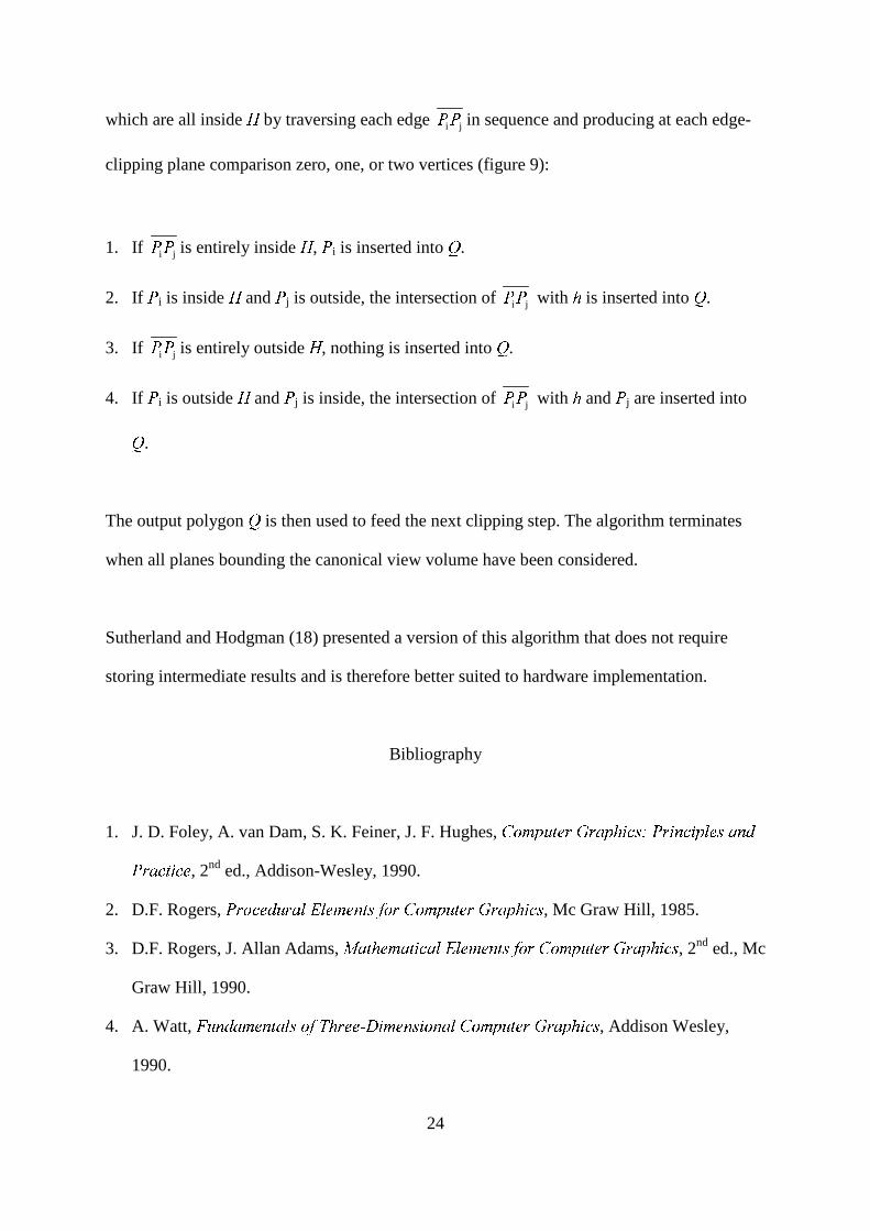
which are all inside ë by traversing each edge ji ìì in sequence and producing at each edge-

clipping plane comparison zero, one, or two vertices (figure 9):

1. If ji íí is entirely inside î , ï i is inserted into ð .

2. If ñ i is inside ò and ó j is outside, the intersection of ji ôô with õ is inserted into ö .

3. If ji ÷÷ is entirely outside ø , nothing is inserted into ù .

4. If ú i is outside û and ü j is inside, the intersection of ji ýý with þ and ÿ j are inserted into

�.

The output polygon � is then used to feed the next clipping step. The algorithm terminates

when all planes bounding the canonical view volume have been considered.

Sutherland and Hodgman (18) presented a version of this algorithm that does not require

storing intermediate results and is therefore better suited to hardware implementation.

Bibliography

1. J. D. Foley, A. van Dam, S. K. Feiner, J. F. Hughes, ��������� �������������� ����������� ��!� �" ���#�� �$�%�&����� �'��� , 2nd ed., Addison-Wesley, 1990.

2. D.F. Rogers, (%)&*�+!,�-�.�)�/�021�0',�34,�5�687:9;*�)<�*�3>=.�6 ,�)?@)�/�=A�B'+�7 , Mc Graw Hill, 1985.

3. D.F. Rogers, J. Allan Adams, CED�F G�H!I@D�F'J K�D�LNM%L'H�I@H!O�FQP:RTS�U�V�S�I>WX�F H!U�Y@U&D�WG�J K�P , 2nd ed., Mc

Graw Hill, 1990.

4. A. Watt, Z�[�\�]�^�_�`�\�a ^�b8c#dfe4gih�j�`�`!kmlon _�`�\!cNn d�\�^�bqp�d�_>r[�a `!j�s@j&^�rh�n t�c , Addison Wesley,

1990.

25

5. I. Sutherland, “Sketchpad: A Man-Machine Graphical Communication System”. In

u%v&w�x�y�y�z�{'|!}�~#wf�4�'��y��!�v�{ |!}���w�{ |�����w��>���� y�v���w�|f�;y!v�y�|�x�y, 329 - 346, 1963.

6. D.B. Conner, A. van Dam, “Sharing Between Graphical Objects Using Delegation” . In

�%�&�����������'�!���#�f�4�'�����i��� ���%�������!����������'���o������ ��N�����¡����¢�£f¤;�����'¥¦¢���� �!��� ����§���������¨���, 63 - 82,

1992.

7. The OpenInventor Architecture Group, ©�ª�«�¬!­�¬�®!«�¬�¯ °�±�²4³�³µ´%«·¶;«!±�«�¬:¸�«�¹»º�¬�¼�º�½ ¾>¿iÀ�«©q¶'¶;Á ¸!Á º�½2´�«·¶T«�±�«�¬�¸!«Âµ°�¸�¼�Ã@«�¬�¯¦¶T°�±�©>ª«�¬%Ä!Å:ÆN¯'«�ÃÇÆ , Addison-Wesley, 1994.

8. R. Carey, G. Bell, ÈiÉ�ÊÌËTÍÏÎÑÐÓÒ�ÔÖÕ%×%Ø�Ø�Ù�Ú'Û�Ú Ê�Ü%Í�Ê·ÝTÊ�Þ�Ê�Ø�ß�ÊλÛ�Ø�à�Û�á , Addison-Wesley, 1997.

9. T. Gaskins, âäã@å�æÇç�â�è�é!ê�è&ë�ì4ì�í î!ê�ïEë�î�ð�ë�ñ , O'Reilly and Associates, 1992.

10. F. Möbius, ò�ó�ôNõ�ö�ö4ó!÷ ø ó�ùÌó�úüû�ó , vol 1. ýoþ ÿ����������ÿ��� ��þ������:ÿ������ ����� . Dr. M. Saendig oHG,

Wiesbaden, Germany, 1967, 36 - 49.

11. J. Plücker, “Ueber ein neues Coordinatensystem” ������������ �!#"%$��'&�(*)�+�)�( ��)�����&-,���.)�/� ���&�0 )1 �0 2�)�34 �0*( 5 , vol. 5, 1830, 1 - 36.

12. L. G. Roberts, 687�9:7�;=<�>�<?7�@�A'BDC�E F�G�H�I�<KJLFM<NA�<�>�E C�E G*7�>OC�>�P-BQC�>�G JL@�R C�E G*7�>O7TS�UWV�XYG 9:<�>�A�G*7�>�C�RZ 7�>�A�E*F�@�[�E�A�\ Technical Report MS-1405, Lincoln Laboratory, MIT, May, 1965.

13. T. DeRose, “A Coordinate-Free Approach to Geometric Programming”, In W. Strasser,

H. Seidel (ed.) ]_^�`�a�b�ced�f�g-h�b�d�i�j k i�`�aTlWm4`�a�n4`�j b�k*i�oQa�g�`�p*k f�q , Springer, 291 - 306, 1989.

14. W.R. Hamilton, “On Quaternions; or on a New System of Imaginaries in Algebra” ,

r-s�t*u v�w�vyxLs�t*z�{�u}|D{�~={���t ���, XXV, 10 - 13, 1844.

15. K. Schoemake, “Animating Rotation with Quaternion Curves” , �������L��� ���'�4���y�L�����N� ,19(3), 245 - 254, 1985.

16. K. Schoemake, “Polar Decomposition for Rotation Extraction” , Notes for Course #C2,

�Q��� ����������M�:� �¢¡¤£¤¥, SIGGRAPH Tutorial Notes, 1991.

17. J.F Blinn, M.E. Newell, “A Homogeneous Formulation for Lines in 3-Space”,

¦-§�¨�©�ª�ª�«�¬*­�®�¯'°�±M²4²´³¤µ¤¦¤¶, 237 - 241, 1977.

26

18. I. Sutherland, G.W. Hodgman, “Reentrant Polygon Clipping” , Communications of the

ACM, 17, 32 - 42, 1974.