Embed Size (px)
Citation preview

For permission to copy, contact [email protected]© 2010 Geological Society of America
Three-dimensional geologic modeling of the Santa Rosa Plain, California
Donald S. Sweetkind*U.S. Geological Survey, Denver Federal Center, Mail Stop 973, Denver, Colorado 80225, USA
Emily M. TaylorU.S. Geological Survey, Denver Federal Center, Mail Stop 980, Denver, Colorado 80225, USA
Craig A. McCabeESRI, 380 New York Street, Redlands, California 92373, USA
Victoria E. LangenheimU.S. Geological Survey, Mail Stop 989, 345 Middlefi eld Road, Menlo Park, California 94025, USA
Robert J. McLaughlinU.S. Geological Survey, Mail Stop 973, 345 Middlefi eld Road, Menlo Park, California 94025, USA
237
Geosphere; June 2010; v. 6; no. 3; p. 237–274; doi: 10.1130/GES00513.1; 11 fi gures; 5 tables; 3 plates; 8 appendix fi gures; 2 supplemental fi gures.
ABSTRACT
New three-dimensional (3D) lithologic and stratigraphic models of the Santa Rosa Plain (California, USA) delineate the thickness, extent, and distribution of subsurface geo-logic units and allow integration of diverse data sets to produce a lithologic, strati-graphic, and structural architecture for the region. This framework can be used to pre-dict pathways of groundwater fl ow beneath the Santa Rosa Plain and potential areas of enhanced or focused seismic shaking.
Lithologic descriptions from 2683 wells were simplifi ed to 19 internally consistent lithologic classes. These distinctive lithologic classes were used to construct a 3D model of lithologic variations within the basin by extrapolating data away from drill holes using a nearest-neighbor approach. Subsur-face stratigraphy was defi ned through the identifi cation of distinctive lithologic pack-ages tied, where possible, to high-quality well control and to surface exposures. The 3D stratigraphic model consists of three bound-ing components: fault surfaces, stratigraphic surfaces, and a surface representing the top of pre-Cenozoic basement, derived from inversion of regional gravity data.
The 3D lithologic model displays a west to east transition from dominantly marine sands to heterogeneous continental sedi-ments. In contrast to previous stratigraphic studies, the new models emphasize the preva-
lence of the clay-rich Petaluma Formation and its heterogeneous nature. Isopach maps of the Glen Ellen Formation and the 3D stratigraphic model show the infl uence of the Trenton Ridge, a concealed basement ridge that bisects the plain, on sedimentation; the thickest deposits of the Glen Ellen Formation are confi ned to north of the Trenton Ridge.
INTRODUCTION
Sonoma County is in the northern part of the San Francisco Bay region of northern Califor-nia, an area that has undergone rapid popula-tion growth and accelerated urbanization in response to economic expansion over several decades. Approximately half of the popula-tion of Sonoma County resides on the Santa Rosa Plain (Fig. 1), a northwest-trending topo-graphic and structural low. Water supply in this area is provided by a combination of surface water delivered via aqueduct from the Russian River and groundwater from beneath the Santa Rosa Plain. The Santa Rosa Plain is known to be underlain by four Miocene and younger formations, each of which has distinct aquifer properties, including: (1) Pliocene–Pleistocene gravels that have been referred to in part as the Glen Ellen Formation (Fox, 1983); (2) domi-nantly marine sands of the Miocene and Plio-cene Wilson Grove Formation; (3) various types of Miocene and Pliocene volcanic rocks; and (4) dominantly fi ne-grained continental sedi-ments of the Miocene and Pliocene Petaluma
Formation (Fig. 1). Although the outcrop dis-tribution of each of these formations has been mapped (e.g., Blake et al., 2002; Wagner et al., 2006; Graymer et al., 2007), the degree of subsurface interfi ngering and overlapping age relations of the Miocene and Pliocene marine and nonmarine units have only recently been recognized and have important signifi cance for the hydrogeologic system. The large increase in population and concomitant changes in land use within Sonoma County requires a reassess-ment of the hydrogeologic system, including the thickness, extent, and three-dimensional (3D) distribution of each of these important aquifers.
The distribution, subsurface extent, and inter-fi ngering relations between the four principal formations refl ect the geomorphologic devel-opment of the basins that underlie the Santa Rosa Plain, the history of uplift and subsid-ence, tectonic activity, including offset along major basin-bounding faults, and the interaction between continental and marine sedimentation. The complexity in stratigraphic and structural relations across faults bounding the Santa Rosa Plain makes it diffi cult to project the geology exposed in the uplands surrounding the plain directly to the subsurface, making 3D subsur-face analysis from well data essential. An under-standing of the extent and 3D geometry of these formations bears on an understanding of basin evolution, the timing of movement of faults the bound and transect the basins that underlie the Santa Rosa Plain, and the relation to volcanism in the nearby Sonoma volcanic fi eld.
Sweetkind et al.
238 Geosphere, June 2010
5100
0052
0000
5300
00
4240000425000042600004270000
010
5K
ILO
ME
TE
RS
10,0
00-m
eter
grid
bas
ed o
n Un
iver
sal T
rans
vers
eM
erca
tor p
roje
ctio
n, Z
one
10, N
orth
Am
eric
an D
atum
198
3.Sh
aded
-rel
ief b
ase
from
1:2
75,0
00-s
cale
Dig
ital E
leva
tion
Mod
el;
sun
illum
inat
ion
from
nor
thw
est a
t 30
degr
ees
abov
e ho
rizon
2526 35
36
Win
dsor
Win
dsor
Bas
inB
asin
Cota
tiCo
tati
Bas
inB
asin
Sebastopol fa
ult
Sebastopol fa
ult
Healdsburg fault
Healdsburg fault
Rodgers Creek fault
Rodgers Creek fault
Bennett Valley fault
Bennett Valley fault
Maacama fault
Maacama fault
Tren
ton R
idge
Tren
ton Ri
dge
Bloo
mfie
ld fa
ult
Bloo
mfie
ldfa
ult
Cota
tiB
asin
Win
dsor
Bas
in
Sebastopol fa
ult
Healdsburg fault
Rodgers Creek fault
Bennett Valley fault
Maacama fault
Tren
ton R
idge
Bloo
mfie
ld fa
ult
Russian River
OR
SR
Mea
cham
Hill
Mea
cham
Hill
Mea
cham
Hill
San
ta R
osa
Win
dso
r
Pet
alu
ma
Ro
hn
ert
Par
k
Co
tati
Seb
asto
po
l
Hea
ldsb
urg
Qua
tern
ary
allu
vium
Qua
tern
ary
and
Plio
cene
gra
vels
(G
len
Elle
n Fo
rmat
ion)
Peta
lum
a Fo
rmat
ion
Wils
on G
rove
For
mat
ion
Neo
gene
vol
cani
c ro
cks
Gre
at V
alle
y se
quen
ce a
nd C
oast
Ran
ge o
phio
lite
Fran
cisc
an C
ompl
ex
Ultr
amaf
ic r
ocks
EX
PL
AN
AT
ION
Map
ped
faul
ts
(af
ter
Gra
ymer
and
oth
ers,
200
6)
Loc
atio
n of
dee
p ba
sins
in th
e Sa
nta
Ros
a Pl
ain,
as
defi
ned
by
-14
mG
al is
osta
tic g
ravi
ty c
onto
ur
(L
ange
nhei
m a
nd o
ther
s, 2
006)
Map
uni
ts
(G
eolo
gy a
fter
Sau
cedo
and
oth
ers,
200
0)
Sim
plif
ied
trac
e of
maj
or f
aults
use
d in
3D
lith
olog
ic a
nd s
trat
igra
phic
mod
els
Mes
ozoi
c ro
cks
Dri
ll ho
le, c
lass
ifie
d by
tot
al d
epth
Sect
ion
boun
dary
; sec
tions
25,
26, 3
5, a
nd 3
6 in
T7N
R9W
ar
e di
scus
sed
in te
xt
Cen
ozoi
c ro
cks Stre
am
<10
0 m
100
- 20
0 m
201
- 30
0 m
301
- 50
0 m
> 5
00 m
122°
30'
123°
38°3
0'
38°
37°3
0’
Are
a of
map
Sono
ma
Cty
Nap
a C
ty
Mar
in C
ty
Sant
aRo
saPl
ain
Paci
fic O
cean
Fig
ure
1. S
impl
ifi ed
geo
logi
c m
ap (m
odi-
fi ed
from
Sau
cedo
et
al.,
2000
; G
raym
er
et a
l., 2
006)
of
the
Sant
a R
osa
Pla
in
and
surr
ound
ing
high
land
s. T
he S
anta
R
osa
Pla
in i
s bo
und
on t
he w
est
by t
he
Seba
stop
ol f
ault
and
on
the
east
by
the
Rod
gers
Cre
ek a
nd H
eald
sbur
g fa
ults
. T
he b
urie
d T
rent
on R
idge
sep
arat
es t
he
nort
hern
Win
dsor
Bas
in fr
om th
e so
uth-
ern
Cot
ati B
asin
. Dri
ll ho
les
used
in t
his
stud
y ar
e cl
assi
fi ed
by t
otal
dep
th.
Tw
o dr
ill h
oles
wit
h hi
gh-q
ualit
y lit
holo
gic
and
bios
trat
igra
phic
da
ta
(Pow
ell
et
al.,
2006
) ar
e la
bele
d: O
R—
Occ
iden
tal
Roa
d w
ell;
SR
—Se
bast
opol
Roa
d w
ell.
3D geologic modeling—Santa Rosa Plain
Geosphere, June 2010 239
Studies of the Santa Rosa Plain that have focused on water availability (Cardwell, 1958; California Department of Water Resources, 1975, 1982) used drill-hole data to develop geologic cross sections and to help estimate the transmissivity of various rock types. However, these previous subsurface interpretations largely were based on limited borehole information from a small number of oil and gas wells and water wells, augmented by projection of surface exposures to the subsurface. Since these water availability studies, much new work has been conducted, including new geologic maps pub-lished by the California Geologic Survey (Wag-ner and Bortugno, 1982; Bezore et al., 2003; Clahan et al., 2003; Wagner et al., 2003, 2006) and geologic maps and other studies published by the U.S. Geological Survey (USGS) (Blake et al., 2002; Graymer et al., 2007; McPhee et al., 2007; McLaughlin et al., 2008; Langenheim et al., 2010). There have also been studies on exposed basin-margin stratigraphy and structure (Fox, 1983; Davies, 1986; Allen, 2003), strati-graphic data from oil and gas wells (Wright and Smith, 1992; Zieglar et al., 2005), and detailed biostratigraphic and chronostratigraphic analy-sis of surface exposures and drill cuttings (Pow-ell et al., 2004, 2006). This paper provides inte-gration of these data sets with existing and new well data to develop a modern context for sub-surface analysis of the Santa Rosa Plain.
In this paper we defi ne the subsurface stratig-raphy and lithologic heterogeneity of the four principal aquifer units using compiled drill-hole data from the Santa Rosa Plain. A 3D model of lithologic variations within the basins that underlie the Santa Rosa Plain is developed by extrapolating data away from drill holes using a 3-dimensional gridding process (Rockware Earth science and GIS software: www. rockware.com). Subsurface stratigraphy is defi ned through the identifi cation of distinctive lithologic pack-ages, tied, where possible, to high-quality well control. Available subsurface data provided suffi -cient detail to allow us to confi dently distinguish major stratigraphic boundaries and enough inter-nal detail within these units to develop a reliable subsurface geologic model. Faults are incorpo-rated as discontinuities in structure contour and isopach maps of the principal units; however; interbasin structural complexities such as fold-ing and thrust faulting are not explicitly consid-ered by these models. This structural complexity is partly accommodated in the model through integration of unit interfi ngering and facies rela-tions changes. These 3D subsurface models provide new insight into the confi guration of the basin-fi ll sediments, the relative importance and lithologic character of each of the four principal basin-fi lling units, and a suitable hydrogeologic
framework for groundwater resource assess-ments of the Santa Rosa Plain.
GEOLOGIC SETTING OF SANTA ROSA PLAIN
The southern part of the Santa Rosa Plain is covered by Quaternary alluvial deposits (Fig. 1). The northern part features low, slightly dissected exposures of late Pliocene and Qua-ternary (Pleistocene and Holocene) fl uvial, lacustrine, and alluvial plain deposits that have in part been referred to as the Glen Ellen Forma-tion (Fox, 1983), along with younger alluvium within stream channels (Graymer et al., 2007) (Fig. 1). The highlands to the east of the Santa Rosa Plain are underlain by various types of Miocene and Pliocene volcanic rocks, in part interbedded with the largely nonmarine and estuarine strata of the Petaluma Formation; both of these units unconformably overlie Mesozoic rocks (Fig. 1). This eastern margin of the Santa Rosa Plain is highly deformed and cut by major right-lateral strike-slip faults. West of the Santa Rosa Plain, a broad, low topographic area is underlain by Miocene to Pliocene, locally fos-siliferous marine sandstone formerly known as the Merced Formation (Cardwell, 1958), now referred to as the Wilson Grove Forma-tion (Fox, 1983). These marine strata dip gen-tly northeastward beneath the Santa Rosa Plain and unconformably overlie Mesozoic rocks (Fig. 1). Interfi ngering of marine sandstone with transitional marine and nonmarine deposits is inferred to occur beneath the Santa Rosa Plain based on exposures at Meacham Hill immedi-ately southwest of the Santa Rosa Plain (Powell et al., 2004). However, this transition zone is obscured by younger deposits beneath most of the plain. Cross sections that accompanied pre-vious groundwater resource assessments of the Santa Rosa Plain (Cardwell, 1958; California Department of Water Resources, 1975, 1982) portray most of the plain as being underlain by Glen Ellen Formation as much as ~300 m thick, underlain, in turn, by an unspecifi ed thickness of Wilson Grove Formation beneath the western half of the plain, and fl anked by Neogene volca-nic rocks on the east. The Petaluma Formation was inferred beneath the Petaluma Valley, but not to the north in the Santa Rosa Plain. We rec-ognize signifi cantly different stratigraphic rela-tions and distributions between the Glen Ellen, Wilson Grove, and Petaluma Formations.
The Santa Rosa Plain is bounded and tran-sected by major faults, including the active northwest-striking, right-lateral Rodgers Creek–Healdsburg fault zone bounding the east side of the plain. The west and southwest side of the plain is bounded by a system of poorly defi ned
Pliocene and younger normal faults, here gener-alized as the Sebastopol fault (Fig. 1).
Inversion of gravity data indicates that the Santa Rosa Plain is underlain by two main structural basins, the Cotati Basin to the south and the Windsor Basin to the north (Fig. 1). These depositional troughs are 2–3 km deep and fi lled with Tertiary and younger deposits (McPhee et al., 2007; Langenheim et al., 2010). These two basins are separated by a shallow west- northwest–striking bedrock ridge (the Trenton Ridge) that bisects the Santa Rosa Plain (McPhee et al., 2007; Williams et al., 2008; Langenheim et al., 2010) (Fig. 1). The Wind-sor Basin to the north is ~9 × 12 km, centered near the town of Windsor, and is located near many of the thickest outcrops of the Glen Ellen Formation in the Santa Rosa Plain. The Cotati Basin to the south is larger, 10 × 18 km, and 2.5–3 km deep. The Cotati Basin has a complex shape that suggests the presence of structurally controlled subbasins. The Glen Ellen Formation is also considerably thinned within much of the Cotati Basin, as the basin fi ll is dominated by the Wilson Grove and Petaluma Formations.
Description of Principal Stratigraphic Units of the Santa Rosa Plain
Quaternary to Pliocene–Pleistocene nonmarine units (Glen Ellen Formation)
The Pliocene–Pleistocene (younger than 3.2 Ma) Glen Ellen Formation was fi rst described by Weaver (1949) as exposures of poorly sorted clays, sands, gravels, and cob-bles near the town of Glen Ellen in the upper Sonoma Valley. Exposures of similar rocks have since been mapped through most of the Santa Rosa Plain, especially to the north and west of Santa Rosa. The unit consists of heterogeneous mixtures of tuffaceous clay, mud, bouldery to pebbly gravel, and sand and silt deposits with interbedded conglomerates. These sediments were deposited in a variety of nonmarine envi-ronments, including coalescing alluvial fans, fan deltas, streams, and lakes. Cardwell (1958) referred to many of these deposits as Glen Ellen Formation, but this terminology has been largely abandoned with the recognition of the existence of a number of other named and unnamed gravel-dominated sequences that overlap in age and are derived from several different local source areas (McLaughlin and Sarna-Wojcicki, 2003; McLaughlin et al., 2005). We retain the use of the term “Glen Ellen” to describe these diverse deposits in this study, mostly for consis-tency with earlier reports concerning the Santa Rosa Plain.
For our study we have combined all late Pliocene and younger nonmarine deposits in

Sweetkind et al.
240 Geosphere, June 2010
Location of well profile
A
B W E
DEPT
H, m
Western end point of profile:122° 50.53' W; 38° 30.13' N
Eastern end point of profile:122° 47.89' W; 38° 31.1' N
1 meter
Gravel
EXPLANATION
Sand and gravel
Sandstone and gravel
Sand
Sandstone
Sand and clay
Sandstone and clay Clay
Clay and sandstone
Clay and sand
Clay and trace gravel
Clay and gravel
Clay, sand and trace gravel
Clay, sand and gravel Conglomerate
Volcanic conglomerate
Basalt
Ash and/or tuff
Undifferentiated basement
No data
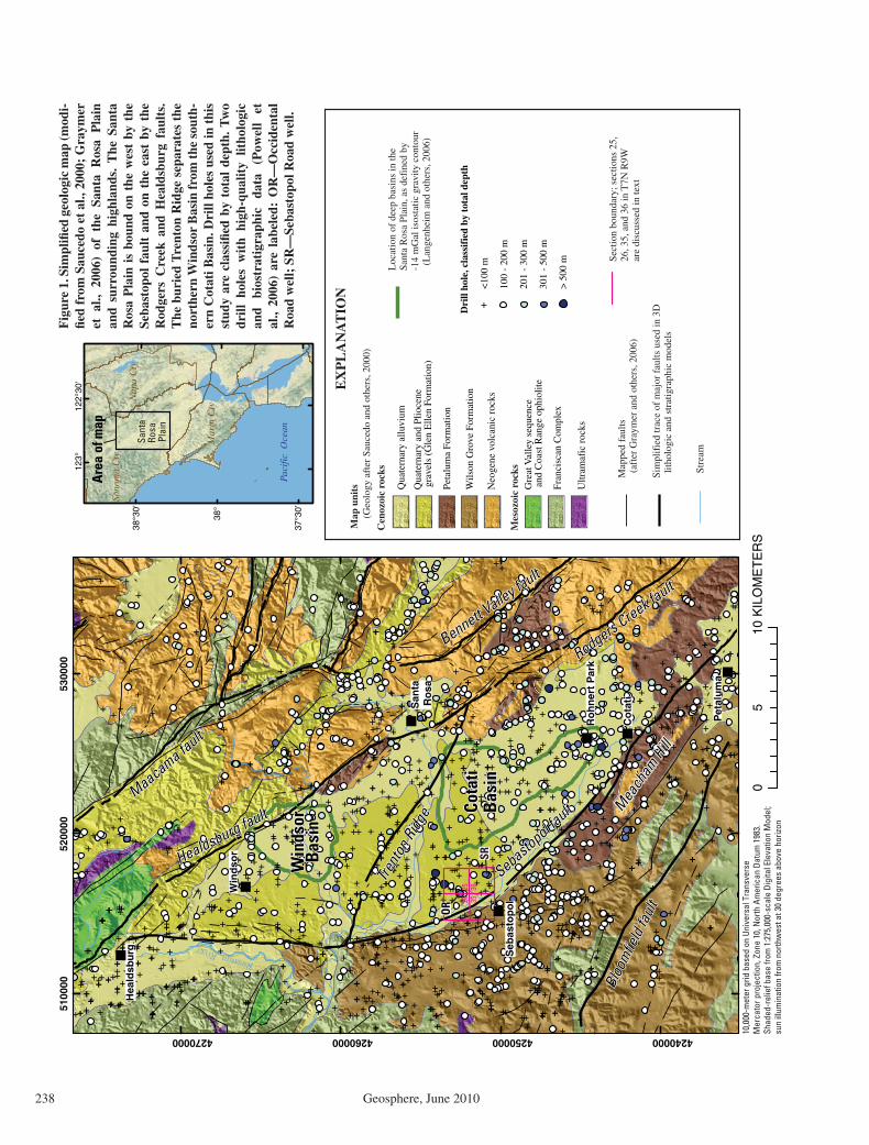
Figure 2. Characteristics of Pliocene–Pleistocene gravels (Glen Ellen Formation). (A) Surface exposure 5 km northwest of Santa Rosa. Height of outcrop is ~2 m. (B) Well profi le showing typical lithologic logs from drill holes. Wells are hung from land surface; depth below land surface is in meters.
3D geologic modeling—Santa Rosa Plain
Geosphere, June 2010 241
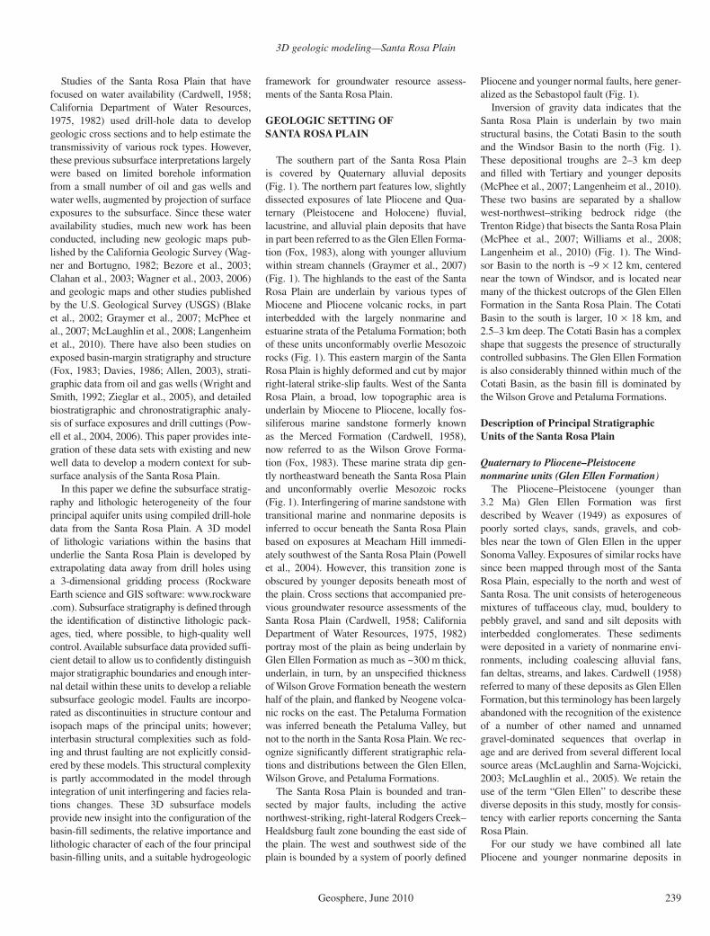
the subsurface into a Glen Ellen unit, including the surfi cial Quaternary deposits, because the younger surfi cial deposits are typically thin and diffi cult to differentiate in drill logs. Outcrop exposures of this unit typically consist of gen-tly to moderately tilted sections of stratifi ed, but poorly sorted heterogeneous mixtures of gravels and sands interbedded with more consolidated conglomerates (Fig. 2A). The unit is generally poorly sorted to unsorted, and unconsolidated to weakly cemented and consolidated. Although no drill-hole or outcrop data document such a thickness, the unit has been interpreted to be as thick as 1000 m (Cardwell, 1958; California Department of Water Resources, 1975). Typi-cal drill-hole lithologic descriptions of this unit (Fig. 2B) are notable for their overall heteroge-neity, generally recording relatively thin beds (<5 m) of coarse and fi ne units, interspersed with coarse gravel intervals. Several nonwelded tuffs occur in parts of this unit.
Late Miocene and Pliocene Wilson Grove Formation
The Pliocene and Late Miocene Wilson Grove Formation is exposed over a broad area on the west side of the Santa Rosa Plain, extend-ing from Petaluma in the south to the Russian River on the north, and from the west edge of the Santa Rosa Plain westward to the Pacifi c Ocean coastline between Bodega and Tomales Bays (Fig. 1). The formation consists of consoli-dated to weakly consolidated deposits of mas-sive or thick-bedded, gray to buff, fi ne-grained to very fi ne grained fossiliferous sand or sand-stone (Fig. 3). The unit includes local beds of mollusk and gastropod shell hash, pebble to boulder conglomerate, and local pumiceous tuff (Fox, 1983; Blake et al., 2002; Powell et al., 2004). The Wilson Grove Formation has a maximum exposed thickness of ~150 m; well logs indicate as much as 300 m thickness. The Wilson Grove Formation is marine, deposited in dune, littoral, and shelf settings. Distal west-ern parts of the formation that are inset into the Mesozoic rocks may represent the head of a submarine canyon (Allen, 2003; Powell et al., 2004). The formation interfi ngers with the Peta-luma Formation in exposures near the town of Cotati and at Meacham Hill immediately south-west of the Santa Rosa Plain. Interfi ngering of marine facies rocks with transitional marine and nonmarine deposits is inferred to occur beneath the Santa Rosa Plain as well.
Outcrop and drill-hole data suggest that the Wilson Grove Formation can be divided into three distinct marine environments represented by lateral variations in lithology (Powell et al., 2004). The fi rst environment includes fi ne-grained marine sandstones (Fig. 3B) that were
A
B
C
25 cm
Figure 3 (continued on following page). Characteristics of the Wilson Grove Formation. (A) Surface exposure 5 km north-northwest of Sebastopol of massive fi ne-grained sand with scattered shell fragments. (B) Surface exposure 15 km southwest of Sebastopol of very fi ne grained marine sandstone facies with distinct shell layer. (C) Surface exposure southeast of Sebastopol showing gravelly sand facies.

Sweetkind et al.
242 Geosphere, June 2010
probably deposited in water depths characteris-tic of upper bathyal or outer shelf settings (Pow-ell et al., 2004) and most commonly occur well to the west of the Santa Rosa Plain. The sec-ond environment includes well-sorted fi ne- to medium-grained sandstone (Fig. 3A) deposited in shallow-marine settings. This facies repre-sents much of the exposed Wilson Grove For-mation, especially north of Sebastopol (Fig. 1).
The third environment is represented by a transitional marine and/or continental facies commonly composed of medium- to coarse-grained, angular sandstone beds interbedded with very well rounded pebble conglomerate beds (Fig. 3C). The transitional unit is interbed-ded with local well-sorted, well-rounded, and polished cobble to pebble gravel (pea gravel) that increases in abundance at the eastern and
southeastern extent of outcrop (e.g., south and east of Sebastopol).
Compared to overlying Quaternary and Pleis-tocene units and to interfi ngered facies of the Petaluma Formation, the Wilson Grove Forma-tion is distinguished in drillers’ lithologic logs by its overall homogeneous sorting, presence of shells, and massive bedding. Drillers typically described the fi ner-grained marine sand of the
Western end point of profile:122° 53.1' W; 38° 23.7' N
Eastern end point of profile:122° 50.88' W; 38° 26.22' N
Location of well profile
D SW NE
DEPT
H, m
Gravel
EXPLANATION
Sand and gravel
Sandstone and gravel
Sand
Sandstone
Sand and clay
Sandstone and clay Clay
Clay and sandstone
Clay and sand
Clay and trace gravel
Clay and gravel
Clay, sand and trace gravel
Clay, sand and gravel Conglomerate
Volcanic conglomerate
Basalt
Ash and/or tuff
Undifferentiated basement
No data
Figure 3 (continued). (D) Well profi le showing typical lithologic logs from drill holes. Wells are hung from land surface; depth below land surface is in meters. Drillers typically describe the fi ne-grained marine facies of the Wilson Grove Formation as clay and sand.

3D geologic modeling—Santa Rosa Plain
Geosphere, June 2010 243
Wilson Grove Formation as clay or clay and sand (Fig. 3D). The presence of fossil shells serves as an important marker in the recognition of the Wilson Grove Formation in the subsur-face. Although shells are infrequently described in the Petaluma Formation, the Petaluma is generally considerably fi ner grained, typically consisting of a silty to clayey mudstone, and is usually easily distinguished from the Wil-son Grove Formation in drillers’ descriptions. The Wilson Grove Formation is mostly poorly cemented; some beds are cemented with cal-cium carbonate and iron and are reported by drillers as hard ledges. The unit contains beds of soft white tuff as much as 3 m thick in outcrop west of Sebastopol; some of these tuff beds have been identifi ed as the Late Miocene Roblar tuff (Sarna-Wojcicki, 1992; Bezore et al., 2003), an important time-stratigraphic marker.
Neogene Volcanic RocksVolcanic rocks exposed in the general vicinity
of the Santa Rosa Plain and present within the basin fi ll include the 3–8 Ma Sonoma Volcanics, the 8.5–9.5 Ma Tolay Volcanics, and the 10.6–11.2 Ma Burdell Mountain Volcanics (Wagner et al., 2005). The Sonoma Volcanics dominate the east side of the Santa Rosa Plain. These volcanic rocks are well exposed to the east of the Rodgers Creek–Healdsburg fault zone and are complexly imbricated by faulting along the southwest side of the fault zone, where they project beneath, and probably correlate with, volcanic units in the subsurface of the Santa Rosa Plain (McLaughlin et al., 2005, 2008).
The Tolay Volcanics and the Burdell Moun-tain Volcanics are exposed in outcrops to the southeast and southwest of the Petaluma Val-ley, respectively, and have been intercepted in the subsurface in the valley based on 40Ar/39Ar dates from oil and gas wells (Wagner et al., 2005). The Tolay Volcanics also are exposed in the fault-bound anticline at Meacham Hill that separates the Santa Rosa Plain from the Peta-luma Valley to the south (Fig. 1), and are present in the uplifted southeast corner of Cotati Basin north and northwest of the town of Rohnert Park (Clahan et al., 2003; Wagner et al., 2005). Sev-eral drill holes in the vicinity of Cotati intercept volcanic rocks at depth that may represent bur-ied equivalents of these older volcanic units.
All of the volcanic units include a wide vari-ety of volcanic rock types including basaltic, andesitic, dacitic, and rhyodacitic fl ows, fl ow breccias, avalanche or talus breccia, tuffs, and several andesitic to rhyodacitic tephra units (Figs. 4A, 4B). Many of the units have relatively limited lateral extent and appear to have erupted from local volcanic vents. The older volcanics are interbedded with the Petaluma or Wilson
Grove Formations, whereas the younger parts of the Sonoma Volcanics overlie the Petaluma For-mation and are interbedded with, or underlie, the Pliocene–Pleistocene Glen Ellen Formation (Wagner et al., 2005). Drillers typically have distinguished volcanic rocks, although they may not have reliably noted the degree of welding in tuffaceous units. The term “volcanic conglom-erate” was often used by drillers due to its typi-cal association with sections of volcanic rocks. We interpret this unit to be volcanic in origin, consisting of fl ow breccia or volcanic agglomer-ate, rather than sedimentary conglomerate dom-inated by volcanic rock clasts. In places, volca-nic rocks directly overlie Mesozoic rocks. The thickness of the volcanic rocks is highly variable and, in general, water wells do not penetrate the entire thickness of the formation (Fig. 4C). For the purpose of the subsurface lithologic and stratigraphic modeling of the Santa Rosa Plain, and in the absence of age or stratigraphic con-trol, the various volcanic rocks are not differ-entiated as separate packages, and therefore are combined in a single unit as Neogene volcanics in the 3D models.
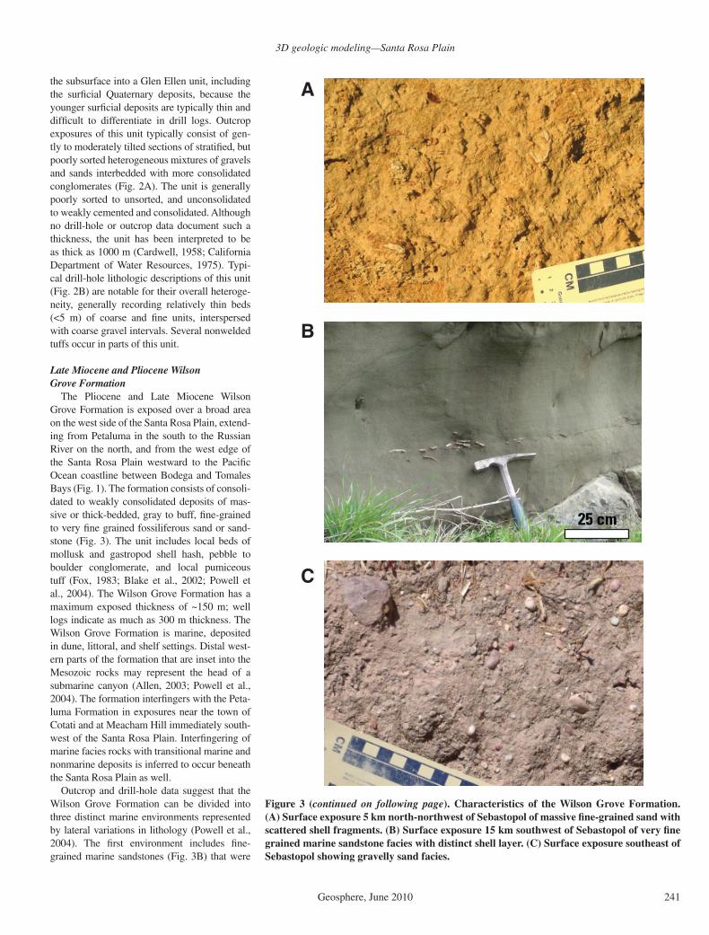
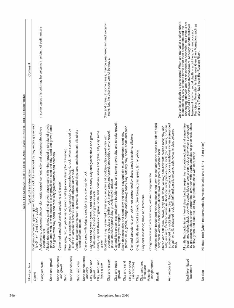
Pliocene and Miocene Petaluma FormationThe Pliocene and Miocene Petaluma Forma-
tion is dominated by deposits of moderately to weakly consolidated silty to clayey mudstone (Fig. 5A), with local beds and lenses of poorly sorted sandstone (Fig. 5B). The Petaluma For-mation is as thick as 900 m in outcrop (Weaver, 1949) and as thick as 1200 m in the subsurface in Petaluma Valley (Morse and Bailey, 1935; Allen, 2003). The unit is intercalated with Neo-gene volcanics (andesitic to rhyolitic) around the margins of the Santa Rosa Plain that have radio-metric ages ranging from ca. 5.0 to ca. 10 Ma (Wagner et al., 2005). The Petaluma Formation consists of transitional marine and nonmarine sediments that were deposited in estuarine, lacustrine, and fl uvial depositional settings (Allen, 2003; Powell et al., 2004). The upper part of the Petaluma Formation is contempora-neous with the Wilson Grove Formation. Where the two formations interfi nger, they represent an oscillating Miocene–Pliocene shoreline (Powell et al., 2004).
Petaluma Formation deposits interpreted from drill-hole lithologic data mostly consist of monotonous sequences of clay with occasional interbeds of sand, probably representing distrib-utary channels and gravel bars (Fig. 5C). The Petaluma Formation is more diverse texturally than the Wilson Grove Formation. The Peta-luma Formation contains more clayey layers, and is fi ner grained and generally less perme-able, with sandy and coarser-grained units being more poorly sorted than coarse units found in
the Wilson Grove Formation. The Petaluma For-mation is predominantly fi ner grained then the Glen Ellen Formation. Although coarse gravelly facies exist in the Petaluma Formation, these coarse beds are thinner (usually <10 m), more poorly sorted, and usually interbedded with fi ne-grained clay that lacks a gravel component (Fig. 5C).
Pre-Miocene Rocks, UndividedPre-Miocene rocks (Eocene? and Cretaceous–
Jurassic) consist largely of Franciscan mélange of the Central belt, Eocene and older rocks of the Franciscan Coastal belt, the Jurassic Coast Range Ophiolite, and the Cretaceous and Juras-sic Great Valley Group (Blake et al., 1984, 2002; McLaughlin and Ohlin, 1984). This unit forms the base of active groundwater fl ow.
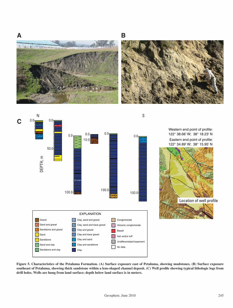
Pre-Miocene rocks are characterized by a variety of consolidated rock types, including penetratively sheared shale (mélange matrix), graywacke, blocks of blueschist, chert, green-stone, thinly interbedded shale and sandstone, and mafi c to ultramafi c ophiolitic rocks. Drillers typically recognize serpentinite; other rock types are given a variety of descriptions (Table 1). All of these consolidated rock types are assigned to a single general lithologic class, i.e., undif-ferentiated basement. The top of pre-Miocene rocks was picked in a drill hole at the highest occurrence of one of the above-described con-solidated rocks, especially where additional intervals of similar rocks occurred below. In rare cases, intervals that could be interpreted as part of the Cenozoic section were reported underlying undifferentiated basement. In these cases, the drill-hole intercepts were compared to the interpreted depth to high-density geophysi-cal basement (Langenheim et al., 2006, 2010; McPhee et al., 2007) to help guide subsurface stratigraphic interpretation.
METHODOLOGY FOR USE OF DRILL-HOLE DATA
Drill-hole data were compiled from a variety of sources, including USGS water resources reports (Cardwell, 1958) and drill-hole compi-lations (Valin and McLaughlin, 2005), oil and gas exploration holes (California Department of Conservation Division of Oil, Gas, And Geo-thermal Resources, www.conservation.ca.gov/dog [July 2008]), data provided by local water agencies, and water wells drilled by indepen-dent entities and compiled as proprietary data by the California Division of Water Resources (CDWR). Drill-hole data in USGS water resources reports (Cardwell, 1958) typically are summaries derived from the original CDWR records. We used the original CDWR data, even

Sweetkind et al.
244 Geosphere, June 2010
Location of well profile
A
CNW SE
DEPT
H, m
B
Western end point of profile:122° 43.79' W; 38° 30.21' N
Eastern end point of profile:122° 40.46' W; 38° 28.66' N
1 meter
Gravel
EXPLANATION
Sand and gravel
Sandstone and gravel
Sand
Sandstone
Sand and clay
Sandstone and clay Clay
Clay and sandstone
Clay and sand
Clay and trace gravel
Clay and gravel
Clay, sand and trace gravel
Clay, sand and gravel Conglomerate
Volcanic conglomerate
Basalt
Ash and/or tuff
Undifferentiated basement
No data
Figure 4. Characteristics of the Neogene volcanics. (A) Surface exposure east of Santa Rosa, showing rhyolite lava fl ow. Height of expo-sure is ~5 m. (B) Surface exposure north of Santa Rosa, showing pumice-rich, reworked nonwelded tuff. (C) Well profi le showing typical lithologic logs from drill holes. Wells are hung from land surface; depth below land surface is in meters. Note that only one well intercepts pre-volcanic basement.
3D geologic modeling—Santa Rosa Plain
Geosphere, June 2010 245
Location of well profile
A
CN S
DEPT
H, m
B
Western end point of profile:122° 38.66' W; 38° 18.23' N
Eastern end point of profile:122° 34.89' W; 38° 15.95' N
Gravel
EXPLANATION
Sand and gravel
Sandstone and gravel
Sand
Sandstone
Sand and clay
Sandstone and clay Clay
Clay and sandstone
Clay and sand
Clay and trace gravel
Clay and gravel
Clay, sand and trace gravel
Clay, sand and gravel Conglomerate
Volcanic conglomerate
Basalt
Ash and/or tuff
Undifferentiated basement
No data
Figure 5. Characteristics of the Petaluma Formation. (A) Surface exposure east of Petaluma, showing mudstones. (B) Surface exposure southeast of Petaluma, showing thick sandstone within a lens-shaped channel deposit. (C) Well profi le showing typical lithologic logs from drill holes. Wells are hung from land surface; depth below land surface is in meters.
Sweetkind et al.
246 Geosphere, June 2010
TAB
LE 1
. GE
NE
RA
LIZ
ED
LIT
HO
LOG
IC C
LAS
SE
S B
AS
ED
ON
DR
ILL-
HO
LE D
ES
CR
IPT
ION
S
Lith
olog
y cl
ass
Typi
cal d
rille
rs’ d
escr
iptio
nC
omm
ent
Gra
vel
Bou
lder
s; c
emen
ted
grav
el; g
rave
l; lo
ose
rock
; roc
k [if
sur
roun
ded
by c
lay
and/
or g
rave
l and
is
<5
ft (~
1.5
m)
thic
k]; r
ubbl
e
Con
glom
erat
eA
gglo
mer
ate;
con
glom
erat
e; c
ongl
omer
ate
grav
el; c
emen
t; cl
ay a
nd c
ongl
omer
ate;
cla
yey
cong
lom
erat
eIn
som
e ca
ses
this
uni
t may
be
volc
anic
in o
rigin
, not
sed
imen
tary
.
San
d an
d gr
avel
Allu
vial
dep
osits
; cla
yey
sand
and
gra
vel;
clay
ey s
and
with
min
or g
rave
l or
stre
aks
of g
rave
l; gr
avel
and
, with
, or
with
str
eaks
of c
lay;
gra
vel w
ith s
and
and
clay
; san
d an
d gr
avel
; san
d an
d gr
avel
with
cla
y; s
and
and
rock
; silt
y gr
avel
; sur
face
and
bou
lder
sS
and
(san
dsto
ne)
and
grav
elC
emen
ted
sand
and
gra
vel;
sand
ston
e an
d gr
avel
San
d B
lue,
gra
y, r
ed, o
r ye
llow
san
d; s
and;
she
lls (
as o
nly
desc
ripto
r of
inte
rval
)
San
d (s
ands
tone
)B
lue
rock
; gra
ywac
ke; s
and
rock
; san
dsto
ne; c
emen
ted
sand
; roc
k (w
hen
surr
ound
ed b
y sh
elly
or
sand
ston
e la
yers
); sa
nd a
nd le
dges
; san
dy r
ock
San
d an
d cl
ayA
dobe
; cla
y sa
ndst
one;
loam
; qui
cksa
nd; s
and
and
clay
; san
d an
d sh
ale;
soi
l; si
lt; s
ticky
sa
nd; s
urfa
ce; t
opso
ilS
and
(san
dsto
ne)
and
clay
Cla
yey
sand
with
ledg
es; s
ands
tone
and
cla
y; s
andy
roc
k
Cla
y, s
and,
and
gr
avel
Cla
y, s
and
and
grav
el; g
rave
l, sa
nd a
nd s
hale
; san
dy c
lay
and
grav
el; s
hale
and
gra
vel;
shal
e an
d ro
ck; t
opso
il an
d gr
avel
or
rock
Cla
y, s
and,
and
tr
ace
grav
elS
andy
cla
y an
d st
reak
s of
gra
vel;
shal
e an
d bo
ulde
rs; s
hale
and
gra
vel;
silty
cla
y so
me
grav
el
Cla
y an
d gr
avel
Bou
lder
s in
cla
y; c
emen
ted
grav
el a
nd c
lay;
cla
y an
d bo
ulde
rs; c
lay,
gra
vel;
clay
with
co
nglo
mer
ate;
cla
y an
d (w
ith)
rock
; cla
yey
sand
and
gra
vel;
embe
dded
cla
y or
gra
vel;
grav
el a
nd c
lay;
gra
vel c
lay;
gra
velly
cla
y; h
ardp
an
Cla
y an
d gr
avel
, in
som
e ca
ses,
may
be
wea
ther
ed a
sh a
nd v
olca
nic
rock
s, b
ut th
e di
stin
ctio
n ca
nnot
be
mad
e.
Cla
y an
d tr
ace
grav
elC
lay
and
little
gra
vel;
clay
and
som
e bo
ulde
rs; c
lay
and
som
e gr
avel
; cla
y an
d st
reak
s gr
avel
; cl
ay w
ith g
rave
l str
inge
rs
Cla
y an
d sa
ndB
asin
dep
osits
; cla
y an
d sa
nd; c
lay
and
shal
e; c
lay
and
silt;
mud
; mud
ston
e; s
and
clay
(b
row
n, b
lue,
gre
en, o
rang
e an
d ye
llow
); sa
ndy
clay
; silt
; silt
y cl
ay; s
hale
; sha
le a
nd s
and
Cla
y an
d sa
nd
(san
dsto
ne)
Cla
y an
d sa
ndst
one;
gra
y ro
ck w
hen
surr
ound
ed b
y sh
ale;
san
dy c
lays
tone
; silt
ston
e
Cla
yC
lay,
typi
cally
des
crib
ed a
s bl
ack,
blu
e, b
row
n, g
ray,
gre
en, t
an, o
r ye
llow
Cla
y, s
and
and
limes
tone
Cla
y an
d lim
esto
ne; s
hale
and
lim
esto
ne
Vol
cani
c co
nglo
mer
ate
Con
glom
erat
e an
d vo
lcan
ic r
ock;
vol
cani
c co
nglo
mer
ate
Bas
alt
And
esite
; bas
alt;
basa
lt an
d ci
nder
s; b
asal
t and
lava
; bas
alt a
nd s
and;
bas
alt b
ould
ers;
bla
ck
ash;
bla
ck v
olca
nic
rock
; cin
ders
; dio
rite;
lava
roc
k; p
orou
s vo
lcan
ic r
ock
Ash
and
/or
tuff
Alte
red
ash;
ash
(bl
ue, b
row
n, g
ray,
red
, whi
te, y
ello
w);
ash-
flow
tuff;
bro
ken
rock
; cla
y an
d as
h; la
va a
sh; f
ract
ured
roc
ks; m
ultic
olor
ed r
ock;
pum
ice
rock
; roc
k (r
ed o
r bl
ack,
or
whe
n su
rrou
nded
by
rock
s th
at a
re d
escr
ibed
as
volc
anic
); ro
ck o
r sa
ndst
one
(whe
n su
rrou
nded
by
ash
or
tuff)
; sha
ttere
d ro
ck; t
uff;
tuff
and
basa
lt; v
olca
nic
ash;
vol
cani
c cl
ay; v
olca
nic
rock
Und
iffer
entia
ted
base
men
t
All
units
that
und
erlie
an
inte
rval
des
crib
ed a
s se
rpen
tine;
ser
pent
ine;
bas
alt a
nd s
erpe
ntin
e;
basa
lt an
d sh
ale;
bla
ck r
ock
with
qua
rtz;
blu
e an
d/or
gre
en r
ock
or c
lay
whe
n su
rrou
nded
by
gra
ywac
ke, s
hale
and
/or
serp
entin
e; o
ily; r
ock
with
qua
rtz
and
blue
or
gree
n ro
ck, s
hale
or
cla
y; g
reen
and
blu
e ro
ck o
r cl
ay; s
erpe
ntin
e; s
hale
with
ser
pent
ine
Onl
y un
its a
t dep
th a
re c
onsi
dere
d. W
hen
an in
terv
al a
t sha
llow
dep
th
is d
escr
ibed
by
any
of th
ese
term
s ot
her
than
ser
pent
ine
and
the
unde
rlyin
g in
terv
als
are
not d
escr
ibed
as
base
men
t, th
is z
one
is n
ot
desc
ribed
as
undi
ffere
ntia
ted
base
men
t. A
lthou
gh u
ndiff
eren
tiate
d ba
sem
ent i
s on
ly u
sed
at d
epth
in a
dril
l hol
e, o
n ra
re o
ccas
ion
Fran
cisc
an F
orm
atio
n is
thru
st o
ver
Gle
n E
llen
For
mat
ion,
suc
h as
al
ong
the
Tren
ton
faul
t nea
r th
e R
ussi
an R
iver
.N
o da
taN
o da
ta, r
ock
[whe
n no
t sur
roun
ded
by v
olca
nic
units
and
> 5
ft (
~1.
5 m
) th
ick]
3D geologic modeling—Santa Rosa Plain
Geosphere, June 2010 247
if it was later published by the USGS, because these data included information from all down-hole intervals, rather than summaries or general-izations of subsurface lithologic data.
A digital database of lithologic information from drill holes was compiled by manually entering lithologic data from the above sources. We culled the immense number of records obtained from CDWR by selecting ~10 repre-sentative drill holes from each of the 36 sec-tions within a township and range, or ~10 holes within each ~1.6 km2 (i.e., square mile) of the study area. In parts of the study area where the population density is low, our drill-hole distribu-tion is correspondingly less. The drill holes that were used represented those that contained the greatest amount of detail in the description of each interval, had a large number of downhole intervals described (as opposed to a single long interval of “sand and gravel” or “alluvium”), were representative of downhole lithology of nearby holes, and represented a distribution of holes that were not clustered but were approxi-mately equally distributed over the study area. The study area includes an area encompassed by three ranges in the east-west direction (R7W, R8W, and R9W) and fi ve townships in the north-south dimension (T5N, T6N, T7N, T8N, and T9N). In all, 2683 drill holes were compiled within this area (Fig. 1).
When available, we selected drill holes with the most detailed logs that were at least 100 m deep, but most important, we selected holes that could be defi nitively located. Total drill-hole
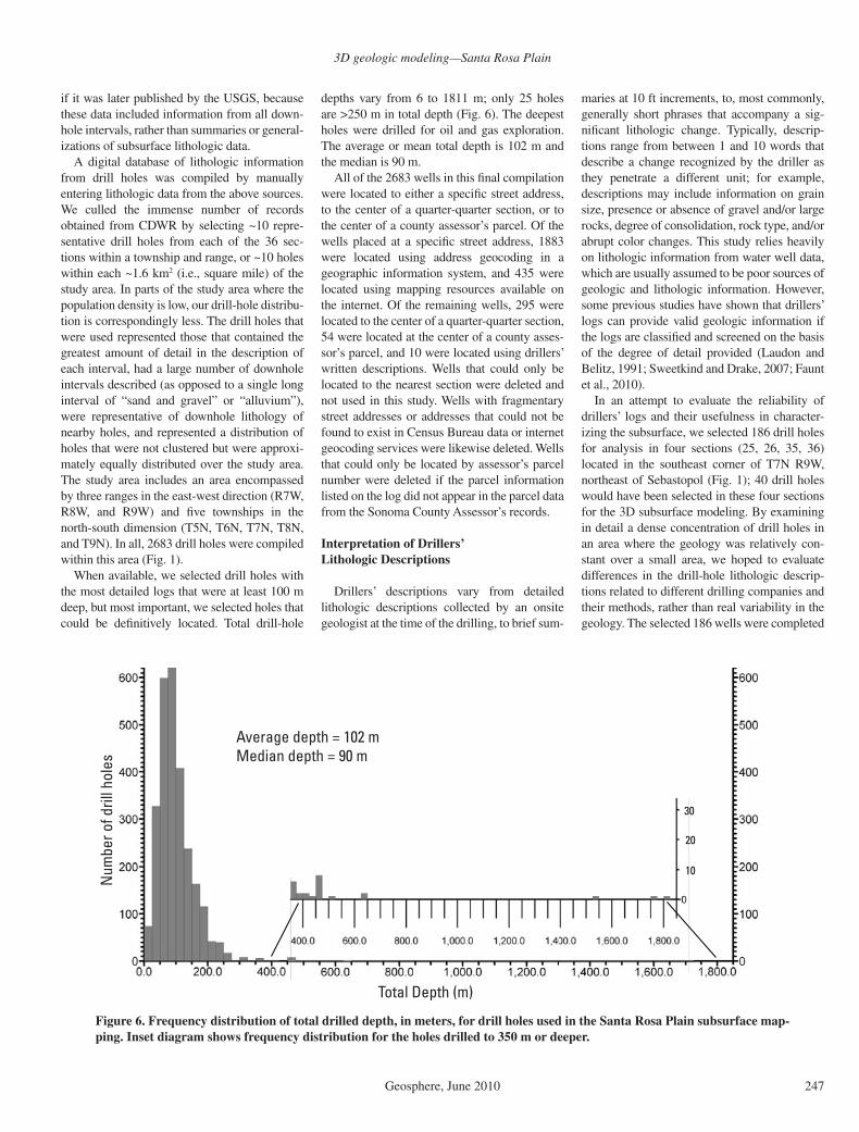
depths vary from 6 to 1811 m; only 25 holes are >250 m in total depth (Fig. 6). The deepest holes were drilled for oil and gas exploration. The average or mean total depth is 102 m and the median is 90 m.
All of the 2683 wells in this fi nal compilation were located to either a specifi c street address, to the center of a quarter-quarter section, or to the center of a county assessor’s parcel. Of the wells placed at a specifi c street address, 1883 were located using address geocoding in a geographic information system, and 435 were located using mapping resources available on the internet. Of the remaining wells, 295 were located to the center of a quarter-quarter section, 54 were located at the center of a county asses-sor’s parcel, and 10 were located using drillers’ written descriptions. Wells that could only be located to the nearest section were deleted and not used in this study. Wells with fragmentary street addresses or addresses that could not be found to exist in Census Bureau data or internet geocoding services were likewise deleted. Wells that could only be located by assessor’s parcel number were deleted if the parcel information listed on the log did not appear in the parcel data from the Sonoma County Assessor’s records.
Interpretation of Drillers’ Lithologic Descriptions
Drillers’ descriptions vary from detailed lithologic descriptions collected by an onsite geologist at the time of the drilling, to brief sum-
maries at 10 ft increments, to, most commonly, generally short phrases that accompany a sig-nifi cant lithologic change. Typically, descrip-tions range from between 1 and 10 words that describe a change recognized by the driller as they penetrate a different unit; for example, descriptions may include information on grain size, presence or absence of gravel and/or large rocks, degree of consolidation, rock type, and/or abrupt color changes. This study relies heavily on lithologic information from water well data, which are usually assumed to be poor sources of geologic and lithologic information. However, some previous studies have shown that drillers’ logs can provide valid geologic information if the logs are classifi ed and screened on the basis of the degree of detail provided (Laudon and Belitz, 1991; Sweetkind and Drake, 2007; Faunt et al., 2010).
In an attempt to evaluate the reliability of drillers’ logs and their usefulness in character-izing the subsurface, we selected 186 drill holes for analysis in four sections (25, 26, 35, 36) located in the southeast corner of T7N R9W, northeast of Sebastopol (Fig. 1); 40 drill holes would have been selected in these four sections for the 3D subsurface modeling. By examining in detail a dense concentration of drill holes in an area where the geology was relatively con-stant over a small area, we hoped to evaluate differences in the drill-hole lithologic descrip-tions related to different drilling companies and their methods, rather than real variability in the geology. The selected 186 wells were completed
10
20
30
Num
ber o
f dril
l hol
es
Total Depth (m)
Average depth = 102 mMedian depth = 90 m
Figure 6. Frequency distribution of total drilled depth, in meters, for drill holes used in the Santa Rosa Plain subsurface map-ping. Inset diagram shows frequency distribution for the holes drilled to 350 m or deeper.
Sweetkind et al.
248 Geosphere, June 2010
by 18 different drilling contractors; ~92 of the holes were drilled by a single company. Most of the holes are shallow. With the exception of 2 holes drilled to a depth of ~450 m, the average depth is ~50 m.
We counted the number of downhole intervals in each of the 186 drillers’ logs and the number of unique descriptive phrases to quantify the level of detail present in the logs. For example, if a driller described four intervals as clay, sand, clay, and sand, respectively, that would con-stitute only two unique descriptive phrases in four downhole intervals. There is no observed correlation between the number of downhole intervals and the total depth of a drill hole (r2 = 0.0817) (Fig. 7A). Deeper holes do not neces-sarily have more downhole intervals than shal-lower holes. This result indicates that holes are described based on the units intersected rather than some random criteria, such as equally spaced description intervals. In addition, there is no correlation between the number of unique descriptive phrases and the total depth of a drill hole (r2 = 0.05) (Fig. 7A). Deeper holes do not have more unique descriptive phrases used than shallow holes. However, there is a signifi cant correlation between the number of downhole intervals and the number of unique descriptive phrases (r2 = 0.70) (Fig. 7B). The more subdivi-sions the driller made, the greater the number of descriptive units used. This indicates that descriptions tend to be unique and not repeated in a single drill hole.
As another test of evaluating the internal consistency of drill-hole data, we compiled the lithologic units described in all of the 186 holes at 25 ft (~7.5 m) depth intervals (Fig. 7C). The compiled drillers’ descriptions were simplifi ed to the same 19 units used in the 3D modeling of the entire Santa Rosa Plain (Table 1). We normalized the data from each depth interval so that the numbers of lithologic keywords are reported as percent of the total for that depth interval (Fig. 7C). Based on detailed lithologic descriptions (Powell et al., 2006) from the nearby Occidental Road and Sebastopol Road drill holes (Fig. 1), the subsurface geology in the four sections was expected to consist of an upper sequence of clayey to pebbly silt, sand, and gravel of dominantly nonmarine distal fl u-vial, lacustrine, and deltaic deposits (the Glen Ellen Formation and correlative strata) over-lying a lower sequence of silt, sand, and peb-bly sand with mollusks of dominantly shelfal marine affi nities (the Wilson Grove Formation). The expected geology is borne out with reason-able consistency by the 186 drillers’ lithologic logs. High in the section, clay and sandy gravel dominate the lithologic descriptions, the section as a whole is poorly sorted, and no shells are
identifi ed (Fig. 7C). A wide variety of lithologic descriptions was used, but this is to be expected of the Glen Ellen Formation and equivalents, and does not necessarily indicate inconsistency between drillers’ descriptions. Below the 150 ft (~45 m) interval, sands and shells dominate the lithologic descriptions, consistent with the inter-preted Wilson Grove Formation (Fig. 7C). It is important that few other lithologic categories are described, lending confi dence to the drillers’ overall interpretation.
Once the initial selection criteria of selecting deep holes with enough descriptive subdivisions in the lithologic log to be useful and reliable locations were met, the drill-hole lithology data, or drillers’ nomenclature, were then simplifi ed. If the physical characteristics of the major rock formations exposed at the surface are mapped, these geologic criteria can be used to help inter-pret and standardize the various descriptions submitted by numerous well drillers. By com-bining observations made at surface exposures with known or inferred facies relations, alluvial units can be distinguished from fi ne-grained marsh and/or palustrine deposits, proximal coarse-grained deposits can be distinguished from fi ne-grained distal deposits, and interfi n-gering of major lithologic packages can be rec-ognized in the subsurface data. This technique was used to simplify the drillers’ descriptions (Table 1).
Interpretation of Stratigraphy from Drill-Hole Data
Because one of the overall goals of this exer-cise was to create a geologic framework suit-able for groundwater resource assessment, the complex Neogene stratigraphy was simplifi ed to four principal units: Glen Ellen Formation, Wilson Grove Formation, Petaluma Formation, and Neogene volcanics, all underlain by a gen-eralize unit, called undifferentiated basement, that includes all pre-Cenozoic rocks. When numerous drillers’ logs were viewed and inter-preted together, it became clear that each of the principal stratigraphic units had a reasonably distinct mappable character in the subsurface such that they could often be distinguished from each other. Assignment of stratigraphic tops was fundamentally lithology based and, as such, was rock-stratigraphic rather than being a true stratigraphic assignment based on timelines or sequence boundaries.
Mappable lithologic sequences were identi-fi ed in well data by analyzing numerous serial cross sections across the Santa Rosa Plain and making stratigraphic interpretations based on rock type, bedding and sorting characteristics, stratigraphic succession, and an understanding
of the relationship between the mapped geologic units and their lithologic characteristics. Strati-graphic tops were picked interactively by view-ing lithologic logs from 10–20 wells in a profi le. Contacts were picked in an iterative fashion from numerous cross sections of varying orientations with combinations of wells examined to elimi-nate spurious picks and maximize the consis-tency of the stratigraphic interpretation. Subsur-face interpretation began with wells spudded in known outcrop or correlations to higher quality data to condition the rest of the data set.
Map relations show that over most of its out-crop area the Wilson Grove Formation uncon-formably overlies pre-Cenozoic rocks, so the unit could be confi dently assigned in the subsur-face. Some complexities arose in the far south-west part of the study area where volcanic rocks, probably related to the Tolay or Burdell Moun-tain Volcanics, were reported near the base of the penetrated section in several wells. Based on known facies and age variations within the Wilson Grove Formation (Powell et al., 2004) and Petaluma Formation (Davies, 1986; Allen, 2003), we initially made stratigraphic picks of a number of subdivisions of each formation based on grain size, sorting, and bedding characteris-tics. This fi ne-scale subdivision was effective where well data could be tied to outcrop con-trol, especially for the Wilson Grove Formation. However, such fi ne-scale subdivision was dif-fi cult to maintain throughout the Cotati Basin, where the units interfi ngered but outcrop control was lacking.
In a similar fashion, subsurface stratigraphic picks of the Glen Ellen Formation were fi rst assigned in drill holes in the Windsor Basin near outcrops of the formation. The unit was identifi -able as a relatively thin bedded, heterogeneous package that contained gravels with a clayey or fi ne-grained matrix, a unit often called clay and gravel by the drillers. The Glen Ellen Formation was readily identifi ed to the north and east of the Trenton fault, but was more diffi cult to iden-tify to the south, where both the Wilson Grove and Petaluma Formations are more gravel rich. Heterogeneous, gravel-rich sediments that over-lie volcanic rock on the east side of the Wind-sor Basin, near the city of Santa Rosa, and in Rincon Valley were also assigned to the Glen Ellen Formation.
For wells drilled on or near an outcrop of vol-canic rocks, we selected the fi rst intercept of vol-canic rocks as the top of the Neogene volcanics unit. In certain areas, the volcanic units are inter-bedded with sediments and in those cases this entire interval was called Neogene volcanics.
The Petaluma Formation was consistently described by drillers as being mostly monot-onous sequences of clay with occasional

3D geologic modeling—Santa Rosa Plain
Geosphere, June 2010 249
R2 =
0.0
817
R2 =
0.0
5
050100
150
200 0
510
1520
2530
3540
NUM
BER
Num
ber
ofin
terv
als
Num
ber
ofD
escr
iptiv
eph
rase
s us
ed
R2 =
0.7
035
0510152025
05
1015
2025
3035
NUM
BER
OF D
OWNH
OLE I
NTER
VALS
NUMBER OF UNIQUE DESCRIPTIVE PHRASES
TOTAL DEPTH, IN M
AB
051015202530354045
DEPT
H IN
TERV
AL
NORMALIZED FREQUENCY
shel
ls
grav
el
sand
and
gra
vel
sand
sand
ston
e
sand
and
cla
y
sand
ston
e an
d cl
ay
clay
, san
d an
d gr
avel
clay
, san
d an
d tr
gra
vel
clay
and
gra
vel
clay
and
trac
e gr
avel
clay
and
san
d
clay
and
san
dsto
ne
clay
ash
and/
or tu
ff
25 ft
N=
182
50 ft
N=
179
75 ft
N=
148
100
ftN
=11
212
5 ft
N=
9815
0 ft
N=
8217
5 ft
N=
6220
0 ft
N=
5422
5 ft
N=
3825
0 ft
N=
3227
5 ft
N=
2230
0 ft
N=
19
C
Fig
ure
7. P
lots
sho
win
g st
atis
tica
l ana
lysi
s of
dri
llers
’ lit
holo
gic
desc
ript
ions
. (A
) N
umbe
r of
inte
rval
s an
d nu
mbe
r of
des
crip
tive
phr
ases
ver
sus
tota
l dep
th. (
B)
Num
ber
of in
ter-
vals
ver
sus
num
ber
of d
escr
ipti
ve p
hras
es. (
C)
Nor
mal
ized
fre
quen
cy o
f lit
holo
gic
unit
s oc
curr
ing
in 2
5 ft
(~7
.5 m
) in
terv
als.

Sweetkind et al.
250 Geosphere, June 2010
interbeds of sand or gravel bars. We initially attempted to identify the following three sub-divisions within the Petaluma Formation: (1) Petaluma Upper, assigned to intervals of Pet-aluma Formation near Santa Rosa above thick sequences of Sonoma Volcanics; (2) Petaluma Middle, assigned to most of the unit beneath the Santa Rosa Plain; and (3) Petaluma Lower, assigned where there were signifi cant amounts of volcanic rocks, typically basalts in the sec-tion, that were inferred to be older volcanic units such as the Tolay Volcanics. However, due to structural complexity and lack of correlatable horizons, we eventually abandoned attempts to subdivide the Petaluma Formation.
3D MODELING RESULTS
3D Lithologic Model
Drillers’ descriptions were simplifi ed to a small number of internally consistent lithologic classes (Table 1) for all 2683 drill holes. When these drill-hole data were viewed together, the 19 lithologic units derived from the drillers’ descriptions fell into distinct spatial groupings (Fig. 8A) that were amenable to stratigraphic classifi cation with some confi dence. The stan-dardized subsurface lithologic data were then used to construct a 3D lithologic model of the study area (Fig. 8B). Interpreted drill-hole lithologic data were numerically interpolated between drill holes by using a cell-based, 3D gridding process using the RockWorks 3D mod-eling software package (Rockware Earth Sci-ence and GIS software: www.rockware.com). In this method, a solid modeling algorithm is used to extrapolate numeric codes that repre-sent a lithologic class. Grid nodes between drill holes are assigned a value that corresponds to a lithologic class based on the relative proxim-ity of each grid node to surrounding drill holes. The interpolation routine looks outward hori-zontally from each drill hole in search circles of ever-increasing diameter. Initially, the algorithm assigns a lithology class to grid nodes imme-diately adjacent to each drill hole, at a vertical discretization defi ned by the modeler. Then the interpolation moves outward from the drill hole by one node and assigns the next circle of grid nodes a lithology class. The interpolation con-tinues in this manner until the program fi nds a cell that is already assigned a lithology class (presumably interpolating toward it from an adjacent drill hole), in which case it skips the node assignment step.
A strength of the 3D gridding process is that the interpolated data in the resulting 3D grid have the appearance of stratigraphic units, with aspect ratios that emphasize the horizon-
tal dimension over the vertical (Fig. 8B). Also, the method preserves the local variability of the lithology in each drill hole with no smoothing or averaging. Thus, where data are abundant, local lithologic variability is incorporated. One limitation of this type of numerical interpola-tion is the sensitivity to the distribution of the data, where values from an isolated drill hole tend to extrapolate outward to fi ll an inordinate amount of the model area. The effect is particu-larly noticeable where a small number of deep drill holes are interspersed with shallower holes. Data from the deepest drill holes in this case tend to overextrapolate over the entire model area. A second limitation of this method is that it is purely deterministic and data based. Alter-natively, it may be possible to use a stochastic approach where the drill-hole data are used as a guide to predict subsurface lithologic vari-ability (e.g., Weissmann et al., 1999). Such an approach would have the benefi t of being able to incorporate depositional process and facies rela-tionships by evaluating the tendency of specifi c lithologic units to be adjacent to each other in specifi c geologic environments. Because of the large-scale nature of the Santa Rosa Plain, the presence of multiple depositional environments, and resource limitations, stochastic modeling approaches were not applied.
Faults were not explicitly included in the creation of the 3D lithologic model, owing to the limitations of the software package used. However, the interpolation methods used here produce lithologic variations that approximate fault truncations of lithologic units where data density is high.
Cell dimensions for the 3D interpolation were 250 m in the horizontal dimensions and 10 m in the vertical dimension. The vertical discretiza-tion was chosen as a compromise between pre-serving geologic detail, such that thin geologic units are not averaged out, and computational effi ciency, such that model runs could be com-pleted in a reasonable time. The model ranges in elevation from 400 m to −400 m, for a total thickness of 800 m, before being trimmed at the surface and base. We trimmed the resulting model at the top using a digital elevation model (DEM) to represent land surface elevations and at the base by a grid of the top of the geo-physically modeled high-density geophysical basement that represents the elevation of pre-Miocene rocks (Langenheim et al., 2006, 2010; McPhee et al., 2007).
For the 3D lithologic model presented here, strata were assumed to be horizontal. The assumption of horizontality is likely more valid for the younger, upper parts of the basin fi ll than for the deeper parts of the alluvial section. Seis-mic refl ection profi les across the eastern side of
the Windsor Basin (Williams et al., 2008) show a progressive increase in refl ector dip beneath ~100–200 m. Several more complicated models were constructed that incorporated stratal tilt or folding. However, the 3D gridding approach is very sensitive to the choice of dip or the magni-tude and style of the fold chosen as a bounding surface; none of the more complicated models yielded results that were higher quality than the simple horizontal model.
An initial test of the strength of the sub-surface 3D lithologic model is to compare the mapped surface geology to that predicted at land surface by the 3D model. The density of drill-hole lithologic data is greatest at the surface, so resolution of the resultant model should be highest. When the solid lithologic model is trimmed with a DEM, the resulting upper model surface compares favorably to the geologic map; for example, compare the general distribution of sand and volcanic-rock lithologic classes in Figure 8B with the map distribution of Wilson Grove Formation and Neogene volcanics, respectively, in Figure 1. The sand-dominated marine deposits in the south and west, the fi ne-grained basin-axis deposits capped by younger, coarser and thin-ner alluvial fans, and the volcanic highlands to the north and east are all well expressed in the 3D model (Fig. 8B). Although no faults were used in the construction of the lithologic model, due to the density of well data the con-tacts between lithologic units are relatively abrupt and are coincident with the major basin-bounding faults (Figs. 8B, A1–2, and A1–4).
3D Stratigraphic Model
In order to tie the basin-fi ll lithology to a stratigraphic context and to mapped surface exposures, we created a 3D stratigraphic model of the Santa Rosa Plain. In contrast to the 3D lithologic model, which used just a single type of data, interpreted drill-hole lithologic data, to populate a 3D volume, the 3D stratigraphic model was built using multiple geologic data sets including geologic maps, surface traces of faults, interpreted subsurface stratigraphic con-tacts from drill-hole data, and the results of geo-physical models. The 3D stratigraphic model, built using EarthVision (Dynamic Graphics, Inc., http://www.dgi.com/) and Rockworks 3D (Rockware Earth science and GIS software: www.rockware.com) geologic mapping soft-ware consists of three bounding components: fault surfaces, stratigraphic surfaces, and a modeled surface representing the top of pre- Cenozoic rocks.
Fault surface traces were generalized from published geologic maps (McLaughlin et al.,

3D geologic modeling—Santa Rosa Plain
Geosphere, June 2010 251
4,270,000
Easting (UTM)
Northing (UTM)
4,260,000
4,250,000
4,240,000
510,000
520,000
530,000
4,270,000
Easting (UTM)
Northing (UTM)
4,260,000
4,250,000
4,240,000
510,000
520,000
530,000
Gravel
Sand and gravel
Sandstone and gravel
Sand
Sandstone
Sand and clay
Sandstone and clay
Clay, sand, and gravel
Clay, sand, and trace gravel
Clay and gravel
Clay and trace gravel
Clay and sand
Clay and sandstone
Explanation of symbols
Clay
Conglomerate
Volcanic conglomerate
Basalt
Ash and (or) tuff
Undifferentiated basement
No data
Vertical exaggeration is 10x.
Cylinders represent the location of drill holes; colors represent lithologic units intercepted downhole. Drill holes are hung from their collar elevation atland surface. Land surface is transparent; as a result, the drill holes have the appearance of hanging in space. Faults are shown as vertical “ribbons” decorated with parallel black lines.
Vertical exaggeration is 6x.
Vertical sections cut through the solid volume 3D lithology model. Sections are hung from land surface. Land surface is transparent; as a result, the sections have the appearance of hanging in space. Tops and bottoms of each section appear irregular because the model was clipped at the topby a digital elevation model and at the base by the modeled elevation of pre-Cenozoic bedrock.
A
B
SF
TR RCF
BVFHF
MF
SF
TRRCF
BVFHF
MF
BVF; Bennett Valley faultHF; Healdsburg faultMF; Maacama faultRCF; Rodgers Creek faultSF; Sebatopol faultTR; Trenton Ridge
Figure 8. Perspective views of drill-hole lithologic data and resultant three-dimensional (3D) lithology model. View is from above and the southwest, looking northeast. UTM—Universal Transverse Mercator. (A) Perspective views of drill-hole litho-logic data. (B) Perspective 3D view of vertical sections cut through the solid volume 3D lithology model. For a fully interactive3D image, see Supplemental Figure 11 in Appendix 2.
1Supplemental Figure 1. Zipped fi le containing a RockPlot3D (http://www/rockware.com/downloads/trialware.php#R [February 2010]) image of the three-dimensional (3D) lithologic model. This 3D image corresponds to Figure 8B and presents vertical sections cut through the 3D solid lithologic model in three dimensions. If you are viewing the PDF of this paper or reading it offl ine, please visit http://dx.doi.org/10.1130/GES00513.S1 or the full-text article on www.gsapubs.org to view Supplemental Figure 1.

Sweetkind et al.
252 Geosphere, June 2010
2005; Graymer et al., 2006). A limited number of faults was included in the framework model to bound the major basin elements, including (Fig. 1) a combined Bennett Valley–Maacama fault trace that offsets Neogene volcanics to the east of the Santa Rosa Plain, a combined Rodg-ers Creek–Healdsburg fault trace that generally bounds the eastern side of the Santa Rosa Plain, a generalized trace of the Sebastopol fault that bounds the western side of the Santa Rosa Plain, a generalized fault that bisects the Santa Rosa Plain and approximates the Trenton Ridge as a single structure, and a generalized trace of the Bloomfi eld fault that offsets the Wilson Grove Formation to the southwest of the Cotati Basin. All faults are presumed vertical for this study; this is probably an acceptable simplifi cation for the major faults with strike-slip motion, but may be less applicable to faults bounding the Trenton Ridge, which have been interpreted as being reverse faults with gentle dip (Fox, 1983) or steep dip (Williams et al., 2008). These faults were incorporated into the structure contour and isopach maps of each of the major units, serving to bound and truncate contoured thickness and unit extents.
Stratigraphic surfaces are derived from strati-graphic information from wells, described in the previous section, along with point data derived by combining the mapped geology and a DEM. A generalized hydrogeologic map (Fig. 1) was constructed by merging geologic map data from several sources (Saucedo et al., 2000; Blake et al., 2002; Graymer et al., 2007) to portray four distinct Cenozoic formations (Pliocene– Pleistocene gravels, the Wilson Grove Forma-tion, Neogene volcanic rocks, and the Peta-luma Formation) and a fi fth unit representing undifferentiated pre-Cenozoic rocks. The 3D geometry of outcrops of each of the fi ve units was defi ned by intersecting the hydrogeologic map with a DEM, resulting in x, y, z coordinate locations within each outcrop area that were exported for use as input data in the stratigraphic modeling. Where possible, interpreted strati-graphic surfaces were tied to high-quality well control where biostratigraphic information was available (Powell et al., 2006), or tied to previ-ously identifi ed formation picks in wells (Valin and McLaughlin, 2005).
The surface representing the top of the geo-physically modeled high-density geophysi-cal basement was derived from inversion of regional gravity measurements (Langenheim et al., 2006, 2010; McPhee et al., 2007), as con-strained by outcrop data and well data. This surface is inferred to represent the elevation of pre-Miocene rocks. This depth-to-basement inversion takes advantage of the large density contrast between dense pre-Cenozoic rocks
(predominantly composed of Mesozoic rocks of the Franciscan Complex and the mafi c Coast Range Ophiolite) and less dense Quaternary–Tertiary sedimentary rocks and Neogene volca-nics. The inversion method allows the density of bedrock to vary horizontally as needed, whereas the density of basin-fi lling deposits is speci-fi ed by a predetermined density-depth relation-ship (Jachens and Moring, 1990). The resulting model of depth to pre-Cenozoic bedrock for the Santa Rosa Plain defi nes both the overall basin geometry and the confi guration of subbasins that are bounded by internal faults. Locally, the modeled depth to geophysical basement from the gravity inversion may not exactly match the depth to pre-Cenozoic rocks observed in every drill hole because of the resolution of the grid model from the inversion or in areas of large gravity gradients.
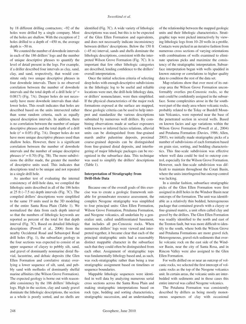
The 3D geologic framework of the Santa Rosa Plain was constructed by standard subsur-face mapping methods of creating isopach maps (Fig. 9) and structure contouring for each of the four principal stratigraphic units. The structural elevation of stratigraphic tops and thickness for each of the four major units were contoured from map and well data using simplifi ed fault traces to bound contoured regions. Data were contoured using an inverse distance algorithm with a mod-erate smoothing routine. Data were considered to be suffi ciently numerous that no prefi ltering, regridding, or declustering of the original data was done prior to contouring. Attempts at con-touring the data using a pre-kriging routine were computationally intensive and did not provide signifi cantly different results.
One challenge in creating the isopach maps is that few of the wells, being for the most part shallow water wells, penetrated the entire thickness of a formation. To provide some 3D control on unit thickness, the modeled depth-to- basement surface was used to defi ne unit thickness where it could be reasonably inferred that the stratigraphic unit would be expected to directly overlie pre-Cenozoic rocks. For exam-ple, where the Wilson Grove Formation crops out to the west of Sebastopol, the base of the unit is exposed and is nearly everywhere unconform-able on pre-Miocene rocks with no intervening units. So, for the Wilson Grove Formation to the west of the Sebastopol fault, the modeled depth-to-basement surface was used to defi ne the base of the formation (Fig. 10). This method was also used for the Neogene volcanics in wells that penetrated a thick sequence of volcanic rocks uninterrupted by sediments. The base of the vol-canic section is rarely exposed in outcrop near the Santa Rosa Plain. However, volcanic rocks unconformably overlie pre-Cenozoic rocks east of Napa Valley. In cases where the base of the
Neogene volcanics was forced to the elevation of the depth-to-basement model, the 3D map-ping incorporates uncertainty that is inherent in the depth-to-basement model. Specifi cally, the variation of density with depth in the volca-nic units can dramatically infl uence the model results. For wells in the center of the Santa Rosa Plain where the top of the Petaluma Forma-tion was interpreted, the base of the Petaluma Formation was defi ned as the elevation of the depth-to-basement surface, forcing the forma-tion to be very thick and fi ll the deepest parts of the basins. This method forces any older Ceno-zoic rocks that might be present beneath the Petaluma Formation and Neogene volcanics to be included in those units.
The Glen Ellen Formation was a special case where wells, especially in the Windsor Basin, did not penetrate the entire thickness of the for-mation, but some other unit would be expected to underlie it. The formation therefore could not be reasonably expected to extend down to the pre-Cenozoic rocks. In order to contour the for-mation, the thickness was arbitrarily picked at ~15 m below the base of wells that bottomed in the Glen Ellen Formation. In areas where the entire thickness of the formation was not pen-etrated, these data give a minimum thickness to the Glen Ellen Formation.
Computer-generated isopach maps were reviewed to identify anomalous data points. These data points were evaluated and, in many cases, reinterpreted to create more consistent isopach trends. Isopach maps were fi ltered to remove extremely thin parts of units, and thick-nesses of 2 m or less typically were set to zero. Isopach maps were hand-edited in selected places to remove outliers that were well outside the main part of the unit. The fi nal grids used to create the 3D framework represent a hybrid approach that combines (1) unit thickness that incorporates the depth-to-basement model, as described above, with (2) unit thickness defi ned by interactive assignment of stratigraphic tops from well data. In places the grids show abrupt transitions where the regions in which the two methodologies were used abut each other.
The 3D stratigraphic framework was con-structed initially in EarthVision and later in Rockworks 3D modeling packages by import-ing gridded surfaces to defi ne the top and base of each stratigraphic horizon that were then stacked in stratigraphic sequence to form a 3D digital solid. The 3D stacking was guided by rules that controlled stratigraphic onlap, trunca-tion of units, and minimum thickness. Stacked grid models for the upper and lower surfaces of each of the stratigraphic units are then dis-played on multiple 3D cross section fence pan-els (Fig. 11).
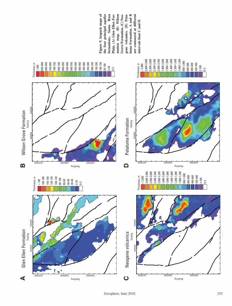
3D geologic modeling—Santa Rosa Plain
Geosphere, June 2010 253
5200
0053
0000
425000042600004270000
NorthingEa
stin
g52
0000
5300
00
425000042600004270000
Northing
East
ing
5200
0053
0000
425000042600004270000
Northing
East
ing
5200
0053
0000
425000042600004270000
Northing
East
ing
> 18
0
Thic
knes
s, m
160-
180
140-
160
120-
140
100-
120
80-1
0060
-80
40-6
020
-40
2-20
0-2 > 2,
800
Thic
knes
s, m
1,60
0-1,
800
1,40
0-1,
600
1,20
0-1,
400
1,00
0-1,
200
800-
1,00
060
0-80
040
0-60
020
0-40
02-
200
0-2
1,80
0-2,
000
2,00
0-2,
200
2,20
0-2,
400
2,40
0-2,
600
2,60
0-2,
800
> 2,
800
Thic
knes
s, m
1,60
0-1,
800
1,40
0-1,
600
1,20
0-1,
400
1,00
0-1,
200
800-
1,00
060
0-80
040
0-60
020
0-40
02-
200
0-2
1,80
0-2,
000
2,00
0-2,
200
2,20
0-2,
400
2,40
0-2,
600
2,60
0-2,
800
> 90
0Th
ickn
ess,
m
450-
500
400-
450
350-
400
250-
300
200-
250
150-
200
100-
150
50-1
002-
500-
2
500-
550
550-
600
600-
650
650-
700
700-
750
750-
800
800-
850
850-
900
Glen
Elle
n Fo
rmat
ion
Wils
on G
rove
For
mat
ion
Neo
gene
vol
cani
csPe
talu
ma
Form
atio
n
AB
CD
Fig
ure
9. I
sopa
ch m
aps
of
the
four
pri
ncip
al a
quif
er
form
atio
ns,
Sant
a R
osa
Pla
in.
(A)
Gle
n E
llen
For
-m
atio
n m
ap.
(B)
Wils
on
Gro
ve F
orm
atio
n. (C
) Neo
-ge
ne
volc
anic
s.
(D)
Pet
a-lu
ma
For
mat
ion.
A a
nd B
ar
e co
ntou
red
at d
iffe
rent
in
terv
als
than
C a
nd D
.

Sweetkind et al.
254 Geosphere, June 2010
3D Subsurface Mapping of Textural Classes
In addition to building a 3D geologic frame-work of stratigraphic units, it is important to assess geologic factors that could affect con-ductivity and storage properties of the aquifer system for characterization of groundwater fl ow. Lateral and vertical variations of sediment texture, including grain size, sorting, and bed-ding, may affect the direction and magnitude of groundwater fl ow and the amount of compaction and potential subsidence. A 3D portrayal of sed-
iment texture was developed from the 3D lithol-ogy model to help characterize grain-size varia-tions of the aquifer system. Textural classes still need to have a stratigraphic context, however, because each formation largely represents a dis-tinct depositional setting and would be expected to have different permeability characteristics than surrounding units. The combination of tex-ture and stratigraphy was accomplished by sam-pling the 3D texture and stratigraphy models and imprinting this geologic information onto nodes in a predefi ned grid. Through this opera-
tion, these discretized stratigraphic and textural data are preserved in a form amenable for guid-ing assessment of vertical and lateral hydraulic conductivity and storage property distributions for the Santa Rosa Plain.
A 16 layer scheme of grids was devised for the study area as required by the anticipated discretization of a planned groundwater fl ow model; the fl ow model is being constructed in California State Plane feet coordinates; as a result the texture model was constructed in feet, rather than in metric units. The tops and bottoms
Outcrop of Wilson Grove Formation
Wilson Grove Formation in subsurface beneath
younger alluvium
Drill holes spudded in Wilson Grove Formation
but do not penetrate base of unit
Wilson Grove Formation
Drill holes intercept top of Wilson Grove Formation in the
subsurface but do not penetrate base of unit
Petaluma FormationWithout any constraints, Petaluma Formation tends to
overextrapolate beneath Wilson Grove Formation
Drill hole that intercepts base of
Wilson Grove Formation and top of underlying Petaluma
Formation
Petaluma Formation
Area where base of Wilson Grove Formation
forced to elevation of pre-Cenozoic basement
Modeled top of pre-Cenozoic basement
Area where base of Wilson Grove Formation
is controlled by the elevation of the top of
the underlying Petaluma Formation
Beneath outcrop area thickness of Wilson Grove Formation is controlled by the elevation of pre-Cenozoic basement
Where enough well control exists, thickness of Wilson Grove
Formation may be controlled by the elevation of the top of the underlying sedimentary unit,
e.g., Petaluma Formation
Interpreted base of Wilson Grove
Formation
Transitional area where base of Wilson Grove
Formation is not constrained by
pre-Cenozoic basement or deep well control
Wilson Grove Formation
??
??
Top of Petaluma Formation
A
B
Figure 10. Example from the Wilson Grove Formation of the use of the modeled depth-to-basement surface to help constrain unit thickness. (A) Outcrop and drill-hole lithologic data. Without drill-hole or outcrop data defi ning the base of the Wilson Grove Formation, the underlying units such as the Petaluma Formation tend to be overextrapolated beneath the Wilson Grove Formation. (B) Constrain-ing unit thickness with the depth-to-basement surface. Beneath surface outcrops of the Wilson Grove Formation, the elevation of the unit is forced to equal the modeled elevation of geophysical basement.
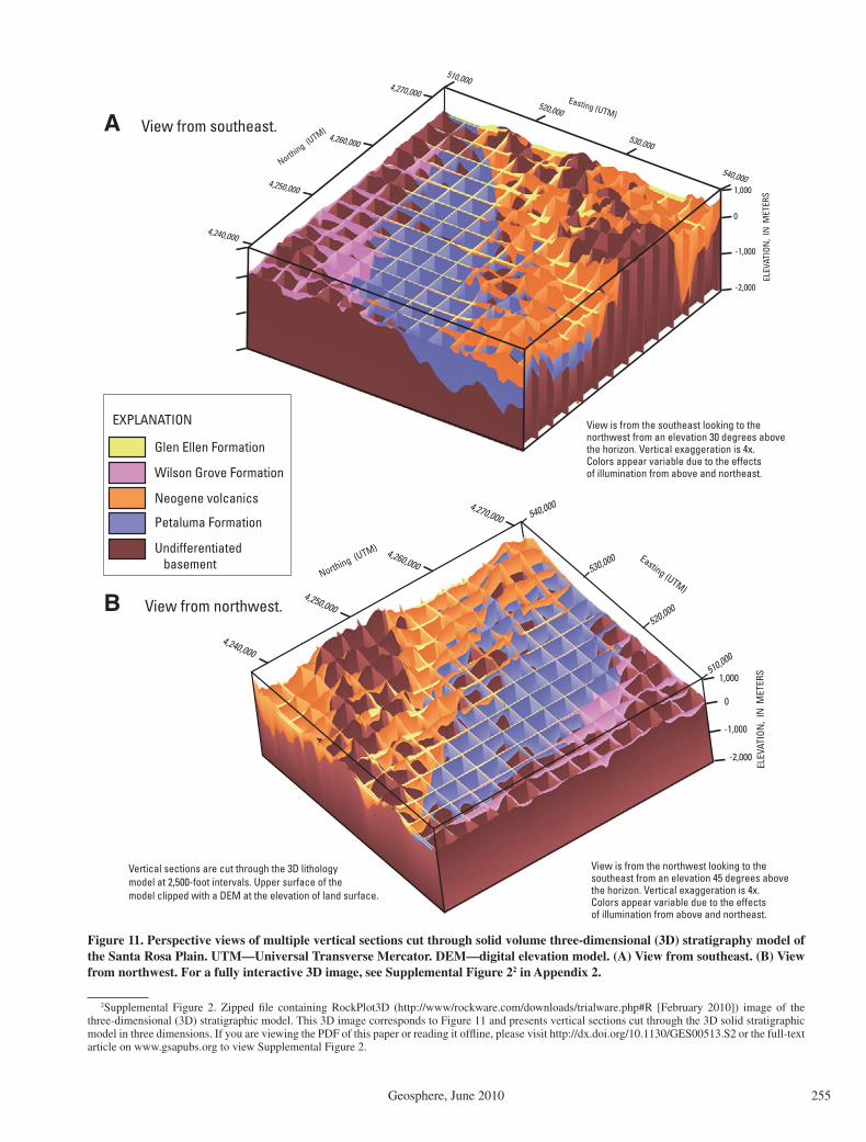
3D geologic modeling—Santa Rosa Plain
Geosphere, June 2010 255
510,000
520,000
530,000
540,000
Easting (UTM)
4,270,000
4,260,000
4,250,000
4,240,000
Northing (UTM)
1,000
ELEV
ATIO
N,
IN M
ETER
S
-1,000
-2,000
0
510,000
520,000
530,000
540,000
4,270,000
4,260,000
4,250,000
4,240,000
1,000
Easting (UTM)
Northing (U
TM)
ELEV
ATIO
N,
IN M
ETER
S
-1,000
-2,000
0
View is from the southeast looking to thenorthwest from an elevation 30 degrees abovethe horizon. Vertical exaggeration is 4x.Colors appear variable due to the effectsof illumination from above and northeast.
Vertical sections are cut through the 3D lithology model at 2,500-foot intervals. Upper surface of the model clipped with a DEM at the elevation of land surface.
Glen Ellen Formation
Wilson Grove Formation
Neogene volcanics
Petaluma Formation
Undifferentiated basement
EXPLANATION
View is from the northwest looking to the southeast from an elevation 45 degrees abovethe horizon. Vertical exaggeration is 4x.Colors appear variable due to the effects of illumination from above and northeast.
View from southeast.
View from northwest.
A
B
Figure 11. Perspective views of multiple vertical sections cut through solid volume three-dimensional (3D) stratigraphy model ofthe Santa Rosa Plain. UTM—Universal Transverse Mercator. DEM—digital elevation model. (A) View from southeast. (B) View from northwest. For a fully interactive 3D image, see Supplemental Figure 22 in Appendix 2.
2Supplemental Figure 2. Zipped fi le containing RockPlot3D (http://www/rockware.com/downloads/trialware.php#R [February 2010]) image of the three-dimensional (3D) stratigraphic model. This 3D image corresponds to Figure 11 and presents vertical sections cut through the 3D solid stratigraphic model in three dimensions. If you are viewing the PDF of this paper or reading it offl ine, please visit http://dx.doi.org/10.1130/GES00513.S2 or the full-text article on www.gsapubs.org to view Supplemental Figure 2.

Sweetkind et al.
256 Geosphere, June 2010
of the 16 layers are parallel to the land surface as defi ned by a DEM. Within each layer, grid cells were 660 ft (~198 m) in the x, y dimension, and of a thickness defi ned for each layer. The top 4 layers are 50 ft (~15 m) thick, the next 8 layers are 100 ft (~30 m) thick, and the bottom 4 layers are 500 ft (~150 m) thick, such that the base of the model volume is 3000 ft (~900 m) below land surface. This discretization scheme created 26,376 grid cells in each layer; a total of 422,016 cells composed the model domain.
Textural classes were defi ned by grouping the lithologic classes used in constructing the 3D lithologic model. Textural classes were based on the percentage of coarse-grained lithologic classes and on degree of sorting; the relative proportion of clay matrix was considered an important variable. Resultant texture classes (Table 2) included coarse grained, intermediate, and fi ne grained; volcanic rocks did not fi t into this scheme and were retained as two additional classes. Using this classifi cation, three texture models were constructed with grid cells 660 ft (~198 m) in the x and y dimension and vertical
TABLE 2. DESCRIPTION OF TEXTURE CLASSES
Texture number Descriptor Lithologic classes* included in texture class
1 Coarse grained Conglomerate; sandstone and gravel; gravel; sand and clay; clay, sand, and gravel; sand and gravel; sand; sandstone
2 Intermediate Clay and gravel3 Fine grained Clay and sand; clay; sandstone and clay; clay and trace gravel; clay and
sandstone; clay, sand and trace gravel4 Tuff Ash and/or tuff5 Basalt Basalt0 Not classifi ed Undifferentiated basement; volcanic conglomerate; shells; undefi ned98 No data Areas where layer is above of below the texture model
*Lithologic classes from three-dimensional lithology model.
TABLE 3. NUMERIC CODES USED FOR STRATIGRAPHIC UNITS
Numeric code Stratigraphic unit1000 Glen Ellen Formation and equivalents and Quaternary
alluvial deposits2000 Wilson Grove Formation3000 Neogene volcanics4000 Petaluma Formation5000 Mesozoic basement rocks, undivided
TABLE 4. NUMERIC CODES USED FOR STRATIGRAPHIC UNITS
Stratigraphic unit (numeric code)
Texture class(texture number)
Glen Ellen(1000)Wilson Grove(2000)Neogene volcanics(3000)Petaluma Formation(4000)Basement, undivided(5000)
Coarse grained (1)
1001
2001
3001
4001
5000
Intermediate(2)
1002
2002
3002
4002
5000
Fine grained (3)
1003
2003
3003
4003
5000
Tuff (4)
1004
2004
3004
4004
5000
Basalt(5)
1005
2005
3005
4005
5000
discretizations of 50 ft, 100 ft, and 500 ft (~15, ~30, and ~150 m) thickness, respectively. Using a geographic information system (GIS), each grid cell for each of the 16 layers was attributed with texture class by intersecting the layering scheme with the classifi ed data from a textural model. Layers 1–4 [each 50 ft (~15 m) thick] were populated with texture by sampling the texture model with 50 ft vertical discretization; layers 5–12 [each 100 ft (~30 m) thick] were populated with texture by sampling the texture model with 100 ft (~30 m) vertical discretiza-tion; and layers 13–16 [each 500 ft (~150 m) thick] were populated with texture by sampling the texture model with 500 ft (~150 m) vertical discretization. Stratigraphic units were assigned a numeric code (Table 3). Using a GIS, each grid cell for each of the 16 layers was attributed with stratigraphic unit by intersecting the layer-ing scheme with the 3D stratigraphic framework and assigning the stratigraphic unit that the cen-troid of each cell is within.
Numeric values for textural class and strati-graphic unit were added to create a new com-
bined attribute called “strat_text” (Tables 4 and 5). This attribute combines stratigraphy and texture class such that gravels in the Petaluma Formation can be distinguished from gravels in the Glen Ellen Formation or Wilson Grove For-mation. Because each formation largely repre-sents a distinct depositional setting, and gravels may have different sorting characteristics and presence of fi ne matrix, this distinction is of use in identifying permeability differences between units. The results of sampling the 3D solid vol-ume texture and stratigraphy models and com-bined attribute strat_text are shown for layers 1–5 (Plate 1), layers 6–10 (Plate 2), and layers 11–16 (Plate 3).
IMPLICATIONS OF SUBSURFACE MODELING TO BASIN EVOLUTION
An understanding of the extent and 3D geom-etry of the major lithologic types and interpreted formations yields insight into the evolution of the Cotati and Windsor Basins, the timing of movement of faults that bound and transect the
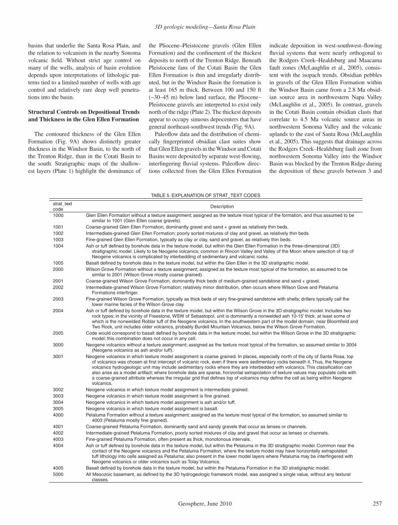
3D geologic modeling—Santa Rosa Plain
Geosphere, June 2010 257
basins that underlie the Santa Rosa Plain, and the relation to volcanism in the nearby Sonoma volcanic fi eld. Without strict age control on many of the wells, analysis of basin evolution depends upon interpretations of lithologic pat-terns tied to a limited number of wells with age control and relatively rare deep well penetra-tions into the basin.
Structural Controls on Depositional Trends and Thickness in the Glen Ellen Formation
The contoured thickness of the Glen Ellen Formation (Fig. 9A) shows distinctly greater thickness in the Windsor Basin, to the north of the Trenton Ridge, than in the Cotati Basin to the south. Stratigraphic maps of the shallow-est layers (Plate 1) highlight the dominance of
the Pliocene–Pleistocene gravels (Glen Ellen Formation) and the confi nement of the thickest deposits to north of the Trenton Ridge. Beneath Pleistocene fans of the Cotati Basin the Glen Ellen Formation is thin and irregularly distrib-uted, but in the Windsor Basin the formation is at least 165 m thick. Between 100 and 150 ft (~30–45 m) below land surface, the Pliocene–Pleistocene gravels are interpreted to exist only north of the ridge (Plate 2). The thickest deposits appear to occupy sinuous depocenters that have general northeast-southwest trends (Fig. 9A).
Paleofl ow data and the distribution of chemi-cally fi ngerprinted obsidian clast suites show that Glen Ellen gravels in the Windsor and Cotati Basins were deposited by separate west-fl owing, interfi ngering fl uvial systems. Paleofl ow direc-tions collected from the Glen Ellen Formation
indicate deposition in west-southwest–fl owing fl uvial systems that were nearly orthogonal to the Rodgers Creek–Healdsburg and Maacama fault zones (McLaughlin et al., 2005), consis-tent with the isopach trends. Obsidian pebbles in gravels of the Glen Ellen Formation within the Windsor Basin came from a 2.8 Ma obsid-ian source area in northwestern Napa Valley (McLaughlin et al., 2005). In contrast, gravels in the Cotati Basin contain obsidian clasts that correlate to 4.5 Ma volcanic source areas in northwestern Sonoma Valley and the volcanic uplands to the east of Santa Rosa (McLaughlin et al., 2005). This suggests that drainage across the Rodgers Creek–Healdsburg fault zone from northwestern Sonoma Valley into the Windsor Basin was blocked by the Trenton Ridge during the deposition of these gravels between 3 and
TABLE 5. EXPLANATION OF STRAT_TEXT CODES
strat_text code Description
1000 Glen Ellen Formation without a texture assignment; assigned as the texture most typical of the formation, and thus assumed to be similar to 1001 (Glen Ellen coarse gravels).
1001 Coarse-grained Glen Ellen Formation, dominantly gravel and sand + gravel as relatively thin beds.1002 Intermediate-grained Glen Ellen Formation; poorly sorted mixtures of clay and gravel, as relatively thin beds.1003 Fine-grained Glen Ellen Formation, typically as clay or clay, sand and gravel, as relatively thin beds.1004 Ash or tuff defi ned by borehole data in the texture model, but within the Glen Ellen Formation in the three-dimensional (3D)
stratigraphic model. Likely to be Neogene volcanics; common in Rincon Valley and Valley of the Moon where selection of top of Neogene volcanics is complicated by interbedding of sedimentary and volcanic rocks.
1005 Basalt defi ned by borehole data in the texture model, but within the Glen Ellen in the 3D stratigraphic model.2000 Wilson Grove Formation without a texture assignment; assigned as the texture most typical of the formation, so assumed to be
similar to 2001 (Wilson Grove mostly coarse grained).2001 Coarse-grained Wilson Grove Formation, dominantly thick beds of medium-grained sandstone and sand + gravel. 2002 Intermediate-grained Wilson Grove Formation; relatively minor distribution, often occurs where Wilson Gove and Petaluma
Formations interfi nger.2003 Fine-grained Wilson Grove Formation, typically as thick beds of very fi ne-grained sandstone with shells; drillers typically call the
lower marine facies of the Wilson Grove clay.2004 Ash or tuff defi ned by borehole data in the texture model, but within the Wilson Grove in the 3D stratigraphic model. Includes two
rock types; in the vicinity of Freestone, WSW of Sebastopol, unit is dominantly a nonwelded ash 10-15’ thick, at least some of which is the nonwelded Roblar tuff of the Neogene volcanics. In the southwestern part of the model domain, near Bloomfi eld and Two Rock, unit includes older volcanics, probably Burdell Mountain Volcanics, below the Wilson Grove Formation.
2005 Code would correspond to basalt defi ned by borehole data in the texture model, but within the Wilson Grove in the 3D stratigraphic model; this combination does not occur in any cell.
3000 Neogene volcanics without a texture assignment; assigned as the texture most typical of the formation, so assumed similar to 3004 (Neogene volcanics as ash and/or tuff).
3001 Neogene volcanics in which texture model assignment is coarse grained. In places, especially north of the city of Santa Rosa, top of volcanics was chosen at fi rst intercept of volcanic rock, even if there were sedimentary rocks beneath it. Thus, the Neogenevolcanics hydrogeologic unit may include sedimentary rocks where they are interbedded with volcanics. This classifi cation can also arise as a model artifact; where borehole data are sparse, horizontal extrapolation of texture values may populate cells witha coarse-grained attribute whereas the irregular grid that defi nes top of volcanics may defi ne the cell as being within Neogene volcanics.
3002 Neogene volcanics in which texture model assignment is intermediate grained.3003 Neogene volcanics in which texture model assignment is fi ne grained.3004 Neogene volcanics in which texture model assignment is ash and/or tuff.3005 Neogene volcanics in which texture model assignment is basalt.4000 Petaluma Formation without a texture assignment; assigned as the texture most typical of the formation, so assumed similar to
4003 (Petaluma mostly fi ne grained).4001 Coarse-grained Petaluma Formation, dominantly sand and sandy gravels that occur as lenses or channels.4002 Intermediate-grained Petaluma Formation, poorly sorted mixtures of clay and gravel that occur as lenses or channels.4003 Fine-grained Petaluma Formation, often present as thick, monotonous intervals.4004 Ash or tuff defi ned by borehole data in the texture model, but within the Petaluma in the 3D stratigraphic model. Common near the
contact of the Neogene volcanics and the Petaluma Formation, where the texture model may have horizontally extrapolated tuff lithology into cells assigned as Petaluma; also present in the lower model layers where Petaluma may be interfi ngered withNeogene volcanics or older volcanics such as Tolay Volcanics.
4005 Basalt defi ned by borehole data in the texture model, but within the Petaluma Formation in the 3D stratigraphic model.5000 All Mesozoic basement, as defi ned by the 3D hydrogeologic framework model, was assigned a single value, without any textural
classes.

Sweetkind et al.
258 Geosphere, June 2010
6325000 6350000 6375000 6400000
1875
000
1900
000
1925
000
1950
000
1975
000
6325000 6350000 6375000 6400000
1875
000
1900
000
1925
000
1950
000
1975
000
6325000 6350000 6375000 6400000
1875
000
1900
000
1925
000
1950
000
1975
000
6325000 6350000 6375000 6400000
1875
000
1900
000
1925
000
1950
000
1975
000
6325000 6350000 6375000 6400000
1875
000
1900
000
1925
000
1950
000
1975
000
25,000-foot grid based on Calfornia State Plane system;Lambert Conformal Conic projection, North Americandatum 1983.
Model grid, shown as faint horizontal and vertical lines, consistsof 168 rows and 157 columns of cells 660 feet on a side
STRATIGRAPHY
Not intersected with layeror not classifiedCoarse-grainedIntermediate-grainedFine-grainedTuffBasalt
TEXTURE CLASS
STRAT_TEXT CLASS
1001; Glen Ellen Formation; coarse-grained1002; Glen Ellen Formation; intermediate-grained1003; Glen Ellen Formation; fine-grained1004; Glen Ellen Formation; tuff1005; Glen Ellen Formation; basalt
1000; Glen Ellen Formation; undifferentiated
2000; Wilson Grove Formation; undifferentiated2001; Wilson Grove Formation; coarse-grained2002; Wilson Grove Formation; intermediate-grained2003; Wilson Grove Formation; fine-grained2004; Wilson Grove Formation; tuff
3000; Neogene volcanics; undifferentiated3001; Neogene volcanics; coarse-grained3002; Neogene volcanics; intermediate-grained3003; Neogene volcanics; fine-grained3004; Neogene volcanics; tuff3005; Neogene volcanics; basalt
4000; Petaluma Formation; undifferentiated4001; Petaluma Formation; coarse-grained4002; Petaluma Formation; intermediate-grained4003; Petaluma Formation; fine-grained4004; Petaluma Formation; tuff4005; Petaluma Formation; basalt
5000; Undifferentiated basement
Simplified trace of major faults used in 3D lithologic and stratigraphic models
Drill hole that penetrates the layer top
Glen Ellen FormationWilson Grove FormationNeogene volcanicsPetaluma FormationUndifferentiatedbasement
Stratigraphy Texture class Strat_Texture
LAYER 1Land surface
to -50’below land surface
LAYER 2-50’ to -100’
below land surface
LAYER 3-100’ to -150’
below land surface
LAYER 4-150’ to -200’
below land surface
LAYER 5-200’ to -300’
below land surface
Plate 1. Maps showing discretized results from three-dimensional (3D) stratigraphy model, solid volume 3D texture class model, and attribute strat_text (see text) for layers 1–5. Thin horizontal and vertical lines portray the grid cell discretization,which consists of 168 rows and 157 columns of cells 660 ft (~198 m) on a side. The locations of drill holes that are deep enough to penetrate the upper surface of each layer, and thus serve as a point of geologic information for that layer, are shown on the stra-tigraphy maps. If you are viewing the PDF of this paper or reading it offl ine, please visit http://dx.doi.org/10.1130/GES00513.SP1 or the full-text article on www.gsapubs.org to view the large-format fi le of Plate 1.
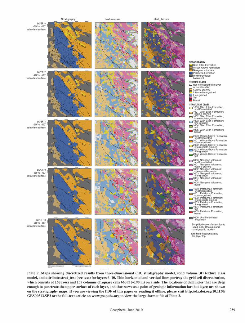
3D geologic modeling—Santa Rosa Plain
Geosphere, June 2010 259
6325000 6350000 6375000 6400000
1875
000
1900
000
1925
000
1950
000
1975
000
6325000 6350000 6375000 6400000
1875
000
1900
000
1925
000
1950
000
1975
000
6325000 6350000 6375000 6400000
1875
000
1900
000
1925
000
1950
000
1975
000
6325000 6350000 6375000 6400000
1875
000
1900
000
1925
000
1950
000
1975
000
6325000 6350000 6375000 6400000
1875
000
1900
000
1925
000
1950
000
1975
000
25,000-foot grid based on Calfornia State Plane system;Lambert Conformal Conic projection, North Americandatum 1983.
Model grid, shown as faint horizontal and vertical lines, consistsof 168 rows and 157 columns of cells 660 feet on a side
Stratigraphy Texture class Strat_TextureLAYER 6
-300’ to -400’below land surface
LAYER 7-400’ to -500’
below land surface
LAYER 8-500’ to -600’
below land surface
LAYER 9-600’ to -700’
below land surface
LAYER 10-700’ to -800’
below land surface
STRATIGRAPHY
Not intersected with layeror not classifiedCoarse-grainedIntermediate-grainedFine-grainedTuffBasalt
TEXTURE CLASS
STRAT_TEXT CLASS
1001; Glen Ellen Formation; coarse-grained1002; Glen Ellen Formation; intermediate-grained1003; Glen Ellen Formation; fine-grained1004; Glen Ellen Formation; tuff1005; Glen Ellen Formation; basalt
1000; Glen Ellen Formation; undifferentiated
2000; Wilson Grove Formation; undifferentiated2001; Wilson Grove Formation; coarse-grained2002; Wilson Grove Formation; intermediate-grained2003; Wilson Grove Formation; fine-grained2004; Wilson Grove Formation; tuff
3000; Neogene volcanics; undifferentiated3001; Neogene volcanics; coarse-grained3002; Neogene volcanics; intermediate-grained3003; Neogene volcanics; fine-grained3004; Neogene volcanics; tuff3005; Neogene volcanics; basalt
4000; Petaluma Formation; undifferentiated4001; Petaluma Formation; coarse-grained4002; Petaluma Formation; intermediate-grained4003; Petaluma Formation; fine-grained4004; Petaluma Formation; tuff4005; Petaluma Formation; basalt
5000; Undifferentiated basement
Simplified trace of major faults used in 3D lithologic and stratigraphic models
Drill hole that penetrates the layer top
Glen Ellen FormationWilson Grove FormationNeogene volcanicsPetaluma FormationUndifferentiatedbasement
Plate 2. Maps showing discretized results from three-dimensional (3D) stratigraphy model, solid volume 3D texture class model, and attribute strat_text (see text) for layers 6–10. Thin horizontal and vertical lines portray the grid cell discretization,which consists of 168 rows and 157 columns of square cells 660 ft (~198 m) on a side. The locations of drill holes that are deepenough to penetrate the upper surface of each layer, and thus serve as a point of geologic information for that layer, are shownon the stratigraphy maps. If you are viewing the PDF of this paper or reading it offl ine, please visit http://dx.doi.org/10.1130/GES00513.SP2 or the full-text article on www.gsapubs.org to view the large-format fi le of Plate 2.
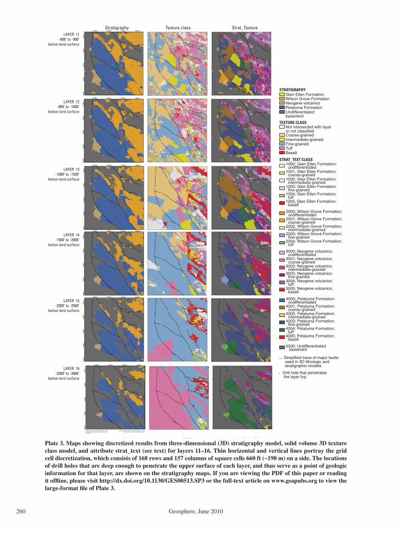
Sweetkind et al.
260 Geosphere, June 2010
6325000 6350000 6375000 6400000
1875
000
1900
000
1925
000
1950
000
1975
000
6325000 6350000 6375000 6400000
1875
000
1900
000
1925
000
1950
000
1975
000
6325000 6350000 6375000 6400000
1875
000
1900
000
1925
000
1950
000
1975
000
6325000 6350000 6375000 6400000
1875
000
1900
000
1925
000
1950
000
1975
000
6325000 6350000 6375000 6400000
1875
000
1900
000
1925
000
1950
000
1975
000
25,000-foot grid based on Calfornia State Plane system;Lambert Conformal Conic projection, North Americandatum 1983.
Model grid, shown as faint horizontal and vertical lines, consistsof 168 rows and 157 columns of cells 660 feet on a side
6325000 6350000 6375000 6400000
1875
000
1900
000
1925
000
1950
000
1975
000
Stratigraphy Texture class Strat_TextureLAYER 11
-800’ to -900’below land surface
LAYER 12-900’ to -1000’
below land surface
LAYER 13-1000’ to -1500’
below land surface
LAYER 14-1500’ to -2000’
below land surface
LAYER 15-2000’ to -2500’
below land surface
LAYER 16-2500’ to -3000’
below land surface
STRATIGRAPHY
Not intersected with layeror not classifiedCoarse-grainedIntermediate-grainedFine-grainedTuffBasalt
TEXTURE CLASS
STRAT_TEXT CLASS
1001; Glen Ellen Formation; coarse-grained1002; Glen Ellen Formation; intermediate-grained1003; Glen Ellen Formation; fine-grained1004; Glen Ellen Formation; tuff1005; Glen Ellen Formation; basalt
1000; Glen Ellen Formation; undifferentiated
2000; Wilson Grove Formation; undifferentiated2001; Wilson Grove Formation; coarse-grained2002; Wilson Grove Formation; intermediate-grained2003; Wilson Grove Formation; fine-grained2004; Wilson Grove Formation; tuff
3000; Neogene volcanics; undifferentiated3001; Neogene volcanics; coarse-grained3002; Neogene volcanics; intermediate-grained3003; Neogene volcanics; fine-grained3004; Neogene volcanics; tuff3005; Neogene volcanics; basalt
4000; Petaluma Formation; undifferentiated4001; Petaluma Formation; coarse-grained4002; Petaluma Formation; intermediate-grained4003; Petaluma Formation; fine-grained4004; Petaluma Formation; tuff4005; Petaluma Formation; basalt
5000; Undifferentiated basement
Simplified trace of major faults used in 3D lithologic and stratigraphic models
Drill hole that penetrates the layer top
Glen Ellen FormationWilson Grove FormationNeogene volcanicsPetaluma FormationUndifferentiatedbasement
Plate 3. Maps showing discretized results from three-dimensional (3D) stratigraphy model, solid volume 3D texture class model, and attribute strat_text (see text) for layers 11–16. Thin horizontal and vertical lines portray the grid cell discretization, which consists of 168 rows and 157 columns of square cells 660 ft (~198 m) on a side. The locations of drill holes that are deep enough to penetrate the upper surface of each layer, and thus serve as a point of geologic information for that layer, are shown on the stratigraphy maps. If you are viewing the PDF of this paper or reading it offl ine, please visit http://dx.doi.org/10.1130/GES00513.SP3 or the full-text article on www.gsapubs.org to view the large-format fi le of Plate 3.

3D geologic modeling—Santa Rosa Plain
Geosphere, June 2010 261
1 Ma. Paleofl ow from northwestern Sonoma Valley was instead diverted southwestward, to the Cotati Basin side of the Trenton Ridge.
Seismic refl ection profi les across the east-ern side of the Windsor Basin (Williams et al., 2008) show a progressive increase in refl ec-tor dip beneath ~100–200 m, indicating active growth of the ridge within relatively young sedi-ments. The ridge appears to affect sedimenta-tion patterns, resulting in differing stratigraphic packages within the Windsor and Cotati Basins, the Windsor Basin being dominated at shallow depths (Plate 1) by the Glen Ellen Formation, and the Cotati Basin being dominated by the Petaluma Formation.
Identifying the Marine-Continental Transition
Interfi ngering of marine sandstone of the Wilson Grove Formation with transitional marine and nonmarine deposits of the Peta-luma Formation is inferred to occur beneath the Santa Rosa Plain’s irregular northwest-trending boundary (Allen, 2003; Powell et al., 2004). Where the two formations inter-fi nger, they represent an oscillating Miocene– Pliocene shoreline (Powell et al., 2004). The 3D stratigraphic model (Fig. 11; see stratig-raphy column in Plates 1, 2, and 3) tends to overrepresent the extent of the Petaluma For-mation because the marine-continental facies transition zone between the Wilson Grove and Petaluma Formations was always coded as Pet-aluma Formation when picking stratigraphic tops from the well data. The strat_text maps in Plates 1, 2, and 3 give a more realistic dis-play of the subsurface extent of the Petaluma Formation and the location of the transition. In these maps, units classifi ed as coarse-grained Petaluma Formation may be seen in places to be continuous with interpreted Wilson Grove Formation. However, the texture class fi ne-grained Petaluma Formation is more conserva-tive and still portrays the Petaluma as occupy-ing much of the subsurface.
Using drillers’ logs presented diffi culty in defi ning the marine-continental transition where the Wilson Grove Formation is deeply buried and transitional in lithologic character. Southeast of the town of Sebastopol, the upper part of the Wilson Grove Formation progres-sively becomes gravel rich southeastward, and the Petaluma Formation is also distinctly grav-elly (Fox, 1983; Clahan et al., 2003; Powell et al., 2004). Many of the gravelly facies in this area were assigned to the Petaluma Formation. The Wilson Grove Formation was interpreted in the subsurface only north of the outcrops of the so-called “sand and gravel of Cotati” (Fox,
1983; Clahan et al., 2003) for this study. Lim-ited high-quality drill-hole information (Pow-ell et al., 2006) assisted in interpretation of this area. Although facies changes within the Wil-son Grove Formation southeast of Sebastopol made stratigraphic interpretation diffi cult, the combined attribute strat_text (Plates 1, 2, and 3) clearly highlights the location of the transi-tion from the dominantly marine sands of the west to more heterogeneous, poorly sorted continental sediments. This transition consists of an irregular northwest-trending boundary, regardless of the formation in which the inter-val was interpreted.
The stratigraphic-texture maps between 150 and 500 ft (~45–150 m) below land surface (Plates 1 and 2) contain suffi cient drill-hole data to highlight the lithologic variability within the Petaluma Formation and its overall heteroge-neous nature. Although individual drill holes are often dominated by clay-rich sediment, the 3D distribution of data shows lenticular pack-ages of spatially restricted sand and gravel deposits that may represent channels depos-ited in an overall estuarine environment. Allen (2003) cited ostracode and diatom data associ-ated with the mudstones and diatomites as sug-gestive of deposition in fresh to brackish water (lagoonal?) settings. Local lenses of lignite are associated with the lagoonal to estuarine strata, suggesting deposition in a large river delta, embayment, or lagoon (Allen, 2003). Grav-els of the Petaluma Formation are, in places, dominated by clasts derived from Franciscan Complex, Coast Range Ophiolite, and Great Valley Sequence sources. More commonly, 30%–50% of gravel clast suites are derived from Tertiary volcanic sources to the east and/or the southeast, consistent with paleofl ow data that suggest that nonmarine Petaluma gravels were deposited in a west-northwest–fl owing fl uvial system (Allen, 2003).
Relative Absence of Volcanic Rocks
The relative absence of volcanic rocks is a striking aspect of the subsurface maps of the Santa Rosa Plain, considering the area’s prox-imity to the Sonoma volcanic fi eld to the east. Although many of the water wells are too shal-low to penetrate a volcanic section at depth, even the rare deeper holes within the basin penetrate relatively few volcanic rocks. Two wells situated on the west side of the Santa Rosa Plain within the Cotati Basin penetrated 840 ft and 1070 ft (~252 m, ~321 m), respectively, of a 5.8 Ma to ca. 4.5 Ma sedimentary section without intercepting volcanic rocks (Powell et al., 2006). Two oil exploration wells situated in the same part of the Cotati Basin penetrated
1460 ft and 2075 ft (~438 m, ~622 m), respec-tively, of sedimentary rocks without hitting volcanic rocks (California Department of Con-servation, Division of Oil, Gas, and Geothermal Resources, www.conservation.ca.gov/dog [July 2008]). The only oil exploration well within the Santa Rosa Plain to intercept volcanic rocks was at the south end of the Cotati Basin. This well penetrated the entire thickness of Petaluma For-mation, which was interbedded with Tolay vol-canic rocks before intersecting Mesozoic rocks at a depth of 5520 ft ~1656 m) (Wright, 1992). The relative absence of volcanic rocks is consis-tent with the relatively quiet aeromagnetic sig-nature from shallow sources over much of the basin (Langenheim et al., 2010). The relative absence of volcanic rocks within the basin may be due to the relatively localized nature of vol-canism, where volcanic rocks are dominated by fl ows of generally limited spatial extent.
In the far southwest part of the study area, volcanic rocks described as basalts were reported near the base of the penetrated sec-tion in several wells. Neogene volcanic rocks are known to underlie the Wilson Grove For-mation to the southeast and southwest of the Petaluma Valley (Bezore et al., 2002, 2003) and have been intercepted in the subsurface in the Petaluma Valley in oil and gas wells (Wagner et al., 2005). These rocks are probably related to the Tolay Volcanics or possibly the Burdell Mountain Volcanics. Volcanic rocks are not known to be present beneath the Wilson Grove Formation farther to the north near Sebasto-pol. The presence of volcanic rocks at the base of the marine section in the southwest part of the study area suggests that west-northwest– striking faults such as the Bloomfi eld fault may have a component of dextral offset such that these older volcanic rocks are offset to the northwest from localities farther to the south-east (e.g., McLaughlin et al., 1996).
Generalized Depositional History of the Santa Rosa Plain
In contrast to previous stratigraphic interpre-tations (Cardwell, 1958; California Department of Water Resources, 1975, 1982), the drill-hole lithology data and resulting 3D lithologic model emphasize the lateral extent of clay-rich Peta-luma Formation throughout the deeper parts of the basins that underlie the Santa Rosa Plain (Figs. 8 and 11). Previous studies have gener-ally interpreted Wilson Grove Formation and Neogene volcanic rocks to underlie the Santa Rosa Plain. The interpreted subsurface extent of the Petaluma Formation is surprising given that, in contrast to Petaluma Valley to the south, out-crops of the Petaluma Formation are uncommon
Sweetkind et al.
262 Geosphere, June 2010
around the margins of the Santa Rosa Plain. The formation crops out to the east of the Santa Rosa Plain, where it is involved within the Rodgers Creek fault zone, and is exposed in the core of fault-bounded Meacham Hill anticline at the southern boundary of the Santa Rosa Plain; no Petaluma Formation crops out to the west or northwest of the Santa Rosa Plain where the Wilson Grove Formation unconformably over-lies pre-Cenozoic rocks (Fig. 1).
Both the Cotati and Windsor Basins appear to contain Petaluma sediments (Plate 2) at depth, although the two basins are now sepa-rated by the Trenton Ridge. The Petaluma Formation is inferred to have been deposited within a single large basin that was subse-quently segmented by the Trenton Ridge. The Petaluma Formation was deposited over a pro-tracted time period during which strike-slip displacement propagated northward associated with northwestward movement of the Men-docino triple junction and the development of the San Andreas and related fault systems (Allen, 2003). Strike-slip offset in the North Bay is interpreted to have undergone a major reorganization ca. 9 Ma whereby slip was transferred from a proto-Hayward fault south-west of the Santa Rosa Plain, to faults on the east side of the Santa Rosa Plain (McLaughlin et al., 1996). This displacement transfer was accomplished across a major right step in the strike-slip system, which resulted in the exten-sional opening of the early Santa Rosa Plain basin. In this scenario, there was initially a single basin fi lled largely by deposition from a west-northwest–fl owing, Miocene–late Plio-cene fl uvial to marine depositional system and interbedded volcanic rocks. Deposition in this initial basin was controlled by transtension from ca. 7 to 5 Ma, followed by transpression that formed the Trenton Ridge and separated the Windsor and Cotati Basins (McLaughlin et al., 1996; Langenheim et al., 2006, 2010).
The gravity inversion (Langenheim et al., 2006, 2010) of the Cotati Basin, south of the Trenton Ridge, suggests a 2–3-km-thick accu-mulation of Wilson Grove and Petaluma Forma-tion sediments beneath the southern part of the Santa Rosa Plain. In this location, however, both of these units indicate shallow-water deposition. Facies considerations suggest that the great sed-imentary thickness cannot be accounted for by fi lling a preexisting structural depression. In this area, basin subsidence must have kept pace with sediment deposition during basin formation.
The marine-continental facies transition is located very close to the western structural margin of the basin as defi ned by the gravity inversion. It appears that the western margin of the basin must have remained relatively high
in order to prevent marine transgression into the Petaluma depocenter. Consistent with this interpretation, the thickness and facies patterns within the Wilson Grove Formation have been interpreted to suggest that the marine sands gradually lapped onto and buried preexisting paleotopographic highs of Franciscan basement (Powell et al., 2004).
CONCLUSIONS
This study relies heavily on lithologic infor-mation from water well data, usually assumed to be poor sources of geologic and lithologic information. However, our analysis and result-ing 3D modeling show that drillers’ logs can provide valid geologic information if the logs are carefully classifi ed and screened. Although lacking time control, the 3D lithologic inter-polation and identifi cation of stratigraphic units work reasonably well where the units are relatively homogeneous and drill-hole data are abundant. Construction of 3D lithologic, strati-graphic, and textural models of the Santa Rosa Plain has resulted in several new interpretations regarding the thickness, extent, and 3D distri-bution of the important geologic units in the Windsor and Cotati Basins.
Interpretation of numerous drillers’ logs from the Santa Rosa Plain has allowed for the delin-eation of the principal stratigraphic units, each of which had a reasonably distinct mappable character in the subsurface. Drillers’ descrip-tions tend to use unique, albeit simple, litho-logic nomenclature to describe each downhole interval, and do not tend to repeat these descrip-tions in a single hole. Careful classifi cation and screening of these data produced a surprisingly clean lithologic data set. Although lacking time control, the 3D lithologic interpolation and identifi cation of stratigraphic units work reasonably well where the units are relatively homogeneous and drill-hole data are abundant. The models break down in the vicinity of rapid facies transitions, where there is signifi cant dip to stratigraphic units, and deep in the section where drill-hole data are scarce.
The compilation of drill-hole data and resul-tant 3D framework modeling allowed us to map the marine-continental transition in some detail and also demonstrated the dominance of the Petaluma Formation within most of the basins that underlie the Santa Rosa Plain. Structural control on depositional patterns is evident in the distribution of the Glen Ellen Formation to the north of the Trenton Ridge. Complexity of the stratigraphic relations at the south end of the Cotati Basin, previously inferred based on geologic mapping (Fox, 1983), is confi rmed by subsurface mapping of lithology.
APPENDIX 1
3D Lithologic and Stratigraphic Model Results Compared to Published Cross Sections
A groundwater resources evaluation of Sonoma County (California Department of Water Resources, 1975, 1982) included 12 geologic cross sections depicting inferred geology beneath the Santa Rosa Plain. Eight of the cross-section lines crossed the entire county (California Department of Water Resources, 1975); the remaining four sections were confi ned to the southern half of the Santa Rosa Plain (California Department of Water Resources, 1982). It is clear that these sections were constructed on the basis of geologic map and well data, but the specifi c data sources used for each section are unknown. In order to make comparisons with these earlier inter-pretations and to directly compare the results of the 3D subsurface lithologic and stratigraphic models, we cut vertical profi les through our solid models of lithol-ogy and stratigraphy along the same lines of section as seven of the previously published cross sections (Fig. A1-1).
End points and section bends from the published cross sections were located in a GIS by georeferenc-ing the index maps from the published reports. Cross sections were constructed through both the 3D solid volume lithologic and stratigraphic models along these same lines of section (part B in Figs. A1-2–A1-8). The original published cross sections were digitized (part C in Figs. A1-2–A1-8) and then scaled to match the cross sections from our models. Each cross section illustration also includes lithologic logs from all drill holes within 500 m on either side of the section line (part A in Figs. A1-2–A1-8); drill holes were projected onto the section perpendicular to the trend of the section line. The drill-hole data provide a convenient display of the density of the subsurface data and the strength (and limitations) of the numeri-cal interpolation.
The southernmost cross section, A–A′′′ (Fig. A1-2) crosses the south end of the study area in Petaluma Valley, south of the Santa Rosa Plain. This section is south of the region where stratigraphy was inter-preted (Fig. A1-1C), so modeled stratigraphy is not shown on the section. However the sandy and sand and clay lithologic units on the west half of the sec-tion (Figs. A1-2A, A1-2B) are typical of the Wilson Grove Formation, and the eastern half of the section is dominated by fi ne-grained units characteristic of the Petaluma Formation. In general pattern, the modeled lithology is very similar to the previously published interpretation (Fig. A1-2C). The nature of the contact between the two major units cannot be determined from the lithologic model alone, but it is likely fault related. No gravelly lithologic units characteristic of the Glen Ellen Formation are evident in the shal-low subsurface. Volcanic units appear at depth in the lithology model on the east side of the section, where they are interbedded within the Petaluma Forma-tion. Sonoma Volcanics were interpreted to occupy the deepest portion of the basin in the previously published interpretation (Fig. A1-2C), based on the existence of outcrops of volcanic rocks to the south of Petaluma Valley; the lithologic models suggest that Neogene volcanic rocks do not project as far north as this section line.
Cross-section line B–B′′′ traverses the southern end of the Santa Rosa Plain, extending through the town of Rohnert Park in a southwest-northeast trend (Fig. A1-1A). On the west (Fig. A1-3A), a relatively thin section of sandy and sand and clay lithologic

3D geologic modeling—Santa Rosa Plain
Geosphere, June 2010 263
4,270,000
Easting (UTM)
Northing (UTM
)
4,260,000
4,250,000
4,240,000
510,000 520,000530,000
4,270,000
Easting (UTM)
Northing (UTM
)
4,260,000
4,250,000
4,240,000
510,000 520,000530,000
400
-400
0
4,270,000
Easting (UTM)
Northing (UTM
)
4,260,000
4,250,000
4,240,000
510,000 520,000530,000
2,000
-2,000
0
Glen Ellen Formation
Wilson Grove Formation
Neogene volcanics
Petaluma Formation
Undifferentiated basement
Gravel
Sand and gravel
Sandstone and gravel
Sand
Sandstone
Sand and clay
Sandstone and clay
Clay, sand, and gravel
Clay, sand, and trace gravel
Clay and gravel
Clay and trace gravel
Clay and sand
Clay and sandstoneClay
Conglomerate
Volcanic conglomerate
Basalt
Ash and (or) tuff
Undifferentiated basement
No data
Quaternary alluviumQuaternary and Pliocene gravels (Glen Ellen Formation)
Petaluma Formation
Wilson Grove Formation
Neogene volcanic rocks
Great Valley sequence and Coast Range ophioliteFranciscan Complex
Ultramafic rocks
Map units (Geology after Saucedo and others, 2000)
Simplified trace of major faults used in 3D lithologic and stratigraphic models
Line of section
Mesozoic rocks
Index geologic map showing cross section locations
Perspective 3D view of vertical sections cut through 3D lithology model
3D representation of vertical fault used in 3D lithologic and stratigraphic models
3D representation of vertical fault used in 3D lithologic and stratigraphic models
All three images have the same viewpoint from thesouth (185 degrees) looking to the north from anelevation of 35 degrees above the horizon. Colors appear variable due to the effectsof illumination in the 3D views.
Vertical exaggeration is 3x.
Vertical exaggeration is 8x.
Vertical exaggeration is 1.5x.
ELEV
ATIO
N,
INM
ETER
S
ELEV
ATIO
N,
INM
ETER
S
Perspective 3D view of vertical sections cut through 3D stratigraphy model
The 3D stratigraphic model does not extend as far south asthe lithologic model. As a result, section A–A’ is not shownand only the northern part of section B–B’ is shown.
A
B
C
H‘’H‘’‘’H‘’H‘’H‘’H‘’’’’’’’’’’’’’
H‘’HHHH ’’
DDDDDDDDDD
D‘D‘D‘D‘D‘D‘D‘D
H‘’H‘’H
CCCC
C‘C‘C‘C‘C‘CCCCCCCC
AAAAAAAAAA‘AAAA A‘’A‘’A‘’AAAA
HHHH
H‘
BBBBBBBBB B‘B‘‘BBBBBB
B‘’B‘’BB‘’BBBB BBBBBB‘BB‘‘’B ’
D2DD D2‘D2‘D2‘D2A2A2A22A2A2A2A222
A2‘A2‘AAA2A
H‘’H‘’H‘’H‘’H‘’H‘’‘’‘ ’’
H‘’HHH ’
D
D‘
H‘’HH‘H‘’HH
CCCCCCC
C‘
AAAAAAAAAA
A‘A‘AAAAAA‘’A‘A‘A‘AA‘AA‘
HHHHHHHHHHHHHHHHHHHHHHHHHHHHHH
H‘HH‘H
B B‘B‘B‘B‘B‘
B‘’BB B‘’B ’B‘
D2D2222222222 D2‘D2‘‘D2‘D2D2D2DD
A2A2A2A22A2
A2‘A
H‘’’’’’’’’’
H‘’’
DDDD
D‘
H‘’
CC
C‘
H
HH‘HHHHH
B‘’BBBB‘’’
D2D2‘2‘2‘2‘2‘2
A2A2A2
A2‘A
Figure A1-1. (A–C) Index geologic map showing the trace of previously published geologic cross sections and perspective views of vertical sections cut through three-dimensional (3D) solid volume lithology and stratig-raphy models along the same lines of section. All three images have the same viewpoint from the south (185°) looking to the north from an eleva-tion of 35° above the horizon. Colors appear variable due to the effects of illumination in the 3D views. UTM—Universal Transverse Mercator.
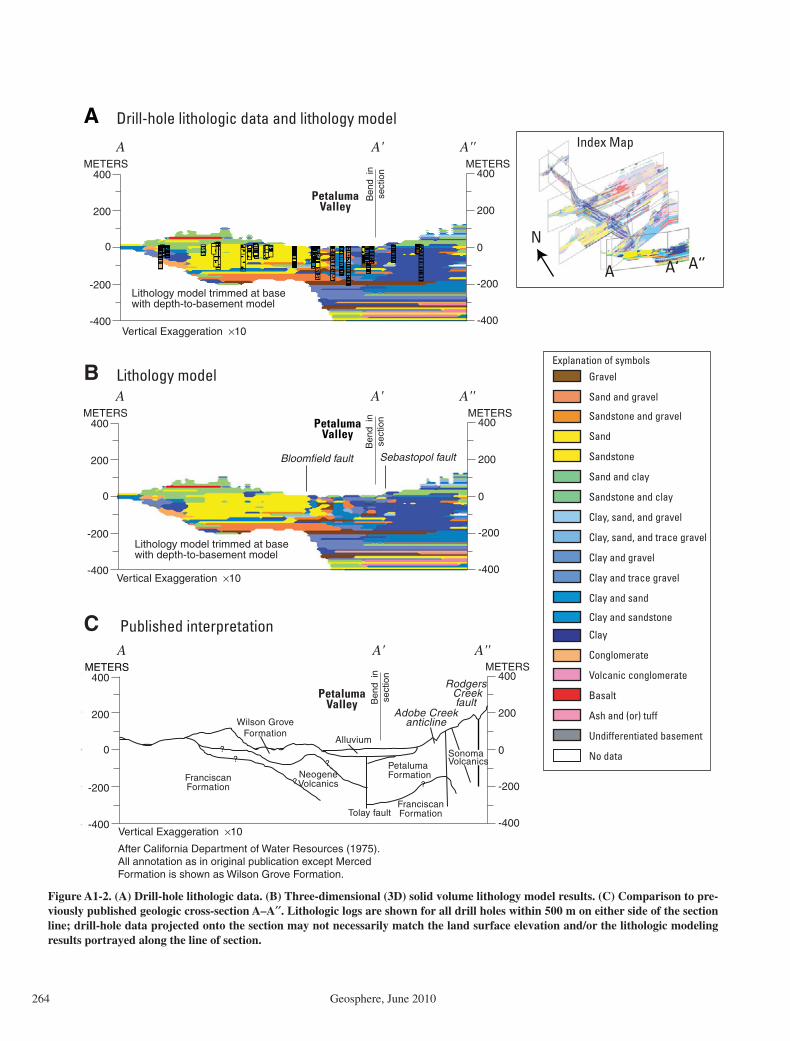
Sweetkind et al.
264 Geosphere, June 2010
Franciscan Formation
NeogeneVolcanics
Wilson GroveFormation
PetalumaFormation
?
?
SonomaVolcanics
?
?
?
Drill-hole lithologic data and lithology model
Vertical Exaggeration ×10
Alluvium
Sebastopol faultBloomfield fault
Vertical Exaggeration ×10
Vertical Exaggeration ×10
Lithology model
Published interpretation
Franciscan FormationTolay fault
Adobe Creekanticline
Rodgers Creekfault
PetalumaValley
PetalumaValley
PetalumaValley
Lithology model trimmed at basewith depth-to-basement model
Lithology model trimmed at basewith depth-to-basement model
A
B
C
0
200
400
-200
-400
0
200
400
-200
-400
0
200
400
-200
-400
0
200
400
-200
-400
0
200
400
-200
-400
0
200
400
-200
-400
Ben
d in
sect
ion
Ben
d in
sect
ion
Ben
d in
sect
ion
A A' A''METERS
A A' A''METERS
A A' A''METERS
METERS
METERS
METERS
A A‘ A‘’
N
Index Map
After California Department of Water Resources (1975). All annotation as in original publication except Merced Formation is shown as Wilson Grove Formation.
Gravel
Sand and gravel
Sandstone and gravel
Sand
Sandstone
Sand and clay
Sandstone and clay
Clay, sand, and gravel
Clay, sand, and trace gravel
Clay and gravel
Clay and trace gravel
Clay and sand
Clay and sandstone
Explanation of symbols
Clay
Conglomerate
Volcanic conglomerate
Basalt
Ash and (or) tuff
Undifferentiated basement
No data
Figure A1-2. (A) Drill-hole lithologic data. (B) Three-dimensional (3D) solid volume lithology model results. (C) Comparison to pre-viously published geologic cross-section A–A′′. Lithologic logs are shown for all drill holes within 500 m on either side of the section line; drill-hole data projected onto the section may not necessarily match the land surface elevation and/or the lithologic modelingresults portrayed along the line of section.

3D geologic modeling—Santa Rosa Plain
Geosphere, June 2010 265
Wils
on G
rove
Wils
onG
rove
Form
atio
nFo
rmat
ion
Peta
lum
aPe
talu
ma
Form
atio
nFo
rmat
ion
Gle
n El
len
Form
atio
n
Neo
gene
volc
anic
s
Wils
on G
rove
Form
atio
n
Peta
lum
aFo
rmat
ion
Und
iffer
entia
ted
base
men
t
Blo
om-
field
faul
tS
ebas
topo
lfa
ult
Rod
gers
Cre
ekfa
ult
Ben
nett
Val
ley
faul
tH–
H’’’’
A2–A
2’D2–D
2’
Lith
olog
y m
odel
trim
med
at b
ase
with
dep
th-t
o-ba
sem
ent m
odel
Bas
e of
lith
olog
y m
odel
(-4
00 m
)
Bsm
t
GE
Wils
on G
rove
For
mat
ion
Fran
cisc
an F
orm
atio
n
Gle
n E
llen
For
mat
ion
Pet
alum
aF
orm
atio
n
Tolay fault
Allu
vium
Son
oma
Vol
cani
cs
Rod
gers
Cre
ekfa
ult
Tola
y fa
ult Pet
alum
aF
orm
atio
n
SVSV
SV
SVSV
Wils
on G
rove
For
mat
ion
Dep
th-t
o-ba
sem
ent m
odel
sug
gest
sba
sin
exte
nds
to -
1,60
0 m
Mea
cham
Hill
antic
line
Neo
gene
Neo
gene
volc
anic
svo
lcan
ics
Neo
gene
volc
anic
s
Neo
gene
Neo
gene
volc
anic
svo
lcan
ics
Neo
gene
volc
anic
s
0
200
400
-200
-400
0200
400
-200
-400
Bend insection
BB
'B
''
ME
TE
RS
ME
TE
RS
B'''
Bend insection
0
200
400
-200
-400
0200
400
-200
-400
Bend insection
BB
'B
''
ME
TE
RS
ME
TE
RS
B'''
Bend insection
0
200
400
-200
-400
0200
400
-200
-400
Bend insection
BB
'B
''M
ET
ER
SM
ET
ER
SB
'''
Bend insection
Ver
tical
Exa
gger
atio
n ×
10
Ver
tical
Exa
gger
atio
n ×
10
Ver
tical
Exa
gger
atio
n ×
10A
fter
Cal
iforn
ia D
epar
tmen
t of W
ater
Res
ourc
es (
1975
). A
ll an
nota
tion
as in
orig
inal
pu
blic
atio
n ex
cept
Mer
ced
Form
atio
n is
sho
wn
as W
ilson
Gro
ve F
orm
atio
n.
BB
‘
B‘’
B‘’’
N
Ind
ex M
ap
Grav
el
Sand
and
gra
vel
Sand
ston
e an
d gr
avel
Sand
Sand
ston
e
Sand
and
cla
y
Sand
ston
e an
d cl
ay
Clay
, san
d, a
nd g
rave
l
Clay
, san
d, a
nd tr
ace
grav
el
Clay
and
gra
vel
Clay
and
trac
e gr
avel
Clay
and
san
d
Clay
and
san
dsto
ne
Expl
anat
ion
of s
ymbo
ls
Clay
Cong
lom
erat
e
Volc
anic
con
glom
erat
e
Basa
lt
Ash
and
(or)
tuff
Undi
ffere
ntia
ted
base
men
t
No
data
Bsm
t, U
ndiff
eren
tiate
d ba
sem
ent
GE,
Gle
n El
len
Form
atio
nSV
, Son
oma
Volc
anic
s
Drill
-hol
e lit
holo
gic
data
and
lith
olog
y m
odel
Lith
olog
y an
d st
ratig
raph
y m
odel
s
Publ
ishe
d in
terp
reta
tion
A B C
Fig
ure
A1-
3.
(A)
Dri
ll-ho
le
litho
logi
c da
ta.
(B)
Thr
ee-
dim
ensi
onal
(3
D)
solid
vo
l-um
e lit
holo
gy m
odel
res
ults
. (C
) Com
pari
son
to p
revi
ousl
y pu
blis
hed
geol
ogic
cr
oss-
sect
ion
B–B
′′. L
itho
logi
c lo
gs
are
show
n fo
r al
l dr
ill h
oles
w
ithi
n 50
0 m
on
eith
er s
ide
of t
he s
ecti
on l
ine;
dri
ll-ho
le
data
pro
ject
ed o
nto
the
sec-
tion
m
ay
not
nece
ssar
ily
mat
ch t
he l
and
surf
ace
ele-
vati
on
and/
or
the
litho
logi
c m
odel
ing
resu
lts
port
raye
d al
ong
the
line
of s
ecti
on.
Sweetkind et al.
266 Geosphere, June 2010
units characteristic of the Wilson Grove Formation is truncated against the structurally complex Meacham Hill anticline (Clahan et al., 2003), as suggested by the irregular Petaluma Formation–Neogene volcanics contact in the stratigraphic model (Fig. A1-3B), but not captured by the horizontal interpolation of the 3D lithologic model except as an abrupt transition to clay-rich Petaluma Formation. East of the Sebastopol fault, the published section (Fig. A1-3C) interprets a dipping section that includes the Wilson Grove and Glen Ellen Formations. In this location both the Wilson Grove and the Petaluma Formations become gravelly, represent-ing a transition to a more continental facies (Powell et al., 2004), mapped as gravel of the Cotati Formation (Fox, 1983; Clahan et al., 2003). In the stratigraphic model these sandy and gravelly facies were assigned to the Petaluma Formation (Fig. A1-3B), although they are known to be transitional. On the east side of the sections both the Rodgers Creek and Bennett Val-ley faults are expressed as abrupt change in lithologic packages and the appearance of the Neogene volca-nics. Again the 3D lithologic model does not incor-porate the structural complexity associated with these faults and implied by the irregular top of the Petaluma Formation (Fig. A1-3B), except as abruptly terminat-ing local packets of lithology that cannot be extrapo-lated very far.
Section C–C′ is >38 km long and crosses the central part of the Santa Rosa Plain in a southwest-northeast–trending direction through the city of Santa Rosa (Fig. A1-1A). The west end of the section is dominated by sandy and sand and clay lithologic units (Fig. A1-4A) characteristic of the Wilson Grove For-mation (Fig. A1-4B). Volcanic units appear at the base of the Wilson Grove section on the west, where they probably represent buried Tolay or Burdell Mountain Volcanics, and near the top of the section, where they represent ashy, nonwelded tuff including outcrop of Roblar tuff (Sarna-Wojcicki, 1992).
The marine-continental facies transition between Wilson Grove Formation and Petaluma Formation is evident from the lithologic model (Fig. A1-4A) beneath the tiepoint with section A2-A2′ (Fig. A1-4B), to the east of the Sebastopol fault. The top of the Wil-son Grove Formation is offset in an east-side-down manner by the Sebastopol fault. The steeply dipping black line that transects the sandy lithology of the Wilson Grove Formation near the Sebastopol fault (Fig. A1-4B) is the Wilson Grove–Petaluma contact as derived from the 3D stratigraphic model. The loca-tion and orientation of this contact between the two formations are obtained via the method by which the base of the Wilson Grove Formation was forced to honor the depth-to-basement surface beneath out-crops of the formation. Basinward, where the Wilson Grove Formation is covered, the base of the formation climbs steeply because the transition zone between the Wilson Grove Formation and Petaluma Forma-tions was always coded as Petaluma Formation when picking stratigraphic tops from the well data. For the stratigraphic model, where units must maintain a pre-scribed stacking order, the base of the Wilson Grove
Formation must climb high in the section to overlie the Petaluma Formation. However, the lithology model clearly shows that the Wilson Grove Formation extends some distance eastward into the basin to the transition between the two formations.
The fi ne-grained units typical of the Petaluma For-mation fi ll most of the center of the basin (Fig. A1-4B), an interpretation not consistent with that of older cross sections (Fig. A1-4C). Intervals interpreted as Peta-luma Formation include locally thick but discontinu-ous gravel packages. To the northeast of the Trenton Ridge, the Glen Ellen Formation shows a distinct thickening and the underlying Petaluma Formation alternates with intervals of Neogene volcanics. Volca-nic units predominate east of the Rodgers Creek fault, along with a thick interval of Glen Ellen Formation in Rincon Valley to the east of the city of Santa Rosa, near the trace of the Bennett Valley fault.
Section line D–D′ crosses the north-central part of the Santa Rosa Plain on a southwest-northeast trend, nearly parallel to section C–C′ (Fig. A1-1A). On the west end of the section, a relatively thin sec-tion of sandy and sand and clay lithologic units char-acteristic of the Wilson Grove Formation overlies the basement rocks (Fig. A1-5A). This depositional unit projects east beyond the Sebastopol fault and is truncated at the northwest end of the Trenton Ridge, where to the northeast the basin fi ll is primarily clay-dominated units of the Petaluma Formation capped by relatively thick, gravel-dominated Glen Ellen Forma-tion (Fig. A1-5B). This section transects the Wind-sor Basin, where the Glen Ellen Formation has been shown to be as thick as 160 m in certain drill holes. It is likely that the stratigraphic model, based on numer-ous shallow water wells, underestimates the thickness of the Glen Ellen Formation here. Neogene volcanics dominate to the east of the Rodgers Creek fault, and continue eastward to the Maacama fault, where they are faulted against basement rocks (McLaughlin et al., 2004). The overall geometry is similar between the sections cut through the 3D models and the pre-viously published section (Fig. A1-5C); however, the published section describes the basin-fi lling clay sec-tion as Glen Ellen Formation, rather than Petaluma Formation, and the published section infers that the Wilson Grove Formation might extend beneath the entire basin, an interpretation that does not appear to be supported by the subsurface data and models.
Cross section H–H′′′′ extends from the southern end of the Santa Rosa Plain west of the town of Cotati and projects north along the west side of the plain to the town of Healdsburg (Fig. A1-6A). The section crosses the curving trace of the Sebastopol fault at the south and north ends of the cross-section line; the section crosses the basement high associated with the Trenton fault near the center of the basin (Fig. A1-6B). The Glen Ellen Formation occurs as a relatively thin mantle to the south of the Trenton Ridge, but nearly doubles in thickness and becomes much more gravel rich north of the fault. The published section (Fig. A1-6C) portrays a very thick section of Glen Ellen Formation throughout the basin, although the
clay-dominated lithologic units are much more typical of the Petaluma Formation. It is possible that some of the Glen Ellen Formation in central Windsor Basin, to the north of the Trenton Ridge, is clayey and possibly lacustrine in nature, and thus would have been classi-fi ed as Petaluma Formation. In contrast to the previ-ously published section (Fig. A1-6C), we do not inter-pret Wilson Grove Formation in the basin as far east as this cross section. At the south end of the section, transitional sand- and gravel-dominated units were assigned to the Petaluma Formation. At the north end of the section, the Neogene volcanics are interpreted within the basin fi ll to the north of the Sebastopol fault (Fig. A1-6B).
We also show vertical profi les through the 3D solid models of lithology and stratigraphy along two shorter cross sections, A2–A2′ and D2–D2′ (Fig. A1-1) across the southern half of the Santa Rosa Plain (California Department of Water Resources, 1982). The advan-tage of showing these shorter lines is that they can be shown at a smaller scale, so that it is easier to see how the lithology model is interpolating between borehole data and how the stratigraphic units were selected from the lithology packages.
Cross-section line A2–A2′ extends from the south-ern end of the Santa Rosa Plain to the southeast of the town of Rohnert Park (Fig. A1-1A). Drill-hole data and the resultant 3D lithologic model (Fig. A1-7A) por-tray a clay-rich section with discrete lenses and sand and gravel. The published cross section (Fig. A1-7C) infers that the Wilson Grove Formation is present at depth along the entire section line; the 3D stratigraphic model includes the discontinuous sandy facies within the Petaluma Formation (Fig. A1-7B), with only thin intervals of overlying Glen Ellen and Wilson Grove Formation sediments. The section trends northwest along the west side of the basin, parallel to the trend of the facies transition between the Wilson Grove Formation and the Petaluma Formation. It is likely that the lenses of sand and gravel material may repre-sent interfi ngering of the two facies; such transitional intervals were routinely coded as Petaluma Formation when picking stratigraphic tops from the well data. The published cross section (Fig. A1-7C) suggests that the Sebastopol fault is crossed at the north end of the section, an interpretation that does not appear to be supported by the available lithologic data.
Cross-section line D2–D2′ trends generally west to east across the southernmost part of the basin, through the town of Rohnert Park (Fig. A1-1A). The line intersects the Rodgers Creek fault on the east side (Fig. A1-8). West of the fault, the Glen Ellen Forma-tion is interpreted to overlie a thick section of the Petaluma Formation (Fig. A1-8B). The discontinuous gravels within the Petaluma probably represent a part of the continental-marine transitional facies known to occur at the south end of the basin. In the published section Fig. A1-8C), the Wilson Grove Formation is projected at depth in the center of the basin, offset by the Sebastopol fault; this interpretation is not apparent from the available lithologic data or the results of the 3D modeling.

3D geologic modeling—Santa Rosa Plain
Geosphere, June 2010 267
??
Lith
olog
y m
odel
trim
med
at b
ase
with
dep
th-t
o-ba
sem
ent m
odel
Blo
om-
field
faul
tS
ebas
topo
lfa
ult
Rod
gers
Cre
ekfa
ult
Ben
nett
Val
ley
faul
tTr
ento
n R
idge
H–H’
’’’A2
–A2’
Peta
lum
aPe
talu
ma
Form
atio
nFo
rmat
ion
Peta
lum
aFo
rmat
ion
Und
iffer
entia
ted
bas
emen
t
Und
iffer
entia
ted
bas
emen
t
Wils
on G
rove
Wils
onG
rove
Form
atio
nFo
rmat
ion
Wils
on G
rove
Form
atio
n
Wils
on G
rove
Wils
onG
rove
Form
atio
nFo
rmat
ion
Wils
on G
rove
Form
atio
n
Gle
n El
len
Form
atio
nG
len
Elle
nFo
rmat
ion
PFPFPF
Dep
th-t
o-ba
sem
ent m
odel
sug
gest
sba
sin
exte
nds
to -
3,00
0 m
Wils
on G
rove
For
mat
ion
Fran
cisc
an
For
mat
ion
Gle
n E
llen
For
mat
ion
Son
oma
Vol
cani
csW
ilson
Gro
veF
orm
atio
n
Son
oma
Vol
cani
cs
Son
oma
Vol
cani
cs
Bsm
t
SV
Bsm
t
SVSV
Gle
n E
llen
For
mat
ion
Neo
gene
Neo
gene
volc
anic
svo
lcan
ics
Neo
gene
volc
anic
s
Neo
gene
Neo
gene
volc
anic
svo
lcan
ics
Neo
gene
volc
anic
s
0
200
400
-200
-400
0200
400
-200
-400
CC
'M
ET
ER
SM
ET
ER
S
Ver
tical
Exa
gger
atio
n ×
10
Afte
r C
alifo
rnia
Dep
artm
ent o
f Wat
er R
esou
rces
(19
75).
All
anno
tatio
n as
in o
rigin
al
publ
icat
ion
exce
pt M
erce
d F
orm
atio
n is
sho
wn
as W
ilson
Gro
ve F
orm
atio
n.
0
200
400
-200
-400
0200
400
-200
-400
CC
'M
ET
ER
SM
ET
ER
S
Ver
tical
Exa
gger
atio
n ×
10
0
200
400
-200
-400
0200
400
-200
-400
CC
'M
ET
ER
SM
ET
ER
S
Ver
tical
Exa
gger
atio
n ×
10
C
C‘
Ind
ex M
ap
N
Grav
el
Sand
and
gra
vel
Sand
ston
e an
d gr
avel
Sand
Sand
ston
e
Sand
and
cla
y
Sand
ston
e an
d cl
ay
Clay
, san
d, a
nd g
rave
l
Clay
, san
d, a
nd tr
ace
grav
el
Clay
and
gra
vel
Clay
and
trac
e gr
avel
Clay
and
san
d
Clay
and
san
dsto
ne
Expl
anat
ion
of s
ymbo
ls
Clay
Cong
lom
erat
e
Volc
anic
con
glom
erat
e
Basa
lt
Ash
and
(or)
tuff
Undi
ffere
ntia
ted
base
men
t
No
data
PF, P
etal
uma
Form
atio
nB
smt,
Und
iffer
entia
ted
base
men
t
SV, S
onom
a Vo
lcan
ics
Drill
-hol
e lit
holo
gic
data
and
lith
olog
y m
odel
Lith
olog
y an
d st
ratig
raph
y m
odel
s
Pub
lishe
d in
terp
reta
tion
A B C Fig
ure
A1-
4. (
A)
Dri
ll-ho
le l
itho
logi
c da
ta. (
B)
Thr
ee-d
imen
sion
al (
3D)
solid
vol
ume
litho
logy
mod
el r
esul
ts. (
C)
Com
pari
son
topr
evio
usly
pub
lishe
d ge
olog
ic c
ross
-sec
tion
C–C
′. L
itho
logi
c lo
gs a
re s
how
n fo
r al
l dr
ill h
oles
wit
hin
500
m o
n ei
ther
sid
e of
the
se
ctio
n lin
e; d
rill-
hole
dat
a pr
ojec
ted
onto
the
sec
tion
may
not
nec
essa
rily
mat
ch t
he la
nd s
urfa
ce e
leva
tion
and
/or
the
litho
logi
cm
odel
ing
resu
lts
port
raye
d al
ong
the
line
of s
ecti
on.

Sweetkind et al.
268 Geosphere, June 2010
men
t
?
H–H’
’’’
Seb
asto
pol
faul
t
Rod
gers
Cre
ekfa
ult
Maa
cam
afa
ult
Tren
ton
Rid
ge
Peta
lum
aPe
talu
ma
Form
atio
nFo
rmat
ion
Peta
lum
aFo
rmat
ion
Und
iffer
entia
ted
bas
emen
t
Wils
on G
rove
Form
atio
nG
len
Elle
nFo
rmat
ion
Und
iffer
entia
ted
bas
emen
tU
ndiff
eren
tiate
d b
asem
ent
Gle
n El
len
Form
atio
n
Lith
olog
y m
odel
trim
med
at
base
Dep
th-t
o-ba
sem
ent m
odel
sug
gest
sba
sin
exte
nds
to -
1,80
0 m
Bas
e of
lith
olog
y m
odel
(-4
00 m
)
Dep
th-t
o-ba
sem
ent m
odel
sug
gest
s ba
sin
exte
nds
to -
2,20
0 m
Wils
on G
rove
For
mat
ion
Fran
cisc
an
For
mat
ion
Gle
n El
len
Form
atio
n
Wils
on G
rove
For
mat
ion
Son
oma
Vol
cani
cs
Bsm
t
SV
SV
SVW
ilson
Gro
veF
orm
atio
n
Allu
vium
Gle
n E
llen
For
mat
ion
Son
oma
Vol
cani
cs
SV
Gle
n El
len
Form
atio
n
Neo
gene
Neo
gene
volc
anic
svo
lcan
ics
Neo
gene
volc
anic
s
Neo
gene
Neo
gene
volc
anic
svo
lcan
ics
Neo
gene
volc
anic
s
0
200
400
-200
-400
0200
400
-200
-400
DD
'M
ET
ER
SM
ET
ER
S
Ver
tical
Exa
gger
atio
n ×
10
0
200
400
-200
-400
0200
400
-200
-400
DD
'M
ET
ER
SM
ET
ER
S
Ver
tical
Exa
gger
atio
n ×
10-6
00-6
00 0
200
400
-200
-400
0200
400
-200
-400
DD
'M
ET
ER
SM
ET
ER
S
Ver
tical
Exa
gger
atio
n ×
10
D
D‘
Ind
ex M
ap
N
Afte
r C
alifo
rnia
Dep
artm
ent o
f Wat
er R
esou
rces
(19
75).
All
anno
tatio
n as
in o
rigin
al
publ
icat
ion
exce
pt M
erce
d F
orm
atio
n is
sho
wn
as W
ilson
Gro
ve F
orm
atio
n.
Grav
el
Sand
and
gra
vel
Sand
ston
e an
d gr
avel
Sand
Sand
ston
e
Sand
and
cla
y
Sand
ston
e an
d cl
ay
Clay
, san
d, a
nd g
rave
l
Clay
, san
d, a
nd tr
ace
grav
el
Clay
and
gra
vel
Clay
and
trac
e gr
avel
Clay
and
san
d
Clay
and
san
dsto
ne
Expl
anat
ion
of s
ymbo
ls
Clay
Cong
lom
erat
e
Volc
anic
con
glom
erat
e
Basa
lt
Ash
and
(or)
tuff
Undi
ffere
ntia
ted
base
men
t
No
data
Bsm
t, U
ndiff
eren
tiate
d ba
sem
ent
SV, S
onom
a Vo
lcan
ics
Drill
-hol
e lit
holo
gic
data
and
lith
olog
y m
odel
Lith
olog
y an
d st
ratig
raph
y m
odel
s
Publ
ishe
d in
terp
reta
tion
A B C
Fig
ure
A1-
5.
(A)
Dri
ll-ho
le
litho
logi
c da
ta.
(B)
Thr
ee-
dim
ensi
onal
(3
D)
solid
vo
l-um
e lit
holo
gy m
odel
res
ults
. (C
) C
ompa
riso
n to
pre
viou
sly
publ
ishe
d ge
olog
ic
cros
s-se
ctio
n D
–D′.
Lit
holo
gic
logs
ar
e sh
own
for
all
drill
hol
es
wit
hin
500
m o
n ei
ther
sid
e of
the
sec
tion
lin
e; d
rill-
hole
da
ta p
roje
cted
ont
o th
e se
c-ti
on
may
no
t ne
cess
arily
m
atch
the
lan
d su
rfac
e el
e-va
tion
an
d/or
th
e lit
holo
gic
mod
elin
g re
sult
s po
rtra
yed
alon
g th
e lin
e of
sec
tion
.

3D geologic modeling—Santa Rosa Plain
Geosphere, June 2010 269
? ?
Peta
lum
aPe
talu
ma
Form
atio
nFo
rmat
ion
Peta
lum
aFo
rmat
ion
Gle
n El
len
Form
atio
n
Bsm
t
Und
iffer
entia
ted
bas
emen
t
Bas
e of
lith
olog
y m
odel
(-
400
m)
Lith
olog
y m
odel
trim
med
at b
ase
with
dep
th-to
-bas
emen
t mod
el
Dep
th-t
o-ba
sem
ent m
odel
su
gges
ts b
asin
ext
ends
to -
3,00
0 m
Dep
th-t
o-ba
sem
ent m
odel
su
gges
ts b
asin
ext
ends
to -
1,10
0 m
Seb
asto
pol
faul
t
Tren
ton
Rid
ge
Wils
on G
rove
For
mat
ion
Ser
pent
inite
Allu
vium
Gle
n E
llen
For
mat
ion
Son
oma
Vol
cani
cs
Gle
n E
llen
For
mat
ion
Allu
vium
J-K
roc
ks
Wils
on G
rove
For
mat
ion
Neo
gene
Neo
gene
volc
anic
svo
lcan
ics
Neo
gene
volc
anic
s
0
200
-200
-400
0200
-200
-400
HH
'
ME
TE
RS
ME
TE
RS
Ver
tical
Exa
gger
atio
n ×
10
H''
H'''
H'''
'
Bend insection
Bend insection
Bend insection
HH
'H
''H
'''H
''''
Bend insection
Bend insection
Bend insection
H–H’
’’’A2
–A2’
D2–D
2’C–
C’D–
D’
0
200
-200
-400
0200
-200
-400
ME
TE
RS
ME
TE
RS
Ver
tical
Exa
gger
atio
n ×
10
-600
-800
-600
-800
0
200
-200
-400
0200
-200
-400
HH
'
ME
TE
RS
ME
TE
RS
Ver
tical
Exa
gger
atio
n ×
10
H''
H'''
H'''
'
Bend insection
Bend insection
Bend insection
Afte
r C
alifo
rnia
Dep
artm
ent o
f Wat
er R
esou
rces
(19
75).
All
anno
tatio
n as
in o
rigin
al
publ
icat
ion
exce
pt M
erce
d Fo
rmat
ion
is s
how
n as
Wils
on G
rove
For
mat
ion.
Ind
ex M
ap HH‘
H‘’
H‘’’
H‘’’’
N
Grav
el
Sand
and
gra
vel
Sand
ston
e an
d gr
avel
Sand
Sand
ston
e
Sand
and
cla
y
Sand
ston
e an
d cl
ay
Clay
, san
d, a
nd g
rave
l
Clay
, san
d, a
nd tr
ace
grav
el
Clay
and
gra
vel
Clay
and
trac
e gr
avel
Clay
and
san
d
Clay
and
san
dsto
ne
Expl
anat
ion
of s
ymbo
ls
Clay
Cong
lom
erat
e
Volc
anic
con
glom
erat
e
Basa
lt
Ash
and
(or)
tuff
Undi
ffere
ntia
ted
base
men
t
No
data
Bsm
t, U
ndiff
eren
tiate
d ba
sem
ent
Drill
-hol
e lit
holo
gic
data
and
lith
olog
y m
odel
Lith
olog
y an
d st
ratig
raph
y m
odel
s
Publ
ishe
d in
terp
reta
tion
A B C Fig
ure
A1-
6. (
A)
Dri
ll-ho
le l
itho
logi
c da
ta. (
B)
Thr
ee-d
imen
sion
al (
3D)
solid
vol
ume
litho
logy
mod
el r
esul
ts. (
C)
Com
pari
son
to p
revi
ousl
y pu
blis
hed
geol
ogic
cr
oss-
sect
ion
H–H
′′′′.
Lit
holo
gic
logs
are
sho
wn
for
all d
rill
hole
s w
ithi
n 50
0 m
on
eith
er s
ide
of th
e se
ctio
n lin
e; d
rill-
hole
dat
a pr
ojec
ted
onto
the
sect
ion
may
not
ne
cess
arily
mat
ch t
he la
nd s
urfa
ce e
leva
tion
and
/or
the
litho
logi
c m
odel
ing
resu
lts
port
raye
d al
ong
the
line
of s
ecti
on.

Sweetkind et al.
270 Geosphere, June 2010
?
?
Base of lithology model (-400 m)
H–H’’’’B–B’’’
Base of lithology model (-400 m)
D2–D2’ C–C’
PetalumaPetalumaFormationFormationPetalumaFormation
Wilson GroveFormation Glen Ellen
Formation
Depth-to-basement model suggests basin extends to -1,100 m
BsmtBsmt
Wilson Grove Formation
Alluvial fan deposits
Petaluma Formation
Basin deposits
Franciscan FormationSebastopolfault
SonomaVolcanics
0
200
-200
-400
0
200
-200
-400
A2 A2'METERS METERS
-600-600
0
200
-200
-400
0
200
-200
-400
A2 A2'METERS METERS
-600-600
-800 -800
0
200
-200
-400
0
200
-200
-400
A2 A2'METERS METERS
-600-600
A2‘
Index Map
N
Gravel
Sand and gravel
Sandstone and gravel
Sand
Sandstone
Sand and clay
Sandstone and clay
Clay, sand, and gravel
Clay, sand, and trace gravel
Clay and gravel
Clay and trace gravel
Clay and sand
Clay and sandstone
Explanation of symbols
Clay
Conglomerate
Volcanic conglomerate
Basalt
Ash and (or) tuff
Undifferentiated basement
No data
Bsmt, Undifferentiated basement
Drill-hole lithologic data and lithology model
Lithology and stratigraphy models
Published interpretation
A
B
C
Figure A1-7. (A) Drill-hole lithologic data. (B) Three-dimensional (3D) solid volume lithology model results. (C) Comparison to previ-ously published geologic cross-section A2–A2′. Lithologic logs are shown for all drill holes within 500 m on either side of the section line; drill-hole data projected onto the section may not necessarily match the land surface elevation and/or the lithologic modelingresults portrayed along the line of section.

3D geologic modeling—Santa Rosa Plain
Geosphere, June 2010 271
Base of lithology model (-400 m)
Base of lithology model (-400 m)
Depth-to-basement model suggests basin extends to -1,800 m
PetalumaPetalumaFormationFormationPetalumaFormation
Glen EllenFormation
Bsmt
RodgersCreekfault
H–H’’’’ B–B’’’A2–A2’
Wilson Grove Formation
Alluvial fan deposits
Petaluma Formation
Basin deposits
Sebastopol fault
SonomaVolcanicsWilson Grove
Formation
PetalumaFormation
SV
SV
0
200
-200
-400
D2 D2'METERS METERS
0
200
-200
-400
400 400
0
200
-200
-400
METERS METERS
0
200
-200
-400
400 400
0
200
-200
-400
METERS METERS
0
200
-200
-400
400 400
D2 D2'
D2 D2'
After California Department of Water Resources (1982). All annotation as in original publication except Merced Formation is shown as Wilson Grove Formation.
Vertical Exaggeration ×10
Vertical Exaggeration ×10
Vertical Exaggeration ×10
Index Map
N
D2 D2‘
Gravel
Sand and gravel
Sandstone and gravel
Sand
Sandstone
Sand and clay
Sandstone and clay
Clay, sand, and gravel
Clay, sand, and trace gravel
Clay and gravel
Clay and trace gravel
Clay and sand
Clay and sandstone
Explanation of symbols
Clay
Conglomerate
Volcanic conglomerate
Basalt
Ash and (or) tuff
Undifferentiated basement
No data
SV, Sonoma Volcanics
Drill-hole lithologic data and lithology model
Lithology and stratigraphy models
Published interpretation
NeogeneNeogenevolcanicsvolcanicsNeogenevolcanics
A
B
C
Figure A1-8. (A) Drill-hole lithologic data. (B) Three-dimensional (3D) solid volume lithol-ogy model results. (C) Comparison to previ-ously published geologic cross-section D2–D2′.Lithologic logs are shown for all drill holes within 500 m on either side of the section line; drill-hole data projected onto the section may not necessarily match the land surface eleva-tion and/or the lithologic modeling results por-trayed along the line of section.
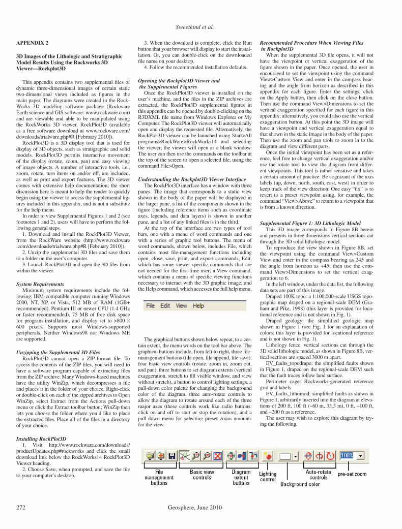
Sweetkind et al.
272 Geosphere, June 2010
APPENDIX 2
3D Images of the Lithologic and Stratigraphic Model Results Using the Rockworks 3D Viewer—Rockplot3D
This appendix contains two supplemental fi les of dynamic three-dimensional images of certain static two-dimensional views included as fi gures in the main paper. The diagrams were created in the Rock-Works 3D modeling software package (Rockware Earth science and GIS software: www.rockware.com) and are viewable and able to be manipulated using the RockWorks 3D viewer, RockPlot3D (available as a free software download at www.rockware.com/ downloads/trialware.php#R [February 2010]).
RockPlot3D is a 3D display tool that is used for display of 3D objects, such as stratigraphic and solid models. RockPlot3D permits interactive movement of the display (rotate, zoom, pan) and easy viewing of image objects. A number of interactive tools, i.e., zoom, rotate, turn items on and/or off, are included, as well as print and export features. The 3D viewer comes with extensive help documentation; the short discussion here is meant to help the reader to quickly begin using the viewer to access the supplemental fi g-ures included in this appendix, and is not a substitute for the help menu.
In order to view Supplemental Figures 1 and 2 (see footnotes 1 and 2), users will have to perform the fol-lowing general steps.
1. Download and install the RockPlot3D Viewer, from the RockWare website (http://www.rockware.com/downloads/trialware.php#R [February 2010]).
2. Unzip the supplemental 3D fi les and save them to a folder on the user’s computer.
3. Launch RockPlot3D and open the 3D fi les from within the viewer.
System RequirementsMinimum system requirements include the fol-
lowing: IBM-compatible computer running Windows 2000, NT, XP, or Vista, 512 MB of RAM (1GB+ recommended), Pentium III or newer CPU (1.4 GHz or faster recommended), 75 MB of free disk space for program installation, and display set to >800 ×600 pixels. Supports most Windows-supported peripherals. Neither Windows98 nor Windows ME are supported.
Unzipping the Supplemental 3D FilesRockPlot3D cannot open a ZIP-format fi le. To
access the contents of the ZIP fi les, you will need to have a software program capable of extracting fi les from the ZIP archive. Many Windows-based machines have the utility WinZip, which decompresses a fi le and places it in the folder of your choice. Right-click or double-click on each of the zipped archives to Open WinZip, select Extract from the Actions pull-down menu or click the Extract toolbar button; WinZip then lets you choose the folder where you’d like to place the extracted fi les. Place all of the fi les in a directory of your choice.
Installing RockPlot3D1. Visit http://www.rockware.com/downloads/
productUpdates.php#rockworks and click the small download link below the RockWorks14 RockPlot3D Viewer heading.
2. Choose Save, when prompted, and save the fi le to your computer’s desktop.
3. When the download is complete, click the Run button that your browser will display to start the instal-lation. Or, you can double-click on the downloaded fi le name on your desktop.
4. Follow the recommended installation defaults.
Opening the Rockplot3D Viewer and the Supplemental Figures
Once the RockPlot3D viewer is installed on the user’s machine, and the fi les in the ZIP archives are extracted, the RockPlot3D supplemental fi gures in this appendix can be opened by double-clicking on the R3DXML fi le name from Windows Explorer or My Computer. The RockPlot3D viewer will automatically open and display the requested fi le. Alternatively, the RockPlot3D viewer can be launched using Start>All programs>RockWare>RockWorks14 and selecting the viewer; the viewer will open as a blank window. The user can then use the commands on the toolbar at the top of the screen to open a selected fi le, using the command File>Open.
Understanding the Rockplot3D Viewer InterfaceThe RockPlot3D interface has a window with three
panes. The image that corresponds to a static view shown in the body of the paper will be displayed in the larger pane, a list of the components shown in the fi gure (including reference items such as coordinate axes, legends, and data layers) is shown in another pane, and a list of any linked fi les is in the third.
At the top of the interface are two types of tool bars, one with a menu of word commands and one with a series of graphic tool buttons. The menu of word commands, shown below, includes File, which contains most fi le-management functions including open, close, save, print, and export commands; Edit, which has some viewer-specifi c commands that are not needed for the fi rst-time user; a View command, which contains a menu of specifi c viewing functions necessary to interact with the 3D graphic image; and the Help command, which accesses the full help menu.
The graphical buttons shown below repeat, to a cer-tain extent, the menu words on the tool bar above. The graphical buttons include, from left to right, three fi le-management buttons (fi le open, fi le append, fi le save), four basic view controls (rotate, zoom in, zoom out, and pan), three buttons to set diagram extents (vertical exaggeration, stretch to fi ll visible window, and view without stretch), a button to control lighting settings, a pull-down color palette for changing the background color of the diagram, three auto-rotate controls to allow the diagram to rotate around each of the three major axes (these controls work like radio buttons: click on and off to start or stop the rotation), and a pull-down menu for selecting preset zoom amounts for the view.
Recommended Procedure When Viewing Files in Rockplot3D
When the supplemental 3D fi le opens, it will not have the viewpoint or vertical exaggeration of the fi gure shown in the paper. Once opened, the user in encouraged to set the viewpoint using the command View>Custom View and enter in the compass bear-ing and the angle from horizon as described in this appendix for each fi gure. Enter the settings, click on the Apply button, then click on the close button. Then use the command View>Dimensions to set the vertical exaggeration specifi ed for each fi gure in this appendix; alternatively, you could also use the vertical exaggeration button. At this point the 3D image will have a viewpoint and vertical exaggeration equal to that shown in the static image in the body of the paper. Then use the zoom and pan tools to zoom in to the diagram and view different parts.
Once the initial viewpoint has been set as a refer-ence, feel free to change vertical exaggeration and/or use the rotate tool to view the diagram from differ-ent viewpoints. This tool is rather sensitive and takes a certain amount of practice. Be cognizant of the axis labels (up, down, north, south, east, west) in order to keep track of the view direction. One easy “fi x” is to revert to a preset viewpoint using, for example, the command “View>Above” to return to a viewpoint that is from a known direction.
Supplemental Figure 1: 3D Lithologic ModelThis 3D image corresponds to Figure 8B herein
and presents in three dimensions vertical sections cut through the 3D solid lithologic model.
To reproduce the view shown in Figure 8B, set the viewpoint using the command View>Custom View and enter in the compass bearing as 245 and the angle from horizon as +45; then use the com-mand View>Dimensions to set the vertical exag-geration to 6.
In the left window, under the data list, the following data sets are part of this image.
Draped 100K topo: a 1:100,000-scale USGS topo-graphic map draped on a regional-scale DEM (Gra-ham and Pike, 1998) (this layer is provided for loca-tional reference and is not shown in Fig. 1).
Draped geology: the simplifi ed geologic map shown in Figure 1 (see Fig. 1 for an explanation of colors; this layer is provided for locational reference and is not shown in Fig. 1).
Lithology fence: vertical sections cut through the 3D solid lithologic model, as shown in Figure 8B, ver-tical sections are spaced 3000 m apart.
EV_faults_topodrape: the simplifi ed faults shown in Figure 1, draped on the regional-scale DEM such that the fault traces follow land surface.
Perimeter cage: Rockworks-generated reference grid and labels.
EV_faults_lithomod: simplifi ed faults as shown in Figure 1, arbitrarily inserted into the diagram at eleva-tions of 200 ft, 100 ft (~60 m, 33.3 m), 0 ft, −100 ft, and −200 ft as a reference.
The user may wish to explore this diagram by try-ing the following.

3D geologic modeling—Santa Rosa Plain
Geosphere, June 2010 273
1. Use the command View>Dimensions to set the vertical exaggeration to 1.5 or 2; this will give a more natural look to the topographic and geologic maps, which are distorted when viewed with a vertical exag-geration of 6.
2. Turn off the perimeter cage and coordinate axes by unchecking the boxes next to each item; this reduces the clutter on the diagram.
3. View the image from the southeast using a preset viewpoint. Use the command View>Above>South-East and adjust the viewing area using the zoom and pan tools. This view is looking along the axis of the Santa Rosa Plain where the continental-marine tran-sition is well expressed in the change from the blue colors of the estuarine clays to the yellows and light greens of the marine sandstones.
Supplemental Figure 2: 3D Stratigraphic ModelThis 3D image corresponds to Figure 11 herein
and presents in three dimensions vertical sections cut through the 3D solid stratigraphic model.
To reproduce the view shown in Figure 11, set the viewpoint using the command View>Custom View and to reproduce Figure 11A, enter the compass bearing as 140 and the angle from horizon as +30; to reproduce Figure 11B, enter the compass bearing as 300 and the angle from horizon as +45. For either viewpoint, use the command View>Dimensions to set the vertical exaggeration to 4.
In the left window, under the data list, the following data sets denoted by an abbreviated fi le name, are part of this image.
Topo: a 1:100,000-scale USGS topographic map draped on a regional-scale DEM (Graham and Pike, 1998); this layer is provided for locational reference and is not shown in Figure 1.
GeoMap: the simplifi ed geologic map shown in Figure 1 (see Fig. 1 for an explanation of colors, this layer is provided for locational reference and is not shown in Fig. 1).
Stratigraphic fence: vertical sections cut through the 3D solid stratigraphic model, as shown in Fig-ure 11 (vertical sections are spaced 2500 m apart).
EV_faults_topodrape: the simplifi ed faults shown in Figure 1, draped on the regional-scale DEM such that the fault traces follow land surface.
Perimeter cage: Rockworks-generated reference grid and labels.
The user may wish to explore this diagram by try-ing the following.
1. Turn off and on the GeoMap data set in the data list by unchecking and checking the box next to the data set name; in this way the user can evaluate the correspondence between mapped surface geology and subsurface geology.
2. Use the lighting tool. If colors in the vertical slices appear too washed out, reduce the level of ambi-ent lighting.
3. From the data list, expand the entry for the data set Stratigraphic Fence by clicking on the plus symbol next to the data set name. The fi ve data sets listed cor-respond to the principal stratigraphic units: GE—Glen Ellen Formation; WG—Wilson Grove Formation; SV—Neogene volcanic units; PF—Petaluma For-mation; and BSMT—undifferentiated pre-Cenozoic basement. You may turn off different stratigraphic units by unchecking the box next to each name. For example, turn off the SV or PF to observe how these units fi ll the deepest parts of the Cenozoic basins.
REFERENCES CITED
Allen, J.R., 2003, Stratigraphy and tectonics of Neogene strata, northern San Francisco Bay area [M.S. the-sis]: San Jose, California, San Jose State University, 183 p.
Bezore, S.P., Randolph-Loar, C.E., and Witter, R.C., 2002, Geologic map of the Petaluma 7.5′ quadrangle, Sonoma and Marin counties, California: A digital database: California Geological Survey Prelimi-nary Geologic Map, scale 1:24,000, ftp://ftp.consrv.ca.gov/pub/dmg/rgmp/Prelim_geo_pdf/petaluma_layout_highres.pdf.
Bezore, S.P., Koehler, R.D., and Witter, R.C., 2003, Geo-logic map of the Two Rock 7.5′ quadrangle, Sonoma County, California: A digital database: California Geological Survey Preliminary Geologic Map, scale 1:24,000, ftp://ftp.consrv.ca.gov/pub/dmg/rgmp/Prelim_geo_pdf/Two_Rock_prelim.pdf.
Blake, M.C., Jr., Howell, D.G., and Jayko, A.S., 1984, Tec-tonostratigraphic terranes of the San Francisco Bay region, in Blake, M.C., ed., 1984, Franciscan geol-ogy of northern California: Pacifi c Section, Society of Economic Paleontologists and Mineralogists Special Publication 43, p. 5–22.
Blake, M.C., Jr., Graymer, R.W., and Stamski, R.E., 2002, Geologic map and map database of western Sonoma, northernmost Marin, and southernmost Mendocino Counties, California: U.S. Geological Survey Miscellaneous Field Studies Map MF-2402, 42 p., scale 1:100,000.
California Department of Water Resources, 1975, Evaluation of ground water resources: Sonoma County: Volume 1, Geologic and hydrologic data: California Depart-ment of Water Resources Bulletin 118–4, 177 p.
California Department of Water Resources, 1982, Evalua-tion of ground water resources: Sonoma County: Volume 2, Santa Rosa Plain: California Department of Water Resources Bulletin 118–4, 107 p.
Cardwell, G.T., 1958, Geology and ground water in the Santa Rosa and Petaluma Valley areas, Sonoma County, California: U.S. Geological Survey Water-Supply Paper 1427, 273 p.
Clahan, K.B., Bezore, S.P., Koehler, R.D., and Witter, R.C., 2003, Geologic map of the Cotati 7.5′ quadrangle, Sonoma County, California: A digital database: California Geological Survey Preliminary Geologic Map, scale 1:24,000, ftp://ftp.consrv.ca.gov/pub/dmg/rgmp/Prelim_geo_pdf/cotati_prelim.pdf.
Davies, E.A., 1986, Stratigraphic and structural relation-ships of the Miocene and Pliocene formations of the Petaluma Valley area of California [M.S. thesis]: Berkeley, University of California, 96 p.
Faunt, C.C., Belitz, K., and Hansen, R.T., 2010, Develop-ment of a three-dimensional model of sedimentary texture in valley-fi ll deposits of Central Valley, Cali-fornia, USA: Hydrogeology Journal, doi: 10.1007/x10040-009-0539-7.
Fox, K.F., Jr., 1983, Tectonic setting of late Miocene, Plio-cene, and Pleistocene rocks in part of the Coast Ranges north of San Francisco, California: U.S. Geological Survey Professional Paper 1239, 33 p.
Graham, S.E., and Pike, R.J., 1998, Elevation maps of the San Francisco Bay region, California–A digital database: U.S. Geological Survey Open-File Report 2005–1318, p. 1–16
Graymer, R.W., Bryant, W., McCabe, C.A., Hecker, S., and Prentice, C.S., 2006, Map of Quaternary-active faults in the San Francisco Bay region: U.S. Geo-logical Survey Scientifi c Investigations Map 2919, http://pubs.usgs.gov/sim/2006/2919.
Graymer, R.W., Brabb, E.E., Jones, D.J., Barnes, J., Nich-olson, R.S., and Stamski, R.E., 2007, Geologic map and map database of eastern Sonoma and western Napa Counties, California: U.S. Geo-logical Survey Scientifi c Investigations Map 2956, scale 1:100,000.
Jachens, R.C., and Moring, B.C., 1990, Maps of the thick-ness of Cenozoic deposits and the isostatic residual gravity over basement for Nevada: U.S. Geo-logical Survey Open-File Report 90–404, 15 p., scale 1:1,000,000.
Langenheim, V.E., Roberts, C.W., McCabe, C.A., McPhee, D.K., Tilden, J.E., and Jachens, R.C., 2006, Prelim-inary isostatic gravity map of the Sonoma Volcanic Field and vicinity, Sonoma and Napa Counties, Cal-ifornia: U.S. Geological Survey Open-File Report 2006–1056, scale 1:100,000, http://pubs.usgs.gov/of/2006/1056/.
Langenheim, V.E., Graymer, R.W., Jachens, R., McLaugh-lin, B., Wagner, D., Sweetkind, D.S., and Williams, R., 2010, Geophysical framework of the northern San Francisco Bay region, northern California: Geosphere, doi: 10.1130/GES00510.1 (in press).
Laudon, J., and Belitz, K., 1991, Texture and depositional history of late Pleistocene–Holocene alluvium in the central part of the western San Joaquin Valley, California: Association of Engineering Geologists Bulletin, v. 28, p. 73–88.
McLaughlin, R.J., and Ohlin, H.N., 1984, Tectonostrati-graphic framework of the Geysers–Clear Lake region, California, in Blake, M.C., Jr., ed., Francis-can geology of northern California: Pacifi c Section, Society of Economic Paleontologists and Mineralo-gists Special Publication 43, p. 221–254.
McLaughlin, R.J., and Sarna-Wojcicki, A., 2003, Geology of the Right Stepover region between the Rodgers Creek, Healdsburg, and Maacama faults, north-ern San Francisco Bay region—A contribution to Northern California Geological Society Field Trip Guide, June 6–8, 2003: U.S. Geological Survey Open-File Report 03–502, 23 p., http://pubs.usgs.gov/of/2003/of03-502/.
McLaughlin, R.J., Sliter, W.V., Sorg, D.H., Russell, P.C., and Sarna-Wojcicki, A.M., 1996, Large-scale right-slip displacement on the East San Francisco Bay region fault system: Implications for the location of late Miocene to Pliocene plate boundary: Tectonics, v. 15, p. 1–18, doi: 10.1029/95TC02347.
McLaughlin, R.J., Sarna-Wojcicki, A.M., Fleck, R.J., Wright, W.H., Levin, V.R.G., and Valin, Z.C., 2004, Geology, tephrochronology, radiometric ages, and cross sections of the Mark West Springs 7.5′ quad-rangle, Sonoma and Napa Counties, California: U.S. Geological Survey Scientifi c Investigations Map 2858, scale 1:24,000.
McLaughlin, R.J., Sarna-Wojcicki, A.M., Fleck, R.J., Lan-genheim, V.E., and Jachens, R.C., 2005, Frame-work geology and structure of the Sonoma Volca-nics and associated sedimentary deposits, of the right-stepped Rodgers Creek–Macama fault system and concealed basins beneath Santa Rosa plain, in Stevens, C., and Cooper, J., eds., Late Neogene transition from transform to subduction margin east of the San Andreas fault in the wine country of the northern San Francisco Bay area, Califor-nia: Fieldtrip guidebook and volume prepared for the joint meeting of the Cordilleran Section-GSA and Pacifi c Section-AAPG, April 29–May 1, 2005, San Jose, California, Fieldtrip 10: Pacifi c Section, SEPM (Society for Sedimentary Geology) Book 98, p. 29–81.
McLaughlin, R.J., Sarna-Wojcicki, A.M., Fleck, R.J., Lan-genheim, V.E., McCabe, C.A., and Wan, E., 2008, Geologic framework of the Santa Rosa 7.5′ quad-rangle, in McLaughlin, R.J., et al., eds., Geologic and geophysical framework of the Santa Rosa 7.5′quadrangle, Sonoma County, California: U.S. Geological Survey Open-File Report 2008–1009, p. 7–33, http://pubs.usgs.gov/of/2008/1009/.
McPhee, D.K., Langenheim, V.E., Jachens, R.C., McLaugh-lin, R.J., and Roberts, C.W., 2007, Basin structure beneath the Santa Rosa Plain, northern Califor-nia: Implications for damage caused by the 1969 Santa Rosa and 1906 San Francisco earthquakes:
Sweetkind et al.
274 Geosphere, June 2010
Seismological Society of America Bulletin, v. 97, p. 1449–1457, doi: 10.1785/0120060269.
Morse, R.R., and Bailey, T.L., 1935, Geological observations in the Petaluma District, California: Geological Society of America Bulletin, v. 46, p. 1437–1456.
Powell, C.L., II, Allen, J.R., and Holland, P.J., 2004, Inverte-brate paleontology of the Wilson Grove Formation (late Miocene to late Pliocene), Sonoma and Marin Counties, California, with some observations on its stratigraphy, thickness, and structure: U.S. Geologi-cal Survey Open-File Report 2004–1017, 106 p., http://pubs.usgs.gov/of/2004/1017.
Powell, C.L., II, McLaughlin, R.J., and Wan, E., 2006, Biostratigraphic and lithologic correlations of two Sonoma County Water Agency pilot wells with the type Wilson Grove Formation, Sonoma County, central California: U.S. Geological Survey Open-File Report 2006–1196, 37 p.
Sarna-Wojcicki, A.M., 1992, Long-term displacement rates of the San Andreas fault system in northern California from the 6-Ma Roblar tuff [abs.], in Bor-chardt, G., et al., eds., Proceedings of the second conference on earthquake hazards in the eastern San Francisco Bay area: California Department of Con-servation, Division of Mines and Geology Special Publication 113, p. 29–30.
Saucedo, G.J., Bedford, D.R., Raines, G.L., Miller, R.J., and Wentworth, C.M., 2000, GIS data for the geologic map of California, version 2.0: California Depart-ment of Conservation, Division of Mines and Geol-ogy, CD 2000–07.
Sweetkind, D.S., and Drake, R.M., II, 2007, Geologic char-acterization of young alluvial basin-fi ll deposits from borehole data in Yucca Flat, Nye County, Nevada: U.S. Geological Survey Scientifi c Investi-gations Series Report 2007–5062, 17 p., http://pubs.usgs.gov/sir/2007/5062/.
Valin, Z.C., and McLaughlin, R.J., 2005, Locations and data for water wells of the Santa Rosa Valley, Sonoma County, California: U.S. Geological Survey Open-
File Report 2005–1318, 16 p., http://pubs.usgs.gov/of/2005/1318.
Wagner, D.L., and Bortugno, E.J., 1982, Geologic map of the Santa Rosa quadrangle: California Division of Mines and Geology Regional Geologic Map 2a, scale 1:250,000.
Wagner, D.L., Randolph-Loar, C.E., Witter, R.C., and Huff-man, M.E., 2003, Preliminary geologic map of the Glen Ellen 7.5′ Quadrangle: California Geo-logical Survey Preliminary Geologic Map, scale 1:24,000, ftp://ftp.consrv.ca.gov/pub/dmg/rgmp/Prelim_geo_pdf/Glen_Ellen_prelim.pdf.
Wagner, D.L., Fleck, R.J., Sarna-Wojcicki, A., and Deino, A., 2005, Golden Gate to southern Sonoma County, Rodgers Creek fault, Burdell Mountain, Donnell Ranch, and southern Sonoma Volcanics, in Stevens, C., and Cooper, J., eds., Late Neogene transition from transform to subduction margin east of the San Andreas fault in the wine country of the northern San Francisco Bay area, California: Fieldtrip guide-book and volume prepared for the joint meeting of the Cordilleran Section-GSA and Pacifi c Section-AAPG, April 29–May 1, 2005, San Jose, California, Fieldtrip 10: Pacifi c Section, SEPM (Society for Sedimentary Geology) Book 98, p. 1–28.
Wagner, D.L., Gutierrez, C.I., and Clahan, K.B., 2006, Geo-logic map of the south half Napa 30′ × 60′ Quad-rangle, California: California Geological Survey Preliminary Geologic Map, scale 1:100,000, ftp://ftp.consrv.ca.gov/pub/dmg/rgmp/Prelim_geo_pdf/Napa100Ksouth_prelim.pdf.
Weaver, C.E., 1949, Geology of the Coast Ranges immedi-ately north of the San Francisco Bay region, Cali-fornia: Geological Society of America Memoir 35, 242 p.
Weissmann, G.S., Carle, S.F., and Fogg, G.E., 1999, Three-dimensional hydrofacies modeling based on soil surveys and transition probability geostatistics: Water Resources Research, v. 35, p. 1761–1770, doi: 10.1029/1999WR900048.
Williams, R.A., Langenheim, V.E., McLaughlin, R.J., Odum, J.K., Worley, D.M., Stephenson, W.J., Kent, R.L., McCullough, S.M., Knepprath, N.E., and Leslie, S.R., 2008, Seismic refl ection profi les image the Rodgers Creek fault and Trenton Ridge beneath urban Santa Rosa, California: Seismologi-cal Research Letters, v. 79, no. 2, p. 317.
Wright, T.L., ed., 1992, Field trip guide to late Cenozoic geol-ogy in the North Bay region: San Anselmo, Califor-nia, Northern California Geological Society, 150 p.
Wright, T.L., and Smith, N., 1992, Right step from the Hay-ward fault to the Rodgers Creek fault beneath San Pablo Bay, in Borchardt, G., et al., eds., Proceed-ings of the second conference on earthquake haz-ards in the eastern San Francisco Bay area: Califor-nia Department of Conservation, Division of Mines and Geology Special Publication 113, p. 407–417.
Zieglar, D.L., Wright, T.L., and Smith, N., 2005, Subsur-face geology in the northern San Francisco Bay region, California: Geological Society of America Abstracts with Programs, v. 37, no. 4, p. 69.
MANUSCRIPT RECEIVED 18 MARCH 2009REVISED MANUSCRIPT RECEIVED 06 JULY 2009MANUSCRIPT ACCEPTED 27 OCTOBER 2009