Embed Size (px)
Citation preview
THREE DIMENSIONAL FINITE ELEMENT MODELING FOR THE LATERALLY
LOADED PASSIVE PILE BEHAVIOR
A THESIS SUBMITTED TO
THE GRADUATE SCHOOL OF NATURAL AND APPLIED SCIENCES
OF
MIDDLE EAST TECHNICAL UNIVERSITY
BY
ANIL EKİCİ
IN PARTIAL FULFILLMENT OF THE REQUIREMENTS
FOR
THE DEGREE OF THE MASTER OF SCIENCE
IN
CIVIL ENGINEERING
JUNE 2013

Approval of the thesis:
THREE DIMENSIONAL FINITE ELEMENT MODELING FOR THE LATERALLY
LOADED PASSIVE PILE BEHAVIOR
submitted by ANIL EKİCİ in partial fulfillment of the requirements for the degree of
Master of Science in Civil Engineering Department, Middle East Technical University
by,
Prof.Dr. Canan Özgen
Dean, Gradute School of Natural and Applied Sciences
Prof.Dr. Ahmet Cevdet Yalçıner
Head of Department, Civil Engineering
Asst. Prof. Dr. Nejan Huvaj Sarıhan
Supervisor, Civil Engineering Dept., METU
Examining Committee Members:
Prof. Dr. Ufuk Ergun
Civil Engineering Dept., METU
Asst. Prof. Dr. Nejan Huvaj Sarıhan
Civil Engineering Dept., METU
Prof. Dr. Sadık Bakır
Civil Engineering Dept., METU
Inst. Dr. Onur Pekcan
Civil Engineering Dept., METU
Dr. Özgür Kuruoğlu
Civil Engineer, Yüksel Proje
Date: 11.06.2013

iv
I hereby declare that all information in this document has been obtained and presented
in accordance with academic rules and ethical conduct. I also declare that, as required
by these rules and conduct, I have fully cited and referenced all material and results
that are not original to this work.
Name, Last name : Anıl, EKİCİ
Signature :
v
ABSTRACT
THREE DIMENSIONAL FINITE ELEMENT MODELING FOR THE LATERALLY
LOADED PASSIVE PILE BEHAVIOR
Ekici, Anıl
M.Sc., Department of Civil Engineering
Supervisor: Asst. Prof. Dr. Nejan Huvaj Sarıhan
June 2013, 116 pages
In this study, some of the factors affecting the slope stabilizing pile response have been
investigated by means of three dimensional finite element solution using PLAXIS 3D
software. Three full scaled field experiments were modeled for the verification of the
proposed 3D models. It was concluded that PLAXIS 3D can successfully predict the
measured pile deflection and force distributions. Afterwards, a parametric study was carried
out. Two series of analyses (i) studying the effect of the pile embedment depth and (ii)
studying the effect of pile spacing were performed. Some of the conclusions of this study
are: (1) There is a critical pile embedment depth necessary to provide sufficient pile
resistance, and this depth depends on unstable soil properties and strength ratio of stable soil
to unstable soil. (2) As piles get closer (smaller s/d), load on each pile decreases and soil
arching increases (i.e. less flowing of the soil between the piles). So there is an optimum pile
spacing by considering soil arching and group reduction phenomena. (3) For sandy soils,
effect of soil arching significantly decreases for pile spacing ratios (s/d) larger than 6. Piles
in group start to behave like individual piles approximately at s/d=8. Stronger soil arching
develops at pile spacing ratios (s/d) between 2 and 4. (4) Significant group reduction
develops when piles are closely spaced. Approximately 30% reduction was observed in
lateral loads exerted to piles in group for s/d=2. Therefore, s/d=4 was seen to be more
optimum value for an effective pile design.
Keywords: Passive piles, slope stabilization, soil arching, group reduction, finite element
method, PLAXIS 3D
vi
ÖZ
ÜÇ BOYUTLU SONLU ELEMANLAR YÖNTEMİYLE YANAL YÜKLÜ PASİF
KAZIK DAVRANIŞININ MODELLENMESİ
Ekici Anıl
Yüksek Lisans, İnşaat Mühendisliği Bölümü
Tez Yöneticisi: Yard. Doç. Dr. Nejan Huvaj Sarıhan
Haziran 2013, 116 sayfa
Bu çalışmada, heyelan kazığı davranışını etkileyen faktörlerden bazıları PLAXIS 3D
yazılımı kullanılarak üç boyutlu sonlu elemanlar yöntemiyle incelenmiştir. Önerilen 3D
modellerin doğruluğu üç tam ölçekli saha deneyi modellenmesiyle kontrol edilmiştir. Sonuç
olarak PLAXIS 3D’nin ölçülmüş kazık deplasman ve yük dağılımlarını başarılı bir şekilde
tahmin edebildiği görülmüştür. Sonrasında parametrik bir çalışma gerçekleştirilmiştir. (i)
kazık gömme derinliğinin ve (ii) kazıklar arası mesafe etkilerinin çalışılması amacıyla 2 seri
analiz yürütülmüştür. Bu çalışmanın sonuçlarının bazıları: (1) Kazığın uç kısmının
hareketsizliğini sağlamak için gerekli kritik bir kazık gömme derinliği vardır ve bu derinlik
hareketli zemin özellikleri ile hareketli ve hareketsiz zemin mukavemetlerinin oranına
bağlıdır. (2) Kazıklar birbirine yaklaştıkça (daha küçük s/d) kazıklara etki eden yük
azalmakta ve zemin kemerlenmesi artmaktadır (zeminin kazıkların arasından daha az
akması). Bu sebeple zemin kemerlenmesi ve grup etkisi azalımı açısından optimum bir
kazıklar arası mesafe vardır. (3) Kumlu zeminler için, zemin kemerlenmesi 6’dan büyük
kazık mesafe oranları (s/d) için önemli ölçüde azalmaktadır. Gruptaki kazıklar yaklaşık
olarak s/d=8 kazık mesafe oranından sonra tekil kazık olarak hareket etmeye başlamaktadır.
2 ve 4 kazık mesafe oranları (s/d) arasında güçlü zemin kemerlenmesi meydana gelmektedir.
(4) Kazıklar sık aralıklarla yerleştirildiğinde önemli ölçüde grup etkisi oluşmaktadır. s/d=2
için gruptaki kazıklara gelen yanal yüklerde yaklaşık olarak %30 azalım görülmüştür. Bu
sebeple s/d=4 kazık mesafe oranının etkili bir kazık tasarımı için daha optimum bir değer
olduğu gözlenmiştir.
Anahtar Kelimeler: Pasif kazıklar, şev stabilizasyonu, zemin kemerlenmesi, grup etkisi
azalımı, sonlu elemanlar yöntemi, PLAXIS 3D

vii
To My Family

viii
ACKNOWLEDGMENTS
I would like to express my deepest gratitude to my advisor, Asst. Prof. Dr. Nejan Huvaj
Sarıhan for her invaluable supervision and continuous support in every stage of this study.
Her sincere friendship and belief in me always gave encouragement and motivation
throughout this research. I am extremely grateful for the opportunity to work with her.
I would also like to thank Prof. Dr. Ufuk Ergun for his comments and guidance throughout
this study. I am grateful to him for sharing his invaluable experience in every stage.
I would like to thank my all but especially in geotechnical engineering division instructors in
METU. I learned all from them throughout my undergraduate and graduate study.
I would like to express my special gratitude to my parents; my mother Nalan Ekici and my
father Aygün Ekici for their continuous support and encouragement. I am grateful for their
understanding and patience in every level of my research.
Finally, I would like to thank my close friends who endured me and gave courage especially
in difficult times. Their continuous support and friendship are deeply appreciated.
ix
TABLE OF CONTENTS
ABSTRACT ............................................................................................................................. v
ÖZ ........................................................................................................................................... vi
ACKNOWLEDGMENTS .................................................................................................... viii
TABLE OF CONTENTS ....................................................................................................... .ix
LIST OF TABLES .................................................................................................................. xi
LIST OF FIGURES .............................................................................................................. xiii
CHAPTERS
1. INTRODUCTION ............................................................................................................... 1
1.1 Problem Statement .................................................................................................. 2
1.2 Research Objectives ............................................................................................... 2
1.3 Scope ...................................................................................................................... 3
2. LITERATURE REVIEW .................................................................................................... 5
2.1 Theoretical Studies ................................................................................................. 8
2.1.1 Modulus of Subgrade Reaction Method ............................................................. 9
2.1.2 Elastic Continuum Methods ............................................................................. 11
2.1.3 Finite Element Method ..................................................................................... 12
2.1.4 Other Studies .................................................................................................... 16
2.2 Experimental Studies ............................................................................................ 21
2.2.1 Laboratory Tests ............................................................................................... 21
2.2.2 Field Tests ........................................................................................................ 22
3. GEOMETRY AND BOUNDARY CONDITIONS OF THE 3D FINITE ELEMENT
MODEL OF PASSIVE PILES .............................................................................................. 27
3.1 Introduction .......................................................................................................... 27
3.2 Model Properties .................................................................................................. 28
3.3 Boundary Size and Surface Fixity Conditions ...................................................... 30
3.3.1 Discussion of Results ....................................................................................... 35
3.4 Evaluation of Mesh Generation ............................................................................ 38
3.4.1 Discussion of Results ....................................................................................... 40
4. CASE HISTORIES ............................................................................................................ 43
4.1 De Beer and Wallays (1972) ................................................................................ 43
x
4.1.1 Case 1. Steel Pipe Pile ...................................................................................... 47
4.1.1.1 Geometry of the Model ................................................................................. 47
4.1.1.2 Material Properties ........................................................................................ 48
4.1.1.3 Discussion of Results .................................................................................... 50
4.1.2 Case 2. Reinforced Concrete Pile ..................................................................... 55
4.1.2.1 Geometry of the Model ................................................................................. 55
4.1.2.2 Material Properties ........................................................................................ 56
4.1.2.3 Discussion of Results .................................................................................... 57
4.2 Esu and D’Elia (1974) .......................................................................................... 62
4.2.1 Geometry of the Model ..................................................................................... 65
4.2.2 Material Properties ........................................................................................... 67
4.2.3 Discussion of Results........................................................................................ 68
5. PARAMETRIC STUDY .................................................................................................... 73
5.1 Description of Simplified Models ......................................................................... 73
5.2 Material Properties ................................................................................................ 75
5.3 Parametric Analyses .............................................................................................. 77
5.3.1 Pile Embedment Depth and Effect of the Stable Soil Strength ........................ 77
5.3.2 Effect of Pile Spacing ....................................................................................... 85
6. SUMMARY AND CONCLUSIONS ................................................................................. 95
6.1 Summarized Points and Conclusions .................................................................... 95
6.2 Future Work and Recommendations..................................................................... 98
REFERENCES ..................................................................................................................... 101
APPENDICES
A. ILLUSTRATIONS FOR CASE HISTORIES ................................................................ 107
A.1 De Beer and Wallays (1972) ............................................................................... 107
A.2 Esu and D’Elia (1974) ........................................................................................ 111
B. ILLUSTRATIONS FOR PARAMETRIC ANALYSES ................................................ 114
xi
LIST OF TABLES
TABLES
Table 2.1 Velocity Classification (Cruden and Varnes 1996)………………………………...8
Table 2.2 Summary table of the relationships between the variables related to geometry and
boundary conditions and their effect ...................................................................................... 24
Table 2.3 Summary table of the relationships between the factors that affect the design of
piles used in slope stabilization .............................................................................................. 25
Table 3.1 Material properties of unstable and stable soil....................................................... 31
Table 3.2 Material properties of embedded pile .................................................................... 31
Table 3.3 Surface boundary fixities for unstable ground ....................................................... 33
Table 3.4 Variation of parameters in boundary size determination analyses ......................... 35
Table 3.5 Variation of parameters in analyses for the evaluation of mesh generation .......... 39
Table 3.6 Results for different types of mesh generation ...................................................... 41
Table 4.1 Given information and some assumptions about the case studies of De Beer and
Wallays (1972) ....................................................................................................................... 44
Table 4.2 Calculation phases for De Beer and Wallays (1972) case studies ......................... 46
Table 4.3 Model boundary dimensions for case 1 (De Beer and Wallays 1972) ................... 47
Table 4.4 Surface fixity conditions for case 1 (De Beer and Wallays 1972) ......................... 47
Table 4.5 Material properties of unstable and stable soils for De Beer and Wallays (1972)
cases ....................................................................................................................................... 49
Table 4.6 Material properties of embedded pile for steel pipe pile (De Beer and Wallays
1972) ...................................................................................................................................... 49
Table 4.7 Model boundary dimensions of case 2 (De Beer and Wallays 1972) .................... 55
Table 4.8 Surface fixity conditions of case 2 (De Beer and Wallays 1972) .......................... 55
Table 4.9 Material properties of embedded pile for reinforced concrete pile case (De Beer
and Wallays 1972) ................................................................................................................. 56
Table 4.10 Given information and some assumptions about the case study of
Esu and D’Elia (1974) ........................................................................................................... 64
Table 4.11 Model boundary dimensions for case study of Esu and D’Elia (1974) ............... 65
Table 4.12 Surface fixity conditions for case study of Esu and D’Elia (1974) ...................... 65
Table 4.13 Calculation phases for numerical analysis of Esu and D’Elia (1974) case study .67
xii
Table 4.14 Material properties of unstable and stable soils for Esu and D’Elia (1974) case
study ....................................................................................................................................... 67
Table 4.15 Material properties of embedded pile for Esu and D’Elia (1974) case study ....... 68
Table 5.1 Model boundary dimensions for single pile analyses............................................. 74
Table 5.2 Model boundary dimensions for analyses with three piles in a row ...................... 74
Table 5.3 Material properties of unstable soil for the analyses of pile embedment depth ..... 76
Table 5.4 Material properties of unstable and stable soils for the analyses of pile spacing ... 76
Table 5.5 Material properties of embedded pile for all analyses............................................ 77
Table 5.6 Variation of pile embedment depth, strength ratio and unstable soil type for
analyses .................................................................................................................................. 78
Table 5.7 Range of critical embedment depths for different unstable soil materials and
strength ratio variation (H=unstable soil thickness) ............................................................... 84
Table 5.8 Variation of the parameters for the analyses of pile spacing effect ........................ 85
Table 5.9 Group reduction values according to the variation of pile spacings for loose silty
sand and dense sand for lateral soil movements of ux=5 cm and ux=10 cm ........................... 93
Table 6.1 Range of critical embedment depths for different unstable soil materials and
strength ratio variation (H=unstable soil thickness)…………………………………………96
xiii
LIST OF FIGURES
FIGURES
Figure 1.1 Landslide stabilization with passive piles for a freeway in Tokat ........................... 1
Figure 2.1 a) Landslide stabilization with reinforced concrete piles in Güzelyalı, Bursa ....... 5
Figure 2.2 b) Landslide stabilization with reinforced concrete piles in Güzelyalı, Bursa ....... 6
Figure 2.3 a) Illustration for active loading of piles (Broms 1964) b) Illustration for passive
loading of piles under an embankment construction (Bransby and Springman 1994) ............ 6
Figure 2.4 Displacements measured by inclinometers at the San Martino landslide (Bertini et
al. 1984) ................................................................................................................................... 7
Figure 2.5 Estimation of load transfer factor from geometric model (Liang and Yamin 2009)
............................................................................................................................................... 14
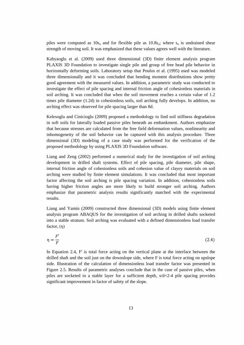
Figure 2.6 (a) Illustration of the slope where the focus of the model was defined (b) 3D
geometric figure of the simplified decoupled model (Kourkoulis et al. 2012) ..................... 15
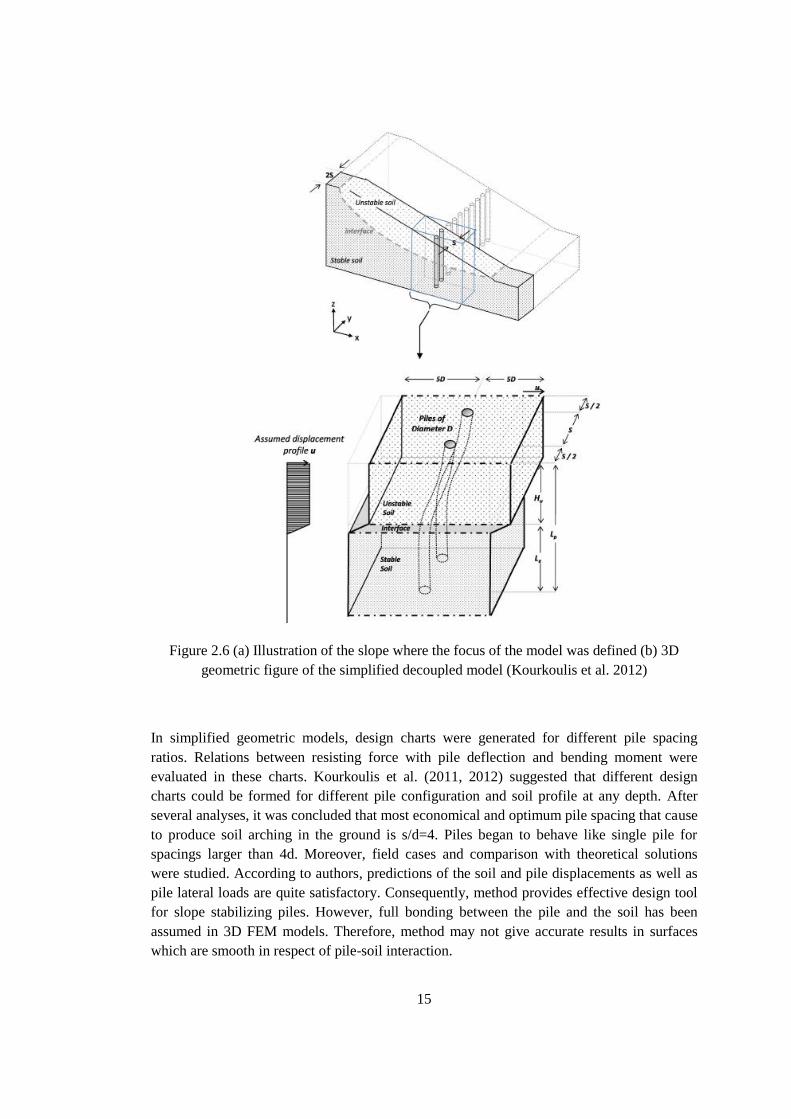
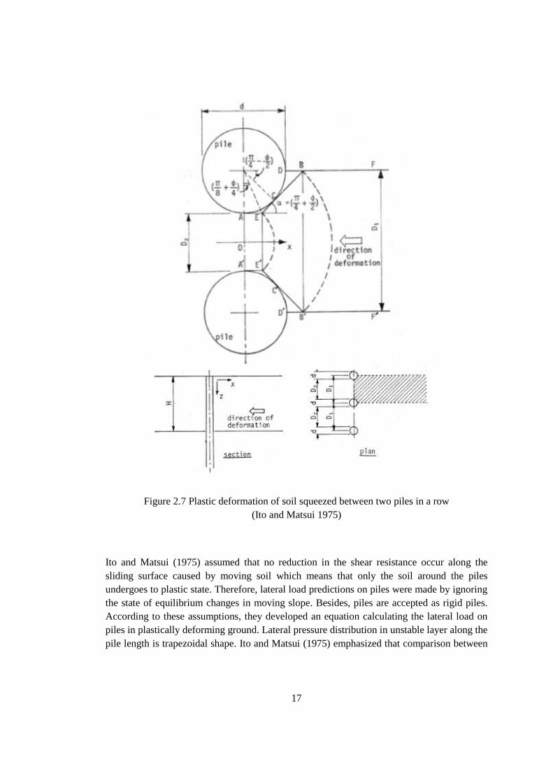
Figure 2.7 Plastic deformation of soil squeezed between two piles in a row (Ito and Matsui
1975) ...................................................................................................................................... 17
Figure 2.8 Ultimate lateral capacities of free head piles (Broms 1964) ................................. 19
Figure 2.9 Ultimate lateral capacities of fixed head piles (Broms 1964) ............................... 20
Figure 2.10 Cross section of the sliding slope (Sommer 1977) ............................................. 23
Figure 3.1 Geometric illustration of the shear box model ..................................................... 29
Figure 3.2 Model illustration of the pile and the surrounding soil ......................................... 30
Figure 3.3 Spilling of unstable soil from right hand side when right boundary is free to move
in the direction of movement ................................................................................................. 32
Figure 3.4 Boundary surfaces for unstable soil (movement in y direction is prevented and z
direction is allowed for all surfaces, At the left side surface, an amount of uniformly
distributed prescribed displacement (ux) was defined to represent a moving landslide mass.
On the right side surface of the box, movement in x-direction is prevented. The rear and
front side surfaces were allowed for movement in x-direction) ............................................ 33
Figure 3.5 Model view of the pile and the surrounding soil .................................................. 34
Figure 3.6 Distribution of horizontal soil deformations in x direction at the ground surface .36
Figure 3.7 Residual horizontal displacements at the ground surface (z=0) in x direction
versus dimension ratio ........................................................................................................... 36
Figure 3.8 Pile deflection versus depth .................................................................................. 37
Figure 3.9 Bending moment versus depth ............................................................................. 38
xiv
Figure 3.10 10 noded tetrahedral mesh element for soil formations (Plaxis 3D Reference
Manual 2010) ......................................................................................................................... 39
Figure 3.11 Model illustration of embedded pile and soil for mesh evaluation analyses ...... 40
Figure 3.12 Medium type of mesh generation........................................................................ 42
Figure 4.1 Lateral soil movement profile of De Beer and Wallays (1972) case studies
(Chen and Poulos 1997) ......................................................................................................... 43
Figure 4.2 Measured and simplified lateral soil movement profiles for case studies of
De Beer and Wallays (1972) .................................................................................................. 45
Figure 4.3 Schematic illustration of the model boundary dimensions ................................... 46
Figure 4.4 Mesh generation for the steel pipe pile case (De Beer and Wallays 1972) ........... 48
Figure 4.5 Illustration of deformed model view for steel pipe pile case (De Beer and Wallays
1972)....................................................................................................................................... 50
Figure 4.6 Lateral soil movement, pile deflection, bending moment and shear force profiles
for steel pipe pile case of De Beer and Wallays (1972) ......................................................... 51
Figure 4.7 Lateral deformation distribution of case 1 in a vertical cross section through
center of the pile (De Beer and Wallays 1972) ...................................................................... 53
Figure 4.8 Lateral deformation distribution of case 1 for different horizontal cross sections
(De Beer and Wallays 1972) .................................................................................................. 54
Figure 4.9 Mesh generation for the reinforced concrete pile case of De Beer and Wallays
(1972) ..................................................................................................................................... 56
Figure 4.10 Illustration of deformed model view for reinforced concrete pile and surrounding
soil (De Beer and Wallays 1972) ........................................................................................... 57
Figure 4.11 Lateral soil movement, pile deflection, bending moment and shear force profiles
for reinforced concrete pile case of De Beer and Wallays (1972) .......................................... 58
Figure 4.12 Lateral deformation distribution of case 2 in a vertical cross section through
center of the pile (De Beer and Wallays 1972) ...................................................................... 60
Figure 4.13 Lateral deformation distribution of case 2 for different horizontal cross sections
(De Beer and Wallays 1972) ................................................................................................. 61
Figure 4.14 Assumed displacement profile for numerical analysis of Esu and D’Elia (1974)
case study ............................................................................................................................... 66
Figure 4.15 Mesh generation for case study of Esu and D’Elia (1974) ................................. 66
Figure 4.16 Lateral soil movement, pile deflection, bending moment and shear force profiles
for case study of Esu and D’Elia (1974) ................................................................................ 69
Figure 4.17 Lateral deformation distribution of Esu and D’Elia (1974) case study for
different horizontal cross sections .......................................................................................... 71
xv
Figure 4.18 Lateral deformation distribution for Esu and D’Elia (1974) case study in a
vertical cross section through center of the pile ..................................................................... 72
Figure 5.1 Model view of the analyses with three piles in a row ........................................... 74
Figure 5.2 Maximum shear force developed in pile shaft for soft, medium, stiff clay type of
unstable soils and strength ratio variations of 1, 3, 5 (lateral soil movement, ux=5 cm;
unstable soil thickness H=10 m) ............................................................................................ 80
Figure 5.3 Bending moment distributions for unstable soil of soft clay (piles were embedded
in stable soils which strength properties determined by strength ratio of 1,3 and 5) ............. 81
Figure 5.4 Bending moment distributions for unstable soil of medium clay (piles were
embedded in stable soils which strength properties determined by strength ratio of 1,3 and 5)
............................................................................................................................................... 81
Figure 5.5 Bending moment distributions for unstable soil of stiff clay (piles were embedded
in stable soils which strength properties determined by strength ratio of 1,3 and 5) ............. 82
Figure 5.6 Pile deflection distributions for unstable soil of medium clay (piles were
embedded in stable soils which strength properties determined by strength ratio of 1,3 and 5)
............................................................................................................................................... 82
Figure 5.7 Horizontal deformation distribution in a line passing through the heads of the
piles ........................................................................................................................................ 86
Figure 5.8 General model view for horizontal deformation distribution in multiple piles in a
row ......................................................................................................................................... 87
Figure 5.9 Horizontal deformation distribution in a vertical cross section passing through the
pile heads in multiple piles in a row ...................................................................................... 87
Figure 5.10 Ratio of soil displacement (in the middle between piles) to pile head
displacement (uip/up) with the variation of pile spacing for loose silty sand and dense sand for
two different lateral soil movement alternatives, ux=5 cm and ux=10 cm ............................. 88
Figure 5.11 Average soil force per pile in a group with the variation of pile spacing for loose
silty sand and dense sand for two different lateral soil movement alternatives, ux=5 cm and
ux=10 cm ................................................................................................................................ 89
Figure 5.12 Average maximum bending moment per pile in a group with the variation of pile
spacing for loose silty sand and dense sand for two different lateral soil movement
alternatives, ux=5 cm and ux=10 cm ....................................................................................... 89
Figure A.1 Overall view for displacements in the direction of soil movement for steel pipe
pile case ................................................................................................................................ 107
Figure A.2 Vertical cross section through model length passing by pile center for
displacements in the direction of soil movement for steel pipe pile case ............................ 108
Figure A.3 Vertical cross section through model width passing by pile center for cartesian
effective stresses in the direction of soil movement for steel pipe pile case ........................ 108
xvi
Figure A.4 Vertical cross section through model length passing by pile center for cartesian
effective stresses in the direction of soil movement for steel pipe pile case ........................ 109
Figure A.5 Overall view for displacements in the direction of soil movement for reinforced
concrete pile case.................................................................................................................. 109
Figure A.6 Vertical cross section through model length passing by pile center for
displacements in the direction of soil movement for reinforced concete pile case .............. 110
Figure A.7 Vertical cross section through model width passing by pile center for cartesian
effective stresses in the direction of soil movement for reinforced concrete pile case ........ 110
Figure A.8 Vertical cross section through model length passing by pile center for cartesian
effective stresses in the direction of soil movement for reinforced concrete pile case ........ 111
Figure A.9 Illustration of deformed model view for embedded pile and surrounding soil for
Esu and D’Elia (1974) case study ........................................................................................ 111
Figure A.10 Overall view for displacements in the direction of soil movement for Esu and
D’Elia (1974) case study ...................................................................................................... 112
Figure A.11 Vertical cross section through model length passing by pile center for
displacements in the direction of soil movement for Esu and D’Elia (1974) case study ..... 112
Figure A.12 Vertical cross section through model width passing by pile center for cartesian
effective stresses in the direction of soil movement for Esu and D’Elia (1974) case study .113
Figure A.13 Vertical cross section through model length passing by pile center for cartesian
effective stresses in the direction of soil movement for Esu and D’Elia (1974) case study.113
Figure B.1 Vertical cross section through model width passing just in front of piles for
mobilized shear stresses (for loose sand, ux=5cm, s/d=4) .................................................... 114
Figure B.2 Vertical cross section through model width passing by center of the piles for
mobilized shear stresses (for loose sand, ux=5cm, s/d=4) .................................................... 114
Figure B.3 Horizontal cross section in ground surface for mobilized shear stresses
(for loose sand, ux=5cm, s/d=4) ............................................................................................ 115
Figure B.4 Horizontal cross section just above the sliding surface for mobilized shear
stresses (for loose sand, ux=5cm, s/d=4) .............................................................................. 115
Figure B.5 Horizontal cross section just below the sliding surface for mobilized shear
stresses (for loose sand, ux=5cm, s/d=4) .............................................................................. 116
Figure B.6 Horizontal cross section in ground surface for incremental cartesian strain (∆γxy)
(for loose sand, ux=5cm, s/d=4) ............................................................................................ 116

1
CHAPTER 1
INTRODUCTION
Landslide is a worldwide natural hazard which frequently causes loss of life and significant
damages to buildings and lifelines. A landslide can be considered as the movement of an
unstable soil layer above a stationary layer due to the gravitational and other forces. There
are many stabilization methods for slopes that are moving. These can be categorized into
reducing the driving forces and increasing the resisting forces of the slope. Flattening of the
slope, reducing the weight of the unstable soil by excavation are some examples of ways to
reduce the driving forces. To increase the resisting forces, soil nailing, stone columns, bio-
chemical ground improvement and other methods are available. Use of passive piles in slope
stabilization has become extremely popular among all these remedial measures in the last
decades (Figure 1.1). Estimation of the lateral loads coming from the sliding of unstable soil,
resultant stresses and bending moments developed in the pile shaft are crucial for an
economical and safe design. There are numerous factors and parameters that affect the
response of piles under lateral soil movements. There exist some studies in the literature that
looks into this topic however three dimensional finite element methodology is not widely
used. In this study, some of the factors that govern the passive pile behavior in response to
ground movements are investigated by three dimensional finite element approach.
Figure 1.1 Lanslide stabilization with passive piles for a freeway in Tokat
2
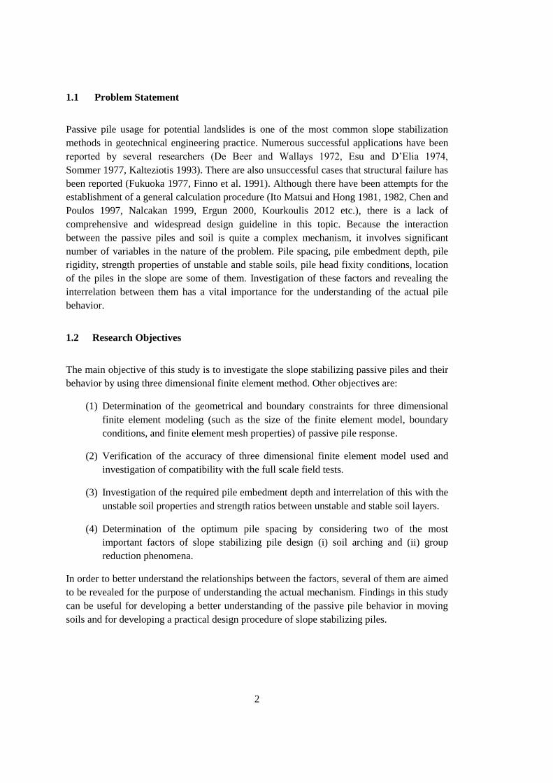
1.1 Problem Statement
Passive pile usage for potential landslides is one of the most common slope stabilization
methods in geotechnical engineering practice. Numerous successful applications have been
reported by several researchers (De Beer and Wallays 1972, Esu and D’Elia 1974,
Sommer 1977, Kalteziotis 1993). There are also unsuccessful cases that structural failure has
been reported (Fukuoka 1977, Finno et al. 1991). Although there have been attempts for the
establishment of a general calculation procedure (Ito Matsui and Hong 1981, 1982, Chen and
Poulos 1997, Nalcakan 1999, Ergun 2000, Kourkoulis 2012 etc.), there is a lack of
comprehensive and widespread design guideline in this topic. Because the interaction
between the passive piles and soil is quite a complex mechanism, it involves significant
number of variables in the nature of the problem. Pile spacing, pile embedment depth, pile
rigidity, strength properties of unstable and stable soils, pile head fixity conditions, location
of the piles in the slope are some of them. Investigation of these factors and revealing the
interrelation between them has a vital importance for the understanding of the actual pile
behavior.
1.2 Research Objectives
The main objective of this study is to investigate the slope stabilizing passive piles and their
behavior by using three dimensional finite element method. Other objectives are:
(1) Determination of the geometrical and boundary constraints for three dimensional
finite element modeling (such as the size of the finite element model, boundary
conditions, and finite element mesh properties) of passive pile response.
(2) Verification of the accuracy of three dimensional finite element model used and
investigation of compatibility with the full scale field tests.
(3) Investigation of the required pile embedment depth and interrelation of this with the
unstable soil properties and strength ratios between unstable and stable soil layers.
(4) Determination of the optimum pile spacing by considering two of the most
important factors of slope stabilizing pile design (i) soil arching and (ii) group
reduction phenomena.
In order to better understand the relationships between the factors, several of them are aimed
to be revealed for the purpose of understanding the actual mechanism. Findings in this study
can be useful for developing a better understanding of the passive pile behavior in moving
soils and for developing a practical design procedure of slope stabilizing piles.
3
1.3 Scope
This study investigates the laterally loaded passive pile behavior by using three dimensional
finite element software Plaxis 3D 2010. A literature review is presented in Chapter 2. In the
scope of this research, three dimensional shear box models have been developed to be able to
control the number of variables for the simulation of actual pile response. In Chapter 3, the
geometry and boundary conditions of the 3D finite element model of passive piles were
studied. A number of case studies have been analyzed to verify the accuracy of the proposed
models (Chapter 4). Afterwards, in Chapter 5, a parametric study is carried out to investigate
the factors affecting the passive pile behavior.

4
5
CHAPTER 2
LITERATURE REVIEW
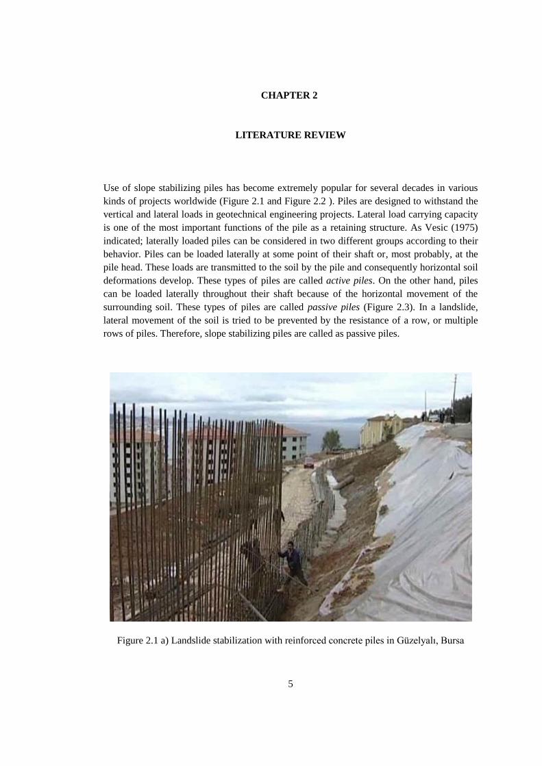
Use of slope stabilizing piles has become extremely popular for several decades in various
kinds of projects worldwide (Figure 2.1 and Figure 2.2 ). Piles are designed to withstand the
vertical and lateral loads in geotechnical engineering projects. Lateral load carrying capacity
is one of the most important functions of the pile as a retaining structure. As Vesic (1975)
indicated; laterally loaded piles can be considered in two different groups according to their
behavior. Piles can be loaded laterally at some point of their shaft or, most probably, at the
pile head. These loads are transmitted to the soil by the pile and consequently horizontal soil
deformations develop. These types of piles are called active piles. On the other hand, piles
can be loaded laterally throughout their shaft because of the horizontal movement of the
surrounding soil. These types of piles are called passive piles (Figure 2.3). In a landslide,
lateral movement of the soil is tried to be prevented by the resistance of a row, or multiple
rows of piles. Therefore, slope stabilizing piles are called as passive piles.
Figure 2.1 a) Landslide stabilization with reinforced concrete piles in Güzelyalı, Bursa
6
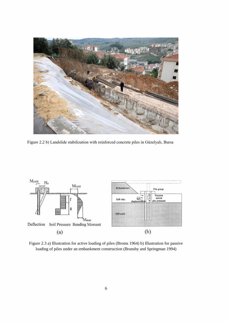
Figure 2.2 b) Landslide stabilization with reinforced concrete piles in Güzelyalı, Bursa
Figure 2.3 a) Illustration for active loading of piles (Broms 1964) b) Illustration for passive
loading of piles under an embankment construction (Bransby and Springman 1994)
7
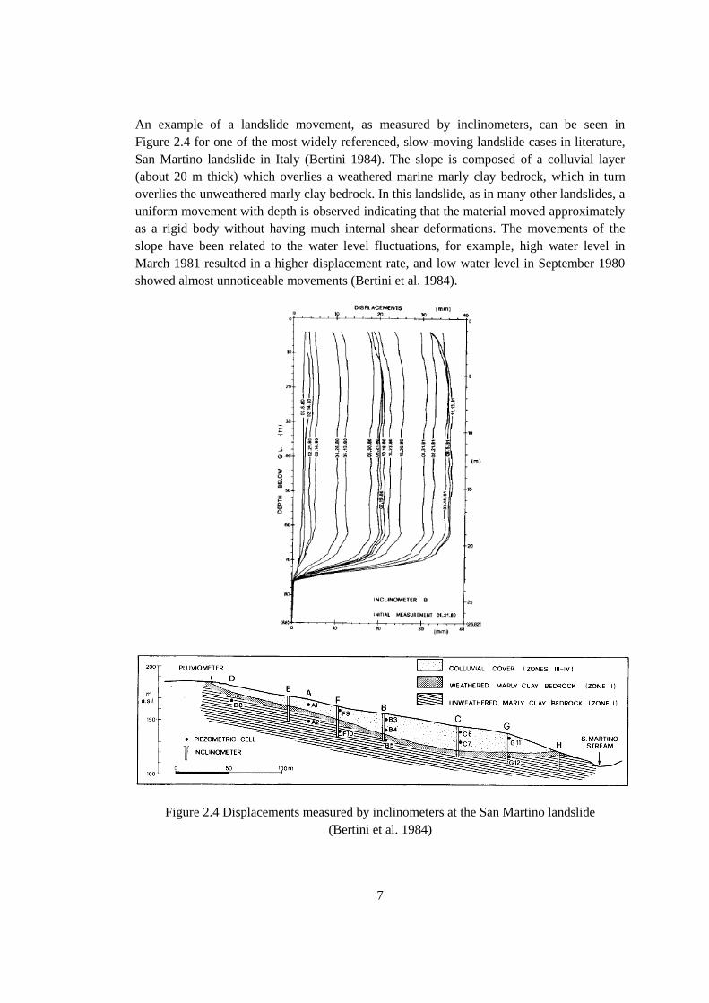
An example of a landslide movement, as measured by inclinometers, can be seen in
Figure 2.4 for one of the most widely referenced, slow-moving landslide cases in literature,
San Martino landslide in Italy (Bertini 1984). The slope is composed of a colluvial layer
(about 20 m thick) which overlies a weathered marine marly clay bedrock, which in turn
overlies the unweathered marly clay bedrock. In this landslide, as in many other landslides, a
uniform movement with depth is observed indicating that the material moved approximately
as a rigid body without having much internal shear deformations. The movements of the
slope have been related to the water level fluctuations, for example, high water level in
March 1981 resulted in a higher displacement rate, and low water level in September 1980
showed almost unnoticeable movements (Bertini et al. 1984).
Figure 2.4 Displacements measured by inclinometers at the San Martino landslide
(Bertini et al. 1984)
8
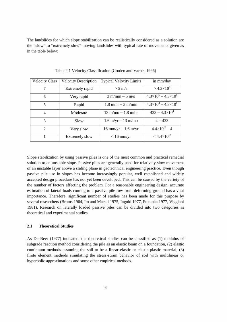
The landslides for which slope stabilization can be realistically considered as a solution are
the “slow” to “extremely slow”-moving landslides with typical rate of movements given as
in the table below:
Table 2.1 Velocity Classification (Cruden and Varnes 1996)
Velocity Class Velocity Description Typical Velocity Limits in mm/day
7 Extremely rapid > 5 m/s > 4.3×10⁸
6 Very rapid 3 m/min – 5 m/s 4.3×10⁶ – 4.3×10
8
5 Rapid 1.8 m/hr – 3 m/min 4.3×10⁴ – 4.3×10
6
4 Moderate 13 m/mo – 1.8 m/hr 433 – 4.3×10⁴
3 Slow 1.6 m/yr – 13 m/mo 4 – 433
2 Very slow 16 mm/yr – 1.6 m/yr 4.4×10⁻²
– 4
1 Extremely slow < 16 mm/yr < 4.4×10⁻²
Slope stabilization by using passive piles is one of the most common and practical remedial
solution to an unstable slope. Passive piles are generally used for relatively slow movement
of an unstable layer above a sliding plane in geotechnical engineering practice. Even though
passive pile use in slopes has become increasingly popular, well established and widely
accepted design procedure has not yet been developed. This can be caused by the variety of
the number of factors affecting the problem. For a reasonable engineering design, accurate
estimation of lateral loads coming to a passive pile row from deforming ground has a vital
importance. Therefore, significant number of studies has been made for this purpose by
several researchers (Broms 1964, Ito and Matsui 1975, Ingold 1977, Fukuoka 1977, Viggiani
1981). Research on laterally loaded passive piles can be divided into two categories as
theoretical and experimental studies.
2.1 Theoretical Studies
As De Beer (1977) indicated, the theoretical studies can be classified as (1) modulus of
subgrade reaction method considering the pile as an elastic beam on a foundation, (2) elastic
continuum methods assuming the soil to be a linear elastic or elastic-plastic material, (3)
finite element methods simulating the stress-strain behavior of soil with multilinear or
hyperbolic approximations and some other empirical methods.
9
2.1.1 Modulus of Subgrade Reaction Method
Hetenyi (1946) assumed piles as beams on an elastic foundation and soil reaction represented
by Winkler springs. Equation 2.1 was proposed by Hetenyi (1946) for the solution of loaded
piles in soils as long as both pile and soil stays in elastic limits (Oztürk 2009).
Where;
M: Bending moment
Q: Axial load on the pile
z: Depth along the pile
y: Lateral deflection of pile at point z
p: Lateral resistance of soil per unit length of pile
In case of slope stabilizing laterally loaded passive piles, axial loading on pile (Q), can be
ignored and Equation 2.1 can be transformed into the following equation with some
modifications as:
( )
Where;
Ep: Deformation modulus of pile
I: Moment of inertia of pile
yp: Lateral displacement of the pile at depth z
ys: Lateral displacement of the soil at depth z if no pile was placed in the slope
Ks: Subgrade reaction modulus of soil
In Equation 2.2, subgrade reaction modulus, (Ks) is variable with depth and relative
displacement (yp-ys). De Beer (1977) indicated that there may be uncertainties of the solution
of Equation 2.2 because of the difficulties of determining lateral displacement of the soil if
no pile exists in the slope, (ys).
10
Fukuoka (1977) studied lateral resistance of passive piles subjected to creep type of soil
movement. Subgrade reaction methodology was used to estimate pile response against
laterally moving slope. Unbalanced force and resistance force values were evaluated as a
function of the inclination of the slope and displacement velocity of the soil mass. For this
reason, careful monitoring of moving slopes was recommended by Fukuoka (1977).
Especially for soils where ground water level fluctuations may occur, determination of the
relationship between displacement velocity and these fluctuations could be essential.
Poulos and Davis (1980) investigated the subgrade reaction modulus of soils and its
variability with depth. Solutions of the Equation 2.2 were developed by considering the
subgrade reaction modulus constant or properly distributed with depth for different pile head
fixity conditions and pile rigidities.
Viggiani (1981) studied lateral loads on piles due to the moving cohesive soil by using
subgrade reaction theory. In his approach, rectangular stress distribution through the pile
shaft was assumed instead of trapezoidal stress distribution. Possible failure mechanisms that
a pile can undergo were investigated for the calculation of total lateral force applied to the
pile. Yield soil pressure on piles due to the moving cohesive soils in undrained condition was
predicted by the equation similar to other researchers (Brinch Hansen, 1961; Broms, 1964)
as
Where;
p: Yield soil pressure along the pile
cu: Undrained shear strength
d: Pile diameter
k :Bearing capacity factor
Several researchers (Brinch Hansen 1961, Broms 1964, De Beer 1977, Ito and Matsui 1975)
proposed different ranges of bearing capacity factor for cohesive soils. It was suggested that
k values should be different for piles in non-displaced soil (active pile) and piles in moving
soil (passive pile). Besides, k values should also be different above and below the slip
surface. It is well known that most of the time, soil movement stops before ultimate pile
capacities are not reached (Ergun 2000). Therefore selection of appropriate bearing capacity
factor has vital importance when using this equation, because calculated pressures are
ultimate soil pressures at failure condition.
11
Ingold (1977) used modulus of subgrade reaction method for a theoretical example of one
row steel pipe pile in a sliding ground. In his solution, pile deflection, shear force and
bending moment distributions through the pile length were estimated. Calculations of these
parameters for different pile head fixity conditions (free, unrotated, hinged and fixed) were
studied. Safety factors against bending moment and shear force failure were determined. It
was concluded that as pile head becomes more rigid, safety factor of pile against failure is
increased. Therefore, Ingold (1977) emphasized the importance of preventing the deflection
of the pile head for the effective usage of piles for slope stabilization.
Magueri and Motta (1992) investigated the variation of subgrade reaction modulus of soils.
They proposed a non-linear hyperbolic function for the estimation of the lateral load on
passive piles. Subgrade reaction modulus depends on the relative pile soil displacement and
initial value of the subgrade reaction modulus.
2.1.2 Elastic Continuum Methods
Oteo (1977) applied the methodology of Begemaan and De Leeuw (1972) for the estimation
of soil pressures and bending moments on passive piles. In this method, piles are exposed to
soil pressure because of the surcharge load at the surface. Horizontal pressures are obtained
by considering the effect of the relative flexibility of the pile which is reasonable to adapt
because Oteo (1977) specified that stiff piles may have a restrictive field of application. Soil
was considered as linearly elastic material in his analyses. It was concluded that if the pile is
stiff, maximum pressure methods can be applied; however if the pile is flexible, methods
using the pile-soil interaction is needed.
Poulos (1973) proposed a calculation method to obtain horizontal pressure and
displacements affecting a pile-soil system. Soil was considered to be an elastic-plastic
material. In this approach, pile displacements were calculated from the bending equation of a
thin strip and soil displacements were evaluated from the Mindlin (1936) equation for
horizontal displacements caused by horizontal loads within a semi-infinite mass
(Nalcakan 1999).
Banerjee and Davies (1978) used point load solution for the calculation of displacement and
bending moment distributions of single pile in both homogenous and non-homogeneous
soils. Linearly increasing soil deformation modulus was introduced in the analyses. As a
result of analyses, higher bending moments in non-homogenous soils were calculated than
those predicted for homogenous soils for both free and fixed head piles.
12
2.1.3 Finite Element Method
Concept of slope stabilization by using passive piles has been investigated by researchers for
a long period of time. However, considerable number of variables in the problem made it
difficult and complex to analyze the factors affecting the real pile-soil interaction. In this
manner, numerical studies and finite element approaches were developed and applied to this
concept to understand the phenomena more accurately (Rowe and Poulos 1979, Chen and
Poulos 1993, 1997). Especially for the last three decades, advances in computer programs
made it possible to evaluate complex geometries and multilayered soil strata. Two and three
dimensional finite element modeling of the problem has been recently used by several
researchers (Chow 1996, Pan et al. 2002, Kahyaoglu et al. 2007, Liang and Yamin 2009,
Kourkoulis et al. 2011, 2012) to capture actual pile-soil interaction behavior and to propose a
feasible design guideline. Accuracy and relatively short calculation time make numerical
methods through softwares an inevitable part of the future of this study.
Rowe and Poulos (1979) used two dimensional (2D) finite element technique to evaluate
undrained soil behavior of slopes reinforced by multi-row pile groups. Effect of piles on the
deformation and stability of slope investigated for different pile head fixity and pile stiffness
conditions. It was concluded that very stiff piles should be used in slopes to get a
considerable effect on slope stability. Increase in pile stiffness, restraints at the top and tip of
the pile enhance the efficiency of the pile. In addition, pile arrangement and soil profile has a
significant effect on pile-soil interaction behavior.
Chen and Poulos (1993) studied passive pile behavior by using finite element methods. In
two dimensional (2D) analyses, group reductions in pile capacities were observed and
compared with single pile results.
Chow (1996) suggested a numerical solution which piles were modeled with beam elements,
soil was modeled using subgrade reaction modulus and pile soil interaction was considered
according to the theory of elasticity. Chow (1996) compared his proposed solution with two
field cases: Esu and D’Elia (1974) and Kalteziotis et. al (1993); one of these cases is for
single pile and the other is for pile groups. Pile deflections, pile rotations, bending moment
and shear force distributions throughout pile length were evaluated in this study. It was
concluded that results show significantly good agreement with the measured values.
Pan et al. (2002) used three dimensional (3D) finite element analysis program ABAQUS to
investigate the behavior of single pile subjected to lateral soil movement. In analyses, pile
was assumed as linearly elastic material. Von Mises constitutive model was used to simulate
non-linear stress-strain behavior of moving soil. Pile was modeled as width of 1 m square
cross section and 15 m length. Undrained behavior of cohesive soil was considered in all
analyses. Normalized p-y curves and variations of ultimate soil pressures with depth were
evaluated for stiff and flexible piles. Consequently, maximum ultimate soil pressures for stiff
13
piles were computed as 10su and for flexible pile as 10.8su; where su is undrained shear
strength of moving soil. It was emphasized that these values agrees well with the literature.
Kahyaoglu et al. (2009) used three dimensional (3D) finite element analysis program
PLAXIS 3D Foundation to investigate single pile and group of free head pile behavior in
horizontally deforming soils. Laboratory setup that Poulos et al. (1995) used was modeled
three dimensionally and it was concluded that bending moment distributions show pretty
good agreement with the measured values. In addition, a parametric study was conducted to
investigate the effect of pile spacing and internal friction angle of cohesionless materials in
soil arching. It was concluded that when the soil movement reaches a certain value of 1.2
times pile diameter (1.2d) in cohesionless soils, soil arching fully develops. In addition, no
arching effect was observed for pile spacing larger than 8d.
Kelesoglu and Cinicioglu (2009) proposed a methodology to find soil stiffness degradation
in soft soils for laterally loaded passive piles beneath an embankment. Authors emphasize
that because stresses are calculated from the free field deformation values, nonlinearity and
inhomogeneity of the soil behavior can be captured with this analysis procedure. Three
dimensional (3D) modeling of a case study was performed for the verification of the
proposed methodology by using PLAXIS 3D Foundation software.
Liang and Zeng (2002) performed a numerical study for the investigation of soil arching
development in drilled shaft systems. Effect of pile spacing, pile diameter, pile shape,
internal friction angle of cohesionless soils and cohesion value of clayey materials on soil
arching were studied by finite element simulations. It was concluded that most important
factor affecting the soil arching is pile spacing variation. In addition, cohesionless soils
having higher friction angles are more likely to build stronger soil arching. Authors
emphasize that parametric analysis results significantly matched with the experimental
results.
Liang and Yamin (2009) constructed three dimensional (3D) models using finite element
analysis program ABAQUS for the investigation of soil arching in drilled shafts socketed
into a stable stratum. Soil arching was evaluated with a defined dimensionless load transfer
factor, (η)
In Equation 2.4, F' is total force acting on the vertical plane at the interface between the
drilled shaft and the soil just on the downslope side, where F is total force acting on upslope
side. Illustration of the calculation of dimensionless load transfer factor was presented in
Figure 2.5. Results of parametric analyses conclude that in the case of passive piles, when
piles are socketed in a stable layer for a sufficient depth, s/d=2-4 pile spacing provides
significant improvement in factor of safety of the slope.

14
Figure 2.5 Estimation of load transfer factor from geometric model
(Liang and Yamin 2009)
Kourkoulis et al. (2011, 2012) proposed a hybrid method for the design of piles used for
slope stabilization. Method consists of mainly two steps. First step includes traditional slope
stability analyses. To increase the safety factor of the slope to a desired value, additional
resisting lateral force to be provided by piles is calculated. In the second step, pile
configurations are estimated by 3D FEM modeling for a prescribed deformation level.
Optimum pile design that gives the required resisting force is determined by this way.
Kourkoulis et al. (2011, 2012) performed parametric model studies to verify the feasibility of
their methodology (Figure 2.6). Prescribed displacements were assumed as uniformly
distributed in the unstable sliding mass. Pile influence distance is accepted as 5d (5 times of
pile diameter) and the geometry of the finite element model is constructed this way to save
some calculation time. Both cohesive and granular soils were modeled as unstable layer with
a sliding height (Hu) varying within 4 to 12 m. Besides, influence of pile spacing on soil
arching, pile embedment depth into stable layer and stiffness of the stable layer effects were
also studied.
15
Figure 2.6 (a) Illustration of the slope where the focus of the model was defined (b) 3D
geometric figure of the simplified decoupled model (Kourkoulis et al. 2012)
In simplified geometric models, design charts were generated for different pile spacing
ratios. Relations between resisting force with pile deflection and bending moment were
evaluated in these charts. Kourkoulis et al. (2011, 2012) suggested that different design
charts could be formed for different pile configuration and soil profile at any depth. After
several analyses, it was concluded that most economical and optimum pile spacing that cause
to produce soil arching in the ground is s/d=4. Piles began to behave like single pile for
spacings larger than 4d. Moreover, field cases and comparison with theoretical solutions
were studied. According to authors, predictions of the soil and pile displacements as well as
pile lateral loads are quite satisfactory. Consequently, method provides effective design tool
for slope stabilizing piles. However, full bonding between the pile and the soil has been
assumed in 3D FEM models. Therefore, method may not give accurate results in surfaces
which are smooth in respect of pile-soil interaction.
16
Dao (2011) studied validation of the recently developed “embedded pile” option in Plaxis 3D
software for lateral loading. In this study, detailed comparison between modeling of the
embedded pile (as a beam element) and modeling of mass volume pile was made for piles
located near the toe of an embankment. It was concluded that embedded pile option in Plaxis
3D is a good tool to model actual laterally loaded pile behavior. However, Dao (2011)
emphasized that modeling smooth surfaces may not give desirable results because embedded
pile option does not consider relative pile soil displacement in lateral direction.
2.1.4 Other Studies
Chen and Poulos (1997) used boundary element method to evaluate vertical pile response
subjected to lateral soil movements. Both pile and soil were assumed to behave elastically in
the analyses. They emphasized the importance of accurate determination of limiting pile soil
pressure. For this purpose, dimensionless group factor, fp was defined as;
Where, pui is limiting soil pressure in pile in a group and pus is limiting soil pressure in
isolated single pile. Dimensionless group factors were listed for several pile configurations
and pile spacing. Moreover, design charts were formed for uniform and linearly increasing
soil stiffness properties, uniform and linearly decreasing lateral soil movements. Maximum
bending moment of pile groups were evaluated in these design charts according to the
different relative pile stiffness values. The design chart method was compared with reported
field case results. It was concluded that design charts generally give overestimation of
maximum bending moments and pile head deflections. However, method gives more
convenient results with the decrease of lateral soil movement. Authors pointed out that
proposed design chart methodology could be useful for preliminary design especially if there
is a lack of detailed site information.
Ito and Matsui (1975) developed a theory to estimate lateral loads on passive piles in
plastically deforming ground. According to Ito and Matsui (1975) two possible plastic states
can occur in the soil around the piles. One of them assumes plastic deformation of soil
satisfying Mohr-Coulomb yield criterion. The other one treats the surrounding ground as a
visco-plastic solid (plastic flow mechanism) which is applicable for mud type of soil layers.
In theory of plastic deformation, lateral load on a pile row was estimated in plain strain
analysis (plain strain condition is in the direction of depth) as shown in Figure 2.7.
17
Figure 2.7 Plastic deformation of soil squeezed between two piles in a row
(Ito and Matsui 1975)
Ito and Matsui (1975) assumed that no reduction in the shear resistance occur along the
sliding surface caused by moving soil which means that only the soil around the piles
undergoes to plastic state. Therefore, lateral load predictions on piles were made by ignoring
the state of equilibrium changes in moving slope. Besides, piles are accepted as rigid piles.
According to these assumptions, they developed an equation calculating the lateral load on
piles in plastically deforming ground. Lateral pressure distribution in unstable layer along the
pile length is trapezoidal shape. Ito and Matsui (1975) emphasized that comparison between
18
load estimations from established theory and field measurements show satisfactory
resemblance.
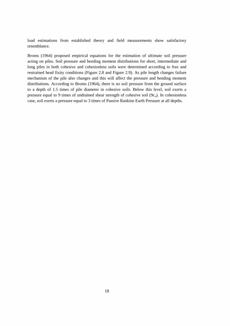
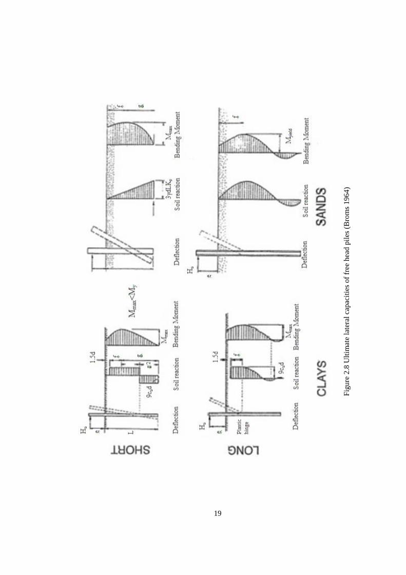
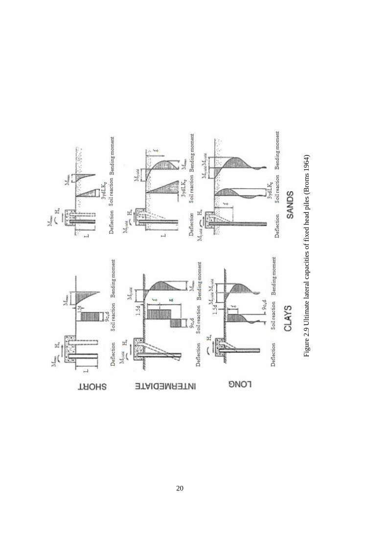
Broms (1964) proposed empirical equations for the estimation of ultimate soil pressure
acting on piles. Soil pressure and bending moment distributions for short, intermediate and
long piles in both cohesive and cohesionless soils were determined according to free and
restrained head fixity conditions (Figure 2.8 and Figure 2.9). As pile length changes failure
mechanism of the pile also changes and this will affect the pressure and bending moment
distributions. According to Broms (1964), there is no soil pressure from the ground surface
to a depth of 1.5 times of pile diameter in cohesive soils. Below this level, soil exerts a
pressure equal to 9 times of undrained shear strength of cohesive soil (9cu). In cohesionless
case, soil exerts a pressure equal to 3 times of Passive Rankine Earth Pressure at all depths.
19
Fig
ure
2.8
Ult
imat
e la
tera
l ca
pac
itie
s of
free
hea
d p
iles
(B
rom
s 1
96
4)
20
Fig
ure
2.9
Ult
imat
e la
tera
l ca
pac
itie
s of
fixed
hea
d p
iles
(B
rom
s 1
96
4)
21
Wang and Yen (1974) developed a method to investigate soil arching in passive piles placed
in infinitely long slopes. One row of rigid piles socketed into a stable stratum was used in the
analyses. Optimum pile spacing that cause soil arching was tried to be determined at the
potential failure condition of the slope.
Reese et al. (1992) proposed a method to estimate the stress and deformation distribution of
a laterally loaded passive pile embedded in a firm stratum. In this approach, driving force of
moving soil and resulting moment were considered to act on pile at the point of unstable to
stable soil layer transition. After the estimation of total driving force and moment coming
from horizontally deforming soil, these values were used for the calculation of load
deformation curve of the pile.
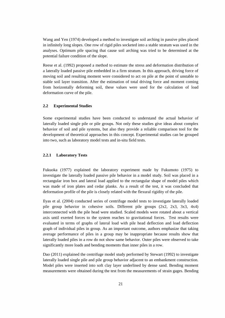
2.2 Experimental Studies
Some experimental studies have been conducted to understand the actual behavior of
laterally loaded single pile or pile groups. Not only these studies give ideas about complex
behavior of soil and pile systems, but also they provide a reliable comparison tool for the
development of theoretical approaches in this concept. Experimental studies can be grouped
into two, such as laboratory model tests and in-situ field tests.
2.2.1 Laboratory Tests
Fukuoka (1977) explained the laboratory experiment made by Fukumoto (1975) to
investigate the laterally loaded passive pile behavior in a model study. Soil was placed in a
rectangular iron box and lateral load applied to the rectangular shape of model piles which
was made of iron plates and cedar planks. As a result of the test, it was concluded that
deformation profile of the pile is closely related with the flexural rigidity of the pile.
Ilyas et al. (2004) conducted series of centrifuge model tests to investigate laterally loaded
pile group behavior in cohesive soils. Different pile groups (2x2, 2x3, 3x3, 4x4)
interconnected with the pile head were studied. Scaled models were rotated about a vertical
axis until exerted forces to the system reaches to gravitational forces. Test results were
evaluated in terms of graphs of lateral load with pile head deflection and load deflection
graph of individual piles in group. As an important outcome, authors emphasize that taking
average performance of piles in a group may be inappropriate because results show that
laterally loaded piles in a row do not show same behavior. Outer piles were observed to take
significantly more loads and bending moments than inner piles in a row.
Dao (2011) explained the centrifuge model study performed by Stewart (1992) to investigate
laterally loaded single pile and pile group behavior adjacent to an embankment construction.
Model piles were inserted into soft clay layer underlined by dense sand. Bending moment
measurements were obtained during the test from the measurements of strain gages. Bending
22
moment increase was seen at the pile head and interface of soft clay to dense sand layer. It
was concluded that centrifuge testing results show very good agreement with the actual field
test results.
Dagistani (1992) and Kin (1993) studied on laterally loaded passive pile behavior in a shear
box model. Shear box with 30x30 cm cross section, maximum depth of 60 cm and movable
part of 15 cm were used in analyses. Pressure distribution on passive piles in cohesive soil
was measured using miniature stress cells. Experiments were conducted for different pile
penetration depths and soil consistencies.
Nalcakan (1999) conducted a laboratory experiment to investigate group action reduction in
passive pile groups. Same shear box model with Dagistani (1992) and Kin (1993) was used
in experiments. Two types of material were investigated in analyses as soft clay and stiff
clay with undrained shear strength of 12 kPa and 85 kPa respectively. Model piles having
30 cm length and 1 cm diameter were inserted into the soil inside the shear box in a row.
After the model was setup, shear box was loaded laterally with a constant shear rate of
0.37 mm/min. Nalcakan (1999) measured displacement of the shear box, total load applied to
the shear box and the load on two selected piles in each test series for different pile spacings.
In tests, pile spacing ratios ranged between s/d=15 (single pile) to s/d=2. Graphs of
displacement ratio (lateral movement divided by pile diameter, %ɛ) with total load and
displacement ratio with load per pile were presented. It was concluded that load on a single
pile mainly depends on undrained shear strength of moving material. Load on a pile
decreases as pile spacing decreases because group action reduction develops when piles are
closely spaced. In addition, single pile load and group reduction also depend on the amount
of displacement ratio (%ɛ). During initial stage of loading (low displacement ratios) lower
values of group reduction was observed.
Ozturk (2009) investigated bending moment distributions of single and group of piles in
cohesionless soil using model piles. Strain gages attached to the pile shafts were used to
measure bending moments during the test. Maximum bending strain was observed
approximately at the depth of 0.7L (L: Pile length) and maximum negative bending strain
measured at the depth of 0.3L for both single pile and pile groups. It was concluded that even
if the amount of loading change general behavior of the bending moment distribution
remains same especially for single piles.
2.2.2 Field Tests
De Beer and Wallays (1972) reported a field test in Belgium to investigate embankment
construction influence on adjacent pile foundations. For this purpose two different cases
were studied. A steel pipe pile having 28 m length, 0.9 m diameter and 1.5 cm wall thickness
was used in one of the cases. In the other case, 23.2 m length and 0.6 m diameter reinforced
concrete pile was used. In both cases pile deflections, bending moments and lateral soil
23
movements in the ground were measured. There is not much information about the
properties of sliding soil however it was indicated that soil profile mainly consists of sandy
materials.
Esu and D’Elia (1974) conducted a field case to investigate the behavior of slope stabilizing
reinforced concrete pile. The test pile was 30 m in length, 0.79 m in diameter and had a
flexural rigidity (EpIp) of 360 MNm2. It was reported that depth of sliding soil is 7.5 m. Not
much information was given about the soil properties of the ground except that it was
considered to consist mainly from cohesive soils. Test pile was instrumented with pressure
cells at the depth of 5 m, 10 m and 15 m along its shaft. Bending moment, shear force and
pile deflection distributions of the pile were presented in the report.
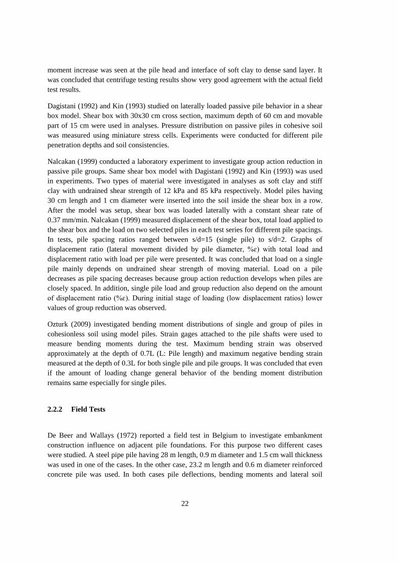
Sommer (1977) reported a field investigation on a sliding slope under an embankment. 15 m
depth of highly plastic preconsolidated clay movement with an inclination of 5°-8° stopped
with 3 m diameter reinforced concrete piers embedding to stable layer into 5m (Figure 2.10).
Earth pressure distributions on piles were recorded with pressure cells. It was observed that
measured soil pressures were much smaller than the (only %30) design pressure which had
been calculated according to the Brinch Hansen formula.
Figure 2.10 Cross section of the sliding slope (Sommer 1977)
24
Kalteziotis et al. (1993) reported a field case where cracks had appeared in the road
pavement of a semi-bridge structure in Greece. Moving soil formation consists of mainly
neogene lacustrine deposits. Sliding soil depth was reported as 4 m. Two rows of concrete
piles having 1 m diameter and 12 m length with pile spacing of 2.5 m were used to stabilize
this landslide. Two of the piles were replaced with steel pipe piles having the same flexural
rigidity with the concrete piles. These steel piles were monitored by using strain gages and
inclinometers. Bending moment, shear force, pile deflection and pile rotation distributions
were presented according to these measurements.
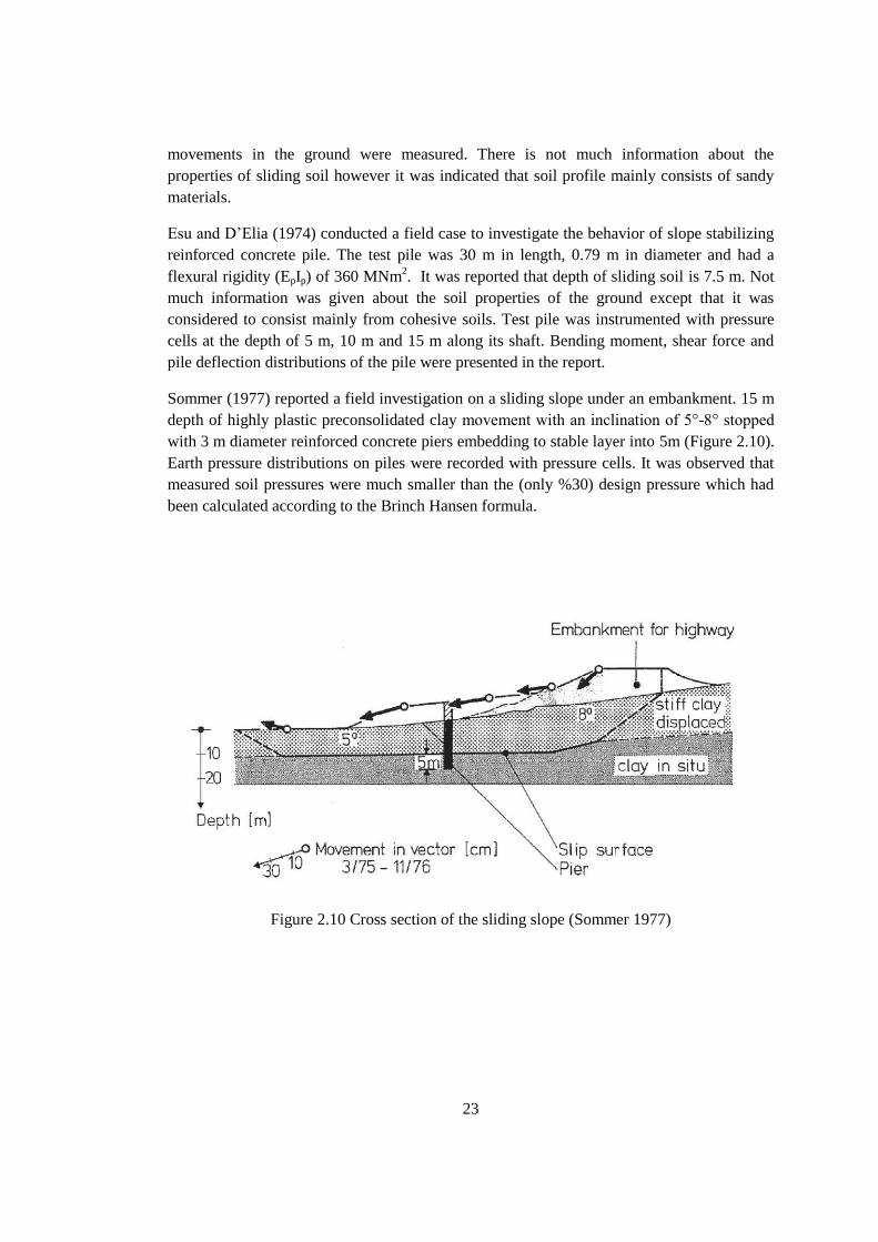
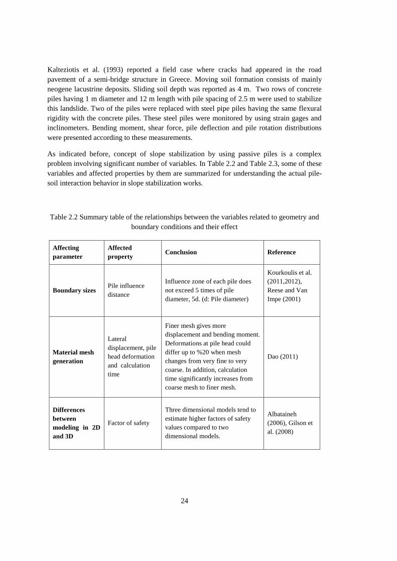
As indicated before, concept of slope stabilization by using passive piles is a complex
problem involving significant number of variables. In Table 2.2 and Table 2.3, some of these
variables and affected properties by them are summarized for understanding the actual pile-
soil interaction behavior in slope stabilization works.
Table 2.2 Summary table of the relationships between the variables related to geometry and
boundary conditions and their effect
Affecting
parameter
Affected
property Conclusion Reference
Boundary sizes
Pile influence
distance
Influence zone of each pile does
not exceed 5 times of pile
diameter, 5d. (d: Pile diameter)
Kourkoulis et al.
(2011,2012),
Reese and Van
Impe (2001)
Material mesh
generation
Lateral
displacement, pile
head deformation
and calculation
time
Finer mesh gives more
displacement and bending moment.
Deformations at pile head could
differ up to %20 when mesh
changes from very fine to very
coarse. In addition, calculation
time significantly increases from
coarse mesh to finer mesh.
Dao (2011)
Differences
between
modeling in 2D
and 3D
Factor of safety
Three dimensional models tend to
estimate higher factors of safety
values compared to two
dimensional models.
Albataineh
(2006), Gilson et
al. (2008)
25
Table 2.3 Summary table of the relationships between the factors that affect the design of
piles used in slope stabilization
Affecting
parameter
Affected
property Conclusion Reference
Factor of safety
of moving slope
Horizontal soil
movements
Horizontal soil deformations are much
larger if the factor of safety (F) of slope
is lower than 1.4. Deformations decrease
substantially above this value.
Marche and Chapuis
(1973), De Beer and
Wallays (1972)
Pile spacing/pile
diameter
(s/d)
Soil arching
As piles are closely spaced, soil arching
develops between the piles. In fact, most
economical and optimum pile spacing
can be chosen as s/d=4.
Kourkoulis et al. (2011)
No arching effect is observed for pile
spacing larger than 8d.
Liang and Zeng (2002),
Kahyaoglu et al. (2009)
Group action
reduction
As pile spacing (s) decreases, piles in a
group take less load compared to a
single pile. Group action reduction
develops.
Broms (1964),
Nalcakan (1999),
Pan et al. (2002)
No significant group effect occurs if pile
spacing is larger than 4d for cohesive
soils.
Chen (2001)
Single pile
load
As pile spacing (s) increases lateral load
per pile also increases.
Nalcakan (1999),
Ergun (2000)
Factor of
safety of slope
As pile spacing (s) increases factor of
safety of slope against failure decreases. Wei (2008)
In case of passive piles are socketed in a
stable layer enough, s/d=2-4 pile spacing
provides significant improvement in
factor of safety of the slope.
Liang and Yamin (2009)
Material
properties of
unstable ground
Lateral pile
load
Lateral force per pile increases as
internal friction (ϕ) and cohesion (c)
parameters increases
Ito and Matsui (1975)
Yield soil pressure on piles due to the
moving cohesive soils increase as
undrained shear strength (cu) of soil
increases.
Brinch Hansen (1961),
Broms (1964),
De Beer (1977),
Viggiani (1981)
Material
properties of
stable ground
Pile deflection
and bending
moment
If piles are embedded in a relatively soft
stratum, larger pile deflections are
required to reach same level of ultimate
resistance as embedded in a stiff
stratum. Additionally, when the stable
ground is stiff, the flexural distortion of
the pile is more localized (close to the
sliding interface) and give larger
bending moments.
Kourkoulis et al. (2011)
26
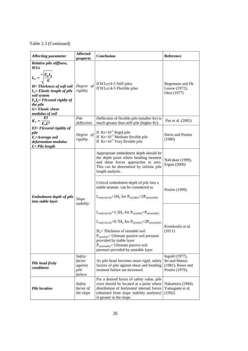
Table 2.3 (Continued)
Affecting parameter Affected
property Conclusion Reference
Relative pile stiffness,
H/Le
√
H= Thickness of soft soil
Le= Elastic length of pile
soil system
EpIp= Flexural rigidty of
the pile
G= Elastic shear
modulus of soil
Degree of
rigidity
If H/Le≤4-5 Stiff piles
If H/Le≥4-5 Flexible piles
Begemann and De
Leeuw (1972),
Oteo (1977)
EI= Flexural rigidity of
pile
Es=Average soil
deformation modulus
L= Pile length
Pile
deflection
Deflection of flexible pile (smaller Kr) is
much greater than stiff pile (higher Kr). Pan et al. (2002)
Degree of
rigidity
If Kr>10-2
Rigid pile
If Kr>10-3
Medium flexible pile
If Kr<10-5
Very flexible pile
Davis and Poulos
(1980)
Embedment depth of pile
into stable layer
Slope
stability
Appropriate embedment depth should be
the depth point where bending moment
and shear forces approaches to zero.
This can be determined by infinite pile
length analysis.
Nalcakan (1999),
Ergun (2000)
Critical embedment depth of pile into a
stable stratum can be considered as
Lem(critical)=1Hu for Pu(stable)=2Pu(unstable)
Poulos (1999)
Lem(critical)=1.5Hu for Pu(stable)=Pu(unstable)
Lem(critical)=0.7Hu for Pu(stable)=3Pu(unstable)
Hu= Thickness of unstable soil
Pu(stable)= Ultimate passive soil pressure
provided by stable layer
Pu(unstable)= Ultimate passive soil
pressure provided by unstable layer
Kourkoulis et al.
(2011)
Pile head fixity
conditions
Safety
factor
against
pile
failure
As pile head becomes more rigid, safety
factors of pile against shear and bending
moment failure are increased.
Ingold (1977),
Ito and Matsui
(1981), Rowe and
Poulos (1979),
Pile location
Safety
factor of
the slope
For a desired factor of safety value, pile
rows should be located at a point where
distribution of horizontal internal forces
(obtained from slope stability analyses)
is greater in the slope.
Nakamura (1984),
Yamagami et al.
(1992)
27
CHAPTER 3
GEOMETRY AND BOUNDARY CONDITIONS OF THE 3D FINITE ELEMENT
MODEL OF PASSIVE PILES
3.1 Introduction
In this thesis study, numerical models have been formed to investigate the factors affecting
the passive pile behavior used in slope stabilization works. Case studies with measured field
data were used to control the accuracy of the numerical model results (Chapter 4). After
verification of finite element analysis solution, a parametric study has been conducted
(Chapter 5). Variations in the factors such as the embedment depth of the pile, material
properties of unstable ground, pile spacing, amount of lateral soil movement, and their
affects were studied. Three dimensional geotechnical finite element package PLAXIS 3D
2010 was used in all analyses for this purpose. Properties and main functions of the 3D finite
element methodology are presented briefly for better understanding of the model designs.
Plaxis 3D 2010 consists of two parts which are input and output program. Input program is
used for the definition of the model and assignment of analysis properties. At the beginning
of the input program, project properties are asked from the user. Model boundaries in two
horizontal directions (x and y) and unit system used in analyses are defined in this part.
Input program includes five main components that are soil, structures, mesh, water levels
and staged construction. In soil mode, soil stratigraphy is assigned to the model by creating
boreholes. In addition, ground water level of a specific point is defined also with boreholes.
Multiple boreholes can be defined in any number at any point. Plaxis 3D interpolates layer
thicknesses and ground water levels that are assigned in every borehole. Desired non-
uniform three dimensional soil profiles and water level can be obtained with this way. In
structures mode, all kinds of geometric entities, structural elements and their configurations
are assigned. In addition, boundary conditions; predefined displacement or loading of a
point, line or a surface can be defined in this part. Both soil and structure modes include
material sets option which is used for the definition of material properties of soil and
structural elements. In mesh mode, geometry is divided into mesh elements with desired
amount of fineness. Plaxis 3D has five default mesh element distributions. These are very
coarse, coarse, medium, fine and very fine mesh generations. In addition, desired amount of
local fineness of a specific volume or geometric entity can be achieved with fineness factor
option. In water levels mode, water levels outside of the model can be defined for the
simulation of external water pressures. Additionally, it can be used as phreatic level for
partially saturated soils. After finalization of all geometric entries, calculation stages are
arranged in staged construction mode according to the purpose of the analysis. All geometric
elements can be activated or deactivated for every stage. Besides, analysis properties of each
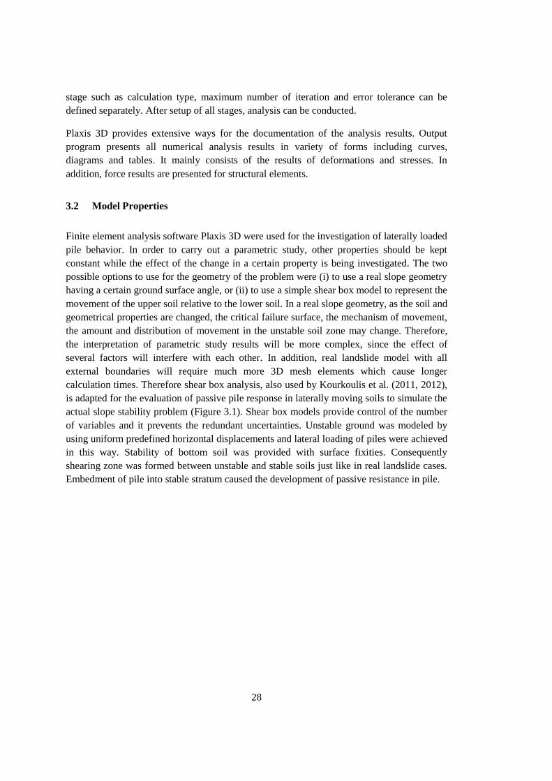
28
stage such as calculation type, maximum number of iteration and error tolerance can be
defined separately. After setup of all stages, analysis can be conducted.
Plaxis 3D provides extensive ways for the documentation of the analysis results. Output
program presents all numerical analysis results in variety of forms including curves,
diagrams and tables. It mainly consists of the results of deformations and stresses. In
addition, force results are presented for structural elements.
3.2 Model Properties
Finite element analysis software Plaxis 3D were used for the investigation of laterally loaded
pile behavior. In order to carry out a parametric study, other properties should be kept
constant while the effect of the change in a certain property is being investigated. The two
possible options to use for the geometry of the problem were (i) to use a real slope geometry
having a certain ground surface angle, or (ii) to use a simple shear box model to represent the
movement of the upper soil relative to the lower soil. In a real slope geometry, as the soil and
geometrical properties are changed, the critical failure surface, the mechanism of movement,
the amount and distribution of movement in the unstable soil zone may change. Therefore,
the interpretation of parametric study results will be more complex, since the effect of
several factors will interfere with each other. In addition, real landslide model with all
external boundaries will require much more 3D mesh elements which cause longer
calculation times. Therefore shear box analysis, also used by Kourkoulis et al. (2011, 2012),
is adapted for the evaluation of passive pile response in laterally moving soils to simulate the
actual slope stability problem (Figure 3.1). Shear box models provide control of the number
of variables and it prevents the redundant uncertainties. Unstable ground was modeled by
using uniform predefined horizontal displacements and lateral loading of piles were achieved
in this way. Stability of bottom soil was provided with surface fixities. Consequently
shearing zone was formed between unstable and stable soils just like in real landslide cases.
Embedment of pile into stable stratum caused the development of passive resistance in pile.
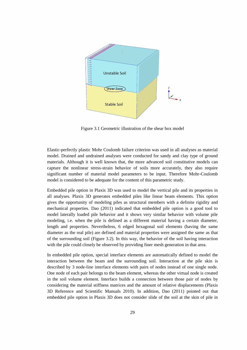
29
Figure 3.1 Geometric illustration of the shear box model
Elastic-perfectly plastic Mohr Coulomb failure criterion was used in all analyses as material
model. Drained and undrained analyses were conducted for sandy and clay type of ground
materials. Although it is well known that, the more advanced soil constitutive models can
capture the nonlinear stress-strain behavior of soils more accurately, they also require
significant number of material model parameters to be input. Therefore Mohr-Coulomb
model is considered to be adequate for the content of this parametric study.
Embedded pile option in Plaxis 3D was used to model the vertical pile and its properties in
all analyses. Plaxis 3D generates embedded piles like linear beam elements. This option
gives the opportunity of modeling piles as structural members with a definite rigidity and
mechanical properties. Dao (2011) indicated that embedded pile option is a good tool to
model laterally loaded pile behavior and it shows very similar behavior with volume pile
modeling, i.e. when the pile is defined as a different material having a certain diameter,
length and properties. Nevertheless, 6 edged hexagonal soil elements (having the same
diameter as the real pile) are defined and material properties were assigned the same as that
of the surrounding soil (Figure 3.2). In this way, the behavior of the soil having interaction
with the pile could closely be observed by providing finer mesh generation in that area.
In embedded pile option, special interface elements are automatically defined to model the
interaction between the beam and the surrounding soil. Interaction at the pile skin is
described by 3 node-line interface elements with pairs of nodes instead of one single node.
One node of each pair belongs to the beam element, whereas the other virtual node is created
in the soil volume element. Interface builds a connection between those pair of nodes by
considering the material stiffness matrices and the amount of relative displacements (Plaxis
3D Reference and Scientific Manuals 2010). In addition, Dao (2011) pointed out that
embedded pile option in Plaxis 3D does not consider slide of the soil at the skin of pile in
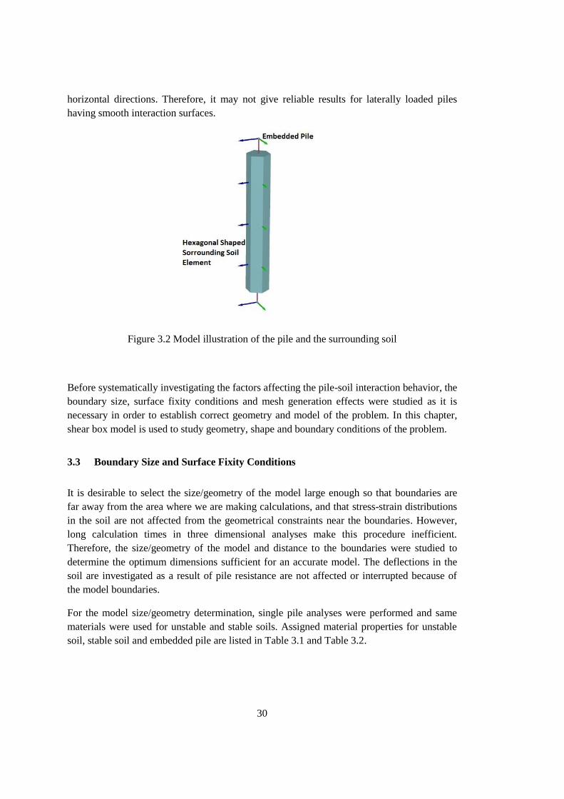
30
horizontal directions. Therefore, it may not give reliable results for laterally loaded piles
having smooth interaction surfaces.
Figure 3.2 Model illustration of the pile and the surrounding soil
Before systematically investigating the factors affecting the pile-soil interaction behavior, the
boundary size, surface fixity conditions and mesh generation effects were studied as it is
necessary in order to establish correct geometry and model of the problem. In this chapter,
shear box model is used to study geometry, shape and boundary conditions of the problem.
3.3 Boundary Size and Surface Fixity Conditions
It is desirable to select the size/geometry of the model large enough so that boundaries are
far away from the area where we are making calculations, and that stress-strain distributions
in the soil are not affected from the geometrical constraints near the boundaries. However,
long calculation times in three dimensional analyses make this procedure inefficient.
Therefore, the size/geometry of the model and distance to the boundaries were studied to
determine the optimum dimensions sufficient for an accurate model. The deflections in the
soil are investigated as a result of pile resistance are not affected or interrupted because of
the model boundaries.
For the model size/geometry determination, single pile analyses were performed and same
materials were used for unstable and stable soils. Assigned material properties for unstable
soil, stable soil and embedded pile are listed in Table 3.1 and Table 3.2.
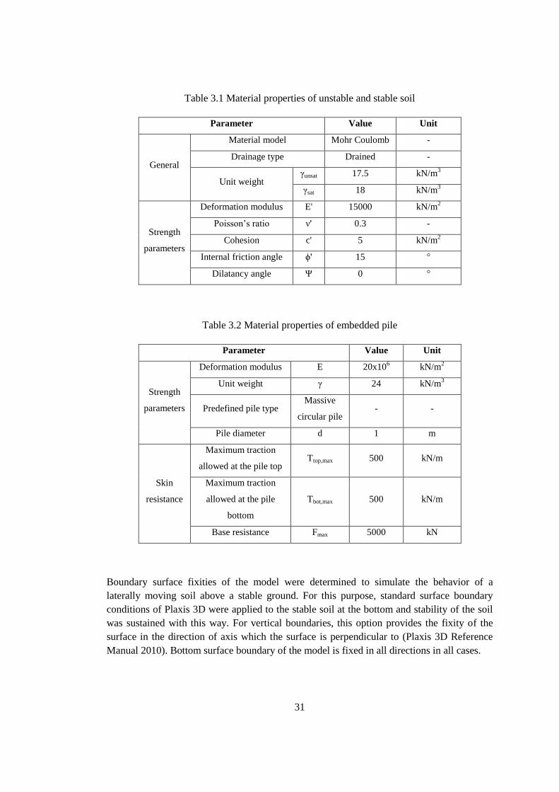
31
Table 3.1 Material properties of unstable and stable soil
Parameter Value Unit
General
Material model Mohr Coulomb -
Drainage type Drained -
Unit weight γunsat 17.5 kN/m
3
γsat 18 kN/m3
Strength
parameters
Deformation modulus E' 15000 kN/m2
Poisson’s ratio ν' 0.3 -
Cohesion c' 5 kN/m2
Internal friction angle ϕ' 15 °
Dilatancy angle Ψ 0 °
Table 3.2 Material properties of embedded pile
Parameter Value Unit
Strength
parameters
Deformation modulus E 20x106 kN/m
2
Unit weight γ 24 kN/m3
Predefined pile type Massive
circular pile - -
Pile diameter d 1 m
Skin
resistance
Maximum traction
allowed at the pile top Ttop,max 500 kN/m
Maximum traction
allowed at the pile
bottom
Tbot,max 500 kN/m
Base resistance Fmax 5000 kN
Boundary surface fixities of the model were determined to simulate the behavior of a
laterally moving soil above a stable ground. For this purpose, standard surface boundary
conditions of Plaxis 3D were applied to the stable soil at the bottom and stability of the soil
was sustained with this way. For vertical boundaries, this option provides the fixity of the
surface in the direction of axis which the surface is perpendicular to (Plaxis 3D Reference
Manual 2010). Bottom surface boundary of the model is fixed in all directions in all cases.

32
Surface boundaries of unstable ground were redefined with surface prescribed displacement
property (Figure 3.3). Movement in y direction is prevented and z direction is allowed for all
surfaces. In x direction, an amount of uniformly distributed prescribed displacement (ux) was
defined on the left side surface of the model box. Rear and front side surfaces were allowed
for movement in x direction. Right side surface movement was first tried to be freely
allowed in x direction however, load increment failure and soil body collapse errors were
generally encountered in the vertical model boundary without any constraint (especially in
cohesionless materials). For analyses that calculation phases were fully completed, excessive
deformations and spilling of soil body from right hand side were observed especially
depending on the assigned material properties and the amount of prescribed displacements
(Figure 3.3). Additional structural support for right side surface boundary could be a solution
but it was observed that they can destroy the nature of the problem by imposing unwanted
friction and geometrical constraints. Therefore, it was determined to take right hand side
surface of the box model fixed in a very far distance which both pile and soil deformations
are not affected from this surface fixity (Table 3.3). In that case, soil in front of the piles does
not freely deform or spill to the right hand side. Proposed model geometry simulates
landslide stabilization cases where soil in front of the piles is not yielded.
Figure 3.3 Spilling of unstable soil from right hand side when right boundary is free to move
in the direction of movement
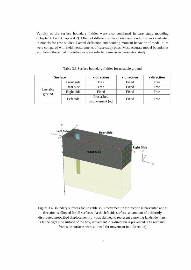
33
Validity of the surface boundary fixities were also confirmed in case study modeling
(Chapter 4.1 and Chapter 4.2). Effect of different surface boundary conditions was evaluated
in models for case studies. Lateral deflection and bending moment behavior of model piles
were compared with field measurements of case study piles. Most accurate model boundaries
simulating the actual pile behavior were selected same as in parametric study.
Table 3.3 Surface boundary fixities for unstable ground
Surface x direction y direction z direction
Unstable
ground
Front side Free Fixed Free
Rear side Free Fixed Free
Right side Fixed Fixed Free
Left side Prescribed
displacement (ux) Fixed Free
Figure 3.4 Boundary surfaces for unstable soil (movement in y direction is prevented and z
direction is allowed for all surfaces, At the left side surface, an amount of uniformly
distributed prescribed displacement (ux) was defined to represent a moving landslide mass.
On the right side surface of the box, movement in x-direction is prevented. The rear and
front side surfaces were allowed for movement in x-direction)
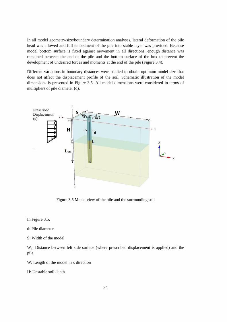
34
In all model geometry/size/boundary determination analyses, lateral deformation of the pile
head was allowed and full embedment of the pile into stable layer was provided. Because
model bottom surface is fixed against movement in all directions, enough distance was
remained between the end of the pile and the bottom surface of the box to prevent the
development of undesired forces and moments at the end of the pile (Figure 3.4).
Different variations in boundary distances were studied to obtain optimum model size that
does not affect the displacement profile of the soil. Schematic illustration of the model
dimensions is presented in Figure 3.5. All model dimensions were considered in terms of
multipliers of pile diameter (d).
Figure 3.5 Model view of the pile and the surrounding soil
In Figure 3.5,
d: Pile diameter
S: Width of the model
W1: Distance between left side surface (where prescribed displacement is applied) and the
pile
W: Length of the model in x direction
H: Unstable soil depth
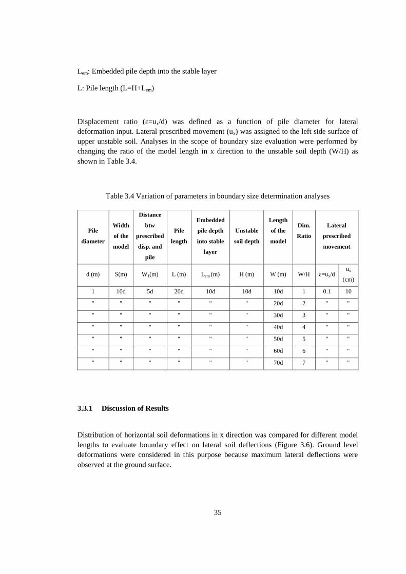
35
Lem: Embedded pile depth into the stable layer
L: Pile length (L=H+Lem)
Displacement ratio (ɛ=ux/d) was defined as a function of pile diameter for lateral
deformation input. Lateral prescribed movement (ux) was assigned to the left side surface of
upper unstable soil. Analyses in the scope of boundary size evaluation were performed by
changing the ratio of the model length in x direction to the unstable soil depth (W/H) as
shown in Table 3.4.
Table 3.4 Variation of parameters in boundary size determination analyses
Pile
diameter
Width
of the
model
Distance
btw
prescribed
disp. and
pile
Pile
length
Embedded
pile depth
into stable
layer
Unstable
soil depth
Length
of the
model
Dim.
Ratio
Lateral
prescribed
movement
d (m) S(m) W1(m) L (m) Lem (m) H (m) W (m) W/H ɛ=ux/d ux
(cm)
1 10d 5d 20d 10d 10d 10d 1 0.1 10
" " " " " " 20d 2 " "
" " " " " " 30d 3 " "
" " " " " " 40d 4 " "
" " " " " " 50d 5 " "
" " " " " " 60d 6 " "
" " " " " " 70d 7 " "
3.3.1 Discussion of Results
Distribution of horizontal soil deformations in x direction was compared for different model
lengths to evaluate boundary effect on lateral soil deflections (Figure 3.6). Ground level
deformations were considered in this purpose because maximum lateral deflections were
observed at the ground surface.
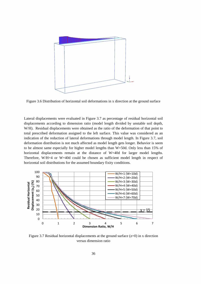
36
Figure 3.6 Distribution of horizontal soil deformations in x direction at the ground surface
Lateral displacements were evaluated in Figure 3.7 as percentage of residual horizontal soil
displacements according to dimension ratio (model length divided by unstable soil depth,
W/H). Residual displacements were obtained as the ratio of the deformation of that point to
total prescribed deformation assigned to the left surface. This value was considered as an
indication of the reduction of lateral deformations through model length. In Figure 3.7, soil
deformation distribution is not much affected as model length gets longer. Behavior is seem
to be almost same especially for higher model lengths than W=50d. Only less than 15% of
horizontal displacements remain at the distance of W=40d for larger model lengths.
Therefore, W/H=4 or W=40d could be chosen as sufficient model length in respect of
horizontal soil distributions for the assumed boundary fixity conditions.
Figure 3.7 Residual horizontal displacements at the ground surface (z=0) in x direction
versus dimension ratio
y = 15
0
10
20
30
40
50
60
70
80
90
100
0 1 2 3 4 5 6 7
Re
sid
ual
Ho
rizo
nta
l D
isp
lace
me
nt
(ux)
(%
)
Dimension Ratio, W/H
W/H=1 (W=10d)W/H=2 (W=20d)W/H=3 (W=30d)W/H=4 (W=40d)W/H=5 (W=50d)W/H=6 (W=60d)W/H=7 (W=70d)
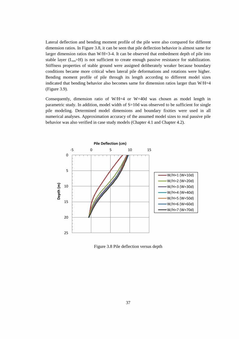
37
Lateral deflection and bending moment profile of the pile were also compared for different
dimension ratios. In Figure 3.8, it can be seen that pile deflection behavior is almost same for
larger dimension ratios than W/H=3-4. It can be observed that embedment depth of pile into
stable layer (Lem=H) is not sufficient to create enough passive resistance for stabilization.
Stiffness properties of stable ground were assigned deliberately weaker because boundary
conditions became more critical when lateral pile deformations and rotations were higher.
Bending moment profile of pile through its length according to different model sizes
indicated that bending behavior also becomes same for dimension ratios larger than W/H=4
(Figure 3.9).
Consequently, dimension ratio of W/H=4 or W=40d was chosen as model length in
parametric study. In addition, model width of S=10d was observed to be sufficient for single
pile modeling. Determined model dimensions and boundary fixities were used in all
numerical analyses. Approximation accuracy of the assumed model sizes to real passive pile
behavior was also verified in case study models (Chapter 4.1 and Chapter 4.2).
Figure 3.8 Pile deflection versus depth
0
5
10
15
20
25
-5 0 5 10 15
De
pth
(m
)
Pile Deflection (cm)
W/H=1 (W=10d)
W/H=2 (W=20d)
W/H=3 (W=30d)
W/H=4 (W=40d)
W/H=5 (W=50d)
W/H=6 (W=60d)
W/H=7 (W=70d)
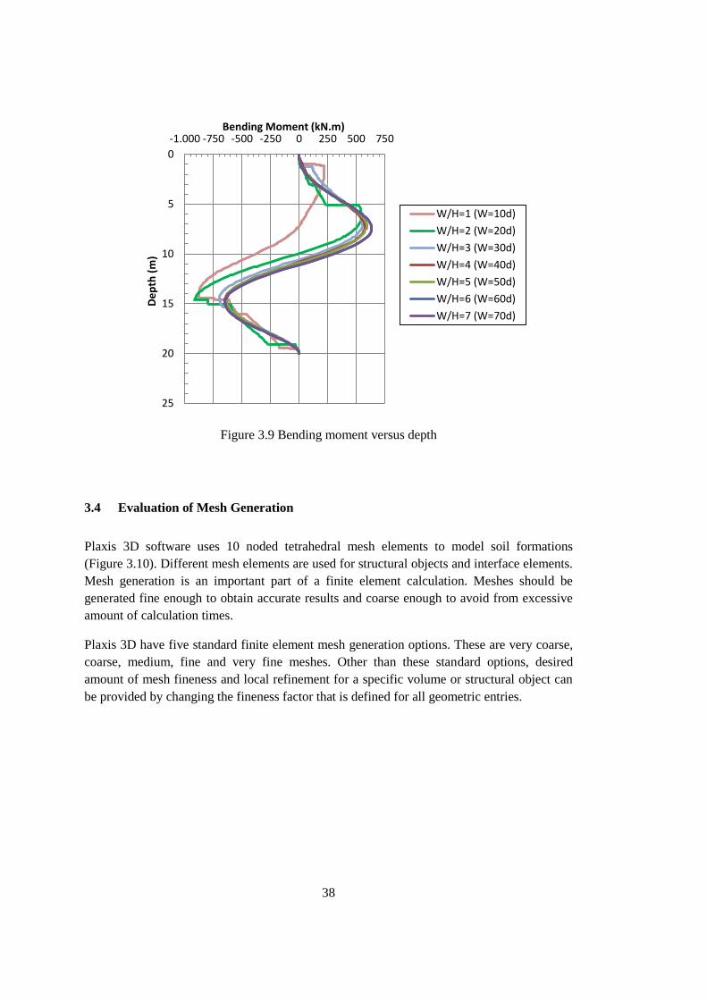
38
Figure 3.9 Bending moment versus depth
3.4 Evaluation of Mesh Generation
Plaxis 3D software uses 10 noded tetrahedral mesh elements to model soil formations
(Figure 3.10). Different mesh elements are used for structural objects and interface elements.
Mesh generation is an important part of a finite element calculation. Meshes should be
generated fine enough to obtain accurate results and coarse enough to avoid from excessive
amount of calculation times.
Plaxis 3D have five standard finite element mesh generation options. These are very coarse,
coarse, medium, fine and very fine meshes. Other than these standard options, desired
amount of mesh fineness and local refinement for a specific volume or structural object can
be provided by changing the fineness factor that is defined for all geometric entries.
0
5
10
15
20
25
-1.000 -750 -500 -250 0 250 500 750D
ep
th (
m)
Bending Moment (kN.m)
W/H=1 (W=10d)
W/H=2 (W=20d)
W/H=3 (W=30d)
W/H=4 (W=40d)
W/H=5 (W=50d)
W/H=6 (W=60d)
W/H=7 (W=70d)
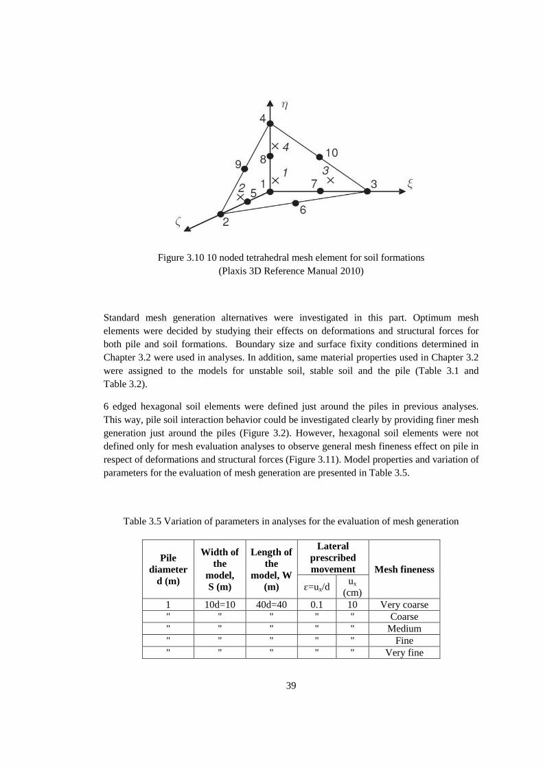
39
Figure 3.10 10 noded tetrahedral mesh element for soil formations
(Plaxis 3D Reference Manual 2010)
Standard mesh generation alternatives were investigated in this part. Optimum mesh
elements were decided by studying their effects on deformations and structural forces for
both pile and soil formations. Boundary size and surface fixity conditions determined in
Chapter 3.2 were used in analyses. In addition, same material properties used in Chapter 3.2
were assigned to the models for unstable soil, stable soil and the pile (Table 3.1 and
Table 3.2).
6 edged hexagonal soil elements were defined just around the piles in previous analyses.
This way, pile soil interaction behavior could be investigated clearly by providing finer mesh
generation just around the piles (Figure 3.2). However, hexagonal soil elements were not
defined only for mesh evaluation analyses to observe general mesh fineness effect on pile in
respect of deformations and structural forces (Figure 3.11). Model properties and variation of
parameters for the evaluation of mesh generation are presented in Table 3.5.
Table 3.5 Variation of parameters in analyses for the evaluation of mesh generation
Pile
diameter
d (m)
Width of
the
model,
S (m)
Length of
the
model, W
(m)
Lateral
prescribed
movement Mesh fineness
ɛ=ux/d ux
(cm)
1 10d=10 40d=40 0.1 10 Very coarse
" " " " " Coarse
" " " " " Medium
" " " " " Fine
" " " " " Very fine
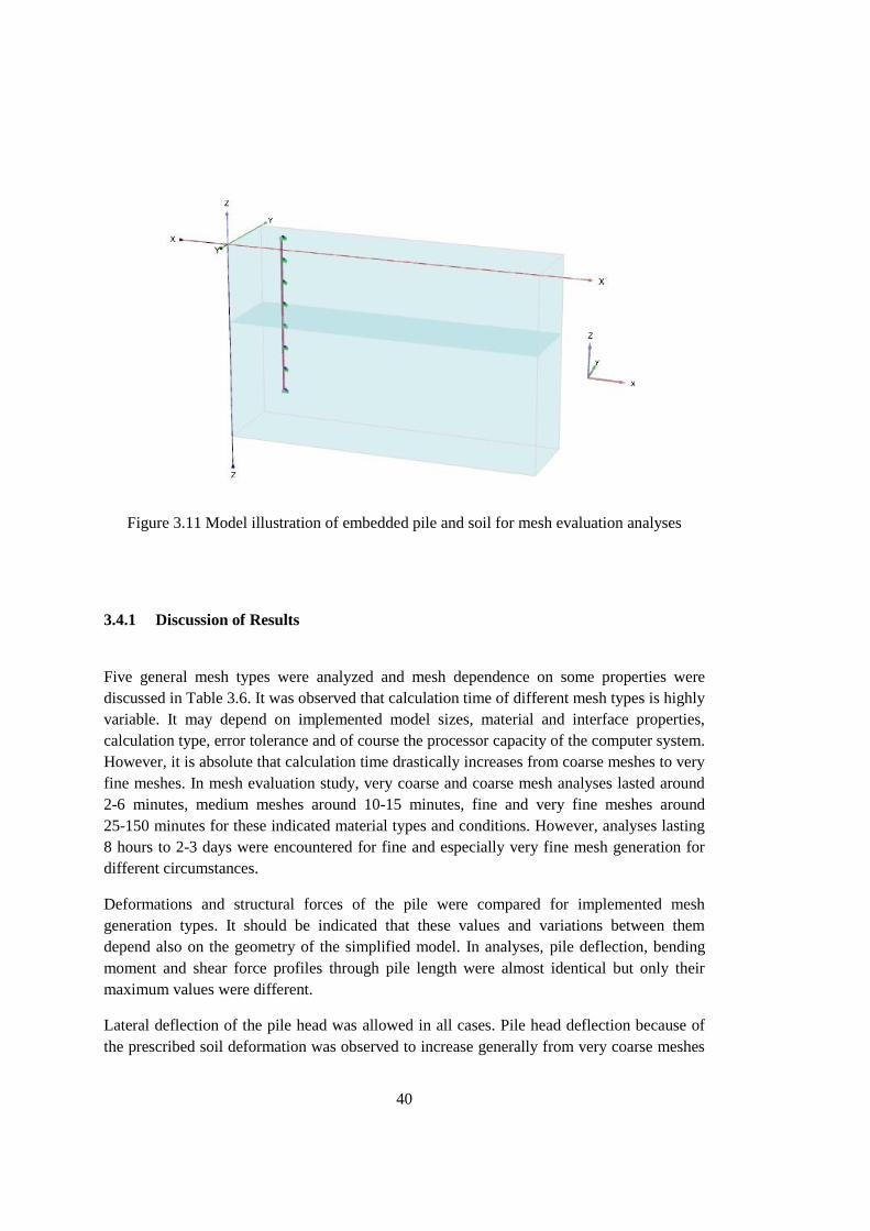
40
Figure 3.11 Model illustration of embedded pile and soil for mesh evaluation analyses
3.4.1 Discussion of Results
Five general mesh types were analyzed and mesh dependence on some properties were
discussed in Table 3.6. It was observed that calculation time of different mesh types is highly
variable. It may depend on implemented model sizes, material and interface properties,
calculation type, error tolerance and of course the processor capacity of the computer system.
However, it is absolute that calculation time drastically increases from coarse meshes to very
fine meshes. In mesh evaluation study, very coarse and coarse mesh analyses lasted around
2-6 minutes, medium meshes around 10-15 minutes, fine and very fine meshes around
25-150 minutes for these indicated material types and conditions. However, analyses lasting
8 hours to 2-3 days were encountered for fine and especially very fine mesh generation for
different circumstances.
Deformations and structural forces of the pile were compared for implemented mesh
generation types. It should be indicated that these values and variations between them
depend also on the geometry of the simplified model. In analyses, pile deflection, bending
moment and shear force profiles through pile length were almost identical but only their
maximum values were different.
Lateral deflection of the pile head was allowed in all cases. Pile head deflection because of
the prescribed soil deformation was observed to increase generally from very coarse meshes
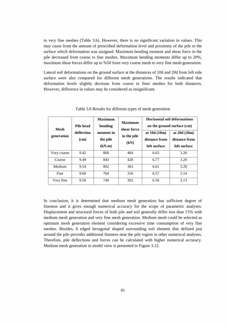
41
to very fine meshes (Table 3.6). However, there is no significant variation in values. This
may cause from the amount of prescribed deformation level and proximity of the pile to the
surface which deformation was assigned. Maximum bending moment and shear force in the
pile decreased from coarse to fine meshes. Maximum bending moments differ up to 20%,
maximum shear forces differ up to %50 from very coarse mesh to very fine mesh generation.
Lateral soil deformations on the ground surface at the distances of 10d and 20d from left side
surface were also compared for different mesh generations. The results indicated that
deformation levels slightly decrease from coarse to finer meshes for both distances.
However, difference in values may be considered as insignificant.
Table 3.6 Results for different types of mesh generation
Mesh
generation
Pile head
deflection
(cm)
Maximum
bending
moment in
the pile
(kN.m)
Maximum
shear force
in the pile
(kN)
Horizontal soil deformations
on the ground surface (cm)
at 10d (10m)
distance from
left surface
at 20d (20m)
distance from
left surface
Very coarse 9.42 868 464 6.63 3.26
Coarse 9.49 843 428 6.77 3.20
Medium 9.54 802 363 6.61 3.20
Fine 9.60 764 316 6.57 3.14
Very fine 9.50 740 302 6.56 3.13
In conclusion, it is determined that medium mesh generation has sufficient degree of
fineness and it gives enough numerical accuracy for the scope of parametric analyses.
Displacement and structural forces of both pile and soil generally differ less than 15% with
medium mesh generation and very fine mesh generation. Medium mesh could be selected as
optimum mesh generation element considering excessive time consumption of very fine
meshes. Besides, 6 edged hexagonal shaped surrounding soil element that defined just
around the pile provides additional fineness near the pile region in other numerical analyses.
Therefore, pile deflections and forces can be calculated with higher numerical accuracy.
Medium mesh generation in model view is presented in Figure 3.12.
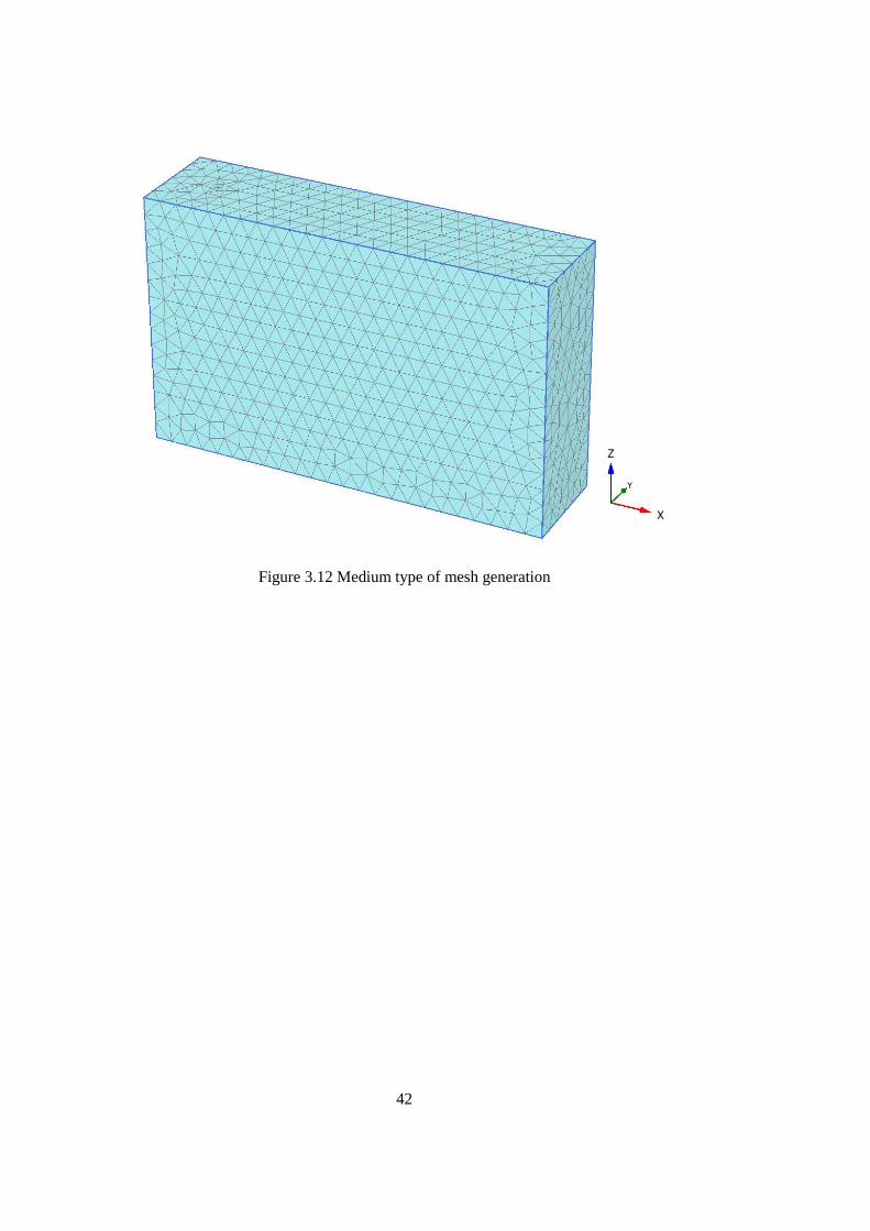
42
Figure 3.12 Medium type of mesh generation

43
CHAPTER 4
CASE HISTORIES
In situ field experiments were studied to verify the accuracy of three dimensional numerical
modeling approach for real passive pile behavior. Three dimensional models of cases were
investigated by comparing their results with measured field data and approximation methods
of some other researchers. Two case histories were selected as De Beer and Wallays (1972)
and Esu and D’Elia (1974) for this purpose. De Beer and Wallays (1972) investigated
embankment construction effects on pile foundations subjected to non-uniform ground
movement in sandy soils. Both steel pipe pile and reinforced concrete pile were used in their
experiment. On the other hand, Esu and D’Elia (1974) conducted a field experiment to study
slope stabilizing reinforced concrete pile in clayey type of soil. Applicability of three
dimensional modeling for different pile materials, different soil materials and different
lateral soil movement distributions could be investigated by these two cases.
4.1 De Beer and Wallays (1972)
Two case studies were reported by De Beer and Wallays (1972) in Belgium for the
investigation of laterally loaded adjacent pile foundations in sandy soils. In one of the cases,
a steel pipe pile having 28 m length, 0.9 m diameter and 1.5 cm wall thickness was used.
Reinforced concrete pile with 23.2 m length and 0.6 m diameter was used in the other case.
Pile top was restrained to move in both cases. Spacing between the adjacent piles has not
been indicated and there is not much information given about the stiffness properties of the
soil profile. Non-uniform lateral soil movement was measured by using inclinometers as it is
seen in Figure 4.1. In addition, deflection and bending moment distribution of piles were
measured for both cases.
Figure 4.1 Lateral soil movement profile of De Beer and Wallays (1972) case studies
(Chen and Poulos 1997)
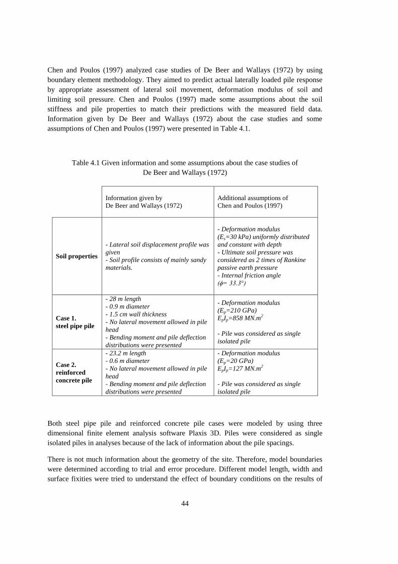
44
Chen and Poulos (1997) analyzed case studies of De Beer and Wallays (1972) by using
boundary element methodology. They aimed to predict actual laterally loaded pile response
by appropriate assessment of lateral soil movement, deformation modulus of soil and
limiting soil pressure. Chen and Poulos (1997) made some assumptions about the soil
stiffness and pile properties to match their predictions with the measured field data.
Information given by De Beer and Wallays (1972) about the case studies and some
assumptions of Chen and Poulos (1997) were presented in Table 4.1.
Table 4.1 Given information and some assumptions about the case studies of
De Beer and Wallays (1972)
Information given by
De Beer and Wallays (1972)
Additional assumptions of
Chen and Poulos (1997)
Soil properties
- Lateral soil displacement profile was
given
- Soil profile consists of mainly sandy
materials.
- Deformation modulus
(Es=30 kPa) uniformly distributed
and constant with depth
- Ultimate soil pressure was
considered as 2 times of Rankine
passive earth pressure
- Internal friction angle
(ϕ= 33.3°)
Case 1.
steel pipe pile
- 28 m length
- 0.9 m diameter
- 1.5 cm wall thickness
- No lateral movement allowed in pile
head
- Bending moment and pile deflection
distributions were presented
- Deformation modulus
(Ep=210 GPa)
EpIp=858 MN.m2
- Pile was considered as single
isolated pile
Case 2.
reinforced
concrete pile
- 23.2 m length
- 0.6 m diameter
- No lateral movement allowed in pile
head
- Bending moment and pile deflection
distributions were presented
- Deformation modulus
(Ep=20 GPa)
EpIp=127 MN.m2
- Pile was considered as single
isolated pile
Both steel pipe pile and reinforced concrete pile cases were modeled by using three
dimensional finite element analysis software Plaxis 3D. Piles were considered as single
isolated piles in analyses because of the lack of information about the pile spacings.
There is not much information about the geometry of the site. Therefore, model boundaries
were determined according to trial and error procedure. Different model length, width and
surface fixities were tried to understand the effect of boundary conditions on the results of
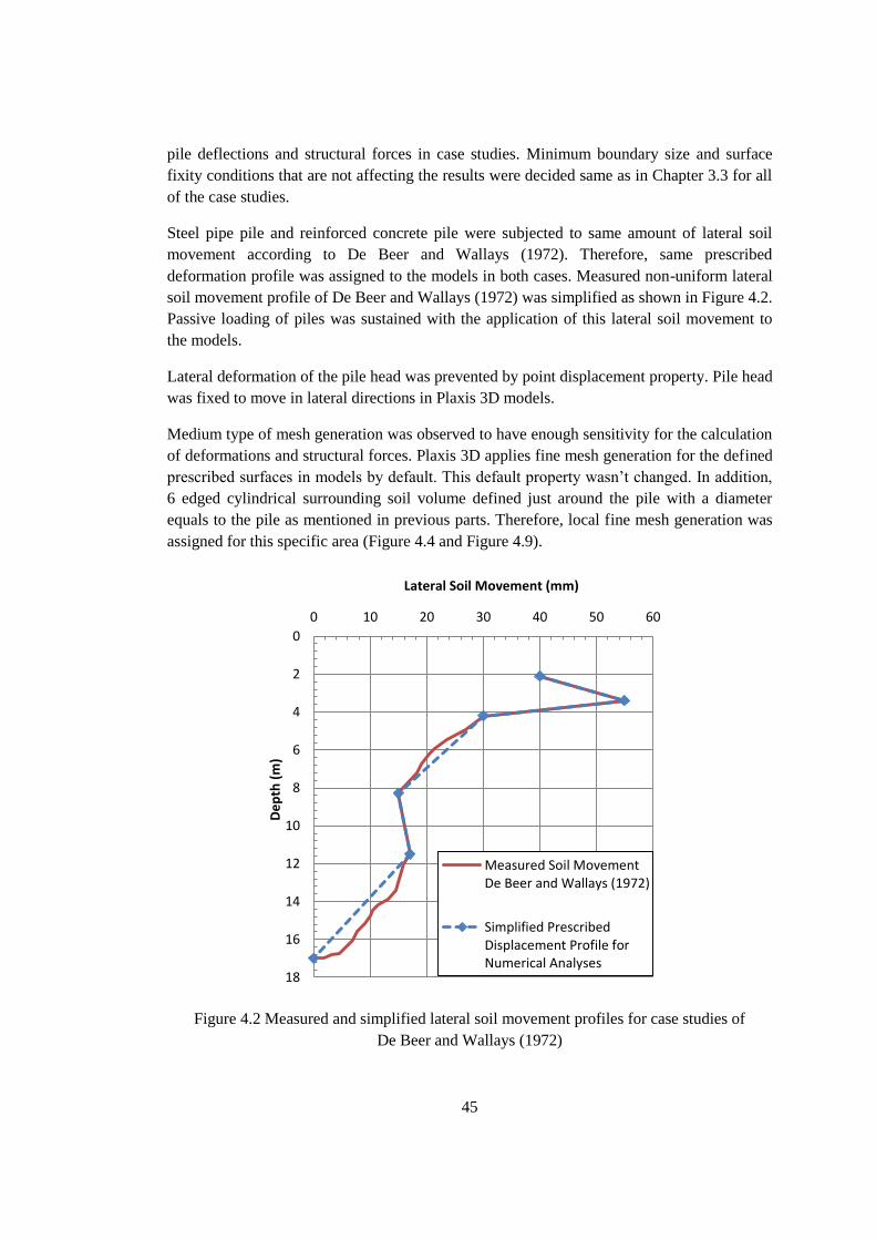
45
pile deflections and structural forces in case studies. Minimum boundary size and surface
fixity conditions that are not affecting the results were decided same as in Chapter 3.3 for all
of the case studies.
Steel pipe pile and reinforced concrete pile were subjected to same amount of lateral soil
movement according to De Beer and Wallays (1972). Therefore, same prescribed
deformation profile was assigned to the models in both cases. Measured non-uniform lateral
soil movement profile of De Beer and Wallays (1972) was simplified as shown in Figure 4.2.
Passive loading of piles was sustained with the application of this lateral soil movement to
the models.
Lateral deformation of the pile head was prevented by point displacement property. Pile head
was fixed to move in lateral directions in Plaxis 3D models.
Medium type of mesh generation was observed to have enough sensitivity for the calculation
of deformations and structural forces. Plaxis 3D applies fine mesh generation for the defined
prescribed surfaces in models by default. This default property wasn’t changed. In addition,
6 edged cylindrical surrounding soil volume defined just around the pile with a diameter
equals to the pile as mentioned in previous parts. Therefore, local fine mesh generation was
assigned for this specific area (Figure 4.4 and Figure 4.9).
Figure 4.2 Measured and simplified lateral soil movement profiles for case studies of
De Beer and Wallays (1972)
0
2
4
6
8
10
12
14
16
18
0 10 20 30 40 50 60
De
pth
(m
)
Lateral Soil Movement (mm)
Measured Soil MovementDe Beer and Wallays (1972)
Simplified PrescribedDisplacement Profile forNumerical Analyses
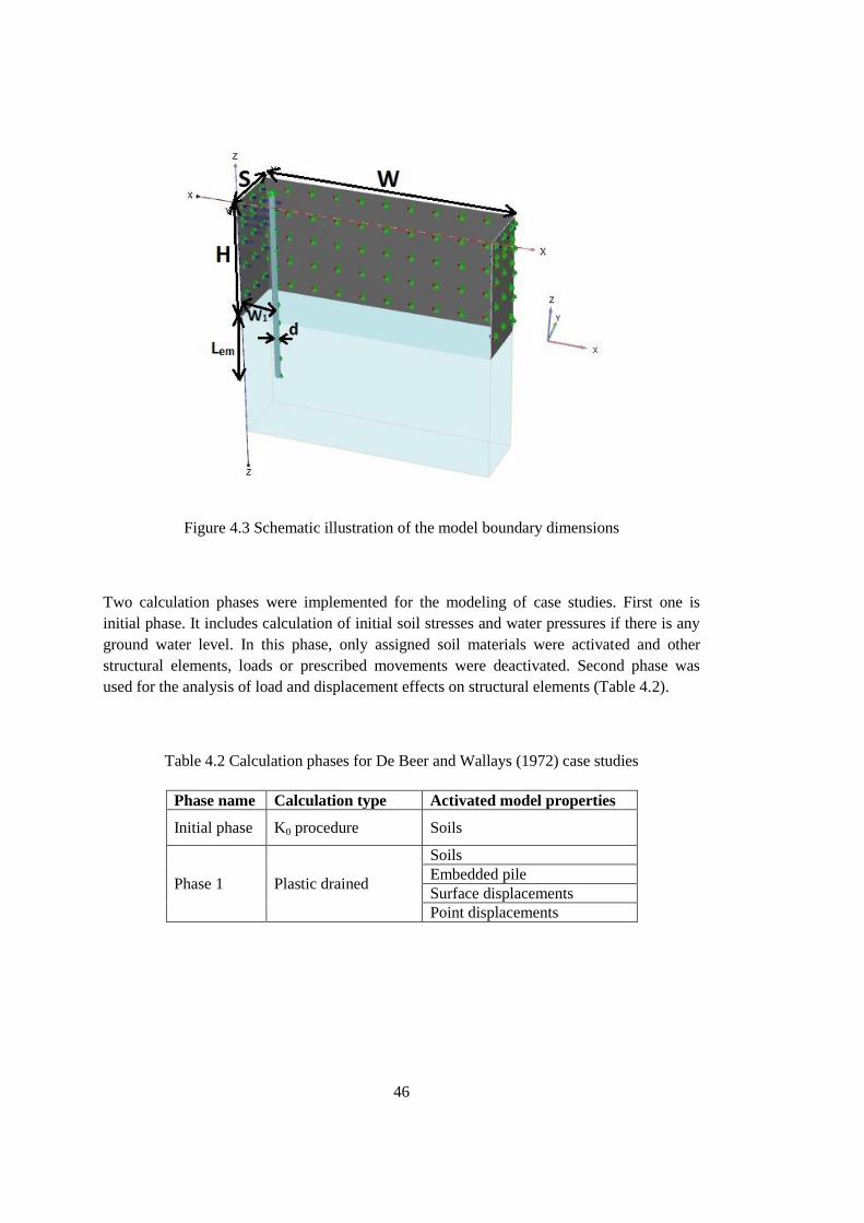
46
Figure 4.3 Schematic illustration of the model boundary dimensions
Two calculation phases were implemented for the modeling of case studies. First one is
initial phase. It includes calculation of initial soil stresses and water pressures if there is any
ground water level. In this phase, only assigned soil materials were activated and other
structural elements, loads or prescribed movements were deactivated. Second phase was
used for the analysis of load and displacement effects on structural elements (Table 4.2).
Table 4.2 Calculation phases for De Beer and Wallays (1972) case studies
Phase name Calculation type Activated model properties
Initial phase K0 procedure Soils
Phase 1 Plastic drained
Soils
Embedded pile
Surface displacements
Point displacements
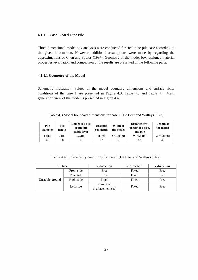
47
4.1.1 Case 1. Steel Pipe Pile
Three dimensional model box analyses were conducted for steel pipe pile case according to
the given information. However, additional assumptions were made by regarding the
approximations of Chen and Poulos (1997). Geometry of the model box, assigned material
properties, evaluation and comparison of the results are presented in the following parts.
4.1.1.1 Geometry of the Model
Schematic illustration, values of the model boundary dimensions and surface fixity
conditions of the case 1 are presented in Figure 4.3, Table 4.3 and Table 4.4. Mesh
generation view of the model is presented in Figure 4.4.
Table 4.3 Model boundary dimensions for case 1 (De Beer and Wallays 1972)
Pile
diameter
Pile
length
Embedded pile
depth into
stable layer
Unstable
soil depth
Width of
the model
Distance btw.
prescribed disp.
and pile
Length of
the model
d (m) L (m) Lem (m) H (m) S=10d (m) W1=5d (m) W=40d (m)
0.9 28 11 17 9 4.5 36
Table 4.4 Surface fixity conditions for case 1 (De Beer and Wallays 1972)
Surface x direction y direction z direction
Unstable ground
Front side Free Fixed Free
Rear side Free Fixed Free
Right side Fixed Fixed Free
Left side Prescribed
displacement (ux) Fixed Free

48
Figure 4.4 Mesh generation for the steel pipe pile case (De Beer and Wallays 1972)
4.1.1.2 Material Properties
Stiffness properties of soil profile and embedded pile were assigned regarding the given
information and assumptions of Chen and Poulos (1997). There is no distinction between
moving and stationary soil profiles in De Beer and Wallays (1972) cases. Therefore, same
materials were used for unstable and stable soils. Assigned material properties for unstable
soil, stable soil and embedded pile were listed in Table 4.5 and Table 4.6.
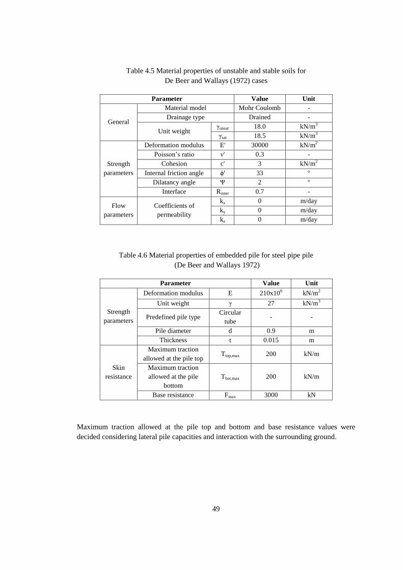
49
Table 4.5 Material properties of unstable and stable soils for
De Beer and Wallays (1972) cases
Parameter Value Unit
General
Material model Mohr Coulomb -
Drainage type Drained -
Unit weight γunsat 18.0 kN/m
3
γsat 18.5 kN/m3
Strength
parameters
Deformation modulus E' 30000 kN/m2
Poisson’s ratio ν' 0.3 -
Cohesion c' 3 kN/m2
Internal friction angle ϕ' 33 °
Dilatancy angle Ψ 2 °
Interface Rinter 0.7 -
Flow
parameters
Coefficients of
permeability
kx 0 m/day
ky 0 m/day
kz 0 m/day
Table 4.6 Material properties of embedded pile for steel pipe pile
(De Beer and Wallays 1972)
Parameter Value Unit
Strength
parameters
Deformation modulus E 210x106 kN/m
2
Unit weight γ 27 kN/m3
Predefined pile type Circular
tube - -
Pile diameter d 0.9 m
Thickness t 0.015 m
Skin
resistance
Maximum traction
allowed at the pile top Ttop,max 200 kN/m
Maximum traction
allowed at the pile
bottom
Tbot,max 200 kN/m
Base resistance Fmax 3000 kN
Maximum traction allowed at the pile top and bottom and base resistance values were
decided considering lateral pile capacities and interaction with the surrounding ground.
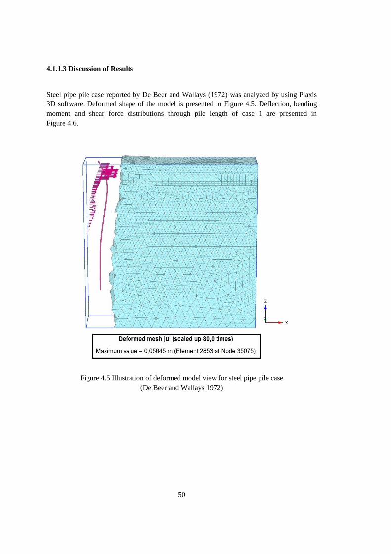
50
4.1.1.3 Discussion of Results
Steel pipe pile case reported by De Beer and Wallays (1972) was analyzed by using Plaxis
3D software. Deformed shape of the model is presented in Figure 4.5. Deflection, bending
moment and shear force distributions through pile length of case 1 are presented in
Figure 4.6.
Figure 4.5 Illustration of deformed model view for steel pipe pile case
(De Beer and Wallays 1972)
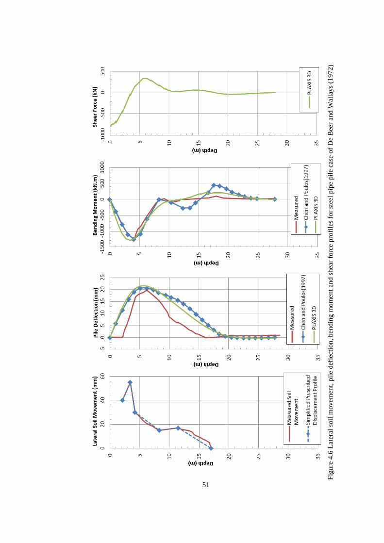
51
Fig
ure
4.6
Lat
eral
soil
mo
vem
ent,
pil
e def
lect
ion, ben
din
g m
om
ent
and s
hea
r fo
rce
pro
file
s fo
r st
eel
pip
e p
ile
case
of
De
Bee
r an
d W
alla
ys
(19
72
)
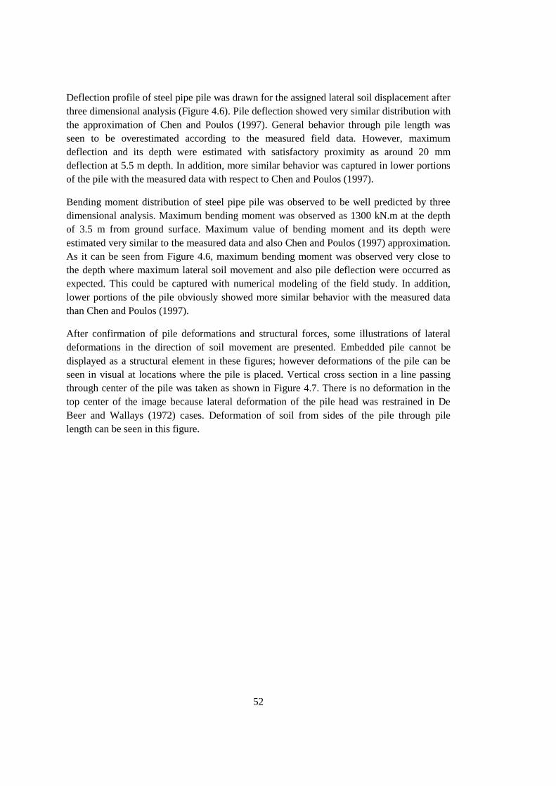
52
Deflection profile of steel pipe pile was drawn for the assigned lateral soil displacement after
three dimensional analysis (Figure 4.6). Pile deflection showed very similar distribution with
the approximation of Chen and Poulos (1997). General behavior through pile length was
seen to be overestimated according to the measured field data. However, maximum
deflection and its depth were estimated with satisfactory proximity as around 20 mm
deflection at 5.5 m depth. In addition, more similar behavior was captured in lower portions
of the pile with the measured data with respect to Chen and Poulos (1997).
Bending moment distribution of steel pipe pile was observed to be well predicted by three
dimensional analysis. Maximum bending moment was observed as 1300 kN.m at the depth
of 3.5 m from ground surface. Maximum value of bending moment and its depth were
estimated very similar to the measured data and also Chen and Poulos (1997) approximation.
As it can be seen from Figure 4.6, maximum bending moment was observed very close to
the depth where maximum lateral soil movement and also pile deflection were occurred as
expected. This could be captured with numerical modeling of the field study. In addition,
lower portions of the pile obviously showed more similar behavior with the measured data
than Chen and Poulos (1997).
After confirmation of pile deformations and structural forces, some illustrations of lateral
deformations in the direction of soil movement are presented. Embedded pile cannot be
displayed as a structural element in these figures; however deformations of the pile can be
seen in visual at locations where the pile is placed. Vertical cross section in a line passing
through center of the pile was taken as shown in Figure 4.7. There is no deformation in the
top center of the image because lateral deformation of the pile head was restrained in De
Beer and Wallays (1972) cases. Deformation of soil from sides of the pile through pile
length can be seen in this figure.
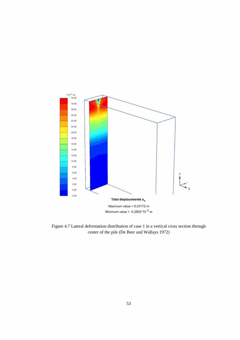
53
Figure 4.7 Lateral deformation distribution of case 1 in a vertical cross section through
center of the pile (De Beer and Wallays 1972)
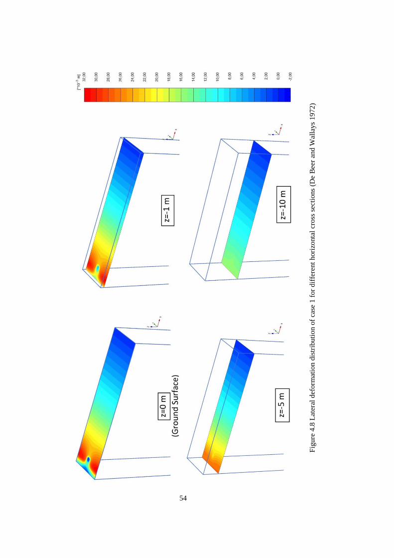
54
Fig
ure
4.8
Lat
eral
def
orm
atio
n d
istr
ibuti
on o
f ca
se 1
for
dif
fere
nt
hori
zonta
l cr
oss
sec
tio
ns
(De
Bee
r an
d W
alla
ys
19
72
)
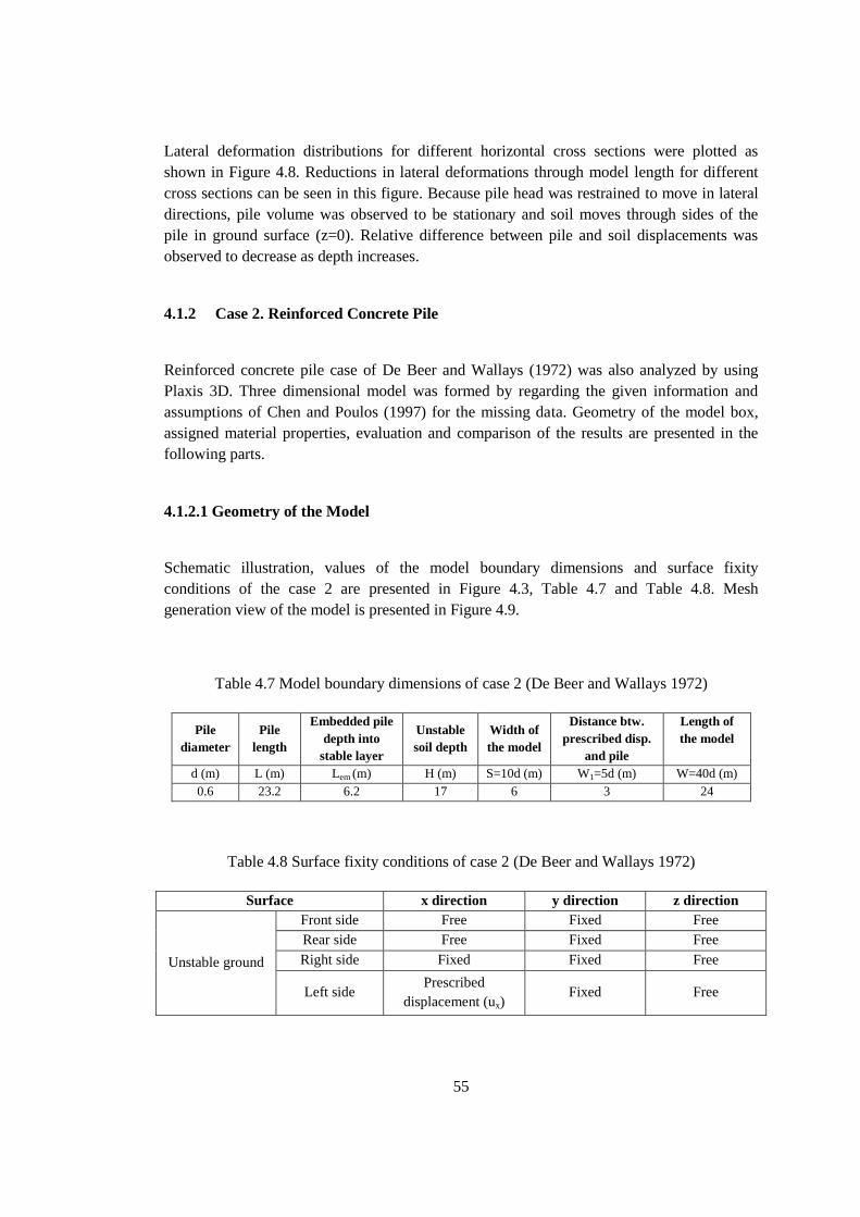
55
Lateral deformation distributions for different horizontal cross sections were plotted as
shown in Figure 4.8. Reductions in lateral deformations through model length for different
cross sections can be seen in this figure. Because pile head was restrained to move in lateral
directions, pile volume was observed to be stationary and soil moves through sides of the
pile in ground surface (z=0). Relative difference between pile and soil displacements was
observed to decrease as depth increases.
4.1.2 Case 2. Reinforced Concrete Pile
Reinforced concrete pile case of De Beer and Wallays (1972) was also analyzed by using
Plaxis 3D. Three dimensional model was formed by regarding the given information and
assumptions of Chen and Poulos (1997) for the missing data. Geometry of the model box,
assigned material properties, evaluation and comparison of the results are presented in the
following parts.
4.1.2.1 Geometry of the Model
Schematic illustration, values of the model boundary dimensions and surface fixity
conditions of the case 2 are presented in Figure 4.3, Table 4.7 and Table 4.8. Mesh
generation view of the model is presented in Figure 4.9.
Table 4.7 Model boundary dimensions of case 2 (De Beer and Wallays 1972)
Pile
diameter
Pile
length
Embedded pile
depth into
stable layer
Unstable
soil depth
Width of
the model
Distance btw.
prescribed disp.
and pile
Length of
the model
d (m) L (m) Lem (m) H (m) S=10d (m) W1=5d (m) W=40d (m)
0.6 23.2 6.2 17 6 3 24
Table 4.8 Surface fixity conditions of case 2 (De Beer and Wallays 1972)
Surface x direction y direction z direction
Unstable ground
Front side Free Fixed Free
Rear side Free Fixed Free
Right side Fixed Fixed Free
Left side Prescribed
displacement (ux) Fixed Free
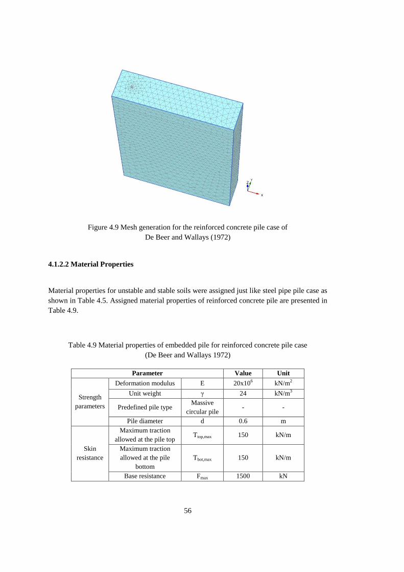
56
Figure 4.9 Mesh generation for the reinforced concrete pile case of
De Beer and Wallays (1972)
4.1.2.2 Material Properties
Material properties for unstable and stable soils were assigned just like steel pipe pile case as
shown in Table 4.5. Assigned material properties of reinforced concrete pile are presented in
Table 4.9.
Table 4.9 Material properties of embedded pile for reinforced concrete pile case
(De Beer and Wallays 1972)
Parameter Value Unit
Strength
parameters
Deformation modulus E 20x106 kN/m
2
Unit weight γ 24 kN/m3
Predefined pile type Massive
circular pile - -
Pile diameter d 0.6 m
Skin
resistance
Maximum traction
allowed at the pile top Ttop,max 150 kN/m
Maximum traction
allowed at the pile
bottom
Tbot,max 150 kN/m
Base resistance Fmax 1500 kN
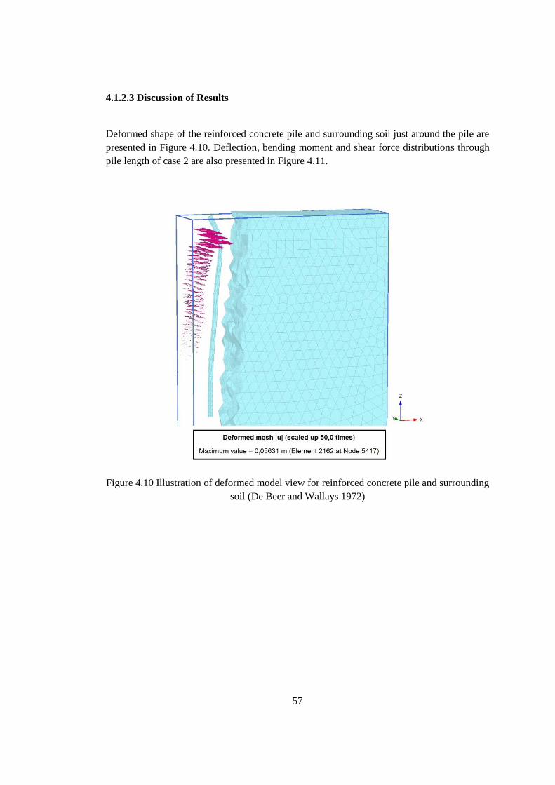
57
4.1.2.3 Discussion of Results
Deformed shape of the reinforced concrete pile and surrounding soil just around the pile are
presented in Figure 4.10. Deflection, bending moment and shear force distributions through
pile length of case 2 are also presented in Figure 4.11.
Figure 4.10 Illustration of deformed model view for reinforced concrete pile and surrounding
soil (De Beer and Wallays 1972)
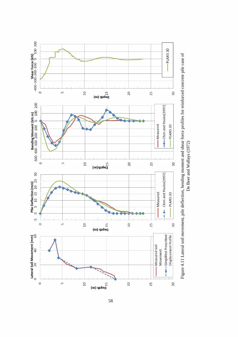
58
Fig
ure
4.1
1 L
ater
al s
oil
mo
vem
ent,
pil
e def
lect
ion,
ben
din
g m
om
ent
and s
hea
r fo
rce
pro
file
s fo
r re
info
rced
con
cret
e pil
e ca
se o
f
De
Bee
r an
d W
alla
ys
(1972)
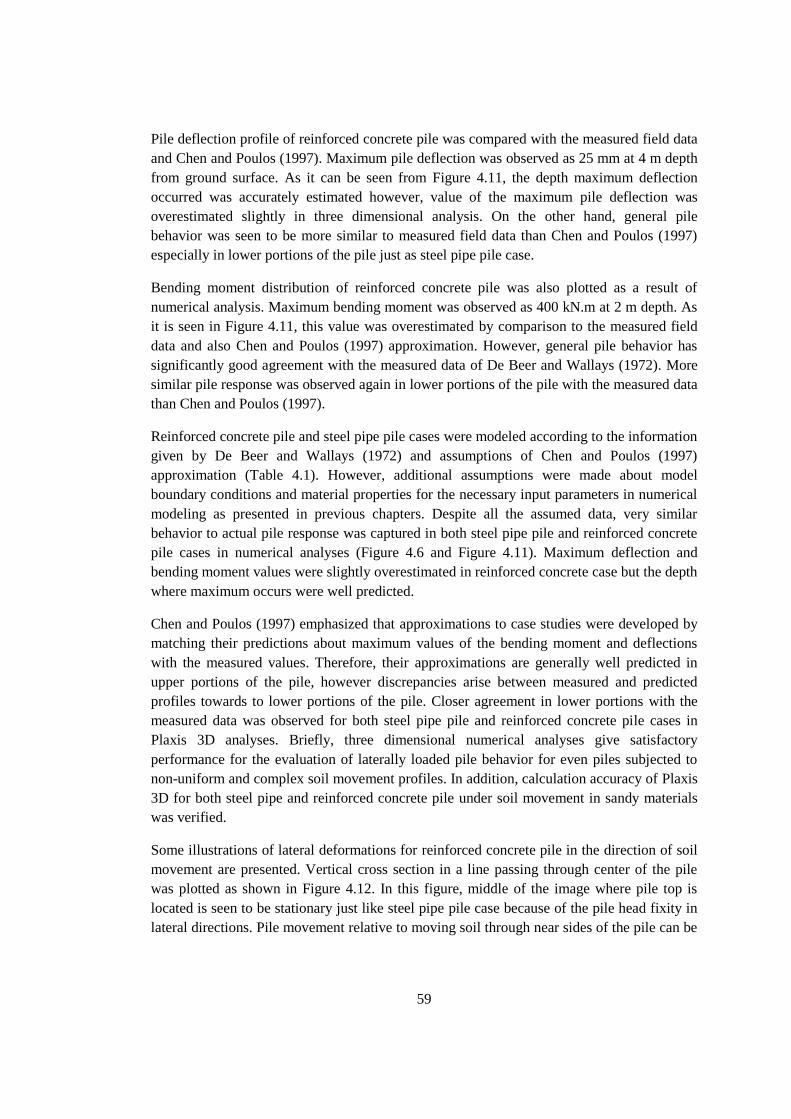
59
Pile deflection profile of reinforced concrete pile was compared with the measured field data
and Chen and Poulos (1997). Maximum pile deflection was observed as 25 mm at 4 m depth
from ground surface. As it can be seen from Figure 4.11, the depth maximum deflection
occurred was accurately estimated however, value of the maximum pile deflection was
overestimated slightly in three dimensional analysis. On the other hand, general pile
behavior was seen to be more similar to measured field data than Chen and Poulos (1997)
especially in lower portions of the pile just as steel pipe pile case.
Bending moment distribution of reinforced concrete pile was also plotted as a result of
numerical analysis. Maximum bending moment was observed as 400 kN.m at 2 m depth. As
it is seen in Figure 4.11, this value was overestimated by comparison to the measured field
data and also Chen and Poulos (1997) approximation. However, general pile behavior has
significantly good agreement with the measured data of De Beer and Wallays (1972). More
similar pile response was observed again in lower portions of the pile with the measured data
than Chen and Poulos (1997).
Reinforced concrete pile and steel pipe pile cases were modeled according to the information
given by De Beer and Wallays (1972) and assumptions of Chen and Poulos (1997)
approximation (Table 4.1). However, additional assumptions were made about model
boundary conditions and material properties for the necessary input parameters in numerical
modeling as presented in previous chapters. Despite all the assumed data, very similar
behavior to actual pile response was captured in both steel pipe pile and reinforced concrete
pile cases in numerical analyses (Figure 4.6 and Figure 4.11). Maximum deflection and
bending moment values were slightly overestimated in reinforced concrete case but the depth
where maximum occurs were well predicted.
Chen and Poulos (1997) emphasized that approximations to case studies were developed by
matching their predictions about maximum values of the bending moment and deflections
with the measured values. Therefore, their approximations are generally well predicted in
upper portions of the pile, however discrepancies arise between measured and predicted
profiles towards to lower portions of the pile. Closer agreement in lower portions with the
measured data was observed for both steel pipe pile and reinforced concrete pile cases in
Plaxis 3D analyses. Briefly, three dimensional numerical analyses give satisfactory
performance for the evaluation of laterally loaded pile behavior for even piles subjected to
non-uniform and complex soil movement profiles. In addition, calculation accuracy of Plaxis
3D for both steel pipe and reinforced concrete pile under soil movement in sandy materials
was verified.
Some illustrations of lateral deformations for reinforced concrete pile in the direction of soil
movement are presented. Vertical cross section in a line passing through center of the pile
was plotted as shown in Figure 4.12. In this figure, middle of the image where pile top is
located is seen to be stationary just like steel pipe pile case because of the pile head fixity in
lateral directions. Pile movement relative to moving soil through near sides of the pile can be
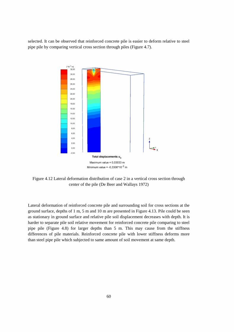
60
selected. It can be observed that reinforced concrete pile is easier to deform relative to steel
pipe pile by comparing vertical cross section through piles (Figure 4.7).
Figure 4.12 Lateral deformation distribution of case 2 in a vertical cross section through
center of the pile (De Beer and Wallays 1972)
Lateral deformation of reinforced concrete pile and surrounding soil for cross sections at the
ground surface, depths of 1 m, 5 m and 10 m are presented in Figure 4.13. Pile could be seen
as stationary in ground surface and relative pile soil displacement decreases with depth. It is
harder to separate pile soil relative movement for reinforced concrete pile comparing to steel
pipe pile (Figure 4.8) for larger depths than 5 m. This may cause from the stiffness
differences of pile materials. Reinforced concrete pile with lower stiffness deforms more
than steel pipe pile which subjected to same amount of soil movement at same depth.
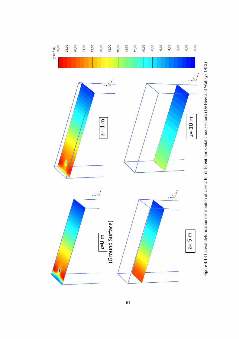
61
Fig
ure
4.1
3 L
ater
al d
eform
atio
n d
istr
ibuti
on o
f ca
se 2
for
dif
fere
nt
hori
zonta
l cr
oss
sec
tio
ns
(De
Bee
r an
d W
alla
ys
19
72
)
62
4.2 Esu and D’Elia (1974)
A field case was reported by Esu and D’Elia (1974) in which a free head reinforced concrete
pile was placed in a sliding slope. The test pile was 30 m in length, 0.79 m in diameter and
had a flexural rigidity (EpIp) of 360 MNm2. Lateral soil movement was reported to take place
in upper 7.5 m however, soil movement distribution of unstable soil was not reported. There
is not much information given about the stiffness properties of the soil profile however, it
was considered to consist mainly from cohesive type of soil materials. Inclinometer
measurements were taken from inside of the pile at the center through pile length to obtain
deflections and rotations. In addition, pile was instrumented with pressure cells at the depth
of 5 m, 10 m and 15 m along its shaft. Bending moment and shear force distributions through
pile length were presented in the report.
Magueri and Motta (1992), Chow (1996), Chen and Poulos (1997), Cai and Ugai (2002)
investigated Esu and D’Elia (1974) field study for the verification of their proposed
methodologies. They used information given by Esu and D’Elia (1974) and made some
additional assumptions for the missing data which was required for their solution. Because
displacement profile of 7.5 m unstable soil was not reported, it was assumed differently by
researchers to match their predictions with the measured field data.
Magueri and Motta (1992) suggested that undrained shear strength (cu) of the clay in site
might be 40 kPa and yield soil pressure (pu) can be estimated as pu=3cu for the upper
unstable soil layer and pu=8cu for the lower stable soil.
Chow (1996) developed a numerical solution which models the pile using beam elements,
soil behavior with subgrade reaction solution and pile soil interaction with the theory of
elasticity. Proposed hybrid method of analysis was used for the prediction of
Esu and D’Elia (1974) case study. For the missing data, Chow (1996) used suggestion of
Magueri and Motta (1992) for the undrained shear strength (cu=40 kPa). Deformation
modulus of clay was assumed to be (Es=200cu) and constant with depth. Sliding soil
movement profile was assumed as 110 mm uniformly distributed through 7.5 m unstable soil
layer.
Chen and Poulos (1997) used simplified boundary element method to analyze case study of
Esu and D’Elia (1974). In addition, maximum bending moment and pile deflection values
were predicted by using design chart estimation. Design charts developed for linearly
increasing soil stiffness and uniform soil movement profile were used for this purpose. Chen
and Poulos (1997) used suggestion of Magueri and Motta (1992) for undrained shear
strength and yield soil pressure values. Soil deformation modulus was estimated to increase
linearly from zero at the ground surface and 16 MPa at the level of the pile base. Sliding soil
movement profile was assumed as 110 mm uniformly distributed through 7.5 m unstable soil
layer.
63
Cai and Ugai (2003) used subgrade reaction solution for the estimation of pile response for
the case study. Stiffness properties of the clay were taken same as Chow (1996) assumptions
which undrained shear strength of soil is cu=40 kPa and deformation modulus is Es=200cu.
However, lateral movement of sliding soil was considered as 137 mm at the ground surface
and 40 mm at the sliding surface (88.5 mm in average).
Information given by Esu and D’Elia (1974) about the case study and additional assumptions
of Chow (1996), Chen and Poulos (1997) and Cai and Ugai (2003) were summarized in
Table 4.10.
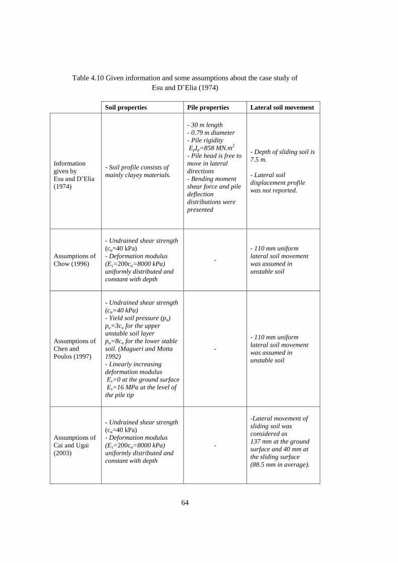
64
Table 4.10 Given information and some assumptions about the case study of
Esu and D’Elia (1974)
Soil properties Pile properties Lateral soil movement
Information
given by
Esu and D’Elia
(1974)
- Soil profile consists of
mainly clayey materials.
- 30 m length
- 0.79 m diameter
- Pile rigidity
EpIp=858 MN.m2
- Pile head is free to
move in lateral
directions
- Bending moment
shear force and pile
deflection
distributions were
presented
- Depth of sliding soil is
7.5 m.
- Lateral soil
displacement profile
was not reported.
Assumptions of
Chow (1996)
- Undrained shear strength
(cu=40 kPa)
- Deformation modulus
(Es=200cu=8000 kPa)
uniformly distributed and
constant with depth
-
- 110 mm uniform
lateral soil movement
was assumed in
unstable soil
Assumptions of
Chen and
Poulos (1997)
- Undrained shear strength
(cu=40 kPa)
- Yield soil pressure (pu)
pu=3cu for the upper
unstable soil layer
pu=8cu for the lower stable
soil. (Magueri and Motta
1992)
- Linearly increasing
deformation modulus
Es=0 at the ground surface
Es=16 MPa at the level of
the pile tip
-
- 110 mm uniform
lateral soil movement
was assumed in
unstable soil
Assumptions of
Cai and Ugai
(2003)
- Undrained shear strength
(cu=40 kPa)
- Deformation modulus
(Es=200cu=8000 kPa)
uniformly distributed and
constant with depth
-
-Lateral movement of
sliding soil was
considered as
137 mm at the ground
surface and 40 mm at
the sliding surface
(88.5 mm in average).
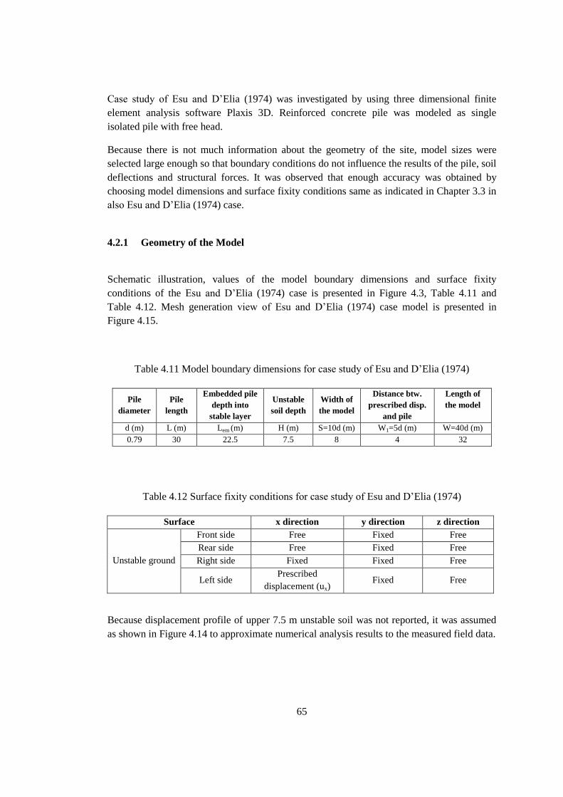
65
Case study of Esu and D’Elia (1974) was investigated by using three dimensional finite
element analysis software Plaxis 3D. Reinforced concrete pile was modeled as single
isolated pile with free head.
Because there is not much information about the geometry of the site, model sizes were
selected large enough so that boundary conditions do not influence the results of the pile, soil
deflections and structural forces. It was observed that enough accuracy was obtained by
choosing model dimensions and surface fixity conditions same as indicated in Chapter 3.3 in
also Esu and D’Elia (1974) case.
4.2.1 Geometry of the Model
Schematic illustration, values of the model boundary dimensions and surface fixity
conditions of the Esu and D’Elia (1974) case is presented in Figure 4.3, Table 4.11 and
Table 4.12. Mesh generation view of Esu and D’Elia (1974) case model is presented in
Figure 4.15.
Table 4.11 Model boundary dimensions for case study of Esu and D’Elia (1974)
Pile
diameter
Pile
length
Embedded pile
depth into
stable layer
Unstable
soil depth
Width of
the model
Distance btw.
prescribed disp.
and pile
Length of
the model
d (m) L (m) Lem (m) H (m) S=10d (m) W1=5d (m) W=40d (m)
0.79 30 22.5 7.5 8 4 32
Table 4.12 Surface fixity conditions for case study of Esu and D’Elia (1974)
Surface x direction y direction z direction
Unstable ground
Front side Free Fixed Free
Rear side Free Fixed Free
Right side Fixed Fixed Free
Left side Prescribed
displacement (ux) Fixed Free
Because displacement profile of upper 7.5 m unstable soil was not reported, it was assumed
as shown in Figure 4.14 to approximate numerical analysis results to the measured field data.
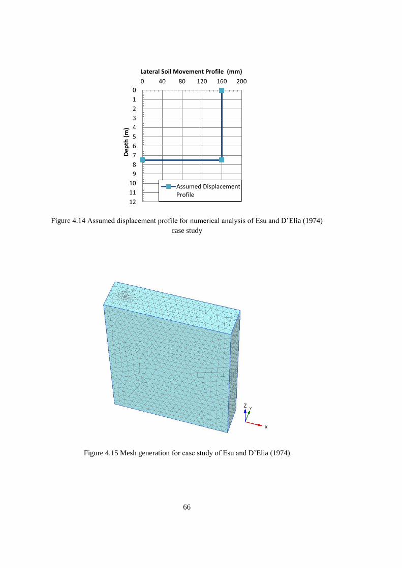
66
Figure 4.14 Assumed displacement profile for numerical analysis of Esu and D’Elia (1974)
case study
Figure 4.15 Mesh generation for case study of Esu and D’Elia (1974)
0
1
2
3
4
5
6
7
8
9
10
11
12
0 40 80 120 160 200
De
pth
(m
)
Lateral Soil Movement Profile (mm)
Assumed DisplacementProfile
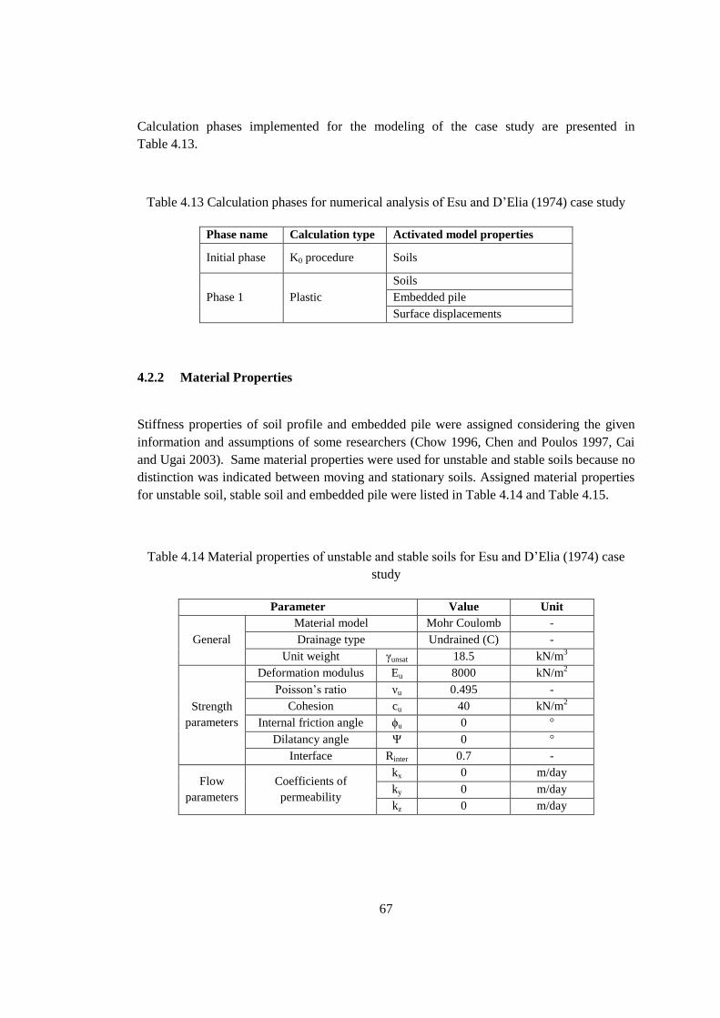
67
Calculation phases implemented for the modeling of the case study are presented in
Table 4.13.
Table 4.13 Calculation phases for numerical analysis of Esu and D’Elia (1974) case study
Phase name Calculation type Activated model properties
Initial phase K0 procedure Soils
Phase 1 Plastic
Soils
Embedded pile
Surface displacements
4.2.2 Material Properties
Stiffness properties of soil profile and embedded pile were assigned considering the given
information and assumptions of some researchers (Chow 1996, Chen and Poulos 1997, Cai
and Ugai 2003). Same material properties were used for unstable and stable soils because no
distinction was indicated between moving and stationary soils. Assigned material properties
for unstable soil, stable soil and embedded pile were listed in Table 4.14 and Table 4.15.
Table 4.14 Material properties of unstable and stable soils for Esu and D’Elia (1974) case
study
Parameter Value Unit
General
Material model Mohr Coulomb -
Drainage type Undrained (C) -
Unit weight γunsat 18.5 kN/m3
Strength
parameters
Deformation modulus Eu 8000 kN/m2
Poisson’s ratio νu 0.495 -
Cohesion cu 40 kN/m2
Internal friction angle ϕu 0 °
Dilatancy angle Ψ 0 °
Interface Rinter 0.7 -
Flow
parameters
Coefficients of
permeability
kx 0 m/day
ky 0 m/day
kz 0 m/day
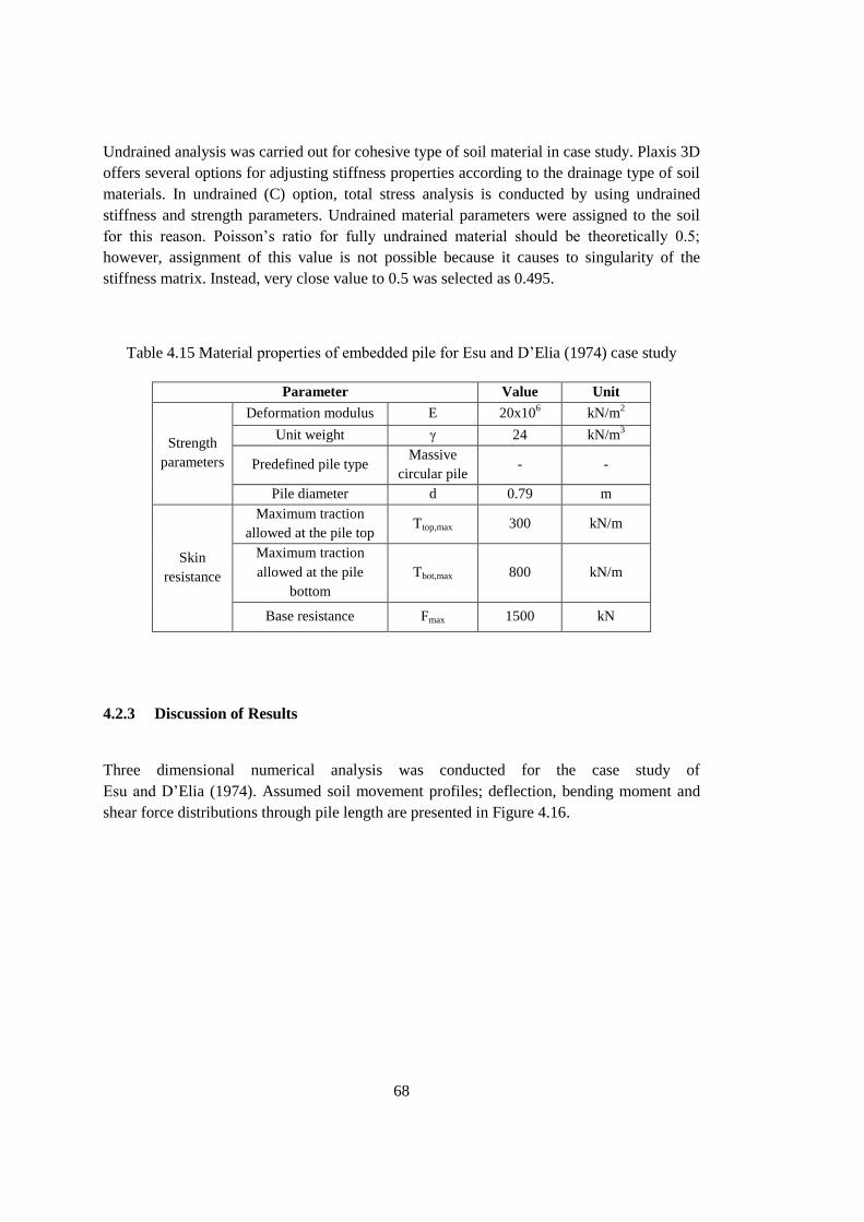
68
Undrained analysis was carried out for cohesive type of soil material in case study. Plaxis 3D
offers several options for adjusting stiffness properties according to the drainage type of soil
materials. In undrained (C) option, total stress analysis is conducted by using undrained
stiffness and strength parameters. Undrained material parameters were assigned to the soil
for this reason. Poisson’s ratio for fully undrained material should be theoretically 0.5;
however, assignment of this value is not possible because it causes to singularity of the
stiffness matrix. Instead, very close value to 0.5 was selected as 0.495.
Table 4.15 Material properties of embedded pile for Esu and D’Elia (1974) case study
Parameter Value Unit
Strength
parameters
Deformation modulus E 20x106 kN/m
2
Unit weight γ 24 kN/m3
Predefined pile type Massive
circular pile - -
Pile diameter d 0.79 m
Skin
resistance
Maximum traction
allowed at the pile top Ttop,max 300 kN/m
Maximum traction
allowed at the pile
bottom
Tbot,max 800 kN/m
Base resistance Fmax 1500 kN
4.2.3 Discussion of Results
Three dimensional numerical analysis was conducted for the case study of
Esu and D’Elia (1974). Assumed soil movement profiles; deflection, bending moment and
shear force distributions through pile length are presented in Figure 4.16.
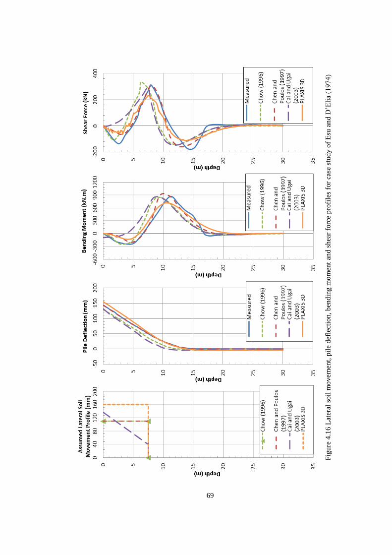
69
Fig
ure
4.1
6 L
ater
al s
oil
mo
vem
ent,
pil
e def
lect
ion,
ben
din
g m
om
ent
and s
hea
r fo
rce
pro
file
s fo
r ca
se s
tud
y o
f E
su a
nd
D’E
lia
(19
74)
70
Lateral soil movement profile in case study was assumed differently by several researchers
to match their predictions about pile deflections and forces with the measured field data. For
the same reason, uniform distribution of 160 mm soil displacement from ground surface
down to the sliding surface was assumed in numerical analysis. This value is higher than the
assumptions of other researchers (Chow 1996, Chen and Poulos 1997, Cai and Ugai 2003).
This indicates that higher amount of soil movement was required in numerical analysis
respect to other approaches to match the same amount of structural forces for relatively same
soil properties.
Pile deflection profile of numerical analysis was compared with the measured field data and
other approximations. Maximum pile deflection was observed around 150 mm at the ground
surface. This value is very similar to the measured field data (Figure 4.16).
Bending moment distribution of case study as a result of numerical analysis was plotted with
the actual field data and other approaches. Maximum bending moment was observed as
715 kN.m at 11 m depth. As it can be seen in Figure 4.16, maximum value was
underestimated by 15 %; however, the depth where maximum bending moment occurred
was accurately predicted. In addition, general bending moment distribution through pile
length shows good agreement with the measured field data.
Shear force distribution acting on the pile shaft is also presented in Figure 4.16. The depth
maximum shear force developed was well predicted as 7.5 m; however, value of the
maximum was underestimated by 20 %. Maximum shear force was observed as 235 kN at
the level of sliding surface.
Distribution of lateral deformations in the direction of soil movement is presented for the
case study. Deformation distributions for different horizontal cross sections were plotted in
Figure 4.17. Vertical cross section in a line passing through center of the pile was plotted as
shown in Figure 4.18.
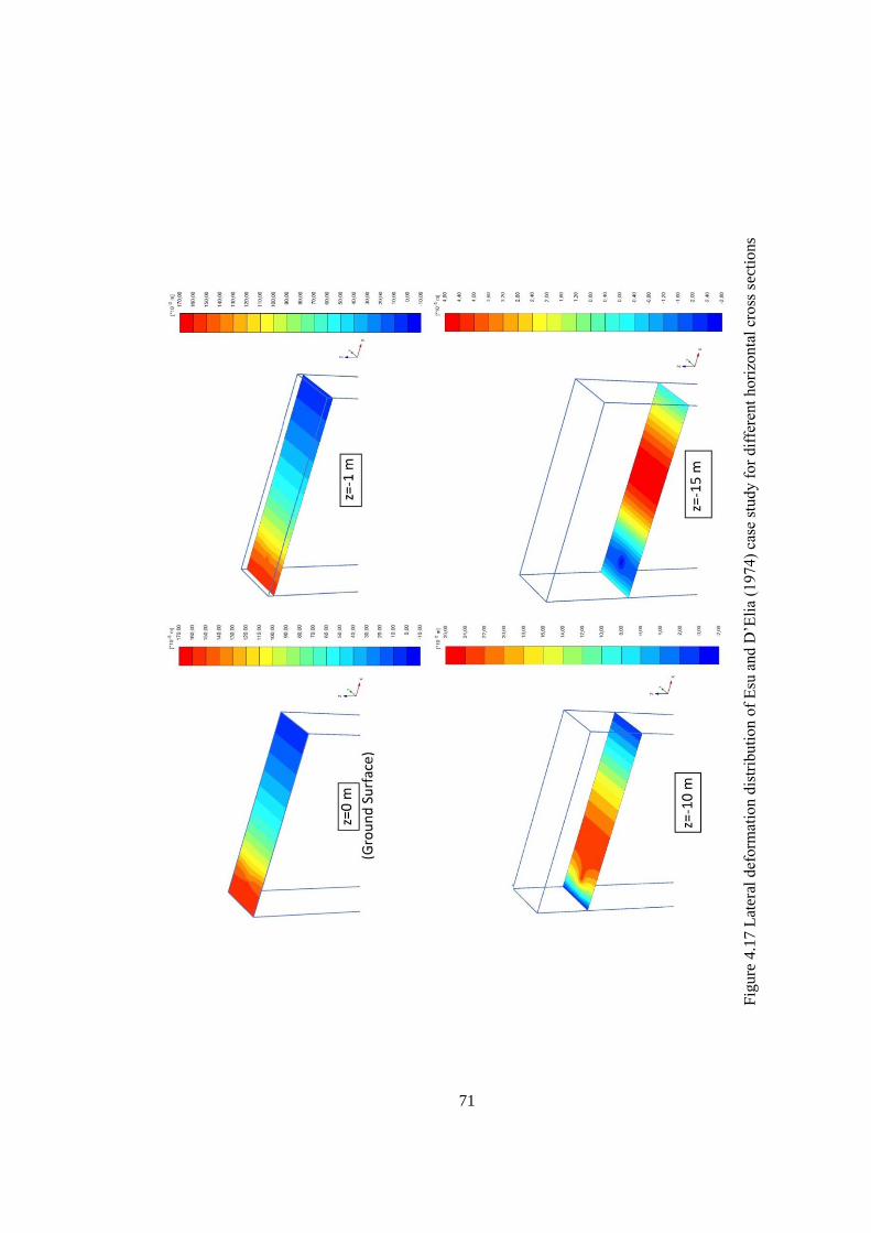
71
Fig
ure
4.1
7 L
ater
al d
eform
atio
n d
istr
ibuti
on o
f E
su a
nd D
’Eli
a (1
974)
case
stu
dy f
or
dif
fere
nt
ho
rizo
nta
l cr
oss
sec
tio
ns
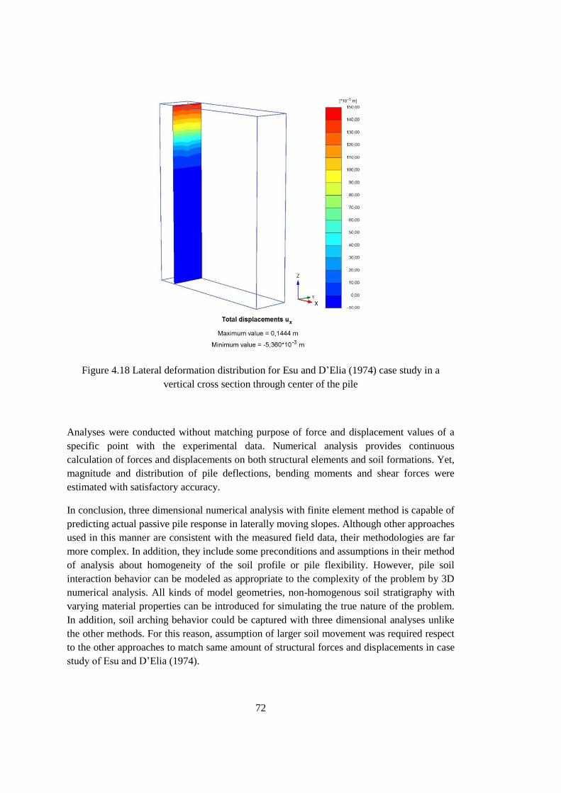
72
Figure 4.18 Lateral deformation distribution for Esu and D’Elia (1974) case study in a
vertical cross section through center of the pile
Analyses were conducted without matching purpose of force and displacement values of a
specific point with the experimental data. Numerical analysis provides continuous
calculation of forces and displacements on both structural elements and soil formations. Yet,
magnitude and distribution of pile deflections, bending moments and shear forces were
estimated with satisfactory accuracy.
In conclusion, three dimensional numerical analysis with finite element method is capable of
predicting actual passive pile response in laterally moving slopes. Although other approaches
used in this manner are consistent with the measured field data, their methodologies are far
more complex. In addition, they include some preconditions and assumptions in their method
of analysis about homogeneity of the soil profile or pile flexibility. However, pile soil
interaction behavior can be modeled as appropriate to the complexity of the problem by 3D
numerical analysis. All kinds of model geometries, non-homogenous soil stratigraphy with
varying material properties can be introduced for simulating the true nature of the problem.
In addition, soil arching behavior could be captured with three dimensional analyses unlike
the other methods. For this reason, assumption of larger soil movement was required respect
to the other approaches to match same amount of structural forces and displacements in case
study of Esu and D’Elia (1974).
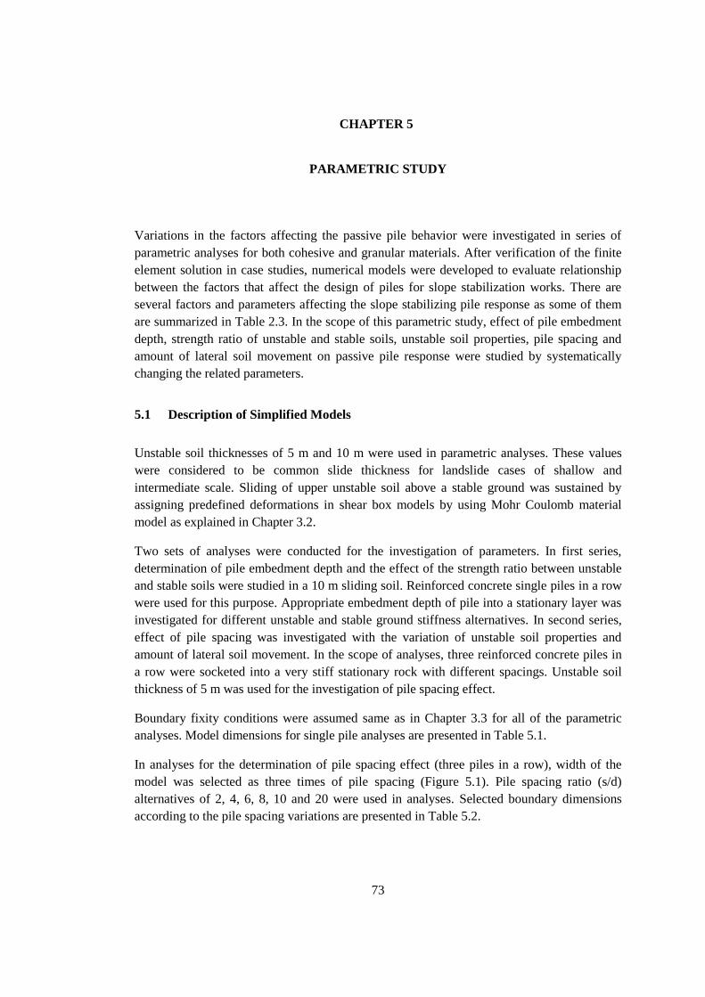
73
CHAPTER 5
PARAMETRIC STUDY
Variations in the factors affecting the passive pile behavior were investigated in series of
parametric analyses for both cohesive and granular materials. After verification of the finite
element solution in case studies, numerical models were developed to evaluate relationship
between the factors that affect the design of piles for slope stabilization works. There are
several factors and parameters affecting the slope stabilizing pile response as some of them
are summarized in Table 2.3. In the scope of this parametric study, effect of pile embedment
depth, strength ratio of unstable and stable soils, unstable soil properties, pile spacing and
amount of lateral soil movement on passive pile response were studied by systematically
changing the related parameters.
5.1 Description of Simplified Models
Unstable soil thicknesses of 5 m and 10 m were used in parametric analyses. These values
were considered to be common slide thickness for landslide cases of shallow and
intermediate scale. Sliding of upper unstable soil above a stable ground was sustained by
assigning predefined deformations in shear box models by using Mohr Coulomb material
model as explained in Chapter 3.2.
Two sets of analyses were conducted for the investigation of parameters. In first series,
determination of pile embedment depth and the effect of the strength ratio between unstable
and stable soils were studied in a 10 m sliding soil. Reinforced concrete single piles in a row
were used for this purpose. Appropriate embedment depth of pile into a stationary layer was
investigated for different unstable and stable ground stiffness alternatives. In second series,
effect of pile spacing was investigated with the variation of unstable soil properties and
amount of lateral soil movement. In the scope of analyses, three reinforced concrete piles in
a row were socketed into a very stiff stationary rock with different spacings. Unstable soil
thickness of 5 m was used for the investigation of pile spacing effect.
Boundary fixity conditions were assumed same as in Chapter 3.3 for all of the parametric
analyses. Model dimensions for single pile analyses are presented in Table 5.1.
In analyses for the determination of pile spacing effect (three piles in a row), width of the
model was selected as three times of pile spacing (Figure 5.1). Pile spacing ratio (s/d)
alternatives of 2, 4, 6, 8, 10 and 20 were used in analyses. Selected boundary dimensions
according to the pile spacing variations are presented in Table 5.2.
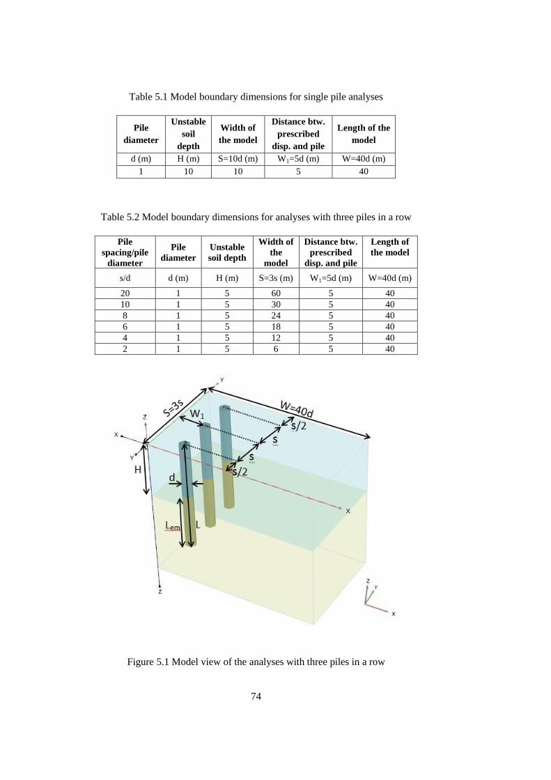
74
Table 5.1 Model boundary dimensions for single pile analyses
Pile
diameter
Unstable
soil
depth
Width of
the model
Distance btw.
prescribed
disp. and pile
Length of the
model
d (m) H (m) S=10d (m) W1=5d (m) W=40d (m)
1 10 10 5 40
Table 5.2 Model boundary dimensions for analyses with three piles in a row
Pile
spacing/pile
diameter
Pile
diameter
Unstable
soil depth
Width of
the
model
Distance btw.
prescribed
disp. and pile
Length of
the model
s/d d (m) H (m) S=3s (m) W1=5d (m) W=40d (m)
20 1 5 60 5 40
10 1 5 30 5 40
8 1 5 24 5 40
6 1 5 18 5 40
4 1 5 12 5 40
2 1 5 6 5 40
Figure 5.1 Model view of the analyses with three piles in a row
75
Medium type of mesh was selected for general mesh element size in all analyses. 6 edged
cylindrical soil volume having the same properties with the surrounding ground was defined
also in parametric analyses (Figure 5.1). Local fineness just around the embedded piles was
obtained in this way.
5.2 Material Properties
Cohesive and granular type of soil materials were studied in parametric models as unstable
and stable soils. Determination of appropriate pile embedment depth mainly depends on the
strength ratio between stable and unstable soils. Therefore, stable soil parameters were
selected as the strength of the stable layer would be the positive multitudes of the unstable
soil strength. Because strength ratio can be defined as undrained shear strength ratios of
stable and unstable soils for cohesive materials (Equation 5.1), undrained behavior of soft,
medium and stiff clayey soils was investigated as sliding material for simplicity in pile
embedment depth analyses.
Ultimate soil pressures for undrained cohesive materials are expressed in terms of undrained
shear strength of that soil such as Pu=Np.cu where Np is a dimensionless coefficient.
Therefore definition of strength ratio indicates ultimate soil pressure ratios of related soils as
well.
Strength ratios of 1, 3 and 5 were considered in analyses for the determination of stable soil
strength parameters for soft, medium and stiff clay type of unstable soils. Material properties
of unstable ground for the determination of pile embedment depth are presented in Table 5.3.
Drained analyses of granular materials were conducted for both sliding and stable layers in
pile spacing analyses. Three piles in a row with different pile spacings were embedded in a
very stiff rock. Unstable cohesionless materials of loose silty sand and dense sand having a
sliding thickness of 5 m were selected for investigation. Thus, clear visualization of relative
pile soil displacement was obtained that is required for the evaluation of soil arching.
Material properties of unstable and stable soils for pile spacing analyses are presented in
Table 5.4.
Same pile properties were used in all of the analyses as presented in Table 5.5.
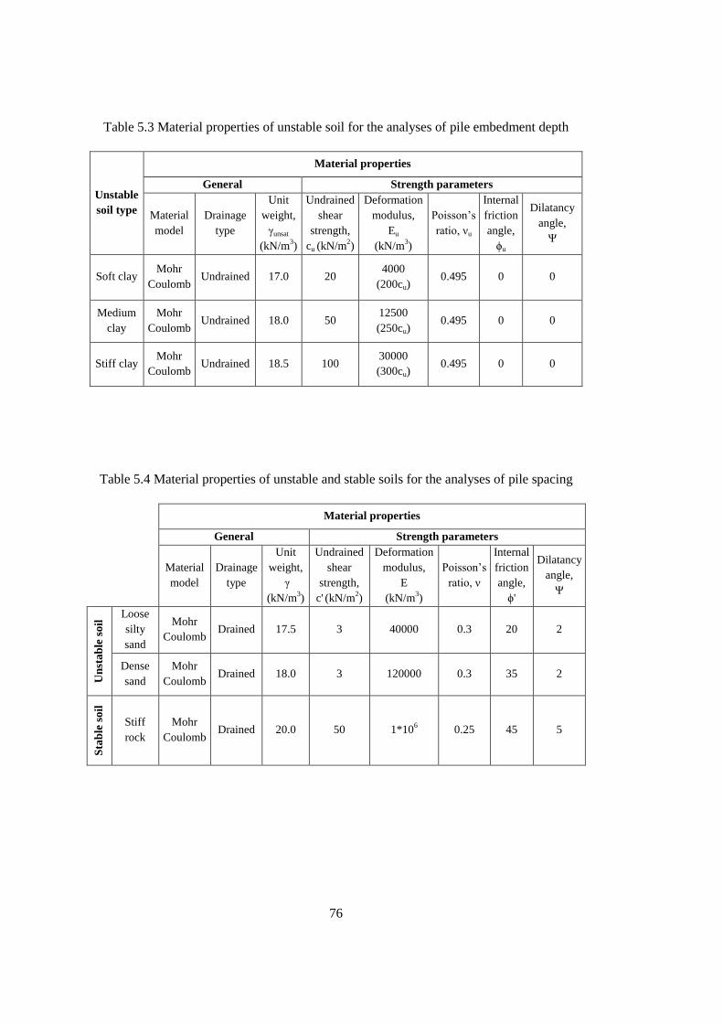
76
Table 5.3 Material properties of unstable soil for the analyses of pile embedment depth
Unstable
soil type
Material properties
General Strength parameters
Material
model
Drainage
type
Unit
weight,
γunsat
(kN/m3)
Undrained
shear
strength,
cu (kN/m2)
Deformation
modulus,
Eu
(kN/m3)
Poisson’s
ratio, νu
Internal
friction
angle,
ϕu
Dilatancy
angle,
Ψ
Soft clay Mohr
Coulomb Undrained 17.0 20
4000
(200cu) 0.495 0 0
Medium
clay
Mohr
Coulomb Undrained 18.0 50
12500
(250cu) 0.495 0 0
Stiff clay Mohr
Coulomb Undrained 18.5 100
30000
(300cu) 0.495 0 0
Table 5.4 Material properties of unstable and stable soils for the analyses of pile spacing
Material properties
General Strength parameters
Material
model
Drainage
type
Unit
weight,
γ
(kN/m3)
Undrained
shear
strength,
c' (kN/m2)
Deformation
modulus,
E
(kN/m3)
Poisson’s
ratio, ν
Internal
friction
angle,
ϕ'
Dilatancy
angle,
Ψ
Un
sta
ble
so
il Loose
silty
sand
Mohr
Coulomb Drained 17.5 3 40000 0.3 20 2
Dense
sand
Mohr
Coulomb Drained 18.0 3 120000 0.3 35 2
Sta
ble
so
il
Stiff
rock
Mohr
Coulomb Drained 20.0 50 1*10
6 0.25 45 5
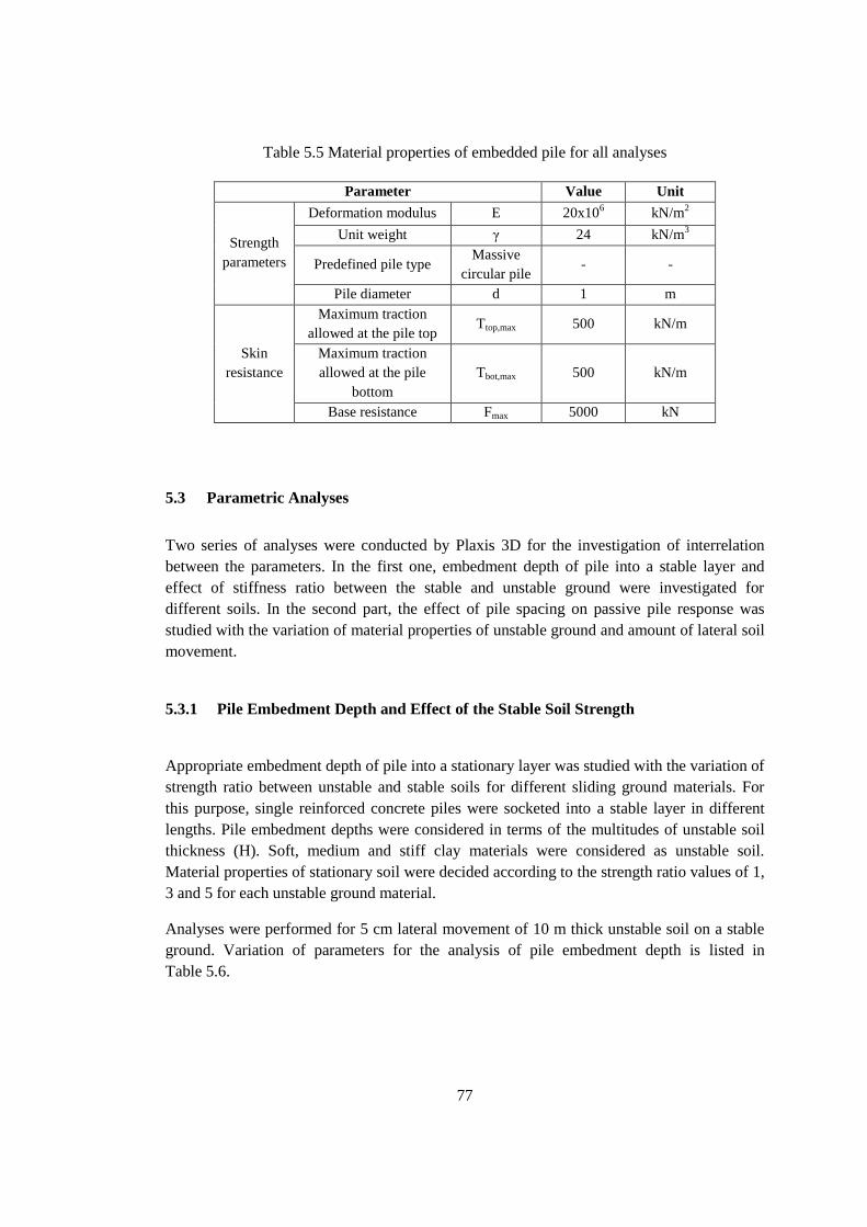
77
Table 5.5 Material properties of embedded pile for all analyses
Parameter Value Unit
Strength
parameters
Deformation modulus E 20x106 kN/m
2
Unit weight γ 24 kN/m3
Predefined pile type Massive
circular pile - -
Pile diameter d 1 m
Skin
resistance
Maximum traction
allowed at the pile top Ttop,max 500 kN/m
Maximum traction
allowed at the pile
bottom
Tbot,max 500 kN/m
Base resistance Fmax 5000 kN
5.3 Parametric Analyses
Two series of analyses were conducted by Plaxis 3D for the investigation of interrelation
between the parameters. In the first one, embedment depth of pile into a stable layer and
effect of stiffness ratio between the stable and unstable ground were investigated for
different soils. In the second part, the effect of pile spacing on passive pile response was
studied with the variation of material properties of unstable ground and amount of lateral soil
movement.
5.3.1 Pile Embedment Depth and Effect of the Stable Soil Strength
Appropriate embedment depth of pile into a stationary layer was studied with the variation of
strength ratio between unstable and stable soils for different sliding ground materials. For
this purpose, single reinforced concrete piles were socketed into a stable layer in different
lengths. Pile embedment depths were considered in terms of the multitudes of unstable soil
thickness (H). Soft, medium and stiff clay materials were considered as unstable soil.
Material properties of stationary soil were decided according to the strength ratio values of 1,
3 and 5 for each unstable ground material.
Analyses were performed for 5 cm lateral movement of 10 m thick unstable soil on a stable
ground. Variation of parameters for the analysis of pile embedment depth is listed in
Table 5.6.
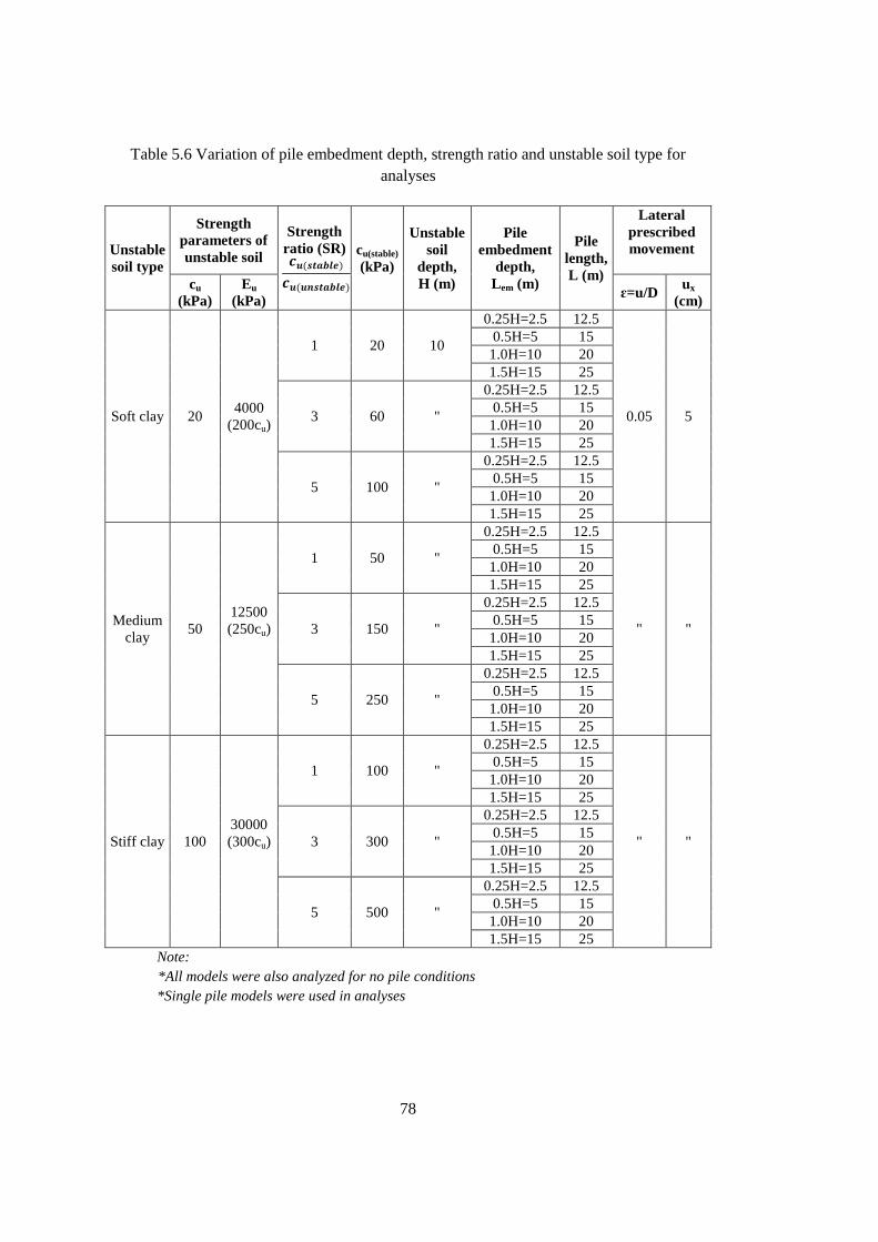
78
Table 5.6 Variation of pile embedment depth, strength ratio and unstable soil type for
analyses
Unstable
soil type
Strength
parameters of
unstable soil
Strength
ratio (SR)
cu(stable)
(kPa)
Unstable
soil
depth,
H (m)
Pile
embedment
depth,
Lem (m)
Pile
length,
L (m)
Lateral
prescribed
movement
cu
(kPa)
Eu
(kPa) ɛ=u/D
ux
(cm)
Soft clay 20 4000
(200cu)
1 20 10
0.25H=2.5 12.5
0.05 5
0.5H=5 15
1.0H=10 20
1.5H=15 25
3 60 "
0.25H=2.5 12.5
0.5H=5 15
1.0H=10 20
1.5H=15 25
5 100 "
0.25H=2.5 12.5
0.5H=5 15
1.0H=10 20
1.5H=15 25
Medium
clay 50
12500
(250cu)
1 50 "
0.25H=2.5 12.5
" "
0.5H=5 15
1.0H=10 20
1.5H=15 25
3 150 "
0.25H=2.5 12.5
0.5H=5 15
1.0H=10 20
1.5H=15 25
5 250 "
0.25H=2.5 12.5
0.5H=5 15
1.0H=10 20
1.5H=15 25
Stiff clay 100
30000
(300cu)
1 100 "
0.25H=2.5 12.5
" "
0.5H=5 15
1.0H=10 20
1.5H=15 25
3 300 "
0.25H=2.5 12.5
0.5H=5 15
1.0H=10 20
1.5H=15 25
5 500 "
0.25H=2.5 12.5
0.5H=5 15
1.0H=10 20
1.5H=15 25
Note:
*All models were also analyzed for no pile conditions
*Single pile models were used in analyses

79
Analyses for the investigation of sufficient embedment depth were conducted for 5 cm
lateral movement of unstable soil material as explained before (Table 5.6). This value was
chosen because resultant bending moment and forces occurred in the pile shaft should not
reach or exceed the ultimate pile capacity values in practical slope stabilization works.
Additionally, further analyses concluded that different lateral movement values cause
variations in bending moment and shear force results; however, it does not create significant
influence on the required embedment depth evaluation without exceeding pile capacities.
Shear force, bending moment, horizontal deflection values and distributions through pile
shaft were evaluated for the analyses which parameter variations are shown in Table 5.6.
Maximum shear force values for different unstable soil materials and strength ratio values
are presented in Figure 5.2. Bending moment distributions for soft medium and stiff type of
unstable soils are presented in Figure 5.3, Figure 5.4 and Figure 5.5. Pile deflection profiles
for unstable soil of medium clay are presented in Figure 5.6.

80
Figure 5.2 Maximum shear force developed in pile shaft for soft, medium, stiff clay type of
unstable soils and strength ratio variations of 1, 3, 5
(lateral soil movement, ux=5 cm; unstable soil thickness H=10 m)
0
100
200
300
400
500
600
700
800
0 1 2 3 4 5 6
Max
imu
m S
he
ar F
orc
e (
KN
)
Strength Ratio (Stable soil cu/Unstable soil cu)
Soft Clay Lem=0.25H Medium Clay Lem=0.25H Stiff Clay Lem=0.25H
Soft Clay Lem=0.5H Medium Clay Lem=0.5H Stiff Clay Lem=0.5H
Soft Clay Lem=1.0 H Medium Clay Lem=1.0H Stiff Clay Lem=1.0H
Soft Clay Lem=1.5H Medium Clay Lem=1.5H Stiff Clay Lem=1.5H
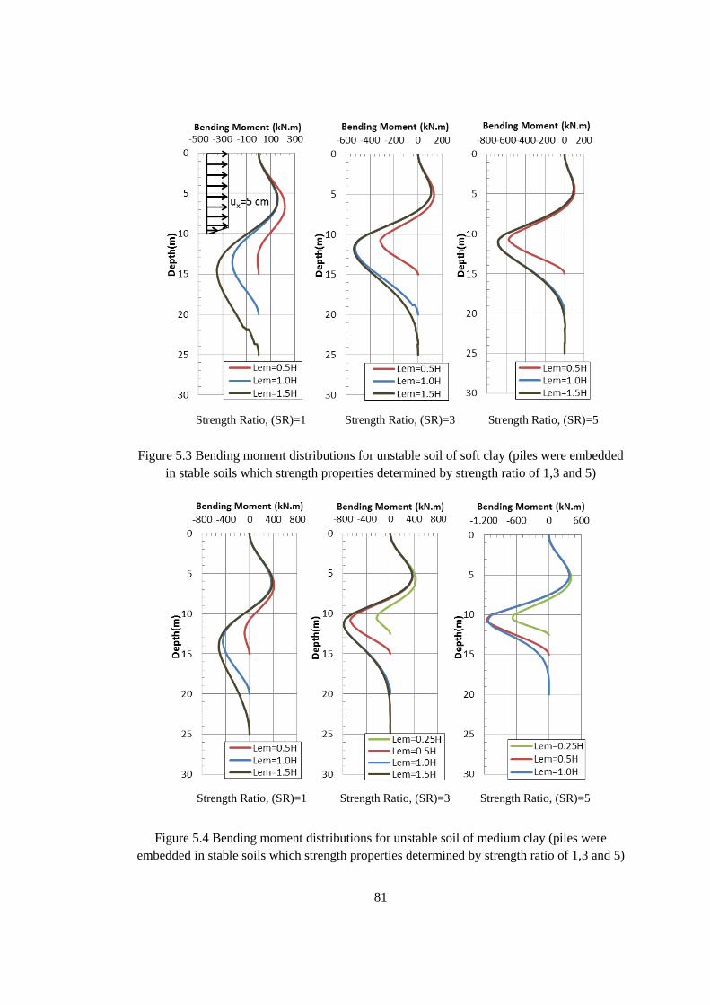
81
Figure 5.3 Bending moment distributions for unstable soil of soft clay (piles were embedded
in stable soils which strength properties determined by strength ratio of 1,3 and 5)
Figure 5.4 Bending moment distributions for unstable soil of medium clay (piles were
embedded in stable soils which strength properties determined by strength ratio of 1,3 and 5)
Strength Ratio, (SR)=1 Strength Ratio, (SR)=3 Strength Ratio, (SR)=5
Strength Ratio, (SR)=1 Strength Ratio, (SR)=3 Strength Ratio, (SR)=5
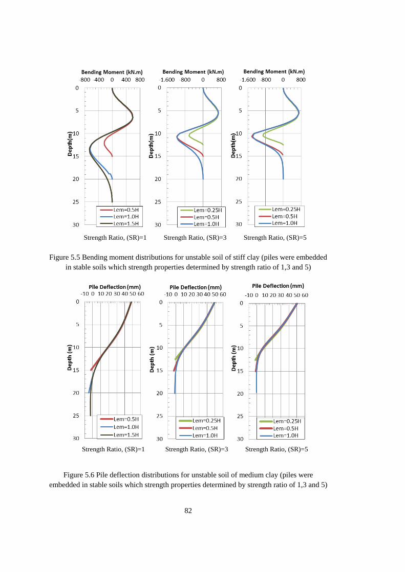
82
Figure 5.5 Bending moment distributions for unstable soil of stiff clay (piles were embedded
in stable soils which strength properties determined by strength ratio of 1,3 and 5)
Figure 5.6 Pile deflection distributions for unstable soil of medium clay (piles were
embedded in stable soils which strength properties determined by strength ratio of 1,3 and 5)
Strength Ratio, (SR)=1 Strength Ratio, (SR)=3 Strength Ratio, (SR)=5
Strength Ratio, (SR)=1 Strength Ratio, (SR)=3 Strength Ratio, (SR)=5
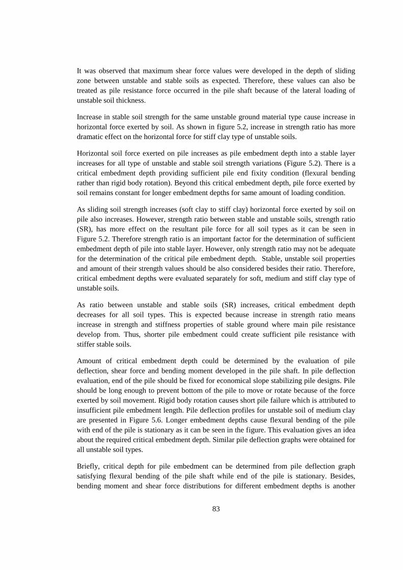
83
It was observed that maximum shear force values were developed in the depth of sliding
zone between unstable and stable soils as expected. Therefore, these values can also be
treated as pile resistance force occurred in the pile shaft because of the lateral loading of
unstable soil thickness.
Increase in stable soil strength for the same unstable ground material type cause increase in
horizontal force exerted by soil. As shown in figure 5.2, increase in strength ratio has more
dramatic effect on the horizontal force for stiff clay type of unstable soils.
Horizontal soil force exerted on pile increases as pile embedment depth into a stable layer
increases for all type of unstable and stable soil strength variations (Figure 5.2). There is a
critical embedment depth providing sufficient pile end fixity condition (flexural bending
rather than rigid body rotation). Beyond this critical embedment depth, pile force exerted by
soil remains constant for longer embedment depths for same amount of loading condition.
As sliding soil strength increases (soft clay to stiff clay) horizontal force exerted by soil on
pile also increases. However, strength ratio between stable and unstable soils, strength ratio
(SR), has more effect on the resultant pile force for all soil types as it can be seen in
Figure 5.2. Therefore strength ratio is an important factor for the determination of sufficient
embedment depth of pile into stable layer. However, only strength ratio may not be adequate
for the determination of the critical pile embedment depth. Stable, unstable soil properties
and amount of their strength values should be also considered besides their ratio. Therefore,
critical embedment depths were evaluated separately for soft, medium and stiff clay type of
unstable soils.
As ratio between unstable and stable soils (SR) increases, critical embedment depth
decreases for all soil types. This is expected because increase in strength ratio means
increase in strength and stiffness properties of stable ground where main pile resistance
develop from. Thus, shorter pile embedment could create sufficient pile resistance with
stiffer stable soils.
Amount of critical embedment depth could be determined by the evaluation of pile
deflection, shear force and bending moment developed in the pile shaft. In pile deflection
evaluation, end of the pile should be fixed for economical slope stabilizing pile designs. Pile
should be long enough to prevent bottom of the pile to move or rotate because of the force
exerted by soil movement. Rigid body rotation causes short pile failure which is attributed to
insufficient pile embedment length. Pile deflection profiles for unstable soil of medium clay
are presented in Figure 5.6. Longer embedment depths cause flexural bending of the pile
with end of the pile is stationary as it can be seen in the figure. This evaluation gives an idea
about the required critical embedment depth. Similar pile deflection graphs were obtained for
all unstable soil types.
Briefly, critical depth for pile embedment can be determined from pile deflection graph
satisfying flexural bending of the pile shaft while end of the pile is stationary. Besides,
bending moment and shear force distributions for different embedment depths is another

84
important evaluation parameter. Bending moment and shear force values reaches their
maximum at a depth near the slip plane and remains constant for longer embedment depths
than a certain critical embedment for a specific loading condition (Figure 5.3, Figure 5.4 and
Figure 5.5). Beyond this critical embedment depth longer pile embedments do not create
additional pile resistance (Figure 5.2).
Ranges of critical pile embedment for different unstable soils and stable strength variations
were determined considering above parameters. First, unstable soil of soft clay was
evaluated for different strength ratio variations (Figure 5.2 and Figure 5.3). If both unstable
and stable soil materials consists of soft clay (SR=1), embedment depth which is 1.5 times of
unstable soil thickness (Lem=1.5H) is not sufficient to create enough pile resistance and pile
fixity. Therefore, deeper pile embedments than Lem=1.5H should be applied to uniform soft
clay soil formations. In the case of SR=3 and SR=5 for unstable soft clay material, same
amount of maximum bending moment and shear force values were obtained for Lem=1.5H
and Lem=1.0H (Figure 5.2 and Figure 5.3). Differences may start to occur in values when
Lem=0.5H. Therefore, critical pile embedment should be in the range of Lem(critical)=1.0H-
0.50H. Exact value of the critical embedment depth approaches to 0.5H from 1.0H as
strength ratio gets increase (SR=3 to SR=5) for soft clay.
Ranges of critical embedment depths were also determined by using the same evaluation
method for medium and stiff clay type of unstable soil materials as shown in Table 5.7.
Table 5.7 Range of critical embedment depths for different unstable soil materials and
strength ratio variation (H=unstable soil thickness)
Strength ratio, (SR)
Unstable soil materials
Soft clay Medium clay Stiff clay
SR=1 >1.5H 1.5H-1.0H 1.0H-0.5H
SR=3 1.0H-0.5H 1.0H-0.5H 0.5H-0.25H
SR=5 1.0H-0.5H 0.5H-0.25H 0.5H-0.25H
Kourkoulis et al. (2011) found that critical embedment depth of pile into a stable layer could
be range from Lem(critical)=1.5Hu for Pu(stable)=Pu(unstable) to Lem(critical)=0.7Hu for Pu(stable)=3Pu(unstable)
where; Hu is the thickness of unstable soil layer, Pu(stable) and Pu(unstable) are ultimate passive soil
pressures provided by stable and unstable layers. Ranges of critical embedment depth for
different unstable soil materials presented in Table 5.7 show good agreement with the
findings of Kourkoulis et al. (2011).

85
5.3.2 Effect of Pile Spacing
Effect of pile spacing on pile response was evaluated by shear box models with the variation
of unstable soil properties and amount of lateral soil movement. Unstable soil thickness (H)
was selected as 5 m and analyses were conducted for three piles in a row embedded in a very
stiff rock (Table 5.2). Pile embedment depth was selected as the thickness of unstable soil
layer (Lem=H) to guarantee full pile end fixity conditions.
Drained analyses were applied for two types of granular soils namely; loose silty sand and
dense sand. Unstable soil movements of ux=5 cm and ux=10 cm were assigned for both loose
silty sand and dense sand. Pile response was evaluated for pile spacing (s/d) alternatives of 2,
4, 6, 8, 10 and 20. Variation of parameters for the analyses of pile spacing effect was
summarized in Table 5.8.
Table 5.8 Variation of the parameters for the analyses of pile spacing effect
Unstable soil
Stable soil
parameters
Unstable
soil
depth,
H (m)
Pile
embedment
depth,
Lem (m)
Pile
spacing
(s/d)
Lateral
prescribed
movement
Type Parameters ɛ=u/D ux
(cm)
Loose silty
sand
c’= 3 kPa
ϕ’=20°
E’=40000 kPa
Ψ=2°
c’= 50 kPa
ϕ’=45°
E’=1x10⁶ kPa
Ψ=2°
5 H=5
20 0.05 5
0.10 10
10 0.05 5
0.10 10
8 0.05 5
0.10 10
6 0.05 5
0.10 10
4 0.05 5
0.10 10
2 0.05 5
0.10 10
Dense sand
c’= 3 kPa
ϕ’=35°
E’=120000 kPa
Ψ=2°
c’= 50 kPa
ϕ’=45°
E’=1x10⁶ kPa
Ψ=2°
5 H=5
20 0.05 5
0.10 10
10 0.05 5
0.10 10
8 0.05 5
0.10 10
6 0.05 5
0.10 10
4 0.05 5
0.10 10
2 0.05 5
0.10 10
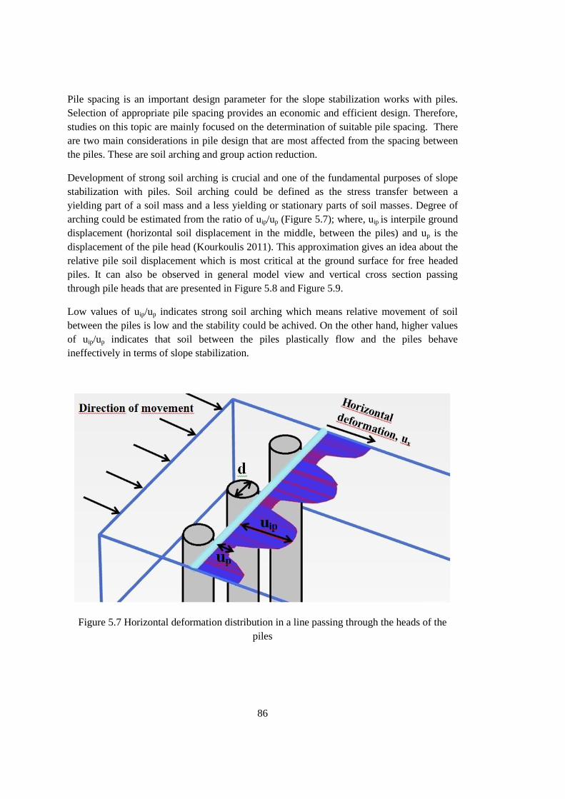
86
Pile spacing is an important design parameter for the slope stabilization works with piles.
Selection of appropriate pile spacing provides an economic and efficient design. Therefore,
studies on this topic are mainly focused on the determination of suitable pile spacing. There
are two main considerations in pile design that are most affected from the spacing between
the piles. These are soil arching and group action reduction.
Development of strong soil arching is crucial and one of the fundamental purposes of slope
stabilization with piles. Soil arching could be defined as the stress transfer between a
yielding part of a soil mass and a less yielding or stationary parts of soil masses. Degree of
arching could be estimated from the ratio of uip/up (Figure 5.7); where, uip is interpile ground
displacement (horizontal soil displacement in the middle, between the piles) and up is the
displacement of the pile head (Kourkoulis 2011). This approximation gives an idea about the
relative pile soil displacement which is most critical at the ground surface for free headed
piles. It can also be observed in general model view and vertical cross section passing
through pile heads that are presented in Figure 5.8 and Figure 5.9.
Low values of uip/up indicates strong soil arching which means relative movement of soil
between the piles is low and the stability could be achived. On the other hand, higher values
of uip/up indicates that soil between the piles plastically flow and the piles behave
ineffectively in terms of slope stabilization.
Figure 5.7 Horizontal deformation distribution in a line passing through the heads of the
piles
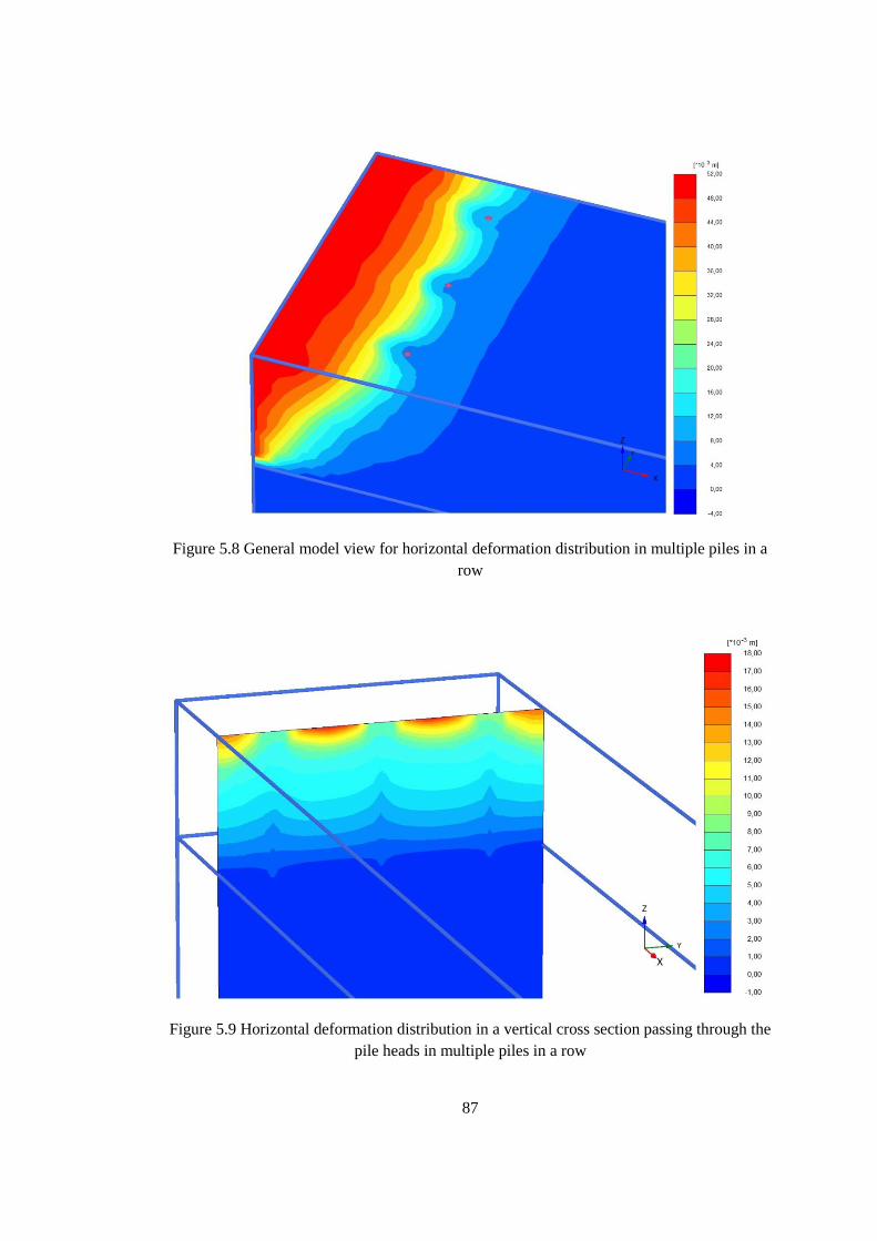
87
Figure 5.8 General model view for horizontal deformation distribution in multiple piles in a
row
Figure 5.9 Horizontal deformation distribution in a vertical cross section passing through the
pile heads in multiple piles in a row
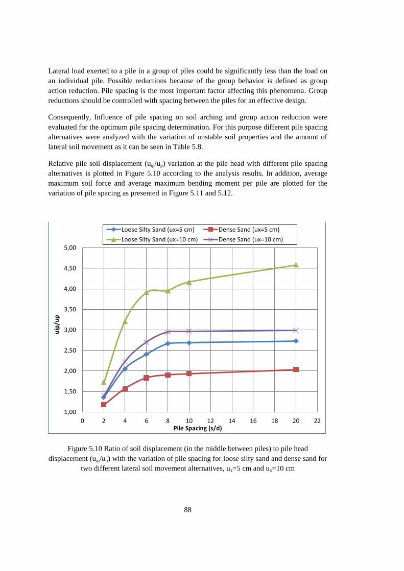
88
Lateral load exerted to a pile in a group of piles could be significantly less than the load on
an individual pile. Possible reductions because of the group behavior is defined as group
action reduction. Pile spacing is the most important factor affecting this phenomena. Group
reductions should be controlled with spacing between the piles for an effective design.
Consequently, Influence of pile spacing on soil arching and group action reduction were
evaluated for the optimum pile spacing determination. For this purpose different pile spacing
alternatives were analyzed with the variation of unstable soil properties and the amount of
lateral soil movement as it can be seen in Table 5.8.
Relative pile soil displacement (uip/up) variation at the pile head with different pile spacing
alternatives is plotted in Figure 5.10 according to the analysis results. In addition, average
maximum soil force and average maximum bending moment per pile are plotted for the
variation of pile spacing as presented in Figure 5.11 and 5.12.
Figure 5.10 Ratio of soil displacement (in the middle between piles) to pile head
displacement (uip/up) with the variation of pile spacing for loose silty sand and dense sand for
two different lateral soil movement alternatives, ux=5 cm and ux=10 cm
1,00
1,50
2,00
2,50
3,00
3,50
4,00
4,50
5,00
0 2 4 6 8 10 12 14 16 18 20 22
uip
/up
Pile Spacing (s/d)
Loose Silty Sand (ux=5 cm) Dense Sand (ux=5 cm)
Loose Silty Sand (ux=10 cm) Dense Sand (ux=10 cm)
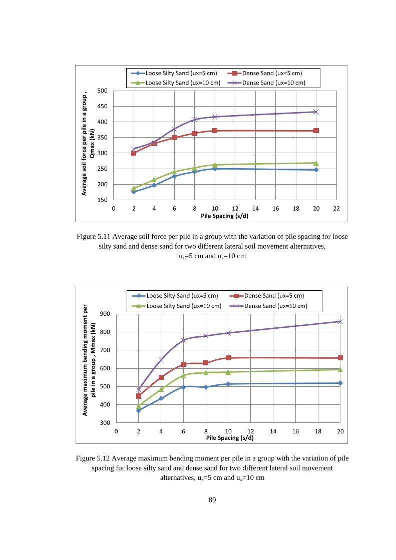
89
Figure 5.11 Average soil force per pile in a group with the variation of pile spacing for loose
silty sand and dense sand for two different lateral soil movement alternatives,
ux=5 cm and ux=10 cm
Figure 5.12 Average maximum bending moment per pile in a group with the variation of pile
spacing for loose silty sand and dense sand for two different lateral soil movement
alternatives, ux=5 cm and ux=10 cm
150
200
250
300
350
400
450
500
0 2 4 6 8 10 12 14 16 18 20 22
Ave
rage
so
il fo
rce
pe
r p
ile in
a g
rou
p ,
Qm
ax (
kN)
Pile Spacing (s/d)
Loose Silty Sand (ux=5 cm) Dense Sand (ux=5 cm)
Loose Silty Sand (ux=10 cm) Dense Sand (ux=10 cm)
300
400
500
600
700
800
900
0 2 4 6 8 10 12 14 16 18 20
Ave
rage
max
imu
m b
en
din
g m
om
en
t p
er
pile
in a
gro
up
, M
max
(kN
)
Pile Spacing (s/d)
Loose Silty Sand (ux=5 cm) Dense Sand (ux=5 cm)
Loose Silty Sand (ux=10 cm) Dense Sand (ux=10 cm)
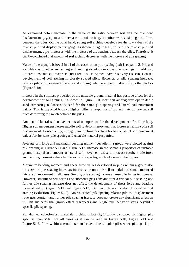
90
As explained before increase in the value of the ratio between soil and the pile head
displacement (uip/up) means decrease in soil arching. In other words, sliding soil flows
between the piles. On the other hand, strong soil arching develops for the low values of the
relative pile soil displacement (uip/up). As shown in Figure 5.10, value of the relative pile soil
displacement, uip/up increases with the increase of the spacing between the piles. Therefore, it
can be concluded that amount of soil arching decreases with the increase of pile spacing.
Value of the uip/up is below 2 in all of the cases when pile spacing (s/d) is equal to 2. Pile and
soil deforms together and strong soil arching develops in close pile spacings. In addition,
different unstable soil materials and lateral soil movement have relatively less effect on the
development of soil arching in closely spaced piles. However, as pile spacing increases
relative pile soil movement thereby soil arching gets more open to affect from other factors
(Figure 5.10).
Increase in the stiffness properties of the unstable ground material has positive effect for the
development of soil arching. As shown in Figure 5.10, more soil arching develops in dense
sand comparing to loose silty sand for the same pile spacing and lateral soil movement
values. This is expected because higher stiffness properties of ground material prevent soil
from deforming too much between the piles.
Amount of lateral soil movement is also important for the development of soil arching.
Higher soil movement causes middle soil to deform more and that increases relative pile soil
displacement. Consequently, stronger soil arching develops for lower lateral soil movement
values for the same pile spacing and unstable material properties.
Average soil force and maximum bending moment per pile in a group were plotted against
pile spacing in Figure 5.11 and Figure 5.12. Increase in the stiffness properties of unstable
ground material and amount of lateral soil movement cause to increase resultant pile force
and bending moment values for the same pile spacing as clearly seen in the figures.
Maximum bending moment and shear force values developed in piles within a group also
increases as pile spacing increases for the same unstable soil material and same amount of
lateral soil movement in all cases. Simply, pile spacing increase cause pile forces to increase.
However, amount of soil forces and moments gets constant after a critical pile spacing and
further pile spacing increase does not affect the development of shear force and bending
moment values (Figure 5.11 and Figure 5.12). Similar behavior is also observed in soil
arching evaluation (Figure 5.10). After a critical pile spacing relative pile soil displacement
ratio gets constant and further pile spacing increase does not create any significant effect on
it. This indicates that group effect disappears and single pile behavior starts beyond a
specific pile spacing.
For drained cohesionless materials, arching effect significantly decreases for higher pile
spacings than s/d=6 for all cases as it can be seen in Figure 5.10, Figure 5.11 and
Figure 5.12. Piles within a group start to behave like singular piles when pile spacing is
91
around s/d=8. However, in the case of loose silty sand with high lateral soil movement,
development of arching seems to be more problematic. Closer pile spacings should be
preferred for loose soils having relatively high lateral soil movement profile.
Variation of average pile force and maximum bending moment values with different pile
spacings were used for the evaluation of group action reduction. As pile spacing increases,
forces exerted on the piles in group also increase until a critical pile spacing ratio (≈s/d=8).
Forces are not significantly different from each other for pile spacings larger than s/d=8. In
group reduction analyses, forces and bending moments were taken as single pile values for
pile spacing ratio which is equal to s/d=20. Reduction values for each pile spacing were
calculated accordingly by Equation 5.1 and Equation 5.2.
(
)
(
)
Where;
Qsingle pile = Average pile force exerted on a singular pile (for pile spacing s/d=20)
Q = Average pile force for related pile spacing ratio
Msingle pile= Maximum bending moment exerted on a singular pile (for pile spacing s/d=20)
M = Maximum bending moment for related pile spacing ratio
Percent of group reduction values of different pile spacing variations for loose silty sand and
dense sand are presented in Table 5.9. Group reduction percentages for all cases and
reductions for both pile force and bending moment values are approximately consistent. It
can be seen in the table that significant group reduction starts to develop for larger pile
spacing ratios than s/d>6. As piles are closely spaced reduction percentages dramatically
increase. In average, 8 % reduction for s/d=6, 18 % reduction for s/d=4 and 31 % reduction
for s/d=2 were observed in pile forces within a group.
It can be concluded that there is an opposite relationship between soil arching and resultant
pile forces caused by the moving soil. Decrease of pile spacing ratio (s/d) causes stronger
soil arching but it also causes the development of group reduction in pile forces. Therefore,
optimum pile spacing should be selected for an economical and effective design. In drained
92
sandy materials, strong soil arching development can be observed for pile spacing ratios (s/d)
between 2 and 4 (Figure 5.10). However, reduction (≈30 %) in forces when pile spacing is
s/d=2 may significantly decrease group efficiency and also design could be uneconomical.
Even though there is an 18 % reduction in pile forces for pile spacing ratio of s/d=4,
sufficient soil arching is still sustained. Therefore, spacing ratio of s/d=4 is seem to be more
optimum value for an effective pile design. However, sliding cases having very soft unstable
soil materials or having excessive lateral soil movements should be specifically investigated
by considering soil arching and group action reduction phenomena.
Findings in this thesis study about pile spacing have good agreement with the conclusions of
other researchers as some of them were quoted in Table 2.3 (Chen 2001, Liang and Zeng
2002, Kahyaoğlu et al. 2009, Liang and Yamin 2009, Kourkoulis et al. 2011).
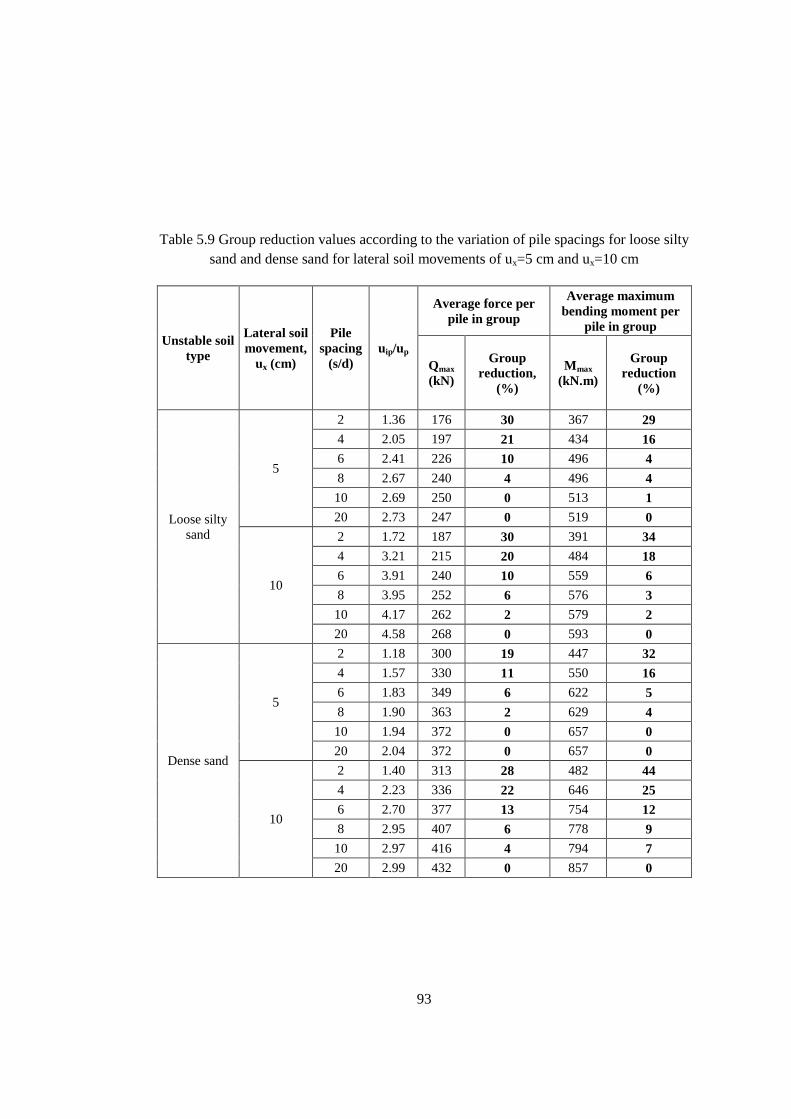
93
Table 5.9 Group reduction values according to the variation of pile spacings for loose silty
sand and dense sand for lateral soil movements of ux=5 cm and ux=10 cm
Unstable soil
type
Lateral soil
movement,
ux (cm)
Pile
spacing
(s/d)
uip/up
Average force per
pile in group
Average maximum
bending moment per
pile in group
Qmax
(kN)
Group
reduction,
(%)
Mmax
(kN.m)
Group
reduction
(%)
Loose silty
sand
5
2 1.36 176 30 367 29
4 2.05 197 21 434 16
6 2.41 226 10 496 4
8 2.67 240 4 496 4
10 2.69 250 0 513 1
20 2.73 247 0 519 0
10
2 1.72 187 30 391 34
4 3.21 215 20 484 18
6 3.91 240 10 559 6
8 3.95 252 6 576 3
10 4.17 262 2 579 2
20 4.58 268 0 593 0
Dense sand
5
2 1.18 300 19 447 32
4 1.57 330 11 550 16
6 1.83 349 6 622 5
8 1.90 363 2 629 4
10 1.94 372 0 657 0
20 2.04 372 0 657 0
10
2 1.40 313 28 482 44
4 2.23 336 22 646 25
6 2.70 377 13 754 12
8 2.95 407 6 778 9
10 2.97 416 4 794 7
20 2.99 432 0 857 0

94
95
CHAPTER 6
SUMMARY AND CONCLUSIONS
6.1 Summarized Points and Conclusions
Some of the important results and conclusions of this study are given below:
1) Three dimensional finite element solution for laterally loaded passive piles: selection
of the geometry/dimensions, boundary conditions and mesh size
Three dimensional shear box models were used for the simulation of laterally loaded passive
pile behavior. Proposed methodology provided more efficient use of calculation time in
hundreds of analyses. In addition, number of variables and the effect of uncertain parameters
such as slope angle, direction and amount of ground movement, interface properties were
tried to be controlled with this way. Sliding of unstable layer was provided by using
predefined displacements on the left side surface of the box model. Piles were embedded in a
stationary layer and lateral loading of piles were sustained with this way.
Analyses results indicated that boundary sizes, surface fixities and mesh generation have
significant effect on the variation of pile forces and moments. Therefore, boundaries should
be large enough that no stress-strain distributions are affected from it. For this purpose,
boundary sizes of the models were controlled for the minimum dimensions that deflections
and forces are not affected or interrupted. Effect of mesh generation was also evaluated and
three dimensional medium type of mesh generation was seen to provide sufficient accuracy
for the scope of this study.
2) Verification of the proposed shear box models with case studies
Three case studies were analyzed to investigate calculation accuracy of three dimensional
finite element solution with shear box models. Three full scale field experiments, two of
them were reported by De Beer and Wallays (1972) and one of them by
Esu and D’Elia (1974), were used for this purpose. Steel pipe pile and reinforced concrete
pile were subjected to non-uniform lateral soil movements in drained sandy soil in De Beer
and Wallays (1972) cases. On the other hand, uniform lateral soil movement of undrained
cohesive clay was exerted to reinforced concrete pile in Esu and D’Elia (1974) case.
Analyses results show satisfactory agreement with the measured field data in pile deflection,
bending moment and shear forces of the reported cases. It was concluded that three
dimensional finite element solution with PLAXIS 3D can accurately calculate the measured
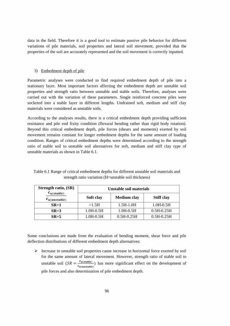
96
data in the field. Therefore it is a good tool to estimate passive pile behavior for different
variations of pile materials, soil properties and lateral soil movement, provided that the
properties of the soil are accurately represented and the soil movement is correctly inputted.
3) Embedment depth of pile
Parametric analyses were conducted to find required embedment depth of pile into a
stationary layer. Most important factors affecting the embedment depth are unstable soil
properties and strength ratio between unstable and stable soils. Therefore, analyses were
carried out with the variation of these parameters. Single reinforced concrete piles were
socketed into a stable layer in different lengths. Undrained soft, medium and stiff clay
materials were considered as unstable soils.
According to the analyses results, there is a critical embedment depth providing sufficient
resistance and pile end fixity condition (flexural bending rather than rigid body rotation).
Beyond this critical embedment depth, pile forces (shears and moments) exerted by soil
movement remains constant for longer embedment depths for the same amount of loading
condition. Ranges of critical embedment depths were determined according to the strength
ratio of stable soil to unstable soil alternatives for soft, medium and stiff clay type of
unstable materials as shown in Table 6.1.
Table 6.1 Range of critical embedment depths for different unstable soil materials and
strength ratio variation (H=unstable soil thickness)
Strength ratio, (SR)
Unstable soil materials
Soft clay Medium clay Stiff clay
SR=1 >1.5H 1.5H-1.0H 1.0H-0.5H
SR=3 1.0H-0.5H 1.0H-0.5H 0.5H-0.25H
SR=5 1.0H-0.5H 0.5H-0.25H 0.5H-0.25H
Some conclusions are made from the evaluation of bending moment, shear force and pile
deflection distributions of different embedment depth alternatives:
Increase in unstable soil properties cause increase in horizontal force exerted by soil
for the same amount of lateral movement. However, strength ratio of stable soil to
unstable soil
has more significant effect on the development of
pile forces and also determination of pile embedment depth.
97
Pile forces because of lateral soil movement increase as embedment depth increases
until a certain critical depth. Beyond this, pile forces remain constant for longer pile
embedment depths.
As strength ratio of stable soil to unstable soil (SR) increases, critical embedment
depth providing sufficient resistance for pile stability decreases for all soil types.
4) Pile spacing
Different pile spacing alternatives were analyzed with the variation of unstable soil
properties and amount of lateral soil movement to evaluate the effect of pile spacing on
passive pile response. Piles were embedded in a very stiff stationary layer with sufficient
embedment depth.
Pile spacing evaluation was made according to two main considerations in pile design that
are most affected from the spacing between piles. These are soil arching and group
reduction. Degree of arching was measured from the ratio of uip/up; where, uip is interpile
ground displacement (horizontal soil displacement in the middle, between the piles) and up is
the displacement of the pile head. This method of analysis uses the consideration of relative
pile soil displacements. Difference between pile and soil displacements was more clearly
observed in sandy materials in 3D analyses. Therefore, drained analysis of cohesionless soil
materials were used as unstable and stable soils. In addition, variation of average pile force
and maximum bending moment values with different pile spacings were used for the
evaluation of group action reduction.
Some conclusions are made from the results of analyses:
Soil arching is most critical at the ground surface for free headed piles where
maximum relative pile soil displacement occurs.
Low values of uip/up indicates strong soil arching which means relative movement of
soil between piles is low and the stability could be achived. On the other hand,
higher values of uip/up indicates that soil between piles plastically flow and piles
behave ineffectively in terms of slope stabilization.
It can be concluded that amount of soil arching decreases with the increase of pile
spacing.
Increase in the stiffness properties of the unstable ground material has positive effect
for the development of soil arching. Dense materials have more soil arching for the
same pile spacing and same lateral soil movement distribution.
98
Increase in the stiffness properties of unstable ground material and amount of lateral
soil movement cause to increase resultant pile force and bending moment values for
the same pile spacing.
For drained sandy materials, arching effect significantly decreases for higher pile
spacings than s/d=6 for all cases. Piles within a group start to behave like singular
piles when pile spacing is approximately around s/d=8.
Decrease of pile spacing ratio (s/d) causes stronger soil arching but it also causes the
development of group reduction. There is an opposite relationship between soil
arching and resultant pile forces caused by the moving soil. Therefore, optimum pile
spacing should be selected for an economical and effective design.
As piles are closely spaced reduction percentages dramatically increase. In average,
8 % reduction for s/d=6, 18 % reduction for s/d=4 and 31 % reduction for s/d=2
were observed in pile forces within a group.
Pile spacing ratio of s/d=4 is seem to be an optimum value for pile design in aspect
of soil arching and group action reduction for sandy materials.
It should be noted that elastic-perfectly plastic Mohr Coulomb failure criterion was used in
all of the analyses in this study as the material constitutive model. Although it is well known
that, the more advanced soil constitutive models can capture the nonlinear stress-strain
behavior of soils more accurately, they also require significant number of material model
parameters to be input. Therefore Mohr-Coulomb model is considered to be adequate for the
content of this parametric study.
It should also be noted that in all of the analyses in this study pile heads are free. In real
project of slope stabilization by piles, typically a pile cap can be used. Pile cap is considered
not to provide any fixity at the pile head.
6.2 Future Work and Recommendations
1. Although there are studies that compare two dimensional and three dimensional
solution differences, investigation in this area can be increased. Parameters that are
most sensitive to the 2D-3D effect can be determined.
2. Effect of some other factors (such as variation of unstable soil thicknesses, rate of
soil movement, ground water conditions) on pile embedment depth, pile spacing,
soil arching and group action reduction can be investigated in further studies. Factors
affecting the design of passive piles such as optimum location of piles in the slope,
effect of pile rigidity, effect of different pile head fixity conditions and pile materials
are some of the topics that need more investigation.

99
3. Landslide cases having very soft unstable soil materials or having excessive lateral
soil movements should be specifically investigated by considering soil arching and
group action reduction phenomena.
4. In order to see the effect on soil arching and group reduction an advanced soil
constitutive model can be used and compared with Mohr Coulomb material model
results.
5. Soil arching and group reduction phenomena should also be studied for undrained
behavior of cohesive soils.
6. More laboratory or field cases measuring the movement of the soil before and after
installation of the pile and movement of the pile, stresses on the pile should be
performed. These studies should also try to quantify group reduction and soil arching
by laboratory and field measurements. The laboratory and field measurements are
invaluable resources to verify the accuracy of numerical methods.

100
101
REFERENCES
PLAXIS 3D Version 2010 (Computer Software), P.O. Box 572, 2600 AN Delft, The
Netherlands
PLAXIS 3D Manuals 2010, P.O. Box 572, 2600 AN Delft, The Netherlands
Abraham, L. W., Lee, T.S., Sharma, S., Boyce, G.M. (1995). “Slope Stability and
Stabilization Methods.” John Wiley & Sons, Inc.
Albataineh, N., (2006). “ Slope Stability Analysis using 2D and 3D methods.” M.S. Thesis,
The Graduate Faculty of University of Akron, Ohio, U.S.A
Banerjee, P. K. and Davies, T. G. (1978). “The behaviour of axially and laterally loaded
single piles embedded in non-homogeneous soils.” Geotechnique, Vol. 21, No. 3, pp. 309-
326.
Begemann, H. K. S. PH. and E. H. De leeuw (1972). “ Horizontal earth pressures on
foundation piles as a result of nearby soil fills.” Proc. 5th. European Conf. Soil. Mech. and
Found. Eng. Madrid. Vol.1. pp.3-10
Bertini, T., Cugusi, F., D'Elia, B., & Rossi-Doria, M. (1984). “Climatic conditions and slow
movements of colluvial covers in central Italy. ” Proc. IV Int. Symp. on landslides, Toronto.
Toronto.
Brinch Hansen (1961). “Ultimate Resistance of Rigid Piles Against Transversal Forces.”
Bulletin of the Danish Geotechnical Intstitude, No:12
Broms, B.B. (1964). “Lateral Resistance of Piles in Cohesionless Soil. ” Journal of Soil
Mechanics and Foundations Division, Vol. 90(3), pp. 123-156.
Broms, B.B. (1964). “Lateral Resistance of Piles in Cohesive Soil.” Journal of Soil
Mechanics and Foundations Division, Vol. 90 (2), pp. 237-263.
Bransby, M. F. and Springman, S. (1994). “ Selection of load transfer functions for passive
lateral loading of pile groups. ” Computers and Geotechnics, Vol. 24, pp. 155-184
Cai, F. and Ugai, K. (2003). “Response of flexible piles under laterally linear movement of
the sliding layer in landslides.” Canadian Geotechnical Journal, 2003, 40(1): 46-53
Chen, C. Y. (2001). “ Numerical Analysis of Slope Stabilization Concepts using piles.” PhD.
Thesis in Civil Engineering, University of Southern California, California, U.S.A.
102
Chen, L.T. and Poulos, H.G. (1993). “Analysis of pile-soil interaction under lateral loading
using infinite and finite elements.” Computer and Geotechnics, Vol. 15, pp. 189-220.
Chen, L.T., and Poulos, H.G. (1997). “Piles subjected to lateral soil movements.” Journal of
Geotechnical and Geoenvironmental Engineering, Vol. 123, No. 9, pp. 802-811.
Chow, Y.K. (1996). “Analysis of Piles for Slope Stabilization,” International Journal for
Numerical and Analytical Methods in Geomechanics”, Vol. 20,pp. 635-646.
Craig, R. F. (2004). Craig's Soil Mechanics. London: Spon Press.
Cruden, D. M., & Varnes, D. J. (1996). Landslide types and processes. In: Turner, K.A.,
Schuster, R.L. (Eds.), Landslides :investigation and mitigation, 247, 36-75.
Dağistani, I. (1992). "Model Study of Lateral Earth Pressure Distribution Developed on a
Rigid Passive Pile." M.S. Thesis in Civil Engineering, Middle East Technical University,
Ankara, Turkey.
Dao, T. P. T. (2011). “Validation of PLAXIS Embedded Piles for Lateral Loading.” M.S.
Thesis in Faculty of Civil Engineering and Geosciences, Section of Geo-Engineering, Delft
University of Technology, Netherlands.
De Beer, E. (1977). “Piles subjected to static lateral loads.” Proceedings, 9th I.C.S.M.F.E.,
Specialty Session 10, Tokyo
De Beer, E. E., and Wallays, M. (1972). "Forces induced in piles by unsymmetrical
surcharges on the soil around the piles." Proc., 5th Eur. Conf. on Soil Mech. and Found.
Engrg., Vol. 1,325-332.
Ergun, M. U., (2000). “Stabilization of Landslides Using Piles.” 8th International
Symposium on Landslides-Landslides in Research, Theory and Practice, Vol 1 pp. 513-18,
Thomas Telford Pub. Co.,London.
Esu, F., and D'Elia, B. (1974). “Interazione terreno-struttura in un palo sollecitato dauna
frana tipo colata.” Rivsita Italiana di Geotechica,Vol:8, pp:27-38
Finno, R J., Lawrence, S. A., Allawh, N. F., and Harahap, I. S. (1991). “Analysis of
performance of pile groups adjacent to deep excavation.” J. Geotech. Engrg., ASCE,
117(6), 934-955.
Fukumoto, Y. (1975). “Experimental study on the behavior of lateral resistance of piles
against a Landsliding.” Journal of Landslides, Vol. 12(1), pp. 20-24.
Fukuoka, M. (1977). “The Effects of Horizontal Loads on Piles due to Landslides.”
Proceedings, 9th I.C.S.M.F.E., Specialty Session 10, Tokyo.
103
Gilson, G. J., Marcos, A. S., Murray F. (2008). “Three-dimensional analysis of the lodalen
landslide.” GeoCongress 2008, New Orleans, LA, USA
Hassiotis, S., Chameau, J. L., and Gunaratne, M. (1997). “Design method for stabilization of
slopes with piles.” J. Geotech. Geoenviron. Eng., 123(4), 314–323.
Hetenyi, M. (1946). “Beams on Elastic Foundation” The University of Michigan Press, Ann
Arbor, 255 pp.
Ilyas,T., Leung, C., Chow, Y., Budi, S. (2004). “Centrifuge model study of laterally loaded
pile groups in clay.” Journal of. Geotechnical and Geoenvironmental Engineering., ASCE,
Vol. 130, No. 3, p. 274-283.
Ingold, T.S. (1977). “A field study of laterally loaded piles.” Proceedings, 9th I.C.S.M.F.E.,
Specialty Session 10, Tokyo.
Ito, T., Matsui, T. (1975). “Methods to estimate lateral force acting on stabilizing piles.”
Soils and Foundations, Vol. 15, No.4, 43-59.
Ito, T., Matsui, T., and Hong, W. P. (1981). “Design method for stabilizing piles against
landslide-one row of piles.” Soils and Foundations, March, Vol.21, No.1, pp. 21-37
Ito, T., Matsui, T., and Hong, W. P. (1982). “Extended design method for multi-row
stabilizing piles against landslide.” Soils and Found., 22. 1-13.
Kahyaoğlu, M.R., Kayalar, A.Ş., İmançlı, G., Özden, G. (2009). “ Computational 3D finite
element analyses of model passive piles.” Computational Materials Science (July 2009), Vol.
46 (1), pg. 193-202
Kalteziotis, N., Zervagiannis, F.R., Seve, G., and Berche, J.C. (1993). “Experimental study
of landslide stabilization by large diameter piles.” Proc. Int. Symp. on Geotechnical
Engineering of Hard Soils-Soft Rock, Vol.2, Athens.
Kelesoglu, M. K., and Cinicioglu, S.F. (2009). “Soil stiffness degradation in the design of
passive piles.” 2nd International Conference on New Developments in Soil Mechanics and
Geotechnical Engineering, 28-30 May 2009. Pp. 194-197. North Cyprus.
Kın, Y. (1993). “Effect of Penetration Depth and Soil Stiffness on Behavior of a Rigid Pile.”
M.S. Thesis in Civil Engineering, Middle East Technical University, Ankara, Turkey.
Kourkoulis, R., Gelagoti, F., Anastasopoulos, I., and Gazetas, G. (2011). “Slope stabilizing
piles and pile-groups: Parametric study and design insights.” J. Geotech. Geoenviron. Eng.,
137(7), 663–678.
Kourkoulis, R., Gelagoti, F., Anastasopoulos, I., and Gazetas, G. (2012). “Hybrid method for
analysis and design of slope stabilizing piles.” J. Geotech. Geoenviron. Eng., 138(1), 1–14.

104
Liang, R. Y., and Yamin, M. M. (2009). “Three-dimensional finite element study of arching
behavior in slope/drilled shafts system.” Int. J. Numer. Anal. Methods Geomech., 34(11),
1157–1168
Liang, R. Y., and Zeng, S. (2002). “Numerical study of soil arching mechanism in drilled
shafts for slope stabilization.” Soils Found., 42(2), 59.
Magueri, M., and Motta E. (1992). “Stresses on Piles Used to Stabilize Landslides,”
Proceedings, 6th International Symposium on Landslides, pp.785-790, Christchurch, New
Zeland.
Marche, R. and Chapuis, R. (1973). “Contrôle de la stabilité des remblais par la mesure des
déplacements horizontaux.” Département de Génie Civil, Ecole Polytechnique de Montréal.
Section de Mécanique des soils, juillet.
Mindlin, R.D. (1936). “Force at a point in the interior of a semi-infinite solid.” Physics,
Vol.7, pp.195-202
Nakamura, H., (1984). “Design of rigid dowel piles for landslide control.” 4th International
Symposium on Landslides, Vol.2, pp. 149-154.
Nalçakan, M.S. (1999). “Stabilization of Landslides by Piles in Cohesive Soils with Special
Reference to Group Action,” PhD. Thesis in Civil Engineering, Middle East Technical
University, Ankara, Turkey.
Oteo, C. S. (1977). “Horizontally loaded piles. Deformation influence” Proceedings, 9th
I.C.S.M.F.E., Specialty Session 10, Tokyo.
Öztürk, Ş. (2009). “Distribution of Bending Moments in Laterally Loaded Passive Pile
Groups a Model Study” Ms. Thesis in Civil Engineering, Middle East Technical University,
Ankara, Turkey.
Pan, J. L., Goh, A. T. C., Wong, K. S. and Selby, A. R. (2002). “Three-dimensional analysis
of single pile response to lateral soil movements.” Int. J. Numer. Anal. Meth. Geomech.,
26: 747–758.
Poulos, H.G. (1973). “Analysis of Piles in Soil Undergoing Lateral Movement,” A.S.C.E,
Journal of the SMFE, Vol. 99(5), pp. 391-406.
Poulos, H.G., and Davis, E.H. (1980). “Pile Foundation Analysis and Design,” John Wiley
and Sons, Inc.
Poulos, H. G. (1999). “Design of slope stabilizing piles.” Slope stability engineering, J. C.
Jiang, N. Yagi, and T. Yamagami, eds., Balkema, Rotterdam, Netherlands.
Reese, L. C., and Van Impe, W. F. (2001). “Single piles and pile groups under lateral
loading.” Balkema, Rotterdam, Netherlands.
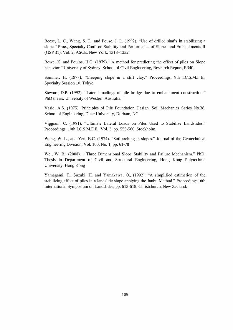
105
Reese, L. C., Wang, S. T., and Fouse, J. L. (1992). “Use of drilled shafts in stabilizing a
slope.” Proc., Specialty Conf. on Stability and Performance of Slopes and Embankments II
(GSP 31), Vol. 2, ASCE, New York, 1318–1332.
Rowe, K. and Poulos, H.G. (1979). “A method for predicting the effect of piles on Slope
behavior.” University of Sydney, School of Civil Engineering, Research Report, R340.
Sommer, H. (1977). “Creeping slope in a stiff clay.” Proceedings, 9th I.C.S.M.F.E.,
Specialty Session 10, Tokyo.
Stewart, D.P. (1992). “Lateral loadings of pile bridge due to embankment construction.”
PhD thesis, University of Western Australia.
Vesic, A.S. (1975). Principles of Pile Foundation Design. Soil Mechanics Series No.38.
School of Engineering, Duke University, Durham, NC.
Viggiani, C. (1981). “Ultimate Lateral Loads on Piles Used to Stabilize Landslides.”
Proceedings, 10th I.C.S.M.F.E., Vol. 3, pp. 555-560, Stockholm.
Wang, W. L., and Yen, B.C. (1974). “Soil arching in slopes.” Journal of the Geotechnical
Engineering Division, Vol. 100, No. 1, pp. 61-78
Wei, W. B., (2008). “ Three Dimensional Slope Stability and Failure Mechanism.” PhD.
Thesis in Department of Civil and Structural Engineering, Hong Kong Polytechnic
University, Hong Kong
Yamagami, T., Suzuki, H. and Yamakawa, O., (1992). “A simplified estimation of the
stabilizing effect of piles in a landslide slope applying the Janbu Method.” Proceedings, 6th
International Symposium on Landslides, pp. 613-618. Christchurch, New Zealand.

106
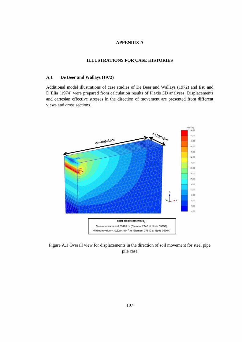
107
APPENDIX A
ILLUSTRATIONS FOR CASE HISTORIES
A.1 De Beer and Wallays (1972)
Additional model illustrations of case studies of De Beer and Wallays (1972) and Esu and
D’Elia (1974) were prepared from calculation results of Plaxis 3D analyses. Displacements
and cartesian effective stresses in the direction of movement are presented from different
views and cross sections.
Figure A.1 Overall view for displacements in the direction of soil movement for steel pipe
pile case
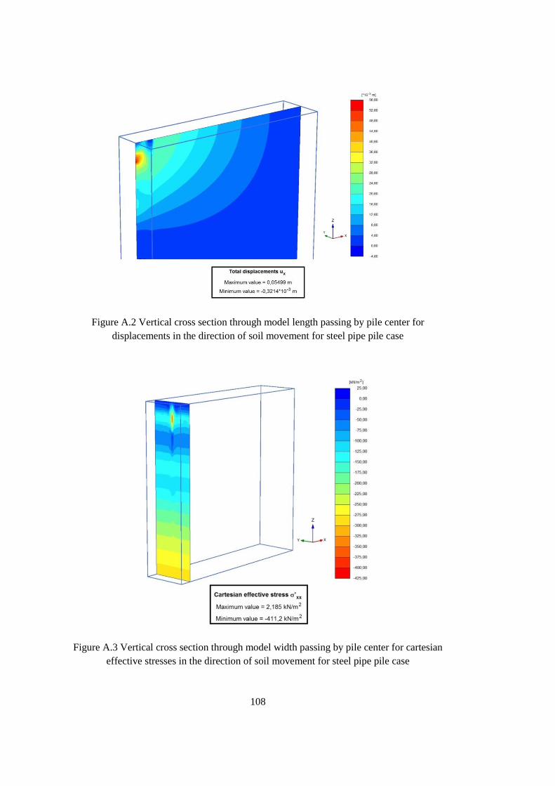
108
Figure A.2 Vertical cross section through model length passing by pile center for
displacements in the direction of soil movement for steel pipe pile case
Figure A.3 Vertical cross section through model width passing by pile center for cartesian
effective stresses in the direction of soil movement for steel pipe pile case
109
Figure A.4 Vertical cross section through model length passing by pile center for cartesian
effective stresses in the direction of soil movement for steel pipe pile case
Figure A.5 Overall view for displacements in the direction of soil movement for reinforced
concrete pile case
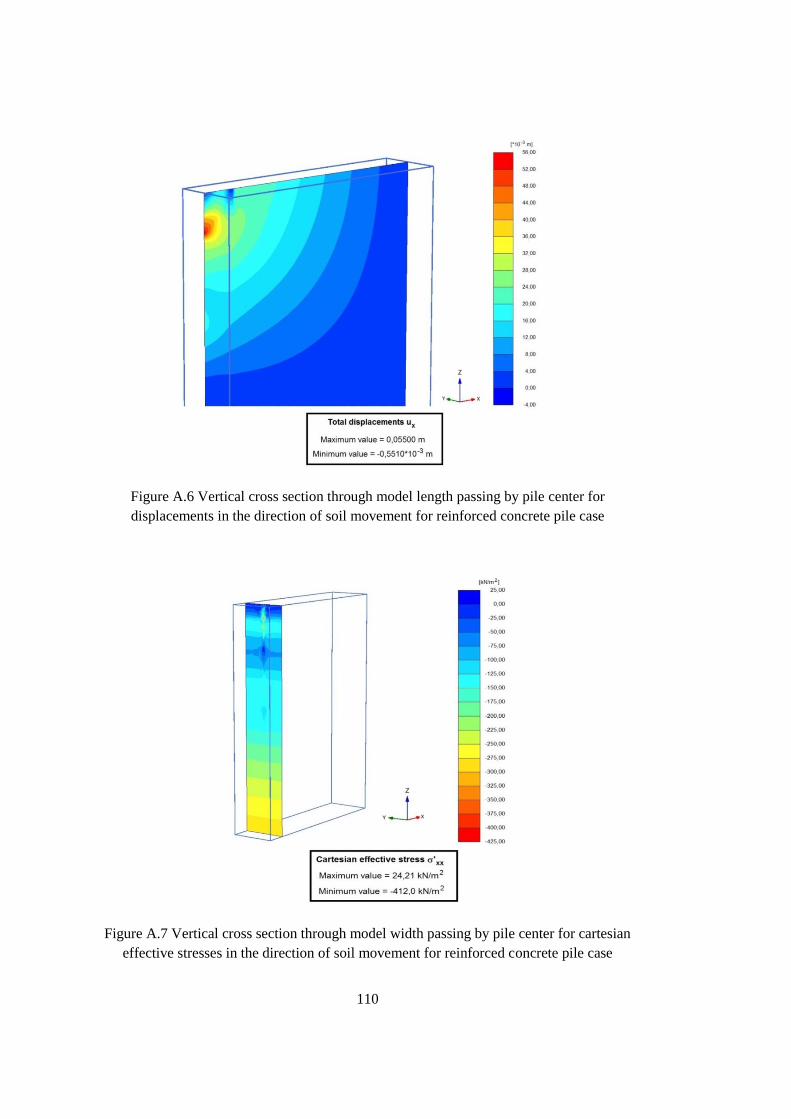
110
Figure A.6 Vertical cross section through model length passing by pile center for
displacements in the direction of soil movement for reinforced concrete pile case
Figure A.7 Vertical cross section through model width passing by pile center for cartesian
effective stresses in the direction of soil movement for reinforced concrete pile case
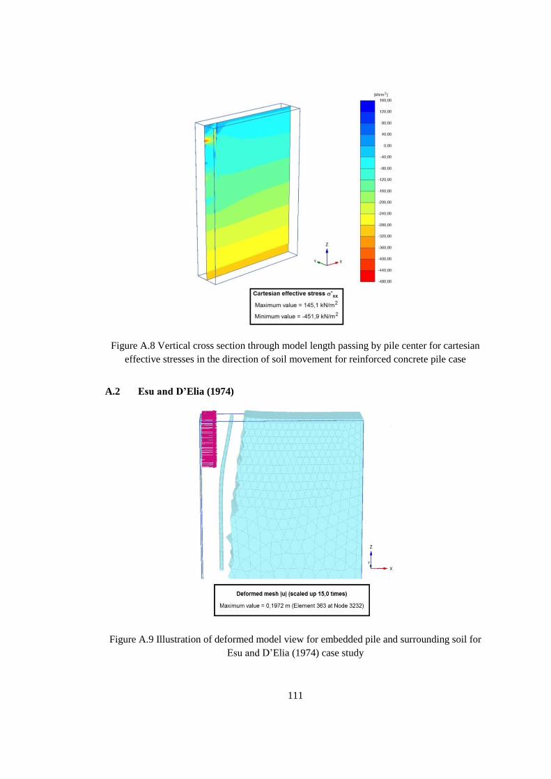
111
Figure A.8 Vertical cross section through model length passing by pile center for cartesian
effective stresses in the direction of soil movement for reinforced concrete pile case
A.2 Esu and D’Elia (1974)
Figure A.9 Illustration of deformed model view for embedded pile and surrounding soil for
Esu and D’Elia (1974) case study
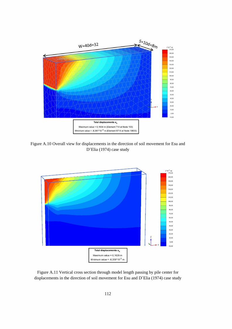
112
Figure A.10 Overall view for displacements in the direction of soil movement for Esu and
D’Elia (1974) case study
Figure A.11 Vertical cross section through model length passing by pile center for
displacements in the direction of soil movement for Esu and D’Elia (1974) case study
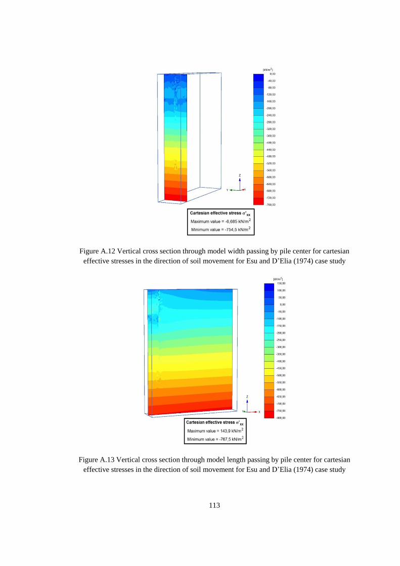
113
Figure A.12 Vertical cross section through model width passing by pile center for cartesian
effective stresses in the direction of soil movement for Esu and D’Elia (1974) case study
Figure A.13 Vertical cross section through model length passing by pile center for cartesian
effective stresses in the direction of soil movement for Esu and D’Elia (1974) case study
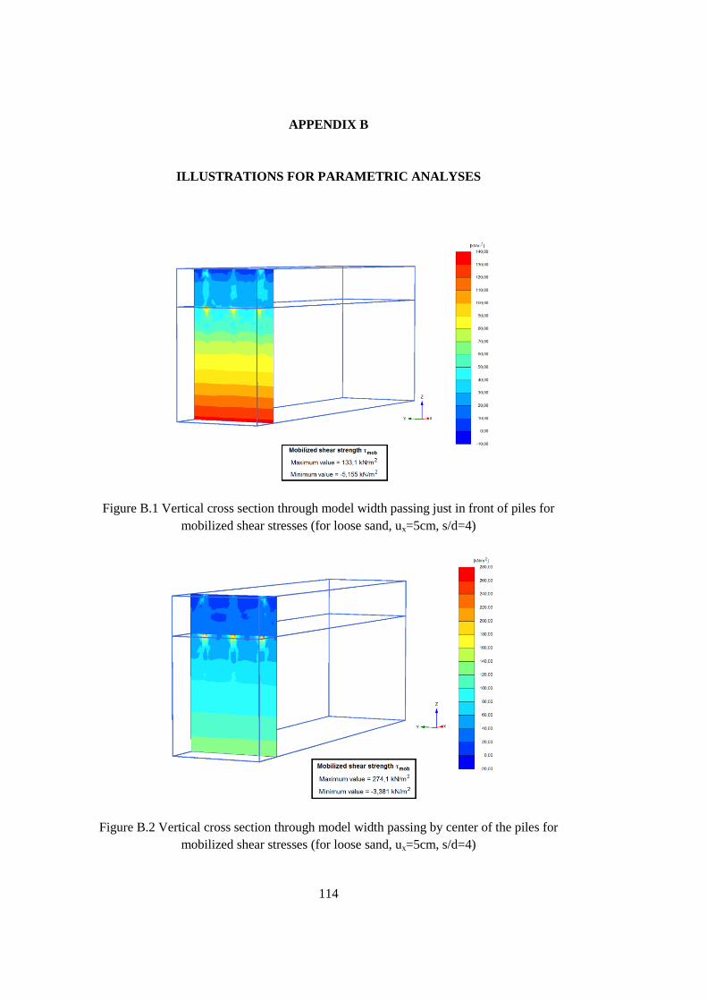
114
APPENDIX B
ILLUSTRATIONS FOR PARAMETRIC ANALYSES
Figure B.1 Vertical cross section through model width passing just in front of piles for
mobilized shear stresses (for loose sand, ux=5cm, s/d=4)
Figure B.2 Vertical cross section through model width passing by center of the piles for
mobilized shear stresses (for loose sand, ux=5cm, s/d=4)
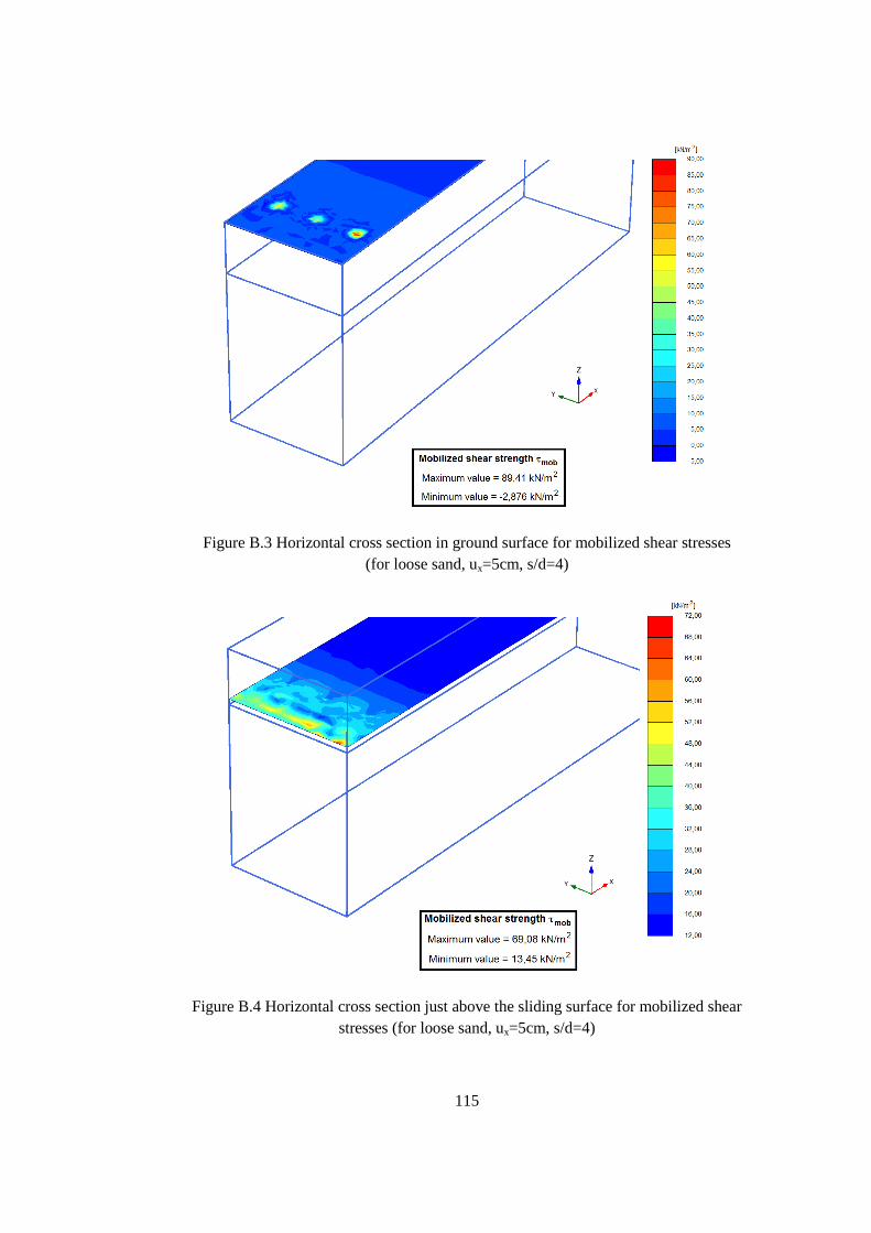
115
Figure B.3 Horizontal cross section in ground surface for mobilized shear stresses
(for loose sand, ux=5cm, s/d=4)
Figure B.4 Horizontal cross section just above the sliding surface for mobilized shear
stresses (for loose sand, ux=5cm, s/d=4)
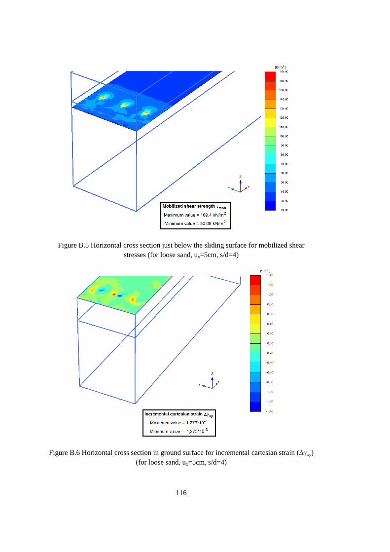
116
Figure B.5 Horizontal cross section just below the sliding surface for mobilized shear
stresses (for loose sand, ux=5cm, s/d=4)
Figure B.6 Horizontal cross section in ground surface for incremental cartesian strain (∆γxy)
(for loose sand, ux=5cm, s/d=4)