Computer-Aided Design 43 (2011) 417–426

Contents lists available at ScienceDirect

Computer-Aided Design

journal homepage: www.elsevier.com/locate/cad

Three dimensional extension of Bresenham’s Algorithm with Voronoi diagramChikit Au a,∗, Tony Woo b

a Department of Engineering, University of Waikato, New Zealandb School of Mechanical and Aerospace Engineering, Nanyang Technological University, Singapore

a r t i c l e i n f o

Article history:Received 14 January 2010Accepted 18 November 2010

Keywords:Voronoi diagramBresenham AlgorithmInteger arithmeticSymmetry

a b s t r a c t

Bresenham’s Algorithm for plotting a two-dimensional line segment is elegant and efficient in itsdeployment of mid-point comparison and integer arithmetic. It is natural to investigate its three-dimensional extensions. In so doing, this paper uncovers the reason for little prior work. The concept ofthe mid-point in a unit interval generalizes to that of nearest neighbours involving a Voronoi diagram.Algorithmically, there are challenges. While a unit interval in two-dimension becomes a unit squarein three-dimension, ‘‘squaring’’ the number of choices in Bresenham’s Algorithm is shown to havedifficulties. In this paper, the three-dimensional extension is based on the main idea of Bresenham’sAlgorithm of minimum distance between the line and the grid points. The structure of the Voronoidiagram is presented for grid points to which the line may be approximated. The deployment of integerarithmetic and symmetry for the three-dimensional extension of the algorithm to raise the computationefficiency are also investigated.

© 2010 Elsevier Ltd. All rights reserved.

1. Introduction

Bresenham’s Algorithm [1] is efficient in generating straightlines and quadrics on a raster system. Furthermore, its concepthas a wide range of applications such as re-sampling of structuredgrids [2], line of sight calculation between a sensor and atarget [3], interpolation in computer numerical control systems [4],ray casting [5], ray tracing [6], volume rendering [7], three-dimensional map representation [8], occlusion checking in re-constructing a three dimensional object [9,10], navigation forautonomous flight [10] and collision detection [11].

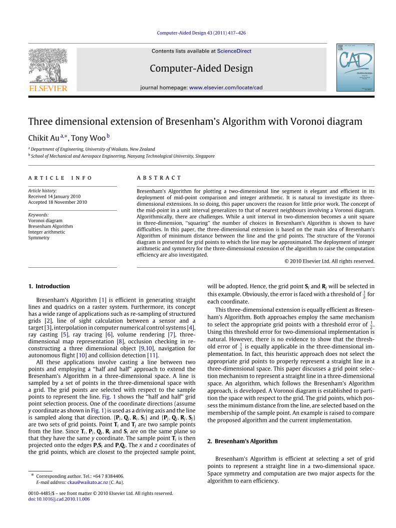
All these applications involve casting a line between twopoints and employing a ‘‘half and half’’ approach to extend theBresenham’s Algorithm in a three-dimensional space. A line issampled by a set of points in the three-dimensional space witha grid. The grid points are selected with respect to the samplepoints to represent the line. Fig. 1 shows the ‘‘half and half’’ gridpoint selection process. One of the coordinate directions (assumey coordinate as shown in Fig. 1) is used as a driving axis and the lineis sampled along that direction. {Pi,Qi,Ri, Si} and {Pj,Qj,Rj, Sj}are two sets of grid points. Point Ti and Tj are two sample pointsfrom the line. Since Ti, Pi,Qi,Ri and Si are on the same plane sothat they have the same y coordinate. The sample point Ti is thenprojected onto the edges PiSi and PiQi. The x and z coordinates ofthe grid points, which are closest to the projected sample point,

∗ Corresponding author. Tel.: +64 7 8384406.E-mail address: ckau@waikato.ac.nz (C. Au).

0010-4485/$ – see front matter© 2010 Elsevier Ltd. All rights reserved.doi:10.1016/j.cad.2010.11.006

will be adopted. Hence, the grid point Si and Rj will be selected inthis example. Obviously, the error is faced with a threshold of 1

2 foreach coordinate.

This three-dimensional extension is equally efficient as Bresen-ham’s Algorithm. Both approaches employ the same mechanismto select the appropriate grid points with a threshold error of 1

2 .Using this threshold error for two-dimensional implementation isnatural. However, there is no evidence to show that the thresh-old error of 1

2 is equally applicable in the three-dimensional im-plementation. In fact, this heuristic approach does not select theappropriate grid points to properly represent a straight line in athree-dimensional space. This paper discusses a grid point selec-tionmechanism to represent a straight line in a three-dimensionalspace. An algorithm, which follows the Bresenham’s Algorithmapproach, is developed. A Voronoi diagram is established to parti-tion the space with respect to the grid. The grid points, which pos-sess theminimumdistance from the line, are selected based on themembership of the sample point. An example is raised to comparethe proposed algorithm and the current implementation.

2. Bresenham’s Algorithm

Bresenham’s Algorithm is efficient at selecting a set of gridpoints to represent a straight line in a two-dimensional space.Space symmetry and computation are two major aspects for thealgorithm to earn efficiency.

418 C. Au, T. Woo / Computer-Aided Design 43 (2011) 417–426

Fig. 1. The ‘‘half and half’’ approach for 3D Bresenham Algorithm.

2.1. Symmetry in two-dimensional space

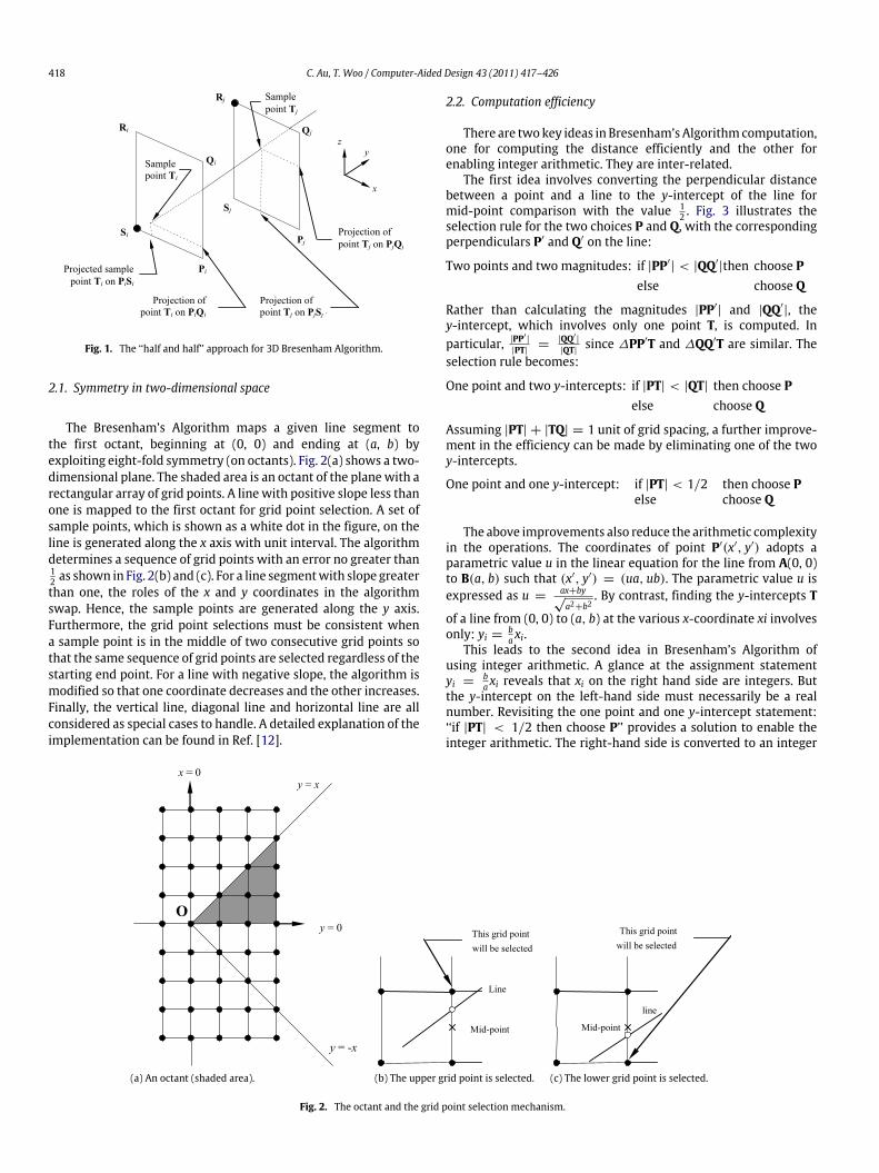
The Bresenham’s Algorithm maps a given line segment tothe first octant, beginning at (0, 0) and ending at (a, b) byexploiting eight-fold symmetry (on octants). Fig. 2(a) shows a two-dimensional plane. The shaded area is an octant of the planewith arectangular array of grid points. A line with positive slope less thanone is mapped to the first octant for grid point selection. A set ofsample points, which is shown as a white dot in the figure, on theline is generated along the x axis with unit interval. The algorithmdetermines a sequence of grid points with an error no greater than12 as shown in Fig. 2(b) and (c). For a line segmentwith slope greaterthan one, the roles of the x and y coordinates in the algorithmswap. Hence, the sample points are generated along the y axis.Furthermore, the grid point selections must be consistent whena sample point is in the middle of two consecutive grid points sothat the same sequence of grid points are selected regardless of thestarting end point. For a line with negative slope, the algorithm ismodified so that one coordinate decreases and the other increases.Finally, the vertical line, diagonal line and horizontal line are allconsidered as special cases to handle. A detailed explanation of theimplementation can be found in Ref. [12].

2.2. Computation efficiency

There are twokey ideas in Bresenham’s Algorithmcomputation,one for computing the distance efficiently and the other forenabling integer arithmetic. They are inter-related.

The first idea involves converting the perpendicular distancebetween a point and a line to the y-intercept of the line formid-point comparison with the value 1

2 . Fig. 3 illustrates theselection rule for the two choices P and Q, with the correspondingperpendiculars P′ and Q′ on the line:

Two points and two magnitudes: if |PP′| < |QQ′

|then choose Pelse choose Q

Rather than calculating the magnitudes |PP′| and |QQ′

|, they-intercept, which involves only one point T, is computed. Inparticular, |PP′

|

|PT| =|QQ′

|

|QT| since ∆PP′T and ∆QQ′T are similar. Theselection rule becomes:

One point and two y-intercepts: if |PT| < |QT| then choose Pelse choose Q

Assuming |PT| + |TQ| = 1 unit of grid spacing, a further improve-ment in the efficiency can be made by eliminating one of the twoy-intercepts.

One point and one y-intercept: if |PT| < 1/2 then choose Pelse choose Q

The above improvements also reduce the arithmetic complexityin the operations. The coordinates of point P′(x′, y′) adopts aparametric value u in the linear equation for the line from A(0, 0)to B(a, b) such that (x′, y′) = (ua, ub). The parametric value u isexpressed as u =

ax+by√a2+b2

. By contrast, finding the y-intercepts T

of a line from (0, 0) to (a, b) at the various x-coordinate xi involvesonly: yi =

ba xi.

This leads to the second idea in Bresenham’s Algorithm ofusing integer arithmetic. A glance at the assignment statementyi =

ba xi reveals that xi on the right hand side are integers. But

the y-intercept on the left-hand side must necessarily be a realnumber. Revisiting the one point and one y-intercept statement:‘‘if |PT| < 1/2 then choose P’’ provides a solution to enable theinteger arithmetic. The right-hand side is converted to an integer

(a) An octant (shaded area). (b) The upper grid point is selected. (c) The lower grid point is selected.

Fig. 2. The octant and the grid point selection mechanism.

C. Au, T. Woo / Computer-Aided Design 43 (2011) 417–426 419

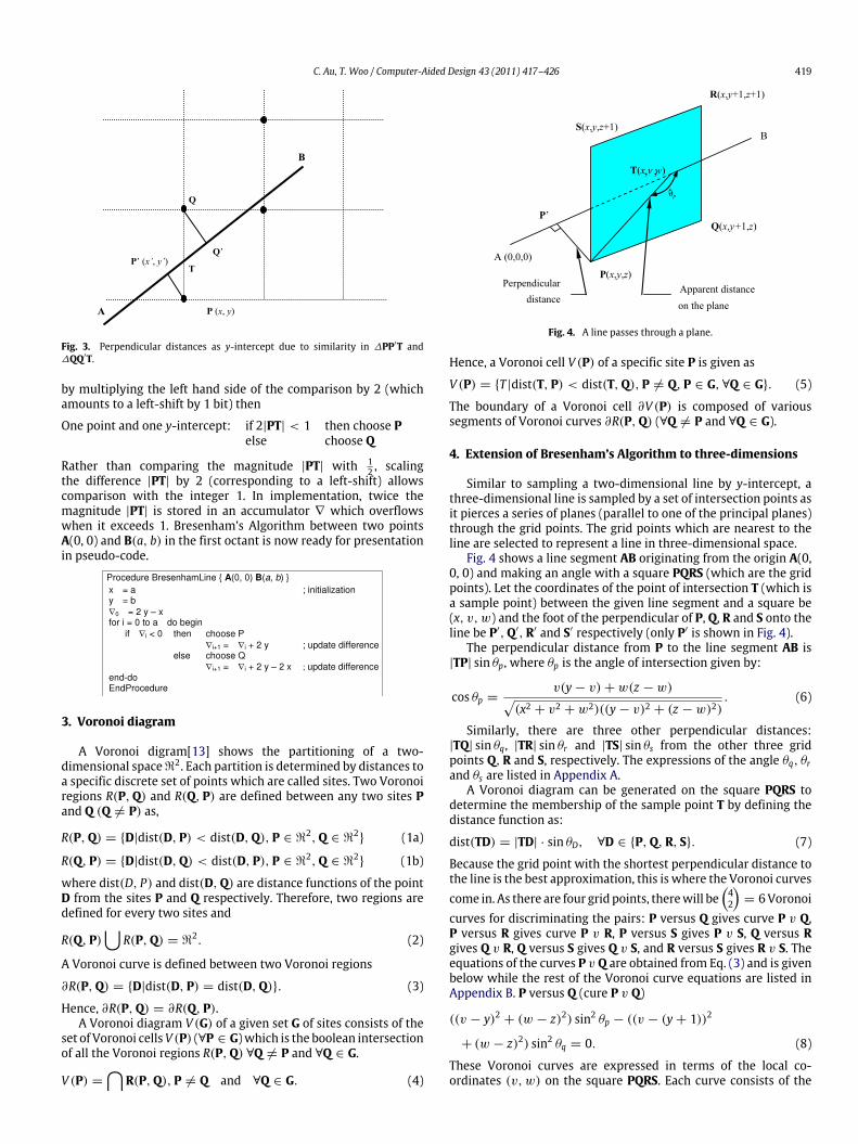
Fig. 3. Perpendicular distances as y-intercept due to similarity in ∆PP′T and∆QQ′T.

by multiplying the left hand side of the comparison by 2 (whichamounts to a left-shift by 1 bit) then

One point and one y-intercept: if 2|PT| < 1 then choose Pelse choose Q

Rather than comparing the magnitude |PT| with 12 , scaling

the difference |PT| by 2 (corresponding to a left-shift) allowscomparison with the integer 1. In implementation, twice themagnitude |PT| is stored in an accumulator ∇ which overflowswhen it exceeds 1. Bresenham’s Algorithm between two pointsA(0, 0) and B(a, b) in the first octant is now ready for presentationin pseudo-code.

3. Voronoi diagram

A Voronoi digram[13] shows the partitioning of a two-dimensional spaceℜ

2. Each partition is determined by distances toa specific discrete set of points which are called sites. Two Voronoiregions R(P,Q) and R(Q, P) are defined between any two sites Pand Q (Q = P) as,

R(P,Q) = {D|dist(D, P) < dist(D,Q), P ∈ ℜ2,Q ∈ ℜ

2} (1a)

R(Q, P) = {D|dist(D,Q) < dist(D, P), P ∈ ℜ2,Q ∈ ℜ

2} (1b)

where dist(D, P) and dist(D,Q) are distance functions of the pointD from the sites P and Q respectively. Therefore, two regions aredefined for every two sites and

R(Q, P)

R(P,Q) = ℜ2. (2)

A Voronoi curve is defined between two Voronoi regions

∂R(P,Q) = {D|dist(D, P) = dist(D,Q)}. (3)

Hence, ∂R(P,Q) = ∂R(Q, P).A Voronoi diagram V (G) of a given set G of sites consists of the

set of Voronoi cellsV (P) (∀P ∈ G)which is the boolean intersectionof all the Voronoi regions R(P,Q) ∀Q = P and ∀Q ∈ G.

V (P) =

R(P,Q), P = Q and ∀Q ∈ G. (4)

Fig. 4. A line passes through a plane.

Hence, a Voronoi cell V (P) of a specific site P is given as

V (P) = {T |dist(T, P) < dist(T,Q), P = Q, P ∈ G, ∀Q ∈ G}. (5)

The boundary of a Voronoi cell ∂V (P) is composed of varioussegments of Voronoi curves ∂R(P,Q) (∀Q = P and ∀Q ∈ G).

4. Extension of Bresenham’s Algorithm to three-dimensions

Similar to sampling a two-dimensional line by y-intercept, athree-dimensional line is sampled by a set of intersection points asit pierces a series of planes (parallel to one of the principal planes)through the grid points. The grid points which are nearest to theline are selected to represent a line in three-dimensional space.

Fig. 4 shows a line segment AB originating from the origin A(0,0, 0) and making an angle with a square PQRS (which are the gridpoints). Let the coordinates of the point of intersection T (which isa sample point) between the given line segment and a square be(x, v, w) and the foot of the perpendicular of P, Q, R and S onto theline be P′,Q′,R′ and S′ respectively (only P′ is shown in Fig. 4).

The perpendicular distance from P to the line segment AB is|TP| sin θp, where θp is the angle of intersection given by:

cos θp =v(y − v) + w(z − w)

(x2 + v2 + w2)((y − v)2 + (z − w)2). (6)

Similarly, there are three other perpendicular distances:|TQ| sin θq, |TR| sin θr and |TS| sin θs from the other three gridpoints Q,R and S, respectively. The expressions of the angle θq, θrand θs are listed in Appendix A.

A Voronoi diagram can be generated on the square PQRS todetermine the membership of the sample point T by defining thedistance function as:

dist(TD) = |TD| · sin θD, ∀D ∈ {P,Q,R, S}. (7)

Because the grid point with the shortest perpendicular distance tothe line is the best approximation, this is where the Voronoi curvescome in. As there are four grid points, therewill be

42

= 6Voronoi

curves for discriminating the pairs: P versus Q gives curve P v Q,P versus R gives curve P v R, P versus S gives P v S, Q versus Rgives Q v R, Q versus S gives Q v S, and R versus S gives R v S. Theequations of the curves P v Q are obtained from Eq. (3) and is givenbelow while the rest of the Voronoi curve equations are listed inAppendix B. P versus Q (cure P v Q)

((v − y)2 + (w − z)2) sin2 θp − ((v − (y + 1))2

+ (w − z)2) sin2 θq = 0. (8)

These Voronoi curves are expressed in terms of the local co-ordinates (v, w) on the square PQRS. Each curve consists of the

420 C. Au, T. Woo / Computer-Aided Design 43 (2011) 417–426

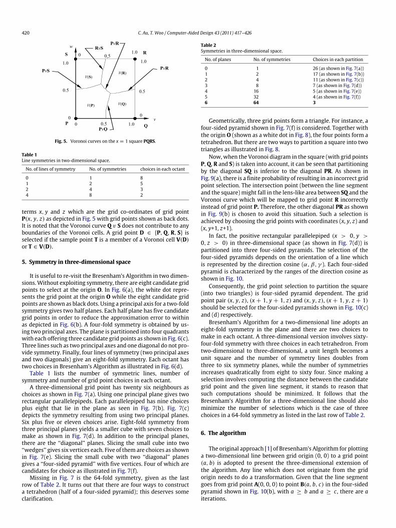
Fig. 5. Voronoi curves on the x = 1 square PQRS.

Table 1Line symmetries in two-dimensional space.

No. of lines of symmetry No. of symmetries choices in each octant

0 1 81 2 52 4 34 8 2

terms x, y and z which are the grid co-ordinates of grid pointP(x, y, z) as depicted in Fig. 5 with grid points shown as back dots.It is noted that the Voronoi curve Q v S does not contribute to anyboundaries of the Voronoi cells. A grid point D ∈ {P,Q,R, S} isselected if the sample point T is a member of a Voronoi cell V(D)or T ∈ V(D).

5. Symmetry in three-dimensional space

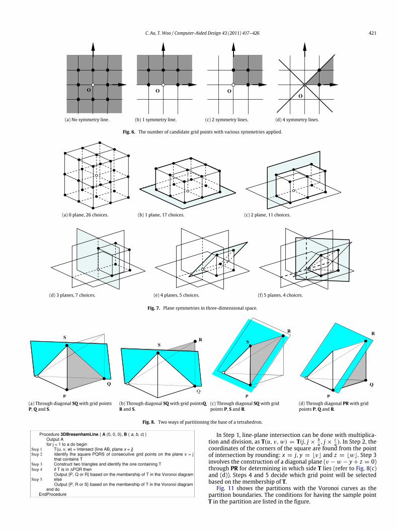
It is useful to re-visit the Bresenham’s Algorithm in two dimen-sions.Without exploiting symmetry, there are eight candidate gridpoints to select at the origin O. In Fig. 6(a), the white dot repre-sents the grid point at the origin O while the eight candidate gridpoints are shown as black dots. Using a principal axis for a two-foldsymmetry gives two half planes. Each half plane has five candidategrid points in order to reduce the approximation error to withinas depicted in Fig. 6(b). A four-fold symmetry is obtained by us-ing two principal axes. The plane is partitioned into four quadrantswith each offering three candidate grid points as shown in Fig. 6(c).Three lines such as two principal axes and one diagonal do not pro-vide symmetry. Finally, four lines of symmetry (two principal axesand two diagonals) give an eight-fold symmetry. Each octant hastwo choices in Bresenham’s Algorithm as illustrated in Fig. 6(d).

Table 1 lists the number of symmetric lines, number ofsymmetry and number of grid point choices in each octant.

A three-dimensional grid point has twenty six neighbours aschoices as shown in Fig. 7(a). Using one principal plane gives tworectangular parallelepipeds. Each parallelepiped has nine choicesplus eight that lie in the plane as seen in Fig. 7(b). Fig. 7(c)depicts the symmetry resulting from using two principal planes.Six plus five or eleven choices arise. Eight-fold symmetry fromthree principal planes yields a smaller cube with seven choices tomake as shown in Fig. 7(d). In addition to the principal planes,there are the ‘‘diagonal’’ planes. Slicing the small cube into two‘‘wedges’’ gives six vertices each. Five of them are choices as shownin Fig. 7(e). Slicing the small cube with two ‘‘diagonal’’ planesgives a ‘‘four-sided pyramid’’ with five vertices. Four of which arecandidates for choice as illustrated in Fig. 7(f).

Missing in Fig. 7 is the 64-fold symmetry, given as the lastrow of Table 2. It turns out that there are four ways to constructa tetrahedron (half of a four-sided pyramid); this deserves someclarification.

Table 2Symmetries in three-dimensional space.

No. of planes No. of symmetries Choices in each partition

0 1 26 (as shown in Fig. 7(a))1 2 17 (as shown in Fig. 7(b))2 4 11 (as shown in Fig. 7(c))3 8 7 (as shown in Fig. 7(d))4 16 5 (as shown in Fig. 7(e))5 32 4 (as shown in Fig. 7(f))6 64 3

Geometrically, three grid points form a triangle. For instance, afour-sided pyramid shown in Fig. 7(f) is considered. Together withthe origin O (shown as a white dot in Fig. 8), the four points form atetrahedron. But there are two ways to partition a square into twotriangles as illustrated in Fig. 8.

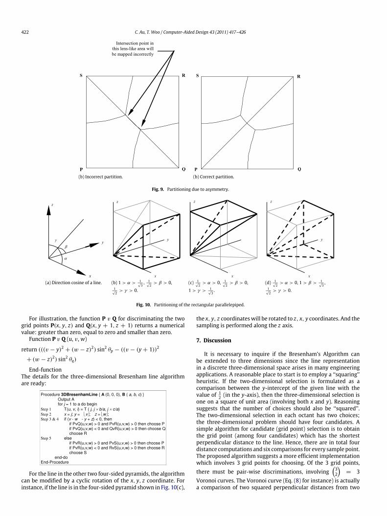
Now, when the Voronoi diagram in the square (with grid pointsP, Q, R and S) is taken into account, it can be seen that partitioningby the diagonal SQ is inferior to the diagonal PR. As shown inFig. 9(a), there is a finite probability of resulting in an incorrect gridpoint selection. The intersection point (between the line segmentand the square) might fall in the lens-like area between SQ and theVoronoi curve which will be mapped to grid point R incorrectlyinstead of grid point P. Therefore, the other diagonal PR as shownin Fig. 9(b) is chosen to avoid this situation. Such a selection isachieved by choosing the grid points with coordinates (x, y, z) and(x, y+1, z+1).

In fact, the positive rectangular parallelepiped (x > 0, y >

0, z > 0) in three-dimensional space (as shown in Fig. 7(d)) ispartitioned into three four-sided pyramids. The selection of thefour-sided pyramids depends on the orientation of a line whichis represented by the direction cosine (α, β, γ ). Each four-sidedpyramid is characterized by the ranges of the direction cosine asshown in Fig. 10.

Consequently, the grid point selection to partition the square(into two triangles) is four-sided pyramid dependent. The gridpoint pair (x, y, z), (x + 1, y + 1, z) and (x, y, z), (x + 1, y, z + 1)should be selected for the four-sided pyramids shown in Fig. 10(c)and (d) respectively.

Bresenham’s Algorithm for a two-dimensional line adopts aneight-fold symmetry in the plane and there are two choices tomake in each octant. A three-dimensional version involves sixty-four-fold symmetry with three choices in each tetrahedron. Fromtwo-dimensional to three-dimensional, a unit length becomes aunit square and the number of symmetry lines doubles fromthree to six symmetry planes, while the number of symmetriesincreases quadratically from eight to sixty four. Since making aselection involves computing the distance between the candidategrid point and the given line segment, it stands to reason thatsuch computations should be minimized. It follows that theBresenham’s Algorithm for a three-dimensional line should alsominimize the number of selections which is the case of threechoices in a 64-fold symmetry as listed in the last row of Table 2.

6. The algorithm

The original approach [1] of Bresenham’s Algorithm for plottinga two-dimensional line between grid origin (0, 0) to a grid point(a, b) is adopted to present the three-dimensional extension ofthe algorithm. Any line which does not originate from the gridorigin needs to do a transformation. Given that the line segmentgoes from grid point A(0, 0, 0) to point B(a, b, c) in the four-sidedpyramid shown in Fig. 10(b), with a ≥ b and a ≥ c , there are aiterations.

C. Au, T. Woo / Computer-Aided Design 43 (2011) 417–426 421

(a) No symmetry line. (b) 1 symmetry line. (c) 2 symmetry lines. (d) 4 symmetry lines.

Fig. 6. The number of candidate grid points with various symmetries applied.

(a) 0 plane, 26 choices. (b) 1 plane, 17 choices. (c) 2 plane, 11 choices.

(d) 3 planes, 7 choices. (e) 4 planes, 5 choices. (f) 5 planes, 4 choices.

Fig. 7. Plane symmetries in three-dimensional space.

(a) Through diagonal SQwith grid pointsP, Q and S.

(b) Through diagonal SQ with grid pointsQ,R and S.

(c) Through diagonal SQwith gridpoints P, S and R.

(d) Through diagonal PRwith gridpoints P, Q and R.

Fig. 8. Two ways of partitioning the base of a tetrahedron.

In Step 1, line-plane intersection can be done with multiplica-tion and division, as T(u, v, w) = T(j, j × b

a , j ×ca ). In Step 2, the

coordinates of the corners of the square are found from the pointof intersection by rounding: x = j, y = ⌊v⌋ and z = ⌊w⌋. Step 3involves the construction of a diagonal plane (v − w − y + z = 0)through PR for determining in which side T lies (refer to Fig. 8(c)and (d)). Steps 4 and 5 decide which grid point will be selectedbased on the membership of T.

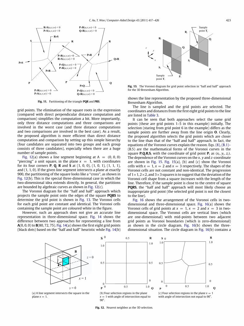
Fig. 11 shows the partitions with the Voronoi curves as thepartition boundaries. The conditions for having the sample pointT in the partition are listed in the figure.

422 C. Au, T. Woo / Computer-Aided Design 43 (2011) 417–426

(b) Incorrect partition. (b) Correct partition.

Fig. 9. Partitioning due to asymmetry.

(a) Direction cosine of a line. (b) 1 > α > 1√3, 1

√2

> β > 0,1

√2

> γ > 0.

(c) 1√2

> α > 0, 1√2

> β > 0,

1 > γ > 1√3.

(d) 1√2

> α > 0, 1 > β > 1√3,

1√2

> γ > 0.

Fig. 10. Partitioning of the rectangular parallelepiped.

For illustration, the function P v Q for discriminating the twogrid points P(x, y, z) and Q(x, y + 1, z + 1) returns a numericalvalue: greater than zero, equal to zero and smaller than zero.

Function P v Q (u, v, w)

return (((v − y)2 + (w − z)2) sin2 θp − ((v − (y + 1))2

+ (w − z)2) sin2 θq)

End-functionThe details for the three-dimensional Bresenham line algorithmare ready:

For the line in the other two four-sided pyramids, the algorithmcan be modified by a cyclic rotation of the x, y, z coordinate. Forinstance, if the line is in the four-sided pyramid shown in Fig. 10(c),

the x, y, z coordinateswill be rotated to z, x, y coordinates. And thesampling is performed along the z axis.

7. Discussion

It is necessary to inquire if the Bresenham’s Algorithm canbe extended to three dimensions since the line representationin a discrete three-dimensional space arises in many engineeringapplications. A reasonable place to start is to employ a ‘‘squaring’’heuristic. If the two-dimensional selection is formulated as acomparison between the y-intercept of the given line with thevalue of 1

2 (in the y-axis), then the three-dimensional selection isone on a square of unit area (involving both x and y). Reasoningsuggests that the number of choices should also be ‘‘squared’’.The two-dimensional selection in each octant has two choices;the three-dimensional problem should have four candidates. Asimple algorithm for candidate (grid point) selection is to obtainthe grid point (among four candidates) which has the shortestperpendicular distance to the line. Hence, there are in total fourdistance computations and six comparisons for every sample point.The proposed algorithm suggests a more efficient implementationwhich involves 3 grid points for choosing. Of the 3 grid points,there must be pair-wise discriminations, involving

32

= 3

Voronoi curves. The Voronoi curve (Eq. (8) for instance) is actuallya comparison of two squared perpendicular distances from two

C. Au, T. Woo / Computer-Aided Design 43 (2011) 417–426 423

Fig. 11. Partitioning of the triangle PQR and PRS.

grid points. The elimination of the square roots in the expression(compared with direct perpendicular distance computation andcomparison) simplifies the computation a bit. More importantly,only three distance computations and three comparisons areinvolved in the worst case (and three distance computationsand two comparisons are involved in the best case). As a result,the proposed algorithm is more efficient than direct distancecomputation and comparison by setting up this simple hierarchy(four candidates are separated into two groups and each groupconsists of three candidates), especially when there are a hugenumber of sample points.

Fig. 12(a) shows a line segment beginning at A = (0, 0, 0)‘‘piercing’’ a unit square, in the plane x = 1, with coordinatesfor its four corners P, Q, R and S at (1, 0, 0), (1, 0, 1), (1, 1, 1),and (1, 1, 0). If the given line segment intersects a plane at exactly900, the partitioning of the square looks like a ‘‘cross’’, as shown inFig. 12(b). This is the special three-dimensional case in which thetwo-dimensional idea extends directly. In general, the partitionsare bounded by algebraic curves as shown in Fig. 12(c).

The Voronoi diagram for the ‘‘half and half’’ approach whichprojects the sample point onto the edges of the square PQRS todetermine the grid point is shown in Fig. 13. The Voronoi cellsfor each grid point are constant and identical. The Voronoi cellscontaining the sample point are coloured white in the figure.

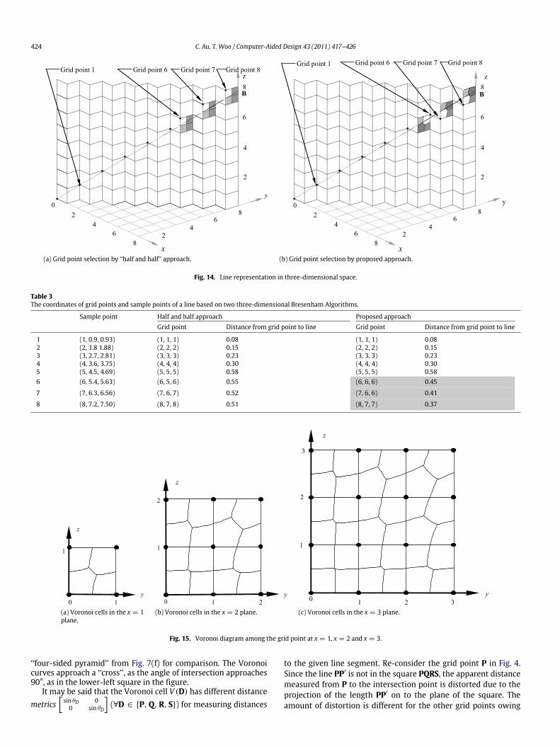
However, such an approach does not give an accurate linerepresentation in three-dimensional space. Fig. 14 shows thedifference between two approaches for representing a line fromA(0, 0, 0) to B(80, 72, 75). Fig. 14(a) shows the first eight grid points(black dots) based on the ‘‘half and half’’ heuristic while Fig. 14(b)

Fig. 13. The Voronoi diagram for grid point selection in ‘‘half and half’’ approachfor the 3D Bresenham Algorithm.

shows the line representation by the proposed three-dimensionalBresenham Algorithm.

The line is sampled and the grid points are selected. Thecoordinates and distances from the first eight grid points to the lineare listed in Table 3.

It can be seen that both approaches select the same gridpoints (these are grid points 1–5 in this example) initially. Theselection (staring from grid point 6 in the example) differs as thesample points are further away from the line origin O. Clearly,the proposed algorithm selects the grid points which are closerto the line than that of the ‘‘half and half’’ approach. In fact, theequations of the Voronoi curves explain the reason. Eqs. (8), (B.1)–(B.5) are the mathematical forms of the Voronoi curves in thesquare PiQiRiSi with the coordinate of grid point Pi as (xi, yi, zi).The dependence of the Voronoi curves on the x, y and z-coordinateare shown in Fig. 15. Fig. 15(a), (b) and (c) show the Voronoicells with x = 1, x = 2 and x = 3 respectively. The shapes of theVoronoi cells are not constant and non-identical. The progressionof 1×1, 2×2, and3×3 squares is to suggest that the deviation of theVoronoi cell shape from a square increases with the length of theline. Therefore, if the sample point is close to the centre of squarePQRS, the ‘‘half and half’’ approach will most likely choose aninappropriate grid point (the selected grid point is not the closestto the line).

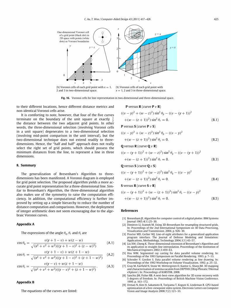
Fig. 16 shows the arrangement of the Voronoi cells in two-dimensional and three-dimensional space. Fig. 16(a) shows theVoronoi cells of grid points at x = 1, x = 2 and x = 3 in two-dimensional space. The Voronoi cells are vertical lines (whichare one-dimensional) with mid-points between two adjacentgrid points as Voronoi boundaries (which is zero-dimensional)as shown in the circle diagram. Fig. 16(b) shows the three-dimensional situation. The circle diagram in Fig. 16(b) contains a

(a) A line segment intersects the square in theplane x = 1.

(b) Four selection regions in the planex = 1 with angle of intersection equal to90°.

(c) Four selection regions in the plane x = 1with angle of intersection not equal to 90°.

Fig. 12. Nearest neighbor as the 3D selection.

424 C. Au, T. Woo / Computer-Aided Design 43 (2011) 417–426

(a) Grid point selection by ‘‘half and half’’ approach. (b) Grid point selection by proposed approach.

Fig. 14. Line representation in three-dimensional space.

Table 3The coordinates of grid points and sample points of a line based on two three-dimensional Bresenham Algorithms.

Sample point Half and half approach Proposed approachGrid point Distance from grid point to line Grid point Distance from grid point to line

1 (1, 0.9, 0.93) (1, 1, 1) 0.08 (1, 1, 1) 0.082 (2, 1.8 1.88) (2, 2, 2) 0.15 (2, 2, 2) 0.153 (3, 2.7, 2.81) (3, 3, 3) 0.23 (3, 3, 3) 0.234 (4, 3.6, 3.75) (4, 4, 4) 0.30 (4, 4, 4) 0.305 (5, 4.5, 4.69) (5, 5, 5) 0.58 (5, 5, 5) 0.586 (6, 5.4, 5.63) (6, 5, 6) 0.55 (6, 6, 6) 0.45

7 (7, 6.3, 6.56) (7, 6, 7) 0.52 (7, 6, 6) 0.41

8 (8, 7.2, 7.50) (8, 7, 8) 0.51 (8, 7, 7) 0.37

(a) Voronoi cells in the x = 1plane.

(b) Voronoi cells in the x = 2 plane. (c) Voronoi cells in the x = 3 plane.

Fig. 15. Voronoi diagram among the grid point at x = 1, x = 2 and x = 3.

‘‘four-sided pyramid’’ from Fig. 7(f) for comparison. The Voronoicurves approach a ‘‘cross’’, as the angle of intersection approaches90°, as in the lower-left square in the figure.

It may be said that the Voronoi cell V (D) has different distancemetrics

sin θD 00 sin θD

(∀D ∈ {P,Q,R, S}) for measuring distances

to the given line segment. Re-consider the grid point P in Fig. 4.Since the line PP′ is not in the square PQRS, the apparent distancemeasured from P to the intersection point is distorted due to theprojection of the length PP′ on to the plane of the square. Theamount of distortion is different for the other grid points owing

C. Au, T. Woo / Computer-Aided Design 43 (2011) 417–426 425

(b) Voronoi cells of each grid point with x = 1,2 and 3 in two-dimensional space.

(b) Voronoi cells of each grid point withx = 1, 2 and 3 in three-dimensional space.

Fig. 16. Voronoi cells for line representation in two-dimensional and three-dimensional space.

to their different locations, hence different distance metrics andnon-identical Voronoi cells arise.

It is comforting to note, however, that four of the five curvesterminate on the boundary of the unit square at exactly 1

2the distance between the two adjacent grid points. In otherwords, the three-dimensional selection (involving Voronoi cellsin a unit square) degenerates to a two-dimensional selection(involving mid-point comparison in the unit interval), but thetwo-dimensional technique does not extend readily to three-dimensions. Hence, the ‘‘half and half’’ approach does not reallyselect the right set of grid points, which should possess theminimum distances from the line, to represent a line in threedimensions.

8. Summary

The generalization of Bresenham’s Algorithm to three-dimensions has been manifested. A Voronoi diagram is employedfor grid point selection. The proposed algorithm yields a more ac-curate grid point representation for a three-dimensional line. Sim-ilar to Bresenham’s Algorithm, the three-dimensional algorithmalso makes use of the symmetry to raise the computation effi-ciency. In addition, the computational efficiency is further im-proved by setting up a simple hierarchy to reduce the number ofdistance computation and comparisons. However, the deploymentof integer arithmetic does not seem encouraging due to the alge-braic Voronoi curves.

Appendix A

The expressions of the angle θq, θr and θs are

cos θq =v(y + 1 − v) + w(z − w)

(x2 + v2 + w2)((y + 1 − v)2 + (z − w)2)(A.1)

cos θr =v(y + 1 − v) + w(z + 1 − w)

(x2 + v2 + w2)((y + 1 − v)2 + (z + 1 − w)2)(A.2)

cos θs =v(y − v) + w(z + 1 − w)

(x2 + v2 + w2)((y − v)2 + (z + 1 − w)2). (A.3)

Appendix B

The equations of the curves are listed:

P versus R (curve P v R)

((v − y)2 + (w − z)2) sin2 θp − ((v − (y + 1))2

+(w − (z + 1))2) sin2 θr = 0. (B.1)

P versus S (curve P v S)

((v − y)2 + (w − z)2) sin2 θp − ((v − y)2

+(w − (z + 1))2) sin2 θs = 0. (B.2)

Q versus R (curve Q v R)

((v − (y + 1))2 + (w − z)2) sin2 θq − ((v − (y + 1))2

+(w − (z + 1))2) sin2 θr = 0. (B.3)

Q versus S (curve Q v S)

((v − (y + 1))2 + (w − z)2) sin2 θq − ((v − y)2

+(w − (z + 1))2) sin2 θs = 0. (B.4)

S versus R (curve S v R)

((v − (y + 1))2 + (w − (z + 1))2) sin2 θs − ((v − y)2

+(w − (z + 1))2) sin2 θr = 0. (B.5)

References

[1] Bresenham JE. Algorithm for computer control of a digital plotter. IBM SystemsJournal 1965;4(1):25–30.

[2] Dimitrov LI, Sramek M. Using 3D-Bresenham for resampling structured grids.In: Proceedings of the 2nd International Symposium on 3D Data Processing,Visualization and Transmission. 2004. p. 926–30.

[3] Proctor MD, Gerber WJ. Line-of-sight attributes for a generalized applicationprogram interface. The Journal of Defense Modeling and Simulation:Applications, Methodology, Technology 2004;1(1):43–57.

[4] Liu XW, Cheng K. Three-dimensional extension of Bresenham’s Algorithm andits application in straight-line interpolation. Proceedings of the Institution ofMechanical Engineers 2002;3:459–63.

[5] Hsu WM. Segmented ray casting for data parallel volume rendering. In:Proceedings of the 1993 Symposium on Parallel Rendering. 1993. p. 7–13.

[6] Schroder P, Gordon S. Data parallel volume rendering as line drawing. In:Proceedings of the 1992 Workshop on Volume Visualization. 1992. p. 25–32.

[7] Gray M, Fairfield N, StoneW, Wettergreen D, Kantor G, Sharp JM. 3D mappingand characterization of sistema zacatón fromDEPTHX (DEep Phreatic THermaleXplorer). In: Proceedings of KARST08, 2008.

[8] Sanchiz JM, Fisher RB. A next-best-view algorithm for 3D scene recovery with5 degrees of freedom. In: Proceedings of British Machine Vision Conference.1999. p. 163–172.

[9] Orman N, Kim H, Sakamoto R, Toriyama T, Kogure K, Lindeman R. GPU-basedoptimization of a free-viewpoint video system. Electronic Letters on ComputerVision and Image Analysis 2008;7(2):121–33.

426 C. Au, T. Woo / Computer-Aided Design 43 (2011) 417–426

[10] Scherer S, Singh S, Chamberlain L, Elgersma M. Flying fast and lowamong obstacles: methodology and experiments. The International Journal ofRobotics Research 2009;7:549–74.

[11] Paiva A, Petronette F, Lewiner T, Tavares G. Particle-based viscoplasticfluid/solid simulation. Computer-Aided Design 2009;41(4):306–14.

[12] Foley JD, Van Dam A, Feiner S, Hughes JF. Computer graphics: principles andpractice in C. 2nd ed. Addison-Wesley; 1997.

[13] Au CK. Spatial and temporal competition as a two dimensional kinetic Voronoidiagram. Computer-Aided Design 2008;40(2):139–49.