Embed Size (px)
Citation preview

Three Analog Neurons Are Turing Universal
Jirı Sıma
Institute of Computer ScienceCzech Academy of Sciences

(Artificial) Neural Networks (NNs)
1. mathematical models of biological neural networks
• simulating and understanding the brain (The Human Brain Project)
• modeling cognitive functions
2. computing devices alternative to conventional computers
already first computer designers sought their inspiration in the human brain(e.g., neurocomputer due to Minsky, 1951)
• common tools in machine learning or data mining (learning from training data)
• professional software implementations (e.g. Matlab, Statistica modules)
• successful commercial applications in AI (e.g. deep learning):
computer vision, pattern recognition, control, prediction, classification, robotics,decision-making, signal processing, fault detection, diagnostics, etc.

The Neural Network Model – Architecture
s computational units (neurons), indexed as V = {1, . . . , s}, connected intoa directed graph (V,A) where A ⊆ V × V

The Neural Network Model – Weights
each edge (i, j) ∈ A from unit i to j is labeled with a real weight wji ∈ R
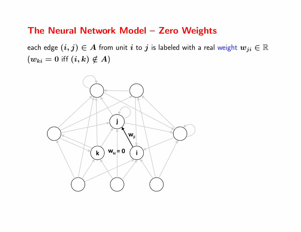
The Neural Network Model – Zero Weights
each edge (i, j) ∈ A from unit i to j is labeled with a real weight wji ∈ R(wki = 0 iff (i, k) /∈ A)

The Neural Network Model – Biases
each neuron j ∈ V is associated with a real bias wj0 ∈ R(i.e. a weight of (0, j) ∈ A from an additional formal neuron 0 ∈ V )

Discrete-Time Computational Dynamics – Network State
the evolution of global network state (output) y(t) = (y(t)1 , . . . , y
(t)s ) ∈ [0, 1]s
at discrete time instant t = 0, 1, 2, . . .

Discrete-Time Computational Dynamics – Initial State
t = 0 : initial network state y(0) ∈ {0, 1}s

Discrete-Time Computational Dynamics: t = 1
t = 1 : network state y(1) ∈ [0, 1]s

Discrete-Time Computational Dynamics: t = 2
t = 2 : network state y(2) ∈ [0, 1]s

Discrete-Time Computational Dynamics – Excitations
at discrete time instant t ≥ 0, an excitation is computed as
ξ(t)j = wj0+
s∑i=1
wjiy(t)i =
s∑i=0
wjiy(t)i
for j = 1, . . . , s
where unit 0 ∈ V has constant output y(t)0 ≡ 1 for every t ≥ 0
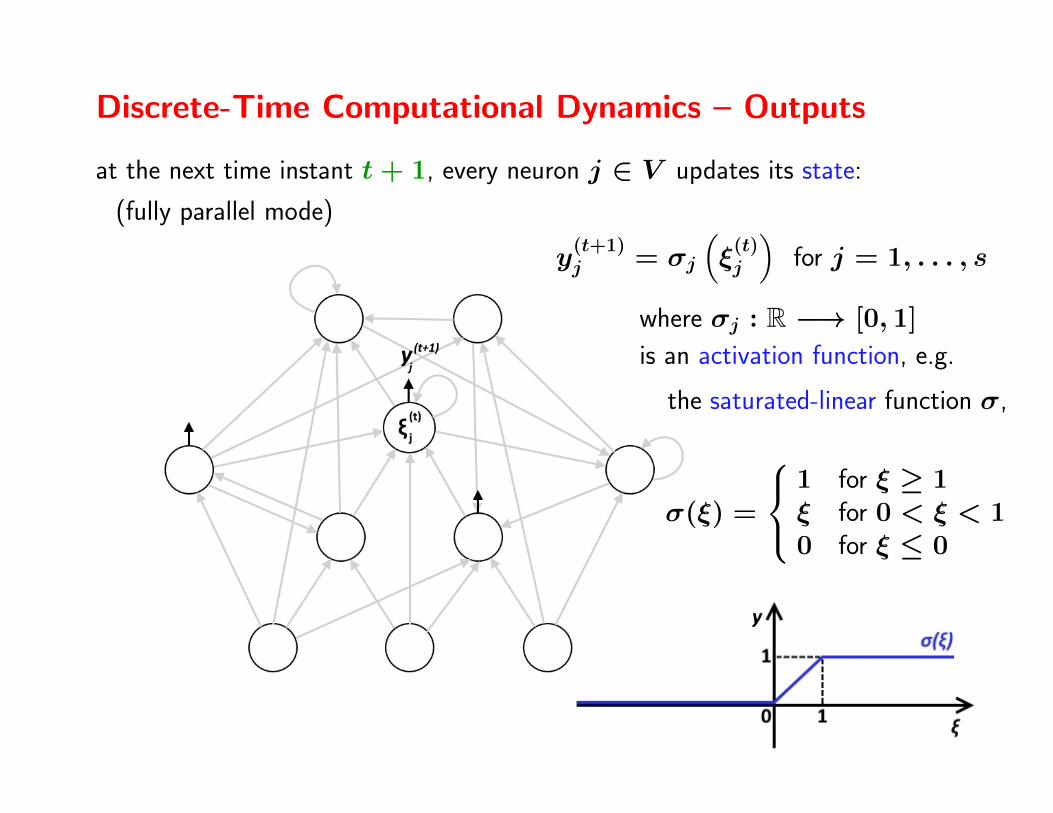
Discrete-Time Computational Dynamics – Outputs
at the next time instant t+ 1, every neuron j ∈ V updates its state:
(fully parallel mode)
y(t+1)j = σj
(ξ
(t)j
)for j = 1, . . . , s
where σj : R −→ [0, 1]
is an activation function, e.g.
the saturated-linear function σ,
σ(ξ) =
1 for ξ ≥ 1ξ for 0 < ξ < 10 for ξ ≤ 0

The Computational Power of NNs – Motivations
• the potential and limits of general-purpose computation with NNs:
What is ultimately or efficiently computable by particular NN models?
• idealized mathematical models of practical NNs which abstract away fromimplementation issues, e.g. analog numerical parameters are true real numbers
• methodology: the computational power and efficiency of NNs is investigatedby comparing formal NNs to traditional computational models such as finiteautomata, Turing machines, Boolean circuits, etc.
• NNs may serve as reference models for analyzing alternative computationalresources (other than time or memory space) such as analog state, continuoustime, energy, temporal coding, etc.
• NNs capture basic characteristics of biological nervous systems (plenty ofdensely interconnected simple unreliable computational units)
−→ computational principles of mental processes

Neural Networks As Formal Language Acceptors
language (problem) L ⊆ Σ∗ over a finite alphabet Σ
y(T (n))out =
{1 if x ∈ L0 if x /∈ L y
(t)halt =
{1 if t = T (n)0 if t 6= T (n)
Y = {out, halt} output neurons
T (n) is the computational timein terms of input length n ≥ 0
online I/O: T (n) = nd
d ≥ 1 is the time overhead forprocessing a single input symbol
X = enum(Σ) ⊆ Vinput neuronsx y(d(i−1))
j = 1 iff j = enum(xi)
x = x1x2 . . . xi−1 ←− xi ←− xi+1xi+2 . . . xn ∈ Σ∗ input word

The Computational Power of Neural Networks
depends on the information contents of weight parameters:
1. integer weights: finite automaton (Minsky, 1967)
2. rational weights: Turing machine (Siegelmann, Sontag, 1995)
polynomial time ≡ complexity class P
3. arbitrary real weights: “super-Turing” computation (Siegelmann, Sontag, 1994)
polynomial time ≡ nonuniform complexity class P/poly
exponential time ≡ any I/O mapping

The Computational Power of Neural Networks
depends on the information contents of weight parameters:
1. integer weights: finite automaton (Minsky, 1967)
2. rational weights: Turing machine (Siegelmann, Sontag, 1995)
polynomial time ≡ complexity class P
polynomial time & increasing Kolmogorov complexity of real weights ≡a proper hierarchy of nonuniform complexity classes between P and P/poly
(Balcazar, Gavalda, Siegelmann, 1997)
3. arbitrary real weights: “super-Turing” computation (Siegelmann, Sontag, 1994)
polynomial time ≡ nonuniform complexity class P/poly
exponential time ≡ any I/O mapping

The Computational Power of Neural Networks
depends on the information contents of weight parameters:
1. integer weights: finite automaton (Minsky, 1967)
a gap between integer a rational weights w.r.t. the Chomsky hierarchy
regular (Type-3) × recursively enumerable (Type-0) languages
2. rational weights: Turing machine (Siegelmann, Sontag, 1995)
polynomial time ≡ complexity class P
polynomial time & increasing Kolmogorov complexity of real weights ≡a proper hierarchy of nonuniform complexity classes between P and P/poly
(Balcazar, Gavalda, Siegelmann, 1997)
3. arbitrary real weights: “super-Turing” computation (Siegelmann, Sontag, 1994)
polynomial time ≡ nonuniform complexity class P/poly
exponential time ≡ any I/O mapping

Between Integer and Rational Weights
25 neurons with rational weights can implement any Turing machine (Indyk,1995)
?? What is the computational power of a few extra analog neurons ??
A Neural Network with c Extra Analog Neurons (cANN)
is composed of binary-state neurons with the Heaviside activation function exceptfor the first c analog-state units with the saturated-linear activation function:
σj(ξ) =
σ(ξ) =
1 for ξ ≥ 1ξ for 0 < ξ < 10 for ξ ≤ 0
j = 1, . . . , csaturated-linearfunction
H(ξ) =
{1 for ξ ≥ 00 for ξ < 0
j = c+ 1, . . . , sHeavisidefunction
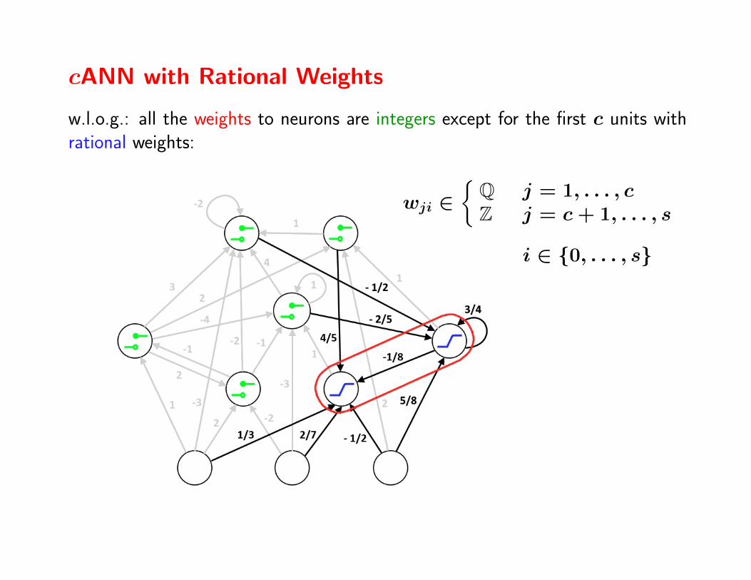
cANN with Rational Weights
w.l.o.g.: all the weights to neurons are integers except for the first c units withrational weights:
wji ∈{Q j = 1, . . . , cZ j = c+ 1, . . . , s
i ∈ {0, . . . , s}
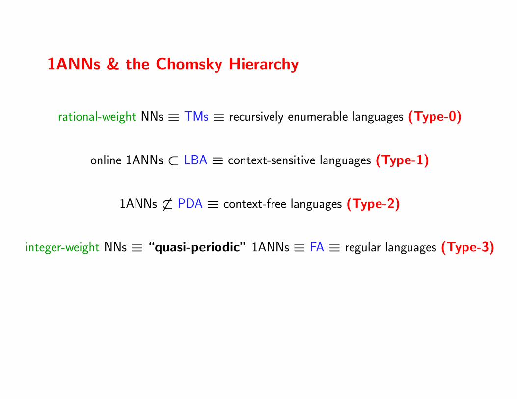
1ANNs & the Chomsky Hierarchy
rational-weight NNs ≡ TMs ≡ recursively enumerable languages (Type-0)
online 1ANNs ⊂ LBA ≡ context-sensitive languages (Type-1)
1ANNs 6⊂ PDA ≡ context-free languages (Type-2)
integer-weight NNs ≡ “quasi-periodic” 1ANNs ≡ FA ≡ regular languages (Type-3)

Non-Standard Positional Numeral Systems
• a real base (radix) β such that |β| > 1
• a finite set A 6= ∅ of real digits
β-expansion of a real number x ∈ R using the digits from ak ∈ A, k ≥ 1:
x = (0 . a1 a2 a3 . . .)β =∞∑k=1
akβ−k
Examples:
• decimal expansions: β = 10, A = {0, 1, 2, . . . , 9}34
= (0 . 74 9)10 = 7 · 10−1 + 5 · 10−2 + 9 · 10−3 + 9 · 10−4 + · · ·any number has at most 2 decimal expansions, e.g. (0 . 74 9)10 = (0 . 75 0)10
• non-integer base: β = 52
, A ={0, 1
2, 7
4
}34
=(0 . 7
412
0 74
0)
52
= 74·(
52
)−1+ 1
2·(
52
)−2+0 ·
(52
)−3+ 7
4·(
52
)−4+ · · ·
most of the representable numbers has a continuum of distinct β-expansions,
e.g. 34
=(0 . 7
412
12. . . 1
20)
52

Quasi-Periodic β-Expansion
eventually periodic β-expansions:(0 . a1 . . . am1︸ ︷︷ ︸
preperiodic
am1+1 . . . am2︸ ︷︷ ︸repetend
)β
(e.g. 19
55= (0 . 3 45)10
)part
eventually quasi-periodic β-expansions:(0 . a1 . . . am1︸ ︷︷ ︸
preperiodic
am1+1 . . . am2︸ ︷︷ ︸quasi-repetend
am2+1 . . . am3︸ ︷︷ ︸quasi-repetend
am3+1 . . . am4︸ ︷︷ ︸quasi-repetend
. . .)β
partsuch that(
0 . am1+1 . . . am2
)β
=(0 . am2+1 . . . am3
)β
=(0 . am3+1 . . . am4
)β
= · · ·
Example: the plastic β ≈ 1.324718 (β3 − β − 1 = 0), A = {0, 1}
1 = (0 . 0 100︸︷︷︸ 0 011 011 1︸ ︷︷ ︸ 0 011 1︸ ︷︷ ︸ 100︸︷︷︸ . . .)βwith quasi-repetends: (0 . 100)β = (0 . 0(011)i1)β = β for every i ≥ 1

Quasi-Periodic Numbers
r ∈ R is a β-quasi-periodic number within A if every β-expansions of r iseventually quasi-periodic
Examples:
• r from the complement of the Cantor set is 3-quasi-periodic within A = {0, 2}( r has no β-expansion at all)
• r = 34
is 52
-quasi-periodic within A ={0 , 1
2, 7
4
}• r = 1 is β-quasi-periodic withinA = {0, 1} for the plastic β ≈ 1.324718
• r ∈ Q(β) is β-quasi-periodic within A ⊂ Q(β) for Pisot β
(a real algebraic integer β > 1 whose all Galois conjugates β′ ∈ C satisfy |β′| < 1)
• r = 4057
= (0 . 0 011)32
is not 32
-quasi-periodic within A = {0, 1}
(greedy 32
-expansion of 4057
= (0 . 100000001 . . .)32
is not eventually periodic)

Regular 1ANNs
Theorem (Sıma, IJCNN 2017). Let N be a 1ANN such that the feedbackweight of its analog neuron satisfies 0 < |w11| < 1. Denote
β = 1w11, A =
{∑i∈V \{1}
w1iw11yi
∣∣∣ y2, . . . , ys ∈ {0, 1}}∪ {0, β} ,
R ={−∑
i∈V \{1}wjiwj1yi
∣∣∣ j ∈ V \ (X ∪ {1}) s.t. wj1 6= 0 ,
y2, . . . , ys ∈ {0, 1}}∪ {0, 1} .
If every r ∈ R is β-quasi-periodic within A, then N accepts a regularlanguage.
Corollary. LetN be a 1ANN such that β = 1w11
is a Pisot number whereas
all the remaining weights are from Q(β). Then N accepts a regular language.
Examples: 1ANNs with rational weights + the feedback weight of analog neuron:
• w11 = 1/n for any integer n ∈ N
• w11 = 1/β for the plastic constant β =3√
9−√
69+3√
9+√
693√18
≈ 1.324718
• w11 = 1/ϕ for the golden ratio ϕ = 1+√
52≈ 1.618034

An Upper Bound on the Number of Analog Neurons
What is the number c of analog neurons to make the cANNs withrational weights Turing-complete (universal) ?? (Indyk,1995: c ≤ 25)
Our main technical result: 3ANNs can simulate any Turing machine
Theorem. Given a Turing machine M that accepts a language L =L(M) in time T (n), there is a 3ANN N with rational weights, whichaccepts the same language L = L(N ) in time O(T (n)).
−→ refining the analysis of cANNs within the Chomsky Hierarchy:
rational-weight 3ANNs ≡ TMs ≡ recursively enumerable languages (Type-0)
online 1ANNs ⊂ LBA ≡ context-sensitive languages (Type-1)
1ANNs 6⊂ PDA ≡ context-free languages (Type-2)
integer-weight NNs ≡ “quasi-periodic” 1ANNs ≡ FA ≡ regular languages (Type-3)

Idea of Proof – Stack Encoding
Turing machine ≡ 2-stack pushdown automaton (2PDA)
−→ an analog neuron implements a stack
the stack contents x1 . . . xn ∈ {0, 1}∗ is encoded by an analog state of a neuronusing Cantor-like set (Siegelmann, Sontag, 1995):
code(x1 . . . xn) =n∑i=1
2xi + 1
4i∈ [0, 1]
that is, code(0x2 . . . xn) ∈[
14, 1
2
)vs. code(1x2 . . . xn) ∈
[34, 1)
code(00x3 . . . xn) ∈[
516, 6
16
)vs. code(01x2 . . . xn) ∈
[716, 1
2
)code(10x3 . . . xn) ∈
[1316, 14
16
)vs. code(11x2 . . . xn) ∈
[1516, 1)
etc.

Idea of Proof – Stack Operations
implementing the stack operations on s = code(x1 . . . xn) ∈ [0, 1] :
• top(s) = H(2s− 1) =
{1 if s ≥ 1
2i.e. s = code(1x2 . . . xn)
0 if s < 12
i.e. s = code(0x2 . . . xn)
• pop(s) = σ(4s− 2 top(s)− 1) = code(x2 . . . xn)
• push(s, b) = σ(s4
+ 2b−14
)= code(b x1 . . . xn) for b ∈ {0, 1}

Idea of Proof – 2PDA implementation by 3ANN
2 stacks are implemented by 2 analog neurons computing push and pop, respectively
−→ the 3rd analog neuron of 3ANN performs the swap operation
2 types of instructions depending on whether the push and pop operations applyto the matching neurons:
1. short instruction: push(b); pop
2. long instruction: push(top); pop; swap; push(b); pop
+ a complicated synchronization of the fully parallel 3ANN 2

Conclusion & Open Problems
• We have refined the analysis of NNs with rational weights by showing that3ANNs are Turing-complete.
• Are 1ANNs or 2ANNs Turing-complete?
conjecture: 1ANNs do not recognize the non-regular context-free languages(CFL\REG) vs. CFL⊂2ANNs
• a necessary condition for a 1ANN to accept a regular language
• a proper hierarchy of NNs e.g. with increasing quasi-period of weights