Thomas Kitching

Bayesian Shape Measurement and

Galaxy Model Fitting

Bayesian Shape Measurement and

Galaxy Model Fitting

Thomas KitchingLance Miller, Catherine Heymans, Alan Heavens, Ludo Van Waerbeke

Miller et al. (2007) accepted, MNRAS (background and algorithm) arXiv:0708.2340

Kitching et al. (2007) in prep. (further development and STEP analysis)

Thomas KitchingLance Miller, Catherine Heymans, Alan Heavens, Ludo Van Waerbeke

Miller et al. (2007) accepted, MNRAS (background and algorithm) arXiv:0708.2340

Kitching et al. (2007) in prep. (further development and STEP analysis)

Thomas Kitching

IntroductionIntroduction Want to calculate the full (posterior) probability for

each galaxy and use this to calculate the shear Bayesian shape measurement in general

Bayesian vs. Frequentist Shear Sensitivity

Model Fitting Why model fitting? The lensfit algorithm/implementation

Results for individual galaxy shapes

Results for shear measurement (STEP-1) <m>, c, <q>

Want to calculate the full (posterior) probability for each galaxy and use this to calculate the shear

Bayesian shape measurement in general Bayesian vs. Frequentist Shear Sensitivity

Model Fitting Why model fitting? The lensfit algorithm/implementation

Results for individual galaxy shapes

Results for shear measurement (STEP-1) <m>, c, <q>

Thomas Kitching

Bayesian Shape Measurement

Bayesian Shape Measurement

Applies to any shape measurement method if p(e) can be determined

For a sample of galaxy with intrinsic distribution f(e) probability distribution of the data is

For each galaxy, i (from data yi) generate a Bayesian posterior probability distribution:

Applies to any shape measurement method if p(e) can be determined

For a sample of galaxy with intrinsic distribution f(e) probability distribution of the data is

For each galaxy, i (from data yi) generate a Bayesian posterior probability distribution:

QuickTime™ and aTIFF (LZW) decompressor

are needed to see this picture.

QuickTime™ and aTIFF (LZW) decompressor

are needed to see this picture.

Thomas Kitching

Want the true distribution of intrinsic ellipticities to be obtained from the data by considering the summation over the data:

Insrinsic p(e) recovered if (y|e) =L(e|y), P(e)=f(e)

Want the true distribution of intrinsic ellipticities to be obtained from the data by considering the summation over the data:

Insrinsic p(e) recovered if (y|e) =L(e|y), P(e)=f(e)

QuickTime™ and aTIFF (LZW) decompressor

are needed to see this picture.

QuickTime™ and aTIFF (LZW) decompressor

are needed to see this picture.

Thomas Kitching

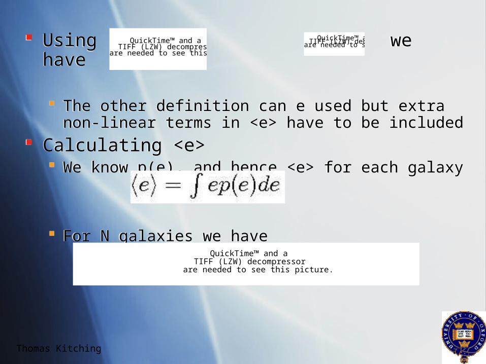
Using we have

The other definition can e used but extra non-linear terms in <e> have to be included

Calculating <e> We know p(e), and hence <e> for each galaxy

For N galaxies we have

Using we have

The other definition can e used but extra non-linear terms in <e> have to be included

Calculating <e> We know p(e), and hence <e> for each galaxy

For N galaxies we have

QuickTime™ and aTIFF (LZW) decompressor

are needed to see this picture.

QuickTime™ and aTIFF (LZW) decompressorare needed to see this picture.

QuickTime™ and aTIFF (LZW) decompressor

are needed to see this picture.

Thomas Kitching

Frequentist : can shapes be measured using Likelihoods alone?

Bayesian and Likelihoods measure different things

Suppose x has an intrinsic normal distribution of variance a=0.3

For each input we measure a normal distribution with variance b=0.4

Frequentist : can shapes be measured using Likelihoods alone?

Bayesian and Likelihoods measure different things

Suppose x has an intrinsic normal distribution of variance a=0.3

For each input we measure a normal distribution with variance b=0.4

QuickTime™ and aTIFF (LZW) decompressor

are needed to see this picture.

QuickTime™ and aTIFF (LZW) decompressor

are needed to see this picture.

Bayesian or Frequentist?Bayesian or Frequentist?

Thomas Kitching

Likelihood unbiased in input to output regression No way to account for the

bias from the likelihood alone

Also with no prior the hard bound |e|<1 can affect likelihood estimators

Bayesian unbiased in output to input regression Best estimate of input

values Distribution narrower but

each point has an uncertainty

If if there are effects due to the hard |e|<1 boundary the prior should contain this information

Likelihood unbiased in input to output regression No way to account for the

bias from the likelihood alone

Also with no prior the hard bound |e|<1 can affect likelihood estimators

Bayesian unbiased in output to input regression Best estimate of input

values Distribution narrower but

each point has an uncertainty

If if there are effects due to the hard |e|<1 boundary the prior should contain this information

QuickTime™ and aTIFF (LZW) decompressor

are needed to see this picture.

Thomas Kitching

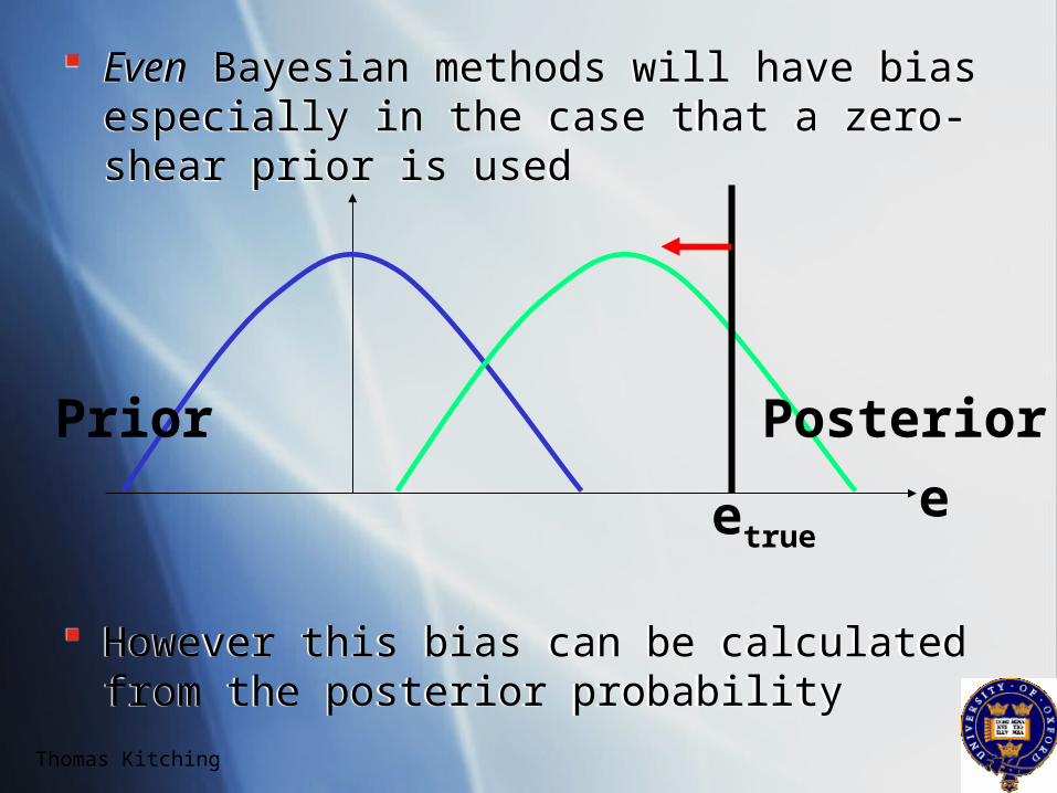
Even Bayesian methods will have bias especially in the case that a zero-shear prior is used

However this bias can be calculated from the posterior probability

Even Bayesian methods will have bias especially in the case that a zero-shear prior is used

However this bias can be calculated from the posterior probability

e

Prior Posterior

etrue

Thomas Kitching

Shear Sensitivity & PriorShear Sensitivity & Prior Since we do not know the Prior distribution we are

forced to adopt a zero-shear prior For low S/N galaxies the prior could dominate resulting in no

recoverable shear, as in all methods However the magnitude of this effect can be determined

Can define a weighted estimate of the shear as

Where we call the shear sensitivity In Bayesian case this can be approximated by

Since we do not know the Prior distribution we are forced to adopt a zero-shear prior For low S/N galaxies the prior could dominate resulting in no

recoverable shear, as in all methods However the magnitude of this effect can be determined

Can define a weighted estimate of the shear as

Where we call the shear sensitivity In Bayesian case this can be approximated by

QuickTime™ and aTIFF (LZW) decompressor

are needed to see this picture.

QuickTime™ and aTIFF (LZW) decompressor

are needed to see this picture.

QuickTime™ and aTIFF (LZW) decompressor

are needed to see this picture.

Thomas Kitching

Thomas Kitching

If the model is a good fit to the data then maximum S/N of parameters should be obtained

If model is a good fit then all information about image is contained in the model Use realistic models based on real galaxy image profiles

Long history of model fitting for non-lensing and lensing applications Galfit Kuijken, Im2shape

Problem is that we need a computationally fast model fitting algorithm for lensing surveys that uses realistic galaxy image profiles

If the model is a good fit to the data then maximum S/N of parameters should be obtained

If model is a good fit then all information about image is contained in the model Use realistic models based on real galaxy image profiles

Long history of model fitting for non-lensing and lensing applications Galfit Kuijken, Im2shape

Problem is that we need a computationally fast model fitting algorithm for lensing surveys that uses realistic galaxy image profiles

Model FittingModel Fitting

Thomas Kitching

lensfitlensfit Measure PSF create a model

convolve with PSF determine the likelihood of the fit

Simplest galaxy model (if form is fixed) has 6 free parameters Brightness, size, ellipticity (x2), position (x2)

It is straightforward to marginalise over position and brightness if the model fitting is done in Fourier space

Key advances and differences FAST model fitting technique Bias is taken into account in a Bayesian way

Measure PSF create a model convolve with PSF determine the likelihood of the fit

Simplest galaxy model (if form is fixed) has 6 free parameters Brightness, size, ellipticity (x2), position (x2)

It is straightforward to marginalise over position and brightness if the model fitting is done in Fourier space

Key advances and differences FAST model fitting technique Bias is taken into account in a Bayesian way

Thomas Kitching

Choice of model is not key, we assume a de Vaucouleurs profile Free parameters are then length scale (r), e1, e2

We use a grid in (e1,e2) Could use MCMC approach Found convergence for e=0.1 <100 points

We adopt a uniform prior for the distribution of galaxy scale-length. This could be replaced by a prior close to the actual distribution of

galaxy sizes, although such a prior would need to be magnitude-dependent

Tested the algorithm Convergence in e and r resolutions Robust to galaxy position error up to a + 10 pixel random offset

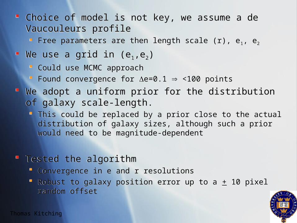
Choice of model is not key, we assume a de Vaucouleurs profile Free parameters are then length scale (r), e1, e2

We use a grid in (e1,e2) Could use MCMC approach Found convergence for e=0.1 <100 points

We adopt a uniform prior for the distribution of galaxy scale-length. This could be replaced by a prior close to the actual distribution of

galaxy sizes, although such a prior would need to be magnitude-dependent

Tested the algorithm Convergence in e and r resolutions Robust to galaxy position error up to a + 10 pixel random offset

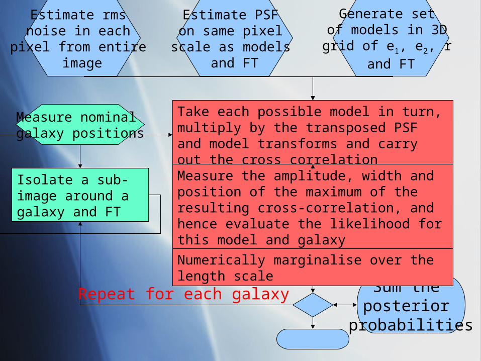
Isolate a sub-image around a galaxy and FT

Take each possible model in turn, multiply by the transposed PSF and model transforms and carry out the cross correlation

Measure the amplitude, width and position of the maximum of the resulting cross-correlation, and hence evaluate the likelihood for this model and galaxy

Sum the posterior

probabilities

Numerically marginalise over the length scale

Repeat for each galaxy

Estimate rms noise in each

pixel from entire image

Estimate PSF on same pixel

scale as models and FT

Generate set of models in 3D grid of e1, e2, r

and FT

Measure nominal galaxy positions

Thomas Kitching

Tests on STEP1Tests on STEP1 Use a grid sampling of e=0.1

Found numerical convergence Use 32x32 sub images sizes

Optimal for close pairs rejection and fitting every galaxy with the sub image

Close pairs rejection if two galaxies lie in a sub image Working on a S/N based rejection criterion

We assume the pixel noise is uncorrelated, which is appropriate for shot noise in CCD detectors

The PSF was created by stacking stars from the simulation allowing sub-pixel registration using sinc-function interpolation Method of PSF characterisation not crucial as long as the PSF is a

good match to the actual PSF Sub pixel variation in PSF not taken into account may lead to high

spatial frequencies which are not included

Use a grid sampling of e=0.1 Found numerical convergence

Use 32x32 sub images sizes Optimal for close pairs rejection and fitting every galaxy with the sub

image Close pairs rejection if two galaxies lie in a sub image

Working on a S/N based rejection criterion We assume the pixel noise is uncorrelated, which is

appropriate for shot noise in CCD detectors The PSF was created by stacking stars from the simulation

allowing sub-pixel registration using sinc-function interpolation Method of PSF characterisation not crucial as long as the PSF is a

good match to the actual PSF Sub pixel variation in PSF not taken into account may lead to high

spatial frequencies which are not included

Thomas Kitching

PriorPrior Use the lens0 STEP1 input catalogue (zero-

sheared) to generate the input prior for each STEP1 image and psf

In reality could iterate the method especially since in reality the intrinsic p(e) will be approximately zero-centered The method should return the intrinsic p(e)

Calculate p(e) Substitute p(e) for the prior and iterate until

convergence is reached

Use the lens0 STEP1 input catalogue (zero-sheared) to generate the input prior for each STEP1 image and psf

In reality could iterate the method especially since in reality the intrinsic p(e) will be approximately zero-centered The method should return the intrinsic p(e)

Calculate p(e) Substitute p(e) for the prior and iterate until

convergence is reached

Thomas Kitching

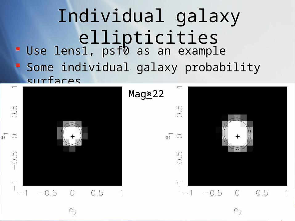
Use lens1, psf0 as an example Some individual galaxy probability surfaces

Use lens1, psf0 as an example Some individual galaxy probability surfaces

Individual galaxy ellipticitiesIndividual galaxy ellipticities

Mag<22Mag>22

Thomas Kitching

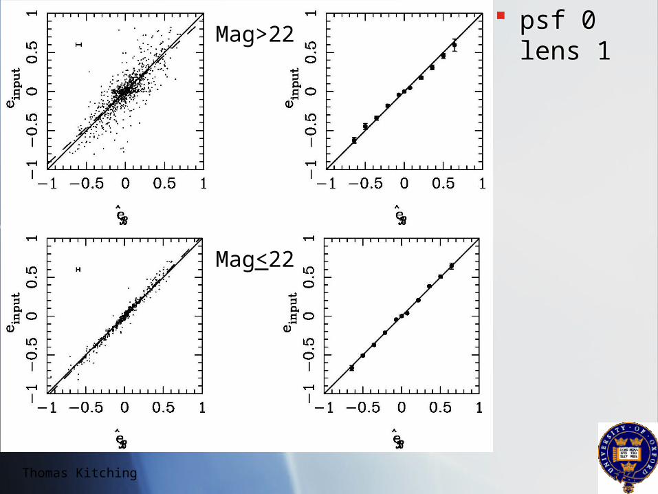
psf 0 lens 1

psf 0 lens 1

Mag>22

Mag<22

Thomas Kitching

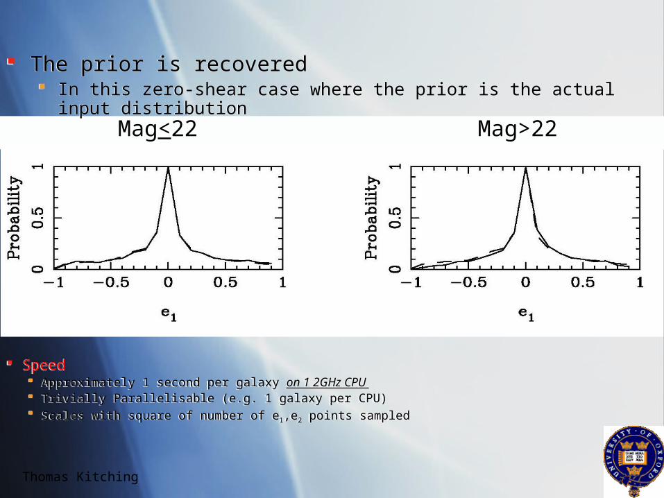
The prior is recovered In this zero-shear case where the prior is the actual input distribution

The prior is recovered In this zero-shear case where the prior is the actual input distribution

Speed Approximately 1 second per galaxy on 1 2GHz CPU Trivially Parallelisable (e.g. 1 galaxy per CPU) Scales with square of number of e1,e2 points sampled

Speed Approximately 1 second per galaxy on 1 2GHz CPU Trivially Parallelisable (e.g. 1 galaxy per CPU) Scales with square of number of e1,e2 points sampled

Mag<22 Mag>22

Thomas Kitching

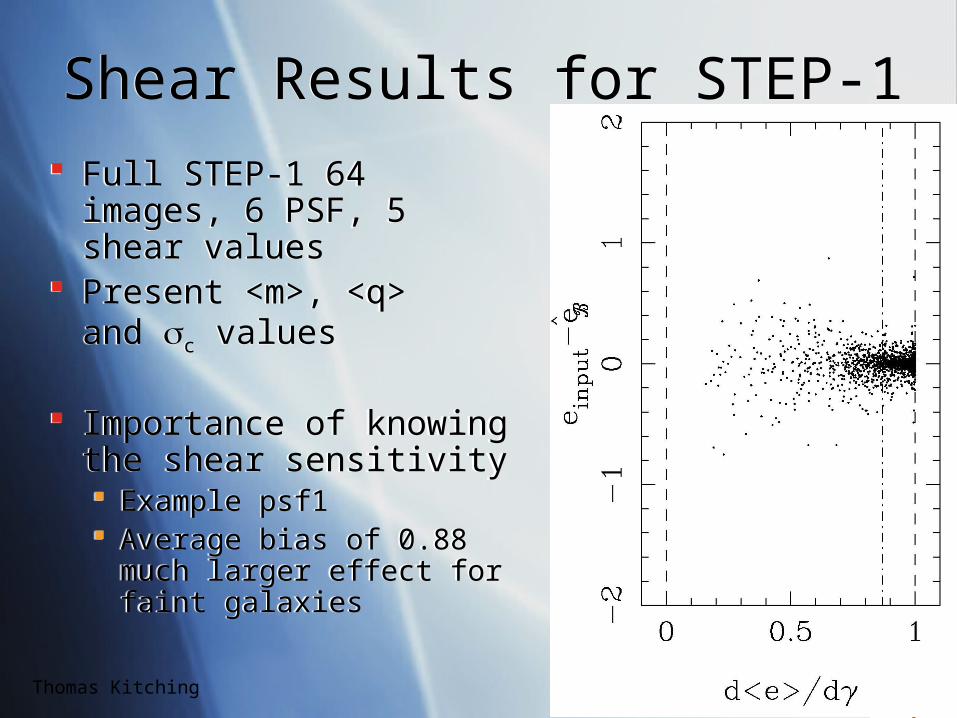
Shear Results for STEP-1Shear Results for STEP-1 Full STEP-1 64 images,

6 PSF, 5 shear values Present <m>, <q>

and c values

Importance of knowing the shear sensitivity Example psf1 Average bias of 0.88 much

larger effect for faint galaxies

Full STEP-1 64 images, 6 PSF, 5 shear values

Present <m>, <q> and c values

Importance of knowing the shear sensitivity Example psf1 Average bias of 0.88 much

larger effect for faint galaxies

Thomas Kitching

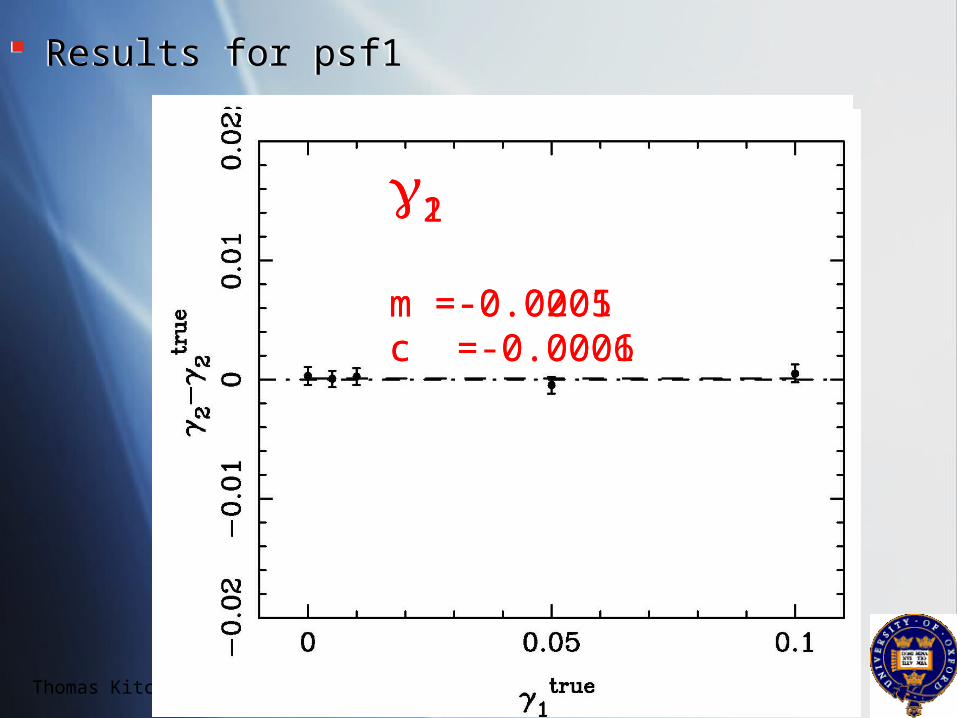
Results for psf1 Results for psf1

1

m =-0.0205c =-0.0006

2

m =-0.0001c = 0.0001

Thomas Kitching

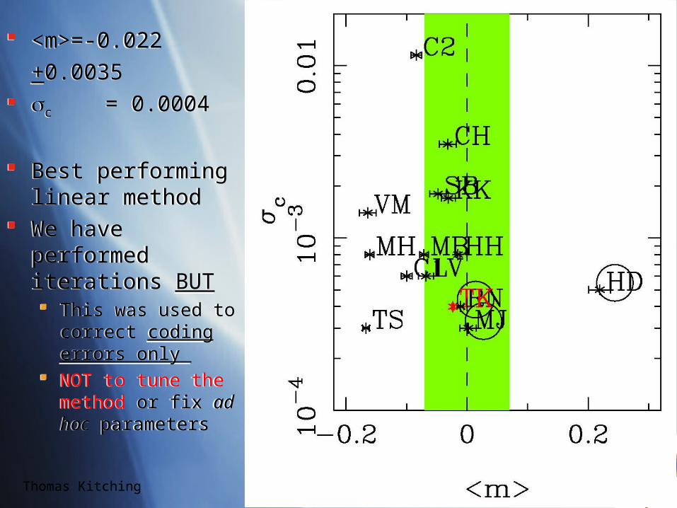
<m>=-0.022+0.0035

c = 0.0004

Best performing linear method

We have performed iterations BUT This was used to

correct coding errors only

NOT to tune the method or fix ad hoc parameters

<m>=-0.022+0.0035

c = 0.0004

Best performing linear method

We have performed iterations BUT This was used to

correct coding errors only

NOT to tune the method or fix ad hoc parameters

Thomas Kitching

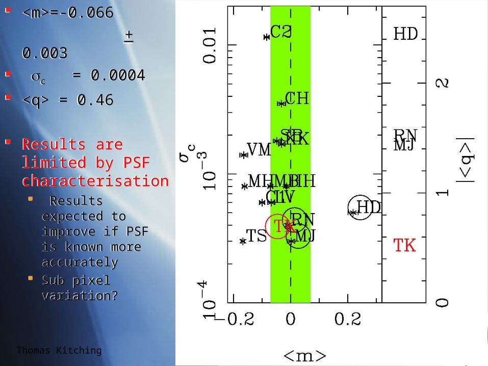
<m>=-0.066 + 0.003 c = 0.0004 <q> = 0.46

Results are limited by PSF characterisation Results expected to

improve if PSF is known more accurately

Sub pixel variation?

<m>=-0.066 + 0.003 c = 0.0004 <q> = 0.46

Results are limited by PSF characterisation Results expected to

improve if PSF is known more accurately

Sub pixel variation?

Thomas Kitching

ConclusionsConclusions Given a shape measurement method that can

produce p(e) Bayesian shape measurement has the potential to yield an unbiased shear estimator

Even in reality, assuming a zero-sheared prior, the shear sensitivity can be calculated to correct for any bias

We presented a fast model fitting method lensfit

lensfit can accurately find individual galaxy ellipticities

Performance is good in the STEP1 simulations with small values of m, c and q

Better PSF characterisation could improve results

Given a shape measurement method that can produce p(e) Bayesian shape measurement has the potential to yield an unbiased shear estimator

Even in reality, assuming a zero-sheared prior, the shear sensitivity can be calculated to correct for any bias

We presented a fast model fitting method lensfit

lensfit can accurately find individual galaxy ellipticities

Performance is good in the STEP1 simulations with small values of m, c and q

Better PSF characterisation could improve results

Thomas Kitching

Thomas Kitching

Radio STEPRadio STEP SKA could produce a very competitive weak lensing

survey 50 km baseline implies angular resolution ≈ 1 arcsec at 1.4 GHz The shear map constructed from continuum shape measurements of

star-forming disk galaxies A subset of spectroscopic redshifts from HI detections 22 per arcmin2 at 0.3 μJy, 20,000 sqdeg survey No photometric redshift uncertainties

Have software ‘MEQtrees’ Can simulate realistic Radio images With realistic Radio PSF’s Note that the PSF is complicated but deterministic (apart from

atmospherics) Radio STEP

Can measure shapes directly in the (u,v) Fourier plane Using the simulated Radio images Progressively complicated PSF’s

SKA could produce a very competitive weak lensing survey 50 km baseline implies angular resolution ≈ 1 arcsec at 1.4 GHz The shear map constructed from continuum shape measurements of

star-forming disk galaxies A subset of spectroscopic redshifts from HI detections 22 per arcmin2 at 0.3 μJy, 20,000 sqdeg survey No photometric redshift uncertainties

Have software ‘MEQtrees’ Can simulate realistic Radio images With realistic Radio PSF’s Note that the PSF is complicated but deterministic (apart from

atmospherics) Radio STEP

Can measure shapes directly in the (u,v) Fourier plane Using the simulated Radio images Progressively complicated PSF’s

QuickTime™ and aTIFF (LZW) decompressor

are needed to see this picture.QuickTime™ and a

TIFF (LZW) decompressorare needed to see this picture.