Embed Size (px)
Citation preview
This�edition�was�last�updated�on�11th�January�2019�
����������� ���������������������������������������We’ve�helped�over�2�million�students�to�learn�Excel.��If�you�carefully�work�through�this�free�book�there�is�absolutely�no�doubt�that�you�will�master�Excel�2019�fundamentals.�
�� ������������������������������ �������������������������!�� ���"����!�� ����������!������������##������� ����������������We�continuously�update�our�free�and�published�books�based�upon�user�feedback�so�that�the�latest�version�has�no�known�errors.��You�can�download�the�most�recent�version�of�this�free�e�book�from:�https://thesmartmethod.com.��This�book�is�only�for�Excel�2019�for�Windows�users.��If�you�are�using�a�different�version:�(2007,�2010,�2013,�2016,�365�or�the�Apple�Mac�version)�download�the�correct�free�e�book�for�your�version�from:��https://thesmartmethod.com.�
$������������ ������������!�� �� It�is�free�(and�you�can�print�it).��Because�this�book�is�free�of�charge,�schools,�colleges,�universities�and�businesses�are�able�teach�their�students�best�practice�Excel�skills�without�the�substantial�cost�of�designing�lesson�plans�or�purchasing�books.��If�printed�copies�are�needed�you�can�print�them�yourself,�or�any�copy�shop�can�print�books�for�you.�
� Smart�Method�books�are�#1�best�sellers.��While�this�e�book�is�entirely�free�of�charge,�every�paper�printed�Smart�Method®�Excel�book�(and�there�have�been�ten�of�them�starting�with�Excel�2007)�has�been�an�Amazon�#1�best�seller�in�its�category.��This�provides�you�with�the�confidence�that�you�are�using�a�best�of�breed�resource�to�learn�Excel.�
� Learning�success�is�guaranteed.��For�over�fifteen�years,�Smart�Method�courses�have�been�used�by�large�corporations,�government�departments�and�the�armed�forces�to�train�their�employees.�The�book�is�ideal�for�teaching�or�self�learning�because�it�has�been�constantly�refined�(during�hundreds�of�classroom�courses)�by�observing�which�skills�students�find�difficult�to�understand�and�then�developing�simpler�and�better�ways�of�explaining�them.�This�has�made�the�book�effective�for�students�of�all�ages�and�abilities.�
� It�is�the�book�of�choice�for�teachers.��As�well�as�catering�for�those�wishing�to�learn�Excel�by�self�study,�Smart�Method®�books�have�long�been�the�preferred�choice�for�Excel�teachers�as�they�are�designed�to�teach�Excel�and�not�as�reference�books.��Books�follow�best�practice�adult�teaching�methodology�with�clearly�defined�objectives�for�each�learning�session�and�an�exercise�to�confirm�skills�transfer.��With�single,�self�contained�lessons�the�books�cater�for�any�teaching�period�(from�minutes�to�hours).�
� No�previous�exposure�to�Excel�is�assumed.��You�will�repeatedly�hear�the�same�criticism�of�most�Excel�books:�“you�have�to�already�know�Excel�to�understand�the�book”.��This�book�is�different.��If�you’ve�never�seen�Excel�before,�and�your�only�computer�skill�is�using�a�web�browser,�you’ll�have�absolutely�no�problems�working�through�the�lessons.���
� It�focuses�upon�the�everyday�Excel�skills�used�in�the�workplace.��This�free�Basic�Skills�book�will�teach�you�the�basics�without�confusing�you�with�more�advanced,�less�used,�Excel�features.�If�you�decide�to�expand�your�Excel�education,�you’ll�be�able�to�move�on�to�other�Smart�Method®�books�(or�e�books)�in�this�series�to�master�even�the�most�advanced�Excel�features.�
� It�provides�a�clearly�defined�route�to�become�a�true�Excel�guru.�If�you�later�decide�that�you�d�like�to�become�a�true�Excel�guru,�we�also�have�Essential�Skills�and�Expert�Skills�books�in�this�series�that�will�teach�you�very�advanced�features�(such�as�Power�Pivot,�Power�Query�(Get�&�Transform),�Power�Maps�(3�D�Maps)�and�OLAP�multi�dimensional�modeling)�that�almost�all�Excel�users�(even�top�professionals)�really�understand.�
� � �
%������������&���������#���������� ���'������������������������(�Excel�is�a�huge�and�daunting�application�and�you’ll�need�to�invest�some�time�in�learning�the�skills�presented�in�this�book.�This�will�be�time�well�spent�as�you’ll�have�a�hugely�marketable�skill�for�life.��With�1.2�billion�users�worldwide,�it�is�hard�to�imagine�any�non�manual�occupation�today�that�doesn’t�require�Excel�skills.�
This�book�makes�it�easy�to�learn�at�your�own�pace�because�of�its�unique�presentational�style.��The�book�contains�43�simple,�self�contained�lessons�and�each�lesson�only�takes�a�few�minutes�to�complete.���
You�can�complete�as�many,�or�as�few,�lessons�as�you�have�the�time�and�energy�for�each�day.��Many�learners�have�developed�Excel�skills�by�setting�aside�just�a�few�minutes�each�day�to�complete�a�single�lesson.��Others�have�worked�through�the�entire�book�in�less�than�five�hours.�
)�� ������!� ���� ����� ����������������������������It�is�important�to�realize�that�Excel�is�probably�the�largest�and�most�complex�software�application�ever�created.��Hardly�anybody�understands�how�to�use�every�Excel�feature,�and�for�almost�all�business�users,�large�parts�of�Excel’s�functionality�wouldn’t�even�be�useful.���
Many�learners�make�the�fundamental�error�of�trying�to�learn�from�an�Excel�reference�book�that�attempts�to�document�(though�not�teach)�everything�that�Excel�can�do.��Of�course,�no�single�book�could�ever�actually�do�this.��There�are�some�single�advanced�Excel�features�(such�as�Power�Pivot,�Power�Query/Get�&�Transform�and�DAX)�that�have�had�entire�500+�page�books�devoted�to�them).���For�most�Excel�business�users,�it�would�clearly�be�a�waste�of�effort�to�attempt�to�master�these�highly�technical�subjects�(though�you�can,�if�you�have�the�time�and�inclination,�master�these�skills�using�our�Expert�Skills�book).���
This�free�Basic�Skills�book�will�teach�you�the�basic�Excel�skills�that�are�used�every�day,�in�offices�all�over�the�world.���
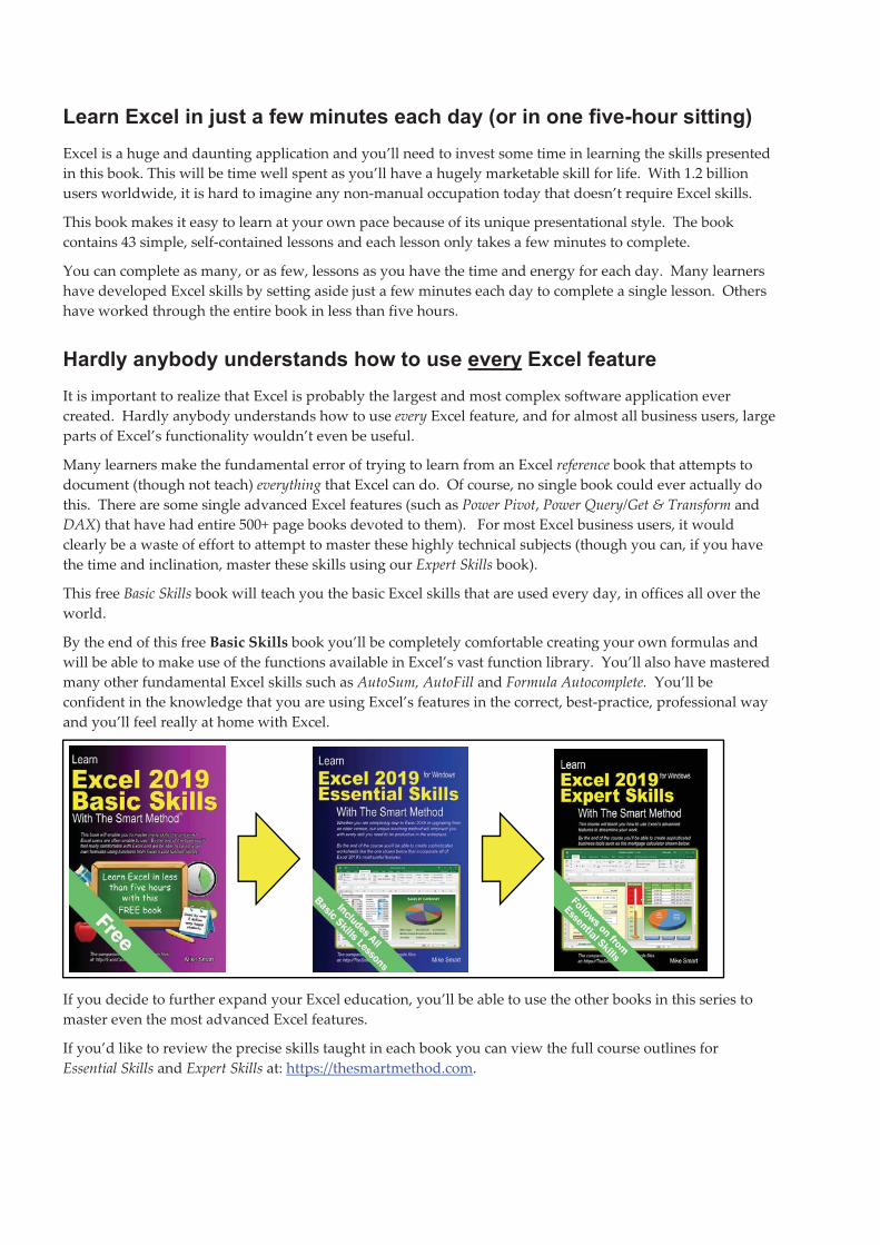
By�the�end�of�this�free�Basic�Skills�book�you’ll�be�completely�comfortable�creating�your�own�formulas�and�will�be�able�to�make�use�of�the�functions�available�in�Excel’s�vast�function�library.��You’ll�also�have�mastered�many�other�fundamental�Excel�skills�such�as�AutoSum,�AutoFill�and�Formula�Autocomplete.��You’ll�be�confident�in�the�knowledge�that�you�are�using�Excel’s�features�in�the�correct,�best�practice,�professional�way�and�you’ll�feel�really�at�home�with�Excel.��
�If�you�decide�to�further�expand�your�Excel�education,�you’ll�be�able�to�use�the�other�books�in�this�series�to�master�even�the�most�advanced�Excel�features.�
If�you’d�like�to�review�the�precise�skills�taught�in�each�book�you�can�view�the�full�course�outlines�for�Essential�Skills�and�Expert�Skills�at:�https://thesmartmethod.com.�
� �
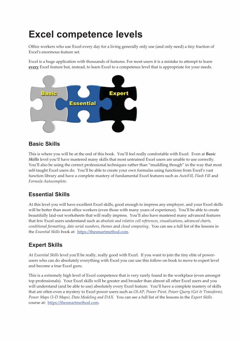
�������#*���������Office�workers�who�use�Excel�every�day�for�a�living�generally�only�use�(and�only�need)�a�tiny�fraction�of�Excel�s�enormous�feature�set.��
Excel�is�a�huge�application�with�thousands�of�features.�For�most�users�it�is�a�mistake�to�attempt�to�learn�every�Excel�feature�but,�instead,�to�learn�Excel�to�a�competence�level�that�is�appropriate�for�your�needs.���
�
������+ �����This�is�where�you�will�be�at�the�end�of�this�book.��You’ll�feel�really�comfortable�with�Excel.��Even�at�Basic�Skills�level�you’ll�have�mastered�many�skills�that�most�untrained�Excel�users�are�unable�to�use�correctly.��You’ll�also�be�using�the�correct�professional�techniques�rather�than�“muddling�though”�in�the�way�that�most�self�taught�Excel�users�do.��You’ll�be�able�to�create�your�own�formulas�using�functions�from�Excel’s�vast�function�library�and�have�a�complete�mastery�of�fundamental�Excel�features�such�as�AutoFill,�Flash�Fill�and�Formula�Autocomplete.�
���������+ �����At�this�level�you�will�have�excellent�Excel�skills,�good�enough�to�impress�any�employer,�and�your�Excel�skills�will�be�better�than�most�office�workers�(even�those�with�many�years�of�experience).��You’ll�be�able�to�create�beautifully�laid�out�worksheets�that�will�really�impress.��You’ll�also�have�mastered�many�advanced�features�that�few�Excel�users�understand�such�as�absolute�and�relative�cell�references,�visualizations,�advanced�charts,�conditional�formatting,�date�serial�numbers,�themes�and�cloud�computing.��You�can�see�a�full�list�of�the�lessons�in�the�Essential�Skills�book�at:��https://thesmartmethod.com.�
��*���+ �����At�Essential�Skills�level�you�ll�be�really,�really�good�with�Excel.��If�you�want�to�join�the�tiny�elite�of�power�users�who�can�do�absolutely�everything�with�Excel�you�can�use�this�follow�on�book�to�move�to�expert�level�and�become�a�true�Excel�guru.�
This�is�a�extremely�high�level�of�Excel�competence�that�is�very�rarely�found�in�the�workplace�(even�amongst�top�professionals).��Your�Excel�skills�will�be�greater�and�broader�than�almost�all�other�Excel�users�and�you�will�understand�(and�be�able�to�use)�absolutely�every�Excel�feature.��You’ll�have�a�complete�mastery�of�skills�that�are�often�even�a�mystery�to�Excel�power�users�such�as�OLAP,�Power�Pivot,�Power�Query�(Get�&�Transform),�Power�Maps�(3�D�Maps),�Data�Modeling�and�DAX.��You�can�see�a�full�list�of�the�lessons�in�the�Expert�Skills�course�at:��https://thesmartmethod.com.�
� � �
��������������*���� ���������������*����
�Winston�Churchill�was�aware�of�the�power�of�brevity.�The�discipline�of�condensing�thoughts�into�one�side�of�a�single�sheet�of�A4�paper�resulted�in�the�efficient�transfer�of�information.��
A�tenet�of�our�teaching�system�is�that�every�lesson�is�presented�on�two�facing�sheets�of�A4.�We’ve�had�to�double�Churchill’s�rule�as�they�didn’t�have�to�contend�with�screen�grabs�in�1939!��If�we�can’t�teach�an�essential�concept�in�two�pages�of�A4�we�know�that�the�subject�matter�needs�to�be�broken�into�two�smaller�lessons.��
)��������!�� ����� �����������������#��Over�the�years�I�have�read�many�hundreds�of�computer�text�books�and�most�of�my�time�was�wasted.��The�big�problem�with�most�books�is�that�I�must�wade�through�thousands�of�words�just�to�learn�one�important�technique.��If�I�don’t�read�everything�I�might�miss�that�one�essential�insight.���
Many�presentational�methods�have�been�used�in�this�book�to�help�you�to�avoid�reading�about�things�you�already�know�how�to�do,�or�things�that�are�of�little�interest�to�you.��
�
�
Pray�this�day,�on�one�side�of�one�sheet�of�paper,�explain�how�the�Royal�Navy�is�prepared�to�meet�the�coming�conflict.��Winston�Churchill,�Letter�to�the�Admiralty,�Sep�1,�1939��
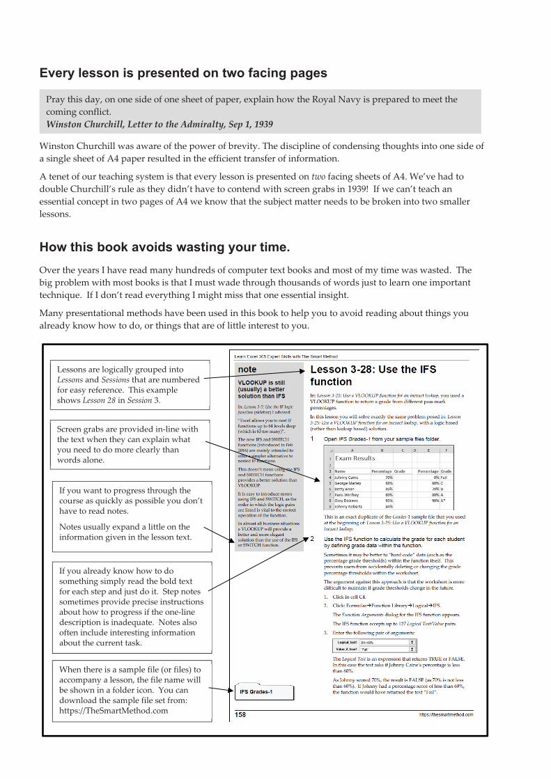
If�you�want�to�progress�through�the�course�as�quickly�as�possible�you�don’t�have�to�read�notes.�
Notes�usually�expand�a�little�on�the�information�given�in�the�lesson�text.�
Screen�grabs�are�provided�in�line�with�the�text�when�they�can�explain�what�you�need�to�do�more�clearly�than�words�alone.�
When�there�is�a�sample�file�(or�files)�to�accompany�a�lesson,�the�file�name�will�be�shown�in�a�folder�icon.��You�can�download�the�sample�file�set�from:�https://TheSmartMethod.com�
If�you�already�know�how�to�do�something�simply�read�the�bold�text�for�each�step�and�just�do�it.��Step�notes�sometimes�provide�precise�instructions�about�how�to�progress�if�the�one�line�description�is�inadequate.��Notes�also�often�include�interesting�information�about�the�current�task.�
Lessons�are�logically�grouped�into�Lessons�and�Sessions�that�are�numbered�for�easy�reference.��This�example�shows�Lesson�28�in�Session�3.�
%�������!��*������*������
�Confucius�would�probably�have�agreed�that�the�best�way�to�teach�IT�skills�is�hands�on�(actively)�and�not�hands�off�(passively).�This�is�another�of�the�principal�tenets�of�The�Smart�Method®�teaching�method.����
Research�has�backed�up�the�assertion�that�you�will�learn�more�material,�learn�more�quickly,�and�understand�more�of�what�you�learn�if�you�learn�using�active,�rather�than�passive�methods.���
For�this�reason,�pure�theory�pages�are�kept�to�an�absolute�minimum�with�most�theory�woven�into�the�hands�on�lessons,�either�within�the�text�or�in�sidebars.�
This�echoes�the�teaching�method�used�in�Smart�Method�classroom�courses�where�snippets�of�pertinent�theory�are�woven�into�the�lessons�themselves�so�that�interest�and�attention�is�maintained�by�hands�on�involvement,�but�all�necessary�theory�is�still�covered.�
�
�
� �
Tell�me,�and�I�will�forget.�Show�me,�and�I�may�remember.�Involve�me,�and�I�will�understand.�
Confucius,�Chinese�teacher,�editor,�politician�and�philosopher�(551�479�BC)��
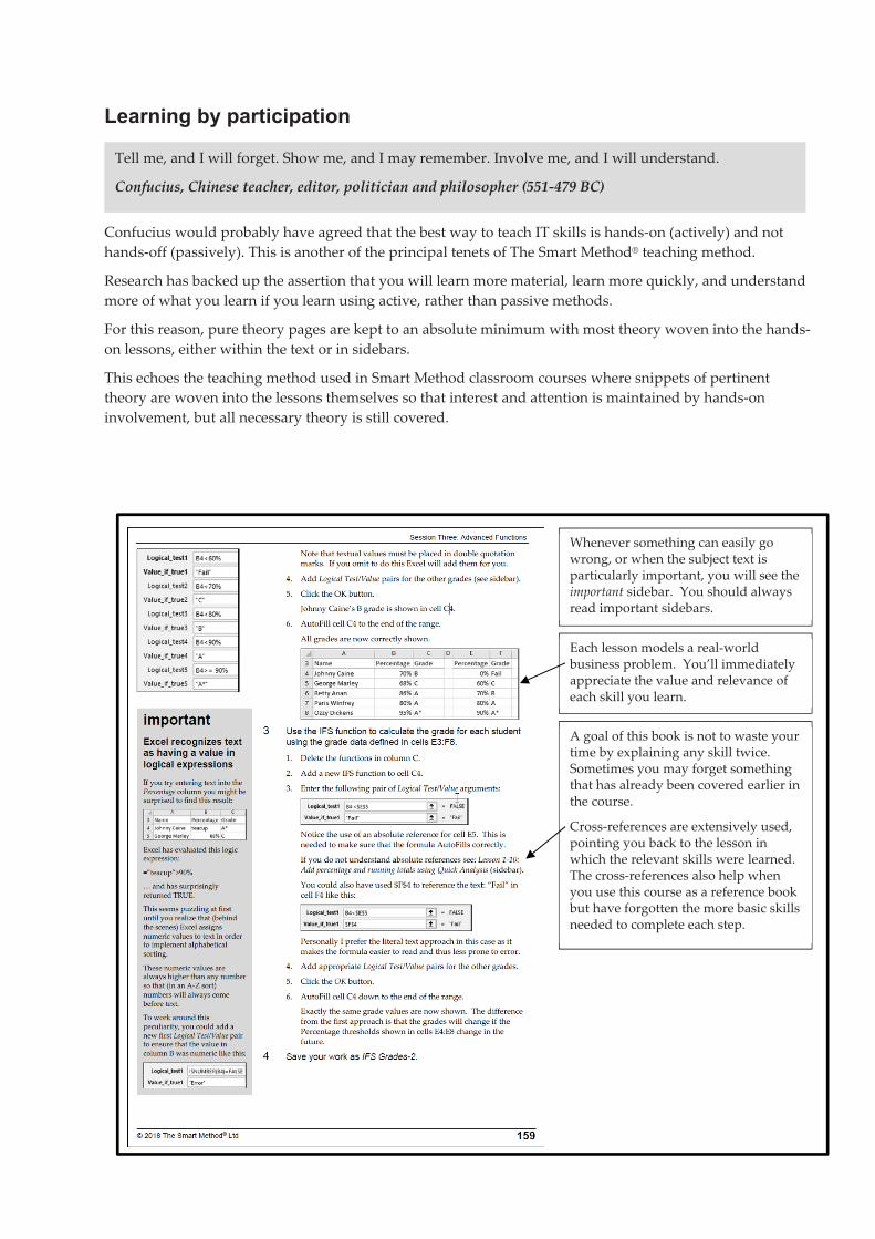
Whenever�something�can�easily�go�wrong,�or�when�the�subject�text�is�particularly�important,�you�will�see�the�important�sidebar.��You�should�always�read�important�sidebars.�
Each�lesson�models�a�real�world�business�problem.��You’ll�immediately�appreciate�the�value�and�relevance�of�each�skill�you�learn.���
A�goal�of�this�book�is�not�to�waste�your�time�by�explaining�any�skill�twice.��Sometimes�you�may�forget�something�that�has�already�been�covered�earlier�in�the�course.�
Cross�references�are�extensively�used,�pointing�you�back�to�the�lesson�in�which�the�relevant�skills�were�learned.��The�cross�references�also�help�when�you�use�this�course�as�a�reference�book�but�have�forgotten�the�more�basic�skills�needed�to�complete�each�step.���
� � �
$����������������*�������������!�� �E�books�can�only�be�obtained�and�downloaded�from�https://thesmartmethod.com�(the�publisher).��Our�e�books�are�published�in�full�color�as�regular�PDF�files.��This�means�that�you�can�read�them�on�just�about�any�device�without�the�bother�of�finding�and�installing�reader�software.����
,�����������#���������##� ����������*����������!�� �Unlike�most�e�books,�this�one�isn’t�locked�to�prevent�printing�(this�is�also�true�for�all�other�Smart�Method�e�Books).��While�this�book�is�useful�for�self�instruction,�it�is�also�ideal�for�teaching�structured,�objective�led,�and�highly�effective�classroom�courses.��Even�though�you�can�read�this�book�on�an�iPad*,�personal�computer�or�e�Book�reader,�some�students�find�it�easier�to�use�if�you�print�it�onto�paper.��You�may�legally�print�copies�of�this�basic�skills�book�(for�yourself�or�your�students)�with�only�two�conditions:�
1.� You�must�print�the�basic�skills�book�exactly�as�it�is�published�and�may�not�add�or�remove�any�book�content�or�copyright�notices.�
2.� You�may�not�make�any�charge�of�any�sort�for�the�basic�skills�books�that�you�print.��It�is�permissible,�however,�to�give�free�copies�of�the�book�to�students�who�attend�a�free�(or�paid�for)�class�or�course.�
For�classroom�courses�you�can�obtain�a�professional�looking�result�by�printing�on�both�sides�of�the�paper.���You�can�then�punch�the�pages�and�place�them�into�a�binder.��Make�sure�that�odd�pages�appear�on�the�right�hand�side.�This�enables�each�two�page�lesson�to�be�viewed�without�turning�the�page.���
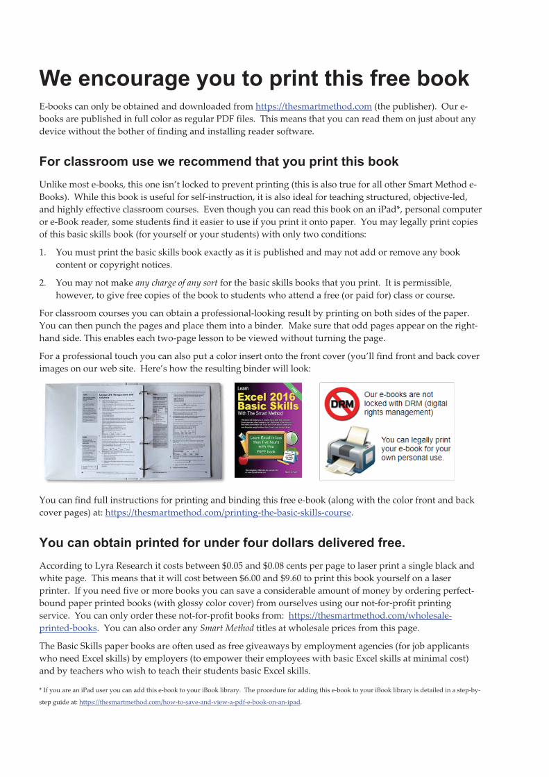
For�a�professional�touch�you�can�also�put�a�color�insert�onto�the�front�cover�(you’ll�find�front�and�back�cover�images�on�our�web�site.��Here’s�how�the�resulting�binder�will�look:�
� �You�can�find�full�instructions�for�printing�and�binding�this�free�e�book�(along�with�the�color�front�and�back�cover�pages)�at:�https://thesmartmethod.com/printing�the�basic�skills�course.�
-��������!�����*���� ������� ������� ������� ���� �����According�to�Lyra�Research�it�costs�between�$0.05�and�$0.08�cents�per�page�to�laser�print�a�single�black�and�white�page.��This�means�that�it�will�cost�between�$6.00�and�$9.60�to�print�this�book�yourself�on�a�laser�printer.��If�you�need�five�or�more�books�you�can�save�a�considerable�amount�of�money�by�ordering�perfect�bound�paper�printed�books�(with�glossy�color�cover)�from�ourselves�using�our�not�for�profit�printing�service.��You�can�only�order�these�not�for�profit�books�from:��https://thesmartmethod.com/wholesale�printed�books.��You�can�also�order�any�Smart�Method�titles�at�wholesale�prices�from�this�page.��
The�Basic�Skills�paper�books�are�often�used�as�free�giveaways�by�employment�agencies�(for�job�applicants�who�need�Excel�skills)�by�employers�(to�empower�their�employees�with�basic�Excel�skills�at�minimal�cost)�and�by�teachers�who�wish�to�teach�their�students�basic�Excel�skills.�
*�If�you�are�an�iPad�user�you�can�add�this�e�book�to�your�iBook�library.��The�procedure�for�adding�this�e�book�to�your�iBook�library�is�detailed�in�a�step�by�
step�guide�at:�https://thesmartmethod.com/how�to�save�and�view�a�pdf�e�book�on�an�ipad.�

�
�
�
�
�
Learn Excel 2019 Basic Skills with The Smart Method
Mike Smart �
� �

� � �
Learn�Excel�2019�Basic�Skills�with�The�Smart�Method®�
Published�by:�
The�Smart�Method®�Ltd�Burleigh�Manor�Peel�Road��Douglas,�IOM�Great�Britain��IM1�5EP��
Tel:�+44�(0)845�458�3282��
E�mail:��Use�the�contact�page�at�https://thesmartmethod.com/contact.�Web:�https://thesmartmethod.com�(this�book’s�dedicated�web�site)�
Copyright�©�2019�by�Mike�Smart�
All�Rights�Reserved.�
You�may�print�this�book�(or�selected�lessons�from�this�book)�provided�that�you�print�the�content�exactly�as�it�is�published,�do�not�add�or�remove�any�book�content�or�copyright�notices,�and�make�no�charge�of�any�sort�for�the�books�that�you�print.���
We�make�a�sincere�effort�to�ensure�the�accuracy�of�all�material�described�in�this�document.�The�Smart�Method®�Ltd�makes�no�warranty,�express�or�implied,�with�respect�to�the�quality,�correctness,�reliability,�accuracy,�or�freedom�from�error�of�this�document�or�the�products�it�describes.�
The�names�of�software�products�referred�to�in�this�manual�are�claimed�as�trademarks�of�their�respective�companies.�Any�other�product�or�company�names�mentioned�herein�may�be�the�trademarks�of�their�respective�owners.�
Unless�otherwise�noted,�the�example�data,�companies,�organizations,�products,�people�and�events�depicted�herein�are�fictitious.�No�association�with�any�real�company,�organization,�product,�person�or�event�is�intended�or�should�be�inferred.�The�sample�data�may�contain�many�inaccuracies�and�should�not�be�relied�upon�for�any�purpose.�
International�Standard�Book�Number�(ISBN13):� 978�1�909253�28�5�(Although�this�book�does�have�an�ISBN�it�will�not�be�generally�available�from�commercial�book�shops�or�wholesalers�as�we�only�allow�it�to�given�away�free�of�charge).�
The�Smart�Method®�is�a�registered�trade�marks�of�The�Smart�Method�Ltd.�
2�4�6�8�10�9�7�5�3�1
�
�
.�������/���� ������� ���
Feedback�...............................................................................................................................................................�11�Downloading�the�sample�files�...........................................................................................................................�11�Problem�resolution�.............................................................................................................................................�11�The�Excel�versions�that�were�used�to�write�this�book�....................................................................................�11�Typographical�Conventions�Used�in�This�Book�.............................................................................................�12�
)�������������������� �0�
Three�important�rules�.........................................................................................................................................�14�How�to�work�through�the�lessons�....................................................................................................................�15�How�to�best�use�the�incremental�sample�files�.................................................................................................�15�
+������1�2�������+ ����� �3�
Session�Objectives�...............................................................................................................................................�17�Lesson�1�1:�Start�Excel�and�open�a�new�blank�workbook�...................................................................................�18�Lesson�1�2:�Check�that�your�Excel�version�is�up�to�date�.....................................................................................�20�Lesson�1�3:�Change�the�Office�Theme�....................................................................................................................�22�Lesson�1�4:�Maximize,�minimize,�re�size,�move�and�close�the�Excel�window�.................................................�24�Lesson�1�5:�Download�the�sample�files�and�open/navigate�a�workbook�..........................................................�26�Lesson�1�6:�Save�a�workbook�to�a�local�file�...........................................................................................................�28�Lesson�1�7:�Understand�common�file�formats�......................................................................................................�30�Lesson�1�8:�Pin�a�workbook�and�understand�file�organization�..........................................................................�32�Lesson�1�9:�View,�move,�add,�rename,�delete�and�navigate�worksheet�tabs....................................................�34�Lesson�1�10:�Use�the�Versions�feature�to�recover�an�unsaved�Draft�file�...........................................................�36�Lesson�1�11:�Use�the�Versions�feature�to�recover�an�earlier�version�of�a�workbook�.......................................�38�Lesson�1�12:�Use�the�Ribbon�...................................................................................................................................�40�Lesson�1�13:�Understand�Ribbon�components�.....................................................................................................�42�Lesson�1�14:�Customize�the�Quick�Access�Toolbar�and�preview�the�printout�.................................................�44�Lesson�1�15:�Use�the�Mini�Toolbar,�Key�Tips�and�keyboard�shortcuts�.............................................................�46�Lesson�1�16:�Understand�views�..............................................................................................................................�48�Lesson�1�17:�Hide�and�Show�the�Formula�Bar�and�Ribbon�................................................................................�50�Lesson�1�18:�Use�the�Tell�Me�help�system�.............................................................................................................�52�Lesson�1�19:�Use�other�help�features�......................................................................................................................�54�
Session�1:�Exercise�...............................................................................................................................................�57�Session�1:�Exercise�answers�...............................................................................................................................�59�
+���������2�4�����5�����$�� ����������� 6��
Session�Objectives�...............................................................................................................................................�61�Lesson�2�1:�Enter�text�and�numbers�into�a�worksheet�.........................................................................................�62�
� �
�
Lesson�2�2:�Create�a�new�workbook�and�view�two�workbooks�at�the�same�time�..........................................�64�Lesson�2�3:�Use�AutoSum�to�quickly�calculate�totals�.........................................................................................�66�Lesson�2�4:�Select�a�range�of�cells�and�understand�Smart�Tags�.........................................................................�68�Lesson�2�5:�Enter�data�into�a�range�and�copy�data�across�a�range�....................................................................�70�Lesson�2�6:�Select�adjacent�and�non�adjacent�rows�and�columns�.....................................................................�72�Lesson�2�7:�Select�non�contiguous�cell�ranges�and�view�summary�information�............................................�74�Lesson�2�8:�AutoSelect�a�range�of�cells�.................................................................................................................�76�Lesson�2�9:�Re�size�rows�and�columns�..................................................................................................................�78�Lesson�2�10:�Use�AutoSum�to�sum�a�non�contiguous�range�.............................................................................�80�Lesson�2�11:�Use�AutoSum�to�calculate�average�and�maximum�values�..........................................................�82�Lesson�2�12:�Create�your�own�formulas�...............................................................................................................�84�Lesson�2�13:�Create�functions�using�Formula�AutoComplete�...........................................................................�86�Lesson�2�14:�Use�AutoFill�for�text�and�numeric�series�........................................................................................�88�Lesson�2�15:�Use�AutoFill�to�adjust�formulas�......................................................................................................�90�Lesson�2�16:�Use�AutoFill�options�.........................................................................................................................�92�Lesson�2�17:�Speed�up�your�AutoFills�and�create�a�custom�fill�series�..............................................................�94�Lesson�2�18:�Understand�linear�and�exponential�series�.....................................................................................�96�Lesson�2�19:�Use�automatic�Flash�Fill�to�split�delimited�text�.............................................................................�98�Lesson�2�20:�Use�manual�Flash�Fill�to�split�text�.................................................................................................�100�Lesson�2�21:�Use�multiple�example�Flash�Fill�to�concatenate�text�..................................................................�102�Lesson�2�22:�Use�Flash�Fill�to�solve�common�problems�...................................................................................�104�Lesson�2�23:�Use�the�zoom�control�......................................................................................................................�106�Lesson�2�24:�Print�out�a�worksheet�......................................................................................................................�108�
Session�2:�Exercise�............................................................................................................................................�111�Session�2:�Exercise�answers�.............................................................................................................................�113�
/� �� ��0�
����
�
�
����������� �������������� ��
/���� �������Welcome�to�Learn�Excel�2019�Basic�Skills�with�The�Smart�Method®.�This�book�has�been�designed�to�enable�students�to�master�Excel�2019�fundamentals�by�self�study.�The�book�is�equally�useful�as�courseware�in�order�to�deliver�courses�using�The�Smart�Method®�teaching�system.�
Smart�Method�publications�are�continually�evolving�as�we�discover�better�ways�of�explaining�or�teaching�the�concepts�presented.�
, !�� �At�The�Smart�Method®�we�love�feedback�–�both�positive�and�negative.�If�you�have�any�suggestions�for�improvements�to�future�versions�of�this�book,�or�if�you�find�content�or�typographical�errors,�the�author�would�always�love�to�hear�from�you.��
You�can�make�suggestions�for�improvements�to�this�book�using�the�online�form�at:�
https://thesmartmethod.com/contact�
Future�editions�of�this�book�will�always�incorporate�your�feedback�so�that�there�are�never�any�known�errors�at�time�of�publication.�
If�you�have�any�difficulty�understanding�or�completing�a�lesson,�or�if�you�feel�that�anything�could�have�been�more�clearly�explained,�we’d�also�love�to�hear�from�you.�We’ve�made�hundreds�of�detail�improvements�to�our�books�based�upon�reader’s�feedback�and�continue�to�chase�the�impossible�goal�of�100%�perfection.��
4������ ���������#*�������In�order�to�use�this�book�it�is�sometimes�necessary�to�download�free�sample�files�from�the�Internet.��
The�process�of�downloading�the�free�sample�files�is�explained�step�by�step�in:�Lesson�1�5:�Download�the�sample�files�and�open/navigate�a�workbook.�
7��!�#�����������If�you�encounter�any�problem�using�any�aspect�of�this�course,�you�can�contact�us�using�the�online�form�at:�
https://thesmartmethod.com/contact�
We’ll�do�everything�possible�to�quickly�resolve�the�problem.�
�������������������������� ��������������!�� ��This�edition�was�written�using�both�the�Excel�2019�perpetual�license�(the�one�time�payment�version).��You’ll�discover�which�version�your�computer�is�running�in:�Lesson�1�2:�Check�that�your�Excel�version�is�up�to�date.��If�you�obtained�your�copy�of�Excel�by�subscription�you�are�using�the�(more�powerful�and�more�fully�featured)�Excel�365�version�of�Excel�and�should�download�our�free�Excel�365�Basic�Skills�book.��
If�you�are�using�Excel�2007,�Excel�2010,�Excel�2013,�Excel�2016,�Excel�365�or�Excel�2016�or�2019�for�Apple�Mac�we�have�a�free�Basic�Skills�e�book�that�matches�your�version�available�from:�https://thesmartmethod.com.�
�
�
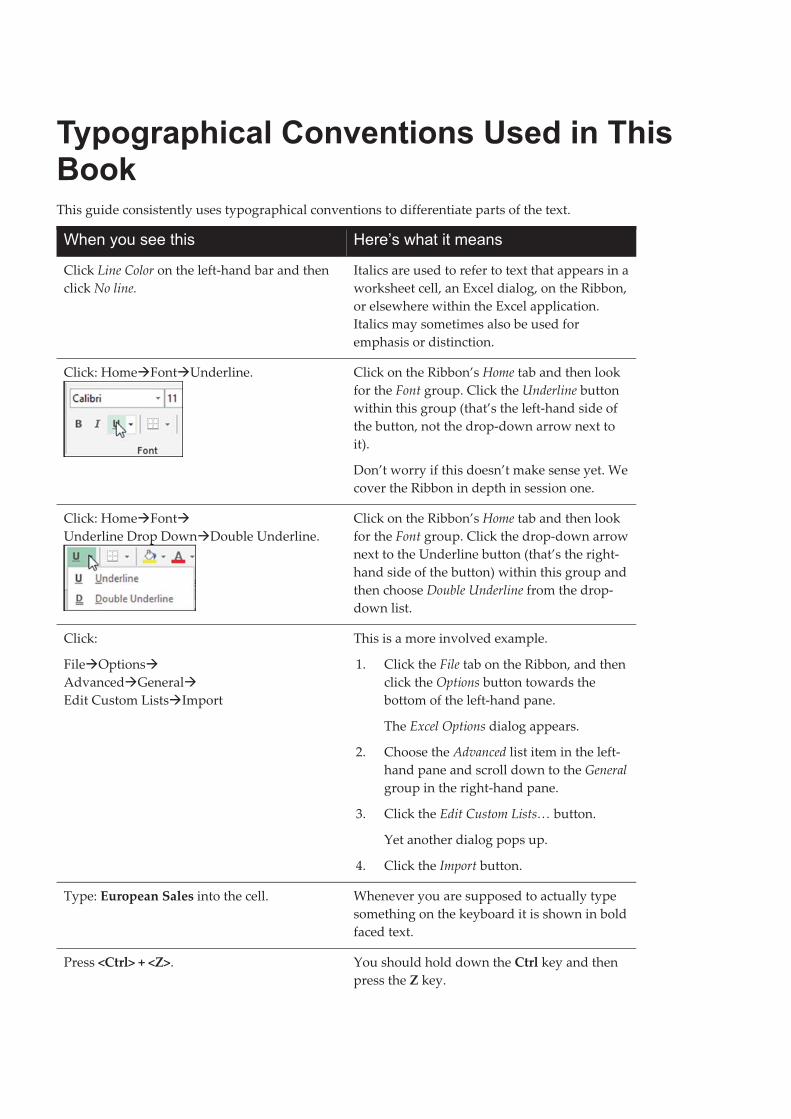
��*����*������.����������5� ������������ �This�guide�consistently�uses�typographical�conventions�to�differentiate�parts�of�the�text.�
������������� ������ ������ ���
Click�Line�Color�on�the�left�hand�bar�and�then�click�No�line.�
Italics�are�used�to�refer�to�text�that�appears�in�a�worksheet�cell,�an�Excel�dialog,�on�the�Ribbon,�or�elsewhere�within�the�Excel�application.��Italics�may�sometimes�also�be�used�for�emphasis�or�distinction.�
Click:�Home�Font�Underline.�
�
Click�on�the�Ribbon’s�Home tab�and�then�look�for�the�Font�group.�Click�the�Underline�button�within�this�group�(that’s�the�left�hand�side�of�the�button,�not�the�drop�down�arrow�next�to�it).�
Don’t�worry�if�this�doesn’t�make�sense�yet.�We�cover�the�Ribbon�in�depth�in�session�one.�
Click:�Home�Font��Underline�Drop�Down�Double�Underline.�
�
Click�on�the�Ribbon’s�Home�tab�and�then�look�for�the�Font�group.�Click�the�drop�down�arrow�next�to�the�Underline�button�(that’s�the�right�hand�side�of�the�button)�within�this�group�and�then�choose�Double�Underline�from�the�drop�down�list.�
Click:��
File�Options��Advanced�General��Edit�Custom�Lists�Import�
�
This�is�a�more�involved�example.��
1.� Click�the�File�tab�on�the�Ribbon,�and�then�click�the�Options�button�towards�the�bottom�of�the�left�hand�pane.��
The�Excel�Options�dialog�appears.��
2.� Choose�the�Advanced�list�item�in�the�left�hand�pane�and�scroll�down�to�the�General�group�in�the�right�hand�pane.�
3.� Click�the�Edit�Custom�Lists…�button.�
Yet�another�dialog�pops�up.�
4.� Click�the�Import�button.�
Type:�European�Sales�into�the�cell.� Whenever�you�are�supposed�to�actually�type�something�on�the�keyboard�it�is�shown�in�bold�faced�text.�
Press�<Ctrl>�+�<Z>.� You�should�hold�down�the�Ctrl�key�and�then�press�the�Z�key.�
�
�
�
When�a�lesson�tells�you�to�click�a�button,�an�image�of�the�relevant�button�will�often�be�shown�either�in�the�page�margin�or�within�the�text�itself.�
�
If�you�want�to�read�through�the�book�as�quickly�as�possible,�you�don’t�have�to�read�notes.��
Notes�usually�expand�a�little�on�the�information�given�in�the�lesson�text.�
�
Whenever�something�can�easily�go�wrong,�or�when�the�subject�text�is�particularly�important,�you�will�see�the�important�sidebar.�
You�should�always�read�important�sidebars.�
�
Tips�add�to�the�lesson�text�by�showing�you�shortcuts�or�time�saving�techniques�relevant�to�the�lesson.�
The�bold�text�at�the�top�of�the�tip�box�enables�you�to�establish�whether�the�tip�is�appropriate�to�your�needs�without�reading�all�the�text.�
In�this�example,�you�may�not�be�interested�in�keyboard�shortcuts�so�do�not�need�to�read�further.�
�
Sometimes�I�add�an�anecdote�gathered�over�the�years�from�my�Excel�classes�or�from�other�areas�of�life.�
If�you�simply�want�to�learn�Excel�as�quickly�as�possible�you�can�ignore�my�anecdotes.��
�
Sometimes�I�indulge�myself�by�adding�a�little�piece�of�trivia�in�the�context�of�the�skill�being�taught.�
Just�like�my�anecdotes�you�can�ignore�these�if�you�want�to.�They�won’t�help�you�to�learn�Excel�any�better!�
�
When�there�is�a�sample�file�(or�files)�to�accompany�a�lesson,�the�file�name�will�be�shown�in�a�folder�icon.��You�can�download�the�sample�file�from:�https://thesmartmethod.com/sample�files.�Detailed�instructions�are�given�in:�Lesson�1�5:�Download�the�sample�files�and�open/navigate�a�workbook.�
����In�Excel�2010/2013/2016/2019�there�are�a�possible�16,585�columns�and�1,048,476�rows.�This�is�a�great�improvement�on�earlier�versions.�
�#*�������Do�not�click�the�Delete�button�at�this�point�as�to�do�so�would�erase�the�entire�table.�
��*��������!������!����������� �!��� �You�can�also�use�the�<Ctrl>+<PgUp>�and�<Ctrl>+<PgDn>�keyboard�shortcuts�to�cycle�through�all�of�the�tabs�in�your�workbook.�
��� ���I�ran�an�Excel�course�for�a�small�company�in�London�a�couple�of�years�ago...�
�������The�feature�that�Excel�uses�to�help�you�out�with�function�calls�first�made�an�appearance�in�Visual�Basic�5�back�in�1996�…�
���$��� 8��,������.����
� �
�
)��������������������This�course�utilizes�some�of�the�tried�and�tested�techniques�developed�after�teaching�vast�numbers�of�people�to�learn�Excel�during�many�years�teaching�Smart�Method�classroom�courses.�
In�order�to�master�Excel�as�quickly�and�efficiently�as�possible�you�should�use�the�recommended�learning�method�described�below.�If�you�do�this�there�is�absolutely�no�doubt�that�you�will�master�the�advanced�Excel�skills�taught�in�this�book.�
�����#*������������
9���.�#*���������������#�!������������ �
It�is�always�tempting�to�jump�around�the�course�completing�lessons�in�a�haphazard�way.�
We�strongly�suggest�that�you�start�at�the�beginning�and�complete�lessons�sequentially.�
That�s�because�each�lesson�builds�upon�skills�learned�in�the�previous�lessons�and�one�of�our�goals�is�not�to�waste�your�time�by�teaching�the�same�skill�twice.�If�you�miss�a�skill�by�skipping�a�lesson�you�ll�find�the�later�lessons�more�difficult,�or�even�impossible�to�follow.�This,�in�turn,�may�demoralize�you�and�make�you�abandon�the�course.�
9��/��*����!�:���#*��������������������������
The�book�is�arranged�into�sessions�and�lessons.��
You�can�complete�as�many,�or�as�few,�lessons�as�you�have�the�time�and�energy�for�each�day.�Many�learners�have�developed�Excel�skills�by�setting�aside�just�a�few�minutes�each�day�to�complete�a�single�lesson.�
If�it�is�possible,�the�most�effective�way�to�learn�is�to�lock�yourself�away,�switch�off�your�telephone,�and�complete�a�full�session,�without�interruption,�except�for�a�15�minute�break�each�hour.�The�memory�process�is�associative,�and�we�ve�ensured�that�the�lessons�in�each�session�are�very�closely�coupled�(contextually)�with�the�others.�By�learning�the�whole�session�in�one�sitting,�you�ll�store�all�that�information�in�the�same�part�of�your�memory�and�will�find�it�easier�to�recall�later.�
The�experience�of�being�able�to�remember�all�of�the�words�of�a�song�as�soon�as�somebody�has�got�you��started��with�the�first�line�is�an�example�of�the�memory�s�associative�system�of�data�storage.�
9;�<��������������������
You�should�take�a�15�minute�break�every�hour�(or�more�often�if�you�begin�to�feel�overwhelmed)�and�spend�it�relaxing�rather�than�catching�up�with�your�e�mails.�Ideally�you�should�relax�by�lying�down�and�closing�your�eyes.�This�allows�your�brain�to�use�all�of�its�processing�power�to�efficiently�store�and�index�the�skills�you�ve�learned.�We�ve�found�that�this�hugely�improves�retention�of�skills�learned.��
In�our�classroom�courses�we�have�often�observed�a�phenomenon�that�we�call��running�into�a�wall�.�This�happens�when�a�student�becomes�overloaded�with�new�information�to�the�point�that�they�can�no�longer�follow�the�simplest�instruction.�If�you�find�this�happening�to�you,�you�ve�studied�for�too�long�without�a�rest.�
�
�
)��������� �������������������
"������ ��������������:���#*�������������������
Keep�attempting�the�exercise�at�the�end�of�each�session�until�you�can�complete�it�without�having�to�refer�to�lessons�in�the�session.�Don�t�start�the�next�session�until�you�can�complete�the�exercise�from�memory.�
"������ ��������������:����������!&������
The�session�objectives�are�stated�at�the�beginning�of�each�session.�
Read�each�objective�and�ask�yourself�if�you�have�truly�mastered�each�skill.�If�you�are�not�sure�about�any�of�the�skills�listed,�revise�the�relevant�lesson(s)�before�moving�on�to�the�next�session.�
You�will�find�it�very�frustrating�if�you�move�to�a�new�session�before�you�have�truly�mastered�the�skills�covered�in�the�previous�session.�This�may�demoralize�you�and�make�you�abandon�the�course.�
)������!�������������#�������#*�������Many�lessons�in�this�course�use�a�sample�file�that�is�incrementally�improved�during�each�lesson.�At�the�end�of�each�lesson�an�interim�version�is�always�saved.�For�example,�a�sample�file�called�Sales�1�may�provide�the�starting�point�to�a�sequence�of�three�lessons.�After�each�lesson,�interim�versions�called�Sales�2,�Sales�3�and�Sales�4�are�saved�by�the�student.�
A�complete�set�of�sample�files�(including�all�incremental�versions)�are�provided�in�the�sample�file�set.�This�provides�three�important�benefits:�
�� If�you�have�difficulty�with�a�lesson�it�is�useful�to�be�able�to�study�the�completed�workbook�(at�the�end�of�the�lesson)�by�opening�the�finished�version�of�the�lesson�s�workbook.�
�� When�you�have�completed�the�book,�you�will�want�to�use�it�as�a�reference.�The�sample�files�allow�you�to�work�through�any�single�lesson�in�isolation,�as�the�workbook�s�state�at�the�beginning�of�each�lesson�is�always�available.�
�� When�teaching�a�class�one�student�may�corrupt�their�workbook�by�a�series�of�errors�(or�by�their�computer�crashing).��It�is�possible�to�quickly�and�easily�move�the�class�on�to�the�next�lesson�by�instructing�the�student�to�open�the�next�sample�file�in�the�set�(instead�of�progressing�with�their�own�corrupted�file�or�copying�a�file�from�another�student).��
�����#������*� ���������������������������������Excel�is�a�huge�and�daunting�application�and�you�ll�need�to�invest�some�time�in�learning�the�skills�presented�in�this�course.�This�will�be�time�well�spent�as�you�ll�have�a�hugely�marketable�skill�for�life.�With�1.2�billion�users�worldwide,�it�is�hard�to�imagine�any�organization�of�any�size�that�does�not�value�and�require�Excel�skills.�
If�you�persevere�with�this�course�there�is�no�doubt�that�you�will�master�Excel.�A�little�time�and�effort�may�be�needed�but�the�skills�you�ll�acquire�will�be�hugely�valuable�for�the�rest�of�your�life.�
Enjoy�the�course.�
�
�
�

� �
�
�
�
�
�
�������������� �������������� � �3
+������1�2�������+ �����
�Even�if�you�are�a�seasoned�Excel�user,�I�urge�you�to�take�Euripides’�advice�and�complete�this�session.�You’ll�fly�through�it�if�you�already�know�most�of�the�skills�covered.��
In�my�classes�I�often�teach�professionals�who�have�used�Excel�for�over�ten�years�and�they�always�get�some�nugget�of�fantastically�useful�information�from�this�session.�
In�this�session,�I�teach�you�the�absolute�basics�you�need�before�you�can�start�to�do�useful�work�with�Excel�2019.�
I�don’t�assume�that�you�have�any�previous�exposure�to�Excel�(in�any�version)�so�I�have�to�include�some�very�basic�skills.��
+������1!&������By�the�end�of�this�session�you�will�be�able�to:�
� Start�Excel�and�open�a�new�blank�workbook�
� Check�that�your�Excel�version�is�up�to�date�
� Change�the�Office�Theme�
� Maximize,�minimize,�re�size,�move�and�close�the�Excel�window�
� Download�the�sample�files�and�open/navigate�a�workbook��
� Save�a�workbook�to�a�local�file�
� Understand�common�file�formats�
� Pin�a�workbook�and�understand�file�organization�
� View,�move,�add,�rename,�delete�and�navigate�worksheet�tabs�
� Use�the�Versions�feature�to�recover�an�unsaved�Draft�file�
� Use�the�Versions�feature�to�recover�an�earlier�version�of�a�workbook�
� Use�the�Ribbon�
� Understand�Ribbon�components�
� Customize�the�Quick�Access�Toolbar�and�preview�the�printout�
� Use�the�Mini�Toolbar,�Key�Tips�and�keyboard�shortcuts�
� Understand�views�
� Hide�and�show�the�Formula�Bar�and�Ribbon�
� Use�the�Tell�Me�help�system�
� Use�other�help�features�
�
A�bad�beginning�makes�a�bad�ending.��
Euripides,�Aegeus�(484�BC���406�BC).������
� ����� !������" �� ��#�!!���������� ��������
�
�=� ��$�%&&��� ������' ��
%�������2�+������������ ��*�������!��� ���� !�� �Excel�2019�will�only�run�on�the�Windows�10�operating�system.��(Earlier�versions�also�supported�the�Windows�7�and�8�operating�systems).�
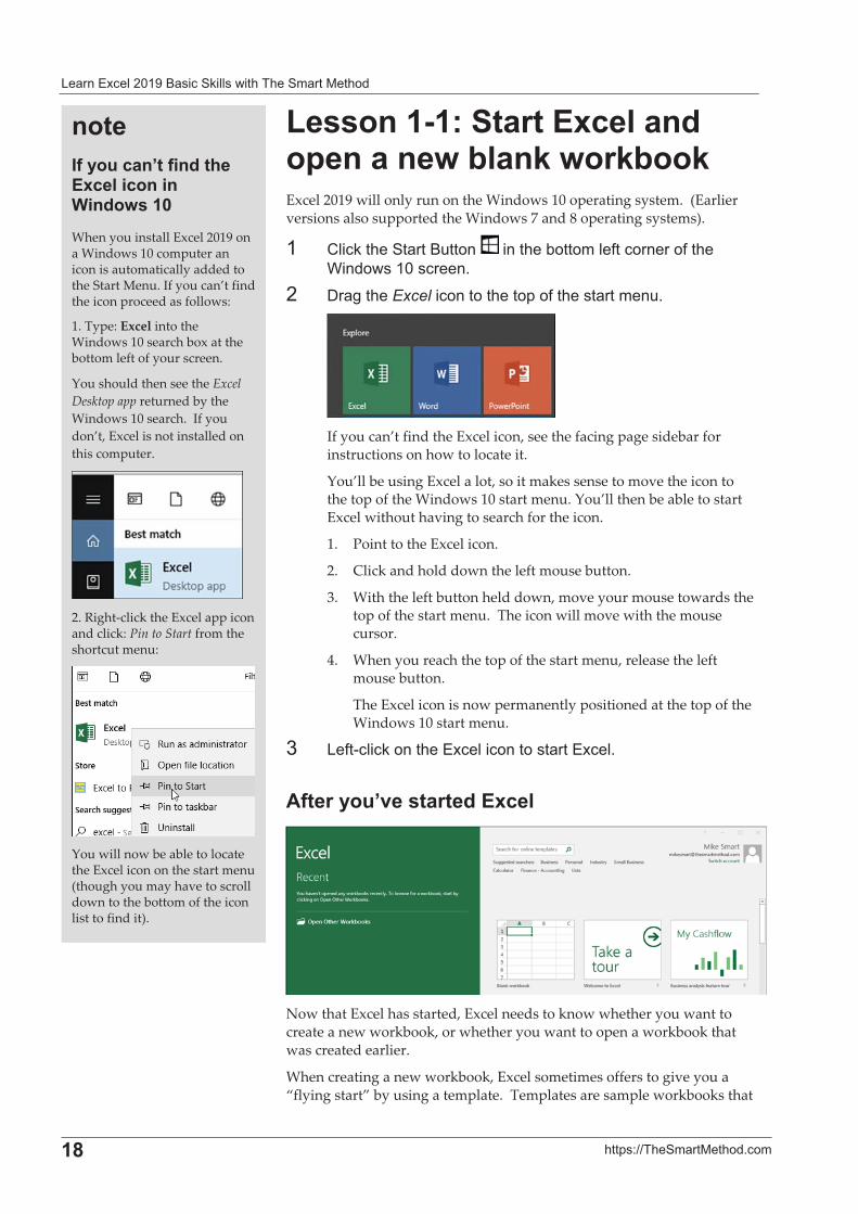
�� (!� #����� ���"������ ������)������!*�� ������*��������������� ��'�
�� +� ,���Excel�� ����������$��*����� ������'�
�If�you�can’t�find�the�Excel�icon,�see�the�facing�page�sidebar�for�instructions�on�how�to�locate�it.�
You’ll�be�using�Excel�a�lot,�so�it�makes�sense�to�move�the�icon�to�the�top�of�the�Windows�10�start�menu.�You’ll�then�be�able�to�start�Excel�without�having�to�search�for�the�icon.�
1.� Point�to�the�Excel�icon.�
2.� Click�and�hold�down�the�left�mouse�button.�
3.� With�the�left�button�held�down,�move�your�mouse�towards�the�top�of�the�start�menu.��The�icon�will�move�with�the�mouse�cursor.�
4.� When�you�reach�the�top�of�the�start�menu,�release�the�left�mouse�button.�
The�Excel�icon�is�now�permanently�positioned�at�the�top�of�the�Windows�10�start�menu.�
-� �*�. !� #�������� !�� �������� ����� !'�
"�������8������� ������
�Now�that�Excel�has�started,�Excel�needs�to�know�whether�you�want�to�create�a�new�workbook,�or�whether�you�want�to�open�a�workbook�that�was�created�earlier.�
When�creating�a�new�workbook,�Excel�sometimes�offers�to�give�you�a�“flying�start”�by�using�a�template.��Templates�are�sample�workbooks�that�
����/���������8����� �����������������$�� �������When�you�install�Excel�2019�on�a�Windows�10�computer�an�icon�is�automatically�added�to�the�Start�Menu.�If�you�can’t�find�the�icon�proceed�as�follows:�
1.�Type:�Excel�into�the�Windows�10�search�box�at�the�bottom�left�of�your�screen.�
You�should�then�see�the�Excel�Desktop�app�returned�by�the�Windows�10�search.��If�you�don’t,�Excel�is�not�installed�on�this�computer.��
�2.�Right�click�the�Excel�app�icon�and�click:�Pin�to�Start�from�the�shortcut�menu:�
�You�will�now�be�able�to�locate�the�Excel�icon�on�the�start�menu�(though�you�may�have�to�scroll�down�to�the�bottom�of�the�icon�list�to�find�it).�
�������/�%�" �� ��#�!!��
�
����������� �������������� ��
you�can�adapt�and�modify�for�your�own�needs.��The�idea�is�very�good,�but�templates�are�not�usually�a�good�choice�as�it�can�take�longer�to�adapt�them�to�your�true�needs�than�to�design�from�scratch�(see�sidebar).�
In�this�lesson�you’ll�create�a�blank�workbook.�
�� (� �� ����)! �#����#)��#'�
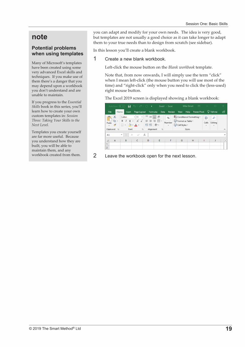
Left�click�the�mouse�button�on�the�Blank�workbook�template.�
Note�that,�from�now�onwards,�I�will�simply�use�the�term�“click”�when�I�mean�left�click�(the�mouse�button�you�will�use�most�of�the�time)�and�“right�click”�only�when�you�need�to�click�the�(less�used)�right�mouse�button.�
The�Excel�2019�screen�is�displayed�showing�a�blank�workbook:�
�
�� � 0������#)��#��$��*���������!����'�
����7��������*��!�#�������������#*������Many�of�Microsoft’s�templates�have�been�created�using�some�very�advanced�Excel�skills�and�techniques.��If�you�make�use�of�them�there’s�a�danger�that�you�may�depend�upon�a�workbook�you�don’t�understand�and�are�unable�to�maintain.�
If�you�progress�to�the�Essential�Skills�book�in�this�series,�you’ll�learn�how�to�create�your�own�custom�templates�in:�Session�Three:�Taking�Your�Skills�to�the�Next�Level.�
Templates�you�create�yourself�are�far�more�useful.��Because�you�understand�how�they�are�built,�you�will�be�able�to�maintain�them,�and�any�workbook�created�from�them.�
� ����� !������" �� ��#�!!���������� ��������
�
��� ��$�%&&��� ������' ��
%�������2�.�� ���������������������������*���� ���"���#�����5* ����Normally�Excel�will�look�after�updates�without�you�having�to�do�anything.��By�default,�automatic�updates�are�enabled.��This�means�that�updates�are�downloaded�from�the�Internet�and�installed�automatically.�
It�is�possible�that�automatic�updates�have�been�switched�off�on�your�computer.��In�this�case�there�is�a�danger�that�you�may�have�an�old,�buggy,�unsupported�and�out�of�date�version�of�Excel�installed.�
This�lesson�will�show�you�how�to�make�sure�that�you�are�using�the�latest�(most�complete,�and�most�reliable)�version�of�Excel.��
�� �� ����� !� ����$�� ����)! �#����#)��#�1�*����� 0����� !� ����������2'�You�learned�how�to�do�this�in:�Lesson�1�1:�Start�Excel�and�open�a�new�blank�workbook.�
�� � #������ �� ���� �� ��$� ��� ��� )!�'�
1.� Click�the�File�button� �at�the�top�left�of�the�screen.�
This�takes�you�to�Backstage�View.��Backstage�View�allows�you�to�complete�an�enormous�range�of�common�tasks�from�a�single�window.�
2.� Click:�Account�� ��in�the�left�hand�list.��
Your�account�details�are�displayed�on�screen.��Notice�the�Office�Updates�button�displayed�in�the�right�hand�pane.�
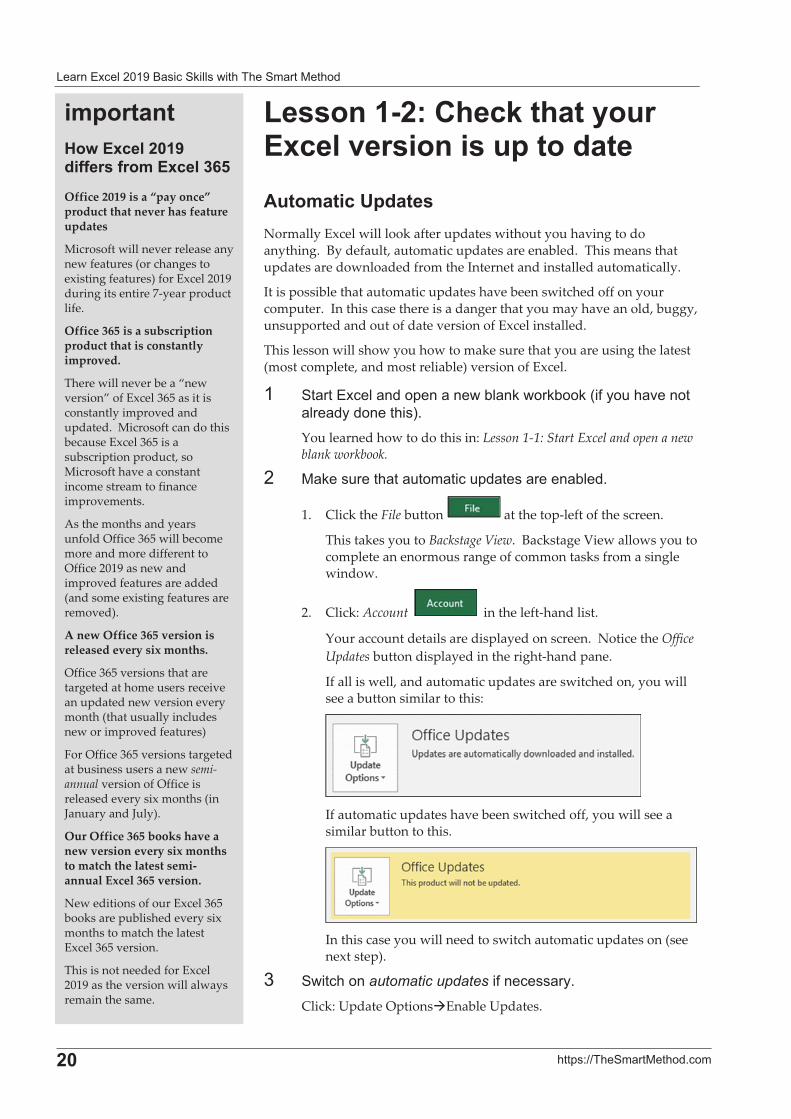
If�all�is�well,�and�automatic�updates�are�switched�on,�you�will�see�a�button�similar�to�this:�
�If�automatic�updates�have�been�switched�off,�you�will�see�a�similar�button�to�this.�
�In�this�case�you�will�need�to�switch�automatic�updates�on�(see�next�step).�
-� ���� ����automatic updates��*�� �� ��'�Click:�Update�Options�Enable�Updates.�
�#*�������)������������� ���������#������;6>�Office�2019�is�a�“pay�once”�product�that�never�has�feature�updates�
Microsoft�will�never�release�any�new�features�(or�changes�to�existing�features)�for�Excel�2019�during�its�entire�7�year�product�life.�
Office�365�is�a�subscription�product�that�is�constantly�improved.�
There�will�never�be�a�“new�version”�of�Excel�365�as�it�is�constantly�improved�and�updated.��Microsoft�can�do�this�because�Excel�365�is�a�subscription�product,�so�Microsoft�have�a�constant�income�stream�to�finance�improvements.�
As�the�months�and�years�unfold�Office�365�will�become�more�and�more�different�to�Office�2019�as�new�and�improved�features�are�added�(and�some�existing�features�are�removed).�
A�new�Office�365�version�is�released�every�six�months.�
Office�365�versions�that�are�targeted�at�home�users�receive�an�updated�new�version�every�month�(that�usually�includes�new�or�improved�features)�
For�Office�365�versions�targeted�at�business�users�a�new�semi�annual�version�of�Office�is�released�every�six�months�(in�January�and�July).���
Our�Office�365�books�have�a�new�version�every�six�months�to�match�the�latest�semi�annual�Excel�365�version.�
New�editions�of�our�Excel�365�books�are�published�every�six�months�to�match�the�latest�Excel�365�version.��
This�is�not�needed�for�Excel�2019�as�the�version�will�always�remain�the�same.�
�������/�%�" �� ��#�!!��
�
����������� �������������� ��
�3� 4*���� ���$� ���� ����,�������� !!5� $$!����'�
Sometimes�Excel�will�download�updates�but�will�not�install�them�automatically.�
In�this�case�you�will�see�an�update�button�similar�to�the�following:�
�If�you�see�this�type�of�button�you�should�apply�the�update.�
Click:�Update�Options�Apply�Updates.�
You�may�be�asked�to�confirm�that�you�want�to�apply�the�update,�and�to�close�any�open�programs�to�apply�the�update.�
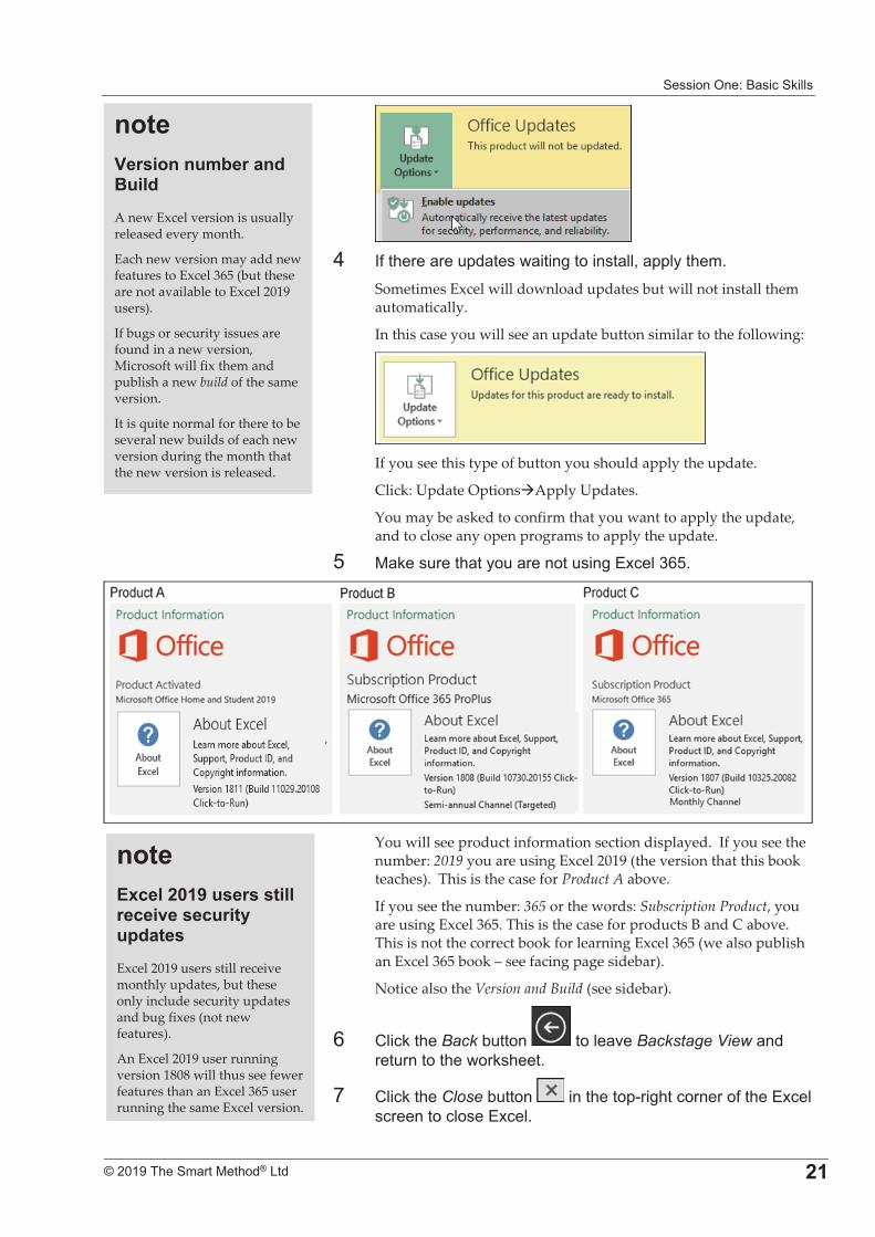
6� � #������ ������ ����������,��� !�-76'�
�
You�will�see�product�information�section�displayed.��If�you�see�the�number:�2019�you�are�using�Excel�2019�(the�version�that�this�book�teaches).��This�is�the�case�for�Product�A�above.�
If�you�see�the�number:�365�or�the�words:�Subscription�Product,�you�are�using�Excel�365.�This�is�the�case�for�products�B�and�C�above.��This�is�not�the�correct�book�for�learning�Excel�365�(we�also�publish�an�Excel�365�book�–�see�facing�page�sidebar).��
Notice�also�the�Version�and�Build�(see�sidebar).��
7� (!� #���Back )������ ����! 0�Backstage View� �����������������#��'��
8� (!� #���Close )����� �������$.��,�� ������*����� !�� ������ !����� !'�
����?��������#!���� ����� �A�new�Excel�version�is�usually�released�every�month.�
Each�new�version�may�add�new�features�to�Excel�365�(but�these�are�not�available�to�Excel�2019�users).�
If�bugs�or�security�issues�are�found�in�a�new�version,�Microsoft�will�fix�them�and�publish�a�new�build�of�the�same�version.��
It�is�quite�normal�for�there�to�be�several�new�builds�of�each�new�version�during�the�month�that�the�new�version�is�released.�
���������������������������������������* ����Excel�2019�users�still�receive�monthly�updates,�but�these�only�include�security�updates�and�bug�fixes�(not�new�features).�
An�Excel�2019�user�running�version�1808�will�thus�see�fewer�features�than�an�Excel�365�user�running�the�same�Excel�version.�
� ����� !������" �� ��#�!!���������� ��������
�
��� ��$�%&&��� ������' ��
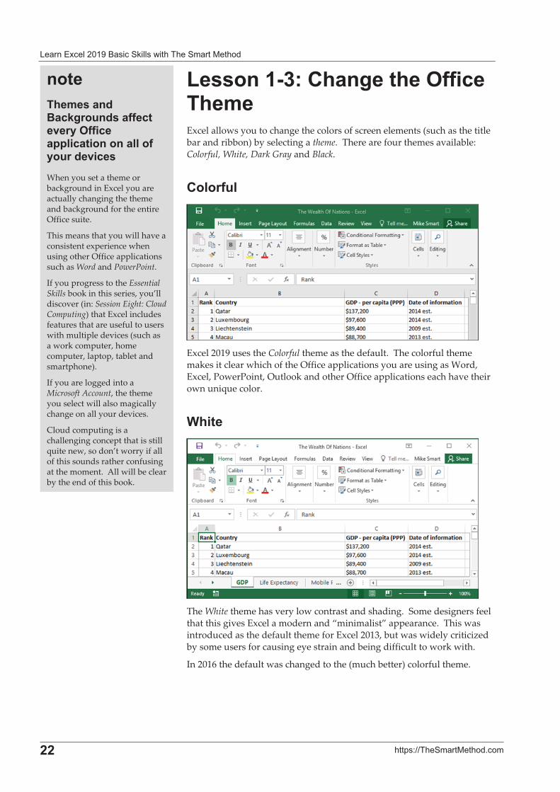
%������;2�.��������1�������#��Excel�allows�you�to�change�the�colors�of�screen�elements�(such�as�the�title�bar�and�ribbon)�by�selecting�a�theme.��There�are�four�themes�available:�Colorful,�White,�Dark�Gray�and�Black.��
.��������
�Excel�2019�uses�the�Colorful�theme�as�the�default.��The�colorful�theme�makes�it�clear�which�of�the�Office�applications�you�are�using�as�Word,�Excel,�PowerPoint,�Outlook�and�other�Office�applications�each�have�their�own�unique�color.�
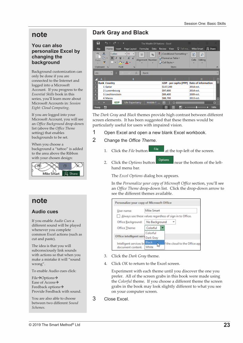
$����
�The�White�theme�has�very�low�contrast�and�shading.��Some�designers�feel�that�this�gives�Excel�a�modern�and�“minimalist”�appearance.��This�was�introduced�as�the�default�theme�for�Excel�2013,�but�was�widely�criticized�by�some�users�for�causing�eye�strain�and�being�difficult�to�work�with.���
In�2016�the�default�was�changed�to�the�(much�better)�colorful�theme.���
������#���� ���� ����� ������������1������**������������������������ �����When�you�set�a�theme�or�background�in�Excel�you�are�actually�changing�the�theme�and�background�for�the�entire�Office�suite.�
This�means�that�you�will�have�a�consistent�experience�when�using�other�Office�applications�such�as�Word�and�PowerPoint.�
If�you�progress�to�the�Essential�Skills�book�in�this�series,�you’ll�discover�(in:�Session�Eight:�Cloud�Computing)�that�Excel�includes�features�that�are�useful�to�users�with�multiple�devices�(such�as�a�work�computer,�home�computer,�laptop,�tablet�and�smartphone).�
If�you�are�logged�into�a�Microsoft�Account,�the�theme�you�select�will�also�magically�change�on�all�your�devices.�
Cloud�computing�is�a�challenging�concept�that�is�still�quite�new,�so�don’t�worry�if�all�of�this�sounds�rather�confusing�at�the�moment.��All�will�be�clear�by�the�end�of�this�book.����
�������/�%�" �� ��#�!!��
�
����������� �������������� �;
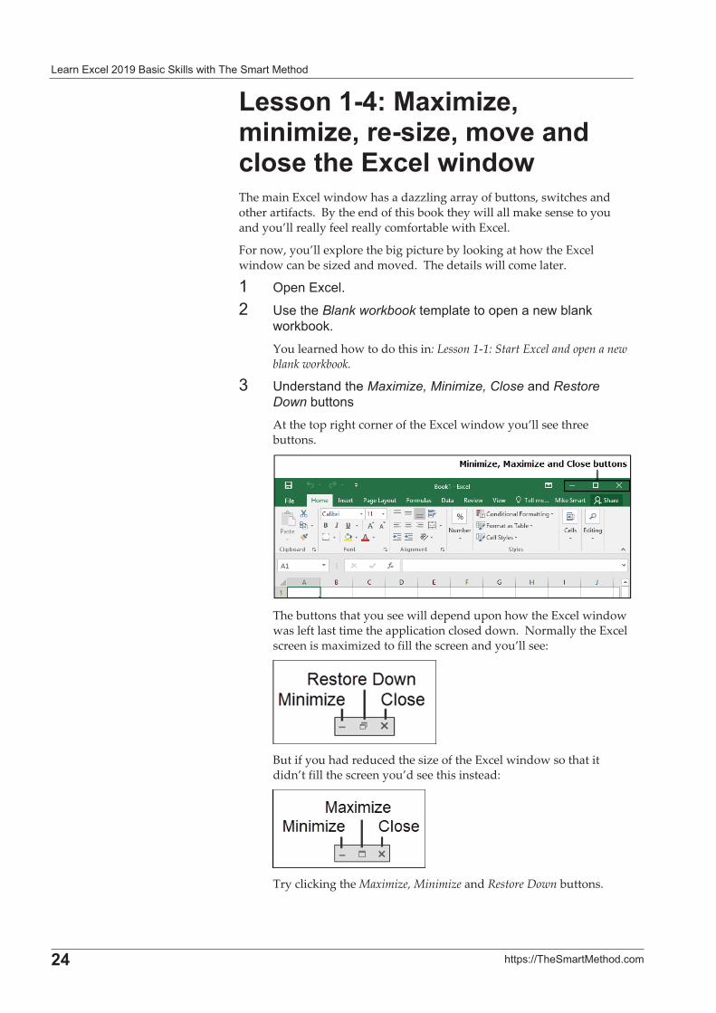
4�� �@������ ����� �
�The�Dark�Gray�and�Black�themes�provide�high�contrast�between�different�screen�elements.��It�has�been�suggested�that�these�themes�would�be�particularly�useful�for�users�with�impaired�vision.�
�� /$���� !� ����$�� ����)! �#��� !����#)��#'�
�� ( �,���Office Theme.�
1.� Click�the�File�button� �at�the�top�left�of�the�screen.�
2.� Click�the�Options�button� �near�the�bottom�of�the�left�hand�menu�bar.�
The�Excel�Options�dialog�box�appears.�
In�the�Personalize�your�copy�of�Microsoft�Office�section,�you’ll�see�an�Office�Theme�drop�down�list.��Click�the�drop�down�arrow�to�see�the�different�themes�available.�
�3.� Click�the�Dark�Gray�theme.�
4.� Click�OK�to�return�to�the�Excel�screen.�
Experiment�with�each�theme�until�you�discover�the�one�you�prefer.��All�of�the�screen�grabs�in�this�book�were�made�using�the�Colorful�theme.��If�you�choose�a�different�theme�the�screen�grabs�in�the�book�may�look�slightly�different�to�what�you�see�on�your�computer�screen.��
-� (!����� !'�
����-������������*�������A������!��������������!�� ����� ��Background�customization�can�only�be�done�if�you�are�connected�to�the�Internet�and�logged�into�a�Microsoft�Account.��If�you�progress�to�the�Essential�Skills�book�in�this�series,�you’ll�learn�more�about�Microsoft�Accounts�in:�Session�Eight:�Cloud�Computing.�
If�you�are�logged�into�your�Microsoft�Account,�you�will�see�an�Office�Background�drop�down�list�(above�the�Office�Theme�setting)�that�enables�backgrounds�to�be�set.�
When�you�choose�a�background�a�“tattoo”�is�added�to�the�area�above�the�Ribbon�with�your�chosen�design:�
�
����"� �������If�you�enable�Audio�Cues�a�different�sound�will�be�played�whenever�you�complete�common�Excel�actions�(such�as�cut�and�paste).���
The�idea�is�that�you�will�subconsciously�link�sounds�with�actions�so�that�when�you�make�a�mistake�it�will�“sound�wrong”.�
To�enable�Audio�cues�click:�
File�Options��Ease�of�Access��Feedback�options��Provide�Feedback�with�sound.�
You�are�also�able�to�choose�between�two�different�Sound�Schemes.�
� ����� !������" �� ��#�!!���������� ��������
�
�0� ��$�%&&��� ������' ��
%������02�����#�A:�#���#�A:����A:�#����� ����������������� ���The�main�Excel�window�has�a�dazzling�array�of�buttons,�switches�and�other�artifacts.��By�the�end�of�this�book�they�will�all�make�sense�to�you�and�you’ll�really�feel�really�comfortable�with�Excel.���
For�now,�you’ll�explore�the�big�picture�by�looking�at�how�the�Excel�window�can�be�sized�and�moved.��The�details�will�come�later.��
�� /$���� !'�
�� 9����Blank workbook���$! ������$�� ����)! �#����#)��#'�You�learned�how�to�do�this�in:�Lesson�1�1:�Start�Excel�and�open�a�new�blank�workbook.�
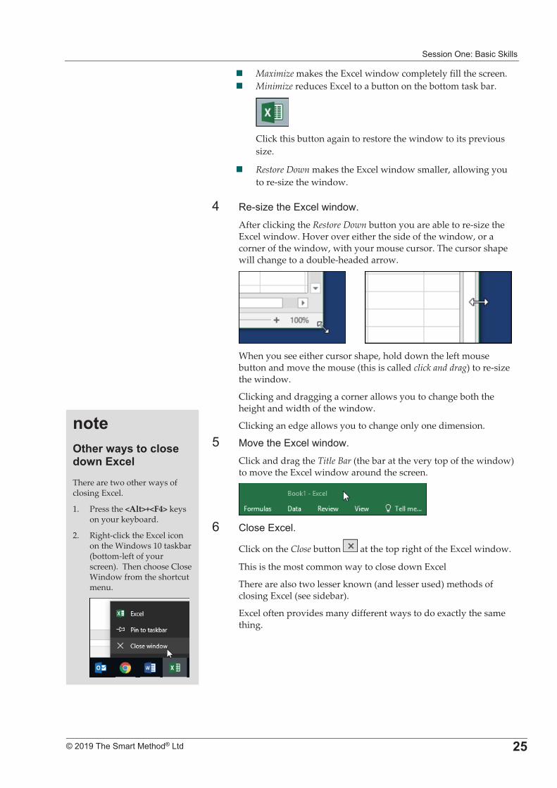
-� 9����� �����Maximize, Minimize, Close� ���Restore Down�)�������At�the�top�right�corner�of�the�Excel�window�you’ll�see�three�buttons.��
�The�buttons�that�you�see�will�depend�upon�how�the�Excel�window�was�left�last�time�the�application�closed�down.��Normally�the�Excel�screen�is�maximized�to�fill�the�screen�and�you’ll�see:�
�But�if�you�had�reduced�the�size�of�the�Excel�window�so�that�it�didn’t�fill�the�screen�you’d�see�this�instead:��
�Try�clicking�the�Maximize,�Minimize�and�Restore�Down�buttons.�
�������/�%�" �� ��#�!!��
�
����������� �������������� �>
� Maximize�makes�the�Excel�window�completely�fill�the�screen.�� Minimize�reduces�Excel�to�a�button�on�the�bottom�task�bar.��
��Click�this�button�again�to�restore�the�window�to�its�previous�size.�
� Restore�Down�makes�the�Excel�window�smaller,�allowing�you�to�re�size�the�window.��
3� :.��;����� !�������'�After�clicking�the�Restore�Down�button�you�are�able�to�re�size�the�Excel�window.�Hover�over�either�the�side�of�the�window,�or�a�corner�of�the�window,�with�your�mouse�cursor.�The�cursor�shape�will�change�to�a�double�headed�arrow.��
�������� �����������When�you�see�either�cursor�shape,�hold�down�the�left�mouse�button�and�move�the�mouse�(this�is�called�click�and�drag)�to�re�size�the�window.�
Clicking�and�dragging�a�corner�allows�you�to�change�both�the�height�and�width�of�the�window.��
Clicking�an�edge�allows�you�to�change�only�one�dimension.�
6� ��0����� !�������'�Click�and�drag�the�Title�Bar�(the�bar�at�the�very�top�of�the�window)�to�move�the�Excel�window�around�the�screen.�
�7� (!����� !'�
Click�on�the�Close�button� �at�the�top�right�of�the�Excel�window.�
This�is�the�most�common�way�to�close�down�Excel��
There�are�also�two�lesser�known�(and�lesser�used)�methods�of�closing�Excel�(see�sidebar).��
Excel�often�provides�many�different�ways�to�do�exactly�the�same�thing.��
����1����������������� ���������There�are�two�other�ways�of�closing�Excel.�
1.� Press�the�<Alt>+<F4>�keys�on�your�keyboard.�
2.� Right�click�the�Excel�icon�on�the�Windows�10�taskbar�(bottom�left�of�your�screen).��Then�choose�Close�Window�from�the�shortcut�menu.�
�
� ����� !������" �� ��#�!!���������� ��������
�
�6� ��$�%&&��� ������' ��
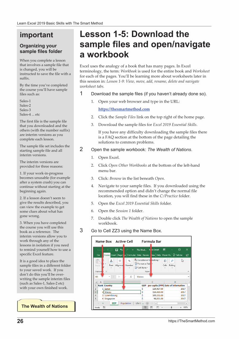
%������>2�4������ ������#*��������� ��*�B������������� !�� �Excel�uses�the�analogy�of�a�book�that�has�many�pages.�In�Excel�terminology,�the�term:�Workbook�is�used�for�the�entire�book�and�Worksheet�for�each�of�the�pages.�You’ll�be�learning�more�about�worksheets�later�in�this�session�in:�Lesson�1�9:�View,�move,�add,�rename,�delete�and�navigate�worksheet�tabs.�
�� +���!� ����� �$!�*�!��1�*����� 0���� !� ���������2'��1.� Open�your�web�browser�and�type�in�the�URL:�
https://thesmartmethod.com�
2.� Click�the�Sample�Files�link�on�the�top�right�of�the�home�page.��
3.� Download�the�sample�files�for�Excel�2019�Essential�Skills.�
If�you�have�any�difficulty�downloading�the�sample�files�there�is�a�FAQ�section�at�the�bottom�of�the�page�detailing�the�solutions�to�common�problems.��
�� /$����� �$!����#)��#%�The Wealth of Nations'��
1.� Open�Excel.�
2.� Click�Open�Other�Workbooks�at�the�bottom�of�the�left�hand�menu�bar.�
3.� Click:�Browse�in�the�list�beneath�Open.��
4.� Navigate�to�your�sample�files.��If�you�downloaded�using�the�recommended�option�and�didn’t�change�the�normal�file�location,�you�will�find�these�in�the�C:/Practice�folder.�
5.� Open�the�Excel�2019�Essential�Skills�folder.�
6.� Open�the�Session�1�folder.�
7.� Double�click�The�Wealth�of�Nations�to�open�the�sample�workbook.�
-� <�����(!!�==-�����,���> ��"��'��
�
�#*�������1�����A�����������#*���������� ��When�you�complete�a�lesson�that�involves�a�sample�file�that�is�changed,�you�will�be�instructed�to�save�the�file�with�a�suffix.��
By�the�time�you’ve�completed�the�course�you’ll�have�sample�files�such�as:�
Sales�1�Sales�2�Sales�3�Sales�4�...�etc�
The�first�file�is�the�sample�file�that�you�downloaded�and�the�others�(with�the�number�suffix)�are�interim�versions�as�you�complete�each�lesson.�
The�sample�file�set�includes�the�starting�sample�file�and�all�interim�versions.�
The�interim�versions�are�provided�for�three�reasons:�
1.�If�your�work�in�progress�becomes�unusable�(for�example�after�a�system�crash)�you�can�continue�without�starting�at�the�beginning�again.�
2.�If�a�lesson�doesn’t�seem�to�give�the�results�described,�you�can�view�the�example�to�get�some�clues�about�what�has�gone�wrong.�
3.�When�you�have�completed�the�course�you�will�use�this�book�as�a�reference.��The�interim�versions�allow�you�to�work�through�any�of�the�lessons�in�isolation�if�you�need�to�remind�yourself�how�to�use�a�specific�Excel�feature.�
It�is�a�good�idea�to�place�the�sample�files�in�a�different�folder�to�your�saved�work.��If�you�don’t�do�this�you’ll�be�over�writing�the�sample�interim�files�(such�as�Sales�1,�Sales�2�etc)�with�your�own�finished�work.�
���$��������C�������
�������/�%�" �� ��#�!!��
�
����������� �������������� �3
Excel�uses�the�letter�of�the�column�and�the�number�of�the�row�to�identify�cells.�This�is�called�the�cell�address.�In�the�above�example,�the�cell�address�of�the�active�cell�is�B3.��
In�Excel�2019�there�are�a�little�over�a�million�rows�and�a�little�over�sixteen�thousand�columns.�You�may�wonder�how�it�is�possible�to�name�these�columns�with�only�26�letters�in�the�alphabet.�
When�Excel�runs�out�of�letters�it�starts�using�two:��X,�Y,�Z�and�then�AA,�AB,�AC�etc.�But�even�two�letters�are�not�enough.�When�Excel�reaches�column�ZZ�it�starts�using�three�letters:��ZX,�ZY,�ZZ�and�then�AAA,�AAB,�AAC�etc.�
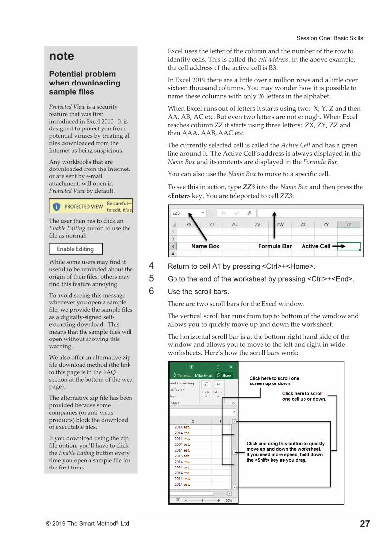
The�currently�selected�cell�is�called�the�Active�Cell�and�has�a�green�line�around�it.�The�Active�Cell’s�address�is�always�displayed�in�the�Name�Box�and�its�contents�are�displayed�in�the�Formula�Bar.��
You�can�also�use�the�Name�Box�to�move�to�a�specific�cell.�
To�see�this�in�action,�type�ZZ3�into�the�Name�Box�and�then�press�the�<Enter>�key.�You�are�teleported�to�cell�ZZ3:�
�3� :�������� !!�?��)��$�����,�@(��!AB@���A���6� <�����������*������#���)��$�����,�@(��!AB@���A'��
7� 9����� ��!!�) ��'�There�are�two�scroll�bars�for�the�Excel�window.��
The�vertical�scroll�bar�runs�from�top�to�bottom�of�the�window�and�allows�you�to�quickly�move�up�and�down�the�worksheet.�
The�horizontal�scroll�bar�is�at�the�bottom�right�hand�side�of�the�window�and�allows�you�to�move�to�the�left�and�right�in�wide�worksheets.�Here’s�how�the�scroll�bars�work:�
�
����7��������*��!�#����� ������ ������#*�������Protected�View�is�a�security�feature�that�was�first�introduced�in�Excel�2010.��It�is�designed�to�protect�you�from�potential�viruses�by�treating�all�files�downloaded�from�the�Internet�as�being�suspicious.�
Any�workbooks�that�are�downloaded�from�the�Internet,�or�are�sent�by�e�mail�attachment,�will�open�in�Protected�View�by�default.�
�The�user�then�has�to�click�an�Enable�Editing�button�to�use�the�file�as�normal:�
�While�some�users�may�find�it�useful�to�be�reminded�about�the�origin�of�their�files,�others�may�find�this�feature�annoying.�
To�avoid�seeing�this�message�whenever�you�open�a�sample�file,�we�provide�the�sample�files�as�a�digitally�signed�self�extracting�download.��This�means�that�the�sample�files�will�open�without�showing�this�warning.�
We�also�offer�an�alternative�zip�file�download�method�(the�link�to�this�page�is�in�the�FAQ�section�at�the�bottom�of�the�web�page).�
The�alternative�zip�file�has�been�provided�because�some�companies�(or�anti�virus�products)�block�the�download�of�executable�files.���
If�you�download�using�the�zip�file�option,�you’ll�have�to�click�the�Enable�Editing�button�every�time�you�open�a�sample�file�for�the�first�time.��
� ����� !������" �� ��#�!!���������� ��������
�
�=� ��$�%&&��� ������' ��
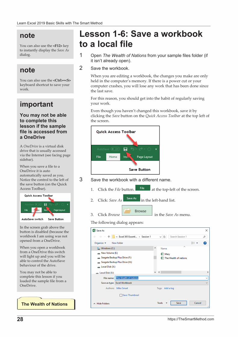
%������62�+�������� !�� ������������������ /$��The Wealth of Nations *���������� �$!�*�!��*�!���1�*�
��������� !� ����$�2'�
�� � 0������#)��#'�When�you�are�editing�a�workbook,�the�changes�you�make�are�only�held�in�the�computer’s�memory.�If�there�is�a�power�cut�or�your�computer�crashes,�you�will�lose�any�work�that�has�been�done�since�the�last�save.�
For�this�reason,�you�should�get�into�the�habit�of�regularly�saving�your�work.�
Even�though�you�haven’t�changed�this�workbook,�save�it�by�clicking�the�Save�button�on�the�Quick�Access�Toolbar�at�the�top�left�of�the�screen.��
�-� � 0������#)��#����� ���**����� �'�
1.� Click�the�File�button.� �at�the�top�left�of�the�screen.�
2.� Click:�Save�As� �in�the�left�hand�list.���
3.� Click�Browse�� ��in�the�Save�As�menu.�
The�following�dialog�appears:�
�
����You�can�also�use�the�<Ctrl>+<S>�keyboard�shortcut�to�save�your�work.��
���$��������C�������
����You�can�also�use�the�<F12>�key�to�instantly�display�the�Save�As�dialog.��
�#*�������-���#�������!��!�������#*����������������������#*�������������� ����#���1�4����A�OneDrive�is�a�virtual�disk�drive�that�is�usually�accessed�via�the�Internet�(see�facing�page�sidebar).�
When�you�save�a�file�to�a�OneDrive�it�is�auto�automatically�saved�as�you.��Notice�the�control�to�the�left�of�the�save�button�(on�the�Quick�Access�Toolbar).�
�In�the�screen�grab�above�the�button�is�disabled�(because�the�workbook�I�am�using�was�not�opened�from�a�OneDrive.�
When�you�open�a�workbook�from�a�OneDrive�this�switch�will�light�up�and�you�will�be�able�to�control�the�AutoSave�behaviour�of�the�drive.�
You�may�not�be�able�to�complete�this�lesson�if�you�loaded�the�sample�file�from�a�OneDrive.�
�������/�%�" �� ��#�!!��
�
����������� �������������� ��
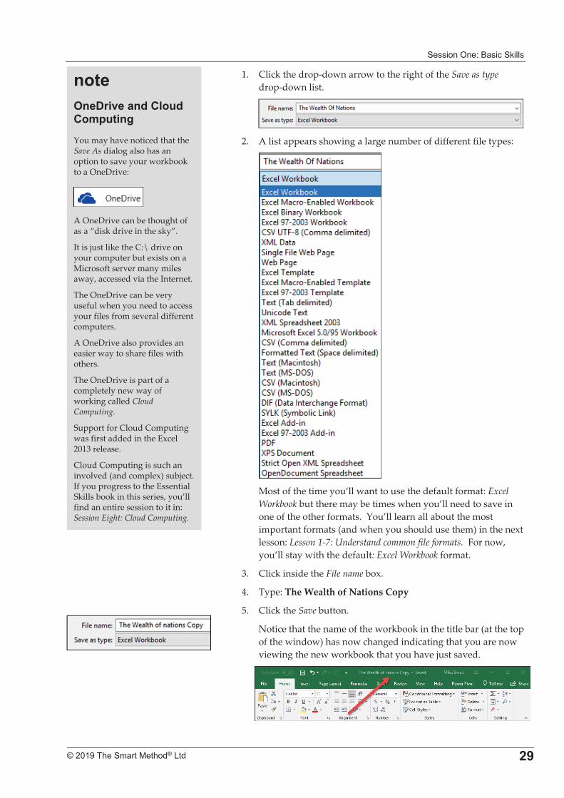
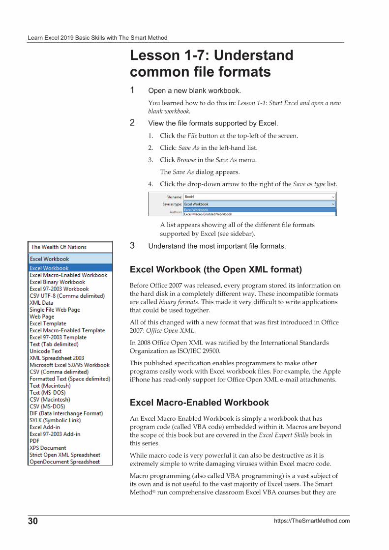
1.� Click�the�drop�down�arrow�to�the�right�of�the�Save�as�type�drop�down�list.�
�2.� A�list�appears�showing�a�large�number�of�different�file�types:��
�Most�of�the�time�you’ll�want�to�use�the�default�format:�Excel�Workbook�but�there�may�be�times�when�you’ll�need�to�save�in�one�of�the�other�formats.��You’ll�learn�all�about�the�most�important�formats�(and�when�you�should�use�them)�in�the�next�lesson:�Lesson�1�7:�Understand�common�file�formats.��For�now,�you’ll�stay�with�the�default:�Excel�Workbook�format.�
3.� Click�inside�the�File�name�box.�
4.� Type:�The�Wealth�of�Nations�Copy�
5.� Click�the�Save�button.�
Notice�that�the�name�of�the�workbook�in�the�title�bar�(at�the�top�of�the�window)�has�now�changed�indicating�that�you�are�now�viewing�the�new�workbook�that�you�have�just�saved.��
�
����1�4������ �.��� �.�#*������You�may�have�noticed�that�the�Save�As�dialog�also�has�an�option�to�save�your�workbook�to�a�OneDrive:�
�
�
A�OneDrive�can�be�thought�of�as�a�“disk�drive�in�the�sky”.�
It�is�just�like�the�C:\�drive�on�your�computer�but�exists�on�a�Microsoft�server�many�miles�away,�accessed�via�the�Internet.�
The�OneDrive�can�be�very�useful�when�you�need�to�access�your�files�from�several�different�computers.���
A�OneDrive�also�provides�an�easier�way�to�share�files�with�others.���
The�OneDrive�is�part�of�a�completely�new�way�of�working�called�Cloud�Computing.���
Support�for�Cloud�Computing�was�first�added�in�the�Excel�2013�release.���
Cloud�Computing�is�such�an�involved�(and�complex)�subject.��If�you�progress�to�the�Essential�Skills�book�in�this�series,�you’ll�find�an�entire�session�to�it�in:�Session�Eight:�Cloud�Computing.�
� ����� !������" �� ��#�!!���������� ��������
�
;�� ��$�%&&��� ������' ��
%������32�5� ����� ���##����������#������ /$�� ����)! �#����#)��#'�
You�learned�how�to�do�this�in:�Lesson�1�1:�Start�Excel�and�open�a�new�blank�workbook.�
�� C�����*�!�*��� �����$$�����)���� !'�1.� Click�the�File�button�at�the�top�left�of�the�screen.�
2.� Click:�Save�As�in�the�left�hand�list.���
3.� Click�Browse�in�the�Save�As�menu.�
The�Save�As�dialog�appears.��
4.� Click�the�drop�down�arrow�to�the�right�of�the�Save�as�type�list.�
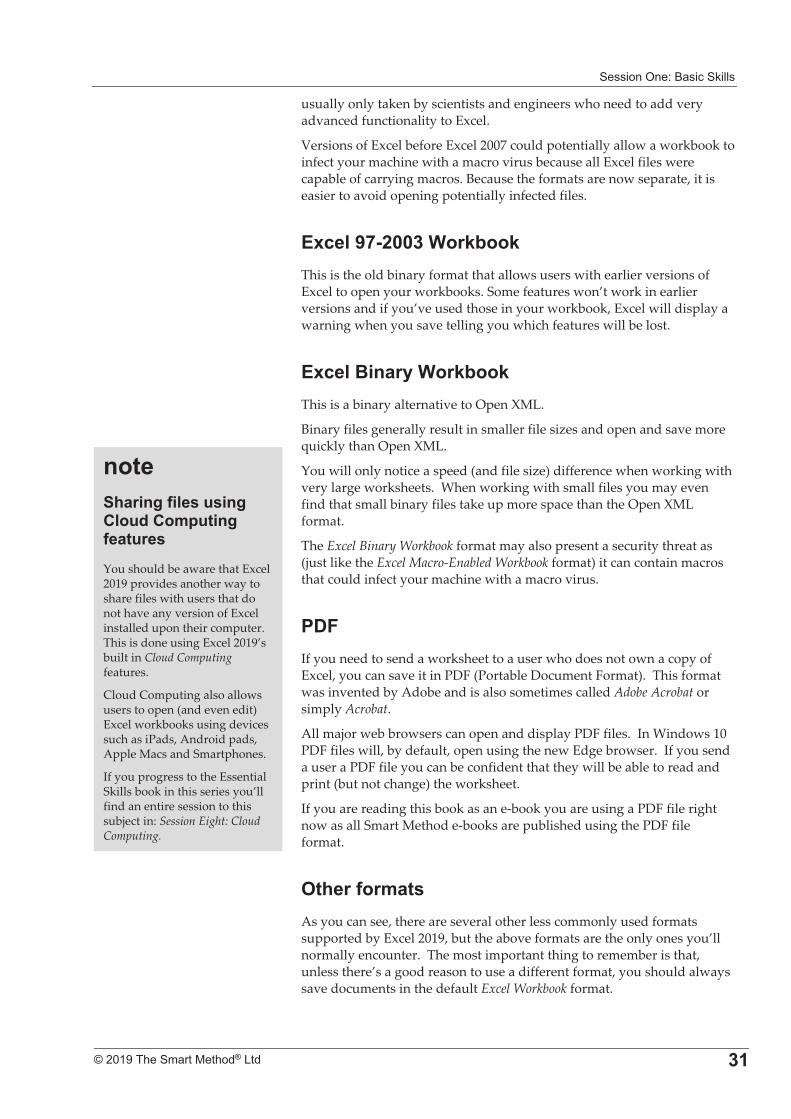
�A�list�appears�showing�all�of�the�different�file�formats�supported�by�Excel�(see�sidebar).���
-� 9����� ������������$��� ���*�!�*��� ��'�
�����$�� !�� �'���1*��D�%����#��(�Before�Office�2007�was�released,�every�program�stored�its�information�on�the�hard�disk�in�a�completely�different�way.�These�incompatible�formats�are�called�binary�formats.�This�made�it�very�difficult�to�write�applications�that�could�be�used�together.�
All�of�this�changed�with�a�new�format�that�was�first�introduced�in�Office�2007:�Office�Open�XML.�
In�2008�Office�Open�XML�was�ratified�by�the�International�Standards�Organization�as�ISO/IEC�29500.���
This�published�specification�enables�programmers�to�make�other�programs�easily�work�with�Excel�workbook�files.�For�example,�the�Apple�iPhone�has�read�only�support�for�Office�Open�XML�e�mail�attachments.�
�������������!� �$�� !�� �An�Excel�Macro�Enabled�Workbook�is�simply�a�workbook�that�has�program�code�(called�VBA�code)�embedded�within�it.�Macros�are�beyond�the�scope�of�this�book�but�are�covered�in�the�Excel�Expert�Skills�book�in�this�series.���
While�macro�code�is�very�powerful�it�can�also�be�destructive�as�it�is�extremely�simple�to�write�damaging�viruses�within�Excel�macro�code.�
Macro�programming�(also�called�VBA�programming)�is�a�vast�subject�of�its�own�and�is�not�useful�to�the�vast�majority�of�Excel�users.�The�Smart�Method®�run�comprehensive�classroom�Excel�VBA�courses�but�they�are�
�������/�%�" �� ��#�!!��
�
����������� �������������� ;�
usually�only�taken�by�scientists�and�engineers�who�need�to�add�very�advanced�functionality�to�Excel.�
Versions�of�Excel�before�Excel�2007�could�potentially�allow�a�workbook�to�infect�your�machine�with�a�macro�virus�because�all�Excel�files�were�capable�of�carrying�macros.�Because�the�formats�are�now�separate,�it�is�easier�to�avoid�opening�potentially�infected�files.��
������3���;�$�� !�� ��This�is�the�old�binary�format�that�allows�users�with�earlier�versions�of�Excel�to�open�your�workbooks.�Some�features�won’t�work�in�earlier�versions�and�if�you’ve�used�those�in�your�workbook,�Excel�will�display�a�warning�when�you�save�telling�you�which�features�will�be�lost.�
������������$�� !�� �This�is�a�binary�alternative�to�Open�XML.��
Binary�files�generally�result�in�smaller�file�sizes�and�open�and�save�more�quickly�than�Open�XML.���
You�will�only�notice�a�speed�(and�file�size)�difference�when�working�with�very�large�worksheets.��When�working�with�small�files�you�may�even�find�that�small�binary�files�take�up�more�space�than�the�Open�XML�format.��
The�Excel�Binary�Workbook�format�may�also�present�a�security�threat�as�(just�like�the�Excel�Macro�Enabled�Workbook�format)�it�can�contain�macros�that�could�infect�your�machine�with�a�macro�virus.�
74,�If�you�need�to�send�a�worksheet�to�a�user�who�does�not�own�a�copy�of�Excel,�you�can�save�it�in�PDF�(Portable�Document�Format).��This�format�was�invented�by�Adobe�and�is�also�sometimes�called�Adobe�Acrobat�or�simply�Acrobat.�
All�major�web�browsers�can�open�and�display�PDF�files.��In�Windows�10�PDF�files�will,�by�default,�open�using�the�new�Edge�browser.��If�you�send�a�user�a�PDF�file�you�can�be�confident�that�they�will�be�able�to�read�and�print�(but�not�change)�the�worksheet.���
If�you�are�reading�this�book�as�an�e�book�you�are�using�a�PDF�file�right�now�as�all�Smart�Method�e�books�are�published�using�the�PDF�file�format.�
1�������#����As�you�can�see,�there�are�several�other�less�commonly�used�formats�supported�by�Excel�2019,�but�the�above�formats�are�the�only�ones�you’ll�normally�encounter.��The�most�important�thing�to�remember�is�that,�unless�there’s�a�good�reason�to�use�a�different�format,�you�should�always�save�documents�in�the�default�Excel�Workbook�format.�
����+������������������.��� �.�#*�������������You�should�be�aware�that�Excel�2019�provides�another�way�to�share�files�with�users�that�do�not�have�any�version�of�Excel�installed�upon�their�computer.��This�is�done�using�Excel�2019’s�built�in�Cloud�Computing�features.��
Cloud�Computing�also�allows�users�to�open�(and�even�edit)�Excel�workbooks�using�devices�such�as�iPads,�Android�pads,�Apple�Macs�and�Smartphones.�
If�you�progress�to�the�Essential�Skills�book�in�this�series�you’ll�find�an�entire�session�to�this�subject�in:�Session�Eight:�Cloud�Computing.�
� ����� !������" �� ��#�!!���������� ��������
�
;�� ��$�%&&��� ������' ��
%������=2�7�������� !�� ��� ��� ����� �����������A�������� (!�������� ������ ����� !'�
�� D��� ����#)��#������Recent Workbooks�!���'�
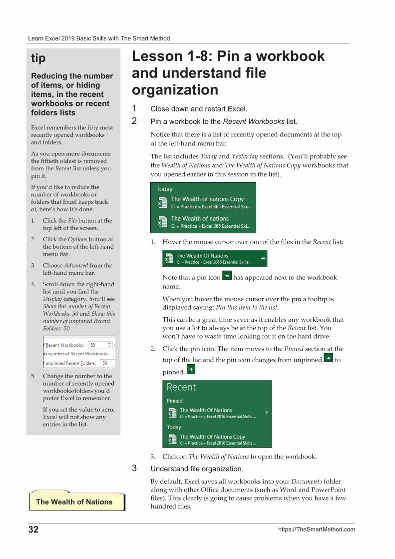
Notice�that�there�is�a�list�of�recently�opened�documents�at�the�top�of�the�left�hand�menu�bar.���
The�list�includes�Today�and�Yesterday�sections.��(You’ll�probably�see�the�Wealth�of�Nations�and�The�Wealth�of�Nations�Copy�workbooks�that�you�opened�earlier�in�this�session�in�the�list).�
�1.� Hover�the�mouse�cursor�over�one�of�the�files�in�the�Recent�list:�
�
Note�that�a�pin�icon� �has�appeared�next�to�the�workbook�name.��
When�you�hover�the�mouse�cursor�over�the�pin�a�tooltip�is�displayed�saying:�Pin�this�item�to�the�list.��
This�can�be�a�great�time�saver�as�it�enables�any�workbook�that�you�use�a�lot�to�always�be�at�the�top�of�the�Recent�list.�You�won’t�have�to�waste�time�looking�for�it�on�the�hard�drive.�
2.� Click�the�pin�icon.�The�item�moves�to�the�Pinned�section�at�the�top�of�the�list�and�the�pin�icon�changes�from�unpinned� �to�
pinned.� �
�3.� Click�on�The�Wealth�of�Nations�to�open�the�workbook.�
-� 9����� ���*�!���, ��; ����'�By�default,�Excel�saves�all�workbooks�into�your�Documents�folder�along�with�other�Office�documents�(such�as�Word�and�PowerPoint�files).�This�clearly�is�going�to�cause�problems�when�you�have�a�few�hundred�files.�
��*�< �����������#!�������#�:������ ������#�:��������������� !�� ������������� ���������Excel�remembers�the�fifty�most�recently�opened�workbooks�and�folders.�
As�you�open�more�documents�the�fiftieth�oldest�is�removed�from�the�Recent�list�unless�you�pin�it.�
If�you’d�like�to�reduce�the�number�of�workbooks�or�folders�that�Excel�keeps�track�of,�here’s�how�it’s�done:�
1.� Click�the�File�button�at�the�top�left�of�the�screen.�
2.� Click�the�Options�button�at�the�bottom�of�the�left�hand�menu�bar.�
3.� Choose�Advanced�from�the�left�hand�menu�bar.��
4.� Scroll�down�the�right�hand�list�until�you�find�the�Display�category.�You’ll�see�Show�this�number�of�Recent�Workbooks:�50�and�Show�this�number�of�unpinned�Recent�Folders:�50.�
5.� Change�the�number�to�the�number�of�recently�opened�workbooks/folders�you’d�prefer�Excel�to�remember.��
If�you�set�the�value�to�zero,�Excel�will�not�show�any�entries�in�the�list.�
���$��������C�������
�������/�%�" �� ��#�!!��
�
����������� �������������� ;;
It�is�better�to�organize�yourself�from�the�start�by�setting�up�an�orderly�filing�system.�
3� (� �� ��Excel���)*�!���)� �������Documents�*�!��'��I�create�a�folder�called�Excel�beneath�the�Documents�folder.�In�this�folder,�I�create�subfolders�to�store�my�work.�You�can�see�a�screen�grab�of�my�Excel�folder�in�the�sidebar�(of�course,�your�needs�will�be�different�to�mine).�
See�sidebar�if�you�don’t�know�how�to�create�a�subfolder.��
6� ������* �!��*�!�!� ��������$�������������Excel�*�!��'��If�you�take�my�advice�and�create�an�Excel�folder,�you�will�waste�a�mouse�click�every�time�you�open�a�file�because�Excel�will�take�you�to�the�Documents�folder�by�default.�
Here’s�how�to�reset�the�default�file�location�to�your�new�Excel�folder:�
1.� Open�Excel�and�click�the�Blank�Workbook�template�to�open�a�new�blank�workbook.�
2.� Click�the�File�button�at�the�top�left�of�the�screen.���
3.� Click�the�Options�button�towards�the�bottom�of�the�left�hand�list.�
The�Excel�Options�dialog�appears.�
4.� Choose�the�Save�category�from�the�left�hand�side�of�the�dialog.�
During�the�remainder�of�the�book�I’ll�explain�the�above�three�steps�like�this:�
Click:�File�Options�Save.���
This�will�save�a�lot�of�time�and�forests!�
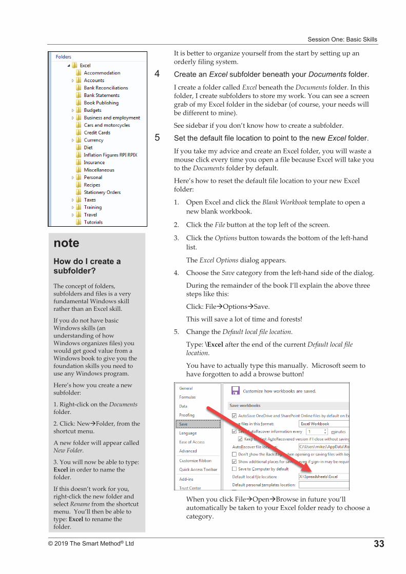
5.� Change�the�Default�local�file�location.�
Type:�\Excel�after�the�end�of�the�current�Default�local�file�location.�
You�have�to�actually�type�this�manually.��Microsoft�seem�to�have�forgotten�to�add�a�browse�button!�
�When�you�click�File�Open�Browse�in�future�you’ll�automatically�be�taken�to�your�Excel�folder�ready�to�choose�a�category.�
����)��� ��/����������!��� �E�The�concept�of�folders,�subfolders�and�files�is�a�very�fundamental�Windows�skill�rather�than�an�Excel�skill.���
If�you�do�not�have�basic�Windows�skills�(an�understanding�of�how�Windows�organizes�files)�you�would�get�good�value�from�a�Windows�book�to�give�you�the�foundation�skills�you�need�to�use�any�Windows�program.�
Here’s�how�you�create�a�new�subfolder:�
1.�Right�click�on�the�Documents�folder.�
2.�Click:�New�Folder,�from�the�shortcut�menu.�
A�new�folder�will�appear�called�New�Folder.�
3.�You�will�now�be�able�to�type:�Excel�in�order�to�name�the�folder.���
If�this�doesn’t�work�for�you,�right�click�the�new�folder�and�select�Rename�from�the�shortcut�menu.��You’ll�then�be�able�to�type:�Excel�to�rename�the�folder.�
� ����� !������" �� ��#�!!���������� ��������
�
;0� ��$�%&&��� ������' ��
%�������2�?��:�#��:�� :����#:� ����� ������������ ������!��When�you�save�an�Excel�file�onto�your�hard�disk,�you�are�saving�a�single�workbook�containing�one�or�more�worksheets.��You�can�add�as�many�worksheets�as�you�need�to�a�workbook.�
There�are�two�types�of�worksheet.�Regular�worksheets�contain�cells.�Chart�sheets,�as�you�would�expect,�each�contain�a�single�chart.�If�you�progress�to�the�Essential�Skills�book�in�this�series,�you’ll�find�an�entire�session�that�will�teach�you�everything�there�is�to�know�about�Excels�powerful�charting�features.���
�� /$��The Wealth of Nations�*���������� �$!�*�!��*�!���1�*���������� !� ����$�2'��
�� ��0�)�������#���'��
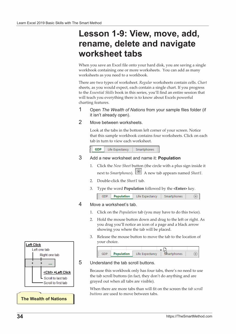
Look�at�the�tabs�in�the�bottom�left�corner�of�your�screen.�Notice�that�this�sample�workbook�contains�four�worksheets.�Click�on�each�tab�in�turn�to�view�each�worksheet.��
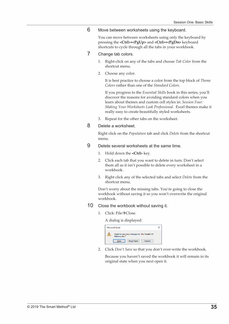
�-� ?��� �������#��� ���� ����%�7�*��������
1.� Click�the�New�Sheet�button�(the�circle�with�a�plus�sign�inside�it�
next�to�Smartphones).�� ��A�new�tab�appears�named�Sheet1.��
2.� Double�click�the�Sheet1�tab.�
3.� Type�the�word�Population�followed�by�the�<Enter>�key.�
�3� ��0� ����#������ )'��
1.� Click�on�the�Population�tab�(you�may�have�to�do�this�twice).��
2.� Hold�the�mouse�button�down�and�drag�to�the�left�or�right.�As�you�drag�you’ll�notice�an�icon�of�a�page�and�a�black�arrow�showing�you�where�the�tab�will�be�placed.��
3.� Release�the�mouse�button�to�move�the�tab�to�the�location�of�your�choice.��
�6� 9����� ������ )�� ��!!�)������'��
Because�this�workbook�only�has�four�tabs,�there’s�no�need�to�use�the�tab�scroll�buttons�(in�fact,�they�don’t�do�anything�and�are�grayed�out�when�all�tabs�are�visible).���
When�there�are�more�tabs�than�will�fit�on�the�screen�the�tab�scroll�buttons�are�used�to�move�between�tabs.��
���$��������C�������
�������/�%�" �� ��#�!!��
�
����������� �������������� ;>
7� ��0�)�������#��������,���#�)� ��'��You�can�move�between�worksheets�using�only�the�keyboard�by�pressing�the�<Ctrl>+<PgUp>�and�<Ctrl>+<PgDn>�keyboard�shortcuts�to�cycle�through�all�the�tabs�in�your�workbook.�
8� ( �,�� )� �!���'��1.� Right�click�on�any�of�the�tabs�and�choose�Tab�Color�from�the�
shortcut�menu.��
2.� Choose�any�color.��
It�is�best�practice�to�choose�a�color�from�the�top�block�of�Theme�Colors�rather�than�one�of�the�Standard�Colors.���
If�you�progress�to�the�Essential�Skills�book�in�this�series,�you’ll�discover�the�reasons�for�avoiding�standard�colors�when�you�learn�about�themes�and�custom�cell�styles�in:�Session�Four:�Making�Your�Worksheets�Look�Professional.��Excel�themes�make�it�really�easy�to�create�beautifully�styled�worksheets.�
3.� Repeat�for�the�other�tabs�on�the�worksheet.��
E� +!�� ����#��'��
Right�click�on�the�Population�tab�and�click�Delete�from�the�shortcut�menu.�
�� +!���0� !����#���� ����� �����'��1.� Hold�down�the�<Ctrl>�key.�
2.� Click�each�tab�that�you�want�to�delete�in�turn.�Don’t�select�them�all�as�it�isn’t�possible�to�delete�every�worksheet�in�a�workbook.�
3.� Right�click�any�of�the�selected�tabs�and�select�Delete�from�the�shortcut�menu.�
Don’t�worry�about�the�missing�tabs.�You’re�going�to�close�the�workbook�without�saving�it�so�you�won’t�overwrite�the�original�workbook.�
��� (!��������#)��#��������� 0��,���'��1.� Click:�File�Close.�
A�dialog�is�displayed:��
�2.� Click�Don’t�Save�so�that�you�don’t�over�write�the�workbook.�
Because�you�haven’t�saved�the�workbook�it�will�remain�in�its�original�state�when�you�next�open�it.��
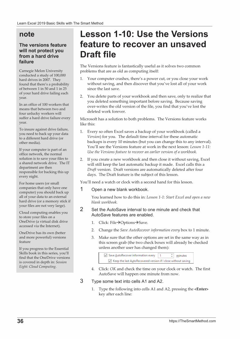
� ����� !������" �� ��#�!!���������� ��������
�
;6� ��$�%&&��� ������' ��
%��������2�5�����?������������������������������ �4���������The�Versions�feature�is�fantastically�useful�as�it�solves�two�common�problems�that�are�as�old�as�computing�itself:�
1.� Your�computer�crashes,�there’s�a�power�cut,�or�you�close�your�work�without�saving,�and�then�discover�that�you’ve�lost�all�of�your�work�since�the�last�save.�
2.� You�delete�parts�of�your�workbook�and�then�save,�only�to�realize�that�you�deleted�something�important�before�saving.��Because�saving�over�writes�the�old�version�of�the�file,�you�find�that�you’ve�lost�the�deleted�work�forever.�
Microsoft�has�a�solution�to�both�problems.��The�Versions�feature�works�like�this:�
1.� Every�so�often�Excel�saves�a�backup�of�your�workbook�(called�a�Version)�for�you.��The�default�time�interval�for�these�automatic�backups�is�every�10�minutes�(but�you�can�change�this�to�any�interval).�You’ll�see�the�Versions�feature�at�work�in�the�next�lesson:�Lesson�1�11:�Use�the�Versions�feature�to�recover�an�earlier�version�of�a�workbook.�
2.� If�you�create�a�new�workbook�and�then�close�it�without�saving,�Excel�will�still�keep�the�last�automatic�backup�it�made.��Excel�calls�this�a�Draft�version.��Draft�versions�are�automatically�deleted�after�four�days.��The�Draft�feature�is�the�subject�of�this�lesson.�
You’ll�need�a�watch�or�clock�with�a�second�hand�for�this�lesson.�
�� /$�� ����)! �#����#)��#'�You�learned�how�to�do�this�in:�Lesson�1�1:�Start�Excel�and�open�a�new�blank�workbook.�
�� �����?���� 0�����0 !������������� ��� #�� ��?���� 0�* ����� ��� )!�'�1.� Click:�File�Options�Save.�
2.� Change�the�Save�AutoRecover�information�every�box�to�1�minute.�
3.� Make�sure�that�the�other�options�are�set�in�the�same�way�as�in�this�screen�grab�(the�two�check�boxes�will�already�be�checked�unless�another�user�has�changed�them):�
�4.� Click:�OK�and�check�the�time�on�your�clock�or�watch.��The�first�
AutoSave�will�happen�one�minute�from�now.�
-� ��$�������������� !!��?�� ���?�'�1.� Type�the�following�into�cells�A1�and�A2,�pressing�the�<Enter>�
key�after�each�line:�
������������������������������*�������������#������ � �����������Carnegie�Melon�University�conducted�a�study�of�100,000�hard�drives�in�2007.��They�found�that�there’s�a�probability�of�between�1�in�50�and�1�in�25�of�your�hard�drive�failing�each�year.���
In�an�office�of�100�workers�that�means�that�between�two�and�four�unlucky�workers�will�suffer�a�hard�drive�failure�every�year.��
To�insure�against�drive�failure,�you�need�to�back�up�your�data�to�a�different�hard�drive�(or�other�media).���
If�your�computer�is�part�of�an�office�network,�the�normal�solution�is�to�save�your�files�to�a�shared�network�drive.��The�IT�department�are�then�responsible�for�backing�this�up�every�night.�
For�home�users�(or�small�companies�that�only�have�one�computer)�you�should�back�up�all�of�your�data�to�an�external�hard�drive�(or�a�memory�stick�if�your�files�are�not�very�large).�
Cloud�computing�enables�you�to�store�your�files�on�a�OneDrive�(a�virtual�disk�drive�accessed�via�the�Internet).�
OneDrive�has�its�own�(better�and�more�powerful)�versions�feature��
If�you�progress�to�the�Essential�Skills�book�in�this�series,�you’ll�find�that�the�OneDrive�versions�is�covered�in�depth�in:�Session�Eight:�Cloud�Computing.�
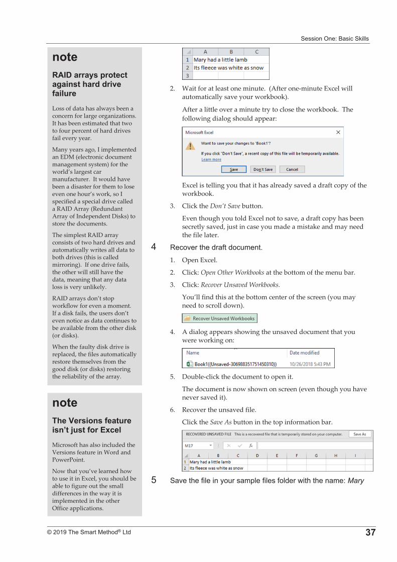
�������/�%�" �� ��#�!!��
�
����������� �������������� ;3
�2.� Wait�for�at�least�one�minute.��(After�one�minute�Excel�will�
automatically�save�your�workbook).�
After�a�little�over�a�minute�try�to�close�the�workbook.��The�following�dialog�should�appear:�
��Excel�is�telling�you�that�it�has�already�saved�a�draft�copy�of�the�workbook.�
3.� Click�the�Don’t�Save�button.�
Even�though�you�told�Excel�not�to�save,�a�draft�copy�has�been�secretly�saved,�just�in�case�you�made�a�mistake�and�may�need�the�file�later.�
3� : �0������ *���� ����'��1.� Open�Excel.�
2.� Click:�Open�Other�Workbooks�at�the�bottom�of�the�menu�bar.�
3.� Click:�Recover�Unsaved�Workbooks.�
You’ll�find�this�at�the�bottom�center�of�the�screen�(you�may�need�to�scroll�down).�
�4.� A�dialog�appears�showing�the�unsaved�document�that�you�
were�working�on:�
�5.� Double�click�the�document�to�open�it.�
The�document�is�now�shown�on�screen�(even�though�you�have�never�saved�it).�
6.� Recover�the�unsaved�file.�
Click�the�Save�As�button�in�the�top�information�bar.�
�6� � 0���*�!���������� �$!�*�!��*�!���������� �%�Mary�
�������?����������������8��&�������������Microsoft�has�also�included�the�Versions�feature�in�Word�and�PowerPoint.�
Now�that�you’ve�learned�how�to�use�it�in�Excel,�you�should�be�able�to�figure�out�the�small�differences�in�the�way�it�is�implemented�in�the�other�Office�applications.�
����<"/4��������*����������������� � �����������Loss�of�data�has�always�been�a�concern�for�large�organizations.��It�has�been�estimated�that�two�to�four�percent�of�hard�drives�fail�every�year.�
Many�years�ago,�I�implemented�an�EDM�(electronic�document�management�system)�for�the�world’s�largest�car�manufacturer.��It�would�have�been�a�disaster�for�them�to�lose�even�one�hour’s�work,�so�I�specified�a�special�drive�called�a�RAID�Array�(Redundant�Array�of�Independent�Disks)�to�store�the�documents.��
The�simplest�RAID�array�consists�of�two�hard�drives�and�automatically�writes�all�data�to�both�drives�(this�is�called�mirroring).��If�one�drive�fails,�the�other�will�still�have�the�data,�meaning�that�any�data�loss�is�very�unlikely.�
RAID�arrays�don’t�stop�workflow�for�even�a�moment.��If�a�disk�fails,�the�users�don’t�even�notice�as�data�continues�to�be�available�from�the�other�disk�(or�disks).���
When�the�faulty�disk�drive�is�replaced,�the�files�automatically�restore�themselves�from�the�good�disk�(or�disks)�restoring�the�reliability�of�the�array.�
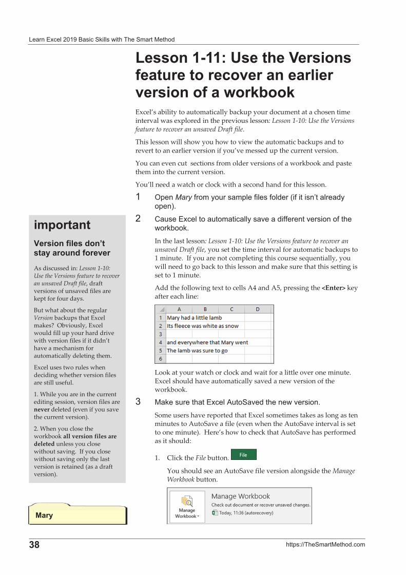
� ����� !������" �� ��#�!!���������� ��������
�
;=� ��$�%&&��� ������' ��
%��������2�5�����?���������������������������������������������� !�� �Excel’s�ability�to�automatically�backup�your�document�at�a�chosen�time�interval�was�explored�in�the�previous�lesson:�Lesson�1�10:�Use�the�Versions�feature�to�recover�an�unsaved�Draft�file.�
This�lesson�will�show�you�how�to�view�the�automatic�backups�and�to�revert�to�an�earlier�version�if�you’ve�messed�up�the�current�version.�
You�can�even�cut��sections�from�older�versions�of�a�workbook�and�paste�them�into�the�current�version.�
You’ll�need�a�watch�or�clock�with�a�second�hand�for�this�lesson.��
�� /$��Mary�*���������� �$!�*�!��*�!���1�*���������� !� ����$�2'��
�� ( ����� !���� ���� �� !!��� 0� ���**����0�������*������#)��#'��In�the�last�lesson:�Lesson�1�10:�Use�the�Versions�feature�to�recover�an�unsaved�Draft�file,�you�set�the�time�interval�for�automatic�backups�to�1�minute.��If�you�are�not�completing�this�course�sequentially,�you�will�need�to�go�back�to�this�lesson�and�make�sure�that�this�setting�is�set�to�1�minute.�
Add�the�following�text�to�cells�A4�and�A5,�pressing�the�<Enter>�key�after�each�line:�
�Look�at�your�watch�or�clock�and�wait�for�a�little�over�one�minute.��Excel�should�have�automatically�saved�a�new�version�of�the�workbook.�
-� � #������ ���� !�?���� 0�������0�����'��Some�users�have�reported�that�Excel�sometimes�takes�as�long�as�ten�minutes�to�AutoSave�a�file�(even�when�the�AutoSave�interval�is�set�to�one�minute).��Here’s�how�to�check�that�AutoSave�has�performed�as�it�should:��
1.� Click�the�File�button.� �
You�should�see�an�AutoSave�file�version�alongside�the�Manage�Workbook�button.�
������
�#*�������?����������� ��8������������ �������As�discussed�in:�Lesson�1�10:�Use�the�Versions�feature�to�recover�an�unsaved�Draft�file,�draft�versions�of�unsaved�files�are�kept�for�four�days.�
But�what�about�the�regular�Version�backups�that�Excel�makes?��Obviously,�Excel�would�fill�up�your�hard�drive�with�version�files�if�it�didn’t�have�a�mechanism�for�automatically�deleting�them.�
Excel�uses�two�rules�when�deciding�whether�version�files�are�still�useful.�
1.�While�you�are�in�the�current�editing�session,�version�files�are�never�deleted�(even�if�you�save�the�current�version).�
2.�When�you�close�the�workbook�all�version�files�are�deleted�unless�you�close�without�saving.��If�you�close�without�saving�only�the�last�version�is�retained�(as�a�draft�version).�
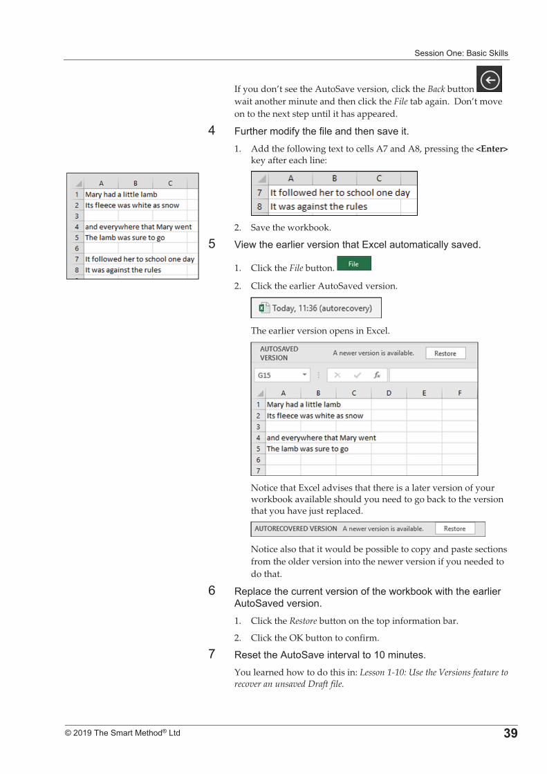
�������/�%�" �� ��#�!!��
�
����������� �������������� ;�
If�you�don’t�see�the�AutoSave�version,�click�the�Back�button�wait�another�minute�and�then�click�the�File�tab�again.��Don’t�move�on�to�the�next�step�until�it�has�appeared.�
3� F���������*����*�!� ������� 0���'��1.� Add�the�following�text�to�cells�A7�and�A8,�pressing�the�<Enter>�
key�after�each�line:�
�2.� Save�the�workbook.�
6� C����� �!���0������� ���� !� ���� �� !!��� 0�'��
1.� Click�the�File�button.� �
2.� Click�the�earlier�AutoSaved�version.�
�The�earlier�version�opens�in�Excel.�
�Notice�that�Excel�advises�that�there�is�a�later�version�of�your�workbook�available�should�you�need�to�go�back�to�the�version�that�you�have�just�replaced.�
�Notice�also�that�it�would�be�possible�to�copy�and�paste�sections�from�the�older�version�into�the�newer�version�if�you�needed�to�do�that.�
7� :$! ��� ������0�������*������#)��#������� �!���?���� 0��0�����'��1.� Click�the�Restore�button�on�the�top�information�bar.�
2.� Click�the�OK�button�to�confirm.�
8� :�����?���� 0�����0 !�������������'�You�learned�how�to�do�this�in:�Lesson�1�10:�Use�the�Versions�feature�to�recover�an�unsaved�Draft�file.�
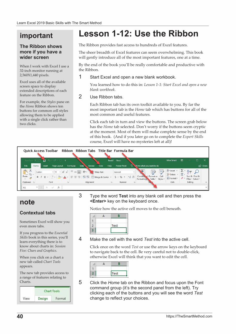
� ����� !������" �� ��#�!!���������� ��������
�
0�� ��$�%&&��� ������' ��
%��������2�5�����<�!!���The�Ribbon�provides�fast�access�to�hundreds�of�Excel�features.�
The�sheer�breadth�of�Excel�features�can�seem�overwhelming.�This�book�will�gently�introduce�all�of�the�most�important�features,�one�at�a�time.��
By�the�end�of�the�book�you’ll�be�really�comfortable�and�productive�with�the�Ribbon.�
�� �� ����� !� ����$�� ����)! �#����#)��#'�You�learned�how�to�do�this�in:�Lesson�1�1:�Start�Excel�and�open�a�new�blank�workbook.�
�� 9��:�))���� )�'�Each�Ribbon�tab�has�its�own�toolkit�available�to�you.�By�far�the�most�important�tab�is�the�Home�tab�which�has�buttons�for�all�of�the�most�common�and�useful�features.��
Click�each�tab�in�turn�and�view�the�buttons.�The�screen�grab�below�has�the�Home�tab�selected.�Don’t�worry�if�the�buttons�seem�cryptic�at�the�moment.�Most�of�them�will�make�complete�sense�by�the�end�of�this�book.��(And�if�you�later�go�on�to�complete�the�Expert�Skills�course,�Excel�will�have�no�mysteries�left�at�all)!�
�
-� ��$����������������� ���)! �#� !!� ������$������F����G�#�������#�)� ����� '�Notice�how�the�active�cell�moves�to�the�cell�beneath.�
�3� � #��� !!������������Test�������� ��0� !!'�
Click�once�on�the�word�Test�or�use�the�arrow�keys�on�the�keyboard�to�navigate�back�to�the�cell.�Be�very�careful�not�to�double�click,�otherwise�Excel�will�think�that�you�want�to�edit�the�cell.�
�6� (!� #���Home�� )������:�))��� ���*� ����$�����F����
��� ���,���$�1�������� ����$ �!�*������!*�2'����� !� #��,� ��*���)������� ���������!!����������Test �,�����*! ������� �� �'�
����.�����������!��Sometimes�Excel�will�show�you�even�more�tabs.��
If�you�progress�to�the�Essential�Skills�book�in�this�series,�you’ll�learn�everything�there�is�to�know�about�charts�in:�Session�Five:�Chars�and�Graphics.��
When�you�click�on�a�chart�a�new�tab�called�Chart�Tools�appears.���
The�new�tab�provides�access�to�a�range�of�features�relating�to�Charts.�
�#*����������<�!!���������#������������������ �������When�I�work�with�Excel�I�use�a�32�inch�monitor�running�at�2,560X1,440�pixels.��
Excel�uses�all�of�the�available�screen�space�to�display�extended�descriptions�of�each�feature�on�the�Ribbon.���
For�example,�the�Styles�pane�on�the�Home�Ribbon�shows�ten�buttons�for�common�cell�styles�allowing�them�to�be�applied�with�a�single�click�rather�than�two�clicks.��
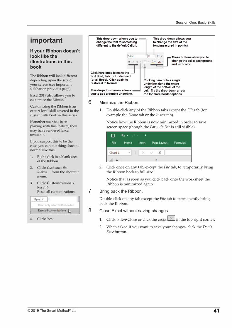
�������/�%�" �� ��#�!!��
�
����������� �������������� 0�
�
�7� ������;���:�))��'�
1.� Double�click�any�of�the�Ribbon�tabs�except�the�File�tab�(for�example�the�Home�tab�or�the�Insert�tab).�
Notice�how�the�Ribbon�is�now�minimized�in�order�to�save�screen�space�(though�the�Formula�Bar�is�still�visible).�
�2.� Click�once�on�any�tab,�except�the�File�tab,�to�temporarily�bring�
the�Ribbon�back�to�full�size.���
Notice�that�as�soon�as�you�click�back�onto�the�worksheet�the�Ribbon�is�minimized�again.�
8� "���,�) #���:�))��'�Double�click�on�any�tab�except�the�File�tab�to�permanently�bring�back�the�Ribbon.�
E� (!����� !��������� 0��,� �,�'�
1.� Click:�File�Close�or�click�the�cross� �in�the�top�right�corner.�
2.� When�asked�if�you�want�to�save�your�changes,�click�the�Don’t�Save�button.�
�#*�������/�������<�!!��� ���8����� ��� ��������������������������!�� �The�Ribbon�will�look�different�depending�upon�the�size�of�your�screen�(see�important�sidebar�on�previous�page).�
Excel�2019�also�allows�you�to�customize�the�Ribbon.��
Customizing�the�Ribbon�is�an�expert�level�skill�covered�in�the�Expert�Skills�book�in�this�series.�
If�another�user�has�been�playing�with�this�feature,�they�may�have�rendered�Excel�unusable.�
If�you�suspect�this�to�be�the�case,�you�can�put�things�back�to�normal�like�this:�
1.� Right�click�in�a�blank�area�of�the�Ribbon.�
2.� Click:�Customize�the�Ribbon…�from�the�shortcut�menu.�
3.� Click:�Customizations��Reset��Reset�all�customizations.�
�4.� Click:�Yes.�
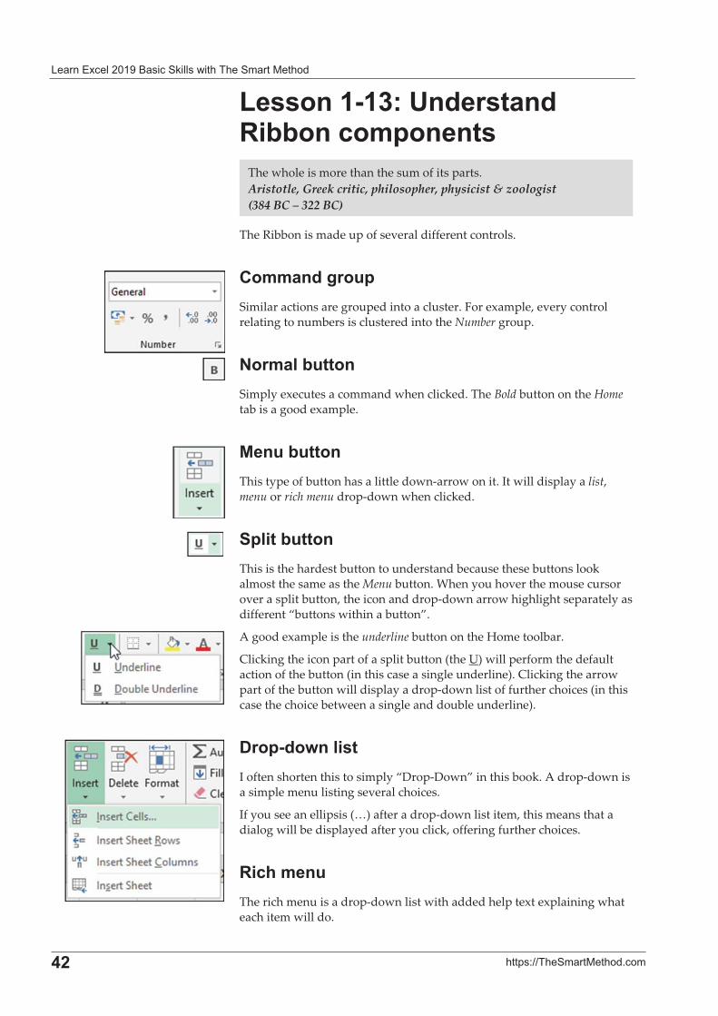
� ����� !������" �� ��#�!!���������� ��������
�
0�� ��$�%&&��� ������' ��
%�������;2�5� ����� �<�!!�����#*�������
�
�
The�Ribbon�is�made�up�of�several�different�controls.��
.�##�� �����*�Similar�actions�are�grouped�into�a�cluster.�For�example,�every�control�relating�to�numbers�is�clustered�into�the�Number�group.�
C��#���!������Simply�executes�a�command�when�clicked.�The�Bold�button�on�the�Home�tab�is�a�good�example.��
����!������This�type�of�button�has�a�little�down�arrow�on�it.�It�will�display�a�list,�menu�or�rich�menu�drop�down�when�clicked.�
+*����!������This�is�the�hardest�button�to�understand�because�these�buttons�look�almost�the�same�as�the�Menu�button.�When�you�hover�the�mouse�cursor�over�a�split�button,�the�icon�and�drop�down�arrow�highlight�separately�as�different�“buttons�within�a�button”.�
A�good�example�is�the�underline�button�on�the�Home�toolbar.�
Clicking�the�icon�part�of�a�split�button�(the�U)�will�perform�the�default�action�of�the�button�(in�this�case�a�single�underline).�Clicking�the�arrow�part�of�the�button�will�display�a�drop�down�list�of�further�choices�(in�this�case�the�choice�between�a�single�and�double�underline).�
4��* ���������I�often�shorten�this�to�simply�“Drop�Down”�in�this�book.�A�drop�down�is�a�simple�menu�listing�several�choices.�
If�you�see�an�ellipsis�(…)�after�a�drop�down�list�item,�this�means�that�a�dialog�will�be�displayed�after�you�click,�offering�further�choices.�
<����#���The�rich�menu�is�a�drop�down�list�with�added�help�text�explaining�what�each�item�will�do.�
The�whole�is more�than�the�sum�of�its�parts.Aristotle,�Greek�critic,�philosopher,�physicist�&�zoologist��(384�BC�– 322�BC)
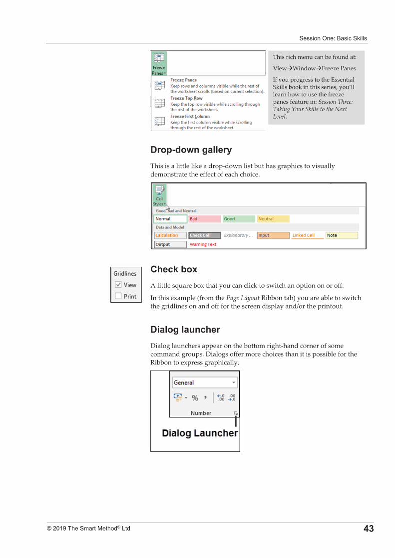
�������/�%�" �� ��#�!!��
�
����������� �������������� 0;
�
�
�
�
�
�
�
4��* �����������This�is�a�little�like�a�drop�down�list�but�has�graphics�to�visually�demonstrate�the�effect�of�each�choice.�
�
.�� �!���A�little�square�box�that�you�can�click�to�switch�an�option�on�or�off.��
In�this�example�(from�the�Page�Layout�Ribbon�tab)�you�are�able�to�switch�the�gridlines�on�and�off�for�the�screen�display�and/or�the�printout.�
4��������������Dialog�launchers�appear�on�the�bottom�right�hand�corner�of�some�command�groups.�Dialogs�offer�more�choices�than�it�is�possible�for�the�Ribbon�to�express�graphically.��
�
This�rich�menu�can�be�found�at:
View�Window�Freeze�Panes�
If�you�progress�to�the�Essential�Skills�book�in�this�series,�you’ll�learn�how�to�use�the�freeze�panes�feature�in:�Session�Three:�Taking�Your�Skills�to�the�Next�Level.�
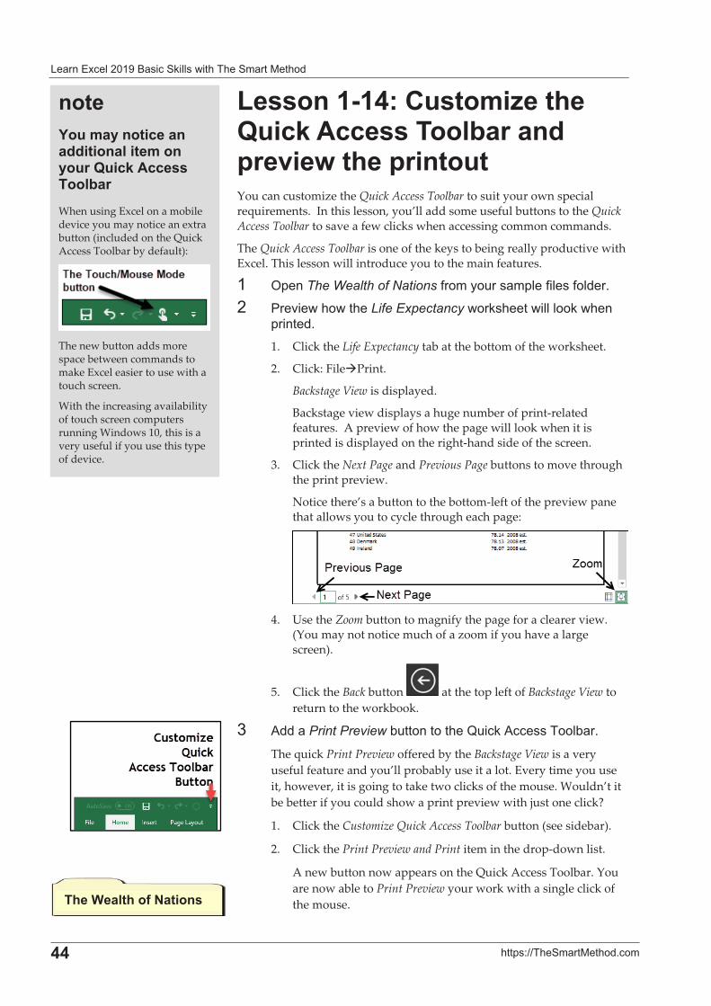
� ����� !������" �� ��#�!!���������� ��������
�
00� ��$�%&&��� ������' ��
%�������02�.����#�A����H��� �"���������!����� �*��������*��������You�can�customize�the�Quick�Access�Toolbar�to�suit�your�own�special�requirements.��In�this�lesson,�you’ll�add�some�useful�buttons�to�the�Quick�Access�Toolbar�to�save�a�few�clicks�when�accessing�common�commands.�
The�Quick�Access�Toolbar�is�one�of�the�keys�to�being�really�productive�with�Excel.�This�lesson�will�introduce�you�to�the�main�features.��
�� /$��The Wealth of Nations�*���������� �$!�*�!��*�!��'�
�� D�0��������Life Expectancy����#�����!!�!��#����$�����'�1.� Click�the�Life�Expectancy�tab�at�the�bottom�of�the�worksheet.�
2.� Click:�File�Print.�
Backstage�View�is�displayed.�
Backstage�view�displays�a�huge�number�of�print�related�features.��A�preview�of�how�the�page�will�look�when�it�is�printed�is�displayed�on�the�right�hand�side�of�the�screen.�
3.� Click�the�Next�Page�and�Previous�Page�buttons�to�move�through�the�print�preview.�
Notice�there’s�a�button�to�the�bottom�left�of�the�preview�pane�that�allows�you�to�cycle�through�each�page:�
�4.� Use�the�Zoom�button�to�magnify�the�page�for�a�clearer�view.�
(You�may�not�notice�much�of�a�zoom�if�you�have�a�large�screen).�
5.� Click�the�Back�button� �at�the�top�left�of�Backstage�View�to�return�to�the�workbook.�
-� ?��� �Print Preview�)�����������G�� #�? ������!) �'�
The�quick�Print�Preview�offered�by�the�Backstage�View�is�a�very�useful�feature�and�you’ll�probably�use�it�a�lot.�Every�time�you�use�it,�however,�it�is�going�to�take�two�clicks�of�the�mouse.�Wouldn’t�it�be�better�if�you�could�show�a�print�preview�with�just�one�click?�
1.� Click�the�Customize�Quick�Access�Toolbar�button�(see�sidebar).�
2.� Click�the�Print�Preview�and�Print�item�in�the�drop�down�list.��
A�new�button�now�appears�on�the�Quick�Access�Toolbar.�You�are�now�able�to�Print�Preview�your�work�with�a�single�click�of�the�mouse.����$��������C�������
����-���#������������� ����������#���������H��� �"���������!���When�using�Excel�on�a�mobile�device�you�may�notice�an�extra�button�(included�on�the�Quick�Access�Toolbar�by�default):�
�The�new�button�adds�more�space�between�commands�to�make�Excel�easier�to�use�with�a�touch�screen.���
With�the�increasing�availability�of�touch�screen�computers�running�Windows�10,�this�is�a�very�useful�if�you�use�this�type�of�device.�
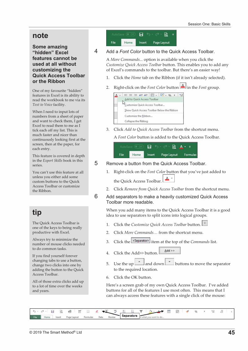
�������/�%�" �� ��#�!!��
�
����������� �������������� 0>
�3� ?��� �Font Color�)�����������G�� #�? ������!) �'�
A�More�Commands...�option�is�available�when�you�click�the�Customize�Quick�Access�Toolbar�button.�This�enables�you�to�add�any�of�Excel’s�commands�to�the�toolbar.�But�there’s�an�easier�way!�
1.� Click�the�Home�tab�on�the�Ribbon�(if�it�isn’t�already�selected).��
2.� Right�click�on�the�Font�Color�button� �in�the�Font�group.�
�3.� Click�Add�to�Quick�Access�Toolbar�from�the�shortcut�menu.�
A�Font�Color�button�is�added�to�the�Quick�Access�Toolbar.�
�6� :��0� �)������*������G�� #�? ������!) �'�
1.� Right�click�on�the�Font�Color�button�that�you’ve�just�added�to�
the�Quick�Access�Toolbar.� �
2.� Click�Remove�from�Quick�Access�Toolbar�from�the�shortcut�menu.�
7� ?����$ � ��������� #� � 0�!�� ������;��G�� #�? ������!) ������� � )!'�When�you�add�many�items�to�the�Quick�Access�Toolbar�it�is�a�good�idea�to�use�separators�to�split�icons�into�logical�groups.�
1.� Click�the�Customize�Quick�Access�Toolbar�button.� ��
2.� Click�More�Commands…�from�the�shortcut�menu.�
3.� Click�the� �item�at�the�top�of�the�Commands�list.�
4.� Click�the�Add>>�button.� �
5.� Use�the�up� �and�down� �buttons�to�move�the�separator�to�the�required�location.�
6.� Click�the�OK�button.�
Here’s�a�screen�grab�of�my�own�Quick�Access�Toolbar.��I’ve�added�buttons�for�all�of�the�features�I�use�most�often.��This�means�that�I�can�always�access�these�features�with�a�single�click�of�the�mouse:�
�
�
��*�The�Quick�Access�Toolbar�is�one�of�the�keys�to�being�really�productive�with�Excel.�
Always�try�to�minimize�the�number�of�mouse�clicks�needed�to�do�common�tasks.��
If�you�find�yourself�forever�changing�tabs�to�use�a�button,�change�two�clicks�into�one�by�adding�the�button�to�the�Quick�Access�Toolbar.�
All�of�those�extra�clicks�add�up�to�a�lot�of�time�over�the�weeks�and�years.�
����+�#��#�A����I�� �J��������������������!��� ���������������������#�A�������H��� �"���������!���������<�!!���One�of�my�favourite�“hidden”�features�in�Excel�is�its�ability�to�read�the�workbook�to�me�via�its�Text�to�Voice�facility.�
When�I�need�to�input�lots�of�numbers�from�a�sheet�of�paper�and�want�to�check�them,�I�get�Excel�to�read�them�to�me�as�I�tick�each�off�my�list.�This�is�much�faster�and�nicer�than�continuously�looking�first�at�the�screen,�then�at�the�paper,�for�each�entry.�
This�feature�is�covered�in�depth�in�the�Expert�Skills�book�in�this�series.�
You�can’t�use�this�feature�at�all�unless�you�either�add�some�custom�buttons�to�the�Quick�Access�Toolbar�or�customize�the�Ribbon.�
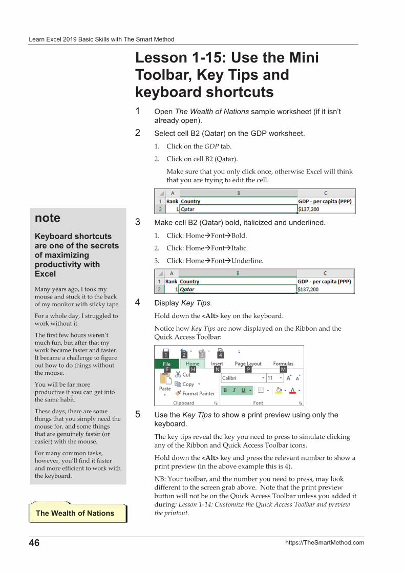
� ����� !������" �� ��#�!!���������� ��������
�
06� ��$�%&&��� ������' ��
%�������>2�5��������������!��:�K����*���� � �!��� ������������� /$��The Wealth of Nations�� �$!����#���1�*����������
!� ����$�2'�
�� �! �� !!�"��1G � �2������<+D����#��'�1.� Click�on�the�GDP�tab.�
2.� Click�on�cell�B2�(Qatar).��
Make�sure�that�you�only�click�once,�otherwise�Excel�will�think�that�you�are�trying�to�edit�the�cell.�
�-� � #� !!�"��1G � �2�)�!�5��� !� �;�� �������!���'�
1.� Click:�Home�Font�Bold.�
2.� Click:�Home�Font�Italic.�
3.� Click:�Home�Font�Underline.�
�3� +��$! ��Key Tips.�
Hold�down�the�<Alt>�key�on�the�keyboard.��
Notice�how�Key�Tips�are�now�displayed�on�the�Ribbon�and�the�Quick�Access�Toolbar:�
�6� 9����Key Tips�������� �$�����$�0�������,���!����
#�)� ��'�The�key�tips�reveal�the�key�you�need�to�press�to�simulate�clicking�any�of�the�Ribbon�and�Quick�Access�Toolbar�icons.�
Hold�down�the�<Alt>�key�and�press�the�relevant�number�to�show�a�print�preview�(in�the�above�example�this�is�4).���
NB:�Your�toolbar,�and�the�number�you�need�to�press,�may�look�different�to�the�screen�grab�above.��Note�that�the�print�preview�button�will�not�be�on�the�Quick�Access�Toolbar�unless�you�added�it�during:�Lesson�1�14:�Customize�the�Quick�Access�Toolbar�and�preview�the�printout.�
����K�!��� ��������������������������������#���#�A����*�� �������������������Many�years�ago,�I�took�my�mouse�and�stuck�it�to�the�back�of�my�monitor�with�sticky�tape.�
For�a�whole�day,�I�struggled�to�work�without�it.�
The�first�few�hours�weren’t�much�fun,�but�after�that�my�work�became�faster�and�faster.��It�became�a�challenge�to�figure�out�how�to�do�things�without�the�mouse.��
You�will�be�far�more�productive�if�you�can�get�into�the�same�habit.��
These�days,�there�are�some�things�that�you�simply�need�the�mouse�for,�and�some�things�that�are�genuinely�faster�(or�easier)�with�the�mouse.��
For�many�common�tasks,�however,�you’ll�find�it�faster�and�more�efficient�to�work�with�the�keyboard.�
���$��������C�������
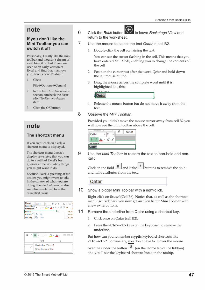
�������/�%�" �� ��#�!!��
�
����������� �������������� 03
7� (!� #���Back )������ ����! 0�Backstage View� �����������������#��'��
8� 9�������������! ��������Qatar���� !!�"�'�1.� Double�click�the�cell�containing�the�text.��
You�can�see�the�cursor�flashing�in�the�cell.�This�means�that�you�have�entered�Edit�Mode,�enabling�you�to�change�the�contents�of�the�cell�
2.� Position�the�cursor�just�after�the�word�Qatar�and�hold�down�the�left�mouse�button.�
3.� Drag�the�mouse�across�the�complete�word�until�it�is�highlighted�like�this:�
�4.� Release�the�mouse�button�but�do�not�move�it�away�from�the�
text.�
E� /)��0���Mini Toolbar'�Provided�you�didn’t�move�the�mouse�cursor�away�from�cell�B2�you�will�now�see�the�mini�toolbar�above�the�cell:�
��� 9����Mini Toolbar����������������������.)�!�� ������.
�� !� '�
Click�on�the�Bold� �and�Italic� �buttons�to�remove�the�bold�and�italic�attributes�from�the�text.�
���� ���� �)�,,����������!) ������ ���,�. !� #'��
Right�click�on�Brunei�(Cell�B6).�Notice�that,�as�well�as�the�shortcut�menu�(see�sidebar),�you�now�get�an�even�better�Mini�Toolbar�with�a�few�extra�buttons.�
��� :��0�������!���*����G � ������,� ����� ���#�'�
1.� Click�once�on�Qatar�(cell�B2).��
2.� Press�the�<Ctrl>+<U>�keys�on�the�keyboard�to�remove�the�underline.��
But�how�can�you�remember�cryptic�keyboard�shortcuts�like�<Ctrl>+<U>?��Fortunately,�you�don’t�have�to.�Hover�the�mouse�
over�the�underline�button� �(on�the�Home�tab�of�the�Ribbon)�and�you’ll�see�the�keyboard�shortcut�listed�in�the�tooltip.��
����������������#���If�you�right�click�on�a�cell,�a�shortcut�menu�is�displayed.�
The�shortcut�menu�doesn’t�display�everything�that�you�can�do�to�a�cell�but�Excel’s�best�guesses�at�the�most�likely�things�you�might�want�to�do.�
Because�Excel�is�guessing�at�the�actions�you�might�want�to�take�in�the�context�of�what�you�are�doing,�the�shortcut�menu�is�also�sometimes�referred�to�as�the�contextual�menu.�
����/������ ��8���� �������������!�������������������������Personally,�I�really�like�the�mini�toolbar�and�wouldn’t�dream�of�switching�it�off�but�if�you�are�used�to�an�early�version�of�Excel�and�find�that�it�annoys�you,�here�is�how�it’s�done:�
1.� Click:��
File�Options�General�
2.� In�the�User�Interface�options�section,�uncheck�the�Show�Mini�Toolbar�on�selection�item.�
3.� Click�the�OK�button.�
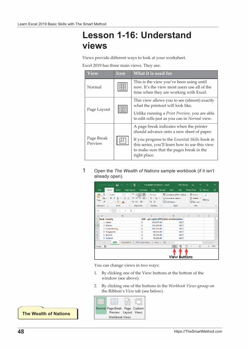
� ����� !������" �� ��#�!!���������� ��������
�
0=� ��$�%&&��� ������' ��
%�������62�5� ����� ������Views�provide�different�ways�to�look�at�your�worksheet.�
Excel�2019�has�three�main�views.�They�are:�
View� Icon What�it�is�used�for
Normal��
This�is�the�view�you’ve�been�using�until�now.�It’s�the�view�most�users�use�all�of�the�time�when�they�are�working�with�Excel.�
Page�Layout��
This�view�allows�you�to�see�(almost)�exactly�what�the�printout�will�look�like.�
Unlike�running�a�Print�Preview,�you�are�able�to�edit�cells�just�as�you�can�in�Normal�view.�
Page�Break�Preview� �
A�page�break�indicates�when�the�printer�should�advance�onto�a�new�sheet�of�paper.�
If�you�progress�to�the�Essential�Skills�book�in�this�series,�you’ll�learn�how�to�use�this�view�to�make�sure�that�the�pages�break�in�the�right�place.�
�
�� /$����The Wealth of Nations�� �$!����#)��#�1�*���������� !� ����$�2'�
�You�can�change�views�in�two�ways:�
1.� By�clicking�one�of�the�View�buttons�at�the�bottom�of�the�window�(see�above).�
2.� By�clicking�one�of�the�buttons�in�the�Workbook�Views�group�on�the�Ribbon’s�View�tab�(see�below).�
����$��������C�������
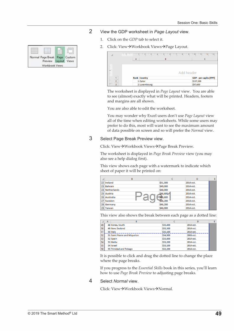
�������/�%�" �� ��#�!!��
�
����������� �������������� 0�
�� C�����<+D����#������Page Layout 0��'�
1.� Click�on�the�GDP�tab�to�select�it.�
2.� Click:�View�Workbook�Views�Page�Layout.�
�The�worksheet�is�displayed�in�Page�Layout�view.��You�are�able�to�see�(almost)�exactly�what�will�be�printed.�Headers,�footers�and�margins�are�all�shown.�
You�are�also�able�to�edit�the�worksheet.�
You�may�wonder�why�Excel�users�don’t�use�Page�Layout�view�all�of�the�time�when�editing�worksheets.�While�some�users�may�prefer�to�do�this,�most�will�want�to�see�the�maximum�amount�of�data�possible�on�screen�and�so�will�prefer�the�Normal�view.�
-� �! ��D ,�"� #�D�0���0��'�
Click:�View�Workbook�Views�Page�Break�Preview.�
The�worksheet�is�displayed�in�Page�Break�Preview�view�(you�may�also�see�a�help�dialog�first).��
This�view�shows�each�page�with�a�watermark�to�indicate�which�sheet�of�paper�it�will�be�printed�on:�
�This�view�also�shows�the�break�between�each�page�as�a�dotted�line:�
�It�is�possible�to�click�and�drag�the�dotted�line�to�change�the�place�where�the�page�breaks.��
If�you�progress�to�the�Essential�Skills�book�in�this�series,�you’ll�learn�how�to�use�Page�Break�Preview�to�adjusting�page�breaks.�
3� �! ��Normal�0��'�
Click:�View�Workbook�Views�Normal.�
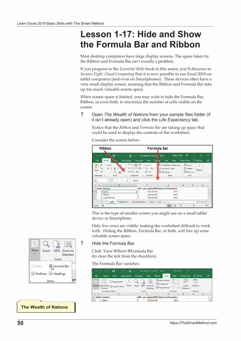
� ����� !������" �� ��#�!!���������� ��������
�
>�� ��$�%&&��� ������' ��
%�������32�)� ��� �+�������,��#���������� �<�!!���Most�desktop�computers�have�large�display�screens.�The�space�taken�by�the�Ribbon�and�Formula�Bar�isn’t�usually�a�problem.��
If�you�progress�to�the�Essential�Skills�book�in�this�series,�you’ll�discover�in:�Session�Eight:�Cloud�Computing�that�it�is�now�possible�to�run�Excel�2019�on�tablet�computers�(and�even�on�Smartphones).��These�devices�often�have�a�very�small�display�screen,�meaning�that�the�Ribbon�and�Formula�Bar�take�up�too�much�valuable�screen�space.�
When�screen�space�is�limited,�you�may�wish�to�hide�the�Formula�Bar,�Ribbon,�or�even�both,�to�maximize�the�number�of�cells�visible�on�the�screen.�
�� /$��The�Wealth of Nations�*���������� �$!�*�!��*�!���1�*���������� !� ����$�2� ��� !� #���Life Expectancy�� )'�Notice�that�the�Ribbon�and�Formula�Bar�are�taking�up�space�that�could�be�used�to�display�the�contents�of�the�worksheet.��
Consider�the�screen�below:�
�This�is�the�type�of�smaller�screen�you�might�see�on�a�small�tablet�device�or�Smartphone.���
Only�five�rows�are�visible,�making�the�worksheet�difficult�to�work�with.��Hiding�the�Ribbon,�Formula�Bar,�or�both,�will�free�up�some�valuable�screen�space.�
�� ������F����! �" �'�Click:�View�Show�Formula�Bar��(to�clear�the�tick�from�the�checkbox).�
The�Formula�Bar�vanishes:�
�
���$��������C�������
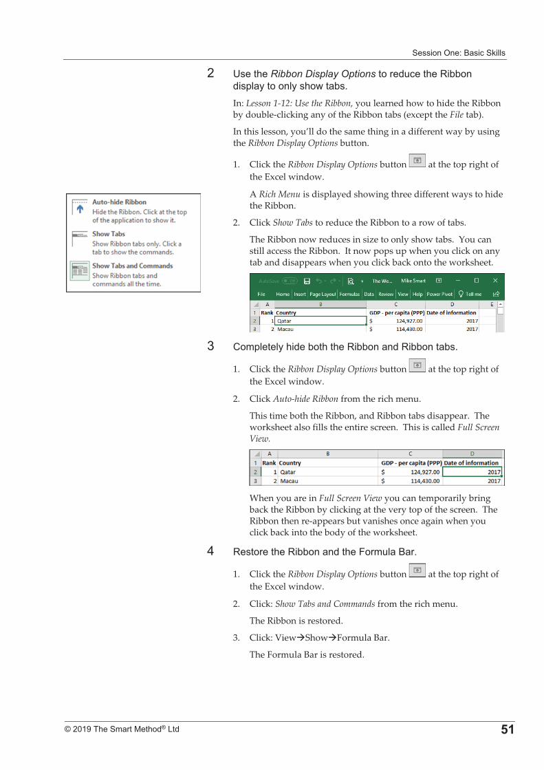
�������/�%�" �� ��#�!!��
�
����������� �������������� >�
�� 9����Ribbon Display Options������� ���:�))������$! �������!������� )�'�In:�Lesson�1�12:�Use�the�Ribbon,�you�learned�how�to�hide�the�Ribbon�by�double�clicking�any�of�the�Ribbon�tabs�(except�the�File�tab).�
In�this�lesson,�you’ll�do�the�same�thing�in�a�different�way�by�using�the�Ribbon�Display�Options�button.�
1.� Click�the�Ribbon�Display�Options�button� �at�the�top�right�of�the�Excel�window.�
A�Rich�Menu�is�displayed�showing�three�different�ways�to�hide�the�Ribbon.�
2.� Click�Show�Tabs�to�reduce�the�Ribbon�to�a�row�of�tabs.�
The�Ribbon�now�reduces�in�size�to�only�show�tabs.��You�can�still�access�the�Ribbon.��It�now�pops�up�when�you�click�on�any�tab�and�disappears�when�you�click�back�onto�the�worksheet.�
�
-� (��$!�!�����)�����:�))��� ���:�))���� )�'�
1.� Click�the�Ribbon�Display�Options�button� �at�the�top�right�of�the�Excel�window.�
2.� Click�Auto�hide�Ribbon�from�the�rich�menu.�
This�time�both�the�Ribbon,�and�Ribbon�tabs�disappear.��The�worksheet�also�fills�the�entire�screen.��This�is�called�Full�Screen�View.�
�When�you�are�in�Full�Screen�View�you�can�temporarily�bring�back�the�Ribbon�by�clicking�at�the�very�top�of�the�screen.��The�Ribbon�then�re�appears�but�vanishes�once�again�when�you�click�back�into�the�body�of�the�worksheet.�
3� :�������:�))��� �����F����! �" �'�
1.� Click�the�Ribbon�Display�Options�button� �at�the�top�right�of�the�Excel�window.�
2.� Click:�Show�Tabs�and�Commands�from�the�rich�menu.�
The�Ribbon�is�restored.�
3.� Click:�View�Show�Formula�Bar.�
The�Formula�Bar�is�restored.�
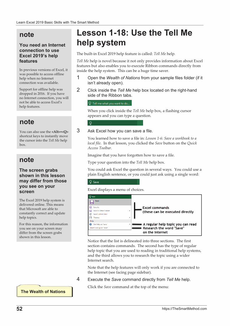
� ����� !������" �� ��#�!!���������� ��������
�
>�� ��$�%&&��� ������' ��
%�������=2�5�������������*�����#�The�built�in�Excel�2019�help�feature�is�called:�Tell�Me�help.�
Tell�Me�help�is�novel�because�it�not�only�provides�information�about�Excel�features�but�also�enables�you�to�execute�Ribbon�commands�directly�from�inside�the�help�system.��This�can�be�a�huge�time�saver.�
�� /$����Wealth of Nations�*���������� �$!�*�!��*�!���1�*���������� !� ����$�2'�
�� (!� #���������Tell Me !$�)���!� ����������,�. ��������*���:�))���� )�'��
�When�you�click�inside�the�Tell�Me�help�box,�a�flashing�cursor�appears�and�you�can�type�a�question.���
�-� ?�#��� !�������� ��� 0� �*�!'�
You�learned�how�to�save�a�file�in:�Lesson�1�6:�Save�a�workbook�to�a�local�file.��In�that�lesson,�you�clicked�the�Save�button�on�the�Quick�Access�Toolbar.�
Imagine�that�you�have�forgotten�how�to�save�a�file.��
Type�your�question�into�the�Tell�Me�help�box.��
You�could�ask�Excel�the�question�in�several�ways.��You�could�use�a�plain�English�sentence,�or�you�could�just�ask�using�a�single�word:�
�Excel�displays�a�menu�of�choices.���
�Notice�that�the�list�is�delineated�into�three�sections.��The�first�section�contains�commands.��The�second�has�the�type�of�regular�help�topic�that�you�are�used�to�reading�in�traditional�help�systems,�and�the�third�allows�you�to�research�the�topic�using�a�wider�Internet�search.�
Note�that�the�help�features�will�only�work�if�you�are�connected�to�the�Internet�(see�facing�page�sidebar).�
3� �� �����Save� ��� ������ �!��*����Tell Me !$'�Click�the�Save�command�at�the�top�of�the�menu:�
����You�can�also�use�the�<Alt>+<Q>�shortcut�keys�to�instantly�move�the�cursor�into�the�Tell�Me�help�box.��
���$��������C�������
����-���� ����/�������������������������������8����*��������In�previous�versions�of�Excel,�it�was�possible�to�access�offline�help�when�no�Internet�connection�was�available.�
Support�for�offline�help�was�dropped�in�2016.��If�you�have�no�Internet�connection,�you�will�not�be�able�to�access�Excel’s�help�features.��
���������������!����������������������#��� ��������#�������������������������The�Excel�2019�help�system�is�delivered�online.�This�means�that�Microsoft�are�able�to�constantly�correct�and�update�help�topics.�
For�this�reason,�the�information�you�see�on�your�screen�may�differ�from�the�screen�grabs�shown�in�this�lesson.�
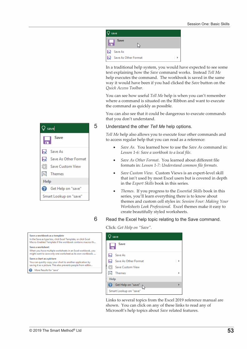
�������/�%�" �� ��#�!!��
�
����������� �������������� >;
�In�a�traditional�help�system,�you�would�have�expected�to�see�some�text�explaining�how�the�Save�command�works.��Instead�Tell�Me�help�executes�the�command.��The�workbook�is�saved�in�the�same�way�it�would�have�been�if�you�had�clicked�the�Save�button�on�the�Quick�Access�Toolbar.�
You�can�see�how�useful�Tell�Me�help�is�when�you�can’t�remember�where�a�command�is�situated�on�the�Ribbon�and�want�to�execute�the�command�as�quickly�as�possible.���
You�can�also�see�that�it�could�be�dangerous�to�execute�commands�that�you�don’t�understand.�
6� 9����� ���������Tell Me !$��$�����'�Tell�Me�help�also�allows�you�to�execute�four�other�commands�and�to�access�regular�help�that�you�can�read�as�a�reference:�
�� Save�As.��You�learned�how�to�use�the�Save�As�command�in:�Lesson�1�6:�Save�a�workbook�to�a�local�file.�
�� Save�As�Other�Format.��You�learned�about�different�file�formats�in:�Lesson�1�7:�Understand�common�file�formats.�
�� Save�Custom�View.��Custom�Views�is�an�expert�level�skill�that�isn’t�used�by�most�Excel�users�but�is�covered�in�depth�in�the�Expert�Skills�book�in�this�series.�
�� Themes.��If�you�progress�to�the�Essential�Skills�book�in�this�series,�you’ll�learn�everything�there�is�to�know�about�themes�and�custom�cell�styles�in:�Session�Four:�Making�Your�Worksheets�Look�Professional.��Excel�themes�make�it�easy�to�create�beautifully�styled�worksheets.�
7� : ������ !�!$���$� ��! ���,������� 0� ��� ��'�
Click:�Get�Help�on�“Save”.��
��Links�to�several�topics�from�the�Excel�2019�reference�manual�are�shown.��You�can�click�on�any�of�these�links�to�read�any�of�Microsoft’s�help�topics�about�Save�related�features.�
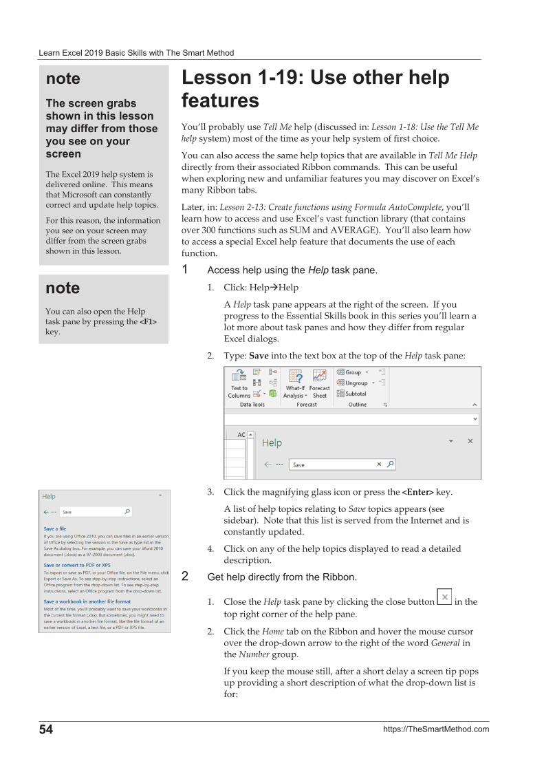
� ����� !������" �� ��#�!!���������� ��������
�
>0� ��$�%&&��� ������' ��
%��������2�5���������*��������You’ll�probably�use�Tell�Me�help�(discussed�in:�Lesson�1�18:�Use�the�Tell�Me�help�system)�most�of�the�time�as�your�help�system�of�first�choice.�
You�can�also�access�the�same�help�topics�that�are�available�in�Tell�Me�Help�directly�from�their�associated�Ribbon�commands.��This�can�be�useful�when�exploring�new�and�unfamiliar�features�you�may�discover�on�Excel’s�many�Ribbon�tabs.��
Later,�in:�Lesson�2�13:�Create�functions�using�Formula�AutoComplete,�you’ll�learn�how�to�access�and�use�Excel’s�vast�function�library�(that�contains�over�300�functions�such�as�SUM�and�AVERAGE).��You’ll�also�learn�how�to�access�a�special�Excel�help�feature�that�documents�the�use�of�each�function.�
�� ? ���!$�����,���Help � �#�$ �'�1.� Click:�Help�Help��
A�Help�task�pane�appears�at�the�right�of�the�screen.��If�you�progress�to�the�Essential�Skills�book�in�this�series�you’ll�learn�a�lot�more�about�task�panes�and�how�they�differ�from�regular�Excel�dialogs.�
2.� Type:�Save�into�the�text�box�at�the�top�of�the�Help�task�pane:�
�3.� Click�the�magnifying�glass�icon�or�press�the�<Enter>�key.�
A�list�of�help�topics�relating�to�Save�topics�appears�(see�sidebar).��Note�that�this�list�is�served�from�the�Internet�and�is�constantly�updated.�
4.� Click�on�any�of�the�help�topics�displayed�to�read�a�detailed�description.�
�� <��!$���� �!��*������:�))��'�
1.� Close�the�Help�task�pane�by�clicking�the�close�button� �in�the�top�right�corner�of�the�help�pane.�
2.� Click�the�Home�tab�on�the�Ribbon�and�hover�the�mouse�cursor�over�the�drop�down�arrow�to�the�right�of�the�word�General�in�the�Number�group.��
If�you�keep�the�mouse�still,�after�a�short�delay�a�screen�tip�pops�up�providing�a�short�description�of�what�the�drop�down�list�is�for:�
���������������!����������������������#��� ��������#�������������������������The�Excel�2019�help�system�is�delivered�online.��This�means�that�Microsoft�can�constantly�correct�and�update�help�topics.�
For�this�reason,�the�information�you�see�on�your�screen�may�differ�from�the�screen�grabs�shown�in�this�lesson.�
����You�can�also�open�the�Help�task�pane�by�pressing�the�<F1>�key.�
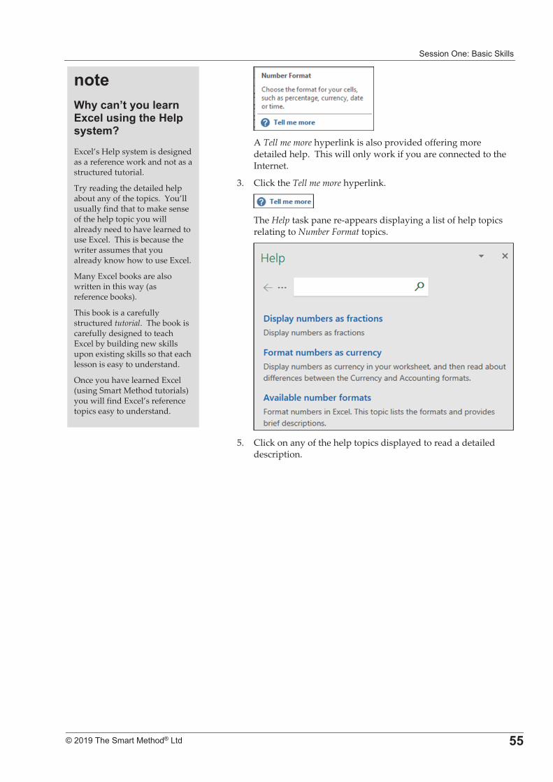
�������/�%�" �� ��#�!!��
�
����������� �������������� >>
�A�Tell�me�more�hyperlink�is�also�provided�offering�more�detailed�help.��This�will�only�work�if�you�are�connected�to�the�Internet.�
3.� Click�the�Tell�me�more�hyperlink.�
�The�Help�task�pane�re�appears�displaying�a�list�of�help�topics�relating�to�Number�Format�topics.�
�5.� Click�on�any�of�the�help�topics�displayed�to�read�a�detailed�
description.�
�
�
�
�
�
����$������8�������������������������)�*�����#E�Excel’s�Help�system�is�designed�as�a�reference�work�and�not�as�a�structured�tutorial.�
Try�reading�the�detailed�help�about�any�of�the�topics.��You’ll�usually�find�that�to�make�sense�of�the�help�topic�you�will�already�need�to�have�learned�to�use�Excel.��This�is�because�the�writer�assumes�that�you�already�know�how�to�use�Excel.�
Many�Excel�books�are�also�written�in�this�way�(as�reference�books).�
This�book�is�a�carefully�structured�tutorial.��The�book�is�carefully�designed�to�teach�Excel�by�building�new�skills�upon�existing�skills�so�that�each�lesson�is�easy�to�understand.��
Once�you�have�learned�Excel�(using�Smart�Method�tutorials)�you�will�find�Excel’s�reference�topics�easy�to�understand.�

�
�
�������������� ������������ � >6
�
�
�
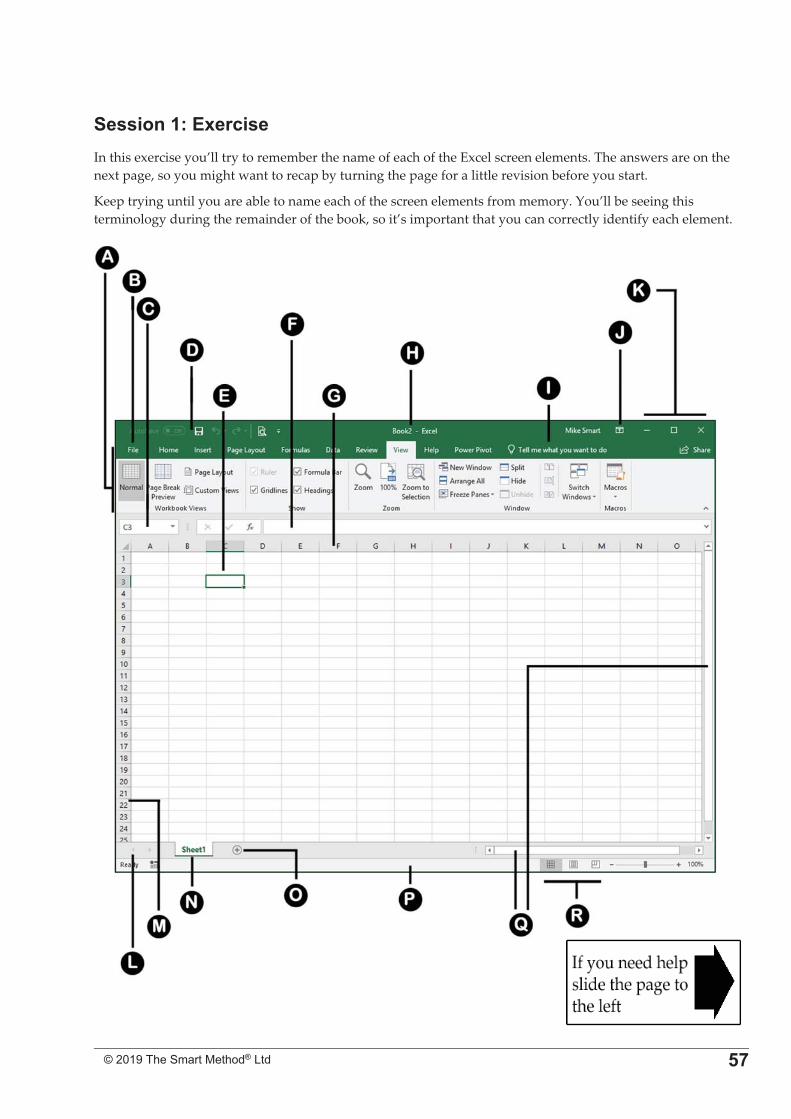
�
�
�������������� �������������� � >3
+�������2���������In�this�exercise�you’ll�try�to�remember�the�name�of�each�of�the�Excel�screen�elements.�The�answers�are�on�the�next�page,�so�you�might�want�to�recap�by�turning�the�page�for�a�little�revision�before�you�start.�
Keep�trying�until�you�are�able�to�name�each�of�the�screen�elements�from�memory.�You’ll�be�seeing�this�terminology�during�the�remainder�of�the�book,�so�it’s�important�that�you�can�correctly�identify�each�element.��
��

�
�
�������������� ������������ � >=
�
�
�
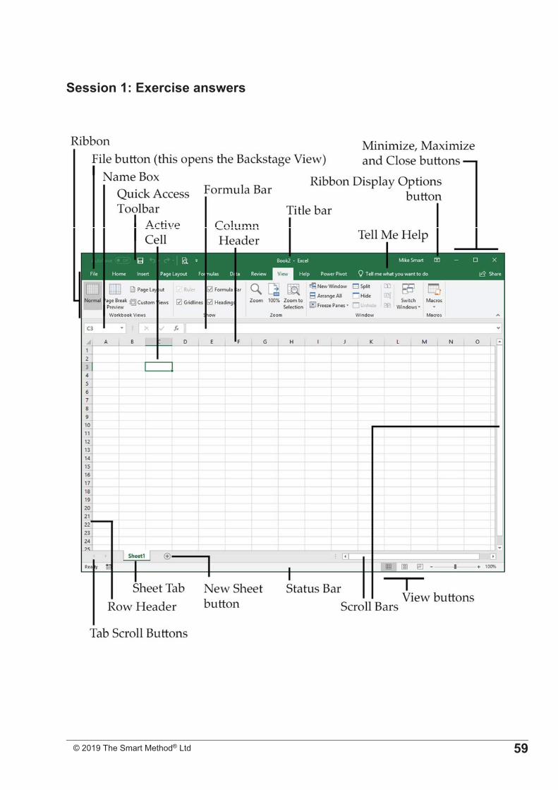
�
�
�������������� �������������� � >�
+�������2�����������������
��

�
�
�������������� ������������ � 6�
�
�
�
�
�������������� �������������� � 6�
+���������2�4�����5�����$�� �����������
�Now�that�you’ve�mastered�the�basics,�you�are�ready�to�do�really�useful�work�with�this�amazing�tool.�In�this�session,�you�will�learn�to�use�all�of�Excel’s�basic�features�properly.�This�will�put�you�far�ahead�of�anybody�that�hasn’t�been�formally�trained�in�Excel�best�practice.�You’ll�be�doing�simple�things,�but�you’ll�be�doing�them�perfectly!�
Even�after�years�of�daily�use,�many�users�are�unable�to�properly�use�Excel’s�fundamental�features.�They�often�reach�their�goal,�but�get�there�in�a�very�inefficient�way,�simply�because�they�were�never�taught�how�to�do�things�correctly.�By�the�end�of�this�session�you’ll�be�astonished�with�how�well�you�are�working�with�Excel.�
+������1!&������By�the�end�of�this�session�you�will�be�able�to:�
� Enter�text�and�numbers�into�a�worksheet�
� Create�a�new�workbook�and�view�two�workbooks�at�the�same�time�
� Use�AutoSum�to�quickly�calculate�totals�
� Select�a�range�of�cells�and�understand�Smart�Tags�
� Enter�data�into�a�range�and�copy�data�across�a�range�
� Select�adjacent�and�non�adjacent�rows�and�columns�
� Select�non�contiguous�cell�ranges�and�view�summary�information�
� AutoSelect�a�range�of�cells�
� Re�size�rows�and�columns�
� Use�AutoSum�to�sum�a�non�contiguous�range�
� Use�AutoSum�to�calculate�average�and�maximum�values�
� Create�your�own�formulas�
� Create�functions�using�Formula�AutoComplete�
� Use�AutoFill�for�text�and�numeric�series�
� Use�AutoFill�to�adjust�formulas�and�use�AutoFill�options�
� Speed�up�your�AutoFills�and�create�a�custom�fill�series�
� Understand�linear�and�exponential�series�
� Use�Flash�Fill�to�split�and�concatenate�text�
� Use�the�zoom�control�
� Print�out�a�worksheet�
Only�those�who�have�the�patience�to�do�simple�things�perfectly�ever�acquire�the�skill�to�do�difficult�things�easily.��
Unknown�author
��
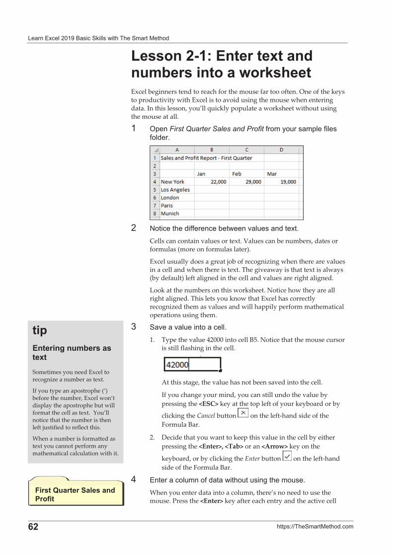
� ����� !������" �� ��#�!!���������� ��������
�
6�� ��$�%&&��� ������' ��
%�������2������������ ���#!������������� ����Excel�beginners�tend�to�reach�for�the�mouse�far�too�often.�One�of�the�keys�to�productivity�with�Excel�is�to�avoid�using�the�mouse�when�entering�data.�In�this�lesson,�you’ll�quickly�populate�a�worksheet�without�using�the�mouse�at�all.��
�� /$��First Quarter Sales and Profit *���������� �$!�*�!��*�!��'�
��� >��� �����**�� �)����0 !��� ������'�
Cells�can�contain�values�or�text.�Values�can�be�numbers,�dates�or�formulas�(more�on�formulas�later).��
Excel�usually�does�a�great�job�of�recognizing�when�there�are�values�in�a�cell�and�when�there�is�text.�The�giveaway�is�that�text�is�always�(by�default)�left�aligned�in�the�cell�and�values�are�right�aligned.��
Look�at�the�numbers�on�this�worksheet.�Notice�how�they�are�all�right�aligned.�This�lets�you�know�that�Excel�has�correctly�recognized�them�as�values�and�will�happily�perform�mathematical�operations�using�them.�
-� � 0� �0 !������� � !!'�1.� Type�the�value�42000�into�cell�B5.�Notice�that�the�mouse�cursor�
is�still�flashing�in�the�cell.�
�At�this�stage,�the�value�has�not�been�saved�into�the�cell.��
If�you�change�your�mind,�you�can�still�undo�the�value�by�pressing�the�<ESC>�key�at�the�top�left�of�your�keyboard�or�by�
clicking�the�Cancel�button� �on�the�left�hand�side�of�the�Formula�Bar.�
2.� Decide�that�you�want�to�keep�this�value�in�the�cell�by�either�pressing�the�<Enter>,�<Tab>�or�an�<Arrow>�key�on�the�
keyboard,�or�by�clicking�the�Enter�button� �on�the�left�hand�side�of�the�Formula�Bar.�
3� ����� � �!�����*�� � ������������,�������'�When�you�enter�data�into�a�column,�there’s�no�need�to�use�the�mouse.�Press�the�<Enter>�key�after�each�entry�and�the�active�cell�
��*�����������#!����������Sometimes�you�need�Excel�to�recognize�a�number�as�text.��
If�you�type�an�apostrophe�(‘)�before�the�number,�Excel�won’t�display�the�apostrophe�but�will�format�the�cell�as�text.��You’ll�notice�that�the�number�is�then�left�justified�to�reflect�this.�
When�a�number�is�formatted�as�text�you�cannot�perform�any�mathematical�calculation�with�it.�
,�����H������+������ �7������
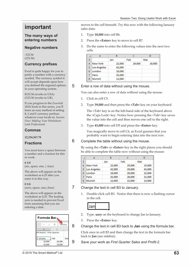
����������%�+���,�9�*�!����#������� !�
�
����������� �������������� 6;
moves�to�the�cell�beneath.�Try�this�now�with�the�following�January�sales�data:�
1.� Type�18,000�into�cell�B6.�
2.� Press�the�<Enter>�key�to�move�to�cell�B7.�
3.� Do�the�same�to�enter�the�following�values�into�the�next�two�cells.�
�6� ����� ������*�� � ������������,�������'�
You�can�also�enter�a�row�of�data�without�using�the�mouse.�
1.� Click�in�cell�C5.��
2.� Type�39,000�and�then�press�the�<Tab>�key�on�your�keyboard.�
The�<Tab>�key�is�on�the�left�hand�side�of�the�keyboard�above�the�<Caps�Lock>�key.�Notice�how�pressing�the�<Tab>�key�saves�the�value�into�the�cell�and�then�moves�one�cell�to�the�right.�
3.� Type�43,000�into�cell�D5�and�press�the�<Enter>�key.��
You�magically�move�to�cell�C6,�as�Excel�guesses�that�you�probably�want�to�begin�entering�data�into�the�next�row.�
7� (��$!����� )!������������,�������'�
By�using�the�<Tab>�or�<Enter>�key�in�the�right�places�you�should�be�able�to�complete�the�table�now�without�using�the�mouse:�
�8� ( �,���������� !!�"-����H �� ��'�
1.� Double�click�cell�B3.��Notice�that�there�is�now�a�flashing�cursor�in�the�cell.�
�2.� Type:�uary�on�the�keyboard�to�change�Jan�to�January.��
3.� Press�the�<Enter>�key.�
E� ( �,���������� !!�"-�) #����L�������,���*����! �) �'�Click�once�in�cell�B3�and�then�change�the�text�in�the�formula�bar�back�to�Jan�(see�sidebar).�
�� � 0���������#� ��First Quarter Sales and Profit-2.
�#*����������#���������������������#!���
C��������#!����123.56�(123.56)�
.�������*������Excel�is�quite�happy�for�you�to�prefix�a�number�with�a�currency�symbol.�The�currency�symbol�it�will�accept�depends�upon�how�you�defined�the�regional�options�in�your�operating�system.��
$123.56�(works�in�USA)�£123.56�(works�in�UK)�
If�you�progress�to�the�Essential�Skills�book�in�this�series,�you’ll�learn�an�easy�method�of�setting�$,�£�and�€�currency�prefixes�whatever�your�locale�in:�Session�Four:�Making�Your�Worksheets�Look�Professional.�
.�##���12,234,567.78�
,���������You�must�leave�a�space�between�a�number�and�a�fraction�for�this�to�work.�
6�1/4��(six,�space,�one,�/,�four)�
The�above�will�appear�on�the�worksheet�as�6.25�after�you�enter�it�in�this�way.�
0�1/4��(zero,�space,�one,/,four)�
The�above�will�appear�on�the�worksheet�as�0.25.�The�leading�zero�is�needed�to�prevent�Excel�from�assuming�that�you�are�entering�a�date.�
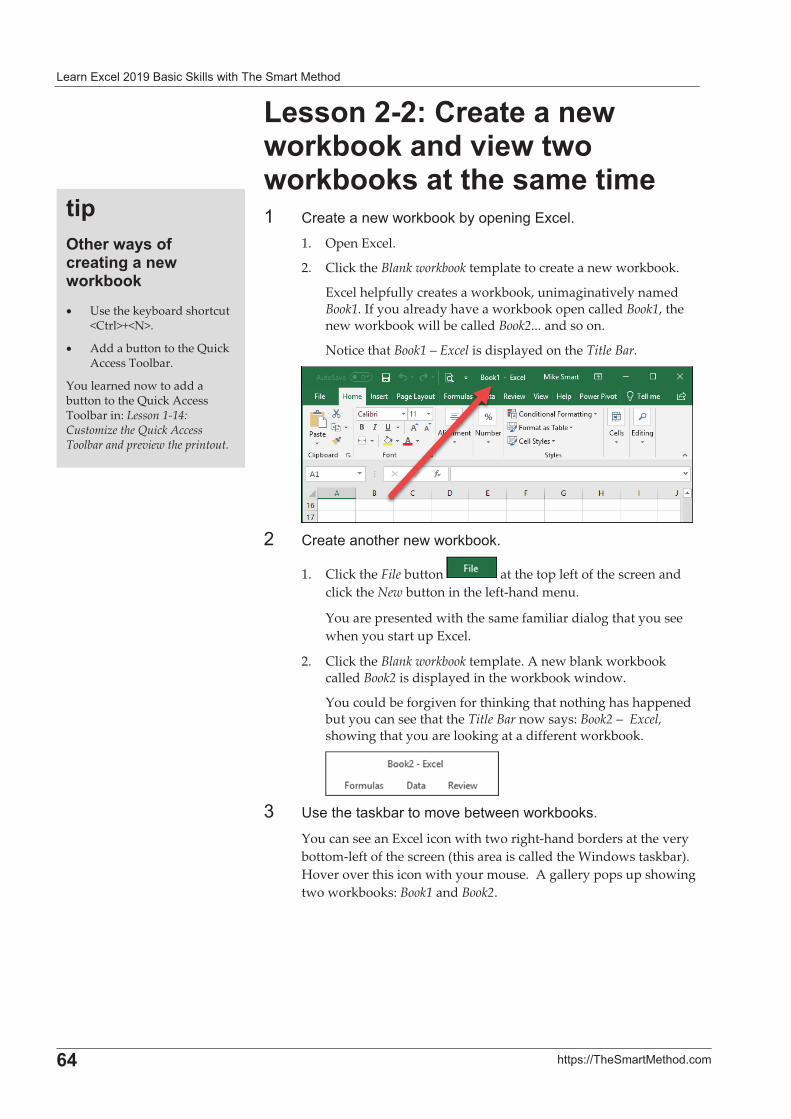
� ����� !������" �� ��#�!!���������� ��������
�
60� ��$�%&&��� ������' ��
%�������2�.������������ !�� ��� ������������ !�� ����������#���#��� (� �� �������#)��#�)���$���,��� !'�
1.� Open�Excel.�
2.� Click�the�Blank�workbook�template�to�create�a�new�workbook.�
Excel�helpfully�creates�a�workbook,�unimaginatively�named�Book1.�If�you�already�have�a�workbook�open�called�Book1,�the�new�workbook�will�be�called�Book2...�and�so�on.�
Notice�that�Book1�–�Excel�is�displayed�on�the�Title�Bar.�
��� (� �� �����������#)��#'��
1.� Click�the�File�button� �at�the�top�left�of�the�screen�and�click�the�New�button�in�the�left�hand�menu.�
You�are�presented�with�the�same�familiar�dialog�that�you�see�when�you�start�up�Excel.�
2.� Click�the�Blank�workbook�template.�A�new�blank�workbook�called�Book2�is�displayed�in�the�workbook�window.�
You�could�be�forgiven�for�thinking�that�nothing�has�happened�but�you�can�see�that�the�Title�Bar�now�says:�Book2�–��Excel,�showing�that�you�are�looking�at�a�different�workbook.�
�-� 9����� �#) �������0�)�������#)��#�'��
You�can�see�an�Excel�icon�with�two�right�hand�borders�at�the�very�bottom�left�of�the�screen�(this�area�is�called�the�Windows�taskbar).��Hover�over�this�icon�with�your�mouse.��A�gallery�pops�up�showing�two�workbooks:�Book1�and�Book2.�
��*�1���������������������������� !�� ��� Use�the�keyboard�shortcut�
<Ctrl>+<N>.�
�� Add�a�button�to�the�Quick�Access�Toolbar.�
You�learned�now�to�add�a�button�to�the�Quick�Access�Toolbar�in:�Lesson�1�14:�Customize�the�Quick�Access�Toolbar�and�preview�the�printout.�
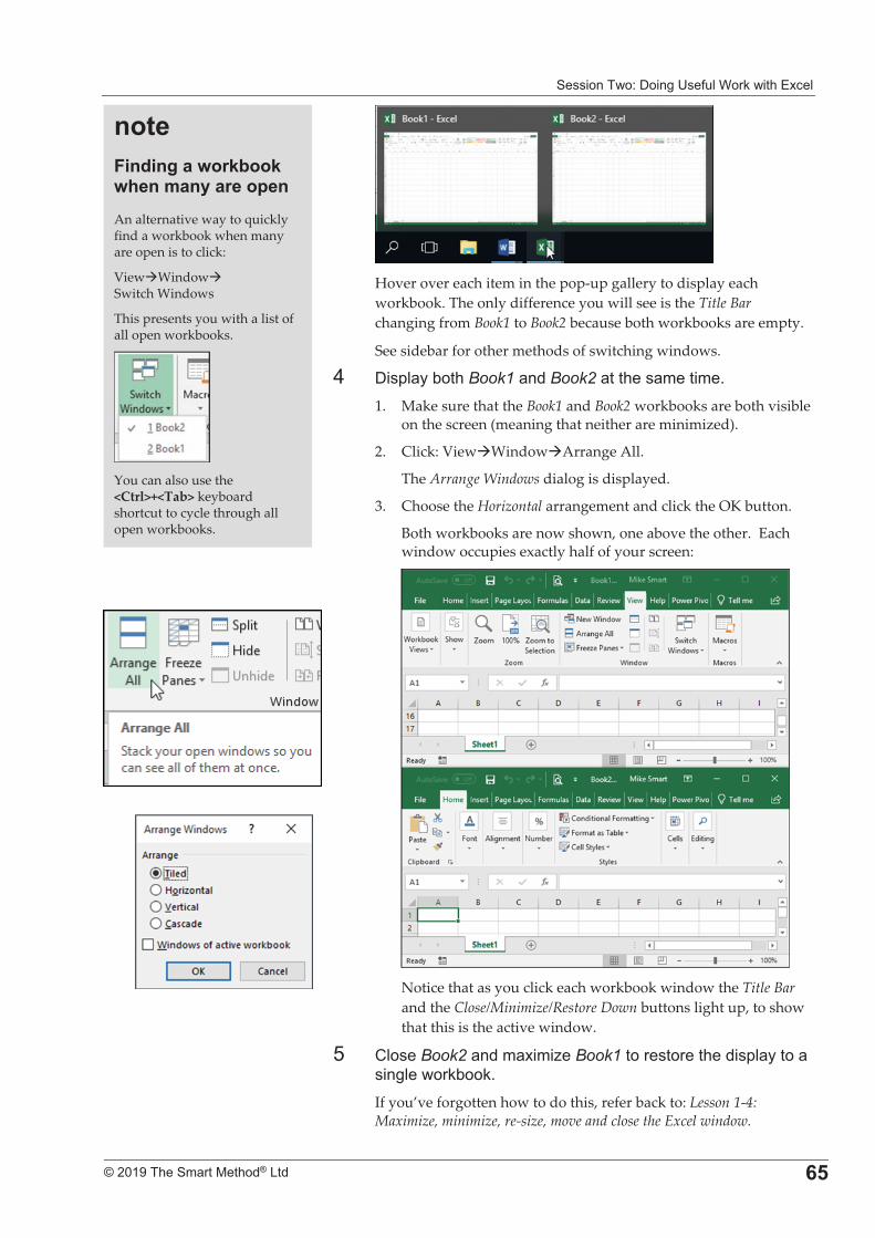
����������%�+���,�9�*�!����#������� !�
�
����������� �������������� 6>
�Hover�over�each�item�in�the�pop�up�gallery�to�display�each�workbook.�The�only�difference�you�will�see�is�the�Title�Bar�changing�from�Book1�to�Book2�because�both�workbooks�are�empty.�
See�sidebar�for�other�methods�of�switching�windows.�
3� +��$! ��)���Book1� ���Book2� ����� �����'�1.� Make�sure�that�the�Book1�and�Book2�workbooks�are�both�visible�
on�the�screen�(meaning�that�neither�are�minimized).�
2.� Click:�View�Window�Arrange�All.��
The�Arrange�Windows�dialog�is�displayed.�
3.� Choose�the�Horizontal�arrangement�and�click�the�OK�button.�
Both�workbooks�are�now�shown,�one�above�the�other.��Each�window�occupies�exactly�half�of�your�screen:�
�Notice�that�as�you�click�each�workbook�window�the�Title�Bar�and�the�Close/Minimize/Restore�Down�buttons�light�up,�to�show�that�this�is�the�active�window.�
6� (!���Book2� ���� ����;�Book1���������������$! ����� ����,!����#)��#'��If�you’ve�forgotten�how�to�do�this,�refer�back�to:�Lesson�1�4:�Maximize,�minimize,�re�size,�move�and�close�the�Excel�window.�
����,�� ��������� !�� �����#��������*��An�alternative�way�to�quickly�find�a�workbook�when�many�are�open�is�to�click:�
View�Window��Switch�Windows�
This�presents�you�with�a�list�of�all�open�workbooks.�
�You�can�also�use�the�<Ctrl>+<Tab>�keyboard�shortcut�to�cycle�through�all�open�workbooks.�
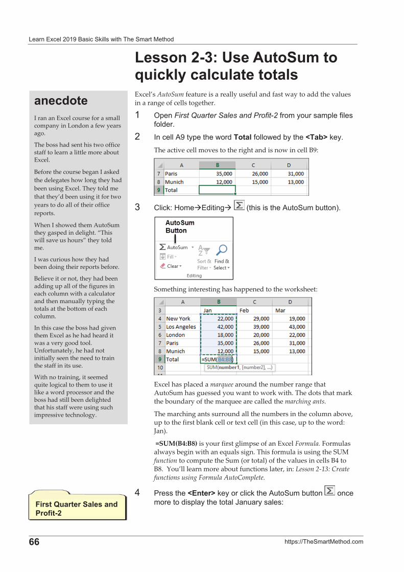
� ����� !������" �� ��#�!!���������� ��������
�
66� ��$�%&&��� ������' ��
%������;2�5��"���+�#����M��� �������������������Excel’s�AutoSum�feature�is�a�really�useful�and�fast�way�to�add�the�values�in�a�range�of�cells�together.��
�� /$��First Quarter Sales and Profit.2�*���������� �$!�*�!��*�!��'�
�� 4�� !!�?����$��������������*�!!����)����F��!G�#�'�The�active�cell�moves�to�the�right�and�is�now�in�cell�B9:�
��
-� (!� #%�����������,�� �1���������?�������)�����2'��
�Something�interesting�has�happened�to�the�worksheet:�
�Excel�has�placed�a�marquee�around�the�number�range�that�AutoSum�has�guessed�you�want�to�work�with.�The�dots�that�mark�the�boundary�of�the�marquee�are�called�the�marching�ants.�
The�marching�ants�surround�all�the�numbers�in�the�column�above,�up�to�the�first�blank�cell�or�text�cell�(in�this�case,�up�to�the�word:�Jan).�
�=SUM(B4:B8)�is�your�first�glimpse�of�an�Excel�Formula.�Formulas�always�begin�with�an�equals�sign.�This�formula�is�using�the�SUM�function�to�compute�the�Sum�(or�total)�of�the�values�in�cells�B4�to�B8.��You’ll�learn�more�about�functions�later,�in:�Lesson�2�13:�Create�functions�using�Formula�AutoComplete.��
3� D������F����G�#����� !� #���?�������)������ ��� �����������$! ������� !�H �� ���� !�%�
��� ���I�ran�an�Excel�course�for�a�small�company�in�London�a�few�years�ago.�
The�boss�had�sent�his�two�office�staff�to�learn�a�little�more�about�Excel.�
Before�the�course�began�I�asked�the�delegates�how�long�they�had�been�using�Excel.�They�told�me�that�they’d�been�using�it�for�two�years�to�do�all�of�their�office�reports.��
When�I�showed�them�AutoSum�they�gasped�in�delight.�“This�will�save�us�hours”�they�told�me.�
I�was�curious�how�they�had�been�doing�their�reports�before.�
Believe�it�or�not,�they�had�been�adding�up�all�of�the�figures�in�each�column�with�a�calculator�and�then�manually�typing�the�totals�at�the�bottom�of�each�column.�
In�this�case�the�boss�had�given�them�Excel�as�he�had�heard�it�was�a�very�good�tool.�Unfortunately,�he�had�not�initially�seen�the�need�to�train�the�staff�in�its�use.��
With�no�training,�it�seemed�quite�logical�to�them�to�use�it�like�a�word�processor�and�the�boss�had�still�been�delighted�that�his�staff�were�using�such�impressive�technology.��
,�����H������+������ �7�������
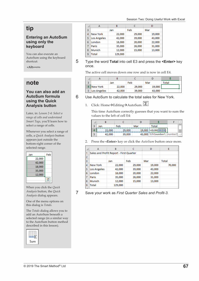
����������%�+���,�9�*�!����#������� !�
�
����������� �������������� 63
�6� ��$������������������� !!��-� ���$������F����G�#��
�� '��The�active�cell�moves�down�one�row�and�is�now�in�cell�E4.�
�7� 9��?���������� ! �! ������� !�� !��*���>��I��#'��
1.� Click:�Home�Editing�AutoSum.� �
This�time�AutoSum�correctly�guesses�that�you�want�to�sum�the�values�to�the�left�of�cell�E4:�
�2.� Press�the�<Enter>�key�or�click�the�AutoSum�button�once�more.�
�8� � 0���������#� ��First Quarter Sales and Profit-3.��
��*������������"���+�#��������������� �!��� �You�can�also�execute�an�AutoSum�using�the�keyboard�shortcut:�
�<Alt>+<=>�
����-������������� ����"���+�#����#�������������H��� �"��������!������
Later,�in:�Lesson�2�4:�Select�a�range�of�cells�and�understand�Smart�Tags,�you’ll�learn�how�to�select�a�range�of�cells.�
Whenever�you�select�a�range�of�cells,�a�Quick�Analysis�button�appears�just�outside�the�bottom�right�corner�of�the�selected�range.�
�
When�you�click�the�Quick�Analysis�button,�the�Quick�Analysis�dialog�appears.�
One�of�the�menu�options�on�this�dialog�is�Totals.�
The�Totals�dialog�allows�you�to�add�an�AutoSum�beneath�a�selected�range�(in�a�similar�way�to�the�AutoSum�button�method�described�in�this�lesson).�
�
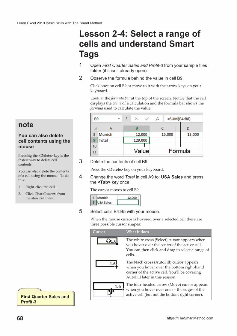
� ����� !������" �� ��#�!!���������� ��������
�
6=� ��$�%&&��� ������' ��
%������02�+��������������������� ��� ����� �+#����������� /$��First Quarter Sales and Profit-3�*���������� �$!�*�!��
*�!���1�*���������� !� ����$�2'�
�� /)��0���*����! �)������0 !����� !!�"�'�Click�once�on�cell�B9�or�move�to�it�with�the�arrow�keys�on�your�keyboard.�
Look�at�the�formula�bar�at�the�top�of�the�screen.�Notice�that�the�cell�displays�the�value�of�a�calculation�and�the�formula�bar�shows�the�formula�used�to�calculate�the�value:�
�-� +!���� ��������*� !!�"�'�
Press�the�<Delete>�key�on�your�keyboard.�
3� ( �,��������Total���� !!�?����%�5+"�+���� ���$������F��!G�#���� '�The�cursor�moves�to�cell�B9.�
�6� �! �� !!��"3%"6��������������'�
When�the�mouse�cursor�is�hovered�over�a�selected�cell�there�are�three�possible�cursor�shapes:�
Cursor What�it�does
�The�white�cross�(Select)�cursor�appears�when�you�hover�over�the�center�of�the�active�cell.�You�can�then�click�and�drag�to�select�a�range�of�cells.�
�The�black�cross�(AutoFill)�cursor�appears�when�you�hover�over�the�bottom�right�hand�corner�of�the�active�cell.�You’ll�be�covering�AutoFill�later�in�this�session.��
The�four�headed arrow�(Move)�cursor�appears�when�you�hover�over�one�of�the�edges�of�the�active�cell�(but�not�the�bottom�right�corner).��
�
����-������������ ������������������������#����Pressing�the�<Delete>�key�is�the�fastest�way�to�delete�cell�contents.�
You�can�also�delete�the�contents�of�a�cell�using�the�mouse.��To�do�this:�
1.� Right�click�the�cell.��
2.� Click�Clear�Contents�from�the�shortcut�menu.�
,�����H������+������ �7�����;�
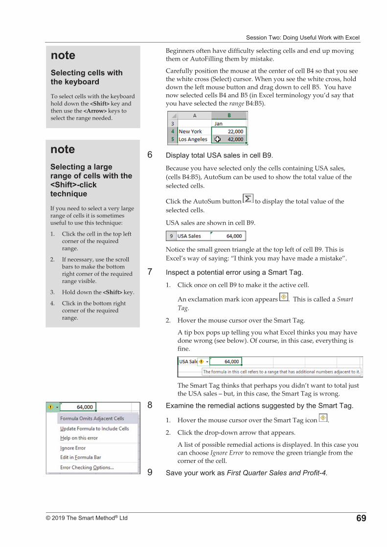
����������%�+���,�9�*�!����#������� !�
�
����������� �������������� 6�
Beginners�often�have�difficulty�selecting�cells�and�end�up�moving�them�or�AutoFilling�them�by�mistake.�
Carefully�position�the�mouse�at�the�center�of�cell�B4�so�that�you�see�the�white�cross�(Select)�cursor.�When�you�see�the�white�cross,�hold�down�the�left�mouse�button�and�drag�down�to�cell�B5.��You�have�now�selected�cells�B4�and�B5�(in�Excel�terminology�you’d�say�that�you�have�selected�the�range�B4:B5).�
� �
7� +��$! ����� !�9�?�� !����� !!�"�'�
Because�you�have�selected�only�the�cells�containing�USA�sales,�(cells�B4:B5),�AutoSum�can�be�used�to�show�the�total�value�of�the�selected�cells.�
Click�the�AutoSum�button� �to�display�the�total�value�of�the�selected�cells.�
USA�sales�are�shown�in�cell�B9.��
�Notice�the�small�green�triangle�at�the�top�left�of�cell�B9.�This�is�Excel’s�way�of�saying:�“I�think�you�may�have�made�a�mistake”.�
8� 4��$ �� �$����� !����������,� ��� ���� ,'�
1.� Click�once�on�cell�B9�to�make�it�the�active�cell.�
An�exclamation�mark�icon�appears� .��This�is�called�a�Smart�Tag.�
2.� Hover�the�mouse�cursor�over�the�Smart�Tag.�
A�tip�box�pops�up�telling�you�what�Excel�thinks�you�may�have�done�wrong�(see�below).�Of�course,�in�this�case,�everything�is�fine.��
�The�Smart�Tag�thinks�that�perhaps�you�didn’t�want�to�total�just�the�USA�sales�–�but,�in�this�case,�the�Smart�Tag�is�wrong.�
E� �� ���������� !� ��������,,����)������ ���� ,'�
1.� Hover�the�mouse�cursor�over�the�Smart�Tag�icon� .�
2.� Click�the�drop�down�arrow�that�appears.��
A�list�of�possible�remedial�actions�is�displayed.�In�this�case�you�can�choose�Ignore�Error�to�remove�the�green�triangle�from�the�corner�of�the�cell.�
�� � 0���������#� ��First Quarter Sales and Profit-4.�
����+�����������������������������������F+����G���� ������M��If�you�need�to�select�a�very�large�range�of�cells�it�is�sometimes�useful�to�use�this�technique:�
1.� Click�the�cell�in�the�top�left�corner�of�the�required�range.�
2.� If�necessary,�use�the�scroll�bars�to�make�the�bottom�right�corner�of�the�required�range�visible.�
3.� Hold�down�the�<Shift>�key.�
4.� Click�in�the�bottom�right�corner�of�the�required�range.��
����+�������������������� �!��� �To�select�cells�with�the�keyboard�hold�down�the�<Shift>�key�and�then�use�the�<Arrow>�keys�to�select�the�range�needed.��
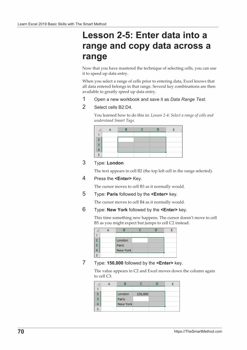
� ����� !������" �� ��#�!!���������� ��������
�
3�� ��$�%&&��� ������' ��
%������>2������ ������������������ ���*�� ������������������Now�that�you�have�mastered�the�technique�of�selecting�cells,�you�can�use�it�to�speed�up�data�entry.�
When�you�select�a�range�of�cells�prior�to�entering�data,�Excel�knows�that�all�data�entered�belongs�in�that�range.�Several�key�combinations�are�then�available�to�greatly�speed�up�data�entry.�
�� /$�� �������#)��#� ���� 0���� ��Data Range Test'�
�� �! �� !!��"�%+3'�You�learned�how�to�do�this�in:�Lesson�2�4:�Select�a�range�of�cells�and�understand�Smart�Tags.�
�-� ��$%�%�� ���
The�text�appears�in�cell�B2�(the�top�left�cell�in�the�range�selected).�
3� D������F����G�J�'�The�cursor�moves�to�cell�B3�as�it�normally�would.�
6� ��$%�7�����*�!!����)����F����G�#�'�The�cursor�moves�to�cell�B4�as�it�normally�would.�
7� ��$%�C��-�� �*�!!����)����F����G�#�'�This�time�something�new�happens.�The�cursor�doesn’t�move�to�cell�B5�as�you�might�expect�but�jumps�to�cell�C2�instead.�
�8� ��$%��>�:����*�!!����)����F����G�#�'�
The�value�appears�in�C2�and�Excel�moves�down�the�column�again�to�cell�C3.�
�
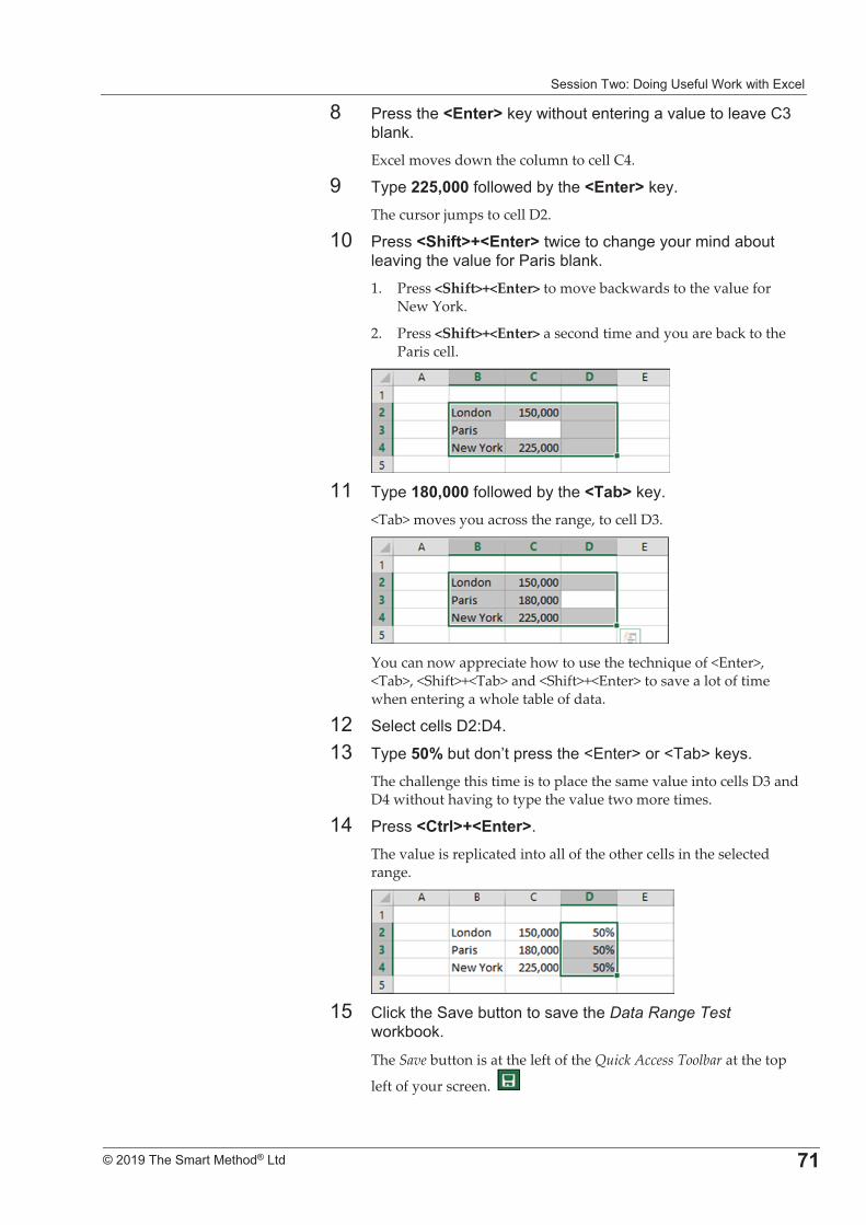
����������%�+���,�9�*�!����#������� !�
�
����������� �������������� 3�
E� D������F����G�#��������������,� �0 !�����! 0�(-�)! �#'�Excel�moves�down�the�column�to�cell�C4.�
�� ��$���>:����*�!!����)����F����G�#�'�The�cursor�jumps�to�cell�D2.�
��� D����F+����GNF����G���� ���� �,����������� )����! 0��,���0 !��*���D ����)! �#'�1.� Press�<Shift>+<Enter>�to�move�backwards�to�the�value�for�
New�York.��
2.� Press�<Shift>+<Enter>�a�second�time�and�you�are�back�to�the�Paris�cell.�
���� ��$��=�:����*�!!����)����F��!G�#�'�
<Tab>�moves�you�across�the�range,�to�cell�D3.�
�You�can�now�appreciate�how�to�use�the�technique�of�<Enter>,�<Tab>,�<Shift>+<Tab>�and�<Shift>+<Enter>�to�save�a�lot�of�time�when�entering�a�whole�table�of�data.�
��� �! �� !!��+�%+3'�
�-� ��$�>�O�)���������$������@����A����@� )A�#��'�The�challenge�this�time�is�to�place�the�same�value�into�cells�D3�and�D4�without�having�to�type�the�value�two�more�times.�
�3� D����F.���GNF����G'��The�value�is�replicated�into�all�of�the�other�cells�in�the�selected�range.�
��6� (!� #���� 0�)���������� 0���Data Range Test�
���#)��#'�
The�Save�button�is�at�the�left�of�the�Quick�Access�Toolbar�at�the�top�
left�of�your�screen.�� �
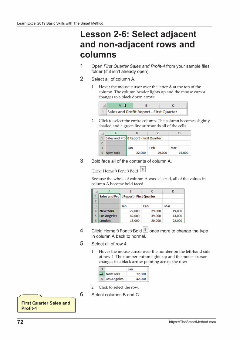
� ����� !������" �� ��#�!!���������� ��������
�
3�� ��$�%&&��� ������' ��
%������62�+����� &������� ����� &������������ �����#����� /$��First Quarter Sales and Profit-4�*���������� �$!�*�!��
*�!���1�*���������� !� ����$�2'�
�� �! �� !!��*� �!����?'�1.� Hover�the�mouse�cursor�over�the�letter�A�at�the�top�of�the�
column.�The�column�header�lights�up�and�the�mouse�cursor�changes�to�a�black�down�arrow:�
�2.� Click�to�select�the�entire�column.�The�column�becomes�slightly�
shaded�and�a�green�line�surrounds�all�of�the�cells.�
�-� "�!��* � !!��*��� ��������*� �!����?'�
Click:�Home�Font�Bold�� �
Because�the�whole�of�column�A�was�selected,�all�of�the�values�in�column�A�become�bold�faced.�
�
3� (!� #%�����F����"�!�� ��� �������� �,�����$���� �!����?�) #�������� !'�
6� �! �� !!��*�����3'�1.� Hover�the�mouse�cursor�over�the�number�on�the�left�hand�side�
of�row�4.�The�number�button�lights�up�and�the�mouse�cursor�changes�to�a�black�arrow�pointing�across�the�row:�
�2.� Click�to�select�the�row.�
7� �! �� �!�����"� ���('�
,�����H������+������ �7�����0�
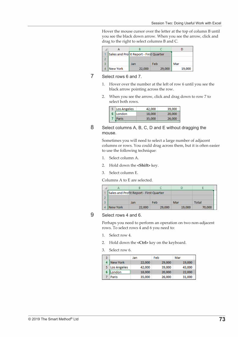
����������%�+���,�9�*�!����#������� !�
�
����������� �������������� 3;
Hover�the�mouse�cursor�over�the�letter�at�the�top�of�column�B�until�you�see�the�black�down�arrow.�When�you�see�the�arrow,�click�and�drag�to�the�right�to�select�columns�B�and�C.�
�8� �! �������7� ���8'�
1.� Hover�over�the�number�at�the�left�of�row�6�until�you�see�the�black�arrow�pointing�across�the�row.��
2.� When�you�see�the�arrow,�click�and�drag�down�to�row�7�to�select�both�rows.�
�E� �! �� �!�����?5�"5�(5�+� �������������� ,,��,���
����'�Sometimes�you�will�need�to�select�a�large�number�of�adjacent�columns�or�rows.�You�could�drag�across�them,�but�it�is�often�easier�to�use�the�following�technique:�
1.� Select�column�A.�
2.� Hold�down�the�<Shift>�key.�
3.� Select�column�E.�
Columns�A�to�E�are�selected.�
��� �! �������3� ���7'�
Perhaps�you�need�to�perform�an�operation�on�two�non�adjacent�rows.�To�select�rows�4�and�6�you�need�to:�
1.� Select�row�4.��
2.� Hold�down�the�<Ctrl>�key�on�the�keyboard.��
3.� Select�row�6.�
�
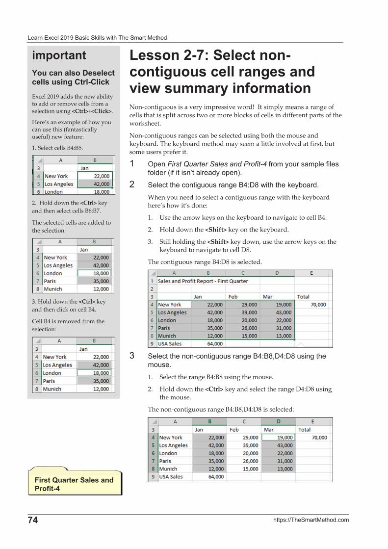
� ����� !������" �� ��#�!!���������� ��������
�
30� ��$�%&&��� ������' ��
%������32�+������������������������������ �������##���������#������Non�contiguous�is�a�very�impressive�word!��It�simply�means�a�range�of�cells�that�is�split�across�two�or�more�blocks�of�cells�in�different�parts�of�the�worksheet.�
Non�contiguous�ranges�can�be�selected�using�both�the�mouse�and�keyboard.�The�keyboard�method�may�seem�a�little�involved�at�first,�but�some�users�prefer�it.��
�� /$��First Quarter Sales and Profit-4�*���������� �$!�*�!��*�!���1�*���������� !� ����$�2'�
�� �! ���� ����,������ �,�"3%+E�������#�)� ��'�When�you�need�to�select�a�contiguous�range�with�the�keyboard�here’s�how�it’s�done:�
1.� Use�the�arrow�keys�on�the�keyboard�to�navigate�to�cell�B4.�
2.� Hold�down�the�<Shift>�key�on�the�keyboard.�
3.� Still�holding�the�<Shift>�key�down,�use�the�arrow�keys�on�the�keyboard�to�navigate�to�cell�D8.�
The�contiguous�range�B4:D8�is�selected.�
�-� �! �������. ����,������ �,�"3%"E5+3%+E�����,���
����'�1.� Select�the�range�B4:B8�using�the�mouse.�
2.� Hold�down�the�<Ctrl>�key�and�select�the�range�D4:D8�using�the�mouse.�
The�non�contiguous�range�B4:B8,D4:D8�is�selected:�
�,�����H������+������ �7�����0�
�#*�������-������������4����������������.���.��� ��Excel�2019�adds�the�new�ability�to�add�or�remove�cells�from�a�selection�using�<Ctrl>+<Click>.�
Here’s�an�example�of�how�you�can�use�this�(fantastically�useful)�new�feature:�
1.�Select�cells�B4:B5.�
2.��Hold�down�the�<Ctrl>�key�and�then�select�cells�B6:B7.���
The�selected�cells�are�added�to�the�selection:�
�
3.�Hold�down�the�<Ctrl>�key�and�then�click�on�cell�B4.���
Cell�B4�is�removed�from�the�selection:�
�
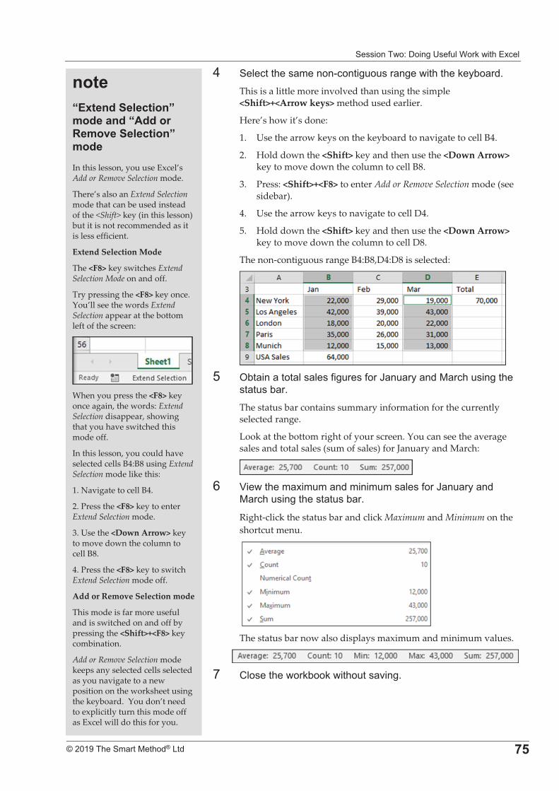
����������%�+���,�9�*�!����#������� !�
�
����������� �������������� 3>
3� �! ����� �����. ����,������ �,�������#�)� ��'�This�is�a�little�more�involved�than�using�the�simple��<Shift>+<Arrow�keys>�method�used�earlier.�
Here’s�how�it’s�done:�
1.� Use�the�arrow�keys�on�the�keyboard�to�navigate�to�cell�B4.�
2.� Hold�down�the�<Shift>�key�and�then�use�the�<Down�Arrow>�key�to�move�down�the�column�to�cell�B8.�
3.� Press:�<Shift>+<F8>�to�enter�Add�or�Remove�Selection�mode�(see�sidebar).�
4.� Use�the�arrow�keys�to�navigate�to�cell�D4.�
5.� Hold�down�the�<Shift>�key�and�then�use�the�<Down�Arrow>�key�to�move�down�the�column�to�cell�D8.�
The�non�contiguous�range�B4:B8,D4:D8�is�selected:�
�6� /)� ��� ���� !�� !��*�,����*���H �� ��� ���� � �����,���
�� ����) �'�The�status�bar�contains�summary�information�for�the�currently�selected�range.�
Look�at�the�bottom�right�of�your�screen.�You�can�see�the�average�sales�and�total�sales�(sum�of�sales)�for�January�and�March:�
�7� C������ ������ ������������ !��*���H �� ��� ���
� � �����,����� ����) �'�
Right�click�the�status�bar�and�click�Maximum�and�Minimum�on�the�shortcut�menu.�
� �The�status�bar�now�also�displays�maximum�and�minimum�values.�
�
8� (!��������#)��#��������� 0��,'��
����I���� �+������J�#� ��� �I" ����<#���+������J�#� �In�this�lesson,�you�use�Excel’s�Add�or�Remove�Selection�mode.��
There’s�also�an�Extend�Selection�mode�that�can�be�used�instead�of�the�<Shift>�key�(in�this�lesson)�but�it�is�not�recommended�as�it�is�less�efficient.���
Extend�Selection�Mode�
The�<F8>�key�switches�Extend�Selection�Mode�on�and�off.�
Try�pressing�the�<F8>�key�once.��You’ll�see�the�words�Extend�Selection�appear�at�the�bottom�left�of�the�screen:�
�When�you�press�the�<F8>�key�once�again,�the�words:�Extend�Selection�disappear,�showing�that�you�have�switched�this�mode�off.�
In�this�lesson,�you�could�have�selected�cells�B4:B8�using�Extend�Selection�mode�like�this:�
1.�Navigate�to�cell�B4.�
2.�Press�the�<F8>�key�to�enter�Extend�Selection�mode.�
3.�Use�the�<Down�Arrow>�key�to�move�down�the�column�to�cell�B8.�
4.�Press�the�<F8>�key�to�switch�Extend�Selection�mode�off.�
Add�or�Remove�Selection�mode�
This�mode�is�far�more�useful�and�is�switched�on�and�off�by�pressing�the�<Shift>+<F8>�key�combination.�
Add�or�Remove�Selection�mode�keeps�any�selected�cells�selected�as�you�navigate�to�a�new�position�on�the�worksheet�using�the�keyboard.��You�don’t�need�to�explicitly�turn�this�mode�off�as�Excel�will�do�this�for�you.�
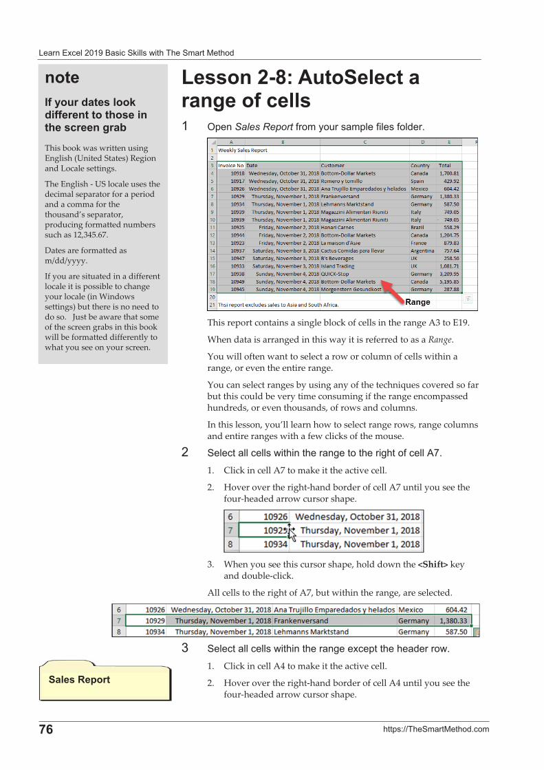
� ����� !������" �� ��#�!!���������� ��������
�
36� ��$�%&&��� ������' ��
%������=2�"���+��������������������� /$��Sales Report *���������� �$!�*�!��*�!��'�
�This�report�contains�a�single�block�of�cells�in�the�range�A3�to�E19.�
When�data�is�arranged�in�this�way�it�is�referred�to�as�a�Range.�
You�will�often�want�to�select�a�row�or�column�of�cells�within�a�range,�or�even�the�entire�range.�
You�can�select�ranges�by�using�any�of�the�techniques�covered�so�far�but�this�could�be�very�time�consuming�if�the�range�encompassed�hundreds,�or�even�thousands,�of�rows�and�columns.�
In�this�lesson,�you’ll�learn�how�to�select�range�rows,�range�columns�and�entire�ranges�with�a�few�clicks�of�the�mouse.�
�� �! �� !!� !!����������� �,��������,���*� !!�?8'�1.� Click�in�cell�A7�to�make�it�the�active�cell.�
2.� Hover�over�the�right�hand�border�of�cell�A7�until�you�see�the�four�headed�arrow�cursor�shape.�
�3.� When�you�see�this�cursor�shape,�hold�down�the�<Shift>�key�
and�double�click.�
All�cells�to�the�right�of�A7,�but�within�the�range,�are�selected.�
�-� �! �� !!� !!����������� �,�� $���� ������'�
1.� Click�in�cell�A4�to�make�it�the�active�cell.�
2.� Hover�over�the�right�hand�border�of�cell�A4�until�you�see�the�four�headed�arrow�cursor�shape.�
+����<*����
����/������� ������� � �����������������������������!�This�book�was�written�using�English�(United�States)�Region�and�Locale�settings.��
The�English���US�locale�uses�the�decimal�separator�for�a�period�and�a�comma�for�the�thousand’s�separator,�producing�formatted�numbers�such�as�12,345.67.���
Dates�are�formatted�as�m/dd/yyyy.���
If�you�are�situated�in�a�different�locale�it�is�possible�to�change�your�locale�(in�Windows�settings)�but�there�is�no�need�to�do�so.���Just�be�aware�that�some�of�the�screen�grabs�in�this�book�will�be�formatted�differently�to�what�you�see�on�your�screen.�
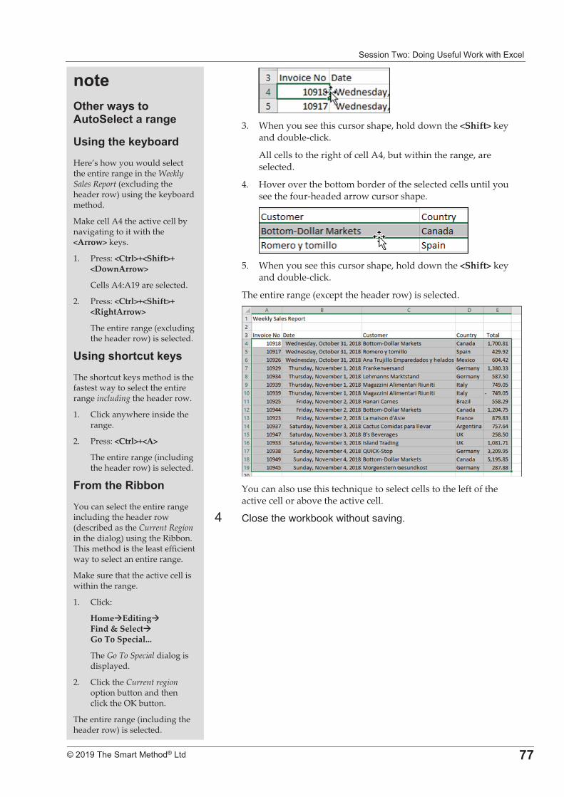
����������%�+���,�9�*�!����#������� !�
�
����������� �������������� 33
�3.� When�you�see�this�cursor�shape,�hold�down�the�<Shift>�key�
and�double�click.�
All�cells�to�the�right�of�cell�A4,�but�within�the�range,�are�selected.�
4.� Hover�over�the�bottom�border�of�the�selected�cells�until�you�see�the�four�headed�arrow�cursor�shape.�
�5.� When�you�see�this�cursor�shape,�hold�down�the�<Shift>�key�
and�double�click.�
The�entire�range�(except�the�header�row)�is�selected.�
�You�can�also�use�this�technique�to�select�cells�to�the�left�of�the�active�cell�or�above�the�active�cell.�
3� (!��������#)��#��������� 0��,'�
����1������������"���+�����������
5�������� �!��� �Here’s�how�you�would�select�the�entire�range�in�the�Weekly�Sales�Report�(excluding�the�header�row)�using�the�keyboard�method.�
Make�cell�A4�the�active�cell�by�navigating�to�it�with�the�<Arrow>�keys.�
1.� Press:�<Ctrl>+<Shift>+�<DownArrow>�
Cells�A4:A19�are�selected.�
2.� Press:�<Ctrl>+<Shift>+�<RightArrow>�
The�entire�range�(excluding�the�header�row)�is�selected.�
5�������������� ���The�shortcut�keys�method�is�the�fastest�way�to�select�the�entire�range�including�the�header�row.�
1.� Click�anywhere�inside�the�range.�
2.� Press:�<Ctrl>+<A>�
The�entire�range�(including�the�header�row)�is�selected.�
,��#����<�!!���You�can�select�the�entire�range�including�the�header�row�(described�as�the�Current�Region�in�the�dialog)�using�the�Ribbon.��This�method�is�the�least�efficient�way�to�select�an�entire�range.�
Make�sure�that�the�active�cell�is�within�the�range.�
1.� Click:��
Home�Editing��Find�&�Select��Go�To�Special...�
The�Go�To�Special�dialog�is�displayed.�
2.� Click�the�Current�region�option�button�and�then�click�the�OK�button.�
The�entire�range�(including�the�header�row)�is�selected.�
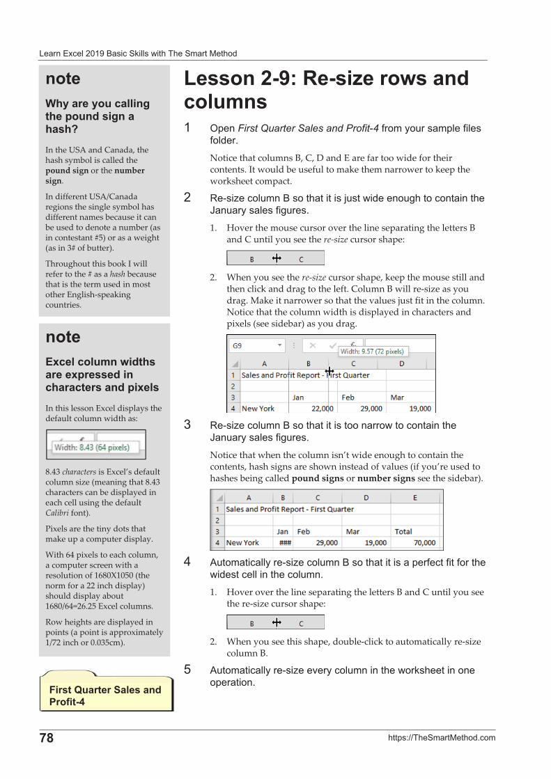
� ����� !������" �� ��#�!!���������� ��������
�
3=� ��$�%&&��� ������' ��
%�������2�<��A�������� �����#����� /$��First Quarter Sales and Profit.4�*���������� �$!�*�!��
*�!��'�Notice�that�columns�B,�C,�D�and�E�are�far�too�wide�for�their�contents.�It�would�be�useful�to�make�them�narrower�to�keep�the�worksheet�compact.�
�� :.��;� �!����"����� ��������K�����������,���� ��� �����H �� ���� !��*�,���'�1.� Hover�the�mouse�cursor�over�the�line�separating�the�letters�B�
and�C�until�you�see�the�re�size�cursor�shape:�
�2.� When�you�see�the�re�size�cursor�shape,�keep�the�mouse�still�and�
then�click�and�drag�to�the�left.�Column�B�will�re�size�as�you�drag.�Make�it�narrower�so�that�the�values�just�fit�in�the�column.�Notice�that�the�column�width�is�displayed�in�characters�and�pixels�(see�sidebar)�as�you�drag.��
�-� :.��;� �!����"����� ������������� �������� ��� �����
H �� ���� !��*�,���'�Notice�that�when�the�column�isn’t�wide�enough�to�contain�the�contents,�hash�signs�are�shown�instead�of�values�(if�you’re�used�to�hashes�being�called�pound�signs�or�number�signs�see�the�sidebar).�
�3� ?���� �� !!���.��;� �!����"����� �������� �$�* ��*���*�����
������ !!������ �!���'�1.� Hover�over�the�line�separating�the�letters�B�and�C�until�you�see�
the�re�size�cursor�shape:�
�2.� When�you�see�this�shape,�double�click�to�automatically�re�size�
column�B.�
6� ?���� �� !!���.��;�0��� �!������������#����������$� ����'�
����$���������������������*��� ������������E�In�the�USA�and�Canada,�the�hash�symbol�is�called�the�pound�sign�or�the�number�sign.�
In�different�USA/Canada�regions�the�single�symbol�has�different�names�because�it�can�be�used�to�denote�a�number�(as�in�contestant�#5)�or�as�a�weight�(as�in�3#�of�butter).��
Throughout�this�book�I�will�refer�to�the�#�as�a�hash�because�that�is�the�term�used�in�most�other�English�speaking�countries.�
,�����H������+������ �7�����0�
�������������#���� ��������*��� ���������������� �*�����In�this�lesson�Excel�displays�the�default�column�width�as:�
�8.43�characters�is�Excel’s�default�column�size�(meaning�that�8.43�characters�can�be�displayed�in�each�cell�using�the�default�Calibri�font).�
Pixels�are�the�tiny�dots�that�make�up�a�computer�display.���
With�64�pixels�to�each�column,�a�computer�screen�with�a�resolution�of�1680X1050�(the�norm�for�a�22�inch�display)�should�display�about�1680/64=26.25�Excel�columns.�
Row�heights�are�displayed�in�points�(a�point�is�approximately�1/72�inch�or�0.035cm).�
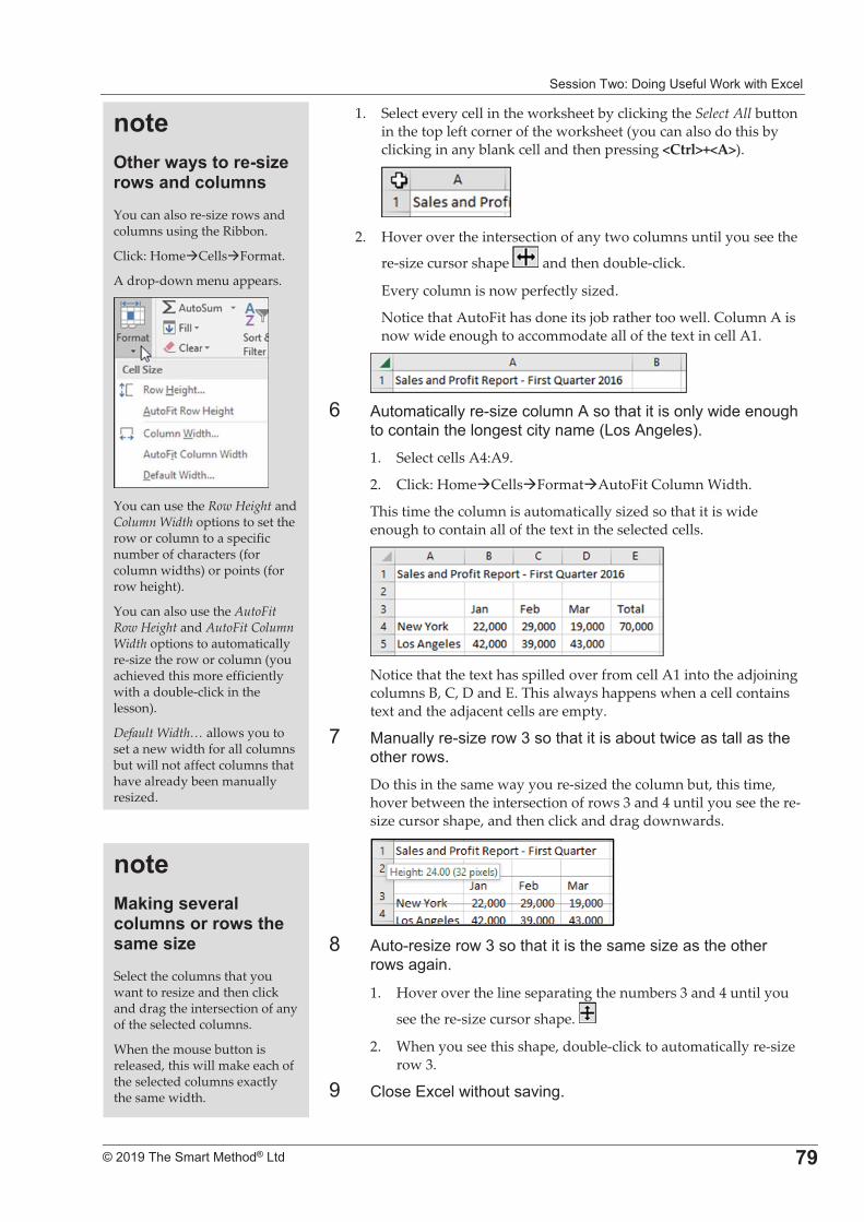
����������%�+���,�9�*�!����#������� !�
�
����������� �������������� 3�
1.� Select�every�cell�in�the�worksheet�by�clicking�the�Select�All�button�in�the�top�left�corner�of�the�worksheet�(you�can�also�do�this�by�clicking�in�any�blank�cell�and�then�pressing�<Ctrl>+<A>).�
�2.� Hover�over�the�intersection�of�any�two�columns�until�you�see�the�
re�size�cursor�shape� �and�then�double�click.�
Every�column�is�now�perfectly�sized.�
Notice�that�AutoFit�has�done�its�job�rather�too�well.�Column�A�is�now�wide�enough�to�accommodate�all�of�the�text�in�cell�A1.��
�7� ?���� �� !!���.��;� �!����?����� ����������!���������,�
��� ��� �����!��,��� ����� ��1����?�,!�2'�1.� Select�cells�A4:A9.�
2.� Click:�Home�Cells�Format�AutoFit�Column�Width.�
This�time�the�column�is�automatically�sized�so�that�it�is�wide�enough�to�contain�all�of�the�text�in�the�selected�cells.�
�Notice�that�the�text�has�spilled�over�from�cell�A1�into�the�adjoining�columns�B,�C,�D�and�E.�This�always�happens�when�a�cell�contains�text�and�the�adjacent�cells�are�empty.�
8� � �� !!���.��;�����-����� �������� )������� � ��� !!� ������������'�Do�this�in�the�same�way�you�re�sized�the�column�but,�this�time,�hover�between�the�intersection�of�rows�3�and�4�until�you�see�the�re�size�cursor�shape,�and�then�click�and�drag�downwards.�
�E� ?���.���;�����-����� ����������� ����;� ��������
����� , ��'�
1.� Hover�over�the�line�separating�the�numbers�3�and�4�until�you�
see�the�re�size�cursor�shape.� �
2.� When�you�see�this�shape,�double�click�to�automatically�re�size�row�3.�
�� (!����� !��������� 0��,'�
����1���������������A�������� �����#���You�can�also�re�size�rows�and�columns�using�the�Ribbon.�
Click:�Home�Cells�Format.�
A�drop�down�menu�appears.�
�You�can�use�the�Row�Height�and�Column�Width�options�to�set�the�row�or�column�to�a�specific�number�of�characters�(for�column�widths)�or�points�(for�row�height).�
You�can�also�use�the�AutoFit�Row�Height�and�AutoFit�Column�Width�options�to�automatically�re�size�the�row�or�column�(you�achieved�this�more�efficiently�with�a�double�click�in�the�lesson).�
Default�Width…�allows�you�to�set�a�new�width�for�all�columns�but�will�not�affect�columns�that�have�already�been�manually�resized.�
������ ��������������#����������������#���A�Select�the�columns�that�you�want�to�resize�and�then�click�and�drag�the�intersection�of�any�of�the�selected�columns.��
When�the�mouse�button�is�released,�this�will�make�each�of�the�selected�columns�exactly�the�same�width.�
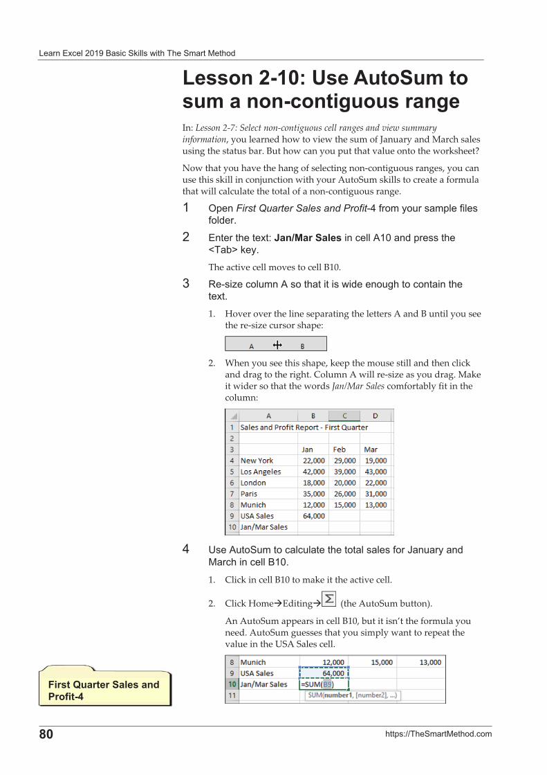
� ����� !������" �� ��#�!!���������� ��������
�
=�� ��$�%&&��� ������' ��
%��������2�5��"���+�#������#�����������������������In:�Lesson�2�7:�Select�non�contiguous�cell�ranges�and�view�summary�information,�you�learned�how�to�view�the�sum�of�January�and�March�sales�using�the�status�bar.�But�how�can�you�put�that�value�onto�the�worksheet?���
Now�that�you�have�the�hang�of�selecting�non�contiguous�ranges,�you�can�use�this�skill�in�conjunction�with�your�AutoSum�skills�to�create�a�formula�that�will�calculate�the�total�of�a�non�contiguous�range.�
�� /$��First Quarter Sales and Profit.3�*���������� �$!�*�!��*�!��'�
�� ����������%�L��B����+������� !!�?��� ���$������@� )A�#�'�The�active�cell�moves�to�cell�B10.�
-� :.��;� �!����?����� ���������������,���� ��� ��������'�1.� Hover�over�the�line�separating�the�letters�A�and�B�until�you�see�
the�re�size�cursor�shape:�
�2.� When�you�see�this�shape,�keep�the�mouse�still�and�then�click�
and�drag�to�the�right.�Column�A�will�re�size�as�you�drag.�Make�it�wider�so�that�the�words�Jan/Mar�Sales�comfortably�fit�in�the�column:�
�
3� 9��?���������� ! �! ������� !�� !��*���H �� ��� ���� � ���� !!�"��'�
1.� Click�in�cell�B10�to�make�it�the�active�cell.�
2.� Click�Home�Editing� ��(the�AutoSum�button).�
An�AutoSum�appears�in�cell�B10,�but�it�isn’t�the�formula�you�need.�AutoSum�guesses�that�you�simply�want�to�repeat�the�value�in�the�USA�Sales�cell.�
�
,�����H������+������ �7�����0�
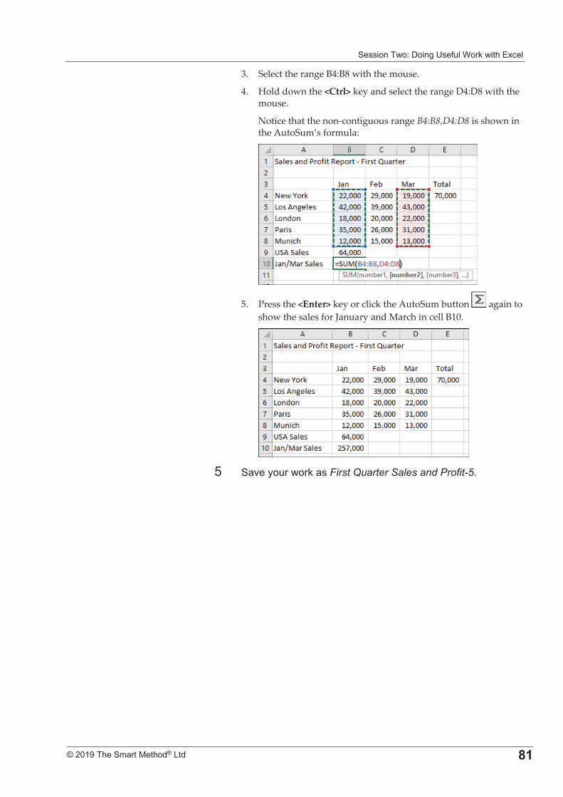
����������%�+���,�9�*�!����#������� !�
�
����������� �������������� =�
3.� Select�the�range�B4:B8�with�the�mouse.�
4.� Hold�down�the�<Ctrl>�key�and�select�the�range�D4:D8�with�the�mouse.�
Notice�that�the�non�contiguous�range�B4:B8,D4:D8�is�shown�in�the�AutoSum’s�formula:�
�
5.� Press�the�<Enter>�key�or�click�the�AutoSum�button� �again�to�show�the�sales�for�January�and�March�in�cell�B10.�
�
6� � 0���������#� ��First Quarter Sales and Profit-5'�
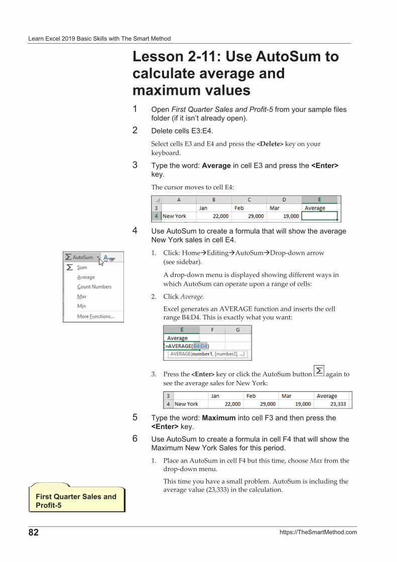
� ����� !������" �� ��#�!!���������� ��������
�
=�� ��$�%&&��� ������' ��
%��������2�5��"���+�#��������������������� �#���#�#��������� /$��First Quarter Sales and Profit.5�*���������� �$!�*�!��
*�!���1�*���������� !� ����$�2'�
�� +!�� !!���-%�3'�
Select�cells�E3�and�E4�and�press�the�<Delete>�key�on�your�keyboard.�
-� ��$�������%�"�������� !!��-� ���$������F����G�#�'�
The�cursor�moves�to�cell�E4:�
�3� 9��?���������� � �� �*����! �� ����!!������� 0� ,�
>��I��#�� !����� !!��3'�
1.� Click:�Home�Editing�AutoSum�Drop�down�arrow�(see�sidebar).��
A�drop�down�menu�is�displayed�showing�different�ways�in�which�AutoSum�can�operate�upon�a�range�of�cells:�
2.� Click�Average.�
Excel�generates�an�AVERAGE�function�and�inserts�the�cell�range�B4:D4.�This�is�exactly�what�you�want:�
�
3.� Press�the�<Enter>�key�or�click�the�AutoSum�button� �again�to�see�the�average�sales�for�New�York:��
�6� ��$�������%�����#�#������ !!�F-� ������$������
F����G�#�'�7� 9��?���������� � �� �*����! ���� !!�F3�� ����!!�������
� ������>��I��#�� !��*�������$����'�1.� Place�an�AutoSum�in�cell�F4�but�this�time,�choose�Max�from�the�
drop�down�menu.�
This�time�you�have�a�small�problem.�AutoSum�is�including�the�average�value�(23,333)�in�the�calculation.�
,�����H������+������ �7�����>�
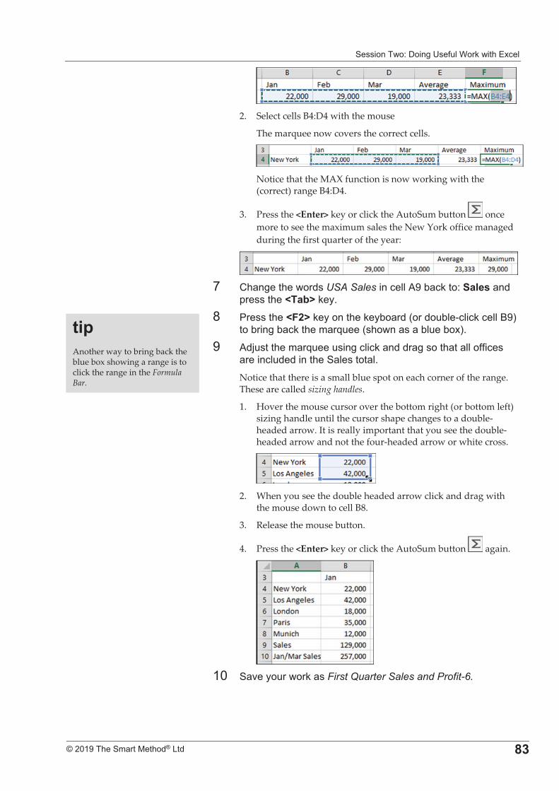
����������%�+���,�9�*�!����#������� !�
�
����������� �������������� =;
�2.� Select�cells�B4:D4�with�the�mouse�
The�marquee�now�covers�the�correct�cells.�
�Notice�that�the�MAX�function�is�now�working�with�the�(correct)�range�B4:D4.�
3.� Press�the�<Enter>�key�or�click�the�AutoSum�button� �once�more�to�see�the�maximum�sales�the�New�York�office�managed�during�the�first�quarter�of�the�year:�
�8� ( �,���������USA Sales���� !!�?��) #���%�+���� ���
$������F��!G�#�'�E� D������F,�G�#�������#�)� ���1������)!. !� #� !!�"�2�
���)���,�) #���� �L��1����� �� �)!��)��2'�
�� ?�K������� �L������,� !� #� ����� ,����� �� !!��**� �� ���� !���������� !����� !'�Notice�that�there�is�a�small�blue�spot�on�each�corner�of�the�range.�These�are�called�sizing�handles.�
1.� Hover�the�mouse�cursor�over�the�bottom�right�(or�bottom�left)�sizing�handle�until�the�cursor�shape�changes�to�a�double�headed�arrow.�It�is�really�important�that�you�see�the�double�headed�arrow�and�not�the�four�headed�arrow�or�white�cross.�
�2.� When�you�see�the�double�headed�arrow�click�and�drag�with�
the�mouse�down�to�cell�B8.�
3.� Release�the�mouse�button.��
4.� Press�the�<Enter>�key�or�click�the�AutoSum�button� �again.�
���� � 0���������#� ��First Quarter Sales and Profit-6.�
��*�Another�way�to�bring�back�the�blue�box�showing�a�range�is�to�click�the�range�in�the�Formula�Bar.�
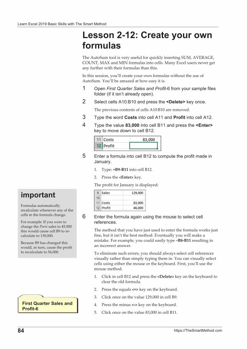
� ����� !������" �� ��#�!!���������� ��������
�
=0� ��$�%&&��� ������' ��
%��������2�.����������������#�����The�AutoSum�tool�is�very�useful�for�quickly�inserting�SUM,�AVERAGE,�COUNT,�MAX�and�MIN�formulas�into�cells.�Many�Excel�users�never�get�any�further�with�their�formulas�than�this.�
In�this�session,�you’ll�create�your�own�formulas�without�the�use�of�AutoSum.�You’ll�be�amazed�at�how�easy�it�is.�
�� /$��First Quarter Sales and Profit.7�*���������� �$!�*�!��*�!���1�*���������� !� ����$�2'�
�� �! �� !!��?��%"��� ���$������F4��G�#���� '�The�previous�contents�of�cells�A10:B10�are�removed.�
-� ��$��������.���������� !!�?��� ���7����������� !!�?��'�3� ��$���0 !��=;:��������� !!�"��� ���$������F����G�
#�������0��������� !!�"��'�
�6� ����� �*����! ������ !!�"������ ��$�����$��*���� �����
H �� ��'�1.� Type:�=B9�B11�into�cell�B12.�
2.� Press�the�<Enter>�key.�
The�profit�for�January�is�displayed:�
�7� �������*����! � , �������,������������! �� !!�
�*�� �'�The�method�that�you�have�just�used�to�enter�the�formula�works�just�fine,�but�it�isn’t�the�best�method.�Eventually�you�will�make�a�mistake.�For�example,�you�could�easily�type�=B8�B11�resulting�in�an�incorrect�answer.�
To�eliminate�such�errors,�you�should�always�select�cell�references�visually�rather�than�simply�typing�them�in.�You�can�visually�select�cells�using�either�the�mouse�or�the�keyboard.�First,�you’ll�use�the�mouse�method.�
1.� Click�in�cell�B12�and�press�the�<Delete>�key�on�the�keyboard�to�clear�the�old�formula.��
2.� Press�the�equals�<=>�key�on�the�keyboard.�
3.� Click�once�on�the�value�129,000�in�cell�B9.�
4.� Press�the�minus�<�>�key�on�the�keyboard.�
5.� Click�once�on�the�value�83,000�in�cell�B11.�
�#*�������Formulas�automatically�recalculate�whenever�any�of�the�cells�in�the�formula�change.�
For�example:�If�you�were�to�change�the�Paris�sales�to�45,000�this�would�cause�cell�B9�to�re�calculate�to�139,000.��
Because�B9�has�changed�this�would,�in�turn,�cause�the�profit�to�recalculate�to�56,000.�
,�����H������+������ �7�����6�
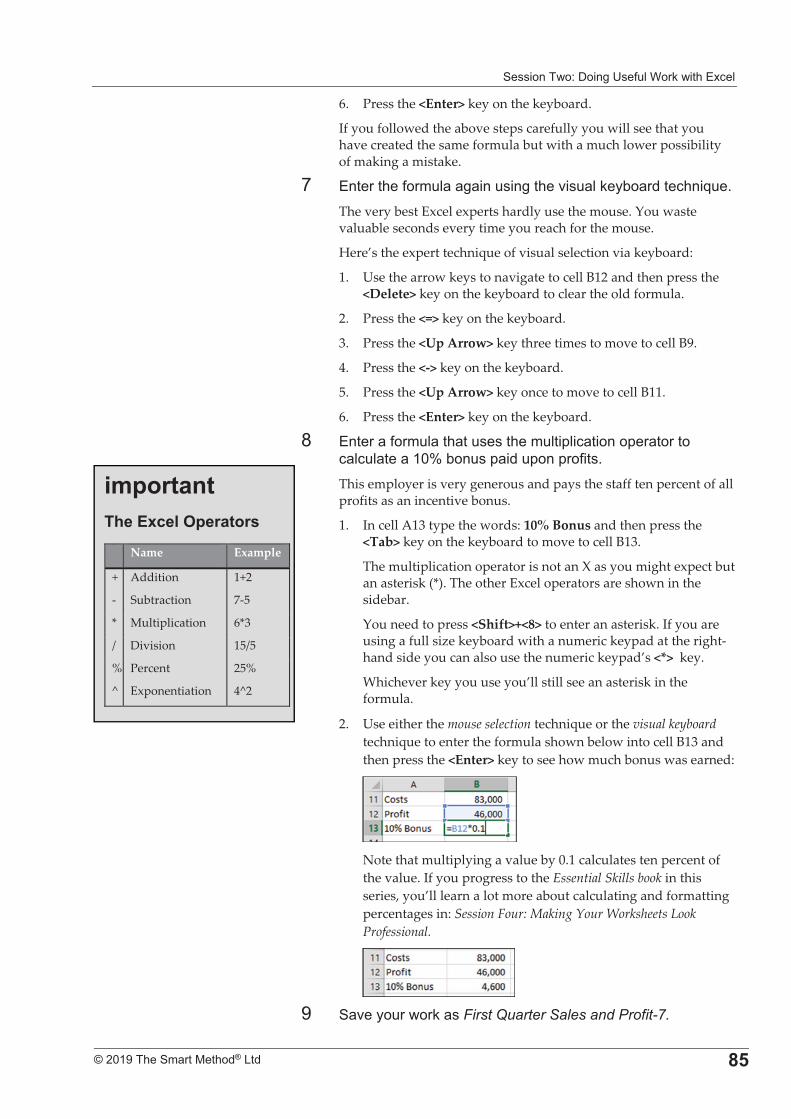
����������%�+���,�9�*�!����#������� !�
�
����������� �������������� =>
6.� Press�the�<Enter>�key�on�the�keyboard.�
If�you�followed�the�above�steps�carefully�you�will�see�that�you�have�created�the�same�formula�but�with�a�much�lower�possibility�of�making�a�mistake.��
8� �������*����! � , �������,���0��� !�#�)� ���� ��L�'�The�very�best�Excel�experts�hardly�use�the�mouse.�You�waste�valuable�seconds�every�time�you�reach�for�the�mouse.��
Here’s�the�expert�technique�of�visual�selection�via�keyboard:�
1.� Use�the�arrow�keys�to�navigate�to�cell�B12�and�then�press�the�<Delete>�key�on�the�keyboard�to�clear�the�old�formula.��
2.� Press�the�<=>�key�on�the�keyboard.�
3.� Press�the�<Up�Arrow>�key�three�times�to�move�to�cell�B9.�
4.� Press�the�<�>�key�on�the�keyboard.�
5.� Press�the�<Up�Arrow>�key�once�to�move�to�cell�B11.�
6.� Press�the�<Enter>�key�on�the�keyboard.�
E� ����� �*����! �� ����������!��$!� ������$� ������� ! �! �� ���M�)�����$ ����$���$��*���'�This�employer�is�very�generous�and�pays�the�staff�ten�percent�of�all�profits�as�an�incentive�bonus.��
1.� In�cell�A13�type�the�words:�10%�Bonus�and�then�press�the�<Tab>�key�on�the�keyboard�to�move�to�cell�B13.��
The�multiplication�operator�is�not�an�X�as�you�might�expect�but�an�asterisk�(*).�The�other�Excel�operators�are�shown�in�the�sidebar.�
You�need�to�press�<Shift>+<8>�to�enter�an�asterisk.�If�you�are�using�a�full�size�keyboard�with�a�numeric�keypad�at�the�right�hand�side�you�can�also�use�the�numeric�keypad’s�<*>��key.���
Whichever�key�you�use�you’ll�still�see�an�asterisk�in�the�formula.�
2.� Use�either�the�mouse�selection�technique�or�the�visual�keyboard�technique�to�enter�the�formula�shown�below�into�cell�B13�and�then�press�the�<Enter>�key�to�see�how�much�bonus�was�earned:�
�Note�that�multiplying�a�value�by�0.1�calculates�ten�percent�of�the�value.�If�you�progress�to�the�Essential�Skills�book�in�this�series,�you’ll�learn�a�lot�more�about�calculating�and�formatting�percentages�in:�Session�Four:�Making�Your�Worksheets�Look�Professional.�
��� � 0���������#� ��First Quarter Sales and Profit-7.
�#*���������������1*�������
� Name� Example�
+� Addition� 1+2�
�� Subtraction� 7�5�
*� Multiplication� 6*3�
/� Division� 15/5�
%� Percent� 25%�
^� Exponentiation� 4^2�
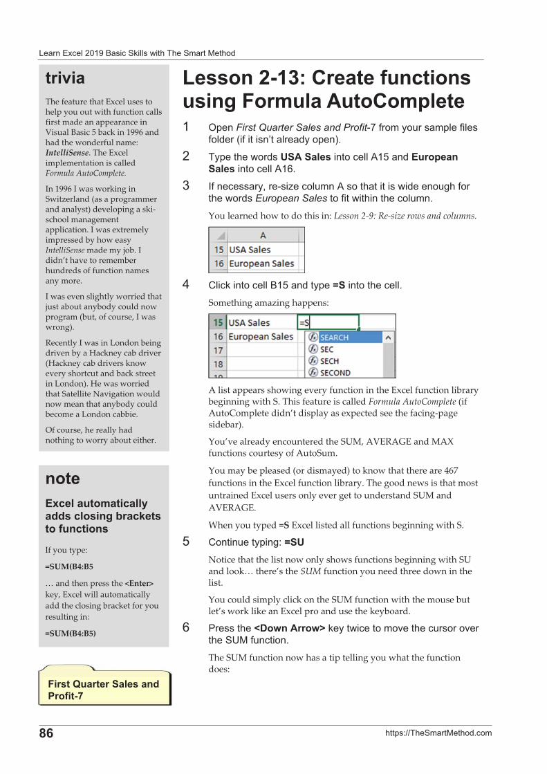
� ����� !������" �� ��#�!!���������� ��������
�
=6� ��$�%&&��� ������' ��
%�������;2�.��������������������,��#����"���.�#*������ /$��First Quarter Sales and Profit.8�*���������� �$!�*�!��
*�!���1�*���������� !� ����$�2'�
�� ��$���������5+"�+��������� !!�?�6� �������*���+��������� !!�?�7'�
-� 4*�� �� ��5��.��;� �!����?����� ���������������,�*�����������European Sales����*����������� �!���'�You�learned�how�to�do�this�in:�Lesson�2�9:�Re�size�rows�and�columns.�
�3� (!� #������ !!�"�6� �����$�P+�������� !!'�
Something�amazing�happens:�
�A�list�appears�showing�every�function�in�the�Excel�function�library�beginning�with�S.�This�feature�is�called�Formula�AutoComplete�(if�AutoComplete�didn’t�display�as�expected�see�the�facing�page�sidebar).�
You’ve�already�encountered�the�SUM,�AVERAGE�and�MAX�functions�courtesy�of�AutoSum.��
You�may�be�pleased�(or�dismayed)�to�know�that�there�are�467�functions�in�the�Excel�function�library.�The�good�news�is�that�most�untrained�Excel�users�only�ever�get�to�understand�SUM�and�AVERAGE.�
When�you�typed�=S�Excel�listed�all�functions�beginning�with�S.�
6� (���������$��,%�P+5�Notice�that�the�list�now�only�shows�functions�beginning�with�SU�and�look…�there’s�the�SUM�function�you�need�three�down�in�the�list.���
You�could�simply�click�on�the�SUM�function�with�the�mouse�but�let’s�work�like�an�Excel�pro�and�use�the�keyboard.�
7� D������F4����"����G�#����� ������0��� �������0�����9��*�� ����'�The�SUM�function�now�has�a�tip�telling�you�what�the�function�does:�
�������The�feature�that�Excel�uses�to�help�you�out�with�function�calls�first�made�an�appearance�in�Visual�Basic�5�back�in�1996�and�had�the�wonderful�name:�IntelliSense.�The�Excel�implementation�is�called�Formula�AutoComplete.�
In�1996�I�was�working�in�Switzerland�(as�a�programmer�and�analyst)�developing�a�ski�school�management�application.�I�was�extremely�impressed�by�how�easy�IntelliSense�made�my�job.�I�didn’t�have�to�remember�hundreds�of�function�names�any�more.��
I�was�even�slightly�worried�that�just�about�anybody�could�now�program�(but,�of�course,�I�was�wrong).�
Recently�I�was�in�London�being�driven�by�a�Hackney�cab�driver�(Hackney�cab�drivers�know�every�shortcut�and�back�street�in�London).�He�was�worried�that�Satellite�Navigation�would�now�mean�that�anybody�could�become�a�London�cabbie.��
Of�course,�he�really�had�nothing�to�worry�about�either.�
,�����H������+������ �7�����3�
�������������#���������� ����������!��� ����������������
If�you�type:�
=SUM(B4:B5�
…�and�then�press�the�<Enter>�key,�Excel�will�automatically�add�the�closing�bracket�for�you�resulting�in:�
=SUM(B4:B5)�
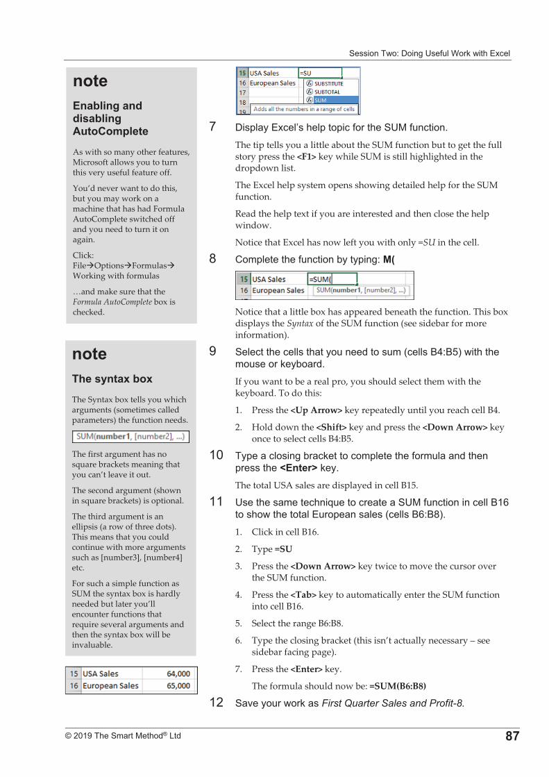
����������%�+���,�9�*�!����#������� !�
�
����������� �������������� =3
�8� +��$! ���� !���!$���$� �*������9��*�� ����'�
The�tip�tells�you�a�little�about�the�SUM�function�but�to�get�the�full�story�press�the�<F1>�key�while�SUM�is�still�highlighted�in�the�dropdown�list.�
The�Excel�help�system�opens�showing�detailed�help�for�the�SUM�function.�
Read�the�help�text�if�you�are�interested�and�then�close�the�help�window.�
Notice�that�Excel�has�now�left�you�with�only�=SU�in�the�cell.�
E� (��$!����*�� �����)����$��,%��'�
�Notice�that�a�little�box�has�appeared�beneath�the�function.�This�box�displays�the�Syntax�of�the�SUM�function�(see�sidebar�for�more�information).�
�� �! ���� !!��� ����������������1 !!��"3%"62���������������#�)� ��'�If�you�want�to�be�a�real�pro,�you�should�select�them�with�the�keyboard.�To�do�this:�
1.� Press�the�<Up�Arrow>�key�repeatedly�until�you�reach�cell�B4.�
2.� Hold�down�the�<Shift>�key�and�press�the�<Down�Arrow>�key�once�to�select�cells�B4:B5.�
��� ��$� � !����,�)� #����� ��$!����*����! � ������$������F����G�#�'�The�total�USA�sales�are�displayed�in�cell�B15.�
��� 9����� ��� ��L����� � �� ��9��*�� �������� !!�"�7������������� !�����$ ��� !��1 !!��"7%"E2'�1.� Click�in�cell�B16.�
2.� Type�=SU�
3.� Press�the�<Down�Arrow>�key�twice�to�move�the�cursor�over�the�SUM�function.�
4.� Press�the�<Tab>�key�to�automatically�enter�the�SUM�function�into�cell�B16.�
5.� Select�the�range�B6:B8.�
6.� Type�the�closing�bracket�(this�isn’t�actually�necessary�–�see�sidebar�facing�page).�
7.� Press�the�<Enter>�key.��
The�formula�should�now�be:�=SUM(B6:B8)�
��� � 0���������#� ��First Quarter Sales and Profit-8.�
��������������!���The�Syntax�box�tells�you�which�arguments�(sometimes�called�parameters)�the�function�needs.�
��The�first�argument�has�no�square�brackets�meaning�that�you�can’t�leave�it�out.��
The�second�argument�(shown�in�square�brackets)�is�optional.�
The�third�argument�is�an�ellipsis�(a�row�of�three�dots).��This�means�that�you�could�continue�with�more�arguments�such�as�[number3],�[number4]�etc.��
For�such�a�simple�function�as�SUM�the�syntax�box�is�hardly�needed�but�later�you’ll�encounter�functions�that�require�several�arguments�and�then�the�syntax�box�will�be�invaluable.�
�������!������� � ���!�����"���.�#*���As�with�so�many�other�features,�Microsoft�allows�you�to�turn�this�very�useful�feature�off.�
You’d�never�want�to�do�this,�but�you�may�work�on�a�machine�that�has�had�Formula�AutoComplete�switched�off�and�you�need�to�turn�it�on�again.�
Click:�File�Options�Formulas��Working�with�formulas�
…and�make�sure�that�the�Formula�AutoComplete�box�is�checked.�
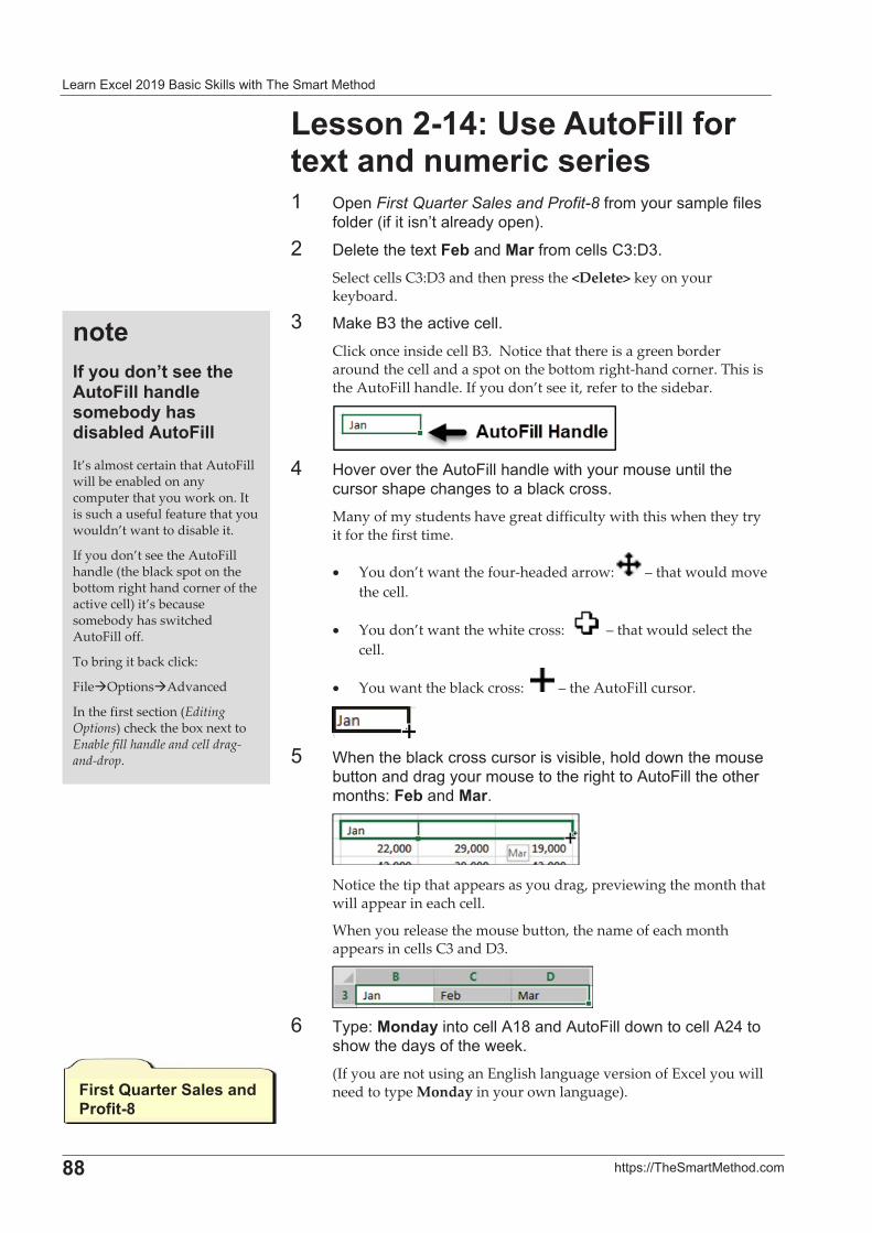
� ����� !������" �� ��#�!!���������� ��������
�
==� ��$�%&&��� ������' ��
%�������02�5��"���,�������������� ���#����������� /$��First Quarter Sales and Profit-8�*���������� �$!�*�!��
*�!���1�*���������� !� ����$�2'�
�� +!��������,!� �������*���� !!��(-%+-'�Select�cells�C3:D3�and�then�press�the�<Delete>�key�on�your�keyboard.�
-� � #�"-��� ��0� !!'�Click�once�inside�cell�B3.��Notice�that�there�is�a�green�border�around�the�cell�and�a�spot�on�the�bottom�right�hand�corner.�This�is�the�AutoFill�handle.�If�you�don’t�see�it,�refer�to�the�sidebar.�
�3� ��0���0����?���F�!!� ��!�������������������!���
������� $� �,����� �)! #� ����'�Many�of�my�students�have�great�difficulty�with�this�when�they�try�it�for�the�first�time.�
�� You�don’t�want�the�four�headed�arrow: �–�that�would�move�the�cell.��
�� You�don’t�want�the�white�cross:� ��–�that�would�select�the�cell.�
�� You�want�the�black�cross:� �–�the�AutoFill�cursor.�
�6� �����)! #� ����� ���������0���)!5��!��������������
)������ ����� ,������������������,�����?���F�!!������������%�,!� ������'�
�Notice�the�tip�that�appears�as�you�drag,�previewing�the�month�that�will�appear�in�each�cell.�
When�you�release�the�mouse�button,�the�name�of�each�month�appears�in�cells�C3�and�D3.�
�7� ��$%���� �������� !!�?�E� ���?���F�!!��������� !!�?�3����
������� ����*����#'�(If�you�are�not�using�an�English�language�version�of�Excel�you�will�need�to�type�Monday�in�your�own�language).�
����/������ ��8�������"���,������� ����#!� ������ ���!� �"���,����It’s�almost�certain�that�AutoFill�will�be�enabled�on�any�computer�that�you�work�on.�It�is�such�a�useful�feature�that�you�wouldn’t�want�to�disable�it.�
If�you�don’t�see�the�AutoFill�handle�(the�black�spot�on�the�bottom�right�hand�corner�of�the�active�cell)�it’s�because�somebody�has�switched�AutoFill�off.�
To�bring�it�back�click:�
File�Options�Advanced�
In�the�first�section�(Editing�Options)�check�the�box�next�to�Enable�fill�handle�and�cell�drag�and�drop.�
,�����H������+������ �7�����=�
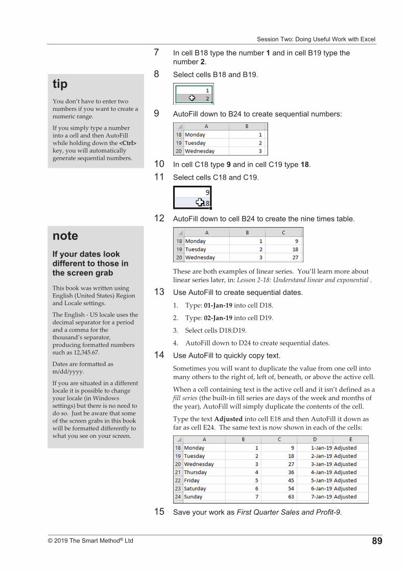
����������%�+���,�9�*�!����#������� !�
�
����������� �������������� =�
8� 4�� !!�"�E���$������)���� ������ !!�"�����$������)���'�
E� �! �� !!��"�E� ���"��'�
��� ?���F�!!���������"�3���� � ���L���� !����)��%�
���� 4�� !!�(�E���$��� ������ !!�(�����$��='���� �! �� !!��(�E� ���(��'�
���� ?���F�!!��������� !!�"�3���� � �������������� )!'�
�These�are�both�examples�of�linear�series.��You’ll�learn�more�about�linear�series�later,�in:�Lesson�2�18:�Understand�linear�and�exponential�.�
�-� 9��?���F�!!���� � ���L���� !�� ��'�1.� Type:�01�Jan�19�into�cell�D18.�
2.� Type:�02�Jan�19�into�cell�D19.�
3.� Select�cells�D18:D19.�
4.� AutoFill�down�to�D24�to�create�sequential�dates.�
�3� 9��?���F�!!����L�� #!�� �$�����'�Sometimes�you�will�want�to�duplicate�the�value�from�one�cell�into�many�others�to�the�right�of,�left�of,�beneath,�or�above�the�active�cell.�
When�a�cell�containing�text�is�the�active�cell�and�it�isn’t�defined�as�a�fill�series�(the�built�in�fill�series�are�days�of�the�week�and�months�of�the�year),�AutoFill�will�simply�duplicate�the�contents�of�the�cell.�
Type�the�text�Adjusted�into�cell�E18�and�then�AutoFill�it�down�as�far�as�cell�E24.��The�same�text�is�now�shown�in�each�of�the�cells:�
��6� � 0���������#� ��First Quarter Sales and Profit-9'�
��*�You�don’t�have�to�enter�two�numbers�if�you�want�to�create�a�numeric�range.�
If�you�simply�type�a�number�into�a�cell�and�then�AutoFill�while�holding�down�the�<Ctrl>�key,�you�will�automatically�generate�sequential�numbers.�
����/������� ������� � �����������������������������!�This�book�was�written�using�English�(United�States)�Region�and�Locale�settings.��
The�English���US�locale�uses�the�decimal�separator�for�a�period�and�a�comma�for�the�thousand’s�separator,�producing�formatted�numbers�such�as�12,345.67.���
Dates�are�formatted�as�m/dd/yyyy.���
If�you�are�situated�in�a�different�locale�it�is�possible�to�change�your�locale�(in�Windows�settings)�but�there�is�no�need�to�do�so.��Just�be�aware�that�some�of�the�screen�grabs�in�this�book�will�be�formatted�differently�to�what�you�see�on�your�screen.�
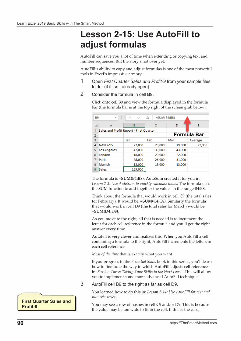
� ����� !������" �� ��#�!!���������� ��������
�
��� ��$�%&&��� ������' ��
%�������>2�5��"���,�������� &�������#�����AutoFill�can�save�you�a�lot�of�time�when�extending�or�copying�text�and�number�sequences.�But�the�story’s�not�over�yet.�
AutoFill’s�ability�to�copy�and�adjust�formulas�is�one�of�the�most�powerful�tools�in�Excel’s�impressive�armory.�
�� /$��First Quarter Sales and Profit.9�*���������� �$!�*�!��*�!���1�*���������� !� ����$�2'�
�� (���������*����! ���� !!�"�'�Click�onto�cell�B9�and�view�the�formula�displayed�in�the�formula�bar�(the�formula�bar�is�at�the�top�right�of�the�screen�grab�below).�
�The�formula�is�=SUM(B4:B8).�AutoSum�created�it�for�you�in:�Lesson�2�3:�Use�AutoSum�to�quickly�calculate�totals.�The�formula�uses�the�SUM�function�to�add�together�the�values�in�the�range�B4:B8.�
Think�about�the�formula�that�would�work�in�cell�C9�(the�total�sales�for�February).�It�would�be:�=SUM(C4:C8).�Similarly�the�formula�that�would�work�in�cell�D9�(the�total�sales�for�March)�would�be�=SUM(D4:D8).�
As�you�move�to�the�right,�all�that�is�needed�is�to�increment�the�letter�for�each�cell�reference�in�the�formula�and�you’ll�get�the�right�answer�every�time.�
AutoFill�is�very�clever�and�realizes�this.�When�you�AutoFill�a�cell�containing�a�formula�to�the�right,�AutoFill�increments�the�letters�in�each�cell�reference.��
Most�of�the�time�that�is�exactly�what�you�want.��
If�you�progress�to�the�Essential�Skills�book�in�this�series,�you’ll�learn�how�to�fine�tune�the�way�in�which�AutoFill�adjusts�cell�references�in:�Session�Three:�Taking�Your�Skills�to�the�Next�Level.��This�will�allow�you�to�implement�some�more�advanced�AutoFill�techniques.�
-� ?���F�!!� !!�"���������,�� ��* �� �� !!�+�'�You�learned�how�to�do�this�in:�Lesson�2�14:�Use�AutoFill�for�text�and�numeric�series.�
You�may�see�a�row�of�hashes�in�cell�C9�and/or�D9.�This�is�because�the�value�may�be�too�wide�to�fit�in�the�cell.�If�this�is�the�case,�
,�����H������+������ �7�������
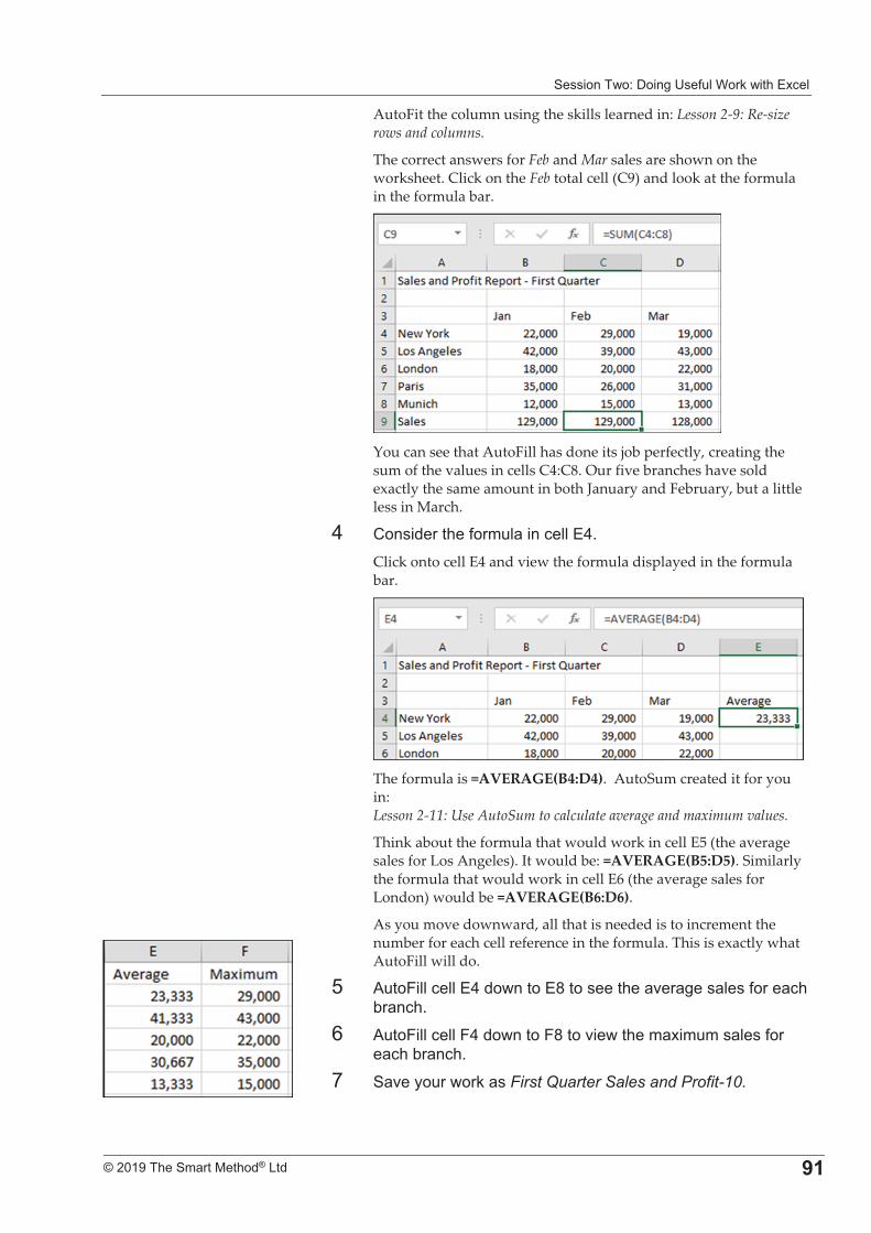
����������%�+���,�9�*�!����#������� !�
�
����������� �������������� ��
AutoFit�the�column�using�the�skills�learned�in:�Lesson�2�9:�Re�size�rows�and�columns.��
The�correct�answers�for�Feb�and�Mar�sales�are�shown�on�the�worksheet.�Click�on�the�Feb�total�cell�(C9)�and�look�at�the�formula�in�the�formula�bar.�
�You�can�see�that�AutoFill�has�done�its�job�perfectly,�creating�the�sum�of�the�values�in�cells�C4:C8.�Our�five�branches�have�sold�exactly�the�same�amount�in�both�January�and�February,�but�a�little�less�in�March.�
3� (���������*����! ���� !!��3'�Click�onto�cell�E4�and�view�the�formula�displayed�in�the�formula�bar.�
�The�formula�is�=AVERAGE(B4:D4).��AutoSum�created�it�for�you�in:�Lesson�2�11:�Use�AutoSum�to�calculate�average�and�maximum�values.�
Think�about�the�formula�that�would�work�in�cell�E5�(the�average�sales�for�Los�Angeles).�It�would�be:�=AVERAGE(B5:D5).�Similarly�the�formula�that�would�work�in�cell�E6�(the�average�sales�for�London)�would�be�=AVERAGE(B6:D6).��
As�you�move�downward,�all�that�is�needed�is�to�increment�the�number�for�each�cell�reference�in�the�formula.�This�is�exactly�what�AutoFill�will�do.�
6� ?���F�!!� !!��3����������E�������� 0� ,�� !��*��� �)� � '�
7� ?���F�!!� !!�F3���������FE����0������ ������� !��*��� �)� � '�
8� � 0���������#� ��First Quarter Sales and Profit-10.
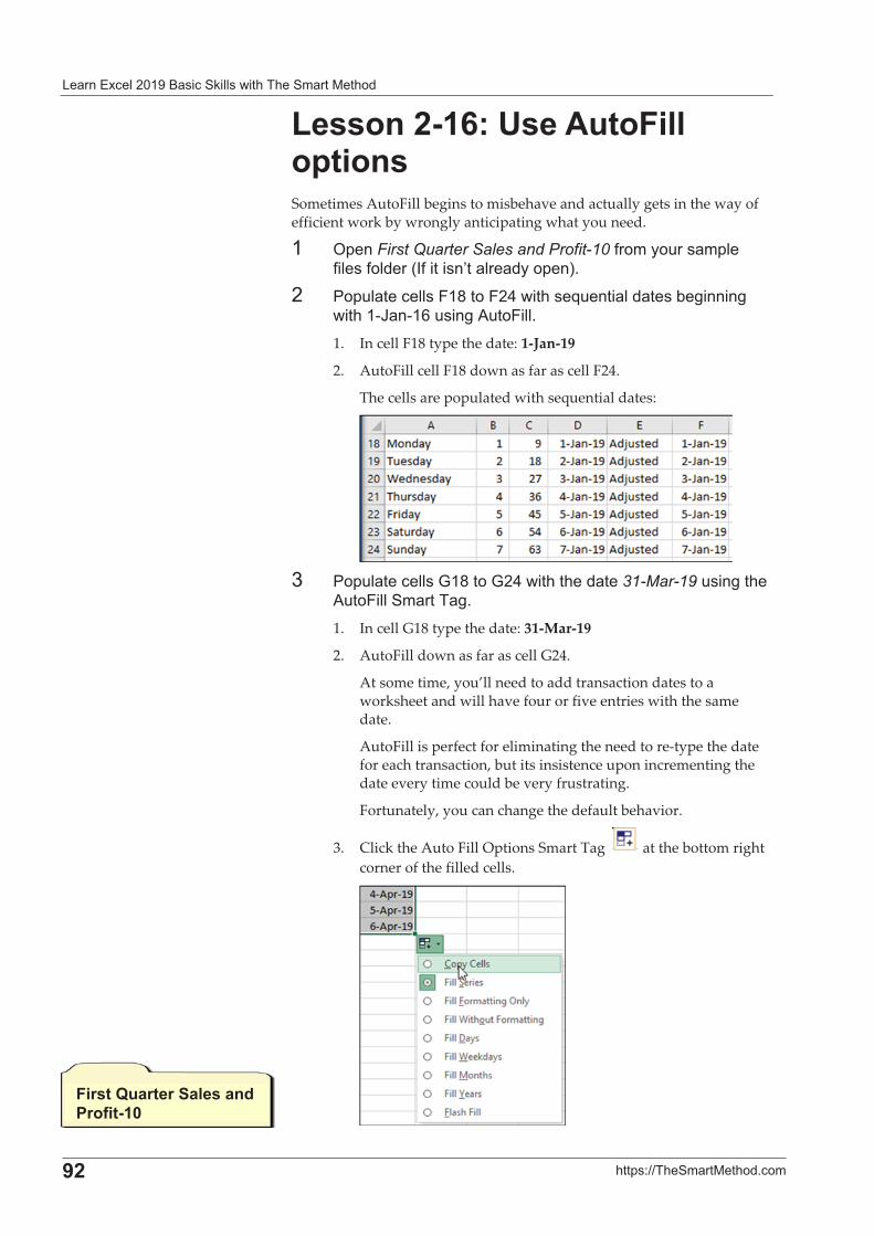
� ����� !������" �� ��#�!!���������� ��������
�
��� ��$�%&&��� ������' ��
%�������62�5��"���,�����*������Sometimes�AutoFill�begins�to�misbehave�and�actually�gets�in�the�way�of�efficient�work�by�wrongly�anticipating�what�you�need.��
�� /$��First Quarter Sales and Profit.10�*���������� �$!�*�!��*�!���14*���������� !� ����$�2'�
�� D�$�! �� !!��F�E����F�3������L���� !�� ���),�����,������.H �.�7�����,�?���F�!!'�1.� In�cell�F18�type�the�date:�1�Jan�19�
2.� AutoFill�cell�F18�down�as�far�as�cell�F24.�
The�cells�are�populated�with�sequential�dates:�
�-� D�$�! �� !!��<�E����<�3�������� ��31-Mar-19�����,���
?���F�!!��� ���� ,'�1.� In�cell�G18�type�the�date:�31�Mar�19�
2.� AutoFill�down�as�far�as�cell�G24.�
At�some�time,�you’ll�need�to�add�transaction�dates�to�a�worksheet�and�will�have�four�or�five�entries�with�the�same�date.��
AutoFill�is�perfect�for�eliminating�the�need�to�re�type�the�date�for�each�transaction,�but�its�insistence�upon�incrementing�the�date�every�time�could�be�very�frustrating.��
Fortunately,�you�can�change�the�default�behavior.��
3.� Click�the�Auto�Fill�Options�Smart�Tag�� �at�the�bottom�right�corner�of�the�filled�cells.�
�
,�����H������+������ �7��������
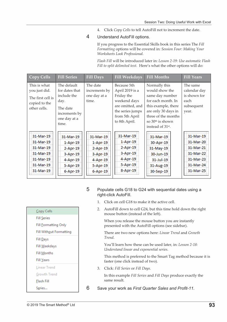
����������%�+���,�9�*�!����#������� !�
�
����������� �������������� �;
4.� Click�Copy�Cells�to�tell�AutoFill�not�to�increment�the�date.�
3� 9����� ���?���F�!!��$�����'�If�you�progress�to�the�Essential�Skills�book�in�this�series�The�Fill�Formatting�options�will�be�covered�in:�Session�Four:�Making�Your�Worksheets�Look�Professional.�
Flash�Fill�will�be�introduced�later�in:�Lesson�2�19:�Use�automatic�Flash�Fill�to�split�delimited�text.��Here’s�what�the�other�options�will�do:�
�
6� D�$�! �� !!��<�E����<�3������L���� !�� �������,� ���,�. !� #�?���F�!!'�1.� Click�on�cell�G18�to�make�it�the�active�cell.��
2.� AutoFill�down�to�cell�G24,�but�this�time�hold�down�the�right�mouse�button�(instead�of�the�left).�
When�you�release�the�mouse�button�you�are�instantly�presented�with�the�AutoFill�options�(see�sidebar).�
There�are�two�new�options�here:�Linear�Trend�and�Growth�Trend.���
You’ll�learn�how�these�can�be�used�later,�in:�Lesson�2�18:�Understand�linear�and�exponential�series.�
This�method�is�preferred�to�the�Smart�Tag�method�because�it�is�faster�(one�click�instead�of�two).�
3.� Click:�Fill�Series�or�Fill�Days.�
In�this�example�Fill�Series�and�Fill�Days�produce�exactly�the�same�result.��
7� � 0���������#� ��First Quarter Sales and Profit-11.�
Copy�Cells� Fill�Series� Fill�Days Fill�Weekdays Fill�Months� Fill�Years
This�is�what�you�just�did.��
The�first�cell�is�copied�to�the�other�cells.�
The�default�for�dates�that�include�the�day.��
The�date�increments�by�one�day�at�a�time.�
The�date�increments�by�one�day�at�a�time.�
Because�5th�April�2019�is�a�Friday�the�weekend�days�are�omitted,�and�the�series�jumps�from�5th�April�to�8th�April.�
Normally�this�would�show�the�same�day�number�for�each�month.�In�this�example,�there�are�only�30�days�in�three�of�the�months�so�30th�is�shown�instead�of�31st.�
The�same�calendar�day�is�shown�for�each�subsequent�year.�
� � � � � �
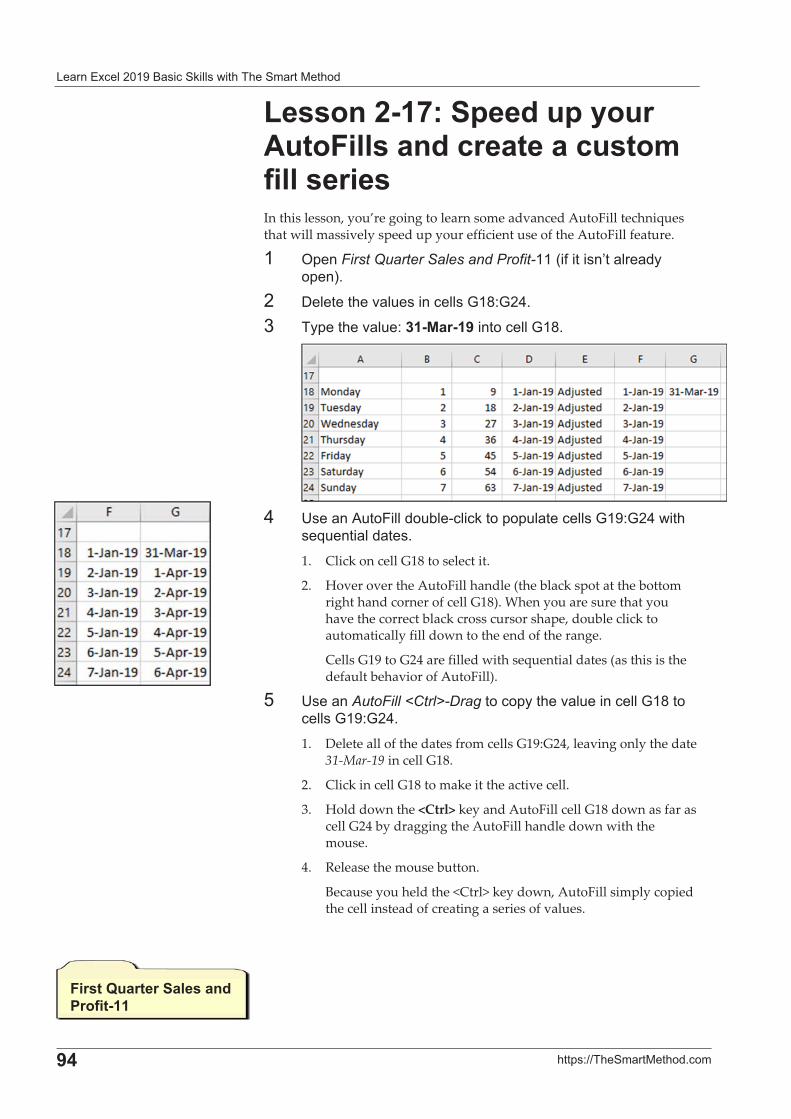
� ����� !������" �� ��#�!!���������� ��������
�
�0� ��$�%&&��� ������' ��
%�������32�+* ��*������"���,������� �������������#�����������In�this�lesson,�you’re�going�to�learn�some�advanced�AutoFill�techniques�that�will�massively�speed�up�your�efficient�use�of�the�AutoFill�feature.�
�� /$��First Quarter Sales and Profit-���1�*���������� !� ����$�2'�
�� +!����0 !������ !!��<�E%<�3'�
-� ��$���0 !�%�;������������ !!�<�E'�
�3� 9�� ��?���F�!!����)!. !� #����$�$�! �� !!��<��%<�3�����
�L���� !�� ��'�1.� Click�on�cell�G18�to�select�it.�
2.� Hover�over�the�AutoFill�handle�(the�black�spot�at�the�bottom�right�hand�corner�of�cell�G18).�When�you�are�sure�that�you�have�the�correct�black�cross�cursor�shape,�double�click�to�automatically�fill�down�to�the�end�of�the�range.�
Cells�G19�to�G24�are�filled�with�sequential�dates�(as�this�is�the�default�behavior�of�AutoFill).�
6� 9�� ��AutoFill <Ctrl>-Drag���� �$����0 !����� !!�<�E���� !!��<��%<�3'�1.� Delete�all�of�the�dates�from�cells�G19:G24,�leaving�only�the�date�
31�Mar�19�in�cell�G18.�
2.� Click�in�cell�G18�to�make�it�the�active�cell.�
3.� Hold�down�the�<Ctrl>�key�and�AutoFill�cell�G18�down�as�far�as�cell�G24�by�dragging�the�AutoFill�handle�down�with�the�mouse.�
4.� Release�the�mouse�button.�
Because�you�held�the�<Ctrl>�key�down,�AutoFill�simply�copied�the�cell�instead�of�creating�a�series�of�values.�
,�����H������+������ �7��������
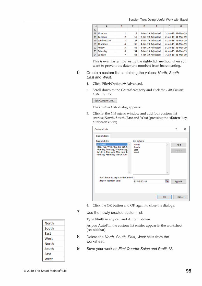
����������%�+���,�9�*�!����#������� !�
�
����������� �������������� �>
�This�is�even�faster�than�using�the�right�click�method�when�you�want�to�prevent�the�date�(or�a�number)�from�incrementing.�
7� (� �� � ������!���� ��� ����,���0 !��%�North, South, East� ���West.�1.� Click:�File�Options�Advanced.�
2.� Scroll�down�to�the�General�category�and�click�the�Edit�Custom�Lists...�button.�
�The�Custom�Lists�dialog�appears.�
3.� Click�in�the�List�entries�window�and�add�four�custom�list�entries:�North,�South,�East�and�West�(pressing�the�<Enter>�key�after�each�entry).�
�4.� Click�the�OK�button�and�OK�again�to�close�the�dialogs.�
8� 9������!�� � ��� ������!���'��
Type�North�in�any�cell�and�AutoFill�down.�
As�you�AutoFill,�the�custom�list�entries�appear�in�the�worksheet�(see�sidebar).��
E� +!����North, South, East, West� !!��*���������#��'��
�� � 0���������#� ��First Quarter Sales and Profit-12.��
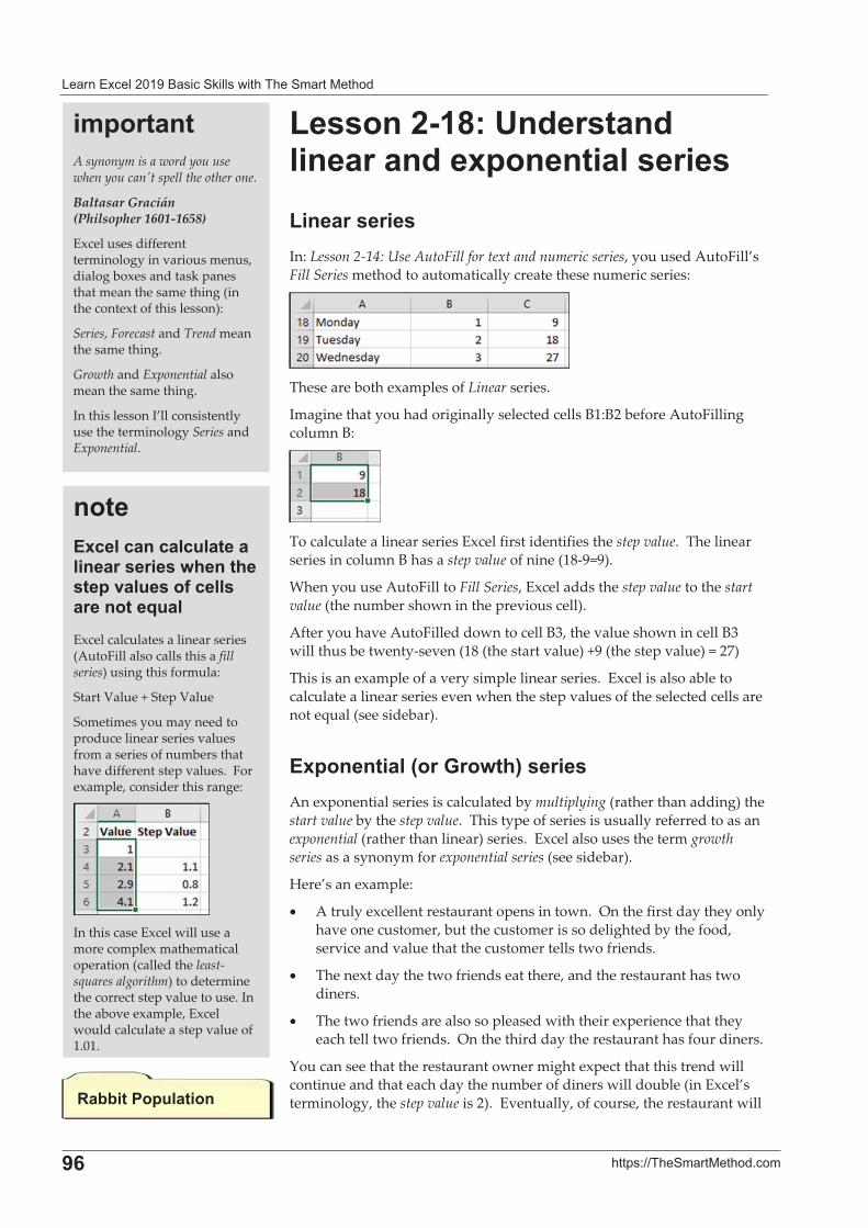
� ����� !������" �� ��#�!!���������� ��������
�
�6� ��$�%&&��� ������' ��
%�������=2�5� ����� ��������� ��*�������������%����������In:�Lesson�2�14:�Use�AutoFill�for�text�and�numeric�series,�you�used�AutoFill’s�Fill�Series�method�to�automatically�create�these�numeric�series:�
�These�are�both�examples�of�Linear�series.�
Imagine�that�you�had�originally�selected�cells�B1:B2�before�AutoFilling�column�B:�
�To�calculate�a�linear�series�Excel�first�identifies�the�step�value.��The�linear�series�in�column�B�has�a�step�value�of�nine�(18�9=9).�
When�you�use�AutoFill�to�Fill�Series,�Excel�adds�the�step�value�to�the�start�value�(the�number�shown�in�the�previous�cell).���
After�you�have�AutoFilled�down�to�cell�B3,�the�value�shown�in�cell�B3�will�thus�be�twenty�seven�(18�(the�start�value)�+9�(the�step�value)�=�27)�
This�is�an�example�of�a�very�simple�linear�series.��Excel�is�also�able�to�calculate�a�linear�series�even�when�the�step�values�of�the�selected�cells�are�not�equal�(see�sidebar).�
��*��������'���@�����(������An�exponential�series�is�calculated�by�multiplying�(rather�than�adding)�the�start�value�by�the�step�value.��This�type�of�series�is�usually�referred�to�as�an�exponential�(rather�than�linear)�series.��Excel�also�uses�the�term�growth�series�as�a�synonym�for�exponential�series�(see�sidebar).�
Here’s�an�example:�
�� A�truly�excellent�restaurant�opens�in�town.��On�the�first�day�they�only�have�one�customer,�but�the�customer�is�so�delighted�by�the�food,�service�and�value�that�the�customer�tells�two�friends.�
�� The�next�day�the�two�friends�eat�there,�and�the�restaurant�has�two�diners.��
�� The�two�friends�are�also�so�pleased�with�their�experience�that�they�each�tell�two�friends.��On�the�third�day�the�restaurant�has�four�diners.�
You�can�see�that�the�restaurant�owner�might�expect�that�this�trend�will�continue�and�that�each�day�the�number�of�diners�will�double�(in�Excel’s�terminology,�the�step�value�is�2).��Eventually,�of�course,�the�restaurant�will�
��������������������������������������������*����������������������M����Excel�calculates�a�linear�series�(AutoFill�also�calls�this�a�fill�series)�using�this�formula:�
Start�Value�+�Step�Value�
Sometimes�you�may�need�to�produce�linear�series�values�from�a�series�of�numbers�that�have�different�step�values.��For�example,�consider�this�range:�
��In�this�case�Excel�will�use�a�more�complex�mathematical�operation�(called�the�least�squares�algorithm)�to�determine�the�correct�step�value�to�use.�In�the�above�example,�Excel�would�calculate�a�step�value�of�1.01.�
<�!!���7�*��������
�#*�������A�synonym�is�a�word�you�use�when�you�can�t�spell�the�other�one.��
Baltasar�Gracián��(Philsopher�1601�1658)�
Excel�uses�different�terminology�in�various�menus,�dialog�boxes�and�task�panes�that�mean�the�same�thing�(in�the�context�of�this�lesson):�
Series,�Forecast�and�Trend�mean�the�same�thing.�
Growth�and�Exponential�also�mean�the�same�thing.�
In�this�lesson�I’ll�consistently�use�the�terminology�Series�and�Exponential.�
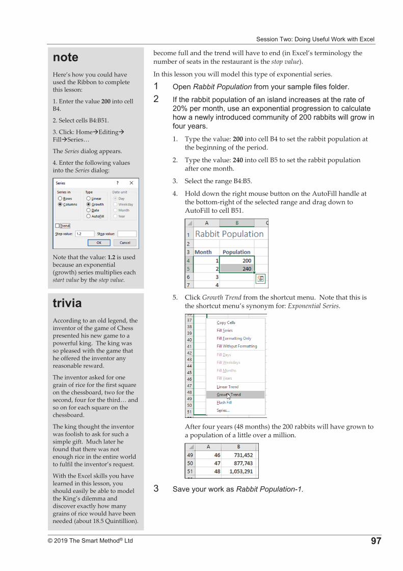
����������%�+���,�9�*�!����#������� !�
�
����������� �������������� �3
become�full�and�the�trend�will�have�to�end�(in�Excel’s�terminology�the�number�of�seats�in�the�restaurant�is�the�stop�value).�
In�this�lesson�you�will�model�this�type�of�exponential�series.�
�� /$��Rabbit�Population *���������� �$!�*�!��*�!��'�
�� 4*���� ))���$�$�! ������*� ����! ����� � ��� ����� ���*���M�$������5���� ���$����� !�$��,���������� ! �! ����� ���!��������� �� ����������*������ ))������!!�,�������*����� ��'�1.� Type�the�value:�200�into�cell�B4�to�set�the�rabbit�population�at�
the�beginning�of�the�period.��
2.� Type�the�value:�240�into�cell�B5�to�set�the�rabbit�population�after�one�month.�
3.� Select�the�range�B4:B5.�
4.� Hold�down�the�right�mouse�button�on�the�AutoFill�handle�at�the�bottom�right�of�the�selected�range�and�drag�down�to�AutoFill�to�cell�B51.�
�5.� Click�Growth�Trend�from�the�shortcut�menu.��Note�that�this�is�
the�shortcut�menu’s�synonym�for:�Exponential�Series.�
�After�four�years�(48�months)�the�200�rabbits�will�have�grown�to�a�population�of�a�little�over�a�million.�
�
-� � 0���������#� ��Rabbit Population-1.��
����Here’s�how�you�could�have�used�the�Ribbon�to�complete�this�lesson:�
1.�Enter�the�value�200�into�cell�B4.�
2.�Select�cells�B4:B51.�
3.�Click:�Home�Editing��Fill�Series…�
The�Series�dialog�appears.�
4.�Enter�the�following�values�into�the�Series�dialog:�
�Note�that�the�value:�1.2�is�used�because�an�exponential�(growth)�series�multiplies�each�start�value�by�the�step�value.�
�������According�to�an�old�legend,�the�inventor�of�the�game�of�Chess�presented�his�new�game�to�a�powerful�king.��The�king�was�so�pleased�with�the�game�that�he�offered�the�inventor�any�reasonable�reward.�
The�inventor�asked�for�one�grain�of�rice�for�the�first�square�on�the�chessboard,�two�for�the�second,�four�for�the�third…�and�so�on�for�each�square�on�the�chessboard.���
The�king�thought�the�inventor�was�foolish�to�ask�for�such�a�simple�gift.��Much�later�he�found�that�there�was�not�enough�rice�in�the�entire�world�to�fulfil�the�inventor’s�request.�
With�the�Excel�skills�you�have�learned�in�this�lesson,�you�should�easily�be�able�to�model�the�King’s�dilemma�and�discover�exactly�how�many�grains�of�rice�would�have�been�needed�(about�18.5�Quintillion).�
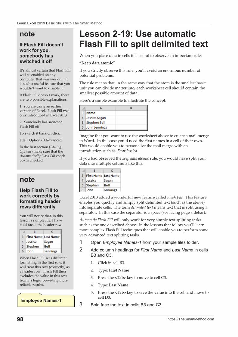
� ����� !������" �� ��#�!!���������� ��������
�
�=� ��$�%&&��� ������' ��
%��������2�5������#�����,�����,��������*���� ��#�� �����When�you�place�data�in�cells�it�is�useful�to�observe�an�important�rule:�
“Keep�data�atomic”�
If�you�strictly�observe�this�rule,�you’ll�avoid�an�enormous�number�of�potential�problems.�
The�rule�means�that,�in�the�same�way�that�the�atom�is�the�smallest�basic�unit�you�can�divide�matter�into,�each�worksheet�cell�should�contain�the�smallest�possible�amount�of�data.�
Here’s�a�simple�example�to�illustrate�the�concept:�
�Imagine�that�you�want�to�use�the�worksheet�above�to�create�a�mail�merge�in�Word.��In�this�case�you’d�need�the�first�names�in�a�cell�of�their�own.��This�would�enable�you�to�personalize�the�mail�merge�with�an�introduction�such�as:�Dear�Jessica.�
If�you�had�observed�the�keep�data�atomic�rule,�you�would�have�split�your�data�into�multiple�columns�like�this:�
�Excel�2013�added�a�wonderful�new�feature�called�Flash�Fill.��This�feature�enables�you�quickly�and�simply�split�delimited�text�(such�as�the�above)�into�separate�cells.��The�term�delimited�text�means�text�that�is�split�using�a�separator.��In�this�case�the�separator�is�a�space�(see�facing�page�sidebar).�
Automatic�Flash�Fill�will�only�work�for�very�simple�text�splitting�tasks�such�as�the�one�described�above.��In�the�lessons�that�follow�you’ll�learn�more�complex�Flash�Fill�techniques�that�will�enable�you�to�perform�some�very�advanced�text�splitting�tasks.�
�� /$��Employee Names-1 *���������� �$!�*�!��*�!��'�
�� ?��� �!���� ���,��*���First Name� ���Last Name���� !!��"-� ���(-'�1.� Click�in�cell�B3.�
2.� Type:�First�Name�
3.� Press�the�<Tab>�key�to�move�to�cell�C3.�
4.� Type:�Last�Name�
5.� Press�the�<Tab>�key�to�save�the�value�into�the�cell�and�move�to�cell�D3.�
-� "�!��* ���������� !!��"-� ���(-'�
����/��,�����,���� ���8����� ��������:���#!� ������������ ��������It’s�almost�certain�that�Flash�Fill�will�be�enabled�on�any�computer�that�you�work�on.�It�is�such�a�useful�feature�that�you�wouldn’t�want�to�disable�it.�
If�Flash�Fill�doesn’t�work,�there�are�two�possible�explanations:�
1.�You�are�using�an�earlier�version�of�Excel.��Flash�Fill�was�only�introduced�in�Excel�2013.�
2.��Somebody�has�switched�Flash�Fill�off.�
To�switch�it�back�on�click:�
File�Options�Advanced�
In�the�first�section�(Editing�Options)�make�sure�that�the�Automatically�Flash�Fill�check�box�is�checked.�
�#*����C�#���
����)�*�,�����,���������� ����������!�����#��������� ������� ���������You�will�notice�that,�in�this�lesson’s�sample�file,�I�have�bold�faced�the�header�row:�
�When�Flash�Fill�sees�different�formatting�in�the�first�row,�it�will�treat�this�row�(correctly)�as�a�header�row.��Flash�Fill�then�excludes�the�value�in�this�row�from�its�logic,�providing�more�reliable�results.�
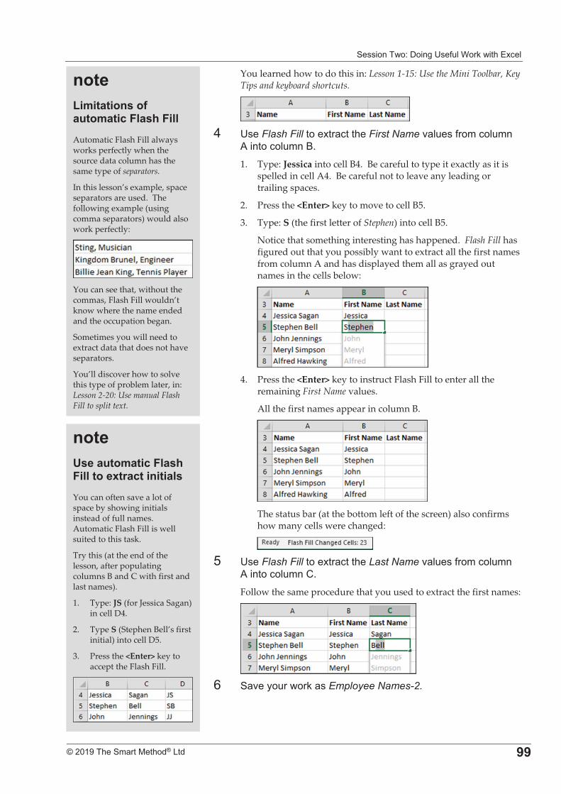
����������%�+���,�9�*�!����#������� !�
�
����������� �������������� ��
You�learned�how�to�do�this�in:�Lesson�1�15:�Use�the�Mini�Toolbar,�Key�Tips�and�keyboard�shortcuts.�
�3� 9��Flash Fill������� ����First Name�0 !���*���� �!����
?������ �!����"'�1.� Type:�Jessica�into�cell�B4.��Be�careful�to�type�it�exactly�as�it�is�
spelled�in�cell�A4.��Be�careful�not�to�leave�any�leading�or�trailing�spaces.�
2.� Press�the�<Enter>�key�to�move�to�cell�B5.�
3.� Type:�S�(the�first�letter�of�Stephen)�into�cell�B5.�
Notice�that�something�interesting�has�happened.��Flash�Fill�has�figured�out�that�you�possibly�want�to�extract�all�the�first�names�from�column�A�and�has�displayed�them�all�as�grayed�out�names�in�the�cells�below:�
�4.� Press�the�<Enter>�key�to�instruct�Flash�Fill�to�enter�all�the�
remaining�First�Name�values.�
All�the�first�names�appear�in�column�B.�
�The�status�bar�(at�the�bottom�left�of�the�screen)�also�confirms�how�many�cells�were�changed:��
�6� 9��Flash Fill������� ����Last Name�0 !���*���� �!����
?������ �!����('�Follow�the�same�procedure�that�you�used�to�extract�the�first�names:�
�7� � 0���������#� ��Employee Names-2.�
����%�#����������������#�����,�����,����Automatic�Flash�Fill�always�works�perfectly�when�the�source�data�column�has�the�same�type�of�separators.���
In�this�lesson’s�example,�space�separators�are�used.��The�following�example�(using�comma�separators)�would�also�work�perfectly:�
�You�can�see�that,�without�the�commas,�Flash�Fill�wouldn’t�know�where�the�name�ended�and�the�occupation�began.�
Sometimes�you�will�need�to�extract�data�that�does�not�have�separators.��
You’ll�discover�how�to�solve�this�type�of�problem�later,�in:�Lesson�2�20:�Use�manual�Flash�Fill�to�split�text.�
����5������#�����,�����,�����������������������You�can�often�save�a�lot�of�space�by�showing�initials�instead�of�full�names.��Automatic�Flash�Fill�is�well�suited�to�this�task.�
Try�this�(at�the�end�of�the�lesson,�after�populating�columns�B�and�C�with�first�and�last�names).�
1.� Type:�JS�(for�Jessica�Sagan)�in�cell�D4.�
2.� Type�S�(Stephen�Bell’s�first�initial)�into�cell�D5.�
3.� Press�the�<Enter>�key�to�accept�the�Flash�Fill.�
�
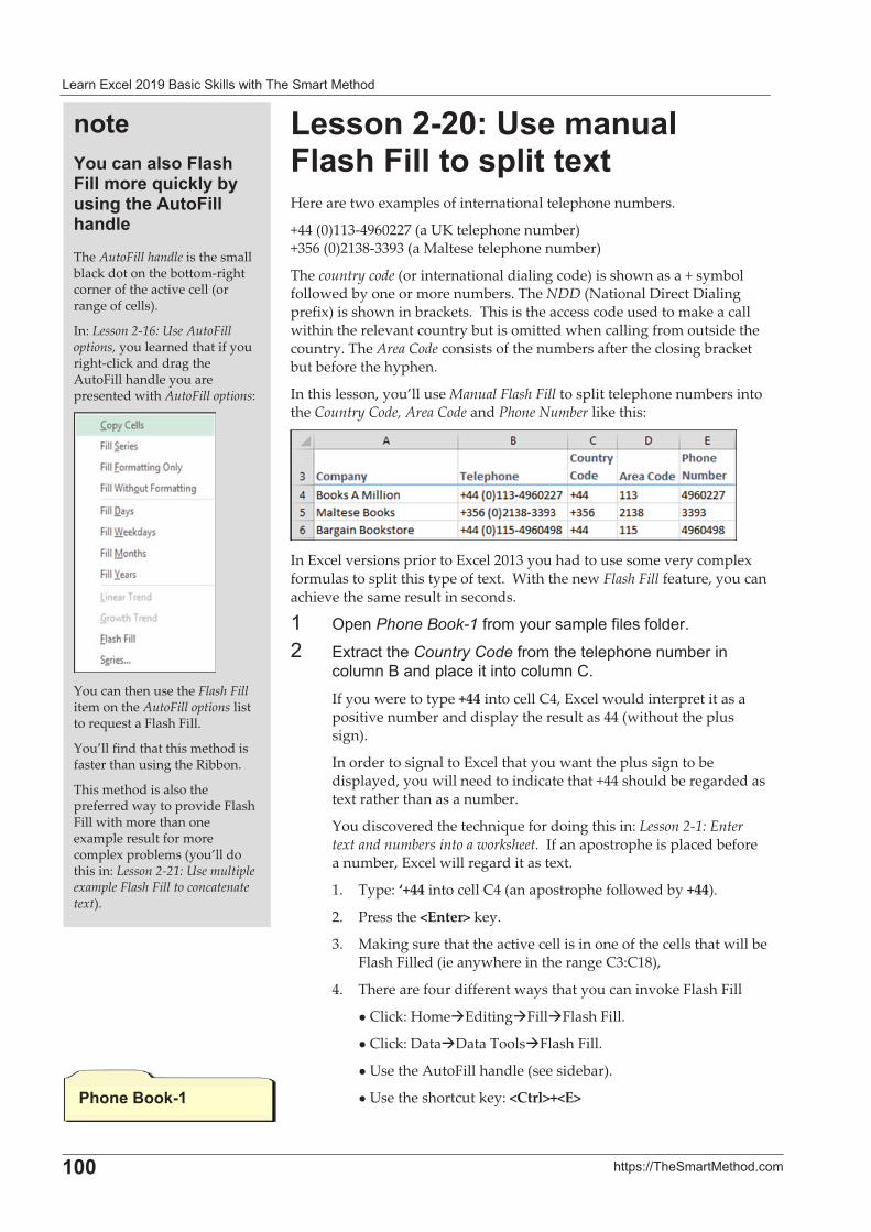
� ����� !������" �� ��#�!!���������� ��������
�
���� ��$�%&&��� ������' ��
%��������2�5��#������,�����,��������*��������Here�are�two�examples�of�international�telephone�numbers.�
+44�(0)113�4960227�(a�UK�telephone�number)��+356�(0)2138�3393�(a�Maltese�telephone�number)�
The�country�code�(or�international�dialing�code)�is�shown�as�a�+�symbol�followed�by�one�or�more�numbers.�The�NDD�(National�Direct�Dialing�prefix)�is�shown�in�brackets.��This�is�the�access�code�used�to�make�a�call�within�the�relevant�country�but�is�omitted�when�calling�from�outside�the�country.�The�Area�Code�consists�of�the�numbers�after�the�closing�bracket�but�before�the�hyphen.�
In�this�lesson,�you’ll�use�Manual�Flash�Fill�to�split�telephone�numbers�into�the�Country�Code,�Area�Code�and�Phone�Number�like�this:�
�In�Excel�versions�prior�to�Excel�2013�you�had�to�use�some�very�complex�formulas�to�split�this�type�of�text.��With�the�new�Flash�Fill�feature,�you�can�achieve�the�same�result�in�seconds.�
�� /$��Phone Book-1 *���������� �$!�*�!��*�!��'�
�� ���� ����Country Code�*�������!$������)����� �!����"� ���$! ��������� �!����('�If�you�were�to�type�+44�into�cell�C4,�Excel�would�interpret�it�as�a�positive�number�and�display�the�result�as�44�(without�the�plus�sign).�
In�order�to�signal�to�Excel�that�you�want�the�plus�sign�to�be�displayed,�you�will�need�to�indicate�that�+44�should�be�regarded�as�text�rather�than�as�a�number.�
You�discovered�the�technique�for�doing�this�in:�Lesson�2�1:�Enter�text�and�numbers�into�a�worksheet.��If�an�apostrophe�is�placed�before�a�number,�Excel�will�regard�it�as�text.�
1.� Type:�‘+44�into�cell�C4�(an�apostrophe�followed�by�+44).�
2.� Press�the�<Enter>�key.�
3.� Making�sure�that�the�active�cell�is�in�one�of�the�cells�that�will�be�Flash�Filled�(ie�anywhere�in�the�range�C3:C18),��
4.� There�are�four�different�ways�that�you�can�invoke�Flash�Fill���
��Click:�Home�Editing�Fill�Flash�Fill.�
��Click:�Data�Data�Tools�Flash�Fill.�
��Use�the�AutoFill�handle�(see�sidebar).�
��Use�the�shortcut�key:�<Ctrl>+<E>��
����-������������,�����,����#���M��� ���!�����������"���,������� ��The�AutoFill�handle�is�the�small�black�dot�on�the�bottom�right�corner�of�the�active�cell�(or�range�of�cells).�
In:�Lesson�2�16:�Use�AutoFill�options,�you�learned�that�if�you�right�click�and�drag�the�AutoFill�handle�you�are�presented�with�AutoFill�options:�
�You�can�then�use�the�Flash�Fill�item�on�the�AutoFill�options�list�to�request�a�Flash�Fill.�
You’ll�find�that�this�method�is�faster�than�using�the�Ribbon.�
This�method�is�also�the�preferred�way�to�provide�Flash�Fill�with�more�than�one�example�result�for�more�complex�problems�(you’ll�do�this�in:�Lesson�2�21:�Use�multiple�example�Flash�Fill�to�concatenate�text).�
7������� ��
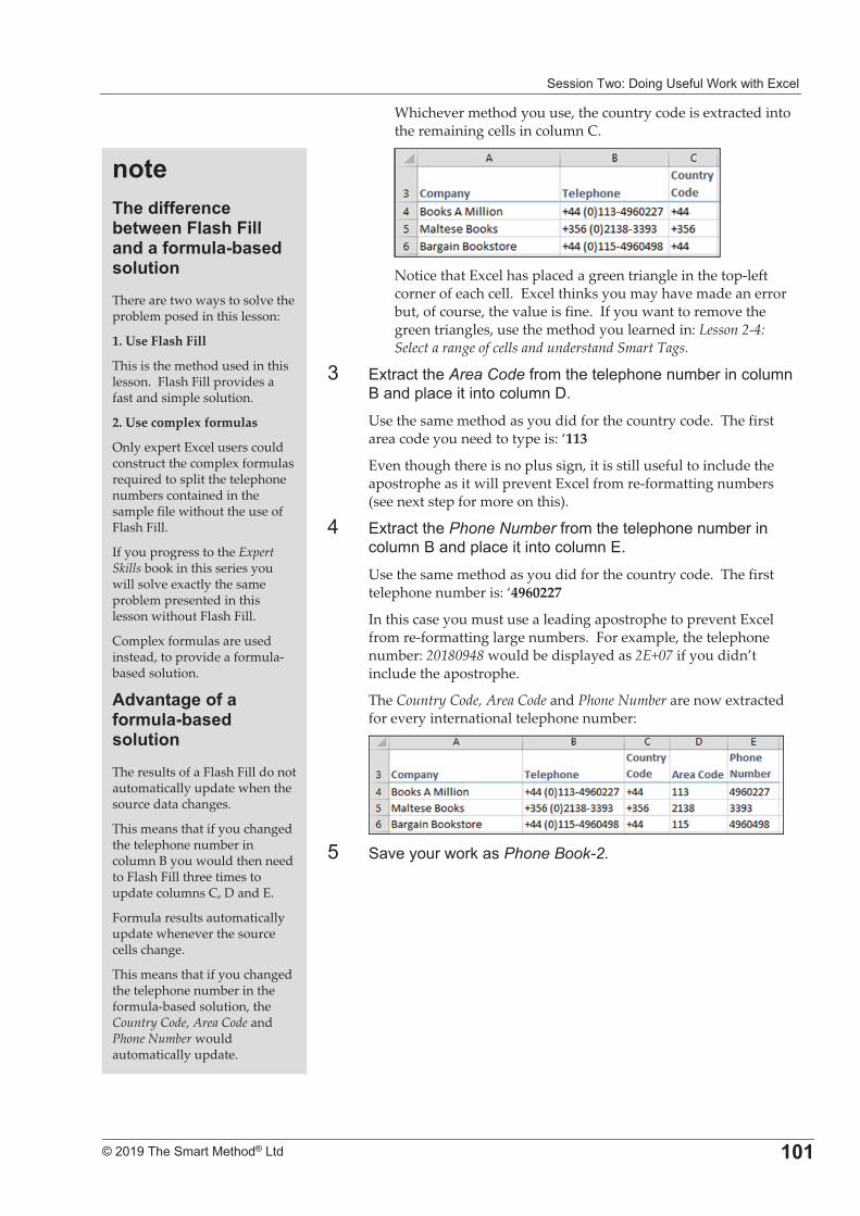
����������%�+���,�9�*�!����#������� !�
�
����������� �������������� ���
Whichever�method�you�use,�the�country�code�is�extracted�into�the�remaining�cells�in�column�C.�
�Notice�that�Excel�has�placed�a�green�triangle�in�the�top�left�corner�of�each�cell.��Excel�thinks�you�may�have�made�an�error�but,�of�course,�the�value�is�fine.��If�you�want�to�remove�the�green�triangles,�use�the�method�you�learned�in:�Lesson�2�4:�Select�a�range�of�cells�and�understand�Smart�Tags.�
-� ���� ����Area Code�*�������!$������)����� �!����"� ���$! ��������� �!����+'�Use�the�same�method�as�you�did�for�the�country�code.��The�first�area�code�you�need�to�type�is:�‘113�
Even�though�there�is�no�plus�sign,�it�is�still�useful�to�include�the�apostrophe�as�it�will�prevent�Excel�from�re�formatting�numbers�(see�next�step�for�more�on�this).�
3� ���� ����Phone Number�*�������!$������)����� �!����"� ���$! ��������� �!�����'�Use�the�same�method�as�you�did�for�the�country�code.��The�first�telephone�number�is:�‘4960227�
In�this�case�you�must�use�a�leading�apostrophe�to�prevent�Excel�from�re�formatting�large�numbers.��For�example,�the�telephone�number:�20180948�would�be�displayed�as�2E+07�if�you�didn’t�include�the�apostrophe.�
The�Country�Code,�Area�Code�and�Phone�Number�are�now�extracted�for�every�international�telephone�number:�
�6� � 0���������#� ��Phone Book-2.
������� �������!����,�����,������ ������#���!�� ����������There�are�two�ways�to�solve�the�problem�posed�in�this�lesson:�
1.�Use�Flash�Fill�
This�is�the�method�used�in�this�lesson.��Flash�Fill�provides�a�fast�and�simple�solution.�
2.�Use�complex�formulas�
Only�expert�Excel�users�could�construct�the�complex�formulas�required�to�split�the�telephone�numbers�contained�in�the�sample�file�without�the�use�of�Flash�Fill.�
If�you�progress�to�the�Expert�Skills�book�in�this�series�you�will�solve�exactly�the�same�problem�presented�in�this�lesson�without�Flash�Fill.�
Complex�formulas�are�used�instead,�to�provide�a�formula�based�solution.�
" ���������������#���!�� ����������The�results�of�a�Flash�Fill�do�not�automatically�update�when�the�source�data�changes.�
This�means�that�if�you�changed�the�telephone�number�in�column�B�you�would�then�need�to�Flash�Fill�three�times�to�update�columns�C,�D�and�E.�
Formula�results�automatically�update�whenever�the�source�cells�change.�
This�means�that�if�you�changed�the�telephone�number�in�the�formula�based�solution,�the�Country�Code,�Area�Code�and�Phone�Number�would�automatically�update.�
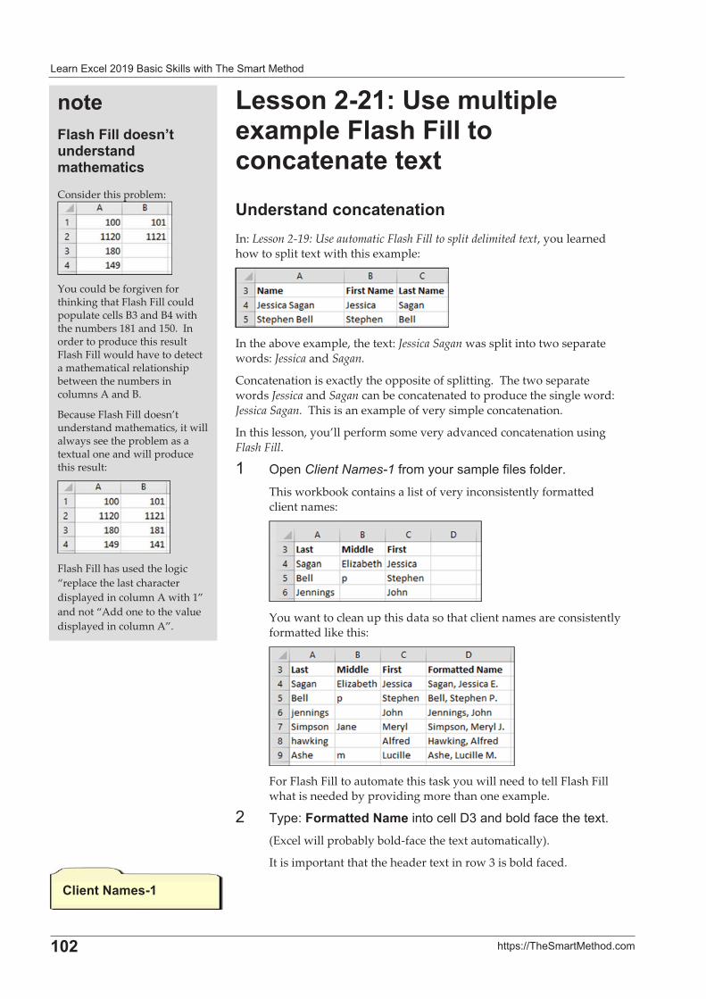
� ����� !������" �� ��#�!!���������� ��������
�
���� ��$�%&&��� ������' ��
%��������2�5��#����*����#*��,�����,���������������������5� ����� ��������������In:�Lesson�2�19:�Use�automatic�Flash�Fill�to�split�delimited�text,�you�learned�how�to�split�text�with�this�example:�
�In�the�above�example,�the�text:�Jessica�Sagan�was�split�into�two�separate�words:�Jessica�and�Sagan.�
Concatenation�is�exactly�the�opposite�of�splitting.��The�two�separate�words�Jessica�and�Sagan�can�be�concatenated�to�produce�the�single�word:�Jessica�Sagan.��This�is�an�example�of�very�simple�concatenation.�
In�this�lesson,�you’ll�perform�some�very�advanced�concatenation�using�Flash�Fill.�
�� /$��Client Names-1 *���������� �$!�*�!��*�!��'�This�workbook�contains�a�list�of�very�inconsistently�formatted�client�names:�
�You�want�to�clean�up�this�data�so�that�client�names�are�consistently�formatted�like�this:�
�For�Flash�Fill�to�automate�this�task�you�will�need�to�tell�Flash�Fill�what�is�needed�by�providing�more�than�one�example.�
�� ��$%�,��#��� �C�#������ !!�+-� ���)�!��* ������'�(Excel�will�probably�bold�face�the�text�automatically).�
It�is�important�that�the�header�text�in�row�3�is�bold�faced.�
.�����C�#���
����,�����,���� ���8���� ����� �#���#������
Consider�this�problem:
�You�could�be�forgiven�for�thinking�that�Flash�Fill�could�populate�cells�B3�and�B4�with�the�numbers�181�and�150.��In�order�to�produce�this�result�Flash�Fill�would�have�to�detect�a�mathematical�relationship�between�the�numbers�in�columns�A�and�B.�
Because�Flash�Fill�doesn’t�understand�mathematics,�it�will�always�see�the�problem�as�a�textual�one�and�will�produce�this�result:�
�
Flash�Fill�has�used�the�logic�“replace�the�last�character�displayed�in�column�A�with�1”�and�not�“Add�one�to�the�value�displayed�in�column�A”.�
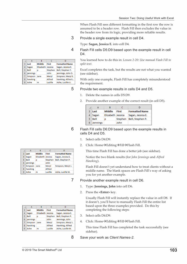
����������%�+���,�9�*�!����#������� !�
�
����������� �������������� ��;
When�Flash�Fill�sees�different�formatting�in�the�first�row�the�row�is�assumed�to�be�a�header�row.��Flash�Fill�then�excludes�the�value�in�the�header�row�from�its�logic,�providing�more�reliable�results.�
-� D��0��� ����,!�� �$!����!����� !!�+3'�Type:�Sagan,�Jessica�E.�into�cell�D4.�
3� F! ��F�!!� !!��+6%+��) ����$������ �$!����!����� !!�+3'�You�learned�how�to�do�this�in:�Lesson�2�20:�Use�manual�Flash�Fill�to�split�text.�
Excel�completes�the�task,�but�the�results�are�not�what�you�wanted�(see�sidebar).�
With�only�one�example,�Flash�Fill�has�completely�misunderstood�the�requirement.�
6� D��0�������� �$!����!������ !!��+3� ���+6'�1.� Delete�the�names�in�cells�D5:D9.�
2.� Provide�another�example�of�the�correct�result�(in�cell�D5).�
�7� F! ��F�!!� !!��+7%+��) ����$������ �$!����!������
!!��+3� ���+6'�1.� Select�cells�D4:D9.�
2.� Click:�Home�Editing�Fill�Flash�Fill.�
This�time�Flash�Fill�has�done�a�better�job�(see�sidebar).�
Notice�the�two�blank�results�(for�John�Jennings�and�Alfred�Hawking).���
Flash�Fill�doesn’t�yet�understand�how�to�treat�clients�without�a�middle�name.��The�blank�spaces�are�Flash�Fill’s�way�of�asking�you�for�yet�another�example.�
8� D��0��� ������ �$!����!����� !!�+7'�1.� Type:�Jennings,�John�into�cell�D6.�
2.� Press�the�<Enter>�key.�
Usually�Flash�Fill�will�instantly�replace�the�value�in�cell�D8.��If�it�doesn’t,�you’ll�have�to�manually�Flash�Fill�the�entire�list�based�upon�the�three�examples�provided.��Do�this�by�completing�the�following�steps:�
3.� Select�cells�D4:D9.�
4.� Click:�Home�Editing�Fill�Flash�Fill.�
This�time�Flash�Fill�has�completed�the�task�successfully�(see�sidebar).�
E� � 0���������#� ��Client Names-2.
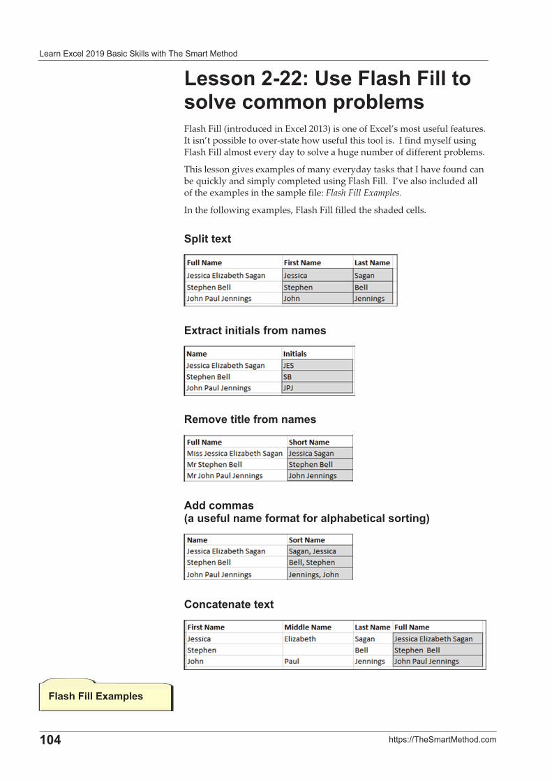
� ����� !������" �� ��#�!!���������� ��������
�
��0� ��$�%&&��� ������' ��
%��������2�5��,�����,��������������##���*��!�#���Flash�Fill�(introduced�in�Excel�2013)�is�one�of�Excel’s�most�useful�features.�It�isn’t�possible�to�over�state�how�useful�this�tool�is.��I�find�myself�using�Flash�Fill�almost�every�day�to�solve�a�huge�number�of�different�problems.�
This�lesson�gives�examples�of�many�everyday�tasks�that�I�have�found�can�be�quickly�and�simply�completed�using�Flash�Fill.��I’ve�also�included�all�of�the�examples�in�the�sample�file:�Flash�Fill�Examples.�
In�the�following�examples,�Flash�Fill�filled�the�shaded�cells.�
+*��������
�
��������������������#���#��
�
<#�����������#���#��
�
" ���##����'����������#����#���������*��!�������������(�
�
.�������������
�
,�����,�������#*���
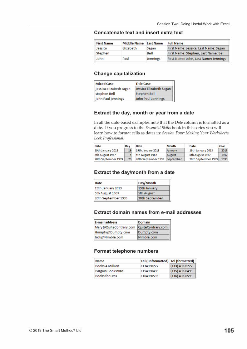
����������%�+���,�9�*�!����#������� !�
�
����������� �������������� ��>
.��������������� ����������������
�
.�������*�����A������
�
����������� ��:�#���������������#��� ���
In�all�the�date�based�examples�note�that�the�Date�column�is�formatted�as�a�date.��If�you�progress�to�the�Essential�Skills�book�in�this�series�you�will�learn�how�to�format�cells�as�dates�in:�Session�Four:�Making�Your�Worksheets�Look�Professional.�
�
����������� ��B#��������#��� ���
�
�������� �#������#�����#�#����� �����
�
,��#�����*������#!���
��
�
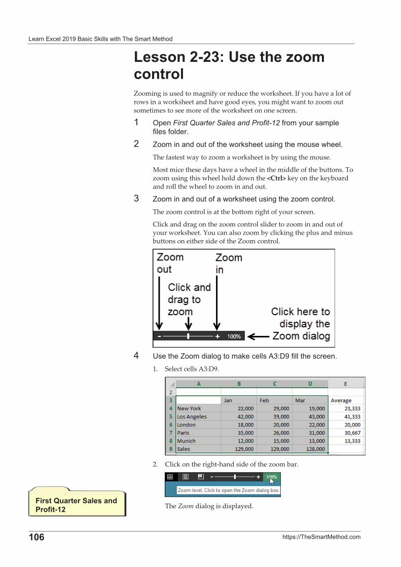
� ����� !������" �� ��#�!!���������� ��������
�
��6� ��$�%&&��� ������' ��
%�������;2�5�����A��#���������Zooming�is�used�to�magnify�or�reduce�the�worksheet.�If�you�have�a�lot�of�rows�in�a�worksheet�and�have�good�eyes,�you�might�want�to�zoom�out�sometimes�to�see�more�of�the�worksheet�on�one�screen.�
�� /$��First Quarter Sales and Profit-12 *���������� �$!�*�!��*�!��'�
�� =������� ��������*������#�������,���������!'�The�fastest�way�to�zoom�a�worksheet�is�by�using�the�mouse.�
Most�mice�these�days�have�a�wheel�in�the�middle�of�the�buttons.�To�zoom�using�this�wheel�hold�down�the�<Ctrl>�key�on�the�keyboard�and�roll�the�wheel�to�zoom�in�and�out.�
-� =������� ��������*� ����#�������,���;���� �����!'�The�zoom�control�is�at�the�bottom�right�of�your�screen.��
Click�and�drag�on�the�zoom�control�slider�to�zoom�in�and�out�of�your�worksheet.�You�can�also�zoom�by�clicking�the�plus�and�minus�buttons�on�either�side�of�the�Zoom�control.��
�3� 9����=������ !�,����� #� !!��?-%+��*�!!���� ��'�
1.� Select�cells�A3:D9.�
�2.� Click�on�the�right�hand�side�of�the�zoom�bar.�
�The�Zoom�dialog�is�displayed.�
,�����H������+������ �7��������
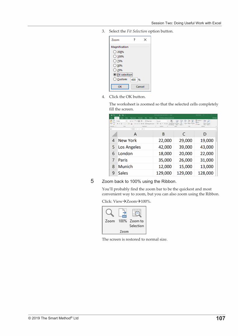
����������%�+���,�9�*�!����#������� !�
�
����������� �������������� ��3
3.� Select�the�Fit�Selection�option�button.�
�4.� Click�the�OK�button.�
The�worksheet�is�zoomed�so�that�the�selected�cells�completely�fill�the�screen.�
�6� =����) #�������M�����,���:�))��'�
You’ll�probably�find�the�zoom�bar�to�be�the�quickest�and�most�convenient�way�to�zoom,�but�you�can�also�zoom�using�the�Ribbon.�
Click:�View�Zoom�100%.�
�The�screen�is�restored�to�normal�size.�
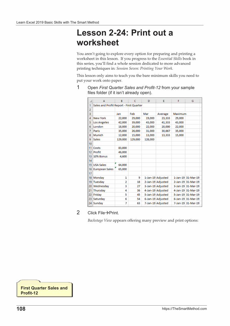
� ����� !������" �� ��#�!!���������� ��������
�
��=� ��$�%&&��� ������' ��
%�������02�7�������������� ����You�aren’t�going�to�explore�every�option�for�preparing�and�printing�a�worksheet�in�this�lesson.��If�you�progress�to�the�Essential�Skills�book�in�this�series,�you’ll�find�a�whole�session�dedicated�to�more�advanced�printing�techniques�in:�Session�Seven:�Printing�Your�Work.�
This�lesson�only�aims�to�teach�you�the�bare�minimum�skills�you�need�to�put�your�work�onto�paper.�
�� /$��First Quarter Sales and Profit.12�*���������� �$!�*�!��*�!���1�*���������� !� ����$�2'��
�
�� (!� #�F�!�D����'��
Backstage�View�appears�offering�many�preview�and�print�options:�
,�����H������+������ �7��������
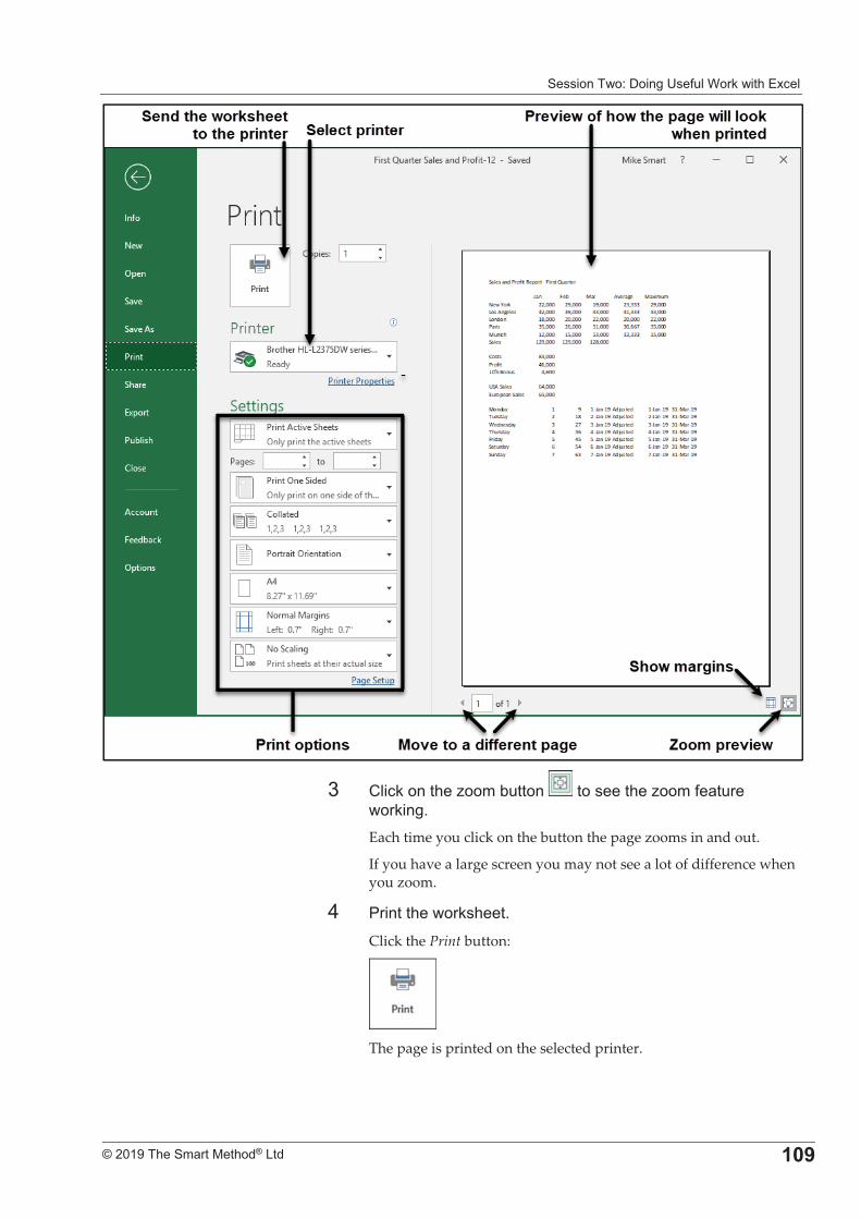
����������%�+���,�9�*�!����#������� !�
�
����������� �������������� ���
�
-� (!� #������;����)������ ��������;����* �������#��,'�Each�time�you�click�on�the�button�the�page�zooms�in�and�out.�
If�you�have�a�large�screen�you�may�not�see�a�lot�of�difference�when�you�zoom.�
3� D����������#��'�
Click�the�Print�button:�
�The�page�is�printed�on�the�selected�printer.�
�
�

�
�
�������������� ������������ � ���
�
�
�
�
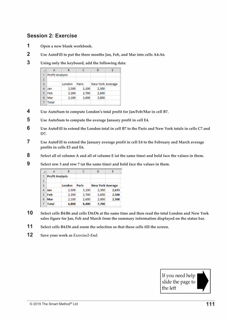
�
�
�������������� �������������� � ���
+�������2���������
�� Open�a�new�blank�workbook.�
�� Use�AutoFill�to�put�the�three�months�Jan,�Feb,�and�Mar�into�cells�A4:A6.�
;� Using�only�the�keyboard,�add�the�following�data:�
�
0� Use�AutoSum�to�compute�London’s�total�profit�for�Jan/Feb/Mar�in�cell�B7.�
>� Use�AutoSum�to�compute�the�average�January�profit�in�cell�E4.�
6� Use�AutoFill�to�extend�the�London�total�in�cell�B7�to�the�Paris�and�New�York�totals�in�cells�C7�and�D7.�
3� Use�AutoFill�to�extend�the�January�average�profit�in�cell�E4�to�the�February�and�March�average�profits�in�cells�E5�and�E6.�
=� Select�all�of�column�A�and�all�of�column�E�(at�the�same�time)�and�bold�face�the�values�in�them.�
�� Select�row�3�and�row�7�(at�the�same�time)�and�bold�face�the�values�in�them.�
�
��� Select�cells�B4:B6�and�cells�D4:D6�at�the�same�time�and�then�read�the�total�London�and�New�York�sales�figure�for�Jan,�Feb�and�March�from�the�summary�information�displayed�on�the�status�bar.�
��� Select�cells�B4:D6�and�zoom�the�selection�so�that�these�cells�fill�the�screen.�
��� Save�your�work�as�Exercise2�End.��
�
�
�

�
�
�������������� ������������ � ���
�
�
�
�
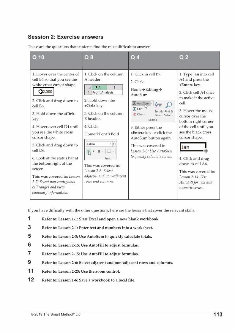
�
�
�������������� �������������� � ��;
+�������2����������������These�are�the�questions�that�students�find�the�most�difficult�to�answer:�
H���� H�=� H�0� H���
1.�Hover�over�the�center�of�cell�B4�so�that�you�see�the�white�cross�cursor�shape.
��2.�Click�and�drag�down�to�cell�B6.��
3.�Hold�down�the�<Ctrl>�key.�
4.�Hover�over�cell�D4�until�you�see�the�white�cross�cursor�shape.�
5.�Click�and�drag�down�to�cell�D6.�
6.�Look�at�the�status�bar�at�the�bottom�right�of�the�screen.�
This�was�covered�in:�Lesson�2�7:�Select�non�contiguous�cell�ranges�and�view�summary�information.�
1.�Click�on�the�column�A�header.�
�2.�Hold�down�the�<Ctrl>�key.�
3.�Click�on�the�column�E�header.�
4.�Click:�
Home�Font�Bold�
�This�was�covered�in:�Lesson�2�6:�Select�adjacent�and�non�adjacent�rows�and�columns.�
1.�Click�in�cell�B7.��
2.�Click:�
Home�Editing��AutoSum�
�3.�Either�press�the�<Enter>�key�or�click�the�AutoSum�button�again.�
This�was�covered�in:�Lesson�2�3:�Use�AutoSum�to�quickly�calculate�totals.�
1.�Type�Jan�into�cell�A4�and�press�the�<Enter>�key.�
2.�Click�cell�A4�once�to�make�it�the�active�cell.�
3.�Hover�the�mouse�cursor�over�the�bottom�right�corner�of�the�cell�until�you�see�the�black�cross�cursor�shape.�
�4.�Click�and�drag�down�to�cell�A6.��
This�was�covered�in:�Lesson�2�14:�Use�AutoFill�for�text�and�numeric�series.�
�
If�you�have�difficulty�with�the�other�questions,�here�are�the�lessons�that�cover�the�relevant�skills:�
�� Refer�to:�Lesson�1�1:�Start�Excel�and�open�a�new�blank�workbook.�
;� Refer�to:�Lesson�2�1:�Enter�text�and�numbers�into�a�worksheet.�
>� Refer�to:�Lesson�2�3:�Use�AutoSum�to�quickly�calculate�totals.�
6� Refer�to:�Lesson�2�15:�Use�AutoFill�to�adjust�formulas.�
3� Refer�to:�Lesson�2�15:�Use�AutoFill�to�adjust�formulas.�
�� Refer�to:�Lesson�2�6:�Select�adjacent�and�non�adjacent�rows�and�columns.�
��� Refer�to:�Lesson�2�23:�Use�the�zoom�control.�
��� Refer�to:�Lesson�1�6:�Save�a�workbook�to�a�local�file.�
�
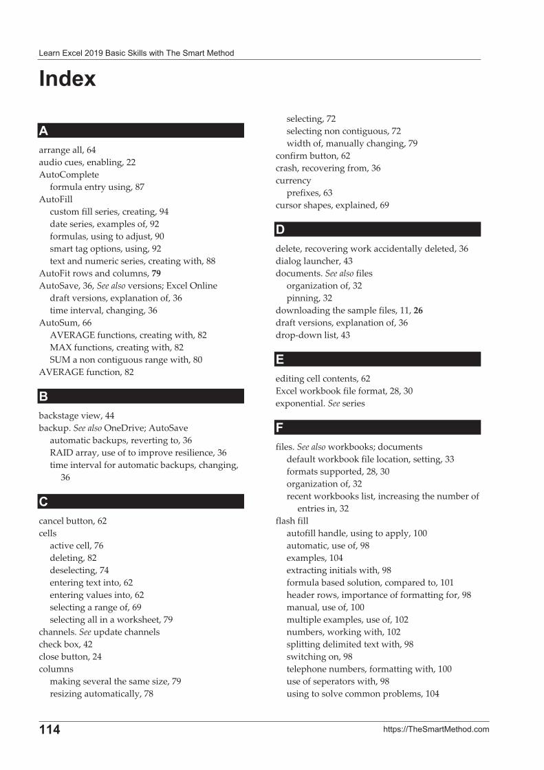
� ����� !������" �� ��#�!!���������� ��������
�
��0� ��$�%&&��� ������' ��
/� ��
"�arrange�all,�64�audio�cues,�enabling,�22�AutoComplete�
formula�entry�using,�87�AutoFill�
custom�fill�series,�creating,�94�date�series,�examples�of,�92�formulas,�using�to�adjust,�90�smart�tag�options,�using,�92�text�and�numeric�series,�creating�with,�88�
AutoFit�rows�and�columns,�79�AutoSave,�36,�See�also�versions;�Excel�Online�
draft�versions,�explanation�of,�36�time�interval,�changing,�36�
AutoSum,�66�AVERAGE�functions,�creating�with,�82�MAX�functions,�creating�with,�82�SUM�a�non�contiguous�range�with,�80�
AVERAGE�function,�82�
��backstage�view,�44�backup.�See�also�OneDrive;�AutoSave�
automatic�backups,�reverting�to,�36�RAID�array,�use�of�to�improve�resilience,�36�time�interval�for�automatic�backups,�changing,�
36�
.�cancel�button,�62�cells�
active�cell,�76�deleting,�82�deselecting,�74�entering�text�into,�62�entering�values�into,�62�selecting�a�range�of,�69�selecting�all�in�a�worksheet,�79�
channels.�See�update�channels�check�box,�42�close�button,�24�columns�
making�several�the�same�size,�79�resizing�automatically,�78�
selecting,�72�selecting�non�contiguous,�72�width�of,�manually�changing,�79�
confirm�button,�62�crash,�recovering�from,�36�currency�
prefixes,�63�cursor�shapes,�explained,�69�
4�delete,�recovering�work�accidentally�deleted,�36�dialog�launcher,�43�documents.�See�also�files�
organization�of,�32�pinning,�32�
downloading�the�sample�files,�11,�26�draft�versions,�explanation�of,�36�drop�down�list,�43�
��editing�cell�contents,�62�Excel�workbook�file�format,�28,�30�exponential.�See�series�
,�files.�See�also�workbooks;�documents�
default�workbook�file�location,�setting,�33�formats�supported,�28,�30�organization�of,�32�recent�workbooks�list,�increasing�the�number�of�
entries�in,�32�flash�fill�
autofill�handle,�using�to�apply,�100�automatic,�use�of,�98�examples,�104�extracting�initials�with,�98�formula�based�solution,�compared�to,�101�header�rows,�importance�of�formatting�for,�98�manual,�use�of,�100�multiple�examples,�use�of,�102�numbers,�working�with,�102�splitting�delimited�text�with,�98�switching�on,�98�telephone�numbers,�formatting�with,�100�use�of�seperators�with,�98�using�to�solve�common�problems,�104�
4����
�
����������� ������������� ��>
formula�bar�explanation�of,�68�graphic�showing�location�of,�28�
formulas�Autocomplete,�creating�with,�86�AutoFill,�adjusting�with,�90�AVERAGE�function,�creating�using�AutoSum,�
82�F2�key�to�display�range�addressed�by,�83�formula�bar,�viewing�in,�68�MAX�function,�creating�using�AutoSum,�82�mouse�selection,�creating�with,�84�multiplication�operator�(*)�using�in,�85�SUM�function,�creating�using�AutoSum,�66�syntax�box,�understanding,�87�visual�keyboard�technique,�creating�with,�85�
fractions,�entering�into�cells,�63�full�screen�view,�50�functions�
AVERAGE,�82�help�topics,�accessing�from�formula�
AutoComplete,�87�MAX,�82�SUM,�66,�80�
@�gallery,�42�goto�special,�77�growth.�See�series�
)�help�system.�See�also�tell�me�help�
F1�key,�accessing�older�help�system�with,�54�formula�AutoComplete,�accessing�help�topics�
from,�87�ribbon,�accessing�help�topics�directly�from,�54�
K�key�tips,�46�keyboard�shortcuts�
AutoSelect�a�range,�77�AutoSum,�66�bold,�47�close,�25�cycle�through�worksheets,�35�flash�fill,�100�italic,�47�ribbon,�show/hide,�40�save,�28�select�every�cell�in�a�worksheet,�78�
underline,�47�workbook,�create�new,�64�
%�license.�See�also�update�channels�
Excel�2019,�20�perpetual�and�subscription,�differences,�20�subscription,�20�
��marching�ants,�66�marquee,�66�MAX�function,�creating�using�AutoSum,�82�maximize�button,�24�menus�
rich,�43�shortcut�(contextual),�47�standard,�42�
mini�toolbar�shortcut�(contextual)�menu,�47�using�when�entering�text,�46�
minimize�button,�24�moving�
the�Excel�window,�24�multiplication�operator�(*),�85�
C�name�box,�26�negative�numbers,�entering�into�cells,�63�normal�view,�48�number�sign�(#),�78�
1�office�theme,�changing,�22�office�version�
checking�Excel�version,�21�version�number�and�build�number�explained,�
20�organizing�
excel�files,�32�sample�files�folder,�26�
7�page�break�preview,�48�page�layout�view,�48�PDF,�workbook�format,�31�pound�sign�(#),�78�printing�
page�break�preview,�48�
� ����� !������" �� ��#�!!���������� ��������
�
��6� ��$�%&&��� ������' ��
previewing�on�screen,�44�protected�view,�potential�problems�when�
downloading�sample�files,�26�
H�quick�access�toolbar�
adding�commands�to,�44�adding�separators�to,�44�deleting�commands�from,�44�
quick�analysis�totals,�creating�with,�67�
quotations�Aristotle,�42�Baltasar�Gracián,�96�Confucius,�5�Euripides,�17�Robert�Collier,�24�Winston�Churchill,�4�
<�RAID�array,�36�ranges�
AutoSelect�,�selecting�automatically�with,�76�copying�data�across,�70�entering�data�into,�70�non�contiguous,�selecting,�74�select�all�button,�to�select�a�range�containing�
every�cell�in�a�worksheet,�79�selecting,�68�selecting�visually�for�formulas�with�the�mouse,�
84�restore�down�button,�24�ribbon�
benefits�of�wide�screen�with,�40�command�groups�on,�42�contextual�tabs,�explanation�of,�40�controls�on,�42�customizing,�40�default,�resetting�to,�40�font�panel�controls,�explanation�of,�40�overview,�40�showing�and�hiding�(minimizing),�40�
rows�making�several�the�same�size,�79�manually�setting�height�of,�79�resizing�automatically,�78�selecting,�72�selecting�non�contiguous,�72�
+�sample�files�
downloading,�11,�26�organizing�folder,�26�potential�protected�view�problem�when�
downloading,�26�save,�28,�30�
AutoSave,�using�to�recover�work�after�crash,�36�selecting�cells,�68�series�
dialog,�96�exponential,�96�growth,�96�linear,�96�start�value,�96�step�value,�96�stop�value,�96�
smart�tag�explained,�68�options,�92�
sounds�enabling�audio�cues,�22�
split�button,�42�start�Excel,�18�SUM�function�
creating�manually�using�formula�AutoComplete,�86�
creating�using�AutoSum,�66�switch�windows,�64�
��tabs.�See�worksheets�telephone�numbers,�formatting�with�flash�fill,�100�tell�me�help�
Alt+Q�keyboard�shortcut,�using�to�access�tell�me�help�box,�52�
execute�command,�using�to,�52�using,�52�
the�smart�method�learning�by�participation,�5�two�facing�pages�rule,�4�
themes.�See�also�office�theme�title�bar,�64�trend.�See�also�series�
linear�and�exponential,�96�trend�line.�See�charts�
5�update�channels�
automatic�updates,�enabling,�20�
4����
�
����������� ������������� ��3
explained,�20�updates.�See�update�channels�
?�values�
currency�prefixes,�using�with,�63�entering�into�cells,�62�fractions,�entering�into�cells,�63�negative�numbers,�entering�into�cells,�63�
versions.�See�also�AutoSave�earlier�versions,�viewing,�38�explanation�of,�36�recovering�an�earlier�version�of�a�workbook,�38�
$�windows�
arrange�all,�using�to�automatically�size,�64�closing,�24�moving,�24�resizing,�24�restoring�down,�24�switching�to�view�a�different�workbook,�64�
workbooks.�See�also�files�changing�default�number�of�worksheets�in,�34�
creating�new,�64�opening,�26�recent�workbooks�list,�increasing�the�number�of�
entries�in,�32�saving,�28,�30�switching�between�open�workbooks,�64�viewing�two�at�the�same�time,�64�views,�48�
worksheets�adding,�34�changing�default�number�of,�34�chart�worksheets,�explanation�of,�34�deleting,�34�maximum�number�of�rows�and�columns�in,�26�navigating,�26,�34�renaming,�34�tab�colors,�changing,�35�
D�XPS,�workbook�format,�31�
Q�zoom�control,�106�
��
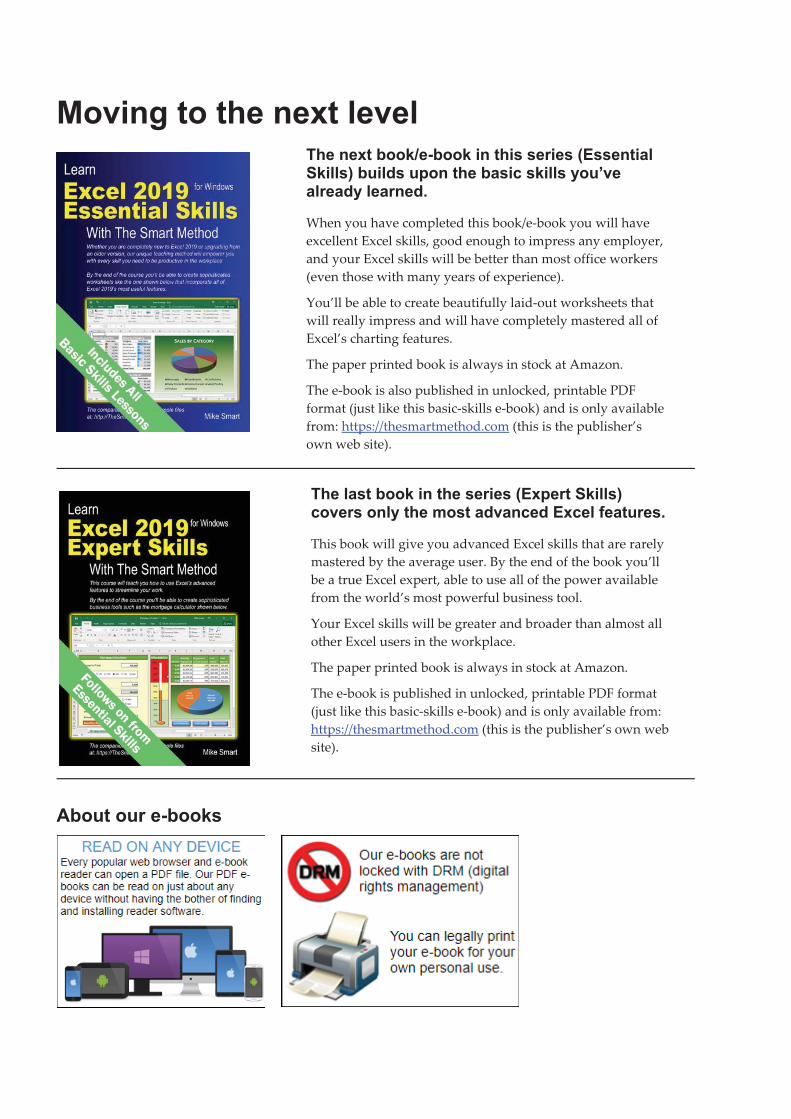
�
�
��������������������������������������������������������
"!��������!�� ����
� �
�������!�� B!�� ��������������'���������+ ����(�!��� ���*������!������ ��������8������ ������ ����
When�you�have�completed�this�book/e�book�you�will�have�excellent�Excel�skills,�good�enough�to�impress�any�employer,�and�your�Excel�skills�will�be�better�than�most�office�workers�(even�those�with�many�years�of�experience).���
You’ll�be�able�to�create�beautifully�laid�out�worksheets�that�will�really�impress�and�will�have�completely�mastered�all�of�Excel’s�charting�features.��
The�paper�printed�book�is�always�in�stock�at�Amazon.���
The�e�book�is�also�published�in�unlocked,�printable�PDF�format�(just�like�this�basic�skills�e�book)�and�is�only�available�from:�https://thesmartmethod.com�(this�is�the�publisher’s�own�web�site).�
��������!�� ������������'��*���+ ����(���������������#����� ���� ����������������
This�book�will�give�you�advanced�Excel�skills�that�are�rarely�mastered�by�the�average�user.�By�the�end�of�the�book�you’ll�be�a�true�Excel�expert,�able�to�use�all�of�the�power�available�from�the�world’s�most�powerful�business�tool.���
Your�Excel�skills�will�be�greater�and�broader�than�almost�all�other�Excel�users�in�the�workplace.��
The�paper�printed�book�is�always�in�stock�at�Amazon.���
The�e�book�is�published�in�unlocked,�printable�PDF�format�(just�like�this�basic�skills�e�book)�and�is�only�available�from:�https://thesmartmethod.com�(this�is�the�publisher’s�own�web�site).�
� � �
�
�
����
%������������**����������������� ������������+#�������� �������������� ���
For�over�900�years�craftsmen�have�traditionally�taught�their�skills�to�an�apprentice.�In�this�model�the�apprentice�learned�his�trade�by�observing�how�the�master�craftsman�used�his�skills.�This�construction�kit�will�teach�you�advanced�Excel�skills�in�the�same�way.�Even�if�you�only�have�basic�Excel�skills,�the�construction�kit�is�designed�in�such�a�way�that�you’ll�be�able�to�construct�a�complex,�polished�professional�Excel�application�that�would�be�well�beyond�the�powers�of�most�advanced�Excel�users.��Available�as�both�a�printed�paper�book�and�e�book.�
Preview�the�first�chapter�free�at:�
https://thesmartmethod.com�
�����.��������
Our�Excel�online�challenges�are�a�little�like�the�exercises�at�the�end�of�each�session�in�this�book.��Unlike�the�exercises,�the�online�challenges�will�test�the�application�of�many�skills�(covered�in�different�sessions�in�the�book).�
We�began�trialling�challenges�in�July�2018�and�(at�time�of�writing�in�January�2019)�we�have�published�three�challenges.�By�the�time�you�read�this�book�we�may�have�produced�more.��
Access�the�challenges�online�at:��
https://thesmartmethod.com/excel�challenges/�
�
�
5���������������� ������������������������������#��������If�you�progress�to�the�Essential�Skills�book�in�this�series�you�will�have�excellent�Excel�skills�and�if�you�the�further�progress�to�the�Expert�Skills�book,�you’ll�be�a�true�Excel�expert�and�will�be�able�to�teach�Excel�skills�at�all�levels.��There�is�a�huge�(and�often�unsatisfied)�demand,�everywhere�in�the�world,�for�Excel�training.�
The�Basic�Skills,�Essential�Skills�and�Expert�Skills�books�are�available�for�all�Excel�versions�in�common�use�(Excel�2007,�2010,�2013,�2016,�2019�and�365�for�Windows�along�with�Excel�2016�&�2019�for�Apple�Mac).��You�can�use�the�books�as�courseware�during�your�classes�and�then�give�each�student�a�copy�of�the�book�to�take�home�as�reference�material�when�the�course�is�over.��For�larger�(100+)�book�orders�we�can�customize�your�books�by�adding�your�own�cover�design�and�logo�and�editing�content�as�required.�
�You�can�quote�the�ISBN�numbers�shown�above�to�any�book�retailer�or�wholesaler.�All�major�distributors�(in�every�country�of�the�world)�have�our�books�in�stock�for�immediate�delivery.��
7������ ������� ������>N�!�� ��������������*������� ���� ���������� �� �
To�place�a�publisher�direct�order�you�only�need�to�order�five�books�or�more�(of�the�same�title).��To�view�wholesale�prices,�go�to�this�web�page:�https://thesmartmethod.com/wholesale�printed�books�
A�new�edition�of�the�Excel�365�book�is�published�in�January�and�July�each�year�(updated�for�each�Excel�365�semi�annual�version�update).�