Embed Size (px)
Citation preview

This work is protected by copyright and other intellectual property rights and duplication or sale of all or part is not permitted, except that material may be duplicated by you for research, private study, criticism/review or educational
purposes. Electronic or print copies are for your own personal, non-commercial use and shall not be passed to any other individual. No quotation may be published without proper acknowledgement. For any other use, or to
quote extensively from the work, permission must be obtained from the copyright holder/s.

1
EFFICIENCY ANALYSIS OF
PUBLIC HIGHER EDUCATION
INSTITUTIONS IN TURKEY WITH
PARAMETRIC AND NON-
PARAMETRIC APPROACHES
by
Taptuk Emre Erkoc
A dissertation submitted to the
Institute of Social Sciences in partial fulfilment of the
requirements for the degree of
Doctor of Philosophy in Economics
June 2014
Keele University

2
Abstract
Although the number of researches measuring the efficiencies of higher education
institutions has grown especially for the last two decades, literature of both parametric and
non-parametric research on HEIs in Turkey is relatively scant compared to the countries
alike. This PhD research that fills this noticeable gap in the literature scrutinises 53 public
universities in Turkey between the full academic year of 2005-2006 and 2009-2010
covering 5-year time span. In this research, albeit the slight changes in the non-parametric
estimation, number of undergraduate students, postgraduate students and research funding
are taken as outputs, capital and labour expenses as input prices and eventually annual
expenses as total cost. Moreover, university-based features are included into the model so
as to apprehend potential heterogeneities among the universities.
The initial conclusions coming out of parametric estimation have certain suggestions
for public HEIs in Turkey. Firstly, mean efficiency performances of Turkish public
universities are fairly dispersed ranging from 70% to 90%. This would encourage a new set
of policy-making decisions to lead inefficient universities to be aware of the success of
their counterparts. Secondly, despite the fact that some universities have relatively poor
efficiency rates, in overall analysis their efficiency scores are indicating optimistic signs
relying on certain models. Lastly, developing different models do matter for efficiency
analysis in the sense that dispersion of efficiency values among Turkish universities does
vary from one model to another.
The results of the non-parametric estimation claims that, firstly, public HEIs in Turkey
are performing in unsatisfactory levels although some of them are doing fairly well. The
lower results for the non-parametric estimation then the parametric one –which is totally
within the expectations-, are referring to the fact that the former method is not able to

3
differentiate the inefficiency from the statistical noise. However, as the non-parametric
model gets closer to the full input/output set, both individual and overall efficiency scores
are getting relatively higher values. Secondly, even though there is not any systemic
increase during this five-year time span, efficiencies of public HEIs in Turkey have
increased at the course of last two years.
Keywords: Cost Efficiency, Technical Efficiency, Public Sector Organizations, Higher
Education Institutions, Stochastic Frontier Analysis, Data Envelopment Analysis, Turkey

4
Acknowledgements
I would like to express my special appreciation and thanks to my advisor Dr Gabriella
Legrenzi who has been a tremendous mentor for me. I would like to thank her for
encouraging my research and for allowing me to grow as a research scientist in economics.
Her advice on both research as well as on my career have been invaluable. Besides, I am
very indebted to my second supervisors Prof Gauthier Lanot and Prof David Leece for
their valuable comments and feedback.
I would also like to thank my committee members, Professor Stephen Cropper, Professor
Bulent Gokay, and Dr Meryem Duygun Fethi for serving as my committee members. I
want to thank them for letting my oral defense be an enjoyable moment, and for their
brilliant comments and suggestions.
I would also like to thank my lecturers in undergraduate years, Dr Ertugrul Gundogan, Dr
Abdulkadir Civan, Prof Mehmet Orhan and Prof Gokhan Bacik as well as colleagues and
friends, Ozcan Keles, Ilknur Kahraman, Dr Cem Erbil, Seref Kavak, Mustafa Demir, Salih
Dogan, Ali Hamza Cakar, Muhammet Keles and Emrah Celik. Thank you for supporting
me for everything, and especially I can’t thank you enough for encouraging me throughout
this experience.
Finally I thank to my family members, words cannot express how grateful I am to my
parents Gokcen and Ramazan Erkoc, my sister Merve, and my brother Ziya for all of the
sacrifices that they’ve made on my behalf. Your love and prayers for me were what
sustained me thus far. This thesis is particularly dedicated to my parents Gokcen and
Ramazan Erkoc, and Fethullah Gulen for being a point of inspiration in pursuing a doctoral
degree in social sciences.

5
Table of Contents
CHAPTER I: Introduction and Research Agenda
I. BACKGROUND AND CONTEXT ........................................................................................ 14
II. OBJECTIVES OF THE DISSERTATION .......................................................................... 17
III. ORGANIZATION OF THE DISSERTATION ................................................................. 19
CHAPTER II: Efficiency of Public Sector Organizations
I. INTRODUCTION .................................................................................................................... 23
II. THEORETICAL FRAMEWORK FOR THE EFFICIENCY OF PUBLIC SECTOR
ORGANIZATIONS ........................................................................................................................ 24
III. ECONOMIC THEORIES OF BUREAUCRACY AND EFFICIENCY OF
GOVERNMENT OUTPUT ........................................................................................................... 29
EARLIER RESEARCH ON BUREAUCRACY ...................................................................................... 29
THREE MODELS OF UTILITY-MAXIMISING BUREAUCRACY ......................................................... 31
Budget Maximisation ................................................................................................................ 31
Slack Maximisation ................................................................................................................... 32
Expense Preference ................................................................................................................... 33
PUBLIC CHOICE THEORY AND BUREAUCRACY ............................................................................. 34
ALTERNATIVE PERSPECTIVES ON BUREAUCRACY ........................................................................ 35
Dunleavy’s Model of Bureau Shaping ...................................................................................... 36
Bureaus with Monopolistic Power ............................................................................................ 36
Bureaucrats and Politicians...................................................................................................... 37
IV. INSTITUTIONAL PERSPECTIVE ON THE EFFICIENCY OF PUBLIC PROVISION
OF SERVICES ................................................................................................................................ 38
V. CONCLUSION ....................................................................................................................... 41
CHAPTER III: Public Higher Education in Turkey
I. INTRODUCTION ....................................................................................................................... 45
II. ECONOMICS OF PUBLIC PROVISION OF HIGHER EDUCATION.......................... 46
III. CHALLENGES FOR PUBLIC HIGHER EDUCATION IN 21ST CENTURY ............. 50
IV. CONTEMPORARY OUTLOOK OF HIGHER EDUCATION IN TURKEY ............... 53
ADMINISTRATIVE AND ACADEMIC STRUCTURE ........................................................................... 54
FINANCE ........................................................................................................................................ 55
ACADEMIC SUCCESS AND RESEARCH ........................................................................................... 57
V. NON-PROFIT UNIVERSITIES IN TURKISH HIGHER EDUCATION ........................ 60
VI. CONCLUSION ...................................................................................................................... 65

6
Chapter IV: Estimation Methodology of Economic Efficiency
I. INTRODUCTION .................................................................................................................... 67
II. DEFINITION OF EFFICIENCY .......................................................................................... 68
III. DATA ENVELOPMENT ANALYSIS (DEA) .................................................................... 74
THEORETICAL FRAMEWORK ......................................................................................................... 75
CRS VS. VRS MODELS ................................................................................................................. 78
INPUT AND OUTPUT ORIENTED MEASUREMENTS ......................................................................... 80
EXTENSIONS IN DEA ..................................................................................................................... 81
Allocative Efficiency ................................................................................................................. 81
Heterogeneity ............................................................................................................................ 84
Additional Methods ................................................................................................................... 85
PREVIOUS EMPIRICAL STUDIES ..................................................................................................... 86
IV. STOCHASTIC FRONTIER ANALYSIS (SFA) ................................................................ 91
ESTIMATING INEFFICIENCY TERM ................................................................................................ 95
STOCHASTIC COST FRONTIER APPROACH .................................................................................... 97
EXTENSIONS IN SFA ..................................................................................................................... 99
Heterogeneity ............................................................................................................................ 99
Panel Data (Fixed Effects and Random Effects Models) ........................................................ 100
EMPIRICAL WORKS ON HIGHER EDUCATION .............................................................................. 102
V. COMPARISON OF DEA AND SFA AND CONCLUDING REMARKS ....................... 106
CHAPTER V: Efficiency Analysis of Public Higher Education Institutions in Turkey:
Application of Stochastic Frontier Analysis (SFA)
I. INTRODUCTION .................................................................................................................. 109
II. COST FUNCTION OF HIGHER EDUCATION INSTIUTIONS .................................. 110
III. SELECTION OF VARIABLES ........................................................................................ 113
SELECTION OF OUTPUTS ............................................................................................................. 113
SELECTION OF INPUTS ................................................................................................................. 114
ENVIRONMENTAL VARIABLES FOR HEIS .................................................................................... 116
IV. DATA AND EMPIRICAL MODEL ................................................................................. 118
V. INTERPRETATION OF RESULTS .................................................................................. 122
COST FRONTIER PARAMETERS .................................................................................................... 122
Cobb-Douglas Specification ................................................................................................... 123
Translog Specification ............................................................................................................ 127
EFFICIENCY LEVEL ...................................................................................................................... 134
COMPARISON OF DIFFERENT MODELS WITH SPEARMAN RANK CORRELATION ......................... 136
DETERMINANTS OF INEFFICIENCY .............................................................................................. 137
VI. LIMITATIONS AND CONCLUDING REMARKS ....................................................... 141

7
CHAPTER VI: Efficiency Analysis of Public Higher Education Institutions in
Turkey: Application of Data Envelopment Analysis (SFA)
I. INTRODUCTION .................................................................................................................. 144
II. SELECTION OF VARIABLES .......................................................................................... 146
OUTPUT MEASURES .................................................................................................................... 146
INPUT MEASURES ........................................................................................................................ 148
ENVIRONMENTAL FACTORS ........................................................................................................ 148
III. DATA AND MODELS ....................................................................................................... 149
DATA DESCRIPTION .................................................................................................................... 150
MODEL SPECIFICATION ............................................................................................................... 152
INCORPORATION OF ENVIRONMENTAL FACTORS ....................................................................... 153
IV. INTERPRETATION OF RESULTS ................................................................................. 154
EFFICIENCY VALUES (TECHNICAL AND COST EFFICIENCY) ....................................................... 154
CONFIDENCE INTERVALS AND BOOTSTRAPPING ........................................................................ 158
MALMQUIST INDEX (INTER-TEMPORAL ANALYSIS) ................................................................... 160
V. SPEARMAN RANK COMPARISON OF DEA MODELS .............................................. 165
VI. DETERMINANTS OF INEFFICIENCY ......................................................................... 168
VII. LIMITATIONS AND CONCLUDING REMARKS ...................................................... 172
CHAPTER VII: Critical Evaluation of Efficiency Results and Their Policy
Implications
I. INTRODUCTION .................................................................................................................. 175
II. COST EFFICIENCIES BASED ON SFA .......................................................................... 176
AVERAGE COST EFFICIENCY SCORES FOR PUBLIC HEIS IN TURKEY ......................................... 177
AVERAGE COST EFFICIENCY SCORES BY LOCATION .................................................................. 178
AVERAGE COST EFFICIENCY SCORES BY SIZE GROUPS ............................................................. 179
AVERAGE COST EFFICIENCY SCORES BY AGE OF HEIS ............................................................. 181
III. TECHNICAL AND COST EFFICIENCIES BASED ON DEA ..................................... 183
AVERAGE EFFICIENCY SCORES FOR PUBLIC HEIS IN TURKEY ................................................... 184
AVERAGE EFFICIENCY SCORES BY LOCATION ........................................................................... 185
AVERAGE EFFICIENCY SCORES BY SIZE GROUPS ....................................................................... 187
AVERAGE EFFICIENCY SCORES BY AGE OF HEIS ....................................................................... 188
IV. ECONOMIES OR DISECONOMIES OF SCALE .......................................................... 189
V. DETERMINANTS OF INEFFICIENCIES ....................................................................... 195
EFFECT OF STRUCTURE OF THE INSTITUTION ON EFFICIENCY .................................................... 198
Effect of Age of the HEI on Efficiency .................................................................................... 198

8
Effect of Size of the HEI on Efficiency .................................................................................... 199
Effect of Load of the HEI on Efficiency .................................................................................. 200
Effect of Having Medical School on Efficiency....................................................................... 200
EFFECT OF STAFF CHARACTERISTICS OF THE HEI ON EFFICIENCY ............................................ 201
Effect of Percentage of Professors on Efficiency .................................................................... 201
Effect of Percentage of Full-Time Academic Staff on Efficiency ............................................ 202
EFFECT OF STUDENT CHARACTERISTICS OF THE HEI ON EFFICIENCY ....................................... 202
Effect of Percentage of Foreign Students on Efficiency .......................................................... 203
VI. SPEARMAN RANK COMPARISON OF EFFICIENCY SCORES IN SFA AND DEA
203
VII. CONCLUSION .................................................................................................................. 205
CHAPTER VIII: Conclusion…………………………………………………………..208
Bibliography……………………………………………………………………………………..214
Appendix A………………………………………………………………………………………240
Appendix B………………………………………………………………………………………248
Appendix C………………………………………………………………………………………250
Appendix D………………………………………………………………………………………255
List of Tables

9
Table 3.1 URAP University Rankings in Turkey……………………………………….....59
Table 3.2 Percentage of State Appropriations to the Budget in Non-Profit HEIs in
Turkey..................................................................................................................................62
Table 3.3 Number of Publications in Non-Profit HEIs in Turkey (2006 vs. 2010).............63
Table 5.1 Literature review on inputs and outputs commonly used……………………..113
Table 5.2 Descriptive Statistics for SFA…………………………………………………117
Table 5.3 Cobb-Douglas Cost-Frontier Results………………………………………….121
Table 5.4 Hypothesis Results for Environmental Variables (Cobb-Douglas)…...............123
Table 5.5 Translog Cost-Frontier Results………………………………………………..125
Table 5.6 Hypothesis Results for Environmental Variables (Translog)……….………...127
Table 5.7 Hypothesis Testing for Model Specification: Cobb-Douglas vs. Translog.......130
Table 5.8 Hypothesis Testing for Model Specification: Incorporation of Environmental
Variables………………………………………………………………………………….130
Table 5.9 Descriptive Statistics for Mean Efficiency Values……………………………131
Table 5.10 Spearman Rank Correlations (SFA)……………………………………….…133
Table 5.11 Regression Results for Determinants of Inefficiencies………………………136
Table 6.1 Descriptive Statistics for DEA………………………………………………...152
Table 6.2 Alternative DEA Models………………………………………………………153
Table 6.3 Summary Statistics for Estimated Efficiencies (CRS)………………………...156

10
Table 6.4 Summary Statistics for Estimated Efficiencies (VRS)………………………...158
Table 6.5 Average Malmquist Results across HEIs……………………………………...162
Table 6.6 Malmquist Index Results by Individual Universities………………………….165
Table 6.7: Spearman Rank Correlation for CRS Models………………………………...167
Table 6.8: Spearman Rank Correlation for VRS Models………………………………...168
Table 6.9: Spearman Rank Correlation for CRS vs. VRS Models……………………….168
Table 6.10 Tobit Regression Results for Pool Data……………………………………...170
Table 6.11 Tobit Regression Results for Panel Data…………………………………….172
Table 7.1 Average Cost Efficiency Scores for Public HEIs in Turkey (Yearly Basis)…..179
Table 7.2 Average Cost Efficiency Scores for Public HEIs in Turkey (by Location)…...180
Table 7.3 Average Cost Efficiency Scores for Public HEIs in Turkey (by Size Groups)..181
Table 7.4 Average Cost Efficiency Scores for Public HEIs in Turkey (by Location)…...183
Table 7.5 Average Technical Efficiency Scores for Public HEIs in Turkey (Yearly
Basis)……………………………………………………………………………………..185
Table 7.6 Average Cost Efficiency Scores for Public HEIs in Turkey (Yearly Basis)…..186
Table 7.7 Average Cost Efficiency Scores for Public HEIs in Turkey (by Location)…...187
Table 7.8 Average Cost Efficiency Scores for Public HEIs in Turkey (by Size Groups)..188
Table 7.9 Average Cost Efficiency Scores for Public HEIs in Turkey (by Location)…...189
Table 7.10 Economies of Scale for Public HEIs in Turkey (Yearly Basis)……………...193

11
Table 7.11 Average Level of Outputs for Public HEIs in Turkey (Yearly Basis)……….194
Table 7.12 Determinants of Cost Inefficiencies………………………………………….198
Table 7.13 Spearman Rank Correlations between SFA and DEA (CRS Models)……….206
Table 7.14 Spearman Rank Correlations between SFA and DEA (VRS Models)……….206

12
List of Figures
Figure 2.1 Provision of Monopolistic Bureau…..................................................…………38
Figure 3.1 Positive Externality for Higher Education Provision……………………….….47
Figure 3.2 Number of Public HEIs in Turkey (1970-2012)……………………………….53
Figure 3.3 Types of Funding in the Turkish Public Higher Education (1995-2005)......….55
Figure 3.4 Percentage of Higher Education Spending in GNP for Turkey……..................56
Figure 3.5 Amount of Research Projects allocated by TÜBİTAK……………...................57
Figure 3.6 Number of Enrolled Students in the Turkish Non-Profit Universities………...60
Figure 3.7 Number of Non-Profit HEIs in Turkey……………………………...................61
Figure 4.1 Level Set, Isoquant Curve and Efficient Set…………………………………...69
Figure 4.2 Technical and Allocative Efficiency…………………………………………...70
Figure 4.3 Koopmans and Farell Efficiency Points……………………………………….77
Figure 4.4 CRS and VRS Frontier Models………………………………………………...78
Figure 4.5 Output Orientation in DEA Frontiers………………………………………….79
Figure 4.6 OLS Production Frontier Estimators…………………………………………..90
Figure 5.1 Average Cost Efficiencies over Time……………………………………...…132
Figure 6.1 95% Confidence Intervals of DEA Efficiency Scores………………………..161
Figure 6.2 Average Malmquist Results across HEIs (2006-2010)……………………….163
Figure 7.1 Average Cost Efficiency Scores for Public HEIs in Turkey (by Location)…..180

13
Figure 7.2 Average Cost Efficiency Scores for Public HEIs in Turkey (by Size
Groups)...............................................................................................................................182
Figure 7.3 Average Cost Efficiency Scores for Public HEIs in Turkey (by Location)…..183
Figure 7.4 Average Cost Efficiency Scores for Public HEIs in Turkey (by Location with
DEA)…………………………………………………………………………………......187
Figure 7.5 Average Cost Efficiency Scores for Public HEIs in Turkey (by Size Groups
with
DEA)……………………………………………………………………………………..189
Figure 7.6 Average Cost Efficiency Scores for Public HEIs in Turkey (by Location with
DEA)……………………………………………………………………………………..190
Figure 7.7 Economies of Scale for Public HEIs in Turkey (2006-2010)………………...193
Figure 7.8 Average Levels of Outputs (Yearly Basis)…………………………………...195

14
CHAPTER I: Introduction and Research Agenda
I. BACKGROUND and CONTEXT
Rising economic inquiry on the provision of goods and services by public institutions
recently sparked an investigative research on the efficient allocation of resources within
public sector organizations (Kang, 1997; Duncombe, Miner, and Ruggiero 1997; Pedraja-
Chaparro et al., 2005). Whereas neo-classical assumptions on the theory of firm put
forward by Coase (1937) and Alchian and Demsetz (1972) assume that a firm is always
expected to operate at the efficient production frontier, unpredicted divergences from the
neo-classical firm postulations attracted attentions of researchers working not only on the
private firms but also on the public sector organizations (Lewis, 2004; Bloom and Van
Reenen, 2007). Accordingly, this particular PhD research stems from the current literature
on the economics and efficiency of public sector organizations, which then carries out its
own analysis on public higher education institutions in Turkey based on the featured
arguments in the aforementioned literature.
In addition to the theoretical motivation of this dissertation, it is apt to reveal its policy-
orientated inspiration here. By the beginning of 21st century, public higher education has
gone through a “state of crisis” in which share of public funding allocated to higher
education reduced by almost 33% throughout the last decade (Ehrenberg, 2006). This
dramatic contraction in the budget schemes primarily had an impact on faculty salaries that
became higher in private universities (Ehrenberg, 2003) as well as raised awareness among
the decision-makers in public higher education concerning efficient usage of resources.
Consequently, administrative bodies both within universities and governmental institutions

15
started to reorient their funding choices through benefiting from the researches measuring
the efficiency performances of the higher education institutions (Robst, 2001).
This change occurred globally, encouraged national and regional entities particularly
European countries to readjust their positions in economically feasible ways. For instance,
Sorbonne and Bologna Declarations (1998, 1999 respectively) as well as Lisbon Strategy
(2000) had a remarkable influence on policy-making of higher education among EU
member and candidate states. Consequently, governments preferred to support new
initiatives that have capabilities to provide cutting-edge research and education facilities to
the lecturers and students by the means of more efficient allocation mechanisms. Turkey -
as a candidate country to join EU- is one of the leading countries to rejuvenate its higher
education system through both opening up new public universities and encouraging non-
profit entrepreneurs to establish universities. Currently, almost 170 universities (including
public and non-profit ones) are operating in Turkish higher education sector (YÖK, 2013).
So as to measure the efficiency performances of HEIs as for the other types of
organizations, certain analytical procedures need to be carried out leaning on the
fundamental postulations of microeconomics. In microeconomic theory, the objective of a
typical firm is proposed as producing maximum amount of output via employing given
inputs with minimum cost, which is a valid postulation for public sector organizations as
well. This microeconomic conception requires or presumes that firms –within the
framework of free market rules- should allocate input and output efficiently with the aim of
obtaining maximum profit and/or minimum cost. Until now, productive efficiency of a
firm has been calculated by measuring the distance to a particular frontier such as the
revenue frontier, profit frontier, cost frontier and production frontier.

16
Revenue frontier efficiency models measure the distance between each organization’s
actual revenue and maximum attainable revenue; profit frontier models figure out the
distance between firms’ actual profit levels and maximum attainable profit; cost frontier
deals with the gap between actual cost and minimum achievable cost level, and finally
production frontier gauges the distance between actual amount of output of the
organizations and the highest level of feasible output (Kumbhakar and Lovell, 2000:57).
Whereas revenue frontier model requires output prices information for the analysis, cost
frontier entails input prices. And the profit frontier needs to incorporate both output and
input prices; production frontier does not demand any information about prices. This PhD
research opts for cost frontier due to the fact that there is a lack of data on the output prices
as well as focuses on multi-output production process that excludes the option of
production frontier.
The number of studies measuring the efficiency levels of higher education institutions
(HEIs) increased in the frontier analysis literature especially during the last decade (Johnes
and Johnes, 2009; Dagbashyan, 2011). The evident decline in state appropriations to the
universities as well as rising costs in higher education can be suggested as the main driving
forces behind this proliferation (Robst, 2001). This in turn stimulates decision-makers in
higher education to be more vigilant about efficiency performances of their institutions.
Accordingly, works in this particular area of research are employed as recommendation
papers both to the administrative bodies of universities and governmental institutions. That
is to say, findings of these papers would be used as “policy-making implications to the
decision makers” in the higher education sector (Erkoc, 2011a).
The growing inquiry among policy-makers concerning resource allocation in higher
education has led academic researchers to dwell on this area more cautiously. Hence, both
the number of academic and policy-reflection papers has gone up in a remarkable way. In

17
those papers, to be able to illustrate and examine efficiency levels of HEIs, two separate
methodologies –stochastic frontier analysis (SFA) and data envelopment analysis (DEA) -
have been applied to university-orientated cases. In this research, efficiency performances
of public HEIs in Turkey are mapped out by employing these two distinctive techniques as
well as the empirical findings are revealed for further policy-making decisions.
II. OBJECTIVES OF THE DISSERTATION
Estimating technical and cost efficiencies of higher education institutions (HEIs)
became an essential field of research in the literature of efficiency analysis particularly
over to the course of the preceding two decades. Unlike other for-profit firms including
banks, utilities and airlines companies that have been under scrutiny concerning their
efficiency performances for many years, not-for-profit motive among HEIs run by either
public or non-profit entrepreneurs has drawn attentions of researchers to assess the central
arguments around incentive-efficiency dichotomy (Dixit, 2002; Ben-Ner, 2002; Burgess
and Ratto, 2003). For instance, Ben-Ner (2002) argues that lack of profit motivation among
non-profit and public organizations would lead them to experience lower efficiency
performances than their for-profit counterparts. To examine this argument on the public
higher education case, a remarkable number of papers have amassed on the efficiencies of
HEIs that took various country settings including Britain, Sweden, Canada, Australia,
China and Greece as their empirical focus (Maria Katharakia and George Katharakis,
2010; Daghbashyan, 2011).
Although the number of researches measuring the efficiencies of higher education
institutions has expanded, literature of both parametric and non-parametric research on
HEIs in Turkey is relatively scant compared to the countries alike. This PhD research that
fills this noticeable gap in the literature scrutinises 53 public universities in Turkey

18
between the full academic year of 2005-2006 and 2009-2010 covering 5-year time span. In
this research, number of undergraduate students, postgraduate students and research
funding are taken as outputs, capital and labour expenses as input prices and eventually
annual expenses as total cost1. Moreover, university-based features are included into the
models so as to apprehend potential heterogeneities among the universities.
In this dissertation, to measure the economic efficiencies of public HEIs in Turkey,
SFA and DEA techniques are employed departing from the traditional measurement
methods. The former method that entails parametric steps to estimate efficiencies of HEIs
is applied to the Turkish dataset in the Chapter V, whilst the latter one is the main focus of
the analysis carried out in Chapter VI with slight data differences. The chief aim to
accommodate two different methodologies is that the results yielded from parametric
technique can be compared and contrasted with the results coming out of the non-
parametric technique. Accordingly, policy recommendations emerging from these two
distinct efficiency estimation methodologies would have vigorous insights for the policy-
makers.
To sum up, this research constructs its own original sphere in the literature by
addressing certain inquiries that have vital importance for efficiency analysis framework,
efficiency in public sector organizations and lastly further policy-making decisions within
Turkish higher education system as follows:
a) Efficiency Analysis Framework: Due to the fact that two different
methodologies are applied to the same case, empirical findings of this research
will make contributions to the long-lasting debate on the robustness of
parametric and non-parametric techniques. Secondly, efficiency results of
1 The dataset for non-parametric analysis has slightly different variables to preserve the consistency in that
particular literature. Additional reasons are enumerated at the end of the Chapter IV.

19
public HEIs in Turkey would provide additional insights to the current literature
in the efficiency of higher education institutions.
b) Efficiency in Public Sector Organizations: Throughout the dissertation,
efficiency performances of public HEIs in Turkey are revealed through relating
the theoretical underpinnings of efficiency of public sector organizations that
are mostly motivated by economic theories of bureaucracy with empirical
conclusions. That is to say, the analyses of this research shed light on the extent
to which public HEIs are using their resources in an efficient manner both
individually and the sector as a whole within the framework of the in (efficient)
allocation of resources in the public sector.
c) Policy-making in Turkish Higher Education: The conclusions will have policy
reflections for the further policy-making process in Turkish public higher
education. Mean efficiency scores of HEIs alongside with their individual
scores have policy-making implications for higher education sector in Turkey
particularly as the apportioned amount of public funding to them becomes a
central theme in the finance of public higher education (YÖK Report, 2007).
Therefore, the estimation results obtained throughout this dissertation would
offer significant insights for further policy-making decisions steered by both
administrative bodies of HEIs and the Council of Higher Education of Turkey.
III. ORGANIZATION OF THE DISSERTATION
This dissertation is consisted of eight chapters including this introduction chapter and
the conclusion. The following two chapters (Chapter II and III) refer to the literature
review of this research, whilst the former one corresponds to the theoretical motivation of
this research; the latter is the summary of policy-orientated inspiration. Chapter IV clarifies

20
the methodological aspect of the research, which examines parametric and non-parametric
approaches to the measurement of efficiency performance. Chapter V and VI apply those
methods to the Turkish public higher education dataset employing SFA and DEA
respectively. Chapter VII articulates the policy conclusions of the findings, and lastly
Chapter VIII concludes. The subsequent paragraphs summarise these chapters in sequence.
Chapter II scrutinises the economic theory of bureaucracy that is put forward as the
major source of inefficient allocation of resources in the public sector organizations,
following a brief introduction to the theoretical framework of the efficiency of public
sector. Besides, alongside with the earlier Weberian (1947) and Downsian (1965)
interpretation of bureaucracy, alternative perspectives on bureaucracy including
contemporary debate on the efficient role of politicians and bureaucrats in the policy-
making is visited referring to the recent papers of Alesina and Tabellini (2007; 2008).
Lastly, institutional framework for the provision of goods and services is introduced to the
chapter to have a comparative understanding of the public sector organizations.
Chapter III points out the challenges and obstacles faced by public higher education
institutions in the 21st century. Secondly, it examines the contemporary outlook of Turkish
higher education regarding to administrative structure, finance and academic success. And
eventually, the role of non-profit universities is discussed to pose the question whether they
might be good substitutes for public universities in the areas where government is
confronting difficulties to provide decent quality services with more efficient allocation
mechanisms.
Chapter IV investigates the theoretical underpinnings of both parametric and non-
parametric efficiency estimation techniques as well as throws some light on the strengths
and weaknesses of these two analytical methods. Furthermore, previous empirical papers

21
(which can be defined as milestones in their areas) for each technique are touched upon to
give a general understanding about the application of parametric and non-parametric
estimation methods on the higher education institutions.
Chapter V is formed as follows: section II discusses different forms of cost function
comprising Cobb-Douglas and Translog cases as well as examine pros and cons of these
models. Section III defines dataset and describes variables composed of input prices,
outputs, total cost and university-based characteristics. The empirical model constructed to
perform this analysis is revealed in section IV. Section V is the interpretation of results that
discusses both the parameters of regression and determinants of inefficiency. Although
stochastic frontier analysis is the prominent way of conducting efficiency analysis, it does
have limitations. These limitations are scrutinised in the concluding section VI.
Chapter VI deals with the interpretation of the results derived from DEA estimation.
Policy-reflection and suggestion aspect of those results will be discussed in Chapter VII
alongside with the results obtained from SFA (Chapter V). Besides, incorporation of
environmental variables in DEA to account for the determinants of efficiency among HEIs
paves the way for comprehending the probable factors behind inefficient usage of
resources as well as conducting a methodological comparison between SFA and DEA.
Chapter VII investigates the policy implications of estimated technical and cost
efficiencies of public HEIs in Turkey by the means of parametric and non-parametric
techniques. Mean technical and cost efficiencies of 53 public HEIs in Turkey as well as the
determinants of inefficiencies were examined and discussed from a policy-reflection
perspective. So as to suggest consistent and reliable statements, the estimated results in
SFA were checked with the conclusions provided by DEA. The overlapping points of the
two methodologies were encouraged and put forward as trustworthy recommendations for

22
decision-makers in the higher education sector either in universities or The Council of
Higher Education. And finally, Chapter VIII that would also be counted as the “non-
technical summary of this dissertation” concludes.

23
CHAPTER II: Efficiency of Public Sector
Organizations
I. INTRODUCTION
Economic insights on the provision of public goods and services by public sector
organizations have been instigated by the probing questions on the efficient allocation of
resources within them concerning neo-classical assumptions on the theory of firm (Coase,
1937; Alchian and Demsetz, 1972). The rationale behind the unprecedented divergences
from the neo-classical firm postulations on the basis of not-to-operate at the efficient
production frontier has attracted attentions of researchers working not only on the private
firms but also on the public sector. Accordingly, it is appropriate to reveal here that the
theoretical motivation for this particular PhD research stems from the current literature on
the economics and efficiency of public sector organizations, which then develops a distinct
inquiry on public higher education institutions in Turkey leaning on the statements
indicated at the course of this chapter.
This chapter investigates theoretical underpinnings of efficient allocation of resources
within public sector organizations on the basis of a variety of arguments. Before examining
the (in) efficient usage of resources in the public sector that is mostly based on the theory
of bureaucracy, methodological and practical challenges to measure the efficiency
performances of public intuitions are visited. Subsequently, institutional framework on the
public provision of goods and services is scrutinised referring particularly to the discussion
on incentive schemes and efficiency. In doing so, theoretical background of this PhD thesis
24
is mapped out relying extensively on the theory of bureaucracy that is assumed as the
primary source of inefficiencies in the public sector organizations.
The outline of Chapter II is as follows: section II explores the theoretical framework
for the efficiency of public sector organizations, section III illuminates the efficiency of
government output based on the theory of bureaucracy including earlier sociological and
economic researches to the contemporary debates, section IV demonstrates the institutional
foundations of the allocation of resources in the public sector referring chiefly to the
incentive-efficiency dichotomy and section V concludes.
II. THEORETICAL FRAMEWORK FOR THE EFFICIENCY OF PUBLIC
SECTOR ORGANIZATIONS
Efficiency analyses of public provision of goods and services have often been
intellectually stimulated by competing views on the function and boundaries of state
intervention into the economic sphere. Although provision of social services by
governments became a significant phenomenon during the modern age especially after the
establishment of nation states (Rosanvallon, 2000), discussions on the appropriate role of
governments in the society are as old as Plato’s The Republic. The accumulated literature
on this particular theme can be mainly classified into two streams as Besley (2011) points
out clearly below:
“(…) One emphasises government in the public interest. It outlines the range of
activities that government can undertake to improve the lives of its citizens. Government
provides underpinnings of the market system by establishing property rights and a means
of adjudication through the courts. (…) The logic behind this has been developed at length
and provides the modern theory of state from a welfare economic point of view.

25
At the other extreme are accounts of government seen mainly as a private interest.
Government can be a focus for rent seeking in which the power to tax results in private,
wasteful efforts to capture the state which then rewards the powerful at the expense of
citizens at large (…)” (Besley, 2011: 1-2).
Even though efficiency of public provision of goods and services forms a relatively
younger literature in the microeconomics, the economics of public sector organizations has
already become a distinct branch namely Public Finance within the discipline of economics
for many years. Besley’s (2011) noteworthy taxonomy above would be extremely helpful
to grasp the fundamentals of this particular sub-division of economics. Due to the fact that
this research is carried out to investigate the efficiency of public sector organizations, this
section will deal with the efficiency literature afterwards. So as to examine an extensive
literature on the economics of public sector, Musgrave and Musgrave (1989) can be
visited. As a final point before moving towards to the central arguments, albeit this
research takes the efficiency analysis of public institutions into the centre of its analysis, it
needs to be stated here that further objectives of public sector organizations such as
fairness, equality, consumer protection, poverty reduction and creating employment
opportunities (instead of providing employment benefits) are still valid and preserve their
significance.
Increasing awareness among the decision makers in the governmental bodies in
relation to the efficient allocation of resources within public sector organizations has
encouraged and expanded academic inquiry for the last three decades in this particular
field (Duncombe, Miner, and Ruggiero 1997). The motivation behind this growing
sensitivity between government authorities is highly associated with the fact that
inefficiencies may “suggest that public service resources could be better used elsewhere in

26
the economy, or that more outputs could be generated within the public services without
additional resources” as well as “undermine the public's support for tax funding of public
services” (Smith and Street, 2005). Thus, researches attempting to measure the efficiencies
of public sector organizations have been used as policy-reflection papers alongside with
their academic contributions and insights even though they have not received sufficient
attentions as put forward by Duncombe, Miner, and Ruggiero (1997).
The major concern of the studies on this area of research is “to measure the relative
efficiency of different public organizations providing the same public service” (Pedraja-
Chaparro et al., 2005). Pedraja-Chaparro et al. (2005) puts forward two different
approaches for the measurement. In the former approach, a set of partial measures of
performance is developed with the aim of understanding the behavior of the organization.
On the other hand, the latter one aims to define a “general index” to reveal the efficiency of
the organization. Therefore, the first method indicates local efficiency performances,
whereas the second one sets forth global efficiency indicators. The most common and
methodologically accepted efficiency indicators are mostly departing from the second
cohort of indicators using a variety of approaches including parametric, semi-parametric
and non-parametric models (Stone, 2002).
Measuring efficiency performances of public sector organizations is noticeably harder
than their private counterparts as they “produce goods that are provided either free at the
point of use or at a price that is not determined by market forces”(IFS Report, 2002) as
well as the “non-tradable nature of goods and services” supplied by them (Pedraja-
Chaparro et al., 2005). Accordingly, price mechanism in the public sector does not
function well enough vis a vis the conventional market procedures that are expected to
ensure and sustain the efficient allocation of resources. That is to say, “signaling” in the

27
market mechanism is highly probable to be substituted by the discretionary actions of the
players in the political arena that would cause inefficiencies as far as the production
process is concerned.
In addition to the inherent problems of the public sector concerning political
manipulation on the provision of welfare services, ill-defined nature of property rights
within them lead actors in the public service to act in reluctant ways on the allocation of
resources. And accordingly “the allocation of public resources is governed by a political
process which usually does not follow the price mechanism” (Kang, 1997). The political
and social constraints, in lieu of market based constraints, on the publicly provided goods
and services result in inefficient allocation of resources as well. Besides, the lack of
competition and the “monopolistic nature of public production” prevent the actors in the
public sector organizations to be cautious about the efficient usage of resources compared
to their competitors in the private sector (Pedraja-Chaparro et al., 2005).
Over and above the previous arguments on the nature of public sector outputs that
would cause inefficiencies, the objective function of public sector organizations needs to
be touched in this section as well. Unlike private companies, public organizations are
assumed to take the “equity goals” into consideration as one of their fundamental functions
in the modern societies corresponds to the redistribution of income (Tullock, 1997). Thus,
while conducting efficiency analysis on publicly run institutions and proposing policy
recommendations, one should be careful about the contradicting nature of the efficiency-
equity dichotomy in the objective function of public institutions (Pedraja-Chaparro et al.,
2005).
As indicated in the preceding paragraphs, outputs produced in the public sector
organizations either in police, post office, health sector and courts is questioned concerning

28
their performance in productivity and efficiency. Chong et al. (2012) claimed that the
reasons behind the lower productivity and efficiency figures in public sector can be
summed up as “inferior outputs, including human and physical capital, technology, and
poor management”. Moreover, Lewis (2004) and Bloom and Van Reenen (2007) stated
that the poor public sector management is mostly motivated by lack of incentives,
supervision and monitoring. Consequently, the statements on poor management in the
public sector encourage comprehensive investigation on bureaucracy that backbones the
organizational structure in the public sector organizations.
The economic insights on the bureaucracy studies are mostly centred on the
fundamental question investigating to what extent efficient or inefficient usage of
resources are linked to the managerial performances of bureaucrats as well as are
comprised predominantly of budget size (Downs, 1965; Niskanen, 1971), slack
maximisation (Migue and Belanger, 1974) and expenditure choices (Williamson, 1964)
models. Moreover, since Migue and Belanger (1974) extended Niskanen (1971)’s
assumption of technical inefficiency in the public sector by incorporating allocative
inefficiency into the model, the number of empirical researches measuring both technical
and allocative efficiencies of public sector organizations have boosted apparently. That is
to say, the aforementioned papers on the economic theory of bureaucracy had paved the
way for the current empirical researches to conduct efficiency analysis on public sector
organizations.
Following the erstwhile theoretical approaches to the efficiency of public sector
influenced mostly by the theory of bureaucracy, empirical papers first started with Hayes
and Chang (1990), Davis and Hayes (1993) and Grosskopf and Hayes (1993) employing
parametric techniques as well as Chalos and Cherian (1995) and Duncombe, Miner and
Ruggiero (1997) that opt for conducting non-parametric methods. And currently, these
29
studies become a distinct area of research (Stone, 2002; Pedraja-Chaparro et al., 2005). To
these researches, efficiency of public sector institutions is highly contingent upon certain
institutional and environmental factors that vary between organizations (Kang, 1997),
which apparently encourages to examine the determinants of possible inefficiencies in the
Turkish public higher education by taking the earlier literature into consideration.
III. ECONOMIC THEORIES OF BUREAUCRACY and EFFICIENCY OF
GOVERNMENT OUTPUT
Public sector employees, who are also called as bureaucrats, form the backbone of the
major part of public sector analyses particularly when the allocation of resources in the
public sector organizations is questioned. Hence, the efficient or inefficient allocation of
resources to provide public services has often been examined on the basis of budget
choices made by bureaucrats (McNutt, 2002:124). This section critically summarises the
fundamental insights and discussions on the bureaucracy starting from Weberian (1947)
analysis and Niskanen’s (1971) theory of bureaucracy to public choice interpretation of it
and ending up with current debates on the relationship between politicians and bureaucrats.
Besides, some of the propositions are extracted to interrogate the relevant theoretical
statements on the theory of bureaucracy with the empirical conclusions of this dissertation.
Earlier Research on Bureaucracy
The preliminary researches on the bureaucracy that were mainly intensified around
sociological paradigms are inspired from Weber’s (1947) seminal work centred essentially
on German example. In his piece, Weber’s first and foremost aim was to put forward
certain set of ideal characteristics for each and every bureaucratic mechanism including
profit-maximising firms (McNutt, 2002:124). Moreover, he was also trying to create the
most appropriate way of management in organizations to assure that a staff can enhance

30
her technical competence as well as apply it to the certain practical cases. Weber’s (1947)
ideals for a well-functioning bureaucracy can be enumerated as “hierarchy, unity of
command, specialization of labour, employment and promotion based on merit, full-time
employment, decisions based on impersonal rules, the importance of documentation and a
separation between the bureaucrats’ work-life and private life”. These aforementioned
characteristics still influence modern conception of bureaucracy and stimulated the
formation of vast literature in this particular area of research (Aucoin, 1995: 157).
Following the early sociological analysis of bureaucracy introduced by Max Weber,
economic insights on bureaucracy initially commenced with the works of Tullock (1965),
Downs (1965) and Niskanen (1971). All three authors were in search of figuring out the
modes of “relations between people within an organisation in receipt of a recurrent block
of funds” (McNutt, 2002:124). And eventually, their theoretical conclusions had formed
the mainstream understanding in microeconomic research for many years. In this sub-
section, Downs’ approach to bureaucracy is stated briefly below; Niskanen and Tullock
will be discussed in the subsequent sub-sections respectively.
Downs’ (1965) fundamental assumption for bureaucrats is that they are solely
motivated by their own self-interests like any other agent in the society. Hence, rather than
specifying public interests, they prefer to maximise their utilities when they are performing
in the bureau. Furthermore, to Downs, an organization can be defined as bureau if a) it is
sufficiently large b) a majority of the employment consists of full-time workers c) hiring,
promotion and retention base upon some sort of assessment d) the significant share of “its
output is not directly or indirectly evaluated in any markets to the organization” (Downs,
1965). And subsequently, he indicates that the “non-market orientation” for bureaucratic
outputs prevents an “objective monetary measure of profitability”, which results in larger
bureau sizes alongside with reluctance towards efficient usage of resources. As a final

31
point, it needs to be stated here that Downs’ preliminary analysis was rather influential on
the further bureaucracy analysis particularly on Niskanen’s theory of bureaucracy.
Three Models of Utility-Maximising Bureaucracy
Utility-maximising notion for managerial structures including bureaucracy has widely
been used in the economics literature concentrating particularly on three different models:
a) Budget Maximisation b) Slack Maximisation c) Expense Preference. The following
paragraphs articulate these models separately.
Budget Maximisation
Niskanen (1971) coined the budget-maximising model for bureaucracy stating that
bureaucrats are willing to increase the level of production until it reaches the largest
amount of budget. The basic reason behind this attitude is that “bureaucrats do not have
property rights to the fiscal residuum of the bureau” which corresponds to the difference
between social costs and benefits incurred in the provision of services (Kang, 1997). That
is to say, bureaucrats prefer producing the goods and services above their social optimum
to utilise the remaining portion with an eye to enhance their position within the institution
they work in (Downs, 1965; Niskanen, 1971).
Niskanen (1971) developed a demand function for output of bureau that is shown
below on the basis of the assumption that demand and cost functions are linear.
(2.1)
where MR is the marginal revenue of the bureau and Q represents the amount of output
provided by bureau. Hence, the total revenue becomes:
(2.2)
and the total cost and marginal cost are narrated as:

32
, (2.3)
The profit-maximising output of the bureau can be shown based upon conventional
microeconomics analysis where MR=MC:
(2.4)
Niskanen’s (1971) hypothesis claims that bureaucrat does not choose the point where profit
is being maximised as in (2.4) but her own budget is being maximised shown below in
(2.5) as long as bureaucrat’s budget line permits that output level2:
(2.5)
The budget-maximising model developed by Niskanen received a fundamental
criticism from Migue and Belanger (1974) on its very assumption that public sector
operates technically efficient but may not be allocatively efficient. They criticised this
assumption and relax it with the statement that public sector may both be technically and
allocatively inefficient and eventually established a slack-maximising model that will be
scrutinised subsequently.
Slack Maximisation
Migue and Belanger (1974) expanded the economic theory of bureaucracy by
disproving the Niskanen’s (1971) ironic approach stating that bureaucrats’ only motivation
is to increase the amount of budget they have and if this is right “then, no expenses other
than those contributing to productivity are incurred since these would compete with
output” (Kang, 1997). In contrary to the Niskanen’s conclusions, they argue that
bureaucrats will opt for the point on the budget line where marginal rate of substitution
among the output of bureau and other expenses is equal to the slope of the budget line
2 For further discussions, see Niskanen (1968, 1971) and Kang (1997)

33
(Migue and Belanger, 1974). Therefore, the relative prices of output and other expenses
become the significant subject of analysis in lieu of maximum amount of attainable output
on the budget line.
The argument between Migue and Belanger (1974) and Niskanen’s (1971) models of
bureaucracy is examined by Wyckoff (1990) leaning on four separate empirical predictions
on the basis of “utility-based model of bureaucratic choice”. The author argues, “slack-
maximizing and budget-maximizing bureaucracies are similar in their response to changes
in cost and in their generation of ‘flypaper effects’, but they differ in their responses to
matching and lump-sum grants”. In relation to the efficient usage of resources, budget
maximization causes technical inefficiency as it leads over provision and cost efficiency;
slack maximization creates allocative inefficiency, due to under-provision, and cost
inefficiency (Duncombe, Miner, and Ruggiero 1997).
Expense Preference
In addition to the budget and slack-maximising models, Williamson (1964) initiated
expense preference model to explain why bureaucrats are inclined to produce above the
expected minimum cost level, which results in cost inefficiencies in the public sector
organizations. Kang (1997) argues that Williamson (1964) meant in the expense preference
model, “Managers do not have a neutral attitude toward all classes of expenses. Instead
some types of have positive values attached to them”. Thus, so as to “enhance individual
and collective objectives of managers”, certain types of expenses such as staff are incurred
in higher amounts even though they do not have any impact on productivity and efficiency
in the organization (Kang, 1997). In other words, if this is the case, cost function of a given
public institution is expected to be highly correlated with labour expenses as well as staff
characteristics (which causes higher labour expenses) would have an impact on the
efficiency performances.

34
Following the arguments put forward in Williamson’s (1964) paper, De Alessi (1969)
reveals an inter-temporal dynamic of bureaucrat’s expenditure preferences that leads the
current amount of expenditures to rise above the optimum. Unlike private companies, De
Alessi (1969) argues, government favours using lower discount rates, which result in
overinvestment in the public sector organizations due to the overestimation of the benefits
yielded from current investments. And accordingly, managers in the government
institutions have an incentive to increase the amount of present investments rather than
waiting for prospective ones (Kang, 1997).
Public Choice Theory and Bureaucracy
Tullock (1965) has the pioneering work on the public choice model of bureaucracy
that had an obvious impact on the Niskanen’s (1971) budget-maximising assumption of
bureaucrats. Prior to the Tullock’s economic analysis of bureaucracy, the sociological
theories were manifesting themselves in this subject inspiring from Weber’s model (1947)
that was reluctant to the economic behaviours of bureaucrats. According to the public
choice thinkers, actors in the political sphere comprised of voters, politicians and
bureaucrats perform their acts concerning conventional free market procedure, which is
also known as catallaxy. Therefore, as far as public choice theory is concerned, bureaucrats
are expected to maximise their utility levels either exploiting the monetary gains or
enjoying higher status in the organization (Tullock and Buchanan, 1965).
Tullock’s (1965) particular hypothesis is centred on the growth of bureaucracy and
output of bureaus from a dynamic or inter-temporal perspective. In his research, he
concluded, “through time, bureaucracy grows in size and did not remain at initial size”
(McNutt, 2003:143). He proposed a growth function of the budget for a given bureau
depending on time as follows:

35
(2.6)
where represents the budget size at time period (t+1), refers to the budget size at
time period t. Additionally, r corresponds to the magnitude of growth in the bureaucracy.
Hence, as the time passes, the budget size is expected to grow referring to the fact that
relatively older public institutions would experience higher inefficiencies as compared to
their younger equivalents. This model also indicates that bureaucrats are desperately keen
to increase the total amount of budget allocated to their bureaus as this increases their
discretionary power over certain expenses that are more preferable to them (Williamson,
1964).
In the following discussions within public choice theory, Brennan and Buchanan
(1980) as well as Mueller (1989) take one step further by incorporating tax base analysis
into the budgetary preferences of bureaus. To these researchers, “if a citizen expected
bureaucrats to maximise their budgets, they would constrain their ability” by imposing a
limit on the tax base through certain legislative attempts (McNutt, 2002:145,146).
Therefore, the extent of budget size is not merely contingent upon the preferences of
bureaucrats but also citizenry constraints concerning the level of taxation are highly
influential determinants of budget size in public sector organizations (Brennan and
Buchanan, 1980; Mueller, 1989).
Alternative Perspectives on Bureaucracy
Over and above the models developed to illustrate the economic underpinnings of the
theory of bureaucracy that became a mainstream reference point for the current literature,
some theoretical alternatives will be shown in this sub-section so as to extend and expand
the reasoned discussions on the (in) efficient allocation of resources within public sector.

36
Dunleavy’s Model of Bureau Shaping
Unlike the previous papers on the bureaucracy, Dunleavy (1991) assumes that the
main motivation for bureaucrats is not pecuniary gains (although they have significance)
but non-pecuniary ones including “status and prestige” and the “intrinsic value of the work
involved” (McNutt, 2002:150). To clarify this, he argues that: “There is always a
pecuniary parameter in bureaucrats concerns (...). But this is unlikely to be a constraint
which is surmounted relatively easily and thereafter is not very influential positively or
negatively in structuring individual behaviour especially when officials are making policy
decisions” (Dunleavy, 1991:201). Hence, bureaucrats are expected to maximise their
utilities through exploiting full-control to shape their bureaus rather than maximising the
sizes of their budgets.
To Dunleavy, bureaus are shaped by a number of policy-decisions consisting of major
internal reorganisations to promote policy work over routine activities, transformations of
internal work practices, redefinition of relations with external partners to enhance policy
contacts, competition with other bureau to protect the scope of interesting work, load
shedding, hiving off and contracting out functions which are seen as undesirable
(Dunleavy, 1991:203-204). The main conclusion derived from Dunleavy’s bureau-shaping
model can be summed up in two propositions: “Firstly, budget maximising will be more
likely in bureaus where the core budget makes up most or all of the program budget, i.e. in
delivery, regulatory, taxing, trading and servicing bureaus. And secondly, other types of
self-interested behaviour by senior bureaucrats will influence the activities of bureaus”
(Dollery and Hamburger, 1995).
Bureaus with Monopolistic Power
This sub-section is devised to reveal the arguments claiming that bureaucrats benefit
from the monopolistic power of their bureaus in providing the public goods to the citizens.

37
McNutt (2003) treats the bureau to act as a private monopolistic firm that chooses to
provide the given public good at ‘MC=MR’ in lieu of the social optimum point at
‘MC=AR’. So as to exploit monopolistic profits, bureaucrats are supposed to prefer
operating at the former point on the basis of “monopoly bureau output” model.
As illustrated in the Figure-2.1, instead of producing at the socially optimum level
where MC curve intersects to demand curve (represents AR curve as well) as proposed by
Niskanen (1971), McNutt (2003) claims that monopolistic bureau is inclined to supply the
public goods and services at point C in which higher prices are charged alongside with
lower amount of provision. Moreover, relying on his conjecture, monopolistic bureau is
expected to experience lower MC levels, which is not in tune with the conventional
analyses on bureaucracy.
Figure-2.1
Bureaucrats and Politicians
The abovementioned arguments on the theory of bureaucracy were lacking of the
relationship between bureaucrats and politicians who both choose and implement policies

38
(Alesina and Tabellini, 2007). Even though the link between these two significant players
in the policy-making attracted the attentions of researchers many years ago, first economic
insight belongs to Rogoff (1985) who particularly focuses on the decision-making process
for monetary policy. In the related paper (1985), he claims that non-elected central banker
with independent and inflation-averse characteristics would enhance social welfare.
Departing from preceding literature on the bureaucracy-politics relationship based
upon principle-agent models (Maskin and Tirole, 2001; Schultz, 2003; Besley and Ghatak,
2005), Alesina and Tabellini (2007) states that “bureaucrats are preferable to politicians in
technical tasks for which ability is more important than effort, or if there is large
uncertainty about whether the policymaker possesses the required abilities to fulfil his
task”. Moreover, they conclude that the policies encompass “highly technical tasks” need
to be handed over to the high-skilled public employees particularly in monetary policy,
regulatory policies and public debt management. In addition to the aforementioned
statements, Alesina and Tabellini (2008) extend their arguments in their following paper
with certain propositions. They reveal the fact that bureaucrats are anticipated to perform
better than politicians if “the criteria for good performance can be easily described ex ante,
and are stable over time (...), the policy consequences touch narrowly defined interest
groups and good performance can be easily formulated and assessed in terms of
efficiency”.
IV. INSTITUTIONAL PERSPECTIVE ON THE EFFICIENCY OF PUBLIC
PROVISION OF SERVICES
Institutional framework for the public provision of goods and services starts with a
generic question: “To what extent other forms of institutions may either be for-profit and
not-for-profit, are capable of providing public goods and services in lieu of public sector

39
organizations?” (Weisbrod, 1988). And accordingly, this particular question stimulates
both empirical and theoretical researches so as to comprehend the possible
failures/weaknesses as well as strengths of public provision of goods and services
concerning particularly the efficient allocation of resources. The application of
heterogeneous demands of consumers (Weisbrod, 1998) and the incentive schemes (Dixit,
2002; Burgess and Ratto, 2003;Ben-Ner, 2006) are frequently visited references in the
papers working on the institutional analysis of provision of public goods and services,
which have significant insights on the efficiency literature of public sector organization.
It is obvious that not only consumers but also suppliers have preferences and priorities
among institutional forms including private, public and non-profit sector in relation to the
provision of public services. Weisbrod (1988) argues that as long as the regulation of non-
profit organizations (NPOs) is easier than regulation of outputs/production
process/distribution of output carried out by public institutions in production of collective
goods, than NPOs become more attractive to provide that particular type of public service
provision. Moreover, heterogonous demands among the collective goods cause an
institutional bifurcation between non-profit and public sector. That is to say, whilst public
sector is more preferable in the markets where consumers have homogenous demand,
heterogeneous demands of society in particular sectors necessitates non-profit sector to
meet the needs of this sort of consumer choice (Weisbrod: 1988).
The chief argument on the inefficient usage of resources within public sector is
interrelated with the trade-off between incentive schemes and efficiency performances of
public sector organizations. In the mainstream microeconomics literature, public
organizations are seen as inefficient entities as there is a lack of appropriate incentive
scheme within them. To Burgess and Ratto (2003) “explicit incentive contracts in the form
of performance-related pay have always been more common in the private sector than in

40
the public sector, but the issue of incentivising the public sector is relatively recent”, hence
the incentive-orientated policies are encouraged to be put into action to overcome this
structural obstacle for the efficient allocation of resources. From a different perspective,
Dixit (2002) argues that sharing a set of “idealistic or ethical purpose” incentivises public
sector employees, and subsequently motivates efficiency performances in a better way.
The reference papers indicated above enumerate a number of points that impact on the
incentive structure in the public sector organizations either in a good or bad way:
a. Multiple Principals (Both)
b. Multiple Tasks (Dixit)
c. Measurement and Monitoring Problems (Burgess and Ratto)
d. Lack of Competition (Dixit)
e. Teams in production and rewards (Burgess and Ratto)
f. Intrinsic motivation (Burgess and Ratto) & Motivated agents (Dixit)
g. Consequences (Dixit)
On the other hand, Ben-Ner (2006) argues that both non-profit and public sector
organizations face more obstacles for operating in the efficient levels than for-profit
counterparts. That is to say, if these organizations were to produce identical goods in the
same circumstances, for-profit firms would be quite advantageous to be more productive
than their rivals in the public and NP sector. After stating this, he points out that several
contingencies like ‘size of communities, educational attainment of consumers, and extent
of social capital’ do influence the comparative degree of efficiency in public and non-profit
organizations. On the contrary, Borzaga and Bacchiega (2003) assert that NPOs would
perform well in the provision of personal and collective goods that are not provided by for-
profit and public organizations efficiently due to two main reasons: firstly, these services

41
usually entail market and contractual failures, and secondly, ‘a certain degree of
redistribution from financiers to consumers’ might be needed for production to start.
In the current literature, one of the components of the comparison between NPOs and
public sector organizations is contingent upon the cost efficiency of service provisions.
This notion stresses the reality that means of income redistribution per se encompass both
production and distribution costs. That is to say, if a certain institution is devised to
perform redistribution, that institution will include administrative/bureaucratic costs to be
able to keep up its operations. Arthur Okun (1975) clarifies this argument with “Leaky-
Bucket” experiment as follows: “However, the program (for income redistribution) has an
unsolved technological problem: the money must be carried from the rich to poor in a
leaky bucket. Some of it will simply disappear in transit, so the poor will not receive all the
money that is taken from the rich”. Hence, an organization with more complicated
administrative structure and bureaucracy is expected to be more inefficient than its less
bureaucratic counterpart. Advocates of NPOs to supply welfare/public services are mostly
triggered off this cost efficient structure of NPOs (Robinson, 1997; Hulme and Edwards,
1997). Estelle James (1990) proposed that thanks to less bureaucracy, lower staff salaries
and reliance on volunteers, NPOs could offer more efficient service delivery than their
public sector counterparts through reducing the costs in a dramatic way. However, one
needs to keep in mind that these arguments are not elucidating the ambiguity on quality
levels of cost-reduced products and/or services.
V. CONCLUSION
After introducing the theoretical framework on the efficiency of public sector, this
chapter examines the economic theory of bureaucracy that is seen as the major source of
inefficient allocation of resources in the public sector organizations. Besides, alongside

42
with the earlier Weberian (1947) and Downsian (1965) interpretation of bureaucracy,
alternative perspectives on bureaucracy including contemporary debate on the efficient role
of politicians and bureaucrats in the policy-making is visited referring to the recent papers
of Alesina and Tabellini (2007; 2008). Lastly, institutional framework for the provision of
goods and services is presented to have a comparative understanding of public sector
organizations vis a vis their non-profit and private counterparts.
While ending this chapter, the implications of economic theories of bureaucracy on the
higher education management in Turkey will be mapped out below on the basis of
abovementioned arguments. The comprehensive analysis will follow those analyses in the
upcoming chapter that focuses entirely on public higher education in Turkey. The relevant
numerical figures on the spending schemes are shown in the Chapter V and VI where the
estimation analyses are carried out.
Niskanen’s first and foremost assumption on the structure of public institutions implies
that bureaucrats prefer budget-maximising spending scheme rather than profit-maximising
one, which departs from Downs’ argument on self-interested bureaucrat. Thus, a chosen
public institution is expected to experience higher spending levels then their non-profit
and/or for-profit counterparts. The Turkish case on higher education spending where public
universities have larger budget allocations than non-profit ones is in tandem with the
conventional analysis on budget choices of bureaucratic institutions.
Following the budget maximising behaviour of bureaucrats put forward by Niskanen,
Williamson’s expense preference model is highly relevant with the Turkish public higher
education due to the fact that relatively higher amount of spending is allocated to labour
expenses than capital and goods and services expenditures. This budget allocation choice is
made by administrative bodies of public universities to be able to get a control over to the

43
organization thanks to recruiting more staff. Therefore, the notion of catallaxy is in
function for the Turkish public higher education, as in the other free market orientated
cases, which suggests that heads of schools, deans and Vice-Chancellors (VCs) maximise
their budget shares as well as the extent of their power over to the institution instead of
social welfare.
In addition to the expense preferences of managers in Turkish public universities, their
appetite towards gaining more control over to the organization seems to be associated with
the Dunleavy’s bureau-shaping model in which top-level managers prioritise preserving
their prestigious position within the organization in addition to the monetary gains. The
VCs in the Turkish public HEIs are extremely powerful actors who have the full authority
on the staff appointments, budget allocation among the schools and departments as well as
the usage of university’s facilities. Besides, according to the state protocol practices, VCs
have the 8th
highest position in the provinces just after the high-ranking judges. Hence,
losing this position would also mean being deprived of the social and political status,
which allows VCs to exercise power over to the organizational bodies in the university.
Throughout the last 10 years, after 2001 banking crisis in Turkey, Turkish public
universities face an upward slope in the allotted budget schemes proving Tullock’s inter-
temporal budget analysis in the public sector organizations, which is indicated in (2.6)
above. The increasing level of spending in the Turkish higher education stimulated a
dramatic increase in the number of public HEIs (investment on new buildings and
campuses) by the beginning of 2005 reminding the De Alessi’s statements on lower
discount rates and overinvestment in the public sector organizations.
As indicated earlier, recent discussions are intensified on the efficient allocation of
power between politicians and bureaucrats as far as the policy-making is concerned, stated

44
by Alesina and Tabellini. For the Turkish higher education case, politicians’ influence over
to the HEIs through appointing the VCs and allocating the budget schemes is rather
obvious. Although higher education management needs technical skills such as being well
informed on cutting-edge research and teaching facilities, political parties have usually
preferred to manipulate universities concerning their own political interests, which
accordingly prevented to develop long-term plans.
The last but not least implication is coming from ‘incentive-efficiency dichotomy’
claiming that public institutions are less efficient than non-profit and for-profit ones owing
to the fact that employees in the public sector organizations face less incentives than their
counterparts in the non-profit and for-profit organizations. Therefore, public HEIs are
expected to experience lower efficiency values than non-profit HEIs; which is supposed to
be true for the Turkish higher education as well. So as to verify this statement, an empirical
research needs to be conducted using both public and non-profit universities’ data.
However, lack of numerical figures on the non-profit universities does not allow
researchers to make that sort of analysis currently.

45
CHAPTER III: Public Higher Education in Turkey
I. INTRODUCTION
The beginning of 21st century led public higher education (PHE hereafter) to undergo a
“state of crisis” in which share of state appropriations transferred to higher education has
reduced by almost one-third throughout the last decade (Ehrenberg, 2006). This dramatic
shrinkage in funding initially had an impact on faculty salaries that became higher in
private universities; accordingly high quality academics are inclined not to work in public
universities. Consequently, research and teaching quality -that are highly contingent upon
faculty’s qualification- in public universities have been surpassed by their non-profit and
private counterparts (Ehrenberg, 2003).
This change in the global scale motivated national and regional entities particularly
European countries to readjust their positions in an appropriate way. For instance,
Sorbonne and Bologna Declarations (1998, 1999 respectively) as well as the Lisbon
Strategy declared in 2000 (Mester, 2009) had a tremendous impact on policy-making of
higher education in terms of standardization of quality of education across EU member and
candidate states. Therefore, governments have supported new initiatives that have
capabilities to provide cutting-edge research and education facilities to the lecturers and
students. Turkey -as a candidate country to join EU- is one of the leading countries to
rejuvenate its higher education system through both opening up new public universities
and encouraging non-profit entrepreneurs to establish universities. Eventually, nearly 60
NP universities are operating in Turkish Higher Education alongside with 100 public
universities contemporarily.

46
Higher education sector in Turkey is merely consisted of public and non-profit
institutions as well as supervised by The Council of Higher Education (Yükseköğretim
Kurulu, YÖK hereafter) that is an autonomous governmental organization. This council
appoints deans and rectors of the universities even non-profit ones evoking statist and
patriarchal type of administration in higher education. Moreover, whereas public
universities are financed by governmental budget assigned by Ministry of Education
annually, tuition fees and donations are the chief resources in non-profit universities. The
higher education report released in 2006 by YÖK paved the way for the further policy-
making decisions in the Turkish higher education. Accordingly, this chapter -that is mostly
influenced by the latest YÖK reports on Turkish higher education and the economics of
higher education literature- constitutes the policy-orientated aspect of this PhD research.
In this chapter, after examining public higher education system and the challenges that
it is facing currently, the role of public universities in the provision of higher education is
discussed relying on Turkish case. Moreover, non-profit universities that became a current
trend in Turkish higher education are examined concerning their contributions to teaching
and research. The outline of the chapter is as follows: Section II reviews literature on
economic dimension of higher education including cost-sharing notions, Section III sheds
light on the discussions around the challenges and obstacles for public universities in 21st
century; Section IV describes Turkish public higher education in connection with a brief
historical background, Section V puts forward NP universities as the current trend in the
higher education of Turkey and finally Section VI concludes.
II. ECONOMICS OF PUBLIC PROVISION OF HIGHER EDUCATION
Economic crisis -motivated mainly by oil crisis- occurred in 1973 symbolises a vital
point for the economic history of higher education. As soon as the drastic consequences of

47
World War II were eliminated, financial structure of countries had gone through a “boom”
period that had positive impact on university education until 1973 crisis. After that date,
enrolment rates and government appropriations to universities had declined dramatically
particularly in the US. To Shumar (1997), “the crisis mentality” ended up with
commodification of education through which students were treated as customers. Besides,
this new environment tailored opportunities to private entrepreneurs to take part in higher
education industry into which they transferred their business interests.
Although Shumar’s (1997) commodification arguments on higher education cannot be
underestimated, fiscal problems of countries -that are mostly induced by government
debts- in the contemporary age cannot be ruled out either. According to the OECD
statistics, EU27 countries spend their 1.13% of their GDP on higher education institutions
(Eurostat, 2012). Moreover, as Clotfelter et al. (1991) indicated clearly, in United States,
expenditures on higher education increased in a considerable way between 1920s and
1980s from 0.7% to 2.6%. This remarkable change in expenditures urged policy-makers to
be more cautious about the efficient allocation of resources within PHE and consequently
to seek alternative mechanisms for the provision of higher education with entrepreneurial
and market-orientated strategies. Therefore, the commodification process cannot be solely
deduced to ideological shift (i.e. from socialism to neo-liberalism), but diversification of
risks in the age of economic and in particular fiscal downturn must be taken into account
seriously.
Relying on public economics literature, governmental support to higher education can
be economically justified on the basis of public goods and positive externality notions that
have similar reflections. These notions basically stimulate governmental intervention to the
markets where third parties are influenced during the market exchange process apart from
demanders and suppliers referring to the concept of “Pigouvian subsidy” (1920). For

48
higher education case, not only two parties –students and university administration- in the
market exchange are getting benefits from it, but also community living around the
university becomes well off. Therefore, total benefit of university education exceeds
private benefit due to addition of social benefit. Eventually, governmental support is
needed to clear the market at the new equilibrium point as depicted in Figure-3.1 below.
Figure-3.1
The possible failure of government intervention to this sector concerning efficient
market paradigm is facing difficulty to set the appropriate tuition level that covers program
costs as well as the amount of increase in tuition over time (Dill, 1997). To overcome this
“economic calculation problem” of governmental institutions (Mises, 1990), deregulation
of higher education and allowing non-governmental actors to get involved in this sector
has been proposed by economists along with international organizations such as World
Bank, UNESCO and OECD. Thanks to the participation of new players in this market,
upward social mobility especially in the developing countries will be ensured via changing
the current structure of education from elite to mass-orientated system in a more efficient

49
way as clearly supported by World Bank under the strategy of “investing for all” and
OECD’s “equity” schemes (OECD, 2005; World Bank, 2011)
The fully marketization of higher education to alleviate governmental deficiencies and
work out funding problem might not be a proper policy-making due to volatile structure of
financial markets which would have a dreadful impact on reel markets including higher
education sector. Thus, some argues that there is a precise need to repositioning of
governments to sustain a balance between competition and regulation (Bloed, 2010). Bloed
(2010) summarises the issue of funding and government intervention in higher education
within the framework of autonomy and regulation dichotomy in four questions:
1. Who is responsible for paying higher education?
2. In what ways public funding is allocated to higher education?
3. What sort of incentives will be created thanks to the allocative mechanism?
4. How much autonomy universities will exercise over to the financial and human
resources?
The first question put forward by Bloed (2010) forms the backbone of economics of
higher education as well as has an apparent connection with “cost-sharing theory”. This
aforementioned approach is in favour of distributing the cost burden of higher education
among the stakeholders comprised of individual students, families and government
(Johnstone, 2004). To Johnstone (2004), sharing the cost in higher education became a
necessity for this age of austerity in which governments are confronting “nearly intractable
shortage of available public (taxpayer-based) revenue” and “growing competition from
other, oftentimes more politically compelling, public needs such as elementary and
secondary education, public health, housing, public infrastructure, welfare and the social
and economic ‘safety net’, and internal and external security.” Hence, encouraging

50
enthusiastic entrepreneurs to establish universities is situated at the top of policy-making
agenda in higher education across the world. Moreover, allocation of funds to the public
higher education institutions with the appropriate incentive scheme receives greater
attention than before, which encourages the researcher of this thesis to conduct an
efficiency analysis on the Turkish PHE case.
III. CHALLENGES FOR PUBLIC HIGHER EDUCATION IN 21ST
CENTURY
In this section of the paper, challenges being confronted by public institutions to
provide higher education particularly for the 21st century will be examined primarily
relying on sustainable and stable funding crisis. By the beginning of new millennium,
public higher education (PHE) seems to be in a “state of crisis” in which share of state
appropriations transferred to higher education has reduced by almost one-third throughout
the last decades (Ehrenberg, 2006). This dramatic shrinkage in funding initially had an
impact on faculty salaries that became higher in private universities; accordingly high
quality academics are inclined not to work in public universities (Ehrenberg, 2003).
Consequently, research and teaching quality -that are highly contingent upon faculty’s
qualification- in public universities have been surpassed by their non-profit and private
counterparts.
The fundamental argument proposed to elucidate funding cuts in higher education is
government’s preferences in spending on a plethora of sectors that have relative weights in
the eyes of policy makers. As indicated by Rizzo (2006) in a panel data analysis for US
state spending preferences, “Public higher education has been crowded out by increasing
demands for state support of K12 education as a result of court-mandated equalization
programs, but more important because of the great deal of discretion legislatures have over

51
higher education spending” (Rizzo, 2006). For governments, the magnitude of positive
externalities in primary and secondary education is exceedingly higher than the 4-year
university education; hence these particular fields of education are seen to be more
attractive for financial support.
Even though share of public funds in higher education has declined in recent years,
they’re still forming the significant share of funding schemes particularly in EU countries
as illustrated in CHINC project’s final report (Lepori et al., 2007). To this report, the trends
in higher education spending among sample countries including UK, Spain, Switzerland,
Norway, Germany, Italy, Netherlands and Czech Republic can be summed up under the
four points:
1. Government appropriations are dominant resources in higher education funding
corresponding to two-thirds in all countries except UK (37% in UK).
2. Tuition fees are significant resources only in Italy, UK and Spain.
3. The aggregate share of grants & contracts are differing from one country to another
ranging from 10% to 20%.
4. Over the period 1995-2003, there is a slight decrease in governmental support to
universities and no apparent change in the level of tuition fees.
This spending trend in EU members was drastically affected by the financial crisis
occurred in 2008 which is out of the aforementioned project above. The salient example
can be pointed out as UK where the current coalition government introduced a new
funding scheme and tuition level to reduce the share of higher education expenditures in
budget relying on Browne’s findings and recommendations (Browne, 2010). Whereas the
average Home/EU fee for an undergraduate degree was £3300 before the newly introduced
scheme that preserves the previous student loan opportunities, it is now ranging from

52
£7500 to £9000 concerning the quality of the education university provides. This particular
case reveals the point that to be able to alleviate the dire consequences of fiscal depression
and have stable funding mechanism, new actors with more efficient resources allocation
structures should get involved in higher education either establishing first-hand universities
or invigorating current ones by means of partnership.
The scale of cutbacks in PHE in US is greater and more ubiquitous than EU as well as
exacerbated by enrolment and inflation rates (Blose et al., 2006). As Rizzo (2006)
indicated evidently, even if the amount of money used up to higher education raised $30
billion to $60 billion between 1974 and 2000, cost-covering capability diminished from
78% to 43%. Mainly for that reason, in lieu of full-time lecturers, adjuncts (part-time
instructors) are opted by public institutions for the teaching positions that are 80% less
expensive than full-time faculty (Bettinger et al., 2006). The simultaneous effect of
increased use of adjuncts in public universities and high-quality faculty’s leave from them
-as mentioned earlier- have adversely affected the reputation of public universities and
motivate students to prefer private universities. However, the impact of this decision onto
the efficiency performances of HEIs still preserves its ambiguity that needs to be
illuminated in this research.
Another challenge faced by PHE particularly in vocational education is lack of
compatibility of traditional education skills with the requirements of labour market (De
Alva, 2000). The gap between necessary skills for employment and provided education
accounts for a significant proportion of unemployment among university graduates and
results in dissatisfaction by employers. The findings of 1998 poll called “Transforming
Post-Secondary Education for the Twenty-First Century” (De Alva, 2000) conducted with
50 state governors revealed four points that seemed to be the most important expectations
from post-secondary education:

53
1. Students should be encouraged to go on lifelong learning
2. Allowing students to access educational facilities at any time, and use technological
instruments for applied work
3. Stimulating collaboration between post-secondary institutions and private sector
4. Integrating job experiences into academic programs
Consequently, both society and policy-makers need to “bring adequate attention to the
fact that PHE is increasingly in jeopardy because of instability and disinvestment on the
part of most state governments” (King, 2006). So as to overcome abovementioned
obstacles in PHE via ruling out ideological obsession, there is a precise need to enhance
effective cooperation among public, private and third sector institutions in higher
education. To prompt these current and prospective stakeholders, it is inevitable to have a
“serious public policy discussion, setting out the public, as well as private, benefits of
having a highly educated workforce, and deciding what fraction of the costs of education
should be borne by the recipients of that education and what fraction should be borne by
the public at large for the benefits they, too, receive” (Wiley, 2006).
IV. CONTEMPORARY OUTLOOK OF HIGHER EDUCATION IN
TURKEY
Higher education sector in Turkey is fundamentally consisted of public and non-profit
institutions as well as supervised by The Council of Higher Education (Yükseköğretim
Kurulu, YÖK hereafter) that is an autonomous governmental organization. This council
appoints deans and rectors of the universities even non-profit ones evoking statist and
patriarchal type of administration in higher education. Moreover, whereas public
universities are financed by governmental budget assigned by Ministry of Education
annually, tuition fees and donations are the chief resources in non-profit universities. This

54
section will examine Turkish higher education sector mostly motivated by YÖK’s report
released in 2006 regarding three points a) administrative and academic structure b) finance
c) academic success including publications, patents and citations.
Administrative and Academic Structure
With respect to the previous legal framework put into action in 1981, five different
institutions were running in Turkish higher education comprising universities, academies,
2-year vocational schools and conservatories, 3-year education institutions belonging to
Ministry of Education and distance learning named as YAYKUR. In the following years,
vocational schools, conservatories and 3-year educational institutions were connected to
university administrations with couple of official amendments. The momentous increase in
number of universities occurred in 1992 where 21 new universities were integrated into the
sector. Furthermore, in 2006 and 2007, government established 41 public universities
mostly in less developed cities as a part of regional development policy. This trend is
shown in Figure-3.2 below. The chief motivation behind the increase in the number of
public HEIs in Turkey can be articulated as “the governmental aspiration for provision of
mass education” (Onder and Onder, 2011).
Figure-3.2
0
20
40
60
80
100
120
1970 1975 1980 1985 1990 1995 2000 2005 2010 2012
Number of Public HEIs in Turkey
Number
of
Public
HEIs

55
YÖK is the main administrative institution to manage universities in Turkey. With
variations among public and non-profit universities, the universities’ administrative bodies
-deans and rectors in particular- are appointed within the YÖK’s regulative procedures.
However, the heads of board of directors in non-profit universities seize more managerial
power than appointed rectors. The other supervisory organization in Turkish higher
education is Interuniversity Council of Turkey (Üniversiteler Arası Kurul, ÜAK hereafter)
that has a responsibility to coordinate universities in terms of academic well being as well
as award associate professorships to the candidates with an oral examination. The
candidates must fulfil certain requirements such as publishing papers in SSCI journals at
least one in domestic journal.
The aforementioned supervisory entities bears the crucial question in minds is that to
what extent Turkish universities are autonomous in decision-making process. Due to the
fact that autonomy is the driving force behind innovation and keeping pace with cutting-
edge academic enhancement, universities should have more autonomous administrative
bodies than any other institution. Current OECD statistics (2005) concerning the level of
autonomy in universities do not have optimistic signs for Turkey. Whereas Turkey’s score
is nearly 1.5 that is one of the lowest, Denmark had 6, Norway 5, Austria 4.5 and South
Korea 2.5. These scores stipulate less influence from supervisory institutions (YÖK and
ÜAK) as well as more emphasis on university-based decision-making.
Finance
Financing higher education in Turkey has been an essential policy issue for
governments owing to centrally planned budget scheme in which public universities’
individual budgets are determined and allocated. The constitutional reference identifying
higher education as a form of public service is founding the legal backbone of
governmental organizations to support universities financially. Whilst the public

56
universities are mostly sustained by “public finance”, non-profit universities have “private
finance” mechanism mostly consisting of tuition fees and private donations. This private
financing scheme in non-profit universities procures more autonomous administration,
which results in academic freedom and research-orientated innovation. On the other hand,
allocations from central budget for public universities can be enumerated as the key factor
behind lower levels of autonomy in decision-making process.
The current financial structure of public HEIs in Turkey are clearly revealed in the
Figure-3.3 with the most-updated data. To this figure, share of central government’s
appropriations decreases by 20%, whereas the share of universities’ own revolving funding
is increased by 50% between 1995 and 2005. However, there is not any evident change on
the share of student contributions in the total higher education budget. As far as the cost-
sharing notions in the finance of higher education is concerned, Turkish universities are
showing an optimistic sign concerning the burden on the public finance, albeit central
government is financing almost 60% of the whole higher education budget.
Figure-3.3
0
10
20
30
40
50
60
70
80
1995 1996 1997 1998 1999 2000 2001 2002 2003 2004 2005
Central
Government
Revolving
Fund
Student
Contribution

57
At the beginning of 1990s, the share of budget financing in public universities’
revenues was 80% that has shown a descending tendency to nearly 50% recently. This
reduction indicates optimistic signs in terms of alleviating the burden on public finance
that is in favour of increasing the share of self-financing resources in universities. The
previously mentioned YÖK report -published in 2006- relying on 2005 statistics was
pointing out the shares of revenue items in public universities. To this report, 57% of
revenue is being formed by universities’ own budgets whereas the share of working funds
is 38%. Moreover, 4% of it comes from students’ contributions and the rest of it –which is
nearly 1%- is other type of resources. To be able to examine the overall outlook of the
share higher education financing in the total national economic activity, Figure-3.4 that
illustrates the share of YÖK’s budget in GNP would be a good reference point.
Figure-3.4 (YÖK, 2006)
Academic Success and Research
To the recent university rankings survey conducted by University Ranking by
Academic Performance (URAP, 2011), three Turkish universities (Hacettepe, İstanbul and
Ankara) succeeded to be in the top 500 universities list, and did other 17 universities in the
0.5
0.7
0.9
1.1
1.3
1995 2000 2005
% share in
GNP

58
top 1000 list. The salient characteristic of top three universities is to have well-established
academic and administrative structure. For instance, İstanbul University was founded in
1846 as the first “secular” higher education institution during the period of Ottoman
Empire. Accordingly, Ankara and Hacettepe universities can be identified as the earliest
academic institutions established at the course of foundation of modern Turkish Republic.
In terms of the academic success of HEIs, research productivity of academics that is
mostly consisted of number of publications and research grants has gained a significant
role in revealing the academic quality of higher education institutions (HEIs) during recent
years. University ranking measures including URAP, are taking the research productivities
of academic staff into account alongside with certain quality indicators. Therefore, it is apt
to demonstrate here that extent to which public HEIs in Turkey is growing concerning their
research outputs. Figure-3.5 below represents the 5-year trend in research funding given by
TÜBİTAK (Scientific and Technological Research Council of Turkey). According to these
records, public HEIs in Turkey do not have a consistent development in research outputs as
far as the amount of research grants awarded by TÜBİTAK is concerned.
Figure-3.5
2000
2500
3000
3500
4000
2006 2007 2008 2009 2010
Amount of Research Projects (x1000TL)
Research
Projects

59
Even though economics of higher education in the developed countries has been
enriched thanks to the papers published particularly throughout the previous decade
(Ehrenberg et al., 2006), the number of researches on the higher education sector in the
developing countries is highly scarce. Following to the restructuring of finance schemes in
HEIs and application of cost-sharing theories in the higher education policy making among
developed countries including UK and United States, the number of papers that are
specifically focused on research productivities of academic staff is considerably growing
as well (Gonzalez-Brambila and Veloso, 2007; Nguyen, 2009). However, there is not any
sign of improvement for developing countries in which Turkey does not become an
exception. Therefore, there is a precise need to conduct comprehensive research on the
Turkish higher education examining particularly the research performance aspect of the
universities in Turkey.
Last but not least, the URAP survey’s results reveal the fact that even though newly
emerging non-profit universities have had remarkable achievements in certain research
areas, their overall academic performance is not sufficient to compete with their public
counterparts currently as shown in Table-3.1. The best university among them –Bilkent
University- became 11th
in the rankings table. Besides, the top 10 universities are still
public ones with relatively higher scores then non-profit universities. On the other hand,
non-profit universities’ appearances in the table within this relatively short time compared
to the public universities indicate optimistic signs for the future of Turkish higher
education as soon as this competition brings quality into the teaching and research.

60
RANKING UNIVERSITY Type of the University SCORE
1 HACETTEPE ÜNİVERSİTESİ PUBLIC 692.59
2 ORTA DOĞU TEKNİK ÜNİVERSİTESİ PUBLIC 689.40
3 İSTANBUL ÜNİVERSİTESİ PUBLIC 677.59
4 ANKARA ÜNİVERSİTESİ PUBLIC 673.77
5 GAZİ ÜNİVERSİTESİ PUBLIC 619.59
6 EGE ÜNİVERSİTESİ PUBLIC 619.35
7
GEBZE YÜKSEK TEKNOLOJİ
ENSTİTÜSÜ PUBLIC 606.15
8 İSTANBUL TEKNİK ÜNİVERSİTESİ PUBLIC 604.75
9 ATATÜRK ÜNİVERSİTESİ PUBLIC 567.98
10 ERCİYES ÜNİVERSİTESİ PUBLIC 565.45
11 BİLKENT ÜNİVERSİTESİ NON-PROFIT 560.88
12
İZMİR YÜKSEK TEKNOLOJİ
ENSTİTÜSÜ PUBLIC 554.04
13 BOĞAZİÇİ ÜNİVERSİTESİ PUBLIC 552.64
14 SABANCI ÜNİVERSİTESİ NON-PRFOIT 551.66
15 DOKUZ EYLÜL ÜNİVERSİTESİ PUBLIC 541.39
16 ONDOKUZ MAYIS ÜNİVERSİTESİ PUBLIC 534.48
17 ÇUKUROVA ÜNİVERSİTESİ PUBLIC 529.28
18 AKDENİZ ÜNİVERSİTESİ PUBLIC 528.79
19 FIRAT ÜNİVERSİTESİ PUBLIC 528.03
20 BAŞKENT ÜNİVERSİTESİ NON-PRFOIT 524.60
Table-3.1 (URAP, 2011)
V. NON-PROFIT UNIVERSITIES IN TURKISH HIGHER EDUCATION
As a concluding section of this chapter, the current phenomenon in Turkish higher
education –which is non-profit universities-, is touched upon due to their growing
significance concerning both their numbers and teaching & research quality. The empirical

61
findings of this research are expected to shed some light on the further policy-making to
encourage non-profit entrepreneurs opening up universities in the areas where their public
counterparts are struggling in terms of resource allocation. Besides, as soon as the cost
structure of public HEIs is mapped out, non-profit universities would benefit from this for
their prospective resource allocation decisions.
In Turkey, first and foremost requirement for opening up a university by entrepreneurs
is not-for-profit motive (Turkish Constitution: Code No.130); hence there is not any for-
profit university in Turkish higher education sector. Whereas the first foundation university
was launched in 1984, numbers of non-profit universities and their student attendance have
dramatically increased during the last decade as shown in Figure-3.6 and 3.7 respectively
(YÖK, 2007). The report released in 2007 by The Council of Higher Education
underscores the significance of non-profit universities “which started to shoulder the
burden carried by public counterparts via providing high quality education to their
students.”
Figure-3.6 (YÖK, 2007)
0
20000
40000
60000
80000
100000
120000
1990 1995 2000 2005Nu
mb
er o
f S
tud
ents
in
No
n-P
rofi
t
HE
Is
Years
Number
of
Students

62
Figure-3.7 (YÖK, 2007)
This YÖK report mentioned above is explaining emergence of non-profit universities
as a supply-side respond to the growing demand in higher education. Due to lack of
sufficient provision by government, consumers lead entrepreneurs particularly non-profit
ones to take part in market and address their needs as clearly pointed out in the previous
chapter. Accordingly, demand-side pressure had a tremendous impact on Turkish higher
education market and triggered the foundation of new universities predominantly at the
midst of 1990s. The positive reaction came from suppliers resulted in a mutual relationship
with consumers and nurtured this noteworthy boost in non-profit university sector.
Non-profit universities have three main financial resources comprising of foundation’s
own initial capital, tuition fees and state appropriations. The lion share of these resources
belongs to tuition fees paid by enrolled students that are varying from one university to
another. Government’s financial support to the non-profit universities is forming a
relatively small proportion of whole budget as well as has certain set of criteria for
universities to be eligible for these benefits. Increasing the number of students granted with
scholarship and training new teaching staffs can be enumerated as principal requirements
for financial assistance by government. Table-3.2 is showing a sample of the share of
0
5
10
15
20
25
30
1985 1990 1995 2000 2005
Nu
mb
er o
f N
on
-Pro
fit
HE
Is
Years
Number of
NP
University

63
government support to the non-profit universities’ whole budgets relying on figures
compiled by YÖK in 2005. As indicated in the table, highest share corresponds to 3.6%
that means that non-profit universities’ self-financing mechanism alleviates the burden
carried out by public finance resources.
UNIVERSITY
Percentage of State
Appropriations to the Budget
(%)
BİLKENT ÜNİVERSİTESİ 1.6
SABANCI ÜNİVERSİTESİ 0.8
BAŞKENT ÜNİVERSİTESİ 2.7
KOÇ ÜNİVERSİTESİ 1.3
KÜLTÜR ÜNİVERSİTESİ 2.6
ÇANKAYA ÜNİVERSİTESİ 3.6
IŞIK ÜNİVERSİTESİ 2.4
HALİÇ ÜNİVERSİTESİ 2.7
ÇAĞ ÜNİVERSİTESİ 1.8
UFUK ÜNİVERSİTESİ 0.9
Table-3.2 (YÖK, 2007)
Last but not least point that must be stressed here is academic performance of NP
universities in particular their research outputs. So as to expose the tremendous
improvement in research among these universities, Table-3.3 is incorporated to the paper.
To this table, within the last five years period between 2006 and 2010, NP universities
almost doubled their number of publications appeared in SCI, SSCI and AHCI.
UNIVERSITY Number of Publications Number of Publications

64
(2010) (2006)
BAŞKENT ÜNİVERSİTESİ 392 357
BİLKENT ÜNİVERSİTESİ 383 244
YEDİTEPE ÜNİVERSİTESİ 230 105
KOÇ ÜNİVERSİTESİ 200 140
FATİH ÜNİVERSİTESİ 188 74
SABANCI ÜNİVERSİTESİ 164 103
TOBB ÜNİVERSİTESİ 115 40
ÇANKAYA ÜNİVERSİTESİ 103 59
ATILIM ÜNİVERSİTESİ 94 52
İZMİR EKONOMİ ÜNİVERSİTESİ 87 31
BAHÇEŞEHİR ÜNİVERSİTESİ 69 12
DOĞUŞ ÜNİVERSİTESİ 68 42
İSTANBUL BİLİM ÜNİVERSİTESİ 49 0
UFUK ÜNİVERSİTESİ 46 8
MALTEPE ÜNİVERSİTESİ 39 11
KÜLTÜR ÜNİVERSİTESİ 36 12
KADİR HAS ÜNİVERSİTESİ 33 15
IŞIK ÜNİVERSİTESİ 30 38
OKAN ÜNİVERSİTESİ 28 0
YAŞAR ÜNİVERSİTESİ 28 6
BEYKENT ÜNİVERSİTESİ 23 0
TOTAL 2405 1349
Table-3.3 (URAC, 2011 and YÖK, 2007)
Even though their academic achievements are not satisfactory to compete with their public
rivals (as indicated in Table-3.1), NP universities have shown stable growth rates in
research activities during the previous academic years. Eventually, one can argue that
concerning these figures in academic performance, they would change the sequence in
university rankings table very soon.

65
VI. CONCLUSION
Economic crisis -motivated mainly by oil crisis- occurred in 1973 symbolises a vital
point for the economic history of higher education. As soon as the drastic consequences of
World War II were eliminated, financial structure of countries had gone through “boom”
period that had positive impact on university education until 1973 crisis. After that date,
enrolment rates and government appropriations to universities had declined dramatically
particularly in US. To Shumar (1997), “the crisis mentality” ended up with
commodification of education through which students were treated as customers. Besides,
this new environment tailored opportunities to private entrepreneurs to take part in higher
education industry into which they transferred their business interests.
Currently, Turkish government’s policies to increase provisions in higher education
sector through establishing new universities pose vital questions as far as the efficient
allocation of resources is concerned. The growing awareness in the efficient usage of funds
allocated to the HEIs is mainly motivated by the fact that the share of social welfare
expenditures has been increasing dramatically for the last 15 years. For instance, education
expenditures in GNP have risen nearly 60% within the time period of 1996-2006 (Turkish
General Directorate of Public Accounts, 2007). Consequently, government authorities
encourage additional care on the performance indicators so as to reconsider the future
allotments to the individual institutions.
The policy related conclusions of this PhD thesis stem exclusively from the
aforementioned arguments revealed throughout this chapter. Universities with relatively
older ages, larger sizes and less-qualified faculty are compared and contrasted with the
universities having opposite characteristics concerning their efficiency performances.
Moreover, global cost structure for the Turkish PHE as well as the individual efficiency

66
scores are put forward to tailor opportunities for the further policy decisions not only for
the public universities but also for the non-profit ones.
In conclusion, this chapter points out the challenges and obstacles faced by public
higher education institutions in 21st century. Secondly, it examines the contemporary
outlook of Turkish higher education regarding to administrative structure, finance and
academic success. And eventually, the role of non-profit universities is discussed to pose
the question whether they might be good substitutes for public universities in the areas
where government is confronting difficulties to provide decent quality services.

67
CHAPTER IV: Estimation Methodology of Economic
Efficiency
I. Introduction
In microeconomic theory, the objective of firms is identified as producing maximum
output using given inputs with minimum cost. In other words, it can be defined as utilising
minimum amount of one input within a given output and other input levels. This
microeconomic notion stipulates or presumes that firms –within the framework of free
market rules- should allocate input and output efficiently with the aim of obtaining
maximum profit and/or minimum cost. Up to now, productive efficiency of a firm has
been calculated by means of measuring the distance to a particular frontier such as the
revenue frontier, profit frontier, cost frontier and production frontier.
Revenue frontier efficiency models measure the distance between each organization’s
actual revenue and maximum attainable revenue; profit frontier models figure out the
distance between firms’ actual profit levels and maximum attainable profit; cost frontier
deals with the gap between actual cost and minimum achievable cost level, and finally
production frontier gauges the distance between actual amount of output of the
organizations and the highest level of feasible output (Kumbhakar and Lovell, 2000:57).
Whereas revenue frontier model requires output prices information for the analysis, cost
frontier entails input prices. And the profit frontier needs to incorporate both output and
input prices; production frontier does not demand any information about prices.
This chapter investigates estimation methodology of economic efficiency on the basis of
both mathematical programming and econometric techniques. Section II defines and

68
illustrates the concept of efficiency regarding microeconomic framework. Section III
examines Data Envelopment Analysis (DEA) that is the major linear programming model
in efficiency analysis. Section IV deals with econometric techniques in particular
Stochastic Frontier Analysis (SFA) that is the mostly used model among parametric
techniques. Section V compares the merits and weaknesses of these aforementioned
methodologies and concludes.
II. Definition of Efficiency
In market economies in which markets exercise power on the behaviours of firms and
individuals, they are expected to achieve the theoretical maximum either in production
and/or consumption. The failure of firms to produce at the “best-practicing” frontier that
can be called as production inefficiency has been elaborated by researchers (Hicks: 1935,
Debreu: 1951, Farrell: 1957, Leibenstein: 1966) on the basis of different approaches. Hicks
(1935) argued that monopolistic firms do not feel any market restraint on them to become
fully efficient as enjoying benefits of monopoly. In a similar vein, Debreu (1951) and
Farrell (1957) proposed that lack of market power on managers in certain cases might
cause inefficiencies among the firms.
The most controversial argument in explaining the inefficiencies of firms is
Leibenstein’s X-inefficiency approach that contradicts with neo-classical microeconomics
theory. To Leibenstein (1966), the failure of firms to produce on the efficient frontier is by
and large motivated by following set of reasons including inadequate motivation,
incomplete contracts, asymmetric information, agency problems and attendant monitoring
difficulties which are lumped together and form X-inefficiency. Stigler (1976) objected to
this approach and put forward that all sources of inefficiency according to Leibenstein

69
(1966) can be shown as the evidence for incomplete production model in which whole set
of relevant variables are failed to be incorporated (Fried et al: 2008, 9).
The pioneering work of Koopmans (1951) provided the earliest formal definition of
technical efficiency as: “A producer is technically efficient if, and only if, it is impossible
to produce more of any output without producing less of some other output or using more
of some input.” Subsequently, Debreu (1951) and Farrell (1957) developed a slightly
different definition of technical efficiency by ruling out the slack units: “one minus the
maximum equiproportionate (radial) reduction in all inputs that is feasible with given
technology and output” (Fried et al: 2008, 20).
To be able to examine those aforementioned means of measurement, it might be
appropriate to introduce some certain notations and formulations:
(4.1)
the production function is derived from input isoquant function to produce
(4.2)
and the efficient input subset is defined as:
(4.3)
eventually interrelation between these three subsets can be represented as:
(4.4)
and depicted in Figure-4.1:

70
Figure-4.1
The Debreu-Farrell input-oriented technical efficiency can be formulated relying on the
production function:
(4.5)
Shephard’s (1953) input distance function is another apparatus that has been used to
figure out the technical efficiency of firms from a relatively different perspective.
Shephard formulated the distance function (based on input measurements) as indicated
below:
(4.6)
It is obvious that, Debreu-Farrell radial contradiction process of inputs is the inverse
iteration of Shephard’s input distance function. Therefore, (4.5) and (4.6) can be related to
each other as:

71
(4.7)
To Debreu-Farrell, the first and foremost requirement of being technically efficient is to
be situated exactly on the isoquant curve I (y). However, Koopmans stipulates the
“absence of coordinatewise improvements” which means “a simultaneous membership in
both efficient subsets (Fried et al: 2008, 25).” For instance, while the point on Figure-
4.1 is technically efficient according to the Debreu-Farrell definition, Koopmans spots this
point -which is outside the efficient subset- as inefficient due to slack usage of . As a
consequence, it is convenient to state, “Debreu-Farrell technical efficiency is necessary,
but not sufficient for Koopmans technical efficiency” (Kang: 1997, 63).
Figure-4.2
In efficiency analysis, Farrell (1957) puts forward two components as fundamentals of
efficiency comprising of technical (TE) and allocative (AE). Whilst the former one arises
when outputs fall short from ideal production given input level, the latter is the result of
inappropriate input choices concerning certain input prices and output level. As indicated
in Figure-4.2, producer utilises two inputs ( ) in order to produce a specific

72
output. At the input bundle of , this producer has the capability to decrease the amount
of inputs all the points in “level set” back to isoquant curve until reaching to the point
That is to say, the input choices at can be radially contradicted with the “absence of
coordinatewise improvements” up to the point . Therefore, relying on both Koopmans
and Debreu-Farrell definitions, technical efficiency of this firm at the point is
calculated as:
(4.8)
where denotes the observed input levels and represents the combination of
technically efficient amounts of inputs.
To have an economically efficient production set, TE is not sufficient alone. The input
combination should be selected appropriately on the basis of their prices. The best-
practicing mixture of inputs concerning the prices is the intersection point of isoquant and
isocost curves where technically feasible production units are produced at the lowest cost.
According to the Figure-4.2, allocative efficiency at is:
(4.9)
where represents the combination of technically efficient amounts of inputs,
refers to the mixture of inputs that has the lowest cost given this output and technology.
In order to convert production efficiency to cost efficiency (particularly for the multiple
output cases), assume that producer faces input prices and aims to
minimise costs. For this case, cost frontier can be narrated as:
(4.10)

73
if the inputs are freely disposable and the level sets L(y) are convex and closed, the cost
frontier above is the dual function of input distance function proposed by Shephard (1953).
Therefore:
(4.11)
cost efficiency can be calculated as the ratio of minimum cost to actual cost:
(4.12)
regarding to the points shown in Figure-2, cost efficiency at is:
(4.13)
As being easily inferred from Figure-2, cost-efficiency has two components that are
allocative and technical efficiency. Whereas corresponds to the technical side of it,
is indicating the allocative component. The product of them gives the value of cost
efficiency.
(4.14)
So as to measure the efficiency levels of firms, two separate methods have been
developed by researchers under the rubric of mathematical programming approach and the
econometric approach. Charnes, Cooper, and Rhodes (1978) originated mathematical
programming approach that is also known as Data Envelopment Analysis (DEA). In DEA,
multiple outputs and inputs are reduced into a single output-input form in which efficiency
measure is yielded after necessary calculations are completed with linear programming.

74
Although DEA is frequently used in efficiency analysis its non-stochastic nature prevents
researchers to attain comprehensive and sustainable results in many cases. Therefore,
econometric approach or stochastic frontier analysis became preferable owing to its ability
to distinguish the impact of variation in technical efficiency from external stochastic error
on the firm’s output. In the following sections, data envelopment and stochastic frontier
analysis will be examined subsequently.
III. Data Envelopment Analysis (DEA)
One of the mainstream methods of efficiency analysis is called as DEA that does not
presume any functional form for production. It basically “involves the use of linear
programming methods to construct a non-parametric piece-wise surface (or frontier) over
the data” (Coelli et al, 2005:162). Therefore, efficiency of each decision-making unit
(DMU hereafter) that might be a bank, hospital, university and so forth is calculated
regarding to the “best practising” producer. In other words, DEA is based upon a
comparative analysis of observed producers to their counterparts (Greene, 2007). The
comprehensive literature of this methodology can be reached in Charnes, Cooper and
Rhodes (1978), Banker, Charnes and Cooper (1984), Thanassoulis and Dyson (1992),
Seiford and Thrall (1990), Thanassoulis (2001) and Cooper, Seiford and Tone (2007).
Data Envelopment Analysis was first coined by Charnes, Cooper and Rhodes (1978)
that had an input-oriented model with constant return to scale (CRS). This method that is
currently known as basic DEA was an extension of “Farrell's measure to multiple - input
multiple - output situations and operationalized it using mathematical programming”
(Emrouznejad, 2000: 17). In subsequent researches, Färe, Grosskopf and Logan (1983) and
Banker, Charnes and Cooper (1984), variable returns to scale (VRS) models were
developed and introduced to the DEA literature. Furthermore, to capture the statistical

75
error and separate it from efficiency term, two-sided deviation was brought in by Varian
(1985) and besides “chance-constrained” efficiency analysis was integrated (Land et al.,
1993) to the DEA models. And eventually, this efficiency estimation methodology is being
used in the wide range of areas including management, operations research and economics.
Theoretical Framework
So as to illustrate basic DEA model mathematically, let’s assume that each decision-
making units (DMUs) use m inputs for the production of n outputs in a given technology
level. denotes the amount of input i (i=1,2,…...,m) produced by jth
DMU (j=1,2,….,k),
whereas represents the quantity of output s (s=1,2,…..,n) produced by jth
DMU
(j=1,2,….,k). The variables (r=1,2…n) and (i=1,2…m) are weights of each output
and input respectively. The technical efficiency of can be written as:
Max = (4.15)
Subject to:
≤1 for j=1,2…k (4.16)
and ≥0 (r=1,2,…..,n) and (i=1,2,……,m) (4.17)
This mathematical representation can be clarified as finding the appropriate values for u
and w that maximise efficiency level of the observed firm subject to all efficiency scores
are less than or equal to 1. To avoid infinite solutions (Coelli et al., 2005:163) and obtain a
linear programming model, Charnes-Cooper transformation can be used as following:

76
Max = (4.18)
subject to:
=1, (4.19)
- ≤ 0 , (4.20)
and ≥0 (r=1,2,…..,n) and (i=1,2,……,m) (4.21)
Via using duality property of linear programming, equivalent form of this envelopment
system can be illustrated as:
Min ϴ (4.22)
subject to:
≤ ϴ (i=1,2…m) (4.23)
≥ (r=1,2…n) (4.24)
≥ 0 for j=1,2…k (4.25)
where ϴ is a scalar and is a k x1 vector of constants. The solution of this linear system
will end up with finding ϴs corresponding to the efficiency level of each DMU. Therefore
ϴ should be less than or equal to 1 as well as the firm with ϴ=1 is technically efficient that
means operating on the frontier concerning Farell’s (1957) proposition.
In the previous section where Farell’s (1957) and Koopman’s (1951) definitions of
efficiency were discussed, the magnitude of “coordinate wise improvements” was
highlighted inspiring from Koopman’s analysis. Therefore, there is a precise need to

77
integrate slack variables into the linear programming model through which efficiency
scores will be gauged concerning the slack usage of any input. The model becomes as
follows:
Min - ɛ ( + ) (4.26)
subject to:
+ =ϴ (i=1,2,……,m) (4.27)
+ = (r=1,2,…..,n) (4.28)
, , ≥ 0 for j=1,2,….,k (4.29)
and are constrained to become non-negative and transformed inequalities into
equations. means that ≤ must be satisfied by every single solution, whereas
denotes that ≤ must be sustained for each input used by .
As a result of all these linear programming iterations, efficiency level of the observed
DMU - in this case- is equal to 100% if and only if:
i. = 1
ii. and = 0 for all (i=1,2,……,m) and (r=1,2,…..,n)
If we turn back again the debate between Farell and Koopmans, proposition (i) is a
necessary condition to Farell for efficiency; however Koopmans states that full efficiency
necessitates both (i) and (ii).

78
Figure-4.3 illustrates DEA in a very generic representation that allows discussing Farell
and Koopmans’s efficiency approaches straightforwardly. To Farell, all the points on the
isoquant curve can be named as efficient combinations of input-1 and input-2 such as point
A, B, C and D. However, Koopmans reveals the fact that points on the isoquant curve with
slack usage of inputs (like point F) cannot be shown as efficient combination of inputs. As
far as the two propositions above are concerned, although point F ensures the former, it is
not in line with the latter requirement that is indispensable for Koopmans efficiency.
Figure-4.3
CRS vs. VRS Models
The analysis up to this point was assuming that DMUs are operating at constant return
to scale (CRS) as put forward by Charnes, Cooper and Rhodes (1978) where t times
increase in inputs will result in t times increase in output (i.e. t*Y = t*f {X}). On the other
hand, in many sectors due to “imperfect competition, government regulations and
constraints on finance” firms cannot be run at optimal scale (Coelli et al., 2005:172).
Therefore, scale efficiency that has an impact on technical efficiency of a firm arises in
these circumstances.

79
So as to capture the magnitude of “scale effect”, Färe, Grosskopf and Logan (1983) and
Banker, Charnes and Cooper (1984) developed a variable returns to scale (VRS) in which
CRS assumption is relaxed. Figure-4.4 illustrates the divergence of VRS models from CRS
ones in a quite generic way. For instance, the efficiency of point B is calculated as the ratio
of regarding VRS frontier, whereas is equal to if CRS frontier is taken as the
reference point. Eventually, it is apparent that VRS frontier takes the magnitude of scale
efficiency into account while measuring the total efficiency.
Figure-4.4
Linear programming model of VRS is quite similar to the CRS as indicated in (4.22),
(4.23), (4.24) and (4.25). Only difference is addition of a convexity constraint to the
system:
= 1, for j=1,2…k (4.30)
The mathematical relationship between VRS and CRS efficiency measurements can be
illustrated as (Coelli et al., 2005:173):
SE, (SE denotes scale efficiency) (4.31)

80
which means that CRS technical efficiency of a firm can be decoupled into pure technical
efficiency and scale efficiency (SE). Even though, an analytical association exists among
CRS and VRS models, input and output efficiency scores are different in VRS unlike in
CRS models (Emrouznejad, 2000: 25).
Input and Output Oriented Measurements
As mentioned earlier, the chief objective of a firm in market economies is either
minimizing input or output maximization. Both in CRS and VRS models, input and output
oriented measurements can be conducted pertaining to the preference of researcher. As
Figure-4.5 demonstrates clearly, output-oriented frontier represents all combinations of
outputs that are attainable by the production unit. Whilst the efficient frontier in input-
oriented model refers to the minimum usage of inputs to produce given output level,
efficient frontier in output-oriented model denotes maximum amount of outputs given
input level.
Figure-4.5

81
In the previous linear programming systems, input-oriented analysis was articulated
relying on radially contraction of input vector without any change in output. In a similar
vein, for output-oriented measurements, technical efficiency is calculated as a proportional
increase in output level lacking any alteration in the amount of inputs. If this narrative is
transliterated to mathematical lexicon as VRS:
Max Φ (4.32)
subject to:
≤ (i=1,2…m) (4.33)
≥ Φ (r=1,2…n) (4.34)
= 1, for j=1,2…k (4.35)
≥ 0 for j=1,2…k (4.36)
In this case, firms confronting higher Φs will have lower technical efficiency scores and
the firm with Φ=1 can be identified as technically efficient in a given technological
progress. Furthermore, due to the fact that input and output oriented DEA models are
estimating same frontier, set of efficient firms will be the same, whilst there might be slight
differences in the efficiency scores of inefficient firms.
Extensions in DEA
Allocative Efficiency
In DEA models, allocative efficiency of a DMU can be gauged alongside the technical
efficiency scores by the means of cost minimisation or revenue/profit maximisation if price

82
information about input set is available. Let’s take VRS cost minimization case with
input-orientated model as an example to demonstrate the measurement of allocative
efficiency via using same linear system of (4.22), (4.23), (4.24) and (4.25):
Min (4.37)
subject to:
+ =ϴ (i=1,2,……,m) (4.38)
+ = (r=1,2,…..,n) (4.39)
, , ≥ 0 for j=1,2,….,k (4.40)
= 1, for j=1,2…k (4.41)
where represents price data about input set and is the cost minimising input
quantities derived by linear programming. Eventually, cost efficiency (i.e. economic
efficiency) of the firm is calculated as the minimum cost to observed cost:
CE= (4.42)
If the price information of output is available as well as “revenue maximisation is a
more appropriate behavioural assumption” (Coelli et al., 2005:184), then programming
model can be converted to revenue maximisation with VRS shown below:
Max
subject to

83
≤ (i=1,2…m) (4.43)
≥ (r=1,2…n) (4.44)
≥ 0 for j=1,2…k (4.45)
= 1, for j=1,2…k (4.46)
where refers to price information of corresponding output levels, is the revenue
maximisation amounts of output attained at the end of solution iterations. Then, revenue
efficiency of the observed DMU is computed as the ratio of observed revenue to maximum
revenue:
RE= (4.47)
Lastly, if both price data of inputs and outputs is available, profit efficiency of the
DMUs can be calculated via using DEA. Profit maximisation with VRS model is specified
as:
Max ( ) (4.48)
subject to
≤ (i=1,2…m) (4.49)
≥ (r=1,2…n) (4.50)
≥ 0 for j=1,2…k (4.51)

84
= 1, for j=1,2…k (4.52)
Profit efficiency of the observed DMU can be computed as the ratio of observed profit to
maximum attainable profit, however in this case efficiency values may be equal to 0 if
observed profit is zero, and undefined if maximum profit is zero:
PE=
Heterogeneity
Another point worth examining in DEA models is that how this mathematical
programming system deals with “environmental factors” that cause inefficiencies out of
firm’s control (Coelli et al., 2005:190). In these cases, efficiency of the DMU could be
influenced by external effects which are not controlled or directed by decision makers
inside the firms and accordingly efficiency scores can be miscalculated due to these
effects. Couple of methods with some weaknesses have been named to cope with this
obstacle up to now.
First method (Banker and Morey, 1986) proposes comparing the efficiency of firm A
with the firms in the sample which have the value for environmental factor (which can be
ordered from worst to best) less than or equal to firm A. The second method developed by
Charnes, Cooper and and Rhodes (1981) puts forward that 1) dividing the sample into two
sub-samples and solution by DEA 2) project all observed points on the frontier 3) solving a
single DEA system and check whether there is any difference in the mean efficiencies of
two sub-samples. Third one suggests the inclusion of environmental variables directly into
the linear system by integrating the expression following where Z indicates environmental
variable:

85
≤ (4.53)
The last one encourages researchers to conduct two-stage method in which solving the
system by DEA in a traditional way forms the former leg and regressing efficiency scores
onto the environmental factors forms the latter one. Although all these four methods have
deficient aspects, they give a decent insight to separate the effects of external factors from
efficiency scores within the DEA method.
Additional Methods
Even though flexibility in DEA is praised frequently in the literature, its structure may
cause troubles if assigned weights to the input/output sets show unrealistic properties
(Coelli et al., 2005:199). For this reason, researchers can construct more realistic models to
“improve the discrimination of models” through weight restrictions (WR) on output and/or
input bundles (Podinovski, 2001). Lower and upper bounds are specified for weights of
input and output sets and then incorporated to the linear programming system:
≤µ≤ (restrictions on output), (restrictions on input) (4.54)
The main problem in WR models is the possibility of ending up with an inappropriate
boundary which is solely contingent upon researchers’ own value judgments.
Another concept in additional methods is super efficiency. This method relaxes the
linear programming system not to use observed DMU as its own peer which results in
efficiency scores with greater than 1. For instance, regarding to this chapter’s
representation, and are dropped from the left hand-side of the input (4.23) and output
(4.24) inequalities correspondingly to eliminate peer effect of . Thanks to this
omission, the analyst is able to compare efficient firms (with ϴ=1) operating just at the

86
frontier with its efficient counterparts, however no changes could be observed for
inefficient firms.
Last additional method in DEA is bootstrapping which provides statistical properties to
DEA estimations (Coelli et al., 2005:202). This method fundamentally produces a number
of random samples that have same sample sizes from initial data set (Sena, 2003). The
chief advantage of this “re-sampling technique” is to allow constructing confidence
intervals and thus conducting hypothesis testing on estimated efficiency scores. As Coelli
et al. (2005) articulates clearly, this re-sampling should not be confused with random noise
motivated from measurement or specification error in stochastic analysis. In addition to the
bootstrapping procedures of efficiency estimation in linear programming, Fethi and
Weyman-Jones (2006) can be visited for the in-depth analysis of stochastic DEA models.
Previous Empirical Studies
Since the first paper published by Charnes, Cooper and Rhodes (1978), DEA has been
applied to a wide range of sectors compromising health care, education and banking.
Particularly, due to their significance in public services provision, hospitals and higher
education institutions (HEIs) have extremely attracted attentions of researchers to conduct
efficiency analysis by the means of DEA. In the following sentences, papers in the higher
education sector are shown and discussed, for a detailed review of literature; bibliography
of this paper can be glanced at.
The pioneering works on this particular area of research may be enumerated as follows:
Johnes and Johnes (1995), Coelli (1996) and Madden, Savage, and Kemp (1997). The first
one applies a basic DEA model to the 36 UK university economics departments for the
1989 academic year. The second paper deals with 36 Australian universities using a
Variable Returns to Scale (VRS) model through which both technical and scale efficiencies

87
of universities were computed. And the third paper investigates 24 Australian university
economics departments between 1987 and 1991. All these three papers form the
fundamentals of the literature in higher education efficiency analysis and encouraged
further researches, even though they put forward inadequate insights on the efficiencies of
HEIs in broad-spectrum. Moreover, the main concern of these aforementioned papers is to
address the reliability of DEA to become an appropriate performance indicator for HEIs as
clearly put forward by Johnes and Johnes (1995): “We conclude that DEA has a positive
contribution to make in the development of meaningful indicators of university
performance”. Accordingly, subsequent researches on the efficiency analysis of HEIs have
been built upon the theoretical as well as methodological framework put forward by Johnes
and Johnes (1995), Coelli (1996) and Madden, Savage, and Kemp (1997).
After the first stream of papers, the most comprehensive work which still preserves its
significance in the literature –due to its inquiry on the determinants of inefficiency- is
Macmillan and Datta’s piece (1998) written on 45 Canadian universities for the 1992-1993
academic year. They estimated efficiencies of universities concerning different
input/output sets to check the robustness of efficiency values and ended up with the fact
that overall efficiency among Canadian universities is nearly 94% which would be
“upwardly biased due to modest number of observations” as the authors argue. In addition
to the efficiency estimates, they conducted two-stage DEA analysis to reveal the
determinants of inefficiency in Canadian higher education sector. They regressed
inefficiency values (1 minus efficiency scores) onto the certain variables that are expected
to motivate inefficiency and concluded that larger full-time equivalent enrolments reduce
inefficiency in Canadian universities. Even though two-stage methodology includes
econometric problems – as indicated in the methodology chapter- Macmillan and Datta’s

88
attempt to understand the factors behind the inefficiencies stimulated straightforward
thinking on this particular question in efficiency performance of HEIs.
Abbott and Doucouliagos’s work (2003) covers 36 Australian universities for the
academic year of 1995. They find that Australian universities are operating very close to
the technically efficient frontier for the different mixture of input and output measurement
sets. However, efficiency results suggest, “There is still room for improvement in several
universities”. In addition to the conventional efficiency estimation for HEIs, this paper
states a number of recommendations for further researches: i) Non-parametric techniques
can be applied to panel data for inter-temporal analysis ii) Disaggregated data is needed to
conduct comparisons between faculties among different universities iii) International
comparisons are necessary for universities as they are currently competing in the global
arena (Abbott and Doucouliagos, 2003).
Johnes (2006) extended her previous works with updated data and more comprehensive
analysis including robustness checks for the efficiency results. She applied DEA with
bootstrapping methods to the universities in England for the academic year 2000-2001.
The findings of the paper reveal that English universities are operating efficiently in
overall ranging from 94% to 96% as to various types of models considered in the paper.
Moreover, as a consequence of bootstrapping procedures –which is the distinctive attribute
of this paper as it is the first research develops bootstrapping method- that are followed up
to construct 95% confidence intervals for efficiency scores of the DMUs pointed out that
there is a significant difference between best- and worst-performing English universities.
Hence, “while DEA cannot reliably be used to discriminate between the middle-
performing HEIs in terms of their level of efficiency, it can discriminate between the
worst- and best performing HEIs”.

89
Casu and Thanassoulis (2006) focus on UK universities’ central administrative services
(CAS) based on 1999/2000 academic year. Their initial findings claim that 17 institutions
out of 108 are found cost-efficient. Besides UK universities have mean inefficiency scores
of 27% on providing CAS. In relation to the scale efficiency estimations, the result
corresponds to the fact that although universities have different sizes, there is not an
indication of scale inefficiency ‘with the exception of a few institutions’. Another
significant analysis coming out of this particular paper is that new universities are paired
with new universities whilst old universities are paired with the old ones as far as the peer
analysis is concerned.
In recent years, DEA is commonly and widely applied to measure efficiency
performance of the HEIs for different datasets with more enhanced methodological papers.
Flegg et al. (2004) computed efficiency values of 45 British universities with multi-period
DEA through which the influence of public funding and student/staff ratios on the
variations in efficiencies among the chosen universities is figured out. Worthington and
Lee (2008) focuses on inter-temporal analysis of efficiency scores among 35 Australian
universities by way of employing Malmquist index. The results of the paper “indicate that
annual productivity growth averaged 3.3% across all universities, with a range from -1.8%
to 13.0%, and was largely attributable to technological progress”. Ying Chu NG and Sung-
ko LI (2009) applied DEA to the Chinese universities, Maria Katharakia and George
Katharakis (2010) preferred 20 Greek public universities for assessing their efficiencies.
The history of efficiency analysis on Turkish HEIs goes back to very recent years; first
paper appeared in the first half of the last decade. In the related paper, Kutlar (2004)
measures technical efficiencies of the faculties in Cumhuriyet University –which is one of
the public HEIs in Turkey- and comes up with the conclusion that whereas Faculties of
Medicine, Administrative Sciences, Education and Engineering have higher efficiency

90
values, Theology, Arts and Fine Sciences faculties confront relatively lower efficiency
scores. Furthermore, results indicate that less-efficient faculties have shown evident
improvements during five years. Following Kutlar’s paper (2004), Baysal et al (2005)
calculate efficiency performances of 50 public HEIs relying on 2004 statistics and set forth
an individual budget projection for universities in 2005. According to this research, overall
technical efficiency among these 50 universities is almost 92%, whilst the worst
performing university is 62% efficient. In relation to the budget projection, this paper
argues that the difference between amount of estimated budget and budget allocated by
government is significant. Whereas 22 out of 50 universities are assigned higher proportion
from the government, 28 of them experience lower public funding in substantial amounts
fluctuating from 42 % to 79%.
Babacan et al (2007) extends Kutlar’s earlier work (2004) so as to compare the
efficiency performance of Cumhuriyet University (CU) with the rest of the public
universities. Throughout five years, CU is performing relatively less inefficient then its
counterparts, although it exploits increasing returns to scale both in input and output
oriented technologies. Ozden’s paper (2008) is the first research that applies DEA onto the
Turkish non-profit universities. To the paper’s analysis, non-profit universities have
differing efficiency values ranging from 52% to 100%. Moreover, the overall efficiency of
non-profit universities in Turkey is calculated as 92%. In addition to the technical
efficiency analysis of public universities carried out in previous papers, Kutlar and
Babacan’s work (2008) gauges the scale efficiencies of them to check whether there are
any gains from economies of scale. The findings reveal the fact that the number of
technically efficient universities had decreased considerably from 33 to 17 in five years.
On the other hand, the number of universities experiencing ‘increasing returns to scale’
(IRS) had risen from 8 to 17 during the same period. The aforementioned papers in the

91
earlier sentences sparked the light on the efficiency analysis of HEIs in Turkey; and
accordingly formed the empirical fundamentals of this PhD research.
IV. Stochastic Frontier Analysis (SFA)
As Greene (1997b) figured out, in general, frontier production function can be
described as “an extension of the familiar regression model based on the microeconomic
premise that a production function represents some sort of ideal, the maximum output
attainable given a set of inputs.” In recent researches, to measure the efficiency level of a
firm/organization, distance between estimated production frontier and observed one is
computed. Prior to current analysis, different approaches have been developed for
efficiency measurement in an econometric way by researchers (Farrell: 1957, Aigner and
Chu: 1968).
The initial framework on parametric frontier analysis commenced with Farell’s (1957)
cross-sectional model where goal-programming techniques were used to estimate
production function. Parametric frontier is specified as:
(4.55)
where i=(1,2,3,…,I) represents the corresponding produces, Y is the level of output, X
refers to a vector of N inputs, is the production frontier depending on inputs and
technology parameters ( ) to be estimated. The last term is the technical efficiency of
the ith
firm calculated as the ratio of observed output over maximum feasible output:
(4.56)

92
Aigner and Chu (1968) reformulated frontier function above with log-linear Cobb-
Douglas production function that was still reflecting the behaviours of deterministic
frontiers:
(4.57)
Even though frontier functions became parameterised with these extensions, technology
parameters are not estimated in any statistical sense, rather they are calculated via using
mathematical programming techniques. Therefore, to be able to “capture the effects of
exogenous shocks beyond the control of analysed units”, alternative econometric
approaches were put forward during the subsequent researches in this particular area of
research (Murillo and Zamorano: 2004).
In two independent papers by Aigner et al. (1977) and Meeusen and van den Broeck
(1977) stochastic frontier function for Cobb-Douglas case was specified as following:
(4.58)
Where represents the logarithm of observed output, is the vector of given inputs
and is a vector of unknown parameters. Accordingly is specified as:
(4.59)
First error component is independently and identically distributed as ~ N (0, ) and
captures the effects of statistical noise such as random effects of measurement error and
external shocks out of firm’s control, while is independently and identically half-normal
distributed ~ (0, ) and intended to capture technical inefficiency which can be
measured as the deficiency in output away from the maximum possible output given by the
stochastic production frontier:

93
(4.60)
The property that ensures all the observed outputs should lie below or on the
stochastic frontier. Any deviation from the aforementioned frontier will be treated as the
result of factors controlled by firm that named as technical and economic inefficiency
(Aigner et al., 1977). Eventually, technical efficiency (economic efficiency will be
discussed in the next section) of the ith
firm can be depicted as:
(4.61)
First and foremost motivation behind efficiency analysis is to estimate maximum
feasible frontier and accordingly measure the efficiency scores of each and every DMU
relative to that frontier. This estimation process was initially originated with different
versions of Ordinary Least Squares (OLS) as shown in Figure-4.6 through which average-
practising frontier was estimated and shifted up by (i) the maximum amount of residuals
(Corrected OLS) coined by Gabrielsen (1975) or (ii) the mean of the residuals (Modified
OLS) used by Richmond (1974). Apparently, the main drawback of these estimation
procedures is taking the efficiency performance of the average producer as a benchmark
(instead of best-practising one) and calculating other observed units’ efficiency concerning
that point.

94
Figure-4.6
In lieu of using OLS, Greene (1980a) preferred Maximum Likelihood Estimation
(MLE) to estimate technology parameters as well as residuals that were eventually
decomposed into statistical noise and inefficiency term by Jondrow et al (1982). The
parameters of this regression ( s) are being estimated by log-likelihood function in which
= + and = ≥0. λ corresponds to a value presenting the magnitude of the
inefficiency term’s impact on the error term. For instance, If λ=0, this means whole
deviation from the stochastic frontier is motivated by noise term and there is not any sort of
technical inefficiency. The log-likelihood function of the stochastic frontier is written as:
(4.62)
Where and are corresponding same representations in (4.58), Φ (x) is the cumulative
density function (cdf) of the standard normal distribution. To estimate s, “iterative
optimisation procedure” is undertaken until the values maximising the function are
obtained (Coelli et al., 2005:246).
Before coming to a conclusion in this introduction section to the stochastic frontier
models, misspecification in frontier functions and its repercussions in estimating

95
technology parameters will be clarified on the basis of, mean efficiency scores and
efficiency rankings of DMUs. Although, misspecification problem has not received
sufficient attention in the literature, some of the researches (Guermat and Hadri, 1999;
Meesters, 2010)3 have visibly shown that it would have a number of adverse effects
particularly in ranking the efficiency scores of DMUs. The findings of these papers that
both used Monte Carlo simulation experiment reveal that technology parameters do not
differ if the model is misspecified. However, Meesters (2010) argues that the coefficient of
constant term may vary significantly from one state to another, thus interpretation of it
might be misleading in the sense that “large coefficient of the constant in the efficiency
term is found, this does not automatically mean that many producers are inefficient.” To be
able to alleviate the serious influences of misspecification, researchers are advised to
employ manifold specifications with different forms of frontier functions (Guermat and
Hadri, 1999).
Estimating Inefficiency Term
It is obvious that the very goal of efficiency estimation procedures is not solely about
figuring out technology parameters but to gauge efficiency performances of each
individual unit. So as to estimate them, residuals (ɛ ) obtained from MLE must be
decomposed into their components. As indicated previously, Jondrow et al. (1982)
developed a method (known as JLMS) which is an indirect estimation of inefficiency term
( ) dependent on :
(4.63)
ϕ and Φ denote standard normal density and cumulative density function, respectively.
The JLMS technique includes two different distribution assumptions for consisting of
3 For a detailed discussion, aforementioned papers can be visited.

96
normal-truncated normal and normal-exponential in separate analysis. The former terms in
the distribution types correspond to the distribution of s, whilst latter terms are indicating
the distribution of . In the case of normal-truncated normal model where the conditional
distribution of on is N ( ) truncated at zero:
, (4.64)
The normal-exponential model in which the conditional distribution of on is assumed
as exponential with density function f ( = exp ( and have a conditional
distribution N ( :
, A= + (4.65)
Thanks to JLMS technique, error term is separated into its components that are statistical
noise and inefficiency term that is the main notion under examination for this particular
research field.
In the estimation of inefficiency term, the major concern of researchers is to decide on
the appropriate distribution function of it. Up till now, Aigner et al. (1977) proposed half-
normal, Stevenson (1980) used truncated normal, Greene (1980) preferred to use gamma,
and finally Beckers and Hammond (1987) extended exponential distribution function for
inefficiency component of error term. Although, to opt for the best-fitted distribution is
overwhelmingly difficult, prior theoretical insights of researchers do shape this decision
making process. Coelli et al. (2005) underlines the notion of parsimony that is in favour of
choosing the less complicated one ceteris paribus. Therefore, half-normal and exponential
distributions are the best candidates that have simpler structures than other aforesaid
options (Coelli et al., 2005: 252).

97
Stochastic Cost Frontier Approach
After examining the concept of stochastic frontier analysis, in this section stochastic
cost frontier approach (SCFA) that will be employed during this PhD research, will be
scrutinized specifically. SCFA paves the way for researchers who are dealing with
economic efficiency analysis in which both technical and allocative efficiency of the given
firms can be worked out.
SCFA basically defines minimum cost in a given output level and input prices relying
on existing technology of production (Farsi et al., 2005). In this way of measurement,
efficiency level of a particular institution or a firm is gauged with respect to the inefficient
usage of inputs within a given cost function. The key difference between stochastic and
deterministic models is that stochastic analysis comprises error term (Karim and
Jhantasana: 2005), therefore it can separate the inefficiency effect from statistical noise.
That is to say, deterministic models are not capable of differentiating the influence of
irrelevant factors or unexpected shocks on output level.
The cost function of a firm represents the minimum amount of expenditure for a
production of a given output; therefore if the producer is operating inefficiently its
production costs must be greater than theoretical minimum. Then, it is quite obvious that
frontier cost function can be assigned as an alternative to frontier cost production (Greene,
1997b). In a similar vein, frontier production function illustrated above can be converted
to frontier cost function which will be articulated below via changing the sign of
inefficiency error component consisting of both technical and allocative inefficiency
(Kumbkahar and Lovell: 2000). Decomposition of the inefficiency term into the technical
and allocative components is the central theme of Aigner et al. (1977) for Cobb Douglas
functions and Kopp and Divert (1982) for general Translog cases.

98
Unlike in the estimation of technical efficiency relying on output-oriented approaches,
SCFA prioritise input-oriented approaches to estimate efficiency on the cost frontier (Zhao,
2006). Furthermore, Zhao (2006) puts forward that estimating cost efficiency differs from
technical efficiency estimations in the sense of ‘data requirements, number of outputs,
quasi-fixity of some inputs and decomposition of efficiency itself’. Eventually, the
function is specified as:
(4.66)
Where is the observed cost, is a vector of input prices, is a vector of output prices,
is a vector of technology parameters to be estimated, is a non-negative stochastic error
capturing the effects of inefficiency and is a symmetric error component has the same
distribution in (4.59) and reflecting the statistical noise. Cost efficiency can be illustrated
as:
(4.67)
Where reflects the ratio of the minimum possible cost, given inefficiency , to actual
total cost. If = , then =1 and we can say that firm i is fully
efficient. Otherwise actual cost for firm i exceeds the minimum cost so that 0 < ≤1.
The fundamental framework behind SCFA is illustrated above. However, an extensive
analysis including panel data models, decomposition of inefficiency into its components,
and using other cost functions like Translog needs to be stated. Instead of doing those
analysis here, Chapter V where SCFA will be applied to a specific case (Higher Education
in Turkey) will comprise them with the results obtained from cost function regression.

99
Extensions in SFA
Recent studies in SFA extended the volume of analysis via integrating
observed/unobserved heterogeneity, panel data models and Bayesian inferences to the
literature. Each of these extensions will be identified and examined in the following
sections separately.
Heterogeneity
Heterogeneity among the organizations is often classified as observed and unobserved
heterogeneity. The former conception refers to the cases where variations can be reflected
in measured variables, whereas the latter term which is usually assumed time-invariant
comes into the function as effects (Greene, 2007). Major concern for researchers to figure
out heterogeneity is the likelihood of treating this given variation as inefficiency that is
actually not. To account for observable heterogeneity in efficiency analysis, variable z is
identified and incorporated to the non-stochastic part of frontier function that has similar
distribution properties for and (4.66):
(4.68)
Couple of models have been developed in order to explore the relationship between
exogenous (environmental) factors (Zs) and inefficiencies as well as separating them from
each other. The earliest paper conducted this analysis is the study of Pitt and Lee (1981)
whom used two-stage approach. In the initial stage, they estimated conventional frontier
function without taking any environmental variables into consideration, and secondly, the
projected efficiencies are regressed onto Zs. The chief problem arises here is that exclusion
of environmental variables in the first stage leads to biased estimators both for parameters
of non-stochastic part of function and inefficiency terms as indicated by Caudill et al.
(1995) and Wang and Schmidt (2002). To achieve the same target from a different

100
technique, Kumbhakar et al. (1991) allowed Z terms to influence directly by assuming
the distribution of it as ( .
Orea and Kumbhakar (2004) came up with another method (one-stage approach) to deal
with heterogeneity named as “latent class stochastic frontier model” (LCSFM) that is the
combination of latent class structure and SFA. This method -applied to Spanish banking
sector- basically segregates the whole dataset to the number of classes which is usually
determined by Akaike Information Criterion (AIC) or Schwarz Criterion (BIC) and
estimates a unique frontier for each class in the sample. Consequently, predicting biased
estimators in “one sample case” due to heterogeneity can be avoided owing to this class
segregation methodology.
Panel Data (Fixed Effects and Random Effects Models)
The stochastic frontier function in previous studies was lack of “time effect” which is
indispensible for panel data models. Preferring panel data in lieu of cross-section offers a
number of advantages due to its data enriched structure. Coelli et al. (2005:275)
enumerates three of these as following:
Some of the distributional assumptions to differentiate statistical noise and
inefficiency terms is relaxed
To obtain more consistent estimators of inefficiencies
Examining the change in inefficiencies over time (which might be a good
indication of technological progress)
To incorporate time effect into the stochastic frontier in (4.58), “t” will be added as a
subscript alongside with i:
, (4.69)

101
The main matter of discussion for this modelling in panel data analysis is whether to treat
inefficiency term as time variant or invariant. Time-invariant inefficiency model imposes
= and is estimated either by fixed effects or random effects approach. On the other
hand, time-variant inefficiency supposes that firms learn from their experiences to enhance
efficiency levels incrementally that can be formulated as = (Coelli et al.,
2005:278). Two diverse functional forms for capturing time effect have been generated:
first one is by Kumbhakar (1990) and the second belongs
to Battese and Coelli (1992) where ɧ, α and β are unknown
parameters to be estimated.
Last point that should be touched upon in this section is heterogeneity in panel data
estimation of efficiency terms that was elucidated in Greene’s (2005) seminal work. In this
paper, Greene (2005) discusses pros and cons of fixed effects and random effects models
as well as propose his own methodology called as “true fixed effects” and “true random
effects” models. The fixed effects model illustrated below treats as firm-specific
inefficiency, thus any heterogeneity among firms is omitted:
(4.70)
To overcome this problem, true fixed effects is brought into:
(4.71)
In random effects model where firm-specific inefficiency is assumed as constant over time,
the frontier function is narrated as:
(4.72)

102
Due to the shortcomings of this model indicated by Greene (2005), he specified a
comprehensive frontier production function to separate firm-specific effects denoted by
from inefficiency terms and called it true random effects:
(4.73)
Some may think that there are three disturbance terms in the regression ( , but
indeed not because the real model has two disturbances:
(4.74)
Empirical Works on Higher Education
The efficiency performances of HEIs have become a central question in higher
education policy-making over the course of recent decades. Accordingly, decision-making
process as regards financing of higher education commenced to include performance
indicators of universities on the basis of empirical findings. The first and foremost
motivation for governmental bodies to set out certain performance measurements in this
particular sector is the belief that these findings “will control higher education costs and
force institutions to provide an education more efficiently" (Robst, 2001). Moreover,
government’s interest in efficiency is seen as a crucial subject “as it seeks to demonstrate
to the taxpayer that resources are being wisely spent” (Izadi et al., 2002).
The increasing awareness among policy-makers concerning resource allocation in
higher education has led academic researchers to dwell on this area more cautiously.
Hence, both the number of academic and policy-reflection papers has gone up in a
remarkable way. In those papers, to be able to illustrate and examine efficiency levels of
HEIs, two separate methodologies –stochastic frontier analysis (SFA) and data

103
envelopment analysis (DEA) - have been applied to the university-orientated cases. This
section reviews the papers in which stochastic frontier framework is implemented.
The pioneering work on this area of research is Robst’s (2001) piece that is mainly
concentrated on figuring out the impact of financial support of the state (called as
appropriations) on cost efficiencies of HEIs in South Carolina. Conducting both OLS and
MLE techniques with half-normal model on 440 institutions for a five-year period, Robst
concludes that universities with smaller state appropriations are not more efficient than the
universities with higher state appropriations. This argument that seems to contradict with
the conventional wisdom, asserts the fact that the amount of state’s financial support does
not have any evident association with efficiency performances of universities.
Besides, thanks to the time-varying inefficiency model where the level of inefficiency
is allowed to vary year by year, Robst’s paper reveals the fact that “most institutions' state
share of revenues fell, but institutions with smaller state share declines increased efficiency
more than institutions with larger state share declines”. It is noticeable from this statement
that in South Carolina case, HEIs faced fewer declines in financial support (coming from
state appropriations) are more adaptive to the ex post conditions as well as have shown
betterments in efficiency levels than their counterparts confronted larger declines.
Following this study, Izadi et al. (2002) undertook a research on 99 UK universities for
1994-1995 full academic year concerning CES multi-product cost function with half
normal model. The main aim of that paper is to “produce measures of scale and scope
economies, and to provide information about the technical efficiency of each institution” in
the given sample. In doing so, both the increase in output level (economies of scale) and
the diversification of it (economies of scope) in UK higher education are taken into
consideration in this paper. After taking required analytical steps, researchers come up

104
with the conclusion that British universities are suffering with inefficient usage of
resources which renders discussion over the level of autonomy among universities as well
as “requires a study of principal–agent issues within higher education”, nonetheless there is
not any comprehensive discussion and/or conclusion on the determinants of inefficiencies.
Besides, whereas “economies of scope are absent” in British universities, there are
economies of scale for post-graduate teaching and research outputs which are compatible
with Johnes (1997).
In another study in which SFA is employed to estimate cost efficiencies of English and
Welsh universities, Stevens (2001) put forward that those universities are showing
remarkable amount of inefficiencies. The paper argues that there is a strong sign of
“convergence in the efficiency of institutions” implying the fact that less efficient
universities are in the route of “catch-up” to the well-practising universities that are
nearer to the cost-frontier. Besides, the introduction of tuition fees appears to be influential
for less efficient institutions to reorganise their cost structures. Lastly, it is worth
emphasising here that Stevens’ work has a unique aspect in the sense that his paper
remains the first research modelling inefficiency levels of universities as a function of their
student and staff characteristics.
Mensah & Werner (2003) extended preceding analyses and integrated financial
flexibility arguments in efficiency literature. Whereas financial autonomy is seen
indispensable for universities to keep up their on-going activities, the extent of its borders
has always been questioned. The level of autonomous decision-making to allocate
resources in HEIs that are mainly consisted of governmental support and donations
specifies the degree of financial flexibility among them. In the paper, Mensah & Werner
disclosed a “positive relationship between the degree of financial flexibility and cost
inefficiency for all types of private higher education institutions” in the selected sample.

105
Therefore, a common belief stating that greater financial flexibility would lead universities
to be more efficient is challenged by that result which encourages more restrictions on
financial decisions.
Panel data analysis on 121 British universities for three full academic years conducted
by Johnes & Johnes (2009) is another substantial study worth examining and emphasising
in this section. In that paper, parametric frontier model is constructed to become closer to
DEA by the means of random parameter model. The main motivation behind this attempt
is to differentiate inefficiencies from unobserved heterogeneities among universities
motivated particularly by “idiosyncratic cost technologies” that have been counted as
inefficiencies in the earlier researches. That is to say, this research alleviates the problem
of unobserved heterogeneity in the estimation of cost efficiencies within higher education
sector “by allowing parameters to vary across institutions, cost functions for institutions
that are obviously quite different from one another can be estimated within a single,
unified framework, obviating the need for separate equations to be estimated for
exogenously determined groups of institutions.”
In addition to its distinctive form of methodology, findings derived from the piece
mentioned above need to be stated here. Firstly, the results are nearly in line with the prior
literature for British HEIs regarding efficiency scores as well as economies of scale and
scope. Secondly, authors argue that technical efficiency is higher in top 5 and civic
universities (located in large cities), whilst Colleges of Higher Education experiences
relatively lower efficiency values. And thirdly, they revealed product-specific returns to
scale for British universities by claiming that the universities exhaust economies of scale
for undergraduate students whereas for post-graduate education they do not.

106
Another research that has significance in the efficiency of HEIs literature is
Daghbashyan’s (2011) recent paper on the economic efficiency of 30 Swedish universities.
In addition to the estimation of economic efficiencies of chosen universities, that paper
sheds light on the arguments around the determinants of inefficiency in higher education.
The chief conclusion from those findings is that Swedish universities are not demonstrating
identical efficiency performances, although their average score is relatively high.
Therefore, for the second step, it is necessary for a researcher to examine and illuminate
the driving forces behind this variation. Daghbashyan (2011) argues that efficiency
variations among the universities are significantly correlated with university-specific
factors including “size, load, staff and student characteristics” by employing truncated
inefficiency term model.
V. Comparison of DEA and SFA and Concluding Remarks
Whereas the superiority of SFA over to the DEA is revealed as a) including statistical
noise into the frontier b) allowing statistical tests on the estimates, DEA is seen
advantageous at times due to the fact that it does not require any specific functional form
for production function and distributional form for inefficiency terms. For that reason,
trade-off between misspecification bias (in SFA) and measurement error (in DEA)
determines the preference of researchers conducting efficiency analysis. To alleviate the
repercussions motivated from this trade-off, statistical properties are trying to be integrated
to the deterministic approaches, even as recent applications using diverse collection of
functional forms prevents stochastic methods to be over-parameterised (Fried et al., 2008).
The first paper comparing SFA and DEA relying on a sample data was Gong and
Sickles (1991). The result put forward by them was claiming that “Our results indicate that
for simple underlying technologies the relative performance of the stochastic frontier

107
models vis-a-vis DEA relies on the choice of functional forms”. In addition to that, severity
of misspecification error accompanied by “degree of correlatedness of inefficiency with
regressors” makes DEA more appealing (Gong and Sickles, 1991). In this particular case,
the loser of the trade-off between misspecification and measurement errors is named as the
former one. In another two separate papers, Bauer et al. (1998) and Cummins and Zi
(1998) using dataset of US banks and life insurance companies, they explored a weak but
positive rank correlation between point estimators of econometric and mathematical
programming techniques (Fried et al., 2008)
The other point that gives idea about the robustness and appropriateness of these two
methodologies is the value of “λ” corresponding to . If λ gets closer to +∞, this
means all variation from frontier is being motivated from inefficiency that is the chief
argument of deterministic frontiers. In a similar vein, in the cases where λ is close to 0,
stochastic analysis is worth opting for (Greene, 2007).
As a result of all these aforementioned arguments, it is extremely obvious that
choosing one method to another will always have a certain amount of opportunity cost
(Erkoc, 2012). Therefore it’d be better to finish this chapter with Sena’s (2003) arguments:
“It is really impossible to suggest one approach to the other, as they both have positive
and negative features; in a sense, they could be used jointly as they provide
complementary information. At any rate, it is clear that the frontier approach offers an
interesting set of tools to measure efficiency and total factor productivity (TFP) and so
contribute to decision-making within both private and public organisations”
This chapter investigates the theoretical underpinnings of both parametric and non-
parametric efficiency estimation techniques as well as sheds some light on the strengths
and weaknesses of these two analytical methods. In the following two chapters a specific

108
dataset is worked out by employing SFA and DEA respectively. As indicated earlier, this
joint application would offer significant insights for the further methodological discussions
around the robustness of parametric and non-parametric methods.
But before moving ahead, it is necessary to reveal the reasons behind the variable
variation between SFA and DEA efficiency estimation models:
1. Number of publications and the amount of research grants are highly
correlated with each other, which caused one of them to be dropped due to the
fact that stochastic frontier models specify a cost function whereas DEA
models do not.
2. Goods and Services expenditures are added to the DEA models, which made
the iteration steps of the likelihood function in SFA noisy and accordingly
halted it.
3. The related literature in SFA and DEA is followed at the expense of full-
fledged overlap in the variable set among them.
4. However, comparison and contrast is carried out on the basis of overlapping
SFA and DEA models particularly for the consistent empirical and policy
implication arguments.

109
CHAPTER V: Efficiency Analysis of Public Higher
Education Institutions in Turkey: Application of
Stochastic Frontier Analysis (SFA)
I. INTRODUCTION
Number of studies measuring the efficiency levels of higher education institutions
(HEIs) has dramatically boosted in the frontier analysis literature especially during the last
decade (Johnes and Johnes, 2009; Dagbashyan, 2011). The evident decline in state
appropriations (share of government’s financial support) to universities as well as
increasing costs in higher education can be put forward as the main driving forces behind
this proliferation (Robst, 2001). This in turn leads decision-makers in higher education to
be more cautious on efficiency performances of their institutions. Accordingly, works in
this particular area of research are being put forward as recommendation papers both to the
administrative bodies of universities and governmental institutions. That is to say, findings
of these papers would have “policy-making implications to the decision makers to set the
priorities in the resource allocation for higher education sector” (Erkoc, 2011a).
Although the number of researches on higher education concerning efficiency analysis
has risen, literature of econometric research on HEIs in Turkey is relatively scarce in
comparison with other equivalent countries. This chapter that fills this salient gap in the
literature investigates 53 public universities in Turkey between the full academic year of
2005-2006 and 2009-2010 covering 5-year time span. In this research, number of
undergraduate students, postgraduate students and research funding are taken as outputs,
capital and labour expenses as input prices and eventually annual expenses as total cost.

110
Moreover, university-based characteristics are integrated to the model so as to capture
possible heterogeneities among the universities.
This research aims to give meaningful answers to the following questions:
1. What are the fundamental components of cost function of HEIs in Turkey?
2. What is the cost elasticity of each factor of production?
3. How do the public HEIs in Turkey perform concerning efficiency levels?
4. Is there any improvement in 5-year time span?
5. What are the determinants of inefficiencies in Turkish public higher education?
The outline of this chapter is as follows: II discusses different forms of cost function
comprising Cobb-Douglas and Translog cases as well as examine pros and cons of these
models. Section III defines dataset and describes variables composed of input prices,
outputs, total cost and university-based characteristics. The empirical model constructed to
perform this analysis is revealed in section IV. Section V is the interpretation of results that
discusses both the parameters of regression and determinants of inefficiency. Although
stochastic frontier analysis is the prominent way of conducting efficiency analysis, it does
have limitations. These limitations are scrutinised in the concluding section VI.
II. COST FUNCTION OF HIGHER EDUCATION INSTIUTIONS
So as to estimate the efficiencies of a variety of organisations including HEIs,
researchers have used different types of frontiers including production, cost, revenue and
profit. Even though each and every of these frontiers have noteworthy strengths and
advantages as indicated in the previous chapter (methodology chapter), one of them is
opted for by the author due to several reasons such as properties of dataset, estimation

111
technique and her own value judgements. In this chapter, cost frontier is employed owing
to certain rationales:
1. The dataset for HEIs in Turkey does not allow the researcher to estimate
revenue and/or profit frontier as it does not contain any information about the
prices of outputs,
2. Multi-production (or multi-output) in HEIs leads the researcher to give up
production frontier, as it is used “single-output” cases for frontier analysis,
3. Since one of the main concerns of this research is to map out the cost structure
of HEIs in Turkey, estimating cost frontier becomes more valuable than any
other alternatives concerning policy-implications.
As already touched upon in the preceding chapter, cost function of multiproduct
organisations and frontier estimation of it will not be discussed here. Instead, primary
insights on HEIs’ cost function will constitute the main arguments in this section.
The empirical inquiry on cost structures of HEIs as multiproduct organisations has
boosted since the beginning of 1990s particularly stemming from two main sources. The
first one is the work of Cohn, Rhine & Santos (1989) that used nearly 2000 American
HEIs. Another source is Groot, McMahon and Volkwein (1991) that preferred
concentrating on a relatively homogenous set consisting of 147 research universities. This
stream of discussions went on with the papers of Dundar and Lewis (1995), and Koshal
and Koshal (1999). Subsequently, frontier estimation methods have burgeoned and been
applied to cost functions of universities (Johnes, 1996). Besides, technical and cost
efficiencies of these institutions were computed using both non-parametric and parametric
approaches.

112
While departing from traditional multiproduct cost functions which formulates total
cost as a function of level of output, input prices and some exogenous factors, cost function
of HEIs can be described as follows:
(5.1)
where C represents total cost, y is the vector of outputs, w corresponds to the vector of
input prices and z is denoting the vector of exogenous factors; β,γ and δ are the regression
parameters to be estimated.
The chief obstacle to estimate cost function particularly for multi-output cases is
opting for appropriate functional relationship between cost variable and independent
variables. Previous researches have bifurcated into restrictive (Cobb-Douglas, CES,
Leontief) and flexible (Translog, Quadratic, Generalised Translog) cost function models
that have both pros and cons. Whereas the former group has simplistic structure and
demands less data for analysis, researchers prefer the latter “because they are less
restrictive and provide local second-order approximation to any well-behaved underlying
cost function” (Daghbashyan, 2011).
For higher education case, authors relating to different data structures used these
aforementioned models. Robst (2001) opted for translog cost function for South Carolina
universities; Izadi et al. (2002) estimated CES function for UK universities, and Johnes &
Johnes (2009) preferred quadratic cost function model for UK universities. In the recently
published paper, Daghbashyan (2011) used Cobb-Douglas functional form due to its
“simplicity enables to focus on the inefficiency problem which is the major concern of this
analysis”. Last but not least, the choice of functional form becomes more central when the
numbers of outputs and inputs as well as observations increase.

113
III. SELECTION OF VARIABLES
After discussing functional form of the cost function for HEIs, components of it will
be illuminated. Relying on traditional cost frontier analysis, outputs, input prices and
environmental variables will be the main locus point for this section concerning higher
education case. For detailed information, Table-5.1 could be visited.
Selection of Outputs
Even though the obstacle of selecting appropriate output matrix is not unique for
higher education, universities’ role in a variety of activities including teaching, research,
community services and business sector makes researchers to be more cautious during the
decision-making process. Besides, lack of data (or detailed data) in this particular sector
precludes researchers to illustrate the perfect picture of HEIs properly.
In higher education literature, while authors (Robst, 2001; Izadi et al., 2002; McMillan
and Chan, 2006; Daghbashyan, 2011) highlight the difficulties of selection process
concerning the impossibility to measure the genuine impact of HEIs in society, they
usually prefer:
i) Number of full-time undergraduate and postgraduate (both master’s and
PhD degrees, but some uses PhD degrees as a separate indicator)
students as the teaching output
ii) Number of publications/patents per academic staff and research funding
as the research output.
The chief shortcoming of these indicators is that they do not represent the quality of
education and research performance of HEIs. For instance, a paper published in one of the
top journals might be seen much more significant than a student graduated from
department of finance or vice versa. So as to overcome this, some put forward to construct

114
weighted average matrix for whole output set via assigning certain values to each output
variable, “however specifying the weights a priori based on value judgements could be
erroneous” (Daghbashyan, 2011). Therefore, previous studies assumed equal weights for
every output indicator due to the fact that the cost of weight-oriented function would
exceed the benefit of it.
In this research, as following the preceding literature, three output categories are
specified:
1. Number of Full-time Undergraduate Students = Total number of undergraduate
students whom are officially registered to the university administration within the
full-time equivalent academic year
2. Number of Full-time Postgraduate Students = Total number of undergraduate
students whom are officially registered to the university administration within the
full-time equivalent academic year
3. Research Grants = Correspond to the amount of funding in a year basis that is
given by The Scientific and Technological Research Council of Turkey
(TÜBİTAK) to the HEIs on project-based applications
Selection of Inputs
Selection of input prices has attracted relatively less attention of researchers than
output selection as it is commonly argued that input bundle should include the prices of
each and every factors of production such as labour, capital and raw materials. However
for this case, lack of corresponding data in those factors becomes a prominent obstacle for
the researchers. In the previous studies, total amount of labour, capital and material
expenditures have been used as proxies for input prices after making necessary scaling
amendments, particularly taking average prices (Coelli et al., 2005). For instance, in some

115
of the studies, average staff cost is used to reflect the price of labour (as indicated in Table-
5.1).
In this research, the dataset for Turkish HEIs allows to take:
i) Total labour expenditures per academic staff as the price of labour
ii) Total capital expenditures per size of the university (summation of number
of undergraduate and postgraduate students) as the price of capital.
Table-5.1: Literature review on inputs and outputs commonly used
Author(s) Sample Outputs Input(s)
Robst (2001) 440 HEIs in South
Carolina
Number of Undergraduate Students
Number of Postgraduate Students
Research Expenditures
Compensation
(State's
Financial
Support)
Izadi (2002) 99 UK Universities
Number of Undergraduate Students
(Arts and Science)
Number of Postgraduate Students
Research Revenues
No Input
Information
Stevens (2001) English and Welsh
Universities
Number of Undergraduate Students
(Arts and Science)
Number of Postgraduate Students
Research Revenues
Average Staff
Cost
Mensah & Werner
(2003)
131 Private HEIs in United
States
Number of Undergraduate Students
Number of Postgraduate Students
Research Revenues
No Input
Information
Johnes & Johnes
(2009) 121 British Universities
Number of Undergraduate Students
(Science and Non-Science)
Number of Postgraduate Students
Research Revenues
No Input
Information
Daghbashyan (2011) 30 Swedish HEIs
Number of Undergraduate Students
(Medicine, Humanity and
Technical)
Number of Postgraduate Students
Research Expenditures
Average Annual
Salary

116
Environmental Variables for HEIs
In addition to the discussions around the selection of outputs and input prices
mentioned above, some environmental variables -embodying HEI-based characteristics-
that would motive either cost function and inefficiency scores will be examined throughout
this section.
The exogenous variables that will be used throughout this research are as follows:
i) Age of the university: Number of years passed since the establishment of
the university regarding to the date of formal acceptance by Ministry of
Education,
ii) Size of the university: The number of total students comprising both
undergraduate and postgraduate students will be used as a proxy variable
for university size (Daghbashyan, 2011).
iii) Load per academic staff: It is the ratio of full time student to all academic
staff,
iv) % Of full-time staff: It is the ratio of full-time academic staff to all
academic staff,
v) % Of professors among academic staff: It is the ratio of professors to all
academic staff,
vi) % Of foreign students: It is the share of students with foreign background,
vii) Dummy variable for having medical school.
It is obvious that variables that would have impacts on either cost frontier or
inefficiency values are not limited to the aforementioned ones. Age and experience of the
academic staff, cognitive qualities of students and a number of macroeconomic indicators
for the cities in which universities are located can definitely be included into the model.

117
Nevertheless, current dataset does not comprise the information about those variables since
statistical institutions in Turkey do not collect and publish them.
As indicated above, HEI-based characteristics are incorporated to the frontier function
for not only their influence over total cost but also inefficiency values. Thanks to the
incorporation of certain environmental factors, some hypotheses in relation to the influence
of those factors onto the cost functions of universities as well as their efficiency
performances will be investigated. These hypotheses can be enumerated as follows:
Hypothesis K1: Universities with younger age incur higher costs due to their lack of
experience in academic and administrative skills.
Hypothesis K2: Universities with younger age incur lower costs due to their better capital
structures and less bureaucracy. Besides, Tullock’s (1965) inter-temporal budget
expansion hypothesis argues that the older the institution gets the higher the inefficiencies
do.
Hypothesis L: The size of universities motivates higher costs and would cause
inefficiencies if they are experiencing diseconomies of scale particularly in teaching output
(number of undergraduate and postgraduate students) as well as bureaucrats in higher
education are inclined to expand their office and budget scheme as suggested by Downs
(1965) and Niskanen (1971).
Hypothesis M: Load factor is evaluated as the possible source of economic efficiency even
though it decreases total costs (Daghbashyan, 2011).
Hypothesis N: Universities with medical schools are expected to face greater amount of
costs motivated from the structural features of this specific discipline. Having a separate
research hospital renders high maintenance costs as well as laboratory-intensified teaching

118
modules are much more costly than any social sciences departments where marginal costs
are visibly lower.
Hypothesis O1: Universities with higher percentages of professors among academic staff
experience fairly higher costs as the salary expenditures would be higher.
Hypothesis O2: Universities with higher percentages of professors among academic staff
“might contribute to the more efficient operation having impact on the education output in
terms of quantity and quality” Daghbashyan (2011) argues.
Hypothesis P: Higher the percentages of full-time academic staff higher the salary
expenditures that will eventually increase the total cost.
Hypothesis Q: The proportion of foreign students within total number of students increases
teaching costs as they represent enhanced and diversified demand in higher education.
Nonetheless its influence on efficiency is still open to discussion.
IV. DATA and EMPIRICAL MODEL
The dataset of this research is a balanced panel that covers 53 public HEIs in Turkey
over the time span from 2005 to 2010, and corresponding to 265 observations. The sample
includes all public HEIs that had operated during the specified period. Hence, universities
opened up 2005 and onwards are excluded from this sample. Besides, sample comprises 14
institutions established in Istanbul, Ankara and Izmir that are the three largest cities of
Turkey, and rest of them are dispersed almost homogenously all around the Turkey.
The large extent of the data consisting of number of undergraduate and postgraduate
students, number of academic staff and profile of them are collected from the statistics of
The Council of Higher Education (YÖK) as well as the Almanac of Student Selection and
Placement Centre (ÖSYM). Moreover, the detailed information on derived input prices is

119
published in Statistical Year Book of Ministry of Education. Lastly, the Scientific and
Technological Research Council of Turkey (TÜBİTAK) releases report on the amount of
research funds granted to the universities annually. The descriptive statistics of the whole
dataset is presented below at Table 5.2:

120
Table-5.2: Descriptive Statistics
Variables Abbreviation Obs Mean Std. Dev. Min Max
Output
Number of Undergraduate Students UG 265 43262.79 148209.7 623 1581743
Number of Postgraduate Students PG 265 2222.034 2556.401 76 12909
Amount of Granted Research Project* RES 265 2856732 4613204 7600 4.76E+07
Input Prices
Price of Labour* LAB 265 44734.24 10632.56 1663.751 83045.56
Price of Capital* CAP 265 1494.715 1723.414 12 14418
Total Cost
Total Annual Expenditures* TC 265 1.28E+08 8.48E+07 8055000 5.10E+08
University-based Characteristics
Age of University AGE 265 27.26415 13.78013 12 66
Size of University SIZE 265 45484.82 148317.2 1408 1584003
Load of Academic Staff LOAD 265 28.66435 83.9492 1.22863 888.6197
Percentage of Professors PROF 265 0.115158 0.064291 0.028874 0.378363
Percentage of Full Time Staff FTS 265 0.856985 0.241984 0.071222 1
Percentage of Foreign Students FORGN 265 0.009205 0.012179 0 0.066902
Dummy for Medical School MED 265 0.679245 0.46765 0 1
Note: *Turkish Liras (TLs)
121
To estimate cost function of public HEIs in Turkey, two separate specifications will be
carried out. The former model is Cobb-Douglas cost function that is narrated as:
(5.2)
The latter specification belongs to Translog cost function and is shown as follows:
(5.3)
where T is the observed annual cost for each and every HEI , , are the
parameters to be estimated, is a non-negative stochastic error capturing the effects of
inefficiency and may have half-normal and truncated distributions and lastly is a
symmetric error component reflecting the statistical noise.
As the structure of inefficiency term as well as incorporating environmental factors
would influence cost function and efficiency performances of universities, different
frontier models that are described below, are developed:
Model A1: Cobb-Douglas cost function, without environmental variables, normally
distributed and time-varying inefficiency terms, and panel data
Model A2: Cobb-Douglas cost function, with environmental variables, normally
distributed and time-varying inefficiency terms, and panel data

122
Model A3: Cobb-Douglas cost function, with environmental variables, normally
distributed inefficiency terms, and pooled data
Model B1: Translog cost function, without environmental variables, normally distributed
and time-varying inefficiency terms, and panel data
Model B2: Translog cost function, with environmental variables, normally distributed and
time-varying inefficiency terms, and panel data
Model B3: Translog cost function, with environmental variables, normally distributed
inefficiency terms, and pooled data.
In the following section, thanks to developing hypothesis testing, statistical superiority of
the models will be compared and contrasted which provide meaningful insights to come up
with best-fitted model.
V. INTERPRETATION OF RESULTS
This section is the summary of the stochastic cost frontier results of public HEIs in
Turkey concerning different cost specification models, the structure of inefficiency values
and the influence of environmental variables. Furthermore, the conclusions of hypothesis
testing for cost function as well as the Spearman rank correlations are revealed to check the
robustness of the results. Last but not least, the determinants of inefficiencies are discussed
by the means of truncated inefficiency (or conditional mean) model.
Cost Frontier Parameters
In this sub-section, parameters of cost function ( , ) will be revealed pertaining
to the various scenarios comprising pooled data and panel data characteristics as well as
different cost specification functions including Cobb-Douglas and Translog. For the panel
data analysis, Battese and Coelli’s (1992) time-variant inefficiency model is preferred so as

123
to capture and illustrate probable improvements during this particular time-period. Besides,
all cost frontiers are estimated with Maximum Likelihood Estimation (MLE) as other
estimation models confront considerable weaknesses to estimate frontiers as pointed out in
the methodology chapter (Chapter IV). In addition to these six models (A1, A2, A3, B1,
B2, and B3), results of supplementary frontier models developed to demonstrate the
influence of distribution of inefficiency term and certain panel data treatments are added to
Appendix A.
Cobb-Douglas Specification
The cost frontier estimates for Cobb-Douglas specification concerning three different
models are shown below in Table-5.3:

124
Table-5.3: Cobb-Douglas Cost-Frontier Results
Variables Model A1 Model A2 Model A3
Constant 1.6942*** 3.9848*** 3.9868***
(-0.5431) (-0.00027) (-0.193)
lnUG 0.6191*** 0.5466*** 0.5458***
(-0.0344) (-0.00037) (-0.021)
lnPG 0.2182*** 0.0290*** 0.0299***
(-0.0175) (-0.00016) (-0.0102)
lnRES 0.1159*** 0.0556*** 0.0558***
(-0.0149) (-0.00012) (-7.00E-04)
lnPLAB 0.3288*** 0.4838*** 0.4833***
(-0.0406) (-0.00027) (-0.0149)
lnPCAP
0.5202***
(-0.03899)
0.3625***
(-0.00022)
0.3627***
(-0.0207)
AGE
0.0054***
0.0054***
(-0.00019) (-0.0004)
SIZE
0.0097*** 0.0000096***
(-0.0002) (-5.70E-08)
LOAD
-.0179*** -.0177***
(-3.40E-03) (-5.70E-04)
PROF
0.1993*** .1975*
(-0.00035) (-0.123)
FT
0.0646*** 0.064***
(-0.00077) (-0.0214)
FORGN
3.1711*** 3.1939***
(-0.0002) (-0.915)
MED
0.0923*** 0.0921***
(-0.00073) (-0.0143)
LAMBDA 2.5361*** 368.184*** 3393.506***
(-0.07407) (-0.0009) (-1691.77)
SIGMA (u) 0.4072*** 0.2297*** 0.22880***
(-0.01661) (-0.004) (-0.0006)
ETA 0.0042 0.01***
(-0.025635) (-0.0045)
LOG (L) 35.00389 48.52817 198.407
Notes: 1. ***, ** and * indicate 1%, 5% and 10% significance levels, respectively.
2. Asymptotic standard errors in parentheses.

125
The statistical power of frontier models is profoundly influenced by the lambda values
that represent the relative shares of inefficiency term ( ) and statistical term ( ) into the
traditional error term ( . If lambda is firmly differing from 0, this signs the fact that the
share of inefficiency term is forming the significant part of the error term. That is to say,
divergence from cost frontier is significantly motivated by inefficiency component; hence
the frontier model comprises consequential information for the efficiency performances of
decision-making units (DMUs).
All these three models examined above have higher values than 0 for lambda as well as
they are significantly different from 0 corresponding to the fact that all estimations are
eligible for efficiency analysis. Besides, likelihood ratio (LR) test indicates that Model A3
has superiority over to the other two models due to the fact that it has the likelihood value
198.4807, whereas the Model I and Model II have 35.00389 and 48.52817 respectively.
In relation to the estimates of parameters, although there are evident discrepancies
among the technology parameters, they by and large resemble each other particularly in
Model A2 and Model A3. In three models, the coefficients of prices of labour and capital
are significantly differing from 0 and accordingly forming the major components of total
cost. Besides, as the Table-5.3 points out apparently, the share of labour seems to be
greater than the share of capital in the total cost excluding Model A1 in which
environmental variables are not included.
The estimated parameters of outputs ( have positive signs that were expected as
well as statistically significant for all three models. As it is easily seen from the cost
frontier estimates, incorporation of environmental variables has reduced the extent of the
impact of the number of postgraduate students and research output over to the total cost.
Moreover, undergraduate teaching is highly influential in the cost function when it is

126
compared with the research output. Its cost elasticity is five times greater than research
output in Model A1, and almost eleven times greater in Model A2 and A3.
The final analysis for this part is the interpretation of Zs representing the coefficients of
exogenous variables. Table-5.3 reveals that each and every exogenous variable is
significantly correlated with total cost regarding different significance levels. The age and
size of the university as well as the percentage of professors and foreign students are
increasing the costs as would be anticipated. The proportion of foreign students seems to
be the most influential variable among all the other ones both in the Model A2 and Model
A3.The load factor of the university that is the ratio of students over academics is
negatively affecting total cost. Although the rise in the load of the academic staff may end
up with lower quality of teaching and research, it is significantly diminishing the total costs
in the universities. And eventually, having medical over and above the percentage of full-
time academic staff is increasing costs in both models (Model A2 and A3). The detailed
results concerning the impact of environmental variables onto the total cost function with
Cobb-Douglas specification are demonstrated in Table-5.4.
Table-5.4: Hypothesis Results for Environmental Variables
Hypothesis/Model Model A2 Model A3
Hypothesis K1 Reject Reject
Hypothesis K2 Accept Accept
Hypothesis L Accept Accept
Hypothesis M Accept Accept
Hypothesis N Accept Accept
Hypothesis O1 Accept Accept
Hypothesis P Accept Accept
Hypothesis Q Accept Accept

127
Translog Specification
Prior to illustrate regression results of Translog specification, it is worth stating here
that although Translog function provides more flexible analysis than Cobb-Douglas, cost
frontier model may suffer from multicollinearity problem which would lead inconsistent
estimates of parameters. The sign of the second-order condition for number of
postgraduate students (which is negative) violates the fundamental rule of cost function
that should be non-decreasing in outputs and input prices and accordingly signals the
problem of multicollinearity.
At this point, there is a precise need to reveal the fact that the strong positive
correlation between first order and second order terms in the Translog cost function
provides still unbiased and efficient parameters for maximum likelihood estimation;
nonetheless the standard errors may get higher values which cause smaller t-ratios for
parameters (Gujarati, 2003). From another perspective Dong (2009) argues
“multicollinearity may not be a severe problem when efficiency scores are used purely for
forecasting purposes”. Since the rest of the parameters have expected signs that are in line
with the assumptions of conventional cost function, cost frontier estimates of Translog
specification are added to this chapter.
The cost frontier estimates of Translog function pertaining to three different models are
as follows (Table-5.5):

128
Table-5.5: Translog Cost-Frontier Results
Variables Model B1 Model B2 Model B3
Constant 9.097305 -0.35439835 -0.354398
(7.355) (0.5667) (1.3788)
lnUG -0.9550621 0.1419931 0.1419931
(1.0081) (0.1083) (0.2261)
lnPG 0.157686 0.2876*** 0.2876278
(0.3396) (0.0423) (0.1784)
lnRES -0.3330358 0.2067*** 0.206725*
(0.5858) (0.026) (1.10E-01)
ln(Pl/Pk) 1.463*** 2.1398*** 2.13988***
(0.4583) (0.0459)
0.5 lnUGxlnUG 0.393*** 0.2945*** 0.29457***
(0.0584) (0.0125) (0.0381)
lnUGxlnPG -.07205** -.0577*** -.05775**
(0.034) (0.0048) (0.023)
lnUGxlnRES -0.0289111 -.0754*** -.0754***
(0.0689) (0.0042) (0.0175)
0.5 lnPGxlnPG 0.050955 -.0155*** -0.0155
(0.0311) (0.0057) (0.0173)
lnPGxlnRES 0.013529 0.0149*** 0.014945
(0.0213) (0.0033) (0.0108)
0.5 lnRESxlnRES 0.024719 0.0301*** 0.031***
(0.026) (0.003) (0.0085)
0.5 ln(Pl/Pk)xln(Pl/Pk) 0.278*** 0.1517*** 0.1521***
(0.046) (0.0051) (0.0441)
lnUGxln(Pl/Pk) -.3577*** -.2548*** -.2614***
(0.04108) (0.0073) (0.0394)
lnPGxln(Pl/Pk) 0.046443 0.0523*** 0.0519*
(0.0367) (0.0042) (0.028)
lnRESxln(Pl/Pk) 0.0848** 0.004532 0.004429
(0.0369) (0.0032) (0.022)
AGE
0.0054*** 0.0052***
(0.0009) (0.0007)
SIZE
0.00001*** 0.000012***
(2.00E-07) (8.70E-07)
LOAD
-.02048*** -.02051***
(6.00E-04) (1.30E-03)
PROF
0.00431235 0.00421345
(0.0617) (0.208)

129
All three models have higher lambda values than 0 that proves the fact that the distance
from the frontier is significantly motivated by inefficiency terms.
The cost frontier parameters for these aforementioned models resemble to each other
with slight dissimilarities. The coefficient of price of labour is statistically significant with
having expected signs. The cost elasticity with respect to the price of labour is
considerably highly across the three models ranging from 1.463 to 2.139. That is to say,
1% increase in price of labour would end up with 1.75% increase in total cost on average.
Number of undergraduate students seems to have insignificant parameter even though it
has expected sign. As the second order term of it has reasonable coefficient for a cost
function with positive sign, the insignificance of it might be the consequence of
multicollinearity that motivated standard error to get higher values. Moreover, the
coefficient of number of postgraduate students is 0.28 in the Model B2 that indicates that if
the number of postgraduate students is raised by 1%, total cost will go up by 0.28%. In a
Table-5.5: Translog Cost Frontier Results (cont’d)
FT
0.0519*** 0.0521***
(0.0143) (0.0344)
FORGN
3.2903*** 3.3102***
(0.8812) (1.0668)
MED
0.0527 0.025
(0.1048) (0.1052)
LAMBDA 2.4406*** 9.0280*** 9.0310***
(0.07096) (0.0285) (3.29802)
SIGMA (u) 0.3114*** 0.1994*** 0.20068***
(0.0069) (0.002) (0.00054)
ETA 0.01 0.01
(0.0236) (0.006)
LOG (L) 76.31421 -2184.374 214.1277
Notes: 1. ***, ** and * indicate 1%, 5% and 10% significance levels
respectively.
2. Asymptotic standard errors in parentheses.

130
similar vein, the parameter of research output gets the values of 0.2 both in Model B2 and
B3 claiming that 1% increase in the amount of research output will influence total cost to
rise by 0.2%. Therefore, it could be argued that the magnitude of the coefficient of number
of postgraduate students seems to be higher than the coefficient of research output.
With regards to the environmental variables, the age and size of the university as well
as the load of academic staff are the highly significant variables for all three models with
their anticipated signs. The rest of the university-based variables except percentage of
professors among academic staff have significant coefficients at least in two models. For
the further conclusions, Table-5.6 could be visited.
Table-5.6: Hypothesis Results for Environmental Variables
Hypothesis/Model Model B2 Model B3
Hypothesis K1 Reject Reject
Hypothesis K2 Accept Accept
Hypothesis L Accept Accept
Hypothesis M Accept Accept
Hypothesis N Indeterminate Accept
Hypothesis O1 Indeterminate Indeterminate
Hypothesis P Accept Indeterminate
Hypothesis Q Accept Accept
The last discussion points for the panel data analysis (both Cobb-Douglas and Translog
specifications) is whether or not inefficiency terms change over time. In the analysis
conducted above, Models A1, A2 and B1, B2 have assumed inefficiencies alter throughout
five years on the basis of Battese and Coelli’s (1992) time-varying efficiency estimation.
The estimated eta concerning four different models has got insignificant values except in
Model A2. This inference leads to reach to the conclusion that inefficiency terms are not

131
varying because of time, but other factors. This may be the consequence of narrow time-
span, thus extending dataset for future research would contribute more sophisticated results
in relation to time-specific effects.
Hypothesis Testing for Model Specification
In the efficiency literature, figuring out the most appropriate frontier has always seen as
a valuable attempt owing to the fact that efficiency scores of the DMUs are estimated with
respect to the chosen frontier. Therefore, researchers in this area of interest have carried
out certain tests and procedures to be able to check the statistical strength of their models
as well as contribute remarkable insights to the theoretical discussions on the structure of
cost and production functions. For this particular research, so as to come up with best-
specified cost frontier model belonging to the public HEIs in Turkey, likelihood ratio (LR)
tests4 which “provide a convenient way to check whether a reduced (restricted) model
provides the same fit as a general (unrestricted) model” will be conducted in two steps.
In the first step, the structure of cost function will be under scrutiny through which
Cobb-Douglas and Translog specifications are compared and contrasted. That is to say,
first step of the hypothesis testing includes checking whether estimated parameters of
second-order terms in Translog cost function are equal to zero or not. In the second step,
validity of incorporating environmental variables into the model will be investigated. To
put it differently, this particular test will scrutinize the likelihood of having all coefficients
of environmental variables equal to zero.
Table-5.7 summarises the test results of first step through which the statistical power of
Cobb-Douglas cost specification is examined against its Translog counterpart. The LR tests
4 For the further explanations about LR test, Appendix B can be visited.

132
for having all the coefficients of second-order terms equal to zero are statistically rejected
with the values ranging from 91.1611 to 137.9374. As a consequence of the first step
hypothesis testing results, Translog specification gains an obvious superiority over to the
Cobb-Douglas; hence the models beginning with B could be preferred vis a vis the models
named by A.
The LR test values of the second step of the hypothesis testing are demonstrated in
Table-5.8. In this particular analysis, incorporation of environmental factors including age,
size and load of the HEIs alongside with their student and staff characteristics into the
model specification is evaluated. The LR test conducted to compare B1 and B2 has the
value of 4521.3 claiming that the likelihood of having all the coefficients for
environmental variables equal to zero is rejected with almost 100% confidence interval.
Conversely, the LR test value between A1 and A2 is equal to 0.136 corresponding to the
fact that null hypothesis cannot be rejected. However, as the Translog specification has
already got superiority over to the Cobb-Douglas, the former LR test value dominates to
the latter one. The results of abovementioned hypotheses are indicated below:

133
Table-5.7: Hypothesis Testing for Model Specification: Cobb-Douglas vs. Translog
Model Null Hypothesis
Value of
LR-Test Prob> χ2 Decision (5% Level)
A1 vs. B1
: All the coefficients of second-order terms are equal to zero
= = = = = = = = = =0
137.9374 0.0000 Reject
A2 vs. B2
: All the coefficients of second-order terms are equal to zero
= = = = = = = = = =0
94.2554 0.0000 Reject
A3 vs. B3
: All the coefficients of second-order terms are equal to zero
= = = = = = = = = =0
91.1611 0.0000 Reject
Table-5.8: Hypothesis Testing for Model Specification: Incorporation of Environmental
Variables
Model Null Hypothesis
Value of
LR-Test Prob> χ2 Decision (5% Level)
A1 vs. A2
: All the coefficients of environmental variables are equal to zero
= = = = = = =0
.136 0.6834 Fail to Reject
B1 vs. B2
: All the coefficients of environmental variables are equal to zero
= = = = = = =0
4521.3765 0.0000 Reject

134
Efficiency Level
The first and foremost requirement of this chapter is to estimate efficiency levels of
public HEIs in Turkey. Even though parameters of cost frontier imply a plethora of
indications for cost function, their capabilities to reveal economic efficiencies are
exceedingly inadequate. So as to estimate (in) efficiencies, Jondrow et al (1982)’s
methodology –which is exclusively discussed in Chapter IV-, preferred to be conducted.
All the models developed for this chapter either Cobb-Douglas and Translog have reliable
lambda values, hence their estimations will be used not only for this section but also for
further empirical and policy-making discussions. The descriptive statistics for the mean
efficiency values are shown below in the Table-5.9. For the university-by-university
efficiency scores, Appendix C5 can be visited.
Table-5.9: Descriptive Statistics for Mean Efficiency Values
Model A1 Model A2 Model A3 Model B1 Model B2 Model B3
Mean 0.691903 0.833028 0.711564 0.749832 0.856211 0.904001
Standard deviation 0.181688 0.103077 0.152195 0.168233 0.0956 0.0395
Minimum 0.12562 0.331731 0.53642 0.269967 0.450127 0.870437
Maximum 0.961819 0.989679 0.965577 0.96937 0.98558 0.990533
These initial statistics mentioned above have certain suggestions for HEIs in Turkey.
Firstly, mean efficiency performances of Turkish public universities are fairly dispersed
ranging from 70% to 90%. This would encourage a new set of policy-making decisions to
lead inefficient universities to be aware of the success of their counterparts. Secondly,
despite the fact that some universities have relatively poor efficiency rates, in overall
analysis their efficiency scores are indicating optimistic signs relying on particularly
5 The names of the HEIs are not revealed in the tables; instead they are coded by PU1, PU2, and PU3 so and
so forth at the Appendix C section, as it may cause unintended consequences in the political levels.

135
Model B2 and B3. Lastly, developing different models do matter for efficiency analysis in
the sense that dispersion of efficiency values among Turkish universities does vary from
one model to another. The comparison of the models used in this section will be performed
in the following paragraphs.
In addition to the distributional behaviour of efficiency values, their inter-temporal
analysis corresponds to the crucial volume of the frontier literature. Whereas
microeconomic notions state that firms ‘learn by doing’ as well as expects improvements
in efficiency, for some cases as in the Turkish higher education sector, inefficiencies
persist over time. As illustrated in the Table-5.5, the coefficient of “eta” value for the
Bettese and Coelli model is insignificant referring to the fact that efficiency does not alter
over time. Figure-5.1 proves this statement in a time profile. Even if there is a very slight
increase in the efficiency, the aforementioned test puts forward that it is not being
motivated by inter-temporal enhancement.
0.5
0.55
0.6
0.65
0.7
0.75
0.8
0.85
0.9
0.95
2006 2007 2008 2009 2010
Mea
n C
ost
Eff
icie
nci
es
Figure-5.1: Average Cost Efficiencies over Time
A1
A2
A3
B1
B2
B3

136
Comparison of Different Models with Spearman Rank Correlation
The other point of discussion worth examining here is to test whether efficiency
rankings in the different models show similarities or not. The similarities or differences
among the models may give an idea about the robustness of the models in the sense that
different rankings would be motivated by the misspecification of the model. “Spearman’s
Rank Correlation” for efficiency estimates whose results are shown in Table-5.10 is carried
out for this comparison.
Table-5.10: Spearman Rank Correlations
Model A1 Model A2 Model A3 Model B1 Model B2 Model B3
Model A1 1
Model A2 .465628 1
Model A3 .792720 .318720 1
Model B1 .684789 .401335 .552452 1
Model B2 .331513 .545335 .226778 .524377 1
Model B3 .239149 .392292 .300739 .345083 1
The first remarkable result of these estimates is that incorporation of environmental
factors into the specification does have a huge impact on efficiency rankings. Lower
correlation value between A1 and A2 signals that worst and best practising universities are
almost different in these models. Secondly, the correlation between B2 and B3 is almost
70% referring to the fact that pooled and panel data models do perform in a very close
manner. Thirdly, the correlation between A1 and B1 is relatively higher stating that the
economic efficiency estimates of Cobb-Douglas and Translog specifications without
environmental variables have nearly parallel efficiency rankings. However, the lower
correlation coefficients between A2 and B2 (0.54) as well as A3 and B3 (0.30) is the exact

137
sign of the extent to which Cobb-Douglas and Translog cost frontiers are diverging from
each other concerning the estimated economic efficiencies of public HEIs in Turkey.
In addition to the previous statements above, the very low correlation between A1 and
B2 alongside with the A1 and B3 shows the joint impact of incorporation of environmental
variables and opting for Translog specification rather than Cobb-Douglas in an apparent
way. Although mean efficiency values are increased by at least 10% by adding
environmental variables into the models as illustrated in Table-5.10, this was not sufficient
to end up with a reliable conclusion regarding to the impact of environmental variables on
the individual HEIs. The spearman rank correlation gives the concluding indication both
for the incorporation of environmental variables and the specification of cost function.
Developing different estimation models has improved the robustness of the efficiency
results for public HEIs in Turkey, which would result in more reliable statements for
policy-making step. The primary influences of heterogeneity among the universities, the
specification of cost frontiers and the estimation techniques are shown thanks to the
Spearman rank correlation coefficient. More detailed analysis in relation to the impact of
environmental variables onto the efficiency performances of HEIs will be the central theme
of the following section.
Determinants of Inefficiency
In the recent stochastic frontier literature, the decisive question for the researches has
become the determinants of inefficiencies among DMUs owing to particularly its key role
in policy-making decisions. So as to measure it, one-step MLE will be carried out with
conditional mean model for inefficiency term ( ) (Kumbhakar & Lovell, 2000). That is to
say, the truncated efficiency distribution is carried out through assuming that the mean of
inefficiency is influenced by certain variables. As Battese and Coelli (1995) indicate that

138
both the frontier function and inefficiency equation would be influenced by the same
variables, hence inefficiency equation for Turkish higher education is specified pertaining
to the dataset that has already been shown in Table-5.2.
In addition to the formulation in (5.3), new specification is needed for the inefficiency
term to be able to conduct one-step analysis narrated in (5.4). Besides, it is assumed that
and are independently distributed of each other. This analysis will be carried out
regarding two different models including B2 without intercept and B2 with the intercept.
B2 is referring to the Translog specification with panel data random effects model with
time-varying efficiency values. The regression model without intercept is taken into the
analysis as the conventional neo-classical economics assumes that firms do not experience
inefficient usage of resources as long as factors causing inefficiency are eliminated. The
pooled data analysis is ruled out, as it has not made any noteworthy impact on the
efficiency estimation. The conditional mean of the inefficiency term is narrated as:
(5.4)
The estimation results of the inefficiencies are pointed out in the Table-5.11:

139
Table-5.11: Regression Results for Determinants of Inefficiencies
Variables Model B2 (Without Intercept) Model B2
AGE 0.0054*** 0.044586
(0.0009) (0.039)
SIZE 0.00001*** .797D-04*
(0.0000002) (.450D-04)
LOAD -.02048*** -0.16852*
(0.0006) (0.098684)
PROF 0.00431235 4.045698
(0.0617) (12.60634)
FTS 0.0519*** 0.277591
(0.0143) (1.381614)
FORGN 3.2903*** 55.24667
(0.8812) (49.17822)
MED 0.0527 1.84628*
(0.1048) (0.964238)
CON N/A 1.499941
(2.63512)
SIGMA (u) 0.1994*** 0.1782***
(0.002) (0.0031)
LOG-L -2184.374 134.65
Notes: 1. ***, ** and * indicate 1%, 5% and 10% significance levels respectively.
2. Asymptotic standard errors in parentheses.
Both two models have significantly reliable lambda values as well as reasonable log-
likelihood ratios. Estimation results imply that size of the HEI is one of the salient factors
behind the mean inefficiency in the given models. That is to say, the increase in the size of
HEIs will end up with higher inefficiencies inside them. The previous discussions (Downs,
1965; Niskanen, 1971) put forward in Chapter II claim the fact that bureaucrats are
inclined to increase the size of their offices and budget schemes through hiring new
employees. The positive sign for SIZE variable is supporting this theoretical argument as
well. Consequently, this interpretation would influence the policy implications on the size
of the university that is proxied by the number of undergraduate and postgraduate students.

140
The other influential variable on the inefficiency terms among university-based
characteristics is load of the teaching staff. Estimates claim that the load factor has an
inverse relationship with the inefficiencies, and accordingly leads HEIs to operate more
efficient. Although the higher levels of load factor would have an adverse effect on the
quality of teaching and student satisfaction, its primary impact on efficiency seems to be
rather optimistic. Besides, this particular finding is in line with the fact that unnecessary
and extravagant employment compared to the workload would cause inefficiencies in the
public sector departing from Williamson’s expense preference model (1964).
The age of the university, percentage of foreign students, and dummy variable for
medical school are the variables that are found to be significant in only one model. In the
first model, the age of HEIs and the share of foreign students are discovered to have
negative relationship with the efficiency performances of HEIs. That is to say, to these
findings, older universities operate less efficiently than younger ones as well as percentage
of students with foreign background decreases the efficiencies within the universities. The
contradicting results for the coefficient of AGE prevent to reveal accurate comments on the
Tullock’s (1968) inter-temporal budget growth hypothesis. The second model estimated
the impact of medical schools in the same direction. HEIs with medical schools are less
efficient than the HEIs with none, which is in line with the expectations. However, as these
estimates are not supported in the two models simultaneously, there is a precise need to
perform robustness checks that will be exercised in the upcoming chapter concerning the
results of Data Envelopment Analysis.
In addition to the previous conclusions, it can be inferred from the results that
percentage of professors in the faculty –which refers to the quality of labour- does not have
any relationship with the cost efficiencies of public HEIs in Turkey. However, the other
variable that signifies the quality of labour is found as significant in the first model.

141
According to the regression results, the percentage of full-time staff motivates the
inefficiency term to rise. This might be the result of full time faculty’s additional cost items
due to their research commitments; hence the unmeasured quality of research may be
reflected by this relationship between the cost inefficiency and the percentage of full-time
academic staff.
VI. LIMITATIONS and CONCLUDING REMARKS
The methodological problems of SFA has already been enumerated and examined in
the previous methodology chapter. Thus, this section deals with the limitations and
challenges of the application of SFA into this particular dataset. Besides, concluding
remarks for the further research are visited with a brief summary of the entire chapter.
The first limitation of this research is affected by the discussions on choosing the best-
fitted functional form for HEIs. This research employs two models for the cost function of
Turkish HEIs a) Cobb-Douglas due to its simplistic and less data demanding structure and
b) Translog for its more flexible cost specification. Therefore, Quadratic, Leontief and
CES functions would be utilised for the following research papers relying on extended and
enriched dataset.
Secondly, the quality of teaching and research outputs could not be integrated into the
frontier model properly owing to lack of data in those areas. Employability rates of
universities as well as impact of research projects should be reflected into the model to be
able to gauge the actual value of outputs. For that reason, the efficiency results might be
suffering from quality problem that is the chief obstacle in the economic efficiency
literature.

142
Thirdly, the proxies for input prices as well as the lack of data in other sorts of input
prices such as goods/services used in production process would influence cost frontier in a
biased manner. Hence, enriched dataset particularly in the prices of input will help
following researches to compute more reliable efficiency estimates in the Turkish Higher
Education. Besides, the quality of inputs (in particular for academic staff) needs to be
included in the frontier if and when the dataset permits it.
Lastly, estimation of the determinants of inefficiency could be suffered from omitted
variable problem. In addition to the variables that are situated into the conditional mean
function of inefficiencies may not be reflecting the whole effects that are significantly
motivating inefficiencies among HEIs. Accordingly, this may create biased estimates of
inefficiencies that were already addressed by Greene (2005) in true effects model.
This chapter investigates 53 public HEIs in Turkey between 2005 and 2010 including 5
full academic terms to estimate both their cost frontier and inefficiencies. The initial
findings of six different models implied that Turkish universities perform quite well
concerning their overall efficiency values; nevertheless there are lots of variations among
them. Besides, within this five-year time span, Turkish universities have not shown any
improvement in their efficiencies based on Battese and Coelli (1995)’s time variant model.
In addition to that, the determinants of inefficiencies in Turkish HEIs are dependent
upon certain variables. The size of HEIs is seen to be the most influential factor behind
inefficiencies referring to the fact that small size universities are highly probable to
experience relatively higher efficiency results. Subsequently, the impact of load factor is as
important as the size effect. The negative coefficient implies that, universities with higher
load factor demonstrate better efficiency performances. Moreover, age of the university,
the percentage of foreign students, percentage of full-time faculty and having medical

143
school are the other variables reducing efficiency in HEIs based on the only one model.
Percentage of professors does not have any influence on the inefficiencies according to the
both two models.
In conclusion, stochastic cost frontier analysis does provide reliable estimates on cost
frontier and inefficiencies of HEIs in Turkey. However, these results need to be exposed to
robustness checks with Data Envelopment Analysis that is exercised in the upcoming
chapter.

144
CHAPTER VI: Efficiency Analysis of Public Higher
Education Institutions in Turkey: Application of Data
Envelopment Analysis (DEA)
I. INTRODUCTION
As already indicated in the previous chapter, estimating technical and cost efficiencies
of higher education institutions (HEIs) has become a central area of research in the
literature of efficiency analysis particularly over the course of the last two decades. Unlike
other for-profit entities that have been under scrutiny in terms of efficiency performance by
researchers such as banking and airlines companies, not-for-profit motive among HEIs run
either public or non-profit entrepreneurs has attracted attentions of researchers to test the
fundamental arguments around incentive-efficiency dichotomy claiming that lack of profit
motivation among non-profit and public organizations would lead them to operate less
efficient then their for-profit counterparts (Ben-Ner, 2002). Eventually, a remarkable
number of papers –whose results are discussed in the following section-, have accumulated
on the efficiencies of HEIs that were applied to various country cases including Britain,
Sweden, Canada, Australia, China and Greece (Katharakia and Katharakis, 2010;
Daghbashyan, 2011).
So as to investigate efficiencies of HEIs, two mainstream methodologies are applied:
Stochastic Frontier Analysis (SFA) and Data Envelopment Analysis (DEA). In the
previous chapter, the former method that entails parametric steps to estimate efficiencies of
HEIs was utilised, whilst the latter one will be the main focus of the analysis carried out in
this chapter. That is to say, in this chapter, efficiencies of public HEIs in Turkey are

145
estimated by employing non-parametric DEA technique. In doing so, the results obtained
from parametric technique can be compared and contrasted with the results put forward by
the non-parametric technique. Accordingly, policy recommendations coming out of these
two distinct efficiency estimation methodologies are revealed in the following chapter.
This chapter is designed to address certain questions that have vital importance for the
various aspects of public HEIs in Turkey regarding their efficiency performances. In other
words, the analysis of this chapter sheds light on the extent to which public HEIs are using
their resources in an efficient manner both individually and the sector as a whole within the
framework of the non-parametric efficiency estimation technique. Those questions are:
1. What are the overall technical and cost efficiency levels of public HEIs in Turkey
concerning different input/output specifications and production/cost frontier?
2. What are the individual efficiencies of public HEIs in Turkey?
3. To what extent efficiency scores are changing throughout 5-year time span?
4. What are the determinants of inefficiency among public HEIs? Do environmental
factors matter for universities concerning efficiency performance?
5. What is/are the limitation(s) of this particular analysis? Are the results reliable for
forthcoming academic and policy-based researches?
Chapter VI deals with the interpretation of the results derived from DEA estimation.
Policy-reflection and suggestion aspect of those results will be discussed in Chapter VI
alongside with the results obtained from SFA (Chapter V). Besides, incorporation of
environmental variables in DEA to account for the determinants of efficiency among HEIs
paves the way for comprehending the probable factors behind inefficient usage of
resources as well as conducting a methodological comparison between SFA and DEA.
146
The organisation of the chapter is as follows: Section II defines and describes the
output/input variables as well as environmental factors that are expected to influence
efficiencies of HEIs. The following section –section III-, illustrates the dataset that is used
for this analysis and also puts forward models comprising different input/output sets over
and above the model of assumed technology. Section IV summarises the mean efficiency
values for selected DEA models and examines them, whereas section V conducts
robustness tests for the models. Section VI illuminates the potential driving forces behind
inefficiencies by employing two-stage DEA method through which efficiency values are
estimated in the first stage and Tobit regression model is carried out to reveal the
association between certain environmental variables and efficiency scores in the second.
Section VII states the limitations of this research and propose a set of statements for future
researches and lastly Section VIII concludes.
II. SELECTION OF VARIABLES
The validity of efficiency analysis is vastly contingent upon the selection of appropriate
output and input variables. Both production and cost frontiers –which is non-parametric in
DEA-, are drawn regarding to the given output and input measures, hence efficiency of
each decision-making unit is calculated as regards to the specified frontier. Therefore, if
decision-making process to choose the output and input bundles builds on wrong
judgments, researchers would end up with biased efficiency results. The following
paragraphs will articulate the variables constituting the dataset of this chapter under three
sections: output measures, input measures and environmental factors.
Output Measures
As mentioned earlier in the Chapter V, the ideal output bundle of universities should be
consisting of various fields of activity including teaching, research, community service and

147
cooperation with business sector due to the fact that services offered by HEIs are not
appealing merely to students and academia. To reflect the contribution of universities into
the society as a whole, there is a precise need to attain wide-ranging data from community
services and the consequences of university-business sector cooperation. However, lack of
sufficient data on related activities does not allow researchers to map out HEIs fully, thus
efficiency estimation may not be performed properly. Within this scenario, efficiencies of
universities that are good at providing community services as well as developing effectual
relations with business sector would culminate in downwardly biased values. Furthermore,
data on the quality of outputs must be incorporated to the models which is seen as the most
challenging and deficient side of efficiency analysis since the measurement of quality
variables contains considerable difficulties (Abbott and Doucouliagos, 2003).
While being aware of these weaknesses and limitations, certain output variables that
are currently measurable will be used in this chapter. For HEIs in Turkey, the following
variables will be taken into the analysis:
i) Number of Full-time Undergraduate Students (UG): This refers to total number
of registered undergraduate students within one academic year. (Graduates are
excluded)
ii) Number of Full-time Postgraduate Students (PG): This corresponds to total
number of registered master’s and doctoral students within one academic year.
(Graduates are excluded)
iii) Number of Indexed Publications per Academic Staff (PUB): It denotes total
number of publications appeared in SCI, SSCI and AHCI indexes per the
number of academic staff

148
iv) Total Amount of Research Grants (RES): This measures total amount of
funding that is given by The Scientific and Technological Research Council of
Turkey (TÜBİTAK) to the HEIs on project-based applications.
Input Measures
Universities produce those outputs by employing certain set of inputs. In the literature
of efficiency analysis of HEIs, for input variables, expenditures of universities that are
divided into different factors such as labour, material, capital, library and total
expenditures are used by researchers (Maria Katharakia and George Katharakis, 2010). In
this chapter, similar variables will be situated into the DEA model as shown below:
i) Number of Academic Staff (FAC): It is the total number of faculty including
full and part-time staff.
ii) Labour Expenditures (LAB): It represents total amount of expenditures
allocated to the salary payments of academic and non-academic staff.
iii) Capital Expenditures (CAP): This represents the remaining amount of
expenditures in the total expenditures when labour related as well as goods and
services expenditures are subtracted.
iv) Goods and Services Expenditures (G&S): This measures the amount of money
allocated to purchase certain goods and services needed to keep up daily
operations.
v) Total Expenditures (TOTEXP): This accounts for the total amount of
expenditures within a specific year.
Environmental Factors
In addition to the measures for outputs and inputs, environmental variables constituting
individual characteristics of HEIs that would have an impact on either cost function or

149
inefficiency scores will be put forward in this section. The hypotheses in relation to the
probable effect of environmental factors over to the efficiency performances of HEIs are
precisely akin to the hypotheses put forward in the previous chapter (Chapter V). Thanks
to the two-stage DEA estimation methodology, the extent to which these university-based
factors are exerting influence upon inefficiencies of HEIs will be illuminated.
The environmental variables that are used throughout the two-stage DEA, as revealed in
the previous chapter, are as follows:
i) Age of the university (AGE): Number of years since the establishment of the
university regarding to the procedures of Ministry of Education.
ii) Size of the university (SIZE): The number of total students comprising both
undergraduate and postgraduate students will be used as a proxy.
iii) Load per academic staff (LOAD): It is the ratio of full time student to all
academic staff.
iv) % of full-time staff (FTS): It is the ratio of full-time academic staff to all
academic staff.
v) % of professors among academic staff (PROF): It is the ratio of professors to all
academic staff.
vi) % of foreign students (FORGN): It is the share of students with foreign
background.
vii) Dummy variable for having medical school (MED).
III. DATA and MODELS
In this section, dataset for the DEA is described concerning the input and output
measures as well as the environmental factors that would influence the efficiency
performances of the given HEIs in Turkey. Secondly, different DEA models are developed

150
to improve the robustness of the results on the basis of CRS-VRS and production/cost
frontier framework. Lastly, incorporation of environmental variables is briefly discussed so
as to have a general methodological understanding on them beforehand.
Data Description
This research covers 53 public universities existing in Turkish Higher Education
between 2005 and 2010 including five full academic years, corresponding to 265
observations. The data for inputs and outputs as well as university-based characteristics
were collected from the website of The Council of Higher Education (YÖK), archives of
Measurement, Selection and Placement Centre (ÖSYM) and the annual reports of Ministry
of Education of Turkey. Moreover, the Scientific and Technological Research Council of
Turkey (TÜBİTAK) releases report on the amount of research funds granted to the
universities annually.
The sample of this research includes a variety of HEIs concerning their size, amount of
expenditures and geography that are distinctly embodied in the relatively wide ranges for
related variables. The variation among the given HEIs is summarised under the rubrics of
institutional features as well as the staff and student characteristics. Table-6.1 summarises
the dataset for the all variables whose explanations are indicated above.

151
Table-6.1: Descriptive Statistics
Variable Mean Std.Dev. Minimum Maximum Obs
Output
UG 43262.8 148210 623 1.58E+06 265
PG 2222.03 2556.4 76 12909 265
PUB 0.231741 8.03E-02 1.93E-03 0.482192 265
RES* 2856.73 4613.2 7.6 47649.8 265
Input
FAC 1510.21 1028.16 275 5437 265
LAB* 68121.7 51690.6 3744 297693 265
G&S* 22117.7 17283.4 2627 109375 265
CAP* 25017.5 10661.6 500 83533 265
Financial Output
TOTEXP* 128236 84787.9 8055 509612 265
University-based Characteristics
AGE 27.26415 13.78013 12 66 265
SIZE 45484.82 148317.2 1408 1584003 265
LOAD 28.66435 83.9492 1.22863 888.6197 265
PROF 0.115158 0.064291 0.028874 0.378363 265
FTS 0.856985 0.241984 0.071222 1 265
FORGN 0.009205 0.012179 0 0.066902 265
MED 0.679245 0.46765 0 1 265
Note: *Thousands of Turkish Liras (TLs)

152
Model Specification
The different specifications of DEA model are needed to perform robustness checks for
the efficiency values assigned to the HEIs. In this chapter, each model will be consisted of
different sets of outputs and inputs departing from the fact that “DEA analysis can be
sensitive to the variables included” as well as to reflect the theoretical discussions on the
selection of variables (outputs and inputs) in the efficiency analysis of higher education
(Macmillan and Datta, 1998).
Developing different models entail two distinct efficiency estimation named as
technical and cost efficiency. That is to say, whereas first four models measure technical
efficiencies of HEIs with respect to the non-parametric production frontier, last two models
compute cost efficiencies of HEIs regarding non-parametric cost frontier. And eventually,
both constant returns to scale (CRS) and variable returns to scale (VRS) optimisation
methods will be applied to the each specification. The illustration of these alternative
models is shown below:
Table-6.2: Alternative DEA Models
Variable Model 1 Model 2 Model 3 Model 4 Model 5* Model 6*
Output
UG X X X X X X
PG X X X X X X
PUB
X X
X
RES X X X X X X
Input
FAC
X
LAB X X X X
G&S
X X X
CAP X X X X
Financial Output
TOTEXP X X
Note: *Cost Specification, financial output is treated as the only input

153
Model 1 and Model 5 are the most parsimonious models as well as corresponding to
the almost same variable set that was already used in the previous chapter through which
Stochastic Frontier Analysis was carried out. Whereas Model 1 computes technical
efficiencies, Model 5 reveals cost efficiencies of universities due to the fact that it uses cost
specification model. Model 2 enriches the previous variable set of Model 1 with the
inclusion of new input variable –which is goods and services expenditures-; Model 3
extends the specification through adding new output variable (publication per faculty).
Model 4 uses all output and input sets available for this research to measure technical
efficiencies of universities. And the last model (Model 6) is arranged to gauge cost
efficiencies of universities with all existing output measures.
Incorporation of Environmental Factors
One of the vehemently debated topics in the recent literature of efficiency analysis is
the incorporation of environmental factors that would be either under the control of
decision-makers or consisted of unmanageable factors (Greene, 2004; Alvarez, Arias and
Greene, 2005). Those environmental variables are expected to have impact on the
computed efficiency scores of the DMUs, thus their influence should be included into the
non-parametric efficiency estimation (Charnes, Cooper and Rhodes, 1981; Banker and
Morey, 1986; Macmillan and Datta, 1998).
So as to amalgamate environmental factors, two different methodologies were
developed. The first method is called as one-stage DEA model in which all environmental
factors are treated as either non-discretionary inputs or outputs (Coelli et al., 2005:194).
Second one is the two-stage method through which linear programming is carried out
based on traditional inputs and outputs at its first stage and in the second stage the derived
efficiency scores are regressed upon to the various environmental factors. Thanks to this
method, the influence of university-based characteristics differing apparently from

154
traditional input sets over to the efficiency performances of HEIs can be estimated by Tobit
regression procedure. Moreover, policy-based implications for decision-makers both in
universities and government could be extracted out of this analysis -which exposes the
determinants of inefficiencies among HEIs so as to allocate resources more efficiently. For
further explanations, Coelli et al. (2005) could be visited.
For this particular research, two-stage methodology will be chosen to investigate the
potential impact of university-based features that cannot be deduced wholly to classical
input variable set. That is to say, as Macmillan and Datta (1998) and Dagbashyan (2011)
argue, the size and age of the university as well as student/staff based characteristics such
as proportion of full-time staff alongside with the professors among faculty and percentage
of students with foreign background are corresponding to the heterogeneity among the
HEIs and diverge evidently from conventional inputs in higher education sector.
IV. INTERPRETATION OF RESULTS
This section focuses predominantly on the topics that are indicated below:
Efficiency values of public HEIs in Turkey referring not only to the production
frontier but also cost frontier are measured (technical and cost efficiencies),
Confidence intervals are developed for their efficiency values through
bootstrapping procedures,
Total factor productivity indexes are estimated thanks to the Malmquist method
both individually and the sector as a whole.
Efficiency Values (Technical and Cost Efficiency)
The summary statistics of technical and cost efficiencies of 53 public universities in
Turkey with CRS frontier are shown in Table-6.3. The corresponding efficiency scores for

155
each and every university will be indicated in the Appendix D6. Whereas the first 4 models
are designed to measure technical efficiencies, the last two are measuring the cost
efficiencies of universities with different output mixtures. Moreover, each model
comprises both input and output orientations so as to detect possible variation coming out
of the type of optimisation choice, even though orientation method does not have any
impact on the ranking of HEIs in terms of their efficiency performances.
Table-6.3: Summary Statistics for Estimated Efficiencies (CRS)
Model/Estimated Efficiencies Orientation Mean St.Dev. Min Max
Model 1 Input 0.2486 0.2209 0.0238 1
Output 0.2916 0.2145 0.0345 1
Model 2 Input 0.3269 0.2276 0.0410 1
Output 0.3401 0.2276 0.0412 1
Model 3 Input 0.3650 0.2195 0.0809 1
Output 0.3949 0.2092 0.1235 1
Model 4 Input 0.4714 0.2147 0.1679 1
Output 0.4734 0.2141 0.1680 1
Model 5 Input 0.2265 0.1905 0.0253 1
Output 0.2623 0.1914 0.0357 1
Model 6 Input 0.2566 0.1873 0.0620 1
Output 0.3111 0.1799 0.0973 1
In the first two models (Model 1 and 2) where output mixture does not include number
of publications per faculty, the overall technical efficiencies of universities are computed
as almost 30% ranging from 25% to 35% concerning different orientations (input/output).
Even though there are universities that perform higher efficiency scores, nearly two-thirds
of them have efficiency scores below than 50%. Furthermore, the dispersion of efficiency
scores is quite significant and revealing the fact that worst practising DMUs are
dramatically differing from best-practising ones. And it may seem to be a bit intriguing
6 The names of the HEIs are not disclosed in the Appendix D due to the same concerns indicated in the
previous chapter.

156
that inclusion of one more input variable (goods and services expenditures) has not had any
adverse impact on efficiency scores in overall, rather it enhanced the weighted
combination of input measures to produce given output set.
Completing output and input matrices via adding new variables leads to an increase in
efficiency scores. In the Model 4 in which all output and input variables are utilised, the
overall efficiency scores more or less doubled if they are compared with the values in
Model 1. When one output variable (number of publication per faculty) is ruled out,
average of efficiency values diminished from 47% to 36% in input-orientation and 47% to
39% in output-orientated measurement. Besides, the performance of worst practising
university has increased by four times in model 3 and eight times in model 4.
In the last two models through which total expenditures are used as the sole input
variable, cost efficiencies of universities are calculated. For the model 5, the mean cost
efficiencies of universities are estimated as 22% and 26% in input and output orientations
respectively. In the model 6 where publication per faculty is added to, efficiency scores
have shown slightly higher values up to 30%. The difference between worst- and best-
practising universities has widened in model 5 and model 6 if they are measured up to
model 3 and 4, whilst it has not significantly changed if the comparison is performed with
Model 1 and 2.
If the findings of CRS-DEA efficiency scores of this research are put side by side the
previous literature on public HEIs in Turkey –even though it is considerably limited-, it
could be argued that the results of these models are diverging notably from them
concerning mean efficiency values and the performance of worst-practising HEIs. For
instance, whereas overall technical efficiencies of public HEIs in Baysal et al’s paper
(2005) are nearly 90%, the mean technical efficiency of public HEIs is 50% in the full

157
model (Model 4). However, Kutlar and Babacan’s (2008) paper revealed the fact that there
is a downward tendency among public HEIs in Turkey concerning efficiency
performances, which is in line with the findings of this chapter. Besides, whereas the
efficiency values of public HEIs in Turkey are scattered within a pretty narrow-range in the
previous literature (Baysal et al, 2005; Kutlar and Babacan, 2008), dispersion of HEIs
pertaining to their efficiency values is remarkable in the research of this chapter which
galvanise a subsequent inquiry on the determinants of this dispersion among the public
HEIs in Turkey.
So as to relax technology assumption and have flexible frontier, efficiency scores are
estimated with VRS in addition to the previous CRS optimisation. Previous theoretical
literature on non-parametric efficiency analysis (Banker et al, 1984; Coelli et al, 1998)
proposes the fact that while VRS increases efficiency values, CRS decreases them. Hence,
overall efficiency scores for public HEIs in Turkey are expected to rise with VRS-DEA
technology. The summary statistics of estimated efficiencies with VRS technology are
indicated in Table-6.4.
Table-6.4: Summary Statistics for Estimated Efficiencies (VRS)
Model/Estimated Efficiencies Orientation Mean St.Dev. Min Max
Model 1 Input 0.2769 0.2326 0.0476 1
Output 0.3303 0.2425 0.0427 1
Model 2 Input 0.3735 0.2267 0.0726 1
Output 0.3708 0.2487 0.0516 1
Model 3 Input 0.4158 0.24 0.1048 1
Output 0.6043 0.1924 0.1695 1
Model 4 Input 0.5647 0.2114 0.2267 1
Output 0.6182 0.1947 0.1755 1
Model 5 Input 0.2525 0.2069 0.0537 1
Output 0.3114 0.2367 0.0416 1
Model 6 Input 0.3074 0.2367 0.0675 1
Output 0.5822 0.1928 0.1071 1

158
The first and foremost interpretation from VRS analysis is that mean efficiencies for all
given models have remarkably increased which is in line with the earlier theoretical
literature. For instance, the overall technical and cost efficiencies of universities have risen
up to 60% with output orientation in Model 4 and Model 6. Besides, overall efficiency
scores with VRS optimisation have converged to the results put forward by the preceding
research indicated above. In addition to that, the worst practising universities for different
models have shown better efficiency performances and almost doubled in some cases. And
eventually, the number of universities that have efficiency estimates lower than 50% has
decreased in particular for the full and nearly-full models in terms of input and output
mixtures.
Even though next chapter performs a rigorous comparison between the results come out
of DEA and SFA, an introduction to that comparison is set forth in the last paragraph of
this section. Due to the fact that non-parametric approach (DEA) does not take external
shocks that are totally differing from inefficiencies into the consideration, its efficiency
estimation is expected to be lower than the estimated values by SFA. For this research, as
in tune with the expectations, whereas overall efficiencies of public HEIs are gathered
around 80% in parametric models, the highest mean efficiency among non-parametric
models correspond to 60%.
Confidence Intervals and Bootstrapping
As discussed in the methodology chapter, non-parametric techniques have a
fundamental shortcoming that is lack of statistical properties in their estimation procedures.
DEA is not immune to this problem that makes its efficiency results less reliable. That is to
say, “although DMUs may appear to vary widely in their efficiency (as denoted by the
DEA efficiency score), the basic DEA technique provides no indication whether the
difference between DMUs is statistically significant” (Johnes, 2006). To overcome this

159
specific obstacle, bootstrapping method that constructs confidence intervals for efficiency
values is introduced (Simar and Wilson, 1998) and becomes a widely used method in the
DEA literature.
Thanks to this method, the distinction between the HEIs concerning efficiency
performances is statistically tested. Moreover, the panel component of the dataset would
tailor a vital opportunity to check whether “time effect” does have any statistical
significance in efficiency values. Thus, if the analysis is reduced to cross-sectional data,
then the impact of time will be ruled out. However, Malmquist index will backbone the
central arguments when the discussion comes to inter-temporal analysis. In addition to the
inter-temporal aspect of the bootstrapping procedure for Turkish public HEIs,
segmentation for them can be carried out to reveal the differentiation among competing
HEIs in terms of their sizes, age and location.
For this specific analysis, 95% confidence bounds are developed for efficiency values in
Model 6 with 10 times replicated sample. The upper and lower limits for the each DMU
are shown in Figure-6.1.
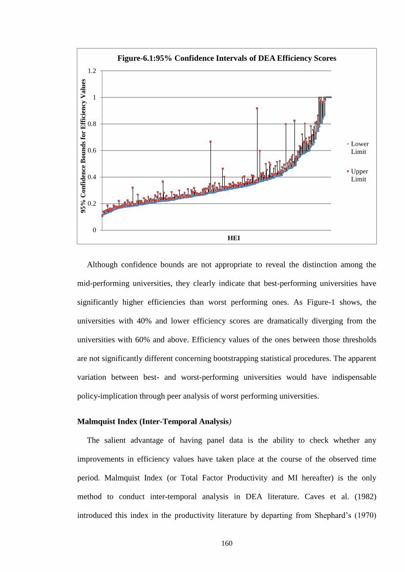
160
Although confidence bounds are not appropriate to reveal the distinction among the
mid-performing universities, they clearly indicate that best-performing universities have
significantly higher efficiencies than worst performing ones. As Figure-1 shows, the
universities with 40% and lower efficiency scores are dramatically diverging from the
universities with 60% and above. Efficiency values of the ones between those thresholds
are not significantly different concerning bootstrapping statistical procedures. The apparent
variation between best- and worst-performing universities would have indispensable
policy-implication through peer analysis of worst performing universities.
Malmquist Index (Inter-Temporal Analysis)
The salient advantage of having panel data is the ability to check whether any
improvements in efficiency values have taken place at the course of the observed time
period. Malmquist Index (or Total Factor Productivity and MI hereafter) is the only
method to conduct inter-temporal analysis in DEA literature. Caves et al. (1982)
introduced this index in the productivity literature by departing from Shephard’s (1970)
0
0.2
0.4
0.6
0.8
1
1.2
95
% C
on
fid
ence
Bo
un
ds
for
Eff
icie
ncy
Va
lues
HEI
Figure-6.1:95% Confidence Intervals of DEA Efficiency Scores
Lower
Limit
Upper
Limit

161
distance function. The desirable property of MI is that it does not require any “behavioural
assumptions such as cost minimisation or profit maximisation” which makes it viable for
the cases where the objective of the DMU is unknown (Mohammadi and Ranaei, 2011).
Furthermore, it should be noted here that if the value yielded by MI is less than 1, it
signifies a decrease in total factor productivity (TFP), whilst the productivity increases if
the MI is greater than 1; and accordingly it refers to a lack of change in TFP if the value is
exactly equal to 1.
For this research, Malmquist values are computed as shown in Table-6.5 with respect to
the cost efficiency values yielded in Model 6. Besides, time periods are assigned to the
transition process between current year and the next one. That is to say, Period 1 refers to
the move from 2005-2006 to 2006-2007 academic years. And subsequent periods are
determined by the same method. Due to the fact that 2009-2010 does not have any
following year, the analysis covers four time periods.
Table-6.5: Average Malmquist Results across HEIs, by period:
Average/Period Period 1 Period 2 Period 3 Period 4
TFP 1.023 0.669 1.487 1.1156
Period 1 indicates a slight increase in TFP, whereas Period 3 and 4 denote relatively
significant improvements. However, Period 2 signals an apparent deterioration in overall
TFP among public HEIs in Turkey. Furthermore, even though there is not any systematic
improvement in efficiencies among universities, during the last two years they have
demonstrated progress in terms of efficiency. Figure-6.2 clearly reveals this inconsistent
improvement through which efficiency performances of universities have witnessed ups
and downs, thus motivates researchers to understand the driving forces behind this
variation. During the following parts of this chapter –in particular determinants of

162
inefficiency part-, the factors influencing efficiencies will be illuminated via focusing on a
set of university-based variables.
Figure-6.2
In addition to the overall analysis, Malmquist index also gives individual results that are
indicated in Table-6.6. The university-by-university TFP scores contribute to the policy-
reflection part of this PhD research especially for the administrative bodies of the
universities as they are more or less representing the overall efficiency improvement or
decline in the given period. Hence, university-based results are discerned to put forward
consistent and accurate implications to the decision makers that will be discussed in the
following chapter in detail.
The initial indication of Table-6.6 is that while the majority of universities demonstrate
a pattern in line with the global results, there are universities that diverge from it.
Secondly, individual MI for HEIs refers to the change in efficiency either might be
increasing or declining. For instance, corresponding numbers to PU1 at the first row
indicate that during Period 1 and 3, efficiency has increased by almost 1.38 and 1.18
0
0.2
0.4
0.6
0.8
1
1.2
1.4
1.6
Period 1 Period 2 Period 3 Period 4
Total Factor Productivity (Whole Sector)
TFP

163
respectively, whilst there are reductions in Period 2 and 4 by nearly 0.70 and 0.91 in that
order. The remaining results can be interpreted in line with this previous analysis.

164
Table-6.6: Malmquist Index Results by Individual Universities
DMU Period 1 Period 2 Period 3 Period 4 DMU Period 1 Period 2 Period 3 Period 4
PU1 1.38098 0.708154 1.18929 0.916409
PU27 0.771978 0.685171 1.18634 1.20868
PU2 0.957281 0.58407 1.34797 1.08764
PU28 0.995265 0.349447 1.77622 1.01924
PU3 0.987611 0.677002 1.34576 0.921349
PU29 0.900853 0.3161 3.146 1.37669
PU4 1.30311 0.441314 1.07625 1.02979
PU30 0.685361 0.887294 1.2091 1.48393
PU5 1.39154 2.46391 0.373723 1.40376
PU31 1.05348 1.27246 1.04622 0.964879
PU6 1.26423 0.339769 1.44612 1.19452
PU32 0.82026 0.82462 1.17716 1.22425
PU7 0.595538 0.535399 2.47136 1.22568
PU33 1.15268 0.519999 1.72779 1.0974
PU8 0.953676 0.49873 1.41648 1.04954
PU34 2.6896 0.3437 0.883345 0.941566
PU9 0.993887 0.442703 1.69871 0.989868
PU35 2.10313 0.174288 1.72769 1.04207
PU10 0.903984 0.503421 1.87971 1.02153
PU36 0.796499 0.308653 2.48261 1.33378
PU11 0.827913 0.588547 1.6671 1.05762
PU37 0.839442 0.654124 1.2494 1.23009
PU12 0.755963 0.617664 1.34207 1.03793
PU38 0.842219 0.425136 2.24111 1.05006
PU13 1.00778 0.436397 1.79705 1.15296
PU39 0.901164 0.640464 1.44407 0.943159
PU14 0.860271 0.805699 1.05009 1.17953
PU40 1.13898 1.35154 1.22783 0.772658
PU15 0.864794 0.358846 1.95619 1.24201
PU41 1.2662 1.19841 0.853576 0.896704
PU16 0.912347 0.573937 1.62128 0.968558
PU42 0.979146 0.754437 1.35364 1.12585
PU17 0.928647 0.64166 1.28266 1.03383
PU43 0.67215 0.507545 1.23131 1.2958
PU18 1.03354 0.676564 1.56012 1.07812
PU44 0.902515 0.562559 1.56232 1.12126
PU19 0.793465 0.70887 1.41905 1.50227
PU45 0.968927 0.968128 0.931011 1.18893
PU20 0.848956 0.39654 2.17574 1.28037
PU46 0.953068 0.416114 2.13487 1.12331
PU21 0.829557 0.294387 2.245 1.54003
PU47 1.25872 0.367228 1.66162 1.04297
PU22 0.893291 1.4754 0.975428 1.10272
PU48 1.05827 0.580433 1.41844 1.25575
PU23 0.944684 1.18116 0.9048 0.959541
PU49 1.12706 0.491447 1.56849 1.08738
PU24 0.964004 0.752682 0.947179 1.01858
PU50 0.862109 0.676965 1.50688 1.12012
PU25 1.26872 0.616404 1.04764 1.0614
PU51 0.866859 0.360474 2.09139 1.00302
PU26 1.10563 1.16791 0.844629 1.10671
PU52 0.904528 0.427983 1.90448 0.950857
PU27 0.771978 0.685171 1.18634 1.20868 PU53 1.13466 0.905077 0.984927 1.06388

165
V. SPEARMAN RANK COMPARISON OF DEA MODELS
After examining efficiency results of HEIs regarding to different DEA optimisation
procedures, this section is tailored to deal with comparison of aforementioned models
relying largely upon Spearman rank correlation. Even though HEIs may get different
efficiency scores for diverse models, Spearman rank correlation checks whether this
divergence influences the rankings of HEIs concerning their efficiency performances. For
this particular analysis, Spearman rank correlation values are calculated to expose the
impact of following scenarios:
i) Introducing new input and/or input variables,
ii) Measuring the efficiencies by the means of non-parametric production or cost
frontier,
iii) Choosing the optimisation method for technology that might be CRS or VRS.
Table-6.7 shows the rank correlations that were driven from CRS whereas Table-6.8 is the
indication of rank correlations between the models assumed VRS frontier. The last table –
which is Table-6.9- demonstrates the rank correlations between CRS and VRS cost frontier
models. Besides, input-oriented efficiency rankings are employed to illustrate those
relationships.

166
Table-6.7: Spearman Rank Correlation for CRS Models
M1 M2 M3 M4 M5 M6
M1 1
M2 0.960115 1
M3 0.871233 0.911632 1
M4 0.824439 0.817994 0.947712 1
M5 0.973117 0.955667 0.869829 0.803156 1
M6 0.862338 0.856157 0.938065 0.904141 0.892113 1
The initial statement coming out of Table-6.7 is that rankings of HEIs in different input
and output sets are by and large same. That is to say, although overall efficiency scores for
HEIs are slightly differing from each other in six models, higher correlation values signify
that the rankings of HEIs are not altering notably. Therefore, it is arguably obvious that
efficiency scores attained by CRS-DEA models have substantial insights both for
researchers and decision-makers. The least correlation coefficient is between Model 4 and
Model 5 but even that one’s value corresponds to 0.8 that denotes strong correlation
between these two models. Furthermore, the simplest model (Model 1) in terms of
input/output mixture has the lowest correlation with the full model (Model 4), thus one can
argue that adding new variables into the model has mattered to certain universities.

167
Table-6.8: Spearman Rank Correlation for VRS Models
M1VRS M2VRS M3VRS M4VRS M5VRS M6VRS
M1VRS 1
M2VRS 0.896564 1
M3VRS 0.869533 0.955112 1
M4VRS 0.850428 0.880198 0.90661 1
M5VRS 0.964431 0.911273 0.871489 0.853839 1
M6VRS 0.941888 0.905349 0.903175 0.902046 0.96187 1
Like in Table-6.7, rank correlation coefficients among the models that employed VRS
frontier are considerably close to each other in Table-6.8. It clearly figures out that as the
models get nearer to the full model (Model 4), spearman rank correlation attains higher
values. Whilst the coefficient is 0.85 between Model 4 and Model 1, it becomes 0.90 when
the relationship between Model 4 and Model 3 is concerned. In addition to that, high
correlation among the results derived from cost and production frontiers encourages
policy-implication aspect of this research to emerge confidently.
Table-6.9: Spearman Rank Correlation for CRS and VRS Cost Models
M5 M6 M5VRS M6VRS
M5 1
M6 0.892113 1
M5VRS 0.925779 0.930118 1
M6VRS 0.875851 0.961316 0.96187 1

168
Even though previous tables (Table-6.7 and Table-6.8) have put forward that efficiency
results have robust properties, conducting comparison between CRS and VRS models
would be much more appropriate to conclude the discussions on the robustness of those
results belonging to the different models. To check this, cost efficiency rankings for
different technology frontier are singled out to perform the test. As expectedly, rank
correlations between CRS and VRS cost efficiency models have got markedly larger
values ranging from 0.87 to 0.96. Accordingly, efficiency scores yielded from diverse
output/input sets as well as preferred technology frontiers have significantly robust insights
both for the following researches and policies.
VI. DETERMINANTS OF INEFFICIENCY
In addition to the estimation of efficiencies, recent literature in efficiency analysis
persuades researchers to take step forward and accordingly interrogate potential factors
influencing efficiency performances of decision-making units (DMUs). This statement is
not different for efficiency analysis of higher education sector through which certain
university-based features are put under spotlight. For this chapter, so as to illuminate the
causes of inefficiencies among public HEIs in Turkey, a set of environmental variables
indicated above will be employed via building upon previous studies.
As the efficiencies of HEIs driven from DEA procedure take values between 0 and 1,
classical regression analysis would not be appropriate to be conducted. Thus, Tobit
regression will be opted for examining determinants of inefficiency by treating data as i)
pooled and ii) panel. Besides, since Tobit regression is designed to censor values lower
than 0, inefficiency scores (1- efficiency scores) of HEIs will be taken as the dependent
variable in lieu of efficiency scores. Therefore, the variable with (+) sign will indicate a
negative relationship with efficiency and vice versa.

169
The next step is deciding which inefficiency values will be preferred as dependent
variable. Previous part on the rank correlation of HEIs was stating that efficiency scores do
resemble each other due to the fact that the lowest correlation coefficient among different
models was 0.82.Hence, choosing any of the inefficiency scores will not be suffered from
‘selection bias’ in a dramatic way. And eventually, for this research, inefficiency scores
yielded from Model 1 and Model 1VRS are selected as the main components of this Tobit
regression analysis. The dependant variable in Model A is the inefficiency scores coming
from Model 1VRS, whilst Model B takes the values from Model 1. Model C prefers the
values from Model 1, when the most insignificant variable is dropped from the regression
model. Table-6.10 reports the results for pooled data:
Table-6.10: Tobit Regression Results for Pool Data
Variables Model A Model B Model C
AGE -.39940D-04 -0.00041009
(-0.0015011) (0.00154432)
SIZE -.17144D-05 -.149576D-05 -.17245D-05
(.11908D-05) (.12252D-05) (.12171D-05)
LOAD 0.002826 0.003159 0.00320543
(-0.002132) (0.00219382) (0.00218055)
PROF -0.13865 -0.2731 -0.30751
(0.39987) (0.41148656) (0.37327346)
FTS 0.09785* 0.12641** 0.1261902**
(0.05941) (0.0611377) (0.06113406)
FORGN 2.00763 2.80765 2.743357
(1.80883) (1.86065793) (1.83340526)
MED 0.06877* 0.0730076* 0.073668*
(0.03811) (0.03921196) (0.03919456)
CON 0.49354*** 0.52245*** 0.51885***
(0.07239) (0.07449951) (0.07229048)
SIGMA (u) 0.02279 0.02243458 0.02243621
(0.0097603) (0.00997657) (0.0099773)
LOG-L 11.88612 7.8755 7.855646
Notes: 1. ***, ** and * indicate 1%, 5% and 10% significance levels respectively.
2. Asymptotic standard errors in parentheses.

170
Table-6.10 reveals that the influence of AGE, SIZE and LOAD of the HEIs on their
efficiency performance is ambiguous which is not in the interior of expectations. That is to
say, although these factors would be the major components of production and/or cost
function of HEIs, their correlations with inefficiency values are statistically vague.
Furthermore, percentage of full-time academic staff among whole faculty (FTS) seems to
be the leading variable concerning its correlation with inefficiency. The coefficient of FTS
implies that as the share of full-time staff increases, inefficiency increases as well, or
alternatively efficiency decreases. Another implication coming out from this table is that
having medical school (MED) reduces efficiency by almost 0.07 which may encourage
researchers to investigate efficiencies of medical schools as a separate research question.
Lastly, the percentage of professors (PROF) and foreign students (FORGN) do not have
any link with inefficiency scores of HEIs according to the aforementioned regression
results.
And Table-6.11 demonstrates the regression results for panel data with random effects
treatment:

171
Table-6.11: Tobit Regression Results for Panel Data
Variables Model A Model B Model C
AGE -.39930D-04 -0.00030839
(-0.00181718) (-0.00177478)
SIZE -.16144D-05 -.169582D-05 -.172415D-05
(.16329D-05) (.17329D-05) (.16559D-05)
LOAD 0.003026 0.0031588 0.00320723
(-0.00285428) (-0.00296712) (-0.00289554)
PROF -0.13954558 -0.27300681 -0.3076005
(-0.5214565) (-0.52132894) (-0.450931990
FTS 0.09774264* 0.12638375** 0.12618928**
(-0.05559317) (-0.05765066) (-0.05743758)
FORGN 2.00752574 2.80685771) 2.7433569
(-2.40340857) (-2.61961309) (-2.49164345)
MED 0.06771132 0.07392279) 0.07367102
(-0.04789048) (-0.05037202) (-0.0483697)
CON 0.49330*** 0.52244*** 0.51884***
(-0.06620654) (-0.06441148) (-0.06442898)
SIGMA (u) 0.02179933 0.02243458 0.02243621
(-0.02372067) (-0.02398005) (-0.02326832)
LOG-L 14.76703 7.875583 10.83485
Notes: 1. ***, ** and * indicate 1%, 5% and 10% significance levels
respectively.
2. Asymptotic standard errors in parentheses.
The Tobit regression results obtained from panel data analysis have not had any
apparent impact on the coefficients of variables, excluding dummy variable for medical
school (MED). MED became insignificant due to a slight increase in its standard deviation
for the all three models. Besides, share of full-time academic staff (FTS) still preserves its
significance on efficiency performance of HEIs for the panel data analysis. The rest of the
variables including AGE, SIZE, LOAD, PROF, and FORGN are not counted as
noteworthy factors pertaining to the results indicated in Table-6.11 that was the case for
pooled data analysis.

172
VII. LIMITATIONS and CONCLUDING REMARKS
Although estimated efficiencies as well as the determinants of inefficiencies among
public HEIs in Turkey have considerable implication both for researchers in this particular
area and decision-makers in the higher education sector, they might be suffering from
certain methodological, structural or computational shortcomings. In this section, those
possible limitations will be illuminated and discussed. Besides, a number of insights and
suggestions will be put forward for forthcoming academic and policy-based inquiries.
The first weakness is stemming from DEA’s well-known methodological problem. As
linear programming assumes deterministic frontier, statistical noises would be treated as
inefficiencies. Therefore, HEIs might be assigned with lower efficiency values than they
were previously done within stochastic frontier framework. So as to overcome this
particular obstacle, number of bootstrapping procedures could be increased and confidence
intervals for efficiency scores in DEA model can be compared and contrasted with the
scores attained by stochastic frontier analysis (SFA).
Secondly, like any other efficiency and/or productivity measurement techniques, the
linear programming suffers from a structural problem that is lack of appropriate quality
assessment variable for output sets. For instance, a specific HEI may have lower numbers
of teaching and research output than the others with almost same input prices and
accordingly end up with higher inefficiency scores. However, its impact both on academia
and society would be considerably greater owing to the quality of the production that
motivates its efficiency performance to rise. Thus, incorporation of post-university status
of students such as employability and annual earnings would alleviate the adverse effects
of this problem for teaching side, whereas adding number of citations to the estimation
process would be appropriate to achieve this for research side.

173
Thirdly, performing two-stage DEA method to estimate the determinants of
inefficiency among HEIs in Turkey may comprise a computational problem. If the
regression results indicate a correlation between certain environmental factors and
inefficiency scores of HEIs, then the efficiency scores estimated at the first stage could
have biased values. Hence, conducting one-stage DEA would have meaningful insights if
their results are compared with the ones in two-stage DEA.
Last but not least, for the Tobit regression analysis to examine the dynamics behind
inefficiency, variable set might not be sufficient to capture the influence of all factors on
efficiency performance of HEIs like managerial skills due to lack of comprehensive
dataset. For that reason, an extended dataset for public HEIs in Turkey would render
opportunities to the potential researchers to map out the determinants of efficiencies for
this particular sector.
Public HEIs that are directly financed by governmental bodies, account for the
significant element of whole education expenditures in Turkey. On a year-to-year basis,
Ministry of Education presents the expenditures of HEIs to the Turkish National Assembly
and looks for sufficient amount of appropriations to them for pursuing their academic and
social goals. This funding exercise that corresponds to almost 60% of HEIs’ own budget
(Erkoc, 2011), recently sparked an interest among academics and policy-makers to
scrutinise the usage of resources allocated to the higher education sector. Accordingly,
efficiency measurements particularly for HEIs have gained great importance to illuminate
the efficiency performances of them.
The research carried out in this chapter is tailored to estimate technical and cost
efficiencies of public HEIs in Turkey by the means of non-parametric technique called
DEA. By doing so, overall efficiencies of HEIs as well as their individual scores are

174
demonstrated on the basis of certain production and cost models motivated by different
sets of input/output as well as the frontier technology (CRS and VRS).
The results of those models, firstly, have shown that public HEIs in Turkey are
performing in unsatisfactory levels although some of them are doing fairly well. Besides,
as the model closes to the full input/output set, both individual and overall efficiency
scores are getting relatively higher values. Secondly, even though there is not any systemic
increase during this five-year time span, efficiencies of public HEIs in Turkey have
increased at the course of last two years. Thirdly, the share of full-time academic staff in
the whole faculty and having medical school are founded as the determinants of
inefficiencies among HEIs regarding Tobit regression analysis.
Consequently, even though those findings might be suffering from couple of
methodological problems as indicated in Section VIII, they would be used as the departure
points both for academic and policy-making interests.

175
CHAPTER VII: Critical Evaluation of Efficiency
Results and Their Policy Implications
I. INTRODUCTION
Average efficiency scores for HEIs alongside with their individual scores have policy-
making implications for higher education sector in Turkey particularly as the apportioned
amount of public funding to them becomes a central topic in the finance of higher
education decision-making (YÖK Report, 2007). Joint impact of increasing demand for
university education as well as limited government funding allocated for HEIs are put
forward as the main driving forces behind the recent growing curiosity on the allocation of
resources in the Turkish higher education (Önder and Önder, 2010). Therefore, the
estimation results obtained in the Chapter V and VI would offer noteworthy insights for
further policy-making decisions conducted by both administrative bodies of HEIs and the
Council of Higher Education of Turkey.
As already indicated in the previous chapters, although the number of researches on the
economic efficiencies of HEIs has generated a remarkable volume of literature, studies
investigating the efficiency aspect of Turkish universities are extremely scant.
Accordingly, policy implications of the efficiency estimates for higher education in Turkey
are mainly inspired from the earlier conclusions put forward by various researchers on
different cases including United States, Sweden and England and so forth. However,
Dundar and Lewis’s (1999) as well as Önder and Önder’s (2010) papers on the Turkish
universities are visited to release consistent statements even though the findings of former
piece are comparatively out-dated.

176
The estimation of economic efficiencies for Turkish public HEIs is performed by two
different methodologies named as Stochastic Frontier Analysis (SFA) and Data
Envelopment Analysis (DEA). Moreover, determinants of inefficiencies are estimated with
these techniques by the econometric procedures introduced by them. Since these two
methods might present differing results, policy recommendations for the given HEIs
should be proposed and strongly supported if there is an agreement between them.
However, in this particular research, parametric model is given slightly higher importance
in policy conclusions, as its suggestions are closer to the previous empirical literature and
theoretical considerations. Otherwise, suggested statements would cause conflicting policy
conclusions and consequently this research will be deviated from its initial motivation.
The policy implications of the findings driven from SFA and DEA are indicated in the
following order throughout this chapter: Section II reviews the mean cost efficiencies of
HEIs concerning the location, age and size of HEIs in a time profile, Section III
summarises both technical and cost efficiencies of HEIs as well as perform categorical
analysis done in the previous section, Section IV deals with the scale economies and its
relationship with the output choices of HEIs in the given five-year time span, Section V is
devised to examine the impact of environmental factors on the efficiency performances of
HEIs, Section VI presents the Spearman rank correlations for SFA and DEA models, and
eventually Section VII concludes.
II. COST EFFICIENCIES BASED ON SFA
Preceding discussions (Robst, 2001; Dagbashyan, 2011) claiming the likely influence
of university-based characteristics on individual efficiency scores of universities lead
researchers to put more emphasis on those factors. Therefore, cost efficiency values of
SFA yielded from Model B2 -which is shown to be the best-fitted model among others by

177
the means of hypothesis testing- are segregated as regards to the location, size group and
age of the HEI so as to infer introductory insights for the probable impact of the
aforementioned factors over to the efficiency performances of HEIs. Over the course of the
following sections, after revealing the mean efficiency scores of HEIs in a yearly basis,
policy reflection of the segregated results will be indicated. Lastly, it should be noted here
that the exact impact of university-based characteristics (if there is/are any) on efficiencies
forms the governing idea of section VI of this chapter.
Average Cost Efficiency Scores for public HEIs in Turkey
Public HEIs in Turkey seem to be operating fairly efficient in overall, even though
there are HEIs apparently underperforming whose efficiency scores are corresponding to
the values less than 50% as indicated in the Table-7.1. Departing from the normality
assumption, one can argue that economic efficiency scores of 95% of public HEIs in
Turkey are nearly within the range of 66% to 93%. Accordingly, the number of public
HEIs performing less efficient than 70% and more efficient than 95% is rather scarce. In
addition to the previous statements, the most significant conclusion coming out of Table-
7.1 is that mean efficiencies of the given HEIs have not changed throughout five-year time
span, albeit individual scores are varying from one to another. Whereas, the worst
performing HEI has the value of 0.45 in 2006, in 2010 the minimum efficiency score is
equal to 0.47. Moreover, the performance of best-practising HEI has not shown any
significant improvement during 5 years.

178
Table-7.1: Average Cost Efficiency Scores for Public HEIs in Turkey (Yearly Basis)
Year Mean St Dev. Min Max
2006 0.853320 0.098284 0.450127 0.98499
2007 0.854779 0.097306 0.455598 0.98514
2008 0.856224 0.096338 0.461015 0.98528
2009 0.857655 0.095380 0.466378 0.98543
2010 0.859071 0.094431 0.471688 0.98558
Overall 0.856211 0.09564 0.450127 0.98558
Average Cost Efficiency Scores by Location
The first data segregation is performed considering the location of HEI to point out
whether efficiency performances of universities in larger cities are differing noticeably
from the ones located in relatively smaller cities. So as to illuminate this, three categories
are developed: i) HEIs located in Istanbul ii) HEIs located in Istanbul, Ankara and Izmir
iii) HEIs located in the rest of the cities. Istanbul is chosen as a separate category owing to
the fact that one-sixth of the whole Turkish population lives in Istanbul as well as one-fifth
of the GDP is generated within the Istanbul region according to the recent statistics (TÜIK:
2012). The second category comprises Ankara and Izmir that are enumerated as the 2nd
and
3rd
largest cities of Turkey. Lastly, third category is constituted to encompass all other
cities dispersed to the different regions of Turkey.
The chief conclusion suggested by Table-7.2 is that HEIs located in Istanbul is
performing marginally better than the mean efficiency revealing the fact that higher life
standards and the demographic conditions do not have any evident association with
efficiency performances of public HEIs in Turkey. Secondly, the noticeable mean
efficiency gap between the first and second categories points that universities placed in
Ankara and Izmir are conspicuously underperforming than their counterparts in Istanbul.
Thirdly, universities opened up in the rest of the cities are operating slightly more efficient

179
than overall efficiency level as well as equally efficient with the universities in Istanbul
except the year 2007. Last but not least, average cost efficiencies of HEIs split into three
different categories have not indicated any considerable increase in their efficiency
performances throughout the given time span. The linear trend depicted in Figure-7.1 is the
confirmation of this statement although universities situated in the rest of cities category
experienced a sharp decline in 2007 whilst their competitors in Istanbul, Ankara and Izmir
performed entirely in the opposite way.
Table-7.2: Average Cost Efficiency Scores for Public HEIs in Turkey (by Location)
Year Istanbul Istanbul-Ankara-Izmir Rest of the Cities Mean Efficiency
2006 0.862773 0.818283 0.865897 0.853320
2007 0.864138 0.820091 0.843344 0.854779
2008 0.865490 0.821881 0.868553 0.856224
2009 0.866828 0.823653 0.869861 0.857655
2010 0.868153 0.825408 0.871156 0.859071
Average Cost Efficiency Scores by Size Groups
The following comparison is exercised with regards to the size of the universities,
which also gives significant insights into the impact of bureaucracy over to the
inefficiencies of HEIs. As indicated earlier, the proxy variable for the university size
0.8
0.825
0.85
0.875
0.9
2006 2007 2008 2009 2010
Figure-7.1: Average Cost Efficiency Scores for Public HEIs in Turkey (by
Location)
Istanbul Istanbul-Ankara-Izmir Rest of the Cities Mean Efficiency
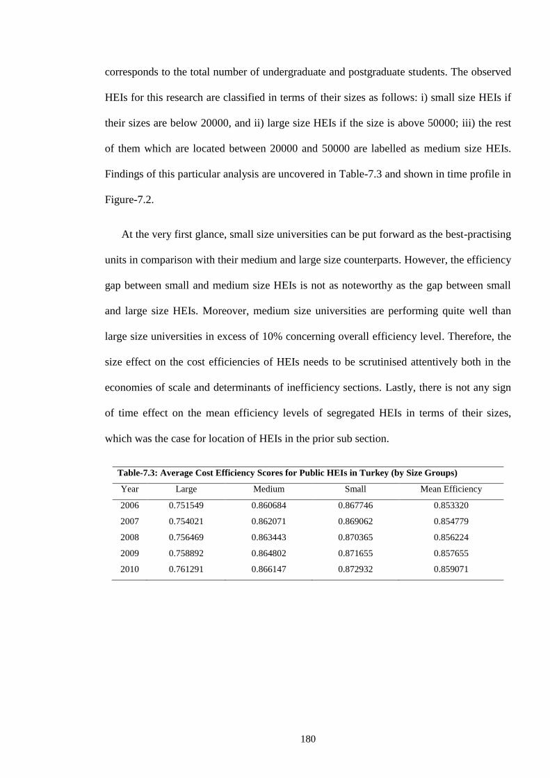
180
corresponds to the total number of undergraduate and postgraduate students. The observed
HEIs for this research are classified in terms of their sizes as follows: i) small size HEIs if
their sizes are below 20000, and ii) large size HEIs if the size is above 50000; iii) the rest
of them which are located between 20000 and 50000 are labelled as medium size HEIs.
Findings of this particular analysis are uncovered in Table-7.3 and shown in time profile in
Figure-7.2.
At the very first glance, small size universities can be put forward as the best-practising
units in comparison with their medium and large size counterparts. However, the efficiency
gap between small and medium size HEIs is not as noteworthy as the gap between small
and large size HEIs. Moreover, medium size universities are performing quite well than
large size universities in excess of 10% concerning overall efficiency level. Therefore, the
size effect on the cost efficiencies of HEIs needs to be scrutinised attentively both in the
economies of scale and determinants of inefficiency sections. Lastly, there is not any sign
of time effect on the mean efficiency levels of segregated HEIs in terms of their sizes,
which was the case for location of HEIs in the prior sub section.
Table-7.3: Average Cost Efficiency Scores for Public HEIs in Turkey (by Size Groups)
Year Large Medium Small Mean Efficiency
2006 0.751549 0.860684 0.867746 0.853320
2007 0.754021 0.862071 0.869062 0.854779
2008 0.756469 0.863443 0.870365 0.856224
2009 0.758892 0.864802 0.871655 0.857655
2010 0.761291 0.866147 0.872932 0.859071

181
Average Cost Efficiency Scores by Age of HEIs
The final comparison is carried out pertaining to age of the universities. Three clusters
are formed here consisting of young, mature and old universities. Young universities
denote the range of 5-20 years, mature ones are between 20 and 40 and the old ones are
above 40 years. To put it bluntly, this classification is selected with a view to reflect three
streams of university establishment in the history of Turkish Republic: i) HEIs opened up
following the foundation of Turkish Republic and inherited the traditional higher education
system of Ottoman Empire ii) HEIs founded at the beginning of 1980s with the
establishment of The Council of Higher Education after military coup occurred in 1980 iii)
HEIs began their education lives in the midst of 1990s.
As indicated in Table-7.4 and Figure-7.3, young universities outperform that of both
mature and old universities over the course of 5 years. This conclusion is tune with the
Tullock’s (1965) inter-temporal budget analysis in public organizations emphasising the
fact that older institutions are expected to face larger inefficiencies than their younger
counterparts. However, the difference between young and mature universities is much
more remarkable than the difference between young and old universities, which is clearly
0.7
0.75
0.8
0.85
0.9
2006 2007 2008 2009 2010
Figure-7.2: Average Cost Efficiency Scores for Public HEIs in Turkey
(by Size Groups)
Large Medium Small Mean Efficiency

182
illustrated in the Figure-3. In relation to the comparison among the mature and old
universities, the superiority goes to the old universities. That is to say, throughout the five-
year time span old universities surpass the mature ones nearly in excess of 5% of mean
efficiency level. Finally, even though young and old universities have not shown any sign
of improvement in the given period, mature universities increased their overall efficiency
performances by approximately 1%.
Table-7.4: Average Cost Efficiency Scores for Public HEIs in Turkey (by Age)
Year Young Mature Old Mean Efficiency
2006 0.882836 0.817887 0.863486 0.853320
2007 0.884001 0.819699 0.864844 0.854779
2008 0.885156 0.821493 0.866189 0.856224
2009 0.886298 0.823269 0.867520 0.857655
2010 0.887430 0.825027 0.868838 0.859071
To sum up all the foregoing arguments demonstrated in Table-7.1, 2,3 and 4 as well as
Figure-7.1, 2 and 3, following statements could be set forth as:
0.8
0.81
0.82
0.83
0.84
0.85
0.86
0.87
0.88
0.89
0.9
2006 2007 2008 2009 2010
Figure-7.3: Average Cost Efficiency Scores for Public HEIs in Turkey (by
Age)
Young Mature Old Mean Efficiency

183
There is not any sign of efficiency improvement among public HEIs in
Turkey over the course of 5 years
HEIs located in Istanbul is performing slightly better than average, whereas
overall efficiency scores of HEIs in Ankara and Izmir are lower than
average
Large size universities are considerably underperforming if they are
compared with their medium and small size universities.
The efficiency gap between small and medium size HEIs is negligible
Younger universities are outstripping mature and old universities, whereas
their superiority over to the mature universities is fairly excessive vis a vis
their dominance against old universities.
III. TECHNICAL AND COST EFFICIENCIES BASED ON DEA
Mean cost efficiency scores of public HEIs throughout the given time period alongside
with the segregated results in relation to the age, size and location of HEIs are summarised
in the previous section through which stochastic frontier framework is carried out. In this
section, technical efficiencies of public HEIs in addition to the cost efficiencies are
revealed departing from the conclusions yielded by Data Envelopment Analysis.
Technical and cost efficiencies of public HEIs are separated into various categories
including age, size and location of the HEI. Besides, Model 4 with Variable Returns to
Scale (VRS) is preferred to reflect the technical efficiencies of HEIs, whereas Model 5
with VRS is employed to expose cost efficiencies of HEIs due to the fact that these models
are relatively closer to the models developed within stochastic frontier framework.

184
Average Efficiency Scores for public HEIs in Turkey
Mean efficiency scores computed by the means of non-parametric method are
diverging evidently from the values derived from parametric one as clearly indicated in
Table-7.5 and Table-7.6. This statement proves the fact that deterministic cost and/or
production frontiers are suffering to differentiate the statistical noise and inefficiency term
and accordingly assume the calculated distance to the given frontier as inefficient usage of
resources.
According to the non-parametric estimation of technical efficiencies of Turkish public
HEIs, over the course of the given five years, the overall technical efficiency among them
is equal to 56% with its peak at the year of 2007 (63%). Moreover, average technical
efficiency scores are experiencing an abrupt decline in 2008 reducing from 63% to 46%
corresponding to a nearly 30% decrease. However, mean efficiency performance of HEIs
reverts back to its initial position in 2010 where the first and last year’s values are
equalised at 59%. Eventually, the higher standard deviations are the signs of vastly
dispersed HEIs with respect to their efficiency scores.
Table-7.5: Average Technical Efficiency Scores for Public HEIs in Turkey (Yearly Basis)
Year Mean St Dev. Min Max
2006 0.595539 0.190676 0.25461 1
2007 0.637129 0.213404 0.32328 1
2008 0.460348 0.190701 0.22840 1
2009 0.526149 0.174249 0.25099 1
2010 0.590723 0.234570 0.2408 1
Overall 0.561978 0.209691 0.22840 1
Non-parametric cost efficiency estimation of public HEIs in Turkey on a yearly basis is
indicated in Table-7.6. To this table, mean cost efficiency scores of public HEIs is roughly
35% ranging from 25% to 42% throughout the five-year time period. The average cost

185
efficiencies diminish sharply from 2007 to 2008, which apply to the case for technical
efficiencies as well. It is appropriate to state that Malmquist index for Period 2 (0.67) -
which was already computed in the Chapter VI - referring to the transition from 2007 to
2008 is another indication of this decline. Although this is not supported by the parametric
findings put forward in Chapter V, the policy of “conversion of existing faculties
belonging to the certain universities into independent public universities” that was put into
action by the current government in 2007 would have an impact on this abrupt decline.
Therefore, there is a precise need to conduct a rigorous investigation to be able to
comprehend this unprecedented reduction among public HEIs in Turkey with the
contribution of more comprehensive dataset and possibly a qualitative research, which
would in turn give a momentous policy-making manoeuvre to prevent prospective
disorders.
Table-7.6: Average Cost Efficiency Scores for Public HEIs in Turkey (Yearly Basis)
Year Mean St Dev. Min Max
2006 0.419750 0.204956 0.19452 1
2007 0.411580 0.207353 0.16361 1
2008 0.246125 0.148379 0.10103 1
2009 0.301860 0.136732 0.12260 1
2010 0.363154 0.213789 0.14119 1
Overall 0.348494 0.195362 0.10103 1
Average Efficiency Scores by Location
Table-7.7 is the summary of the mean cost efficiency results concerning the location of
public HEIs in Turkey originated from the non-parametric estimation. The initial indication
of this table is that HEIs located in Istanbul is comparatively more efficient than their
counterparts sited in the rest of the cities all around the Turkey. Yet, their overall
efficiency performance reduced from 64% to 61% throughout the time period specified for

186
this research, which could easily be seen in the Figure-7.4. Secondly, universities in the
category of the “rest of the cities” are put forward as the least efficient group, which would
be the consequence of larger sample size than the former two categories. Thirdly,
universities founded in Ankara and Izmir have relatively poorer efficiency values than the
ones in Istanbul as already proposed in the policy-reflection findings of stochastic frontier
framework, hence a closer scrutiny on those HEIs would be helpful in terms of efficiency
betterment.
Table-7.7: Average Cost Efficiency Scores for Public HEIs in Turkey (by Location)
Year Istanbul Istanbul-Ankara-Izmir Rest of the Cities Mean Efficiency
2006 0.645518 0.598173 0.355701 0.419750
2007 0.572871 0.537799 0.366270 0.411580
2008 0.272592 0.262450 0.240264 0.246125
2009 0.455129 0.410949 0.262700 0.301860
2010 0.618147 0.536798 0.300821 0.363154
0.2
0.25
0.3
0.35
0.4
0.45
0.5
0.55
0.6
0.65
0.7
2006 2007 2008 2009 2010
Figure-7.4: Average Cost Efficiency Scores for Public HEIs in Turkey (by
Location)
Istanbul Istanbul-Ankara-Izmir Rest of the Cities Mean Efficiency

187
Average Efficiency Scores by Size Groups
Mean cost efficiency scores with regards to the size group of HEIs measured by DEA
is a bit at odds with the conclusions stated by the previous SFA estimation. Whereas small
size HEIs are doing quite well in the latter, large size universities form the most efficient
category in the former. Nonetheless, the difference between small and medium size HEIs
is neither systemic nor significant, which is in line with the statements asserted by the
parametric estimation. Following the earlier discussions on the impact of time over to the
efficiency performances of HEIs, Table-7.8 claims that large size HEIs improved
themselves by almost 40% during five years, whilst the efficiencies of medium and small
size HEIs deteriorated by approximately 20% and 25% respectively. Figure-7.5 approves
this with its illustrative competency and claims that whilst small and medium size
universities start the time profile by the line of 0.4, they finally end up with the line of 0.3.
On the other hand, large size universities starting point is almost 0.6 and ends with 0.8
corresponding to a 30% increase in overall. However, due to the fact that the sample of
large-size universities is narrower than medium and small size universities, this conclusion
would not be that much helpful without a full-fledged analysis on the determinants of
inefficiencies among the all universities included in the whole sample.
Table-7.8: Average Cost Efficiency Scores for Public HEIs in Turkey (by Size Groups)
Year Large Medium Small Mean Efficiency
2006 0.569233 0.422496 0.382532 0.419750
2007 0.564668 0.408102 0.380898 0.411580
2008 0.365510 0.220639 0.249111 0.246125
2009 0.441509 0.304916 0.266511 0.301860
2010 0.806079 0.337780 0.292478 0.363154

188
Average Efficiency Scores by Age of HEIs
The last data segregation is performed to point out whether the age of HEIs is
influential on the efficiency performances in average. Table-7.9 demonstrates the mean
cost efficiencies of public HEIs in Turkey in terms of their age groups including young,
mature and old. To keep in mind that these clusters also refer to three streams of university
establishment in Turkey since the Turkish Republic was founded. The crucial inference
coming out of the table and the Figure-7.6 below is that the efficiency variation among
young, mature and old HEIs is blurred; hence any clear-cut conclusion cannot be deduced
from these findings. However, young universities are the ones that assign a value lower
than mean efficiency four times out of observed five years.
Table-7.9: Average Cost Efficiency Scores for Public HEIs in Turkey (by Age)
Year Young Mature Old Mean Efficiency
2006 0.405218 0.435015 0.421597 0.419750
2007 0.407148 0.413917 0.419430 0.411580
2008 0.265248 0.245704 0.181879 0.246125
2009 0.284560 0.313221 0.325472 0.301860
2010 0.305191 0.394770 0.462524 0.363154
0.2
0.3
0.4
0.5
0.6
0.7
0.8
2006 2007 2008 2009 2010
Figure-7.5: Average Cost Efficiency Scores for Public HEIs in Turkey
(by Size Groups)
Large Medium Small Mean Efficiency

189
The summary of the abovementioned findings revealed in the Table-7.5, 6,7,8 and
9 as well as Figure-7.4, 5 and 6 is as follows:
The average technical and cost efficiencies of public HEIs in Turkey have
not shown any sign of betterment throughout the given 5 years
HEIs located in Istanbul outperform remarkably better than their
competitors dispersed to the rest of the cities including Ankara and Izmir
Small and medium size universities are noticeably operating less efficient
then the larger size universities
The efficiency performances of small and medium size HEIs resemble to
each other
The efficiency gap among young, mature and old universities is blurred;
hence any policy-reflection statement cannot be put forward.
IV. ECONOMIES or DISECONOMIES OF SCALE
The economies of scale of multi-product organizations have always been under
scrutiny since Kim’s paper (1987) in which theory of multi-product firm was developed
0.15
0.2
0.25
0.3
0.35
0.4
0.45
0.5
2006 2007 2008 2009 2010
Figure-7.6: Average Cost Efficiency Scores for Public HEIs in
Turkey (by Age)
Young Mature Old Mean Efficiency

190
and empirically tested with the survey of water utilities in US. In relation to the outputs,
the firms are expected to develop an optimal behaviour that “chooses the output levels
corresponding to the minimum cost of a unit of output, which is closely related to
economies of scale” (Dong, 2009). To measure the scale economies of a multi-product
firm, following Baumol (1976) and Panzar and Willig (1977)’s methodology, Kim defined
the formulation as follows:
(7.1)
where TC represents total cost and Y refers to the given output levels for different
products. If ES > 1, economies of scale occurs; conversely, if ES < 1 diseconomies of scale
is reigning over to the cost function. And eventually, if ES = 1, there is neither economies
nor diseconomies of scale.
Although there is a considerable amount of literature on the scale economies of multi-
product firms, the number of researches on the HEIs is relatively scarce. The previous
literature on the economic efficiency analysis of HEIs has not paid adequate attention to
this aspect of the analysis and overlooked it. And accordingly, none of the researches on
the Turkish higher education sector has touched upon this topic except Dundar and Lewis
(1999). In the related paper, authors argue, “Product specific economies of scale for
undergraduate instruction were found for faculties in the social science and engineering
subject groups but not in health sciences” (Dundar and Lewis, 1999). Moreover, some of
the HEIs were found as exploiting the economies of scale in the postgraduate teaching,
nonetheless none of them was stated to face scale economies concerning the level of their
research outputs in the cited paper.

191
In this section, economies of scale assigned to the public HEIs in Turkey is examined
concerning the Cobb-Douglas specification due to the following reason: it is highly
probable for Translog cost specification to be suffering from multicollinearity as one of the
second-order terms ( ) is experiencing a negative value. Although efficiency estimation
of the HEIs could be conducted despite of this problem, it would not be appropriate to
measure economies of scale with this specification, since the coefficients of first-order
terms might have biased values owing to the multicollinearity. For this particular analysis,
the economies of scale for public HEIs in Turkey are computed by the formulation below
departing from (7.1):
(7.2)
Scale economies of public HEIs in Turkey is measured and summarised in the Table-
7.10 as well as put into a time report in Figure-7.7. To these findings, public HEIs are
operating in the high levels of economies of scale, which is line with arguments put
forward by Dundar and Lewis (1999), although the magnitude of it exhibits a downward
trend declining from 1.84 to 1.53 between 2006 and 2010. Since the scale efficient firm
produces at a point where there is neither ‘economies of scale’ nor ‘diseconomies of scale’,
public HEIs in Turkey are suffering from scale inefficiency in overall over to the course of
given five years. So as to overcome this problem, it would be better for public HEIs in
Turkey to increase the amount of outputs up to the point where the value of overall
economies is equal to 1.
The declining trend in the scale economies might be the sign of this production
readjustment; hence a segregated analysis in relation to the type of output would give
meaningful insights both to the empirical aspect of this research and the policy-making

192
decision in HEIs alongside the Council of Higher Education. That is to say, the relationship
between the scale economies and the types of output including undergraduate and
postgraduate teaching as well as the amount of research projects throughout the five-year
time span needs to be examined in detail.
Table-7.10: Economies of Scale for Public HEIs in Turkey (Yearly Basis)
Year Economies of Scale
2006 1.846722
2007 1.661129
2008 1.659200
2009 1.564210
2010 1.536098
2006-2010 1.584283
Overall scale economies results indicated in the Table-7.10 have triggered further
inquiry on the yearly change in the level of outputs provided by public HEIs in Turkey.
The mean values of outputs on yearly basis are illustrated in Table-7.11. To this table, the
number of undergraduate and postgraduate students increased in a remarkable way, even
though the number of undergraduate students had experienced ebbs and flows. However,
the amount of research projects diminished by almost 10% during five years.
1
1.2
1.4
1.6
1.8
2
2006 2007 2008 2009 2010
Figure-7.7 : Economies of Scale for Public HEIs in Turkey
(2006-2010)

193
The extent to which these institutions are exploiting economies of scale is profoundly
contingent upon the levels of output mentioned above. As indicated earlier, to become a
scale efficient firm and sector, HEIs are advised to increase the level of outputs until
economies of scale is utilised in a full capacity. So as to achieve this, public HEIs in
Turkey have shown an optimistic signal concerning teaching outputs, nevertheless the
decline in research output seems to be causing HEIs to experience scale inefficiency. As
shown in Figure-7.8, constant increase in the number of undergraduate students throughout
five years, had an impact on the magnitude of economies of scale converging to 1.5, and
optimistically towards 1 in the couple of years with the accompany of possible increase in
the levels of other types of outputs. The minor increase in the amount of research output in
2010 represents the optimistic side of the expectations. Otherwise, the persistent growth in
the number of undergraduate students in order to exploit economies of scale fully would
have repercussions on the efficiency performances of HEIs, which will be considered in
the succeeding section.
Table-7.11: Average Level of Outputs for Public HEIs in Turkey (Yearly Basis)
Year UG Students PG Students Res. Projects (x1000)
2006 38471.1886 2492.56603 2906.1
2007 38745.0754 2419.66037 3480.07
2008 38968.0943 847.264150 2723.7
2009 45190.6415 2351.75471 2523.4
2010 54938.9434 2998.92452 2650.3
2006-2010 43262.78868 2222.03396 2856.7

194
The findings of the scale economies of public HEIs in Turkey have certain indications
for policy recommendation:
Public HEIs in Turkey are exploiting the economies of scale in greater levels
ranging from 1.85 to 1.53 between 2006 and 2010
There is an obvious decline in the magnitude of economies of scale diminishing
from 1.85 in 2006 to 1.53 in 2010
The respond from HEIs to increase their undergraduate and postgraduate
teaching appears to be a wise decision, but is still insufficient to reach the point
where economies of scale is entirely cleared
The reduction in the amount of research output has an adverse effect on this
convergence process to end up with constant returns to scale.
0
5000
10000
15000
20000
25000
30000
35000
40000
45000
50000
55000
60000
2006 2007 2008 2009 2010
Figure-7.8: Average Levels of Outputs (Yearly Basis)
Undergradauet Students Postgraduate Students Research Projects

195
V. DETERMINANTS OF INEFFICIENCIES
In the previous sections, policy implications of cost and technical efficiency estimates
of public HEIs in Turkey were presented and examined concerning both parametric and
non-parametric estimation techniques. Moreover, categorical analysis was performed to
see whether efficiency performances vary from one group to another with respect to the
location, age and size of HEIs. In this section, so as to comprehend the variation in the
efficiency scores of HEIs completely, we will scrutinise the probable factors that might
cause this variation. The methodologies to estimate the impact of environmental factors
over to the cost efficiencies of public HEIs in Turkey for parametric and non-parametric
approaches were illustrated in Chapter V and VI respectively. Whilst the former one uses
conditional mean method, the latter employs Tobit regression analysis since the
inefficiency terms are ranging from 0 to 1.
The literature on the determinants of cost efficiencies among HEIs is relatively scarce
in comparison with the other areas of research in the efficiency analysis. Robst (2001),
Stevens (2001) and Daghbashyan (2011) give significant insights on this particular topic
focusing on HEIs in South Carolina, England and Wales, and Sweden correspondingly.
However, there is not any single research for HEIs in Turkey. Hence, statements put
forward by Robst (2001), Stevens (2001) and Daghbashyan (2011) will be tested as long as
the dataset for Turkish HEIs allows. To these papers, the share of government revenues,
size and load factor of HEIs, student/staff characteristics such as percentage of full-time
academic staff, number of professors, number of foreign students have impacts on the
efficiencies of HEIs. For Turkish case, age, size and load factor of HEIs; student and staff
characteristics alongside the dummy for having medical school form the environmental
factors that would have influences on the efficiencies of public HEIs in Turkey either in a
positive or negative way are included in the model. Table-7.12 below summarises the

196
statistics for the estimated coefficients of those factors, their individual analyses are
performed in the succeeding sub-sections.

197
Table-7.12: Determinants of Cost Inefficiencies
Variables DEA 1 DEA 2 SFA 1 SFA 2
AGE -0.00041009 -0.00030839 0.0054*** 0.044586
(-0.00154432) (-0.00177478) (0.0009) (0.039)
SIZE -.149576D-05 -.169582D-05 0.00001*** .797D-04*
(.12252D-05) (.17329D-05) (0.0000002) (.450D-04)
LOAD 0.003159 0.0031588 -.02048*** -0.16852*
(-0.00219382) (-0.00296712) (0.0006) (0.098684)
PROF -0.2731 -0.27300681 0.00431235 4.045698
(-0.41148656) (-0.52132894) (0.0617) (12.60634)
FTS 0.12641** 0.12638375** 0.0519*** 0.277591
(-0.0611377) (-0.05765066) (0.0143) (1.381614)
FORGN 2.80765 2.80685771 3.2903*** 55.24667
(-1.86065793) (-2.61961309) (0.8812) (49.17822)
MED 0.0730076* 0.07392279 0.0527 1.84628*
(-0.03921196) (-0.05037202) (0.1048) (0.964238)
CON 0.52245*** 0.52244864
N/A 1.499941
(-0.07449951) (-0.06441148) (2.63512)
SIGMA (u) 0.02243458*** 0.02243458 0.1994*** 0.1782***
(-0.00997657) (-0.02398005) (0.002) (0.0031)
LOG-L 7.8755 7.875583 -2184.374 134.65
Notes: 1. ***, ** and * indicate 1%, 5% and 10% significance levels
respectively.
2. Asymptotic standard errors in parentheses.

198
Effect of Structure of the Institution on Efficiency
This section deals with possible statistical relationships between the structural
properties of HEIs such age, size and load factor of universities as well as having medical
school inside the university and the cost inefficiencies of universities. Whereas the age,
size and the medical school are expected to have a positive relationship with inefficiencies,
the load factor is predicted to lower inefficiencies in HEIs. The rigorous analyses for the
each factor are indicated in the next paragraphs.
Effect of Age of the HEI on Efficiency
Although previous researches have not taken the age of the HEI into consideration
while accounting for the determinants of inefficiencies, our categorical analysis in section
II has paved the way for further investigation on this factor. In the Section II, young
universities are found out as the most efficient group of HEIs compared to their old and
mature counterparts. Hence, age of the HEI is incorporated both to the conditional mean
model of stochastic cost frontier and Tobit regression of two-stage DEA approach. The
initial expectation is that if universities get older, their efficiency performances will be
diminished; thus expected sign of the coefficient for age of HEI is positive. This
expectation is also motivated by Tullock’s (1965) inter-temporal budget expectation in
bureaucratic institutions particularly in public ones.
To the estimation results yielded from three different models, the age of HEI is
founded as significant with its expected sign in only one model. The other two models put
forward insignificant coefficients for this factor, and the DEA model stated negative sign
that is not expected for the age of HEI. The estimated coefficient of the first model claims
that if the age of HEI increases by 1 year, overall inefficiencies rise by 0.5%. Accordingly,
elder HEIs are likely to experience higher levels of inefficiencies, which is line with the
prior anticipations revealed in the section II. However, this conclusion cannot be directly

199
converted into a policy-recommendation statement since it is not supported with other
three models.
Effect of Size of the HEI on Efficiency
The size of HEIs that is proxied by the number of undergraduate and postgraduate
students for this research “is expected to increase costs, its effect on economic efficiency is
not clear” (Daghbashyan, 2011). Besides, Downs (1965) and Naskanen’s (1971) analyses
on the bureaucratic size in the public sector organizations are taken into account
beforehand. In her paper, Daghbashyan (2011) figured out a negative correlation between
the sizes of HEIs and cost efficiencies claiming that “big universities are less efficient” in
pooled data analysis, nevertheless in the panel data model, this relationship disappears and
therefore the discussion preserves its ambiguity. In the previous sections of this chapter
(Section II and III), we presented contradictory conclusions from parametric and non-
parametric approaches in relation to the size effect. Whereas former claims that overall
efficiencies of small size HEIs are higher than large size HEIs, the latter asserts exactly the
opposite.
Estimated parameters for the size effect in Table-7.12 illustrate a positive association
between the size of HEI and mean inefficiencies in the last two models even though Tobit
regression does not support this. The positive sign for this particular coefficient refers to
the fact that if the size of HEI grows, its inefficiency increases and accordingly efficiency
performance decreases. However the magnitude of this influence is not as noteworthy as
the statistically significant factors. It corresponds to the fact that if the size of HEIs
increases by 1000 students, the mean efficiencies of universities diminish by 0.1% and
0.7% according to the third and forth models in sequence. If one considers this conclusion
with the estimates of unexploited economies of scale in Turkish public higher education,

200
she can come to the conclusion that public HEIs in Turkey should give more weight to the
research output rather than teaching outputs.
Effect of Load of the HEI on Efficiency
Load per lecturer is predicated as an alleviating factor on the cost function of HEIs in
all models presented in Chapter V. The resulting question in relation to the load factor is
that to what extent it influences cost efficiencies of HEIs. Daghbashyan (2011) argues that
high load would decrease the efficiencies of HEIs by “decreasing the quality of teaching”.
In her paper, the pooled data analysis fortifies this statement revealing that there is an
inverse relationship between the load per lecturer and mean efficiencies of Swedish HEIs
albeit panel data models negate it.
For the Turkish case, findings are diverging markedly from the Daghbashyan’s (2011)
research and revealing a positive correlation among load per lecturer and cost efficiency
estimates of public HEIs in Turkey. The estimated coefficient for the load factor indicates
that one point increase in load per lecturer decreases mean inefficiency by nearly 2%
which would have a huge impact on the efficiency performances in overall. Yet, as
Daghbashyan (2011) argues the constant increase in the load factor would cause
inefficiencies at some point through which the decline in the quality of teaching
counterweights the gains from cost of labour.
Effect of Having Medical School on Efficiency
None of the previous papers have touched upon the impact of medical schools on the
cost structure of HEIs. Hence, incorporating dummy variable for medical school into the
cost frontier of public HEIs in Turkey may seem to be a bit odd. However, conventional
wisdom among administrative bodies of HEIs as well as the Council of Higher Education
emphasises that medical schools and teaching hospitals form the major sources of

201
inefficient usage of resources in the universities. Predicated coefficients of medical school
dummy have significant values in the Cobb-Douglas specification (not in the Translog) and
claiming that HEIs with medical school are relatively costly than the ones without medical
school.
The regression analyses for inefficiency estimates yielded in DEA 1 and SFA 2 support
this conventional wisdom. To these models, signs of the estimated coefficients of dummy
variable for medical school are positive, which is line with the expectations, nonetheless
the value in the SFA 2 –which is 1.8- does not have any realistic insight for policy
recommendation due to the fact that inefficiency values are truncated at 1. Eventually,
while medical schools would shift the cost function of HEIs to the upward, their impacts
on the cost efficiencies are still ambiguous.
Effect of Staff Characteristics of the HEI on Efficiency
The characteristics of academic staff have been included into the efficiency estimation
models of HEIs in various specifications such as the proportion of women faculty (Derlacz
and Parteka, 2011), share of professors (Stevens, 2001; Daghbashyan, 2011) and the
ethnicity of faculty members (Stevens, 2011). The dataset for Turkish public HEIs allows
the author of this research to examine the impact of proportion of professors and full-time
academic staff as Daghbashyan (2011) put forward that the quality of labour has
significant influence over to the cost efficiencies of HEIs.
Effect of Percentage of Professors on Efficiency
In relation to the influence of percentage of professors on the efficiencies of HEIs, both
Stevens (2001) and Daghbashyan (2011) claim that it positively affects efficiency
performances of HEIs relying upon English and Swedish cases. However, all four models
presented in the Table-7.12 are completely giving congruent conclusions concerning the

202
irrelevance of this environmental variable to motivate the cost efficiencies of public HEIs
in Turkey. Although share of professors induces higher costs in the universities as
suggested by the Cobb-Douglas estimates of cost frontier of public HEIs in Turkey, its
impact on cost efficiencies is trivial.
Effect of Percentage of Full-Time Academic Staff on Efficiency
So as to reflect the quality of labour into our analysis, percentage of full-time faculty is
amalgamated both into the cost frontier and conditional mean of cost inefficiencies. The
effect of share of full-time faculty is found out as the significant component of cost frontier
function in almost every model presented in the Chapter V. Therefore, it is reasonable to
expect that proportion of full-time academic staff would have an impact on the cost
efficiencies of HEIs, since it has an obvious association with the quality of labour and
teaching.
The estimated coefficients for share of full-time faculty in SFA 1 and two DEA models
figure out a positive correlation between this particular variable and the inefficiency terms.
That is to say, if the share of full-time lecturers among the whole faculty increases, the
overall efficiency scores of HEIs are expected to move downwards. Therefore, hiring part-
time lecturers for certain modules would be constructive in order to alleviate inefficient
usage of resources. However, a redundant increase in the number of part-time faculty
might deteriorate the student satisfaction concerning lack of fully-fledged teaching
provision.
Effect of Student Characteristics of the HEI on Efficiency
The characteristics of students have not attracted the attentions of researchers as much
as the staff characteristics have had. Percentage of students with foreign background
(Daghbashyan, 2011), the age of the students (Stevens, 2001; Daghbashyan, 2011) and the

203
socio-economic background of the registered students (Stevens, 2001) are the fundamental
variables that form the student characteristics in the earlier literature. In this research,
dataset gives permission to examine the influence of percentage of foreign students over to
the cost efficiencies of public HEIs in Turkey.
Effect of Percentage of Foreign Students on Efficiency
Daghbashyan (2011) revealed an inverse relationship between the share of foreign
students and cost efficiencies of Swedish HEIs in the pooled data analysis claiming, “HEI
enrolling more foreign students will probably be less efficient ceteris paribus”. The
estimated coefficient of percentage of foreign students demonstrated in the Table-7.12 is in
tune with this statement owing to the fact that it has a positive sign. Yet, both the second
model of SFA and the two-stage DEA approach do not endorse this conclusion. Therefore,
any policy reflection statement departing from these particular findings would not be
appropriate for further decision-making regarding the policy shift in the enrolment of
foreign students to the Turkish public HEIs.
VI. SPEARMAN RANK COMPARISON OF EFFICIENCY SCORES IN SFA
AND DEA
Estimating economic efficiencies with different methodologies (parametric and non-
parametric approaches) provide overwhelming insights so as to comprehend the full
picture behind the efficiency performances of organizations either be public or private. In
this research, both SFA and DEA are employed to reveal how public HEIs in Turkey
utilise their inputs to be able to produce certain set of outputs. As a consequence of these
estimations, rankings of the given HEIs are identified as regards to their individual
technical and cost efficiency scores. The following question in relation to the efficiency

204
rankings of HEIs is that to what extent they experience similar sequence in different model
specifications and estimation method.
Table-7.13 and 7.14 are the illustrations of the Spearman rank correlations of these
models developed for SFA and DEA earlier. In the former table, comparison is carried out
with stochastic frontier (SF) specifications against the DEA models with constant returns
to scale (CRS), the latter prefers to focus on the relationship between same set of
parametric models against the DEA with variable returns to scale (VRS) production
technology. The first three SF models labelled by A refer to the Cobb-Douglas function,
whilst the last three beginning with B correspond to the Translog cost specification.
The correlation between SFA and CRS-DEA models in terms of efficiency rankings of
HEIs is almost trivial varying from -11% to 30% as indicated in Table-7.13 fully. The
highest correlations exist amongst M6 and A3 as well as M6 and B1. On the other hand,
the lowest values are experienced in the row of B2 and B3 implying the fact that efficiency
estimates of Translog cost function are utterly diverging from the values obtained through
CRS-DEA. Moreover, the correlation scores are getting higher while moving towards right
direction revealing that cost specification models of CRS-DEA are behaving relatively
closer to the stochastic frontier models.
The efficiency rankings of public HEIs suggested by SFA show slightly better
correlations with VRS-DEA in overall. Although the highest correlation score has not
changed, the individual scores have improved by smaller amounts. The pairs facing
relatively larger values in the Table-7.14 are named as A2-M2VRS and B1-M6VRS.
Although rather larger values were experienced while calculating the rank correlations
between the models in parametric and non-parametric estimations separately, inter-
methodological values are extremely low. Therefore, spearman rank correlations obtained

205
in this section do not provide strong and reliable conclusions for ranking public HEIs in
Turkey in the same order and accordingly would cause inconsistent policy reflections.
Table-7.13: Spearman Rank Correlations between SFA and DEA (CRS Models)
SFA/DEA M1 M2 M3 M4 M5 M6
A1 0.021429 0.065393 0.113137 0.059395 0.093828 0.209057
A2 -0.031838 -0.008397 0.047081 0.012964 0.0197 0.126302
A3 0.164924 0.21829 0.2189 0.156379 0.222275 0.286742
B1 0.07351 0.079148 0.148139 0.122135 0.153768 0.293937
B2 -0.15319 -0.123704 -0.059058 -0.075183 -0.079839 0.025152
B3 -0.111865 -0.052438 -0.004763 -0.026958 -0.048521 0.036357
Table-7.14: Spearman Rank Correlations between SFA and DEA (VRS Models)
SFA/DEA M1VRS M2VRS M3VRS M4VRS M5VRS M6VRS
A1 0.115976 0.195864 0.162811 0.186083 0.191467 0.20891
A2 0.048712 0.095744 0.085643 0.091816 0.090115 0.110613
A3 0.237726 0.307955 0.25147 0.268254 0.29484 0.296588
B1 0.217003 0.240123 0.189069 0.276184 0.282273 0.304895
B2 -0.076367 -0.003579 -0.042323 0.003382 0.002167 0.016603
B3 -0.059088 0.031393 -0.012698 -0.014765 0.000486 0.019704
VII. CONCLUSION
This chapter investigates the policy implications of estimated technical and cost
efficiencies of public HEIs in Turkey by the means of parametric and non-parametric
techniques. Mean technical and cost efficiencies of 53 public HEIs in Turkey as well as the
determinants of inefficiencies were examined and discussed from a policy-reflection
perspective. So as to suggest consistent and reliable statements, the estimated results in
SFA were checked with the conclusions provided by DEA. The overlapping points of the
two methodologies were encouraged and put forward as trustworthy recommendations for
decision-makers in the higher education sector either in universities or The Council of
Higher Education.

206
The initial inferences illuminated the average technical and cost efficiencies of HEIs in
the five-year time span focusing particularly on the categorical analysis of location, age
and size of HEIs on the basis of ex ante considerations. Firstly, there is not any
improvement observed in the mean efficiencies of HEIs during the given five years.
Secondly, HEIs located in Istanbul is operating fairly more efficient than their counterparts
founded in the rest of the cities dispersed all over the Turkey. Thirdly, the efficiency gaps
between HEIs in terms of their sizes and ages were calculated differently in SFA and DEA
models, hence the discussion was left to the following section examining the impact of
environmental factors on the efficiencies of HEIs.
The following section scrutinised scale economies within public higher education in
Turkey and cross-examine the output choices of universities in the five-year time profile.
HEIs were found to exploit greater levels of economies of scale, although it demonstrated a
downward slope from 2006 to 2010. The increase in the number of undergraduate students
alongside a rather minor rise in the number of postgraduate students provided optimistic
signs so as to use economies of scale fully. However, research output was not in tune with
this progress and shrunk in five years.
Economic efficiencies of HEIs were discovered to be varying from one to another;
hence the factors behind this variation were illuminated and inspected in a separate section.
According to the two SFA and two DEA models, none of the environmental variables was
found to be significant in all four models. However, the size of university, load factor,
having medical school and the percentage of full-time academic staff were found
significant in at least two out of four models with their expected signs. Whereas the
variables of university size, having medical school and share of full-time academic staff
have inverse relationship with the efficiency performances of HEIs, load factor had an
encouraging impact on them.

207
Last inquiry of this chapter concentrated on the Spearman rank correlations of
efficiency rankings of HEIs calculated for the SFA and DEA models. Even though the
correlations were relatively higher within SFA and DEA models indicated in Chapter IV
and V, inter-methodological rank correlations were found extremely low corresponding to
30% at the highest level.

208
CHAPTER VIII: Conclusion
Although the number of researches conducting an efficiency analysis on higher
education institutions has grown specifically for the last two decades, literature of both
parametric and non-parametric research on HEIs in Turkey is relatively negligible in
comparison with the countries alike. This PhD research that fills this noticeable gap in the
literature scrutinises 53 public universities in Turkey between the full academic year of
2005-2006 and 2009-2010 covering 5-year time span. In this research, albeit the slight
changes in the non-parametric estimation, number of undergraduate students, postgraduate
students and research funding are taken as outputs, capital and labour expenses as input
prices and eventually annual expenses as total cost. Moreover, university-based features
are included into the model so as to capture potential heterogeneities among the
universities.
In this dissertation, to measure the economic efficiencies of public HEIs in Turkey,
SFA and DEA techniques are employed departing from the conventional efficiency
measurement techniques. The former method that requires parametric steps to estimate
efficiencies of HEIs is applied to the Turkish dataset in the Chapter V, whilst the latter one
is the main focus of the analysis carried out in Chapter VI with slight data differences. The
chief aim to accommodate two different methodologies is that the results yielded from
parametric technique can be compared and contrasted with the results coming out of the
non-parametric technique. Accordingly, policy recommendations emerging from these two
distinct efficiency estimation methodologies would have noteworthy insights for the
policy-makers.
This research gives meaningful answers by employing SFA and DEA to the following
questions framing the summary of the research inquiry of this dissertation:

209
1. What are the fundamental components of cost function of HEIs in Turkey regarding
to the input prices, output levels and university-based characteristics? Is there any
sign of economies or diseconomies of scale?
2. What are the overall technical and cost efficiency levels of public HEIs in Turkey
concerning different input/output specifications and production/cost frontier? Is
there any improvement in 5-year time span?
3. What are the individual economic efficiencies of public HEIs in Turkey?
4. What are the determinants of inefficiencies among public HEIs? Do environmental
factors matter for universities concerning their efficiency performances?
5. Do the findings of parametric and non-parametric methods differ from each other?
6. What are the fundamental policy conclusions of the efficiency results?
7. What is/are the limitation(s) of this particular analysis? Are the results reliable for
forthcoming academic and policy-based researches?
Summary of the Findings
The brief answers coming out of both parametric and non-parametric models to the
questions above are summed up in the following paragraphs:
The parametric estimation suggests, firstly, mean efficiency performances of Turkish
public universities are fairly dispersed ranging from 70% to 90%. This would encourage a
new set of policy-making decisions to lead inefficient universities to be aware of the
success of their counterparts. Secondly, despite the fact that some universities have
relatively poor efficiency rates, in overall analysis their efficiency scores are indicating
optimistic signs relying on particularly Model B2 and B3. Lastly, developing different
models do matter for efficiency analysis in the sense that dispersion of efficiency values
among Turkish universities does vary from one model to another. The comparison of the
models used in this section will be performed in the following paragraphs.

210
The results of the non-parametric estimation claims that, firstly, public HEIs in Turkey
are performing in unsatisfactory levels although some of them are doing fairly well. The
lower results for the non-parametric estimation then the parametric one –which is totally
within the expectations-, are referring to the fact that the former method is not able to
differentiate the inefficiency from the statistical noise. However, as the non-parametric
model gets closer to the full input/output set, both individual and overall efficiency scores
are getting relatively higher values. Secondly, even though there is not any systemic
increase during this five-year time span, efficiencies of public HEIs in Turkey have
increased at the course of last two years. Thirdly, the share of full-time academic staff in
the whole faculty and having medical school are founded as the determinants of
inefficiencies among HEIs regarding Tobit regression analysis.
In addition to that, the determinants of inefficiencies in Turkish HEIs are found to be
dependent upon certain variables. According to the two SFA and two DEA models, none
of the environmental variables was found to be significant in all four models. However, the
size of university, load factor, having medical school and the percentage of full-time
academic staff were found significant in at least two out of four models with their expected
signs. Whereas the sizes of university, having medical school and share of full-time
academic staff have inverse relationship with the efficiency performances of HEIs, load
factor has an encouraging impact on them.
Additionally, scale economies within public higher education in Turkey is scrutinised
and the output choices of universities in the five-year time profile are cross-examined.
HEIs are found to exploit greater levels of economies of scale, although it demonstrated a
downward slope from 2006 to 2010. The increase in the number of undergraduate students
alongside a rather minor rise in the number of postgraduate students provided optimistic

211
signs so as to use economies of scale fully. However, research output was not in tune with
this progress and shrunk in five years.
Last inquiry of the thesis is concentrated on the Spearman rank correlations of
efficiency rankings of HEIs calculated for the SFA and DEA models. Even though the
correlations were relatively higher within SFA and DEA models indicated in Chapter V
and VI, inter-methodological rank correlations were found relatively low corresponding to
30% at the highest level.
Summary of the Policy Conclusions
The initial inferences illuminated the average technical and cost efficiencies of HEIs in
the five-year time span have certain policy implications that are summed as follows:
There is not any sign of efficiency improvement among public HEIs in Turkey
over the course of 5 years. Therefore, further budget projections should be
allocated while taking this finding into consideration.
HEIs located in Istanbul is performing slightly better than average, whereas
overall efficiency scores of HEIs in Ankara and Izmir are lower than average.
Large size universities are considerably underperforming if they are compared
with their medium and small size universities.
The efficiency gap between small and medium size HEIs is negligible.
Younger universities are outstripping mature and old universities, whereas their
superiority over to the mature universities is fairly excessive vis a vis their
dominance against old universities.
Due to the fact that ‘economies of scale’ is observed among the observed
universities, there is a precise need to increase the level of output to exploit it.
However, the size effect motivated mostly by teaching output would have an

212
adverse impact on the efficiency performances. Therefore, appropriate policy
formulations are needed to increase the research output to diminish the
magnitude of scale inefficiency.
All in all, this PhD thesis has significant contributions (as well as gains its originality)
that can be summed up under three major pillars:
Efficiency Analysis Framework: To the best of the author’s knowledge, this
dissertation belongs to the pioneering stream of researches conducting a
comprehensive efficiency analysis on the public sector organizations employing
both parametric and non-parametric estimation techniques. It applies SFA and
DEA simultaneously on the same case and concludes that efficiency estimation
conducted by parametric and non-parametric approaches does matter
concerning not only mean efficiency values but also efficiency rankings of
DMUs. Hence, policy recommendations coming out of one particular
estimation method needs to be compared with the other to reach more robust
conclusions.
Efficiency Analysis of Turkish Higher Education: This thesis is the first
research that applies simultaneously parametric and non-parametric efficiency
estimation approaches to the public sector organizations particularly to the HEIs
in Turkey. Besides, it works on a comprehensive and original higher education
dataset that includes input prices, output levels and certain university-based
characteristics. Accordingly, its results would have remarkable policy
conclusions to the administrative bodies as the recent developments in the
Turkish higher education makes them highly central for the further policy-
devising with regards to the public funding of the universities.

213
Efficiency Literature on Higher Education & Public Sector: The parametric and
non-parametric efficiency results of Turkish public higher education would
offer significant insights for the researchers who are working specifically on the
efficiency analysis in higher education. Moreover, as clarified in the second
chapter, the theoretical motivation of this dissertation is formed by the literature
on efficiency debate in the public sector organizations. The theoretical
arguments of the earlier researchers on this area including Niskanen, Tullock,
Williamson, and Dunleavy are reconciled and even challenged at some points
by the empirical findings of this particular research.
Last but not least, further researches that can be departed from this thesis would tend to
focus on certain areas indicated below:
Developing this dataset by incorporating new input and output measurements,
environmental factors and quality indicators to construct more comprehensive
models,
Employing different cost functions (CES, Leontief, Quadratic) and comparing
the results with the ones used here,
Comparative efficiency analysis between public and non-profit HEIs in Turkey
would be a good area of research as a following step,
Due to the fact that the findings suggest that the level of research output needs
to be increased to exploit economies of scale, a separate research inquiry can
be developed to figure out the determinants of research performance among the
public HEIs in Turkey and provide policy recommendations to them.

214
BIBLIOGRAPHY
Abbott, M., and Doucouliagos, C. 2003, The efficiency of Australian universities: a data
envelopment analysis, Economics of Education Review, 22(1), 89–97.
Adler, S., 1990, Economic calculation in the socialist commonwealth, Ludwig Von Mises
Inst.
Afriat S.N. 1972, Efficiency Estimation of Production Functions, International Economic
Review, 13(3): 568–598.
Ahn, S.C., Lee, Y.H. and Schmidt, P. 1994, GMM Estimation of a Panel Data Regression
Model with Time-Varying Individual Effects. Working Paper, Department of Economics,
Michigan State University, East Lansing, MI.
Aigner, D.J. and Chu, S.F. 1968, On Estimating the Industry Production Function.
American Economic Review, 58(4): 826–39.
Aigner, D.J., Lovell, C.A.K. and Schmidt, P.J. 1977, Formulation and estimation of
stochastic frontier production function models. Journal of Econometrics, 6: 21–37.
Alchian, A.A. and Demsetz, H., 1972. Production, information costs, and economic
organization. The American Economic Review, 62(5), pp. 777-795.
Alexander F. King 2006, Concluding Remarks, What’s Happening to Public Higher
Education, The Johns Hopkins University Press.
Alesina, A. and Tabellini, G., 2007, Bureaucrats or politicians? Part I: a single policy task.
The American Economic Review, 97(1), pp. 169-179.

215
Alesina, A. and Tabellini, G., 2008, Bureaucrats or politicians? Part II: Multiple policy
tasks. Journal of Public Economics, 92(3), pp. 426-447.
Ali, A.I. 1994, Computational Aspects of DEA, in Data Envelopment Analysis. Theory,
Methodology and Applications, Charnes, A., Cooper, W.W., Lewin, A.Y. and L.M.
Seiford (Eds.), Boston: Kluwer Academic Publishers.
Ali, A.I. and Seiford, L.M. 1993, The Mathematical Programming Approach to Efficiency
Analysis, in The Measurement of Productive Efficiency: Techniques and Applications,
Aljar Meesters 2010, The Influence of Misspecification in Stochastic Frontier Analysis
Models: A simulation approach,
Alva Jorge Klor de 2000, 21st Century Challenges to Higher Education in the Age of
Information, EDUCAUSE March/April.
Alvarez, A., C. Arias and W. Greene, 2005, Accounting for Unobservables in Production
Models: Management and Inefficiency, Working Paper, Department of Economics,
University of Oviedo,Spain.
Anouze, A and Emrouznejad, A. 2006, Efficiency analysis of Islamic banks: A case of
Gulf Cooperation Council (GCC), paper presented at the OR48 Annual Conference , 11-13
September, United Kingdom
Athanassopoulos, A. D., & Shale, E. 1997, Assessing the comparative efficiency of higher
education institutions in the UK by means of data envelopment analysis. Education
Economics, 5(2), 117–134.

216
Atkinson, S.E. and Cornwell, C. 1994a, Estimation of Output and Input Technical
Efficiency Using a Flexible Functional Form and Panel Data. International Economic
Review, 35(1): 245–256.
Atkinson, S.E. and Cornwell, C. 1994b, Parametric Estimation of Technical and Allocative
Inefficiency with Panel Data. International Economic Review, 35(1): 231–243.
Aucoin, P., 1995, The new public management: Canada in comparative perspective.
Cambridge Univ Press.
Avkiran, N. K. 2001, Investigating technical and scale efficiencies of Australian
universities through data envelopment analysis. Socio-Economic Planning Sciences, 35(1),
57–80.
Bacchiega, A. and Borzaga, C., 2003, The economics of the third sector, The Study of the
Nonprofit Enterprise. Springer, pp. 27-48.
Badunenko, M. Fritsch, A. Stephan. 2008, What drives the productive efficiency of a firm?
The importance of industry, location, RD and size. CESIS WP 126
Banker, R.D., R.F. Charnes, & W.W. Cooper 1984, Some Models for Estimating Technical
and Scale Inefficiencies in Data Envelopment Analysis, Management Science vol. 30, pp.
1078–1092
Banker, R.D., Charnes, A., Cooper, W.W. and Maindiratta, A. 1988, A Comparison of
DEA and Translog Estimates of Production Frontiers Using Simulated Observations from
a Know Technology. In Applications of modern production theory: Efficiency and
Productivity, A. Dogramaci and R. Fare (eds.) Boston: Kluwer Academic Publishers.

217
Banker, R.D. & Morey, R.C. 1986, Efficiency Analysis for Exogenously Fixed Inputs and
Outputs, Operations Research, vol. 34, no. 4, pp. 513-521.
Battese, G.E. and Coelli, T.J. 1988, Prediction of Firm-Level Technical Efficiencies with a
Generalized Frontier Production Function and Panel Data. Journal of Econometrics, 38:
387–399.
Battese G. & Coelli T. 1995, A model for technical inefficiency effects in a stochastic
frontier production function for panel data. Empirical Economics 20: 325-332
Battese G. 1997, A note on the estimation of Cobb-Douglas production functions when
some explanatory variables have zero values, Journal of Agriculture Economics. 48 (2)
250-252
Battese, G.E. and Coelli, T.J. 1992, Frontier Production Functions, Technical Efficiency
and Panel Data: With Application to Paddy Farmers in India, Journal of Productivity
Analysis, 3(1–2): 153–169.
Bauer, Paul W., Allen N. Berger, Gary D. Ferrier, and David B. Humphrey, 1998,
Consistency Conditions for Regulatory Analysis of Financial Institutions: A Comparison
of Frontier Efficiency Techniques, Journal of Economics and Business 50, 85-114.
Baumol, W.J. 1976, Scale Economies, Average Cost, and the Profitability of Marginal
Cost Pricing, In Public and Urban Economics, ed. R.E. Grieson. Lexington, Mass.: D.C.
Heath/Lexington Books.
Beckers, D. and C. Hammond 1987, A Tractable Likelihood Function for the Normal-
Gamma Stochastic Frontier Model, Economics Letters, 24, pp. 33-38.

218
Ben-Ner, A., 2002, The Shifting Boundaries of the Mixed Economy and the Future of the
Non-profit Sector, Annals of Public and Cooperative Economics, Vol. 73, No. 1, pp. 5-40,
March 2002. Available at SSRN: http://ssrn.com/abstract=313236
Ben-Ner, A., 2006, For-profit, state, and non-profit: how to cut the pie among the three
sectors. Jean-Ph.Touffut, Cheltenham, pp. 40-67.
Bera, A.K. and Sharma, S.C. 1996, Estimating Production Uncertainty in Stochastic
Frontier Production Frontier Models. Working Paper, Department of Economics,
University of Illinois, Champaign, IL.
Besley, T., 2011, Principled agents?: The political economy of good government. OUP
Catalogue.
Besley, T. and Ghatak, M., 2005, Incentives, risk and accountability in organizations,
Cambridge University Press.
Bettinger Eric P. and Long Bridget Terry 2006, The Increasing Use of Adjunct Instructors
at Public Institutions: Are We Hurting Students, What’s Happening to Public Higher
Education, The Johns Hopkins University Press.
Bhattacharyya, A., Lovell, C.A.K. & Sahay, P. 1997, The Impact of Liberalisation on the
Productive Efficiency of Indian Commercial Banks, European Journal of Operational
Research, vol. 98, no. 2, pp. 332-345.
Bloed Ben Jong 2010, Funding Higher Education: A View Across Europe, Modern
European Platform Higher Education Modernisation
Blose Gary L., Porter John D., and Kokkelenberg Edward C. 2006, The Effect of
Institutional Funding Cuts on Baccalaureate Graduation Rates in Public Higher

219
Education,What’s Happening to Public Higher Education, The Johns Hopkins University
Press, 2006
Bloom, N., and Van Reenen J. 2007, Measuring and Explaining Management Practices
across Firms and Countries, Quarterly Journal of Economics 122(4): 1351‐1408.
Brennan, G. and Buchanan, J.M., 1980, The power to tax: Analytic foundations of a fiscal
constitution, Cambridge University Press.
Browne, J., 2010, Browne Review: Securing a Sustainable Future for Higher Education,
Browne report executive summary.
Buchanan, J.M. and Tullock, G., 1965, The calculus of consent: Logical foundations of
constitutional democracy, University of Michigan Press.
Burgess, S. and Ratto, M., 2003, The role of incentives in the public sector: issues and
evidence, Oxford review of economic policy, 19(2), pp. 285-300.
Byrnes, P., Fare, R. and Grosskopf, S. 1984, Measuring Productive Efficiency: An
Application to Illinois Strip Mines, Management Sciences, 30: 671–681.
Casu, B. and Thanassoulis, E 2006, Evaluating cost efficiency in central administrative
services in UK universities, Omega the international journal of management science 34
(5)pp 417-426
Caudill SB, Ford JM, Gropper DM 1995, Frontier Estimation and Firm-Specific In-
efficiency Measures in the Presence of Heteroscedasticity. Journal of Business &
Economic Statistics 13: 105-111
Caves R. & Barton D. 1990, Efficiency in US manufacturing industries, MIT Press.

220
Chakraborty K., Biswas B., Lewis C. 2001, Measurement of technical efficiency in public
education: A stochastic and non-stochastic production function approach, Southern
Economic Journal 67(4): 889-905.
Chalos, P. and Cherian, J., 1995, An application of data envelopment analysis to public
sector performance measurement and accountability. Journal of Accounting and Public
Policy, 14(2), pp. 143-160.
Chang, H., 1998, Determinants of hospital efficiency: The case of central government-
owned hospitals in Taiwan. Omega International Journal of Management Science 26 (2),
307–317.
Chattopadhyah S, Ray CS. 1996, Technical, scale, and size efficiency in nursing home
care: a non-parametric analysis of Connecticut homes. Health Economics; 5:363–73.
Chilingerian, J., and Sherman, D. H. 1990, Managing physician efficiency and
effectiveness in providing hospital services, Health Serv. Manag. Rev. 3(1):3-15.
Chilingerian J. 1995, Evaluating physician efficiency in hospitals: A multivariate analysis
of best practices. European Journal of Operational Research, 80:548-74.
Chambers R. 1988, Applied production analysis: A dual approach. Cambridge University
Press
Charnes, A., Cooper, W. W., & Rhodes, E. 1981, Evaluating program and managerial
efficiency: An application of DEA to program follow-through. Management Science,
27(6), 668–697.
Chong A., La Porta R., Lopez-de-Silanes F. and Shleifer A. 2012, NBER Working Paper
No. 18268.

221
Chote, R., Emmerson, C. and Simpson, H., 2003, Measuring public sector efficiency,
190327429X, 9781903274293, London: Institute for Fiscal Studies.
Clotfelter Charles T., Ehrenberg Ronald G., Getz Malcolm, and Siegfried John J. 1991,
Introduction to Economic Challenges in Higher Education, Economic Challenges in
Higher Education, University of Chicago Press.
Coase, R.H., 1937, The nature of the firm, Economica, 4 (16), pp. 386-405.
Cubbin, J., and Tzanidakis, G. 1998, Regression versus dataenvelopment analysis for
efficiency measurement: Anapplication to the England and Wales regulated waterindustry.
Utilities Policy, 7, 75–85.
Charnes, A., Cooper, W.W. & Rhodes, E. 1978, Measuring the Efficiency of Decision
Making Units, European Journal of Operational Research, vol. 2, no. 6, pp. 429-444.
Charnes, A., Cooper, W.W., Lewin, A.Y. and Seiford, L.M. 1994, Data Envelopment
Analysis: Theory, Methodology and Applications. Boston: Kluwer Academic Publishers.
Cobb, C. and Douglas, P.H. 1928, A Theory of Production, American Economic Review,
Supplement 18: 139–165.
Coelli, T. 1995, Estimators and Hypothesis Tests for a Stochastic Frontier Function: A
Monte Carlo Analysis. Journal of Productivity Analysis, 6(4): 247–268
Coelli T. (1996). Assessing the performance of Australian universities using data
envelopment analysis. Centre for science and productivity analysis. NSW: University of
New England.
Coelli, T., Rao, D.S.P. and Battese, G. 2005, An Introduction to Efficiency and Productivy
Analysis (2nd
Edition). Springer Science Business Media,LLC.

222
Coelli, T., & Perelman, S. 1999, A comparison of parametric and non-parametric distance
functions: With application to European railways. European Journal of Operational
Research, 117, 326–339.
Cohn E., Sherrie L., Rhine L., Santos M. 1989, Institutions of higher education as multi-
product firms: economies of scale and scope. The Review of Economics and Statistics 71
(284-290)
Cooper, W.W., Seiford, L.M. & Tone, K. (eds) 2007, Data Envelopment Analysis: A
Comprehensive Text with Models, Applications, References and DEA-Solver Software,
second edition edn, Springer, New York.
Cornes, R. 1992, Duality and Modern Economics. New York: Cambridge University Press.
Cornwell, C. and Schmidt, P. 1996, Production Frontiers and Efficiency Measurement, In
The Econometrics of Panel Data: A Handbook of the Theory with Applications, Matyas L.
and Sevestre, P., (Eds.), Boston: Kluwer Academic Publishers.
Cornwell, C., Schmidt, P. and Sickles, R.C. 1990, Production Frontiers with Cross-
Sectional and Time-Series Variations in Efficiency Levels, Journal of Econometrics,
46(1/2): 185–200.
Cummins, J. David and Hongmin Zi, 1998, Comparison of Frontier Efficiency Methods:
An Application to the U.S. Life Insurance Industry, Journal of Productivity Analysis, 10:
131–152.
Daghbashyan Zara 2011, The Economic Efficiency of Swedish Higher Education
Institutions, CESIS Electronic Working Paper Series, Paper No. 245

223
Dantzig, G. B. 1951, Maximization of a linear function of variables subject to linear
inequalities, In T. C. Koopmans (Ed.), Activity analysis of production and allocation. New
York: Wiley.
Davis, M.L. and Hayes, K., 1993, The demand for good government, The review of
economics and statistics, pp. 148-152.
De Alessi, L., 1969, Implications of property rights for government investment choices.
The American Economic Review, 59(1), pp. 13-24.
De Alva, J.K., 2000, Remaking the Academy: 21st-Century Challenges to Higher
Education in the Age of Information, Educause (March/April 2000), 40.
Debreu, G. 1951, The Coefficient of Resource Utilization, Econometrica, 19(3): 273–292.
Declaration, B., 1999, The European higher education area, Joint declaration of the
European Ministers of Education, 19.
Declaration, S.J., 2008, Joint Declaration on Harmonisation of the Architecture of the
European Higher Education System.(1998). Paris. Internetinis puslapis:
http://www.bologna-berlin2003.de/pdf/Sorbonne_declaration.pdf.
Dill David D. (1997), “Higher education markets and public policy”, Higher Education
Policy, Vol.10. No. 314, pp. 167-155, 1997
Dixit, A., 2002, Incentives and organizations in the public sector: An interpretative review.
Journal of human resources, pp. 696-727.
Dollery, B. and Hamburger, P., 1995, The Dunleavy and Niskanen Models of Bureaucracy:
The Case of the Australian Federal Budget Sector, 1982-92. Department of Economics,
University of New England.

224
Downs, A., 1965, A theory of bureaucracy, The American Economic Review, 55(1/2), pp.
439-446.
Duncombe, W., Miner, J. and Ruggiero, J., 1997, Empirical evaluation of bureaucratic
models of inefficiency, Public Choice, 93(1-2), pp. 1-18.
Dundar, H., & Lewis, D. R. 1995, Departmental productivity in American universities:
economies of scale and scope, Economics of Education Review, 14, 199–244.
Dundar, H. and Lewis, D. R. 1999, Equity, quality and efficiency effects of reform in
Turkish higher education, Higher Education Policy. 12, 343-366.
Dunleavy, P., 1991, Bureaucracy, democracy and public choice, Hemel Hemsted,
Harvester: Wheatsheaf.
Ehrenberg, R.G., 2003, Reaching for the brass ring: The US News & World Report
rankings and competition. The Review of Higher Education, 26(2), pp. 145-162.
Ehrenberg, R.G., 2006, What's happening to public higher education? Praeger Pub Text.
Emrouznejad, Ali 2000, The assessment of dynamic efficiency of decision making units
using data envelopment analysis. PhD thesis, University of Warwick.
Erkoc, T. E. 2011a, Non-Profit Universities and the Challenges of Public Higher Education
in 21st Century: The Case of Turkey, CEBA 2011 Conference Proceedings.
Erkoc, T. E. 2011b, Mapping out Economics of Non-Profit Sector in Turkish Context,
European Journal of Economic and Political Studies, Vol.4, No.2.
Erkoc, T. E. 2012, Estimation Methodology of Economic Efficiency: Stochastic Frontier
Analysis vs. Data Envelopment Analysis, International Journal of Academic Research in
Economics and Management Sciences, Vol. 1, No. 1.

225
Fare, R., S. Grosskopf, and J. Logan: 1983, The Relative Efficiency of Illinois Electric
Utilities, Resources and Energy, Vol. 5, No. 4, pp. 349-367.
Fare, R., Grosskopf, S. and Lovell, C.A.K. 1985, The Measurement of Efficiency of
Production. Boston: Kluwer Academic Publishers.
Fare, R., Grosskopf, S. and Lovell, C.A.K. 1994, Production Frontiers, Cambridge,
Cambridge University Press.
Fare, R. and Lovell, C.A.K. 1978, Measuring the Technical Efficiency of Production,
Journal of Economic Theory, 19: 150–162.
Farrell, M.J. 1957, The Measurement of Productive Efficiency, Journal of the Royal
Statistical Society (A general), 120: 253–281.
Farsi, M., Filippini, M. and Kuenzle, M., 2005, Unobserved heterogeneity in stochastic
cost frontier models: an application to Swiss nursing homes, Applied Economics, 37(18),
2127-2141.
Ferna´ndez, C., Koop, G. and Steel, M.F.J. 2000a, A Bayesian Analysis of Multiple-
Output Production Frontiers, Journal of Econometrics, 98: 47–79.
Ferna´ndez, C., Osiewalski, J. and Steel, M.F.J. 1997, On the Use of Panel Data in
Stochastic Frontier Models with Improper Priors, Journal of Econometrics, 79: 169–193.
Fethi M. Duygun and Pasiouras F. 2010, Assessing bank efficiency and performance with
operational research and artificial intelligence techniques: A survey, European Journal of
Operational Research 204 (2), 189-198,

226
Fethi, M. D. and Weyman-Jones, T.G. 2006, "Stochastic DEA", in Avkiran, N.,
Productivity Analysis in the Service Sector with Data Envelopment Analysis, ISBN:
0958055017 (3rd edition)
Flegg, A. T., & Allen, D. O. 2007a, Congestion in the new British universities.Economic
Issues, 12(2), 47−81.
Flegg, A. T., & Allen, D. O. 2007b, Does expansion cause congestion? The case of the
older British universities, 1994 to 2004, Education Economics, 15(1), 75−102.
Flegg, A.T., Allen, D.O., in press. Congestion in the Chinese automobile and textile
industries revisited. Socio-Economic Planning Science, (October 2008, Electronic
publication ahead of print). (doi:10.1016/j.seps2008.10.003).
Flegg, A. T., Allen, D. O., Field, K., &Thurlow, T. W. 2004, Measuring the efficiency of
British universities: a multi-period data envelopment analysis. Education Economics,
12(3), 231−249
Fried, H.O., Lovell, C.A.K. & Schmidt, S.S. 2007, The Measurement of Productive
Efficiency: Techniques and Applications, Oxford University Press, New York.
Gabrielsen, A. 1975, On Estimating Efficient Production Functions Working Paper no A-
35, Chr. Michelsen Institute, Department of Humanities and Social Sciences, Bergen,
Norway.
Glass J., McKillop D, Hyndman N. 1995, Efficiency in the provision of university teaching
and research: an empirical analysis of UK universities. Journal of Applied Econometrics
10, 61-72

227
Gong, Byeong-Ho & Sickles, Robin C., 1991,Finite Sample Evidence on the Performance
of Stochastic Frontiers and Data Envelopment Analysis Using Panel Data, Working Papers
91-12, C.V. Starr Center for Applied Economics, New York University.
Greene, W. 1980a, Maximum likelihood Estimation of Econometric Frontier Functions.
Journal of Econometrics, 13(1): 27–56.
Greene, W. 1980b, On the Estimation of a Flexible Frontier Production Model, Journal of
Econometrics, 13(1): 101–115.
Greene, W. 1982, Maximum Likelihood Estimation of Stochastic Frontier Production
Models, Journal of Econometrics, 18(2): 285–289.
Greene, W. 1990, A Gamma-Distributed Stochastic Frontier Model, Journal of
Econometrics, 46: 141–163.
Greene, W. 1997a, Econometric Analysis, 3rd Edn, Prentice-Hall: Englewood Cliffs, NJ.
Greene, W. 1997b, Frontier Production Functions. In Handbook of Applied Econometrics.
Volume II: Microeconomics, M.H. Pesaran and Schmidt, P. (Eds.), Oxford: Blackwell.
Greene, W.H. 2003, Simulated Likelihood Estimation of the Normal-Gamma Stochastic
Frontier Function, Journal of Productivity Analysis, vol. 19, no. 12, pp. 179-190.
Greene, W.H. 2005, Reconsidering Heterogeneity in Panel Data Estimators of the
Stochastic Frontier Model, Journal of Econometrics, vol. 126, no. 2, pp. 269-303.
Greene, W.2007, The Econometric Approach to Efficiency Analysis. In The Measurement
of Productive Efficiency: Techniques and Applications, Harold O. Fried, Lovell, C.A.K.
and Schmidt, S.S. (Eds.), Oxford: Oxford University Press: 68–119.

228
Gonzalez-Brambila, C., & Veloso, F. M. 2007, The determinants of research output and
impact: A study of Mexican researchers. Research Policy, 36(7), 1035-1051.
Groot, H., McMahon, W. W., and Volkwein, J. F. (1991), The cost structure of American
Research universities. Review of Economics and Statistics, 73(3), 424-31
Grosskopf, S. 1996, Statistical inference and non-parametric efficiency: A selective survey.
Journal of Productivity Analysis, 7, 161–176.
Grosskopf, S. and Hayes, K.J., 1993. Local public sector bureaucrats and their input
choices, Journal of Urban Economics, 33, pp. 151-166.
Guermat and Hadri 1999, Misspecification in Stochastic Frontier Models Back propagation
Neural Network versus Translog Model: A Monte Carlo Comparison Harold O. Fried,
Lovell, C.A.K. and Schmidt, S.S. (Eds.), Oxford: Oxford University Press: 121–159.
Hausman, J.A. 1978, Specification Tests in Econometrics, Econometrica, 46(6): 1251–71.
Hayes, K. and Chang, S., 1990, The relative efficiency of city manager and mayor-council
forms of government, Southern Economic Journal, pp. 167-177.
Hicks, J.R. 1935, "Annual Survey of Economic Theory: The Theory of Monopoly",
Econometrica, vol. 3, no. 1, pp. 1-20.
Holloway, G., D. Tomberlin and X. Irz, 2005, “Hierarchical Analysis of Production
Efficiency in a Coastal Trawl Fishery,” in R. Scarpa and A. Alberini, ed., Simulation
Methods in Environmental and Resource Economics, Kluwer, Nijoff Academic Publishers,
forthcoming.
Hulme, D. and Edwards, M., 1997, NGOs, states and donors: too close for comfort?
Macmillan London.

229
Institute for Fiscal Studies 2002, Chapter 8: Measuring public sector efficiency, The IFS
Green Budget: January 2002, Commentary no. 87, IFS, London
Izadi H., Johnes G., Oskrochi R., Crouchley R. 2002, Stochastic frontier estimation of a
CES cost function: the case of higher education in Britain. Economic of Education Review
21, 61-71
James, E., 1990, Economic theories of the nonprofit sector: A comparative perspective.
The third sector, comparative studies of non-profit organizations, De Gruyter, Berlin, New-
York, pp. 21-30.
Jenny Hans H. 1968, Pricing and Optimum Size in a Non-profit Institution: The
University, The American Economic Review, Vol. 58, No. 2, Papers and Proceedings of
the Eightieth Annual Meeting of the American Economic Association, pp. 270-283
Johnes, G., 2004, CIDEA: Software for evaluating confidence intervals in DEA problems.
Mimeo, Lancaster University Management School, available from
http://www.lancs.ac.uk/people/ecagj/cidea1.html.
Johnes, J. 2004, Efficiency measurement, In G. Johnes, & J.Johnes (Eds.), The
International handbook on the economics of education. Cheltenham: Edward Elgar.
Johnes, J., 2005, Measuring teaching efficiency in higher education: An application of data
envelopment analysis to Economics graduates for UK universities. European Journal of
Operational Research, forthcoming, 174/1, 443-456
Johnes G. & Johnes J. 1993, Measuring the research performance of UK economics
departments: An application of data envelopment analysis. Oxford Economic Papers 45
Johnes G. & Johnes J. 2009, Higher education institutions’ costs and efficiency: Taking the

230
decomposition a further step. Economics of Education Review 28(1), 107– 113
Johnstone Bruce D. 2004, The economics and politics of cost sharing in higher education:
comparative perspectives, Economics of Education Review 23 (2004) 403 – 410.
Jondrow, J, Lovell, C.A.K., Materov, I.S. and Schmidt, P. 1982, On the Estimation of
Technical Inefficiency in the Stochastic Frontier Production Function Model, Journal of
Econometrics, 23: 269–274.
Jongbloed, B., 2010, Funding higher education: a view across Europe. Brussels: ESMU.
Kang, B., 1997, Frontier Education Production Functions and the Sources of Public
Education Efficiency, PhD thesis, New York: Binghamton University State University of
New York.
Karim, M.Z.A and Jhantasana, Ch 2005, Efficiency and Profitability In Thailand's Life
Insurance Industry: A Cost Frontier Function and Hausman test, 1997-2002. International
Journal of Applied Econometrics and Quantitative Studies,2.
Katharakia M. and Katharakis G. 2010, A comparative assessment of Greek universities’
efficiency using quantitative analysis, International Journal of Educational Research 49
(2010) 115–128.
Kim, Y.H. 1987, Economies of Scale in Multi-Product Firms: An Empirical Analysis,
Economica 54 (214), 185-206.
Kim, Y. and Schmidt, P. 2000, A Review and Empirical Comparison of Bayesian and
Classical Approaches to Inference on Efficiency Levels in Stochastic Frontier Models with
Panel Data, Journal of Productivity Analysis, 14: 91–118.

231
Kleit, A. and D. Terrell, 2001, Measuring Potential Efficiency Gains from Deregulation of
Electricity Generation: A Bayesian Approach, The Review of Economics and Statistics,
83, pp. 523-530.
Koop, G. 1994, Recent Progress in Applied Bayesian Econometrics, Journal of Economic
Surveys, 8: 1–34.
Koop, G., Osiewalski, J. and Steel, M.F.J. 1994, Bayesian Efficiency Analysis with a
Flexible Form: The AIM Cost Function, Journal of Business and Economic Statistics, 12:
339–346.
Koop, G., Osiewalski, J. and Steel, M.F.J. 1997, Bayesian Efficiency Analysis through
Individual Effects: Hospital Cost Frontiers, Journal of Econometrics, 76: 77–106.
Koopmans, T.C. 1951, An analysis of Production as Efficient Combination of Activities.
In Activity Analysis of Production and Allocation, Koopmans, T.C., eds, Cowles
Commission for Research in Economics, Monograph no. 13. New York.
Kopp, R.J. and Diewert, W. 1982, The Decomposition of Frontier Cost Function
Deviations into Measures of Technical and Allocative Efficiency. Journal of Econometrics,
19(2/3): 319–332.
Koshal R. K. and Koshal M. 1999, Economies of scale and scope in higher education: a
case of comprehensive universities, Economics of Education Review 18 (1999) 269–277.
Kumbhakar SC, Ghosh S., MCGukin J. 1991, A generalized frontier approach for
estimating determinants of inefficiency in US dairy firms, Journal of Business and
Economics Statistics 9, 279-286

232
Kumbhakar, S.C. 1988, Estimation of Input-Specific Technical and Allocative Inefficiency
in Stochastic Frontier Models, Oxford Economic Papers, 40: 535–549.
Kumbhakar, S.C. 1989, Estimation of Technical Efficiency Using Flexible Functional
Form and Panel Data, Journal of Business and Economic Statistics, 7: 253–358.
Kumbhakar, S.C. 1990, Production Frontiers, Panel Data and Time-Varying Technical
Inefficiency. Journal of Econometrics, 46(1/2): 201–211.
Kumbhakar, S.C. 1991a, Estimation of Technical Inefficiency in Panel Data Models with
Firm-and Time-Specific Effects, Economics Letters, 41: 11–16.
Kumbhakar, S.C. 1991b, The Measurement and Decomposition of Cost-Inefficiency: The
Translog Cost System, Oxford Economic Papers, 43: 667–683.
Kumbhakar, S.C. 1996, Efficiency Measurement with Multiple Outputs and Multiple
Inputs, Journal of Productivity Analysis, 7: 225–255.
Kumbhakar, S.C. 1997, Modelling Allocative Inefficiency in a Translog Cost Function and
Cost Share Equations: An Exact Relationship. Journal of Econometrics, 76(1/2): 351–356.
Kumbhakar, S.C. and Lovell, C.A.K. 2000, Stochastic Frontier Analysis, Cambridge
University Press, Cambridge.
Kuo J. & Ho Y. 2008, The cost efficiency impact of the university operation fund on
public universities in Taiwan. Economic of Education Review 27-21
Land, K.C., Lovell, C.A.K. & Thore, S. 1993, Chance-constrained Data Envelopment
Analysis, Managerial and Decision Economics, vol. 14, no. 6, pp. 541-554.
Lee, Y.H. and Schmidt, P. 1993, A Production Frontier Model with Flexible Temporal
Variation in Technical Inefficiency. In The Measurement of Productive Efficiency:

233
Techniques and Applications, Harold O. Fried, Lovell, C.A.K., Schmidt, S.S. (Eds.),
Oxford: Oxford University Press: 237–255.
Leibenstein, H. 1966, "Allocative Efficiency vs. 'X-efficiency'", American Economic
Review, vol. 56, no. 3, pp. 392-415.
Lepori, B., M. Benninghoff, B. Jongbloed, C. Salerno and S. Slipsæter 2007, Changing
models and patterns of higher education funding: some empirical evidence, in: A.
Bonaccorsi and C. Daraio, Universities and strategic knowledge creation, Specialization
and performance in Europe, PRIME Series on Research and Innovation Policy in Europe,
Cheltenham: Edward Elgar Publishing Limited.
Lewis, W. 2004, The Power of Productivity. Chicago, IL: University of Chicago Press.
Lovell, C.A.K. 1993, Production Frontiers and Productive Efficiency, In The Measurement
of Productive Efficiency: Techniques and Applications, Harold O. Fried, Lovell y, C.A.K.,
Schmidt, S.S. (Eds.), Oxford: Oxford University Press: 3–67.
Madden G., Savage S. & Kemp S. 1997, Measuring public sector efficiency: A study of the
Economics Department at Australian universities, Education Economics 5(2), 153–168
Maskin, E. and Tirole, J., 2001, Markov perfect equilibrium: I. Observable actions, Journal
of Economic Theory, 100(2), pp. 191-219.
McMillan M. and Chan W. 2006, University efficiency: A comparison and consolidation
of results from stochastic and non-stochastic methods. Education Economics 14(1) 1-30
McNutt, P.A., 2002, The economics of public choice, Edward Elgar Pub.
Meeusen, W. and van den Broeck, J. 1977, Efficiency Estimation from Cobb-Douglas
production functions with composed error, International Economic Review, 18: 435–444.
234
Mester, G., 2009, Lisbon Strategy 2000 in Higher Education of Europe, Proceeding of the
International Conference on Advances in the Internet, Processing, Systems, and
Interdisciplinary research, VIPSI 2009, pp. 1-5.
Mensah Yaw M. and Werner R. 2003, Journal of Accounting and Public Policy, vol. 22,
issue 4, pages 293-323
Migue, J. and Belanger, G., 1974, Toward a General Theory of Managerial Discretion, 17
PUB. CHOICE, 27, pp. 29.
Mises L.E. (1935), Economic Calculation in the Socialist Commonwealth,
http://mises.org/pdf/econcalc.pdf. 1920, reprinted in Hayek
Ministers, O.E., 2006, Higher education: Quality, equity and efficiency. Retrieved May,
11, pp. 2012.
Mohammadi A. and Habibollah R. 2011, The Application of DEA based Malmquist
Productivity Index in Organizational Performance Analysis, International Research Journal
of Finance and Economics ISSN 1450-2887 Issue 62
Mostafa, M. 2007, Modeling the efficiency of GCC banks: a data envelopment analysis
approach, International Journal of Productivity and Performance Management, 56, 7, 623-
643.
Mueller, D.C. 1989, Public choice II, Cambridge Surveys of Economic Literature.
Murillo-Zamorano L. 2004, Economic efficiency and frontier techniques, Journal of
Economic Surveys 18(1)
Musgrave, R. A., and Musgrave P.B. 1989, Public finance in theory and practice.

235
Nguyen H. 2009, What are Country-level Determinants of Economic Research
Productivity?, MA Thesis, The University of Texas at Arlington
Niskanen, W.A., 1968, The peculiar economics of bureaucracy, The American Economic
Review, 58(2), pp. 293-305.
Niskanen, W. A., 1971, Bureaucracy and representative government.
Okun, A.M., 1975, Equality and efficiency: The big trade off. Brookings Institution Press.
Onder Cetin and Onder Rana Kasapoglu 2011, “Resource endowments and responses to
regulatory pressure: Publications of economics, management, and political science
departments of Turkish universities in indexed journals, 2000 – 2008”, Higher Education:
The International Journal of Higher Education and Educational Planning, v61 n4 p463-
481.
Orea, L., Kumbhakar, S.C., 2004. Efficiency measurement using a latent class stochastic
frontier model. Empirical Economics 29 (1), 69–183.
Organization for Economic Cooperation and Development 2005, University Research
Management, Developing Research in New Institutions, Paris: OECD.
Panzar, J. C. and Willig, R. D. 1981, Economies of scope, The American Economic
Review, 71(2): 268–272.
Pedraja-Chaparro, F., Salinas-Jimenez, J. and Smith, P., 2005, Assessing public sector
efficiency: Issues and methodologies, available at SSRN 2018855.
Pigou, A., The Economics of Welfare, 1920.
Pitt, M.M. and Lee, L.F. 1981, The Measurement and Sources of Technical Inefficiency in
the Indonesian Weaving Industry, Journal of Development Economics, 9: 43–64.

236
Podinovski, V.V. 2001, Validating absolute weight bounds in Data Envelopment Analysis,
Journal Of The Operational Research Society 52 (2001): 221-225.
Richmond, J. 1974, Estimating the Efficiency of Production, International Economic
Review, 15: 515–521.
Rizzo Michael J. 2006, State Preferences for Higher Education Spending: A Panel Data
Analysis 1977-2001, What’s Happening to Public Higher Education, The Johns Hopkins
University Press.
Robinson, D., 1997, Social capital and policy development, Institute of Policy Studies
Victoria University of Welling.
Robst J. 2001, Cost efficiency in public higher education institutions, Journal of Higher
Education 72(6)
Rogoff K. 1985, The optimal degree of commitment to an intermediate monetary target,
The Quarterly Journal of Economics 100 (4), 1169-1189
Rosanvallon, P., 2000, The new social question: rethinking the welfare state, Princeton
University Press.
Salerno C. 2003, What we know about the efficiency of higher education institutions: the
best evidence, The Centre for Higher Education Policy Studies, University of Twente.
Sathye, M. 2003, Efficiency of Banks in A Developing Economy: The Case of India,
European Journal of Operational Research, vol. 148, no. 3, pp. 662-671.
Schmidt, P. 1976, On the Statistical Estimation of Parametric Frontier Production
Functions, Review of Economics and Statistics, 58: 238–239.

237
Schmidt, P. and Lin, T.F. 1984, Simple Tests of Alternative Specifications in Stochastic
Frontier Models, Journal of Econometrics, 24(3): 349–361.
Schmidt, P. and Lovell, C.A.K. 1979, Estimating Technical and Allocative Inefficiency
Relative to Stochastic Production and Cost Frontiers. Journal of Econometrics, 9: 343–366.
Schmidt, P. and Lovell, C.A.K. 1980, Estimating Stochastic Production and Cost Frontiers
when Technical and Allocative Inefficiency are Correlated, Journal of Econometrics,
13(1): 83–100.
Schmidt, P., and Sickles, R.C. 1984, Production Frontiers and Panel Data, Journal of
Business and Economic Statistics, 2: 299–326.
Schultz, C., 2003, Information, polarization and delegation in democracy, Economic Policy
Research Unit, Institute of Economics, University of Copenhagen.
Seiford, L.M. 1996, Data Envelopment Analysis: The Evolution of the State of the Art
(1978–1995). Journal of Productivity Analysis, 7(2–3): 99–137.
Seiford, L.M. and Thrall, R.M. 1990, Recent Developments in DEA: The Mathematical
Approach to Frontier Analysis, Journal of Econometrics, 46: 7–38.
Sena, Vania 2003, The frontier approach to the measurement of productivity and technical
efficiency. Economic issues, 8 (2), pp. 71-97.
Shephard, R.W. 1953, Cost and Production Functions, Princeton, University Press,
Princeton.
Sherman D. H. 1986, Managing productivity of health care organizations. Measuring
Efficiency: An Assessment of Data Envelopment Analysis. New Directions for Program
Evaluation (R. H. Silkman, ed.), Jossey-Bass, San Francisco.

238
Sherman, D.H. and Gold F. 1985, Bank Branch Operating Efficiency: Evaluation with
Data Envelopment Analysis, Journal of Banking and Finance, pp. 297-315.
Shumar, W., 1997, College for sale: A critique of the commodification of higher education,
Falmer Press London.
Siddharthan K, Ahern M, Rosenman R. 2000, Data envelopment analysis to determine the
efficiencies of health maintenance organizations. Health Care Management Science; 3:23–
9
Simar, L., & Wilson, P. W. 1998, Sensitivity analysis of efficiency scores: How to
bootstrap in non-parametric frontier models, Management Science, 44(1), 49–61.
Simar, L., & Wilson, P. W., 1999, Performance of the bootstrap for DEA estimators and
iterating the principle, Discussion Paper, Universite´ Catholique de Louvain.
Smith, P.C. and Street, A., 2005, Measuring the efficiency of public services: the limits of
analysis. Journal of the Royal Statistical Society: Series A (Statistics in Society), 168(2),
pp. 401-417.
Stevens P. 2001, The determinants of economic efficiency in English and Welsh
universities. National Institute of Economic and Social Research, London. Discussion
paper N 185.
Stevenson, R. 1980, Likelihood Functions for Generalized Stochastic Frontier Estimation.
Journal of Econometrics, 13(1): 58–66.
Stigler G. 1976, The Xistence of X-efficiency, American Economic Review, 66: 213–6

239
Stone, M., 2002, How not to measure the efficiency of public services (and how one
might), Journal of the Royal Statistical Society: Series A (Statistics in Society), 165(3), pp.
405-434.
Tarmo Räty, 2002. "Efficient Facet Based Efficiency Index: A Variable Returns to Scale
Specification," Journal of Productivity Analysis, Springer, vol. 17(1), pages 65-82,
January.
Thanassoulis, E. 2001, Introduction to the Theory and Application of Data Envelopment
Analysis: A Foundation Text with Integrated Software, Kluwer Academic Publishers,
Norwell.
Thanassoulis, E. & Dyson, R.G. 1992, "Estimating Preferred Target Input-output Levels
Using Data Envelopment Analysis", European Journal of Operational Research, vol. 56,
no. 10, pp. 80-97.
Tullock, G., 1965, The politics of bureaucracy. 1st edn. Michigan: Public Affairs Press.
Tullock, G., 1997, Economics of income redistribution, Kluwer Academic Publishers
Boston.
University Ranking by Academic Performance 2011,
http://www.urapcenter.org/2010/country.php?ccode=TR.
Van den Broeck, J., Koop, G., Osiewalski, J. and Steel, M. 1994, Stochastic Frontier
Models: a Bayesian Perspective, Journal of Econometrics, 61: 273–303.
Varian, H. R. 1985, Non-Parametric Analysis of Optimizing Behaviour with Measurement
Error, Journal of Econometrics, Vol. 30, pp. 445-458.
Wang, H. & Schmidt, P. 2002, "One-Step and Two-Step Estimation of the Effects of

240
Exogenous Variables on Technical Efficiency Levels", Journal of Productivity Analysis,
vol. 18, no. 2, pp. 129-144.
Weber, M., 1947, Legitimate authority and bureaucracy, Organization theory, London:
Penguin Books.
Weisbrod, B.A., 1988, The nonprofit economy. Cambridge MA. , Harvard University.
Weisbrod, B.A. and Arrow, F.B.K., 1998, To profit or not to profit the commercial
transformation of the nonprofit sector.
Wiley John D. 2006, Why We Won’t See any Public Universities ‘Going Private’, What’s
Happening to Public Higher Education, The Johns Hopkins University Press, 2006
Williamson, O.E., 1964, The economics of discretionary behavior: managerial objectives
in a theory of the firm, Carnegie Institute of Technology.
Wolszczak-Derlacz J. and Parteka A. 2011, Efficiency of European public higher
education institutions: a two-stage multi country approach, Scientometrics, 2011
December; 89(3): 887–917.
World Bank Group, 2011, World Development Report 2012: Gender Equality and
Development, World Bank Publications.
Worthington, A. C., & Lee, B. L. 2008, Efficiency, technology and productivity change in
Australian universities, 1998–2003. Economics of Education Review, 27(3),285−298.
Wyckoff, P.G., 1990, The simple analytics of slack-maximizing bureaucracy, Public
Choice, 67(1), pp. 35-47.
YÖK (The Council of Higher Education of Turkey) 2006, Türkiye’nin yükseköğretim
stratejisi (Turkey’s Higher Education Strategy), Ankara, 2006

241
YÖK (The Council of Higher Education of Turkey) 2007, Vakif Universiteleri Raporu
(Report on Non-profit Universities in Turkey), Ankara, 2007
YÖK (The Council of Higher Education of Turkey) 2013, Available at:
http://www.yok.gov.tr/web/guest/universiteler (Last accessed 26th April, 2013)
Zhao X. 2006, Essays on the Bayesian Estimation of Stochastic Cost Frontier,PhD Thesis
Submitted to Graduate School of the Louisiana State University

242
APPENDIX A (Supplementary Cost Frontier Results for SFA)
The cost frontier of 53 public universities in Turkey with 5-year time span is already
estimated by the means of maximum likelihood estimation (MLE). In addition to the six
models indicated in the chapter V, additional six models (3 with pooled, 3 with panel data
analysis) with Cobb-Douglas cost specification are developed so as to test the influence of
the distribution of inefficiency values as well as the exogenous variables. The findings of
the models summarised below by and large do not contradict with the estimates of the
models narrated in the Chapter V.
i) Pooled Data
In the pooled data analysis, Model I assumes the distribution as half-normal without
exogenous variables, Model II corresponds to the half-normal model with exogenous
variables and Model III prefers truncated-distributed values with exogenous variables. As
the “estimated variance matrix of estimates is singular” for exponential case, it could not
be depicted here. The results derived from this estimation are revealed as follows:

243
Table A1: Regression Results for Pooled Data
Variables Model I Model II Model III
lnTC Coefficient St. Err. Coefficient St. Err. Coefficient St. Err.
Constant 4.05364*** 0.50199 5.61273*** 0.22057 4.55273*** 0.52189
lnLAB .49087*** 0.04947 .57648*** 0.02037 1.02739*** 0.02496
lnCAP .44475*** 0.04092 .30918*** 0.01845 .31542*** 0.02789
lnUG .17093*** 0.01547 .25273*** 0.01061 .31408*** 0.01624
lnPG .19685*** 0.01888 0.01295 0.01046 -.02093 0.01783
lnRES .10258*** 0.0162 .05021*** 0.00669 .08455*** 0.01126
AGE
.00527*** 0.00064 .00228** 0.00091
SIZE
.99514D-05*** .571D-06 .1089D-04*** .764D-06
LOAD
-.01875*** 0.00105 -.02106*** 0.00142
PROF
-.1572 0.17685 -.54973** 0.22948
FTS
.05616** 0.02694 .08676* 0.04916
FORGN
4.29065*** 0.83071 6.37192*** 1.4439
MED
.10793*** 0.01984 0.04834 0.03641
Lambda .97528*** 0.17108 2.40793*** 0.36194 31.5849 299.8731
Log-Likelihood 7.56385 247.2138 130.11114
Notes: 1. ***, ** and * indicate 1%, 5% and 10% significance levels
respectively.
2. Asymptotic standard errors in parentheses.
The reliability of frontier models is heavily contingent upon the lambda values that
denote the contributions of inefficiency term ( ) and statistical term ( ) into the
traditional error term ( . If lambda is strictly higher than 0, that means the share of
inefficiency terms cannot be underestimated, therefore the frontier model is worth
examining and taking into account regarding econometric paradigms.
All these three models examined above have higher values than 0 for lambda but the
value for Model III is not significantly different from 0 corresponding to the fact that its
estimations are not eligible for efficiency analysis. Besides, likelihood ratio (LR) test
indicates that Model II is the best-fitted model that has the LR value 247.21380, whereas
the Model I and Model II have 7.56385 and 130.11114 respectively.

244
In relation to the estimates of parameters, even though there are couple of
dissimilarities they by and large resemble to each other. In three models, Ws –the
parameters of the input prices- are significantly motivating the cost function with different
elasticity levels. Besides, as the Table-2 points out apparently, the impact of labour seems
to be greater than the capital’s influence over to the total cost. That is to say, the elasticity
of labour is relatively higher than the elasticity of capital concerning the three different
models. Eventually, the total elasticity of input prices is equal to 0.934 in Model I, 0.885 in
Model II and 1.34 in Model III.
The estimated parameters of outputs ( have positive signs which were expected
beforehand as well as statistically significant for all three models except the number of
postgraduate students. The coefficient of number of postgraduate students is statistically
significant in only Model I in which exogenous variables are excluded. Moreover,
undergraduate teaching is highly influential in the cost function when it is compared with
the research output. Its cost elasticity is five times greater than research output in Model II,
and four times greater in Model III.
The last analysis for this part is the interpretation of Zs representing the coefficients of
the exogenous variables. All exogenous variables are significantly motivating cost function
either in one model or both. The age and size of the university as well as the percentage of
professors and foreign students are increasing the costs as would be anticipated. The
proportion of foreign students seems to be the most influential variable among all the other
ones both in the Model I and Model II. The load of the university that is the ratio of
students over academics is negatively affecting total cost. Although the rise in the load of
the academic staff may end up with lower quality of teaching and research, it is
significantly diminishing the total costs in the universities. Dummy variable for medical

245
school is raising costs regarding Model I, whereas percentage of full-time academic staff is
reducing costs along with Model II.
ii) Panel Data
In addition to the pooled data analysis, this section reveals the results of panel data
analysis in which different models have been put forward. Model IV assumes fixed effects
with time invariant inefficiency (Scmidt and Sickles, 1984), Model V prefers random
effects with time invariant inefficiency (Pitt and Lee, 1981), Model VI corresponds to
Battese and Coelli (1992)’s time variant inefficiency model, and all three have half-normal
distribution for inefficiency term. The regression results of these models are shown in
Table-3.
Table A2: Regression Results for Panel Data
Variables Model IV Model V Model VI
lnTC Coefficient St.Err. Coefficient St.Err. Coefficient St.Err.
Constant
6.81696*** 0.26708 5.61273*** 0.20111
lnLAB .64629*** 0.01633 .63597*** 0.01594 .57648*** 0.02155
lnCAP .24809*** 0.01323 .25873*** 0.01066 .30918*** 0.01462
lnUG .05804*** 0.02058 .10998*** 0.01741 .25273*** 0.02429
lnPG .01610** 0.00761 .02284** 0.01143 .01295 0.0126
lnRES 0.0083 0.00952 0.02105 0.01395 .05021*** 0.00993
AGE .01921*** 0.00283 .01415*** 0.00163 .00527*** 0.00092
SIZE .40139D-05*** .6406D-06 .47139D-05*** .1791D-05 .98103D-05*** .403D-06
LOAD -.00752*** 0.00122 -.00881*** 0.00073 -.01875*** 0.00161
PROF -2.20015*** 0.25453 -1.86846*** 0.39613 -.15726 0.17692
FTS .08803* 0.04873 .09353*** 0.03473 0.05616 0.05261
FORGN 1.48195 1.76076 4.86780*** 1.45 4.29065*** 1.08433
MED 0.0.. (Fixed Parameter) .29244*** 0.05829 .10793** 0.04471
Lambda NA
6.88635 4.40665 2.40793*** 0.11732
Log-
Likelihood 453.61209 304.73927 246.12648
Eta
0.01 0.02703
Notes: 1. ***, ** and * indicate 1%, 5% and 10% significance levels
respectively.
2. Asymptotic standard errors in parentheses.

246
Both Model V and Model IV have higher lambda values than 0, nonetheless the value
for Model V is not statistically greater than 0 which proves the fact that variation in error
term is predominantly motivated by noise term. Model IV does not have a unique lambda
value due to its way of estimation (fixed effects model), but gives noteworthy ideas about
the parameters of cost function. Concerning LR test, Model IV has the value with (i)
variables and group effect 453.61209 and (ii) only variables 236.05839. Model V’s log-
likelihood score is 304.73927, whereas Model VI’s is 246.12648. Eventually, Model IV
considering both variables and group effect seems to be best-fitted model pertaining to LR
test.
The cost frontier parameters for these aforementioned models resemble to each other
with slight dissimilarities. The parameters of input prices (Ws) are statistically significant
via having expected signs. Besides, the total cost elasticity of input prices for Model IV, V
and VI are nearly same (0.893, 0.894 and 0.877 respectively). Number of undergraduate
students seems to be most influential component of cost function among the other outputs.
However, both number of postgraduate students and research output do impact on total
cost for at least one model. The age and size of the university as well as the load of
academic staff are the highly significant variables for all three models with their
anticipated signs. The rest of the university-based variables have significant coefficients at
least in two models (with expected signs).
One of the main discussion points for the panel data analysis is whether or not
inefficiency changes over time. In the analysis conducted above, Model IV and V assumed
inefficiencies do not alter throughout five years, whereas Model VI took time variant
inefficiency into consideration. The estimated eta on the table that tests whether
inefficiency is dependent upon time indicates time effect on the inefficiency is
insignificant. That is to say, inefficiency terms are not varying because of time, but other

247
factors. This may be the consequence of narrow time-span, thus extending dataset for
future research would contribute more sophisticated results in relation to time-specific
effects.

248
APPENDIX B
Likelihood Ratio (LR) Test
In statistical theory, a likelihood ratio test is the widely used method to compare the fit
of two models, one of which is nested within the other. This test is often carried out when
inspecting whether a simplifying assumption for a model is valid, as when two or more
model parameters are assumed to be related. That is to say, The LR test scrutinises whether
a reduced model (Model R) offers as good a fit to the data as the fully specified model
(Model U).
Both models are fitted to the data and their log-likelihood values estimated. The test
statistics (usually symbolised by D) is twice the difference in these log-likelihoods as
shown in the following steps below:
LR-Test (D) = ,
And, if we take necessary analytical steps, the function will look like:
LR-Test (D) =
=
The model with more parameters will always fit at least as well (have a greater log-
likelihood). Whether it fits significantly better and should thus be preferred can be
determined by deriving the probability or p-value of the obtained difference D. In many
cases, the probability of the test statistic can be approximated by a Chi-Square ( )
distribution with ( − ) degrees of freedom, where and are the degrees of
freedom of models R and U respectively.

249
The null hypothesis ( ) for the LR-test claims that the restricted model (Model R)
gives nearly similar log-likelihood values as the unrestricted model (Model U). Thus, if
the log-likelihood test statistic gets higher value then the appropriate critical value from the
Chi-Square (χ2) table, then the null hypothesis is rejected; which means that the
restrictions on Model U in terms of the number of parameters are invalid. On the other
hand, the null hypothesis is failed to be rejected if the log-likelihood test statistic gets
lower value than the Chi-Square critical value, referring to the fact that the restrictions on
the Model U are valid.

250
APPENDIX C (Efficiency Scores by University with SFA)
DMU Year A1 A2 A3 B1 B2 B3
PU1 2006 0.78399 0.898249 0.878057 0.821898 0.9058333 0.9158799
PU2 2006 0.678519 0.879478 0.837422 0.731415 0.835875 0.876529
PU3 2006 0.862877 0.833423 0.9074355 0.864572 0.880993 0.870437
PU4 2006 0.61225 0.80718 0.53642 0.634353 0.792947 0.870437
PU5 2006 0.527316 0.331731 0.909076 0.705538 0.450127 0.870437
PU6 2006 0.586453 0.886021 0.708885 0.700213 0.829694 0.896341
PU7 2006 0.537357 0.803359 0.649243 0.677597 0.846151 0.870437
PU8 2006 0.894821 0.798202 0.9382472 0.9372701 0.871642 0.870437
PU9 2006 0.847348 0.9126067 0.893291 0.843284 0.9543802 0.950587
PU10 2006 0.514756 0.848543 0.643467 0.666221 0.890133 0.870437
PU11 2006 0.585763 0.752013 0.702777 0.557812 0.9126395 0.954693
PU12 2006 0.663833 0.797558 0.641196 0.96812 0.9362975 0.9467896
PU13 2006 0.937506 0.915845 0.9655775 0.755601 0.772629 0.870437
PU14 2006 0.51746 0.798631 0.599066 0.572623 0.886045 0.9801068
PU15 2006 0.574346 0.741218 0.640634 0.680045 0.714406 0.870437
PU16 2006 0.9611603 0.753951 0.9341284 0.9640287 0.88945 0.912572
PU17 2006 0.521611 0.88638 0.658879 0.681148 0.865445 0.9297352
PU18 2006 0.580086 0.811989 0.563625 0.659216 0.84293 0.870437
PU19 2006 0.534285 0.694024 0.53642 0.526917 0.677786 0.870437
PU20 2006 0.646994 0.9182438 0.53642 0.9220505 0.858145 0.870437
PU21 2006 0.45205 0.710317 0.609611 0.54984 0.711848 0.885316
PU22 2006 0.582148 0.811028 0.623358 0.674119 0.857144 0.870437
PU23 2006 0.9164437 0.832267 0.9124413 0.9203458 0.863235 0.870437
PU24 2006 0.847736 0.770991 0.786631 0.828061 0.899275 0.870437
PU25 2006 0.663622 0.684567 0.665386 0.745251 0.713334 0.870437
PU26 2006 0.697173 0.882228 0.82582 0.799843 0.855691 0.870437
PU27 2006 0.485069 0.759991 0.53642 0.552281 0.819933 0.870437
PU28 2006 0.893804 0.9331578 0.9543462 0.9164666 0.9632006 0.9735254
PU29 2006 0.12562 0.71523 0.53642 0.269967 0.71292 0.870437
PU30 2006 0.895449 0.9294202 0.9042282 0.526708 0.660486 0.870437
PU31 2006 0.9204872 0.874341 0.891569 0.9627565 0.9208762 0.886924
PU32 2006 0.9360508 0.9709218 0.9454489 0.9614591 0.9695697 0.9257918
PU33 2006 0.595892 0.9381395 0.630026 0.653577 0.9454246 0.9224811
PU34 2006 0.647765 0.892151 0.619191 0.692698 0.88275 0.9232459
PU35 2006 0.800859 0.86003 0.9437181 0.887592 0.9260402 0.892393
PU36 2006 0.802792 0.9083875 0.897717 0.879709 0.89786 0.9443358
PU37 2006 0.696773 0.832681 0.712031 0.764961 0.9228166 0.897171
PU38 2006 0.868891 0.804741 0.865603 0.742607 0.9213422 0.9030006
PU39 2006 0.892151 0.9670764 0.9043803 0.9167486 0.843422 0.870437
PU40 2006 0.9250737 0.9500054 0.899742 0.9567117 0.9686385 0.9436172
PU41 2006 0.452332 0.783413 0.53642 0.9512563 0.9388299 0.870437
PU42 2006 0.747187 0.791113 0.877025 0.48015 0.821856 0.870437
PU43 2006 0.563994 0.9400028 0.53642 0.833287 0.881568 0.9084418
PU44 2006 0.645451 0.9451639 0.679596 0.638499 0.9545908 0.9344634
PU45 2006 0.816725 0.9204615 0.842593 0.887573 0.9387974 0.9004487
PU46 2006 0.9258769 0.755618 0.9384443 0.9346695 0.786259 0.870437
PU47 2006 0.81428 0.9892579 0.9261181 0.9250082 0.9849915 0.9869278
PU48 2006 0.785926 0.886692 0.791555 0.876331 0.891239 0.879215
PU49 2006 0.448795 0.777315 0.53642 0.417552 0.9046095 0.9453713
PU50 2006 0.259927 0.710447 0.53642 0.317648 0.729891 0.870437
PU51 2006 0.790936 0.810916 0.886754 0.766904 0.809485 0.870437
PU52 2006 0.551561 0.736205 0.53642 0.572426 0.783589 0.870437
PU53 2006 0.713328 0.829693 0.833568 0.80169 0.9309269 0.9207303
Table C1 : Efficiency Scores of Public HEIs (Year 2006)

251
DMU Year A1 A2 A3 B1 B2 B3
PU1 2007 0.784912 0.899262 0.9098865 0.82367 0.9067702 0.90844
PU2 2007 0.679891 0.880677 0.53642 0.734088 0.837508 0.870437
PU3 2007 0.863462 0.83508 0.9391524 0.86592 0.882177 0.9192091
PU4 2007 0.613905 0.809099 0.774973 0.637991 0.795007 0.870437
PU5 2007 0.529333 0.33838 0.9565608 0.708468 0.455598 0.870437
PU6 2007 0.588218 0.887156 0.66903 0.703196 0.831388 0.870437
PU7 2007 0.539332 0.805316 0.67406 0.680805 0.847681 0.9452166
PU8 2007 0.89527 0.80021 0.898513 0.9378943 0.872919 0.870437
PU9 2007 0.848 0.9134763 0.9124898 0.844843 0.9548341 0.9905329
PU10 2007 0.516827 0.85005 0.68233 0.669542 0.891226 0.870437
PU11 2007 0.587531 0.75448 0.676202 0.562212 0.9135088 0.9775271
PU12 2007 0.665267 0.799573 0.706293 0.9684372 0.9369314 0.9454349
PU13 2007 0.9377727 0.9166824 0.9593184 0.758033 0.774892 0.870437
PU14 2007 0.519519 0.800634 0.53642 0.576875 0.887179 0.888135
PU15 2007 0.576163 0.743793 0.639694 0.683229 0.717247 0.870437
PU16 2007 0.961326 0.756399 0.9425197 0.9643867 0.89055 0.870437
PU17 2007 0.523652 0.887511 0.568806 0.684321 0.866784 0.882285
PU18 2007 0.581878 0.81386 0.628054 0.662607 0.844493 0.870437
PU19 2007 0.536273 0.697068 0.67839 0.531624 0.680992 0.870437
PU20 2007 0.648501 0.9190573 0.59522 0.9228262 0.859557 0.870437
PU21 2007 0.454389 0.713199 0.53642 0.554319 0.714715 0.870437
PU22 2007 0.583931 0.812908 0.59102 0.677362 0.858566 0.876783
PU23 2007 0.9168003 0.833936 0.9306736 0.9211384 0.864596 0.870437
PU24 2007 0.848385 0.773269 0.832905 0.829771 0.9002777 0.9712391
PU25 2007 0.665057 0.687706 0.65022 0.747786 0.716187 0.870437
PU26 2007 0.698465 0.883399 0.722009 0.801834 0.857127 0.870437
PU27 2007 0.487267 0.762379 0.53642 0.556736 0.821724 0.870437
PU28 2007 0.894257 0.9338229 0.9189362 0.9172978 0.9635668 0.9748498
PU29 2007 0.129352 0.718064 0.53642 0.277231 0.715777 0.870437
PU30 2007 0.895895 0.9301224 0.898552 0.531418 0.663864 0.870437
PU31 2007 0.9208266 0.875591 0.9377624 0.9631271 0.9216635 0.917612
PU32 2007 0.9363237 0.9712111 0.9510121 0.9618426 0.9698725 0.9728485
PU33 2007 0.597617 0.9387551 0.709236 0.657024 0.9459677 0.9821918
PU34 2007 0.649268 0.893224 0.53642 0.695755 0.883917 0.870437
PU35 2007 0.801709 0.861423 0.9630706 0.888711 0.9267761 0.899
PU36 2007 0.803634 0.909299 0.9355067 0.880906 0.898877 0.9749609
PU37 2007 0.698067 0.834345 0.838263 0.7673 0.9235846 0.9249283
PU38 2007 0.86945 0.806684 0.874187 0.745168 0.9221248 0.9190408
PU39 2007 0.892611 0.967404 0.9019006 0.917577 0.84498 0.870437
PU40 2007 0.9253935 0.9505028 0.9220488 0.9571424 0.9689505 0.9611319
PU41 2007 0.45467 0.785568 0.53642 0.9517413 0.9394386 0.93853
PU42 2007 0.748265 0.793192 0.812357 0.485323 0.823628 0.870437
PU43 2007 0.565854 0.9405998 0.614385 0.834946 0.882746 0.87376
PU44 2007 0.646964 0.9457096 0.716064 0.642096 0.9550426 0.9605508
PU45 2007 0.817507 0.9212529 0.799104 0.888692 0.9394064 0.9138475
PU46 2007 0.9261932 0.75805 0.9376431 0.9353196 0.788385 0.870437
PU47 2007 0.815073 0.9893648 0.9291189 0.9257544 0.9851409 0.9238465
PU48 2007 0.786839 0.88782 0.839038 0.877562 0.892321 0.873699
PU49 2007 0.451148 0.77953 0.53642 0.423347 0.9055586 0.9161161
PU50 2007 0.263086 0.713328 0.53642 0.324437 0.732578 0.870437
PU51 2007 0.791828 0.812798 0.873815 0.769223 0.81138 0.870437
PU52 2007 0.553475 0.73883 0.56645 0.576681 0.785742 0.870437
PU53 2007 0.714551 0.831388 0.864232 0.803663 0.9316142 0.939898
Table C2 : Efficiency Scores of Public HEIs (Year 2007)

252
DMU Year A1 A2 A3 B1 B2 B3
PU1 2008 0.78583 0.900264 0.620815 0.825425 0.9076979 0.9311718
PU2 2008 0.681258 0.881865 0.614907 0.736734 0.839125 0.9713838
PU3 2008 0.864044 0.836721 0.646943 0.867254 0.88335 0.870437
PU4 2008 0.615553 0.810998 0.53642 0.641593 0.797046 0.870437
PU5 2008 0.531342 0.344963 0.53642 0.711369 0.461015 0.870437
PU6 2008 0.589975 0.888278 0.53642 0.706149 0.833066 0.870437
PU7 2008 0.541298 0.807253 0.53642 0.683981 0.849197 0.870437
PU8 2008 0.895717 0.802198 0.755264 0.9385123 0.874184 0.870437
PU9 2008 0.848648 0.9143372 0.688696 0.846387 0.9552835 0.9175032
PU10 2008 0.518889 0.851542 0.53642 0.67283 0.892308 0.879267
PU11 2008 0.589291 0.756923 0.53642 0.566568 0.9143694 0.9111524
PU12 2008 0.666696 0.801567 0.589055 0.9687513 0.9375589 0.912393
PU13 2008 0.9380383 0.9175114 0.794964 0.76044 0.777131 0.870437
PU14 2008 0.52157 0.802618 0.53642 0.581086 0.888302 0.870437
PU15 2008 0.577972 0.746342 0.53642 0.686381 0.720061 0.870437
PU16 2008 0.9614911 0.758823 0.948134 0.964741 0.891639 0.897019
PU17 2008 0.525685 0.88863 0.53642 0.687462 0.868109 0.870437
PU18 2008 0.583662 0.815712 0.53642 0.665964 0.846041 0.870437
PU19 2008 0.538252 0.700083 0.53642 0.536285 0.684167 0.870437
PU20 2008 0.650001 0.9198627 0.59277 0.923594 0.860954 0.870437
PU21 2008 0.456717 0.716053 0.53642 0.558754 0.717554 0.870437
PU22 2008 0.585707 0.81477 0.53642 0.680572 0.859973 0.870437
PU23 2008 0.9171554 0.835589 0.93603 0.9219231 0.865943 0.9139855
PU24 2008 0.849033 0.775525 0.887051 0.831465 0.9012699 0.894245
PU25 2008 0.666487 0.690813 0.886086 0.750295 0.719011 0.9650608
PU26 2008 0.699752 0.88456 0.53642 0.803806 0.858548 0.870437
PU27 2008 0.489455 0.764744 0.53642 0.561146 0.823498 0.870437
PU28 2008 0.894709 0.9344814 0.696531 0.9181207 0.9639293 0.9545225
PU29 2008 0.133067 0.720869 0.53642 0.284423 0.718605 0.870437
PU30 2008 0.89634 0.9308177 0.829141 0.53608 0.667208 0.870437
PU31 2008 0.9211645 0.876829 0.820758 0.963494 0.922443 0.939704
PU32 2008 0.9365955 0.9714975 0.823228 0.9622223 0.9701722 0.9732484
PU33 2008 0.599334 0.9393644 0.53642 0.660437 0.9465053 0.898898
PU34 2008 0.650765 0.894287 0.53642 0.698783 0.885072 0.9009074
PU35 2008 0.802555 0.862802 0.569627 0.889818 0.9275047 0.9884105
PU36 2008 0.804472 0.9102015 0.610367 0.882091 0.899883 0.9051804
PU37 2008 0.699355 0.835994 0.540955 0.769615 0.924345 0.9308973
PU38 2008 0.870008 0.808608 0.766031 0.747703 0.9228997 0.9592794
PU39 2008 0.893069 0.9677283 0.816635 0.9183971 0.846522 0.870437
PU40 2008 0.9257119 0.9509953 0.881687 0.9575688 0.9692595 0.9736639
PU41 2008 0.456997 0.787702 0.53642 0.9522215 0.9400411 0.9540242
PU42 2008 0.74934 0.795249 0.53642 0.490444 0.825383 0.870437
PU43 2008 0.567707 0.9411908 0.53642 0.836588 0.883913 0.9004071
PU44 2008 0.648471 0.9462498 0.555668 0.645657 0.95549 0.9776771
PU45 2008 0.818286 0.9220365 0.74305 0.889799 0.9400093 0.9629256
PU46 2008 0.9265082 0.760458 0.824046 0.9359632 0.790491 0.870437
PU47 2008 0.815862 0.9894706 0.696557 0.9264931 0.9852887 0.9898175
PU48 2008 0.787749 0.888936 0.53642 0.87878 0.893392 0.870437
PU49 2008 0.45349 0.781724 0.53642 0.429085 0.9064983 0.901003
PU50 2008 0.266231 0.71618 0.53642 0.331159 0.735239 0.870437
PU51 2008 0.792717 0.81466 0.667915 0.771519 0.813257 0.870437
PU52 2008 0.555381 0.741429 0.53642 0.580893 0.787874 0.870437
PU53 2008 0.715769 0.833066 0.653399 0.805617 0.9322947 0.9591514
Table C3 : Efficiency Scores of Public HEIs (Year 2008)

253
DMU Year A1 A2 A3 B1 B2 B3
PU1 2009 0.786744 0.9012564 0.657408 0.827162 0.9086163 0.878574
PU2 2009 0.682618 0.88304 0.736939 0.739353 0.840726 0.9522636
PU3 2009 0.864625 0.838346 0.7146 0.868575 0.88451 0.870437
PU4 2009 0.617193 0.812879 0.639916 0.645159 0.799066 0.870437
PU5 2009 0.533342 0.351481 0.715723 0.714241 0.466378 0.9857623
PU6 2009 0.591725 0.88939 0.53642 0.709073 0.834727 0.870437
PU7 2009 0.543255 0.809171 0.53642 0.687125 0.850698 0.870437
PU8 2009 0.896162 0.804166 0.858556 0.9391241 0.875436 0.891292
PU9 2009 0.849294 0.9151896 0.780545 0.847916 0.9557285 0.9176767
PU10 2009 0.520942 0.853019 0.53642 0.676085 0.89338 0.916084
PU11 2009 0.591044 0.759342 0.53642 0.570881 0.9152214 0.870437
PU12 2009 0.668118 0.803541 0.719359 0.9690622 0.9381802 0.9395134
PU13 2009 0.9383027 0.9183322 0.881946 0.762824 0.779349 0.870437
PU14 2009 0.523612 0.804582 0.53642 0.585254 0.889413 0.884728
PU15 2009 0.579773 0.748866 0.616319 0.689501 0.722846 0.870437
PU16 2009 0.9616554 0.761223 0.9586655 0.9650919 0.892718 0.9044641
PU17 2009 0.527709 0.889738 0.53642 0.690572 0.869422 0.870437
PU18 2009 0.585439 0.817546 0.559522 0.669288 0.847573 0.870437
PU19 2009 0.540223 0.703067 0.53642 0.540899 0.687309 0.870437
PU20 2009 0.651495 0.9206601 0.674467 0.9243543 0.862338 0.9872871
PU21 2009 0.459036 0.718878 0.53642 0.563144 0.720364 0.870437
PU22 2009 0.587475 0.816613 0.571348 0.68375 0.861366 0.870437
PU23 2009 0.9175089 0.837224 0.888036 0.9226999 0.867277 0.877089
PU24 2009 0.849677 0.777759 0.826901 0.833142 0.9022523 0.9553623
PU25 2009 0.66791 0.69389 0.53642 0.75278 0.721807 0.870437
PU26 2009 0.701034 0.885708 0.737679 0.805758 0.859956 0.9082022
PU27 2009 0.491634 0.767085 0.53642 0.565513 0.825254 0.870437
PU28 2009 0.895158 0.9351333 0.871652 0.9189354 0.9642882 0.9705863
PU29 2009 0.136767 0.723647 0.53642 0.291543 0.721405 0.870437
PU30 2009 0.896782 0.9315061 0.873297 0.540696 0.67052 0.870437
PU31 2009 0.9215009 0.878055 0.9262174 0.9638572 0.9232147 0.931875
PU32 2009 0.9368661 0.9717812 0.9157892 0.9625982 0.970469 0.9750103
PU33 2009 0.601044 0.9399678 0.56425 0.663816 0.9470376 0.9531904
PU34 2009 0.652255 0.895339 0.789821 0.70178 0.886216 0.9739506
PU35 2009 0.803398 0.864167 0.700354 0.890914 0.928226 0.9531187
PU36 2009 0.805306 0.911095 0.711514 0.883264 0.9008791 0.870437
PU37 2009 0.700638 0.837626 0.698964 0.771908 0.9250978 0.9522412
PU38 2009 0.870562 0.810512 0.895356 0.750214 0.9236669 0.9502905
PU39 2009 0.893525 0.9680495 0.9128042 0.9192091 0.848049 0.870437
PU40 2009 0.9260289 0.9514829 0.9119821 0.957991 0.9695654 0.9769586
PU41 2009 0.459315 0.789814 0.53642 0.9526969 0.9406378 0.964648
PU42 2009 0.75041 0.797287 0.711943 0.495514 0.827121 0.87557
PU43 2009 0.569552 0.941776 0.53642 0.838214 0.885068 0.877118
PU44 2009 0.649971 0.9467846 0.559341 0.649183 0.9559329 0.9355179
PU45 2009 0.819061 0.9228122 0.77452 0.890896 0.9406063 0.9439158
PU46 2009 0.9268219 0.762841 0.893765 0.9366004 0.792576 0.870437
PU47 2009 0.816648 0.9895754 0.648037 0.9272245 0.9854351 0.9743956
PU48 2009 0.788655 0.890041 0.821396 0.879986 0.894453 0.9419753
PU49 2009 0.455823 0.783896 0.53642 0.434766 0.9074287 0.885371
PU50 2009 0.269362 0.719004 0.53642 0.337814 0.737873 0.870437
PU51 2009 0.793601 0.816505 0.728517 0.773793 0.815115 0.870437
PU52 2009 0.557278 0.744002 0.610246 0.585063 0.789984 0.870437
PU53 2009 0.716982 0.834727 0.644157 0.807551 0.9329684 0.9212938
Table C4 : Efficiency Scores of Public HEIs (Year 2009)

254
DMU Year A1 A2 A3 B1 B2 B3
PU1 2010 0.787654 0.9022389 0.767158 0.828881 0.9095256 0.9082813
PU2 2010 0.683972 0.884204 0.789741 0.741947 0.84231 0.9605904
PU3 2010 0.865202 0.839954 0.9230925 0.869883 0.88566 0.9464476
PU4 2010 0.618827 0.814741 0.672563 0.64869 0.801065 0.878911
PU5 2010 0.535334 0.357934 0.795343 0.717084 0.471688 0.870437
PU6 2010 0.593468 0.890491 0.53642 0.711968 0.836371 0.870437
PU7 2010 0.545204 0.811069 0.53642 0.690239 0.852183 0.870437
PU8 2010 0.896605 0.806115 0.9149096 0.9397298 0.876675 0.9053305
PU9 2010 0.849937 0.9160334 0.836742 0.849429 0.956169 0.9555686
PU10 2010 0.522987 0.854482 0.53642 0.679308 0.894441 0.9582798
PU11 2010 0.592789 0.761737 0.53642 0.575151 0.916065 0.870437
PU12 2010 0.669535 0.805496 0.605044 0.96937 0.9387953 0.945001
PU13 2010 0.938566 0.9191448 0.9240525 0.765184 0.781545 0.870437
PU14 2010 0.525645 0.806526 0.698886 0.589381 0.890514 0.9134102
PU15 2010 0.581566 0.751365 0.53642 0.692591 0.725604 0.870437
PU16 2010 0.9618191 0.763599 0.9607401 0.9654392 0.893785 0.883814
PU17 2010 0.529725 0.890835 0.53642 0.693651 0.870721 0.870437
PU18 2010 0.587209 0.819361 0.590645 0.672579 0.849089 0.870437
PU19 2010 0.542185 0.706021 0.749438 0.545467 0.690421 0.890029
PU20 2010 0.652982 0.9214495 0.756656 0.925107 0.863707 0.885296
PU21 2010 0.461345 0.721675 0.53642 0.567491 0.723147 0.870437
PU22 2010 0.589236 0.818438 0.679139 0.686897 0.862746 0.9074792
PU23 2010 0.917861 0.838844 0.816461 0.9234691 0.868597 0.870437
PU24 2010 0.850318 0.77997 0.805455 0.834802 0.9032249 0.9672066
PU25 2010 0.669327 0.696935 0.55865 0.75524 0.724575 0.870437
PU26 2010 0.702309 0.886845 0.76448 0.807691 0.861349 0.953199
PU27 2010 0.493804 0.769402 0.539919 0.569836 0.826993 0.885101
PU28 2010 0.895605 0.9357788 0.832429 0.919742 0.9646435 0.9239036
PU29 2010 0.140451 0.726396 0.53642 0.298592 0.724177 0.870437
PU30 2010 0.897223 0.9321876 0.9008094 0.545266 0.673798 0.9385753
PU31 2010 0.9218359 0.879268 0.9280837 0.9642168 0.9239787 0.9404865
PU32 2010 0.9371355 0.9720619 0.9426869 0.9629703 0.9707629 0.9751803
PU33 2010 0.602746 0.9405651 0.570474 0.667161 0.9475646 0.958745
PU34 2010 0.65374 0.89638 0.878038 0.704747 0.887348 0.9860585
PU35 2010 0.804237 0.865519 0.555354 0.892 0.9289402 0.873976
PU36 2010 0.806137 0.9119796 0.636006 0.884425 0.9018654 0.870437
PU37 2010 0.701916 0.839241 0.648122 0.774177 0.925843 0.9198037
PU38 2010 0.871115 0.812398 0.878222 0.752699 0.9244264 0.883835
PU39 2010 0.89398 0.9683674 0.875157 0.920013 0.849561 0.879768
PU40 2010 0.9263446 0.9519657 0.9465662 0.958409 0.9698682 0.968286
PU41 2010 0.461622 0.791905 0.546774 0.9531675 0.9412284 0.9749183
PU42 2010 0.751475 0.799304 0.709876 0.500534 0.828841 0.887617
PU43 2010 0.571389 0.9423553 0.743125 0.839824 0.886212 0.870437
PU44 2010 0.651465 0.9473141 0.640976 0.652673 0.9563713 0.9566871
PU45 2010 0.819834 0.9235803 0.876844 0.891981 0.9411972 0.9732723
PU46 2010 0.9271342 0.765201 0.9115337 0.9372312 0.794639 0.870437
PU47 2010 0.817431 0.9896791 0.655296 0.9279487 0.98558 0.9761378
PU48 2010 0.789557 0.891135 0.888024 0.88118 0.895503 0.9524558
PU49 2010 0.458145 0.786046 0.538432 0.44039 0.9083498 0.887161
PU50 2010 0.27248 0.7218 0.53642 0.344403 0.740482 0.870437
PU51 2010 0.794482 0.81833 0.685451 0.776044 0.816955 0.870437
PU52 2010 0.559168 0.746549 0.676939 0.589192 0.792074 0.870437
PU53 2010 0.71819 0.836371 0.53642 0.809466 0.9336353 0.9213007
Table C5 : Efficiency Scores of Public HEIs (Year 2010)

255
APPENDIX D (Efficiency Scores by University with DEA)
DMU Year Cost Efficiency (M6) Technical Efficiency (M4)
PU1 2006 0.262179 0.333098
PU2 2006 0.276096 0.472727
PU3 2006 0.414664 0.516568
PU4 2006 0.266805 0.453831
PU5 2006 0.286331 0.734843
PU6 2006 0.558222 0.616307
PU7 2006 0.397065 0.513855
PU8 2006 0.371578 0.5745
PU9 2006 0.565024 0.676755
PU12 2006 0.598811 0.923331
PU10 2006 0.328986 0.501097
PU13 2006 0.414246 0.566913
PU11 2006 0.275399 0.429099
PU14 2006 0.205531 0.412056
PU15 2006 0.545306 0.615662
PU16 2006 0.569399 0.676372
PU17 2006 0.31085 0.397419
PU18 2006 0.322513 0.621256
PU19 2006 0.345708 0.459482
PU20 2006 0.69661 1
PU21 2006 0.641669 0.74309
PU22 2006 0.194526 0.407197
PU23 2006 0.35764 0.549494
PU24 2006 1 1
PU25 2006 0.248038 0.254616
PU26 2006 0.236026 0.441942
PU27 2006 0.23578 0.653453
PU28 2006 0.793699 0.941645
PU29 2006 0.335461 0.788882
PU30 2006 0.551716 0.842997
PU31 2006 0.357681 0.693732
PU32 2006 0.297158 0.460418
PU33 2006 0.328685 0.50544
PU34 2006 0.290973 0.605465
PU35 2006 0.330799 0.429386
PU36 2006 1 1
PU37 2006 0.272834 0.389623
PU43 2006 1 1
PU38 2006 0.499322 0.76087
PU39 2006 0.365014 0.599386
PU40 2006 0.303157 0.523459
PU41 2006 0.419671 0.679957
PU42 2006 0.227201 0.37347
PU44 2006 0.388515 0.530348
PU45 2006 0.280685 0.400658
PU46 2006 0.707338 0.771117
PU47 2006 0.582704 0.738096
PU48 2006 0.2842 0.394096
PU49 2006 0.287122 0.442521
PU50 2006 0.221141 0.349938
PU51 2006 0.628511 0.665991
PU52 2006 0.361343 0.628765
PU53 2006 0.206848 0.502348
Table D1: Efficiency Results of HEIs by DEA (Year 2006)

256
DMU Year Cost Efficiency (M6) Technical Efficiency (M4)
PU1 2007 0.320909 0.496559
PU2 2007 0.24547 0.323287
PU3 2007 0.376216 0.535253
PU4 2007 0.390699 0.526535
PU5 2007 0.447602 0.9137
PU6 2007 0.729051 0.904135
PU7 2007 0.233051 0.394274
PU8 2007 0.357547 0.661801
PU9 2007 0.57948 0.745277
PU12 2007 0.414349 0.683991
PU10 2007 0.289302 0.447529
PU13 2007 0.415663 0.641831
PU11 2007 0.200592 0.387476
PU14 2007 0.190577 0.34191
PU15 2007 0.470126 0.786538
PU16 2007 0.510669 0.682999
PU17 2007 0.278098 0.459451
PU18 2007 0.34637 0.620788
PU19 2007 0.263944 0.402726
PU20 2007 0.568995 0.99279
PU21 2007 0.542044 0.671486
PU22 2007 0.16361 0.387274
PU23 2007 0.295983 0.527974
PU24 2007 0.970593 1
PU25 2007 0.304033 0.487594
PU26 2007 0.203858 0.508806
PU27 2007 0.227318 0.532209
PU28 2007 0.785496 1
PU29 2007 0.307503 0.722894
PU30 2007 0.43307 0.97547
PU31 2007 0.281175 0.682529
PU32 2007 0.270981 0.49455
PU33 2007 0.382771 0.596466
PU34 2007 1 1
PU35 2007 0.714146 1
PU36 2007 0.791499 1
PU37 2007 0.215652 0.39542
PU43 2007 0.762677 0.847433
PU38 2007 0.434651 0.876568
PU39 2007 0.31652 0.571345
PU40 2007 0.26918 0.523996
PU41 2007 0.444391 0.860336
PU42 2007 0.220042 0.390407
PU44 2007 0.33539 0.528439
PU45 2007 0.230128 0.465207
PU46 2007 0.666468 0.76605
PU47 2007 0.734692 1
PU48 2007 0.314659 0.483831
PU49 2007 0.321233 0.510371
PU50 2007 0.180207 0.333912
PU51 2007 0.542475 0.655967
PU52 2007 0.325875 0.589502
PU53 2007 0.19673 0.432994
Table D2: Efficiency Results of HEIs by DEA (Year 2007)

257
DMU Year Cost Efficiency (M6) Technical Efficiency (M4)
PU1 2008 0.219306 0.491723
PU2 2008 0.178026 0.384222
PU3 2008 0.232129 0.522696
PU4 2008 0.185273 0.313715
PU5 2008 1 1
PU6 2008 0.268788 0.384252
PU7 2008 0.1198 0.264277
PU8 2008 0.254981 0.539346
PU9 2008 0.277033 0.501346
PU12 2008 0.27265 0.514219
PU10 2008 0.170451 0.372066
PU13 2008 0.187469 0.392684
PU11 2008 0.148269 0.343887
PU14 2008 0.12883 0.348217
PU15 2008 0.18941 0.31191
PU16 2008 0.314185 0.539525
PU17 2008 0.164286 0.29234
PU18 2008 0.198443 0.594374
PU19 2008 0.160028 0.344267
PU20 2008 0.43831 0.981986
PU21 2008 0.172953 0.228404
PU22 2008 0.165518 0.400813
PU23 2008 0.277303 0.53278
PU24 2008 0.721119 1
PU25 2008 0.207822 0.259573
PU26 2008 0.185952 0.418308
PU27 2008 0.154217 0.430891
PU28 2008 0.270913 0.355981
PU29 2008 0.101034 0.229241
PU30 2008 0.385302 0.804373
PU31 2008 0.271016 0.745633
PU32 2008 0.22145 0.452119
PU33 2008 0.209271 0.397311
PU34 2008 0.240567 0.586437
PU35 2008 0.138895 0.253291
PU36 2008 0.265681 0.325446
PU37 2008 0.148289 0.322194
PU43 2008 0.377598 0.542085
PU38 2008 0.320085 0.772965
PU39 2008 0.237561 0.495483
PU40 2008 0.257453 0.508133
PU41 2008 0.464597 0.830392
PU42 2008 0.139066 0.332126
PU44 2008 0.169859 0.388239
PU45 2008 0.212509 0.365793
PU46 2008 0.311365 0.462737
PU47 2008 0.287884 0.387518
PU48 2008 0.198033 0.381385
PU49 2008 0.157368 0.380813
PU50 2008 0.113108 0.294067
PU51 2008 0.235092 0.354775
PU52 2008 0.154116 0.335306
PU53 2008 0.163968 0.386802
Table D3: Efficiency Results of HEIs by DEA (Year 2008)

258
DMU Year Cost Efficiency (M6) Technical Efficiency (M4)
PU1 2009 0.256065 0.556161
PU2 2009 0.175412 0.378005
PU3 2009 0.317745 0.566135
PU4 2009 0.174622 0.250999
PU5 2009 0.476182 0.76918
PU6 2009 0.382569 0.621514
PU7 2009 0.299137 0.596411
PU8 2009 0.242759 0.48394
PU9 2009 0.461167 0.667144
PU12 2009 0.297765 0.451621
PU10 2009 0.23918 0.387135
PU13 2009 0.317675 0.58131
PU11 2009 0.184217 0.395073
PU14 2009 0.122601 0.259631
PU15 2009 0.36207 0.518925
PU16 2009 0.439816 0.615246
PU17 2009 0.254332 0.405791
PU18 2009 0.301535 0.709936
PU19 2009 0.207595 0.41233
PU20 2009 0.487408 1
PU21 2009 0.36221 0.595333
PU22 2009 0.170186 0.450857
PU23 2009 0.238573 0.42244
PU24 2009 0.698691 1
PU25 2009 0.234673 0.325069
PU26 2009 0.134307 0.411991
PU27 2009 0.168205 0.413506
PU28 2009 0.553472 0.62611
PU29 2009 0.289564 0.655674
PU30 2009 0.404886 0.707603
PU31 2009 0.225574 0.854871
PU32 2009 0.191522 0.419256
PU33 2009 0.328578 0.496473
PU34 2009 0.1937 0.455771
PU35 2009 0.204868 0.302701
PU36 2009 0.620438 0.699006
PU37 2009 0.152016 0.290404
PU43 2009 0.566646 0.74938
PU38 2009 0.361954 0.649577
PU39 2009 0.253231 0.490035
PU40 2009 0.194725 0.556457
PU41 2009 0.320894 0.744753
PU42 2009 0.170658 0.370733
PU44 2009 0.262671 0.476738
PU45 2009 0.18318 0.344592
PU46 2009 0.582718 0.743388
PU47 2009 0.459155 0.565897
PU48 2009 0.243327 0.342091
PU49 2009 0.234998 0.420434
PU50 2009 0.162708 0.351465
PU51 2009 0.411902 0.5605
PU52 2009 0.23952 0.363896
PU53 2009 0.179017 0.402437
Table D4: Efficiency Results of HEIs by DEA (Year 2009)

259
DMU Year Cost Efficiency (M6) Technical Efficiency (M4)
PU1 2010 0.258093 0.447135
PU2 2010 0.173308 0.386538
PU3 2010 0.301877 0.433258
PU4 2010 0.172697 0.2408
PU5 2010 1 1
PU6 2010 0.45827 1
PU7 2010 0.372884 0.75126
PU8 2010 0.225274 0.476348
PU9 2010 0.445015 0.613278
PU12 2010 0.334975 0.435132
PU10 2010 0.223656 0.38806
PU13 2010 0.368342 0.690602
PU11 2010 0.197696 0.40134
PU14 2010 0.173111 0.259036
PU15 2010 0.451961 0.846367
PU16 2010 0.418016 0.686288
PU17 2010 0.262717 0.478091
PU18 2010 0.317823 1
PU19 2010 0.386889 0.586292
PU20 2010 0.517915 1
PU21 2010 0.554127 1
PU22 2010 0.219703 0.435162
PU23 2010 0.237256 0.447909
PU24 2010 0.758289 1
PU25 2010 0.256233 0.376057
PU26 2010 0.141199 0.418938
PU27 2010 0.202506 0.417415
PU28 2010 0.580252 0.698271
PU29 2010 1 1
PU30 2010 0.478677 0.752808
PU31 2010 0.193615 0.8772
PU32 2010 0.267362 0.433021
PU33 2010 0.352723 0.552386
PU34 2010 0.226009 0.516224
PU35 2010 0.211627 0.349878
PU36 2010 1 1
PU37 2010 0.18825 0.332294
PU43 2010 0.726163 1
PU38 2010 0.367048 0.716895
PU39 2010 0.227504 0.419827
PU40 2010 0.181968 0.428097
PU41 2010 0.35646 0.686968
PU42 2010 0.210827 0.440779
PU44 2010 0.286163 0.47783
PU45 2010 0.231405 0.381936
PU46 2010 0.652435 0.782252
PU47 2010 0.476269 0.602942
PU48 2010 0.319599 0.47203
PU49 2010 0.264962 0.46981
PU50 2010 0.191301 0.373061
PU51 2010 0.416804 0.577912
PU52 2010 0.216769 0.330297
PU53 2010 0.193189 0.420338
Table D5: Efficiency Results of HEIs by DEA (Year 2010)