Embed Size (px)
Citation preview


This thesis is dedicated to my family

Acknowledgements
All praises to Allah All-Mighty for giving me the courage and the ability to success-
fully do the assigned tasks. In addition I would like to express my gratitude to King
Abdulaziz City of Science and Technology (KACST) for providing this opportunity and
required funding for conducting this research. I would also thank King Fahd University
of Petroleum and Minerals (KFUPM) for ensuring a highly conducive environment for
research and providing state-of-the-art labs for the design, implementation and testing of
the hardware.
I would like to express my gratitude to my thesis committee for taking the time to
review the thesis and to provide their helpful comments. My thesis advisor, Dr. Salam
Zummo’s contribution cannot be overlooked, the innovative ideas provided by him made
this thesis possible as it is. I express my deepest thanks to Mr. Ahmar Shafi for spending
time in the hardware implementation as well as the protocol design phase of this work.
Last but not the least I would like to acknowledge all the RA/Lecturer-B community at
KFUPM for their comments and suggestions in making this thesis presentable and in its
final form.
iv

Contents
LIST OF TABLES xi
LIST OF FIGURES xiii
ABSTRACT xvii
CHAPTER 1. INTRODUCTION 1
1.1 Motivation . . . . . . . . . . . . . . . . . . . . . . . . . . . . . . . . . . . . 4
1.2 WSN Applications . . . . . . . . . . . . . . . . . . . . . . . . . . . . . . . 6
1.3 WSN Design Challenges . . . . . . . . . . . . . . . . . . . . . . . . . . . . 7
1.3.1 Causes and Implications of Energy Wastage . . . . . . . . . . . . . 10
1.4 Literature Survey - WSN MAC Layer Protocols . . . . . . . . . . . . . . . 11
1.4.1 Sensor-MAC (S-MAC) . . . . . . . . . . . . . . . . . . . . . . . . . 16
1.4.2 Scheduled-Channel Polling (SCP-MAC) . . . . . . . . . . . . . . . 22
1.4.3 Medium Reservation Preamble-Based MAC (MRP-MAC) . . . . . 25
1.4.4 Demand-Wakeup MAC (DW-MAC) . . . . . . . . . . . . . . . . . 28
1.5 Literature Survey - Routing Layer Protocols . . . . . . . . . . . . . . . . . 30
v
1.5.1 Threshold Sensitive Energy Efficient Sensor Network Protocol (TEEN) 32
1.5.2 Low Energy Adaptive Clustering Hierarchy (LEACH) . . . . . . . . 34
1.6 Results of Literature Survey . . . . . . . . . . . . . . . . . . . . . . . . . . 35
1.7 Adopted Approach . . . . . . . . . . . . . . . . . . . . . . . . . . . . . . . 36
1.8 Proposed Objectives . . . . . . . . . . . . . . . . . . . . . . . . . . . . . . 37
1.8.1 Hardware Design . . . . . . . . . . . . . . . . . . . . . . . . . . . . 37
1.8.2 MAC and Routing Layer Protocol Design . . . . . . . . . . . . . . 38
1.9 Summary of Achievements and Contributions . . . . . . . . . . . . . . . . 39
1.10 Thesis Organization . . . . . . . . . . . . . . . . . . . . . . . . . . . . . . 40
CHAPTER 2. HARDWARE DESIGN AND IMPLEMENTATION 41
2.1 KFUPM Wireless Sensor Node . . . . . . . . . . . . . . . . . . . . . . . . 42
2.1.1 Atmel ATmega128 Microcontroller . . . . . . . . . . . . . . . . . . 43
2.1.2 RF Subsystem - CC2420 Transceiver . . . . . . . . . . . . . . . . . 46
2.1.3 New Circuit Design . . . . . . . . . . . . . . . . . . . . . . . . . . . 48
2.1.4 Sink Node . . . . . . . . . . . . . . . . . . . . . . . . . . . . . . . . 50
2.1.5 Improvement of KFUPM Sensor Node . . . . . . . . . . . . . . . . 51
2.2 Power Consumption - Theoretical Model . . . . . . . . . . . . . . . . . . . 52
2.2.1 Literature Survey . . . . . . . . . . . . . . . . . . . . . . . . . . . . 52
2.2.2 Calculation Methodology . . . . . . . . . . . . . . . . . . . . . . . 55
2.2.3 Power Calculations for Member Nodes . . . . . . . . . . . . . . . . 56
2.2.4 Power Calculations for Cluster Head Node . . . . . . . . . . . . . . 62
vi
2.2.5 Average Battery Life for Each Node . . . . . . . . . . . . . . . . . 67
2.3 Power Consumption - Experimental Analysis . . . . . . . . . . . . . . . . . 68
2.3.1 Power Measurements for MCU in Different States . . . . . . . . . . 69
2.3.2 Transmission Power Measurements . . . . . . . . . . . . . . . . . . 69
2.3.3 Transmission Power Measurements at Varying Payload Sizes . . . . 74
2.3.4 Sleep State Power Measurements . . . . . . . . . . . . . . . . . . . 74
2.4 Node Energy Model . . . . . . . . . . . . . . . . . . . . . . . . . . . . . . 75
2.4.1 Transmission Energy Model . . . . . . . . . . . . . . . . . . . . . . 75
2.4.2 Receiving Energy Model . . . . . . . . . . . . . . . . . . . . . . . . 78
2.4.3 Sleep Mode Energy Model . . . . . . . . . . . . . . . . . . . . . . . 78
2.5 Experimental and Theoretical Lifetime Comparisons . . . . . . . . . . . . 79
2.5.1 Power Calculations for Member Nodes . . . . . . . . . . . . . . . . 79
2.5.2 Power Calculations for Cluster Head Nodes . . . . . . . . . . . . . 80
2.6 Conclusions . . . . . . . . . . . . . . . . . . . . . . . . . . . . . . . . . . . 81
CHAPTER 3. SENSOR NODE SOFTWARE DEVELOPMENT 83
3.1 Software for KFUPM Sensor Node . . . . . . . . . . . . . . . . . . . . . . 84
3.1.1 TinyOS . . . . . . . . . . . . . . . . . . . . . . . . . . . . . . . . . 84
3.1.2 nesC Programming Domain . . . . . . . . . . . . . . . . . . . . . . 87
3.1.3 Development of “KFUPM” Software Interface . . . . . . . . . . . . 88
3.1.4 Installation and Configuration of TinyOS Software Libraries . . . . 90
3.1.5 Cygwin Environment . . . . . . . . . . . . . . . . . . . . . . . . . . 90
vii
3.1.6 Compiling Software Code into the Node . . . . . . . . . . . . . . . 91
3.2 The Network Monitoring Application . . . . . . . . . . . . . . . . . . . . . 92
3.2.1 Related Work . . . . . . . . . . . . . . . . . . . . . . . . . . . . . . 93
3.2.2 Components Used in Developing . . . . . . . . . . . . . . . . . . . 96
3.2.3 The NMA Design . . . . . . . . . . . . . . . . . . . . . . . . . . . . 97
3.3 Conclusions . . . . . . . . . . . . . . . . . . . . . . . . . . . . . . . . . . . 100
CHAPTER 4. MAC AND ROUTING PROTOCOL IMPLEMENTA-
TION 102
4.1 Related Work . . . . . . . . . . . . . . . . . . . . . . . . . . . . . . . . . . 103
4.2 Protocol Design Considerations . . . . . . . . . . . . . . . . . . . . . . . . 105
4.2.1 MAC . . . . . . . . . . . . . . . . . . . . . . . . . . . . . . . . . . 105
4.2.2 Routing . . . . . . . . . . . . . . . . . . . . . . . . . . . . . . . . . 105
4.3 Implementation Assumptions . . . . . . . . . . . . . . . . . . . . . . . . . 108
4.4 System/Network Default Settings . . . . . . . . . . . . . . . . . . . . . . . 110
4.5 Implemented Protocol - MAC . . . . . . . . . . . . . . . . . . . . . . . . . 112
4.5.1 Packet Format . . . . . . . . . . . . . . . . . . . . . . . . . . . . . 112
4.5.2 Scheduling Control . . . . . . . . . . . . . . . . . . . . . . . . . . . 119
4.5.3 Link Formation . . . . . . . . . . . . . . . . . . . . . . . . . . . . . 120
4.5.4 Formation of Clusters . . . . . . . . . . . . . . . . . . . . . . . . . 122
4.5.5 Control and Data Packets Transfer . . . . . . . . . . . . . . . . . . 123
4.5.6 Channel Contention and Multiple Access Control . . . . . . . . . . 124
viii
4.5.7 Data Transfer . . . . . . . . . . . . . . . . . . . . . . . . . . . . . . 125
4.5.8 Head Rotation Operation . . . . . . . . . . . . . . . . . . . . . . . 126
4.5.9 Differences between S-MAC Protocol and Implemented Protocol . . 128
4.6 Implemented Protocol - Routing . . . . . . . . . . . . . . . . . . . . . . . . 130
4.6.1 Network Topology . . . . . . . . . . . . . . . . . . . . . . . . . . . 130
4.6.2 Data Delivery Models of the Network . . . . . . . . . . . . . . . . . 136
4.6.3 Differences between LEACH/TEEN Protocols and Implemented
Protocol . . . . . . . . . . . . . . . . . . . . . . . . . . . . . . . . . 138
4.7 Conclusions . . . . . . . . . . . . . . . . . . . . . . . . . . . . . . . . . . . 140
CHAPTER 5. SIMULATION RESULTS 141
5.1 S-MAC Simulation . . . . . . . . . . . . . . . . . . . . . . . . . . . . . . . 142
5.1.1 Simulation Parameters . . . . . . . . . . . . . . . . . . . . . . . . . 142
5.1.2 Energy Analysis . . . . . . . . . . . . . . . . . . . . . . . . . . . . 144
5.1.3 End-to-End Latency Analysis . . . . . . . . . . . . . . . . . . . . . 146
5.1.4 Throughput Analysis . . . . . . . . . . . . . . . . . . . . . . . . . . 147
5.2 Routing Protocol Simulation . . . . . . . . . . . . . . . . . . . . . . . . . . 149
5.2.1 Simulation Parameters . . . . . . . . . . . . . . . . . . . . . . . . . 149
5.2.2 Energy Consumption Analysis . . . . . . . . . . . . . . . . . . . . . 150
5.2.3 Network Lifetime Analysis . . . . . . . . . . . . . . . . . . . . . . . 151
5.2.4 Received Packet Analysis . . . . . . . . . . . . . . . . . . . . . . . 153
5.3 Conclusion . . . . . . . . . . . . . . . . . . . . . . . . . . . . . . . . . . . . 154
ix

CHAPTER 6. DESIGN OF SENSOR NETWORKDEPLOYMENTAP-
PLICATION 156
6.1 Antenna Characteristics . . . . . . . . . . . . . . . . . . . . . . . . . . . . 157
6.1.1 Antenova Standard Antenna . . . . . . . . . . . . . . . . . . . . . . 158
6.1.2 Stubby Antenna . . . . . . . . . . . . . . . . . . . . . . . . . . . . 164
6.2 Design Methodology . . . . . . . . . . . . . . . . . . . . . . . . . . . . . . 168
6.3 Application Design . . . . . . . . . . . . . . . . . . . . . . . . . . . . . . . 170
6.3.1 Case 1: Fixed Cost and PRR . . . . . . . . . . . . . . . . . . . . . 171
6.3.2 Case 2: Fixed Deployment Area and PRR . . . . . . . . . . . . . . 176
6.4 Conclusion . . . . . . . . . . . . . . . . . . . . . . . . . . . . . . . . . . . . 179
CHAPTER 7. CONCLUSIONS AND FUTURE RESEARCH 181
7.1 Contributions and Achievements . . . . . . . . . . . . . . . . . . . . . . . 181
7.2 Future Research . . . . . . . . . . . . . . . . . . . . . . . . . . . . . . . . . 182
REFERENCES 185
VITAE 197
x
List of Tables
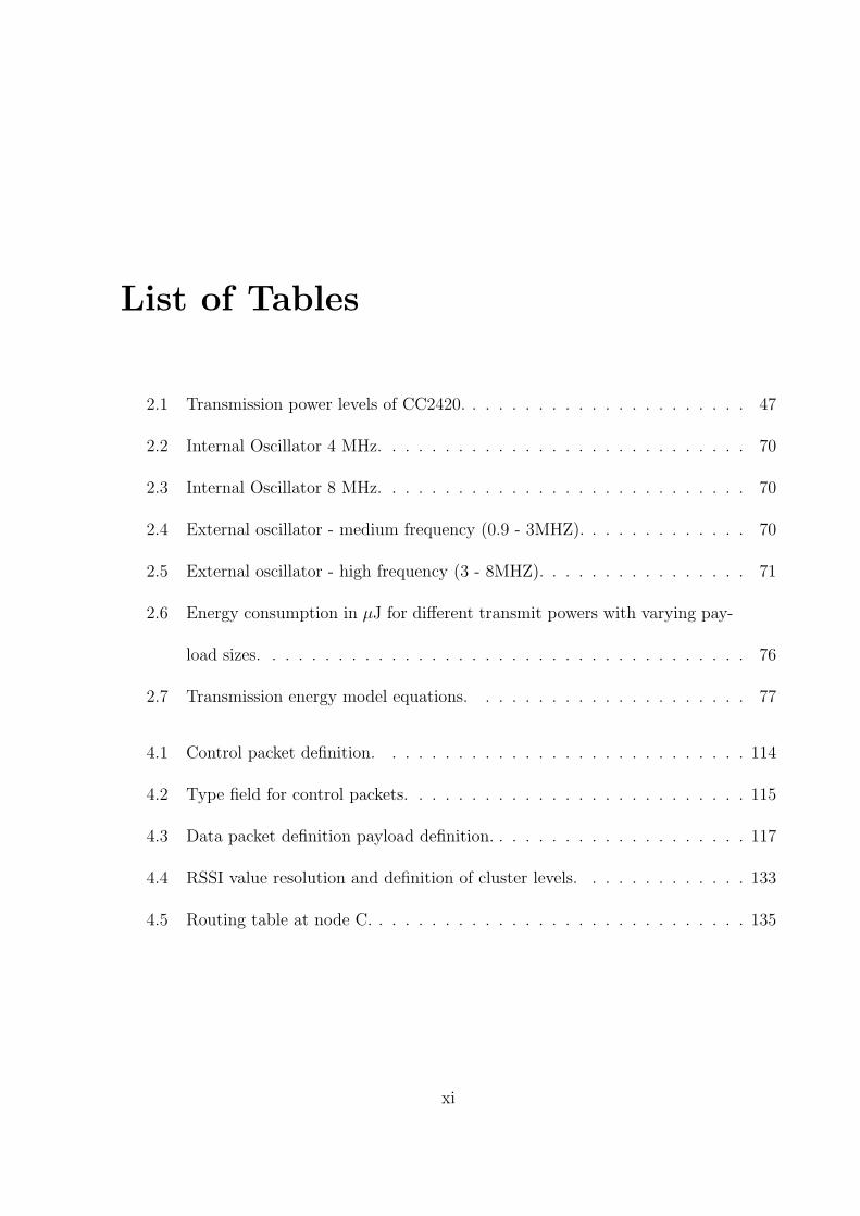
2.1 Transmission power levels of CC2420. . . . . . . . . . . . . . . . . . . . . . 47
2.2 Internal Oscillator 4 MHz. . . . . . . . . . . . . . . . . . . . . . . . . . . . 70
2.3 Internal Oscillator 8 MHz. . . . . . . . . . . . . . . . . . . . . . . . . . . . 70
2.4 External oscillator - medium frequency (0.9 - 3MHZ). . . . . . . . . . . . . 70
2.5 External oscillator - high frequency (3 - 8MHZ). . . . . . . . . . . . . . . . 71
2.6 Energy consumption in µJ for different transmit powers with varying pay-
load sizes. . . . . . . . . . . . . . . . . . . . . . . . . . . . . . . . . . . . . 76
2.7 Transmission energy model equations. . . . . . . . . . . . . . . . . . . . . 77
4.1 Control packet definition. . . . . . . . . . . . . . . . . . . . . . . . . . . . 114
4.2 Type field for control packets. . . . . . . . . . . . . . . . . . . . . . . . . . 115
4.3 Data packet definition payload definition. . . . . . . . . . . . . . . . . . . . 117
4.4 RSSI value resolution and definition of cluster levels. . . . . . . . . . . . . 133
4.5 Routing table at node C. . . . . . . . . . . . . . . . . . . . . . . . . . . . . 135
xi
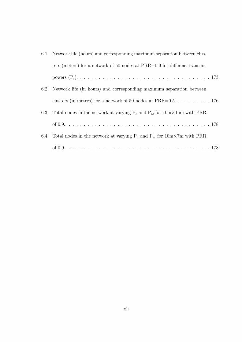
6.1 Network life (hours) and corresponding maximum separation between clus-
ters (meters) for a network of 50 nodes at PRR=0.9 for different transmit
powers (Pt). . . . . . . . . . . . . . . . . . . . . . . . . . . . . . . . . . . . 173
6.2 Network life (in hours) and corresponding maximum separation between
clusters (in meters) for a network of 50 nodes at PRR=0.5. . . . . . . . . . 176
6.3 Total nodes in the network at varying Pc and Pic for 10m×15m with PRR
of 0.9. . . . . . . . . . . . . . . . . . . . . . . . . . . . . . . . . . . . . . . 178
6.4 Total nodes in the network at varying Pc and Pic for 10m×7m with PRR
of 0.9. . . . . . . . . . . . . . . . . . . . . . . . . . . . . . . . . . . . . . . 178
xii

List of Figures
1.1 Wireless sensor network operational distribution. . . . . . . . . . . . . . . 2
1.2 Slots assigned in TDMA frames. . . . . . . . . . . . . . . . . . . . . . . . . 12
1.3 Virtual and physical carrier sense mechanism. . . . . . . . . . . . . . . . . 18
1.4 S-MAC frame. . . . . . . . . . . . . . . . . . . . . . . . . . . . . . . . . . . 20
1.5 Channel contention procedure. . . . . . . . . . . . . . . . . . . . . . . . . . 21
1.6 Polling synchronization. . . . . . . . . . . . . . . . . . . . . . . . . . . . . 23
1.7 Adaptive polling. . . . . . . . . . . . . . . . . . . . . . . . . . . . . . . . . 24
1.8 MRP-MAC transmission mechanism. . . . . . . . . . . . . . . . . . . . . . 26
1.9 Single-hop packet flow in DW-MAC. . . . . . . . . . . . . . . . . . . . . . 29
1.10 Multi-hop transmission in DWMAC. . . . . . . . . . . . . . . . . . . . . . 30
1.11 Network topology set-up in the TEEN protocol. . . . . . . . . . . . . . . . 34
2.1 Block diagram of a wireless sensor node. . . . . . . . . . . . . . . . . . . . 42
2.2 Pin configuration of ATmega128. . . . . . . . . . . . . . . . . . . . . . . . 44
2.3 Pin configuration of CC2420. . . . . . . . . . . . . . . . . . . . . . . . . . 46
2.4 CC2420EM transceiver module. . . . . . . . . . . . . . . . . . . . . . . . . 48
xiii

2.5 PCB size comparison (in mm) of KFUPM sensor node (a)optimized (b)initial
design. . . . . . . . . . . . . . . . . . . . . . . . . . . . . . . . . . . . . . . 53
2.6 PCB design of KFUPM final version (a)Top (b) bottom. . . . . . . . . . . 54
2.7 KFUPM sensor node in final shape. . . . . . . . . . . . . . . . . . . . . . . 54
2.8 Complete S-MAC cycle. . . . . . . . . . . . . . . . . . . . . . . . . . . . . 56
2.9 Shunt resistor power measurement circuit. . . . . . . . . . . . . . . . . . . 68
2.10 VSHUNT measurement for 50 % duty cycle (mV). . . . . . . . . . . . . . . 71
2.11 Measurement of VSHUNT (mV) for transmission at -25 dBm with payload
size of (a) 16 Bytes (b) 22 Bytes. . . . . . . . . . . . . . . . . . . . . . . . 72
2.12 Measurement of VSHUNT (mV) for transmission at 0 dBm with payload
size of (a) 16 Bytes (b) 22 Bytes. . . . . . . . . . . . . . . . . . . . . . . . 73
2.13 Node transmission energy model. . . . . . . . . . . . . . . . . . . . . . . . 77
3.1 NMA main screen shot. . . . . . . . . . . . . . . . . . . . . . . . . . . . . 98
3.2 Node 7 routes data through CHs 11, 15, 4 and 10 . . . . . . . . . . . . . . 100
4.1 Timing diagram of duty cycles of CH and Member Nodes. . . . . . . . . . 113
4.2 Boot-up process of a sensor node. . . . . . . . . . . . . . . . . . . . . . . . 121
4.3 Channel contention of member node to send data packet. . . . . . . . . . . 127
4.4 An illustration example of a network topology. . . . . . . . . . . . . . . . . 132
5.1 Energy consumed per delivered packet with varying packet generation rate. 144
5.2 Average end-to-end latency over different hops. . . . . . . . . . . . . . . . 146
xiv

5.3 Average data throughput at varying traffic rates. . . . . . . . . . . . . . . 148
5.4 Average energy consumed by the network. . . . . . . . . . . . . . . . . . . 150
5.5 Network life vs. varying cluster sizes. . . . . . . . . . . . . . . . . . . . . . 152
5.6 Successful packet reception analysis. . . . . . . . . . . . . . . . . . . . . . 154
6.1 Antenova antenna. . . . . . . . . . . . . . . . . . . . . . . . . . . . . . . . 158
6.2 Antenova antenna radiation pattern from the datasheet. . . . . . . . . . . 159
6.3 Radiation pattern in dBm of the Antennova around the azimuthal axis. . . 160
6.4 Received signal strength with varying azimuthal angle at specific transmitter-
receiver separation for Antennova antenna. . . . . . . . . . . . . . . . . . . 161
6.5 Received signal strength with varying distance in an indoor environment
for Antennova antenna. . . . . . . . . . . . . . . . . . . . . . . . . . . . . . 162
6.6 Received signal strength with varying distance in an outdoor environment
for Antennova antenna. . . . . . . . . . . . . . . . . . . . . . . . . . . . . . 163
6.7 PRR measurements for different transmit powers in an outdoor environment.164
6.8 Stubby antenna radiation pattern from the data sheet. . . . . . . . . . . . 165
6.9 Radiation pattern in dBm of the Stubby antenna around the azimuthal axis.166
6.10 Received signal strength with varying azimuthal angle at specific transmitter-
receiver separation for Stubby antenna. . . . . . . . . . . . . . . . . . . . . 167
6.11 Received signal strength with varying distance for Stubby antenna. . . . . 168
6.12 Transmission radius at different power levels. . . . . . . . . . . . . . . . . . 169
xv

6.13 Network life (in hours) of a network with 50 nodes at PRR=0.9 for a fixed
area. . . . . . . . . . . . . . . . . . . . . . . . . . . . . . . . . . . . . . . . 172
6.14 End-to-end latency at different cluster sizes for network size of 50 nodes at
PRR=0.9. . . . . . . . . . . . . . . . . . . . . . . . . . . . . . . . . . . . . 174
6.15 Network life (in hours) of a network with 50 nodes at PRR=0.5 for fixed
area. . . . . . . . . . . . . . . . . . . . . . . . . . . . . . . . . . . . . . . . 175
6.16 Number of cluster in the network for a PRR of 0.9 and target area of (a)
10m×15m and (b)10m×7m. . . . . . . . . . . . . . . . . . . . . . . . . . . 179
xvi

xvii
ABSTRACT
Name: Farooq Sultan
Title: Custom design and implementation of a wireless sensor node, energy-efficient MAC and routing protocols.
Major Field: Telecommunication Engineering
Date of Degree: January 2011
The use of wireless sensor networks in environmental monitoring applications has increased
rapidly. Due to the presence of extremely versatile as well as low cost devices in the market,
setting up a network now has become easy. A custom build wireless sensor node, named the
KFUPM node, has been successfully designed, implemented and tested with the network for
monitoring temperature and light. An expansion port for adding external sensors has been
provided to ease the need for sensing multiple phenomenon. Widely employed MAC protocol, S-
MAC, has been implemented with unique algorithm which exhibits much better energy
conservation as compared to basic S-MAC. A routing protocol based on cluster head rotation has
been designed and implemented. By employing a cluster head rotation policy, the new protocol
promises better energy consumption as compared to the existing protocols thus leading to the
enhancement of the overall network life. A network design utility has been created to provide
complete specifications for a network setup for a given network cost and an acceptable message
reception rate.

xviii
ABSTRACT (ARABIC)
خالصة الرسالة
فاروق سلطاناالسم الكامل:
كفاءة في استخدام الطاقة وبروتوكوالت التوجيه.MACالعرف تصميم وتنفيذ عقدة استشعار السلكية، ‘ عنوان الرسالة:
التخصص: هندسة االتصاالت
2011 ينايرتاريخ الشهادة:
وقد ازداد استخدام شبكات االستشعار الالسلكية في تطبيقات الرصد البيئي بسرعة. بسبب وجود متعددة للغاية ، فضال عن
األجهزة منخفضة التكلفة في السوق ، وإقامة شبكة وأصبح من السهل اآلن. مخصصة لبناء الالسلكية العقدة االستشعار، واسمه
، وقد تم تصميم بنجاح وتنفيذها واختبارها مع شبكة لرصد درجات الحرارة والضوء. وقد تم توفير منفذ KFUPMعقدة
-S البروتوكول ، MACإلضافة أجهزة استشعار التوسع الخارجي لتخفيف الحاجة لالستشعار عن ظاهرة متعددة. استعماال
MAC نفذت مع الخوارزمية الفريدة التي يسلك أفضل بكثير الحفاظ على الطاقة مقارنة األساسية ،S-MAC وقد تم تصميم .
بروتوكول توجيه على أساس التناوب رئيس الكتلة وتنفيذها. عن طريق استخدام سياسة التناوب رئيس الكتلة، وبروتوكول جديد
وعود أفضل استهالك الطاقة بالمقارنة مع البروتوكوالت القائمة مما يؤدي إلى تعزيز شبكة الحياة العامة. تم إنشاء أداة تصميم
الشبكات لتوفير مواصفات كاملة إلعداد شبكة لتكلفة شبكة معينة واستقبال رسائل معدل مقبول.

CHAPTER 1
INTRODUCTION
Human centric networks are designed to process the data provided by humans and consist
of computers. Such networks usually do not have any interaction with the outside world
and operate on the data provided to them. On the other hand embedded systems, interact
with the environment to control some part of a device. Embedded systems usually do not
interact with humans and are designed to repeat a task as required by the application.
Human need is fueling the convergence of both form of systems leading to a network that
has the ability to interact with machines as well as the humans simultaneously. This
combination has given rise to the ambient intelligence, which includes thousands of tiny
devices that can form networks and have the abilities to interact with both the humans
and machines alike. This has led to the introduction of a new kind of network called
Wireless Sensor Network or WSN. Sensor networks trace back to 1986 when DARPA
announced the Distributed Sensor Networks Program [1]. Since then the advances in
1

microcontroller and sensor technology have led to the design of extremely small wireless
sensor nodes providing high degree of energy efficiency while ensuring sufficiently long
distance wireless communications. A typical WSN consists of two parts as shown in Fig.
1.1.
Figure 1.1: Wireless sensor network operational distribution.
The data acquisition part of the WSN comprises of a large number of tiny wireless devices,
called nodes, deployed over a physical environment that actively cooperate in order to
accomplish one or more tasks. A typical sensor node consists of four main parts; power
supply, sensors, micro controller unit (MCU) and a transceiver to send and receive data.
The power supply is used to power the node. The sensor circuitry can transform physical
quantities into an electric signal. An analog-to-digital converter (ADC), typically a part
2
of the MCU, changes the analog signals generated by the sensors into digital signals and
sends them to the processing part. The processor can then perform simple operations on
the received digital signal, and can store it into memory. Finally, the transceiver sends
and receives data to different destinations as and when required. The sensor nodes relay
their sensed data through each other or directly to the base station depending on the scale
of the network and their position with respect to the base node. The base station may
send control commands (downstream messages) down into the networks, for example a
request to increase their sampling frequency. Sensors are designed to support unattended
operation for long durations, frequently in remote areas, in smart buildings or even in
hostile environments. A set of sensing components forms an essential part of the device;
popular examples include temperature, accelerometer, humidity, infrared light, pressure,
and magnetic sensors, as well as chemical sensors. WSN have applications in all fields
such as structural monitoring [2, 3], environmental monitoring [4] and object tracking.
Owing to the hostility and remoteness of the operating region, [6, 7] have highlighted some
critical factors for the efficient operation of a WSN. Power efficiency for longer network
life, fault tolerance for network integrity, scalability for variable network topologies and
dynamic network setup are just some of the desirable features for a practical WSN.
The data distribution part of the network is responsible for collecting the data from the
base station node and distributing it through different mediums. WiFi, LAN and even
long distance radio communication techniques are used to accomplish this task. The
work presented in this thesis is done at the data acquisition level of the WSN. Designs at
3
hardware level (sensor node) as well as protocol level are done to ensure cost as well as
energy efficiency.
This chapter introduces the motivation behind the work in Section 1.1. Section 1.2 sheds
light on the the WSN applications. Section 1.3 presents the details of challenges faced
in the design of WSN. Sections 1.4 and 1.5 present the literature survey of the existing
technologies at MAC and routing layers for WSNs. Results of the literature review are
presented in Section 1.6. Section 1.7 presents the adopted methodology and the proposed
objectives of this work are presented in Section 1.8. Section 1.9 contains the achievements
and contributions of this thesis and the report concludes with Section 1.10 which gives
the report organization.
1.1 Motivation
To meet the challenges presented in the previous section, one needs to have a thorough
understanding of the operation cycle of a WSN. Moreover, the implementation requires
devising ingenious ways to put a designed protocol into work on actual sensor nodes.
Because of a wide variety of applications, a wireless sensor node has to be “general pur-
pose”. It should have the ability to interface multiple types of sensors and must be
interoperable with the different brands available in market. This task is a challenge in
itself, as the existing IEEE802.15.4 based wireless sensor nodes have a limited interface
ability. Proprietary sensors can only be interfaced and the manufacturer requires sufficient
time to produce the desired product. In addition, some of the devices available in the
4

market require special downloading boards for application code transfer which requires
dedicating a part of the budget for buying the downloading device itself.
As far as the protocols are concerned, this thesis emphasizes on the design of protocols
aimed at increasing the network operating time. To fulfil this requirement the selected
medium access control (MAC) and routing protocols must be energy efficient and should
have the ability to provide an acceptable data throughput for the network to be meaning-
ful. As far as the routing protocols go, cluster based hierarchical protocols have proved
to provide a much better data throughput for large networks [6, 7]; comprising of 100 of
nodes. The issue of selecting a permanent cluster head leads to higher energy dissipation
and therefore a reduced network life; since the death of the cluster head causes issues in
the selection of the new cluster head. When the cluster head runs out of power, until
the selection of the new cluster head, the cluster remains out of touch from the rest of
the network and in doing so leads to multiple packet loss. This head selection procedure
should be streamlined so that the network is not disrupted while providing an acceptable
level of end to end throughput.
The implementation of the designed protocol on hardware presents multiple challenges.
Although the design details are presented in detail in literature, no mention of imple-
mentation process is done. Due to the unavailability of implementation details, unique
methods must be devised while ensuring the network operation is not compromised.
In order to deploy a WSN in a given area, the least number of nodes required to cover a
major part of the area must be determined. Since the number of nodes is directly related
5

to the cost of the network, the process becomes a crucial part of the network deployment
stage.
1.2 WSN Applications
The wide range of applications of WSNs mentioned in literature are:
Building automation
WSN can be deployed in buildings to monitor live activities like temperature/humidity
and in turn operate the heating/cooling equipment depending upon the sensed values.
In addition, intrusion detection can be accomplished to enhance the security situation of
a locality. Intelligent buildings [1] employing systems like BACnet are examples of this
approach.
Environmental monitoring
WSNs have been used to monitor environmental phenomenon like volcanic activity [9] to
alert evacuation teams beforehand. This type of system has also been used to monitor
temprature/humidity condition in tea plantation [10] to operate the irrigation system
autonomously.
Health sciences
WSNs in the form of body area networks (BANs) have been used to monitor health
activity of patients remotely. The network gathers the vital information and sends it to
the doctor over the internet. Thus the doctor has the complete up to date information
about the patient without any dedicated monitoring.
6

1.3 WSN Design Challenges
As mentioned earlier, to ensure proper operation of a WSN, efficient power consumption
must be ensured throughout the network. In addition, self healing ability of the network,
cost efficiency and flexible network architecture must also be provisioned to enable seam-
less operation of the network. A brief detail of the above identified challenges is given
below:
Power Consumption
Power consumption is the most important design factor for WSNs. Conserving power at
each node, eventually leads to the extension of the overall network life. On the hardware
front, efficient design of the node could serve as a major factor in deciding the power
consumption figures. At the application level, power conservation can be incorporated into
the design of the protocols by introducing novel design and implementation procedures
that take the energy reserves into account. For example, minimizing the number of
collisions or choosing the shortest path to the destination can help save power. A major
part of the power is wasted during transmission and reception of radio packets. Since
transmission and reception is inevitable, short distance transmission and simple circuitry
for modulation\demodulation can be employed to save power [6, 7]. It is important to
know the causes of energy wastage so that appropriate action must be taken to overcome
or reduce them. In WSNs energy wastage occurs in three domains namely; sensing, data
7

processing and communications [12]. However, the losses during communications are
considered to be the major factor of the network life [7]. The different causes of energy
wastage have been identified and discussed in the following text.
1. Packet collisions
Packet collisions cause nodes to retransmit [13], which in turn results in wastage
of the battery power. A collision occurs when multiple nodes transmit at the same
time [13]. Since all the nodes share the same channel, collision avoidance must be
ensured for proper delivery of packets within the network. The situation becomes
even worse when multiple packets start to arrive at a receiving node simultaneously.
2. Overhearing
Over-hearing means that a node starts receiving packets that are not destined for
it. In normal operation, a node receives a packet and then starts to parse it. In
this process, the node determines the destination address in the packet header and
discards it if the receiving node is not the destination of the packet. The time
required to complete this process depends on the length of the packet header and
also on the location of the destination address in the header.
3. Control packet overhead
The main objective of the WSN is to relay information to the sink. Control packets
are, however, necessary for establishing and efficient performance of the system.
A large number of control packets decrease the effective data throughput of the
8
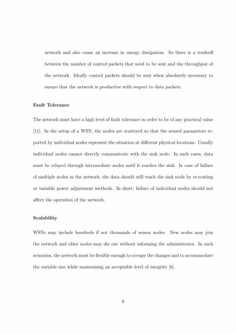
network and also cause an increase in energy dissipation. So there is a tradeoff
between the number of control packets that need to be sent and the throughput of
the network. Ideally control packets should be sent when absolutely necessary to
ensure that the network is productive with respect to data packets.
Fault Tolerance
The network must have a high level of fault tolerance in order to be of any practical value
[11]. In the setup of a WSN, the nodes are scattered so that the sensed parameters re-
ported by individual nodes represent the situation at different physical locations. Usually
individual nodes cannot directly communicate with the sink node. In such cases, data
must be relayed through intermediate nodes until it reaches the sink. In case of failure
of multiple nodes in the network, the data should still reach the sink node by re-routing
or variable power adjustment methods. In short, failure of individual nodes should not
affect the operation of the network.
Scalability
WSNs may include hundreds if not thousands of sensor nodes. New nodes may join
the network and older nodes may die out without informing the administrator. In such
scenarios, the network must be flexible enough to occupy the changes and to accommodate
the variable size while maintaining an acceptable level of integrity [6].
9

Cost of Network Deployment
The deployment cost is a very important design factor for sensor networks because of the
large number of nodes required, as well as the fact that in most networks the nodes are
disposable [7]. The cost includes both the hardware and the software required to monitor
the network.
1.3.1 Causes and Implications of Energy Wastage
As mentioned in 1.3, the limited power supply of the nodes make it inevitable to use
energy conservation techniques to design the network that lasts a longer period of time.
It is, therefore, important to know the causes of energy wastage so that appropriate
action must be taken to overcome or reduce them. In WSNs energy wastage occurs in
three domains namely; sensing, data processing and communications [12]. However, the
losses during communications are considered to be the major factor of the network life [7].
The different causes of energy wastage have been identified and discussed in the following
text.
Once the packets collide, the data gets corrupt; such packets have to be discarded
[13] and retransmissions have to be requested, increasing the energy consumption in the
network. Moreover, when the control packets collide, the complete network setup is
affected. The delay in packet delivery also increases due to collisions. As an indirect
consequence of retransmissions, the effective throughput of the system decreases, since
majority of the time is wasted in retransmissions.
10

Over-hearing wastes valuable energy in reading and receiving packets that are not intended
for the desired node. Moreover, until the completion of this process, all the other packets
intended for the node are not received, thus increasing the latency in the network and
resulting in collisions.
Over-emitting causes high power dissipation and must be avoided by time synchronization
schemes or scheduling. Although the losses in idle listening are not severe but, they must
also be minimized to increase the network life time.
1.4 Literature Survey - WSN MAC Layer Protocols
Literature has been extensively reviewed for existing work in the field of MAC and routing
protocols to establish the basic understanding of the WSN protocol design. Protocols in
WSNs have some unique challenges that are not present in general wireless networks.
The two main challenges are the varying topology nature, and the low power requirement
of the sensor networks [16, 17]. The authors in [7, 13] have presented comprehensive
survey and comparison of various MAC protocols proposed for WSNs. The authors have
summarized the key requirements for MAC protocol design, analyzed the advantages and
disadvantages of some popular MAC protocols and also outlined promising directions for
future work.
In order for all the nodes to communicate, medium access is the most important factor.
Keeping all the energy wastage causes discussed in Section 1.3.1 in mind, the MAC proto-
cols must be able to reduce latency and provide fair access to all the nodes in the network.
11

Based on the method of medium access, the MAC layer protocols can be widely divided
into two main categories:
Characterization-Based Protocols
In characterization-based protocols, nodes are provided access based on a schedule that
is maintained at the setup of the network. This schedule can be created in any of the
following three forms:
1. Time Division Multiple Access (TDMA)
According to the TDMA scheme, time slots are created and assigned to individual
nodes (see Figure 1.2). The node can communicate only in the time slot assigned
to it. The advantage of this scheme is that the probability of packet collision is
almost negligible [18] and consequently power conservation is much better than any
of the other schemes. Also, the end-to-end delay for the packets is deterministic but
usually high [19]. On the down side, this scheme suffers from intense latency issues.
TDMA-based MAC protocols require a central administrative body for strict time
synchronization and slot allocation.
Figure 1.2: Slots assigned in TDMA frames.
2. Frequency Division Multiple Access (FDMA)
12
FDMA-based MAC protocols divide the available bandwidth into channels which
are allocated to the nodes throughout the network. Unlike the time based protocol
(TDMA), the latency is much less for these class of protocols [18]. The disadvantage
of FDMA approach is the use of highly complex and sophisticated radios that have
the ability to operate at multiple frequency bands. In addition, there is a need
for a central administration unit that allocates the frequencies to the nodes and
implements reuse strategies for dense networks.
3. Code Division Multiple Access (CDMA)
CDMA-based protocols are good candidates for WSN owing to their ability to tackle
interference issues. Each node assigns itself a pseudo noise (PN) code which is
then used for communications over the channel. Considering the limited power
and computational abilities of the sensor node, this assignment becomes an issue
in highly populated networks [20]. Broadcast communications do not work well
with CDMA, since each node can decode the information sent using its code. So
separate radio channels along with separate PN codes are required to accomplish
the broadcast operation in CDMA-based protocols [20].
Contention Based Protocols
In contention-base protocols, unlike the scheduling based, nodes are not bounded by time
slots, frequency channels or PN codes. Instead, a node continuously scans the channel
[18] and transmits the data as soon as it gets a vacant slot. Although, the control packet
overhead associated is high, but the resulting latency is much lower as compared to the
13

scheduling based counterparts.
In [16], the authors proposed a medium access protocol called the sensor medium ac-
cess control (S-MAC) for ad-hoc WSNs. This protocol depends on the request-to-send
(RTS)/clear-to-send (CTS) mechanism of the IEEE 802.11 to avoid collisions. It was
shown that S-MAC had 2-6 times less power consumption than IEEE 802.11. In [17]
timeout-MAC (T-MAC) protocol has been proposed to solve the problem of idle listen-
ing in a wireless sensor network. The T-MAC dynamically adapts a listen/sleep duty
cycle in a novel way, through finely grained timeouts, while having minimum complexity.
Both S-MAC and T-MAC operate on the principle of adopting sleep-wake schedules to
synchronize the wake timings of all the nodes within a vicinity.
To further reduce the energy wastage due to idle listening, low-power listening (LPL)
has been employed to reduce the duty cycles to less than 0.1%. WiseMAC [21] and
B-MAC [22] are examples of this implementation. In LPL, nodes wake up for a very
brief period to check the channel activity without actually receiving data. This is called
channel polling. The work in [23] puts forward power control mechanism based on S-
MAC protocol and modifies the competitive mechanism of S-MAC resulting in enhanced
S-MAC (ES-MAC). The energy-efficient and high throughput MAC (ET-MAC) protocol
proposed in [24] embeds some extra information in long wake up preamble frame and it
also uses collision avoidance signaling and handshaking. These ideas help wireless nodes
to stay at sleep mode as much as possible. Their simulation results and analysis showed
that with dynamic traffic load, this protocol achieves improvement in energy-efficiency
14

and throughput, over well known MAC protocols like S-MAC and B-MAC.
In [25], the authors have proposed a new MAC protocol for WSNs for environmental
monitoring applications. The proposed MAC scheme is specifically designed for WSNs
which have periodic traffic with different sampling rates. Moreover, in [26], the authors
have proposed an event based MAC (EB-MAC) that is tailored for event-based systems
like environmental monitoring. EB-MAC arranges data transfer dynamically using an
election based scheduling technique. Trathnig et. al. have presented elastic-MAC (E-
MAC) protocol in [27], which has been shown as energy efficient protocol for low-traffic
delay-tolerant WSNs. The proposed protocol uses asynchronous distributed transmission
scheduling to achieve high energy efficiency. In [28], a novel cluster network topology-
based adaptive MAC protocol for WSNs was proposed. In [33] demand wakeup-MAC
(DW-MAC) protocol has been presented that allows nodes to wake-up on demand during
the sleep intervals to receive or send the data to ensure that the collision in data packets
are minimized. This demand wake-up increases the effective channel capacity at increasing
loads.
From the above discussion, we conclude that there are a wide variety of MAC layer
protocols available. A few contention based MAC protocols have been selected based on
their popularity and will be discussed in more detail in the following text.
15

1.4.1 Sensor-MAC (S-MAC)
The S-MAC [16] protocol is regarded as one of the most energy-efficient protocols at the
MAC layer. It trades off some performance reduction in both per hop fairness and latency
for energy efficiency [29]. S-MAC achieves its efficiently by utilizing a combined scheduling
and contention scheme. The basic idea behind the S-MAC protocol is the locally managed
synchronization and periodic sleep-listen schedules employed in the CSMA technique. The
S-MAC protocol requires the periodic sleep of all the nodes throughout the network. This
design reduces energy consumption, but increases latency, since a sender must wait for the
receiver to wake up before it can send out the data. Each node sleeps for some time, and
then wakes up and listens to see if any other node wants to talk to it. During sleeping,
the node turns off its radio, and sets a timer to awake itself later. A complete cycle of
listen and sleep is termed as a frame and the duty cycle is defined as the ratio of the listen
interval to the frame length. The sleep interval can be changed according to different
application requirements, which actually changes the duty cycle and these values are the
same for all nodes.
For multiple access control, the collisions are avoided by virtual and physical carrier sense
(CS). There is a duration field in each transmitted frame that indicates how long the
remaining transmission will be for. If a node receives a packet destined to another node,
it knows how long to keep silent from this field. The node records this value in a variable
called the network allocation vector (NAV) and sets a timer for it. Every time when
16

the timer fires, the node decrements its NAV until it reaches zero. Before initiating a
transmission, a node first looks at its NAV as indicated by the flowchart in Figure 1.3.
If its value is not zero, the node determines that the medium is still busy. This is called
virtual carrier sense. Physical carrier sense is performed at the physical layer by listening
to the channel for possible transmissions. Carrier sensing time is randomized within a
contention window to avoid collisions and starvation. The medium is determined as free if
both virtual and physical carrier sense indicates that it is free. All sender nodes perform
carrier sense before initiating a transmission. If a node fails to get the medium, it goes to
sleep and wakes up when the receiver is free and listening again. Unicast packets follow
the sequence of RTS/CTS/DATA/ACK between the sender and the receiver. After the
successful exchange of RTS and CTS, the two nodes will use their normal sleep time for
data packet transmission. In order to explain this protocol some assumptions have been
considered.
Assumptions
This protocol assumes that all the nodes in the network are stationary and are able to
transmit at variable levels of power. The nodes are deployed randomly and have the
ability to communicate with neighboring nodes. To conserve energy [29], most of the
data communications is done between neighbors rather than between end points. This
means, to transmit data between two locations, nodes transmit to their neighbors and
the data reaches the destination over a multi-hop path.
17

Figure 1.3: Virtual and physical carrier sense mechanism.
18
The nodes are assumed to operate dedicated applications that result in the activity being
reported. This enables the nodes to be hard-coded rather than generally programmed.
Every node has the ability to aggregate redundant data before transmission to avoid con-
gesting the network by sending copies of the same packet. The applications are assumed
to tolerate some level of latency since environmental monitoring will have long idle periods
followed by data bursts in case of alarm.
Protocol Definition
In WSNs, the network is idle most of the time when there is no activity. However, in
conditions of alarm, the network becomes highly congested. During the idle state, it is
not wise to keep the nodes constantly powered on as this results in the depletion of energy
resources. Instead, as shown in Figure 1.4, schedules are created [30] for each node to
turn them on (wake-up) and turn them off (put them to sleep). Schedules are created
such that every node goes to sleep periodically after some time and then wakes up. The
wake time is usually very small as compared to the sleep period. During the wake period,
the node continuously listens to its surroundings and also transmits any packets that it
needs to during this time. During the sleep period, the nodes turns off its radio, and in
some cases the MCU, to save energy. As shown in Figure 1.4, the wake period is usually
fixed at the time of programming, however, the sleep period can be flexed depending on
the amount of information that needs to be sent.
Individual nodes are given the liberty to choose their schedules independently [29] but
19

Figure 1.4: S-MAC frame.
it is usually preferred that a group of nodes follow the same schedule to reduce the control
overhead [30]. Neighboring nodes synchronize their schedules and make sure that all wake
up at the same time so that data is routed (with minimum latency) to the sink node.
Maintaining Synchronization
Nodes maintain their synchronization by broadcasting SYNC packets. The SYNC packets
are very concise and contain the address of the sending node and the time of its next sleep.
When any node receives this SYNC packet, it adjusts its timers so that it sleeps at the
same time as the node that sent the SYNC. The timer adjustment is all done relative to the
received SYNC, the absolute times are not important. Schedule Selection Criterion
When selecting a schedule for a node, there are three cases that could arise;
1. When a node wakes up initially, it starts to listen the medium for synchronization
(SYNC) packets. If it does not receive a SYNC packet within the desired time, it
broadcasts its own SYNC packet.
2. If, during the initial listen period, the node receives a SYNC packet from a neighbor,
it starts to follow it.
3. If a node receives a new schedule (SYNC packet) when it has already adopted one,
then if the node does not have any neighbors, it will discard the old schedule and
20
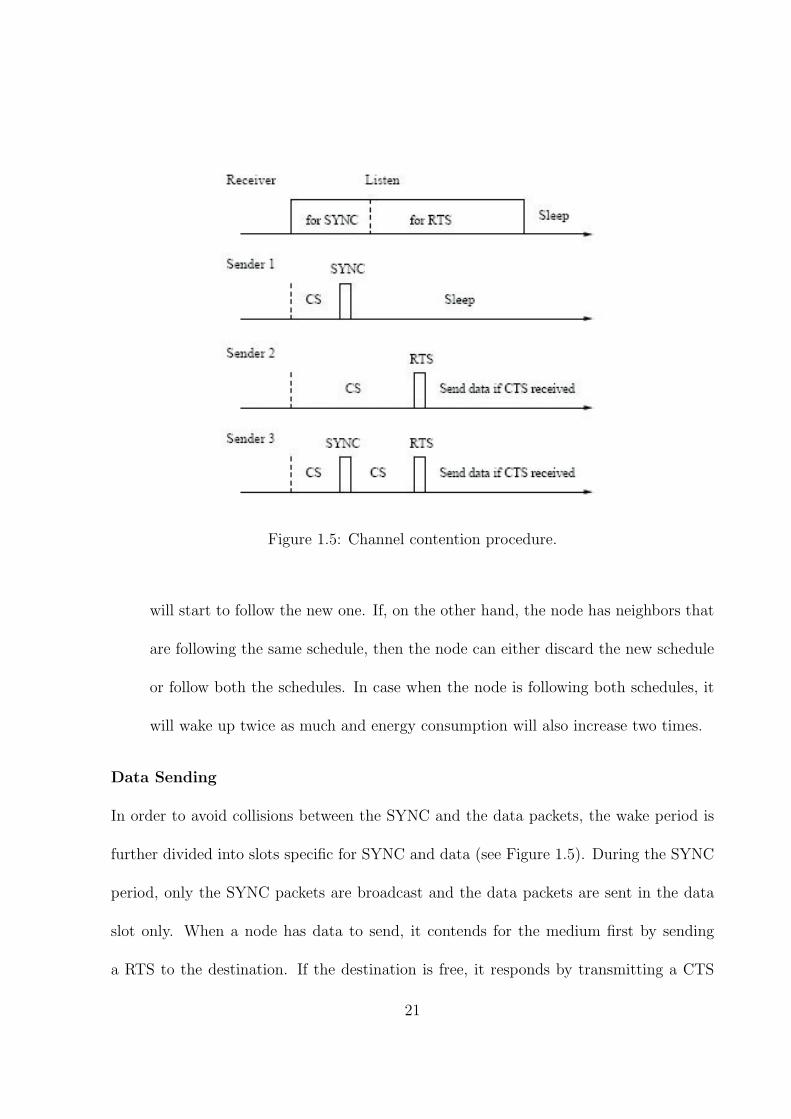
Figure 1.5: Channel contention procedure.
will start to follow the new one. If, on the other hand, the node has neighbors that
are following the same schedule, then the node can either discard the new schedule
or follow both the schedules. In case when the node is following both schedules, it
will wake up twice as much and energy consumption will also increase two times.
Data Sending
In order to avoid collisions between the SYNC and the data packets, the wake period is
further divided into slots specific for SYNC and data (see Figure 1.5). During the SYNC
period, only the SYNC packets are broadcast and the data packets are sent in the data
slot only. When a node has data to send, it contends for the medium first by sending
a RTS to the destination. If the destination is free, it responds by transmitting a CTS
21
packet. When the sending node receives the CTS, it sends its data to the destination
node and waits for the acknowledgement (ACK). If the ACK is not received within some
predefined time, the complete procedure is repeated again. The nodes whose RTS are
rejected back off, go to sleep and try again in the next wake period.
Collision and Over-Hearing Avoidance
Collision and over-hearing avoidance is accomplished by carrying out both physical and
virtual carrier sensing. In physical carrier sensing, the node scans the channel for the
presence of any signal and if a signal is found, it backs off for a random amount of time
and repeats again later. In virtual carrier sensing, the node reads the network allocation
vector (NAV) field of the packet it receives. When a node hears an RTS or a CTS not
destined for itself, it reads the NAV and starts to decrement it until it becomes zero.
When the NAV becomes zero, only then the transmission can be done. Physical and
virtual carrier sensing is done before transmitting every packet to ensure that collisions
are avoided.
1.4.2 Scheduled-Channel Polling (SCP-MAC)
In SCP-MAC, the concept of LPL is utilized [31]. In LPL, the nodes wake up for small
intervals of time and listen for activity on the channel without receiving anything. If
the channel is idle, the nodes go back to sleep, otherwise they receive the data and then
examine or process it. This complete process is referred to as channel polling. Unlike
S-MAC, the polling time is very brief and is synchronized between all the nodes. Due to
22

Figure 1.6: Polling synchronization.
the extremely small size of the polling windows, this method is far more energy efficient
as compared to the standard S-MAC [31].
Synchronizing Channel Polling
Channel polling reduces the cost of discovering the presence of information since it is
far cheaper than actually knowing what the information is [31]. The interval of polling is
usually several times less than the actual wake period used in S-MAC. Unlike the ordinary
LPL scheme in which senders send a long preamble before the actual information, the
preamble in SCP-MAC is very small and serves the purpose of informing the receiving
node to wake up for packet reception (Figure 1.6). The length of the polling period is
designed in conjunction with the length of the wake-up signal as both are related to the
network size. The wake-up period is chosen to be slightly larger than the polling period to
ensure the listening node gets the wake-up signal. The primary purpose of synchronizing
the polling times is that short wake-up signals are required to be transmitted by the
senders before the actual packet. The scheduling of polling periods reduces the energy
cost due to over-hearing but increases the cost of maintaining and transmitting schedules.
Adaptive Polling Scheme
In event-driven applications, the network remains idle most of the time and is flooded
23
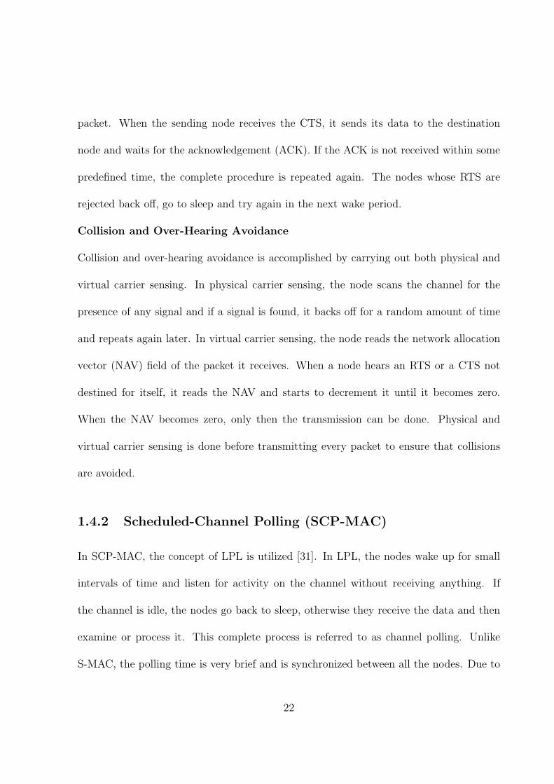
by data packets in the event of an activity. If the normal polling schedules are used,
the per-hop latency increases and the collisions also increase since bursts of data are
being transmitted between nodes simultaneously.In order to counter this, the network
intelligently detects traffic flow and adds additional polling slots if the data is thought to
have increased (Figure 1.7). This results in a decrease in per-hop latency and enables the
network to operate at varying traffic loads [31].
Figure 1.7: Adaptive polling.
Contention
The contention in SCP-MAC involves two steps:
1. In the first step, the sending node sends a wake-up tone that coincides with the
polling period of the destination. This wake-up packet is extremely small and serves
the purpose of waking up the destination to be able to receive data.
2. Once the destination node wakes up, the sender transmits the data packet.
One advantage of this two-step contention phase is that the probability of collision in
data packets decreases as only the nodes that pass the first step proceed to send the data,
other nodes will back off. Moreover, it is considered that the collision in the wake-up
24

tones can be tolerated and the retransmission of such tones does not increase the energy
consumption by a considerable amount.
Overhearing Avoidance
SCP-MAC protocol enables overhearing avoidance by using either RTS/CTS or by em-
ploying packet headers. When the RTS/CTS scheme is used, the process is the same
as that in S-MAC. In case of message headers, upon receiving a packet, the node starts
to read the destination address in the packet header. If the current node is not the
destination, the reception is stopped.
1.4.3 Medium Reservation Preamble-Based MAC (MRP-MAC)
MRP-MAC is based mainly upon the S-MAC protocol with a few modifications for efficient
data transmission. In S-MAC, the wake period is divided into SYNC and data intervals,
this makes the wake period excessively long. Moreover, if a node does not get access to
the medium, it stays awake for the remainder of the wake period. This extra listening
in back-off situation is a cause of energy wastage. To counter these problems, [32] have
devised MRP-MAC which introduces separate contention windows for the transmitting
nodes and enables the nodes to sleep during the contention period when they do not have
data to transmit.
25

Protocol Definition
MRP-MAC is a synchronized duty-cycle protocol [32] like S-MAC. However, unlike S-
MAC, the complete cycle of a node is divided into three windows rather than two. There
is an additional contention window as shown in Figure 1.8. The transmitting nodes
Figure 1.8: MRP-MAC transmission mechanism.
contend during the contention period while all the other nodes sleep. The neighboring
nodes wake up during the brief listen period to check for activity and go to sleep again if
the channel is idle.
Unlike S-MAC, MRP-MAC does not have separate slots for SYNC and data packets within
the wake period. Instead, both types of packets are received in the brief listen window.
To contend for the medium, the nodes with data packets are given priority as compared
to the nodes that are sending SYNC packets [32]. To save energy, the synchronization
information is carried in both the SYNC as well as in the data packet. The RTS packets
are combined with SYNC packets to produce a combined SY NCRTS packet. This packet
26
serves as RTS and also contains the SYNC information, thus reducing the number of
SYNC packets that are transmitted.
Packet Transmission
In MRP-MAC, nodes have two wake-up points, the transmitter wakes up at the start of
the contention period while the receiving nodes wake up in the listen period. When the
transmitter wakes up, it has to contend for the channel by using carrier sense multiple
access (CSMA). The successful node that gets the channel broadcasts a MRP packet.
The MRP contains a predefined sequence of bits and its sole purpose is to make the other
nodes realize that the channel has been occupied. At the end of the contention period,
the listen interval starts. The length of the listen interval is chosen to be slightly larger
than the contention period so that the nodes can receive the CTS or the data. Both the
nodes involved in communication remain awake in the listen period until the transmission
is finished.
Node Synchronization
To synchronize the neighboring nodes, SYNC packets are exchanged periodically between
the neighboring nodes. Also the SYNC information is contained in the data and the
SY NCRTS packets which reduce the number of SYNC packets transmitted thus increasing
the effective throughput of the system.
27

1.4.4 Demand-Wakeup MAC (DW-MAC)
Unlike the previously discussed schemes, this protocol allows nodes to wake-up on demand
during the sleep intervals to receive or send the data to ensure that the collisions in data
packets are minimized. This demand wake-up increases the effective channel capacity at
increasing loads [33].
Protocol Description
In this protocol, each duty cycle is divided into SYNC, data and sleep intervals. The basic
concept of this protocol is that nodes wake-up during the sleep intervals and transmit data.
In DW-MAC scheduling and contention is integrated. When a node has some data to
send, it contents for the channel access first by using CSMA. Once the channel access is
complete, the node transmits a special scheduling (SCH) frame instead of the RTS. The
length of this frame is adjusted such that the corresponding length of the sleep interval can
be determined from the SCH duration. Essentially, there is a one-to-one mapping between
the SCH duration and the sleep interval duration. SCH has no other information than
the address of the intended receiver so that only the destined node wakes up. Moreover
SCH has no timing information and just replaces the contention packets RTS/CTS. This
decreases the control packet overhead and decreases collisions at the receivers.
Single-hop Packet Flow
Considering an example from Figure 1.9 in which node A wants to transmit to node B.
After performing CSMA, node A contends for the channel and sends an SCH frame to
28
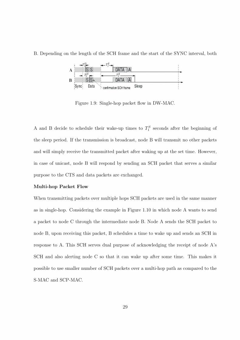
B. Depending on the length of the SCH frame and the start of the SYNC interval, both
Figure 1.9: Single-hop packet flow in DW-MAC.
A and B decide to schedule their wake-up times to T S1 seconds after the beginning of
the sleep period. If the transmission is broadcast, node B will transmit no other packets
and will simply receive the transmitted packet after waking up at the set time. However,
in case of unicast, node B will respond by sending an SCH packet that serves a similar
purpose to the CTS and data packets are exchanged.
Multi-hop Packet Flow
When transmitting packets over multiple hops SCH packets are used in the same manner
as in single-hop. Considering the example in Figure 1.10 in which node A wants to send
a packet to node C through the intermediate node B. Node A sends the SCH packet to
node B, upon receiving this packet, B schedules a time to wake up and sends an SCH in
response to A. This SCH serves dual purpose of acknowledging the receipt of node A’s
SCH and also alerting node C so that it can wake up after some time. This makes it
possible to use smaller number of SCH packets over a multi-hop path as compared to the
S-MAC and SCP-MAC.
29

Figure 1.10: Multi-hop transmission in DWMAC.
1.5 Literature Survey - Routing Layer Protocols
The MAC layer serves the purpose of enabling the multiple nodes to transmit while giving
equal opportunity to all the member nodes. In order for the data to reach the sink node,
the packets must be routed over multiple hops to conserve transmission power. Routing
layer protocols ensure the timely delivery of the packets to the sink while keeping in view
the scalability and the constantly changing topology of the network .
In [6] a comprehensive survey is presented for the routing protocols for WSNs. Further,
very recently in [34, 36] the authors have presented a review and comparisons of recent
routing protocols in WSNs and classified them into categories based on the network struc-
ture in WSNs. In [37] Schurgers et al have derived practical guidelines to enhance the
routing in WSNs based on the energy histogram and have developed a spectrum of new
routing techniques. Their first approach aggregates packet streams in a robust way, re-
sulting in energy reductions by a factor of 2 to 3. In the second approach, which relies
only on localized metrics, the network lifetime increases up to 90% as compared to the
30

first approach.
Heinzelman et. al. has proposed one of the most popular hierarchical routing algorithms
for WSNs called low-energy adaptive clustering hierarchy (LEACH). LEACH has been
shown to achieve a factor of more than 7 reduction in energy consumption compared
to direct communication type of routing protocols and a factor of 4-8 compared to the
minimum transmission energy type of routing protocol. Later, Lindsey et. al. proposed
an improvement of the LEACH protocol in [38], referred to as power-efficient gathering
in sensor information systems (PEGASIS). The difference from LEACH is the use of
multi-hop routing by forming chains and selecting only one node to transmit to the sink
instead of using multiple nodes. PEGASIS has been shown to outperform LEACH by
about 100-300% for different network sizes and topologies.
Another very attractive routing protocol; namely, the threshold-sensitive energy efficient
sensor network protocol (TEEN), has been proposed in [39]. This is a hierarchical protocol
designed to be responsive to sudden changes in the sensed attributes such as temperature
and humidity etc. TEEN pursues a hierarchical approach along with the use of a data-
centric mechanism. However, TEEN is not good for applications where periodic reports
are needed since the user may not get any data at all if the thresholds are not reached. The
same authors later proposed an improvement in the TEEN protocol by making it adaptive
to the requirements of the application in use [40]. The adaptive-threshold sensitive energy
efficient sensor network protocol (APTEEN) is an extension to TEEN and aims at both
capturing periodic data collections and reacting to time critical events. Simulations of
31

TEEN and APTEEN have shown them to outperform LEACH in several aspects.
Another energy-aware WSN routing protocol called reliable and energy efficient protocol
(REEP) [41], in which sensor nodes establish more reliable and energy-efficient paths for
data transmission. The authors have evaluated the performance of REEP under different
scenarios, and have shown it to be superior to the popular data-centric routing protocol,
directed-diffusion (DD). Yabin et al proposed a redundancy-based directional reliable
multi-hop clustering routing algorithm (DRMC) [42]. DRMC mechanism is claimed to
keep the proper lifetime, the stability and expansibility of the network, in addition to
improving the speed and reliability of the routing process.
Since TEEN and LEACH have influenced the actual hardware implementation of this
thesis, a brief review of these two protocols in given in the coming text.
1.5.1 Threshold Sensitive Energy Efficient Sensor Network Pro-
tocol (TEEN)
Threshold sensitive Energy Efficient sensor Network protocol (TEEN)[39] is a hierar-
chical protocol designed to be responsive to sudden changes in the sensed environmental
attributes such as temperature. Responsiveness is important for time-critical applications,
in which the network operates in a reactive mode.
The network architecture in TEEN is based on a hierarchical grouping where closer nodes
form clusters and this process goes on the second level until base station (sink) is reached.
After the clusters are formed, the cluster head broadcasts two thresholds to the nodes.
32

These are hard and soft thresholds for sensed attributes. The Hard threshold is the
minimum possible value of an attribute to trigger a sensor node to switch on its transmitter
and transmit to the cluster head. Thus, the hard threshold allows the nodes to transmit
only when the sensed attribute is in the range of interest, thus reducing the number of
transmissions significantly. Once a node senses a value at or beyond the hard threshold,
it transmits data only when the value of that attribute changes by an amount equal to or
greater than the soft threshold. As a consequence, soft threshold will further reduce the
number of transmissions if there is little or no change in the value of sensed attribute.
Packet Flow Mechanism
This model uses hierarchical clustering scheme [39, 44] in which the nodes are classified
into clusters as shown in Figure 1.11. Nodes are grouped into clusters and a cluster head
is selected from amongst them. The selection of cluster head can be fixed but is usually
taken as dynamic to distribute the energy consumption evenly throughout the network
[44]. Once the cluster head has been selected, the remaining nodes become its members.
All the member nodes sense and forward the data to their respective cluster heads. Once
the head node gets the data, it needs to forward it to the next head in the upper level.
This process continues until the packet reaches the sink.
Hard threshold (HT) and soft threshold (ST) are defined by the user and serve as the
limits of the forwarded data [43]. HT defines the limit for the minimum sensed value
after which the data should be transmitted, whereas ST defines the minimum difference
33
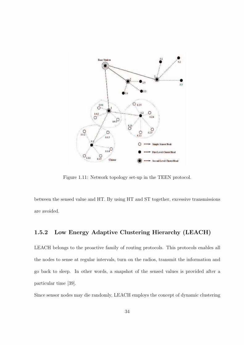
Figure 1.11: Network topology set-up in the TEEN protocol.
between the sensed value and HT. By using HT and ST together, excessive transmissions
are avoided.
1.5.2 Low Energy Adaptive Clustering Hierarchy (LEACH)
LEACH belongs to the proactive family of routing protocols. This protocols enables all
the nodes to sense at regular intervals, turn on the radios, transmit the information and
go back to sleep. In other words, a snapshot of the sensed values is provided after a
particular time [39].
Since sensor nodes may die randomly, LEACH employs the concept of dynamic clustering
34

where the cluster memberships keep varying from time to time. LEACH is completely
distributed and requires no global knowledge of the network. However, LEACH uses
single-hop routing where each node can transmit directly to the CH and the sink. There-
fore, it is not applicable to networks deployed in large regions. Furthermore, the idea of
dynamic clustering brings extra overhead, e.g. head changes, advertisements etc., which
may diminish the gain in energy consumption.
When the network is set-up, the nodes are distributed into clusters. Once the clusters
have been created, the head node transmits TDMA-based schedules to notify the member
nodes of their respective time slots during which communication takes place. When all
the nodes have sent the data to the cluster head, the head node aggregates the data and
forwards to the cluster head in the second level. Due to time slots, the cluster heads has
to be awake for a larger amount of time as compared to the member nodes. Also the
aggregation of data requires processing, which in turn consumes valuable energy.
Due to the high energy dissipation at the cluster head, it is expected to die out early. To
prevent this event from happening, the cluster head responsibility is rotated among the
member nodes [45]. This enables uniform energy consumption in the network ensuring
that no single node dies out earlier.
1.6 Results of Literature Survey
After surveying the literature for the existing MAC and routing layer protocols, we con-
clude that the reduction of energy consumption on individual nodes results in an increase
35

in the overall operating life of the network. This increase in lifetime is highly desirable
and can be achieved by the following two methods:
1. Making the hardware design more energy efficient.
2. Designing protocols that aim to reduce energy wastage.
Redesigning the hardware for energy efficiency is usually not preferred unless special
requirements on the design are not available on the already offered devices. Usually
protocols are tuned to behave in an energy efficient manner.
As for the hardware itself, all the devices currently available in the market are limited in
terms of the activity they can sense. This limitation has been put forward to enforce the
monopoly of the corporations manufacturing the nodes. Sensing some special phenomenon
using the present hardware is not possible without requesting the manufacturer for a
modification of the device; resulting in increase in cost.
1.7 Adopted Approach
Traditional WSN design focusses on improving energy efficiency and data throughput by
adopting design methods for MAC and routing protocols. However, the energy consumed
by the wireless node during the operation of the application is usually side lined. The
approach adopted for the design and implementation of the MAC and routing protocols
ensures energy efficiency on the application level by using programming platforms like
TinyOS which insure a high degree of energy efficiency by limiting the resources being
36

used.
The protocols have been simulated and fine tuned before implementing them on actual
hardware. The implementation details have been devised after intense brainstorming and
after extensive testing of the network. The network has been tested with 30 nodes for a
sufficient period of time to confirm the operation of the programmed protocols.
In order to create a model to provide an approximation on the network size, received
radio power measurements have been performed at two different locations. This data has
been used to construct a model that can provide the approximate network size for a given
region of interest.
1.8 Proposed Objectives
The main objective of this thesis is to design and implement an energy-efficient WSN
for monitoring applications that will help industrial as well as environmental activity
monitoring in the big cities of the Kingdom. The design of the prototype WSN will
involve the following two phases:
1.8.1 Hardware Design
1. We intend to design our own, custom created hardware nodes, called the KFUPM
nodes. The desired features of KFUPM nodes are given below:
• Using off-the-shelf sensing devices (sensors).
37

• Designing appropriate conditioning circuits for the sensors used.
• Using off-the-shelf micro-controllers and RF transceivers.
• Provision of extension ports for connecting multiple sensors.
• Onboard power supply to last for sufficiently long time.
2. An analysis of the energy consumption of the KFUPM nodes in different operating
modes will be presented in this thesis.
3. A study of the relationship between the transmission power and the covered distance
for the transceivers used for KFUPM nodes will also be carried out.
4. On field experimentation will be carried out at different locations to investigate the
effect of environment on the radio coverage. This analysis will, in turn, pave the way
to the formulation of guidelines for an efficient network design using the KFUPM
nodes.
1.8.2 MAC and Routing Layer Protocol Design
The second part of this thesis will emphasize on the design and implementation of MAC
and Routing protocols to set-up a network. Our literature survey has concluded that
although several protocols have been presented and analyzed, no hardware implementation
details for either MAC or routing protocols is presented. The aims for this part of the
thesis are:
38

1. Unique implementation strategies will be formulated to ensure an exact translation
of the protocols on KFUPM nodes.
2. An attempt to implement an energy efficient routing protocol will be done.
3. We also plan to present a methodology to determine a rough estimate of the network
life based on the protocols designed.
4. The software that runs the protocol stack, application firmware, and data processing
application will be designed and coded in a manner that is efficient in terms of
memory resources and power consumption.
5. Finally, we will attempt to design and implement the core of the WSN technology
to be application and hardware independent so that other applications can utilize
the same WSN structure with minor changes in the sensor node design.
1.9 Summary of Achievements and Contributions
This thesis has led to the successful design and fabrication of a one-of-a-kind wireless
sensor node (KFUPM node) at a reasonable price and having the same if not higher
sensing abilities. KFUPM node can be programmed by a cheap off-the-shelf programmer
rather than using special sensor boards (MIB 510) as for the Crossbow Mica devices.
Temperature and light sensors have been included on the node and extra ports have been
provided to interface additional sensors if required.
39
On the software front, a MAC layer protocol inspired from S-MAC has been implemented
with some unique implementation procedures not mentioned in literature. LEACH and
TEEN have been used as references to devise a routing protocol that serves the purpose
of data routing as well as keeps the power consumption in check. An interactive network
monitoring application has been created to observe the network conditions and to record
the data for future usage. A network deployment application has been completed that
estimates the approximate network size based on the environment and the target area.
The complete system has been tested with 25 nodes with several clusters at different
levels from the sink node. The network performed well and remained stable throughout
the experiment.
1.10 Thesis Organization
This thesis is organized as follows. Chapter 2 has the hardware design and node creation
process for KFUPM nodes. Chapter 3 focusses on the software interface development for
the KFUPM platform. Chapter 4 presents the implementation details of the MAC and
the routing layer protocols. The simulation results of the designed protocols are presented
in Chapter 5. The radio measurements and design of the network design application are
explained in Chapter 6. The thesis concludes with a summary of achievements and an
overview of future work provided in Chapter 7.
40

CHAPTER 2
HARDWARE DESIGN AND
IMPLEMENTATION
Wireless sensor nodes require hardware implementation and programming so that it can
communicate with other nodes in the network [46]. Figure 2.1 shows the logical block
diagram of a typical wireless sensor node. It consists of the following parts:
• Processor Subsystem (typically consisting of a microcontroller)
• RF Subsystem (typically consisting of a radio transceiver)
• Sensor Subsystem (includes sensors for temperature, humidity, light, gas, dust etc).
• Power supply and batteries
This chapter presents the hardware level design details for our hardware platforms. Sec-
tion 2.1 sheds light on the design details of the KFUPM wireless sensor node node. The
41
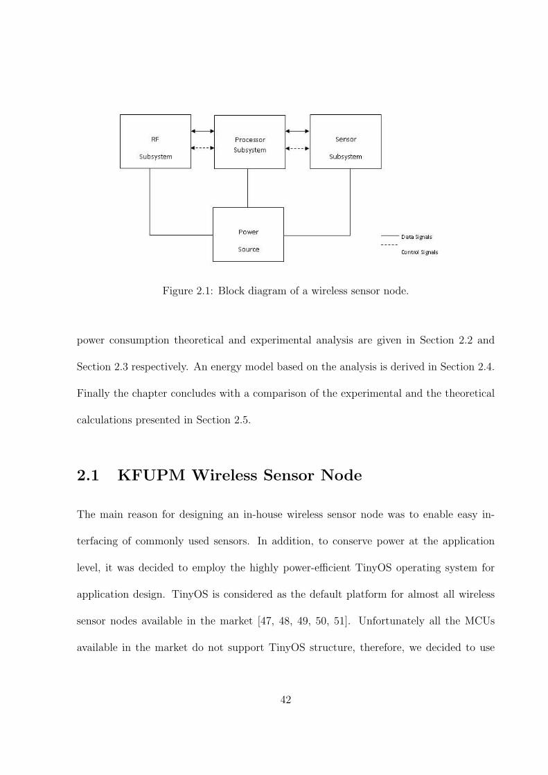
Figure 2.1: Block diagram of a wireless sensor node.
power consumption theoretical and experimental analysis are given in Section 2.2 and
Section 2.3 respectively. An energy model based on the analysis is derived in Section 2.4.
Finally the chapter concludes with a comparison of the experimental and the theoretical
calculations presented in Section 2.5.
2.1 KFUPM Wireless Sensor Node
The main reason for designing an in-house wireless sensor node was to enable easy in-
terfacing of commonly used sensors. In addition, to conserve power at the application
level, it was decided to employ the highly power-efficient TinyOS operating system for
application design. TinyOS is considered as the default platform for almost all wireless
sensor nodes available in the market [47, 48, 49, 50, 51]. Unfortunately all the MCUs
available in the market do not support TinyOS structure, therefore, we decided to use
42

the higher model of the microcontroller (ATmega128) supporting TinyOS. Some of the
features of the KFUPM node are given in the following text.
2.1.1 Atmel ATmega128 Microcontroller
The ATmega128 is a low-power, high-performance 8-bit microcontroller offering 128KB
of in-system self-programmable flash program memory, 4KB EEPROM, and 4KB internal
SRAM. It allows executing powerful instructions in a single clock cycle, achieving through-
put approaching 1 million instructions per second (MIPS) allowing the system designer
to optimize power consumption versus processing speed. It comes in surface-mount com-
pact form factor thus achieving smaller sized circuit designs. The pin configuration of the
ATmega128 is shown in Figure 2.2.
Recall that a mandatory requirement of the WSN design is to conserve the power in the
sensor nodes. Hence, this microcontroller has support for different power save modes.
Sleep modes enable the application to shut down unused modules of the MCU, thereby
saving power. The ATmega128 provides six different power-save modes as explained
below:
• Idle Mode:
In this mode the CPU stops but the SPI, analog comparator, ADC, two-wire in-
terface, timers/counters, watchdog and the interrupt system continue to operate
normally. This mode also enables the MCU to wake-up from an external trigger.
• ADC Noise Reduction Mode:
43
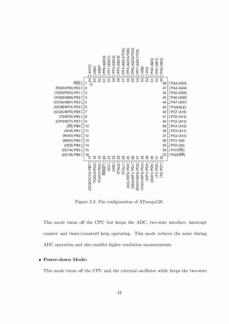
Figure 2.2: Pin configuration of ATmega128.
This mode turns off the CPU but keeps the ADC, two-wire interface, interrupt
counter and timer/counter0 keep operating. This mode reduces the noise during
ADC operation and also enables higher resolution measurements.
• Power-down Mode:
This mode turns off the CPU and the external oscillator while keeps the two-wire
44
interface, external interrupts and the watchdog counter keep operating. This mode
educes the noise during ADC operation and also enables higher resolution measure-
ments. The MCU can wake-up from this mode only from external interrupts.
• Power-save Mode:
This mode is the same as compared to power-down mode except that all the timers
ar also enabled. This enables the MCU to wake-up when timers/counters overflow.
• Standby Mode:
The only difference between this mode and the power-down mode is that the oscil-
lator continues to run. This feature can be used when the oscillator is being used
time external circuitry attached to the MCU.
• Extended Standby Mode:
This mode is similar to the power-save mode with the exception that the oscillator
keeps operational.
Our nodes required several buffers and keeping track of different timing events and desir-
ably ATmeg128 offers 32 general-purpose working registers, real-time counter (RTC), four
flexible timers/counters with compare modes. It has 10-bit ADC with optional differential
input stage with programmable gain that were required for the sensors.
45
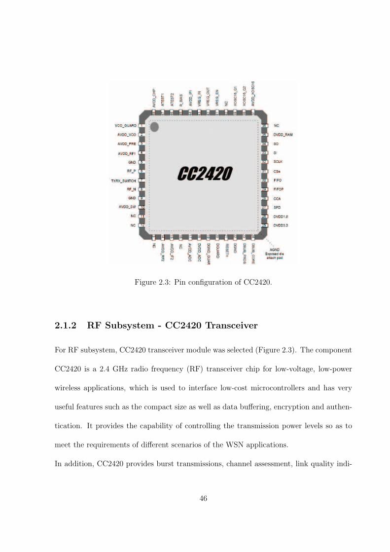
Figure 2.3: Pin configuration of CC2420.
2.1.2 RF Subsystem - CC2420 Transceiver
For RF subsystem, CC2420 transceiver module was selected (Figure 2.3). The component
CC2420 is a 2.4 GHz radio frequency (RF) transceiver chip for low-voltage, low-power
wireless applications, which is used to interface low-cost microcontrollers and has very
useful features such as the compact size as well as data buffering, encryption and authen-
tication. It provides the capability of controlling the transmission power levels so as to
meet the requirements of different scenarios of the WSN applications.
In addition, CC2420 provides burst transmissions, channel assessment, link quality indi-
46

cation and packet timing information. These features reduce the load in any host micro-
controller. The CC2420 as shown uses serial peripheral interface (SPI) to communicate
with the microcontroller (4-wires serial). Also there are 4 extra lines out of the CC2420
to assist the microcontroller in monitoring the status of the wireless communication. It
has 256 Bytes buffer for transmitting and receiving data. The CC2420 supports ZigBee
with direct sequence spread spectrum (DSSS) transmission at 2 Mchips/sec and provides
an effective data rate of 250 kbps [57]. Moreover, CC2420 has the ability to adjust the
transmission power levels as indicated in Table 2.1.
Table 2.1: Transmission power levels of CC2420.
Power Level Transmitted Power in dBm
31 0
27 -1
23 -3
19 -5
15 -7
11 -10
7 -15
3 -25
We used the daughter board module CC2420EM. It is a Zigbee enabled RF transceiver
47

Figure 2.4: CC2420EM transceiver module.
with TinyOS support produced by Chipcon. This board has the CC2420 module with
its configurations parts and circuits ready and soldered on a PCB with a 40-pins socket
along with its antenna as shown in Figure 2.4.
2.1.3 New Circuit Design
For the circuitry design all efforts have been made to reduce the size and weight of the
sensor nodes by designing more efficient PCBs and using smaller components with better
surface-space utilization e.g. double-sided PCBs. We also searched for smaller sized
antenna to be replaced on the RF transceiver.
At this stage, we also decided to equip the wireless nodes initially with two types of
sensors for environmental monitoring e.g. light and temperature. The light sensor was
installed on-board and the temperature sensor was interfaced with the node via the ex-
pansion ports. Nodes sense the raw data and provide the corresponding analog voltage
to the microcontroller that is converted to digital format by the internal ADC of the
48

microcontroller for the processing and later transmission by the RF transceiver to the
neighboring nodes. Some of the features of KFUPM node are:
Small Size
The KFUPM node has a reduced area with double-sided PCB design structure. The over-
all design was also improved so that the dimensions were reduced to a 6.09cm×4.19cm. A
smaller, more compact antenna was used to reduce the effective height of the platform. In
addition, the optimization in physical area was achieved by relocating some components
and using comparatively compact passive components e.g. by using small size 1/8 Watt
resistors instead of the standard 1/4 Watt. The crystal oscillators have also been used in
a way so as to conserve the space.
Use of LEDs
The LEDs used in the new design are surface mount type and have smaller physical di-
mensions thus freeing up crucial space and saving the area of the node. The actual area
of the ultimate functional node can be even smaller when the LEDs and their peripheral
circuitry are removed as they are used in the prototype only for the debugging purposes to
let us know the different states of the node during its operation. The current assignments
of the LEDs are as follows:
All OFF: Node in Sleep Mode
Green ON: Member Node awake
Blue ON: Node sending data
Red ON: Head node awake
49
Power Source
The KFUPM node is a totally self-powered unit and has an onboard battery pack as the
power source. All the wireless nodes in our prototype network are identical in every aspect
except the sink/base node and they are powered using batteries. Only the sink node is
powered by the commercial power via the USB port of the Network Monitoring Server.
Moreover, an ON-OFF switch was also embedded into the design to enable resetting the
devices and to avoid the wastage of energy during testing. The wireless nodes are powered
by 3 AAA sized (1.5VDC) batteries providing a total supply of 4.5V.
Extension Ports
The designed node has a set of extension ports that provide us the capability to add
external sensors. Currently, the node houses on-board light sensor and has provision of
installing temperature and humidity sensors on board using those extension ports. We
also have the option to add an extra analog sensor and a digital sensor with a 4.5V power
port also available for powering the sensors.
Before producing larger numbers of wireless nodes for our network programming, the
design was extensively tested for one-to-one communication and then the testing scenarios
were extended to more nodes.
2.1.4 Sink Node
In addition to the wireless sensor nodes, one sink node was also required to receive the
data from the wireless network. This sink node has one of the purposes of collecting the
50

data from the sensor nodes in the wireless network and forwarding it to a server so that
proper analysis and actions of the data can be performed. Generally, it is assumed that
the sink node has unlimited reserves of energy as it is connected to the commercial power
supply. Moreover, the sink node is also used to synchronize all the nodes in the network
by sending a beacon signal at regular intervals.
The sink node connects serially to a PC USB port using a serial-to-USB connection type
converter. Connecting via serial port requires the conversion of the local circuit voltages
(know as TTL level) to higher levels (RS-232) so that serial ports can understand the data
being received. MAX232CPE by MAXIM Corporation is an example of a voltage level
converter. This IC when connected along with peripheral circuitry converts the circuit
level voltages (=5V) to serial level (=15V) and vice versa. This enables us to connect the
base station with the PC through the serial port. Once the connection is made, the serial
port is read through software to view the incoming packets.
2.1.5 Improvement of KFUPM Sensor Node
The KFUPM node was further optimized by redesigning the PCB to reduce the physical
dimensions of the wireless node. A comparison of the physical dimensions of original
and the optimized model is given in the Figure 2.5. As can be seen, the new version is
approximately 20% smaller in area than initial design. The top and bottom layers of the
optimized version are shown in Figure 2.6 along with the finished product in Figure. 2.7.
In summary, the KFUPM node has been locally designed, developed and optimized for
51

efficient performance. A list of key features of the KFUPM wireless sensor node are given
below:
• Atmel ATmega1281 micro controller.
• CC2420 Radio transceiver module.
• On-board sensors (light).
• External sensor interfaced with the expansion port (temperature).
• Power source (on-board power supply and batteries).
• Some peripheral circuitry (e.g. biasing circuits, LEDs, etc).
• A serial programming circuit to burn the code on the device using USB.
2.2 Power Consumption - Theoretical Model
2.2.1 Literature Survey
Literature survey was done for calculating the battery life of the nodes using the transceiver
CC2420 and ATmega128 microcontroller but none of the work found was of similar na-
ture. In [52] a new radio battery consumption model is presented to select the most
suitable topology and design an energy efficient communication protocol for WSN em-
ploying the older, CC1000 radio unit. In [53], a theoretical energy model based on simple
finite automata is presented. This model can be used for online accounting, simulation
52
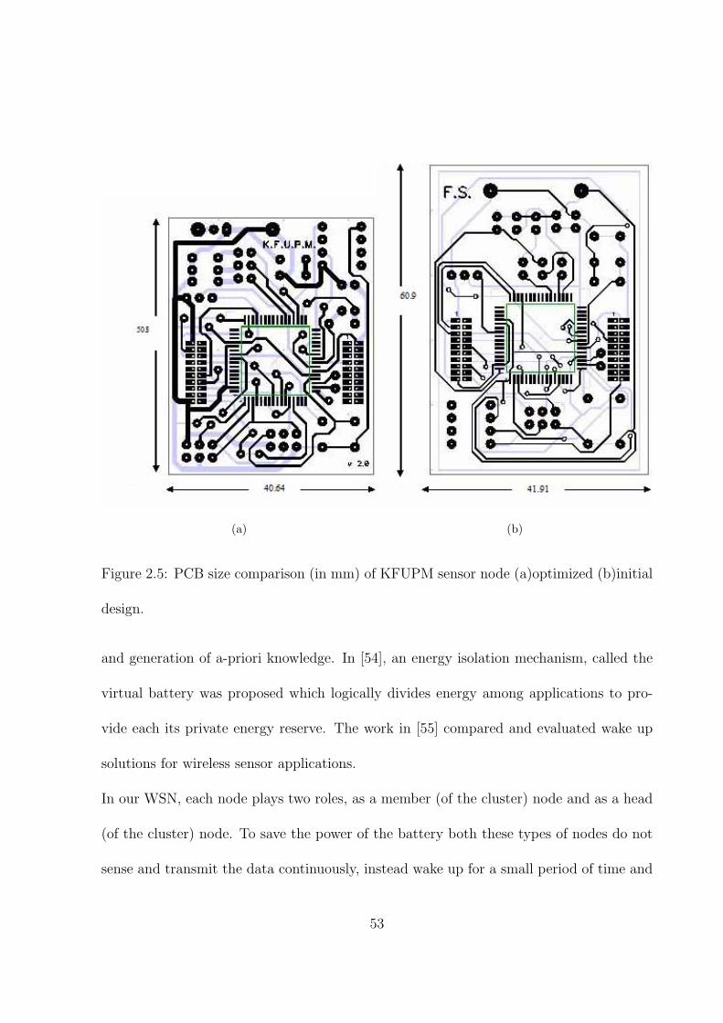
(a) (b)
Figure 2.5: PCB size comparison (in mm) of KFUPM sensor node (a)optimized (b)initial
design.
and generation of a-priori knowledge. In [54], an energy isolation mechanism, called the
virtual battery was proposed which logically divides energy among applications to pro-
vide each its private energy reserve. The work in [55] compared and evaluated wake up
solutions for wireless sensor applications.
In our WSN, each node plays two roles, as a member (of the cluster) node and as a head
(of the cluster) node. To save the power of the battery both these types of nodes do not
sense and transmit the data continuously, instead wake up for a small period of time and
53
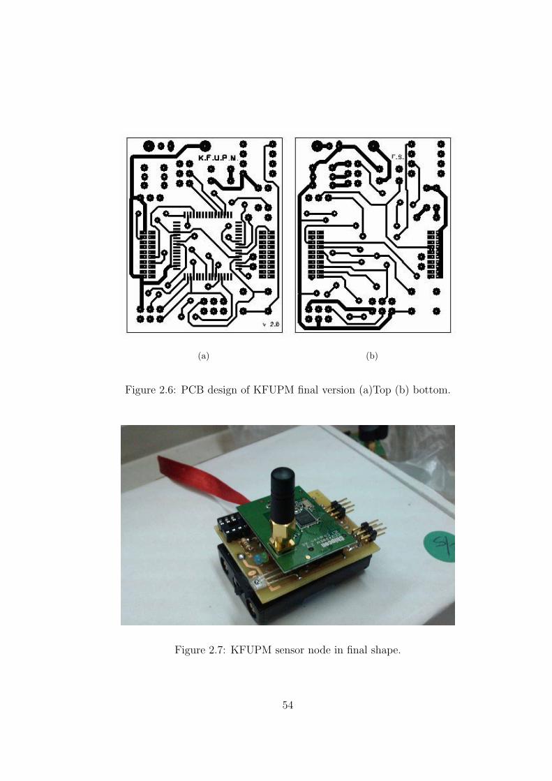
(a) (b)
Figure 2.6: PCB design of KFUPM final version (a)Top (b) bottom.
Figure 2.7: KFUPM sensor node in final shape.
54

then sleep. Head nodes wake up for a little more time as compared to member node.
Head nodes also receive data from member nodes and then transmit towards the sink
node, whereas member nodes wake up for lesser time and do not receive data from other
nodes except CTS byte from the heed node and transmit data to the head node. So the
nodes in head-node mode consume more power than the member-node mode. In order
to consume the same average power in all the nodes, each node in the same cluster will
become a head node at its own turn.
2.2.2 Calculation Methodology
To calculate the current consumption of the node, we will be referring to the default
consumption figures given in the data sheets for the various components. For calculating
the current consumed as per the duty cycles proposed in the previous sections, we will
consider the total fraction of time a node is awake, sleep or in any other modes. By
considering proportions of time in particular power modes, the significance of the time
duration of operation of a network vanishes; enabling all the calculations to provide
average consumption figures [56]. By multiplying the fraction of time a node is in a given
power mode with the current consumption of that mode, we get the current consumption
when the particular duty cycle is used. Figure 2.8 shows one complete frame employed in
S-MAC protocol. This figure will be used extensively in the proceeding calculations, so
some terms must be explained as below:
Tf : The total frame duration.
55

Figure 2.8: Complete S-MAC cycle.
tw: Wake duration of the node.
ttran: Time during the wake interval spent in sending messages.
tidle: Time during wake interval spent in idle mode.
2.2.3 Power Calculations for Member Nodes
The full cycle of wake and sleep for a member node spans 4 seconds, in which it wakes
up for 150ms (tw) and sleeps for 3850ms. Let pa indicate the fraction of time a member
node is awake and ps indicate the fraction of time the node is asleep. Observing Figure
2.8 we can calculate the values of pa and ps as follows:
pa =twTf
=150
4000= 0.0375. (2.1)
ps = 1− pa = 1− 0.0375 = 0.9625. (2.2)
56
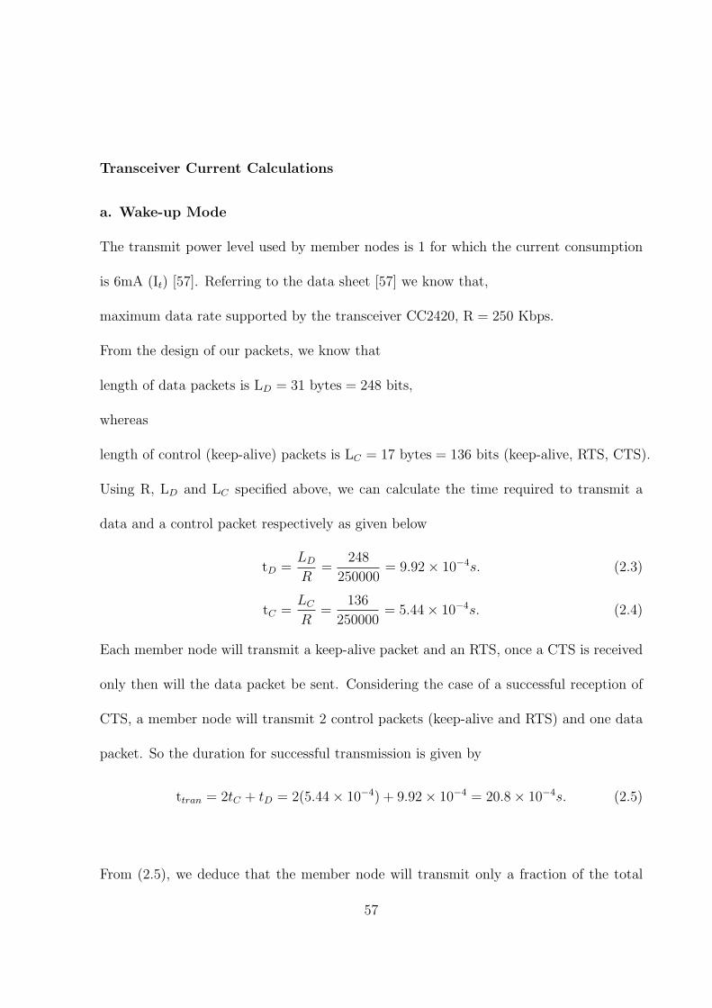
Transceiver Current Calculations
a. Wake-up Mode
The transmit power level used by member nodes is 1 for which the current consumption
is 6mA (It) [57]. Referring to the data sheet [57] we know that,
maximum data rate supported by the transceiver CC2420, R = 250 Kbps.
From the design of our packets, we know that
length of data packets is LD = 31 bytes = 248 bits,
whereas
length of control (keep-alive) packets is LC = 17 bytes = 136 bits (keep-alive, RTS, CTS).
Using R, LD and LC specified above, we can calculate the time required to transmit a
data and a control packet respectively as given below
tD =LD
R=
248
250000= 9.92× 10⁻⁴s. (2.3)
tC =LC
R=
136
250000= 5.44× 10⁻⁴s. (2.4)
Each member node will transmit a keep-alive packet and an RTS, once a CTS is received
only then will the data packet be sent. Considering the case of a successful reception of
CTS, a member node will transmit 2 control packets (keep-alive and RTS) and one data
packet. So the duration for successful transmission is given by
ttran = 2tC + tD = 2(5.44× 10⁻⁴) + 9.92× 10−4 = 20.8× 10⁻⁴s. (2.5)
From (2.5), we deduce that the member node will transmit only a fraction of the total
57

wake period (pa,t) calculated as follows:
pa,t =ttrantw
=20.8× 10⁻⁴
150× 10−3= 0.0139. (2.6)
Using pa,t, It and pa form Equations (2.1) and (2.6) we calculate the current consumed
during transmission, It,a as below
It,a = pa,t × It × pa
= 0.0139× 6mA× 0.0375
= 0.0031mA.
(2.7)
The member node does not sense and transmit every cycle, instead it does so every third
cycle, hence the overall current consumption must be decreased by a factor of 3 resulting
in It,a =13× 0.0031mA = 0.0010mA.
b. Listening Mode
This mode corresponds to the time during the wake interval when the node is not sending
but waiting for packets to arrive from other nodes indicated by tidle in Figure 2.8. In this
mode, the node is just sitting idle and waiting for any packets that are intended for it.
So, the transceiver is in idle mode and only the microcontroller is operating in full power
mode. The current consumed by transceiver CC2420 during this time is 426µA (Iidle)
[57]. Since the fraction of wake period spent during listening is given by
pa,l = 1− pa,t = 1− 0.0139 = 0.9861, (2.8)
58

then, current consumed by transceiver CC2420 during listening only can be computed as
It,l = pa,l × Iidle ×1
3
= 0.9861× 0.426mA× 0.0375× 1
3
= 0.0052mA.
(2.9)
c. Sleep Mode
The current consumption of transceiver CC2420 during power down mode is 0.02 µA (Is)
[57]. Hence
It,s = Is × ps = 0.2× 10−4 × 0.9625 = 1.9250× 10⁻⁵mA. (2.10)
d. Idle Mode
As the member node transmits data every 3rd wake time, it will be transmitting just the
keep-alive packets in the two cycles in-between. Let pctrl be the fraction of time spent in
transmitting keep-alive packets and pi be the fraction of time spent being idle, then
pctrl =tctw
=5.44× 10⁻⁴
150× 10−3= 0.0022. (2.11)
pi = 1− pctrl = 0.9978. (2.12)
Since this scenario occurs two-third of the time, the current consumed during the idle
mode Ii,tx can be given by
Ii,tx = pctrl × It × pa ×2
3
= 0.0022× 6mA× 0.0375× 2
3
= 3.3× 10⁻⁴mA.
(2.13)
59

Similarly, current consumed during idling, Ii,l
Ii,l = pi × Iidle × pa ×2
3
= 0.9978× 0.426mA× 0.0375× 2
3
= 0.0106mA.
(2.14)
e. Receive Mode
Member nodes will receive CTS byte from the CH node. During the receiving of a packet,
the transceiver consumes 18.8 mA (Ir) [57]. The time available for receiving a CTS is
indicated by tidle in Figure 2.8. Using (2.3) and (2.4), tidle can be calculated as,
tidle = tw − ttran = 150× 10−3 − 20.8× 10−4 = 0.148s. (2.15)
Hence the fraction of time spent receiving is given by,
prx =tctidle
=5.44× 10⁻⁴
0.148= 0.0037s. (2.16)
and the current consumed during receiving is given by,
Irx = pa × Ir × prx ×1
3
= 0.0375× 18.8mA× 0.0037× 1
3
= 8.6× 10⁻⁴mA.
(2.17)
Memory (flash) Logger Current Calculations
In our node design memory logger is never used during run-time. So, it will consume
current as in sleep mode which is 2 µA as mentioned in the manufacturer’s data sheet
60

[58]. Hence, the current consumption of memory logger is as follows
Iml = 0.002mA× 1 = 0.002mA. (2.18)
Microcontroller Current Calculations
The ATmega128 microcontroller (with internal RC oscillator, 4 MHz) has been used. Its
consumption as illustrated in the manufacturer’s data sheet [58] is the following. The cur-
rent consumption during wake-up time IMCU,w = 9mA, whereas the current consumption
during sleep time is, IMCU,s = 17µA. Hence current consumption during wake-up time is
given by,
IM,w = IMCU,w × pa
= 9× 0.0375
= 0.3375mA,
(2.19)
and the current consumption during sleep time is as follows,
IM,s = IMCU,s × ps
= 17× 10−3 × 0.9625
= 0.0164mA.
(2.20)
Combining (2.19) and (2.20) we get the total current consumption of MCU as follows,
IM,T = IM,w + IM,s
= 0.3375 + 0.0164
= 0.3539mA.
(2.21)
61

Total Current Consumption
Adding the current consumptions of the transceiver, MCU and the memory logger (Bold
figures),we get the total current consumption as,
IT = It,a + It,l + It,s + Ii,tx + Ii,l + Irx + Iml + IM,T
= 0.001 + 0.0052 + 1.925× 10⁻⁵ + 3.3× 10⁻⁴
+ 0.0106 + 8.6× 10⁻⁴ + 0.002 + 0.3539
= 0.3739mA.
(2.22)
Battery Life
The best battery available at the time of these calculations had a rating of 1175mAh.
Hence the battery life time of a member node is given by,
LMN =1175mAh
0.3739mA
≈ 3143 hours
≈ 130 Days.
(2.23)
2.2.4 Power Calculations for Cluster Head Node
The cycle of wake and sleep for a head node spans 4 seconds in which it wakes up for
300ms and sleeps for 3700ms. Following a similar procedure to the that followed for the
calculation of the member node we can calculate the values of pa and ps as follows:
pa =twTf
=300
4000= 0.0750. (2.24)
ps = 1− pa = 1− 0.0750 = 0.9250. (2.25)
62

Transceiver Current Calculations
a. Wake-up Mode
The transmit power level used by cluster head nodes is 3 for which the current consumption
is 8.5mA (It) [57]. Referring to the calculations in Section 2.2.3 the fraction of wake period
spent during transmission is as follows,
pa,t =ttrantw
=20.8× 10⁻⁴
300× 10−3= 0.0069. (2.26)
Using (2.24) and (2.26) we calculate the current consumed during transmission (Tx) as,
It,a = pa,t × It × pa
= 0.0069× 8.5mA× 0.075
= 0.0044mA.
(2.27)
As the head node transmits CTS every third cycle so ,It,a becomes,
It,a =13× 0.0044mA = 0.0015mA.
b. Listening Mode
In this mode, it is assumed that the head node will receive one packet from the member
nodes on average and after that it will transmit it towards the sink node. So, the total
time for listening can be calculated as follows,
tl = tw − ttrans = 300ms− 20.8× 10⁻⁴s = 0.2979s. (2.28)
Hence, the fraction of time to receive,
prx =tCtl
=5.44× 10⁻⁴
0.2979= 0.0018. (2.29)
63

So, the current consumed by transceiver CC2420 during receiving the CTS is given as,
ICTS,rx = pa × Ir × prt ×1
3
= 0.075× 18.8mA× 0.0018× 1
3
= 8.37× 10⁻⁴mA.
(2.30)
c. Sleep Mode
Current consumption of transceiver CC2420 during power down mode is 0.02 µA [57].
Hence, the current consumed during sleep is
It,s = Is × ps = 0.2× 10−4 × 0.9250 = 1.85× 10⁻⁵mA. (2.31)
d. Idle Mode
As the cluster head transmits every 3rd wake time, so it will be idle during other two-
thirds of the wake times except it receives control (keep-alive) packet only from member
nodes. Assuming two packets are received as an average from member nodes. Fraction of
wake period spent on reception of control packet can be calculated as,
pctrl =tctw
=5.44× 10⁻⁴
300× 10−3= 0.0018. (2.32)
Whereas, the fraction of wake period spent during idling is given as,
pi = 1− pctrl = 1− 0.0018 = 0.9982. (2.33)
Hence, the current consumed during receiving in the idle mode is as follows,
Ii,tx = pctrl × It × pa ×2
3
= 0.0018× 18.8mA× 0.0750× 2
3
= 0.0017mA
(2.34)
64

and current consumed in idling is,
Ii,l = pi × Iidle × pa ×2
3
= 0.9982× 0.426mA× 0.0750× 2
3
= 0.0213mA.
(2.35)
e. Receive Mode
After the cluster head replies to the member node with a CTS, the member node sends
the data packet to the cluster head. So, fraction of time spent receiving data packet is,
pr,d =tDtl
=9.92× 10⁻⁴
0.2979= 0.0033. (2.36)
and current consumed during receiving can be calculated as follows,
Irx = pai × Ir × pr,d ×1
3
= 0.0750× 18.8mA× 0.0033× 1
3
= 0.00155mA.
(2.37)
Memory (flash) Logger Current Calculations
In our design memory logger is never used during run-time. So it will consume power as
in sleep mode which is 2 µA as mentioned in the manufacturer’s data sheet. So, current
consumption of memory logger is as follows,
Iml = 0.002mA× 1 = 0.002mA. (2.38)
Microcontroller Current Calculations
The ATmega128 microcontroller (with internal RC oscillator, 4 MHz) is used. Current
65

consumed during wake-up is given as,
IM,w = IMCU,w × pa
= 9× 0.075 = 0.675mA.
(2.39)
and current consumed during sleep is,
IM,s = IMCU,s × ps
= 17× 10−3 × 0.9250 = 0.0157mA.
(2.40)
Hence, the total current consumption of the MCU is,
IM,T = IM,w + IM,s
= 0.675 + 0.0157
= 0.6907mA.
(2.41)
Total Current Consumption
Adding the current consumptions of the transceiver, MCU and the memory logger (bold
figures)we get, the total current consumption as follows,
IT = It,a + ICTS,rx + It,s + Ii,tx + Ii,l + Irx + Iml + IM,T
= 0.0015 + 8.37× 10⁻⁴ + 1.85× 10⁻⁵ + 0.0017
+ 0.0213 + 0.00155 + 0.002 + 0.6907
= 0.7196mA.
(2.42)
Battery Life
The best battery available at the time of these calculations had a rating of 1175mAh. So,
66

the battery life of a member node is given by,
LCH =1175mAh
0.7196mA
≈ 1632 hours
≈ 68 Days.
(2.43)
2.2.5 Average Battery Life for Each Node
As mentioned above, in order to consume power averagely in all the nodes, each node in
the same cluster will become head node at its own turn. It is assumed that at a minimum
there will be at least two nodes in each cluster, one will be the head and other will be the
member node. These two nodes will change the role alternately after a fixed interval of
time (40 seconds). The power consumption/battery life will be the average of above two
calculations. So, battery life time of each node
130 + 68
2= 99 days. (2.44)
The assumption of at least 2 nodes in a cluster is based on the fact that if there are more
than 2 nodes in a cluster then each node will play the role of head node for a lesser time.
When the node will be head for a smaller fraction of time then obviously it will consume
shorter power.So if there are three nodes in a cluster the battery life will be
130 + 130 + 68
3= 109 days. (2.45)
67

Figure 2.9: Shunt resistor power measurement circuit.
2.3 Power Consumption - Experimental Analysis
Section 2.2 presented a theoretical approach to estimating the network life. To measure
the power consumption of the designed node, TinyOS applications were used to operate
the node in different modes. In order to measure the actual power consumed by the node,
the shunt resistor [59] approach has been adopted. Fig. 2.9 shows the complete circuit
setup for the experiment. The main idea here is to use a small (RSHUNT = 10 Ω ) shunt
resistor to measure the current in the loop (I). Once the current is measured, the power
can be calculated by the relation in 2.46.
PNODE = (VSUPPLY - VSHUNT )×VSHUNT
RSHUNT
(2.46)
where PNODE is the power consumed by the node, VSUPPLY is the supply voltage (4.5V),
VSHUNT is the voltage drop across the shunt resistor, RSHUNT is the shunt resistor and
VSHUNT
RSHUNTis the current, I, flowing in the loop (Fig. 2.9).
68

2.3.1 Power Measurements for MCU in Different States
The ATmega128L MCU can be clocked by either using the on-chip oscillator or by using
an external crystal. The wireless node has an external 8 MHz crystal oscillator to provide
highly accurate clock pulses for the MCU and the radio. The on-chip oscillator option
provides clock pulses with minimum delay but is fairly inaccurate. On the contrary, by
using an external oscillator, highly accurate pulses can be produced but some amount of
delay is introduced due to the finite amount of time taken by the external oscillator to
initialize. The power consumption of the node under the different modes of internal and
external oscillators has been analyzed and the results have been provided in Tables 2.2,
2.3, 2.4 and 2.5. A simple application in TinyOS, TestApp was written that periodically
broadcast packets every 2 seconds with 50% duty cycle. Fig. 2.10 shows a view of the
VSHUNT for the complete duty cycle. From Tables 2.2, 2.3, 2.4 and 2.5 it is obvious that
the internal oscillator modes consume less power. However, for the external oscillator,
when operating at less than the oscillator frequency (0.9 - 3MHz) some frequency limiting
circuitry functions consuming more power as compared to the high frequency range (3 -
8MHz) as indicated in Tables 2.4 and 2.5.
2.3.2 Transmission Power Measurements
To measure transmission energy, a TinyOS application called the SendingMote was pro-
grammed onto one of the wireless nodes. This application turns the node on and keeps
69

Table 2.2: Internal Oscillator 4 MHz.
Configuration VMAX(mV) VMIN(mV) VAV G(mV) PAV G(W)
MCU(ON), Radio(ON) 372 352 361 0.149
MCU(ON), Radio(OFF) 56 40 48 0.021
Table 2.3: Internal Oscillator 8 MHz.
Configuration VMAX(mV) VMIN(mV) VAV G(mV) PAV G(W)
MCU(ON), Radio(ON) 440 380 391 0.160
MCU(ON), Radio(OFF) 56 40 48 0.021
Table 2.4: External oscillator - medium frequency (0.9 - 3MHZ).
Configuration VMAX(mV) VMIN(mV) VAV G(mV) PAV G(W)
MCU(ON), Radio(ON) 432 376 402 0.164
MCU(ON), Radio(OFF) 248 48 76.1 0.033
transmitting packets of 28 byte payloads every second. The transmission power of the
radio was changed between 0, -5, -10, -15 and -28 dBm and the resulting PNODE was
calculated using 2.46, where VSHUNT was measured from the circuit of Fig. 2.9. Some of
70

Table 2.5: External oscillator - high frequency (3 - 8MHZ).
Configuration VMAX(mV) VMIN(mV) VAV G(mV) PAV G(W)
MCU(ON), Radio(ON) 424 368 407 0.167
MCU(ON), Radio(OFF) 124 48 65.4 0.029
Figure 2.10: VSHUNT measurement for 50 % duty cycle (mV).
the results for VSHUNT at transmission power of -25 dBm and 0 dBm are shown in Fig.
2.11 and Fig. 2.12 respectively. It is observed that VSHUNT is, on average, 191 mV for -25
dBm transmissions and 320 mV for 0 dBm as indicated by Fig. 2.11 and Fig. 2.12. Once
the packet has been transmitted, the radio returns to the listen state where it consumes
an almost constant current of 35mA (VSHUNT = 350 mV).
71

(a)
(b)
Figure 2.11: Measurement of VSHUNT (mV) for transmission at -25 dBm with payload
size of (a) 16 Bytes (b) 22 Bytes. 72

(a)
(b)
Figure 2.12: Measurement of VSHUNT (mV) for transmission at 0 dBm with payload size
of (a) 16 Bytes (b) 22 Bytes. 73

2.3.3 Transmission Power Measurements at Varying Payload
Sizes
The amount of data to be transmitted has a direct impact on the energy consumption.
As the payload size increases, the radio needs to be turned on for a longer time, thus
consuming more power. Since TinyOS allows a maximum default payload size of 28
bytes, in order to quantify the energy consumption of the node at different payload sizes,
the SendingMote application has been employed and for each of the five transmission
powers mentioned in Section IV-B, the payload sizes are varied as 10, 16, 22 and 28 bytes.
Observing the results of VSHUNT for two different payloads in Fig. 2.11 and Fig. 2.12,
the voltage remains the same, however, the duration of the transmission increases with
payload size (Fig. 2.11b and Fig. 2.12b). From Fig. 2.11 and Fig. 2.12 it is observed
that it requires 1.13 ms to transmit 16 bytes as compared to 1.25 ms for 22 bytes payload
regardless of the transmit power.
2.3.4 Sleep State Power Measurements
To monitor the energy consumption pattern during the sleep state, the TestApp applica-
tion was used. This application operated the node in a cycle of 2s with 50% duty cycle,
i.e., the radio is ON for 1s and OFF for 1s. The results shown in Fig. 2.10 indicate
a current consumption of 35mA (VSHUNT = 350 mV) during the active state and 3mA
(VSHUNT = 30 mV) during the sleep state.
74

2.4 Node Energy Model
The relationship between power and energy is characterized as
ENODE = PNODE × tMODE (2.47)
where ENODE is the energy consumed by the nodes, PNODE is the power consumed by
the node (from Eq. 2.46) and tMODE is the time spent by the node in a given operating
mode.
As observed from Fig. 2.11 and Fig. 2.12, VSHUNT does not remain constant over
the entire interval. Therefore, the average value of VSHUNT has been considered in the
calculation to provide a much stable result.
2.4.1 Transmission Energy Model
A node was programmed with the SendingMote application and each time the transmis-
sion power was changed between 0, -5, -10, -15 and -25 dBm. Table 2.6 contains the
results of the energy consumption relative to the payload size.
75

Table 2.6: Energy consumption in µJ for different transmit powers with varying payload
sizes.
Transmit Power in dBm 10 Bytes 16 Bytes 22 Bytes 28 Bytes
0 126 151 168.46 192.53
-5 99.9 119.7 133.56 152.64
-10 90.47 108.48 120.96 138.24
-15 83.88 100.57 112.14 128.16
-25 77.94 93.45 104.20 119.08
By using the curve fitting toolbox in MATLAB, we find that the energy consumption
changes as a linear function of payload size. Fig.2.13 shows the measured data and
the fitted curves for the corresponding data set. The fitting toolbox gives us a linear
approximation of our measured data, the coefficients for the different power levels are
given in Table 2.7.
76

Table 2.7: Transmission energy model equations.
Transmit Power in dBm p1 p2 p1x + p2
0 3.617×10⁻⁶ 9.077×10⁻⁵ 3.617×10⁻⁶x + 9.077×10⁻⁵
-5 2.868×10⁻⁶ 7.196×10⁻⁵ 2.868×10⁻⁶x + 7.196×10⁻⁵
-10 2.596×10⁻⁶ 6.520×10⁻⁵ 2.596×10⁻⁶x + 6.520×10⁻⁵
-15 2.407×10⁻⁶ 6.046×10⁻⁵ 2.407×10⁻⁶x + 6.046×10⁻⁵
-25 2.236×10⁻⁶ 5.618×10⁻⁵ 2.236×10⁻⁶x + 5.618×10⁻⁵
10 12 14 16 18 20 22 24 26 280.6
0.8
1
1.2
1.4
1.6
1.8
2x 10
−4
Payload size (Bytes)
Ene
rgy
cons
umpt
ion
(J)
Tx at 0dBmTx at −5dBmTx at −10dBmTx at −15dBmTx at −25dBm
Figure 2.13: Node transmission energy model.
77

2.4.2 Receiving Energy Model
Unlike the transmission process, the reception of a packet is independent of the payload
size. Considering the node listens for 1s the energy consumed is:
PNODE = V× I
= 4.5V × 35mA = 157.5mW.
(2.48)
ENODE = PNODE × tMODE
= 157.5mW × 1s = 157.5mJ.
(2.49)
2.4.3 Sleep Mode Energy Model
Similar to the receiving mode, the sleep mode consumption is also constant as observed
from Fig. 4. Assuming the node stays asleep for 1s, the energy consumption is:
ENODE = PNODE × tMODE
= V× I× tMODE
= 4.5V × 3mA× 1s
= 157.5mJ.
(2.50)
78

2.5 Experimental and Theoretical Lifetime Compar-
isons
2.5.1 Power Calculations for Member Nodes
Referring to Section 2.2.3, the only factors that have changes in the measurements have
been the current values in different modes. The power measurements in Section 2.4
has been used to provide a much accurate power consumption statistics. The currents
consumed in the different modes are:
It = 19.2mA. (2.51)
Iidle = 1mA. (2.52)
Is = 0.2mA. (2.53)
By using the methodology mentioned in Section 2.4, the total current consumed by the
member node in the different states can be derived from Equations 2.7, 2.9, 2.10, 2.14
and 2.17 as
It,a = 0.0033mA. (2.54)
It,l = 0.0123mA. (2.55)
Is = 1.925× 10⁻⁵mA. (2.56)
The calculations for the memory logger and the MCU remain the same, summing all the
79

current consumed in different modes, we get,
IT = 0.4940mA. (2.57)
Battery Life
Taking the battery with a rating of 1175 mAh, the life time of a member node is
LMN =1175mAh
0.4940mA≈ 100Days. (2.58)
2.5.2 Power Calculations for Cluster Head Nodes
Referring to Section 2.2.3, the only factors that have changes in the measurements have
been the current values in different modes. The power measurements in Section 2.4
has been used to provide a much accurate power consumption statistics. The currents
consumed in the different modes are:
It = 22mA. (2.59)
Iidle = 1mA. (2.60)
Is = 0.2mA. (2.61)
By using the methodology mentioned in Section 2.4, the total current consumed by the
cluster head node in the different states can be derived as
It,a = 0.0038mA. (2.62)
It,tx = 0.002mA. (2.63)
80

It,l = 0.0499mA. (2.64)
Irx = 0.0016mA. (2.65)
The calculations for the memory logger, the MCU and the other states remain the same,
summing all the current consumed in different modes, we get,
IT = 0.7509mA. (2.66)
Battery Life
Taking the battery with a rating of 1175 mAh, the life time of a cluster head node is
LMN =1175mAh
0.7509mA≈ 63Days. (2.67)
Comparing the network lifetime figures in Section 2.4 with ones calculated above, it is clear
that, the current consumed by the radio during transmission, sleep and idle is different
than the figures provided in the datasheet. This difference results in a decrease in the
lifetime of the network based on actual measurements.
2.6 Conclusions
A detailed description of the design and optimization process of KFUPM hardware nodes
was presented in this chapter. The details of the individual components as well as the
design comparison was made. The optimized version was considered as the final version
owing to its smaller size as compared to earlier designs. This chapter also provided an
81

insight into the energy consumption and the life time estimation of the KFUPM node. By
using the actual power consumption measurement figures, a linear relationship between
payload size and the consumed energy has been derived. Moreover, employing the actual
power consumption values, it is concluded that the network life is less due to a difference
in the actual measured current and the ones provided in the datasheets.
82

CHAPTER 3
SENSOR NODE SOFTWARE
DEVELOPMENT
Programming is an important part of the wireless sensor node that controls all the func-
tionalities of the node including the sensing, data processing, networking protocols imple-
mentation and relaying of data. As discussed in Chapter 1, system programming must
be done in such a way that the energy wastage in kept at the least possible value.
Software model development of KFUPM node is explained in Section 3.1. The network
monitoring application design details are presented in Section 3.2 with the chapter con-
cluding with a summary in Section 3.3.
83

3.1 Software for KFUPM Sensor Node
Assembly language is naturally very difficult and time consuming to program as well as
to debug. In addition it does not ensure minimum MCU usage to save energy. Because
of its associated complexity, Assembly language has its own limitations on the advanced,
complex and efficient programming requirements such as in WSNs. Owing to associated
severe constraints with Assembly language, a higher level of programming paradigm called
TinyOS [51, 60] has been used to create the software interface for the designed node. The
system software developed in this work for the implementation of the WSN prototype is
hardware platform independent. All the software codes can be compiled for any hardware
platform supported by TinyOS.
3.1.1 TinyOS
TinyOS, developed by U.C. Berkeley, is a small, efficient and open-source operating system
developed specifically for WSNs [51]. The software itself provides inter-connectable blocks
and modules which can be used according to the application requirements. The operating
system provides control to handle both sensing as well as device power consumption by
varying transmission power levels. Other operating systems like Nano-Qplus [61] do exist
for WSN, but the large adaptability and a huge user base has made TinyOS the most
widely used platform.
Keeping the limited resource potential of the devices, a new programming language has
84
been derived from C/C++ called the nesC. To facilitate the programmer, nesC supports
component based programming, independent of the hardware platform being used. The
components need to be connected according to application and the scheduler inherent
to TinyOS controls the operation of the components [62]. Unlike traditional C/C++,
TinyOS features event-based scheduler, which releases the resources once they are not
being used. This action saves memory and also provides lower power consumption due to
less data in the RAM.
TinyOS has mainly been associated with proprietary hardware. Crossbow Technologies is
considered as the leader in providing wireless sensor nodes as well as supporting hardware.
Mica/MicaZ, Telos/TelosB and Iris motes are examples of some wireless sensor devices
from crossbow [47]. The TinyOS package itself comes with complete support for all the
above mentioned devices. Since porting TinyOS to KFUPM nodes, a platform had to
be defined within TinyOS directories to enable programming. The pin assignment, data
flow direction and the handshaking procedures between the onboard devices had to be
defined for successful migration to TinyOS. TinyOS enhancement proposals (TEP) are
provided by TinyOS and are maintained to provide up-to-date support to the users. TEP
131 [63] is one such document that explains the mandatory conditions for porting TinyOS
to custom platforms. By studying the said document, a custom software model for the
KFUPM platform was successfully created and was tested by compiling test examples
provided in the TinyOS package.
Keeping the changing technology needs in mind, TinyOS has been developed so that newer
85
hardware devices can be easily accommodated in the already present software structure.
This means a flexible hardware abstraction has been adopted in TinyOS [62]. In order to
maintain flexibility in the hardware domain, TinyOS hardware structure consists of the
following three domains.
1. Hardware Presentation Layer (HPL):
This is the lowest level defined in TinyOS. Individual hardware components i.e., micro-
controllers, radio devices and sensors etc. are defined in this layer. Memory mapping
of individual devices and the definition of ports of each device is done in this layer.
2. Hardware Adaptation Layer (HAL):
This layer works on top of the interfaces provided by HPL. In other words, the com-
bination of the interfaces of individual components that form a platform is defined in
this layer. Definition of ADC channels and interconnection of individual components
on the platform are some examples of this layer. HAL is platform dependent.
3. Hardware Interface Layer (HIL):
HIL ports the platform-dependency provided by HAL to a platform-independent inter-
face design. This is the top most level and is independent of the hardware components
or the platform being used.
Since the hardware platform being used has been custom built, HAL had to be developed
to define the platform (KFUPM). TinyOS already contains HPL support for several com-
ponents that are available in the market. Therefore, using the HPL support provided by
86
TinyOS HAL interface for the KFUPM platform has ben defined. The system definition
(HIL) was then done independent of the platform specifics according to the demands of
TinyOS.
3.1.2 nesC Programming Domain
The network embedded systems C (nesC) is a component-based, event-driven program-
ming language used to build applications for the TinyOS platform. nesC is built as an
extension to the C programming language with components “wired” together to run ap-
plications on TinyOS. This language enables the release of resources when they are not
been used, thus freeing the vital memory caches. In order to make the migration from
C/C++ to nesC easier, nesC has a similar syntax as that of the C language. On the
contrary, the only thing that distinguishes nesC from C domain is the way the code is
organized in nesC. All the applications in nesC are divided into three classes:
1. Interfaces:
Interfaces define the relation between two components [62]. One component provides an
interface to another component that uses it. The providing component must implement
some commands ; which are similar to C/C++ functions. On the other hand, the
using interface must signal events to mark the completion of commands. To enable
concurrency, nesC supports split-phase operations which prevent the usage of a single
resource by a particular component for larger amounts of time.
87

2. Configurations:
Configurations are interconnected components that provide a complete functionality of
an application. This interconnection is termed as wiring in nesC. While wiring different
components, it must be ensured that the commands offered by a component are all
implemented in the using component. If any commands are not wired, the program
does not compile.
3. Tasks:
Tasks are designed to run long latency operations. Once started, a task runs till
completion without any interruptions. nesC handles tasks with the help of a first-in
first-out (FIFO) scheduler. All the tasks that are posted in the scheduler are run
according to FIFO.
3.1.3 Development of “KFUPM” Software Interface
At the beginning, considerable time was spent exploring the TinyOS application develop-
ment platform. While studying TinyOS it was realized that a specific software interface
had to be developed defining all the details of the hardware architecture of the custom
node being developed.
HPL Design
As explained in Chapter 1, TinyOS package has support available for some of the widely
used components. Components like the ATmega128, CC2420 radio and the on-board
88

LEDs had HIL support already available. We had to develop the HIL interpretation for
the light sensor (TSL13S) and the temperature sensor (LM-35) for the complete represen-
tation. Both the light as well as the temperature sensors are activity-to-voltage devices,
i.e., they sense and provide an output voltage that is proportional to the sensed quantity
(whether it is the light or the temperature). Since the basic sensing mechanism is the
same, only a single interface was required to be created and could be replicated for the
second sensor. We implemented a Read interface and wired it to the output pin of the
sensor. Calling the Read interface causes the MCU to sample the voltage at the particular
pin to which sensor is connected, thus enabling us to get the digital value of the sensed
quantity.
HAL Design
HAL design for the KFUPM node was created by specifying the connections between the
different components on the platform. Using the circuit diagram presented in Figure ??
we created a platform.h file that included all the components and the location of their
HPL files on the disk and defined the KFUPM interface. The next step involved defining
the pin connection of the different devices to the MCU. A configuration file was written
and the general-purpose I/O pin connections were defined. This marked the completion
of the HAL layer and with that KFUPM platform was completely defined.
89
3.1.4 Installation and Configuration of TinyOS Software Libraries
In order to implement the codes using TinyOS, the first step involved was to install all
the binary batches and libraries necessary to build TinyOS applications. This involves
libraries such as Avr-gcc compiler, nesC compiler, tinyOS tools repository, avr-libc library,
avr-binutils, cygwin, avrDUDE and libusb [64].
3.1.5 Cygwin Environment
TinyOS is best suited and developed to be used with Unix/Linux. However, to use this
application in Windows environment, an additional patch called Cygwin is required which
basically emulates the Linux environment in windows. Cygwin was successfully installed
and configured on the programming PC.
Cygwin is a Unix/Linux-like environment and command-line interface for Microsoft Win-
dows. It is free and open source software, released under the GNU General Public License
version 2. It provides native integration of Windows-based applications, data, and other
system resources with applications, software tools, and data of the Unix-like environment.
Thus it is possible to launch Windows applications from the Cygwin environment, as well
as to use Cygwin tools and applications within the Windows operating context. Cygwin
consists of two parts: a Dynamic-link library (DLL) as an API compatibility layer pro-
viding a substantial part of the POSIX API functionality, and an extensive collection of
software tools and applications that provide a Unix-like look and feel.
90
3.1.6 Compiling Software Code into the Node
To be able to download the codes to the hardware it is important that the PC recognizes
the attached custom node. Since there are no drivers available for the custom built node,
an application called the AVR Downloader-UploaDEr (AVRDUDE)[64] was utilized for
this purpose. This application enables to connect and directly transfer the compiled binary
files in either .hex or .srec format to the attached node via USB interface. AVRDUDE can
program the flash and electrically erasable programmable read-only memory (EEPROM),
fuse and the lock bits of the AVR microcontroller [64].
In order to download or install the desired files onto the node, the AVRISP MKII pro-
grammer has been used. This programmer has the ability to get connected via the USB
port. The default hardware drivers that come with this programmer do not work with
the AVRDUDE utility. We had to create our own hardware drivers so that AVRDUDE
would recognize the port to which the MKII was attached. To do that we used an ap-
plication called libusb. This utility makes it possible to create dummy drivers so that a
particular USB port on the computer can be accessed as if some hardware was attached
to it. Once the driver was created we got complete support for out MKII programmer
and data download became successful.
91

3.2 The Network Monitoring Application
The network monitoring application is an important component of any WSN. It is required
for the monitoring of the status of the whole network in addition to the network topologies
and sensed values over time.
A network monitoring application in the form of front end graphical user interface (GUI)
for the monitoring of our developed WSN. This interface provides complete network topol-
ogy diagram along with a view of the recently received data. The complete route followed
by a particular data packet is also shown instantaneously and also offline in this ap-
plication. We have developed this application for the project not only for the network
monitoring purpose but also to help us demonstrate the operation, different functionalities
and capabilities of our developed WSN prototype. In addition, the application is linked
with a database in which the history of the sensed data and their routes as well as the
sensing nodes is kept.
This application will be running at the server computer to which the sink/base node is
connected showing different attributes of the network in the form of graphical icons and
visual indicators. Several attributes of the network are shown on the front-end application
such as
• The newly born nodes.
• Formation of clusters.
92

• Current head nodes.
• Current sensing member nodes.
• The values of current sensed data such as temperature and light intensity of the
area.
• Dead nodes getting out of service in case if not active due to any reason for a specific
period of time.
• The route taken by the data from the sensing node up to the sink/base node.
• The nodes and data for the UGN.
• The ability to view the route and data history of any particular sensor node.
3.2.1 Related Work
An extensive literature survey was carried out for the related work but surprisingly not
much published work was found in that regard. In [66] Java-based GUI for visualization
of wireless data channel communication and the infrastructure backbone activities was
developed. It provides a graphical interface for the user to explore the various services
offered by the WSN such as temperature and light intensity queries of the building.
Secondly, it ensures the validation of the proper operation of the network via augmented
visualization of the network topology, the sensor readings, the node health status and the
service protocol state.
93

In [67] a GUI is designed for monitoring current and past measurements for all patients
being monitored. All communication between the base station and the PC is done through
the universal asynchronous receive and transmit (UART). A separate thread from the
main graphical user interface thread is used to maintain constant monitoring of the serial
port. Here, the user can add a new patient to the monitoring network at any time by
keying in the patient name and the ID of his assigned sensor node. Once entered in the
system, all readings received by the PC from the patient’s sensor node, will be stored in
an object corresponding to the patient. All stored readings can be viewed by selecting
the desired patient name in the list.
In [68], the GUI on PDA for patient pulse-rate, and temperature monitoring was pre-
sented. It offers four different GUIs. The first is located on the local nurse control
station, and it tracks the motion of the resident using motion activations. The second
GUI can run on a PDA, permitting a care giver to request real-time environmental con-
ditions of the living space and the vital signs of the resident. It uses a query management
system distributed among the PDA, and the sensor devices. The interface graphically
presents requested data for clear consumption by the user. Third GUI is an LCD inter-
face board is also designed for the MicaZ for wearable applications. It presents sensor
readings, reminders and queries, and can accept rudimentary input from the wearer. The
fourth GUI is from a direct medical application based on motion sensors, exists to study
the behavioral profile of the user’s sleep/wake patterns and life habits, and to detect some
pathologies in the early stages.
94
In [69] the GUI is developed using JAVA to monitor deployment of the sensor network, to
initialize the network, and to query the statuses of sensors. In this GUI, the main part is
“building plan panel” showing the connection between different sensors located at stairs,
exits and emergency exits.
In [70], a graphical user interface (GUI) has been developed in LabVIEW that includes
the commands compliant with the IEEE 802.14.51 ZigBee radio sub-specification to send
and receive the information in the WSN and shows all active messages in the front panel.
This application operates in a PC server and users can control and monitor all parameters.
In [71], the GUI shows the current network topology and serves as a control center from
which the user can remotely task the WSN. Moreover, it displays the data collected, which
are also persistently stored in a database.
In [72], the GUI platform was developed using Borland C++ Builder programming that
is able to interact with the hardware (coordinator) at the base station. Firstly, the user
has to discover the surrounding nodes and setting the data polling rate using the buttons
provided on the side of the screen. Different colors of the nodes show that the connection
between the node and the base station is established or not established. To know the
values of the parameters being sensed, the user is able to directly zoom to each sensor
node and all the values will be displayed by clicking on the desired node. Here, the actual
values of temperature, pH and water turbidity are displayed in real-time. The user can
get a one shot display of measurement status at every sensor node by clicking on the
coordinator icon. Shown together are the Link Quality Indicator (LQI) values for every
95

connection between sensor nodes and the coordinator.
All the GUIs discussed above are specific to the application in question. Another problem
with the described GUI is that none of them are available for general use. Keeping our
network requirements in mind, we decided to create a custom interface that would be
easy to implement and simple to operate.
3.2.2 Components Used in Developing
The latest state-of-the-art software tools are used to develop this GUI, e.g.
• Microsoft Visual Studio 2008.
• Microsoft .NET Framework 3.5.
• Visual C 3.5.
• AddFlow 2.0 for .NET.
• Microsoft Access.
The developed NMA can run on Windows XP or Windows Vista/7 platform. The screen
resolution should be at least 1024 X 768 for best viewing. Since .Net platform does not na-
tively provide all the required functionalities that were needed to develop the application,
we used a software module called AddFlow to help create dynamic icons of nodes, their
sensed values and their routes in the form of workflow diagrams. AddFlow is compatible
with Visual Studio .NET 2008 so it works under the control of main module programmed
in .Net platform for the required graphical functionalities of the application.
96

Using AddFlow, the drawings can be made and updated dynamically very effectively.
Distinct shapes, styles, colors and fonts can be defined on a per item basis (for a node or
a link) or as default properties for the display.
3.2.3 The NMA Design
As shown in the Figure 3.1, the main screen of NMA consists of four parts:
Network Viewing Pane
This part of the main window is used to display the network diagram. All the packets
received by the sink node are decoded. After extracting the routing information from the
received packet, the application draws the route in the network viewing space. In addition,
the corresponding values of the sensed parameters (light intensity and temperature) are
also displayed along the route. Within the network viewing window, eleven horizontal
lines are drawn corresponding to the eleven available power levels. After receiving the
packet, the levels of all the nodes throughout the path are determined and the node is
drawn in the corresponding space in the network viewing window.
Data Viewing Window
This portion of the NMA is used to display the light and the temperature values of the
recently received packet at the sink node along with the ID of the sensing node. Although
the sensed parameters are also being displayed along the node on the network, due to
the congested space in the network viewing window the font size is relatively small. The
97

Figure 3.1: NMA main screen shot.
received data is displayed in the data viewing window with a larger font size for ease of
monitoring.
Application Control and Options
This part of NMA provides different controls and options available for the operation of
the application. the following buttons constitute the application control part.
Data Port Selection: As the server machine may have several USB ports, the port
to which the sink node is connected must be selected for the operation of NMA. This
98

drop-down menu lists all the ports available on the server machine. The administrator
has to select the correct port based on the connection of the base node.
Receive Data: This button opens the input/output port for communications. The port
that has been selected from the dropdown list must be opened using this button to enable
communication with the sink node.
Refresh Network: This button clears or refreshes the network viewing window and the
network is drawn again from scratch as packets are received.
Remove/Add Levels: These buttons invert the operation of each other. By default the
network viewing window contains the power level lines (Figure 3.1) and the network is
drawn around them. If viewing of the network becomes difficult due to increased number
of nodes, the level lines can be removed by using remove levels and can be made visible
again by add levels.
Clear Unsync Nodes: In case of alarm, unsynchronized nodes from the incident-based
portion of the network will start to transmit data. Only five unsynchronized nodes have
been programmed to be displayed on the NMA simultaneously. Since there can be only
a few unsynchronized nodes (five for this prototype system), once the administrator sees
and acknowledges the alarm he can reset or turn it off by the clear Unsync button which
removes the unsync node display once the alarm has been acknowledged.
Report: This button opens the report window where the history of the routes for each
node can be observed in the report window.
Restart: This button restarts the complete application. The port is closed and needs to
99

be opened again once the restart is complete.
Exit: This button shuts down and exists the application properly by deleting the un-
wanted history from the data base and by closing the communications port formally. For
error-free exits, the button must be utilized. Fig. 3.2 shows a screen shot of the working
instance of NMA.
Figure 3.2: Node 7 routes data through CHs 11, 15, 4 and 10
3.3 Conclusions
A detailed explanation of the design and implementation of the software models for the
KFUPM node was presented in this chapter. Due to the immense abilities of TinyOS
regarding energy conservation, it was employed and was explained in conjunction to
100

the nesC programming language. All the different patches required for the operation
of TinyOS were mentioned in brief detail. The creation of a software interface model in
TinyOS for the new KFUPM sensor node has been achieved and subsequent tests have
proven its workability. In order to monitor the network, NMA was custom created for
this application and has been used extensively for testing.
101
CHAPTER 4
MAC AND ROUTING PROTOCOL
IMPLEMENTATION
In order to set up the WSN, protocols must be implemented both at the MAC as well
as on the routing layer to first establish the link level connections up to the sink node
and then to route the sensed data reliably. The primary objective in WSNs protocols
design is to maximize the node and ultimately the network lifetime. These protocols
have to ensure communications network that is robust, reliable, and flexible as well as
energy conservative/efficient at the same time. The protocols must also ensure that
the topology changes are well covered. The birth or death of a node must not affect the
operation of the network and the data acquisition as well as the routing operations should
continue in a streamlined manner. For the sink node to receive the data from all the nodes
in the network, a routing protocol must be implemented such that the data is reliably
102

propagated through the network. At the network layer, the main aim is to find ways for
energy-efficient route setup and reliable routing of the data from the sensor nodes to the
sink node such that the lifetime of the network is maximized.
Section 4.1 provides a brief overview of the work already done at MAC and routing. Basic
design considerations are presented in Section 4.2. In Section 4.3, the design assumptions
are presented followed by network default settings in Section 4.4. Section 4.5 presents the
details of MAC layer protocol implementation. The routing layer protocol implementation
is presented in Section 4.6.
4.1 Related Work
A detailed survey of the protocols reported in the literature specifically for the WSNs
was made as explained in Chapter 1. The implementation of the MAC layer protocols
heavily depend on the nature and type of application in use. Since we had proposed to
develop the WSN for environmental monitoring applications (e.g. temperature, humidity
and light) we selected the class and type of the protocols to best suit the requirements of
these types of applications. These protocols have been selected based on the criteria of
simplicity and efficiency and to best suit the environmental monitoring application with
the essential requirements of the energy conservation and scalability.
A number of published papers and their corresponding MAC protocols were studied. Two
promising protocols were studied in detail; namely the S-MAC [16], and the most recent
one SCP-MAC [65].
103

Routing in WSNs is very different from ordinary networks due to several characteristics
that distinguish them from contemporary communication and wireless ad hoc networks,
such as:
• In WSN it is not possible to build a global addressing scheme for the deployment
of large number of sensor nodes.
• On the contrary to ordinary networks, almost all applications of sensor networks
require the flow of sensed data from multiple regions (sources) to a particular sink.
• The most important factor is that sensor nodes are tightly constrained in terms
of transmission power, on-board energy, processing capacity and storage and thus
require careful resource management.
Due to such differences, many new algorithms have been proposed for the problem of
routing data in sensor networks. These routing mechanisms have considered the charac-
teristics of sensor nodes along with the application and architecture requirements.
However, it is important to note that the algorithmic details of S-MAC, SCP-
MAC and for the routing layer protocols were not explained in literature of
any of the data link layer and networking protocols. Hence we had to create
and devise exact and efficient ways to implement the algorithmic details of
the protocols by extensive brainstorming, detailed discussions, and hundreds
of hours of testing and experimentation to come up with the right approach
to achieve the desired goal required from these networking protocols.
104

4.2 Protocol Design Considerations
4.2.1 MAC
For all shared-medium networks including the WSNs, medium access control (MAC) is an
important layer that enables the successful operation of the network. One fundamental
task of this layer is to establish links and avoid collisions from interfering nodes. To design
a good MAC protocol for the static wireless sensor networks, two important attributes
are considered. The very first is the energy efficiency; sensor nodes are to be battery-
powered, and it is often very difficult to change or recharge batteries for these nodes.
Thus, prolonging the network lifetime for these nodes is a critical issue.
Another important attribute is the scalability and the adaptivity to changes in network
size and node density. Some nodes may die over time and some new nodes may join later.
A good MAC protocol should gracefully accommodate such network changes. Other typ-
ically important attributes like fairness, latency, throughput, and bandwidth utilization
may be secondary in sensor networks.
4.2.2 Routing
Design Factors
The following factors play an important role deciding about the class and architecture of
network protocols to be used in WSN:
105
1. Network dynamics: The sensed event can be either dynamic or static depending on
the application. Monitoring static events allows the network to work in a reactive
mode, simply generating traffic when reporting. Dynamic events in most applica-
tions require periodic reporting and consequently generate significant traffic to be
routed to the sink. In our case of environmental monitoring, we will assume that
we are monitoring static events.
2. Network topology: Another consideration is the topological deployment of the
nodes. This is again application dependent and affects the performance of the
routing protocol. The deployment is either deterministic or self-organizing. In
deterministic situations, the sensor nodes are manually placed. However in self or-
ganizing systems, the sensor nodes are scattered randomly creating an infrastructure
in an ad hoc manner.
3. Routing mode: Since the transmission power of a wireless radio is proportional to
the exponent of the traveled distance squared, multi-hop routing consumes less en-
ergy than direct communication with the sink node. However, multi-hop routing
introduces significant overhead for topology management and medium access con-
trol. Direct routing would perform well enough if all the nodes were very close to
the sink. In our case, we intend to use multi-hop routing with clustering in order
to optimize the complexity and energy efficiency.
4. Data delivery models: Depending on the application of the sensor network, the data
106
delivery model to the sink can be continuous, event-driven, query-driven or hybrid.
In the continuous delivery model, each sensor sends data periodically. In the event-
driven and query-driven models, the transmission of data is triggered when an event
occurs or a query is generated by the sink. Some networks apply a hybrid model
using a combination of continuous, event-driven and query-driven data delivery.
For our application, we plan to use event-driven model as the sensor nodes will be
reporting when there is some kind of change in the entity being monitored.
5. Data aggregation/fusion: Since sensor nodes might generate significant redundant
data and hence, similar packets from multiple nodes can be aggregated so that the
number of transmissions would be reduced. It is well known that energy consumed
in processing such redundant packets is much less than energy required for transmis-
sion. Therefore, we also plan to make use of data aggregation in order to conserve
energy in transmission.
Classification of Routing Protocols for WSNs
Almost all of the routing protocols can be classified as data-centric, hierarchical or
location-based.
• Data-centric protocols are query-based and depend on the naming of desired data,
which helps in eliminating many redundant transmissions.
• Hierarchical protocols aim at clustering the nodes so that cluster heads can do some
aggregation and reduction of data in order to save energy.
107
• Location-based protocols utilize the position information to relay the data to the
desired regions rather than to the whole network.
• There are some protocols that are hybrid and combine the characteristics of the
above three categories to achieve their specific application objectives.
Based on the above mentioned considerations and assumptions, a detailed literature sur-
vey was made for routing layer protocols and few appropriate hierarchical protocols were
studied for potential implementation in our network e.g. low-energy adaptive clustering
hierarchy (LEACH) [16], power-efficient gathering in sensor information systems (PEGA-
SIS) protocols [38], threshold sensitive energy efficient sensor network protocol (TEEN)
[39], and adaptive threshold sensitive energy efficient sensor network protocol (APTEEN)
[40]. The choice to go for hierarchical based protocol was based to simplify the data rout-
ing process. If peer based routing was selected, then every sensor node had to know every
other sensor node in its surrounding causing memory wastage in updating and maintain-
ing node tables. In hierarchical based protocols, only the head maintains the address
tables of its peers, the member nodes do not need to have any tables.
4.3 Implementation Assumptions
During the implementation of the MAC and network protocol, we have made the following
assumptions that have to be considered while understanding the operation of our network:
• The network is assumed to be static, i.e. the nodes are stationary and will remain
108

in the same physical position throughout the lifetime of the network.
• All the nodes have same energy reserves, i.e., they are running on exactly the same
type of batteries.
• The nodes are placed/scattered randomly in the field and the nodes form the network
and later organize themselves automatically.
• The sink node has unlimited power supply, so power conservation techniques need
not apply to the sink.
• The coverage of the sink node is assumed to be all over the network. In other words,
all the nodes can hear the packets transmitted by the sink.
• Only the member nodes are responsible for sensing. The CH nodes do not per-
form sensing and serve for relaying and routing the data packet from sensing nodes
towards the sink node.
• The member nodes communicate in Unicast only with their corresponding CHs.
• The keep alive messages are not acknowledged.
• For demonstration purposes and due to the limited number of nodes available, we
have assumed that all the nodes will group them in maximum of 10 clusters dis-
tributed in 5 levels (although the values of the power levels can be any of the 11
allowed levels).
109
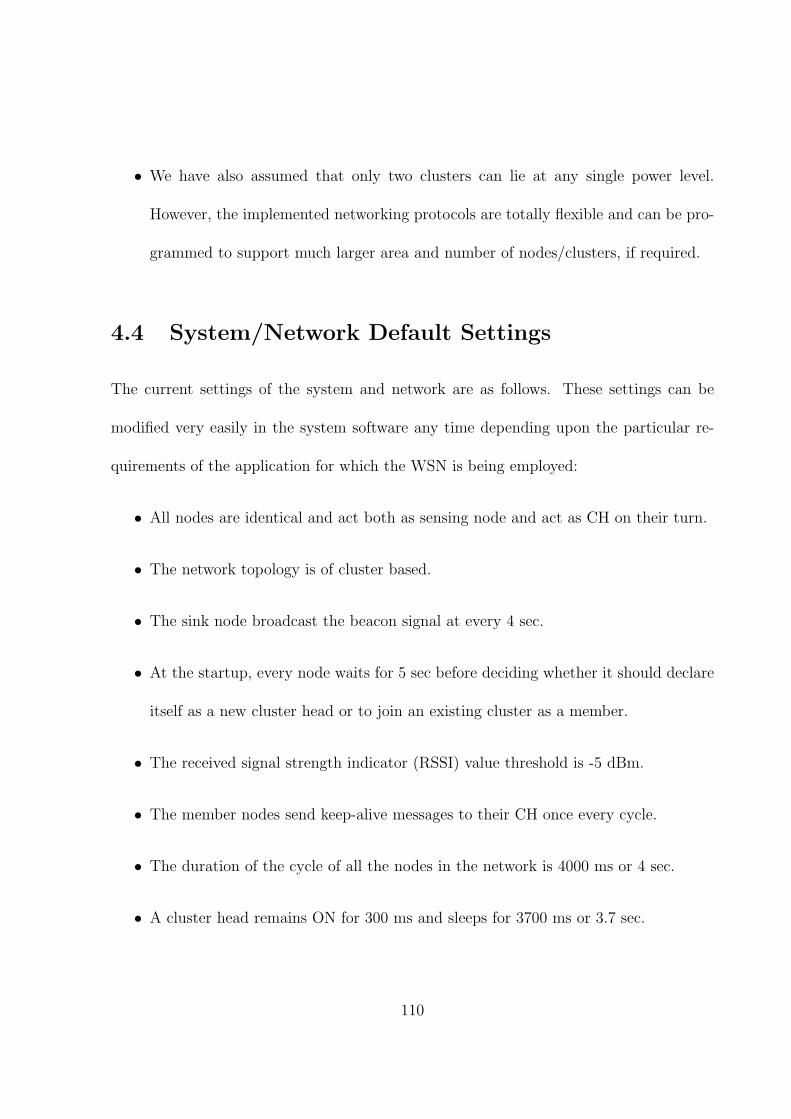
• We have also assumed that only two clusters can lie at any single power level.
However, the implemented networking protocols are totally flexible and can be pro-
grammed to support much larger area and number of nodes/clusters, if required.
4.4 System/Network Default Settings
The current settings of the system and network are as follows. These settings can be
modified very easily in the system software any time depending upon the particular re-
quirements of the application for which the WSN is being employed:
• All nodes are identical and act both as sensing node and act as CH on their turn.
• The network topology is of cluster based.
• The sink node broadcast the beacon signal at every 4 sec.
• At the startup, every node waits for 5 sec before deciding whether it should declare
itself as a new cluster head or to join an existing cluster as a member.
• The received signal strength indicator (RSSI) value threshold is -5 dBm.
• The member nodes send keep-alive messages to their CH once every cycle.
• The duration of the cycle of all the nodes in the network is 4000 ms or 4 sec.
• A cluster head remains ON for 300 ms and sleeps for 3700 ms or 3.7 sec.
110

• The member nodes are awake for 100 ms and asleep for 3900 ms or 3.90 sec. Thus
keeping the same duration of the cycle as that of the cluster heads.
• The responsibility of CH is shifted to other members of the cluster after every 10
cycles or 40 sec.
• The cluster ID is generated by the first CH by padding 0 to its own hard-coded
node ID. This cluster ID is maintained by all the nodes throughout the cluster life.
• The communication between the member node and CHs occurs at the lowest trans-
mission power of the transceiver (mode 1) whereas for inter-CHs communications,
a higher transmission power level (mode 3) is used.
• If a CH does not receive a keep-alive from a particular node for more than 3 cycles,
it is considered dead and is removed from the cluster table.
• After the rotation of the CH, the routing tables are updated within 5 sec.
• The data is relayed from the sensing node to the sink node by multi-hop dynamic
routes.
• In the main synchronized network, the environment attributes are being sensed
continuously/periodically and being relayed to the sink on a regular basis.
• In the unsynchronized portion of the network, the nodes keep sensing the environ-
ment on continuous basis but report the values only in case of a predefined incident.
111

• Routing tables are updated after every 20 sec.
• The levels once assigned to a node will remain constant during the lifetime of the
node.
Figure 4.1 shows the complete timing process graphically. The sink node sends the beacon
periodically after every 4 sec. When a node wakes up it listens for 5 seconds, receives the
beacon and declares itself head by broadcasting the keep-alive and sleeping after 300ms
(Figure 4.1). Similarly a member node on boot-up receives the keep alive of the CH and
goes to sleep after 100ms as indicated.
4.5 Implemented Protocol - MAC
As mentioned above also, the MAC protocol that we have actually implemented has many
ideas from the S-MAC protocol. Several factors were not mentioned in the literature and
have been devised to accomplish the desired tasks.
4.5.1 Packet Format
As suggested in S-MAC protocol, there are two types of packets in our implementation;
namely, control packets and data packets. The specific format of these packets has not
been defined in S-MAC and therefore we have defined the payload structure of each of
these packet types depending on our intended application’s need and requirements. The
packets are parsed into two sections; namely, the header part and the payload part. The
112
Figure 4.1: Timing diagram of duty cycles of CH and Member Nodes.
header section of the packet is created by the transceiver and we don’t have control over it.
The payload section of the packet is where we define different fields for different operations
both in the control packet and in the data packet.
Control Packets
Control packets are the packets that are responsible for setting up the point-to-point links
and clusters, establishing the network topology and ensuring smooth and reliable data
113

transfer between the nodes. The control packets are obviously overhead for the network
operation and ultimately decrease the effective throughput of the system. Therefore, they
are desired to be minimally transmitted and only if/when required. Also, since there is
no data in these packets, it was a design requirement to make them as small as possible
so that least energy is wasted for the transmission of this packet type. The format of the
control packets is shown in Table 4.1. It is a 16-bytes packet with the header of 13 bytes
long and the remaining 3 bytes are used in different scenarios for different purposes as
explained below.
Table 4.1: Control packet definition.
Byte number Function Type
1,2 Packet start identifier Radio header
3 Leading zeros Radio header
4,5 Destination ID Radio header
6,7 Source ID Radio header
8 Payload Length Radio header
9 Group ID Radio header
10 Message type Radio header
11 Cluster ID (CID) Payload
12 Node level (NL) Payload
13 Identifier Payload
14,15 Checksum Radio header
16 packet end identifier Radio header
114
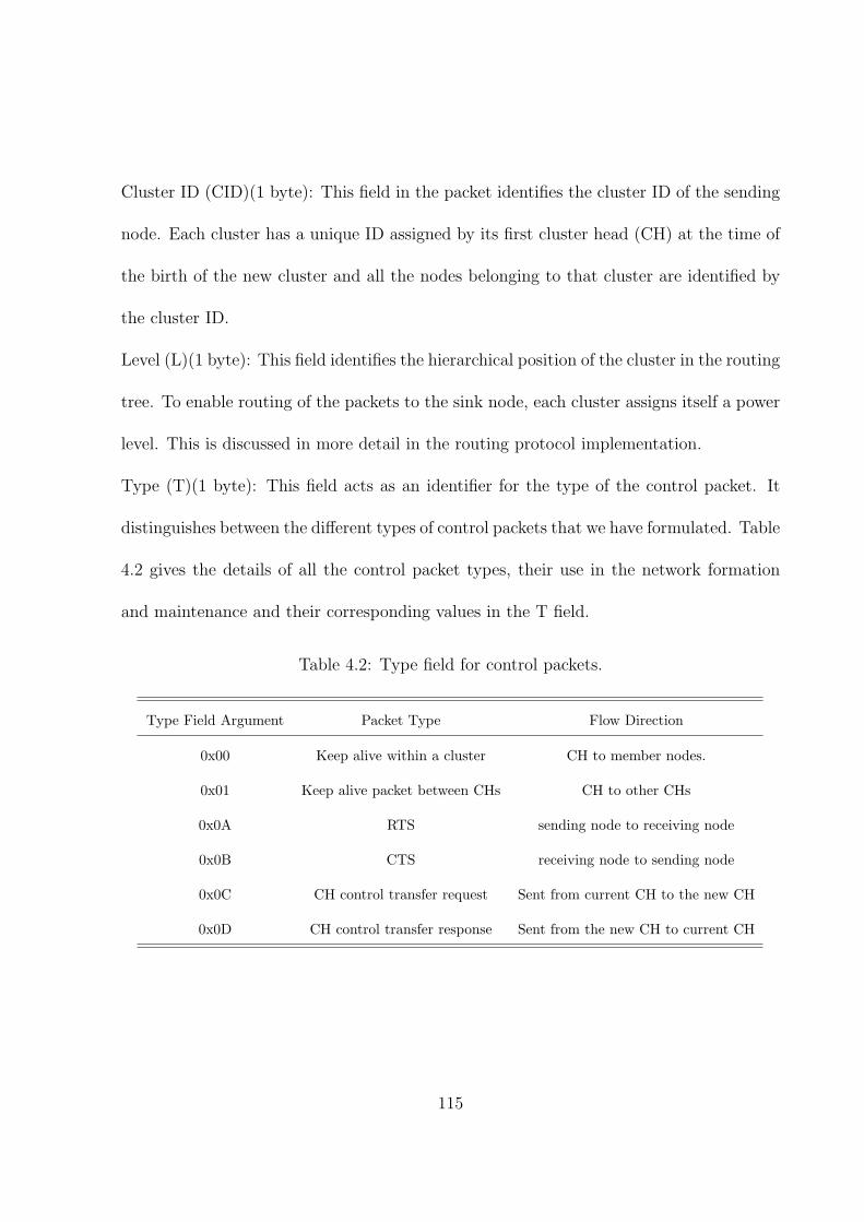
Cluster ID (CID)(1 byte): This field in the packet identifies the cluster ID of the sending
node. Each cluster has a unique ID assigned by its first cluster head (CH) at the time of
the birth of the new cluster and all the nodes belonging to that cluster are identified by
the cluster ID.
Level (L)(1 byte): This field identifies the hierarchical position of the cluster in the routing
tree. To enable routing of the packets to the sink node, each cluster assigns itself a power
level. This is discussed in more detail in the routing protocol implementation.
Type (T)(1 byte): This field acts as an identifier for the type of the control packet. It
distinguishes between the different types of control packets that we have formulated. Table
4.2 gives the details of all the control packet types, their use in the network formation
and maintenance and their corresponding values in the T field.
Table 4.2: Type field for control packets.
Type Field Argument Packet Type Flow Direction
0x00 Keep alive within a cluster CH to member nodes.
0x01 Keep alive packet between CHs CH to other CHs
0x0A RTS sending node to receiving node
0x0B CTS receiving node to sending node
0x0C CH control transfer request Sent from current CH to the new CH
0x0D CH control transfer response Sent from the new CH to current CH
115
Data Packets
The data packet is used to carry the data, from the sensing member node to the cor-
responding CH, and subsequently from the CH to CH until the data reaches the sink
node and ultimately received by the server. The complete length of the data packet is
31 bytes including the header and the payload. The header is 13 bytes long and the
remaining portion of the packet is the payload that we have formulated according to our
requirements.
We have used the payload part of the data packet not only to carry the sensed data
but also to carry the routing information along the route (for the debugging purpose
only) as well as to display the routing information on the front-end application (for the
demonstration purposes only). In the practical deployment of the network, most part of
this routing information is not needed and thus the packet size can be reduced to just 4
bytes required for storing light and temperature data. The format of the data packet is
shown in Table 4.3.
The definitions and descriptions of different fields of data packet in the payload part of
the data packet are explained below.
Temp and Light (4 bytes): These two fields constitute the data field jointly. The Temp
field contains the sensed value of the ambient temperature and the light field contains the
sensed reading of light intensity.
Hop Count (HC) (1 byte): This field serves the purpose of indicating the hop count of
the packet at a particular intermediate node. The hop count enables to easily and quickly
116
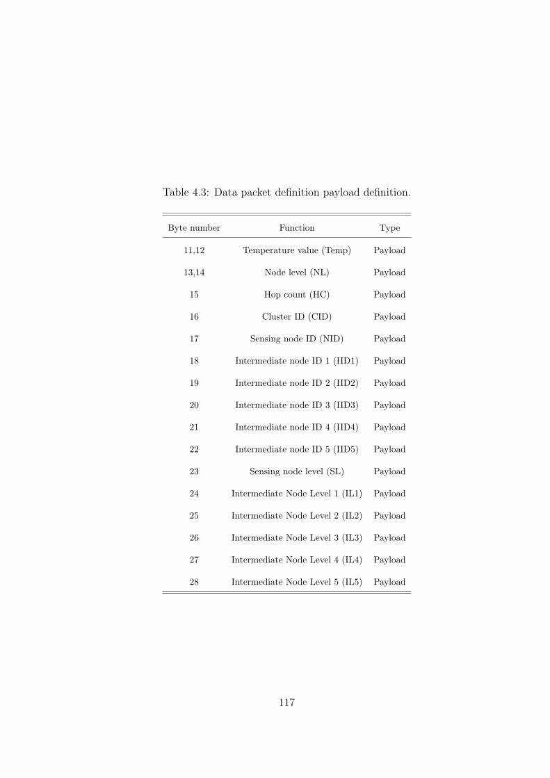
Table 4.3: Data packet definition payload definition.
Byte number Function Type
11,12 Temperature value (Temp) Payload
13,14 Node level (NL) Payload
15 Hop count (HC) Payload
16 Cluster ID (CID) Payload
17 Sensing node ID (NID) Payload
18 Intermediate node ID 1 (IID1) Payload
19 Intermediate node ID 2 (IID2) Payload
20 Intermediate node ID 3 (IID3) Payload
21 Intermediate node ID 4 (IID4) Payload
22 Intermediate node ID 5 (IID5) Payload
23 Sensing node level (SL) Payload
24 Intermediate Node Level 1 (IL1) Payload
25 Intermediate Node Level 2 (IL2) Payload
26 Intermediate Node Level 3 (IL3) Payload
27 Intermediate Node Level 4 (IL4) Payload
28 Intermediate Node Level 5 (IL5) Payload
117
fill in the next node ID in the packet without reading the complete packet. For example,
if the hop count is 2, this means the packet has already traveled two hops, so the next
address is placed at IID-3 without reading the complete address path.
Cluster ID (CID) (1 byte): This field in the packet identifies the cluster ID of the
sending node. Each cluster is has a unique ID assigned by its first CH at the time of the
birth of the new cluster and all the nodes belonging to that cluster are identified by the
cluster ID.
Sensing Node ID (NID) (1 byte): This field carries the ID of the sensing node. This
unique ID is assigned to each node at boot-up and is hard-coded inside every node. Each
node is given a unique ID that is not repeated in the remainder of the network.
Intermediate Node ID (IID1 - IID5) (5 bytes): These 5 fields are used to convey
the complete route information the packet traverses from the sensing node to the sink. In
the current implementation, we have programmed the system to operate for a maximum
of six hops including the hop from the sensing node to the CH. If the packet reaches the
sink with less than six hops, the remaining corresponding fields are set to zero, otherwise,
the fields have the node IDs of all the intermediate heads that relay the data packet.
Sensing Node Level (1 byte): This field contains the assigned power level of the
sensing node.
Intermediate Node Level 1 (IL1 - IL5) (5 bytes): These fields provide the power
levels of the intermediate CHs.
118

4.5.2 Scheduling Control
Similar to the S-MAC, our implementation also incorporates the coordinated sleeping of
the nodes to conserve the power. The sink node serves as the data collection center and
also the schedule synchronization source of the network. The sink node is connected via
USB port to the Network Monitoring Server for the onward processing of the received
data and monitoring of the network status. All the nodes in the network are synchronized
with the sink node.
Since the sink node is assumed to have unlimited amount of power, the transmission of
the beacon signal is done at the maximum available power level of the radio. The sink
node transmits a broadcast beacon signal once every cycle i.e. once in every 4 seconds.
This beacon signal prompts all the nodes in the network to sleep after predefined time
and at the same time provides a counter value. At the time of startup, all the nodes are
randomly placed. When the first node wakes up, it receives the beacon signal from the
sink. Upon receiving this packet from the sink, the CHs adjusts their timers such that
they go to sleep 300 ms after the reception of the beacon signal while the member nodes
sleep after 100 ms of the reception of the beacon signal. This means that the duty cycle
for the CHs is 300 / 4000 and the duty cycle for the member nodes is 100 / 4000.
The wake time for the CHs is chosen to be larger than the member nodes because the
member nodes simply need to sense the data and pass it on to the corresponding CH. But
the CHs not only have to receive data from multiple member nodes, they also have to
119
take part in the data relaying and routing process also. Therefore, they must keep awake
for longer time compared to the member nodes. The beacon signal also has a countdown
value that is decremented in each subsequent signal by 4, that indicates the time left until
the CH responsibility shifts to another node. Therefore, all the new nodes that boot up
later in the network are also tuned to the cluster shifting schedule.
4.5.3 Link Formation
At the time of startup, a node wakes-up and checks for the existence of any neighboring
CHs. This node waits for 5 seconds and if it does not receive any signal from any nearby
node, it declares itself a CH of a new cluster, otherwise, if the newly wakeup node receives
keep alive control signal from an existing cluster head, it measures the signal strength and
if the signal strength is below the threshold , it discards the signal from the other cluster
head and assumes that it has to make its own cluster by declaring itself the head of that
new cluster. This decision is made depending on the threshold value of the RSSI of the
received keep alive control packet. More specifically, when any wireless node receives
the signal, it measures the power of the received signal by reading RSSI register of the
CC2420 Transceiver. CC2420 has this built-in RSSI providing a digital value that can be
read by the microcontroller from the 8-bit register. If the RSSI value is less than -5 dBm,
it is considered that the new node is physically sufficiently away from the CH that it is
better to form a new cluster instead of joining that existing cluster. This means that the
new node must form a new cluster and become the CH. The threshold value of -5 dBm
120

Figure 4.2: Boot-up process of a sensor node.
121
has been selected after extensive experimentation and has been found to be optimum for
a typical indoor environment. This link formation process is represented in flowchart of
Figure 4.2.
If the node receives control signal from an existing CH and the signal strength is above
the threshold, it joins that cluster as a member and assigns itself the cluster ID of that
head. More specifically, if the RSSI of the received keep-alive control packet is greater
than -5 dBm, then this new node becomes member of that cluster and adopts the cluster
ID that it receives in the the control packet. If a node receives signals from two or more
CHs it joins as a member of the cluster whose head is nearer to it by measuring the signal
strength of their keep alive signals and comparing their powers.
4.5.4 Formation of Clusters
As other cluster heads wake up, as explained above, they start following the same wake-up
schedule which synchronizes them with the timing of the network. With the course of
time more clusters can be formed as well as more member nodes can join the clusters and
population of the cluster as well as the network grows.
The cluster ID is generated by multiplying the node ID of the first cluster head node with
10. This scheme of generating cluster IDs allows to support a large number of clusters.
During the whole operation of the network, all the nodes keep this same cluster ID. Each
of the CHs create and maintain a cluster table that has the node IDs of its members.
This table is created after receiving the keep-alive packets from the member nodes and is
122

used to select the next CH in the rotation. The next CH is selected as the node which
has the next lower cluster ID than the current CH. In other words CHs are selected based
on descending order of node IDs of all the entries of the cluster tables. If a CH does not
receive a keep-alive from a particular node for more than 3 cycles, it is considered dead
and is removed from the cluster table. New entries are added and old ones are refreshed
and updated as the keep-alive messages are received.
The cluster tables are formed and maintained by the CHs only and the member nodes
don’t need to maintain these tables. When a CH becomes the member node after the
cluster rotation, it flushes the clusters table it was keeping and the new CH starts building
its own cluster table.
Every CH broadcasts a keep alive packet in each alternate cycle (i.e after every 8s).
The purpose of this keep alive is to tell the immediate neighboring CH nodes about the
presence of this node and to keep its entry in the routing table entries. As a result, each of
the CHs refresh and maintain a routing table to select the proper route, this is discussed
in detail in Section 4.6.
4.5.5 Control and Data Packets Transfer
All the member nodes within a cluster regularly (once in three cycles, i.e. every 12
seconds) sense the temperature and light of the environment and send the raw data to
their respective CHs soonest as per the multiple access algorithm. In addition to that, the
member nodes also send the keep-alive message to their corresponding CHs once every
123
cycle to help the CH to update its cluster table. It should be noted that the member
nodes send data only to their assigned CH (unicast communication) and not to other
cluster heads. Once the cluster head gets the data, it routes the data towards the base
with the help of the intermediate CHs.
The transmission power of the transceiver CC2420 radio unit can be adjusted at different
settings. For the sake of conservation of the energy used in the transmission power, the
communications between member nodes and the CHs have been programmed at lowest
transmission power (mode 1) of the transceiver so that only the concerned nodes within
the cluster get the data with full conservation of power. For inter-cluster head communi-
cations, a higher transmission power level (mode 3) is used in order to give heads more
coverage as they need to communicate with other clusters heads at further distances.
4.5.6 Channel Contention and Multiple Access Control
In our implementation, the member nodes sample the temperature and light sensors every
12s and send the sensed values to their CHs. But because of the wireless medium and
multiple candidates contend for transmission, every node must check whether any signal
is present on the wireless channel or not so that collisions can be avoided. This is done
both by physical and virtual carrier sense as explained below.
In physical carrier sensing, the node scans the channel physically to check the presence of
any signal. If the channel is found to be busy, the node backs off and tries again in the next
cycle. On the other hand in virtual carrier sense, the node during its wake time listens
124

to the transmissions in its vicinity. When it receives a frame destined to another node
it extracts the duration field value (containing the remaining time to finish the current
transmission) from the frame and put it in the NAV register and starts decrementing it as
indicated in Figure 1.3. A member node takes decision to send a (control or data) packet
only when the NAV gets zero and at the same time the physical carrier sensing also turns
up negative. Similar procedure is followed when the packet is passed from one head node
to another head node for relaying the data towards the sink node.
The virtual carrier sensing is performed before the physical carrier sense. Since physical
carrier sensing involves powering ON the radio and actually listening to the channel, there-
fore this step consumes more power as compared to the virtual carrier sensing. Therefore,
it has been decided to carry out virtual carrier sensing to decrease the probability of find-
ing the channel busy and only proceed with the physical carrier sensing to ensure that
there is no transmission in the neighborhood and the channel is free.
4.5.7 Data Transfer
Once the data is sensed by the sensing node and is available for transmission after making
sure the wireless channel is free, the sensing node sends a unicast RTS packet to its CH.
When the RTS is received by the CH, depending on whether the CH node is free or not, the
CH responds by sending a unicast CTS packet to the corresponding sensing node. Upon
receiving the CTS, the node transmits the data packet to the CH. After the successful
delivery of the data the CH sends the ACK signal to the member node to confirm that
125
it has received the data properly. If the intended receiver does not receive the packet
for some reason such as collision, the ACK is not received by the member node and the
contention process is repeated again. The same procedure is followed for the data transfer
from one CH to the another CH. Flowchart in Figure 4.3 shows the implemented MAC
protocol.
To ensure that the whole message is transferred during the wake interval of the nodes, a
check has been added to ensure that the intended recipient node sends the CTS only if
there is sufficient time available in the wake period to complete the transaction. If there
is insufficient time to complete the communication, the intended recipient does not send
the CTS and the sensing node contends for the channel again in the next wake period.
4.5.8 Head Rotation Operation
As mentioned earlier, in order to balance the power consumption among the nodes in a
cluster, the cluster head responsibility is rotated every 10 cycles, i.e., every 40s. This is
performed in a descending order of the node IDs of the member nodes in the cluster table.
Two special type of control packets called the handshaking packets (Table 4.2) are ex-
changed between the CH and the member nodes for handshaking of the CH responsibility
handover rotation.
Once the switch over of CH takes place, the new CH listens to the keep-alive messages
of the neighboring CHs as well as the keep-alive messages of the member nodes to create
routing tables and cluster tables, respectively. This process takes time that varies de-
126

Figure 4.3: Channel contention of member node to send data packet.
127

pending on the time taken by all the members and neighbor CH to send their keep-alive
packets. At the same time, the new CH also transmits its own keep-alive message to alert
the neighboring clusters that now it is acting as the head of the cluster and all the routing
must be done through it instead of the old CH.
4.5.9 Differences between S-MAC Protocol and Implemented
Protocol
As the implementation details were not found during the literature survey, we had to
devise unique methods to implement the S-MAC protocol. In the process of doing so,
we created a protocol that was different from the S-MAC. Some of the most important
differences are listed below.
1. S-MAC is designed for multi-hop networks, and does not require that all nodes are
synchronized together. While our implementation enable the nodes to communicate
with each others, the sleep times are synchronized, i.e., all the nodes sleep and wake-
up at the same time. These schedules are maintained by every node, thus enabling
them to know when the neighboring node will be awake so that data can be sent to
it. The advantage of our approach is that it reduces the latency of the network as
if the different group of nodes follow different schedules, they increase the delay in
relaying the data in a multi-hop environment.
2. All nodes are free to choose their own listen/sleep schedules, while in our imple-
128

mentation the whole network has a single schedule that is controlled by the sink
node and followed by all the nodes in the network. This was chosen to simplify the
scheduling process as well as to have a single master clock in the network. If there
are different groups of nodes trying to schedule the periodic sleeping, it will result
in large timing difference among the nodes due to the natural different clock drifts
speeds in different nodes processors. Also, in the implementation of S-MAC, they
also expect that nodes only rarely see multiple schedules, since each node tries to
follow an existing schedule before choosing an independent one. In S-MAC, since
neighboring nodes coordinate their sleep schedules the clock drift on each node can
cause synchronization errors. Whereas in our techniques the synchronization pro-
cess remain robust to such errors and simple at the same time. Moreover, all the
exchanged timestamps are relative rather than absolute.
3. In S-MAC, the network consists of large numbers of nodes to take advantage of
short-range, multi-hop communications to conserve energy. Most communications
will occur between nodes as peers, rather than to a single base station. In our case,
the infrastructure is cluster-based and the member nodes communicate with their
CHs only, and the data is relayed in a multi hop routing manner by cluster heads
only.
4. In S-MAC, the nodes do not follow their sleep schedules until they finish the trans-
mission, while in our implementation, the intended recipient node makes sure that
there is enough time left in the wake period for receiving the data successfully before
129

its sleep time and only in that case the CTS signal is sent to the sender. This again
simplifies the whole operation as the schedules remain undisturbed.
5. Also, S-MAC protocol does not restrict on using a predefined packet structure and
leaves this on the specific implementation. This gives us the flexibility to use custom
designed payload structures according to our requirements.
4.6 Implemented Protocol - Routing
The routing layer protocol for our implementation has been mostly inspired by the com-
bination of LEACH and TEEN protocols. However, as mentioned for the MAC protocol
implementation also, the algorithmic details of LEACH and TEEN were not explained in
literature and we had to invent and devise exact and efficient ways to implement these al-
gorithmic details by extensive brainstorming, detailed discussions, and hundreds of hours
of testing and experimentation to come up with the best approach to achieve the desired
goal required from these networking protocols.
4.6.1 Network Topology
The sink node has a constant power supply and therefore has no energy constraints. It can
transmit with high power to all the nodes. Thus, there is no need for routing mechanism
from the sink node to any wireless network node. However, the wireless network nodes
are assumed to be far away from the sink node and because of their power constraints it
130

is not feasible to communicate directly to the sink node.
The network topology that we have implemented is of a clustered type multi-hop routing
similar to the LEACH protocol as shown in Figure 4.4. The model consists of clusters
(represented by the cloud) each consisting of a number of nodes. In each cluster at any
given time, one node acts as a cluster head (CH) (nodes A, B, C, and D etc.), whereas
the remaining nodes are the member nodes in that cluster (nodes A-1, A-2, B-1, B-2,
etc.). Only the member nodes perform the data sensing and the CHs are responsible for
receiving the data from the member node and route it reliably and efficiently to the sink
node.
Initially, the CH was fixed and hard-coded in our program but later the CH was success-
fully programmed to be dynamically rotated based on criteria defined in the Section 4.5.8
and then the head responsibility rotates among the member nodes in order to balance the
power consumption load between all member nodes equally.
Network Tree and Routing Tables
During the network setup phase, a logical network tree is created which comprises of all the
clusters placed at different power levels. These levels indicate the depth of the tree relative
to the sink node. To decide the levels, the sink or base node (S) regularly broadcasts a
beacon signal. When any wireless node receives the beacon signal, it measures the power
of the received signal by reading RSSI register of the CC2420 Transceiver. CC2420 has
this built-in RSSI providing a digital value that can be read by the microcontroller from
131

Figure 4.4: An illustration example of a network topology.
132

the 8 bit register.
Table 4.4: RSSI value resolution and definition of cluster levels.
RSSI Range in dBm Assigned Level
RSSI ≥ 0 1
-10 < RSSI ≤ -1 2
-13 < RSSI ≤ -10 3
-16 < RSSI ≤ -13 4
-19 < RSSI ≤ -16 5
-22 < RSSI ≤ -19 6
-25 < RSSI ≤ -22 7
-28 < RSSI ≤ -25 8
-31 < RSSI ≤ -28 9
-34 < RSSI ≤ -31 10
RSSI ≤ -34 11
Depending upon the received value of RSSI, every cluster head node assigns itself a
level. To assign the levels to corresponding RSSI values, ranges have been defined so that
adequate number of levels is created. The resolutions of the RSSI have been carefully
defined after a large number of experimentation and testing and are shown in Table 4.4.
It is to be noted here that if levels are assigned over narrow intervals of RSSI, a large
number of levels will be created. This can produce situations in which different levels are
assigned to nodes that are physically close to each other. On the contrary, if a wide interval
133
is used, then in situations where the signal strength doesn’t vary, majority of the cluster
heads will be associated to the same level. We have assigned this interval distribution
after rigorous testing of the network and monitoring of the physical separation between
the nodes in an indoor environment.
Formation and Updating of Routing Tables
When each of the cluster heads have been assigned a level, a logical tree structure is
formed. Each cluster head keeps sending a keep-alive control packet periodically in every
cycle to inform the neighboring cluster heads that it is alive. In this packet, the level
of the node is also broadcast. The neighboring nodes receive this message and store the
node ID and the corresponding level in its routing table. In case, a node dies, and the
neighboring nodes don’t receive keep-alive message from that node for 3 successive cycles,
its neighbors update their routing tables accordingly by assuming it is dead and flushing
its entry from their routing tables. In order to accommodate for the topology changes,
the routing tables are also updated every head rotation process. This enables the network
to include any new CH and to remove the CH that have died.
Routing Operation
When a CH has some data to send to the sink node it consults its routing table and
selects the node which is in an upper level (i.e. a level closer to the sink). For example,
considering the network of Figure 4.4, the node C would have the address table given in
Table 4.2. When node C wants to send data to the sink, it looks through the routing table
134

and sends the packet to the node that is one level higher in hierarchy or closer (level 2)
to the sink. So, node C will send data to node B. Assume that node B dies due to some
reason, then the next closer node (node A at level 1) will be the new recipient of data
from node C and this process continues. One important rule in this approach is that,
data is always sent to the CH that is at a strictly lower level than the current CH. This
prevents data from cycling between the nodes.
Table 4.5: Routing table at node C.
Node ID Level
A 1
B 2
D 4
S 0
A CH forwards the data to the CH higher up in the tree and this continues until the data
reaches the sink node (S). If the sending CH has another CH on the same power level as
its own, the sending CH will send only to the CH that is strictly higher in the level (lower
level number) in the tree. If the sending CH finds two CHs on the same level up in the
tree, then it forwards its data to the CH whose entry is the first one found in the routing
table.
The protocol that we have implemented takes care of the changes in the topology of
the network. For example, if a new node is added anywhere in the network, it either
135
associates itself with one of the existing clusters or otherwise starts its own cluster. This
new node becomes part of the routing mechanism automatically as if it has joined an
existing cluster, it takes turn to become CH and ultimately becomes part of a particular
routing chain. If that new node has started a new cluster then that cluster will update
and may improve the already existing routes depending upon its location and existing
power levels in the network.
If a node dies, it is dynamically taken care of by updating the cluster tables that ultimately
reflects on the update in the routing tables as well. We also expect that the clusters
closer to the sink node will exhaust their energy reserves sooner than the clusters that
are relatively further away form the sink node. In that situation or for any other reason,
if the whole cluster dies, the routing tables at the remaining clusters adopt this change
in the routing information by updating their routing tables insuring that the process of
data delivery from the alive network continues.
4.6.2 Data Delivery Models of the Network
There are two formations of network possible: static monitoring and dynamic monitoring.
Dynamic events in most applications require periodic reporting and consequently generate
regular traffic to be routed to the sink. Monitoring static events allows the network to
work in a reactive mode, simply generating traffic and reporting when an incident occurs.
We have implemented both approaches in our network.
136
Monitoring of Dynamic Events: Synchronized Network
Similar to LEACH, our main network acts in a proactive manner and regularly sense and
forwards data to the sink node. The implemented network protocol in this part of the
network takes care of this job efficiently and very robustly. All the member nodes are
periodically sensing during their wake time and are sleep most of their life in order to
conserve their energy reserves. The sensing nodes wakes up periodically and send the
sensed data to their CH. The purpose of making our network proactive is to enable the
regular reporting and monitoring of the elements in the environment.
Incident-based Monitoring: Unsynchronized Group of Nodes (UGN)
At the same time, like TEEN, the network also has the ability to act in a reactive mode. A
portion of the network, called the unsynchronized group of nodes (UGN), operate outside
the domain of our main network. These nodes remain in the sleep state (transceiver
OFF, CPU at low power mode 1) most of the time. At the same time they keep sensing
the environment continuously and only wakeup to report an incident if the sensed value
crosses a pre-defined threshold. In contrast to the main network, these nodes do not form
clusters and don’t follow any time schedules. They also don’t need to maintain the cluster
tables, network topology and routing tables.
Once there is an incident occurrence (threshold crossing of the sensed value) to be reported
is ready, the node wakes up and listens for the keep-alive messages from the main network.
Due to the criticality of the situation that this node needs to report, this node hands over
137

the data to the CH of the main network from which it receives the signal first, regardless
of its distance and location on the network. The UGN sensing node follows all the MAC
protocol procedures as described in Section 4.5 to contend for the channel and to deliver
the data reliably to the first CH it hears from. After successful delivery of the incident,
this nodes goes to its sleep mode again and the data is relayed to the sink node by the
main network CHs according to their routing tables.
4.6.3 Differences between LEACH/TEEN Protocols and Imple-
mented Protocol
LEACH is based on a clustered approach. The nodes group themselves into clusters
and decide a cluster head that communicates with its peers to route data. The protocol
implemented has some implementation differences with LEACH that are:
1. In LEACH, the cluster heads change randomly over time in order to balance the
energy dissipation of nodes whereas in our implementation the CHs are rotated
periodically in pre-defined manner.
2. In LEACH, the nodes form clusters dynamically, i.e., with the death of any node
the memberships of the clusters are updated and nodes can reorganize themselves
in different manner as earlier. In our case the nodes form fixed clusters and they
retain their membership till the end. This not only simplifies the implementation,
it also results in savings of energy from the overhead of communication required for
138

making new clusters.
3. LEACH uses single-hop routing where each node can transmit directly to the cluster-
head and the sink. Our implementation employs multi-hop dynamic routing thus
resulting in savings of transmission power required as multi hop routing is much more
energy efficient in terms of transmission power required to communicate between
two nodes.
Although TEEN is also based on clusters, but the definition of hard and soft thresh-
old makes to suitable only for incident based reporting. Following are some differences
between our protocol and the TEEN protocol.
1. As explained in the TEEN protocol, the nodes group themselves into clusters, and
elect a cluster head from amongst them. In our implementation, the CHs are not
elected but the responsibility is rotated among all the members evenly and period-
ically in order the load balances the power consumption within the cluster.
2. The TEEN protocol defines only two levels of clusters, one among the member
nodes and the second one among the CH. On contrary, we have defined a total of
eleven (11) cluster levels so that our system can support large sizes of networks with
small multi-hop routed communications among the CHs thus saving lot of power for
transmission.
3. In TEEN, the thresholds are set by the sink node, but in our implementation of the
UGN, the thresholds are pre-programmed in the sensing nodes. The UGNs in our
139
network wake-up only when there is some alarm that must be reported to the sink.
By pre-programming the threshold levels, the UGNs do not need to wake-up and
listen to the sink node to receive thresholds, thus conserving power.
4.7 Conclusions
This chapter presented a detailed discussion on the S-MAC as well as the TEEN and
LEACH protocols and their usage in the WSN domain. All the important design con-
siderations for MAC and routing protocols have been highlighted. At the same time, a
complete discussion on the implemented protocols at MAC and routing layers has been
provided. A comparison of features of the implemented and the original protocols show
that our MAC protocol has a better synchronization and easier implementation capabil-
ities as compared to S-MAC. Similarly the comparison of the existing routing protocols
with the implemented protocol reveals that our head rotation policy enables a better
energy consumption throughout the cluster as compared to LEACH and TEEN. On the
contrary our MAC protocol assumes that all the nodes can receive signals from the sink,
which can become difficult in different environments. Also, the pre-programmed thresh-
olds can become difficult to change as priorities for alarms change.
140

CHAPTER 5
SIMULATION RESULTS
Chapter 4 presented the design details of the MAC and the routing protocols actually
implemented on the KFUPM nodes. Although the implementation process had to be
devised in a unique manner, the actual design of the protocol has been simulated on the
network simulator (ns-2.28). This chapter presents the simulation results of the basic
S-MAC, the implemented S-MAC and the routing protocols. Comparisons in the perfor-
mance of the implemented S-MAC and the basic S-MAC as well as the LEACH and the
designed routing protocols have been presented to indicate the energy-efficient behavior
of the designed methodology.
The rest of the chapter is organized as follows: Section 5.1 presents the simulation results
and commentary on the S-MAC protocols, Section 5.2 has the results for the routing
protocol simulations and comparison studies and the chapter concludes with a summary
in Section 5.3.
141

5.1 S-MAC Simulation
S-MAC is one the most basic MAC layer protocol designs to be used in WSN. [73] et al.
have simulated the protocol with some duty cycle dynamics based on traffic rates and
have provided a comparatively energy efficient model. The basic S-MAC with dynamic
sleep schedules was introduced by [16] which provided increased energy efficiency at the
cost of higher end-to-end packet latencies.
As mentioned in Section 1.4, S-MAC is based on a fixed duty cycle. All the neighboring
nodes follow the same schedules, with some of the nodes following multiple schedules to
help relay information from nodes having different sleep schedules. This section presents
the simulation parameters and results of the ns-2.28 [74] simulation of the S-MAC proto-
col.
5.1.1 Simulation Parameters
The following parameters have been fixed for simulation:
1. All the simulations for S-MAC comprise of a network consisting of 30 nodes. The
nodes have been arranged such that the data from the first node reaches the sink
node over 10 hops.
2. The simulation time for this protocol is 1000 machine seconds. At the end of the
simulation the required parameters are examined.
142

3. Each node has been programmed with energy reserves of 19035 Joules which corre-
spond to 4.5 V DC with the batteries having a rating of 1175 mAh.
4. Each of the 30 nodes generates 31 Byte packets. Among these 31 Bytes 18 Bytes
belong to the payload itself, whereas the remaining constitute the MAC headers.
5. The traffic generated is poisson distributed with the different inter-arrival times to
observe the effect of varying traffic loads.
6. The S-MAC has been programmed with a 10% duty cycle having a complete cycle
period of 4 seconds.
7. In order to test the S-MAC protocol, a simple routing protocol has been used that
just passes the packets between immediate neighbors.
8. The results generated by ns-2.28 are written in a text file and include the time
when each packet was sent/received. It also indicates that if any packets have been
dropped or not. In addition the energy remaining at the end of each packet transfer
is also indicated by the result script. Since the major interest in this section is on
the MAC layer, only the MAC layer traces have been turned on. The routing and
application level traces have been turned off, so that only the packets from the MAC
layer can be monitored.
9. A python script has been written to extract data throughput, end-to-end delay and
energy consumed by the network.
143

5.1.2 Energy Analysis
To analyze the energy consumption per delivered packet the CSMA/CA, basic S-MAC
and the implemented S-MAC have been simulated with 10% duty cycles for the later
two cases. The traffic generation has been varied by changing the inter-arrival time of
the packets at the generating nodes. Using a small inter-arrival time means the packets
are generated faster and hence imply a congested network. Fig. 5.1 shows the energy
consumed per packet delivered with respect to varying traffic generation rate.
0 2 4 6 8 100
2
4
6
8
10
12
14
16
18
20
Interarrival time (s)
Ene
rgy
cons
umed
(m
J)
CSMA/CABasic S−MAC with 10% duty cycleImplemented S−MAC with 10% duty cycle
Figure 5.1: Energy consumed per delivered packet with varying packet generation rate.
In Fig. 5.1 S-MAC results have been compared with the case of CSMA/CA and the
144

implemented S-MAC. It can be observed that when the network is highly congested (inter-
arrival 0.001-2s) it is more efficient to not deploy any sleep cycles. By keeping the nodes
ON continuously, all the packets can be delivered to the destination successfully with little
energy cost per delivered packet. During the same period, a 10% duty cycle basic S-MAC
shows an almost constant energy cost since only 10% of the generated packets are sent
regardless of the generation rate. The node is OFF for 90% of the time, so the packets
generated during that time will either be delayed or dropped because of the limited buffer
size. The implemented S-MAC, as explained in Section 4.7.9 employs same sleep schedules
for all the nodes in the network as opposed to the basic S-MAC which supports some of
the nodes following multiple schedules to overcome the tight synchronization issues. From
Fig. 5.1 it is obvious that when the network is highly congested the energy consumed by
the nodes per delivered packet is less because the nodes are ON only once in the duty cycle
(since a single schedule is being followed). This means that a larger number of packets
are either delayed or dropped due to the single schedule in the implemented approach.
As the packet generation rate decreases (high inter-arrival times), the results of CSMA/CA
indicate an almost linear increase in energy consumption per delivered packet. The reason
of this being that the nodes are constantly ON and the packets being generated are less
hence increasing the cost. When either of the S-MAC approaches are analyzed, the cost
remains approximately constant regardless of the packet generation rate because the node
is transmitting only 10% of the time. Fig. 5.1 portrays the superiority of the duty cycle
S-MAC in case of varying traffic loads by indicating an almost constant packet cost.
145
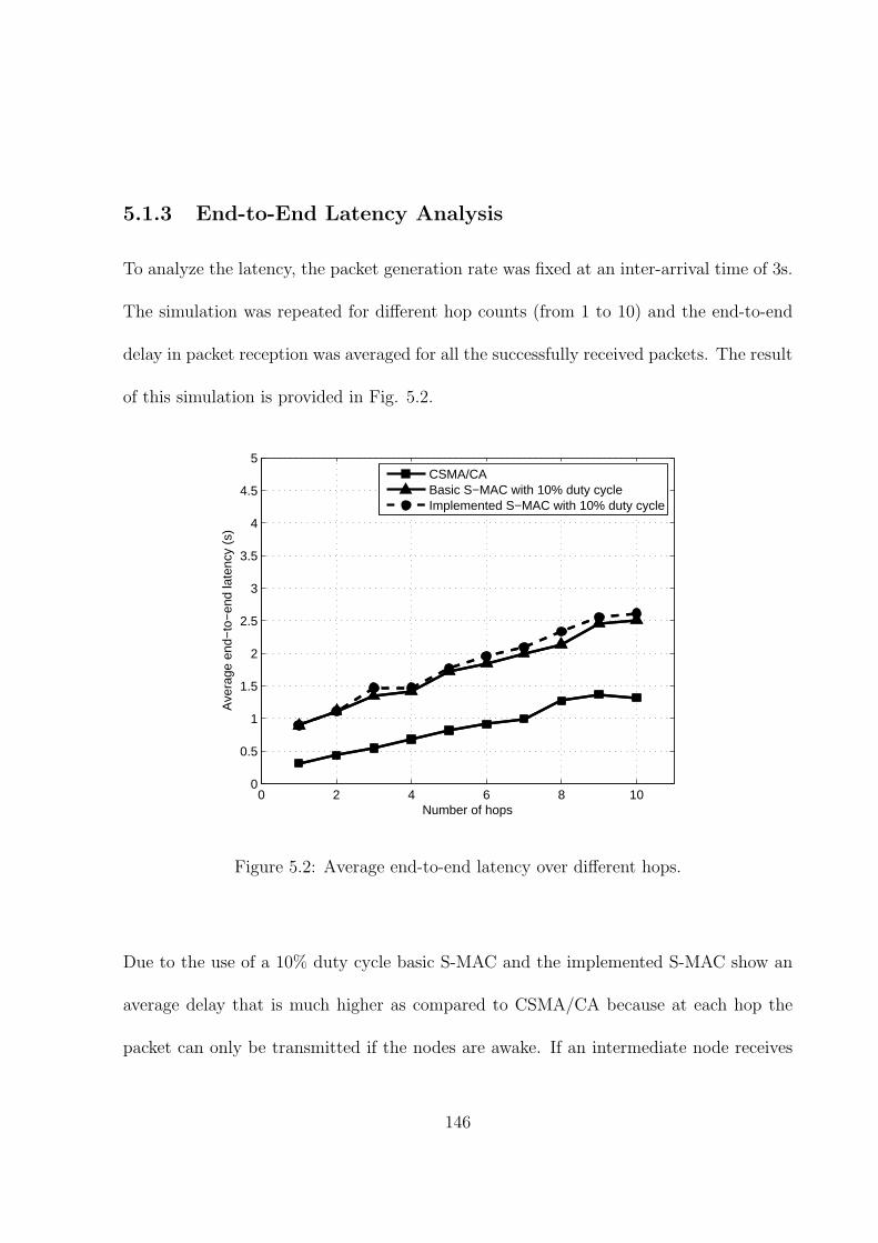
5.1.3 End-to-End Latency Analysis
To analyze the latency, the packet generation rate was fixed at an inter-arrival time of 3s.
The simulation was repeated for different hop counts (from 1 to 10) and the end-to-end
delay in packet reception was averaged for all the successfully received packets. The result
of this simulation is provided in Fig. 5.2.
0 2 4 6 8 100
0.5
1
1.5
2
2.5
3
3.5
4
4.5
5
Number of hops
Ave
rage
end
−to
−en
d la
tenc
y (s
)
CSMA/CABasic S−MAC with 10% duty cycleImplemented S−MAC with 10% duty cycle
Figure 5.2: Average end-to-end latency over different hops.
Due to the use of a 10% duty cycle basic S-MAC and the implemented S-MAC show an
average delay that is much higher as compared to CSMA/CA because at each hop the
packet can only be transmitted if the nodes are awake. If an intermediate node receives
146

a packet and it does not have enough time to forward it, it will delay this process to the
next wake cycle, thus introducing delay into the packet. Moreover, it is observed that
the end-to-end latency in case of the implemented protocol increases with the number
of hops and is higher than the basic S-MAC approach. The reason for this increase is
the fact that the basic protocol enables some of the nodes to follow multiple schedules
thus enabling them to wake-up more than once in a given cycle. This multiple wake-up
enables the basic S-MAC to forward a larger number of packets per cycle and hence the
end-to-end delay is decreased. In the case of implemented S-MAC, since each node is ON
only once in a cycle, therefore only a limited n=umber of packets can be transmitted thus
delaying the packets till the next cycle. For a system with operating with CSMA/CA,
this delay is only because of the time taken by the nodes to forward the packets, which
as seen in Fig. 5.2 is nearly linear.
5.1.4 Throughput Analysis
Throughput has been defined as the number of bytes of payload that are actually received
at the destination without retransmissions. The result of this simulation is provided in
Fig. 5.3. To measure this parameter, the simulation was run over the entire 1000s interval
and the received bytes were determined to calculate the average throughput. As it was
observed in Section 5.1.2, when CSMA/CA is employed, a highly congested network (inter-
arrival 0.001-2s) provides the highest data throughput since a huge number of packets are
being received at the destination. As the packet generation decreases, the throughput
147

also starts to decrease, until it becomes almost constant at nearly 4.6 Bytes/sec. Since
the packets being generated are less, the throughput is understandably less.
0 2 4 6 8 100
5
10
15
20
25
30
35
Message inter−arrival time (s)
Ave
rage
dat
a th
roug
hput
(B
ytes
/s)
CSMA/CABasic S−MAC with 10% duty cycleImplemented S−MAC with 10% duty cycle
Figure 5.3: Average data throughput at varying traffic rates.
In case of 10% duty cycle basic S-MAC, the throughput remains nearly constant at 4.6
Bytes/sec because of the small duty cycle. Regardless of the number of packets being
generated, the transmission takes place only 10% of the time resulting in nearly uniform
throughput figures as indicated in Fig. 5.3. The throughput for the implemented pro-
tocol is lower than the basic S-MAC because all the nodes in the implemented protocol
are ON only once in a cycle as opposed to multiple times in case of the basis S-MAC.
However, as the network becomes less congested, the throughput for both the basic and
148
the implemented protocol converge.
5.2 Routing Protocol Simulation
As described in Section 4.8, the designed protocol has been inspired from the periodic
monitoring protocol call LEACH. Therefore, the results of the designed protocol will be
compared with simulation results of LEACH and conclusions will be made based on these
figures.
5.2.1 Simulation Parameters
In addition to the assumptions mentioned in Section 5.1, following parameters have been
fixed for simulation:
1. All the simulations of a network consisting of 51 nodes. 50 nodes form the sensing
network, where as the last node acts as the sink (destination) node collecting all the
packets.
2. For the designed protocol, the head shifting takes place every 100s.
3. Implemented S-MAC with 10% duty cycle has been selected as the MAC protocol
of choice for all the simulations in this section.
149
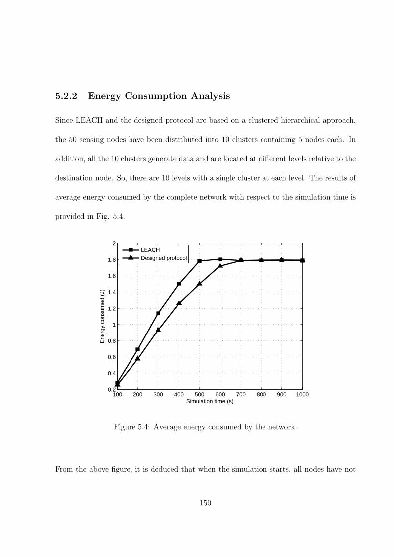
5.2.2 Energy Consumption Analysis
Since LEACH and the designed protocol are based on a clustered hierarchical approach,
the 50 sensing nodes have been distributed into 10 clusters containing 5 nodes each. In
addition, all the 10 clusters generate data and are located at different levels relative to the
destination node. So, there are 10 levels with a single cluster at each level. The results of
average energy consumed by the complete network with respect to the simulation time is
provided in Fig. 5.4.
100 200 300 400 500 600 700 800 900 10000.2
0.4
0.6
0.8
1
1.2
1.4
1.6
1.8
2
Simulation time (s)
Ene
rgy
cons
umed
(J)
LEACHDesigned protocol
Figure 5.4: Average energy consumed by the network.
From the above figure, it is deduced that when the simulation starts, all nodes have not
150

woken up. As the simulation time elapses, the nodes start to wake up at random times
and start joining the respective clusters, this leads to a gradual increase in the energy
consumed (Fig. 5.4) regardless of the protocol adopted. At around 700s the energy
consumption for both LEACH and the designed protocol becomes constant since all the
50 sensing nodes have initialized and have joined the clusters.
It is observed from the curve that, although the energy consumption is following the
same pattern for both the protocols, the LEACH tends to have a higher average energy
consumption due to a fixed cluster head. A look at the curve for the designed protocol
indicates that the head shifting process has in fact led to an improvement in energy
consumption during the initialization stage of the network. As the network matures, the
consumptions of both the protocols become the same.
5.2.3 Network Lifetime Analysis
The network lifetime can be defined with respect to any application; [76] have defined
the network life as the time from the start of the network until the first node depletes its
energy and dies, on the other hand [77] define thenetwork lifetime interms of the service
offered to the end-user. For the proposed setup it has been defined as the time from
the start of the network till the failure of the first cluster. Each cluster is deployed in a
different physical area sensing the characteristics from that area. If a complete cluster
fails, the corresponding area can no longer be sensed and therefore the network breaks.
In case of the LEACH protocol, the cluster head has been fixed. Since the cluster head
151

is responsible for connecting the cluster with the rest of the network, its death means
the death of the cluster. Although the sensing nodes of the corresponding cluster are
still sensing, their inability to communicate with the other clusters means their data
cannot reach the sink node. For the designed protocol, the cluster head responsibility
rotates between all the available cluster members. This process ensures that the energy
consumption among all the nodes in the cluster is uniform and the complete cluster dies
simultaneously as compared to just the cluster head.
In order to analyze the network lifetime, LEACH and the designed protocol have been
simulated with different cluster sizes and the impact of cluster size on the network has
been analyzed as shown in Fig. 5.5.
0 10 20 30 40 500
100
200
300
400
500
600
Cluster size (nodes)
Life
time
(Hou
rs)
LEACHDesigned protocol
Figure 5.5: Network life vs. varying cluster sizes.
152

It is observed from both the curves that as the cluster size increases, the lifetime decreases;
since the number of nodes in the cluster are increasing. In case of LEACH, an increase in
cluster size means that the cluster head has to communicate and relay information from
more member nodes which requires more energy and hence the cluster dies earlier. For the
designed protocol, since the cluster head responsibility is being rotated among the member
nodes, an increase in the cluster size means a decrease in the time each member node has
to spend as the cluster head. This leads to lesser energy consumption at individual
nodes, but the energy dissipation due to the added communication requirement for the
new member nodes is there.
From Fig. 5.4 it is clear that as the cluster size increases both the curves start to converge.
When all the 50 nodes form a single cluster the lifetime provided by the designed protocol
is marginally better because of head rotation as compared to the LEACH.
5.2.4 Received Packet Analysis
As discussed in previous sections, head rotation mechanism improves the energy con-
sumption figures and adds to the overall network life of the system. However, this comes
at the price of reduced packet delivery. When a cluster head transfers its responsibilities
to another member, the undelivered packets, if any, at the old cluster head are dropped.
In addition, the other member nodes require some time to realize that the cluster head
has now changed. All this process leads to a decrease in the PRR at the sink node. A
comparison of LEACH and the designed protocol is given in Fig. 5.6. It can be observed
153
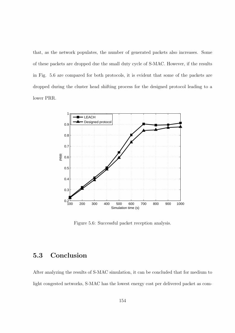
that, as the network populates, the number of generated packets also increases. Some
of these packets are dropped due the small duty cycle of S-MAC. However, if the results
in Fig. 5.6 are compared for both protocols, it is evident that some of the packets are
dropped during the cluster head shifting process for the designed protocol leading to a
lower PRR.
100 200 300 400 500 600 700 800 900 10000.2
0.3
0.4
0.5
0.6
0.7
0.8
0.9
1
Simulation time (s)
PR
R
LEACHDesigned protocol
Figure 5.6: Successful packet reception analysis.
5.3 Conclusion
After analyzing the results of S-MAC simulation, it can be concluded that for medium to
light congested networks, S-MAC has the lowest energy cost per delivered packet as com-
154
pared to CSMA/CA. The implemented approach of using strict synchronization through-
out the network results is comparatively less energy consumption per delivered packet as
compared to the basic S-MAC. The cost for energy-efficiency is paid in terms of higher
end-to-end delays over multiple hops and comparatively less data throughput. The chap-
ter also included the analysis of LEACH and the new designed routing protocol. From
the simulation results, the designed protocol shows a much better energy utilization as
compared to LEACH. At practical cluster sizes (5-10 nodes per cluster) the network life
offered by the designed protocol is almost twice as compared to the LEACH protocol.
This increase in network life comes at the compromise of the offered PRR.
155

CHAPTER 6
DESIGN OF SENSOR NETWORK
DEPLOYMENT APPLICATION
The deployment of a WSN is highly dependent on the target environment. As with wireless
communications, factors like fading and interference vary depending on the environment.
Indoor channels are considered worst because of the high level of interference due to
reflection from walls and other equipment in the vicinity. In fact, the presence of chairs,
tables and even the material of the wall itself affects the signal propagation characteristics.
On the contrary, an outdoor or open space has comparatively better signal propagation
aspects. As with the indoor environment, the presence of foliage, sand and mud have an
affect on the signal propagation in the outdoors. After knowing the type of environment
in which the network is to be setup, the question of network size arises; more specifically,
what is the least number of nodes that could be used to cover a particular area with some
156
propagation characteristics. This chapter tries to find the answer for this question by
creating a MATLAB application that provides the deployment figures for two different
cases. Actual received signal strength measurements have been used to reach a conclusion
regarding the number of nodes required to create a network. The KFUPM node has the
ability to extract the received signal strength (RSS) from the received packet. This ability
was utilized in all of the measurements in this chapter.
Section 6.1 presents the antenna characteristics based on experimental analysis for the two
types of antennas used for the measurements. The design methodology of the application
is presented in Section 6.2 and application design details along with the analysis of two
distinct case studies is presented in Section 6.3. Finally the chapter concludes with Section
6.4 presenting the conclusion.
6.1 Antenna Characteristics
For the KFUPM wireless sensor node, the CC2420EM transceiver unit operates in the
industrial, scientific and medical (ISM) band. The unit also comes with an external an-
tenna that could be changed as desired. One of the most important parameters in wireless
communications is the radiation pattern of the antenna itself. During the simulations, an
omni-directional antenna radiation pattern is assumed to simplify the process, which may
not be true in practice. Therefore, a radiation pattern measurement has been performed
for two different kinds of antennas to provide an accurate representation of the signal
propagation which would be employed in the design of the application.
157

6.1.1 Antenova Standard Antenna
The CC2420EM unit comes with an Antenova antenna that has a hight of about 3.5
inches as shown in Fig. 6.1. The Antenova antenna is designed to operate at 2.4 GHz with
applications in WiFi, Bluetooth and ZigBee. The antenna works with linear polarization
providing a peak gain of 2.2 dBi and an 80% operating efficiency [78]. The radiation
pattern in the azimuthal range as provided in the datasheet is shown in Fig. 6.2.
Figure 6.1: Antenova antenna.
158

Figure 6.2: Antenova antenna radiation pattern from the datasheet.
In order to measure the radiation pattern of this antenna, two KFUPM nodes have been
used. The receiving node was connected to the PC and its location was fixed. The
transmitting node was programmed to transmit 4 packets/second at at transmit power of
0 dBm. Each of the transmitted packets contained a sequence number which was used to
determine any lost packets at the receiver. All the measurements were performed in an
open environment at Building 33 (university stadium).
The distance between the transmitter and the receiver is fixed at 10 cm. In addition the
transmitter was rotated 22.5 degrees to get receive power measurement for 16 different
angles. The results of this measurement are provided in Fig. 6.3. Comparing the radiation
patterns in Fig. 6.2 and Fig. 6.3 it is obvious that the antenna does not display a
159

completely omni-directional coverage as indicated in the datasheet.
0°
15°
30°
45°
60°75°90°105°
120°
135°
150°
165°
±180°
−165°
−150°
−135°
−120°−105° −90° −75°
−60°
−45°
−30°
−15°
−25−24.5−24−23.5−23
Figure 6.3: Radiation pattern in dBm of the Antennova around the azimuthal axis.
As indicated in Fig. 6.3, the received signal power varies depending on the orientation of
the antenna. One important thing that must be analyzed here is the relationship of this
variance with the distance from the receiver. For this setup, the received signal power
was measured by varying the transmitter-receiver distance between 10 cm, 2 m, 4 m and
8 m. The results of this experiment are provided in Fig. 6.4.
160
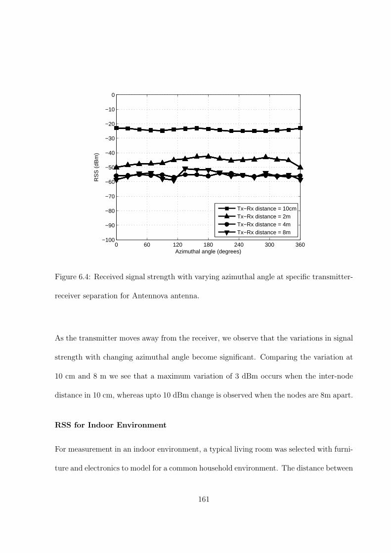
0 60 120 180 240 300 360−100
−90
−80
−70
−60
−50
−40
−30
−20
−10
0
Azimuthal angle (degrees)
RS
S (
dBm
)
Tx−Rx distance = 10cmTx−Rx distance = 2mTx−Rx distance = 4mTx−Rx distance = 8m
Figure 6.4: Received signal strength with varying azimuthal angle at specific transmitter-
receiver separation for Antennova antenna.
As the transmitter moves away from the receiver, we observe that the variations in signal
strength with changing azimuthal angle become significant. Comparing the variation at
10 cm and 8 m we see that a maximum variation of 3 dBm occurs when the inter-node
distance in 10 cm, whereas upto 10 dBm change is observed when the nodes are 8m apart.
RSS for Indoor Environment
For measurement in an indoor environment, a typical living room was selected with furni-
ture and electronics to model for a common household environment. The distance between
161

the transmitter and receiver was varied and the received signal strength was recorded as
shown in Fig. 6.5. Due to the presence of different objects in the vicinity, the signal
strength fluctuates. At 4 m distance it becomes higher as compared to 3m which is due
to the reflections caused by the objects. In addition the height of the node relative to the
ground was changed to see the effect. It is observed that when the nodes are placed at
ground level, the reflections from the ground cause severe attenuation leading to a lower
received signal strength as compared to the case when the nodes are elevated at 60 cm.
0 1 2 3 4 5 6 7 8 9−100
−90
−80
−70
−60
−50
−40
−30
−20
−10
0
Distance (m)
RS
S (
dBm
)
Height above ground 60cmHeight above ground 0cm
Figure 6.5: Received signal strength with varying distance in an indoor environment for
Antennova antenna.
162

RSS for Outdoor Environment
The outdoor measurements were performed in Building 33 (stadium). Again the distance
between the transmitter and the receiver was changed form 10 cm to 60 m and the nodes
were placed at a height of 60 cm. The RSS figures were recorded as displayed in Fig. 6.6.
0 10 20 30 40 50 60−90
−80
−70
−60
−50
−40
−30
−20
−10
Distance (m)
RS
S (
dBm
)
Figure 6.6: Received signal strength with varying distance in an outdoor environment for
Antennova antenna.
One important factor in case of WSN is the packet receive ratio (PRR) defined as the
fraction of transmitted packets successfully received. As each of the transmitted packets
has a sequence number, the receiver extracts this sequence number and determines any
missing sequence numbers to calculate the PRR. For the transmission power of 0 dBm even
at a distance of 60 m the PRR remains 1, indicating that all the packets are successfully
received. However, when the transmit power is decreased to -5, -10, -15 and -25 dBm, the
163
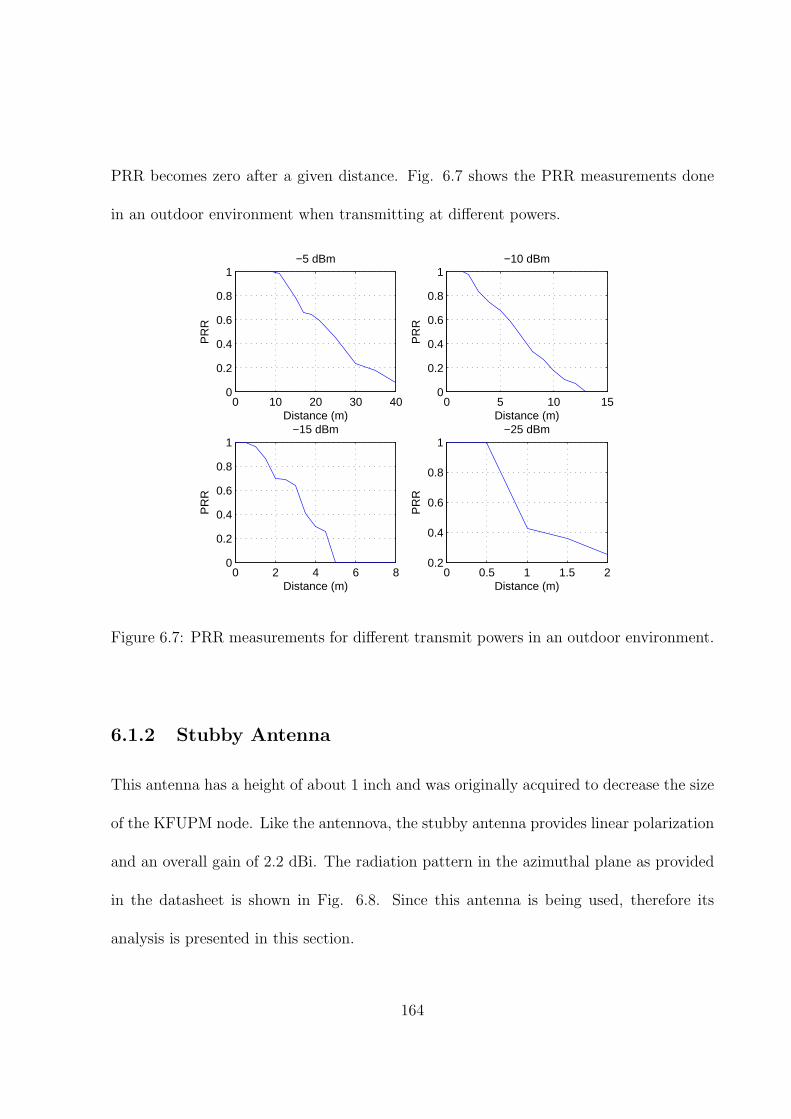
PRR becomes zero after a given distance. Fig. 6.7 shows the PRR measurements done
in an outdoor environment when transmitting at different powers.
0 10 20 30 400
0.2
0.4
0.6
0.8
1−5 dBm
Distance (m)
PR
R
0 5 10 150
0.2
0.4
0.6
0.8
1−10 dBm
Distance (m)P
RR
0 2 4 6 80
0.2
0.4
0.6
0.8
1−15 dBm
Distance (m)
PR
R
0 0.5 1 1.5 20.2
0.4
0.6
0.8
1−25 dBm
Distance (m)
PR
R
Figure 6.7: PRR measurements for different transmit powers in an outdoor environment.
6.1.2 Stubby Antenna
This antenna has a height of about 1 inch and was originally acquired to decrease the size
of the KFUPM node. Like the antennova, the stubby antenna provides linear polarization
and an overall gain of 2.2 dBi. The radiation pattern in the azimuthal plane as provided
in the datasheet is shown in Fig. 6.8. Since this antenna is being used, therefore its
analysis is presented in this section.
164

Figure 6.8: Stubby antenna radiation pattern from the data sheet.
The procedure adopted for the Antenova antenna as described in Section 6.1.1 is replicated
by changing the transmit antenna to a stubby antenna. The radiation pattern is provided
in Fig. 6.9. Comparing the radiation pattern of the two antennas, it is obvious that the
stubby antenna provides a much omni-directional coverage as compared to the Antennova.
This advantage comes at the cost of the signal strength; as the stubby antenna has an
RSS of -25 dBm as compared to -23 dBm for the Antennova. Observing the radiation
patterns from Fig. 6.8 and Fig. 6.9 complete omni-directional behavior is confirmed by
the measurements.
165
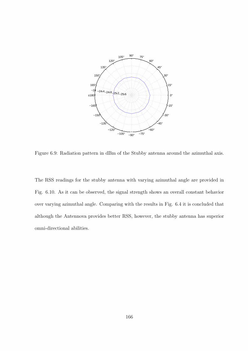
0°
15°
30°
45°
60°75°90°105°
120°
135°
150°
165°
±180°
−165°
−150°
−135°
−120°−105° −90° −75°
−60°
−45°
−30°
−15°
−25.6−25.2−24.8−24.4−24
Figure 6.9: Radiation pattern in dBm of the Stubby antenna around the azimuthal axis.
The RSS readings for the stubby antenna with varying azimuthal angle are provided in
Fig. 6.10. As it can be observed, the signal strength shows an overall constant behavior
over varying azimuthal angle. Comparing with the results in Fig. 6.4 it is concluded that
although the Antennova provides better RSS, however, the stubby antenna has superior
omni-directional abilities.
166
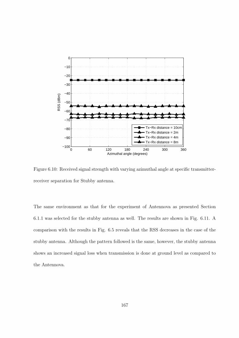
0 60 120 180 240 300 360−100
−90
−80
−70
−60
−50
−40
−30
−20
−10
0
Azimuthal angle (degrees)
RS
S (
dBm
)
Tx−Rx distance = 10cmTx−Rx distance = 2mTx−Rx distance = 4mTx−Rx distance = 8m
Figure 6.10: Received signal strength with varying azimuthal angle at specific transmitter-
receiver separation for Stubby antenna.
The same environment as that for the experiment of Antennova as presented Section
6.1.1 was selected for the stubby antenna as well. The results are shown in Fig. 6.11. A
comparison with the results in Fig. 6.5 reveals that the RSS decreases in the case of the
stubby antenna. Although the pattern followed is the same, however, the stubby antenna
shows an increased signal loss when transmission is done at ground level as compared to
the Antennova.
167
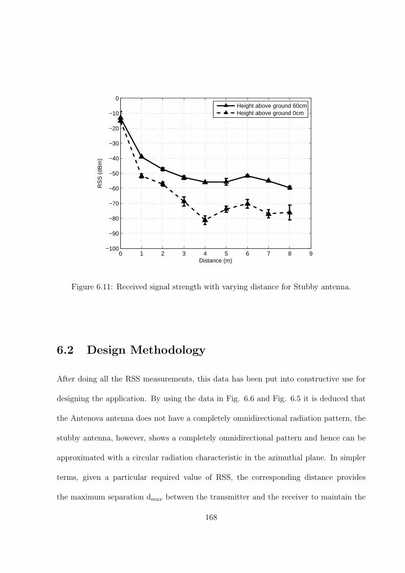
0 1 2 3 4 5 6 7 8 9−100
−90
−80
−70
−60
−50
−40
−30
−20
−10
0
Distance (m)
RS
S (
dBm
)
Height above ground 60cmHeight above ground 0cm
Figure 6.11: Received signal strength with varying distance for Stubby antenna.
6.2 Design Methodology
After doing all the RSS measurements, this data has been put into constructive use for
designing the application. By using the data in Fig. 6.6 and Fig. 6.5 it is deduced that
the Antenova antenna does not have a completely omnidirectional radiation pattern, the
stubby antenna, however, shows a completely omnidirectional pattern and hence can be
approximated with a circular radiation characteristic in the azimuthal plane. In simpler
terms, given a particular required value of RSS, the corresponding distance provides
the maximum separation dmax between the transmitter and the receiver to maintain the
168

required value of RSS.
As the Antennova has an approximately omni-directional radiation pattern, this corre-
sponds to a transmission radius of the node, i.e. rtrans = dmax. It must be noted that
each node in a cluster acts as a member nodes as well as a cluster head. Since the cluster
head is responsible for communicating with other clusters it transmits at higher power
levels when communicating with other cluster heads and uses -25 dBm (the least possible
transmit power) when communicating with own cluster members. Consider the scenario
presented in Fig. 6.12.
Figure 6.12: Transmission radius at different power levels.
169
Consider two clusters, C1 and C2 comprising of nodes 1,2,3,4 and 5,6,7,8 respectively. The
cluster size has been limited to 4 nodes per cluster for simplicity. It is evident from the
above figure that node 1 of C1 is furthest away from nodes 7 and 8 of C2. In order for
both the cluster heads to communicate they must lie within the transmission radii of each
other. The worst case condition occurs when node 1 is the cluster head of C1 and node
7 or 8 is the cluster head of C2. Let rmax represents the maximum transmission radius
when transmitting within the cluster (-25 dBm) and rcluster be the maximum transmission
radius when transmitting at the higher power level. It is evident from Fig. 6.12 that the
rcluster must be large enough so that the next hop cluster node is within its transmission
radius.
This imposes a bound on the maximum separation between two closest clusters to be less
than or equal to rcluster to ensure that cluster heads which are farthest away from each
other do communicate. If the separation is less than rcluster, communication is possible at
stronger RSS but more nodes are required to cover the region.
6.3 Application Design
The deployment of a WSN requires a trade-off between cost, network life and the end-
to-end latency existing in the network. Cost and network life is directly related to the
number of nodes and their transmission powers in the network. The end-to-end latency,
as seen in from the simulation results of Fig. 5.2 is dependent on the number of hops.
This section presents two case studies and provides analysis of the different factors for
170

network design.
In WSN the PRR plays a much important role as compared to the actual RSS. In the
radio measurement results presented in Fig. 6.6, it is observed that packets are received at
extremely low RSS (-90 dBm) but are can be used for successful extraction of information.
In the following case studies the PRR measurements presented in Fig. 6.7 have been
used to determine the inter-node and inter-cluster spacing. In addition, the node power
consumption figures presented in Table 2.6 have been utilized to determine the operating
life of the network based on actual measurements. The end-to-end latency has been
determined from the S-MAC simulation results presented in Fig. 5.2. In short, the
practical PRR measurements, the power consumption measurements for the KFUPM
node and the simulation results have been combined to generate a model to help in the
deployment of a WSN.
6.3.1 Case 1: Fixed Cost and PRR
In this case the cost and the desired PRR are fixed and are provided to the application.
The cost is provided as the total number of nodes available to setup the network. Fig.
6.13 provides the results of the simulation for a network comprising of 50 nodes at a PRR
of 0.9.
171

0 10 20 30 40 5025
30
35
40
45
50
55
60
65
Cluster size (nodes)
Net
wor
k Li
fe (
hour
s)
Tx:−5 dBmTx:−10 dBmTx:−15 dBmTx:−25 dBm
Figure 6.13: Network life (in hours) of a network with 50 nodes at PRR=0.9 for a fixed
area.
It can be observed that regardless of the transmit power, when a smaller number of nodes
are placed in a cluster, the resulting network topology has a large number of clusters thus
increasing the overall network life. As the number of nodes per cluster increases the net-
work life decreases and becomes nearly constant for extremely large network sizes. Table
6.1 shows the complete network life in hours as well as the maximum separation between
clusters required to maintain a PRR of 0.9 for the different inter-cluster transmission
powers.
172
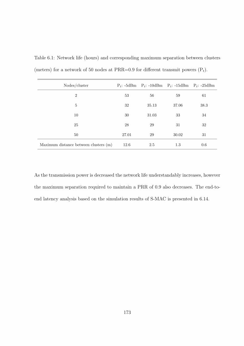
Table 6.1: Network life (hours) and corresponding maximum separation between clusters
(meters) for a network of 50 nodes at PRR=0.9 for different transmit powers (Pt).
Nodes/cluster Pt: -5dBm Pt: -10dBm Pt: -15dBm Pt: -25dBm
2 53 56 59 61
5 32 35.13 37.06 38.3
10 30 31.03 33 34
25 28 29 31 32
50 27.01 29 30.02 31
Maximum distance between clusters (m) 12.6 2.5 1.3 0.6
As the transmission power is decreased the network life understandably increases, however
the maximum separation required to maintain a PRR of 0.9 also decreases. The end-to-
end latency analysis based on the simulation results of S-MAC is presented in 6.14.
173

0 10 20 30 40 500.5
1
1.5
2
2.5
3
3.5
4
4.5
5
5.5
Cluster size (nodes)
End
−to
−en
d la
tenc
y (s
)
Figure 6.14: End-to-end latency at different cluster sizes for network size of 50 nodes at
PRR=0.9.
The end-to-end latency presented in Fig. 6.14 has a higher value when the network has
a large number of clusters (small number of nodes/cluster) because of the effect of nodes
backing off due to insufficient time to transmit packets to the next hop nodes because of
the duty cycle. As the number of hops decreases, the delay also drops.
Fig. 6.15 presents the network life figures for a network with 50 nodes and a required
PRR of 0.5. As it can be observed from Fig. 6.13 and Fig. 6.15, the network life is
not dependent on the PRR, but on the number of nodes/cluster. PRR just controls the
maximum separation between adjacent clusters as indicated in Table 6.1 and Table 6.2.
174
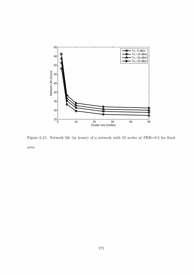
0 10 20 30 40 5025
30
35
40
45
50
55
60
65
Cluster size (nodes)
Net
wor
k Li
fe (
hour
s)
Tx:−5 dBmTx:−10 dBmTx:−15 dBmTx:−25 dBm
Figure 6.15: Network life (in hours) of a network with 50 nodes at PRR=0.5 for fixed
area.
175

Table 6.2: Network life (in hours) and corresponding maximum separation between clus-
ters (in meters) for a network of 50 nodes at PRR=0.5.
Nodes/cluster Pt: -5dBm Pt: -10dBm Pt: -15dBm Pt: -25dBm
2 53 56 59 61
5 32 35.13 37.06 38.3
10 30 31.03 33 34
25 28 29 31 32
50 27.01 29 30.02 31
Maximum distance between clusters (m) 23.7 6.7 3.3 0.9
One thing that can be observed from the maximum separation figures given in Table 6.1
and Table 6.2 is that the lower the desired PRR, the higher is the maximum separation;
which in turn means a larger physical area can be covered with the same number of nodes
at each of the different transmit power ranges.
6.3.2 Case 2: Fixed Deployment Area and PRR
In case 1, the physical dimensions of the target area were not taken into account, instead,
the network was designed for a particular deployment cost. In some scenarios, the sit-
uation might demand designing the network for a given physical dimension where cost
might not be an important factor. Since the cost (number of nodes in the network) is not
specified by the user, the design must include an analysis of the number of nodes/cluster
176
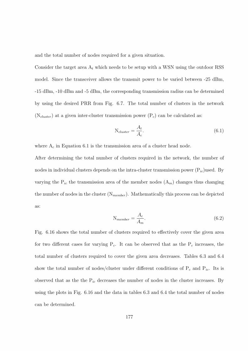
and the total number of nodes required for a given situation.
Consider the target area At which needs to be setup with a WSN using the outdoor RSS
model. Since the transceiver allows the transmit power to be varied between -25 dBm,
-15 dBm, -10 dBm and -5 dBm, the corresponding transmission radius can be determined
by using the desired PRR from Fig. 6.7. The total number of clusters in the network
(Ncluster) at a given inter-cluster transmission power (Pc) can be calculated as:
Ncluster =At
Ac
. (6.1)
where Ac in Equation 6.1 is the transmission area of a cluster head node.
After determining the total number of clusters required in the network, the number of
nodes in individual clusters depends on the intra-cluster transmission power (Pic)used. By
varying the Pic the transmission area of the member nodes (Am) changes thus changing
the number of nodes in the cluster (Nmember). Mathematically this process can be depicted
as:
Nmember =Ac
Am
. (6.2)
Fig. 6.16 shows the total number of clusters required to effectively cover the given area
for two different cases for varying Pc. It can be observed that as the Pc increases, the
total number of clusters required to cover the given area decreases. Tables 6.3 and 6.4
show the total number of nodes/cluster under different conditions of Pc and Pic. Its is
observed that as the the Pic decreases the number of nodes in the cluster increases. By
using the plots in Fig. 6.16 and the data in tables 6.3 and 6.4 the total number of nodes
can be determined.
177

Table 6.3: Total nodes in the network at varying Pc and Pic for 10m×15m with PRR of
0.9.
Pic: -5dBm Pic: -10dBm Pic: -15dBm Pic: -25dBm
Pc: -5dBm 1 25 94 441
Pc: -10dBm - 8 32 136
Pc: -15dBm - - 29 145
Pc: -25dBm - - - 133
Table 6.4: Total nodes in the network at varying Pc and Pic for 10m×7m with PRR of
0.9.
Pic: -5dBm Pic: -10dBm Pic: -15dBm Pic: -25dBm
Pc: -5dBm 1 25 94 441
Pc: -10dBm - 4 16 68
Pc: -15dBm - - 14 70
Pc: -25dBm - - - 62
178
−25 −20 −15 −10 −50
20
40
60
80
100
120
140
Inter cluster transmit power (dBm)
Net
wor
k si
ze (
clus
ters
)
(a)
−25 −20 −15 −10 −50
10
20
30
40
50
60
70
Inter cluster transmit power (dBm)
Net
wor
k si
ze (
clus
ters
)(b)
Figure 6.16: Number of cluster in the network for a PRR of 0.9 and target area of (a)
10m×15m and (b)10m×7m.
6.4 Conclusion
In order to provide accurate network deployment statistics, real life radio measurements
are required to ensure the network design operation according to the desired level. The
transmission radiation analysis of the stubby antenna proves it to me completely omni-
directional in the azimuthal plane whereas the Antenova does not exhibit complete omni-
directional characteristics. By using the PRR measurements and analyzing the results of
the two cases presented, it is concluded that, for a fixed cost network a decrease in the
desired PRR result in an increase in the coverage area of the network where as the end-
to-end latency and the lifetime of the network remain independent of the PRR. When
a desired physical area is to be deployed with a WSN, it was found that for a given
179

inter-cluster transmission power, the total number of nodes increase as the intra-cluster
transmission power drops, resulting in highly dense clusters.
180

CHAPTER 7
CONCLUSIONS AND FUTURE
RESEARCH
7.1 Contributions and Achievements
As was proposed the following tasks have been successfully completed:
1. Creation of Wireless Node: Using off-the-shelf sensors and components, we have
successfully created a KFUPM wireless node that can support a maximum of four
different sensors (two digital and two analog). The node has a high performance
MCU with a double sided design to reduce the size to a minimum. The use of special
stub antennas has further decreased the overall height of our node.
2. MAC Protocol: A MAC protocol inspired from the famous S-MAC protocol
has been implemented on KFUPM nodes. Uniquely devised MAC implementation
181

scheme as well as special payload formats have been used on the KFUPM devices.
The simulation results of the implemented and the basic S-MAC reveal the energy
efficiency of the implemented protocol as compared to the basic S-MAC at the cost
of higher latency and slightly lower throughput.
3. Routing Protocol: Useful features of both TEEN and LEACH have been com-
bined into a new protocol that employs cluster head approach and at the same time
is suitable for dynamic environments in addition to the incident based (UGN). Dy-
namic head shifting has been employed to increase the lifetime of the network. The
simulation results prove that the designed protocol promises an almost twice the
network life as compared to LEACH with acceptable delay.
4. Deployment Application Design: A special application to provide an approx-
imation to the size of a typical network based on real-life measurements has been
designed. Based on the presented case studies, network design can be done for either
fixed cost of fixed area.
7.2 Future Research
WSN is a diverse field and due to the diverse nature of applications several enhancements
to the current work cane be done. Following few ideas can be used to enhance the proposed
network.
1. The protocols presented in this report assumed static network, i.e., the nodes are
182

stationary all the time. The same scheme can be modified to accommodate mobile
nodes. As the nodes move, their power levels change relative to a central sink, and
the network topology changes constantly.
2. By using multiple sink nodes, the network coverage can be increased. Each of the
sink nodes would be connected to a central server which would supervise the data
collection from all the sinks. No hand-offs would be required as the member nodes
would not be permanently assigned to sink nodes.
3. By using a single sink node, the coverage could be increased by enabling the sensing
nodes to relay or regenerate the beacon signal from the sink. This would enable
the nodes which could not directly receive the beacon from sink node to get the
regenerated beacon signal from the other nodes thus providing synchronization.
Although a single synchronization would be achieved, clock drift would need to be
countered to ensure tight schedules.
4. Variable transmission power control can be implemented to provide much tighter
control on transmission energy consumption. Each node would transmit at the
least required transmission power that caused successful packet transmission to the
neighboring node. This would prevent unnecessary interference between nodes far
away from each other.
5. The present approach assumes eleven fixed power levels to create the routing tree.
These levels could be adjusted dynamically depending on the environment in which
183

the system is operating.
184
REFERENCES
[1] R. Lacoss, “Distributed sensor networks,”Technical Report, DARPA project, 1986.
[2] S. Pakzad, G. Fenves, S. Kim, S. Glaser and J. W. Demmel, “Multi-purpose wireless
accelerometer for civil infrastructure monitoring,”Fifth International Workshop on
Structural Health Monitoring, 2005.
[3] S. Kim, S. Pakzad, D. Culler, J. Demmel, G. Fenves, S. Glaser and M. Turon, “Health
monitoring of civil infrastructure using wireless sensor networks,”Sixth International
Conference on Information Processing in Sensor Networks, 2007.
[4] A. Mainwaring, J. Polatre, R. Szewczyk and J. Anderson, “wireless sensr network for
habitat monitoring,”Second International Conference on Embedded Networked Sensor
Systems, 2004.
[5] X. Wang, F. Sun and X. Kong, “Research on optimal coverage problem of WSN,”
International Conference on Communications and Mobile Computing, April 2009.
185

[6] M. Aboelaze and F. Aloule, “Current and future trends in sensor networks: A survey,”
IEEE International Conference on Wireless and Optical Communications Networks
(WOCN), March 2005.
[7] I. F. Akyildiz, W. Su, Y. Sankarasubramaniam, and E. Cayirci, “A survey on sensor
networks,”IEEE Communications Magazine, Vol. 40, Issue 8, pp. 102-114, August
2002.
[8] C. Leiden and M. Wilensky, “Layering TCP/IP protocols,” TCP/IP for Dummies,
Chapter 2, pp. 23-25, 2009.
[9] G. Werner-Allen, K. Loricz, J. Johnson, J. Lees and M. Welesh, “Fidelity and yield in
a volcano monitoring sensor network,”Seventh International Symposium on Operating
System Design and Implementation, 2006.
[10] D. Sun, S. Jiang, W. Wang and J. Tang, “Wireless sensor network design and imple-
mentation in a tea plantation for drought monitoring,”2010 International Conference
on Cyber-Enabled Distributed Computing and Knowledge Discovery, 2010.
[11] G. Hoblos, M. Staroswiecki, and A. Aitouchei, “Optimal design of fFault tolerant
sensor networks,”Proc. Of the IEEE Int’l Conf. on Control Applications, September
2000.
[12] K. Sohrabi, J. Gayo, V. Aalawadhi and G. J. Pottie, “Protocols for self-rrganization
of a wireless sensor network,” IEEE Personal Communications, October 2000.
186

[13] I. Demirkol, C. Ersoy and F. Aagoz, “MAC protocols for wireless sensor networks: a
survey,” Topics in AD HOC and Sensor Networks, IEEE Communications Magazine,
Vol. 44, Issue 4, pp. 115 - 121, April 2006.
[14] V. Rajendra, K. Obraczka and J. J. Garcia-Luna-Acevec, “Energy-efficient, collision-
free medium access control for wireless sensor networks,” SenSys, February 2003, Los
Angeles, California, USA.
[15] I. Lee, J. Y-T. Leung and S. H. Sun, “Wireless Sensor Networks,” Handbook of
Real-Time and Embedded Systems, Chapter 20, pp. 20.3-20.4, 2008.
[16] W. Ye, J. Heidemann, and D. Estrin, “Medium access control with coordinated adap-
tive sleeping for wireless sensor networks,” IEEE/ACM transactions on networking,
Vol. 12, Issue 3, pp. 493-506, June 2004.
[17] T. van Dam , K. Langendoen, “An adaptive energy-efficient MAC protocol for wire-
less sensor networks,” Proceedings of the 1st international conference on embedded
networked sensor systems, November 2003, Los Angeles, California, USA.
[18] M. Miladi, T. Ezzedine and R. Bouallegue, “Latency of energy efficient MAC proto-
cols for wireless sensor networks,” International Conference on Digital Telecommuni-
catinos (ICDT), 2006.
[19] B. K. Singh and K. E. Tepe, “A novel real-time MAC layer protocol for wireless sen-
sor network applications,” IEEE International Conference on Electronics/Information
Technology (EIT), 2009.
187

[20] K. Benkic, “Proposed Use of CDMA Technique in Wireless Sensor Networks,” 14th
International Workshop on Systems, Signals and Image Processing, 2007.
[21] A. El-Hoiydi, J.-D. Decotignie, C. Enz, and E. Le Roux, “WiseMAC: An ultra low
power MAC protocol for the wisenet wireless sensor networks (poster abstract),” Pro-
ceedings of the First ACM SenSys Conference, July 2003, Los Angeles, California,
USA.
[22] J. Polastre, J. Hill, and D. Culler, “Versatile low power media access for wireless
sensor networks,” Proceedings of the 2nd ACM SenSys Conference, November 2004,
Baltimore, MD, USA.
[23] X. Changbiao and L. Lin, “ES-MAC: Research on Enhanced S-MAC Technology,”
Wireless Communications, Networking and Mobile Computing, 2008.
[24] H. S. Aghdasi and M. Abbaspour, “ET-MAC: An Energy-Efficient and High
Throughput MAC Protocol for Wireless Sensor Networks,” Communication Networks
and Services Research Conference, 2008.
[25] M. Vahabi, M. A. Rasid, A. Fadlee and M. Hossein, “Adaptive MAC protocol for
wireless sensor networks in periodic data collection applications,” Information Tech-
nology International Symposium, 2008.
[26] Z. Merhi, M. Elgamel, and M. Bayoumi, “EB-MAC: An event based medium ac-
cess control for wireless sensor networks,” Pervasive Computing and Communications,
2009, PerCom 2009.
188

[27] T. Trathnigg, J. Moser, and R. Weiss, “An energy-efficient MAC protocol for low
traffic wireless sensor networks,” Wireless Communications and Mobile Computing
Conference, 2008, IWCMC ’08.
[28] G. Yao, H. Liu, C. Hu and L. Shi, “A cluster based adaptive low power MAC proto-
col for wireless sensor networks,” Wireless Communications, Networking and Mobile
Computing, 2008. WiCOM ’08.
[29] W. Ye, J. Heidemann and D. Estrin, “An energy-efficient MAC protocol for wireless
sensor networks,” Procedings of INFOCOM, June 2002.
[30] W. Song, Y. Liu and S. Zhang, “Research on SMAC protocol for WSN,” 4th Interna-
tional Conference on Wireless Communications, Networking and Mobile Computing,
2008. (WiCOM ’08)
[31] W. Ye, F. Silva and J. Heidemann, “Ultra-low duty cycle MAC with scheduled chan-
nel polling,” SenSys ’06, November 2006.
[32] P. Sthapit, Y. T. Park and J. Pyun, “Medium reservation preamble based MAC
for sireless sensor networks,” 9th IEEE International Conference on Computer and
Information Technology, 2009. (CIT ’09)
[33] Y. Sun, S. Du, O. Gurewitz and D. B. Johnson, “DW-MAC: A Low Latency, Energy-
Efficient Demand-Wakeup MAC Protocol for Wireless Sensor Networks,” MobiHoc
’08, May, 2008.
189

[34] I. Wan, D. Yuan and Xianghua Xu, “A Review of Routing Protocols in Wireless
Sensor Networks,” Wireless Communications, Networking and Mobile Computing,
2008.
[35] K. Pavai, A. Sivagami and D. Sridhara, “Study of Routing Protocols in Wireless
Sensor Networks,” International Conference on Advances in Computing, Control, and
Telecommunication Technologies, 2009.
[36] D. Baghyalakshmi, J. Ebenezer and S. A. V. Satyamurty, “Low Latency and Energy
Efficient Routing Protocols for Wireless Sensor Networks,” International Conference
on Wireless communications and Sensor Computing, 2010.
[37] C. Schurgers and M. Srivastava, “Energy efficient routing in sensor networks,” Pro-
ceeding of Milcom, 2001.
[38] S. Lindsey and C.S. Raghavendra, “PEGASIS: power efficient gathering in sensor
information systems,” Proceedings of the IEEE Aerospace Conference, March 2002.
[39] A. Manjeshwar and D.P. Agrawal, “TEEN: a protocol for enhanced efficiency in
wireless sensor networks,” Proceedings of the 1st International Workshop on Parallel
and Distributed Computing Issues in Wireless Networks and Mobile Computing, April
2001.
[40] A. Manjeshwar and D.P. Agrawal,, “APTEEN: a hybrid protocol for efficient routing
and comprehensive information retrieval in wireless sensor networks,” Proceedings
190
of the 2nd International Workshop on Parallel and Distributed Computing Issues in
Wireless Networks and Mobile computing, April 2002.
[41] F. Zabin, S. Misra,I. Woungang, and H.F. Rashvand, “REEP: data-centric, energy-
efficient and reliable routing protocol for wireless sensor networks,” IET Communica-
tions, Vol. 2, Issue 8, pp. 995-1008, September 2008.
[42] Y. Liu, R. Du, H. Zhang, H. Sheng, J. Zhao and X. Zhang, “Study on directional
reliable multi-hop clustering routing protocol in wireless sensor network,” Wireless
Communications, Networking and Mobile Computing, 2008 .
[43] D. Baghyalakshmi, J. Ebenezer and S. A. V. Satyamurty, “Low latency and energy
efficient routing protocols for wireless sensor networks,” International Conference on
Wireless communications and Sensor Computing, 2010. (ICWCSC ’10)
[44] K. Pavai, A. Sivagami and D. Sridhara, “Study of routing protocols in wireless sen-
sor networks,” International Conference on Advances in Computing, Control, and
Telecommunication Technologies, 2009. (ACT ’09)
[45] Y. Tsai, “Coverage-preserving routing protocols for randomly distributed wireless
sensor networks,” IEEE Transactions on Wireless Communications, Vol. 6, No. 4,
April 2007.
[46] J. Hill, R. Szewczyk, A. Woo, S. Hollar, D. E. Culler, and K. S. J. Pister, “System
architecture directions for networked sensors,” Architectural Support for Programming
Languages and Operating Systems, 2000.
191

[47] Crossbow Technology Inc., http : //www.xbow.com/Home/HomePage.aspx
[48] Crossbow Technology, Inc., MPR/MIB Mote Hardware Users Manual, Apr. 2005.
[49] Intel Corporation, http : //www.intel.com/research/exploratory/wirelesssensors.htm
http : //www.xbow.com/Support/Supportpdffiles/MPR −
MIBSeriesUsersManual.pdf
[50] J. Polastre, R. Szewczyk, and D. Culler, “Telos: Enabling ultra-low power wireless
research,” The Fourth International Conference on Information Processing in Sensor
Networks: Special track on Platform Tools and Design Methods for Network Embed-
ded Sensors (IPSN/SPOTS), April 2005.
[51] J. Hill, R. Szewczyk, A. Woo, P. Levis, K. Whitehouse, J. Polastre, D. Gay, S.
Madden, M. Welsh, D. Culler, and E. Brewer, “Tinyos: An operating system for
sensor networks,” 2003.
[52] A. Tiwari, P. Ballal, and F. L. Lewis, “Energy-efficient wireless sensor network design
and implementation for condition-based maintenance,” ACM Transactions on Sensor
Networks, Vol. 3, No. 1, Article 1, March 2007.
[53] S. Kellner, M. Pink, D. Meier, and E.-O. Blab, “Towards a realistic energy model for
wireless sensor networks,” Proceedings of IEEE Fifth Annual Conference on Wireless
On demand Network Systems and Services, Germany, January 2008.
192

[54] Q. Cao, D. Fesehaye, N. Pham, Y. Sarwar, and T. Abdelzaher, “Virtual battery: An
energy reserve abstraction for embedded sensor networks,” Proceedings of the 29th
IEEE Real-time Systems Symposium, December 2008.
[55] T. M. Wendt, L. M. Reindl, “Wake-up methods to extend battery life time of wire-
less wensor nodes” IEEE International Instrumentation and Measurement Technology
Conference Victoria, Vancouver Island, Canada, May 2008.
[56] “MPR-MIB users manual,” Crossbow, Rev. A, PN:7430-0021-08, pp. 20, June 2007.
[57] “2.4 GHz IEEE 802.15.4/ZigBee-ready RF transceiver” Chipcon products from Texas
Instruments CC2420.
[58] “8-bit AVR microcontroller with 128K bytes in-system programmabel flash ” Atmel
ATmega128, ATmega128L.
[59] A. Milenkovic, M. Milenkovic, E. Jovanov, D. Hite and D. Rasko, “An environment
for runtime power monitoring of wireless sensor network platforms,” in Proceedings of
Thirty Seventh Southeastern Symposium on System Theory 2008, pp. 406-410. SSST
’08.
[60] P. Levis, S. Madden, D. Gay, J. Polastre, R. Szewczyk, A. Woo, E. Brewer and D.
Culler, “The emergence of networking abstractions and techniques in tinyos,” Pro-
ceedings of the First USENIX/ACM Symposium on Network Systems Design and
Implementation (NSDI), 2004.
193
[61] S. Park, J. W. Kim, K. Y. Shin and D. Kim, “A nano operating system for wireless
sensor networks,” 8th international conference on advanced communication technolo-
gies, 2006.
[62] G.-Z. Yang and M. Yacoub, “Body sensor networks: Development kit and program-
ming guide,” Body sensor networks, Appendix B, 2008.
[63] M. Leoold, “Creating a new platform for TinyOS 2.x,” TEP131, 2007. Available at
http : //www.tinyos.net/tinyos− 2.1.0/doc/html/tep131.html
[64] B. S. Dean, “AVRDUDE - version 5.4,” 2006.
[65] Wei Ye , F. Silva and J. Heidemann, “Ultra-low duty cycle MAC with scheduled chan-
nel polling,” Proceedings of the 4th international conference on Embedded networked
sensor systems, 2006.
[66] S.i Li, V. Handziski, A. Kpke, M. Kubisch, and A. Wolisz, “A wireless sensor net-
work testbed Supporting controlled in-building experiments,” Proceedings of the 2nd
international workshop on Multi-hop ad hoc networks: from theory to reality, 2006.
[67] W. Walker, T. Polk, A. Hande, and D. Bhatia, “Remote blood pressure monitoring
using a wireless sensor network,” Proceedings of the IEEE Sixth Annual Emerging
Information Technology Conference, 2006.
[68] G. Virone, A. Wood, L. Selavo, Q. Cao, L. Fang, T. Doan, Z. He, R. Stoleru, S. Lin,
and J.A. Stankovic, “An advanced wireless sensor network for health monitoring,”
194

Transdisciplinary Conference on Distributed Diagnosis and Home Healthcare (D2H2),
2006.
[69] M. Pan, C. Tsai, W. Yang, and Y. Tseng, “Implementation of an emergency guid-
ing system by wireless sensor networks,” IEEE International Symposium on Network
Computing Applications (IEEE NCA), 2006 (Fast Abstract).
[70] J. Higuera, J. Polo, and M. Gasulla, “A ZigBee wireless sensor network compliant
with the IEEE1451 standard,” SAS 2009 - IEEE Sensors Applications Symposium,
New Orleans, LA, USA - February 17-19, 2009.
[71] M. Ceriotti, L. Mottola, G. P. Picco, A. L. Murphy, S. Guna, M. Corr, M. Pozzi, D.
Zonta, and P. Zanon,, “Monitoring heritage buildings with wireless sensor networks:
the Torre Aquila deployment,” roceedings of the 8th ACM/IEEE International Con-
ference on Information Processing in Sensor Networks (IPSN09), San Francisco, CA,
USA, April 2009.
[72] Z. Rasin, and M. Abdullah, “Water quality monitoring system using Zigbee based
wireless sensor network,” International Journal of Engineering and Technology IJET,
Vol. 9, No. 10, Feb. 2010.
[73] D. Yoo, S. Park, S. Choi and S.H. Park, “Dynamic S-MAC protocol for wireless
sensor networks based on network traffic states,” APCC 2008.
[74] Network Simlator ns-2.28, available online at: http://www.isi.edu/nsnam/ns/.
195
[75] K. Park, “Basic mathematics for QoS,” QoS in Packet Networks, Chapter 2, pp.
51-60, 2005.
[76] S. Phoha, T. F. La Porta and C. Griffin, “Load balanced query protocols for wireless
sensor networks,” Sensor Network operations, Chapter 5, pp. 265-267, 2006.
[77] A. Swami, “Law of sensor network lifetime and its applications,” Wireless sensor
networks: signal processing and communications perspectives, Chapter 5, pp. 93-94,
2007.
[78] Antennova, “Titanis 2.4 GHz swivel SMA antenna,” Product Specifications, Part
No. B4844/B6090, July 2010.
196

VITAE
Farooq Sultan
Born in Dammam, Saudi Arabia on 30th July, 1986
Nationality: Pakistani
Received B.S. Telecommunications Engineering from COMSATS Institute of Information
Technology (CIIT) in August 2008
Worked in Pakistan Telecommunications Corporation Ltd. (PTCL) as a trainee engineer at
the international gateway exchange, Rawalpindi
Joined King Fahd University of Petroleum & Minerals, Dhahran, Saudi Arabia as a
Research Assistant in February, 2009
Completed M.S. in Telecommunications Engineering from King Fahd University of
Petroleum & Minerals, Dhahran, Saudi Arabia in January 2011
E-mail: [email protected]
Phone: 0561505634
Present Address: P.O. Box 1661, King Fahd University of Petroleum & Minerals,
Dhahran- 31261, Saudi Arabia
Permanent Address: H. No. 81, Street 35-A, Sector I-9/4, Islamabad, Pakistan