This report is very disappointing. What kind of software ... · Rank Interval of a Country • The HEI ranks the countries of the world in a manner that is consistent with the Land,

This report is very disappointing.What kind of software are you using?

Stone-Age Space-Age Syndrome

Space-age analysis

Stone-age analysis

Space-age dataStone-age data

Multiple IndicatorsMultiple Indicators

Partial OrderingsPartial Orderings

andand

Ranking and PrioritizationRanking and Prioritization

without Combining Indicatorswithout Combining Indicators

G. P. PatilG. P. PatilC. TaillieC. Taillie

Multiple Indicators

Two indicators of a person’s size:I1 = HeightI2 = Weight

Scatter Plot:

Is A bigger than B ?

B

A

Height

Wei

ght

Combining IndicatorsSimple Average

I1 = HeightI2 = Weight

Size = (I1 + I2)/2

Bigger than A

A

Height

Wei

ght

Smaller than A

Contour of constant size

Combining IndicatorsWeighted Average


Size = w1 I1 + w2 I2 , w1 + w2 = 1w1 and w2 reflect:• Units of measurement• Relative importance of the two indicators

A

Slope determines tradeoffbetween Height and Weight

Wei

ght


Height

Combining IndicatorsNon-Linear Combination


Size = F(I1 , I2)

A

Height

Wei

ght


Tradeoff varies

Partial Ordering


A

Height

Wei

ght

Bigger than A

Smaller than A

Not comparablewith A


UNEP HEINational Land, Air, Water IndicatorsHEI with revised data:• Land: undomesticated land to total land area• Air: (air indicator1 + air indicator2) / 2, where

air indicator1 = renewable energy use to total energy use; air indicator2 = GDP per unit energy use, based on maximum and minimum concept

• Water: (water indicator1 + water indicator2) / 2, where water indicator1 = ratio of water available after annual withdrawals to internal water resources; water indicator2 = ratio of people with access to an improved water source to total population

UNEP HEI Data Matrix

Hasse Diagram---All Countries(labels are HEI ranks)

1 2 3

4

5 6 7

8 9

10 11 12 13

14 15

16

17 18 19

20

21 22 23

24

25 26 27

28

29 30

31

32

33

34

35

36

37

38 39 40 41

42 43

44 45 46 47 48 49

50

51

52

53

54

55

56 57

58 59

60

61

62

63

64

65

66

67

68

69

70

71

72

73 74

75

76

77

78

79

80

81

82

83

84

85

86

87 88 89

90

91

92

93

94

95

96

97

98

99 100

101

102

103

104

105

106

Hasse Diagram --- Western Europe

Norway

Sweden Finland Austria Switz.

Italy Portugal Greece Spain

France

Den.

Ireland

UK Germany

Belgium Neth.

Hasse Diagram --- Latin America

Peru Uruguay Venezu. Co.Rica Colomb.

Guat. Hondur. Brazil

Chile

Panama

El Salv.

Bolivia

Nicarag.

Argen.

Ecuador Mexic

Hasse Diagram --- Middle East

Iran Leb. Israel Kuwait

UAEm S.Arab.

Egypt Yemen

Jordan Syria

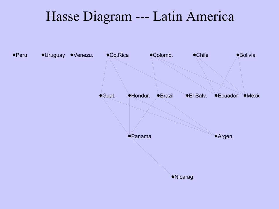
Rank Interval of a Country

• The HEI ranks the countries of the world in a manner that is consistent with the Land, Air, and Water indicators

• There are many other consistent rankings possible• As we vary over all the consistent rankings, each country

receives a set of possible ranks. This set of ranks turns out to be an interval of consecutive integers and is called the Rank Interval for the country.

• A wide rank interval indicates much ambiguity or disagreement when the country in question is compared with other countries

• Conversely, a narrow interval indicates general consensusregarding a country’s comparative standing

Computing Rank Intervals

Rank Interval for A: all integers r such that B(A) ≤ r ≤ W(A)

Ambiguity for A: length of rank interval = W(A) − B(A)

Height

Wei

ght

Bigger than A

Smaller than A



Frequency = B(A) =best possible rank for A

Frequency = W(A) = worst possible rank for A

(rank 1 is best)

A

0 10 20 30 40 50 60 70 80 90 100 110

Midpoint

0

10

20

30

40

50

60

70

80

90

100

110

Ran

k In

terv

als

Upper endpoints

Lower endpoints

Midpoints

Rank Intervals vs Midpoints

0 10 20 30 40 50 60 70 80 90 100 110

HEI Rank

0

10

20

30

40

50

60

70

80

90

100

110

Ran

k In

terv

als

Upper endpoints

Lower endpoints

Midpoints

Rank Intervals vs HEI Ranks

Watersheds of Mid-Atlantic Region


•114 Watersheds ( 8-digit HUCs )

•9 indicators used here

•Data Matrix (extract):HUC POPDENS POPCHG RDDENS SO4DEP RIPFOR STRD DAMS CROPSL INTALL2040101 51.72 54 2.74 2050 13.84 6.51 32.33 5.99 69.482040103 114.53 35 1.7 2087 8.06 6.05 85.41 5.59 77.932040104 76.16 81 3.61 2150 7.46 5.69 86.57 1.75 38.782040105 625.06 25 7.71 2443 22.94 9.68 37.64 13.68 91.492040106 488.13 13 2.73 2435 16.76 7.18 42.02 7.5 72.32040201 1291.56 20 6.92 2634 28.83 6.87 47.12 5.48 1002040202 3533.76 -5 16.01 2817 33.71 10.65 49.04 2.11 99.932040203 816.35 -1 3.32 2799 30.94 10.15 45.89 9.46 93.232040205 596.15 15 3.17 2913 26.65 6.68 12.17 5.4 100

Watersheds of Mid-Atlantic RegionIndicator Description

Proportion stream-length with nearby roadsSTRD

Proportion forested stream-lengthRIPFOR

Sulfate depositionSO4DEP

Road densityRDDENS

1970-1990 population changePOPCHG

Proportion of WS with interior forest habitatINTALL

Proportion of WS with crops on >3 percent slopeCROPSL

Impoundments per 1000 km stream-lengthDAMS

1990 population densityPOPDENS

Watersheds of Mid-Atlantic RegionHasse Diagrams

60 connected components in Hasse Diagram:

58 of the components are isolates

1 component (secondary component) contains 4 watersheds

1 component (primary component) contains 52 watersheds

2060010 2060008

2060007

2060006

Watersheds of Mid-Atlantic RegionHasse Diagram for Secondary Component

Note: Labels are HUC numbers

Watersheds of Mid-Atlantic RegionHasse Diagram for Primary Component

Note: Labels are row numbers in data matrix


Watersheds of Mid-Atlantic RegionEchelon Analysis of Primary Hasse Connected Component

Blue: Underwater Sandy: Newly exposed (beach) Green: Previously exposed

1

2

3

4

5

6

Watersheds of Mid-Atlantic RegionEchelon “Tree” for Primary Hasse Connected Component

3

4

a

bc

d

e

FG

H3

4

a

bc

d

e

FG

H a b c d e

F G H

Note: Echelon “Tree” is really a “Forest” because the primary Hasse connected component is geographically disconnected (with three pieces)

Watersheds of Mid-Atlantic RegionRank-Intervals for Primary Hasse Connected Component

To be prepared

Ranking Partially Ordered Sets – 1

• S = partially ordered set (poset) with elements a, b, c, ….

• How can we rank the elements of S consistent with the partial order? Such rankings are called linear extensions of the partial order.

• Different people with different perceptions and priorities may choose different rankings.

• How many rankings assign rank 1 to element a ? Rank 2 ? Rank 3 ? , etc.

• If rankings are chosen randomly (equal probability), what is the likelihood that element x receives rank i ?

Ranking Partially Ordered Sets – 2An Example

Poset(Hasse Diagram)

Some linear extensionsa a a b b

b

c

e f

a c c b a a

d b

e

d

f

e

b

d

f

c

d

e

f

c c

d e

e d

f fJump Size: 3 1 5 4 2

Jump or Imputed Link (-------) is a link in the ranking that is not implied by the partial order

Ranking Partially Ordered Sets – 2a

• How can we enumerate all possible linear extensions of a given poset (16 for the example) ?

• All possibilities can be laid out in a tree diagram, called the linear extension decision tree:– Start from the root node– Select any maximal element from the poset– Remove that element from the poset– Select any maximal element from the reduced poset– Continue selecting and removing maximal elements

until the poset is exhausted• There is a one-to-one correspondence between paths

through the tree and the linear extensions

Ranking Partially Ordered Sets – 2b

Linear extension decision treePoset(Hasse Diagram)

a

c

e b

e d

e

c

e d

e e

c

e

c

c

e d

e e

c

b a

bb

c

e f

a

d d

d ad

b

dd d d ff f ff f

f f ef f ef ef eff ef efJump Size: 1 3 3 2 3 5 4 3 3 2 4 3 4 4 2 2

Ranking Partially Ordered Sets – 3In the example from the preceding slide, there are a total of 16 linear extensions, giving the following frequency table.

Rank

16

0

0

0

0

7

9

1

16

0

0

2

4

5

5

2

16

0

1

4

6

3

2

3 Totals654Element

161060f

16006c

16046d

161616Totals

16663e

16001b

16000a

• Each (normalized) row gives the rank-frequency distribution for that element

• Each (normalized) column gives a rank-assignment distribution across the poset

Ranking Partially Ordered Sets – 3aRank-Frequency Distributions

0

0.2

0.4

0.6

0.8

Element a

0

0.2

0.4

0.6

0.8

Element c

0

0.2

0.4

0.6

0.8

1 2 3 4 5 6

Element e

0

0.2

0.4

0.6

0.8

Element b

0

0.2

0.4

0.6

0.8

Element d

0

0.2

0.4

0.6

0.8

1 2 3 4 5 6

Element f

Rank Rank

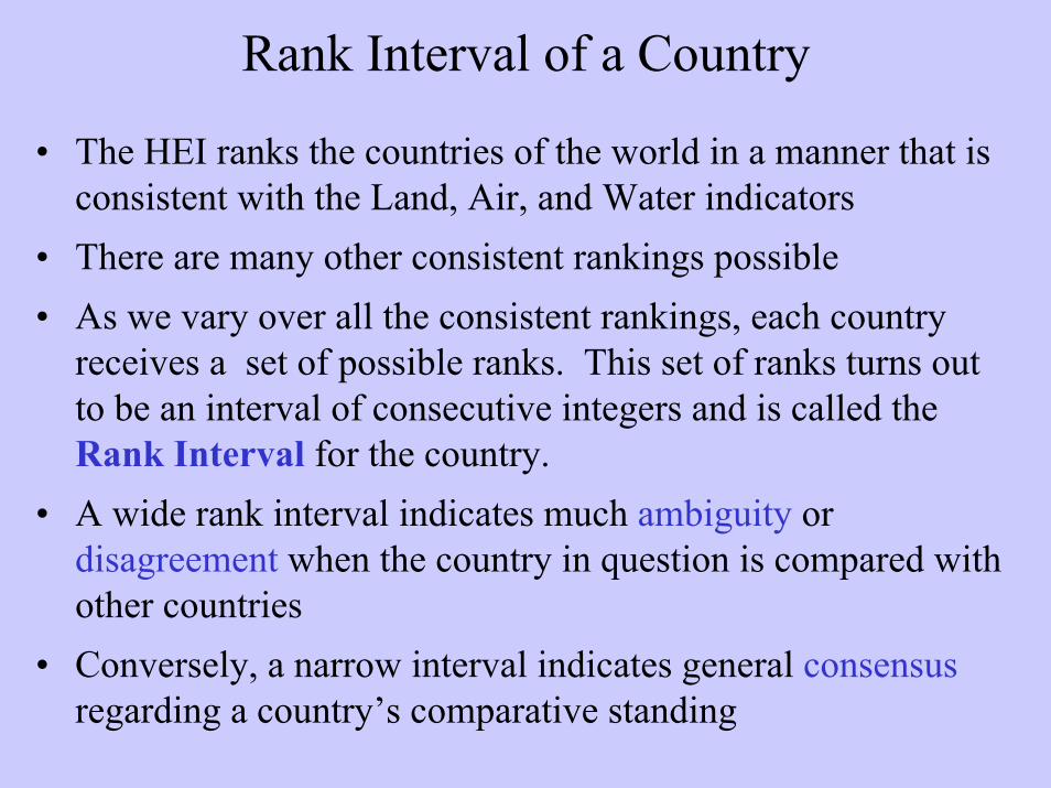
Ranking Partially Ordered Sets – 3b

0

4

8

12

16

1 2 3 4 5 6

Rank

Cum

ulat

ive

Freq

uenc

yabcdef

16

The curves are stacked one above the other and the result is a linear ordering of the elements: a > b > c > d > e > f

Ranking Partially Ordered Sets – 3cProperties of Rank-Frequency Distributions

• The rank-frequency distributions for any poset are unimodal

• In fact, there is a theorem which asserts that each rank-frequency distribution is log-concave, i.e., if

f1 , f2 , and f3are the frequencies (relative or absolute) for any three consecutive ranks assigned to an element of the poset, then

( f2)2 ≥ f1 ⋅ f3f1

f2 f3

Cumulative Rank Frequency Operator Cumulative Rank Frequency Operator ––11An example where An example where must be iteratedmust be iterated

a

f

e

b

ad

c

h

g

2

a

f

e

b

ad

c

h

g

Original Poset(Hasse Diagram)

a f

eb

c g d

h

Cumulative Rank Frequency Operator Cumulative Rank Frequency Operator –– 22An example where An example where results in tiesresults in ties

Original Poset(Hasse Diagram)

a

cb

d

a

b, c (tied)

d

•Ties reflect symmetries among incomparable elements in the original Hasse diagram

• Elements that are comparable in the original Hasse diagram will not become tied after applying operator

Cumulative Rank Frequency Operator Cumulative Rank Frequency Operator –– 33

• In most cases of practical interest, the number of linear extensions, e(S), is too large for actual enumeration in a reasonable length of time.

• For the HEI data set, the number of linear extensions satisfies:8.6 × 10105 ≤ e(S) ≤ 1.9 × 10243

which is completely beyond present-day computational capabilities.

• So what do we do?

• Markov Chain Monte Carlo (MCMC) applied to the uniformdistribution on the set of all linear extensions lets us estimate the normalized rank-frequency distributions. Estimating the absolute frequencies (approximate counting) is also possible but somewhat more difficult.

More Indicators do not necessarily mean More Information and More Discrimination

• Suppose two indicator columns are exactly the same.• The second column does not add new information or

discriminatory capability to that of the first column. • Likewise, there is little new information when there is a

strong underlying (rank-)correlation between the two indicators.

• Landscape ecologists have discovered that some fifty landscape pattern metrics amount to essentially five to ten indicators.

Multiple Indicators can convey Redundant Information

Combining Indicators (e.g., by averaging) typically fails to adjust for the Redundancy

Logo for Statistics, Ecology, Environment, and Society

Documents

This report is very disappointing. What kind of software ... · Rank Interval of a Country • The HEI ranks the countries of the world in a manner that is consistent with the Land,