Embed Size (px)
Citation preview

This report is based on research conducted
under Grant No. ATA 74-19135 from the
National Science Foundation and with support
from the Earthquake Research Affiliates.
Any opinions, findings, and conclusions or
reconunendations expres sed in this publication
are those of the authors and do not necessarily
reflect the views of the National Science
Foundation.
An Investigation of the Dynamic Characteristics of an EarthDam
BIBLIOGRAPHIC DATA 11. Report No.SHEET
4. Title and Subtitle
EERL 78-02 12
.
-~-- -- - ~~-~------
5. 'Repfffl' I"l'a'fe- -, -~ -
August 19786.
7. Author(s)
A. M. Abdel-Ghaffar and R. F. Scott9. Performing Organization Name and Address
California Institute of Technology1201 E. California Blvd.Pasadena, CA 91125
12. Sponsoring Organization Name and Address
National Science FoundationWashington, D.C. 20550
15. Supplementary Notes
16. Abstracts
8. Performing Organization Rept.
No. EERL 78-0210. Project/Task/Work Unit No.
11. Contract/Grant No.
ENV77 -2368713. Type of Report & Period
Covered
14.
An investigation has been made to analyze observations of the effect of two earthquakes (with ML = 6.3 and 4.7) on Santa Felicia Dam, a rolled-fill embankment locatedin Southern California. The dam is 236.5 ft high and 1,275 ft long by 30 ft wide atthe crest. The purpose of the investigation is: (1) to study the nonlinear behaviorof the dam during the two earthquakes, (2) to provide data on the in-plane dynamicshear moduli and damping factors for the materials of the dam during real earthquakeconditions, and (3) to compare these properties with those previously available fromlaboratory investigations.
17. Key Words and Document Analysis.
Earth DamsDynamic AnalysisDynamic TestsDampingDynamic ResponseShear ModulusEa rthqua kesSoil Dynami csDisplacement
170. Descriptors
StrainsVibration
17b. Identifiers/Open-Ended Terms
Dynamic Response of Earth DamEarth Dam Response to EarthquakesVibration Tests of Earth Dam
17c. COSATI Field/Group
18. Availability Statement
FORM NTIS 35 (REV. 372)
1302 Civil Engineering
Release unlimited
1313 Structural Engineering19•. Security Class (This 21. No. of Pages
Report)UNCLASSIFIED
20. Security Class (This 22. PricePage
UNCLASSIFIED-~'j'/ i
USCOMM~DC 14952-P72

INSTRUCTIONS FOR COMPLETING FORM NTIS-35 (10-70) (Bibliographic Data Sheet based on COSATI
Guidelines to Format Standards for Scientific and Technical Reports Prepared by or for the Federal Government,
PB"l80 600).
1. Report Number. Each individually bound report shall carry a unique alphanumeric designation selected by the perfotming
otganization or ptovided by the sponsoring organization. Use uppercase letters and Arabic numerals only. Examples
FASEB-NS-S7 and FAA-RD-6S-09.
2. Leave blank.
3- Recipient's Accession Number.. Reserved for use by each report recipient.
4. Title and Subtitle. Title should indicatec!early and briefly the subject coverage of the report, and be displayed prominently. Set subtitle, if used, in smaller type or otherwise subordinate it to main title. When a report is prepared in morethan one volume, repeat the primary title, add volume number and include subtitle for the specific volume.
S. Report Date. Each report shall carry a date indicating at least month and year. Indicate the basis on which it was selected
(e.g., date of issue, date of approval, date of preparation.
6. Performing Or\1ani zation Code. Leave blank.
7. Author(s). Give name(s) in conventional order (e.g., John R. Doe, or J.Robert Doe). List author's affiliation if it differsfrom the performing organization.
8. Performing Organization Report Number. Insert if performing organization wishes to assign this number.
9. Performing Organization Name and Address. Give name, street, city, state, and zip code. List no more than two levels ofan organizational hierarchy. Display the name of the organization exactly as it should appear in Government indexes suchas USGRDR-I.
10. Project/Task/Work Unit Number. Use the project, task and work unit numbers under which the report was prepared.
11. Contract/Grant Number. Insert contract or grant number under which report was prepared.
12. Sponsoring Agency Name and Address. Include zip code.
13. Type of Report and Period Covered. Indicate interim, final, etc., and, if applicable, dates covered.
14. Sponsoring Agency Code. Leave blank.
15. Supplementary Notes. Enter information not included elsewhere but useful, such as: Prepared in cooperation with.Translation of . .. Presel}ted at conference of ... To be published in . " Supersedes... Supplements ...
16. Abstract. Include a brief (200 words or less) factual summary of the most significant information contained in the report.If the report contains a significant bibliography or literature survey, mention it here.
17. Key Words and Document Analysis. (a). Descriptors. Select from the Thesaurus of Engineering and Scientific Terms theproper authorized terms that identify the major concept of the research and are sufficiently specific and precise to be usedas index entries for cataloging.(b). Identifiers and Open-Ended Terms. Use identifiers for project names, code names, equipment designators, etc. Useopen-ended terms written in descriptor form for those sub jects for which no descriptor exists.
(c). COSATI Field/Group. Field and Group assignments are to be taken from the 1965 COSATI Subject Category List.Since the majority of documents are multidisciplinary in nature, the primary Field/Group assignment(s) will be the specificdisc ipline, area of human endeavor, or type of physical ob ject. The application(s) will be cross-referenced with sec ondaryField/Group assignments that will follow the primary posting(s).
18. Distribution Statement. Denote releasability to the public or limitation for reasons other than security for example "Re
lease unlimited". Cite any availability to the public, ·with address and price.
19 & 20. Security Clossification. Do not submit classified reports to the National Technical
21. Number of Pages. Insert the total number of pages, including this one and unnumbered pages, but excluding distribution
list, if any.
22. Price. Insert the price set by the National Technical Information Service or the Government Printing Office, if known.
..FORM NTIS-35 (REVo 3-72) USCOMM-DC 14952-P72

CALIFORNIA INSTITUTE OF TECHNOLOGY
EARTHQUAKE ENGINEERING RESEARCH LABORATORY
AN INVESTIGATION OF THE DYNAMICCHARACTERISTICS OF AN EARTH DAM
By
A. M. Abdel-Ghaffar and R. F. Scott
Report No. EERL 78-02
A Report on Research Conducted under Grants fromthe National Science Foundation and
the Earthquake Research Affiliates Program atthe California Institute of Technology
Pasadena, California
August, 1978
, I
II

-,

TABLE OF CONTENTS
Title
Abstract
Introduction
A. Input Information
A-I. Description of Santa Felicia Dam
Page
1
3
9
9
A -II. Strong -Motion Instrumentation of the Dam 16
A-II-I. Location of the Strong -Motion Instrumentation 16
A-II-2. Up-grading of the Strong-Motion Accelerographs 17
A-III. Performance of the Dam During Two Earthquakes 21
A-Ill-I. San Fernando Earthquake of Feb. 9, 1971 21
A-III-2. Southern California Earthquake of April 8, 1976 34
A-IV. Analyses of Recorded Motions 40
A-IV -1. Amplification Spectra 40
A-IV -2. Relative Acceleration, Velocity and Displacement 60
A-V. Field Wave-Velocity Measurements 66
B. Analysis
B-I. Basis of the Analysis
B-II. Free Vibration Analysis for Earth Dams
B-II-I. Obtaining Natural Frequencies and Modes ofVibration by Using Existing Shear -Beam Theories
B -II- 2. Calculation of Natural Frequencies for SantaFelicia Dam
B-III. Hystereti~ Response of the Fundamental Mode in theUpstream-Downstream Direction
B -IV. Dynamic Shear Moduli of the Dam Material
, ..
80
80
85
85
90
97
127
Title
B -IV -1. Dynamic Response Analysis for Earth Darns
B-IV -2. Calculation of the Dynamic Shear Moduli ofSanta Felicia Darn Material
B-V. Equivalent Viscous Damping Factors of the DarnMaterial
C. Evaluation
C-I. Comparison Between the Obtained Results andPreviously Available Data
C-II. Conclusions
References
D. Appendices
127
137
146
151
151
158
161
163
Appendix A
Appendix B
Standard Data Proces sing of the SouthernCalifornia Earthquake of April 9, 1976Santa Felicia Darn (Ventura County)California)
Previously Available Data on the ShearModuli and Damping Factors for Sandsand Saturated Clays
;v
163
190

,
ACKNOWLEDGMENTS
The authors wish to acknowledge the work of Dr. John B. Berrill
who calculated the time differences between the crest and the base records
of the Santa Felicia Darn from the 1971 San Fernando earthquake.
The authors are grateful to Kinemetrics Inc. of Pasadena,
California, for providing the instruments for the wave-velocity measure
ments and to the United Water Conservation District of Ventura County,
California for giving permission to make the tests on Santa Felicia Darn.
The assistance provided by R. ReHes, P. Spanos and J -H Prevost in
conducting the tests is greatly appreciated. Gratitude is also extended to
Sai-Man Li for the time and effort he contributed to the digitization and
computer proce ssing of the 1976 earthquake records.
This research was supported by grants from the National Science
Foundation and the Earthquake Research Affiliates program at the
California Institute of Technology.

ABSTRACT
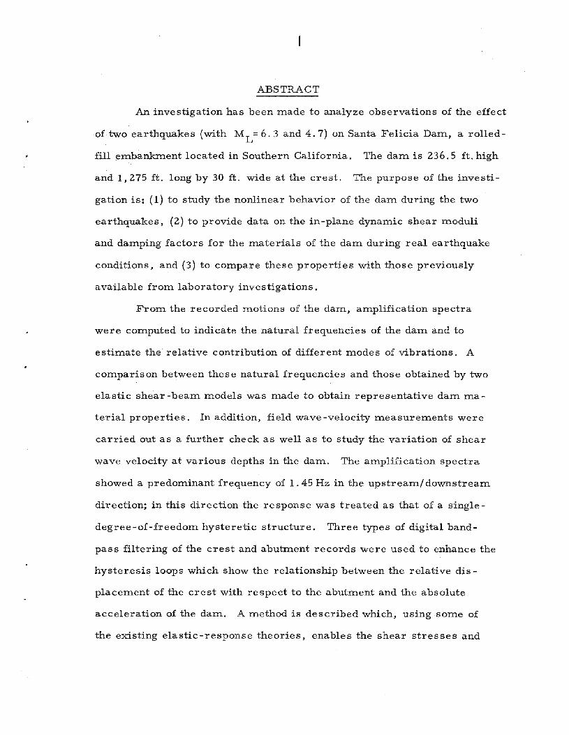
An investigation has been made to analyze observations of the effect
of·two earthquakes (with ML
= 6. 3 and 4.7) on Santa Felicia Dam, a rolled
fill embankment located in Southern California. The dam is 236.5 ft. high
and 1,275 ft. long by 30 ft. wide at the crest. The purpose of the investi
gation is: (1) to study the nonlinear behavior of the dam during the two
earthquakes, (2) to provide data on the in-plane dynamic shear moduli
and damping factors for the materials of the dam during real earthquake
conditions, and (3) to compare these properties with those previously
available from laboratory investigations.
From the recorded motions of the dam, amplification spectra
were computed to indicate the natural frequencies of the dam and to
estimate the relative contribution of different modes of vibrations. A
comparison between these natural frequencies and those obtained by two
elastic shear-beam :models was made to obtain representative dam ma
terial properties. In addition, field wave -velocity measurements were
carried out as a further check as well as to study the variation of shear
wave velocity at various depths in the dam. The amplification spectra
showed a predominant frequency of l. 45 Hz in the upstream/ downstream
direction; in this direction the response was treated as that of a single
degree-of-freedom hysteretic structure. Three types of digital band
pass filtering of the crest and abutment records were used to enhance the
hysteresis loops which show the relationship between the relative dis
placement of the crest with respect to the abutment and the absolute
acceleration of the dam. A method is described which, using some of
the existing elastic -response theories, enables the shear stresses and
-2-
strains, and consequently the shear ITloduli, to be evaluated froITl the
hysteresis loops. The equivalent viscous daITlping factors were calculated
frOITl the areas inside the hysteresis loops. The shear ITloduli and the
daITlping factors were deterITlined as functions of the induced strains in
the daITl. Finally, the shear ITloduli and daITlping factors obtained for
the daITl were cOITlpared with previously available laboratory data for
sands and saturated clays.
-3-
INTRODUCTION
As far as the field of Earthquake Engineering is concerned, there
are very few Ilco:mplete ll instru:mental records to indicate the nature
of the response of earth da:ms to strong earthquakes; however, there
are li:mited records available for s:maller shocks. The ter:m I·co:mplete"
records :means records that are capable of providing a co:mpletely
adequate definition of input ground :motion as well as da:m structural
respons e. The input :motion can be :measured by strong -:motion
accelerographs, often :mounted on da:m abut:ments or at an appropriate
site in the i:m:mediate vicinity of the da:m that is not obviously influenced
in a :major way by local geologic structural features, as indicated by
Bolt and Hudson (1975). The instru:rnents to :measure da:m response can
usually be :mounted at different locations (at least two) on the crest,
avoiding special super structures which :may introduce localized dyna:mic
behavior.
The H:mited instru:mental records available for s:maller shocks and
:microtre:mors, in both the United States and Japan, indicate that the ground
:motion is increasingly :magnified with increasing elevation over the height
of the da:m. Consequently, an earth da:m does not behave as a rigid body
during an earthquake, but rather the :magnitude and distribution of acceler
ation on the da:m are influenced by its dyna:mic response characteristics.
Clearly, the behavior during these s:maller shocks and :microtre:mors would
be a poor indication of a da:m l s perfor:mance during strong earthquake
shaking because of the nonlinear behavior of soils.
Much effort and progress have been :made in the develop:ment of
-4-
analytical as well as num.erical techniques for evaluating the respc>nseof
earth dam.s subjected to earthquake m.otions. Successful application of
all these existing techniques is essentially dependent on the incorporation
of representative dam.-m.aterial properties in the analyses. Because the
behavior of earth dam.s during earthquakes is governed by their dynam.ic
response characteristics. it is possible to learn m.uch about the dynam.ic
properties of such structures from. exam.ination of their response to strong
earthquake shaking. Unfortunately direct m.easurem.ents are infrequent.
since m.oderately large earthquakes are rare. It is difficult, without
m.easurem.ents, to com.pare behavior with earthquake design requirem.ents
(Bolt and Hudson. 1975), in order to estim.ate the perform.ance of other
dam.s and to m.ake rational design decisions for repair and strengthening
of the structures.
It is the purpose of this investigation to: (1) discuss the
problem. of analyzing the behavior of earth dam.s during earthquakes,
(2) provide som.e data, from. the earthquake-response obser-
vations, on the dynam.ic shear m.oduli and dam.ping factors for earth dam.
m.aterials, (3) correlate this data with that obtained for sands and saturated
clays (m.ost of the data available to date have been developed for sands
and saturated clays only) and finally (4) perm.it better understanding of
the response characteristics of earth dam.s to earthquakes.
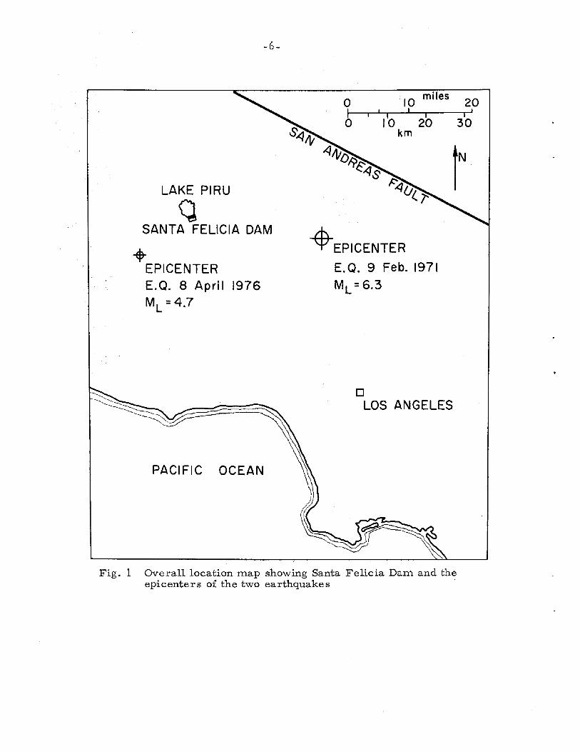
This study deals with results from. observations of the effect of
two earthquakes (one with M L = 6. 3 and an epicentral distance of 33.0 Km.
and the other with M L = 4. 7 and an epicentral distance of 14.0 Km.. see
Fig. 1) on an actual earth dam.: Santa Felicia Dam.; it is a rolled-fill
em.bankm.ent located in Santa Paula, Ventura County. California and built
in 1954-55. The dam. is 236.5 ft high. 1,275 ft long at the crest, 450 ft long
-5-
across the valley at the base, 30 ft. wide at the crest and approximately
1,400 ft. wide at the base. The dam was equipped with two accelerographs
(AR-240) in June 1967; one accelerograph was located at the central section
of the dam crest (55 feet east of the crest midpoint), and an abutment ac
celerograph was placed in the caretaker's shop at the downstream end of
the dam. Recently (in early 1977) the existing AR-240 accelerograph on
the abutment was replaced with a new and improved instrument (SMA-I)
that will give better information on the timing of recorded ground motion
through greater reliability and earlier triggering. Records from two
earthquakes were recovered and analyzed in this study; that from the
San Fernando earthquake o± February 9, 1971 (ML
=6. 3) and that from
the Southern California earthquake of April 8, 1976 (ML
=4.7). Amplification
spectra of the dam were computed for the two earthquakes by dividing the
Fourier amplitude spectrum of the acceleration recorded at the crest by
that recorded at the abutment. Analysis of the observed records reveals
that the acceleration amplitude is amplified mostly at the dam crest. In
the upstream/ downstream direction the spectra show a predominant single
peak at the fundamental frequency of 1.45Hz. In addition, a visual in
spection of the amplification spectra obtained from the two earthquakes
reveals that the values of the resonant frequencies vary slightly from one
earthquake to the other. Certain existing elastic shear -beam theories
were used to check the values of the resonant frequencies corresponding
to peak values of the amplification spectra and to estimate the shear wave
velocity of the dam material. Field wave -velocity measurements were
carried out for Santa Felicia Dam to: (1) further check the suggested shear
wave velocity which was estimated from the observed resonant frequencies
-6-
20I
LAKE PIRU
QSANTA FELICIA DAM
..-EPICENTERE. Q. 8 Apri I 1976ML =4.7
PACIFIC OCEAN
oIo
-Eft-EPICENTER
E.Q. 9 Feb. 1971ML =6.3
oLOS ANGELES
I30
Fig. 1 Overall1ocation map showing Santa Felicia Dam and theepicenters of the two earthquakes
-7-
as well as from use of the existing shear -beam theories, (2) study
the variation of the shear wave velocity at various depths in the dam, and
finally (3) establish a representative and reliable mean value of the
material constants for use in earthquake response analysis.
In this investigation, the response of the upstream/downstream
fundamental mode is treated as that of a single -degree-of-freedom
hysteretic structure, as suggested for a building structure by Iemura
and Jennings (1973). Three types of digital band-pass filtering of the
crest and the abutment records were used to give hysteresis loops which
show the relationship between the relative displacement of the crest with
respect to the abutment anu the absolute acceleration of the dam. In
evaluating the earthquake response of the dam, one-dimensional shear
beam theory with shear modulus varying with depth was used to estimate
dynamic shear strains and stresses. However, a two-dimensional theory
with constant shear modulus wa~ used to compare the results. An effort
was made to simplify the presentation of the mathematics necessary for
dynamic analysis of the dam models. Using two existing elastic-response
theories, a method was outlined whereby the shear stresses and strains
could be determined as functions of the maximum absolute acceleration
and maximum relative displacement, respectively, for each hysteresis
loop; this enables evaluation of the shear moduli. The equivalent linear
shear modulus was expressed as the secant modulus determined by the
slope of the line joining the extreme points of the hysteresis loop. Although
the assumption of elastic behavior during earthquakes is not strictly correct
for earth dams, it was used to provide a basis for establishing the natural
frequencies of the dam, and in addition to give at least a qualitative picture
-10-
level and has a capacity of 100,000 acre feet (Ref. 1).
From the geological point of view, the Santa Felicia Dam site
lies within a series of sandstones and shales of Miocene Age which have
been conspicuously folded and tilted. The sandstones are predominantly
medium-grained and loosely cemented. The shales are variable in
character, ranging from silty to clay. The geological formations are
inter stratified in a great variety of combinations. Thus, the bedrock
at Santa Felicia Dam consists of sandstone strata of varying degrees of
hardness interlayered with shale seams of varying thickness. In general,
the geological conditions were favorable for the construction of the dam
(Ref. 21).
The geology of the site was, utilized to provide a sound, watertight
and economical section and to assure a firm seal between the bedrock and
the impervious central core throughout the dam's length. The sands and
gravel of the stream bed, 70 to 90 ft in thickness at the dam site, were
used as a foundation for the pervious shells of the dam, up - and down
stream from the impervious core.
The embankment has a total of about 3,400,000 cubic yards of core
and shell material which is basically of an alluvial nature and which was
obtained from borrow pits at the reservoir site and from sites up- and
down- stream. The alluvium consists of clay, sand, gravel and boulders.
Suitable gravelly materials from the core cut-off trench excavation were
used for construction of the pervious shell embankments. The core ma
terial (824,500 cubic yards) was selected from the upstream impervious
borrow pit areas on the basis of laboratory tests. In the construction
of the embankment, the impervious core materials were spread in almost
horizontal layers not more than 8 inches thick before compaction, and
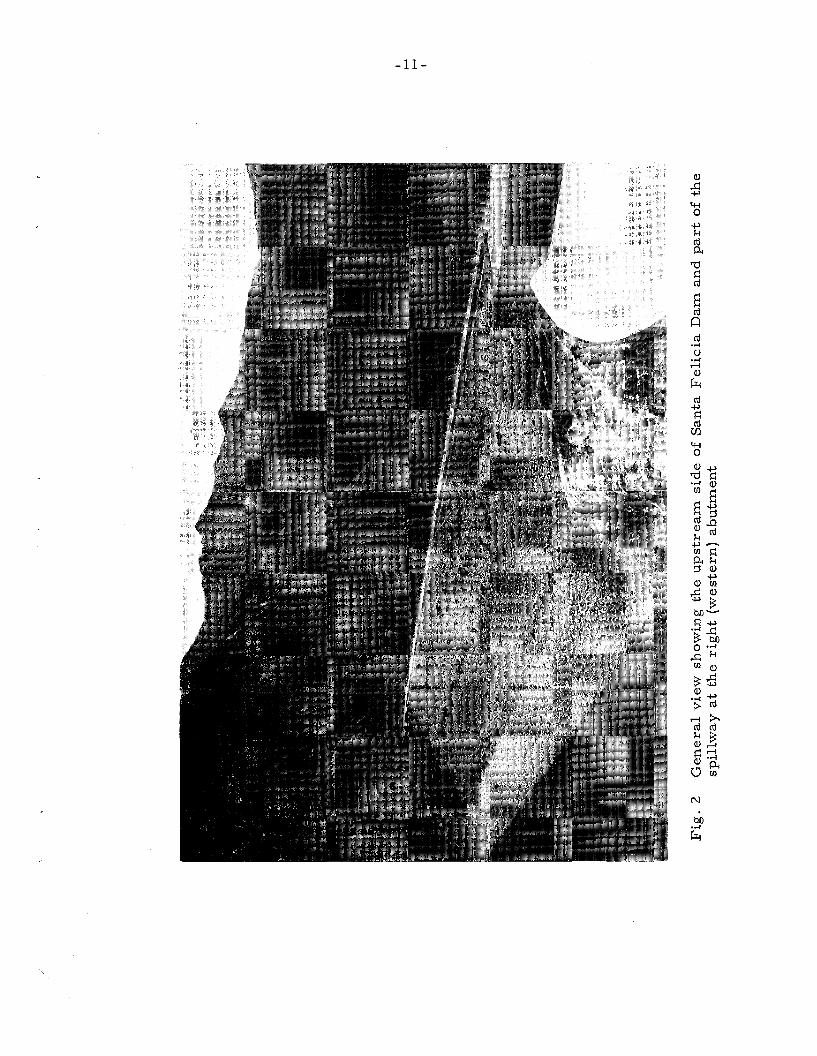
Fig
.2
Gen
era
lv
iew
sho
win
gth
eu
pst
ream
.si
de
of
San
taF
eli
cia
Dam
.an
dp
art
of
the
spil
lway
at
the
rig
ht
(west
ern
)ab
utm
.en
t
I ......
......
I

-12-
SANTA FELICIA DAM
SANTA PAULA. CALIFORNIA
IAXIS OF DAM
CROSS SECTION OF THE DAM
2' OFDUMPEDRIPRAP
PERVIOUSSHELL
DOWNSTREAM
DEVELOPED PROFILE ON AXIS DAM LOOKING UPSTREAM
rCREST DETAIL
300I
UPSTREAM
eRE.E.\<?\R\.l
f I
l II OUTLETP WORKS
oI
PLAN VIEW
Fig. 3 Structural details of Santa Felicia Dam

-13-
pervious shell materials in layers not over 18 inches in thickness.
Fifty-ton four-wheel pneumatic-tired rollers were used for compacting
the impervious core and the pervious shell. After all suitable materials
from the core trench excavation had been utilized, the sands and gravels
of the river bed were used in the pervious fills. The core material has
a high degree of impermeability, is granular in nature and possesses
considerable strength. A one-foot layer of gravel and cobble was placed
on the downstream slope of the darn and on the upstream face. The latter
was designed to serve as both a bed and a drain for the riprap. The
purpose of the layer on the downstream face of the darn was to prevent
erosion of the face of the darn from rain.
The laboratory and fieldtests, during and before construction,
included moisture determinations, density-in-place tests, particle size
analyses, specific gravity determinations, and permeability tests.
Table 1 indicates design values conservatively assumed to be representative
of the typical soils as determined from results of the soil testing program
in the field and laboratory.
In order to prevent leakage through the rock formations underlying
the darn and to insure a good cut off from the reservoir, a continuous grout
curtain was provided in the bedrock throughout the entire length of the
darn approximately parallel to the axis, and to a depth of 120 ft. below
the surface bedrock. A similar curtain of grout was placed beneath the
crest of the spillway and joined to the main curtain of the darn.
The ungated concrete spillway of the darn has a discharge capacity
of 105,000 cubic feet per second with the water surface five feet below
the top of the darn. This allows for the "maximum possible flood"

-14-
estiITlated for the streaITl and is three tiITles the greatest flood that has
occurred during the period of record.
The outlet works structure, which extends through the base of the
daITl, is built priITlarily on the rock bench which forITls a part of the right
or west abutITlent at about streaITl bed level. The function of the outlet
works is to release, control the flow of stored water for spreading and
and to recharge the ground water for dOITlestic and industrial water supply,
irrigation and other downstreaITl uses.
More detailed inforITlation concerning the design and construction
is given by Price (1956).

-15-
TABLE 1
Characteristics of Santa Felicia Dam Materials (Ref. 1)
Property Core Shell Foundation
Dry unit weight 114 pcf 125 pcf 116 pcfMoist unit weight 131 pC£ 131 pcf 122 pC£
Saturated unit weight 134 pC£ 141 pC£ 135 pcfSubmerged unit weight 73 pcf 79 pC£ 73 pcfCoefficient of friction 0.60 0.84 0.81
Permeability 0.001 ft/day 20 ft/day 150 ft/daySpecific gravity 2.68 2.69 2.69
-16-
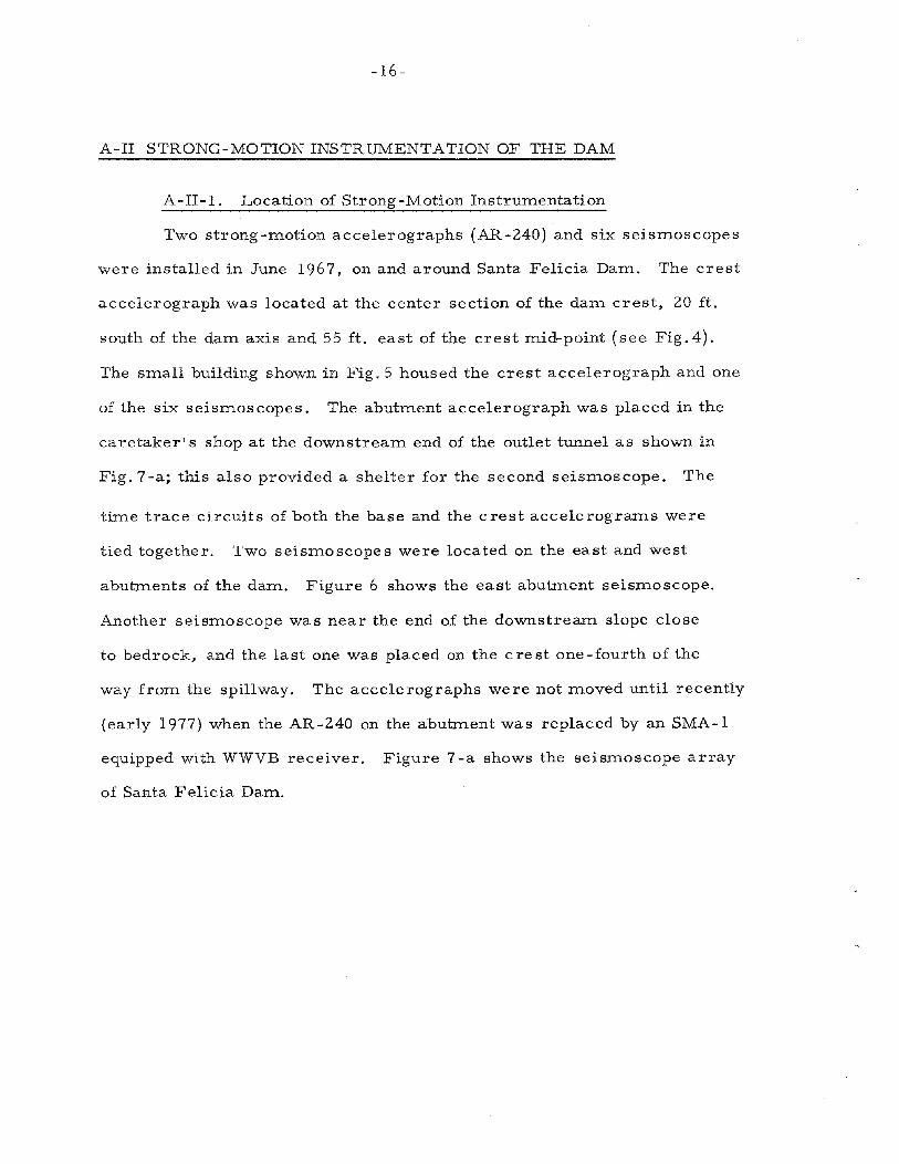
A-II STRONG-MOTION INSTRUMENTATION OF THE DAM
A-II-l. Location of Strong-Motion Instrumentation
Two strong-motion accelerographs (AR-240) and six seismoscopes
were installed in June 1967, on and around Santa Felicia Darn. The crest
accelerograph was located at the center section of the darn crest, 20 ft.
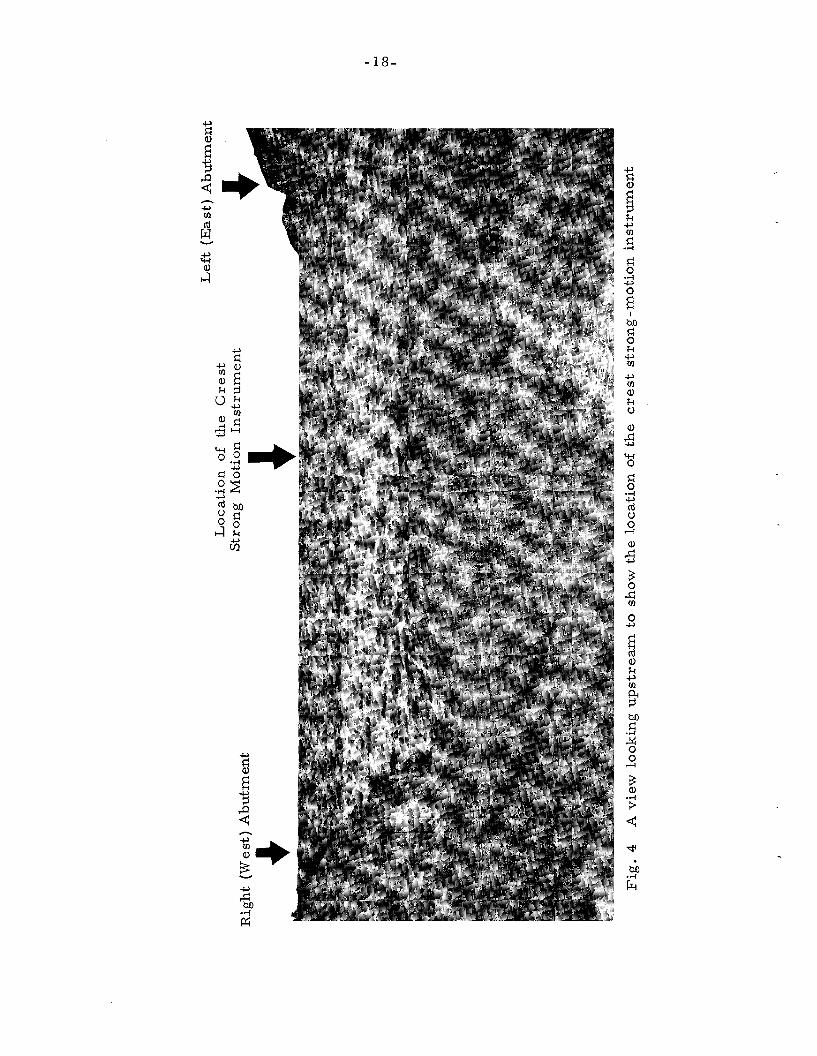
south of the darn axis and 55 ft. east of the crest mid-point (see Fig.4).
The small building shown in Fig. 5 housed the crest accelerograph and one
of the six seismoscopes. The abutment accelerograph was placed in the
caretaker's shop at the downstream end of the outlet tunnel as shown in
Fig. 7-a; this also provided a shelter for the second seismoscope. The
time trace circuits of both the base and the crest accelerograms were
tied together. Two seismoscopes were located on the east and west
abutments of the darn. Figure 6 shows the east abutment seismoscope.
Another seismoscope was near the end of the downstream slope close
to bedrock, and the last one was placed on the crest one-fourth of the
way from the spillway. The accelerographs were not moved until recently
(early 1977) when the AR-240 on the abutment was replaced by an SMA-1
equipped with WWVB receiver. Figure 7-a shows the seismoscope array
of Santa Felicia Darn.
-17-
A-II-2 Up-grading of the Strong-Motion Accelerographs
Recent concern about the so-called "Palmdale Uplift" along the
San Andreas Fault has led both seismologists and earthquake engineers
to re -examine the strong -motion earthquake recorders in that general
area, as indicated by Housner~ In particular, the Lake Hughes array
of strong -motion accelerographs is being upgraded and extended. This
array starts with an instrument by the San Andreas Fault near Lake Hughes
and extends in a southwesterly direction with four accelerographs spaced
a couple of miles apart. The strong-motion accelerograph below
Santa Felicia Dam makes a logical extension of this area. As mentioned
before, the abutment accelerograph was replaced with a new and improved
instrument; however, the crest accelerograph has not been replaced
since it was installed in June 1967. Generally, this improvement will
give better information on the timing of the recorded ground motion
through greater reliability, earlier triggering, and higher compatibility
with the radio time receivers. In addition, if the accelerograph on the
crest of the dam is replaced with a new, improved instrument, this would
provide much better information for analyzing the structural behavior
of the dam, especially if a strong earthquake originates on the San
Andreas Fault.
Rig
ht
(Wes
t)A
bu
tmen
t
•L
ocati
on
of
the
Cre
st
Str
on
gM
oti
on
Inst
rum
en
t
Left
(East
)A
bu
tmen
t
I I-'
00 I
Fig
.4
Av
iew
loo
kin
gu
pst
ream
tosh
ow
the
locati
on
of
the
cre
st
stro
ng
-mo
tio
nin
stru
men
t

-19-
Fig. 5 Location of the crest accelerograph
Fig. 6 East (left) abutment s eismoscope
-20-
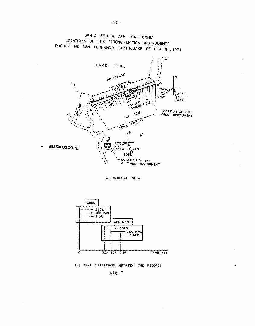
SANTA FELICIA DAM. CALIFORNIA
LOCATIONS OF THE STRONG - MOTION INSTRUMENTS
DURING THE SAN FERNANDO EARTHQUAKE OF FEB. 9 • 1971
N
II,,
IIIIII
PIRULAKE
," ,
I,......... ..,..--
I --I
':>'$I' 1/
,~ If / LOCATION OF THE, ,';/ : ( -3 CREST INSTRUMENT\ \ '''' I \,\ \, I \ I
\'~ I IIII".." , \', ....-:----) :
---_, I, _,
\ _ -, \ _1,_.... I'
I' 2
• SEISMOSCOPE ((!i~_~~w \SII4'\ (--_.> S08E, \
\ '. LOCATION OF THE" \ ABUTMENT INSTRUMENT
(01 GENERAL VIEW
rABUTMENT II .. S82W, I • VERTICAL,
~S08E, ,I , ,, , ,
o TIME. sec
(b) TIME DIFFERENCES BETWEEN THE RECORDS
Fig. 7
-21-
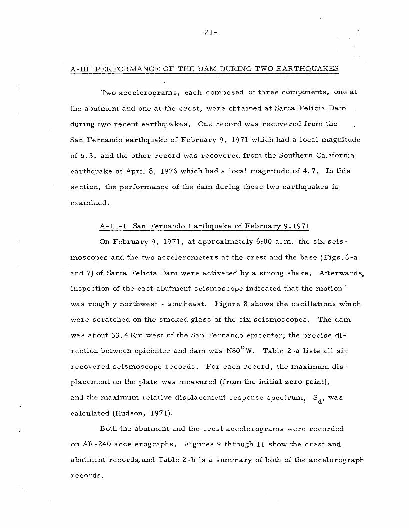
A-III PERFORMANCE OF THE DAM DURING TWO EARTHQUAKES
Two accelerograms, each composed of three components, one at
the abutment and one at the crest, were obtained at Santa Felicia Dam
during two recent earthquakes. One record was recovered from the
San Fernando earthquake of February 9, 1971 which had a local magnitude
of 6.3, and the other record was recovered from the Southern California
earthquake of April 8, 1976 which had a local magnitude of 4. 7. In this
section, the performance of the darn during these two earthquakes is
examined.
A-III-l San Fernando Earthquake of February 9,1971
On February 9, 1971, at approximately 6:00 a.m. the six seis
moscopes and the two accelerometers at the crest and the base (Figs. 6-a
and 7) of Santa Felicia Darn were activated by a strong shake. Mterwards,
inspection of the east abutment seismoscope indicated that the motion
was roughly northwest - southeast. Figure 8 shows the oscillations which
were scratched on the smoked glass of the six seismoscopes. The darn
was about 33.4 Km west of the San Fernando epicenter; the precise di
rection between epicenter and dam was N80o
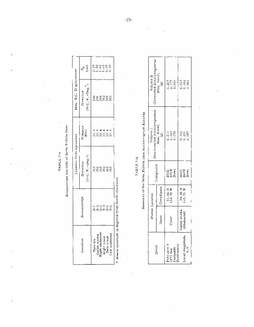
W. Table 2-a lists all six
recovered seismoscope records. For each record, the maximum dis
placement on the plate was measured (from the initial zero point),
and the maximum relative displacement response spectrum, Sd' was
calculated (Hudson, 1971).
Both the abutment and the crest accelerograms were recorded
on AR-240 accelerographs. Figures 9 through 11 show the crest and
abutment records, and Table 2-b is a summary of both of the accelerograph
records.
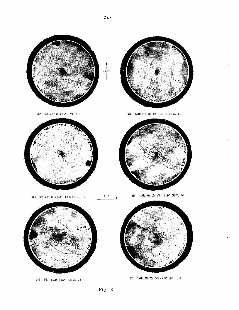
262 SANTA FELICIA DAr1 - TOE, S-l
264 SANTA FELICIA DAM - RIGHT ABUT., S-3
266 SANTA FELICIA DAM - CREST. S-5
-22-
tiWRTH
I
2 C~l
263 SANTA FELICIA DAr-, - OUTLET WORKS, S-2
265 SANTA FELICIA DAM - RIGHT CREST. S-4
267 SANTA FELICIA DAM - LEFT ABUT" S-6
Fig. 8
TA
BL
E2
-a
Seis
luO
sco
pe
Reco
rds
of
San
taF
eli
cia
Dall
l
Lo
cati
on
fro
lll
Ep
icen
ter
Max
.R
eI.
Dis
pla
cell
len
t
Lo
ca
tio
nS
eis
rn
osc
op
eD
irecti
on
Dis
tan
ce
Dir
ecti
on
Sd
(N-C
.W
.-D
eg
.*)
(Kll
l)*
(Cll
l)(N
-C.
W.
-Deg
.)
Dall
lto
eS
-l2
82
33
.42
90
2.1
0
Ou
tlet
wo
rks
S-2
28
23
3.4
29
51
.24
Rig
ht
ab
utl
llen
tS
-32
82
33
.42
88
1.8
2R
igh
tcre
st
S-4
28
23
3.4
3Q2
5.6
3
Dall
lcre
st
S-5
28
23
3.4
30
56
.28
Left
ab
utl
llen
tS
-62
82
33
.43
03
2.3
0
*M
ean
sd
irecti
on
ind
eg
rees
fro
lll
No
rth
clo
ck
wis
e
TA
BL
E2
-b
SU
llll
llar
yo
fth
eS
an
taF
eli
cia
Dall
lA
ccele
rog
rap
hR
eco
rds
Sta
tio
nL
ocati
on
Vo
lUlu
eI
Vo
lull
leII
Ev
en
t-
Co
lllp
on
en
t(U
nco
rrecte
dA
ccele
rog
rall
ls)
(Co
rrecte
dA
ccele
rog
rall
ls)
Max
.A
ccel.
Max
.A
ccel.
Nall
leC
oo
rdin
ate
(g)
(g)
Feb
ruary
93
4.4
6N
S1
5E
0.2
11
0.2
07
19
71
San
Cre
st
11
8.7
5W
S7
5W
0.1
84
0.1
77
Fern
an
do
Do
wn
0.0
70
0.0
66
Eart
hq
uak
eO
utl
et
wo
rks
34
.46
NS
08
E0
.23
10
.21
7L
ocal
llla
gn
itu
de
(Ab
utl
llen
t)1
18
.75
WS
82
W0
.23
10
.20
26
.3D
ow
n0
.08
70
.06
5
It'o
J\J
-J I

-24-
Standard data processing, including the uncorrected digitized
accelerograms, the corrected accelerograms, integrated velocity
and displacement records, the response spectrum curves and finally
the Fourier amplitude spectra, of these records can be found in Caltech
Reports Nos. EERL 71-22, 73-50, 73-83 and 73-103.
It is important to indicate that the time trace circuits were
interconnected, so that the timing pips on both the abutment and the
crest accelerograms represent the same absolute time, plus or minus
some multiple of 0.5 seconds (since the instruments did not necessarily
trigger simultaneously). The first 3 to 3.5 seconds of the abutment
record have been lost due to double exposure. Furthermore, the edge
of the doubly-exposed area is not normal to the axis of the film and hence
the recoverable traces in each of the three directional components start
at different times, as illustrated in Fig. 7 -b.
However, by comparing peaks in the Caltech-digitized Vol. II
record with the same peaks in a copy of the original record, it appears
that, in the digitization process, the time scale of the digitized record
was reset to zero at the beginning of each trace, so that the relation
between the components was eradicated.
The time differences, to the nearest. 02 sees, between the Vol. II
time scales of the crest and abutment (outlet works) records are given
in Table 3. They were found by first comparing displacement peaks in
the two records to find the approximate time difference to the nearest
timing mark. An allowance of approximately 0.2 sees was made for the
displacement pulse to travel the height of the dam (273 ft.). Knowing
the time differences to the nearest 0.5 sees, corresponding acceleration
peaks in the digitized and in the original records were compared to find
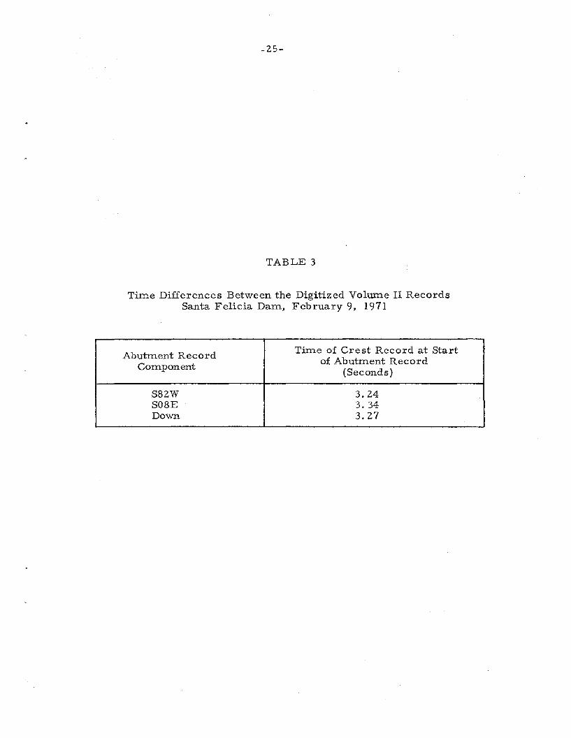
-25-
TABLE 3
Time Differences Between the Digitized Volume II RecordsSanta Felicia Dam, February 9, 1971
Abutment Record Time of Crest Record at Start
Component of Abutment Record(Seconds)
S82.W 3.2.4S08E 3.34Down 3.2.7
-26-
the precise time differences.
Finally, since neither instrument was exactly aligned with the darn
axis (578. 6°W) the horizontal components of each record were rotated to
be parallel and normal to the darn axis (see Fig. 6 -a). The rotations
were small; 3.40
at the abutment and 3.6 0 in the opposite direction at
the crest. The difference between the starting times of the base record
components were taken into account, and rotated horizontal components
were obtained starting at 3.34 secs on the crest record time scale as
shown in Fig. 6-b.
A further complication in the base record developed due to the
fact that the floor of the valve house, to which the instrument was fixed,
apparently rested on a concrete standpipe rather than on firm ground.
Presumably this is the cause of the peaks in the Fourier amplitude
spectra of the abutment record, near 10 Hz (this will be shown later in
this report).
-27-
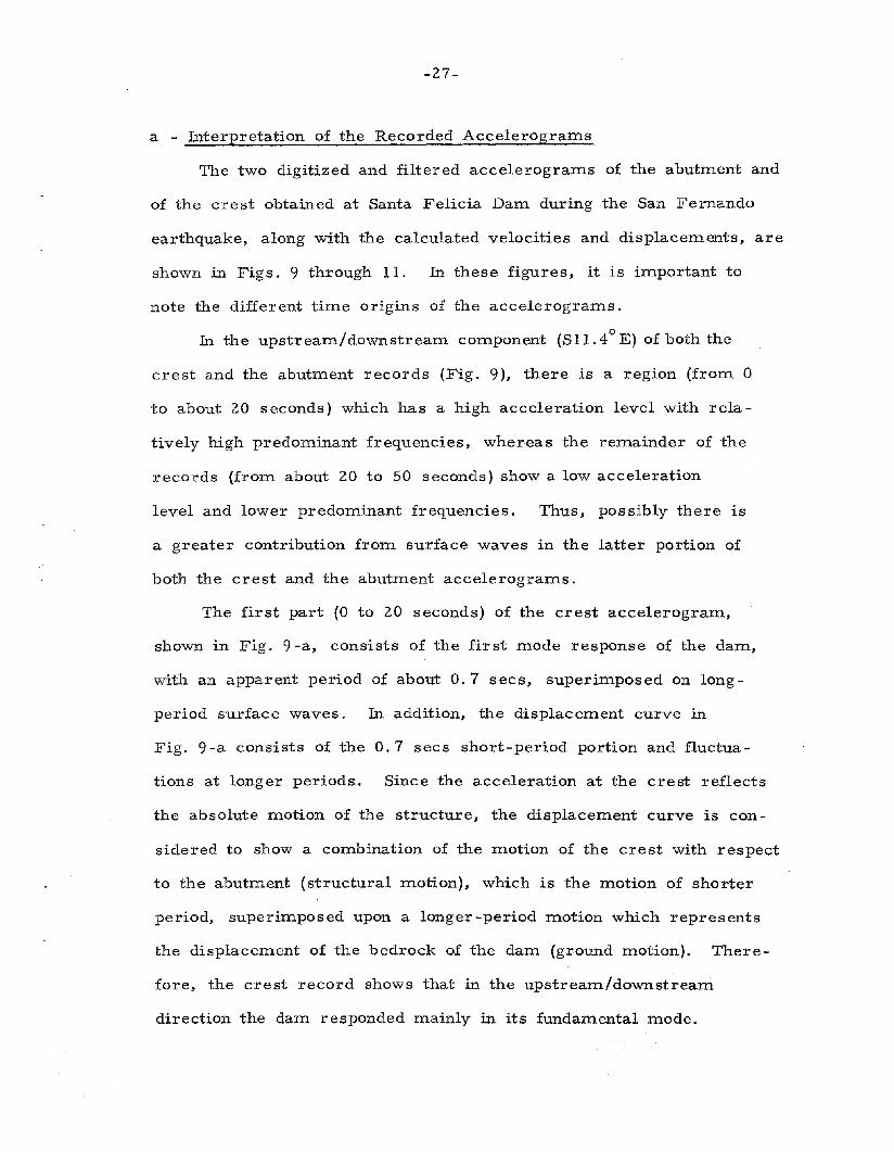
a - Interpretation of the Recorded Accelerograms
The two digitized and filtered accelerograms of the abutment and
of the crest obtained at Santa Felicia Dam during the San Fernando
earthquake, along with the calculated velocities and displacements, are
shown in Figs. 9 through 11. In these figures, it is important to
note the different time origins of the accelerograms.
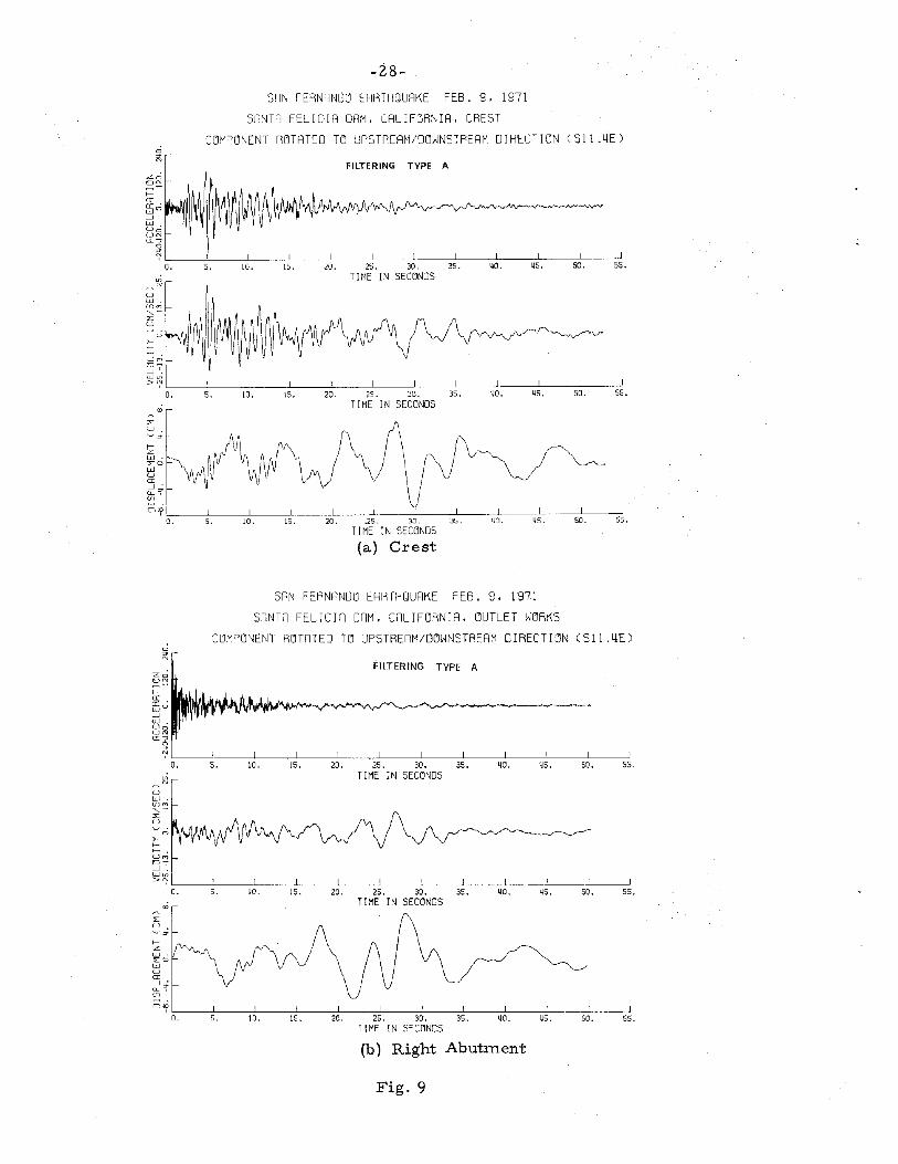
In the upstream/downstream component (Sl1.4°E) of both the
crest and the abutment records (Fig. 9), there is a region (from 0
to about 20 seconds) which has a high acceleration level with rela
tively high predominant frequencies, whereas the remainder of the
records (from about 20 to 50 seconds) show a low acceleration
level and lower predominant frequencies. Thus, possibly there is
a greater contribution from surface waves in the latter portion of
both the crest and the abutment accelerograms.
The first part (O to 20 seconds) of the crest accelerogram,
shown in Fig. 9 -a, consists of the first mode response of the dam,
with an apparent period of about O. 7 secs, superimposed on long
period surface waves. In addition, the displacement curve in
Fig. 9 -a consists of the O. 7 secs short-period portion and fluctua
tions at longer periods. Since the acceleration at the crest reflects
the absolute motion of the structure, the displacement curve is con
sidered to show a combination of the motion of the crest with respect
to the abutment (structural motion), which is the motion of shorter
period, superimposed upon a longer-period motion which represents
the displacement of the bedrock of the dam (ground motion). There
fore, the crest record shows that in the upstream/downstream
direction the dam responded mainly in its fundamental mode.
-28-
SRN FERNRNDO ERRTHOURKE FEB. 9, 1971
SRNTR FELICIR DRM. CRLI FORN IR. CREST
COMPONENT ROTATED TO UPSTRERM/DOWNSTRERM DIRECTION (S11.4U0
"N AFILTERING TYPEZa0c:
f-er(L'W O
--'w.UoUN
cr~
O. S. 10. 15. 20. 25. 30. 35. 40. ~S. 50. 55.
"'TIME IN SECCJNDS
N
UW.If)M,,-::>::U
u~0---,'w"'>')
o. S. 10. 15. 20. 25. 30. 35. 40. 45. SO. 55.
TIME IN SECONDS~
::>::U~"
f-Zw·::>::0WUer-l'O-'i'(f)
~~I I I I I I I I I I Io. 5. 10. lS. 20. .25. 30. 35. 40. 45. so. 55.
TIME IN SECONDS
(a) Crest
SRN FERNRNDO ERRTHOURKE FEB. 9. 1971
SRNTR FELICIR DRM. CRLIFORNIR. OUTLET WORKS
COMPONENT RIHRTEO TO UPSTRERM/DOWNSTRERM DIRECTION (SI1.4U0
"NFILTERING TYPE A
f-er(L'W O
--'w.UoUNa: g
') I I I I I I I I IO. S. 10. 15. 20. 25. 30. 35. 40. 45. 50. 55.
"' TIME IN SECONDSN
UW.(f)M,,-:>::U
0>-f-~ .UM0--l'W"'>')
o. S. 10. 15. 20. 25. 30. 35. 40. 45. SO. 55.
,p TI ME I N SECONDS
::>::U
f-ZW.::>::0WUer-l'0-,(f)
O,?o. S. 10. 15. 20. 25. 30. 35. 40. 45. SO. 55.
TIME IN SECONDS
(b) Right Abutment
Fig. 9
-29-
SRN FERNRNDO ERRTHQURKE FEB. 9. 1971
SRNTR FELICIR DRM, CRLIFORNIR. CREST
COMPONENT ROTATED PRRRLLEL TO DRM RXIS (S78 .6W)0
;::
20FILTERING TYPE A
o~
f-a:0::'W
O
-JW.UoUN
cc~
O. 5. 10. 15. 20. 25. 30. 35. 40. 45. 50. 55.
iG TIME IN SECONDS~
UW.(f)<o,-::EU
0>-f-
U~0--J '.W'">';' ----------I
O. 5. 10. 15. 20. 25. 30. 35. 40. 45. 50. 55.
.; TIME IN SWJNDS~
::EU
~"f-2W·::EOWUa:-J'Cl.'I'(f)
0"1 I I I I I IO. 25. 30. 35. 40. 45. 50. 55.
TIME IN SECONDS
(a) Crest
SRN FERNRNDO ERRTHQURKE FEB. 9. 1971
SRNTR FELICIR DRM. CRLIFORNIR. OUTLET WORKS
VERTICRL COMPONENT
55.
55.
55.
50.
50.
50.
45.
45.
40.
40.35.
~. ~. ~. E.TI ME I N SECONDS
Right(b) Abutment
Fig. 11
I I !
20. 25. 30.
TI ME I N SECONDS
FILTERING TYPE A
15.10.5.
~
20O~
f-a:a:'W O-JWUoUN
cr~
O.
~
\GUwen'",-:>:U~ 0>-f-~ .U",0--J'W'">~
O.
.;~
:>:U~;
f-2W:>:0WUa:-J'CL'iif)
O,\,o.
-31-
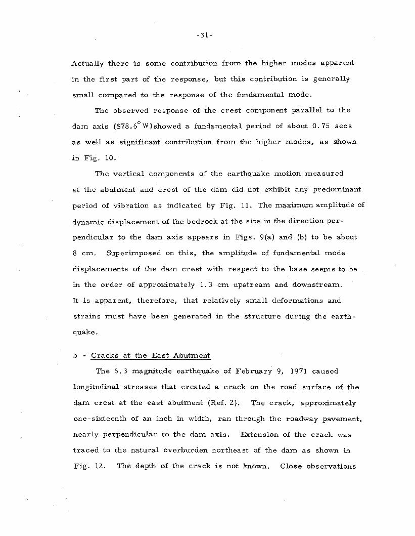
Actually there is some contribution from the higher modes apparent
in the first part of the response, but this contribution is generally
small compared to the response of the fundamental mode.
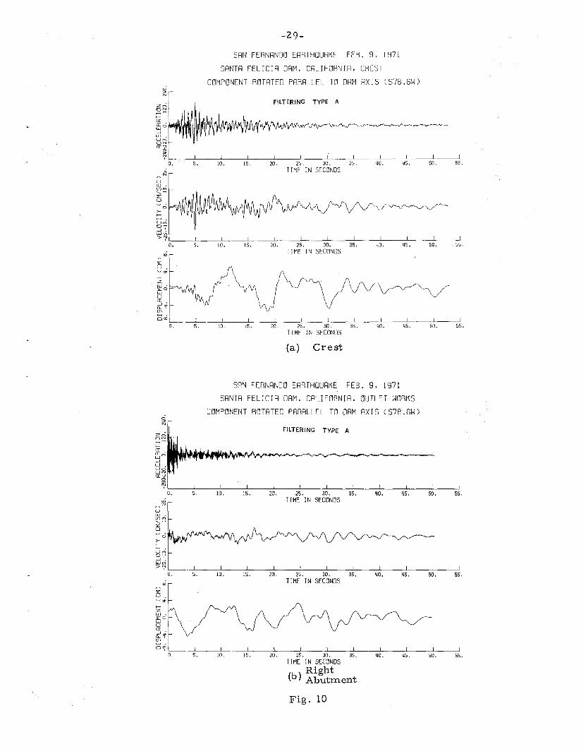
The observed response of the crest component parallel to the
dam axis (S78.6°W)showed a fundamental period of about 0.75 secs
as well as significant contribution from the higher modes, as shown
in Fig. 10.
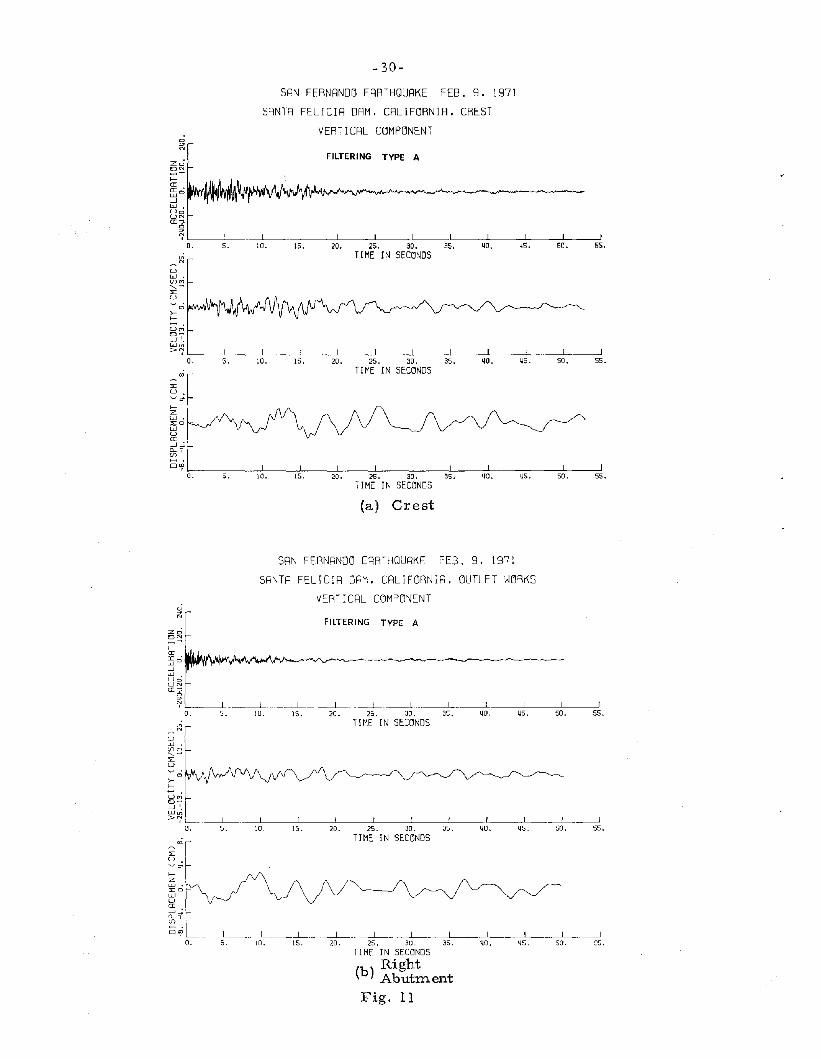
The vertical components of the earthquake motion measured
at the abutment and crest of the dam did not exhibit any predominant
period of vibration as indicated by Fig. 11. The maximum amplitude of
dynamic displacement of the bedrock at the site in the direction per
pendicular to the dam axis appear s in Figs. 9(a) and (b) to be about
8 cm. Superimposed on this, the amplitude of fundamental mode
displacements of the dam crest with respect to the base seems to be
in the order of approximately 1.3 cm upstream and downstream.
It is apparent, therefore, that relatively small deformations and
strains must have been generated in the structure during the earth
quake.
b - Cracks at the East Abutment
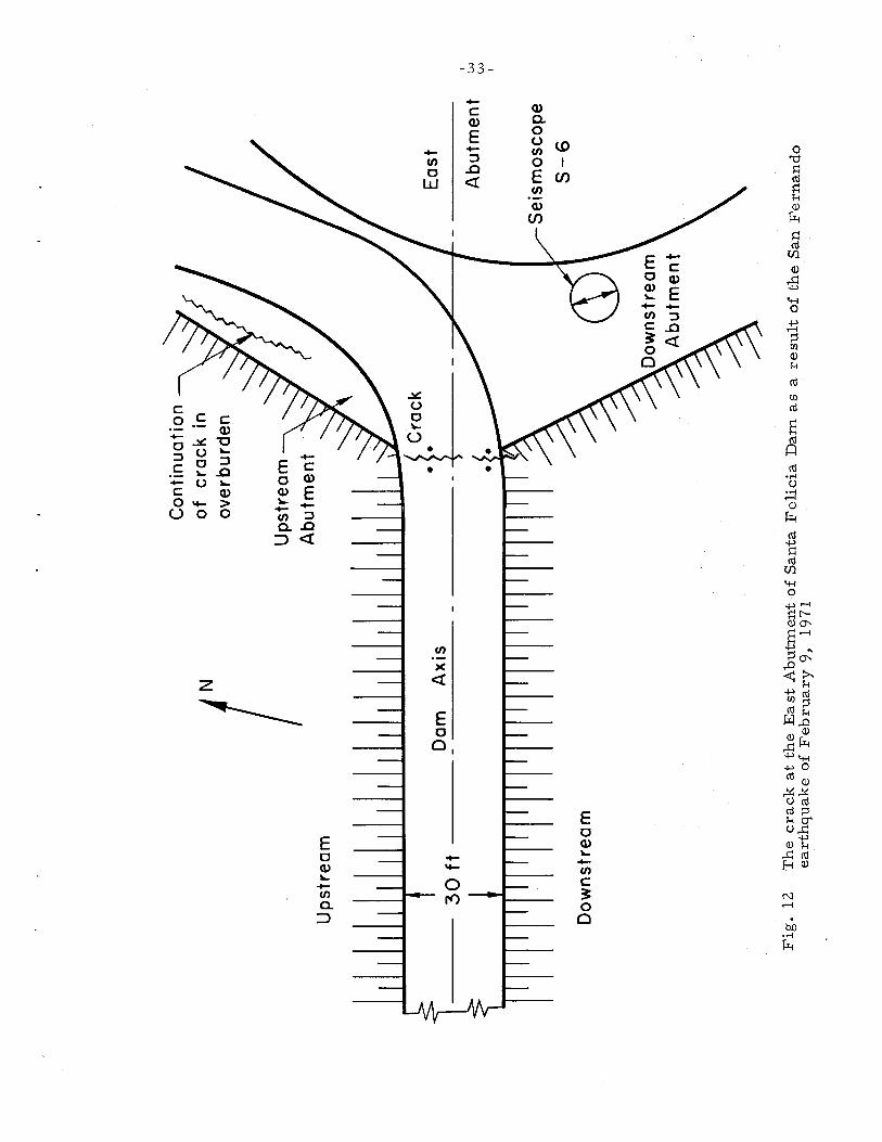
The 6.3 magnitude earthquake of February 9, 1971 caused
longitudinal stresses that created a crack on the road surface of the
dam crest at the east abutment (Ref. 2). The crack, approximately
one-sixteenth of an inch in width, ran through the roadway pavement,
nearly perpendicular to the dam axis. Extension of the crack was
traced to the natural overburden northeast of the dam as shown in
Fig. 12. The depth of the crack is not known. Close observations

-32 -
on February 9, 1971 of both abutments, upstream and downstream,
revealed no other cracking or seepage which might indicate a hazard-
ous condition. This narrow meandering crack across the crest at
·the east abutment appears to have no structural significance since it
is in a portion of the roadway which is east of the dam proper.
Nonetheless, investigations have implied that there has been a
continuous small longitudinal movement of the dam crest toward the
east abutment, which indicates a compression of the dam against
this abutment, but the 1/16 -inch lateral crack which occurred during
the earthquake indicates tension at this point, which is close to the
point of contact of the dam crest with the abutment. So while this
may be only an insignificant surface crack, it is possible that the
sharp ridge forming the abutment has been sheared, possibly leaving
an es sentially loose block of rock. Perhaps the depth and extent
of this crack should be investigated to make sure that it will not be
a hazard when the reservoir is full and spilling.
In general, the performance of the dam and the outlet works
appeared quite satisfactory; in spite of an indicated seismic ac-
celeration of nearly O.25g, the earthquake had only minor effects.
Apart from the earthquake, the total settlements and lateral movements
to date of the dam are well within normal limits and the additional
amounts caused by the earthquake are quite normal.
Copies of various drawings, a post-San Fernando inspection
report and miscellaneous correspondence between Professor Housner
and UWCD are filed in the Earthquake Engineering Library at
Caltech. (1, 2)
Up
str
ea
m
Do
wn
str
ea
m
N
Co
nti
nu
ati
on
of
cra
ck
ino
ve
rbu
rde
n
Ea
st
Ab
utm
en
t
5e
ism
os
co
pe
5-6
I W W I
Fig
.12
Th
ecra
ck
at
the
East
Ab
utm
en
to
fS
an
taF
eli
cia
Dam
as
are
sult
of
the
San
F'e
rnan
do
eart
hq
uak
eo
fF
eb
ruary
9,
19
71

- 34-
A -III-Z Southern California Earthquake of April 8, 1976
Two accelerograph records were recovered at the Santa Felicia
Dam. from. the U. S. Geological Survey's national network of strong
m.otion instrum.entation(7) following the Southern California earth-
quake of April 8, 1976. One was recorded at the base and the other
at the crest. The m.axim.um. indicated acceleration during this 4. 7
local m.agnitude event was O.05g. The dam. was 14 Km. northeast
of the epicenter. Table 4 is a sum.m.ary of the accelerograph
records of Santa Felicia Dam..
The seism.oscope records from. this sm.all earthquake show so
little m.otion that they are indistinguishable from. plates left on a
seism.oscope for an extended period of tim.e. However, the ac
celerograph recordings are very interesting in the analysis of the
behavior of the dam. in spite of the relatively sm.all C\.m.plitude of
m.otion. Unlike the recordings during the San Fernando earthquake,
the two horizontal com.ponents of the 1976 earthquake m.otion (SlZo E
and S78°W) were recorded alm.ost perpendicular to the dam. axis
(SIlo 4°E) and the longitudinal axis of the dam. (S78.6°W). In addition,
the recovered record of the crest has a duration of about 18 sec s,
while the recovered record of the right abutm.ent has only 6 seconds
duration. The corrected accelerogram. and integrated velocity and
displacem.ent traces (Vol. II data) of the two records are shown in
Figs. 13 through 15; the standard data processing of the other three
volum.es (I, III and IV) can be found in Appendix A.
The observed responses of both the crest and the abutm.ent
show long period m.otions in the integrated velocity and displacem.ent;
this could be due to hum.an digitization error, to the shortness of

-35-
the records or to a contribution from surface waves. The response
of the fundamental mode in the upstream/downstream direction
(component SllE) with an apparent period of about 0.7 seconds is
indicated by the computed velocity plot of Fig. 13. Similarly, the
component parallel to the darn axis showed a fundamental period of
about 0.73 seconds superimposed on long-period surface waves.
In this event, the amplitude of the dynamic displacement of the
crest with respect to the base (component SIZo
E) in the fundamental
mode was only about 1 mm.

-36-
TABLE 4
Summary of the Santa Felicia Dam Accelerograph
Station LocationEvent Component Max. Acceleration
Name Coordinate (g)
8 April 1976 Crest 34.46N SIZE 0.0515Z1 GMT 118.75W S78W 0.05
Southern California Down 0.03Earthquake
Right 34.46N SIZE 0.05Local Magnitude Abutment U8.75W S78W 0.04
4.7 Down 0.03

-37-
SANTA FELICIA DAM,CREST,E/Q ~F APRIL 6 1976-0721 PSTSANTA FELICIA DAM •CREST CtJ1P S12 E
(!) PEAK VALUES I AeGEl = -115.9 CHlSECI5EC VELOCITY = -1.1.3 CHlSEC OISPt. = -1.11 CII
6L- ----L --1- ....L..- --l
-2
-so
>"'u~ =0 W-J~IrI_+~~__:A__f"T_J..,......,...~"7""<___t""_<;_"7"""V'.....,.....~.,p....C:::.L.~~:::::=~...o-.""';;:=:=__--UJ>
50 L- ----L --1- ....L..- --l
-6
ZlOu
::lHa:,ffilH DirlS!tjua:
...zUJEW~ 5 0 ~-------==~:---------r"::...-----~-Q..
~o
5 10TI HE - SECONDS
(a) Crest
15 20
-55
SRNTR FELICIR DRM.RIGHT RBUTMENT.E/Q OF RPRIL B 1976-0721 PSTINO.420 SRNTR FELICIR DRM.RIGHT RBUTMENT COMPo S12E
(') PERK VRLUES: RCCEL ~ 50.5 CM/SEc/SEC VELOCITY ~ -2.4 CM/SEC DISPL ~ -.5 CM
zofa:0:w--.JWUUa:
55 '--"----------- ---'-- ---'
-4
4'-----------__---.1 '---- --'
-2
fZWLW
5~ °l-------=:=-_=::::::::=====:::::::==~-- _<L(f)
o
Fig. 13
2~0-------------~5--------------....J
TI ME - SECONDS 10
(b Right) Abutment
Corrected accelerograms and computed velocities and displacements in the upstream/downstream direction
-38-
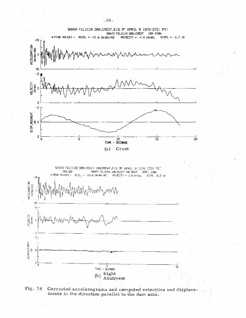
SANTA FELICIA DAM.CREST.E/Q ~F APRIL 8 1976-0721 PSTSANTA FELICIA DAM.CREST COM S7BW
(!) PEAK VALUES: RCCEL = -31.l! CM/SECISEC VELOCITY = -1.9 CH/SEC OISPL = -1.7 CM
>I-<.J
~~OH:..v-4AAiHt--A--+\--fr--..,,--*-H-t\-,.-~-::-typ---'---------__\_M:_::;_-------uJ~>
-35
2L----------L- ---.l..- ..L- ---'
-2
35 L- --L ---.l..- ..L- ---'
-2
I:zw::0:w
Sli Oa..~Cl
20 5 10
TI HE - SECONDS15 20
(a) Crest
SRNTR FELICIR DRM.RIGHT RBUTMENT.E/Q ~F RPRIL 8 1975-0721 PSTIN~.420 SRNTR FELICIR ORM.RIGHT RBUTMENT C~MP. S78W
(') PERK VRLUE5: RCCEL = -33.6 eM/SEc/SEC VEL~C ITY = 1.0 CM/SEC 0I 5PL =0.2 CM
2'------------ -'----- _
-2
-35
z·0
f-a:a:: 0w-!WUUIT
35
-2
fZW:>:w
~i3 O~~===~--=~-=""-====---=;ii::=~--------------"-(j)
o2 ::;-0--------------------::'-5---------------------'10
Tl ME - 5EC~ND5
(b) Right. Abutment
Fig. 14 Corrected accelerograms and computed velocities and displacements in the direction parallel to the dam axis.

-39-
SANTA FELICIA OAH.CREST.E/Q OF APRIL B 1976-0721 PSTSANTA FELICIA DAM.CREST COM DOWN
(!) PER( VALUES: ACGEl = -17.7 CIl/SEClSEC VElOC ITY = 1.7 CHISEC OI SPl = -1.5 CH
201552L.-----------'-- --'-- ..L- ---.J
o
IZ
~LLI
a!Zi0 f---------"""'""=---------------7"'''-------------''r------lCLenCl
2L.- --l.- ---l. ...L- _J
-2
20 L.- --l.- ---l. ...L- ~_ _J
-2
-20
>I- u..... ....,~~Ot--tt--:.-...:.\-1I''-+-..--,.-------1'+----1+--+t----t'r---T-'H-\-t'--''~------------''-....---------
uJ~>
(a) Crest
SRNTR FELICIR DRM.RIGHT RBUTMENT.E/Q OF RPRIL B 1976-0721 PSTINO.420 SANTA FELICIA DAM.RIGHT ABUTMENT COMPo DO~N
<'J PEAK VALUES: ACCEL = 22.4 CM/SEc/SEC VELOCITY =0.7 CM/SEC DISPL =0. I CM-25
zSI-a:a: 0w--JWUUa:
25
-2
>-I- u~w
UVl 00'---J>:W U>
2
-2
I-zw:>::wu>: 0a:u--J"-tn
0
20 5 10
TI ME - SEmNOS
(b) RightAbutment
\ Fig. 15 Corrected accelerograms and computed velocities and displacements in the vertical direction
-40-
A -IV ANALYSES OF RECORDED MOTIONS
A -IV -1 Amplification Spectra
a - San Fernando Earthquake
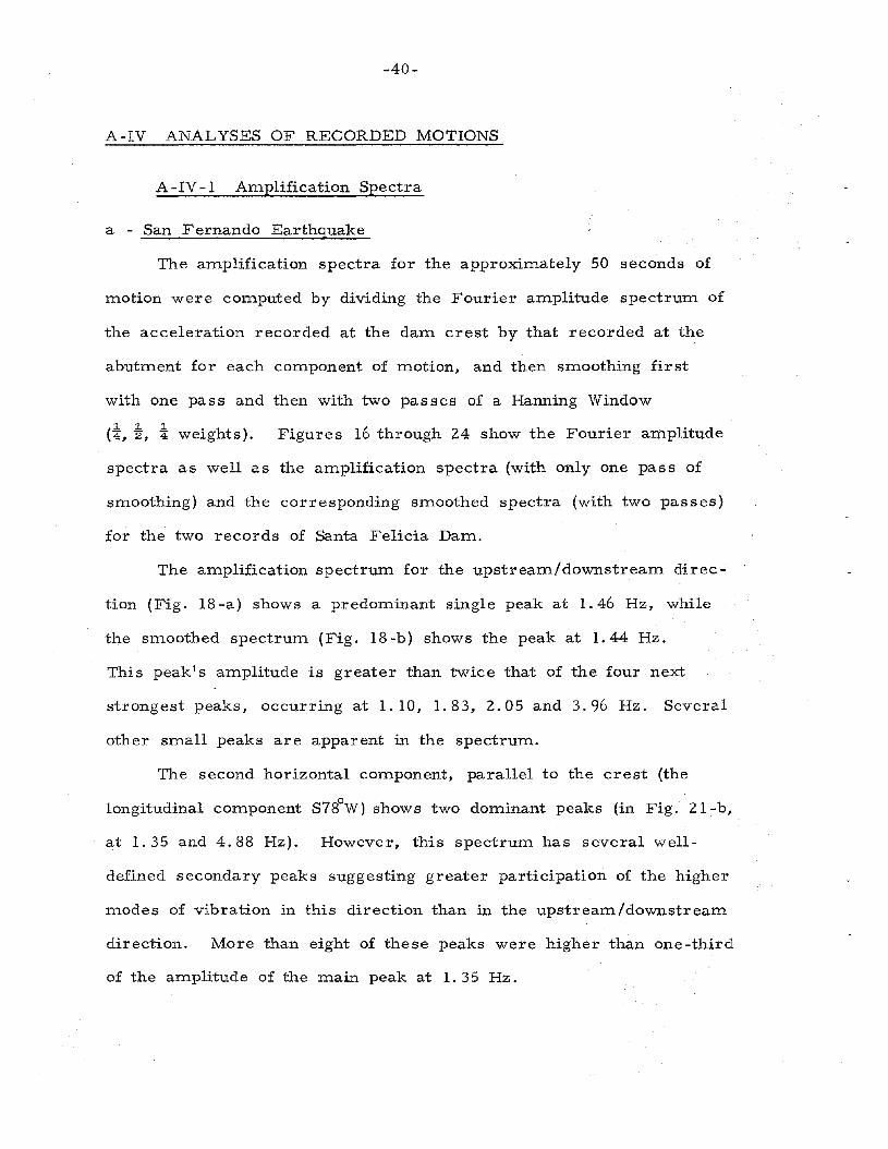
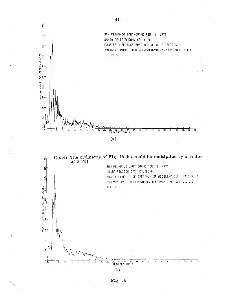
The amplification spectra for the approximately 50 seconds of
motion were computed by dividing the Fourier amplitude spectrum of
the acceleration recorded at the dam crest by that recorded at the
abutment for each component of motion, and then smoothing first
with one pass and then with two passes of a Hanning Window
1. 1. 1.(4, 2, 4 weights). Figures 16 through 24 show the Fourier amplitude
spectra as well as the amplification spectra (with only one pass of
smoothing) and the corresponding smoothed spectra (with two passes)
for the two records of Santa Felicia Dam.
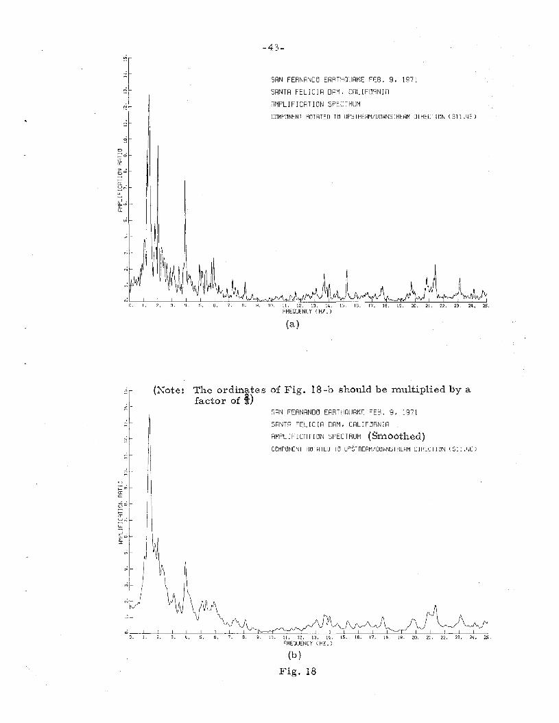
The amplification spectrum for the upstream/downstream direc-
tion (Fig. 18-a) shows a predominant single peak at 1.46 Hz, while
the smoothed spectrum (Fig. 18-b) shows the peak at 1.44 Hz.
This peak's amplitude is greater than twice that of the four next
strongest peaks, occurring at 1. 10, 1. 83, 2.05 and 3.96 Hz. Several
other small peaks are apparent in the spectrum.
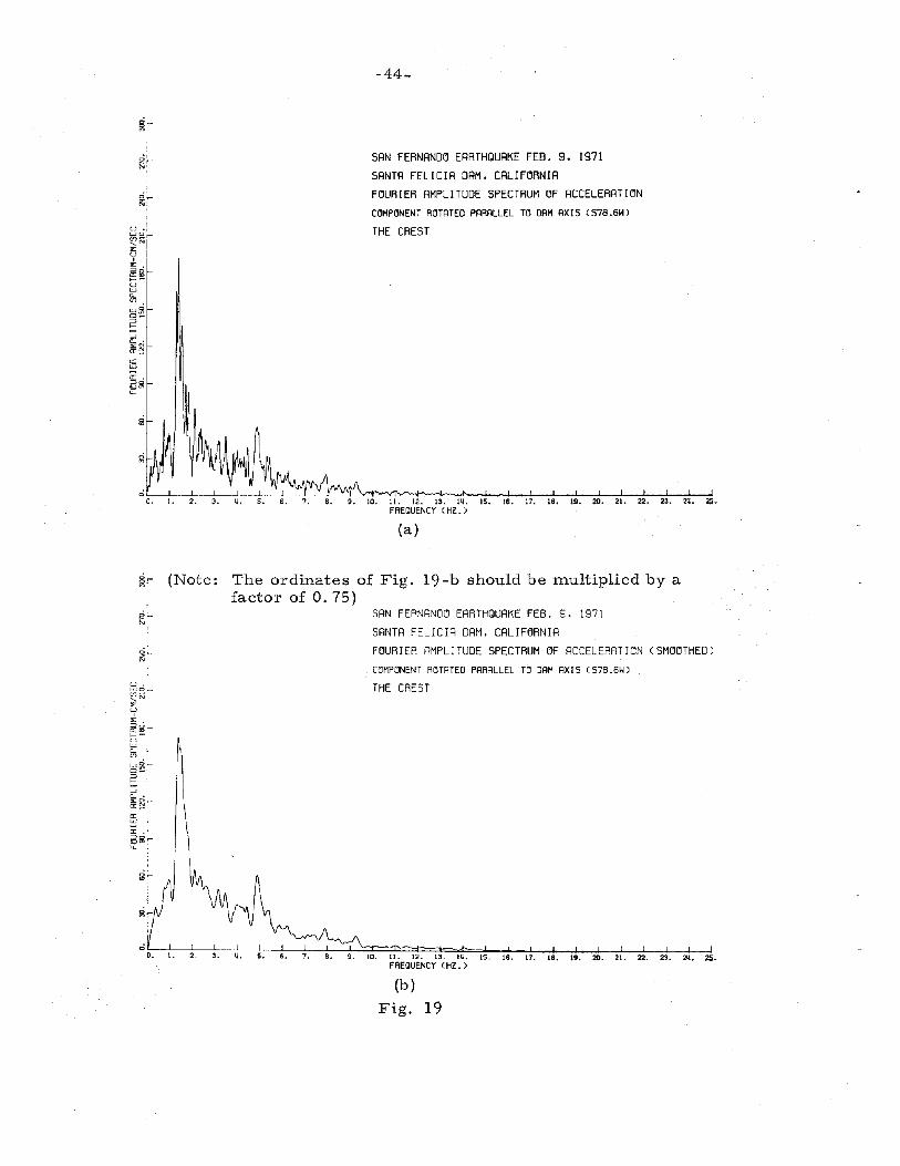
The second horizontal component, parallel to the crest (the
longitudinal component S78°W) shows two dominant peaks (in Fig. 21-b,
at 1. 35 and 4.88 Hz). However, this spectrum has several well-
defined secondary peaks suggesting greater participation of the higher
modes of vibration in this direction than in the upstream/downstream
direction. More than eight of these peaks were higher than one-third
of the amplitude of the main peak at 1. 35Hz.
-41-00
'"
~
~
uwo(J1-,N:>:U
J:>::::JO0:'"e--UW<e-(J1
~~:::Je-
~<e-:>:0a:~
0:~0::::JODmLL
g
g
'00, 1,
SRN FERNRND~ ERRTHQURKE FEB. 9. 1971
SRNTR FELICIR DRM. CRLIF~RNIR
F~URIER RMPLITUDE SPECTRUM ~F RCCELERRTI~N
COMPONENT ROTATED TO UPSTREAM/DOWNSTREAM DIRECTION (SII.4E)
THE CREST
9. 10. 11. 12. 13. 1~. 15. 16. 17. 18. 19. 20. 21. 22. 23. 2~ :ISFREQUENCY (HZ.)
(a)
(Note: The ordinates of Fig. 16 -b should be multiplied by a factorof 0.75)
o~N
u.wo~N::E
'-;'::E,:::Jo0:'"e-UW<een
~~:::Je-..-J<e- ':>:0a:~
0:W
0:.:00DroLL
o<D
o
'"
SRN FERNRND~ ERRTHQURKE FEB. 9. 19~I
SRNTR FELICIR DRM. CRLIFORNIRF~URIER RMPLITUDE SPECTRUM OF RCCELERRT[~N (SM~~THED)
COMPONENT ROTRTED TO UPSTRERM/DOWNSTRERM DIRECTION (SII.4EJ
THE CREST
o _--1 --1- 1 I I I IO. 1. 2. 3, ~. 5. 6. 7. 8, 9, 10, 11. 12, 13. 1~. 15. 16. 17. 18. 19. 20. 21. 22. 23, 2~ 25.
FREQUENCY (HZ.)
(b)
Fig. 16

-42-oo
om
u.WO(f)<
'-.:;:U
I
50O:<DI-
G:la..(f)
~fX:::JI-
-..Ja.. .:;:0a:""0:w
0:.:::100'"LL
oN
SRN FERNRNDO ERRTHQURKE FEB. 9. 1911
SRNTR FELICIR DRM. CRLIFORNIR
FOURIER RMPLITUDE SPECTRUM OF RCCELERRTION
COMPONENT ROTATED TO UPSTREAM/DOWNSTREAM DIRECTION (SIl.4E)
THE RBUTMENT
0~..l---!:-----!:---,L----:!-----,!---:!---!--------!:--+-----l_L--L:''''.L:..~-l~~L-~~::""b..c±=:c::,j~~o. 1. 2. 3. ij. 5. 6. 7. 8. 9. 10. 11. 12. 13. lij. 15. 16. 17. 18. 19. 20. 21. 22. 23. 2ij. <5.
FREQUENCY (HZ.)
(a)
g (Note: The ordinates of Fig. 17 -b should be multiplied by afactor of 0.75)
o<D
U.WD(f)'""'-.
"'T".:::10eo<DuWa..(f)
~~:::JJ--
-..Ja...:;:0a:""0:w
SRN FERNRNDO ERRTHQURKE FEB. 9. 1971
SRNTR FELICIR DRM. CRLIFORNIRFOURIER RMPLITUDE SPECTRUM OF RCCELERRTION (SMOOTHED)
COMPONENT ROTATED TO UPSTREAM/DOWNSTREAM DIRECTION (Sll.4E)
THE RBUTMENT
Dl-....L_l.---L_.l.--.--1_-L----J_-L_L-....L_l.---L_-L..--.-J_-L---lL:::....r::.....::::...L----.L~oe::"±=::r::::::::::±=::::::=::::=Jo. 1. 2. 3. ij. 5. 6. 7. 8. 9. 10. 11. 12. 13. lij. 15. 16. 17. 18. 19. 20. 21. 22. 23. 2ij. 25.
FREQUENCY (HZ.)
(b)
Fig. 17
-43-~
-'"
N
-"
0
~ai0:a:Z·0'"
C-o:U·
~..JCLWL0:
en
;
'"0:
..:
0O. 1.
SRN FERNRND~ ERRTHQURKE FEB. 9. 1971
SRNTR FELICIR DRM. CRLIF~RNIR
RMPLIFICRTI~N SPECTRUM
C~MP~NENT R~TRTED T~ UP5TRERM/O~WN5TRERM OIRECTI~N (511 .4El
(a)
The ordinates of Fig. 18-b should be multiplied by afactor of i)
SRN FERNRND~ ERRTHQURKE FE8. 9. 1971
SRNTR FELICIR DRM. CRLIF~RNIR
RMPLIF ICRT WN SPECTRUM (Smoothed)C~MP~NENT R~TRTED T~ UPSTRERM/D~WN5TRERM DIRECTI~N (511 .4El
o'-----'---_L----'--_-'-----'-_-L--'-_--'----l=.:'-'-_L----'--_-'-----'-_-L-----'_--'-_L....::....L_-'------'--_-"--'-_--'----l0.1. 2. 3. ll. 5. 6. 11.12.13. Ill..
FREQUENCY (HZ.)
l (Note:
~
'"
N
-"
0
;::m0:a:z'0'"
c-
I0:~~CL
..J,CLwL0:
Ien
r;i I
:~(b)
Fig. 18
w.wo~N>:wI
>:.ifill>--wW(l
en.
~~::>>--
-'(l- •
ffl'Ja::wa::.~fi!u...
-44-
SAN FERNAND~ EARTHQUAKE FEB. 9. 1971SANTA FELICIA DAM. CALIF~RNIA
FOURIER AMPLITUDE SPECTRUM OF ACCELERATI~N
COMPONENT ROTATED PARALLEL TO DAM AXIS (S7B.6W)
THE CREST
11. 12. 13. 1~. IS. 16. 17. 18. 19. 20. 21. 22. 23. ~.45.
FREQUENCY (HZ.)
(a)
~ (Note: The ordinates of Fig. 19 -b should be m.ultiplied by afactor of O. 75)
w.wo~N>:w
I
~oa::.,>--wW(len
~~::>>---'(l-.
>:1iJer_a::w
a::.~fi!u...
SRN FERNRNDO ERRTHQUAKE FEB. 9. 1971SANTR FELICIR DRM. CALIFORNIAFOURIER AMPLITUDE SPECTRUM OF ACCELERRTION (SMOOTHED)COMPONENT ROTATED PARALLEL TO DAM AXIS (S7B.6W)
THE CREST
11. 12. 13. 1~. 15. 16. 17. 18. 19. 20. 21. 22. 23. 2'oi, ;!S.FREQUENCY (HZ.)
(b)
Fig. 19

-45-
SRN FERNRND~ ERRTHQURKE FEB. 9. 1971
SRNTR FELICIR DRM. CALIF~RNIA
F~URIER AMPLITUDE SPECTRUM ~F ACCELERATI~N
COMPONENT ROTRTED PRRRLLEL TO DRM RXIS (578.6W)
THE RBUTMENT
a:UJ
(a)
(Note: The ordinates of Fig. 20 -b should be multiplied by ag factor of 0.75)
u.UJo<n~
":E
'-I:E.::00cr:w>uUJ"'-<no
~55
i"
SRN FERNANDO ERRTHQURKE FEB. 9. 1971SRNTR FELICIR DRM. CRLIFDRNIA
FDURIER RMPLITUDE SPECTRUM OF ACCELERATION (SMO~THED)
COMPONENT ROTRTED PRRRLLEL TO DRM RXIS (S7B.6W)
THE RBUTMENT
(b)
Fig. 20

-46-
SRN FERNRND~ ERRTHQURKE FEB. 9. 1971SRNTR FELICIR DRM. CRLIF~RNIR
RMPLIFICRTI~N SPECTRUMCOMPONENT ROTRTED PRRRLLEL TO DAM RXIS (S78.6~)
(a)
(Note: The ordinates of Fig. 21-b should be multiplied by afactor of %)
SRN FERNRND~ ERRTHQURKE FEB. 9. 1971SRNTR FELICIR DRM. CRLIF~RNIR
RMPLIFICRTI~N SPECTRUMCOMPONENT ROTRTED PRR~LLEL TO DRM AXIS (S78.6~)
(b)
Fig. 21
-47-
SAN FERNANDO EARTHQUAKE FEB. 9. 1971
SANTA FELICIA DAM. CALIFORNIAFOURIER AMPLITUDE SPECTRUM OF ACCELERATION
VERTICAL COMPONENT
THE CREST
o lO.-lL.-,L._L3._Lij._J...
S.-J...6.--L~!..!.~~!:..'i-~11j,t.:41,t:.~13~.~lij!"'.~15~.~16;!".""-:1~7 ."""';1-:8.-;1~9.~,~O~. ~2;71=.=2~2~.~23~.';2ij~.="i2S .
FREQUENCY (HZ.)
§
oj
~
u.wo"' ...."->:u
I>:.
~guWll-
'"~~:::J>--::::;ll- •>:0cr:"0:W
0:.iSl'lu..
~fj
e
(a)
§(Note: The ordinates of Fig. 22 -b should be multiplied by a
factor of O. 75)
SRN FERNRNDo ERRTHQURKE FEB. 9. 1971SRNTR FELICIR DRM. CRLIFoRNIRFOURIER RMPLITUDE SPECTRUM OF RCCELERRTION (SMOOTHED)
VERTICAL COMPONENT
THE CREST
O~+-}:--+-;---+--;'-;--;------!;-=+----;;~+:~P::~==7.!'=~=~~==c'!=~==c:b==!'=':'!=~=='o. 1. 2. 3. ij. 5. 6. 7. 9. 10. 11. 12. 13. lij. 15. 16. 17. 18. 19. 20. 21. 22. 23. 211. 25.FREQUENCY (HZ.)
U.we"' ....":EU
I:E.:::Je0:'">-UWtL
'"~ffi:::J>---..JtL •>:0cr:"0:W
0:.iSl'lu..
(b)
Fig. 22

-48 -
SRN FERNRNDO ERRTHQURKE FEB. 9. 1971SRNTR FELICIR DRM. CRLIFORNIRFOURIER RMPLITUDE SPECTRUM OF RCCELERRTION
VERTICAL C~MP~NENT
THE RBUTMENT
0l-t------L_-L-----l.-~~--.L2L....:..-L--l~!-iJL~~~~~~~.....d.~-+~o. 1. 2. 3. Y. 5. 6. 7. 8. 9. 10. II. 12. 13. lij.
FREQUENCY (HZ.)
(a)
oo
u.wo",e-
">:u
I>:.::00cew>uwCL
'"~~::0>---1CL'>:0cr:~
cewce.6:'"-
(Note: The ordinates of Fig. 23 -b should be multiplied by afactor of 0.75)
SRN FERNRNDO ERRTHQURKE FEB. 9. 1971SRNTR FELICIR DRM. CRLIFORNIRFOURIER RMPLITUDE SPECTRUM OF RCCELERRTION (SMOOTHED)VERTICAL C~MP~NENT
THE RBUTMENT
(b)
Fig. 23

-49-
SRN FERNRNDO ERRTHQURKE FEB. 9. 1971SRNTR FELICIR DRM. CRLIFORNIR
RMPLIFICRTION SPECTRUM
VERTICAL COMPONENT
(a)
8.>-'"a:a:z·0"
--'.!l:"'a:
(Note: The ordinates of Fig. 24-b should be multiplied by a:d
factor of s)SRN FERNRNDO ERRTHQURKE FEB. 9. 1971
SRNTR FELICIR DRM. CRLIFORNIRRMPLIFICRTION SPECTRUM
VERTICAL COMPONENT
(b)
Fig. 24

-50-
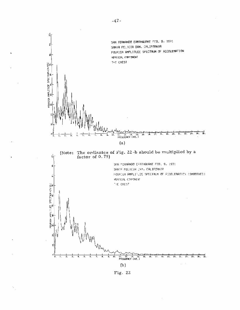
The amplification spectrum of the vertical component (Fig. 24-b)
shows two dominant peaks at about 2.20 and 5.15 Hz; it also has
several well-defined secondary peaks. The high peaks in the frequency
range 20 to 25 Hz in Fig. 24 do not look real, and they can be dis
regarded.
Finally, it is important to note the peaks in the Fourier am-
plitude spectra of the abutment records at about 10 Hz. These peaks
were caused, as indicated previously, by the vibrations of the concrete
standpipe on which the floor of the valve house rests. The strong
motion instrument was fixed on this floor rather than on firm ground.
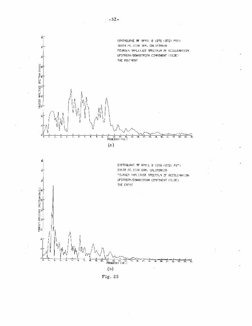
b - The 1976 Southern California Earthquake
The Fourier amplitude spectra and the amplification spectra of
the April 8, 1976 Southern California earthquake are shown in
Figs. 25 through 29.
The amplification spectrum for the upstream/downstream direc
tion (Fig. 26) again shows a dominant peak at 1.46 Hz; there is
another high peak at 2.73 Hz, and several other smaller peaks
occurred at 1.66, 1.86,2.08,2.25 and 3.81 Hz.
For the component parallel to the dam axis, shown in Fig. 29-a,
there are several well-defined strong peaks occurring at 1. 27, 1. 66,
1.86, 3.22, 4.20, 5.57 and 6.93 Hz; these peaks have almost the
same amount of participation in the response of the dam in that
direction.
The vertical component (Fig. 29 -b) shows one dominant peak at
2.25 Hz, in addition to several high secondary peaks at 0.98,1.76,
3.03, 3.22,4.10 and 6.64 Hz.

-51-
Tables 5, 6 and 7 contain the frequencies and relative heights
of peaks in the three components I amplification spectra for the two
earthquakes. They also show the effects of smoothing on both the
frequencies and the amplitudes for the 1971 San Fernando earthquake.
These tables further indicate that the two earthquakes have shaken
the darn at essentially the same resonant frequencies.
-52-
ERRTHQURKE ~F RPR1L 8 1976 (0721 PST)
SRNTA FELIC1R ORM. CRLIF~RN1A
F~UR1ER RMPLITUDE SPECTRUM ~F ACCELERRTI~N
UPSTRERM/D~WNSTRERM C~MP~NENT (SI2E)
THE ABUTMENT
I. 2. 3. ~. 5. 6. 7. 8. 9. 10. ll. 12. 13. '".FREQUENCY (HZ.)
(a)
ro
ERRTHQURKE ~F RPR1L 8 1976 (0721 PST)p: SRNTR FELIC1R DRM. CRLlmRN1R
F~UR1ER RMPLITUDE SPECTRUM ~F RCCELERRT1~N
ti UPSTRERM/D~WNSTREAM C~MP~NENT (SI2ElTHE CREST
~.en~.....'"U
I
'":::J •o:rot;~
WCLenw<oo~
i"-.JCL."'Na:~
0:w0::0 •
~~
~
,;
<0o. I. 2. 15. l6. 17. 18. 19. 20. 21. 22. 23. ~. 25.
(b)
Fig. 25

o en ,p r--
o ;::u:i
a: a: z o ~ ~If)
a: u U-~ -.J
.(L
::!'
~ a:
0') N
ERRT
HQUR
KE~F
RPRI
L8
1976
(072
1PS
T)
SRNT
RFE
LIC
IRDR
M.CRLIF~RNIR
RMPLIFICRTI~N
SPEC
TRUM
UPSTRERM/D~WNSTRERM
C~MP~NENT
(S12
E)
I U"1 W I
oI
I,
r,
,V
I!
-I
!!
Yt
II
''-J
I!
,,y
lV'
,,
II
!
O.
I.2
.3
.ll
.5
.6
.7
.8
.9
.10
.11
.12
.13
.Il
l.15
.16
.1
7.
18
.19
.2
0.
21
.2
2.
23
.2
ll.
25FR
EQUE
NCY
(HZ
.)
Fig
.26

-54-
EARTHQUAKE ~F APRIL 8 1976 (0721 PST)
SANTA FELICIA DAM. CALIF~RNIA
F~URIER AMPLITUDE SPECTRUM ~F ACCELERATI~N
C~MP~NENT PARALLEL T~ DAM AXIS (S78W)
THE ABUTMENT
(a)
EARTHQUAKE ~F APRIL 8 1976 (0721 PST)
SANTA FELICIA DAM. CALIFDRNIA
FDURIER AMPLITUDE SPECTRUM ~F ACCELERATIDN
CDMPDNENT PARALLEL T~ DAM AXIS (S78W)
THE CREST
,~"'"''6. 7. 8. 9. 10. 11. 12. 13. Ill. 15. 16. 17. 18. 19. 20. 21. 22. 23. 2G. 25.fRECUENCY (HZ.)
(b)
Fig. 27

-55-
ERRTHQURKE ~F RPRIL 8 1976 (0721 PST)
SRNTR FELICIR DRM. CRLIF~RNIR
F~URIER RMPLITUDE SPECTRUM ~F RCCELERRTI~N
VERTICRL C~MP~NENT
THE RBUTMENT
23. 21l. 2."i
(a)
ERRTHQURKE ~F RPRIL 8 1976 (0721 PST)
SRNTR FELICIR DRM. CRLIF~RNIR
F~URIER RMPLITUDE SPECTRUM ~F RCCELERRTI~N
VERTICRL C~MP~NENT
THE CREST
11. 12. 13. II/., 15. 16. 17. lB. 19. 20. 21. 22. 23. 214 2'5FREQUENCY (HZ.)
(b)
Fig. 28

oo-Wcr:IT:
is
.-56 -
ERRTHQURKE OF RPRIL 8 1976 (0721 PST)
SRNTR FELICIR DRM. CRLIFORNIR
RMPLIFICRTION SPECTRUM
COMPONENT PRRRLLEL TO DRM RXIS (S78W)
11. 12. 13. Ii.!. 15. 16. 17. lB. 19. 20. 21. 22. 23. 2lL 25.FREQUENCY (HZ.)
(a)
ERRTHQURKE OF RPRIL 8 1976 (0721 PST)
SRNTR FELICIR DRM. CRLIFORNIR
RMPLIFICRTION SPECTRUM
VERTICRL COMPONENT
(b)
Fig. 29
25.

TA
BL
E5
Ob
serv
ed
Natu
ral
Fre
qu
en
cie
san
dM
od
al
Part
icip
ati
on
so
fth
eS
an
taF
eli
cia
Darn
Du
rin
gS
an
Fern
an
do
Eart
hq
uak
e(1
97
1)
an
dS
ou
thern
Cali
forn
iaE
art
hq
uak
e(1
97
6)
Up
stre
am
/Do
wn
stre
am
Co
mp
on
en
t(5
11
.6
°E)
San
Fern
an
do
Eart
hq
uak
e,
Feb
ruary
9,
19
71
So
.C
al.
Eart
hq
uak
eA
pri
l8
,1
97
6
Am
pli
ficati
on
Sm
oo
thed
Am
pli
ficati
on
Am
pli
ficati
on
Sp
ectr
um
Sp
ectr
um
Sp
ectr
um
Fre
qu
en
cy
Am
pli
ficati
on
Part
icip
ati
on
Fre
qu
en
cy
Am
pli
ficati
on
Part
icip
ati
on
Fre
qu
en
cy
Am
pli
ficati
on
Part
icip
ati
on
(Hz)
Rati
oF
acto
r(H
z)
Rati
oF
acto
r(H
z)R
ati
oF
acto
r
1.1
03
.86
0.3
01.
103
.21
0.3
6-
--
1.4
61
2.7
31.
001
.44
9.0
21.
00
1.4
63
.33
1.0
01.
66
2.2
90
.69
1.8
34
.80
0.3
81.
81
3.7
20
.41
1.8
61.
610
.48
2.0
59
.62
0.7
62
.03
3.9
40
.44
2.0
81.
73
0.5
22
.27
3.3
60
.26
2.2
72
.83
0.3
12
.25
1.7
80
.53
2.4
72
.73
0.2
12
.47
1.8
80
.21
--
-2
.88
2.1
50
.17
2.8
81
.36
0.1
52
.73
3.0
50
.92
3.1
32.
250
.18
3.1
02
.25
0.2
53
.13
1.05
0.3
23
.49
2.2
00
.17
3.4
71.
31
0.1
43
.61
1.
16
0.3
53
.96
7.4
60
.59
3.9
32
.97
0.3
33
.81
1.3
50
.41
4.2
71.
61
0.1
34
.25
1.4
50
.16
4.0
01
.03
0.3
14
.93
2.3
10
.18
4.9
01
.07
0.1
2-
--
5.0
81.
92
0.1
55
.08
1.3
60
.15
--
-5
.40
1.96
0.1
55
.32
1.3
90
.15
--
-5
.93
2.7
20
.21
5.9
31
.32
0.1
5-
--
7.2
51.
39
0.1
18
.12
1.2
00
.09
8.1
10
.57
0.0
6-
--
I\.
n ......,
I

TA
BL
E6
Ob
serv
ed
Natu
ral
Fre
qu
en
cie
san
dM
od
al
Part
icip
ati
on
so
fth
eS
an
taF
eli
cia
Darn
Du
rin
gS
an
Fern
an
do
Eart
hq
uak
e(1
97
1)
an
dS
ou
thern
Cali
forn
iaE
art
hq
uak
e(1
97
6)
Co
mp
on
en
tP
ara
llel
toD
arn
Ax
is(S
78
.6
°W)
San
Fern
an
do
Eart
hq
uak
e,
Feb
ruary
9,
19
71
So
.C
al.
Eart
hq
uak
eA
pri
l8
,1
97
6
Am
pli
ficati
on
Sm
oo
thed
Am
pli
ficati
on
Am
pli
ficati
on
Sp
ectr
um
Sp
ectr
um
Sp
ectr
um
Fre
qu
en
cy
Am
pli
ficati
on
Part
ieip
ati
on
Fre
qu
en
cy
Am
pli
ficati
on
Part
icip
ati
on
Fre
qu
en
cy
Am
pli
ficati
on
Part
icip
ati
on
(Hz)
Rati
oF
acto
r(H
z)
Rati
oF
acto
r(H
z)R
ati
o'
Facto
r
0.9
92
.10
0.2
50
.99
2.2
00
.33
--
-1
.3
48
.51
1.0
01
.3
56
.59
1.
00
1.2
72
.06
1.
00
1.
70
4.5
90
.54
1.7
04
.00
0.6
11
.6
61
.3
80
.67
1.
87
6.5
40
.77
1.8
64
.07
0.6
21
.8
61
.50
0.7
32
.03
4.9
80
.59
2.
152
.93
0.4
42
.15
0.7
80
.38
2.3
28
.52
1.0
02
.32
4.1
00
.62
--
-2
.88
7.0
60
.83
2.9
13
.51
0.5
32
.64
0.7
80
.38
3.2
24
.95
0.5
83
.15
3.4
80
.53
3.
Z2
1.
87
0.9
13
.52
8.2
90
.97
3.4
93
.20
0.4
93
.71
1.
130
.55
3.8
52
.91
0.3
4-
--
--
-4
.03
3.9
70
.47
4.0
32
.8
00
.43
4.2
01
.6
30
.79
4.4
43
.55
0.4
24
.42
2.4
00
.36
4.5
90
.90
0.4
44
.86
7.6
60
.90
4.8
84
.91
0.7
5-
--
5.4
24
.54
0.5
35
.44
2.5
50
.39
5.5
71
.6
20
.79
5.9
81
.5
10
.18
--
--
--
6.1
31
.4
90
.18
6.1
01
.13
0.1
76
.05
1.
110
.54
--
--
--
6.9
31
.9
00
.92
7.9
62
.84
0.3
37
.91
1.2
10
.18
7.5
20
.82
0.4
0-
--
--
-9
.96
1.7
20
.83
I V1
cc J

TA
BL
E7
Ob
serv
ed
Natu
ral
Fre
qu
en
cie
san
dM
od
al
Part
icip
ati
on
so
fth
eS
an
taF
eli
cia
Darn
Du
rin
gS
an
Fern
an
do
Eart
hq
uak
e(1
97
1)
an
dS
ou
thern
Cali
forn
iaE
art
hq
uak
e(1
97
6)
Vert
ical
Co
mp
on
en
t
San
Fern
an
do
Eart
hq
uak
e,
Feb
ruary
9,
19
71
So
.C
al.
Eart
hq
uak
eA
pri
l8
,1
97
6
Am
pli
ficati
on
Sm
oo
thed
Am
pli
ficati
on
Am
pli
ficati
on
Sp
ectr
um
Sp
ectr
um
Sp
ectr
um
Fre
qu
en
cy
Am
pli
ficati
on
Part
icip
ati
on
Fre
qu
en
cy
Am
pli
ficati
on
Part
icip
ati
on
Fre
qu
en
cy
Am
pli
ficati
on
Part
icip
ati
on
(Hz)
Rati
oF
acto
r(H
z)R
ati
oF
acto
r(H
z)R
ati
oF
acto
r
0.6
32
.02
0.1
9-
--
--
-0
.95
2.4
90
.24
.95
1.8
40
.31
0.9
84
.45
0.6
31
.37
6.3
80
.62
1.3
72
.68
0.4
4-
--
--
--
--
1.4
60
.97
0.1
41
.81
4.5
80
.44
1.7
83
.22
0.5
31.
76
3.8
60
.54
2.1
71
0.3
61.
00
2.2
06
.03
1.0
02
.25
7.1
21
.00
2.3
45
.28
0.5
12
.34
4.8
90
.81
2.6
41
.8
40
.26
2.9
35
.67
0.5
52
.91
2.7
00
.45
3.0
33
.98
0.5
63
.22
3.4
40
.33
3.2
02
.38
0.3
93
.22
3.0
00
.42
3.5
44
.52
0.4
43
.54
-3
.52
1.4
60
.21
3.6
94
.08
0.3
93
.64
2.6
10
.43
3.7
11
.84
0.2
63
.98
3.4
40
.33
3.9
82
.51
0.4
24
.10
3.0
20
.42
4.3
22
.38
0.2
3-
--
--
-4
.59
3.9
10
.38
4.5
92
.66
0.4
4-
--
5.1
55
.82
0.5
65
.15
4.6
80
.78
5.0
70
.79
0.1
15
.32
3.2
40
.31
--
-5
.47
1.0
50
.15
5.7
14
.81
0.4
6-
--
--
-6
.03
4.
70
0.4
55
.98
2.9
60
.49
--
-6
.23
3.4
20
.33
6.3
02
.06
0.3
46
.15
1.5
70
.22
6.5
22
.97
0.2
9-
--
6.6
43
.74
0.5
37
.18
1.5
40
.15
7.1
51.
28
0.2
17
.13
1.2
20
.17
7.5
95
.09
0.4
97
.59
2.0
70
.34
--
-7
.93
1.5
20
.15
--
--
--
8.1
82
.44
0.2
48
.13
1.3
80
.23
--
-
I Vl
cD I
-60-
A-IV -2 Relative Acceleration, Velocity and Displacement
It is important to know the motion of the crest with respect to
that of the abutment of the dam, as it will be employed later on.
From the two recorded accelerograms of the 1971 San Fernando
earthquake, the relative acceleration, velocity and displacement of
the crest with respect to the abutment was obtained by taking the time
differences of the two accelerograms (Table 3) into consideration.
Figures 30, 31 and 32 show the subtracted and corrected relative
values of acceleration, v~locity and displacement of the 1971
San Fernando earthquake; they all start at 3.34 seconds on the un
distorted crest record of Fig. 6 -b. The subtraction of the long
period ground displacement has not resulted in even comparatively
smooth curves for relative displacement, as anticipated; instead, the
relative displacement of the two horizontal components still includes
even longer fluctuations with longer period of about 15 seconds; this
could be due to a processing error in the digitizing of the accelero
grams.
Comparing Figs. 9 and 31 (which are on different time scales),
it is seen that for the upstream/downstream component, the relative
velocity and displacement still show an apparent dominant period of
about 0.7 seconds superimposed on long period fluctuations. Some
possible contributions of the higher modes to the acceleration, velocity
and displacement are still evident in these figures. Similarly, by
comparing Figs. 11 and 31, one can see the response of the fundamen
tal mode at period of about 0.75 seconds as well as contributions from
the higher modes.
-61-
Since for the 1976 earthquake, the durations of the crest and
abutment records are not the same, only part of the crest record is
considered in calculating relative motion. And since the two recorded
accelerograms have an accurate time correspondence, the relative
velocity and displacement of the crest with respect to the abutment
can be obtained by subtracting the calculated ground velocity and dis
placement from the record measured at the crest. The subtracted
and corrected relative acceleration, velocity and displacement of only
the upstream/downstream component are plotted in Fig. 33. The
relative velocity curve shows the response of the predominant fun
damental mode with apparent period of about 0.69 seconds as well
as some contribution from higher modes.

SRN
FERN
RNDO
ERRT
HQUR
KEFE
B.
9.
1971
SRNT
RFE
LIC
IRDR
M.
CRLI
FORN
IR
RELR
TIV
ERC
CEL
..V
EL.
RND
DIS
P.OF
CRES
TW
.R.T
.RB
UTM
ENT
COM
PONE
NTRO
TRTE
DTO
UPST
RERM
/DOW
NSTR
ERM
DIR
ECTI
ON
(Sll
.WE)
o =>'
NF
ILT
ER
ING
TY
PE
A2
02~ ~
,rr
.,
rr
O
,~
,~
,~.
,U
o
,U
N,
rr~
,o
,~I'
I!
I 0'
N I
20.
25.
30.
35.
TIM
EIN
SECO
NDS
O.
o>
I- ......
,U
'"
8-
,-l
",
,~~
,!,
J,
I
tn",N
U w.
en", ,,
L U
O.
cDL U ~=>'
I 2 w
·L
OW U rr -l'
~1
......
.o
'?II!!
!\/!
I!
I!
!
O.
5.
10.
15.
20.
25.
30.
35.
ijO.
ij5.
50.
55.
TIM
EIN
SECO
NDS
Fig
.3
0
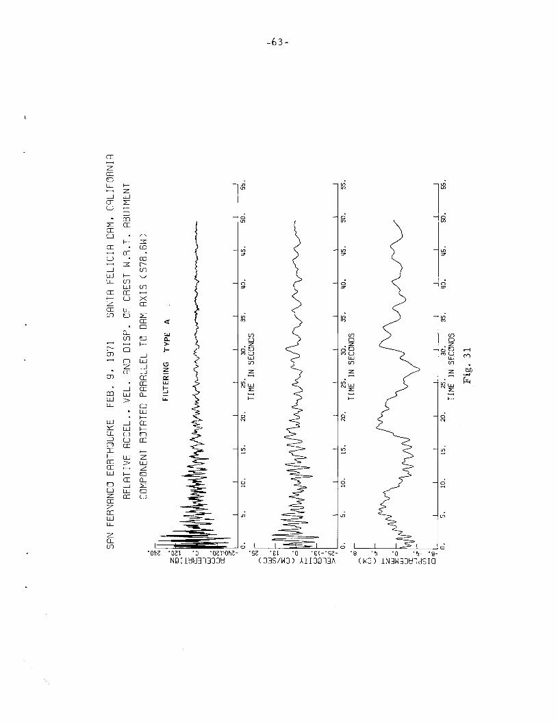
SRN
FERN
RNDO
ERRT
HQUR
KEFE
B.
9,19
71SR
NTR
FELI
CIR
DRM
,CR
LIFO
RNIR
RELR
TIV
ER
CC
EL.,
VEL
.RN
DD
ISP.
OFCR
EST
W.R
.T.
RBUT
MEN
T
COM
PONE
NTRO
TRTE
DPR
RRLL
ELTO
DRM
RXIS
CS7
8.6W
)C;
;=1
'N .1
"~
FIL
TE
RIN
GT
YP
EA
20
ON
~-
~ 0:
a::
'W
O
---1
W.
Uo
UN
0:;
:';
=1' N I
O.
5.
10.
15.
20.
25.
30.
35.
ItO.
ItS.
50.
55.
lfl_
TIM
EIN
SECO
NDS
,.....N ~~~
~~!IA~
I 0'
lJ,J
•A
•II
•1
\I
~.
0>- ~ ~
.u
",
0-
---1
'.W
tn>
NI
O.
5.
10.
15.
20.
25.
30.
35.
itO
.It
S.50
.55
.
w-
TIM
EIN
SECO
NDS
,.....
:::E
U ~=1'
~ 2 W·
:::E
OW U 0
:--
-1'
a..'f
Ul~
.o
wI
O.
5.
10.
15.
20
.25
.30
.35
.ItO
.1t
5.50
.5
5.
TIM
EIN
SECO
NDS
Fig
.31
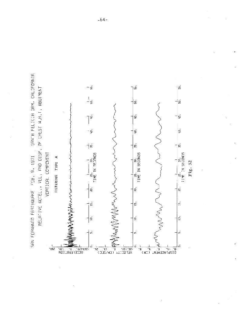
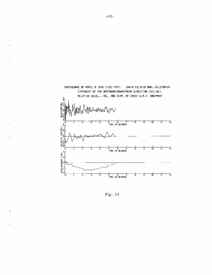
-65-
EARTHQUAKE ~F APRIL 8 1976 (0721 PST) SANTA FELICIA DAM. CALIF~RNIA
C~MP~NENT ~F THE UPSTREAM/D~WNSTREAM DIRECTI~N (Sll.4E)RELATIVE ACCEL .• VEL. AND DISP. ~F CREST W.R.T. ABUTMENT
z"!:::!'>-~qUJO-J
~IJ!
~~
~l!----L._~--~---;:--,L---,-----:!--~-----!,----,L--~-----:~---:-'------:-:!o. I. 2. 3. ij. 5. 6. 7. 8. 9. 10. II. 12.TI ME IN SECONDS
I. 2. 3. ij. 5. 6. 7. B. 9. 10. II. 12.
N TIME IN SECONDS~
:0:
~...:>-zUJ •:0:0UJUa:-J'0..-~l.0')'
O. I. 2. 3. ij. 5. 6. 7. B. 9. 10. II. 12.TIME IN SECONDS
Fig. 33

-66-
A - V FIELD WAVE-VELOCITY MEASUREMENTS
The most reliable method of determining values of the dam's
material constants, such as elastic moduli and Poisson's ratio, is
by measuring the velocities of shear and compression (or dilatation)
waves through the material in situ.
Field wave-velocity measurements or seismic tests were carried
out for Santa Felicia Dam with the following objectives:
1 - To check the order of magnitude of the suggested shear
wave velocity (assumed constant throughout the dam) which
was estimated from the observed resonant frequency of the
amplification spectrum as well as from the use of the
existing shear -beam theories, as mentioned later.
2 - To study the variation of the shear wave velocity at various
depths in the dam, because the earth fill used for Santa
Felicia Dam was cohesive in the core and cohesionless for
the shell materials.
3 - To establish a representative and reliable mean value of the
material constants for use in the earthquake response analyses.
4 - To compare shear modulus and consequently shear strain
resulting from seismic tests with those resulting from the
two earthquakes.
The wave-velocity measurements were made using the Bison
Model 157GB Signal Enhancement Seismograph, a geophone and a
sledge hammer, shown in Fig. 34. This equipment was generously
made available by Kinemetrics, Inc., Pasadena, California.
The experimental procedures were carried out in the following
manner:
-67-
1 - A line of hammer stations was used along both the crest
and the upstream slope of the dam. First the crest was
divided into three parts, each part (about 300 ft long)
having a line of three hammer stations (about 100 ft apart)
as shown in Fig. 35. Then the seismograph was placed at
one end of each part, and the signals from the three hammer
impact stations of that part were observed; the process was
reversed at the other end. Second, the dam was struck
twice with the sledge hammer at two different points On
the upstream slope, and both the seismograph and the geo
phone were mounted on the downstream slope as shown in
Fig. 36.
2 - The seismic signals were produced by the hammer impacts
at the individual hammer stations. Then the signal
travelled through the subsurface of the dam and caused
minute vibrations of the geophone.
3 - The electrical output of the geophone was transmitted to
the seismograph where it was amplified, digitized, and
stored in electronic memory. Then the wave form was
displayed on the viewing screen where the signal could be
viewed for as long as desired, until erased, and where it
also could be photographed.
4 - The travel time of the seismic wave through the dam be
tween the hammer impact instant and any position on the
wave form could be displayed digitally to three significant
figures. Successive time measurements at increasing
hammer distance can be interpreted in terms of subsurface
structure and seismic velocities, as will be illustrated later.
-70-
To enhance the signal at any hammer or impact station, the
impact at this station was repeated so the in-phase signals, added
together, reinforce each other and give a large total signal; signals
which are randomly phased tend to cancel each other. The signals
from any impact station always arrived at exactly the same time
with respect to the impact instant (which initiated the process).
Since the summed seismic signal at all times can be observed, it
is possible to use one or two or three or as many impacts as
necessary in order to bring out the true seismic signal.
The time intervals between the initiation of a seismic wave
at the source and its arrival at the geophone, for both shear and
compression waves, were instantaneously available. Figure 35
and Tables 8 and 9 show the field time readings for the arrival of
the waves and the corresponding impact distance. The digital
readout of time appears directly above the seismic wave form on
the oscilloscope of the Bison apparatus, and by means of a visible
marker on the wave form, the digital time reading can be referenced
to any desired part of the signal such as the first motion or the
fir st peak (or trough).
The seismograph does not tell what path the travelling wave
has followed; this information can be obtained by means of seismic
graphs (plots showing the field readings versus impact distance) such
as those shown in Fig. 35. The seismic waves change in direction
as the wave velocity increases with depth continuously or as they pass
from one subsurface layer into the next; i. e., there is always re
fraction at the faces of discontinuity within the dam. In calculating
shear wave velocities from the crest measurements, it was assumed
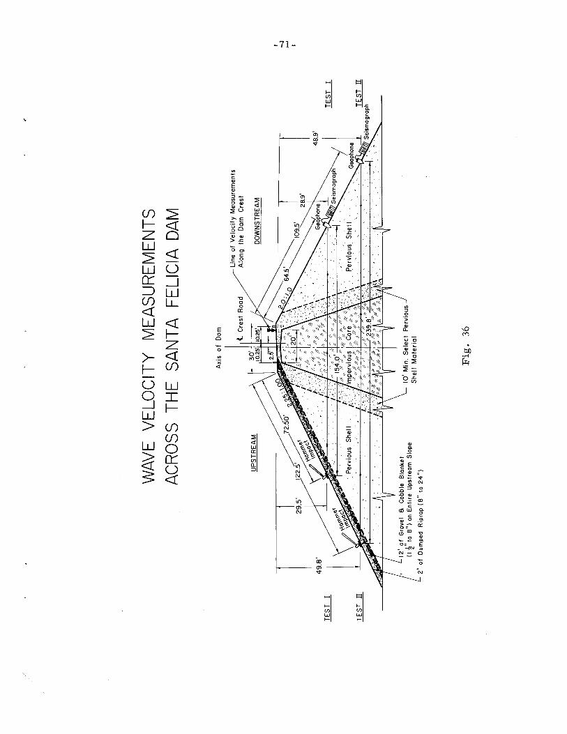
WAV
EV
ELO
CIT
YM
EA
SU
RE
ME
NTS
AC
RO
SSTH
ES
AN
TAFE
LIC
IADA
M
Axi
so
fD
am
~
TE
ST
I
TE
ST
II
UP
ST
RE
AM
49
.8' 12
'o
fG
rove
la
Cob
ble
81an
ket
(Irt
o8
")on
En
tire
Ups
trea
mS
lope
2'
of
Dum
ped
Rip
rop
(8"
to2
4")
Fig
.36
Line
of
Ve
loci
tyM
easu
rem
ents
Alo
ng
the
Dam
Cre
st
DO
WN
ST
RE
AM
48.9
'
TE
ST
I
I -J ,.....
I
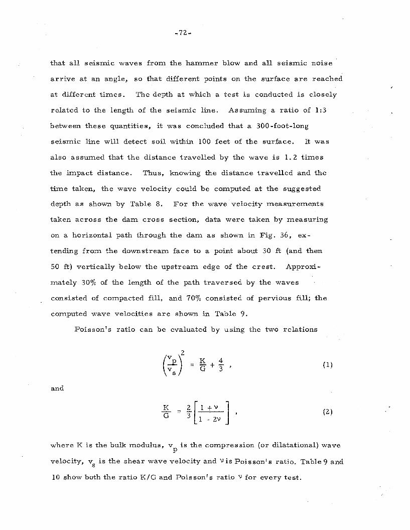
..,72..,
that all seismic waves from the hammer blow and all seismic noise
arrive at an angle, so that different points on the surface are reached
at different times. The depth at which a test is conducted is closely
related to the length of the seismic line. Assuming a ratio of 1:3
between these quantities, it was concluded that a 300 -foot-long
seismic line will detect soil within 100 feet of the surface. It was
also assumed that the distance travelled by the wave is 1.2 times
the impact distance. Thus, knowing the distance travelled and the
time taken, the wave velocity could be computed at the suggested
depth as shown by Table 8. For the wave velocity measurements
taken across the darn cross section, data were taken by measuring
on a horizontal path through the darn as shown in Fig. 36, ex-
tending from the downstream face to a point about 30 ft (and then
50 ft) vertically below the upstream edge of the crest. Approxi-
mately 30% of the length of the path traversed by the waves
consisted of compacted fill, and 700/0 consisted of pervious fill; the
computed wave velocities are shown in Table 9.
Poisson's ratio can be evaluated by using the two relations
and
K 4G + 3" ' (1)
K= ~[1+\) ],G 3 1 _ 2\)
(2 )
where K is the bulk modulus, v is the compression (or dilatational) wavep
velocity, v is the shear wave velocity and \) is Poisson's ratio. Table 9 ands
10 show both the ratio K/G and Poisson's ratio \) for every test.
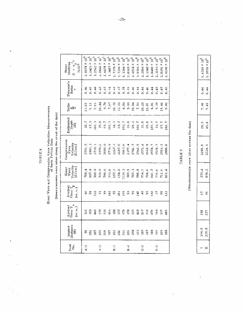
TA
BL
E8
Sh
ear
Wav
ean
dC
OIn
pre
ssio
nW
av
eV
elo
cit
ies
Measu
rem
en
tso
fS
an
taF
eli
cia
Dam
(Measu
rem
en
tsw
ere
tak
en
alo
ng
the
cre
st
of
the
dam
)
Sh
ear
Co
mp
ress
ion
Sh
ear
Test
Imp
act
Arr
ival
Arr
ival
Wav
eW
av
eE
stim
ate
dR
ati
oP
ois
so
n's
Mo
du
lus
No
.D
ista
nce
Tim
eT
Tim
eT
Velo
cit
yV
elo
cit
yD
ep
thK
Rati
o=
v2
p(f
t)s
P(f
t)G
\>G
(m.s
.)(m
.s.)
(ftl
sec)
(ft!
sec)
s1
b!f
t2
A-I
98
16
64
67
08
.42
55
6.5
32
.71
1.
69
0.4
62
.01
74
X1
06
20
23
05
89
89
7.8
29
02
.36
7.3
9.1
20
.45
3.2
40
3X
10
6
30
74
45
13
59
00
.02
73
9.1
10
2.3
7.9
30
.44
3.2
56
2X
106
A-2
10
51
75
517
20
.02
47
0.6
35
.01
0.4
40
.45
2.0
84
0X
106
20
93
35
99
78
0.0
26
00
.06
9.7
9.7
80
.45
2.4
45
8X
106
30
74
64
14
29
11
.62
73
4.9
10
2.3
7.6
70
.44
3.3
40
7X
106
B-1
10
31
88
55
65
7.5
22
47
.33
4.3
10
.35
0.4
51.
73
79
X10
6
20
63
77
10
16
54
.02
68
7.0
68
.71
5.5
50
.47
1.7
19
4X
10
6
31
14
79
14
51
23
5.3
28
63
.61
03
.74
.04
0.3
96
.13
44
X10
6
B-2
10
51
78
53
70
7.9
23
77
.43
5.0
9.9
50
.45
2.0
14
5X
106
20
83
35
98
78
7.3
27
46
.76
9.3
10
.84
0.4
62
.49
18
X10
6
31
14
60
14
09
88
.82
94
2.9
10
3.7
7.5
30
.44
3.9
30
5X
10
6
C-l
10
51
67
49
75
4.5
25
71
.4
35
.01
0.2
90
.45
2.2
88
5X
106
20
73
35
95
72
8.6
26
60
.96
9.0
12
.01
0.4
62
.13
40
X10
6
30
84
79
14
28
41
.7
25
78
.71
02
.78
.06
0.4
42
.84
80
Y:10
6
C-2
10
116
5"4
77
34
.62
57
8.7
33
.79
.39
0.4
52
.16
93
X10
6
20
33
37
89
71
1.6
29
14
.36
7.7
15
.44
0.4
72
.03
56
X10
6
30
84
85
13
38
51
.42
80
0.0
10
2.7
9.4
90
.45
2.9
14
0X
106
TA
BL
E9
(Measu
rem
en
tsw
ere
tak
en
acro
ss
the
dar
n)
I1
54
.01
98
67
77
7.8
22
98
.52
9.
57
.40
0.4
42
.43
20
X1
06
II2
39
.82
77
95
85
0.2
25
24
.34
9.8
7.4
90
.44
2.9
05
8X
106
I ......
I.N I
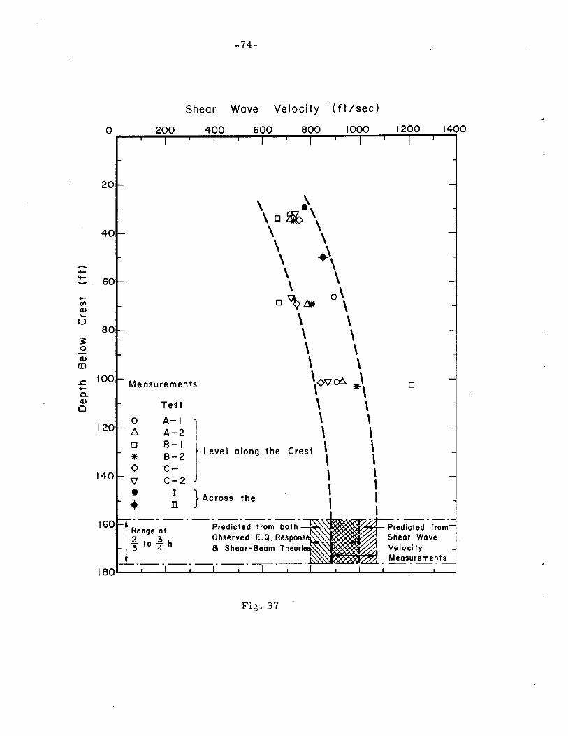
-74-
Shear Wave Velocity (ft /sec)
o 1400
20
\ ~\ o~ \
40 \ \\ \\ .\- \ \+-- 60 \ \-
+- \In o~~ 0 \Q)~ \ \0
80 \ \~0 \ \-Q) \ \co
L: 100 Measurements \0'\700 .\+- 0a.
\ \Q)Test0
0 A-I \ \120 f). A-2 \ \
0 B-1Leve I along the Crest \ \
* B-2 \ ,0 C-I
\,
140 '\7 C-2 I• I } Across the\ I• n I I
160 --------------- - -----Range of Predicted from both Predicted from
.£ to 2. hObserved E.Q. Respons Shear Wave
3 4 a Shear-Beam Theori VelocityMeasurements----------------
180
Fig. 37
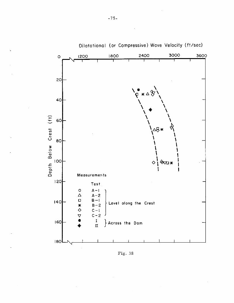
-75-
Dilatationa I (or Compressive) Wave Velocity (ft /sec)
o 3000 3600
20
\ . \
40~ * ~ ~',\ \
\ . ,\ \
..... \ \- 60 \ \
..... \~8* ~(/)
Cl) \ \~ \u 80 \\ \3: \0 \- \Cl) ,
en \100 O\~*,
.£: ,.....a. , ICl)
0 Measurements
120Test
0 A-I~ A-2
140 0 8-1'IE 8-2 Leve I along the Crest
0 C-I'V C-2
160 • I} Across the Dam• II
Fig. 38
-76-
Figure 37 shows the relationship between the measured shear
wave velocity and the suggested depth at which this velocity is estima-
ted, for the different tests; Fig. 39 shows the same relationship for
the compression wave velocity. The area between the two dashed
lines (in Figs. 38 and 39) is suggested for the region where data
points are clustered. The extrapolated region is not necessarily
representative of the darn materials.
following observations can be made:
From the two figures the
1 - The low value of v (or v ) in the region close to thes p
crest (at a depth of about 30 ft) and the relatively large
increase of v (or v ) below the crest, at a depth ofs p
about 100 ft, would seem to indicate that this darn con-
sists of mainly cohesionless materials where the shear
modulus varies with the confining pressure. It could also,
however, be due to the variable nature of the fill material
since the darn material consists of gravel, sand and silty
clay. Thus, it can be assumed that the shear wave
velocity is not constant throughout the darn.
2 - Due to the velocity variation throughout the darn, it was
thought desirable to establish a mean value for use in
dynamic respons e analyses and for use in comparing this
mean value with the value computed from the amplification
spectrum. Since measurements were not taken through the
whole depth of the darn, it was decided to take the value of
the velocity (in the extrapolated area) at a depth equal to
2 :3(s to 4) h or at approximately 158 - 177 ft below the crest.

-77 -
This gives a range of v between 870 ft/ sec and abouts
1,070 ft/sec, as compared to the computed v of 850 ft/ secs
mentioned later. Thus, the value of v computed from thes
observed earthquake response was at least of the same
order of magnitude as values determined from the wave
velocity measurements. To obtain average values of v fors
the entire dam using seismic techniques, a comprehensive
testing program would be necessary.
3 - As seen in Tables 8 and 9, the seismic tests give a mean
value for Poisson's ratio 'J of 0.45; this can be taken as
representative of the dam material. This value is also in
the same order of magnitude as that suggested by Martin
(1965) for this type of dam.
4 - In any dynamic respons e analyses, shear -beam models with
shear modulus varying with the depth (to be mentioned later)
would be more appropriate than models with constant shear
modulus to estimate dynamic shear strains and stresses.
However, it would be interesting to compare results ob-
tained by the two type s of models.
It is worthwhile to compare values of shear modulus resulting
from the measured shear wave velocity (assuming the density P is
constant throughout the dam) with those values computed from the:L
relation G(y) = SO(Y y/2)3 mentioned later. From the analysis in
section B-II, a value of vsO
= (So/p)i = 195.0 (ft 4/3 Ib- l / 6 sec-I)
was obtained, leading to So = o. 1529 X 106
; then by using Y = 129.33
3 6 .l-Ib/ft one can have G(y) = 0.6053 X 10 (y):3. This curve has been
-78-
plotted in Fig. 39 along with all the values of G from the different
tests. It is difficult to determine the exact trend of the observed dataJ,.
points but they fit reasonably well with the curve G(y) = SO(yy/2)3,
especially at shallow depths, up to 90 ft, say beyond which there is
deviation from the curve of G(y).
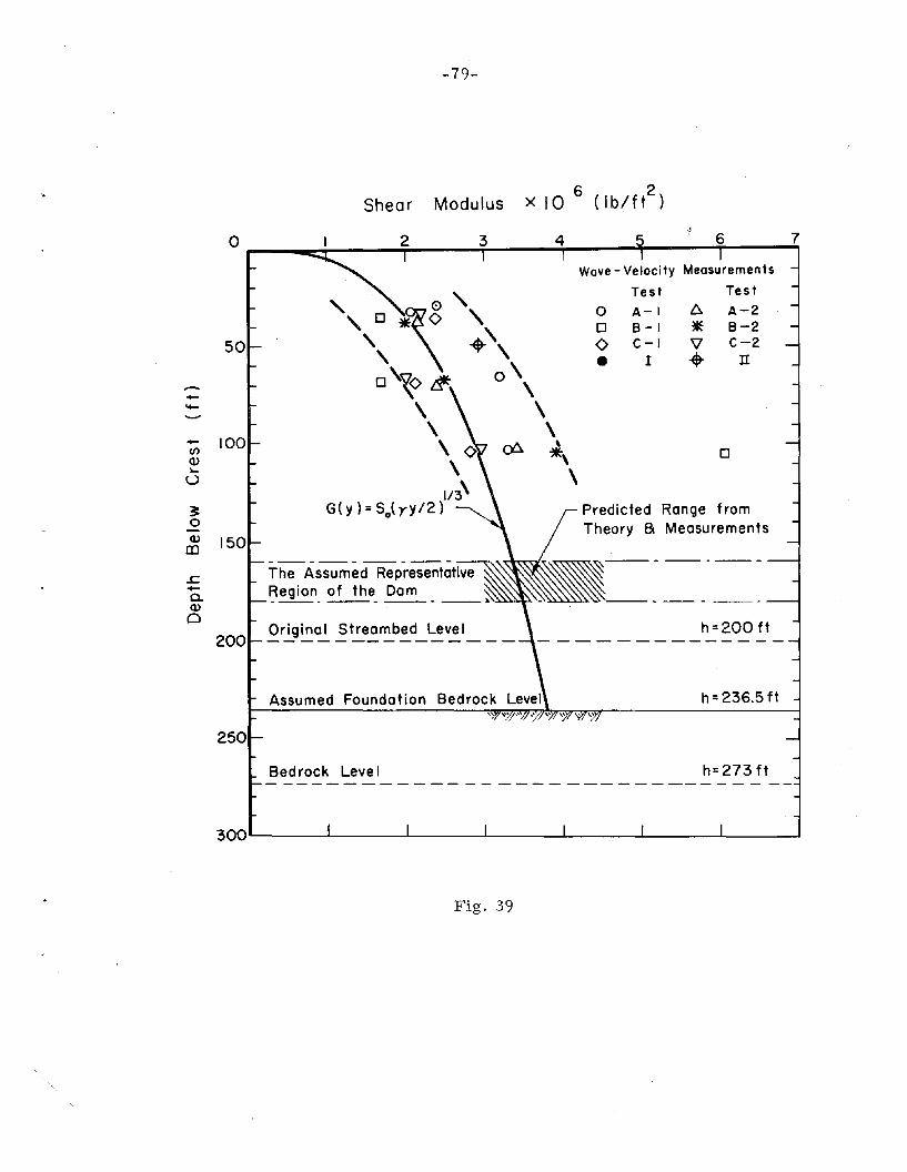
-79-
Shear Modulus x 10 6 (I b/ft2
)
h=236.5 ft
h=200 f.t
Predicted Range fromTheory 8 Measurements
Wove - Velocity Measurements
Test Test
o A-I 6 A-2o 8-1 * 8-2o C-) \l C-2• I .. n
o
Assumed Foundation
- - - - - - - - - ,-;-:-",,\."",,1w;J("\.\."0~The Assumed Representative~_eg_io_n__of_t_he__D_a_m ~,~~'--'>.>u.>..>~
Original Streambed Level
o r--__~-----=r_--_T_---:;__--+--__;r_----:.7
50
-+-'+-
+- 100(/)
Q)"-
U
30-Q) 150co
.£:+-a.Q)
0
200
250
Bedrock Level h= 273 ft
Fig. 39
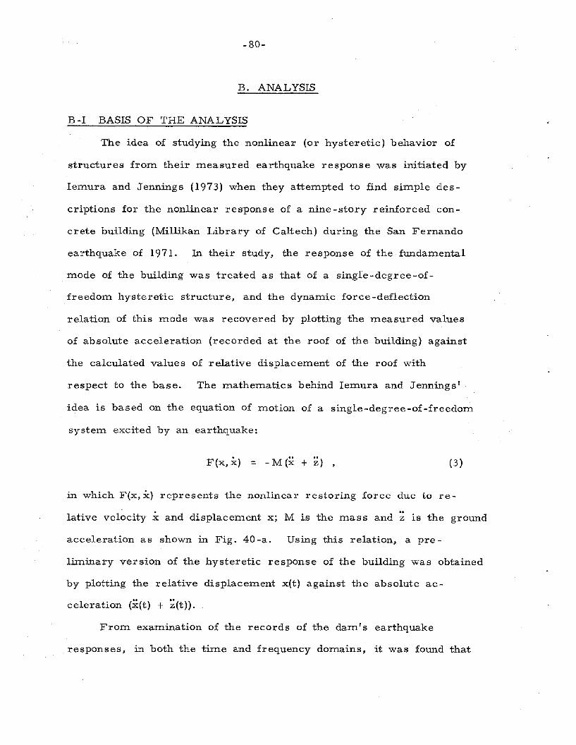
-80-
B. ANALYSIS
B -I BASIS OF THE ANALYSIS
The idea of studying the nonlinear (or hysteretic) behavior of
structures from their measured earthquake response was initiated by
Iemura and Jennings (1973) when they attempted to find simple des
criptions for the nonlinear response of a nine-story reinforced con
crete building (Millikan Library of Caltech) during the San Fernando
earthquake of 1971. In their study, the response of the fundamental
mode of the building was treated as that of a single-degree-of
freedom hysteretic structure, and the dynamic force-deflection
relation of this mode was recovered by plotting the measured values
of absolute acceleration (recorded at the roof of the building) against
the calculated values of relative displacement of the roof with
respect to the base. The mathematics behind Iemura and Jennings'
idea is based on the equation of motion of a single-degree-of-freedom
system excited by an earthquake:
F(x,x) = -M(x + z) , (3)
1n which F(x, x) represents the nonlinear restoring force due to re
lative velocity x and displacement x; M is the mass and ~ is the ground
acceleration as shown in Fig. 40 -a. Using this relation, a pre
liminary version of the hysteretic response of the building was obtained
by plotting the relative displacement x(t) against the absolute ac
celeration (x(t) + ~(t».
From examination of the records of the dam' s earthquake
responses, in both the time and frequency domains, it was found that

-81-
the dam responded primarily in its fundamental mode in the upstream/
downstream direction, although there was some vibration of the higher
modes apparent in the response and in the amplification spectra.
Consequently, the response in the fundamental mode of the dam in
its upstream/downstream direction was treated as that of a single
degree-of-freedom hysteretic structure, in order to study the dam's
nonlinear behavior. By applying Iemura-Jennings' basic idea, a
preliminary version of the hysteretic response of the earth dam was
obtained. From this, certain parameters such as equivalent soil
moduli and damping factors can be estimated.
Because most soils, including earth dam fills, have curvilinear
stress -strain relationships (Seed and Idriss, 1970) as shown in
Fig. 41, the equivalent linear shear modulus is usually expressed
as the secant modulus determined by the slope of the line joining
the extreme points of the hysteresis loops, while the damping factor
is proportional to the area inside the hysteresis loop. It is apparent
that each of these properties will depend on the magnitude of the
strain for which the hysteresis loop is determined, and thus both
shear moduli and damping factors must be determined as functions of
the induced strain in an earth dam or any soil specimen. As indicated
by Fig. 41 for large dynamic strains, such as those which would occur
in earth dams subjected to large earthquakes, the effective shear
modulus would be less than that for the low amplitude vibrations,
obtained in small earthquakes or in field tests, due to the nonlinear
hysteretic behavior exhibited by the dam's materials.
It is the purpose of this investigation to provide some data on
the dynamic shear moduli and damping factor s for the Santa Felicia Dam

-82-
(a) BASIC IDEA OF THE ANALYSIS
VERTICAL
LSllAE
r Sll.•
E
S78.6W
Equivalent S.D.O.F.
.....--...j.~i(t)i>-------=z-ol/
G
Hysteretic Reaponse
F(X,X)
//
---L-~~---X
Damping
xo
• z(t)
Real Structure
+
I ..l-----'Z~.......,;..I
(b) DIFFERENT FILTERINGS
Q.Ecec.5!UC::IU...GI-•c•..I-
TYPE A
Frequency In Hz
TYPE B
1.0
TYPE C
in Hz
Fig. 40
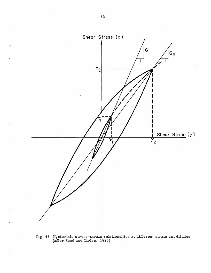
-83-
Shear Stress (T)
Shear Strain (y)
Y2
Fig. 41 Hysteretic stress -strain relationships at different strain amplitudes(after Seed and Idriss, 1970)

-84-
materials, from the earthquake observations; most available data
to date have been developed for sands and saturated clays by means
of laboratory tests.

-85-
B-II FREE VIBRATION ANALYSIS FOR EARTH DAMS
B-II-l Obtaining Natural Frequencies and Modes of Vibrationby Using Existing Shear -Beam Theories
Certain existing shear -beam theories are useful in obtaining a
check on the order of magnitude of the resonant frequencies
corresponding to peak values of the amplification spectrum curves
and in estimating the shear wave velocity of the darn material. Use
of these theories can establish a value for the shear wave velocity
(assumed, as a first approximation, constant throughout the dam) from,
for instance, the observed fundamental frequency. This estimated
value of shear wave velocity can then be used to calculate other
frequencies higher than the fundamental. Then a comparison be-
tween the values of resonant frequencies obtained from the earthquake
observations and those computed by applying the existing theories,
can be made. Actually, a visual inspection of the amplification spectra
obtained from the two earthquakes reveals that the values of the
resonant frequencies vary slightly from one earthquake to the other.
Earth darns are large three -dimensional structures constructed
from inelastic and non -homogeneous materials. Consequently, the
computation of natural frequencies and modes of vibration is extremely
difficult, and as a result, existing theories and analyses of earth
dams make many simplifying assumptions. The basic assumption in
all these theories is that of horizontal shear deformation with shear
stress uniformly distributed over horizontal planes. In this area, it
is important to mention Mononobe, et. al., (1936), Hatanaka (1955),
Ambraseys (1960), Minami (1960), Rashid (1961), Keightley (1963) and
Martin (1965). These investigators and others have contributed

-86 -
significantly to the development of the so-called shear-beam or "slice"
theories of earth dams, for models ranging from an infinitely long
beam with triangular cross -section resting on a rigid foundation,
through a triangular elastic wedge in a rectangular canyon, and a
truncated elastic wedge resting on an elastic foundation, to a case
where the shear modulus varies with the depth of the dam. For the
completeness of this report, a brief presentation of the results of
some of these theories follows.
1 - The One-dimensional Shear-beam Theory (Infinite Length)
a - Constant Shear Modulus
Dams constructed of homogeneous compacted earth fill con-
sisting of material which is cohesive in nature can, at first
approximation, be assumed to have a constant shear modulus.
The equation of motion governing free vibration of an elastic
wedge considered as a shear beam with depth h, infinite length and
constant shear modulus, G, is given by
= G[o2u+ 1.. ou]P oy2 Yoy , (3)
where u(y, t) is the displacement at depth y in the x-direction (see
Fig. 42), and P is the mass density of the dam materials.
The natural frequencies and modes of vibration can be given by
Wn
y (y)n
= 13 n J Gh p n =1,2,3, ...
n=l,2,3, ...
(4)
(5)
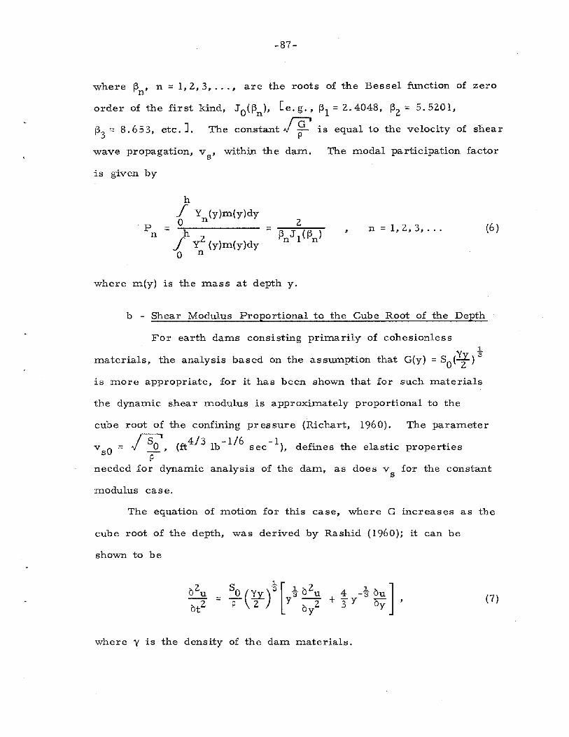
-87-
where 13 , n = 1,2,3, ... , are the roots of the Bessel function of zeron
order of the first kind, J O(13n ), [e. g., 13 1 =2.4048, 132 = 5.5201,
133
= 8.653, etc.], The constant J ~ I is equal to the velocity of shear
wave propagation, v s' within the dam. The modal participation factor
is given by
Pn =
hf Y (y)m(y)dyo n
h 2f Y (y)m(y)dyo n
n =1,2,3, ... (6 )
where m(y) is the mass at depth y.
b - Shear Modulus Proportional to the Cube Root of the Depth
For earth dams consisting primarily of cohesionless~
materials, the analysis based on the assumption that G(y) = SO(Yf) ~
is more appropriate, for it has been shown that for such materials
the dynamic shear modulus is approximately proportional to the
cube root of the confining pressure (Richart, 1960). The parameter
IS' 4/3 -1/6 -1. .v sO = ,; ~, (ft lb sec), defmes the elastlc properties
pneeded for dynamic analysis of the dam, as does v s for the constant
modulus case.
The equation of motion for this case, where G increases as the
cube root of the depth, was derived by Rashid (1960); it can be
shown to be
= So (Y.:i.)~ [ ~ a2u + 4 -~ au]P 2 Y ay2 3 y oy (7)
where y is the density of the dam materials.

-88-
TWO DIMENSIONAL SHEAR-BEAM THEORY
=.1 ~[ 2 (r7rh)2 ]1/2W nr hlp f3n + -r
First Mode of Symmetric Vi brotion
(wll • n = I, r = I )
.1b
First Mode of Antisymmetric Vibration
(w'2' n = I, r =2 )
Fig. 42

· -89-
The natural frequencies and modes of vibration are given by
Wn
an J§= 1. 2h5f6(2/y}lf6 p' n = 1,2,3, ... (8)
where the values of a are given by the zero values of the Besseln
function, JO. 2 (an }, [e. g., al
= 2.707, a2
= 5.83, a3
= 8.95, etc. J.
The modal participation factor is given by
pn =
hf Y (y)m(y)dyo n
h 2f Y (y}m(y}dyo n
=2
a 0.8 J1
2(a )n . n
n = 1,2, 3, ...
( 1O)
2 - The Two-dimensional Shear-beam Theory (Finite Length)
In this case, the darn is assumed to be a triangular wedge in
a rectangular canyon with finite length 1. and a constant shear
modulus G.
The equation of motion is given by (see Ref. 3)
2 [2 2 ]auG a u a u 1 auat2 = P ay2 + a z 2 + Yoy
The natural frequencies and modes of vibration are given by
(II)
Wnrn, r = 1, 2, 3, ... (12)
'.1, r, = l, 2, 3, ...
( 13)

-90-
where the numerical values of j3 are the same as those for the onen
dimensional case. Figure 42 shows the first symmetric and first
antisymmetric mode shapes for the two-dimensional model of the dam.
The modal participation factor is given by
pn,r =
h P../ /' y (y) Z (z) m (y) dydza ~ n r
h p. 2 2./ /' y (y) Z (z) m(y) dydza ~ n r
=8
rrr j3 Jl
(13 )n n
n,r, =1,2,3, ...
(14)
The results for the two -dimensional problem where the shear
modulus G increases as the cube root of the depth, and for the
Ambrasey's model of a truncated elastic wedge are very lengthy but
can be found in Refs. 10 and 11.
B-II-2 Calculation of Natural Frequencies for Santa Felicia Dam
Inspection of the amplification spectrum curves obtained from the
two earthquakes shows the fundamental frequency, fl
, in the upstream/
downstream direction, to be about 1.45 Hz (or WI = 2rrf l = 9.11 rad/sec).
1 - For the one-dimensional case with constant G, substituting
values of h = 236.5 and of WI = 9.11 rad/sec, in Eg.4,
gives a value of v = 895.98 ft/sec. The depth of the dams
h was taken to be the average value of the depth to the bed-
rock level(273 ft) and the depth to the original streambed
level (200 it).
2 - For the one-dimensional case with G proportional to the cube
root of the depth, the specific weight Y was assumed equal
to 129.33 lb/ft3 , which is probably representative of most of
the dam materials based on the average of the dry, moist

-91-
and saturated weight characteristics of both the core and
shell materials of Table 1. Substituting values of Y = 129.33
3 -4 2 6lb/ft (p = Y/g = 4.02 lb ft sec), h= 23 .5 ft and
WI = 9.11 rad/sec in Eq. 8 gives a value of v sO = 191.35
(ft4 / 3 lb -1/6 sec -1).
3 - For the two-dimensional theory of a triangular wedge in a
rectangular canyon, the trapezoidal canyon of Santa Felicia
Dam (Fig. 3) is represented by an equivalent rectangle of
length .P. equal to the average of the crest length and the
length of the base of the trapezoidal section, i. e. ,
.P. = 0.5 (1275 + 450) = 912.5 ft. Now substituting values
of fll
= 1.45 Hz, .P. = 912.5 ft, h = 236.5 ft in Eq. 12
gives a value of v = 848.66 ft/sec. This is fairly closes
to, but still lower than, the value obtained by the one-
dimensional theory, with G being constant.
4 - Setting fll
= 1.45 Hz in Ambrasey's truncated, finite
length shear wedge model results in a shear wave
velocity, v , of 850.23 ft/sec. This is very close to thes
value obtained from the two-dimensional shear beam theory.
5 - Martin (1965) has indicated that the fundamental mode of
vibration is generally the predominant mode controlling the
response of an earth dam, and hence it is of interest to
observe the variation of fundamental period over the range
of shear wave velocities appropriate for earth dams. He
suggested the curves of Fig. 43 which show the variation of
fundamental period for earth dams of varying heights for
both the one-dimensional theory and the two-dimensional

-92 -
6.0 r__----,-----"T-----.------r-----.------,
G == Const. (Compacted Earth Fill)
-- fl =CD ( 1- D Theory)4.5 ----i=h (2-D Theory)
Santa Felicia Dam3.0 .f/h =3.86
-0 1.5Q)f/)-
"C0 a 600~
Q)Dam Heig hta..
600
Santa Felicia
-l/h=3.86
1.5
a
2.0..----.---:--=-3.----.-----r---..,..----,)1/ ( . IG = So(yy/2 Cohesion ess
-- .e =00 (1- D Theory)
---- i= h (2-D Theory)
1.0
0.5
o-cQ)
Eo
"CC::JU.
Dam
Fig. 43 Variation of fundamental period with dam height and materialproperties (after Martin, 1965)
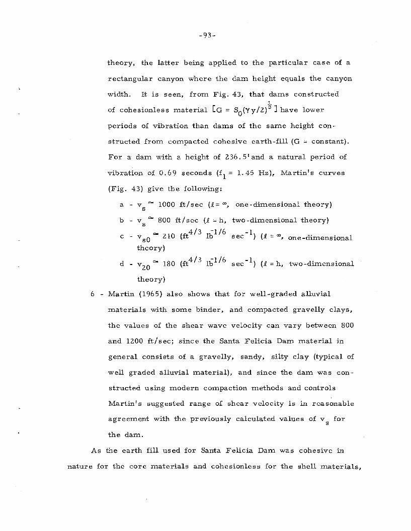
-93-
theory, the latter being applied to the particular case of a
rectangular canyon where the dam height equals the canyon
width. It is seen, from Fig. 43, that dams constructed1,.
of cohesionless material [G = SO{"yy/2)3 ] have lower
periods of vibration than dams of the same height con-
structed from compacted cohesive earth-fill (G = constant).
For a dam with a height of 236.5' and a natural period of
vibration of 0.69 seconds (fl
= 1.45 Hz), Martin's curves
(Fig. 43) give the following:
a - v """ 1000 ft/ sec (i = 00, one-dimensional theory)s
b - v """ 800 ftl sec (i = h, two -dimensional theory)s
c - v sO "'" 210 (ft4
/3 Ib l
/6
sec-I) (1 =<;:J, one-dimensional
theory)
d - v20
""" 180 (ft4 / 3 Ib'1/6 sec-I) (i =h, two-dimensional
theory)
6 - Martin (1965) also shows that for well-graded alluvial
materials with some binder, and compacted gravelly clays,
the values of the shear wave velocity can vary between 800
and 1200 ft/sec; since the Santa Felicia Dam material in
general consists of a gravelly, sandy, silty clay (typical of
well graded alluvial material), and since the dam was con-
structed using modern compaction methods and controls
Martin's suggested range of shear velocity is in reasonable
agreement with the previously calculated values of v fors
the dam.
As the earth fill used for Santa Felicia Dam was cohesive in
nature for the core materials and cohesionless for the shell materials,
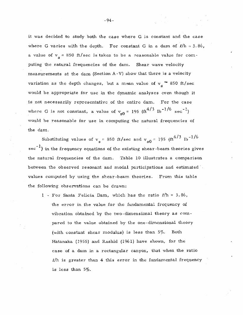
-94-
it was decided to study both the case where G is constant and the case
where G varies with the depth. For constant G in a dam of llh = 3.86,
a value of v = 850 ft/sec is taken to be a reasonable value for coms
puting the natural frequencies of the dam. Shear wave velocity
measurements at the dam (Section A - V) show that there is a velocity
variation as the depth changes, but a mean value of v Qo< 850 ft/ secs
would be appropriate for use in the dynamic analyses even though it
is not necessarily representative of the entire dam. For the case
where G is not constant, a value of vsO
= 195 (ft4 / 3 Ib- l / 6 sec-I)
would be reasonable for use in computing the natural frequencies of
the dam.
S b .. 1 / 4/3 -1/6u shtuhng va ues of v = 850 ft sec and v 0 = 195 (ft Ibs s
sec -I) in the frequency equations of the existing shear-beam theories gives
the natural frequencies of the dam. Table 10 illustrates a comparison
between the observed resonant and modal participations and estimated·
values computed by using the shear-beam theories. From this table
the following obs ervations can be drawn:
1 - For Santa Felicia Dam, which has the ratio llh = 3.86,
the error in the value for the fundamental frequency of
vibration obtained by the two-dimensional theory as com-
pared to the value obtained by the one -dimensional theory
(with constant shear modulus) is less than 5%. Both
Hatanaka (1955) and Rashid (1961) have shown, fo r the
case of a dam in a rectangular canyon, that when the ratio
llh is greater than 4 this error in the fundamental frequency
is less than 5%.

TA
BL
E10
Co
mp
aris
on
Betw
een
Ob
serv
ed
Reso
na
nt
Freq
uen
cie
sa
nd
Mo
da
lP
arti
cip
ati
on
san
dT
ho
seC
om
pu
ted
by
the
Ex
isti
ng
Sh
ear
Beam
Th
eo
ries
Ob
serv
ati
on
sT
heo
reti
cal
An
aly
ses
San
Fern
an
do
So
.C
ali
forn
iaT
wo
-dim
en
sio
na
lT
heo
rie
sO
ne-d
imen
sio
na
lT
heo
rie
sE
art
hq
uak
e,
19
71
Eart
hq
uak
e,
19
76
Sm
oo
thed
Am
pli
ficati
on
Tri
an
gu
lar
Ela
sti
cA
mb
rasey
s'
Mo
del
Co
nst
an
tS
hear
Vari
ab
leS
hear
Am
pli
ficati
on
Am
pli
ficati
on
Wed
ge
(Tru
ncate
dE
lasti
cM
od
ulu
sM
od
ulu
sS
pectr
um
Sp
ectr
um
Sp
ectr
um
(Eq
.8)
Wed
ge)
(Eq
.2)
(Eq
.5)
Fre
qP
arti
cip
ati
on
Fre
qP
art
icip
ati
on
Fre
qP
arti
cip
ati
on
Fre
qP
art
ieip
ati
on
Fre
qP
art
icip
Fre
qP
art
icip
Fre
qP
art
icip
Mo
de
fF
acto
rM
od
ef
Facto
rM
od
ef
Fa
cto
rM
od
ef
Facto
rn
,rn
,rn
PP
n/P
ln
PP
n/P
lH
zF
acto
rH
zF
acto
rH
zF
acto
rn
,rP
P!P
n,r
PP
n/P
l,1
nn
(Hz)
(Hz)
n,r
n,r
1,1
(Hz)
n,r
(Hz)
nn
1.
10
0.3
01
.10
0.3
6-
--
--
--
--
-
1.4
61
.0
01.
44
1.
00
1.4
61
.0
0{
1,
11.
45
2.0
41
.0
01
,1
1.4
52
.04
1.
00
11
.3
81
.60
1.
00
11
.4
61
.8
41
.0
0
--
--
1.6
60
.69
--
--
--
--
1.
83
0.3
81
.8
10
.41
1.
86
0.4
81
,21
.6
61
.0
20
.50
1,2
1.6
71
.0
20
.50
2.0
50
.76
2.0
30
.44
2.0
80
.52
I,3
1.9
60
.68
0.3
31
,31
.9
50
.68
0.3
3
2.2
70
.26
(2~
27
0.3
1{
2.2
50
.53
{1
.42
.32
0.5
10
.25
1,4
2.3
20
.51
0.2
52
.47
0.2
1-
--
2.8
80
.17
2.8
80
.15
2.7
30
.92
1,5
2.7
00
.41
0.2
01
,52
.71
0.4
10
.20
3.1
30
.18
3.1
00
.25
3.
13
0.3
21
,63
.11
0.3
40
.17
1,6
3.
11
0.3
4O
.1
7
0.1
7(
0.1
4{
{2
,1
3.1
91
.3
50
.66
2,1
3.2
11
.3
50
.66
23
.16
1.
06
0.6
62
3.
18
1.4
70
.80
3.4
93
.47
3.6
10
.35
2,2
3.2
90
.68
0.3
32
,23
.33
0.6
80
.66
2,3
3.4
50
.45
0.2
22
,33
.48
0.4
50
.22
0.5
9{
{{
1,7
3.5
40
.29
0.1
41
,73
.54
0.2
90
.14
3.9
63
.93
0.3
33
.81
0.4
12
,43
.67
0.3
40
.17
2,4
3.6
80
.34
0.1
72
,53
.92
0.2
70
.13
2,5
3.9
60
.27
O.
13
0.1
3{
{{
1,8
3.9
70
.26
0.1
31
,83
.97
0.2
6O
.1
34
.27
4.2
5-
4.0
00
.31
2,6
4.2
20
.23
O.
11
2,6
4.2
50
.23
0.1
11
,94
.41
0.2
30
.11
1,9
4.4
10
.23
O.
11
0.1
8{
{2
,74
.54
0.1
90
.09
2,7
4.5
4O
.19
0.0
94
.93
4.9
0-
--
I,10
4.8
60
.20
0.1
01
,10
4.8
70
.20
0.1
02
,84
.88
0.1
70
.08
2,8
4.9
00
.17
0.0
85
.08
0.1
55
.08
0.1
5-
-3
,1
4.9
71
.09
0.5
33
,1
5.1
41
.10
0.5
43
4.9
50
.85
0.5
33
4.8
91
.3
0O
.7
05
.40
0.1
55
.32
O.
15-
-2
,95
.25
0.1
50
.07
2,9
5.2
8O
.1
50
.07
5.9
30
.21
5.9
3O
.1
52
,10
5.6
30
.14
0.0
72
,10
5.6
40
.14
0.0
7
IC
DV
1 I

-96-
2 - The one -dimensional theory with shear modulus proportional
to the cube root of the dam depth gives approximately the
same fundamental frequency as does the two-dimensional
theory with constant shear modulus.
3 - The two one-dimensional theories are not good in evaluating
natural frequencies higher than the fundamental frequency.
Actually, w (or f ) in the one-dimensional theory corres-n n
ponds to w (or f ) with r = 1 in the two-dimensionalnr nr
theory.
4 - In general, values of the observed resonant frequencies vary
slightly from those predicted by the theoretical analyses as
seen from Table 10, but overall, it is fair to say that the
correspondence between observation and analysis is good
over the entire frequency range evaluated.

-97-
B-III HYSTERETIC RESPONSE OF THE FUNDAMENTAL MODE INTHE UPSTREAM/DOWNSTREAM DIRECTION
A preliminary version of the hysteretic response of Santa
Felicia Dam was obtained by plotting the measured and corrected values
of acceleration (recorded during the San Fernando earthquake of 1971),
shown in Fig. 9, against the calculated values of relative displacement,
shown in Fig. 30, using the actual time difference between the crest
and abutment records. The time dependence of the hysteretic behavior
of the dam for the first 20 seconds of the corrected record is shown
in Fig. 44; each trajectory is plotted every 0.02 seconds and each
loop is plotted every second. It is important to note that the
corrected acceleration (and consequently the calculated displacement)
was wide band-pass filtered using an Ormsby digital filter with cut-
off frequencies of 0.07 and 25 Hz and roll-off termination frequencies
of 0.05 and 27 Hz as shown in Fig. 40-b. This is standard filtering
at Caltech; in this report this filtering is designated by "filtering
type A".
It was anticipated that a reasonable estimate of the first-mode
hysteresis of the dam, during the first 20 seconds of the response,
would be obtained, because the first mode of the vibration predominates
at this time. However, the first portion of the response (0 to 2.0 sees)
showed marked fluctuations along the badly tangled trajectory of the
supposed first-mode hysteresis. This fluctuation and tangling was
thought to be the result of the non-negligible contributions of the higher
modes of vibration of the dam, as well as of long-period human digitiza-
Hon errors.
To obtain reasonable hysteresis loops and to remove the long-
period component (f < < 1.45 Hz) that is superimposed on the response,
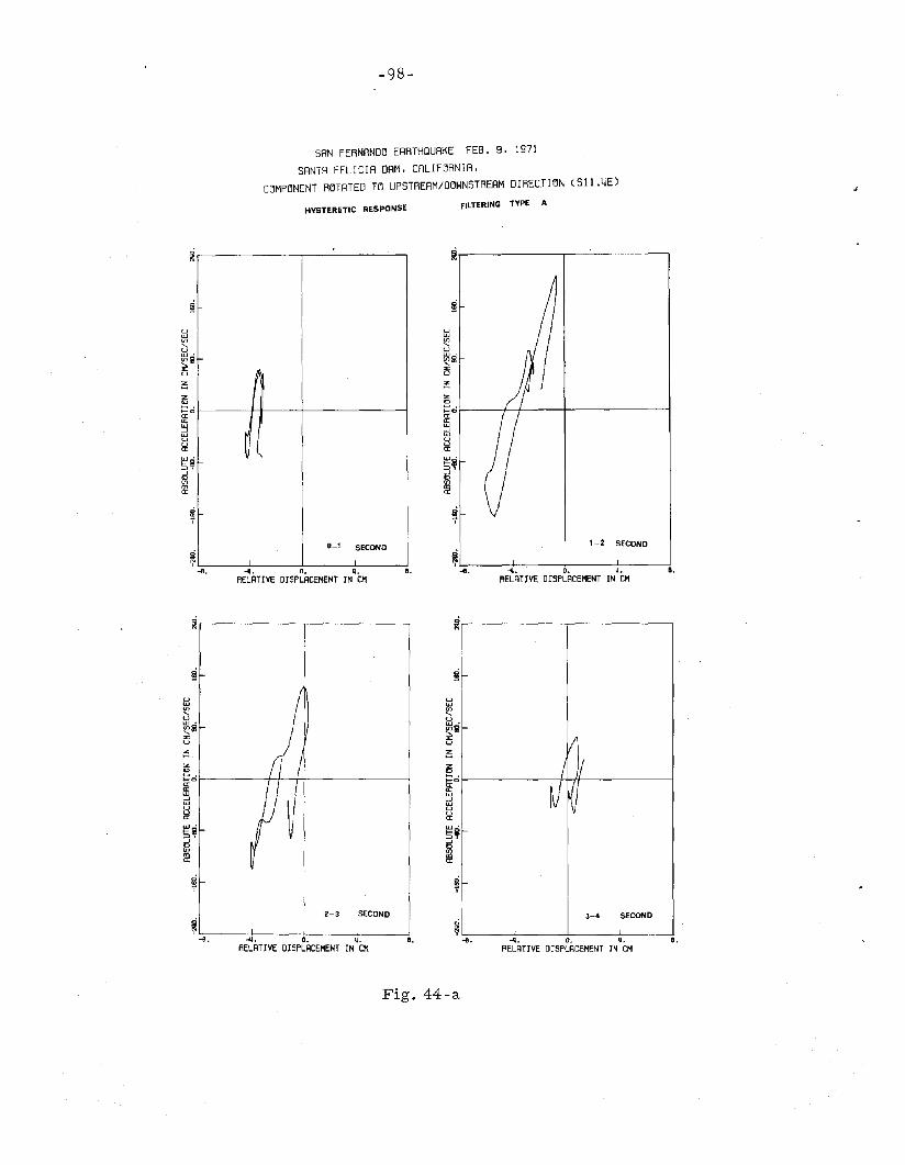
-98-
SAN FERNAND~ EARTHQUAKE FEB. 9. 1971
SANTA FELICIA DAM. CALIF~RNIA.
C~MP~NENT R~TATED T~ UPSTREAM/D~WNSTRERM DIRECTI~N (SII.4E)
HYSTERETIC RESPONSEFILTERING TYPE A
8.
1-2 SECOND
~~_-;!-~_L__-----l- _ _l-e. -41. O. II.
RELATIVE DISPLACEMENT IN CM
~r--------'--'----~
uUJ
~UUJ'
~i
~
S.~o1-----+-/'-----+--------UJ
~
8....q. o. q.RELATIVE DISPLACEMENT IN CM
~
~
Iii
,;~
~ ~
,
0-1 SECOND
uwen"'uUJen~u
8.-4. O. IJ..RELATIVE OISPLACEMENT IN CM
~
~
Iii1/
,;I )1
~R
3-4 SECOND
-e
uUJen
"'uUJ
~U
~
~r---------'------~
2-3 SECOND
~~_~~-+__-L-_-J-e. -II. O. ~ 8
RELATIVE DISPLACEMENT IN eM •
is~ .~or-------++-I+--------JUJ-'
~5¥~
Fig. 44-a

-99-
SAN FERNANDQ EARTHQUAKE FEB. 9. 1971
SANTA FELICIA DAM. CALIFQRNIA.CQMPQNENT RQTATED TQ UPSTREAM/DQWNSTREAM DIRECTIQN (S11.4E)
HYSTERETIC RESPONSE FILTERING TYPE A
/,
t
~
4-5 SECOND
~r------------r--------...,
uw(f)
"u
~il>:u
~
z~>-0a:a:w-'wu
a!~lil
~'l:la:
-8. -4. o. II.RELATIVE DISPLACEMENT IN CM
6.
§
uw(f)
"-uw·~lil>:u
~
z~.>-0~W-'Wu5!w·>-lil::>,i!5~
Iii..0
7-8.
5-6 SECOND
....q,. O. 1.1.RELATIVE DISPLACEMENT IN CM
6.
~r------------r----------,
6.-II. o. q.RELATIVE DISPLACEMENT IN CM
-8.
!i
j)P I
I
7-8 SECOND
I8.-'I. O. ~.
RELATIVE DISPLACEMENT IN CM
6-7 SECOND
~
uw(f)
"-uw·~lil>:u
~z~.)--0
a:a::w-'wuua:
~~i!5(f)lDa:
~
~,-8.
Fig. 44-b
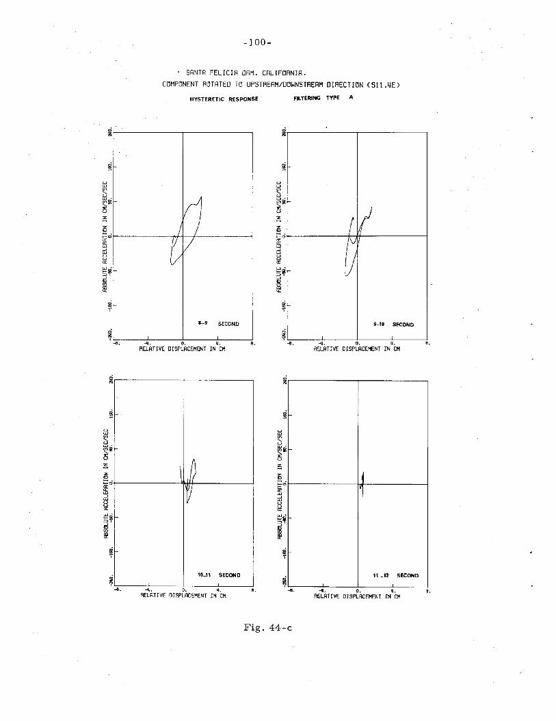
-100-
. SRNTR FELICIR DRM. CRLIFORNIR.COMPONENT RDTRTED TO UPSTREAM/DOWNSTREAM DIRECTION (Sll.4E)
HYSTERETIC RESPONSE fiLTERING TYPE A
8.-II. O. q.RELATIVE DISPLACEMENT IN eM
-6.
/!IV
rj
1
9-10 SECOND
18.-II. O. q.
RELATIVE DISPLACEMENT IN CM
Ir/ /
~V,
,
8-9 SECOND
,
8.-II. o. q.RELATIVE DISPLACEMENT IN eM
-6.
~1
11 _12 SECOND
,8.-II. O. q.
RELATIVE DISPLACEMENT IN CM-6.
lll~Iv
,
1
10-11 SECOND
,
Fig. 44-c

-101-
SRN FERNRNDO ERRTHQURKE FEB. 9. 1971SRNTR FELICIA DAM. CALIFORNIA.
COMPONENT ROTATED TO UPSTREAM/DOWNSTREAM DIRECTION CSll.4E)
HYSTERETIC RESPONSE fiLTERING TYPE A
0~
§
iii
~f
~
~
~12 _13 SECOND
.AI'V
13_14 SECOND
i-e. -'I. O. ~.
RELRTIVE DISPLRCEMENT IN CM8.
ww(f)
"w~Iil
~
-e. -'I. O. Q.
RELRTIVE DISPLACEMENT IN CJ18.
8.-'I. O. Q.
RELRTIVE DISPLACEMENT IN CJ1-e.
II
~ Ir
I
ILI6 SECOND.
ww(f)
"u
~Iil'"w~
8.-'I. O. ~.
RELRTIVE- DISPLACEMENT IN CJ1-e.
~
§
iii
If'"
\
~
~
~14 _15 SECOND
Fig. 44-d
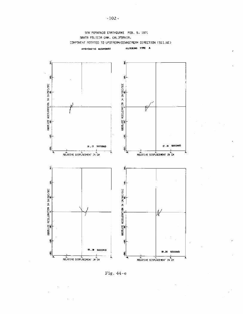
-102 -
SAN FERNANDO EARTHQUAKE FEB. 9. 1971SANTA FELICIA DAM. CALIFORNIA.
COMPONENT ROTATED TO UPSTREAM/DOWNSTREAM DIRECTION (Sll.~E)
HYSTERETIC RESPONSE FILTERING TYPE A
~
~
si
JI
~
gI
~16 _ 17 SECOND
,1/11
ILII SECOND
'\ )J
ILI9 SECOND
~
~
si
AI1J.f
~
~
~19-20 SECOND
u
Sw
§
~.
~.
-4. O. ij.
RELATfVE DfSPLACEMENT IN CM
...(1,. O. ll.RELATIVE DISPLACEMENT IN CM
e.
8.
~~.
~.
-II. O. ~.
RELATIVE DISPLACEMENT IN CM
..q. o. ~.
RELATIVE DISPLACEMENT fN CM
e.
8.
Fig. 44-e
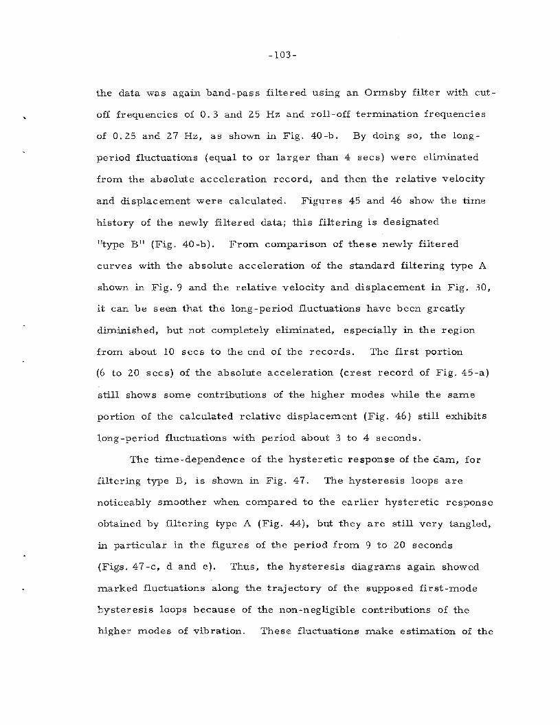
-103-
the data was again band-pass filtered using an Ormsby filter with cut
off frequencies of O. 3 and 25 Hz and roll-off termination frequencies
of 0.25 and 27 Hz, as shown in Fig. 40-b. By doing so, the long
period fluctuations (equal to or larger than 4 secs) were eliminated
from the absolute acceleration record, and then the relative velocity
and displacement were calculated. Figures 45 and 46 show the time
history of the newly filtered data; this filtering is designated
"type B" (Fig. 40-b). From comparison of these newly filtered
curves with the absolute acceleration of the standard filtering type A
shown in Fig. 9 and the relative velocity and displacement in Fig. 30,
it can be seen that the long -period fluctuations have been greatly
diminished, but not completely eliminated, especially in the region
from about 10 secs to the end of the records. The first portion
(6 to 20 secs) of the absolute acceleration (crest record of Fig. 45-a)
still shows som,e contributions of the higher modes while the same
portion of the calculated relative displacement (Fig. 46) still exhibits
long -period fluctuations with period about 3 to 4 seconds.
The time-dependence of the hysteretic response of the dam, for
filtering type B, is shown in Fig. 47. The hysteresis loops are
noticeably smoother when compared to the earlier hysteretic response
obtained by filtering type A (Fig. 44), but they are still very tangled,
in particular in the figures of the period from 9 to 20 seconds
(Figs. 47 -c, d and e). Thus, the hysteresis diagrams again showed
marked fluctuations along the trajectory of the supposed first-mode
hysteresis loops because of the non-negligible contributions of the
higher modes of vibration. These fluctuations make estimation of the

-104-
slope of each loop very difficult as well as esti:mation of the area inside the
loop - - the two para:meters necessary to esti:mate the equivalent shear
:modulus and the equivalent viscous da:mping.
Finally, very narrow band-pass filtering was used in the ex
pectation of obtaining good hysteresis loops. Because of the assu:mp
tion of a single-degree-of-freedo:m response, the effect of the second
:mode of vibration was e1i:minated as well as any higher :modes that
:may have participated in the response. Thus, a narrow band-pass
filtering around 1.45 Hz (the natural frequency of the da:m in the
upstrea:m/downstrea:m direction) was applied to the abut:ment and crest
records in order to produce reasonable loops. This had cut-off
frequencies at 1. 27 and 1. 50 Hz and roll-off ter:mination frequencies
of 1. 25 and 1. 60 Hz (Fig. 40-b). The filtered acceleration records
and the calculated velocities and displace:ments are shown in Figs. 48
and 49, which can be co:mpared with the accelerations, velocities and
displace:ments resulting fro:m both filtering type A and type B of
Figs. 9, 10, 30, 45 and 46. Fro:m this co:mparison, it is apparent
that the response of the higher :modes and the long -period fluctuations
( ;;;: 4 seconds) have been eli:minated.
Using the results shown in Figs. 48-a and 49, the relationship
between the first :mode's absolute acceleration, which is proportional
to the nonlinear restoring force (Eq. 3), and the relative displace:ment
was plotted every 0.02 sees and is given in Fig. 50.
It was particularly unfortunate that the first 3 to 3.5 sees of ,the
abut:ment record were lost due to double exposure because this part
of the record would have provided very useful infor:mation on the
s:mall a:mplitude :motion of the da:m at the beginning of the earthquake.
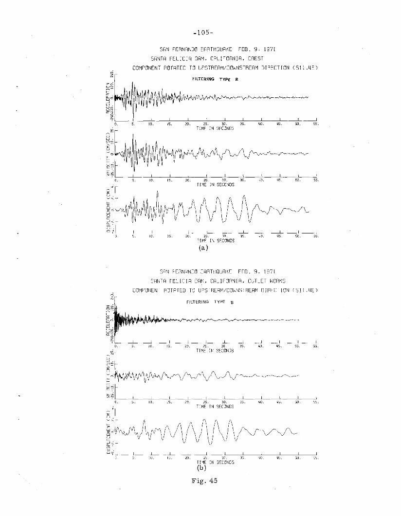
-105-
SRN FERNRNDO ERRTHQURKE FEB. 9. 1971
SRNTR FELICIR DRM. CRLI FDRN IR. CREST
COMPONENT ROTRTED TO UPSTRERM/DOWNSTRERM DIRECTION (SII .4E)0
'"N FILTERING TYPE BZoo~
f-a:tI:'W O
--'w.UoUN
cc~
O. 5. 10. 15. 20. 25. 30. 35. 40. 45. 50. 55.
iGTl ME ] N SECONDS
Uw.en",,-""U~o
>-f-
U";0---,'w~
>~
O. 5. 10. 15. 20. 25. 30. 35. 40. 45. 50. 55.
,; Tl ME ] N SECONDS~
""U~N
f-Zw·""0wUa:--' .a...~en
D'f I I I 1 I ! I IO. 5. 10. 15. 20. 25. 30. 35. 40. 45. 50. 55.
TI ME ] N SECONDS
(a)
SRN FERNRNDO ERRTHQURKE FEB. 9. 1971
SRNTR FELICIR DRM. CRLI FORN IR• OUTLET WORKS
COMPONENT ROTRTED TO UPSTRERM/DOWNSTRERM DIRECTION (SII.l.jE)0
'"NFILTERING TYPE B

SRN
FERN
RNDO
ERRT
HQUR
KEFE
B.
9.
1971
SRNT
RFE
LIC
IRDR
M.
CRLI
FORN
IR
RELR
TIV
ERC
CEL
.•V
EL.
RND
DIS
P.OF
CRES
TW
.R.T
.RB
UTM
ENT
COM
PONE
NTRO
TRTE
DTO
UPST
RERM
/DOW
NSTR
ERM
DIR
ECTI
ON
(S11
.4E
)a o
j'N
FIL
TE
RIN
GT
YP
EB
Zo
;2~
I IT
. ~o,
,~
,w
.,
,~~
IJ
CIc
'iI
~I
I~l'
I
I ......
o 0'
I
55.
55.
50.
50.
45.
40.
10.
o. o.
~~
u w.
w'"
'-~
:::E
U ~o
~ I- -.
,,
~~I
II
-l
~I
II
~~,
!,
oj'
:::E
U ~N
I Z l.LJ
•::
:Eo
l.LJ
U a: -l.
(L
'"<
n'
~.
0=rI
!!
!I
!I
!!
!!
I
O.
5.
10.
15.
20.
25.
30.
35.
40.
45.
SO.
55.
TIM
EIN
SECD
NDS
Fig
.4
6

-107-
SRN FERNRNDO ERRTHQURKE FEB. 9. 1971SRNTR FELrCIR DRM. CRLIFORNIR.
COMPONENT ROTRTED TO UPSTRERM/DOWNSTRERM DIRECTION (S11.4E)
HYSTERETIC RESPONSE FILTERING TYPE B
~.
1-2 SECOND
-2. O. 2.RELATIVE DISPLACEMENT IN CM
~r-------.,...-------,
~
uw(f)
"-uw·~~>:u
~z~.>-0a:cr:w--'wuua:w·>-~::> ,--'<>(f)
'"a:
~
.;ij:
-II.~.2. O. 2.RELATIVE DISPLACEMENT IN CM
~.
10f\)/~v
0-1 SECOND
- -
w,
~>-0a:cr:w--'wuua:
~~::>,--'<>(f)
'"a:
.;~r-----------,r---------,
~.-2. O. 2.RELATIVE DISPLRCEMENT IN CM
-~.
I~~
,
,
3-4 SECOND
,
uw(f)
"u
~~>:uz
z<>>-0a:cr:w--'tJua:
~~::>--'<>(f)
'"a:
~.-2. O. 2.RELATIVE DISPLACEMENT IN CM
2-3 SECOND
~
uw(f)
"-uw·~~>:u
~z<>>-0a:cr:w--'wuua:w·>-16::>,--'<>(f)
'"a:
~
0
'l'-~.
Fig. 47-a

-108-
SRN FERNRNDO ER~THQURKE FEB. 9. 1971
SRNTR FELICIR DRM. CRLIFORNIR.COMPONENT ROTRTED TO UPSTRERM/DOWNSTRERM DIRECTION (Sll.4E)
HYSTERETIC RESPONSE
~r----------.---------'
ww
'""-ww·~1il:l:w
3z""~ot------+-+f---------la::w--'wwwa:
~g::> ,--'""'"lDa:
ow.
4-5 SECOND
~ :;-~,.---::_t2.-------;O-. ----;2~.-----,J~.RELRTIVE DISPLRCEMENT IN CM
~,.,----------,,---------,
FILTERING TYPE B
~r---------,----------'
ww
'""-Ww·~1il:l:wZ
z"";:ol-----~--,4---I------1~woJwwa:
~~--'""'"lDa:
5-6 SECOND
~I..;;- + -:!,- ~ .-J-II. -2. O. 2. q.
RELRTIVE DISPLRCEMENT IN CM
~r-------'----------'
!£
ww'""-ww·~1il:l:w
3z"";:cia:a::w--'wwwa:w·>-1il::>.--'""'"lDa:
~
~-~.
6-7 SECOND
-2. O. 2.RELRTIVE DISPLRCEMENT IN CM
!£
ww'""-ww·~1il:l:w
3z~.>-0a:a::w--'wwwa:w·>-2::>.--'""'"lDa:
~
~-II.
7-8 SECOND
-2. O. 2.RELRTIVE DISPLACEMENT IN CM
q.
Fig. 47-b

-109-
SRN FERNRNDO ERRTHQURKE FEB. 9. 1971
SRNTA FELICIA DAM. CALIFORNIA.COMPONENT ROTATED TO UPSTREAM/DOWNSTREAM DIRECTION (SII.4E)
HYSTERETIC RESPONSE FILTERING TYPE B
~r---------,----------' ~.-------,-------~
~
uUJen"-uUJ •
~lil>:u
~ZID
>-0a:c::UJ-'UJUua:UJ •>-lil:::>,-'IDenQ)a:
~
~-~.
8-9 SECOND
-2. O. 2.RELRTlVE DISPLRCEMENT IN CM
~
uUJen"-uUJ •
~lil:0::u
~
ZID
>-0a:a:UJ-'UJUua:UJ •>-lil:::> ,-'IDenQ)a:
~
~-~.
9-10 SECOND
-2. O. 2.RELRTlVE DISPLRCEMENT IN CM
-2. O. 2.RELRT I VE DJSPLACEMENT IN CM
-\I.
f'\,~I
11 .12 SECOND
,
z~>-0a:c::UJ
u:luua:
~liI:::> ,-'IDenQ)a:
\ ()D
,
,
10_11 SECOND
,-2. O. 2.
RELRT I VE DISPLRCEMENT IN CM
z~>-0~UJ-'UJUua:
~i-'IDenQ)a:
uUJen"u
~il>:u
~
Fig. 47-c

-11 0-
SAN FERNANDO EARTHQUAKE FEB. 9. 1971SANTR FELICIA DAM. CALIFORNIA.
COMPONENT ROTATED TO UPSTREAM/DOWNSTREAM DIRECTION (S11.4E)
HYSTERETIC RESPONSE FILTERING TYPE B
~r--------.....,---------,
.I
\ /
13-14 SECOND
-2. O. 2 •RELATIVE DISPLACEMENT IN CM
.....
~1-0
15u:luucr
~il::0,-''"(f)~
~.
12 _ 13 SECOND
-2. O. 2.RELATIVE DISPLACEMENT IN CM
guw'"....uw·g:il2:u
~z'"~ .1-0cra:w-'wuucrw·I-il::0 ,-''"'"lDcr
0<D,
~-ij.
Q.-2. O. 2.RELATIVE OlSPLACEMENT IN eM
Jf/
ILII SECOND
.....
uw(f)....u
~~2:U
Z
z'"1-0cra:w-'wuucr
~il::0 ,
~lDcr
ij.2. O. 2.RELATIVE DISPLACEMENT IN CM
.....
YrV 1/
,
,
14 _15 SECOND
,-
o<D
o<D
z'"1-0cra:UJ-'UJuif~~-''"tnlDcr
uUJtn....U
~~2:U
Z
Fig. 47-d
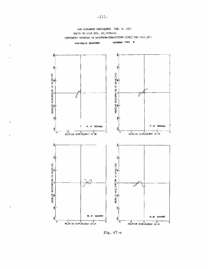
-111-
SAN FERNANDD EARTHQUAKE FEB. 9. 1971SANTA FELICIA DAM. CALIFDRNIA.
CDMPDNENT RDTATED TO UPSTREAM/DOWNSTREAM DIRECTION (SII.4E)
HYSTERETIC RESPONS~FILTERING TYPE B
L.---A
Ii
ILI8 SECOND
-2. O. 2.RELATIVE DISPLACEMENT lN CM
-2. O. 2.RELATIVE D1SPLACEMENT IN CM
-1,\.
oJ,
7,
,
16 _ 11 SECOND
,
2. O. 2.RELATIVE OlSPLACEMENT IN CM
-1,\.
~
£.--...
\
,
19-20 SECOND
-
uUJV1"U
~~z:uz
z.,>-0l!UJ.JUJUUcr
~i.J.,V1CDcr
2. O. 2.RELATIVE D1SPLACEMENT lN CM
\/)IJ ~
,
18 _19 SECOND
- -
ow
uUJV1"u
~iz:uz
Fig. 47-e
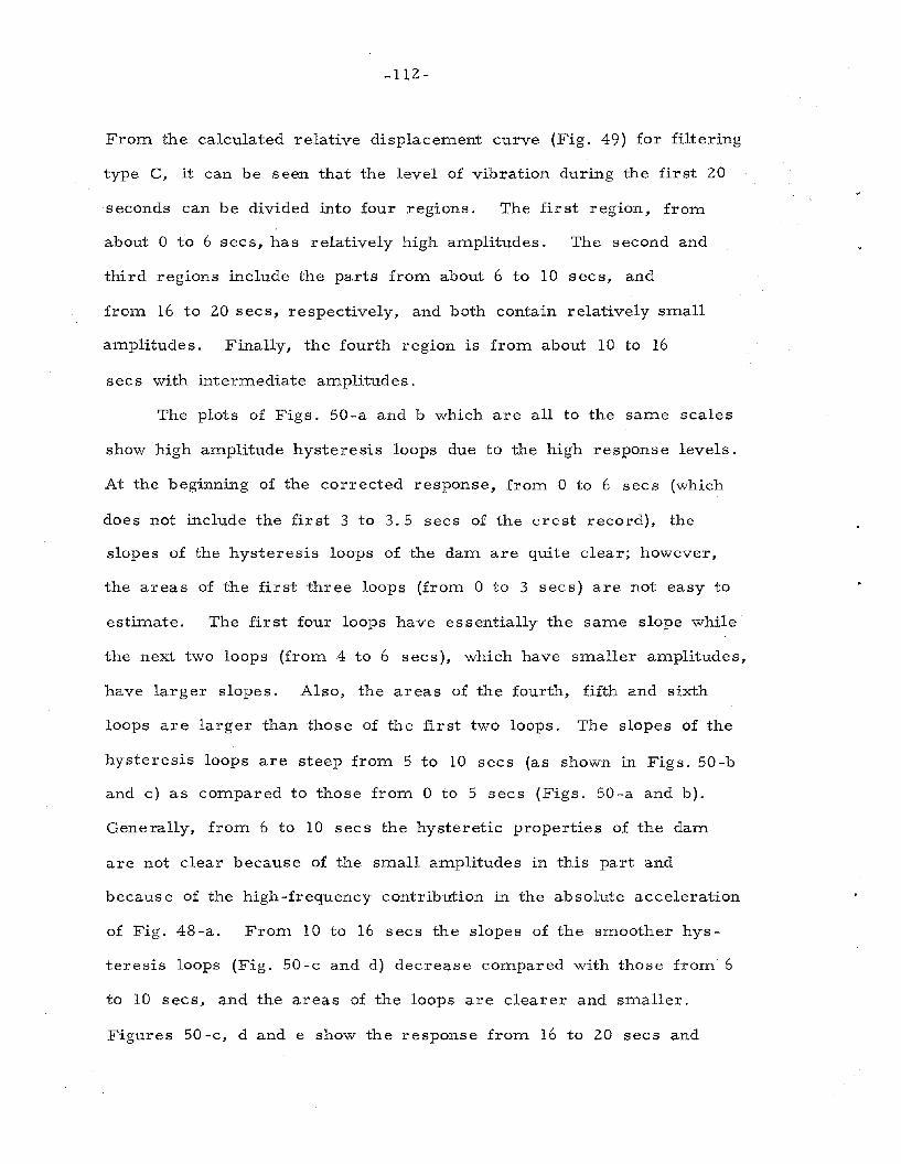
-112-
From the calculated relative displacement curve (Fig. 49) for filtering
type C, it can be seen that the level of vibration during the first 20
seconds can be divided into four regions. The first region, from
about 0 to 6 secs, has relatively high amplitudes. The second and
third regions include the parts from about 6 to 10 secs, and
from 16 to 20 secs, respectively, and both contain relatively small
amplitudes. Finally, the fourth region is from about 10 to 16
secs with intermediate amplitudes.
The plots of Figs. 50-a and b which are all to the same scales
show high amplitude hysteresis loops due to the high response levels.
At the beginning of the corrected response, from 0 to 6 secs (which
does not include the first 3 to 3.5 sees of the crest record), the
slopes of the hysteresis loops of the dam are quite clear; however,
the areas of the first three loops (from 0 to 3 sees) are not easy to
estimate. The first four loops have essentially the same slope while
the next two loops (from 4 to 6 secs), which have smaller amplitudes,
have larger slopes. Also, the areas of the fourth, fifth and sixth
loops are larger than those of the first two loops. The slopes of the
hysteresis loops are steep from 5 to 10 secs (as shown in Figs. 50-b
and c) as compared to those from 0 to 5 sees (Figs. 50-a and b).
Generally, from 6 to 10 secs the hysteretic properties of the dam
are not clear because of the small amplitudes in this part and
becaus e of the high-frequency contribution in the absolute acceleration
of Fig. 48-a. From 10 to 16 sees the slopes of the smoother hys
teresis loops (Fig. 50 -c and d) decrease compared with those from 6
to 10 secs, and the areas of the loops are clearer and smaller.
Figures 50-c, d and e show the response from 16 to 20 secs and
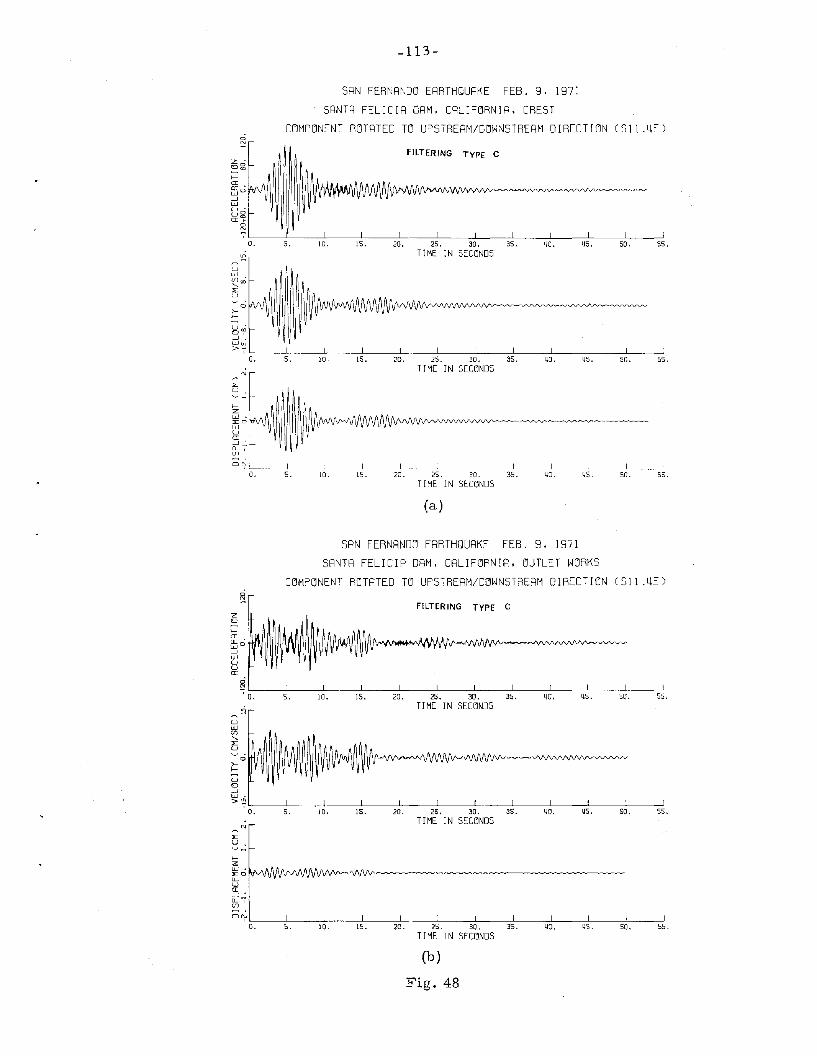

SAN
FERN
ANDO
EART
HQUR
KEFE
B.
9.19
71SR
NTR
FELI
CIA
DAM
.CR
LIFO
RNIR
RELA
TIVE
ACCE
L..
VEL
.RN
DD
ISP.
OFCR
EST
W.R
.T.
RBUT
MEN
T
COM
PONE
NTRO
TATE
DTO
UPST
REAM
/DOW
NSTR
ERM
DIR
ECTI
ON
(Sll.~E)
o N
FIL
TE
RIN
GT
YP
EC
zc;;
Ow
~ f- a a::C
;;W -1 W U
•u
5j
a,.
0 N , O.
~~ u w en
";"- L
:U ~o
>- f--
II
II
II
II
II
I5
.10
.15
.20
.25
.30
.35
.40
.45
.50
.55
.TI
ME
INSE
COND
SI ..... ..... >l>
I
§~1.
~-
55.
50.
10.
5.
u.
o"i
'-1
.W
lf)
>..
L_
--------l
I~------.L
II
II
I
O.
45.
f-
;
ffj.11
1111
111'
1111
111'
,A
',"I
1\1\
1\1\
1\/"
hd
AA
,h
hO
h"
hO
hh
yo'l\r
04
.J\J
VV
lil)
\tif
((li
irl1
\r4
JV
VV
0v
vo~
00
w u a -1•
0..
.en
'>-
<•
0";J
I[
II
II
II
f
O.
5.
10•
15.
20.
25.
30.
35.
40.
TIM
EIN
SECClI~DS
Fig
.4
9
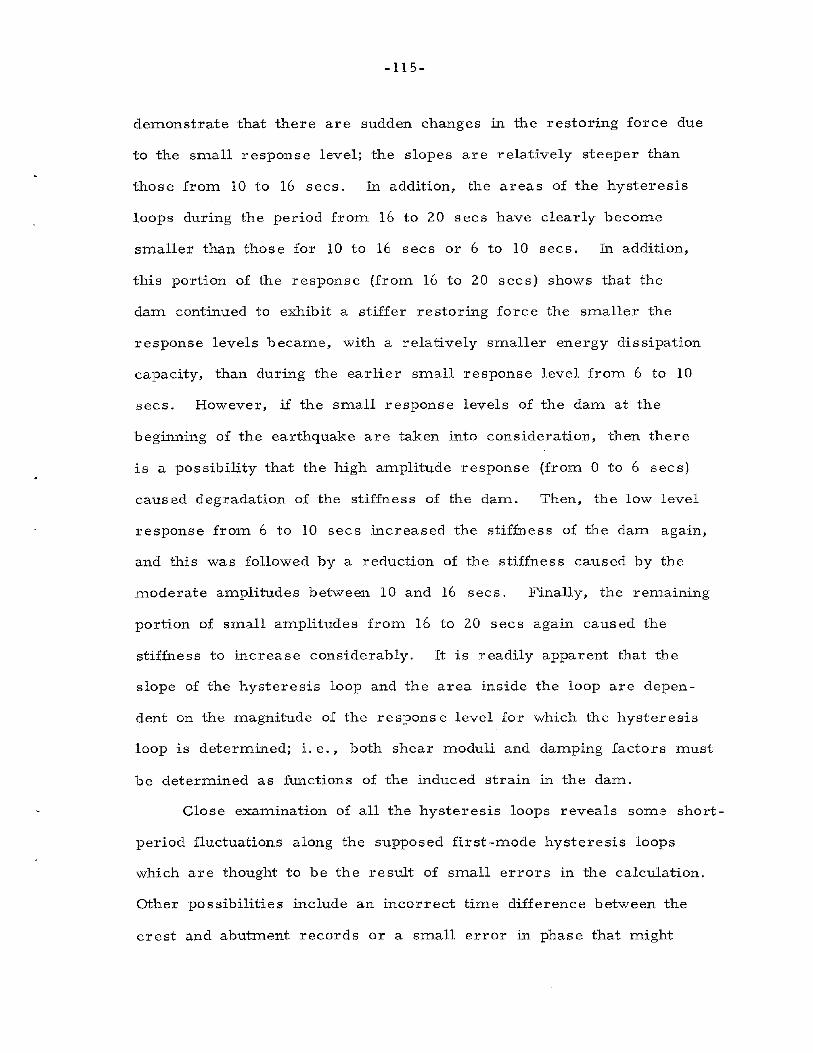
-115-
demonstrate that there are sudden changes in the restoring force due
to the small response level; the slopes are relatively steeper than
those from 10 to 16 sees. In addition, the areas of the hysteresis
loops during the period from 16 to 20 sees have clearly become
smaller than those for 10 to 16 sees or 6 to 10 sees. In addition,
this portion of the response (from 16 to 20 sees) shows that the
darn continued to exhibit a stiffer restoring force the smaller the
response levels became, with a relatively smaller energy dissipation
capacity, than during the earlier small response level from 6 to 10
sees. However, if the small response levels of the darn at the
beginning of the earthquake are taken into consideration, then there
is a possibility that the high amplitude response (from 0 to 6 sees)
caus ed degradation of the stiffness of the darn. Then, the low level
response from 6 to 10 sees increased the stiffness of the darn again,
and this was followed by a reduction of the stiffness caused by the
moderate amplitudes between 10 and 16 sees. Finally, the remaining
portion of small amplitudes from 16 to 20 sees again caus ed the
stiffness to increase considerably. It is readily apparent that the
slope of the hysteresis loop and the area inside the loop are depen
dent on the :magnitude of the respons e level for which the hysteresis
loop is determined; i. e., both shear moduli and damping factors must
be determined as functions of the induced strain in the darn.
Close examination of all the hysteresis loops reveals some short
period fluctuations along the supposed first-mode hysteresis loops
which are thought to be the result of small errors in the calculation.
Other possibilities include an incorrect time difference between the
crest and abutment records or a small error in phase that might

-116 -
have been introduced because of the application of the digital filter sub
routine to the records.
Finally, the accelerations recorded at the abutment and crest of
Santa Felicia Dam in the upstream/downstream direction during the
small earthquake of April 8, 1976 were narrow band-pas s filtered
(filtering type C), and the velocities and displacements were calculated.
Figures 51 and 52 show the filtered and calculated motions as well as
the relative motion of the crest with respect to the abutment. The
first-mode hysteretic response of the dam during the first 6 seconds
of the crest record is shown in Fig. 53. The scales of Fig. 53 are
all the same but are different from those of Fig. 50. Close
examination of the absolute filtered acceleration (the crest record in
Fig. 51-a), shows that the acceleration record started with a rela
tively high peak; this initial peak caused distortion of the first hys
teresis loop (from 0 to 1 sec) of Fig. 53 -a. The appearance of this
peak at the very beginning of the record is actually a result of the
accuracy of the digital filter calculation, because by comparing
Fig. 51-a with Fig. 13 which has the corrected crest acceleration
(filtering type A or the standard Caltech filtering), it can be seen
that the absolute acceleration started at zero and then peaked
abruptly. Thus the digital filter used in the analyses could cause
small errors in phase between the crest and abutment records, in
addition to small errors in the calculation. Also, in the filtered
absolute acceleration there is some high-frequency motion super
imposed on the smoothed curve from 0 to 2 sees; this could also be
due to error s resulting from the application of the digital filter.
In general, the slopes of the hysteresis loops resulting from the 1976
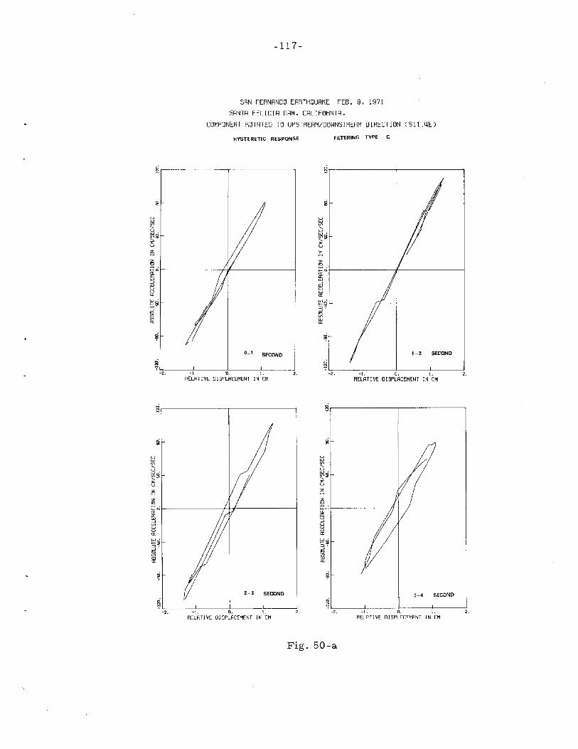
-117 -
SRN FERNRNDO ERRTHQURKE FEB. 9. 1971SRNTR FELICIR DRM. CRLIFORNIR.
COMPONENT ROTRTED TO UPSTRERM/DOWNSTRERM DIRECTION CS11.4E)
HYSTERETIC RESPONSE
~,--------~--------.,
FILTERING TYPE C
N,----------r-----------,
-I. '0. I.RELAT I VE DISPLACEMENT IN CM
Iii
uW
!Cuw'!Cg:cu
isz.,;:0a:a::W-'WUua:W'
~~-'.,<nCOa:
~
~-2,
0-1 SECOND
2,
Iii
uW<n
"uW •!Cg:cu
isz.,.... 0a:a::W-'Wuua:W'.... g:::>,-'.,<n£Da:
~
~-2. -I. O. l.
RELATI VE DISPLACEMENT IN CM2.
N,----------r-----------, N,-----------,----------,
Iii
uW<n
"uW •
~~u
isz.,""0a:a::W-'WUua:
~g:::>,-'.,<n£Da:
~
~-2. -I. Q. 1.
RELATIVE DISPLACEMENT IN CM2.
oi
uW<n
"uW •!Cg:cu
isz.,""0a:a::W-'WUua:W·.... g:::>,-'.,<n£Da:
~
0
-2.
3-4 SECOND
-1. O. 1.RELATI VE DISPLACEMENT IN CM
2.
Fig. 50-a
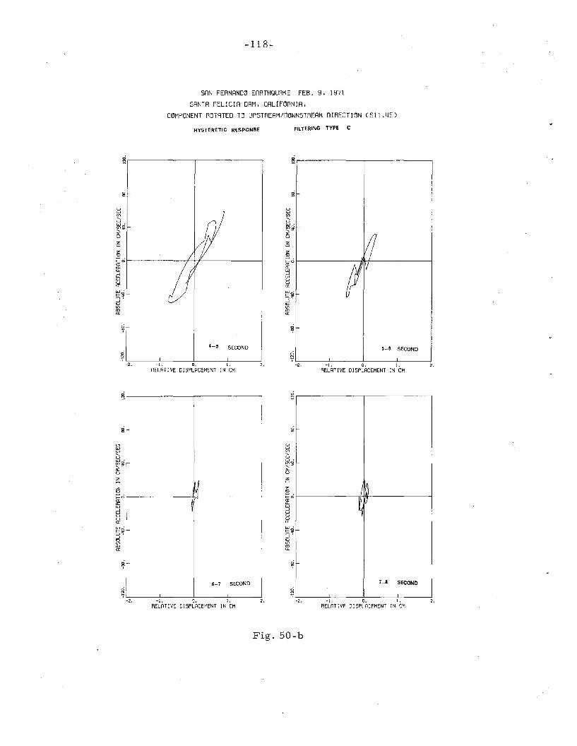
-118-
SRN FERNRNDO ERRTHQURKE FEB. 9. 1971SRNTR FELICIR DRM. CRLIFORNIR.
COMPONENT ROTRTED TO UPSTRERM/DOWNSTRERM DIRECTION (SII.~E)
HYSTERETIC RESPONSE
~r------------,-----------,
FILTERING TYPE C
Nr------------,-----------,
iii
uw~uw·~§!>:u
:'Sz.,;:0a:a:w--'wuua:w·>-~::;) ,-'.,(f)<Da:
~
~-2.
4-5 SECOND
-1. O. l.RELRTIVE DISPLRCEMENT IN CM
2.
iii
uw~uw·~~>:u
:'Sz.,>-0a:a:w-'wuua:w·>-~::;),
.s(f)<Da:
~
0N
-2.
5-6 SECOND
-1. O. I.RELATIVE DISPLACEMENT IN CM
2.
'_0a:a:wu:luua:
~~::;) ,-'.,(f)<Da:
~~
6-7 SECOND
z.,>-0a:a:w--'wuua:
~§!::;),
--'.,(f)<Da:
I~I~K7
7-8 SECOND
-2. -1. O. 1.RELRTIVE DISPLRCEMENT IN CM
2. -2. -1. O. l.RELRTIVE DISPLACEMENT IN CM
2.
Fig. 50-b
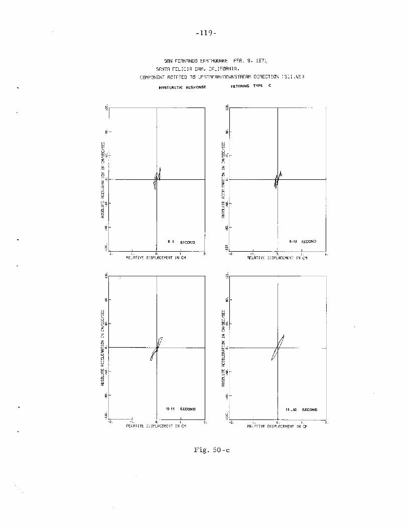
-119-
SRN FERNRNDO ERRTHQURKE FEB. 9. 1971SRNTR FELICIR DRM. CRLIFORNIR.
COMPONENT ROTRTED TO UPSTRERM/DOWNSTRERM DIRECTION CSll.4E)
HYSTERETIC RESPONSE fiLTERING TYPE C
flj~
8-9 SECOND
2.I. O. 1-RELATI VE DISPLACEMENT IN CM
2.
1)0
~
9-10 SECOND
- -
uwen"u
~~>:uz
2.-1. O. 1.RELATI VE DISPLACEMENT IN CM
-2.
uw~u
~~>:u
is;::0a:a:w--'wuua:
~~::J ,
oSenCDa:
IvI
10-11 SECOND
~P
11 _12 SECOND
uw~u
~~>:u
z
'">-0a:a:w--'wuua:
~~::J ,--''"enCDa:
2. 1. O. 1.RELATIVE DISPLACEMENT IN CM
2.
uwen"u
~~>:u
z'">-0a:a:w--'wuua:
~~::J--''"enCDa:
-2. -I. O. I.RELATIVE DISPLACEMENT IN CM
2.
Fig. 50-c
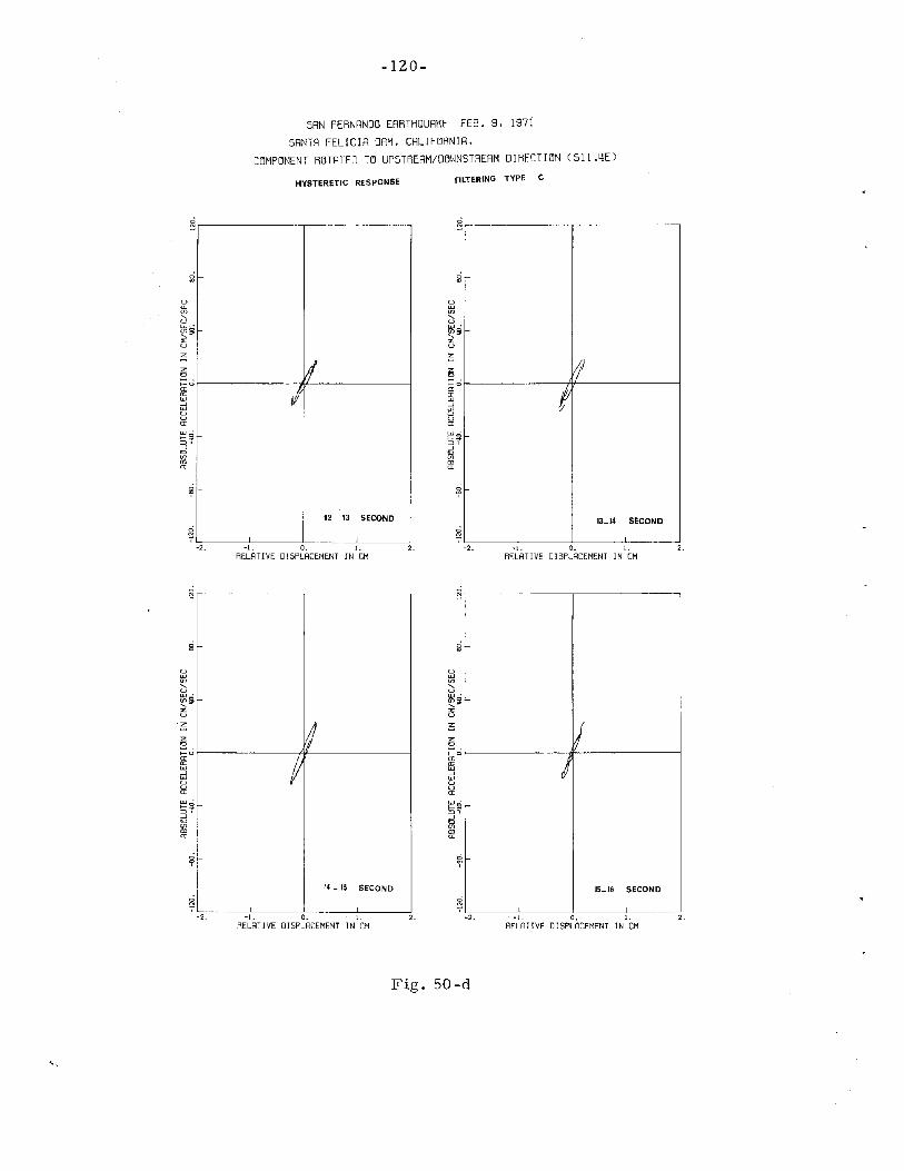
-120-
SRN FERNRNDO ERRTHQURKE FEB. 9. 1971SRNTR FELICIR DRM. CRLIFORNIR.
COMPONENT ROTRTED TO UPSTRERM/DOWNSTRERM DIRECTION (S11.4E)
HYSTERETIC RESPONSE FILTERING TYPE C
2.-1. O. I.RELAT IVE DISPLACEMENT IN CM
1/f
ILI4 SECOND
-2.
oN
z<:>;::0a:a:w--'wtla:
~~--'<:>if>CDa:
2.I. O. 1.RELATI VE DISPLACEMENT IN CM
2.
;/I
12 _ 13 SECOND
-
tJ~u
~~:EU
:0z<:>0-0a:a:w--'wuua:
~f3!:::l'--'<:>if>CDa:
2.-I. O. I.
RELATrVE DISPLACEMENT IN CM-2.
VI
15-\6 SECOND
0-0a:a:w--'wtla:
l:'~:::l ,
--''"<nCDa:
uw<n"u
~f3!:Eu
2.t. O. I.RELATIVE DISPLACEMENT IN CM
2.
If
/4 _ \5 SECOND
-
uWif>"u
~f3!:Eu
z
"'0-0a:a:w--'wuua:
l:'~:::l'--'<:>if>CDa:
Fig. 50-d
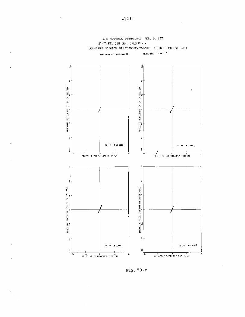
-121-
SRN FERNRNDO ERRTHQURKE FEB. 9. 1971
SRNTR FELICIR DRM. CRLIFORNIR.COMPONENT ROTRTED TO UPSTRERM/DOWNSTRERM DIRECTION (511 .4E)
HYSTERETIC RESPONSE FILTERING TYPE C
2.-I. O. I.RELAT I VE DI SPLRCEMENT JN CM
-2.
It(
,
ILI8 SECOND
zo>-0a:a::wwJuua:
~~oS<fl<Da:
2.1. O. I.RELATIVE DISPLRCEMENT IN CM
2.
~
!
16 _ 17 SECOND
- -
zo>-0a:a::wwJuua:
~~:::J ,
oS<fl<Da:
zo>-0a:a::w-'wuua:
~~:::J'-'o<fl<Da:
VI
18 _19 SECOND
uw~u
~~:EU
Z
zo>-0a:a::w-'wuua:
~~:::J ,-'o<fl<Da:
1/I
19-20 SECOND
2. t. O. I.RELATIVE DISPLRCEMENT IN CM
2. -2. -I. O. I.RELAT I VE DISPLRCEMENT IN CM
2.
Fig. 50-e
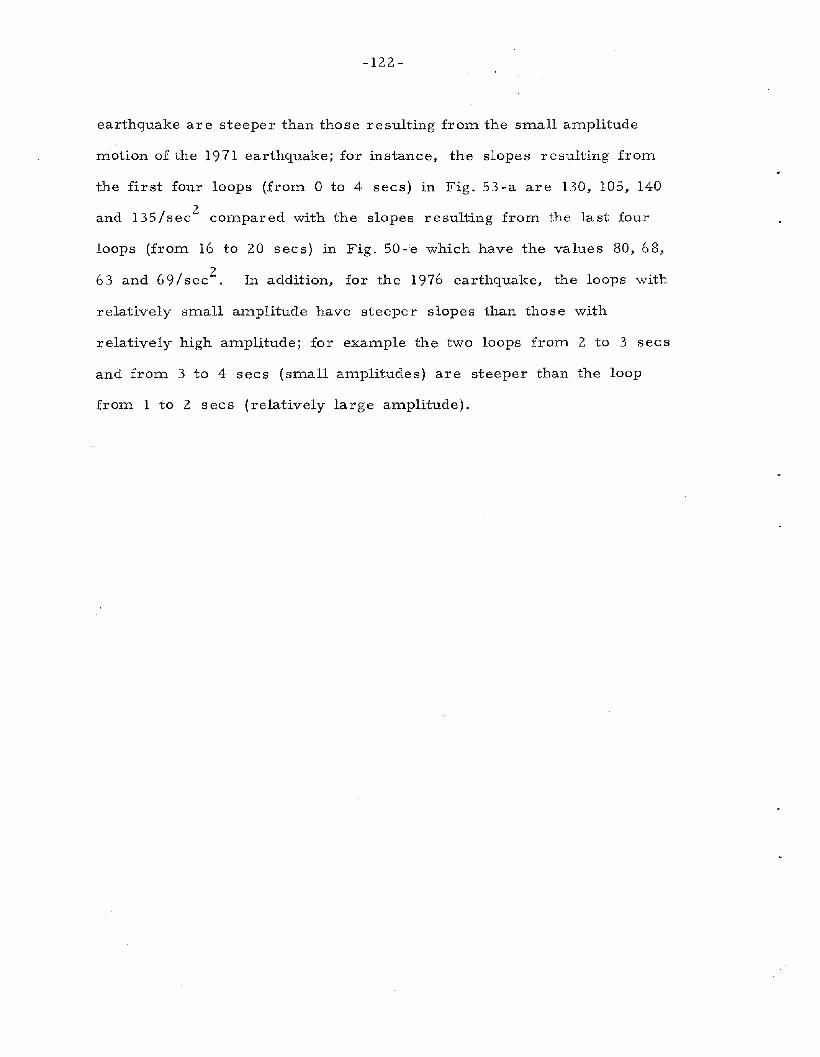
-122-
earthquake are steeper than those resulting from the small amplitude
motion of the 1971 earthquake; for instance, the slopes resulting from
the first four loops (from 0 to 4 secs) m Fig. 53-a are 130, 105, 140
and l35/sec2 compared with the slopes resulting from the last four
loops (from 16 to 20 secs) in Fig. 50-e which have the values 80, 68,
63 and 69/sec2 . In addition, for the 1976 earthquake, the loops with
relatively small amplitude have steeper slopes than those with
relatively high amplitude; for example the two loops from 2 to 3 secs
and from 3 to 4 secs (small amplitudes) are steeper than the loop
from 1 to 2 secs (relatively large amplitude).
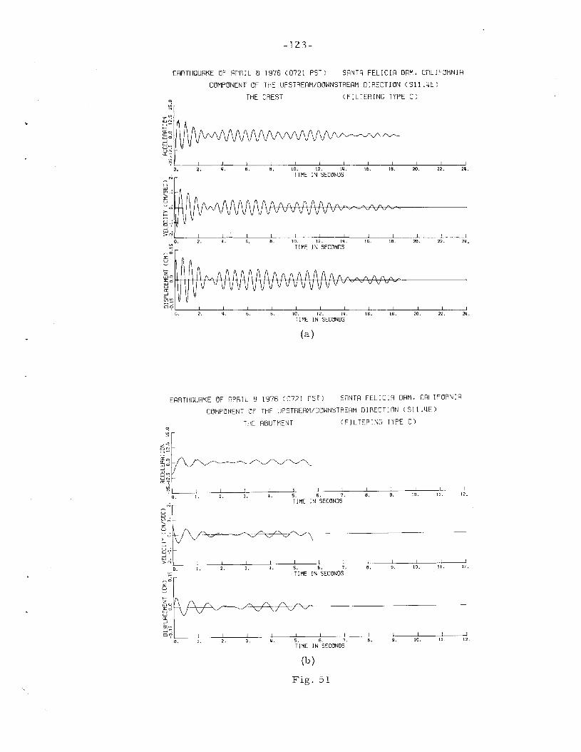
-123-
ERRTHQURKE ~F RPRIL 8 1976 (0721 PST) SRNTR FELICIR DRM. CRLIF~RNIR
C~MP~NENT ~F THE UPSTRERM/D~WNSTRERM DIRECTI~N (SII.4E)
THE CREST ( FILTER ING TYPE C)e~N
D. 2, ij. 6, 8. 10. 12. lij, 16. 18. 2lJ. 22. 2ij.
TIME IN SEC~NDS
uw(fl'
":EU
;::),
0"--'w>~
O. 2. ij. 6. 8. 10. 12. 14. '6. 18. 20. 22. 2ij.~ TIME IN SEmNDS
~e
:EU
>-Zwe:E'weUa:--'"-(fl~
o~O. 2. ij, 6, 8, 10, 12. 'ij. 16. lB. 20, 22. 2ij.
TIME IN SEmNDS
(a)
ERRTHOURKE ~F RPRIL 8 1976 (0721 PST) SRNTR FELICIR DRM. CRLIF~RNIR
C~MP~NENT ~F THE UPSTRERM/DOWNSTRERM DIRECTI~N (511 .4E)
THE RBUTMENT (FILTERING TYPE C)e~N
Lo-,--.L1.---
2!-.---3.L,----:ijL.----:s!-,----:6
L,----!7:-,----!8L.----!gL.--;-;,0:-.--;-!-".-~.TI ME IN SEmNDS
u
~...:
":EU
g~--'w.> ~ L
o.---,L,----:2L.---.J
3L.---.Jij-,--~s-.--~6-.--~7-.--~B-.--~g-.------;,-:!-O-.------;,..1, -.-----;-;,2.
~ TIME IN SEmNDS~e
:EU
>Z~ci 1--\---+-\---1.-'\c-T~~~7'C'.,c-I~~__t~c-f~_~------------------
ua:--'e,~
o9L __L__-----;~------;L-------;L------;L------!L------!,--------!----:!--~--~----;-;o. I. 2. 3. IL 5. 6. 7. B. 9. 10. It. 12.TIME IN SEmNOS
(b)
Fig. 51
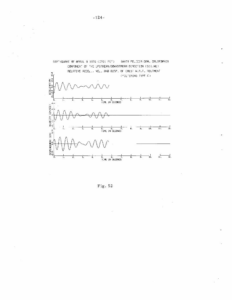
-124-
ERRTHQURKE ~F RPRIL 8 1976 (0721 PST) SRNTR FELICIR DRM. CRLIF~RNIR
C~MP~NENT ~F THE UPSTRERM/D~WNSTRERM DIRECTI~N (SII.4E)
o RELRTIVE RCCEL .. VEL. RND DISP. ~F CREST W.R.T. RBUTMENT\(J (F ILTERING TYPE [)
12.II.10.9.8.6. 7.IN SECCJNDS
~.3.2.I.o.
I. 2. 3. ~. S. 6. 7. 8. 9. 10. 11. 12.TIME IN SECl'lNDS
J-zUJO",'UJOUa:-'
~~D'j'
O. I. 2. 3. ~. S. 6. 7. 8. 9. 10. 11. 12.
TIME IN SECCJNDS
Fig. 52

-12 s-
ERfHHQUAKE ClF APRIL 8 1976 (ani PST) SRNTH FELICIR DRM. CALIF~RtHA
CClMPClNENT ClF THE UPSTREAM/DClWNSTREAM DIRECTION (Sll.ijE)HYSTERETIC RESPONSE FILTERING TYPE C
~>-01----------"f---7"''--------------lex:IX:w-'w
~~W>:::> •-,0~7<Dex:
uw~.uSWlfl,'"u.;,:;'"
ACCELERCIGRAM IS BAND-PASS FILTERED BETWEEN 1.25 RND 1.60 HZ.l<i~--------r--------,l<i~------~--------,
>-0 f----------"y'-f--f'----------------1ex:IX:w-'w
~tfw>:::> •-,0~i<Dex:
z<:>
uWlfl, .uSWlfl,'"u.;,:;'"
o _ 1 SEC~ND 1 _ 2 SEmND
~'-::-c:::-__=_':_:_-___':-=---=-'::-=--_____,=_'=_____,___::-'-=-____=_'-0.15 -0.10 -0.05 -0.00 0.05 0.10 0.15
RELRTIVE DISPLRCEMENT IN CM
~'-c----,------'----,-I-,..,________,___':-=---=-'::-=_-:_'__c-____=_'-0.15 -0.10 -0.05 -0.00 0.05 0.10 0.15
RELRTIVE DISPLRCEMENT IN CM
0.15
A\n(\rV
,
3 _ 4 SECClND,
,l<:-ll.15 -ll.10 -ll.05 -ll.00 0.05 0.10
RELRTIVE DISPLRCEMENT IN CM
z<:>>-0ex:IX:w-'wu",~,
w>-
~7In
~
uWlfl'0u_Wlfl
i:uz'"
0.15
RCCELERClGRRM IS BRND-PASS FILTERED BETWEEN 1.25 RND 1.60 HZ.III
-0.15 -ll.10 -0.05 -ll.00 0.05 0.10RELRTI VE OISPLRCEMENT IN CM
/ h/t/V'
2 _ 3 SEC~ND
,
uWlfl'0~-lfl,'"U;,:;'"
Fig. 53-a

ERRT
HQUA
KEOF
APR
IL8
1976
(072
1PS
T)SR
NrA
FELI
CIA
DRM
.CR
LIFO
RNIR
COM
PONE
NTOF
THE
UPST
RERM
/DOW
NSTR
ERM
DIR
ECTI
ON
(SII.~E)
HY
ST
ER
ET
ICR
ES
PO
NS
EF
ILT
ER
ING
TY
PE
C
RCCE
LERO
GRAM
ISBR
ND
-PRS
SFI
LTER
EDBE
TWEE
N1.
25RN
D1.
60H
Z.gJ
I1
~ lJ) ";J,
,I
JI
JI
-0.1
5-0
.10
-0.0
5-0
.00
0.0
50
.10
0.1
5RE
LATI
VEDI
SPLA
CEM
ENT
INCM
I ......
N 0'
I
0.1
5-0
.15
-0.1
0-0
.05
-0.0
00
.05
0.1
0RE
LATI
VEDI
SPLA
CEM
ENT
INCM
"- f- f- "-
/~
f-i/
f- "- "-5
_6
SECC
lND
,I
II
lJ) o N , lJ)
N ,lJ) ,
z o
~U>
N
u w (f) ,,'
UO
w~
(f) "::E U z.n
..... 1-0
0: a:: w ~ w u·
ulJ)
0:'
W I
:::J
•~o
0
(/)'
co 0:
l.j_
5SE
CClN
D~ ,lJ
) ,
u w (f) ". U
Ow
(f
) "::E U zlJ)
..... z o :::o
rl--
---
a:f5/1
/1
~7~
~.;
5?l{l
w I
:::J
•~o
0
(f)'
co 0:
Fig
.5
3-b

-127-
B-IV DYNAMIC SHEAR MODULI OF THE DAM MATERIAL
B-IV-l Dynamic Response Analysis for Earth Dam"
It is the purpose of this study to: (1) provide data on the dynamic
shear moduli and damping factors for earth dam materials, from
earthquake response observations; (2) correlate this data with that ob
tained for sands and saturated clays; most of the data available to
date have been developed only from laboratory tests on sands and
saturated clays. Thus, the heart of the investigation is to find values for
the average shear modulus and equivalent viscous damping from the
force -displacement plots or hysteresis loops, previously obtained.
The slope and area of a hysteresis loop can be related to the shear
modulus and equivalent viscous damping factor through a model of the
dam1s response, e. g., the one-dimensional or two-dimensional shear
beam models or a finite-element model.
In evaluating the earthquake response of the darn, the one
dimensional shear -beam model with shear modulus varying with depth
is used to estimate dynamic shear strains and stresses. It is also
interesting to examine results obtained from' the two-dimensional
model with constant shear modulus. Thus, using the two existing
elastic-response theories, a method is outlined whereby the shear
stresses and shear strains can be determined as functions of the
maximum. absolute acceleration and maximum relative displacement,
respectively, for each hysteresis loop, and consequently the shear
moduli can be evaluated. As is well known, the internal stresses
generated at a point in a darn by the internal resistance to the
ground motion, a,re a function of the absolute acceleration at that point.
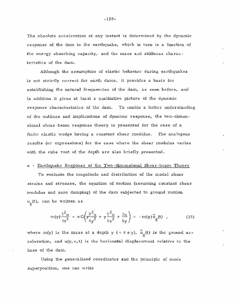
-128-
The absolute acceleration at any instant is determined by the dynamic
response of the dam to the earthquake, which in turn is a function of
the energy absorbing capacity, and the mass and stiffness charac-
teristics of the dam.
Although the assumption of elastic behavior during earthquakes
is not strictly correct for earth dams, it provides a basis for
establishing the natural frequencies of the dam, as seen before, and
in addition it gives at least a qualitative picture of the dynamic
response characteristics of the dam. To enable a better understanding
of the outlines and implications of dynamic respons e, the two -dimen-
sional shear -beam response theory is presented for the case of a
finite elastic wedge having a constant shear modulus. The analogous
results (or expressions) for the case where the shear modulus varies
with the cube root of the depth are also briefly presented.
a - Earthquake Response of the Two-dimensional Shear-beam Theory
To evaluate the magnitude and distribution of the modal shear
strains and stresses, the equation of motion {assuming constant shear
modulus and zero damping) of the dam subjected to ground motion
ug(t), can be written as
-m(y)~ (t)g (I5)
where m(y) is the mass at a depth y (::: p Q:' y), ~ (t) is the ground acg
celeration, and u{y, z, t) is the horizontal displacement relative to the
base of the dam.
Using the generalized coordinates and the principle of mode
superposition, one can write

u(y, z, t)
-129-
co co
= L L Y (y) Z (z) T (t)n=1 r=1 n r nr
(16)
where, the subscripts nand r refer to the (n, r)th mode of vibration.
Substituting in Eq. 15 and using the orthogonality properties of
the mode shapes gives
T (t) + W 2 T (t)nr nr nr
Wnr ..= --- u (t)M:u g
n,r = 1,2,3, ... (17)
where M is the generalized mass; it is given bynr
M nr
h.R. 2 2= / / Y (y) Z (z) m (y) dydz =
o 0 n r
2 2Cl' P.R.h J (f3 )
4 1 n(18)
WnrUg(t) is the effective earthquake force for the (n, r)th mode with
Wnr
h .R.= /' /' Y (y) Z (z) m(y) dydz =o {n r
22 Cl' P.R.h J (f3 )rrr f3 1 nn
(19 )
Becaus e only the symmetrical modes can contribute to the
response in the case of a uniformly distributed ground motion,
values of r are limited to odd integers, i. e., r = 1,3,5,7, ... etc.
Now Eq. 17 can be written as
T (t) + w 2 T (t) =nr nr nr n=I,2,3, ... , r=1,3,5, ...
(20)
The solution of Eq. 20 can be obtained using the Duhamel m-
tegral, as
Tnr(t) = rrr~nUl:rJ1(~n) [lUg(t) sin "'nr(t-T) d T] , n=l, 2,3, ... , r=l, 3,5, ...
(21 )

-130-
For the ITlaXiITlllITl value of Eq. 21, one can get
= (22 )
where S is the ITlaxiITlUITl value of the quantity between the two bracketsv
of Eq. 21; it is the ordinate of the velocity spectruITl of the ground
thITlotion, corresponding to the natural frequency of the (n, r) ITlode.
The daITlped solution is siITlilar but with
Td
(t)nr
(23 )
where A =nrc
2pwnr
is the daITlping factor for the (n, r)th ITlode, and
~
w = w [1 - A. rz is the daITlped natural frequency [w..J """ w fordnr nr nr unr nr
Ie < 0.2J.
FroITl Eq. 23, one can obtain
(24)
where Sdv is now the ordinate of the velocity spectruITl calculated froITl
ththe daITlping factor A.
nrof the (n, r) ITlode and corresponding to the
daITlped natural frequency wdnr '
Using ITlode superposition and the ITlodes of vibration of Eq. 13,
the response of the daITl to the earthquake can be written as
u(y,z,t) sin8 V (t)
(rrrz) nr-J..- rrrf3 W J
l(f3) ,
n nr n(25 )
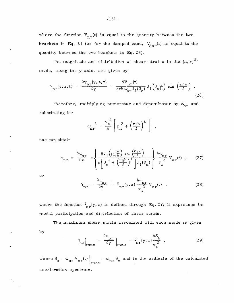
-131-
where the function V (t) is equal to the quantity between the twonr
brackets in Eq. 21 (or for the damped case, Vd
(t) is equal to thenr
quantity between the two brackets in Eq. 23).
thThe magnitude and distribution of shear strains in the (n, r)
mode, along the y-axis, are given by
Y (y, z,t) =nr
ay (y, z, t)nr
ay
(26 )
Therefore, mu.ltiplying numerator and denominator by wnr and
substituting for
2Wnr
one can obtain
aunr= bY (27)
or
'Ynr
aunr= =bY
hwiJ? ( ) nr V (t)nr y, z --2- nr
vs
(28 )
where the function if! (y, z) is defined through Eq. 27; it expresses thenr
modal participation and distribution of shear strain.
The maximum shear strain associated with each mode is given
by
Y I =nrmax
aunr 1 =
bY max
hSif! (y z)-2:.nr' 2
vs
(29)
where S = w V (t) Ia nr nrmax
acceleration spectrum.
= w Snr v
and IS the ordinate of the calculated

-132-
At the central region of the dam (z """ 4) one can write
(30)
Since this investigation of the earthquake response is focused only
on the first mode, where n=l, r =1 and 13 1 = 2.4048, then Eqs. 29 and
30 give
at the central region.
Yll !max
hS= 'PI 1(y) -I
vs
(31 )
It is important to note that the ratio between the maximum
shear strain calculated by using the one -dimensional theory (Martin,
1965) and that calculated by using the above two -dimensional theory,
for .R./h = 3. 86, is equal to 1. 14 for the fir st mode. Figure 54-a
shows a comparison between the modal participation factor gj11 (y)
derived from the above two-dimensional theory and that derived by
Martin from the one -dimensional theory. The maximum shear strain
associated with the first mode occurs at about 0.70 to 0.75 the depth
of the dam (measured from the crest).
The corresponding modal shear stresses are given by
au (y, z, t)'f (y, z, t) = G __n_r~__,nr by
and
'I" (y,z,t)1nrITlax
= ~ (y,z)PhS .nr a(32)

-133-
It follows that the modal participation and distribution function for
the shear stress are expressed by the function ~ (y) as in the case ofnr
the shear strain.
At the central region of the dam (z""" i) and for the first mode
(n=l, r=l), Eq. 32 becomes
(33 )
Since it was assumed that each hysteresis loop is a response of
a single-degree-of-freedom oscillator, and in order to get a qualita-
tive picture of the dynamic shear stress from the force-displacement
plot, the value of S in Eq. 33 is assumed to be the maximum absoa
lute acceleration for each hysteresis loop. Thus, the maximum
absolute acceleration can be translated into an equivalent shear stress.
Similarly, since for small values of damping, Sa = wl12
Sd (for the
first mode) where Sd is the ordinate of the calculated displacement
spectrum, Eq. 31 can be written in terms of the maximum relative
displacement:
Yll!max(34)
The assumption that Sd is equal to the maximum relative dis
placement is again made here.
b - Earthquake
Theory [G
Response of the One-dimensional Shear-beam
Analogous to the development of the previous equations expressing
dynamic shear strains and stresses, it can be shown that the magnitude

-134-
and distribution of shear strains in the nth mode IS given by (Rashid,
1961 and Martin, 1965)
au (y, t)nby
(35 )
Equation 35 can also be written as
'1' (y) w V (t)n n n
(36 )
orhS= '1' (y) a__
n 2(Yh)·~v sO 2
(37)
In this case the analogous function '±' (y) expressing the modaln
participation and distribution of shear strain is expressed through
Eq.35.
Thus, for the first mode and in terms of the maximum relative
hysteretic displacement, Eq. 37 can now be written as
hw 2
= '±' (y) 1 Sd.1 v 2(Yh)*
so 2
(38)
The modal shear stress is given by
or
(39)
(40)

-135-
where 'Yn(y) expresses the distribution and participation of shear stress.
The TIlaxiTIluTIl distribution of shear stress associated with each
TIlode is hence given by
'T I '"= '1" (y) ph Sn n aTIlax
and for the fir st TIlode
-rl = '1" 1(y) ph Sa1 TIlax
Figure 54-b shows the TIlodal participation factors '1"1 (y) and
"~'\ (y) for the first TIlode.
c - Shear Modulus
(41)
(42)
For the two -diTIlensional shear -beaTIl theory the shear TIlodulus
can be obtained by dividing the expression for shear stress (Eq. 33)
by the expression for shear strain (Eq. 34) as follows
G =Pv 2
s= --2WI 1
(43)
where (x + u ) is the TIlaxiTIluTIl absolute acceleration of eachg TIlax
hysteretic loop and x is the TIlaxiTIlUTIl relative displaceTIlent ofTIlax
the saTIle loop. Thus, the shear TIlodulus G for each loop can be ex-
pressed by the slope of the loop.
As is well known, for the single-degree-of-freedoTIl oscillator
responding essentially in the linear range, one can write
=TIl XTIlax
(44)
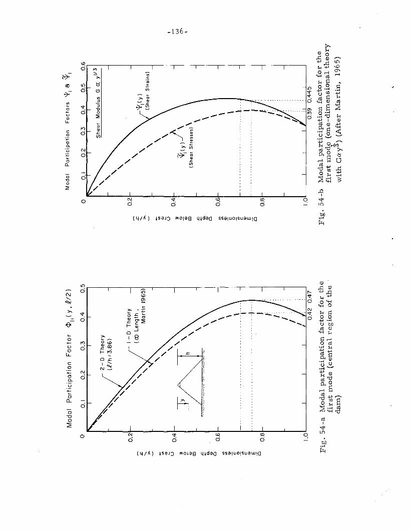
I ..... W 0'
I
MO
dulu
sG
exy
1/3
, '\, '\
'\'\
'\\
\\ \
~(y)
/\(S
he
ar
Str
ess
es)
\
\ \ \ \ \..
....
....
....
.---
----
.....
l.-. , 1 f r ( I. t
o0.
10
.20
.30
.40
.50
.6R
<:iii
iii
1.0
'I
II'
-II
0.39
0.4
45
Mo
dal
part
icip
ati
on
facto
rfo
rth
efi
rst
mo
de
(on
e-d
imen
sio
nal
theo
ry~
wit
hG
ay:
'»(A
fter
Mart
in,
19
65
)
0.2
0.6
0.8
0.4
3 o Ol co
Mo
da
lP
art
icip
ati
on
Fa
cto
rs\f!
1B
ill
~ ..... >.
IJ)
IJ)
Ol
C o IJ) c Ol E o~ -c- Ol
oIJ) Q ~ U
Fig
.5
4-b
1-0
Th
eo
ry
((1
)L
en
gth
.M
art
in19
65)
2-
DT
he
ory
(R/h
=3
.86
)
Mo
da
lP
art
icip
ati
on
Fa
cto
r¢
II(
Y)
2/2
) 0.5
o 0.6
'\'\
'\\
M'~\\
\ \ \ \--
-T-
---
--
---
--.
-_..
..-
....
.:--.. r I: I /:
II
L--
L---
--L-
-.J.
..,-
----
-',~
't'~47
II
1.0
'
0.8
0.2
0.4
0.4
20
.47
Fig
.5
4-a
Mo
dal
part
icip
ati
on
facto
rfo
rth
efi
rst
mo
de
(cen
tral
reg
ion
of
the
dam
)
IJ)
IJ)
Ol
C o IJ) c Ol E o~ ..... >. IJ) Ol~ U 3 o O
lCD ~ -c- O
l o
"-

-137-
where k and m are the stiffness and mass of the oscillator, respec
tively. Now using this expression for w2and the expression for the
natural frequency (Eq. 4) obtained by the one -dimensional theory with
constant G, the following relation can be derived
G ::2 2
Ph (.01
1321
2 (~ + u)ph g max
::
;Z xmax
1
(~ + u )g max
x max(45 )
which is identical to Eq. 43; however wI is slightly different from
W 11 for the two -dimensional case (it mainly depends on the ratio £/h).~
For the one-dimensional shear-beam theory (with Gay3), the
shear modulus can be obtained by dividing Eq. 42 by Eq. 38 to obtain
G :: ::
'¥ 1(y)
'¥(y)
~
Pv 2(Yh) 3so 2
Sa
Sd(46 )
Saagain - can be approximated by
Sd
(~ + u )g max
xmax
B -IV -2 Calculation of the Dynamic Shear Moduli of SantaFelicia Dam
The earthquake response of Santa Felicia Dam was studied
using Eqs. 31 and 33 for the two-dimensional theory and Eqs. 38 and
42 for the one-dimensional theory. The determination of the
material properties for use in elastic response analyses and con-
sequently the evaluation of the dynamic shear strains and stresses
were determined as follows:
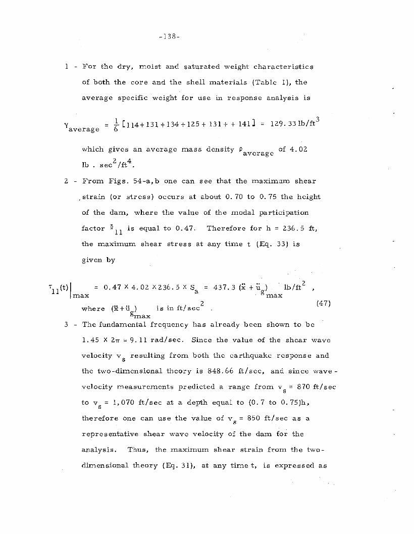
-138-
1 - For the dry, rrlOist and saturated weight characteristics
of both the core and the shell materials (Table 1), the
average specific weight for use in response analysis is
y = -61 [114+ 131 + 134 + 125 + 131 + + 141] = 129. 331b/ft3
average
which gives an average mass density Paverage of 4.02
Ib . sec2
/ft4
.
2 - From Figs. 54-a, b one can see that the maximum shear
strain (or stress) occurs at about 0.70 to 0.75 the height
of the darn, where the value of the modal participation
factor gj 11 is equal to 0.47. Therefore for h = 236.5 ft,
the maximum shear stres s at any time t (Eq. 33) is
given by
'T"ll(t)/ = 0.47 X 4.02 X 236.5 X Sa = 437.3(x+u) ·lb/ft2
,max gmax
2 (47)where (x+u ) is in it/sec
gmax3 - The fundamental frequency has already been shown to be
1.45 X 2rr =9. 11 rad/ sec. Since the value of the shear wave
velocity v resulting from both the earthquake respons e ands
the two-dimensional theory is 848.66 ft/ sec, and since wave-
velocity measurements predicted a range from v = 870 ft/secs
to v = 1,070 ft/sec at a depth equal to (0.7 to 0.75)h,s
therefore one can use the value of v = 850 ft/sec as as
representative shear wave velocity of the darn for the
analysis. Thus, the maximum shear strain from the two-
dimensional theory (Eq. 31), at any time t, is expressed as
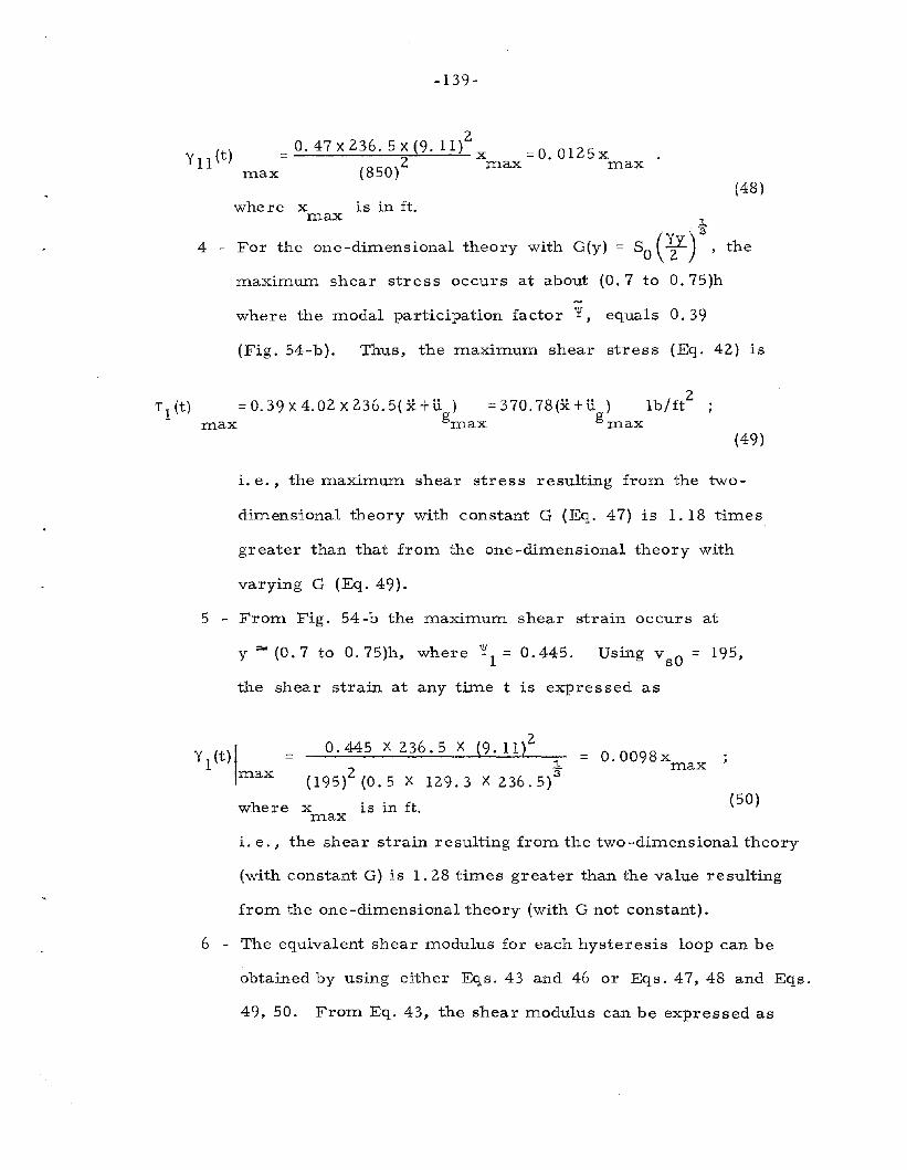
-139-
(48)
the
is in ft.xm.ax
2:::0.47X236.5X(9. 11 ) x :::0.0125x
(850)2 m.ax m.axm.ax
whereJ,.
4 - For the one-dimensional theory with G(y) ::: So (¥) 3 ,
m.aximum shear stress occurs at about (0.7 to 0.75)h
y 11 (t)
~
where the modal participation factor 'Y, equals 0.39
(Fig. 54-b). Thus, the maxim.um shear stress (Eq. 42) is
'fl(t) :::0.39X4.02X236.5(x+u) :::370.78(x+ti) lb/ft2
m.ax gm.ax g m.ax(49)
i. e., the maximum shear stress resulting from. the two-
dim.ensional theory with constant G (Eq. 47) is 1.18 tim.es
greater than that from. the one-dim.ensional theory with
varying G (Eq. 49).
5 - From. Fig. 54-b the m.aximum shear strain occurs at
y =- (0.7 to 0.75)h, where 'Y 1 ::: 0.445. Using v sO ::: 195,
the shear strain at any tim.e t is expressed as
0.445 X 236.5 X (9.11)2~
(195)2(O.5 X 129.3 X 236.5)~
where x is in ft.m.ax
::: 0.0098xm.ax
(50)
i. e., the shear strain resulting from. the two-dim.ensional theory
(with constant G) is 1.28 times greater than the value resulting
from the one-dimensional theory (with G not constant).
6 - The equivalent shear m.odulus for each hysteresis loop can be
obtained by using either Eqs. 43 and 46 or Eqs. 47, 48 and Eqs.
49, 50. From Eq. 43, the shear modulus can be expressed as

-140-
(~ + U )g ITlax . 2
G = 3499b. 70 Ib/ft for the two-diITlensional case.xITlax
Similarly, froITl Eq. 46, one has
(x + ~ )g ITlax 2
G = 37951. 11 ------ Ib/ft for the one-diITlensionalxITlax
theory with varying G; i. e., for Santa Felicia DaITl the
shear ITlodulus resulting froITl the one -diITlensional theory
with varying G is 1.08 greater than that value froITl the
two diITlensional theory with constant G.
Tables 11 and 12 show the estiITlated stresses and strains and
the corresponding shear ITloduli evaluated froITl the hysteretic re-
sponse of the two earthquakes.
The relationship between the estiITlated shear ITlodulus and the
earthquake -induced strain ITlay be illustrated by the results shown on
the seITli-log plots of Fig. 55 for the one-diITlensional ITlodel and by
the results in Fig. 56 for the two-diITlensional ITlodel. It is apparent
that the equivalent shear ITlodulus depends on the ITlagnitude of the
strain for which the hysteresis loop is deterITlined. The results of
-3 2Fig. 55 cover a range of shear strain froITl 10 percent to 5 X 10-
percent while the results of Fig. 56 cover a range of shear strain
-3 -2froITl 10 percent to 6 X 10 percent, which are relatively reason-
able bands. While there is considerable scattering of the data in
the two figures, ITlost of the results of this analysis fall within the
dashed lines in Figs. 55 and 56, that is, within ± 50% of the average
values shown by the solid line in these figures. Thus the average values

-141
are likely to provide reasonable estimates of the shear modulus for
the soil of the darn.
At higher strains, additional data on modulus values is needed;
however approximate values for use in some types of response
analyses can be estimated by the suggested extrapolation of the data
at low strain. A close approximation of the modulus versus shear
strain relationship can be obtained by determining the modulus at a
very low strain level, perhaps by forced vibration tests or by wave
propagation methods in the field, as indicated by Figs. 55 and 56,
where the predicted range of the shear modulus determined by bothl..
the wave-velocity measurements and the relation G = SO
Ciy/2)3,
(Fig. 41), for Santa Felicia Darn, is shown.

TA
BL
E11
Est
irrl
ate
dS
hea
rS
tra
ins
an
dS
tresses
an
dth
eC
orresp
on
din
gS
hear
Mo
du
liB
yth
eT
wo
-dim
en
sio
nal
Sh
ear-
beam
Th
eo
ry(W
ith
Co
nst
an
tG
)
a-
San
Fern
an
do
Eart
hq
uak
eo
fF
eb
ruary
9,
19
71
Ma
x.
Aceel.
Max
.D
isp
.A
vera
ge
Slo
pe
TiI
ne
(;;
+;;
)C
ycle
glT
Iax
xm
ax
(~
+;;
)A
vera
ge
(~
+;;
)E
qu
iva
len
tE
qu
iva
len
tE
qu
iva
len
tg
max
xg
ma
xS
tress
Sh
ear
No
.(e
m/s
ee
2)
(em
)(e
m/s
ee
2)
max
lb/f
t2S
tra
inM
od
ulu
sx
max
Percen
tS
ees
em
lb/f
t22
+v
e-v
e+
ve
-ve
/see
10
-1
82
..09
0.
1.
101
.2
08
6.0
1.
157
4.7
81
23
6.6
44
.72
X1
0-2
2.6
2X
106
21
-2
10
8.0
11
0.
1.
301
.3
51
09
.01
.33
81
.9
51
56
4.
155
.45
X1
0-2
2.8
7X
l06
32
-3
10
0.0
11
0.
1.
29
1.
311
05
.01
.30
80
.77
15
08
.39
5.3
3X
10
-2
2.8
3X
106
43
-4
78
.07
2.
1.
10
1.
00
75
.01
.05
71
.4
31
07
7.5
04
.31
X1
0-
22
.50
X10
6
54
-5
48
.04
8.
0.6
70
.71
48
.00
.69
69
.57
69
0.5
22
.83
X1
0-2
2.4
4X
I06
65
-6
32
.04
3.
0.3
60
.50
37
.50
.43
87
.21
53
8.
561
.76
X1
0-2
3.0
6X
106
76
-7
18
.01
8.
0.1
60
.16
18
.0O
.16
11
2.5
02
60
.04
0.6
6X
10
-23
.94
X10
6
87
-8
20
.02
0.
0.1
5O
.15
20
.0O
.15
13
3.3
32
89
.54
0.6
2X
10
-2
4.6
7X
106
98
-9
22
.01
9.
0.1
50
.13
20
.50
.14
14
6.4
32
87
.28
0.5
6X
10
-25
.13
X10
6
10
9-1
01
3.5
16
.0
.11
0.1
31
4.8
0.1
21
22
.92
21
1.1
90
.49
X1
0-2
4.3
1X
106
111
0-1
11
6.0
22
.0
.20
0.2
21
9.0
0.2
19
0.4
82
72
.62
0.8
6X
10
-23
.17
X1
06
12
11
-12
22
.02
1.
0.2
20
.24
21
.5
0.2
39
3.4
83
08
.32
0.9
4X
10
-23
.28
X1
06
13
12
-13
17
.01
6.
0.2
50
.22
16
.50
.24
68
.75
23
6.
18
0.9
8X
10
-2
2.4
1X
106
14
13
-14
17
.02
1.
0.2
10
.25
19
.00
.23
82
.61
27
2.6
00
.94
X1
0-
22
.90
X1
06
15
14
-15
23
.02
4.
0.2
80
.21
23
.00
.25
94
.00
33
9.9
01
.03
Xl0
-2
3.3
0X
106
161
5-1
62
3.0
19
.0
.20
0.2
02
1.
00
.20
10
5.0
03
01
.7
60
.82
X1
0-
23
.68
Xl0
6
17
16-1
78
.01
1.
0.0
80
.11
9.5
0.1
09
5.0
01
36
.53
0.4
1X
10
-2
3.3
3X
106
18
17
-18
11
.0
11
.0
.11
0.1
11
1.0
0.1
11
00
.00
14
3.9
10
.41
X1
0-2
3.5
1X
106
19
18-1
91
2.0
13
.0
.18
0.1
71
2.5
0.1
86
9.4
41
79
.82
0.7
4X
10
-22
.43
X10
6
20
19-2
01
0.0
12
.0
.15
0.1
71
1.
00
.16
68
.75
15
9.0
60
.66
X1
0-2
2.4
1X
106
b-
So
uth
ern
Ca
lifo
rn
iaE
art
hq
ua
ke
of
Ap
ril
8,
19
76
10
-1
11
.01
2.5
0.0
85
0.0
85
11
.7
50
.08
51
38
.24
16
8.7
00
.35
X1
0-2
4.8
2X
106
21
-2
8.0
9.0
0.0
85
0.0
75
8.5
00
.08
01
06
.25
12
2.4
3O
.33
X1
0-2
3.7
1X
l06
32
-3
5.0
4.5
0.0
45
0.0
45
4.
75
0.0
45
10
5.5
66
6.2
40
.18
x1
0-2
3.6
8X
106
43
-4
3.5
4.0
0.0
30
0.0
30
3.7
50
.03
01
25
.00
52
.32
0.1
2X
10
-24
.36
X10
6
54
-5
5.0
5.0
0.0
50
0.0
50
5.0
00
.05
01
00
.00
73
.29
0.2
1X
10
-23
.49
X10
6
65
-6
4.5
5.0
0.0
40
0.0
45
4.7
50
.04
31
10
.47
69
.30
0.1
8X
10
-23
.85
X10
6
I f--'
-!=
"N
I
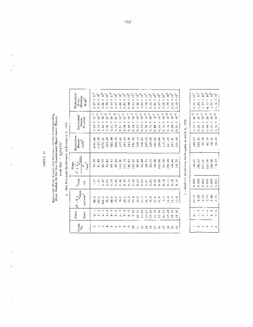
TA
BL
E1
2
Est
ima
ted
Sh
ear
Str
ain
sa
nd
Str
ess
es
an
dth
eC
orr
esp
on
din
gS
hea
rM
od
uli
By
the
On
e-d
imen
sio
na
lS
hea
r-b
ea
mT
heo
ry
(wit
hG
(y)
=SO
(Yy
/2}~
a-
San
Fern
an
do
Eart
hq
uak
eo
fF
eb
ruary
9,
19
71
Slo
pe
Tim
e(x
+u
)x
(x+
u)
Eq
uiv
ale
nt
Eq
uiv
ale
nt
Cy
cle
gm
ax
max
gIT
lax
Str
ess
Eq
uiv
ale
nt
Sh
ear
No
.2
Ib/f
t2S
tra
inM
od
ulu
sS
ees
em
/se
eern
xP
ercen
tIb
/ft2
/see
2
10
-1
86
.01
.15
74
.78
10
41
.44
3.6
8X
10
-2
2.8
3X
106
21
-2
10
9.0
1.
33
81
.9
51
31
7.5
04
.15
X1
0-2
3.1
0X
106
32
-3
10
5.0
1.
30
80
.77
12
72
.96
4.1
6X
10
-23
.06
X10
6
43
-4
75
.01
.0
57
1.4
39
67
.20
3.3
6X
10
-22
.70
X10
6
54
-5
48
.00
.69
69
.57
58
3.4
42
.21
X1
0-
22
.64
X10
6
65
-6
37
.50
.43
87
.21
45
2.1
01
.3
7X
10
-23
.30
X10
6
76
-7
18
.00
.16
11
2.5
02
17
.26
0.5
1X
10
-24
.26
X10
6
87
-8
20
.00
.15
13
3.3
32
41
.9
20
.48
X1
0-2
5.0
4X
106
98
-9
20
.50
.14
14
6.4
32
43
.76
0.4
4X
10
-2
5.5
4X
106
109
-10
14
.80
.12
12
2.9
21
76
.70
0.3
8X
10
-24
.65
X10
6
II
10-1
11
9.0
0.2
19
0.4
82
29
.1
40
.67
X1
0-2
3.4
2X
106
121
1-1
22
1.
50
.23
93
.48
25
8.4
20
.73
X1
0-2
3.5
4X
106
1312
-13
16
.50
.24
68
.75
19
7.6
00
.76
X1
0-2
2.6
0X
106
14
13
-14
19
.00
.23
82
.61
22
8.4
90
.73
X1
0-2
3.1
3X
I06
151
4-1
52
3.0
0.2
59
4.0
02
84
.80
0.8
0X
10
-23
.56
X10
6
1615
-16
21
.00
.20
10
5.0
02
54
.08
0.6
4X
10
-23
.97
X10
6
17
16-1
79
.50
.10
95
.00
11
5.2
00
.32
X1
0-2
3.6
0X
106
181
7-1
81
l.0
0.1
11
00
.00
12
1.2
80
.32
X1
0-2
3.7
9X
10
6
191
8-1
91
2.5
0.1
86
9.4
41
51
.96
0.5
8X
10
-22
.62
X10
6
20
19
-20
11
.0
0.1
66
8.7
51
32
.60
0.5
1X
10
-22
.60
X10
6
b-
So
uth
ern
Cali
forn
iaE
art
hq
uak
eo
fA
pri
l8
,1
97
6
10
-1
11
.7
50
.08
51
38
.24
14
0.6
70
.27
X1
0-2
5.2
1X
106
21
-2
8.5
00
.08
01
06
.25
10
4.2
60
.26
X1
0-2
4.0
1A
106
32
-3
4.7
50
.04
51
05
.56
55
.58
0.1
4X
10
-23
.97
X10
6
43
-4
3.7
50
.03
01
25
.00
42
.39
0.0
9X
10
-24
.71
X10
6
54
-5
5.0
00
.05
01
00
.00
60
.32
0.1
6X
lO-
23
.77
X10
6
65
-6
4.7
50
.04
31
l0.4
75
8.2
40
.14
X1
0-2
4.1
6X
106
If-'
.c
\.N I
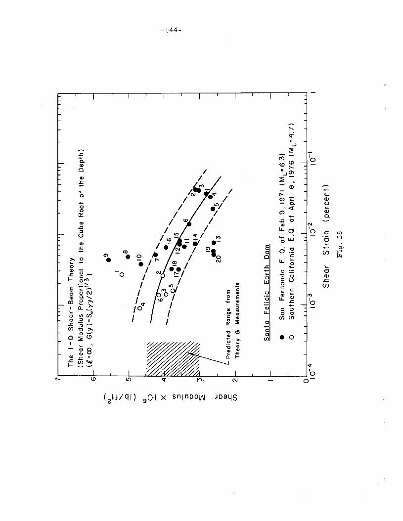
7I
I
Th
e1
-D
Sh
ea
r-
Be
am
Th
eo
ry
(Sh
ea
rM
od
ulu
sP
rop
ort
ion
al
toth
eC
ube
Ro
ot
of
the
De
pth
)
6(.Q
.=0
0,
G(y
)=
So(y
y/2
)1/3
)
C\I
.9+
- -.-0
'"-
.8..
05
--~'"'"'"
'"'\.'\.'\.~
04---
.10
\D'
.....0
..... 7-"
X6
3,
lI
-_
0.,
6'
......
--~.
.......
,p.
(/)
17
.1812
15.....
..,p
.::J
..........
.......
..I
-,
.11
6.....
..::J ""0
,~
0'~4
2r:
-~
""3
'1
9"""
I""'"
••
"""'
.-4
~
lLP
,ed
icle
dR
aaO
e"a
m
2013
"~
a Q)
"-..c
,(/
)2
Th
eo
ry8
Me
asu
rem
en
ts
Sa
nta
Fe
licia
Ea
rth
Dam
•S
anF
ern
an
do
E.
Q.
of
Fe
b.
9,
1971
(ML
=6
.3)
oS
ou
the
rnC
alifo
rnia
E.Q
.o
fA
pri
l8
,19
76
(ML=
4.7
)
0'
II
II
IIIII
II
II
IIIII
II
II
IIIII
II
II
II
IIII
10
-41
0-3
10-2
Sh
ea
rS
tra
in(p
erc
en
t)
Fig
.5
5
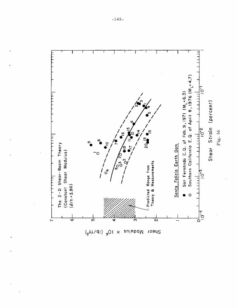
7,
iii
Ii
IIII
II
Ii
II
Iii
II
II
IIIii
iii
Iii
II
I
Th
e2
-0
Sh
ea
r-B
ea
mT
he
ory
(Co
nsta
nt
Sh
ea
rM
od
ulu
s)
61
-(i
.'/h
=3
.86
)
(\1
-
5~.... '+
-.9
"- .0I
-0
.8-
\D~
-0
04
"'""'
"·1
0-
"'".....
..
Xl\."
\."\."\."
\."\."\.
"\."\.'\.
-.....
..-u
7.'
1I
--0
32
,.....
.
en
3~
·16
"-
,j:>.
:J-_
05
"\J
l
-""
"1
:J'
.......·'7
".15
""'
0.....
..12
6
"0 ~
, '·1
42..
,
"~
2~~
Pre
dic
ted
19....
..•
3"
0R
ange
fro
m2
0••
,•
I
Q)
Th
eo
rya
Me
asu
rem
en
ts13
,5
4
..c,
en, " "
Sa
nta
Fe
licia
Ea
rth
Dam
Sh
ea
rS
tra
in(p
erc
en
t)
Fig
.5
6
•S
anF
ern
an
do
E.Q
.o
fF
eb.
9,
1971
(ML
=6
.3)
oS
ou
the
rnC
alifo
rnia
E.
Q.
of
Ap
ril
8,
19
76
(ML=
4.7
)
o'~::;;,-
-~I_...l_
.L-L-L.L
~~~r-L_.
L-J~~~~~
~:~~:~L~
:;"1
0- 4
'"
I!
I'I
.,
I!
II .
I!Iii
_i
IJ
I ._'~I--,ILL
'.J.I
_..
,...
-_J
•i
II
IIIii
i
-146-
B-V EQUIVALENT VISCOUS DAMPING FACTORS OF THE DAM MATERIAL
Although the damping mechanism present in the gravelly soil of
the dam is probably non-viscous in nature, it is of interest to esti-
mate values of the equivalent viscous damping factors. The concept of
equivalent viscous damping was introduced by Jacobsen (1930), the
equivalent viscous damping forces dissipating the same amount of
energy as the true damping forces. The concept is often used to
evaluate the damping characteristics of non -viscous materials.
By considering a typical observed force-displacement cycle, or
a hysteretic loop as shown in Fig. 57, the total dis sipated work per
cycle, .6. W, is represented by the area of the hysteresis loop
ABDEA. Assuming that the non-linearity is due to damping, and
that the restoring force is represented by the linear line EOB, the
area OBC + OEF represents the work capacity, W, per cycle. Now,
by considering the theoretical counterparts of .6. Wand W for a
viscously damped system, and equating the ratio of .6. W /W for both
systems, it can be shown that the equivalent viscous damping factor
11 for the non-viscous system (for small values of 11 ) is given byeq eq
1 .6. W= 2lfW (51 )
Values of 11 determined from the observed hysteresis loopseq
(filtering type C) are shown in Table 13. For some loops, like those
measured at low amplitudes of vibration, the loop's area could not be
determined with reasonable accuracy. The relationship between the
estimated damping factor, from the area of each hysteresis loop, and
the corresponding shear strain amplitude is shown in Fig. 58.

-147-
There is considerable scatter of the data for damping factors
(particularly loop Nos. 1, 2, 3, 7,8 and 10). However, approximate
upper and lower bound relationships are shown by dashed JAnes, arid
a representative average relationship for all of the data is shown by
the solid line. This aver~ge relationship can provide. a basis
for evaluating the relationship between the damping ratio and the
strain for this earth darn for which limited data is available. So the
probable damping ratios at other strains can also be closely ap-
proximated by the extrapolated solid line.
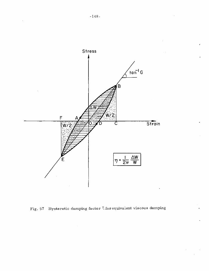
-148-
Stress
. ;-:#~ ~.
, ~.~,.~..;~~:~
~W .i::'~:·':'·~··-:i!:'·~·
Strain
Fig. 57 Hysteretic daITlping factor Tl for equivalent viscous daITlping
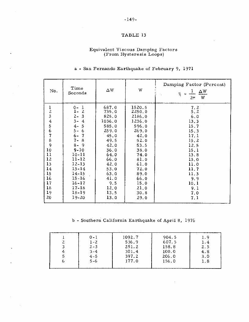
-149-
TABLE 13
Equivalent Viscous Damping Factors(From Hysteresis Loops)
a - San Fernando Earthquake of February 9, 1971
No.
123456789
1011121314151617181920
TimeSeconds
0- 11- 22- 33- 44- 55- 66- 77- 88- 99-10
10-1111-1212-1313-1414-1515-1616-1717-1818-1919-20
t:..w
687.0735.0825.0
1036.0585.0259.045.049.542.036.064.066.042.053.063.041. 0
9.512.013.513.0
w
1520.52250.02186.01236.0596.0269.042.052.053.538.074.081. 061. 072.089.066.015.021. 030.829.0
Damping Factor (Percent)I 1 t:..W
T\ =-2n W
7.25.26.0
13.315.715.317. 115.212.515.113.813.011. 011.711. 39.9
10. 19. 17.07.1
b - Southern California Earthquake of April 8, 1976
1 0-1 1092.7 904.5 1.92 1-2 536.9 607.5 1.43 2-3 251. 2 158.8 2.54 3-4 301.4 100.0 4.85 4-5 397.2 206.0 3.06 5-6 177.0 156.0 1.8

30
,iii
iii
iii
Iii
iii
iii
iii
IIii
Ii
IIiii
I,
Ii
Sa
nta
Fe
licia
Ea
rth
Dam
.'.3 ·2
25
......... - c: Q)
u ~ Q)
20
0.. o - o 0:::
15
~ C 0.. E ~
10 5 1
0-4
•S
anF
ern
an
do
E.
Q.
of
Fe
b.
9.
1971
(ML=
6.3
)
oS
ou
the
rnC
alifo
rnia
E.Q
.o
fA
pri
l8
.19
76
(ML=
4.7
)
.7.....
.........
.10
.8"
......
..5
/~/.
/"1
14
~913
el2
....~-
I16
81
5//
/~7
14/'"
/18
//
19
/",
../,,/
20
/
,,"0
4/
/0
5",
30
06
"./
I/~
00 2
10
-2
Sh
ea
rS
tra
in(p
erc
en
t)
Fig
.5
8
I ......
VI
o I

-151-
C. EVALUATION
C-I COMPARISON BETWEEN THE OBTAINED RESULTS ANDPREVIOUSLY AVAILABLE DATA
In a compr ehensive survey Seed and Idri s s (1970) summariz ed,
in a convenient form, the available data from laboratory and field
tests concerning the dynamic shear moduli and damping factor s fo r
sands and saturated clays. In their study they suggested that the
primary factors affecting shear moduli and damping factors are:
strain amplitude, effective mean principal stress, void ratio, number
of cycles of loading and degree of saturation for cohesive soils.
They indicated that all investigations have shown that modulus values
for sands are strongly influenced by the confining pressure, the
strain amplitude and the void ratio (or relative density) but not sig-
nificantly by variations in grain size characteristics. In gene ral,
...the shear modulus, G, and confining pressure, () , are related bym
the relation
(52)
so that the influence of void ratio and strain amplitude can be ex-
pressed through their influence on the parameter k 2 . Thus for
practical purposes, values of k 2 may be considered to be determined
mainly by the void ratio or relative density and the strain amplitude
of the motion. A number of investigations, using different laboratory
testing procedures, have presented data on the relationships between
these factors. Figure B-1 in Appendix B shows the results of an
investigation which illustrates the relationship between the factor k 2
and strain at a relative density of about 0.75%. Each investigator

-152-
who contributed to the results in Fig. B-1 used a different range for
the effective confining pressures. A representative average relation
ship, which was suggested by Seed and Idriss, for all of the test data
is shown by the solid line. This average relationship may well
provide values of k2
with sufficient accuracy for many practical pur
poses. Other relationships have been obtained and are summarized
for different relative densities. Thus a close approximation to the
modulus versus shear strain relationship for any sand can be ob
tained by determining the modulus at a very low strain level, say
by wave propagation methods in the field, and then reducing this
value for other strain levels in accordance with obtained results
similar to the approximate curve of Fig. B-l.
For gravelly soils it is extremely difficult to perform any lab
investigation because of the large diameter of the test specimens
required. However, Seed and Idriss (1970) summarized the results
of a very limited number of moduli determinations for gravelly soils,
based on in-situ shear wave velocity measurements; Fig. B-2
(Appendix B) shows these results. From Fig. B-2 it may be seen
that at small strain levels, modulus values are between 1. 25 and 2.5
times greater than those for dense sands. Seed and Idriss suggested
that at higher strains, the moduli for gravelly soils decrease in a
manner similar to that for sands. Thus by applying the moduli re
ducing factors of the data obtained for sands to the limited data shown
by solid circular points in Fig. B-2, they estimated variations in shear
moduli with strain as shown in Fig. B-2. From this, approximate
values for use in some types of response analyses can be estimated
by the procedure shown in Fig. B-2.
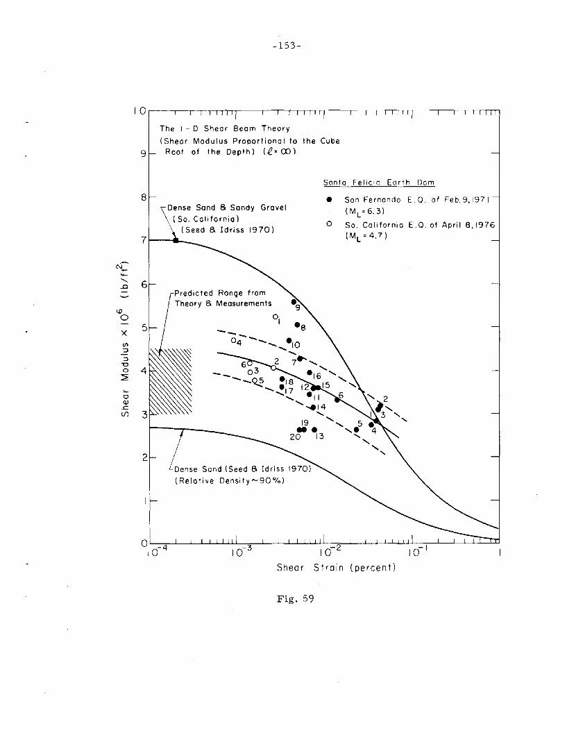
-153-
The 1- D Shear Beam Theory
(Shear Modulus Proportional to the Cube9 Root of the Depth) (.e= 00)
Santo Felicia Earth Dam
8 •Dense Sand 8 Sandy Grovel
(So. California)
°(Seed 8 Idriss 1970)7
N=-"- 6.DPredicted Range fromTheory 8 Measurements
U)
0 °1X
5 ---en:J
II:J"'00 4~
...0<lJ
J::(/)
19••20 13
2Dense Sand (Seed 8 Idriss 1970)
(Relative Density-90%)
Son Fernando E.Q. of Feb.9,1971
(M l = 6.3)
So. California E.Q. of April 8,1976(M l =4.7)
Shear Strain (percent)
Fig. 59
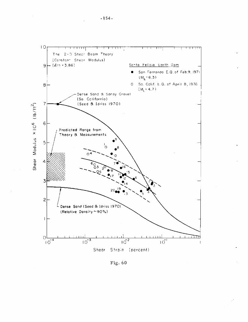
-154-
9
The 2 - 0 Shear Beam Theory
(Constant Shear Modulus)
U'/h =3.86) Santo Felicia Earth Dam
-I10
• Son Fernando E.Q. of Feb,9, 1971
(M L =6.3)
o So. Calif. E.Q. of April 8,1976
(M L=4.7)
Range fromMeasurements
Dense Sand B Sandy Grovel
(So. Co lifornia)
(Seed 8 Idriss 1970)
Dense San(i (Seed 8 Idriss
(Relative Density ~90%)
2
71--_1::...-
8
6
o -410
x
...oQ.l..c(/)
\.Do
N'+-
'.0
Shear Strain (percent)
Fig. 60
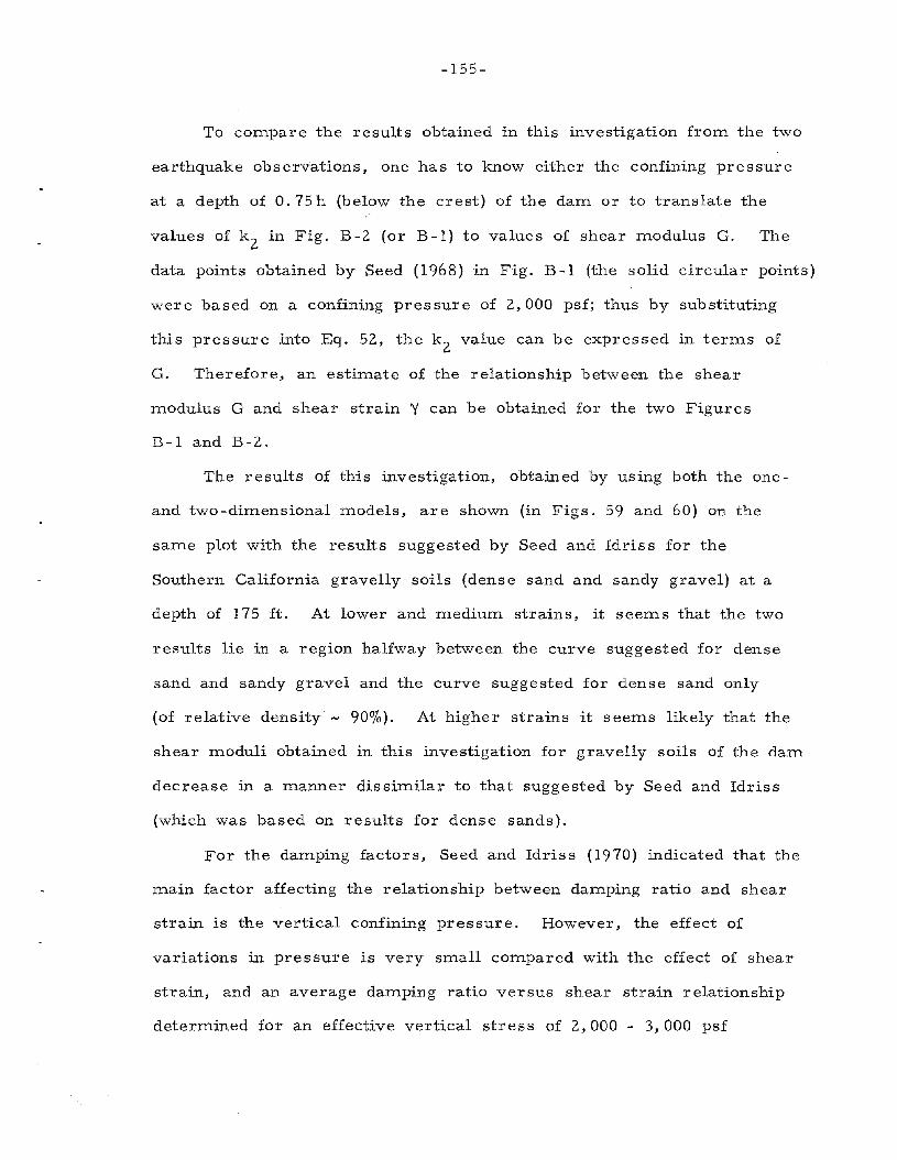
-155-
To compare the results obtained in this investigation from the two
earthquake observations, one has to know either the confining pressure
at a depth of O. 75 h (below the crest) of the dam or to translate the
values of k2
in Fig. B-2 (or B-1) to values of shear modulus G. The
data points obtained by Seed (1968) in Fig. B-1 (the solid circular points)
were based on a confining pres sure of 2,000 psf; thus by substituting
this pressure into Eq. 52, the k 2 value can be expressed in terms of
G. Therefore, an estimate of the relationship between the shear
modulus G and shear strain Y can be obtained for the two Figures
B-1 and B-2.
The results of this investigation, obtained by using both the one
and two-dimensional models, are shown (in Figs. 59 and 60) on the
same plot with the results suggested by Seed and Idris s for the
Southern California gravelly soils (dense sand and sandy gravel) at a
depth of 175 ft. At lower and medium strains, it seems that the two
results lie in a region halfway between the curve suggested for dense
sand and sandy gravel and the curve suggested for dense sand only
(of relative density ~ 90%). At higher strains it seems likely that the
shear moduli obtained in this investigation for gravelly soils of the dam
decrease in a manner dis similar to that suggested by Seed and Idriss
(which was based on results for dense sands).
For the damping factors, Seed and Idriss (1970) indicated that the
main factor affecting the relationship between damping ratio and shear
strain is the vertical confining pressure. However, the effect of
variations in pressure is very small compared with the effect of shear
strain, and an average damping ratio versus shear strain relationship
determined for an effective vertical stress of 2, 000 - 3, 000 psi

-156-
would appear to be adequate for many practical purposes as indicated
by Seed and Idriss. Results of previous investigations of damping
ratios for saturated clays and sands are presented in Fig. B-3 and
B-4 (Appendix B). Approximate upper and lower bound relationships
between damping ratio and shear strain are shown by the dashed
lines, and a representative average relationship for all of the test
data is shown by the solid line. This average relationship provides
a basis for evaluating the relationship between damping ratio and
strain for any particular clay or sand.
Additional data on damping ratios for gravelly soils is badly
needed as acknowledged by Seed and Idriss who nonetheless suggested
that gravelly soils I damping factor is approximately the same as that
for sandy materials. A comparison between the results of this
investigation and those shown in Fig. B-3 and B-4 is shown in
Fig. 61. It is apparent that damping ratios for gravelly soils are
somewhat different from those for sands, contrary to Seed and
Idriss. Clearly, more data on these dynamic characteristics is
required, particularly for very low and very high strain levels.
In general, however, it is believed that the data presented here
will broaden the understanding of soil properties for earthquake
dynamic analyses of earth dams.

I ~ U1
-..J I
10
Da
mp
ing
Ra
tio
sfo
r
Sa
tura
ted
Cia
ys
(See
d8
Idri
ss,
19
70
)
/,e
;("<
"<
10
-1
(pe
rce
nt)
10
-2
Sh
ea
rS
tra
in
Fig
.6
1
Da
mp
ing
Ra
tio
sfo
rS
ands
(See
d8
Idri
ss,
19
70
)
.7~so
.ca
liJf
[sa
nF
ern
an
dO
]E
.Q
.E
.Q
.
4/8
,19
76
Fe
b.9
,1
97
6
ML
=4
.7M
L=
6.3
I.•
II•
•I
10
-3
Sa
nta
Fe
licia
Ea
rth
Dam
(Gra
velly
So
ils)
-5 o~
10
-4
35'
IIiii
IIII
iI
Iii
Iii
II
II
Iiii
IIIii
II
IIII
Iiii
IIiii
30
15
2025
10
o 01
C a. E o oo a::~ -C Q) o ~ Q) a.

-158-
CONCLUSIONS
The analyses and the results presented in this investigation lead
to the following conclusions concerning the seismic behavior of an
earth dam:
1 - Since an earthquake is an occurrence that can never be
exactly repeated, it is recommended that not less than
four strong-motion accelerographs be installed on and
around major dams. Two of these should be located
to record earthquake motions at the base and two to
measure dam response. The purpose of requiring two
instruments is to provide backup to obtain useful infor
mation in the event of instrument malfunction (Bolt and
Buds on, 1975) such a s the double expo sure situation
which occurred during the 1971 San Fernando earthquake
at Santa Felicia Dam.
2 - Amplification spectra are good criteria to indicate the
natural frequencies of the structure and to estimate the
relative contribution of different modes.
3 - A visual inspection of the amplification spectra obtained
from the 1971 San Fernando and the 1976 Southern California
earthquakes revealed that the values of the resonant or natural
frequencies vary slightly from one earthquake to the other.
4 - The amplification spectra also showed that the dam
responded primarily in its fundamental mode in the
upstream/downstream direction. The peak amplification ratio
of horizontal acceleration at the dam crest to that of the
-159-
base is 1: 13 for the large earthquake, and 1:4 for the sTIlall
earthquake, in a norTIlal direction to the daTIl axis; i. e., the
rate of aTIlplification in that direction increases with the
intensity of earthquake shaking over this l"ange of intensity.
5 - The other two directional cOTIlponents indicate siTIlilar
aTIlp1i£ication patterns, but they are lacking pronounced single
peaks.
6 - Very narrow band-pass filtering, around the fundaTIlental
frequency, is needed to obtain a good hysteresis loop, if
the daTIl is treated as a single-degree-o£-freedoTIl hysteretic
oscillator.
7 - The cOTIlparison of the cOTIlputed natural frequencies using
existing shear -beaTIl theories, with those obtained froTIl
observed records shows that these dynaTIlic characteristics
can be evaluated by the existing theories.
8 - Although the assUITlption of elastic behavior during earthquakes
is not strictly correct for earth daTIls, it provides a basis for
establishing the natural frequencies o£ the daTIl, and it gives
at least a qualitative picture of the dynaTIlic response charac
teristics of the daTIl. There£ore, the earthquake response of
a TIlassive structure, such as an earth daTIl, can be approxi
TIlated by using the existing elastic -response theories.
9 - The shear TIlodulus and the daTIlping factor obtained froTIl the
hysteresis loop depend on the TIlagnitude of the strain for
which the hysteresis loop is deterTIlined.
-160-
10 - Data obtained from the wave-velocity measurements of the
dam materials indicated that the dam consists of mainly
cohesionless materials where the shear modulus varies
with the confining pressure (or the depth below the crest).
11 - Damping effect increases with the intensity of vibration.
12 - Estimation of shear moduli and damping factor s of the dam
materials is pos sible from the earthquake records of the
dam.
13 - From the comparison between the obtained results and
previously available data for dense sand, it seems that
at lower and medium strain levels, the two results for
the shear modulus correlate very well; however at the
higher strains, the shear moduli obtained in this
investigation for the gravelly materials of the dam de
crease in a manner dissimilar to that suggested by Seed
and Idriss (1970) for sand. The comparison also shows
that the damping ratios for gravelly soils are somewhat
higher than those obtained for sands.
14 - Finally, the data presented here are likely to provide
reasonable estimates of the shear moduli and damping factors
for the gravelly materials of Santa Felicia Dam.
-161-
REFERENCES
1 - Price, W. P. , Jr., "Technical Record of Design and Construction,Santa Felicia Dam", United Water Conservation District of VenturaCounty, California, Santa Paula, California (1956). [CaltechEarthquake Engineering Library Call No.3. 2. 2b PR 1956 J.
2 - Correspondence between Professor George Housner of the CaliforniaInstitute of Technology and the United Water Conservation Districtof Ventura County, California [Caltech Earthquake EngineeringLibrary Call No. 10.1. 8a] .
3 - Ma:rtin, G. R., "The Response of Earth Dams to Earthquakes ",Ph. D. Theses, 1965, Civil Engineering Department, Universityof California, Berkeley.
4 - Seed, H. B. and Idriss, 1. M. (1970), tlSoil Moduli and DampingFactors for Dynamic Response Analyses", Report No. EERC 70-10,December, College of Engineering, University of California,Berkeley.
5 - Hudson, D. E., Editor, "Strong -Motion Instrumental Data on theSan Fernando Earthquake of Feb. 9, 1971, Earthquake EngineeringResearch Laboratory, California Institute of Technology, Sept. 1971.
6 - "Strong-Motion Earthquake Accelerograms, Corrected Accelerogramsand Integrated Ground Velocity and Displacement Curves, Vol. II,Part E," Earthquake Engineering Research Laboratory ReportEERL 73 -50, California Institute of Technology, 1973.
7 - "Seismic Engineering Program Report", April-June 1976, Geological Survey Circular 736-B, U.S. Department of the Interior, 1976.
8 - Mononobe,N. , Takata,A. , and Matumura, M. (1936), "SeismicStability of the Earth Dam 'l, Second Congress on Large Dams,Washington, 1936, Vol. IV, pp. 435-442.
9 - Hatanaka, M. (1955), "Fundamental Considerations on the EarthquakeResistant Properties of the Earth Dam", Disaster Prevention ResearchInstitute, Kyoto University, Bulletin No. 11, Dec. 1955.
10 - Ambraseys, N. N. (l960a), "On the Seismic Behavior of Earth Dams ",Proceedings of the Second World Conference on Earthquake Engineering,Japan, 1960, Vol. I, pp. 331-354.
11 - Ambraseys, N.N. (1960b), "On the Shear Response of a Two Dimensional Wedge Subjected to an Arbitrary Disturbance", Bulletin of theSeismological Society of America, Vol. 50, Jan. 1960, pp. 45-56.
12 - Minami, 1., (1960), "A Consideration of Earthquake Proof DesignMethods for Earth Dams!!, Proceedings of the Second World Conferenceon Earthquake Engineering, Japan; 1960, Vol. III, pp. 1061-1074.

-162-
13 - Rashid, Y.R. (1961), "Dynamic Response of Earth Dams to Earthquakes ", Graduate Student Research Report, University ofCalifornia, Berkeley, 1961.
14 - Keightley, W. o. (1964), IIA Dynamic Investigation of BouquetCanyon Dam ", Earthquake Engineering Research Laboratory,California Institute of Technology, Sept. 1964.
15 - Jacobsen, L. S., "Steady Forced Vibration as Influenced byDamping", Transaction A. S. C. E. APM-52-15, 1930.
16 - Seed, H. B. and Idriss, 1. M., llInfluence of Soil Conditions onGround Motions During Earthquakes", Proceedings ASCE,Journal of Soil Mechanics and Foundations Division, SMl,Jan. 1969, pp. 99-137.
17 - Kawakami, F. and Asada, A., "Earthquake Response of an EarthDam", The Technology Reports of the Tohoku University, Vol. 32(1967) No.2, June 1967, pp. 247-174.
18 - Iemura, H. and Jennings, P. C., "Hysteretic Reponse of a NineStory Reinforced Concrete Building During the San FernandoEarthquake", Earthquake Engineering Research Laboratory,Report No. EERL 73 -07, California Institute of Technology,Oct. 1973.
19 - Mori, Y. and Kawakami, F., "Dynamic Properties of the AinonoEarth Dam and Ushino Rock-Fill Dam", Transactions of JSCE,Vol. 7, 1975, pp. 122 - 123 .
20 - Bolt, B. A. and Hudson, D. E., "Seismic Instrumentation of Dams ",ASCE, Journal of the Geotechnical Engineering Division, Nov. 1975,pp. 1095 -1104.
21 - Morrison, P., Maley, R., Brady, G. and Prcella, R. , "EarthquakeRecordings on or Near Dams", Report, USCOLD Committee onEarthquakes, Printed at California Institute of Technology, Pasadena,November 1977.

-163-
D. APPENDICES
APPENDIX A
Standard Data Proces sing of the Southern CaliforniaEarthquake of April 8, 1976
Santa Felicia Darn (Ventura County, California)
This appendix contains the computed plots of:
1 - Volume I which contains the uncorrected digitized acce1erograms,
2 - Volume III which contains the response spectrum curves withlinear and three-way logarithmic plots,
3 - Volume IV which contains Fourier amplitude spectra withlinear and logarithmic plots.

SRNT
RFE
LIC
IRD
RM.R
IGH
TRB
UTM
ENT
RPRI
L8
1976
S78W
2 Of-_
-I -2
o ......
2~ zl
II
II
II
II
II
II
II
II
DLJW
N.....
.0
'~ I
~Ot-~
~ f-~
-Iw LLJ
-2u u C
I
S12
E2 Of-~
-I -2
II
II
II
II
II
II
II
II
o2
ij6
810
12li
j16
1820
222i
j26
28
30
TIM
EIN
5EC
ClN
05
Fig
.A
-I

SRNT
RFE
LIC
IROR
M.C
REST
.ERR
THQU
RKE
OF8
RPRI
L19
76I
II
II
II
II
I\
II
II
I
S78W
2 0 -I -2I
DOWN
~.....
.0
0'
.....2r
U1
""-
I~ Z
ot--vNr~""""rv'VVV'---rN"--....rv'VV-------~-----~""""""~~~----------
z: o ..... ~
-I0:
:w -l
-2W u u a:
II
II
II
II
II
II
II
II
o2
46
810
1214
16,Q
~n
~~
?U?6
2830
TIM
EIN
5EC~ND5
S12
E2 o -1 -2
II
II
II
II
!I
II
!I
II
o2
46
810
1214
1618
2022
2426
2830
TIM
EIN
5EC~ND5
Fig
.A
-2

-166-
RESPONSE SPECTRUM
SRNTR FELICIR DRM,CREST,E/Q ~F RPRIL 8 1976-0721 PST
SANTA FELICIA DAM.CREST C~MP S12E
DAMPING VALUES ARE O. 2. 5, 10 AND 20 PERCENT OF CRITICAL
200
A
-&'--7f-*, 100
.-+--c¢"-~-----j,"----1 80
~if-----r---fV-----i60
1 P~~~-¥-It-;~·-MqW~"..¥~+~~~~M~,L-~~~~ -+-'B-:;;.--r-+-~ I
.8 .8
6
100 f------'...r-~_f"r._
80~~~~~+-
60 I---*-+-+---lo<--M.
200
20 20
0Q)({)
-..........10 10
c8.- 8
>- 6 6f--0
4 40-JW>
2 2
PERIOD (sees)
Fig. A-3

RELA
TIVE
VELO
CITY
RESP~NSE
SPEC
TRUM
SANT
AFE
LICI
AD
AM
.CRE
ST.E
/QOF
APRI
L8
1976
-072
1PS
TSA
NTA
FELI
CIA
DAM
.CRE
STCO
MPS1
2EDA
MPI
NGVA
LUES
ARE
O.
2.5
.10
AND
20PE
RCEN
TOF
CRIT
ICA
L20
iI
II
II
iI
II
II
II
II
II
II
II
II
I
16u ~ .....
.. z ....
SV--------
FS·
I ~12
.... u CD ~ UJ > .... I-
85 ~
q
2PE
RIOD
-SE
COND
SF
ig.
A-4
37
1115
I ..... 0'
-.J
I
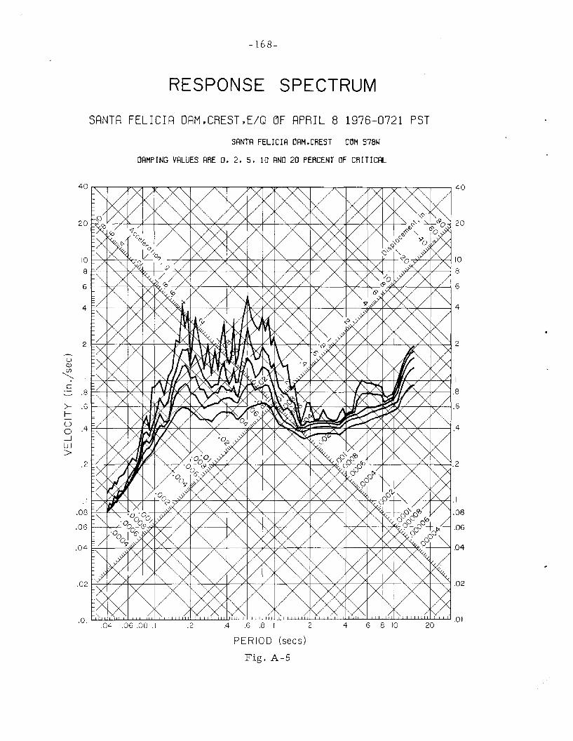
-168-
RESPONSE SPECTRUM
SRNTR FELICIR DRM,CREST,E/Q ~F RPRIL 8 1976-0721 PST
SANTA FELICIA DAM.CREST C~M S78W
DAMPING VALUES ARE O. 2. 5. 10 AND 20 PERCENT ~F CRITICAL
20
.04
.06
-&"--7f-~'---j 10
*---+-<---7<::---+~~~'k---+--r-'X'--¥-*-+~~~-+~"---C>~j,L--------18
10 t-----''rl-~i'<'7
8 F-----t--'''c--¥--''17:--+--
6 I-----'!'-c--r-+c-_+_~
.0 1 L..J..U.ti.llllL-L...L.LL.LU.LLL.LLJ...LLJ....l..Lll...L.LL.LLLll.l..u..w.L.Ll--'--'--LLllJ..LJ....LL.L.J...LJ..L.U.-L..J...J...l...I....I...~L.L.L.U...J...J....J...J....L.Ju..u.~..LW...w...J..'-'-:.J....J...J...J..l .0 I.04 .06 .08 .1 .2 .4
20
. I f---'Y'-1lk--~-+'-I
.08 r-7---+-"':-~
. 0 6 f------+<--,L
2 2
()Q)(/)
""'-..1
c.- .8
>- .6I--0 .4 .40---JW>
.2
PERIOD (sees)
Fig. A-5

RELA
TIVE
VEL~CITY
RESP~NSE
SPEC
TRUM
SANT
AFE
LICI
ADA
M.C
REST
.E/Q
OFAP
RIL
819
76-0
721
PST
SANT
AFE
LICI
ADA
M.C
REST
COM
S78W
DAM
PING
VALU
ESAR
EO
.2.
5.10
AND
20PE
RCEN
TOF
CRIT
ICAL
10r=
II
I•
II
II
II
I•
II
I•
II
II
II.,
8
~ "z ......
SV--------
FS
I ~6
.... U 10 u:l ;> LLI
;> .... ~l!
5 UJ
(C
2
2PE
RIOD
-SE
COND
SF
ig.
A-6
37
1115
I .......
0'
-0 I
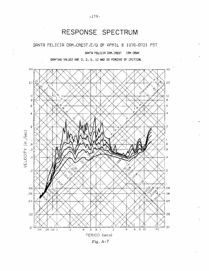
-170-
RESPONSE SPECTRUM
SRNTR FELICIR DRM,CREST,E/Q ~F RPRIL 8 1976-0721 PST
SRNTR FELICIR DAM.CREST C~M D~WN
DAMPING VALUES ARE D. 2, 5, 10 AND 20 PERCENT ~F CRITICAL
20
.04
.06
-d--7f---'><c-; 10
*---tr'------~'_+--'T-----f?Pk_____+_~~¥-*+~~__".I___+~'____7<~i>"__18
-r------h+--f""-r:--+~hful---+-*~-___f',++- ,~~'---_/_--f'.v'-------1 6
I0 r------''l<f--''<-i'r
8 F---P~b<'---'''1:r.-+-
6 f-----~_/_-h----~.,4'6
.0 I LUJ..JJ..u.LlL.J....LLLLUJ..J..L.L.J...l.-Lll.llll...L.L.LLLll.l.l.Lil1J..L1.J-.1...LlLll.J.LJ....lJ,..J.-J..J..J.J.J.LLLL.l..LLLl..ll-LU..ll...J...J....J...J...WU-J.J-l....l..-'-.J...J...J..J...J.J..u...J...J...J.-.U .0 I.04 .06 .08 .1 .2 .4.6.8 I 2 4 6 8 10
20
• I f-----+---"'.-u.~--+
.0 8 1-7--+--,~r;
.06 r--------f'<-jr
2 2
u(l)
~c.- .8
>- .6f--U
.4 .40---JW>
.2
PERIOD (sees)
Fig. A-7

RELA
TIVE
VELO
CITY
RESP
ONSE
SPEC
TRUM
SANT
AFE
LICI
ADA
M.C
REST
.E/Q
OFAP
RIL
819
76-0
721
PST
SANT
AFE
LICI
ADA
M.C
REST
COM
DOWN
DAM
PING
VALU
ESAR
EO
.2.
5.10
AND
20PE
RCEN
TOF
CRIT
ICAL
10r=
II
II
II
II
II
II
II
II
II
II
II
II
8
~ "z ..... I ~6
..... U 10 rd > LIJ
> ..... t-II
5 ~
2
2PE
RICI
D-
SECO
NDS
Fig
.A
-8
SV--------
FS
I ......
-J ......
I
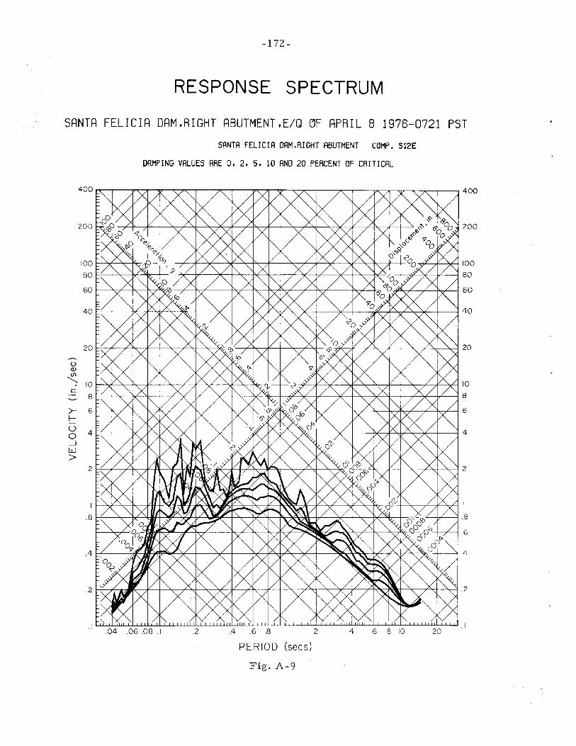
-172 -
RESPONSE SPECTRUM
SANTA FELICIA OAM,RIGHT ABUTMENT,E/Q ~F APRIL 8 1976-0721 PST
SANTA FELICIA DAM.RIGHT ABUTMENT COMPo S12E
DAMPING VALUES ARE O. 2. 5. 10 AND 20 PERCENT OF CRITICAL
200 200
.6
.4
--+-"-c----+--,iL---'V-! 1
L.-.f-r'-----1 .8
I r)f-~k-7H'-FV,J~r-r~~P7I;~~:-±~ ~""'x----JL-~---''dL-~---1'&
.8 i=-L-~,-<--¥-~tt-t--.:¥L-¥;'I--+r-~~C+~--f.,L~~~~:\----+;,L-----'x"------t~-----b~b---1f--r
100 100
80 80
60 60
40 40
20 20
<.)Q)
.z 10 10c:
8.- 8
>- 6 6I--U 4 40-.JW>
2 2
PERIOD (sees)
Fig. A-9

RELA
TIVE
VEL~CITY
RESP~NSE
SPEC
TRUM
SANT
AFE
LICI
ADA
M.R
IGHT
ABUT
MEN
T.E/
QOF
APRI
L8
1976
-072
1PS
TSA
NTA
FELI
CIA
DAM
.RIG
HTAB
UTM
ENT
COM
PoS1
2£DA
MPI
NGVA
LUES
ARE
O.
2.5
.10
AND
20PE
RCEN
TOF
CRIT
ICAL
10iiiiii
IIiii
IIiiiii
II
II
II
i
8
~ ........
Z - 1 ~6
..... u ~ > UJ
::> ..... 5
~~
SV-------
FS
I ......
--J
W I
2 °01
""-'..
......_
----
----
---
2PE
RIOD
-SE
COND
SF
ig.
A-I
O
37
1115

-174-
RESPONSE SPECTRUM
SANTA FELICIA DAM,RIGHT ABUTMENT,E/Q OF APRIL 8 1976-0721 PST
SANTA FELICIA DAM.RIGHT ABUTMENT COMPo S7e~
DAMPING VALUES ARE O. 2. 5. 10 AND 20 PERCENT OF CRITICAL
200
A
-+-"-c---+-+-'if-1 I
"--lr---l 8
.6
-&-7f--Y-i 100
-+-~--¥---+L----j 80
,~d--r----P'if--l60
I00 f-",,f->..,..-.!''''''
80 F-'---t--".----'bf---'''I7:-+_
60 I---+O-:'<--i'c---kc~!
200
20 20
(.)Q)
~.10 10
c8.- 8
>- 6 6~-U 4 40-lW>
2 2
PERIOD (sees)
Fig. A-ll
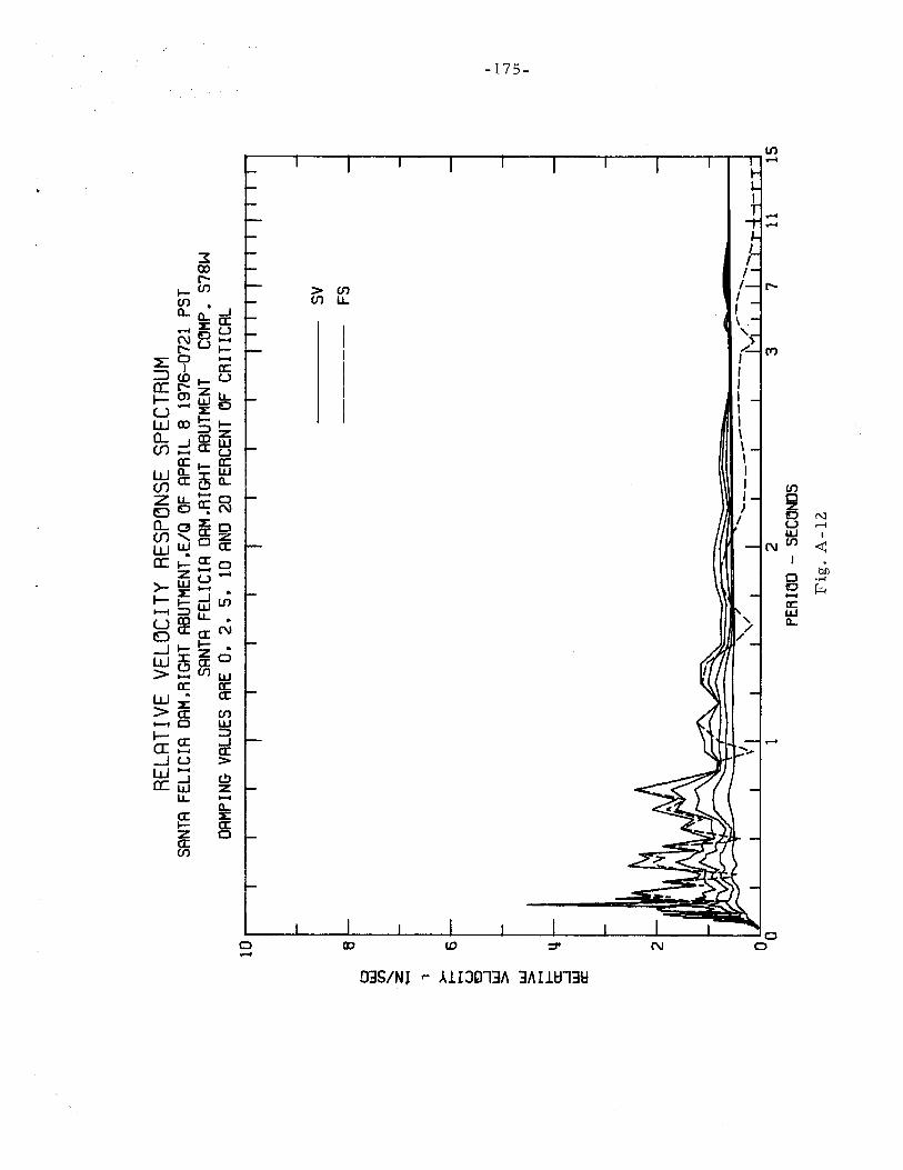
RELA
TIVE
VEL~CITY
RESP~NSE
SPEC
TRUM
SANT
AFE
LICI
AoA
M.R
IGHT
ABUT
MEN
T.E/
Q~F
APRI
L8
1976
-072
1PS
TSA
NTA
FELI
CIA
DAM
.RIG
HTAB
UTM
ENT
C~MP.
S78W
DAM
PING
VALU
ESAR
EO
.2.
5.
10AN
D20
PERC
ENT
~F
CRIT
ICAL
10iii
I,
IIi'
iiii
iii
Ii
IIIii
ii
8
f;1 "Z -.. 1 ~
6.... u \!
:) -I ~ uJ
:> .... 5:q
-I
uJ «:
2
2PE
RIOD
-SE
COND
SF
ig.
A-1
2
SV-----
FS
711
15
I t-'
--J
U"1
J

-176-
RESPONSE SPECTRUM
SANTA FELICIA DAM,RIGHT ABUTMENT,E/Q ~F APRIL 8 1976-0721 PST
SANTA FELICIA DAM.RIGHT ABUTMENT COMPo DOWN
DAMPING VALUES ARE O. 2. 5. 10 AND 20 PERCENT OF CRITICAL
20
-&----+~'--l 10
*----1r'---------*-+~___fX'~_+______r'---'X'-----\:;,L--_____7<~~_f>(__>,r____lr____:'9.l'___7~¥____j8
---r------1'<;+--------f'~~_____f'''v'1'''d'_---r<----f''d_-_____1~_____f' &~<-----:T'___f>.v_''_______j6
10 f-------',<f------>~r:
8 F-'----t--"..,--b<:'->v.--t-
6 f--~T'_~----f.<-~,
20
.1
.08
.06 .06
,04 .04
.02 .02
2 2
()Q)<.f) .
............
c-- .8
>- .6f--U
.40....JW>
.2
PERIOD (sees)
Fig. A-13

RELA
TIVE
VEL~CITY
RESP~NSE
SPEC
TRUM
SANT
AFE
LICI
ADA
M.R
IGHT
ABUT
MEN
T.E/
Q~F
APRI
L8
1976
-072
1PS
TSA
NTA
FELI
CIA
DAM
.RIG
HTAB
UTM
ENT
C~MP.D~WN
DAM
PING
VALU
ESAR
EO
.2.
5.10
AND
20PE
RCEN
T~F
CRIT
ICAL
10iii
II
iI
Iiii
II
IIiii
II
II
IF
1
8
~ "z -- I ~6
--U E:l ...J ~ UJ
:> ..... Ii:I!
...J
UJ ex:
2
SV--------
FS
I ......
--J
--J
I
12
PERI
OD-
SECO
NDS
Fig
.A-1
4
37
1115

F~URIER
AMPL
ITUD
ESP
ECTR
UM~F
ACCE
LERA
TION
SANT
AFE
LICI
AO
AM
.CRE
ST.E
/QOF
APR
IL8
1976
-072
1PS
TSA
NTA
FELI
CIA
OAM
.CRE
STCO
MPS1
2E30
,iiiiiiiiiiiiiiiiiiiiiiii
i
fd (f) ......
E:
U
J E:
;::) cr::~ fd Cl
...(f
)
L&J
o i=? --I Q..
E:
a::
cr::
L&J -cr:: ;:
:)£
)u.
.
20 10-
--
--
--
--
--
--
--
--
--
--
95PE
RCEN
TCC
lIIFI
OEN
CELE
VEL
1 ..... -J
00 I
O'
II
II
II
II
II
II
I-C
"'.
.C]:
::::
t"'
II
,..
-J,
II
,,
o5
1015
2025
Fig
.A
-IS
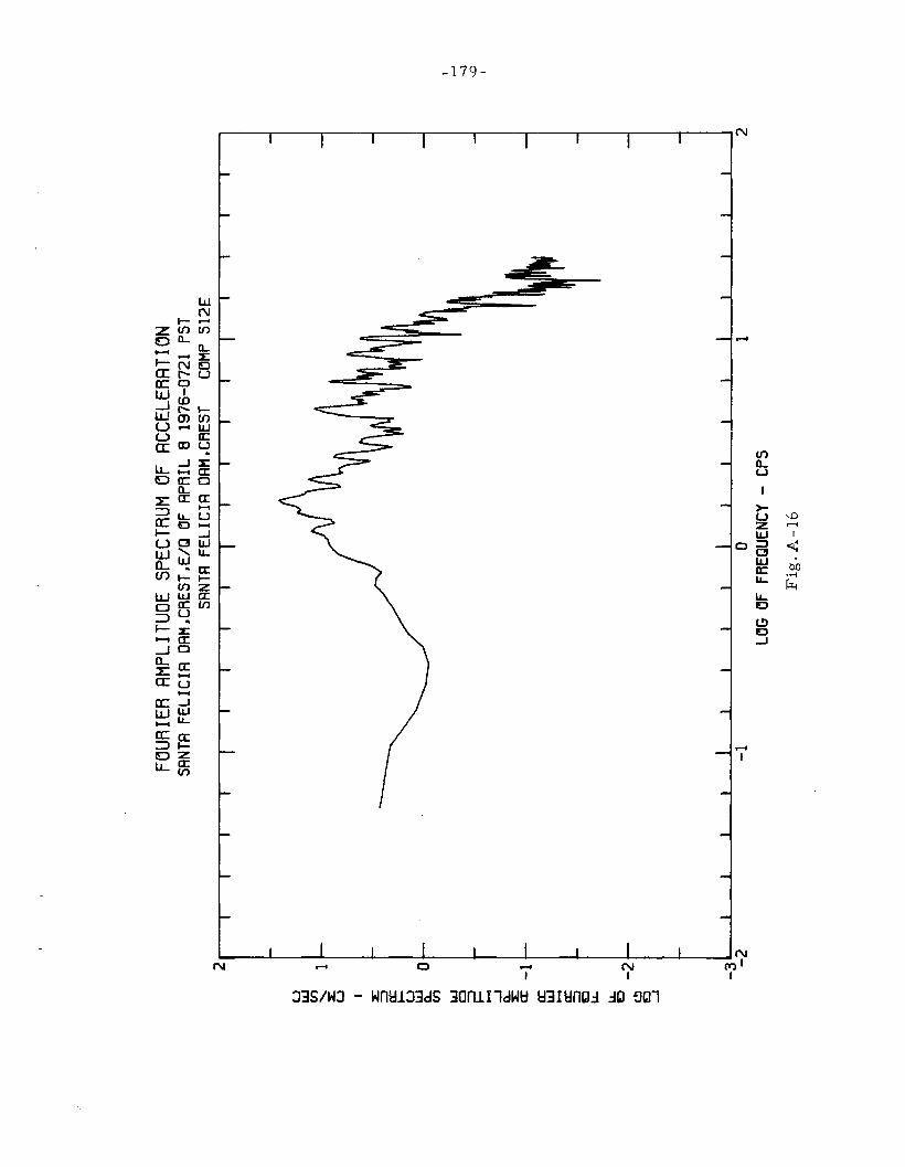
F~URIER
AMPL
ITUD
ESP
ECTR
UM~F
ACCE
LERA
TION
SANT
AFE
LICI
AO
AH
.CRE
ST.E
/QOF
APRI
L8
1976
-072
1PS
TSA
NTA
FELI
CIA
DAM
,CRE
STCO
MPS1
2E2
.I
Iiii
iii
iii
iI
II
Ii
II
i
frl ~1
x: U I :z:::~ a: I- frl
0Q
..U
')
~ CJ ~ .... -l
Q.. ~
-1
ffi .... cc:~ E:
JI.L
-
I.L-
E:I
-2c..!
:lE:
J-l
t ......
--J
-.0 I
-3'
,,
,,
I,
,I
II
,I
II
,,
II
II
-2-1
01
2LO
GOF
FREQ
UENC
Y-
CPS
Fig
.A-1
6

FOUR
IER
AMPL
ITUD
ESP
ECTR
UMOF
ACCE
LERA
TION
SANT
AFE
LICI
AOA
M.C
AEST
.E/Q
OFAP
RIL
819
76-0
721
PST
SANT
AFE
LICI
ADA
M.C
REST
COM
S78W
20.
ijIii
,i
Ij
i»
ii
»,
ji
»iii
jj
Ii
--
--
--
--
--
--
--
--
--
95PE
RCEN
TC
MlD
EN
CE
LEV
EL
10
U LIJ
(f) .....
.E U I
%:
::::> a:::
I- td Q..
(f) LIJ
Cl
::> I- ..... .....J
Q..
E cr ffi ..... a:::
::::> o LL..
0010
15FR
EQUE
NCY
-CP
S
Fig
.A
-I7
2025
I ......
00 o I
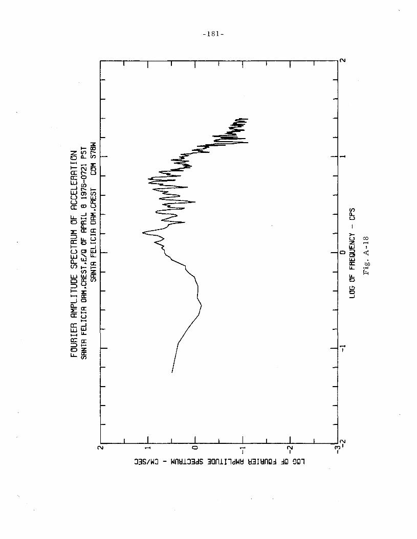
F~URIER
AMPL
ITUD
ESP
ECTR
UM~F
ACCE
LERA
TION
SANT
AFE
LICI
ADA
M.C
AEST
.E/Q
OFAP
RIL
819
76-0
721
PST
SANT
AFE
LICI
ADA
M.C
REST
COM
S78W
2.iii
Ii
II
IIii
Iii
iii
Ii
I
u UJ en
1.....
.. s: U I %:
::)
a::~ u U
J0
Q.. en
~r'~
J~
1
UJ
I-'
CI
CXl
::J
I-'
~I
-...J 0- s: a:
-1a: U
J>
-I a::
::)
10
l.!-
I.!-
E)
-2C
l1
0...
J
-3'
I,
I,
II
,,
II
I,
,,
I,
,I
,I
-2-1
01
2LO
GOF
FREQ
UENC
Y-
CPS
Fig
.A
-18

9 8
~7
(I)
"'- :E U I6
::E:
:;:) a: ..- u
5U
JQ
..(I)
UJ
CI
Y:;
:) ..- -...J Q..
:E a:3
a: UJ -a: :;:)
2lO u.
.
1 00
FOUR
IER
AMPL
ITUD
ESP
ECTR
UMOF
ACCE
LERA
TION
SANT
AfE
LIC
IAD
AH
.CRE
ST.E
lQD
fAP
RIL
819
76-0
721
PST
SANT
AfE
LIC
IAOA
H.CR
EST
COM
DOWN
--
--
--
--
--
--
--
--
-95
PERC
ENT
CO
tFIO
ENC
ELE
VEL
10fR
EQUE
NCY
-CP
S
Fig
.A
-19
25
I ..... 00 N I

F~URIER
AMPL
ITUD
ESP
ECTR
UMOF
ACCE
LERA
TION
SRNT
AFE
LICI
AD
AM
.CRE
ST.E
/QOF
APRI
L8
1976
-072
1PS
TSA
NTA
FELI
CIA
DAH.
CAES
rCO
MDO
WN2.
iI
IIIii
II
Iiii
Iiii
II
i
u UJ ~
1~ U
I z: ~ a:: .- frl
0Q
..V
l
UJ
CJ => .- .... -I
Q.. ~
-1a:
:U
J .... a:: 5 LL.
LL.
o-2
<.!>
E)
-I
I .......
00
W I
-3'
,,
,,
,,
,I
,,
II
,I
,,
,I
II
-2-1
01
2LO
GOF
FREQ
UENC
Y-
CPS
Fig
.A
-ZO
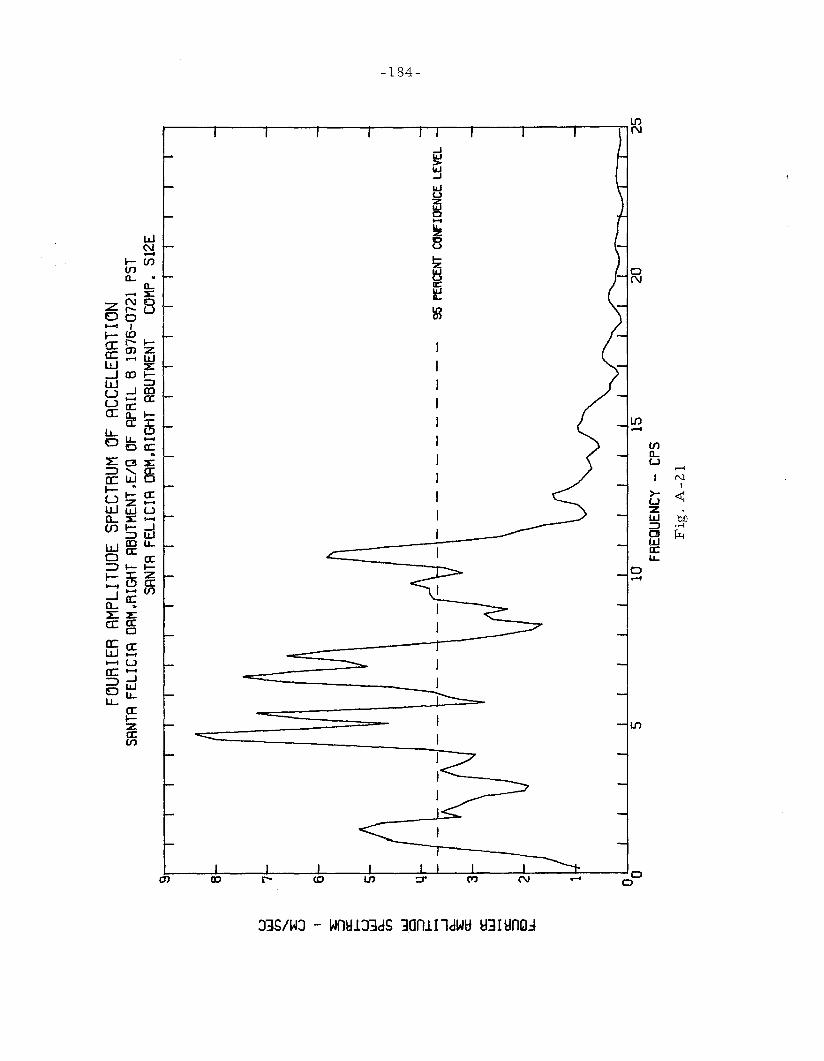
F~URIER
AMPL
ITUD
ESP
ECTR
UMOF
ACCE
LERA
TION
SANT
AFE
LICI
AOA
M.R
IGHT
ABUT
MEN
T.E/
QOF
APR
IL8
1976
-072
1PS
TSA
NTA
FELI
CIA
ORM
.RIG
HTAB
UTM
ENT
COM
PoS1
2E
I ..... (Xl
>!'>-
I
-•-
--
--
--
--
--
95PE
RCEN
TCCJ~IOENCE
LEVE
L
1015
2025
FREQ
UENC
Y-
CPS
Fig
.A
-21
9 e
u..,
IJJ en "- s:::
U I6
~ :::J cc:
I- W
5a..
.en U
J0
4:::
JI- -...J a...
s:::
a:3
cc:
IJJ -cc: :::J
20 u.
.
1 00

FOUR
IER
AMPL
ITUD
ESP
ECTR
UM~F
ACCELERATI~N
SANT
AFE
LICI
ADA
M.R
IGHT
ABUT
MEN
T.E/
QOF
APRI
L8
1976
-072
1PS
TSA
NTA
FELI
CIA
OAM
.RIG
HTAB
UTM
ENT
COM
PoS1
2E2.
IIii
Iii
IIiii
iii
Iii
,1
fd ~1
~ I :E:
::::> a:::
I- fd Q..
CJ'
)
W CI
~ ......
-..l
Q.. ~
-1
ffi ......
a:::
::::>
E:) u..
u..
E:)
-2(..
!)E
:)-.
.l
I !-'
00
U1
I
-3'
II
II
II
II
II
II
II
II
II
II
-2-1
a1
2LO
GOF
FREQ
UENC
Y-
CPS
Fig
.A
-22

10 9
(.J
8LL
J en .......~ (.
J7
I
~ ::::> a:
6I-
(.J
LLJ
0- en w
50 ::::
>I- ---l
40
-~ a:
a:
LLJ
3-a: ::::
>lD lJ
..
F~URIER
AMPL
ITUD
ESP
ECTR
UM~F
ACCELERATI~N
SANT
AFE
LICI
ADA
M.R
IGHT
ABUT
MEN
T.E/
QOF
APR
ILB
1976
-072
1PS
TSA
NTA
FELI
CIA
DAM
.RIG
HTAB
UTM
ENT
COM
PoS7
8W
--
--
--
--
--
--
95PE
RCEN
TCO~IOENCE
LEV
EL
I J-'
00 0"
I
atI
II
II
II
II
II
II
II
I,-~I~
o5
1015
2025
FREQ
UENC
Y-
CPS
Fig
.A
-23
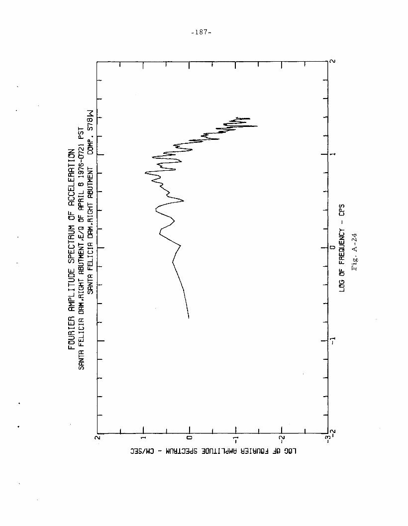
FOUR
IER
AMPL
ITUD
ESP
ECTR
UMOF
ACCE
LERA
TION
SANT
AFE
LICI
ADA
M.R
IGHT
ABUT
MEN
T.E/
QOf
APRI
L8
1976
-072
1PS
TSA
NTA
fELI
CIA
DAM
.RIG
HTAB
UTM
ENT
COM
PoS78~
2.iii
iii
IiIi
IIii
II
II
iI
U IJJ en
1.....
..:E U
I :E ;:)
I
a::
I
l-
. ~~.....
..
u
00
IJJ
°1--
.)
0-
J
en w CI => I- ......
.....J
0-
:E ex-1
a::
IJJ ......
a::
;:)
E:)~ lL
..E
:)-2
~ E:)
.....J
-3'
,,
II
II
,,
II
II
II
I,
,,
,J
-2-1
01
2LO
GO
ffR
EQUE
NCY
-CP
SF
ig.
A-2
4
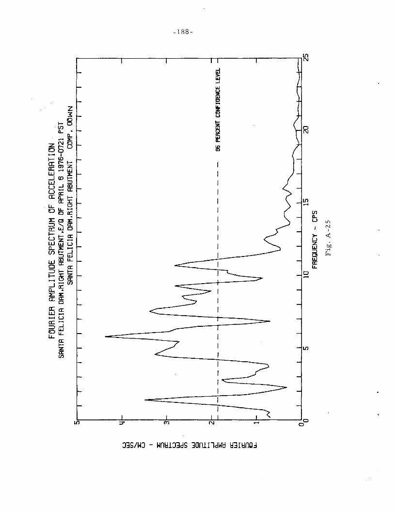
FOUR
IER
AMPL
ITUD
ESP
ECTR
UMOF
ACCE
LERA
TION
SANT
AFE
LICI
ADA
M.R
IGHT
ABUT
MEN
T.E/
QOF
APRI
L8
1976
-072
1PS
TSA
NTA
FELI
CIA
DAM
.RIG
HTAB
UTM
ENT
COM
PoDO
WN
5.Iii
Iii
iii
Iii
iii
Ii
II
Iiii
Ii
--
--
-1
-1
--
--
--
--
--
-95
PERC
ENTC6~IOENCE
LEVE
L
I >-'
00
00 I
LJ 13 2
frl (f) ........ :E:
CJ I :E:
:::::> a:::
I- frl a...
(f) w o ~ ~ -l a...
:E:
a:
a:::
UJ~ a::
::::::
>lD \J
...
01
II
II
II
II
II
II
II
II
II
't":
I't~I
o5
1015
2025
FREQ
UENC
Y-
CPS
Fig
.A
-25

FOUR
IER
AMPL
ITUD
ESP
ECTR
UMOF
ACCE
LERA
TION
SANT
AFE
LICI
ADA
M,R
IGHT
ABUT
MEN
T.Et
Q~F
APRI
L8
1976
-072
1PS
TSA
NTA
FELI
CIA
DAM
.RIG
HTAB
UTM
ENT
C~MP.
OOW
M2
.Iii
iii
iii
Iiii
Iii
iii
i
~ ~1
~ u ~ :::> cc ..... ~0
Cl..
(f') ~ ~ .... -I~ If
-1
ffi .... cc :::> E:!
1.1-
1.1-
E:!
-2C
)E
:!-I
I I-'
00
'-.D I
-3'
II
II
II
I,
,I
II
II
II
II
,I
-2-1
01
2L~G
~F
FREQ
UENC
Y-
CPS
Fig
.A
-26

-190-
APPENDIX B
Previously Available Data on the Shear Moduliand Damping Factors for Sands and Saturated Clays
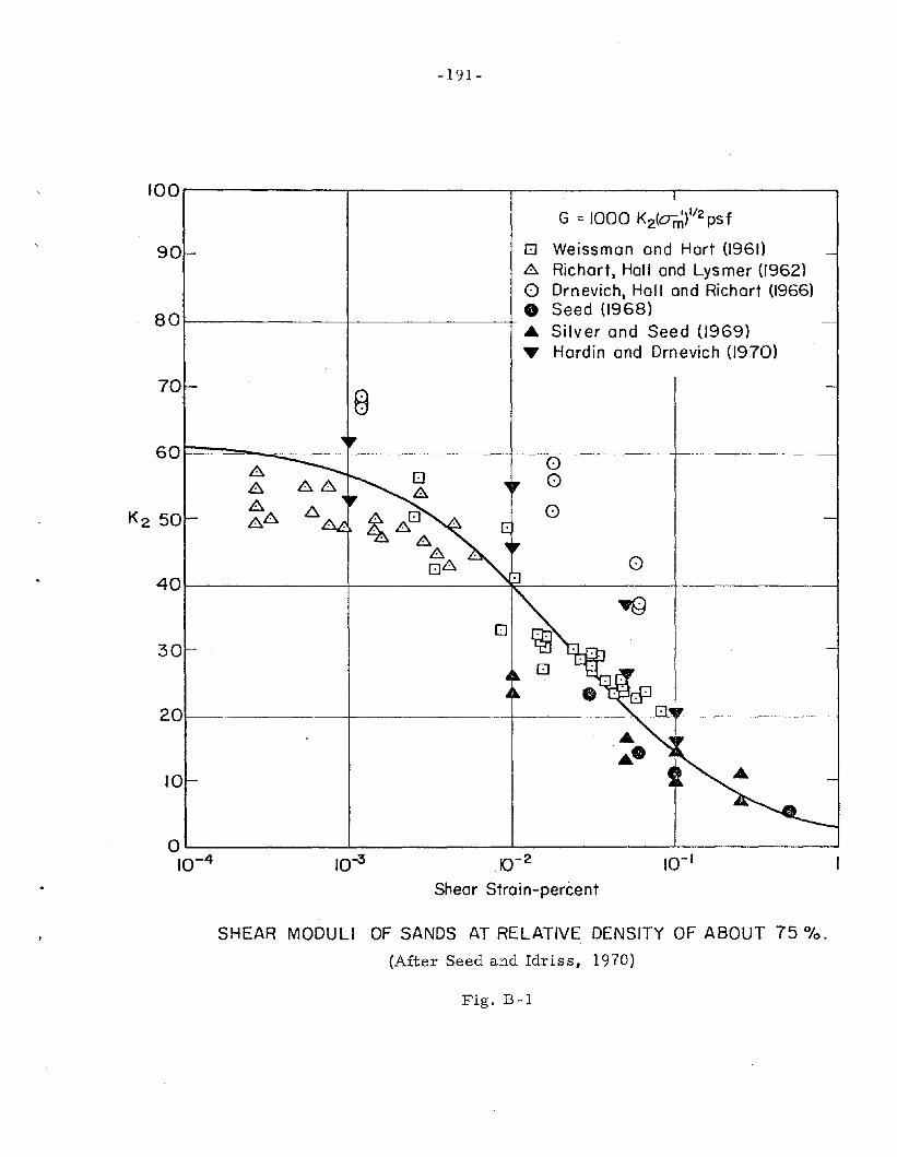
-191-
100.---------,,--------,.---------.-------""-'
90
G = 1000 K2(o-~)1I2psf
o Weissman and Hart (l96J)8 Richart, Hall and Lysmer {/962)o Drnevich, Hall and Richart (1966)
8 0 I-------~f______-----__I_. Seed (1968)A Silver and Seed (1969)• Hardin and Drnevich (1970)
708
o
10
201--------+-------+-----~-L.J~------~
30
401--------+-------~-------+--------~
10- 2
Shear Strain-percent
Ol.-- -L- --'-_--L L- ---I
10-4
SHEAR MODULI OF SANDS AT RELATIVE DENSITY OF ABOUT 75 0/0.
(After Seed and Idriss, 1970)
Fig. B-1
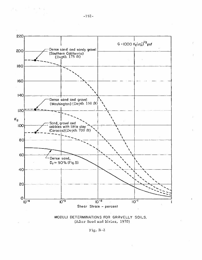
220
200
180
160
140
120
80
60
40
20
-192-
I 112G =1000 K2(o-rA> psf
r- Dense sand and sandy grovelL (Southern California)(Depth 175 ft)
f--- _ -- ............................ ..... ..... ..... .... ....
........,",
"","LDense sand and gravel \
_ _ _ _ _ _ (Washington) (Depth 150 ~t) \,
--- \
-- ..... ".... \..... ..... \....r- Sand, grovel and .... ,.L cobbles with little cloy .... ,
,\(Caracas)(Depth 700 ft) .... \
~-- ------ .... 1', \---- ......... \....... ..... .... ,
... .... \..... .... \..... , ,7--r--- .... .... \
.... .... \
LDense sand,~~ ,....
".... , ~
Dr~ 90% (Fig.5).... , \,
", ............... ,
'''" """
~< ' ", ", ", .... ,.................. ' ....
"""'"~
':'-..... ........ ...... ......... ........ --..... _-
10-2
Shear Strain - percent
MODULI DETERMINATIONS FOR GRAVELLY SOILS.(After Seed and Idris 5, 1970)
Fig. B-2

••
40
1I
\I
[I
I f-'
--0
W I
~-
30
1--
35
1--
"'VT
aylo
ran
dM
enzi
es((
96
3)
oT
aylo
ran
dH
ug
he
s((
96
5)
•Id
riss
(19
66
)-¢
-K
rize
kan
dF
ran
klin
(196
7)o
Thi
ers
and
Se
ed
(19
68
)•
Kov
acs
(19
68
)__
.....
8.
Do
no
van
([9
69
)(>
Ta
ylo
ran
dB
acc
hu
s(196~)
+-
+T
ayl
or
and
Ba
cch
us
(19
69
)g
...H
ard
inan
dD
rne
vich
(19
70
)u25r-------+--------+--------+---------;;L--t---{~_F_--__;;L_;
~"
~."
I~
/~
~/
,~
)D'0
20
--
II
~I
I~
IS
I~
/E
15r-------t-------+
------<
")---L
,r.I(II--_
_~_-_+_~------l
o Cl
I /+
100
"/
..."'V
.//"~
~/
~/
5-
....~--
-------
to I Wt-rj ..... (J
Q
1001
II
II
I
10
-410
-310
-210
-(
Sh
ea
rS
tra
in-
pe
rce
nt
DA
MP
ING
RA
TIO
SF
OR
SA
TU
RA
TE
DC
LA
YS
.(A
fter
Seed
an
dId
riss,
19
70
)

II
28
,I
8.
We
issm
an
and
Ha
rt(1
961)
•H
ard
in(1
96
5)
It
--./0
24
1--
0D
rne
vich
,H
all
and
Ric
ha
rt(9
66
)/
8M
ats
ush
ita
,K
ish
ida
and
Kyo
(l9
67
)/
/•
Silv
er
and
See
d(1
96
9)
/..
Do
no
van
(19
69
)....
,.-
20
""--
-..
.H
ard
inan
dD
rne
vich
(19
70
),."
eA
"~
vK
ish
ida
and
Tak
ano
(19
70
),.
,,;'
u,.
•~
,..
/"~
,.z.
~16
//:_.P-
.-/18-
,//
I~
.~
"~I,.
~to
c12
.....
,J".0
."
A
E,.
-o
;'c
8 41'~~7~
....""'"'f
A...
"->=
<I
I
'~.
~.'.
._..!
'lJ-
--
.-D-~~
m0
/=--
-:;.~---~-
1--
<:r
'I
I1
0-4
10-3
10-2
10
-1
Sh
ea
rS
tra
in-p
erc
en
t
DA
MP
ING
RA
TIO
SFO
RS
AN
DS
.(A
fter
Seed
an
dId
riss,
19
70
)