Embed Size (px)
Citation preview
This Report has been prepared by RIVM, EFTEC, NTUA and IIASA in association withTME and TNO under contract with the Environment Directorate-General of the EuropeanCommission.
RIVM report 481505016
Technical Report on Water Quantity and QualityB.J.de Haan, A. Beusen, C. Sedee,D.W. Pearce, A. Howarth
Novmeber 2000
RIVM, P.O. Box 1, 3720 BA Bilthoven, telephone: 31 - 30 - 274 91 11; telefax: 31 - 30 - 274 29 71
Technical Report on Water Quantity and Quality
2
Technical Report on Water Quantity and Quality
This report has been prepared by RIVM, EFTEC, NTUA and IIASA in association with TME and TNOunder contract with the Environment Directorate-General of the European Commission.This report is one of a series supporting the main report (XURSHDQ�(QYLURQPHQWDO�3ULRULWLHV��DQ�,QWHJUDWHG(FRQRPLF�DQG�(QYLURQPHQWDO�$VVHVVPHQW.Reports in this series have been subject to limited peer review.
The report consists of three parts:
Section 1:Environmental assessmentPrepared by B.J. de Haan, A. Beusen (RIVM), C. Sedee (TME)
Section 2:Benefit assessmentPrepared by D.W. Pearce, A. Howarth (EFTEC)
Section 3:Policy assessmentPrepared by D.W. Pearce, A. Howarth (EFTEC)
There are supporting Annexes that present additional information of the methodology and data.A. Water supply and sectoral demandB. Waste water treatmentC. Measure to restrict animal husbandry to carrying capacityD. Methane emission reductions in agriculture.Annex E demonstrates the impact of the policies contained in the baseline on the potential nitrateconcentration in Europe’s coastal zones.Prepared by B.J. de Haan, A. Beusen (RIVM), C. Sedee (TME)
5HIHUHQFHVReferences made in the sections on benefit and policy packages have been brought together in the7HFKQLFDO�5HSRUW�RQ�0HWKRGRORJ\��&RVW�%HQHILW�$QDO\VLV�DQG�3ROLF\�5HVSRQVHV. The references made in thesection on environmental assessment follows at the end of section 1.
The findings, conclusions, recommendations and views expressed in this report represent those of theauthors and do not necessarily coincide with those of the European Commission services.
Technical Report on Water Quantity and Quality
3
7DEOH�RI�&RQWHQWV
�� (19,5210(17$/�$66(660(17 �
��� ,QWURGXFWLRQ �
��� (QYLURQPHQWDO�WUHQGV�DQG�DEDWHPHQW�FRVW �1.2.1 Baseline assessment. 61.2.2 Assessment methodology 81.2.3 Results 10
��� &RQFOXVLRQV ��
��� 5HIHUHQFHV ��
�� %(1(),7�$66(660(17 ��
��� :DWHU�VWUHVV ��2.1.1 Public opinion 172.1.2 Expert opinion 172.1.3 Benefit estimation 172.1.4 Water availability analysis 192.1.5 Water quality analysis 23
��� &RDVWDO�]RQHV ��2.2.1 Public opinion 262.2.2 Expert opinion 262.2.3 Benefit estimation 26
�� 32/,&<�$66(660(17 ��
��� 3ROLF\�SDFNDJH�ZDWHU�VWUHVV ��3.1.1 Key issues 333.1.2 Recommended policy initiatives for water availability 333.1.3 Recommended policy initiatives for water quality 353.1.4 Multiple benefits 36
��� 3ROLF\�DVVHVVPHQW�ZDWHU�VWUHVV ��3.2.1 Causal criterion 363.2.2 Efficiency criterion 373.2.3 Administrative complexity 383.2.4 Equity criterion 383.2.5 Jurisdictional criterion 38
��� 3ROLF\�SDFNDJH�FRDVWDO�]RQHV ��3.3.1 Key issues 393.3.2 Recommended policy initiatives 393.3.3 Multiple Benefits 41
��� 3ROLF\�DVVHVVPHQW�FRDVWDO�]RQHV ��3.4.1 Causal criterion 423.4.2 Efficiency criterion 42

Technical Report on Water Quantity and Quality
4
3.4.3 Administrative complexity 433.4.4 Equity criterion 433.4.5 Jurisdictional criterion 43
Technical Report on Water Quantity and Quality
5
��� (QYLURQPHQWDO�DVVHVVPHQW
���� ,QWURGXFWLRQHuman activities are placing severe pressures on Europe’s water resources. Increasing demand, adverseclimate conditions and increasing problems of pollution have focused governments’ attention on how waterresources are managed. Europe needs to ensure that a stable supply of clean water meets both the needs ofsociety and the natural environment. There are three main threats to the quality of the supplied water:• Water abstraction may cause problems with respect to low flows in rivers, lowering ground water
tables in nature areas, and salt-water intrusion in coastal areas. The subsequent long-time loss ofground water as a natural resource affects drinking water supply, soil quality and biodiversity.
• Ground water is polluted by nitrogen and pesticides leaking through the root zone of the soil. Longresidence times make nitrogen pollution now a risk for drinking water of future generations.
Also,• The condition of surface waters deteriorated as manifested by algae growth, periods of oxygen deficits,
fish kills, etc. In many areas this poor environmental condition is attributable to enhanced nitrogen andphosphorus loading. Generally, phosphate excess distorts the ecosystems in inland waters, whilenitrogen excess damages ecosystems in marine waters. Eutrophication of inland and marine waters wasidentified in the Dobris Assessment (EEA, 1995) as a major European environmental issue.
This Technical Report analyses the potential of new policy measures for water management at EU-level.Here, the assessment of water management consists of analysing the potential for reducing the pressures. Atfirst, the existing policy measures will be described in the baseline (BL) assessment. The EEA haspublished this assessment in the State of the Environment Report (EEA, 1999). Next, it is argued that nogeneric emission reduction targets can be set as the ecological constraints for water management vary inEurope. Comparable data are lacking. Hence, a Technology Driven scenario (TD) and Accelerated Policiesscenario (AP) assessment have not been carried out. The 'conclusions' section finalises the section.Coastal zone water quality is only reflected through the analysis of nutrient overload by diffuse and pointsources to rivers and atmospheric deposition. Annex E demonstrates the impact of the policies contained inthe baseline on the potential nitrate concentration in Europe’s coastal zones.
���� (QYLURQPHQWDO�WUHQGV�DQG�DEDWHPHQW�FRVWProblem sketch (DPSIR) and related economic sectors
The underlying factor in water stress problems is the absence of owner liability for surface and groundwater. Agriculture is responsible for diffuse pollution through run-off water carrying manure and artificialfertilisers (NO3 and PO4), that have not been consumed by the crops, entering the main streams andgroundwater. Also, ammonia (NH3) evaporated from animal manure is deposited downwind, upsettingfragile - mostly forest - ecosystems. Urban households and industries feed wastewater treatment plants,which - despite the efforts to remove pollutants - emit BOD/COD, NO3 and PO4 into surface water. Theimpact of the transport sector via NOx emission and deposition is of minor importance.
Eurobarometer ranks water management as one of the three most serious environmental problems. Expertscite water management also as a serious problem. South European countries rank ‘water scarcity andpollution’ first. Most probably this reflects water availability rather than pollution. It is ranked fifth byNorth European countries.
Technical Report on Water Quantity and Quality
6
������ �%DVHOLQH�DVVHVVPHQW�
At EU level, the Urban WasteWater Directive and the Nitrates Directive create strong incentives for theMember States to prevent excessive nutrient loading of the aquatic environment. However, theimplementation of these directives is behind schedule and should be accelerated. The nature of thedirectives is discussed below. The proposed Framework water Directive has been excluded from theBaseline assessment.
Full compliance with the Urban WasteWater Treatment Directive - as assumed in the BaseLine - by 2010will remove most of the problems of surface water pollution by wastewater. The policy target is to be metin the BaseLine; no additional targets have been set. As no sufficient information was available on the areadesignated as sensitive by the Member States, the assessment assumes that the whole EU-15 territory issensitive to eutrophication and the severest requirements of the Urban WasteWater Treatment Directiveapply.
The EU Nitrates Directive limits the disposal of manure on agricultural land to 170 kgN/ha to protectground water and surface water quality. Despite this Directive, the principal driving force of nutrientspollution remains intensive animal husbandry and particularly the pigs and poultry sector, which isconcentrated at specialised farms in the regions of Niedersachsen, Nordrhein-Westfalen, the Netherlands,Flanders, Bretagne, Cataluna, and Lombardy. The share of pigs and poultry in these ‘hot spots’ of intensivelivestock production exceeds 50% of total animals. Table C.1 in the Annex on animal husbandry displaysthe animal density in the ‘hot spot’ regions. Apart from nutrients from manure disposal, farmers applyartificial nutrients to a level ranging from 100 to 200 kg N/ha. At farm level pigs and poultry holdings mayrange up to a density of 20 LU/ha1, thus exceeding the manure disposal limit by far. Compared to cattle, pigand poultry farms face more problems in reducing excess amounts of nitrogen from manure.
&XUUHQW�VWDWXV�RI�%/�SROLFLHV��SROLF\�JDS�RU�QRWThe Nitrate Directive and the Urban WasteWater Directive address the problem of ground water andsurface water eutrophication. These directives have been initiated in the 90’s; year 2003 awaits their fullimplementation. Excessive nitrate pollution remains a problem distorting marine ecosystems. These twodirectives make part of the baseline assessment (EEA, 1999).Remarkably, there seems to be no directive to limit the phosphate emission of the agricultural sector.Regionally, phosphate saturation of the topsoil has become a major problem. However, the phosphateconcentration in EU’s main rivers has a decreasing trend. This is probably due to the introduction ofphosphate-free detergents. A further decrease is not expected as agricultural pressures remain unchangedand amelioration has long delay times.
Good management of freshwater resources in the semi-arid regions is necessary for the maintenance of therequired standards of water quality and quantity, and therefore for reaching the goals of EU policies. Thetargets for the 5EAP and for the EU Action Programme for Integrated Groundwater Protection (GAP) areto be implemented by the year 2000. One of GAP’s main purposes is to integrate the groundwaterprotection requirements into the Common Agricultural Policy (DGVI) and into Regional Policy (DGXVI).This proved not to be a very effective strategy as GAP currently lacks legal status.
Both water scarcity and quality deterioration affect particularly the southern areas of Europe, where a highpercentage of land is used for agricultural purposes and is supplied by groundwater for irrigation with itsassociated problems of nitrates and pesticides saturation. The 5EAP aims to maintain the water resources,so that the regional balances between demand and supply are guaranteed. Risk management is anotheraspect, which is targeted by the 5EAP objectives for the EU. The main sources of risk to human health and 1 LU is livestock unit: an indicator in which species and classes of livestock are converted to comparablesize. For example, a dairy cow counts one LU, while sheep and goats count 0.1 LU, pigs count 0.25 LU,and poultry 0.0125 LU. 1 LU/ha can roughly be considered as equivalent to a manure disposal of 80kgN/ha.
Technical Report on Water Quantity and Quality
7
the environment related to the semi-arid regions are floods, and forest fires. These are grouped as “naturalhazards”, but there are no EU policy targets to reduce these events (ETC-IW, 1996).
There are no BL policies directed to prevent ground water overexploitation, although sometimes, nationallaws set limits in relation to the natural recharge by precipitation. For example, Denmark limits groundwater abstraction to 25% of the natural recharge. Eurostat reviewed European regions where watershortages are known to occur and the estimated water demands based on an inventory among nationalgovernments (Eurostat, 1998). Irrigation makes the largest part of Europe’s water demand. A smalldecrease in the demand has been projected (EEA, 1999)
With respect to coastal zone management, the assessed indicator is nitrate load, though no absolute targetcan be set. The relation between nitrate load and good bathing water quality could not be defined. TheNorth Sea Action Programme defined the policy target ‘halving the load to coastal water’. Other catchmentareas are yet to follow. As agricultural emissions constitute the largest burden for coastal sea loads, anagricultural nitrate load indicator seems to be most appropriate of all indicators.
Several other pressures threaten the quality of Europe’s coastal zones, particularly, urbanisation and thedevelopment of sports and leisure facilities. Though several EU-directives call for good quality waterquality for fish and shellfish, overfishing remains the largest threat to the natural balance of marine biota(EEA, 1999). Neither land use planning or overfishing has been part of this assessment.
6SLOORYHUThere is some spillover from and to the problem of acidification and eutrophication marine biodiversitywould greatly benefit from actions against the excessive nitrogen inputs to surface water. Soil degradationis often associated with overexploitation of natural ground water resources.
6XEVLGLDULW\ Two reasons favour the subsidiarity of the problem solution. Firstly, the main ongoing pressure is a) water-thirsty crop production and b) intensive animal husbandry, both of which are concentrated in only a fewEuropean regions. Secondly, the varying soil properties make specific regional policy targets moreeffective than generic ones. Hence, regional authorities can best handle the acceleration of the currentpolicies.
6XVWDLQDELOLW\It is difficult to set generic policy targets based on ecological constraints. The proposed EU FrameworkWater Directive (COM(97) 49 final) (FWD) will provide legal status to water management policies bydefining constraints based on local conditions. This requires an EU-wide inventory of local waterconditions. Although many monitoring systems are in operation nationally, these need to be harmonised.On behalf of DGXI, EEA is establishing its EUROWATERNET. This monitoring and information networkfor inland water resources will allow the FWD to become effective (EEA, 1998). Several existing directiveswill be enforced under the framework. GAP’s main requirements can now be found in the FWD willproviding legal status. The FWD will also encompass the nitrates and urban wastewater treatment directive.The FWD does not make part of the baseline assessment as it was agreed that the final cut-off date forexisting and proposed EU policies would be August 1997.
5HFRPPHQGDWLRQWater management is still a prominent European problem. The current policies are being implemented andthe results are underway. Particularly, the eutrophication of marine waters and water abstraction forirrigation needs further attention. While pursuing the compliance of the current nitrate and urban wastewater treatment directives, the Commission might want to accelerate its policies by introducing – in therelevant regions - a compulsory bookkeeping of irrigation water abstraction, nutrients and pesticides atfarm level to stimulate good agricultural practises and enable control.The introduction of the EUROWATERNET monitoring system should alleviate data problems in the nearfuture. It is recommended to ensure that an associated assessment model tailored to the data and policyobjectives should be developed.

Technical Report on Water Quantity and Quality
8
������ $VVHVVPHQW�PHWKRGRORJ\
�������� :DWHU�GHPDQGThe water resources available to satisfy the European water demands are restricted by social-economic andenvironmental factors. The preferred source for water supply is ground water as it has good and stablequality. Most water abstracted, however, is surface water. Where it is abundant, it suitable for irrigationpurposes. Ground water is the main source for drinking water.Ground water demands are increasing and so are the environmental concerns as to water withdrawal. As aconsequence, some regions in Europe have water problems. The preferred source of water for public watersupply, small industrial water needs and the irrigation of private plots, is groundwater. Groundwaterrecharge and also the total of locally available water resources are governed by net precipitation, being thedifference of precipitation and the actual evapotranspiration. Simple mathematical relations can be used toquantify potential and actual evapotranspiration. The difference between the two represents the existingagricultural water needs. We applied a GIS approach to quantify water needs for public and industrial watersupplies and water needs for irrigation in the various European regions. Comparing calculated water needsand the availability of groundwater and local surface water, based on net precipitation, indicates areaswhere water shortages may be expected and where a minimum amount of water will be needed. Thoseareas generally correspond relatively well to areas with water problems as indicated by an inventory carriedout among European national governments.
Ground water overexploitation for irrigation is probably a regional scale problem. However, the ETC-IWdatabase supplies only national trends of water abstraction. Hence, the real problems will often remainhidden in the statistics. A secondary problem is that there seems to be no well-defined policy target as yet.The GIS assessment method analyses precipitation, evaporation, ground water recharge and surface flow ona very fine grid of 10’ by 10’ or 10 km x 20 km. The results show the clear North South divide in wateravailability. However, there is a large variability within the Mediterranean countries as well.
It is important to note that water demand should not be met regardless the true cost of supply. Probably, agreat deal of the irrigation uses of water in the EU are uneconomic, i.e. they would fail a test thatconsumer’s ‘willingness to pay’ for water supply exceeds its true cost (Pearce, 1999). Correct water pricingis the preferred mechanism for bringing supply and demand into balance.
�������� :DVWH�ZDWHUThe assessment methodology analyses the Member States 1995 waste water treatment and consequentlyupdates this current treatment state (EEA, 1999) to the required state according to the Urban Waste WaterTreatment Directive by 2010. We assume that the whole EU territory will be regarded as sensitive toeutrophication and hence the severest requirements are imposed. Not all Member States did assign sensitiveareas as yet. Quite a few already assigned their whole territory though.The urban wastewater treatment directive differentiates between rural areas and conglomerations. In ruralareas, agglomeration smaller than 2000 inhabitants, connection to waste water treatment plants will not beobligatory, while larger conglomerations have to ensure sewerage connection and treatment of waste waterby either biological or chemical nutrient removal. The following table reviews the gradual implementationof these requirements:
Table 1.1.Non-sensitive areas Sensitive areas
Agglomeration (x 1000 inh.)
Sewerageconnectionbefore
Secondarytreatmentbefore
Sewerageconnectionbefore
Secondarytreatmentbefore
Allowed maximalconcentration indrain water (mg/l)N P
< 2 Not req. Not req. Not req. Not req. Not sp. Not sp.2 –10 2006 Not req. 2006 2006 Not sp. Not sp.10 – 15 2006 2006 1999 2006 15 2
Technical Report on Water Quantity and Quality
9
15 – 100 1999 2001 1999 1999 15 2> 100 1999 2001 1999 1999 10 1
Source: CEC, 1991.
The regulation on allowed maximal concentration in treatment plant drain water effectively demandsagglomerations situated in sensitive areas and larger than 100,000 inhabitants to invest in tertiary – i.e.chemical - treatment.Depending on the Member State population statistics, the Moses model assesses the required sewerageconnection and mix of waste water treatment technology and the associated costs of investment andoperation (TME, 1998). See Annex B on waste water treatment for details.
�������� $JULFXOWXUDO�HPLVVLRQVBased on livestock units (LU), animal density in the EU is almost 1 LU per ha. Given the requirement ofthe Nitrate Directive – not more than 170 kg N/ha manure should be spread – the EU as a whole seems notto have a problem. However, considering livestock density at farms, about half of the livestock is kept indensities exceeding 1.5 LU per ha. This implies that many farm holdings need to dispose of the excessmanure by transporting the slurry to neighbouring farmers or to other regions.Cattle are the dominant animal category with a share of about half of total livestock population. Pigs form25% of the total population. The share of pigs in national livestock population is highest in Denmark(62%), Belgium and the Netherlands (both 42%). These estimates are based on well over 7 million farmholdings in the Farm Accountancy Data Network (FADN).Several economic instruments (van Zeijts et al., 1999) have recently been discussed. Van Zeijts et al.recommend the establishment of a mineral accounts combined with a nutrient surplus levy in relevantregions. However, recent observations in the Netherlands have shown that a considerable number offarmers choose to pay the levy rather than the costs of reliable manure transport. Hence, the targets set inthe Nitrate Directive are not met and the Dutch governments faces action in the Court of Justice. Thissuggest the levy is too low and must be based on the costs of transport (the marginal abatement costs).Manure releases ammonia and methane, which are agents for acidification, eutrophication, and climatechange. The 7HFKQLFDO�5HSRUW�RQ�$FLGLILFDWLRQ��(XWURSKLFDWLRQ�DQG�7URSRVSKHULF�2]RQH discusses severaltechnological solutions that minimise air emissions from stables and fields after manure spreading. Wesought alternatives to these by setting limits to animal densities on farms and in regions.
�������� 2XWOLQH�RI�WKH�PRGHOV�XVHGSeveral models have been applied to assess water management problems in the EU. The majority of themodels have been used in previous policy assessments. Attention has been paid to ensure datahomogeneity. Considering the subnational character of the problem, we inserted regional detail in theassessment. However, due to the variety of sources, some inconsistencies could not be avoided.The Annexes A, B, C, D, and E specify the models and data used. The short account below lists theelements used.:DWHU�DEVWUDFWLRQ
ETC-IW data set containing estimates of country specific data on water abstraction per economicsector (EEA, 1999).CARMEN model accounts for the net precipitation to assess water supply and water demand(FSU, 1996).
1XWULHQWVLEI model calculates manure arising, application and the consequences of the introduction oflivestock limits (LEI, 1999)ETC-IW data set containing estimates of country specific data on waste water composition,sewage connection rates, sewage treatment (EEA, 1999)RAINS model to calculate dispersion of ammonia (Alcamo et al., 1990)CARMEN model accounts for all diffuse and point sources of nutrients to ground and marinewater (RIVM, 1998).
&RVWV
Technical Report on Water Quantity and Quality
10
RAINS model evaluates the costs of emission abatement, andMOSES model to evaluate the costs of implementation of wastewater treatment.TME model to estimate of manure transports in regions where exceedances of the norms(acidification strategy, nitrate directive) are expected.
�������� %HQHILWV�IURP�7'�DQG�$3The water stress problem requires that local conditions be taken into account. The proposed WaterFramework Directive, which might have come near to an AP scenario, takes this into account as it refers tolocal ecological targets and abatement action plans. However, models are not yet instrumented to assess theimpact of the proposed framework due to lacking consistent regional data. Hence, the benefits of a TD orAP scenario have not been evaluated.In the UK, the data availability situation did warrant a cost benefit analysis of the proposed waterframework directive (WRc, 1999). Potentially, costs range from £3 to £11 billion. These costs aredominated by those of controlling municipal point sources and agricultural diffuse sources. Benefits areexpected to range from £2 to £6 billion. The largest benefits arise from improved amenity for owners ofriparian homes, and from improving low flow regimes in rivers.
�������� ,GHQWLILFDWLRQ�RI�PDMRU�XQFHUWDLQWLHVContrary to problems like climate change, regional physical and ecological conditions define the waterstress problem. However, this precise environmental data is scarce and often not comparable. Particularly,on irrigation water abstraction, wastewater composition and manure application the newEUROWATERNET must provide tailored information to assess the Action Programmes the MemberStates must submit to comply to the Nitrates Directive, Urban Waste Water Treatment Directive, and theproposed Water Framework Directive. Furthermore, the impact of such programmes is often ill defined asvulnerable areas requiring strongest action have not yet been formally designated.
������ 5HVXOWV
�������� 0HDVXUHV�UHODWHG�WR�ZDWHU�GHPDQG�The water demand model projects national trends for each economic sector based on observed demand dataseries. However, the requirements of the EU Action Programme for Integrated Groundwater Protection(GAP) have not been made explicit in these data series. Where implemented, removal of subsidies on watersupply to internalise water supply costs in the water price might already have contributed to meet theserequirements. The water demand projections should reflect the impacts implicitly.
Considering the present and future water demand per sector, the total water demand in the EU will remainrelatively stable. The rate of growth of the main driving forces is expected to slow and the efficiency ofwater use is expected to improve, as national water conservation policies and actions have an increasinglypositive impact.However, the semi-arid areas of the EU - Portugal, Spain, Italy and Greece – remain very susceptible to theeffects of desertification due to the imbalance between natural resources and abstractions for irrigation. Thetrend in irrigated area and the allocated amount of water per hectare will slightly decrease. Hence, thedemand for irrigation water is decreasing.
7DEOH�����:DWHU�GHPDQG�IRU�LUULJDWLRQ�UHODWLYH�WR�WKH�DPRXQW�RI�DYDLODEOH�QHW�SUHFLSLWDWLRQ�DQG�WR�WKHDPRXQW�RI�DQQXDO�UHVRXUFHV��QHW�SUHFLSLWDWLRQ�DQG�LPSRUW�
precipitation evaporation Net precip Allocated toirrigation
irrigation tonet precip
Irrigation toResources
mm mm mm mm % %Greece 849 492 357 312 20 16
Technical Report on Water Quantity and Quality
11
Italy 983 428 555 1188 28 27Portugal 886 474 412 607 18 9Spain 662 432 230 546 25 25Source: EEA, 1999.
�������� 0HDVXUHV�UHODWHG�WR�ZDVWH�ZDWHU�WUHDWPHQW�Full compliance to the urban waste water treatment directive - as assumed in the BaseLine - by 2010 willremove most of the problems to surface water pollution by waste water. The policy target is to be met in theBaseLine, and no additional targets have been set in the other scenarios. As no sufficient information wasavailable on the area designated as vulnerable by the Member States, the assessment assumes that thewhole EU-15 territory is vulnerable to eutrophication and the severest requirements of the UrbanWasteWater Treatment Directive apply.
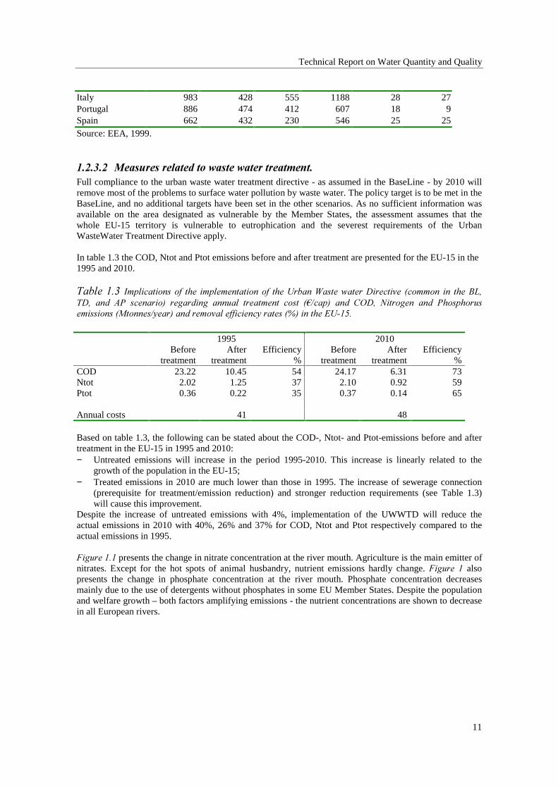
In table 1.3 the COD, Ntot and Ptot emissions before and after treatment are presented for the EU-15 in the1995 and 2010.
7DEOH�����,PSOLFDWLRQV�RI� WKH� LPSOHPHQWDWLRQ�RI� WKH�8UEDQ�:DVWH�ZDWHU�'LUHFWLYH� �FRPPRQ� LQ� WKH�%/�7'�� DQG� $3� VFHQDULR�� UHJDUGLQJ� DQQXDO� WUHDWPHQW� FRVW� �¼�FDS�� DQG� &2'�� 1LWURJHQ� DQG� 3KRVSKRUXVHPLVVLRQV��0WRQQHV�\HDU��DQG�UHPRYDO�HIILFLHQF\�UDWHV�����LQ�WKH�(8����
1995 2010Before
treatmentAfter
treatmentEfficiency
%Before
treatmentAfter
treatmentEfficiency
%COD 23.22 10.45 54 24.17 6.31 73Ntot 2.02 1.25 37 2.10 0.92 59Ptot 0.36 0.22 35 0.37 0.14 65
Annual costs 41 48
Based on table 1.3, the following can be stated about the COD-, Ntot- and Ptot-emissions before and aftertreatment in the EU-15 in 1995 and 2010:− Untreated emissions will increase in the period 1995-2010. This increase is linearly related to the
growth of the population in the EU-15;− Treated emissions in 2010 are much lower than those in 1995. The increase of sewerage connection
(prerequisite for treatment/emission reduction) and stronger reduction requirements (see Table 1.3)will cause this improvement.
Despite the increase of untreated emissions with 4%, implementation of the UWWTD will reduce theactual emissions in 2010 with 40%, 26% and 37% for COD, Ntot and Ptot respectively compared to theactual emissions in 1995.
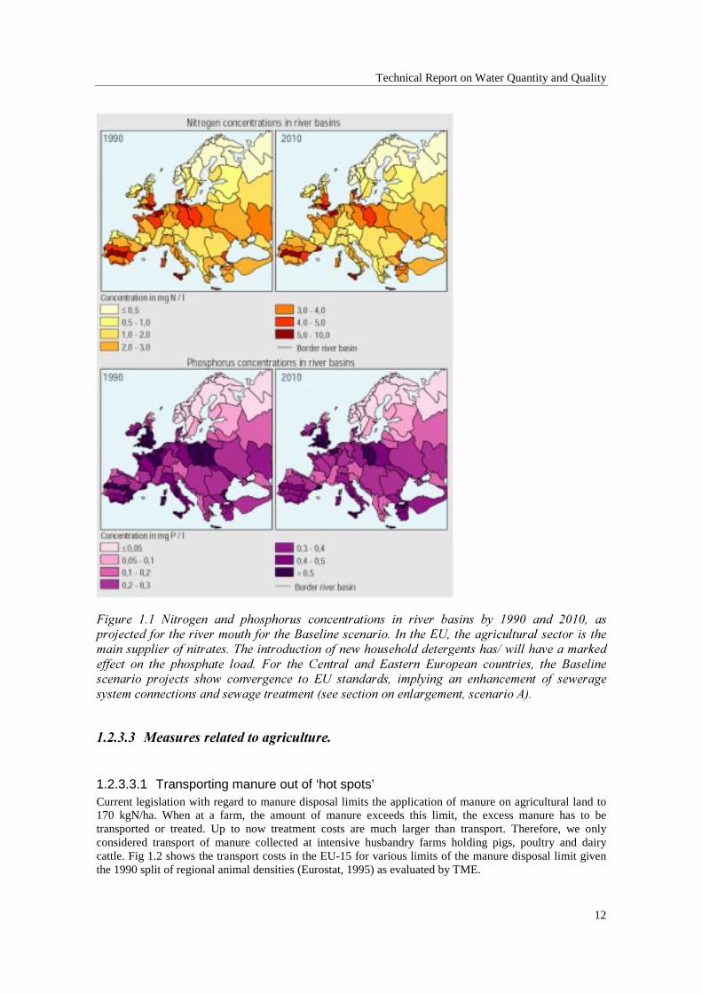
)LJXUH���� presents the change in nitrate concentration at the river mouth. Agriculture is the main emitter ofnitrates. Except for the hot spots of animal husbandry, nutrient emissions hardly change. )LJXUH� � alsopresents the change in phosphate concentration at the river mouth. Phosphate concentration decreasesmainly due to the use of detergents without phosphates in some EU Member States. Despite the populationand welfare growth – both factors amplifying emissions - the nutrient concentrations are shown to decreasein all European rivers.
Technical Report on Water Quantity and Quality
12
)LJXUH� ���� 1LWURJHQ� DQG� SKRVSKRUXV� FRQFHQWUDWLRQV� LQ� ULYHU� EDVLQV� E\� ����� DQG� ������ DVSURMHFWHG�IRU�WKH�ULYHU�PRXWK�IRU�WKH�%DVHOLQH�VFHQDULR��,Q�WKH�(8��WKH�DJULFXOWXUDO�VHFWRU�LV�WKHPDLQ�VXSSOLHU�RI�QLWUDWHV��7KH�LQWURGXFWLRQ�RI�QHZ�KRXVHKROG�GHWHUJHQWV�KDV��ZLOO�KDYH�D�PDUNHGHIIHFW� RQ� WKH� SKRVSKDWH� ORDG�� )RU� WKH� &HQWUDO� DQG� (DVWHUQ� (XURSHDQ� FRXQWULHV�� WKH� %DVHOLQHVFHQDULR� SURMHFWV� VKRZ� FRQYHUJHQFH� WR� (8� VWDQGDUGV�� LPSO\LQJ� DQ� HQKDQFHPHQW� RI� VHZHUDJHV\VWHP�FRQQHFWLRQV�DQG�VHZDJH�WUHDWPHQW��VHH�VHFWLRQ�RQ�HQODUJHPHQW��VFHQDULR�$��
�������� 0HDVXUHV�UHODWHG�WR�DJULFXOWXUH�
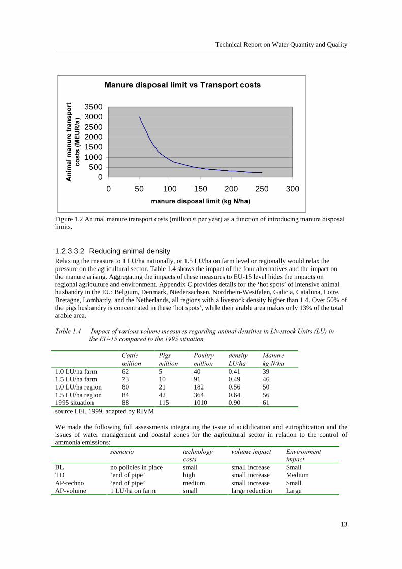
1.2.3.3.1 Transporting manure out of ‘hot spots’Current legislation with regard to manure disposal limits the application of manure on agricultural land to170 kgN/ha. When at a farm, the amount of manure exceeds this limit, the excess manure has to betransported or treated. Up to now treatment costs are much larger than transport. Therefore, we onlyconsidered transport of manure collected at intensive husbandry farms holding pigs, poultry and dairycattle. Fig 1.2 shows the transport costs in the EU-15 for various limits of the manure disposal limit giventhe 1990 split of regional animal densities (Eurostat, 1995) as evaluated by TME.
Technical Report on Water Quantity and Quality
13
�0DQXUH�GLVSRVDO�OLPLW�YV�7UDQVSRUW�FRVWV
0500
100015002000250030003500
0 50 100 150 200 250 300
PDQXUH�GLVSRVDO�OLPLW��NJ�1�KD�
$QLP
DO�P
DQXUH�WUDQVS
RUW�
FRVWV��0
(85�D�
Figure 1.2 Animal manure transport costs (million ¼�SHU�\HDU��DV�D�IXQFWLRQ�RI�LQWURGXFLQJ�PDQXUH�GLVSRVDOlimits.
1.2.3.3.2 Reducing animal densityRelaxing the measure to 1 LU/ha nationally, or 1.5 LU/ha on farm level or regionally would relax thepressure on the agricultural sector. Table 1.4 shows the impact of the four alternatives and the impact onthe manure arising. Aggregating the impacts of these measures to EU-15 level hides the impacts onregional agriculture and environment. Appendix C provides details for the ‘hot spots’ of intensive animalhusbandry in the EU: Belgium, Denmark, Niedersachsen, Nordrhein-Westfalen, Galicia, Cataluna, Loire,Bretagne, Lombardy, and the Netherlands, all regions with a livestock density higher than 1.4. Over 50% ofthe pigs husbandry is concentrated in these ‘hot spots’, while their arable area makes only 13% of the totalarable area.
7DEOH���� �,PSDFW�RI�YDULRXV�YROXPH�PHDVXUHV�UHJDUGLQJ�DQLPDO�GHQVLWLHV�LQ�/LYHVWRFN�8QLWV��/8��LQWKH�(8����FRPSDUHG�WR�WKH������VLWXDWLRQ�
&DWWOHPLOOLRQ
3LJVPLOOLRQ
3RXOWU\PLOOLRQ
GHQVLW\/8�KD
0DQXUHNJ�1�KD
1.0 LU/ha farm 62 5 40 0.41 391.5 LU/ha farm 73 10 91 0.49 461.0 LU/ha region 80 21 182 0.56 501.5 LU/ha region 84 42 364 0.64 561995 situation 88 115 1010 0.90 61source LEI, 1999, adapted by RIVM
We made the following full assessments integrating the issue of acidification and eutrophication and theissues of water management and coastal zones for the agricultural sector in relation to the control ofammonia emissions:
VFHQDULR WHFKQRORJ\FRVWV
YROXPH�LPSDFW (QYLURQPHQWLPSDFW
BL no policies in place small small increase SmallTD ‘end of pipe’ high small increase MediumAP-techno ‘end of pipe’ medium small increase SmallAP-volume 1 LU/ha on farm small large reduction Large
Technical Report on Water Quantity and Quality
14
The AP-techno scenario assesses cost-effective solutions to both acidification and ozone exposure and doesnot limit emissions as such. The scenario assesses a package of measures for SOx, NOx, NMVOC and NH3
emission abatement. The impact of the volume measure (in AP-volume) is quite extreme: pigs and poultrypopulations reduce by a factor of 10. However, in acidification abatement this drastic scenario - with itsNH3 emission reduction - will allow for larger emissions of SOx and NOx, as both packages, techno andvolume, meet the same emission target. By and large the AP volume will bring about a transfer of costsfrom the transport, industry and energy sectors to the agriculture sector. Also, there are more spillovereffects. The AP-volume has fewer emissions of methane (climate change), and particulate matter PM10
(chemical risks, urban stress).
Table 1.5 reviews the obtained results aggregated to EU-15 level. Emission reduction to 60% of 1990levels are obtained by both this AP and the TD scenario at the expense of reducing the pigs and poultrysector by a factor of 10 or of increasing control costs of ¼���ELOOLRQ�SHU�\HDU�
Table 1.5 Comparison of the various scenarios.(8�����ILJXUHV�IURP�5$,16� ���� �����%/ �����$3�
WHFKQR�����$3�
YROXPH�����7'
Cows (millions) 91 84 84 73 84Pigs (millions) 117 118 118 15 118Poultry (millions) 929 1004 1004 100 1004
Total CH4 emission 9652 8985 8985 7682 8985
Total N production 8973 7738Total PO4 productionNH3 emission (kton) 3576 3153 2969 2206 2156NH3 abatement costs (M¼�\U� 317 1405 49 11471Total abatement costs (G¼�\U� 53 59 61 87Area exceed acid. 25% 5% 3% 3% 2%Area exceed eutrop. 55% 41% 36% 28% 24%
Technical Report on Water Quantity and Quality
15
���� &RQFOXVLRQV
KEY MESSAGES
• water quality protection represents the key attribute, although water supply is an important issue inMediterranean countries.
• water use will probably remain relatively stable, if not decline, for some sectors through more efficientmanagement and pricing during the outlook period.
• Wastewater from point sources will most likely be effectively treated by the end of the assessmentperiod. This will significantly reduce nutrient impacts on downstream rivers and marine areas.
• the most important aspect to be addressed by new policy measures relates to agricultural runoff.
Current EU directives have addressed adequate water quality management. This applies particularly to theNitrates Directive and the Urban WasteWater Treatment Directive, which have been entered in the Baselineassessment. Implementation of these directives is on its way, though large implementation failures havebeen reported. Implementation costs are:
The water stress problem requires that local conditions will be taken into account. The proposed WaterFramework Directive, that should encompass all previous directives into one binding legal framework,takes this into account as it refers to local ecological targets and abatement action plans. However, modelsare not yet instrumented to assess the impact of this proposal due to lacking consistent regional data.Hence, no TD or AP policy scenarios have been evaluated. The introduction of a monitoring system –EUROWATERNET - should alleviate this data problem in the near future (EEA, 1998). It is recommendedto ensure that an associated assessment model will be developed.
In the UK, the data availability situation did warrant a cost benefit analysis of the proposed WaterFramework Directive (WRc, 1999). Potentially, costs range from £3 to £11 billion, which are dominated bythe costs of controlling municipal point sources and agricultural diffuse sources. Benefits are expected torange from £2 to £6 billion. The largest benefits arise from improved amenity for owners of riparian homes,and from improving low flow regimes in rivers. However, many uncertainties remain with regards toassumptions and sensitivity analyses stressed the limitation of the above-mentioned results.

Technical Report on Water Quantity and Quality
16
���� 5HIHUHQFHV
Alcamo, J., Shaw, R., and Hordijk, L. (eds.) (1990) 7KH�5$,16�0RGHO�RI�$FLGLILFDWLRQ� Science and Strategiesin Europe. Kluwer Academic Publishers, Dordrecht, The Netherlands.
EEA, 1995, Europe’s Environment. Dobris Assessment
EEA, 1998, EUROWATERNET, Technical Report no. 7. European Environment Agency, Copenhagen
EEA, 1999, Environment in the European Union at the turn of the century. ISBN 92-9157-202-0,Copenhagen
ETC-IW, 1996, Water resources problems in southern Europe, ISBN 92-9167-056-1, Copenhagen
Eurostat, 1998, Water in Europe. Part 1: Renewable water resources, Eurostat Statistical Office of theEuropean Communities, Luxembourg;
RIVM, 1996, Potential water supply vs. domestic water demand on a European scale. Reportcommissioned by the European Commission’s Forward Study Unit Project 95/C 124/09.
LEI, 1999, Managing nitrogen pollution from intensive livestock production in the EU; economic andenvironmental benefits of reducing nitrogen pollution by nutritional management in relation to thechanging CAP regime and the Nitrates directive. ISBN 90-5242-494-2, The Hague, AgriculturalEconomics Institute (LEI).
NERI, 1997, Integrated environmental assessment on eutrophication.Club de Bruxelles, Water in Europe. What to expect from the EU policy.
RIVM, 1998, CARMEN, an information system for water eutrophication policies. Compilation of researchreports. Internal note.
WRc, 1999, Potential costs and benefits of implementing the proposed water resources frameworkdirective, final report to the department of the Environment, Transport and the Regions, report no. DETR4477/5 WRc plc, Medmenham UK.
Technical Report on Water Quantity and Quality
17
��� %HQHILW�DVVHVVPHQW
���� :DWHU�VWUHVV
������ 3XEOLF�RSLQLRQ
Eurobarometer 1995 and 1992 both rank ‘water management’ as one of the top three most seriousenvironmental problem. Variance about this ranking is quite narrow: there is a 1st ranking in Ireland andDenmark and a 2nd ranking in England and the eight2 European countries covered in the ISSP (1993)survey.
������ ([SHUW�RSLQLRQ
GEP et al (1997) report rankings for ‘water scarcity and pollution’. The pollution is due to agriculturalpractices, air pollution (acidification) and industrial waste. Eutrophication is not given a separate category.Water management is ranked third, with 21.6% of researchers citing it as a first or second problem. As isexpected, water scarcity and pollution is ranked first by South European countries. Most probably thisreflects concern about water availability rather than pollution. It is ranked third by North Europeancountries.
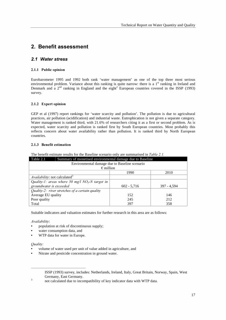
������ %HQHILW�HVWLPDWLRQ
The benefit estimate results for the Baseline scenario only are summarised in 7DEOH�����Table 2.1 Summary of monetised environmental damage due to Baseline
Environmental damage due to Baseline scenario¼�PLOOLRQ
1990 2010$YDLODELOLW\: not calculated3
QXDOLW\����DUHDV�ZKHUH� ���PJ�O�12��1� WDUJHW� LQJURXQGZDWHU�LV�H[FHHGHG 602 - 5,716 397 - 4,5944XDOWL\�����ULYHU�VWUHWFKHV�RI�D�FHUWDLQ�TXDOLW\Average EU qualityPoor qualityTotal
152245397
146212358
Suitable indicators and valuation estimates for further research in this area are as follows:
$YDLODELOLW\:• population at risk of discontinuous supply;• water consumption data, and• WTP data for water in Europe.
4XDOLW\�• volume of water used per unit of value added in agriculture, and• Nitrate and pesticide concentration in ground water.
ISSP (1993) survey, includes: Netherlands, Ireland, Italy, Great Britain, Norway, Spain, WestGermany, East Germany.
3 not calculated due to incompatibility of key indicator data with WTP data.
Technical Report on Water Quantity and Quality
18
:DWHU�PDQDJHPHQW�LQGLFDWRUV
Water management addresses two issues: water availability and water quality. As far as cost-benefit analysis isconcerned the following are the relevant indicators:
:DWHU�DYDLODELOLW\� is defined with respect to ground water availability and water stress. Where water stress isdefined as a situation in which there is less than 200 litres/cap/day availability. Two variants of this are given byRIVM: the first indicator (ground water availability) assumes 1/4 of groundwater recharge is available forconsumption. The second indicator (water stress) assumes that 1/4 groundwater recharge is available and 1/10of total upstream discharge is available. However, these data are available for the Baseline scenario only.
:DWHU�TXDOLW\: the indicators are; i) areas where 50 mg/l NO3-N target in groundwater is exceeded and ii) riverstretches of a certain quality.
There are studies of the WTP to avoid nitrates in groundwater, however the indicator is not currently availableat the EU:15 level. N and P concentrations in coastal areas are covered in the eutrophication analysis of theBaltic Sea dealt with in the benefit assessment of ’Coastal Zones’.
:DWHU�DYDLODELOLW\�DQDO\VLV
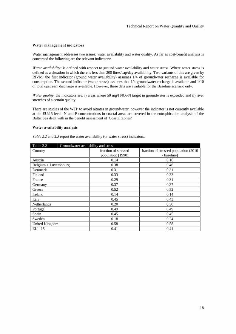
7DEOH���� and 2.� report the water availability (or water stress) indicators.
Table 2.2 Groundwater availability and stressCountry fraction of stressed
population (1990)fraction of stressed population (2010
- baseline)Austria 0.14 0.16Belgium + Luxembourg 0.38 0.46Denmark 0.31 0.31Finland 0.33 0.33France 0.29 0.31Germany 0.37 0.37Greece 0.52 0.52Ireland 0.14 0.14Italy 0.45 0.43Netherlands 0.20 0.30Portugal 0.49 0.49Spain 0.45 0.45Sweden 0.18 0.24United Kingdom 0.58 0.58EU - 15 0.41 0.41
Technical Report on Water Quantity and Quality
19
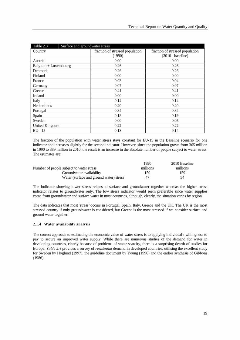
Table 2.3 Surface and groundwater stressCountry fraction of stressed population
(1990)fraction of stressed population
(2010 - baseline)Austria 0.00 0.00Belgium + Luxembourg 0.26 0.26Denmark 0.26 0.26Finland 0.00 0.00France 0.03 0.04Germany 0.07 0.07Greece 0.41 0.41Ireland 0.00 0.00Italy 0.14 0.14Netherlands 0.20 0.20Portugal 0.34 0.34Spain 0.18 0.19Sweden 0.00 0.05United Kingdom 0.22 0.22EU - 15 0.13 0.14
The fraction of the population with water stress stays constant for EU-15 in the Baseline scenario for oneindicator and increases slightly for the second indicator. However, since the population grows from 365 millionin 1990 to 389 million in 2010, the result is an increase in the absolute number of people subject to water stress.The estimates are:
1990 2010 BaselineNumber of people subject to water stress millions millions
Groundwater availability 150 159Water (surface and ground water) stress 47 54
The indicator showing lower stress relates to surface and groundwater together whereas the higher stressindicator relates to groundwater only. The low stress indicator would seem preferable since water suppliescome from groundwater and surface water in most countries, although, clearly, the situation varies by region.
The data indicates that most ’stress’ occurs in Portugal, Spain, Italy, Greece and the UK. The UK is the moststressed country if only groundwater is considered, but Greece is the most stressed if we consider surface andground water together.
������ :DWHU�DYDLODELOLW\�DQDO\VLV
The correct approach to estimating the economic value of water stress is to applying individual’s willingness topay to secure an improved water supply. While there are numerous studies of the demand for water indeveloping countries, clearly because of problems of water scarcity, there is a surprising dearth of studies forEurope. 7DEOH���� provides a survey of UHVLGHQWLDO demand in developed countries, utilising the excellent studyfor Sweden by Hoglund (1997), the guideline document by Young (1996) and the earlier synthesis of Gibbons(1986).
Technical Report on Water Quantity and Quality
20
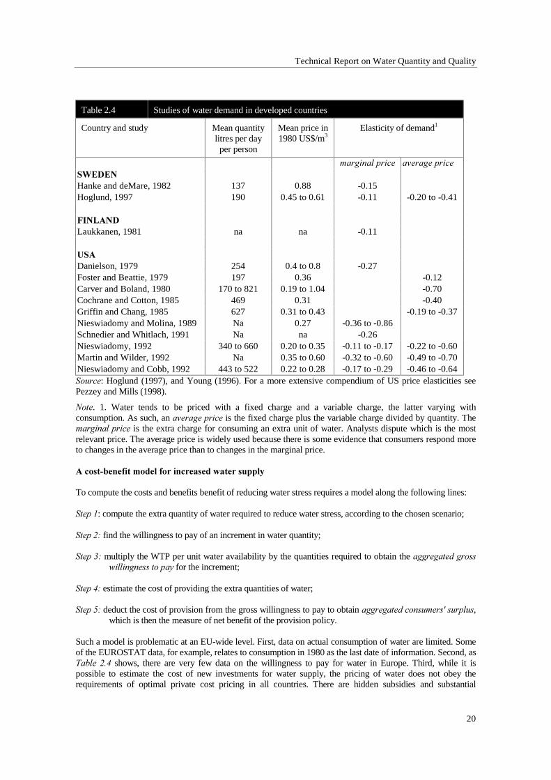
Table 2.4 Studies of water demand in developed countries
Country and study Mean quantitylitres per dayper person
Mean price in1980 US$/m3
Elasticity of demand1
PDUJLQDO�SULFH DYHUDJH�SULFH6:('(1Hanke and deMare, 1982 137 0.88 -0.15Hoglund, 1997 190 0.45 to 0.61 -0.11 -0.20 to -0.41
),1/$1'Laukkanen, 1981 na na -0.11
86$Danielson, 1979 254 0.4 to 0.8 -0.27Foster and Beattie, 1979 197 0.36 -0.12Carver and Boland, 1980 170 to 821 0.19 to 1.04 -0.70Cochrane and Cotton, 1985 469 0.31 -0.40Griffin and Chang, 1985 627 0.31 to 0.43 -0.19 to -0.37Nieswiadomy and Molina, 1989 Na 0.27 -0.36 to -0.86Schnedier and Whitlach, 1991 Na na -0.26Nieswiadomy, 1992 340 to 660 0.20 to 0.35 -0.11 to -0.17 -0.22 to -0.60Martin and Wilder, 1992 Na 0.35 to 0.60 -0.32 to -0.60 -0.49 to -0.70Nieswiadomy and Cobb, 1992 443 to 522 0.22 to 0.28 -0.17 to -0.29 -0.46 to -0.646RXUFH: Hoglund (1997), and Young (1996). For a more extensive compendium of US price elasticities seePezzey and Mills (1998).
1RWH. 1. Water tends to be priced with a fixed charge and a variable charge, the latter varying withconsumption. As such, an DYHUDJH�SULFH is the fixed charge plus the variable charge divided by quantity. ThePDUJLQDO�SULFH is the extra charge for consuming an extra unit of water. Analysts dispute which is the mostrelevant price. The average price is widely used because there is some evidence that consumers respond moreto changes in the average price than to changes in the marginal price.
$�FRVW�EHQHILW�PRGHO�IRU�LQFUHDVHG�ZDWHU�VXSSO\
To compute the costs and benefits benefit of reducing water stress requires a model along the following lines:
6WHS��: compute the extra quantity of water required to reduce water stress, according to the chosen scenario;
6WHS����find the willingness to pay of an increment in water quantity;
6WHS����multiply the WTP per unit water availability by the quantities required to obtain the DJJUHJDWHG�JURVVZLOOLQJQHVV�WR�SD\ for the increment;
6WHS����estimate the cost of providing the extra quantities of water;
6WHS����deduct the cost of provision from the gross willingness to pay to obtain DJJUHJDWHG�FRQVXPHUV�VXUSOXV,which is then the measure of net benefit of the provision policy.
Such a model is problematic at an EU-wide level. First, data on actual consumption of water are limited. Someof the EUROSTAT data, for example, relates to consumption in 1980 as the last date of information. Second, as7DEOH� ��� shows, there are very few data on the willingness to pay for water in Europe. Third, while it ispossible to estimate the cost of new investments for water supply, the pricing of water does not obey therequirements of optimal private cost pricing in all countries. There are hidden subsidies and substantial
Technical Report on Water Quantity and Quality
21
regulation which prevents water being priced at marginal supply costs everywhere. This means that estimatingthe costs of new supply is not always relevant: policy measures to price water correctly, even at private costlevels, will often be more appropriate. But estimating the costs of such policies requires analysis andinformation beyond the scope available for this study. Fourth, ’water stress’ is itself a ’fuzzy’ concept. Water isused in various ways: for domestic consumption, for agriculture, industry, and for environmental purposes. Theconcept of ’stress’ implies that any one of these sectors can be, in some sense, ’short’ of water. But shortages inone sector could be relieved by reducing supplies in another sector. Economic analysis would suggest thatwater should be allocated to the sector with the highest WTP so that the final allocation of water supplies meetsthe condition that marginal WTP is equal in all uses. But this is not how water is allocated, so that there areconsiderable allocation distortions. In the presence of those distortions, ’water stress’ becomes a concept ofdoubtful validity.
'DWD�RQ�ZDWHU�FRQVXPSWLRQ
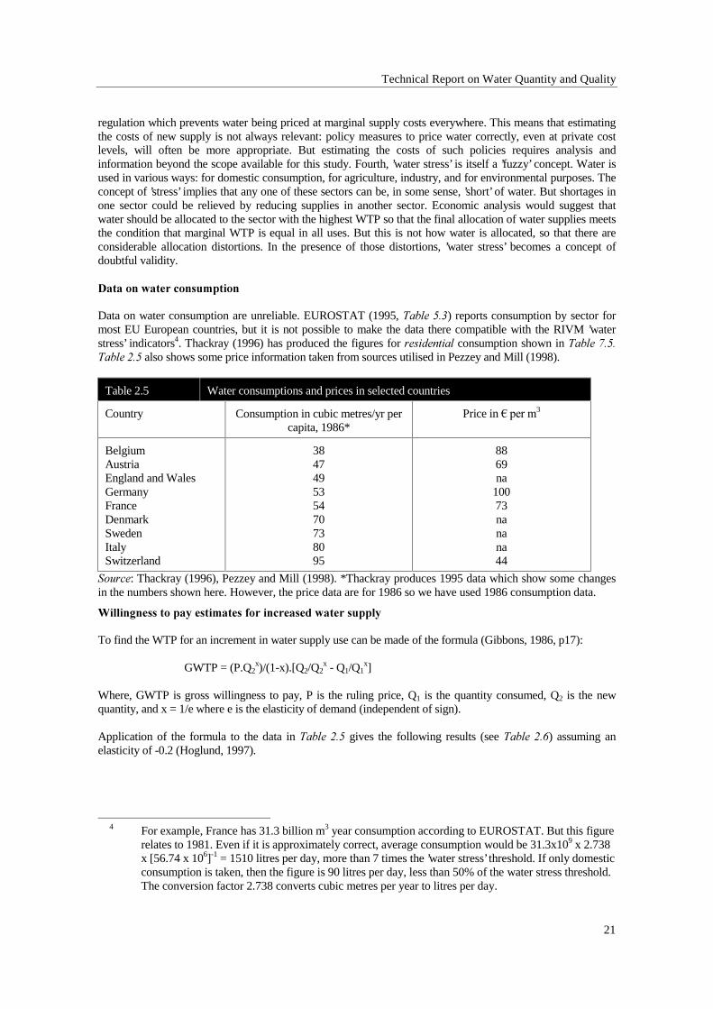
Data on water consumption are unreliable. EUROSTAT (1995, 7DEOH����) reports consumption by sector formost EU European countries, but it is not possible to make the data there compatible with the RIVM ’waterstress’ indicators4. Thackray (1996) has produced the figures for UHVLGHQWLDO consumption shown in 7DEOH�����7DEOH���� also shows some price information taken from sources utilised in Pezzey and Mill (1998).
Table 2.5 Water consumptions and prices in selected countries
Country Consumption in cubic metres/yr percapita, 1986*
Price in ¼�SHU�P3
BelgiumAustriaEngland and WalesGermanyFranceDenmarkSwedenItalySwitzerland
384749535470738095
8869na
10073nanana44
6RXUFH: Thackray (1996), Pezzey and Mill (1998). *Thackray produces 1995 data which show some changesin the numbers shown here. However, the price data are for 1986 so we have used 1986 consumption data.
:LOOLQJQHVV�WR�SD\�HVWLPDWHV�IRU�LQFUHDVHG�ZDWHU�VXSSO\
To find the WTP for an increment in water supply use can be made of the formula (Gibbons, 1986, p17):
GWTP = (P.Q2x)/(1-x).[Q2/Q2
x - Q1/Q1x]
Where, GWTP is gross willingness to pay, P is the ruling price, Q1 is the quantity consumed, Q2 is the newquantity, and x = 1/e where e is the elasticity of demand (independent of sign).
Application of the formula to the data in 7DEOH���� gives the following results (see 7DEOH����) assuming anelasticity of -0.2 (Hoglund, 1997).
4 For example, France has 31.3 billion m3 year consumption according to EUROSTAT. But this figure
relates to 1981. Even if it is approximately correct, average consumption would be 31.3x109 x 2.738x [56.74 x 106]-1 = 1510 litres per day, more than 7 times the ’water stress’ threshold. If only domesticconsumption is taken, then the figure is 90 litres per day, less than 50% of the water stress threshold.The conversion factor 2.738 converts cubic metres per year to litres per day.
Technical Report on Water Quantity and Quality
22
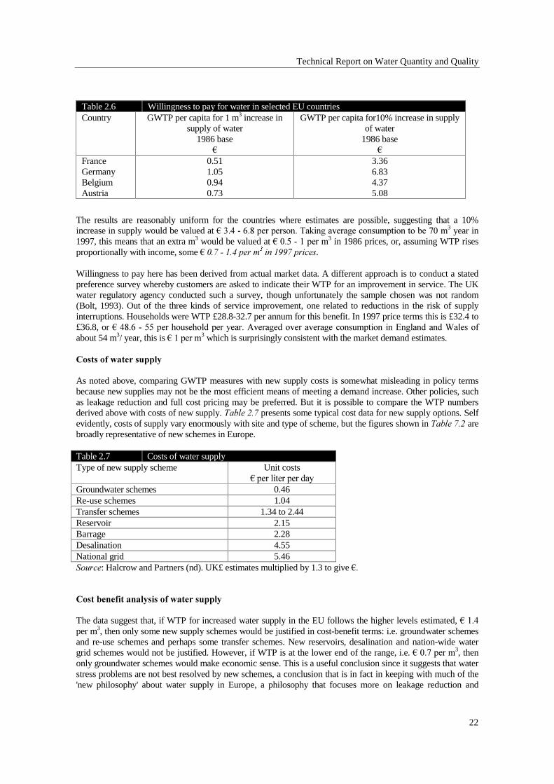
Table 2.6 Willingness to pay for water in selected EU countriesCountry GWTP per capita for 1 m3 increase in
supply of water1986 base
¼
GWTP per capita for10% increase in supplyof water
1986 base¼
FranceGermanyBelgiumAustria
0.511.050.940.73
3.366.834.375.08
The results are reasonably uniform for the countries where estimates are possible, suggesting that a 10%increase in supply would be valued at ¼�����������SHU�SHUVRQ��7DNLQJ�DYHUDJH�FRQVXPSWLRQ�WR�EH����P3 year in1997, this means that an extra m3 would be valued at ¼���������SHU�P3 in 1986 prices, or, assuming WTP risesproportionally with income, some ¼�����������SHU�P��LQ������SULFHV.
Willingness to pay here has been derived from actual market data. A different approach is to conduct a statedpreference survey whereby customers are asked to indicate their WTP for an improvement in service. The UKwater regulatory agency conducted such a survey, though unfortunately the sample chosen was not random(Bolt, 1993). Out of the three kinds of service improvement, one related to reductions in the risk of supplyinterruptions. Households were WTP £28.8-32.7 per annum for this benefit. In 1997 price terms this is £32.4 to£36.8, or ¼�����������SHU�KRXVHKROG�SHU�\HDU��$YHUDJHG�RYHU�DYHUDJH�FRQVXPSWLRQ� LQ�(QJODQG�DQG�:DOHV�RIabout 54 m3/ year, this is ¼���SHU�P3 which is surprisingly consistent with the market demand estimates.
&RVWV�RI�ZDWHU�VXSSO\
As noted above, comparing GWTP measures with new supply costs is somewhat misleading in policy termsbecause new supplies may not be the most efficient means of meeting a demand increase. Other policies, suchas leakage reduction and full cost pricing may be preferred. But it is possible to compare the WTP numbersderived above with costs of new supply. 7DEOH���� presents some typical cost data for new supply options. Selfevidently, costs of supply vary enormously with site and type of scheme, but the figures shown in 7DEOH���� arebroadly representative of new schemes in Europe.
Table 2.7 Costs of water supplyType of new supply scheme Unit costs
¼�SHU�OLWHU�SHU�GD\Groundwater schemes 0.46Re-use schemes 1.04Transfer schemes 1.34 to 2.44Reservoir 2.15Barrage 2.28Desalination 4.55National grid 5.466RXUFH: Halcrow and Partners (nd). UK£ estimates multiplied by 1.3 to give ¼�
&RVW�EHQHILW�DQDO\VLV�RI�ZDWHU�VXSSO\
The data suggest that, if WTP for increased water supply in the EU follows the higher levels estimated, ¼����per m3, then only some new supply schemes would be justified in cost-benefit terms: i.e. groundwater schemesand re-use schemes and perhaps some transfer schemes. New reservoirs, desalination and nation-wide watergrid schemes would not be justified. However, if WTP is at the lower end of the range, i.e. ¼�����SHU�P3, thenonly groundwater schemes would make economic sense. This is a useful conclusion since it suggests that waterstress problems are not best resolved by new schemes, a conclusion that is in fact in keeping with much of the'new philosophy' about water supply in Europe, a philosophy that focuses more on leakage reduction and
Technical Report on Water Quantity and Quality
23
demand management first and new supplies only last. Once again, it is important to understand that these arevery broad averages: it does not mean that a new reservoir in some location is never justified.
&RQFOXVLRQ�RQ�ZDWHU�DYDLODELOLW\
There is a clear WTP on the part of EU residents for increased water supply but comparison of this WTP withthe costs of new supplies suggests fairly strongly that new schemes are not generally justified in cost-benefitterms. The focus of policy should be on correct water pricing and demand management schemes (see the policydiscussion).
������ :DWHU�TXDOLW\�DQDO\VLV
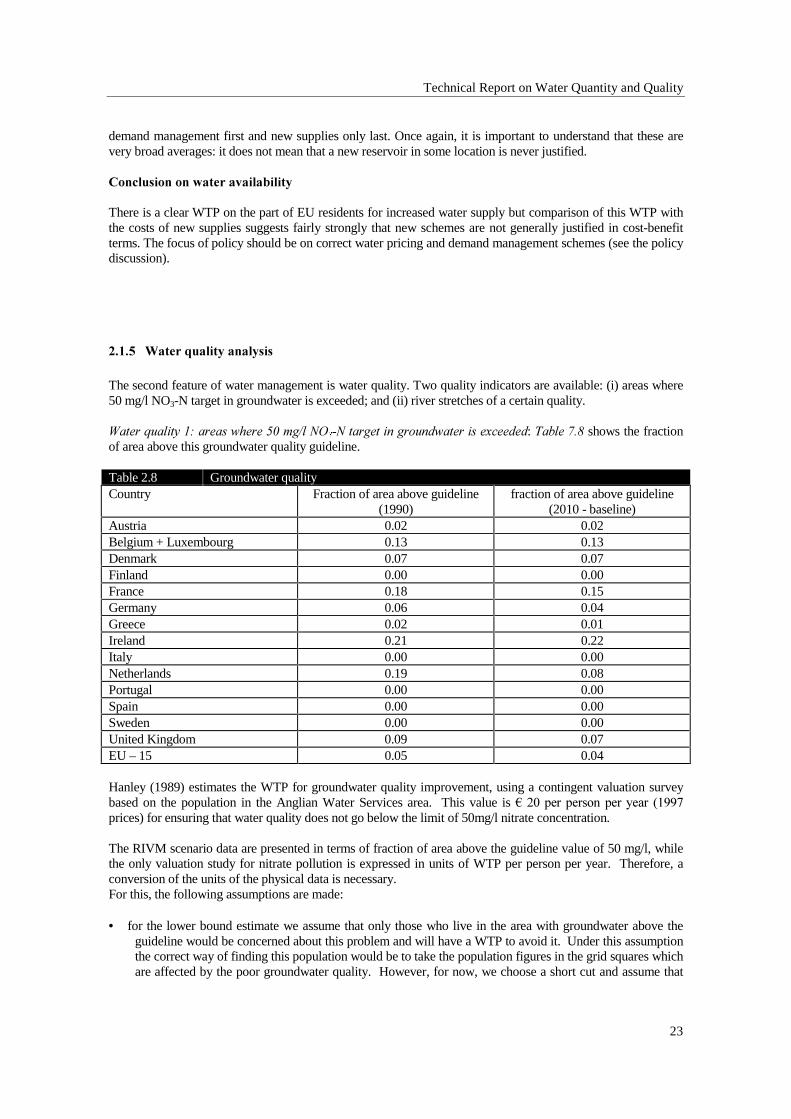
The second feature of water management is water quality. Two quality indicators are available: (i) areas where50 mg/l NO3-N target in groundwater is exceeded; and (ii) river stretches of a certain quality.
:DWHU�TXDOLW\����DUHDV�ZKHUH����PJ�O�12��1�WDUJHW�LQ�JURXQGZDWHU�LV�H[FHHGHG: 7DEOH���� shows the fractionof area above this groundwater quality guideline.
Table 2.8 Groundwater qualityCountry Fraction of area above guideline
(1990)fraction of area above guideline
(2010 - baseline)Austria 0.02 0.02Belgium + Luxembourg 0.13 0.13Denmark 0.07 0.07Finland 0.00 0.00France 0.18 0.15Germany 0.06 0.04Greece 0.02 0.01Ireland 0.21 0.22Italy 0.00 0.00Netherlands 0.19 0.08Portugal 0.00 0.00Spain 0.00 0.00Sweden 0.00 0.00United Kingdom 0.09 0.07EU – 15 0.05 0.04
Hanley (1989) estimates the WTP for groundwater quality improvement, using a contingent valuation surveybased on the population in the Anglian Water Services area. This value is ¼����SHU�SHUVRQ�SHU� \HDU� �����prices) for ensuring that water quality does not go below the limit of 50mg/l nitrate concentration.
The RIVM scenario data are presented in terms of fraction of area above the guideline value of 50 mg/l, whilethe only valuation study for nitrate pollution is expressed in units of WTP per person per year. Therefore, aconversion of the units of the physical data is necessary.For this, the following assumptions are made:
• for the lower bound estimate we assume that only those who live in the area with groundwater above theguideline would be concerned about this problem and will have a WTP to avoid it. Under this assumptionthe correct way of finding this population would be to take the population figures in the grid squares whichare affected by the poor groundwater quality. However, for now, we choose a short cut and assume that
Technical Report on Water Quantity and Quality
24
the fraction of area affected in a country is identical to the fraction of population affected in that country.This implies a uniform population distribution, which is not strictly correct, but is best that can be assumedunder the circumstances.
• for the upper bound estimate we assume that the whole population in a country is concerned about thisproblem and hence will have a WTP to avoid it regardless of the fraction of the total area affected or thelevel of pollution. Therefore, we aggregate the individual WTP estimate over the whole population.
7DEOH���� shows the damage valuations for the baseline scenario in 1990 and 2010.
Table 2.9 Damage costs in 1990, 2010 in the Baseline: ¼�PLOOLRQ�������SULFHV�(VWLPDWH ���� ����lower bound 602 397upper bound 5,716 4,594
Note; Baseline scenario relates relates to areas where 50mg / l NO3-N target in groundwater is exceeded.
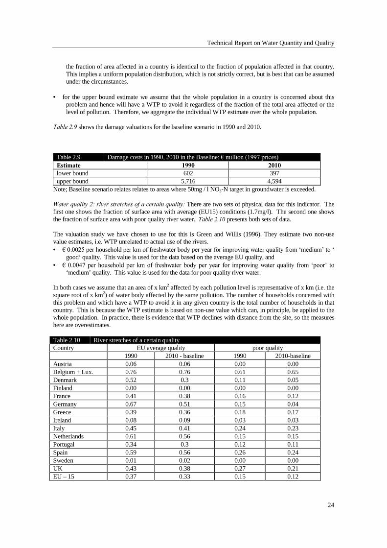
:DWHU�TXDOLW\����ULYHU�VWUHWFKHV�RI�D�FHUWDLQ�TXDOLW\��There are two sets of physical data for this indicator. Thefirst one shows the fraction of surface area with average (EU15) conditions (1.7mg/l). The second one showsthe fraction of surface area with poor quality river water. 7DEOH����� presents both sets of data.
The valuation study we have chosen to use for this is Green and Willis (1996). They estimate two non-usevalue estimates, i.e. WTP unrelated to actual use of the rivers.• ¼��������SHU�KRXVHKROG�SHU�NP�RI�IUHVKZDWHU�ERG\�SHU�\HDU�IRU�LPSURYLQJ�ZDWHU�TXDOLW\�IURP�µPHGLXP¶�WR�µ
good’ quality. This value is used for the data based on the average EU quality, and• ¼��������SHU�KRXVHKROG�SHU�NP�RI� IUHVKZDWHU�ERG\�SHU� \HDU� IRU� LPSURYLQJ�ZDWHU�TXDOLW\� IURP� µSRRU¶� WR
‘medium’ quality. This value is used for the data for poor quality river water.
In both cases we assume that an area of x km2 affected by each pollution level is representative of x km (i.e. thesquare root of x km2) of water body affected by the same pollution. The number of households concerned withthis problem and which have a WTP to avoid it in any given country is the total number of households in thatcountry. This is because the WTP estimate is based on non-use value which can, in principle, be applied to thewhole population. In practice, there is evidence that WTP declines with distance from the site, so the measureshere are overestimates.
Table 2.10 River stretches of a certain qualityCountry EU average quality poor quality
1990 2010 - baseline 1990 2010-baselineAustria 0.06 0.06 0.00 0.00Belgium + Lux. 0.76 0.76 0.61 0.65Denmark 0.52 0.3 0.11 0.05Finland 0.00 0.00 0.00 0.00France 0.41 0.38 0.16 0.12Germany 0.67 0.51 0.15 0.04Greece 0.39 0.36 0.18 0.17Ireland 0.08 0.09 0.03 0.03Italy 0.45 0.41 0.24 0.23Netherlands 0.61 0.56 0.15 0.15Portugal 0.34 0.3 0.12 0.11Spain 0.59 0.56 0.26 0.24Sweden 0.01 0.02 0.00 0.00UK 0.43 0.38 0.27 0.21EU – 15 0.37 0.33 0.15 0.12
Technical Report on Water Quantity and Quality
25
7DEOH����� shows the damage values for (a) fraction of surface area with average (EU15) conditions and (b)fraction of surface area with poor quality river water.
Table 2.11 Damage cost in 1990, 2010 due to water quality, Baseline scenario: ¼�PLOOLRQEstimate 1990 2010Average EU quality 152 146‘poor quality’ 245 212Total 397 358
The damage associated with ‘poor’ quality is greater than that associated with average EU quality. This isbecause the unit WTP to improve the former is greater than that for the latter.
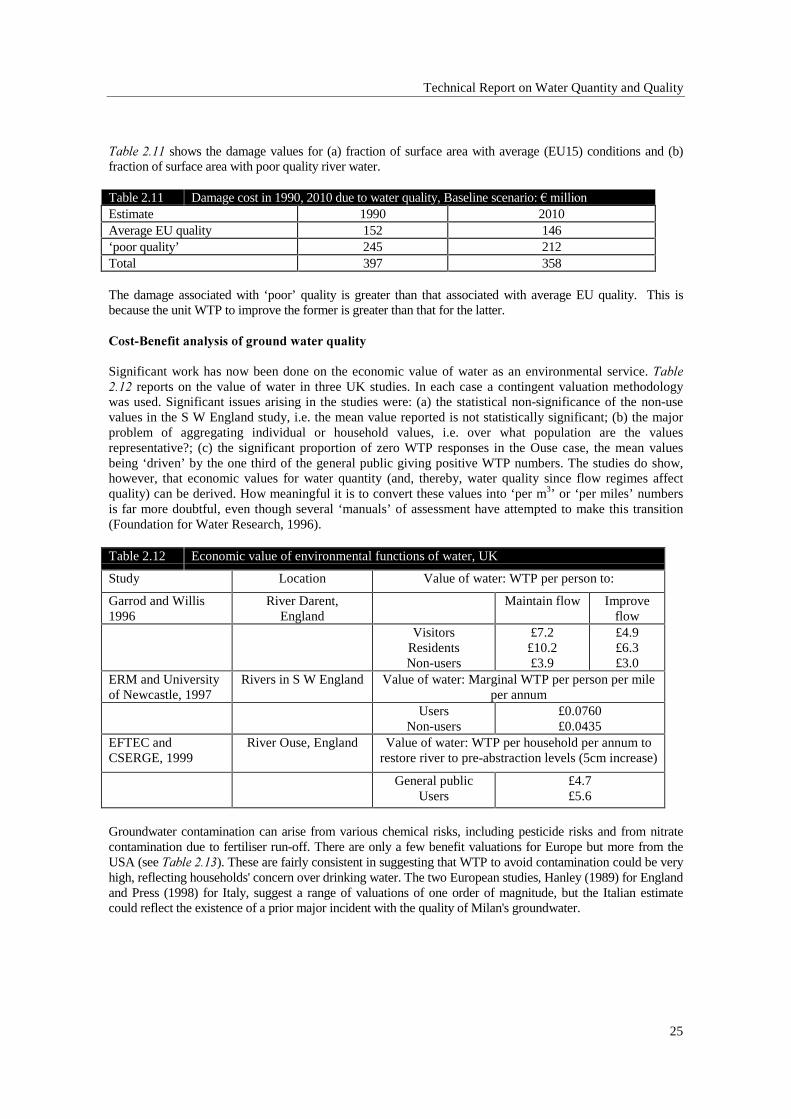
&RVW�%HQHILW�DQDO\VLV�RI�JURXQG�ZDWHU�TXDOLW\
Significant work has now been done on the economic value of water as an environmental service. 7DEOH���� reports on the value of water in three UK studies. In each case a contingent valuation methodologywas used. Significant issues arising in the studies were: (a) the statistical non-significance of the non-usevalues in the S W England study, i.e. the mean value reported is not statistically significant; (b) the majorproblem of aggregating individual or household values, i.e. over what population are the valuesrepresentative?; (c) the significant proportion of zero WTP responses in the Ouse case, the mean valuesbeing ‘driven’ by the one third of the general public giving positive WTP numbers. The studies do show,however, that economic values for water quantity (and, thereby, water quality since flow regimes affectquality) can be derived. How meaningful it is to convert these values into ‘per m3’ or ‘per miles’ numbersis far more doubtful, even though several ‘manuals’ of assessment have attempted to make this transition(Foundation for Water Research, 1996).
Table 2.12 Economic value of environmental functions of water, UK
Study Location Value of water: WTP per person to:
Garrod and Willis1996
River Darent,England
Maintain flow Improveflow
VisitorsResidentsNon-users
£7.2£10.2£3.9
£4.9£6.3£3.0
ERM and Universityof Newcastle, 1997
Rivers in S W England Value of water: Marginal WTP per person per mileper annum
UsersNon-users
£0.0760£0.0435
EFTEC andCSERGE, 1999
River Ouse, England Value of water: WTP per household per annum torestore river to pre-abstraction levels (5cm increase)
General publicUsers
£4.7£5.6
Groundwater contamination can arise from various chemical risks, including pesticide risks and from nitratecontamination due to fertiliser run-off. There are only a few benefit valuations for Europe but more from theUSA (see 7DEOH�����). These are fairly consistent in suggesting that WTP to avoid contamination could be veryhigh, reflecting households' concern over drinking water. The two European studies, Hanley (1989) for Englandand Press (1998) for Italy, suggest a range of valuations of one order of magnitude, but the Italian estimatecould reflect the existence of a prior major incident with the quality of Milan's groundwater.
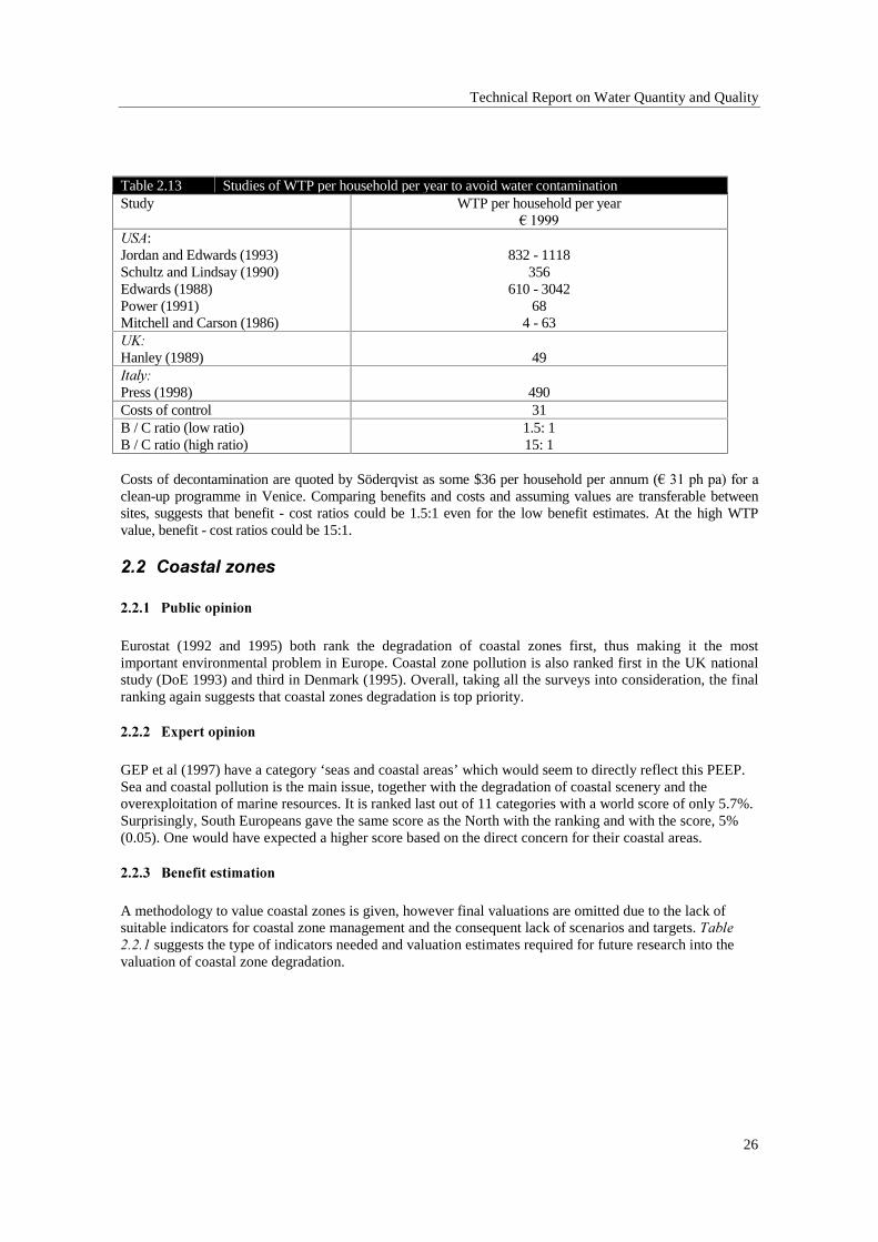
Technical Report on Water Quantity and Quality
26
Table 2.13 Studies of WTP per household per year to avoid water contaminationStudy WTP per household per year
¼�����86$:Jordan and Edwards (1993)Schultz and Lindsay (1990)Edwards (1988)Power (1991)Mitchell and Carson (1986)
832 - 1118356
610 - 304268
4 - 638.�Hanley (1989) 49,WDO\�Press (1998) 490Costs of control 31B / C ratio (low ratio)B / C ratio (high ratio)
1.5: 115: 1
Costs of decontamination are quoted by Söderqvist as some $36 per household per annum (¼����SK�SD��IRU�Dclean-up programme in Venice. Comparing benefits and costs and assuming values are transferable betweensites, suggests that benefit - cost ratios could be 1.5:1 even for the low benefit estimates. At the high WTPvalue, benefit - cost ratios could be 15:1.
���� &RDVWDO�]RQHV
������ 3XEOLF�RSLQLRQ
Eurostat (1992 and 1995) both rank the degradation of coastal zones first, thus making it the mostimportant environmental problem in Europe. Coastal zone pollution is also ranked first in the UK nationalstudy (DoE 1993) and third in Denmark (1995). Overall, taking all the surveys into consideration, the finalranking again suggests that coastal zones degradation is top priority.
������ ([SHUW�RSLQLRQ
GEP et al (1997) have a category ‘seas and coastal areas’ which would seem to directly reflect this PEEP.Sea and coastal pollution is the main issue, together with the degradation of coastal scenery and theoverexploitation of marine resources. It is ranked last out of 11 categories with a world score of only 5.7%.Surprisingly, South Europeans gave the same score as the North with the ranking and with the score, 5%(0.05). One would have expected a higher score based on the direct concern for their coastal areas.
������ %HQHILW�HVWLPDWLRQ
A methodology to value coastal zones is given, however final valuations are omitted due to the lack ofsuitable indicators for coastal zone management and the consequent lack of scenarios and targets. 7DEOH������suggests the type of indicators needed and valuation estimates required for future research into thevaluation of coastal zone degradation.
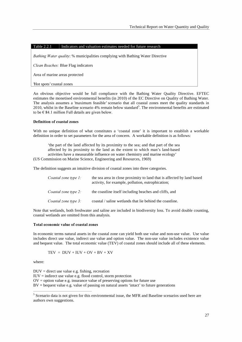
Technical Report on Water Quantity and Quality
27
Table 2.2.1 Indicators and valuation estimates needed for future research
%DWKLQJ�:DWHU�TXDOLW\: % municipalities complying with Bathing Water Directive
&OHDQ�%HDFKHV� Blue Flag indicators
Area of marine areas protected
’Hot spots’ coastal zones
An obvious objective would be full compliance with the Bathing Water Quality Directive. EFTECestimates the monetised environmental benefits (in 2010) of the EC Directive on Quality of Bathing Water.The analysis assumes a ’maximum feasible’ scenario that all coastal zones meet the quality standards in2010, whilst in the Baseline scenario 4% remain below standard5. The environmental benefits are estimatedto be ¼������PLOOLRQ�)XOO�GHWDLOV�DUH�JLYHQ�EHORZ�
'HILQLWLRQ�RI�FRDVWDO�]RQHV
With no unique definition of what constitutes a ‘coastal zone’ it is important to establish a workabledefinition in order to set parameters for the area of concern. A workable definition is as follows:
‘the part of the land affected by its proximity to the sea; and that part of the seaaffected by its proximity to the land as the extent to which man’s land-basedactivities have a measurable influence on water chemistry and marine ecology’
(US Commission on Marine Science, Engineering and Resources, 1969)
The definition suggests an intuitive division of coastal zones into three categories.
&RDVWDO�]RQH�W\SH��� the sea area in close proximity to land that is affected by land basedactivity, for example, pollution, eutrophication;
&RDVWDO�]RQH�W\SH��� the coastline itself including beaches and cliffs, and
&RDVWDO�]RQH�W\SH��� coastal / saline wetlands that lie behind the coastline.
Note that wetlands, both freshwater and saline are included in biodiversity loss. To avoid double counting,coastal wetlands are omitted from this analysis.
7RWDO�HFRQRPLF�YDOXH�RI�FRDVWDO�]RQHV
In economic terms natural assets in the coastal zone can yield both use value and non-use value. Use valueincludes direct use value, indirect use value and option value. The non-use value includes existence valueand bequest value. The total economic value (TEV) of coastal zones should include all of these elements.
TEV = DUV + IUV + OV + BV + XV
where:
DUV = direct use value e.g. fishing, recreationIUV = indirect use value e.g. flood control, storm protectionOV = option value e.g. insurance value of preserving options for future useBV = bequest value e.g. value of passing on natural assets ‘intact’ to future generations
5 Scenario data is not given for this environmental issue, the MFR and Baseline scenarios used here areauthors own suggestions.
Technical Report on Water Quantity and Quality
28
XV = existence value e.g. value derived from just knowing a species/system is conserved
In terms of placing monetary values on coastal zones and analysing the benefits of any given scenario it isconvenient to follow the approach of dividing coastal zones into the three sections detailed above.
An additional threat to coastal zones is the potential sea level rise resulting from global warming.Valuations for coastal damage due to sea level rise are included in ’climate change’, thus they are omittedfrom this analysis.
The contingent valuation method (CVM) can provide valuations of both use and non-use value dependingon the design and location of the questionnaire. For this reason we concentrate on CVM valuation studiesto derive valuation for coastal zone damage.
A specific problem concerning coastal zone valuation is the process of aggregation from individual WTPmeasures to Europe wide valuations of coastal zones. For example, a number of studies provide WTPvalues for bathing water quality. However, all studies concentrate on direct use value by questioning localresidents and holiday-makers at coastal resorts. To aggregate such valuations would require information onthe proportion of the European population living in coastal areas and the number of people taking holidaysin European coastal resorts. Even if such data is available the valuations will still ignore non-use values.Issues concerning aggregation will be highlighted. We proceed by considering the coastal zone type 1, seaarea in close proximity to land.
&RDVWDO�]RQH�W\SH����VHD�DUHD�LQ�FORVH�SUR[LPLW\�WR�ODQG
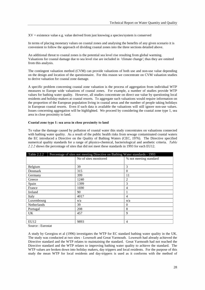
To value the damage caused by pollution of coastal water this study concentrates on valuations connectedwith bathing water quality. As a result of the public health risks from sewage contaminated coastal watersthe EC introduced a Directive on the Quality of Bathing Waters (CEC, 1976). The Directive specifiednumerical quality standards for a range of physico-chemical, bacteriological and aesthetic criteria. 7DEOH����� shows the percentage of sites that did not meet these standards in 1993 for each EU12.
Table 2.2.2 Percentage of sites not meeting Directive on Bathing Water standards - 1993No of sites monitored % not meeting standard
Belgium 39 3Denmark 315 0Germany 399 11Greece 1240 2Spain 1399 3France 1690 4Ireland 90 1Italy 4017 4Luxembourg n/a n/aNetherlands 39 0Portugal 208 8UK 457 9
EU12 9893 4Source : Eurostat
A study by Georgiou et al (1996) investigates the WTP for EC standard bathing water quality in the UK.The study was conducted at two sites - Lowesoft and Great Yarmouth. Lowesoft had already achieved theDirective standard and the WTP relates to maintaining the standard. Great Yarmouth had not reached theDirective standard and the WTP relates to improving bathing water quality to achieve the standard. TheWTP values are broken down into holiday makers, day trippers and local residents. For the purpose of thisstudy the mean WTP for local residents and day-trippers is used as it conforms with the method of
Technical Report on Water Quantity and Quality
29
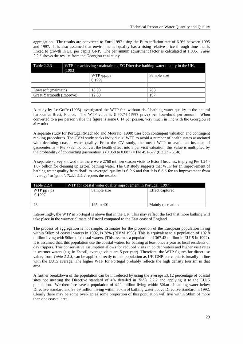
aggregation. The results are converted to Euro 1997 using the Euro inflation rate of 6.9% between 1995and 1997. It is also assumed that environmental quality has a rising relative price through time that islinked to growth in EU per capita GNP. The per annum adjustment factor is calculated at 1.005. 7DEOH����� shows the results from the Georgiou et al study.
Table 2.2.3 WTP for achieving / maintaining EC Directive bathing water quality in the UK,(1993).
WTP /pp/pa¼�����
Sample size
Lowesoft (maintain) 18.08 203Great Yarmouth (improve) 12.80 197
A study by Le Goffe (1995) investigated the WTP for ‘without risk’ bathing water quality in the naturalharbour at Brest, France. The WTP value is ¼� ������ ������ SULFH�� SHU� KRXVHKROG� SHU� DQQXP�� � :KHQconverted to a per person value the figure is some ¼����SHU�SHUVRQ��YHU\�PXFK�LQ�OLQH�ZLWK�WKH�*HRUJLRX�HWal results
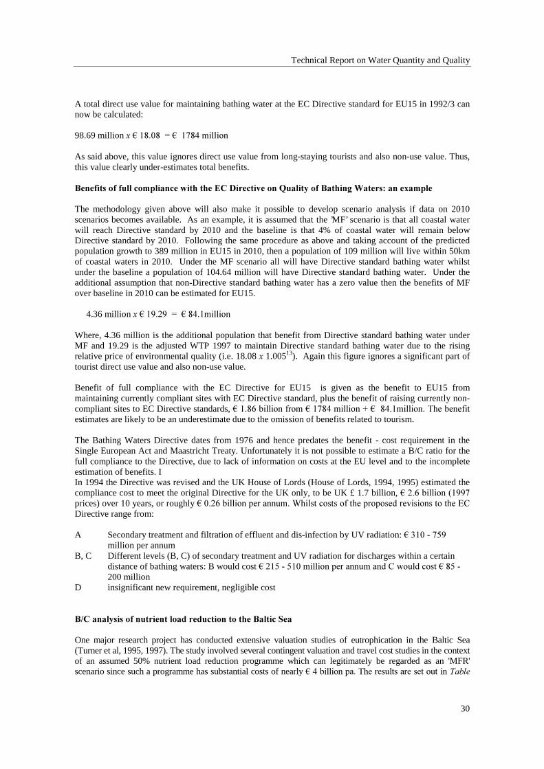
A separate study for Portugal (Machado and Mourato, 1998) uses both contingent valuation and contingentranking procedures. The CVM study seeks individuals’ WTP to avoid a number of health states associatedwith declining coastal water quality. From the CV study, the mean WTP to avoid an instance ofgasroenteritis = Pte 7782. To convert the health effect into a per visit valuation, this value is multiplied bythe probability of contracting gasroenteritis (0.058 to 0.087) = Pte 451-677 (¼��������������
A separate survey showed that there were 2760 million season visits to Estoril beaches, implying Pte 1.24 -1.87 billion for cleaning up Estoril bathing water. The CR study suggests that WTP for an improvement ofbathing water quality from ‘bad’ to ‘average’ quality is ¼�����DQG�WKDW�LW�LV�¼�����IRU�DQ�LPSURYHPHQW�IURP‘average’ to ‘good’. 7DEOH������ reports the results.
Table 2.2.4 WTP for coastal water quality improvement in Portugal (1997)WTP pp / pa ¼�����
Sample size Effect captured
48 195 to 401 Mainly recreation
Interestingly, the WTP in Portugal is above that in the UK. This may reflect the fact that more bathing willtake place in the warmer climate of Estoril compared to the East coast of England.
The process of aggregation is not simple. Estimates for the proportion of the European population livingwithin 50km of coastal waters in 1992, is 28% (RIVM 1998). This is equivalent to a population of 102.8million living with 50km of coastal waters. (This assumes a population of 367.43 million in EU15 in 1992).It is assumed that, this population use the coastal waters for bathing at least once a year as local residents orday trippers. This conservative assumption allows for reduced visits in colder waters and higher visit ratesin warmer waters (e.g. in Estoril, average visits are 5 per year). Therefore, the WTP figures for direct usevalue, from 7DEOH������, can be applied directly to this population as UK GNP per capita is broadly in linewith the EU15 average. The higher WTP for Portugal probably reflects the high density tourism in thatarea.
A further breakdown of the population can be introduced by using the average EU12 percentage of coastalsites not meeting the Directive standard of 4% detailed in 7DEOH� ����� and applying it to the EU15population. We therefore have a population of 4.11 million living within 50km of bathing water belowDirective standard and 98.69 million living within 50km of bathing water above Directive standard in 1992.Clearly there may be some over-lap as some proportion of this population will live within 50km of morethan one coastal area
Technical Report on Water Quantity and Quality
30
A total direct use value for maintaining bathing water at the EC Directive standard for EU15 in 1992/3 cannow be calculated:
98.69 million [ ¼�������� �¼�������PLOOLRQ
As said above, this value ignores direct use value from long-staying tourists and also non-use value. Thus,this value clearly under-estimates total benefits.
%HQHILWV�RI�IXOO�FRPSOLDQFH�ZLWK�WKH�(&�'LUHFWLYH�RQ�4XDOLW\�RI�%DWKLQJ�:DWHUV��DQ�H[DPSOH
The methodology given above will also make it possible to develop scenario analysis if data on 2010scenarios becomes available. As an example, it is assumed that the ’MF’ scenario is that all coastal waterwill reach Directive standard by 2010 and the baseline is that 4% of coastal water will remain belowDirective standard by 2010. Following the same procedure as above and taking account of the predictedpopulation growth to 389 million in EU15 in 2010, then a population of 109 million will live within 50kmof coastal waters in 2010. Under the MF scenario all will have Directive standard bathing water whilstunder the baseline a population of 104.64 million will have Directive standard bathing water. Under theadditional assumption that non-Directive standard bathing water has a zero value then the benefits of MFover baseline in 2010 can be estimated for EU15.
4.36 million [ ¼�������� ��¼�����PLOOLRQ
Where, 4.36 million is the additional population that benefit from Directive standard bathing water underMF and 19.29 is the adjusted WTP 1997 to maintain Directive standard bathing water due to the risingrelative price of environmental quality (i.e. 18.08 [ 1.00513). Again this figure ignores a significant part oftourist direct use value and also non-use value.
Benefit of full compliance with the EC Directive for EU15 is given as the benefit to EU15 frommaintaining currently compliant sites with EC Directive standard, plus the benefit of raising currently non-compliant sites to EC Directive standards, ¼������ELOOLRQ�IURP�¼������PLOOLRQ���¼������PLOOLRQ��7KH�EHQHILWestimates are likely to be an underestimate due to the omission of benefits related to tourism.
The Bathing Waters Directive dates from 1976 and hence predates the benefit - cost requirement in theSingle European Act and Maastricht Treaty. Unfortunately it is not possible to estimate a B/C ratio for thefull compliance to the Directive, due to lack of information on costs at the EU level and to the incompleteestimation of benefits. IIn 1994 the Directive was revised and the UK House of Lords (House of Lords, 1994, 1995) estimated thecompliance cost to meet the original Directive for the UK only, to be UK £ 1.7 billion, ¼�����ELOOLRQ������prices) over 10 years, or roughly ¼������ELOOLRQ�SHU�DQQXP��:KLOVW�FRVWV�RI�WKH�SURSRVHG�UHYLVLRQV�WR�WKH�(&Directive range from:
A Secondary treatment and filtration of effluent and dis-infection by UV radiation: ¼����������million per annum
B, C Different levels (B, C) of secondary treatment and UV radiation for discharges within a certaindistance of bathing waters: B would cost ¼�����������PLOOLRQ�SHU�DQQXP�DQG�&�ZRXOG�FRVW�¼�����200 million
D insignificant new requirement, negligible cost
%�&�DQDO\VLV�RI�QXWULHQW�ORDG�UHGXFWLRQ�WR�WKH�%DOWLF�6HD
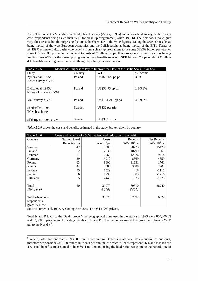
One major research project has conducted extensive valuation studies of eutrophication in the Baltic Sea(Turner et al, 1995, 1997). The study involved several contingent valuation and travel cost studies in the contextof an assumed 50% nutrient load reduction programme which can legitimately be regarded as an 'MFR'scenario since such a programme has substantial costs of nearly ¼���ELOOLRQ�SD��7KH�UHVXOWV�DUH�VHW�RXW�LQ�7DEOH
Technical Report on Water Quantity and Quality
31
�����. The Polish CVM studies involved a beach survey (Zylicz, 1995a) and a household survey, with, in eachcase, respondents being asked their WTP for clean-up programme (Zylicz, 1995b). The first two surveys givevery close results, but the surprising feature is the sheer size of the WTP figures. Taking the Swedish results asbeing typical of the west European economies and the Polish results as being typical of the EITs, Turner HWDO.(1997) estimate Baltic basin wide benefits from a clean-up programme to be some SEK69 billion per year, orsome ¼�ELOOLRQ�����SHU�DQQXP�FRPSDUHG�WR�FRVWV�RI�¼�ELOOLRQ�����SD��,I�QRQ�UHVSRQGHQWV�DUH�WUHDWHG�DV�KDYLQJimplicit zero WTP for the clean up programme, then benefits reduce to SEK billion 37.9 pa or about ¼�ELOOLRQ4.4: benefits are still greater than costs though by a fairly narrow margin.
Table 2.2.5 Median Willingness to Pay to Improve the State of the Baltic Sea. (1994US$)Study Country WTP % IncomeZylicz et al, 1995aBeach survey, CVM
Zylicz et al, 1995bhousehold survey, CVM
Mail survey, CVM
Sandstr∧m, 1995,TCM beach use
S∧derqvist, 1995, CVM
Poland
Poland
Poland
Sweden
Sweden
US$65-122 pp.pa
US$30-73 pp.pa
US$104-211 pp.pa
US$32 per trip
US$333 pp.pa
3-5%
1.3-3.3%
4.6-9.5%
7DEOH������ shows the costs and benefits estimated in the study, broken down by country.
Table 2.2.6 Costs and benefits of a 50% nutrient load reduction in the BalticCountry Nutrient Load
Reduction %Costs
SWkr106 paBenefits
SWkr106 paNet BenefitsSWkr106 pa
SwedenFinlandDenmarkGermanyPolandRussiaEstoniaLatviaLithuania
Total�7RWDO�LQ�¼�
Total when non-respondentsgiven WTP=0
425251396344555655
50
53002838296240109600586
152917992446
31070¼�����
31070
2072310799123768369
116313488418583923
69310¼�����
37892
1542379619414435917612902
-1111-1216-1523
38240
6822
Source:Turner et al, 1997. Assuming SEK 8.65117 = ¼���������SULFHV��
Total N and P loads to the ’Baltic proper’ (the geographical zone used in the study) in 1993 were 860,000 tNand 33,000 tP per annum. Allocating benefits to N and P in the load ratios would then give the following WTPper tonne N and P6:
6 Where; total nutrient load = 893,000 tonnes per annum. Benefits relate to a 50% reduction of nutrients,therefore we consider 446,500 tonnes nutrients per annum, of which N loads represent 96% and P loads are4%. Total benefits are assumed to be ¼������PLOOLRQ�DQG�XVLQJ�WKH�ORDG�UDWLRV�ZH�HVWLPDWH�WKH�EHQHILW�GXH�WR
Technical Report on Water Quantity and Quality
32
¼�W�1� WTP = ¼����������W¼�W�3 WTP = ¼����������W
These are averages for the countries combined. It makes little sense to express WTP per tonne for individualcountries since the questionnaire approach made it clear that the benefits would accrue from a combinedprogramme rather than any unilateral action.
Overall, if we take a 50% nutrient load reduction as being an ambitious programme consistent with MFRassumptions, then an MFR scenario addressing eutrophication from all sources, suggests that benefits exceedcosts.
N is roughly 7690.5 x 106, whilst damage due to P is about 320.4 x 10⁶. Dividing by the tonnes of N and Preleased to the Baltic, gives a WTP of ¼��������SHU�W1�DQG�IRU�3�¼��������SHU�W3�
Technical Report on Water Quantity and Quality
33
��� 3ROLF\�DVVHVVPHQW
���� 3ROLF\�SDFNDJH�ZDWHU�VWUHVV
������ .H\�LVVXHV
:DWHU�DYDLODELOLW\
Data for water management suggest that significant numbers of people within the EU suffer ’water stress’. Thecost-benefit analysis (see section 2: Benefit Assessment) indicated that WTP in the domestic sector was greaterthan the cost of new supplies for only the cheapest sources of supply, such as new groundwater schemes and re-use schemes. It was suggested there that this indicated the need for policy measures that did not focus on newinvestments in supply, but which stressed demand management and leakage control. The discussion is relevantto the :DWHU�5HVRXUFHV�)UDPHZRUN�'LUHFWLYH which, would aim to set a framework for:
LQWHJUDWHG� ZDWHU� PDQDJHPHQW� DQG� FRKHUHQW� SROLFLHV�� H�J�� EHWZHHQ� JURXQGZDWHU� DQGVXUIDFH� ZDWHU�� DQG� WDNLQJ� LQWR� DFFRXQW� IXWXUH� ZDWHU� GHPDQGV� DQG� WKH� EXUGHQ� WKH\� ZLOOLPSRVH� RQ� WKH� HQYLURQPHQW�� QHWZRUN� IRU� WKH� H[FKDQJH� RI� LQIRUPDWLRQ�� LGHQWLI\LQJ� ZDWHUUHVRXUFH�LVVXHV�WKDW�DUH�OLNHO\�WR�HPHUJH�LQ�WKH�IXWXUH��DQG�FROOHFWLQJ�LQIRUPDWLRQ�
The focus is on river basin management planning and ecological and hydrological monitoring. As noted byKopke (1996) future policy must embrace the reduction of wasted water as well as increasing new supplies.
&RUUHFW�ZDWHU�SULFLQJ
The main requirement is to price water at long run marginal cost, (LRMC) as part of a longer run commitmentto full social pricing. The correct pricing of water must account for the (i) extraction and distribution costs (ii)the environmental costs of low flow regimes and (iii) the opportunity costs of water use.
The basic principle of economic pricing of water is given by the formula:
P = MC + MEC + MUC
where MC is the (long run) marginal cost of supply (LRMC), MEC is the marginal external cost associatedwith water abstraction and disposal, and MUC is the marginal ’user cost’ which is designed to reflect the cost offoregone future benefits because of use of the water today. MUC would tend to zero in a fully sustainable watersupply and use system.
The first step towards correct water pricing is the removal of subsidies. Where cross-subsidisation of lowincome consumers is required this can be achieved by ’lifeline’ tariffs, i.e. charging low prices for lowconsumption and very much higher prices for higher consumption.
Once the above is achieved, the recommended policy options are as follows:
������ 5HFRPPHQGHG�SROLF\�LQLWLDWLYHV�IRU�ZDWHU�DYDLODELOLW\
:DWHU�WUDGLQJ�ULJKWV
Water should be allocated to its "highest" value uses through market mechanisms involving, wherepossible, trading of water rights (assuming water is priced at LRMC). Such trading regimes may belocalised but could also include broader national and even transboundary trades.

Technical Report on Water Quantity and Quality
34
There seems to be no experience of water trading in the EU. A consultation process in the UK (resultsreported in ENDS report, June 1998) showed that none of the interested parties (industry, regulators,academia and general public) thought that a system of tradable rights was a viable instrument for waterpolicy mainly for administrative reasons. However, water trading systems exist in USA, Australia, Mexicoand Chile. Such measures are likely to show, that some agricultural uses of water in Europe are notcommercially justified (Pearce 1999). For example, if irrigation water was priced in this way, we doubt ifsome of the agricultural activity in water scarce areas would have an economic justification.
It is clear that tradable rights systems do not ’bite’ in terms of economic and environmental efficiency untilthere is real scarcity. Trends in global warming, growth of population, and growth of tourism, all suggeststhis will be a serious problem in the future for parts of Europe, especially Mediterranean Europe.Implementing a system of tradable rights on an experimental basis, perhaps for irrigation water only (whichis how the schemes largely operate in Australia and California), appears to be a potentially most effectivemeasure.
$EVWUDFWLRQ���XVH�FKDUJH�EDVHG�RQ�FRUUHFW�ZDWHU�SULFLQJ
Based on the above observations, we can conclude that after achieving full private costs (removing subsidies),demand management schemes, such as abstraction / use charge could be used to achieve the target of 200 litreper capita per day. These charges would need to have the following characteristics:
• to cover at least the clean-up and future investment costs, if the ideal case of estimating environmentaldamage costs proves impossible, charges should be differentiated by the location of abstraction (highfor environmentally sensitive areas lower for less sensitive areas), differentiated by timing ofabstraction (high in dry seasons lower in wetter ones), differentiated by unit of abstraction orconsumption (progressive rates), and the revenues should be earmarked especially for the industrialusers in order to encourage water saving technologies.
• the more detailed the instrument, the more difficult it will be to implement it. However, given the currentdiscussions on the Water Resources Framework Directive, location specific instruments can be dealt with(the Directive suggests water basin based management tools). Whatever the design, the most crucial issueremains to be that of price elasticity of demand for water. In various studies over the years, the demand isfound to be inelastic (UHIHU�WR�%HQHILW�$VVHVVPHQW�6HFWLRQ��). This implies one of two policy solutions: (i)a very high charge so that consumption behaviour can be changed or (ii) a well designed earmarkingscheme for the revenues of a lower charge system. The first option would be politically difficult to getacceptance, while the second one may face the opposition of the Ministries of Finance who would preferto add the revenues to the general budgets.
:DWHU�PHWHUV
Metering of the water use by the domestic sector is the first step in charging for water use. Metering providesthe basic information on the extent to which domestic use is a stress factor and helps with measuring theeffectiveness of any policy instrument.
In addition, the experience with metering shows that the mere existence of meters and meter-based water ratesencourage users to reduce their consumption with attached costs and benefits.
Pezzey and Mill (1998) report that metering in Europe is widespread, with 66% of households having meters inDenmark, 84% in Hungary, Spain and Sweden. But the UK has only 10% of households subject to metering(although this is rapidly changing) and Norway has only 5%. A policy of increasing the level of metering doesnot therefore appear to be called for outside of the UK. The general effect of introducing meters is to reduceconsumption by 10% and perhaps more (Pezzey and Mill, 1998; Herrington, 1997).
Technical Report on Water Quantity and Quality
35
The major water pricing and water metering initiative, however, must be in the irrigation sector (see correctwater pricing discussion).
+DUPRQLVHG�9$7�UDWHV�IRU�ZDWHU
VAT rates could be harmonised within each Member State so that water is not treated differently to othercommodities. VAT is not a good proxy for environmental taxes, but if environmental charges are notconsidered feasible, VAT is a potential basis for second best environmental charging.
Moret, Ernst and Young (1996) note that water to domestic consumers is often supplied with a lower rate ofVAT than the standard rate. This suggests, for example, that water consumption in France is 1-4% higherthan would be the case if the standard French rate of VAT was charged. They cite Denmark and Finland asthe only countries with VAT rates equal to the normal internal rate.
������ 5HFRPPHQGHG�SROLF\�LQLWLDWLYHV�IRU�ZDWHU�TXDOLW\
1�IHUWLOLVHU�WD[�ZLWK�SD\PHQWV�WR�RUJDQLF�FURSV
Due to the inelasticity of demand for fertilisers, it is likely that a fertiliser tax will probably not change thequantity of fertiliser used. Therefore we recommend a hypothecated tax on fertilisers, where the revenuesraised are used to clean up the water. We also suggest giving payments to farmers to switch crops, i.e. toorganic produce. Thus, a suitable policy option to address one cause of water contamination would be afertiliser tax plus payments to organic crops.
Some evidence of the effects of a nitrogen fertiliser tax can be gauged from the experience of Austria’slevy on fertilisers 1986-1994 (it was abolished on Austria’s entry to the EU in 1995). Hofreither andSinabell (1998) show that the levy was first introduced to secure revenues to assist with the financing of netgrain exports from Austria in the 1980s. They find a price elasticity of demand for N-fertilisers of –0.2.After the introduction of the levy, fertiliser consumption fell in Austria, but Hofreither and Sinabell showthat the direct price effect of the levy contributed to only part of this change. Moreover, much of the impactof the levy was offset by reductions in the base price of fertilisers. What effect there was, they argue, arosefrom the fact that the levy acted as a signal to farmers, and the general public, about the ‘scarcity’ of theAustrian environment. The Austrian experience confirms the wider view that fertiliser taxes are likely to beimperfect instruments for securing reductions in nitrogen use so long as the focus is on the price elasticityalone. But it also suggests that economic instruments can have a ‘signalling’ effect, which leads to changesin behaviour.
:DVWH�ZDWHU�HIIOXHQW�FKDUJHV
In most EU Member States, effluent charges are implemented, even though in most cases these charges aim torecover the cost of monitoring or clean-up rather than to change polluting behaviour. Effluent charges do nottherefore currently cover the 'full costs' of discharge (i.e. LRMC + MEC, see correct water pricing discussion).
In a 1988 survey of industrial polluters in the Netherlands, about 66% said that the reason for their reduction ofeffluent discharges was the effluent charge. Between 1975 and 1990, the government effluent charge increasedby 250%. The discharge of oxygen-demanding materials decreased by 25% between 1975 and 1990, whileheavy metal discharges decreased by 45% on average during the same period. Correspondingly, the totalincome from the charge decreased over the same period.
We assume that 66% of the decrease in effluents between 1975 and 1990 was due to the charge, i.e. 16.5%decrease in oxygen-demanding materials and 29.7% decrease in heavy metal discharges. Considering thatthis is the result of an increase in the effluent charges of 250% during the same period, the elasticity is -0.07 and -0.12 for oxygen demanding materials and heavy metals, respectively.
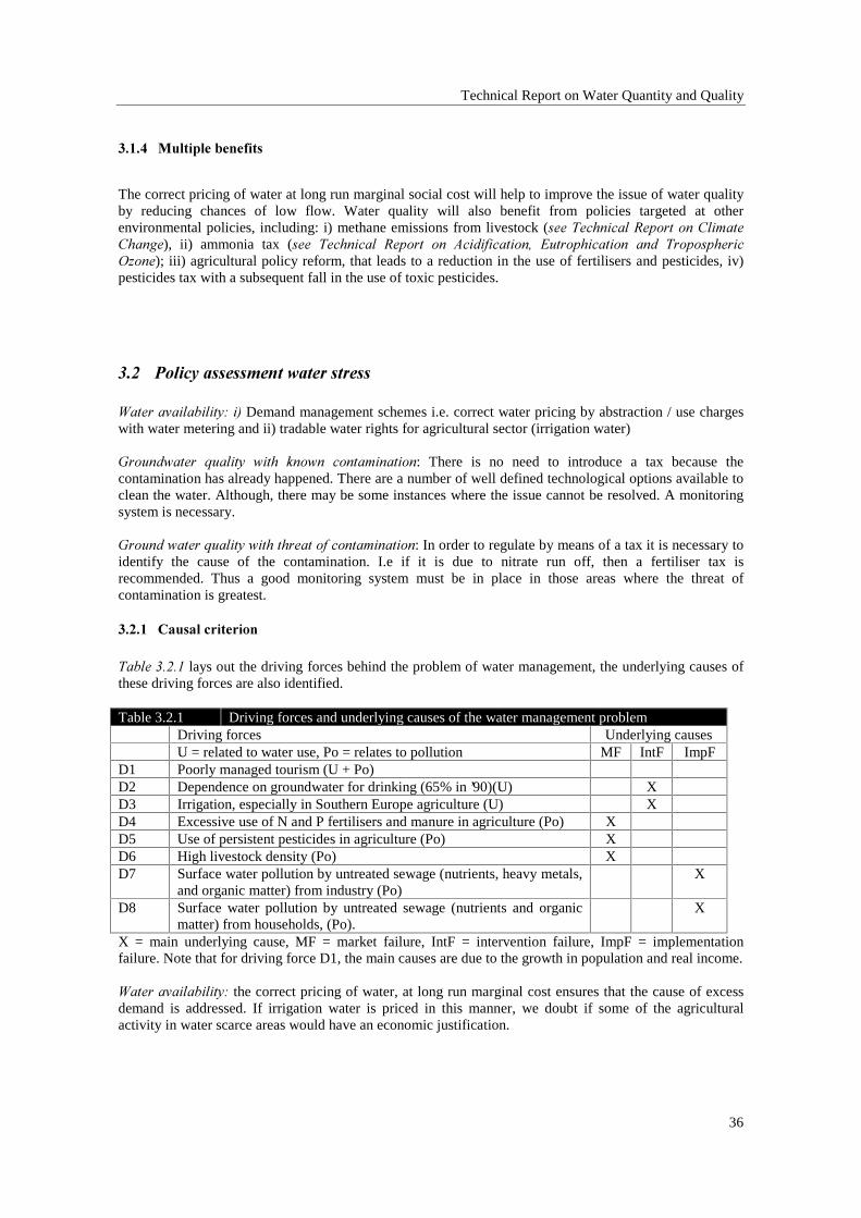
Technical Report on Water Quantity and Quality
36
������ 0XOWLSOH�EHQHILWV
The correct pricing of water at long run marginal social cost will help to improve the issue of water qualityby reducing chances of low flow. Water quality will also benefit from policies targeted at otherenvironmental policies, including: i) methane emissions from livestock (VHH�7HFKQLFDO�5HSRUW�RQ�&OLPDWH&KDQJH), ii) ammonia tax (VHH� 7HFKQLFDO� 5HSRUW� RQ� $FLGLILFDWLRQ�� (XWURSKLFDWLRQ� DQG� 7URSRVSKHULF2]RQH); iii) agricultural policy reform, that leads to a reduction in the use of fertilisers and pesticides, iv)pesticides tax with a subsequent fall in the use of toxic pesticides.
���� �3ROLF\�DVVHVVPHQW�ZDWHU�VWUHVV
:DWHU�DYDLODELOLW\��L��Demand management schemes i.e. correct water pricing by abstraction / use chargeswith water metering and ii) tradable water rights for agricultural sector (irrigation water)
*URXQGZDWHU� TXDOLW\� ZLWK� NQRZQ� FRQWDPLQDWLRQ: There is no need to introduce a tax because thecontamination has already happened. There are a number of well defined technological options available toclean the water. Although, there may be some instances where the issue cannot be resolved. A monitoringsystem is necessary.
*URXQG�ZDWHU�TXDOLW\�ZLWK�WKUHDW�RI�FRQWDPLQDWLRQ: In order to regulate by means of a tax it is necessary toidentify the cause of the contamination. I.e if it is due to nitrate run off, then a fertiliser tax isrecommended. Thus a good monitoring system must be in place in those areas where the threat ofcontamination is greatest.
������ &DXVDO�FULWHULRQ
7DEOH������ lays out the driving forces behind the problem of water management, the underlying causes ofthese driving forces are also identified.
Table 3.2.1 Driving forces and underlying causes of the water management problemDriving forces Underlying causesU = related to water use, Po = relates to pollution MF IntF ImpF
D1 Poorly managed tourism (U + Po)D2 Dependence on groundwater for drinking (65% in ’90)(U) XD3 Irrigation, especially in Southern Europe agriculture (U) XD4 Excessive use of N and P fertilisers and manure in agriculture (Po) XD5 Use of persistent pesticides in agriculture (Po) XD6 High livestock density (Po) XD7 Surface water pollution by untreated sewage (nutrients, heavy metals,
and organic matter) from industry (Po)X
D8 Surface water pollution by untreated sewage (nutrients and organicmatter) from households, (Po).
X
X = main underlying cause, MF = market failure, IntF = intervention failure, ImpF = implementationfailure. Note that for driving force D1, the main causes are due to the growth in population and real income.
:DWHU�DYDLODELOLW\��the correct pricing of water, at long run marginal cost ensures that the cause of excessdemand is addressed. If irrigation water is priced in this manner, we doubt if some of the agriculturalactivity in water scarce areas would have an economic justification.

Technical Report on Water Quantity and Quality
37
:DWHU�TXDOLW\��the fertiliser tax may not address the cause. This is because the tax will probably not changethe quantity of fertiliser used, due to the inelasticity of demand. Unlike pesticides, fertilisers are generallyuniform in their effect on the environment, so there is no basis for a fertiliser tax based on toxicity to reducethe contamination due to fertilisers. In this instance we argue for a hypothecated tax on fertilisers, wherethe revenues raised are used to clean up the water. We suggest giving payments to farmers to switch crops,i.e. to organic produce. Thus a fertiliser tax plus payments to organic crops policy option will address onecause of water contamination. The pesticide tax discussed in ’chemical risks’ is also relevant for waterquality. If the pesticide tax reduces use of highly toxic and persistent pesticides, then such a measure can besaid to address the underlying cause.
������ (IILFLHQF\�FULWHULRQ
%HQHILW�FRVW�UDWLR
Due to the absence of scenarios for the issue of water management, B/C ratios are given only for therecommended policy actions.
:DWHU�DYDLODELOLW\� B / C ratios for new supply schemes are as follows:
Ground water schemes:Re-use schemes:Transfer schemes:
1.5 - 3.00.6 - 1.30.5 - 1.0
Reservoir:Barrage:Desalination:National grid:
0.3 - 0.60.3 - 0.60.15 - 0.30.12 - 0.25
There is a WTP on the part of EU residents for increased water supply but comparison of this WTP with thecosts of new supplies suggests fairly strongly that new schemes are not generally justified in cost-benefit terms.The low B/C ratios suggest that the only option that makes economic sense are groundwater schemes. Thehigh B/C ratios indicate that groundwater schemes, re-use schemes and some transfer schemes are justifiedin cost benefit terms. New reservoirs, desalination and nation-wide water grid schemes would not bejustified7.
The above observations suggest that water stress problems are not best resolved by new supply schemes.Instead, the focus of policy should be on correct water pricing, demand management schemes and leakagereduction.
:DWHU�TXDOLW\� B / C ratios for groundwater contamination clear up range from 1.5:1 to 15:1 (UHIHUWR�6HFWLRQ����%HQHILW�DVVHVVPHQW)Benefits are an underestimate because clean-up of water will also have majoreffects on the improvement of bathing water.
&RVW�HIIHFWLYHQHVV
Correct pricing of water will alleviate water stress and it will also help to improve water quality byreducing chances of low flow (see above for the low B / C ratios of new supply schemes). Correct pricingof water with trading of water rights is a cost effective policy option that ensures water will be allocated to"highest" value use.
3XEOLF�RSLQLRQ
Eurobarometer (1995) shows that 69% of respondents believe that decisions of the environment should betaken at the Community level, rather than at national level. It also shows that most Europeans are preparedto change their consumption behaviour as a step to slow down or perhaps even stop the deterioration in theenvironment as a whole. Despite this, there is currently strong opposition to the compulsory introduction ofwater metering by households. 7 It is important to understand that the B/C ratios are based on very broad average costs and benefits. It doesnot mean that a new reservoir, for example, in some location is never justified
Technical Report on Water Quantity and Quality
38
������ $GPLQLVWUDWLYH�FRPSOH[LW\
:DWHU� DYDLODELOLW\: administrative complexity for abstraction / use charges is low as regulators alreadyexist. There is some conflict however, between the role regulators are playing in lowering prices due to theliberalisation of the market and the need to raise prices due to environmental concerns.
The most serious problem with a system of tradable water rights is that where there is a tradition of riparianlaw, it effectively means that the legal system needs to be changed considerably. However, where there is atradition of appropriative water rights, as in California, introducing tradable water rights is not a serious issue.
A consultation process in the UK showed that none of the interested parties (industry, regulators, academiaand general public) thought that a system of tradable rights was a viable instrument for water policy mainlyfor administrative reasons (results reported in ENDS report, June 1998).
:DWHU� TXDOLW\�� paying farmers to switch crops, i.e. changing an output subsidy to a payment for anenvironmental service seems to fit with recent changes in the CAP. Thus, administrative complexity isconsidered to be low as the institutions are already in place.
������ (TXLW\�FULWHULRQ
:DWHU�DYDLODELOLW\: experience with proper pricing of water suggests that the ’poor’ need not suffer as watercosts may decline as more efficient use is practised. If distributional problems arise, ’lifeline’ pricing can bepractised whereby a rising tariff for high consumers is used to subsidise low volume (users paying a belowmarginal cost tariff).
:DWHU�TXDOLW\: the distributional incidence of the fertiliser tax is not known, but the occupational group willbe affected (i.e. agricultural sector). In the long run the fertiliser tax will affect the price of food. As aproportion of individual’s income it is expected to be negligible.
������ -XULVGLFWLRQDO�FULWHULRQ
:DWHU�TXDOLW\�� if Member States have the freedom to manage their own distribution of subsidies then thepayments to farmers to switch crops may not need be a centralised issue afterall. However, competitioncould be affected which then suggests there is an argument for centralisation.
:DWHU�DYDLODELOLW\: correct water pricing will affect competition. Water is a major cost to some sectors, i.e.agriculture. Thus this policy option may be a centralised issue even though water scarcity is a localisedenvironmental problem.
0DFURHFRQRPLF�HIIHFW
Details provided in 7HFKQLFDO� 5HSRUW� RQ� 6RFLR�(FRQRPLF7UHQGV�� 0DFUR�(FRQRPLF� ,PSDFWV� DQG� &RVW,QWHUIDFH�
Technical Report on Water Quantity and Quality
39
���� 3ROLF\�SDFNDJH�FRDVWDO�]RQHV
������ .H\�LVVXHV
%HDFK�TXDOLW\ is generally covered by existing Directives, i.e. Urban Waste Water, Bathing Water, but theissue of implementation is outstanding.
)LVKHULHV suffer the classic problems of open access resources, this suggests the eventual introduction oftradable fishing quotas is required. This implies wholesale reform of the CFP, which currently providessubsidies to fishing.
'HYHORSPHQW�RI�FRDVWDO�DUHDV�� the introduction of a development tax� for marinas, sports complexes withrequirements to offset biodiversity and habitat damage or a system of transferable development rights. Seealso ELRGLYHUVLW\�ORVV.
������ 5HFRPPHQGHG�SROLF\�LQLWLDWLYHV
/DQG�XVH�SODQQLQJ
Land use planning which contains regulations on what type of activity or structures can and cannot takeplace has been thought of as the principle mechanism for coastal zone management. Such plans exist inmost EU countries, however, their implementation differ between different sites and in connection withother related policies.
The recent report on the EC’s Integrated Coastal Zone Management (ICZM) project remarks that land useplanning alone is not a sufficient vehicle for ICZM due mainly to (EC, 1999):
• their lack of scope: narrow focus on terrestrial parts of the coastal zone; narrow focus on structuresrather than activities; weak linkages between the land use planning and sectoral planning systems andlimited applicability of controls outside urban areas;
• their lack of flexibility: difficulty of adapting the plans to local needs; difficulty with renewing plansdue to resource constraints and appeal processes being time consuming and costly
In order to guarantee adequate coastal zone management other mechanisms are required, recommendedactions are listed below. Measures targeted at biodiversity loss are also relevant for coastal zonemanagement.
7UDQVIHUDEOH�GHYHORSPHQW�ULJKWV
The use of transferable development rights provides a market mechanism for simultaneously protectinglandscapes and natural endowments and encouraging development in appropriate locations.
The key to achieving development in an efficient and equitable fashion seems to lie in separating themarket for the right to develop from the right to use land. Transferable development rights (TDRs) operatein the following way: in a certain jurisdiction (i.e. country, region), 'sending' areas where developmentshould be limited or prohibited are identified according to some criteria (e.g. landscape uniqueness, speciesprotection, conservation of ecosystem processes, role in flood control, conservation of farmland). Also,'receiving areas' are identified, these are areas where development is to be facilitated and encouraged.Development rights are identified as follows: the land owners in the sending areas are given developmentunits, designated per unit area, e.g. one residential unit of a certain size per 10 acres, but these can only beexercised in the receiving zone. If developers in the receiving zone wish to exceed the standarddevelopment densities (or other norms to be defined) , then they must purchase the right to do so in the
Technical Report on Water Quantity and Quality
40
development rights market. The legal instrument developed to transfer development rights in the US is aneasement document and a deed of transfer which are recorded and approved by the Planning Board.
TDRs are in existence on in the US. Montgomery County, Maryland and the Pinelands, New Jersey havesuccessfully implemented a TDR programme. Pizor (1986) summarises their experience and suggests thatthe success of TDRs depends on (a) an institution, e.g. planning department, with responsibility forexplaining and promoting the concept, providing price data and facilitating trades; and (b) the receivingareas must be well sited for immediate development. Necessary infrastructure should be in place and thereceiving sites should be in market areas which, from a market perspective, are most suitable and attractivefor development; and (c) guarantee of delivery, i.e. if the developer pays for rights then s/he can exercisethem; and (d) prohibitions on development in the sending areas must be comprehensive and mandatory, andthe TDR must be mandatory on lands suited for preservation; and (e) provide a bank as a buyer of lastresort for TDRs of sending landowners in the event of recession; and (f) reduce regulatory complexity, i.e.if developers have confidence that they can use the rights profitably, this will increase the probability thatthey will be used; and lastly (f) in so far as it is possible, design TDRs to fit the needs of the developmentchain, rather than the needs of planners.
�2ZQHU�OLDELOLW\�DQG�SHUIRUPDQFH�ERQGV�DJDLQVW�RLO�VSLOOV
Although issue of oil spills is not thoroughly investigated in this study an initial discussion is presented in7HFKQLFDO�UHSRUW��RQ�1XFFOHDU�$FFLGHQWV. For this reason, we present potential measures that could reducethe risk of oil spills.
Where tanker and installation owners are clearly identifiable, and cause and effect can be established, there isscope for the use of OLDELOLW\ mechanisms, and SHUIRUPDQFH�ERQGV. These are discussed more fully in Annex 3:major accidents. Other measure to encourage oil spill prevention include:
2LO� SROOXWLRQ� FRPEDWLQJ� FKDUJH: Finland levies an oil pollution combating charge on imported oil. Thecharge is levied on imported petroleum in the amount of FIM 2.20 (¼� ������ SHU� WRQQH� RI� RLO� DQG� LVdifferentiated on the basis of the environmental safety of the cargo boats. For instance, the charge rate isdouble for oil transported in cargo boats without double hulls. A cargo boat of 100,000 tonnes is liable to acharge of about FIM 160,000 (¼���������SHU� MRXUQH\�� IRU�YHVVHOV�RI� WKH� VDPH� VL]H� DQG� GRXEOH� KXOOV�� WKHcharge will be about FIM 80,000 (¼���������7KH�FKDUJH�LV�HDUPDUNHG�IRU�HQYLURQPHQWDO�PHDVXUHV��VXFK�DVcleaning oil spills (North Council of Ministers, 1994).
The oil pollution tax rebate (from one cargo trip) is sufficient to cover the extra interest expense incurred inproducing a vessel with double hulls (which is about 15% more expensive than producing a vessel with asingle hull). The revenue of this charge, which amounted to FIM 36 million (¼�����PLOOLRQ��LQ�������DFFUXHVto the oil-protection fund and is earmarked to buy equipment for cleaning oil spills.
Similarly, in Sweden, Gothenburg harbour levies harbour charges differentiated according to type of ballasttanks. Since 1993, cargo boats above a certain tonnage with segregated ballast tanks and/or double hullsarriving at the harbour have been granted rebates in the harbour charge, this is calculated on the basis ofgross tonnage excluding segregated ballast tanks.
The rebates in Sweden, which range from 15 to 20%, provide incentives to construct vessels withsegregated ballast tanks. Currently, the dominant proportion of petroleum waste in the North Sea isreported to stem from illegal discharges from vessels without segregated ballast tanks rinsing out their oiltanks (North Council of Ministers, 1994).
Since 1979, all operators on the UK continental shelf are required to have oil spill contingency plansapproved by the Department of Transport and of Trade and Industry. Within 25 miles of the coast and inenvironmentally sensitive areas, operators must be prepared for rapid response to a spill and to minimiseimpact on shore. All operators are members of the Offshore Pollution Liability Association, which makesfunds up to US$ 100 million (¼� ����� PLOOLRQ�� SHU� LQFLGHQW� DYDLODEOH� WR� SD\� WKH� RSHUDWRUV� OLDELOLW\� IRUdamage and remedial action. The UK supported increases in the liability and compensation ceilings in the

Technical Report on Water Quantity and Quality
41
framework of the 1984 and 1992 protocols following the Amoco Cadiz and Exxon Valdez disasters(OECD, 1994).
������ 0XOWLSOH�%HQHILWV
Policies targeted at coastal zones specifically, such as land use planning, tradable development rights andowner liability / performance bonds against oil spills, will also benefit biodiversity loss. Whilst, coastalzones will be affected by varying degrees from policies targeted at other environmental issues. We list aselection of policy options recommend for other environmental issues, expected to provide multiplebenefits to coastal zones:
i) N fertiliser tax (see ZDWHU�PDQDJHPHQW);ii) effluent charges (see ZDWHU�PDQDJHPHQW);iii) agricultural policy reform (see ELRGLYHUVLW\�ORVV);iv) mitigation banking (see ELRGLYHUVLW\�ORVV);v) owner liability and performance bond schemes against oil spills (see PDMRU�DFFLGHQWV);vi) methane tax on livestock (see FOLPDWH�FKDQJH);vii) ammonia tax on livestock (see DFLGLILFDWLRQ).
Eutrophication in regional waters, such as the Baltic Sea can be reduced by policy initiatives that ensurenutrient reduction. The preliminary cost benefit analysis of a 50% nutrient load reduction in the Baltic Seashows benefits exceed costs, with a ratio of 2.2. This suggests that the seemingly ambitious programme isjustified in cost benefit terms.
These policies will benefit coastal zone areas due to expected reduction of nutrient loads to waters and theprotection of coastal lands. Unfortunately, there is insufficient data to estimate what this spill over effectwould be.
���� 3ROLF\�DVVHVVPHQW�FRDVWDO�]RQHV
Land use planning is already widely used by most Member States. However, in order to guarantee adequatecoastal zone management other mechanisms are required, such as transferable development rights, (TDR);This scheme provides a market mechanism for simultaneously protecting landscapes and naturalendowments and encouraging development in appropriate locations.
Policy initiatives targeted at other environmental concerns will also contribute to coastal zone management,these include:
- agri-environmental schemes (see biodiversity loss);- fertiliser tax with payments to switch to organic crops (see water management);- increased ’owner liability’ to include not just loss of livelihood and property but also disamenity and,
ultimately, non-use values (see major accidents).
Technical Report on Water Quantity and Quality
42
������ &DXVDO�FULWHULRQ
7DEOH������ presents the driving forces behind the coastal zone management problem, the underlying causesare also identified.
Table 3.41 Driving forces and underlying causes of coastal zone management problemsUnderlying causes
MF IntF ImpFD1 Recreation / tourism, hunting XD2 Urbanisation and trafficD3 Industrial, fishery and aqua-culture growthD4 Shipping and offshore activities XD5 Agricultural intensification, fertiliser and pesticide use XX = main underlying cause, MF = market failure, IntF = intervention failure, ImpF = implementationfailure. Note that for D1, D2 main causes also include population growth and growth in real income, whilstfor D3, growth in real income is the main cause.
The policies recommended for coastal zone management, biodiversity loss and water management, aremeasures which can be designed especially to target the most important sources of pressure to coastalresources: urbanisation, transport, industry, agriculture, fisheries, tourism. Oil spills are dealt with directlyin ’major accidents’ through the ’owner liability’ legislation, whereby the scope of ’damage’ is increased toinclude property and direct economic losses to disamenity and ecological damage and even to non-use values.Clearly, the analysis presented above mainly focus on water quality aspects related to eutrophication andbathing, and does not adequately cover fishing issues. Further work would be required on these issues.?
������ (IILFLHQF\�FULWHULRQ
Scenarios are not established for coastal zone management in this study. However, B/C ratios nutrientcontrol initiatives near Baltic Sea are provided.
%�&�DQDO\VLV�IRU�WKH�(&�'LUHFWLYH�RQ�4XDOLW\�RI�%DWKLQJ�:DWHUV
Although limited costs and benefits information exist, to estimate the B/C ratio for full compliance of theEC Directive bathing water quality would be too arbitrary and uncertain. Thus, such analysis has not beenundertaken in this report.
%�&�UDWLR�IRU�SROLF\�LQLWLDWLYHV�WR�UHGXFH�QXWULHQW�ORDGLQJ�WR�%DOWLF�6HD
Eutrophication in regional waters, such as the Baltic Sea can be reduced by policy initiatives that ensurenutrient reduction. The preliminary cost benefit analysis of a 50% nutrient load reduction in the Baltic Seashows benefits exceed costs, with a ratio of 2.2. This suggests that the seemingly ambitious programme isjustified in cost benefit terms.
&RVW�HIIHFWLYHQHVV�
7UDQVIHUDEOH� GHYHORSPHQW� ULJKWV; TDRs ensure development takes place in an efficient manner byseparating the market for the right to develop from the right to use land. In return, for developmentrestrictions on private holdings, landowners are awarded with alternative rights in designated growth areas,located outside the environmentally sensitive areas. These rights can be used for development or if a marketexists, they can be sold for profit to other developers who want to develop in this zone.

Technical Report on Water Quantity and Quality
43
)LVKLQJ�TXRWDV��one of the main objectives of quota-based fisheries management is to improve economicefficiency by reducing over capitalisation. The quota is set according to total allowable catch. Participantsthen use the most optimal configuration of inputs (i.e. capital, labour, time) to achieve their individualquota. Fishers will chose to fish when the price is high opportunity cost of time low and the climaticconditions safe, such behaviour contributes to higher socio-economic gain from the resource in the longrun, OECD (1996). Trading quotas means the more efficient operators buy out the less efficient operators,thus the fleet will be composed only of the most efficient operator. This reduces the unit costs of operation,whilst also compensating the marginal producers.
Countries that implement individual transferable quotas for fisheries management combine them with inputrestrictions to prevent certain types of environmentally damaging gear to be used. The introduction ofquotas may lead to increased technological efficiency that could threaten marine ecosystems, but on theother hand, greater gear efficiency may result in more investments to reduce by-catch.
3XEOLF�RSLQLRQ
Although public opinion regarding the issue of coastal zone management is not known with certainty, theresults of the Eurobaromter (1995) suggest that the European population may be in favour of the suggestedmeasures as a means to managing coastal regions in a sustainable manner.
������ $GPLQLVWUDWLYH�FRPSOH[LW\
7UDQVIHUDEOH�GHYHORSPHQW�ULJKWV. Institutions are most likely to be in place, for example, those responsiblefor land use planning could oversee this scheme. It would be responsible for explaining and promoting theconcept, providing price data and facilitating trades. Areas for development should have the necessaryinfrastructure in place and should be most suitable and attractive for immediate development. It may benecessary to set up an appropriate legal structure to zone land and enforce restrictions.
)LVKLQJ�TXRWDV� Any tradable quota system needs to be flexible to allow review and modification accordingto biological and economic (equity) requirements. Institutions must oversee the initial distribution of quotasthrough grand-fathering and auctioning. Quota management can be subject to cheating and / or underreporting when local conditions make it difficult to monitor catches. The current EU Common FisheriesPolicy suffers from poor monitoring at the national level.
������ (TXLW\�FULWHULRQ
7UDQVIHUDEOH�GHYHORSPHQW�ULJKWV��These schemes have the potential to operate in an equitable manner if amature market exists for the land with development rights, such that, compensated land owners have theoption to sell their rights at a profit.
)LVKLQJ�TXRWDV� Trading quotas automatically compensates the marginal producers removed from the fleet.In reducing the fleet to the most efficient operators a quota scheme may have beneficial effects onpopulation management. But experience has shown that quota systems can exclude small-scale andindependent fishers from fisheries, which fall increasingly under the control of large corporations.
Schemes for conflict resolution between fishermen and wildlife could be based on capturing some of theWTP for wildlife. For example, case studies estimating WTP for Cornish grey seals and Mediterraneanmonk seals exist, if their WTP is captured it could be used to compensate fishermen in order to avoid ’hotspots’ of conflict, i.e. a kind of marine set-aside.
������ -XULVGLFWLRQDO�FULWHULRQ
Coastal zone management is predominantly a local issue. Centralisation of policies would only benecessary if some Member States were reluctant to act on their own.

Technical Report on Water Quantity and Quality
44
0DFURHFRQRPLF�HIIHFW
Details of macroeconomic effects are presented in 7HFKQLFDO�5HSRUW�RQ�6RFLR�(FRQRPLF�7UHQGV��0DFUR(FRQRPLF�,PSDFWV�DQG�&RVW�,QWHUIDFH�
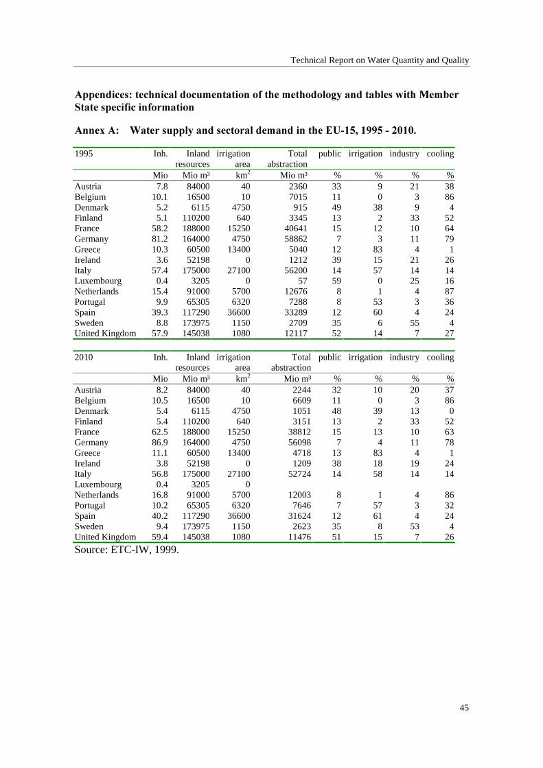
Technical Report on Water Quantity and Quality
45
$SSHQGLFHV��WHFKQLFDO�GRFXPHQWDWLRQ�RI�WKH�PHWKRGRORJ\�DQG�WDEOHV�ZLWK�0HPEHU6WDWH�VSHFLILF�LQIRUPDWLRQ
$QQH[�$� �:DWHU�VXSSO\�DQG�VHFWRUDO�GHPDQG�LQ�WKH�(8�����������������
1995 Inh. Inlandresources
irrigationarea
Totalabstraction
public irrigation industry cooling
Mio Mio m³ km2 Mio m³ % % % %Austria 7.8 84000 40 2360 33 9 21 38Belgium 10.1 16500 10 7015 11 0 3 86Denmark 5.2 6115 4750 915 49 38 9 4Finland 5.1 110200 640 3345 13 2 33 52France 58.2 188000 15250 40641 15 12 10 64Germany 81.2 164000 4750 58862 7 3 11 79Greece 10.3 60500 13400 5040 12 83 4 1Ireland 3.6 52198 0 1212 39 15 21 26Italy 57.4 175000 27100 56200 14 57 14 14Luxembourg 0.4 3205 0 57 59 0 25 16Netherlands 15.4 91000 5700 12676 8 1 4 87Portugal 9.9 65305 6320 7288 8 53 3 36Spain 39.3 117290 36600 33289 12 60 4 24Sweden 8.8 173975 1150 2709 35 6 55 4United Kingdom 57.9 145038 1080 12117 52 14 7 27
2010 Inh. Inlandresources
irrigationarea
Totalabstraction
public irrigation industry cooling
Mio Mio m³ km2 Mio m³ % % % %Austria 8.2 84000 40 2244 32 10 20 37Belgium 10.5 16500 10 6609 11 0 3 86Denmark 5.4 6115 4750 1051 48 39 13 0Finland 5.4 110200 640 3151 13 2 33 52France 62.5 188000 15250 38812 15 13 10 63Germany 86.9 164000 4750 56098 7 4 11 78Greece 11.1 60500 13400 4718 13 83 4 1Ireland 3.8 52198 0 1209 38 18 19 24Italy 56.8 175000 27100 52724 14 58 14 14Luxembourg 0.4 3205 0Netherlands 16.8 91000 5700 12003 8 1 4 86Portugal 10.2 65305 6320 7646 7 57 3 32Spain 40.2 117290 36600 31624 12 61 4 24Sweden 9.4 173975 1150 2623 35 8 53 4United Kingdom 59.4 145038 1080 11476 51 15 7 26
Source: ETC-IW, 1999.
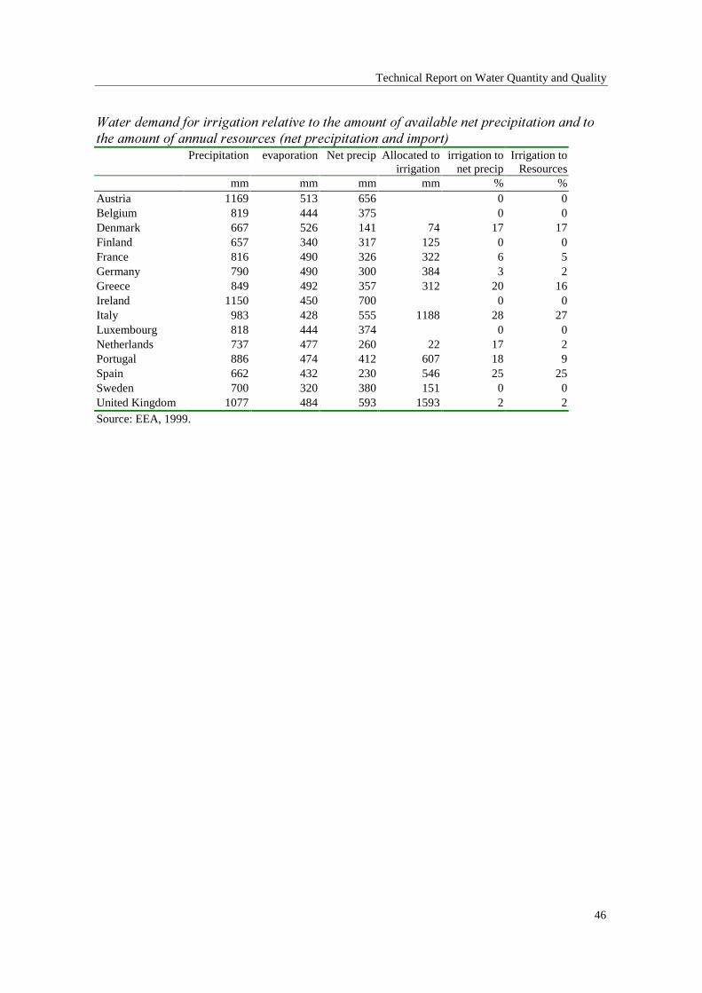
Technical Report on Water Quantity and Quality
46
:DWHU�GHPDQG�IRU�LUULJDWLRQ�UHODWLYH�WR�WKH�DPRXQW�RI�DYDLODEOH�QHW�SUHFLSLWDWLRQ�DQG�WRWKH�DPRXQW�RI�DQQXDO�UHVRXUFHV��QHW�SUHFLSLWDWLRQ�DQG�LPSRUW�
Precipitation evaporation Net precip Allocated toirrigation
irrigation tonet precip
Irrigation toResources
mm mm mm mm % %Austria 1169 513 656 0 0Belgium 819 444 375 0 0Denmark 667 526 141 74 17 17Finland 657 340 317 125 0 0France 816 490 326 322 6 5Germany 790 490 300 384 3 2Greece 849 492 357 312 20 16Ireland 1150 450 700 0 0Italy 983 428 555 1188 28 27Luxembourg 818 444 374 0 0Netherlands 737 477 260 22 17 2Portugal 886 474 412 607 18 9Spain 662 432 230 546 25 25Sweden 700 320 380 151 0 0United Kingdom 1077 484 593 1593 2 2Source: EEA, 1999.
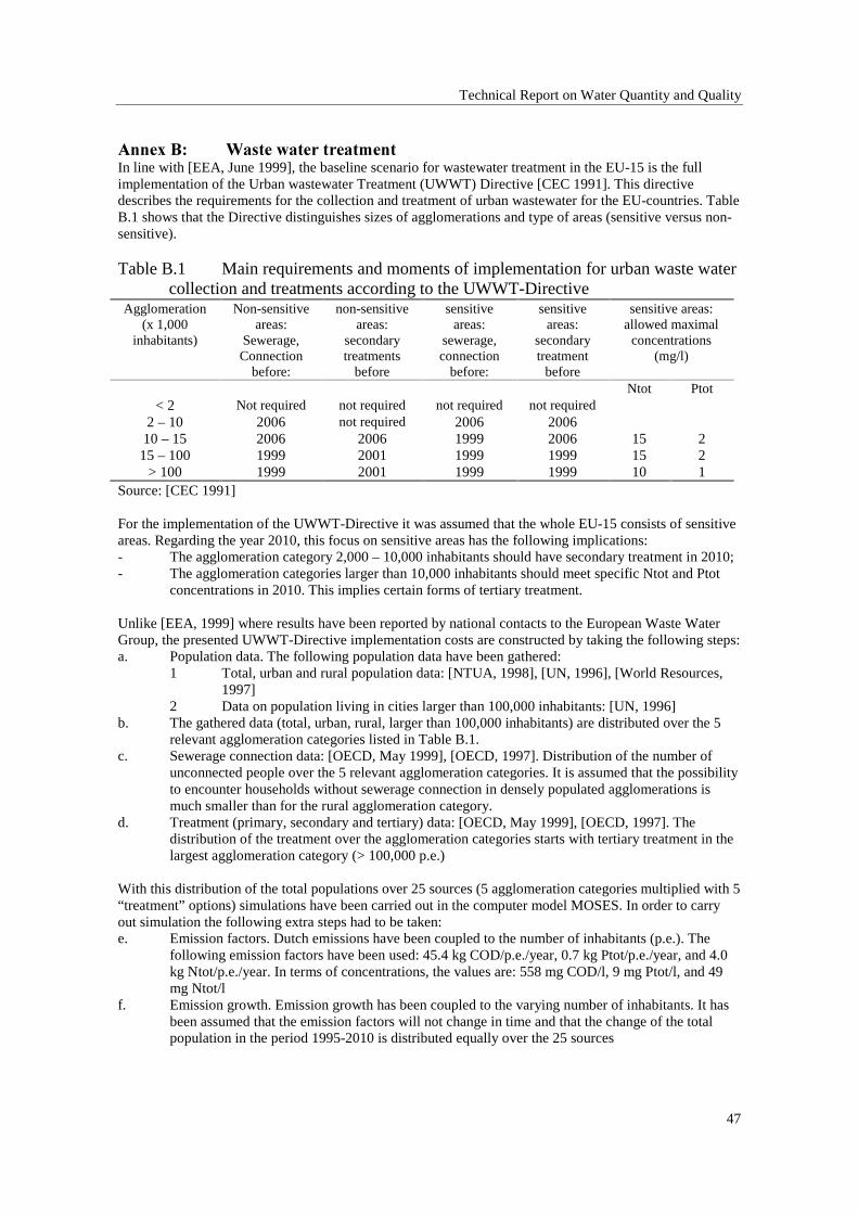
Technical Report on Water Quantity and Quality
47
$QQH[�%� �:DVWH�ZDWHU�WUHDWPHQWIn line with [EEA, June 1999], the baseline scenario for wastewater treatment in the EU-15 is the fullimplementation of the Urban wastewater Treatment (UWWT) Directive [CEC 1991]. This directivedescribes the requirements for the collection and treatment of urban wastewater for the EU-countries. TableB.1 shows that the Directive distinguishes sizes of agglomerations and type of areas (sensitive versus non-sensitive).
Table B.1 Main requirements and moments of implementation for urban waste watercollection and treatments according to the UWWT-Directive
Agglomeration(x 1,000
inhabitants)
Non-sensitiveareas:
Sewerage,Connection
before:
non-sensitiveareas:
secondarytreatments
before
sensitiveareas:
sewerage,connection
before:
sensitiveareas:
secondarytreatment
before
sensitive areas:allowed maximal
concentrations(mg/l)
Ntot Ptot< 2 Not required not required not required not required
2 – 10 2006 not required 2006 200610 – 15 2006 2006 1999 2006 15 215 – 100 1999 2001 1999 1999 15 2
> 100 1999 2001 1999 1999 10 1Source: [CEC 1991]
For the implementation of the UWWT-Directive it was assumed that the whole EU-15 consists of sensitiveareas. Regarding the year 2010, this focus on sensitive areas has the following implications:- The agglomeration category 2,000 – 10,000 inhabitants should have secondary treatment in 2010;- The agglomeration categories larger than 10,000 inhabitants should meet specific Ntot and Ptot
concentrations in 2010. This implies certain forms of tertiary treatment.
Unlike [EEA, 1999] where results have been reported by national contacts to the European Waste WaterGroup, the presented UWWT-Directive implementation costs are constructed by taking the following steps:a. Population data. The following population data have been gathered:
1 Total, urban and rural population data: [NTUA, 1998], [UN, 1996], [World Resources,1997]
2 Data on population living in cities larger than 100,000 inhabitants: [UN, 1996]b. The gathered data (total, urban, rural, larger than 100,000 inhabitants) are distributed over the 5
relevant agglomeration categories listed in Table B.1.c. Sewerage connection data: [OECD, May 1999], [OECD, 1997]. Distribution of the number of
unconnected people over the 5 relevant agglomeration categories. It is assumed that the possibilityto encounter households without sewerage connection in densely populated agglomerations ismuch smaller than for the rural agglomeration category.
d. Treatment (primary, secondary and tertiary) data: [OECD, May 1999], [OECD, 1997]. Thedistribution of the treatment over the agglomeration categories starts with tertiary treatment in thelargest agglomeration category (> 100,000 p.e.)
With this distribution of the total populations over 25 sources (5 agglomeration categories multiplied with 5“treatment” options) simulations have been carried out in the computer model MOSES. In order to carryout simulation the following extra steps had to be taken:e. Emission factors. Dutch emissions have been coupled to the number of inhabitants (p.e.). The
following emission factors have been used: 45.4 kg COD/p.e./year, 0.7 kg Ptot/p.e./year, and 4.0kg Ntot/p.e./year. In terms of concentrations, the values are: 558 mg COD/l, 9 mg Ptot/l, and 49mg Ntot/l
f. Emission growth. Emission growth has been coupled to the varying number of inhabitants. It hasbeen assumed that the emission factors will not change in time and that the change of the totalpopulation in the period 1995-2010 is distributed equally over the 25 sources
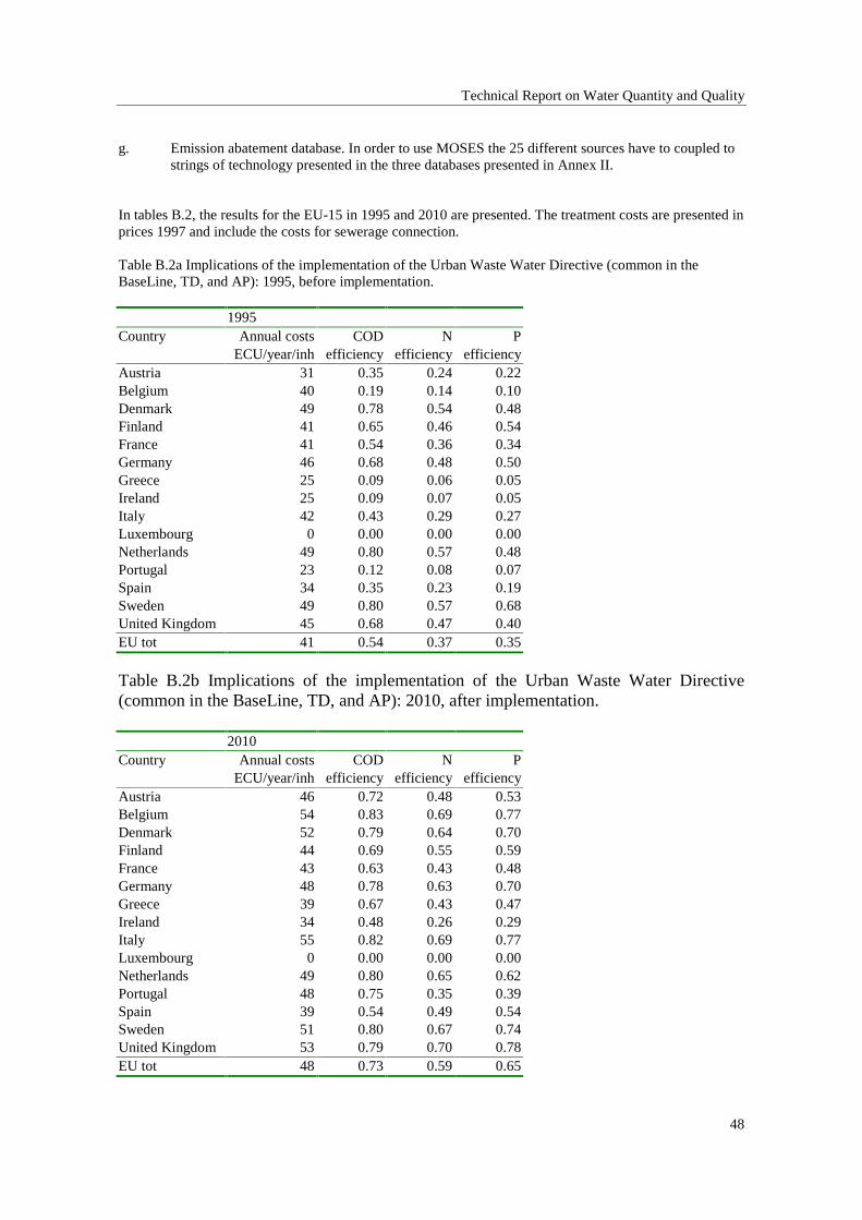
Technical Report on Water Quantity and Quality
48
g. Emission abatement database. In order to use MOSES the 25 different sources have to coupled tostrings of technology presented in the three databases presented in Annex II.
In tables B.2, the results for the EU-15 in 1995 and 2010 are presented. The treatment costs are presented inprices 1997 and include the costs for sewerage connection.
Table B.2a Implications of the implementation of the Urban Waste Water Directive (common in theBaseLine, TD, and AP): 1995, before implementation.
1995Country Annual costs COD N P
ECU/year/inh efficiency efficiency efficiencyAustria 31 0.35 0.24 0.22Belgium 40 0.19 0.14 0.10Denmark 49 0.78 0.54 0.48Finland 41 0.65 0.46 0.54France 41 0.54 0.36 0.34Germany 46 0.68 0.48 0.50Greece 25 0.09 0.06 0.05Ireland 25 0.09 0.07 0.05Italy 42 0.43 0.29 0.27Luxembourg 0 0.00 0.00 0.00Netherlands 49 0.80 0.57 0.48Portugal 23 0.12 0.08 0.07Spain 34 0.35 0.23 0.19Sweden 49 0.80 0.57 0.68United Kingdom 45 0.68 0.47 0.40EU tot 41 0.54 0.37 0.35
Table B.2b Implications of the implementation of the Urban Waste Water Directive(common in the BaseLine, TD, and AP): 2010, after implementation.
2010Country Annual costs COD N P
ECU/year/inh efficiency efficiency efficiencyAustria 46 0.72 0.48 0.53Belgium 54 0.83 0.69 0.77Denmark 52 0.79 0.64 0.70Finland 44 0.69 0.55 0.59France 43 0.63 0.43 0.48Germany 48 0.78 0.63 0.70Greece 39 0.67 0.43 0.47Ireland 34 0.48 0.26 0.29Italy 55 0.82 0.69 0.77Luxembourg 0 0.00 0.00 0.00Netherlands 49 0.80 0.65 0.62Portugal 48 0.75 0.35 0.39Spain 39 0.54 0.49 0.54Sweden 51 0.80 0.67 0.74United Kingdom 53 0.79 0.70 0.78EU tot 48 0.73 0.59 0.65
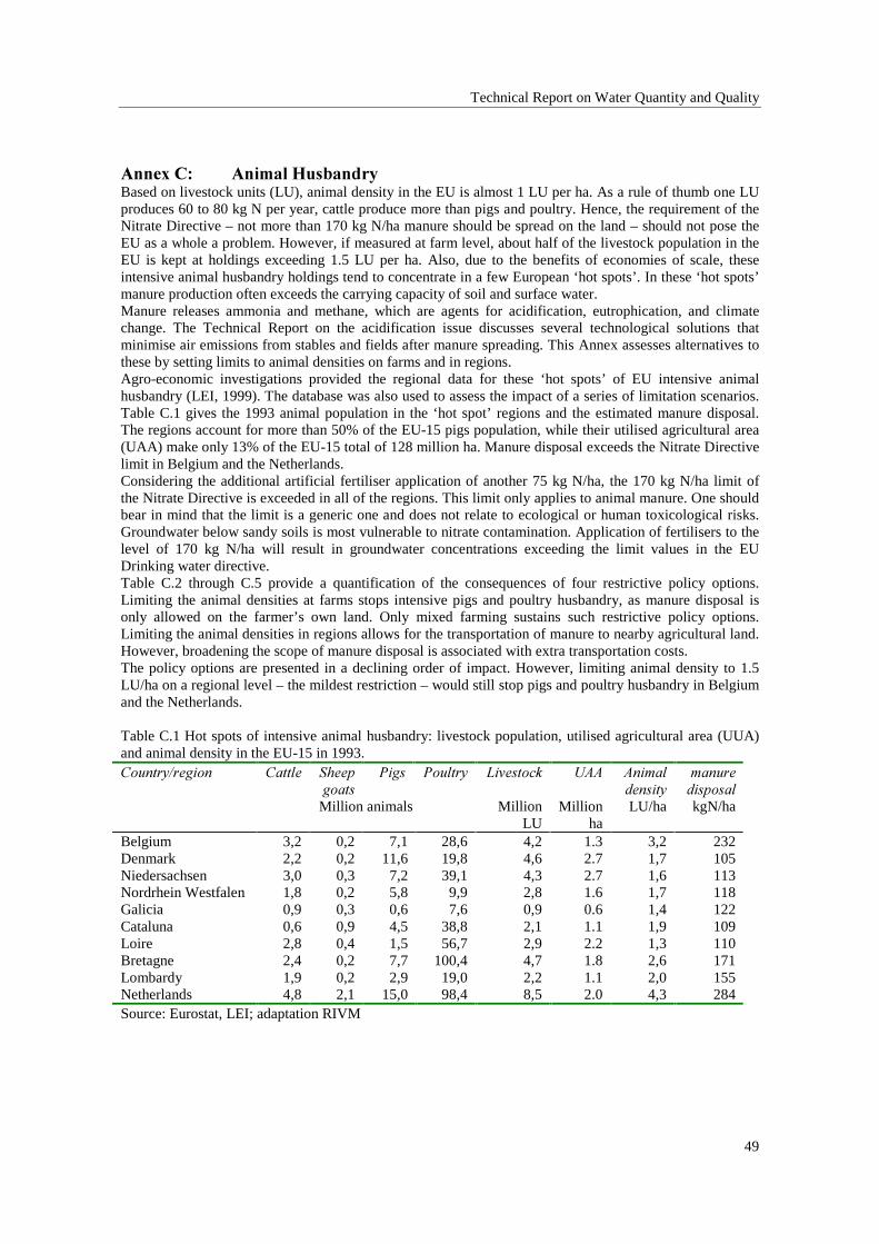
Technical Report on Water Quantity and Quality
49
$QQH[�&� �$QLPDO�+XVEDQGU\Based on livestock units (LU), animal density in the EU is almost 1 LU per ha. As a rule of thumb one LUproduces 60 to 80 kg N per year, cattle produce more than pigs and poultry. Hence, the requirement of theNitrate Directive – not more than 170 kg N/ha manure should be spread on the land – should not pose theEU as a whole a problem. However, if measured at farm level, about half of the livestock population in theEU is kept at holdings exceeding 1.5 LU per ha. Also, due to the benefits of economies of scale, theseintensive animal husbandry holdings tend to concentrate in a few European ‘hot spots’. In these ‘hot spots’manure production often exceeds the carrying capacity of soil and surface water.Manure releases ammonia and methane, which are agents for acidification, eutrophication, and climatechange. The Technical Report on the acidification issue discusses several technological solutions thatminimise air emissions from stables and fields after manure spreading. This Annex assesses alternatives tothese by setting limits to animal densities on farms and in regions.Agro-economic investigations provided the regional data for these ‘hot spots’ of EU intensive animalhusbandry (LEI, 1999). The database was also used to assess the impact of a series of limitation scenarios.Table C.1 gives the 1993 animal population in the ‘hot spot’ regions and the estimated manure disposal.The regions account for more than 50% of the EU-15 pigs population, while their utilised agricultural area(UAA) make only 13% of the EU-15 total of 128 million ha. Manure disposal exceeds the Nitrate Directivelimit in Belgium and the Netherlands.Considering the additional artificial fertiliser application of another 75 kg N/ha, the 170 kg N/ha limit ofthe Nitrate Directive is exceeded in all of the regions. This limit only applies to animal manure. One shouldbear in mind that the limit is a generic one and does not relate to ecological or human toxicological risks.Groundwater below sandy soils is most vulnerable to nitrate contamination. Application of fertilisers to thelevel of 170 kg N/ha will result in groundwater concentrations exceeding the limit values in the EUDrinking water directive.Table C.2 through C.5 provide a quantification of the consequences of four restrictive policy options.Limiting the animal densities at farms stops intensive pigs and poultry husbandry, as manure disposal isonly allowed on the farmer’s own land. Only mixed farming sustains such restrictive policy options.Limiting the animal densities in regions allows for the transportation of manure to nearby agricultural land.However, broadening the scope of manure disposal is associated with extra transportation costs.The policy options are presented in a declining order of impact. However, limiting animal density to 1.5LU/ha on a regional level – the mildest restriction – would still stop pigs and poultry husbandry in Belgiumand the Netherlands.
Table C.1 Hot spots of intensive animal husbandry: livestock population, utilised agricultural area (UUA)and animal density in the EU-15 in 1993.&RXQWU\�UHJLRQ &DWWOH 6KHHS
JRDWV3LJV 3RXOWU\ /LYHVWRFN 8$$ $QLPDO
GHQVLW\PDQXUHGLVSRVDO
Million animals MillionLU
Millionha
LU/ha kgN/ha
Belgium 3,2 0,2 7,1 28,6 4,2 1.3 3,2 232Denmark 2,2 0,2 11,6 19,8 4,6 2.7 1,7 105Niedersachsen 3,0 0,3 7,2 39,1 4,3 2.7 1,6 113Nordrhein Westfalen 1,8 0,2 5,8 9,9 2,8 1.6 1,7 118Galicia 0,9 0,3 0,6 7,6 0,9 0.6 1,4 122Cataluna 0,6 0,9 4,5 38,8 2,1 1.1 1,9 109Loire 2,8 0,4 1,5 56,7 2,9 2.2 1,3 110Bretagne 2,4 0,2 7,7 100,4 4,7 1.8 2,6 171Lombardy 1,9 0,2 2,9 19,0 2,2 1.1 2,0 155Netherlands 4,8 2,1 15,0 98,4 8,5 2.0 4,3 284Source: Eurostat, LEI; adaptation RIVM
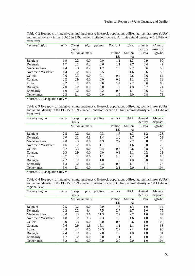
Technical Report on Water Quantity and Quality
50
Table C.2 Hot spots of intensive animal husbandry: livestock population, utilised agricultural area (UUA)and animal density in the EU-15 in 1993, under limitation scenario A: limit animal density to 1 LU/ha onfarm level&RXQWU\�UHJLRQ FDWWOH 6KHHS
JRDWVSLJV SRXOWU\ OLYHVWRFN 8$$ $QLPDO
GHQVLW\0DQXUHGLVSRVDO
Million animals MillionLU
Millionha
LU/ha kgN/ha
Belgium 1.9 0.2 0.0 0.0 1.1 1.3 0.9 90Denmark 1.7 0.2 0.3 0.6 1.1 2.7 0.4 42Niedersachsen 2.4 0.3 0.2 1.2 1.6 2.7 0.6 59Nordrhein Westfalen 1.4 0.2 0.3 0.5 1.0 1.6 0.6 58Galicia 0.6 0.3 0.0 0.1 0.4 0.6 0.6 64Cataluna 0.2 0.9 0.0 0.0 0.2 1.1 0.2 18Loire 2.2 0.4 0.0 0.6 1.4 2.2 0.6 66Bretagne 2.0 0.2 0.0 0.0 1.2 1.8 0.7 71Lombardy 1.0 0.2 0.0 0.2 0.6 1.1 0.6 59Netherlands 2.3 2.1 0.0 0.0 1.5 2.0 0.8 78Source: LEI; adaptation RIVM
Table C.3 Hot spots of intensive animal husbandry: livestock population, utilised agricultural area (UUA)and animal density in the EU-15 in 1993, under limitation scenario B: limit animal density to 1.5 LU/ha onfarm levelCountry/region cattle Sheep
goatspigs poultry livestock UAA Animal
densityManuredisposal
Million animals MillionLU
Millionha
LU/ha kgN/ha
Belgium 2.5 0.2 0.1 0.3 1.6 1.3 1.2 123Denmark 2.0 0.2 0.8 1.4 1.6 2.7 0.6 53Niedersachsen 2.8 0.3 0.8 4.3 2.2 2.7 0.8 75Nordrhein Westfalen 1.6 0.2 0.6 1.1 1.3 1.6 0.8 73Galicia 0.7 0.3 0.0 0.4 0.5 0.6 0.8 78Cataluna 0.3 0.9 0.0 0.0 0.3 1.1 0.2 22Loire 2.7 0.4 0.0 1.1 1.8 2.2 0.8 80Bretagne 2.2 0.2 0.1 1.0 1.5 1.8 0.8 82Lombardy 1.3 0.2 0.1 0.4 0.8 1.1 0.7 76Netherlands 3.0 2.1 0.0 0.0 2.1 2.0 1.1 104Source: LEI; adaptation RIVM
Table C.4 Hot spots of intensive animal husbandry: livestock population, utilised agricultural area (UUA)and animal density in the EU-15 in 1993, under limitation scenario C: limit animal density to 1.0 LU/ha onregional levelCountry/region cattle Sheep
goatspigs poultry livestock UAA Animal
densityManuredisposal
Million animals MillionLU
Millionha
LU/ha kgN/ha
Belgium 2.5 0.2 0.0 0.0 1.3 1.3 1.0 114Denmark 2.2 0.2 4.4 7.5 2.7 2.7 1.0 75Niedersachsen 3.0 0.3 2.1 11.3 2.7 2.7 1.0 87Nordrhein Westfalen 1.8 0.2 1.3 2.3 1.6 1.6 1.0 86Galicia 0.9 0.3 0.0 0.0 0.6 0.6 1.0 100Cataluna 0.6 0.9 1.8 15.1 1.1 1.1 1.0 68Loire 2.8 0.4 0.5 19.3 2.2 2.2 1.0 93Bretagne 2.4 0.2 0.5 7.0 1.8 1.8 1.0 94Lombardy 1.7 0.2 0.0 0.0 1.1 1.1 1.0 102Netherlands 3.2 2.1 0.0 0.0 2.0 2.0 1.0 104
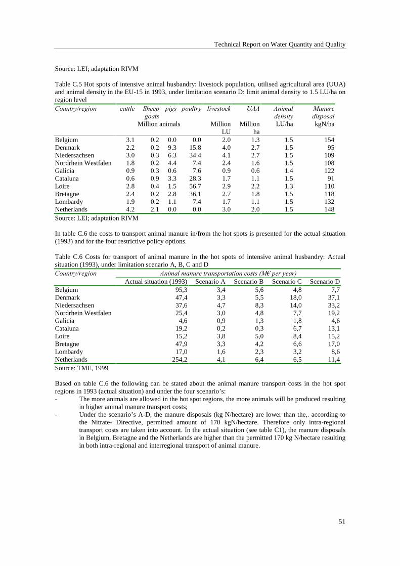
Technical Report on Water Quantity and Quality
51
Source: LEI; adaptation RIVM
Table C.5 Hot spots of intensive animal husbandry: livestock population, utilised agricultural area (UUA)and animal density in the EU-15 in 1993, under limitation scenario D: limit animal density to 1.5 LU/ha onregion level&RXQWU\�UHJLRQ FDWWOH 6KHHS
JRDWVSLJV SRXOWU\ OLYHVWRFN 8$$ $QLPDO
GHQVLW\0DQXUHGLVSRVDO
Million animals MillionLU
Millionha
LU/ha kgN/ha
Belgium 3.1 0.2 0.0 0.0 2.0 1.3 1.5 154Denmark 2.2 0.2 9.3 15.8 4.0 2.7 1.5 95Niedersachsen 3.0 0.3 6.3 34.4 4.1 2.7 1.5 109Nordrhein Westfalen 1.8 0.2 4.4 7.4 2.4 1.6 1.5 108Galicia 0.9 0.3 0.6 7.6 0.9 0.6 1.4 122Cataluna 0.6 0.9 3.3 28.3 1.7 1.1 1.5 91Loire 2.8 0.4 1.5 56.7 2.9 2.2 1.3 110Bretagne 2.4 0.2 2.8 36.1 2.7 1.8 1.5 118Lombardy 1.9 0.2 1.1 7.4 1.7 1.1 1.5 132Netherlands 4.2 2.1 0.0 0.0 3.0 2.0 1.5 148Source: LEI; adaptation RIVM
In table C.6 the costs to transport animal manure in/from the hot spots is presented for the actual situation(1993) and for the four restrictive policy options.
Table C.6 Costs for transport of animal manure in the hot spots of intensive animal husbandry: Actualsituation (1993), under limitation scenario A, B, C and D
$QLPDO�PDQXUH�WUDQVSRUWDWLRQ�FRVWV��0¼�SHU�\HDU�&RXQWU\�UHJLRQActual situation (1993) Scenario A Scenario B Scenario C Scenario D
Belgium 95,3 3,4 5,6 4,8 7,7Denmark 47,4 3,3 5,5 18,0 37,1Niedersachsen 37,6 4,7 8,3 14,0 33,2Nordrhein Westfalen 25,4 3,0 4,8 7,7 19,2Galicia 4,6 0,9 1,3 1,8 4,6Cataluna 19,2 0,2 0,3 6,7 13,1Loire 15,2 3,8 5,0 8,4 15,2Bretagne 47,9 3,3 4,2 6,6 17,0Lombardy 17,0 1,6 2,3 3,2 8,6Netherlands 254,2 4,1 6,4 6,5 11,4Source: TME, 1999
Based on table C.6 the following can be stated about the animal manure transport costs in the hot spotregions in 1993 (actual situation) and under the four scenario’s:- The more animals are allowed in the hot spot regions, the more animals will be produced resulting
in higher animal manure transport costs;- Under the scenario’s A-D, the manure disposals (kg N/hectare) are lower than the,. according to
the Nitrate- Directive, permitted amount of 170 kgN/hectare. Therefore only intra-regionaltransport costs are taken into account. In the actual situation (see table C1), the manure disposalsin Belgium, Bretagne and the Netherlands are higher than the permitted 170 kg N/hectare resultingin both intra-regional and interregional transport of animal manure.
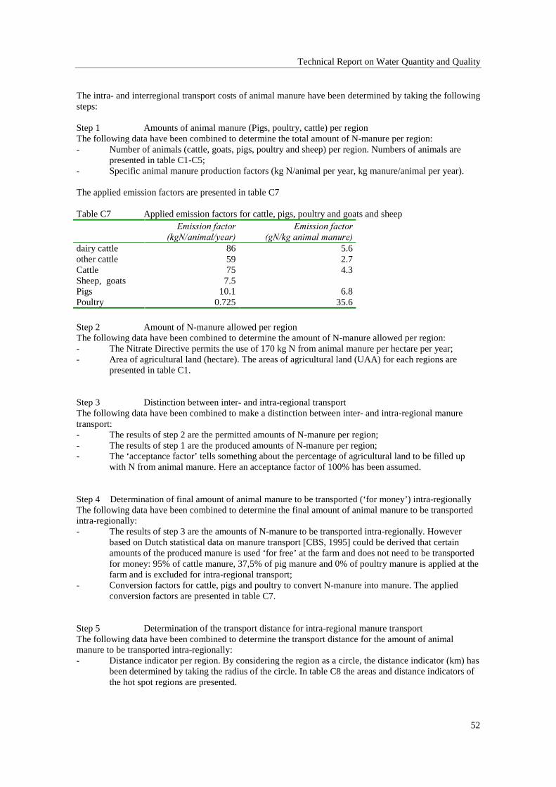
Technical Report on Water Quantity and Quality
52
The intra- and interregional transport costs of animal manure have been determined by taking the followingsteps:
Step 1 Amounts of animal manure (Pigs, poultry, cattle) per regionThe following data have been combined to determine the total amount of N-manure per region:- Number of animals (cattle, goats, pigs, poultry and sheep) per region. Numbers of animals are
presented in table C1-C5;- Specific animal manure production factors (kg N/animal per year, kg manure/animal per year).
The applied emission factors are presented in table C7
Table C7 Applied emission factors for cattle, pigs, poultry and goats and sheep(PLVVLRQ�IDFWRU
�NJ1�DQLPDO�\HDU�(PLVVLRQ�IDFWRU
�J1�NJ�DQLPDO�PDQXUH�dairy cattle 86 5.6other cattle 59 2.7Cattle 75 4.3Sheep, goats 7.5Pigs 10.1 6.8Poultry 0.725 35.6
Step 2 Amount of N-manure allowed per regionThe following data have been combined to determine the amount of N-manure allowed per region:- The Nitrate Directive permits the use of 170 kg N from animal manure per hectare per year;- Area of agricultural land (hectare). The areas of agricultural land (UAA) for each regions are
presented in table C1.
Step 3 Distinction between inter- and intra-regional transportThe following data have been combined to make a distinction between inter- and intra-regional manuretransport:- The results of step 2 are the permitted amounts of N-manure per region;- The results of step 1 are the produced amounts of N-manure per region;- The ‘acceptance factor’ tells something about the percentage of agricultural land to be filled up
with N from animal manure. Here an acceptance factor of 100% has been assumed.
Step 4 Determination of final amount of animal manure to be transported (‘for money’) intra-regionallyThe following data have been combined to determine the final amount of animal manure to be transportedintra-regionally:- The results of step 3 are the amounts of N-manure to be transported intra-regionally. However
based on Dutch statistical data on manure transport [CBS, 1995] could be derived that certainamounts of the produced manure is used ‘for free’ at the farm and does not need to be transportedfor money: 95% of cattle manure, 37,5% of pig manure and 0% of poultry manure is applied at thefarm and is excluded for intra-regional transport;
- Conversion factors for cattle, pigs and poultry to convert N-manure into manure. The appliedconversion factors are presented in table C7.
Step 5 Determination of the transport distance for intra-regional manure transportThe following data have been combined to determine the transport distance for the amount of animalmanure to be transported intra-regionally:- Distance indicator per region. By considering the region as a circle, the distance indicator (km) has
been determined by taking the radius of the circle. In table C8 the areas and distance indicators ofthe hot spot regions are presented.
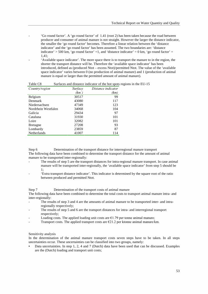
Technical Report on Water Quantity and Quality
53
- ‘Go round factor’. A ‘go round factor’ of 1.41 (root 2) has been taken because the road betweenproducer and consumer of animal manure is not straight. However the larger the distance indicator,the smaller the ‘go round factor’ becomes. Therefore a linear relation between the ‘distanceindicator’ and the ‘go round factor’ has been assumed. The two boundaries are: ‘distanceindicator’ > 500 km, ‘go round factor’ =1, and ‘distance indicator’ = 0 km, ‘go round factor’ =1,41;
- ‘Available space indicator’. The more space there is to transport the manure to in the region, theshorter the transport distance will be. Therefore the ‘available space indicator’ has beenintroduced, defined as (produced Ntot – excess Ntot)/permitted Ntot. The value of the ‘availablespace indicator’ varies between 0 (no production of animal manure) and 1 (production of animalmanure is equal or larger than the permitted amount of animal manure).
Table C8 Surfaces and distance indicator of the hot spots regions in the EU-15&RXQWU\�UHJLRQ 6XUIDFH
�NP��'LVWDQFH�LQGLFDWRU
�NP�Belgium 30517 99Denmark 43080 117Niedersachsen 47349 123Nordrhein Westfalen 34068 104Galicia 29434 97Cataluna 31930 101Loire 32082 101Bretagne 27208 93Lombardy 23859 87Netherlands 41007 114
Step 6 Determination of the transport distance for interregional manure transportThe following data have been combined to determine the transport distance for the amount of animalmanure to be transported inter-regionally:- The results of step 5 are the transport distances for intra-regional manure transport. In case animal
manure will be transported inter-regionally, the ‘available space indicator’ from step 5 should be1;
- ‘Extra transport distance indicator’. This indicator is determined by the square root of the ratiobetween produced and permitted Ntot.
Step 7 Determination of the transport costs of animal manureThe following data have been combined to determine the total costs to transport animal manure intra- andinter-regionally:- The results of step 3 and 4 are the amounts of animal manure to be transported inter- and intra-
regionally respectively;- The results of step 5 and 6 are the transport distances for intra- and interregional transport
respectively;- Loading costs. The applied loading unit costs are ¼�����SHU�WRQQH�DQLPDO�PDQXUH�- Transport costs. The applied transport costs are ¼�����SHU�NWRQQH�DQLPDO�PDQXUH�NP�
Sensitivity analysisIn the determination of the animal manure transport costs seven steps have to be taken. In all stepsuncertainties occur. These uncertainties can be classified into two groups, namely:• Data uncertainties. In step 1, 2, 4 and 7 (Dutch) data have been used that can be discussed. Examples
are the (Dutch) loading and transport unit costs;
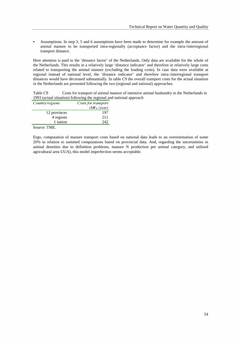
Technical Report on Water Quantity and Quality
54
• Assumptions. In step 3, 5 and 6 assumptions have been made to determine for example the amount ofanimal manure to be transported intra-regionally (acceptance factor) and the intra-/interregionaltransport distance.
Here attention is paid to the ‘distance factor’ of the Netherlands. Only data are available for the whole ofthe Netherlands. This results in a relatively large ‘distance indicator’ and therefore in relatively large costsrelated to transporting the animal manure (excluding the loading costs). In case data were available atregional instead of national level, the ‘distance indicator’ and therefore intra-/interregional transportdistances would have decreased substantially. In table C9 the overall transport costs for the actual situationin the Netherlands are presented following the two (regional and national) approaches.
Table C9 Costs for transport of animal manure of intensive animal husbandry in the Netherlands in1993 (actual situation) following the regional and national approach&RXQWU\�UHJLRQV &RVWV�IRU�WUDQVSRUW
�0¼���\HDU�12 provinces 197
4 regions 2111 nation 242
Source: TME.
Ergo, computation of manure transport costs based on national data leads to an overestimation of some20% in relation to summed computations based on provincial data. And, regarding the uncertainties inanimal densities due to definition problems, manure N production per animal category, and utilisedagricultural area UUA), this model imperfection seems acceptable.
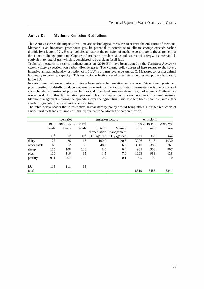
Technical Report on Water Quantity and Quality
55
$QQH[�'� �0HWKDQH�(PLVVLRQ�5HGXFWLRQV
This Annex assesses the impact of volume and technological measures to restrict the emissions of methane.Methane is an important greenhouse gas. Its potential to contribute to climate change exceeds carbondioxide by a factor of 21. Hence, policies to restrict the emission of methane contribute to the abatement ofthe climate change problem. Capture of methane provides a useful source of energy, as methane isequivalent to natural gas, which is considered to be a clean fossil fuel.Technical measures to restrict methane emission (2010-BL) have been treated in the 7HFKQLFDO�5HSRUW�RQ&OLPDWH�&KDQJH section non-carbon dioxide gases. The volume policy assessed here relates to the severeintensive animal husbandry restriction of 1.0 LU/ha at farm level (see Annex C: Measures to restrict animalhusbandry to carrying capacity). This restriction effectively eradicates intensive pigs and poultry husbandryin the EU.In agriculture methane emissions originate from enteric fermentation and manure. Cattle, sheep, goats, andpigs digesting foodstuffs produce methane by enteric fermentation. Enteric fermentation is the process ofanaerobic decomposition of polysaccharides and other feed components in the gut of animals. Methane is awaste product of this fermentation process. This decomposition process continues in animal manure.Manure management – storage or spreading over the agricultural land as a fertiliser - should ensure eitheraerobic degradation or avoid methane evolution.The table below shows that a restrictive animal density policy would bring about a further reduction ofagricultural methane emissions of 18% equivalent to 52 ktonnes of carbon dioxide.
scenarios emission factors emissions1990 2010-BL 2010-vol 1990 2010-BL 2010-volheads heads heads Enteric
fermentationManure
managementsum sum Sum
106 106 106 CH4 kg/head CH4 kg/head ton ton tondairy 27 26 16 100.0 20.6 3226 3113 1930other cattle 65 62 62 48.0 6.3 3510 3388 3367sheep 115 108 108 8.0 0.4 965 903 907pigs 120 116 15 1.5 7.0 1023 983 128poultry 951 967 100 0.0 0.1 95 97 10
LU 115 111 65total 8819 8483 6341
Technical Report on Water Quantity and Quality
56
$QQH[�( &RDVWDO�=RQHV
&RQWH[W
In this assessment, coastal zone issues are only represented through the analysis of nutrient loadings. Othercoastal issues, such as urbanization, tourism, and over-fishing are not taken into account.
In many coastal areas, poor water quality and distorted marine ecosystems are attributable to excessnitrogen, particularly along the margins of enclosed seas which have relatively little connection to the openocean. Water quality is generally well covered by existing EU directives, including the Bathing WaterDirective and the UWWTD. However, full implementation has yet to be achieved. The most appropriateindicator to measure the impact on bathing water quality is agricultural nitrate load, which reflects thelargest pollution source for coastal seas. However, policy targets for this area have not generally beenestablished.
In the context of this study, there is a close linkage to water management. The biodiversity of marineecosystems benefits from actions to limit excessive nitrogen releases to surface water.
$VVHVVPHQW�DQG�7UHQGV
The agricultural intensification since 1950 has brought about an increase in the amounts of excess nutrientsentering the surface waters and the coastal seas. )LJXUH���presents the nitrogen enrichment in coastal zones.The indicator is potential nitrate concentration. The index is labelled SRWHQWLDO and represents all nutrientinputs to the seas, including air deposition, oceanic influx and exchanges. The index does not account forremoval processes in the seas themselves.In general, there will be little change in the location or degree of enrichment between 1990 and 2010 underthe continuation of existing policies (EEA, 1998). This can be considered as a positive result of thesepolicies as the impact of population and welfare growth – both factors amplifying emissions – have beenmitigated. The enrichment trend, which started since 1950, has come to a halt. To reverse the trend,additional policies are required.The Nitrate Directive has some positive impact on coastal zone eutrophication, but has not been designedfor coastal zone management. The Nitrate Directive refers to manure and not to artificial fertiliser, whichcontributes to some 50% of the total agricultural N input. Hence, overall reductions due to the NitrateDirective are small.Trends for surface freshwater are provided in Section 2.4.2.

Technical Report on Water Quantity and Quality
57
good
fair
poor
bad
good
fair
poor
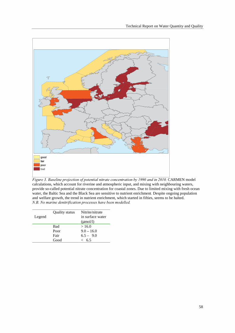
Technical Report on Water Quantity and Quality
58
good
fair
poor
bad
good
fair
poor
)LJXUH����%DVHOLQH�SURMHFWLRQ�RI�SRWHQWLDO�QLWUDWH�FRQFHQWUDWLRQ�E\������DQG�LQ������ CARMEN modelcalculations, which account for riverine and atmospheric input, and mixing with neighbouring waters,provide so-called potential nitrate concentration for coastal zones. Due to limited mixing with fresh oceanwater, the Baltic Sea and the Black Sea are sensitive to nutrient enrichment� Despite ongoing populationand welfare growth, the trend in nutrient enrichment, which started in fifties, seems to be halted.1�%��1R�PDULQH�GHQLWULILFDWLRQ�SURFHVVHV�KDYH�EHHQ�PRGHOOHG�
LegendQuality status Nitrite/nitrate
in surface water(µmol/l)
Bad > 16.0Poor 9.0 – 16.0Fair 6.5 – 9.0Good < 6.5