Embed Size (px)
Citation preview
This PDF is a selection from a published volume from the National Bureauof Economic Research
Volume Title: NBER Macroeconomics Annual 2012, Volume 27
Volume Author/Editor: Daron Acemoglu, Jonathan Parker, and Michael Woodford, editors
Volume Publisher: University of Chicago Press
ISSN: 0889-3365
Volume ISBN: cloth: 978-0-226-05277-9; paper: 978-0-226-05280-9, 0-226-05280-X
Volume URL: http://www.nber.org/books/acem12-2
Conference Date: April 20-21, 2012
Publication Date: May 2013
Chapter Title: Which Financial Frictions? Parsing the Evidence from the Financial Crisis of 2007 to 2009
Chapter Author(s): Tobias Adrian, Paolo Colla, Hyun Song Shin
Chapter URL: http://www.nber.org/chapters/c12741
Chapter pages in book: (p. 159 - 214)

3
Which Financial Frictions? Parsing the Evidence from the Financial Crisis of 2007 to 2009
Tobias Adrian, Federal Reserve Bank of New York
Paolo Colla, Bocconi University
Hyun Song Shin, Princeton University and NBER
I. Introduction
The fi nancial crisis of 2007 to 2009 has given renewed impetus to the
study of fi nancial frictions and their impact on macroeconomic activity.
Economists have refi ned existing models of fi nancial frictions to con-
struct narratives of the recent crisis. Although the recent innovations
to the modeling of fi nancial frictions share many common elements,
they also differ along some key dimensions. These differences may not
matter so much for story- telling exercises that focus on constructing
logically consistent narratives that highlight particular aspects of the
crisis. However, the differences begin to take on more signifi cance when
economists turn their attention to empirical or policy- related questions
that bear on the costs of fi nancial crises. Since policy questions must
make judgments on the relative weight given to specifi c features of the
models, the underpinnings of the models matter for the debates.
A long- running debate in macroeconomics is whether fi nancial fric-
tions manifest themselves mainly through shocks to the demand for
credit or to its supply. Frictions operating through shocks to demand
may be the result of the deterioration of the creditworthiness of bor-
rowers, perhaps through tightening collateral constraints or to declines
in the net present value of the borrowers’ projects. Shocks to supply
arise from tighter lending criteria applied by the lender, especially by
the banking sector. The outcome of this debate has consequences not
only for the way that economists approach the theory but also for the
conduct of fi nancial regulation and macro stabilization policy.
Our paper has two main objectives. The fi rst is to revisit the debate
on the demand and supply of credit to fi rms in the light of the evidence
© 2013 by the National Bureau of Economic Research. All rights reserved.
978-0-226-05277-9/2013/2012-0301$10.00
This content downloaded from 198.71.7.231 on Mon, 1 Jun 2015 10:35:09 AMAll use subject to JSTOR Terms and Conditions

160 Adrian, Colla, and Shin
from the recent crisis. We argue that the evidence points overwhelm-
ingly to a shock in the supply of intermediated credit by banks and
other fi nancial intermediaries. Firms that had access to direct credit
through the bond market took advantage of their access and tapped
the bond market in large quantities. For such fi rms, the decline in bank
lending was largely made up through increased borrowing in the bond
market. However, the cost of credit rose steeply, whether for direct or
intermediated credit, suggesting that the demand curve for bond fi -
nancing shifted out as a response to the inward shift in the bank credit
supply curve. Our fi nding echoes the earlier study by Kashyap, Stein,
and Wilcox (1993), who pointed to the importance of shocks to the
supply of intermediated credit as a key driver of fi nancial frictions.
The evidence suggests a number of follow- up questions. Our second
objective in this paper is to enumerate these questions and explore pos-
sible routes to answering them. What is so special about the banking
sector? Why did the recent economic downturn affect the banking sec-
tor so differently from the bond investors? Kashyap, Stein, and Wilcox
(1993) envisaged a specifi c shock to the banking sector through tighter
reserve constraints coming from monetary policy tightening, thereby
squeezing bank lending. However, the downturn from 2007 to 2009 was
more widespread, hitting not only the banking sector but the broader
economy. We still face the question of why the banking sector behaves
in such a different way from the rest of the economy.
If banks were simply a veil, and merely refl ected the preferences of
the depositors who provide funding to the banks for on- lending, then
banks would be irrelevant for fi nancial conditions. A challenge for any
macro model with a banking sector is to explain how one dollar that
goes through the banking system is different from one dollar that goes
directly to borrowers from savers. Holding savers’ wealth fi xed, when
the banking sector contracts in a deleveraging episode, money that used
to fl ow to borrowers through the banking sector now fl ows to borrow-
ers directly through the bond market. Thus, showing that the banking
sector “matters” in a macro context entails showing that the relative
size of the direct and intermediated fi nance in an economy matters for
fi nancial conditions.
We begin in section II by laying out some aggregate evidence from
the Flow of Funds and highlight the points of contact with the theoreti-
cal literature on fi nancial frictions. In section III, we delve deeper into
the micro evidence on fi rm- level fi nancing decisions and fi nd that it
corroborates the evidence in the aggregate data. Based on the evidence,
This content downloaded from 198.71.7.231 on Mon, 1 Jun 2015 10:35:09 AMAll use subject to JSTOR Terms and Conditions

Which Financial Frictions? 161
we draw up a checklist for a theory of fi nancial frictions, and sketch a
simple static model of direct and intermediated credit that attempts to
address the checklist.
Along the way, we review the theoretical literature in the light of the
evidence. Although many of the recent modeling innovations bring us
closer to addressing the full set of facts, there are a number of areas
where modeling innovations are still needed. We hope that our paper
may be a spur to further efforts at closing these gaps.
II. Preliminaries
A. Aggregate Evidence
Most models of fi nancial frictions share the feature that the total quantity
of credit to the nonfi nancial corporate sector decreases in a downturn,
whether it is due to a decline in the demand for credit or its supply.
However, even this basic proposition needs some qualifi cation when
we examine the evidence in any detail.
Figure 1 shows the total credit to the US nonfi nancial noncorporate
business sector from 1990 (both farm and nonfarm). Mortgages of vari-
ous types fi gure prominently in the composition of total credit and sug-
gest that the availability of collateral is an important determinant of
credit to the noncorporate business sector. The trough in total credit
Fig. 1. Credit to US nonfi nancial noncorporate businesses
Source: US Flow of Funds, tables L103, L104.
This content downloaded from 198.71.7.231 on Mon, 1 Jun 2015 10:35:09 AMAll use subject to JSTOR Terms and Conditions

162 Adrian, Colla, and Shin
comes in the second quarter of 2011, and the peak to trough (Q4:2008 to
Q2:2011) decline in total credit is roughly 8 percent.
Figure 2 examines the evolution of credit to the corporate business sec-
tor in the United States (the nonfarm, nonfi nancial corporate business
sector). The left- hand panel is in levels, taken from table L.102 of the US
Flow of Funds, while the right- hand panel plots the quarterly changes,
taken from table F.102 of the Flow of Funds.
The plots reveal some distinctive divergent patterns in the various
components of credit. In the left hand panel, the lower three compo-
nents are (broadly speaking) credit that is provided by banks and other
intermediaries, while the top series is the total credit obtained in the
form of corporate bonds. The narrow strip between the bond and bank
fi nancing is the amount of commercial paper.
While the loan series show the typical procyclical pattern of rising
during the boom and then contracting sharply in the downturn, bond
fi nancing behaves very differently. On the right- hand panel, we see that
bond fi nancing surges during the crisis period, making up most of the
lost credit due to the contraction of loans.
The substitution away from intermediated credit toward the bond
market is reminiscent of the fi nding in Kashyap, Stein, and Wilcox
(1993), who documented that fi rms reacted to a tightening of credit by
banks by issuing commercial paper. While commercial paper plays a
relatively small role in the total quantity of credit in fi gure 2, the prin-
ciple that fi rms switch to alternatives to bank fi nancing is very much in
evidence.
Nevertheless, the aggregate nature of the data from the Flow of
Funds means that some caution is needed in drawing any fi rm conclu-
sions. Several questions spring to mind. First, the Flow of Funds data
are snapshots of the total amounts outstanding, rather than actual fl ows
associated with new credit. Ideally, the evidence should be on the fl ow
of new credit.
Second, to tell us whether the shock is demand- or supply- driven,
information on the price of the new credit is crucial, but the Flow of
Funds is silent on prices. A demand- driven fall in credit would exert
less upward pressure on rates than a supply- driven shock. A simultane-
ous analysis of quantities and prices may enable to disentangle shocks
to demand from shocks to supply.
Third, the aggregate nature of the Flow of Funds data masks differ-
ences in the composition of fi rms, both over time and in cross- section.
The variation over time may simply refl ect changes in the number of
This content downloaded from 198.71.7.231 on Mon, 1 Jun 2015 10:35:09 AMAll use subject to JSTOR Terms and Conditions

Fig.
2.
Cre
dit
to
US
no
nfi
nan
cial
corp
ora
te s
ecto
r (l
eft-
han
d p
an
el)
an
d c
han
ges
in
ou
tsta
nd
ing
co
rpo
rate
bo
nd
s
an
d l
oan
s to
US
no
nfi
nan
cial
corp
ora
te s
ecto
r (r
igh
t- h
an
d p
an
el)
No
tes:
Th
e le
ft p
an
el i
s fr
om
US
Flo
w o
f F
un
ds,
tab
le L
102. R
igh
t p
an
el i
s fr
om
tab
le F
102. L
oan
s in
rig
ht
pan
el a
re
defi
ned
as
sum
of
mo
rtg
ag
es, b
an
k l
oan
s n
ot
else
wh
ere
class
ifi e
d (
n.e
.c.)
, an
d o
ther
lo
an
s.
This content downloaded from 198.71.7.231 on Mon, 1 Jun 2015 10:35:09 AMAll use subject to JSTOR Terms and Conditions

164 Adrian, Colla, and Shin
fi rms operating in the market. In cross- section, we should take account
of corporate fi nancing decisions (loan versus bond fi nancing) that are
related to fi rm characteristics.
To address these justifi ed concerns, we construct a micro- level data
set on new loans and bonds issued by nonfi nancial US corporations
between 1998 and 2010. Our data set includes information about quan-
tities and prices of new credit, which give us insights on whether the
quantity changes are due to demand or supply shocks. Second, our data
set contains information on fi rm characteristics (asset size, Tobin’s Q,
tangibility, ratings, profi tability, leverage, etc.) that previous studies
have identifi ed as drivers of the mix of loan and bond fi nancing. The
cross- section information gives us another perspective on how credit
supply affects fi rms’ corporate choices since we can control for demand-
side proxies. Finally, we make use of the reported purpose of loan and
bond issuances to single out new credit for “real investment”—that is,
general corporate purposes, including capital expenditure, and liquid-
ity management—which allows us to focus on corporate real activi-
ties (see Ivashina and Scharfstein 2010). By doing so, we exclude new
debt that is issued for acquisitions (acquisition, takeover, and leveraged
buyout/management buyout, LBO/MBO); capital structure manage-
ment (debt repayment, recapitalization, and stock repurchase); as well
as credit lines used as commercial paper backup.
We examine new issuances across all fi rms in our sample and ask
whether the features we observe in the aggregate also hold at the mi-
cro level. We fi nd that they do. During the economic downturn of 2007
to 2009, the total amount of new issuances decreased by 50 percent.
When we look at loans and bonds separately, we uncover a 75 percent
decrease in loans but a twofold increase in bonds. However, the cost of
both types of fi nancing show a steep increase (fourfold increase for new
loans, and threefold increase for bonds). We take this as evidence of an
increase in demand of bond fi nancing and a simultaneous contraction
in banks’ supply of loan fi nancing.
To shed further light on fi rm- level substitution between loan and
bond fi nancing, we conduct further disaggregated tests to be detailed
later. Our tests are for fi rms that have access to the bond market—prox-
ied by being rated—so that we can allow the demand and supply fac-
tors to play out in the open. We fi nd that loan amounts decline but bond
amounts increase, leaving total fi nancing unchanged, while the cost of
both loan and bond fi nancing increases. Thus, the evidence points to
a contraction in the supply of bank credit that pushes fi rms into the
This content downloaded from 198.71.7.231 on Mon, 1 Jun 2015 10:35:09 AMAll use subject to JSTOR Terms and Conditions

Which Financial Frictions? 165
bond market, which raises the price of both types of credit. The micro
evidence therefore corroborates the aggregate evidence from the Flow
of Funds. We conclude that the decline in the supply of bank fi nancing
trains the spotlight on those fi rms that do not have access to the bond
market (such as the noncorporate businesses in fi gure 1). It would be
reasonable to conjecture that fi nancial conditions tightened sharply for
such fi rms.
To understand the substitution between loan and bond fi nancing bet-
ter, we follow Denis and Mihov (2003) and Becker and Ivashina (2011)
to examine the choice of bond versus loan issuance in a discrete choice
framework. Becker and Ivashina (2011) fi nd evidence of substitution
from loans to bonds during times of tight monetary policy, tight lend-
ing standards, high levels of nonperforming loans, and low bank equity
prices. Controlling for demand factors, we fi nd that the 2007 to 2009
crisis reduced the probability of obtaining a loan by 14 percent. We fur-
ther corroborate the evidence in Becker and Ivashina (2011) by using
two proxies for the fi nancial sector risk- bearing capacity (for the growth
in broker- dealer leverage, see Adrian, Moench, and Shin 2011; for the
excess bond premium, see Gilchrist and Zakrajšek 2011) and document
that a contraction in intermediaries’ risk- bearing capacity reduces the
probability of loan issuance between 18 and 24 percent depending on
the proxy employed. Finally, we investigate which fi rm characteristics
insulate borrowers from the effect of bank credit supply shocks in the
2007 to 2009 crisis. Our analysis highlights that fi rms that are larger or
have more tangible assets, higher credit ratings, better project quality,
less growth opportunities, and lower leverage were better equipped to
withstand the contraction of bank credit during the crisis.
B. Modeling Financial Frictions
The evidence gives insights on how we should approach modeling
fi nancial frictions if we are to capture the observed features. Perhaps
the three best- known workhorse models of fi nancial frictions used in
macroeconomics are Bernanke and Gertler (1989), Kiyotaki and Moore
(1997), and Holmström and Tirole (1997). However, in the benchmark
versions of these models, the lending sector is competitive and the fo-
cus of the attention is on the borrower’s net worth instead. The results
from the benchmark versions of these models should be contrasted
with the approach that places the borrowing constraints on the lender
(i.e., the bank) as in Gertler and Kiyotaki (2010).
This content downloaded from 198.71.7.231 on Mon, 1 Jun 2015 10:35:09 AMAll use subject to JSTOR Terms and Conditions

166 Adrian, Colla, and Shin
Bernanke and Gertler (1989) use the costly state verifi cation (CSV) ap-
proach to derive the feature that the borrower’s net worth determines
the cost of outside fi nancing. The collateral constraint in Kiyotaki and
Moore (1997) introduces a similar role for the borrower’s net worth
through the market value of collateral assets whereby an increase in
borrower net worth due to an increase in collateral value serves to in-
crease borrower debt capacity. But in both cases, the lenders are treated
as being competitive and no meaningful comparisons are possible be-
tween bank and bond fi nancing. In contrast, the evidence from fi gure
2 points to the importance of understanding the heterogeneity across
lenders and the composition of credit. The role of the banking sector in
the cyclical variation of credit emerges as being particularly important.
A bank is simultaneously both a borrower and a lender—it bor-
rows in order to lend. As such, when the bank itself becomes credit-
constrained, the supply of credit to the ultimate end- users of credit
(nonfi nancial businesses and households) will be impaired. In the ver-
sion of the Holmström and Tirole (1997) model with banks, credit can
fl ow either directly from savers to borrowers or indirectly through the
banking sector. The ultimate borrowers face a borrowing constraint
due to moral hazard, and must have a large enough equity stake in
the project to receive funding. Banks also face a borrowing constraint
imposed by depositors, but banks have the useful purpose of mitigating
the moral hazard of ultimate borrowers through their monitoring. In
Holmström and Tirole (1997), the greater monitoring capacity of banks
eases the credit constraint for borrowers who would otherwise be shut
out of the credit market altogether. Firms follow a pecking order of fi -
nancing choices where low net worth fi rms can only obtain fi nancing
from banks and are shut out of the bond market, while fi rms with high
net worth have access to both, but use the cheaper bond fi nancing.
Repullo and Suarez’s (2000) model is in a similar spirit. Bolton and
Freixas (2000) focus instead on the greater fl exibility of bank credit in
the face of shocks, as discussed by Berlin and Mester (1992), with the
implication that fi rms with higher default probability favor bank fi -
nance relative to bonds. De Fiore and Uhlig (2011, 2012) explore the im-
plications of the greater adaptability of bank fi nancing to informational
shocks in the spirit of Berlin and Mester (1992) and examine the shift
toward greater reliance on bond fi nancing in the Eurozone during the
recent crisis.
Our empirical results reported in the following suggest that the in-
teraction between direct and intermediated fi nance should be high on
This content downloaded from 198.71.7.231 on Mon, 1 Jun 2015 10:35:09 AMAll use subject to JSTOR Terms and Conditions

Which Financial Frictions? 167
the agenda for researchers. We review the new theoretical literature on
banking and intermediation in a later section.
C. Focus on Banking Sector
We are still left with a broader theoretical question of what makes the
banking sector so special. In Kashyap, Stein, and Wilcox (1993), the
shock envisaged was a monetary tightening that hit the banking sector
specifi cally through tighter reserve requirements that led to a shrinking
of bank balance sheets. However, the downturn in 2007 to 2009 was
more widespread, hitting not only the banking sector but the broader
economy.
A clue lies in the way that banks manage their balance sheets. Fig-
ure 3 is the scatter plot of the quarterly change in total assets of the
sector consisting of the fi ve US investment banks examined in Adrian
and Shin (2008, 2010) where we plot both the changes in assets against
equity, as well as changes in assets against debt. More precisely, it plots
{(∆At, ∆Et)} and {(∆At, ∆Dt)} where ∆At is the change in total assets of
Fig. 3. Scatter chart of {(∆At, ∆Et)} and {(∆At, ∆Dt)} for changes in assets, equity, and
debt of US investment bank sector consisting of Bear Stearns, Goldman Sachs, Lehman
Brothers, Merrill Lynch, and Morgan Stanley between Q1:1994 and Q2:2011
Source: Securities and Exchange Commission (SEC) 10Q fi lings.
This content downloaded from 198.71.7.231 on Mon, 1 Jun 2015 10:35:09 AMAll use subject to JSTOR Terms and Conditions

168 Adrian, Colla, and Shin
the investment bank sector at quarter t, and where ∆Et and ∆Dt are the
change in equity and change in debt of the sector, respectively.
The fi tted line through {(∆At, ∆Dt)} has slope very close to 1, meaning
that the change in assets in any one quarter is almost all accounted for
by the change in debt, while equity is virtually unchanged. The slope of
the fi tted line through the points {(∆At, ∆Et)} is close to zero.1
Commercial banks show a similar pattern to investment banks.
Figure 4 is the analogous scatter plot of the quarterly change in total
assets of the US commercial bank sector, which plots {(∆At, ∆Et)} and
{(∆At, ∆Dt)} using the FDIC Call Reports. The sample period is between
Q1:1984 and Q2:2010. We see essentially the same pattern as for invest-
ment banks, where every dollar of new assets is matched by a dollar
in debt, with equity remaining virtually unchanged. Although we do
not show here the scatter charts for individual banks, the charts for
individual banks reveal the same pattern. Banks adjust their assets dol-
lar for dollar through a change in debt with equity remaining “sticky.”
The fact that banks tend to reduce debt during downturns could be
explained by standard theories of debt overhang or adverse selection
in equity issuance. However, what is notable in fi gures 3 and 4 is the
Fig. 4. Scatter chart of {(∆At, ∆Et)} and {(∆At, ∆Dt)} for changes in assets, equity, and
debt of US commercial bank sector at t between Q1:1984 and Q2:2010
Source: FDIC call reports.
This content downloaded from 198.71.7.231 on Mon, 1 Jun 2015 10:35:09 AMAll use subject to JSTOR Terms and Conditions

Which Financial Frictions? 169
fact that banks do not issue equity even when assets are increasing. The
fi tted line through the debt issuance curve holds just as well when as-
sets are increasing as it does when assets are decreasing. This feature
presents challenges to an approach where the bank capital constraint
binds only in downturns, or to models where the banking sector is a
portfolio maximizer.
Figures 3 and 4 show that banks’ equity is little changed from one
quarter to the next, implying that total lending is closely mirrored by
the bank’s leverage decision. Bank lending expands when its leverage
increases, while a sharp reduction in leverage (“deleveraging”) results
in a sharp contraction of lending. Adrian and Shin (2008, 2010) showed
that US investment banks have procyclical leverage where leverage and
total assets are positively related.
Figure 5 is the scatter chart of quarterly asset growth and quarterly
leverage growth for US commercial banks for the period Q1:1984 to
Q2:2010. We see that leverage is procyclical for US commercial banks
also. However, we see that the sharp deleveraging in the recent crisis
happened comparatively late, with the sharpest decline in assets and
leverage taking place in Q1:2009. Even up to the end of 2008, assets
and leverage were increasing, possibly refl ecting the drawing down of
credit lines that had been granted to borrowers prior to the crisis.
The equity series in the scatter charts in fi gures 3, 4, and 5 are of book
Fig. 5. Scatter chart of quarterly asset growth and quarterly leverage growth of the US
commercial bank sector, Q1:1984 to Q2:2010
Source: FDIC Call Reports.
This content downloaded from 198.71.7.231 on Mon, 1 Jun 2015 10:35:09 AMAll use subject to JSTOR Terms and Conditions

170 Adrian, Colla, and Shin
equity, giving us the difference between the value of the bank’s portfo-
lio of claims and its liabilities. An alternative measure of equity would
have been the bank’s market capitalization, which gives the market price
of its traded shares. Since our interest is in the supply of credit, which
has to do with the portfolio decision of the banks, book equity is the
appropriate notion. Market capitalization would have been more ap-
propriate if we were interested in new share issuance or mergers and
acquisitions decisions.
Crucially, it should be borne in mind that market capitalization is
not the same thing as the marked- to- market value of the book equity, which
is the difference between the market value of the bank’s portfolio of
claims and the market value of its liabilities. Take the example of a secu-
rities fi rm holding only marketable securities that fi nances those securi-
ties with repurchase agreements. Then, the book equity of the securities
fi rm refl ects the haircut on the repos, and the haircut will have to be
fi nanced with the fi rm’s own book equity. This book equity is the arche-
typal example of the marked- to- market value of book equity.
In contrast, market capitalization is the discounted value of the future
free cash fl ows of the securities fi rm, and will depend on cash fl ows
such as fee income, which do not depend directly on the portfolio held
by the bank.
Since we are interested in lending decisions of intermediaries, it is the
portfolio choice of the banks that is our main concern. As such, book
value of equity is the appropriate concept when measuring leverage.
Consistent with our choice of book equity as the appropriate notion of
equity for lending decisions, Adrian, Moench, and Shin (2011) fi nd that
market risk premiums depend on book leverage, rather than leverage
defi ned in terms of market capitalization.
The scatter charts in fi gures 3, 4, and 5 also suggest another important
conceptual distinction. They suggest that we should be distinguishing
between two different hypotheses for the determination of risk premi-
ums. In particular, consider the following pair of hypotheses.
Risk premium depends on the net worth of the banking sector.
Risk premium depends on the net worth of the banking sector and the leverage of the banking sector.
In most existing models of fi nancial frictions, net worth is the state
variable of interest. This is true even of those models that focus on the
net worth of banking sector, such as Gertler and Kiyotaki (2010). How-
This content downloaded from 198.71.7.231 on Mon, 1 Jun 2015 10:35:09 AMAll use subject to JSTOR Terms and Conditions

Which Financial Frictions? 171
ever, the scatter charts in fi gures 3, 4, and 5 suggest that the leverage of
the banks may be an important, separate factor in determining market
conditions. Evidence from Adrian, Moench, and Shin (2011) suggests
that book leverage is indeed the measure that has stronger explanatory
power for risk premiums in comparison to the level of net worth as
such.
The explicit recognition of the role of fi nancial intermediaries holds
some promise in explaining the economic impact of fi nancial frictions.
When intermediaries curtail lending, directly granted credit (such as
bond fi nancing) must substitute for bank credit, and market risk premi-
ums must rise in order to induce nonbank investors to enter the market
for risky corporate debt and take on a larger exposure to the credit risk
of nonfi nancial fi rms. The sharp increase in spreads during fi nancial cri-
ses would be consistent with such a mechanism. The recent work of Gil-
christ, Yankov, and Zakrajšek (2009) and Gilchrist and Zakrajšek (2011)
point to the importance of the credit risk premium as measured by the
“excess bond spreads” (EBP; that is, spreads in excess of fi rm funda-
mentals) as an important predictor of subsequent economic activity as
measured by industrial production or employment. Adrian, Moench,
and Shin (2011) and Adrian and Shin (2010) link credit risk premiums
directly to fi nancial intermediary balance sheet management, and real
economic activity.
Motivated by the initial evidence, we turn to an empirical study that
uses micro- level data in section III. We will see that the aggregate evi-
dence is confi rmed in the micro- level data. After sifting through the
evidence, we turn our attention to sketching out a possible model of
direct and intermediated credit. Our model represents a departure from
the standard practice of modeling fi nancial frictions in two key respects.
First, it departs from the practice of imposing a bank capital constraint
that binds only in the downturn. Instead, the capital constraint in the
model will bind all the time—both in good times and bad. Second,
our model is aimed at replicating the procyclicality of leverage where
banks adjust their assets dollar for dollar through a change in debt, as
revealed in the scatter plots in fi gures 3, 4, and 5. Procyclicality of lever-
age runs counter to the common modeling assumption that banks are
portfolio optimizers with log utility, implying that leverage is high in
downturns (we review the literature in a later section). To the extent
that banking sector behavior is a key driver of the observed outcomes,
our focus will be on capturing the cyclical features of fi nancial frictions
as faithfully as we can.
This content downloaded from 198.71.7.231 on Mon, 1 Jun 2015 10:35:09 AMAll use subject to JSTOR Terms and Conditions

172 Adrian, Colla, and Shin
One feature of our model is that as bank lending contracts sharply
through deleveraging, the direct credit from bond investors must ex-
pand to take up the slack. However, for this to happen, prices must
adjust in order that the risk premium rises suffi ciently to induce risk-
averse bond investors to make up for the lost banking sector credit.
Thus, a fall in the relative credit supplied by the banking sector is asso-
ciated with a rise in risk premiums. Financial frictions during the crisis
of 2007 to 2009 appear to have worked through the spike in spreads as
well as through any contraction in the total quantity of credit. Having
studied the microevidence in detail and the theory, we turn to a discus-
sion of the recent macroeconomic modeling in section V. We argue that
the evidence presented in this paper presents a challenge for many of
the post- crisis general equilibrium models. Section VI concludes.
III. Evidence from Microdata
A. Sample
We use micro- level data to investigate the fl uctuations in fi nancing re-
ceived by US listed fi rms during the period 1998 to 2010, with special
focus on the 2007 to 2009 fi nancial crisis. In our following data analysis,
we will identify the eight quarters from Q3:2007 to Q2:2009 as the crisis
period.
Our sample consists of nonfi nancial (Standard Industrial Classifi ca-
tion [SIC] codes 6000–6999) fi rms incorporated in the United States that
lie in the intersection of the Compustat quarterly database, the Loan
Pricing Corporation’s Dealscan database of new loan issuances (LPC),
and the Securities Data Corporation’s New Bond Issuances database
(SDC). For a fi rm to be included in our analysis, we require the fi rm-
quarter observation in Compustat to have positive total assets (hence-
forth, Compustat sample), and have data available for its incremen-
tal fi nancing from LPC and SDC. Our sample construction procedure,
described following, identifi es 3,896 fi rms (out of the 11,538 in the
Compustat sample) with new fi nancing between 1998 and 2010. Firm-
quarter observations with new fi nancing amount to 4 percent of the
Compustat sample, and represent 13 percent of their total assets (see
table 1).
Loan information comes from the June 2011 extract of LPC, and in-
cludes information on loan issuances (from the facility fi le: amount, is-
This content downloaded from 198.71.7.231 on Mon, 1 Jun 2015 10:35:09 AMAll use subject to JSTOR Terms and Conditions

Which Financial Frictions? 173
sue date, type, purpose, maturity, and cost2) and borrowers (from the
borrower fi le: identity, country, type, and public status). We apply the
following fi lters: (1) the issue date is between January 1998 and Decem-
ber 2010 (172,243 loans); (2) the loan amount, maturity, and cost are
nonmissing, and the loan type and purpose are disclosed (90,131 loans);
(3) the loan is extended for real investment purposes3 (42,979 loans). We
then use the Compustat- LPC link provided by Michael Roberts (Chava
and Roberts 2008) to match loan information with the Compustat
sample, and end up with 12,373 loans issued by 3,791 unique fi rms.4
Our screening of bond issuances follows similar steps to the ones
we use for loan issuances. We retrieve from SDC information on nonfi -
nancial fi rms’ bond issuances (amount, issue date, cost,5 purpose, and
maturity) and apply the following fi lters: (1) the issue date is between
January 1998 and December 2010, and the borrower is a nonfi nancial
US fi rm (38,953 bonds); (2) the bond amount, maturity, purpose, and
cost are nonmissing (9,706 bonds); (3) the bond is issued for real invest-
ment purposes6 (7,480 bonds). We then merge bond information with
the Compustat sample using issuer CUSIPs, and obtain 3,222 bonds
issued by 902 unique fi rms.
The summary statistics in table 2 compare our restricted sample to
the full sample of loans and bonds issued for real investment purposes.
Table 1Frequency of New Debt Issuances
Firm-quarters
Observations Total Assets Firms
Compustat sample 308,184 533,472 11,538
[100] [100] [100]
Our sample:
With new debt issuances 11,463 68,637 3,896
[3.72] [12.87] [33.77]
With new loan issuances 9,458 38,717 3,791
[3.07] [7.26] [32.86]
With new bond issuances 2,322 34,454 902
[0.75] [6.27] [7.82]
Notes: Compustat sample refers to all US incorporated nonfi nancial (SIC codes 6000 to
6999) fi rm- quarters in the Compustat quarterly database with positive total assets. We
merge the Compustat sample with loan issuances from the Loan Pricing Corporation’s
Dealscan database (LPC) and bond issuances from the Securities Data Corporation’s New
Bond Issuances database (SDC). Percentages of the Compustat sample are reported in
square brackets. Total assets are expressed in January 1998 constant $bln.
This content downloaded from 198.71.7.231 on Mon, 1 Jun 2015 10:35:09 AMAll use subject to JSTOR Terms and Conditions

174 Adrian, Colla, and Shin
In particular, our sample includes 79 percent of loans issued by non-
private US corporations, and represents 87 percent in terms of dollar
amount. Moreover, our sample captures 50 percent of US nonfi nan-
cial public fi rms and subsidiaries’ bond issuances (about 57 percent in
terms of dollar amount). On average, loans in our sample are issued
for $239 million, have maturity of 43 months, and are priced at 217 bps
(basis point) (32 bps for credit lines, using the all- in- undrawn spread).
These are economically very similar to the average values in the full
LPC sample. Relative to loans, bonds in our sample are on average is-
sued for larger amounts ($326 million), longer maturities (100 months),
and are more expensive (266 bps). Again, these values are very similar
to their counterpart in the full SDC sample. The t- test for the difference
in means detects signifi cant differences between our sample and full
LPC and SDC samples for the average issuance amount only.
B. Patterns of New Issuances
The pattern of total new credit that includes both loan and bond fi nanc-
ing shows a marked decline in new debt issuances and a simultaneous
increase in their cost during the recent fi nancial crisis.
Table 2 Characteristics of New Issuances
Loan issuances Bond issuances
Our
sample
Full LPC
sample t-stat
Our
sample
Full SDC
sample t-stat
Issuances # 12,373 15,736 3,222 6,435
Amount (total) 2,952.74 3,411.90 1,050.60 1,831.72
Amount 0.239 0.217 4.011*** 0.326 0.285 5.728***
Maturity 43.00 42.57 1.583 100.09 98.90 1.110
Cost 216.71 220.27 –1.952* 265.84 264.95 0.185
Cost (undrawn) 32.44 32.22 0.529
Notes: This table presents means aggregated across all fi rms for our sample of new debt
issuances. Full LPC sample includes tranches with valid amount, maturity, purpose, and
spread issued by nonprivate US corporations for investment purposes. Full SDC sample
includes tranches with valid amount, maturity, purpose, and spread issued by nonfi nan-
cial US public fi rms and subsidiaries for investment purposes. We report the t- statistic
for the unpaired t- test for differences in amounts, maturities, and spreads between our
sample and the full samples. For loan issuances, “Cost” is the all- in- drawn spread and
“Cost (undrawn)” is the all- in- undrawn spread (available for credit lines only). There are
7,782 (resp., 8,817) issuances with nonmissing all- in- undrawn spread in our sample (resp.
Full LPC sample). Amount is expressed in January 1998 constant $bln, cost is expressed
in bps, and maturity is expressed in months.
This content downloaded from 198.71.7.231 on Mon, 1 Jun 2015 10:35:09 AMAll use subject to JSTOR Terms and Conditions

Which Financial Frictions? 175
Total Financing
The evolution of total credit (both loans and bonds) presented in fi gure
6 shows a marked decrease in total amount and number of issuances
from peak to trough. This can be seen from panel A, which graphs the
quarterly total amount of new debt (loans plus bonds) issued expressed
in billions of January 1998 dollars, with panel C showing the averages.
Panel E graphs the total number of new debt issuances.
Due to seasonality in new debt fi nancing activity, we include the
smoothed version of all series (solid line) as a moving average strad-
dling the current term with two lagged and two forward terms. Figure
6 highlights the steep reduction in total fi nancing as the crisis unfolds;
total credit halved from $182.25 billion in Q2:2007, the peak of the credit
boom, to $90.65 billion during Q2:2009, the trough of the crisis. During
the same period, the number of new issuances decreases by about 30
percent.
We turn to the cost of credit and its maturity. For every quarter, we
use a weighted average of the cost (in bps) and the maturity (in months)
of individual facilities, where the weights are given by the amount of
each facility relative to the amount of issuances in that quarter. Panel B
of fi gure 6 shows that the cost of new debt quadrupled during the crisis,
from 99 bps in Q2:2007 to 403 bps in Q2:2009.7
Loan Financing
Bank fi nancing was drastically reduced during the crisis; loan issu-
ance at the trough of the cycle totaled $40 billion, about one- quarter
of loan issuance at the peak of the credit boom ($155.69 billions during
Q2:2007). The number of new loans more than halved from 318 issu-
ances during Q2:2007 to 141 issuances during Q2:2009. This reduction
in bank lending can be seen in fi gure 7, which presents the quarterly
evolution of loan issuances. The total amount of loans are in panel A;
the average amount of loans are in panel C; and the total number of
loans issued are in panel E.
In parallel with the decline in loan fi nancing activity, the cost of loans
rose steeply. Loan spreads more than quadrupled during the fi nancial
crisis, from 90 bps in Q2:2007 to a peak of 362 bps in Q2:2009.8 The
2001 recession did not show such a substantial increase in loan spreads;
spreads oscillated between 128 bps (Q2:2001) and 152 bps (Q4:2001).
Panel B of fi gure 7 graphs these results for the cost of loan fi nancing.
This content downloaded from 198.71.7.231 on Mon, 1 Jun 2015 10:35:09 AMAll use subject to JSTOR Terms and Conditions

176 Adrian, Colla, and Shin
Maturities of newly issued loans tend to shorten during recessions,
and increase during booms, as can be seen from panel D in fi gure 7. Fi-
nally, in fi gure 7, panel F, we graph the quarterly total amount of loans
by type (credit lines or term loans).9 In the aftermath of the credit boom,
both revolvers and term loans fell sharply. New credit lines totaled
$24.15 billion in Q2:2009, which is roughly 25 percent of the credit lines
initiated at the peak of the credit boom ($124.03 during Q2:2007). New
term loans halved from $30.05 billion in Q2:2007 to $15.68 billion in
Q2:2009. Issuances of revolvers start trending upwards from 2010 and,
as of Q4:2010, total credit lines correspond to about 40 percent of their
dollar values at the peak of the credit boom. Issuances of term loans
increase at a slower pace, and during Q4:2010, reach about 25 percent
of their Q2:2007 levels.
Bond Financing
In contrast to bank lending, bond issuance increased during the crisis;
issuance of new bonds totaled $50.64 billion in Q2:2009—about twice
Fig. 6. New debt issuances
Notes: Panel A: total amount of debt issued (billion of January 1998 USD). Panels B and D:
cost of debt issued (in bps). In panel D we use the all- in- undrawn spread for credit lines
between Q3:2007 and Q2:2009. Panel C: average amount of debt issued. Panel E: number
of debt issuances. Panel F: maturity of debt issued (in months). All panels report the raw
series (dashed line) and its smoothed version (solid line).
This content downloaded from 198.71.7.231 on Mon, 1 Jun 2015 10:35:09 AMAll use subject to JSTOR Terms and Conditions

Which Financial Frictions? 177
as much as during the peak of the credit boom ($26.56 billion during
Q2:2007). This can be seen in fi gure 8. In addition, the number of newly
issued bonds doubles from 54 during Q2:2007 to 116 during Q2:2009.
Moreover, fi gure 8 confi rms that the credit boom in the run- up to the
crisis was not exclusively a bank credit boom, since total bond issuances
increase from 2005 onwards also.
Figure 8 graphs the evolution of the cost and maturity of bonds (pan-
els B and D, respectively). Several similarities emerge between loan and
bond fi nancing. First, bond maturities shorten during recessions and
increase during booms; this is confi rmed by comparing maturities dur-
ing the years leading to the peak of the credit boom to maturities dur-
ing the latest recession. Second, the credit boom preceding the recent
fi nancial crisis is accompanied by a reduction in spreads. Finally, bond
spreads almost tripled during the fi nancial crisis, from 156 bps during
Q2:2007 to 436 bps during Q2:2009, similar to the increase experienced
by loan spreads.
The micro- level evidence permits two conclusions. First, we confi rm
Fig. 7. New loan issuances
Notes: Panel A: total amount of loans issued (billion of January 1998 USD). Panel B: cost
of loans issued (in bps). Panel C: average amount of loans issued. Panel D: maturity of
loans issued (in months). Panel E: number of loans issued. Panel F: total amount of credit
lines (dotted) and term loans (solid). All panels report the raw series (dashed line) and its
smoothed version (solid line).
This content downloaded from 198.71.7.231 on Mon, 1 Jun 2015 10:35:09 AMAll use subject to JSTOR Terms and Conditions

178 Adrian, Colla, and Shin
the evidence from the Flow of Funds that nonfi nancial corporations in-
creased funding in the bond market, as bank loans shrank. Secondly,
credit spreads increased sharply, for both loans and bonds. In the next
two sections, we will investigate the extent to which the substitution from
bank fi nancing to bond fi nancing is related to institutional characteristics.
Kashyap, Stein, and Wilcox (1993) showed that following monetary
tightening, nonfi nancial corporations tended to issue relatively more
commercial paper. The authors link this substitution in external fi -
nance directly to monetary policy shocks, and argue that the evidence
supports the lending channel of monetary policy over the traditional
Keynesian demand channel, where tighter monetary policy leads to
lower aggregate demand, and hence lower demand for credit. Under
the lending channel, it is credit supply that shifts. Kashyap, Stein, and
Wilcox’s (1993) evidence that commercial paper issuance increases
while bank lending declines points toward the bank lending channel.
We will return to this interpretation later, when we present our model
of fi nancial intermediation.
Our empirical fi ndings complement Kashyap, Stein, and Wilcox
Fig. 8. New bond issuances
Notes: Panel A: total amount of bonds issued (billion of January 1998 USD). Panel B: cost
of bonds issued (in bps). Panel C: average amount of bonds issued. Panel D: maturity of
bonds issued (in months). Panel E: number of bonds issued. All panels report the raw
series (dashed line) and its smoothed version (solid line).
This content downloaded from 198.71.7.231 on Mon, 1 Jun 2015 10:35:09 AMAll use subject to JSTOR Terms and Conditions

Which Financial Frictions? 179
(1993) in two ways. First, we highlight the relatively larger role of the
bond market compared to commercial paper in offsetting the contrac-
tion in bank credit. As we saw for the corporate business sector in the
United States, the increase in aggregate bond fi nancing largely offsets
the contraction in bank lending. Second, the micro- level data allow us
to observe the yields at which the new bonds and loans are issued. We
can therefore go beyond the aggregate data used by Kashyap, Stein,
and Wilcox.
We are still left with a broader theoretical question of what makes the
banking sector special. Kashyap, Stein, and Wilcox envisaged the shock
to the economy as a monetary tightening that hit the banking sector
specifi cally through tighter reserve constraints that hit the asset side of
banks’ balance sheets. In other words, they looked at a specifi c shock to
the banking sector. However, the downturn in 2007 to 2009 was more
widespread, hitting not only the banking sector but the broader econ-
omy. We still face the question of why the banking sector behaves in
such a different way from the rest of the economy. We suggest one pos-
sible approach to this question in our theory section.
C. Closer Look at Corporate Financing: Univariate Sorts
We now investigate the effect of the crisis on fi rms’ choices between
bank and bond fi nancing and the cross- sectional differences in new fi -
nancing behavior. We work with a sample covering four years, which
we divide equally into two subperiods—before crisis (from Q3:2005 to
Q2:2007) and during the crisis (from Q3:2007 to Q2:2009). This balanced
approach is designed to average out seasonal patterns in our quarterly
data (see Duchin, Ozbas, and Sensoy 2010).
We restrict our attention to the sample of fi rms that issue loans and/
or bonds during the fi nancial crisis. By doing so, we select fi rms that
have access to both types of funding and address the fi rm’s choice be-
tween forms of credit. In selecting fi rms that have access to both types
of credit, we do not imply that these fi rms are somehow typical. In-
stead, our aim is to use this sample in our identifi cation strategy for dis-
tinguishing shocks to the demand or supply of credit. If the cost of both
types of credit increased but the quantity of bank fi nancing fell and
bond fi nancing rose, then this would be evidence of a negative shock to
the supply of bank credit.
We fi rst examine evidence on these fi rms’ issuances before and dur-
ing the crisis with univariate sorts, controlling for relevant fi rm charac-
This content downloaded from 198.71.7.231 on Mon, 1 Jun 2015 10:35:09 AMAll use subject to JSTOR Terms and Conditions
180 Adrian, Colla, and Shin
teristics. For a fi rm to be included in our analysis (“new debt issuer”)
we require that: (1) it issues at least one loan or one bond during the
crisis, and has positive assets in at least one quarter during the crisis;
(2) it has positive assets in at least one quarter before the crisis; (3) it has
nonmissing observations for the relevant sorting variable in Q2:2005.
Finally, in order to investigate possible substitution effects between the
two sources of fi nancing, we follow Faulkender and Petersen (2006) and
require fi rms to be rated during Q2:2005, as a way of ensuring that we
select fi rms that have access to the bond market.
For every fi rm that meets these criteria we measure cumulative new
debt issuances over the precrisis and the crisis period to gauge the in-
cremental fi nancing immediately before the crisis (Q2:2007) and at the
trough of the crisis (Q2:2009).10 The fi rm- level spread on new debt is
calculated as the value- weighted spread.
We build on previous literature (Houston and James 1996; Krishnas-
wami, Spindt, and Subramaniam 1999; Denis and Mihov 2003) to iden-
tify the fi rm- level characteristics that affect corporate reliance on bank
and bond fi nancing: size and tangibility (considered as proxies for in-
formation asymmetry), Tobin’s Q (proxying for growth opportunities),
credit rating, profi tability (which proxies for project quality), and lever-
age. All variables are defi ned in table B1 (see appendix B) and mea-
sured during Q2:2005. Measuring fi rm- level characteristics well before
the onset of the crisis mitigates endogeneity concerns.
Table 3 provides summary statistics of these variables. The last six
columns in table 3 report the percentage of per- period new fi nancing
that is due to new debt issuers, conditional on the availability of each
sorting variable: for instance, the top row indicates that our sample has
492 new debt issuers with valid total assets during Q2:2005, and these
new debt issuers account for 52 percent and 80.7 percent, respectively,
of the new issuances before and during the crisis.
We sort new issuers in two groups (below and above median) along
each of the sorting variables, and report in table 4, panel A, cross-
sectional means of fi rm- level cumulative total loan and bond fi nancing
before and during the crisis. We report the t- statistics for difference in
means during and before the crisis for amounts and spreads.
For the vast majority of fi rms in our sample, we do not see statisti-
cally signifi cant differences in the amount of total fi nancing. We fi nd
some evidence that only the more indebted fi rms and those with lower
ratings see lower credit during the crisis. This can be seen in panel A
of table 4. Moreover, total fi nancing increases during the crisis for the
This content downloaded from 198.71.7.231 on Mon, 1 Jun 2015 10:35:09 AMAll use subject to JSTOR Terms and Conditions

Tab
le 3
Su
mm
ary
Sta
tist
ics
Bef
ore
cri
sis
(%)
Cri
sis
(%)
Vari
ab
le
Mea
n
Med
ian
5%
95%
O
bs
To
tal
Lo
an
B
on
d
To
tal
Lo
an
B
on
d
Siz
e8.2
32
8.1
47
6.1
61
10.4
67
492
52.0
50.4
62.9
80.7
74.0
89.1
To
bin
’s Q
1.7
16
1.4
54
0.9
91
3.5
25
364
37.4
35.9
47.9
62.3
54.9
71.5
Tan
gib
ilit
y0.3
77
0.3
17
0.0
42
0.8
28
487
51.0
49.4
61.9
80.0
72.7
88.9
Rati
ng
BB
B–
BB
BB
A+
492
52.0
50.4
62.9
80.7
74.0
89.1
Pro
fi ta
bil
ity
0.0
37
0.0
34
0.0
13
0.0
73
469
49.2
47.4
61.3
76.3
68.4
86.0
Lev
erag
e
0.3
23
0.2
87
0.0
87
0.6
56
476
49.0
47.8
56.8
77.2
69.0
87.3
No
tes:
Th
is t
ab
le r
epo
rts
sum
mary
sta
tist
ics
for
the
sam
ple
of
new
deb
t is
suer
s. A
new
deb
t is
suer
is
defi
ned
as
a fi
rm
iss
uin
g n
ew d
ebt
bet
wee
n
Q3:2
007 a
nd
Q2:2
009, w
ith
po
siti
ve
ass
ets
du
rin
g t
he
qu
art
er(s
) o
f is
suan
ce a
nd
du
rin
g a
t le
ast
on
e q
uart
er b
etw
een
Q3:2
005 a
nd
Q2:2
007, a
nd
rate
d
in Q
2:2
005. A
ll v
ari
ab
les
are
mea
sure
d i
n Q
2:2
005. D
efi n
itio
ns
of
the
vari
ab
les
are
pro
vid
ed i
n t
ab
le B
1.
This content downloaded from 198.71.7.231 on Mon, 1 Jun 2015 10:35:09 AMAll use subject to JSTOR Terms and Conditions

182
Tab
le 4
Fin
an
cin
g b
efo
re a
nd
du
rin
g t
he
Cri
sis
A. A
mou
nt
To
tal
Lo
an
Bo
nd
Rel
ati
ve
to M
edia
n
Bef
ore
C
risi
s
Cri
sis
t-
stat.
B
efo
re
Cri
sis
C
risi
s
t- st
at.
B
efo
re
Cri
sis
C
risi
s
t- st
at.
Siz
e Bel
ow
0.3
13
0.3
83
2.4
76**
0.2
80
0.2
88
0.2
90
0.0
33
0.0
95
5.5
20**
*A
bo
ve
1.7
91
1.7
09
–0.5
32
1.4
91
0.7
70
–6.1
22**
*0.3
00
0.9
39
6.2
55**
*T
ob
in’s
QB
elo
w1.0
66
0.9
89
–0.6
65
0.9
14
0.5
74
–3.4
75**
*0.1
52
0.4
15
3.2
89**
*A
bo
ve
0.9
81
1.1
93
1.4
99
0.7
89
0.4
87
–3.1
53**
*0.1
92
0.7
06
5.0
37**
*T
an
gib
ilit
yB
elo
w0.9
84
1.1
59
1.4
55
0.8
18
0.5
39
–3.1
64**
*0.1
66
0.6
20
5.1
99**
*A
bo
ve
1.1
01
0.9
34
–1.6
22
0.9
35
0.5
11–
4.7
18**
*0.1
66
0.4
23
4.2
36**
*R
ati
ng
Bel
ow
0.7
83
0.6
33
–2.4
14**
0.7
08
0.4
37
–4.5
26**
*0.0
75
0.1
96
5.2
86**
*A
bo
ve
1.5
35
1.7
86
1.3
28
1.2
03
0.6
93
–3.7
15**
*0.3
32
1.0
93
5.5
58**
*P
rofi
tab
ilit
yB
elo
w0.9
29
0.8
15
–1.1
38
0.7
97
0.4
77
–3.8
77**
*0.1
32
0.3
38
3.1
78**
*A
bo
ve
1.1
58
1.2
59
0.8
04
0.9
50
0.5
48
–4.0
67**
*0.2
09
0.7
115.6
96**
*L
ever
ag
eB
elo
w1.1
05
1.3
69
2.0
41**
0.9
04
0.5
94
–3.2
00**
*0.2
02
0.7
76
5.7
53**
*A
bo
ve
0.9
44
0.6
97
–
2.7
62**
*
0.8
35
0.4
25
–
4.8
71**
*
0.1
09
0.2
72
5.1
33**
*
This content downloaded from 198.71.7.231 on Mon, 1 Jun 2015 10:35:09 AMAll use subject to JSTOR Terms and Conditions

183
B. C
ost
To
tal
Lo
an
Bo
nd
Rel
ati
ve
to
Med
ian
B
efo
reC
risi
s
Cri
sis
t-
stat.
B
efo
reC
risi
s
Cri
sis
t-
stat.
B
efo
reC
risi
s
Cri
sis
t-
stat.
Siz
e Bel
ow
129.2
6262.1
18.1
85**
*11
6.8
7205.6
96.2
05**
*218.4
0449.8
46.2
22**
*A
bo
ve
73.5
5263.0
211
.855**
*66.1
8144.3
26.8
58**
*11
2.9
8376.8
79.3
94**
*T
ob
in’s
QB
elo
w106.8
0269.2
39.0
27**
*94.8
8193.6
77.2
90**
*178.8
1479.2
17.8
47**
*A
bo
ve
84.8
7244.2
410.6
70**
*77.1
0151.1
85.5
26**
*126.1
3347.3
78.2
03**
*T
an
gib
ilit
yB
elo
w89.8
7250.1
810.5
36**
*81.3
3170.4
77.2
65**
*122.0
6360.0
17.9
01**
*A
bo
ve
103.3
2277.5
510.1
25**
*92.0
0190.3
27.0
86**
*166.6
0444.0
08.1
11**
*R
ati
ng
Bel
ow
132.9
4302.4
310.9
49**
*120.8
7216.4
07.9
99**
*208.0
2528.2
410.0
55**
*A
bo
ve
42.5
4190.9
910.8
68**
*34.4
092.8
06.2
61**
*81.0
0280.2
48.7
84**
*P
rofi
tab
ilit
yB
elo
w106.2
5269.2
29.0
71**
*96.3
6187.0
06.9
04**
*174.3
0464.3
26.5
13**
*A
bo
ve
86.4
8254.2
711
.009**
*74.8
6166.2
06.7
64**
*134.7
5366.3
28.7
40**
*L
ever
ag
eB
elo
w68.4
7243.2
610.6
78**
*58.0
7139.7
97.2
37**
*103.9
5362.7
28.8
54**
*A
bo
ve
122.8
2
280.3
8
9.5
29**
*
112.0
9
209.1
2
6.8
87**
*
197.4
6
448.9
1
6.9
71**
*
No
tes:
Th
is t
ab
le p
rese
nts
cro
ss- s
ecti
on
al
mea
ns
of
new
deb
t is
suer
s’ fi
nan
cin
g.
A n
ew d
ebt
issu
er i
s d
efi n
ed a
s a fi
rm
iss
uin
g n
ew d
ebt
bet
wee
n
Q3:2
007 a
nd
Q2:2
009, w
ith
po
siti
ve
ass
ets
du
rin
g t
he
qu
art
er(s
) o
f is
suan
ce a
nd
du
rin
g a
t le
ast
on
e q
uart
er b
etw
een
Q3:2
005 a
nd
Q2:2
007, a
nd
rate
d
in Q
2:2
005. S
ort
ing
in
to b
elo
w a
nd
ab
ov
e m
edia
n g
rou
ps
is b
ase
d o
n v
ari
ab
les
mea
sure
d d
uri
ng
Q2:2
005. D
efi n
itio
ns
of
the
vari
ab
les
are
pro
vid
ed i
n
tab
le B
1.
“B
efo
re c
risi
s” (
resp
., “
Cri
sis”
) re
fers
to
th
e ei
gh
t q
uart
ers
bet
wee
n Q
3:2
005 a
nd
Q2:2
007 (
resp
., b
etw
een
Q3:2
007 a
nd
Q2:2
009).
Fir
m- l
evel
am
ou
nts
are
cu
mu
late
d o
ver
th
e re
lev
ant
per
iod
s. F
irm
- lev
el s
pre
ads
are
com
pu
ted
usi
ng
th
e am
ou
nt
of
each
deb
t ty
pe
rela
tiv
e to
th
e to
tal am
ou
nt
of
deb
t is
sued
as
wei
gh
ts. P
anel
A (
resp
., B
) re
po
rts
cro
ss- s
ecti
on
al m
ean
s o
f lo
an, b
on
d, a
nd
to
tal
amo
un
ts i
n $
bln
(re
sp.,
spre
ads
in b
ps)
. We
test
fo
r si
g-
nifi
can
t d
iffe
ren
ces
in c
orp
ora
te fi
nan
cin
g b
ehav
ior
du
rin
g t
he
cris
is a
nd
rep
ort
th
e t-
stat
isti
c fo
r th
e p
aire
d (
un
pai
red
) t-
test
fo
r d
iffe
ren
ces
in a
mo
un
ts
(sp
read
s) d
uri
ng
an
d b
efo
re t
he
cris
is. *
**, *
*, a
nd
* d
eno
te s
tati
stic
al
sig
nifi
can
ce a
t th
e 1 p
erce
nt,
5 p
erce
nt,
an
d 1
0 p
erce
nt
lev
els,
res
pec
tiv
ely.
This content downloaded from 198.71.7.231 on Mon, 1 Jun 2015 10:35:09 AMAll use subject to JSTOR Terms and Conditions

184 Adrian, Colla, and Shin
smaller and less indebted fi rms. Panel B highlights that the main effect
of the crisis is on the cost, rather than on the amount of new debt, with
two to four times wider spreads.
Splitting new fi nancing into loan and bond issuances reveals that
loan fi nancing signifi cantly decreased during the crisis. New loans de-
creased by 35 to 50 percent relative to their precrisis levels, with the
exception of smaller fi rms in our subsample that experienced a 3 per-
cent increase in loan fi nancing during the crisis (not statistically sig-
nifi cant). We also fi nd strong evidence that all fi rms resorted to more
bond fi nancing. The total amount of new bond issuances is about 2.5 to
4 times larger relative to its precrisis level. Moreover, the cost of both
loan and bond fi nancing increased signifi cantly for all new debt issuers:
loan spreads during the crisis are 175 percent and 265 percent larger
than before the crisis, and the increase in bond spreads ranges between
200 and 350 percent.
Discussion
The evidence speaks in favor of a (fi rm- level) compositional effect dur-
ing the recent fi nancial crisis. Firms substitute loans for bonds, leaving
the total amount of new fi nancing unaltered. This evidence is consistent
with the bird’s- eye view of the US Flow of Funds reported at the outset
and, importantly, is obtained tracking a constant sample of fi rms over
time.
Taking the fi ndings in the present subsection together with the aggre-
gate patterns of new debt issuances documented earlier suggests that
the substitution between loans and bonds was stronger for fi rms having
access to both funding sources. Bank- dependent fi rms suffered a reduc-
tion in bank fi nancing without being able to tap the bond market and,
as a result, witnessed a marked decrease in the amount of new credit.
Moreover, we uncover a signifi cant (both economically and statistically)
increase in the cost of new fi nancing, thus corroborating the evidence
from the aggregate patterns of new fi nancing that we discussed earlier.
The evidence presented here may appear to be in contrast to Gertler
and Gilchrist’s (1993, 1994) fi nding that monetary contractions reallo-
cate funding from small fi rms to large fi rms. However, we should bear
in mind that we consider publicly- traded fi rms recorded in Compustat,
and we further restrict our attention to rated fi rms, while Gertler and
Gilchrist make use of the US Census Bureau’s Quarterly Financial Report for Manufacturing Corporations (QFR). The QFR is likely to pick up a
This content downloaded from 198.71.7.231 on Mon, 1 Jun 2015 10:35:09 AMAll use subject to JSTOR Terms and Conditions

Which Financial Frictions? 185
relatively larger share of small fi rms. Indeed, the sorting of fi rms by size
in our table 4 shows the smallest fi rm to have $230 million total assets
and the fi rst percentile value to be $322 million (nominal assets during
Q2:2005). In addition, we consider a broad defi nition of credit (loans
and bonds), while Gertler and Gilchrist focus on short- term debt, with
maturity less than one year.
With these differences in mind, we have retrieved corporate liabili-
ties’ data from QFR for the period Q2:2007 to Q2:2010, by fi rm class size
(“All Manufacturing” quarterly series). We compute short- term debt
(the sum of loans from banks with maturity shorter than one year, com-
mercial paper, and other short- term loans) for large fi rms as the sum of
short- term debt for fi rms in the class size $250 million to $1 billion and
those with total assets larger than $1 billion. We view these asset class
sizes as the most comparable to fi rms in our sample. Similarly, we com-
pute short- term debt for small fi rms by aggregating the two size classes
with assets under $25 million and $25 to $50 million.
Figure 9 plots short- term debt cumulative quarterly growth rates as
log- deviations from their Q2:2007 values. It shows a marked reduc-
tion in short- term debt for small fi rms relative to their precrisis levels.
Therefore our fi ndings on cross- sectional variation based on fi rm size
can be reconciled with those in Gertler and Gilchrist.
Fig. 9. Short- term debt for small and large fi rms
Notes: Cumulative quarterly growth rates as log- deviations from their Q2:2007 values.
Large (resp., small) fi rms are those with total assets above $250 million (resp., below $50
million). Data on short- term debt are sourced from QFR and aggregated across fi rm class
sizes.
This content downloaded from 198.71.7.231 on Mon, 1 Jun 2015 10:35:09 AMAll use subject to JSTOR Terms and Conditions

186 Adrian, Colla, and Shin
To the extent that small fi rms are wholly reliant on bank lending, the
brunt of any bank lending contraction will be felt most by such fi rms. In
the Flow of Funds, the noncorporate business sector would correspond
best to such fi rms. In the online appendix we report empirical fi ndings
for nonpublic fi rms in LPC and SDC. We fi nd that the crisis decreases
total amounts of loans by a similar magnitude as for our sample (28
percent at the trough, relative to peak), and the spreads register a fi ve-
fold increase. Bond volumes are very small, as expected for these fi rms.
D. Financing Choices: Logit Evidence
We now investigate the determinants of new issuances in a regression
framework. Our results extend earlier studies of Denis and Mihov
(2003) and Becker and Ivashina (2011). We adopt the methodology of
Denis and Mihov (2003) to study the marginal choice between bank and
bond fi nancing.11 We follow Becker and Ivashina (2011) by including
aggregate proxies for bank credit supply.
To be included in our sample, we require a fi rm to have new credit
in at least one quarter between 1998 and 2010. In addition, fi rms are
required to have nonmissing fi rm characteristics (specifi ed later) during
the quarter prior to issuance.
For every fi rm- quarter (i, t) in our sample with new debt issuance—
be it a loan or bond—we set the indicator variable Bond Issuancei,t to be
one (resp., zero) if fi rm i issues a bond (resp., loan) during quarter t. For
a fi rm issuing both types of debt during a given quarter we set Bond
Issuancei,t = 1 if the total amount of bond fi nancing exceeds that of loan
fi nancing, and zero otherwise. Finally, we require a fi rm to be rated dur-
ing the quarter prior to issuance. Our fi nal sample includes 4,276 fi rm-
quarter observations (2,940 loan issuances and 1,336 bond issuances,
corresponding to 1,177 unique issuers) with complete information on
all fi rm characteristics. All fi rm characteristics are measured in the quar-
ter prior to issuance and, with the exception of rating, are winsorized
at the 1 percent level. Table B1 details the construction of our variables,
and panel A of table 5 reports summary statistics for our sample.
In table 6, column (1) reports the results of logit regression of Bond
Issuance on fi rm characteristics. Consistent with the fi ndings in Hous-
ton and James (1996); Krishnaswami, Spindt and Subramaniam (1999);
and Denis and Mihov (2003) we fi nd that reliance on bond fi nancing is
positively associated with size, project and credit quality, and leverage.
This content downloaded from 198.71.7.231 on Mon, 1 Jun 2015 10:35:09 AMAll use subject to JSTOR Terms and Conditions

Which Financial Frictions? 187
As with Denis and Mihov (2003), we do not fi nd evidence of a signifi -
cant relation between growth opportunities and fi nancing sources, sug-
gesting that fi rms may resolve the underinvestment problem through
some unobserved characteristics of debt (such as maturity or covenants)
rather than the debt source. To gauge the economic importance of our
fi ndings, we compute in panel B of table 6 the implied changes in the
probability of issuing bonds for hypothetical changes in our indepen-
dent variables, assuming that each fi rm characteristic changes from its
fi fth percentile value to its ninety- fi fth percentile value while the other
variables are kept at their means. Our results highlight that fi nancing
choices are most strongly linked with fi rm size. Moreover, table 6, panel
B, indicates that changes in Tobin’s Q and tangibility are not only statis-
tically insignifi cant, but have a relatively small impact on the implied
probability of bond issuance.
To understand the impact of the recent fi nancial crisis on corporate
fi nancing we reestimate a logit model adding Crisis (an indicator vari-
able equal to one for each of the eight quarters between Q3:2007 and
Q2:2009, and zero otherwise) to the above-mentioned control variables.
Column (2) of table 6 shows that the crisis signifi cantly decreases the
Table 5Descriptive Statistics
A. Firm Characteristics
Variable Mean Median 5th % 95th % N. of Obs.
Size 8.186 8.034 5.486 10.489 4,276
Tobin’s Q 1.546 1.316 0.862 3.004 4,276
Tangibility 0.402 0.369 0.052 0.853 4,276
Rating 11.72(BBB–) 12(BBB–) 6.67(B) 17(A) 4,276
Profi tability 0.034 0.032 0.004 0.072 4,276
Leverage 0.360 0.335 0.112 0.689 4,276
B. Bank Credit Supply Indicators
BD Leverage 5.192 4.069 –46.057 56.760 52
EBP 0.061 – 0.169 –0.696 1.224 51
Notes: This table presents summary statistics of fi rm characteristics and bank credit
supply indicators for the sample used in our multivariate analysis. We require a fi rm
to issue new debt in at least one quarter between 1998 and 2010, to be rated the quarter
prior to issuance, and to have nonmissing values for the fi rm characteristics in panel
A. All fi rm characteristics are measured the quarter before issuance. Bank credit supply
indicators in panel B are observed every quarter between Q1:1998 and Q4:2010 with the
sole exception of EBP, which is not available in Q4:2010. Defi nitions of the variables are
provided in table B1.
This content downloaded from 198.71.7.231 on Mon, 1 Jun 2015 10:35:09 AMAll use subject to JSTOR Terms and Conditions

Table 6Corporate Financing Choices and Bank Credit Supply Contraction
Dep. Variable: Prob. of Bond vs. Loan Issuance
Bank credit supply (1)
Crisis
(2)
BD leverage
(3)
EBP
(4)
A. Logit Regressions
Size 0.358*** 0.337*** 0.366*** 0.354***
(0.042) (0.042) (0.042) (0.042)
Tobin’s Q 0.062 0.061 0.119 0.087
(0.074) (0.075) (0.076) (0.075)
Tangibility –0.266 –0.285 –0.236 –0.244
(0.205) (0.203) (0.206) (0.211)
Rating 0.049** 0.052*** 0.045** 0.039*
(0.019) (0.019) (0.019) (0.020)
Profi tability 11.559*** 11.286*** 11.733*** 12.622***
(2.508) (2.506) (2.503) (2.538)
Leverage 0.935*** 1.007*** 0.798*** 0.796***
(0.255) (0.255) (0.263) (0.259)
Bank credit supply 0.621*** –0.009*** 0.591***
(0.087) (0.001) (0.046)
Observations 4,276 4,276 4,276 4,153
Pseudo R2 0.067 0.075 0.079 0.095
B. Changes in Implied Probabilities
Size 0.326 0.308 0.331 0.317
Tobin’s Q 0.028 0.028 0.054 0.039
Tangibility –0.044 –0.047 –0.039 –0.04
Rating 0.106 0.113 0.097 0.081
Profi tability 0.164 0.161 0.167 0.177
Leverage 0.114 0.122 0.097 0.095
Bank credit supply 0.140 –0.179 0.238
Notes: This table presents logit regression results to explain corporate fi nancing choices.
To be included in the analysis, we require a fi rm to issue new debt in at least one quarter
between 1998 and 2010, to be rated the quarter prior to issuance, and to have nonmissing
values for the fi rm characteristics in panel A. The dependent variable is Bond Issuance, a
dummy variable that takes a value of one if a fi rm issues a bond in a given quarter, and
zero if it issues a loan. Panel A reports logit regression results of Bond Issuance on a set of
control variables defi ned in table B1. Controls in column (1) include fi rm characteristics
only, which we augment with the Crisis indicator in column (2), or with different bank
credit supply indicators in columns (3) and (4). Firm characteristics are measured the
quarter prior to debt issuance. All regressions include a constant (untabulated). Panel B
reports the implied change in Bond Issuance when each control variable increases from its
fi fth to its ninety- fi fth percentile value and the other variables are kept at their means. The
implied probability change for Crisis is computed when Crisis changes from 0 to 1 and
the other variables are kept at their means. Standard errors are clustered at the fi rm level
and reported in parentheses. ***, **, and * denote statistical signifi cance at the 1 percent, 5
percent, and 10 percent levels, respectively.
This content downloaded from 198.71.7.231 on Mon, 1 Jun 2015 10:35:09 AMAll use subject to JSTOR Terms and Conditions

Which Financial Frictions? 189
probability of obtaining credit. The estimates in column (2) imply an in-
crease in the probability of issuing bonds during the crisis of 14 percent,
keeping fi rm characteristics at their mean values.
In order to understand better the importance of bank credit supply
over the business cycle (not just the recent fi nancial crisis), we employ
a variety of quarterly time- series variables proxying for bank credit
(panel B of table 5 contains descriptive statistics of these variables be-
tween Q1:1998 and Q4:2010):
• BD leverage. Annual growth in broker- dealer leverage computed
from the Flow of Funds. High values of BD leverage indicate easier
credit conditions. The broker- dealer leverage variable has been used
by Adrian, Moench, and Shin (2011) to price both the cross- section and
time series of asset returns. The authors show that the broker- dealer
leverage variable is thus a good proxy for both the time series and the
cross- section of asset returns.
• EBP. Excess bond premium (in percentage points) as computed in
Gilchrist and Zakrajšek (2011).12 Higher values correspond to a reduc-
tion in the effective risk- bearing capacity of the fi nancial sector, and
thus a contraction in credit supply. The excess bond premium is a mea-
sure of the risk premium embedded in the cross- section of corporate
bond yields, and has strong forecasting power for real activity.
Columns (3) and (4) of table 6 report logit regression results of Bond Issuance on fi rm characteristics and the above measures of bank credit
supply in lieu of the crisis indicator. The previously highlighted depen-
dence of fi rms’ fi nancing choices on fi rm- characteristics remains valid
across all specifi cations. Firms with lower information asymmetries,
better credit and project quality, and more indebtedness are more likely
to resort to bond fi nancing. Moreover, all our measures of bank credit
supply measures signifi cantly affect fi rms’ fi nancing decisions, and in
the direction we expected.
In order to gauge the economic signifi cance of our results, we con-
sider in panel B changes in implied probabilities when each variable—
be it a fi rm characteristic or a proxy for bank credit—increases from its
fi fth percentile value to its ninety- fi fth percentile value while the other
variables are kept at their means. We fi nd that, depending on the proxy
employed, a contraction in bank credit supply increases the probability
of bond issuances between 17.90 percent (BD leverage) and 23.8 percent
(EBP).13
This content downloaded from 198.71.7.231 on Mon, 1 Jun 2015 10:35:09 AMAll use subject to JSTOR Terms and Conditions
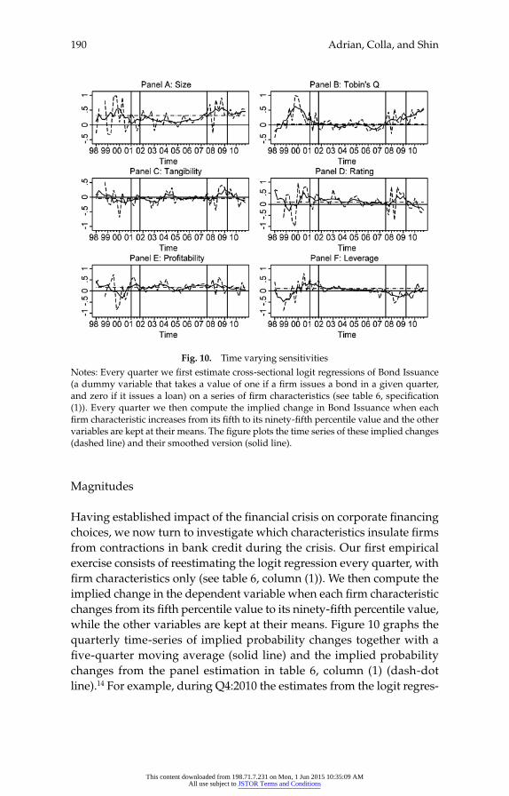
190 Adrian, Colla, and Shin
Magnitudes
Having established impact of the fi nancial crisis on corporate fi nancing
choices, we now turn to investigate which characteristics insulate fi rms
from contractions in bank credit during the crisis. Our fi rst empirical
exercise consists of reestimating the logit regression every quarter, with
fi rm characteristics only (see table 6, column (1)). We then compute the
implied change in the dependent variable when each fi rm characteristic
changes from its fi fth percentile value to its ninety- fi fth percentile value,
while the other variables are kept at their means. Figure 10 graphs the
quarterly time- series of implied probability changes together with a
fi ve- quarter moving average (solid line) and the implied probability
changes from the panel estimation in table 6, column (1) (dash- dot
line).14 For example, during Q4:2010 the estimates from the logit regres-
Fig. 10. Time varying sensitivities
Notes: Every quarter we fi rst estimate cross- sectional logit regressions of Bond Issuance
(a dummy variable that takes a value of one if a fi rm issues a bond in a given quarter,
and zero if it issues a loan) on a series of fi rm characteristics (see table 6, specifi cation
(1)). Every quarter we then compute the implied change in Bond Issuance when each
fi rm characteristic increases from its fi fth to its ninety- fi fth percentile value and the other
variables are kept at their means. The fi gure plots the time series of these implied changes
(dashed line) and their smoothed version (solid line).
This content downloaded from 198.71.7.231 on Mon, 1 Jun 2015 10:35:09 AMAll use subject to JSTOR Terms and Conditions

Which Financial Frictions? 191
sion predict a 26.3 percent and 79.4 percent probability of bond issu-
ance, respectively, for a fi rm with Size equal to 6.278 (fi fth percentile)
and 10.386 (ninety- fi fth percentile) while the other fi rm characteristics
are stuck at their Q4:2010 mean values. The rightmost point in fi gure
10, panel A, corresponds to 53.1 percent; that is, the difference between
these two probabilities. Figure 10 provides suggestive evidence that the
larger and more profi table fi rms, and those with more tangible assets
and better ratings, were more likely to resort to bond fi nancing during
the crisis, while heavily indebted fi rms were more likely to issue loans.
Interaction Effects
Further insights on the sensitivity of fi nancing choice to fi rm character-
istics can be obtained by augmenting the logit regression in column (2)
of table 6 with an interaction term between a given fi rm characteristic
and the crisis indicator.15
Regression results are reported in table 7. In line with our previous
fi ndings of table 6, the probability of bond issuance is positively related
to fi rm size, credit and project quality, and leverage. In addition, fi rms
are more likely to resort to bond fi nancing during the crisis.
Due to the nonlinearity, the sign of the interaction term need not cor-
respond to the direction of the effect of fi rm characteristics during the
crisis. Moreover, the statistical signifi cance of the interaction effect can-
not be evaluated by looking at the standard error of the interaction term
(Huang and Shields 2000). We therefore compute implied probabilities
of bond issuance outside and during the crisis, and test for signifi cant
differences between them.
Figure 11 graphs the results for the different fi rm characteristics. We
fi rst consider the coeffi cient estimates of the logit model with the inter-
action term between size and the crisis indicator (see table 7, column
(1)) and compute the implied probabilities of bond issuance during the
crisis over the entire range of values for fi rm size, keeping the other
fi rm characteristics at their means. The solid line in the left panel of fi g-
ure 11, panel A, plots these probabilities (Crisis = 1) as a function of Size,
and the dotted line portrays the same probabilities evaluated outside of
the crisis (Crisis = 0). In the right panel of fi gure 11, panel A, we plot the
difference in these predicted probabilities associated with a change in
the crisis indicator (solid line) together with its 95 percent confi dence
interval (shaded region).16 We then repeat the same steps for the logit
models in table 7, columns (2) to (6).
This content downloaded from 198.71.7.231 on Mon, 1 Jun 2015 10:35:09 AMAll use subject to JSTOR Terms and Conditions

192 Adrian, Colla, and Shin
Figure 11 shows that, conditional on the crisis, more profi table fi rms
and those with more tangible assets are more likely to issue bonds; the
difference in predicted probabilities increases with both tangibility and
profi tability and is statistically signifi cant for all fi rms (fi gure 11, panels
C and E).
Similarly, larger and better rated fi rms resort more to bond fi nancing
during the crisis; the difference in implied probabilities is positive and
statistically signifi cant for all fi rms with “Size” larger than the twenty-
fi fth percentile value (total assets larger than $1,405 million, fi gure 11,
panel A) and those with “Rating” above the twentieth percentile value
(Standard and Poor’s long-term issuer rating class BB- or higher, fi gure
11, panel D). We also document in fi gure 11, panels B and F, that the dif-
ference in predicted probabilities is decreasing in growth opportunities
Fig. 11. Sensitivity during crisis
Notes: Sensitivity of bond issuance probability to fi rm characteristics during and outside
the crisis. Implied probabilities are based on the logit regression specifi cations of table 7,
which include a series of fi rm characteristics, the crisis indicator, and an interaction term
between the crisis indicator and one selected fi rm characteristic. For every specifi cation,
the left panel plots the probability of bond issuance during (Crisis = 1, solid line) and out-
side the crisis (Crisis = 0, dotted line) over the entire range of values of the selected fi rm
characteristic, keeping the other control variables at their mean levels. The right panel
plots the difference in these predicted probabilities (solid line) together with its 95 percent
confi dence interval (shaded).
This content downloaded from 198.71.7.231 on Mon, 1 Jun 2015 10:35:09 AMAll use subject to JSTOR Terms and Conditions

Tab
le 7
Sen
siti
vit
y o
f F
irm
Ch
ara
cter
isti
cs d
uri
ng
th
e C
risi
s
Dep
. V
ari
ab
le: P
rob
ab
ilit
y o
f B
on
d v
s. L
oan
Iss
uan
ce
Fir
m c
hara
cter
isti
c
Siz
e
(1)
To
bin
’s Q
(2)
Tan
gib
ilit
y
(3)
Rati
ng
(4)
Pro
fi ta
bil
ity
(5)
Lev
erag
e
(6)
Siz
e 0.2
93**
*0.3
37**
*0.3
37**
*0.3
31**
*0.3
37**
*0.3
33**
*
(0.0
44)
(0.0
42)
(0.0
42)
(0.0
42)
(0.0
42)
(0.0
42)
To
bin
’s Q
0.0
69
0.0
67
0.0
59
0.0
65
0.0
61
0.0
66
(0.0
75)
(0.0
77)
(0.0
75)
(0.0
74)
(0.0
75)
(0.0
75)
Tan
gib
ilit
y
–0.2
66
–0.2
86
–0.3
45
–0.2
50
–0.2
85
–0.2
75
(0.2
04)
(0.2
03)
(0.2
17)
(0.2
04)
(0.2
03)
(0.2
03)
Rati
ng
0.0
51**
*0.0
53**
*0.0
53**
*0.0
39**
0.0
52**
*0.0
54**
*
(0.0
20)
(0.0
19)
(0.0
20)
(0.0
20)
(0.0
20)
(0.0
20)
Pro
fi ta
bil
ity
11
.041**
*11
.327**
*11
.323**
*11
.019**
*11
.294**
*11
.046**
*
(2.5
05)
(2.5
06)
(2.5
09)
(2.4
98)
(2.8
29)
(2.5
09)
Lev
erag
e 1.0
04**
*1.0
10**
*1.0
14**
*0.9
81**
*1.0
07**
*1.2
12**
*
(0.2
55)
(0.2
55)
(0.2
55)
(0.2
55)
(0.2
55)
(0.2
66)
Cri
sis
0.4
97**
*0.6
22**
*0.6
17**
*0.5
58**
*0.6
21**
*0.5
84**
*
(0.0
95)
(0.0
87)
(0.0
87)
(0.0
92)
(0.0
88)
(0.0
88)
Cri
sis
× F
irm
ch
ara
cter
isti
c 0.2
76**
*–
0.0
45
0.3
14
0.0
94**
*–
0.0
41
–1.4
92**
*
(0.0
70)
(0.1
24)
(0.3
28)
(0.0
30)
(4.6
60)
(0.5
34)
Ob
serv
ati
on
s 4,2
76
4,2
76
4,2
76
4,2
76
4,2
76
4,2
76
Pse
ud
o R
2
0.0
78
0.0
75
0.0
75
0.0
77
0.0
75
0.0
76
No
tes:
Th
is t
ab
le p
rese
nts
lo
git
reg
ress
ion
res
ult
s to
ex
pla
in t
he
sen
siti
vit
y o
f co
rpo
rate
fi n
an
cin
g c
ho
ices
to
fi r
m c
ha
ract
eris
tics
du
rin
g t
he
cris
is.
To
b
e in
clu
ded
in
th
e an
aly
sis,
we
req
uir
e a fi
rm
to
iss
ue
new
deb
t in
at
lea
st o
ne
qu
art
er b
etw
een
19
98
an
d 2
01
0,
to b
e ra
ted
th
e q
ua
rter
pri
or
to i
ssu
-an
ce,
an
d t
o h
av
e n
on
mis
sin
g v
alu
es f
or
fi rm
ch
ara
cter
isti
cs m
easu
red
on
e q
ua
rter
pri
or
to d
ebt
issu
an
ce.
Th
e d
epen
den
t v
ari
ab
le i
s B
on
d I
ssu
an
ce,
a d
um
my
vari
ab
le t
hat
tak
es a
valu
e o
f o
ne
if a
fi r
m i
ssu
es a
bo
nd
in
a g
iven
qu
art
er,
an
d z
ero
if
it i
ssu
es a
lo
an
. W
e re
po
rt l
og
it r
egre
ssio
n r
esu
lts
of
Bo
nd
Iss
uan
ce o
n a
set
of
fi rm
ch
ara
cter
isti
cs d
efi n
ed i
n t
ab
le B
1 a
nd
an
in
tera
ctio
n t
erm
defi
ned
as
the
pro
du
ct b
etw
een
th
e C
risi
s in
dic
ato
r a
nd
th
e fi
rm c
hara
cter
isti
c in
dic
ate
d i
n t
he
colu
mn
hea
der
. All
reg
ress
ion
s in
clu
de
a c
on
stan
t (u
nta
bu
late
d).
Sta
nd
ard
err
ors
are
clu
ster
ed a
t th
e fi
rm l
evel
an
d
rep
ort
ed i
n p
are
nth
eses
. **
*, *
*, a
nd
* d
eno
te s
tati
stic
al
sig
nifi
ca
nce
at
the
1 p
erce
nt,
5 p
erce
nt,
an
d 1
0 p
erce
nt
lev
els,
res
pec
tiv
ely.
This content downloaded from 198.71.7.231 on Mon, 1 Jun 2015 10:35:09 AMAll use subject to JSTOR Terms and Conditions

194 Adrian, Colla, and Shin
and indebtedness, and signifi cantly larger than zero for fi rms with To-
bin’s Q less than 3.552 (slightly above the ninety- fi fth percentile value)
and those with “Leverage” below 0.197 (75 percent percentile value).
Our analysis shows that fi rms that are larger or have more tangible
assets, higher credit ratings, better project quality, less growth opportu-
nities, and lower leverage, were better equipped to withstand the con-
traction of bank credit during the crisis.
Discussion
The full range of results in the present subsection can be pieced together
to draw some tentative conclusions. First of all, the decomposition of
borrowing into bank and bond fi nance, and the fi nding that bank and
bond fi nance evolve in opposite directions during the crisis allows us to
conclude that the contraction of bank credit was due to a fall in supply.
This fi nding is robust to the exclusion of fi rm quarters with simultane-
ous issuance of both loans and bonds, as well as to the inclusion of
industry fi xed effects (see the online appendix posted on the authors’
homepages). This conclusion is in line with Kashyap, Stein, and Wilcox
(1993), and points to a credit channel or risk- taking channel of mon-
etary policy.
A further identifi cation assumption in our analysis of corporate fi -
nancing choices is the conditioning on fi rm characteristics lagged one
quarter. This may raise concerns since inference may be confounded if
variation in fi rm characteristics is endogenous to unobserved variation
in fi nancing choices. We have therefore repeated the analysis in tables 6
and 7 and fi gure 11 measuring fi rm characteristics eight quarters prior
to debt issuance. This way the probability of issuing bonds at the onset
of the crisis (Q3:2007) is related to fi rm- level control variables measured
during Q3:2005, and the same probability at the trough of the crisis
(Q2:2009) depends on fi rm characteristics measured during Q2:2007.
Our results are unchanged when we use variables measured eight quar-
ters prior to debt issuance.
Finally, we corroborate evidence in Becker and Ivashina (2011) that
fi nancing choices are signifi cantly associated with aggregate proxies for
credit supply. A decrease in broker- dealer leverage or an increase in
EBP trigger a substitution from loans to bonds.
We have further investigated the role played by fi rm characteristics
during quarters of reduced bank credit supply. We have repeated the
analysis in table 7 by replacing the crisis indicator with our proxies for
This content downloaded from 198.71.7.231 on Mon, 1 Jun 2015 10:35:09 AMAll use subject to JSTOR Terms and Conditions

Which Financial Frictions? 195
credit supply, and adding the interaction between fi rm characteristics
and credit supply proxies. We confi rm the signifi cant association be-
tween fi nancing sources and the credit supply proxies we uncover in
table 7 (direct effect).
To understand whether (and how) fi rm characteristics affect the sub-
stitution from loans to bonds during episodes of credit supply contrac-
tion, we have reproduced the analysis in fi gure 11 using credit supply
proxies in lieu of the crisis indicator. Consistent with our previous
results, we fi nd that, regardless of the credit supply proxy employed,
larger fi rms resort more to bond fi nancing when banks credit supply
contracts. We fi nd overall evidence that the same holds true for less in-
debted fi rms, while the relevance of other fi rm characteristics is mixed.
IV. Model of Bank and Bond Finance
Motivated by our empirical results, we now sketch a model of direct
and intermediated credit. To set the stage, it is useful to take stock of the
desired empirical features encountered along the way.
• First, the contrast between loan and bond fi nancing points to the im-
portance of accommodating both direct and intermediated credit.
• Second, during the recent downturn, loan fi nancing contracted but
bond fi nancing increased to make up some of the gap.
• Third, even as the two categories of credit diverged in quantity, the
spreads on both types of credit rose.
• Fourth, bank lending changes dollar for dollar with a change in debt,
with equity being “sticky.” Thus, credit supply by banks is the conse-
quence of their choice of leverage for a given level of equity.
• Fifth, as a consequence, bank leverage is procyclical. Leverage is high
when assets are large.
We sketch a model that accommodates these fi ve features. It is a
model of direct and intermediated credit where lending by banks is
seen as the fl ip side of a credit risk model.17 Our model represents a de-
parture from existing approaches to modeling fi nancial frictions in two
respects. First, it departs from the practice of imposing a bank capital
constraint that binds only in the downturn. Instead, the capital con-
straint in our model binds all the time—both in good times and bad.
Indeed, during the booms, the constraint binds in spite of the dampened
risks.
This content downloaded from 198.71.7.231 on Mon, 1 Jun 2015 10:35:09 AMAll use subject to JSTOR Terms and Conditions

196 Adrian, Colla, and Shin
Second, it is a model that is aimed at replicating as faithfully as pos-
sible the procyclicality of leverage. We have seen from the scatter charts
of bank balance sheet management that banks adjust their assets dollar
for dollar through a change in debt, with equity remaining “sticky.” To
the extent that banking sector behavior is a key driver of the observed
outcomes, capturing these two features is important, and we address
our modeling task to replicating these features.
A. Bank Credit Supply
Bank credit supply is modeled as the fl ip side of a credit risk model,
where banks adjust lending so as to satisfy a risk constraint. In particu-
lar, banks are risk neutral and maximize profi t subject only to a value-
at- risk (VaR) constraint that limits the probability of bank failure. The
VaR constraint stipulates that the probability of bank failure has to be
no higher than some (small) threshold level α > 0.18 In keeping with
market practice, the particular model of credit risk that drives the VaR
constraint will be the Vasicek (2002) model, adopted by the Basel Com-
mittee for Banking Supervision (BCBS 2005).
The notation to be used is as follows. The bank lends out amount C
(with “C” standing for “credit”) at date 0 at the lending rate r, so that
the bank is owed (1 + r)C in date 1 (its notional assets). The lending is
fi nanced from the combination of equity E and debt funding L, where
L encompasses deposit and money market funding. The cost of debt
fi nancing is f so that the bank owes (1 + f )L at date 1 (its notional li-
abilities).
The economy has a continuum of binary projects, each of which suc-
ceeds with probability 1 – ε and fails with probability ε. Each project
uses debt fi nancing of 1, which the borrower will default on if the
project fails. Thus, if the project fails, the lender suffers a credit loss of
1. The correlation in defaults across loans follows the Vasicek (2002)
model. Project j succeeds (so that borrower j repays the loan) when Zj >
0, where Zj is the random variable
Zj = −�−1(ε) + �Y + 1 − �Xj (1)
where �(⋅) is the cumulative distribution function (c.d.f.) of the standard
normal, Y and {Xj} are independent standard normals, and ρ is a con-
stant between zero and one. Variable Y has the interpretation of the
economy- wide fundamental factor that affects all projects, while Xj is
the idiosyncratic factor for project j. The parameter ρ is the weight on
This content downloaded from 198.71.7.231 on Mon, 1 Jun 2015 10:35:09 AMAll use subject to JSTOR Terms and Conditions

Which Financial Frictions? 197
the common factor, which limits the extent of diversifi cation that lend-
ers can achieve. Note that the probability of default is given by
Pr(Zj < 0) = Pr( �Y + 1 − �Xj < �−1(ε))
= �(�−1(ε)) = ε. (2)
Conditional on Y, defaults are independent. The bank can remove
idiosyncratic risk by keeping C fi xed but diversifying across borrowers.
We assume that loans are packaged into bonds and banks hold such
diversifi ed bonds, rather than loans directly. By holding bonds, banks
can diversify away all idiosyncratic risk, and only the systematic risk
from the common factor Y is refl ected in the credit risk. The realized
value of the bank’s assets at date 1 is then given by the random variable
w(Y) where
w(Y) ≡ (1 + r)C ⋅ Pr(Zj ≥ 0|Y)
= (1 + r)C ⋅ Pr( �Y + 1 − �Xj ≥ �−1(ε)|Y)
= (1 + r)C ⋅ �
�Y − �−1(ε)
1 − �
⎛
⎝⎜⎞
⎠⎟. (3)
Then, the c.d.f. of w(Y) is given by
F(z) = Pr(w ≤ z)
= Pr(Y ≤ w−1(z))
= �(w−1(z))
= �
�−1(ε) + 1 − ��−1[z/(1 + r)C]
�
⎛
⎝⎜⎞
⎠⎟. (4)
The density over the realized assets of the bank is the derivative of (4)
with respect to z. Figure 12 plots the densities over asset realizations,
and shows how the density shifts to changes in the default probability
ε (left- hand panel) or to changes in ρ (right- hand panel). Higher values
of ε imply a fi rst degree stochastic dominance shift left for the asset re-
alization density, while shifts in ρ imply a mean- preserving shift in the
density around the mean realization 1 – ε.
The bank adjusts the size of its asset book C and funding L given eq-
uity E so as to keep its probability of default to α > 0. Since the bank is
risk- neutral and maximizes profi t, the VaR constraint binds whenever
expected return from the bond is positive. The constraint is that the
bank limits total assets so as to keep the probability of its own failure to
This content downloaded from 198.71.7.231 on Mon, 1 Jun 2015 10:35:09 AMAll use subject to JSTOR Terms and Conditions

198 Adrian, Colla, and Shin
α. Since the bank fails when the asset realization falls below its notional
liabilities (1 + f )L, the bank’s total assets C satisfi es
Pr(w < (1 + f )L) = �
�−1(ε) + 1 − ��−1[(1 + f )L/(1 + r)C]
�
⎛
⎝⎜⎞
⎠⎟= �. (5)
Rearranging (5), we can derive an expression for the ratio of notional
liabilities to notional assets for the bank.
Notional liabilitiesNotional assets
=(1 + f )L(1 + r)C
= ���−1(�) − �−1(ε)
1 − �
⎛
⎝⎜⎞
⎠⎟ (6)
From here on, we will use the shorthand φ to denote this ratio of no-
tional liabilities to notational assets. That is,
�(�, ε, �) ≡ �
��−1(�) − �−1(ε)
1 − �
⎛
⎝⎜⎞
⎠⎟, (7)
where φ is a monotonic transformation of the leverage ratio, lying be-
tween zero and one. The higher is φ, the higher is bank leverage and the
greater is credit supply.
We can solve for the bank’s total assets C and liability aggregate L
from (6) and the balance sheet identity C = E + L to give
C = E
1 − [(1 + r)/(1 + f )] ⋅ �and L = E
[(1 + f )/(1 + r)] ⋅ (1/�) − 1. (8)
Fig. 12. The two charts plot the densities over realized assets when C(1 + r) = 1
Notes: The left- hand chart plots the density over asset realizations of the bank when ρ =
0.1 and ε is varied from 0.1 to 0.3. The right- hand chart plots the asset realization density
when ε = 0.2 and ρ varies from 0.01 to 0.3.
This content downloaded from 198.71.7.231 on Mon, 1 Jun 2015 10:35:09 AMAll use subject to JSTOR Terms and Conditions

Which Financial Frictions? 199
Note that both C and L are proportional to bank equity E, so that an
aggregation property holds for bank lending and bank funding. There-
fore, the leverage of the bank and the banking sector are interchangeable
in our model, and is given by
Leverage = C
E= 1
1 − (1 + r)/(1 + f ) ⋅ �. (9)
B. Direct Credit
Now consider the credit coming directly from bond investors. Bond in-
vestors (“households”) are risk averse with mean- variance preferences,
and have identical risk tolerance τ. Households hold a portfolio con-
sisting of three component assets—risky bonds, cash, and deposits in
the bank. As stated already, deposits include claims on money market
funds that serve as the base of the shadow banking system. We assume
that deposits are guaranteed by the government (at least implicitly) so
that households treat cash and deposits as being perfect substitutes. We
also assume that the households have suffi cient endowments so that
the wealth constraint is not binding in their choice of holding for the
risky bonds. The demand for bonds (supply of credit) of mean- variance
investor i with risk tolerance τ is then given by the fi rst- order condition:
Ci = �[(1 − ε)(1 + r) − 1]
�2(1 + r)2, (10)
where σ2 is the variance of the bond with unit notional value.19 Clearly,
σ2 is a function of ρ and ε. The variance σ2 refl ects the fundamentals of
the asset realization density given in fi gure 12.
Suppose there is measure N of mean- variance investors in the
economy, and that T = τN. Aggregating the bond holdings across all
households, the aggregate supply of credit from bond investors is thus
given by:
CH =
T[(1 − ε)(1 + r) − 1]�2(1 + r)2
, (11)
where H stands for the household sector. In Appendix A, we show that
the variance σ2 is given by
�2 = �2(�
−1(ε), �−1(ε); �) − ε2, (12)
where �2(⋅, ⋅; �) is the cumulative bivariate standard normal with correla-
tion ρ.20
This content downloaded from 198.71.7.231 on Mon, 1 Jun 2015 10:35:09 AMAll use subject to JSTOR Terms and Conditions

200 Adrian, Colla, and Shin
The right- hand panel of fi gure 13 plots the variance σ2 as a function
of ε. The variance is maximized when ε = 0.5, and is increasing in ρ. The
left- hand panel of fi gure 13 plots the normalized leverage φ as a func-
tion of ε.
Since bank liabilities are fully guaranteed by the government they
earn the risk- free rate. Further, let the risk- free rate be zero, so that f =
0. Since bank credit supply is increasing in φ while bond investor credit
supply is decreasing in σ2, the effect of an increase in ε (assuming that ε
< 0.5) is to decrease credit supply from both groups of creditors.
C. Comparative Statics of Credit Supply
The risk premium on the bond is given by its expected return in excess
of the risk- free rate. Given our assumption that the risk- free rate is zero,
the risk premium π is given by
� = (1 − ε)(1 + r) − 1. (13)
Consider the iso- lending curves for banks that plot the combination
of default probability ε and risk premium π that give rise to the same
credit supply by banks. The iso- lending curve for banks corresponding
to bank credit CB is given by
�(ε) = 1 − E
CB
⎛⎝⎜
⎞⎠⎟
1 − ε�(ε)
− 1. (14)
Fig. 13. Left- hand panel plots the normalized leverage φ as a function of ε; right- hand
panel plots the variance σ2 as a function of epsilon for two values of ρ
This content downloaded from 198.71.7.231 on Mon, 1 Jun 2015 10:35:09 AMAll use subject to JSTOR Terms and Conditions

Which Financial Frictions? 201
For banks, the iso- lending curve has the property that when ε is
small, the iso- lending curve is close to being vertical in (ε, π)- space.
From (14), we have
′� (ε) = − 1 − E
CB
⎛⎝⎜
⎞⎠⎟
1 − ε�2
′� (ε) + 1�
⎡⎣⎢
⎤⎦⎥
, (15)
where ′� (ε) → −∞ as ε → 0. Hence, the slope of the iso- lending curve
tends to +∞ as ε → 0. Figure 14 plots the iso- lending curves in (ε, π)-
space for banks (left panel) and bond investors (right panel).
The vertical limiting case of the bank iso- lending curves is revealing
about the behavioral traits of banks. To say that the iso- lending curve
is vertical is to say that bank lending decisions depend only on the
“physical” risk ε, rather than the risk premium π. This feature comes
from the combination of the risk- neutrality of the bank, and the con-
straint that limits its probability of failure. Risk neutrality means that
the risk premium π enters only through its VaR constraint. Conven-
tional risk- averse portfolio investors would focus on the trade- off be-
tween physical risk ε and the risk premium π. The right- hand panel
of fi gure 14 shows the iso- lending curves of the bond investors, to be
derived shortly. Although we have used mean- variance preferences for
convenience for the bond investors, any conventional risk averse pref-
erences would imply a nontrivial trade- off between physical risk and
risk premium.
The bond investors’ iso- lending curves in (ε, π)- space follow from
Fig. 14. Iso- lending curves in (ε, π)- space for banks (left panel) and bond investors
(right panel)
Note: Parameter values are as indicated in the boxes.
This content downloaded from 198.71.7.231 on Mon, 1 Jun 2015 10:35:09 AMAll use subject to JSTOR Terms and Conditions

202 Adrian, Colla, and Shin
the supply of credit by households given by (11), from which we can
derive the following quadratic equation in π
CH�2
T(1 − ε)2(1 + �)2 − (1 + �) + 1 = 0. (16)
The iso- lending curve for bond investors corresponding to bond credit
supply of CH is given by
�(ε) =
1 − 1 − 4CH�2/T(1 − ε)2
2CH�2/T(1 − ε)2− 1. (17)
Let us now close the model by positing an aggregate demand for
credit. The demand for credit is a decreasing function of the risk pre-
mium, and is denoted by K(π). The market clearing condition is then
E
1 − [(1 + �)/(1 − ε)]�CB
+ T(1 − ε)2�
� 2(1 + �)2
CH
= K(�). (18)
How does the risk premium π vary to shifts in the physical risks ε?
Provided that ε is small—so that it lies in the plausible range for the
probability of default—and provided that the risk premium is not too
large, we can show that the risk premium π is an increasing function of ε.
Proposition 1. Suppose ε is small so that |∂�/∂ε|> �/(1 − ε) and the risk premium is small so that π < 1. Then the market risk premium π is strictly increasing in ε.
In other words, an increase in physical risk also raises the market risk
premium. To prove proposition 1, note fi rst that credit supply by bond
investors is declining in ε, and that bank lending declines in ε if
|∂�/∂ε|> �/(1 − ε). Meanwhile, we can also show ∂CB/∂� > 0 and—as-
suming π < 1—we also have ∂CH/∂� > 0 . Defi ning the excess supply
of credit function G(ε, π) ≡ CB + CH – K(π), we have
d�
dε= − ∂G/∂ε
∂G/∂�= − (∂CB/∂ε) + (∂CH/∂ε)
(∂CB/∂�) + (∂CH/∂�) − ′K (�)> 0. (19)
Since bank credit is declining in ε, the balance sheet identity implies
that the funding L used by banks is also declining.
This content downloaded from 198.71.7.231 on Mon, 1 Jun 2015 10:35:09 AMAll use subject to JSTOR Terms and Conditions

Which Financial Frictions? 203
D. Relative Size of Banking Sector
We now come to our key result, which addresses the relative size of
the banking sector and its relationship to risk premiums. Provided that
credit demand K(π) is not too elastic, a decline in ε is followed by an
increase in the size of the banking sector, both in absolute terms and as
a proportion to the total credit provided in the economy.
Proposition 2. Suppose that ε is small enough so that the iso- lending curve of banks is steeper than the iso- lending curve of bond investors. Then, there is M > 0 such that, provided ′K (�) ≤ M, an increase in ε is associated with a contraction of banking sector assets, both in absolute terms and as a proportion of the total credit received by borrowers.
Proposition 2 can be demonstrated using a graphical argument using
the iso- lending curves for banks and bond investors. Figure 15 illus-
trates an initial equilibrium given by the crossing point for the iso-
lending curves for banks and bond investors. In this illustration, total
credit supply is 20, with 10 coming from banks and 10 coming from
bond investors. The four regions indicated in fi gure 15 correspond to
the four combinations of credit supply changes by banks and bond
investors. Region A is when both banks and bond investors increase
credit supply, while region C is where both reduce credit supply.
Now, consider a negative economic shock that raises the default prob-
ability ε. Such a shock shifts the economy to the right- hand side of the
Fig. 15. Crossing point for the iso- lending curves of banks and households
This content downloaded from 198.71.7.231 on Mon, 1 Jun 2015 10:35:09 AMAll use subject to JSTOR Terms and Conditions

204 Adrian, Colla, and Shin
banks’ iso- lending curve, implying a decrease in bank credit. In addi-
tion, the market risk premium π rises, as a consequence of proposition
1. Since bank credit supply contracts, bond credit supply must increase
for the market to clear. Thus, the new equilibrium (ε, π) pair must lie
in region D in fi gure 15. In region D, bank credit supply contacts while
bond credit supply expands.
In this way, when default risk starts to increase as the fi nancial cycle
turns, there will be an amplifying effect through the risk premium π. As
ε increases due to the deterioration of fundamentals, we have the com-
bination of sharply higher risk premiums and the contraction in bank
lending. Bond investors are then induced by the higher risk premiums
to close the credit supply gap in the market. The recoiling from risks,
sharply higher risk premiums, and the substitution of bank lending by
bond fi nancing explains the substitution away from bank fi nancing to
bond fi nancing that we see in the data. Given a fairly inelastic credit
demand curve (at least in the short run), the sharp contraction in loans
from fi nancial intermediaries will have to be made up somehow. The
slack is taken up by the increase in bond fi nancing. However, for this
to happen, prices must adjust in order that the risk premium rises suf-
fi ciently to induce risk- averse bond investors to make up for the lost
banking sector credit. Thus, a fall in the relative credit supplied by the
banking sector is associated with a rise in risk premiums.
For macro activity, such a rise in the risk premium exerts contrac-
tionary effects on the real economy. Gilchrist, Yankov, and Zakrajšek
(2009) documents evidence that credit spreads have substantial effect on
macro activity measures. Thus, the fi nancial friction that such a mecha-
nism generates is one that works through prices, rather than through a
shrinkage in the total quantity of credit. Exactly how increased spreads
impact the real economy is a subject that is ripe for further investigation.
V. Modeling Financial Frictions
Since the fi nancial crisis, a new wave of dynamic, general equilibrium
macro models that incorporate fi nancial frictions have been developed.
The evidence in our study presents a challenge to many of these mod-
els, as we point to a very specifi c set of empirical facts, with tight im-
plications for the modeling of fi nancial frictions. The challenge for the
theory is to capture the fi ve stylized facts that we documented earlier:
(1) coexistence of bank and bond fi nance; (2) substitution from bank to
bond fi nance during recessions and crisis; (3) increasing credit spreads;
(4) stickiness of equity; (5) procyclicality of bank leverage. Our model
This content downloaded from 198.71.7.231 on Mon, 1 Jun 2015 10:35:09 AMAll use subject to JSTOR Terms and Conditions

Which Financial Frictions? 205
from the previous section presents a microfoundation that is rational-
izing all fi ve stylized facts. However, no dynamic general equilibrium
model has, to date, incorporated such a setup for the fi nancial sector. In
this section, we review the recent macroeconomic literature with fi nan-
cial frictions in light of our evidence.21
In the seminal contributions of Bernanke and Gertler (1989) and Ber-
nanke, Gertler, and Gilchrist (1999), the fi nancial accelerator generates
only one of the fi ve stylized facts: credit spreads increase during down-
turns. However, in the fi nancial accelerator approach, the fi nancial
friction resides with the corporate borrower. There are no banks, and
hence the model has nothing to say about the substitutability between
loans and bonds. In a recent extension of the Bernanke, Gertler, and Gil-
christ setting, Gertler and Kiyotaki (2010) use the frictions of Bernanke
and Gertler (1989) and apply them to both the corporate sector and
the banking sector. As a result, Gertler and Kiyotaki (2010) are able to
talk about the role of the banking sector in business cycle fl uctuations.
However, Gertler and Kiyotaki (2010) still do not generate procyclical
leverage of the fi nancial intermediaries. This is because of their assump-
tion of the particular fi nancing constraint.
Perhaps the most distinctive feature of bank balance sheet manage-
ment is the fact that banks adjust assets dollar for dollar through a
change in debt, with equity remaining sticky. We have not attempted
to resolve the microfoundations for such behavior, but understanding
the underlying corporate fi nance behind this feature seems critical. For
banks that adjust lending to shifts in VaR, a good rule of thumb is that
they adjust their balance sheets in order to keep their probability of
failure constant in the face of changing fi nancial conditions. In periods
of heightened market stress, banks contract lending and shed risky ex-
posures, while in tranquil conditions, banks expand lending so as to
utilize any slack in the balance sheet.
The banks’ practice of adjusting their assets dollar for dollar through
debt also poses some conceptual challenges for modeling of fi nancial
frictions. Many attempts at modeling fi nancial frictions have employed
log preferences, or constraints that bind only in the downturn. Recent
examples of analyses where one or both of these assumptions are em-
ployed are Brunnermeier and Sannikov (2009, 2010) and He and Krish-
namurthy (2010, 2012a, 2012b). The determination of risk premiums
and spillovers using log utility was examined by Xiong (2001).
Log utility has been a convenient means to simplify the dynamic
portfolio problem, as portfolio choices based on log utility imply lever-
age that is proportional to the ratio of the risk premium to the variance
This content downloaded from 198.71.7.231 on Mon, 1 Jun 2015 10:35:09 AMAll use subject to JSTOR Terms and Conditions

206 Adrian, Colla, and Shin
of returns (Merton 1969). In order for leverage to be procyclical, the
ratio of risk premium to variance of returns (equivalently, the Sharpe
ratio divided by volatility) must also be procyclical. However, support-
ing evidence is lacking. If anything, to the extent that the Sharpe ratio
tends to be low in booms and high in busts, it would be plausible to
fi nd that log utility investors show countercyclical leverage, rather than
procyclical leverage. To the extent that banking sector behavior is a key
driver of the observed outcomes, capturing procyclical leverage seems
crucial. On this score, it would be fair to say that existing macro models
of fi nancial frictions are still some way off from being fully satisfactory.
Imposing additional constraints on banks so that their lending con-
tracts would be one way to bring the model closer to observed behavior,
but such an approach implies constraints that bind only in the down-
turn, rather than binding all the time. The scatter charts we have seen
for the balance sheet management of banks suggest that such an asym-
metric approach may not be completely satisfactory.
In an international context, Mendoza (2010) develops a model of
emerging market crisis that does feature procyclical leverage of the
economy in the aggregate. Bianchi and Mendoza (2010) study a quan-
titative model of systemic risk, where agents do not take externalities
of fi nancial fragility on others into account. The model features over-
leveraging in the boom, countercyclical risk premiums, and excessive
volatility associated with the systemic risk externality. Jermann and
Quadrini (2012) study the fi nancial policies of the corporate sector in
a model that features procyclical leverage for the business sector. The
crucial ingredients to the model are adjustments at both the debt and
equity issuance margin. However, this model does not feature a bank-
ing sector, and therefore does not capture the substitution between loan
and bond fi nancing.
There is also a recent literature that is extending standard dynamic
stochastic general equilibrium (DSGE) models to include a banking sec-
tor. Gertler and Karadi (2011) present a parsimonious DSGE model with
a banking sector, production, and sticky prices, allowing them to study
monetary policy. The model again captures increases in spreads during
crisis, but does not produce a substitution between loans and bonds.
In addition, the paper does not feature the procyclicality of the bank-
ing sector that we documented earlier. Christiano, Motto, and Rostagno
(2009) offer a rich quantitative DSGE model with three production sec-
tors, and a banking sector. Curdia and Woodford (2009) incorporate
banks that intermediate between households. Nevertheless, the relative
This content downloaded from 198.71.7.231 on Mon, 1 Jun 2015 10:35:09 AMAll use subject to JSTOR Terms and Conditions

Which Financial Frictions? 207
size of the banking sector is not well addressed in these papers, where
all credit is intermediated credit.
One important message from our investigation is that net worth, by
itself, cannot serve as the state variable that fully determines fi nancial
conditions. The leverage of the banking sector emerges as being a key
determinant (and refl ection) of fi nancial conditions. As such, under-
standing how the leverage of fi nancial intermediaries fl uctuates over
the cycle emerges as perhaps the most pressing question in the study of
macroeconomic fl uctuations.
VI. Conclusion
The fi nancial crisis of 2007 to 2009 has sparked keen interest in models
of fi nancial frictions and their impact on macro activity. Most models
share the feature that corporate borrowers suffer a contraction in the
quantity of credit. However, the evidence suggests that although bank
lending contracts during the crisis, bond fi nancing actually increases
to make up much of the gap. This paper reviews both aggregate and
micro- level data and highlights the shift in the composition of credit
between loans and bonds.
The review of the evidence on the fl uctuations in credit to nonfi nan-
cial fi rms allows us to draw up a checklist of key empirical stylized
facts that may be used to guide the modeling exercise at the micro level.
Although the workhorse models of fi nancial frictions used in macro-
economics capture some key empirical features, they fail to address oth-
ers. We documented fi ve stylized facts:
1. Both bank and bond fi nancing are quantitatively important in pro-
viding credit to nonfi nancial corporations.
2. In the recent fi nancial crisis, and downturns more generally, credit
in the form of loans contract, but bond fi nancing increases to make up
most of the gap.
3. Credit spreads for both types of credit rise in downturns.
4. Bank lending changes dollar for dollar with a change in debt, with
equity being sticky. Thus, credit supply by banks is the consequence of
their choice of leverage.
5. Bank leverage is procyclical.
Motivated by this evidence, we have formulated a model of direct
and intermediated credit that captures these fi ve stylized facts. In our
This content downloaded from 198.71.7.231 on Mon, 1 Jun 2015 10:35:09 AMAll use subject to JSTOR Terms and Conditions

208 Adrian, Colla, and Shin
model, the impact on real activity comes from the spike in risk premi-
ums, rather than contraction in the total quantity of credit. However, to
date, none of the macroeconomic equilibrium models have adequately
addressed all fi ve stylized facts. In reviewing the recent literature, we
uncover that some models capture the procyclicality, others offer a
substitution between bond and loan fi nancing, but no model captures
all fi ve stylized facts. Embedding a model such as the one we present
within a general equilibrium framework appears as a promising avenue
for research.
Appendix A
Variance of Asset Realizations in Vasicek (2002)
In this appendix, we present the derivation of the variance of the nor-
malized asset realization w(Y) = w(Y)/C(1 + r) in Vasicek (2002). Let
k = �−1(ε) and X1, X2, . . ., Xn be i.i.d. standard normal. Thus,
E[wn] = E �Y � − k
1 − �
⎛
⎝⎜⎞
⎠⎟⎛
⎝⎜⎞
⎠⎟
n⎡
⎣⎢⎢
⎤
⎦⎥⎥
= E Pr �Y + 1 − �Xi > k Y⎡
⎣⎤⎦i=1
n∏⎡⎣ ⎤⎦
= E Pr �Y + 1 − �X1 > k,… , �Y + 1 − �Xn > k Y⎡
⎣⎤⎦
⎡⎣
⎤⎦
= Pr �Y + 1 − �X1 > k,… , �Y + 1 − �Xn > k⎡
⎣⎤⎦
= Pr[Z1 > k,… , Zn > k] ,
where (Z1, . . ., Zn) is multivariate standard normal with correlation ρ.
Hence
E[w] = 1 − ε
and
�2 = var[w] = var[1 − w]
= Pr[1 − Z1 ≤ k, 1 − Z2 ≤ k] − ε2
= �2(k, k; �) − ε2
= �2(�−1(ε), �−1(ε); �) − ε2,
where �2(⋅, ⋅; �) is the cumulative bivariate standard normal with corre-
lation ρ.
This content downloaded from 198.71.7.231 on Mon, 1 Jun 2015 10:35:09 AMAll use subject to JSTOR Terms and Conditions

Ap
pen
dix
B
Var
iab
le C
onst
ruct
ion
Tab
le B
1V
ari
ab
le D
escr
ipti
on
Vari
ab
le
D
escr
ipti
on
So
urc
e
A. I
ssue
Lev
el In
dica
tors
Lo
an
P
rim
ary
pu
rpo
se “
Cap
ital
exp
end
itu
re”, “
Co
rpo
rate
pu
rpo
ses”
, “
Eq
uip
men
t p
urc
hase
”,
“In
frast
ruct
ure
”, “
Rea
l es
tate
”, “
Tra
de
fi n
an
ce”, o
r “
Wo
rkin
g c
ap
ital”
LP
C
Rev
olv
er
Lo
an
ty
pe
is “
Rev
olv
er/
Lin
e <
1 Y
r.”, “
Rev
olv
er/
Lin
e >
= Y
r.”, “
Rev
olv
er/
Ter
m L
oan
”, o
r “
364
-
Day
Faci
lity
”
LP
C
Ter
m l
oan
L
oan
ty
pe
is “
Ter
m L
oan
”, o
r “
Ter
m L
oan
” w
ith
tra
nch
e in
dic
ato
r A
to
H
LP
C
Bo
nd
P
rim
ary
use
“B
uil
din
gs”
, “
Cap
ital
exp
end
itu
res”
, “
Co
nst
ruct
ion
”, “
Gen
eral
corp
ora
te
pu
rpo
se”, “
Pro
per
ty d
evel
op
men
t”,
“R
ail
way
s”, “
Wo
rkin
g c
ap
ital”
SD
C
B. F
irm
Lev
el V
aria
bles
Siz
e ln
(Ass
ets
[atq
], e
xp
ress
ed i
n J
an
uary
1998 c
on
stan
t U
SD
mln
.)
Co
mp
ust
at
To
bin
’s Q
(A
sset
s +
Mark
et v
alu
e o
f eq
uit
y [
prc
cq*c
shp
rq]
– C
om
mo
n e
qu
ity
[ce
] –
Def
erre
d t
ax
es
[tx
dit
cq])
/ A
sset
s. B
ou
nd
ed a
bo
ve
at
10.
Co
mp
ust
at
Tan
gib
ilit
y
Net
pro
per
ty, p
lan
t, a
nd
eq
uip
men
t (p
pen
tq)
/ A
sset
s C
om
pu
stat
Rati
ng
E
ach
mo
nth
ly S
&P
lo
ng
- ter
m i
ssu
er r
ati
ng
(sp
ltic
rm)
is a
ssig
ned
an
in
teg
er n
um
ber
ran
gin
g
fro
m 1
(S
D o
r D
) to
21 (
A).
Rati
ng
is
the
qu
art
erly
av
erag
e o
f m
on
thly
rati
ng
s.
Co
mp
ust
at
Pro
fi ta
bil
ity
O
per
ati
ng
in
com
e b
efo
re d
epre
ciati
on
(o
ibd
qp
) /
Ass
ets
Co
mp
ust
at
Lev
erag
e
(Deb
t in
cu
rren
t li
ab
ilit
ies
(dlc
q)
+ L
on
g- t
erm
deb
t (d
lttq
)) /
Ass
ets
C
om
pu
stat
(con
tinu
ed)
This content downloaded from 198.71.7.231 on Mon, 1 Jun 2015 10:35:09 AMAll use subject to JSTOR Terms and Conditions

Tab
le B
1C
on
tin
ued
Vari
ab
le
D
escr
ipti
on
So
urc
e
C. t
ime
seri
es v
aria
bles
Cri
sis
Ind
icato
r v
ari
ab
le e
qu
al
to o
ne
for
each
of
the
eig
ht
qu
art
ers
bet
wee
n Q
3:2
007 a
nd
Q2:2
009, an
d
zer
o o
ther
wis
e.
BD
lev
erag
e A
nn
ual
gro
wth
in
bro
ker
- dea
ler
lev
erag
e.
Fed
eral
Res
erv
e
EB
P
E
xce
ss b
on
d p
rem
ium
(in
per
cen
tag
e p
oin
ts).
Gil
chri
st a
nd
Zak
rajš
ek (
2011
)
No
tes:
Th
is t
ab
le p
rov
ides
a d
etail
ed d
escr
ipti
on
of
ou
r v
ari
ab
le c
on
stru
ctio
n.
Ch
ara
cter
isti
cs o
f n
ew d
ebt
issu
an
ces
in p
an
el A
are
ret
riev
ed f
rom
the
Lo
an
Pri
cin
g C
orp
ora
tio
n’s
Dea
lsca
n d
ata
base
of
new
lo
an
iss
uan
ces
(LP
C)
an
d t
he
Sec
uri
ties
Data
Co
rpo
rati
on
’s N
ew B
on
d I
ssu
an
ces
data
-
base
(S
DC
). F
irm
ch
ara
cter
isti
cs i
n p
an
el B
are
ret
riev
ed f
rom
th
e C
om
pu
stat
qu
art
erly
data
base
. T
ime
seri
es v
ari
ab
les
in p
an
el C
are
ob
serv
ed a
t
qu
art
erly
fre
qu
ency
.
This content downloaded from 198.71.7.231 on Mon, 1 Jun 2015 10:35:09 AMAll use subject to JSTOR Terms and Conditions

Which Financial Frictions? 211
Endnotes
Paper for the NBER Macro Annual Conference, April 20–21, 2012. We thank Daron Acemoglu, Olivier Blanchard, Thomas Eisenbach, Mark Gertler, Simon Gilchrist, Arvind Krishnamurthy, Guido Lorenzoni, Jonathan Parker, Michael Woodford, and participants at the Chicago Macroeconomic Fragility conference and the 2012 AEA meetings for com-ments on earlier versions of the paper. We also thank Michael Roberts and Simon Gil-christ for making available data used in this paper. For acknowledgments, sources of research support, and disclosure of the authors’ material fi nancial relationships, if any, please see http://www.nber.org/chapters/c12741.ack.
1. Notice that the slopes of the two fi tted lines add up to 1 in fi gure 3. This is a conse-quence of the balance sheet identity: ∆At = ∆Et + ∆Dt, and the additivity of covariance.
2. We measure the cost of loans with the all- in- drawn spread, which is defi ned as total (recurring fees plus interest) spread paid over six- month London Interbank Offered Rate (LIBOR) for each dollar drawn down. On occasions, we also make use of the all- in un-drawn spread as a measure of the cost a borrower pays for each dollar available (but not drawn down) under a credit line. Bradley and Roberts (2004) and Strahan (1999) contain further details on how LPC computes spreads.
3. Loan fi nancing may be intended for a variety of purposes. Stated purposes (based on the LPC fi eld “primary purpose”) can be broadly grouped into M&A (acquisition, takeover, LBO/MBO), refi nancing/capital structure management (debt repayment, re-capitalization, and stock repurchase), liquidity management (working capital and trade fi nance), and general corporate purposes (corporate purposes and capital expenditure); credit lines may also serve as commercial paper backup (see, among others, Drucker and Puri [2009] for a classifi cation of loan purposes). Following Ivashina and Scharfs-tein (2010), we consider as real investment loans those used for general corporate pur-poses and liquidity management. Specifi cally, we defi ne as real investment loans those with LPC primary purpose “Capital expenditure”, “Corporate purposes”, “Equipment purchase”, “Infrastructure”, “Real estate”, “Trade fi nance”, or “Working capital.” After merging LPC with Compustat the vast majority of loan facilities in our fi nal sample are extended for corporate purposes (7,029 issuances, corresponding to 56.81 percent of our sample) or working capital (4,971 issuances, 40.18 percent of our sample).
4. The May 2010 linking table provided by Michael Roberts enables us to match 11,765 loans with our Compustat sample; we further link 608 loans issued in 2010. We match a loan (and a bond) issued in a given quarter with Compustat data for the same quarter.
5. We measure the cost of bonds with the spread to benchmark, which is defi ned by SDC as the number of basis points over the comparable maturity treasury. Our results are qualitatively unchanged if we measure the cost of bonds subtracting the six- month LIBOR from the yield to maturity (see the online appendix).
6. Mirroring our classifi cation of loans, we defi ne a real investment bond as having pri-mary purpose (based on the SDC fi eld “primary use of proceeds”) “Buildings”, “Capital expenditures”, “Construction”, “General corporate purpose”, “Property development”, “Railways”, “Working capital.”
7. With our data sets we cannot determine whether a credit line, after being extended, is indeed used. However, Campello et al. (2011) show that fi rms drew down on their lines during the crisis, which suggests that the all- in- drawn spread is indeed the proper mea-sure of the cost of revolvers during the crisis. An alternative measure for the cost of credit lines during the crisis by using the all- in- undrawn spread, is shown in fi gure 6, panel D. Even here, we uncover a steep increase in the cost of new fi nancing during the crisis, which tripled relative to precrisis levels (331 bps during Q2:2009).
8. If we used the all- in- undrawn spread for revolvers during the fi nancial crisis, the cost of bank fi nancing would more than double to 215 bps during Q2:2009.
9. Our type split (credit lines and term loans) covers 97 percent of all loans in our sample, which is why the sum of loan types does not add to total loan fi nancing in fi gure 7, panel A. Loans that are not classifi ed include bridge loans, delay draw term loans, synthetic leases, and other loans.
This content downloaded from 198.71.7.231 on Mon, 1 Jun 2015 10:35:09 AMAll use subject to JSTOR Terms and Conditions

212 Adrian, Colla, and Shin
10. We exclude new debt tranches (and thus, possibly fi rms) issued before the crisis that mature before Q2:2007, and those issued during the crisis that mature before Q2:2009.
11. We include only fi rm- level variables in an attempt to isolate the effect of borrower’s preferences. Relative to Denis and Mihov (2003) we therefore exclude the amount issued because it may partially refl ect supply.
12. We thank Simon Gilchrist for sharing this series with us.13. We refer to a contraction in bank credit supply as an increase in EBP from its fi fth to
ninety- fi fth percentile, or a decrease in BD leverage from its ninety- fi fth to fi fth percentile.14. Figure 10 does not include Q3:1998 because a linear combination of the control
variables exactly predicts Bond Issuance (eight bond and eleven loan issuances).15. The interaction term is very highly correlated with the crisis indicator—correla-
tions range between 0.82 and 0.98. To avoid multicollinearity concerns, we therefore de-mean fi rm characteristics before creating the interaction terms. As a result, correlations between the interaction term and Crisis oscillate between –0.16 and 0.28.
16. To assess statistical signifi cance we use 1,000 draws from a multivariate normal distribution with mean equal to the estimated coeffi cient vector from the logit model, and variance matrix equal to the estimated variance- covariance matrix for the coeffi cient estimates (King, Tomz, and Wittenberg 2000; Zelner 2009).
17. The model was introduced in Shin (2011) in the context of cross- border banking and capital fl ows.
18. See Adrian and Shin (2008) for a possible microfoundation for the VaR constraint as a consequence of constraints imposed by creditors.
19. Equivalently, σ2 is the variance of w(Y)/(1 + r)C. 20. See Vasicek (2002) for additional properties of the asset realization function w(Y). 21. Brunnermeier, Eisenbach, and Sannikov (2011) and Quadrini (2011) offer more
comprehensive surveys of the literature on general equilibrium macroeconomic models with fi nancial frictions.
References
Adrian, Tobias, Emmanuel Moench, and Hyun Song Shin. 2011. “Financial In-termediation, Asset Prices, and Macroeconomic Dynamics.” Federal Reserve Bank of New York Staff Report no. 422.
Adrian, Tobias, and Hyun Song Shin. 2008. “Procyclical Leverage and Value at Risk.” Federal Reserve Bank of New York Staff Report no. 338.
———. 2010. “Liquidity and Leverage.” Journal of Financial Intermediation 19 (3): 418–37.
Basel Committee on Banking Supervision. 2005. “International Convergence of Capital Measurement and Capital Standards: A Revised Framework.” Bank for International Settlements, November 2005. http://www.bis.org/publ/bcbs118.pdf
Becker, Bo, and Victoria Ivashina. 2011. “Cyclicality of Credit Supply: Firm Level Evidence.” Working Paper, Harvard Business School.
Berlin, Mitchell, and Loretta Mester. 1992. “Debt Covenants and Renegotia-tion.” Journal of Financial Intermediation 2:95–133.
Bernanke, Ben, and Mark Gertler. 1989. “Agency Costs, Net Worth, and Busi-ness Fluctuations.” American Economic Review 79 (1): 14–31.
Bernanke, Ben, Mark Gertler, and Simon Gilchrist. 1999. “The Financial Accel-erator in a Quantitative Business Cycle Framework.” In Handbook of Macro-economics, edited by John B. Taylor and Michael Woodford, 1341–93. North Holland: Elsevier.
Bianchi, Javier, and Enrique Mendoza. 2010. “Overborrowing, Financial Crises and ‘Macro- Prudential’ Taxes.” Working Paper, University of Maryland.
Bolton, Patrick, and Xavier Freixas. 2000. “Equity, Bonds, and Bank Debt: Capi-
This content downloaded from 198.71.7.231 on Mon, 1 Jun 2015 10:35:09 AMAll use subject to JSTOR Terms and Conditions

Which Financial Frictions? 213
tal Structure and Financial Market Equilibrium under Asymmetric Informa-tion.” Journal of Political Economy 108 (2): 324–51.
Bradley, Michael, and Michael R. Roberts. 2004. “The Structure and Pricing of Corporate Debt Covenants.” Working Paper, Duke University.
Brunnermeier, Markus, Thomas Eisenbach, and Yuliy Sannikov. 2011. “Macro-economics with Financial Frictions: A Survey.” Working Paper, Princeton University.
Brunnermeier, Markus, and Yuliy Sannikov. 2009. “A Macroeconomic Model with a Financial Sector.” Working Paper, Princeton University.
———. 2010. “The i Theory of Money.” Working Paper, Princeton University.Campello, Murillo, Erasmo Giambona, John R. Graham, and Campbell H. Har-
vey. 2011. “Liquidity Management and Corporate Investment during a Fi-nancial Crisis.” Review of Financial Studies 24 (6): 1944–79.
Chava, Sudheer, and Michael R. Roberts. 2008. “How Does Financing Impact Investment? The Role of Debt Covenants.” Journal of Finance 63 (5): 2085–121.
Christiano, Lawrence, Roberto Motto, and Massimo Rostagno. 2009. “Financial Factors in Economic Fluctuations.” Working Paper, Northwestern University.
Curdia, Vasco, and Michael Woodford. 2009. “Credit Spreads and Optimal Monetary Policy.” Federal Reserve Bank of New York Staff Report no. 385.
De Fiore, Fiorella, and Harald Uhlig. 2011. “Bank Finance versus Bond Fi-nance.” Journal of Money, Credit, and Banking 43:1399–421.
———. 2012. “Corporate Debt Structure and the Financial Crisis.” Working Pa-per, University of Chicago.
Denis, David J., and Vassil T. Mihov. 2003. “The Choice Among Bank Debt, Non- Bank Private Debt, and Public Debt: Evidence from New Corporate Borrowings.” Journal of Financial Economics 70 (1): 3–28.
Drucker, Steven, and Manju Puri. 2009. “On Loan Sales, Loan Contracting, and Lending Relationships.” Review of Financial Studies 22 (7): 2835–72.
Duchin, Ran, Oguzhan Ozbas, and Berk A. Sensoy. 2010. “Costly External Fi-nance, Corporate Investment, and the Subprime Mortgage Credit Crisis.” Journal of Financial Economics 97 (3): 418–35.
Faulkender, Michael, and Mitchell A. Petersen. 2006. “Does the Source of Capi-tal Affect Capital Structure?” Review of Financial Studies 19 (1): 45–79.
Gertler, Mark, and Simon Gilchrist. 1993. “The Role of Credit Market Imperfec-tions in the Monetary Transmission Mechanism: Argument and Evidence.” Scandinavian Journal of Economics 95 (1): 43–64.
———. 1994. “Monetary Policy, Business Cycles, and the Behavior of Small Manufacturing Firms.” Quarterly Journal of Economics 109 (2): 309–40.
Gertler, Mark, and Peter Karadi. 2011. “A Model of Unconventional Monetary Policy.” Journal of Monetary Economics 58 (1): 17–34.
Gertler, Mark, and Nobuhiro Kiyotaki. 2010. “Financial Intermediation and Credit Policy in Business Cycle Analysis.” In Handbook of Monetary Econom-ics, edited by Benjamin M. Friedman and Michael Woodford, 547–99. North Holland: Elsevier.
Gilchrist, Simon, Vladimir Yankov, and Egon Zakrajšek. 2009. “Credit Mar-ket Shocks and Economic Fluctuations: Evidence from Corporate Bond and Stock Markets.” NBER Working Paper no. 14863. Cambridge, MA: National Bureau of Economic Research.
Gilchrist, Simon, and Egon Zakrajšek. 2011. “Credit Spreads and Business Cycle Fluctuations.” American Economic Review 102 (4): 1692–720.
He, Zhiguo, and Arvind Krishnamurthy. 2010. “Intermediary Asset Pricing.” Working Paper, Northwestern University.
This content downloaded from 198.71.7.231 on Mon, 1 Jun 2015 10:35:09 AMAll use subject to JSTOR Terms and Conditions

214 Adrian, Colla, and Shin
———. 2012a. “A Model of Capital and Crises.” Review of Economic Studies 79 (2): 735–77.
———. 2012b. “A Macroeconomic Framework for Quantifying Systemic Risk.” Working Paper, Northwestern University.
Holmström, Bengt, and Jean Tirole. 1997. “Financial Intermediation, Loanable Funds, and the Real Sector.” Quarterly Journal of Economics 112 (3): 663–92.
Houston, Joel, and Christopher James. 1996. “Bank Information Monopolies and the Mix of Private and Public Debt Claims.” Journal of Finance 51 (5): 1863–89.
Huang, Chi, and Todd G. Shields. 2000. “Interpretation of Interaction Effects in Logit and Probit Anlyses: Reconsidering the Relationship between Registra-tion Laws, Education, and Voter Turnout.” American Politics Research 28 (1): 80–95.
Ivashina, Victoria, and David S. Scharfstein. 2010. “Bank Lending during the Financial Crisis of 2008.” Journal of Financial Economics 97 (3): 319–38.
Jermann, Urban, and Vincenzo Quadrini. 2012. “Macroeconomic Effects of Fi-nancial Shocks.” American Economic Review 102 (1): 238–71.
Kashyap, Anil, Jeremy Stein, and David Wilcox. 1993. “Monetary Policy and Credit Conditions: Evidence from the Composition of External Finance.” American Economic Review 83 (1): 78–98.
King, Gary, Michael Tomz, and Jason Wittenberg. 2000. “Making the Most of Statistical Analyses: Improving Interpretation and Presentation.” American Journal of Political Science 44 (2): 347–61.
Kiyotaki, Nobuhiro, and John Moore. 1997. “Credit Cycles.” Journal of Political Economy 105 (2): 211–48.
Krishnaswami, Sudha, Paul A. Spindt, and Venkat Subramaniam. 1999. “Infor-mation Asymmetry, Monitoring, and the Placement Structure of Corporate Debt.” Journal of Financial Economics 51 (3): 407–34.
Mendoza, Enrique. 2010. “Sudden Stops, Financial Crises and Leverage.” American Economic Review 100 (5): 1941–66.
Merton, Robert C. 1969. “Lifetime Portfolio Selection under Uncertainty: The Continuous- Time Case.” Review of Economics and Statistics 51 (3): 247–57.
Quadrini, Vincenzo. 2011. “Financial Frictions in Macroeconomic Fluctua-tions.” Working Paper, University of Southern California.
Repullo, Rafael, and Javier Suarez. 2000. “Entrepreneurial Moral Hazard and Bank Monitoring: A Model of the Credit Channel.” European Economic Review 44 (10): 1931–50.
Shin, Hyun Song. 2011. “Global Banking Glut and Loan Risk Premium.” Work-ing Paper, Princeton University.
Strahan, Philip E. 1999. “Borrower Risk and the Price and Nonprice Terms of Bank Loans.” Federal Reserve Bank of New York Staff Report no. 90.
Vasicek, Oldrich A. 2002. “The Distribution of Loan Portfolio Value.” Risk 15 (12): 160–62.
Xiong, Wei. 2001. “Convergence Trading with Wealth Effects: An Amplifi ca-tion Mechanism in Financial Markets.” Journal of Financial Economics 62 (2): 247–92.
Zelner, Bennet A. 2009. “Using Simulation to Interpret Results from Logit, Probit, and Other Nonlinear Models.” Strategic Management Journal 30 (12): 1335–48.
This content downloaded from 198.71.7.231 on Mon, 1 Jun 2015 10:35:09 AMAll use subject to JSTOR Terms and Conditions