[This paper is still in preliminary form; please do not quote without permission from the authors. ]

DO RESERVATION POLICIES AFFECT PRODUCTIVITY

IN THE INDIAN RAILWAYS?

Ashwini Deshpande* and Thomas E. Weisskopf**

November 2009

Abstract: Our objective in this paper is to shed some empirical light on a claim often made by critics of affirmative action policies: that increasing the representation of members of marginalized communities in jobs – and especially in relatively skilled positions – comes at a cost of reduced efficiency. We undertake a systematic empirical analysis of productivity in the Indian Railways in order to determine whether the policy of reserving jobs for Scheduled Castes and Scheduled Tribes has actually reduced productive efficiency in the railway system. We find no evidence that affirmative action in hiring has reduced the efficiency of the Indian Railways. Indeed, some of our results suggest that the opposite is true, providing tentative support for the claim that greater labour force diversity boosts productivity. JEL codes: J 78; L 92 *Delhi School of Economics, University of Delhi, India. Email: ashwini@econdse.org ** University of Michigan, Ann Arbor, USA. Email: tomw@umich.edu Acknowledgements: Financial support for this paper was provided by the Research Office of the Office of the Dean, College of Literature, Science & the Arts; by the Center for South Asian Studies; and by the Residential College (all at the University of Michigan, Ann Arbor); as well as by a research grant from Anthony Heath, one of the organizers of the British Academy conference on international experiences of affirmative action. Smriti Sharma provided sterling research assistance. We are especially grateful to K. L, Krishna, B.N.Goldar, J.V. Meenakshi and G. Alivelu for critical insights and suggestions. Staff of the Railway Board library and offices were helpful during the data collection process. Needless to add, we are responsible for all errors and omissions.

1

1. Affirmative Action in India

Many countries around the world have introduced affirmative action policies in an effort

to reduce historically persistent social, political and economic disadvantages of marginalized communities. Affirmative action (AA) may be defined as the provision of some amount of preference, in processes of selection to desirable positions in a society, to members of groups that are under-represented in those positions. Whatever the form in which such preference is provided, it always has the effect of increasing the number of members of an eligible under-represented group selected to a desirable position.1 In India AA has from the beginning taken the form of "reservations" (reserved seats or positions), to which eligible candidates can gain access without competing with candidates from non-eligible groups.2

Reservation policies in India originated in the early 20th century in some of the southern provinces of the country, under the British Raj, in response to growing popular movements against domination by members of the (uppermost) Brahmin caste. Shortly after independence in 1947, the framework for India's current AA policies was grounded firmly in the national constitution – although the Indian constitution’s authorization of preferences for particular groups coexists uneasily with its general affirmation of equal opportunity and non-discrimination. In the political domain seats are reserved in central and state legislative assemblies for candidates from disadvantaged groups, in constituencies where those groups form a relatively significant (though still a minority) part of the population.

India's AA policies are also applied in the spheres of employment and education, and it is in these spheres that such policies are most controversial. Reservations in jobs and in admissions to higher educational institutions are mandated throughout most of the public sector – including government services, government enterprises and government-controlled colleges and universities – with just a few exceptions (e.g., in key strategic areas such as national defense). On the other hand, reservation policies do not apply at all to private enterprises, and private educational institutions have rarely been concerned about representation of marginalized groups. Indeed, the last 4-5 years have seen fierce opposition to a central government proposal to extend AA to private sector employment. One of the outcomes of the debate has been the formulation by the Confederation of Indian Industries (CII) of a set of purely voluntary measures geared towards the expression of corporate social responsibility rather than the implementation of AA policies to remedy systematic under-representation of marginalized groups.

The primary Indian beneficiaries of affirmative action are the "Scheduled Castes" (SCs), former "untouchables" now often called Dalits, and the "Scheduled Tribes" (STs), indigenous tribes marginalized from mainstream Indian society and often called Adivasis. In 2001 the SC and ST constituted about 16 percent and 8 percent of the Indian population, respectively.3 These are the only groups for whom seats are reserved in the national legislature as well as in state 1 Note that AA does not necessarily result in the displacement of better qualified applicants from the general population by less qualified applicants from marginalized groups. Depending on the circumstances, an AA policy might either help to offset biases in conventional selection procedures or introduce additional biases into such procedures. 2 See Weisskopf (2004), chapter 1, for a detailed discussion of affirmative action policies in India (with comparisons to AA in the United States). 3 According to the 2001 Census of India, Scheduled Castes and Scheduled Tribes accounted for 16.2 per cent and 8.2 per cent of the Indian population, respectively.

2

legislative assemblies. The proportions of reserved seats for SCs and STs in public sector institutions under the control of the Central Government – 15 and 7.5 percent – were set roughly according to the proportions of these groups in the overall Indian population. Likewise, the proportions of reserved seats for SCs and STs at the state level are set roughly in according to their proportions in the state populations. However, quotas for the most desirable positions are usually only partially filled, because of an insufficient number of eligible candidates who meet the minimum qualifications set for such positions.

In addition to SCs and STs, a substantial share of the Indian population belonging to “Other Backward Classes” (OBCs) has long been eligible for reservations in public sector employment and in admissions to public higher educational institutions within most Indian states.4 In principle, OBCs encompass communities that are socially and economically relatively deprived; they are often also marginalized by caste discrimination – albeit to a lesser extent than Dalits. Since the early 1990s OBCs have become eligible for employment and educational reservations at the all-India level too. At this level OBCs – defined according to a set of economic and social criteria outlined by a Central Government commission – are currently eligible for reservations of 27% of available seats.5

Critics of AA policies have raised many different kinds of arguments against them. In India, the most frequent complaint about reservation policies is that they conflict with considerations of merit and result in the selection of less qualified candidates ahead of more qualified candidates. Most critics argue that a poorer quality of government service, or poorer academic performance, is to be expected from the beneficiaries of reservations. For example, in a sharp attack on a proposed expansion of all-India reservations to OBCs, Ashok Guha (1990a, 1990b) wrote that reservations in public employment impair the efficiency and quality of public services by reducing the average competence standard of civil service entrants, reduce their incentive to perform well and their motivation to improve, undermine the morale of workers and supervisors, and stimulate caste conflict in public institutions, thus harming teamwork and cooperation. In a more moderate critique, A.M. Shah (1991: 1734) wrote that: “Efficiency or merit is not a fetish of the elite, as frequently alleged. It is in fact an essential ingredient in every field of life…The policy of job reservations needs to be replaced by effective programmes of affirmative action to promote efficiency, merit and skills among the weaker sections of society….This does not mean that we abandon the goal of social justice but use different methods to achieve the same goal.” Some critics have even suggested that the failure to allocate key jobs on a strictly meritocratic basis has resulted in very serious harm as well as gross inefficiency. Critics have even charged that the frequency of Indian railway accidents would likely increase because reservation policies result in a larger proportion of less competent railway officials and lower overall staff morale. See, for example, “Job Reservation in Railways and Accidents,” Indian Express, September 19, 1990 (cited by D. Kumar 1992: 301).

4 The various Indian states define OBCs somewhat differently for the purpose of eligibility for reservations; this is a matter of considerable contention, and the scope of OBC reservations has gradually been expanded in most states. 5 Despite the extension of AA to OBCs, the census still does not count OBCs separately; thus there is no single, unambiguous estimate of the proportion of OBCs in the national population. Different studies have yielded considerably divergent estimates, some of them as high as 50%. However, the Indian Supreme Court has ruled that overall reservation quotas cannot exceed 50 percent in a given institution; given the 22.5 percent quotas for SCs and STs, the OBC quota must be limited to 27 percent.

3

One can easily find in Indian public discourse just as many arguments in favor as against reservation policies.6 The most frequently and passionately voiced argument – ever since the concerns of the then “untouchables” were brought to bear forcefully on national consciousness by such prominent figures as Jotiba Phule in the 19th century and Dr. B.R. Ambedkar in the early 20th century – is that of compensatory social justice for communities that have long been denied equal treatment and equal opportunity. To counter critics who warn that reservations in hiring will adversely affect efficiency in the Indian public sector, proponents of such reservations often reject the notion that hiring is otherwise truly meritocratic. Thus Sachchidananda (1990: 19) wrote that: “The erosion in the level of competence in government and public sector enterprises is due to corruption, nepotism, connections, etc…. and not reservations for SC and ST. It is well known that the relation between merit and selection is compounded by considerations of class, community and caste.” Indeed, in a study of modern urban Indian highly-skilled labour markets, which are assumed to be completely meritocratic, Deshpande and Newman (2007) show how caste and religious affiliations of job applicants shape employers’ beliefs about their intrinsic merit. The polemics around reservation policies in the India public sector labour market are unquestionably very heated. Surprisingly, however, there have been few – if any – careful empirical studies of the actual consequences of such reservation policies in practice. We hope that this paper begins to fill that gap. 2. The Plan of this Study This study was motivated by a desire to examine in a rigorous manner the effect of affirmative action in the labour market on the productive efficiency of Indian enterprises that reserve jobs for members of marginalized communities. In the United States, where affirmative action in hiring has been practiced in many industries since the 1960s, a variety of studies of this kind have been carried out.7 Some of these studies have estimated industry-level production or cost functions, augmented by information on the extent and/or way in which labour inputs were affected by affirmative action. Other studies have analyzed company-level financial data to determine whether and how stock prices have been affected by evidence of affirmative action. Yet others have compared supervisor performance ratings of individual employees in establishments that do and do not practice affirmative action. The most comprehensive survey of such studies in the United States concludes that "There is virtually no evidence of significantly weaker qualifications or performance among white women in establishments that practice affirmative action…" and that "There is some evidence of lower qualifications for minorities hired under affirmative action programs…" but "Evidence of lower performance among these minorities appears much less consistently or convincingly…" (Holzer & Neumark, 2000).

In India, to our knowledge, no systematic quantitative study of the effect of affirmative action in the labour market on enterprise efficiency has yet been carried out. We sought to overcome this gap by identifying an important Indian industry with a reservations policy in hiring, and for which we could obtain sufficiently detailed data to carry out a quantitative analysis of productive efficiency that would allow us to measure the impact of its reservations 6 See Weisskopf (2004), chapter 2, for an extensive discussion of arguments made in India – as well as the United States – for and against affirmative action policies. 7 See Holzer and Neumark (2000), especially section 4.4, on which we have drawn for the information on U.S. studies described in this paragraph.

4

policy. We chose to undertake a study based on the estimation of an industry-level production function because this approach has been applied by economists to a great many industries in India,8 and because this approach provides a simple way of assessing quantitatively the impact of a reservations policy.

Since reservation policies apply in India only to the public sector, we considered several

public sector industries before settling on the Indian Railways (IR) as our best choice. The IR is one of the most important industries of any kind in India, and it is the dominant industry providing essential freight and passenger transport services to Indians throughout the country. Moreover, as we discovered, the IR systematically collects a great deal of data on all aspects of its operations.9 We were further encouraged to focus on the IR when we learned of a recent study of productivity trends in the Indian Railways (Alivelu, 2008), which reviews the literature on productivity in the IR and goes on to estimate the growth of total factor productivity in the IR from 1981-2 to 2002-03, using a growth-accounting technique pioneered by Robert Solow (1957). Finally, we found the choice of the IR as the focus of our study particularly appropriate, inasmuch as the debate about affirmative action in India has prominently featured claims that job reservations for Scheduled Castes and Tribes have adversely affected the performance of the Indian Railways.

We began our work expecting to estimate a production function for the all-India

operations of the IR, in which we would regress in the usual manner a measure of total output (the dependent variable) in terms of measures of various inputs – such as labour, capital, and materials – and time variables to reflect technical progress (the independent variables). Then we would assess the impact of reservations on productivity either (1) introducing additional independent variables into the basic regression equation, which would reflect the extent to which the labour force was made up of SC and ST employees who could be presumed to have benefited from the policy of reservations, or (2) by correlating residuals from the regression equation – presumed to reflect efficiency as well as random variation – with measures of the proportion of SC and ST beneficiaries of reservations.

As we pursued our work, however, we recognized that we could greatly enhance the

power of our econometric analysis by moving from a single time-series data set of observations on the all-India operation of the IR to a pooled cross-section-and-time series data set of observations on the operations of the railway in each of the regional zones into which the IR is administratively divided. No previous quantitative study of productivity in the IR, as far as we are aware, has been based on data disaggregated by zone. In our econometric analysis we were able to proceed with a pooled data set that distinguished eight IR zones and a time span of 23 years – from 1980 through 2002, producing a total of 184 zone-years of pooled observations. The beginning year of our time span was 1980, because prior to that year some key data were unavailable at the zone level; the end year was set at 2002, because in 2003 the number of IR zones was increased and new boundaries came into effect. Throughout the period from 1980 to 2002 the IR was operating with nine zones; but we could include only eight of these zones in our analysis because insufficient data were available for one of them (the Northern Railway).

8 See Goldar (1997) for a very useful survey of econometric work on Indian industries, focusing primarily on the estimation of production functions. 9 We were very fortunate that our extremely able research assistant, Smriti Sharma, had family connections to IR officials, which facilitated our access to essential information and data from the IR.

5

We also learned during the course of our work that we could usefully employ a second and newer technique for analyzing pooled data sets on production in multiple units of a particular industry, as an alternative to traditional production function analysis. This newer technique is known as Data Envelopment Analysis (DEA). It requires no a priori assumptions about the functional form of production relations, and it allows for much greater disaggregation of input and output variables than is possible in production function analysis. DEA generates results in the form of annual rates of change of total factor productivity, which can then be regressed on or correlated with variables hypothesized to affect productivity growth – such as the proportion of SC and ST employees in total employment.10

3. An Overview of the Data We begin with a brief description of the Indian Railways.11 As noted above, the IR is divided for administrative convenience into regional zones; these zones are further sub-divided into divisions. The number of zones in the Indian Railways increased from six to eight in 1951, nine in 1952, and finally 16 in 2003. The 9 zones in effect during the period 1952-2002 were: Central Railway (CR), Eastern Railway (ER), Northern Railway (NR), North-Eastern Railway (NER), North-East Frontier Railway (NFR), Southern Railway (SR), South Central Railway (SCR), South Eastern Railway (SER) and Western Railway (WR). A complete list of the nine zones along their headquarters and their divisions is shown in Appendix A.

The IR as a whole now operates about 9000 passenger trains, which transport 18 million

passengers daily; its freight operations involve the transport of bulk goods such as coal, cement, foodgrains and iron ore. The IR makes around 65% of its revenues, and most of its profits, from the freight service; a significant part of these freight profits are used to cross-subsidize passenger service, enabling it to charge lower fares to consumers. During the period from 1980 to 2002, IR gross receipts (earned from passenger and freight traffic) grew consistently from 26 to 411 trillion rupees at current prices; this represents a fourfold increase at constant prices.

Total track kilometers in the Indian railway system increased modestly from 104,880 kms

in 1980 to 109,221 in 2002. During this period the proportion of routes that are electrified increased more rapidly, from just 7% in 1980 to more than 20% in 2002. Coal had long been the main source of fuel for the IR; but by 2002 almost all IR's operations were fueled by more efficient (and less polluting) diesel or electric power. Since the 1980s there have also been significant technological improvements in the form of track modernization, gauge conversion, and upgrading of signaling and telecommunications equipment. And in the 1990s the IR switched from small freight consignments to larger container movement, which helped to speed up its freight operations.

In specifying the variables needed for our production-function and data-envelopment

analyses, we sought as far as possible to make use of physical rather than value measures. We did so because the IR is not a profit-oriented enterprise. While it does seek to cover its costs, it has numerous politically-determined objectives – as reflected in the cross-subsidization of

10 For a thorough explication of the DEA approach, see Ray (2004). We relied on Coelli (1996) as a guide to our use of the technique. 11 The information contained in the first three paragraphs of this section is based on Government of India, Ministry of Railways, Directorate of Economics and Statistics (2008), Key Statistics (1950-51 to 2006-07), and Government of India, Ministry of Railways (annual), Appropriation Accounts, Annexure G.

6

passenger by freight traffic – that make profitability a poor standard by which to evaluate IR performance, and that lead to pricing decisions that do not necessarily reflect the marginal cost or benefit of the commodity in question. In the following paragraphs, we describe in broad terms how we defined and measured the variables used in our analyses; further details, as well as sources of all the underlying data, are given in Appendix B. Output variables. The output produced by the Indian Railways consists of passenger service and freight service, measured physically in terms of passenger-kilometers (PK) and net tonne-kilometers (NTK), respectively. In the case of passenger service, four different types of rail transport are distinguished in IR data: suburban traffic and three class categories of non-suburban traffic, each measured in PK. In the case of freight service, nine different categories of transported commodities are distinguished in IR data, each measured in terms of NTK. For both passenger and freight service, the IR also provides data on revenues from each type of passenger rail service and each type of transported commodity, as well as data on total revenues and expenditures on key inputs such as labour and fuel. All of the data are available in annual time series for each zone as well as for all-India.

We generated a time series index of total passenger output in each zone from time series indices (with a value of 100 in the base year 1980) for each of the four service types, using a procedure that weights observations of the latter in each year according to the proportion of revenues contributed by that service type to total passenger service revenues in that year. Similarly, we generated a time series index of total freight output in each zone from time series indices (with a value of 100 in the base year 1980) for each of the nine transported commodity categories, weighting observations of the latter in each year according to the proportion of revenues contributed by that commodity category to total freight revenues in that year. We also generated time series indices in each zone for total railway output, by weighting the indices for total passenger output and total freight output in each year according to their proportion of total railway revenue generated. Finally, in order to preserve scale differences between zones, we multiplied all the observations in each zonal index for total passenger output, total freight output, and total railway output, by the ratio of the corresponding (passenger, freight or total) zonal revenue to the corresponding (passenger, freight or total) all-India revenue in the base-year 1980.

Although we believe that the above measures of railway output, based on physical measures, are superior to any value measures of railway output, we do recognize that industry outputs are most often measured in terms of gross revenue or value added. We therefore compiled data on total railway revenue – deflated to constant prices by means of a price deflator for transport services – for each zone and for all-India from 1980 to 2002, as an alternative aggregate output variable. We chose not to work with a value added variable because we did not have data on non-fuel inputs.

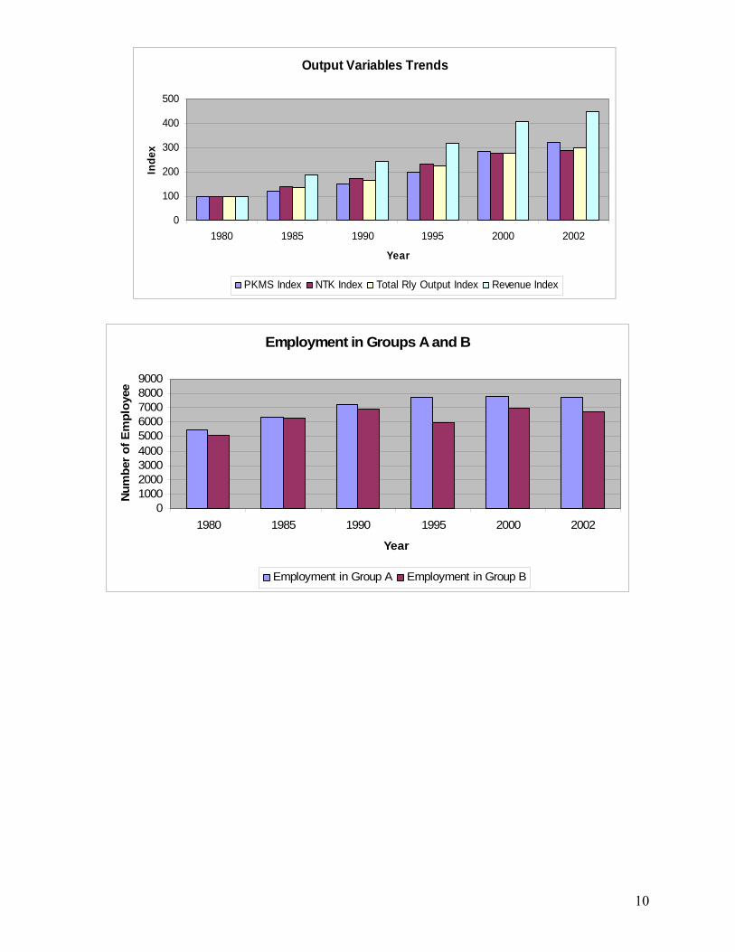
Labour variables. The Indian Railways hire workers in four different labour categories: categories A and B include administrative officers and professional workers; category C includes semi-skilled and clerical staff; and category D includes relatively unskilled attendants, peons and cleaning staff. The IR provides employment data at the all-India and zonal levels for each of the four categories of labour. We could thus easily compile time series data for A-category employment, B-category employment, C-category employment, and D-category employment – as well as total employment – in each zone (and for all-India) from 1980 to 2002. Such employment figures serves as raw measures of the volume of labour input, but they fail to reflect changes in the average quality of labour that result from changes in the category-composition of the labour force. We posit that the average quality of labour improves to the extent that the category-composition of jobs (the pattern of A+B, C and D employment) shifts in

7

the direction of a greater proportion of higher-skilled jobs and a lesser proportion of lower-skilled jobs.

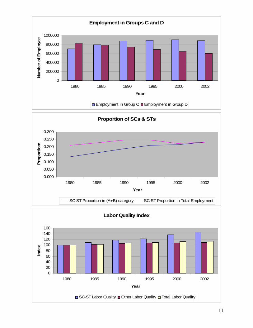
In order to take account of the effects of changes in the average quality of labour over

time, we constructed time series indices of a new variable measuring the volume of "effective" labour input for each zone (and for all-India). To do so we made use of data available from the IR on average wage rates and total wage bills for categories A+B (taken together), C and D. In every case we started with separate indices of employment in categories A+B, C and D, each having a value of 100 in the base year 1980. Then for every case we calculated a corresponding time series index of effective labour input by weighting observations of the three separate indices in each year according to their shares of the total wage bill in that year – the same kind of weighting procedure used to aggregate measures of different kinds of passenger or freight service into a single passenger or freight output index. We then defined (for each zone and for all-India) initial time series indices of the quality of labour, in which each year's value is the ratio of the same year's value in the corresponding index of effective labour input to the same year's value in the corresponding index of total employment (obtained by indexing total employment to 100 in 1980). Using this method, the value of the initial quality of labour index in every zone, as well as in all-India, is set equal to 1 in 1980. This is misleading, however, because the category-composition of labour was not the same in every case. To make the quality of labour indices comparable across zones, we defined the (final) quality of labour index for a given zone as the product of its initial quality of labour index and a "zonal base-year labour-quality ratio" expressing the average quality of its category-composition of labour relative to that of all-India in 1980. Finally, to obtain the desired quality-reflecting measure of the volume of labour input, we created a new variable labeled effective labour whose value in each zone and year is obtained by multiplying the level of total employment in that zone and year by the corresponding value of the quality of labour index.

In addition to having time series of total employment and of effective labour as alternative measures of labour input, we were interested in working with labour input measures that separate SCST labour from other kinds of labour. The IR provides extensive employment data for each of the four categories of labour not only for all employees, but also for Scheduled Caste & Tribe (SCST) employees. It is therefore easy to compile time series data for each zone and for all-India on SCST total employment and on other total employment. In the case of effective labour, however, the task of generating separate time series in each zone for the volume of effective SCST labour and the volume of effective other labour is much more complicated. To generate such series, we had to use the same kind of procedures described in the previous paragraph, in order to obtain first the required effective labour and quality of labour indices for SCST labour and for other labour, and then the corresponding zonal base-year labour-quality ratios. The ultimate objective of our quantitative analysis is of course to examine the effect of affirmative action in the labour market on measures of efficiency and productivity. Toward this end, in both the production-function and the data envelopment analyses, we need to make use of time series in each zone of a variable reflecting the SCST proportion of total employment. We have worked with four measures of this key variable. The first is the ratio of SCST employees to total employees in all labour categories (A, B, C, D), and the second is the ratio of SCST employees to total employees in labour categories A+B only. The main rationale for using the latter variable is that one can be reasonably certain that SCST employees in the upper two categories owe their employment to the reservation of positions for SC and ST applicants; whereas many of the SCST employees in the lower two categories did not need reservations in order to be hired. Calculating time series of the SCST proportion of total or A+B employment in

8

each zone from 1980 to 2002 can easily be done from the available IR data. When we examined graphs of these time series, however, we discovered that there were some distinctly outlying observations that appear to have been subject to measurement error. We therefore introduced a second pair of measures of the SCST proportion of total employment, differing from the first pair only in that – in each case – roughly a dozen outlying zone-year observations were removed from the full pooled data set of 8*23=184 observations.

Capital variables. The IR distinguishes between three types of capital stock – structural engineering, rolling stock, and machinery & equipment – and makes available annual current-price data on book value and gross investment for each type of capital, going back to 1966 for each zone and to 1952 for all-India. We chose to work with estimates of gross rather than net capital stock, because measures of net capital stock decline in value as the number of its productive future years decline, whereas measures of gross capital stock tend to be proportional to the capital value actually consumed during a given year. Book value data on capital stock are notoriously poor measures of the value of capital inputs, because they aggregate annual additions to capital stock that are valued at different prices every year; so we made use of the perpetual inventory method to generate time series of constant-price gross capital stock of each type, from 1980 to 2002, for each zone and for all-India. We first compiled long time series of constant-price gross investment for each type of capital, deflating the available figures on current-price gross investment by appropriate price deflators. In some cases we had to use a backward extrapolation procedure to estimate annual constant-price investment up to 'n' years prior to 1980, where 'n' represents the average service life of the relevant type of capital stock. To estimate the gross capital stock of a given type in a given zone (or all-India) for each year T from 1980 through 2002, we then summed the corresponding constant-price investments for the years T-n through T-1. Thus we ended up with time series for constant-price gross structural engineering works, gross rolling stock, gross machinery & equipment, and gross total capital stock in each zone and for all-India.

Constant-price gross capital stock measures that are calculated as in the previous

paragraph do have one important shortcoming, in that they fail to reflect the extent to which embodied-in-capital technological progress increases the productive potential of a piece of constant-price capital stock from year to year. Just as we sought to adjust a raw measure of labour input (employment) to take account of changes in labour quality associated with the category-composition of labour in generating a better measure (volume of effective labour), so we found it desirable to adjust our raw measure of capital input (constant-price gross capital stock) to take account of changes in capital quality associated with the age structure of capital to generate a better measure that we call "effective capital input." Thus we calculated the average vintage of gross capital stock of each type (and for all types together), in each zone and for all-India in each year from 1980 to 2002, by adding together (1) the average age of the gross capital stock at the beginning of the year and (2) the number of years elapsed from the beginning of that year to the middle of the year 2002. We then used the average vintage of capital stock figures to generate, for each type of capital and for total capital, in every year from 1980 to 2002, for each zone and for all-India, a capital obsolescence fraction – based on the assumption that a unit of constant-price gross investment loses 1% of its value as productive capital for each year elapsed since it was created. Finally, for each type of capital stock and for total capital stock, in every year from 1980 to 2002, for each zone and for all-India, we calculated the value of effective capital stock by multiplying the constant-price gross capital stock by the corresponding capital obsolescence fraction.

Material input variables. The main material input used by a railway system is fuel; and

the IR provides annual data for all-India and by zone on seven different forms of fuel input –

9

coal, diesel oil, electricity, etc. – both in terms of physical units of measurement (tonnes, kilolitres, kilowatt-hours, etc.) and in terms of current-price cost. Using standard conversion factors to convert all the measures of fuel in physical terms into their equivalent in coal-tonnes, we compiled time series of total coal-tonnes of fuel input for each zone and for all-India from 1980 through 2002.

In the case of fuel input, as with capital and labour inputs, we saw reason to generate a

second, more nuanced variable to take account of changes in fuel quality associated with changes in the proportions of different kinds of fuel utilized by the IR. In particular, diesel- and electricity-powered locomotion is significantly more efficient than locomotion powered by other fuels, because it enables greater acceleration, allows for easier maintenance, and generates less pollution. (Pollution from coal, coke and wood used in steam engines has adverse effects on railway employees and passengers as well as on the countryside.) We sought therefore to construct a fuel input variable that would take account of the extent to which locomotion is powered by the more efficient fuels. We first calculated for each zone and year the share of coal-tonnes of fuel accounted for by diesel oil and electricity, which we label fuel quality. We then calculated the corresponding effective fuel input by multiplying the simple amount of coal-tonnes of fuel input by (1 + .25*fq), where 'fq' represents fuel quality. Thus our measure of effective fuel gives diesel & electric fuel a weight of 125% as compared with 100% for other fuels, which appeared to us to be a reasonable estimate of the extent of to which the quality of the former is superior to that of the latter.

Our production-function and data-envelopment analyses in the next section of the paper

make use of the variables identified via bold type in the preceding paragraphs. For each variable we compiled a data set of 184 observations, representing 23 annual observations from 1980 to 2002 for each of 8 IR zones (the Central, Eastern, North Eastern, Northeast Frontier, Southern, South Central, South Eastern, and Western Railway). In order to provide readers with a general idea of how the variables trended over the time period in question, we provide here a set of ten figures displaying time trends of the variables measured at the all-India level for the IR as a whole. Each figure shows – for a related group of variables – the all-India values at five-year intervals and in the final year 2002. Except where otherwise indicated, the values of the variables are expressed as indices keyed to 100 in the base year 1980.12

12 The underlying data on which the figures are based are described in Appendix B; both the all-India and the zonal time series data are available from the authors on request.

Output Variables Trends

0

100

200

300

400

500

1980 1985 1990 1995 2000 2002

Year

Inde

x

PKMS Index NTK Index Total Rly Output Index Revenue Index

Employment in Groups A and B

0100020003000400050006000700080009000

1980 1985 1990 1995 2000 2002

Year

Num

ber o

f Em

ploy

ee

Employment in Group A Employment in Group B

10

Employment in Groups C and D

0

200000

400000

600000

800000

1000000

1980 1985 1990 1995 2000 2002

Year

Num

ber

of E

mpl

oyee

Employment in Group C Employment in Group D

Proportion of SCs & STs

0.000

0.050

0.100

0.150

0.200

0.250

0.300

1980 1985 1990 1995 2000 2002

Year

Pro

porti

ons

SC-ST Proportion in (A+B) category SC-ST Proportion in Total Employment

Labor Quality Index

020406080

100120140160

1980 1985 1990 1995 2000 2002

Year

Inde

x

SC-ST Labor Quality Other Labor Quality Total Labor Quality

11

Labor Variables

0

50

100

150

200

1980 1985 1990 1995 2000 2002

Year

Inde

x

SC-ST Employment Index SC-ST Effective Labor Index Others Employment IndexOthers Effective Labor Index Total Employment Index Total Effective Labor Index

Materials Indices

020406080

100120140

1980 1985 1990 1995 2000 2002

Year

Inde

x

Unadjusted Material Index Effective Materials Index

12

Constant-Price Gross Capital Stock

0100200300400500600700800

1980 1985 1990 1995 2000 2002

Year

Inde

x

Machinery Index Structural Engg. Index Rolling Stock Index Total Capital Index

Average Vintage of Capital Stock

0

10

20

30

40

50

1980 1985 1990 1995 2000 2002

Year

Age

in Y

ears

Average Vintage-Machinery Average Vintage-Structural EnggAverage Vintage-Rolling Stock Average Vintage-Total Capital

Effective Capital Measures

0200400600800

10001200

1980 1985 1990 1995 2000 2002

Year

Inde

x

Effective Machinery Index Effective Structural Engg. IndexEffective Rolling Stock Index Total Effective Capital Index

13

14

4. Production function analysis

Using the variables constructed as above, we estimated a log-linear Cobb-Douglas production function.13 The equation estimated was ln (output) = β0 + β1 ln (effective capital1) + β2 ln (effective labour) + β3 ln (effective fuel) + β4 time + u where t was introduced to capture the effect of technical change and u is the composite error term that captures both the zone specific and random effects. Our panel is a balanced macro panel, with the number of zones (N), 8, being less than the number of time periods (T), 23. Heterogeneous panel

In panels with large N and small T, it is common to pool the observations, assuming homogeneity of the slope coefficients. Our panel has small N and large T, but is a heterogeneous panel, since Indian railway zones are very diverse in terms of size, whether measured in terms of geographical area, or in terms of volume of passenger and freight outputs. We tested for the equality of coefficients on the zonal dummy variables by estimating the LSDV (least squares dummy variable) model (see Appendix C for the estimates). As the output indicates, none of the zonal dummies are significant (neither are the coefficients on effective capital and effective fuel), but a test of equality of coefficients rejects the hypothesis of equality of the zonal dummies. On the whole, the LSDV estimation does not yield robust estimates.

The quintessential question in such cases is whether or not to pool the data, since the assumption of homogeneity, if the underlying data are heterogeneous, can lead to biases in estimation. We conducted a simple Chow Test based on the regression output in Appendix C14. While this test rejects the poolability hypothesis, the literature on the poolability question indicates that this test is not unambiguously decisive, because it assumes u ~ N(0, σ2 I). If there is reason to believe that the assumption holds, then one can base the decision to pool or not on the Chow Test. However, Baltagi (2005, p. 59) asks firstly, whether the Chow test is the right test to perform if u ~ N (0, Ω) and, secondly, if the Chow test will still have a F distribution, if u ~ N(0, Ω). It turns out that the answer to the first question is no, and the answer to the second question depends on the assumptions about the distribution of the error term. It follows, therefore, that the decision on whether or not to pool cannot be based on the outcome of this Chow Test, but has to be made keeping in mind the nature of the data and the specific economic issues to be investigated.

13 We also estimated a Translog production, but the estimates indicated a poor fit: most of the coefficients were not significant; the coefficients associated with the inputs did not satisfy monotonicity, and the estimated equation displayed high multicollinearity. We estimated the function using the actual values of the variables as well as the normalised values (around the mean), and both specifications displayed similar problems. 14 The sum of squares of residuals from the pooled regression: 6.512 The sum of above from the individual zonal regressions: 0.828 So, F= numerator/ denominator, where numerator= [(6.512-0.828) /5*(8-1)], and denominator=[0.828/8*(23-5)] The F value = 0.1624/0.0058= 28.24 (p < 0.001), which is significant, thus rejecting the poolability hypothesis.

15

Also, not pooling the data would mean separate regressions, either over the cross-section units or over the time series for each cross section. However, this approach runs the following risks highlighted by Baltagi and Griffin (1997): pure cross section studies cannot control for unobservable zonal effects and pure time series studies cannot control for unobservable events/shocks affecting Indian Railways or for behavioural changes over time. Thus, there are very clear advantages to using pooled data and our estimates confirm the advantages of pooling over running separate zonal estimates and over the LSDV model. Choice of estimation technique

Having decided to use the pooled data, the next question was the choice of estimation technique based on the standard error component model of panel data: random effects (RE) or fixed effects (FE). We also ran tests to gauge the presence of serial correlation, cross sectional dependence and heteroskedasticity. The standard procedure for deciding between RE and FE is the Hausman test. However, since the Hausman test in our case was undefined15, we tested for RE/FE and serial correlation by using a standard test in STATA that includes the Breusch and Pagan (1980) Lagrange Multiplier test for random effects, the Baltagi and Li (1995) test for first order serial correlation, the Baltagi and Li (1991) joint test for serial correlation and random effects. lnq[zne,t] = Xb + u[zne] + v[zne,t] v[zne,t] = lambda v[zne,(t-1)] + e[zne,t] Estimated results: | Var sd = sqrt(Var) ---------+----------------------------- lnq | 0.5922468 0.7695757 e | 0.009546 0.09770371 u | 0.0452246 0.21266087 Tests: Random Effects, Two Sided: ALM (Var(u)=0) = 700.24 Pr>chi2(1) = 0.0000 Random Effects, One Sided: ALM (Var(u)=0) = 26.46 Pr>N(0,1) = 0.0000 Serial Correlation: ALM (lambda=0) = 14.08 Pr>chi2(1) = 0.0002 Joint Test: LM (Var(u)=0,lambda=0) = 846.49 Pr>chi2(2) = 0.0000 The first two tests suggest the use of RE estimation over FE and the next test indicates the presence of serial correlation.

15 Hausman's test is based on estimating the variance of the difference of the estimators [var(b-B)] by the difference of the variances [var(b)-var(B)]. Var(b)-Var(B) is a consistent estimator of var(b-B), but it is not necessarily positive definite. In that case, the Hausman test is undefined.

16

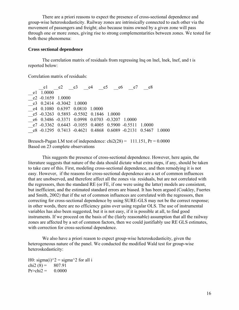
There are a priori reasons to expect the presence of cross-sectional dependence and group-wise heteroskedasticity. Railway zones are intrinsically connected to each other via the movement of passengers and freight; also because trains owned by a given zone will pass through one or more zones, giving rise to strong complementarities between zones. We tested for both these phenomena: Cross sectional dependence

The correlation matrix of residuals from regressing lnq on lnel, lnek, lnef, and t is reported below: Correlation matrix of residuals: __e1 __e2 __e3 __e4 __e5 __e6 __e7 __e8 __e1 1.0000 __e2 -0.1659 1.0000 __e3 0.2414 -0.3042 1.0000 __e4 0.1080 0.6397 0.0810 1.0000 __e5 -0.3263 0.5893 -0.5502 0.1846 1.0000 __e6 0.3486 -0.3371 0.0998 0.0703 -0.3207 1.0000 __e7 -0.3362 0.6443 -0.1055 0.4005 0.5900 -0.5511 1.0000 __e8 -0.1295 0.7413 -0.4621 0.4868 0.6089 -0.2131 0.5467 1.0000 Breusch-Pagan LM test of independence: chi2(28) = 111.151, Pr = 0.0000 Based on 23 complete observations

This suggests the presence of cross-sectional dependence. However, here again, the literature suggests that nature of the data should dictate what extra steps, if any, should be taken to take care of this. First, modeling cross-sectional dependence, and then remedying it is not easy. However, if the reasons for cross-sectional dependence are a set of common influences that are unobserved, and therefore affect all the zones via residuals, but are not correlated with the regressors, then the standard RE (or FE, if one were using the latter) models are consistent, but inefficient, and the estimated standard errors are biased. It has been argued (Coakley, Fuertes and Smith, 2002) that if the set of common influences are correlated with the regressors, then correcting for cross-sectional dependence by using SURE-GLS may not be the correct response; in other words, there are no efficiency gains over using regular OLS. The use of instrumental variables has also been suggested, but it is not easy, if it is possible at all, to find good instruments. If we proceed on the basis of the (fairly reasonable) assumption that all the railway zones are affected by a set of common factors, then we could justifiably use RE GLS estimates, with correction for cross-sectional dependence. We also have a priori reason to expect group-wise heteroskedasticity, given the heterogeneous nature of the panel. We conducted the modified Wald test for group-wise heteroskedasticity: H0: sigma(i)^2 = sigma^2 for all i chi2 (8) = 807.91 Pr>chi2 = 0.0000

17

This indicates the presence of group-wise heteroskedasticity. STATA allows for RE GLS estimation with built-in correction for all the three problems: autocorrelation, cross sectional correlation and heteroskedasticity: and we have reported these results below.

However, for the sake of thoroughness, we also tried two different alternatives to the error components model, both of which essentially use OLS. One method consisted of applying the Prais-Winsten correction for autocorrelation, correcting for heteroskedasticity and cross sectional dependence and then applying OLS to the corrected data (the “xtpcse” command in STATA). The other method consisted of applying OLS to the panel data, but with Newey-West standard errors that are robust to both auto correlation and heteroskedasticity but do not correct for cross-sectional correlation.

The final econometric question that needed to be addressed was the following: STATA

allows for two variations of estimation in the context of autocorrelation: one, which assumes a common AR1 process and the second, which assumes a panel-specific AR1 process. The choice between the two cannot be determined on the basis of a test, but has to be made in the context of the specific issue being investigated. We estimated both variants. The ρ in the common AR1 is not a simple average of the individual ρ (from the panel specific AR1 estimation), and if the spread of the individual ρ was large, we would unambiguously use PSAR(1). However, an examination of the ρ from the output suggests that the individual ρ’s are distributed with a small spread around the common ρ, thus making the choice between the two variants more difficult. We report below the GLS estimates, as it is the most general technique (OLS can be subsumed under GLS), with both these variants, but also include a comparative discussion of the estimates from the other two techniques. Regression output We carried out a variety of different regression runs, which varied in terms of the variables included in the specification of the production function and/or the ways in which those variable were measured. Our runs varied along the following dimensions: 1. Which dependent variable we include in the regression: a physical measure, total output (q), or a value measure, total revenue (r). We believe that 'q' is the more reliable measure, because 'r' is dependent on pricing decisions that tend to be somewhat arbitrary. 2. Which measure of the three inputs we use as independent variables in the regression: the adjusted measures of effective labour (el), effective capital stock (ek), and effective fuel (ef); or the raw measures of total employment (l), unadjusted capital stock (k), and unadjusted fuel (f) – which in our view are considerably less accurate, because they fail to take account of differences in quality between different subcategories of each input. 3. Whether or not we replace the effective labour input variable (el) by two separate labour input variables, representing effective SC&ST labour (elscst) and effective other labour (elother). 4. Whether we include or exclude a variable representing the proportion of SC&ST employees among all employees (“scp”), or alternatively the proportion of SC&ST among category A+B employees (“scabp”), as an independent variable in the regression equation. If such a variable is excluded, we correlate 'scp' or 'scabp' with residuals from the regression. The reason for considering 'scabp' as an alternative to 'scp' is that it measures the impact of having SC and ST employees in decision making positions (categories A+B), which are arguably the most critical to overall productivity in the Indian Railways. Also, there is very strong reason to believe that

18

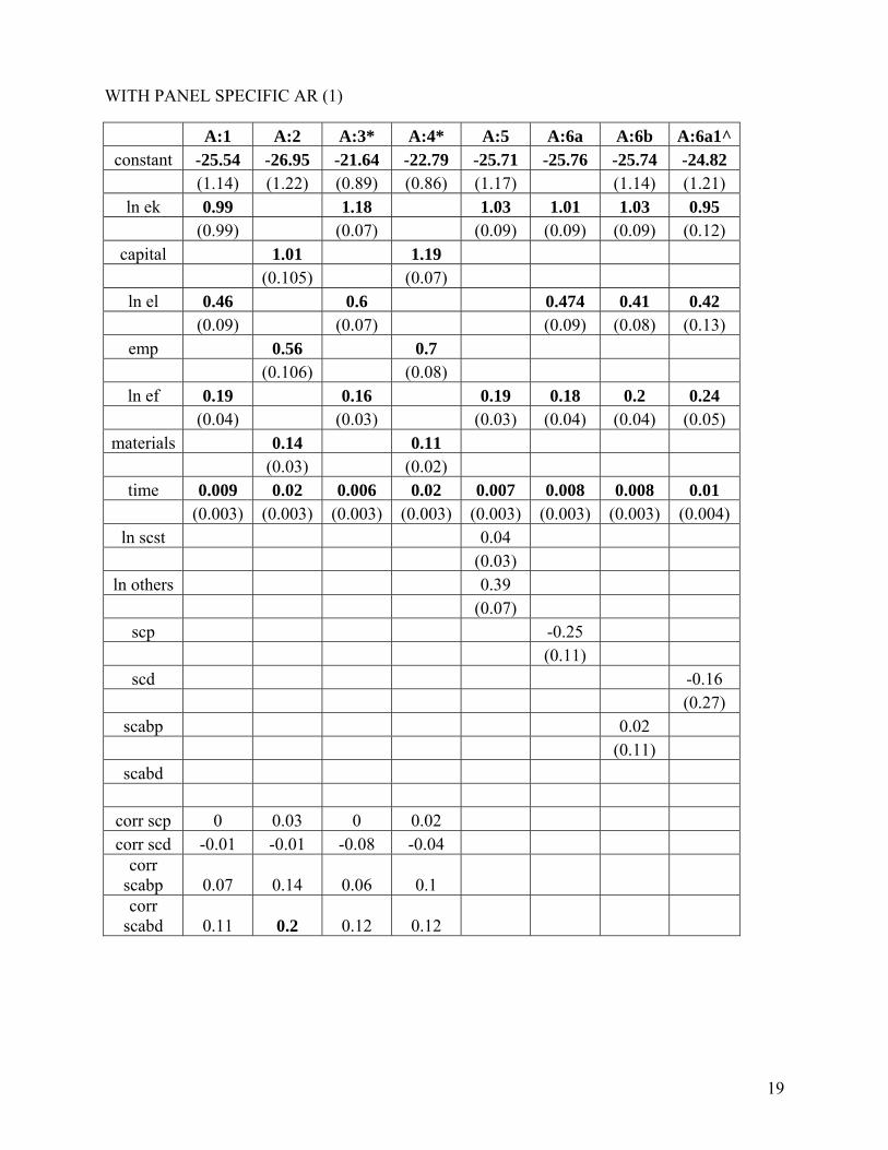
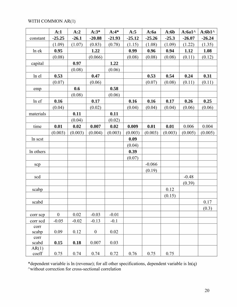
the presence of SC-ST employees in the A and B categories of jobs (as opposed, for instance, to category D jobs) is mainly attributable to affirmative action, thus, ‘scabp’ is a key variable of interest, if one is interested in assessing the productivity impact of AA. 5. Whether to include all 184 zone-year observations that we compiled, or to exclude zone-years in which the figures we had for the variable representing an SC&ST proportion of employees was highly questionable (because it represented an obvious outlier in the time series for a zone). We found 15 observations of 'scp' that were highly questionable, and 12 observations of 'scabp' that were highly questionable (mostly for different zone-years in the two cases). We believe that the regressions and correlations in which the questionable zone-years are excluded provide more reliable results. Thus we estimated the following specifications with each of the estimation techniques discussed above: Specification 1: ln q on ln ek, ln el, ln ef, t Specification 2: ln q on ln k, ln l, ln f, t Specification 3: ln revenue on ln ek, ln el, ln ef and t Specification 4: ln revenue on ln k, ln l, ln f and t Specification 5: ln q on ln ek, ln elscst, ln elothers, ln ef and t Specification 6a: ln q on ln ek, ln el, ln ef, scstp, and t Specification 6b: ln q on ln ek, ln el, ln ef scstabp and t In the case of specifications 1-4, the regression residuals were correlated with 'scp' and with 'scabp', first with all zone-year observations included and then with the relevant questionable zone-years excluded. In the case of specifications 6a and 6b, the regressions were run first with all zone-year observations included and then with the relevant questionable zone-years excluded (“scd” and “scabd”).16 The GLS estimates of these specifications, with correction for autocorrelation, cross-sectional dependence and heteroskedasticity across panels, are the following:

16 For GLS estimation, when we included “scd” and “scabd” in the regression, STATA did not allow for correction for all the three problems. Hence in the table, the regressions with these two variables correct only for serial correlation and heteroskedasticity, and not for cross-sectional correlation.

19

WITH PANEL SPECIFIC AR (1)

A:1 A:2 A:3* A:4* A:5 A:6a A:6b A:6a1^constant -25.54 -26.95 -21.64 -22.79 -25.71 -25.76 -25.74 -24.82

(1.14) (1.22) (0.89) (0.86) (1.17) (1.14) (1.21) ln ek 0.99 1.18 1.03 1.01 1.03 0.95

(0.99) (0.07) (0.09) (0.09) (0.09) (0.12) capital 1.01 1.19

(0.105) (0.07) ln el 0.46 0.6 0.474 0.41 0.42

(0.09) (0.07) (0.09) (0.08) (0.13) emp 0.56 0.7

(0.106) (0.08) ln ef 0.19 0.16 0.19 0.18 0.2 0.24

(0.04) (0.03) (0.03) (0.04) (0.04) (0.05) materials 0.14 0.11

(0.03) (0.02) time 0.009 0.02 0.006 0.02 0.007 0.008 0.008 0.01

(0.003) (0.003) (0.003) (0.003) (0.003) (0.003) (0.003) (0.004) ln scst 0.04

(0.03) ln others 0.39

(0.07) scp -0.25

(0.11) scd -0.16

(0.27) scabp 0.02

(0.11) scabd

corr scp 0 0.03 0 0.02 corr scd -0.01 -0.01 -0.08 -0.04

corr scabp 0.07 0.14 0.06 0.1 corr

scabd 0.11 0.2 0.12 0.12

20

WITH COMMON AR(1) A:1 A:2 A:3* A:4* A:5 A:6a A:6b A:6a1^ A:6b1^constant -25.25 -26.1 -20.88 -21.93 -25.12 -25.26 -25.3 -26.07 -26.24

(1.09) (1.07) (0.83) (0.78) (1.15) (1.08) (1.09) (1.22) (1.35) ln ek 0.95 1.22 0.99 0.96 0.94 1.12 1.08

(0.08) (0.066) (0.08) (0.08) (0.08) (0.11) (0.12) capital 0.97 1.22

(0.08) (0.06) ln el 0.53 0.47 0.53 0.54 0.24 0.31

(0.07) (0.06) (0.07) (0.08) (0.11) (0.11) emp 0.6 0.58

(0.08) (0.06) ln ef 0.16 0.17 0.16 0.16 0.17 0.26 0.25

(0.04) (0.02) (0.04) (0.04) (0.04) (0.06) (0.06) materials 0.11 0.11

(0.04) (0.02) time 0.01 0.02 0.007 0.02 0.009 0.01 0.01 0.006 0.004

(0.003) (0.003) (0.004) (0.003) (0.003) (0.003) (0.003) (0.005) (0.005) ln scst 0.09

(0.04) ln others 0.39

(0.07) scp -0.066

(0.19) scd -0.48

(0.39) scabp 0.12

(0.15) scabd 0.17

(0.3) corr scp 0 0.02 -0.03 -0.01 corr scd -0.05 -0.02 -0.13 -0.1

corr scabp 0.09 0.12 0 0.02 corr

scabd 0.15 0.18 0.007 0.03 AR(1) coeff 0.75 0.74 0.74 0.72 0.76 0.75 0.75

*dependent variable is ln (revenue); for all other specifications, dependent variable is ln(q) ^without correction for cross-sectional correlation

21

Looking at the two sets of results (as well as the “xtpcse” and “Newey-West” output reported in Appendix C), we see that when ln q is used as the dependent variable, the coefficient of the intercept ranges between -25.25 to -27.4, but mostly hovers around -26. Similarly, the coefficients of time (0.006 to 0.02) and capital (0.95 to 1.18) vary within a very narrow band and those for effective fuel vary from 0.13 to 0.19, except for the Newey-West estimates that are considerably higher (0.33 to 0.43). The more substantial variation is in the coefficients of effective labour, depending on the specification, but that is because labour is also defined in several different ways. On the whole, therefore, we find that our alternative estimates fall within a relatively small range and appear to be fairly robust. Several of the specifications yield a coefficient of capital greater than 1, which seem implausible. We thus narrow our attention to those estimates where the coefficient of capital is less than one.

In the table above, focusing on column A:1, we see that with the assumption of common

AR(1) process, correlation of the residual with “scabd” is positive and significant17, providing some support to the view that when individuals from the marginalized groups enter decision-making and managerial positions (A and B job categories), they make a positive and significant contribution to Indian Railways output. (This residual is positive in A:2 as well, but we need to note that this regression uses the unadjusted, rawer versions of the explanatory variables). In the case of “xtpcse” regression with specification 1, under the assumption of PSAR1, both “scabp” and “scabd” are significantly and positively correlated with the residual. With the assumption of common AR1, similar to the GLS regressions, “scabd” is significantly and positively correlated. In all other cases, the correlation with the residual is not significant. These results taken together clearly reject the hypothesis that higher proportions of SC&ST employees in A and B jobs contribute negatively to productivity levels in the Indian Railways, and they provide some evidence that higher proportions of SC&ST employees in A and B jobs contribute positively to Indian Railway productivity.

Our results for specification 6a and 6b show that when “scp” or “scabp” are included as

separate regressors, in addition to “ln el”, they are insignificant. This suggests that the effective labour variable captures most of the impact of the labour variable and that higher proportions of SC&ST employees do not have an independent significant impact on total output. When SCST labour and other labour are included as separate regressors, then the Newey-West estimates indicate that both are insignificant but that their coefficients are not significantly different from each other. 5. Data envelopment analysis

As explained in section 2, we also tried an alternative approach to investigate the impact of affirmative action on productivity in the Indian Railways: a two-stage procedure in which the first stage was a data envelopment analysis (DEA) of productivity changes and the second stage was an econometric analysis of factors potentially influencing those productivity changes. DEA allows one to analyze productivity in the context of a pooled data set of time series data on inputs and outputs for multiple production units within a given industry. It does not require specification of any particular functional relationship between input and output variables; and it allows one to work with more than one output variable as well as multiple input variables. On the other hand, it is not based on stochastic processes and therefore does not produce any measures of the statistical significance of the results obtained.

17 With PSAR1, the correlation is positive but not significant.

22

For the first stage of our alternative approach we initially used DEA to estimate annual changes in total factor productivity ("tfpch") from 1980-81 to 2001-2002 in each railway zone, taking into account two output variables (passenger transport and freight transport) and eight input variables (employment in each of the four labour categories A, B, C, and D; constant-price gross capital stock of each type – structural engineering, rolling stock, machinery & equipment; and total fuel input (in coal-tonnes). Then for the second stage we sought to explain our estimated "tfpch" values (for each zone and pair of years) in terms of several variables that appeared likely to influence annual total factor productivity change. The independent variables consisted of three that were designed to capture the quality of the three types of inputs (labour, capital, and fuel) and one to reflect the scale of production. For labour quality we used “scabp” or "scapd," since our primary focus is on the impact of SCST as opposed to other labour on productivity;18 for capital we used the average vintage of gross capital stock (of all types); and for fuel we used fuel quality (the share of coal-tonnes of fuel accounted for by diesel oil and electricity). For the scale of production, we used our aggregated measure of total railway output. We regressed the estimated values of "tfpch" (from year 't' to year 't+1') on the four independent variables (measured in year 't'), thus pooling 22 time series observations for each zone. Since we were dealing with panel data again, we conducted the tests for choosing between RE/FE and serial correlation; this time the tests indicated the use of FE estimation with no significant presence of serial correlation.

Subsequently we undertook a slightly different variant of our alternative approach. For

the first stage we did new DEA run in which we used the “effective” measures of the capital stock and fuel input variables instead of the unadjusted "raw" measures of the first run. In other words, we incorporated the 'quality" of the capital stock and fuel inputs into the first stage of the analysis, making it unnecessary to consider them in the second stage. For the second stage of this variant we simply correlated the estimated “tfpch” values (from year 't' to year 't+1') from the first stage with the various SC-ST proportion variables (measured in year 't').19

For each of the variants of our two-stage DEA-based approach we undertook two

separate analyses – one including observations for all eight zones, and the other including observations for seven zones, excluding the NFR zone. The reason for excluding this zone is that the figures for NFR constant-price gross rolling stock indicated a substantial and implausible decline throughout the period 1980-2002; in no other zone did we encounter such an implausible trend for any variable.20 The key results of our DEA-based analyses are those that indicate the extent to which total factor productivity change ("tfpch") is associated with the employment proportions of SC&ST employees – variously measured by the SC&ST proportion of total employment ("scp") and the SC&ST proportion of A+B-category employment ("scab"), or the same measures when highly questionable observations have been excluded ("scd" and "scabd"). In the case of our first variant, using raw measures of capital stock and fuel inputs and undertaking a second-stage

18 Since DEA analysis permits us to use four separate labour input variables for the four different labour categories, there is no need to adjust for the category-composition of labour – as we had to do in our production-function analysis. 19 Thus in the second variant we also dropped from consideration the possible effect of the scale of production, which had proven insignificant in the results for the first variant 20 We chose not to exclude the NFR zone from our production-function analyses, because then we were using a single aggregate capital stock variable for capital input – and it showed substantial and plausible growth over the period from 1980 to 2002.

23

regression analysis of "tfpch," the association is given by the estimated coefficient on the "sc…" variable. In the case of the second variant, using effective measures of capital stock and fuel inputs, the association is given by the correlation of "tfpch" with the "sc…" variable. The key results we obtained are given in the following table.21 Association of tfpch with “sc...” variables variant #1 variant #2 8 zones 7 zones 8 zones 7 zones

scp 0.2 0.32 0.1 0.02 (0.32) (0.22) (0.171) (0.788)

scd 0.24 0.4 0.13 0.1 (0.38) (0.26) (0.096) (0.213)

scab -0.03 0.12 0.13 0.17 (0.3) (0.18) (0.079) (0.028)

scabd 0.01 0.21 0.15 0.24 (0.44) (0.27) (0.049) (0.004)

Figures in bold are significant at 5% or better (Figures in parentheses under variant #1 are standard errors) (Figures in parentheses under variant #2 are p-values) This table indicates that, under variant #1, the 2nd-stage regression runs to explain "tfpch" yielded positive coefficients on the "sc…" variables in all but one of the 8 cases, but no coefficient was even close to being significant at 5% (the coefficient value would have to be roughly twice the standard error in order to reach significance at the 5% level). The correlations under variant #2 are all positive, though the in 5 of the 8 cases they were not significant at 5%. There is clearly no support here for the claim that higher proportions of SC&ST employees result in slower growth in total factor productivity.

Under variant #2, significant positive correlations with "tfpch" were obtained for "scabd"

in the 8-zone case and for both "scab" and "scabd" in the 7-zone case. In particular, the correlation in the case of "scabd" in the 7-zone case is 24% and the p-value just .4%, reflecting a remarkably high level of significance. This is especially noteworthy because we have every reason to believe that the results of 7-zone runs are more reliable than the results of 8-zone runs, and that the "scabd" tests are more reliable than the "scab" tests, because in these cases we are excluding highly questionable observations in the underlying data. Thus here we find evidence

21 The results for variant #1 are based on 2nd-stage regressions excluding the scale of production variable, whose estimated coefficient value proved to be quite insignificant under most specifications.

24

in support of the claim that higher proportions of SC&ST employees in A and B jobs contributes to more rapid total factor productivity growth. 22

6. Concluding Comments

Analyzing an extensive data set on the operations of one of the largest employers in the public sector in India, the Indian Railways, we find no evidence whatsoever to support the claim of critics of affirmative action that increasing the proportion of SC&ST employees will adversely impact productivity or productivity growth. On the contrary, some of the results of our analysis suggest that the proportion of SC&ST employees in the upper (A+B) job categories is positively associated with productivity and productivity growth.

Our finding of such positive associations in the case of A and B jobs is especially

relevant to debates about the effects of AA on behalf of members of SC and ST communities, for two reasons. First, the efficacy with which higher-level managerial and decision-making jobs are carried out is likely to have a considerably bigger impact on overall productivity than the efficacy with which lower-level semi-skilled and unskilled jobs are fulfilled. Thus critics of reservations are likely to be much more concerned about the potentially adverse effects of favoring SC&ST candidates for A and B jobs than for C and D jobs. Second, it is precisely in the A and B jobs – far more than in C and D jobs – that reservations have been indispensable for raising the proportion of SC&ST employees. Even without reservations, one would expect substantial numbers of SC&ST applicants to be hired into C and D jobs; but without reservations very few SC&ST applicants would have been able to attain jobs at the A and B level.

The results we have obtained from our analysis of productivity in the Indian Railways are

consistent with the results from productivity studies in the United States (briefly described in section 2), in that there is no statistically significant evidence that AA in the labour market has an adverse effect on productivity. Our results are stronger, however, in that we do find some suggestive evidence that AA in the labour market actually has a favorable effect.

It is beyond the scope of our paper to explain just how and why AA in the labour market

may have such a favorable effect. We believe, however, that the answer may be found in one or both of the following suggestions that others have advanced to explain such a finding. Individuals from marginalized groups may well display especially high levels of work motivation when they succeed in attaining decision-making and managerial positions, because of the fact that they have reached these positions in the face of claims that they are not sufficiently capable – and so they feel a strong desire to prove their detractors wrong. Alternatively, individuals from marginalized groups may simply believe that they have to work doubly hard to prove that they are just as good as their peers. References: Alivelu. G. (2008). “Analysis of Productivity Trends on Indian Railways,” Journal of Transport Research Forum, 47(1): 107-120.

22 We also examined 2nd-stage correlations of "sc…" variables with estimates of "tfpch" values generated from a 1st-stage DEA run in which raw measures – rather than effective measures – of capital stock and fuel inputs were used; this resulted in correlation results very similar to those shown under variant #2 in Table 2.

25

Baltagi, B.H. (2008). Econometric Analysis of Panel Data, Fourth Edition, Chichester (U.K.): John Wiley and Sons. Baltagi, B.H. and J.M Griffin (1997). “Pooled Estimators vs. Their Heterogeneous Counterparts in the Context of Dynamic Demand for Gasoline,” Journal of Econometrics 77 : 303-327 Baltagi, B.H. and Q. Li (1995). “Testing AR(1) against MA(1) Disturbances in an Error Component Model,” Journal of Econometrics 68: 133-151 Baltagi, B.H. and Q. Li (1991). “A Joint Test for Serial Correlation and Random Individual Effects,” Statistics and Probability Letters 11: 277-280 Breusch, T.S.. and A.R. Pagan (1980). “The Lagrange Multiplier Test and its Applications to Model Specification in Econometrics,” Review of Economic Studies 47:239-253 Christensen, L. R, and D.W. Jorgenson (1969). “The Measurement of US Real Capital Input, 1929-1957,” Review of Income and Wealth, 15 (4): 293-320. Coakley, J, A-M. Fuertes and R. Smith (2002). "A Principal Components Approach to Cross-Section Dependence in Panels," http://econpapers.repec.org/cpd/2002/58_Fuertes.pdf (accessed on October 3, 2009). Coelli, Tim (1996). A Guide to DEAP Version 2.1: A Data Envelopment Analysis (Computer) Program, Working Paper No. 96/08 of the Centre for Efficiency and Productivity Analysis, Department of Econometrics, University of New England, Armidale, New South Wales, Australia. Deshpande, A. and K. Newman (2007). “Where the Path Leads: The Role of Caste in Post University Employment Expectations,” Economic and Political Weekly, 42: 4133-4140. Goldar, B. (1997). "Econometrics of Indian Industry," in K.L. Krishna (ed.), Econometric Applications in India, Delhi: Oxford University Press. Government of India, Ministry of Industry, Central Statistical Organization (annual). Index Numbers of Wholesale Price Indices. Government of India, Ministry of Railways Appropriation Accounts. Government of India, Ministry of Railways, Annual Statistical Statements. Government of India, Ministry of Railways (1999 reprint). Indian Railways Financial Code. Government of India, Ministry of Railways, Directorate of Economics and Statistics, (2008). Key Statistics (1950-51 to 2006-07). Government of India, Ministry of Railways, General Manager’s Annual Reports Guha, A. (1990a). “The Mandal Mythology,” Seminar, 375: 51-53.

26

Guha, A. (1990b). “Reservations in Myth and Reality,” Economic and Political Weekly, 25: 2716-18). Holzer, H. and Neumark, D. (2000) “Assessing Affirmative Action,” Journal of Economic Literature, 38: 483-568. Kumar, D. (1990). “The Affirmative Action Debate in India,”Asian Survey, 32: 290-302. Manohar Rao M, J. Nachane (1982). V. Ajit, D. M. Karnik and V. V. Subba Rao. “A Framework for Optimizing Energy Usage in Industries – A Case Study of Indian Railways,” Indian Economic Journal, 30(2): 39-54. Ray, Subhash C. (2004). Data Envelopment Analysis: Theory and Techniques for Economics and Operations Research, Cambridge (U.K.): Cambridge University Press Sachchidananda (1990). “Welcome Policy,” Seminar, 375: 18-21. Shah, A.M. (1991). “Job Reservations and Efficiency,” Economic and Political Weekly, 26: 1732-4. Solow, Robert (1957). "Technical Change and the Aggregate Production Function," The Review of Economics and Statistics, 39 (3): 312-320. Weisskopf, Thomas E. (2004). Affirmative Action in the United States and India: A Comparative Perspective, London: Routledge.

27

APPENDIX A

Indian Railway Zones 1952-2002 (with headquarters and divisions)

Zone Headquarters Divisions

Northern Railway Delhi Ambala, Delhi, Ferozpur, Moradabad, Lucknow, Allahabad, Bikaner, Jodhpur

Western Railway Mumbai Central Mumbai Central, Vadodara, Ratlam, Kota, Ajmer, Jaipur, Rajkot, Bhavnagar

Southern Railway Chennai (Chennai Central)

Chennai, Tiruchirapalli, Madurai, Palghat, Thiruvananthapuram, Bangalore, Mysore

South Central Railway

Secunderabad Secunderabad, Hyderabad, Vijayawada, Hubli, Guntakal

South Eastern Railway

Kolkata (Howrah) Kharagpur, Chakradharpur, Bilaspur, Waltair, Adra, Khurda Road, Sambhalpur, Nagpur

Eastern Railway Kolkata (Howrah) Howrah, Sealdah, Danapur, Dhanbad, Malda, Asansol, Mughalsarai

Central Railway Mumbai (Mumbai CST) Mumbai, Bhusaval, Bhopal, Jabalpur, Jhansi, Solapur, Nagpur

North Eastern Railway

Gorakhpur Sonepur, Samastipur, Lucknow, Izzatnagar, Varanasi

Northeast Frontier Railway

Maligaon (Guwahati) Katihar, Tinsukia, Alipurduar, Lumding

Source: Government of India, Ministry of Railways, Directorate of Economics and Statistics, (2008). Key Statistics (1950-51 to 2006-07).

28

APPENDIX B

Data Source and Variable Construction (details) In this appendix we identify the sources and provide further details on the construction of the variables that were used in our estimation of production functions (in section 4) and in our data envelopment analyses (in section 5). Output Variables The output of the Indian Railways (IR) includes passenger and freight service. IR statistics distinguish four different kinds of passenger output:

• Suburban (all classes) • Non-suburban, that is further divided into three types, as follows:

Upper class (all air conditioned classes + first class ordinary) Mail (mail in first, sleeper and second classes) Ordinary (ordinary in second and sleeper classes)

Physical output is measured in terms of passenger-kilometers (PKMS), defined as the number of passengers carried multiplied by the average distance traveled. The IR collects data on PKMS as well as on revenues received for each of the four kinds of service. The underlying data on PKMS and on revenues, by year and by zone for each type of service, were obtained from Statement 12 of GOI, Ministry of Railways Annual Statistical Statements. IR statistics distinguish nine different types of freight output, according to the type of commodity carried:

• Coal (for steel plants; washeries; thermal power houses; other uses) • Raw materials for steel plants • Pig Iron and Finished Steel Booked From Steel Plants • Iron Ore for Export • Cement • Food grains • Fertilizers • Mineral oils • Other commodities

Physical output is measured in terms of net tonne-kilometers (NTK), defined as the tonnes of freight carried multiplied by the average distance traveled. The IR collects data on NTK as well as on revenues received for each of the nine commodity categories. The underlying data on NTK and on revenues, by year and by zone for each commodity category, were obtained from Statement 13 of GOI, Ministry of Railways Annual, Statistical Statements. To calculate observations of the variable total railway revenue by zone-year, we simply aggregated all the revenues received for passenger service and for freight transport and then deflated the total by the corresponding (all-India) price deflator for transport services (obtained from Index Numbers of Wholesale Price Indices, Ministry of Industry, GOI).

29

To calculate zone-year observations of the variables measuring total passenger output, total freight output and total railway output in physical terms, we aggregated the underlying data for each kind of passenger service and each type of freight transport as follows (note that all index time series take the value of 100 in the base-year 1980):

(1) For each zone create a PKMS index time series for each kind of passenger service. Calculate a total passenger output index by multiplying each value in the PKMS index by the corresponding proportion of total passenger revenue and then summing the products.

(2) For each zone create an NTK index time series for each type of freight transport. Calculate a total freight output index by (a) multiplying each value in the NTK index by the corresponding proportion of total freight revenue and then (b) summing the products.

(3) For each zone calculate a total railway output index by (a) multiplying each value in the total passenger output index and in the total freight output index by the corresponding proportion of total railway revenue and then (b) summing the products.

(4) The resultant zonal total passenger output, total freight output and total railway output indices will all have the value of 100 in 1980. To account for the heterogeneity of zone sizes, compute for each zone the ratio of zonal passenger, freight and total railway revenues to the corresponding all-India revenues in 1980.

(5) Calculate for each zone scale-adjusted indices of total passenger output, total freight output and total railway output by multiplying all values in each of the three zonal output indices (obtained in step 3) by the corresponding ratio (obtained in step 4).

Labour variables The Government of India has a standard classification of employment categories for all its undertakings, and the Indian Railways are no exception. The employment categories are as follows:

• Groups A and B together (Engineers, Personnel Officers, Traffic Service Officers,

Financial Advisors, Doctors) • Group C:

Grade 1: Workshop and Artisan Staff (station masters, technicians, supervisors, nurses, pharmacists)

Grade 2: Running Staff (engine drivers, guards, train ticket examiners) Grade 3: Other staff (clerical staff)

• Group D: Grade 1: Workshop and Artisan Staff (gangmen, peons) Grade 2: Running staff (train sweepers, train attendants) Grade 3: Other staff (office peons, hospital attendants, sweepers)

Annual data on the total number of employees and on average wage per employee for each of the above seven distinct categories of labour, for all-India and in each zone, are provided in Statement 40-II of GOI, Ministry of Railways Annual Statistical Statements. We used the figures for total number of employees defined as the sum of total permanent and temporary employees.23 We calculated the average wage per employee as the sum of the following components available from the source: pay and leave salary, running and overtime allowance, dearness allowance, 23 Figures for temporary employees are given separately for the two subcategories of those with "less than three years of service" and those with "three years of service and over."

30

traveling and compensatory allowance, provident fund contribution, gratuity, and pension benefits. In the case of employment, but not average wages, data are also available separately for total number of employees in Group A and in Group B. Our time series data for the raw labour input variables A-category employment, B-category employment, C-category employment, D-category employment and total employment were compiled very easily from the disaggregated data on total number of employees described just above. As noted in the text of section 3, we posited that overall labour quality improves to the extent that the category-composition of employees shifts towards more higher-skilled employees and less lower-skilled employees. In order to take account of such changes in labour quality as well as changes in the quantity of raw labour input from year to year, we created all-India and zonal time series for the quality of labour and the volume of effective labour as follows (all index time series take the value of 100 in the base-year 1980, unless otherwise noted):

(1) Using the disaggregated total employment data for each zone (and all-India), create an employment index time series for each labour category and a total employment index time series for labour of all categories taken together.

(2) For each zone (and all-India), calculate the wage bill for each labour category by multiplying employment in each category by the corresponding average wage, and calculate the total wage bill by summing the wage bills of each category..

(3) Calculate an effective labour index by (a) multiplying each value in the employment index for each labour category by the corresponding proportion of the total wage bill represented by that category and then (b) summing the products.

(4) Calculate the labour quality index by dividing the effective labour index by the corresponding total employment index; note that this index will be keyed to a value of 1.0 in 1980.

(5) The calculated zonal effective labour indices and quality of labour indices will all have the value of 100 in 1980. To account for the fact the category composition of labour – and hence the quality of labour – was not the same in 1980 for all zones, compute for each zone the zonal base-year labour quality ratio by calculating how the zonal category-composition of labour in 1980 compares to the all-India category-composition of labour in 1980. (This can be done by treating the zonal category-composition of labour in 1980 as if it were the all-India category-composition of labour in 1981, and then taking the resulting value of the all-India labour quality index in 1981 as the zonal base-year labour quality ratio.) Thus the category-composition of all jobs at the all-India level in 1980 serves as the standard that defines the 1.0 point of the labour quality scale.

(6) Calculate for each zone the final quality-adjusted indices of labour quality and effective labour by multiplying all values in each of the zonal labour quality and effective labour indices (obtained in step 3) by the corresponding zonal base-year labour quality ratio (obtained in step 5).

For the purposes of our analysis we needed to distinguish SCST labour from non-SCST labour. ,General Managers’ Annual Report, Ministry of Railways, GOI provides data, for all-India and in each zone, on the number of Scheduled Caste & Tribe (SCST) employees in each of the four categories of labour (A,B,C,D). These data could easily be combined with the data on total employment to yield the SCST proportion of total employment first in all labour categories and then in labour categories A+B only. We also wished to undertake some production-function regressions in which SCST labour would be treated as a labour input separate from the input of other kinds of labour. Using the total employment and SCST employment data described above, it was easy to compile time series

31

data, for all-India and in each zone, on the raw measures of SCST total employment and other total employment. More difficult was the generation of time series of the quality of labour indices and of the volume of quality-adjusted effective labour indices for SCST labour and for other labour. We did this in the same way that we calculated time series data for overall quality of labour and effective labour indices, except that the absence of data on SCST employment at the below-Group Grade level limited us to consideration of three (rather than seven) labour categories: A+B, C, and D. Capital Variables Data on capital investment and capital stock in the IR are reported in Annexure G of Government of India, Ministry of Railways, Appropriation Accounts. For each of three types of capital stock – structural engineering, rolling stock, and machinery & equipment – we obtained time series data on (1) gross investment during the year and (2) book value of capital stock at the end of the year, both valued at current prices. These data were available for all-India from 1952 through 2002, and for each of the 8 zones from 1966 through 2002. In order to get the during-the-year constant-price gross investment figures for each type of capital, we deflated the current-price gross investment data using separate price indices for each type of capital. The appropriate indices are available in Government of India, Ministry of Industry, Central Statistical Organization, Index Numbers of Wholesale Price Indices (annual). We then extrapolated zonal constant-price gross investment time series from 1966 back to 1952, under the assumption that, for each type of capital, the ratio of zonal constant-price gross investment in a given year to zonal constant-price book value of gross capital stock at the end of the year 1966 (obtained by deflating the corresponding current-price values with the 1966 price index for each type of capital) was the same as the corresponding ratio for all-India. We used the perpetual inventory method24 to generate estimates of constant-price gross capital stock of each type, in each zone and for all-India, at the beginning of each year from 1980 through 2003. Based on information on the working lives of different kinds of railway capital provided in Government of India, Ministry of Railways (1999 reprint), Indian Railways Financial Code, Vol I, Chapter 2, Paragraph 219, we assumed that the lifetimes of the 3 types of capital are as follows: equipment and structures: 45 years; rolling stock: 30 years; machinery: 15 years. In other words, constant-price gross capital stock of each type at the beginning of year T is obtained by adding up constant-price investment for the years T-n through T-1, where 'n' is the average lifetime of that kind of capital. (Since we had investment figures going back only to 1952, the summing of past annual gross investments to get current beginning-of-year gross capital stock figures sometimes had to be truncated before going back the full 'n' years of capital lifetime. Thus in calculating gross rolling stock figures for the beginning of the years 1980 and 1981, we should have summed past gross investments back to 1950 and 1951; but we could only take these summations back to 1952; likewise, in calculating gross structural engineering stock figures for the beginning of the years 1980 through 1996, we should have summed past gross investments back to 1935 through 1951; but we could only take these summations back to 1952. Since annual investments in railway capital in the years prior to 1952 were surely much lower than in later years, we can be confident that the failure to account for investment in those pre-1952 years did not make a significant difference to our estimates of gross capital stocks from 1980 onwards.) 24 See Christensen and Jorgenson (1969) for a discussion of the perpetual inventory method.

32

We then generated data for the average value of constant-price gross structural engineering works, gross rolling stock, and gross machinery & equipment, in each zone and for all-India, during a given year from 1980 to 2002 by averaging the corresponding values of constant-price gross capital stock at the beginning of that year and at the beginning of the next year. Total constant-price gross capital stock for any zone (and for all-India) in each year from 1980 to 2002 was obtained simply as the sum of the estimates of constant-price gross capital stock of each type in that zone (or all-India) in the same year. In order to calculate the average vintage of gross capital stock of each type, in each zone and for all-India in each year from 1980 to 2002, we needed to add together the average age of the gross capital stock at the beginning of the year and the number of years elapsed from the beginning of that year to the middle of the year 2002. The average age of gross capital stock of each type, at the beginning of any given year in any zone or for all-India, was obtained by summing the products of (1) each constant-price gross investment component of that constant-price gross capital stock and (2) the difference between the given year (of the capital stock) and the year in which the investment took place, and then dividing that sum of products by the constant-price gross capital stock (i.e., the sum of the constant-price gross investment component of the gross capital stock). We calculated the average vintage of total gross capital stock of each type ( and for all types together), in each year, for each zone and for all-India, by taking an average of the vintages for each type of capital stock, weighted by the proportion of that type of capital in total constant-price gross capital stock. To generate a capital obsolescence fraction corresponding to each estimate of the vintage of total gross capital stock, we assumed that a unit of constant-price gross investment loses 1% of its value as productive capital for each year elapsed since it was created. The capital obsolescence fraction (KOF) is thus related to the average vintage of gross capital stock (AVK) by the formula: KOF = e^(-.01*AVK). We could then calculate the value of effective capital stock, for each type of capital and for total capital stock, in each year, for each zone and for all-India, by multiplying the constant-price gross capital stock by the corresponding capital obsolescence fraction. Material Input Variables The main material input used by the IR is fuel, consumed (1) by locomotives and (2) for all other purposes – such as pumping stations, workshops, steamers, and electricity generating stations. Annual data on the amount and cost (at current prices) of fuel inputs, for all-India and in each zone, are provided in Statement 27(a) of GOI, Ministry of Railways Annual, Statistical Statements. This source lists seven kinds of materials used as fuel inputs, listed below with conversion factors used to convert physical measures of the materials into “coal-tonne equivalents” (CTE):

(1) Coal (1 tonne = 1 CTE) (2) Firewood (2.5 tonnes = 1 CTE) (3) Diesel oil – high speed (1.19775 kilolitres = 11 CTE) (4) Diesel oil – light (1.19775 kilolitres = 11 CTE) (5) Petrol (1.4094 kilolitres = 7.5 CTE) (6) Kerosene oil (.70626 kilolitres = 1 CTE) (7) Electric power (1000 KwH= 0.769231 CTE)*

33

The conversion factors for items (2) through (6) are provided in the above-mentioned source. To obtain the conversion factor for electric power, we followed the method given in Manohar et al (1982): 1000 KwH= 1 mtcr (Metric Ton Coal Replacement) = 1/1.3 tonnes of coal = 0.769231 CTE. Using the above conversion factors, we converted physical measures of inputs of all of the fuel types into a single physical measure of total fuel input in CTE. Because diesel- and electricity-powered locomotion is cleaner and more efficient than locomotion powered by other fuels, we wanted to work with a fuel input variable that would take account of the extent to which locomotion is powered by the more efficient fuels. We first calculated, for each zone and for all-India, annual values of a fuel quality variable defined as the proportion of total CTE of fuel accounted for by diesel oil and electricity. We then calculated the corresponding annual values of effective fuel input by multiplying the total CTE fuel input by (1 + .25*fq), where 'fq' is the value of fuel quality.

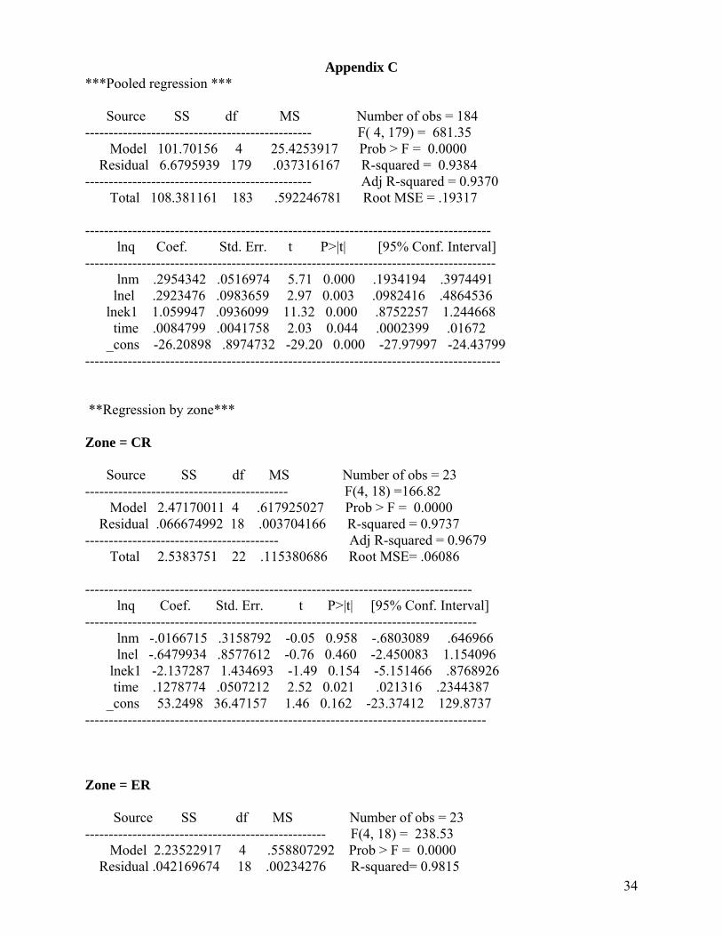
34

Appendix C

***Pooled regression *** Source SS df MS Number of obs = 184 ------------------------------------------------ F( 4, 179) = 681.35 Model 101.70156 4 25.4253917 Prob > F = 0.0000 Residual 6.6795939 179 .037316167 R-squared = 0.9384 ------------------------------------------------ Adj R-squared = 0.9370 Total 108.381161 183 .592246781 Root MSE = .19317 -------------------------------------------------------------------------------------- lnq Coef. Std. Err. t P>|t| [95% Conf. Interval] --------------------------------------------------------------------------------------- lnm .2954342 .0516974 5.71 0.000 .1934194 .3974491 lnel .2923476 .0983659 2.97 0.003 .0982416 .4864536 lnek1 1.059947 .0936099 11.32 0.000 .8752257 1.244668 time .0084799 .0041758 2.03 0.044 .0002399 .01672 _cons -26.20898 .8974732 -29.20 0.000 -27.97997 -24.43799 ---------------------------------------------------------------------------------------- **Regression by zone*** Zone = CR Source SS df MS Number of obs = 23 ------------------------------------------- F(4, 18) =166.82 Model 2.47170011 4 .617925027 Prob > F = 0.0000 Residual .066674992 18 .003704166 R-squared = 0.9737 ----------------------------------------- Adj R-squared = 0.9679 Total 2.5383751 22 .115380686 Root MSE= .06086 ---------------------------------------------------------------------------------- lnq Coef. Std. Err. t P>|t| [95% Conf. Interval] ----------------------------------------------------------------------------------- lnm -.0166715 .3158792 -0.05 0.958 -.6803089 .646966 lnel -.6479934 .8577612 -0.76 0.460 -2.450083 1.154096 lnek1 -2.137287 1.434693 -1.49 0.154 -5.151466 .8768926 time .1278774 .0507212 2.52 0.021 .021316 .2344387 _cons 53.2498 36.47157 1.46 0.162 -23.37412 129.8737 ------------------------------------------------------------------------------------- Zone = ER Source SS df MS Number of obs = 23 --------------------------------------------------- F(4, 18) = 238.53 Model 2.23522917 4 .558807292 Prob > F = 0.0000 Residual .042169674 18 .00234276 R-squared= 0.9815

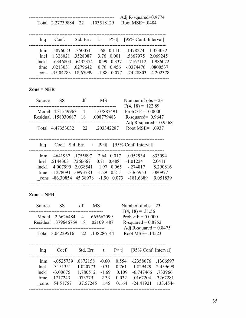
35

----------------------------------------------------- Adj R-squared=0.9774 Total 2.27739884 22 .103518129 Root MSE= .0484 ------------------------------------------------------------------------------------- lnq Coef. Std. Err. t P>|t| [95% Conf. Interval] ------------------------------------------------------------------------------------- lnm .5876023 .350051 1.68 0.111 -.1478274 1.323032 lnel 1.328021 .3528087 3.76 0.001 .5867975 2.069245 lnek1 .6346804 .6432374 0.99 0.337 -.7167112 1.986072 time .0213031 .0279642 0.76 0.456 -.0374476 .0800537 _cons -35.04283 18.67999 -1.88 0.077 -74.28803 4.202378 --------------------------------------------------------------------------------------- Zone = NER Source SS df MS Number of obs = 23 ------------------------------------------------------ F(4, 18) = 122.89 Model 4.31549963 4 1.07887491 Prob > F = 0.0000 Residual .158030687 18 .008779483 R-squared= 0.9647 ------------------------------------------------------- Adj R-squared= 0.9568 Total 4.47353032 22 .203342287 Root MSE= .0937 ------------------------------------------------------------------------------------ lnq Coef. Std. Err. t P>|t| [95% Conf. Interval] ------------------------------------------------------------------------------------ lnm .4641937 .1755897 2.64 0.017 .0952934 .833094 lnel .5144303 .7266667 0.71 0.488 -1.01224 2.0411 lnek1 4.007999 2.038541 1.97 0.065 -.274817 8.290816 time -.1278091 .0993783 -1.29 0.215 -.3365953 .080977 _cons -86.30854 45.38978 -1.90 0.073 -181.6689 9.051839 --------------------------------------------------------------------------------------- Zone = NFR Source SS df MS Number of obs = 23 ---------------------------------------------- F(4, 18) = 31.56 Model 2.6626484 4 .665662099 Prob > F = 0.0000 Residual .379646769 18 .021091487 R-squared = 0.8752 ----------------------------------------------- Adj R-squared = 0.8475 Total 3.04229516 22 .138286144 Root MSE= .14523 ------------------------------------------------------------------------------------- lnq Coef. Std. Err. t P>|t| [95% Conf. Interval] -------------------------------------------------------------------------------------- lnm -.0525739 .0872158 -0.60 0.554 -.2358076 .1306597 lnel .3151351 1.020773 0.31 0.761 -1.829429 2.459699 lnek1 -3.00675 1.780512 -1.69 0.109 -6.747466 .733966 time .1717243 .073779 2.33 0.032 .0167204 .3267281 _cons 54.51757 37.57245 1.45 0.164 -24.41921 133.4544 ----------------------------------------------------------------------------------------

36

Zone = SR Source SS df MS Number of obs = 23 ------------------------------------------- F(4, 18) = 485.39 Model 2.88260296 4 .720650741 Prob > F = 0.0000 Residual .026724076 18 .001484671 R-squared = 0.9908 ------------------------------------------- Adj R-squared = 0.9888 Total 2.90932704 22 .132242138 Root MSE= .03853 -------------------------------------------------------------------------------------- lnq Coef. Std. Err. t P>|t| [95% Conf. Interval] -------------------------------------------------------------------------------------- lnm .0194405 .0903071 0.22 0.832 -.1702877 .2091687 lnel .5130145 .3449908 1.49 0.154 -.2117844 1.237813 lnek1 .8723733 .3242574 2.69 0.015 .1911337 1.553613 time .0076581 .0149312 0.51 0.614 -.0237111 .0390274 _cons -20.88111 6.290768 -3.32 0.004 -34.09752 -7.664699 --------------------------------------------------------------------------------------- Zone = SCR Source SS df MS Number of obs = 23 ------------------------------------------------------ F (4, 18) = 202.11 Model 2.23070409 4 .557676022 Prob > F = 0.0000 Residual .049665972 18 .002759221 R-squared = 0.9782 ------------------------------------------------------- Adj R-squared= 0.9734 Total 2.28037006 22 .103653184 Root MSE= .05253 -------------------------------------------------------------------------------------- lnq Coef. Std. Err. t P>|t| [95% Conf. Interval] -------------------------------------------------------------------------------------- lnm -.0626318 .3675773 -0.17 0.867 -.8348831 .7096195 lnel 1.144545 .3430548 3.34 0.004 .4238135 1.865276 lnek1 .7530725 1.337281 0.56 0.580 -2.05645 3.562595 time .014872 .0564729 0.26 0.795 -.1037733 .1335172 _cons -25.15977 31.88182 -0.79 0.440 -92.141 41.82145 ---------------------------------------------------------------------------------------- Zone = SER Source SS df MS Number of obs = 23 ------------------------------------------- F(4, 18) = 304.40 Model 4.62211302 4 1.15552825 Prob > F = 0.0000 Residual .068329167 18 .003796065 R-squared = 0.9854 ------------------------------------------- Adj R-squared = 0.9822 Total 4.69044219 22 .213201918 Root MSE= .06161 ----------------------------------------------------------------------------------- lnq Coef. Std. Err. t P>|t| [95% Conf. Interval] -----------------------------------------------------------------------------------

37

lnm -.7655755 .3974798 -1.93 0.070 -1.60065 .0694985 lnel 1.727474 .735049 2.35 0.030 .1831929 3.271754 lnek1 1.022586 .9080419 1.13 0.275 -.8851396 2.930311 time .0358731 .0309221 1.16 0.261 -.0290918 .100838 _cons -27.46923 25.48984 -1.08 0.295 -81.0214 26.08294 --------------------------------------------------------------------------------------- Zone = WR Source SS df MS Number of obs = 23 --------------------------------------------------- F(4, 18) = 390.78 Model 2.37447194 4 .593617985 Prob > F= 0.0000 Residual .027343342 18 .001519075 R-squared= 0.9886 ---------------------------------------------------- Adj R-squared = 0.9861 Total 2.40181528 22 .109173422 Root MSE = .03898 ---------------------------------------------------------------------------------- lnq Coef. Std. Err. t P>|t| [95% Conf. Interval] ---------------------------------------------------------------------------------- lnm .6297147 .1652924 3.81 0.001 .2824483 .9769811 lnel .5752051 .5351916 1.07 0.297 -.5491908 1.699601 lnek1 .6428869 .3291257 1.95 0.067 -.0485805 1.334354 time .0116365 .0139175 0.84 0.414 -.0176031 .040876 _cons -26.53268 11.77631 -2.25 0.037 -51.27378 -1.791582 -------------------------------------------------------------------------------------- XTPCSE results WITH PSAR1 B:1 B:2 B:3* B:4* B:5 B:6a B:6a1 B:6b B:6b1 constant -26.59 -27.4 -20.93 -21.81 -26.71 -26.64 -27.04 -26.7 -26.97 (1.63) (1.74) (1.26) (1.1) (1.73) (1.62) (1.36) (1.62) (1.31) ln ek 0.95 1.1 1.01 0.96 1.04 0.99 1.05 (0.15) (0.12) (0.15) (0.15) (0.14) (0.15) (0.13) ln el 0.71 0.69 0.7 0.6 0.65 0.57 (0.16) (0.13) (0.16) (0.16) (0.15) (0.14) ln ef 0.12 0.16 0.12 0.12 0.12 0.13 0.13 (0.07) (0.06) (0.07) (0.07) (0.07) (0.07) (0.06) time 0.01 0.02 0.01 0.03 0.008 0.01 0.008 0.01 0.007 (0.005) (0.005) (0.006) (0.005) (0.005) (0.005) (0.005) (0.005) ` ln scst 0.1

38

(0.05) ln others 0.54 (0.13) scp -0.17 (0.23) scd -0.32 (0.34) scabp -0.17 (0.18) scabd -0.09 (0.297) emp 0.82 0.83 (0.18) (0.13) capital 0.94 1.08 (0.17) (0.11) materials 0.08 0.1 (0.06) (0.05) corr scp 0.03 0.06 0 0.03 corr scd -0.01 0.03 -0.09 -0.04 corr scabp 0.14 0.2 0.03 0.08 corr scabd 0.2 0.27 0.05 0.1 WITH COMMON AR1 B:1 B:2 B:3* B:4* B:5 B:6a B:6a1 B:6b B:6b1 constant -26.28 -27 -20.99 -21.88 -26.17 -26.28 -26.65 -26.25 -26.71 (1.42) (1.36) (1.35) (1.26) (1.5) (1.41) (1.17) (1.39) (1.1) ln ek 1.01 1.21 1.04 1.01 1.05 1.01 1.04 (0.12) (0.12) (0.12) (0.12) (0.12) (0.12) (0.11) ln el 0.54 0.47 0.54 0.51 0.53 0.53 (0.11) (0.11) (0.11) (0.12) (0.11) (0.13) ln ef 0.16 0.19 0.16 0.16 0.16 0.16 0.16 (0.07) (0.06) (0.07) (0.07) (0.06) (0.07) (0.06) time 0.009 0.02 0.01 0.03 0.007 0.008 0.008 0.009 0.007 (0.006) (0.005) (0.006) (0.006) (0.006) (0.006) (0.005) (0.006) (0.005) ln scst 0.09 (0.06) ln others 0.4 (0.1) scp -0.05 (0.28) scd -0.37 (0.42) scabp -0.12 (0.2) scabd 0.1 (0.33) emp 0.61 0.57 (0.11) (0.11) capital 1.01 1.2 (0.1) (0.1) materials 0.12 0.14 (0.06) (0.05)

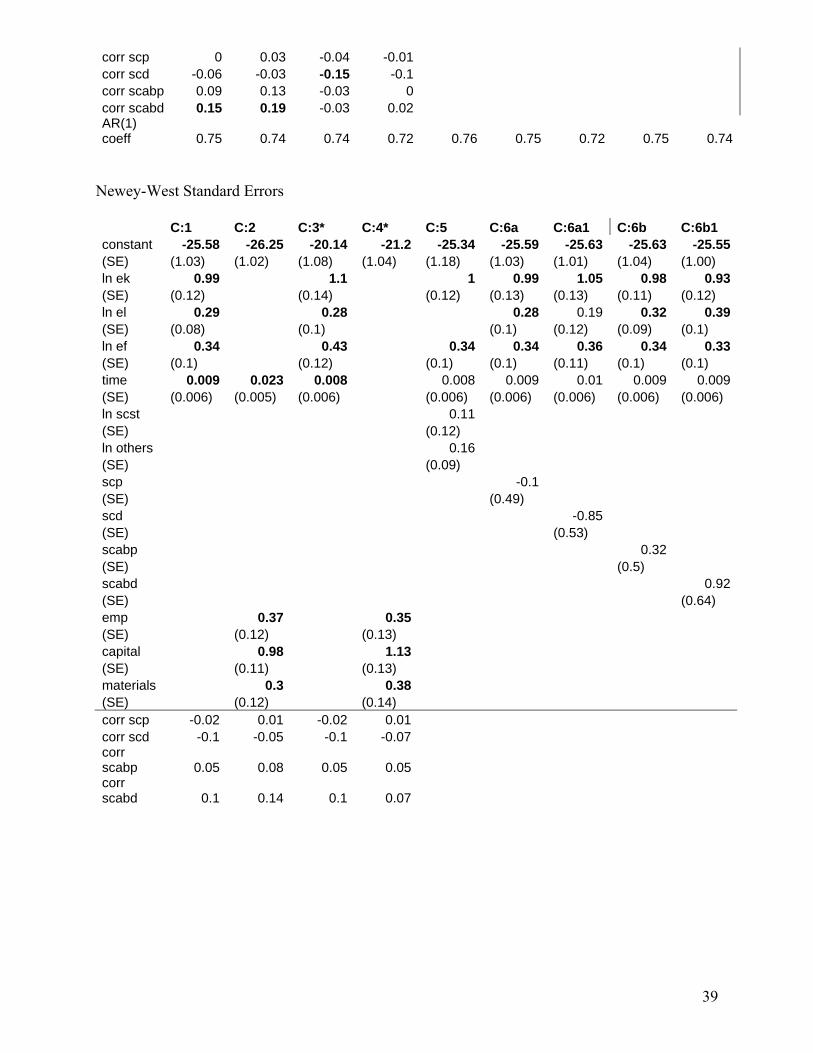
39

corr scp 0 0.03 -0.04 -0.01 corr scd -0.06 -0.03 -0.15 -0.1 corr scabp 0.09 0.13 -0.03 0 corr scabd 0.15 0.19 -0.03 0.02 AR(1) coeff 0.75 0.74 0.74 0.72 0.76 0.75 0.72 0.75 0.74

Newey-West Standard Errors C:1 C:2 C:3* C:4* C:5 C:6a C:6a1 C:6b C:6b1 constant -25.58 -26.25 -20.14 -21.2 -25.34 -25.59 -25.63 -25.63 -25.55(SE) (1.03) (1.02) (1.08) (1.04) (1.18) (1.03) (1.01) (1.04) (1.00) ln ek 0.99 1.1 1 0.99 1.05 0.98 0.93(SE) (0.12) (0.14) (0.12) (0.13) (0.13) (0.11) (0.12) ln el 0.29 0.28 0.28 0.19 0.32 0.39(SE) (0.08) (0.1) (0.1) (0.12) (0.09) (0.1) ln ef 0.34 0.43 0.34 0.34 0.36 0.34 0.33(SE) (0.1) (0.12) (0.1) (0.1) (0.11) (0.1) (0.1) time 0.009 0.023 0.008 0.008 0.009 0.01 0.009 0.009(SE) (0.006) (0.005) (0.006) (0.006) (0.006) (0.006) (0.006) (0.006) ln scst 0.11 (SE) (0.12) ln others 0.16 (SE) (0.09) scp -0.1 (SE) (0.49) scd -0.85 (SE) (0.53) scabp 0.32 (SE) (0.5) scabd 0.92(SE) (0.64) emp 0.37 0.35 (SE) (0.12) (0.13) capital 0.98 1.13 (SE) (0.11) (0.13) materials 0.3 0.38 (SE) (0.12) (0.14) corr scp -0.02 0.01 -0.02 0.01 corr scd -0.1 -0.05 -0.1 -0.07 corr scabp 0.05 0.08 0.05 0.05 corr scabd 0.1 0.14 0.1 0.07