Embed Size (px)
Citation preview
C H A P T E R 1
Speech Signal Representations
This chapter presents several representations for speech signals useful in speech coding, synthesis and recognition. The central theme of the chapter is the decomposition of the speech signal as a source passed through a linear time-varying filter. This filter can be derived from models of speech production based on the theory of acoustics where the source represents the air flow at the vocal cords, and the filter represents the resonances of the vocal tract which change over time. Such a source-filter model is illustrated in Figure 1.1. We describe methods to compute both the source or exci-tation e[n], and the filter h[n] from the speech signal x[n].
Figure 1.1 Basic source-filter model for speech signals.
To estimate the filter we present methods inspired by speech production models (such as linear predictive coding and cepstral analysis) as well as speech perception models (such
267
x[n]e[n] h[n]
268 Speech Signal Representations
as mel-frequency cepstrum). Once the filter has been estimated, the source can be obtained by passing the speech signal through the inverse filter. Separation between source and filter is one of the most difficult challenges in speech processing.
It turns out that phoneme classification (either by human or by machines) is mostly de-pendent on the characteristics of the filter. Traditionally, speech recognizers estimate the fil-ter characteristics and ignore the source. Many speech synthesis techniques use a source-fil -ter model because it allows flexibility in altering the pitch and the filter. Many speech coders also use this model because it allows a low bit rate.
We first introduce the spectrogram as a representation of the speech signal that high-lights several of its properties and describe the Short-time Fourier analysis, which is the ba-sic tool to build the spectrograms of Chapter 2. We then introduce several techniques used to separate source and filter: LPC and cepstral analysis, perceptually motivated models, for-mant tracking and pitch tracking.
1.1. SHORT-TIME FOURIER ANALYSIS
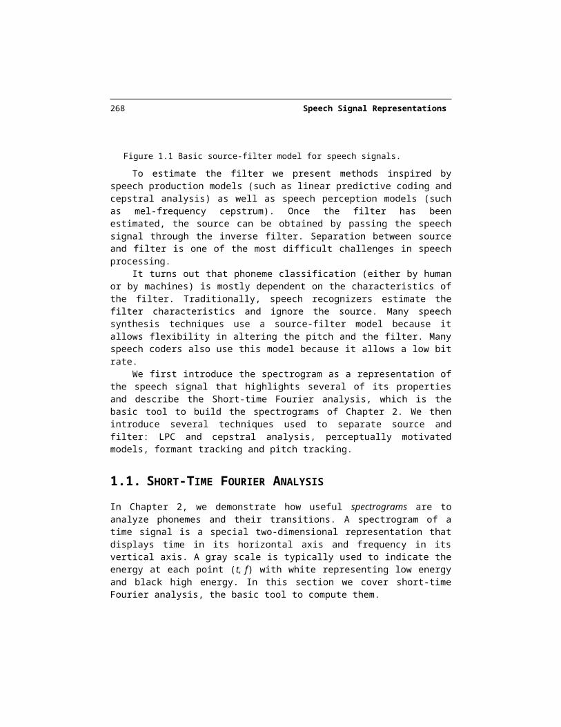
In Chapter 2, we demonstrate how useful spectrograms are to analyze phonemes and their transitions. A spectrogram of a time signal is a special two-dimensional representation that displays time in its horizontal axis and frequency in its vertical axis. A gray scale is typically used to indicate the energy at each point (t, f) with white representing low energy and black high energy. In this section we cover short-time Fourier analysis, the basic tool to compute them.
0 0.1 0.2 0.3 0.4 0.5 0.6-0.5
0
0.5
Time (seconds)
Freq
uenc
y (H
z)
0 0.1 0.2 0.3 0.4 0.5 0.60
1000
2000
3000
4000
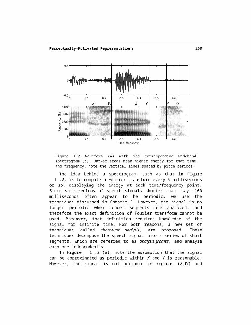
Figure 1.2 Waveform (a) with its corresponding wideband spectrogram (b). Darker areas mean higher energy for that time and frequency. Note the vertical lines spaced by pitch periods.
X YZ W H G
Perceptually-Motivated Representations 269
The idea behind a spectrogram, such as that in Figure 1.2, is to compute a Fourier transform every 5 milliseconds or so, displaying the energy at each time/frequency point. Since some regions of speech signals shorter than, say, 100 milliseconds often appear to be periodic, we use the techniques discussed in Chapter 5. However, the signal is no longer pe-riodic when longer segments are analyzed, and therefore the exact definition of Fourier transform cannot be used. Moreover, that definition requires knowledge of the signal for in-finite time. For both reasons, a new set of techniques called short-time analysis, are pro-posed. These techniques decompose the speech signal into a series of short segments, which are referred to as analysis frames, and analyze each one independently.
In Figure 1.2 (a), note the assumption that the signal can be approximated as periodic within X and Y is reasonable. However, the signal is not periodic in regions (Z,W) and (H,G). In those regions, the signal looks like random noise. The signal in (Z,W) appears to have dif-ferent noisy characteristics than those of segment (H,G). The use of an analysis frame im-plies that the region is short enough for the behavior (periodicity or noise-like appearance) of the signal to be approximately constant. If the region where speech seems periodic is too long, the pitch period is not constant and not all the periods in the region are similar. In essence, the speech region has to be short enough so that the signal is stationary in that re-gion: i.e., the signal characteristics (whether periodicity or noise-like appearance) are uni-form in that region. A more formal definition of stationarity is given in Chapter 5.
Similarly to the filterbanks described in Chapter 5, given a speech signal , we de-fine the short-time signal of frame m as
the product of by a window function , which is zero everywhere but in a small region.
While the window function can have different values for different frames m, a popular choice is to keep it constant for all frames:
where for . In practice, the window length is on the order of 20 to 30 ms.
With the above framework, the short-time Fourier representation for frame m is de-fined as
with all the properties of Fourier transforms studied in Chapter 5.
270 Speech Signal Representations
0 0.005 0.01 0.015 0.02 0.025 0.03 0.035 0.04 0.045 0.05-5000
0
5000(a)
0 1000 2000 3000 400020406080
100120
dB
(b)
0 1000 2000 3000 400020406080
100120
dB
(c)
0 1000 2000 3000 400020406080
100120
dB
(d)
0 1000 2000 3000 400020406080
100120
dB
(e)
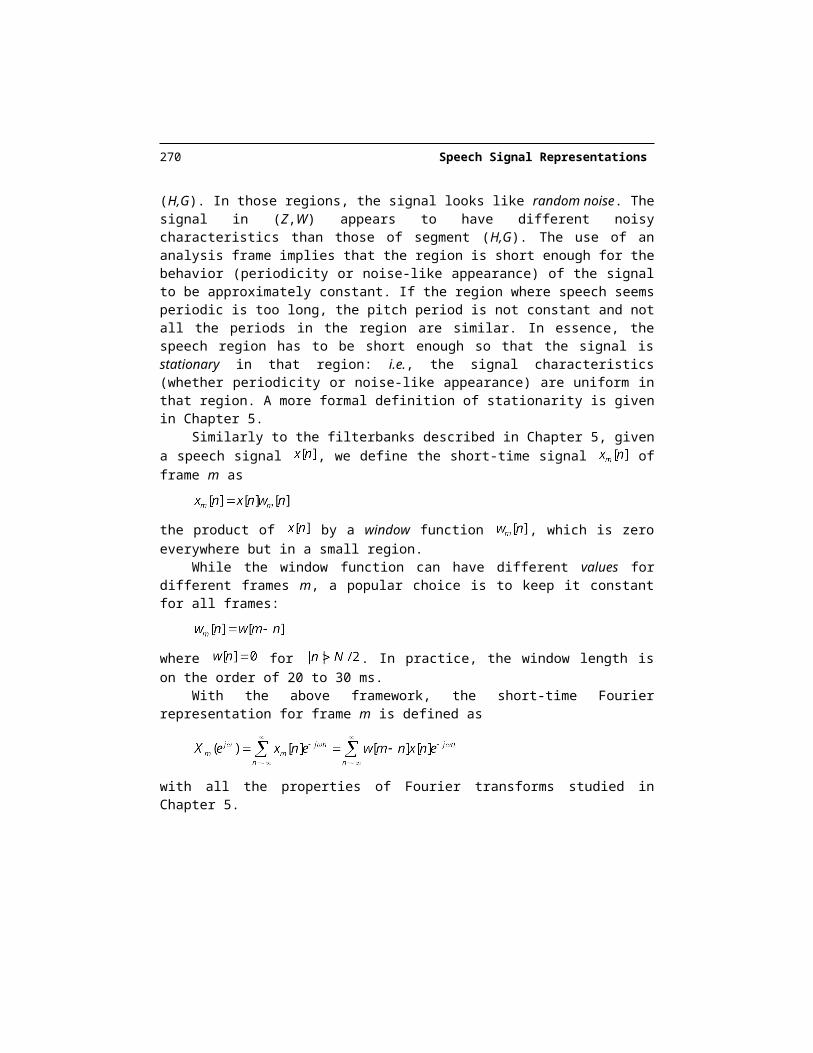
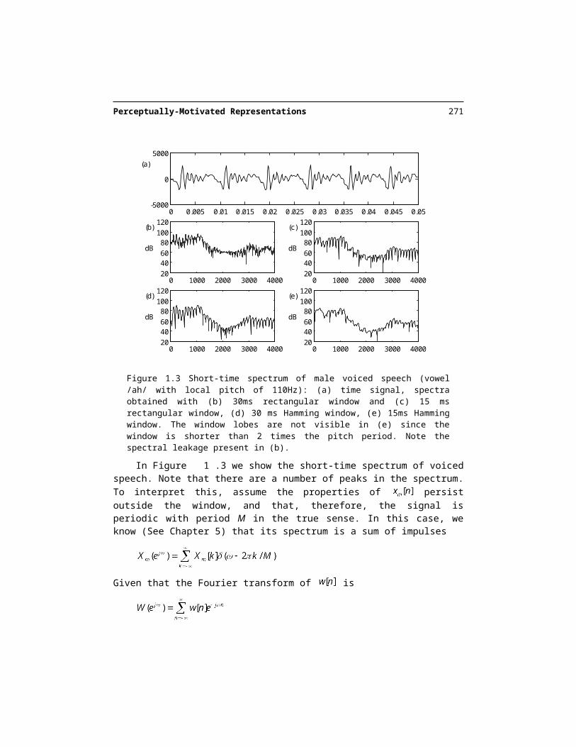
Figure 1.3 Short-time spectrum of male voiced speech (vowel /ah/ with local pitch of 110Hz): (a) time signal, spectra obtained with (b) 30ms rectangular window and (c) 15 ms rectangular window, (d) 30 ms Hamming window, (e) 15ms Hamming window. The window lobes are not visible in (e) since the window is shorter than 2 times the pitch period. Note the spectral leak-age present in (b).
In Figure 1.3 we show the short-time spectrum of voiced speech. Note that there are a number of peaks in the spectrum. To interpret this, assume the properties of persist outside the window, and that, therefore, the signal is periodic with period M in the true sense. In this case, we know (See Chapter 5) that its spectrum is a sum of impulses
Given that the Fourier transform of is
so that the transform of is . Therefore, using the convolution prop-erty, the transform of for fixed m is the convolution in the frequency domain
Perceptually-Motivated Representations 271
which is a sum of weighted , shifted on every harmonic, the narrow peaks seen in Figure 1.3 (b) with a rectangular window. The short-time spectrum of a periodic signal ex-hibits peaks (equally spaced apart) representing the harmonics of the signal. We es-timate from the short-time spectrum , and see the importance of the length and choice of window.
Eq. indicates that one cannot recover by simply retrieving , although the approximation can be reasonable if there is a small value of such that
for
which is the case outside the main lobe of the window’s frequency response.Recall from Section 5.4.2.1, that for a rectangular window of length N, .
Therefore, Eq. is satisfied if , i.e. the rectangular window contains at least one pitch period. The width of the main lobe of the window’s frequency response is inversely propor-tional to the length of the window. The pitch period in Figure 1.3 is M=71 at a sampling rate of 8kHz. A shorter window is used in Figure 1.3 (c), which results in wider analysis lobes, though still visible.
Also recall from Section 5.4.2.2 that for a Hamming window of length N, : twice as wide as that of the rectangular window, which entails . Thus, a Hamming window must contain at least two pitch periods for Eq. to be met. The lobes are visible in Figure 1.3 (d) since N=240, but they are not visible in Figure 1.3 (e) since N=120, and
.In practice, one cannot know what the pitch period is ahead of time, which often
means you need to prepare for the lowest pitch period. A low-pitched voice with a requires a rectangular window of at least 20ms and a Hamming window of at
least 40ms for condition in Eq. to be met. If speech is non-stationary within 40ms, taking such long window implies obtaining an average spectrum during that segment instead of several distinct spectra. For this reason, the rectangular window provides better time resolu-tion than the Hamming window. Figure 1.4 shows analysis of female speech for which shorter windows are feasible.
But the frequency response of the window is not completely zero outside its main lobe, so one needs to see the effects of this incorrect assumption. From Section 5.4.2.1 note that the second lobe of a rectangular window is only approximately 17dB below the main lobe. Therefore, for the kth harmonic the value of contains not , but also a weighted sum of . This phenomenon is called spectral leakage because the ampli-tude of one harmonic leaks over the rest and masks its value. If the signal’s spectrum is white, spectral leakage does not cause a major problem, since the effect of the second lobe on a harmonic is only . On the other hand, if the signal’s spec-
272 Speech Signal Representations
trum decays more quickly in frequency than the decay of the window, the spectral leakage results in inaccurate estimates.
From Section 5.4.2.2, observe that the second lobe of a Hamming window is approxi-mately 43 dB, which means that the spectral leakage effect is much less pronounced. Other windows, such as Hanning, or triangular windows, also offer less spectral leakage than the rectangular window. This important fact is the reason why, despite its better time resolution, rectangular windows are rarely used for speech analysis. In practice, window lengths are on the order of 20 to 30 ms. This choice is a compromise between the stationarity assumption and the frequency resolution.
In practice, the Fourier transform in Eq. is obtained through an FFT. If the window has length N, the FFT has to have a length greater or equal than N. Since FFT algorithms of-ten have lengths that are powers of 2 ( ), the windowed signal with length N is aug-mented with zeros either before, after or both. This process is called zero-padding. A larger value of L provides with a finer description of the discrete Fourier transform; but it does not increase the analysis frequency resolution: this is the sole mission of the window length N.
0 0.005 0.01 0.015 0.02 0.025 0.03 0.035 0.04 0.045 0.05-5000
0
5000(a)
0 1000 2000 3000 400020406080
100120
dB
(b)
0 1000 2000 3000 400020406080
100120
dB
(c)
0 1000 2000 3000 400020406080
100120
dB
(d)
0 1000 2000 3000 400020406080
100120
dB
(e)
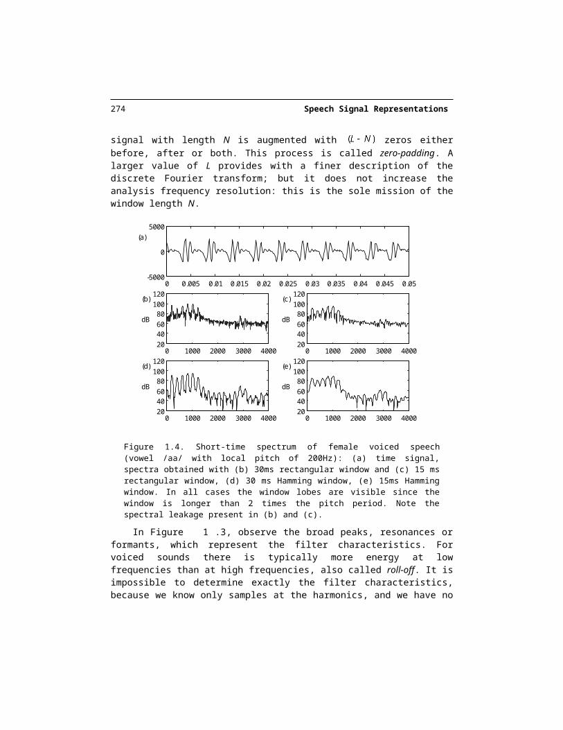
Figure 1.4. Short-time spectrum of female voiced speech (vowel /aa/ with local pitch of 200Hz): (a) time signal, spectra obtained with (b) 30ms rectangular window and (c) 15 ms rec-tangular window, (d) 30 ms Hamming window, (e) 15ms Hamming window. In all cases the window lobes are visible since the window is longer than 2 times the pitch period. Note the spectral leakage present in (b) and (c).
Perceptually-Motivated Representations 273
In Figure 1.3, observe the broad peaks, resonances or formants, which represent the filter characteristics. For voiced sounds there is typically more energy at low frequencies than at high frequencies, also called roll-off. It is impossible to determine exactly the filter characteristics, because we know only samples at the harmonics, and we have no knowledge of the values in between. In fact, the resonances are less obvious in Figure 1.4 because the harmonics sample the spectral envelope less densely. For high-pitched female speakers and children, it is even more difficult to locate the formant resonances from the short-time spec-trum.
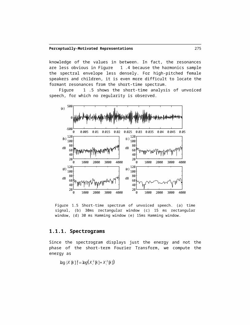
Figure 1.5 shows the short-time analysis of unvoiced speech, for which no regularity is observed.
0 0.005 0.01 0.015 0.02 0.025 0.03 0.035 0.04 0.045 0.05-500
0
500(a)
0 1000 2000 3000 400020406080
100120
dB
(b)
0 1000 2000 3000 400020406080
100120
dB
(c)
0 1000 2000 3000 400020406080
100120
dB
(d)
0 1000 2000 3000 400020406080
100120
dB
(e)
Figure 1.5 Short-time spectrum of unvoiced speech. (a) time signal, (b) 30ms rectangular win-dow (c) 15 ms rectangular window, (d) 30 ms Hamming window (e) 15ms Hamming window.
1.1.1. Spectrograms
Since the spectrogram displays just the energy and not the phase of the short-term Fourier Transform, we compute the energy as
274 Speech Signal Representations
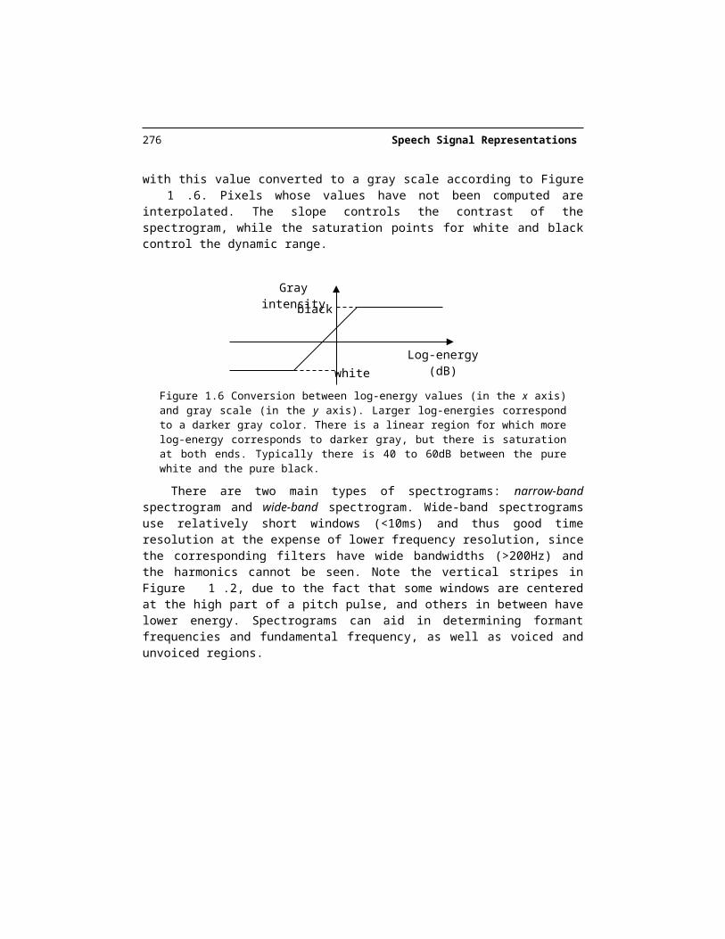
with this value converted to a gray scale according to Figure 1.6. Pixels whose values have not been computed are interpolated. The slope controls the contrast of the spectrogram, while the saturation points for white and black control the dynamic range.
Figure 1.6 Conversion between log-energy values (in the x axis) and gray scale (in the y axis). Larger log-energies correspond to a darker gray color. There is a linear region for which more log-energy corresponds to darker gray, but there is saturation at both ends. Typically there is 40 to 60dB between the pure white and the pure black.
There are two main types of spectrograms: narrow-band spectrogram and wide-band spectrogram. Wide-band spectrograms use relatively short windows (<10ms) and thus good time resolution at the expense of lower frequency resolution, since the corresponding filters have wide bandwidths (>200Hz) and the harmonics cannot be seen. Note the vertical stripes in Figure 1.2, due to the fact that some windows are centered at the high part of a pitch pulse, and others in between have lower energy. Spectrograms can aid in determining for-mant frequencies and fundamental frequency, as well as voiced and unvoiced regions.
0 0.1 0.2 0.3 0.4 0.5 0.6-0.5
0
0.5
Time (seconds)
Freq
uenc
y (H
z)
0 0.1 0.2 0.3 0.4 0.5 0.60
2000
4000
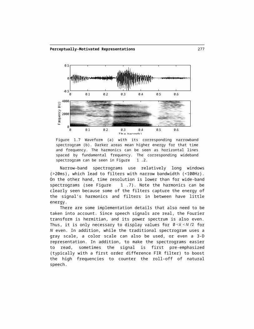
Figure 1.7 Waveform (a) with its corresponding narrowband spectrogram (b). Darker areas mean higher energy for that time and frequency. The harmonics can be seen as horizontal lines spaced by fundamental frequency. The corresponding wideband spectrogram can be seen in Figure 1.2.
Log-energy (dB)
Gray intensity
black
white
Perceptually-Motivated Representations 275
Narrow-band spectrograms use relatively long windows (>20ms), which lead to filters with narrow bandwidth (<100Hz). On the other hand, time resolution is lower than for wide-band spectrograms (see Figure 1.7). Note the harmonics can be clearly seen because some of the filters capture the energy of the signal’s harmonics and filters in between have little en-ergy.
There are some implementation details that also need to be taken into account. Since speech signals are real, the Fourier transform is hermitian, and its power spectrum is also even. Thus, it is only necessary to display values for for N even. In addition, while the traditional spectrogram uses a gray scale, a color scale can also be used, or even a 3-D representation. In addition, to make the spectrograms easier to read, sometimes the sig-nal is first pre-emphasized (typically with a first order difference FIR filter) to boost the high frequencies to counter the roll-off of natural speech.
By inspecting both narrow and wide band spectrograms, we can learn the filter’s mag-nitude response and whether the source is voiced or not. Nonetheless it is very difficult to separate source and filter due to nonstationarity of the speech signal, spectral leakage and the fact that only the filter’s magnitude response can be known at the signal’s harmonics.
1.1.2. Pitch-Synchronous Analysis
In the previous discussion, we assumed that the window length is fixed, and saw the trade-offs between a window that contained several pitch periods (narrow-band spectrograms) and a window that contained less than a pitch period (wide-band spectrograms). One possibility is to use a rectangular window whose length is exactly one pitch period, and this is called pitch-synchronous analysis. To reduce spectral leakage a tapering window, such as Ham-ming, or Hanning, can be used with the window covering exactly two pitch periods. This lat-ter option provides a very good compromise between time and frequency resolution. In this representation, no stripes can be seen in either time or frequency. The difficulty in comput-ing pitch synchronous analysis is that, of course, we need to know the local pitch period, which, as we see in Section 1.7, is not an easy task.
1.2. ACOUSTICAL MODEL OF SPEECH PRODUCTION
Speech is a sound wave created by vibration that is propagated in the air. Acoustic theory analyzes the laws of physics that govern the propagation of sound in the vocal tract. Such a theory should consider three-dimensional wave propagation, the variation of the vocal tract shape with time, losses due to heat conduction and viscous friction at the vocal tract walls, softness of the tract walls, radiation of sound at the lips, nasal coupling and excitation of sound. While a detailed model that considers all of the above is not yet available, there are some models that provide a good approximation in practice, as well as a good understanding of the physics involved.
276 Speech Signal Representations
1.2.1. Glottal Excitation
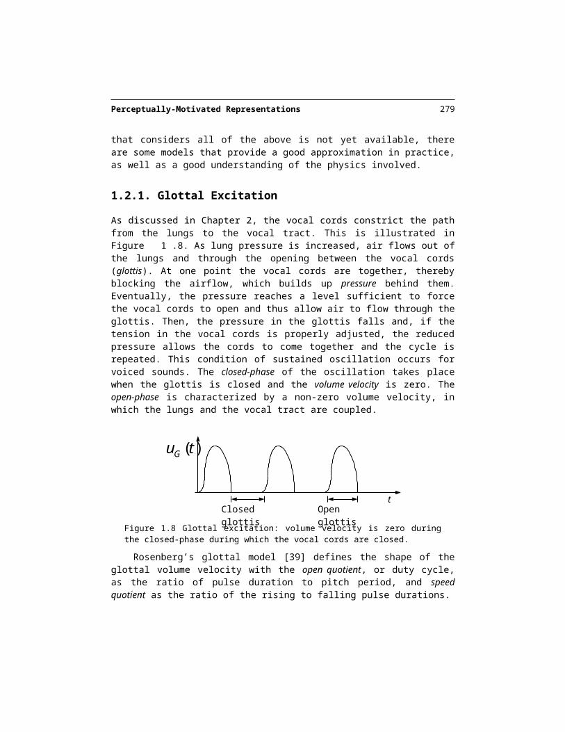
As discussed in Chapter 2, the vocal cords constrict the path from the lungs to the vocal tract. This is illustrated in Figure 1.8. As lung pressure is increased, air flows out of the lungs and through the opening between the vocal cords (glottis). At one point the vocal cords are together, thereby blocking the airflow, which builds up pressure behind them. Eventually, the pressure reaches a level sufficient to force the vocal cords to open and thus allow air to flow through the glottis. Then, the pressure in the glottis falls and, if the tension in the vocal cords is properly adjusted, the reduced pressure allows the cords to come to-gether and the cycle is repeated. This condition of sustained oscillation occurs for voiced sounds. The closed-phase of the oscillation takes place when the glottis is closed and the volume velocity is zero. The open-phase is characterized by a non-zero volume velocity, in which the lungs and the vocal tract are coupled.
Figure 1.8 Glottal excitation: volume velocity is zero during the closed-phase during which the vocal cords are closed.
Rosenberg’s glottal model [39] defines the shape of the glottal volume velocity with the open quotient, or duty cycle, as the ratio of pulse duration to pitch period, and speed quotient as the ratio of the rising to falling pulse durations.
1.2.2. Lossless Tube Concatenation
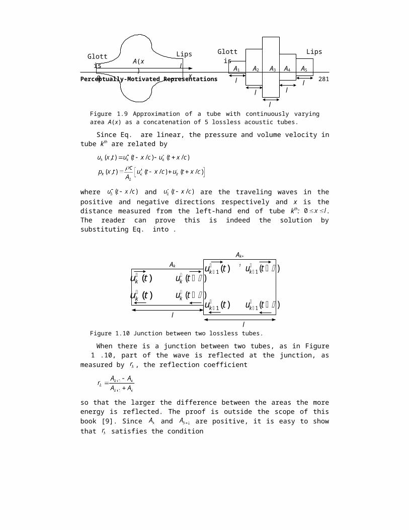
A widely used model for speech production is based on the assumption that the vocal tract can be represented as a concatenation of lossless tubes, as shown in Figure 1.9. The constant cross-sectional areas of the tubes approximate the area function A(x) of the vocal tract. If a large number of tubes of short length is used, we reasonably expect the frequency re-sponse of the concatenated tubes to be close to those of a tube with continuously varying area function.
For frequencies corresponding to wavelengths that are long compared to the dimen-sions of the vocal tract, it is reasonable to assume plane wave propagation along the axis of the tubes. If in addition we assume that there are no losses due to viscosity or thermal con-duction, and that the area A does not change over time, the sound waves in the tube satisfy the following pair of differential equations:
Closed glottis Open glottist
u tG ( )
Perceptually-Motivated Representations 277
where is the sound pressure in the tube at position x and time t, is the volume velocity flow in the tube at position x and time t, is the density of air in the tube, c is the velocity of sound and A is the cross-sectional area of the tube.
Figure 1.9 Approximation of a tube with continuously varying area A(x) as a concatenation of 5 lossless acoustic tubes.
Since Eq. are linear, the pressure and volume velocity in tube kth are related by
where and are the traveling waves in the positive and negative di-rections respectively and x is the distance measured from the left-hand end of tube kth:
. The reader can prove this is indeed the solution by substituting Eq. into .
Figure 1.10 Junction between two lossless tubes.
A1 A2 A3 A4 A5
l
Glottis Lips
l
l
l
lx0
lA(x)
Glottis Lips
l
u tk ( )
u tk ( )
u tk
1( )
u tk
1( )
u tk 1( )
u tk 1( )
u tk ( )
u tk ( )
l
Ak
Ak+
1
278 Speech Signal Representations
When there is a junction between two tubes, as in Figure 1.10, part of the wave is re-flected at the junction, as measured by , the reflection coefficient
so that the larger the difference between the areas the more energy is reflected. The proof is outside the scope of this book [9]. Since and are positive, it is easy to show that satisfies the condition
A relationship between the z-transforms of the volume velocity at the glottis and the lips for a concatenation of N lossless tubes can be derived [9] using a dis-crete-time version of Eq. and taking into account boundary conditions for every junction:
where is the reflection coefficient at the glottis and is the reflection coefficient at the lips. Eq. is still valid for the glottis and lips, where is the equivalent area at the glottis and being the equivalent area at the lips. and are the equivalent impedances at the glottis and lips respectively. Such impedances relate the vol-ume velocity and pressure, for the lips the expression is
In general, the concatenation of N lossless tubes results in an N-pole system as shown in Eq. . For a concatenation of N tubes, there are at most N/2 complex conjugate poles, or resonances or formants. These resonances occur when a given frequency gets trapped in the vocal tract because it is reflected back at the lips and then again back at the glottis.
Since each tube has length l and there are N of them, the total length is . The propagation delay in each tube , and the sampling period is , the roundtrip in a tube. We can find a relationship between the number of tubes N and the sampling fre-quency :
For example, for = 8000 kHz, c = 34000 cm/s, L = 17 cm, the average length of a male adult vocal tract, we obtain N = 8, or alternatively 4 formants. Experimentally, the vo-
Perceptually-Motivated Representations 279
cal tract transfer function has been observed to have approximately 1 formant per kilohertz. Shorter vocal tract lengths (females or children) have fewer resonances per kilohertz and vice versa.
The pressure at the lips has been found to approximate the derivative of volume veloc-ity, particularly at low frequencies. Thus, can be approximated by
which is 0 for low frequencies and reaches asymptotically. This dependency with fre-quency results in a reflection coefficient that is also a function of frequency. For low fre-quencies , and no loss occurs. At higher frequencies, loss by radiation translates into widening of formant bandwidths.
Similarly, the glottal impedance is also a function of frequency in practice. At high frequencies, is large and so that all the energy is transmitted. For low frequen-cies, whose main effect is an increase of bandwidth for the lower formants.
1 2 3 4 5 6 7 8 9 10 110
10
20
30
Are
a (c
m2)
Distance d = 1.75cm
0 500 1000 1500 2000 2500 3000 3500 4000-20
0
20
40
60
Frequency (Hz)
(dB)
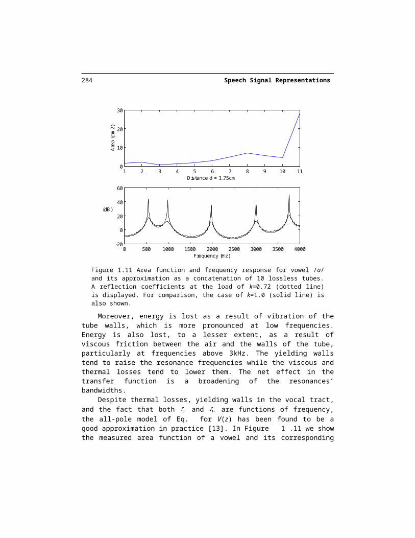
Figure 1.11 Area function and frequency response for vowel /a/ and its approximation as a concatenation of 10 lossless tubes. A reflection coefficients at the load of k=0.72 (dotted line) is displayed. For comparison, the case of k=1.0 (solid line) is also shown.
Moreover, energy is lost as a result of vibration of the tube walls, which is more pro -nounced at low frequencies. Energy is also lost, to a lesser extent, as a result of viscous fric-tion between the air and the walls of the tube, particularly at frequencies above 3kHz. The yielding walls tend to raise the resonance frequencies while the viscous and thermal losses

280 Speech Signal Representations
tend to lower them. The net effect in the transfer function is a broadening of the resonances’ bandwidths.
Despite thermal losses, yielding walls in the vocal tract, and the fact that both and are functions of frequency, the all-pole model of Eq. for V(z) has been found to be a
good approximation in practice [13]. In Figure 1.11 we show the measured area function of a vowel and its corresponding frequency response obtained using the approximation as a concatenation of 10 lossless tubes with a constant . The measured formants and corre-sponding bandwidths match quite well with this model despite all the approximations made. Thus, this concatenation of lossless tubes model represents reasonably well the acoustics in-side the vocal tract. Inspired by the above results, we describe in Section 1.3 linear predic-tive coding, an all-pole model for speech.
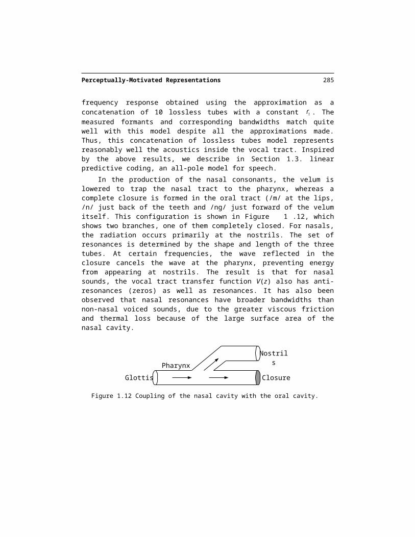
In the production of the nasal consonants, the velum is lowered to trap the nasal tract to the pharynx, whereas a complete closure is formed in the oral tract (/m/ at the lips, /n/ just back of the teeth and /ng/ just forward of the velum itself. This configuration is shown in Figure 1.12, which shows two branches, one of them completely closed. For nasals, the radi-ation occurs primarily at the nostrils. The set of resonances is determined by the shape and length of the three tubes. At certain frequencies, the wave reflected in the closure cancels the wave at the pharynx, preventing energy from appearing at nostrils. The result is that for nasal sounds, the vocal tract transfer function V(z) also has anti-resonances (zeros) as well as resonances. It has also been observed that nasal resonances have broader bandwidths than non-nasal voiced sounds, due to the greater viscous friction and thermal loss because of the large surface area of the nasal cavity.
Figure 1.12 Coupling of the nasal cavity with the oral cavity.
1.2.3. Source-Filter Models of Speech Production
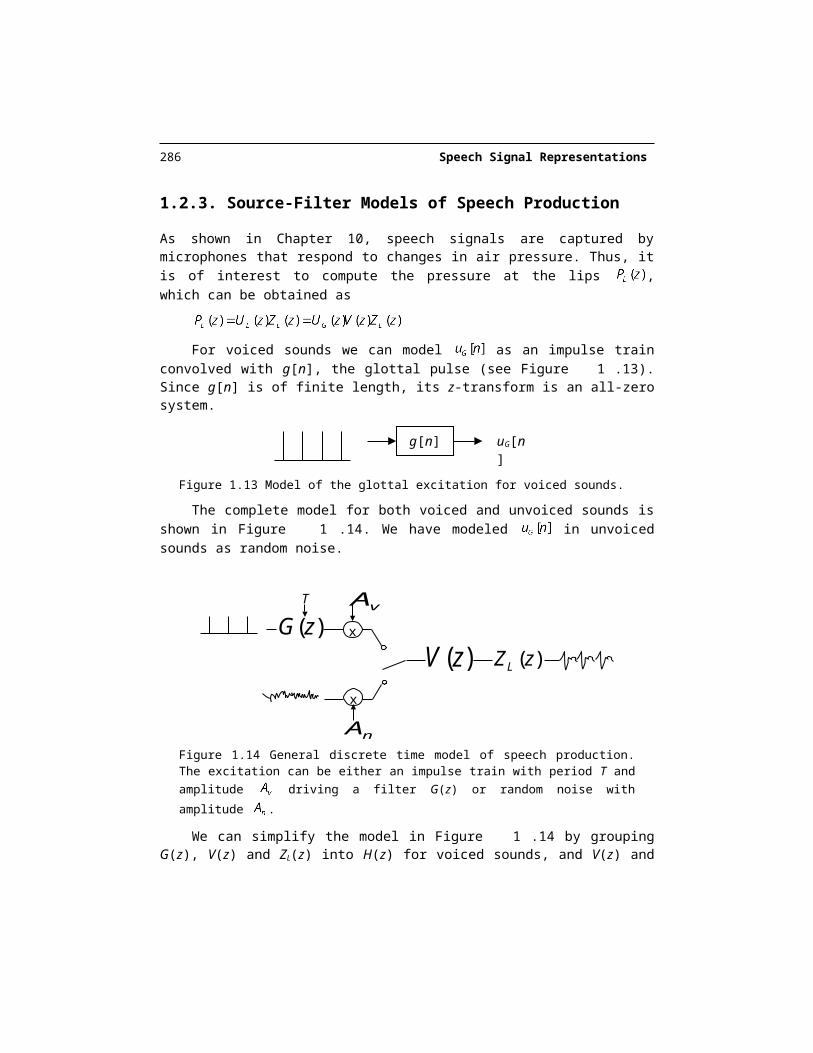
As shown in Chapter 10, speech signals are captured by microphones that respond to changes in air pressure. Thus, it is of interest to compute the pressure at the lips , which can be obtained as
For voiced sounds we can model as an impulse train convolved with g[n], the glottal pulse (see Figure 1.13). Since g[n] is of finite length, its z-transform is an all-zero system.
Closure
Nostrils
Pharynx
Glottis
Perceptually-Motivated Representations 281
Figure 1.13 Model of the glottal excitation for voiced sounds.
The complete model for both voiced and unvoiced sounds is shown in Figure 1.14. We have modeled in unvoiced sounds as random noise.
Figure 1.14 General discrete time model of speech production. The excitation can be either an impulse train with period T and amplitude driving a filter G(z) or random noise with am-
plitude .
We can simplify the model in Figure 1.14 by grouping G(z), V(z) and ZL(z) into H(z) for voiced sounds, and V(z) and ZL(z) into H(z) for unvoiced sounds. The simplified model is shown in Figure 1.15, where we make explicit the fact that the filter changes over time.
Figure 1.15 Source-filter model for voiced and unvoiced speech.
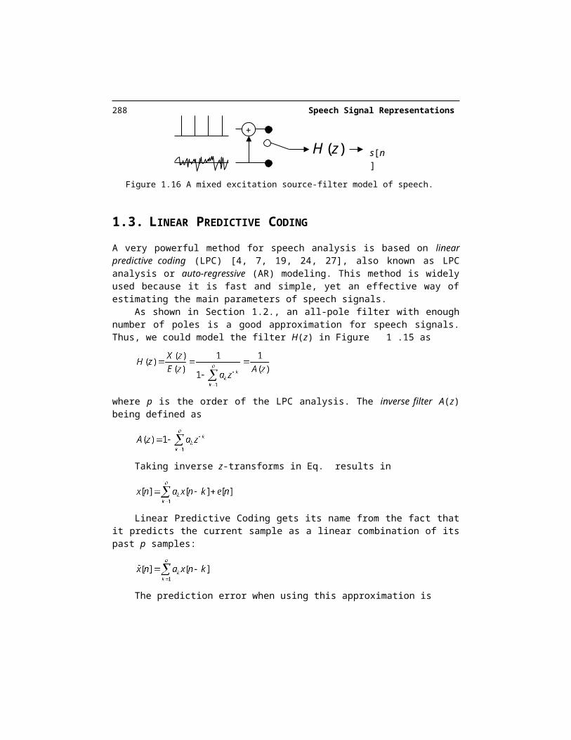
This model is a decent approximation, but fails on voiced fricatives, since those sounds contain both a periodic component and an aspirated component. In this case, a mixed excitation model can be applied where for voiced sounds a sum of both an impulse train plus colored noise (Figure 1.16).
The model in Figure 1.15 is appealing because the source is white (has a flat spec-trum) and all the coloring is in the filter. Other source-filter decompositions attempt to model the source as the signal at the glottis, in which the source is definitely not white. Since G(z), ZL(z) contain zeros, and V(z) can also contain zeros for nasals, is no longer all-pole. However, recall from in Chapter 5, we state that the z-transform of
is
V z( ) ( )LZ zG z( )
T
x
Av
x
An
g[n] uG[n]
( )H z s[n]
282 Speech Signal Representations
for
so that by inverting Eq. we see that a zero can be expressed with infinite poles. This is the reason why all-pole models are still reasonable approximations as long as enough number of poles is used. Fant [12] showed that on the average the speech spectrum contains one pole per kHz. Setting the number poles p to , where is the sampling frequency ex-pressed in kHz, has been found to work well in practice.
Figure 1.16 A mixed excitation source-filter model of speech.
1.3. LINEAR PREDICTIVE CODING
A very powerful method for speech analysis is based on linear predictive coding (LPC) [4, 7, 19, 24, 27], also known as LPC analysis or auto-regressive (AR) modeling. This method is widely used because it is fast and simple, yet an effective way of estimating the main pa-rameters of speech signals.
As shown in Section 1.2, an all-pole filter with enough number of poles is a good ap-proximation for speech signals. Thus, we could model the filter H(z) in Figure 1.15 as
where p is the order of the LPC analysis. The inverse filter A(z) being defined as
Taking inverse z-transforms in Eq. results in
Linear Predictive Coding gets its name from the fact that it predicts the current sample as a linear combination of its past p samples:
( )H z s[n]
+

Perceptually-Motivated Representations 283
The prediction error when using this approximation is
1.3.1. The Orthogonality Principle
To estimate the predictor coefficients from a set of speech samples, we use the short-term analysis technique. Let’s define as a segment of speech selected in the vicinity of sample m:
We define the short-term prediction error for that segment as
Figure 1.17 The orthogonality principle. The prediction error is orthogonal to the past samples.
In the absence of knowledge about the probability distribution of , a reasonable esti-mation criterion is minimum mean squared error introduced in Chapter 4. Thus, given a sig-nal , we estimate its corresponding LPC coefficients as those that minimize the total prediction error . Taking the derivative of Eq. with respect to and equating to 0 we obtain:
1mx
2mx
mx
em
mx
284 Speech Signal Representations
where we have defined and as vectors of samples, and their inner product has to be 0. This condition, known as orthogonality principle, says that the predictor coefficients that minimize the prediction error are such that the error must be orthogonal to the past vectors, and is seen in Figure 1.17.
Eq. can be expressed as a set of p linear equations
For convenience, we can define the correlation coefficients as
so that Eq. and can be combined to obtain the so-called Yule-Walker equations
Solution of the set of p linear equations results in the p LPC coefficients that minimize the prediction error. With satisfying Eq. , the total prediction error in Eq. takes on the following value
It is convenient to define a normalized prediction error u[n] with unity energy
and a gain G, such that
The gain G can be computed from the short-term prediction error
1.3.2. Solution of the LPC Equations
The solution of the Yule-Walker equations in Eq. can be achieved with any standard matrix inversion package. Because of the special form of the matrix here, some efficient solutions are possible which are described below. Also, each solution offers a different insight so we
Perceptually-Motivated Representations 285
present three different algorithms: the covariance method, the autocorrelation method and the lattice method.
1.3.2.1. Covariance Method
The covariance method [4] is derived by define directly the interval over which the summa-tion in Eq. takes place:
so that in Eq. becomes
and Eq. becomes
which can be expressed as the following matrix equation
where the matrix in Eq. is symmetric and positive definite, for which efficient methods are available, such as the Cholesky decomposition. For this method, also called the squared root method, the matrix is expressed as
where is a lower triangular matrix (whose main diagonal elements are 1’s), and is a diagonal matrix. So each element of can be expressed as
or alternatively
and for the diagonal elements
286 Speech Signal Representations
or alternatively
with
The Cholesky decomposition starts with Eq. then alternates between Eq. and . Once the matrices and have been determined, the LPC coefficients are solved in a two-step process. The combination of Eq. and can be expressed as
with
or alternatively
Therefore, given matrix and Eq. , can be solved recursively as
with the initial condition
Having determined , Eq. can be solved recursively similarly
with the initial condition
where the index i in Eq. proceeds backwards.The term covariance analysis is somewhat of a misnomer, since we know from Chap-
ter 5 that the covariance of a signal is the correlation of that signal with its mean removed. It was called this way because the matrix in Eq. has the properties of a covariance matrix, though this algorithm is more like a cross-correlation.

Perceptually-Motivated Representations 287
1.3.2.2. Autocorrelation Method
The summation in Eq. had no specific range. In the autocorrelation method [24, 27], we as-sume that is 0 outside the interval :
with being a window (such as a Hamming window) which is 0 outside the interval . With this assumption, the corresponding prediction error is non-zero over
the interval , and, therefore, the total prediction error takes on
With this range, Eq. can be expressed as
or alternatively
with being the autocorrelation sequence of
Combining Eq. and we obtain
which corresponds to the following matrix equation
The matrix in Eq. is symmetric and all the elements in its diagonals are identical. Such ma-trices are called Toeplitz. Durbin’s recursion exploits this fact resulting in a very efficient al-gorithm (for convenience, we omit the subscript m of the autocorrelation function), whose proof is outside the scope of this book:
288 Speech Signal Representations
1. Initialization
2. Iteration. For do the following recursion
3. Final solution
where the coefficients , called reflection coefficients, are bounded between –1 and 1 (see Section 1.3.2.3). In the process of computing the predictor coefficients of order p, the recur-sion finds the solution of the predictor coefficients for all orders less than p.
Substituting by the normalized autocorrelation coefficients defined as
results in identical LPC coefficients, and the recursion is more robust to problems with arith-metic precision. Likewise, the normalized prediction error at iteration i is defined by divid-ing Eq. by R[0], which using Eq. results in
The normalized prediction error is, using Eq. and
1.3.2.3. Lattice Formulation
In this section, we derive the lattice formulation [7, 19], an equivalent algorithm to the Levinson Durbin recursion that has some precision benefits. It is advantageous to define the forward prediction error obtained at stage i of the Levinson Durbin’s procedure as

Perceptually-Motivated Representations 289
whose z-transform is given by
with being defined by
which combined with Eq. , results in the following recursion
Similarly, we can define the so-called backward prediction error as
whose z-transform is
Now combining Eq. , and we obtain
whose inverse z-transform is given by
Also, substituting Eq. into and using Eq. , we obtain
whose inverse z-transform is given by
Eq. and define the forward and backward prediction error sequences for an ith order predic-tor in terms of the corresponding forward and backward prediction errors of an ( i-1)th order predictor. We initialize the recursive algorithm by noting that the 0th order predictor is equiv-alent to using no predictor at all, thus

290 Speech Signal Representations
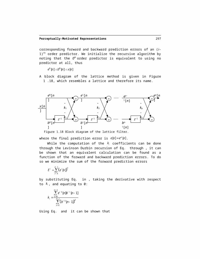
A block diagram of the lattice method is given in Figure 1.18, which resembles a lattice and therefore its name.
Figure 1.18 Block diagram of the lattice filter.
where the final prediction error is .While the computation of the coefficients can be done through the Levinson Durbin
recursion of Eq. through , it can be shown that an equivalent calculation can be found as a function of the forward and backward prediction errors. To do so we minimize the sum of the forward prediction errors
by substituting Eq. in , taking the derivative with respect to , and equating to 0:
Using Eq. and it can be shown that
since minimization of both result in identical Yule-Walker equations. Thus Eq. can be alter-natively expressed as
x[n]
z-1 +
+e0[n]
b0[n]
-k1
-k1
z-1 +
+e1[n]
b1[n]
-k2
-k2
z-1 +
+ep-1[n]
bp-1[n]
-kp
-kp
ep[n]
Perceptually-Motivated Representations 291
where we have defined the vectors and . The inner product of two vectors x and y is defined as
and its norm as
Eq. has the form of a normalized cross-correlation function, and, therefore, the reason the reflection coefficients are also called partial correlation coefficients (PARCOR). As with any normalized cross-correlation function, the coefficients are bounded by
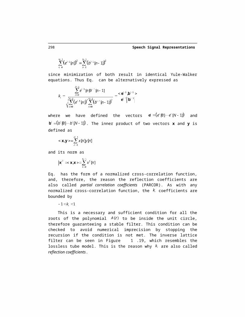
This is a necessary and sufficient condition for all the roots of the polynomial to be inside the unit circle, therefore guaranteeing a stable filter. This condition can be checked to avoid numerical imprecision by stopping the recursion if the condition is not met. The in-verse lattice filter can be seen in Figure 1.19, which resembles the lossless tube model. This is the reason why are also called reflection coefficients.
Figure 1.19 Inverse lattice filter used to generate the speech signal given its residual.
Lattice filters are often used in fixed-point implementations because lack of precision doesn’t result in unstable filters. Any error may take place, due to quantization for example, is generally not be sufficient to cause to fall outside the range in Eq. . If due to round-off error, the reflection coefficient falls outside the range, the lattice filter can be ended at the previous step.
More importantly, linearly varying coefficients can be implemented in this fashion. While, typically, the reflections coefficients are constant during the analysis frame, we can implement a linear interpolation of the reflection coefficients to obtain the error signal. If the coefficients of both frames are in the range in Eq. , the linearly interpolated reflections coef-ficients also have that property, and thus the filter is stable. This is a property that the predic-tor coefficients don’t have.
x[n]
b0[n]
ep[n]
bp[n]
+
+
kp
-kp
z-1
ep-1[n]
bp-1[n]
+
+
kp-1
-kp-1
z-1
e1[n]
b1[n]
+
+
k1
-k1
z-1
292 Speech Signal Representations
1.3.3. Spectral Analysis via LPC
Let’s now analyze the frequency domain behavior of the LPC analysis by evaluating
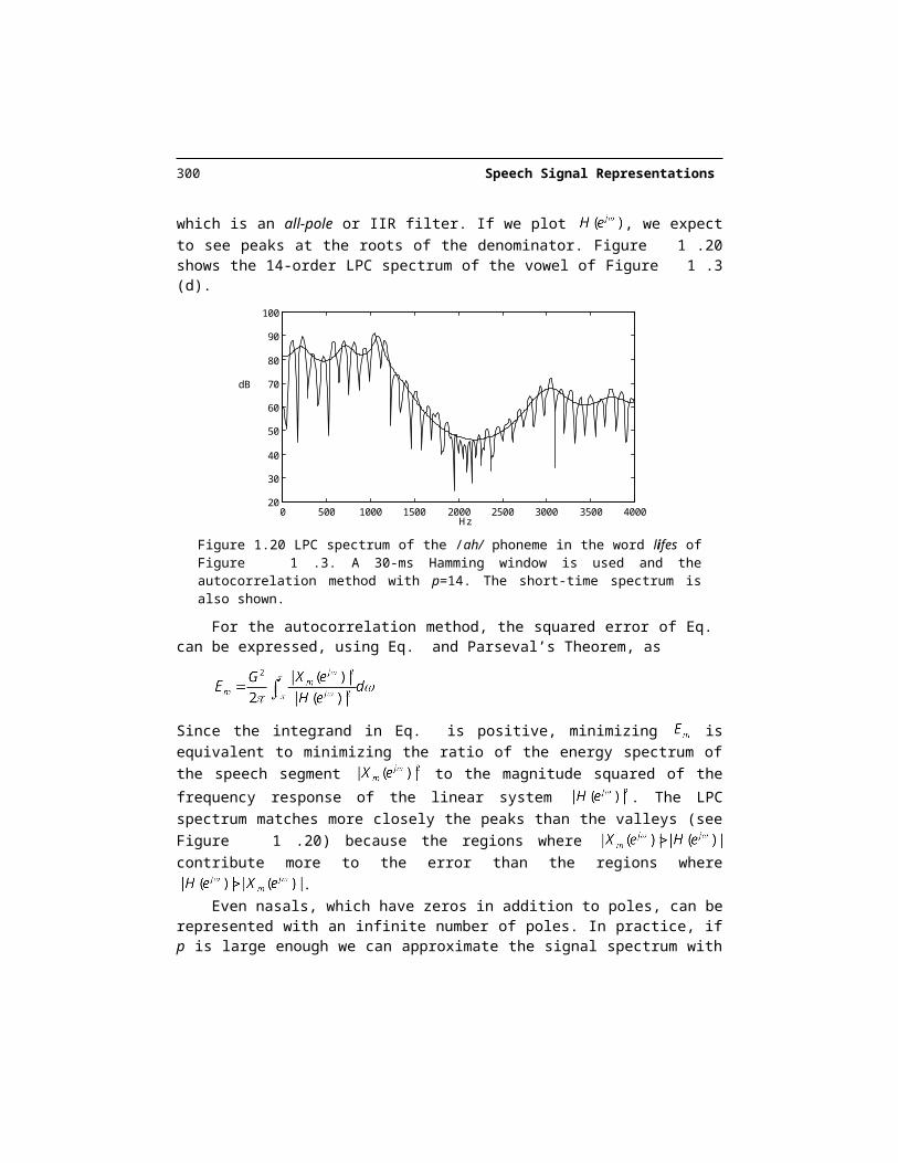
which is an all-pole or IIR filter. If we plot , we expect to see peaks at the roots of the denominator. Figure 1.20 shows the 14-order LPC spectrum of the vowel of Figure 1.3 (d).
0 500 1000 1500 2000 2500 3000 3500 400020
30
40
50
60
70
80
90
100
dB
Hz
Figure 1.20 LPC spectrum of the /ah/ phoneme in the word lifes of Figure 1.3. A 30-ms Ham-ming window is used and the autocorrelation method with p=14. The short-time spectrum is also shown.
For the autocorrelation method, the squared error of Eq. can be expressed, using Eq. and Parseval’s Theorem, as
Since the integrand in Eq. is positive, minimizing is equivalent to minimizing the ratio of the energy spectrum of the speech segment to the magnitude squared of the frequency response of the linear system . The LPC spectrum matches more closely the peaks than the valleys (see Figure 1.20) because the regions where
contribute more to the error than the regions where .
Even nasals, which have zeros in addition to poles, can be represented with an infinite number of poles. In practice, if p is large enough we can approximate the signal spectrum
Perceptually-Motivated Representations 293
with arbitrarily small error. Figure 1.21 shows different fits for different values of p. The higher p, the more details of the spectrum are preserved.
0 500 1000 1500 2000 2500 3000 3500 400020
30
40
50
60
70
80
90
100
dB
Hz
p=4p=8p=14
Figure 1.21 LPC spectra of Figure 1.20 for various values of the predictor order p.
The prediction order is not known for arbitrary speech, so we need to set it to balance spectral detail with estimation errors.
1.3.4. The Prediction Error
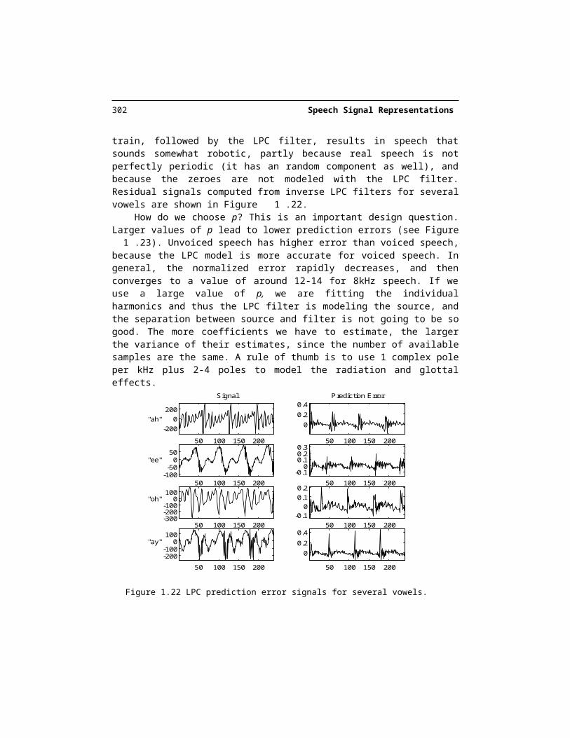
So far, we have concentrated on the filter component of the source-filter model. Using Eq. we can compute the prediction error signal, also called the excitation, or residual signal. For unvoiced speech synthetically generated by white noise following an LPC filter we expect the residual to be approximately white noise. In practice, this approximation is quite good, and replacement of the residual by white noise followed by the LPC filter typically results in no audible difference. For voiced speech synthetically generated by an impulse train follow-ing an LPC filter, we expect the residual to approximate an impulse train. In practice, this is not the case, because the all-pole assumption is not altogether valid, and, thus, the residual, although it contains spikes, is far from an impulse train. Replacing the residual by an im-pulse train, followed by the LPC filter, results in speech that sounds somewhat robotic, partly because real speech is not perfectly periodic (it has an random component as well), and because the zeroes are not modeled with the LPC filter. Residual signals computed from inverse LPC filters for several vowels are shown in Figure 1.22.
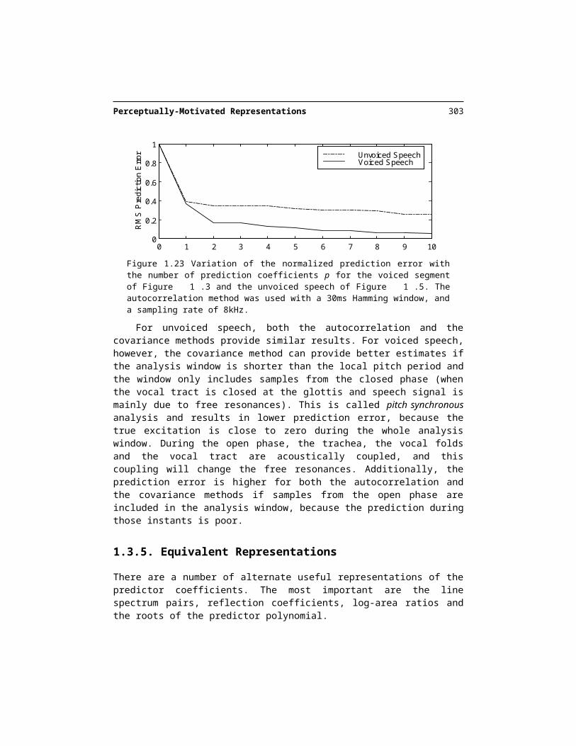
How do we choose p? This is an important design question. Larger values of p lead to lower prediction errors (see Figure 1.23). Unvoiced speech has higher error than voiced speech, because the LPC model is more accurate for voiced speech. In general, the normal-ized error rapidly decreases, and then converges to a value of around 12-14 for 8kHz speech. If we use a large value of p, we are fitting the individual harmonics and thus the LPC filter is modeling the source, and the separation between source and filter is not going to be so good. The more coefficients we have to estimate, the larger the variance of their estimates, since
294 Speech Signal Representations
the number of available samples are the same. A rule of thumb is to use 1 complex pole per kHz plus 2-4 poles to model the radiation and glottal effects.
50 100 150 200
-2000
200
Signal
"ah"
50 100 150 200
00.20.4
Prediction Error
50 100 150 200-100-50
050
"ee"
50 100 150 200
-0.10
0.10.20.3
50 100 150 200-300-200-100
0100
"oh"
50 100 150 200-0.1
00.10.2
50 100 150 200
-200-100
0100
"ay"
50 100 150 200
00.2
0.4
Figure 1.22 LPC prediction error signals for several vowels.
0 1 2 3 4 5 6 7 8 9 100
0.2
0.4
0.6
0.8
1
p
RM
S P
redi
ctio
n E
rror Unvoiced Speech
Voiced Speech
Figure 1.23 Variation of the normalized prediction error with the number of prediction coeffi-cients p for the voiced segment of Figure 1.3 and the unvoiced speech of Figure 1.5. The auto-correlation method was used with a 30ms Hamming window, and a sampling rate of 8kHz.
For unvoiced speech, both the autocorrelation and the covariance methods provide similar results. For voiced speech, however, the covariance method can provide better esti-mates if the analysis window is shorter than the local pitch period and the window only in-cludes samples from the closed phase (when the vocal tract is closed at the glottis and speech signal is mainly due to free resonances). This is called pitch synchronous analysis and results in lower prediction error, because the true excitation is close to zero during the whole analysis window. During the open phase, the trachea, the vocal folds and the vocal tract are acoustically coupled, and this coupling will change the free resonances. Addition-
Perceptually-Motivated Representations 295
ally, the prediction error is higher for both the autocorrelation and the covariance methods if samples from the open phase are included in the analysis window, because the prediction during those instants is poor.
1.3.5. Equivalent Representations
There are a number of alternate useful representations of the predictor coefficients. The most important are the line spectrum pairs, reflection coefficients, log-area ratios and the roots of the predictor polynomial.
1.3.5.1. Line Spectral Frequencies
Line Spectral Frequencies (LSF) [18] is an equivalent representation of the predictor coeffi-cients that is very popular in speech coding. It is derived from computing the roots of the polynomials P(z) and Q(z) defined as
To gain insight on these roots, look at a second order predictor filter with a pair of complex roots:
where and . Inserting Eq. into and result in
From Eq. we see that is a root of P(z) and a root of Q(z), which can be divided out and results in
where and are given by
296 Speech Signal Representations
It can be shown that and for all possible values of and . With
this property, the roots of P(z) and Q(z) in Eq. are complex and given by and
respectively. Because they lie in the unit circle, they can be uniquely repre-sented by their angles
where and are the line spectral frequencies of A(z). Since , , and thus . It’s also the case that
and thus . Furthermore, as , we see from Eq. that and . We conclude that, given a pole at , the two line spectral frequencies bracket it, i.e.
, and that they are closer together as the pole of the second order resonator gets closer to the unit circle.
We have proven that for a second order predictor, the roots of P(z) and Q(z) lie in the unit circle, that are roots and that once sorted the roots of P(z) and Q(z) alternate. Al-though we do not prove it here, it can be shown that these conclusions hold for other predic -tor orders, and, therefore, the p predictor coefficients can be transformed into p line spectral frequencies. We also know that is always a root of Q(z), whereas is a root of P(z) for even p and a root of Q(z), for odd p.
To compute the LSF for , we replace and compute the roots of and by any available root finding method. A popular technique given that there
are p roots, they are real in and bounded between 0 and 0.5, is to bracket them by observ-ing changes in sign of both functions in a dense grid. To compute the predictor coefficients from the LSF coefficients we can factor P(z) and Q(z) as a product of second order filters as in Eq. , and then .
In practice, LSF are useful because of sensitivity (a quantization of one coefficient generally results in a spectral change only around that frequency) and efficiency (LSF result in low spectral distortion). This doesn’t occur with other representations. As long as the LSF coefficients are ordered, the resulting LPC filter is stable, though the proof is outside the scope of this book. LSF coefficients are used in Chapter 7 extensively.
1.3.5.2. Reflection Coefficients
For the autocorrelation method, the predictor coefficients may be obtained from the reflec-tion coefficients by the following recursion
Perceptually-Motivated Representations 297
where . Similarly, the reflection coefficients may be obtained from the prediction co-efficients using a backward recursion of the form
where we initialize .Reflection coefficients are useful when implementing LPC filters whose values are in-
terpolated over time because, unlike the predictor coefficients, they are guaranteed to be sta-ble at all times as long as the anchors satisfy Eq. .
1.3.5.3. Log-area Ratios
The log-area ratio coefficients are defined as
with the inverse being given by
The log-area ratio coefficients are equal to the natural logarithm of the ratio of the ar-eas of adjacent sections of a lossless tube equivalent of the vocal tract having the same trans-fer function. Since for stable predictor filters , we have from Eq. that
. For speech signals, it is not uncommon to have some reflection coefficients close to 1, and quantization of those values can cause a large change in the predictor’s trans-fer function. On the other hand, the log-area ratio coefficients have relatively flat spectral sensitivity (i.e. small change in their values causes a small change in the transfer function) and thus are useful in coding.
1.3.5.4. Roots of Polynomial
An alternative to the predictor coefficients results from computing the complex roots of the predictor polynomial:
298 Speech Signal Representations
These roots can be represented as
where , and represent the bandwidth, center frequency and sampling frequency re-spectively. Since are real, all complex roots occur in conjugate pairs so that if is a root, so is . The bandwidths are always positive, because the roots are inside the unit circle ( ) for a stable predictor. Real roots can also occur. While algorithms exist to compute the complex roots of a polynomial, in practice there are some-times numerical difficulties in doing so.
If the roots are available, it is straightforward to compute the predictor coefficients by using Eq. . Since the roots of the predictor polynomial represent resonance frequencies and bandwidths, they are used in formant synthesizers of Chapter 16.
1.4. CEPSTRAL PROCESSING
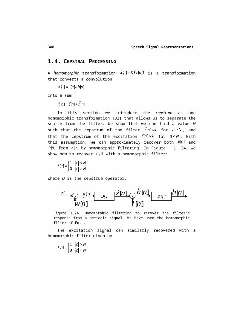
A homomorphic transformation is a transformation that converts a convolu-tion
into a sum
In this section we introduce the cepstrum as one homomorphic transformation [32] that allows us to separate the source from the filter. We show that we can find a value N such that the cepstrum of the filter for , and that the cepstrum of the excita-
tion for . With this assumption, we can approximately recover both and from by homomorphic filtering. In Figure 1.24, we show how to recover
with a homomorphic filter:
where D is the cepstrum operator.
Perceptually-Motivated Representations 299
Figure 1.24. Homomorphic filtering to recover the filter’s response from a periodic signal. We have used the homomorphic filter of Eq. .
The excitation signal can similarly recovered with a homomorphic filter given by
1.4.1. The Real and Complex Cepstrum
The real cepstrum of a digital signal is defined as
and the complex cepstrum of is defined as
where the complex logarithm is used:
and the phase is given by
You can see from Eq. and that both the real and the complex cepstrum satisfy Eq. and thus are homomorphic transformations.
If the signal is real, both the real cepstrum and the complex cepstrum are also real signals. Therefore the term complex cepstrum doesn’t mean that it is a complex signal but rather that the complex logarithm is taken.
It can easily be shown that is the even part of :
From here on when we refer to cepstrum without qualifiers, we are referring to the real cepstrum, since it is the most widely used in speech technology.
x D[ ]n] x[n]
w n[ ]
ˆ[ ]x n x
l n[ ]D-1[ ]
[ ]h n h n[ ]
300 Speech Signal Representations
The cepstrum was invented by Bogert et al. [6] and its term was coined by reversing the first syllable of the word spectrum, given that it is obtained by taking the inverse Fourier transform of the log-spectrum. Similarly, they defined the term quefrency to represent the in-dependent variable n in c[n]. The quefrency has dimension of time.
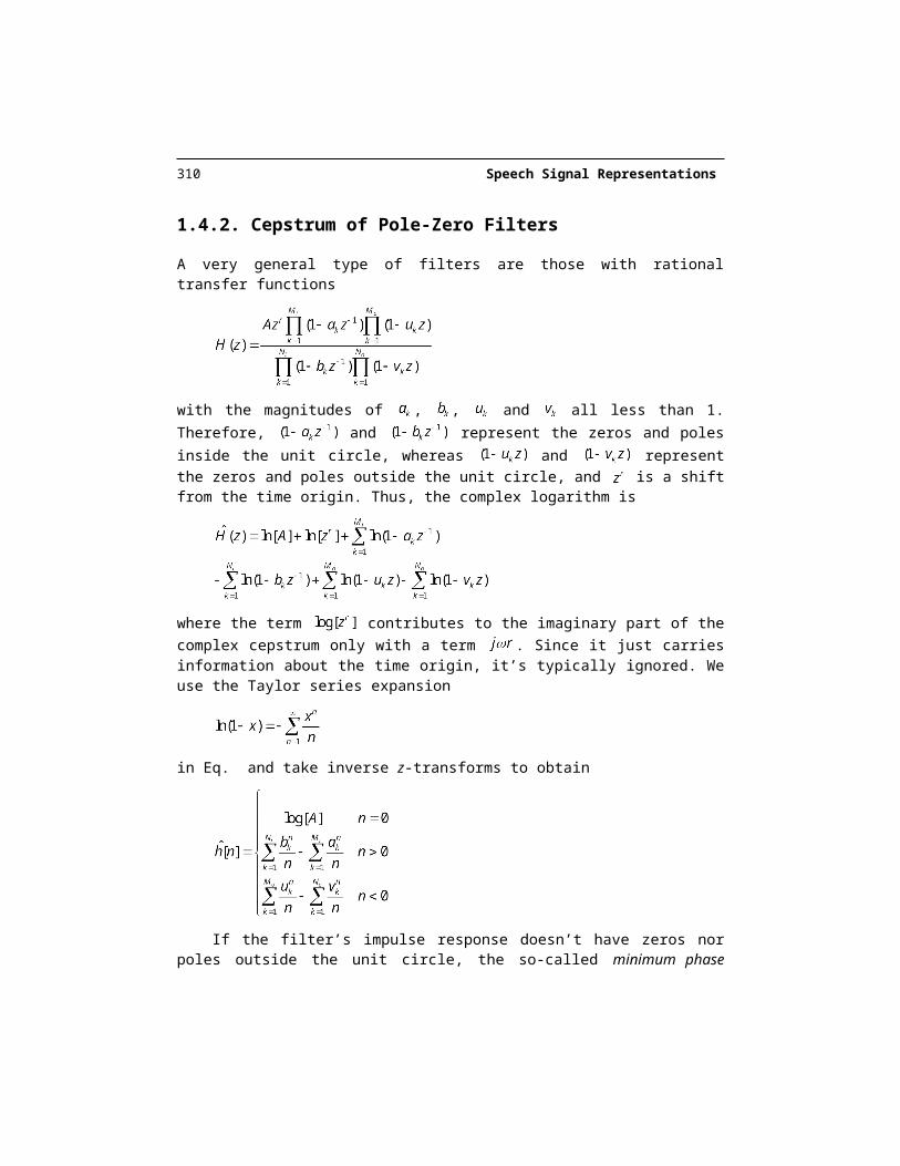
1.4.2. Cepstrum of Pole-Zero Filters
A very general type of filters are those with rational transfer functions
with the magnitudes of , , and all less than 1. Therefore, and represent the zeros and poles inside the unit circle, whereas and
represent the zeros and poles outside the unit circle, and is a shift from the time origin. Thus, the complex logarithm is
where the term contributes to the imaginary part of the complex cepstrum only with a term . Since it just carries information about the time origin, it’s typically ignored. We use the Taylor series expansion
in Eq. and take inverse z-transforms to obtain

Perceptually-Motivated Representations 301
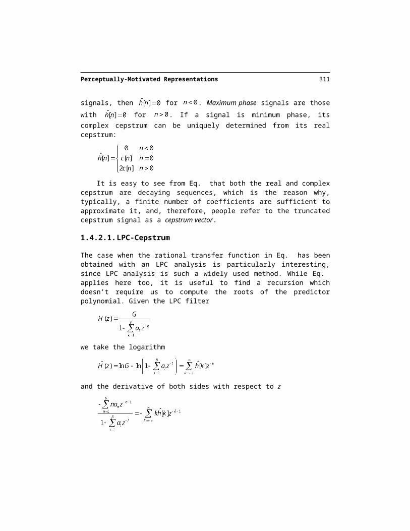
If the filter’s impulse response doesn’t have zeros nor poles outside the unit circle, the so-called minimum phase signals, then for . Maximum phase signals are those
with for . If a signal is minimum phase, its complex cepstrum can be uniquely determined from its real cepstrum:
It is easy to see from Eq. that both the real and complex cepstrum are decaying se-quences, which is the reason why, typically, a finite number of coefficients are sufficient to approximate it, and, therefore, people refer to the truncated cepstrum signal as a cepstrum vector.
1.4.2.1. LPC-Cepstrum
The case when the rational transfer function in Eq. has been obtained with an LPC analysis is particularly interesting, since LPC analysis is such a widely used method. While Eq. ap-plies here too, it is useful to find a recursion which doesn’t require us to compute the roots of the predictor polynomial. Given the LPC filter
we take the logarithm
and the derivative of both sides with respect to z
Multiplying both sides by we obtain
302 Speech Signal Representations
which after replacing , and equating terms in results in
so that the complex cepstrum can be obtained from the LPC coefficients by the following re-cursion
where the value for can be obtained from Eq. and . We note that while there are a fi-nite number of LPC coefficients, the number of cepstrum coefficients is infinite. Speech recognition researchers have shown empirically that a finite number is sufficient: 12-20 de-pending on the sampling rate and whether or not frequency warping is done. In Chapter 8 we discuss the use of cepstrum in speech recognition.
This recursion should not be used in the reverse mode to compute the LPC coefficients from any set of cepstrum coefficients, because the recursion in Eq. assumes an all-pole model with all poles inside the unit circle, and that might not be the case for an arbitrary cepstrum sequence, and, therefore, yield a set of unstable LPC coefficients. In some experi -ments it has been shown that quantized LPC-cepstrum can yield unstable LPC coefficients over 5% of the time.
1.4.3. Cepstrum of Periodic Signals
It is important to see what the cepstrum of periodic signals look like. To do so, let’s consider the following signal
which can be viewed as an impulse train of period N multiplied by an analysis window, so that only M impulses remain. Its z-transform is
Perceptually-Motivated Representations 303
which is a polynomial in rather than . Therefore, can be expressed as a prod-uct of factors of the form and . Following the derivation in Section 1.4.2, it is clear that its complex cepstrum is be nonzero only at integer multiples of N:
A particularly interesting case is when with , so that Eq. can be ex-pressed as
so taking the logarithm of Eq. and expanding it in Taylor series using Eq. results in
which lets us compute the complex cepstrum as
An infinite impulse train can be obtained by making and in Eq. .
We see from Eq. that the cepstrum of an impulse train goes to 0 as n increases. This justifies our assumption of homomorphic filtering.
1.4.4. Cepstrum of Speech Signals
We can compute the cepstrum of a speech segment by windowing the signal with a window of length N. In practice, the cepstrum is not computed through Eq. since root finding algo-rithms are slow and offer numerical imprecision for the large values of N used. Instead, we can compute the cepstrum directly through its definition of Eq. , using the DFT as follows:
304 Speech Signal Representations
The subscript means that the new complex cepstrum is an aliased version of given by
which can be derived by using the Sampling Theorem of Chapter 5 by reversing the con-cepts of time and frequency.
This aliasing introduces errors in the estimation that can be reduced by choosing a large value for N.
Computation of the complex cepstrum requires computing the complex logarithm, and in turn the phase. However, given the principal value of the phase , there are infinite possible values for :
From Chapter 5 we know that if is real, is an odd function and also con-
tinuous. Thus we can do phase unwrapping by choosing to guarantee that is a smooth function, i.e. by forcing the difference between adjacent values to be small:
A linear phase term r as in Eq. , would contribute to the phase difference in Eq. with , which may result in errors in the phase unwrapping if is changing suffi-
ciently rapidly. In addition, there could be large changes in the phase difference if is noisy. To guarantee that we can track small phase differences, a value of N several times larger than the window size is required: i.e. the input signal has to be zero-padded prior to the FFT computation. Finally, the delay r in Eq. , can be obtained by forcing the phase to be an odd function, so that:
For unvoiced speech, the unwrapped phase is random, and therefore only the real cep-strum has meaning. In practical situations, even voiced speech has some frequencies at which noise dominates (typically very low and high frequencies), which results in phase
that changes drastically from frame to frame. Because of this, the complex cepstrum in Eq. is rarely used for real speech signals. Instead, the real cepstrum is used much more of-ten:
Perceptually-Motivated Representations 305
Similarly, it can be shown that for the new real cepstrum is an aliased version of given by
that again has aliasing which can be reduced by choosing a large value for N.
1.4.5. Source-Filter Separation via the Cepstrum
We have seen that, if the filter is a rational transfer function, and the source is an impulse train, the homomorphic filtering of Figure 1.24 can approximately separate them. Because of problems in estimating the phase in speech signals (See Section 1.4.4), we generally com-pute the real cepstrum using Eq. , and , and then compute the complex cepstrum under the assumption of a minimum phase signal according to Eq. . Figure 1.25 shows the result of separating source and filter using this cepstral deconvolution for voiced speech and Figure1.26 for unvoiced speech.
The real cepstrum of white noise with an expected magnitude spectrum is 0. If colored noise is present, the cepstrum of the observed colored noise
is identical to the cepstrum of the coloring filter , other than a gain factor. The above is correct if we take an infinite number of noise samples, but in practice, this cannot be done and a limited number has to be used, so that this is only an approximation, though it is often used in speech processing algorithms.

306 Speech Signal Representations
0 50 100 150 200-2
0
2(a)
0 1000 2000 3000 4000-5
0
5
dB
(b)
0 50 100 150 200-2
0
2(c)
0 1000 2000 3000 4000-5
0
5
dB
(d)
0 50 100 150 200-0.5
0
0.5(e)
time0 1000 2000 3000 4000
-5
0
5
dB
(f)
Frequency (Hz)
Figure 1.25 Separation of source and filter using homomorphic filtering for voiced speech with the scheme of Figure 1.24 with N=20 in the homomorphic filter of Eq. with the real cepstrum: (a) windowed signal, (b) log-spectrum, (c) filter’s impulse response, (d) smoothed log-spec-trum, (e) windowed excitation signal (f) log-spectrum of high-part of cepstrum. Note that the windowed excitation is not a windowed impulse train because of the minimum phase assump-tion.
0 50 100 150 200-2
-1
0
1
2(a)
0 1000 2000 3000 4000-5
0
5
dB
(b)
0 50 100 150 200-2
-1
0
1
2(c)
time0 1000 2000 3000 4000
-5
0
5
Frequency (Hz)
dB
(d)
Figure 1.26. Separation of source and filter using homomorphic filtering for unvoiced speech with the scheme of Figure 1.24 with N=20 in the homomorphic filter of Eq. with the real cep-strum: (a) windowed signal, (b) log-spectrum, (c) filter’s impulse response, (d) smoothed log-spectrum.

Perceptually-Motivated Representations 307
1.5. PERCEPTUALLY-MOTIVATED REPRESENTATIONS
In this Section, we describe some aspects of human perception, and methods motivated by the behavior of the human auditory system: Mel-Frequency Cepstrum Coefficients (MFCC) and Perceptual Linear Prediction (PLP). These methods have been successfully used in speech recognition. First we present several non-linear frequency scales that have been used in such representations.
1.5.1. The Bilinear Transform
The transformation
for belongs to the class of bilinear transforms. It is a mapping in the complex plane that maps the unit circle onto itself. The frequency transformation is obtained by mak-ing the substitution and :
This transformation is very similar to the Bark and mel scale for an appropriate choice of the parameter (see Chapter 2). Oppenheim [31] showed that the advantage of this transformation is that it can be used to transform a time sequence in the linear frequency into another time sequence in the warped frequency as it can be shown in Figure 1.27. This bilin-ear transform has been successfully applied to cepstral and autocorrelation coefficients.
Figure 1.27. Implementation of the frequency warped cepstral coefficients as a function of the linear-frequency cepstrum coefficients. Both sets of coefficients are causal. The input is the time-reversed cepstrum sequence, and the output can be obtained by sampling the outputs of the filters at time n=0. The filters used for w[m] m>2 are the same. Note that, for a finite length cepstrum, an infinite length warped cepstrum results.
11 1 z
( )11
2 1
1
zz
zz
1
11
z
z
1
11
c[-n]
n=0 n=0 n=0 n=0
w[0] w[1] w[2] w[3]
308 Speech Signal Representations
For a finite number of cepstral coefficients the bilinear transform in Figure 1.27 results in an infinite number of warped cepstral coefficients. Since truncation is usually done in practice, the bilinear transform is equivalent to a matrix multiplication, where the matrix is a function of the warping parameter . Shikano [43] showed these warped cepstral coeffi-cients were beneficial for speech recognition.
1.5.2. Mel-Frequency Cepstrum
The Mel-Frequency Cepstrum Coefficients (MFCC) is a representation defined as the real cepstrum of a windowed short-time signal derived from the FFT of that signal. The differ-ence with the real cepstrum is that a nonlinear frequency scale is used, which approximates the behavior of the auditory system. Davis and Mermelstein [8] showed the MFCC represen-tation to be beneficial for speech recognition.
Given the DFT of the input signal
we define a filterbank with M filters ( ), where filter m is triangular filter given by:
Such filters compute the average spectrum around each center frequency with increasing bandwidths, and are displayed in Figure 1.28.
Figure 1.28 Triangular filters used in the computation of the mel-cepstrum using Eq. .
Alternatively, the filters can be chosen as
…
1[ ]H k 3[ ]H k 4[ ]H k 5[ ]H k 6[ ]H k2[ ]H k
f[0] f[1] f[2] f[3] f[4] f[5] f[6] f[7]
k

Perceptually-Motivated Representations 309
which satisfies . The mel-cepstrum computed with or will dif-
fer by a constant vector for all inputs, so the choice becomes unimportant when used in a speech recognition system that has trained with the same filters.
Let’s define and as the lowest and highest frequencies of the filterbank in Hz, Fs the sampling frequency in Hz, M the number of filters, and N the size of the FFT. The boundary points f[m] are uniformly spaced in the mel-scale:
where the mel-scale B is given by Eq. (2.6), and B-1 is its inverse
We then compute the log-energy at the output of each filter as
The mel frequency cepstrum is then the Discrete Cosine Transform of the M filter out-puts:
where M varies for different implementations from 24 to 40. For speech recognition, typi-cally only the first 13 cepstrum coefficients are used. It is important to note that the MFCC representation is no longer a homomorphic transformation. It would be if the order of sum-mation and logarithms in Eq. were reversed:
In practice, however, the MFCC representation is approximately homomorphic for fil-ters that have a smooth transfer function. The advantage of the MFCC representation using
310 Speech Signal Representations
instead of is that the filter energies are more robust to noise and spectral estimation errors. This algorithm has been used extensively as a feature vector for speech recognition systems.
While the definition of cepstrum in Section 1.4.1 uses an inverse DFT, since S[m] is even, a DCT-II can be used (See Chapter 5) instead.
1.5.3. Perceptual Linear Prediction (PLP)
Perceptual Linear Prediction (PLP) [16] uses the standard Durbin recursion of Section 1.3.2.2 to compute LPC coefficients, and typically the LPC coefficients are transformed to LPC-cepstrum using the recursion in Section 1.4.2.1. But unlike standard linear prediction, the autocorrelation coefficients are not computed in the time domain through Eq. .
The autocorrelation is the inverse Fourier transform of the power spectrum
of the signal. We cannot compute the continuous-frequency Fourier transform eas-ily, but we can take an FFT to compute X[k], so that the autocorrelation can be obtained as the inverse Fourier transform of . Since the discrete Fourier transform is not per-forming linear convolution but circular convolution, we need to make sure that the FFT size is larger than twice the window length (See Section 5.3.4) for this to hold. This alternate way of computing autocorrelation coefficients should yield identical results, and entails two FFTs and N multiplies and adds. Since normally only a small number p of autocorrelation coefficients is needed, this is generally not a cost effective way to do it, unless the first FFT has to be computed for other reasons.
Perceptual Linear Prediction uses the above method, but replaces by a percep-tually motivated power spectrum. The most important aspect is the non-linear frequency scaling, which can be achieved through a set of filterbanks similar to those described in Sec-tion 1.5.2, so that this critical-band power spectrum can be sampled in approximately 1-Bark intervals. Another difference is that, instead of taking the logarithm on the filterbank energy outputs, a different non-linearity compression is used, often the cubic root. It is reported [16] that the use of this different non-linearity is beneficial for speech recognizers in noisy condi-tions.
1.6. FORMANT FREQUENCIES
Formant frequencies are the resonances in the vocal tract and, as we saw in Chapter 2, they convey the differences between different sounds. Expert spectrogram readers are able to rec-ognize speech by looking at a spectrogram, particularly at the formants. It has been argued that they are very useful features for speech recognition, but they haven’t been widely used because of the difficulty in estimating them.
One way of obtaining formant candidates at a frame level is to compute the roots of a pth order LPC polynomial [3, 26]. There are standard algorithms to compute the complex
Perceptually-Motivated Representations 311
roots of a polynomial with real coefficients [36], though convergence is not guaranteed. Each complex root can be represented as
where and are the formant frequency and bandwidth respectively of the ith root. Real roots are discarded and complex roots are sorted by increasing f, discarding negative values. The remaining pairs ( , ) are the formant candidates. Traditional formant trackers discard roots whose bandwidths are higher than a threshold [46], say 200Hz.
Closed-Phase analysis of voiced speech [5] uses only the regions for which the glottis is closed and thus there is no excitation. When the glottis is open, there is a coupling of the vocal tract with the lungs and the resonance bandwidths are somewhat larger. Determination of the closed-phase regions directly from the speech signal is difficult, so often times an Electroglottograph (EGG) signal is used [23]. EGG signal are obtained by placing elec-trodes at the speaker’s throat and are very accurate in determining the times where the glottis is closed. Using samples in the closed-phase, covariance analysis can yield accurate results [46]. For female speech, the closed-phase is short, and sometimes non-existent, so such anal-ysis can be a challenge. EGG signals are useful also for pitch tracking and are described in more detail in Chapter 16.
Another common method consists of finding the peaks on a smoothed spectrum, such as that obtained through an LPC analysis [26, 40]. The advantage of this method is that you can always compute the peaks and it is more computationally efficient than extracting the complex roots of a polynomial. On the other hand, this procedure generally doesn’t estimate the formant’s bandwidth. The first 3 formants are typically estimated this way for formant synthesis (see Chapter 16), since they are the ones that allow sound classification, whereas the higher formants are more speaker-dependent.
Sometimes, the signal goes through some conditioning, which includes sampling rate conversion to remove frequencies outside the range we are interested in. For example, if we are only interested in the first 3 formants, we can safely downsample the input signal to 8kHz, since we know all three formants should be below 4kHz. This downsampling reduces computation and the chances of the algorithm to find formant values outside the expected range (otherwise peaks or roots could be chosen above 4kHz which we know do not corre-spond to any of the first 3 formants). Pre-emphasis filtering is also often used to whiten the signal.
Because of the thresholds imposed above, it is possible that the formants are not con-tinuous. For example, when the vocal tract’s spectral envelope is changing rapidly, band-widths obtained through the above methods are overestimates of the true bandwidths and they may exceed the threshold and thus be rejected. It is also possible for the peak-picking algorithm to classify a harmonic as a formant during some regions where it is much stronger than the other harmonics. Due to the thresholds used, a given frame could have no formants, only one formant (either first, second or third), two, three or more. Formant alignment from one frame to another has often been done using heuristics to prevent such discontinuities.

312 Speech Signal Representations
1.6.1. Statistical Formant Tracking
It is desirable to have an approach that does not use any thresholds on formant candidates and uses a probabilistic model to do the tracking instead of heuristics [1]. The formant can-didates can be obtained from either roots of the LPC polynomial, peaks in the smoothed spectrum or even from a dense sample of possible points. If the first n formants were de-sired, and we have (p/2) formant candidates, a maximum of r n-tuples are considered where r is given by
A Viterbi search (see Chapter 8) is then carried out to find the most likely path of for -mant n-tuples given a model with some a priori knowledge of formants. The prior distribu-tion for formant targets is used to determine which formant candidate to use of all possible choices for the given phoneme (i.e. we know that F1 for an AE should be around 800Hz). Formant continuity is imposed through the prior distribution of the formant slopes. This al-gorithm produces n formants for every frame, including silence.
Since we are interested in obtaining the first three formants (n=3) and F3 is known to be lower than 4kHz, it is advantageous to downsample the signal to 8kHz to avoid obtaining formant candidates above 4kHz, and to let us use a lower order analysis which offers fewer numerical problems when computing the roots. With p=14, it results in a maximum of r=35 triplets for the case of no real roots.
Let X be a sequence of T feature vectors of dimension n:
where ‘ denotes transpose.We estimate the formants with the knowledge of what sound occurs at that particular
time, for example by using a speech recognizer that segments the waveform into different phonemes (See Chapter 9) or states within a phoneme. In this case we assume that the output distribution of each state i is modeled by one Gaussian density function with a mean
and covariance matrix . We can define up to N states, with being the set of all means and covariance matrices for all:
Therefore, the log-likelihood for X is given by
Maximizing X in Eq. leads to the trivial solution , a piecewise function whose value is that of the best n-tuple candidate. This function has discontinuities at state boundaries and thus not likely to represent well the physical phenomena of speech.
Perceptually-Motivated Representations 313
This problem arises because the slopes at state boundaries do not match the slopes of natural speech. To avoid these discontinuities, we would like to match not only the target formants at each state, but also the formant slopes at each state. To do that, we augment the feature vector at frame t with the delta vector . Thus, we increase the parameter space of with the corresponding means and covariance matrices of these delta pa-rameters, and assume statistical independence among them. The corresponding new log-likelihood has the form
Time (seconds)
Freq
uenc
y (H
z)
0 0.2 0.4 0.6 0.8 1 1.2 1.4 1.60
500
1000
1500
2000
2500
3000
3500
4000
Figure 1.29. Spectrogram and 3 smoothed formants.
Maximization of Eq. with respect to requires solving several sets of linear equa-tions. If and are diagonal covariance matrices, it results in a set of linear equations for each of the M dimensions
where B is a tridiagonal matrix (all values are zero except for those in the main diagonal and its two adjacent diagonals), which leads to a very efficient solution [36]. For example, the values of B and c for T=3 are given by
314 Speech Signal Representations
where just one dimension is represented, and the process repeated for all dimensions with a computational complexity of O(TM).
Figure 1.30. Raw formants (ragged gray line) and smoothed formants (dashed line).
The maximum likelihood sequence is close to the targets while keeping the slopes close to for a given state i, thus estimating a continuous function. Because of the delta coefficients, the solution depends on all the parameters of all states and not just the current state. This procedure can be performed for the formants as well as the bandwidths.

Perceptually-Motivated Representations 315
The parameters , , and can be re-estimated using the EM algorithm de-scribed in Chapter 8. In [1] it is reported that 2 or 3 iterations are sufficient for speaker-de-pendent data.
The formant track obtained through this method can be rough, and it may be desired to smooth it. Smoothing without knowledge about the speech signal would result in either blur-ring the sharp transitions that occur in natural speech, or maintaining ragged formant tracks where the underlying physical phenomena vary slowly with time. Ideally we would like a larger adjustment to the raw formant when the error in the estimate is large relative to the variance of the corresponding state within a phoneme. This can be done by modeling the formant measurement error as a Gaussian distribution. Figure 1.29 shows an utterance from a male speaker with the smoothed formant tracks and Figure 1.30 compares the raw and smoothed formants. When no real formant is visible from the spectrogram, the algorithm tends to assign a large bandwidth (not shown in the figure).
1.7. THE ROLE OF PITCH
Pitch determination is very important for many speech processing algorithms. The concate-native speech synthesis methods of Chapter 16 requires pitch tracking on the desired speech segments if prosody modification is to be done. Chinese speech recognition systems use pitch tracking for tone recognition, which is important in disambiguating the myriad of ho-mophones. Pitch is also crucial for prosodic variation in text-to-speech systems (See Chapter 15) and spoken language systems (see Chapter 17). While in the previous sections we have dealt with features representing the filter, pitch represents the source of the model illustrated in Figure 1.1.
Pitch determination algorithms also use short-term analysis techniques, which means that for every frame we get a score that is a function of the candidate pitch periods T. These algorithms determine the optimal pitch by maximizing
We describe several such functions computed through the autocorrelation method and the normalized cross-correlation method, as well as the signal conditioning that is often per -formed. Other approaches based on cepstrum [28] have also been used successfully. [17, 45] provide a good summary of techniques used for pitch tracking.
Pitch determination using Eq. is error prone, and a smoothing stage is often done. This smoothing takes into consideration that the pitch does not change quickly over time and is described in Section 1.7.4.
1.7.1. Autocorrelation Method
A commonly used method to estimate pitch is based on detecting the highest value of the au-tocorrelation function in the region of interest. This region must exclude as that is the

316 Speech Signal Representations
absolute maximum of the autocorrelation function [37]. As discussed in Chapter 5, the sta-tistical autocorrelation of a sinusoidal random process
is given by
which has maxima for , the pitch period and its harmonics, so that we can find the pitch period by computing the highest value of the autocorrelation. Similarly, it can be shown that any WSS periodic process x[n] with period also has an autocorrelation R[m] which exhibits its maxima at .
In practice, we need to obtain an estimate from knowledge of only N samples. If we use a window w[n] of length N on x[n] and assume it to be real, the empirical autocorre-lation function is given by
whose expected value can be shown to be
where
which, for the case of a rectangular window of length N, is given by
which means that is a biased estimator of R[m]. So, if we compute the peaks based on Eq. , the estimate of the pitch will also be biased. Although the variance of the estimate is difficult to compute, it is easy to see that as m approaches N, fewer and fewer samples of x[n] are involved in the calculation, and thus the variance of the estimate is expected to in -crease. If we multiply Eq. by , the estimate will be unbiased but the variance will be larger.
If we use the empirical autocorrelation in Eq. for the random process in Eq. results in an expected value of
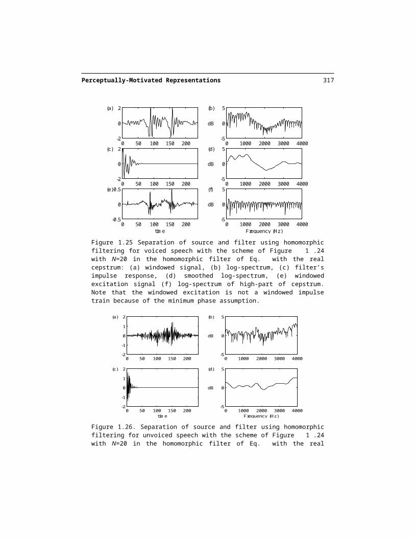
Perceptually-Motivated Representations 317
whose maximum coincides with the pitch period for .Since pitch periods can be as low as 40Hz (for a very low-pitched male voice) or as
high as 600Hz (for a very high-pitched female or child’s voice), the search for the maximum is conducted within a region. This F0 detection algorithm is illustrated in Figure 1.31 where the lag with highest autocorrelation is plotted for every frame. In order to see periodicity present in the autocorrelation, we need to use a window that contains at least two pitch peri-ods, which, if we want to detect a 40Hz pitch, implies 50ms (See Figure 1.32). For window lengths so long, the assumption of stationarity starts to fail because a pitch period at the be-ginning of the window can be significantly different than at the end of the window. One pos-sible solution to this problem is to estimate the autocorrelation function with different win-dow lengths for different lags m.
0 500 1000 1500 2000 2500 3000 3500 4000 4500 5000-0.5
0
0.5
10 20 30 40 50 600
50
100
Figure 1.31 Waveform and unsmoothed pitch track with the autocorrelation method. A frame shift of 10ms and a Hamming window of 30ms and a sampling rate of 8kHz were used. Notice two frames in the voiced region have an incorrect pitch. The pitch values in the unvoiced re-gions are essentially random.
The candidate pitch periods in Eq. can be simply , i.e. the pitch period is any integer number of samples. For low values of , the frequency resolution is lower than for high values of . To maintain a relatively constant frequency resolution, we do not have to search all the pitch periods for large . Alternatively, if the sampling frequency is not high, we may need to use fractional pitch periods (often done in the speech coding algorithms of Chapter 7)
318 Speech Signal Representations
50 100 150 200 250 300-1
0
1
50 100 150 200 250 300-1
0
1
Figure 1.32 Autocorrelation function for frame 40 in Figure 1.31. The maximum occurs at 89 samples. A sampling frequency of 8kHz and window shift of 10ms is used. The top figure is using a window length of 30ms, whereas the bottom one is using 50ms. Notice the quasi peri-odicity in the autocorrelation function.
The autocorrelation function can be efficiently computed by taking a signal, windowing it, taking a FFT, and then the square of the magnitude.
1.7.2. Normalized Cross-Correlation Method
A method that is free from these border problems and has been gaining in popularity is based on the normalized cross-correlation [2]
where is a vector of N samples centered at time t, and is the inner product between the two vectors defined as
so that using Eq. , the normalized cross-correlation can be expressed as
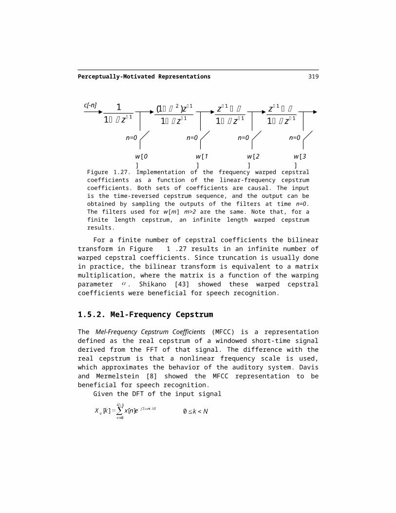
Perceptually-Motivated Representations 319
where we see that the numerator in Eq. is very similar to the autocorrelation in Section 1.7.1, but where N terms are used in the addition for all values of T.
0 500 1000 1500 2000 2500 3000 3500 4000 4500 5000-0.5
0
0.5
(a)
10 20 30 40 50 600
100
200
(b)
10 20 30 40 50 600
100
200
(c)
Figure 1.33 Waveform (a) and unsmoothed pitch track with the normalized cross-correlation method. A frame shift of 10ms, window length of 10ms and a sampling rate of 8kHz were used. (b) is the standard normalized cross-correlation method, whereas (c) has a decaying term. If we compare it the autocorrelation method of Figure 1.31, the middle voiced region is cor-rectly identified in both (b) and (c) but there are two frames at the beginning of (b) that have pitch halving that are eliminated with the decaying term. Again, the pitch values in the un-voiced regions are essentially random.
The maximum of the normalized cross-correlation method is shown in Figure 1.33 (b). Unlike the autocorrelation method, the estimate of the normalized cross-correlation is not bi-ased by the term . For perfectly periodic signals, this results in identical values of the normalized cross-correlation function for kT. This can result in pitch halving, where 2T can be chosen as the pitch period, which happens in Figure 1.33 (b) at the beginning of the utterance. Using a decaying bias with , can be useful in reducing pitch halving, as we see in Figure 1.33 (c).
Because the number of samples involved in the calculation is constant, this estimate is unbiased and has lower variance than that of the autocorrelation. Unlike the autocorrelation method, the window length could be lower than the pitch period, so that the assumption of stationarity is more accurate and it has more time resolution. While pitch trackers based on the normalized cross-correlation typically perform better than those based on the autocorre-lation, they also require more computation, since all the autocorrelation lags can be effi-ciently computed through 2 FFTs, and N multiplies and adds (see Section 5.3.4).
Let’s gain some insight about the normalized cross-correlation. If x[n] is periodic with period T, then we can predict it from a past vector T samples in the past as:
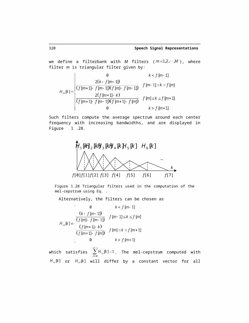
320 Speech Signal Representations
where is the prediction gain. The normalized cross-correlation measures the angle between the two vectors as can be seen in Figure 1.34 and since it is a cosine, it has the property that
.
Figure 1.34. The prediction of with results in an error
If we choose the value of the prediction gain as to minimize the prediction error
and assume is a zero-mean Gaussian random vector with a standard deviation , then
so that the maximum likelihood estimate corresponds to finding the value T with highest normalized cross-correlation. Using Eq. , it is possible that . In this case, there is negative correlation between and , and it is unlikely that T is a good choice for pitch. Thus, we need to force , so that Eq. is converted into
The normalized cross-correlation of Eq. predicts the current frame with a frame that occurs T samples before. Voiced speech may exhibit low correlation with a previous frame at a spectral discontinuity, such as those appearing at stops. To account for this, an enhance-ment can be done to consider not only the backward normalized cross correlation, but also the forward normalized cross-correlation by looking at a frame that occurs T samples ahead of the current frame, and taking the highest of both.
xt-T
et
xt
xt-T
θ
Perceptually-Motivated Representations 321
1.7.3. Signal Conditioning
Noise in the signal tends to make pitch estimation less accurate. To reduce this effect, signal conditioning or pre-processing has been proposed prior to pitch estimation [44]. Typically this involves bandpass filtering to remove of frequencies above 1 or 2kHz, and below 100 Hz or so. High frequencies do not have much voicing information and have significant noise energy, whereas low frequencies can have 50/60 Hz interference from power lines or non-linearities from some A/D subsystems that can also mislead a pitch estimation algorithm.
In addition to the noise in the very low frequencies and aspiration at high bands, the stationarity assumption is not so valid at high frequencies. Even a slowly changing pitch, say, nominal 100Hz increasing 5Hz in 10ms, results in a fast changing harmonic: the 30 th
harmonic at 3000Hz changes 150Hz in 10ms. The corresponding short-time spectrum no longer shows peaks at those frequencies.
Because of this, it is advantageous to filter out such frequencies prior to the computa-tion of the autocorrelation or normalized cross-correlation. If an FFT is used to compute the autocorrelation, this filter is easily done by setting to 0 those undesired frequency bins.
1.7.4. Pitch Tracking
Pitch tracking using the above methods typically fails in several cases:
Sub-harmonic errors. If a signal is periodic with period T, it is also periodic with period 2T, 3T, etc. Thus, we expect to see the scores to be also high for the multi-ples of T, which can mislead the algorithm. Because the signal is never perfectly stationary, those multiples, or sub-harmonics, tend to have slightly lower scores than the fundamental. If the pitch is identified as 2T, pitch halving is said to occur.
Harmonic errors. If harmonic M dominates the signal’s total energy, the score at pitch period T/M will be large. This can happen if the harmonic falls in a formant frequency that boosts its amplitude considerably compared to that of the other har-monics. If the pitch is identified as T/2, pitch doubling is said to occur.
Noisy conditions. When the SNR is low, pitch estimates are quite unreliable for most methods.
Vocal fry. While pitch is generally continuous, for some speakers it can suddenly change and even go in half, particularly at the end of an unstressed voiced region. The pitch here is really not well defined and imposing smoothness constraints can hurt the system.
F0 jumps up or down by an octave occasionally. Breathy voiced speech is difficult to distinguish from periodic background noise. Narrow-band filtering of unvoiced excitations by certain vocal tract configurations
can lead to signals that appear periodic.Because of these reasons, pitch trackers do not determine the pitch value at frame m
based exclusively on the signal at that frame. For a frame where there are several pitch can-
322 Speech Signal Representations
didates with similar scores, the fact that pitch does not change abruptly with time is benefi-cial in disambiguation, because possibly the following frame has a more clear pitch candi -date, which can help.
To integrate the normalized cross-correlation into a probabilistic framework, you can combine tracking with the use of a priori information [10]. Let’s define
as a sequence of input vectors for M consecutive frames centered at equally spaced time instants, say 10ms. Furthermore, if we assume that are indepen-dent of each other, the joint distribution takes on the form:
where is the pitch track for the input. The maximum a posteriori (MAP) estimate of the pitch track is:
according to Bayes rule, with the term being given by Eq. and by Eq. for example.
The function constitutes the a priori statistics for the pitch and can help disam-biguating the pitch, by avoiding pitch doubling or halving given knowledge of the speaker’s average pitch, and by avoiding rapid transitions given a model of how pitch changes over time. One possible approximation is given by assuming that the a priori probability of the pitch period at frame i depends only on the pitch period for the previous frame:
One possible choice for is to decompose it into a component that depends on and another that depends on the difference . If we approximate both as Gaussian densities we obtain
so that when Eq. and are combined, the log probability of transitioning to at time t from pitch at time t-1 is given by
so that the log-likelihood in Eq. can be expressed as
Perceptually-Motivated Representations 323
which can be maximized through dynamic programming. For a region where pitch is not supposed to change, , the term in Eq. acts as a penalty that keeps the pitch track from jumping around. A mixture of Gaussians can be used instead to model different rates of pitch change, like in the case of Mandarin Chinese with 4 tones characterized by dif -ferent slopes. The term attempts to get the pitch close to its expected value to avoid pitch doubling or halving, with the average being different for male and female speakers. Pruning can be done during the search without loss of accuracy (See Chapter 12).
Pitch trackers also have to determine whether a region of speech is voiced or un-voiced. A good approach is to build a statistical classifier built with techniques described in Chapter 8 based on energy and the normalized cross-correlation described above. Such clas-sifiers, i.e. a HMM, penalize jumps between voiced and unvoiced frames to avoid voiced re-gions having isolated unvoiced frame inside and vice versa. A threshold can be used on the a posteriori probability to determine voiced from unvoiced frames.
1.8. HISTORICAL PERSPECTIVE AND FUTURE READING
In 1978, Lawrence R. Rabiner and Ronald W. Schafer [38] wrote a book summarizing the work to date on digital processing of speech, which is still today a good source for the reader interested in further reading in the field. The book by Deller, Hansen and Proakis [9] in-cludes more recent work as is also an excellent reference. O’Shaughnessy [33] also has a thorough description of the subject. Malvar [25] covers filterbanks and lapped transforms extensively.
The extensive wartime interest in sound spectrography lead Koenig and his colleagues at Bell Laboratories [22] in 1946 to the invaluable development of a tool that has been used for speech analysis since then: the spectrogram. Potter et al [35] showed the usefulness of the analog spectrogram in analyzing speech. The spectrogram facilitated research in the field and led Peterson and Barney [34] to publish in 1952 a detailed study of formant values of different vowels. The development of computers and the FFT led Oppenheim, in 1970 [30], to develop digital spectrograms, which imitated the analog counterparts.
The MIT Acoustics Lab started work in speech in 1948 with Leo R. Beranek, who, in 1954, published the seminal book Acoustics, where he studied sound propagation in tubes. In 1950, Kenneth N. Stevens joined the lab and started work on speech perception. Gunnar Fant visited the lab at that time and as a result started a strong speech production effort at KTH in Sweden.
The 1960s marked the birth of digital speech processing. Two books, Gunnar Fant’s Acoustical Theory of Speech Production [13] in 1960 and James Flanagan’s Speech Analy-sis: Synthesis and Perception [14] in 1965, had a great impact and sparked interest in the field. The advent of the digital computer prompted Kelly and Gertsman to create in 1961 the
324 Speech Signal Representations
first digital speech synthesizer [21]. Short-time Fourier analysis, cepstrum, LPC analysis, pitch and formant tracking, digital filterbanks were the fruit of that decade.
Short-time Frequency Analysis was first proposed for analog signals by Fano [11] in 1950 and later by Schroeder and Atal [42].
The mathematical foundation behind linear predictive coding dates to the auto-regres-sive models of George Udny Yule (1927) and Gilbert Walker (1931), which lead to the well-known Yule-Walker equations. These equations resulted in a Toeplitz matrix, named after Otto Toeplitz (1881-1940) who studied it extensively. N. Levinson suggested in 1947 an ef-ficient algorithm to invert such matrix, which J. Durbin refined in 1960 and is now known as the Levinson-Durbin recursion. The well-known LPC analysis consisted the application of the above results to speech signals, which were developed by Bishnu Atal [4], J. Burg [7], Fumitada Itakura and S. Saito [19] in 1968, Markel [27] and John Makhoul [24] in 1973.
The cepstrum was first proposed in 1964 by Bogert, Healy and John Tukey [6], and further studied by Alan V. Oppenheim [29] in 1965. The popular mel-frequency cepstrum was proposed by Davis and Mermelstein [8] in 1980, by combining the advantages of cep-strum with knowledge of the non-linear perception of frequency by the human auditory sys-tem that had been studied by E. Zwicker [47] in 1961.
The study of digital filterbanks was first proposed by Schafer & Rabiner in 1971 for IIR and in 1975 for FIR filters.
Formant Tracking was first investigated by K. Stevens and James Flanagan in the late 1950s, with the foundations for most modern techniques developed by Schafer and Rabiner [40], Itakura [20] and Markel [26]. Pitch tracking through digital processing was first stud-ied by B. Gold [15] in 1962, and then improved by A. M. Noll [28], M. Schroeder [41] and M. Sondhi [44] in the late 1960s.
REFERENCES[1] Acero, A. Formant Analysis and Synthesis using Hidden Markov Models. in Eu-
rospeech. 1999. Budapest.[2] Atal, B.S., Automatic Speaker Recognition Based on Pitch Contours, . 1968, Poly-
technic Institute of Brooklyn.[3] Atal, B.S. and L. Hanauer, Speech Analysis and Synthesis by Linear Prediction of
the Speech Wave. Journal of the Acoustical Society of America, 1971. 50: p. 637-655.
[4] Atal, B.S. and M.R. Schroeder. Predictive Coding of Speech Signals. in Report of the 6th International Congress on Acoustics. 1968. Tokyo, Japan.
[5] Berouti, M.G., D.G. Childers, and A. Paige. Glottal Area versus Glottal Volume Velocity. in Int. Conf. on Acoustics, Speech and Signal Processing. 1977. Hartford, Conn.
[6] Bogert, B., M. Healy, and J. Tukey, eds. The Quefrency Alanysis of Time Series for Echoes. Proc. Symp. On Time Series Analysis, ed. M. Rosenblatt. 1963, J. Wiley: New York. 209-243.
[7] Burg, J. Maximum Entropy Spectral Analysis. in Proc. of the 37th Meeting of the Society of Exploration Geophysicists. 1967.
Perceptually-Motivated Representations 325
[8] Davis, S. and P. Mermelstein, Comparison of Parametric Representations for Monosyllable Word Recognition in Continuously Spoken Sentences. IEEE Trans. on Acoustics, Speech and Signal Processing, 1980. 28(4): p. 357-366.
[9] Deller, J.R., J.H.L. Hansen, and J.G. Proakis, Discrete-Time Processing of Speech Signals. 2000: IEEE Press.
[10] Droppo, J. and A. Acero. Maximum a Posteriori Pitch Tracking. in Int. Conf. on Spoken Language Processing. 1998. Sydney.
[11] Fano, R.M., Short-time Autocorrelation Functions and Power Spectra. Journal of the Acoustical Society of America, 1950. 22(Sep): p. 546-550.
[12] Fant, G., ed. On the Predictability of Formant Levels and Spectrum Envelopes from Formant Frequencies. In For Roman Jakobson. 1956, Mouton: The Hague, The Netherlands.
[13] Fant, G., Acoustic Theory of Speech Production. 1970, The Hague, NL: Mouton.[14] Flanagan, J., Speech Analysis Synthesis and Perception. 1972, New York, NY:
Springer-Verlag.[15] Gold, B., Computer Program for Pitch Extraction. Journal of the Acoustical Soci-
ety of America, 1962. 34(7): p. 916-921.[16] Hermansky, H., Perceptual Linear Predictive (PLP) Analysis of Speech. Journal of
the Acoustical Society of America, 1990. 87(4): p. 1738--1752.[17] Hess, W., Pitch Determination of Speech Signals. ed. 1983: Springer-Verlag, New
York, NY.[18] Itakura, F., Line Spectrum Representation of Linear Predictive Coefficients. Journal
of the Acoustical Society of America, 1975. 57(4): p. 535.[19] Itakura, F. and S. Saito, Analysis Synthesis Telephony Based on the Maximum Like-
lihood Method, in Proc. 6th Int. Congress on Acoustic. 1968: Tokyo, Japan. p. 17-.[20] Itakura, F.I. and S. Saito, A Statistical Method for Estimation of Speech Spectral
Density and Formant Frequencies. Elec. and Comm. in Japan, 1970. 53-A(1): p. 36-43.
[21] Kelly, J.L. and L.J. Gerstman, An Artificial Talker Driven From Phonetic Input. Journal of Acoustical Society of America, 1961. 33: p. 835.
[22] Koenig, R., H.K. Dunn, and L.Y. Lacy, The Sound Spectrograph. Journal of the Acoustical Society of America, 1946. 18: p. 19-49.
[23] Krishnamurthy, A.K. and D.G. Childers, Two Channel Speech Analysis. IEEE Trans. on Acoustics, Speech and Signal Processing, 1986. 34: p. 730-743.
[24] Makhoul, J., Spectral Analysis of Speech by Linear Prediction. IEEE Transactions on Acoustics, Speech and Signal Processing, 1973. 21(3): p. 140-148.
[25] Malvar, H., Signal Processing with Lapped Transforms. 1992: Artech House.[26] Markel, J.D., Digital Inverse Filtering - A New Tool for Formant Trajectory Esti-
mation. IEEE Trans. on Audio and Electroacoustics, 1972. AU-20(June): p. 129-137.
[27] Markel, J.D. and A.H. Gray, On Autocorrelation Equations as Applied to Speech Analysis. IEEE Transaction on Audio and Electroacoustics, 1973. AU-21(April): p. 69-79.

326 Speech Signal Representations
[28] Noll, A.M., Cepstrum Pitch Determination. Journal of the Acoustical Society of America, 1967. 41: p. 293--309.
[29] Oppenheim, A.V., Superposition in a Class of Nonlinear Systems, . 1965, Research Lab. Of Electronics, MIT: Cambridge, Massachusetts.
[30] Oppenheim, A.V., Speech Spectrograms Using the Fast Fourier Transform. IEEE Spectrum, 1970. 7(Aug): p. 57-62.
[31] Oppenheim, A.V. and D.H. Johnson, Discrete Representation of Signals. The Pro-ceedings of the IEEE, 1972. 60(June): p. 681-691.
[32] Oppenheim, A.V., R.W. Schafer, and T.G. Stockham, Nonlinear Filtering of Multi-plied and Convolved Signals. Proc. of the IEEE, 1968. 56: p. 1264-1291.
[33] O'Shaughnessy, D., Speech Communication -- Human and Machine. 1987: Addi-son-Wesley.
[34] Peterson, G.E. and H.L. Barney, Control Methods Used in a Study of the Vowels. Journal of the Acoustical Society of America, 1952. 24(2): p. 175-184.
[35] Potter, R.K., G.A. Kopp, and H.C. Green, Visible Speech. 1947, New York: D. Van Nostrand Co. Republished by Dover Publications, Inc. 1966.
[36] Press, W.H., et al., Numerical Recipes in C. 1988, New York, NY: Cambridge Uni-versity Press.
[37] Rabiner, L.R., On the Use of Autocorrelation Analysis for Pitch Detection. IEEE Transactions on Acoustics, Speech and Signal Processing, 1977. 25: p. 24-33.
[38] Rabiner, L.R. and R.W. Schafer, Digital Processing of Speech Signals. ed. 1978: Prentice-Hall, Englewood Cliffs, NJ.
[39] Rosenberg, A.E., Effect of Glottal Pulse Shape on the Quality of Natural Vowels. Journal of the Acoustical Society of America, 1971. 49: p. 583-590.
[40] Schafer, R.W. and L.R. Rabiner, System for Automatic Formant Analysis of Voiced Speech. Journal of the Acoustical Society of America, 1970. 47: p. 634--678.
[41] Schroeder, M., Period Histogram and Product Spectrum: New Methods for Funda-mental Frequency Measurement. Journal of the Acoustical Society of America, 1968. 43(4): p. 829-834.
[42] Schroeder, M.R. and B.S. Atal, Generalized Short-Time Power Spectra and Auto-correlation. Journal of the Acoustical Society of America, 1962. 34(Nov): p. 1679-1683.
[43] Shikano, K., K.-F. Lee, and R. Reddy. Speaker Adaptation through Vector Quanti-zation. in IEEE Int. Conf. on Acoustics, Speech and Signal Processing. 1986. Tokyo, Japan.
[44] Sondhi, M.M., New Methods for Pitch Extraction. IEEE Transactions on Audio and Electroacoustics, 1968. 16(June): p. 262-268.
[45] Talkin, D., ed. A Robust Algorithm for Pitch Tracking. Speech Coding and Synthe-sis, ed. K.a. Paliwal. 1995, Elsevier: Amsterdam.
[46] Yegnanarayana, B. and R.N.J. Veldhuis, Extraction of Vocal-Tract System Charac-teristics from Speech Signals. IEEE Transaction on Speech and Audio Processing, 1998. 6(July): p. 313-327.
[47] Zwicker, E., Subdivision of the Audible Frequency Range into Critical Bands. Jour-nal of the Acoustical Society of America, 1961. 33(Feb): p. 248.