Embed Size (px)
Citation preview

This is a reprint of material published in M. Wels: Prob-abilistic Modeling for Segmentation in Magnetic Resonance Images of the Human Brain, Logos Verlag, Berlin, 2010, ISBN 978-3-8325-2631-3, ISSN 1617-0695. Please consider purchasing the original publication at www.logos-verlag.de. © Logos Verlag Berlin GmbH 2010

Probabilistic Modeling for Segmentation
in Magnetic Resonance Images
of the Human Brain
(Wahrscheinlichkeitstheoretische Modellierung für die
Segmentierung in Magnetresonanztomographieaufnahmen
des menschlichen Gehirns)
Der Technischen Fakultät der
Universität Erlangen-Nürnberg
zur Erlangung des Grades
DOKTOR-INGENIEUR
vorgelegt von
Michael Wels
Erlangen – 2010

Als Dissertation genehmigt von der
Technischen Fakultät der
Universität Erlangen-Nürnberg
Tag der Einreichung: 12.02.2010
Tag der Promotion: 15.06.2010
Dekan: Prof. Dr.-Ing. R. German
Berichterstatter: Prof. Dr.-Ing. J. Hornegger
Prof. Dr. G. Székely

To my family, my parents, and my sister.

Acknowledgments
A debt of gratitude to my supervisors Prof. Joachim Hornegger, PhD, Dorin Comani-
ciu, PhD, and Martin Huber, PhD, and their institutions, i.e., the University of Erlangen-
Nuremberg and the Siemens AG, for their willingness to financially support the research
activities this piece of work provides record of. Also, for providing excellent working
environments with teams naturally contributing cutting edge technologies as part of their
daily work. I am proud and feel honored for having had the opportunity to conduct my
PhD studies together with their groups at the University of Erlangen-Nuremberg’s Pattern
Recognition Lab in Erlangen, Germany, at Siemens Corporate Technology’s SE 5 SCR 2
department in Erlangen, Germany, and at Siemens Corporate Research’s Integrated Data
Systems department in Princeton, NJ, USA.
I would like to express my thanks to Prof. Gábor Székely, PhD,from the ETH Zürich’s
Computer Vision Laboratory for agreeing to review this thesis. I deeply appreciate the
honor given to me herewith.
I am very grateful to my direct supervisors Gustavo Carneiro,PhD, and Yefeng Zheng,
PhD, for their remarkable expertise in the field of data-baseguided medical image segmen-
tation, and their leadership skills making working together with them efficient, effective,
and also very rewarding. I enjoyed being part of their teams and being able to ask them for
help at any time.
Special thanks to my fellow colleagues in the aforementioned groups for their method-
ological and technological support, inspiring discussions, their honest feedback and the
favorable reception I experienced both in Erlangen as well as in Princeton. In particular I
would like to thank Prof. Elmar Nöth, PhD, Prof. Elli Angelopoulou, PhD, Florian Jäger,
Yu Deuerling-Zheng, Andreas Wimmer, Ingmar Voigt, Dieter Hahn, PhD, Michael Balda,
Anja Borsdorf, PhD, Eva Kollorz, Christian Riess, Christian Schaller, Benjamin Keck, An-
dreas Maier, PhD, Martin Spiegel, Michael Lynch, PhD, Alexey Tsymbal, PhD, Cristian
Mircean, PhD, Sascha Seifert, PhD, Michael Kelm, PhD, MaríaJimena Costa, PhD, Paul
Pandea, Terrence Chen, PhD, Bogdan Georgescu, PhD, AlexanderSchwing and Zhuowen
Tu, PhD.
Many thanks to Prof. Martin Styner, PhD, Tobias Heimann, PhD, and Prof. Bram
van Ginneken, PhD, for giving me the opportunity to take partin the MICCAI 2007 Work-
shop on 3D Segmentation in the Clinic: A Grand Challenge competition and their efforts
in establishing new benchmarking possibilities for medialimage segmentation algorithms.
Thanks to Alessandro Rossi, MD, Prof. Gundula Staatz, MD, Alexander Aplas, MD,
Clement Vachet, and Paul Pandea for providing data for my research and helping to gener-
ate ground-truth annotations.

Thanks also to Elsevier Limited for kindly granting permission to reprint material from
Gray’s Anatomy [104].
Michael Wels

Abstract
This thesis deals with the fully automatic generation of semantic annotations for medical
imaging data by means of medical image segmentation and labeling. In particular, we
focus on the segmentation of the human brain and related structures from magnetic res-
onance imaging (MRI) data. We present three novel probabilistic methods from the field
of database-guided knowledge-based medical image segmentation. We apply each of our
methods to one of three MRI segmentation scenarios: 1) 3-D MRI brain tissue classifi-
cation and intensity non-uniformity correction, 2) pediatric brain cancer segmentation in
multi-spectral 3-D MRI, and 3) 3-D MRI anatomical brain structure segmentation. All
the newly developed methods make use of domain knowledge encoded by probabilistic
boosting-trees (PBT), which is a recent machine learning technique. For all the meth-
ods we present uniform probabilistic formalisms that groupthe methods into the broader
context of probabilistic modeling for the purpose of image segmentation. We show by
comparison with other methods from the literature that in all the scenarios our newly devel-
oped algorithms in most cases give more accurate results andhave a lower computational
cost. Evaluation on publicly available benchmarking data sets ensures reliable compara-
bility of our results to those of other current and future methods. We also document the
participation of one of our methods in the ongoing online caudate segmentation challenge
(www.cause07.org), where we rank among the top five methods for this particular segmen-
tation scenario.


Kurzfassung
Thema dieser Arbeit ist die vollautomatische Bereitstellung semantischer Annotationen
für medizinisches Bildmaterial. Hierzu werden Segmentierungs- und Segmenterkennungs-
techniken aus der medizinischen Bildverarbeitung verwandt. Ausgangspunkt der Betrach-
tungen sind Magnetresonanztomographieaufnahmen (MRT-Aufnahmen) des menschlichen
Gehirns. Hierfür präsentieren wir drei neuentwickelte datenbankgetriebene, wissens-
basierte Segmentierungsverfahren. Alle Verfahren werdenjeweils in einem von drei
Segmentierungsszenarios aus dem Bereich der neuroradiologischen Magnetresonanzto-
mographie (MRT) angewandt: Wir befassen uns erstens mit derGewebeklassifikation
und Korrektur von Magnetfeldinhomogenitäten in 3-D MRT-Aufnahmen des Gehirns,
zweitens mit der Segmentierung pädiatrischer Hirntumore in multi-spektralen 3-D MRT-
Aufnahmen und drittens mit der Segmentierung anatomischerHirnstrukturen in 3-D MRT-
Aufnahmen. Die Probabilistic Boosting-Tree-Technik (PBT-Technik) aus dem Bereich
des maschinellen Lernens bildet die gemeinsame Kernkomponente der drei neuentwickel-
ten Methoden. Sie alle sind durchgängig wahrscheinlichkeitstheoretisch formuliert und
können daher in den Gesamtkontext der probabilistische Modelle nutzenden Bildsegmen-
tierungsverfahren eingruppiert werden. In allen drei Szenarios zeigen Vergleiche zu an-
deren den neuesten Stand der Technik repräsentierenden Methoden, dass unsere neuent-
wickelten Algorithmen in den meisten Fällen bei geringeremRechenaufwand akkuratere
Ergebnisse liefern. Durch die Verwendung von frei verfügbaren Benchmark-Datensätzen
wird die verlässliche Vergleichbarkeit unserer Evaluationsergebnisse auch hinsichtlich
künftiger Verfahren gewährleistet. Darüber hinaus dokumentieren wir in dieser Arbeit
die Teilnahme einer unserer Methoden am fortgesetzten “Online Caudate Segmentation
Challenge”-Wettbewerb (www.cause07.org), bei dem wir unter den fünf besten Segmen-
tierungsverfahren für das dortige Szenario rangieren.


Contents
Contents i
List of Figures v
List of Tables ix
1 Introduction 1
1.1 The Human Brain . . . . . . . . . . . . . . . . . . . . . . . . . . . . . . 1
1.2 Magnetic Resonance Imaging . . . . . . . . . . . . . . . . . . . . . . . . 4
1.3 Medical Image Segmentation . . . . . . . . . . . . . . . . . . . . . . . .7
1.4 Knowledge-Based Approaches to Medical Image Segmentation . . . . . . 9
1.5 EU Research Project Health-e-Child . . . . . . . . . . . . . . . . . . .. 9
1.6 Contributions . . . . . . . . . . . . . . . . . . . . . . . . . . . . . . . . 10
1.7 Outline . . . . . . . . . . . . . . . . . . . . . . . . . . . . . . . . . . . 11
2 Brain Tissue Classification and Intensity Non-Uniformity Correction 13
2.1 Motivation . . . . . . . . . . . . . . . . . . . . . . . . . . . . . . . . . . 14
2.2 Related Work . . . . . . . . . . . . . . . . . . . . . . . . . . . . . . . . 16
2.2.1 MRI Tissue Classification . . . . . . . . . . . . . . . . . . . . . 16
2.2.2 MRI INU Correction . . . . . . . . . . . . . . . . . . . . . . . . 17
2.3 Method . . . . . . . . . . . . . . . . . . . . . . . . . . . . . . . . . . . 17
2.3.1 DMC-EM Brain Tissue Segmentation . . . . . . . . . . . . . . . 17
2.3.2 MRI INU Estimation . . . . . . . . . . . . . . . . . . . . . . . . 20
2.3.3 Modality-Specific Unary Clique Potentials . . . . . . . . . .. . 23
2.3.4 Coherence Preserving Pair-wise Clique Potentials . . . .. . . . . 26
2.3.5 Summary . . . . . . . . . . . . . . . . . . . . . . . . . . . . . . 26
2.4 Validation . . . . . . . . . . . . . . . . . . . . . . . . . . . . . . . . . . 27
2.4.1 Experimental Setup . . . . . . . . . . . . . . . . . . . . . . . . . 27
2.4.2 Results on Multi-Spectral Simulated Data . . . . . . . . . . .. . 30
2.4.3 Results on Mono-Spectral Simulated Data . . . . . . . . . . . .. 31
2.4.4 Results on Normal Subjects Mono-Spectral Scans . . . . . .. . . 32
i

2.5 Discussion . . . . . . . . . . . . . . . . . . . . . . . . . . . . . . . . . . 34
2.6 Conclusions . . . . . . . . . . . . . . . . . . . . . . . . . . . . . . . . . 38
3 Pediatric Brain Tumor Segmentation 43
3.1 Motivation . . . . . . . . . . . . . . . . . . . . . . . . . . . . . . . . . . 43
3.2 Related Work . . . . . . . . . . . . . . . . . . . . . . . . . . . . . . . . 46
3.2.1 Preprocessing: MRI Inter-Scan Intensity Standardization . . . . . 46
3.2.2 MRI Brain Tumor Segmentation . . . . . . . . . . . . . . . . . . 46
3.2.3 Image Segmentation Using Max-Flow/Min-Cut Computation . . 47
3.3 MRI Inter-Scan Intensity Standardization . . . . . . . . . . . .. . . . . 48
3.4 Segmentation Method . . . . . . . . . . . . . . . . . . . . . . . . . . . . 50
3.4.1 Posterior Mode Image Segmentation . . . . . . . . . . . . . . . .50
3.4.2 Histogram-Based Observation Model . . . . . . . . . . . . . . . 55
3.4.3 Discriminative Model-Constrained MRF Prior Model . . . .. . . 55
3.4.4 Discriminative Model-Constrained Graph Cuts Segmentation . . . 56
3.4.5 Summary . . . . . . . . . . . . . . . . . . . . . . . . . . . . . . 60
3.5 Validation . . . . . . . . . . . . . . . . . . . . . . . . . . . . . . . . . . 60
3.5.1 Experimental Setup . . . . . . . . . . . . . . . . . . . . . . . . . 60
3.5.2 Quantitative Results Using 2-D Haar-Like Features . . .. . . . . 63
3.5.3 Quantitative Results Using 3-D Haar-Like Features . . .. . . . . 64
3.6 Discussion . . . . . . . . . . . . . . . . . . . . . . . . . . . . . . . . . . 65
3.7 Conclusions . . . . . . . . . . . . . . . . . . . . . . . . . . . . . . . . . 67
4 Brain Structure Segmentation 69
4.1 Motivation . . . . . . . . . . . . . . . . . . . . . . . . . . . . . . . . . . 70
4.2 Related Work . . . . . . . . . . . . . . . . . . . . . . . . . . . . . . . . 71
4.3 Method . . . . . . . . . . . . . . . . . . . . . . . . . . . . . . . . . . . 72
4.3.1 Combined 3-D Shape Detection and Shape Inference . . . . .. . 72
4.3.2 3-D Shape Detection: Similarity Transformation Estimation . . . 74
4.3.3 3-D Shape Inference under Global Shape Constraints . . .. . . . 75
4.3.4 Global Shape Model . . . . . . . . . . . . . . . . . . . . . . . . 76
4.3.5 Meta-Structure Detection . . . . . . . . . . . . . . . . . . . . . . 79
4.4 Validation . . . . . . . . . . . . . . . . . . . . . . . . . . . . . . . . . . 81
4.4.1 Material and Experimental Setup . . . . . . . . . . . . . . . . . .81
4.4.2 Quantitative Results . . . . . . . . . . . . . . . . . . . . . . . . 83
4.5 Discussion . . . . . . . . . . . . . . . . . . . . . . . . . . . . . . . . . . 84
4.6 Conclusions . . . . . . . . . . . . . . . . . . . . . . . . . . . . . . . . . 88
ii

5 Summary and Outlook 91
5.1 Summary and Contributions . . . . . . . . . . . . . . . . . . . . . . . . 91
5.2 Discussion and Technological Considerations . . . . . . . . .. . . . . . 93
5.3 Future Work . . . . . . . . . . . . . . . . . . . . . . . . . . . . . . . . . 95
5.4 Conclusions . . . . . . . . . . . . . . . . . . . . . . . . . . . . . . . . . 96
A Discriminative Modeling 97
A.1 Probabilistic Boosting-Trees . . . . . . . . . . . . . . . . . . . . . .. . 97
A.2 AdaBoost . . . . . . . . . . . . . . . . . . . . . . . . . . . . . . . . . . 98
B Segmentation Accuracy Assessment 103
B.1 Mask-Based Segmentation Accuracy Measures . . . . . . . . . . . .. . 103
B.2 Shape-Based Segmentation Accuracy Measures . . . . . . . . . . .. . . 104
C Procrustes Analysis 107
C.1 Ordinary Procrustes Analysis . . . . . . . . . . . . . . . . . . . . . . .. 107
C.2 Generalized Procrustes Anaylsis . . . . . . . . . . . . . . . . . . . .. . 108
D Acronyms and Abbreviations 111
Bibliography 113
Index 123
iii

iv

List of Figures
1.1 Coronal section of the human brain. From Gray’s Anatomy [104], p. 311.
Reprinted with permission from copyright holder. . . . . . . . . .. . . . 2
1.2 Axial section of the human brain. From Gray’s Anatomy [104], p. 328.
Reprinted with permission from copyright holder. . . . . . . . . .. . . . 3
1.3 Protons with random spin orientation. . . . . . . . . . . . . . . .. . . . 4
1.4 Precessing protons after parallel or anti-parallel alignment of spins due to
the external magnetic fieldB0. . . . . . . . . . . . . . . . . . . . . . . . 5
1.5 The modern MRI scanner Siemens MAGNETOM Verio 3T. . . . . . . .7
1.6 Coronal (a) and axial (b) section of the human brain in a typical T1-weighted
3-D MRI scan. . . . . . . . . . . . . . . . . . . . . . . . . . . . . . . . 8
2.1 The processing pipeline of the proposed DMC-EM method formulti-spectral
brain tissue segmentation and INU correction. . . . . . . . . . . .. . . . 15
2.2 The 3-D Haar-like feature prototypes used in the DMC-EM algorithm’s
discriminative model. . . . . . . . . . . . . . . . . . . . . . . . . . . . . 25
2.3 Axial slices of original images, the segmentation results, the ground-truth
and the estimated INU field for one mono-spectral T1-weighted BrainWeb
volume (5% noise, 20% INU) (a–d), one volume of the IBSR 20 Normal
Subjects data set (e–h), and one volume of the IBSR 18 Subjectsdata set
(i–l) . . . . . . . . . . . . . . . . . . . . . . . . . . . . . . . . . . . . . 31
2.4 Coronary slices of original multi-spectral (T1-weighted, T2-weighted, and
PD-weighted) BrainWeb images of 5% noise and 20% INU (a–c) andesti-
mated INU fields (d–f). Average INU correction accuracy on multi-spectral
BrainWeb data in terms of the COV before and after INU correction (g–i). 33
2.5 Achieved accuracy for GM segmentation in terms of the Dice coefficient
for the IBSR 20 data set by the DMC-EM algorithm, the HMRF-EM al-
gorithm with probabilistic atlas-based unary clique potentials and proba-
bilistic atlas-based initialization, and the HMRF-EM algorithm with zero-
valued unary clique potentials and probabilistic atlas-based initialization. . 34
v

2.6 Achieved accuracy for WM segmentation in terms of the Dicecoefficient
for the IBSR 20 data set by the DMC-EM algorithm, the HMRF-EM al-
gorithm with probabilistic atlas-based unary clique potentials and proba-
bilistic atlas-based initialization, and the HMRF-EM algorithm with zero-
valued unary clique potentials and probabilistic atlas-based initialization. . 35
2.7 Achieved accuracy for GM segmentation in terms of the Dice coefficient
for the IBSR 18 data set by the DMC-EM algorithm, the HMRF-EM al-
gorithm with probabilistic atlas-based unary clique potentials and proba-
bilistic atlas-based initialization, and the HMRF-EM algorithm with zero-
valued unary clique potentials and probabilistic atlas-based initialization. . 36
2.8 Achieved accuracy for WM segmentation in terms of the Dicecoefficient
for the IBSR 18 data set by the DMC-EM algorithm, the HMRF-EM al-
gorithm with probabilistic atlas-based unary clique potentials and proba-
bilistic atlas-based initialization, and the HMRF-EM algorithm with zero-
valued unary clique potentials and probabilistic atlas-based initialization. . 37
3.1 Two different cases of pediatric brain tumors exhibiting heterogeneous
shape and appearance. Columns (a) and (b) show axial slices ofthe typi-
cally acquired pulse sequences (row-wise from left to right: T2-weighted,
T1-weighted, and T1-weighted after contrast enhancement)and the expert
annotated ground-truth overlaid to the T2-weighted pulse sequence. . . . 44
3.2 The processing pipeline of the proposed segmentation method. Each set
of images schematically represents the input and/or outputof individual
processing steps. . . . . . . . . . . . . . . . . . . . . . . . . . . . . . . 45
3.3 Partial schematic representation of the graph considered (M = 2, N = 2)
and its relation to the initial discrete PDFsp = pf and q = pg. The
vertices(ν, µ) ∈ V ofG are depicted as dots aligned in a quadratic scheme
of maximum size2b − 1× 2b − 1. The edgesE are depicted as arrows. . 49
3.4 Axial slice of a reference volumes (a) and axial slice of an original volume
(b) and associated histograms with 256 bins (c). All images displayed at
identical intensity window. . . . . . . . . . . . . . . . . . . . . . . . . . 51
3.5 Axial slice of a reference volumes (a) and axial slice of anormalized vol-
ume (b) and associated histograms with 256 bins (c). All images displayed
at identical intensity window. . . . . . . . . . . . . . . . . . . . . . . . . 52
3.6 Axial slice of a reference volumes (a) and axial slice of an original volume
(b) and associated histograms with 256 bins (c). All images displayed at
identical intensity window. . . . . . . . . . . . . . . . . . . . . . . . . . 53
vi

3.7 Axial slice of a reference volumes (a) and axial slice of anormalized vol-
ume (b) and associated histograms with 256 bins (c). All images displayed
at identical intensity window. . . . . . . . . . . . . . . . . . . . . . . . . 54
3.8 Example of a max-flow/min-cut problem instance with its associated ex-
tended graph. Vertexs denotes the source node and vertext the sink node.
The flow value on edger0 = (t, s) is about to be optimized. The edges of
a possible cut separating the green from the red vertices aredisplayed as
dashed arrows. . . . . . . . . . . . . . . . . . . . . . . . . . . . . . . . 57
3.9 The rendered result for patient No. 1 overlaid on the T2-weighted pulse
sequence. Due to the coarse axial resolution the extracted surface has been
smoothed [106] before rendering. . . . . . . . . . . . . . . . . . . . . . .58
3.10 Segmentation results obtained by leave-one-patient-out cross validation
for a system using 2-D Haar-like features. The odd rows show selected
slices of the T2-weighted pulse sequences of the six available patient data
sets. The even rows show the associated segmentation results (red) and
the ground-truth segmentation (green) overlaid on the T2-weighted pulse
sequence. . . . . . . . . . . . . . . . . . . . . . . . . . . . . . . . . . . 61
3.11 Segmentation results obtained by leave-one-patient-out cross validation
for a system using 3-D Haar-like features. The odd rows show selected
slices of the T2-weighted pulse sequences of the six available patient data
sets. The even rows show the associated segmentation results (red) and
the ground-truth segmentation (green) overlaid on the T2-weighted pulse
sequence. . . . . . . . . . . . . . . . . . . . . . . . . . . . . . . . . . . 62
4.1 The processing pipeline of the proposed 3-D shape detection and infer-
ence method. Each image (detection and delineation of the left caudate)
schematically represents the input and/or output of individual processing
steps. . . . . . . . . . . . . . . . . . . . . . . . . . . . . . . . . . . . . 70
4.2 Invariance ofc ∈ R2 under relative reorientation, relative anisotropic rescal-
ing and relative shape positioning. . . . . . . . . . . . . . . . . . . . .. 73
4.3 Invariance ofc ∈ R2 andR ∈ SO(2) under relative anisotropic rescaling
and relative shape positioning. . . . . . . . . . . . . . . . . . . . . . . .74
4.4 2-D steerable features encoding different orientations and scalings with
respect to a 2-D point of interestc ∈ R2 (a–c). . . . . . . . . . . . . . . . 75
4.5 Spherical coordinate system with zenith angleγ and azimuth angleφ. . . 79
4.6 Composition of meta-structure for decreasing detectiontime. . . . . . . . 80
vii

4.7 Segmentation results obtained on the IBSR 18 data set No. 10 in an axial
(a), coronal (b), and right (c) and left (d) sagittal view. The segmented
structures are the left and right caudate (dark-blue/yellow), the left and
right putamen (orange/blue), the left and right globus pallidus (green/red),
and the left and right hippocampus (turquoise/violet). . . .. . . . . . . . 89
A.1 A PBT with a strong discriminative probabilistic model ineach tree node. 98
A.2 Schematic representation ofT = 4 iterations of the Discrete AdaBoost
algorithm. The strong classifier available at the end of eachiterationt =
1, . . . , T is denoted byH(t). . . . . . . . . . . . . . . . . . . . . . . . . 99
viii

List of Tables
2.1 Summary of the publicly available standard databases from the BrainWeb
repository used for evaluation purposes. . . . . . . . . . . . . . . .. . . 27
2.2 Summary of the publicly available standard databases from the IBSR used
for evaluation purposes. . . . . . . . . . . . . . . . . . . . . . . . . . . . 28
2.3 Summary of the methods used for benchmarking. . . . . . . . . .. . . . 29
2.4 Average segmentation accuracy for multi-spectral (T1-weighted, T2-weight-
ed, and PD-weighted) simulated BrainWeb data of noise levels1%, 3%,
5%, 7%, and 9%, and INUs of 20% and 40%. From left to right the
columns contain the tissue class and the achieved average Dice and Jac-
card coefficients. . . . . . . . . . . . . . . . . . . . . . . . . . . . . . . 30
2.5 Average segmentation accuracy for mono-spectral (T1-weighted) simu-
lated BrainWeb data of noise levels 1%, 3%, 5%, 7%, and 9%, and INUs
of 20% and 40%. From left to right the columns contain the tissue class
and the achieved average Dice and Jaccard coefficients. . . . .. . . . . . 39
2.6 Average INU correction accuracy in terms of the COV beforeand after
INU correction for the mono-spectral BrainWeb data set (a), the IBSR 18
Subjects data set (b), and the IBSR 20 Normal Subjects Data set(c). . . . 40
2.7 Average segmentation accuracy for IBSR 20 with exclusionof data set No.
1 that has been used for training. From left to right the columns contain
the tissue class and the achieved average Dice and Jaccard coefficients. . . 40
2.8 Average segmentation accuracy for IBSR 18. From left to right the columns
contain the tissue label and the achieved average Dice and Jaccard coeffi-
cients for all the data sets and for data sets 1–9 and 11–18 with outlier data
set 10 removed in brackets. . . . . . . . . . . . . . . . . . . . . . . . . . 41
3.1 Performance indices obtained by leave-one-patient-out cross validation fo
a system using 2-D Haar-like features for all of the examineddata sets.
From left to right the columns contain the achieved Dice coefficient, Jac-
card coefficient, and Pearson correlation coefficient. . . . .. . . . . . . . 64
ix

3.2 Performance indices obtained by leave-one-patient-out cross validation for
a system using 3-D Haar-like features for all of the examineddata sets.
From left to right the columns contain the achieved Dice coefficient, Jac-
card coefficient, and Pearson correlation coefficient. . . . .. . . . . . . . 65
4.1 Summary of the publicly available standard data used formodel generation
and evaluation purposes. . . . . . . . . . . . . . . . . . . . . . . . . . . 82
4.2 Average segmentation accuracy for IBSR 18 of models trained from mutu-
ally exclusive training and test data. . . . . . . . . . . . . . . . . . .. . 83
4.3 Average left/right caudate segmentation accuracy for the MICCAI’07 test-
ing data set without optional caudate tail detection. As of 02/25/2009 this
method ranks number 11 in the overall ranking list on www.cause07.org
(“LME Erlangen”). . . . . . . . . . . . . . . . . . . . . . . . . . . . . . 84
4.4 Average left/right caudate segmentation accuracy for the MICCAI’07 test-
ing data set with optional caudate tail detection. As of 03/10/2009 this
method ranks number 2 in the overall ranking list on www.cause07.org
(“Segmentation Team”). . . . . . . . . . . . . . . . . . . . . . . . . . . 85
4.5 Pearson correlation for the volume measurements in the three testing groups
as well as in total. This coefficient captures how well the volumetric mea-
surements correlate with those of the reference segmentations. . . . . . . 86
4.6 The volumetric measurements of the 10 data sets of the same young adult
acquired on 5 different scanners within 60 days. The COV indicates the
stability of the algorithm in a test/re-test situation including scanner vari-
ability. . . . . . . . . . . . . . . . . . . . . . . . . . . . . . . . . . . . . 86
x

Chapter 1
Introduction
1.1 The Human Brain
The brain or encephalon is a component of the human central nervous system (CNS). It lies
in the cranial cavity and is enveloped by a system of membranes—the so-called meninges.
According to reference [96], it can be divided into six parts:
1. the myelencephalon or medulla oblongata,
2. the pons,
3. the mesencephalon or midbrain,
4. the cerebellum,
5. the diencephalon or interbrain, and
6. the telencephalon, cerebrum, or great brain.
The first three parts form the brainstem, which, for instance, contains cardiac and res-
piratory centers. [96]
The cerebellum primarily holds important parts of the motorsystem. [96]
The interbrain contains, among other things, the thalamus and the hypothalamus. The
thalamus relays sensation, special sense and motor signalsfrom the peripheral nervous sys-
tem to the great brain. The hypothalamus contains several control centers of the autonomic
nervous system. They regulate a number of vital functions like body temperature and the
body’s water and energy balance. [3]
The great brain, being the largest part of the human brain, isseparated into the two equal
sized cerebral hemispheres with respect to the midsagittalplane. The corpus callosum is
the only connection between them. The surface of the cerebrum, that is to say, the cerebral
cortex, consists of elevations or gyri and depressions or sulci. On a cellular level, the cortex
1

2 Chapter 1. Introduction
is formed by neurons and their unmyelinated fibers causing the tissue to appear gray during
dissection or in anatomical specimens. The hippocampus, for instance, is a cortical part
of the limbic system, which is associated with congenital and acquired behavior and the
origin of drive, motivation, and emotion. [96] In contrast,the white matter (WM) below
the cortical gray matter (GM) of the cortex is composed of myelinated axons interconnect-
ing different regions of the CNS. However, there are sub-cortical GM structures or nuclei
embedded in the cerebral WM like the basal ganglia consistingof the putamen, the cau-
date nucleus, the globi pallidi, the subthalamic nucleus, and the substantia nigra. The basal
ganglia are associated with a variety of functions, among other things, motor control [96].
Also parts of the limbic system like the amygdala are sub-cortical nuclei. Figs. 1.1 and 1.2
give an overview of the anatomical structures within the cerebrum. [33, 104]
Thalamostriate vein
Caudate nucleus
Fornix
Thalamus, anterior part
Internal medullarylamina
Thalamus, lateral part
Thalamus, medial part
Subthalamicnucleus
Substantia nigra
Crus cerebri
External capsule
Extreme capsule
Putamen
Internal capsule
Globus pallidus
Optic tract
Pes hippocampi
Collateral sulcus
Figure 1.1: Coronal section of the human brain. From Gray’s Anatomy [104], p. 311.Reprinted with permission from copyright holder.
Both the brain and the spinal chord are surrounded by cerebralspinal fluid (CSF) or
liquor cerebrospinalis. It is produced and circulates in the ventricular system consisting of
the right and left lateral ventricles (see Figs. 1.1 and 1.2)and the third and fourth ventri-
cle. The ventricular system is connected to the exterior of the spinal chord and cerebral
hemispheres via the apertures and the cerebellomedullary cistern. Occupying the space
between the arachnoid mater, that is, the middle layer of themeninges and the pia mater,

1.1. The Human Brain 3
Extremecapsule
Externalcapsule
Claustrum
Insula
Opticradiation
Genu ofcorpus callosum
Anterior hornof lateral ventricle
Caudate nucleuas (head)
Septum pellucidum
Anterior limbof internal capsule
Column of fornix
Genu of internal capsule
Putamen
Globus pallidus
Posterior limbof internal capsule
Thalamus
Tail of caudate nucleusHippocampus
Inferior hornof lateral ventricle
Striate cortex
Posterior horn oflateral ventricle
Figure 1.2: Axial section of the human brain. From Gray’s Anatomy [104], p. 328.Reprinted with permission from copyright holder.
that is, the innermost layer of the meninges, the CSF mechanically protects the brain but
also distributes neuroendocrine factors and prevents brain ischemia. [96]
The brain can be affected by lesions, which can be either intra-axial, i.e., within the
brain, or extra-axial, i.e., outside the brain. Meningiomas, which arise from the meninges,
and acoustic neuromas are typical extra-axial tumors. Intra-axial lesions can be primary
or secondary, in which secondary brain lesions are the most common type. They can be
metastatic tumor deposits, for example, from breast or lungcarcinoma, or can be caused
by metastatic infection. Primary brain lesions are less frequent and range from benign to
extremely aggressive with a poor prognosis. Arising from different cell lines they include
gliomas, oligodendrocytomas, and choroid plexus tumors. Though occurring at any age

4 Chapter 1. Introduction
there are two peaks of incidence: one in the first few years of life and the other later in the
early to middle age. [33]
In the case of a conspicuous anamnesis it is a standard procedure to guide further neu-
rological differential diagnosis by means of radiologicalimaging. Amongst the various
imaging modalities used, magnetic resonance imaging (MRI) usually shows a higher soft
tissue contrast than computed tomography (CT) or traditional X-ray imaging, which makes
MRI the method of choice especially for neuroradiological examinations. Moreover, MRI,
together with ultrasound (US) imaging, does not expose patients to any ionizing radia-
tion during image acquisition and is therefore virtually harmless. Both MRI and US are
therefore also well-suited for the radiological examination of pediatric patients.
1.2 Magnetic Resonance Imaging
In the following we give a short introduction to the principles of MRI, which is also known
as magnetic resonance tomography (MRT). It follows the representation of Laubenberger
and Laubenberger [68] with additional information taken from Weishaupt et al. [117]. A
more detailed description can be found in reference [15].
The phenomenon of nuclear magnetic resonance (NMR) was independently discovered
by F. Block and G. M. Purcell in 1946. In 1974 P. C. Lauterbur was the first to use MRI
to picture a living organism: a mouse. The first magnetic resonance (MR) image of the
human body, depicting a thorax, was acquired in 1977 by P. Mansfield.
Figure 1.3: Protons with random spin orientation.

1.2. Magnetic Resonance Imaging 5
B0
Figure 1.4: Precessing protons after parallel or anti-parallel alignment of spins dueto theexternal magnetic fieldB0.
All atomic nuclei with an odd number of protons (atomic number) feature a spin or
magnetic moment, that is, the nuclei rotate about their own axes like spinning tops as
shown in Fig. 1.3. Hydrogen, nitrate, sodium, and phosphor,for instance, are some of the
atoms sharing this property. Among these atoms, hydrogen isthe most frequently found
atom in living tissues such that, almost exclusively, hydrogen atoms contribute to todays
clinical MR image generation.
In an MRI scanner (see Fig. 1.5(a)) the protons’ spin axes are aligned, parallel or an-
tiparallel, with the streamlines of the strong external magnetic field (B0 field) of the scanner
building up a stable state longitudinal magnetization along thez-axis (see Fig. 1.5(b)). Ad-
ditionally, due to the external field, the axes start precessing about the axis of alignment
(z-axis) similar to a spinning top. The characteristic speed of this precession is called Lar-
mor or precession frequencyω0 [MHz], which is proportional to the strengthB0 [T] of the
external magnetic field, that is,
ω0 = γ0 ·B0 (1.1)

6 Chapter 1. Introduction
whereγ0 is the gyromagnetic ratio of the type of nuclei of interest. Both phenomena, paral-
lel or antiparallel alignment and precession, are depictedin Fig. 1.4. The orientation of the
spins as well as their phase coherence can be altered by radiofrequency (RF) pulses having
the same frequency as the Larmor frequency. A90◦ pulse, for instance, causes the spins
rotating about thez-axis to also rotate about the axis induced by the RF pulse, which, due
to having exactly the same frequency, appears to be static from the spins’ relative point of
view. The resulting complex movement of spins statistically cancels longitudinal magneti-
zation along thez-axis and establishes transversal magnetization rotatingin phase within
thexy-plane (see Fig. 1.5(b)). The latter can be measured with theMRI scanner’s receiver
coils. Immediately after excitation with an RF pulse, the equilibrium state longitudinal
magnetization starts to recover causing transverse magnetization to fade. This process is
called T1, longitudinal, or spin-lattice relaxation. Alsophase coherence gradually van-
ishes thereby additionally decreasing transverse magnetization. The process of dephasing
is called T2, transverse, or spin-spin relaxation.
The duration of both kinds of relaxation is constant for specific substances. Different
pulse sequences make use of this fact and regulate the scanner’s sensitivity to certain re-
laxation parameters (T1-weighted or T2-weighted imaging). According to the weighting,
certain substances or organs appear brighter or darker in the acquired image dependant on
their proton density.
In order to spatially resolve the location of the received MRsignal, that is, the measured
change of transverse magnetization over time, additional gradient coils covering the three
dimensions of real space are used. They vary locally the external magnetic fieldB0. Thus,
in accordance with Equation (1.1) excitation can be steeredto specific locations by the
strength of the RF pulses applied. This makes MRI an inherent 3-D radiological imaging
modality where no tomographic reconstruction from severalplanar, that is, 2-D, projections
is required as it is the case, for instance, in CT imaging.
However, the 3-D images acquired need interpretation by a trained expert radiologist.
He or she knows which part of the body and which organs in particular are to be seen
on the images. With the help of his anatomical knowledge his perception is enriched by
a certain understanding of the decomposition of the depicted scene into meaningful, not
merely anatomical, entities. A subtle analysis of the imageat hand immediately takes
place without being necessarily apperceived as a mental event on its own behalf by the
observer himself. This differs entirely from how a computer“perceives” not only radiolog-
ical but images, in the common sense, in general; namely recognizing them as what they in
fact are by definition—nothing but a volume or matrix of signal measurements. Bridging
the gap between mere data and a preferably automatically generated semantic description
of the depicted content is an important aspect within the scientific field of medical image
analysis. This general problem can be decomposed into several steps ranging from rela-
tively concrete to very abstract interpretations of the image content. In the early stages it

1.3. Medical Image Segmentation 7
x
y
z
(a) (b)
Figure 1.5: The modern MRI scanner Siemens MAGNETOM Verio 3T(www.medical.siemens.com, 07/24/2009) (a) and its associated coordi-nate system (b).
is mostly useful to address image segmentation and labeling, that is, uniquely identifying
certain image regions as meaningful entities.
1.3 Medical Image Segmentation
In the following we give a formal description of the problem of medical image segmenta-
tion and labeling, which is the problem of giving semantic information to coherent image
regions. These preliminary remarks are necessary as in the course of this thesis three med-
ical image segmentation scenarios will be discussed in order to exemplify the potential of
our newly developed machine learning-based and database-guided algorithms for segment-
ing and labeling 3-D brain MR images.
Let the familyX = (xs)s∈S be a 2-D, that is,S = { 1, . . . , X } × { 1, . . . , Y }, or
3-D, that is,S = { 1, . . . , X } × { 1, . . . , Y } × { 1, . . . , Z }, X,Y, Z ∈ N+, medical
image. Its values or measurementsxs ∈ Rn, n ∈ N
+, can be either scalar,n = 1, or
multi-spectral,n > 1. The latter is sometimes also called a vector-valued or multi-channel
medical image [84]. Thexs are usually quantified in an appropriate manner for electronic
processing. As it will beS = { 1, . . . , X } × { 1, . . . , Y } × { 1, . . . , Z } in most parts of
this thesis we will refer to thes as image voxels.

8 Chapter 1. Introduction
(a) (b)
Figure 1.6: Coronal (a) and axial (b) section of the human brain in a typical T1-weighted3-D MRI scan. From the Internet Brain Segmentation Repository (IBSR),www.cma.mgh.harvard.edu/ibsr.
Following Pham et al. [84], the problem of image segmentation (without labeling) can
be defined as the search for a partition of an image, i.e., a partition of the set of its voxels,
into homogeneous and connected regions. Formally, one searches for
S =K⋃
k=1
Sk (1.2)
where
∀i,j∈{ 1,...,K },i6=j Si ∩ Sj = ∅ (1.3)
and
∀xs ,xt∈Sk,k∈{ 1,...,K } ∃(sl)1,...,L,L∈N+,s1=s,sL=t ∀i∈{ 1,...,L } |si−1 − si| ≤ 1 (1.4)
or
∀xs ,xt∈Sk,k∈{ 1,...,K } ∃(sl)1,...,L,L∈N+,s1=s,sL=t ∀i∈{ 1,...,L } maxd∈{ 1,2,3 }
|s(i−1)d− sid | ≤ 1 (1.5)
depending on whether a 3-D 6-neighborhood or 26-neighborhood is considered, respec-
tively.
Ideally, everySk corresponds to an anatomical structure or other, from a physician’s
view, meaningful entity in the image. The requirement of connectedness is sometimes re-

1.4. Knowledge-Based Approaches to Medical Image Segmentation 9
laxed such that actually a classification problem instead ofa classical segmentation prob-
lem is addressed. This is occasionally of interest in medical imaging when multiple regions
of the same tissue class are about to be detected. The total number of tissue classes,K, is
usually determined based on prior knowledge about the anatomy considered. In the case
of brain MR images, for instance, it is common practice to assumeK = 3 tissue classes:
GM, WM, and CSF. [84]
The process of assigning a descriptive designation to each of the resulting segments
is called labeling. Though formally independent from each other we will never address
pure image segmentation without labeling throughout this thesis. So, whenever we talk of
image segmentation we actually mean image segmentation andregion labeling.
1.4 Knowledge-Based Approaches to Medical Image Seg-
mentation
Throughout this thesis, we focus on the application of knowledge-based approaches to
medical image segmentation integrating domain knowledge across several layers of geo-
metrical abstraction. In particular, we follow the paradigm of database-guided medical im-
age segmentation [44] where the vast majority of domain knowledge used to guide the seg-
mentation process is initially represented by large collections of medical imaging data with
accompanying ground-truth segmentations. Models are generated from these databases by
means of machine learning techniques. These models are thenused, often in combination
with traditional techniques, for image segmentation.
We explore the capabilities of three newly developed segmentation algorithms of that
kind in three distinct scenarios from the broader field of 3-Dbrain MR image segmentation:
3-D MRI brain tissue classification and intensity non-uniformity (INU) correction, pedi-
atric brain tumor segmentation in 3-D MRI, and 3-D MRI brain structure segmentation.
We are able to show by experimental validation that our knowledge-based approaches out-
perform most of the current state-of-the-art methods to these particular segmentation chal-
lenges with respect to segmentation accuracy (see Chapters 2–4) and also with respect to
computation time (see Chapters 3 and 4). The results obtainedand the current state-of-the-
art to be found in the literature (see Chapters 2–4) encourageus to advance the hypothesis
that database-guided knowledge-based approaches state the answer both to today’s as well
as to tomorrow’s medical image segmentation challenges.
1.5 EU Research Project Health-e-Child
The research efforts on providing semantic descriptions ofMR images of the human brain
by means of medical image segmentation and the associated results documented in this the-

10 Chapter 1. Introduction
sis are part of the research project Health-e-Child (www.health-e-child.org). The Health-
e-Child Project is embedded in the European Union’s sixth framework program (FP6) that
aims to improve integration and coordination of research within the European Union.
Health-e-Child (project identifier: IST-2004-027749) is scheduled from 01/01/2006 to
12/31/2009.
The project’s vision is the development of an integrated healthcare platform for Eu-
ropean pediatrics that provides seamless integration of traditional and emerging sources
of biomedical information. In the long run, Health-e-Child wants to provide access to
biomedical knowledge repositories for personalized and preventive healthcare, for large-
scale information-based biomedical research and training, and for informed policy making.
For the beginning the project focus will be on individualized disease prevention, screening,
early diagnosis, therapy and follow-up of three representative pediatric diseases selected
from the following three major categories: heart diseases,inflammatory diseases, and brain
tumors. By building a European network of leading clinical centers it will be possible to
share and annotate biomedical data, validate systems clinically, and diffuse clinical excel-
lence across Europe by setting up new technologies, clinical workflows, and standards.
Health-e-Child’s key concept is the vertical and longitudinal integration of information
across all information layers of biomedical abstraction, that is to say, genetic, cell, tissue,
organ, individual and population layer, to provide a unifiedview of a person’s biomedical
and clinical condition. This will enable sophisticated knowledge discovery and decision
support.
It is intended to integrate diagnostically relevant knowledge and data from multiple
sources with radiological imaging being one of them. In order to address this particular
part dealing with radiological images of the broader complex of themes within Health-e-
Child our research activities aim for providing explicit semantics for medical imaging data
by means of medical image segmentation and labeling as mentioned above. These seman-
tics can then be used for multiple purposes, for example, fortraditional medical decision
making, such as diagnostics and therapy planning and control, as input to computer-aided
diagnosis (CAD) systems, for morphological studies, for image enhancement, and in gen-
eral as input to any system aiming for semantic data integration.
1.6 Contributions
Contributions to the scientific progress could be made in all medical image segmentation
scenarios addressed by this thesis. They can be summarized as follows:
• For the first scenario we introduce a novel fully automated method for brain tissue
classification, that is, segmentation into cerebral GM, cerebral WM, and CSF, and
intra-scan INU correction in 3-D MR images.

1.7. Outline 11
• For the second scenario we present a novel fully automated approach to pediatric
brain tumor segmentation in multi-spectral 3-D MR images.
• For the third scenario we introduce a novel method for the automatic detection and
segmentation of (sub-)cortical GM structures in 3-D MR images based on the re-
cently introduced concept of marginal space learning (MSL).
• As a minor contribution we adapt a dynamic programming approach for 1-D his-
togram matching to mono-spectral MRI inter-scan intensity standardization in the
second and third scenario. We give a graph theoretic re-formulation of the algorithm
and extend it to minimize the Kullback-Leibler divergence instead of the histograms’
sum of squared differences. This necessary pre-processingstep allows us to make
use of machine learning methods relying on intensity-basedfeatures in the context
of MRI.
1.7 Outline
In the following chapter, that is,Chapter 2, we describe our novel fully automated method
for brain tissue classification and intra-scan INU correction in 3-D MR images. It combines
supervised MRI modality-specific discriminative modeling and unsupervised statistical ex-
pectation maximization (EM) segmentation into an integrated Bayesian framework. The
Markov random field (MRF) regularization involved takes intoaccount knowledge about
spatial and appearance related homogeneity of segments andpatient-specific knowledge
about the global spatial distribution of brain tissue. It isbased on a strong discrimina-
tive model provided by a probabilistic boosting-tree (PBT) for classifying image voxels.
It relies on surrounding context and alignment-based features derived from a probabilistic
anatomical atlas. The context considered is encoded by 3-D Haar-like features of reduced
INU sensitivity. Detailed quantitative evaluations on standard phantom scans and stan-
dard real world data show the accuracy and robustness of the proposed method. They also
demonstrate relative superiority in comparison with otherstate-of-the-art approaches to
this kind of computational task.
Chapter 3 details on our novel fully automated approach to pediatric brain tumor seg-
mentation in multi-spectral 3-D MR images. It is a top-down segmentation approach based
on an MRF model that combines PBTs and low-level segmentation via graph cuts. The
PBT algorithm provides a strong discriminative prior model that classifies tumor appear-
ance while a spatial prior takes into account pair-wise voxel homogeneities in terms of
classification labels and multi-spectral voxel intensities. The discriminative model relies
not only on observed local intensities but also on surrounding context for detecting can-
didate regions for pathology. A mathematically sound formulation for integrating the two

12 Chapter 1. Introduction
approaches into a unified statistical framework is given. The results obtained in a quantita-
tive evaluation are mostly better than those reported for current state-of-the-art approaches
to 3-D MRI brain tumor segmentation.
Chapter 4 introduces a novel method for the automatic detection and segmentation of
(sub-)cortical GM structures in 3-D MR images of the human brain. The method is a top-
down segmentation approach based on the recently introduced concept of MSL [130, 131].
It is shown that MSL naturally decomposes the parameter space of anatomy shapes along
decreasing levels of geometrical abstraction into subspaces of increasing dimensionality by
exploiting parameter invariance. This allows us to build strong discriminative models from
annotated training data on each level of abstraction, and touse these models to narrow the
range of possible solutions until a final shape can be inferred. The segmentation accuracy
achieved is mostly better than the one of other state-of-the-art approaches using standard-
ized distance and overlap accuracy metrics. For benchmarking, the method is evaluated on
two publicly available gold standard databases consistingin total of 42 T1-weighted 3-D
brain MRI scans from different scanners and sites.
Chapter 5 concludes the thesis and summarizes its main contributions. We discuss
technological and methodological aspects of our work and give an outlook on future re-
search directions with regards to the chosen scenarios. Finally, we name challenges med-
ical image segmentation and understanding faces in order tobe of continuous value in
today’s increasingly cross-linked medical environment and infrastructure.
Chapter 2
3-D MRI Brain Tissue Classification and
INU Correction
In this chapter we describe a fully automated method for brain tissue classification, which
is the segmentation into cerebral GM, cerebral WM, and CSF, andINU correction in brain
MRI volumes. It combines supervised MRI modality-specific discriminative modeling and
unsupervised statistical EM segmentation into an integrated Bayesian framework. While
both the parametric observation models as well as the non-parametrically modeled INUs
are estimated via EM during segmentation itself, an MRF priormodel regularizes segmen-
tation and parameter estimation. Firstly, the regularization takes into account knowledge
about spatial and appearance related homogeneity of segments in terms of pair-wise clique
potentials of adjacent voxels. Secondly and more importantly, patient-specific knowledge
about the global spatial distribution of brain tissue is incorporated into the segmentation
process via unary clique potentials. They are based on a strong discriminative model
provided by a PBT for classifying image voxels. It relies on surrounding context and
alignment-based features derived from a probabilistic anatomical atlas. The context con-
sidered is encoded by 3-D Haar-like features of reduced INU sensitivity. Alignment is
carried out fully automatically by means of an affine registration algorithm minimizing
cross-correlation. Both types of features do not immediately use the observed intensities
provided by the MRI modality but instead rely on specifically transformed features, which
are less sensitive to MRI artifacts. Detailed quantitative evaluations on standard phan-
tom scans and standard real world data show the accuracy and robustness of the proposed
method. They also demonstrate relative superiority in comparison to other state-of-the-
art approaches to this kind of computational task: our method achieves average Dice co-
efficients of0.94 ± 0.02 (WM) and 0.92 ± 0.04 (GM) on simulated mono-spectral and
0.93± 0.02 (WM) and0.91± 0.04 (GM) on simulated multi-spectral data from the Brain-
Web repository. The scores are0.81± 0.09 (WM) and0.82± 0.06 (GM) and0.87± 0.05
(WM) and 0.83 ± 0.12 (GM) for the two real-world data sets—consisting of 20 and 18
13
14 Chapter 2. Brain Tissue Classification and Intensity Non-Uniformity Correction
patient volumes, respectively—provided by the Internet Brain Segmentation Repository.
Preliminary results have been published in reference [125].
2.1 Motivation
Several inquiries in medical diagnostics, therapy planning and monitoring, as well as in
medical research, require highly accurate and reproducible brain tissue segmentation in
3-D MRI. For instance, studies of neurodegenerative and psychiatric diseases often rely on
quantitative measures obtained from MRI scans that are segmented into the three common
tissue types present in the human brain: cerebral GM, cerebral WM, and CSF. There is a
need for fully automatic segmentation tools providing reproducible results in this particular
context as manual interaction for this type of volumetric labeling is typically considered un-
acceptable for the following reasons: having 3-D scans manually annotated by radiologists
may notably delay clinical workflow, and the annotations obtained may vary significantly
among experts as a result of individual experience and interpretation. The mentioned au-
tomatic tools face a challenging segmentation task due to the characteristic artifacts of the
MRI modality, such as intra-/inter-scan INU [119, 60], partial volume effects (PVE) [114],
and Rician noise [80]. The human brain’s complexity in shape and natural intensity vari-
ations additionally complicate the segmentation task at hand. Once a sufficiently good
segmentation is achieved it can also be used in enhancing theimage quality, as intra-scan
INUs can be easily estimated due to the knowledge of the tissue type and the associated
image intensities to be observed at a specific spatial site [119]. As can be seen later there
are several interleaved approaches similar to our contribution following this idea where the
tissue segmentation and the INU are estimated simultaneously.
The extended hidden Markov random field expectation maximization (HMRF-EM)
approach with simultaneous INU correction presented here is, in contrast to Zhang et
al. [129]1 , consistently formulated to work on multi-spectral 3-D brain MRI data. Further,
we present a mathematically sound integration of prior knowledge encoded by a strong dis-
criminative model into the statistical framework. The learning-based component, that is,
a PBT [108], providing the discriminative model exclusivelyrelies on features of reduced
sensitivity to INUs and therefore makes this approach MRI modality-specific. Usually,
more discriminative features are used for medical image segmentation by means of dis-
criminative PBT modeling, for instance, in CT data [111]. However, those features do not
take into account the particularities of the MRI modality, which makes them less suited for
MR image segmentation. Approaching the problem this way neglects the fact that relying
1Although not detailed in the original publication a multi-spectral implementation of Zhang et al.’smethod [129] already exists and can be downloaded from www.fmrib.ox.ac.uk/fsl.

2.1. Motivation 15
on modality-specific features can significantly increase segmentation accuracy in certain
cases. [97, 98]
Exhaustive quantitative evaluations on publicly available simulated and real world MRI
scans show the relative superiority with regards to robustness of our newly proposed method
in comparison to other state-of-the-art approaches [94, 6,13, 93, 2, 1, 5, 4, 74, 129, 113].
While other methods may reach particular high values on a particular database we present
comparable and mostly better results in terms of segmentation accuracy on a variety of
benchmarking databases from different sources. This demonstrates the increased robust-
ness of our approach.
Estimation and HardPBT Probability
Classification
DMC−EMOptimizationStripping
BET SkullAtlas Alignment
FLIRT Probabilistic
Figure 2.1: The processing pipeline of the proposed DMC-EM method for multi-spectralbrain tissue segmentation and INU correction.
Our method consists of four steps: first, the whole brain is extracted from its sur-
roundings with the Brain Extraction Tool (BET) [100] working on the T1-weighted pulse
sequence. As BET skull stripping fails on some of the data setswe use for evaluation we
extended the original preprocessing tool BET. We introducedthresholding for background
exclusion, morphological operations and connected component analysis to generate ini-
tializations (center and radius of initial sphere) for the BET main procedure that are closer
to the intra-cranial surface to be computed. Then, an initial spatially variant prior of the
brain soft tissue on different tissue classes is obtained bymeans of a strong modality spe-
cific discriminative model, that is to say, a PBT probability estimator. This also gives an
initial segmentation of the brain soft tissue. Subsequently, the final segmentation and the
multi-spectral INU fields are estimated via an extended HMRF-EM approach that operates
on multi-spectral input data. We will refer to our method as the discriminative model-
constrained HMRF-EM approach (DMC-EM). The whole processingpipeline is depicted
in Fig. 2.1.

16 Chapter 2. Brain Tissue Classification and Intensity Non-Uniformity Correction
2.2 Related Work
2.2.1 MRI Tissue Classification
Most approaches in the field of MRI brain tissue segmentation are based on Bayesian
modeling, which typically involves providing a prior modeland a generative observation
model. With these models the most likely tissue class being responsible for the observed
intensity values at a certain voxel can be inferred. Offline generated observation mod-
els, that is, models generated from annotated training data, usually are very sensitive to
MRI artifacts. [54] For this reason parametric models are typically estimated online, that
is, simultaneously with an associated segmentation maximizing an a posteriori probability
distribution density by means of EM [13, 94, 93, 4, 86, 37, 129, 113, 62, 119]. Apart from
EM optimization methods comprise max-flow/min-cut computation [102, 101], segmen-
tation by weighted aggregation [2], and finding the maximizer of the posterior marginals
(MPM) in a maximum a posteriori (MAP) setting [74]. Recently also non-parametric [2]
approaches for generating observation models within Bayesian frameworks and entirely
learning-based [1] approaches to brain tissue classification have been proposed. Some of
them [1, 2] do not take into account INUs and scanner-specificcontrast characteristics
present in the data sets used for model generation, which mayresult in model over-fitting
and poor generalization capabilities.
Commonly used prior models comprise, next to the assumption of spatially uniform
prior probabilities, spatial interdependencies among neighboring voxels through prior prob-
abilities modeled as hidden Markov random fields (HMRF) [94, 93, 74, 129, 62], hid-
den Markov chains (HMC) [13], or non-parametric adaptive Markov priors [5]. They
are sometimes combined with prior probabilities derived from probabilistic or anatomi-
cal atlases [5, 74, 86, 113] or replaced by them [6, 4] that canalso be integrated into the
overall MRF-based formulation as external field energies [94, 86]. The same holds for
prior knowledge encoded by fuzzy localization maps [93] that can also be integrated into
the overall framework via external fields. Alignment of the atlas can be achieved either
by rigid [6, 113], affine [94, 2, 5], or non-rigid [13, 74, 86] registration algorithms, either
before optimization or simultaneously [6, 4]. Bazin and Pham[6] additionally incorporate
prior knowledge obtained from a topological atlas into a fuzzy classification technique for
topology preservation. Cuadra et al. [30] compare and validate different statistical non-
supervised brain tissue classification techniques in MRI volumes.
Conceptually, our approach aligns with the mentioned EM-based approaches using
Markov random field priors and aligned probabilistic atlases. In contrast, though, our
method makes use of more general prior knowledge in terms of astrong discriminative
model initializing and continually constraining the segmentation process. It is motivated
by recent advances in medical image segmentation that make use of prior knowledge in a
2.3. Method 17
similar manner, i.e., in terms of discriminative modeling,to improve segmentation accu-
racy and robustness [121, 77, 21, 28, 111]. We have chosen thePBT algorithm for dis-
criminative modeling as it has been found to perform well in avariety of medical imaging
settings [126, 77, 121, 111, 19, 131].
In many cases the related approaches completely lack a quantitative evaluation [129]
or are exclusively quantitatively validated on synthetic data [94, 93, 4]. In other cases
quantitative evaluation is carried out only on a small collection of scans from a single
source of data [13, 38, 1, 2, 119]. All this imposes a restriction on the generalization
capabilities of such methods.
2.2.2 MRI INU Correction
While some of the papers mentioned above address further segmentation of cerebral gray
matter into individual structures [94, 93, 2, 6], which is beyond the scope of this chapter,
only some of them additionally address INU correction [13, 101, 102, 4, 129, 113, 119].
INUs are usually modeled as multiplicative noise corrupting the images in the intensity
domain and as additive noise in the log-domain. They can be described either non-
parametrically as bias or gain fields in the literal sense [129, 119] or parametrically by
polynomial basis functions [13, 112], by means of cubic B-splines [102, 101] or through
the exponential of a linear combination of low frequency basis functions [4]. Other ap-
proaches rely on segmentation methods but focus on INU correction [112, 53]. Vovk et
al. [116] recently reviewed most of the relevant data-driven approaches in the field includ-
ing non-segmentation-based approaches like the well-known nonparametric nonuniform
intensity normalization (N3) [99] and homomorphic unsharpmasking (HUM) [14]. An-
other detailed review can be found in reference [7]. As we consider INU correction to be
a possible application of our novel segmentation approach but not the main focus of our
contribution we refer the reader to the reviews mentioned for further information.
2.3 Method
2.3.1 DMC-EM Brain Tissue Segmentation
Image or volume segmentation by means of the DMC-EM approach,which extends the
HMRF-EM approach of Zhang et al. [129], is closely related to learning finite Gaussian
mixtures (FGM) via the EM algorithm. For both cases letS = { 1, 2, . . . , N }, N ∈ N, be
a set of indices to image voxels. At each indexs ∈ S there are two random variablesYs and
Xs that take discrete valuesys ∈ Y = { 1, . . . , K },K ∈ N, andxs ∈ X = { 1, . . . , 2d }L.
The former,Ys, denotes the hidden class label, that is, the underlying tissue class, at voxel
s, whereas the latter,Xs, states the vector of observed intensity values taken from the
18 Chapter 2. Brain Tissue Classification and Intensity Non-Uniformity Correction
L ∈ N aligned input pulse sequences each having a bit depth ofd ∈ N. The observable
intensities at every voxels are assumed to be causally linked to the underlying class labels
by parameterized Gaussian distribution densitiesp(xs|ys = k) = N(xs; θk) with class
specific parametersθk = (µk,Σk), µk ∈ RL, Σk ∈ R
L×L and symmetric positive-definite.
Starting from initial values for those parameters and some prior probabilitiesp(0)(k) for the
occurrence of each class label a proper statistical model interms of prior probabilitiesp(k),
k ∈ Y, and parametersΘ = (θk)k∈Y can be estimated by means of EM iteratively in an
unsupervised manner.
In contrast to the FGM model that considers every voxel’s classification isolated from
its local neighborhood the DMC-EM model assumes external influences and spatial inter-
dependencies among neighboring voxels. Both can be incorporated into the existing model
by describing the familyY = (Ys)s∈S of unknown class labels as an MRF. According to
Li [69], within an MRF every voxel at indexs is associated with a subsetNs ⊆ S \ { s }of neighboring indices having the propertiess 6∈ Ns and s ∈ Nt ⇔ t ∈ Ns for all
s, t ∈ S. The family of random variablesY is said to form an MRF onS with respect
to the neighborhood systemN = {Ns | s ∈ S } if and only if p(y) > 0 for all possible
configurationsy = (ys)s∈S , andp(ys|(yt)t∈S\{ s }) = p(ys|yNs) for all s ∈ S. They are
called the positivity property and the Markov property of the MRF.
The graphG = (V,E) with verticesV = { vs | s ∈ S } and edgesE = { (vs, vt) | s ∈S, t ∈ Ns } associated with an MRF contains multiple sets of cliques, which are sets of
complete sub-graphs,Cn denoting all the sets of vertices’ indices within cliques ofsize
n ∈ { 1, . . . , |V | }.Under these circumstances, according to the Hammersley-Clifford theorem, the joint
probability density function (PDF)p(y) can equivalently be described by a Gibbs dis-
tribution p(y) = 1Z
exp(−U(y)). HereU(y) =∑
n
∑
cn∈CnVcn
(y) denotes the energy
function, which is a sum of clique potentialsVcn, andZ =
∑
y exp(−U(y)) denotes the
partition function, which is a normalization constant.
In contrast to Zhang et al. [129] our model considers both unary (n = 1) as well
as pair-wise (n = 2) clique potentials as we want to introduce an MRF prior that con-
strains segmentation by an external field, provided by a strong discriminative model, and
by mutual spatial dependencies among pairs of neighboring voxels. In this case the energy
function can be stated as
U(y) =∑
s∈S
(
Vs(ys) +β
2
∑
t∈Ns
Vst(ys, yt)
)
. (2.1)
For the purpose of image segmentation it is common practice [30, 129] to ignore further
dependencies, i.e., higher-ordered clique potentials. These potentials increase the degrees
of freedom of the MRF and therefore require more training datafor reliable parameter

2.3. Method 19
estimation. Thus, by applying Bayes’ rule and by marginalizing over the possible class
labels, we have
p(ys|yNs) = p(ys|(yt)t∈S\{ s })
=p(ys, (yt)t∈S\{ s })
∑
k∈Y p(ys = k, (yt)t∈S\{ s })
=exp(−Vs(ys)−
∑
t∈NsVst(ys, yt))
∑
k∈Y exp(−Vs(ys = k)−∑t∈NsVst(ys = k, yt))
(2.2)
with the labelsyNsunderstood as observable evidence.
Due to the fact that Equation (2.2) can be formulated dependent on unary and pair-wise
clique potentials it is possible to introduce prior knowledge into the classification process.
In order to make a strong discriminative model constrain expectation maximization we
will later define unary clique potentials based on tissue class probability estimations from
PBT classifiers. With regards to the pair-wise clique potentials, which are defined on fully
labeled data, the best segmentationarg maxy p(y|x;Θ(i−1)) that is needed to properly
evaluateVst(ys, yt) in iterationi is not available during iterative expectation maximization.
This means, in accordance with Zhang et al. [129], a currently best segmentation using the
MAP
y∗ = arg maxy
p(y|x;Θ(i−1)) (2.3)
where
p(y|x;Θ(i−1)) =p(x|y;Θ(i−1))p(y)
p(x)
=1
Z
∏
s
p(xs|ys; θ(i−1)) · exp(−Vs(ys)−
∑
t∈NsVst(ys, yt))
p(xs)
∝∏
s
N(xs|θ(i−1)) · exp(−Vs(ys)−∑
t∈Ns
Vst(ys, yt))
(2.4)
has to be found in every iterationi of the overall expectation maximization procedure to
form the complete dataset where we assume the intensitiesXs to be i.i.d. In our method
forming the complete dataset is done by iterated conditional modes (ICM) as proposed by
Besag [9] and adapted for brain tissue segmentation by Zhang et al. [129]. Alternatives
for this processing step include optimization via multi-class generalized max-flow/min-cut
algorithms. The two-class base algorithms of this nature will be discussed in more detail
in Chapter 3.

20 Chapter 2. Brain Tissue Classification and Intensity Non-Uniformity Correction
Once a sufficiently good approximation of the currently bestsegmentation is computed
the parameters of the intensity model can be updated by
µ(t)k =
∑
s∈S p(ys = k|xs,yNs; θ
(t−1)k )xs
∑
s∈S p(ys = k|xs,yNs; θ
(t−1)k )
(2.5)
and
Σ(t)k =
∑
s∈S p(ys = k|xs,yNs; θ
(t−1)k )(xs − µ
(t)k )(xs − µ
(t)k )T
∑
s∈S p(ys = k|xs,yNs; θ
(t−1)k )
. (2.6)
It has to be mentioned that this so-called Besag pseudo-likelihood approach [113] that
relies on an approximation of a complete labeling is only oneof a variety of sometimes
more principled approaches addressing the entire EM parameter update with a unified op-
timization strategy. Alternative methods allow “fuzzy” class-memberships and handle the
spatial priors directly by other numerical maximizations methods such as mean field-like
approximations [128, 62, 112] or non-iterative heuristic approaches [113]. We refer to Mar-
roquin et al. [74] for a more detailed discussion of the possible design choices concerning
this step within the overall procedure.
The complete DMC-EM procedure can be summarized as follows: starting from initial
valuesy(0) andΘ(0), in each iterationi the current segmentationy(i) is approximated and
used to compute the posterior probabilitiesp(ys = k|xs,yNs; θ
(i−1)k ) for each voxels ∈ S.
Subsequently, the parametersΘ(i) are updated.
At this current point our method equals the HMRF-EM approach [129]. In the fol-
lowing sections we will derive unary and pair-wise clique potentials that take into account
probability estimations from a strong MRI modality-specificdiscriminative model, i.e. a
PBT, and spatial coherence in terms of observed intensities and current classification la-
bels, respectively. This combination of discriminative modeling via the PBT algorithm
and MAP tissue classification via the EM algorithm through the formulation of appropri-
ate unary clique potentials is what we consider the major contribution of our work. It is
also what makes the difference between our DMC-EM algorithm and the HMRF-EM al-
gorithm [129]. Further we will extend the approach from its theoretical point of view in
order to simultaneously estimate multi-spectral INUs similarly to Zhang et al. [129] who
presented a mono-spectral extension of their method for this purpose.
2.3.2 MRI INU Estimation
As shown by Zhang et al. [129] the HMRF-EM as well as our DMC-EM method can easily
be extended to simultaneously estimate the INU field according to the method of Wells et

2.3. Method 21
al. [119]. The INUs are modeled by a multiplicative gain fieldg = (gs)s∈S that disturbs
the true intensitiesi∗ = (i∗s)s∈S . That is
is = i∗s · gs (2.7)
for one of the MRI channels at voxels ∈ S wherei = (is)s∈S are the disturbed and
observed intensities. Although less appropriate for modeling INUs caused by induced cur-
rents and inhomogeneous excitation within the acquisitiondevice the multiplicative model
adequately describes the inhomogeneous sensitivity of thereception coil. [99] After loga-
rithmic transformation of intensities the gain field can be treated as an additive bias field
b = (bs)s∈S and
xs = x∗s + bs, (2.8)
wherexs = ln(is), x∗s = ln(i∗s), andbs = ln(gs). In the case of multi-spectral images we
have
xs = x∗s + bs. (2.9)
For DMC-EM this means that the class-conditional probabilities are no longer only depen-
dent on the parametersΘ of the Gaussian distributions but also of the bias fieldb, that
is,
p(xs|ys, bs) = N(xs − bs; θk). (2.10)
Following Wells et al. [119] the joint probability of intensities and tissue class conditioned
on the bias field can be stated as
p(xs, ys|bs) = p(xs|ys, bs)p(ys). (2.11)
Marginalization overY yields
p(xs|bs) =∑
k∈Y
p(xs|ys = k, bs)p(ys = k), (2.12)
which is a class-independent PDF consisting of a mixture of Gaussian populations. By ap-
plying the MAP principle to the posterior probability of thebias field, which can be derived
from Equation (2.12), an initial expression for the bias field estimate can be formulated.
Then, a zero-gradient condition with respect tob leads to a non-linear bias field estimator
fulfilling a necessary condition for optimality:
b =[
Σ−1 + Σ
−1b
]−1
r, (2.13)

22 Chapter 2. Brain Tissue Classification and Intensity Non-Uniformity Correction
wherer = (rs)s∈Sare the mean residuals
rs =∑
k∈Y
p(ys = k|xs, bs)(xs − µk)TΣ
−1k (xs − µk) (2.14)
andΣ−1 = (Σ−1
s)s∈Sare the mean inverse covariances with entries
Σ−1s =
∑
k∈Y
p(ys = k|xs, bs)Σ−1k (2.15)
written down as a family ofL×L matrices. Please refer to Wells et al. [119] for a detailed
description of the mathematical assumptions and derivation steps involved.
Using an approximation instead of the optimal estimator thebias field at every voxel
s ∈ S is given by
bs =(
F[Σ−1])−1
s· (F[r])s (2.16)
whereF is a low-pass filter working component-wise on the matrix- orvector-valued, in
our case, volumesr andΣ−1 [118].
The DMC-EM algorithm for simultaneous brain tissue segmentation and INU correc-
tion of multi-spectral data with a predefined numberT of iterations can be stated as de-
picted in Algorithm 1. In accordance with Zhang et al. [129] the parameter update is
consistently based on the original, non-corrected data such that the complete bias field can
be estimated appropriately in each iteration.
As pointed out by Zhang et al. [129] and originally discovered by Guillemaud and
Brady [53] the method of Wells et al. [119], which serves as thebase of our INU correction
system, does not adequately work on image segments whose actual intensity distribution
is not Gaussian. Such a tissue class usually has a large variance, which prevents the mean
from being representative. In our system this is the case forthe CSF tissue class that does
not only include the ventricular system inside but also around the brain. Especially at the
outer bounds of the automatically generated brain mask, this class may include several
other non-brain structures introducing intensity values different from the ones expected
from true CSF, which correspondingly increases intra-classvariance. Inspired by Wells et
al. [119], where everything but GM and WM is excluded both fromthe INU estimation
as well as from the segmentation, we therefore estimate the bias field only on the current
GM and WM segments assuming the current CSF segment to be part ofthe background.
However, in contrast to Wells et al. [119], we do address CSF segmentation, together with
GM and WM segmentation, during iterative tissue classification.
In the following we will derive appropriate higher dimensional feature vectorsz for
PBT training and PBT probability estimation. In order to keep the discriminative models
MRI modality-specific we have to make sure that the featuresz used are not sensitive to
inter- and intra-scan INUs as probability estimation will be performed on the non-corrected

2.3. Method 23
Algorithm 1 : DMC-EM algorithm
Input : (Multi-spectral) MRI volumex, parametersΘ(0) = (θ(0)k = (µ
(0)k ,Σ
(0)k ))k∈Y , initial
segmentationy(0)
Output : ParametersΘ(t), segmentationy(t), and bias fieldb(t)
begint← 0;Θ
(t) ← Θ(0);
b(t) ← 0;repeat
t← t + 1;
// 1. Estimate the class labels by MRF-MAP estimation (see Equation (2.3))y(t) ← arg maxy p(y|x;Θ(t−1), b);
// 2. Calculate the posterior distributions for the corrected and non-corrected intensitiesforall voxelss do
forall class labelsk do
p(ys = k|xs,yNs;θ
(t−1)k , bs)← N(xs−bs;θ
(t−1)k
)p(ys=k|yNs
)∑
l∈Y N(xs−bs;θ(t−1)l
)p(ys=l|yNs
);
p(ys = k|xs,yNs;θ
(t−1)k )← N(xs;θ
(t−1)k
)p(ys=k|yNs
)∑
l∈Y N(xs;θ(t−1)l
)p(ys=l|yNs
);
endend
// 3. Update the parameters of the observation model (see Equations (2.5) and (2.6))
µ(t)k ←
∑
s∈S p(ys=k|xs,yNs
;θ(t−1)k
)xs
∑
s∈S p(ys=k|xs,yNs
;θ(t−1)k
);
Σ(t)k ←
∑
s∈S p(ys=k|xs,yNs
;θ(t−1)k
)(xs−µ(t))(xs−µ(t))T
∑
s∈S p(ys=k|xs,yNs
;θ(t−1)k
);
// 4. Estimate the bias field (see Equation (2.16))forall voxelss do
bs =[
F(Σ−1)]−1
s· [Fr]s;
enduntil t=T ;
end
input data. We will therefore rely on 3-D Haar-like [111] features of reduced INU sensitiv-
ity and probabilistic atlas-based whole brain anatomy features. Both types of features are
the result of specific transformations and do not immediately use the observed intensities
provided by the MRI modality.
2.3.3 MRI Modality-Specific Discriminative Model-Based Unary
Clique Potentials
Probabilistic Boosting-Tree
The discriminative classifier PBT [108] recursively groups boosted ensembles of weak
classifiers to a tree structure during learning from expert annotated data (see Appendix A).
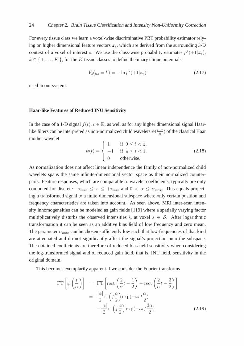
24 Chapter 2. Brain Tissue Classification and Intensity Non-Uniformity Correction
For every tissue class we learn a voxel-wise discriminativePBT probability estimator rely-
ing on higher dimensional feature vectorszs, which are derived from the surrounding 3-D
context of a voxel of interests. We use the class-wise probability estimatespk(+1|zs),
k ∈ { 1, . . . , K }, for theK tissue classes to define the unary clique potentials
Vs(ys = k) = − ln pk(+1|zs) (2.17)
used in our system.
Haar-like Features of Reduced INU Sensitivity
In the case of a 1-D signalf(t), t ∈ R, as well as for any higher dimensional signal Haar-
like filters can be interpreted as non-normalized child waveletsψ( t−τα
) of the classical Haar
mother wavelet
ψ(t) =
1 if 0 ≤ t < 12,
−1 if 12≤ t < 1,
0 otherwise.
(2.18)
As normalization does not affect linear independence the family of non-normalized child
wavelets spans the same infinite-dimensional vector space as their normalized counter-
parts. Feature responses, which are comparable to wavelet coefficients, typically are only
computed for discrete−τmax ≤ τ ≤ +τmax and0 < α ≤ αmax. This equals project-
ing a transformed signal to a finite-dimensional subspace where only certain position and
frequency characteristics are taken into account. As seen above, MRI inter-scan inten-
sity inhomogeneities can be modeled as gain fields [119] where a spatially varying factor
multiplicatively disturbs the observed intensitiesis at voxel s ∈ S. After logarithmic
transformation it can be seen as an additive bias field of low frequency and zero mean.
The parameterαmax can be chosen sufficiently low such that low frequencies of that kind
are attenuated and do not significantly affect the signal’s projection onto the subspace.
The obtained coefficients are therefore of reduced bias fieldsensitivity when considering
the log-transformed signal and of reduced gain field, that is, INU field, sensitivity in the
original domain.
This becomes exemplarily apparent if we consider the Fourier transforms
FT
[
ψ
(
t
α
)]
= FT
[
rect
(
2
αt− 1
2
)
− rect
(
2
αt− 3
2
)]
=|α|2
si(
fα
2
)
exp(−iπf α2
)
−|α|2
si(
fα
2
)
exp(−iπf 3α
2) (2.19)
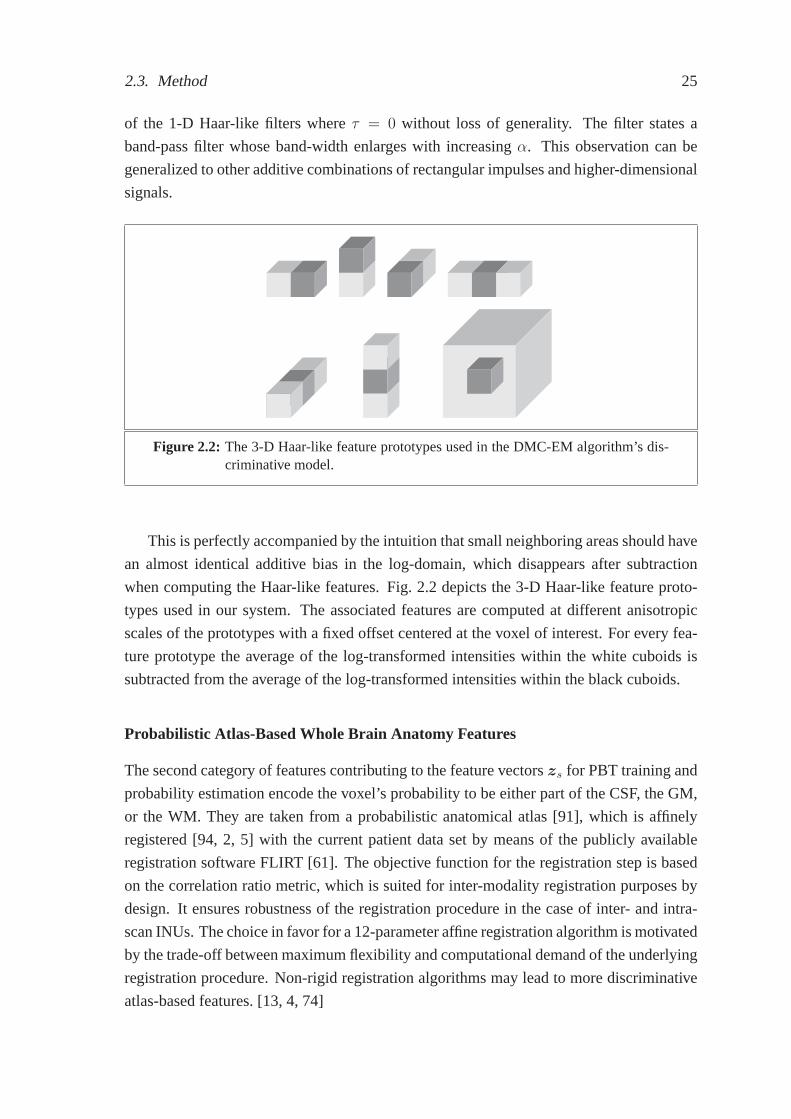
2.3. Method 25
of the 1-D Haar-like filters whereτ = 0 without loss of generality. The filter states a
band-pass filter whose band-width enlarges with increasingα. This observation can be
generalized to other additive combinations of rectangularimpulses and higher-dimensional
signals.
Figure 2.2: The 3-D Haar-like feature prototypes used in the DMC-EM algorithm’s dis-criminative model.
This is perfectly accompanied by the intuition that small neighboring areas should have
an almost identical additive bias in the log-domain, which disappears after subtraction
when computing the Haar-like features. Fig. 2.2 depicts the3-D Haar-like feature proto-
types used in our system. The associated features are computed at different anisotropic
scales of the prototypes with a fixed offset centered at the voxel of interest. For every fea-
ture prototype the average of the log-transformed intensities within the white cuboids is
subtracted from the average of the log-transformed intensities within the black cuboids.
Probabilistic Atlas-Based Whole Brain Anatomy Features
The second category of features contributing to the featurevectorszs for PBT training and
probability estimation encode the voxel’s probability to be either part of the CSF, the GM,
or the WM. They are taken from a probabilistic anatomical atlas [91], which is affinely
registered [94, 2, 5] with the current patient data set by means of the publicly available
registration software FLIRT [61]. The objective function for the registration step is based
on the correlation ratio metric, which is suited for inter-modality registration purposes by
design. It ensures robustness of the registration procedure in the case of inter- and intra-
scan INUs. The choice in favor for a 12-parameter affine registration algorithm is motivated
by the trade-off between maximum flexibility and computational demand of the underlying
registration procedure. Non-rigid registration algorithms may lead to more discriminative
atlas-based features. [13, 4, 74]

26 Chapter 2. Brain Tissue Classification and Intensity Non-Uniformity Correction
2.3.4 Coherence Preserving Pair-wise Clique Potentials
Inspired by Boykov and Funka-Lea [10] the interaction potentials used in our system are
Vst(ys, yt) ∝ exp
(
− 1
2L
L∑
l=1
(xsl− xtl)
2
(Σl,l)(t)ys
)
· δ(ys, yt)
dist(s, t)(2.20)
where vectors(xs1, . . . , xsL
)T and(xt1 , . . . , xtL)T denote the observed intensities at voxels
s andt taken fromL ∈ N aligned input pulse sequences and
δ(ys, yt) =
{
1 if ys 6= yt,
0 otherwise.(2.21)
The functiondist(s, t) denotes the physical distance between voxelss andt, which varies
when working on image volumes with anisotropic voxel spacing. The model emphasizes
homogeneous classifications among neighboring voxels but weights penalties for hetero-
geneity according to intensity similarities of the voxels involved. It assumes the noise
among neighboring voxels of an input volume to be distributed in a multivariate Gaussian
manner without taking into account dependencies among the spectral channels. Disconti-
nuities between voxels of similar intensities are penalized if the multi-spectral intensity
differences|xsl− xtl |, l = 1, . . . , L, are on average smaller than the associated stan-
dard deviations√
(Σl,l)(t)ys of the considered tissue classys in iterationt. However, if the
multi-spectral voxel intensities are very different, thatis to say, the differences|xsl− xtl|,
l = 1, . . . , L, are on average larger than the associated standard deviations√
(Σl,l)(t)ys the
penalty is small.
2.3.5 Summary
Reconsidering the processing pipeline of our DMC-EM approachdepicted in Fig. 1 we
make use of the results from the PBT probability estimation and classification step in the
subsequent DMC-EM optimization step in two ways: first, we usethe PBT hard classifica-
tion as initial segmentationy(0) wherey(0)s = arg maxk p
k(+1|zs) at the beginning of the
EM iterations. Based on this initial hard classification the parametersΘ(0) are initialized
via class-wise maximum likelihood estimation. Second, theprobability estimates serve as
constraints for the maximization of Equation (2.3) via ICM within every iterationt as well
as for the parameter updates given by Equations (2.5) and (2.6). This is achieved by defin-
ing the unary clique potentials as functions of the PBT probability estimates in Equation
(2.17). We therefore utilize the discriminative model involved not only as a preprocessing
step but also throughout the whole optimization procedure to repeatedly regularize model
adaptation.

2.4. Validation 27
Multi-spectral BrainWeb Mono-spectral BrainWeb
Source www.bic.mni.mcgill.ca/brainweb www.bic.mni.mcgill.ca/brainwebVolume Size 181× 217× 181 181× 217× 181Voxel Spacing 1.0× 1.0× 1.0 mm3 1.0× 1.0× 1.0 mm3
Spectral Channels T1, T2, PD T1Number of Scans 10 10
Table 2.1: Summary of the publicly available standard databases from the BrainWebrepository used for evaluation purposes.
2.4 Validation
2.4.1 Experimental Setup
For quantitative evaluation of the proposed method we carried out experiments both on
mono-spectral as well as on multi-spectral (T1-weighted, T2-weighted, PD-weighted) pub-
licly available simulated MRI scans from Cocosco et al. [22] (see Table 2.1). All the
simulated MRI volume sequences share resolution and size of1.0 × 1.0 × 1.0 mm3 and
181 × 217 × 181, respectively. INU and noise levels vary among 20% and 40%, and
1%, 3%, 5%, 7%, and 9%, correspondingly. The noise in the simulated images follows
a Rayleigh distribution in the background and a Rician distribution in the signal regions.
The noise level represents the percent ratio of the standarddeviation of the white Gaussian
noise added to the real and imaginary channels during simulation versus a reference tissue
intensity.
Furthermore, our system was quantitatively evaluated on two sets of real T1-weighted
MRI scans provided by the Center of Morphometric Analysis at the Massachusetts General
Hospital (see Table 2.2), which are publicly available on the Internet Brain Segmentation
Repository (IBSR). One of the data sets consists of 20 coronal T1-weighted MRI volumes
(256×65×256) of normal subjects with a resolution of1.0×3.1×1.0 mm3 (IBSR 20). The
other one (IBSR 18) consists of 18 scans (256×256×128) of normal subjects with varying
resolutions (0.84×0.84×1.5 mm3, 0.94×0.94×1.5 mm3, and1.0×1.0×1.5 mm3). Both
the sets are accompanied by ground-truth segmentations of the three tissue types of interest
(CSF, GM, and WM). All the scans had been subject to a specific preprocessing including
spatial normalization before they were released in the IBSR. However, our system does not
make use of the additional spatial information provided herewith and the scans are treated
as if they were native scans according to the common quality standards of radiological
image acquisition.
All the images were re-oriented to a uniform orientation (“RAI”; right-to-left, anterior-
to-posterior, inferior-to-superior). The discriminative model involved was trained on one
volumetric scan of the IBSR 20 data set, which is therefore excluded from the quantitative

28 Chapter 2. Brain Tissue Classification and Intensity Non-Uniformity Correction
IBSR 18 IBSR 20
Source www.cma.mgh.harvard.edu/ibsrwww.cma.mgh.harvard.edu/ibsrVolume Size 256× 256× 128 256× 65× 256Voxel Spacing 0.84× 0.84× 1.5 mm3, 1.0× 3.1× 1.0 mm3
0.94× 0.94× 1.5 mm3,1.0× 1.0× 1.5 mm3
Spectral Channels T1 T1Number of Scans 18 20
Table 2.2: Summary of the publicly available standard databases from the IBSR used forevaluation purposes.
evaluations. In order to keep our system as general as possible, we use the same model
for multi-spectral data and carry out PBT probability estimation and hard classification
based on the T1-weighted pulse sequences. We measure segmentation accuracy by means
of the Dice coefficient and the Jaccard coefficient to ensure comparability to other work
(see Tables 2.4–2.7). We refer to Appendix B for details on how both the coefficients are
computed. The quality of INU correction is quantified by the class-wise coefficient of
variation (COV = standard deviation / average) achieved.
Table 2.3 summarizes the methods whose accuracy will be compared one against the
other later. All of them were evaluated on at least one of the publicly available standard
databases mentioned above.
Due to the larger amount of free parameters involved, especially with regards to the
PBT model, we did not have the ambition to evaluate every possible choice of parameter
settings throughout the processing pipeline. For every processing step design choices were
based on what can be found in the literature, e.g., [111]. Forexample, we set the weight
of the pair-wise clique potentialsβ = 1.2 in accordance with Cuadra et al. [30] whose
Potts model-based pair-wise clique potentials have approximately the same range as ours.
The PBT voxel classifiers were built from approximately one million samples randomly
selected from one training volume. The samples are voxels within the brain of the patients
and are uniformly distributed over all the input slices of the training scan. For PBT prob-
ability estimation and classifier training the scans were re-sampled to a voxel spacing of
2.0×2.0×2.0mm3. The maximum number of features selected by AdaBoost in each tree
node was set to 8. The maximum depth of the trees learned was restricted to 10 and a soft
thresholding parameter ofǫ = 0.05 was used. The 3-D voxel context chosen for computing
the 747 Haar-like features used per individual voxel samplewas of size 30×30×30mm3
centered at the voxel of interest.
In a standard C++ implementation of our segmentation framework, it takes about 12
minutes to process one mono-spectral MRI volume (181 × 217 × 181) without brain ex-
traction and affine alignment on a Fujitsu Siemens notebook equipped with an Intel Core
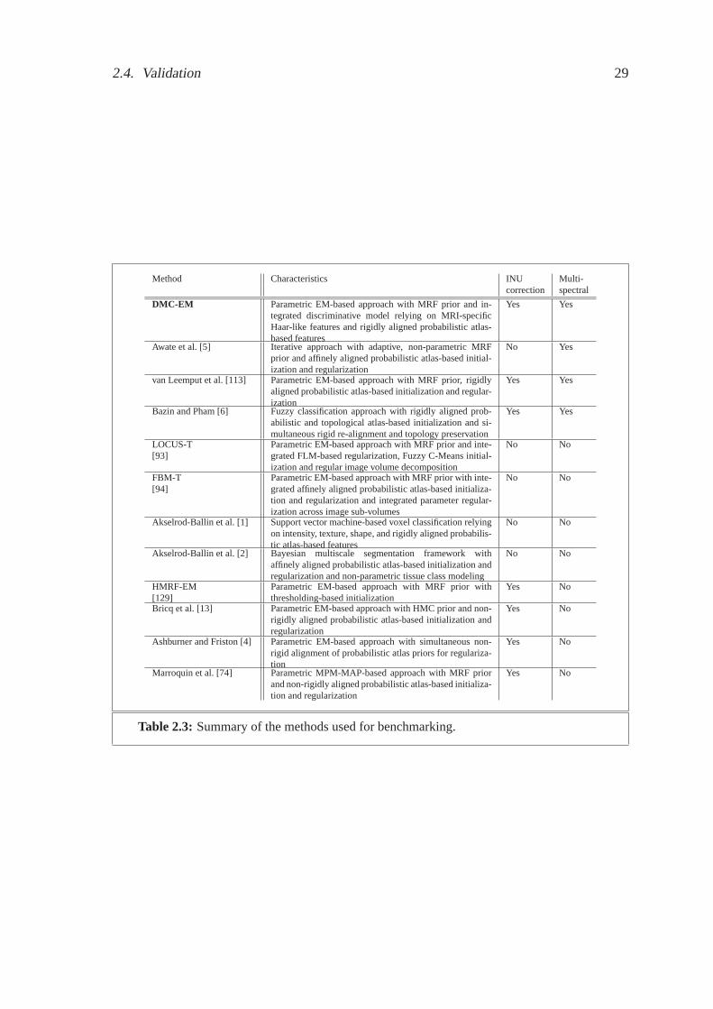
2.4. Validation 29
Method Characteristics INU Multi-correction spectral
DMC-EM Parametric EM-based approach with MRF prior and in-tegrated discriminative model relying on MRI-specificHaar-like features and rigidly aligned probabilistic atlas-based features
Yes Yes
Awate et al. [5] Iterative approach with adaptive, non-parametric MRFprior and affinely aligned probabilistic atlas-based initial-ization and regularization
No Yes
van Leemput et al. [113] Parametric EM-based approach with MRF prior, rigidlyaligned probabilistic atlas-based initialization and regular-ization
Yes Yes
Bazin and Pham [6] Fuzzy classification approach with rigidly aligned prob-abilistic and topological atlas-based initialization andsi-multaneous rigid re-alignment and topology preservation
Yes Yes
LOCUS-T[93]
Parametric EM-based approach with MRF prior and inte-grated FLM-based regularization, Fuzzy C-Means initial-ization and regular image volume decomposition
No No
FBM-T[94]
Parametric EM-based approach with MRF prior with inte-grated affinely aligned probabilistic atlas-based initializa-tion and regularization and integrated parameter regular-ization across image sub-volumes
No No
Akselrod-Ballin et al. [1] Support vector machine-based voxel classification relyingon intensity, texture, shape, and rigidly aligned probabilis-tic atlas-based features
No No
Akselrod-Ballin et al. [2] Bayesian multiscale segmentation framework withaffinely aligned probabilistic atlas-based initialization andregularization and non-parametric tissue class modeling
No No
HMRF-EM[129]
Parametric EM-based approach with MRF prior withthresholding-based initialization
Yes No
Bricq et al. [13] Parametric EM-based approach with HMC prior and non-rigidly aligned probabilistic atlas-based initialization andregularization
Yes No
Ashburner and Friston [4] Parametric EM-based approach with simultaneous non-rigid alignment of probabilistic atlas priors for regulariza-tion
Yes No
Marroquin et al. [74] Parametric MPM-MAP-based approach with MRF priorand non-rigidly aligned probabilistic atlas-based initializa-tion and regularization
Yes No
Table 2.3: Summary of the methods used for benchmarking.

30 Chapter 2. Brain Tissue Classification and Intensity Non-Uniformity Correction
2 Duo CPU (2.20 GHz) and 3 GB of memory. During all our experiments, mono-spectral
and multi-spectral, we keep a uniform parameter setting forall the free parameters involved
both for PBT training and probability estimation as well as for DMC-EM optimization. We
can therefore exclude over-adaptation to one particular set of MRI scans.
Method Tissue Class Dice Coeff. Jaccard Coeff.
DMC-EM WM 0.94± 0.02 0.89± 0.04GM 0.92± 0.03 0.85± 0.06CSF 0.77± 0.03 0.63± 0.03
Marroquin et al. [74] WM 0.95± 0.02 -GM 0.94± 0.02 -CSF - -
van Leemput et al. [113] WM 0.92± 0.03 -GM 0.93± 0.02 -CSF - -
Bazin and Pham [6] WM 0.94± 0.02 -GM 0.92± 0.02 -CSF 0.92± 0.01 -
Awate et al. [5] WM 0.95± 0.01 -GM 0.91± 0.01 -CSF - -
Table 2.4: Average segmentation accuracy for multi-spectral (T1-weighted, T2-weight-ed, and PD-weighted) simulated BrainWeb data of noise levels 1%, 3%, 5%,7%, and 9%, and INUs of 20% and 40%. From left to right the columnscontain the tissue class and the achieved average Dice and Jaccard coefficients.
2.4.2 Quantitative Results on Multi-Spectral Simulated BrainWeb
Data
Results on multi-spectral BrainWeb data obtained by DMC-EM arecomparable to those of
Bazin and Pham [6]2 and van Leemput et al. [113]3 as depicted in Table 2.4. They are close
to those of Awate et al. [5]4 and worse than those of Marroquin et al. [74]5. However, the
quantitative results reported in reference [5] might have been subject to a misconception in
the used evaluation software as the images presented show obvious segmentation failures
at the outer bounds of the brain for one of the BrainWeb data sets (5% noise and 40%
bias). For details refer to Awate et al. [5], p. 735, Figs. 1(b) and 1(c). For the sake of a fair
comparison it has to be mentioned though that both Awate et al. [5] as well as van Leemput
2“varying levels of noise and inhomogeneity” [6]3Average over noise levels 1–9% and INU level 40%4Average over noise level 0–9% and INU level 40%5Average over noise levels 1–9% and INU levels 0% and 40%

2.4. Validation 31
(a) (b) (c) (d)
(e) (f) (g) (h)
(i) (j) (k) (l)
Figure 2.3: Axial slices of original images, the segmentation results, the ground-truthand the estimated INU field for one mono-spectral T1-weighted BrainWebvolume (5% noise, 20% INU) (a–d), one volume of the IBSR 20 NormalSubjects data set (e–h), and one volume of the IBSR 18 Subjects data set(i–l) .
et al. [113] report results computed on data collections exclusively corrupted by an INU
level of 40%.
Fig. 2.4 shows that INU, measured by the average COV, is reduced for all the spectral
channels.
2.4.3 Quantitative Results on Mono-Spectral Simulated BrainWeb
Data
As Table 2.5 shows, the results achieved for mono-spectral BrainWeb data are compara-
ble to those of other state-of-the-art approaches to brain tissue classification [5, 93, 94,
6, 74, 4]. The results of Ashburner and Friston [4] are reported by Tsang et al. [107].

32 Chapter 2. Brain Tissue Classification and Intensity Non-Uniformity Correction
The results are better than those of van Leemput et al. [113] and the original HMRF-EM
approach [129]6. Awate et al. [5], van Leemput et al. [113], and Bazin and Pham [6] av-
erage over the same BrainWeb data sets as mentioned above for their experimental results.
Again, comparability to the methods of Awate et al. [5] and van Leemput et al. [113] may
be limited due to the fact that both are exclusively evaluated on BrainWeb data sets cor-
rupted by an INU level of 40%. Scherrer et al. [93, 94] presentaverage values in exactly
the same manner as we do for our system. For Ashburner and Friston [4] and Zhang et al.’s
HMRF-EM [129] the values are averaged over noise levels 1%, 3%, 5%, and 7% and INU
level 20%. For Bricq et al. [13] the values are averaged over noise levels 0%, 1%, 3%, 5%,
7%, and 9% and INU level 20%, for Marroquin et al. [74] over noise levels 0%, 1%, 3%,
5%, 7%, and 9% and INU levels 0% and 20%. In accordance with Marroquin et al. [74]
and Bricq et al. [13] we only observe a limited gain in segmentation accuracy when going
from mono-spectral to multi-spectral data. This effect maybe due to the fact that all the
channels of the multi-spectral BrainWeb data set are generated from the same underlying
phantom in a deterministic manner. Therefore the additional information provided about
the phantom’s true composition with respect to tissue typesmay be rather redundant than
of any additive value. Fig. 2.3 gives a visual impression of the results obtained for mono-
spectral input data. With regards to INU correction, it can be seen from Table 2.6(a) that
the average COV is reduced.
2.4.4 Quantitative Results on Normal Subjects Mono-Spectral Scans
With regards to experimental comparison our method shows better results in terms of seg-
mentation accuracy (Jaccard coefficient) than the methods of Akselrod-Ballin et al. [1] and
Marroquin et al. [74] (see Table 2.7) for the IBSR 20 data set. In terms of the Dice co-
efficient DMC-EM reaches a higher accuracy for GM segmentation than the method of
Ashburner and Friston [4]7 and the original HMRF-EM [129]8. Table 2.6(b) shows that all
the data sets were, on average, successfully corrected for INU.
As depicted in Figs. 2.5 and 2.6 DMC-EM constantly gives better results than pure
HMRF-EM with zero-valued unary clique potentials and probabilistic atlas-based initial-
ization. Except for a few cases it also gives better results than the HMRF-EM approach
with probabilistic atlas-based unary clique potentials and probabilistic atlas-based initial-
ization.
On the IBSR 18 data set our method performs comparably to otherstate-of-the-art
approaches with regards to segmentation accuracy (see Table 2.8). However, one has to
note here that the method of Akselrod-Ballin et al. [2] relieson stationary observation
6Reported by Tsang et al. [107]7Reported by Tsang et al. [107]8Reported by Tsang et al. [107]

2.4. Validation 33
(a) (b) (c)
(d) (e) (f)
Label COV Org. COVWM 0.07 0.09GM 0.12 0.13
Label COV Org. COVWM 0.17 0.18GM 0.21 0.23
Label COV Org. COVWM 0.07 0.08GM 0.07 0.09
(g) (h) (i)
Figure 2.4: Coronary slices of original multi-spectral (T1-weighted, T2-weighted, andPD-weighted) BrainWeb images of 5% noise and 20% INU (a–c) and esti-mated INU fields (d–f). Average INU correction accuracy on multi-spectralBrainWeb data in terms of the COV before and after INU correction (g–i).
models that have been derived in a cross-validation settingfrom separate training volumes,
which all origin from the same source of data. Their method might therefore be highly
biased to uniform contrast characteristics present in the IBSR 18 data set and the results do
not necessarily adequately reflect the performance of the method when applied to a larger
variety of data sets in clinical practice. Even though the quantitative results of Awate et
al. [5] are very impressive the visual impression of the segmentation results presented does
not match with this observation as the coronal slices depicted there (p. 737, Figs. 5(b) and
5(c)) show obvious misclassifications especially at the outer bounds of the brain.
Figs. 2.7 and 2.8 show that the introduction of discriminative model dependent unary
clique potentials and PBT initialization improves segmentation accuracy for the IBSR 18
data set. In comparison to the HMRF-EM approach with zero-valued unary clique po-
tentials and probabilistic atlas-based initialization and to the HMRF-EM approach with
probabilistic atlas-based unary clique potentials and probabilistic atlas-based initialization
DMC-EM usually reaches a higher segmentation accuracy in terms of the Dice coefficient
for GM and WM.

34 Chapter 2. Brain Tissue Classification and Intensity Non-Uniformity Correction
0
0.1
0.2
0.3
0.4
0.5
0.6
0.7
0.8
0.9
1
2 3 4 5 6 7 8 9 10 11 12 13 14 15 16 17 18 19 20
Image Number
GM
Dic
eC
oe
ffic
ien
t
DMC-EM HMRF-EM/Atlas/unary HMRF-EM/Atlas
Figure 2.5: Achieved accuracy for GM segmentation in terms of the Dice coefficient forthe IBSR 20 data set by the DMC-EM algorithm, the HMRF-EM algorithmwith probabilistic atlas-based unary clique potentials and probabilistic atlas-based initialization, and the HMRF-EM algorithm with zero-valued unaryclique potentials and probabilistic atlas-based initialization.
2.5 Discussion
Our newly proposed DMC-EM approach to fully automated 3-D Brain MRI tissue classi-
fication and INU correction makes use of two different types of spatial priors: the first one,
which contributes the unary clique potentials of the hiddenMarkov random field’s Gibbs
distribution, is derived from a strong discriminative model, in our case a PBT classifier,
that has been built from annotated training data. It only makes use of features of reduced
INU sensitivity and therefore prevents the model from over-fitting to scanner specific tissue
contrast characteristics, which is experimentally validated by detailed evaluations on pub-
licly available patient data sets from different sources and scanners. Usually, if the set of
features is not carefully chosen, using supervised learning for MRI brain tissue classifica-
tion ties a method to the exact acquisition protocol the classifier is trained for: for instance,
Han et al. [54] introduced an intensity renormalization procedure into the method of Fischl
et al. [37, 38]. As seen in our experiments an appropriate choice of features can help to cir-
cumvent this dependency without the need for additional pre-processing. Our experimental
setup did not allow specially adapted parameter settings for any of the data sets. All free
parameters were kept fixed during experimentation. By not only including prior knowl-
edge from an affinely preregistered probabilistic atlas ourdiscriminative model is capable
of producing more patient specific external fields. The second prior used, constituting the

2.5. Discussion 35
0
0.1
0.2
0.3
0.4
0.5
0.6
0.7
0.8
0.9
1
2 3 4 5 6 7 8 9 10 11 12 13 14 15 16 17 18 19 20
Image Number
WM
Dic
eC
oe
ffic
ien
t
DMC-EM HMRF-EM/Atlas/unary HMRF-EM/Atlas
Figure 2.6: Achieved accuracy for WM segmentation in terms of the Dice coefficient forthe IBSR 20 data set by the DMC-EM algorithm, the HMRF-EM algorithmwith probabilistic atlas-based unary clique potentials and probabilistic atlas-based initialization, and the HMRF-EM algorithm with zero-valued unaryclique potentials and probabilistic atlas-based initialization.
pair-wise clique potentials, is a smoothing prior that penalizes certain configurations in
local neighborhoods depending on similarity of observed intensities, physical distance be-
tween image voxels, and estimated image noise. This makes the approach robust against
different levels of noise, which is also shown by quantitative experimental evaluation.
From the theoretical point of view, in contrast to Zhang et al. [129], a consistent multi-
spectral formulation of our DMC-EM framework both for brain tissue segmentation as
well as for INU correction is presented. Accordingly, evaluation is carried out on mono-
and multi-spectral patient data. On all the data sets our method achieves a segmentation
accuracy that is either higher or comparable to the state-of-the-art even though progress in
this highly investigated branch of research is difficult dueto the well-established competi-
tiveness of the methods available.
From visually inspecting our segmentation results we observe that our method seems
to reveal weaknesses when it comes to deep GM structure segmentation. Even though
the caudate nuclei and the putamen could be successfully segmented in all the images de-
picted in Fig. 2.3 the globus pallidus and the thalamus were misclassified in all the three
image volumes. As both structures appear brighter than mostof the other GM structures
our observation model that models tissue classes as single Gaussian distributions seems to
restrictive in this case. The problem may be solved by tryingto model individual tissue
classes, and not only the whole brain, by mixtures of Gaussians. In addition, more complex

36 Chapter 2. Brain Tissue Classification and Intensity Non-Uniformity Correction
0
0.1
0.2
0.3
0.4
0.5
0.6
0.7
0.8
0.9
1
1 2 3 4 5 6 7 8 9 10 11 12 13 14 15 16 17 18
Image Number
GM
Dic
eC
oe
ffic
ien
t
DMC-EM HMRF-EM/Atlas/unary HMRF-EM/Atlas
Figure 2.7: Achieved accuracy for GM segmentation in terms of the Dice coefficient forthe IBSR 18 data set by the DMC-EM algorithm, the HMRF-EM algorithmwith probabilistic atlas-based unary clique potentials and probabilistic atlas-based initialization, and the HMRF-EM algorithm with zero-valued unaryclique potentials and probabilistic atlas-based initialization.
discriminative models could be considered that further decompose cervical GM into indi-
vidual structures [126]. By doing so the dominance of the prior model over the observation
model could be steered separately for individual anatomical entities.
It has to be mentioned also that particular high values for segmentation accuracy on the
BrainWeb data sets (see Tables 2.4 and 2.5) do not necessarilymean a particular method is
giving anatomically correct segmentation results. As depicted in Fig. 2.3(c) the associated
ground-truth annotation suffers from obvious weaknesses in the area of the globus pallidus
and the thalamus.
Concerning PVEs our method is conceptually predisposed to explicitly handle the ef-
fect that individual voxels may be composed of different tissue types due to the limited
resolution of the acquisition devices. The inherent mixture model estimation of our algo-
rithm provides an insight on how or to which degree differenttissue types contribute to a
certain voxel. However, we decided not to focus on handling PVEs and rather transform
our results into hard classifications for evaluation purposes after algorithmic processing.
Similarly to, for instance, the method of Marroquin et al. [74] our method seems not to
be of high accuracy with respect to CSF estimation. This may becaused by the fact that
we consider the complete fluid filled space outside and insidethe brain to be the CSF seg-
ment. It includes both the ventricular system as well as the subarachnoid space. Especially
the segmentation of the latter may be subject to errors originating from imperfections of

2.5. Discussion 37
0
0.1
0.2
0.3
0.4
0.5
0.6
0.7
0.8
0.9
1
1 2 3 4 5 6 7 8 9 10 11 12 13 14 15 16 17 18
Image Number
WM
Dic
eC
oe
ffic
ien
t
DMC-EM HMRF-EM/Atlas/unary HMRF-EM/Atlas
Figure 2.8: Achieved accuracy for WM segmentation in terms of the Dice coefficient forthe IBSR 18 data set by the DMC-EM algorithm, the HMRF-EM algorithmwith probabilistic atlas-based unary clique potentials and probabilistic atlas-based initialization, and the HMRF-EM algorithm with zero-valued unaryclique potentials and probabilistic atlas-based initialization.
the initial skull stripping procedure. However, our methodis carried out completely auto-
matically without any user interaction. Results for CSF segmentation might be better if a
“perfect” initial skull stripping was assumed.
With regards to INU correction our method suffers from the same limitations as the
method of Wells et al. [119] does due to the fact that it forms the base of our approach. In
a broader context, focusing on the method of Wells et al. [119] can be seen as an exem-
plary choice. Other more robust techniques that parametrically constrain estimated INU
fields might in fact benefit in an equal manner if they were embedded in our modality-
specific discriminative model-constrained HMRF-EM approach. DMC-EM is comparable
fast when compared to other state-of-the-art approaches and it takes only a few minutes to
process a data volume. The system presented in this chapter does not address sub-cortical
segmentation but we will come back to this issue in Chapter 4. On the other hand, any
generic state-of-the-art approach to organ segmentation will profit significantly from class-
wise intensity standardized and INU corrected MRI input volumes.

38 Chapter 2. Brain Tissue Classification and Intensity Non-Uniformity Correction
2.6 Conclusions
We have presented an MRI modality-specific discriminative model-constrained HMRF-
EM (DMC-EM) approach to brain tissue segmentation and INU correction in multi-
spectral 3-D MRI. The major contribution of our work is a strong discriminative model
obtained by a PBT classifier that is integrated into the framework by means of unary
clique potentials in a mathematically sound manner. The discriminative model used is
MRI modality specific as it only relies on features of reduced INU sensitivity taking into
account the particularities of the MRI modality. As experimentally validated the choice
of features prevents our method from being tied to a particular acquisition protocol at a
specific site or scanner. Detailed quantitative evaluations on publicly available benchmark-
ing databases demonstrate this increased robustness of ourapproach. At the same time the
segmentation accuracy achieved is comparable to those of other state-of-the-art approaches
to brain tissue classification in MRI data.
In the following chapter we will see how discriminative model-constrained MRF mod-
eling and appropriate optimization techniques can be used to also address the problem of
segmenting pathologic tissue types in multi-spectral 3-D MR images of the human brain—a
common problem in neuroradiology that has not been considered in this chapter. Patho-
logic tissue is typically characterized by a high variability both in appearance as well as in
shape and only occurs in patients suffering from a specific disease.

2.6. Conclusions 39
Method Tissue Class Dice Coeff. Jaccard Coeff.
DMC-EM WM 0.93± 0.03 0.87± 0.05GM 0.91± 0.05 0.83± 0.07CSF 0.76± 0.04 0.61± 0.05
Bricq et al. [13] WM 0.95± 0.02 -GM 0.95± 0.03 -CSF - -
LOCUS-T [93] WM 0.94 -GM 0.92 -CSF 0.80 -
FBM-T [94] WM 0.94 -GM 0.92 -CSF 0.80 -
Bazin and Pham [6] WM 0.94± 0.01 -GM 0.92± 0.02 -CSF 0.92± 0.01 -
Ashburner and Friston [4] WM - -GM 0.92 -CSF - -
Marroquin et al. [74] WM 0.93± 0.03 -GM 0.92± 0.03 -CSF - -
Awate et al. [5] WM 0.95± 0.01 -GM 0.91± 0.01 -CSF - -
van Leemput et al. [113] WM 0.90± 0.03 -GM 0.90± 0.02 -CSF - -
HMRF-EM [129] WM - -GM 0.89 -CSF - -
Table 2.5: Average segmentation accuracy for mono-spectral (T1-weighted) simulatedBrainWeb data of noise levels 1%, 3%, 5%, 7%, and 9%, and INUs of 20% and40%. From left to right the columns contain the tissue class and the achievedaverage Dice and Jaccard coefficients.

40 Chapter 2. Brain Tissue Classification and Intensity Non-Uniformity Correction
Label COV Org. COVWM 0.06 0.08GM 0.12 0.13
Label COV Org. COVWM 0.08 0.09GM 0.16 0.17
Label COV Org. COVWM 0.08 0.10GM 0.16 0.18
(a) (b) (c)
Table 2.6: Average INU correction accuracy in terms of the COV before and after INUcorrection for the mono-spectral BrainWeb data set (a), the IBSR 18 Subjectsdata set (b), and the IBSR 20 Normal Subjects Data set (c).
Method Tissue Class Dice Coeff. Jaccard Coeff.
DMC-EM WM 0.81± 0.09 0.69± 0.12GM 0.82± 0.06 0.71± 0.08CSF 0.83± 0.05 0.71± 0.07
Akselrod-Ballin et al. [1] WM - 0.67GM - 0.68CSF - -
Marroquin et al. [74] WM - 0.68GM - 0.66CSF - 0.23
Ashburner and Friston [4] WM - -GM 0.79 -CSF - -
HMRF-EM [129] WM - -GM 0.76 -CSF - -
Table 2.7: Average segmentation accuracy for IBSR 20 with exclusion of data set No.1 that has been used for training. From left to right the columns contain thetissue class and the achieved average Dice and Jaccard coefficients.

2.6. Conclusions 41
Method Label Dice Coeff. Jaccard Coeff.
DMC-EM WM 0.87± 0.05 (0.88± 0.01) 0.77± 0.06 (0.79± 0.02)GM 0.83± 0.12 (0.86± 0.04) 0.73± 0.13 (0.76± 0.06)CSF 0.76± 0.09 (0.77± 0.08) 0.62± 0.11 (0.63± 0.10)
Bazin and Pham [6] WM 0.82± 0.04 -GM 0.88± 0.01 -CSF - -
Akselrod-Ballin et al. [2] WM 0.87 -GM 0.86 -CSF 0.83 -
Awate et al. [5] WM 0.89± 0.02 -GM 0.81± 0.04 -CSF - -
Bricq et al. [13] WM 0.87± 0.02 -GM 0.80± 0.06 -CSF - -
Table 2.8: Average segmentation accuracy for IBSR 18. From left to right the columnscontain the tissue label and the achieved average Dice and Jaccard coefficientsfor all the data sets and for data sets 1–9 and 11–18 with outlier data set 10removed in brackets.

42 Chapter 2. Brain Tissue Classification and Intensity Non-Uniformity Correction

Chapter 3
Fully Automated Pediatric Brain Tumor
Segmentation in 3-D MRI
In this chapter we present a fully automated approach to the segmentation of pediatric
brain tumors in multi-spectral 3-D MRI images. It is a top-down segmentation approach
based on an MRF model that combines PBTs and lower-level segmentation via graph cuts.
The PBT algorithm provides a strong discriminative prior model that classifies tumor ap-
pearance while a spatial prior takes into account pair-wisevoxel homogeneities in terms
of classification labels and multi-spectral voxel intensities. The discriminative model re-
lies not only on observed local intensities but also on surrounding context for detecting
candidate regions for pathology. A mathematically sound formulation for integrating the
two approaches into a unified statistical framework is given. The method is applied to the
challenging task of detection and delineation of pediatricbrain tumors. This segmentation
task is characterized by a high non-uniformity of both pathology as well as surrounding
non-pathologic brain tissue. Despite dealing with more complicated cases ofpediatric
brain tumorsthe results obtained in a quantitative evaluation are mostly better than those
reported for current state-of-the-art approaches to 3-D MRIbrain tumor segmentation in
adult patients. The entire processing of one multi-spectral data set does not require any
user interaction, and our method is about 20% faster than thefastest previously proposed
method. It takes only 5 minutes to process one volume sequence including preprocessing.
The main contributions of this chapter have been published in references [121] and [120].
Parts of the presented system have also been used in references [122] and [124].
3.1 Motivation
Detection and delineation of pathology, such as cancerous tissue, within multi-spectral
brain MR images is an important problem in medical image analysis. For example, a pre-
cise and reliable segmentation of brain tumors present in the childlike brain is regarded
43

44 Chapter 3. Pediatric Brain Tumor Segmentation
(a) (b)
Figure 3.1: Two different cases of pediatric brain tumors exhibiting heterogeneous shapeand appearance. Columns (a) and (b) show axial slices of the typicallyacquired pulse sequences (row-wise from left to right: T2-weighted, T1-weighted, and T1-weighted after contrast enhancement) and the expertan-notated ground-truth overlaid to the T2-weighted pulse sequence.
critical when aiming for the automatic extraction of diagnostically relevant quantitative
or more abstract findings. This may include the volume of the tumor or its relative loca-
tion. Once these findings are obtained they can be used both for guiding CAD and therapy
planning as well as for traditional decision making. However, the manual labeling of volu-
metric data is usually time consuming, which has the potential to delay clinical workflow,
such that there is a need for fully automatic segmentation tools in this particular context.
Furthermore, manual annotations may vary significantly among experts as a result of indi-
vidual experience and interpretation.
As multi-spectral 3-D MRI is the method of choice for the examination of neurolog-
ical pathology such as brain cancer in pediatric patients, automatic approaches first have
to be capable of dealing with the characteristic artifacts of this imaging modality: Rician
noise [80], PVEs [114], and intra-/inter-scan INUs [119, 60]. Second and more impor-
tantly, they have to be robust enough to handle the heterogeneous shape and appearance
of pediatric brain tumors in different patients (see Fig. 3.1). In the case of pediatric brain
tumors not only pathology underlies significant variation in shape and appearance but also
the non-pathological “background”, which is caused by ongoing myelination of WM dur-
ing maturation [78]. This may cause WM to appear darker in pediatric T1-weighted MRI
scans than in adult patient data sets.

3.1. Motivation 45
PBT ProbabilityEstimation
1. BET Skull Stripping2. Anisotropic Diffusion Filtering3. DHW Intensity Standardization
Pre-Processing:Graph CutsOptimization
Discriminative Model-Constrained Graph Cuts
Figure 3.2: The processing pipeline of the proposed segmentation method. Each set ofimages schematically represents the input and/or output of individual pro-cessing steps.
In this chapter, we describe a fully automatic solution based on a novel top-down seg-
mentation scheme that uses a statistical model of pathologyappearance as a constraint
for a subsequent optimization problem. The statistical model is provided by a machine
learning technique that is able to work with high-dimensional feature vectors allowing to
encode characteristic voxel contexts. The optimization problem itself is stated as a search
for an MAP estimate of the most likely binary image segmentation, which permits efficient
computation of a solution by means of a discrete max-flow/min-cut optimization proce-
dure and is optimal in terms of Bayesian classification theory. The overall system block
diagram, including preprocessing (brain extraction [100], smoothing, and MRI intensity
standardization [29]) is depicted in Fig. 3.2.

46 Chapter 3. Pediatric Brain Tumor Segmentation
3.2 Related Work
3.2.1 Preprocessing: MRI Inter-Scan Intensity Standardization
In general, MR images exhibit varying contrast characteristics even though they were ac-
quired with an identical acquisition protocol but with a different scanner at a different site.
With regards to the distribution of intensities within images depicting the interior of the
human skull the associated histograms appear non-linearlydeformed. These inter-scan
variations make image interpretation difficult as individual intensities lack a unique mean-
ing regarding the underlying tissue type. This is especially true with regards to automatic
image post-processing like image segmentation that often heavily relies on observed in-
tensity values when deciding on which tissue class a specificvoxel of an image belongs
to. For this purpose several authors suggested approaches for MRI inter-scan intensity
standardization or normalization.
Nyúl et al. [81, 82] and Ge et al. [43] propose a two-step 1-D histogram matching
approach. In the first step, parameters (percentiles, modes, etc.) of the reference histogram
are derived from a set of reference images. In the second step, those parameters are used
to map the histogram of a newly acquired MR image onto the reference histogram by
matching specific landmark locations and linear interpolation.
Jäger and Hornegger [60] use a variational approach to register multivariate PDFs in
the form of multi-dimensional joint histograms for establishing intensity mappings for MRI
intensity standardization to multi-spectral template images.
In a similar manner, we try to find an intensity mapping between a reference image and
a newly acquired image by bringing the associated histograms into line with each other
during preprocessing. The method we use for histogram registration is based on dynamic
histogram warping (DHW) [29] from a technical perspective. The technique is strongly
related to dynamic time warping (DTW) [66], which is used for 1-D sequence compari-
son. However, we apply DHW to MRI volumes of the human brain in order to standardize
intensities and not for the purpose of achieving constant image brightness in 2-D images.
Later we will present a graph theoretic re-formulation of the original dynamic program-
ming approach proposed by Cox and Hingorani [29]. For measuring similarity between
histograms we adapted it such that the Kullback-Leibler divergence [67] is minimized,
which is appropriate to measure PDF similarity.
3.2.2 MRI Brain Tumor Segmentation
Approaches in the field of MRI brain tumor segmentation rarelyrely on pure data-driven
approaches, with Gibbs et al.’s method [47] being an early exception, due to the complex-
ity in terms of tumor shape and appearance of the segmentation task. The vast majority

3.2. Related Work 47
of methods make use of domain knowledge using different types of representation and
combine it with low-level imaging techniques. Fletcher-Heath et al. [39] use unsupervised
fuzzy clustering followed by 3-D connected components withan intermediate step incor-
porating knowledge about the usual distribution of CSF and location of the ventricular
system. Ho et al. [57] have the evolution of a level set function guided by a tumor proba-
bility map that is generated by exploiting higher-level domain knowledge on how contrast
enhancement in T1-weighted images affects tumor appearance. Corso et al. [26, 25] use
the multi-level segmentation by weighted aggregation algorithm with tissue class-specific
Gaussian mixture models for brain, tumor, and edema. Geringet al. [46] use trained para-
metric statistical models for intensity distributions of non-pathologic brain tissue to detect
model outliers on the voxel level that are considered tumor voxels in a multi-layer MRF
framework. In a similar manner Moon et al. [76, 75] and later Prastawa et al. [87, 88]
detect outliers based on refined intensity distributions for healthy brain tissue initially de-
rived from a registered probabilistic atlas, which introduces structural domain knowledge.
Registration is also used in combination with voxel intensities in the adaptive template-
moderated classification algorithm by Kaus et al. [64, 63]. More recent approaches try
to enrich low-level segmentation techniques, like level set evolution [21] or hierarchical
clustering [28], by using supervised machine learning on higher dimensional feature sets
associated with each image voxel. These feature sets are capable of representing a more
general variety of domain knowledge on different levels of abstraction. For instance, Zook
and Iftekharuddin [132] analyze the fractal dimension of tumor area versus non-tumor area
and show that this is a statistically significant indicator for tumor appearance. Based on
this idea, Iftekharuddin et al. [58] use multi-resolution texture features generated by a com-
bination of fractal Brownian motion and wavelet multi-resolution analysis together with
self-organizing maps. In a similar manner we make use of the recently proposed technique
of PBTs [108] in combination with 2-D [83, 115] and 3-D Haar-like features [111] for su-
pervised learning, which has proven its robustness and its capability for efficient training
and classification in numerous applications [110, 18]. Both types of features are closely
related to 3-D Haar-like features of reduced INU sensitivity, which are explained in Chap-
ter 2 in more detail. The probability estimates provided by PBT are then used to constrain
the highly efficient computation of minimum cuts [11] for image segmentation based on
an MRF prior model. It takes into account both coherence of classification labels as well
as multi-spectral intensity similarities within voxel neighborhoods.
3.2.3 Image Segmentation Using Max-Flow/Min-Cut Computation
In this chapter, we give an integrated formulation for combining PBT classification and
computation of minimum cuts. Opposed to other methods [26, 28, 25, 21] there is no
involvement of a time consuming bias field correction step indata preprocessing in our
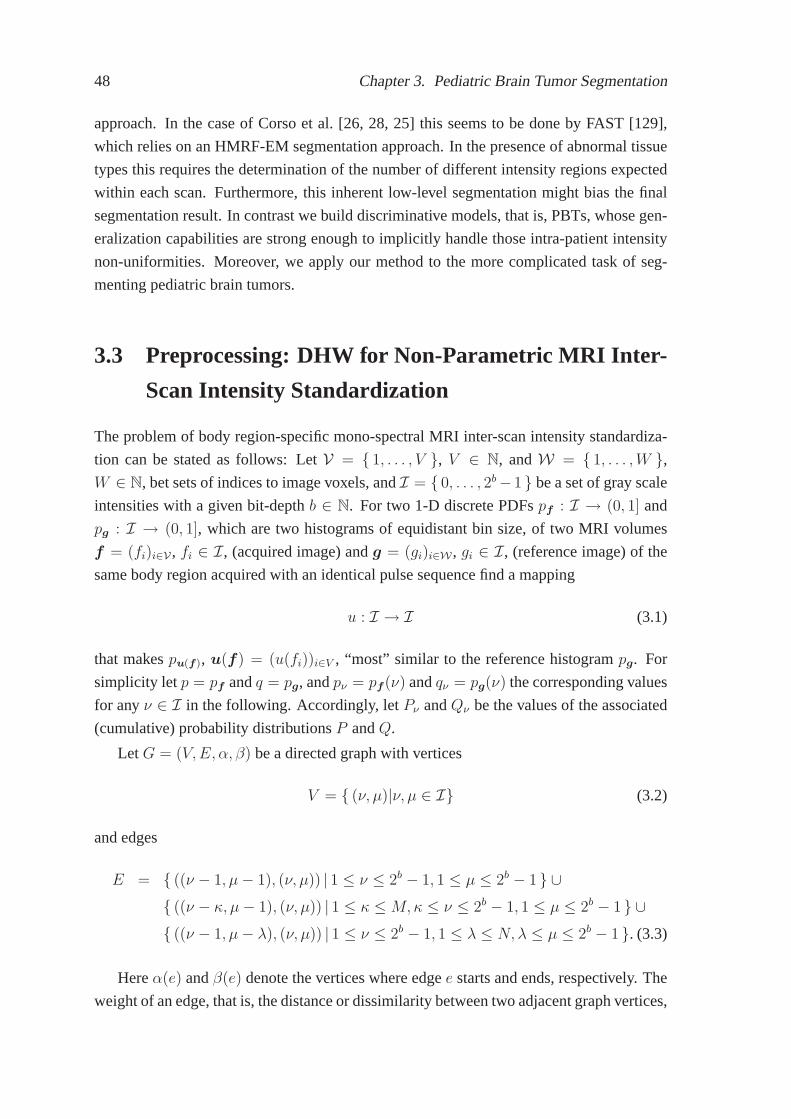
48 Chapter 3. Pediatric Brain Tumor Segmentation
approach. In the case of Corso et al. [26, 28, 25] this seems to be done by FAST [129],
which relies on an HMRF-EM segmentation approach. In the presence of abnormal tissue
types this requires the determination of the number of different intensity regions expected
within each scan. Furthermore, this inherent low-level segmentation might bias the final
segmentation result. In contrast we build discriminative models, that is, PBTs, whose gen-
eralization capabilities are strong enough to implicitly handle those intra-patient intensity
non-uniformities. Moreover, we apply our method to the morecomplicated task of seg-
menting pediatric brain tumors.
3.3 Preprocessing: DHW for Non-Parametric MRI Inter-
Scan Intensity Standardization
The problem of body region-specific mono-spectral MRI inter-scan intensity standardiza-
tion can be stated as follows: LetV = { 1, . . . , V }, V ∈ N, andW = { 1, . . . ,W },W ∈ N, bet sets of indices to image voxels, andI = { 0, . . . , 2b−1 } be a set of gray scale
intensities with a given bit-depthb ∈ N. For two 1-D discrete PDFspf : I → (0, 1] and
pg : I → (0, 1], which are two histograms of equidistant bin size, of two MRI volumes
f = (fi)i∈V , fi ∈ I, (acquired image) andg = (gi)i∈W , gi ∈ I, (reference image) of the
same body region acquired with an identical pulse sequence find a mapping
u : I → I (3.1)
that makespu(f), u(f) = (u(fi))i∈V , “most” similar to the reference histogrampg. For
simplicity letp = pf andq = pg, andpν = pf(ν) andqν = pg(ν) the corresponding values
for anyν ∈ I in the following. Accordingly, letPν andQν be the values of the associated
(cumulative) probability distributionsP andQ.
LetG = (V,E, α, β) be a directed graph with vertices
V = { (ν, µ)|ν, µ ∈ I} (3.2)
and edges
E = { ((ν − 1, µ− 1), (ν, µ)) | 1 ≤ ν ≤ 2b − 1, 1 ≤ µ ≤ 2b − 1 } ∪{ ((ν − κ, µ− 1), (ν, µ)) | 1 ≤ κ ≤M,κ ≤ ν ≤ 2b − 1, 1 ≤ µ ≤ 2b − 1 } ∪{ ((ν − 1, µ− λ), (ν, µ)) | 1 ≤ ν ≤ 2b − 1, 1 ≤ λ ≤ N, λ ≤ µ ≤ 2b − 1 }. (3.3)
Hereα(e) andβ(e) denote the vertices where edgee starts and ends, respectively. The
weight of an edge, that is, the distance or dissimilarity between two adjacent graph vertices,

3.3. MRI Inter-Scan Intensity Standardization 49
p3
p0
q0
q1
· · ·
p1
p2
...
q2q3
Figure 3.3: Partial schematic representation of the graph considered (M = 2, N = 2)and its relation to the initial discrete PDFsp = pf andq = pg. The ver-tices(ν, µ) ∈ V of G are depicted as dots aligned in a quadratic scheme ofmaximum size2b − 1× 2b − 1. The edgesE are depicted as arrows.
can then be defined as a mappingd : E → R representing the non-negative summands of
any with respect the number of bins monotonic additive bin-by-bin histogram dissimilarity
measure. The dissimilarity measure is implicitly applied to deformed versions ofp and
q where for an edgee = ((ν − κ, µ − 1), (ν, µ)) an amount ofκ successive bins ofp
are contracted. In an equal manner an edgee = ((ν − 1, µ − λ), (ν, µ)) represents the
contraction ofλ successive bins ofq, which corresponds to the uniform expansion of one
bin of p. This vice-versa relation is of particular interest as we want to deformp non-
linearly to matchq, which can be achieved as follows: due to the specific structure ofG a
shortest pathw = (e1, . . . , et) along vertices(v1, . . . , vt+1) from (0, 0) to (2b − 1, 2b − 1)
can be computed efficiently via dynamic programming. This gives, on the one hand, the
minimum distanceD(p′, q′) =∑t
i=1 d(ei) of deformed histogramsp′ andq′ achievable at
the given constraintsM andN , and, on the other hand, the associated mapping that makes
p most similar toq. The corresponding assignment foru is then
u(ν) = π(2)2 (vi+1) for π(2)
1 (vi) < ν ≤ π(2)1 (vi+1), i ∈ { 1, . . . , t }. (3.4)
Hereπ(2)2 : I × I → I with π(2)
2 (ν, µ) = µ for all ν, µ ∈ I denotes the projection on
the second component of a two-dimensional vertex. Analogously, π(2)1 is the projection on
the first component of a two-dimensional vertex.

50 Chapter 3. Pediatric Brain Tumor Segmentation
Note that the parametersM andN serve as smoothness constraints as they steer al-
lowed deformation relative to the major diagonal of the underlying graph scheme (see
Fig. 3.3).
Possible dissimilarity measures (see Rubner et al. [92] for details) involve the simplest
Minkowski-form distanceDL1(p, q) =
∑
ν |pν − qν | where the edge weight would be
dL1((ν − κ, µ− λ), (ν, µ)) = |(Pν − Pν−κ)− (Qµ −Qµ−λ)|. (3.5)
It is also possible to use the discrete Kullback-Leibler divergence in its symmetrical form
DKL(p, q) =∑
ν(pν − qν) · log(pν/qν) with according edge weight
dKL((ν−κ, µ−λ), (ν, µ)) = ((Pν −Pν−κ)− (Qµ−Qµ−λ)) · log
(
Pν − Pν−κ
Qµ −Qµ−λ
)
. (3.6)
Both distances are additive, i.e., separable, and monotonicwith respect to the number of
bins of the two input histograms considered. Monotonicity is ensured due to the fact that
the summands involved are strictly non-negative. Separability and simultaneous mono-
tonicity state the precondition for making distance measures applicable in the context of
dynamic programming. Other dissimilarity measures like, for instance, the earth mover’s
distance (EMD) [92], may better match the intuition of dissimilarity between different
PDFs. However, their computation is usually more complex and their separable and mono-
tonic reformulation may be non-trivial or even impossible.
Fig. 3.4 shows exemplary results for several volumetric brain MR images. For all the
experiments we restricted intensity standardization to brain soft tissue only in order to pre-
vent background voxels from dominating the standardization process and therefore achiev-
ing sub-optimal results. Skull stripping was achieved by preprocessing the data sets with
FSL BET [100]. Likewise, the background can also be excluded by simple thresholding
methods.
3.4 Segmentation Method
Our segmentation method relies on the integrated formulation of an objective function that
is subject to optimization via the efficient graph cuts algorithm [11]. In the following we
derive this objective function from the general MAP framework for image segmentation.
3.4.1 Posterior Mode Image Segmentation
In general, the problem of segmenting an image can be stated as the search for an MAP
estimate of the most likely class labels given appropriate prior and observation models in
terms of PDFs. LetS = { 1, 2, . . . , N }, N ∈ N, be a set of indices to image voxels. At

3.4. Segmentation Method 51
(a) (b)
(c)
Figure 3.4: Axial slice of a reference volumes (a) and axial slice of an original volume(b) and associated histograms with 256 bins (c). All images displayed atidentical intensity window.

52 Chapter 3. Pediatric Brain Tumor Segmentation
(a) (b)
(c)
Figure 3.5: Axial slice of a reference volumes (a) and axial slice of a normalized volume(b) and associated histograms with 256 bins (c). All images displayed atidentical intensity window.
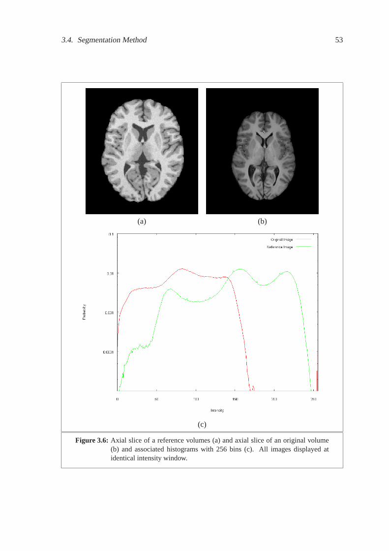
3.4. Segmentation Method 53
(a) (b)
(c)
Figure 3.6: Axial slice of a reference volumes (a) and axial slice of an original volume(b) and associated histograms with 256 bins (c). All images displayed atidentical intensity window.
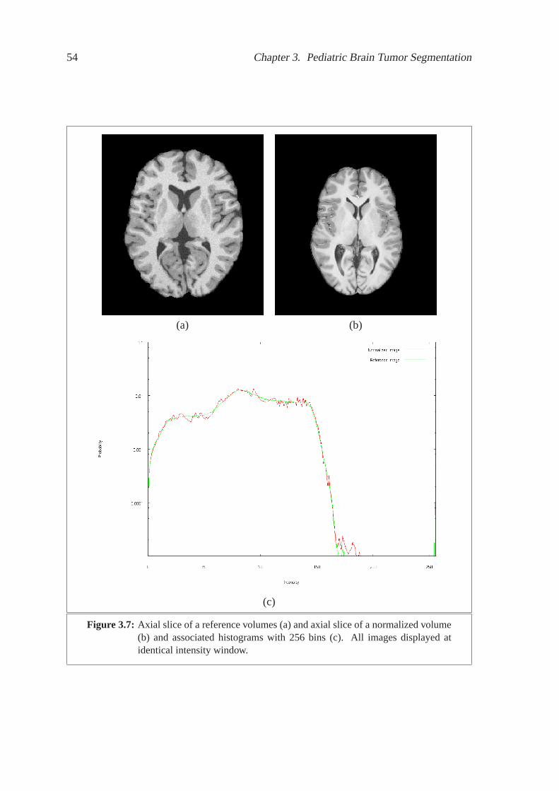
54 Chapter 3. Pediatric Brain Tumor Segmentation
(a) (b)
(c)
Figure 3.7: Axial slice of a reference volumes (a) and axial slice of a normalized volume(b) and associated histograms with 256 bins (c). All images displayed atidentical intensity window.

3.4. Segmentation Method 55
each indexs ∈ S there are two random variables:ys ∈ Y = {+1,−1 } andxs ∈ X =
RM ,M ∈ N. The former,ys, denotes the unobservable binary segmentation of voxels into
fore- and background, whereas the latter,xs, states the observable vector of multi-spectral
intensities that are assumed to be causally linked to the underlying class labelsy ∈ Y by
a unified observation model defined by a PDFp(x|y) for x ∈ X . The emergence of the
class labels themselves is described by a prior modelp(y). The segmentation task at hand
can now be stated as the search for an MAP estimate
Y ∗ = arg maxY
p(Y |X) (3.7)
wherep(Y |X) is the joint posterior probability over the image domainS with Y =
(ys)s∈S andX = (xs)s∈S . Using Bayes’ rule and the independence ofp(X) from Y ,
we have:
Y ∗ = arg maxY
ln p(X|Y ) + ln p(Y ). (3.8)
To concretize this optimization problem a region-specific probability term and an appro-
priate prior need to be identified.
3.4.2 Histogram-Based Observation Model
We assume the multi-spectral observations to be independently and identically distributed
(i.i.d.), that is,p(X|Y ) =∏
s∈S p(xs|ys). The PDFs for that are estimated during segmen-
tation via histograms by understanding an initial PBT voxel classification as intermediate
segmentation that is close to the final result.
3.4.3 Discriminative Model-Constrained MRF Prior Model
For the prior distribution we assume an MRF prior model
p(Y ) ∝ exp(−U(Y ;1
λ)) (3.9)
formulated, according to the Hammersley-Clifford Theorem,as a Gibbs distribution with
energy function
U(Y ;1
λ) =
∑
s∈S
(
Vs(ys) +1
λ
∑
t∈Ns
Vst(ys, yt)
)
(3.10)
where1λ
with λ ∈ (0,+∞) controls the relative influence of the spatial prior, i.e., the pair-
wise clique potentials, over the external influences, i.e.,the unary clique potentials. The set
Ns describes the neighborhood of voxels. As done in Chapter 2 we ignore higher-ordered
clique potentials.

56 Chapter 3. Pediatric Brain Tumor Segmentation
The unary clique potentialsVs(ys) are provided by a PBT classifier. As described in
Appendix A the PBT provides an approximationp(ys|zs) of the true posterior probability
p(ys|zs) at its root node for feature vectorszs associated with individual voxelss. Here
ys ∈ {−1,+1 } denotes the classification outcome, that is, background or foreground.
Thus, we have
Vs(ys) = ln p(ys|zs). (3.11)
For our first experiment, the feature vectorszs used for PBT classification consist of
individual multi-spectral intensities, inter-channel intensity gradients, and 2-D Haar-like
features [83, 115] computed on an intra-axial 2-D context surrounding the voxel of interest.
The Haar-like features are derived from a subset of the extended set of Haar-like feature
prototypes [70] and are represented only implicitly in memory by (rotated) integral images.
This allows fast re-computation of the features with respect to a given voxel when they
are actually assessed. As we intend to capture a discriminative representation of the full
2-D context, and not only of local edge characteristics at the central voxel, 2-D Haar-like
feature values are computed according to the given prototypes on every valid origin and
scale within the chosen voxel context.
For our second experiment, the feature vectorszs used for PBT probability estima-
tion consist of individual multi-spectral intensities andmulti-spectral 3-D Haar-like fea-
tures [108] computed on a 3-D context surrounding the voxel of interest. The Haar-like
features are derived from a set of 3-D Haar-like feature prototypes centered at the voxel of
interest and are held implicitly in memory by means of integral volumes. Equally to the
2-D case, the features are re-computed on-the-fly when they are actually assessed.
Similar to what is done in Chapter 2 the pair-wise interactionpotentials are
Vst(ys, yt) = exp
(
−1
2
L∑
l=1
(xsl− xtl)
2
σ2l
)
· δ(ys, yt)
dist(s, t)(3.12)
where vectorsxs = (xs1, . . . , xsL
)T andxt = (xt1 , . . . , xtL) denote the observed intensi-
ties at voxelss andt taken fromL ∈ N aligned input pulse sequences.
3.4.4 Discriminative Model-Constrained Graph Cuts Segmentation
With the equality
Y ∗ = arg maxY
∑
s∈S
ln p(xs|ys) +∑
s∈S
Vs(ys)−1
λ
∑
s∈S
∑
t∈Ns
Vst(ys, yt)
= arg minY
(
∑
s∈S
−λ · (ln p(xs|ys) + Vs(ys))
)
+∑
s∈S
∑
t∈Ns
Vst(ys, yt) (3.13)

3.4. Segmentation Method 57
the initial maximization problem can be transformed into a minimization problem that is in
a suitable form for optimization by the graph cuts algorithm[11]. Note that the reciprocal
of the regularization parameter in (3.10) can equivalentlybe used to weight the influence
of the external influences in combination with the observation model over the prior model.
s
t
r0
Figure 3.8: Example of a max-flow/min-cut problem instance with its associated ex-tended graph. Vertexs denotes the source node and vertext the sink node.The flow value on edger0 = (t, s) is about to be optimized. The edgesof a possible cut separating the green from the red vertices are displayed asdashed arrows.
The graph cuts algorithm [11] originates from the family of max-flow/min-cut algo-
rithms within combinatorial optimization theory. They canbe used [11, 52] to minimize
energies of the form
E(Y ) =∑
s∈S
Ds(ys) +∑
s∈S
∑
t∈Ns
Vst(ys, yt). (3.14)
In our case the data penalty function is given by
Ds(ys) = −λ · (ln p(xs|ys) + Vs(ys)). (3.15)
whereas the interaction potentialsVst remain unchanged.

58 Chapter 3. Pediatric Brain Tumor Segmentation
Figure 3.9: The rendered result for patient No. 1 overlaid on the T2-weighted pulsesequence. Due to the coarse axial resolution the extracted surface hasbeensmoothed [106] before rendering.
Let the graphM = (V,E) with verticesV = { vs | s ∈ S } and edgesE =
{ (vs, vt) | s ∈ S, t ∈ Ns } represent the associated MRF described before. The objec-
tive of any max-flow/min-cut computation is to find a maximum flow in the extended
directed weighted graphG = (V ′, E ′, c) where the set of verticesV ′ = V ∪ { s, t } is
extended by two terminal nodes—the source nodes and the sink nodet. The edges of
the graph areE ′ = E ∪ { (s, v)|v ∈ V } ∪ { (v, t)|v ∈ V } ∪ { (t, s) }, and the function
c : E ′ → R ∪ {+∞} denotes the edge capacities. A flow is a functionβ : E ′ → R with∑
(vi,vj)∈V :vj=v β(vi, vj) =∑
(vi,vj)∈V :vi=v β(vi, vj) for all v ∈ V . It is admissible with
respect toc if and only if 0 ≤ β(r) ≤ c(r) for all r ∈ E ′. The maximum flowβ∗ searched
for reaches the highest possible flow value on edge(t, s) among all admissible flows, that
is, β∗ = arg maxβ β(t, s). In accordance with Equation (3.13) the capacities are
c(vi, vj) =
Vij(yi, yj) if vi 6= s and vj 6= t,
Dj(yj = −1) if vi = s,
Di(yi = +1) if vj = t.
(3.16)
According to the theorem of Ford and Fulkerson the problem offinding a maximum flow
is equivalent to the problem of finding a minimum cut, which isa partitionC∗ = S∗ ∪ T ∗,
S∗ ∩ T ∗ = ∅ with s ∈ S∗ andt ∈ T ∗, whose cost∑
(vi,vj):vi∈S,vj∈T c(vi, vj) is minimal
among all possible cuts. Note that a minimum cost cut equivalently defines a globally
optimal binary labeling, that is to say, a segmentation, of the graph nodes. Fig. 3.8 shows
an exemplary max-flow/min-cut problem with its associated graph.
Boykov and Kolmogorov [11] identified two categories of combinatorial optimization
algorithms for this kind of problem: 1) Goldberg-Tarjan style “push-relabel” algorithms

3.4. Segmentation Method 59
and 2) Ford-Fulkerson style “augmenting paths” algorithms. Either type has polynomial
time complexity.
In “push-relabel” algorithms [48] there are active nodes having excess flow, i.e., inflow
that has not yet been explained by an appropriate outflow to a neighboring node and its
connections to the sink node. During optimization for everynode a heuristic is kept that
gives a low bound estimate on the cost to reach the sink starting from that point along
non-saturated edges. In the course of computing the maximumflow the excess flows are
stepwise propagated to nodes being closer to the sink node with regards to the estimated
distance. This so-called push operation is typically applied to active nodes with the highest
estimated distance to the sink node or based on a FIFO selection strategy. Alternatively,
the heuristic value of a node can be updated in a relabel operation. Both operations are
applied as long as the accompanying preconditions are met.
In “augmenting paths” algorithms [40, 36, 32] the overall flow in the graph is suc-
cessively increased along augmenting paths in the so-called residual graph, which stores
information about the remaining available capacities in the network. This is repeated as
long as there are such augmenting paths. In the beginning theedge capacities in the resid-
ual graph are equal to those in the original graph and there isnot any flow from the source
to the sink. In each iteration it is searched for a path [40] orshortest path [36, 32], in the
sense of the amount of edges involved, from source to sink in the residual graph. If such a
path is found the algorithm augments the overall flow in the network by increasing it along
the involved edges such that at least one of the edges in the path is completely saturated.
Accordingly, the remaining capacities along the augmenting path are decreased by exactly
the same amount in the residual graph. Saturated edges are not considered any further.
Formally, the residual graph associated with G and an admissible flow β is defined
asGβ = (V,E ′β) whereE ′
β = { e1|e ∈ E ′ \ { (t, s) }, β(e) < c(e) } ∪ { e−1|e ∈ E ′ \{ (t, s) }, β(e) > 0 } andπ(2)
1 (e1) = π(2)1 (e) andπ(2)
2 (e1) = π(2)2 (e), andπ(2)
1 (e−1) = π(2)2 (e)
andπ(2)2 (e−1) = π
(2)1 (e) for all e ∈ E ′. An augmenting path is a pathp = (eδ1
1 , . . . , eδk
k ),
k ∈ N, in Gβ with the following properties: (1)π(2)1 (eδ1
1 ) = s, e1 6= (t, s), andπ(2)2 (eδk
k ) =
t, ek 6= (t, s), (2)∀i:δi=1β(ei) < c(ei), and (3)∀i:δi=−1β(ei) > 0.
While the Edmonds-Karp [36] or Dinic [32] algorithm use breadth-first search to
completely rebuild the tree of shortest paths inGβ from time to time, Boykov and Kol-
mogorov [11] integrated strategies to decrease computation time used for this expensive
operation to a minimum (see Algorithm 2). In step 1 of their algorithm two search trees
are used, one from the source and the other one from the sink. They are reused to find an
augmenting path in every iteration, and never completely rebuilt. In step 2 the current flow
is increased along the found augmenting path. Accordingly,saturated edges are removed
from the residual graph. Thus, the search trees may be split into forests and some of their
nodes may become orphans, that is, the connections to their parent nodes are no longer
part ofGβ. In the adoption stage (step 3) the forests are tried to be reconnected to form

60 Chapter 3. Pediatric Brain Tumor Segmentation
two search trees again. We refer to the original work of Boykovand Kolmogorov [11] for
details on the three steps involved.
Algorithm 2 : Graph cuts algorithmInput : extended directed weighted graphG, an admissible flowβOutput : minimum cutC∗ = S∗ ∪ T ∗ and a maximum flowβ∗
begin
// Initialize search treesS → { s }, T → { t };
// Enter main loopwhile truedo
1. GrowS or T to find an augmenting pathp from s to t;if p emptythen
break;end2. Augmentβ onp;3. Adopt orphans;
end
// Return minimum cut and maximum flowS∗ = S, T ∗ = T , β∗ = β;returnS∗, T ∗, β∗;
end
The augmenting paths found in step 1 of Algorithm 2 are not necessarily shortest aug-
menting paths. Therefore, the worst case time complexitiesof the Edmonds-Karp algo-
rithm (O(|V ||E ′|2)) and Dinic algorithm (O(|V |2|E ′|)) relying on this fact are no longer
valid. However, the cost of the maximum flowβ∗(t, s) after rescaling capacities to integer
values is an upper bound on the number of augmentations needed for the algorithm. Thus,
the worst case complexity isO(|V |2|E ′| · β∗(t, s)). Though no longer guaranteeing opti-
mal worst case runtime complexity the approach of Boykov and Kolmogorov has proven
to significantly outperform other standard algorithms in various experiments. [11]
3.4.5 Summary
In total, our approach to pediatric brain tumor segmentation can be summarized as shown
in Algorithm 3. We will refer to our algorithm as the discriminative model-constrained
graph cuts algorithm (DMC-GC).
3.5 Validation
3.5.1 Experimental Setup
For quantitative evaluation of the proposed method there were six multi-spectral expert
annotated data sets of pediatric patients aged from 1 year and 5 months to 15 years and

3.5. Validation 61
Figure 3.10: Segmentation results obtained by leave-one-patient-out cross validation fora system using 2-D Haar-like features. The odd rows show selected slices ofthe T2-weighted pulse sequences of the six available patient data sets. Theeven rows show the associated segmentation results (red) and the ground-truth segmentation (green) overlaid on the T2-weighted pulse sequence.

62 Chapter 3. Pediatric Brain Tumor Segmentation
Figure 3.11: Segmentation results obtained by leave-one-patient-out cross validation fora system using 3-D Haar-like features. The odd rows show selected slices ofthe T2-weighted pulse sequences of the six available patient data sets. Theeven rows show the associated segmentation results (red) and the ground-truth segmentation (green) overlaid on the T2-weighted pulse sequence.

3.5. Validation 63
Algorithm 3 : DMC-GC algorithmInput : (multi-spectral) MRI volumeXOutput : binary segmentationYbegin
PBT probability estimation for unary clique potentials (see Equation (3.11));Fore-/background observation model generation based on thresholdp(+1|zs) ≥ 0.5;Computation of binary segmentationY through optimizing Equation (3.13) via graph cutsalgorithm (see Algorithm 2);
end
10 months available—among them four pilocytic astrocytomas, one pilomyxoid astrocy-
toma, and one anaplastic astroblastoma. Each scan consistsof three 3-D images acquired at
different pulse sequences (T2-weighted, T1-weighted, andT1-weighted after contrast en-
hancement). The resolution is512×512×20 with a voxel spacing of 0.45×0.45×6.0 mm3.
Where necessary due to patient movement during image acquisition the pulse sequences
were co-aligned by means of the MedINRIA affine registration tool (www-sop.inria.fr/ as-
clepios/software/MedINRIA). As mentioned above, all the sequences were preprocessed
by the following pipeline: skull stripping by the BET [100], gradient anisotropic diffu-
sion filtering (www.itk.org), and MRI inter-scan intensity standardization by DHW [29].
Note that all of the preprocessing steps involved, including co-alignment, can be performed
fully automatically without any user interaction. We referto Appendix B for details on the
mask-based segmentation accuracy measures used in Tables 3.1 and 3.2.
The PBT voxel classifiers built were restricted to a maximum depth of 10 with 10 weak
classifiers per tree node. The graph cuts optimization, using Vladimir Kolmogorov’s pub-
licly available implementation [11], is carried out on the original image resolution withNs
defined to be a standard 6-neighborhood on the 3-D image lattice. The standard deviation
(σ1, . . . , σL) for the interaction potentials in (3.12) was estimated offline as “camera noise”
within manually delineated homogeneous regions throughout the patient volumes.
It takes about 1–2 minutes to process one of the multi-spectral MRI volumes in a non-
optimized C++ implementation of our segmentation method on aFujitsu Siemens Comput-
ers notebook equipped with an Intel Pentium M 2.0 GHz processor and 2 GB of memory.
With the same hardware as above training one classifier takesabout 4 hours. Preprocessing
the images takes about 3 minutes so a total amount of 5 minutesis needed for processing
one patient data set. In terms of total processing time our method is therefore faster than
the method of Corso et al. [28], which is claimed to be fastest among current approaches
to fully automatic MRI brain tumor segmentation.
3.5.2 Quantitative Results Using 2-D Haar-Like Features
For our first experiment with 2-D Haar-like features we considered a voxel context of size
11× 11 on volumes down-sampled to a voxel spacing of 2.0×2.0×6.0 mm3. A leave-one-

64 Chapter 3. Pediatric Brain Tumor Segmentation
Data set Dice Jaccard Pearson
1 0.93 0.87 0.932 0.93 0.87 0.933 0.90 0.81 0.904 0.96 0.92 0.965 0.63 0.46 0.676 0.85 0.73 0.85
Average 0.86 0.78 0.87
Table 3.1: Performance indices obtained by leave-one-patient-out cross validationfo asystem using 2-D Haar-like features for all of the examined data sets. From leftto right the columns contain the achieved Dice coefficient, Jaccard coefficient,and Pearson correlation coefficient.
out cross validation on the patient data sets and their accompanying PBT models yielded
best average segmentation scores in terms of the Jaccard coefficient for λ ∈ [0.1, 0.5] such
that finally λ = 0.2 was chosen for computing the results depicted in Fig. 3.10. In or-
der to remove small regions of false positive voxels only thelargest connected component
of the graph cuts result is considered to be the final segmentation. With Jaccard coeffi-
cients of0.78 ± 0.17 the segmentation results are better than those published byCobzas
et al. (0.60) [21] and, except for one case, in a similar rangeas those of Corso et al.,
(0.85) [26] and (0.86) [28], who all work with adult patient data sets and partly on four
pulse sequences [28]. However, comparability of results islimited because of different
characteristics between the data sets used by the mentionedscientists, for example, pedi-
atric patients versus adult patients, additional usage of more expressive pulse sequences,
presence of necrotic tissue within the tumors, restrictionto a certain histological type of
tumor, etc.
3.5.3 Quantitative Results Using 3-D Haar-Like Features
In our second experiment with 3-D Haar-like features we considered a voxel context of
size25 × 25 × 8 likewise on volumes down-sampled to a voxel spacing of 2.0×2.0×6.0
mm3. A leave-one-patient-out cross validation on the data setsand their accompanying
PBT models yielded best average segmentation scores in termsof the Jaccard coefficient
for λ ∈ [0.03, 0.06] such that finallyλ = 0.05 was chosen for computing the results
depicted in Figs. 3.9 and 3.11. With an average Jaccard coefficient of0.81± 0.05 (see Ta-
ble 3.2) the segmentation results are better than those published by Cobzas et al. (0.60) [21]
and Wels et al. (0.78) [121] and in a similar range as those of Corso et al., (0.85) [26] and

3.6. Discussion 65
Data set Dice Jaccard Pearson
1 0.93 0.87 0.932 0.92 0.85 0.923 0.87 0.78 0.884 0.89 0.81 0.905 0.89 0.80 0.896 0.85 0.73 0.85
Average 0.89 0.81 0.90
Table 3.2: Performance indices obtained by leave-one-patient-out cross validationfor asystem using 3-D Haar-like features for all of the examined data sets. From leftto right the columns contain the achieved Dice coefficient, Jaccard coefficient,and Pearson correlation coefficient.
(0.86) [28], where some methods [21, 28, 26] work with adult patient data sets and partly
on four pulse sequences [28].
3.6 Discussion
The most limiting aspect for the method presented arises from the variety in tumor ap-
pearance. Whereas non-pathologic tissue types usually share a rather regular appearance
pathologic tissue types such as pediatric brain tumors do not: pathologic vascularization
may or may not be involved. There can be multiple cysts withinthe pathologic complex,
which are typically filled with CSF complicating dissociation of the ventricular system.
The presence of the tumor may have led to the formation of an edema surrounding pathol-
ogy. Finally, parts of the tumor may already have become necrotic contributing another
possible manifestation of tumor tissue. An appropriate appearance model would have to be
capable of anticipating any of these possible tissue types,which was only possible for our
system through building more general models based on a larger amount of training data
better capturing variation of tumor appearance. In contrast, the standard composition of
the healthy brain follows certain regularities, which is a fact our system, as presented in
this chapter, does not take into consideration more explicitly. However, we could show by
experimentation that our discriminative model is able to capture the heterogeneous appear-
ance of pediatric brain tumors and non-pathologic background when appropriate training
data is given.
Similarly as with tumor appearance, expert users may use different annotation protocols
depending on the purpose of their computer-aided radiological decision making. These dif-
ferences in protocols may cause difficulties for fully automatic brain tumor segmentation.

66 Chapter 3. Pediatric Brain Tumor Segmentation
For an initial characterization of the disease at hand the whole pathologic complex is of
interest and tumor surrounding edema can give a clue in explaining certain neuropatholog-
ical symptoms. For image-guided surgery or radiotherapy edema and the cystic portion of
the tumor are merely of secondary interest. Further delineation of the pathologic complex
into different parts, for example, cystic portion, necrotic portion, and solid tumor tissue,
may be of additional value.
With regards to preprocessing, while inter-scan intensitynon-uniformities are ad-
dressed by means of DHW, our approach lacks an appropriate wayto deal with intra-scan
intensity non-uniformities. As seen in the previous chapter many of the methods, includ-
ing the one presented there, assume the brain not to be invaded by new tissue types, which
will necessarily be the case if it comes to a brain tumor. The presence of non-foreseen
tissue types may also affect the distribution of intensities, and the assumption that the his-
togram of the acquired image is a deformed version of the histogram of the standardization
template may no longer hold. In such cases DHW, or any other histogram registration
technique, is likely to give suboptimal results.
In the approach presented in this chapter, the discriminative probability estimates are
generated for every voxel regardless whether its classification is critical, that is, it is close
to the tumor boundary, or not. Typically, one is more interested in an accurate delineation
along the boundaries of the pathologic tissue rather than inthe pure classification into fore-
and background voxels. Evaluating every voxel can become a costly operation as soon as
the data considered has a higher axial resolution. In this case, however, the 3-D context
will be much more distinct, which may allow to build strongerdiscriminative models based
on 3-D Haar-like features.
Even though solutions to those limiting factors could not beaddressed in the scope
of this chapter and for the introduced system, the used methodology of discriminative
model-constrained graph cuts optimization for pediatric brain tumor segmentation in 3-D
MRI shows how discriminative and generative modeling can be combined. The improved
mathematical representation given clearly identifies the unary clique potentials of the MRF
prior model as the key concept for imposing external constraints from a strong discrimi-
native model on the segmentation process. The segmentationproblem itself is modeled
as a Bayesian classification problem, which by its nature at first involves generative mod-
eling. Previously, we intended to use the discriminative model directly as observation
model. [121]
Furthermore, the application of a proven optimal algorithmfor optimizing the derived
objective function representing the segmentation problemprevents the method from be-
ing attracted by local minima—a problem generally faced by gradient descend methods
whose derivation rely only on a necessary but not sufficient condition for optimality of the
solution. However, any method, optimal or approximative, for optimizing MRF posterior
probabilities in the form of Equation (3.13), for example, ICM [9] as used in Chapter 2, can

3.7. Conclusions 67
replace the chosen optimization strategy from a practical point of view. The generic nature
of the discriminative model-constrained graph cuts approach presented in this chapter may
also allow the approach to be applied in domains other than pediatric brain tumor detec-
tion and segmentation. As shown by our experiments multi-spectral input data can easily
be brought in the process of discriminative model generation by pulse sequence specific
(Haar-like) features. In fact, it can be taken advantage of any “clues” for classification at
the level of individual voxels.
We did not try and use any shape model like it will be done in Chapter 4 for deep
gray matter structure detection and segmentation, which would indeed be inappropriate for
brain tumor segmentation due to the high irregularity of notonly tumor appearance but
also tumor shape.
3.7 Conclusions
The contribution of this chapter is threefold: we presenteda graph theoretic reformulation
of DHW and applied it to the preprocessing problem at hand, that is, MRI inter-scan in-
tensity standardization. Then, starting from the well-known MAP framework for image
segmentation we derived a constrained minimization problem suitable for max-flow/min-
cut optimization via the graph cuts algorithm that incorporates an observation model pro-
vided by a discriminative PBT classifier into the process of segmentation. Furthermore,
we successfully applied the method to the difficult problem of fully automatic pediatric
brain tumor segmentation in multi-spectral 3-D MRI. The experimental results obtained
are mostly better than those recently published for fully automatic brain tumor segmenta-
tion in adult patients.
In the following chapter we will come back to the problem of segmenting the usual,
non-pathologic brain anatomy in 3-D MR images of the human brain. We will focus in
particular on the segmentation of (sub-)cortical GM structures. Chapter 4 naturally extends
Chapter 2 from a conceptual point of view as we are now interested in a finer decomposition
of the brain’s anatomy while we only addressed the common tissue types, which are GM,
WM, and CSF, beforehand.

68 Chapter 3. Pediatric Brain Tumor Segmentation

Chapter 4
3-D MRI Brain Structure Segmentation
In this chapter, we present a novel method for the automatic detection and segmentation
of (sub-)cortical gray matter structures in 3-D MR images ofthe human brain. Essen-
tially, the method is a top-down segmentation approach based on the recently introduced
concept of marginal space learning (MSL). We show that MSL naturally decomposes the
parameter space of anatomy shapes along decreasing levels of geometrical abstraction into
subspaces of increasing dimensionality by exploiting parameter invariance. At each level
of abstraction, that is, in each subspace, we build strong discriminative models from anno-
tated training data, and use these models to narrow the rangeof possible solutions until a
final shape can be inferred. Contextual information is introduced into the system by repre-
senting candidate shape parameters with high-dimensionalvectors of 3-D generalized Haar
features and steerable features derived from the observed volume intensities. Unlike most
approaches in the literature, we allow for inter-patient intensity non-uniformities, typical
in MRI examinations, and handle them with a fast intensity standardization strategy based
on DHW as it is also done in Chapter 3. Likewise, for the sake of an increased generaliza-
tion capability of the final system, we do not assume the scansto be spatially normalized
or skull stripped. Our system allows us to detect and segment8 (sub-)cortical gray mat-
ter structures in T1-weighted 3-D MRI brain scans from a variety of different scanners
in 13.9 seconds, on average. In order to ensure comparability of the achieved results and
to validate robustness, we evaluate our method on two publicly available gold standard
databases consisting of several T1-weighted 3-D brain MRI scans from different scanners
and sites. The proposed method achieves an accuracy better than most state-of-the-art ap-
proaches using standardized distance and overlap metrics.The main contributions of this
chapter have been published in reference [126]. A predecessor system has been described
in reference [123].
69

70 Chapter 4. Brain Structure Segmentation
DynamicHistogramWarping
Position-OrientationDetection
ShapeInference
PositionDetection
Full SimilarityTransformation
Detection
MSL 3-D Shape Detection and Inference
Figure 4.1: The processing pipeline of the proposed 3-D shape detection and inferencemethod. Each image (detection and delineation of the left caudate) schemat-ically represents the input and/or output of individual processing steps.
4.1 Motivation
Currently, many scientific questions in neurology, like the revelation of mechanisms affect-
ing generative or degenerative processes in brain development, require quantitative volu-
metric analysis of (sub-)cortical gray matter structures in large populations of patients and
healthy controls. For instance, atrophy in the presence of Alzheimer’s disease consider-
ably affects morphology of the hippocampus. In addition, 3-D segmentation of various
deep gray matter structures facilitates image-based surgical planning, therapy monitoring,
and the generation of patient-specific geometrical models from imaging data for further
processing. As a result of unclear boundaries, shape complexity, and different anatomi-
cal definitions, precise manual delineation is usually timeconsuming and user dependent.
Moreover, typical artifacts present in MRI (Rician noise [80], PVEs [114], and intra-/inter-
scan INUs [119, 60]) challenge the consistency of manual delineations. Therefore, a sys-
tem for the automatic detection and segmentation of (sub-)cortical gray matter structures
not only has the potential to increase segmentation consistency, but also has the capability
of facilitating large-scale neuromorphological studies.
We propose a fully automatic method for the detection and delineation of the following
eight (sub-)cortical gray matter structures: the left and right caudate nucleus, hippocampus,
globus pallidus, and putamen. Our method consists of two major steps: 1) following an idea
of Jäger and Hornegger [60], we standardize the observed MRI intensities by non-rigidly
aligning their histogram to a template histogram by means ofDHW [29] (see Chapter 3 for
details); and 2) for each (sub-)cortical structure of interest we detect and infer its position,
orientation, scale, and shape in an extended MSL framework [130, 131], which explicitly
integrates shape inference into the overall MSL formulation. Fig. 4.1 depicts the complete
processing pipeline of the proposed method.

4.2. Related Work 71
4.2 Related Work
Recent methods [77, 109, 27] for (sub-)cortical gray matter structure segementation in 3-D
MRI make use of machine learning in a similar manner as we do, but follow a bottom up
approach ascending from the lowest level of abstraction, that is, the level of individual vox-
els, to the level of complete anatomical entities. Note thatthe methods mentioned above
require the input volumes to be spatially normalized beforethe segmentation workflow can
take place, which is a step that is not present in our approach. In references [77, 109, 27]
a partly manually initialized nine parameter (translation, orientation, and anisotropic scal-
ing) registration is part of the systems presented. Also, the feature pools for discriminative
model generation are usually enriched by features explicitly encoding normalized loca-
tion. [77, 109] In accordance with this observation, Tu et al. [109] and Corso et al. [27]
only evaluate on spatially normalized data sets from one type of MRI scanner that are not
publicly available. Nevertheless, Morra et al. [77] reportstate-of-the-art results on data
sets that were not subject to spatial normalization.
Alignment of a probabilistic atlas by means of an twelve parameter affine registration
also plays an important role in other approaches [94, 2]. While in reference [94] quanti-
tative evaluation is only carried out on simulated data, themethod of Akselrod-Ballin et
al. [2] is trained and evaluated on only one publicly available dataset that has been subject
to a specific preprocessing including intensity standardization. By generating observation
or discriminative models based on intensity values withoutexplicitly allowing for inter-
scan intensity variations [77, 109, 27, 2], the models are atthe risk of being over-adapted
to specific contrast-characteristics of the data at hand. Morra et al. [77] repudiate this con-
ceptual objection by achieving a high segmentation accuracy on data sets whose intensities
were not standardized. In turn, Pohl et al. [85] take into account intensity inhomogeneities
in their statistical framework for combined atlas registration and segmentation but do not
provide details on whether the data sets used for evaluationcontain varying intensity char-
acteristics, that is to say, come from different scanners and sites. Bazin and Pham [6],
presenting an atlas-based segmentation that combines topological and statistical atlases,
evaluate their method on a larger variety of publicly available data sets, amongst them the
ones we use for validation of our system.
From a technological point of view our approach is related tothe following methods:
Zheng et al. [130, 131] were the first to introduce MSL and apply it to automatic segmen-
tation and geometrical modeling of the four heart chambers from 3-D cardiac CT volumes.
Further developments and derivations of the methodology are used for polyp detection and
segmentation in 3-D CT colongraphy [73], liver segmentationin 3-D abdominal CT [71],
and semantic indexing of fetal anatomies from 3-D ultrasound [17, 19]. It is also applied
for tracking the left heart ventricle in 4-D ultrasound sequences [127] and the aortic valve
in 4-D CT sequences [59].

72 Chapter 4. Brain Structure Segmentation
4.3 Method
4.3.1 Combined 3-D Shape Detection and Shape Inference
For combined 3-D rigid anatomy detection and shape inference we use a method based
on the concept of MSL [130, 131]. We estimate the structure ofinterest’s centerc =
(c1, c2, c3) ∈ R3, orientationR ∈ SO(3), scales = (s1, s2, s3)
T ∈ { s ∈ R3 | si > 0, i =
1, 2, 3 }, and shapex = (x1, y1, z1, . . . , xn, yn, zn)T ∈ R3n. The shape consists of canoni-
cally sampled 3-D pointsxi = (xi, yi, zi)T , i ∈ { 1, . . . , n }, on the surface of an object to
be segmented. Note thatR is relative toc, s is relative toc andR, andx is relative toc, R,
ands. LetV = { 1, 2, . . . , N }, N ∈ N, be a set of indices to image voxels,Y = (yv)v∈V ,
yv ∈ {−1, 1 }, a binary segmentation of the image voxels into object and non-object vox-
els, andf be a function withY = f(I,Θ) that provides a binary segmentation of volume
I using segmentation parametersΘ = (c,R, s,x). Let Z = (zΘ) be a family of high-
dimensional feature vectors extracted from a given input volumeI = (iv)v∈V and associ-
ated with different discretized configurations ofΘ. In our contextZ includes voxel-wise
context encoding 3-D generalized Haar-like features [111](see Chapter 2) to characterize
possible object centers and steerable features [130, 131] that are capable of representing
hypothetical orientations and optionally scaling relative to a given object center or shape
surface point. These features were chosen for our method because of their fast computation
and effective representation as demonstrated in references [130, 131].
We search for the optimal parameter vector
Θ∗ = arg max
Θ
p(y = 1|Θ, I,M (Θ)) = arg maxΘ
p(y = 1|Z,M (Θ)) (4.1)
maximizing the posterior probability of the presence, thatis, y = 1, of a sought anatomy
given the discriminative modelM (Θ) and the featuresZ extracted from the input volume
I using a certain set of values for the parametersΘ.
Let π(c)(Z), π(c,R)(Z), π(c,R,s)(Z), π(c,R,s,x)(Z) denote the vectors of components of
Z associated with individual groups of elements(c), (c,R), (c,R, s), and(c,R, s,x)
of the parameter vectorΘ. The MSL method avoids exhaustively searching the high-
dimensional parameter space spanned by all the possibleΘ by exploiting the fact that
ideally for any discriminative model for center detection with parametersM (c) working
on a restricted amount of possible features
c∗ = arg maxcp(y = 1|π(c)(Z),M (c)) (4.2)

4.3. Method 73
y
x
c
0 1
1
Figure 4.2: Invariance ofc ∈ R2 under relative reorientation, relative anisotropic rescal-
ing and relative shape positioning.
holds, as the object center is invariant under relative reorientation, relative rescaling, and
relative shape positioning. Similarly, we have
R∗ = arg maxR
p(y = 1|π(c∗,R)(Z),M (c,R)) (4.3)
for combined position-orientation detection with model parametersM (c,R) where only
featuresπ(c∗,R)(Z) with c = c∗ are considered. This is due to the fact that position and
orientation are invariant under relative rescaling and relative shape positioning. Equations
(4.2) and (4.3) are illustrated for the 2-D case wherec ∈ R2 andR ∈ SO(2) in Figs. 4.2
and 4.3. Analogous considerations yield
s∗ = arg maxsp(y = 1|π(c∗,R∗,s)(Z),M (c,R,s)) (4.4)
for the object’s scaling, and
x∗ = arg maxx
p(y = 1|π(c∗,R∗,s∗,x)(Z),M (c,R,s,x,y,z),M (c,R,s,x)) (4.5)
for the object’s shape whereM (c,R,s,x,y,z) are the parameters of a local shape model with
respect to individual surface points(x, y, z)T and parametersM (c,R,s,x) represent a global
shape model.
Equations (4.2)–(4.5) naturally set up a chain of discriminative models exploiting
search space parameter invariance for combined 3-D shape detection and shape inference.
It allows us to apply different discriminative models descending along geometrical abstrac-
tion as, in our framework, the object centerc alone is the most abstract and the complete
set of parametersΘ is the least abstract shape representation. Therefore, MSLestablishes

74 Chapter 4. Brain Structure Segmentation
y
x
c
0 1
1
R
Figure 4.3: Invariance ofc ∈ R2 andR ∈ SO(2) under relative anisotropic rescaling
and relative shape positioning.
a hierarchical decomposition of the search space along decreasing levels of geometrical
abstraction with increasing dimensionality of the considered parameter subspace.
4.3.2 3-D Shape Detection: Similarity Transformation Estimation
LetZ be the set of annotated image volumes in their transformed feature representation as
mentioned above. We will refer toZ as the training data. In order to find the first parts of
the optimal parameter vectorΘ∗ describing a nine parameter similarity transformation, that
is, c∗ ∈ R3, R∗ ∈ SO(3), ands∗ ∈ { s ∈ R
3 | si > 0, i = 1, 2, 3 }, we have to learn dis-
criminative modelsp(y = 1|π(c)(Z)), p(y = 1|π(c∗,R)(Z)), andp(y = 1|π(c∗,R∗,s)(Z)).
Following the concept of MSL [130, 131] we generate a set of positive and negative train-
ing examplesC = { (π(c)(Z), y) |Z ∈ Z } to train a PBT model [108] for position de-
tection. The feature vectorsπ(c)(Z) consist of 3-D generalized Haar-like features [111]
encoding the voxel context of candidate object centers based on observed intensity val-
ues. Decreasing the level of geometric abstraction we analogously train a PBT model
for combined position-orientation detection based on an extended set of training examples
G = { (π(c,R)(Z), y) |Z ∈ Z } whereπ(c,R)(Z), associated with(c,R) and an image
volume, is made of 3-D steerable features [130, 131]. They allow varying 3-D orientations
and 3-D scalings to be encoded in terms of aligned and scaled intensity sampling patterns.
Various 2-D steerable features encoding different 2-D orientations and 2-D scalings with
respect to a 2-D point of interest are depicted in Fig. 4.4. Inaccordance with this scheme,
steerable features are also used to finally train a PBT for fullnine parameter similarity
transformation detection based onS = { (π(c,R,s)(Z), y) |Z ∈ Z } whereπ(c,R,s)(Z) is
derived from(c,R, s) and the associated image volume.

4.3. Method 75
y
x0 1
1
c
y
x0 1
1
c
y
x
c
0 1
1
(a) (b) (c)
Figure 4.4: 2-D steerable features encoding different orientations and scalings withre-spect to a 2-D point of interestc ∈ R
2 (a–c).
4.3.3 3-D Shape Inference under Global Shape Constraints
For the final object shape we further decompose
π(c,R,s,x)(Z) =(
π(c,R,s,xi,yi,zi)(Z))
i=1,...,n
whereπ(c,R,s,xi,yi,zi)(Z) are the features associated with an image volume and individ-
ual relatively aligned candidate points(c,R, s, xi, yi, zi) for the surface of the object of
interest. In order to apply discriminative modeling we assume the(xi, yi, zi)T and corre-
spondinglyπ(c,R,s,xi,yi,zi)(Z) to be i.i.d. and approximate
x∗ = arg maxx
p(y = 1|π(c∗,R∗,s∗,x)(Z),M (c,R,s,x,y,z),M (c,R,s,x))
≈ arg maxx
[
n∏
i=1
p(yi = 1|π(c∗,R∗,s∗,xi,yi,zi)(Z),M (c,R,s,x,y,z))
]
·p(x|c∗,R∗, s∗,M (c,R,s,x)) (4.6)
in an iterative manner. The termp(yi = 1|π(c,R,s,xi,yi,zi)(Z)) describes the probability
that the relatively aligned point(c,R, s, xi, yi, zi) is part of the shape to be inferred, that
is, lies on its surface, andp(x|c∗,R∗, s∗,M (c,R,s,x)) is a global shape model [24]. We
estimatep(y = 1|π(c,R,s,x,y,z)(Z)) with a PBT model [108] using steerable features [130,
131] trained onX = { (π(c,R,s,x,y,z)(Z), y) |Z ∈ Z }. An iterative approach to minimize
Equation (4.6) is suitable as, in practice,x = (x1, y1, z1, . . . , xn, yn, zn)T ∈ R3n only
varies around the mean shape positioned relatively to the(c∗,R∗, s∗) detected before at
time t = 0 and the previous most likely anatomy shape in each iterationt = 1, . . . , T .

76 Chapter 4. Brain Structure Segmentation
4.3.4 Global Shape Model
Active Shape Models
The concept of active shape models (ASM) allows for prior shape information during seg-
mentation. They have been proposed by Cootes et al. [23, 24]. In the following we explain
them in accordance with the presentation in reference [103]. The shapes are represented
by clouds of points, which are either manually or automatically placed at certain charac-
teristic locations within the class of images to be processed. Once these sets of labeled
point features, or landmarks, are established for each image they are linearly aligned to
each other in order to remove translation, rotation, and scaling as far as possible. This is
done using generalized Procrustes analysis (GPA) [51], which is described in detail in Ap-
pendix C. After GPA all the shapes are transformed to a common coordinate system—the
model space of the ASM. The remaining variability can be described as a prior model by
means of a point distribution model (PDM).
Point Distribution Models
Let y1,y2, . . . ,yN , N ∈ N+, be aligned shapes in the model space with sequences of
n ∈ N+ pointsyi = (xi1 , yi1 , zi1 , . . . , xin , yin , zin)T ∈ R
3n for i ∈ { 1, . . . , N }. The mean
shapey is given by
y =1
N
N∑
i=1
yi. (4.7)
The associated covariance matrix can be computed by
S =1
N − 1
N∑
i=1
(yi − y)(yi − y)T . (4.8)
Let
D =1√
N − 1(y1 − y, . . . ,yN − y) ∈ R
3n×N (4.9)
be the whitened design matrix of the shape population. The covariance matrix can now be
rewritten to
S = DDT . (4.10)
Principal component analysis (PCA) by means of singular value decomposition (SVD)
of D = UΣV T with U = (uij)i=1,...,3n,j=1,...,3n ∈ R3n×3n, Σ = (σij)i=1,...,3n,j=1,...,N ∈
R3n×N , and V = (vij)i=1,...,N,j=1,...,N ∈ R
N×N yields the 3n eigenvectorsui =
(u1i, . . . , u3ni)T , i ∈ { 1, . . . , 3n }, associated with eigenvaluesσ2
11 ≥ . . . ≥ σ23n3n of S
on the main diagonal ofΣΣT . Using onlym ∈ { 1, . . . , 3n } eigenvectors any shapey in
the training set can be approximated in shape space by

4.3. Method 77
y ≈ y + Pb (4.11)
where P = (u1, . . . ,um) is the matrix of them selected eigenvectors, andb =
(b1, . . . , bm)T are the shape parameters. The value ofm is chosen such that a sufficently
large portion of the total variance
τ =N∑
k=1
τk, (4.12)
τk = σ2kk, in the training data can be explained by the model. For instance, Zheng et
al. [131] choosem such thatτ ≤ 0.98. By varying the values ofb different shapes can be
generated. Assuming a multivariate Gaussian distributionthe probability for one particular
shapey is given by
p(y) =
(
1∏m
i=1 2πσ2ii
) 1
2
exp
(
−1
2
m∑
i=1
(
biσii
)2)
. (4.13)
So, restricting the shape parameters bym is equal to setting the contribution of eigenvectors
um+1, . . . ,uN in the shape space representation of the current shape to zero. Therefore,
for any given shape in shape space representation the overall shape probability is increased
by this projection onto anm-dimensional subspace of the shape space.
During model fitting a current shapex in real space is deformed by a displacement
vector∆x = (∆x1,∆y1,∆z1, . . . ,∆xn,∆yn,∆zn)T . In our case the displacement is gen-
erated by sampling candidate surface points along the normal of each shape point ofx in
a certain range. In order to apply shape constraints on the new shapex + ∆x it has to be
transformed to the model space of the ASM such that it can be represented via the mean
shape and a linear combination of eigenvectors similar to Equation (4.11). By means of
full ordinary Procrustes analysis (OPA) [34] (see AppendixC) we obtain
(s, R, t) = arg mins,R,t‖y −M(s,R, t)[x + ∆x]‖2 (4.14)
where‖y‖ = (∑n
i=1 x2i + y2
i + z2i )
1
2 is the Euclidean norm. The operatorM(s,R, t)[x]
applies the similarity transformation associated with scaling factor s, orientationR, and
translationt to all points ofx. We are now able to transform the deformed shape into
the model space of the ASM yieldingM(s, R, t)[x]. Thus, the variation of the shape that
cannot be explained by the mean shape but, instead, needs to be explained by the shape
parameters is
Pb = M(s, R, t)[x]− y (4.15)

78 Chapter 4. Brain Structure Segmentation
as we wanty + Pb ≈M(s, R, t)[x]. The update of the shape parameters is then given by
b = P T (M(s, R, t)[x]− y) (4.16)
sinceP T = P−1. By transforming back to real space we get the new shape instance
x′ = M−1(s, R, t)[y + Pb]. (4.17)
Model Generation
Even though our approach relies on triangular meshes as the appropriate representation of
ground-truth annotations all the annotations we used for model generation are only avail-
able as mask annotations. That is, they are represented as volume data sets of exactly
the same size as the original volumes with all the voxels labeled with respect to the (sub-
)cortical structure they belong to. In order to transform these to mesh representations we
first use the marching cubes algorithm [72] to construct densely sampled triangular meshes.
Then, for establishing topologically meaningful point correspondences between individual
surface points(xik , yik , zik)T and(xjk
, yjk, zjk
)T , k ∈ { 1, . . . , n }, of different shapesxi
andxj by construction we canonically resample the resulting shapes in the following man-
ner: 1) For more spherical structures like the putamen or theglobus pallidus we use a
spherical coordinate system to parameterize the organ surface similarly to what is done by
Ling et al. [71] and Seifert et al. [95]. Specifically, we define a functionS(γ, φ) ∈ R3,
γ ∈ [0, π], φ ∈ [0, 2π) that canonically maps spherical coordinatesγ andφ to the surface
of a given shape with respect to its centerc and local coordinate systemR. The parame-
tersc andR are chosen to be the input mesh’s center of gravity and the eigenvectors of a
PCA applied to the mesh’s surface points, respectively. In practice, the ranges of the zenith
angleγ and the azimuth angleφ are sampled uniformly and for any discrete configuration
the function valueS(γ, φ) is chosen to be the point where the ray
g = c + λ
cosφ sin γ
sinφ sin γ
cos γ
, λ ≥ 0, (4.18)
intersects with the surface of the input shape; 2) for more tubular structures like the caudate
nucleus or the hippocampus we also make use of the marching cubes algorithm to generate
initial meshes from mask annotations. We defineT (t, φ) ∈ R3, t ∈ [0, 1], φ ∈ [0, 2π)
to parametrical resample mesh surface points with respect to an approximated compact
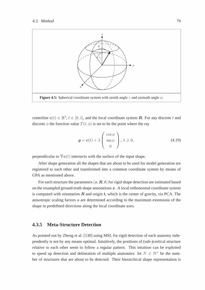
4.3. Method 79
y
z
x
φ
γ
Figure 4.5: Spherical coordinate system with zenith angleγ and azimuth angleφ.
centerlinec(t) ∈ R3, t ∈ [0, 1], and the local coordinate systemR. For any discretet and
discreteφ the function valueT (t, φ) is set to be the point where the ray
g = c(t) + λ
cosφ
sinφ
0
, λ ≥ 0, (4.19)
perpendicular to∇c(t) intersects with the surface of the input shape.
After shape generation all the shapes that are about to be used for model generation are
registered to each other and transformed into a common coordinate system by means of
GPA as mentioned above.
For each structure the parameters(s,R, t) for rigid shape detection are estimated based
on the resampled ground-truth shape annotationsx. A local orthonormal coordinate system
is computed with orientationR and origint, which is the center of gravity, via PCA. The
anisotropic scaling factorss are determined according to the maximum extensions of the
shape in predefined directions along the local coordinate axes.
4.3.5 Meta-Structure Detection
As pointed out by Zheng et al. [130] using MSL for rigid detection of each anatomy inde-
pendently is not by any means optimal. Intuitively, the positions of (sub-)cortical structure
relative to each other seem to follow a regular pattern. Thisintuition can be exploited
to speed up detection and delineation of multiple anatomies: let N ∈ N+ be the num-
ber of structures that are about to be detected. Their hierarchical shape representation is
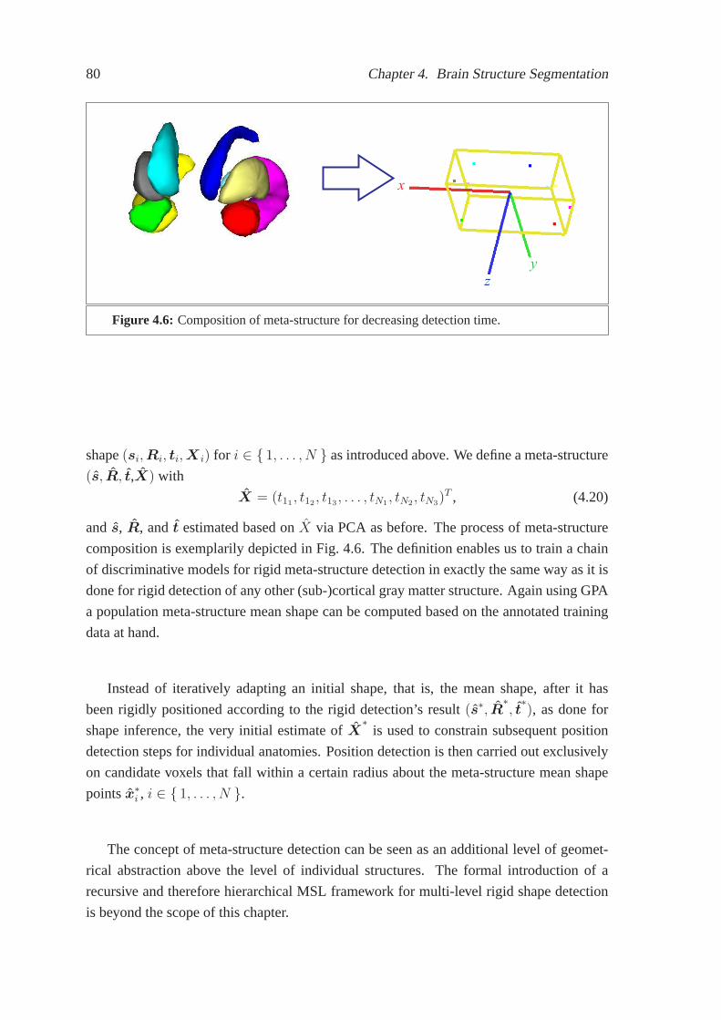
80 Chapter 4. Brain Structure Segmentation
z
y
x
Figure 4.6: Composition of meta-structure for decreasing detection time.
shape(si,Ri, ti,X i) for i ∈ { 1, . . . , N } as introduced above. We define a meta-structure
(s, R, t,X) with
X = (t11, t12
, t13, . . . , tN1
, tN2, tN3
)T , (4.20)
ands, R, andt estimated based onX via PCA as before. The process of meta-structure
composition is exemplarily depicted in Fig. 4.6. The definition enables us to train a chain
of discriminative models for rigid meta-structure detection in exactly the same way as it is
done for rigid detection of any other (sub-)cortical gray matter structure. Again using GPA
a population meta-structure mean shape can be computed based on the annotated training
data at hand.
Instead of iteratively adapting an initial shape, that is, the mean shape, after it has
been rigidly positioned according to the rigid detection’sresult (s∗, R∗, t
∗), as done for
shape inference, the very initial estimate ofX∗
is used to constrain subsequent position
detection steps for individual anatomies. Position detection is then carried out exclusively
on candidate voxels that fall within a certain radius about the meta-structure mean shape
pointsx∗i , i ∈ { 1, . . . , N }.
The concept of meta-structure detection can be seen as an additional level of geomet-
rical abstraction above the level of individual structures. The formal introduction of a
recursive and therefore hierarchical MSL framework for multi-level rigid shape detection
is beyond the scope of this chapter.

4.4. Validation 81
4.4 Validation
4.4.1 Material and Experimental Setup
For training and quantitative evaluation of our system there were four sets of T1-weighted
MRI scans available (see Table 4.1). The first one is a subset ofthe “Designed Database
of MR Brain Images of Healthy Volunteers”1 [16] (DDHV) containing 20 scans. The as-
sociated ground-truth annotations were manually recovered from automatically generated
segmentations [50] of the structures of interest. The second collection of 18 MRI scans was
provided by the Center of Morphometric Analysis at the Massachusetts General Hospital
and is publicly available on the Internet Brain SegmentationRepository2 (IBSR 18). The
scans are accompanied by detailed ground-truth annotations including the (sub-)cortical
structures that are of interest here.3 A subset4 of the data provided by the “NIH MRI Study
of Normal Brain Development”5 consisiting of 10 pediatric data sets states another collec-
tion (NIH) of annotated MRI scans used for model generation. They have been manually
annotated by the authors for training purposes. Additionally, we use data provided by
the ongoing “3-D Segmentation in the Clinic: A Grand Challenge” competition6 [56] for
training and evaluation of the proposed method. The collection consists of several volu-
metric T1-weighted MRI brain scans of varying spatial resolution and size from multiple
sources. The vast majority of data (29 scans) has been provided by the Psychiatry Neu-
roimaging Laboratory (PNL) at the Brigham and Women’s Hospital (BWH), Boston. The
other 20 data sets arose from a pediatric study, a Parkinson’s Disease study, and a test/re-
test study carried out at the University of North Carolina’s (UNC) Neuro Image Analysis
Laboratory (NIAL), Chapel Hill. Only scans BWH PNL 1–15 (MICCAI’07 training) are
accompanied by expert annotations for the left and right caudate nucleus, whereas for all
the other data sets (MICCAI’07 testing) the ground-truth annotations of those two struc-
tures are held back by the providers. A predefined evaluationprotocol is carried out fully
1The database was collected and made available by the CASILabat the University of North Car-olina, Chapel Hill. The images were distributed by the MIDASData Server at Kitware, Inc. (insight-journal.org/midas)
2www.cma.mgh.harvard.edu/ibsr3We corrected the ground-truth annotations for the left and the right caudate in the IBSR 18 data set to
better meet the protocol applied by the “3-D Segmentation inthe Clinic: A Grand Challenge” competitionwhere the caudate is grouped with the nucleus accumbens in the delineations [56, 6].
4The following 10 data sets were used: defaced_native_100{2,3,7}_V{1,2}_t1w_r2, defaced_na-tive_100{1,4,8}_V2_t1w_r2, and defaced_native_1005_V2_t1w_r2.
5The “NIH MRI Study of Normal Brain Development” is a multi-site, longitudinal study of typi-cally developing children, from ages newborn through youngadulthood, conducted by the Brain Devel-opment Cooperative Group and supported by the NICHD, the NIDA, the NIMH, and the NINDS (Con-tract #s N01-HD02-3343, N01-MH9-0002, and N01-NS-9-2314,-2315, -2316, -2317, -2319 and -2320).A listing of the participating sites and a complete listing of the study investigators can be found atwww.bic.mni.mcgill.ca/nihpd/info/participating_centers.html. This manuscript reflects the view of the au-thor and may not reflect the opinions or views of the NIH.
6www.cause07.org

82 Chapter 4. Brain Structure Segmentation
automatically after uploading the testing fraction of the data to the Cause’07 file server.
Evaluation is supposed to happen independently of any segmentation system developers in
order to prevent over-adaptation to the testing data sets provided. First of all, the results
are quantitatively evaluated on the BWH PNL scans 16–29, whichare all considered to be
routine scans, on 5 of the pediatric scans, and on 5 scans of patients older than 55 years (see
Tables 4.3 and 4.4). Additionally, a system’s accuracy is tested on 10 datasets of the same
young healthy person acquired within 60 days on 5 different scanners (see Table 4.6). The
COV of the volumetric measurements is an indicator on how stable the method operates in
a test/re-test situation including scanner variability. We refer to [45, 56] and Appendix B
for details on the used evaluation measures and to reference[56] for details on the used
scoring system.
DDHV IBSR 18 NIH MICCAI’07training testing
Volume Size 176×256×160 256×256×128 124×256×256, 256×124×156 256×256×198,176×256×256, 256×124×256,160×256×256 176×256×160,
256×192×256Voxel Spacing(mm3) 1.0×1.0×1.0 0.84×0.84×1.5, 1.3×0.94×0.94, 0.94×1.5×0.94 0.94×0.94×0.94.0,
0.94×0.94×1.5, 1.5×0.94×0.94, 0.94×1.5×0.94,1.0×1.0×1.5 1.5×0.98×0.98, 1.0×1.0×1.0,
1.4×1.02×1.02 1.02×1.02×1.02Sequence T1 T1 T1 T1 T1Number of Scans 20 18 10 15 24Gound-truth Yes Yes Yes Yes No
Table 4.1: Summary of the publicly available standard data used for model generationand evaluation purposes.
All the images were re-oriented to a uniform orientation (“RAI”; right-to-left, anterior-
to-posterior, inferior-to-superior) and resampled to isotropic voxel spacing (1.0×1.0×1.0
mm3) for processing. For increasing the amount of training datawe exploited natural brain
symmetry and therefore doubled the size of any training dataset used for model generation
by mirroring all the data sets with respect to the mid-sagittal plane. Throughout all our
experiments we ensured that training and testing data are mutually exclusive: we trained
models on all the available annotated data but left out IBSR 181–9 and IBSR 18 10-18
in turn for testing. As a result of not having any accompanying ground-truth annotations
MICCAI’07 testing was never part of the training data.
As stated in reference [56] there are differences in the annotation protocols used for
annotating the caudate nuclei in data sets originating fromthe BWH and the UNC. In the
former the “tail” of the caudate is continued much further dorsaly. We therefore decided to
detect it as a separate structure that can be attached to the caudate nucleus if required. We
did not try to automatically determine the annotation protocol used from the imaging data
itself as this may lead to over-fitted systems. Moreover, in contrast to Tu et al. [109], we

4.4. Validation 83
Structure Overlap Err. Dice Coeff. Volume Diff. Abs. Dist. RMS Dist. Max. Dist.[%] [%] [%] [mm] [mm] [mm]
Left/right caudate nucleus 32.42 80.49 9.57 0.67 1.10 7.76Left/right hippocampus 41.96 73.34 21.14 0.91 1.33 6.34Left/right globus pallidus 39.72 74.97 20.97 0.79 1.24 5.53Left/right putamen 29.82 82.37 13.76 0.72 1.15 6.60
Table 4.2: Average segmentation accuracy for IBSR 18 of models trained from mutuallyexclusive training and test data.
did not build models based on disjoint training data sets, which may be another cause for
over-fitting.
As our real discriminative models are not ideal as assumed for theoretical considera-
tions we keep the top 100 candidates after position detection and the top 25 candidates after
position-orientation detection for further processing steps in order to make the full similar-
ity transformation detection more robust. For our shape models we sampled the shapes of
the 8 (sub-)cortical structures of interest withn = 402 surface points for the caudate and
the hippocampus and withn = 322 surface points for the remaining structures. Subspace
projection of the ASMs is constrained bym = 46 eigenvectors for all structures accord-
ing to Zheng et al.’s [131] aforementioned heuristic. For shape inference we useT = 3
iterations.
In an optimized and parallelized C++ implementation of our segmentation method it
takes about 5–10 seconds to detect and segment each (sub-)cortical structure in an MRI
volume on a Fujitsu Siemens notebook equipped with an Intel Core 2 Duo CPU (2.20
GHz) and 3 GB of memory. Intensity standardization takes 1–2seconds. The overall
timing, without meta-structure detection, is comparable to the graph shifts algorithm [27]
(50 seconds for 8 structures) and better than the auto context model (ACM) approach [77]
(60 seconds for 1 structure), the hybrid discriminative/generative approach [109] (8 min.
for 8 structures), and the method of Chupin et al. [20].
4.4.2 Quantitative Results
As can be seen from Table 4.2 in terms of the Dice coefficient our method achieves better
results (80%,73%,75%,82%) for the segmentation of the caudate nuclei, hippocampi, globi
pallidi, and putamina on the same IBSR 18 data set than the methods of Akselrod-Ballin et
al. [2] (80%, 69%, 74%, 79%) and Gouttard et al. [50] (76%,67%,71%,78%) except for the
caudate nuclei in reference [2], where we reach a comparableaccuracy. It also reaches a
higher score for the caudate nuclei and putamina on IBSR 18 than the method of Bazin and
Pham [6] (78%,81%), which does not address segmentation of the hippocampi and globi
pallidi. Fig. 4.7 gives a visual impression of the results obtained on IBSR 18.

84 Chapter 4. Brain Structure Segmentation
Cases Overlap Err. Volume Diff. Abs. Dist. RMS Dist. Max. Dist. Total[%] Score [%] Score [mm] Score [mm] Score [mm] Score Score
UNC Ped 10 25.86 83.74 4.88 91.43 0.60 77.84 1.18 78.8510.36 69.5480.28UNC Ped 14 23.73 85.08 -0.56 99.02 0.47 82.68 0.83 85.11 5.80 82.93 86.96UNC Ped 15 25.76 83.80 9.80 82.81 0.59 78.14 1.02 81.81 7.00 79.41 81.20UNC Ped 19 30.30 80.94 -8.78 84.60 0.65 76.08 1.00 82.09 4.69 86.20 81.98UNC Ped 30 28.77 81.91 4.66 91.83 0.63 76.65 1.03 81.58 6.81 79.98 82.39UNC Eld 01 58.98 62.90 18.25 67.98 1.44 46.66 1.85 67.01 6.38 81.24 65.16UNC Eld 12 35.79 77.49 43.78 23.19 0.79 70.56 1.14 79.68 5.05 85.14 67.21UNC Eld 13 33.30 79.06 17.86 68.66 0.70 73.99 1.03 81.58 5.15 84.85 77.63UNC Eld 20 28.48 82.09 17.75 68.87 0.63 76.67 1.09 80.53 9.35 72.51 76.13UNC Eld 26 43.14 72.87 40.87 28.30 0.95 64.94 1.37 75.55 6.16 81.90 64.71BWH PNL 16 39.27 75.30-24.62 56.80 1.60 40.67 4.60 17.9034.02 0.62 38.26BWH PNL 17 33.14 79.15-22.83 59.94 1.36 49.75 4.34 22.5734.75 2.51 42.78BWH PNL 18 34.44 78.34-20.96 63.22 1.17 56.68 2.70 51.8319.04 44.0158.82BWH PNL 19 34.47 78.32 -7.38 87.06 1.27 52.87 3.52 37.1329.85 12.2053.52BWH PNL 20 33.60 78.87 0.79 98.61 1.07 60.38 3.38 39.6533.35 2.05 55.91BWH PNL 21 41.34 74.00-27.02 52.60 1.80 33.47 4.55 18.6934.73 0.00 35.75BWH PNL 22 39.85 74.94-26.38 53.72 1.35 50.18 3.56 36.3729.24 13.9945.84BWH PNL 23 28.98 81.77-10.88 80.91 0.81 70.18 2.15 61.5918.77 44.8067.85BWH PNL 24 28.86 81.85 -9.44 83.44 0.74 72.52 1.74 68.9114.18 58.2973.00BWH PNL 25 32.91 79.30 7.43 86.97 1.33 50.80 3.83 31.6130.85 9.27 51.59BWH PNL 26 43.12 72.88-15.38 73.01 1.06 60.62 2.05 63.3313.61 59.9665.96BWH PNL 27 28.25 82.23 -8.48 85.12 1.48 45.24 4.74 15.2932.80 3.53 46.28BWH PNL 28 34.30 78.43-23.58 58.63 1.43 46.97 4.36 22.0730.99 8.86 42.99BWH PNL 29 33.83 78.72 -1.74 92.92 0.88 67.40 1.87 66.5416.19 52.3971.59
Average UNC Ped 26.88 83.09 2.00 89.94 0.59 78.28 1.01 81.89 6.93 79.61 82.56Average UNC Eld 39.94 74.88 27.70 51.40 0.90 66.57 1.30 76.87 6.42 81.13 70.17Average BWH PNL 34.74 78.15-13.61 73.78 1.24 54.12 3.39 39.5326.60 22.3253.58
Average All 34.19 78.50 -1.75 72.49 1.03 61.75 2.46 56.1418.30 46.5163.08
Table 4.3: Average left/right caudate segmentation accuracy for the MICCAI’07 testingdata set without optional caudate tail detection. As of 02/25/2009 this methodranks number 11 in the overall ranking list on www.cause07.org (“LME Er-langen”).
The overall average score (75.19) in Table 4.4 shows that forsegmenting the caudate
nuclei our method performs better than the methods of Morra et al. [77] (73.38), Bazin and
Pham [6] (64.73) and Tu et al. [109] (59.71). All the mentioned authors report on results
computed on the same MICCAI’07 testing data set. In fact, our method with integrated
caudate tail tip detection ranks number 2 in the overall ranking list on www.cause07.org
(“Segmentation Team”) as of 03/10/2009.
4.5 Discussion
One of the limiting aspects of our extended MSL method is the fact that all the patient data
sets we used for model generation origin from patients not being affected by pathologies

4.5. Discussion 85
Cases Overlap Err. Volume Diff. Abs. Dist. RMS Dist. Max. Dist. Total[%] Score [%] Score [mm] Score [mm] Score [mm] Score Score
UNC Ped 10 29.87 81.22 17.06 70.08 0.64 76.38 1.05 81.22 7.18 78.88 77.55UNC Ped 14 31.55 80.16 7.48 86.87 0.85 68.53 1.89 66.1815.82 53.4871.05UNC Ped 15 25.66 83.86 5.55 90.26 0.58 78.36 1.10 80.2810.30 69.7280.50UNC Ped 19 24.66 84.49 4.22 92.59 0.65 75.80 1.51 73.0313.33 60.8077.34UNC Ped 30 24.83 84.39 1.90 93.72 0.50 81.31 0.88 84.23 7.02 79.34 84.60UNC Eld 01 40.31 74.65 14.92 73.83 0.93 65.39 1.62 71.0513.18 61.2469.23UNC Eld 12 33.13 79.16 12.60 77.89 0.72 73.23 1.37 75.4612.38 63.5773.86UNC Eld 13 29.09 81.71 5.83 89.77 0.57 78.92 0.97 82.71 9.46 72.18 81.06UNC Eld 20 32.23 79.73 12.25 78.51 0.65 75.83 1.01 81.92 6.90 79.72 79.14UNC Eld 26 37.64 76.33 8.05 85.88 0.79 70.72 1.58 71.8015.95 53.0971.56BWH PNL 16 37.12 76.65-26.96 52.71 0.65 75.79 1.08 80.73 8.51 74.96 72.17BWH PNL 17 27.83 82.50-12.83 77.50 0.49 82.01 0.91 83.75 6.24 81.66 81.48BWH PNL 18 30.31 80.94-23.71 58.41 0.60 77.88 1.06 81.0010.60 68.8273.41BWH PNL 19 33.96 78.64-11.82 79.26 0.70 74.11 1.20 78.66 8.07 76.28 77.39BWH PNL 20 29.52 81.43 -8.94 84.31 0.51 81.26 0.91 83.81 6.61 80.56 82.28BWH PNL 21 40.36 74.61-34.83 38.89 0.89 66.92 1.46 73.8910.30 69.7264.81BWH PNL 22 38.96 75.50-30.52 46.46 0.79 70.62 1.20 78.63 8.48 75.07 69.25BWH PNL 23 29.45 81.48 -8.69 84.75 0.78 70.94 2.25 59.8321.33 37.2666.85BWH PNL 24 24.30 84.72 -6.49 88.62 0.45 83.32 0.91 83.7113.70 59.6980.01BWH PNL 25 29.33 81.55 -6.12 89.27 0.81 69.86 2.18 61.0321.43 36.9767.73BWH PNL 26 34.45 78.34-24.77 56.54 0.65 75.84 1.30 76.7014.69 56.8168.84BWH PNL 27 25.99 83.65-13.91 75.59 0.53 80.30 1.01 81.93 6.48 80.94 80.48BWH PNL 28 34.00 78.62-22.87 59.87 0.64 76.20 1.13 79.81 6.85 79.86 74.87BWH PNL 29 28.47 82.09 0.87 90.60 0.54 80.14 0.99 82.2913.39 60.6279.15
Average UNC Ped 27.31 82.82 7.24 86.70 0.65 76.08 1.29 76.9910.73 68.4478.21Average UNC Eld 34.48 78.31 10.73 81.18 0.73 72.82 1.31 76.5911.57 65.9674.97Average BWH PNL 31.72 80.05-16.54 70.20 0.65 76.08 1.26 77.5611.19 67.0974.20
Average All 31.38 80.27 -5.91 75.92 0.66 75.40 1.27 77.2411.17 67.1475.19
Table 4.4: Average left/right caudate segmentation accuracy for the MICCAI’07 testingdata set with optional caudate tail detection. As of 03/10/2009 this methodranks number 2 in the overall ranking list on www.cause07.org (“SegmentationTeam”).
disturbing the usual composition and appearance of the human brain’s anatomy in a, from
a medical imaging perspective, serious manner. For instance, there are not any intracranial
mass lesions such as tumors, abscesses, or hemorrhages deforming the surrounding tissue.
This may lead to a decreased robustness of the system againstthis kind of pathological
changes in the human brain and may yield sub-optimal resultsin such cases. From our
point of view there are two ways to overcome this issue: first,one could try to increase
the amount of training data and therefore allowing the involved models to also capture
pathological abnormalities. Second, one could try to implement recovering strategies in
case deforming pathologies prevent proper detection of anatomies.
Aiming for comparable validation results we evaluated our approach on two publicly
available databases (IBSR 18 and MICCAI’07 testing) for the caudate nucleus and on one

86 Chapter 4. Brain Structure Segmentation
Correlation UNC Ped UNC Eld BWH PNL TotalLeft 0.53 0.94 0.65 0.71Right 0.63 0.95 0.50 0.69Average 0.58 0.79 0.58 0.70
Table 4.5: Pearson correlation for the volume measurements in the three testing groupsas well as in total. This coefficient captures how well the volumetric measure-ments correlate with those of the reference segmentations.
Test/Re-Test Left Right Total
UNC 03 [mm3] 3745 3714 7459UNC 04 [mm3] 3950 3781 7731UNC 09 [mm3] 3906 4011 7918UNC 11 [mm3] 3871 3822 7693UNC 17 [mm3] 3751 3735 7486UNC 18 [mm3] 3935 3988 7923UNC 21 [mm3] 3765 3714 7479UNC 22 [mm3] 4047 3782 7829UNC 24 [mm3] 4142 3770 7912UNC 25 [mm3] 2783 3119 5902
Mean [mm3] 3790 3744 7533Stdev [mm3] 357 231 572
COV [%] 9.0 6.0 8.0
Table 4.6: The volumetric measurements of the 10 data sets of the same young adult ac-quired on 5 different scanners within 60 days. The COV indicates the stabilityof the algorithm in a test/re-test situation including scanner variability.
publicly available databases (IBSR 18) for all the other (sub-)cortical gray matter struc-
tures. Both IBSR 18 and MICCAI’07 testing have been established to allow objective
comparison of segmentation methods. Especially the web-based evaluation of results on
MICCAI’07 testing is designed to validate accuracy and robustness of segmentation ap-
proaches.
Though better than recently reported results, or at least comparable, a Dice coefficient
of, for instance, 73% for the hippocampus might be considered too low for reliable vol-
umetric studies from a clinical perspective. Some methods [77, 20, 55, 85] reach higher
scores for certain structures when evaluated on non-publicly available data sets. However,
comparability to scores computed on different databases islimited due to different charac-
teristics of the data with respect to MRI artifacts and pathology. The typical MRI artifacts,
such as Rician noise [80], PVEs [114], and intra-/inter-scanINUs [119, 60], might be there
in a more or less distinctive manner. Also, as mentioned above, the presence of pathology

4.5. Discussion 87
may significantly affect the achievable segmentation accuracy on a particular database.
From our point of view, objective comparison of segmentation methods is only possible by
using publicly available benchmark databases.
With respect to the achieved overall score on MICCAI’07 testing our method (~75), as
well as all the others presented in the overall ranking at www.cause07.org as of 05/20/2009,
still fails to keep up with the score (~90) presumed typical for a human expert when man-
ually delineating the left and right caudate nucleus [56]. The decision to assign an overall
score of approximately 90 to the segmentation accuracy achievable by an independent hu-
man observer was based on preliminary tests [56].
In comparison to registration-based approaches working with anatomical atlases [94, 6,
2, 85] exhaustive labeling of all the anatomical structuresin the human brain independently
from each other with our extended MSL framework may become a lengthy undertaking on
today’s hardware—even though processing is comparably fast for a manageable amount
of anatomies. Exploiting geometrical knowledge about the anatomies and their relation to
each other, like already done by introducing meta-structure detection, even on the level of
common boundaries may help to overcome this drawback of the current system. While
currently only the translation search ranges for individual anatomies are constrained by
meta-structure detection this may be extended by also constraining search ranges for ori-
entation and scaling. However, this may be at the risk of propagating detection errors from
one level of geometrical abstraction to the one beneath.
Another critical point is the considerable amount of annotated training data necessary
to generate robust models for the presented approach. Zhenget al. [131, 130] evaluate their
MSL approach on more than 300 CT volume data sets in a cross validation setup. Ling et
al. [71] work with almost 200 CT scans. Yet, the amount of available training data can be
easily augmented by suitable annotation tools allowing to correct automatically generated
annotations generated by systems trained on less data.
In the current system all the parameters for training rigid detection are estimated based
on the shape information itself. There are not any characteristic anatomical landmarks of a
high recognition factor, both facilitating manual labeling as well as fully automatic detec-
tion, used for deriving the associated local coordinate systems. Only for the detection and
segmentation of the caudate nuclei the approximated centerline used for mesh re-sampling
is unilaterally bounded by the manually annotated tail tip.Paying respect to anatomical
characteristics in defining such landmarks may improve the overall accuracy of the system
in certain cases [130, 131]. The ease of defining appropriatelandmarks depends on the
addressed segmentation scenario.
The system presented is comparably fast: without meta-structure detection it takes
only 1–2 minutes to segment 8 (sub-)cortical gray matter structures. Processing time can
be decreased to on average 13.9 seconds by means of meta-structure detection. This makes

88 Chapter 4. Brain Structure Segmentation
our approach even preferable to the method of Corso et al. [28], which is found to be the
fastest in our literature research.
In comparison to Zheng et al. [130, 131] we give a slightly different, though sound,
mathematical formulation of an extended MSL approach that also integrates shape infer-
ence. We show that MSL naturally decomposes the search spacealong levels of geomet-
rical abstraction successively refining anatomy representation. This allows the use of a
chain of discriminative models. As machine learning-, and therefore knowledge-based, ap-
proaches are used on every level of abstraction, the method is entirely top-down—not only
from a geometrical but also from a methodological point of view. Knowledge is incorpo-
rated into the system by exploiting a large database of expert-annotated training data for
model generation, which aligns the method with the paradigmof database-guided medical
image segmentation [44].
4.6 Conclusions
The contributions of this chapter are as follows: we integrated shape inference into the
overall MSL methodology from the theoretical point of view.We showed that MSL de-
composes the parameter space of anatomy shapes along decreasing levels of geometrical
abstraction into subspaces of increasing dimensionality and applied MSL to the difficult
problem of (sub-)cortical gray matter structure detectionand shape inference. Experi-
ments on publicly available gold standard databases show that our method works equally
fast, robust, and accurate at a state-of-the-art level.
In the following chapter we will summarize the core contributions of this thesis. We
will also discuss general technological and methodological considerations, give a brief
outlook on future work, and draw conclusions.

4.6. Conclusions 89
(a) (b)
(c) (d)
Figure 4.7: Segmentation results obtained on the IBSR 18 data set No. 10 in an axial (a),coronal (b), and right (c) and left (d) sagittal view. The segmented structuresare the left and right caudate (dark-blue/yellow), the left and right putamen(orange/blue), the left and right globus pallidus (green/red), and the left andright hippocampus (turquoise/violet).

90 Chapter 4. Brain Structure Segmentation

Chapter 5
Summary and Outlook
5.1 Summary and Contributions
This thesis dealt with probabilistic modeling for segmentation of the human brain and
related structures from MRI data. The human brain plays an important role in centrally
controlling a vast majority of functions of the human body. Moreover, it hosts all aspects
of human consciousness. This makes every disease infectingthe human brain a critical
issue that requires the newest and most accurate means of medical diagnostics and therapy
available. Many diseases affect morphology and usual appearance of the human brain in
radiological examinations. For its excellent soft tissue contrast MRI is the radiological
modality of choice for imaging the human’s central nervous system.
When it comes to the analysis of radiological images one usually wants to bridge the
gap between sequences of signal measurements, which is whatradiological 2-D images
or 3-D images actually are, and a semantic description of what is depicted—one wants
to “understand” the medical images at hand. Providing this understanding, that is to say,
these semantics, can serve several purposes when dealing with radiological pictorial mate-
rial: on the one hand they can be used for improved traditional medical decision making,
i.e., medical diagnostics and therapy planning and monitoring. On the other hand, explicit
semantics stored in a machine-readable format allow usage of the data and the patient-
specific knowledge supplied herewith for higher level post-processing: computer-aided di-
agnostics and treatment planning and also retrospective studies of certain diseases and their
progress may all be based on the automatic extraction of diagnostically relevant quantita-
tive or more abstract findings. The research project Health-e-Child, wherein this work of
research is embedded, is dedicated to this emerging field within medical informatics and
covers pooling and intelligently post-processing semantically enriched medical data and
storing general medical knowledge in the context of pediatrics. Finally, explicit semantics
can even be used for knowledge-based image enhancement as exemplified in Chapter 2.
91

92 Chapter 5. Summary and Outlook
Throughout this thesis we examined ways to provide explicitsemantics for medical
imaging data by means of medical image segmentation and labeling, which is a standard
methodology for the problem of partly understanding medical images. We exemplified
this general approach to the problem by developing and successfully applying three new
methods from the field of database-guided knowledge-based approaches for three distinct
medical image segmentation scenarios: 3-D MRI brain tissue classification and INU cor-
rection, pediatric brain tumor segmentation in multi-spectral 3-D MRI, and 3-D MRI brain
structure segmentation. Together, all the three chosen scenarios cover a broader range
of how the human brain’s morphology and usual condition can be affected by pathology.
With regards to the results our methods achieve we can conclude that database-guided
knowledge-based approaches, exemplified by the three developed methods of this thesis,
are well-suited for the purpose of fully automatically generating semantic descriptions for
medical imaging data.
For the first scenario we presented a fully automated method,that is, the DMC-EM al-
gorithm, for brain tissue classification into GM, , and CSF regions and intra-scan INU cor-
rection in 3-D MR images. In its integrated multi-spectral Bayesian formulation based on
the MRF methodology we could combine supervised MRI modality-specific discriminative
modeling and unsupervised EM segmentation. The MRF regularization involved took into
account knowledge about spatial and appearance related homogeneity of segments using
pair-wise clique potentials and patient-specific knowledge about the global spatial distri-
bution of brain tissue using PBT-based unary clique potentials. The PBT features used rely
on surrounding context and alignment-based features derived from a pre-registered proba-
bilistic anatomical atlas. The context considered is encoded by 3-D Haar-like features of
reduced INU sensitivity. Our detailed quantitative evaluations on standard phantom scans
and standard real world data showed the accuracy and robustness of the proposed method.
By comparison with other state-of-the-art approaches we were able to demonstrate our
method’s relative superiority with regards to the chosen medical imaging scenario.
In the second scenario, we addressed fully automatic pediatric brain tumor segmenta-
tion in multi-spectral 3-D MRI. The developed method, that is, the DMC-GC algorithm,
is based on an MRF model that combines PBT discriminative modeling and lower-level
segmentation via graph cuts. The PBT algorithm provides a prior model in terms of an ex-
ternal field classifying tumor appearance while a spatial prior takes into account pair-wise
voxel homogeneities both in terms of classification labels as well as in terms of multi-
spectral voxel intensities. As above the discriminative model relies not only on observed
local intensities but also on surrounding context for detecting candidate regions for pathol-
ogy. We were able to provide a mathematically sound formulation for integrating the two
approaches into a unified statistical framework. In a quantitative evaluation we obtained
results that were mostly better than those reported for current state-of-the-art approaches
to 3-D MRI brain tumor segmentation.

5.2. Discussion and Technological Considerations 93
The third and final scenario comprised 3-D MRI brain structuresegmentation where we
developed a novel method for the automatic detection and segmentation of (sub-)cortical
GM structures in 3-D MR images of the human brain. The method is based on the MSL
concept. We showed that MSL naturally decomposes the parameter space of anatomy
shapes along decreasing levels of geometrical abstractioninto subspaces of increasing di-
mensionality. This is done by exploiting parameter invariance. This insight allows us to
build strong discriminative PBT models from annotated training data on each level of ab-
straction. During shape detection and inference the range of possible solutions is narrowed
using these models until a final shape is found. We could extend the original MSL formal-
ism to also cover shape inference and not only rigid shape detection. The segmentation
accuracy achieved is mostly better than the one of other state-of-the-art approaches for
(sub-)cortical GM structure segmentation. For benchmarking purposes, our method was
evaluated on publicly available gold standard databases consisting of several T1-weighted
3-D brain MRI scans from different scanners and sites. The choice of images within these
databases is guided by the intention to reflect the challenging environment a segmentation
algorithm has to face when applied in clinical practice.
Next to these major contributions the following minor contribution was made: in the
second and third scenario we adapted the DHW approach for 1-Dhistogram matching
whose original purpose is ensuring constant image brightness in traditional gray scale im-
ages to mono-spectral MRI inter-scan intensity standardization. We gave a graph theoretic
re-formulation of the algorithm and extended it to minimizethe Kullback-Leibler diver-
gence between 1-D histograms of equal bin size. Inter-scan intensity standardization is
one of the prerequisites to the application of machine learning-based segmentation tech-
niques relying directly or indirectly on observed image intensities.
5.2 Discussion and Technological Considerations
Although we discussed issues related to the particular systems and scenarios we presented
at the end of each chapter there are some more general technological and methodological
considerations and aspects that need to be mentioned.
With regards to the broader subject of semantic imaging we had to restrict our discourse
on this matter to three well-defined MRI segmentation scenarios. A more general and more
theoretical dealing with the fully automatic semantic analysis of medical pictorial material
would have gone far beyond the scope of this work.
Due to the characteristics of the chosen scenarios we were limited to the analysis of
static morphological points of view. The study of other medical imaging modalities for
the purpose of semantic analysis, such as 3-D+t or functional imaging, is necessary to
also address physiological and pathophysiological aspects of the human body. Also, we

94 Chapter 5. Summary and Outlook
concentrated on the important first steps towards explicit semantics for medical imaging
data—medical image segmentation and labeling. From our point of view, narrowing the
topic that way appears reasonable in order to deal with it in asufficiently concise manner
that is in accordance with the ambition of this kind of scientific piece of writing.
From a technological point of view, focusing on database-guided knowledge-based ap-
proaches involving machine learning might also appear as ifwe unnecessarily imposed a
restriction on the scope of this work. However, we found out from the literature that this
methodology represents a current trend in today’s medical image segmentation and that
this kind of approaches is well-suited for semantic imagingpurposes. An important ques-
tion arises nevertheless: are the databases used for model-generation large enough to cover
the large variety of possible deformations the human brain,as in our case, can be subject
to? This is certainly questionable due to the almost unpredictable impact of possible mal-
functions and diseases on morphology. On the other hand the investigation of pathology
by radiological imaging is fundamental for medical inquiries. Encouraged by what is to be
found in the literature and by the evaluation results of our methods we believe that suffi-
ciently large databases can be chosen covering at least the common spectrum of possible
deformations and changes in anatomical appearance also in the case of pathology.
Throughout this thesis we made extensively use of the PBT algorithm (see Appendix A)
for machine learning. The technique is closely related to the cascade approach of Viola
and Jones [115]. Though generic in formulation the PBT algorithm is usually used in
combination with AdaBoost [41] as strong classifier within each tree node. As a matter of
fact, PBT is still lacking a detailed analysis from a theoretical point of view revealing its
robustness against over-fitting and effects of certain parameter settings. A comparison with
other boosting strategies, such as random forests [12] or pure AdaBoost, would definitely
be worth investigation. As we approached involved technologies from the entire medical
image segmentation scenario’s point of view we did not have the ambition to evaluate all
imaginable design choices concerning our methods. However, most of the design choices
are well founded in the literature.
Where possible we decided to evaluate our approaches on publicly available gold stan-
dard data sets. Even though this ensures comparability of different methods, researchers
relying on these data sets are at the risk of another subtle methodological error: “training
on the test data” [35, 56] . It is the case when a classifier or method undergoes a longer
series of refinements, which are guided by repeated experiments on the same test data. As
some of the used benchmarking databases have been persisting in the public domain for
quite some time the best-performing methods may be over-adapted to specific character-
istics of these data collections. These characteristics may not represent the general case
of a particular medical image segmentation scenario. This disadvantage was addressed by
Heimann et al. [56] with their onsite segmentation contest at MICCAI 2007 in Brisbane,
Australia, and their ongoing online caudate segmentation challenge (www.cause07.org).

5.3. Future Work 95
In the contest, the final evaluation was carried out on a thirdset of previously unseen data
sets that were not distributed to the participants with the training and testing data. From the
opposite point of view, due to the limited number of data setsavailable, the question arises
whether these collections reflect the possible spectrum of challenges that can be associated
with a certain segmentation scenario. Another aspect is “saturation” meaning that new
methods are likely to only achieve marginal improvements onbenchmarking data sets that
have already been used for evaluation purposes by many researchers. In this case signifi-
cant improvements are almost impossible. However, we are convinced that evaluation on
publicly available gold standard or benchmarking data setsis one of the best ways to ob-
jectively compare methods as, despite the aforementioned objections, every method faces
the same replicable prerequisites.
Most often we carried out benchmarking by comparing complete systems. This means
we assessed methods on the highest level of abstraction withrespect to their processing
pipeline and compared their final segmentation results. This aligns with our ambition to
approach medical imaging scenarios from an integral perspective rather than from a pure
technological perspective with focus restricted in terms of technological categories. Usu-
ally, we did not evaluate individual processing steps separately.
Typically there was only one ground-truth annotation per dataset available both for
training as well as for evaluation of all the three scenarios’ systems. Therefore, we could
not study any intra- and inter-observer variability this being a limitation of the data sets at
hand.
Even though addressed to some extend computational performance of our systems was
not one of the major aspects of this work. Improvements may bepossible due to new
hardware developments and more elaborated implementations properly exploiting present
and future hard- and software capabilities.
5.3 Future Work
As mentioned above enriching medical imaging content with semantic annotations of any
kind is an emerging field in today’s medical informatics research. Future work on this topic
will have to address, but is not limited to, the following scientific questions:
• Which kind of features should semantics be generated from? Step-wise along a
chain of explicit semantic descriptors, which are also understandable to humans, or
immediately from the signal measurements by means of classical low-level feature
extraction and pattern recognition-style classification?
• How can semantics be intelligently integrated into applications of added value? How
would these applications look like? How can they make use of distributed sources of
semantic content over the internet?

96 Chapter 5. Summary and Outlook
• How can these applications be kept scalable despite the hugeamount medical imag-
ing data generated every day all over the world? Both with regards to the processing
as wells as to the generation of semantic content.
• How can the clinical workflow benefit from semantic annotations in medical imaging
data?
• Are there ways to flexibly combine semantics generated from different sources of
data within a field of knowledge? Which formal representations should be chosen
for this purpose?
Next to these more general inquiries there are also possibilities for future research deal-
ing directly with the three medical imaging scenarios we concentrated on and the associated
methods we proposed. They include, but are not restricted to, the following questions:
• Can the methods be applied to other body regions and other imaging modalities?
• How can robustness against disease-related changes in morphology be increased?
• How do different design choices in terms of low-level image features or techniques,
for instance, other machine learning techniques, affect the accuracy and performance
of the methods?
• Can more complicated shapes like, for example, the entire cerebral cortex be ad-
dressed by similar methods?
• Can the methods be made more MRI-specific by feeding knowledge about the MR
image acquisition back into the segmentation process?
5.4 Conclusions
In this work, we addressed probabilistic modeling for segmentation in MR images of the
human brain in three distinct scenarios. In all scenarios, we concentrated on database-
guided knowledge-based approaches that make use of machinelearning in order to provide
probabilistic models. We could show that our newly developed, fully automatic approaches
are well-suited for the problem of providing explicit semantics for medical imaging data
in terms of labeled image regions. Regarding the methodologies applied, major and minor
advances in research could be made as summarized above. Both from our work as well
as from what can be found in the literature we conclude that database-guided knowledge-
based approaches are at the point of becoming the state-of-the-art in medical image seg-
mentation. They successfully combine traditional medicalimaging with machine learning
and pattern recognition techniques.

Appendix A
Discriminative Modeling
A.1 Probabilistic Boosting-Trees
Training a probabilistic boosting-tree (PBT) (see Fig. A.1)resembles inducing a mul-
tivariate binary decision tree from a set of weighted labeled training examplesT =
{ (zn, yn, wn) |n = 1, . . . , N } ∈ T ,N ∈ N, with feature vectorszn ∈ Z = RM ,M ∈ N,
labelsyn ∈ {−1,+1 }, and weightswn ∈ [0, 1] with∑N
n=1wn = 1. Within each nodev
of the tree a strong discriminative modelHv(z) ∈ (−1,+1) for feature vectorsz ∈ RM ,
M ∈ N, is generated. By construction, all those modelsH(z) asymptotically approach an
additive logistic regression model [42]
H(z) ≈ 1
2lnp(y = +1|z)
p(y = −1|z)(A.1)
wherey ∈ {−1,+1 } denotes the outcome of the associated binary classificationtask.
Accordingly, at each nodev of the resulting PBT there are current approximations of
the posterior probabilitiespv(+1|z) = qv(z) = exp(2H(z))/(1 + exp(2H(z))) and
pv(−1|z) = 1− qv(z). During classification those values are used to guide tree traversing
and combined propagation of posteriors in order to get a finalapproximationp(y|z) of the
true posterior probabilityp(y|z) at the tree’s root node.
While training the classifier, those probabilities are used to successively split the set
of training data relative to the prior probabilitypv(y = +1) associated with the current
training (sub-)set in nodev into two new subsets. We writepv instead ofpv(y = +1)
in the following for simplicity. The soft thresholding parameterǫ > 0 sees to pass on
training samplesz that are close to the current node’s decision boundary, thatis to say, if
qv(z) ∈ [(1− ǫ)pv; (1 + ǫ)pv], to both of the resulting subsets and associated subtrees. See
Algorithm 4 for details on how a PBT is built.
During classification the values forqv(z) are used to guide tree traversing and combined
propagation of posteriors in order to get final approximations pv(y|z) of the true posterior
97

98 Appendix A. Discriminative Modeling
... ...
... ...
......
qv1
qv2qv3
qv4qv5
d = 1
d = 2
d = 3
r−1v1
r+1v1
r+1v1
r−1v2
r+1v2
Figure A.1: A PBT with a strong discriminative probabilistic model in each tree node.
probabilitiespv(y|z) at each tree nodev: for outgoing edgesr−1v andr1
v associated with
the possible classifications the approximationpv(y|z) can be computed via the recursive
formula
pv(y|z) =
pβ(r−1v )(y|z) if qv(z) < (1− ǫ)pv,
pβ(r+1v )(y|z) if qv(z) > (1 + ǫ)pv,
∑
i pβ(riv)(y|z) · qv(i|z) otherwise,
(A.2)
whereβ(r) denotes the vertex where edger ends andqv(+1|z) = qv(z) andqv(−1|z) =
1− qv(z).
A.2 AdaBoost
Probabibilistic boosting-trees can be built in combination with several strong learning al-
gorithms providing the strong classifier within each tree node. In the following we give
a concise description of the most commonly used one, which isAdaBoost [41]. It is
called Discrete AdaBoost by Friedman et al. [42]. In the two-class classification setting
we have a setT = { (zn, yn, wn) |n = 1, . . . , N } ∈ T of weighted labeled training data,
N ∈ N, with feature vectorszn ∈ Z = RM , M ∈ N, labelsyn ∈ {−1,+1 }, and weights
wn = 1/N . The purpose of Discrete AdaBoost is to find a strong classifier
H(z) =T∑
t=1
αtht(z), (A.3)

A.2. AdaBoost 99
that is, a linear combination ofT ∈ N weak classifiersht(z) giving hard classification
outcomes with weightsαt ∈ R; the corresponding prediction of this strong classifier is
sgn(H(z)). The procedure builds weak classifiers on weighted trainingsamples in turn
giving higher weight to those that are currently misclassified (see Fig. A.2). A detailed
description of Discrete AdaBoost is given in Algorithm 5.
h1 =
h2 =h1 =
h1 = h2 = h3 =
h1 =H(1)
H(2)
H(3)
h1 = h2 = h3 =H(4)
h4 =
Figure A.2: Schematic representation ofT = 4 iterations of the Discrete AdaBoost algo-rithm. The strong classifier available at the end of each iterationt = 1, . . . , Tis denoted byH(t).
For the purpose of discriminative brain tissue modeling, weuse a generalized version
of AdaBoost, which is called Real AdaBoost [42] (see Algorithm 6). One of the major
differences to Discrete AdaBoost is the fact that the weak learners return class probability
estimatesf(z) = p(y = +1|z) instead of hard classifications. We generate class proba-
bility estimates by means of decision stumps, which are inductively learned decision trees
of depth 1, returning the probability distributions ofy ∈ {−1,+1 } after only one split of
a training data setT . A split is found by choosing a feature vector componentzm and an
accompanying thresholdθm that “best” separates the positive from the negative samples.
We refer to Quinlan [90] for details on this.

100 Appendix A. Discriminative Modeling
Algorithm 4 : PBTInput : set of weighted labeled training examplesT = { (zn, yn, wn) |n = 1, . . . , N } ∈ T , N ∈ N,
with feature vectorszn ∈ Z = RM , M ∈ N, labelsyn ∈ {−1,+1 }, and weights
wn ∈ [0, 1],∑N
n=1 wn = 1, a strong discriminative probability estimatorL : T × N→ { f : Z → (0, 1) with f(z) = p(y = +1|z) }, the number of weak classifiersS ∈ N per tree node, the current tree depthd ∈ N (initially d = 0), and the maximum treedepthD ∈ N
Output : Probabilistic Boosting-Tree nodebegin
Let v be the current tree node;
// Compute the empirical distributionpv ←
∑N
n=1 wnδ(+1, yn);
// Train a strong discriminative modelqv ← L[T , S];
// Initialize subsetsif d=D then
returnvelse
Add new tree nodesβ(r−1v ) andβ(r+1
v );T −1 = ∅;T +1 = ∅;for n = 1, . . . , N do
if qv(zn) < (1− ǫ)pv thenT −1 ← T −1 ∪ { (zn, yn, wn) };
elseif qv(zn) > (1 + ǫ)pv thenT +1 ← T +1 ∪ { (zn, yn, wn) };
elseT −1 ← T −1 ∪ { (zn, yn, wn) };T +1 ← T +1 ∪ { (zn, yn, wn) };
endend
end
// Increase tree depth and normalized← d + 1;for n = 1, . . . , |T −1| do
wn ← wn/(∑|T −1|
n=1 wn);endfor n = 1, . . . , |T +1| do
wn ← wn/(∑|T +1|
n=1 wn);end
// Repeat procedure recursivelyβ(r−1
v )← PBT [T −1,L, S, d,D];β(r+1
v )← PBT [T +1,L, S, d,D];
returnv;end
end

A.2. AdaBoost 101
Algorithm 5 : Discrete AdaBoostInput : set of weighted labeled training examplesT = { (zn, yn, wn) |n = 1, . . . , N } ∈ T , N ∈ N,
with feature vectorszn ∈ Z = RM , M ∈ N, labelsyn ∈ {−1,+1 }, and weights
wn = 1/N , a weak learning algorithmL : T → {h : Z → {−1,+1 } }, and the number ofweak classifiersT ∈ N
Output : strong classifierH : Z → R with H(z) =∑T
t=1 αtht(z)begin
for t = 1, . . . , T do
// Build weak classifierht ← L[T ];
// Compute error rateǫ← 0;for n = 1, . . . , N do
if ht(xn) 6= yn thenǫ← ǫ + wn;
endend
// Adapt sample weightsfor n = 1, . . . , N do
if ht(xn) = yn thenwn ← wn · ǫ/(1− ǫ);
endendfor n = 1, . . . , N do
wn ← wn/(∑N
n=1 wn);end
// Compute weights of weak classifiersαm ← log 1−ǫ
ǫ;
end
returnH(z) =∑T
t=1 αtht(z);end

102 Appendix A. Discriminative Modeling
Algorithm 6 : Real AdaBoostInput : set of weighted labeled training examplesT = { (zn, yn, wn) |n = 1, . . . , N } ∈ T , N ∈ N,
with feature vectorszn ∈ Z = RM , M ∈ N, labelsyn ∈ {−1,+1 }, and weights
wn = 1/N , a discriminative probability distribution estimatorL : T → { f : Z → (0, 1) with f(z) = p(y = +1|z) }, and the number of weak classifiersT ∈ N
Output : strong classifierH : Z → R with H(z) =∑T
t=1 ht(z)begin
for t = 1, . . . , T do
// Build probability estimatorft ← L[T ];∀zht(Z)← 0.5 · log ft(z)
1−ft(z) ;
// Adapt sample weightsfor n = 1, . . . , N do
wn ← wn · exp (−ynht(z));endfor n = 1, . . . , N do
wn ← wn/(∑N
n=1 wn);end
end
returnH(z) =∑T
t=1 ht(z);end

Appendix B
Segmentation Accuracy Assessment
In this appendix, we formally introduce the measures used toassess the quality of auto-
matically generated segmentation results. They can be grouped into two classes: First, the
ones considering individual voxels and the labels assignedto them. We will refer to them
as mask-based segmentation accuracy measures. Second, theones taking into account the
shape of structures that were about to be detected. They quantify match or mismatch be-
tween automatically segmented shapes and their counterparts defined in the ground-truth
annotations. Accordingly, they are referred to as shape-based segmentation accuracy mea-
sures. Gerig et al. [45] and Niessen et al. [79] give a more detailed overview of various
accuracy measures and their characteristics.
B.1 Mask-Based Segmentation Accuracy Measures
Let S = { 1, . . . , N }, N ∈ N, be a set of indices to image voxles and letx = (xs)s∈S and
y = (ys)s∈S be labelings of a given image in terms ofK ∈ N possible voxel labels where
xs, ys ∈ X = { 1, . . . , K } for all s ∈ S—in shortx,y ∈ XN . The former,x, can be
thought of as a labeling, i.e., segmentation in our nomenclature, produced by a automatic
or semi-automatic system, and the latter,y, as a ground-truth labeling of a medical image
at hand.
The number of true positives with respect to a certain label is defined as
TP(x,y, k) = |{ s ∈ S|xs = k, ys = k }|. (B.1)
Analoguously, we have
FP(x,y, k) = |{ s ∈ S|xs = k, ys 6= k }| (B.2)
103

104 Appendix B. Segmentation Accuracy Assessment
for the number of false positives,
FN (x,y, k) = |{ s ∈ S|xs 6= k, ys = k }| (B.3)
for the number of false negatives, and
TN (x,y, k) = |{ s ∈ S|xs 6= k, ys 6= k }| (B.4)
for the number of true negatives.
The Dice coefficient (Dice coeff.) [31], measuring similarity between the ground-truth
and a segmentation result with respect to a certain label, isdefined as
D(x,y, k) =2 · TP(x,y, k)
FP(x,y, k) + 2 · TP(x,y, k) + FN (x,y, k). (B.5)
Similarily, the Jaccard coefficient (Jaccard coeff.) [105]is defined as
J(x,y, k) =TP(x,y, k)
FP(x,y, k) + TP(x,y, k) + FN (x,y, k). (B.6)
It gives raise to the volumetric overlap error (overlap err.) [56], which is defined as
VOE (x,y, k) = 1− J(x,y, k). (B.7)
The relative absolute volume difference (volume diff.) is defined by
VD(x,y, k) =|{ s ∈ S|xs = k }| − |{ s ∈ S|ys = k }|
|{ s ∈ S|ys = k }| . (B.8)
For the Pearson correlation coefficient [35] the two sets of components ofx andy are
interpreted as random samples of two discrete random variablesX andY . The correlation
coefficient is then defined as
ρ =σXY
σXσY
(B.9)
whereσXY is the covariance ofX andY , andσX andσY are the standard deviations ofX
andY , respectively.
B.2 Shape-Based Segmentation Accuracy Measures
The calculation of shape based accuracy measures is typically not straightforward when no
point to point correspondences of the shape representationare available. [45] In the “3-D
Segmentation in the Clinic: A Grand Challenge” competition1 [56] the base representa-
1www.cause07.org

B.2. Shape-Based Segmentation Accuracy Measures 105
tion of segmentation results and ground-truth annotationsis chosen to be mask images.
Accordingly, informal descriptions on how to compute the measures are provided [56]:
For the average symmetric absolute surface distance (abs. dist.), the border voxels of
the segmentation result and the ground-truth annotation are determined. They are defined
as those voxels of the structure having at least one neighbor, of their 18 nearest neigh-
bors, that does not belong to the structure. For each border voxel of the segmentation
result the closest voxel on the border of the ground-truth annotation is found out. This is
done using Euclidean distance in physical space, that is, anisotropic voxel spacing is taken
into account. The average of all these distances both from the segmentation result to the
ground-truth annotation as well as vice versa gives the average symmetric absolute surface
distance. The root mean square symmetric absolute surface distance (RMS dist.) is similar
to the previous one. It stores the squared distances betweenthe two sets of border vox-
els instead of the plain Euclidean distances. Afterwards these values are averaged and the
square root is extracted. The maximum symmetric absolute surface distance (max. dist.)
differs from both the previous measures in that the maximum of all voxel distances is taken
instead of the average.

106 Appendix B. Segmentation Accuracy Assessment

Appendix C
Procrustes Analysis
C.1 Ordinary Procrustes Analysis
The purpose of ordinary Procrustes analysis (OPA) is the matching of two shapesx,y ∈R
nm of n ∈ N+ control points of dimensionm ∈ N
+ with similarity transformations
using least square techniques. As we deal with 3-D objects and shapes we restrict our
considerations tom = 3. References [103] and [34] give a more detailed representation of
the results we are going to present here. They also consider the more general case.
By carrying out a full OPA we want to solve for
(s, R, t) = arg mins,R,t
O(x,y)
= arg mins,R,t‖y −M(s,R, t)[x]‖2 (C.1)
where‖x‖ = (∑n
i=1 x2i1
+ x2i2
+ x2i3)
1
2 is the Euclidean norm inRn3. The operator
M(s,R, t) : Rn3 → R
n3 applies the affine transformation associated with scaling fac-
tor s ∈ R, orientationR ∈ SO(3) (3-D rotation group), and translationt ∈ R3 to all
points(xi1 , xi2 , xi3)T , i ∈ { 1, . . . , n }, of shapex. The functionO : R
n3 × Rn3 → R is
called ordinary (Procrustes) sum of squares.
Let c1 = 1n
∑n
i=1(xi1 , xi2 , xi3)T andc2 = 1
n
∑n
i=1(yi1 , yi2 , yi3)T the centers of grav-
ity of shapex and shapey, respectively. Let furtherx = M(1,1,−c1)[x] and y =
M(1,1,−c2)[y] be the zero mean versions ofx andy where1 ∈ SO(3) is the neutral
element of the 3-D rotation groupSO(3). Following the representation in reference [103]
107

108 Appendix C. Procrustes Analysis
a solution to Equation (C.1) is given by(s, R, t) with translationt = c1 − c2, orientation
R = UV T [65] where
A =
y11y21
· · · yn1
y12y22
· · · yn2
y13y23
· · · yn3
·
x11x12
x13
x21x22
x23
......
...
xn1xn2
xn3
= V ΣUT (C.2)
with
Σ =
λ1 0 0
0 λ2 0
0 0 λ3
∈ R
3×3, (C.3)
and scaling
s =
∑n
i=1 xPi1yi1 + xP
i2yi2 + xP
i3yi3
∑n
i=1 x2i1
+ x2i2
+ x2i3
(C.4)
where xP = M(1, R,0)[x]. Equation (C.2) involves a singular value decomposition
(SVD) of both the shapes’ covariance matrix, which can be solved for through fast nu-
merical algorithms [89].
C.2 Generalized Procrustes Anaylsis
While full OPA serves to match one shape to another, the problem of finding a population
mean shapex of two and more shapes is addressed by full generalized Procrustes analysis
(GPA) [51], which is a direct generalization of OPA. We describe GPA in accordance with
Dryden and Mardia [34] in the following. The approach is motivated by the perturbation
model
xi = M(si,Ri, ti)[x + ei], (C.5)
i ∈ { 1, . . . , N }, N ∈ N+\{ 1 }, for a population of shapesxi ∈ R
n3, n ∈ N+, where
ei ∈ Rn3 are zero mean independent random error vectors. In cases where the shapes are
commensurate in scale the perturbation model is
xi = M(1,Ri, ti)[x + ei]. (C.6)

C.2. Generalized Procrustes Anaylsis 109
Methodically, GPA is an ordinary least squares approach to finding an estimate ofx. For
that, the objective function
(si, Ri, ti)i=1,...,N = arg min(si,Ri,ti)i
G(x1,x2, . . . ,xN)
= arg min(si,Ri,ti)i
1
N
N∑
i=1
N∑
j=i+1
‖M(si,Ri, ti)[xi]−M(sj,Rj, tj)[xj]‖2
(C.7)
is minimized subject to a constraint on the centroid size of the average, that is to say,
(
n∑
i=1
3∑
j=1
(xij − cj)2
)1
2
= 1 (C.8)
wherec = (c1, c2, c3)T is the centroid ofx. The average configuration is
x =n∑
i=1
M(si, Ri, ti)[xi]. (C.9)
The functionG : (Rn3)N → R is called generalized (Procrustes) sum of squares.
Algorithm 7 serves to estimate the “nuisance parameters” [34, 49] (si, Ri, ti), i ∈{ 1, . . . , N }. Once they are found the full Procrustes coordinates of eachof the xi, i ∈{ 1, . . . , N }, are given by
xPi = M(si, Ri, ti)[xi]. (C.10)
In accordance with Equation (C.6), the removement of scaling, that is, step 3 in Algo-
rithm 7, can be omitted. [51]
In general, it may be possible to find more realistic estimates of x by a total least
squares approach where the perturbation model additionally takes into account variations
of the shapes’ surface sampling points. A detailed analysisof this is out of scope of this
appendix.

110 Appendix C. Procrustes Analysis
Algorithm 7 : GPA algorithm [34]Input : population of shapesxi ∈ R
n3, n ∈ N+, i ∈ { 1, . . . , N }, N ∈ N
+\{ 1 }Output : population of shapesxP
i ∈ Rn3, i ∈ { 1, . . . , N }, aligned in model space, nuisance
parameters(si, Ri, ti), i ∈ { 1, . . . , N }begin
// 1. Remove translationsforall i ∈ { 1, . . . , N } do
// Compute centroidci of shapexi
ti = −ci ;xP
i = M(1,1, ti)[xi];end∆G = +∞ ;repeat
// 2. Remove rotationsrepeat
forall i ∈ { 1, . . . , N } doxi = 1
N−1
∑
j 6=i xPj ;
(si, Ri, ti) = arg mins,R,t O(xPi , xi) ;
xPi = M(1, Ri,0)[xP
i ] ;end∆G = |G(xP
1 ,xP2 , . . . ,xP
N )−G(xP1 , xP
2 , . . . , xPN )| ;
forall i ∈ { 1, . . . , N } doxP
i = xPi ;
enduntil ∆G < ǫ for someǫ > 0 ;// 3. Remove scaling// a) Compute correlation matrix
C =(
corr(xPi , xP
j ))
i=1,...,N,j=1,...,N;
// b) Compute eigenvector corresponding to largest eigenvalue of correlation matrixv = (v1, . . . , vN )T ;// c) Update scaling parametersforall i ∈ { 1, . . . , N } do
si =(∑
N
k=1 ‖xP
k‖2
‖xP
i‖2
)12
vi [8];
xPi = M(si,1,0)[xP
i ] ;end∆G = |G(xP
1 ,xP2 , . . . ,xP
N )−G(xP1 , xP
2 , . . . , xPN )| ;
forall i ∈ { 1, . . . , N } doxP
i = xPi ;
enduntil ∆G < ǫ for someǫ > 0 ;
end

Appendix D
Acronyms and Abbreviations
1-D one-dimensional
2-D two-dimensional
3-D three-dimensional
abs. dist. (average symmetric) absolute (surface) distance
ASM active shape model
BET Brain Extraction Tool
CAD computer-aided diagnosis
CNS central nervous system
COV coefficient of variation
CSF cerebral spinal fluid
CT computed tomography
DHW dynamic histogram warping
Dice coeff. Dice coefficient
DMC-EM discriminative model-constrained HMRF-EM
DMC-GC discriminative model-constrained graph cuts
DTW dynamic time warping
EM expectation maximization
EMD earth mover’s distance
FAST FMRIB’s Automated Segmentation Tool
FGM finite Gaussian mixture
FLIRT FMRIB’s Linear Registration Tool
FN false negatives
FP false positives
GM (cerebral) gray matter
GPA generalized Procrustes analysis
HMC hidden Markov chains
HMRF hidden Markov random field
111

112 Appendix D. Acronyms and Abbreviations
HMRF-EM hidden Markov random field expectation maximization
HUM homomorphic unsharp masking
i.i.d. independently and identically distributed
IBSR Internet Brain Segmentation Repository
ICM iterated conditional modes
INU intensity non-uniformity
Jaccard coeff. Jaccard coefficient
MAP maximum a posteriori
max. dist. maximum (symmetric absolute surface) distance
MICCAI medical image computing and computer-assisted intervention
MPM maximizer of the posterior marginals
MR magnetic resonance
MRF Markov random field
MRI magnetic resonance imaging
MRT magnetic resonance tomography
MSL marginal space learning
N3 nonparametric nonuniform intensity normalization
NMR nuclear magnetic resonance
OPA ordinary Procrustes analysis
overlap err. (volumetric) overlap error
PBT probabilistic boosting-tree
PCA principal component analysis
PD proton density
PDF probability density function
PDM point distribution model
PVE partial volume effect
RAI right-to-left, anterior-to-posterior, inferior-to-superior
RF radio frequency
RMS dist. root mean square (symmetric absolute surface) distance
SVD singular value decomposition
TN true negatives
TP true positives
US ultrasound
volume diff. (relative absolute) volume difference
WM (cerebral) white matter

Bibliography
[1] A. Akselrod-Ballin, M. Galun, J. M. Gomori, R. Basri, and A. Brandt. Atlas guidedidentification of brain structures by combining 3D segmentation and SVM classi-fication. In R. Larsen, M. Nielsen, and J. Sporring, editors,Int. Conf. Med. ImageComput. Comput.-Assist. Interv., Copenhagen, Denmark, pages 209–216, Oct. 2006.
[2] A. Akselrod-Ballin, M. Galun, J. M. Gomori, A. Brandt, and R.Basri. Prior knowl-edge driven multiscale segmentation of brain MRI. In N. Ayache, S. Ourselin, andA. Maeder, editors,Int. Conf. Med. Image Comput. Comput.-Assist. Interv., Bris-bane, Australia, pages 118–126, Oct. 2007.
[3] E. Anger, editor. Meyers Taschenlexikon: In 10 Bänden. BI-Taschenbuchverl.,Mannheim, 1992.
[4] J. Ashburner and K. J. Friston. Unified segmentation.NeuroImage, 26(3):839–851,Apr. 2005.
[5] S. P. Awate, T. Tasdizen, N. Foster, and R. T. Whitaker. Adaptive Markov modelingfor mutual-information-based, unsupervised MRI brain-tissue classification.Med.Image Anal., 10(5):726–739, Oct. 2006.
[6] P.-L. Bazin and D. L. Pham. Homeomorphic brain image segmentation with topo-logical and statistical atlases.Med. Image Anal., 12(5):616–625, Oct. 2008.
[7] B. Belaroussi, J. Milles, S. Carme, Y. M. Zhu, and H. Benoit-Cattin. Intensity non-uniformity correction in MRI: existing methods and their validation. Med. ImageAnal., 10(2):234–246, Apr. 2006.
[8] J. M. F. Ten Berge. Orthogonal procrustes rotation for twoor more matrices.Psy-chometrika, 42:267–276, 1977.
[9] J. Besag. On the statistical analysis of dirty pictures.J. Roy. Stat. Soc. B Stat. Meth.,48(3):259–302, 1986.
[10] Y. Boykov and G. Funka-Lea. Graph cuts and efficient N-D image segmentation.Int. J. Comput. Vis., 70(2):109–131, Nov. 2006.
[11] Y. Boykov and V. Kolmogorov. An experimental comparisonof min-cut/max-flowalgorithms for energy minimization in vision.IEEE Trans. Pattern Anal. Mach.Intell., 26(9):1124–1137, Sept. 2004.
[12] L. Breiman. Random forests.Mach. Learn., 45(1):5–32, Oct. 2001.
[13] S. Bricq, Ch. Collet, and J. P. Armspach. Unifying framework for multimodal brainMRI segmentation based on hidden Markov chains.Med. Image Anal., 12(6):639–652, Dec. 2008.
113

114 Bibliography
[14] B. H. Brinkmann, A. Manduca, and R. A. Robb. Optimized homomorphic unsharpmasking for MR grayscale inhomogeneity correction.IEEE Trans. Med. Imag.,17(2):161–171, Apr. 1998.
[15] M. A. Brown and R. C. Semelka.MRI: Basic Principles and Applications. JohnWiles & Sons, Inc., Hoboken, NJ, USA, 3 edition, 2003.
[16] E. Bullitt, D. Zeng, G. Gerig, S Aylward, S. Joshi, J. K. Smith, W. Lin, and M. G.Ewend. Vessel tortuosity and brain tumor malignancy: A blinded study. Acad.Radiol., 12(10):1232–1240, Oct. 2005.
[17] G. Carneiro, F. Amat, B. Georgescu, S. Good, and D. Comaniciu. Semantic-basedindexing of fetal anatomies from 3-D ultrasound data using global/semi-local con-text and sequential sampling. InIEEE Comput. Soc. Conf. Comput. Vis. PatternRecogn., Achorage, AK, USA, June 2008.
[18] G. Carneiro, B. Georgescu, S. Good, and D. Comaniciu. Automatic fetal measure-ments in ultrasound using constrained probabilistic boosting tree. InInt. Conf. Med.Image Comput. Comput.-Assist. Interv., Brisbane, Australia, Oct. 2007.
[19] G. Carneiro, B. Georgescu, S. Good, and D. Comaniciu. Detection and measurementof fetal anatomies from ultrasound images using a constrained probabilistic boostingtree. IEEE Trans. Med. Imag., 27(9):1342–1355, Sept. 2008.
[20] M. Chupin, A. Hammers, E. Bardinet, O. Colliot, R. S. N. Liu, J. S. Duncan, L. Gar-nero, and L. Lemieux. Fully automatic segmentation of the hippocampus and theamygdala from MRI using hybrid prior knowledge. InInt. Conf. Med. Image Com-put. Comput.-Assist. Interv., Brisbane, Australia, pages 875–882, Oct. 2007.
[21] D. Cobzas, N. Birkbeck, M. Schmidt, M. Jagersand, and A. Murtha. 3D variationalbrain tumor segmentation using a high dimensional feature set. In Proceedings ofthe Mathematical Methods in Biomedical Image Analysis (MMBIA) Workshop, Riode Janeiro, Brazil, Oct. 2007.
[22] C. A. Cocosco, V. Kollokian, R. K.-S. Kwan, and A. C. Evans. BrainWeb: Onlineinterface to a 3D MRI simulated brain database. InInt. Conf. Func. Mapp. Hum.Brain, Copenhagen, Denmark, page 425, May 1997.
[23] T. F. Cootes, A. Hill, C. J. Taylor, and J. Haslam. The use ofactive shape modelsfor locating structures in medical images.Image Vis. Comput., 12(6):355–366, Jul.1994.
[24] T. F. Cootes, C. J. Taylor, D. H. Cooper, and J. Graham. Active shape models—theirtraining and application.Comput. Vis. Image Understand., 61(1):38–59, Jan. 1995.
[25] J. J. Corso, E. Sharon, S. Dube, S. El-Saden, U. Sinha, andA. Yuille. Efficientmultilevel brain tumor segmentation with integrated Bayesian model classification.IEEE Trans. Med. Imag., 27(5):629–640, May 2008.
[26] J. J. Corso, E. Sharon, and A. L. Yuille. Multilevel segmentation and integratedBayesian model classification with an application to brain tumor segmentation. InInt. Conf. Med. Image Comput. Comput.-Assist. Interv., Copenhagen, Denmark,pages 790–798, Oct. 2006.
[27] J. J. Corso, Z. Tu, A. Yuille, and A. Toga. Segmentation ofsub-cortical structuresby the graph-shifts algorithm. InInt. Conf. Inform. Process. Med. Imag., Kerkrade,the Netherlands, pages 183–197, July 2007.

Bibliography 115
[28] J. J. Corso, A. Yuille, N. L. Sicotte, and A. Toga. Detection and segmentation ofpathological structures by the extended graph-shifts algorithm. In Int. Conf. Med.Image Comput. Comput.-Assist. Interv., Brisbane, Australia, pages 985–993, Oct.2007.
[29] I. J. Cox and S. L. Hingorani. Dynamic histogram warping of image pairs for con-stant image brightness. InInt. Conf. Image Process., Vol. II, Washington, D.C., USA,pages 366–369, Oct. 1995.
[30] M. Bach Cuadra, L. Cammoun, T. Butz, O. Cuisenaire, and J.-P. Thiran. Comparisonand validation of tissue modelization and statistical classification methods in T1-weighted MR brain images.IEEE Trans. Med. Imag., 24(12):1548–1565, Dec. 2005.
[31] L. R. Dice. Measures of the amount of ecologic association between species.Ecol-ogy, 26(3):297–302, July 1945.
[32] E. A. Dinic. Algorithm for solution of a problem of maximum flow in a networkwith power estimation.Soviet Math. Dokl., 11(5):1277–1280, 1970.
[33] R. L. Drake, W. Vogl, and A. W. M. Mitchell.Gray’s Anatomy for Students. Else-vier/Churchill Livingstone, Philadelphia, PA, USA, London, UK, 2005.
[34] I. L. Dryden and K. V. Mardia. Statistical Shape Analysis. John Wiley & Sons,Chichester, West Sussex, England, 1998.
[35] R. O. Duda, P. E. Hart, and D. G. Stork.Pattern Classification. John Wiley & Sons,2 edition, 2001.
[36] J. Edmonds and R. M. Karp. Theoretical improvements in algorithmic efficiency fornetwork flow problems.J. ACM, 19(2):248–264, Apr. 1972.
[37] B. Fischl, D. H. Salat, E. Busa, M. Albert, M. Dieterich, C. Haselgrove, A. van derKouwe, R. Killiany, D. Kennedy, S. Klaveness, A. Montillo, N.Makris, B. Rosen,and A. M. Dale. Whole brain segmentation: Automated labelingof neuroanatomicalstructures in the human brain.Neuron, 33(3):341–355, Jan. 2002.
[38] B. Fischl, D. H. Salat, A. J. van der Kouwe, N. Makris, F. Ségonne, B. T. Quinn, andA. M. Dale. Sequence-independent segmentation of magneticresonance images.NeuroImage, 23(1):69–84, Sept. 2004.
[39] L.M. Fletcher-Heath, L. O. Hall, D. B. Goldgof, and F. R. Murtagh. Automaticsegmentation of non-enhancing brain tumors in magnetic resonance images.Artif.Intell. Med., 21(1–3):43–63, 2001.
[40] L. R. Ford and D. R. Fulkerson. Maximal flow through a network. Can. J. Math.,8:399–404, 1956.
[41] Y. Freund and R. E. Schapire. A decision-theoretic generalization of on-line learningand an application to boosting. InEurop. Conf. Comput. Learn. Theor., pages 23–37,Mar. 1995.
[42] J. Friedman, T. Hastie, and R. Tibshirani. Additive logistic regression: a statisticalview of boosting.Ann. Stat., 28(2):337–407, Apr. 2000.
[43] Y. Ge, J. K. Udupa, L. G. Nyúl, L. Wei, and R. I. Grossman. Numerical tissuecharacterization in MS via standardization of the MR image intensity scale.J. Magn.Reson. Imag., 12(5):715–721, 2000.

116 Bibliography
[44] B. Georgescu, X. S. Zhou, D. Comaniciu, and A. Gupta. Database-guided segmen-tation of anatomical structures with complex appearance. In IEEE Comput. Soc.Conf. Comput. Vis. Pattern Recogn., San Diego, CA, USA, June 2005.
[45] G. Gerig, M. Jomier, and M. Chakos. Valmet: A new validation tool for assessingand improving 3D object segmentation. InInt. Conf. Med. Image Comput. Comput.-Assist. Interv., Utrecht, The Netherlands, pages 516–523, Oct. 2001.
[46] D. T. Gering, W. E. L. Grimson, and R. Kikinis. Recognizingdeviations from nor-malcy for brain tumor segmentation. InInt. Conf. Med. Image Comput. Comput.-Assist. Interv., Tokyo, Japan, pages 388–395, Sept. 2002.
[47] P. Gibbs, D. L. Buckley, S. J. Blackband, and A. Horsman. Tumour volume de-termination from MR images by morphological segmentation.Phys. Med. Biol.,41(11):2437–2446, 1996.
[48] A. V. Goldberg and R. E. Tarjan. A new approach to the maximum-flow problem.J. ACM, 35(4):921–940, Oct. 1988.
[49] C. R. Goodall and K. V. Mardia. A geometrical derivation ofthe shape density.Adv.Appl. Probab., 23:496–514, 1992.
[50] S. Gouttard, M. Styner, S. Joshi, R. G. Smith, H. Cody, and G. Gerig. Subcorticalstructure segmentation using probabilistic atlas priors.In SPIE Med. Imag.: ImageProcess., San Diego, CA, USA, volume 6512, pages 65122J–1–11, Feb. 2007.
[51] J. C. Gower. Generalized Procrustes analysis.Psychometrika, 40(1):33–50, Mar.1975.
[52] D. Greig, B. Porteous, and A. Seheult. Exact maximum a posteriori estimation forbinary images.J. Roy. Stat. Soc. B Stat. Meth., 51(2):271–279, 1989.
[53] R. Guillemaud and J. M. Brady. Estimating the bias field of MR images. IEEETrans. Med. Imag., 16(3):238–251, June 1997.
[54] X. Han and B. Fischl. Atlas renormalization for improvedbrain MR image seg-mentation across scanner platforms.IEEE Trans. Med. Imag., 26(4):479–486, Apr.2007.
[55] R. A. Heckemann, J. V. Hajnal, P. Aljabar, D. Rueckert, andA. Hammers. Auto-matic anatomical brain MRI segmentation combining label propagation and decisionfusion. NeuroImage, 33(1):115–126, Oct. 2006.
[56] T. Heimann, M. Styner, and B. van Ginneken. Workshop on 3Dsegmentation in theclinic: A grand challenge. In: T. Heimann, M. Styner, B. van Ginneken (Eds.): 3DSegmentation in the Clinic: A Grand Challenge, Oct. 2007. 7–15.
[57] S. Ho, E. Bullitt, and G. Gerig. Level set evolution with region competition: Au-tomatic 3-D segmentation of brain tumors. InInt. Conf. Pattern Recogn., Quebec,Canada, pages 532–535, Aug. 2002.
[58] K. M. Iftekharuddin, M. A. Islam, J. Shaik, C. Parra, and R.Ogg. Automatic braintumor detection in MRI: Methodology and statistical validation. In SPIE Med.Imag.: Image Process., Bellingham, WA, USA, volume 5747, pages 2012–2022,2005.
[59] R. I. Ionasec, B. Georgescu, E. Gassner, S. Vogt, O. Kutter, M. Scheuering,N. Navab, and D. Comaniciu. Dynamic model-driven quantitative and visual evalu-ation of the aortic valve from 4D CT. InInt. Conf. Med. Image Comput. Comput.-Assist. Interv., New York, NY, USA, pages 686–694, Sept. 2008.

Bibliography 117
[60] F. Jäger and J. Hornegger. Nonrigid registration of joint histograms for inten-sity standardization in magnetic resonance imaging.IEEE Trans. Med. Imag.,28(1):137–150, Jan. 2009.
[61] M. Jenkinson and S. M. Smith. A global optimisation method for robust affineregistration of brain images.Med. Image Anal., 5(2):143–156, June 2001.
[62] T. Kapur, W. E. L. Grimson, R. Kikinis, and W. M. Wells. Enhanced spatial priorsfor segmentation of magnetic resonance imagery. InInt. Conf. Med. Image Comput.Comput.-Assist. Interv., Cambridge, MA, USA, pages 457–468, Oct. 1998.
[63] M. R. Kaus, S. K. Warfield, A. Nabavi, P. M. Black, F. A. Jolesz, and R. Kikinis.Automated segmentation of MR images of brain tumors.Radiology, 218:586–591,2001.
[64] M. R. Kaus, S. K. Warfield, A. Nabavi, E. Chatzidakis, P. M. Black, F. A. Jolesz, andR. Kikinis. Segmentation of meningiomas and low grade gliomas in MRI. In Int.Conf. Med. Image Comput. Comput.-Assist. Interv., Cambridge, UK, pages 1–10,Sept. 1999.
[65] D. G. Kendall. Shape manifolds, procrustean metrics, and complex projectivespaces.Bull. London Math. Soc., 16(2):81–121, 1984.
[66] J. B. Kruskal and M. Liberman.Time Warps, String Edits, and Macromolecules:The Theory and Practice of Sequence Comparison, chapter The Symmetric Time-Warping Problem: From Continuous to Discrete, pages 125–161. Addison Wesley,Reading, MA, USA, 1983.
[67] S. Kullback and R. A. Leibler. On information and sufficiency. Ann. Math. Stat.,22(1):79–86, 1951.
[68] T. Laubenberger and J. Laubenberger.Technik der medizinischen Radiologie: Di-agnostik, Strahlentherapie, Strahlenschutz für Ärzte, Medizinstudenten und MTRA.Dt. Aerzte-Verl., Cologne, Germany, 7 edition, 1999.
[69] S. Z. Li. Markov Random Field Modeling in Image Analysis. Computer SienceWorkbench. Springer-Verlag Tokio, Japan, July 2001.
[70] R. Lienhart, A. Kuranov, and V. Pisarevsky. Empirical analysis of detection cascadesof boosted classifiers for rapid object detection. InDAGM-Symposium, pages 297–304, Sept. 2003.
[71] H. Ling, S. K. Zhou, Y. Zheng, B. Georgescu, M. Suehling, and D. Comaniciu.Hierarchical, learning-based automatic liver segmentation. In IEEE Comput. Soc.Conf. Comput. Vis. Pattern Recogn., Brisbane, Achorage, AK, USA, June 2008.
[72] W. E. Lorensen and H. E. Cline. Marching cubes: A high resolution 3D surfaceconstruction algorithm.Comput. Graph., 21(4):163–169, July 1987.
[73] L. Lu, A. Barbu, M. Wolf, J. Liang, M. Salganicoff, and D. Comaniciu. Accuratepolyp segmentation for 3D CT colongraphy using multi-stagedprobabilistic binarylearning and compositional model. InIEEE Comput. Soc. Conf. Comput. Vis. PatternRecogn., Anchorage, AK, USA., July 2008.
[74] J. L. Marroquin, B. C. Vemuri, S. Botello, F. Calderon, and A.Fernandez-Bouzas.An accurate and efficient Bayesian method for automatic segmentation of brainMRI. IEEE Trans. Med. Imag., 21(8):934–945, Aug. 2002.

118 Bibliography
[75] N. Moon, E. Bullitt, K. van Leemput, and G. Gerig. Automatic brain and tumorsegmentation. InInt. Conf. Med. Image Comput. Comput.-Assist. Interv., Tokyo,Japan, pages 372–379, Sept. 2002.
[76] N. Moon, E. Bullitt, K. van Leemput, and G. Gerig. Model-based brain and tumorsegmentation. InInt. Conf. Pattern Recogn., Quebec, Canada, pages 528–531, Aug.2002.
[77] J. H. Morra, Z. Tu, L. G. Apostolova, A. E. Green, A. W. Toga, and P. M. Thompson.Automatic subcortical segmentation using a contextual model. In Int. Conf. Med.Image Comput. Comput.-Assist. Interv., New York, NY, USA, pages 194–201, Sept.2008.
[78] M. Murgasova, L. Dyet, A. D. Edwards, M. A. Rutherford, J.V. Hajnal, andD. Rueckert. Segmentation of brain MRI in young children. InInt. Conf. Med. Im-age Comput. Comput.-Assist. Interv., Copenhagen, Denmark, pages 687–694, Oct.2006.
[79] W. J. Niessen, C. J. Bouma, K. L. Vincken, and M. A. Viergever. Error metrics forquantitative evaluation of medical image segmentation. InR. Klette, H. S. Stiehl,M. A. Viergever, and K. L. Vincken, editors,Perform. Char. Comput. Vis., Compu-tational Imaging and Vision, Dordrecht, 2000.
[80] R. D. Nowak. Wavelet-based Rician noise removal for magnetic resonance imaging.IEEE Trans. Image Process., 8(10):1408–1419, 1999.
[81] L. G. Nyúl and J. K. Udupa. On standardizing the MR image intensity scale.Magn.Reson. Med., 42:1072–1081, 1999.
[82] L. G. Nyúl, J. K. Udupa, and X. Zhang. New variants of a method of MRI scalestandardization.IEEE Trans. Med. Imag., 19(2):143–150, Feb. 2000.
[83] M. Oren, C. Papageorgiou, P. Sinha, E. Osuna, and T. Poggio. Pedestrian detectionusing wavelet templates. InIEEE Comput. Soc. Conf. Comput. Vis. Pattern Recogn.,San Juan, Puerto Rico, pages 193–199, June 1997.
[84] D. L. Pham, C. Xu, and J. L. Prince. Current methods in medical image segmenta-tion. Annu. Rev. Biomed. Eng., 2:315–337, 2000.
[85] K. M. Pohl, J. Fisher, J. J. Levitt, M. E. Shenton, R. Kikinis, W. E. L. Grimson,and W. M. Wells. A unifying approach to registration, segmentation, and intensitycorrection. InInt. Conf. Med. Image Comput. Comput.-Assist. Interv., Palm Springs,CA, USA, pages 310–318, Oct. 2005.
[86] K. M. Pohl, W. M. Wells, A. Guimond, K. Kasai, M. E. Shenton, R. Kikinis, W. E. L.Grimson, and S. K. Warfield. Incoperating non-rigid registration into expectationmaximization algorithm to segment MR images. InInt. Conf. Med. Image Comput.Comput.-Assist. Interv., Tokyo, Japan, pages 564–572, Sept. 2002.
[87] M. Prastawa, E. Bullitt, S. Ho, and G. Gerig. Robust estimation for brain tumorsegmentation. InInt. Conf. Med. Image Comput. Comput.-Assist. Interv., Montreal,Canada, pages 530–537, Nov. 2003.
[88] M. Prastawa, E. Bullitt, S. Ho, and G. Gerig. A brain tumorsegmentation frameworkbased on outlier detection.Med. Image Anal., 8(3):275–283, Sept. 2004.
[89] W. H. Press, S. A. Teukolsky, W. T. Vetterling, and B. P. Flannery. NumericalRecipes in C: The Art of Scientific Computing. Cambridge University Press, Cam-bridge, UK, 2 edition, 1992.

Bibliography 119
[90] J. R. Quinlan. Induction of decision trees.Mach. Learn., 1(1):81–106, Mar. 1986.
[91] D. E. Rex, J. Q. Ma, and A. W. Toga. The LONI pipeline processing environment.NeuroImage, 19(3):1033–1048, July 2003.
[92] Y. Rubner, C. Tomasi, and L. J. Guibas. The earth mover’s distance as a metric forimage retrieval.Int. J. Comput. Vis., 40(2):99–121, 2000.
[93] B. Scherrer, M. Dojat, F. Forbes, and C. Garbay. LOCUS: LOcal Cooperative Uni-fied Segmentation of MRI brain scans. InInt. Conf. Med. Image Comput. Comput.-Assist. Interv., Brisbane, Australia, pages 219–227, Nov. 2007.
[94] B. Scherrer, F. Forbes, C. Garbay, and M. Dojat. Fully Bayesian joint model for MRbrain scan and structure segmentation. InInt. Conf. Med. Image Comput. Comput.-Assist. Interv., New York, NY, USA, pages 1066–1074, Sept. 2008.
[95] S. Seifert, A. Barbu, S. K. Zhou, D. Liu, J. Feulner, M. Huber, M. Suehling, A. Cav-allaro, and D. Comaniciu. Hierarchical parsing and semanticnavigation of full bodyCT data. InSPIE Med. Imag.: Image Process., Orlando, FL, USA, volume 7259,pages 725902–1–8, Feb. 2009.
[96] S. Silbernagl and A. Despopoulos.Taschenatlas der Physiologie. Georg ThiemeVerl., Stuttgart, Germany, New York, NY, USA, Dt. Taschenbuch-Verl., München,Germany, 4 edition, 1991.
[97] G. Slabaugh, G. Unal, T. Fang, and M. Wels. Ultrasound-specific segmentation viadecorrelation and statistical region-based active contours. In IEEE Comput. Soc.Conf. Comput. Vis. Pattern Recogn., New York, NY, USA, pages 45–53, June 2006.
[98] G. Slabaugh, G. Unal, M. Wels, T. Fang, and B. Rao. Statistical region-based seg-mentation of ultrasound images.Ultrasound Med. Biol., 35(5):781–795, May 2009.
[99] J. G. Sled, A. P. Zijdenbos, and A. C. Evans. A nonparametric method for auto-matic correction of intensity nonuniformity in MRI data.IEEE Trans. Med. Imag.,17(1):87–97, Feb. 1998.
[100] S. M. Smith. Fast robust automated brain extraction.Hum. Brain Mapp., 17(3):143–155, Nov. 2002.
[101] Z. Song, N. Tustison, B. Avants, and J. Gee. Adaptive graph cuts with tissue priorsfor brain MRI segmentation. InIEEE Int. Symp. Biomed. Imag.: From Nano ToMacro, Arlington, VA, USA, pages 762–765, Apr. 2006.
[102] Z. Song, N. Tustison, B. Avants, and J. C. Gee. Integratedgraph cuts for brain MRIsegmentation. InInt. Conf. Med. Image Comput. Comput.-Assist. Interv., Copen-hagen, Denmark, pages 831–838, Oct. 2006.
[103] M. Sonka and J. M. Fitzpatrick.Handbook of Medical Imaging, Vol. 2: Medi-cal Image Processing. SPIE—The International Society of Optical Engineering,Bellingham, Washington, USA, 2004.
[104] S. Standring.Gray’s Anatomy: The Anatomical Basis of Clinical Practice. Else-vier/Churchill Livingstone, Edinburgh, UK, 40 edition, 2008.
[105] P.-N. Tan, M. Steinbach, and V. Kumar.Introduction to Data Mining. Addison-Wesley, 2005.
[106] G. Taubin. A signal processing approach to fair surface design. InAnnu. Conf.Comput. Graph. (SIGGRAPH), Los Angeles, CA, USA, pages 351–358, Aug. 1995.

120 Bibliography
[107] O. Tsang, A. Gholipour, N. Kehtarnavaz, K. Gopinath, R.Briggs, and I. Panahi.Comparison of tissue segmentation algorithms in neuroimageanalysis softwaretools. In Int. IEEE EMBS Conf., Vancouver, BC, Canada, pages 3924–3928, Aug.2008.
[108] Z. Tu. Probabilistic boosting-tree: Learning discriminative models for classification,recognition, and clustering. InIEEE Int. Conf. Comput. Vis., Beijing, China, pages1589–1596, Oct. 2005.
[109] Z. Tu, K. L. Narr, P. Dollár, I. Dinov, P. M. Thompson, and A. W. Toga.Brain anatomical structure segmentation by hybrid discriminative/generative mod-els. IEEE Trans. Med. Imag., 27(4):495–508, Apr. 2008.
[110] Z. Tu, X. Zhou, D. Comaniciu, and L. Bogoni. A learning based approach for 3Dsegmentation and colon detagging. InEur. Conf. Comput. Vis., Graz, Austria, pages436–448, May 2006.
[111] Z. Tu, X. S. Zhou, A. Barbu, L. Bogoni, and D. Comaniciu. Probabilistic 3D polypdetection in CT images: The role of sample alignment. InIEEE Comput. Soc. Conf.Comput. Vis. Pattern Recogn., New York, USA, pages 1544–1551, June 2006.
[112] K. van Leemput, F. Maes, D. Vandermeulen, and P. Suetens. Automated model-based bias field correction of MR images of the brain.IEEE Trans. Med. Imag.,18(10):885–896, Oct. 1999.
[113] K. van Leemput, F. Maes, D. Vandermeulen, and P. Suetens. Automated model-based tissue classification of MR images of the brain.IEEE Trans. Med. Imag.,18(10):897–908, Oct. 1999.
[114] K. van Leemput, F. Maes, D. Vandermeulen, and P. Suetens. A unifying frameworkfor partial volume segmentation of brain MR images.IEEE Trans. Med. Imag.,22(1):105–119, Jan. 2003.
[115] P. Viola and M. Jones. Robust real-time object detection. In International Workshopon Statistical Learning and Computational Theories of Vision, Vancouver, Canada,pages 1–25, July 2001.
[116] U. Vovk, F. Pernuš, and B. Likar. A review of methods for correction of intensityinhomogeneity in MRI.IEEE Trans. Med. Imag., 26(3):405–421, Mar. 2007.
[117] D. Weishaupt, V. D. Köchli, and B. Marincek.How Does MRI Work? An Introduc-tion to the Physics and Function of Magnetic Resonance Imaging. Springer-Verl.Berlin Heidelberg New York, 2 edition, 2006.
[118] W. M. Wells. Efficient synthesis of Gaussian filters by cascaded uniform filters.IEEE Trans. Pattern Anal. Mach. Intell., PAMI-8(2):234–239, Mar. 1986.
[119] W. M. Wells, W. E. L. Grimson, R. Kikinis, and F. A. Jolesz. Adaptive segmentationof MRI data. IEEE Trans. Med. Imag., 15(4):429–442, Aug. 1996.
[120] M. Wels, G. Carneiro, A. Aplas, M. Huber, J. Hornegger, and D. Comaniciu. Dis-criminative model-constrained 3-D MR image segmentation.In HSS-CooperationSeminar: Pattern Recognition in Medical and Health Engineering, Wildbad Kreuth,Bavaria, Germany, pages 28–29, July 2008.
[121] M. Wels, G. Carneiro, A. Aplas, M. Huber, J. Hornegger, and D. Comaniciu. Adiscriminative model-constrained graph cuts approach to fully automated pediatricbrain tumor segmentation in 3-D MRI. InInt. Conf. Med. Image Comput. Comput.-Assist. Interv., New York, NY, USA, pages 67–75, Sept. 2008.

Bibliography 121
[122] M. Wels, M. Huber, and J. Hornegger. A boosting approach for multiple sclerosislesion segmentation in multi-spectral 3D MRI. InRuss.-Bav. Conf. Biomed. Eng.,Erlangen, Germany, pages 116–120, July 2007.
[123] M. Wels, M. Huber, and J. Hornegger. Fully automated knowledge-based segmen-tation of the caudate nuclei in 3D MRI. In3D Segmentation in the Clinic: A GrandChallenge (Int. Conf. Med. Image Comput. Comput.-Assist. Interv. 2007 WorkshopProceedings), Brisbane, QLD, Australia, pages 19–27, Oct. 2007.
[124] M. Wels, M. Huber, and J. Hornegger. Fully automated segmentation of multiplesclerosis lesions in multispectral MRI.Pattern Recogn. Image Anal. (OGRW 2007,Ettlingen, Germany, Aug. 20–23, 2007), 18(2):347–350, June 2008.
[125] M. Wels, G. Staatz, A. Rossi, M. Huber, and J. Hornegger.Anisotropic hiddenMarkov random field modeling for unsupervised MRI brain tissue segmentation andbrain tumor detection.Int. J. Comput. Assist. Radiol. Surg. (Proceedings of the 21stInternational Congress and Exhibition, Berlin, Germany, June 27–30, 2007), 2:457,2007. Suppl. 1.
[126] M. Wels, Y. Zheng, G. Carneiro, M. Huber, J. Hornegger, and D. Comaniciu. Fastand robust 3-D MRI brain structure segmentation. InInt. Conf. Med. Image Comput.Comput.-Assist. Interv., London, UK, pages 575–583, Sept. 2009.
[127] L. Yang, B. Georgescu, Y. Zheng, P. Meer, and D. Comaniciu. 3D ultrasound track-ing of the left ventricles using one-step forward prediction and data fusion of collab-orative trackers. InIEEE Comput. Soc. Conf. Comput. Vis. Pattern Recogn., Achor-age, AK, USA, June 2008.
[128] J. Zhang. The mean field theory in EM procedures for Markov random fields.IEEETrans. Signal Process., 40(10):2570–2583, Oct. 1992.
[129] Y. Zhang, M. Brady, and S. Smith. Segmentation of brain MR images through ahidden Markov random field model and the expectation-maximization algorithm.IEEE Trans. Med. Imag., 20(1):45–57, Jan. 2001.
[130] Y. Zheng, A. Barbu, B. Georgescu, M. Scheuering, and D. Comaniciu. Fast auto-matic heart chamber segmentation from 3D CT data using marginal space learningand steerable features. InIEEE Int. Conf. Comput. Vis., Rio de Janeiro, Brazil, Oct.2007.
[131] Y. Zheng, A. Barbu, B. Georgescu, M. Scheuering, and D. Comaniciu. Four-chamber heart modeling and automatic segmentation for 3D cardiac CT volumesusing marginal space learning and steerable features.IEEE Trans. Med. Imag.,27(11):1668–1681, Nov. 2008.
[132] J. M. Zook and K. M. Iftekharuddin. Statistical analysis of fractal-based brain tumordetection algorithms.Magn. Reson. Imag., 23(5):671–678, June 2005.

122 Bibliography

Index
Symbols
3-D Segmentation in the Clinic: A Grand
Challenge,81–82, 94–95, 104
A
AdaBoost, 28, 94,98–99
Alzheimer’s disease,70
amygdala,2
annotation protocol,65–66
apertures,2
arachnoid mater,2, 36
ASM, see(active) shape models
augmenting path,59
augmenting paths algorithms,59
average symmetric absolute surface dis-
tance,105
azimuth angle,78
B
B0 field, 5–6
basal ganglia,2
Besag pseudo-likelihood approach,20
BET, 15, 50, 63
bias field, 17,21–22, 24–25, 47
brain,1–2, 14, 65, 67, 91
lesions,3–4
brain structure segmentation,69–88, 93
brain tissue classification, 14, 16,17–20, 31,
92
brain tissue segmentation,seebrain tissue
classification
brain tumor segmentation,43–67
brainstem,1
BrainWeb, 27, 36
C
caudate nucleus,2, 35, 70, 78, 81–85, 87
cerebellomedullary cistern,2
cerebellum,1
cerebral
cortex,1, 96
gray matter,2, 9, 14, 32, 33, 92
hemispheres,1, 2
spinal fluid,2, 9, 14, 22, 36, 65, 92
white matter,2, 9, 14, 33, 44, 92
cerebrum,seegreat brain
clique,18
potential,18
higher-ordered clique potential,18,
55
pair-wise clique potential,18, 19, 26,
28, 55–56, 92
unary clique potential,18, 19, 20, 23–
26, 32, 33, 38, 55, 56, 66, 92
coefficient of variation,28, 82
computed tomography, 4, 6, 14, 71, 87
corpus callosum,1
correlation ratio,25
COV, seecoefficient of variation
cranial cavity,1
CSF,seecerebral spinal fluid
CT, seecomputed tomography
cut
minimum cut,58
123

124 Index
cyst,65
D
database-guided medical image segmenta-
tion, 7,9, 88, 92, 94, 96
decision stump,99
decision tree,99
Designed Database of MR Brain Images of
Healthy Volunteers,81
DHW, seedynamic histogram warping
Dice coefficient,104
diencephalon,seeinterbrain
Dinic algorithm,59–60
discriminative model
-constrained graph cuts algorithm,55–
57, 60, 66–67, 92
-constrained hidden Markov random
field expectation maximization, 15,
18, 20,17–20, 22, 26, 34, 38, 92
DMC-EM, see discriminative model-
constrained hidden Markov random
field expectation maximization
DMC-GC, see discriminative model-
constrained graph cuts algorithm
dynamic histogram warping, 46,48–50, 66,
67, 70, 93
dynamic programming, 46,49, 50
E
earth mover’s distance, 50
edema,65
Edmonds-Karp algorithm,59–60
EM, seeexpectation maximization
EMD, seeearth mover’s distance
encephalon,seebrain
energy function,18–19, 55
expectation maximization, 16,17, 18, 20, 26
F
false negatives,104
false positives,104
FAST,48
FGM, seefinite Gaussian mixture
finite Gaussian mixture,18
learning,17
FLIRT, 25
flow, 58
admissible flow,58
maximum flow,58, 58
FN, seefalse negatives
Ford and Fulkerson
theorem of Ford and Fulkerson,58
FP,seefalse positives
G
gain field, 17,21–22, 24
Gibbs distribution,18, 34, 55
globus pallidus,2, 35, 36, 70, 78, 83
GM, seecerebral gray matter
GPA,see(generalized) Procrustes analysis
graph,18, 48, 58
extended directed weighted graph,58
residual graph,59–60
graph cuts algorithm, 50,56–60, 63, 67, 92
gray matter,seecerebral gray matter
great brain,1
gyri, 1
H
Haar
-like feature prototypes,25, 56
-like features,24–25, 28, 47, 56, 63, 64,
72, 74, 92
of reduced INU sensitivity, 23,24–25,
34, 38, 47, 92
mother wavelet,24

Index 125
Hammersley-Clifford theorem,18, 55
Health-e-Child,9–10, 91
hippocampus,2, 70, 78, 83, 86
HMRF-EM, see hidden Markov random
field expectation maximization
hypothalamus,1
I
IBSR, see Internet Brain Segmentation
Repository
ICM, seeiterated conditional modes
integral image,56
integral volume,56
interbrain,1
Internet Brain Segmentation Repository,27,
32–33, 81–83, 85, 86
iterated conditional modes,19, 26, 66
J
Jaccard coefficient,104
K
knowledge-based medical image segmenta-
tion, 9, 88, 92, 96
Kullback-Leibler divergence, 46,50, 93
L
labeling,7–9, 92, 94, 103
manual labeling, 14,44, 70, 87
Larmor frequency,5, 6
limbic system,2
liquor cerebrospinalis,see cerebral spinal
fluid
longitudinal relaxation,6
M
magnetic moment,5
magnetic resonance,4–6
imaging, 4, 91
intensity non-uniformity, 15–17,20–
22, 24, 25, 27, 37, 44, 70, 86, 92
intensity non-uniformity estimation,
20–22
inter-scan intensity standardization,
37, 46, 48–50, 63, 66–67, 69, 70,
93
tomography, see magnetic resonance
imaging
marching cubes algorithm,78
marginal space learning, 69–71,74, 79, 88,
93
extended marginal space learning, 70,
72–74, 84, 88, 93
hierarchical marginal space learning, 80
Markov
random field,18–19, 47, 55–56, 58, 66,
92
hidden Markov random field expecta-
tion maximization, 14, 15, 17,20,
32, 33, 48
max-flow/min-cut algorithms, 57–60
maximum symmetric absolute surface dis-
tance,105
mean inverse covariances,22
mean residuals,22
mean shape, 76, 77, 80,108
medical image,7, 92
multi-spectral medical image,7
scalar medical image,7
MedINRIA affine registration tool,63
medulla oblongata,1
meninges,1, 2, 3
mesencephalon,seemidbrain
meta-structure detection,79–80
midbrain,1
Minkowski-form distance,50

126 Index
MR, seemagnetic resonance
MRI, seemagnetic resonance imaging
MRT, seemagnetic resonance imaging
MSL, seemarginal space learning
myelencephalon,seemedulla oblongata
myelination,2, 44
N
necrotic tissue,64, 65, 66
NIH MRI Study of Normal Brain Develop-
ment,81
NMR, seenuclear magnetic resonance
nuclear magnetic resonance,seemagnetic
resonance
O
OPA,see(ordinary) Prcrustes analysis
P
partial volume effect,14, 36, 44, 70, 86
partition function,18
PBT,seeprobabilistic boosting-tree
PCA,seeprincipal component analysis
PDM, seepoint distribution models
Pearson correlation coefficient,104
pediatric brain tumors,44, 48, 65
pia mater,2
point distribution models,76–78
pons,1
principal component analysis, 76, 78–80
probabilistic
atlas-based whole brain anatomy fea-
tures,25
boosting-tree, 14, 15, 17, 19, 20, 22–26,
28, 30, 33, 34, 38, 47, 48, 55, 56,
63, 64, 67, 74, 75, 92–94,97–98
Procrustes
generalized Procrustes analysis, 76,
108–109
ordinary Procrustes analysis, 77,107–
108
projection,49, 77, 83
push-relabel algorithms,59
putamen,2, 35, 70, 78, 83
PVE,seepartial volume effect
R
random forests, 94
relative absolute volume difference,104
root mean square symmetric absolute sur-
face distance,105
S
segmentation,8–9, 50–55
segmentation accuracy measures,103
mask-based segmentation accuracy
measures, 103,103–104
shape-based segmentation accuracy
measures, 103,104–105
semantic (imaging),6, 10, 91, 93–96
shape detection,74
shape inference,75
shape model, 67
shape models,75–79
active shape models,76
shape parameters,77
shape space,76, 77
singular value decomposition, 76, 108
sink node,58
source node,58
spatial normalization,71
spherical coordinate system,78
spin-lattice relaxation,see longitudinal re-
laxation
spin-spin relaxation,see transverse relax-
ation
steerable features, 72,74, 75

Index 127
substantia nigra,2
subthalamic nucleus,2
sulci,1
SVD, seesingular value decomposition
T
T1 relaxation,seelongitudinal relaxation
T2 relaxation,seetransverse relaxation
telencephalon,seegreat brain
thalamus,1, 35, 36
TN, seetrue negatives
total variance,77
TP,seetrue positives
transverse relaxation,6
true negatives,104
true positives,103
V
ventricular system,2, 22, 36, 47, 65
volumetric overlap error,104
W
white matter,seecerebral white matter
X
X-ray imaging,4
Z
zenith angle,78

128 Index