1

The purpose of this document is to guide the user through the

experiment setup for Fluorescence Activated Single Cell Cloning

(FASCC). It does not contain any procedure of setting up a Fluorescence

staining assay itself, i.e. utilizing CellTrackerTM or Calcein and seeding

the cells into a plate in an appropriate dilution, since this may vary due

to customer requirements and internal procedures.

This experiment guide assumes that the user is familiar with running a normal application

with the YT-software.

Content

1. Materials & Procedures .................................................................................................. 2

1.1 Material ................................................................................................................. 3

1.1.1 Staining of the Cells ........................................................................................ 3

1.1.2 Sample Carrier................................................................................................. 3

1.1.3 Centrifuge ....................................................................................................... 3

1.2 Procedure ............................................................................................................... 3

2. Experiment Setup .......................................................................................................... 5

2.1 Experiment Design .................................................................................................. 5

2.1.1 Levels in FASCC Experiments ............................................................................ 6

2.1.2 Autostart Nanoview ......................................................................................... 7

2.1.3 Sub ROI Creation ............................................................................................. 7

3. The Pre-Scan Measurement ............................................................................................ 8

3.1 Optical Setup and Preparation Pre-Scan ................................................................... 8

3.2 Measurement Pre-Scan ........................................................................................... 9

3.3 Evaluation of Pre-Scan .......................................................................................... 10

3.3.1 Result Table in Analyst ................................................................................... 10

3.3.2 ROI Filter Settings .......................................................................................... 11

Content

2

4. The Nanoview Measurement ........................................................................................ 12

4.1 Optical Setup and Preparation Nanoview ............................................................... 12

4.1.1 Preparation Nanoview Measurement .............................................................. 13

4.1.2 Measurement Nanoview ................................................................................ 14

4.1.3 Evaluation Nanoview ..................................................................................... 15

5. The Confluence Measurement ..................................................................................... 15

5.1 Optical Setup and Preparation Confluence ............................................................ 15

5.2 Measurement Confluence ..................................................................................... 17

5.3 Evaluation Confluence .......................................................................................... 18

6. Operator Explanation and Setting for FASCC ................................................................ 20

6.1 General Working Principles of FASCC Operators .................................................... 20

6.1.1 Fluorescence Evaluation ................................................................................. 20

6.1.2 Brightfield Evaluation ..................................................................................... 21

6.2 Show Cases for FASCC Pre Operator ..................................................................... 21

6.2.1 Too Many Objects Found in Cluster Analysis ................................................... 21

6.2.2 Object Could Not Be Found in Pre-Scan .......................................................... 22

6.2.3 Eliminating Lint or Debris ............................................................................... 23

6.3 Show Cases for FASCC Nanoview Operator ........................................................... 24

6.3.1 Erratically Identified Cell Doublet .................................................................... 24

6.3.2 Hard to Identify Cell Doublet.......................................................................... 25

7. Making a Template for FASCC ..................................................................................... 26

7.1 Template Preparation for FASCC ........................................................................... 26

1. Materials & Procedures

This chapter lists the requirements for setting up the NYONE® or CELLAVISTA® for FASCC: As

already mentioned the kind of equipment may vary on individual user requirements. The

following items are a suggestion, which have shown to achieve reliable results.

1. Materials & Procedures

3

1.1 Material

1.1.1 Staining of the Cells

For the appropriate staining different kits are commercially available. The following two are the

most common and have been successfully used on NYONE® and CELLAVISTA®.

• CellTrackerTM (available for different wavelengths and functions)

• Calcein AM

1.1.2 Sample Carrier

It is required to use sample carriers with black walls. The format may vary from any number

according to the SBS standard. Typical formats are 96- and 384-well plates in standard and half

volume size. It should be checked, whether the adhesives of the plates generate

autofluorescence at the rims. Depending on the signal strength this might disturb the analysis.

Handling of the sample carrier: The clear bottom of the sample carrier must never be touched

with fingers (not even with gloves) at any time before measurement. Place your thumb and

fingers at the rim on the longer side of the plate. The transparent bottom is part of the optical

path and may lead to erratic measurements if stained with finger prints or dirt.

1.1.3 Centrifuge

To ensure that all cells are at the bottom of the sample carrier (e.g. a 384-well plate) we

recommend to spin down the cells. A swing out rotor is required to guarantee a fast

sedimentation process with uniform distribution of the cells. Setup the centrifuge to ca. 30 x g

and 1 minute spinning time. Furthermore, it is required to use acceleration and deceleration

(centrifuge brake) at maximum to optimize uniform distribution. Please Note: These

centrifugation parameters have to be evaluated by the user in order to reduce ghost wells, it

might be necessary to significantly increase the centrifugational force, depending on the cells

and mediums densities.

1.2 Procedure

In general, you should refer to the standard protocol of the assay provider.

Hereafter you will find a protocol which should work.

4

An example for CellTrackerTM could be:

• Mix well 0.5 µL of CellTrackerTM (10 mM) with 800 µL of serum-free medium and 200 µL

of your cell suspension

• Incubate at 37 °C for 30 min

• Spin the cells down at 600 x g for 5 min

• Wash the cells and re-suspend with 1 mL of PBS--

• Spin the cells down at 600 x g for 5 min

• Wash the cells and re-suspend with 1 mL of PBS--

• Spin the cells down at 600 x g for 5 min

• Re-suspend with 1 mL of media and serum

According to your dilution factor mix media with your cell suspension and distribute it into your

sample carrier with approximately 0.5 cells per well.

An example for Calcein with adherent cells could be:

1. Aspirate culture medium

2. Wash cells with PBS--

3. Aspirate PBS

4. Detach cells with Trypsin

5. Suspend cells in 5 mL serum-free medium

6. Mix 1 mL cell suspension with 1 mL serum-free medium and add 0.1 µL Calcein stock

solution (≙ 0.1 µM)

7. Incubate cells 30 min at 37 °C in the incubator on a slowly rotating device (30 rpm) or invert

tube 3-4 times during incubation

Protect stained cells from light during the following steps!

8. Centrifuge cells 5 min at 300 x g

9. Aspirate supernatant

10. Re-suspend cells in 1 mL serum-free medium

11. Count cells with the suspension cell count operator of the YT-software

12. Calculate how to dilute the suspension to obtain 0.5 cells per well in e.g. 40 µL medium

(depending on the well format you are using)

13. Dilute cell suspension in normal growth medium

14. Seed cells into the microplate e.g. 40 µL/well (for optimizing the optical settings seed more

cells into one well e.g. A1)

15. Centrifuge plate 3 min at 200 x g to spin down the cells and to remove air bubbles

16. Image cells shortly after staining (30 min to 3 h, depending on staining concentration)

Any rough handling of the filled plate before or after centrifugation may result in

inhomogeneous distribution of the cells and should be avoided!

5

2. Experiment Setup

Click on the FASCC icon to start a new FASCC experiment.

2.1 Experiment Design

The FASCC experiment consists of 2 - 3 measurement steps in a single experiment on d0

(e.g. seeding day) (Fig. 3).

1. Pre-Scan

With the pre-scan the stained cells are measured with the 4x lens and one fluorescent

channel of the appropriate wavelength

2. Nanoview (post scan)

The Nanoview scan will spot the identified cells (filtered as single cell in a well) to be

reviewed in a higher resolution (10x or 20x) in fluorescence and brightfield.

3. Confluence (optionally)

As a third step a full well confluence measurement in brightfield can be carried out as a

last verification that there is no other cell in the well (for manual scan by eye) or as a

starting point for a confluence measurement series to monitor either proliferation or size

of the colony growth.

After measuring on seeding day, the growth rate of the monoclonal cell lines can be assessed

with Confluence Measurements (only the third phase) over time (e.g. d1, d5, d7, etc.).

2. Experiment Setup

Fig. 1: FASCC pre-scan setup page

6

The page setup differs slightly to the normal experiment designs of the YT-software. This

difference will be described in the following chapter more detailed.

2.1.1 Levels in FASCC Experiments

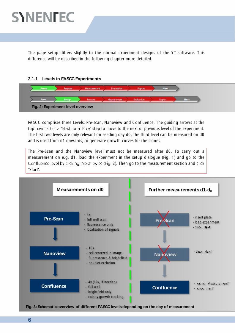
FASCC comprises three Levels: Pre-scan, Nanoview and Confluence. The guiding arrows at the

top step to move to the next or previous level of the experiment.

The first two levels are only relevant on seeding day d0, the third level can be measured on d0

and is used from d1 onwards, to generate growth curves for the clones.

The Pre-Scan and the Nanoview level must not be measured after d0. To carry out a

measurement on e.g. d1, load the experiment in the setup dialogue (Fig. 1) and go to the

2). Then go to the measurement section and click

Fig. 2: Experiment level overview

Further measurements d1-dn Measurements on d0

Fig. 3: Schematic overview of different FASCC levels depending on the day of measurement

- 4x

- full well scan

- fluorescence only

- localization of signals

- 10x

- cell centered in image

- fluorescence & brightfield

- doublet exclusion

- 4x (10x, if needed)

- full well

- brightfield only

- colony growth tracking

-

-

- insert plate

- load experiment

-

-

Pre-Scan

Nanoview

Confluence

Pre-Scan

Nanoview

Confluence

7

common experiment setups.

2.1.2 Autostart Nanoview

Autostart Nanoview automatically enters the next level and starts the next measurement using

the pre-defined selection filter. This check box should only be set after you have setup all optical

and operator analyzing parameters for your cell line.

2.1.3 Sub ROI Creation

It can be chosen between full well or merge result rois . This selection becomes active for the

next level, i.e. does not have any impact on current measurement.

1. Merge result ROIs:

The pre-scan determines the exact location of the potential clones inside the cells. With

this information the Nanoview scan can be done directly on the spot of the cell. If you

choose this option the objective lens will be directly positioned at the position of the cell

with this single sub-image only.

Fig. 4: Start to set up Start with choosing an experiment

name, your used plate type, the right

autofocus settings and the required

objective.

Fig. 5: Choose sub ROI creation for nanoview

8

2. Full well:

This option should be chosen in case it is uncertain if a second cell might have been

missed for any reason in the pre-scan and you want to ensure that there is no other cell

in the well. It is usually only used in a validation phase because it will take a little more

time due to the full well scan.

3. The Pre-Scan Measurement

3.1 Optical Setup and Preparation Pre-Scan

An optical setup and preparation is required - like for any experiment - if the properties of the

cells and the fluorescence are unknown or no template is available for such known assay.

Therefore it might be advantageous to put some more cells in a well (typically A1) for optical

adjustment.

Proceed as you would normally proceed for optical preparation by setting the channels for the

optical settings.

For e.g. CellTrackerTM Green, LED_Blue for Source and Emi_Green for Emi

After selecting the appropriate optical setting proceed with the preparation.

The settings for the fluorescence are determined using the same criteria as for any fluorescence

experiment. Having several cells in a well for adjustment allows better distribution of the

3. The Pre-Scan Measurement

Fig. 6: Fluorescence channel Choose your required light

source and emission filter.

9

potential fluorescence signals to be expected. Saturation of the fluorescence signal is not desired

but must be accepted if the weakest cell cannot be detected.

Otherwise try not to have too many cells in signal saturation (i.e. 255 counts). Increase exposure,

gain and intensity accordingly. Therefore, the used exposure and gain intensity should be set to

100%. There should be no fear of bleaching because the source will only illuminate the probe

while exposing with an automatic electronic shutter.

Under normal circumstances the default settings of the operator will work properly. You can

check the function and the correct identification of the cells by clicking on Process Image .

3.2 Measurement Pre-Scan

Click on the arrow for measurement and start the measurement by clicking the Start button

on the lower left side.

Process Images During Measurement and Show Images are set as default and should be left

in that state.

Fig. 7: FASCC pre-

Fig. 8: Options for measurement

10

3.3 Evaluation of Pre-Scan

3.3.1 Result Table in Analyst

The result table gives the best overview of the results. The total cell count will be displayed. It is

now possible to cross check the results and alter operator settings and reprocess as required by

the circumstances.

Fig. 9: FASCC pre-

Fig. 10: Analyst flag: Result table

11

3.3.2 ROI Filter Settings

The ROI Filter is used for selecting only the wells with potential single cells. Other numbers may

be set but are not recommended for FASCC.

Object Filter settings for Total Cell Count:

Fig. 11:

Fig. 12:

12

After clicking the Apply button the areas of single cells will be set. Close the Object Filter

window and proceed to the next level → Nanoview.

4. The Nanoview Measurement

The layout of the experiment page looks very similar to the pre-scan page. The major difference

is that you cannot choose any wells to be measured as this has been determined automatically

by the Object Filter setting in the previous level.

4.1 Optical Setup and Preparation Nanoview

The Sub ROI will be set to full well for a subsequent full well confluence measurement. Objective

default is 10x but other resolutions can be chosen, e.g. 20x, depending on what is most suitable.

In case that the Objective is changed, it is necessary to go back to the Evaluation page of the

pre-scan and set the ROI Filter again before continuing with the channel selection.

The channels should be set as follows: The Fluorescence channel as channel 1 and the Brightfield

channel as channel 2. Ensure that the Emi is set to the same filter for both channels otherwise

unnecessary changes of the filter will be carried out.

4. The Nanoview Measurement

Fig. 13:

13

4.1.1 Preparation Nanoview Measurement

When you click on the preparation arrow the lens will be positioned exactly over the first cell

found in the pre-scan. From here on you can setup the optics for the fluorescence and brightfield

channel.

The operator settings should only be altered if a doublet has been found and was not resolved.

This can only be done when the whole plate has been measured and the probability of finding

a doublet is higher. Another possibility in the evaluation phase would be to seed out more cells

per well and to search for doublets to ensure that the operator parameters are set properly. But

nevertheless the default values should work in most cases.

Fig. 14: Channel selection

Fig. 15:

14

4.1.2 Measurement Nanoview

When you switch to the measurement arrow you may observe the little rectangles, which show

the ROI (region of interest) to be measured in Nanoview. To start the experiment, click on the

Start button.

Fig. 16:

Fig. 17:

15

4.1.3 Evaluation Nanoview

After the measurement you can use the object filter in the same manner as for the pre-scan. The

Nanoview operator will separate doublets in either fluorescence or brightfield.

It is important to set the object filter to ensure that only real single clones will be monitored in

the subsequent confluence measurement.

5. The Confluence Measurement

As a last verification that there is only one cell in the well or as a starting point for a confluence

measurement series to monitor either proliferation or size of the colony growth, a full well

confluence measurement can be carried out.

If the confluence measurement of day 0 is already done and you want to carry out an e.g. daily

confluence measurement to observe the growth of the colonies, you do not have to consider

the Pre- ick on

uence

measurement as on day 0.

5.1 Optical Setup and Preparation Confluence

The layout of the setup page looks very similar to the Nanoview setup page. The well selection

The default objective is the 4x but other resolutions can be chosen, e.g. the 10x, depending on

what is most suitable. In case that the objective is changed, it is necessary to go back to the

Evaluation page of the Nanoview and set the ROI Filter again.

The next step is to go to the prepare page and to set up the optical and autofocus settings. If

icroplate will proceed automatically to the first well with one

cell.

Before an image can be obtained an autofocus must be carried out followed by a snapshot to

get an overview of the current image for the right optical settings (Fig. 18).

5. The Confluence Measurement

Fig. 18: Start with an autofocus

16

and use

cells and hide the histogram by clicking on the appropriate button. To cross check your settings,

upper left corner (Image Info Fig. 20). A value at abt. 130 counts reflects good settings. Press

actual overview of your settings.

Fig. 19: How to proceed with a confluence measurement after the seeding day (d1 - dn)

Open the FASCC application

Load your experiment

Continuous Confluence

Measurements after

Seeding Day (d0)

Click on to check your optical settings

Over an incubation period evaporation of

media can influence optical conditions.

TIP: Check and readjust the optical

settings before measuring again!

17

focus offset box and move the mouse wheel up/down or position the mouse cursor right into

the image and press CTRL while turning the mouse wheel. A good focus offset has been

achieved when suspension cells appear bright inside and dark at the rim, which is called the

Once all optical settings have been completed and the required image quality was found, the

image processing should now be tested. gs and view

the results. It is recommended to start using the Default parameters which in general ensure to

meet the desired results.

In case the result is not satisfactory the Image Processing Parameters can either be re-adjusted

or previously saved parameters may be used or the parameters can be reset to default.

Now proceed with the Measurement.

5.2 Measurement Confluence

There are two further options which may be chosen

on the lower left side to start the measurement.

hile the measurement will

be carried out. These options allow to zoom into the appropriate wells and to watch the imaging

process.

P the corresponding

arrow (Fig. 21).

Fig. 21: workflow arrows

Fig. 20: Image Info current grey value

18

5.3 Evaluation Confluence

You can now check your results by scrolling through the result table, the Heat map, a timed

chart graph, the Scatter plot and Histogram to obtain an overview. Therefore, click on the

the right. For each type of result presentation many different properties like

The above seen different colors of the Heat map represent the cell confluence according to the

covered area within each well. Blue represents a low and red a high cell confluence.

The Time chart allows the measurement of cells over several days and also presents details for

each well by simply clicking on the appropriate curve (Fig. 23).

Fig. 22: Analyst with the variety of result presentations

19

port the data from previously carried out experiments

(Fig. 24).

In case you are not satisfied with your results you can alter the image processing parameters

accordingly, check same by

clic ).

Fig. 23: Time chart Single or several curves and fields

may be selected by pressing

a) clicking on the required curve/field

or b) dragging the mouse cursor to

mark several fields at once.

Fig. 24: Possible options after measurement is done

20

6. Operator Explanation and Setting for FASCC

6.1 General Working Principles of FASCC Operators

The FASCC operators are divided into the FASCC Pre- and the FASCC Nanoview operator. Both

work similar except for the FASCC Nanoview which additionally utilizes a brightfield image for

evaluation. Thereby you can see that the parameter tables differ. For the pre-scan you will only

find parameters which are effective on fluorescent images.

If you take a closer look at the table for Nanoview there are parameter settings in the upper

section which are designed to set the parameters for the cluster analysis. In the lower section it

is possible to toggle between Fluorescence and Brightfield to adjust the parameters for the

different channels accordingly.

6.1.1 Fluorescence Evaluation

For both operators the fluorescence evaluation is done in two sequences. In a first step the

fluorescence image is evaluated and checked for fluorescent objects according to the parameter

settings. In a second step there is a so called Cluster Analysis which will be automatically

Fig. 25a: Parameter table for FASCC Pre

6. Operator Explanation and Setting for FASCC

Fig. 25b: Parameter table for FASCC Nanoview

21

performed on the initially identified objects. This closer look tries to separate two or more cells

from each other (if there are any) by taking a closer look into that relevant object. Depending

on the parameters these additional objects could be resolved. This analysis cycle is done for both

operators, the Pre and Nanoview.

6.1.2 Brightfield Evaluation

After its Fluorescence Cluster analysis the FASCC Nanoview operator uses the Brightfield

cluster analysis to double check for additional cells.

6.2 Show Cases for FASCC Pre Operator

6.2.1 Too Many Objects Found in Cluster Analysis

In the following you will see how altering the parameters generate different results.

Fig. 26: In this example the set default parameters

erroneously resolved this cell into three

objects using a 4x magnification.

Fig. 27:

the very little blob. But the result is not

satisfactory.

22

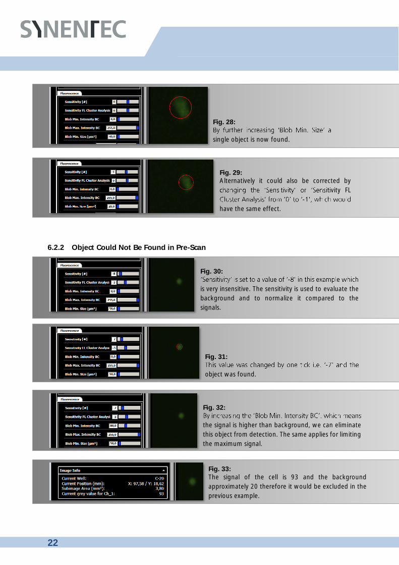
6.2.2 Object Could Not Be Found in Pre-Scan

Fig. 28:

single object is now found.

Fig. 29: Alternatively it could also be corrected by

vity FL

-

have the same effect.

Fig. 30: -

is very insensitive. The sensitivity is used to evaluate the

background and to normalize it compared to the

signals.

Fig. 31: -

object was found.

Fig. 32:

the signal is higher than background, we can eliminate

this object from detection. The same applies for limiting

the maximum signal.

Fig. 33: The signal of the cell is 93 and the background

approximately 20 therefore it would be excluded in the

previous example.

23

6.2.3 Eliminating Lint or Debris

Obviously one can see that this is not a cell. It looks more like lint or some dirt inside the well. It

is by far larger than any cell. This can be eliminated by confining the cell size through alteration

of Blob Max. Size .

Fig. 34: Detected lint

Fig. 35: Change the to exclude lint

24

6.3 Show Cases for FASCC Nanoview Operator

6.3.1 Erratically Identified Cell Doublet

In the following example (Fig.36-38) a light reflex was identified as a cell. This can be eliminated

by either reducing the Blob Min. Size or by taking geometrical aspects of the cell into account.

If we take the size as the only option we might end up losing a small cell somewhere else.

Another parameter change could help to avoid this. A critical parameter is also the so called

Longishness which describes to what extent the object reaches a perfect circle. A longishness

of 100 means a perfect circle and a longishness of 0 means a line.

With a value of 40 for longishness we could also eliminate the reflex.

Fig. 36: Detected light reflex

Fig. 37: Size change eliminated the reflex

Fig. 38: eliminated the reflex

25

6.3.2 Hard to Identify Cell Doublet

In the following case the second cell (if it is one) is smaller and much fainter than the first (bigger)

one. By observing the brightfield image this becomes clearer.

The image processing could use the brightfield image to identify them as two cells. On the left

side of the image processing table the sole parameter for the brightfield analysis is shown. It is

the sensitivity for the BF Cluster analysis

Fig. 39: Cell doublet in the fluorescence channel

Fig. 40: Cell doublet in the brightfield channel

26

7. Making a Template for FASCC

Saving a template in FASCC differs from the conventional template creating. It is not possible

to use the Save as Template button in the Experiment setup.

7.1 Template Preparation for FASCC

You need a defined experiment and have already carried out all steps through the levels from

pre-scan, Nanoview and confluence (which could be omitted). When the measurement in the

confluence level has been completed go back to the Nanoview and the pre-scan level and set

the checkboxes to Autostart Nanoview

Ins

If the Save Experiment is not applicable please toggle between one of the Autofocus options,

e.g. from one shot to each well and back. Then the button should become active and you can

save the experiment.

Now generate a new experiment by pressing the button New Experiment from Template and

use the previously saved experiment as template. Ensure that the Autostart Nanoview mode is

set and save this experiment. This is now your new template without any imaging data, which

can be used as a template.

SYNENTEC GmbH, Otto-Hahn-Str. 9a, 25337 Elmshorn, Germany www.synentec.com, AppSupport@synentec.com

SYNENTEC GmbH

Otto-Hahn-Str. 9a

25337 Elmshorn/Germany

Phone +49 (0)4121 46311-0

7. Making a Template for FASCC

26

Fig. 41: