Thieves, Thugs, and Neighborhood Poverty

David Bjerk

Robert Day School of Economics and Finance

Claremont McKenna College

500 East Ninth Street, Claremont CA 91711

Ph: 909-607-4471

david.bjerk@cmc.edu

April 25, 2010

Abstract

This paper develops a model of crime analyzing how such behavior is associated

with individual and neighborhood poverty. The model shows that even under relatively

minimal assumptions, a connection between individual poverty and both property and

violent crimes will arise, and moreover, "neighborhood" e¤ects can develop, but will

di¤er substantially in nature across crime types. A key implication is that greater

economic segregation in a city should have no e¤ect or a negative e¤ect on property

crime, but a positive e¤ect on violent crime. Using IV methods, I show this implication

to be consistent with the empirical evidence.

Keywords: Crime; Segregation; Neighborhood E¤ects; Instrumental Variables; Poverty.

1

�I don�t care if I got money, or work Monday through Friday. I just go shoot a

motherf*@#er on the weekends. If that�s what need to be done to keep my hood

and my young ones around here safe, then that�s what to get done�(quoted by

Landesman, 2007).

1 Introduction

High rates of crime and violence in poor neighborhoods have been described by numerous

scholars and journalists (Wilson, 1987; Krivo and Peterson, 1996; Kotlowitz, 1991; Patterson,

1991; Messner and Tardi¤, 1986, to name just a few). However, the quote above from a man

residing in a high-poverty housing project in south Los Angeles emphasizes that not only is

crime a large part of life in high-poverty neighborhoods, but also that violent crimes may

often serve a quite di¤erent purpose than basic property crime. Namely, while the motivation

for basic property crimes is generally purely monetary, becoming involved in violent crime

may have a defensive motivation as well.

While this defensive motivation for violence has long been recognized by sociologists

(Massey 1995; Anderson, 1999) and more recently by economists (Silverman, 2004; O�Flaherty

and Sethi, 2010), the mechanisms through which such motivations are exacerbated by indi-

vidual and neighborhood poverty are less well understood. This paper attempts to explicitly

model some of the key distinctions between participation in violent crimes versus basic

property crimes, as well as the ways such participation decisions might be a¤ected by an

individual�s own economic circumstances as well as the economic circumstances of his neigh-

bors. The paper also considers the broader implications of how these forces interact with

the degree to which a city is segregated by economic status to a¤ect overall crime rates.

While there may be numerous, and possibly quite complex, paths through which poverty

and neighborhood characteristics may a¤ect criminal behavior, the model developed here

traces out the implications of two quite simple assumptions regarding behavior and criminal

interactions. The �rst is simply that individuals incur diminishing marginal utility in money.

The second is with respect to how violent crimes di¤er from basic property crimes. Speci�-

cally, when it comes to basic property crimes, I assume that by choosing to become a thief at

any given period in time, an individual will simply have additional consumption beyond his

legal income in that period. Alternatively, when it comes to violent crimes, I assume that

individuals can choose to become either a thug (i.e., an individual who engages in violence)

or a law-abider (i.e., an individual who does not engage in violence). This will mean that

when two law-abiders encounter one another in their neighborhood, they pass each other

without incident. On the other hand, when a law-abider encounters a thug, the thug will

2

attack him and take some of his money. However, when two thugs encounter one another,

violence can still ensue but not necessarily with certainty. More importantly though, even

when violence does ensue in such encounters, I assume that neither is able to take money

from the other. In this way, choosing to be a thug can not only serve o¤ensive purposes,

allowing thugs to take money from law-abiders in their neighborhood, but also be defen-

sive in terms of ensuring ones�own money will not be taken by other thugs and potentially

preventing an attack from occurring in the �rst place.

As will be shown below, the above assumptions are su¢ cient to ensure that poor individ-

uals are more likely to become both thieves and thugs than an otherwise similar population

of non-poor individuals. With respect to becoming a thief, the intuition is quite straight-

forward. The diminishing marginal utility of money assumption will mean a poor individual

will value a �xed amount of money above and beyond his legal income more than will a

rich individual, meaning that poor individuals will have a stronger incentive than non-poor

individuals to steal, all else equal.

However, without additional assumptions, an individual will be no more or less likely to

become a thief if he lives in an extremely poor neighborhood versus a richer neighborhood,

meaning no �neighborhood e¤ects�will arise when it comes to basic property crimes. How-

ever, if it is further assumed that the return to theft is greater when a greater fraction of

one�s neighbors are non-poor, neighborhood e¤ects do arise, with individuals becoming more

likely to become thieves the smaller the fraction of their neighbors that are poor. Therefore,

all else equal, this model suggest that the degree to which a city�s poor residents are resi-

dentially segregated from the city�s non-poor residents will either have no e¤ect or even a

negative e¤ect on the city�s overall rate of basic property crime.

On the other hand, beyond the two basic assumptions discussed above, no further as-

sumptions are necessary for neighborhood e¤ects to arise with respect to violent crimes, as

an individual�s motivation to become a violent person (i.e., a thug) depends on the likelihood

he will run into other thugs in his neighborhood, which in turn can depend on the level of

poverty in his neighborhood. In fact, the model actually shows that the e¤ect of neigh-

borhood poverty on individual incentives to become a violent person becomes increasingly

stronger as the neighborhood poverty rate rises, which in turn implies that the more a city

is segregated by poverty status, the greater will be the overall rate of violent crime� the

opposite of what was true with respect to basic property crimes.

The latter part of the paper then empirically examines these two key implications of

the model at the citywide level� namely that all else equal, greater (exogenous) economic

segregation should have either a negligible or negative impact on basic property crimes

such as burglary, larceny and motor vehicle theft, but should have a positive impact on

3

interpersonal violent crimes such as robbery and aggravated assault. Using MSA level data

for the United States from the year 2000, I �nd support for these implications. In particular,

after I instrument for the economic segregation for each MSA using data on how public

housing is allocated in the MSA, the fraction of local public funds in the MSA coming from

the state or Federal government, the number of municipal governments in the MSA, and the

number of larger rivers in the MSA, I �nd greater economic segregation has a negative but

somewhat imprecisely estimated e¤ect on burglary, a negligible e¤ect on larceny and motor

vehicle theft, and a positive and signi�cant e¤ect on robbery and aggravated assault.

2 Related Literature

The theoretical model developed below relates to three particular streams of literature. The

�rst is that of neighborhood e¤ects, where individual behavior is directly a¤ected by the

characteristics and/or actions of his neighbors. For example, preferences for peer confor-

mity may alter an individual�s taste for engaging in crime (Glaeser et al.,1996; Brock and

Durlauf, 2001), or an individual�s information about payo¤s to crime may evolve di¤er-

ently depending on the number of criminals in his neighborhood (Lochner and Heavner,

2002; Calvo-Armengol and Zenou, 2004; Calvo-Armengol et al. 2007; Patacchini and Zenou,

2008). Somewhat relatedly, one individual�s criminal behavior may create a positive exter-

nality for other potential criminals in that one person�s criminal behavior taxes �xed police

resources, which in turn lowers the probability of detecting/arresting other criminals (Ferrer,

2010), or similarly, one neighborhoods�level of private policing may a¤ect the relative payo¤s

to crime in another neighborhood (Helsely and Strange, 2005). While these papers describe

how �neighborhood e¤ects� can arise given these assumptions, where a given individual�s

optimal behavior may be depend on which neighborhood he lives in, the model developed

below takes a step back to consider how individual and neighborhood level poverty in and of

themselves can a¤ect criminal behavior even in absence of the types of assumptions discussed

above.

The second area of research this model builds on is the literature on the relationship

between crime and segregation. In this vein, Verdier and Zenou (2004) develop a model of

labor market discrimination, crime, and racial segregation. While their model can imply

a correlation between crime and neighborhood income, it does not lead to �neighborhood

e¤ects� per say in that the actual characteristics of the an individual�s neighbors do not

directly a¤ect his own criminality. O�Flaherty and Sethi (2007) also model the relationship

between racial segregation and a particular type of crime� namely robbery. An important

4

contribution of this model is that criminal activity (namely robbery) and racial segregation

are simultaneously determined, with both a¤ecting the other. Moreover, individual criminal

behavior is a¤ected by the racial/income characteristics of his neighbors. However, a key

implication of O�Flaherty and Sethi�s model is that while higher robbery rates can lead to

greater segregation as the wealthier whites move away from the poorer blacks, greater segre-

gation should lead to lower robbery rates, as robbers would expect to meet more resistance

to robbery attempts when a city is more segregated. Therefore, this model suggests that

the simple correlation between robbery and segregation could be either positive or negative.

However, according to the model, exogenous sources of segregation should lead to lower rates

of robbery. As will be shown below, this is the opposite prediction from that generated in

the model developed here, suggesting that �nding exogenous sources of segregation will be a

key aspect to any attempts to empirically distinguish between O�Flaherty and Sethi�s model

and the one developed below.

The model developed below arguably most closely relates to the work describing how

violence may play a strategic role. In particular, the sociological work of Anderson (1999)

and Massey (1995) discusses how individuals adapt to high poverty isolated neighborhoods

by becoming obsessively concerned with �respect� in order to lower the risk of their own

criminal victimization, where such respect is maintained primarily through strategic use of

force. Relatedly, Jankowski (1991) argues that one of the central motivations for joining a

gang is often self-protection, even if by joining a gang an individual commits to perpetrating

violent acts against others. Silverman (2004) and O�Flaherty and Sethi (2010) develop

explicit models of such strategic violence, where individuals use violence as way of preempting

or deterring violence being done to them. While these papers consider the strategic role

of violence, they generally do not make explicit why such behaviors are connected to an

individual�s own income and the income distribution in the individual�s neighborhood, or

how the overall amount of violence may be a¤ected by the degree to which the poor are

residentially segregated from the non-poor in the overall community. The model below

attempts to develop these connections more formally.

3 Model of Crime, Poverty, and Neighborhood Com-

position

Consider a community made up of a large number of individuals who live for an in�nite

number of periods, where each individual can be classi�ed as having either low income or

high income. In the absence of committing any crime, assume low income individuals have !`

5

dollars available for consumption each period, while high income individuals have !h dollars

available for consumption each period, and individuals cannot save or borrow across peri-

ods. Let individuals value consumption in any given period according the a utility function

u, where u is an increasing strictly concave function in consumption, meaning individuals

incur diminishing marginal utility in money. Finally, suppose the overall community can be

divided up into a collection of neighborhoods, where each individual lives in one and only

one neighborhood. Let �k denote the fraction of residents in a given neighborhood k who

have low income (i.e. are poor), and let � denote the community-wide fraction of residents

who have low income.

3.1 Participation in Basic Property Crimes

First consider an individual�s decision to become a thief, or to engage in a property crime that

does not involve a direct confrontation with other individuals (e.g., Burglary, Larceny, Motor

Vehicle Theft). By becoming a thief, an individual i adds b units of additional consumption

above and beyond the consumption possible though consuming his legal income that period,

but also incurs a utility cost of �ip: In words, �ip represents each individual i�s disutility (or

possibly his utility if �ip < 0) associated with being a thief, such guilt or pleasure, as well

as the expected disutility associated with the possibility of receiving a jail sentence. This

parameter will be referred to as each individual�s �criminal propensity,� with a lower �ipindicating a higher criminal propensity. In order to focus only on the role income, assume

that �ip is an i.i.d. random draw from a normal distribution with mean �p and variance

�2p, and therefore is independent across individuals. Note that this means that this model

explicitly considers an environment where individual�s preferences and/or judicial costs for

committing or not committing crime are not directly in�uenced directly by their neighbors�

preferences or neighborhood characteristics, which has been the focus of much of the previous

literature on neighborhood e¤ects and crime (e.g. Glaeser, et al.,1996; Brock and Durlauf,

2001; Lochner and Heavner, 2002; Calvo-Armengol and Zenou, 2004; Calvo-Armengol et al.,

2007; Patacchini and Zenou, 2008; Ferrer, 2010; Helsley and Strange, 2005; Wilson, 1987;

Krivo and Peterson, 1996).

Given the discussion from above, an individual chooses to become a thief if and only if

u(!i + b) � �ip � u(!i), meaning the equilibrium fraction of individuals of income level !j(for j 2 f`; hg) living in neighborhood k who choose to become thieves in any given periodequals

��j = �p(u(!j + b)� u(!j)); (1)

6

where �p is the cumulative distribution for the normally distributed random variable �ip:

Because of the strict concavity of the u function, it is straightforward to see that ��h < ��` .

In words, because the utility associated with any �xed monetary payo¤ from stealing is

lower for high income individuals, high income individuals are less likely to become thieves.

Hence, the greater the overall fraction of a neighborhood who are of low income, the greater

the fraction of the neighborhood who become thieves. This argument also holds at the

community-wide level. Therefore, in this simple model, the rate of basic property crimes

committed in a neighborhood (or a whole community), should be increasing in the fraction

of neighborhood (community) made up of poor individuals. A second thing to notice about

��j as given in equation (1) is that it does not depend on �k. In words, the probability that

an individual becomes a thief does not depend on the income of his neighbors, meaning there

are no �neighborhood e¤ects�with respect to basic property crimes without making further

assumptions. Therefore, after controlling for the overall fraction of the community made up

of poor individuals, the level of economic segregation in the community as a whole should

have no direct e¤ect on the overall rate of basic property crimes.

One reasonable extension is to assume that the monetary bene�t to being a thief is greater

when fewer of one�s neighbors are poor, or if the monetary bene�t to being a thief is given

by b(�k), then b0(�k) < 0: In this case, equation (1) would become

��j(�k) = �p(u(!j + b(�k))� u(!j)):

Since b(�k) is decreasing in �k, the above equation implies that the fraction of individuals of

any given income level j who choose to become thieves is decreasing in �k. Therefore, when

the monetary bene�t to being a thief depends on the economic status of one�s neighbors,

there will exist neighborhood e¤ects with respect to becoming a thief. Moreover, note that

the change in expected criminality from moving an individual of income level !j from a

neighborhood k to a richer neighborhood k0 (meaning �k < �k0 and b(�k) > b(�k0)), will

equal

���j = �p(u(!j + b(�k))� u(!j))� �p(u(!j + b(�k0))� u(!j)):

Further note that the concavity of the u function implies [u(!j + b(�k))� u(!j)]� [u(!j +b(�k0)) � u(!j)] will be larger when !j = !` than when !j = !h. Therefore, a su¢ cient

condition for ���` > ���h is for � to be weakly convex when evaluated at or before u(!` +

b(�k))� u(!`). Given �p is the cdf of a normal distribution, this would be true for exampleif ��`(0) � 0:5, or if less than half of the poor individuals would choose to become thieves

even if they were the only poor person in their neighborhood.

7

Recalling that ���j denotes the expected change in criminality with respect to basic

property crimes from moving an individual of income level !j from a richer to a poorer

neighborhood, we can infer that an important implication of ���` being greater than ���h

is that there will be bigger increase in expected criminality when moving a poor individual

from a poorer neighborhood to a richer neighborhood than would be o¤set by the decrease

in expected criminality from moving a rich individual from the richer neighborhood to the

poorer neighborhood. This in turn implies that when the monetary bene�t to committing

a given basic property crime is inversely related to the fraction of the neighborhood that is

poor, less segregation will actually increase this type of basic property crime and vice versa.

In summary, the simple model laid out in this section shows that in the absence of assum-

ing preferences, information regarding payo¤s to crime, or policing depend on the behavior

or characteristics of one�s neighbors, greater segregation by income will either have no e¤ect,

or a negative e¤ect on community-wide basic property crimes, depending on whether the

monetary bene�t of basic property crime becomes greater the neighborhood poverty rate

decreases.

3.2 Participation in Interpersonal Violent Crime

Now consider crimes against persons, such as muggings, robberies, and assaults. In modelling

these crimes, assume each individual decides whether to be a �thug� or a �law-abider,�

then proceeds to encounter other individuals in his neighborhood at a rate of one person

per period. By choosing to be a law-abider, an individual commits to acting passively

when encountering anyone in his neighborhood. Alternatively, by choosing to be a thug, an

individual commits to violently attacking any law-abider he encounters in his neighborhood

and having a violent interaction with another thug with probability p 2 [0; 1].Therefore, when a law-abider and a thug encounter each other, the one-sided violence will

allow the thug to successfully rob the law-abider, thereby increasing the thug�s consumption

in that period by b; while decreasing the law-abider�s consumption that period by b and

further imposing a cost of c on the law-abider due to pain and su¤ering. We can think of

these interactions as �robberies.�Note that I assume that b does not depend on the income

of one�s victim. While the model is robust to loosening this assumption a little bit, I feel that

such an assumption is generally justi�ed. After all, it is not clear that poor individuals carry

less cash on them than do rich individuals, especially since poor individuals are less likely to

store their wealth in bank accounts or credit cards. A similar assumption and justi�cation

is made by O�Flaherty and Sethi (2007).

On the other hand, when two thugs encounter each other violence arises with probability

8

p, and when it does, both individuals will still incur a cost of c due to pain and su¤ering but

no money will change hands. We can think of these interactions as �aggravated assaults.�

Finally, when two law-abiders encounter each other, no violence takes place, meaning no

money changes hands and no pain and su¤ering arises.

The above assumptions can be motivated two ways. First, choosing to be a thug can

be interpreted as an individual learning the �ghting skills and/or obtaining the weapons

necessary to take possessions from law-abiders, who do not have such skills and/or weapons.

However, since other thugs also have �ghting skills and/or weapons, thugs cannot take

possessions from each other, but will incur substantial pain and su¤ering when they �ght. A

second, complementary interpretation is that choosing to be a thug is equivalent to joining a

street gang, where gang members take property from the non-gang members they encounter

in their neighborhood, while at the same time must periodically engage in violence when

encountering rival gang members, but do not lose their own property in such altercations.

Such motivation is consistent with some of the ethnographic literature on gangs. For example,

in summarizing the work of Savitz et al. (1980), Spergel (1990) states �(j)oining a gang may

also result from rational calculations to achieve personal security, particularly for males, in

certain neighborhoods.�

Finally, analogous to the basic property crime model, by choosing to be a thug an indi-

vidual i must further incur a utility cost �iv each period, where once again �iv is drawn from a

normal distribution with mean �v and variance �2v and is independent across individuals (but

is �xed for a given individual across periods). As before, this criminal propensity parameter

�iv captures the e¤ort and any feelings of guilt (or pleasure) associated with being a thug and

engaging in violence, as well as the expected disutility of being arrested and punished for

being a thug.

The above assumptions mean that the expected utility for any given period for an in-

dividual i of income level !j living in neighborhood k associated with becoming a thug is

given by

�[u(!j)� pc] + (1� �)u(!j + b)� �iv;

where � is the the likelihood he encounters a thug as opposed to a law-abider in his neigh-

borhood (which arises endogenously as shown below). Alternatively, the expected utility

from being a law-abider for any given period for an individual i of income level !j living in

neighborhood k is given by

�[u(!j � b)� c] + (1� �)u(!j):

9

Given the above expected utilities, we can derive that optimal behavior for an individual

i of income level j living in neighborhood k is to become a thug if and only if

�[u(!j)� u(!j � b) + (1� p)c] + (1� �)[u(!j + b)� u(!j)] � �iv: (2)

Like with basic property crimes, the above expression indicates that it will generally be those

with a low �iv, meaning those with high criminal propensities, who will choose to become

thugs.

In order to further simplify equation (2), de�ne �t(!j) to equal u(!j)�u(!j�b). In words,�t(!j) + (1� p)c is the opportunity cost incurred by not being a thug when encountering athug, for an individual with income !j. Similarly, de�ne �a(wj) to equal u(!j + b)� u(!j),meaning �a(!j) is the opportunity cost incurred by not being a thug when encountering a

law-abider, for an individual with income !j.

Given these de�nitions, equation (2) becomes

�(�t(!j) + (1� p)c) + [1� �]�a(!j) � �iv: (3)

This equation highlights the important components with respect to the decision individuals

make regarding whether or not to become a thug in this environment. Namely, the fraction

of individuals in a neighborhood choosing to become thugs is increasing in both the monetary

bene�t that can be obtained from doing so (i.e. �a(!j)), as well as the monetary and pain

and su¤ering cost that can be avoided by doing so (i.e. �t(!j)+(1�p)c). This latter bene�tto being a thug is one thing that makes the decision to become a thug di¤erent from the

decision to become a thief. Moreover, also unlike the decision regarding whether or not

to become a thief, the decision to become a thug depends on the overall fraction of other

individuals in the neighborhood who are thugs (i.e. �).

From equation (3), we can now derive this fraction of individuals of income level !j living

in neighborhood k choosing to be a thug to be

�j = �v(�(�t(!j) + (1� p)c) + [1� �]�a(!j)); (4)

where �v again denotes the cdf of a normal distribution. For simplicity, I will refer to the

fraction of individuals of a given group who choose to be a thug as the violent criminal

participation rate for this group.

A Nash Equilibrium in this environment will be when all individual criminal participation

decisions are optimal given everyone else�s criminal behavior. Intuitively, a Nash Equilibrium

will be an overall neighborhood violent crime participation rate � such that when each

individual makes his criminal participation decision that maximizes his expected utility given

10

this �; the resulting overall fraction of individuals in neighborhood k who choose to be thugs

equals �. This leads to Proposition 1.

Proposition 1 Given there is su¢ cient variation in violent criminal propensity over thepopulation (namely �v >

�t(!`)+(1�p)c��a(!`)p2�

), then for any �k 2 [0; 1], there exists a uniqueNash Equilibrium characterized by violent criminal participation rates for each income group

f��`(�k); ��h(�k)g; and an overall violent criminal participation rate ��(�k) = �k��`(�k)+(1��k)�

�h(�k), such that the following two equations hold:

��`(�k) = �v(��(�k)(�t(!`) + (1� p)c) + [1� ��(�k)]�a(!`));

��h(�k) = �v(��(�k)(�t(!h) + (1� p)c) + [1� ��(�k)]�a(!h));

Proof. In Proofs Appendix.

Note that the assumption regarding the variance in criminal propensity (i.e. �v >�t(!`)��a(!`)p

2�) is essentially just a regularity condition that assumes the distribution of criminal

propensity is relatively di¤use.

Given the existence and uniqueness of an equilibrium, a �rst thing to note is that the

strict concavity of the u function implies that (�t(!`) + (1 � p)c) > (�t(!h) + (1 � p)c) (orequivalently �t(!`) > (�t(!h)), and �a(!`) > �a(!h).1 In words, low income individuals will

have a greater incentive to become thugs than will higher income individuals all else equal.

The intuition is similar to that with respect to basic property crimes. Since each individual�s

utility function exhibits diminishing marginal utility in consumption (and therefore income),

the greater the individual�s legal income each period, the smaller is the utility lost from

getting a relatively small amount of money taken from them in any given period, and the

smaller is the utility gained by taking a relatively small amount of money from someone else.

This intuition can be seen in Figure 1.

These di¤ering incentives across income types leads to Proposition 2.

Proposition 2 In any neighborhood k, a greater fraction of low income individuals will

participate in interpersonal violent crimes (i.e. be thugs) than high income individuals, or

1Technically, this result is only guaranteed when !h � b > !` + b. In other words, when the changesin wealth associated with mugging or being mugged are small compared to the overall income di¤erencesbetween high income and low income individuals.

11

��`(�k) > ��h(�k).

Proof. In Proofs Appendix.

At this point it is worth noting that the model suggests that there is likely be a strong

correlation between those who choose to become thieves and those who choose to become

thugs for two reasons. First, it is certainly reasonable to think that there is a strong cor-

relation between �ip and �iv within individuals. In other words, those who incur relatively

low disutility from committing burglaries also likely incur relatively low disutility from com-

mitting assaults and robberies. However, even in the absence of a correlation between the

preference parameters �ip and �iv, the model still suggests that there will be a large overlap

between those who commit property crimes and those who commit violent crimes due to the

fact that both types of crime will be correlated with an individual�s economic circumstances.

The next thing to examine is how the likelihood of becoming a thug depends on the

poverty rate of one�s neighbors (i.e. �k), which leads to Proposition 3.

Proposition 3 Given there is su¢ cient variation in violent criminal propensity over thepopulation (namely �v >

�t(!`)+(1�p)c��a(!`)p2�

), then for both high and low income individuals,

the fraction choosing to participate in interpersonal violent crimes is increasing in the fraction

of their neighborhood that has low income, or@��j (�k)

@�k> 0 for j = h; `.

Proof. In Proofs Appendix.

Proposition 3 shows that, in this model, an individual with income level j is more likely

to become a thug if he lives in a relatively poor neighborhood than in a relatively rich neigh-

borhood, meaning there exist neighborhood e¤ects with respect to violent crime. Intuitively,

when an individual expects a relatively high fraction of his neighbors to be thugs (as he

would in a high poverty neighborhood), his own incentive to become a thug is primarily

defensive, in the sense of being able to prevent other thugs from taking his property. Alter-

natively, when an individual expects very few of his neighbors to be thugs (as he would in

a low poverty neighborhood), his own incentive to become a thug is primarily to o¤ensive,

in the sense of being able to successfully take property from others. Due to the diminishing

marginal utility of consumption, we know �t(!j)+(1�p)c > �a(!j) for j = h; ` and p 2 [0; 1],meaning the defensive incentive for becoming a thug in a poor neighborhood is greater than

the o¤ensive incentive in a richer neighborhood.

Pushing the model a little bit further, we can examine whether the strength of this

neighborhood e¤ect (i.e.@��j (�k)

@�k) di¤ers by the income level of the individual. This leads to

12

Proposition 4.

Proposition 4 If ��`(1) � 0:5, the neighborhood e¤ect will be stronger for low income indi-viduals than high income individuals, or @��` (�k)

@�k>

@��h(�k)

@�k.

Proof. In Proofs Appendix.

Intuitively, from Figure 1 above, we know that regardless of income level, the opportunity

cost associated with not being a thug when encountering a law-abider is smaller than the

opportunity cost of not being a thug when encountering another thug. This di¤erence in

opportunity costs accounts for the greater likelihood of becoming a thug in low poverty

neighborhoods (where the likelihood of encountering a thug is high) than in higher poverty

neighborhoods (where the likelihood of encountering a thug is low). Moreover, the strict

concavity of the u function implies that this di¤erence in opportunity costs is greater for low-

income individuals than high-income individuals (as can also be seen in Figure 1). Thus, low-

income individuals will be more in�uenced by the income characteristics of their neighbors

than will higher-income individuals when it comes to committing violent crimes.2

We can now analyze how the income distribution within a neighborhood, as well as

how income is distributed across neighborhoods within the overall community, a¤ect the

rate of interpersonal violent crime. To start this analysis, �rst recall that the equilibrium

fraction of individuals in any particular neighborhood k choosing to become thugs is given by

��(�k) = �k��`(�k)+ (1��k)��h(�k). Taking the derivative of this equation and re-arranging

gives

@��(�k)

@�k= (��`(�k)� ��h(�k)) + �k

@��`(�k)

@�k+ (1� �k)

@��h(�k)

@�k:

From Proposition 2 we know that the �rst expression in parentheses in the above equation

is positive, and from Proposition 3 we know that the second and third expressions in the

above expression are also positive. Therefore, if we assume the overall rate of interpersonal

violent crime within a neighborhood at any given point time is a strictly increasing function of

2The su¢ cient condition for this result, namely ��` (1) � 0:5; essentially says that this result will alwayshold if a relatively large fraction of poor individuals incur su¢ cient disutility from choosing to engage inthe thug life such that they will still choose not to become thugs even if all of their neighbors are poor(i.e. a large fraction of individuals have a low criminal propensity or high �iv). It is worth noting that thisis a su¢ cient condition for Proposition 4 to hold, but is not necessary. If we drop the assumption that �i

is normally distributed, a su¢ cient condition for Proposition 4 is that the cumulative distribution of �i issimply weakly convex prior to ��` (1).

13

the fraction of the residents in the neighborhood who are thugs at that time, then increasing

the fraction of the neighborhood made up of low income individuals will increase the overall

rate of interpersonal violent crime in the neighborhood.

Furthermore, note that if we take the second derivative of ��(�k) and re-arrange, we

obtain

@2��(�k)

@�2k= 2

�@��`(�k)

@�k� @�

�h(�k)

@�k

�+ �k

@2��`(�k)

@�2k+ (1� �k)

@2��h(�k)

@�2k:

From Proposition 4, we know the expression in parentheses in the above equation is positive.

Moreover, as long as we again assume ��`(1) � 0:5 and �v >�t(!`)��a(!`)p

2�, both of the latter

two terms in the above expression are also positive (see Appendix for formal proof), implying@2��(�k)@�2k

> 0. This leads to Proposition 5.

Proposition 5 The rate of interpersonal violent crime in the community as a whole isincreasing in the degree to which its neighborhoods are segregated by income.

Proof. Given @��(�k)@�k

> 0 and @2��(�k)@�2k

> 0, we know the fraction of a neighborhood that

chooses to become thugs is an increasing strictly convex function of the fraction of the

neighborhood that is poor. Therefore, for any given community wide fraction poor �, the

interpersonal crime rate in the overall community is minimized when all neighborhoods have

the same fraction of the poor. Alternatively, the rate of interpersonal crime in the community

as a whole becomes greater the more its neighborhoods are segregated by income.

The intuition for Proposition 5 comes from Proposition 4, which showed that neighbor-

hood e¤ect more strongly in�uences poor individuals than rich individuals. Therefore, the

rate of interpersonal violent crime should necessarily be higher the more poor individuals

are segregated from richer individuals all else equal. Note that just the opposite was true

with respect to the basic property crime model developed above.

In summary, this model reveals the important role of poverty at both the individual and

neighborhood level can play when it comes to crime rates. The model shows how even with

very few assumptions, the strategic role of violence can interact with neighborhood poverty

rates to create neighborhood e¤ects on individual decisionmaking. Notably, a key feature

of this model is that it implies that neighborhood e¤ects with respect to violent crime are

likely to be more pronounced and di¤erent in nature than any that might arise with respect

to basic property crime. This is in contrast to many of the other models of neighborhood

e¤ects highlighted at the beginning of Section 2, where the neighborhood e¤ects that arise

in those models would not necessarily di¤er across crime types. While this is not the �rst

14

model suggesting a link between segregation and crime (for example the O�Flaherty and Sethi

(2007) paper discussed above, as well as sociological work such as Blau and Blau (1982)),

it is unique in its focus on primarily income driven forces, and its di¤erential predictions of

the e¤ect of segregation on di¤erent types of crime.

4 Empirically Evaluating the Model

While the model presented above was in many ways quite simplistic, abstracting from many

other potentially important determinants of crime rates in cities, there is still value in at-

tempting some empirical analysis of the propositions of the model. While it would be

optimal to empirically evaluate all of these propositions, there are a variety of hurdles one

must face in attempting to do so. These hurdles are highest with respect to testing the

individual-level propositions 2 - 4. Mostly notably, there are severe data constraints as one

would need individual level data regarding criminal participation distinguished by crime type

and frequency, own legal income, as well as information regarding the income characteristics

of each individual�s neighbors. A reasonably large and representative dataset containing such

data is not readily available to my knowledge.

Given these data constraints, I will focus on the key community-level implications inher-

ent in Section 3.2 and Proposition 5, or that, all else equal, greater economic segregation

in a city should lead to higher rates of violent interpersonal crimes but have negligible or

even a negative impact on basic property crime rates. These community-level implications

do not face the same data constraints as the individual-level implications since information

on criminal activity by crime type, as well as measures of economic segregation (as well as a

host of other community-level characteristics) are readily available at the MSA/PMSA level

(�MSAs�from here on). The data and variables I use for this analysis are described below.

It is also important to note that the preceding models of basic property and violent

crime considered segregation to be exogenous to the community. Clearly, while the degree to

which a city is segregated by poverty status may have an impact on di¤erent types of crime

for the reasons speci�ed in the model, it may also be true that greater criminal activity

a¤ects the level of segregation by poverty status in overall community. Therefore, given

the model treated the level of segregation in a community as exogenous, I will attempt to

focus on plausibly exogenous variation in segregation across cities using instrumental variable

methods as will be discussed in more detail below.

FBI Uniform Crime Reports (UCR)

15

The FBI Uniform Crime Reporting Program is a nationwide program covering roughly

94 percent of the total U.S. population, and 96 percent of the population living in MSAs.

(Federal Bureau of Investigation, 2000).3 In this analysis, I use the 2000 FBI UCR data

to look at separately at the �ve most common Index crimes� robbery, aggravated assault,

burglary, larceny-theft, and motor vehicle theft.4 A major distinction between these crime

categories is that Aggravated Assault and Robbery are de�ned to be violent crimes involving

a direct confrontation with the victim, while Burglary, Larceny, and Motor Vehicle Thefts are

de�ned as non-violent property crimes that explicitly do not involve a direct confrontation

with the victim (Federal Bureau of Investigation, 2000).5 Therefore, I will refer to Aggravated

Assault and Robbery as �violent interpersonal crimes,�and Burglary, Larceny, and Motor

Vehicle Thefts as �basic property crimes.�

I also use the FBI UCR data from 1999 to measure the number of o¢ cers per 1000

residents in each city, to account for di¤erences in police presence across cities. Moreover,

since the FBI UCR crime data are reported at the county level, I determined crime rates

and o¢ cer rates for each MSA by aggregating all relevant data for counties that fall within

a particular MSA. Because most counties either fall in one MSA or fall in zero MSAs, this

generally provided accurate MSA crime information. However, several New England counties

are divided between two or more distinct MSAs. Since I could not determine which MSA

to assign the reported crimes in these counties to, I had to exclude these New England

MSAs that contained shared counties from the analysis.6 Finally, I dropped all MSAs with

fewer than 150,000 residents since their crime rates, especially for violent crime, �uctuate

substantially from year to year even though there are relatively modest changes in the number

of crimes.

MSA Population CharacteristicsData regarding MSA population characteristics come for the most part from the 2000

United States Census Summary File 3. I use these data to obtain measures of a variety of

3This data was made available through the National Archive for Criminal Justice Data (NACJD) andthe Inter-University Consortium for Political and Social Research (ICPSR) study #3451.

4I do not look at the two other Index crimes� rape and murder� because the number of these crimesare relatively small, especially in smaller cities, making the rates somewhat uninformative. In particular, inmany smaller cities there are less than 5 of such crimes reported in a given year, meaning for example thatone more murder in a given year will increase the murder rate in that city by 20 percent or more.

5Car-jacking, or taking an individual�s car by threat or force, is counted as robbery, not a motor vehicletheft.

6This criteria excluded the following MSAs: Bangor ME, Boston MA-NH, Burlington VT, HartfordCT, Lewiston-Auburn ME, Manchester NH, Pitts�eld MA, Portland ME, Portsmouth-Rochester NH-ME,Spring�eld MA. The Miami FL MSA, the Bloomington-Normal IL MSA, and the Champaign-Urbana ILMSA were also dropped from the sample because the FBI UCR reports did not provide crime data for theseMSAs in 2000.

16

demographic characteristics for each MSA (see Table I for particular variables). I also use

data from the Department of Housing and Urban Development�s �A Picture of Subsidized

Households - 1998�to determine the fraction of households in each MSA that receive housing

assistance. Finally, to control for the potential e¤ects of weather on criminal activity (see

Jacob et al., 2007), I determined the average number of very hot days (i.e. temperature of

90 degrees or higher) per 100 days for each state, as well as the average number of very cold

days (i.e. temperature of 32 degrees or lower) per 100 days for each state using data from

the National Climatic Data Center.

Table I summarizes all of the above variables for the sample used in this analysis.

4.1 The Correlation between Economic Segregation and Crime

While there exist several plausible ways to measure the level of income segregation within

a city, I primarily employ the isolation index.7 This index attempts to measure the extent

to which individuals of one group are only exposed to one another, rather than members

of the other group, in their neighborhoods (Massey and Denton, 1988). In the context of

segregation by poverty status, this index is essentially computed to be the fraction poor in

the census tract occupied by the average poor individual in that MSA, and is given by the

following formula:

Poverty Isolation Index =NXi=1

pooripoortotal

pooripersonsi

;

where i denotes census tract. The higher this index is, the greater the level of segregation.

Looking at this segregation statistic when it is computed using all census tracts in each

MSA reveals a potentially problematic issue, namely that among the twenty MSAs with the

highest Poverty Isolation Index are College Station TX, Gainsville FL, Athens GA, Talahas-

see FL, Lafayette IN, Madison WI, Provo-Orem UT, and Las Cruces NM; all moderate to

small MSAs containing large universities. The concern this raises is that full-time students

who do not live in dormitories will generally be counted as poor, since they earn little or no

income while in school. Moreover, such students tend to live almost exclusively in census

tracts surrounding their University, causing MSAs with relatively high college student pop-

ulations to appear relatively segregated by poverty status, but not in the way we generally

are attempting to capture. Therefore, I also computed the Poverty Isolation Index for each

MSA excluding those census tracts containing over 60 percent students. This will be the

7All segregation measures used in this paper were computed using the Census Summary File 3 datadiscussed previously.

17

preferred measure of Poverty Segregation, however, as I will also show, results do not di¤er

substantively by using Poverty Isolation Indices computed using all census tracts.

We can begin by looking at the relationship between crime and poverty segregation by

using simple OLS speci�cations, regressing the MSA crime rate, for each type of crime sepa-

rately, on the Poverty Isolation Index for the MSA and a variety of other MSA characteristics.

Table II shows separate speci�cations for each type of crime, where the dependant variable

is the rate of that crime per 100,000 residents, standardized to have a mean of zero and

standard deviation of one. I use these standardized rates in order to facilitate comparing

magnitudes across crimes, as the overall rates per 100,000 residents di¤er dramatically across

crimes (as can be seen in Table I).

Looking at the �rst row of Table II, we can see that conditional on the MSA level

characteristics, the correlation between segregation by poverty status and crime rates is

relatively weak across all crime categories, but there is some evidence that segregation by

poverty status is positively correlated with motor vehicle theft, robbery, and aggravated

assault.8

While these OLS results reveal some small di¤erences in the correlation between poverty

segregation and crime across di¤erent types of crime, these results are not necessarily very

informative about the degree to which such economic segregation actually a¤ects MSA-wide

crime rates for these di¤erent types of crimes. In particular, as alluded to previously, the

level of segregation in an MSA may be endogenous since people generally have substantial

choice about where to live within a city and crime rates might a¤ect this decision.

Such selection may bias the causal interpretation of the OLS results for several reasons.

For example, as alluded to previously, O�Flaherty and Sethi (2007) (as well as Cullen and

Levitt (1999)) argue that rising crime rates may lead to �ight from central cities, especially

by the wealthy (and therefore disproportionately white). This means that any positive rela-

tionship between crime and segregation may arise not because greater segregation increases

crime, but because greater crime leads to greater economic and racial segregation. Therefore,

the OLS results presented previously may be upwardly biased.

Alternatively, as violent crime increases in a city, for example as gangs become more

8I also constructed Racial Isolation Indices for each MSA (using all census tracts). The coe¢ cients onthe Racial Isolation Index in speci�cations otherwise ananlogous to those in Table II are insigni�cantlydi¤erent from zero at any standard level of signi�cance in the Burglary, Larceny, and Motor Vehicle Theftspeci�cations. However, the coe¢ cients on the Racial Isolation Index are positive and signi�cant at the 1percent level in the Robbery and Aggravated Assault speci�cations. Like the coe¢ cients in Table II, thesecoe¢ cients were also relatively small in magnitude, with the coe¢ cients indicating that a one standarddeviation in the Racial Isolation Index is correlated with a 0.25 and 0.31 standard deviation increase inRobbery and Aggravated Assault rates respectively� �ndings consistent with Shihadeh and Flynn (1996).The estimated coe¢ cients on the other variables are almost identical to those in Table II.

18

prominent, individuals living in the neighborhoods where these gangs operate have a greater

incentive to take on the expenses associated with moving. Indeed, escaping from gangs and

crime was the primary reason participants in the MTO housing relocation program gave for

signing up for the program (Kling, Ludwig, and Katz, 2005). Given that these neighborhoods

where violence and gang activity are greatest are often the poorest neighborhoods in a city,

those emigrating from these neighborhoods will generally be poorer than the residents of the

neighborhoods they move to. Therefore, it is also possible that as crime increases, a city

becomes somewhat less economically segregated than it would be otherwise, meaning the

OLS results discussed previously could also be downwardly biased.9

4.2 Controlling for the Potential Endogeneity of Segregation

To overcome the potential simultaneity bias we must �nd some characteristics that vary

across Metropolitan areas that a¤ect current income segregation, but can be credibly ex-

cluded from having any direct relationship to current levels of criminal activity. Given the

existence of such variables, we can then use them as instruments in Two-stage Least Squares

(2SLS) approach.10

The �rst instrument for segregation by poverty status that I employ is the fraction of

public housing assistance that was allocated in the form of apartments in government owned

public housing structures as opposed to allocated via Section 8 housing vouchers or certi�-

cates (or other types of subsidies to non-government property owners). The data used to

create this instrument once again comes from the HUD�s �A Picture of Subsidized House-

holds - 1998�described above. By design, public housing structures group poor individuals

together to a greater extent than do housing vouchers which can generally be used anywhere

in the city. Indeed, the HUD data shows that the census tracts surrounding Public Housing

Structures are almost 40 percent poor on average, compared with an average of around 20

percent poor for census tracts surrounding those units procured via vouchers or certi�cates.

Moreover, since public housing projects constitute a stock of facilities that generally have

existed for a considerable number of years prior to the year 1998 (the year in which the

measures come from for this analysis), it is unlikely that the overall fraction of housing

assistance provided via apartments in public housing projects in 1998 was directly related to

the factors determining the crime conditions in the MSA in the period around 2000, especially

9For more formal and detailed discussions of racial and economic segregation that are not related tocrime, see Sethi and Somanathan (2004) and Bayer et al. (2004).10Optimally, one might want to look at the relationship between changes in economic segregation over

time and changes in crime rates. However, such a method would not allevaite the basic endogeneity concernon its own, and therefore would require time-varying instruments for economic segregation. As will be seenbelow, the instruments used here are not time varying.

19

after controlling for a variety of other MSA characteristics (including the overall fraction of

households receiving housing subsidies of either form in each MSA). Indeed, data from �A

Picture of Subsidized Housing in the 1970s�(also made available by HUD) con�rms that the

number of in-kind public housing units used to provide housing assistance throughout U.S.

cities in 1998 was essentially determined several decades ago. Speci�cally, over 87 percent

of the public housing projects that existed in 1977 still existed and were in use in 1998.

Moreover, very few public housing projects were built between the 1970s and 1998, with 62

percent of all public housing projects that existed and were in use in 1998 being constructed

prior to 1977, and over 92 percent of those projects larger than 200 units being constructed

prior to 1977. Overall, this evidence reveals that most of the current use of public housing

project units was determined by decisions made in the 1970s or before, well prior to the large

increases in crime that occurred in the 1980s or any of the decreases in crime that took place

over the 1990s.

The second variable I use as an instrument for segregation by poverty status was �rst

used by Cutler and Glaeser (1997) as an instrument for racial segregation� namely the share

of local government revenue in an MSA that comes from the state or federal government in

1962.11 With more money coming from outside sources, there is less of an incentive for

individuals within a city to segregate by income, since a smaller fraction of local public

goods are funded through local taxes. Therefore, a greater fraction of local revenue coming

from the state or federal government should lead to less economic segregation in an MSA.12

The �rst column of numbers in Table III shows the results of the �rst stage regression

of the Poverty Isolation Index calculated using all census tracts on the two instruments

meeting the exclusion restriction and the other MSA characteristics included in the original

regressions from Table II. The second column of numbers in Table III shows the analogous

results that arise when using the Poverty Isolation Index calculated using only census tracts

made up of less than 60 percent students. As can be seen, the two instruments discussed

above are signi�cantly related to Poverty Isolation Index (using either calculation method) in

the predicted manner. However, as should be expected, both the magnitude of the estimated

coe¢ cients on the excluded instruments, as well as the F-statistic for the joint signi�cance

of the two instruments, are larger when using the Poverty Isolation Index calculated using

only census tracts made up of less than 60 percent students.13 Therefore, I will again focus

11This data comes from the Census of Governments 1962, made available by the Inter-University Consor-tium for Political and Social Research (ICPSR) website.12Note that while Cutler and Glaeser (1997) motivate this instrument identically to here, they use theirs to

instrument for racial segregation, under the further motivation that income and race are strongly correlatedin the U.S.13Indeed, the F-statistic on the joint signi�cance of the instruments when using the Poverty Segregation

Index calculated without the student heavy census tracts is arguably large enough to mitigate any concerns

20

on the results using this construction of the Poverty Isolation Index.

Table IV shows the results from the 2SLS speci�cations. The �rst column in Table IV

reveals that, if anything, greater segregation by poverty status actually decreases rates of

burglary. While not statistically signi�cant at standard levels of signi�cance (p-value 0.117),

the coe¢ cient is relatively large in magnitude, suggesting that a one standard deviation

increase in the Poverty Isolation Index leads to a decrease in burglary rates by roughly two-

thirds of a standard deviation.14 Alternatively, the results shown in Table IV with respect to

larceny and motor vehicle theft reveal little e¤ect of segregation by poverty status on these

crimes.

Finally, the most notable results are shown in the last two columns of Table IV, which

suggest that greater segregation by poverty status leads to much higher rates of the violent

interpersonal crimes of robbery and aggravated assault, with these e¤ects being statistically

signi�cant at the 10 percent level or higher. The point estimates indicate that a one standard

deviation increase in the Poverty Isolation Index is associated with an increase in robbery

rates by roughly two-thirds of a standard deviation and almost nine-tenths of a standard

deviation increase in the rate of aggravated assault.15

Table V shows that the above 2SLS results are robust to other measures of segregation.

In particular, the top panel of Table V reveals the coe¢ cients on di¤erent poverty segrega-

tion measures in otherwise analogous 2SLS speci�cations. The top row of numbers in Table

V simply repeats the coe¢ cients on the Poverty Segregation Index shown in the top row of

Table IV. The remaining rows show the analogous coe¢ cients when using several alternative

construction methods for measures of segregation. Speci�cation 1 uses the (standardized)

Poverty Isolation Index calculated using all census tracts (including those made up of over

60 percent college students). Speci�cation 2 uses the (standardized) Poverty Dissimilarity

Index, which answers the question "what share of the poor population would need to change

census tracts for the poor and non-poor to be evenly distributed within a city?" and is con-

structed using the formula 12

PNi=1 j

pooripoortotal

� non-poorinon-poortotal

j for each MSA (Massey and Denton,1988). Speci�cation 3 uses the (standardized) Poverty Dissimilarity Index but constructed

without using those census tracts made up of over 60 percent college students. Speci�cation

regarding weak instrument bias (Stock and Yogo, 2002).14This translates to an almost 50 percent lower burglary rate (computed using the mean and standard

deviation for burglaries from Table I).15Given the mean and standard deviation for robbery rates per 100 thousand residents are 133 and 85

respectively, the above estimates suggest that a one standard deviation increase in poverty segregation leadsto a roughly 40 percent higher robbery rate, all else equal. Similarly, given the mean and standard deviationfor aggravated assault rates are 321and 165 respectively, the above estimates suggest that a one standarddeviation increase in poverty segregation leads to roughly 45 percent higher aggravated assault rate, all elseequal.

21

4 once again uses the (standardized) Isolation Index computed using all census tracts, but

adjusts for the overall fraction of the MSA that is poor (see Cutler and Glaeser, 1997).16

Speci�cation 5 again uses this "adjusted" Poverty Isolation Index, but computes it exclud-

ing those census tracts made up of over 60 percent college students. One concern regarding

all of these poverty segregation measures is that they treat the poor as being distinct from

everyone else including the near poor, which obviously is not true. Therefore, Speci�cation 6

again uses the Poverty Isolation Index calculated using all census tracts, but excludes those

individuals in each census tract whose household earnings are above the poverty line but less

than one and a half times the poverty line (the "near" poor), and Speci�cation 7 uses the

Poverty Isolation Index that both excludes those census tracts made up of over 60 percent

students and excludes those individuals who are "near" poor.

As the upper panel of Table V shows, the coe¢ cients on the segregation index in the

Burglary speci�cations are negative using all seven alternative indices and signi�cantly so

in six of them with magnitudes both somewhat smaller and larger than the coe¢ cients that

arise using the preferred measure (i.e. top row). The coe¢ cients on the poverty segrega-

tion indices in the Larceny and Motor Vehicle Theft speci�cations are negative using all

seven alternative measures, but never even close to being statistically di¤erent from zero.

However, the coe¢ cients on the alternative poverty segregation indices in the Robbery and

Aggravated Assault speci�cations are always positive and signi�cantly so in twelve of the

fourteen speci�cations, with magnitudes again both somewhat smaller and somewhat larger

than those shown in the top row of Table V.

Finally, the lower panel of Table V shows the 2SLS coe¢ cients on three di¤erent indices

of racial segregation. As can be seen, the results generally mimic the results of the economic

segregation indices� greater racial segregation seems to have no e¤ect on larceny and motor

vehicle theft, a negative impact on burglary (in fact signi�cantly so), and a positive and

signi�cant impact on robbery and aggravated assault. To the extent that racial segregation

is another measure of economic segregation, this evidence is consistent with the model.

Interestingly, even thought the instruments are argued to be a¤ecting income segregation,

the F-statistic on the instruments suggests that they are even more strongly correlated with

racial segregation. This could either be because the instruments do indeed have a more

16This index is constructed to be the followingPN

i=1(p o o ri

p o o rtotal

p o o rip e r s o n si

)�( p o o rtotalp e r s o n stotal

)

min(p o o rtotalp e r s o n s`

;1)�( p o o rtotalp e r s o n stotal

); where persons` is the

number of persons in the census tract with the lowest population with in the city and i once again denotescensus tract. The �rst term in the top part of the above equation is the fraction poor in the census tractoccupied by the average poor individual. From this, we can subtract the percentage poor in the city as awhole to eliminate the e¤ect coming from the overall size of the poor population. This whole term is thennormalized to be between zero and one, with one indicating the city is the most segregated it can possiblybe.

22

direct impact on racial segregation than economic segregation, or because race is actually a

better measure of true economic circumstances than income from one year as measured by

the Census.

In their paper on the consequences of ghettos, Cutler and Glaeser (1997) also use two

further instruments for (racial) segregation beyond the fraction of local government rev-

enue coming from the State or Federal governments� namely the number of local municipal

governments in each MSA, and the number of rivers �owing through each MSA.17 I also

estimated the 2SLS speci�cations using these variables as additional instruments for poverty

segregation. However, as the top three rows of Table VI show, using these additional in-

struments leads to no substantive di¤erences in the estimated results, but does dramatically

lower the F-statistic on the joint signi�cance of the excluded instruments in the �rst stage

regression. The fact that these further instruments do not seem to add much power to the

analysis is the reason why they were not included in the "preferred" speci�cations shown in

Table IV. Moreover, the last row of Table VI shows the coe¢ cients on the Poverty Isolation

Index variable in the �ve 2SLS speci�cations using only the Cutler and Glaeser instruments

(i.e. the fraction of local revenue received from state or federal sources, the number of mu-

nicipal governments in each MSA, and the number of rivers in each MSA). These coe¢ cients

show that not using the �fraction of public housing given in-kind� instrument does alter

the coe¢ cients a good deal (especially those in the larceny and motor vehicle theft speci�-

cations), but the general conclusion remains that greater economic segregation appears to

have di¤erential e¤ects on violent crimes versus basic property crimes.

4.3 Discussion of Empirical Results

Clearly, the validity of the 2SLS results presented above rest on the validity of the proposed

instruments. On the most basic level, Table III (and the last column of Table V) showed

that both of the primary instruments argued to meet the exclusion restriction are indeed

signi�cantly correlated with segregation in the predicted manner. Therefore, one criteria for

the validity of the instruments seems to be met. Moreover, given we have more excluded

instruments than potentially endogenous variables, the model is overidenti�ed, which means

we can directly test whether it is inappropriate to exclude the instruments discussed above

from being related to crime in 2000 other than through segregation (Wooldridge, 2002). The

instruments pass this test. In particular, the p-value on the Sargan Overidenti�cation test

17There has been considerable debate on how this variable should be property measured (see Rothstein(2007) and Hoxby (2007)). Given it is not the focus of this analysis, I simply decided to use the numberof �long� rivers �owing through each MSA as coded by Jesse Rothstein. Thanks to Jesse Rothstein forproviding me with this data.

23

statistics for the speci�cations in Table IV range from 0.13 (Motor Vehicle Theft) to 0.81

(Robbery).

Another potential test of the validity of these instruments is to see if they have a sig-

ni�cant relationship to other key metro area characteristics, such as the poverty rate or the

poverty rate for blacks, after controlling for segregation by poverty status, as well as the

other metro area characteristics. If they do, this suggests that these proposed instrumental

variables may directly in�uence a variety of characteristics of a city in addition to segrega-

tion, which may then have their own direct a¤ects on crime.18 However, running similar �rst

stage regressions to those shown in Table III, but using �percent living in poverty�as the

dependant variable and adding the Poverty Isolation Index to the right-hand side variables,

the coe¢ cients on the two excluded instruments are small in magnitude and statistically in-

signi�cant at any standard level of signi�cance. Similarly, when I regress �percent of blacks

living in poverty� on the instruments, any of the segregation indices, and the remaining

right-hand side variables, the coe¢ cients on the two instruments are again small and statis-

tically insigni�cant. In other words, other than through their relationship to segregation, the

two instruments do not appear to be related to poverty rates as a whole or poverty rates for

blacks. Moreover, when I do the analogous exercise with "percent of households headed by

single mother" as the dependant variable I again get coe¢ cients that are small in magnitude

on both instruments, but while small in magnitude, the coe¢ cient on the public housing

instrument is signi�cantly negative at the 5% level. In other words, if anything, after con-

trolling for all of the other metro area characteristics, a higher fraction of public housing

given in-kind leads to lower rates of single parent headed households. Therefore, the above

tests are consistent (though admittedly not conclusive) with the notion that instruments are

not simply picking up the e¤ects of some omitted variable that a¤ects both current crimes

rates and the composition of public housing subsidies and/or the historical sources of local

revenue.

Even given the above discussion however, it is certainly plausible that something about

one of the key instruments, namely fraction of public housing given in kind, is directly related

to criminal activity. For example, there is a large literature on the relationship between

public housing and crime related to the notion of �defensible space�(Jacobs, 1961; Newman,

1972). Advocates for defensible space in public housing argue that criminality in large public

housing projects is often facilitated by unmaintained common areas that residents must pass

through but have very little control over, such as hallways and common courtyards, and

residents in such facilities are often separated by both physical barriers and distance from

the wider community at large. While the empirical work on defensible space issues is varied

18Thanks to Francisco Martorell for suggesting this.

24

and shows some mixed results (Repetto, 1974; Pyle, 1976; Du¤ala, 1976; Molumby, 1976;

Mawby, 1977), this notion that lack of defensible space in public housing projects can directly

impact crime does not necessarily invalidate this instrument. In particular, the instrument

can still be argued to be an exogenous source of current segregation, as two of the key aspects

of the theorized relationship between lack of defensible space and crime relate directly to

the model of crime developed in the previous section. Namely, the presence of unmaintained

common areas that residents must pass through increases the likelihood of encounters with

thugs, which all else equal will increase relative payo¤ to becoming a thug. Similarly, the

separation of the residents of large housing projects from the broader less poverty stricken

community is exactly the type of segregation at work in the model. Hence, these issues with

respect to defensible space closely mirror those in the model. All this being said, one must

certainly consider the possibility that the results discussed in the previous subsection are

in�uenced by some particular unmodeled relationship between criminality and the physical

environment inherent in public housing structures.

In the end, though, perhaps the strongest evidence that mitigates concerns regarding the

invalidity of the proposed instruments are the di¤erential �ndings across crime types in the

2SLS speci�cations. In particular, if the instruments were strongly related to unmeasured

variables a¤ecting opportunities for the poor and/or black residents, such as social services

availability and schooling, or there was a fundamental di¤erence between living in public

housing structures versus otherwise economically similar neighborhoods, we should expect

the 2SLS results to be similar across crime types, or even more strongly positive for basic

property crimes. Intuitively, if the instruments are directly related to some omitted variable

measuring relative depravation or lack of opportunities for the poor and/or blacks, such

relative deprivation should impact basic property crime behavior in similar ways to violent

crime behavior. However, the 2SLS results discussed above contradict this, and instead

reveal that these instruments appear to have a negative or negligible relationship with basic

property crimes, but a strong positive relationship to violent crimes.

Finally, it is also interesting to consider the di¤erences in the empirical results across the

di¤erent basic property crime categories within the context of the model. For example, the

empirical results suggested that greater economic segregation has an arguably negative im-

pact on burglary rates. In the context of the model, this suggests that an individual�s payo¤

to burglary depends on the economic characteristics of his neighbors. This would be true

if burglars focused their crimes on the other residents of their neighborhoods. This seems

plausible, as a person would generally only break and enter a residence or commercial estab-

lishment if he had knowledge of something valuable to steal. Clearly, such information would

be better locally than more distantly. On the other hand, the empirical results suggested

25

that greater segregation had no impact on larceny and motor vehicle theft. In the context of

the model this would suggest an individual�s payo¤ to these crimes does not depend on the

economic characteristics of his neighbors. Given larceny and motor vehicle theft generally

involve taking readily observable items, perpetrators of such crimes can easily travel to other

neighborhoods to commit such crimes, suggesting it to be reasonable that the payo¤ to such

crimes has little relationship to his own neighbor�s characteristics.

5 Conclusion

The model developed in this paper showed that a very standard behavioral assumption,

namely that individuals incur diminishing marginal utility of money, can have substantial

implications when it comes to criminal participation. In particular, the model not only

showed how such an assumption can cause poverty to a¤ect an individual�s likelihood of

engaging in all types of crime, but also that �neighborhood e¤ects�can actually arise under

very minimal additional assumptions, particularly when it comes to violent crime.

Importantly, the model also showed that the diminishing marginal utility of money as-

sumption will mean that this neighborhood e¤ect with respect to violent crime will be

stronger for poor individuals than non-poor individuals, or in other words, that violent

criminal behavior of poor individuals may be more in�uenced by their neighborhood eco-

nomic characteristics than is the violent criminal behavior of non-poor individuals. This in

turn was shown to imply that while greater (exogenous) economic segregation might have

no e¤ect or potentially even a negative e¤ect on the overall amount of basic property crime,

it may be expected to lead to a higher level of violence than would occur if the poor were

more evenly dispersed throughout the city.

While this implication was shown to be consistent with several empirical �ndings, cer-

tainly more evidence is necessary to de�nitively conclude that this model provides an im-

portant component regarding the connections between crime and poverty. However, if true,

this theoretical model leads to a very important conclusion. Namely, that when it comes to

violent crime, not only do an individual�s own economic characteristics matter, but so do

the economic characteristics of his neighbors. Therefore, while it is clear that policies dic-

tating how public housing is allocated and how an urban area is developed will a¤ect who is

victimized by crime, such policies may also have a signi�cant impact on who commits crime

and the overall amount of crime that occurs. Moreover, the results of this paper suggest

that demolition and decreased use of large housing projects over the last decade may be an

important component in declining rates of violence over the last decade.

26

Acknowledgment Thanks to Jenny Hunt, Lance Lochner, Nicolas Marceau, John Dono-hue, Rucker Johnson, Jacob Klerman, Paco Martorell, Steve Raphael, and Je¤rey Timber-

lake, as well as seminar participants at McMaster University, UQAM, York University, Rice

University, University of Houston, Texas A&M, Claremont McKenna College, RAND, The

Goldman School at UC-Berkeley, USC, and San Diego State University. I also want to thank

the editor of this journal as well as two anonymous referees for their helpful comments.

27

6 Proofs Appendix

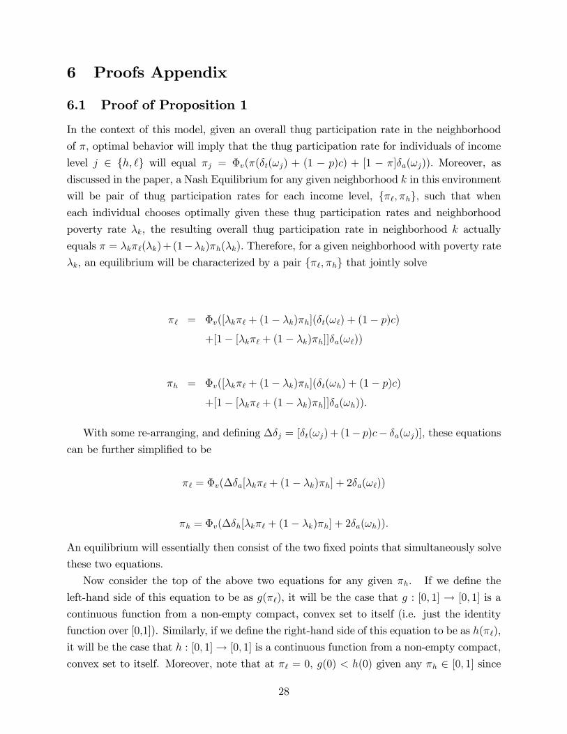
6.1 Proof of Proposition 1

In the context of this model, given an overall thug participation rate in the neighborhood

of �; optimal behavior will imply that the thug participation rate for individuals of income

level j 2 fh; `g will equal �j = �v(�(�t(!j) + (1 � p)c) + [1 � �]�a(!j)): Moreover, asdiscussed in the paper, a Nash Equilibrium for any given neighborhood k in this environment

will be pair of thug participation rates for each income level, f�`; �hg; such that wheneach individual chooses optimally given these thug participation rates and neighborhood

poverty rate �k, the resulting overall thug participation rate in neighborhood k actually

equals � = �k�`(�k)+ (1��k)�h(�k): Therefore, for a given neighborhood with poverty rate�k, an equilibrium will be characterized by a pair f�`; �hg that jointly solve

�` = �v([�k�` + (1� �k)�h](�t(!`) + (1� p)c)+[1� [�k�` + (1� �k)�h]]�a(!`))

�h = �v([�k�` + (1� �k)�h](�t(!h) + (1� p)c)+[1� [�k�` + (1� �k)�h]]�a(!h)):

With some re-arranging, and de�ning ��j = [�t(!j) + (1� p)c� �a(!j)]; these equationscan be further simpli�ed to be

�` = �v(��a[�k�` + (1� �k)�h] + 2�a(!`))

�h = �v(��h[�k�` + (1� �k)�h] + 2�a(!h)):

An equilibrium will essentially then consist of the two �xed points that simultaneously solve

these two equations.

Now consider the top of the above two equations for any given �h. If we de�ne the

left-hand side of this equation to be as g(�`), it will be the case that g : [0; 1] ! [0; 1] is a

continuous function from a non-empty compact, convex set to itself (i.e. just the identity

function over [0,1]). Similarly, if we de�ne the right-hand side of this equation to be as h(�`),

it will be the case that h : [0; 1]! [0; 1] is a continuous function from a non-empty compact,

convex set to itself. Moreover, note that at �` = 0, g(0) < h(0) given any �h 2 [0; 1] since

28

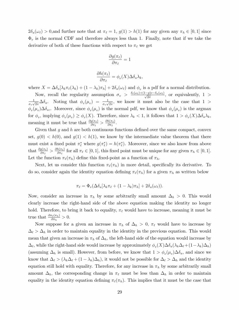
2�a(!`) > 0;and further note that at �` = 1, g(1) > h(1) for any given any �h 2 [0; 1] since�v is the normal CDF and therefore always less than 1. Finally, note that if we take the

derivative of both of these functions with respect to �` we get

@g(�`)

@�`= 1

@h(�`)

@�`= �v(X)��a�k;

where X = ��a[�k�`(�k) + (1� �k)�h] + 2�a(!`) and �v is a pdf for a normal distribution.Now, recall the regularity assumption �v >

�t(!`)+(1�p)c��a(!`)p2�

; or equivalently, 1 >1

�vp2���a. Noting that �v(�v) =

1�vp2�; we know it must also be the case that 1 >

�v(�v)��a,. Moreover, since �v(�v) is the normal pdf, we know that �v(�v) is the argmax

for �v; implying �v(�v) � �v(X). Therefore, since �k < 1, it follows that 1 > �v(X)��a�k,meaning it must be true that @g(�`)

@�`> @h(�`)

@�`:

Given that g and h are both continuous functions de�ned over the same compact, convex

set, g(0) < h(0); and g(1) < h(1), we know by the intermediate value theorem that there

must exist a �xed point ��` where g(��`) = h(�

�`). Moreover, since we also know from above

that @g(�`)@�`

> @h(�`)@�`

for all �` 2 [0; 1], this �xed point must be unique for any given �h 2 [0; 1].Let the function �`(�h) de�ne this �xed-point as a function of �h:

Next, let us consider this function �`(�h) in more detail, speci�cally its derivative. To

do so, consider again the identity equation de�ning �`(�h) for a given �h as written below

�` = �v(��a[�k�` + (1� �k)�h] + 2�a(!`)):

Now, consider an increase in �h by some arbitrarily small amount �h > 0: This would

clearly increase the right-hand side of the above equation making the identity no longer

hold. Therefore, to bring it back to equality, �` would have to increase, meaning it must be

true that @�`(�h)@�h

> 0.

Now suppose for a given an increase in �h of �h > 0; �` would have to increase by

�` > �h in order to maintain equality in the identity in the previous equation. This would

mean that given an increase in �h of �h; the left-hand side of the equation would increase by

�`, while the right-hand side would increase by approximately �v(X)��a(�k�`+(1��k)�h)

(assuming �h is small): However, from before, we know that 1 > �v(�v)��a, and since we

know that �` > (�k�`+ (1� �k)�h), it would not be possible for �` > �h and the identity

equation still hold with equality. Therefore, for any increase in �h by some arbitrarily small

amount �h; the corresponding change in �` must be less than �h in order to maintain

equality in the identity equation de�ning �`(�h). This implies that it must be the case that

29

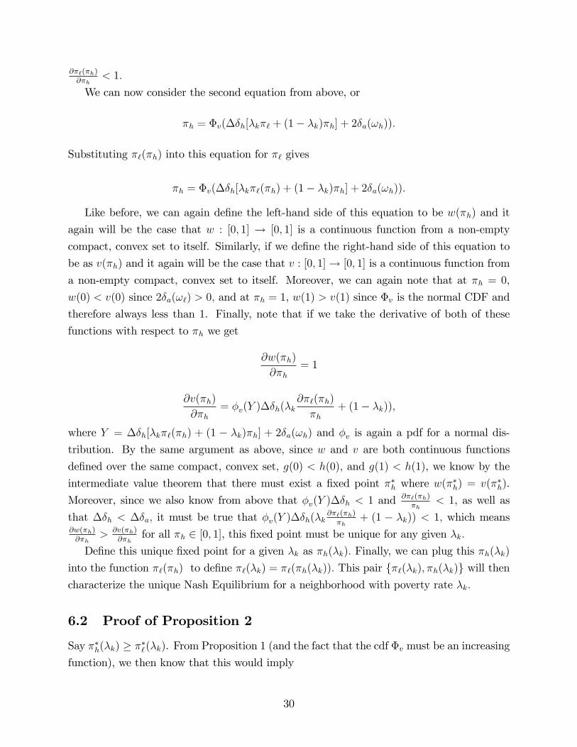
@�`(�h)@�h

< 1:

We can now consider the second equation from above, or

�h = �v(��h[�k�` + (1� �k)�h] + 2�a(!h)):

Substituting �`(�h) into this equation for �` gives

�h = �v(��h[�k�`(�h) + (1� �k)�h] + 2�a(!h)):

Like before, we can again de�ne the left-hand side of this equation to be w(�h) and it

again will be the case that w : [0; 1] ! [0; 1] is a continuous function from a non-empty

compact, convex set to itself. Similarly, if we de�ne the right-hand side of this equation to

be as v(�h) and it again will be the case that v : [0; 1]! [0; 1] is a continuous function from

a non-empty compact, convex set to itself. Moreover, we can again note that at �h = 0,

w(0) < v(0) since 2�a(!`) > 0; and at �h = 1, w(1) > v(1) since �v is the normal CDF and

therefore always less than 1. Finally, note that if we take the derivative of both of these

functions with respect to �h we get

@w(�h)

@�h= 1

@v(�h)

@�h= �v(Y )��h(�k

@�`(�h)

�h+ (1� �k));

where Y = ��h[�k�`(�h) + (1 � �k)�h] + 2�a(!h) and �v is again a pdf for a normal dis-tribution. By the same argument as above, since w and v are both continuous functions

de�ned over the same compact, convex set, g(0) < h(0); and g(1) < h(1), we know by the

intermediate value theorem that there must exist a �xed point ��h where w(��h) = v(��h).

Moreover, since we also know from above that �v(Y )��h < 1 and @�`(�h)�h

< 1, as well as

that ��h < ��a; it must be true that �v(Y )��h(�k@�`(�h)�h

+ (1 � �k)) < 1; which means@w(�h)@�h

> @v(�h)@�h

for all �h 2 [0; 1], this �xed point must be unique for any given �k:De�ne this unique �xed point for a given �k as �h(�k): Finally, we can plug this �h(�k)

into the function �`(�h) to de�ne �`(�k) = �`(�h(�k)): This pair f�`(�k); �h(�k)g will thencharacterize the unique Nash Equilibrium for a neighborhood with poverty rate �k:

6.2 Proof of Proposition 2

Say ��h(�k) � ��`(�k). From Proposition 1 (and the fact that the cdf �v must be an increasingfunction), we then know that this would imply

30

��(�k)(�t(!h)+(1�p)c)+[1���(�k)]�a(!h) � ��(�k)(�t(!`)+(1�p)c)+[1���(�k)]�a(!`):

Re-writing the above expression we get

��(�k)[�t(!h)� �t(!`)] + (1� ��(�k))[�a(!h)� �a(!`)] � 0:

Noting that �t(!`) > �a(!`) > �t(!h) > �a(!h) (as can be seen in Figure 1), we can see that

the above equation cannot hold. Therefore, it cannot be true that ��h(�k) � ��h(�k), meaning��h(�k) < �

�h(�k), con�rming Proposition 1.

6.3 Proof of Proposition 3

From Proposition 1 and the de�nition of ��(�k), we know that for j = h; `, the following

equation must hold

��j(�k) = �v([�k��`(�k) + (1� �k)��h(�k)](�t(!j) + (1� p)c)

+[1� �k��`(�k)� (1� �k)��h(�k)]�a(!j)):

Taking the derivative of the above equation with respect to �k and re-arranging we get

@��j(�k)

@�k= �v(x

�j(�k))[�t(!j)� �a(!j) + (1� p)c]

� + �k

@��`(�k)

@�k+ (1� �k)

@��h(�k)

@�k

�(5)

where �v is the pdf of the normal distribution evaluated at x�j(�k) = [�k�

�`(�k) + (1 �

�k)��h(�k)](�t(!j)+(1�p)c)+[1��k��`(�k)� (1��k)��h(�k)]�a(!j) and = ��`(�k)���h(�k)

(where is known to be strictly positive by Proposition 2). Next, note that the above

equation implicitly de�nes two equations of the following form:

A = �v(x�`(�k))��a[ + �kA+ (1� �k)B] (6)

B = �v(x�h(�k))��h[ + �kA+ (1� �k)B]; (7)

where A = @��` (�k)

@�k; B =

@��h(�k)

@�k, and again ��j = [�t(!j) + (1 � p)c � �a(!j)] (where ��j

can easily be con�rmed to be strictly positive). Solving equation (6) for A then substituting

31

into equation (7) and re-arranging we get

B

�(x�h(�k))��h= 0 +

��(x�`(�k))��a(1� �k)1� �(x�`(�k))��a�k

B + (1� �k)B; (8)

where 0 = 1��(x�` (�k))��a�k

:Now recall the assumed regularity condition that �t(!`)+(1�p)c��a(!`)p2�

<

�v. This implies 1�vp2���a < 1; or equivalently (noting that �(�v) =

1�vp2�given "iv is nor-

mally distributed) that

1� �(�v)��a > 0: (9)

Furthermore, given that "iv is normally distributed we know �(�") � �(x) for all x. Finally,recalling that 0 < �k < 1, we know that it must be true that 1� �(x�`(�k))��a�k > 0, andtherefore 0 > 0:

We can now simplify equation (8) to get

B =�(x�h(�k))��h[1� �(x�`(�k))��a�k]

1� �(x�`(�k))��a�k � (1� �k)�(x�h(�k))��h 0: (10)

Now note that the above equation implies B > 0 as long as (i) 1��(x�`(�k))��a�k > 0, and(ii) 1��(x�`(�k))��a��(1��)�(x�h(�k))��h > 0. Condition (i) was shown to hold above. Toprove that condition (ii) will hold true, note that ��a > ��h (as can be con�rmed in Figure

1) and recalling 0 < �k < 1, we know that 1 � �k�(x�`(�k))��a � (1 � �k)�(x�h(�k))��h >1� �(x�`(�k))��a. Noting again that the regularity assumption implies 1� �(x)��a > 0 forall x (as shown above), we know that condition (ii) must also hold. Therefore, B > 0, which

con�rms @��h(�k)

@�k> 0. An analogous argument can be made to show @��` (�k)

@�k> 0 by solving

equation (7) for B and substituting into equation (6).

6.4 Proof of Proposition 4

First, recall equation (5) above

@��j(�k)

@�k= �(x�j(�k))[�t(!j)� �a(!j) + (1� p)c]

� + �k

@��`(�k)

@�k+ (1� �k)

@��h(�k)

@�k

�:

From the above expression we can see that @��` (�k)

@�k>

@��h(�k)

@�kif (i) �t(!`) � �a(!`) >

�t(!h) � �a(!h) and (ii) �(x�`(�k)) � �(x�h(�k)). Given our assumption that u in an in-

creasing strictly concave function, we know condition (i) will always be true (see Figure 1).

Regarding condition (ii), given our assumption that �v is the cdf of the normal distribu-

32

tion and therefore convex for all x such that �(x) � 0:5, we know �v(x1) � �v(x2) for all

x2 � x1 � 0:5: Therefore, recalling that

��j(�k) = �v(x�j(�k))

and ��`(�k) > ��h(�k); we know that �v(x�`(�k)) � �v(x

�h(�k)) as long as �

�`(�k) < 0:5.

Given ��`(�k) < ��`(1) (as implied by Proposition 3), this con�rms that if �

�`(1) < 0:5 then

@��` (�k)

@�k>

@��h(�k)

@�kfor all �k � 1:

6.5 Proof that @2��j (�k)

@�2k> 0 for j = h; `

From the proof of Proposition 2 we know

@��j(�k)

@�k= �v(x

�j(�k))��j

� + �k

@��`(�k)

@�k+ (1� �k)

@��h(�k)

@�k

�:

where again ��j = [�t(!j)��a(!j)+(1�p)c] and = ��`(�k)���h(�k): Taking the derivativeof the above expression we get

@2��j(�k)

@�2k= �0v(x

�j(�k))��

2j

� + �k

@��`(�k)

@�k+ (1� �k)

@��h(�k)

@�k

�+

�v(x�j(�k))��j

�2

�@��`(�k)

@�k� @�

�h(�k)

@�k

�+ �k

@2��`(�k)

@�2k+ (1� �k)

@2��h(�k)

@�2k

�Simplifying the above expression we get

@2��j(�k)

@�2k= �j + �v(x

�j(�k))��j

��j + �k

@2��`(�k)

@�2k+ (1� �k)

@2��h(�k)

@�2k

�where �j = �

0v(x

�j(�k))��

2j

h + �k

@��` (�k)

@�k+ (1� �k)@�

�h(�k)

@�k

iand �j = 2

�@��` (�k)

@�k� @��h(�k)

@�k

�:

From Proposition 2 we know �j > 0 as long as ��`(1) � 0:5 (which will ensure �0v(x�j(�k)) > 0as discussed above in the proof to Proposition 3), and from Proposition 3 we know �j > 0.

We can simplify the above equation one more time to become

@2��j(�k)

@�2k= �v(x

�j(�k))��j

� j + �k

@2��`(�k)

@�2k+ (1� �k)

@2��h(�k)

@�2k

�(11)

where now j =�j

�v(x�j (�k))��j

+�j. Note again that since �j > 0 and �j > 0 (as shown above),

it must also be true that j > 0:

As in the proof of Proposition 2, note that equation (11) implicitly de�nes two equations

33

A = �v(x�`(�k))��a[ ` + �kA+ (1� �k)B] (12)

B = �v(x�h(�k))��h[ h + �kA+ (1� �k)B]; (13)

where A = @2��` (�k)

@�2k; B =

@2��h(�k)

@�2k. Solving equation (12) for A then substituting into equation

(13) and re-arranging we get

B

�(x�h(�k))��h= 0h +

��(x�`(�k))��a(1� �k)1� �(x�`(�k))��a�k

B + (1� �k)B; (14)

where 0h = h(1��(x�` (�k))��a�k)+ `�(x�` (�k))��a�k

1��(x�` (�k))��a�k. Note that 0h > 0 as long as 1��(x�`(�k))��a�k >

0. As shown in the proof to Proposition 2, this will always hold given the assumption that

"iv is normally distributed and the regularity condition that��ap2�< �v. Given this, note that

equation (14) is of the same form as equation (10) in the proof to Proposition 2. Therefore,

the proof that B > 0 follows identically from that in the analogous proof to Proposition 2,

meaning @2��h(�k)

@�2k> 0. As in the proof to Proposition 2, the proof that A > 0, and therefore

that @2��` (�k)

@�2k> 0, follows in a similar manner.

34

References

[1] Anderson, E., 1999. Code of the street: decency, violence and the moral life of the inner

city. New York: W.W. Norton and Company.

[2] Bayer, P., McMillan, R., Rueben, K., 2004. What drives racial segregation? New evi-

dence using census microdata. Journal of Urban Economics 56(3): 574-35.

[3] Blau, J.R., Blau, P.M., 1982. The cost of inequality: metropolitan structure and violent

crime. American Sociological Review 47: 114-129.

[4] Brock, W., Durlauf, S.N., 2001. Discrete choice with social interactions. Review of

Economic Studies 68(2): 235-260.

[5] Calvo-Armengol, A., Zenou, Y., 2004. Social networks and crime decisions: The Role

of Social Structure in Facilitating Delinquent Behavior. International Economic Review

45(3): 939-958.

[6] Calvo-Armengol, A., Verdier, T., Zenou, Y., 2007. Strong ties and weak ties in employ-

ment and crime. Journal of Public Economics 91: 203-233.

[7] Cullen, J.B., Levitt, S.D., 1999. Crime, urban �ight, and the consequences for cities.

Review of Economics and Statistics 81(2): 159-69.

[8] Cutler, D., Glaeser, E., 1997. Are ghettos good or bad? Quarterly Journal of Economics

112(3): 827-72.

[9] Cutler, D., Glaeser, E., Vigdor, J., 1999. The rise and decline of the american ghetto.

Journal of Political Economy 107(3): 455-506.

[10] Du¤ala, T., 1976. Convenience stores: armed robbery, and the physical environmental

features. American Behavioral Scientist 20: 227-247.

[11] Duncan, O.D, Duncan, B., 1955. Amethodological analysis of segregation indices. Amer-

ican Sociological Review 20(2): 210-17.

[12] Federal Bureau of Investigation, 2000. Crime in the United States 2000, Uniform Crime

Reports. U.S. Department of Justice, Washington D.C.

[13] Ferrer, R., 2010. Breaking the law when others do: A model of law enforcement with

neighborhood externalities. European Economic Review 54(2): 163-180.

35

[14] Glaeser, E., Sacerdote, B., Scheinkman, J., 1996. Crime and social interactions. Quar-

terly Journal of Economics 111: 507-548.

[15] Heavner, L., Lochner, L., 2002. Social networks and the aggregation of individual deci-

sion. Working Paper, University of Western Ontario Department of Economics.

[16] Helsley, R.W., Strange, W.C., 2005. Mixed markets and crime. Journal of Public Eco-

nomics 89: 1251-1275.

[17] Hoxby, C., 2007. Does competition among public schools bene�t students and taxpayers?

Reply. American Economic Review 97(5): 2026-2037.

[18] Jacob, B., Lefgren, L., Moretti, E., 2007. Dynamics of criminal behavior: evidence from

weather shocks. Journal of Human Resources 42(3): 489-527.

[19] Jacobs, J., 1961, The death and life of great american cities. New York: Random House.

[20] Jankowski, M.S., 1991. Islands in the street: gangs and american urban society. Berke-

ley: Unversity of California Press.

[21] Kling, J., Ludwig, J., Katz, L., 2005. Neighborhood e¤ects on crime for female and male

youth: evidence from a randomized housing voucher experiment. Quarterly Journal of

Economics 120(1).

[22] Kotlowitz, A., 1991. There are no children here, New York: Random House Inc.

[23] Krivo, L., Peterson, R.D., 1996. Extremely disadvantaged neighborhoods and urban

crime. Social Forces 75(2): 619-650.

[24] Landesman, P., 2007. Nine miles and spreading. LA Weekly, December 14-20: 44-51.

[25] Logan, J.R., Messner, S., 1987. Racial residential segregation and suburban violent

crime. Social Science Quarterly 68: 510-527.

[26] Massey, D.S., 1995. Getting away with murder: segregation and violent crme in urban

america. University of Pennsylvania Law Review 143(5): 1203-1232.

[27] Mawby, R.I., 1977. Defensible space: a theoretical and empirical appraisal. Urban Stud-

ies 14: 169-180.

[28] Massey, D.S., Denton, N., 1988. Suburbanization and segregation in U.S. metropolitan

areas. American Journal of Sociology 94(3): 592-626.

36

[29] Messner, S. F., Tardi¤, K., 1986. Economic inequality and levels of homicide: an analysis

of urban neighborhoods. Criminology 24: 297-317.

[30] Molumby, T., 1976. Patterns of crime in a university housing project. American Behav-

ioral Scientist 20: 247-261.

[31] Murray, M.P., 2006. Avoiding invalid instruments and coping with weak instruments.

Journal of Economic Perspectives 20(4): 111-132.

[32] Newman, O., 1972. Architectual design for crime prevention. Washington, D.C.: U.S.

Department of Justice.

[33] O�Flaherty, B., Sethi, R., 2007. Crime and segregation. Journal of Economic Behavior

and Organization 64: 391-405.

[34] � � . 2010. Peaceable kingdoms and war zones: preemption, ballistics and murder in

newark, in: DiTella, R., Edwards, S., Schargrodsky, E., (Eds). University of Chicago

Press.

[35] Patacchini, E., Zenou, Y., 2008. The strength of weak ties in crime. European Economic

Review 52: 209-236.

[36] Patterson, E.B., 1991. Poverty, income inquality, and community crime rates. Criminol-

ogy 29: 755-76.

[37] Pyle, G.F., 1976. Spatial and temporal aspects of crime in Cleveland, Ohio. American

Behavioral Scientist 20: 175-199.

[38] Repetto, T.A., 1974. Residential Crime. Cambridge, MA: Ballinger.

[39] Rothstein, J., 2007. Does competition among public schools bene�t students and tax-

payers? A comment on Hoxby (2000). American Economic Review 97(5): 2026-2037.

[40] Sampson, R.J., 1985. Race and criminal violence: a demographically disaggregated

analysis of urban homicide. Crime and Delinquency 31:47-82.

[41] Savitz, L. D., Rosen, L. , Lalli, M., 1980. Delinquency and gang membership as related

to victimization. Victimology 5(2-4):152-60.

[42] Sethi, R., Somanathan, R., 2004. Inequality and segregation. Journal of Political Econ-

omy 112(6): 1296-1321.

37

[43] Shihadeh, E., Flynn, N., 1996. Segregation and crime: the e¤ect of black isolation on

the rates of black urban violence. Social Forces 74(4): 1325-1352.

[44] Shihadeh, E., Maume, M., 1997. Segregation and crime: the relationship between black

centralization and urban black homicide. Homicide Studies 1(3): 254-280.

[45] Silverman, D., 2004. Street crime and street culture. International Economic Review

45(3): 761-786.

[46] Spergel, I.A., 1990. Youth gangs: continuity and change. Crime and Justice 12: 171-275.

[47] Stock, J., Yogo, M., 2002. Testing for weak instruments in linear IV regression. NBER

Technical Working Paper 284.

[48] Taeuber, K.E., Taeuber, A.F., 1965. Negroes in Cities: Residential Segregation and

Neighborhood Change. Chicago: Aldine.

[49] Tiebout, C., 1956. A pure theory of local expenditures. Journal of Political Economy

64(5): 416-24.

[50] U.S. Dept. of Justice, Federal Bureau of Investigation. (2002). UNIFORM CRIME RE-

PORTING PROGRAM DATA [UNITED STATES]: COUNTY-LEVEL DETAILED

ARREST AND OFFENSE DATA, 2000 [Computer �le]. 3rd ICPSR ed. Ann Arbor,

MI: Inter-university Consortium for Political and Social Research [producer and dis-

tributor].

[51] Verdier, T., Zenou, Y. 2004. Racial beliefs, location, and the causes of crime,�Interna-

tional Economic Review 45(3): 731-760.

[52] Wilson, W.J., 1987. The Truly Disadvantaged. Chicago: University of Chicago Press.

[53] Wooldridge, J.W., 2002. Econometric Analysis of Cross Section and Panel Data. Cam-

bridge MA: MIT Press.

38

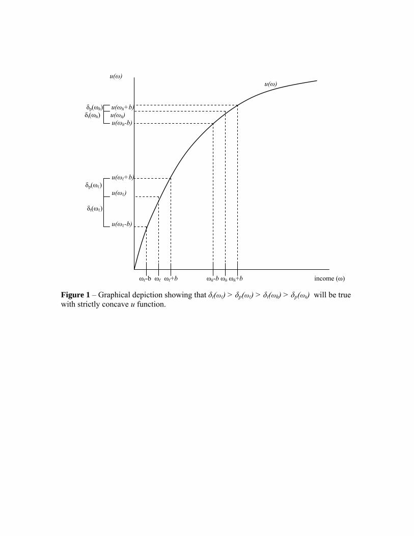
u(ω) u(ω) δp(ωh) u(ωh+b) δt(ωh) u(ωh) u(ωh-b) u(ωℓ+b) δp(ωℓ) u(ωℓ) δt(ωℓ) u(ωℓ-b) ωℓ-b ωℓ ωℓ+b ωh-b ωh ωh+b income (ω) Figure 1 – Graphical depiction showing that δt(ωℓ) > δp(ωℓ) > δt(ωh) > δp(ωh) will be true with strictly concave u function.

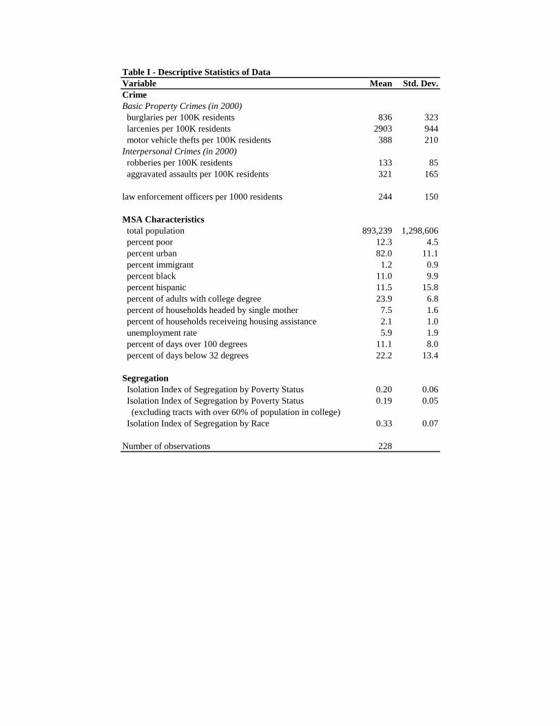
Table I - Descriptive Statistics of DataVariable Mean Std. Dev.Crime Basic Property Crimes (in 2000) burglaries per 100K residents 836 323 larcenies per 100K residents 2903 944 motor vehicle thefts per 100K residents 388 210Interpersonal Crimes (in 2000) robberies per 100K residents 133 85 aggravated assaults per 100K residents 321 165

law enforcement officers per 1000 residents 244 150

MSA Characteristics total population 893,239 1,298,606 percent poor 12.3 4.5 percent urban 82.0 11.1 percent immigrant 1.2 0.9 percent black 11.0 9.9 percent hispanic 11.5 15.8 percent of adults with college degree 23.9 6.8 percent of households headed by single mother 7.5 1.6 percent of households receiveing housing assistance 2.1 1.0 unemployment rate 5.9 1.9 percent of days over 100 degrees 11.1 8.0 percent of days below 32 degrees 22.2 13.4

Segregation Isolation Index of Segregation by Poverty Status 0.20 0.06 Isolation Index of Segregation by Poverty Status 0.19 0.05 (excluding tracts with over 60% of population in college) Isolation Index of Segregation by Race 0.33 0.07

Number of observations 228

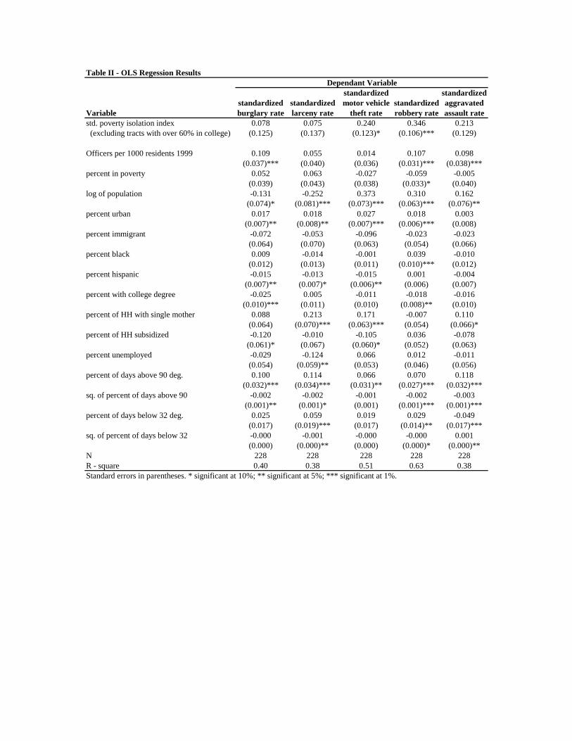
Table II - OLS Regession Results

standardized standardizedstandardized standardized motor vehicle standardized aggravated

Variable burglary rate larceny rate theft rate robbery rate assault ratestd. poverty isolation index 0.078 0.075 0.240 0.346 0.213 (excluding tracts with over 60% in college) (0.125) (0.137) (0.123)* (0.106)*** (0.129)

Officers per 1000 residents 1999 0.109 0.055 0.014 0.107 0.098(0.037)*** (0.040) (0.036) (0.031)*** (0.038)***

percent in poverty 0.052 0.063 -0.027 -0.059 -0.005(0.039) (0.043) (0.038) (0.033)* (0.040)

log of population -0.131 -0.252 0.373 0.310 0.162(0.074)* (0.081)*** (0.073)*** (0.063)*** (0.076)**

percent urban 0.017 0.018 0.027 0.018 0.003(0.007)** (0.008)** (0.007)*** (0.006)*** (0.008)

percent immigrant -0.072 -0.053 -0.096 -0.023 -0.023(0.064) (0.070) (0.063) (0.054) (0.066)

percent black 0.009 -0.014 -0.001 0.039 -0.010(0.012) (0.013) (0.011) (0.010)*** (0.012)

percent hispanic -0.015 -0.013 -0.015 0.001 -0.004(0.007)** (0.007)* (0.006)** (0.006) (0.007)

percent with college degree -0.025 0.005 -0.011 -0.018 -0.016(0.010)*** (0.011) (0.010) (0.008)** (0.010)

percent of HH with single mother 0.088 0.213 0.171 -0.007 0.110(0.064) (0.070)*** (0.063)*** (0.054) (0.066)*

percent of HH subsidized -0.120 -0.010 -0.105 0.036 -0.078(0.061)* (0.067) (0.060)* (0.052) (0.063)

percent unemployed -0.029 -0.124 0.066 0.012 -0.011(0.054) (0.059)** (0.053) (0.046) (0.056)

percent of days above 90 deg. 0.100 0.114 0.066 0.070 0.118(0.032)*** (0.034)*** (0.031)** (0.027)*** (0.032)***

sq. of percent of days above 90 -0.002 -0.002 -0.001 -0.002 -0.003(0.001)** (0.001)* (0.001) (0.001)*** (0.001)***

percent of days below 32 deg. 0.025 0.059 0.019 0.029 -0.049(0.017) (0.019)*** (0.017) (0.014)** (0.017)***

sq. of percent of days below 32 -0.000 -0.001 -0.000 -0.000 0.001(0.000) (0.000)** (0.000) (0.000)* (0.000)**

N 228 228 228 228 228R - square 0.40 0.38 0.51 0.63 0.38

Dependant Variable

Standard errors in parentheses. * significant at 10%; ** significant at 5%; *** significant at 1%.

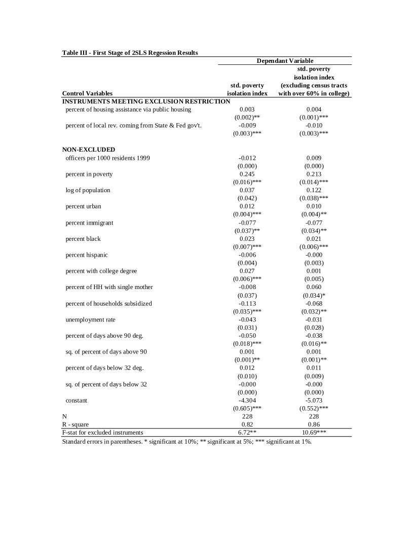
Table III - First Stage of 2SLS Regession Results

std. povertyisolation index

std. poverty (excluding census tractsControl Variables isolation index with over 60% in college)INSTRUMENTS MEETING EXCLUSION RESTRICTION percent of housing assistance via public housing 0.003 0.004

(0.002)** (0.001)*** percent of local rev. coming from State & Fed gov't. -0.009 -0.010

(0.003)*** (0.003)***

NON-EXCLUDED officers per 1000 residents 1999 -0.012 0.009

(0.000) (0.000) percent in poverty 0.245 0.213

(0.016)*** (0.014)*** log of population 0.037 0.122

(0.042) (0.038)*** percent urban 0.012 0.010

(0.004)*** (0.004)** percent immigrant -0.077 -0.077

(0.037)** (0.034)** percent black 0.023 0.021

(0.007)*** (0.006)*** percent hispanic -0.006 -0.000

(0.004) (0.003) percent with college degree 0.027 0.001

(0.006)*** (0.005) percent of HH with single mother -0.008 0.060

(0.037) (0.034)* percent of households subsidized -0.113 -0.068

(0.035)*** (0.032)** unemployment rate -0.043 -0.031

(0.031) (0.028) percent of days above 90 deg. -0.050 -0.038

(0.018)*** (0.016)** sq. of percent of days above 90 0.001 0.001

(0.001)** (0.001)** percent of days below 32 deg. 0.012 0.011

(0.010) (0.009) sq. of percent of days below 32 -0.000 -0.000

(0.000) (0.000) constant -4.304 -5.073

(0.605)*** (0.552)***N 228 228R - square 0.82 0.86F-stat for excluded instruments 6.72** 10.69***

Dependant Variable

Standard errors in parentheses. * significant at 10%; ** significant at 5%; *** significant at 1%.

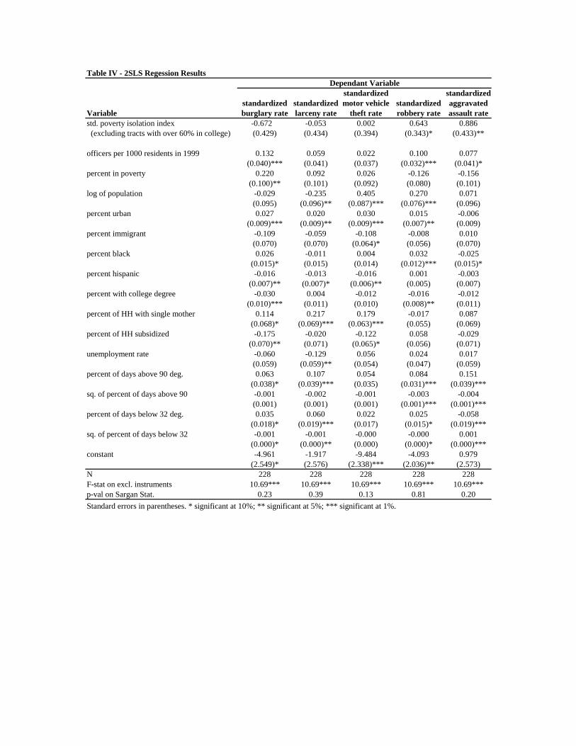
Table IV - 2SLS Regession Results

standardized standardizedstandardized standardized motor vehicle standardized aggravated

Variable burglary rate larceny rate theft rate robbery rate assault ratestd. poverty isolation index -0.672 -0.053 0.002 0.643 0.886 (excluding tracts with over 60% in college) (0.429) (0.434) (0.394) (0.343)* (0.433)**

officers per 1000 residents in 1999 0.132 0.059 0.022 0.100 0.077(0.040)*** (0.041) (0.037) (0.032)*** (0.041)*

percent in poverty 0.220 0.092 0.026 -0.126 -0.156(0.100)** (0.101) (0.092) (0.080) (0.101)

log of population -0.029 -0.235 0.405 0.270 0.071(0.095) (0.096)** (0.087)*** (0.076)*** (0.096)

percent urban 0.027 0.020 0.030 0.015 -0.006(0.009)*** (0.009)** (0.009)*** (0.007)** (0.009)

percent immigrant -0.109 -0.059 -0.108 -0.008 0.010(0.070) (0.070) (0.064)* (0.056) (0.070)

percent black 0.026 -0.011 0.004 0.032 -0.025(0.015)* (0.015) (0.014) (0.012)*** (0.015)*

percent hispanic -0.016 -0.013 -0.016 0.001 -0.003(0.007)** (0.007)* (0.006)** (0.005) (0.007)

percent with college degree -0.030 0.004 -0.012 -0.016 -0.012(0.010)*** (0.011) (0.010) (0.008)** (0.011)

percent of HH with single mother 0.114 0.217 0.179 -0.017 0.087(0.068)* (0.069)*** (0.063)*** (0.055) (0.069)

percent of HH subsidized -0.175 -0.020 -0.122 0.058 -0.029(0.070)** (0.071) (0.065)* (0.056) (0.071)

unemployment rate -0.060 -0.129 0.056 0.024 0.017(0.059) (0.059)** (0.054) (0.047) (0.059)

percent of days above 90 deg. 0.063 0.107 0.054 0.084 0.151(0.038)* (0.039)*** (0.035) (0.031)*** (0.039)***

sq. of percent of days above 90 -0.001 -0.002 -0.001 -0.003 -0.004(0.001) (0.001) (0.001) (0.001)*** (0.001)***

percent of days below 32 deg. 0.035 0.060 0.022 0.025 -0.058(0.018)* (0.019)*** (0.017) (0.015)* (0.019)***

sq. of percent of days below 32 -0.001 -0.001 -0.000 -0.000 0.001(0.000)* (0.000)** (0.000) (0.000)* (0.000)***

constant -4.961 -1.917 -9.484 -4.093 0.979(2.549)* (2.576) (2.338)*** (2.036)** (2.573)

N 228 228 228 228 228F-stat on excl. instruments 10.69*** 10.69*** 10.69*** 10.69*** 10.69***p-val on Sargan Stat. 0.23 0.39 0.13 0.81 0.20

Dependant Variable

Standard errors in parentheses. * significant at 10%; ** significant at 5%; *** significant at 1%.

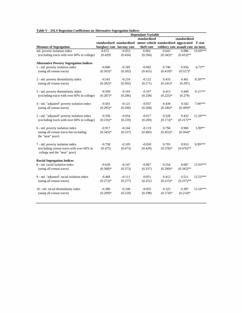
Table V - 2SLS Regession Coefficients on Alternative Segregation Indices

standardized standardizedstandardized standardized motor vehicle standardized aggravated F-stat

Measure of Segregation burglary rate larceny rate theft rate robbery rate assault rate on instr.std. poverty isolation index -0.672 -0.053 0.002 0.643 0.886 10.69*** (excluding tracts with over 60% in college) (0.429) (0.434) (0.394) (0.343)* (0.433)**

Alternative Poverty Segregation Indices1 - std. poverty isolation index -0.840 -0.185 -0.082 0.746 0.936 6.72** (using all census tracts) (0.503)* (0.502) (0.455) (0.419)* (0.527)*

2 - std. poverty dissimilarity index -0.541 -0.216 -0.122 0.433 0.461 8.18*** (using all census tracts) (0.302)* (0.302) (0.271) (0.241)* (0.297)

3 - std. poverty dissimilarity index -0.509 -0.193 -0.107 0.413 0.449 9.11*** (excluding tracts with over 60% in college) (0.287)* (0.286) (0.258) (0.225)* (0.279)

4 - std. "adjusted" poverty isolation index -0.501 -0.121 -0.057 0.439 0.542 7.00*** (using all census tracts) (0.295)* (0.296) (0.268) (0.246)* (0.309)*

5 - std. "adjusted" poverty isolation index -0.356 -0.054 -0.017 0.328 0.432 12.20*** (excluding tracts with over 60% in college) (0.216)* (0.220) (0.200) (0.173)* (0.217)**

6 - std. poverty isolation index -0.917 -0.244 -0.119 0.794 0.960 5.99** (using all census tracts but excluding (0.545)* (0.537) (0.485) (0.452)* (0.564)* the "near" poor)

7 - std. poverty isolation index -0.758 -0.105 -0.030 0.703 0.933 8.99*** (excluding census tracts with over 60% in (0.475) (0.473) (0.429) (0.378)* (0.476)** college and the "near" poor)

Racial Segregation Indices8 - std. racial isolation index -0.628 -0.147 -0.067 0.554 0.687 12.93*** (using all census tracts) (0.368)* (0.373) (0.337) (0.290)* (0.342)**

9 - std. "adjusted" racial isolation index -0.468 -0.111 -0.051 0.412 0.511 12.52*** (using all census tracts) (0.273)* (0.277) (0.251) (0.215)* (0.257)**

10 - std. racial dissimilarity index -0.380 -0.108 -0.055 0.325 0.387 15.24*** (using all census tracts) (0.209)* (0.218) (0.198) (0.174)* (0.214)*

Dependant Variable

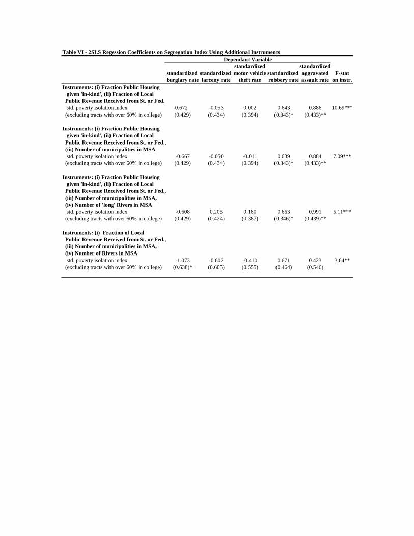
Table VI - 2SLS Regession Coefficients on Segregation Index Using Additional Instruments

standardized standardizedstandardized standardized motor vehicle standardized aggravated F-statburglary rate larceny rate theft rate robbery rate assault rate on instr.

Instruments: (i) Fraction Public Housing given 'in-kind', (ii) Fraction of Local Public Revenue Received from St. or Fed. std. poverty isolation index -0.672 -0.053 0.002 0.643 0.886 10.69*** (excluding tracts with over 60% in college) (0.429) (0.434) (0.394) (0.343)* (0.433)**

Instruments: (i) Fraction Public Housing given 'in-kind', (ii) Fraction of Local Public Revenue Received from St. or Fed., (iii) Number of municipalities in MSA std. poverty isolation index -0.667 -0.050 -0.011 0.639 0.884 7.09*** (excluding tracts with over 60% in college) (0.429) (0.434) (0.394) (0.343)* (0.433)**

Instruments: (i) Fraction Public Housing given 'in-kind', (ii) Fraction of Local Public Revenue Received from St. or Fed., (iii) Number of municipalities in MSA, (iv) Number of 'long' Rivers in MSA std. poverty isolation index -0.608 0.205 0.180 0.663 0.991 5.11*** (excluding tracts with over 60% in college) (0.429) (0.424) (0.387) (0.346)* (0.439)**

Instruments: (i) Fraction of Local Public Revenue Received from St. or Fed., (iii) Number of municipalities in MSA, (iv) Number of Rivers in MSA std. poverty isolation index -1.073 -0.602 -0.410 0.671 0.423 3.64** (excluding tracts with over 60% in college) (0.638)* (0.605) (0.555) (0.464) (0.546)

Dependant Variable