Embed Size (px)
Citation preview
THICKNESS MEASUREMENT OF SOLID HYDROGEN THIN FILM
FOR MUON CATALYZED FUSION
VIA ENERGY LOSS OF ALPHA PARTICLES
By
Makoto C Fujiwara
B.S., Yamanashi University, 1992
A.S., Kobe City College of Technology, 1990
A THESIS SUBMITTED IN PARTIAL FULFILLMENT OF
THE REQUIREMENTS FOR THE DEGREE OF
MASTER OF APPLIED SCIENCE
IN
THE FACULTY OF GRADUATE STUDIES
DEPARTMENT OF PHYSICS
W E ACCEPT THIS THESIS AS CONFORMING
TO THE REQUIRED STANDARD
THE UNIVERSITY OF BRITISH COLUMBIA
OCTOBER 1994
© MAKOTO C FUJIWARA, 1994
In presenting this thesis in partial fulfilment of the requirements for an advanced
degree at the University of British Columbia, I agree that the Library shall make it
freely available for reference and study. I further agree that permission for extensive
copying of this thesis for scholarly purposes may be granted by the head of my
department or by his or her representatives. It is understood that copying or
publication of this thesis for financial gain shall not be allowed without my written
permission.
(Signature)
Department of Physics
The University of British Columbia Vancouver, Canada
Date October 17, 1994
DE-6 (2/88)
Abstract
A novel target system for films of solid hydrogen isotopes has enabled unique experiments
in muon catalyzed fusion. In order to understand the experimental data a knowledge of
target thickness and uniformity is essential, but only indirect information was available.
Conventional techniques for a thickness measurement do not apply, due to the limited
available space and cryogenic requirements of the system. In this thesis, a method of
thickness and uniformity measurement via the energy loss of alpha particles is presented.
A critical review of the literature on the stopping powers of alpha particles was necessary,
given no experimental data for solid hydrogen.
An absolute precision of ~5% at optimal condition was obtained in the thickness
determination. The uncertainty in the relative measurements can be less than 1%. The
average target thickness per unit gas input, weighted by the Gaussian beam profile of
FWHM 20-25 mm is determined to 3.29±0.16 μg/(cm²-torr-litre). A significant non-
uniformity in the thickness distribution was observed with an average deviation of about
7%. The linearity of deposited hydrogen thickness upon gas input was confirmed within
the accuracy. The cross contamination from the other side of the diffuser nozzle is found
to be less than 0.8 x 10 - 3 with 90% confidence level. The result is compared to a Monte
Carlo study to understand deposition mechanism.
The importance of the stopping process in the alpha-sticking problem in muon cat
alyzed D-T fusion is discussed in detail. The physical phase effect of the stopping power
of hydrogen may partly explain the discrepancy in the sticking values between theory
and experiment at high densities. The concept of a new experiment to measure directly
the sticking probability at high density is proposed. This offers certain advantages over
ii
LAMPF/RAL measurements. A Monte Carlo simulation of the experiment is performed.
A very preliminary result from a test run is presented.
111
Table of Contents
Abstract ii
List of Tables viii
List of Figures ix
Acknowledgement xi
1 INTRODUCTION 1
1.1 Muon Catalyzed Fusion 1
1.2 Experiments with Hot Muonic Atoms from Cold Targets 4
2 TARGET THICKNESS MEASUREMENT 10
2.1 Motivation and Goal 10
2.2 Previous Measurements 11
2.2.1 Pressure and Volume 11
2.2.2 Muon Stops 12
2.2.3 Cross Contamination 12
2.3 Principle of the Method 13
3 ENERGY LOSS OF CHARGED PARTICLES 15
3.1 Bethe-Bloch Theory 16
3.1.1 Mean Excitation Potential 17
3.1.2 Density and Shell Correction 18
iv
3.1.3 Higher Order Correction 19
3.2 Low Energy Region 20
3.2.1 Break Down of the Bethe-Bloch Theory 20
3.2.2 Varelas-Biersack Formula 20
3.3 Effect of the Physical Phase 21
3.3.1 Overview 21
3.3.2 Heavy Ions 23
3.3.3 Condensed Gases 24
4 E X P E R I M E N T 26
4.1 Apparatus 26
4.1.1 Target System 26
4.1.2 Silicon Detector 28
4.1.3 Electronics and Data Acquisition System 30
4.1.4 Calibration and Noise 32
4.2 Experimental Runs 34
4.2.1 Series 1 34
4.2.2 Series 2 36
5 A N A L Y S I S OF DATA 38
5.1 Determination of Thickness 38
5.2 Energy-Range Tables 40
5.2.1 Northcliffe and Schilling (1970) 40
5.2.2 Ziegler (1977) 41
5.2.3 Ziegler, Biersack and Littmark (1985) 41
5.2.4 ICRU (1993) 42
5.2.5 Comparison of Tables 43
v
5.3 Uncertainties 47
5.3.1 Stopping Powers and Ranges 47
5.3.2 Peak Energy Determination 49
5.3.3 Random Noise 50
6 R E S U L T S A N D D I S C U S S I O N 51
6.1 Uniformity 51
6.1.1 Thickness Profile 51
6.1.2 Effect of Deposition Condition 54
6.2 Linearity in Target Deposition 54
6.3 Cross Contamination 58
6.4 Neon Targets 59
6.5 Alternative Deposition 60
6.6 Effective Thickness for Beam Experiment 60
6.7 Mechanism of Gas Deposition 65
6.7.1 Monte Carlo Simulation of Gas Deposition 65
6.7.2 Non-uniformity 67
6.8 Summary of the Method 67
6.8.1 Performance 67
6.8.2 Possible Improvements 68
6.8.3 Thickness Measurement in Beam 69
7 S T O P P I N G P O W E R S A N D A L P H A - S T I C K I N G I N fiCF 72
7.1 Brief Review of the Sticking Problem 72
7.1.1 Theory 73
7.1.2 Experiments 74
7.2 Stopping Power and the Reactivation 78
vi
7.3 Direct Measurement of the Sticking Probability at High Density 80
7.3.1 Introduction 80
7.3.2 Description of Experiment 81
7.3.3 Comparison with LAMPF/RAL Experiments 84
7.3.4 Monte Carlo Simulations 86
7.3.5 Test Measurement 91
7.3.6 Discussion 96
7.3.7 Readiness 98
7.4 Towards the Future 98
8 C O N C L U S I O N 102
Bibl iography 104
vn
List of Tables
5.1 Comparison of the hydrogen thickness between TRIM-92 and ICRU cor
responding to the same energy loss of alpha particles 46
6.1 Average of target thickness and the standard deviation weighted by beam
profile 63
Vlll
List of Figures
1.1 Simplified diagram of muon catalyzed fusion cycle in a D 2 / T 2 mixture. . 3
1.2 Schematic view of the solid hydrogen target system 6
1.3 Measurement of energy-dependent molecular formation rate via time of
flight experiment 8
4.1 Schematic views of the experimental set up 27
4.2 Alpha counts versus vertical position of the silicon detector 29
4.3 Data collecting electronics diagram 31
4.4 Alpha particle energy spectrum of a high resolution americium source for
energy calibration 32
4.5 Amplitude and fit of test pulser signal and the ADC channels 33
4.6 Shift in the position of source spots due to thermal contraction of the
target system 35
5.1 Alpha particle energy spectra with different thicknesses of hydrogen film. 39
5.2 Comparison of alpha particle stopping powers in gaseous hydrogen by var
ious tables 44
5.3 Comparison of gaseous and solid hydrogen stopping powers 45
5.4 Variation of the thickness due to the use of different range tables 48
6.1 Target thickness profile from Series 1 52
6.2 Typical thickness profile from Series 2 53
6.3 Thickness profile with different diffuser positions 55
ix
6.4 Thickness profile with the cryo-pump port open and closed during target
deposition 56
6.5 Test of linearity of deposition 57
6.6 Thickness profile of neon targets 59
6.7 Alternative deposition 61
6.8 Monte Carlo simulation of gas deposition 66
6.9 Thickness measurement in beam 70
7.1 Summary of experimental results of the effective sticking ufj* as function
of the density <j), plotted with theoretical predictions 75
7.2 Schematic view of a direct measurement of the alpha-sticking in a solid
target 82
7.3 Monte Carlo simulation for the direct measurement of alpha-sticking with
various degrader thickness 87
7.4 Determination of the sticking probability from two separate measurements. 90
7.5 Influence of the silicon detector size on the peak width in the energy spec
trum 92
7.6 Schematic top view of the test run for the sticking experiment 94
7.7 Data from a test run for the sticking experiment 95
7.8 Comparison of collinear and non-collinear Si-n coincidence 97
x
Acknowledgement
I am most grateful to Professor G. M. Marshall for his guidance and support throughout
my stay in Canada. His att i tude has always encouraged me to think of new ideas. I
would like to thank Professor D. F. Measday for his continuous support and advice on
my study at UBC and for valuable comments on this thesis. I appreciate their time for
reading and correcting my thesis so many times.
I wish to thank members of Muonic Hydrogen Group, in particular, Mr. P. E. Knowles
Dr. F. Mulhauser and Professor A. Olin for their continued help with the experiment and
for taking time to answer my many questions, and Professors G. A. Beer, T. M. Huber,
S. K. Kim, A. R. Kunselman, G. R. Mason, and Dr. J. L. Beveridge for their assistance
and helpful discussions. Professor Kunselman also proofread this thesis.
Thanks are due to Professors J. M. Bailey, W. N. Hardy, Drs. R. Jacot-Guillarmod
and M. Senba for fruitful discussions on the stopping power problem. I also wish to thank
Drs. M. Faifman, V. Markushin, C. Petitjean, J. Zmeskal and Professor C. J. MartofFfor
valuable discussions and their criticism on my idea of the sticking experiment.
Technical support from Messrs. C. Ballard, M. Good, K. Hoyle and help from Mr.
K. Bartlett , Ms. J. Douglas and Ms. M. Maier are gratefully acknowledged.
I am much indebted to Professors E. Torikai and K. Nagamine for their continuous
encouragement and support. The helpful discussions with Drs. K. Ishida, P. Strasser,
S. Sakamoto are also acknowledged.
I would like to thank the Rotary Foundation of the Rotary International and the
University of British Columbia for their scholarship support.
xi
Chapter 1
I N T R O D U C T I O N
A novel target system of solid thin films has been developed at TRIUMF for the exper
iments studying the reaction of muonic hydrogen isotopes. Of the main interest with
this new system is the study of processes in muon catalyzed fusion (/uCF). Some unique
measurements have been conducted and many more will come in the near future. This
thesis will concentrate on characterizations of the solid thin targets in terms of thickness
and uniformity. Following the introduction in this chapter, the principle will be discussed
in Chapter 2. Chapter 3 treats the energy loss of the charged particles in detail. The
experiments and data analysis is described in detail in Chapter 4 and 5, respectively.
The results will be presented and discussed in Chapter 6. Chapter 7 is devoted to the
applications of the knowledge of stopping processes to other problem in /iCF.
1.1 M u o n Catalyzed Fusion
Since its discovery in cosmic rays in 1937, the muon has played an important role in our
understanding of nature. The muon has been extensively studied to determine its own
properties and interactions as well as for a probe to reveal the nature of other particles
and nuclei. Despite these efforts over 50 years, its existence itself is still considered to
be one of the biggest mysteries in modern science. The muon has a mean life of 2.2
/is which is the second longest for all unstable particles (under weak decay) discovered
so far. Similarly to the neutron, the longest lived unstable particle, it provides a rich
variety of applications in diverse areas of science including condensed matter, medical
1
Chapter 1. INTRODUCTION 2
and archeological research, and perhaps, energy production.
Although its fundamental properties and interactions are of tremendous interest,
much of the behaviour of a negative muon can simply be described, for our purpose
regarding catalysis of nuclear fusion, by that of a heavy electron. When a muon pene
trates matter, it gets rapidly thermalized and captured by an atom replacing an orbiting
electron. Since the mass of muons is roughly 207 times that of electrons, the binding en
ergy of the muonic atoms is about 207 times larger and the dimension 207 times smaller
than that of ordinary atoms. A muonic hydrogen atom can approach another nucleus
to a much closer distance than a normal atom or a bare nucleus can, because it is a
compact neutral object. When a muonic hydrogen collides with other atoms, a muonic
molecular ion may be formed. Again, its dimension is about 200 times smaller than
diatomic molecular ions such as H^\ The striking difference in the muonic molecule is,
however, that because of the closer internuclear distance, the tunneling of nuclear wave
functions is enhanced exponentially and nuclear fusion may occur very rapidly, except
of course for the p//p case. After the fusion, most of the time the muon is released and
participates in another series of processes leading to fusion.
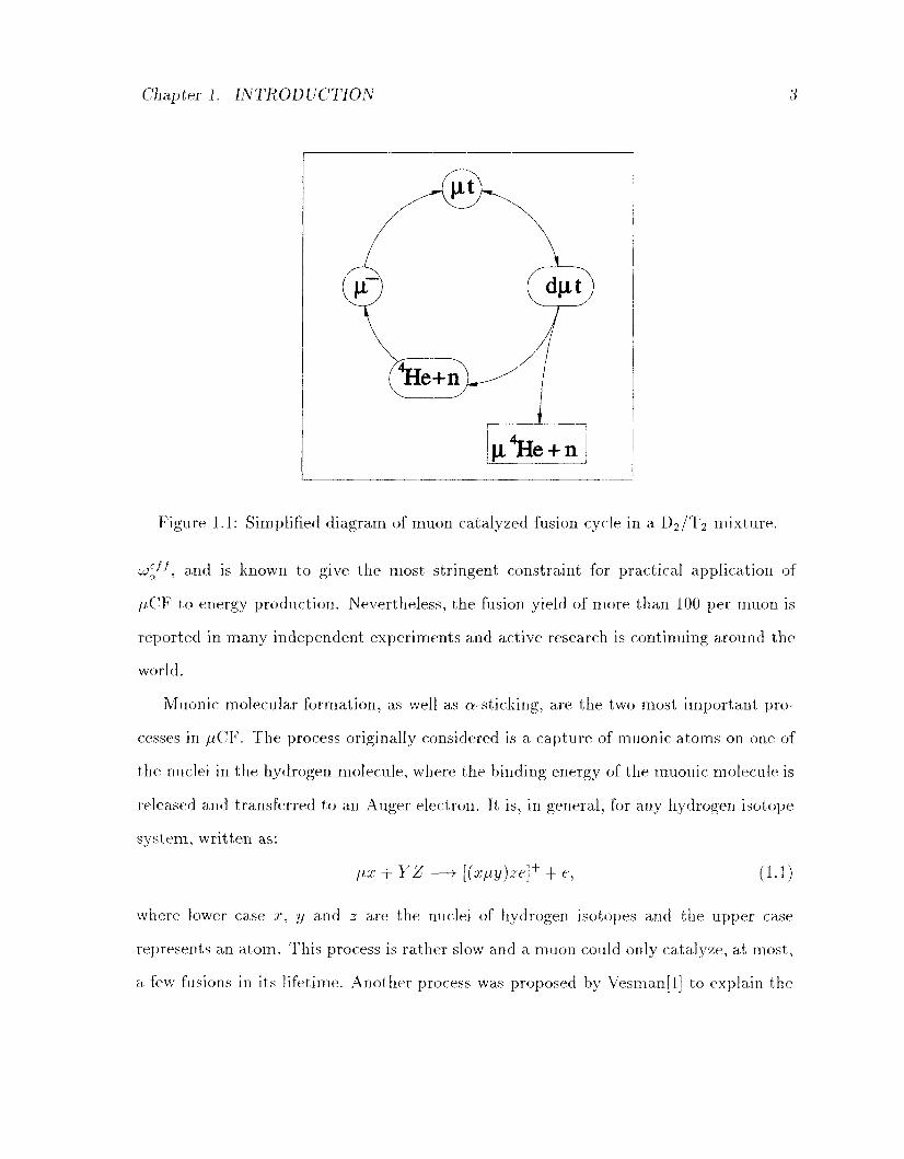
Fig. 1.1 illustrates the simplified cycling processes in one of the most interesting
systems, a deuterium - tritium mixture. A negative muon incident on a D 2 / T 2 target
gets captured by either d or t forming fid or fj,t, respectively. The muon in ^d transfers
to a triton due to its deeper Coulomb potential. A muonic molecule dyut is then formed
mainly via the resonance mechanism which will be described later. Almost immediately
after the d/ut formation the fusion takes place producing a neutron and an alpha particle
with an energy release of 17.6 MeV. A small fraction (~ 0.6%) of muons get attached to
the a after the fusion. This probability is called the (effective) alpha sticking coefficient1
' in fact, initially ~ 1% of muons stick, but about 1/3 of them get stripped from the helium nuclei due to collisions with the atoms in the target.
Chapter 1. INTRODUCTION 3
Figure 1.1: Simplified diagram of muon catalyzed fusion cycle in a D 2 /T 2 mixture.
weJ^, a n d is known to give the most stringent constraint for practical application of
fiCF to energy production. Nevertheless, the fusion yield of more than 100 per muon is
reported in many independent experiments and active research is continuing around the
world.
Muonic molecular formation, as well as a-sticking, are the two most important pro
cesses in /j,CF. The process originally considered is a capture of muonic atoms on one of
the nuclei in the hydrogen molecule, where the binding energy of the muonic molecule is
released and transferred to an Auger electron. It is, in general, for any hydrogen isotope
system, written as:
fix + YZ-^[(xfxy)ze]+ + e, (1.1)
where lower case x. y and z are the nuclei of hydrogen isotopes and the upper case
represents an atom. This process is rather slow and a muon could only catalyze, at most,
a few fusions in its lifetime. Another process was proposed by Vesman[l] to explain the
Chapter 1. INTRODUCTION 4
unexpectedly high fusion rate in the d^ud system. The process, in general, can be written
as:
fix + YZ —> [(x/j,y)zee\*. (1-2)
In the Vesman mechanism, because of the existence of a loosely bound state in the muonic
molecule, the binding energy is absorbed as rotational and vibrational excitation quanta
in the 6-body molecular complex. The muonic molecule xfiy and the hydrogen nucleus
z constitute the two nuclei of the compound molecule, with the symbol * referring to
its excited state. For the d/ut system the reaction rate is, indeed, enhanced by about
100 times by the resonance process. Due to the delicate mechanism of the resonance,
the molecular formation process shows a strong temperature dependence. Hence, the
total fusion rate depends on temperature as well. It is interesting to note that in yuCF
phenomena, a nuclear reaction which releases millions of electron volts of energy, is
affected by a temperature which typically has an energy scale of milli-electron volts.
Here we see a beautiful interplay of nuclear and atomic/molecular physics. Thus, detailed
understanding of molecular formation is of essential importance in /J.CF research.
1.2 Exper iments with Hot Muonic A t o m s from Cold Targets
History tells us many of the discoveries in science were serendipitous. Often people were
looking for one thing, and found something else that was totally unexpected. The muonic
hydrogen experiments at TRIUMF have a similar story. They were originally designed
to search for the emission of /ip into vacuum in its excited state, for a precision test of
Quantum Electrodynamics. To the dismay of the group, this was not realized. After
several runs, however, it was found that energetic /j,d atoms, instead of ^ p , were emitted
in large amounts. Thus, the source of a neutral "beam" of hot /u,d was discovered.
The importance of isolated muonic hydrogen in vacuum was immediately realized as
Chapter 1. INTRODUCTION 5
a tool for research in /J,CF and related processes. Following this discovery, a new versatile
target system for solid thin layers was developed for the study of a variety of the reactions
of muonic hydrogen isotopes.
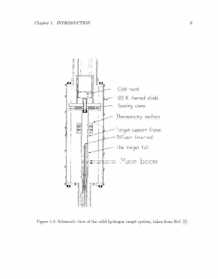
Fig. 1.2 illustrates the schematic view of the target system. Two thin target foils
made of 51 /im gold are supported by 1.6 mm copper frames. They are connected to the
cold head of the cryostat which is cooled to 3 K by pumping on liquid helium. Target
spacing can be varied from 15 mm to 40 mm. A 90 K copper thermal shield protects
the system from radiation heating. All the copper present in the system is gold plated
in order to reduce the emissivity.
The hydrogen is introduced through the gas deposition mechanism (diffuser) which
can be inserted between the two target support frames. It has many small holes through
which the gas is released towards either one of the target foils. The gas condenses and
solidifies when it reaches the cold foil surface. The system is kept in an ultra-high vacuum
of 10~8 - 10 - 1 0 torr except during the gas deposition when the pressure goes up to a few
times 10 - 6 torr. All three isotopes of hydrogen, as well as other gases such as neon, can
be used in the targets, both pure and in mixtures. Although the handling of tritium
requires special attention due to its radioactivity, it is an essential ingredient in the high
cycling muon catalyzed processes.
One of the main goals in the E613 experiment at TRIUMF using the target system
mentioned above is the energy-dependent measurements of reaction processes via the
time of flight method. Fig. 1.3 illustrates one such measurement, where energy-dependent
molecular formation rate can be investigated in the following manner. The muon beam
is stopped in solid protium ( 1H2 ) with a concentration of tritium of one part in a
thousand (Ct = 10 - 3 ) . In this upstream target, muonic protium /up is formed and the
negative muon is transferred to a triton forming jit. Upon the transfer the difference in
the binding energies gives the /j,t a kinetic energy of ~ 45 eV in the laboratory frame.
Chapter 1. INTRODUCTION 6
Cold head
9 0 K thermal shield
Spacing clamp
Thermometry anchors
Target support frame
Diffuser (inserted)
Thin target foil
Muon beam
Figure 1.2: Schematic view of the solid hydrogen target system, taken from Ref. [2]
Chapter 1. INTRODUCTION 7
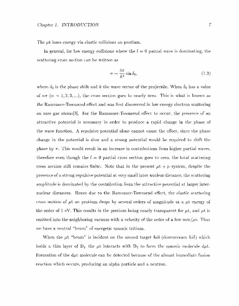
The fit loses energy via elastic collisions on protium.
In general, for low energy collisions where the / = 0 partial wave is dominating, the
scattering cross section can be written as
4n cr ~ —-sin^o, (1.3)
where So is the phase shift and k the wave vector of the projectile. When S0 has a value
of tire (n = 1,2,3,...), the cross section goes to nearly zero. This is what is known as
the Ramsauer-Townsend effect and was first discovered in low energy electron scattering
on rare gas atoms[3]. For the Ramsauer-Townsend effect to occur, the presence of an
attractive potential is necessary in order to produce a rapid change in the phase of
the wave function. A repulsive potential alone cannot cause the effect, since the phase
change in the potential is slow and a strong potential would be required to shift the
phase by n. This would result in an increase in contributions from higher partial waves,
therefore even though the / = 0 partial cross section goes to zero, the total scattering
cross section still remains finite. Note that in the present fit + p system, despite the
presence of a strong repulsive potential at very small inter-nuclear distance, the scattering
amplitude is dominated by the contribution from the attractive potential at larger inter-
nuclear distances. Hence due to the Ramsauer-Townsend effect, the elastic scattering
cross section of fit on protium drops by several orders of magnitude at a fit energy of
the order of 1 eV. This results in the protium being nearly transparent for fit, and fit is
emitted into the neighboring vacuum with a velocity of the order of a few mm//js. Thus
we have a neutral "beam" of energetic muonic tritium.
When the fit "beam" is incident on the second target foil (downstream foil) which
holds a thin layer of D2 the fit interacts with D2 to form the muonic molecule d//t.
Formation of the d^ut molecule can be detected because of the almost immediate fusion
reaction which occurs, producing an alpha particle and a neutron.
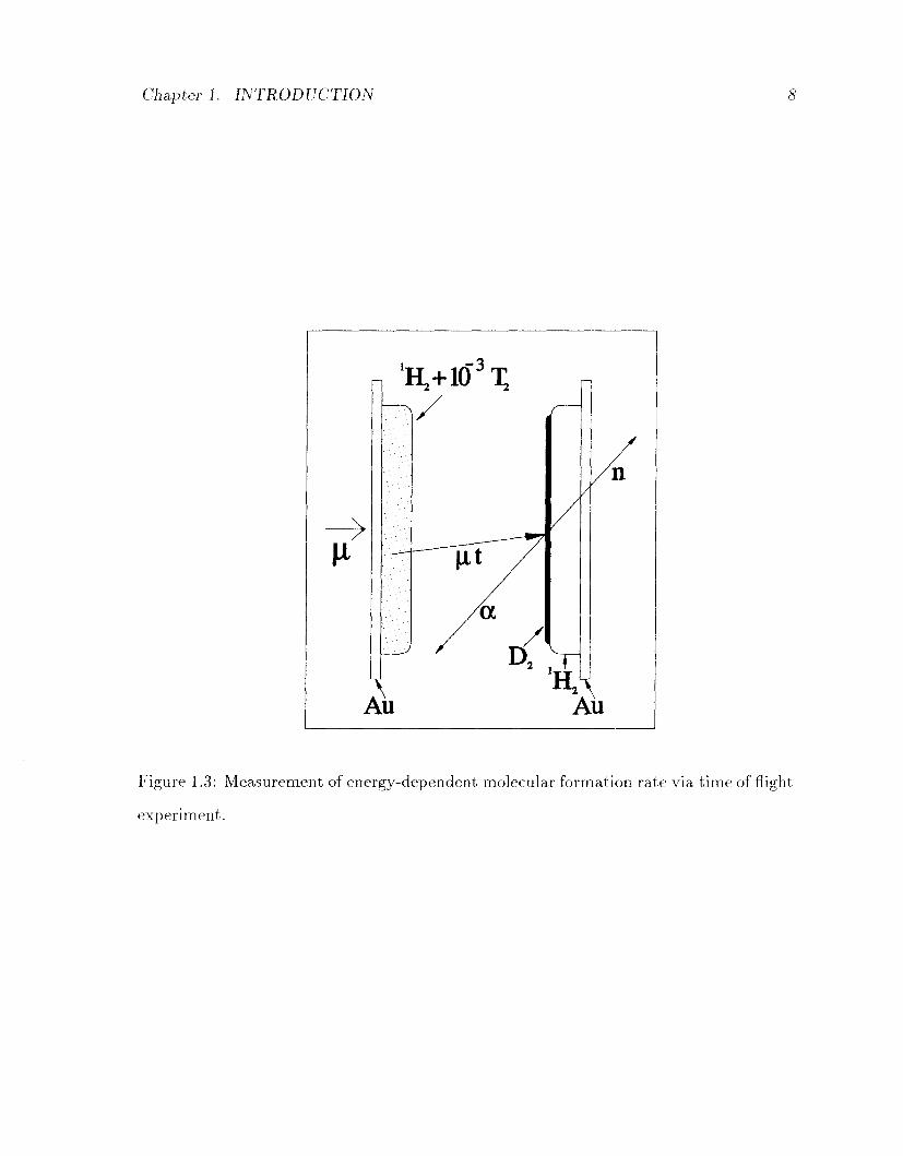
Chapter 1. INTRODUCTION
Figure 1.3: Measurement of energy-dependent molecular formation rate via time of flight
experiment.
Chapter 1. INTRODUCTION 9
A recent theoretical calculation predicts strong aresonances in d^ut formation at an
energy of the order of 1 eV[4]. The energy range corresponds to a temperature of ~
10,000 K and is inaccessible by conventional targets. The target system described here
gives a unique way to measure the molecular formation cross section in the predicted
resonant energy region. Furthermore, it provides event by event energy information,
via the time of flight method, allowing an energy-dependent measurement of the cross
sections. Given the distance of two target foils, the time interval between the entry of
the muon and the fusion reaction gives the velocity, hence energy, of the /it, except for
the unkown angle of emission. The angular dispersion of the emitted /it can be reduced
by using a collimating device. The time taken by the muon to be emitted after stopping,
and the time taken for fusion after the molecule is formed, are both very fast compared
to the time of flight, and can be neglected. A recent Monte Carlo study indicates the
importance of the contribution from the /it + d elastic scattering process[5]. This has to
be carefully considered in extracting the molecular formation cross section.
The emission of a fit in vacuum was observed for the first time in the December
1993 run. The principle of the measurement has been proven, which yielded a number
of unambiguous fusion events with time of flight information[6]. The measurement with
optimized conditions has just taken place in July-August 1994. The analysis of the result
is now in progress.
Chapter 2
T A R G E T T H I C K N E S S M E A S U R E M E N T
2.1 Mot ivat ion and Goal
For any experiment in science, having a good understanding of the experimental sys
tem is essential. Our solid hydrogen isotope target system is no exception to this rule.
Knowledge of the target thickness and uniformity is important, in particular, for the
measurements of molecular formation and scattering cross sections, since it limits the
precision of the measurements. The uncertainty in the thickness directly propagates to
the final results. Also for X-ray measurements, the thickness of the layer affects the
absorption of photons, which is an important correction for the absolute intensity.
As mentioned earlier, the target we use in the beam experiments includes all three
isotopes of hydrogen and their mixtures, as well as other elements such as neon. The
thickness ranges from a few jUg/cm2 to a few mg/cm2 , corresponding to a few hundreds
of nanometers to a few mm for hydrogen.
The goal of precision for the fiCF experiments discussed in section 1.2 is perhaps
10%, therefore a few percent accuracy in the thickness measurement should be aimed at.
It should be noted, however, that if the variation of the thickness in the film is greater
than the uncertainty of the thickness measurement, it is the former that dominates
the uncertainty of the final result. Also, there is some uncertainty over the control of
gas input in the deposition process. This becomes increasingly important for very thin
targets. Hence the pursuit of better precision in the thickness measurement would be
10
Chapter 2. TARGET THICKNESS MEASUREMENT 11
less important, in the case where the above factors are dominating.
In addition to the E613 experiment at TRIUMF, the present measurement may give
some insights to other experiments which use solid thin films as a target. A novel method
on slow negative muon production via //CF proposed by Nagamine[7] uses a similar target
and gas deposition mechanism[8, 9]. The uncertainty in the target film thickness is con
sidered as one of the possible causes for disagreements between the recent measurements
and the simulation[10]. Another example is an experiment on low energy kaon-nucleon
interactions at DA$NE, a </> factory. Olin et al. proposed the use of a solid hydrogen tar
get inside the collider beam pipe[l l] . The unique target system, combined with tagged,
mono-energetic kaons from <j> decay, is expected to provide unprecedented statistics in a
low background environment for low energy kaon studies. Furthermore, the possibility
of utilizing a solid target for the measurement of a sticking processes, probably the most
important processes in terms of the practical application of /iCF, is currently being in
vestigated. The present measurement is hoped to provide useful information for these
ongoing or potential experiments.
2.2 Previous Measurements
2.2.1 Pressure and Volume
Prior to the present measurement, some information on our target thickness was available.
One is described here and the others in following sections.
The first measurement was done as follows. The hydrogen gas was deposited onto
a cold foil while pumping the system with a cryopump. After the vacuum system was
closed, the cryostat was warmed up to evaporate the frozen hydrogen. By measuring the
total pressure, combined with the knowledge of the total volume of the system, one can
estimate the amount of gas which actually sticks inside the system. This method tells
Chapter 2. TARGET THICKNESS MEASUREMENT 12
us that roughly 83% of the gas stays inside the system[12]. However, it does not provide
the information on whether the gas sticks to the target foil at which the muon beam is
directed. It could have been deposited anywhere in the vacuum system.
2.2.2 Muon Stops
Another piece of information came from the muon stopping signals. 99.9% of the muons
which stop in the hydrogen decay and emit an energetic electron. It can be detected by
an array of wire chambers, and the position of the decay can be estimated by tracing
back the electron track. The spectrum of the decay electrons from muons stopping in
hydrogen has a characteristic time constant of about 2.2 /is, and can be distinguished
from the ones stopped in heavier material in the system, which have much smaller life
times due to the capture on a nucleus via the semi-leptonic weak interaction. By looking
at the yield of the decay electrons one can estimate how much hydrogen is on the target
foil. This method, however, is subject to a large systematic uncertainty and it is very
difficult to obtain the absolute thickness.
2.2.3 Cross Contaminat ion
If the hydrogen molecule does not stick to the cold foil at first contact, it could bounce
around the diffuser and stick to the other cold foil, causing cross contamination of the
targets. This would make the experiments using two target foils of different compositions
such as the one described in section 1.2 impossible.
The cross contamination was checked by observing the yield of fid emission. Since
the mechanism of emission is based on the subtle condition of the Ramsauer Townsend
resonance, its yield is very sensitive to any contamination on the surface. The /id emis
sion target was first prepared in the upstream foil, and emission was observed. The thick
deuterium target was then deposited in the down stream foil. If there was a significant
Chapter 2. TARGET THICKNESS MEASUREMENT 13
contamination from the downstream target on the upstream one, it would affect the
emission yield of //d. The comparison with the case where a known amount of D2 was in
tentionally put on top of the emission target, gives the upper limit of cross contamination
to be less than ~ 1%.
All the information discussed in this section is rather indirect. None of it gives the
absolute thickness nor the uniformity. This leads us to perform a specific experiment for
more direct thickness measurement, and its principle is described in the following section.
2.3 Principle of the M e t h o d
There are a number of conventional ways for measuring the thickness of thin films, such
as optical interferometry and microscopy. However, the spatial limitations and cryogenic
requirements of the target system do not allow such methods.
For condensed gases, a few methods have been reported. For example, S0rensen et
al. used a quartz crystal oscillator to measure the thickness of solid hydrogen films [13]
for the measurement of ranges of keV electrons[14]. This is a common technique for
ordinary films made from evaporation. From the frequency change of oscillation, the
amount of gas frozen on the quartz is determined. However, they found at least 40%
non-linearity in the frequency change-thickness relation with a D2 film as thin as 40
\im. The signal from the oscillator also deteriorated with increasing film thickness and
it finally stopped oscillating. They attributed this to the smallness of the densities of
hydrogen and deuterium. It should be recalled that our target thicknesses range up to 1
mm or more. Also it would not be possible to test the uniformity of films in this method,
unless multiple crystals are used.
Chu et al. measured the thickness of argon, oxygen and CO2 films with the Rutherford
Chapter 2. TARGET THICKNESS MEASUREMENT 14
Backscattering (RBS) method[15]. This popular technique for ordinary thin films is
known to give fairly accurate results, provided there is an accurate calibration sample[16].
However, due to the small cross section for backward scattering, a dedicated accelerator
is necessary for this measurement to provide sufficiently intense beam of ions.
We will use a method which meets the requirements and limitations imposed by
the target system and still is relatively simple: By depositing a film directly on top of a
radioactive source, and by measuring the residual energy of the transmitted particles, the
energy loss of the particles is obtained. The energy loss can be related to the thickness of
the film using the stopping power of charged particles in the material. Direct deposition
provides measurements with better accuracy and wider dynamic ranges. The uniformity
of the film can be easily determined by using an array of sources and sampling the
different positions. The knowledge of the energy loss process of charged particles in
matter is essential for this method. This will be discussed in detail in the following
chapter.
Chapter 3
E N E R G Y LOSS OF C H A R G E D PARTICLES
The energy loss process of charged particles has been studied since the beginning of the
century. A precise understanding has been demanded not only in nuclear physics, but
also in medicine, biology, material science, device research and many other fields. These
processes for charged particles include electronic excitation, ionization, nuclear collision,
Cherenkov radiation and bremsstrahlung.
Heavy1 charged particles in matter lose the energy mainly via inelastic interactions
with the bound electrons of the medium (electronic stopping power). Elastic Coulomb
collisions in which recoil energy is imparted to atoms (nuclear stopping power) be
comes important at very low velocity. For example, the nuclear stopping power con
tributes more than 1% of total stopping power only below 150 keV in hydrogen for alpha
particles[17, 18]. Radiative energy loss due to emission of bremsstrahlung (radiative
stopping power) is significant for electrons and positrons, but negligible for heavier par
ticles, since it is inversely proportional to the square of projectile mass. Other processes
such as nuclear reactions and Cherenkov radiation have also only negligible contributions
for heavy particles unless extremely relativistic. The latter is included in the standard
formula of stopping power mentioned below.
The following sections review different aspects of the energy loss mechanism. Sec
tion 3.1 treats relativistic particles in terms of the Bethe-Bloch formula. The lower
energy region is discussed in section 3.2. The effect of physical phase on energy loss is
: B y "heavy" it is meant tha t the mass of the particle is comparable to or greater than that of the nucleus.
15
Chapter 3. ENERGY LOSS OF CHARGED PARTICLES 16
considered in section 3.3.
3.1 Be the -B loch Theory
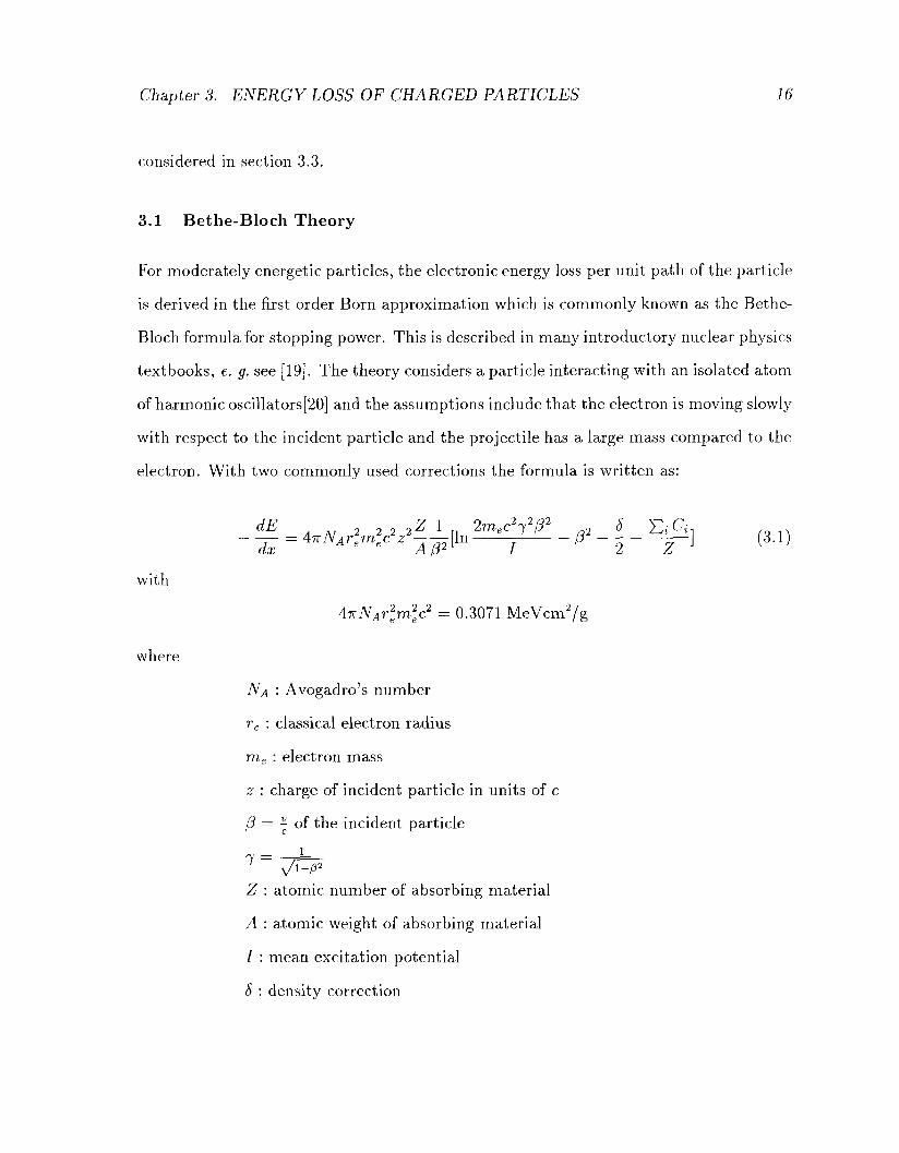
For moderately energetic particles, the electronic energy loss per unit path of the particle
is derived in the first order Born approximation which is commonly known as the Bethe-
Bloch formula for stopping power. This is described in many introductory nuclear physics
textbooks, e. g. see [19]. The theory considers a particle interacting with an isolated atom
of harmonic oscillators[20] and the assumptions include that the electron is moving slowly
with respect to the incident particle and the projectile has a large mass compared to the
electron. With two commonly used corrections the formula is written as:
dE . M 2 2 2 2 Z l 2 m e C V / 3 2 2 5 £,-£•
'^=47rNAr^CZAW^ 7 P ~2-—] (3-1}
wi ith
w here
47rNAr2em
2ec
2 = 0.3071 MeVcm2 /g
NA '• Avogadro's number
re : classical electron radius
me : electron mass
z : charge of incident particle in units of e
(3 = - of the incident particle
Z : atomic number of absorbing material
A : atomic weight of absorbing material
/ : mean excitation potential
5 : density correction
Chapter 3. ENERGY LOSS OF CHARGED PARTICLES 17
C{ : shell correction for i th shell
Some important points are discussed in following sections.
3.1.1 Mean Exci tat ion Potent ial
The mean excitation potential I is the prime parameter in the formula, and the nature
of the target materials is concentrated in this number. It is theoretically defined for
gases[21] as:
r £ In EdE In 7 = ^ 5 5 , (3-2)
where df/dE is the density of optical dipole oscillator strength ( / ) per unit energy of
excitation (E) above the ground state. The oscillator strength is proportional to the
photo-absorption cross section, but use of this is justified only for dilute gases for which
there is only a weak correlation between the positions of the electrons in the medium[22].
For condensed matter, instead, I is expressed in terms of the dielectric-response function
2 f°° In 7 = — - / c j l m [ - l / e ( u ; ) ] l n ( ^ ) ^ , (3.3)
TTWp JO
where u>p is the electron plasma frequency, which describes the collective response of
electrons to a disturbance. e(u>) is defined in D = e(oj)E, and is generally a complex
number. For non-magnetic materials, it can be related to the refractive index[22]. The
classical damped harmonic oscillator model is known to give the same value of e(u>) as
the corresponding quantum mechanical calculation[23].
The value of the mean excitation potential depends on the electronic structure of
the material, and is very difficult to calculate accurately except for the simplest atomic
gases. Empirical formulas for the Z-dependence of I exist[19, 24, 25], e. g. IjZ =
Chapter 3. ENERGY LOSS OF CHARGED PARTICLES 18
9.76 + 58.8/Z 1 1 9 for Z > 13, but it is known that / does not depend on Z smoothly, due
to the effects of the atomic shell structures.
Most of the time values for / have been determined for each element from actual stop
ping power measurements by fitting the data to equation 3.1. For the element for which
data is not available, the / value has to be deduced from semi-empirical interpolation. For
some simple gaseous materials, when optical data are abundant, / values can be deter
mined by fitting the experimental polarizability to get semi-empirical oscillator-strength
distributions.
Determination of / values is one of the main tasks for authors of stopping power
tables. The most recent compilation of / values was made by Berger and Seltzer in
preparation for the stopping power table of electrons and positrons[22, 26]2. Since the
/ value is independent of projectile, it can be applied to heavy charged particles as
well. They quote values as accurate as 1-2% for Al and Ag, for example. However, it
is worth mentioning that Sabin et al. recently commented[27] that it is impossible to
determine the experimental mean excitation energies with precision better than ~ 5 eV
for Al. They claim an experimental value of / with less than ~ 5% uncertainty is useless
as long as other correction terms such as shell, Barkas and Bloch corrections are not
known accurately. As will be mentioned, these corrections are obtained by fitting the
experimental stopping powers. Therefore, the experimental / value depends on the choice
of the corrections.
3.1.2 Dens i ty and Shell Correction
The correction due to the density effect 5, also called the polarization correction, is
only important at very high energy. The polarization in the medium atoms caused by
2The Particle Data Book cites the latter article, which is much more difficult to obtain yet contains less information. In the opinion of the present author, the former should be cited instead.
Chapter 3. ENERGY LOSS OF CHARGED PARTICLES 19
the projectile perturbs the electron field, reducing the stopping power. A semiempirical
formula was developed by Sternheimer and values obtained by employing claimed up-
to-date values of / are found in Ref. [25, 28]. The shell correction C; is to compensate
the effect that electrons in inner shells of atoms do not participate in the energy loss
processes of the projectile. This is more important at lower energy. Again, this is not
precisely known and a semiempirical formula must be employed[29, 30].
3.1.3 Higher Order Correction
Higher order terms in the projectile charge z are sometimes used for the correction due
to departures from the first Born approximation. The Barkas correction is proportional
to z3, giving the different stopping powers between positively and negatively charged
particles. This is named after Barkas who first observed in the 1950's that the range of
negative pions is longer than that of positive pions. This is still an active field of research
both experimentally and theoretically. For example, the antiproton proton stopping
power in hydrogen below 120 keV was recently measured at Low-Energy Antiproton
Ring at CERN by Adamo et al. [31]. The maximum in the antiproton stopping power
was about 60% of that for proton, showing a significant Barkas effect.
The Bloch correction takes into account the perturbation of the wave functions of the
atomic electrons due to the incident particles (quantum mechanical impact-parameter
method). This is derived without the use of the first-order Born approximation and the
correction is important only at large projectile velocities. With this correction added,
the high energy limit of equation 3.1 approaches the classical stopping formula of Bohr.
Chapter 3. ENERGY LOSS OF CHARGED PARTICLES 20
3.2 Low Energy Region
3.2.1 Break Down of the Be the -B loch Theory
With corrections described above, the Bethe-Bloch formula is known to give results ac
curate to a few percent for protons and alpha particles of energies down to j3 ~ 0.05 (~
10 MeV for alphas, ~ 2.5 MeV for protons). However, many of the assumptions in the
Bethe-Bloch formula start to become inadequate at lower energies. In the low energy
limit, stopping power in the Bethe-Bloch formula equation 3.1 is inversely proportional
to the kinetic energy of the projectile. However, after a certain maximum, the actual
stopping power decreases with decreasing energy. Clearly, even with various corrections,
the theory of Bethe-Bloch, which proves so successful in the relativistic regions, breaks
down at low energies. This is the case typically below (3 ~ 0.05.
An additional complication for projectiles with Z > 1 is that, at low velocities, ions
start to have partially bound electrons, and their effective charge states are no longer
equal to Z. Reduced charge states result in lower stopping powers. This effect is more
significant at lower velocities, and the ions are finally neutralized at very low velocity.
According to Ziegler et al. , despite a long controversy, a consensus seems to exist which
claims that protons always exist as bare nuclei with an effective charge equal to one, at
least in the condensed targets[20j. However, it is pointed out by Senba that in noble gases
(in gaseous phase) nearly 100% of protons with initial energy of 100 MeV experience an
electron capture process at least once by the time they slow down to 1 MeV[32, 33].
3.2.2 Varelas-Biersack Formula
Below j3 ~ 0.05, no satisfactory theoretical prediction of stopping powers is available.
Therefore an empirical fit to the experimental data is the only way. Varelas and Bier-
sack proposed a phenomenological formula for low energy stopping powers with five
Chapter 3. ENERGY LOSS OF CHARGED PARTICLES 21
parameters [34]:
^ = 7 ^ + 7 ^ , (3-4) •J Jlow '-'high
where S is the electronic stopping power and Siow (low energy stopping) is
Shw = A\E (3-5)
and Shigh (high energy stopping) is
Shigh = ^]n(l+ ^ + EA5) (3.6)
This formula is used by several authors to bridge between the Bethe-Bloch region and
the very low energy region where some theoretical guide exists. At the very low energies,
namely of the order of keV, stopping powers proportional to the projectile velocities
are predicted by the free electron gas model. Many stopping power tables assume this
relationship or a similar one3.
3.3 Effect of the Physical Phase
Because the present work involves solidified gases, it is important to consider the effect
of the physical phase on stopping powers. Unfortunately, no experimental data exists,
to the author's knowledge, for solid hydrogen and a charged particle with energies of
interest to us. Therefore, in this section, we will discuss existing studies of the issue in
detail.
3.3.1 Overview
An obvious effect of the physical phase on stopping powers is the polarization effect
at relativistic energies due to the density change (the density effect in the Bethe-Bloch
3A recent measurement reports, however, a departure from the velocity proportionality[35].
Chapter 3. ENERGY LOSS OF CHARGED PARTICLES 22
formula). This is theoretically rather well understood as discussed in section 3.1. However
for protons it reaches the 1% level only above 500 MeV, so clearly it is negligible for us. A
channeling effect occurs in the crystalline structure of solids. In a single crystal material,
it can reduce stopping power by as much as 30% in a certain direction, but our targets are
likely to be multi-crystal, so no observable effect is expected. In fact, the measurements
of stopping powers of a few MeV 4He ions in frozen gases by Chu et al. , who used a
pin hole deposition mechanism, report no such effects after measuring at several different
angles [15].
The phase effects can be expected, at least in the Bethe-Bloch region, to reveal
themselves in a higher value of / , the mean excitation potential. Experimental pho-
toabsorption studies, as well as theoretical considerations show general upward shifts in
the dipole oscillator strength distributions in solids compared with gases. Changes in
outer electron arrangements may lead to changes in electronic excitation levels as ag
gregation occurs. For example, in Berger and Seltzer's compilation of mean ionization
potentials[22], gaseous and liquid hydrogen have different / values, namely, 19.2 ± 0.4
eV for molecular gaseous hydrogen and 21.8 ± 1 . 6 eV for liquid hydrogen. The liquid
value is obtained by reanalyzing data from the year 1952 and has a large uncertainty.
Notice stopping power depends only logarithmically on the mean excitation potential,
therefore the change in the stopping power AS/S should be smaller than the change in
mean excitation potential A / / / , that is AS/S < AI/1.
Early studies on phase effects were done in water and organic material using a par
ticles. For a review, see [36]. They are conflicting in the magnitude, the sign and even
in the existence of such effects. Later studies show a consistent tendency of signifi
cant differences for a particles in the energy region of 0.3 to a few MeV. A survey of
stopping power data in hydrocarbons and related materials was done by Thwaites and
Watt[37], and they concluded that stopping powers in gases are greater than in solids
Chapter 3. ENERGY LOSS OF CHARGED PARTICLES 23
and liquids. A similar comparison by Ziegler et al.[38] describes the averaged ratio of
(experimental /theory) gas J {experimental /theory) soud. The ratio is greater than unity
for a particles below ~ 4 MeV in low Z material, and increases to as high as 1.4 at 0.5
MeV.
Recent reviews[39, 40] conclude the existence of 5-10% physical effects for protons and
alpha particles at maximum stopping power energies in organic and similar materials. It
is also suggested that for compound materials, the chemical binding significantly changes
the stopping power, hence causing a break down of Bragg's additivity rule 4.
3.3.2 Heavy Ions
Stopping powers of heavier ions are measured in heavy ion accelerators such as GSI,
Orsay and Chalk River. Although it is not directly relevant to our measurement, it may
be instructive to look at the phase effects for heavy ions. Significant gas-solid effects are
reported for 2-6 MeV/nucleon Cu, Kr and Ag projectiles[41], the gas stopping powers
being lower than those of solid media. The effect is higher for the lighter degraders and
heavier projectiles. The effect is explained to be due to an enhancement of the effective
charge, namely the ionic charge state in a solid degrader. Because of the shorter time
interval between successive collisions, the ionization rate in solid is higher, resulting in a
higher effective charge. The effect was negligible in Ne and Ar[42]. It should be noted,
however, that their measurements were done only in gases, and comparisons with solids
rely on the theoretical calculations by one of the authors of the paper. On the other
hand, Geissel et al. actually measured stopping powers of 3.6-7.9 MeV/u uranium both
in gases and in solids of various z[43]. They found up to 20 % greater stopping in solid
than in gas. Note that although these author call these "density effects," it should not
4It states that the stopping power of a compound is given by the average of the stopping powers of each element weighted by their composition.
Chapter 3. ENERGY LOSS OF CHARGED PARTICLES 24
be confused with the density effect corrections in the Bethe-Bloch formula, which gives
smaller stopping powers for a higher density medium when the projectile is relativistic.
3.3.3 Condensed Gases
Several measurements exist for the stopping powers of frozen gases. For low energies, the
situation is rather confusing. B0rgesen et al. reported[44] a factor of two lower stopping
power for 1-2 keV protons in solid nitrogen than gas. It was also shown[45] that , while
the electronic stopping power of keV protons in solid H2 and D2 , and of keV deuterons
in solid H2 is closely identical to that in a gas, for deuterons in solid D2 the stopping
power is only a half as large. It should be noted that the D3 ion was used for the latter,
after they found no difference between H+, H j and fhj~. For a review of stopping power
for keV light ions in condensed molecular gases, see B0rgesen[46].
In the MeV range, stopping powers for frozen gases were measured by Chu et al. in
solid argon, oxygen and carbon dioxide[15]. They found a 5% lower stopping power in
the solid from 0.5-1 MeV than in the gas, although no significant phase effect from 1 to
2 MeV was observed. Solid argon was also measured by Besenbacher et al, who found
no phase effect within a 3% uncertainty[47].
As we have seen in this section, the current status of the phase effect appears rather
inconclusive and thus it may give a dominating contribution to the uncertainty of our
thickness measurements. However, a few points are worth mentioning. Most of the
reported phase effects at least agree that the largest effect occurs at energy of stopping
power (around 0.5-1 MeV for alpha particles in hydrogen) or lower, whereas the initial
energy of an americium alpha source is about 5.5 MeV, which is almost in the Bethe-
Bloch region where a better theoretical prediction exists. Most of our measurements
center around 4-5 MeV, and we rarely go below 2.5 MeV. The specific choice of stopping
Chapter 3. ENERGY LOSS OF CHARGED PARTICLES 25
power values will be discussed in section 5.2.
In concluding this chapter, it can be said that the study of energy loss processes of
charged particles is still an ongoing science. In fact, more than 200 papers were published
on stopping power measurements from 1978 to 1987[48]5. There are many open questions
including chemical binding effects, physical phase effects and Bragg's additivity rule for
compounds. For instance, a recent volume of Nuclear Instruments and Method B is
devoted to aggregation and chemical effects in stopping[49], reflecting the demand for
a more and more precise understanding for the applications of radiation in radiology,
material studies and device fabrication, to name a few. Nevertheless, the current state
of knowledge should serve our purpose for measurements of target thickness. Details of
the experimental methods and the analysis are discussed in the following chapters.
5 I t is interesting to note that the survey of the geographical distribution of papers shows Canada ranks near the top of the list. This is largely due to the contribution of the Chalk River group.
Chapter 4
E X P E R I M E N T
4.1 Apparatus
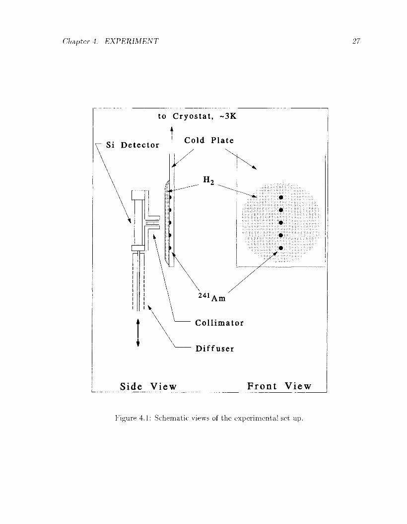
4.1 .1 Target S y s t e m
The cryogenic solid hydrogen target system used in the present experiment is the same
as the one used for the beam experiments described in section 1.2, except for one of
the target foils as discussed below. Shown in Fig. 4.1 are the schematic views of the
experimental set up. Americium 241 is electrodeposited on the gold plated oxygen free
copper plate to form an array of spot sources. The americium is covered with a thin gold
layer for safety purposes. The spot diameter is less than 3 mm and 5 spots are separated
by 10 mm center to center.
The spot sources were custom-manufactured by Isotope Product Laboratory1. This
plate replaces the upstream target foil for the beam experiment. The target plate is
cooled to approximately 3K, and solidifies the hydrogen gas onto it when it is introduced
through the diffuser mechanism. Alpha particles penetrating through the hydrogen film
are detected by a passivated, implanted planar silicon detector (Canberra, model FD/S-
600-29-150-RM, serial number 12913), which is mounted on the top of the diffuser.
The silicon detector is collimated such that it only accepts the alphas from one spot
source at a time. Furthermore, the collimator consists of an array of small holes (diameter
1 mm) in order to reduce the angular dispersion of the alpha beam. The collimated
^On N. San Fernando Blvd, Burbank, CA
26
Chapter 4. EXPERIMENT 27
Si Detector
to Cryostat, ~3K n
Cold Plate
Side View Front View
Figure 4.1: Schematic views of the experimental set up.
Chapter 4. EXPERIMENT 28
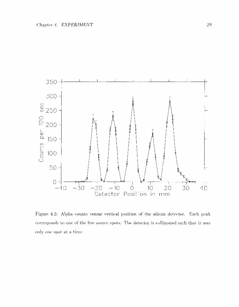
detector can move vertically to allow a measurement of the thickness at five different
positions by detecting the alpha particles from each of the five spot sources. The profile
of alpha counts in the silicon detector versus vertical position of detector for a bare target
(with no hydrogen) is shown in Fig. 4.2.
This proves that we see only one source spot at a time, avoiding that complication in
interpreting the data.
4.1.2 Silicon Detec tor
A silicon detector is used for the energy spectroscopy of alpha particles. The silicon
surface barrier detector (SSB) is probably the most common detector used for charged
particle spectroscopy. It is, in principle, a reverse biased diode. Instead of an np junction
as in normal diodes, the junction is formed between a metal and semiconductor, typically
gold and p-type silicon, creating a Schottky barrier[23]. Ion-implanted detectors have
similar structure, but instead of a metal contact, acceptor ions are implanted by an
accelerator to form p-type silicon at the surface. They offer some advantages over the
SSB such as low leakage current and small dead layer, which contribute to a better energy
resolution. They are also known to provide a more robust surface than an SSB which is
very sensitive to surface contamination.
The detector used for the present experiment has an active area of 600 mm 2 (diameter
27.6 mm) , and thickness of 150 /an with a dead layer of 50 am. It is operated with
reverse bias of 30 V, which fully depletes the detector. In fact, 10 to 15 volts would be
sufficient to deplete the thickness corresponding to the range of 5.5 MeV alpha particles
but appropriate bias gives better energy resolution due to the larger depletion depth
which results in a lower capacitance. This would also provide a better time resolution
because of the faster charge collection, although it is not of much importance in the
present experiment.
Chapter 4. EXPERIMENT 29
^20 - 1 0 0 10 20 Detector Position in mm
Figure 4.2: Alpha counts versus vertical position of the silicon detector. Each peak
corresponds to one of the five source spots. The detector is collimated such that it sees
only one spot at a time.
Chapter 4. EXPERIMENT 30
Hydrogen in a semiconductor is known to influence its properties, and has become
one of the hot topics in condensed matter physics[50, 51]. In particular, ^/SR, another re
markable application of the muon, has proven to be an almost exclusive probe of isolated
hydrogen-like atoms in semiconductors[52, 53]. Thus, a solid state detector is normally
considered to be incompatible with hydrogen gas. For example, in the measurements of
stopping powers of twelve different gases, Bimbot et al. used a special target configu
ration for hydrogen gas[42]. Our silicon detector, however, performs without significant
degradation in a hydrogen rich, low temperature (~ 90 K) environment. (It has proven
to work satisfactorily even in a trit ium environment in our December 1993 run[6].)
The silicon detector had a resolution of ~ 30 keV for 5.5 MeV alpha particles as
determined with an americium source at room temperature. Cooling down to a lower
temperature improves the resolution, and at 90 K it reaches ~ 20 keV. The leakage
current dropped from 0.1 //A to nearly zero (<C 0.01 fiA). In the meantime the apparent
energy for the same source drops significantly due to the increase in the band gap. This
drift in gain becomes a source of the uncertainty for the final results as described in
section 5.3.
4.1.3 Electronics and D a t a Acquis i t ion S y s t e m
The electronics diagram is shown in Fig. 4.3. The signal from the silicon detector is di
vided into an energy and a timing output with a charge sensitive preamplifier (Canberra
2003BT). The preamplifier works as a charge to voltage converter providing a positive
polarity pulse to the energy output as well as providing a negative polarity fast differ
entiated pulse to the timing output. It should be noted that , due to a 110 MQ resistor
in series with the detector, the actual bias applied to the detector is reduced depending
on the leakage current. The energy signal from the preamplifier is further amplified with
a linear spectroscopy amplifier. An 8000 channel ADC (Analog to Digital Converter)
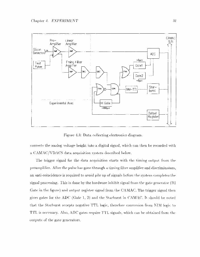
Chapter 4. EXPERIMENT 31
Pre- Linear Amplifier Amplifier
Silicon \ |N
Detector/" H>
Test Pulser
Timing Filiter Amplifier
Experimental Area
~5/is
Gatel
Gate2
-5/u.s
NIM-TTL-
HI Gate
-400/is
ADC
Star-burst
Output Register
CAMAC BUS
\S
Figure 4.3: Data collecting electronics diagram.
converts the analog voltage height into a digital signal, which can then be recorded with
a CAMAC/VDACS data acquisition system described below.
The trigger signal for the data acquisition starts with the timing output from the
preamplifier. After the pulse has gone through a timing filter amplifier and discriminators,
an anti-coincidence is required to avoid pile up of signals before the system completes the
signal processing. This is done by the hardware inhibit signal from the gate generator (HI
Gate in the figure) and output register signal from the CAMAC. The trigger signal then
gives gates for the ADC (Gate 1, 2) and the Starburst in CAMAC. It should be noted
that the Starburst accepts negative TTL logic, therefore conversion from NIM logic to
TTL is necessary. Also, ADC gates require TTL signals, which can be obtained from the
outputs of the gate generators.
Chapter 4. EXPERIMENT 32
4000
3000
§ 2000 o o
1000-
FWHM ~20keV
5.486MeV
0 4350 4400 4450 4500 4550 4600
alpha particle energy [ch]
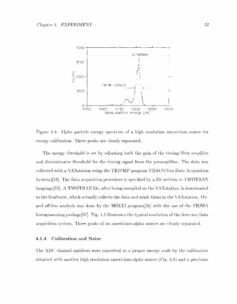
Figure 4.4: Alpha particle energy spectrum of a high resolution americium source for
energy calibration. Three peaks are clearly separated.
The energy threshold is set by adjusting both the gain of the timing filter amplifier
and discriminator threshold for the timing signal from the preamplifier. The data was
collected with a VAXstation using the TRIUMF program VDACS(Vax Data Acquisition
System) [54]. The data acquisition procedure is specified by a file written in TWOTRAN
language[55]. A TWOTRAN file, after being compiled on the VAXstation, is downloaded
to the Starburst, which actually collects the data and sends them to the VAXstation. On-
and off-line analysis was done by the MOLLI program[56] with the use of the FIOWA
histogramming package[57]. Fig. 4.4 illustrates the typical resolution of the detector/data
acquisition system. Three peaks of an americium alpha source are clearly separated.
4.1.4 Calibration and Noise
The ADC channel numbers were converted to a proper energy scale by the calibration
obtained with another high resolution americium alpha source (Fig. 4.4) and a precision
Chapter 4. EXPERIMENT 33
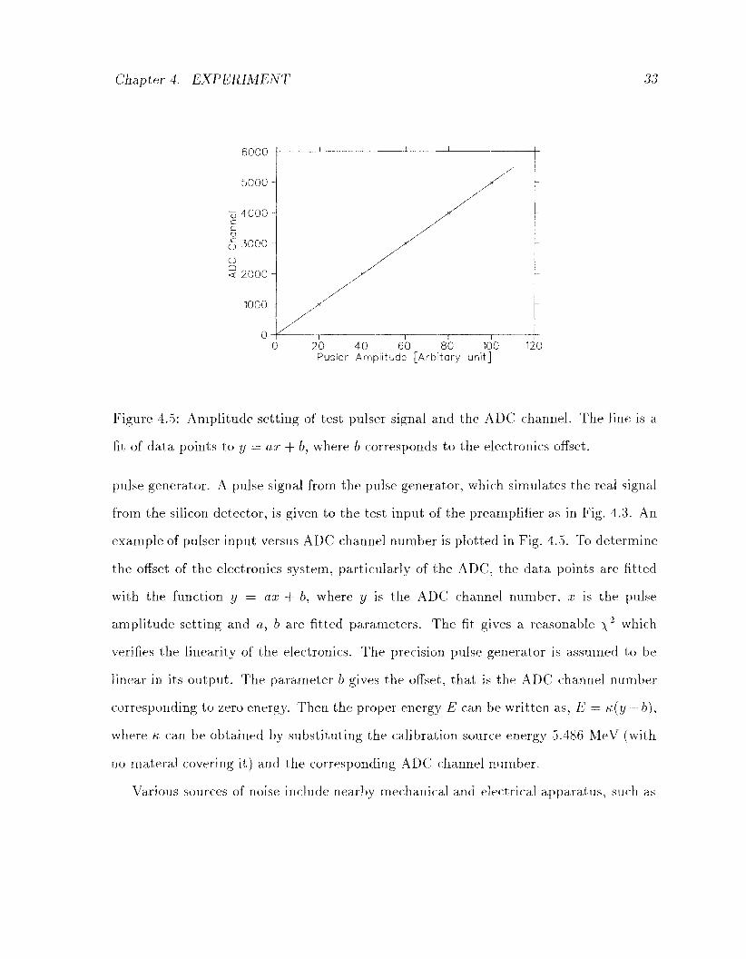
6000 -) ' ' ' ' '
5000- y /
v 4000 - X
c / 5 3000 - y ^ o / / < 2 0 0 0 - x ^
1000 - y /
0 20 40 60 80 100 120 Pusler Amplitude [Arbitary unit]
Figure 4.5: Amplitude setting of test pulser signal and the ADC channel. The line is a
fit of data points to y — ax + 6, where b corresponds to the electronics offset.
pulse generator. A pulse signal from the pulse generator, which simulates the real signal
from the silicon detector, is given to the test input of the preamplifier as in Fig. 4.3. An
example of pulser input versus ADC channel number is plotted in Fig. 4.5. To determine
the offset of the electronics system, particularly of the ADC, the data points are fitted
with the function y = ax + b, where y is the ADC channel number, x is the pulse
amplitude setting and a, b are fitted parameters. The fit gives a reasonable x'2 which
verifies the linearity of the electronics. The precision pulse generator is assumed to be
linear in its output. The parameter b gives the offset, that is the ADC channel number
corresponding to zero energy. Then the proper energy E can be written as, E = K,(y — b),
where K can be obtained by substituting the calibration source energy 5.486 MeV (with
no materal covering it) and the corresponding ADC channel number.
Various sources of noise include nearby mechanical and electrical apparatus, such as
Chapters EXPERIMENT 34
the turbo molecular pump, the mechanical pump, cryopump, quadrupole mass spectrom
eter and ion gauge. The sources of noise are both microphonic and electronic. It was
also found that cables for the thermometer, when connected to the voltage meter, cause
a huge random noise. There were some other occasional, large fluctuations whose sources
could not be identified, possibly from the mini cyclotron near the experimental area.
4.2 Experimental Runs
Before the measurements with solid hydrogen, tests of the silicon detector, electronics
and data acquisition were conducted with the test vacuum chamber. Optimization of
bias voltage and amplifier shaping time as well as set up and debugging of the data
acquisition hardware and software was achieved. The following two separate runs were
conducted in the Muonic Hydrogen Group working area located in the Meson Hall at
TRIUMF.
4.2.1 Series 1
The first series of runs was mainly devoted to the verification of the principle of the
method. One hundred litres of liquid helium was consumed to give about 40 hours of
measurement time, running continuously. It takes roughly 4-10 hours, depending on
liquid helium flow rate, to cool down the cryostat from room temperature to 3 K. While
cooling down, the leakage current drops to nearly zero (<C 0.01 // A) and the voltage drop
across the resistor in the preamplifier becomes negligible. Therefore the bias voltage has
to be readjusted to prevent the break down of the detector. It was realized that the
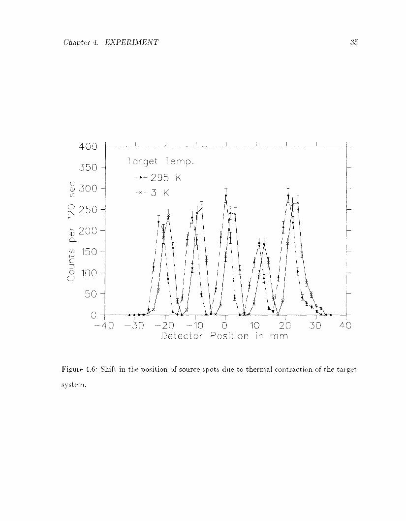
source position shifted by as much as 2.5 mm due to thermal contraction when the
cryostat cooled. This is illustrated by the plot of source array profiles in Fig. 4.6.
Thickness measurements were done in the three different targets. The amount of
Chapter 4. EXPERIMENT 35
400
3 5 0 -
S 3 0 0 -
g 2 5 0 -
0) 200
i5 150 H c o 100
50
0 -40 - 3 0
T • ~r - 2 0 - 1 0 0 10 20
Detector Position in mm 40
Figure 4.6: Shift in the position of source spots due to thermal contraction of the target
system.
Chapter 4. EXPERIMENT 36
molecular gas introduced to the target is quoted in units of torr-litre, where one torr-litre
corresponds to the number of molecules in 1 litre of gas at a pressure of 1 torr at room
temperature (~295 K). The three measured targets included a gas injection of 20 torr-
litres, 20 torr-litres deposited on top of the existing 20 torr-litre target (giving a total
of 40 torr-litres) and separately deposited 150 torr-litres. Five spots were measured in
each target except the 20 torr-litre target where only 3 spots were measured. The source
spot position y is noted in terms of its vertical distance with respect to the center of the
target foil, hence the beam. Therefore we have source spots at y = —20, —10,0,10 and
20 mm. The gas deposition was conducted typically at a rate of 1 torr-litre per second
for thick target deposition. For thin targets, the rate was much slower.
4.2.2 Series 2
In the second run, the diffuser position was changed by 2.5 m m to compensate the thermal
contraction effect (Fig. 4.6). Different deposition conditions such as deposition rate and
with or without cryo-pumping were tried to check the effect on thickness and uniformity.
The gas input used here was 150, 300, and 400 torr-litres. Also in this run, various
measurements were tried as follows.
Cross Contaminat ion
Cross contamination was tested in the following way, where all the measurements were
done at y = 0 mm (center spot). First a large amount of gas (1000 torr-litres) was
deposited on the other target foil (downstream target foil) and the alpha particle energy
from the source on the upstream foil was measured. If there is any cross contamination,
a corresponding energy shift of the alpha particles should be observed. One torr-litre of
gas was then deposited on the upstream target foil to compare the energy shift. Finally
Chapter 4. EXPERIMENT 37
another 1000 torr liters of gas was deposited on top of the existing target on the down
stream foil and the thickness of the up stream foil was checked again.
N e o n Targets
Neon targets with gas input of 7.5 and 20 torr-litres were also measured. Neon films were
used in beam experiments for the measurement of muon transfer rates. It is important to
know the absolute thickness and uniformity to interpret the muonic X-ray data correctly.
Another M e t h o d of Depos i t ion
Another set of targets was made in a very different way. Instead of blowing hydrogen
gas directly onto the cold target foil, the diffuser was completely removed away from
the foil, and the gas was introduced into the system with all pumping valves closed.
300 torr-litres of gas was used for this measurement. Relatively high vacuum pressure
was kept (~ 10~4 torr) during introduction of the gas to allow interaction between the
gas molecules. The gas is expected to be deposited onto all the cold parts in the system
including the target foils. The measurement was originally aimed as a test for the DA$NE
experiment proposed by Olin et al. [11]. Its implication for the uniformity of our target
is discussed in section 6.5.
Chapter 5
A N A L Y S I S OF DATA
5.1 Determinat ion of Thickness
Shown in Fig 5.1 is an example of the energy spectra of alpha particles penetrating
through the hydrogen film. Each peak represents alphas from the target with different
amounts of gas let in, namely 0, 150, and 300 torr-litres. Clearly, one can observe alpha
particles losing more energy when going through the target with the larger amount of
injected hydrogen. Also, the peak becomes wider due to the energy straggling effect.
Notice that the bare target spectrum with no hydrogen has an asymmetric shape with
a smaller second peak and a low energy tail. This is partly due to the energy loss in the
gold overlayer on top of the americium, which was added for safety purposes. Backscat-
tering of alpha particles from the gold substrate is also possible. Single scatterings with
large energy loss from the collimator material as well as hydrogen can account for the low
energy tails. Each bare spot has a slightly different energy and peak shape, probably due
to variations in thickness of the sources and gold overlayers. It is this asymmetric and
irregular shape of the peaks that makes it difficult to fit the data with a normal function
such as a Gaussian. Instead, as recommended by Hanke and Laursen[58], we determine
the mean channel values < N> from the distribution function f(N) in the ADC spectra:
r<N>+i
/ f(N)NdN
<^>=^|fe , (5-1) / f(N)dN
where e is a finite cut off value. The effect of the value of t upon the final results
38

Chapter 5. ANALYSIS OF DATA 39
in
700
600
5 0 0 -
4 0 0 -c
S 300
2 0 0 -
100
0 torr —litre
150 tor r —litre
300 t o r r - l i t r e
- r _ 1800 2300 2800 3300 3800
a Energy [ch] 4300 4800
Figure 5.1: Alpha particle energy spectra with different thicknesses of hydrogen film.
The numbers indicate the amount of hydrogen gas injected in units of torr-litre.
Chapter 5. ANALYSIS OF DATA 40
is discussed in the section 5.3. < N > is then converted to the energy scale by the
calibration which was described in section 4.1.4.
Given the range of alpha particles as a function of energy, Range(E), the thickness
of the target can be obtained by:
Thickness = Range(Etmt) — Range(Efm), (5-2)
where Etmt is the initial energy of the alpha particles and Eftn, the energy after pen
etrating through the target. This avoids the complication of numerically integrating
stopping power cross sections. A correction due to the "wiggled" path of the particle
may be necessary and will be considered later. The specific choice of energy-range values
is discussed in the following section.
5.2 Energy-Range Tables
It is very important to use an accurate stopping power and/or range table in determi
nation of the thickness by energy loss. A few energy-range tables published in the past
decades, plus more recent ones are discussed and their values compared in this section.
5.2.1 Northcliffe and Schilling (1970)
An energy-range table by Northcliffe and Schilling[59] was once considered as a standard.
With emphasis on heavy ions, they compiled stopping power and range tables for ions of
all atomic numbers at energies of 0.01 -12 MeV/amu with no uncertainty specified. How
ever, there now exist many experiments which disagree with the table by large amounts.
For example, Bianco and Richer found a 35% deviation in the stopping power of alpha
particles in D2 gas from the table[60]. Geissel et al. claim that heavy ion stopping powers
in light elements are underestimated by 15% in the table[43].
Chapter 5. ANALYSIS OF DATA 41
5.2.2 Ziegler (1977)
At present the most commonly used stopping power table for alpha particles is probably
the one by Ziegler[17]. He divided the projectile energy into three regions. These are
the high energy region, or Bethe-Bloch region, where the Bethe-Bloch formula is used
to obtain the stopping powers, the low energy region, where velocity proportionality is
assumed, and the intermediate energy region, where the experimental data are fitted to
the parameterization discussed in section 3.2 (equations 3.4-3.6).
Ziegler also included in his table empirically estimated values of stopping power in
condensed gases by interpolating from the elements for which solid data are available.
Approximately 40 % lower stopping power for solid hydrogen over the gas is given for
alpha particles of 1 MeV. More recent measurements[15, 47], however, disprove such large
phase effects in other condensed gases which are similarly predicted by the same table.
Therefore its accuracy for solid hydrogen is dubious.
The proton range table by Janni[30] is widely used in the intermediate energy physics
community. The emphasis is put on the statistical treatment of the experimental in
formation in terms of least-square curve fitting as well as determining mean ionization
potentials. All the range values are tabulated with their uncertainties. In (gaseous)
hydrogen, for example, he quotes a 2% error for 5 MeV protons.
5.2.3 Ziegler, Biersack and Lit tmark (1985)
For material studies and device technology, the use of Ziegler, Biersack and Littmark's
tabulation for solids[20] together with their Monte Carlo code1 is very common. It is
known to give a good agreement with experiments for materials commonly used, such Si
and GaAs. For solid targets for which there are few experimental data, an "interpolation
'TRIMfTRansport of Ions in Matter). It is available from James F. Ziegler. IBM-Research, 28-0, Yorktown, NY 10598 USA
Chapter 5. ANALYSIS OF DATA 42
procedure" is used. This is based on the assumption that the deviation between the
experimental and theoretical stopping powers K
K — ^expf ^theory
depends smoothly on the target's atomic number. However, extrapolation to atomic
number 1 may be less reliable. The accuracy of 5% is quoted for alpha particles.
5.2.4 ICRU (1993)
The latest table on stopping powers and ranges is compiled by the International Commis
sion of Radiation Units and Measurements (ICRU) [18]. The mission of ICRU is explained
by Inokuti et al. [61] to recommend internationally acceptable values of physical quantities
relevant to radiation measurements and radiological dosimetry. The report committee on
stopping power consists of members such as Berger, Inokuti, Anderson, Bichsel, Seltzer,
Thwaites, Watt and Sternheimer to name a few. These authors are frequently cited in
this thesis and can be considered as the experts in the field of stopping power stud
ies. The report contains the stopping powers and ranges of protons, alpha particles and
negative pions. In the case of alpha particles in hydrogen, electronic stopping power
for energies higher than ~ 2 MeV are calculated by the Bethe-Bloch theory with vari
ous corrections such as shell, density and deviation from first-order Born approximation.
Mean excitation energies were taken from Ref. [22], which was originally prepared for
the ICRU report on electron and positron stopping powers. For alpha particle energies
lower than 1 MeV, the Varelas-Biersack formula (equations 3.4-3.6) is used with new
coefficients compiled by Watt[62], based on the available experimental data. The energy
region between 1 and 2 MeV is interpolated by a cubic spline function. The ranges are
calculated in the continuous-slowing-down approximation(csda). In this approximation,
Chapter 5. ANALYSIS OF DATA 43
energy-loss fluctuations are neglected, and charged particles are assumed to lose their en
ergy continuously along their tracks at a rate given by the stopping power, as expressed
in
R0(E0 ->• Eat) = p fE°[Selec(E) + Snuc(E)}-ldE, (5.3)
J Est
where R0 is the csda range of a particle slowing down from an initial energy EQ to an
energy at which particles are consider to be stopped Est. In the ICRU table, Est is taken
to be 10 eV. The csda range is generally larger than the average penetration depth Pavi
which is the projection of the range on the initial direction of the particle track due to
its "wiggling" caused by multiple scattering. In the table the detour factor (, which is
defined as the ratio Pav/ R0, is given to take this effect into account. Thus, equation 5.2
can be modified to:
Thickness — ((Emt) • Range(Emt) - ((Efm) • Range(Efin), (5.4)
where Eint and Ejin are the initial and final energies of the alpha particle respectively.
5.2.5 Comparison of Tables
Figures 5.2-5.3 compare the stopping powers of alpha particles in hydrogen from the
various tables discussed above. Shown in Fig. 5.2 are stopping powers in gaseous hydro
gen. As one can see, Northcliffe and Schilling[59] deviate significantly from Ziegler[17]
and ICRU[18], whereas the latter two are in good agreement.
Fig. 5.3(a) compares stopping of solid hydrogen predicted by Ziegler(1977)[17] and
Ziegler et al. (1985)[20] with that of gas by ICRU. For Ziegler et al. (1985), only elec
tronic stopping power is plotted, but nuclear stopping is negligible for our purposes.
While Ziegler(1977) shows a large phase effect, ICRU and Ziegler et al. (1985) are also
significantly different at the stopping power maximum and at very low energy. However,
differences between the latter two are rather small in Fig. 5.3(b), where the energy of
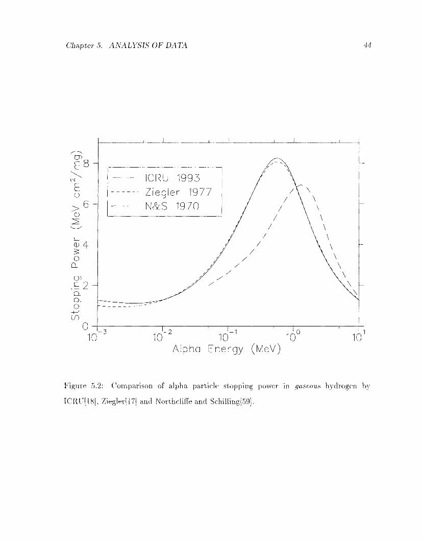
Chapters. ANALYSIS OF DATA 44
10 10 10 10 10 Alpha Energy (MeV)
Figure 5.2: Comparison of alpha particle stopping power in gaseous hydrogen by
ICRU[18], Ziegler[17] and Northcliffe and Schilling[59].
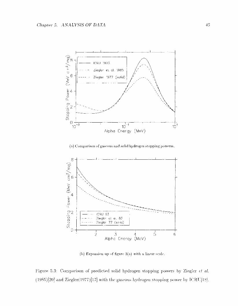
Chapter 5. ANALYSIS OF DATA 45
E*
E u > 0)
6 -
(D 4
o CL
cr> .E2H CL CL
o CO
ICRU 1993
Ziegler et al. 1985
Ziegler 1977 (solid)
10 10 ' Alpha Energy (MeV)
10'
(a) Comparison of gaseous and solid hydrogen stopping powerss.
en E
E6 u
> CD
CD
O C L
Cno _ C /-
'CL CL o
- f-J
CO
ICRU 93 Ziegler et al. 85 Ziegler 77 (solid)
3 4 Alpha Energy (MeV)
(b) Expansion up of figure 3(a) with a linear scale.
Figure 5.3: Compar i son of predic ted solid hydrogen s topping powers by Ziegler et al.
(1985)[20] and Ziegler(1977)[l7] with the gaseous hydrogen s topping power by ICRU[18].
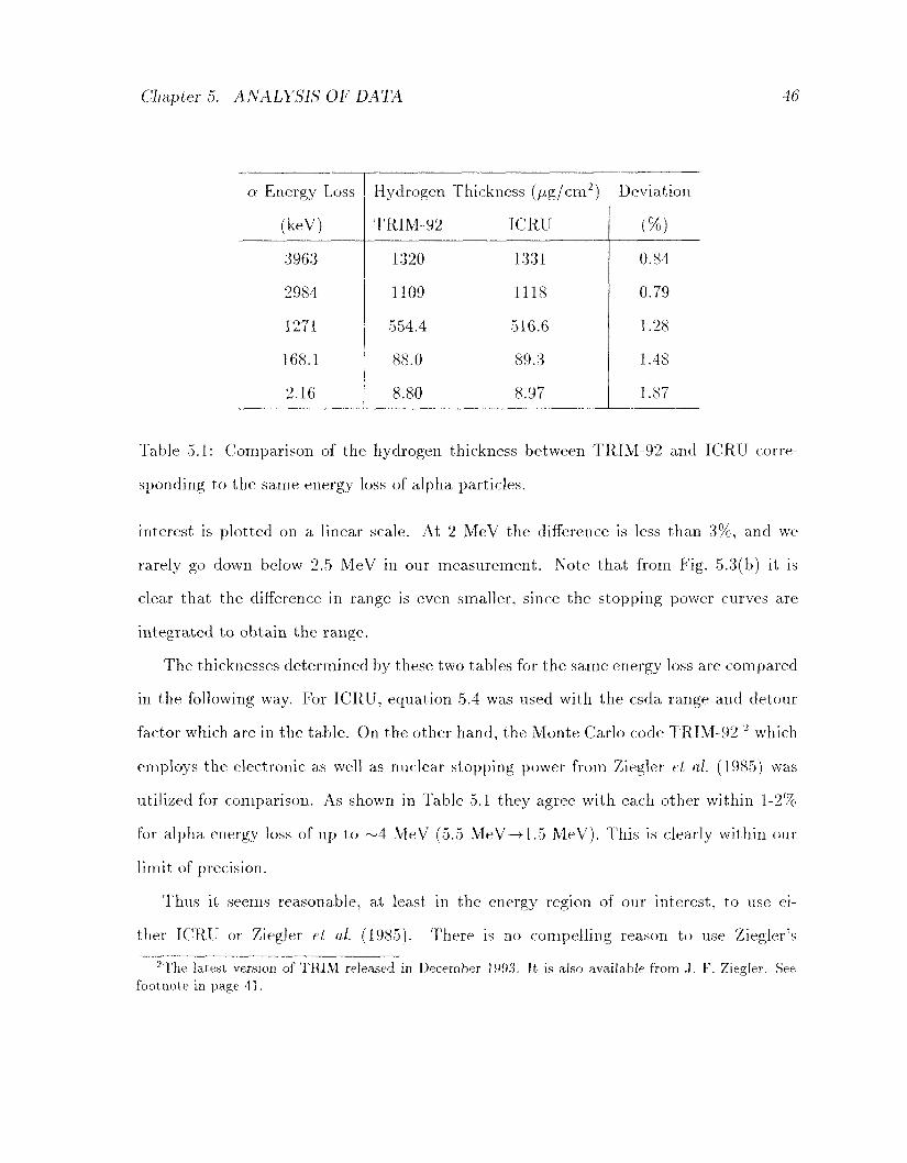
Chapter 5. ANALYSIS OF DATA 46
a Energy Loss
(keV)
3963
2984
1271
168.1
2.16
Hydrogen
TRIM-92
1320
1109
554.4
88.0
8.80
Thickness (//g/cm2)
ICRU
1331
1118
516.6
89.3
8.97
Deviation
(%)
0.84
0.79
1.28
1.48
1.87
Table 5.1: Comparison of the hydrogen thickness between TRIM-92 and ICRU corre
sponding to the same energy loss of alpha particles.
interest is plotted on a linear scale. At 2 MeV the difference is less than 3%, and we
rarely go down below 2.5 MeV in our measurement. Note that from Fig. 5.3(b) it is
clear that the difference in range is even smaller, since the stopping power curves are
integrated to obtain the range.
The thicknesses determined by these two tables for the same energy loss are compared
in the following way. For ICRU, equation 5.4 was used with the csda range and detour
factor which are in the table. On the other hand, the Monte Carlo code TRIM-92 2 which
employs the electronic as well as nuclear stopping power from Ziegler et al. (1985) was
utilized for comparison. As shown in Table 5.1 they agree with each other within 1-2%
for alpha energy loss of up to ~ 4 MeV (5.5 MeV-»1.5 MeV). This is clearly within our
limit of precision.
Thus it seems reasonable, at least in the energy region of our interest, to use ei
ther ICRU or Ziegler et al. (1985). There is no compelling reason to use Ziegler's
2The latest version of TRIM released in December 1993. It is also available from J. F. Ziegler. See footnote in page 41.
Chapter 5. ANALYSIS OF DATA 47
old values(1977). In fact, Ziegler et al. themselves suggest that their older one is less
accurate[20]. For reasons of convenience for our thickness determination we shall use the
ICRU table, which provides the integrated ranges. The tabulated values are interpolated
with fourth order polynomials, and equation 5.4 is used to obtain the target thickness.
5.3 Uncertaint ies
There are several sources of systematic uncertainties in the determination of the target
thickness, other than the statistical uncertainty which is negligible most of the time.
These include the knowledge of stopping powers, detector calibration, computation of
mean energy and angular dispersion of alpha particles.
5.3.1 Stopping Powers and Ranges
In most cases, the dominant contribution to the systematic error comes from the
knowledge of stopping powers. This is illustrated in Fig. 5.4, where variation of the
thickness due to the stopping power value is shown in the case of ICRU and Northcliffe
and Schilling. As large as a 25% difference can be observed. However, we can safely
disregard Northcliffe and Schilling as discussed in section 5.2. The ICRU table[18] claims
an uncertainty of ~ l - 2 % at 4 MeV, and ~2-5% at 1 MeV for the stopping power of alpha
particles. This is of course in gaseous hydrogen, and its application to solid requires
caution. Ziegler et a/.[20] quote an average accuracy of 5%. This is the average deviation
of their values from 3290 available data points on alpha particle stopping power. In either
case, there is no legitimate way to determine the uncertainty in the stopping power for
solid hydrogen, since there exist no experimental data. However, since the above two
tables agree fairly well in the energy region of interest, we shall quote 5% uncertainty in
the stopping power, hence the range including the phase effect. This can be improved.
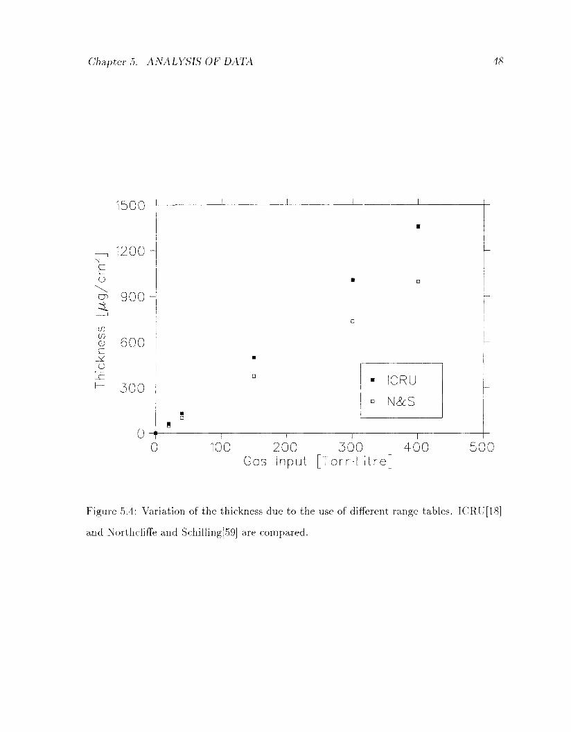
Chapter 5. ANALYSIS OF DATA 48
100 200 Gas Input
300 400 or r -L i t re ]
500
Figure 5.4: Variation of the thickness due to the use of different range tables. ICRU[18]
and Northcliffe and Schilling[59] are compared.
Chapter 5. ANALYSIS OF DATA 49
in the future, if the stopping power of solid hydrogen becomes available.
5.3.2 P e a k E n e r g y Determinat ion
To make a thickness measurement, one must measure two energies, before and after the
deposition of the film. Computation of the centroid as well as the calibration of the
silicon detector can be a source of systematic uncertainty in determining such energies.
Computat ion of Centroid
Some arbitrariness in the cut-off value e in the integral in equation 5.1 in taking the
centroid may affect the results. The influence of the choice of e on the thickness was
tested by changing e. This was found to be less than ~ 5 keV for bare, 20 torr-litre and
40 torr-litre targets, ~10 keV for 150 torr-litre, ~30 keV for 300 torr-litre and ~60 keV
for 400 torr-litre targets. Due to the lower energy tail and increasing width of the peak,
determination of a centroid is subject to a larger systematic uncertainty for increasing
thickness of the target.
Detec tor Calibration
The calibration of the silicon detector was found to be very sensitive to its temperature.
This effect is accounted for by the change in the average energy required to create an
electron-hole in the silicon as the temperature shifts. Namely, the band gap in silicon
increases as the temperature decreases. With a few exceptions, where we suffered an
accidental large temperature change in the detector, the calibration of the detection
system is taken to be accurate to 2 channels (~0.5%).
The above two uncertainties are, however, negligible in the measurement of thick
targets compared to the uncertainty in the stopping power. They become important
Chapter 5. ANALYSIS OF DATA 50
only in thin (<40 torr-litre) targets.
5.3.3 R a n d o m Noise
Occasionally the appearance of significant noise distorted the spectrum, resulting in a
shift in the centroid. The effect can be as large as 10 keV in the peak energy determi
nation. This was monitored by the signal from the test pulser, simultaneously recorded
with the alpha spectrum, which is sensitive to such noise. When substantial noise is
found, a larger uncertainty in the centroid is quoted accordingly.
Other uncertainties such as path difference due to angular dispersion of alpha particles
and the uncertainty in gas handling are estimated to be negligible compared to the above
sources.
Chapter 6
RESULTS A N D D I S C U S S I O N
6.1 Uniformity
6.1.1 Thickness Profile
Series 1
Fig. 6.1 shows the thickness profile from the first series of runs. Data from three different
targets with gas input of 20, 40 and 150 torr-litres are plotted. The 40 torr-litre target
was made by depositing 20 torr-litres on the existing 20 torr-litre target. Data at y =
—20 and —10 mm do not exist for the 20 torr-litre targets. The error bars include the
uncertainty in the stopping power as well as other errors. Hence, the relative uniformity
can be determined more accurately.
Series 2
A typical thickness profile from the second series of runs is shown in Fig. 6.2. The
diffuser position was displaced by 2.5 mm in Series 2 as mentioned in section 4.2. Data
from targets with 150 torr-litre and 300 torr-litre gas input are plotted. Similarly to Fig.
6.1, the error bars include the stopping power uncertainty.
A few remarks can be made on the thickness profiles. First, there is a drop in thickness
at both edges. Second, the shape is asymmetric with respect to the center of the beam.
These non-uniformities will be discussed in section 6.7, but first we shall look at results
from other measurements.
51
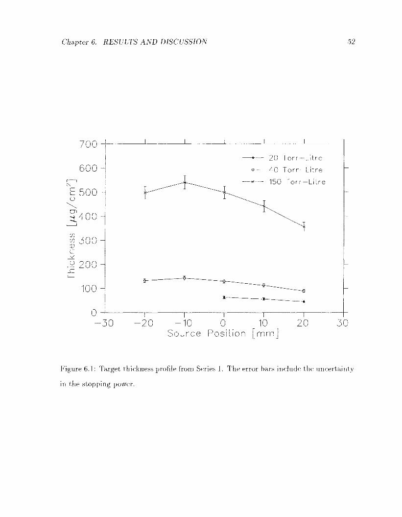
Chapter 6. RESULTS AND DISCUSSION 52
700
6 0 0 -
E 500 -o
^ 4 0 0
^ 3 0 0 CD
c
."$ 200
100
0 -30
•—
e—
H—
20 Torr- Litre
- 40 To r r -L i t r e
- 150 To r r -L i t r e
•20 - 1 0 0 10 Source Position [ m m ]
20 30
Figure 6.1: Target thickness profile from Series 1. The error bars include the uncertainty
in the stopping power.
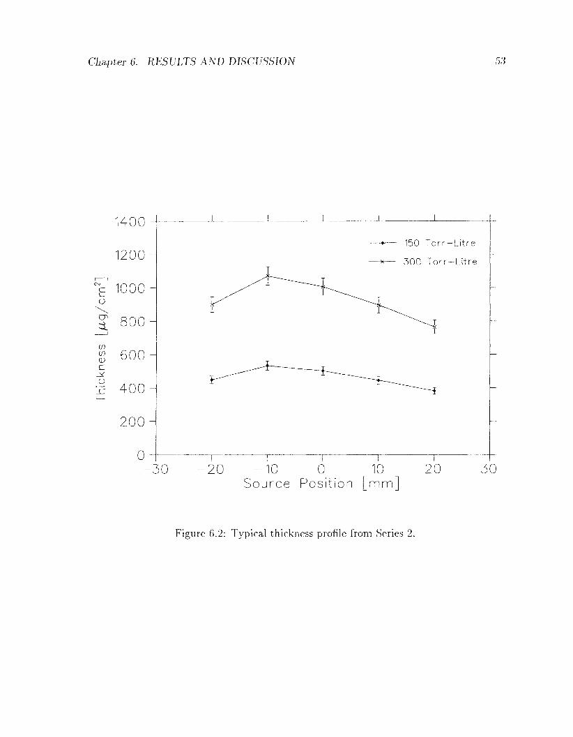
Chapter 6. RESULTS AND DISCUSSION 53
1400
1200
NE 1000 o
;oo
% 600 H c
•F 400
200 H
0
150 Tor r -L i t re
300 Tor r -L i t re
-30 - 2 0 -10 0 10 20 Source Position [ m m ]
30
Figure 6.2: Typical thickness profile from Series 2.
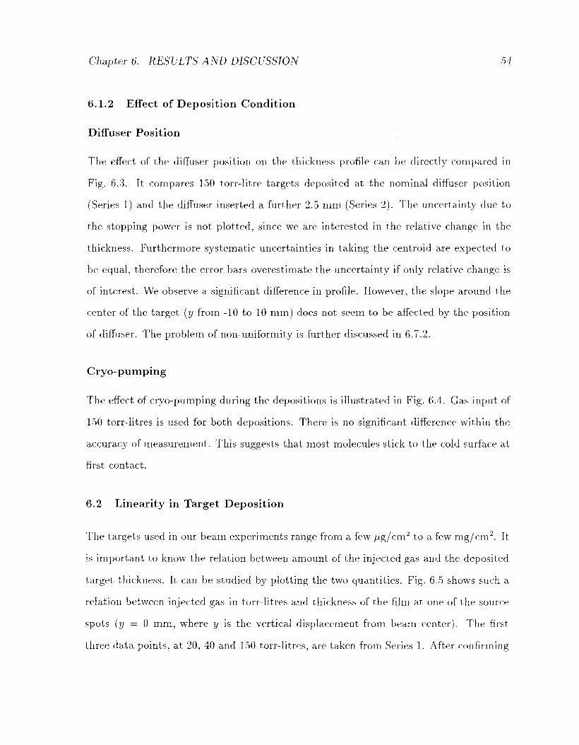
Chapter 6. RESULTS AND DISCUSSION 54
6.1.2 Effect of Depos i t ion Condit ion
Diffuser Posit ion
The effect of the diffuser position on the thickness profile can be directly compared in
Fig. 6.3. It compares 150 torr-litre targets deposited at the nominal diffuser position
(Series 1) and the diffuser inserted a further 2.5 mm (Series 2). The uncertainty due to
the stopping power is not plotted, since we are interested in the relative change in the
thickness. Furthermore systematic uncertainties in taking the centroid are expected to
be equal, therefore the error bars overestimate the uncertainty if only relative change is
of interest. We observe a significant difference in profile. However, the slope around the
center of the target (y from -10 to 10 mm) does not seem to be affected by the position
of diffuser. The problem of non-uniformity is further discussed in 6.7.2.
Cryo-pumping
The effect of cryo-pumping during the depositions is illustrated in Fig. 6.4. Gas input of
150 torr-litres is used for both depositions. There is no significant difference within the
accuracy of measurement. This suggests that most molecules stick to the cold surface at
first contact.
6.2 Linearity in Target Depos i t ion
The targets used in our beam experiments range from a few //g/cm2 to a few mg/cm2 . It
is important to know the relation between amount of the injected gas and the deposited
target thickness. It can be studied by plotting the two quantities. Fig. 6.5 shows such a
relation between injected gas in torr-litres and thickness of the film at one of the source
spots (y = 0 mm, where y is the vertical displacement from beam center). The first
three data points, at 20, 40 and 150 torr-litres, are taken from Series 1. After confirming
Chapter 6. RESULTS AND DISCUSSION
i i i r -20 -10 0 JO 20
Source Position [ m m ]
Figure 6.3: Thickness profile with different diffuser positions. Series 1 corresponds to the
nominal diffuser position, and Series 2 is with diffuser inserted a further 2.5 mm. The
error bars do not include the uncertainty in the stopping power.
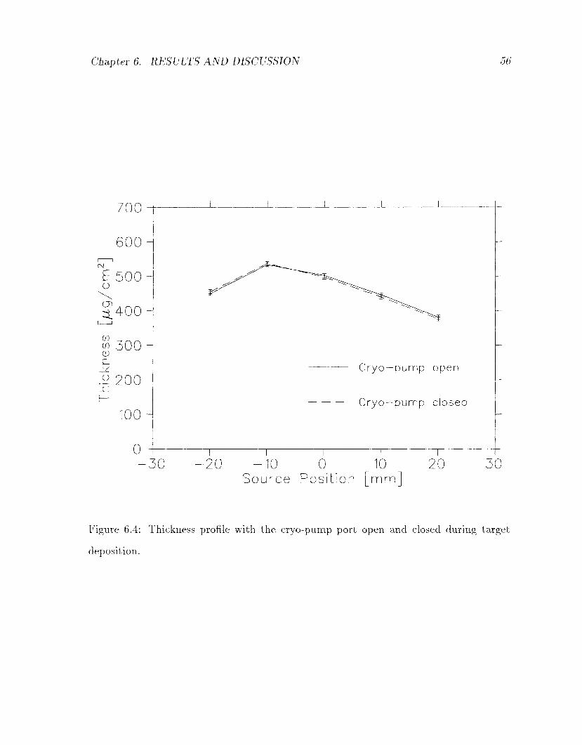
Chapter 6. RESULTS AND DISCUSSION 56
700
600
£ 500 o
5400
S300H CD C
."̂ 200 SI
100
0 -30
Cryo—pump open
Cryo—pump closed
1 I I I r~
-20 -10 0 JO 20 Source Position [mm]
30
Figure 6.4: Thickness profile with the cryo-pump port open and closed during target
deposition.
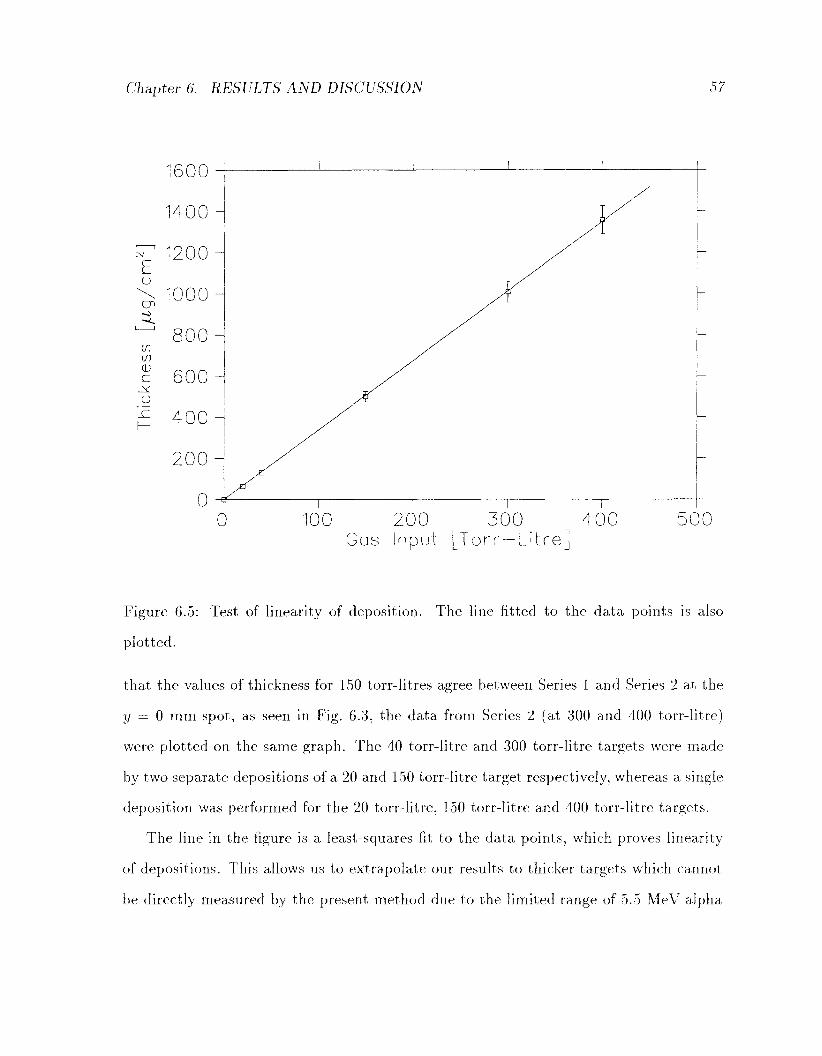
Chapter 6. RESULTS AND DISCUSSION 57
0 100 200 Gas input
300 400 500 [Tor r — L i t re ]
Figure 6.5: Test of linearity of deposition. The line fitted to the data points is also
plotted.
that the values of thickness for 150 torr-litres agree between Series 1 and Series 2 at the
y = 0 mm spot, as seen in Fig. 6.3, the data from Series 2 (at 300 and 400 torr-litre)
were plotted on the same graph. The 40 torr-litre and 300 torr-litre targets were made
by two separate depositions of a 20 and 150 torr-litre target respectively, whereas a single
deposition was performed for the 20 torr-litre, 150 torr-litre and 400 torr-litre targets.
The line in the figure is a least-squares fit to the data points, which proves linearity
of depositions. This allows us to extrapolate our results to thicker targets which cannot
be directly measured by the present method due to the limited range of 5.5 MeV alpha
Chapter 6. RESULTS AND DISCUSSION 58
particles. It should be recalled that our standard targets for muonic hydrogen isotope
production are made with ~1000 torr-litres of injected gas.
The fit gives the conversion relation
Thickness (pg/crn2) = (3.38 ±0.17) x H2 Input (torr — litres), (6-1)
for the central spot, y — 0 mm. Since the fitted line goes through all the data points,
uncertainty is quoted only from that of the stopping power (5%).
6.3 Cross Contaminat ion
The cross contamination was checked by depositing as much as 1000 torr-litres of gas
from the other side of the diffuser to the downstream foil. It was measured only at the
central spot, y = 0 mm. The first trial was rather inconclusive, giving the thickness
of 1.4±3.2 /ig/cm2 on the upstream foil. With improved calibration and stable tem
perature, we obtained 1.62±0.84 ^g/cm 2 of cross deposition, assuming no random noise
effect (section 5.3.3). The systematic uncertainties in computing the centroid described
in section 5.3 are negligible, since the energy loss is very small and there is very lit
tle change in the peak shape. The error in calibration is also neglected here, because
measurements were made consecutively with a very short interval and the detector gain
was stable. Thus, the quoted uncertainty comes only from statistics. With the conver
sion factor derived in section 6.2, 3.38 /ug/(cm2-torr-litre), 1000 torr-litres correspond to
~ 3.4 mg/cm2 . Comparing this with the above value, we get 0.48 ± 0.25 x 10~3 cross
contamination, or an upper limit of 0.8 x 10~3 with 90% confidence level.
To check the sensitivity of our measurement to a small amount of gas such as is
being discussed in this section, 1 torr-litre of hydrogen was deposited. This gives us
3.07±0.90/ig/cm2 with uncertainty similarly derived as above. The result is consistent
with the conversion factor obtained in section 6.2.
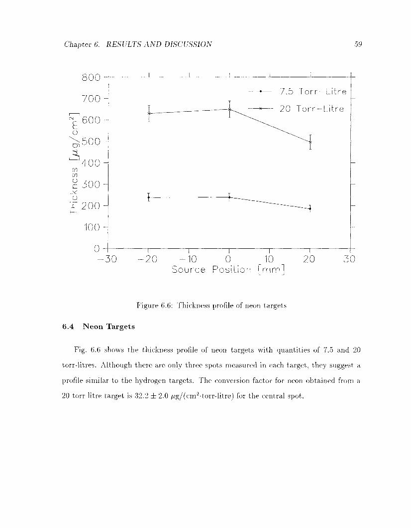
Chapter 6. RESULTS AND DISCUSSION 59
800
7 0 0 ^
^ 6 0 0
^ 5 0 0 H
^ 4 0 0 CO to
^ 3 0 0
'£ 200 H h -
100^
0 - 3 0
j
7.5 Torr —Litre
20 Torr —Litre
J
-20 - 1 0 0 10 20 Source Position [ m m ]
30
Figure 6.6: Thickness profile of neon targets
6.4 N e o n Targets
Fig. 6.6 shows the thickness profile of neon targets with quantities of 7.5 and 20
torr-litres. Although there are only three spots measured in each target, they suggest a
profile similar to the hydrogen targets. The conversion factor for neon obtained from a
20 torr-litre target is 32.2 ± 2.0 //.g/(cm2-torr-litre) for the central spot.
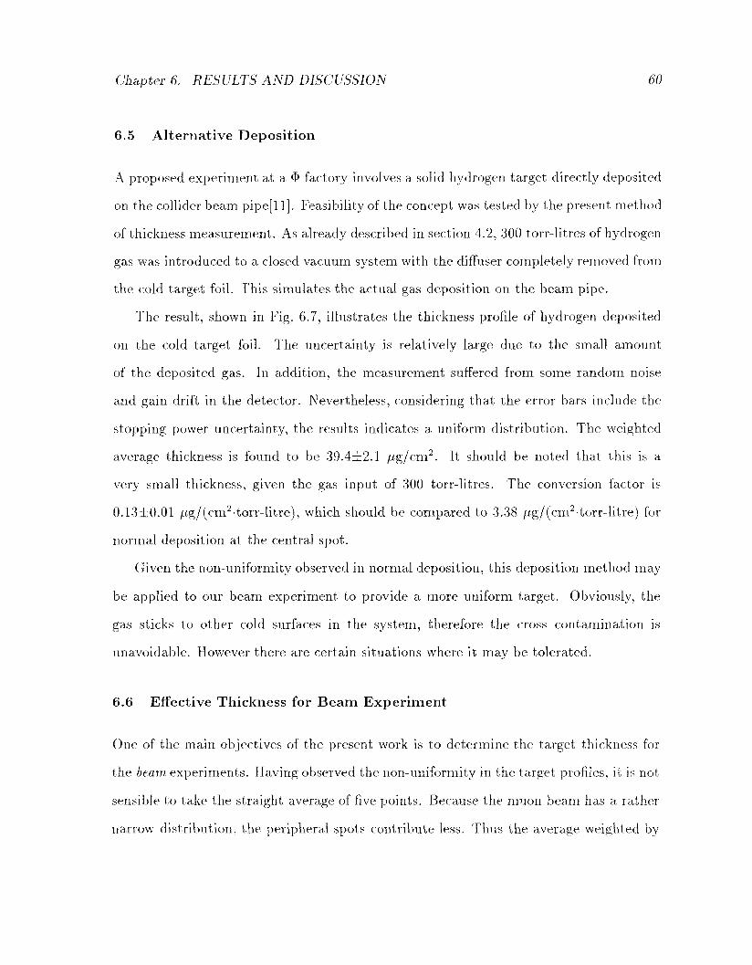
Chapter 6. RESULTS AND DISCUSSION 60
6.5 Alternat ive Depos i t ion
A proposed experiment at a $ factory involves a solid hydrogen target directly deposited
on the collider beam pipe[l 1]. Feasibility of the concept was tested by the present method
of thickness measurement. As already described in section 4.2, 300 torr-litres of hydrogen
gas was introduced to a closed vacuum system with the diffuser completely removed from
the cold target foil. This simulates the actual gas deposition on the beam pipe.
The result, shown in Fig. 6.7, illustrates the thickness profile of hydrogen deposited
on the cold target foil. The uncertainty is relatively large due to the small amount
of the deposited gas. In addition, the measurement suffered from some random noise
and gain drift in the detector. Nevertheless, considering that the error bars include the
stopping power uncertainty, the resirits indicates a uniform distribution. The weighted
average thickness is found to be 39.4±2.1 /ig/cm2 . It should be noted that this is a
very small thickness, given the gas input of 300 torr-litres. The conversion factor is
0.13±0.01 /ug/(cm2-torr-litre), which should be compared to 3.38 /ug/(cm2-torr-litre) for
normal deposition at the central spot.
Given the non-uniformity observed in normal deposition, this deposition method may
be applied to our beam experiment to provide a more uniform target. Obviously, the
gas sticks to other cold surfaces in the system, therefore the cross contamination is
unavoidable. However there are certain situations where it may be tolerated.
6.6 Effective Thickness for B e a m Exper iment
One of the main objectives of the present work is to determine the target thickness for
the beam experiments. Having observed the non-uniformity in the target profiles, it is not
sensible to take the straight average of five points. Because the muon beam has a rather
narrow distribution, the peripheral spots contribute less. Thus the average weighted by
Chapter 6. RESULTS AND DISCUSSION 61
e n bU
5 0 -CM
E ^ 4 0 -cn
^ 3 0 -ir> CD
- § 2 0 -o
1c 1—
10-
n u n
—
•30 •20 -10 0 10 Source Position [mm
20 30
Figure 6.7: Alternative deposition: Hydrogen gas is introduced to the entire cryotstat
with vacuum pump closed. The gas may stick uniformly to all the cold surfaces and
walls.
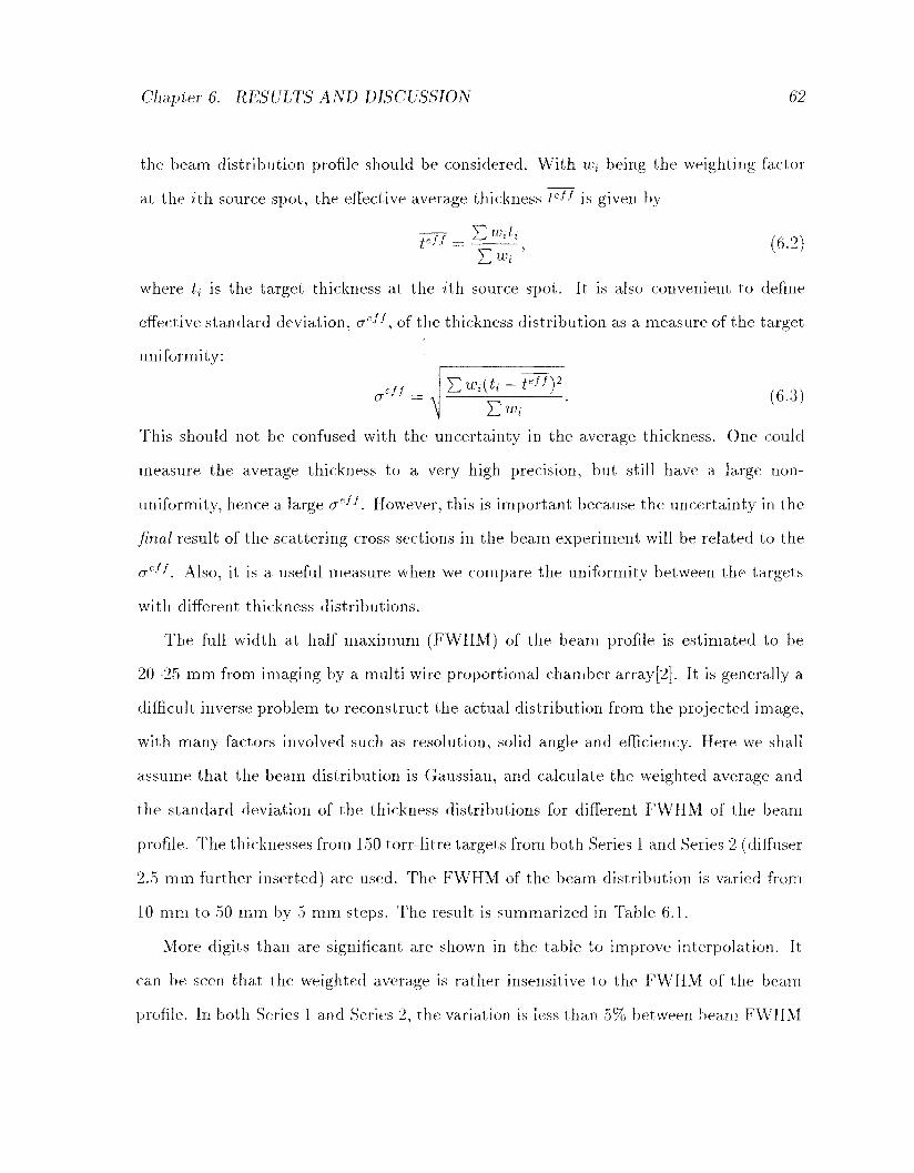
Chapter 6. RESULTS AND DISCUSSION 62
the beam distribution profile should be considered. With wt being the weighting factor
at the ith source spot, the effective average thickness te^ is given by
V" = ^ i , (6.2)
where tt is the target thickness at the ith source spot. It is also convenient to define
effective standard deviation, ae^, of the thickness distribution as a measure of the target
uniformity:
\ S ^ - ' • " ! ! . ,6 .3,
This should not be confused with the uncertainty in the average thickness. One could
measure the average thickness to a very high precision, but still have a large non-
uniformity, hence a large <je^. However, this is important because the uncertainty in the
final result of the scattering cross sections in the beam experiment will be related to the
ae^. Also, it is a useful measure when we compare the uniformity between the targets
with different thickness distributions.
The full width at half maximum (FWHM) of the beam profile is estimated to be
20-25 mm from imaging by a multi wire proportional chamber array[2]. It is generally a
difficult inverse problem to reconstruct the actual distribution from the projected image,
with many factors involved such as resolution, solid angle and efficiency. Here we shall
assume that the beam distribution is Gaussian, and calculate the weighted average and
the standard deviation of the thickness distributions for different FWHM of the beam
profile. The thicknesses from 150 torr-litre targets from both Series 1 and Series 2 (diffuser
2.5 mm further inserted) are used. The FWHM of the beam distribution is varied from
10 mm to 50 mm by 5 mm steps. The result is summarized in Table 6.1.
More digits than are significant are shown in the table to improve interpolation. It
can be seen that the weighted average is rather insensitive to the FWHM of the beam
profile. In both Series 1 and Series 2, the variation is less than 5% between beam FWHM
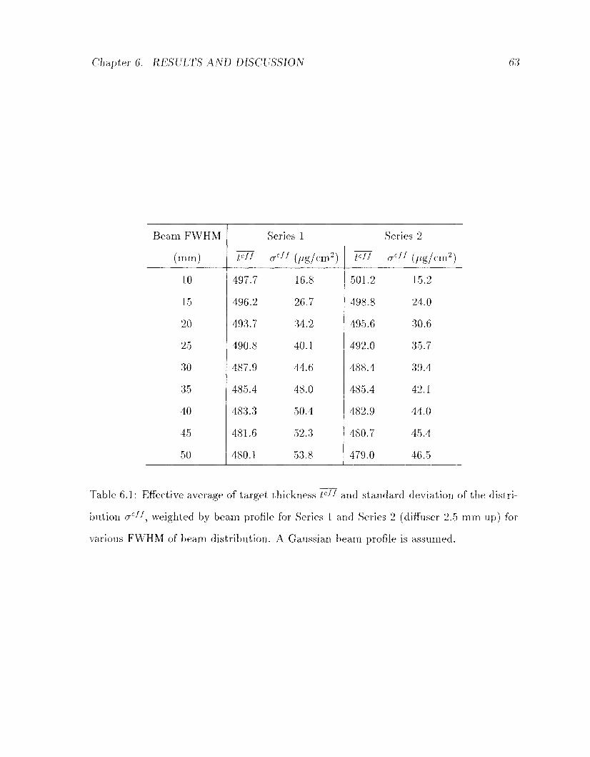
Chapter 6. RESULTS AND DISCUSSION 63
Beam FWHM
(mm)
10
15
20
25
30
35
40
45
50
t*ff
497.7
496.2
493.7
490.8
487.9
485.4
483.3
481.6
480.1
Series 1
cr6^ (/ig/cm2)
16.8
26.7
34.2
40.1
44.6
48.0
50.4
52.3
53.8
fell
501.2
498.8
495.6
492.0
488.4
485.4
482.9
480.7
479.0
Series 2
<T e / / (yUg/cm 2 )
15.2
24.0
30.6
35.7
39.4
42.1
44.0
45.4
46.5
Table 6.1: Effective average of target thickness te^ and standard deviation of the distri
bution oe^, weighted by beam profile for Series 1 and Series 2 (diffuser 2.5 mm up) for
various FWHM of beam distribution. A Gaussian beam profile is assumed.
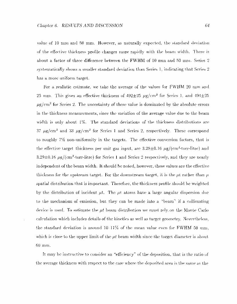
Chapter 6. RESULTS AND DISCUSSION 64
value of 10 mm and 50 mm. However, as naturally expected, the standard deviation
of the effective thickness profile changes more rapidly with the beam width. There is
about a factor of three difference between the FWHM of 10 mm and 50 mm. Series 2
systematically shows a smaller standard deviation than Series 1, indicating that Series 2
has a more uniform target.
For a realistic estimate, we take the average of the values for FWHM 20 mm and
25 mm. This gives an effective thickness of 492±25 fig/cm2 for Series 1, and 494±25
/ig/cm2 for Series 2. The uncertainty of these value is dominated by the absolute errors
in the thickness measurements, since the variation of the average value due to the beam
width is only about 1%. The standard deviations of the thickness distributions are
37 fig/cm2 and 33 /ig/cm2 for Series 1 and Series 2, respectively. These correspond
to roughly 7% non-uniformity in the targets. The effective conversion factors, that is
the effective target thickness per unit gas input, are 3.28±0.16 yUg/(cm2-torr-litre) and
3.29±0.16 //g/(cm2-torr-litre) for Series 1 and Series 2 respectively, and they are nearly
independent of the beam width. It should be noted, however, these values are the effective
thickness for the upstream target. For the downstream target, it is the fit rather than fi
spatial distribution that is important. Therefore, the thickness profile should be weighted
by the distribution of incident fit. The fit atoms have a large angular dispersion due
to the mechanism of emission, but they can be made into a "beam" if a collimating
device is used. To estimate the fit beam distribution we must rely on the Monte Carlo
calculation which includes details of the kinetics as well as target geometry. Nevertheless,
the standard deviation is around 10-11% of the mean value even for FWHM 50 mm,
which is close to the upper limit of the fit beam width since the target diameter is about
60 mm.
It may be instructive to consider an "efficiency" of the deposition, that is the ratio of
the average thickness with respect to the case where the deposited area is the same as the
Chapter 6. RESULTS AND DISCUSSION 65
physical area of the diffuser. At 295 K, one torr-litre of hydrogen molecules ^H^) weighs
108.7 fig. Given the diameter of the diffuser, 6.0 mm, the thickness for 100% efficiency
is 3.78 /ig/(cm2-torr-litre). If we compare this with the effective average thickness (3.29
/ig/(cm2-torrditre)), then we obtain 87% deposition efficiency. If we compare with the
straight (non-weighted) average of 3.11 /ig/(cm2-torr-litre)), the efficiency becomes 82%.
It is interesting to note, however, that the thickest target spot (y = —10 mm) has an
efficiency as high as 95%.
6.7 Mechanism of Gas Depos i t ion
In this section, the mechanism of the gas deposition is discussed based on what we have
learned from the above measurements.
6.7.1 Monte Carlo Simulation of Gas Depos i t ion
A Monte Carlo simulation was conducted to gain a better understanding of the gas
deposition process. The following assumptions were made in the calculation:
• The gas molecules diffuse isotropically from the diffuser.
• The sticking probability of the molecule onto the cold foil is 100%.
• There is no interaction between the gas molecules.
• The perforation structure of the diffuser is neglected.
The result is shown in Fig. 6.8(a) and 6.8(b). The former shows the surface plot of
the 2-dimensional distribution of deposited gas. The latter is a 5 ram wide slice in the
horizontal direction. This cut roughly corresponds to the detector acceptance of alphas
from the sources and should be compared with the measured thickness profile. We notice
Chapter 6. RESULTS AND DISCUSSION 66
(a) Thickness Profile of Deposited Gas
ZD
>-, o
LQ
CO GO CD
c o
CD
en O
1000
8 0 0 -
600 -
400
200
10 0 10 Posit ion ( m m )
2 0 3 0
(b) Thickness Profile in Vertical Direction
Figure 6.8: Monte Carlo simulation of gas deposition.
Chapter 6. RESULTS AND DISCUSSION 67
that with the above idealized condition, ~ 25% drop at both edges is observed. This at
least partly explains the measured non-uniformity, in particular, the drop at the edges of
the target thickness profile. However, this does not explain the asymmetry in the profile.
6.7.2 N o n - u n i f o r m i t y
The non-uniformity in the target can be partly explained by the finite size of the diffuser.
The acceptance of the peripheral spots on the target foil with respect to the diffuser is
smaller than that of the central points, unless the diffuser is very large compared to the
target foil. This is confirmed by the Monte Carlo simulation above.
On the other hand, the cause of the asymmetric target thickness profile is not too
obvious. A few possible explanations exist. For example, it is possible that there is an
asymmetry in the perforation structure of the diffuser. In particular, the diameter of the
small holes might slightly vary from one to another. If this happens in a systematic way,
it could cause the observed asymmetry in the thickness profile. Another plausible expla
nation is that since the hydrogen gas is introduced from the bottom part of the diffuser,
more gas comes out from the bottom than the top, hence the asymmetry in the profile.
In fact, the preliminary results from the recent measurements with a different diffuser
supports this model. However, because the diffusers are not identical, this interpretation
requires caution. Another possibility is the migration of hydrogen due to gravity.
6.8 S u m m a r y of t h e M e t h o d
6.8.1 P e r f o r m a n c e
As we have seen, the method for film thickness measurement via energy loss of alpha
particles proves to give a reasonably good accuracy. For a hydrogen film of the thickness
of a few hundreds ifg/cm2 or larger, the accuracy is limited by the knowledge of the
Chapter 6. RESULTS AND DISCUSSION 68
stopping power. If accurate stopping power data are provided in the future, The intrinsic
uncertainty of the method can be less than 1%. The present method applies to the
thickness range of a few /ig/cm2 to a few mg/cm2 , although both very thin and very
thick targets are subject to larger uncertainties.
One of the advantages of the present method is its relative simplicity compared with
other methods such as Rutherford Backscattering, which requires a dedicated accelerator.
Also the uniformity can be easily determined by moving the detector, which is very
difficult for other methods.
It should now be possible to apply the present method to other experiments where thin
solid targets are required. Typical examples are an experiment on slow /i~ production[7,
8, 9] and a low energy kaon scattering experiment[11].
6.8.2 Possible Improvements
The upper limit of the thickness that can be measured with present method is determined
by the range of the alpha particles. This can be improved by using an alpha source whose
energy is higher than americium. For example, 212Po provides alpha particles of energy
as high as 8.8 MeV. This would also reduce the uncertainty in the stopping power, since
the relevant energy region moves closer to the Bethe-Bloch region where the theoretical
prediction is more reliable.
The measurement of the stopping power of solid hydrogen is not only useful for our
purpose of improving the accuracy in the thickness measurement, but also very important
for the fundamental understanding of the energy loss process as well as for radiological
applications since hydrogen is a major constituent of the human body. It also plays a
significant role in the alpha-sticking problem, as becomes apparent in the next chapter.
It would be possible to measure the stopping power from the energy loss, if one can make
the solid hydrogen film of a known thickness. Hardy suggested a possible method to
Chapter 6. RESULTS AND DISCUSSION 69
prepare this by using a chamber of known base area and with a wall with a temperature
gradient[63]. This, if achieved, would undoubtedly help resolve the frustrating situation
of the study of the physical phase effect, and deserves further investigation.
6.8.3 Thickness Measurement in B e a m
After the establishment of the present method, it was realized that a similar thickness
measurement could be done during the actual beam experiments. Of course, the muon
beam is more "expensive" than an americium source, so it is not very practical when we
already have a system which is satisfactory. However, it may be worthy of a consideration,
and in fact, it turned out to be the case.
The idea is to use muon catalyzed fusion reactions in a D-T mixture target layer as
a source of mono-energetic alpha particles1. By depositing a sample layer on top of the
source layer, and by measuring the energy shift of the alpha particles, one can determine
the thickness of the former in the same way as we have done. This original concept
was modified by a suggestion of Knowles[65] to use the layer of protium with 10 - 3
tri t ium concentration to cause more fusions in the source layer. Further consideration
lead to an optimal target arrangement as in Fig. 6.9. The muon is stopped in the first
layer, and the formation of the ^p and the transfer to the /j,t take place rapidly. Due to
the Ramsauer-Townsend effect, the fit is emitted to the adjacent layer, where the fusion
reaction provides a 3.5 MeV alpha particle. The thickness of the sample layer is measured
by the energy loss of the alpha particle. The efficiency can be improved by using the
D2/T2 mixture in the source layer to allow the cycling of/ iCF reactions.
The few differences which exist in the conditions between the actual beam exper
iments and the source thickness measurements are considered to be negligible, but if
:A similar method using protons from D-D fusion is proposed independently by Strasser[64].
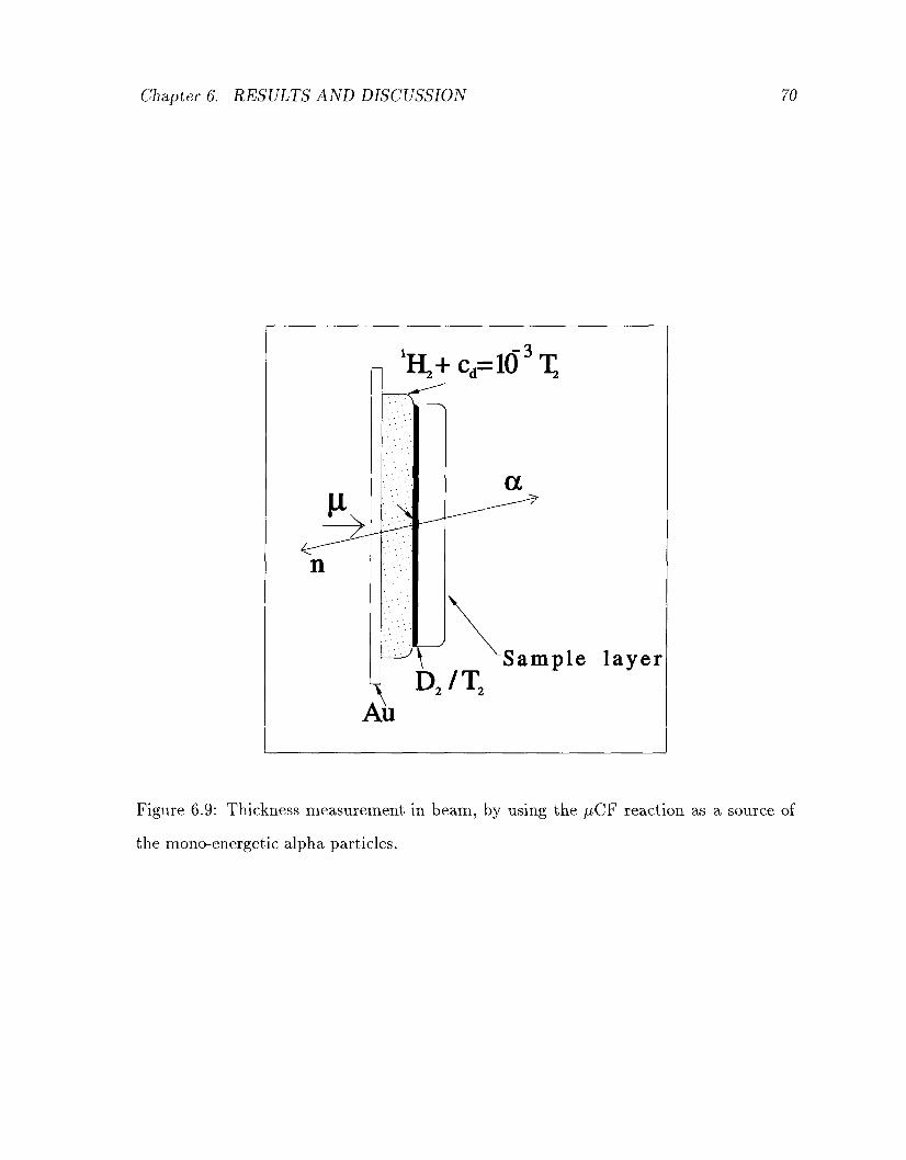
Chapter 6. RESULTS AND DISCUSSION
%+ca=l63X
A D2/T2
Sample layer
Figure 6.9: Thickness measurement in beam, by using the //CF reaction as
the mono-energetic alpha particles.
Chapter 6. RESULTS AND DISCUSSION 71
there appears to be any doubt in the future, the thickness measurement in beam de
scribed above can provide the information. A possible effect on the deposition efficiency
might come from the radiation heat load of the trit ium in the target or the difference in
the thickness of the Au foils on which hydrogen is deposited.
Nevertheless, the use of the muon beam is probably not justifiable only for the thick
ness measurement, given the situation that we can do as well or better in off-line exper
iments. However, this same target configuration turns out to give interesting opportuni
ties for measurements of very important parameters in /uCF, as we shall see in the next
chapter.
Chapter 7
S T O P P I N G P O W E R S A N D A L P H A - S T I C K I N G IN //CF
The importance of the alpha particle stopping power in hydrogen in /iCF is not confined
to the target thickness measurement. In fact, the stopping power is deeply related to the
alpha-sticking process, one of the most important in / /CF. We shall begin the discussion
with the review of the sticking problem. Its relevance to the stopping power in terms of
the reactivation, as well as a possible new experiment, are described in the sections that
follow.
7.1 Brief R e v i e w of the Sticking Problem
Contrary to the initial expectation of Alvarez[66], it is not the short lifetime of the
muon that gives the upper limit on the efficiency of /iCF. Even if the muon were stable,
one would not obtain enough energy to achieve economical break-even according to our
present understanding, as long as there remains the alpha-sticking process. Therefore,
this process has attracted the greatest attention of the fxCF researchers around the world
in recent years. A good understanding has been gained for D-D fusion, but for the D-T
system there are discrepancies among different groups as well as between theory and
experiment. We will concentrate on the D-T case, which is the most interesting in terms
of practical applications.
As briefly described in Chapter 1, the alpha-sticking is a process where the muon gets
72
Chapter 7. STOPPING POWERS AND ALPHA-STICKING IN fiCF 73
attached to the helium nuclus (a) after the fusion reaction:
d/j,t —>• /j,a + n . (7.1)
After the muons stick to the helium nuclei, some of them get reactivated, or "stripped"
from the nucleus, in collisions with the target atoms. The effective alpha-sticking prob
ability ioeJ 1 is written as
a ^ a f l l - f l ) , (7.2)
where u°s is the initial sticking and R, the reactivation probability.
7.1.1 T h e o r y
The calculation of the initial sticking and the reactivation should be distinguished, since
they are two separate processes. As for the initial sticking, there exists a remarkable
agreement amongst many authors in recent years. It is based on the framework of
the sudden approximation[67], that is the fusion process is considered to be very fast
compared to the time scale of the muonic motion. The sticking of a fj,~ to a given state
k of muonic helium is then given by the overlap of the intial and final wave functions,
Pk = | < 4W > I2, (7-3)
where tpl is the normalized initial wave function of the d/ut molecule in the limit of zero
internuclear distance, and i\)k is the final wave function of the recoiling na. Accurate
calculation of the muonic molecule wave function is a complex task, but recent works
using at least six different mathematical methods converge to a consistent value of u;°.
The latest calculations incorporate the nuclear effect, and give the value u°s = (0.92 ±
0.01)%[68].
The reactivation occurs mainly via two processes:
Chapter 7. STOPPING POWERS AND ALPHA-STICKING IN pCF 74
Ionization The ionization of the \i~ from the helium nucleus in collision with a hydrogen
isotope x, followed by its atomic capture on another hydrogen isotope y. (x and y
could be different isotopes in a mixture.)
H~a-\-x —> jj,~+a + x,
fi~+y -» n~y.
Transfer The exchange reaction between the alpha and a hydrogen isotope x.
(j,~a + x—}a + /j,~x (7-5)
At higher densities ionization through the multi-step excitation becomes increasingly
important. These processes are calculated by scaling the similar cross sections in ordinary
atomic collisions, p + He+ to the muonic system. The most recent calculation predicts
R to be 0.27 at density <f> — 0.05 and 0.34 at <f> = 1.2 with about 10% uncertainty, where
4> is the liquid hydrogen density[69].
Combining the values of OJ°S and R, we obtain the theoretical value for the effective
sticking ujeJJ{th) to be
ue/f(th) = 0.67 ± 0.03% {cf> = 0.05) (7.6)
uesff(th) = 0.61 ± 0.03% (<f> = 1.2). (7.7)
A slight density dependence comes from that of the reactivation probability.
7.1.2 Exper iments
Fig. 7.1 summarizes the current status of the sticking problem. A few remarks deserve
mention. First, there is a discrepancy between two major experiments. The 1986 LAMPF
data show a strong density dependence, while PSI data are only slightly dependent on
(7.4)
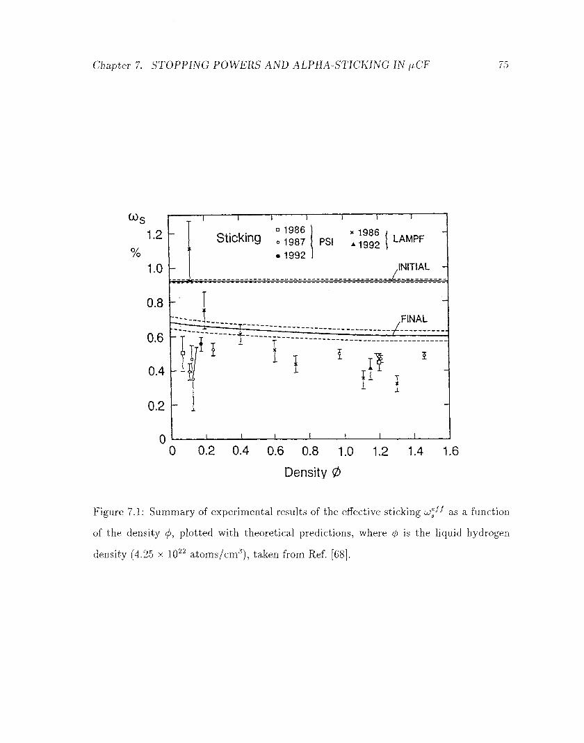
Chapter 7. STOPPING POWERS AND ALPHA-STICKING IN pCF 75
00c
%
1.2
1.0
0.8
0.6
0.4
0.2
0
~ . • • D 1986
Sticking 0 1 9 8 7 . 1992
* 1986 . PSI . --.«« ' LAMPF
±1992
• • ' • ' • . J £ i t 'g J. j ' i i . - i - U ' j t J j - j . i i . « i i . . . :_-_-,: = = _-_-_-_-= = = : / :
INITIAL -
r*I
FINAL
ih
0 0.2 0.4 0.6 0.8 1.0 1.2 1.4 1.6
Density 0
Figure 7.1: Summary of experimental results of the effective sticking ueJ^ as a function
of the density <f>, plotted with theoretical predictions, where (f> is the liquid hydrogen
density (4.25 x 10²² atoms/cm3), taken from Ref. [68].
Chapter 7. STOPPING POWERS AND ALPHA-STICKING IN ^CF 76
the target density1. Second, all the experimental values, except the LAMPF data at low
density, are substantially smaller than the theoretical values.
Let us take a look at the methods used in these experiments. Most of the early
experiments use the neutron method, where the time evolution of the detected neutrons
is fitted to the model describing the kinetics of the reactions. The main difficulty with
this method is that the sticking probability is one of the many parameters in the formula
and a complete understanding of the detailed kinetics of the fusion cycle is required
at least in the steady state. A typical example of a process yet to be understood is a
scavenging of the muon due to transfer to 3He and 4He, which accumulate slowly in the
target from the beta decay of tritium and as a product of the fusion reaction, respectively.
In addition, this method requires an absolute calibration of the neutron detector. This
is difficult to do to a high accuracy, and is suggested to be one of the sources for the
discrepancy between the experiments[68]. Thus, the neutron method is model-dependent
and indirect in determining the sticking probability.
The X-ray method provides more direct information on the sticking process. It detects
the characteristic X-ray of the muonic helium atom formed after a fusion event. A
fraction of the sticking occurs to excited states of muonic helium and it may de-excite
via emission of an X-ray. The experimental difficulty arises from a large bremsstrahlung
background from tritium beta decay. Therefore the experiments were done at a low
trit ium concentration at PSI. On the other hand, the pulsed beam structure of KEK
enabled the measurement to be done at a high tritium concentration.
Although the X-ray method offers a more direct observation of the sticking than the
neutron method, the extraction of the sticking value from the observed X-ray intensities
relies on detailed knowledge of the population of the excited states of /xa. The initial
population of each state is determined by the partial sticking fraction, but the state
JThe analysis of 1986 LAMPF data may be unreliable at low densities[70].
Chapter 7. STOPPING POWERS AND ALPHA-STICKING IN JJLCF 77
can be further populated by the collisional excitations from the lower states, or can be
depleted by ionization. In addition, processes such as Auger transitions, Stark mixing
and multi-step collisions have to be taken into account correctly. This, on the other
hand, means that the method can provide very useful information on the kinetics of the
fia as well as the sticking. An experiment with an improved accuracy is planned at the
RIKEN muon channel at Rutherford Appleton Lab in the UK, and the results are eagerly
awaited.
The most direct method of measuring the sticking probability is the detection of the
charged particles fia and a. The sticking probability can be determined from its very
definition:
N s M 4. M
y '
where N^a and Na are the number of each species. In this method, the serious systematic
uncertainties involved in the indirect methods in extracting us from the complex series of
processes are avoided. No knowledge of the obscure processes such as muon scavenging
to impurities or excitation and de-excitation of fj,a is required. The experiments with
this method have been done in two ways. The detection of the /j,a/a by a surface
barrier detector placed outside a low density (0 ~ 0.001) gas target, was first achieved
at LAMPF[71, 72] and later at RAL[73]. Because of the small reactivation in the low
density gas target, this method is more sensitive to the intial sticking, uo°s. Despite these
pioneering efforts, the experiments suffered from many problems, some of them intrinsic
to the method, and only preliminary results have been published so far:
u>°(exp) = 0.80 ± 0A5(stat.) ± (0A2)(syst.)% (7.9)
Lu°s(exp) = 0.69 ± 0A0(stat.) ± (0A4)(syst.)% (7.10)
This will be discussed in further detail in section 7.3. Another way was originally
developed at St. Petersburg for the D-D fusion experiment, for which they used the
Chapter 7. STOPPING POWERS AND ALPHA-STICKING IN piCF 78
hydrogen ionization chamber as a target as well as an active detector. Two recent theses
report the result of the PSI measurement of D-T sticking[74, 75] using a similar chamber.
This provides the most direct and model-independent value of the effective sticking at
medium density (<f> ~ 0.17):
ueff = 0.565 ± 0.046{stat.) ± 0.025(syst.)%. (7.11)
The combined uncertainty gives 9.3% relative accuracy. With a reactivation model as
sumed, the relative uncertainty reduces to 6.6%.
The current status of the sticking problem in the D-T system may be summarized
as follows[68]. At medium density (</> ~ 0.17), the experimental effective sticking value
is two standard deviations lower than the theory. At high density (1.0 < (j> < 1.4), the
experimental values are lower by three standard deviations. If we assume the theoretical
initial sticking u;° = 0.92 ± 0.01%, which appears rather reliable as discussed above, the
reactivation probability must be increased by 30%. We will take a careful look into the
problem of the reactivation in the following chapter.
7.2 Stopping Power and the React ivat ion
The stopping process of /j,a in the target medium is very important in the reactivation
problem, because it competes with the stripping process. R, the reactivation probability
at the end of slowing down is calculated[76] from
R = 1 — exp(-I),
I=fE'^dE, (7.12) JEf b
where E{ is the initial energy, Ej is the threshold energy for the stripping reaction (~few
keV), crstr is the stripping cross section, and S, the stopping power of ficx. Since the R
depends exponentially on / , it is very sensitive to the cross sections for stripping and

Chapter 7. STOPPING POWERS AND ALPHA-STICKING IN ^iCF 79
the stopping power. Because the pia is a tightly bound compact object of charge one,
its stopping power is assumed to be equivalent to that of protons of the same velocity
in most calculations. Thus the proton stopping power tables such as those of Anderson
and Ziegler[77] and Janni[30] are often used. It should be pointed out that there exists
the following problem, even if the above assumption is correct. As we have seen in detail
in Chapter 3, no experimental data on the stopping power is available in the condensed
phase of hydrogen for heavy charged particles for the energy of interest. The phase effect
is known to become more important at energies of the maximum stopping power (~1
MeV) and lower, but in the present case, one needs the stopping powers for the energy
from 3.5 MeV all the way down to a few keV2.
The latest calculation on the reactivation probability was done by Stodden et al. [69],
and this is claimed to be the most accurate calculation with about 10% uncertainty in R.
They used the stopping powers from Anderson and Ziegler[77] and assume their error to
be 10% over the entire density range. It should be pointed out that all the PSI neutron
data at high density (Fig. 7.1) are taken in the liquid or solid phase[78, 79]. Given the
rather controversial situation on the phase effect, the above uncertainty in the stopping
power may well be underestimated at densities above <f> ~0.95. In fact, their final error
bar in the calculation of R at high density (0 = 1.2) is 20% smaller than that at low
density (</> = 0.05), which is in the opposite direction to the reliability of the stopping
powers. Thus, the failure to take the phase effect into account in the reactivation calcu
lation may, at least in part, explain the larger discrepancy in the effective sticking values
between theory and experiment at high density3.
2For the case of our thickness measurement, we had a rather fortunate situation, that is we were only interested in the stopping powers of the energy region between 5.5 MeV and about 3 MeV, which is not too far from the Bethe-Bloch region where the theoretical prediction is more reliable.
3 "Unrealistic" parameterization for density dependent stopping powers[80] to explain LAMPF's sticking data, which shows a very strong dependence on density, is not relevant (nor acceptable) here. We are concerned about the discrete change in the stopping power due to the physical phase transition.
Chapter 7. STOPPING POWERS AND ALPHA-STICKING IN fiCF 80
One obvious remark from equation 7.12 is, if the stopping power of the /ia were
reduced for any reason, the efficiency of the fusion reactions would increase due to the
increased reactivation probability. This may be the key for achieving the practical use
of /J.CF. More complete understanding of the stopping process of charged particles could
open up new opportunities.
It is interesting to note that the injection of frozen hydrogen pellets is considered the
leading candidate for re-fueling tokamak thermonuclear fusion reactors[81, 82]. It is one
of the attempts to solve the problem of how to deposit atoms of fuel deep within the
magnetically confined, hot plasma. Here again, the energy loss process in solid hydrogen
will become important.
With these in mind, the measurement of the stopping power of hydrogen in the
condensed phase appears more than justifiable from the /iCF point of view, as well from
an interest in the basic atomic physics. Feasibility of film growth suggested by Hardy[63]
should be seriously considered.
7.3 Direct Measurement of the Sticking Probabi l i ty at High Dens i ty
7.3.1 Introduction
A struggle with the frustrating situation of the stopping power problems (Chapters 3 and
5), together with the realization of the potential of the /iCF reaction as a source of alpha
particles (Section 6.8.3), motivated some new considerations. After a recently published
review by Petitijean[68] attracted the author's attention to the sticking problem, an
idea came for a very ambitious series of experiments; the first systematic study of the
reactivation process, and a model-independent measurement of the intial sticking.
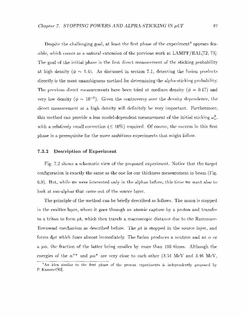
Chapter 7. STOPPING POWERS AND ALPHA-STICKING IN (iCF 81
Despite the challenging goal, at least the first phase of the experiment4 appears fea
sible, which comes as a natural extension of the previous work at LAMPF/RAL[72, 73].
The goal of the initial phase is the first direct measurement of the sticking probability
at high density (<f> ~ 1.4). As discussed in section 7.1, detecting the fusion products
directly is the most unambiguous method for determining the alpha-sticking probability.
The previous direct measurements have been tried at medium density (</> = 0.17) and
very low density (<f> ~ 10 - 3 ) . Given the controversy over the density dependence, the
direct measurement at a high density will definitely be very important. Furthermore,
this method can provide a less model-dependent measurement of the initial sticking w°,
with a relatively small correction (< 10%) required. Of course, the success in this first
phase is a prerequisite for the more ambitious experiments that might follow.
7.3.2 Descr ipt ion of Exper iment
Fig. 7.2 shows a schematic view of the proposed experiment. Notice that the target
configuration is exactly the same as the one for our thickness measurement in beam (Fig.
6.9). But, while we were interested only in the alphas before, this t ime we want also to
look at mu-alphas that come out of the source layer.
The principle of the method can be briefly described as follows. The muon is stopped
in the emitter layer, where it goes through an atomic capture by a proton and transfer
to a triton to form /ut, which then travels a macroscopic distance due to the Ramsauer-
Townsend mechanism as described before. The /it is stopped in the source layer, and
forms dyut which fuses almost immediately. The fusion produces a neutron and an a or
a fj,a, the fraction of the latter being smaller by more than 100 times. Although the
energies of the a++ and /ia+ are very close to each other (3.54 MeV and 3.46 MeV,
4An idea similar to the first phase of the present experiments is independently proposed by P. Kammel[83].
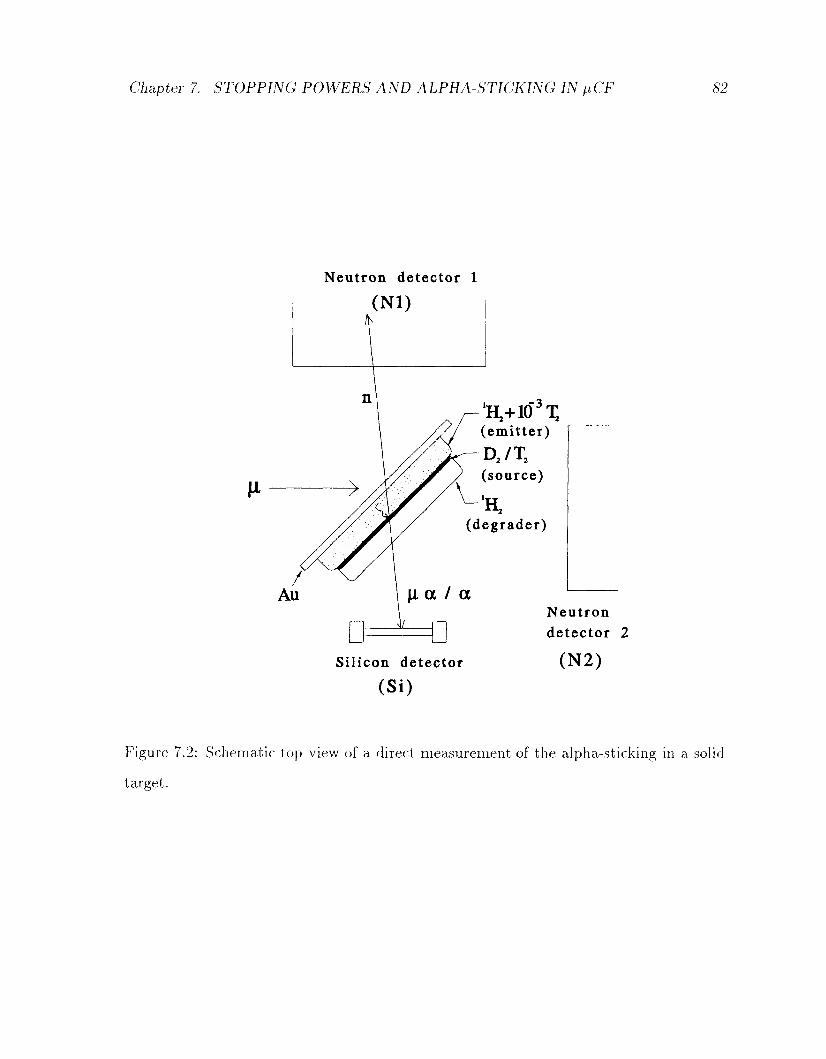
Chapter 7. STOPPING POWERS AND ALPHA-STICKING IN pCF 82
V
Neutron detector 1
(Nl)
H.+MTT; (emitter) D2/T2
(source)
(degrader)
j i a / a
Silicon detector
Neutron detector 2
(N2) (Si)
Figure 7.2: Schematic top view of a direct measurement of the alpha-sticking in a solid
target.
Chapter 7. STOPPING POWERS AND ALPHA-STICKING IN fiCF 83
respectively), the difference in the stopping powers permits us to separate them by the
energy loss in the degrader layer. Recalled that the stopping power is proportional to
the square of the projectile charge in the Bethe-Bloch formula. The /ia being singly
charged, there is about a factor of four difference in the stopping power between fia and
a. It should be emphasized, however, that for the purpose of separating the two species,
knowledge of their absolute stopping powers in solid hydrogen is not important, but only
the fact that they differ significantly.
In oder to gain in the counting rate, a few things can be tried. The D2/T2 mixture
may be used in the source layer which allows the cycling reactions. Due to the diffusion
of the fjt out of the source layer, a large cycling is unlikely, but some improvement in
the rate is expected. In certain cases, it may be advantageous to use the protium layer
with ~ 10~3 tritium concentration as the degrader. Considering that the emission of the
fit is isotropic, this acts as another emitter layer, as well as the degrader, emitting the
fit backward into the source layer. The increase in the fusion rate can be significant for
thick degraders.
The fast fusion neutrons are detected in the liquid scintillation counters. Demanding
collinear coincidence between a//j,a and the neutron (Si and Nl) is an extremely powerful
technique in reducing the background as we will see later. The existence of the neutron
counter, N2 in Fig. 7.2 is useful for the estimation of the accidental background, as well
as for monitoring real (physics related) backgrounds such as protons from D-D fusion
following the D-T fusion.
The uniformity of the target layers, in particular of the degrader layer, might be im
portant in order to achieve a high energy resolution. Unfortunately, as we have seen in
this thesis, there is a significant non-uniformity in our target. If this turns out to be
the limitaion for the energy resolution, the alternative deposition described in section 6.5
may be applied to provide a more uniform target. However, the relatively high deposition
Chapter 7. STOPPING POWERS AND ALPHA-STICKING IN fiCF 84
pressure (~ 10 - 4 torr) may cause some problem when depositing multi-layered targets.
Off-line measurements should be conducted to test the possibility.
It is convenient to generalize the effective sticking and reactivation in equation 7.2
and define
W . e "(T) = w , 0 ( l - i 2 ( T ) ) , (7.13)
where ueJ^(T) and R(T) are a function of the thickness (px) of the material that the fia
goes through. Hence,
(7.14)
(7.15)
(7.16)
(7.17)
where r^a is the range of the \xa in the given material. The symbols on the right hand
sides of equations refer to their conventional uses.
The direct observable in this method is the effective sticking at the degrader thickness
Td, namely ufj*'(Td)- If Td can be made such that the reactivation probability R(Td) is
small, then this method will come close to measuring the initial sticking u° .
By changing the thickness of the degrader layer, a systematic study of the reactivation
process can be performed for the first time. However, our sensitivity to the stripping
process is limited to medium energy or higher (> 0.5MeV).
7.3.3 Comparison with L A M P F / R A L Exper iments
Apart from the difference in the density at which measurements are done, the present
method offers certain advantages over the LAMPF/RAL experiments. The experiment
"!ff(T)\0
"Z'HT)^
R(T)\o--
R(T)\r»a
= -°,
= »l"
= o,
= R,
Chapter 7. STOPPING POWERS AND ALPHA-STICKING IN fiCF 85
at LAMPF suffered from a very low muon stop rate. Only ~0.05% of the incident muons
were stopped in the target at 490 torr, and the rest stopped in the walls producing a large
background. Although improved, still only 1% was stopped at RAL. We have confirmed
in our experiments that we can stop more than 30% of the muons in our solid targets,
providing a better signal to background ratio.
In the gaseous targets, since the fusion can occur anywhere within the target cell,
the amount of target material that the a or the fxa must go though before reaching the
detector can vary substantially, resulting in large fluctuations in the energy loss. On the
other hand, in our system the fusion occurs only in the spatially well "confined" source
layer, therefore the energy loss which occurs in the degrader is well defined. This will
result in much better energy resolution for the two species.
The spatial "confinement" of the fusion source offers a further advantage. Since the
source layer is isolated from the degrader, we can control the energy loss process of the
a and /ia by adjusting only the degrader, without affecting the dynamics in the fusion
layer. This is in contrast to the LAMPF experiments, where the measurements were
done at two different densities; low density to allow both a and fia to reach the detector,
and high density to allow only fia to reach the detector. We now know the existence of
highly non-linear processes in density, the typical example being the epithermal molecular
formation which we are trying to measure in E613. Thus, the interpretation of the data
becomes very difficult when the different densities are compared, due to the change in the
molecular/atomic dynamics in the target. Since we confine the dynamics in the source
layer, we can control the processes after the fusion rather freely without affecting the
fusion process itself.
Another major problem with the LAMPF/RAL measurement is the diffusion of tri
tium out of the target cell window. This can cause a few things. One is the reduction
in the target tritium concentration, hence the decease in fusion rate. This could create
Chapter 7. STOPPING POWERS AND ALPHA-STICKING IN fiCF 86
a problem in the normalization of the data. Another is the diffusion of tritium into the
solid state detector, resulting in the deterioration of the resolution. To prevent the latter,
the double enclosure with two windows and D2 buffer gas is used in their target. This
causes extra stripping in these materials before the [ia. reaches the detector, which adds
to the systematic uncertainties in obtaining the initial sticking probability. Also, because
of the presence of the diffused trit ium in the buffer D2 gas, some fusion reactions take
place there. This creates a serious background, because they all resemble a [ia event due
to the small enery loss5. In our target system, however, the silicon detector is adjacent
to the solid target, with nothing but ultra-high vacuum between them. It has proven to
work very well in the trit ium environment in past beam runs. Therefore the protection of
the silicon detector wich a buffer gas or a coating with alminum dioxide, as investigated
for the RAL experiment[85] is not necessary. Of course, the amount of tritium present
in our target is much smaller, about 10 Ci, compared to 750 Ci for the RAL experiment.
7.3.4 M o n t e Carlo Simulat ions
M e t h o d
In order to illustrate the feasibility of the proposed experiment, Monte Carlo calcu
lations were performed. The prime objective is to gain a qualitative understanding with
a simplified model, therefore quantitative values in the result should not be taken too
seriously.
The calculations were performed with the following assumptions. The a and fia
originate uniformly from the source layer, 15 torr-litre (~105 /Ug/cm2 for D2)6 in thickess.
According to a recent theoretical study[5] and our recent experimental runs (July-August
5A Monte Carlo study shows that a timing resolution of 1.2 ns, for both the silicon and neutron detctors combined, is required to separate this background[84]. The above resolution appears rather unrealistic for a conventinal alpha and neutron detection system.
6The conversion is based on the preliminary result for a new diffuser system.
Chapter 7. STOPPING POWERS AND ALPHA-STICKING IN /.iCF 87
7 -
6 -
25~
3 4 -
| 3 -< 2 ^
1 -
0 -
i i i > i i
Degrader 20 torr—liter y-
ax (1 /20 )
H
i i i i I I
-
/ -
,
. J n
1.0 0.5 1.0 1.5 2.0 2.5 3.0 3.5 4.0 Energy (MeV)
4 -
| 2
<
I 1 1 I I
Degrader 40 t o r r - l i t e r
«x (1 /20 )
I i i i "^ i
h < i
1.0 0.5 1.0 1.5 2.0 2.5 3.0 3.5 4.1 Energy (MeV)
3.0
2.5
. " 2.0
>- 1.5 o
ID
4c 1.0
0.5
0.0
Degrader 80 torr—liter
ax (1 /20 )
i.O 0.5 1.0 1.5 2.0 2.5 3.0 3.5 4 Energy (MeV)
0 0.5 1.0 1.5 2.0 2.5 3.0 3.5 4.0 Energy (MeV)
Figure 7.3: Monte Carlo simulation for the direct measurement of alpha-sticking with
various degrader thicknesses. The alpha counts are compressed by factor of 20 for a
comparison.
Chapter 7. STOPPING POWERS AND ALPHA-STICKING IN fiCF 88
1994), this thickness is sufficient to stop most of the energetic /it atoms which are emitted
into the source layer from the emitter layer. Both the /x«+ and a + + were assumed to
originate uniformly from the source layer with an initial energy of 3.5 MeV and lose energy
in the rest of the source layer as well as in the degrader layer. The alpha particle stopping
powers were taken from the ICRU tables for gaseous hydrogen[18]. For mu-alphas, simply
one fourth of the alpha particle stopping power was taken for the same energy. Straggling
and multiple scattering in layers were ignored, but a separate calculation by TRIM-92 7
shows that it contributes only ~1 .5% with the energy loss of 1 MeV. Also, the reactivation
of the muon is not taken into account. It is estimated to be less than 5% for a moderately
thin degrader. All the solid hydrogen layers are assumed to be uniform. The source radius
is taken to be 10 mm, though the actual size may be larger than this. The detector radius
is 10 mm unless otherwise specified. The target and the detector are separated by 45 mm,
center to center, as in the actual apparatus.
Resul ts and Analys is
The histograms in Fig. 7.3 show the energy spectra of two charged species, a and /j,a, in a
silicon detector with various thicknesses of the degrader layer. The a peak is compressed
by a factor of 20 for an easier comparison. With a moderate amount of the degrader
(between ~ 40 torr-litre (140 jug/cm2) and ~ 80 torr-litre (280 /ig/cm2)) , two peaks can
clearly be separated. The most direct measurement of sticking can be achieved in this
region by simply counting the number of the two species detected. With a degrader of 20
torr-litre (140 /ig/cm2) or less, the separation of the two is rather difficult. This region
can be investigated by using muonic X-ray and/or nuclear capture gamma ray, as will be
discussed in section 7.4. At larger thicknesses of degrader, alphas no longer make their
way through and most of them stop or fall below the detector threshold. In this region,
7See footnote in page 46
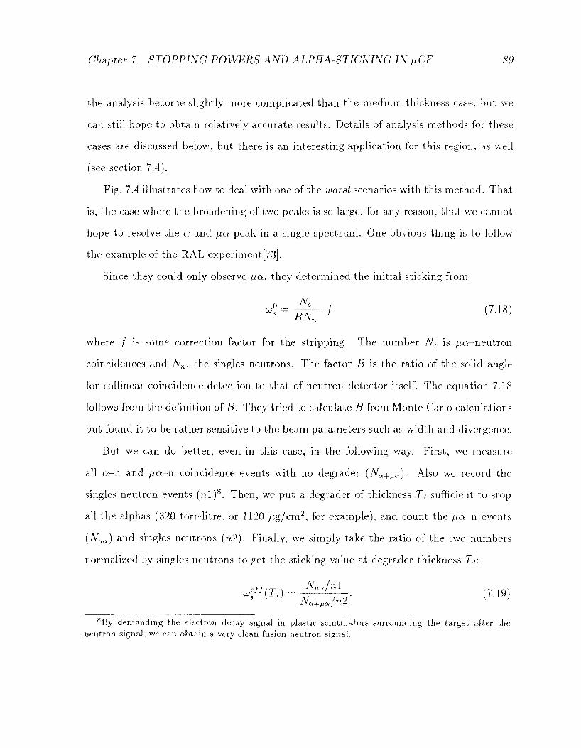
Chapter 7. STOPPING POWERS AND ALPHA-STICKING IN pCF 89
the analysis become slightly more complicated than the medium thickness case, but we
can still hope to obtain relatively accurate results. Details of analysis methods for these
cases are discussed below, but there is an interesting application for this region, as well
(see section 7.4).
Fig. 7.4 illustrates how to deal with one of the worst scenarios with this method. That
is, the case where the broadening of two peaks is so large, for any reason, that we cannot
hope to resolve the cv and fia peak in a single spectrum. One obvious thing is to follow
the example of the RAL experiment[73].
Since they could only observe /j,a, they determined the initial sticking from
J-m-' <7-18)
where / is some correction factor for the stripping. The number A^ is / ia-neutron
coincidences and A^, the singles neutrons. The factor B is the ratio of the solid angle
for collinear coincidence detection to that of neutron detector itself. The equation 7.18
follows from the definition of B. They tried to calculate B from Monte Carlo calculations
but found it to be rather sensitive to the beam parameters such as width and divergence.
But we can do better, even in this case, in the following way. First, we measure
all a-n and / / a -n coincidence events with no degrader (Na+fia). Also we record the
singles neutron events (ral)8. Then, we put a degrader of thickness Tj sufficient to stop
all the alphas (320 torr-litre, or 1120 /ig/cm2 , for example), and count the fia-i\ events
(A^or) a n d singles neutrons (n2). Finally, we simply take the ratio of the two numbers
normalized by singles neutrons to get the sticking value at degrader thickness T^\
:ff(Td)= J V A ! V (7.19) U) Na+fia/n2
8 By demanding the electron decay signal in plastic scintillators surrounding the target after the neutron signal, we can obtain a very clean fusion neutron signal.
Chapter 7. STOPPING POWERS AND ALPHA-STICKING IN fiCF 90
J L_
C
D
X)
<
0
No Degrader n a + yua
0.0 0.5 1.0 1.5 2.0 2.5 3.0 3.5 4.0 Energy (MeV)
.6
• 5 H
.4 c
^ .3
< . 2 -
Degrader
320 to r r —litre . . . .
ill t=i:ii i nam 111 iia
.11! !!B!! I ! ! ! ! !
Ei::=i:i= JU 11 f i i i i i i i f iiiiiii
: i i l i s : : : i : :!B:; : i
0.0 0.5 1.0 1.5 2.0 2.5 Energy (MeV)
/j,a
3.0 3.5 4.0
Figure 7.4: Determination of the sticking probability from two separate measurements.
Counts in each spectrum will be normalized to the single neutrons.
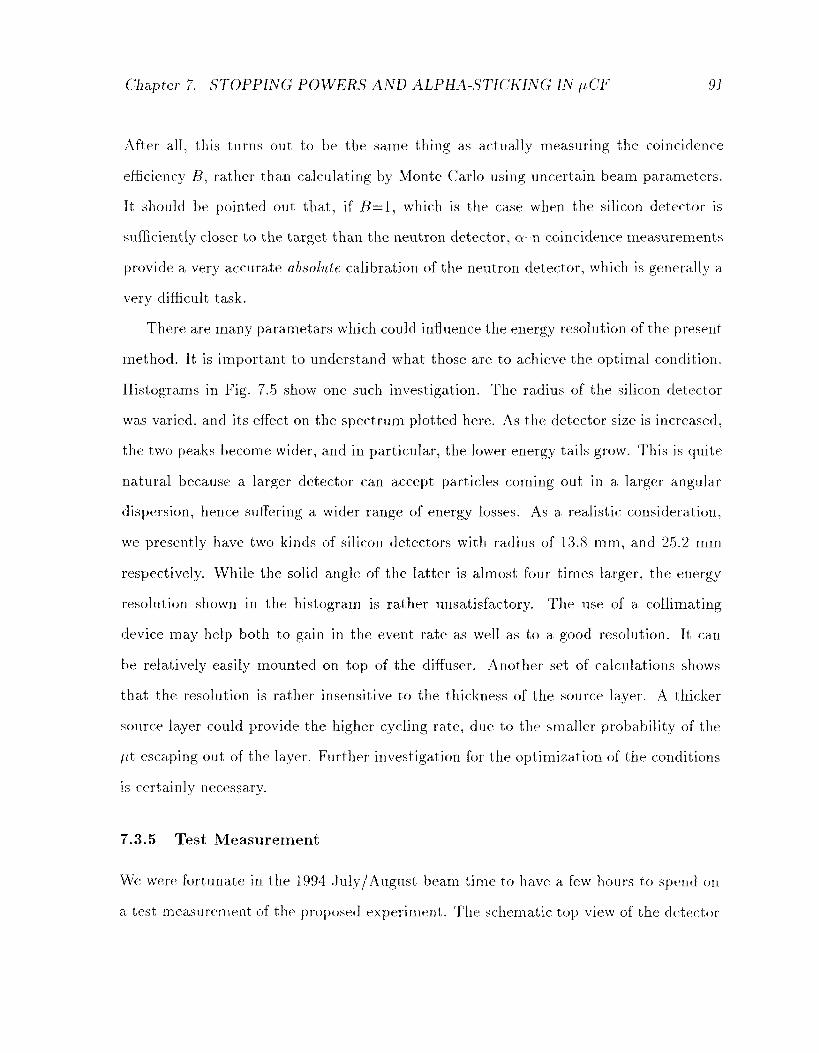
Chapter 7. STOPPING POWERS AND ALPHA-STICKING IN fiCF 91
After all, this turns out to be the same thing as actually measuring the coincidence
efficiency J3, rather than calculating by Monte Carlo using uncertain beam parameters.
It should be pointed out that , if B=l, which is the case when the silicon detector is
sufficiently closer to the target than the neutron detector, a - n coincidence measurements
provide a very accurate absolute calibration of the neutron detector, which is generally a
very difficult task.
There are many parametars which could influence the energy resolution of the present
method. It is important to understand what those are to achieve the optimal condition.
Histograms in Fig. 7.5 show one such investigation. The radius of the silicon detector
was varied, and its effect on the spectrum plotted here. As the detector size is increased,
the two peaks become wider, and in particular, the lower energy tails grow. This is quite
natural because a larger detector can accept particles coming out in a larger angular
dispersion, hence suffering a wider range of energy losses. As a realistic consideration,
we presently have two kinds of silicon detectors with radius of 13.8 mm, and 25.2 mm
respectively. While the solid angle of the latter is almost four times larger, the energy
resolution shown in the histogram is rather unsatisfactory. The use of a collimating
device may help both to gain in the event rate as well as to a good resolution. It can
be relatively easily mounted on top of the diffuser. Another set of calculations shows
that the resolution is rather insensitive to the thickness of the source layer. A thicker
source layer could provide the higher cycling rate, due to the smaller probability of the
/it escaping out of the layer. Further investigation for the optimization of the conditions
is certainly necessary.
7.3.5 Test M e a s u r e m e n t
We were fortunate in the 1994 July/August beam time to have a few hours to spend on
a test measurement of the proposed experiment. The schematic top view of the detector
Chapter 7. STOPPING POWERS AND ALPHA-STICKING IN nCF 92
3 . 0 -
2 . 5 -
J3 2 . 0 -'c 3
Arb
itary
b In
0 . 5 -
o . o -
i I ;
Rd =10 mm
ax (1 /20 )
^
i ' "\ 1
A
i
i
\ l
i
/
1 1
2.5
2.0-
Rj =15 m m
ax(l/20)
i.O 0.5 1.0 1.5 2.0 2.5 3.0 3.5 4. Energy (MeV) Energy (MeV)
2.0
rT 1.0-
0.5-
0.0 ).0 0.5 1.0 1.5 2.0 2.5 3.0 3.5 4
Energy (MeV) 0.0 0.5 1.0 1.5 2.0 2.5 3.0 3.5 4.0
Energy (MeV)
Figure 7.5: Influence of the silicon detector size on the peak width in the energy spectrum
is plotted. Rd refers to the detector radius. A degrader of 70 torr-litre (245 /zg/cm2) is
used in the calculations.
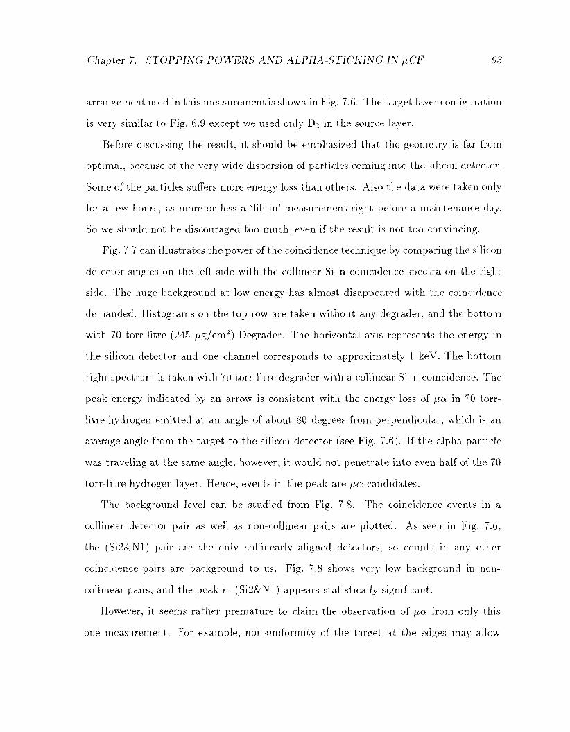
Chapter 7. STOPPING POWERS AND ALPHA-STICKING IN pCF 93
arrangement used in this measurement is shown in Fig. 7.6. The target layer configuration
is very similar to Fig. 6.9 except we used only D2 in the source layer.
Before discussing the result, it should be emphasized that the geometry is far from
optimal, because of the very wide dispersion of particles coming into the silicon detector.
Some of the particles suffers more energy loss than others. Also the data were taken only
for a few hours, as more or less a 'fill-in' measurement right before a maintenance day.
So we should not be discouraged too much, even if the result is not too convincing.
Fig. 7.7 can illustrates the power of the coincidence technique by comparing the silicon
detector singles on the left side with the collinear Si-n coincidence spectra on the right
side. The huge background at low energy has almost disappeared with the coincidence
demanded. Histograms on the top row are taken without any degrader, and the bottom
with 70 torr-litre (245 /ig/cm2) Degrader. The horizontal axis represents the energy in
the silicon detector and one channel corresponds to approximately 1 keV. The bottom
right spectrum is taken with 70 torr-litre degrader with a collinear Si-n coincidence. The
peak energy indicated by an arrow is consistent with the energy loss of /j,a in 70 torr-
litre hydrogen emitted at an angle of about 80 degrees from perpendicular, which is an
average angle from the target to the silicon detector (see Fig. 7.6). If the alpha particle
was traveling at the same angle, however, it would not penetrate into even half of the 70
torr-litre hydrogen layer. Hence, events in the peak are fia candidates.
The background level can be studied from Fig. 7.8. The coincidence events in a
collinear detector pair as well as non-collinear pairs are plotted. As seen in Fig. 7.6,
the (Si2&Nl) pair are the only collinearly aligned detectors, so counts in any other
coincidence pairs are background to us. Fig. 7.8 shows very low background in non-
collinear pairs, and the peak in (Si2&Nl) appears statistically significant.
However, it seems rather premature to claim the observation of fia from only this
one measurement. For example, non-uniformity of the target at the edges may allow
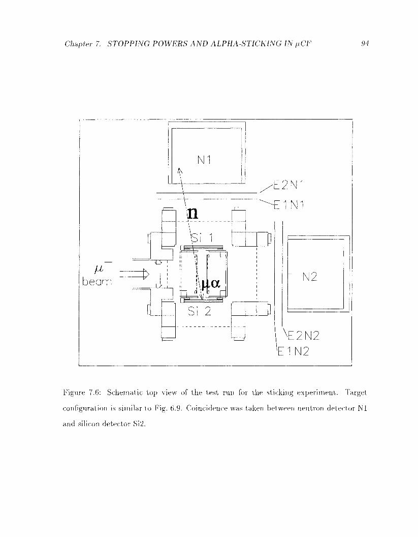
Chapter 7. STOPPING POWERS AND ALPHA-STICKING IN fiCF 94
Figure 7.6: Schematic top view of the test run for the sticking experiment. Target
configuration is similar to Fig. 6.9. Coincidence was taken between neutron detector Nl
and silicon detector Si2.
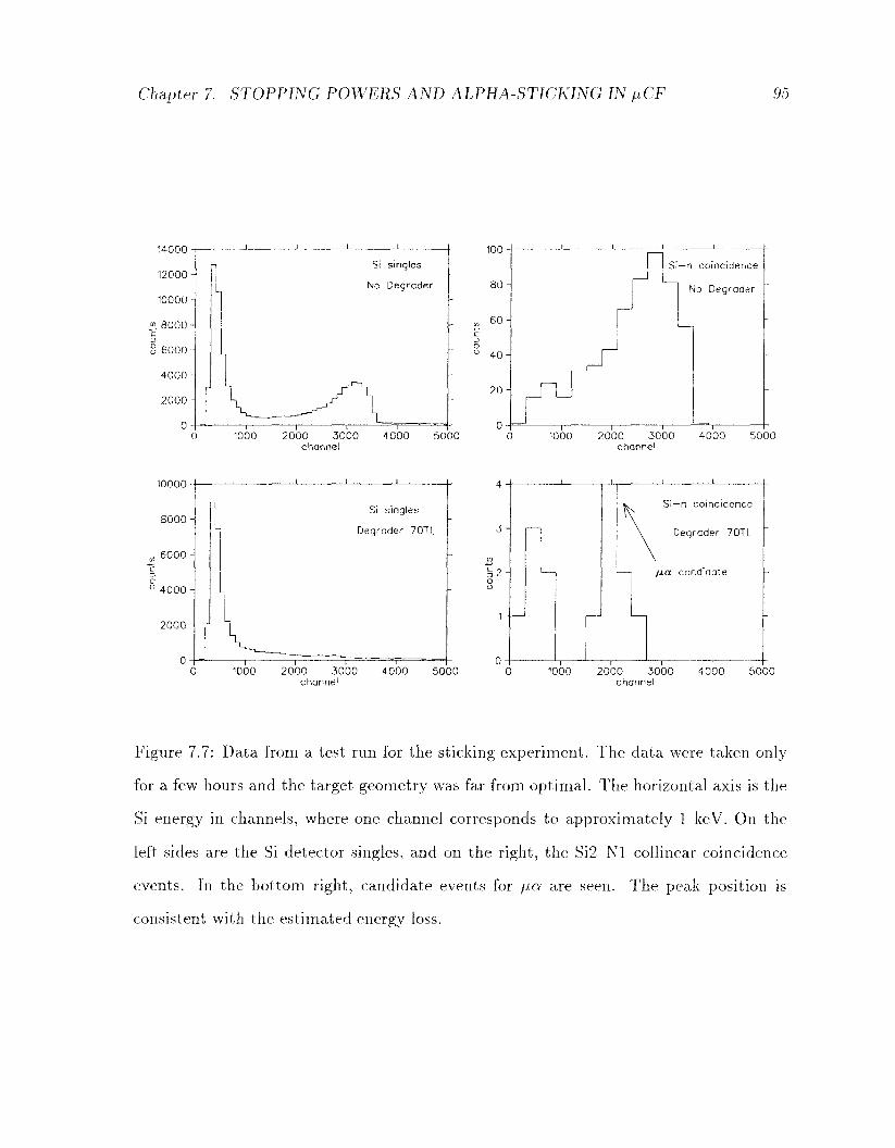
Chapter 7. STOPPING POWERS AND ALPHA-STICKING IN nCF 95
14000
12000
10000 -
» 8000 -c
S 6000
4000
2000
0
Si singles
No Degrader
0
10000
8000 H
„ 6000 c
° 4000 -
2000
1000
1000
2000 3000 channel
4000 5000
Si singles
Degrader 70TL
2000 3000 channel
4000 5000
100
8 0 -
6 0 -
40
20
3 -
i 2 -
Si—n coincidence
No Degrader
1000 2000 3000 4000 5000 channel
Si—n coincidence
Degrader 70TL
•—i / i a candidate
1000 2000 3000 channel
4000 5000
Figure 7.7: Data from a test run for the sticking experiment. The data were taken only
for a few hours and the target geometry was far from optimal. The horizontal axis is the
Si energy in channels, where one channel corresponds to approximately 1 keV. On the
left sides are the Si detector singles, and on the right, the Si2-Nl collinear coincidence
events. In the bottom right, candidate events for /J,a are seen. The peak position is
consistent with the estimated energy loss.
Chapter 7. STOPPING POWERS AND ALPHA-STICKING IN fiCF 96
alpha particles to escape from the degrader layer, and imitate fia events. But, at least,
the feasibility of the direct sticking measurement in the solid hydrongen target has been
successfully demonstrated.
7.3.6 Discussion
Rate Es t imates and Precis ion
The incident muon rate R^ is typically 5 x 10³/s in 12 cm2 at 27 MeV/c, with Sp/p = 0.04.
The muon stopping fraction f^, is known to be approximately 0.3. According to a Monte
Carlo study of Markushin[5], the fusion yield per stopped muon, Y/ is about 0.06 with
source layer thickness of ~15 torr-litre, which is consistent with our experimental data.
For the silicon detector of 25 mm radius at 45 mm from the target foil, the solid angle tst
is ~7 .5%. The NE213 liquid scintillation neutron counter has ~20% intrinsic efficiency
en, and we take the geometrical efficiency for the Si-n coincidence ec, that is the ratio of
the solid angle of for collinear coincidence detction to that of the silicon detector itself,
to be 0.3. Assuming effective sticking u>^J (Td) of ~0 .8%, allowing ~10% reactivation in
the degrader {R{Td) — 0.1), the overall coincidence event rate for /j,a-n coincidence is
Rc = Rf,-h-Yf coesff(T) • est • en • ec. (7.20)
The event rate can be estimated to be ~ 3 x 10 _ 3 /s or 1500 events in a 5 day period. Even
if we assume a signal to background ratio of 1:1, which seems rather unlikely from the
test run, this corresponds to ~ 3.5% statistical uncertainty. This is without considering
the cycling reactions, which may improve the rate by an order of magnitude or more.
The sources of systematic uncertainties include the correction due to the reactivation
in the target and the energy dependence of the detection efficiency of the silicon detector.
As for the former, the correction itself appears to be less than 10% at a moderate thickness
of the degrader, so even if we allow 30% uncertainty in the reactivation correction, the
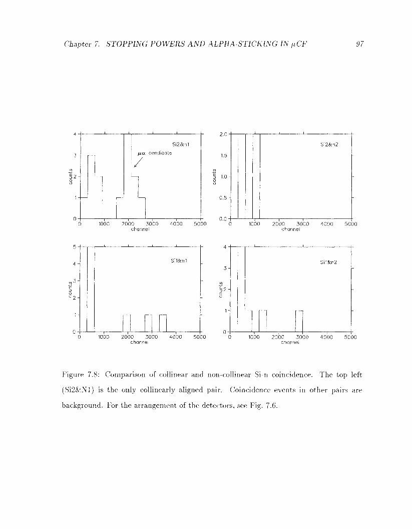
Chapter 7. STOPPING POWERS AND ALPHA-STICKING IN pCF 97
Si2&n1
/ua candidate
2.0
1.5
1.0
0 . 5 -
~t • 1 •—i 1 r o.o 1000 2000 3000 4000 5000 0
channel
Si2&n2
1000 2000 3000 channel
4000 5000
1000 2000 3000 4000 channel
5000 2000 3000 channel
4000 5000
Figure 7.8: Comparison of collinear and non-collinear Si-n coincidence. The top left
(Si2&Nl) is the only collinearly aligned pair. Coincidence events in other pairs are
background. For the arrangement of the detectors, see Fig. 7.6.
Chapter 7. STOPPING POWERS AND ALPHA-STICKING IN ^CF 98
contribution to the final result is 3%. Besides, we can check the reactivation calculation
by changing the degrader thickness. For the silicon detector efficiency, we plan to make
an off-line measurement.
If the clear separation of the two peaks in one spectrum is achieved, as in the Monte
Carlo calculation, we can, in principle, expect the most accurate measurement of the
initial sticking, with the precision almost comparable to the PSI ionization chamber
measurement.
7.3.7 R e a d i n e s s
It should be emphasized that the proposed experiment, at least in its initial phase, does
not require a major rebuild of the existing apparatus for E6I3. Turning the diffuser
mechanism and a target foil by 45 degrees should not be a problem, since the former has
a rotational symmetry, and the latter can be easily bent if we remove the second target
foil that we do not use.
Testing of the deposition and the measurement of thickness in an off-line experiment
is necessary before the beam run, but otherwise we do not foresee the need for much
preparation in terms of hardware.
Of course, more refined Monte Carlo simulations are necessary to determine the op
timal conditions.
7.4 Towards t h e F u t u r e
Although the method described above provides a fairly accurate value for the initial stick
ing probability, it is not totally free from theoretical assumptions about the reactivation
process. A potential method for a model-independent measurement of the initial sticking
by directly measuring the reactivation probability, together with other applications of
Chapter 7. STOPPING POWERS AND ALPHA-STICKING IN /uCF 99
our apparatus is discussed in this section. (What will be proposed here are, in reality,
severely limited by the event rates at least with TRIUMF intensity, but let us be a little
imaginative, in ending the thesis!)
One of the routine methods of detecting the presence of negative muons is the ob
servation of muonic X-rays, or similarly nuclear capture gamma-rays. Unfortunately,
the original idea of using the muonic silicon X-rays from the silicon detector to identify
\ia for the initial sticking measurement, turned out to be not very useful, because the
probability of the stripping process in silicon is dependent on the initial energy of the
/ua, and its correction would be somewhat dependent on the knowledge of /ia kinetics.
We instead proposed to use gold and look for the 356 keV muonic capture gamma rays.
Let us assume that from the intial phase of the sticking measurement we know
uj^f(Td), the effective sticking with degrader thickness Td. Recall that
coe/f(Td) = co°s(l-R(Td)). (7.21)
Our objective here is to determine tu° by measuring R(Td), the reactivation probability
at degrader thickness Td.
The apparatus we propose is the same as the initial phase (Fig. 7.2), except we have
a germanium X-ray detector instead of the silicon, and we place a gold plate in front of
it to strip off the muons from mu-alphas and then observe the characteristic gamma rays
(and X-rays) from gold. It was shown by Cohen[86] that the muon in /J,a with initial
energy of 3.5 MeV gets completely stripped by the time the /j,a travels 10 //m in gold, or
by the time it loses energy to 2.5 MeV.
First, with a target with no degrader, we measure the number of 356 keV gold capture
gammas (for example) from the muon that was stripped off from fia. Coincidence with
a fusion neutron collinear with fia emission is demanded to clean up the signal. Let us

Chapter 7. STOPPING POWERS AND ALPHA-STICKING IN fiCF 100
call this number Y0, which can be written
Y0 = Nfio°s-e0, (7.22)
where Nj is a normalized number of all fusion events and e0 is the detection efficiency
including germanium, neutron and coincidence solid angle.
Second, we add a degrader of thickness Td, which must be the same thickness as the
previous measurement where ueJ^[Td) was obtained. We again measure the gold capture
gamma rays in coincidence with the neutron (Yi), which is now written
Y1 = NfU°8-(l-R(Td))-e1, (7.23)
where t\ is the detection efficiency for this time. If Td is not too large, i. e., the energy
of the fia is not too low, it appears safe to assume the probability of the muon getting
stripped from fia in gold is 100% according to Cohen[86j. Since other efficiencies cancel
with each other, we have e0 = £i, so we can simply take the ratio of the observed gamma-
neutron coincidence counts (normalized to singles neutrons) Yi, Yo to obtain
1 - R{Td) = £ . (7.24)
It should be noted that the above assumption is much less dependent on the theoretical
model of the \IOL kinetics, upon which the calculation of the reactivation probability R
depends heavily. It can also be tested, for example, using a beam of muonic helium which
will be described later. Thus, combining the above value of R{Td) with the u^^(Td), we
can determine the nearly model-independent value of the initial sticking uPs.
The last thing proposed in this thesis is the use of fiCF as a source for a beam of
muonic helium. In our starndard three-layered target arrangement, if we put a degrader
that is thick enough to stop all the alphas, we obtain a "beam" of muonic helium with
Chapter 7. STOPPING POWERS AND ALPHA-STICKING IN fiCF 101
rather well defined energy. An example of the energy distribution was already shown
in Fig. 7.4. This would be complimentary to a keV muonic helium source, proposed
by Nagamine[87], since our beam typically has energy of order of 1 MeV, although the
intensity is much lower. New "Atomic Physics" experiments with muonic helium beam
may become possible. Some infesting exapmles include the test of Cohen's prediction
on the stripping process in gold foil and the study of transefer process to neon which
can be deposited directly on top of the beam source layer. It may also be possible to
obtain a muonic 3He beam from the sticking in the D-D fusion reactions, which could be
interesting for muon capture studies.
All the discussion in this section ignores the problem of the event rates, and may be
rather unrealistic, at least with the muon intensity of TRIUMF. However, some of them
may become possible in future muon facilities. At least the initial phase of the sticking
experiment, which was discussed in detail in section 7.3, appears feasible, and a research
proposal for TRIUMF Experiment Evaluation Committee is currently being prepared.
Chapter 8
C O N C L U S I O N
The energy loss of alpha particles was utilized to determine the thickness and uniformity
of solid hydrogen and other frozen gas targets for muon catalyzed fusion experiments. The
energy of alpha particles from an array of americium sources was measured by a silicon
detector. By moving the detector and measuring at different positions, the uniformity
of the films was determined. For the conversion of the measured energy loss into the
thickness, the latest stopping power and range table by ICRU[18] was employed, after
critical review of the many tables.
An accuracy of about 5% was achieved at a few hundred /ig/cm2 , which is limited
by the stopping power uncertainty. The linear relation between the hydrogen thickness
and the amount of injected gas was confirmed within the accuracy. This enables the
extrapolation of the results beyond the range of measurement accessible by the present
method. The cross contamination is found to be less than 0.8 x 10~3 with 90% confidence
level. A significant non-uniformity in the target profile was observed. This could be
partly explained by a solid angle effect, which is consistent with a Monte Carlo study.
However, an asymmetry in the thickness distribution is not clearly understood. While
cryo-pumping during the deposition does not affect the target profile within the accuracy,
the position change of the diffuser by 2.5 mm gives a significant difference in the thickness
distributions. The effective thickness per unit gas input is determined to be 3.29±0.16
/Ug/(cm2-torr-litre) and the average non-uniformity (the weighted standard deviation of
102
Chapter 8. CONCLUSION 103
the thickness distribution) is about 7% for a Gaussian beam distribution of FWHM 20-
25 mm. The neon targets had similar thickness profile to the hydrogen. An alternative
method of deposition is also described, which may improve the uniformity of the target.
The present method of thickness measurement can now be applied to other experiments
where solid thin targets are required.
The importance of the stopping process in the alpha-sticking problem in muon cat
alyzed D-T fusion was discussed in detail. The physical phase effect of the stopping
power of hydrogen may partly explain the discrepancy in the sticking values between
theory and experiment at high densities. The concept of a new experiment to measure
directly the sticking probability at high density was proposed. This offers certain advan
tages over LAMPF/RAL measurements. A Monte Carlo simulation of the experiment
was performed. A very preliminary result from a test run is presented. Preparation of
the research proposal for TRIUMF Experiments Evaluation Committee is in progress.
Bibliography
[1] E. A. Vesman, Pis 'ma Zh. Eksp. Teor. Fiz. 5, 113 (1967), [JETP Lett., 5, 91-93 (1967)].
[2] P. Knowles, Hyperfine Int. 82, 521 (1993).
[3] H. Faxen and J. Holtsmark, Z. Physik 45, 307 (1927), and references therein.
[4] M. P. Faifman and L. I. Ponomarev, Phys. Lett. B 265, 201 (1991).
[5] V. E. Markushin, 1994, private communication.
[6] G. M. Marshall, TRIUMF Annual Report, Scientific Activities 1993, p. 34, unpublished.
[7] K. Nagamine, Proc. Japan Academy 65, 225 (1989).
[8] K. Nagamine et al, Muon Catalyzed Fusion 5 / 6 , 371 (1990/91).
[9] P. Strasser et al., Hyperfine Interactions 82, 543 (1992).
[10] P. Strasser, Ph.D. thesis, University of Tokyo, 1994.
[11] A. Olin, 1993, TRIUMF Research Proposal E703.
[12] P. Knowles, The E613 Frozen Gas Target System, 1992, E613 Internal Report, unpublished.
[13] H. S0rensen, Appl. Phys. 9, 321 (1976).
[14] J. Schou et al, J. Appl. Phys. 49, 816 (1978).
[15] W. K. Chu et al, Nucl. Instr. and Meth. 149, 115 (1978).
[16] W. K. Chu et al, Backscattering Spectrometry (Academic Press, Inc., New York, New York, 1978).
[17] J. F. Ziegler, Helium Stopping Powers and Ranges in All Elemental Matter (Perga-mon Press, New York/Toronto/Oxford/Sydney/Frankfurt/Paris, 1977).
[18] ICRU Report 49, Stopping Powers and Ranges for Protons and Alpha Particles (In-ernational Commision of Radiation Units and Measurements, Bethesda, Maryland, 1993).
104
Bibliography 105
[19] E. Segre, Nuclei and Particles (The Benjamin/Cummings Publishing Co., Inc., Reading, Massachusetts, 1977).
[20] J. F. Ziegler et ai, The Stopping and Range of Ions in Solids (Pergamon Press, New York/Toronto/Oxford/Sydney/Frankfurt/Paris, 1985).
[21] S. M. Seltzer et ai, Int. J. Appl. Radiat. Isot. 33 , 1189 (1982).
[22] M. J. Berger and S. M. Seltzer, NBS Publication, NBSIR 82-2550, 1982.
[23] G. Burns, Solid State Physics (Academic Press, Inc., San Diego, California, 1985).
[24] Particle Data Group, Review of Particle Properties, Phys. Rev. D Vol. 45 (1992).
[25] R. M. Sternheimer et ai, Phys. Rev. B 26, 6067 (1982).
[26] M. J. Berger and S. M. Seltzer, Proceedings of the Seminar on Charge States and Dynamic Screening of Swift Ions in Solids, Honolulu, January 25-29, 1982.
[27] J. R. Sabin and J. Oddershede, Nucl. Instr. and Meth. B44 , 253 (1990).
[28] R. M. Sternheimer et ai, Atomic Data and Nuclear Data Tables 30, 261 (1984).
[29] J. F. Ziegler, Handbook of Stopping Cross-Sections for Energetic Ions in all Elements (Pergamon Press, New York/Toronto/Oxford/Sydney/Frankfurt/Paris, 1980).
[30] J. F. Janni, Atomic Data and Nuclear Data Tables 27, 147 (1982).
[31] A. Adamo et ai, Phys. Rev. A 47, 2239 (1993).
[32] M. Senba, J. Phys. B: At. Mol. Opt. Phys. 23, 1545 (1990).
[33] M. Senba, 1994, private communication.
[34] C. Varelas and J. Biersack, Nucl. Instr. and Meth. 79, 213 (1970).
[35] R. Golser and D. Semrad, Phys. Rev. Lett. 66, 1831 (1991).
[36] D. I. Thwaites, Radiat. Res. 95, 495 (1983).
[37] D. I. Thwaites and D. E. Watt, Phys. Med. Biol. 23 , 426 (1978).
[38] J. F. Ziegler and W. K. Chu, J. Appl. Phys. 47, 2239 (1976).
[39] D. I. Thwaites, Nucl. Instr. and Meth. B 12, 84 (1985).
[40] D. I. Thwaites, Nucl. Instr. and Meth. B 27, 293 (1987).
Bibliography 106
[41] R. Bimbot et ai, Nucl. Instr. and Meth. B 44, 19 (1989).
[42] R. Bimbot et ai, Nucl. Instr. and Meth. B 44, 1 (1989).
[43] H. Geissel et ai, Nucl. Instr. and Meth. 194, 21 (1982).
[44] P. B0rgesen et ai, Nucl. Instr. and Meth. 194, 71 (1982).
[45] P. B0rgesen et ai, Nucl. Instr. and Meth. 200, 571 (1982).
[46] P. B0rgesen, Nucl. Instr. and Meth. B 12, 73 (1985).
[47] F. Bensenbacher et ai, Nucl. Instr. and Meth. 188, 657 (1981).
[48] D. Powers, Nucl. Instr. and Meth. B 4 0 / 4 1 , 324 (1989).
[49] Nucl. Instr. and Meth. Vol. 93 No.2 (1994).
[50] Hydrogen in Semiconductors, edited by J. I. Pankove and N. M. Johnson (Academic Press, San Diego, CA, 1990), Chap. 15.
[51] S. J. Pearton et ai, Hydrogen in Crystalline Semiconductors (Springer, New York, NY, 1992).
[52] R. F. Kiefl, Hydrogen in Semiconductors (Academic Press, San Diego, CA, 1990), Chap. 15, p. 547.
[53] R. F. Kiefl, Physica B 170, 33 (1991).
[54] The VDACS Data Acquisition Primer, 1991, ver. 3.0, unpublished.
[55] TWOTRAN Reference Manual, 1993, unpublished.
[56] MOLLI Manual, 1985, unpublished.
[57] FIOWA Manual, 1981, ver. 3, unpublished.
[58] C. Hanke and J. Laursen, Nucl. Instr. and Meth. 151, 253 (1978).
[59] L. C. Northcliffe and R. F. Schilling, Nuclear Data Tables A 7 , 233 (1970).
[60] W. D. Bianco et ai, Nucl. Instr. and Meth. 140, 215 (1977).
[61] M. Inokuti, Nucl. Instr. and Meth. B 27, 249 (1987).
[62] D. E. Watt, Stopping Powers and Ranges in 30 Elements for Alpha Particles (1 keV to 100 MeV), 1988, report prepared for the ICRU Stopping Power Committee.

Bibliography 107
[63] W. N. Hardy, 1994, private communication.
[64] P. Strasser, 1994, private communication.
[65] P. Knowles, 1994, private communication.
[66] L. W. Alvarez et ai, Phys. Rev. 105, 1127 (1957).
[67] A. Messiah, Quantum Mechanics (North-Holland Publishing Co., Amsterdam, 1958).
[68] C. Petitjean, Hyperfine Int. 82, 273 (1993).
[69] C. D. Stodden et ai, Phys. Rev. A 41 , 1281 (1990).
[70] S. E. Jones et ai, Hyperfine Int. 82, 303 (1993).
[71] S. E. Jones et ai, AIP Conf. Proc. 181, 2 (1989).
[72] M. A. Paciotti et ai, AIP Conf. Proc. 181, 38 (1989).
[73] J. D. Davies et ai, J. Phys. G 16, 1529 (1990).
[74] T. A. Case, Ph.D. thesis, UC Berkeley, 1993.
[75] K. Lou, Ph.D. thesis, ETH Zurich, 1993.
[76] L. Bracci et ai, Nucl. Phys. A 364, 383 (1981).
[77] H. H. Anderson and J. F . Ziegler, Hydrogen Stopping Powers and Ranges in All Elements (Pergamon Press, New York/Toronto/Oxford/Sydney/Frankfurt/Paris, 1977).
[78] C. Petitjean, Muon Catalyzed Fusion 1, 89 (1987).
[79] C. Petitjean, Muon Catalyzed Fusion 2, 37 (1988).
[80] H. E. Rafelski and B. Muller, AIP Conf. Proc. 181, 355 (1989).
[81] C. T. Chang et ai, Nucl. Fusion 20, 859 (1980).
[82] S. L. Milora, J. of Fusion Energy 1, 15 (1981).
83] P. Kammel, 1994, private communication.
[84] C. G. L. Henderson et ai, Hyperfine Int. 82, 327 (1993).
85] W. A. Cilliers et ai, Hyperfine Int. 82, 337 (1993).

Bibliography 108
[86] J. S. Cohen, Phys. Rev. A 37, 2343 (1988).
[87] K. Nagamine, Hyperfine Int. 82, 343 (1993).