arX

iv:1

604.

0352

2v1

[q-

fin.

GN

] 2

9 Ja

n 20

16

The Topology of African Exports: emerging

patterns on spanning trees

Tanya Araujo and M. Ennes FerreiraISEG, University of Lisbon Miguel Lupi 20, 1248-079 Lisbon

UECE - Research Unit on Complexity and Economics

Abstract

This paper is a contribution to interweaving two lines of researchthat have progressed in separate ways: network analyses of interna-tional trade and the literature on African trade and development.Gathering empirical data on African countries has important limi-tations and so does the space occupied by African countries in theanalyses of trade networks. Here, these limitations are dealt with bythe definition of two independent bipartite networks: a destinationshare network and a commodity share network.

These networks - together with their corresponding minimal span-ning trees - allow to uncover some ordering emerging from Africanexports in the broader context of international trade. The emerg-ing patterns help to understand important characteristics of Africanexports and its binding relations to other economic, geographic andorganizational concerns as the recent literature on African trade, de-velopment and growth has shown.

*Financial support from national funds by FCT (Fundacao para a Cienciae a Tecnologia). This article is part of the Strategic Project: UID/ECO/00436/2013

Keywords: Trade networks, African exports, Spanning trees, Bipartitegraphs

1

1 Introduction

A growing literature has presented empirical findings of the persistent impactof trade activities on economic growth and poverty reduction ([1],[2],[3],[4],[5],[6]). Besides discussing on the relation between trade and development, theyalso report on the growth by destination hypothesis, according to which, thedestination of exports can play an important role in determining the tradepattern of a country and its development path.

Simultaneously, there has been a growing interest in applying conceptsand tools of network theory to the analysis of international trade ([7],[8],[9],[10],[11],[12],[13]). Trade networks are among the most cited examples of the useof network approaches. The international trade activity is an appealing ex-ample of a large-scale system whose underlying structure can be representedby a set of bilateral relations.

This paper is a contribution to interweaving two lines of research thathave progressed in separate ways: network analyses of international tradeand the literature on African trade and development.

The most intuitive way of defining a trade network is representing eachworld country by a vertex and the flow of imports/exports between them bya directed link. Such descriptions of bilateral trade relations have been usedin the gravity models ([14]) where some structural and dynamical aspects oftrade have been often accounted for.

While some authors have used network approaches to investigate the in-ternational trade activity, studies that apply network models to focus onspecific issues of African trade are less prominent. Although African coun-tries are usually considered in international trade network analyses, the spacethey occupy in these literature is often very narrow.

This must be partly due to the existence of some relevant limitationsthat empirical data on African countries suffer from, mostly because partof African countries does not report trade data to the United Nations. Theusual solution in this case is to use partner country data, an approach referredto as mirror statistics. However, using mirror statistics is not a suitablesource for bilateral trade in Africa as an important part of intra-African tradeconcerns import and exports by non-reporting countries.

A possible solution to overcome the limitations on bilateral trade datais to make use of information that, although concerning two specific tradingcountries, might be provided indirectly by a third and secondary source.That is what happens when we define a bipartite network and its one-mode

2

projection. In so doing, each bilateral relation between two African countriesin the network is defined from the relations each of these countries hold withanother entity. It can be achieved in such a way that when they are similarenough in their relation with that other entity, a link is defined betweenthem.

Our approach is applied to a subset of 49 African countries and based onthe definition of two independent bipartite networks where trade similaritiesbetween each pair of African countries are used to define the existence of alink. In the first bipartite graph, the similarities concern a mutual leadingdestination of exports by each pair of countries and in the second bipartitegraph, countries are linked through the existence of a mutual leading exportcommodity between them.

Therefore, bilateral trade discrepancies are avoided and we are able tolook simultaneously at network structures that emerge from two fundamen-tal characteristics (exporting destinations and exporting commodities) of theinternational trade. As both networks were defined from empirical datareported for 2014, we call these networks destination share networks

(DSN14) and commodity share networks (CSN14), respectively.Its worth noticing that the choice of a given network representation is

only one out of several other ways to look at a given system. There may bemany ways in which the elementary units and the links between them areconceived and the choices may depend strongly on the available empiricaldata and on the questions that a network analysis aims to address ([15]).

The main question addressed in this paper is whether some relevant char-acteristics of African trade would emerge from the bipartite networks abovedescribed. We hypothesized that specific characteristics could come out andshape the structures of both the DSN14 and the CSN14. We envision thatthese networks will allow to uncover some ordering emerging from African ex-ports in the broader context of international trade. If it happens, the emerg-ing patterns may help to understand important characteristics of Africanexports and its relation to other economic, geographic and organizationalconcerns.

To this end, the paper is organized as follows: next section presents theempirical data we work with, Section three describes the methodology andsome preliminary results from its application. In Section four we presentfurther results and discuss on their interpretation in the international tradesetting. Section five concludes and outlines future work.

3

2 Data

Trade Map - Trade statistics for international business development ([16]) -provides a dataset of import and export data in the form of tables, graphsand maps for a set of reporting and non-reporting countries all over the world.There are also indicators on export performance, international demand, al-ternative markets and competitive markets. Trade Map covers 220 countriesand territories and 5300 products of the Harmonized System (HS code).

Since the Trade Map statistics capture nationally reported data of such alarge amount of countries, this dataset is an appropriate source to the empir-ical study of temporal patterns emerging from international trade. Neverthe-less, some major limitations should be indicated, as for countries that do notreport trade data to the United Nations, Trade Map uses partner countrydata, an issue that motivated our choice for defining bipartite networks.

Our approach is applied to a subset of 49 African countries (see Table 1)and from this data source, trade similarities between each pair of countriesare used to define networks of links between countries.

Table 1 shows the 49 African countries we have been working with. It alsoshows the regional organization of each country, accordingly to the followingclassification: 1 - Southern African Development Community (SADC); 2 -Uniao do Magreb Arabe (UMA); 3 - Comunidade Economica dos Estadosda Africa Central (CEEAC); 4 - Common Market for Eastern and SouthernAfrica (COMESA) and 5 - Comunidade Economica dos Estados da AfricaOcidental (CEDEAO).

For each African country in Table 1, we consider the set of countries towhich at least one of the African countries had exported in the year of 2014.The specification of the destinations of exports of each country followed theInternational Trade Statistics database ([16]) from where just the first and

the second main destinations of exports of each country were taken.Similarly and also for each African country in Table 1, we took the set of

commodities that at least one of the African countries had exported in 2014.The specification of the destinations of exports of each country followed thesame database from where just the first and the second main export

commodities of each country were taken.For each country (column label ”Country”) in Table 1, besides the

regional organization (column label ”O”) and the first and second desti-nations (column labels ”Destinations”) and commodities (column labels”Products”), we also considered the export value in 2014 (as reported in

4

[16]) so that the size of the representation of each country in the networksherein presented is proportional to its corresponding export value in 2014.

Country O Destinations Products Country O Destinations Products

Seychelles SEY 1 FRA UK 16 3 Gabon GAB 3 CHI JAP 27 44

Angola AGO 1 CHI USA 27 71 Burundi BUR 3 PAK RWA 9 71

Mozambique MOZ 1 CHI ZAF 27 76 St.Tome STP 3 BEL TUR 18 10

D.R.Congo DRC 1 CHI ZMB 74 26 Kenya KEN 4 ZMB TZA 9 6

Botswana BWT 1 BEL IND 71 75 Egypto EGY 4 ITA GER 27 85

South Africa ZAF 1 CHI USA 71 26 Ethiopia ETH 4 CHI SWI 27 9

Zambia ZAM 1 CHI KOR 74 28 Uganda UGA 4 RWA NET 9 27

Tanzania TZA 1 IND CHI 71 26 Eritrea ERI 4 CHI IND 26 9

Namibia NAM 1 BWA ZAF 71 3 Comoros NGA 4 IND GER 9 89

Zimbabwe ZWE 1 CHI ZAF 71 24 Rwanda RWA 4 CHI MAS 26 9

Mauritius MUS 1 USA FRA 61 62 Guine Bissau GuB 5 IND CHI 8 44

Lesotho LES 1 USA BEL 71 61 Ghana GHA 5 ZAF EMI 27 18

Malawi MWI 1 BEL GER 24 12 Cote d’Ivoire CIV 5 USA GER 18 27

Swaziland SWA 1 ZAF IND 33 17 Nigeria NGA 5 IND BRA 27 18

Madagascar MDG 1 FRA USA 75 9 Burkina Faso BFA 5 SWI CHI 71 52

Algeria MDG 2 ESP ITA 27 28 Senegal SEN 5 SWI IND 27 3

Lybia LYB 2 ITA FRA 27 72 Benin BEN 5 BFA CHI 52 27

Morocco MAR 2 ESP FRA 85 87 Liberia LIB 5 CHI POL 26 89

Tunisia TUN 2 FRA ITA 85 62 Mali MAL 5 SWI CHI 52 71

Mauritania MRT 2 CHI SWI 26 3 Niger NIG 5 FRA BFA 26 27

Cameroon CMR 3 ESP CHI 27 18 Togo TOG 5 BFA LEB 52 39

Chad CHA 3 USA JAP 27 52 Sierra Leone SLe 5 CHI BEL 26 71

C.African R. CAR 3 CHI IDN 44 52 Cabo Verde CaV 5 ESP POR 3 16

Congo COG 3 CHI ITA 27 89 Guinea GIN 5 KOR IND 27 26

Eq.Guine EqG 3 CHI UK 27 29

Table 1: African countries and their classification into regional organizations,

their main exporting commodities and their leading destinations of exports in

2014. Source: International Trade Map (http://www.trademap.org) ([16]).

2.1 The Destinations of Exports

The following list of 28 countries (Countries14) that imported from Africa in2014 on a first and second destination basis (as just the first and the second

5

main destinations of exports of each country were taken) are grouped in fivepartition clusters: ”African Countries” , ”USA”, ”China” , ”Europe”

and ”Other”.

1. African Countries

Zambia(ZMB) Tanzania(TZA) Botswana(BWA) South Africa(ZAF) Rwanda(RWA) B.Faso(BFA)

2. USA

3. China

4. Europe

France(FRA) Switzerland(SWI) Netherlands(NET) Italy(ITA) Poland(POL)

United Kindom(UK) Spain(ESP) Portugal(POR) Belgium(BEL) Germany(GER)

5. Other

Malaysia(MAS) India(IND) Emirates(EMI) Turkey(TUR) Brazil(BRA)

Korea(KOR) Japan(JAP) Indonesia(IDN) Lebanon(LEB) Pakistan(PAK)

Figure 1 shows the distribution of the frequencies of the two leadingdestinations of exports of each country in Table 1. The first histogram (right)in Figure 1 allows for the observation of the leading destinations of exportsfrom Africa in 2014 and to the way they are distributed by countries. It alsoshows the distribution of the frequencies (left plot) of the first and seconddestinations when frequencies are aggregated in the five partition clustersabove described.

The first plot shows that the top-five destinations of African exports in2014 were China, South Africa, Switzerland, France and India. China holdsthe highest frequency, being followed by India and by two EU countries(Switzerland and France). The second histogram shows that when frequen-cies are aggregated in five partition clusters, ”Europe” holds the highestfrequency, being followed by ”China”.

6

0 10 20 30 40 50 60 70 80 900

5

10

15

20

25

ZAF

China

India

France Switzerland

Italy

BrazilKorea

Distribution of frequencies of 1st and 2nd destinations

0 1 2 3 4 5 60

5

10

15

20

25

30

35

40

Africa

China

USA

Europe

Other

Aggregated distribution of frequencies of 1st and 2nd destinations

Figure 1: The distribution of the frequencies of the two leading destinationsby country and the same distribution when destinations are aggregated infive partition clusters.

2.2 The Exporting Commodities

The following list of 27 commodities (Commodities14) imported from Africain 2014 on a first and second product basis (as just the first and the sec-ond main export commodities of each country were taken) are aggregated infive partition clusters: ”Petroleum”, ”Raw Materials”, ”Diamonds”,

”Manufactured Products” and ”Other Raw Materials”.

1. Petroleum: HS code: 27(Oil Fuels)

2. Raw Materials (HS code)

03 (fish) 06(trees) 08(fruit) 09(coffee) 10(cereals) 16(meat)

17(sugars) 18(cocoa) 24(tobacco) 33(oils) 44(wood) 52(cotton)

3. Diamonds: HS code: 71(Pearls)

4. Manufactured Products (HS code)

28(inorg.chemic.) 29(org.chemic.) 39(plastics) 61(art.apparel) 62(art.apparel) 72(iron-steel)

74(copper) 75(nickel) 76(Aluminium) 85(electricals) 87(vehicles) 89(boats)

5. Other Raw Materials: HS code: 26(Ores)

Figure 2 shows the distribution of the frequencies of the two leadingexport products of each country in Table 1. The second plot (left) shows the

7

same distribution when the products are aggregated according to the fivepartitions of commodities above presented.

0 10 20 30 40 50 60 70 80 900

2

4

6

8

10

12

14

16

18

20

22

Petroleum

Wood

Cotton

Cocoa

Electricals

Pearls

Ores

Fish

Coffee

Articles

Distribution of frequencies of 1st and 2nd export products

0 1 2 3 4 5 60

5

10

15

20

25

30

35

40

Petroleum

Raw Materials

Pearls Manufactured

Other R−M

Aggregated distribution of frequencies of 1st and 2nd export products

Figure 2: The distribution of the frequencies of the two leading export com-modities by country and the same distribution when commodities are aggre-gated in five partition clusters.

From the first histogram in Figure 2, one is able to observe the mostrequested products exported from Africa in 2014 and to the way their fre-quencies are distributed. Not surprisingly, Petroleum crude holds the high-est frequency, being followed by Pearls, Ores and by Coffee. The top-fiveexporting commodities in 2014 when frequencies are aggregated are ”RawMaterials”, and ”Other Raw Materials”, with which ”Petroleum” shares asimilar frequency.

3 Methodology

Network-based approaches are nowadays quite common in the analysis ofsystems where a network representation intuitively emerges. It often happensin the study of international trade networks.

As earlier mentioned, the choice of a given network representation is onlyone out of several other ways to look at a given system. There may be many

8

ways in which the elementary units and the links between them are defined.Here we define two independent bipartite networks where trade similaritiesbetween each pair of countries are used to define the existence of every linkin each of those networks.

In this section, we analyze the projections of those bipartite networks, theearlier described DSN14 and CSN14 networks are weighted graphs and theweight of each link corresponds to the intensity of the similarity between thelinked pair of countries. In the next section, the weighted networks are furtheranalyzed through the construction of their corresponding minimal spanningtress (MST). In so doing, we are able to emphasize the main topologicalpatterns that emerge from the network representations and to discuss theirinterpretation in the international trade setting.

3.1 Bipartite Graphs

A bipartite network B consists of two partitions of nodes V and W , suchthat edges connect nodes from different partitions, but never those in thesame partition. A one-mode projection of such a bipartite network onto V isa network consisting of the nodes in V ; two nodes v and v′ are connected inthe one-mode projection, if and only if there exist a node w ∈ W such that(v, w) and (v′, w) are edges in the corresponding bipartite network (B).

In the following, we explore two bipartite networks and their correspond-ing one-mode projections, the earlier described DSN14 and CSN14 networks.

3.1.1 Topological Coefficients

The adoption of a network approach provides well-known notions of graphtheory to fully characterize the structure of the projections DSN14 and CSN14.These notions are formally defined as topological coefficients. Here, we con-centrate on the calculation of five coefficients. Three of them are quantitiesrelated to averages values of one topological coefficient defined at the nodelevel, as the network degree 〈k〉, the betweenness centrality 〈B〉 and the av-erage clustering coefficient 〈C〉. The other two coefficients are measured atthe network level, they are the density (d) of the network and the networkdiameter (D).

1. the average degree (〈k〉) of a network measures the average number oflinks connecting each element of the network.

9

2. the betweenness centrality (〈B〉) measured as the fraction of pathsconnecting all pairs of nodes and containing the node of interest (i).

3. the clustering coefficient (〈C〉) measures the average probability thattwo nodes having a common neighbor are themselves connected

Ci =E(vi)

vi(vi − 1)(1)

where E(vi) is the size of the neighbourhood (vi) of the node i and theneighbourhood of i consisting of all nodes adjacent to i.

4. the diameter of the network (〈D〉) measuring the shortest distance be-tween the two most distant nodes in the network.

5. the density (0 ≤ d ≤ 1) of the network is the ratio of the number oflinks in the network to the number of possible links

d =2L

n(n− 1)(2)

where L is the number of links and n is the number of nodes.Here, these coefficients are computed for different sub-graphs of both the

DSN14 and the CSN14. The nodes (countries) in each sub-graph are groupedaccordingly to the partition clusters of main destinations (”African Coun-tries”, ”USA”, ”China”, ”Europe” and ”Other”) and by partition of mainexporting commodity (”Petroleum”, ”Raw Materials”, ”Diamonds”, ”Manu-factured Products” and ”Other Raw Materials”). We also apply these mea-sures to the partition clusters defined by the regional organizations to whichthe countries belong (SADC, UMA, CEEAC, COMESA and CEDEAO). Inso doing, it is possible to compare in terms of topological coefficients the dif-ferent structures of the DSN14 and the CSN14 networks. For each of them,the topological coefficients are computed at the node level and then aver-aged by partitions of interest (main destination, main commodity or regionalorganization).

3.2 First Results

As a first approach and from the 49 African countries in Table 1 we start bydeveloping the DSN14 of 2014. Then, and from the same set of countries andthe same year, we develop the CSN14.

10

3.2.1 Connecting countries by a mutual export destination

The bipartite network DSN14 consists of the following partitions:

• the set A of 49 African countries presented in Table 1 and

• the set of Countries14 (Section 2.1) to which at least one of the countriesin A had exported in 2014 on a first and second main destination basis.

As such, in the DSN14 two countries are linked if and only if they shareda mutual destination of exports in 2014 among their two main export des-tinations. We have considered the two main destinations of exports of eachcountry in Table 1 (columns ”Destinations”). Otherwise, if just the maindestination was considered, the resulting DSN14 would comprise a set of dis-connected and complete sub-graphs as, by definition, each country has justone main destination. Therefore, links in the DSN14 are weighted by thenumber of coincident destinations a pair of countries share (among the twomain destinations of each country in the pair), consequently, every link L(i,j)

in the DSN14 takes value in the set {0, 1, 2}.As an example, L(AGO,ZAF ) = 2 since AGO and ZAF share two main

destinations of exports in 2014: China and USA.Another example is L(CMR,CAV ) = 1 due to CMR and CaV mutual desti-

nation of exports to ESP in 2014.Among the many examples of missing links there are the cases of AGO and

KEN (L(AGO,KEN) = 0) and AGO and CaV (L(AGO,CAV ) = 0) since neitherAGO and KEN nor AGO and CaV share any mutual leading destination ofexports in 2014.

Figure 3 presents the DSN14, a network of 49 African countries linked bymutual leading destinations of exports in 2014. Nodes are colored accordingto the partition cluster to which their main export destination belongs: rednodes identify countries whose main export destination is ”China”, yellowfor ”Europe”, green for ”USA”, blue for ”African countries” and purple forthe cluster of ”Other”.

Such a partition of the set of countries into five clusters - defined by thecountry main destination of exports - allows for computing the average valuesof some topological coefficients by partition cluster.

In so doing, and as we shall see later in the paper, it is possible to compareimportant patterns coming out from the DSN14 and to evaluate the extentto which the emerging patterns relate to geographic, regional or economicconcerns.

11

In all networks presented in this paper, the size of each node is propor-tional to the export value of the country in 2014. Therefore, the largestnodes are ZAF, AGO, DZA and NGA since these countries hold the largestamounts of export values in 2014. Figure 3 shows that the highest con-nected nodes are those whose main export destination is ”China”(coloredred), showing that these countries are those that share (with other countriesin the whole network) the highest numbers of mutual destinations of exports.On the other hand, there are countries like TOG and STP that share veryfew mutual destinations with any other countries in the network.

The remarkable (red) bulk of highly connected countries in the ”China”destination cluster is the very first pattern coming out from our approach. Itis followed by another interesting result that clusters together the exportersto ”Europe”(colored yellow), in the left upper side of Figure 3. There, an-other (small) cluster of exporters to ”USA”(colored green) can also be seen.On the other hand, countries that have ”African countries”(purple) as thefirst destination of exports seem to be the less clustered in the DSN14, be-ing followed by those that export mainly to countries in the partition of”Other”(colored blue) like TOG and STP.

Another evidence coming out from the network in Figure 3 is that, exclud-ing NGA, the strongest connected countries coincide with the countries withthe highest amounts of export values in 2014 (the larger nodes). Not sur-prisingly, it shows a positive non-negligible correlation between the amountof exports of a country and its weighted degree in the DSN14: the countrieswith the highest amounts of exports in 2014 tend to be those that clusteras exporters to the most frequent African export destinations: ”China” and”Europe”(most of the large nodes are yellow and red nodes).

Table 2 shows some topological coefficients computed for each node of theDSN14 and averaged by partition of main destination. The second column(”Size” ) shows the number of countries in each partition. The averages ofthe weighted degree (〈k〉), betweenness (〈B〉) and clustering (〈C〉) of eachpartition show that there is a remarkable clustering in the ”China”partitionand that although the ”Europe”cluster has the same number of nodes, itsvalues of 〈k〉 , 〈B〉 and mostly 〈C〉 are far below those of the ”China”partition,confirming the relevance of the partition of ”China”exporters as the very firstpattern coming out from our approach.

12

Partition Size 〈k〉 〈B〉 〈C〉Africa 7 15.8 22.3 0.78USA 4 11.6 12.4 0.73

Europe 16 19.4 27.4 0.73China 16 25.5 32.1 0.96Other 6 14.5 17.5 0.68

Table 2: The DSN14 topological coefficients averaged by partition of main

destination.

To have an idea on the influence of regional concerns in the patterns thatcome out in the DSN14, Figure 4 shows the same network of Figure 3 butnow the colors of the nodes are defined by their regional organizations: bluefor SADC countries, green for UMA, yellow for countries in the CEEAC, redfor those in COMESA and purple for the countries in CEDEAO.

At a first glance, the degree (number of links) of each country and thegeneral pattern of their connections do not seem to be conditioned by anyregional concern since the bulk of countries in the most connected part ofthe network comprises countries of different regional organizations. How-ever, there is a slightly negative difference regarding COMESA (purple) andCEDEAO (red) countries. Together with UMA countries (green) they arethe fewest connected countries in the entire DSN14.

Table 3 shows some topological coefficients computed for each node ofthe DSN14 and averaged by partition of regional organization. The averagesof the weighted degree (〈k〉), betweenness (〈B〉) and clustering (〈C〉) of eachpartition show that although CEEAC partition (yellow) has just 8 countries,these countries have the greatest centrality (〈k〉 and 〈B〉) and clustering in thewhole DSN14. This is certainly due to the fact that half of CEEAC countrieshas ”China”as their main export destination and that besides exporting toChina, the exports of CEEAC countries are concentrated in a small numberof other destinations.

Likely CEEAC countries, SADC members also display a high value ofbetweenness centrality (〈B〉), which is certainly related to the fact that halfof the countries in these regional organizations occupy positions in the bulkof highly connected countries in the ”China”partition at the bottom of Fig-ures 3 and 4. In contrast, UMA countries display low betweenness centrality,

13

showing that besides having ”Europe”as their main export destination, thesecond destination of exports of UMA countries is spread over several coun-tries.

Partition Size 〈k〉 〈B〉 〈C〉SADC 15 17.2 26.7 0.7UMA 5 12.2 6.5 0.65

CEEAC 8 17 25.9 0.86COMESA 7 14.5 13 0.62CEDEAO 14 14.8 16.6 0.83

Table 3: The DSN14 topological coefficients averaged by partition of regional

organization.

3.2.2 Connecting countries by a mutual export commodity

Here we develop the commodity share network (CSN14) where African coun-tries in Table 1 are the network nodes and the intensity of a link betweeneach pair of them depends on the number of commodities that they share asexport products in 2014.

The bipartite network CSN14 consists of the following partitions:

• the set A of 49 African countries presented in Table 1 and

• The set of commodities Commodities14 (Section 2.2) that at least oneof the countries in the first partition have exported in 2014 on a firstand second commodity basis.

Therefore, in the CSN14 two countries are linked if and only if they shareda mutual leading export commodity in 2014. We have considered the twomain export products of each country in Table 1 (columns ”Products”). Oth-erwise, if just the main product was considered, the resulting CSN14 wouldcomprise a set of disconnected sub-graphs as each country has just one mainexporting product. Links in the CSN14 are weighted by the number of co-incident products a pair of countries share (among the two main products),consequently, every link L(i,j) in CSN14 takes value in the set {0, 1, 2}.

As an example, the intensity of the link between KEN and UGA equalstwo (L(KEN,UGA) = 2) since KEN and UGA share two mutual leading ex-port products in 2014, they are Petroleum and Coffee. As another example,L(ERI,RWA) = 1 due to ERI and RWA mutual leading exports of Ores in

14

2014. Among the many examples of missing links there are the cases ofMOZ and KEN (L(MOZ,KEN) = 0) since MOZ and KEN did not share anymutual leading export product in 2014.

Figure 5 presents the CSN14, a network of 49 African countries linked byat least one mutual leading export commodity in 2014. Nodes are coloredaccordingly to the partition cluster to which their main exporting productbelongs: blue nodes have ”Petroleum” as the main export commodity in2014, red nodes identify countries whose main export products are ”Manu-factured”, yellow for ”Diamonds”, green for ”Raw Materials” and purple forthe cluster of ”Other Raw Materials”.

Similarly to what was done within the DSN14, the partition of the set ofcountries into five clusters by main export commodity allows for computingthe average values of some topological coefficients by partition cluster. Inso doing it is possible to compare important patterns coming out from theCSN14. Like in the DSN14 representations, the size of each node is propor-tional to the export value of the country in 2014.

Likewise observed in the DSN14, the graph in Figure 5 suggests the ex-istence of a positive and strong correlation between the amount of exportsof a country and its weighted degree in the CSN14: the countries with thehighest amounts of exports in 2014 (the larger nodes) tend to be those thatcluster as petroleum exporters (blue), being followed by those that export”Diamonds” (yellow) and ”Manufactured”(red).

The highest degrees belong to AGO, NGA and ZAF, showing that thesecountries are those that share (with other countries in the whole network) thehighest numbers of mutual export commodities. On the other hand, thereare countries like MWI and SWA that share just one exporting commoditywith the all other countries in the network.

In the CSN14 of Figure 5, the bulk of highly connected countries are placedat the right side. It corresponds to the cluster of ”Petroleum” exporters(blue), a highly clustered and almost fully connected set of nodes. It isfollowed by the cluster of ”Diamonds” exporters (yellow) at the left side. Thevery first pattern coming out from our CSN14 is the remarkable centrality ofAGO.

Table 4 shows some topological coefficients computed for each node of theCSN14 and averaged by partition of main exporting product. The averages

15

of the weighted degree (〈k〉), betweenness (〈B〉) and clustering (〈C〉) of eachpartition show that the strongest connected countries are those whose mainexporting product is ”Petroleum”. In terms of connectivity, they are followedby the cluster of Manufactured Products, even though this cluster has justsix countries.

There is a very high value of betweenness centrality (〈B〉) characterizingcountries in the (small) ”Diamonds” cluster, being certainly led by the cen-trality of ZAF. Although this cluster has just seven countries, it displays thesecond highest betweenness in the ranking of partitions. In so doing, we areinformed that the countries whose main exporting commodity is ”Diamonds”have a large sharing of common export products with other countries in thewhole network. The same applies to the cluster of ”Petroleum” exporters.

Partition Size 〈k〉 〈B〉 〈C〉Petroleum 15 21.6 35.5 0.82

RawMaterials 15 9.9 14.1 0.72Diamonds 7 14.2 33.7 0.70

Manufactured 6 18.6 22.3 0.77OtherRM 6 4.5 5.8 0.48

Table 4: The CSN14 topological coefficients averaged by partition of main

exporting product.

Another interesting characteristic is the poor connectivity pattern ofcountries in the ”Raw Materials” partition cluster. Even being a large par-tition in size, its average weighed degree (〈k〉) is the second smallest in theCSN14. It means that countries that mainly export raw materials have asmall share of mutual export products with other countries.

When a regional perspective is taken, the CSN14 in Figure 6 is the samenetwork presented in Figure 5 but nodes are colored according to theirregional organizations: blue for SADC countries, green for UMA, yellowfor countries in the CEEAC, red for those in COMESA and purple for thecountries in CEDEAO.

Table 5 shows some topological coefficients computed for each node ofthe CSN14 and averaged by partition of regional organization. There, theCEEAC partition (yellow) although having just eight countries, has the great-est clustering (〈C〉) in the whole CSN14. On the contrary, the SADC cluster,

16

although comprising a large number of countries, is the one of the poorestclustering value in the ranking of five partitions presented in Table 5.

Another evidence coming out from the regional perspective is that with-out AGO and MOZ, the large set of fifteen SADC countries (blue) would beexcluded from the large cluster of ”Petroleum” exporters. This is certainlyrelated to the small clustering that SADC countries have in the CSN14, beingmost of SADC countries mainly diamond and ore exporters.

Partition Size 〈k〉 〈B〉 〈C〉SADC 15 10.7 27.7 0.56UMA 5 11 11.7 0.76

CEEAC 8 16.3 19 0.8COMESA 7 16.8 29.6 0.72CEDEAO 14 16.9 21.4 0.78

Table 5: The CSN14 topological coefficients averaged by partition of regional

organization.

3.2.3 Comparing the destination share and the commodity share

networks

Table 6 shows some network coefficients computed for the DSN14 and theCSN14. The coefficients 〈k〉, 〈B〉 and 〈C〉 were computed at the node leveland averaged by network. The averages of the weighted degree (〈k〉), be-tweenness (〈B〉) and clustering (〈C〉) of these networks show that for the 49African countries in 2014, sharing a mutual leading export product happensless often than sharing a mutual leading destination of exports, since thedegree of the DSN14 is greater than the degree of the CSN14.

The columns (”density”) and (”diameter”) provide values for the mosttypical coefficients in network analysis. These coefficients are not computedat the node level but for each (entire) network. Since the diameter of theCSN14 is larger than the diameter of the DSN14, the 49 African countries areon average closer to each other when connected by a mutual leading exportdestination than when connected by a mutual exporting product.

Graph Size 〈k〉 〈B〉 〈C〉 density diameter

DSN14 49 15.6 19.7 0.76 0.31 3CSN14 49 14.3 23.1 0.72 0.28 5

Table 6: Comparing topological coefficients obtained for DSN14 and CSN14.

17

The DSN14 also has a larger clustering coefficient than the CSN14, show-ing that when a country shares a mutual export destination with other twocountries, these two other countries also tend to share a mutual export des-tination between them. The densities of DSN14 and CSN14 confirm thattopological distances in the DSN14 are shorter than in the CSN14 and thaton average going from one country in the DSN14 to any other country in thesame graph takes less intermediate nodes than in the CSN14.

Although the networks DSN14 and CSN14 inform about the degree of thenodes, their densely-connected nature does not help to discover any dominanttopological pattern besides the distribution of the node’s degree. Movingaway from a dense to a sparse representation of a network, one shall ensurethat the degree of sparseness is determined endogenously, instead of by an apriory specification. It has been often accomplished ([17],[18]) through theconstruction of a Minimal Spanning Tree (MST), in so doing one is able todevelop the corresponding representation of the network where sparsenessreplaces denseness in a suitable way.

3.3 The Minimum Spanning Tree Approach

In the construction of a MST by the nearest neighbor method, one definesthe 49 countries (in Table 1) as the nodes (Ni) of a weighted network wherethe distance dij between each pair of countries i and j corresponds to theinverse of weight of the link (dij =

1Lij

) between i and j.

From the NxN distance matrix D, a hierarchical clustering is then per-formed using the nearest neighbor method. Initially N clusters correspondingto the N countries are considered. Then, at each step, two clusters ci and cjare clumped into a single cluster if

d{ci, cj} = min{d{ci, cj}}

with the distance between clusters being defined by

d{ci, cj} = min{dpq} with p ∈ ci and q ∈ cj

This process is continued until there is a single cluster. This clusteringprocess is also known as the single link method, being the method by whichone obtains the minimal spanning tree (MST) of a graph.

In a connected graph, the MST is a tree of N − 1 edges that minimizesthe sum of the edge distances. In a network with N nodes, the hierarchical

18

clustering process takes N − 1 steps to be completed, and uses, at each step,a particular distance di,j ∈ D to clump two clusters into a single one.

4 Results

In this section we discuss the results obtained from the MST of each one-mode projected graphs DSN14 and CSN14. As earlier mentioned, the MSTof a graph may allow for discovering relevant topological patterns that arenot easily observed in the dense original networks. As in the last section, webegin with the analysis of the DSN14 and then proceed to the CSN14.

We look for eventual topological structures coming out from empiricaldata of African exports, in order to see whether some relevant characteristicsof African trade have any bearing on the network structures that emergefrom the application of our approach. In the last section, we observed someslight influence of the regional position of each country in its connectivity.With the construction of the minimum spanning trees we envision that somestronger structural patterns would come to be observed on the trees.

4.1 The MST of the destination share network

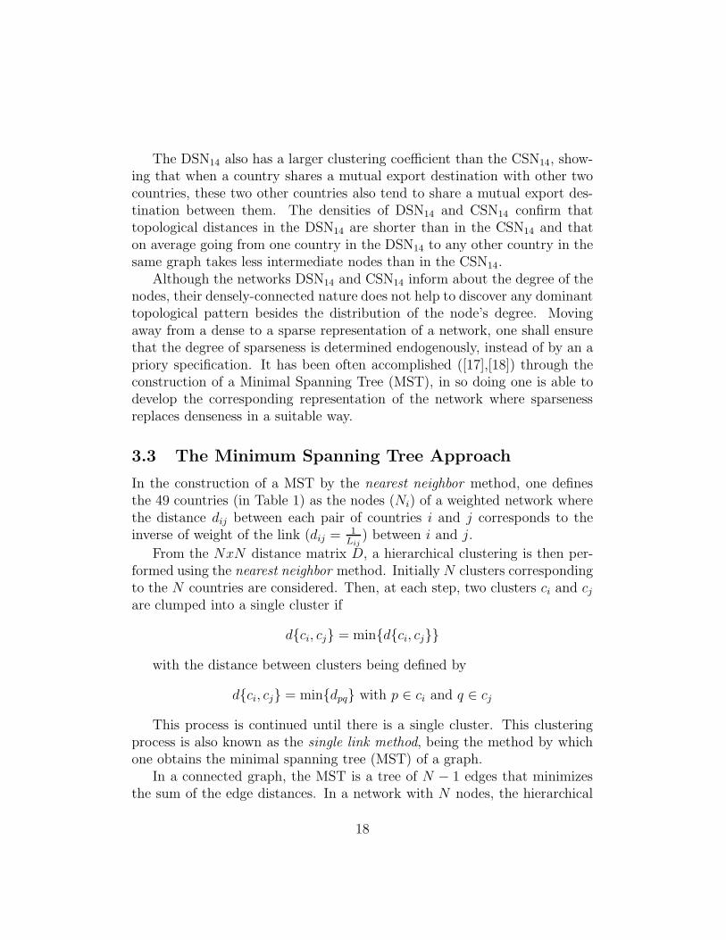
Figure 7 shows the MST obtained from the DSN14 and colored according toeach country main destination of exports in 2014.

The first evidence coming out from the MST in Figure 7 is the centralposition of AGO clustering together the entire set of ”China” exporters (red)in 2014. Another important pattern that emerges in the MST is the branchof UMA countries (yellow) in the right side of the tree, being ”Europe”their most frequent destination of exports. Similarly, part of the countriesthat export mostly to ”Other” seems to cluster on the left branch (purple).Interestingly, the countries that exports to ”African countries” (blue) occupythe less central positions on the tree. This result illustrates the suitabilityof the MST to separate groups of African countries according to their mainexport destinations and the show how opposite are the situations of thosethat export to ”China” from the countries that have Africa itself as theirmain export destinations.

19

Regarding centrality, AGO occupies the most central position of the net-work since this country exports to the top most African export destinations(”China” and ”Europe”) being therefore, and by this means, easily connectedto a large amount of other countries. Indeed, AGO is the center of the mostcentral cluster of ”China” exporters. On the other hand, many leaf posi-tions are occupied by countries that exports to other African countries asthey have the smallest centrality in the whole network, they are KEN, NAMand SWA. Their weak centrality is due to the fact that their leading exportdestinations are spread over several countries (ZMB, TZA, ZAF, BWA andIND).

4.2 The MST of the commodity share network

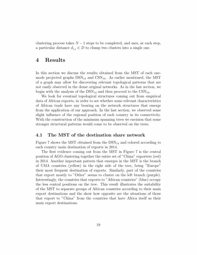
Figure 8 shows the MST obtained from the CSN14 and colored according tothe main export commodity of each country in 2014. The first observationon the MST presented in Figure 8 is that, centrality is concentrated in afewer number of countries (when compared to the MST of the DSN14).

The top most central and connected positions are shared by countriesbelonging to two regional organizations: SADC and CEDEAO, being mainlyrepresented by ZAF and AGO and clustering countries whose main exportcommodities are ”Diamonds” and ”Petroleum”, respectively. Unsurprisingly,centrality and connectivity advantages seem to be concentrated in these twoleading commodity partitions (”Diamonds” and ”Petroleum”) and organiza-tion groups (SADC and CEDEAO).

Indeed, half of CEDEAO countries occupy the upper branch rooted inZAF and having ”Diamonds”(yellow) as their main export commodity. An-other regional cluster is rooted in AGO and tie together several UMA coun-tries whose main export commodity is ”Petroleum”(blue). On the otherhand, half of UMA countries are far from each other on the tree, they oc-cupy the leaf positions, being weakly connected to the other African countriesto which, the few connections they establish rely on having ”Manufactured”as their main export commodity. Likewise, there is a branch clustering ex-porters of ”Raw Materials”(green) being also placed at the leaf positions onthe tree. Such a lack of centrality of ”Raw Materials” exporters in the CSN14

seems to be due to the fact that their leading export products are spread over

20

many different commodities (the ”Raw Materials” partition comprises 12 dif-ferent commodities).

5 Concluding remarks

In the last decade, a debate has taken place in the network literature aboutthe application of network approaches to model international trade. In thiscontext, and even though recent research suggests that African countries areamong those to which exports can be a vehicle for poverty reduction, thesecountries have been insufficiently analyzed.

We have proposed the definition of trade networks where each bilateralrelation between two African countries is defined from the relations each ofthese countries hold with another entity. Both networks were defined fromempirical data reported for 2014.They are independent bipartite networks: adestination share network (DSN14) and a commodity share network (CSN14).In the former, two African countries are linked if they share a mutual leadingdestination of exports, and in the latter, countries are linked through theexistence of a mutual leading export commodity between them.

Our conclusions can be summarized in the following.

1. Sharing a mutual export destination happens more often: The veryfirst remark coming out from the observation of both the DSN14 andthe CSN14 is that, in 2014 and for the 49 African countries, sharinga mutual exporting product happens less often than sharing a mutualdestination of exports.

2. Great exporting countries tend to be more linked: There is a positivecorrelation between strong connected countries in both the DSN14 andthe CSN14 and those with high amounts of export values in 2014. It isin line with recent research placed in two different branches of the liter-ature on international trade: the World Trade Web (WTW) empiricalexploration ([7],[8],[9],[10], [11],[12],[13]) and the one that specificallyfocus on African trade ([1],[2],[3],[4],[5],[6]). References ([2],[4]) reportson the role of export performance to economic growth. They also dis-cuss on the relation between trade and development, and on the growthby destination hypothesis, according to which, the destination of ex-ports can play an important role in determining the trade pattern of acountry and its development path.

21

3. Destination matters: The idea that destination matters is in line withour finding that in the DSN14, the highest connected nodes are thosewhose main export destination is China. According to Baliamoune-Lutz ([4]) export concentration enhances the growth effects of exportingto China, implying that countries which export one major commodityto China benefit more (in terms of growth) than do countries that havemore diversified exports.

• The China effect: One of the patterns that came out from ourDSN14 shows that half of CEEAC and SADC countries belongsto the bulk of ”China” destination cluster, having high between-ness centrality. Additionally, the ”China” destination group ofcountries displays the highest clustering coefficient (0.96), mean-ing that, besides having China as their main exports destination,the second destination of exports of the countries in this group ishighly concentrated on a few countries.

• The role of Intra-African trade: Another important pattern com-ing out from the MST of the DSN14 shows how opposite are thesituations of the countries that export to ”China” from the coun-tries that have Africa itself as their main export destinations. Inthe MST of the destination share network, many leaf positions areoccupied by intra-African exporters as they have the smallest cen-trality in the whole network. Their weak centrality is due to thefact that their leading export destinations are spread over severalcountries. This result is in line with the results reported by ref-erence ([2]) where the growing importance of intra-African tradeis discussed and proven to be a crucial channel for the expansionof African exports. Moreover, Kamuganga found significant cor-relation between the participation in intra-African trade and thediversification of exports.

• The Angola cluster: our results highlighted the remarkable cen-trality of AGO as the center of the most central cluster of ”China”exporters. Indeed, AGO is the country that holds the most centralposition when both DSN14 and CSN14 are considered. This coun-try occupies in both cases the center of the largest central clus-ters: ”China” exporters in DSN14 and exporters of ”Petroleum”in CSN14.

22

• UMA countries anti-diversification: In the opposite situation, wefound that UMA countries display very low centrality, showingthat besides having ”Europe” as their first export destination,the second destination of exports of UMA countries is spread overseveral countries. This result is in line with reference ([6]) reporton European unilateral trade preferences and anti-diversificationeffects. We showed that UMA countries occupy a separate branchin the MST of the DSN14, being ”Europe” their most frequentdestination of exports.

4. In the CSN14, the highest connected nodes are those that cluster as”Petroleum” exporters, being followed by those that export ”Diamonds”.Unsurprisingly, ”Raw Materials” exporters display very low connec-tivity as their second main exporting product is spread over severaldifferent commodities.

5. Organizations matter: Regional and organizational concerns seem tohave some impact in the CSN14.

• SADC and Petroleum: The group of SADC countries, althoughcomprising a large number of elements, is the one with the poorestconnectivity and clustering in the CSN14. It is certainly due tothe fact that without AGO and MOZ, this large group of countriesdoes not comprise ”Petroleum” exporters.

• UMA countries anti-diversification: Again in the CSN14, its MSTshows that UMA countries are placed on a separate branch. Al-though they are countries with high amounts of export values in2014, UMA countries display low connectivity and low centrality.The leaf positions in the MST of either DSN14 or CSN14 - whileoccupied by countries with very low centrality and connectivity -were shown to characterize countries that export mainly to ”Eu-rope” and whose main exporting product is ”Raw Materials”.

Future work is planned to be twofold. We plan to further improve thedefinition of networks of African countries, enlarging the set of similaritiesthat define the links between countries in order to include aspects like motherlanguage, currencies, demography and participation in trade agreements. Onthe other hand, we also plan to apply our approach to different time periods.As soon as we can relate the structural similarities

23

(or differences) and their evolution in time to certain trade characteristics,the resulting knowledge shall open new and interesting questions for futureresearch on African trade.

References

[1] Portugal-Perez, A. and Wilson, J.S. (2008) Trade Costs in Africa: Bar-riers and Opportunities for Reform, in Policy Research Working Paper4619.

[2] Kamuganga, Dick N. (2012) What drives Africa‘s export diversifica-tion?, in Graduate Institute of International and Development StudiesWorking Paper, No. 15/2012.

[3] Ackah, C. and Morrissey O. (2007) Trade Protection as Income Protec-tion in Poor Countries in GEP-Murphy Institute Conference on NewPolitical Economy of Globalization, New Orleans.

[4] Baliamoune-Lutz, M. (2011) Growth by Destination (Where You ExportMatters): Trade with China and Growth in African Countries in AfricanDevelopment Review, Special Issue: Special Issue on the 2010 AfricanEconomic Conference on “Setting the Agenda for Africa’s EconomicRecovery and Long-term Growth” V.23, 2.

[5] Ackah, C. and Morrissey O. (2005) Trade policy and performance inSub-Saharan Africa since the 1980s, in School of Economics, Universityof Nottingham: CREDIT Research Paper 07/01.

[6] Gamberoni, E. (2007) Do Unilateral Trade Preferences help Export Di-versification? an Investigation of the Impact of the European UnilateralTrade Preferences on Intensive and Extensive Margin of Trade, IHEIDworking paper 17.

[7] Serrano, M.; Boguna, M. and Vespignani, A. (2007) Patterns of domi-nant flows in the trade web, in J. Econ. Interact. Coord., V.2.

[8] Almog, A.; Squartini, T. and Garlaschelli, D. (2015) The Double Roleof GDP in Shaping the Structure of the International Trade Network,arXiv:1512.02454.

24

[9] Fagiolo, G.; Reyes J. and Schiavo S. (2009) World-trade web: Topolog-ical properties, dynamics, and evolution, in Phys. Rev. E, V.79.

[10] Saracco, F.; Di Clemente, R.; Gabrielli, A. and Squartini, T. (2015) De-tecting the bipartite World Trade Web evolution across 2007: a motifs-based analysis, arXiv:1508.03533.

[11] De Benedictis, L.; Tajoli, L. (2011) The world trade network, in TheWorld Economy, V.34.

[12] Picciolo, F.; Squartini, T.; Ruzzenenti, F.; Basosi, R. and Garlaschelli,D. (2012) The role of distances in the World Trade Web, in Proceedingsof the Eighth International Conference on Signal-Image Technology &Internet-Based Systems (SITIS 2012).

[13] Yang, Y; Poonb, J., Liua, Y. and Bagchi-Senb, S. (2015) Small and flatworlds: A complex network analysis of international trade in crude oil,in Energy (Elsevier) V.93.

[14] Bergstrand, J. (1985) The Gravity Equation in International Trade:some Microeconomic, Foundations and Empirical Evidence, in Reviewof Economics and Statistics, V. 67, 3.

[15] Araujo. T. and Banisch, S. (2014), Multidimensional Analysis of Lin-guistic Networks, in Towards a Theory of Complex Linguistic Networks,Springer, Berlin.

[16] International Trade Map (http://www.trademap.org).

[17] Araujo, T., Spelta, A. (2012), The Topology of Cross-border Exposures:beyond the minimal spanning tree approach, in Physica A, V.391.

[18] Dias, J. (2012) Sovereign debt crisis in the European Union: A minimumspanning tree approach, in Physica A, V. 391.

25

Figure 3: The DSN14 colored by partition of main destination.

26

Figure 4: The DSN14 colored by partition of regional organization.

27

Figure 5: The CSN14 colored by partition of main export commodity.

28

Figure 6: The CSN14 colored by partition of regional organization.

29

Europe

Figure 7: The MST of the CSN14 colored by partition of main destination.

30

Figure 8: The MST of the CSN14 colored by partition of main exportingcommodity.

31