Thesis_Heim_print_version

IN-CYLINDER INVESTIGATION OF ENGINE SIZE- AND SPEED-SCALING

EFFECTS

by

Douglas Michael Heim

A dissertation submitted in partial fulfillment of the

requirements for the degree of

Doctor of Philosophy

(Mechanical Engineering)

at the

UNIVERSITY OF WISCONSIN – MADISON

2011

ii

ABSTRACT

Two geometrically scaled, two-valve, optically accessible, single-cylinder

research engines were designed and fabricated to study the fundamentals of engine size-

and speed-scaling effects. All dimensions between the engines scale by the factor of

1.69. Two different port geometries and two different port orientations and both

shrouded and non-shrouded intake valves were tested to vary the intake-generated flow.

Prior to testing the engines, the different head configurations were tested on a steady flow

bench. Flow, swirl, and tumble parameters were measured to quantify the performance

of the engine heads.

The engines were motored at speeds ranging from 300-1200 RPM for the larger

engine and from 600-1800 RPM for the smaller engine at an atmospheric intake pressure.

Particle image velocimetry data were taken on a single plane, parallel to the piston

surface, in the engines using both a low magnification to characterize the large-scale flow

phenomena, and a high magnification to characterize the turbulence field. The low

magnification data for conditions with higher levels of swirl were analyzed to determine

the location of the swirl center and the angular velocity. The high magnification data

(acquired at TDC) were investigated using both ensemble- and spatial-averaging to

define a mean velocity field, and all of the results from the spatial-average method were

investigated as a function of cutoff frequency. The fluctuating velocity fields were used

to calculate turbulence intensity, two-point fluctuating velocity correlations, and

longitudinal and transverse integral length scales. Turbulence intensity measurements

showed close agreement between the large and small engines. The longitudinal

lengthscales were insensitive to direction of separation and were on average twice the

iii

transverse lengthscale, indicating a high level of isotropy in the flow. The longitudinal

lengthscales, when normalized by the TDC clearance, showed good agreement between

the large and small engines.

Turbulent kinetic energy spectra were calculated, and were found to show an

extended inertial subrange for the higher engine speeds; the spectra were fit well by the

model spectrum of Pope. Lower engine speeds and the use of high cutoff frequencies in

the spatial-averaging method were found to reduce the presence of the inertial subrange,

and may result in a low Reynolds number condition where the turbulence is not fully

developed and scale separation is not achieved. The spectral analysis provided

lengthscales (L11) that were similar between the small and large engines when normalized

by the TDC clearance. Kolmogorov scales between the small and large engines also

showed similarity when compared at the same mean piston speed. Taylor-scale Reynolds

numbers were calculated for all engine conditions and collapsed onto a single curve when

plotted against an inlet valve Mach index.

iv

DEDICATION

This work is dedicated to my parents. I will always be grateful for the love and support

they have shown me. I have traveled many paths in life because of the opportunities they

provided for me.

v

Funding for this project was provided by the Wisconsin Small Engine Consortium.

vi

TABLE OF CONTENTS

Abstract ............................................................................................................................... ii

Dedication .......................................................................................................................... iv

Table of Contents ............................................................................................................... vi

List of Figures ................................................................................................................... xii

List of Tables ................................................................................................................. xxiii

Nomenclature ...................................................................................................................xxv

Chapter 1. Introduction ........................................................................................................1

1.1. Motivation .................................................................................................................1

1.2. Objective ...................................................................................................................2

1.3. Outline .......................................................................................................................2

Chapter 2. Review of Literature...........................................................................................3

2.1. Principle of Similitude ..............................................................................................3

2.2. Engine Size-Scaling ..................................................................................................4

2.3. Engine Speed-Scaling .............................................................................................12

2.4. Measurement and Analysis of Turbulence Length Scales and Turbulent Spectra in

Engines ...........................................................................................................................25

Chapter 3. Experimental Setup ..........................................................................................29

vii

3.1. Description of Engines ............................................................................................29

3.2. Engine Heads ...........................................................................................................31

3.3. Engine Optical Access ............................................................................................39

3.4. Dynamometer ..........................................................................................................41

3.5. Intake and Exhaust Systems ....................................................................................41

3.6. Intake Air Flow Metering ........................................................................................43

3.7. Cylinder Pressure ....................................................................................................44

3.8. Oil and Vacuum System ..........................................................................................44

3.9. Coolant System .......................................................................................................46

3.10. Optical System ......................................................................................................47

3.11. Camera System ......................................................................................................47

3.12. Particle Image Velocimetry (PIV) System ............................................................50

Chapter 4. Steady Flow Characterization of Intake Ports ..................................................52

4.1. Experimental Equipment .........................................................................................52

4.2. Flow Coefficient ......................................................................................................57

4.3. Swirl Coefficient and Swirl Ratio Definitions ........................................................59

4.4. Impulse-Type Meter Initial Testing ........................................................................60

4.5. Vane-Type Meter Testing .......................................................................................62

4.6. Swirl References .....................................................................................................64

viii

4.6.1. Zero-Swirl Reference .......................................................................................66

4.6.2. Known-Swirl Reference ...................................................................................66

4.6.3. Honeycomb Geometry and Swirl Reference Results .......................................67

4.7. Swirl Coefficient Testing ........................................................................................72

4.8. Tumble Coefficients and Testing ............................................................................76

Chapter 5. Optical Engine Measurements and Analysis ....................................................79

5.1. Engine Conditions ...................................................................................................79

5.2. Engine Flow Rate ....................................................................................................79

5.3. Engine Peak Pressure ..............................................................................................81

5.4. Methods of Determining Mean and Fluctuating Velocity Fields ............................84

5.5. PIV FOV Locations and First-Choice Vector Statistics ..........................................85

5.6. Low-Magnification PIV Results – Analysis of Swirl Progression and Rotation

Rate .................................................................................................................................88

5.7. High-Magnification PIV Results .............................................................................96

5.7.1. Turbulence Intensity .........................................................................................99

5.7.2. Correlation Length Scale Analysis .................................................................108

5.7.2.1. Correlation Length Scale Analysis – Ensemble-Average Method ..........112

5.7.2.2. Correlation Length Scale Analysis – High-Magnification FOV

Comparison, Ensemble-Average Method ............................................................123

5.7.2.3. Correlation Length Scale Analysis – Spatial-Average Method ..............124

ix

5.7.2.4. Correlation Length Scale Analysis – High-Magnification FOV

Comparison, Spatial-Average Method.................................................................132

5.7.3. Energy Spectra Analysis.................................................................................134

5.7.3.1. Energy Spectra Analysis – Ensemble Average Method ..........................137

5.7.3.2. Energy Spectra Analysis – Ensemble Average Method: L11 ...................140

5.7.3.3. Energy Spectra Analysis – Ensemble Average Method: L11, High-

Magnification FOV Comparison .........................................................................142

5.7.3.4. Energy Spectra Analysis – Ensemble Average Method: Re£ ..................143

5.7.3.5. Energy Spectra Analysis – Ensemble Average Method: η .....................146

5.7.3.6. Energy Spectra Analysis – Spatial-Average Method ..............................148

5.7.3.7. Energy Spectra Analysis – Spatial-Average Method: L11 .......................150

5.7.3.8. Energy Spectra Analysis – Spatial-Average Method: L11, High-

Magnification FOV Comparison .........................................................................156

5.7.3.9. Energy Spectra Analysis – Spatial-Average Method: Re£ ......................158

5.7.3.10. Energy Spectra Analysis – Spatial-Average Method: η ........................160

5.8. Discussion .............................................................................................................166

Chapter 6. Summary and Conclusions .............................................................................179

6.1. Conclusions ...........................................................................................................179

6.2. Future Work ..........................................................................................................183

References ........................................................................................................................184

x

Appendix A: Valve Lift Profile .......................................................................................189

Appendix B: Intake Port Drawings ..................................................................................191

Appendix C: Flow Coefficients and Uncertainty Analysis..............................................196

C.1. Flow Coefficients .................................................................................................196

C.2. Flow Coefficient Uncertainty Analysis ................................................................199

Appendix D: Swirl Coefficient and Swirl Ratio Uncertainty Analysis ...........................204

D.1. Swirl Coefficient Uncertainty Analysis ...............................................................204

D.2. Swirl Ratio Uncertainty Analysis .........................................................................207

Appendix E: MATLAB Code ..........................................................................................208

E.1. MATLAB Code to Calculate the Low-Magnification FOV Swirl Center and

Angular Velocity ..........................................................................................................208

E.2. MATLAB Code to Calculate the Turbulence Intensity of the Ensemble Average

Data ..............................................................................................................................212

E.3. MATLAB Code to Calculate the Turbulence Intensity of the Spatial-Average

Data ..............................................................................................................................216

E.4. MATLAB Code to Calculate the Correlation Lengthscales Using the Ensemble

Average Data, Single-Sided Correlation ......................................................................220

E.5. MATLAB Code to Calculate the Correlation Lengthscales Using the Spatial-

Average Data, Double-Sided Correlation ....................................................................226

xi

E.6. MATLAB Code to Calculate the Energy Spectra Using the Ensemble Average

Data ..............................................................................................................................232

E.7. MATLAB Code to Calculate the Energy Spectra Using the Spatial-Average

Data ..............................................................................................................................235

E.8. MATLAB Function to Calculate the Pope 1-D Model Spectrum in the Horizontal

Direction .......................................................................................................................236

E.9. MATLAB Function to Calculate the Sum Squared Error Between the Measured

Spectra and Pope 1-D Model Spectrum in the Horizontal Direction ...........................238

E.10. MATLAB Function to Calculate the Pope Model Spectrum Constant cL ..........240

E.11. MATLAB Function for Calculating the Difference in the Turbulent Kinetic

Energy ..........................................................................................................................241

xii

LIST OF FIGURES

Figure 2.1: MIT similar engine design, from [12] ..............................................................5

Figure 2.2: Volumetric efficiency vs. mean piston speed of MIT similar engines, from

[12] .......................................................................................................................................7

Figure 2.3: Volumetric efficiency vs. a preliminary Mach index, from [13] .....................9

Figure 2.4: Volumetric efficiency vs. a modified Mach index, from [13]........................10

Figure 2.5: Indicated mean effective pressure vs. mean piston speed of MIT

geometrically similar engines, from [11] ...........................................................................11

Figure 2.6: Pressure traces of MIT geometrically similar engines, from [11] ..................11

Figure 2.7: Variation with engine speed of the turbulence intensity normalized by the

mean piston speed, from [3]...............................................................................................14

Figure 2.8: Variation with engine speed of the RMS velocity fluctuation normalized by

the mean piston speed, from [4] .........................................................................................15

Figure 2.9: Turbulence intensity versus crank angle without swirl, from [5]...................17

Figure 2.10: Turbulence intensity versus crank angle with swirl, from [5] ......................17

Figure 2.11: TDC turbulence intensity versus engine speed with and without swirl, from

[5] .......................................................................................................................................18

Figure 2.12: TDC ensemble averaged cyclic variation, from [5] .....................................18

Figure 2.13: Effect of cyclic variation in the bulk velocity on turbulence intensity, from

[7] .......................................................................................................................................20

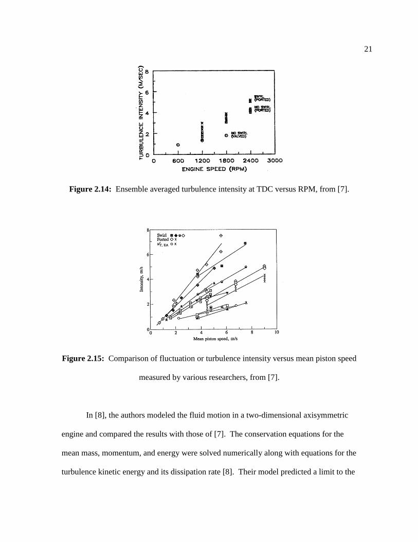
Figure 2.14: Ensemble averaged turbulence intensity at TDC versus RPM, from [7] .....21

xiii

Figure 2.15: Comparison of fluctuation or turbulence intensity versus mean piston speed

measured by various researchers, from [7] ........................................................................21

Figure 2.16: Variation of axial turbulence intensity with engine speed at TDC, no swirl,

from [9] ..............................................................................................................................22

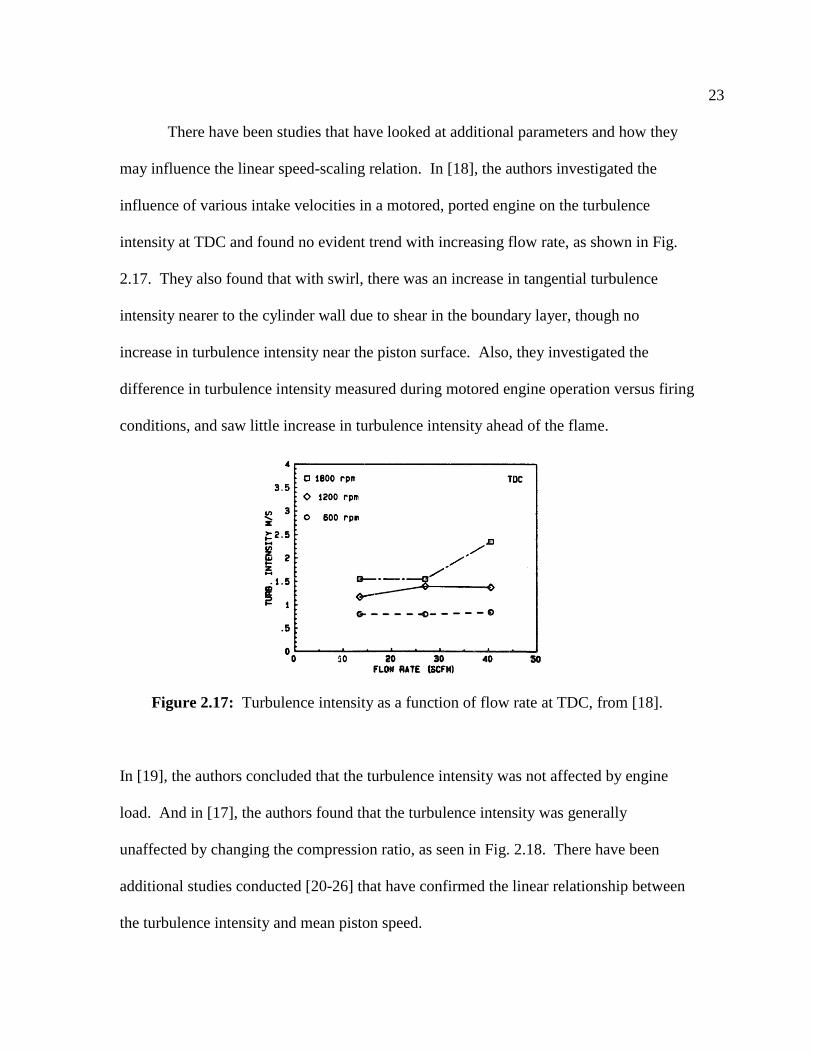
Figure 2.17: Turbulence intensity as a function of flow rate at TDC, from [18] ..............23

Figure 2.18: Turbulence intensity as a function of compression ratio, modified from

[17] .....................................................................................................................................24

Figure 2.19: Fluctuation integral length scale/instantaneous clearance height vs. crank

angle, from [32] .................................................................................................................26

Figure 3.1: Instantaneous piston speed/mean piston speed as a function of crank angle

for the small and large engines ..........................................................................................30

Figure 3.2: Percent difference of the instantaneous piston speed/mean piston speed

between the large and small engines ..................................................................................31

Figure 3.3: Small engine head (left side) and large engine head ......................................33

Figure 3.4: Valve and valve seat geometry .......................................................................34

Figure 3.5: Intake and exhaust non-dimensional valve lift versus crank angle profiles of

both large and small engines ..............................................................................................35

Figure 3.6: Top view of engine showing (a) 0-degree and (b) 90-degree port orientations

with respect to engine cylinder ..........................................................................................36

Figure 3.7: Intake port geometries of the (a) performance port and (b) utility port .........37

Figure 3.8: (a) Performance port right half and (b) utility port right half showing grooves

that mate with a divider plate .............................................................................................38

xiv

Figure 3.9: Cross-sectional view of the (a) large and (b) small optically accessible

engines ...............................................................................................................................40

Figure 3.10: Intake surge tank schematic for small and large engines. Dimensions refer

to small engine, large engine is scaled approximately by 1.69 scaling factor ...................43

Figure 3.11: Small engine oil and vacuum system ............................................................45

Figure 3.12: Small engine coolant system .........................................................................46

Figure 3.13: Resolution image of high-magnification FOV using 200 mm lens for large

engine .................................................................................................................................49

Figure 3.14: Intensity ratio versus line pairs per mm of resolution target for high-

magnification FOVs of large and small engines ................................................................49

Figure 4.1: (a) Flow test setup of small head, (b) swirl test setup of large head, and (c)

tumble test setup of small head on the flow bench next to large tumble adapter ..............53

Figure 4.2: (a) Vane-type swirl meter test setup, (b) Impulse-type torque meter test

setup ...................................................................................................................................54

Figure 4.3: Front and side views of tumble testing arrangement ......................................55

Figure 4.4: Signal-to-noise ratio of large and small heads using impulse swirl meter from

[44] .....................................................................................................................................61

Figure 4.5: Performance ports using mockup shrouded valves. Vane-type meter tested

with standard 5.2 inch diameter paddle. + CW Swirl, - CCW Swirl ................................63


with Dp/B=1.2 custom paddles. + CW Swirl, - CCW Swirl. The impulse-type meter

measurements are the same as Fig. 4.5 ..............................................................................64

Figure 4.7: (a-b) Zero-swirl and (c-d) known-swirl reference fixtures ............................65

xv

Figure 4.8: Impulse- and vane-type meter response to a known angular momentum flux

produced from the known-swirl reference tube for the small and large fixtures. For all

cases a cell height-to-diameter ratio of 1.4 was used .........................................................69

Figure 4.9: Swirl conversion efficiency as a function of the cell aspect ratio for (a) the

vane-type meter, and (b) the impulse-type meter ..............................................................71

Figure 4.10: Swirl coefficients versus non-dimensional valve lift of the (a) performance

ports, non-shrouded valves, (b) utility ports, non-shrouded valves, and (c) both ports,

shrouded valves. + CW Swirl, - CCW Swirl .....................................................................74

Figure 4.11: S/N ratio from swirl coefficient tests of ports in 0-degree orientation ..........75

Figure 4.12: (a) Top-down view of engine head indicating head angle direction on

tumble adapter. Bold arrow is affixed to engine head. (b) Small head at 90° head

angle ...................................................................................................................................77

Figure 4.13: (a) Tumble coefficients versus engine head angle for the utility ports in the

90-degree orientation with the non-shrouded valves .........................................................78

Figure 5.1: Volumetric efficiency versus mean piston speed for all engine running

conditions ...........................................................................................................................80

Figure 5.2: Volumetric efficiency versus mean piston speed for two separate runs in the

small engine .......................................................................................................................81

Figure 5.3: Cylinder peak pressure versus mean piston speed .........................................83

Figure 5.4: Top view of engine cylinder showing FOVs with respect to engine cylinder

for both engines..................................................................................................................86

Figure 5.5: Percent difference between turbulence intensity calculated using N images

versus 200 images with four engine conditions, high-magnification FOV, ensemble

average method ..................................................................................................................87

xvi

Figure 5.6: Top view of engine cylinder showing low-magnification FOV velocity fields

at TDC for the utility port with the shrouded valve at 600 rpm. (a) Ensemble average, (b)

calculated solid body, and (c)-(d) two randomly chosen instantaneous velocity fields ....91

Figure 5.7: Top view of engine cylinder showing swirl center locations at 90 bTDC, 45

bTDC, and TDC, ports in 0-degree orientation. Large engine data at 300, 600, 900, and

1200 rpm, small engine data at 600, 1200, and 1800 rpm. Axes made non-dimensional

by cylinder radius. Open symbols: small engine, filled symbols: large engine. Utility

port: (a) shrouded valve, (b) non-shrouded valve. Performance port: (c) shrouded valve,

(d) non-shrouded valve ......................................................................................................92

Figure 5.8: Normalized angular velocity vs. crank angle, ports in 0-degree orientation.

Open symbols: small engine, filled symbols: large engine. Utility port: (a) shrouded

valve, (b) non-shrouded valve. Performance port: (c) shrouded valve, (d) non-shrouded

valve ...................................................................................................................................94

Figure 5.9: Average normalized angular velocity at TDC vs. swirl ratio, ports in 0-degree

orientation ..........................................................................................................................95

Figure 5.10: Selected images showing the resulting velocity fields using the two methods

of computing the mean velocity field for the given condition: large engine, utility port,

shrouded valve, 0-degree orientation, 1200 rpm. (a) Ensemble average velocity field, (b)

individual cycle instantaneous velocity field, and spatial-average velocity fields for the

individual cycle (b) using cutoff lengthscales of (c) 5 mm, (d) 10 mm, and (e) 15 mm ...99

Figure 5.11: Selected images showing the high-magnification FOV turbulence intensity

found using the (a) ensemble average method and (b) the spatial-average method at a

cutoff lengthscale of 10 mm. (c) contains the same data as (b) but omits the five rows

and columns nearest the edges to illustrate the data used for processing. Engine

condition: large engine, utility port, shrouded valve, 0-degree orientation, 1200 rpm ....102

Figure 5.12: Turbulence intensity at TDC versus mean piston speed using the ensemble

average method ................................................................................................................103

Figure 5.13: TDC turbulence intensity versus mean piston speed slope using the spatial-

average method. Ensemble average data are included at fc = 0 ......................................104

xvii


average method. Cutoff frequency made non-dimensional using TDC clearance.

Ensemble average data are included at fc = 0 ...................................................................105


average method. Cutoff frequency made non-dimensional using TDC clearance. Spatial

average slopes normalized by ensemble average slope ...................................................106


average method. Comparison of data taken in high-magnification FOV versus second

high-magnification FOV ..................................................................................................107



high-magnification FOV. Ensemble average data are included at fc = 0 ........................108

Figure 5.18: Representative single- and double-sided correlations in the vertical direction

using ensemble- and spatial-averaged data using three cutoff lengthscales. Engine

condition: Large engine, UP, SV, 0-deg orientation ........................................................111

Figure 5.19: Correlation coefficients using the ensemble average method in the vertical

direction. Engine condition: large engine, utility port, shrouded valve, 0-degree

orientation, 1200 rpm .......................................................................................................113

Figure 5.20: Longitudinal and transverse integral lengthscales versus mean piston speed

in the vertical and horizontal directions using the ensemble average method. Engine

condition: utility port, shrouded valve, 0-degree orientation ...........................................114

Figure 5.21: Non-dimensional longitudinal and transverse integral lengthscales versus

mean piston speed in the vertical and horizontal directions using the ensemble average

method. Engine conditions: Utility port, (a) SV, 0-deg., (b) NV, 0-deg., (c) NV, 90-deg.,

and Performance port, (d) SV, 0-deg., (e) NV, 0-deg., (f) NV, 90-deg ...........................118

Figure 5.22: Non-dimensional integral lengthscales for all engine conditions and speeds

in the vertical versus horizontal directions using the ensemble average method ............118

xviii

Figure 5.23: Non-dimensional modified longitudinal integral lengthscales versus mean

piston speed in the vertical and horizontal directions using the ensemble average method.

Engine conditions: Utility port, (a) SV, 0-deg., (b) NV, 0-deg., (c) NV, 90-deg., and

Performance port, (d) SV, 0-deg., (e) NV, 0-deg., (f) NV, 90-deg ..................................122

Figure 5.24: Modified non-dimensional longitudinal lengthscales for all engine

conditions and speeds in the vertical versus horizontal directions using the ensemble

average method ................................................................................................................123

Figure 5.25: Comparison of transverse integral lengthscales calculated in the two high-

magnification FOVs versus mean piston speed in the vertical and horizontal directions

using the ensemble average method ................................................................................124

Figure 5.26: Representative double-sided correlations in the vertical direction for spatial-

averaged data using three cutoff lengthscales and corresponding best-fit curves. Engine

condition: Large engine, UP, SV, 0-deg orientation ........................................................126

Figure 5.27: Longitudinal and transverse integral lengthscales in the horizontal direction

using the spatial-average method. (a) Lii versus fc, (b) Lii/hTDC versus fc, and (c) Lii/hTDC

versus fc*hTDC. Engine condition: Utility port, non-shrouded valve, 0-degree orientation,

all engine speeds ..............................................................................................................128

Figure 5.28: Longitudinal and transverse integral lengthscales in the horizontal and

vertical directions using the spatial-average method. Open symbols: small engine, filled

symbols: large engine. Engine conditions: Utility port, (a)-(b) SV, 0-deg., (c)-(d) NV, 0-

deg., (e)-(f) NV, 90-deg., and Performance port, (g)-(h) SV, 0-deg., (i)-(j) NV, 0-deg.,

(k)-(l) NV, 90-deg ............................................................................................................132


magnification FOVs versus fc in the vertical and horizontal directions using the spatial-

average method. Engine condition: large engine, (a) utility port, shrouded valve, 0-deg.

orientation, and (b) performance port, shrouded valve, 0-deg. orientation .....................134

Figure 5.30: Model and calculated one-dimensional energy spectra in the vertical

direction using the ensemble average method to determine the mean velocity field.

Engine condition: utility port, 0-degree orientation, shrouded valve, (a) large engine at

300-1200 rpm and (b) small engine at 600-1800 rpm .....................................................140

xix

Figure 5.31: Non-dimensional longitudinal integral lengthscales versus mean piston

speed in the vertical and horizontal directions using the energy spectra analysis-ensemble

average method. Open symbols: small engine, filled symbols: large engine. Engine

conditions: Utility port, (a) SV, 0-deg., (b) NV, 0-deg., (c) NV, 90-deg., and Performance

port, (d) SV, 0-deg., (e) NV, 0-deg., (f) NV, 90-deg .......................................................142

Figure 5.32: Comparison of longitudinal integral lengthscales calculated in the two high-


using the energy spectra analysis-ensemble average method. Engine condition: large

engine, utility port, 0-deg. orientation, shrouded valve and performance port, 0-deg.

orientation, shrouded valve ..............................................................................................143

Figure 5.33: Turbulence Reynolds number versus mean piston speed in the vertical and

horizontal directions using the energy spectra analysis-ensemble average method. Open

symbols: small engine, filled symbols: large engine. Engine conditions: Utility port, (a)

SV, 0-deg., (b) NV, 0-deg., (c) NV, 90-deg., and Performance port, (d) SV, 0-deg., (e)

NV, 0-deg., (f) NV, 90-deg ..............................................................................................145

Figure 5.34: Kolmogorov lengthscales versus mean piston speed in the vertical and




NV, 0-deg., (f) NV, 90-deg ..............................................................................................148


direction using the spatial-average method to determine the mean velocity field for three

cutoff frequencies. Engine condition: utility port, 0-degree orientation, shrouded valve,

(a) large engine at 1200 rpm and (b) small engine at 1200 rpm ......................................150

Figure 5.36: Longitudinal integral lengthscales in the horizontal and vertical directions

using the energy spectra analysis, spatial-average method. (a) L11 versus fc, (b) L11/hTDC

versus fc, and (c) L11/hTDC versus fc*hTDC. Engine condition: Utility port, shrouded valve,

0-degree orientation, all engine speeds ............................................................................152

xx


calculated using the energy spectra analysis, spatial-average method. Open symbols:

small engine, filled symbols: large engine. Engine conditions: Utility port, (a) SV, 0-

deg., (b) NV, 0-deg., (c) NV, 90-deg., and Performance port, (d) SV, 0-deg., (e) NV, 0-

deg., (f) NV, 90-deg .........................................................................................................154

Figure 5.38: Comparison of longitudinal integral lengthscales calculated using the

energy spectra and correlation lengthscale analyses with the spatial-average data. Engine

conditions: Utility port, 0-deg., (a) SV, horizontal direction, (b) SV, vertical direction,

(c) NV, horizontal direction, (d) NV, vertical direction ..................................................156

Figure 5.39: Comparison of longitudinal integral lengthscales calculated in the two high-


using the energy spectra analysis, spatial-average method. Engine condition: large

engine, (a) utility port, 0-deg. orientation, shrouded valve, and (b) performance port, 0-

deg. orientation, shrouded valve ......................................................................................157

Figure 5.40: Turbulence Reynolds number versus normalized cutoff frequency in the

vertical and horizontal directions (not specified) using the energy spectra analysis,

spatial-average method. Open symbol: small engine, filled symbol: large engine. Engine


port, (d) SV, 0-deg., (e) NV, 0-deg., (f) NV, 90-deg .......................................................159

Figure 5.41: Kolmogorov lengthscales versus normalized cutoff frequency in the vertical

and horizontal directions (not specified) using the energy spectra analysis, spatial-average

method. Open symbols: small engine, filled symbols: large engine. Engine conditions:

Utility port, (a) SV, 0-deg., (b) NV, 0-deg., (c) NV, 90-deg., and Performance port, (d)

SV, 0-deg., (e) NV, 0-deg., (f) NV, 90-deg .....................................................................161

Figure 5.42: Kolmogorov lengthscales versus mean piston speed for fc*hTDC = 0.7 in the

vertical and horizontal directions using the energy spectra analysis, spatial-average

method. Open symbol: small engine, filled symbol: large engine. Engine conditions:



xxi






Figure 5.44: Normalized longitudinal integral lengthscales found using the correlation

analysis versus energy spectra analysis for the ensemble average method data. All engine

conditions. Open symbols: small engine, filled symbols, large engine ..........................169


analysis versus energy spectra analysis for the spatial-average method data at fc*hTDC =

1.7. All engine conditions. Open symbols: small engine, filled symbols, large

engine ...............................................................................................................................170

Figure 5.46: Ratio of L11/£ versus Rλ from (a) model spectrum [60] and (b) for all engine

conditions using model spectrum analysis with ensemble-average data .........................173

Figure 5.47: Re£ from model spectrum versus ReL11 from correlation analysis for all

engine conditions with ensemble-average data ................................................................174

Figure 5.48: Rλ calculated using the energy spectra analysis, ensemble average method

versus Z. Open symbol: small engine, filled symbol: large engine. (a) Vertical direction,

(b) horizontal direction. Small engine Rλ multiplied by the scaling factor 1.69, (c)

vertical direction, (d) horizontal direction .......................................................................177

Figure B.1: Large engine performance intake port engineering drawing .......................191

Figure B.2: Side close-up view detailing flow path of large engine performance intake

port ...................................................................................................................................192

Figure B.3: Large engine utility intake port engineering drawing..................................193

Figure B.4: Side close-up view detailing flow path of large engine utility intake

port ...................................................................................................................................194

xxii

Figure B.5: Back close-up view detailing flow path of large engine utility intake

port ...................................................................................................................................195

Figure C.1: Flow coefficients versus crank angle degrees of performance port with non-

shrouded valve in the (a) 0- and (b) 90-degree orientations and (c) shrouded valve in 0-

degree orientation.............................................................................................................197

Figure C.2: Flow coefficients versus crank angle degrees of utility port with non-



Figure C.3: Flow coefficients versus crank angle degrees of exhaust ports ...................198

Figure C.4: Uncertainty on the sample mean flow coefficients for the performance ports,

90-degree orientation, non-shrouded valves ....................................................................200

Figure C.5: Uncertainty on the sample mean flow coefficients for the utility ports, 90-

degree orientation, non-shrouded valves .........................................................................201


degree orientation, shrouded valves .................................................................................202

Figure D.1: Uncertainty of the sample mean swirl coefficients for the utility ports, 0-

degree orientation, shrouded valves .................................................................................206

Figure D.2: Uncertainty of the sample mean swirl coefficients for the performance ports,

0-degree orientation, non-shrouded valves ......................................................................207

xxiii

LIST OF TABLES

Table 3.1: Dimensions of the large and small engines .....................................................30

Table 3.2: Engine head dimensions ..................................................................................35

Table 3.3: Important valve lift timing events, 0° is TDC of the intake stroke. Crank angle

degree of valve open and valve close events reported at 5% of peak lift ..........................35

Table 4.1: Dimensions of swirl adapter fixtures ...............................................................55

Table 4.2: Dimensions of tumble adapter fixtures ............................................................55

Table 4.3: Intake port mass-weighted average flow coefficients and uncertainties of the

small and large heads in the 0- and 90-degree port orientations ........................................58

Table 4.4: Exhaust port mass-weighted average flow coefficients...................................59

Table 4.5: Dimensions of the zero- and known-swirl references ......................................65

Table 4.6: Intake port swirl ratios and uncertainties of the small and large heads in the 0-

and 90-degree port orientations .........................................................................................75

Table 5.1: Crank angle degree of peak pressure relative to TDC of compression stroke

listed at the engine mean piston speed ...............................................................................83

Table 5.2: PIV statistics for percentage of first-choice vectors for each engine and

FOV....................................................................................................................................88

Table 5.3: Longitudinal and transverse integral lengthscales averaged over all engine

speeds in the vertical and horizontal directions using the ensemble average method.

Dimensions in mm ...........................................................................................................119

xxiv

Table A.1: Intake non-dimensional valve lift profile between 105 and 270 crank angle

degrees. The intake and exhaust profiles are identical and symmetric about the peak lift,

such that the exhaust profile can easily be deduced from this table, the valve inner seat

diameter, and the peak lift locations found in Table 3.3 ..................................................189

Table C.1: Uncertainty of the sample mean flow coefficients for ports with non-shrouded

valves in 90-degree orientation ........................................................................................200

Table C.2: Uncertainty of the sample mean flow coefficients for utility ports with

shrouded valves in 0-degree orientation ..........................................................................202

Table D.1: Uncertainty of the sample mean swirl coefficients for the ports in the 0-


xxv

NOMENCLATURE

Lower-case Roman

c air speed of sound

cL model energy spectrum constant

dI diameter of impulse torque meter honeycomb cells

dP diameter of paddle meter honeycomb cells

f£ model spectrum non-dimensional function

fη model spectrum non-dimensional function

hTDC TDC clearance

k turbulent kinetic energy

l length dimension

m mass flow rate

1,2/ Nt t-distribution test statistic

u fluctuating velocity

u’ turbulence intensity

u velocity vector

uCf flow coefficient uncertainty

uCf,avg mass-average flow coefficient uncertainty

uCs swirl coefficient uncertainty

uf fluctuation intensity

uRs swirl ratio uncertainty

uV mean voltage change uncertainty

Upper-case Roman

Ap piston area

Aref reference area

aTDC after Top Dead Center

Av valve inner seat area

B engine cylinder bore

bTDC before Top Dead Center

C model energy spectrum constant

Cf flow coefficient

Cf,avg mass-weighted average flow coefficient

fC sample mean flow coefficient

Cs swirl coefficient

xxvi

Ct tumble coefficient

CCW counter-clockwise

CW clockwise

D inner seat diameter

DI diameter of impulse torque meter honeycomb flow rectifier

DP diameter of paddle meter paddle wheel

DR diameter of swirl reference tubes

Dv valve head diameter

E11( 1) one-dimensional kinetic energy spectrum

EV exhaust valve

EVC exhaust valve close

EVO exhaust valve open

FFT fast-Fourier transform

FOV field-of-view

H swirl adapter fixture height

HI height of impulse torque meter honeycomb flow rectifier

HP height of paddle meter paddle wheel

HP horsepower

IFFT inverse fast-Fourier transform

IR intensity ratio

IV intake valve

IVC intake valve close

IVO intake valve open

L valve lift

£ lengthscale characteristic of large eddies

LR length of swirl reference tubes

LDA laser Doppler anemometry

LDV laser Doppler velocimetry

LFE laminar flow element

N number of samples/measurements/images etc.

Nc number of cycles

Ncolumns number of columns of PIV data

NV non-shrouded valve

P pressure

PP performance port

PIV particle image velocimetry

PLIF planar laser induced fluorescence

R2 fixture offset from the centerline of the cylinder bore

Rλ Taylor-scale Reynolds number

xxvii

Re£ turbulence Reynolds number

RMS root mean squared

RPM rotations per minute

S engine piston stroke

SCf flow coefficient sample standard deviation

SCs swirl coefficient sample standard deviation

SR flow straightener length

SV voltage change sample standard deviation

SV shrouded valve

S/N signal-to-noise ratio

T torque

Teq equivalent torque

TDC top dead center

U instantaneous velocity

U mean velocity

CRU cycle-resolved mean velocity

EAU ensemble average velocity

UP utility port

V torque sensor mean voltage change

V velocity

VB Bernoulli velocity

Vdisp displaced cylinder volume

Vmps mean piston speed

Vps instantaneous piston speed

Z inlet valve Mach index

Lower-case Greek

α probability of making a type-I error

ε rate of dissipation

η Kolmogorov lengthscale

ηV volumetric efficiency

κ wavenumber

κ1 one-dimensional wavenumber

μ viscosity of air

ν kinematic viscosity

θ crank angle

θR angle of reference tube

xxviii

ρ density of air

ρ11 longitudinal correlation coefficient

ρ22 transverse correlation coefficient

ω paddle wheel angular velocity

Upper-case Greek

Ω angular velocity magnitude

ΩEngine engine angular rotation rate

1

CHAPTER 1

INTRODUCTION

1.1. Motivation

The motivation for this investigation is to study the fundamentals of engine size-

and speed-scaling effects and how they influence the in-cylinder velocity, turbulence, and

mixing. The principle of similitude of internal combustion engines has been promulgated

for many years [1-2]. Speed-scaling laws have been proposed and tested by various

authors [3-10] and size-scaling investigations have been performed [11, 12]. Although

these studies have provided useful information, there have been no studies performed to

the authors‟ knowledge that have thoroughly investigated size-scaling effects from a

fundamental point-of-view.

The development of engines is time consuming and difficult, and relies critically

on the evolution of existing designs. The problem becomes more difficult when the size

of the engine is changed significantly, i.e. when one tries to adapt a well-designed engine

to a new size. The current investigation is directly testing the engine size- and speed-

scaling effects. The results will be used by small engine manufacturers as a guide to

better predict the resulting fluid turbulence, mixing, and combustion when developing a

new engine. This will help small engine manufacturers reduce new engine development

time and costs.

2

1.2. Objective

The objectives of this research are to experimentally investigate the effects of

size-scaling on such parameters as turbulence intensity and mixing and to verify the

existing speed-scaling relations on the same engines. This was accomplished by first

designing and fabricating two scaled, optically accessible, motored engines. Particle

image velocimetry (PIV) experiments were conducted in both engines during the

compression stroke to measure the velocity field in a plane parallel to and below the

engine head. Turbulence statistics were computed from the velocity field data. The

turbulence statistics are compared between the two scaled engines.

1.3. Outline

This thesis is divided into 6 chapters. Chapter 2 contains a review of the various

studies that have been previously performed related to internal combustion engine size-

and speed-scaling. Chapter 2 also contains a review of the relevant papers related to

turbulence measurements and analysis in engines. Chapter 3 details the geometry of the

engines used in this study and the experimental setup. Chapter 4 contains steady flow

bench data characterizing the engine heads. Chapter 5 describes the PIV experiments

performed and the resulting data analysis. Chapter 6 is a summary and conclusion of this

study.

3

CHAPTER 2

REVIEW OF LITERATURE

The following presents a review of the various studies that have been performed

and the theory related to internal combustion engine flow field size-scaling, speed-

scaling, and turbulence.

2.1. Principle of Similitude

Internal combustion engine size-scaling is best understood by first applying the

principle of similitude, which has been applied to machinery of various types over the

years. Some of the early studies applying this principle to internal combustion engines

can be found in [1, 2]. In general, similar engines have their respective parts made of the

same materials and have linear dimensions that are proportional. The ratio of the lengths

of similar parts is the same, regardless of the part; consequently similar engines are scale

reproductions of each other. Thus, the stroke-to-bore and compression ratios are equal,

the mean flow velocities through the valve ports are equal for equal mean piston speeds,

and the volumetric efficiencies and gas pressures are equal [2].

The rate at which combustion occurs in an internal combustion engine has long

been understood to depend on the in-cylinder mixture turbulence. As stated in [2],

similar engines should have the same turbulence with the same piston speed, which

indicates the same rate of combustion. The time required for combustion is proportional

to the length of flame travel. The crank angle period required for combustion is then

proportional to the combustion time multiplied by the engine revolution rate, which is

4

equal to a constant. Thus, the crank angles required for combustion and the losses due to

combustion times should be the same in similar engines at the same piston speed [2].

2.2. Engine Size-Scaling

The topic of how engine size-scaling affects engine performance holds much

importance. Engine unit size, which is closely related to how much power can be

produced, is one of the main parameters addressed by an engine designer when first

designing a new engine. A better understanding of how the engine processes scale aids

the designer in making sound engineering decisions that reduce development time and

expenses.

While the similitude of engines is well understood, and the theory behind it is

capable of mathematical proof, to the author‟s knowledge, there has only been one

research study conducted directly testing the effect of size on performance of similar

spark-ignition internal combustion engines. In the research paper [11], and later in a

book on the subject of internal combustion engines [12], the author C.F. Taylor describes

a study undertaken at the Massachusetts Institute of Technology to better understand

engine size-scaling. In the study, three similar single-cylinder engines were built using

the same scaled drawing as shown in Fig. 2.1.

5

Figure 2.1: MIT similar engine design, from [12].

The engines had cylinder bores of 2.5, 4.0, and 6.0 inches. The operating variables that

were held the same between the engines included the inlet air pressure and temperature,

exhaust pressure, the fuel-air ratio and coolant supply temperature.

The first topic that was investigated in this study was the air flow. Since the

speed of sound is the limiting gas velocity at the smallest cross section of a flow system,

when pressures and temperatures on the upstream side of this section are the same (and

shapes are the same), maximum mass flow will be proportional to the square of the

typical dimension [11]. In the case of internal combustion engines, the inlet-valve

6

opening is usually the smallest cross-sectional area. Also, for flows less than critical,

Taylor argues that the previous considerations suggest that a Mach index which defines

the relation of flow velocity to sound velocity will have great importance.

Using dimensional analysis, Taylor states that for a series of similar engines

operating under similar conditions, volumetric efficiency is a function of two non-

dimensional parameters, the Mach Index defined as:

c

Vmps (2.1)

where Vmps is the mean piston speed and c is the speed of sound in air at the inlet

conditions, and the Reynolds Index defined as:

lVmps (2.2)

where l is a typical length dimension, and μ is the viscosity of air at inlet conditions. It

might be inferred that, in reciprocating engines, variations in viscous forces and in heat

transfer coefficients, which depend on the Reynolds number, will be of considerably less

importance than the forces due to inertia of the gas, which are dependent upon the Mach

number [11]. Figure 2.2 shows that for the three similar engines, the volumetric

efficiency is only a function of the mean piston speed (or the Mach Index as the speed of

sound in air is the same at the same temperature). Similar engines running at the same

values of mean piston speed and at the same inlet and exhaust pressures, inlet

temperature, coolant temperature, and fuel-air ratio will have the same volumetric

efficiency within measurable limits [12]. It was also noted that this trend would not hold

unless the connected inlet and exhaust systems are similar due to differences in pressure-

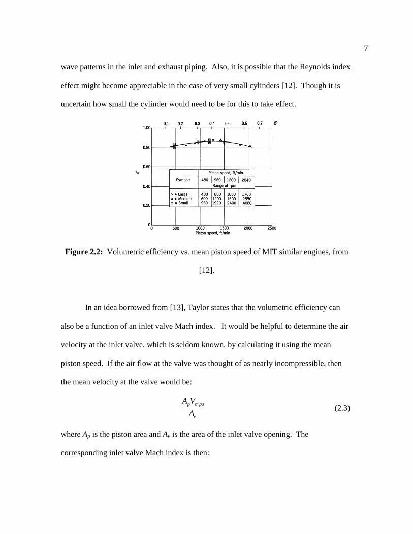
7

wave patterns in the inlet and exhaust piping. Also, it is possible that the Reynolds index

effect might become appreciable in the case of very small cylinders [12]. Though it is

uncertain how small the cylinder would need to be for this to take effect.

Figure 2.2: Volumetric efficiency vs. mean piston speed of MIT similar engines, from

[12].

In an idea borrowed from [13], Taylor states that the volumetric efficiency can

also be a function of an inlet valve Mach index. It would be helpful to determine the air

velocity at the inlet valve, which is seldom known, by calculating it using the mean

piston speed. If the air flow at the valve was thought of as nearly incompressible, then

the mean velocity at the valve would be:

v

m psp

A

VA (2.3)

where Ap is the piston area and Av is the area of the inlet valve opening. The

corresponding inlet valve Mach index is then:

8

cA

VA

v

m psp (2.4)

If the mean flow area through the inlet valve is proportional to πD2/4, where D is the

valve inner seat diameter, then the inlet valve Mach index can be written as:

cD

VB mps

2

2

(2.5)

where B is the cylinder bore dimension.

To test this new Mach index in [13], a single engine was equipped with several

inlet valve sizes, lifts, and shapes, valve timing being held constant. Shown in Fig. 2.3

are the test data showing volumetric efficiency versus the inlet valve Mach index. The

correlation was poor, so the flow coefficients were found at various lifts under low

velocity, steady flow conditions. A mean inlet flow coefficient, Cf,avg, was then obtained

by averaging the steady-flow coefficients obtained at each lift over the actual curve of lift

versus crank angle used in the tests [12]. Cf,avg is a mass-weighted average and is found

by summing at each crank angle, θ, the steady-flow coefficient, Cf, multiplied by the

mass flow rate, m , found from the steady flow tests divided by the sum of the mass flow

rate at each crank angle.

m

mC

Cf

avgf

, (2.6)

A new inlet valve Mach index was defined as:

cCD

VBZ

avgf

m ps

,2

2

(2.7)

9

Figure 2.3: Volumetric efficiency vs. a preliminary Mach index, from [13].

Figure 2.4 shows the volumetric efficiency plotted versus Z containing the same data as

from Fig. 2.3. This shows that the volumetric efficiency is a unique function of Z over

the wide range of engine speeds and engine parameters tested. Applied to engine-scaling,

similar engines run at the same mean piston speed and at the same inlet air temperature

will have the same value of Z, the inlet valve Mach index, and thus the same volumetric

efficiency, as long as the mean inlet flow coefficients are the same. Thus, steady flow

testing and calculation of this mean inlet flow coefficient can be a good indicator of how

closely the volumetric efficiency will match among similar engines.

10

Figure 2.4: Volumetric efficiency vs. a modified Mach index, from [13].

Another important result from Taylor‟s work concerns the indicated mean

effective pressure of similar engines. At the same volumetric efficiency and fuel-air

ratio, indicated mean effective pressure will be the same, provided thermal efficiency is

the same [11]. Since a larger cylinder has a greater volume-to-surface ratio, it could be

expected that the larger engines in this study would then have lower heat losses and a

higher thermal efficiency compared to the smaller engines. Figure 2.5 shows the results

of indicated mean effective pressure versus mean piston speed for the three similar

engines. Apparently, with the range of size of engines tested for this study, the

differences in thermal efficiency is smaller than measurement uncertainty and the curves

are equal.

11

Figure 2.5: Indicated mean effective pressure vs. mean piston speed of MIT

geometrically similar engines, from [11].

Finally, Taylor plotted the pressure traces from the three similar engines, shown

in Fig. 2.6. Again, the operating conditions were held the same and data were taken at

the same mean piston speed. The traces are said to be the same within the accuracy of

the measurements.

Figure 2.6: Pressure traces of MIT geometrically similar engines, from [11].

12

While Taylor‟s investigation was very thorough and covered the basics of how

engines scale, there is much information that is lacking and many topics that could have

been further explored. There is no information given on the geometry of the intake port

or their effect on the flow into the engine cylinder. There are many types of port

configurations that can affect variables such as tumble, swirl, and volumetric efficiency.

These all have an effect on the resulting fluid mechanics and turbulence which in turn

affect combustion and performance.

2.3. Engine Speed-Scaling

The effect of engine speed on the fluid turbulence in-cylinder has been an area of

much research. With the development and subsequent wide-spread use of such

measurement techniques as hotwire anemometry and laser Doppler anemometry (LDA)

in the 1970‟s, it became possible to make limited measurements of the flow field inside

the engine cylinder. This has helped to enhance our understanding of the in-cylinder

large-scale bulk fluid motion as well as the small-scale turbulence. Understanding how

the fluid turbulence scales with the engine speed is essential in determining combustion

rates and performance as turbulent flame speed is related to fluid turbulence.

There have been a number of studies looking at the relation between the turbulent

flame speed and the turbulence intensity. In [14], in which turbulence in a motored

engine was compared with combustion in the same engine, they determined that a flame

speed ratio, the ratio of the turbulent to the laminar flame speed, was a linear function of

the turbulence intensity. In [15], hotwire turbulence measurements were compared with

burning velocities computed from pressure-time data over a range of engine speeds and

13

spark-timing to develop an equation that showed a linear relation between the flame

speed ratio and turbulence intensity. Since the turbulent flame speed is a function of

turbulence intensity, it is important to understand how the turbulence scales with the

engine speed.

There have been many studies that have used hotwire anemometry and laser

Doppler anemometry to make fluid measurements in-cylinder and have investigated

engine speed-scaling. The purpose of some studies was to investigate and verify speed-

scaling relations, while other studies with differing objectives have reported their findings

related to speed-scaling. The following is a review of the relevant papers on this topic,

which include the important data and speed-scaling relations.

One of the earlier papers to take fluid measurements with hotwire anemometry

and to vary the speed of a motored engine was published by Witze [3]. His engine was

outfitted with various access ports in which to insert the hotwire anemometer probe.

One-dimensional velocity measurements were obtained at a single point slightly below

the deck of the engine head. An ensemble average velocity was calculated for N discrete

velocity measurements as:

N

EA UN

U )(1

)( (2.8)

where U is the instantaneous velocity and θ is a specified crank angle. The fluctuating

component of velocity was then calculated as:

)()()( EAUUu (2.9)

and a fluctuation intensity was defined as:

14

)()( 2uu f (2.10)

Velocity data were acquired at engine speeds ranging from 500 to 2500 RPM. Figure 2.7

shows the turbulence intensity (denoted as turbulence intensity, but whose definition is

consistent with fluctuation intensity) normalized by the mean piston speed versus crank

angle. It is seen that it is a good first-order approximation to assume the mean velocity

and turbulence intensity to be linearly proportional to engine speed [3]. The author does

not conclude what the proportionality constant might be, but makes the generalized

statement that the turbulence intensity varies linearly with mean piston speed.

Figure 2.7: Variation with engine speed of the turbulence intensity normalized by the

mean piston speed, from [3].

A subsequent paper that made use of laser Doppler anemometry to make velocity

measurements in-cylinder of a motored engine was published by Rask in [4]. Similar to

15

Witze‟s study, Rask made single-component velocity measurements at a single point

below the engine head deck while varying the rotational speed of the engine. An

ensemble average velocity and a fluctuation intensity (also referred to as an RMS

velocity fluctuation) were calculated in the same manner as done by Witze. Shown in

Fig. 2.8 are the results, with the RMS velocity fluctuation normalized by the mean piston

speed versus the crank angle for three different engine speeds. As can be seen, there is

very good agreement throughout the compression stroke for the range of engine speeds

investigated. It was concluded that the RMS velocity fluctuation appear to scale well

with engine speed.

Figure 2.8: Variation with engine speed of the RMS velocity fluctuation normalized by

the mean piston speed, from [4].

Liou and Santavicca [5] made laser Doppler velocimetry (LDV) measurements in

a motored engine both with and without significant swirl. Single-component velocity

measurements were made at multiple points in a plane at the center of the TDC clearance

height. For this study, the velocity measurement data rates were sufficiently high to

enable the calculation of a cycle-resolved mean velocity. Measurements were taken at

16

approximately one-degree crank angle windows. A Fourier transform of the velocity

versus time was taken, transforming the data into the frequency domain. A cut-off

frequency was chosen based on the upper frequency limit of the ensemble averaged

velocity frequency spectrum. Turbulence frequency components that lay above the cut-

off frequency were set to zero, and the inverse transform taken to yield the mean velocity

in each cycle. The cycle-resolved mean velocity is expected to be closer to the true mean

velocity than the ensemble average velocity as the ensemble average velocity is

influenced by the cycle-to-cycle variation in the bulk flow. The fluctuating component of

velocity was calculated as:

)()()( CRUUu (2.11)

where CRU is the cycle-resolved mean velocity. The turbulence intensity was then

calculated using the cycle-resolved fluctuating component of the velocity. Thus, the

turbulence intensity is usually smaller than the fluctuation intensity as it does not include

cyclic variations in the bulk flow. However, it is also dependent on the choice of an

appropriate cut-off frequency when calculating the cycle-resolved mean velocity.

Figures 2.9-2.12 show the results from [5]. Figures 2.9 and 2.10 plot the

turbulence intensity averaged from the measurements at four points in the engine cylinder

versus crank angle for three different engine speeds, with no significant swirl (Fig. 2.9)

and with significant swirl (Fig. 2.10). The magnitude of the turbulence intensity is seen

to be greater with swirl than without swirl. Figure 2.11 shows the turbulence intensity at

TDC versus engine speed for the cases with and without swirl. It is seen that the

turbulence intensity near TDC is found to scale approximately linearly with RPM (also

17

with mean piston speed, not shown) both with and without swirl. Also shown in Fig.

2.12 is the RMS of the difference between the cycle-resolved mean velocity and the

ensemble averaged velocity. This indicates that in cases with less bulk fluid motion, such

as without swirl, the difference between the cycle-resolved mean velocity and an

ensemble averaged velocity will be greater than with swirl. Therefore, one must be

careful when making comparisons between the fluctuating intensity of cases with and

without significant bulk fluid motion and must account for variations in the ensemble

averaged velocity.

Figure 2.9: Turbulence intensity versus crank angle without swirl, from [5].

Figure 2.10: Turbulence intensity versus crank angle with swirl, from [5].

18

Figure 2.11: TDC turbulence intensity versus engine speed with and without swirl, from

[5].

Figure 2.12: TDC ensemble averaged cyclic variation, from [5].

One of the most fundamental investigations and collection of information related

to the speed-scaling of engines is found in [7]. In this paper, the authors collected the

speed-scaling data from seven previous investigations conducted between 1973 and 1980.

The data from this collection were taken in motored two-valve engines with various

geometries, with pancake and wedge-type pistons, over a wide range of RPMs and

19

compression ratios, and with and without swirl. The data were acquired by taking either

hotwire anemometry or laser Doppler anemometry measurements and ensemble

averaging of the velocity was used to ultimately determine the fluctuation intensity.

The authors of [7] also conducted a speed-scaling investigation using two separate

motored engines, one with four valves and no swirl and the other ported, both with and

without swirl. Single- and two-component velocity data were acquired using laser

Doppler anemometry at multiple locations in the clearance volume in the ported engine

and at a single location in the four valve engine. The data were acquired at high enough

rates in order to compute a cycle-resolved mean velocity and the turbulence intensity. As

shown in Fig. 2.13, the authors computed and plotted both the fluctuation intensity and

turbulence intensity versus crank angle. Once again, we see there is a larger difference

between the fluctuation intensity and turbulence intensity when there is no bulk organized

fluid motion as in the no swirl case. Figure 2.14 shows the turbulence intensity versus

engine speed for the three engine configurations. As can be seen, there is clearly a

nearly linear relationship between the turbulence intensity and engine speed.

The authors of [7] then plotted the data of fluctuation intensity and turbulence

intensity versus mean piston speed from their study as well as from the previous

investigations they surveyed. Figure 2.15 shows these data and lines connecting the data

show the linear relationship that exists. The authors note that in the same engine, the

turbulence intensity is smaller without swirl than with swirl and that for the case without

swirl, their turbulence intensity would have been higher by a factor of two to three and

would have matched the other studies‟ highest reported intensities, had they similarly

defined turbulence as a fluctuation intensity. Also, the details of the intake system

20

influence only the values of the proportionality constant between turbulence intensity and

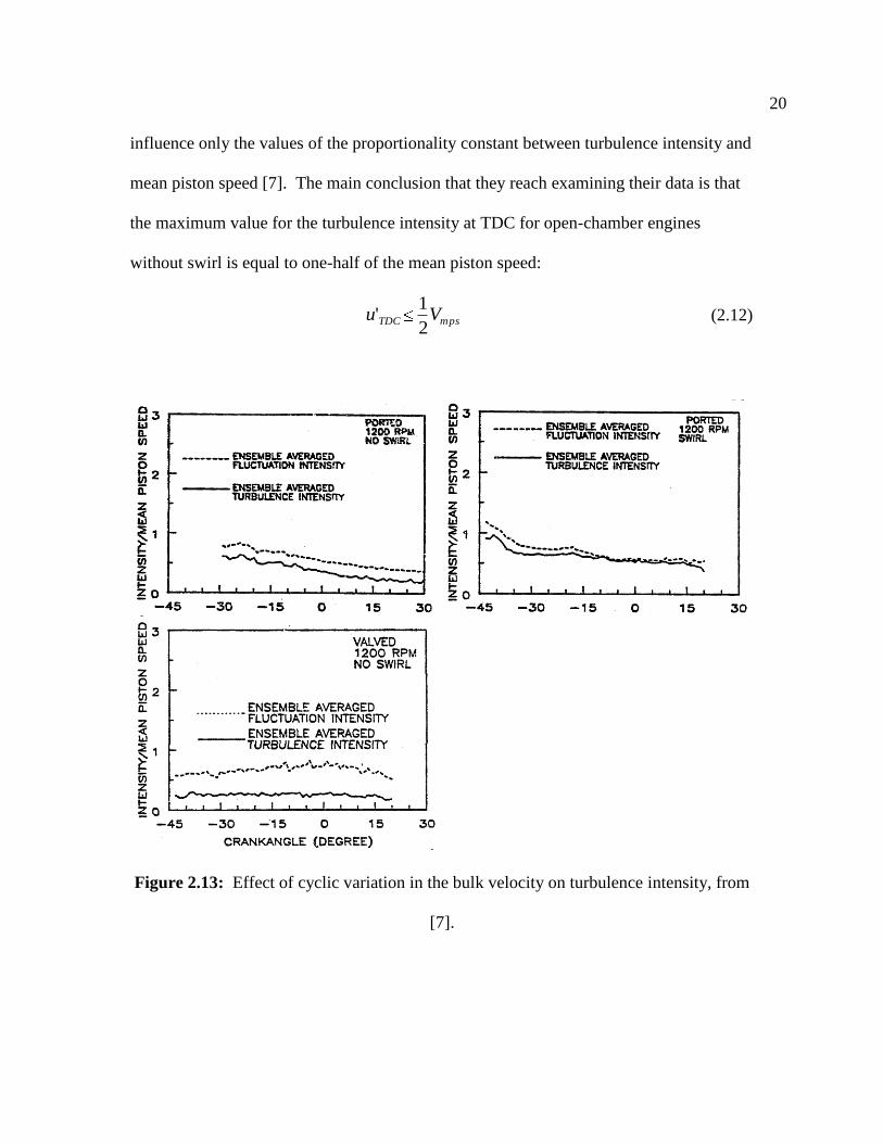
mean piston speed [7]. The main conclusion that they reach examining their data is that

the maximum value for the turbulence intensity at TDC for open-chamber engines

without swirl is equal to one-half of the mean piston speed:

mpsTDC Vu2

1' (2.12)

Figure 2.13: Effect of cyclic variation in the bulk velocity on turbulence intensity, from

[7].

21

Figure 2.14: Ensemble averaged turbulence intensity at TDC versus RPM, from [7].

Figure 2.15: Comparison of fluctuation or turbulence intensity versus mean piston speed

measured by various researchers, from [7].

In [8], the authors modeled the fluid motion in a two-dimensional axisymmetric

engine and compared the results with those of [7]. The conservation equations for the

mean mass, momentum, and energy were solved numerically along with equations for the

turbulence kinetic energy and its dissipation rate [8]. Their model predicted a limit to the

22

value of the turbulence intensity at TDC due to the dominance of the turbulence

dissipation over the diffusivity of the turbulence generated by the intake process. Their

computations concluded the same speed-scaling relation as found in Eqn. (2.12).

In [9], LDA velocity measurements were made in a motored engine in the TDC

clearance mid-plane across a diameter of the cylinder. The authors thought previous

investigations that characterized the TDC turbulence on measurements made at a single

point in the engine cylinder were inadequate. In a two-valve engine with no swirl, they

took velocity measurements in the range from 300-2000 RPM and plotted the axial

turbulence intensity versus the mean piston speed from five distinct locations, as shown

in Fig. 2.16. They note a non-uniform distribution of the turbulence intensity along the

measurement plane with maximum values occurring towards the cylinder center.

Similarly, in cases with swirl, there seems to be higher intensities at the location of the

swirl center, as reported in [16-18]. There also seems to be an increase in non-uniformity

with an increase in engine speed as seen in Fig. 2.16.

Figure 2.16: Variation of axial turbulence intensity with engine speed at TDC, no swirl,

from [9].

23

There have been studies that have looked at additional parameters and how they

may influence the linear speed-scaling relation. In [18], the authors investigated the

influence of various intake velocities in a motored, ported engine on the turbulence

intensity at TDC and found no evident trend with increasing flow rate, as shown in Fig.

2.17. They also found that with swirl, there was an increase in tangential turbulence

intensity nearer to the cylinder wall due to shear in the boundary layer, though no

increase in turbulence intensity near the piston surface. Also, they investigated the

difference in turbulence intensity measured during motored engine operation versus firing

conditions, and saw little increase in turbulence intensity ahead of the flame.

Figure 2.17: Turbulence intensity as a function of flow rate at TDC, from [18].

In [19], the authors concluded that the turbulence intensity was not affected by engine

load. And in [17], the authors found that the turbulence intensity was generally

unaffected by changing the compression ratio, as seen in Fig. 2.18. There have been

additional studies conducted [20-26] that have confirmed the linear relationship between

the turbulence intensity and mean piston speed.

24

Figure 2.18: Turbulence intensity as a function of compression ratio, modified from

[17].

There has been much research investigating the relation between turbulence

intensity and engine speed. As was shown in [7], at TDC in an engine without swirl, the

turbulence intensity can be equal to or less than half of the mean piston speed. While the

investigations conducted to date have provided many useful insights into this topic, they

are also lacking in some respects. Many of the investigations made velocity

measurements at either one or a limited number of points in the cylinder, which tends to

support the opinion that their conclusions were based off a limited, if not an insufficient,

amount of data. Many of the studies were performed with a fixed intake port geometry,

which limited varying the engine geometry and the investigation of the effects of such

parameters as tumble and swirl. There have also been no studies to date that have

investigated the linear speed-scaling relation as applied to engine size-scaling to see what

kind of correlation exists among exactly scaled engines. A study to fill in some of the

missing and inadequate information, where the previous studies have been insufficient,

would provide a wealth of information useful in the development of engines.

25

2.4. Measurement and Analysis of Turbulence Length Scales and Turbulent Spectra

in Engines

The characterization of the turbulence requires more than just the turbulence

intensity. Integral length scale measurements, which give an estimate of the size of

turbulent eddies in the flow, have been made in several studies. Many of the earlier

investigations used Taylor‟s hypothesis to indirectly calculate integral length scales [3,

27-29]. Time-varying velocity data were collected and Taylor‟s hypothesis used to relate

the time scales to length scales. However, the conditions for which Taylor‟s hypothesis

is valid are generally not satisfied in the non-stationary flow field of an internal

combustion engine. Direct measurements of the integral length scales have been

performed using multi-point LDV and PIV measurements [30-34]. Longitudinal length

scales were found to decrease during the compression stroke, where a minimum was

reached very near TDC. In one study [31] an increase in the longitudinal length scale

was observed with an increase in engine swirl ratio, while [35] observed an opposite

trend. Fraser et al. [32] measured the transverse length scale at a number of engine crank

angles and normalized the data by the instantaneous engine clearance height, shown in

Fig. 2.19. A maximum value of about 0.2 near TDC was observed and they reported

values ranging from 0.08-0.37 found by other investigators. However, the transverse

length scale magnitude depended on the data analysis method used in calculating the

mean flow velocity [33]. Fraser and Bracco [36] measured transverse length scales at

multiple places in-cylinder and in different directions. Their results supported the

conclusion of a high level of isotropy and homogeneity in engine turbulence.

26

Figure 2.19: Fluctuation integral length scale/instantaneous clearance height vs. crank

angle, from [32].

PIV has increasingly been used in the analysis of in-cylinder flows [26, 35, 37-

44]. Typically, a Reynolds decomposition of the flow field is performed to separate the

mean velocity from the fluctuating component. One of the challenges of data analysis in

engine flows is to define an appropriate mean velocity. The method used to calculate the

mean velocity field directly affects the subsequent analysis. Many data acquisition

systems are only fast enough to take a single set of PIV images per engine cycle. One

method of calculating the mean velocity field then is to acquire the velocity data at a set

crank angle for a large enough number of engine cycles. The data are then averaged over

all the cycles at each point to find an ensemble average [26, 35, 44]. Another method of

calculating the mean velocity field at a specified crank angle for each cycle is to perform

a spatially resolved analysis [37-39]. The two dimensional Fourier transform is

performed on the velocity field of an individual cycle, a filter is applied using an

27

appropriate cutoff length scale, and the inverse Fourier transform is performed resulting

in a filtered mean velocity field for that cycle. Sufficiently fast data acquisition systems

allow for a time-resolved mean velocity field to be calculated for an individual cycle

[40], as is performed with single-point LDV measurements.

PIV has been used to measure energy spectra in engines. The methods used to

calculate spectra vary. Funk et al [35] used the ensemble average method to determine

the mean and fluctuating velocity components in the flow field and these were then used

to calculate the mean kinetic energy and turbulent kinetic energy fields, respectively. A

low pass Gaussian weighted filter was applied to the data at different length scales to

determine the energy content at various length scales. Fajardo and Sick [41] used a

filtering method similar to [35], but filtered the instantaneous velocity fields, without

using a Reynolds decomposition, to determine an energy spectra. An alternative method

of calculating the energy spectra, found in [45], is used in the current study. This method

involves using a Reynolds decomposition to determine the fluctuating velocity fields and

then the turbulent kinetic energy fields. An interlacing technique [46] is then applied to

the turbulent kinetic energy fields to calculate the energy spectra versus wavenumber.

PIV has also been used to try to determine the Reynolds numbers of flows in

engines. Daneshyar and Hill [47] calculated a mean-flow Reynolds number of 12,000

using the spatial-mean swirl velocity from PIV data, the TDC clearance height, and an

assumed kinematic viscosity. Reuss et al [39] based a turbulence Reynolds number of

200 on the turbulence intensity estimated from their PIV measurements and a velocity

integral lengthscale found from two-point velocity-correlation measurements. Funk et al

[35] used large-Reynolds-number flow theory and the assumption that the equilibrium

28

range has been resolved in their measurements to base a turbulence Reynolds number off

the Kolmogorov and integral lengthscales. Fajardo and Sick [41] assumed a turbulent

Reynolds number on the order of 1,000 for their engine conditions to arrive at an estimate

of the Kolmogorov lengthscale on the order of 50μm. Thus, it is apparent that there have

been many procedures used to analyze PIV data that provide varying levels of agreement

in their results.

29

CHAPTER 3

EXPERIMENTAL SETUP

This chapter describes the engines and related systems used in this study.

3.1. Description of Engines

This study was conducted using two precisely scaled, single-cylinder, two-valve,

optical engines. The scaling factor between the two engines was 1.69, which was set by

the crank radius ratio between the two chosen engines. The larger of the two engines,

henceforth referred to as the “large engine,” is an existing single-cylinder, optical

research engine. The smaller engine, henceforth referred to as the “small engine,” is a

Kohler Courage XT-7 base engine that has been converted into a single-cylinder, optical

research engine. The dimensions of the engines are shown in Table 3.1. The connecting

rod to crank radius ratio is seen to differ slightly between the two engines (all other

geometric parameters are matched exactly), and this affects the profile of piston speed

versus crank angle. The instantaneous piston speed/mean piston speed ratio [48] as a

function of crank angle for the two engines is shown in Fig. 3.1, and Fig. 3.2 shows the

percent difference of these values for the small engine compared to the large engine,

which confirms that the difference in connecting rod to crank radius ratio causes a

negligible difference.

30

(Dimensions

in mm)

Connecting

Rod

Length

Crank

Radius

Connecting

Rod to

Crank

Radius

Ratio

Bore,

B

Stroke,

S

Compression

Ratio

TDC

clearance

Large

Engine 144.8 38.0 3.81 82.0 76.0 10.0 8.44

Small

Engine 84.0 22.5 3.73 48.6 45.0 10.0 5.00

Table 3.1: Dimensions of the large and small engines.

0 30 60 90 120 150 1800

0.5

1

1.5

2

Crank Angle Degrees

Vps / V

mps

Large EngineLarge Engine

Small Engine Small Engine

Figure 3.1: Instantaneous piston speed/mean piston speed as a function of crank angle

for the small and large engines.

31

0 30 60 90 120 150 180-0.8

-0.6

-0.4

-0.2

0

0.2

0.4

Crank Angle Degrees

Perc

ent D

iffe

rence

of V

ps / V

mps

Be

twe

en

La

rge

an

d S

ma

ll E

ng

ine

s

Figure 3.2: Percent difference of the instantaneous piston speed/mean piston speed

between the large and small engines.

3.2. Engine Heads

The large and small engine heads for this study were designed for ease of use and

so that a number of intake conditions could be easily investigated. The engine heads are

fabricated out of aluminum plates, onto which the intake and exhaust ports, valves,

springs, rocker arms, and camshaft are easily assembled. The intake ports are modular in

design and, on the bottom, feature a tongue and groove lip that mates with a counter-bore

on the aluminum plate. This feature allows the intake ports to be rotated 90 degrees

about the intake-valve axis. The exhaust ports were also modular in design for the reason

of ease of manufacturing, but were not meant to be rotated. The intake and exhaust ports

were secured to the base aluminum plate by the use of a port housing fixture and shim

plates. The port housing fixture assembles on the top of the ports and bolts onto the

aluminum plate; the shim plates are inserted between the housing fixture and the top of

32

the ports to effectively compress the assembly and keep the ports from rotating. Valves

can then be installed and the valve springs attach on top of the port housing fixture.

An assembly that includes the camshaft and rocker arms then bolts onto the back

side of the engine head. Two sealed cylindrical roller bearings mount onto either end of

the camshaft and are supported by two block assemblies that bolt directly to the engine

head aluminum plate. A rocker arm assembly bolts on top of the two blocks that hold the

camshaft. The rocker arm assembly consists of two rocker arms that secure to and rotate

about a rod by the use of two sealed ball bearings. At the front end of the rocker arms, an

adjustable lash screw pushes down on top of the valve stem. At the back end of the

rocker arms, a sealed needle roller bearing follower is attached and is acted upon by the

camshaft lobes. The use of the sealed bearings at all three locations in this assembly

eliminates the need for splash lubrication of the engine head. The same camshaft and

rocker arm assembly is used in both the large and small engine heads. The assembly is

modified slightly for the small engine head so that the valve lift profile is appropriately

scaled. This is accomplished by extending the back end of the rocker arms and moving

the axis about which the rocker arms rotate relative to the axis about which the camshaft

rotates. Figure 3.3 details the small and large engine heads.

33

Port HousingFixtures

Shim Plate Shim Plate

Intake Port

Exhaust Port

Rocker ArmsCamshaft Blocks

Flowbench Intake Horn

Aluminum Base Plate

Spring and Valve

Figure 3.3: Small engine head (left side) and large engine head.

The geometry of the valve and seat are shown in Fig. 3.4. Table 3.2 includes the

dimensions shown in Fig. 3.4. Both regular (non-shrouded) and shrouded intake valves

were used to study varying levels of swirl. Throughout this thesis the non-shrouded

valve will be abbreviated as NV, and the shrouded valve as SV. The shrouded valve

features a 180-degree cylindrical shroud. It should also be noted that when the intake and

exhaust valves are fully closed, the surface of the valve head is flush with the engine head

surface. The engine cylinder then closely approximates a right cylinder, with a flat piston

and engine head surface. There are a number of reasons to make the engine head surface

flat. First, it makes it easy for the person cutting the valve seat inserts to make the proper

cut. Checking that the valves are flush with the head ensures that the valve lift profiles

are properly scaled. Second, in industry there are various valve head geometries and the

valve can either sit flush with the head or can protrude at different distances. As optical

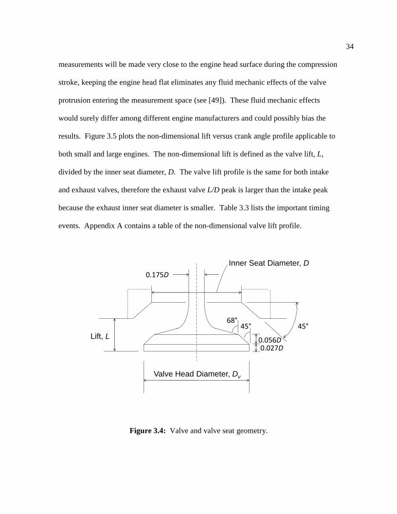
34

measurements will be made very close to the engine head surface during the compression

stroke, keeping the engine head flat eliminates any fluid mechanic effects of the valve

protrusion entering the measurement space (see [49]). These fluid mechanic effects

would surely differ among different engine manufacturers and could possibly bias the

results. Figure 3.5 plots the non-dimensional lift versus crank angle profile applicable to

both small and large engines. The non-dimensional lift is defined as the valve lift, L,

divided by the inner seat diameter, D. The valve lift profile is the same for both intake

and exhaust valves, therefore the exhaust valve L/D peak is larger than the intake peak

because the exhaust inner seat diameter is smaller. Table 3.3 lists the important timing

events. Appendix A contains a table of the non-dimensional valve lift profile.

Valve Head Diameter, Dv

Lift, L

Inner Seat Diameter, D

45°45°68°

0.027D0.056D

0.175D

Figure 3.4: Valve and valve seat geometry.

35

(Dimensions

in mm)

Intake

Valve

Diameter,

Dv

Exhaust

Valve

Diameter,

Dv

Intake

Inner

Seat

Diameter,

D

Exhaust

Inner

Seat

Diameter,

D

Intake

and

Exhaust

Maximum

Lift, L

Intake

Valve

Shroud

Height

Shroud

Outer

Diameter

Large

Engine

Head

35.0 28.0 31.8 25.4 7.9 8.6 29.4

Small

Engine

Head

20.7 16.6 19.1 15.1 4.7 5.1 17.4

Table 3.2: Engine head dimensions.

0.35

0.30

0.25

0.20

0.15

0.10

0.05

0.00

L/D

-360 -270 -180 -90 0 90 180 270 360

Crank Angle Degrees

Exhaust Intake

Figure 3.5: Intake and exhaust non-dimensional valve lift versus crank angle profiles of

both large and small engines.

EVO EVC EV Peak

Lift IVO IVC

IV Peak

Lift

Small and

Large

Head

-235° 25° -105° -25° 235° 105°

Table 3.3: Important valve lift timing events, 0° is TDC of the intake stroke. Crank

angle degree of valve open and valve close events reported at 5% of peak lift.

36

The intake ports were designed so that multiple conditions could be evaluated. As

mentioned previously, the intake ports are modular and feature a tongue and groove lip,

allowing them to be rotated about the valve axis. Figure 3.6 illustrates the two port

orientations that were tested. The 0-degree orientation, Fig. 3.6(a), has the port directed

tangentially relative to the near cylinder wall such that it would tend to produce a swirl-

dominated flow. The 90-degree orientation, Fig. 3.6(b), has the port directed

perpendicularly relative to the near cylinder wall such that it would tend to produce a

tumble-dominated flow. The shrouded valve was used only with the 0-degree orientation

while the non-shrouded valve was used with both 0- and 90-degree port orientations.

Cylinder Wall

Cylinder Axis

Exhaust Valve

Intake Valve

Intake Port

Shroud

Intake ValveIntake Port

90°

Cylinder Wall

Cylinder Axis

Exhaust Valve

(a) (b)

Figure 3.6: Top view of engine showing (a) 0-degree and (b) 90-degree port orientations

with respect to engine cylinder.

Two different intake port geometries were designed for this investigation. Engine

port geometry will vary among manufacturers and can be influenced by such factors as

intended use, performance, manufacturing cost, and manufacturing processes. The ports

37

designed for this study were based on geometries common to the companies that

supported this research. Figure 3.7 shows the solid model cross-section for the two ports,

the green highlighted region shows the flow path. Detailed engineering drawings of the

ports can be found in Appendix B. Figure 3.7(a) shows the port termed the performance

port, referred to hereafter as PP. This port design would be found in higher performance

engines as it tends to increase volumetric efficiency and promotes strong organized in-

cylinder flows. The angle between the port inlet and the port bottom surface was 35

degrees. Other dimensions were based on guidelines to maximize volumetric efficiency

provided in [50]. Figure 3.7(b) shows the port termed the utility port, referred to

hereafter as UP. This port design would be found in utility-type engines such as

lawnmowers or generators where design is based to a greater degree on ease and cost of

manufacturing. This port is based on a Kohler CH-14 engine port, with the inlet parallel

to the port bottom surface and a 90 degree bend at the outlet.

(a) (b)

Figure 3.7: Intake port geometries of the (a) performance port and (b) utility port.

38

The ports were fabricated in two halves that bolt together to form the complete

port. This was done for two reasons. It made it is easier to machine the complex port

geometry. [It also makes it functionally possible to perform the planar laser-induced

fluorescence (PLIF) experiments to be discussed later.] Figures 3.8(a) and (b) show the

right half of the performance port and utility port, respectively. Highlighted in green is a

small groove machined into the port inner surface that mates with a divider plate, shown

in yellow. The divider plate position is just to one side of the valve guide. This makes it

possible to completely separate the port inner area into two flow paths, one path that can

be seeded with a fuel tracer needed for PLIF measurements and the other path left

unseeded.

(a)

(b)

Figure 3.8: (a) Performance port right half and (b) utility port right half showing

grooves that mate with a divider plate.

39

3.3. Engine Optical Access

The engines for this study are optically accessible, Bowditch-type single cylinder

research engines. A cross-sectional view of the large engine is shown in Fig. 3.9(a) and

the small engine in Fig. 3.9(b). The upper portion of the cylinder is replaced with a

quartz ring window to allow the passage of a laser sheet into the cylinder. The ring

window for the large engine clamps between two plates and was designed this way such

that another investigation could use the assembly. The ring window for the small engine

clamps directly underneath the engine head such that measurements could be acquired

through TDC. The piston surface is flat and contains a centered, round sapphire window

that permits optical access to 53% of the cylinder bore (43.2 mm and 25.4 mm in

diameter for the large and small engines, respectively). An Edmund Optics UV-enhanced

imaging mirror sits at a 45-degree angle beneath the piston window, inside the Bowditch

piston, to allow visual access for a camera into the cylinder.

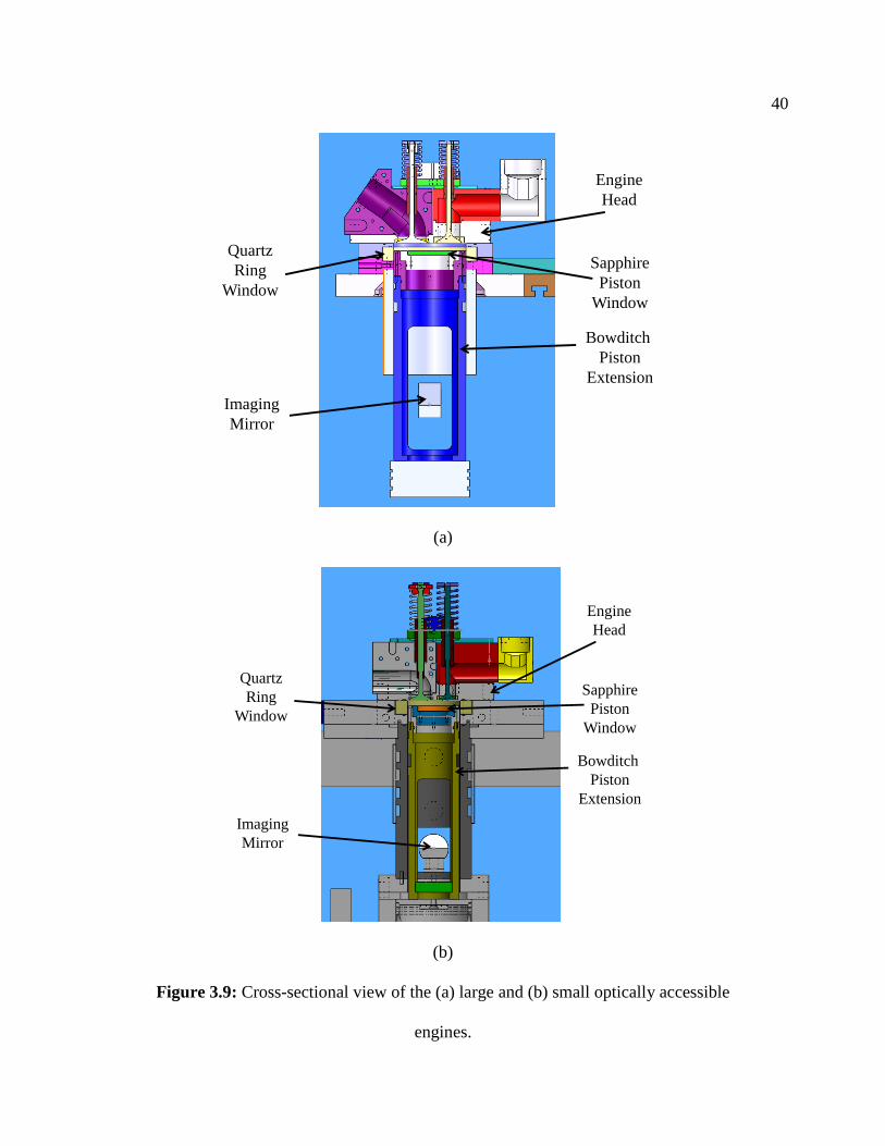
40

Imaging

Mirror

Bowditch

Piston

Extension

Sapphire

Piston

Window

Engine

Head

Quartz

Ring

Window

(a)

Imaging

Mirror

Bowditch

Piston

Extension

Sapphire

Piston

Window

Engine

Head

Quartz

Ring

Window

(b)

Figure 3.9: Cross-sectional view of the (a) large and (b) small optically accessible

engines.

41

3.4. Dynamometer

The large engine was motored using a General Electric type TLC-20

dynamometer. The maximum rated speed of the dynamometer is 5000 RPM with a

maximum delivery as a motor of 40 HP and was controlled with a Reliance Electric

MaxPak PLUS VS Drive, model 600840-2A. The small engine was motored using an

A.O. Smith Century AC motor. The maximum rated speed of the motor is 3470 RPM

with rated power of 3 HP.

3.5. Intake and Exhaust Systems

The intake system for each engine consisted of three cylindrical tanks. A

schematic of the system is shown in Fig. 3.10. Surge Tank 1 feeds both Surge Tank 2

and 3. Surge Tank 2 feeds into the smaller partition of the intake port while Surge Tank

3 feeds into the larger partition. For PIV measurements, oil droplets are introduced just

upstream of Surge Tank 1 so that they mix evenly before entering Surge Tanks 2 and 3.

For PLIF measurements, a fuel tracer is introduced just before entering Surge Tank 2 so

that it mixes evenly before entering the smaller partition of the intake port and the larger

partition is fed by air only. The configuration of the system is such that the pressure drop

across both partitions of the intake port is approximately the same. The exhaust surge

tank was cylindrical in shape and the same size as the intake tanks. Flexible wire-

reinforced PVC tubing was used to connect the tanks and intake and exhaust ports. All

basic dimensions of the surge tanks and tubing scaled at the 1.69 ratio.

The intake system was heated such that the air entering the engines was at 50°C.

The intake surge tanks for the large engine each had a 5 Watt/in2, 3” x 24” flexible

42

silicone-rubber heater attached to the surface. This was the same rated power that had

been used with the single intake tank for previous studies. An inline heater upstream of

Surge Tank 1 was also turned on. At the lower speeds, it took an excessive amount of

time to get to the steady state temperature. Thus, a flow directing baffle was inserted at

the top of Surge Tanks 2 and 3 to direct the flow along the tank wall, helping to reduce

stratification and enhancing the heat transfer to the air. It is recommended that the tank

heaters be replaced with higher power heater strips for future work. The intake surge

tanks for the small engine each had a 10 Watt/in2, 6 x 12 in

2 flexible silicone-rubber

heater attached to the surface. Experiments were performed with a pressure just upstream

of Surge Tank 1 at ~98 kPa.

43

Pressure98kPa

Flowmeter

BuildingAir In

77”ø1.25”

ø1.25”

9.6”

ø5.6”

ø1.25”

ø0.75”

DividedIntake Port

ExhaustPort

ø1.25”

Engine

34”

7”

12”54”

BuildingExhaust

Tank 1Tank 2 Tank 3ExhaustTank

Oil Droplets(PIV)

34”

Figure 3.10: Intake surge tank schematic for small and large engines. Dimensions refer

to small engine, large engine is scaled approximately by 1.69 scaling factor.

3.6. Intake Air Flow Metering

The air flow rate into the large engine was measured using three choked-flow

orifices upstream of the intake surge tank system. The orifices had been calibrated

previously by another student and information can be found in [51]. The air flow rate

into the small engine was initially measured using a Meriam Instrument model 50MH10-

2 laminar flow element (LFE) meter. The LFE was calibrated using a Singer, American

Meter Division, AL-175 bellows meter. An Omega Engineering model PX278-01D5V

44

pressure transducer was used to measure the pressure drop across the LFE. However,

when the engine was running, pressure waves in the intake system made it hard to get

reliable and repeatable data since flow through the LFE oscillated at a high frequency.

The air flow rate was subsequently acquired by placing the bellows meter directly at the

exit of the exhaust tank to measure the flow rate out of the engine.

3.7. Cylinder Pressure

Pressure data were acquired using a Kistler model 7061B piezoelectric pressure

transducer. The pressure transducer was mounted into the cylinder head such that its

surface was flush with the flat engine head deck. The charge produced by the transducer

was converted to a voltage by a Kistler type 510 dual mode amplifier. The linear

response of the change in voltage with a change in pressure was determined by

calibration with a Chandler Engineering/Ametek dead weight pressure tester. A Hi-

Techniques Win600 data acquisition system was used to record pressure traces versus

engine crank angle. The engine crank angle was sent to the data acquisition system by a

BEI, model H25D-SS-360-ABZC, shaft encoder with 1 degree precision. Pressure traces

were acquired for 50 consecutive engine cycles and averaged to find a mean pressure

trace.

3.8. Oil and Vacuum System

The oil and vacuum system for the large engine was the same as described in [51].

The only difference for the oil system plumbing was that the lines leading up to the

engine head were capped, as oil was not needed for the engine head. The oil and vacuum

45

system for the small engine is shown in Fig. 3.11. The oil flow rate was adjusted such

that the oil pressure exiting the pump was near 138 kPa. This ensured the right amount of

oil flowed to the crankcase. Inside the crankcase two jets were positioned to spray

towards the bottom of the piston and cylinder wall while a third was routed to the

crankshaft journal bearing. A vacuum pump was employed to pull a vacuum on the

crankcase to limit oil migration, and two needle valves were used to hold the oil reservoir

about 28 kPa below the crankcase pressure (when the oil system was on). This ensured a

return flow of oil from the crankcase to the oil reservoir. Any oil that made it past the

needle valves was collected in the oil separator to reduce the amount of oil entering the

vacuum pump and the building exhaust line.

OilPump

Piston

OilReservoir

OilSeparator

VacuumPump

Figure 3.11: Small engine oil and vacuum system.

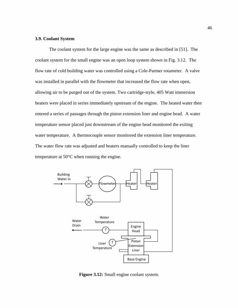
46

3.9. Coolant System

The coolant system for the large engine was the same as described in [51]. The

coolant system for the small engine was an open loop system shown in Fig. 3.12. The

flow rate of cold building water was controlled using a Cole-Parmer rotameter. A valve

was installed in parallel with the flowmeter that increased the flow rate when open,

allowing air to be purged out of the system. Two cartridge-style, 405 Watt immersion

heaters were placed in series immediately upstream of the engine. The heated water then

entered a series of passages through the piston extension liner and engine head. A water

temperature sensor placed just downstream of the engine head monitored the exiting

water temperature. A thermocouple sensor monitored the extension liner temperature.

The water flow rate was adjusted and heaters manually controlled to keep the liner

temperature at 50°C when running the engine.

Building Water In

Flowmeter Heater

Base Engine

PistonExtension

Liner

Heater

EngineHeadT

TLinerTemperature

WaterTemperatureWater

Drain

Figure 3.12: Small engine coolant system.

47

3.10. Optical System

The second harmonic (532 nm) of an Ekspla model NL303D dual Nd:YAG laser

was used to generate the laser excitation for the PIV experiments. The two beams were

made collinear and directed towards the optical engine. For the large engine, the pulse

energy of each laser beam was held at 230 mJ, and a laser sheet was generated using a 50

mm focal length cylindrical lens and a 500 mm focal length spherical lens separated by

20 mm. The laser sheet was located 4.6 mm below the cylinder head deck. For the small

engine, the pulse energy of each laser beam was held at 100 mJ, and a laser sheet was

generated using a 100 mm focal length cylindrical lens and a 500 mm focal length

spherical lens separated by 240 mm. The laser sheet was located 2.7 mm below the

cylinder head deck. The location of the laser sheet was such that at TDC the laser sheet

was nearly equidistant between the engine head surface and piston surface.

3.11. Camera System

A Princeton Instruments MicroMAX interline transfer CCD camera was used to

acquire particle images for the PIV experiments. The camera has a 1300x1030 pixel

CCD array with 6.7 m square pixels. The read-out rate of the camera was such that at

600 rpm an image pair was acquired every other engine cycle. Thus, no two image pairs

were ever acquired during the same cycle. For both engines, a low-magnification field-

of-view (FOV) was imaged using a 105 mm f/2.8 AF Micro Nikkor lens. For the large

engine, the low-magnification FOV had an image magnification of 0.15 and a FOV of

57.4 mm by 45.3 mm was achieved. For the small engine, the low-magnification FOV

had an image magnification of 0.25 and a FOV of 33.9 mm by 26.8 mm was achieved. A

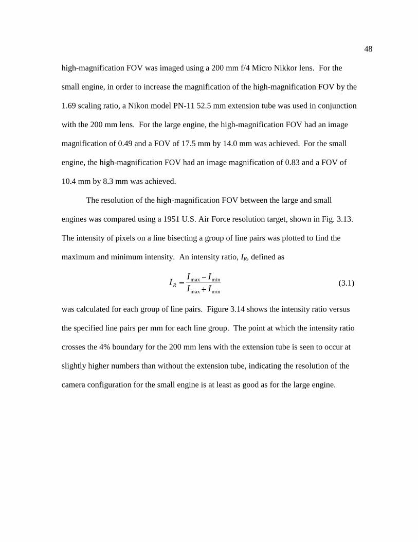
48

high-magnification FOV was imaged using a 200 mm f/4 Micro Nikkor lens. For the

small engine, in order to increase the magnification of the high-magnification FOV by the

1.69 scaling ratio, a Nikon model PN-11 52.5 mm extension tube was used in conjunction

with the 200 mm lens. For the large engine, the high-magnification FOV had an image

magnification of 0.49 and a FOV of 17.5 mm by 14.0 mm was achieved. For the small

engine, the high-magnification FOV had an image magnification of 0.83 and a FOV of

10.4 mm by 8.3 mm was achieved.

The resolution of the high-magnification FOV between the large and small

engines was compared using a 1951 U.S. Air Force resolution target, shown in Fig. 3.13.

The intensity of pixels on a line bisecting a group of line pairs was plotted to find the

maximum and minimum intensity. An intensity ratio, IR, defined as

minmax

minmax

II

IIIR (3.1)

was calculated for each group of line pairs. Figure 3.14 shows the intensity ratio versus

the specified line pairs per mm for each line group. The point at which the intensity ratio

crosses the 4% boundary for the 200 mm lens with the extension tube is seen to occur at

slightly higher numbers than without the extension tube, indicating the resolution of the

camera configuration for the small engine is at least as good as for the large engine.

49

Figure 3.13: Resolution image of high-magnification FOV using 200 mm lens for large

engine.

1.0

0.8

0.6

0.4

0.2

0.0

(Im

ax-I

min)/

(Im

ax+

I min)

6050403020100

Line Pairs Per mm

Large Engine Small Engine 4% Boundary

Figure 3.14: Intensity ratio versus line pairs per mm of resolution target for high-

magnification FOVs of large and small engines.

50

3.12. Particle Image Velocimetry (PIV) System

For the PIV experiments, a TSI model 9306A six jet atomizer was used to seed

the intake flow with olive oil droplets estimated to have a mean diameter of 0.5 to 2 μm.

According to [52], oil droplets at this diameter have been shown to faithfully follow the

turbulent flow fields at frequencies between 1 and 10 kHz. The particles were introduced

just upstream of the intake surge tanks to ensure sufficient mixing, see Fig. 3.10. The

seeding density was adjusted to allow at least ten particle pairs for the smallest PIV

interrogation window [53] of 32x32 pixels. The temporal separation of laser pulses

ranged from 10 to 160 μs for the large engine and from 7 to 80 μs for the small engine

and was set such that the maximum in-plane particle displacement would not exceed a

quarter of the interrogation window [53]. The first laser pulse of each pulse pair occurred

at the crank angle of interest. Since the rules of [53] were followed in order to ensure

accurate data, the second laser pulse of each pulse pair did not always occur at the same

crank angle for all conditions investigated.

The PIV images were analyzed using the TSI Insight3G software. The software

calculated velocity vectors by utilizing a multiple-pass algorithm with 50% overlap and

an FFT correlation engine. Velocity vectors were validated by comparing the ratio of the

two highest correlation peaks to a set threshold value. Vectors passing the test are termed

first-choice vectors, while vectors failing the test were replaced by a median vector of its

nearest neighbors. The initial interrogation grid was 64 64 pixels and the final

interrogation grid was 32 32 pixels, which resulted in velocity vectors spaced on a 16

pixel grid. For the large engine, velocity vectors were thus spaced 708 μm for the low-

magnification FOV and 217 μm for the high-magnification FOV, corresponding to

51

interrogation zones 1.42 and 0.43 mm, respectively. For the small engine, velocity

vectors were thus spaced 419 μm for the low-magnification FOV and 128 μm for the

high-magnification FOV, corresponding to interrogation zones 0.84 and 0.25 mm,

respectively.

52

CHAPTER 4

STEADY FLOW CHARACTERIZATION OF INTAKE PORTS

This chapter describes the steady flow testing conducted on the engine heads.

4.1. Experimental Equipment

The steady flow testing of the intake ports was conducted on a SuperFlow 600

flow bench. The flow bench pulls air into the machine with an associated pressure drop

across an attached test section ranging from 0.25 to 11.96 kPa. The volumetric flow rate

was found from the pressure drop across a calibrated orifice inside the flow bench using

an inclined manometer. The density of the air was calculated from temperature and

humidity data acquired using a Mannix model J411-TH Digital Hygro Thermometer, and

the barometric pressure was measured using a Heise model CM dial pressure gauge. The

engine heads were tested at the industry-standard pressure drop of 6.97 kPa.

The steady flow and swirl testing were performed using a different swirl adapter

fixture for each size engine head, and tumble testing was performed using a different

tumble adapter fixture for each size engine head. For swirl and tumble coefficient

testing, the swirl and tumble adapter fixtures were bolted to the flow bench with the swirl

meter beneath the fixtures, see Figs. 4.1-4.3. The valve lift was adjusted and measured

using a modified micrometer that mounted to the engine head. Intake horns were

connected to the entrance of the intake ports. The intake horns have radii of curvature

large enough to minimize the pressure drop at the inlet to the intake ports. The

dimensions of the swirl adapter fixtures for both large and small engine heads are shown

in Table 4.1. The bore dimension of the fixtures were the same as the engine cylinder

53

bore, and the height of the fixtures was 1.5 times the bore. The dimensions of the tumble

adapter fixtures are shown in Table 4.2. For all testing, data were collected and averaged

over a 40 second period.

(a) (b)

(c)

Figure 4.1: (a) Flow test setup of small head, (b) swirl test setup of large head, and (c)

tumble test setup of small head on the flow bench next to large tumble adapter.

54

B

H

DP

HP

L

Intake Port

Intake Horn

Swirl Adapter

Fixture

Paddle Wheel

Honeycomb

D

ω

(a)

B

H

DI

HI

L

Intake Port

Intake Horn

Swirl Adapter

Fixture

Impulse Torque

Meter

Honeycomb

D

T

(b)

Figure 4.2: (a) Vane-type swirl meter test setup, (b) Impulse-type torque meter test setup.

55

Swirl Meter Swirl Meter

Engine Head

Cylinder Axis

d1

d3

d2

d3

Figure 4.3: Front and side views of tumble testing arrangement.

(Dimensions in mm) Large Fixture Small Fixture

B 82.0 48.6

H 123.0 72.8

Table 4.1: Dimensions of swirl adapter fixtures.

(Dimensions in mm) Large Fixture Small Fixture

d1 261.0 154.5

d2 139.8 83.6

d3 87.0 50.8

Table 4.2: Dimensions of tumble adapter fixtures.

Swirl testing was conducted using two different types of swirl meters (to be

explained below). The vane-type swirl meter used for this study was an Audie

Technology paddle-style swirl meter. The meter featured a honeycomb paddle wheel

132.1 mm in diameter and made of polycarbonate plastic with tubular cells. The outer

diameter of the paddle featured a smooth, thin polycarbonate sheet wrapped around the

56

honeycomb to form a continuous cylinder-like shape. The swirl meter provided an

electronic output of two pulses per revolution, which are also used to determine both the

direction of rotation and the rotation rate with the addition of an HP model 5315A

Universal Counter.

An impulse-type swirl meter (see Fig. 4.2(b)) was designed for this study. In this

meter, a Transducer Techniques RTS-5 torque sensor was secured at the bottom and a

shaft was attached at one end to the sensor and on the other end to a honeycomb flow

straightener. This torque sensor was chosen for its rated torque measurement range of up

to 0.035 N-m. The honeycomb was made of the same material and tubular structure as

used in the vane-type meter. The design of the impulse-type meter allowed different

honeycomb flow straighteners to be easily tested. Dimensions of the honeycomb flow

straightener will be discussed in a later section. A Daytronic model 3270 strain gage

conditioner/indicator provided the excitation voltage for the torque sensor and a

LabVIEW data acquisition system recorded the instantaneous voltage at a rate of 10Hz.

The impulse-type meter was calibrated by applying a set of known torques to the

center of the honeycomb flow straightener. For each applied torque, a corresponding

voltage was recorded. Before and after each applied torque, the zero-torque voltage was

recorded and averaged. The average zero-torque voltage was subtracted from the

applied-torque voltage to obtain the voltage difference. The voltage difference was

plotted against the applied torques to determine a linear calibration curve. Calibration

data were collected for counterclockwise torques applied to the honeycomb flow

straightener.

57

4.2. Flow Coefficient

Flow coefficients were calculated for both small and large heads to examine and

compare the steady flow through the intake ports. Flow coefficients are a comparison of

the actual to a theoretical mass flow into the engine. Data were collected over the full

range of valve lift, L. The flow coefficient, Cf, is defined as:

vB

fAV

mC

(4.1)

where m is the measured mass flow rate, is the density, VB is the Bernoulli velocity

defined as:

PVB

2 (4.2)

where P is the pressure drop across the test section, and Av is the valve inner seat area

defined as:

4

2DAv (4.3)

where D is the valve inner seat diameter. Appendix C contains graphs of flow coefficient

data plotted versus crank angle degrees for both 0- and 90-degree port orientations and

shrouded and non-shrouded valves. A mass-weighted average flow coefficient, Cf,avg, as

defined in Eqn. (2.6), was calculated for all the data so that a comparison could be made

between the small and large heads using a single metric. This number is included in the

graphs and in Table 4.3. For the 0- and 90-degree port orientations with the non-

shrouded valves, Cf,avg of the small head compared to the large head differs by 4.3% and -

3.6% for the performance ports and by 3.6% and 0.9% for the utility ports, respectively.

58

For the ports with the shrouded valves, Cf,avg differs by -4.1% and -1.3% for the utility

port and performance port, respectively. As discussed in Appendix C, an uncertainty

analysis of the flow coefficients was conducted at several non-dimensional valve lifts. In

an attempt to calculate a single uncertainty for Cf,avg, the uncertainty propagation method

from [54] was used to calculate uCf,avg, also detailed in Appendix C; the results are

presented in Table 4.3. As is inherent with the propagation method, the uncertainties

become smaller. The engine head exhaust flow was tested on the flowbench by blowing

air past the valves and out the ports. Using the same calculations as for the intake ports

to determine the flow coefficients, a graph of the flow coefficients for the exhaust ports is

included in Appendix C and mass-weighted average flow coefficients are included in

Table 4.4. For the exhaust ports, the average flow coefficient of the small head compared

to the large head differs by 6.0%. The difference in flow coefficients for the intake and

exhaust between the large and small heads appears small enough that the heads can be

considered similar.

Large Head Small Head

Valve Port Orientation Cf,avg uCf,avg Cf,avg uCf,avg

Shrouded Utility 0-degree 0.293 0.001 0.281 0.001

Performance 0-degree 0.303 0.001 0.299 0.001

Non-shrouded Utility 0-degree 0.446 0.001 0.462 0.001

90-degree 0.430 0.001 0.434 0.001

Performance 0-degree 0.481 0.003 0.502 0.001

90-degree 0.499 0.003 0.481 0.001

Table 4.3: Intake port mass-weighted average flow coefficients and uncertainties of the

small and large heads in the 0- and 90-degree port orientations.

59

Exhaust Ports, Cf,avg

Small Head 0.461

Large Head 0.435

Table 4.4: Exhaust port mass-weighted average flow coefficients.

4.3. Swirl Coefficient and Swirl Ratio Definitions

Swirl coefficients were calculated for both the small and large heads. As with the

flow coefficients, the swirl coefficients should be similar among geometrically similar

engines. The swirl coefficient, Cs, is a characteristic non-dimensional rotation rate and is

calculated for vane-type meters as

B

sV

BC (4.4)

where ω is the vane or paddle wheel angular velocity and B is the cylinder bore. For

impulse-type swirl meters, the swirl coefficient is calculated as

BVm

TC

B

s

8 (4.5)

where T is the torque measured by the meter. The swirl ratio, Rs, is a convenient single

metric that takes into account the flow and swirl coefficients over the entire lift profile of

the engine. The swirl ratio is the ratio of the angular velocity of the flow to the

crankshaft angular rotation rate. The swirl ratio is calculated as

2

2)(

4 IVC

IVO

IVC

IVO

dCA

dCCABS

R

fV

sfV

vs (4.6)

60

where ηV is the volumetric efficiency, assumed equal to 1 for all calculations, S is the

engine stroke, and θIVO and θIVC are the crank angle, in radians, at intake valve open and

intake valve close, respectively.

4.4. Impulse-Type Meter Initial Testing

Swirl and tumble data were originally to be taken using an impulse-type swirl

meter used in a previous investigation [44]. The heads were tested with the non-shrouded

valves using the performance ports in the 0-degree orientation as this configuration of

port and orientation was thought to produce the most air swirl and, thus, the largest

voltage signal as measured by the torque sensor. At each valve lift, approximately 400

voltage samples from the torque sensor were acquired over a time period of 40 seconds.

A signal-to-noise ratio was defined as:

VuVNS // (4.7)

where V is the torque sensor mean voltage change and uV is the 95% uncertainty of the

mean voltage change defined as:

N

Su V

V 96.1 (4.8)

where SV is the voltage change sample standard deviation and N is the number of voltage

samples. Equation (4.8) is based on a t-probability distribution where the t-statistic is

based on an infinite number of samples. Figure 4.4 shows the signal-to-noise ratio of the

large and small heads. As can be seen, the signal-to-noise ratio of both heads quickly

tends towards zero as the lift is decreased from the maximum lift. It is not surprising that

the small head S/N falls off quicker than the large head because geometrically similar

61

engines with the same pressure drop produce an angular momentum flux proportional to

the engine bore cubed [55]. Thus, the small engine head will produce approximately

21% of the torque compared to the large head.

120

100

80

60

40

20

0

S/N

0.250.200.150.100.050.00

L/D

Performance Port, 0-degree Orientation, Non-shrouded Valves

Small Head

Large Head

Figure 4.4: Signal-to-noise ratio of large and small heads using impulse swirl meter

from [44].

After this test, it was decided to fabricate shrouded valves in order to also study

conditions with higher levels of swirl. Based on the 1.69 scale ratio, and assuming for a

given head we want to increase the swirl coefficient by a factor of ten using the shrouded

valves, then for a given non-dimensional valve lift the ratio of torque is approximately

48:1 between the large and small heads. Thus, a measurement device with a very high

dynamic range is required to cover the entire test range of interest. These results

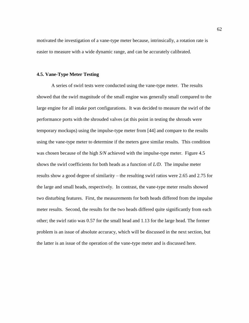
62

motivated the investigation of a vane-type meter because, intrinsically, a rotation rate is

easier to measure with a wide dynamic range, and can be accurately calibrated.

4.5. Vane-Type Meter Testing

A series of swirl tests were conducted using the vane-type meter. The results

showed that the swirl magnitude of the small engine was generally small compared to the

large engine for all intake port configurations. It was decided to measure the swirl of the

performance ports with the shrouded valves (at this point in testing the shrouds were

temporary mockups) using the impulse-type meter from [44] and compare to the results

using the vane-type meter to determine if the meters gave similar results. This condition

was chosen because of the high S/N achieved with the impulse-type meter. Figure 4.5

shows the swirl coefficients for both heads as a function of L/D. The impulse meter

results show a good degree of similarity – the resulting swirl ratios were 2.65 and 2.75 for

the large and small heads, respectively. In contrast, the vane-type meter results showed

two disturbing features. First, the measurements for both heads differed from the impulse

meter results. Second, the results for the two heads differed quite significantly from each

other; the swirl ratio was 0.57 for the small head and 1.13 for the large head. The former

problem is an issue of absolute accuracy, which will be discussed in the next section, but

the latter is an issue of the operation of the vane-type meter and is discussed here.

63

-0.8

-0.6

-0.4

-0.2

0.0

Cs

0.250.200.150.100.050.00

L/D

Impulse Meter

Vane Meter

Open Symbol: Small HeadFilled Symbol: Large Head


with standard 5.2 inch diameter paddle. + CW Swirl, - CCW Swirl.

Due to the difference in the diameters of the two swirl adapter fixtures, it was

thought that there might be a difference in air frictional losses from the paddle outside of

the cylinder bore (the same size paddle was used for both heads). The portion of the

paddle outside of the cylinder would experience air friction tending to retard the motion

of the paddle, which is consistent with the lower Cs measured for the small head. In order

to test the effect of air frictional losses on the rotational speed of the paddle, custom

paddles were fabricated of the same honeycomb material and geometry as the original

paddle wheel but with a smaller paddle diameter, DP. For both the small and large heads,

the ratio of the paddle diameter to the swirl adapter fixture, DP/B, was set to 1.2. Figure

4.6 shows the results of the constant DP/B tests for the same conditions as Fig. 4.5. It can

be seen that by controlling DP/B the differences between the two vane-type meter

64

measurements has been eliminated, and one could conclude that self similarity has been

achieved. There are, however, still differences in the absolute value of swirl coefficient

between the impulse- and vane-type meter measurements.

-0.8

-0.6

-0.4

-0.2

0.0

Cs

0.250.200.150.100.050.00

L/D

Impulse Meter

Vane Meter



with Dp/B=1.2 custom paddles. + CW Swirl, - CCW Swirl. The impulse-type meter

measurements are the same as Fig. 4.5.

4.6. Swirl References

Seeing the differences in the absolute value of swirl coefficients between the

impulse- and vane-type meter measurements, it was desired to verify the accuracy of the

meters to gain confidence in the swirl measurements. This was accomplished by

developing two reference fixtures, a zero-swirl reference shown in Figs. 4.7(a-b) and a

65

known-swirl reference shown in Figs. 4.7(c-d), with the relevant dimensions given in

Table 4.5.

LR DR

SR

Flow Straightener

B

θR

Swirl Adapter

Fixture

(a) (b)

LR

DR

SR

Flow Straightener

B

AA

Section A-A (Enlarged)

R1

R2

Swirl Adapter

Fixture

θR

(c) (d)

Figure 4.7: (a-b) Zero-swirl and (c-d) known-swirl reference fixtures.

(Dimensions in mm) Vertical Reference Angled Reference

θR 90° 45°

SR 127.0

DR 19.1

LR 444.5

R2, Small Swirl Adapter

Fixture 13.2

R2, Large Swirl Adapter

Fixture 19.1

Table 4.5: Dimensions of the zero- and known-swirl references.

66

4.6.1. Zero-Swirl Reference

The purpose of the zero-swirl reference is to check for a zero swirl offset. The

zero-swirl reference features a tube that is coaxial with the swirl adapter fixture and a flat

plate that secures to the top of the swirl adapter fixture. A flow straightener was installed

at the inlet of the tube in order to ensure a uniform incoming flow. Tests were performed

at flow rates corresponding to a pressure drop of 6.97 kPa across the test section. The

flow entering the swirl adaptor fixture has a dominant axial velocity profile due to the

geometry of the tube. Since the incoming generated flow has zero swirl, the vane-type

meter should not rotate to a significant degree in either direction and the impulse-type

meter should not indicate any significant torque. Any measurement showing significant

levels of swirl would be an indication that the testing setup is flawed and needs to be

corrected.

4.6.2. Known-Swirl Reference

The purpose of the known-swirl reference is to produce a known amount of swirl

for a given pressure drop. This fixture features a tube with its axis offset from the swirl

adapter fixture axis and a flat plate that secures to the top of the swirl adapter fixture.

The tube is installed in the flat plate at an angle R relative to the horizontal. Again, a

flow straightener was installed at the inlet of the tube. Tests were performed at flow rates

corresponding to a pressure drops ranging from 0.25 to 11.21 kPa across the test section.

For a given geometry (R2 and R), it can be shown [56] that the angled-tube

geometry provides a constant value of Cs. Thus, using Eq. (4.5) one can find the angular

momentum flux (T) entering the swirl adapter fixture. This can be compared to the

67

measured torque, T, from the impulse-type swirl meter or to an equivalent torque, Teq,

from the vane-type swirl meter. Teq is found by equating Eqs. (4.4) and (4.5) and finding

the torque as a function of the measured , and is defined as

8

2BmTeq

(4.9)

For these calculations, the measured velocity, V, which is determined from the volume

flow rate and pipe area, is used in place of the Bernoulli velocity. By making these

comparisons, one can get a quantitative measure of the accuracy of the swirl meters.

4.6.3. Honeycomb Geometry and Swirl Reference Results

It was desired to evaluate the effect of honeycomb cell size diameter (dP, dI) and

height (HP, HI) on measurement accuracy in both impulse- and vane-type swirl meters,

the subscripts P and I refer to the paddle and impulse meters, respectively. Again, the

aim was to gain confidence in the accuracy of the measurements. The impulse-type

meter described in §4.1 was used for the remainder of this study due to its higher

accuracy at small torques.

Both vane- and impulse-type swirl meters were first checked with the zero-swirl

reference. In general, the paddle in the vane-type meter tended to oscillate slightly from

side to side, but no significant rotation was observed. The impulse-type meter torque

sensor voltage oscillated about the zero-flow voltage and indicated a torque offset of

about 1% of the maximum torque produced using the known-swirl reference.

Figure 4.8 shows the results of the known-swirl reference of the vane- and

impulse-type swirl meters for both the large and small fixtures with a honeycomb cell

68

aspect ratio (HI /dI or HP /dP) of 1.4. For the vane meter measurements DP/B =1.2 was

used. Both measurement techniques show excellent linearity with respect to the angular

momentum flux, but there is not a direct 1:1 correspondence between the measured (or

derived in the case of the vane meter) torque and the expected value, i.e. the inlet angular

momentum flux. The high degree of linearity indicates that a single conversion

efficiency can be used to describe the performance of the swirl meters with the known-

swirl reference, and this efficiency is the slope of the lines in Fig. 4.8. For the data in

Fig. 4.8, the efficiency ranges from 0.93 for the small fixture using the impulse-type

meter, to 0.31 for the large fixture using the vane-type meter. From Fig. 4.8 it is clear

that the conversion efficiency is a function of both the meter type and the fixture size.

The impulse-type meter gives results that are larger in magnitude than the vane-type

meters by nearly a factor of two, and the impulse-meter results are closer to but still less

than the correct value.

69

35x10-3

30

25

20

15

10

5

0

T o

r T

eq [

N-m

]

35x10-3

302520151050

Angular Momentum Flux [N-m]

Impulse Meter

Vane Meter


Figure 4.8: Impulse- and vane-type meter response to a known angular momentum flux

produced from the known-swirl reference tube for the small and large fixtures. For all

cases a cell height-to-diameter ratio of 1.4 was used.

Figure 4.9 shows the effect of the honeycomb flow straightener or vane cell size

and height, using polycarbonate honeycombs having a tubular geometry, on the

conversion efficiency. The honeycomb cell diameters tested were 6.4 and 3.8 mm. For

the vane-type meter DP/B was again set to 1.2 to minimize the frictional losses, and the

honeycomb height was limited to 16.0 mm (HI/dI = 4.3) by the meter design. For the

impulse-type meter longer honeycombs were tested, up to HI /dI =17, and a fixed

straightener diameter of DI =104.1 mm was used. The vane-type meter, Fig. 4.9(a),

showed a weak sensitivity to the cell geometry, but as was seen in Fig. 4.8 the conversion

efficiency is poor. For the large fixture, the conversion efficiency was ~0.32 and for the

small fixture it was near 0.44. The low conversion efficiency for the large fixture could

70

be due to friction at the hub, which would be greater for the larger vane size, or from slip

between the air and the paddle. If air slip was causing the low conversion efficiency, one

might expect that the higher HP /dP cases would perform better, which was not the case.

The impulse-type meter showed a stronger sensitivity to the flow straightener geometry,

with the conversion efficiency decreasing with increasing aspect ratio of the honeycomb.

This result agrees with the findings of Tanabe et al. [57], who found that honeycomb

geometries with smaller drag coefficients in uniform flow (i.e. larger cell size and smaller

honeycomb height) gave higher swirl coefficients. In comparison to the vane-type meter,

the conversion efficiency of the impulse-type meter is significantly larger. Differences

do exist between the two fixture sizes and the magnitude of the conversion efficiency can

be as low as 0.7. Thus, the results from an impulse-style meter will under-predict the true

level of swirl. It is possible that the losses in the bore extension (H/B=1.5) tube could

account for some of the under-prediction seen with the impulse-type meter.

71

0.5

0.4

0.3

0.2

Co

nve

rsio

n E

ffic

iency

543210

HP / dP

Large Fixture

Small Fixture

1.0

0.9

0.8

0.7

0.6

Co

nve

rsio

n E

ffic

iency

151050

HI / dI

Large Fixture

Small Fixture

(a) (b)

Figure 4.9: Swirl conversion efficiency as a function of the cell aspect ratio for (a) the

vane-type meter, and (b) the impulse-type meter.

The reason for conducting these tests was to gain confidence in the accuracy of

the swirl measurements. From these data it is clear that the impulse-type swirl meter

should be used to make the measurements. Examining Fig. 4.9(b) it is also evident that

the honeycomb cell aspect ratio of HI /dI =1.4 will give the most accurate torque

measurements of the angular momentum flux entering the swirl adapter fixture, which is

confirmed by the findings of [57]. Thus, this honeycomb geometry was used for the

remainder of the study. One might look at the difference in the conversion efficiency of

the HI /dI =1.4 honeycomb for the large and small fixtures and conclude that swirl

measurements of the small and large engine heads will be inherently biased. This is not

the case. First, the known-swirl reference tube is a highly idealized flow which is not

necessarily produced by the engine heads. It has been shown [58, 59] that swirl

72

measurement accuracy is also dependent on the flow field produced by the engine head

and varies over the range of valve lift. Second, it was found that the small head with the

shrouded valve produces a maximum angular momentum flux of about 0.007 N-m (for

comparison, the large head with the shrouded valve produces 0.034 N-m). Examining

Fig. 4.8, in this lower range the conversion efficiency of the small fixture is very similar

to that of the large fixture over its entire range. Third, a repeatability study would need to

be performed to get a better measure of the average conversion efficiency. However, this

is not necessary. The data clearly give us confidence that the impulse-type swirl meter

with the HI /dI =1.4 honeycomb give the most accurate measurements that are similar

between the small and large swirl adapter fixtures.

4.7. Swirl Coefficient Testing

Swirl coefficient engine head data were taken with the impulse-type swirl meter

with the HI /dI =1.4 honeycomb geometry. Data were collected over the full range of

valve lift, L. The results are shown in Figs. 4.10(a-c) with the swirl coefficients plotted

versus non-dimensional valve lift for both 0- and 90-degree port orientations and

shrouded and non-shrouded valves. Figures 4.10(a-b) indicate that the ports with the

non-shrouded valves produce low levels of swirl. As expected, the ports in the 0-degree

orientation produce more swirl in the counter-clockwise (CCW) direction compared to

the ports in the 90-degree orientation. Inspecting Fig. 4.10(c), the ports with the

shrouded valves produce significantly more swirl compared to the non-shrouded valves

as evidenced by the greater magnitude swirl coefficients.

73

The swirl ratio, Rs, as defined in Eqn. (4.6), was calculated for all data so that a

comparison could be made between the small and large heads using a single metric. This

number is included in Table 4.6. An uncertainty analysis was performed on the swirl

coefficients at five different valve lifts, and the uncertainty propagation method from [54]

was again used to calculate the swirl ratio uncertainty, uRs, also included in Table 4.6.

The uncertainty results and analysis can be found in Appendix D. For the 0- and 90-

degree port orientations with the non-shrouded valves, Rs of the small head compared to

the large head differs by 77% and -63% for the performance ports and by -5.6% and

151% for the utility ports, respectively. For the ports with the shrouded valves, Rs differs

by 7.7% and 10.8% for the utility port and performance port, respectively.

Comparing the swirl coefficients and swirl ratios of the small and large heads

with the non-shrouded valves, there appears to be good trend-wise agreement in the data

over the valve lift. The magnitudes of the swirl coefficients are also similar. The swirl

ratios are small in magnitude and tend to be influenced more by the swirl coefficients at

the higher valve lifts. Comparing the small and large heads with the shrouded valves,

there is again good trend-wise agreement in the data. The swirl ratios are about 13 times

greater than the ports in the same orientation with the non-shrouded valves. Inspection of

the uncertainty of the swirl coefficients in Appendix D would suggest that there is close

similarity in the swirl produced by the shrouded valves.

74

-0.2

-0.1

0.0

0.1

0.2

Cs

0.250.200.150.100.050.00

L/D

0-degree Orientation



Performance Port, NV

-0.2

-0.1

0.0

0.1

0.2

Cs

0.250.200.150.100.050.00

L/D




Utility Port, NV

(a) (b)

-0.8

-0.6

-0.4

-0.2

0.0

0.2

0.4

Cs

0.250.200.150.100.050.00

L/D

Performance Port

Utility Port


0-degree Orientation, SV

(c)

Figure 4.10: Swirl coefficients versus non-dimensional valve lift of the (a) performance

ports, non-shrouded valves, (b) utility ports, non-shrouded valves, and (c) both ports,

shrouded valves. + CW Swirl, - CCW Swirl.

75


Valve Port Orientation Rs uRs Rs uRs

Shrouded Utility 0-degree -3.214 0.032 -2.967 0.065

Performance 0-degree -3.058 0.030 -2.728 0.058

Non-shrouded Utility 0-degree -0.251 0.008 -0.265 0.008

90-degree 0.128 0.009 -0.065 0.008

Performance 0-degree -0.234 0.008 -0.054 0.007

90-degree 0.121 0.008 0.045 0.007

Table 4.6: Intake port swirl ratios and uncertainties of the small and large heads in the 0-

and 90-degree port orientations.

Figure 4.11 gives the S/N ratio from the swirl coefficient tests calculated in the

same manner as set forth in §4.4. Between the large and small engine heads, the S/N

ratio is quite similar.

140

120

100

80

60

40

20

0

S/N

0.250.200.150.100.050.00

L/D


PP, SV

UP SV

PP, NV

UP, NV


Figure 4.11: S/N ratio from swirl coefficient tests of ports in 0-degree orientation.

76

4.8. Tumble Coefficients and Testing

Tumble coefficients were measured for both the small and large heads with the

utility port in the 90-degree orientation. Tumble, sometimes referred to as barrel swirl, is

analogous to regular swirl, but with its axis perpendicular to the engine cylinder axis.

The tumble adapter converts the tumbling flow into a swirling flow to be measured by the

swirl meter. As it is not known on which plane intersecting the cylinder axis the tumble

is maximum, tests were performed by rotating the engine head about the cylinder axis.

The same impulse-type swirl meter and honeycomb geometry used for the swirl testing

was used for the tumble tests. Data were taken at four valve lifts corresponding to 100,

75, 50, and 25% of maximum lift and the head was rotated in 30 degree increments. As

the optical engines were not designed to take PIV data in the tumble plane for

comparison to steady flow data, it was decided not to take a more encompassing data set.

Figure 4.12 shows a top-down view of the engine head on the tumble adapter defining the

engine head angles, with the bold arrow affixed to the engine head and indicating the

head direction. Also, the geometry of the small engine head only allowed data to be

collected between 0 and 180 degrees.

77

Intake ValveExhaust Valve

Engine Head

Swirl Meter

90°

180° 0°

(a) (b)

Figure 4.12: (a) Top-down view of engine head indicating head angle direction on

tumble adapter. Bold arrow is affixed to engine head. (b) Small head at 90° head angle.

The tumble coefficient, Ct, is defined in the same manner as the swirl coefficient:

BVm

TC

B

t

8 (4.10)

A tumble ratio, Rt, defined in Eqn. (4.11), was calculated in the same manner as the swirl

ratio to provide a single metric for comparison between the large and small heads,

however it should be noted that it is less accurate than the swirl ratio since it was

approximated using data at only four valve lifts.

2

2)(

4 IVC

IVO

IVC

IVO

dCA

dCCABS

R

fV

tfV

vt (4.11)

Figure 4.13 shows the tumble coefficients versus the engine head angle for the

four values of non-dimensional valve lift tested. At all but the second lowest valve lift,

78

the trends and magnitudes of the tumble coefficients are similar. At the highest valve lift

between 0 and 180 head angle degrees, the maximum tumble coefficients are within 0.1%

between the small and large heads. The maximum tumble ratios, Rt, for the large and

small heads are 0.54 and 0.48, respectively. Again, the data show very close similarity

between the two engine heads.

-0.25

-0.20

-0.15

-0.10

-0.05

0.00

0.05

0.10

0.15

0.20

0.25

C

t

3303002702402101801501209060300

Engine Head Angle

L/D = 0.05

L/D = 0.12

L/D = 0.20

L/D = 0.25


Figure 4.13: (a) Tumble coefficients versus engine head angle for the utility ports in the

90-degree orientation with the non-shrouded valves.

79

CHAPTER 5

OPTICAL ENGINE MEASUREMENTS AND ANALYSIS

This chapter describes the measurements acquired in the optical engines,

including the flow rate, pressure traces, and PIV data and analysis. All MATLAB code

related to the PIV analysis can be found in Appendix E.

5.1. Engine Conditions

The engines were run over a range of speeds and data were collected over a range

of crank angles. The large engine was run at speeds of 300, 600, 900, and 1200 rpm.

The small engine was run at speeds of 600, 1200, and 1800 rpm. These speeds were

chosen to give roughly the same range of mean piston speed. The engine speeds were in

multiples of 300 rpm so that the PIV data could be easily acquired with the available

laser, which fired at a constant frequency of 10 Hz.

5.2. Engine Flow Rate

The mass flow rate into each engine was measured as described in §3.6. The

volumetric efficiency, ηV, at each engine conditions was calculated as

th

measv

m

m

(5.1)

where m easm is the measured mass flow rate and thm is the theoretical mass flow rate

defined as

120

RPMVm

disp

th (5.2)

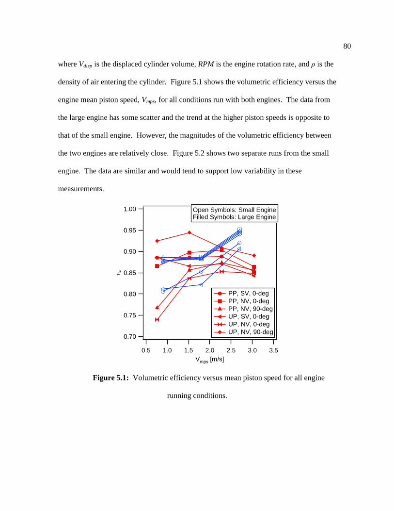
80

where Vdisp is the displaced cylinder volume, RPM is the engine rotation rate, and ρ is the

density of air entering the cylinder. Figure 5.1 shows the volumetric efficiency versus the

engine mean piston speed, Vmps, for all conditions run with both engines. The data from

the large engine has some scatter and the trend at the higher piston speeds is opposite to

that of the small engine. However, the magnitudes of the volumetric efficiency between

the two engines are relatively close. Figure 5.2 shows two separate runs from the small

engine. The data are similar and would tend to support low variability in these

measurements.

1.00

0.95

0.90

0.85

0.80

0.75

0.70

ηv

3.53.02.52.01.51.00.5

Vmps [m/s]

PP, SV, 0-deg

PP, NV, 0-deg

PP, NV, 90-deg

UP, SV, 0-deg

UP, NV, 0-deg

UP, NV, 90-deg

Open Symbols: Small EngineFilled Symbols: Large Engine

Figure 5.1: Volumetric efficiency versus mean piston speed for all engine

running conditions.

81

1.00

0.95

0.90

0.85

0.80

0.75

0.70

ηv

3.53.02.52.01.51.00.5

Vmps [m/s]

Small EnginePP, SV, 0-deg

Run 1

Run 2

Figure 5.2: Volumetric efficiency versus mean piston speed for two separate runs in the

small engine.

5.3. Engine Peak Pressure

Pressure traces for all running conditions were acquired for both engines. The

peak pressures of the engines are shown in Fig. 5.3 versus the mean piston speed. Similar

to the trend of pressure traces matching in geometrically similar engines at the same

piston speed that Taylor [11] observed, Fig. 5.3 shows a similar trend in the peak pressure

with mean piston speed. If the large engine peak pressures are linearly interpolated to the

same mean piston speed as the small engine, the small engine peak pressures are lower by

-1 to -9%.

The crank angles at which the peak pressures occurred for both engines are in

Table 5.1. The peak pressure occurred at crank angles before TDC for all conditions and

82

tended to approach TDC at higher engine speeds. Normally, the peak pressure in non-

optical engines is within one degree of TDC, whereas the peak pressure for these engines

ranged from -5 to -1 bTDC. It is possible that there was blow-by past the teflon piston

rings causing the crank angle at which the peak pressure occurred to retard, as there was

an audible whooshing noise apparent at low engine speeds during compression. The

crank position sensor used with the pressure acquisition system had one degree of

resolution which also limits the precision of the measurement. Examining Table 5.1, the

data show that the small engine peak pressures occur at crank angles roughly 1-2 degrees

before that of the large engine. The TDC position of the piston was determined for both

engines using an MHC Industrial Supply dial indicator with 0.025 mm resolution. After

the data collection was complete, the TDC position of the small engine was measured by

another student using a Philtec D170 fiber optic displacement sensor while the engine

was motoring. This sensor indicated the previous TDC position of the small engine was

roughly 1.5 degrees aTDC. If this is indeed the case, and if the large engine TDC

position was nearly correct, this would mean the crank angles at which the peak pressures

occur were nearly the same between the two engines at the same mean piston speed.

83

1800

1600

1400

1200

1000

Cylin

de

r P

ea

k P

ressu

re [

kP

a]

3.53.02.52.01.51.00.5

Vmps [m/s]


PP, SV, 0-deg

PP, NV, 0-deg

PP, NV, 90-deg

UP, SV, 0-deg

UP, NV, 0-deg

UP, NV, 90-deg

Figure 5.3: Cylinder peak pressure versus mean piston speed.

Large

Engine

UP,

SV,

0-deg

UP,

NV,

0-deg

UP,

NV,

90-deg

PP,

SV,

0-deg

PP,

NV,

0-deg

PP,

NV,

90-deg

0.76 m/s -3 -3 -2 -3 -3 -3

1.52 m/s -2 -3 -2 -2 -3 -3

2.28 m/s -2 -3 -2 -2 -3 -3

3.04 m/s -2 -3 -1 -2 -2 -2

Small

Engine

UP,

SV,

0-deg

UP,

NV,

0-deg

UP,

NV,

90-deg

PP,

SV,

0-deg

PP,

NV,

0-deg

PP,

NV,

90-deg

0.90 m/s -5 -4 -4 -5 -5 -4

1.80 m/s -4 -3 -3 -4 -4 -3

2.70 m/s -3 -3 -3 -3 -3 -3

Table 5.1: Crank angle degree of peak pressure relative to TDC of compression stroke

listed at the engine mean piston speed.

84

5.4. Methods of Determining Mean and Fluctuating Velocity Fields

In analyzing the PIV data, two methods were used to determine the mean velocity

fields. The data acquisition system available for this study was only fast enough to take a

single set of PIV images per engine cycle. Therefore, it was sought to perform the

analysis using the methods appropriate for the spatially resolved, multiple-realization

data available. The analyses can then be compared to investigate the relative agreement

of each method. In the first method, an ensemble-average velocity field was calculated

by averaging the velocity vectors at each location (x,y) as

cN

i

c

iEA iyxUN

yxU1

, 2,1),,(1

),( (5.3)

where Ui is the instantaneous velocity, Nc is the number of cycles, and i=1,2 refers to the

components of the velocity in the x- and y-directions, respectively. In the second method,

a spatial-average velocity field was calculated based on a cutoff lengthscale for each

individual cycle. The analysis computes the average velocity in the x- and y-directions

separately. A two-dimensional fast-Fourier transform (FFT) was performed on the

velocity field. The two-dimensional spectrum was multiplied by a Fermi-Dirac soft

cutoff filter [33], which was calculated as

))1.0/()exp((1

1

ccxy

(5.4)

where κxy is the two-dimensional wavenumber defined as

22

yxxy (5.5)

and κc is the cutoff wavenumber defined as

85

c

cL

2 (5.6)

where Lc is the cutoff lengthscale. The filter gradually sets the Fourier coefficients above

κc to zero. To avoid confusion and make understanding of the data easier, all subsequent

analysis is plotted versus a cutoff frequency, fc, defined as

c

cL

f1

(5.7)

Finally, the two-dimensional inverse fast-Fourier transform (IFFT) is performed on the

Fourier coefficients. The result is a low-pass or spatially averaged velocity field.

A Reynolds decomposition of the velocity fields was performed using both the

ensemble- and spatial-average methods to decompose the velocity field into average, Ū,

and fluctuating, u, components. The fluctuating velocity is defined as

.2,1),(),(),( iyxUyxUyxu iii (5.8)

5.5. PIV FOV Locations and First-Choice Vector Statistics

The locations relative to the cylinder, where the PIV data were acquired for the

low- and high-magnification FOVs, as described in §3.11, are shown in Fig. 5.4. The

filled gray circle represents the portion of the cylinder that was visibly accessible. The

solid-line rectangle shows the location of the low-magnification FOV and the dashed-line

rectangle shows the location of the high-magnification FOV. The dotted-line rectangle

shows the location of a second high-magnification FOV used only to collect data for the

large engine.

86

Cylinder Wall

Cylinder Axis

Exhaust Valve

Intake Valve

Low-Magnification

FOV

High-Magnification

FOVSecond

High-Magnification

FOV

Cylinder

Visible

Area

Figure 5.4: Top view of engine cylinder showing FOVs with respect to engine cylinder

for both engines.

Images were acquired with the low-magnification FOV at crank angles of 90

bTDC, 45 bTDC, and TDC of the compression stroke. This was done such that the bulk

fluid motion could be studied approaching TDC. Images were acquired with the high-

magnification FOV only at TDC of the compression stroke since we were interested in

studying the turbulence properties at this crank angle. For each condition, a set of 50

cycles were captured for the low-magnification FOV and a set of 200 cycles for the high-

magnification FOV. Figure 5.5 shows the percentage difference in the turbulence

intensity (defined in §5.7.1) calculated using N images versus 200 images for the high-

magnification FOV for four engine conditions. The percentage difference for 30 or more

87

images is below 3%, indicating a sufficient number of images were acquired in order to

ensure convergence in the resulting analysis.

-30

-25

-20

-15

-10

-5

0

5

100×

(<u'>

N I

mages-<

u'>

200 Im

ages)/

<u'>

200 Im

ages

200150100500

Number of Images, N

NV, 1200 rpm

SV, 1200 rpm

NV, 600 rpm

SV, 600 rpm

Utility Port, 0-deg OrientationOpen Symbol: Small EngineFilled Symbol: Large Engine

Figure 5.5: Percent difference between turbulence intensity calculated using N images

versus 200 images with four engine conditions, high-magnification FOV, ensemble

average method.

The percentage of first-choice vectors for each condition was calculated and

Table 5.2 gives the relevant statistics for each engine and FOV. The high-magnification

FOV data were very good with a high percentage of first-choice vectors for all engine

conditions. For both engines, the low-magnification FOV compared to the high-

magnification FOV had fewer first-choice vectors, partly due to an increase in laser light

reflecting off valve seat and pressure transducer surfaces that inhibited determination of

„good‟ vectors in those locations.

88

FOV Maximum Minimum Median Mean

Large

Engine

Low-

Magnification 95 78 88 88

High-


Small

Engine

Low-


High-


Table 5.2: PIV statistics for percentage of first-choice vectors for each engine and FOV.

5.6. Low-Magnification PIV Results – Analysis of Swirl Progression and Rotation

Rate

The low-magnification FOV PIV data were acquired to observe the bulk in-

cylinder fluid motion. The ports in the 0-degree orientation resulted in a bulk swirling

motion in the plane of measurement. The ports in the 90-degree orientation did not

exhibit a bulk swirling motion. Thus, only the data acquired with the ports in the 0-

degree orientation were analyzed to determine the location of the swirl center and rate of

angular rotation. In this analysis, only the ensemble average method was used to

determine the mean velocity field for a given condition. The camera magnification was

chosen so that the entire visible cross-section area of the cylinder could be imaged.

Images were acquired at crank angles of 90 bTDC, 45 bTDC, and TDC of the

compression stroke during different cycles.

The method used to calculate the swirl center location and angular velocity is as

follows. The PIV ensemble-average velocity fields were calculated for a given condition

over 50 cycles. An algorithm was developed that assumed a solid body rotation and

calculated the location and angular velocity magnitude, Ω, that minimized the sum

89

squared difference between the solid body and ensemble average velocity fields. The

average sum squared error per velocity vector for a given ensemble average velocity field

ranged from 0.12 to 6.63 m2/s

2 with a median of 0.47 m

2/s

2 for the large engine and from

0.02 to 4.79 m2/s

2 with a median of 0.44 m

2/s

2 for the small engine. Figure 5.6 shows

representative low-magnification PIV velocity fields. Figure 5.6(a) is the ensemble

average velocity field for a given engine condition. Figure 5.6(b) shows the best-fit solid

body velocity field calculated for Fig. 5.6(a), where the calculated swirl center is shown

as a yellow cross in Fig. 5.6(a). Figures 5.6(c) and (d) show two randomly chosen

instantaneous velocity fields. As can be seen, the yellow cross is not exactly on the swirl

center in Fig. 5.6(a). This is attributed to the non-solid body rotation of the ensemble

average velocity field (in fact, the instantaneous velocity fields, Figs. 5.6(c)-(d), have no

well defined swirl center). The algorithm, which tries to fit a solid body rotation, gives a

good estimate of the angular velocity of the ensemble average velocity field. While the

swirl center may not exactly match the ensemble average velocity image, this method is

more descriptive of the flow field as a whole.

x [mm] [m/s]

y [m

m]

-25 -20 -15 -10 -5 0 5 10 15 20 25

-15

-10

-5

0

5

10

15

0

1

2

3

4

5

(a)

90

x [mm] [m/s]

y [m

m]

-25 -20 -15 -10 -5 0 5 10 15 20 25

-15

-10

-5

0

5

10

15

0

1

2

3

4

5

(b)

x [mm] [m/s]

y [m

m]

-25 -20 -15 -10 -5 0 5 10 15 20 25

-15

-10

-5

0

5

10

15

0

1

2

3

4

5

(c)

91

x [mm] [m/s]

y [m

m]

-25 -20 -15 -10 -5 0 5 10 15 20 25

-15

-10

-5

0

5

10

15

0

1

2

3

4

5

(d)

Figure 5.6: Top view of engine cylinder showing low-magnification FOV velocity fields

at TDC for the utility port with the shrouded valve at 600 rpm. (a) Ensemble average, (b)

calculated solid body, and (c)-(d) two randomly chosen instantaneous velocity fields.

Figure 5.7 shows the swirl center locations for both ports with each valve. The

location of the swirl centers at a given crank angle did not vary much over the range of

engine speeds, therefore, Fig. 5.7 omits individual labels of the engine speed and for

clarity boxes the data at a given crank angle. The swirl center locations of the ports with

the shrouded valve tend to be better grouped together at a given crank angle compared to

the data with the non-shrouded valve. The swirl center precesses in time, where the

location is seen to change with crank angle. At TDC, the swirl centers for all port

configurations are located nearest to the cylinder axis. Between the two engines, the

swirl center locations, scaled by the cylinder radii, are grouped in the same location in the

cylinder at the same crank angle time, indicating that the phasing is consistent across size

scaling.

92

-0.6

-0.4

-0.2

0.0

0.2

0.4

0.6y/(

B/2

)

-0.4 0.0 0.4

x/(B/2)

TDC

90 bTDC

45 bTDC

UP, SV, 0-deg Cylinder Axis

-0.6

-0.4

-0.2

0.0

0.2

0.4

0.6

y/(

B/2

)

-0.4 0.0 0.4

x/(B/2)

TDC

90 bTDC

45 bTDC

UP, NV, 0-deg Cylinder Axis

(a) (b)

-0.6

-0.4

-0.2

0.0

0.2

0.4

0.6

y/(

B/2

)

-0.4 0.0 0.4

x/(B/2)

TDC

90 bTDC

45 bTDC

PP, SV, 0-deg Cylinder Axis

-0.6

-0.4

-0.2

0.0

0.2

0.4

0.6y/(

B/2

)

-0.4 0.0 0.4

x/(B/2)

TDC

90 bTDC 45 bTDC

PP, NV, 0-deg Cylinder Axis

(c) (d)

Figure 5.7: Top view of engine cylinder showing swirl center locations at 90 bTDC, 45

bTDC, and TDC, ports in 0-degree orientation. Large engine data at 300, 600, 900, and

1200 rpm, small engine data at 600, 1200, and 1800 rpm. Axes made non-dimensional

by cylinder radius. Open symbols: small engine, filled symbols: large engine. Utility

port: (a) shrouded valve, (b) non-shrouded valve. Performance port: (c) shrouded valve,

(d) non-shrouded valve.

93

Figure 5.8 shows the flow angular velocity magnitude normalized by the engine

angular rotation rate at each crank angle. Normalizing the data by the engine rotation rate

nearly collapses the multiple speeds onto one curve. The shrouded valve for either port

results in about a three to fourfold increase in angular velocity over the non-shrouded

valve. A decreasing trend can be seen for the angular velocity as the piston approaches

TDC for almost all conditions in both engines, which is attributable to viscous losses at

the wall. The one notable exception to this trend is seen with the small engine in Fig.

5.8(c), where the angular rotation rate markedly increases from 90 to 45 bTDC at all

engine speeds and on average is 2% greater than the large engine at 45 bTDC. There is

nothing in the data that would suggest this is erroneous. However, it should be noted that

the data is limited in that only 28% of the cylinder cross-section area is being imaged. It

is not known if increased visible access to the cylinder would change the results

significantly.

If the normalized angular velocity magnitudes at all engine speeds are averaged at

TDC and compared between the large and small engines, the small engine produces a

smaller rotation rate for all conditions. For the utility port, the normalized angular

velocity of the small engine compared to the large engine is lower by 28% and 16% for

the shrouded and non-shrouded valves, respectively. For the performance port, the

normalized angular velocity of the small engine compared to the large engine is lower by

26% and 33% for the shrouded and non-shrouded valves, respectively. One possible

factor in the lower normalized angular velocity of the small engine is the ratio of the

cylinder area to volume. The ratio of the cylinder area to volume of the small engine

increases by the scaling factor of 1.69 compared to the large engine. Thus, there could be

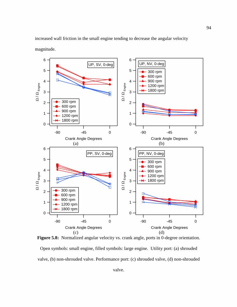
94

increased wall friction in the small engine tending to decrease the angular velocity

magnitude.

6

5

4

3

2

1

0

Ω / Ω

Engin

e

-90 -45 0

Crank Angle Degrees

UP, SV, 0-deg

300 rpm

600 rpm

900 rpm

1200 rpm

1800 rpm

6

5

4

3

2

1

0Ω

/ Ω

Engin

e

-90 -45 0

Crank Angle Degrees

300 rpm

600 rpm

900 rpm

1200 rpm

1800 rpm

UP, NV, 0-deg

(a) (b)

6

5

4

3

2

1

0

Ω / Ω

Engin

e

-90 -45 0

Crank Angle Degrees

300 rpm

600 rpm

900 rpm

1200 rpm

1800 rpm

PP, SV, 0-deg

6

5

4

3

2

1

0

Ω / Ω

Engin

e

-90 -45 0

Crank Angle Degrees

300 rpm

600 rpm

900 rpm

1200 rpm

1800 rpm

PP, NV, 0-deg

(c) (d)

Figure 5.8: Normalized angular velocity vs. crank angle, ports in 0-degree orientation.

Open symbols: small engine, filled symbols: large engine. Utility port: (a) shrouded

valve, (b) non-shrouded valve. Performance port: (c) shrouded valve, (d) non-shrouded

valve.

95

Figure 5.9 shows the average normalized angular velocity at TDC versus swirl

ratio found from steady flow testing. For the large engine, the normalized angular

velocity of the ports with the shrouded valve are, on average, 19% higher than the swirl

ratio values while the ports with the non-shrouded valve are about three times higher than

predicted by the steady swirl ratio. For the small engine, the normalized angular velocity

of the ports with the shrouded valve are on average 4% lower than the swirl ratio values

while the ports with the non-shrouded valve are on average seven times higher than

predicted by the steady swirl ratio. Thus, at higher levels of swirl the steady flow tests

are good at predicting the in-cylinder rotation rate as the normalized angular velocity at

TDC is proportional to Rs. However, at very low levels of swirl, Rs largely underpredicts

the normalized angular velocity. This trend in measurement accuracy is consistent across

size scaling.

5

4

3

2

1

0

Avera

ge Ω

(TD

C)

/ Ω

Engin

e

543210

Rs

PP, SV

PP, NV

UP, SV

UP, NV

One-to-One Line

Ports in 0-deg OrientationOpen Symbol: Small EngineFilled Symbol: Large Engine

Figure 5.9: Average normalized angular velocity at TDC vs. swirl ratio, ports in 0-

degree orientation.

96

5.7. High-Magnification PIV Results

The high-magnification FOV PIV data were acquired to study the small-scale

fluid turbulence. The location of the high-magnification FOV relative to the low-

magnification FOV was shown in Fig. 5.4. Unless otherwise specified as the second

high-magnification FOV location, all high-magnification data were acquired in the high-

magnification FOV location. Images were acquired only at TDC of the compression

stroke. For each condition, a set of 200 cycles were captured. Data were analyzed for all

port orientations and engine running conditions.

As described in §5.4, two methods were used to calculate the mean velocity field.

One of the challenges of data analysis in engine flows is to define an appropriate mean

velocity. Therefore, it was sought to perform the analysis using the methods appropriate

for the spatially resolved, multiple-realization data available. Figure 5.10 shows the

results using both methods of finding the mean velocity field for the high-magnification

FOV for a condition with high swirl. Figure 5.10(a) shows the ensemble average velocity

field. Figure 5.10(b) shows the instantaneous velocity field of an individual cycle and

Figs. 5.10(c)-(e) show the spatial average velocity field for the cycle shown in Fig.

5.10(b) using three different cutoff frequencies.

97

x [mm] [m/s]

y [

mm

]

5 10 15

-12

-10

-8

-6

-4

-2

0

2

4

6

8

10

12

14

(a)

x [mm] [m/s]

y [

mm

]

2 4 6 8 10 12 14 16

-12

-10

-8

-6

-4

-2

0

2

4

6

8

10

12

14

(b)

98

x [mm] [m/s]

y [

mm

]

2 4 6 8 10 12 14 16

-12

-10

-8

-6

-4

-2

0

2

4

6

8

10

12

14

(c)

x [mm] [m/s]

y [

mm

]

2 4 6 8 10 12 14 16

-12

-10

-8

-6

-4

-2

0

2

4

6

8

10

12

14

(d)

99

x [mm] [m/s]

y [

mm

]

2 4 6 8 10 12 14 16

-12

-10

-8

-6

-4

-2

0

2

4

6

8

10

12

14

(e)

Figure 5.10: Selected images showing the resulting velocity fields using the two

methods of computing the mean velocity field for the given condition: large engine,

utility port, shrouded valve, 0-degree orientation, 1200 rpm. (a) Ensemble average

velocity field, (b) individual cycle instantaneous velocity field, and spatial-average

velocity fields for the individual cycle (b) using cutoff lengthscales of (c) 5 mm, (d) 10

mm, and (e) 15 mm.

5.7.1. Turbulence Intensity

As is done often in engines flows, the fluctuating velocity component is defined

by its root mean square value, deemed the turbulence intensity, u’. The turbulence

intensity was calculated from the fluctuating velocity as

.)},(),({1

),('2

21

2

1 yxuyxuN

yxucN

c

(5.9)

In computing the mean velocity and turbulence intensity for the ensemble-average

method, only first-choice vectors were included in the analysis. However, due to the high

100

number of first-choice vectors, an analysis using all vectors made a negligible difference

in the results. The mean velocity fields for the spatial-average method utilized both first-

choice and interpolated vectors. In processing the spatial average velocity fields, there

are inherent edge effects arising from the use of the Fourier transform method causing an

increase in the calculated turbulence intensity around the edgesof the image. In an effort

to reduce this bias, the analysis using the spatial-average method omitted the five rows or

columns of data nearest the edge of the image. The use of a window function with the

FFT did not give substantial improvement.

Figure 5.11 shows the high-magnification FOV turbulence intensity using both

methods of finding the mean velocity field for the same engine condition as Fig. 5.10.

Figure 5.11(a) shows the turbulence intensity found with the ensemble average method.

The turbulence intensity is seen to be non-uniform and tends to be greatest in magnitude

at the location corresponding to the ensemble average swirl center where the mean

velocity is the smallest (see Fig. 5.10(a)). Figure 5.11(b) shows the turbulence intensity

found using the spatial-average method with a cutoff lengthscale of 10 mm. The

turbulence intensity is seen to be fairly uniform towards the center of the image and

increases in magnitude towards the edges, which is an artifact of the filtering procedure.

Figure 5.11(c) contains the same turbulence intensity field as Fig. 5.11(b), but omits the

five rows and columns of data near the edges, displaying the data used for subsequent

processing. It can be seen that the edge effects introduced by the filter are removed. The

effect of the swirl center precession, which causes the higher apparent turbulence near the

swirl center, is eliminated by the use of the spatial filtering. These images highlight the

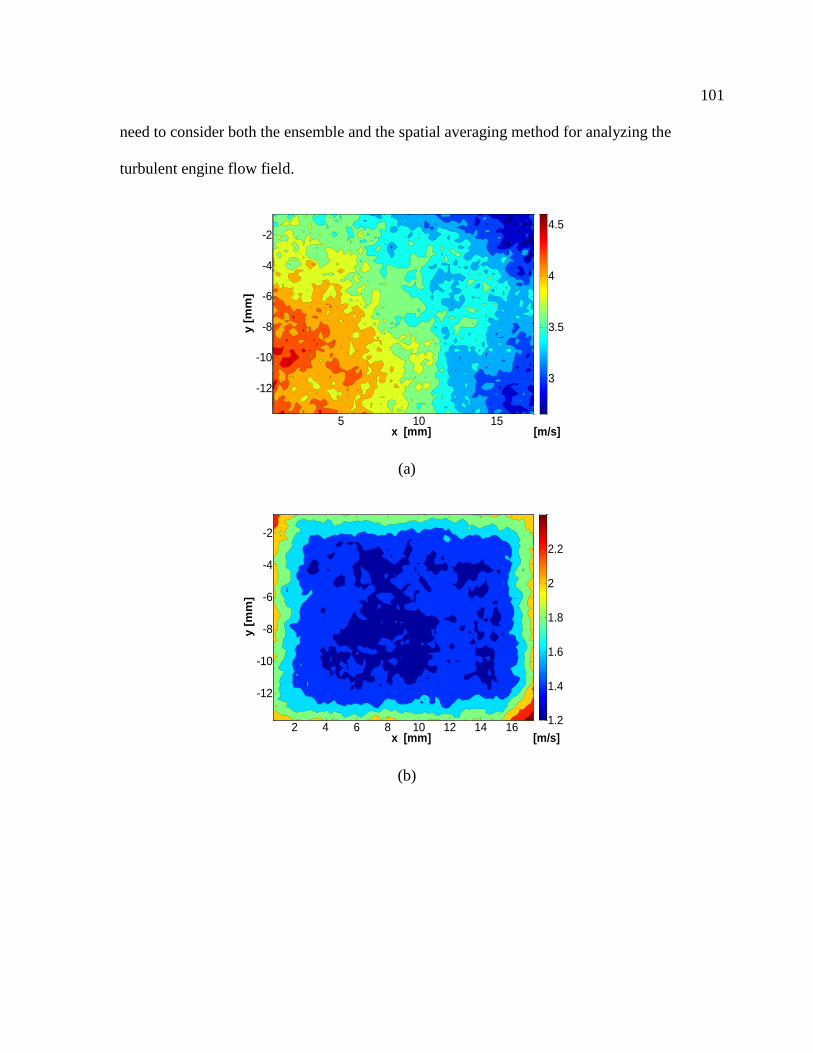
101

need to consider both the ensemble and the spatial averaging method for analyzing the

turbulent engine flow field.

x [mm] [m/s]

y [

mm

]

5 10 15

-12

-10

-8

-6

-4

-2

3

3.5

4

4.5

(a)

x [mm] [m/s]

y [

mm

]

2 4 6 8 10 12 14 16

-12

-10

-8

-6

-4

-2

1.2

1.4

1.6

1.8

2

2.2

(b)

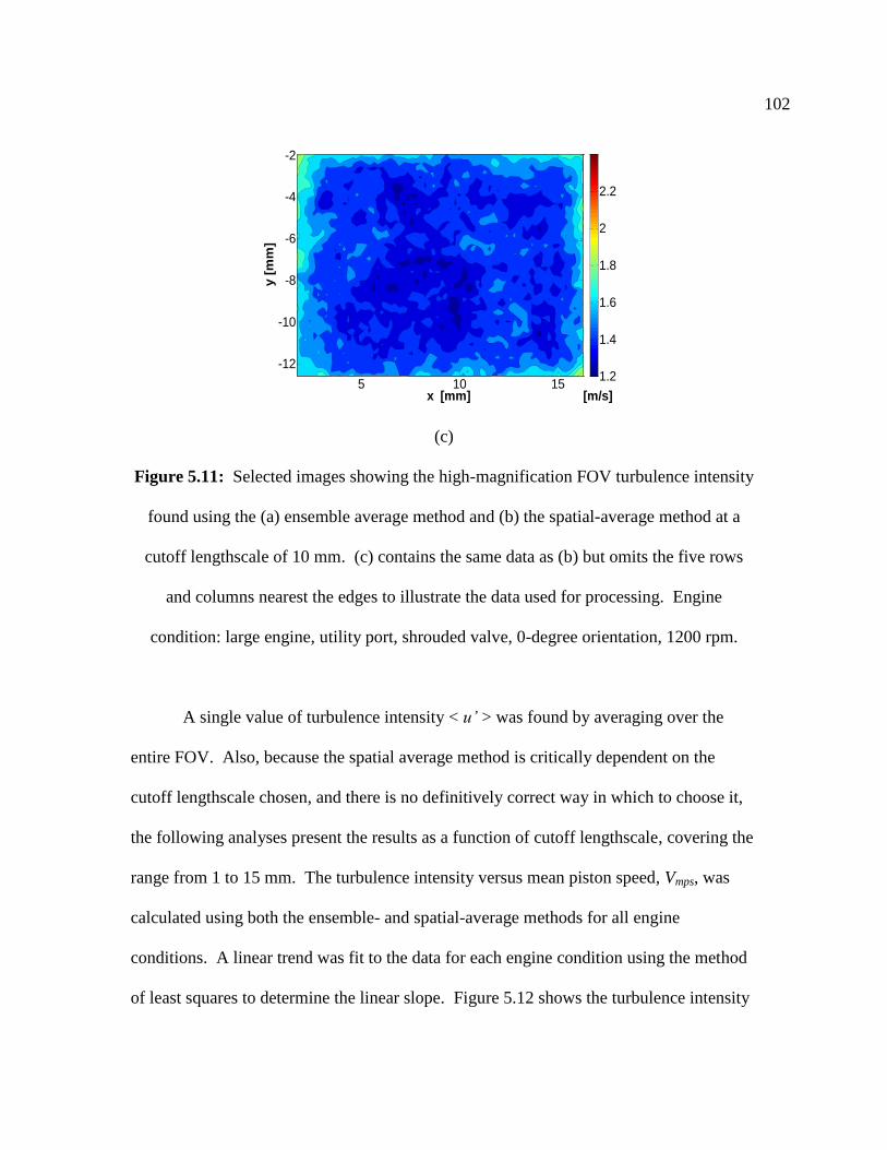
102

x [mm] [m/s]

y [

mm

]

5 10 15

-12

-10

-8

-6

-4

-2

1.2

1.4

1.6

1.8

2

2.2

(c)

Figure 5.11: Selected images showing the high-magnification FOV turbulence intensity

found using the (a) ensemble average method and (b) the spatial-average method at a

cutoff lengthscale of 10 mm. (c) contains the same data as (b) but omits the five rows

and columns nearest the edges to illustrate the data used for processing. Engine

condition: large engine, utility port, shrouded valve, 0-degree orientation, 1200 rpm.

A single value of turbulence intensity < u’ > was found by averaging over the

entire FOV. Also, because the spatial average method is critically dependent on the

cutoff lengthscale chosen, and there is no definitively correct way in which to choose it,

the following analyses present the results as a function of cutoff lengthscale, covering the

range from 1 to 15 mm. The turbulence intensity versus mean piston speed, Vmps, was

calculated using both the ensemble- and spatial-average methods for all engine

conditions. A linear trend was fit to the data for each engine condition using the method

of least squares to determine the linear slope. Figure 5.12 shows the turbulence intensity

103

versus mean piston speed for the ensemble average method, not including the linear trend

data. For all conditions, there is a high degree of linearity between the mean piston speed

and turbulence intensity. The ports with the shrouded valve show a marked increase in

turbulence intensity compared to the non-shrouded valve. The port shape and orientation

is seen to have a weak effect on the turbulence intensity. There is fairly close agreement

between the small and large engines.

5

4

3

2

1

0



Ensem

ble

Avera

ge [m

/s]

543210

Vmps [m/s]

PP, SV, 0-deg

PP, NV, 0-deg

PP, NV, 90-deg

UP, SV, 0-deg

UP, NV, 0-deg

UP, NV, 90-deg



average method.

Figure 5.13 presents the linear trend slope of < u’ > vs. Vmps as a function of cutoff

frequency, fc, for the spatial-average method. For comparison, the slope using the

ensemble average method is included at fc = 0. As can be seen, using the spatial-

averaging method does not affect the conclusions of the effect of the shrouded valve

104

compared to the non-shrouded valve, or the port shape and orientation discussed above.

As expected, a higher cutoff frequency results in a decrease in turbulence intensity.

1.6

1.4

1.2

1.0

0.8

0.6

0.4

0.2

0.0



Spatial-A

vera

ge / V

mps

1.21.00.80.60.40.20.0

fc [mm-1

]

Ensemble Average

PP, 0º, SV

PP, 0º, NV

PP, 90º, NV

UP, 0º, SV

UP, 0º, NV

UP, 90º, NV



average method. Ensemble average data are included at fc = 0.

In order to compare the data in Fig. 5.13 on a non-dimensional basis, the cutoff

frequency was multiplied by the TDC clearance, hTDC, of each engine, the result is in Fig.

5.14. The data for both ports with the non-shrouded valves collapse well between the

two engines. The data with shrouded valves show good similarity, with slight differences

at higher cutoff frequencies.

105

1.6

1.4

1.2

1.0

0.8

0.6

0.4

0.2

0.0



Spatial-A

vera

ge / V

mps

86420

fc*hTDC

Ensemble Average

PP, 0º, SV

PP, 0º, NV

PP, 90º, NV

UP, 0º, SV

UP, 0º, NV

UP, 90º, NV



average method. Cutoff frequency made non-dimensional using TDC clearance.

Ensemble average data are included at fc = 0.

Figure 5.15 normalizes the data displayed in Fig. 5.14 by the ensemble-average

slope for each engine condition. It is seen that the data nearly collapse onto a single

curve.

106

0.1

2

3

4

5

6

7

8

91

S

patial-A

vera

ge /

E

nsem

ble

Avera

ge

3 4 5 6 7 8

12 3 4 5 6 7 8

10

fc*hTDC

PP, 0º, SV

PP, 0º, NV

PP, 90º, NV

UP, 0º, SV

UP, 0º, NV

UP, 90º, NV



average method. Cutoff frequency made non-dimensional using TDC clearance. Spatial

average slopes normalized by ensemble average slope.

PIV data were acquired with both ports and shrouded valve in the large engine

using the second high-magnification FOV location, as shown in Fig. 5.4, and these data

were compared with the data from the high-magnification FOV. It was of interest to see

what differences might be present in the data, since on an ensemble average basis, the

swirl center was located nearer to the high-magnification FOV. Figure 5.16 shows the

turbulence intensity versus mean piston speed for the ensemble average method

comparing data taken in the two high-magnification FOVs in the large engine. There is

very little difference in the data, indicating at least for these conditions and analysis, the

turbulence if fairly homogeneous.

107

5

4

3

2

1

0



Ensem

ble

Avera

ge [m

/s]

543210

Vmps [m/s]

PP

UP

Large Engine, SV, 0-deg

Open Symbol: Second High-Magnification FOVFilled Symbol: High-Magnification FOV



high-magnification FOV.

The data taken in the two high-magnification FOVs in the large engine were also

compared using the spatial-average method to determine the slope of < u’ > vs. Vmps, and

the results are shown in Fig. 5.17. Overall, there is fairly close agreement in the data,

indicating relatively homogenous turbulence in-cylinder.

108

1.6

1.4

1.2

1.0

0.8

0.6

0.4

0.2

0.0

S

patial-A

vera

ge / V

mps

1.21.00.80.60.40.20.0

fc [mm-1

]

Ensemble Average

PP

UP


Open Symbol: Second High-Magnification FOVFilled Symbol: High-Magnification FOV



high-magnification FOV. Ensemble average data are included at fc = 0.

5.7.2. Correlation Length Scale Analysis

Two-point correlation data were calculated to estimate longitudinal and transverse

integral lengthscales. Integral lengthscales are a measure of the size of eddies in the

turbulent flow. The correlation coefficients were calculated in both x-(horizontal) and y-

(vertical) directions as

)()0(

)()0()(

22ruu

ruur

ji

ji

ij (5.10)

where the indices (i, j) refer to the components of the fluctuating velocity relative to the

direction of the calculation. For instance, u1 refers to the fluctuating x-velocity

109

component for the correlation in the x-(horizontal) direction, but u1 refers to the

fluctuating y-velocity component for the correlation in the y-(vertical) direction. ρ11 is

referred to as the longitudinal correlation coefficient and ρ22 is referred to as the

transverse correlation coefficient.

Two procedures were used to determine the correlation coefficients. A single-

sided correlation was calculated for the ensemble-averaged data. In this procedure for

example, in the horizontal (1) direction and for each row of fluctuating velocity data, the

correlation coefficient was calculated between the velocity at the leftmost position in the

row and the respective velocity component r to the right; a similar calculation was

performed starting at the rightmost position with a displacement r to the left. The values

for a given separation distance were then averaged over all rows, and all engine cycles.

A double-sided correlation was calculated for the spatial-averaged data. As

mentioned previously with the spatial-averaged data, there were edge effects inherent

from the use of the Fourier-based filtering method. These edge effects were evident in

calculating single-sided correlations with the spatial-averaged data, even after eliminating

the five rows or columns of data nearest the edge of the image. Thus, a slightly different

procedure was used to calculate the spatial-average correlation coefficients. This

procedure gives rise to what will be referred to as a double-sided correlation. In this

procedure for example, in the horizontal (1) direction and for each row of fluctuating

velocity data, the double-sided correlation coefficient was calculated between the

velocity in the center of the row and the respective velocity component a distance r to the

left and to the right of the center. The values for a given separation distance were then

averaged over all rows, and all engine cycles. Because of this procedure, the double-

110

sided correlation coefficients extend to a distance that is only half the width or height of

the PIV image.

Even though two different procedures are being used to calculate the correlation

coefficients, both single- and double-sided correlation procedures give nearly identical

results when analyzing the ensemble-averaged data. Figure 5.18 shows representative

data using both correlation procedures and both averaging methods to calculate the

longitudinal and transverse correlation coefficients in the vertical direction for a given

engine condition. It can be seen that there is very good agreement between the ensemble-

averaged data single- and double-sided correlations, and it is believed that the use of the

double-sided procedure is not affecting the results, but effectively eliminates issues

associated with the spatial filtering procedure. It is observed that the spatial-averaged

correlations more quickly die off for short cutoff lengths (high cutoff frequencies), which

is consistent with expectation.

1.0

0.8

0.6

0.4

0.2

0.0

-0.2

ρ11

121086420

Δy [mm]

Double-sided

Single-sided

Lc = 5 mm

Lc = 10 mm

Lc = 15 mm

Open Symbol: Ensemble-averagedFilled Symbol: Spatial-averaged, Double-sided

(a)

111

1.0

0.8

0.6

0.4

0.2

0.0

-0.2

ρ22

121086420

Δy [mm]

Double-sided

Single-sided

Lc = 5 mm

Lc = 10 mm

Lc = 15 mm

Open Symbol: Ensemble-averagedFilled Symbol: Spatial-averaged, Double-sided

(b)

Figure 5.18: Representative single- and double-sided correlations in the vertical

direction using ensemble- and spatial-averaged data using three cutoff lengthscales.

Engine condition: Large engine, UP, SV, 0-deg orientation.

Longitudinal and transverse integral lengthscales were calculated using the

correlation data. The longitudinal lengthscale, L11, is defined as

drL0

1111 (5.11)

where dr equals dx or dy depending on the direction under investigation. Similarly, the

transverse lengthscale, L22, is defined as

.0

2222 drL (5.12)

112

The integrals were approximated by simple rectangular integration at each data point up

until the first zero crossing point. The longitudinal correlation data did not always cross

the zero ordinate, e.g. Fig. 5.18(a), so a best-fit equation was used to extend the data to

the zero crossing. (There were a couple engine conditions where the ensemble-averaged

data transverse correlations did not cross the zero ordinate, but were close enough such

that using the best-fit equation did not significantly affect the lengthscale calculation.

Therefore, all transverse lengthscales reported were calculated without the best-fit

equation.) The best-fit equation used was a double-modified exponential empirical

function [33] defined as

).exp(2

1)exp(2

1 xdxd

cxbxb

aR (5.13)

Equation 5.13 was fit to the correlation coefficients by minimizing the sum squared

difference for all data points. The best-fit curves were then used to compute the

longitudinal integral lengthscales, Eqn. 5.11, by approximating the integral using simple

rectangular integration up until the first zero crossing point.

5.7.2.1. Correlation Length Scale Analysis – Ensemble-Average Method

Figure 5.19 shows the longitudinal and transverse single-sided correlation results

for a given engine condition. Also included are the cross-velocity correlations ρ12 and

ρ21, which for all conditions tended to be close to zero as expected. According to [60], in

homogeneous isotropic turbulence with zero mean velocity, the two-point correlation, ρij

= 0 for i ≠ j. The best-fit curve is also included in the figure.

113

1.0

0.8

0.6

0.4

0.2

0.0

-0.2

ρ

2520151050

Δy [mm]

ρ11

ρ22

ρ12

ρ21

ρ11 Best-Fit

Figure 5.19: Correlation coefficients using the ensemble average method in the vertical

direction. Engine condition: large engine, utility port, shrouded valve, 0-degree

orientation, 1200 rpm.

Figure 5.20 shows the longitudinal and transverse integral lengthscales versus

mean piston speed for both engines for a given engine condition. To make a more

meaningful comparison between the engines, all integral lengthscale data have been made

non-dimensional by the TDC clearance height, hTDC. Figure 5.21 shows the resulting

non-dimensional integral lengthscales versus mean piston speed for all engine conditions.

There appears to be fairly close agreement between the large and small engines. Figure

5.22 shows the non-dimensional integral lengthscales calculated in the vertical direction

versus the horizontal direction for all engine conditions and speeds. As can be seen, there

is close agreement between the lengthscales in either direction, indicating a high level of

114

isotropy. Over the range of engine speeds tested, the L11 and L22 values stay fairly

constant, and because of this, an average lengthscale was calculated over the four engine

speeds for the large engine and three engine speeds for the small engine, these are

included in the Table 5.3. For isotropic turbulence the transverse integral scale is one

half of the longitudinal scale [60]. For all engine conditions, L22/ L11 averaged over all

engine speeds ranged between 0.62 and 0.38 with a mean of 0.50 for the large engine,

and for the small engine ranged between 0.63 and 0.40 with a mean of 0.49, close to the

isotropic limit.

10

8

6

4

2

0

Lii

[mm

]

3.53.02.52.01.51.00.5

Vmps [m/s]

L11, Vertical

L22, Vertical

L11, Horizontal

L22, Horizontal

UP, SV, 0-degOpen Symbol: Small EngineFilled Symbol: Large Engine

Figure 5.20: Longitudinal and transverse integral lengthscales versus mean piston speed

in the vertical and horizontal directions using the ensemble average method. Engine

condition: utility port, shrouded valve, 0-degree orientation.

115

1.0

0.8

0.6

0.4

0.2

0.0

Lii

/ h

TD

C

3.53.02.52.01.51.00.5

Vmps [m/s]

L11, Vertical

L22, Vertical

L11, Horizontal

L22, Horizontal


(a)

1.0

0.8

0.6

0.4

0.2

0.0

Lii

/ h

TD

C

3.53.02.52.01.51.00.5

Vmps [m/s]

L11, Vertical

L22, Vertical

L11, Horizontal

L22, Horizontal

UP, NV, 0-degOpen Symbol: Small EngineFilled Symbol: Large Engine

(b)

116

1.0

0.8

0.6

0.4

0.2

0.0

Lii

/ h

TD

C

3.53.02.52.01.51.00.5

Vmps [m/s]

L11, Vertical

L22, Vertical

L11, Horizontal

L22, Horizontal


(c)

1.0

0.8

0.6

0.4

0.2

0.0

Lii

/ h

TD

C

3.53.02.52.01.51.00.5

Vmps [m/s]

L11, Vertical

L22, Vertical

L11, Horizontal

L22, Horizontal

PP, SV, 0-degOpen Symbol: Small EngineFilled Symbol: Large Engine

(d)

117

1.0

0.8

0.6

0.4

0.2

0.0

Lii

/ h

TD

C

3.53.02.52.01.51.00.5

Vmps [m/s]

L11, Vertical

L22, Vertical

L11, Horizontal

L22, Horizontal

PP, NV, 0-degOpen Symbol: Small EngineFilled Symbol: Large Engine

(e)

1.0

0.8

0.6

0.4

0.2

0.0

Lii

/ h

TD

C

3.53.02.52.01.51.00.5

Vmps [m/s]

L11, Vertical

L22, Vertical

L11, Horizontal

L22, Horizontal


(f)

118

Figure 5.21: Non-dimensional longitudinal and transverse integral lengthscales versus

mean piston speed in the vertical and horizontal directions using the ensemble average

method. Engine conditions: Utility port, (a) SV, 0-deg., (b) NV, 0-deg., (c) NV, 90-deg.,

and Performance port, (d) SV, 0-deg., (e) NV, 0-deg., (f) NV, 90-deg.

1.0

0.8

0.6

0.4

0.2

0.0

Lii (V

ert

ical) / h

TD

C

1.00.80.60.40.20.0

Lii (Horizontal) / hTDC

L11

L22

One-to-One Line

Open Symbol: Small EngineFilled Symbol: Large Engine

Figure 5.22: Non-dimensional integral lengthscales for all engine conditions and speeds

in the vertical versus horizontal directions using the ensemble average method.

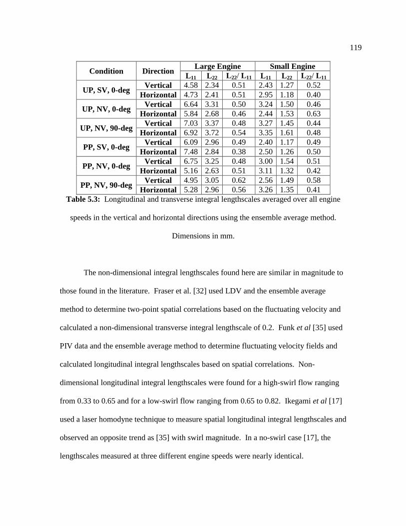
119

Condition Direction Large Engine Small Engine

L11 L22 L22/ L11 L11 L22 L22/ L11

UP, SV, 0-deg Vertical 4.58 2.34 0.51 2.43 1.27 0.52

Horizontal 4.73 2.41 0.51 2.95 1.18 0.40

UP, NV, 0-deg Vertical 6.64 3.31 0.50 3.24 1.50 0.46

Horizontal 5.84 2.68 0.46 2.44 1.53 0.63

UP, NV, 90-deg Vertical 7.03 3.37 0.48 3.27 1.45 0.44

Horizontal 6.92 3.72 0.54 3.35 1.61 0.48

PP, SV, 0-deg Vertical 6.09 2.96 0.49 2.40 1.17 0.49

Horizontal 7.48 2.84 0.38 2.50 1.26 0.50

PP, NV, 0-deg Vertical 6.75 3.25 0.48 3.00 1.54 0.51

Horizontal 5.16 2.63 0.51 3.11 1.32 0.42

PP, NV, 90-deg Vertical 4.95 3.05 0.62 2.56 1.49 0.58

Horizontal 5.28 2.96 0.56 3.26 1.35 0.41

Table 5.3: Longitudinal and transverse integral lengthscales averaged over all engine

speeds in the vertical and horizontal directions using the ensemble average method.

Dimensions in mm.

The non-dimensional integral lengthscales found here are similar in magnitude to

those found in the literature. Fraser et al. [32] used LDV and the ensemble average

method to determine two-point spatial correlations based on the fluctuating velocity and

calculated a non-dimensional transverse integral lengthscale of 0.2. Funk et al [35] used

PIV data and the ensemble average method to determine fluctuating velocity fields and

calculated longitudinal integral lengthscales based on spatial correlations. Non-

dimensional longitudinal integral lengthscales were found for a high-swirl flow ranging

from 0.33 to 0.65 and for a low-swirl flow ranging from 0.65 to 0.82. Ikegami et al [17]

used a laser homodyne technique to measure spatial longitudinal integral lengthscales and

observed an opposite trend as [35] with swirl magnitude. In a no-swirl case [17], the

lengthscales measured at three different engine speeds were nearly identical.

120

For some engine conditions the best-fit curve extended for a substantial distance,

which may have caused a bias in the calculation of L11. Because of this, a modified

longitudinal integral lengthscale, L11*, was calculated by directly integrating the

correlation data up to the final data point or up to the zero crossing point, whichever

occurred first. Because the high-magnification FOV horizontal distance is 1.25 times the

vertical distance, L11* was calculated in the horizontal direction by integrating the

correlation data up to a maximum distance equal to the vertical direction distance. This

was done so that a comparison could be made between the small and large engines

without the influence of a best-fit curve. L11* is not to be considered a true measure of

L11. Note that the distance to the final data point scales by the scaling factor between the

small and large engines because the high-magnification FOV scales between the two

engines. Figure 5.23 shows L11* made non-dimensional by hTDC versus mean piston

speed for all engine conditions. There appears to be good similarity in the modified

integral lengthscale between the two engines. Figure 5.24 shows the modified non-

dimensional integral lengthscales calculated in the vertical direction versus the horizontal

direction for all engine conditions and speeds. Compared with the longitudinal integral

lengthscales seen in Fig. 5.22, the data exhibit less scatter. There is close agreement

between the lengthscales in either direction, indicating a high level of isotropy, and the

difference between the small and large engine data appear smaller.

121

1.0

0.8

0.6

0.4

0.2

0.0

L11

* / h

TD

C

3.53.02.52.01.51.00.5

Vmps [m/s]

Vertical

Horizontal


1.0

0.8

0.6

0.4

0.2

0.0

L11

* / h

TD

C

3.53.02.52.01.51.00.5

Vmps [m/s]

Vertical

Horizontal


(a) (b)

1.0

0.8

0.6

0.4

0.2

0.0

L11

* / h

TD

C

3.53.02.52.01.51.00.5

Vmps [m/s]

Vertical

Horizontal


1.0

0.8

0.6

0.4

0.2

0.0

L11

* / h

TD

C

3.53.02.52.01.51.00.5

Vmps [m/s]

Vertical

Horizontal

PP, SV, 0-degOpen Symbol: Small EngineFilled Symbol: Large Engine

(c) (d)

122

1.0

0.8

0.6

0.4

0.2

0.0

L11

* / h

TD

C

3.53.02.52.01.51.00.5

Vmps [m/s]

Vertical

Horizontal


1.0

0.8

0.6

0.4

0.2

0.0

L11

* / h

TD

C

3.53.02.52.01.51.00.5

Vmps [m/s]

Vertical

Horizontal


(e) (f)

Figure 5.23: Non-dimensional modified longitudinal integral lengthscales versus mean

piston speed in the vertical and horizontal directions using the ensemble average method.


Performance port, (d) SV, 0-deg., (e) NV, 0-deg., (f) NV, 90-deg.

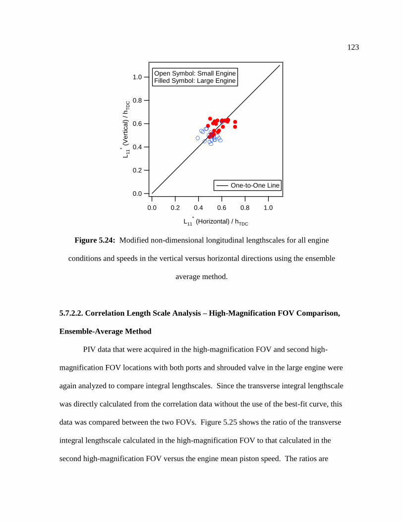
123

1.0

0.8

0.6

0.4

0.2

0.0

L11

* (V

ert

ical) / h

TD

C

1.00.80.60.40.20.0

L11

* (Horizontal) / hTDC


One-to-One Line

Figure 5.24: Modified non-dimensional longitudinal lengthscales for all engine

conditions and speeds in the vertical versus horizontal directions using the ensemble

average method.

5.7.2.2. Correlation Length Scale Analysis – High-Magnification FOV Comparison,

Ensemble-Average Method

PIV data that were acquired in the high-magnification FOV and second high-

magnification FOV locations with both ports and shrouded valve in the large engine were

again analyzed to compare integral lengthscales. Since the transverse integral lengthscale

was directly calculated from the correlation data without the use of the best-fit curve, this

data was compared between the two FOVs. Figure 5.25 shows the ratio of the transverse

integral lengthscale calculated in the high-magnification FOV to that calculated in the

second high-magnification FOV versus the engine mean piston speed. The ratios are

124

close to one, with the majority of data points being slightly greater than one. For

homogeneous turbulence, one would expect these ratios to be unity, thus there is some

inhomogeneity in the length scale despite the high level of homogeneity seen in the

turbulence intensity (see Fig. 5.16).

1.8

1.6

1.4

1.2

1.0

0.8

0.6

0.4

0.2

L22(H

.-M

. F

OV

) /

L22(S

eco

nd

H.-

M.

FO

V)

3.02.52.01.51.00.5

Vmps [m/s]

PP, Vertical

PP, Horizontal

UP, Vertical

UP, Horizontal




using the ensemble average method.

5.7.2.3. Correlation Length Scale Analysis – Spatial-Average Method

For the spatial-average method, both first-choice and interpolated velocity vectors

were included in the analysis of determining the average velocity fields and the resulting

correlations. The correlations in the horizontal and vertical directions were calculated

according to the double-sided procedure. Integral lengthscales were again calculated

125

using Eqs. 5.11 and 5.12 where the integrals were approximated by simple rectangular

integration at each data point up until the first zero crossing point. Equation 5.13 was

used to extend the longitudinal correlation data to the zero ordinate; the transverse

correlations crossed the axis over the entire range of cutoff lengthscales used in the

analysis. As the correlations exhibited oscillatory behavior about the zero ordinate for

small cutoff lengths (see Fig. 5.18(a)), it was necessary to change the fitting procedure

for the longitudinal correlation coefficients. In computing the minimum sum squared

difference between the best-fit equation and the correlation data, at each data point the

squared difference was divided by the separation distance. This applied a weighting to

the fit of the best-fit equation, allowing it to more faithfully match the correlation data at

small separation distances. Figure 5.26 shows the same spatial-averaged longitudinal

correlation results as Fig. 5.18(a), now with the best-fit curves using the applied

weighting. The best-fit curves are seen to follow the data at small separation distances

fairly well.

126

1.0

0.8

0.6

0.4

0.2

0.0

-0.2

ρ11

121086420

Δy [mm]

Lc = 5 mm, Best-Fit

Lc = 10 mm, Best-Fit

Lc = 15 mm, Best-Fit

Figure 5.26: Representative double-sided correlations in the vertical direction for

spatial-averaged data using three cutoff lengthscales and corresponding best-fit curves.

Engine condition: Large engine, UP, SV, 0-deg orientation.

Using this method, the integral lengthscales based on the spatial-average

correlation data were calculated. Figure 5.27 shows the longitudinal and transverse

lengthscales in the horizontal direction as a function of the cutoff frequency for both

engines with the utility port in the 0-degree orientation and non-shrouded valve. Labels

indicating the engine mean piston speed are omitted since the lengthscales change little

with engine speed. Figure 5.27(a) shows the integral lengthscales versus cutoff

frequency. In the same manner as for the ensemble average data, Fig. 5.27(b) shows the

integral lengthscales made non-dimensional by the TDC clearance, hTDC. The data do not

exhibit similarity. Finally, Fig. 5.27(c) shows the same data with the cutoff frequency

127

made non-dimensional by hTDC. The data now collapse onto two distinct curves for the

longitudinal and transverse lengthscales. Also, examining the figures, the small engine

lengthscales at small fc (large Lc) seem to level off. However, this is likely a result of the

larger Lc used in this analysis being greater than the dimensions of the small engine high-

magnification FOV, as this will affect the calculation of the spatial-average velocity field.

In light of this effect, the remaining data will be shown only for Lc equal to or smaller

than the image domain size (8 mm for the small engine and 14 mm for the large engine).

3.0

2.5

2.0

1.5

1.0

0.5

Lii

(Horizonta

l) [m

m]

6 7 8 9

0.12 3 4 5 6 7 8 9

1

fc [mm-1

]

L11

L22


(a)

128

0.5

0.4

0.3

0.2

0.1

Lii

(Ho

rizo

nta

l) /

hT

DC

6 7 8 9

0.12 3 4 5 6 7 8 9

1

fc [mm-1

]


L11

L22

(b)

0.5

0.4

0.3

0.2

0.1

Lii

(Ho

rizo

nta

l) /

hT

DC

3 4 5 6 7 8 9

12 3 4 5 6 7 8 9

10

fc*hTDC


L11

L22

(c)

Figure 5.27: Longitudinal and transverse integral lengthscales in the horizontal direction

using the spatial-average method. (a) Lii versus fc, (b) Lii/hTDC versus fc, and (c) Lii/hTDC

129

versus fc*hTDC. Engine condition: Utility port, non-shrouded valve, 0-degree orientation,

all engine speeds.

The remaining engine conditions were analyzed in the same manner with both the

integral lengthscales and cutoff frequency made non-dimensional by the TDC clearance.

The results are shown in Fig. 5.28. Again, there is fairly close agreement between the

engines when the data are made non-dimensional in this fashion. The transverse

lengthscales in both the vertical and horizontal directions give very similar results for a

given engine condition. Further, the transverse lengthscales are seen to be quite

consistent comparing all conditions. The longitudinal lengthscales at the lower values of

fc are seen to be somewhat erratic and oscillatory. This is due, in part, to the method used

to fit Eqn. 5.13 to the correlation data, the rate at which the best-fit equation tended to

zero was sensitive to the shape of the correlation data.

0.8

0.6

0.4

0.2

0.0

Lii

(Horizonta

l) / h

TD

C

5 6 7 8 9

12 3 4 5 6 7 8 9

10

fc*hTDC

UP, SV, 0-deg

L11

L22

0.8

0.6

0.4

0.2

0.0

Lii

(Vert

ical) / h

TD

C

5 6 7 8 9

12 3 4 5 6 7 8 9

10

fc*hTDC

UP, SV, 0-deg

L11

L22

(a) (b)

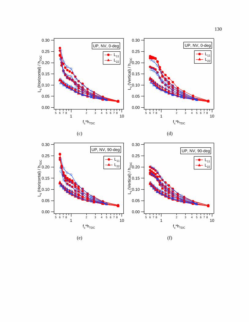
130

0.30

0.25

0.20

0.15

0.10

0.05

0.00

Lii

(Ho

rizo

nta

l) /

hT

DC

5 6 7 8

12 3 4 5 6 7 8

10

fc*hTDC

UP, NV, 0-deg

L11

L22

0.30

0.25

0.20

0.15

0.10

0.05

0.00

Lii

(Ve

rtic

al) /

hT

DC

5 6 7 8

12 3 4 5 6 7 8

10

fc*hTDC

UP, NV, 0-deg

L11

L22

(c) (d)

0.30

0.25

0.20

0.15

0.10

0.05

0.00

Lii

(Horizo

nta

l) /

hT

DC

5 6 7 8

12 3 4 5 6 7 8

10

fc*hTDC

UP, NV, 90-deg

L11

L22

0.30

0.25

0.20

0.15

0.10

0.05

0.00

Lii

(Ve

rtic

al) /

hT

DC

5 6 7 8

12 3 4 5 6 7 8

10

fc*hTDC

UP, NV, 90-deg

L11

L22

(e) (f)

131

1.0

0.8

0.6

0.4

0.2

0.0

Lii

(Horizonta

l) / h

TD

C

5 6 7 8 9

12 3 4 5 6 7 8 9

10

fc*hTDC

PP, SV, 0-deg

L11

L22

1.0

0.8

0.6

0.4

0.2

0.0

Lii

(Vert

ical) / h

TD

C

5 6 7 8 9

12 3 4 5 6 7 8 9

10

fc*hTDC

PP, SV, 0-deg

L11

L22

(g) (h)

0.30

0.25

0.20

0.15

0.10

0.05

0.00

Lii

(Ho

rizo

nta

l) /

hT

DC

5 6 7 8

12 3 4 5 6 7 8

10

fc*hTDC

PP, NV, 0-deg

L11

L22

0.30

0.25

0.20

0.15

0.10

0.05

0.00

Lii

(Vert

ica

l) /

hT

DC

5 6 7 8

12 3 4 5 6 7 8

10

fc*hTDC

PP, NV, 0-deg

L11

L22

(i) (j)

132

0.30

0.25

0.20

0.15

0.10

0.05

0.00

Lii

(Ho

rizo

nta

l) /

hT

DC

5 6 7 8

12 3 4 5 6 7 8

10

fc*hTDC

PP, NV, 90-deg

L11

L22

0.30

0.25

0.20

0.15

0.10

0.05

0.00

Lii

(Ve

rtic

al) /

hT

DC

5 6 7 8

12 3 4 5 6 7 8

10

fc*hTDC

PP, NV, 90-deg

L11

L22

(k) (l)

Figure 5.28: Longitudinal and transverse integral lengthscales in the horizontal and

vertical directions using the spatial-average method. Open symbols: small engine, filled

symbols: large engine. Engine conditions: Utility port, (a)-(b) SV, 0-deg., (c)-(d) NV, 0-

deg., (e)-(f) NV, 90-deg., and Performance port, (g)-(h) SV, 0-deg., (i)-(j) NV, 0-deg.,

(k)-(l) NV, 90-deg.

5.7.2.4. Correlation Length Scale Analysis – High-Magnification FOV Comparison,

Spatial-Average Method



again analyzed to compare integral lengthscales, this time using the spatial-average data.

Again, since the transverse integral lengthscale was directly calculated from the

correlation data without the use of the best-fit curve, these data were compared between

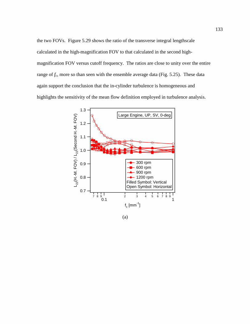
133

the two FOVs. Figure 5.29 shows the ratio of the transverse integral lengthscale

calculated in the high-magnification FOV to that calculated in the second high-

magnification FOV versus cutoff frequency. The ratios are close to unity over the entire

range of fc, more so than seen with the ensemble average data (Fig. 5.25). These data

again support the conclusion that the in-cylinder turbulence is homogeneous and

highlights the sensitivity of the mean flow definition employed in turbulence analysis.

1.3

1.2

1.1

1.0

0.9

0.8

0.7

L22(H

.-M

. F

OV

) /

L22(S

eco

nd

H.-

M.

FO

V)

7 8 9

0.12 3 4 5 6 7 8 9

1

fc [mm-1

]

Large Engine, UP, SV, 0-deg

300 rpm

600 rpm

900 rpm

1200 rpm

Filled Symbol: VerticalOpen Symbol: Horizontal

(a)

134

1.3

1.2

1.1

1.0

0.9

0.8

0.7

L22(H

.-M

. F

OV

) /

L22(S

eco

nd

H.-

M.

FO

V)

7 8 9

0.12 3 4 5 6 7 8 9

1

fc [mm-1

]

Large Engine, PP, SV, 0-deg

300 rpm

600 rpm

900 rpm

1200 rpm


(b)


magnification FOVs versus fc in the vertical and horizontal directions using the spatial-

average method. Engine condition: large engine, (a) utility port, shrouded valve, 0-deg.

orientation, and (b) performance port, shrouded valve, 0-deg. orientation.

5.7.3. Energy Spectra Analysis

A one-dimensional kinetic energy spectrum, E11( 1), was calculated from the PIV

data in both the vertical and horizontal directions. Analysis was performed for all engine

conditions using the ensemble- and spatial-average methods.

The turbulent kinetic energy, k, was calculated at each velocity vector location

and for each engine cycle as

135

.2

3)(

2

1 22 vuk (5.14)

The multiplication by the 3/2 term assumes the flow is isotropic to convert the two-

dimensional turbulent kinetic energy into its three-dimensional equivalent. It is assumed

that the flow is isotropic a priori before computing further statistics of the flow.

However, omitting the 3/2 term will not affect the resulting similarity, or lack thereof, in

the spectra, which is a measure of the isotropy. An interlacing technique described in

[46] was used to compute the one-dimensional kinetic energy spectrum. The horizontal

and vertical spectra were computed in the same manner. For example in the x-direction,

the FFT of k was performed on a row and then multiplied by the complex conjugate of

the FFT of the adjacent row to produce an energy spectrum. This procedure was

performed on all adjacent rows and the results were averaged over all rows, and all

engine cycles to arrive at a mean spectrum. The corresponding one-dimensional

wavenumbers, κ1, in the horizontal direction are

2/,...,1,02

1 columns

columns

NjforjXN

(5.15)

where ΔX is the horizontal distance between two adjacent velocity vectors (217 μm for

the large engine and 128 μm for the small engine) and Ncolumns is the (even) number of

columns of PIV data.

A one-dimensional model spectrum from Pope [60] was then matched to the

calculated spectrum. The model energy spectrum function is defined as

ffCE £3/53/2)( (5.16)

136

where C is a constant equal to 1.5, ε is the rate of dissipation of turbulent kinetic energy,

and f£ and fη are non-dimensional functions [60]. In order to compute the model energy

spectrum function, a turbulence Reynolds number, Re£, must first be assumed, and is

defined as

3/422/1

£

£ £Re

kk (5.16)

where £ is a lengthscale characteristic of the large eddies of the flow and is given by

k3/2

/ε, η is the Kolmogorov lengthscale, and ν is the kinematic viscosity. Here, k is the

turbulent kinetic energy averaged over all vector locations and engine cycles, i.e. <k>.

Based on Re£ and k, all other parameters needed to calculate E(κ) can be determined. In

particular, ε can be written as a function of k and Re£ from Eqn. 5.16; the experimental

value of k was used. The one-dimensional model kinetic energy spectrum can then be

calculated using [60]

.1)(

)(

1

2

2

1111 d

EE (5.17)

An algorithm was developed that finds Re£ and £ (η and £ are related from η = £ Re£ -3/4

)

that minimizes the sum squared difference between the measured and model one-

dimensional energy spectra. Once £ and Re£ are determined, the corresponding model

energy spectrum function can also be used to calculate the longitudinal integral

lengthscale as [60]

dE

uL

02

1

11

)(

2 (5.18)

137

where <u12> is the average squared fluctuating velocity component in the same direction

as the horizontal or vertical analysis, where the average is taken over all vector locations

and all engine cycles.

5.7.3.1. Energy Spectra Analysis – Ensemble Average Method

Figure 5.29(a) shows the results for the large engine with the utility port and the

shrouded valve at 1200 rpm using the ensemble-average method of finding the mean

velocity field. Both vertical and horizontal spectra are displayed. The data axes are non-

dimensionalized using ε, η, and ν. As can be seen in Fig. 5.29, the measured horizontal

and vertical spectra are closely matched, suggesting a high level of isotropy. The

calculated spectra follow Pope‟s model spectrum through the inertial subrange where the

energy spectra acquire the traditional -5/3 wavenumber power law dependence. At the

higher wavenumbers, there is a slight trailing off of the calculated spectra compared to

the model spectra. The measured spectra begin to deviate from the model spectra close to

a wavenumber corresponding to twice the interrogation region size of 868 m, or 0.007

rad/ m, which corresponds to the true Nyquist limit because the real sampling distance is

the interrogation window size (434 m) and not the vector spacing. Figure 5.29(b) shows

the same analysis for the small engine with the utility port and the shrouded valve at 1800

rpm. Again, a similar result is observed with the measured spectra beginning to deviate

from the model spectra close to a wavenumber corresponding to twice the interrogation

region size of 512 m, or 0.012 rad/ m.

138

106

107

108

109

1010

1011

1012

E11(κ

1)/

(εν

5)1

/4

0.0012 4 6 8

0.012 4 6 8

0.12 4 6 8

1

κ1η

2x Interrogation Size

Interrogation Size

Horizontal

Model - Horizontal Vertical

Model - Vertical Slope -5/3

Large EngineUP, SV, 0-deg1200 rpm

(a)

105

106

107

108

109

1010

1011

1012

E11(κ

1)/

(εν

5)1

/4

0.0012 4 6 8

0.012 4 6 8

0.12 4 6 8

1

κ1η

2x Interrogation Size

Interrogation Size

Small EngineUP, SV, 0-deg1800 rpm

Horizontal

Model - Horizontal Vertical

Model - Vertical Slope -5/3

(b)

Figure 5.29: Model and calculated one-dimensional energy spectra in the vertical and

horizontal directions using the ensemble average method to determine the mean velocity

139

field. Engine condition: utility port, 0-degree orientation, shrouded valve, (a) large

engine at 1200 rpm and (b) small engine at 1800 rpm.

Figures 5.30(a) and (b) show the vertical analysis results for the utility port using

the shrouded valve over the range of engine speeds for the large and small engines,

respectively. There are two main effects of the engine speed. Firstly, the higher engine

speed gives rise to a higher kinetic energy, which is seen as the integral under the curves.

The second effect is that as the engine speed decreases, the inertial subrange shortens.

For the large engine at 300 rpm and the small engine at 600 rpm, there is not much of the

spectra following the -5/3

dependence. This suggests that the scale separation principles

of Kolmogorov may not be satisfied.

105

106

107

108

109

1010

1011

1012

E11(κ

1)/

(εν

5)1

/4

0.0012 4 6 8

0.012 4 6 8

0.12 4 6 8

1

κ1η

300 rpm

600 rpm

900 rpm

1200 rpm

UP, SV, 0-degVertical Direction

Model, 300 rpm Model, 1200 rpm Slope -5/3

Large Engine

(a)

140

105

106

107

108

109

1010

1011

1012

E11(κ

1)/

(εν

5)1

/4

0.0012 4 6 8

0.012 4 6 8

0.12 4 6 8

1

κ1η

600 rpm

1200 rpm

1800 rpm

UP, SV, 0-degVertical Direction

Model, 600 rpm Model, 1800 rpm Slope -5/3

Small Engine

(b)


direction using the ensemble average method to determine the mean velocity field.

Engine condition: utility port, 0-degree orientation, shrouded valve, (a) large engine at

300-1200 rpm and (b) small engine at 600-1800 rpm.

5.7.3.2. Energy Spectra Analysis – Ensemble Average Method: L11

The resulting longitudinal integral lengthscales found in the vertical and

horizontal directions for both engines and each engine condition were normalized by the

TDC clearance, hTDC, and are shown versus mean piston speed in Fig. 5.31. The

longitudinal integral lengthscale is seen to stay relatively constant with mean piston speed

for all engine conditions, similar to the results in §5.7.2.1 where the lengthscales were

calculated using the correlation data. Inspecting Eqn. 5.18, it would be expected that L11

141

should remain nearly constant as E(κ) integrates to <k> and the ratio of <k> to <u12> is

nearly constant. The normalized L11 also show good similarity between the small and

large engines, for all engine conditions achieving a value of about 0.2. Compared with

L11 /hTDC from §5.7.2.1, this analysis give values that are about two to three times lower

in magnitude.

0.6

0.5

0.4

0.3

0.2

0.1

0.0

L11 / h

TD

C

3.53.02.52.01.51.00.5

Vmps [m/s]

UP, SV, 0-deg

Vertical

Horizontal

0.6

0.5

0.4

0.3

0.2

0.1

0.0

L11 / h

TD

C

3.53.02.52.01.51.00.5

Vmps [m/s]

UP, NV, 0-deg

Vertical

Horizontal

(a) (b)

0.6

0.5

0.4

0.3

0.2

0.1

0.0

L11 / h

TD

C

3.53.02.52.01.51.00.5

Vmps [m/s]

UP, NV, 90-deg

Vertical

Horizontal

0.6

0.5

0.4

0.3

0.2

0.1

0.0

L11 / h

TD

C

3.53.02.52.01.51.00.5

Vmps [m/s]

PP, SV, 0-deg

Vertical

Horizontal

(c) (d)

142

0.6

0.5

0.4

0.3

0.2

0.1

0.0

L11 / h

TD

C

3.53.02.52.01.51.00.5

Vmps [m/s]

PP, NV, 0-deg

Vertical

Horizontal

0.6

0.5

0.4

0.3

0.2

0.1

0.0

L11 / h

TD

C

3.53.02.52.01.51.00.5

Vmps [m/s]

PP, NV, 90-deg

Vertical

Horizontal

(e) (f)

Figure 5.31: Non-dimensional longitudinal integral lengthscales versus mean piston

speed in the vertical and horizontal directions using the energy spectra analysis-ensemble

average method. Open symbols: small engine, filled symbols: large engine. Engine


port, (d) SV, 0-deg., (e) NV, 0-deg., (f) NV, 90-deg.

5.7.3.3. Energy Spectra Analysis – Ensemble Average Method: L11, High-

Magnification FOV Comparison


magnification FOV locations with both ports and the shrouded valve in the large engine

were again analyzed to compare longitudinal integral lengthscales. Figure 5.32 shows the

ratio of L11 calculated in the high-magnification FOV to that calculated in the second

high-magnification FOV versus the engine mean piston speed using the energy spectra

143

analysis. The ratios are again close to unity, indicating a measure of homogeneity in the

flow. Compared to Fig. 5.25, where L22 was calculated using correlation data with the

ensemble average method and the ratio found between the two FOVs, the magnitudes of

the ratios are very similar.

1.8

1.6

1.4

1.2

1.0

0.8

0.6

0.4

0.2

L11(H

.-M

. F

OV

) /

L11(S

eco

nd

H.-

M.

FO

V)

3.02.52.01.51.00.5

Vmps [m/s]

PP, Vertical

PP, Horizontal

UP, Vertical

UP, Horizontal


Figure 5.32: Comparison of longitudinal integral lengthscales calculated in the two

high-magnification FOVs versus mean piston speed in the vertical and horizontal

directions using the energy spectra analysis-ensemble average method. Engine condition:

large engine, utility port, 0-deg. orientation, shrouded valve and performance port, 0-deg.

orientation, shrouded valve.

5.7.3.4. Energy Spectra Analysis – Ensemble Average Method: Re£

The resulting turbulence Reynolds numbers found in the vertical and horizontal

directions for both engines and each engine condition are shown versus mean piston

144

speed in Fig. 5.33. Examining the data, the turbulence Reynolds number increases

monotonically with engine speed for all engine conditions. The ports with the shrouded

valve compared to the non-shrouded valve exhibit turbulence Reynolds numbers of

greater magnitude at the same mean piston speed. For a given mean piston speed and

engine condition, the large engine turbulence Reynolds numbers are roughly two to three

times greater in magnitude compared to the small engine.

5000

4000

3000

2000

1000

0

Re

£

3.53.02.52.01.51.00.5

Vmps [m/s]

UP, SV, 0-deg

Vertical

Horizontal

5000

4000

3000

2000

1000

0

Re

£

3.53.02.52.01.51.00.5

Vmps [m/s]

UP, NV, 0-deg

Vertical

Horizontal

(a) (b)

145

5000

4000

3000

2000

1000

0

Re

£

3.53.02.52.01.51.00.5

Vmps [m/s]

UP, NV, 90-deg

Vertical

Horizontal

5000

4000

3000

2000

1000

0

Re

£

3.53.02.52.01.51.00.5

Vmps [m/s]

PP, SV, 0-deg

Vertical

Horizontal

(c) (d)

5000

4000

3000

2000

1000

0

Re

£

3.53.02.52.01.51.00.5

Vmps [m/s]

PP, NV, 0-deg

Vertical

Horizontal

5000

4000

3000

2000

1000

0

Re

£

3.53.02.52.01.51.00.5

Vmps [m/s]

PP, NV, 90-deg

Vertical

Horizontal

(e) (f)

Figure 5.33: Turbulence Reynolds number versus mean piston speed in the vertical and




NV, 0-deg., (f) NV, 90-deg.

146

5.7.3.5. Energy Spectra Analysis – Ensemble Average Method: η

The resulting Kolmogorov lengthscales found in the vertical and horizontal

directions for both engines and each engine condition are shown versus mean piston

speed in Fig. 5.34. Examining the data, the Kolmogorov lengthscale decreases

monotonically with engine speed for all engine conditions. The ports with the shrouded

valve compared to the non-shrouded valve exhibit Kolmogorov lengthscales of smaller

magnitude at the same mean piston speed. Between the small and large engines, the

Kolmogorov lengthscales are roughly the same for a given mean piston speed. An

overview of all the parameters points to an interesting dynamic. The large-scale

turbulence or integral lengthscales are determined by the geometry of the engine, and so

they scale by the size of the engine. At the same mean piston speed, the turbulence

Reynolds numbers of the small engine compared to the large engine decreases in such a

way that the small-scale turbulence or Kolmogorov lengthscales are similar. The flows

created by the shrouded versus non-shrouded valves indicate higher turbulence Reynolds

numbers, effectively pushing the Kolmogorov lengthscales farther down the energy

cascade to smaller lengthscales.

147

40

30

20

10

0

η [

μm

]

3.53.02.52.01.51.00.5

Vmps [m/s]

UP, SV, 0-deg

Vertical

Horizontal

40

30

20

10

0

η [

μm

]

3.53.02.52.01.51.00.5

Vmps [m/s]

UP, NV, 0-deg

Vertical

Horizontal

(a) (b)

40

30

20

10

0

η [

μm

]

3.53.02.52.01.51.00.5

Vmps [m/s]

UP, NV, 90-deg

Vertical

Horizontal

40

30

20

10

0

η [

μm

]

3.53.02.52.01.51.00.5

Vmps [m/s]

PP, SV, 0-deg

Vertical

Horizontal

(c) (d)

148

40

30

20

10

0

η [

μm

]

3.53.02.52.01.51.00.5

Vmps [m/s]

PP, NV, 0-deg

Vertical

Horizontal

40

30

20

10

0

η [

μm

]

3.53.02.52.01.51.00.5

Vmps [m/s]

PP, NV, 90-deg

Vertical

Horizontal

(e) (f)

Figure 5.34: Kolmogorov lengthscales versus mean piston speed in the vertical and




NV, 0-deg., (f) NV, 90-deg.

5.7.3.6. Energy Spectra Analysis – Spatial-Average Method

The same one-dimensional kinetic energy spectrum analysis was performed for all

engine conditions using the spatial-average method to obtain the mean velocity field for

each engine cycle. Figure 5.35(a) shows the vertical spectra results for the large engine

utility port at 1200 rpm and the shrouded valve using three different cutoff lengthscales.

The portion of the energy spectra that follows the traditional -5/3 wavenumber power law

dependence becomes smaller as the cutoff lengthscale decreases. Figure 5.35(b) shows

the same analysis for the small engine utility port at 1200 rpm and the shrouded valve.

149

Again, a similar trend is observed as the cutoff lengthscale decreases. The energy

spectrum analysis was performed over cutoff lengthscales ranging from 1 to 15 mm. The

longitudinal integral lengthscales, Kolmogorov lengthscales, and turbulence Reynolds

numbers were again calculated.

106

107

108

109

1010

1011

E11(κ

1)/

(εν

5)1

/4

0.0012 4 6 8

0.012 4 6 8

0.12 4 6 8

1

κ1η

Lc = 5 mm

Lc = 10 mm

Lc = 15 mm

Model, Lc = 5 mm

Model, Lc = 10 mm

Model, Lc = 15 mm

Slope -5/3

Large Engine, 1200 rpmUP, SV, 0-degVertical Direction

(a)

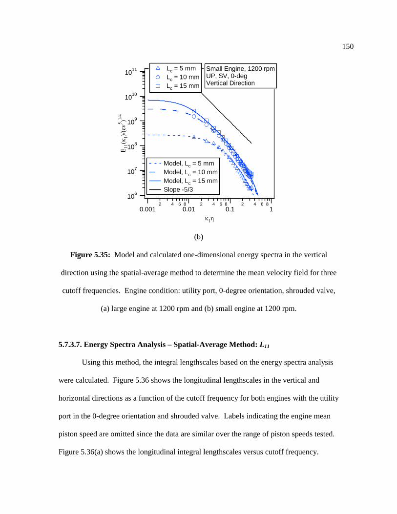
150

106

107

108

109

1010

1011

E11(κ

1)/

(εν

5)1

/4

0.0012 4 6 8

0.012 4 6 8

0.12 4 6 8

1

κ1η

Small Engine, 1200 rpmUP, SV, 0-degVertical Direction

Model, Lc = 5 mm

Model, Lc = 10 mm

Model, Lc = 15 mm

Slope -5/3

Lc = 5 mm

Lc = 10 mm

Lc = 15 mm

(b)


direction using the spatial-average method to determine the mean velocity field for three

cutoff frequencies. Engine condition: utility port, 0-degree orientation, shrouded valve,

(a) large engine at 1200 rpm and (b) small engine at 1200 rpm.

5.7.3.7. Energy Spectra Analysis – Spatial-Average Method: L11

Using this method, the integral lengthscales based on the energy spectra analysis

were calculated. Figure 5.36 shows the longitudinal lengthscales in the vertical and

horizontal directions as a function of the cutoff frequency for both engines with the utility

port in the 0-degree orientation and shrouded valve. Labels indicating the engine mean

piston speed are omitted since the data are similar over the range of piston speeds tested.

Figure 5.36(a) shows the longitudinal integral lengthscales versus cutoff frequency.

151

Figure 5.36(b) shows the integral lengthscales made non-dimensional by the TDC

clearance, hTDC. Figure 5.36(c) shows the same data with the cutoff frequency made non-

dimensional by hTDC. This normalization appears to nearly collapse the data onto one

curve for both small and large engines. Again, at large Lc approaching the size of the

high-magnification FOV, the lengthscales tend to level off for the small engine. This is a

result of calculating the spatial-average velocity field with values of Lc greater than the

dimensions of the small engine high-magnification FOV. Due to this effect, the

remaining data will be shown only for Lc equal to or smaller than the image domain size

(8 mm for the small engine and 14 mm for the large engine).

2.5

2.0

1.5

1.0

0.5

0.0

L11 [m

m]

6 7 8 9

0.12 3 4 5 6 7 8 9

1

fc [mm-1

]

UP, SV, 0-deg

Vertical

Horizontal


(a)

152

0.4

0.3

0.2

0.1

0.0

L11 / h

TD

C

6 7 8 9

0.12 3 4 5 6 7 8 9

1

fc [mm-1

]

UP, SV, 0-deg


Vertical

Horizontal

(b)

0.4

0.3

0.2

0.1

0.0

L11 / h

TD

C

3 4 5 6 7 8 9

12 3 4 5 6 7 8 9

10

fc*hTDC

UP, SV, 0-deg

Vertical

Horizontal


(c)


using the energy spectra analysis, spatial-average method. (a) L11 versus fc, (b) L11/hTDC

153

versus fc, and (c) L11/hTDC versus fc*hTDC. Engine condition: Utility port, shrouded valve,

0-degree orientation, all engine speeds.

The remaining engine conditions were analyzed in the same manner with both L11

and fc made non-dimensional by hTDC. The results are shown in Fig. 5.37. Again, there is

fairly close agreement between the small and large engines when the data are made non-

dimensional in this fashion. The longitudinal lengthscales in both the vertical and

horizontal directions give very similar results for a given engine condition. The one

exception to this appears to be the large engine with both ports and the shrouded valve,

where the horizontal direction gives slightly larger values than the vertical direction.

0.3

0.2

0.1

0.0

L11 / h

TD

C

5 6 7 8 9

12 3 4 5 6 7 8 9

10

fc*hTDC

UP, SV, 0-deg

Vertical

Horizontal

0.3

0.2

0.1

0.0

L11 / h

TD

C

5 6 7 8 9

12 3 4 5 6 7 8 9

10

fc*hTDC

UP, NV, 0-deg

Vertical

Horizontal

(a) (b)

154

0.3

0.2

0.1

0.0

L11 / h

TD

C

5 6 7 8 9

12 3 4 5 6 7 8 9

10

fc*hTDC

UP, NV, 90-deg

Vertical

Horizontal

0.3

0.2

0.1

0.0

L11 / h

TD

C

5 6 7 8 9

12 3 4 5 6 7 8 9

10

fc*hTDC

PP, SV, 0-deg

Vertical

Horizontal

(c) (d)

0.3

0.2

0.1

0.0

L11 / h

TD

C

5 6 7 8 9

12 3 4 5 6 7 8 9

10

fc*hTDC

PP, NV, 0-deg

Vertical

Horizontal

0.3

0.2

0.1

0.0

L11 / h

TD

C

5 6 7 8 9

12 3 4 5 6 7 8 9

10

fc*hTDC

PP, NV, 90-deg

Vertical

Horizontal

(e) (f)


calculated using the energy spectra analysis, spatial-average method. Open symbols:

small engine, filled symbols: large engine. Engine conditions: Utility port, (a) SV, 0-

deg., (b) NV, 0-deg., (c) NV, 90-deg., and Performance port, (d) SV, 0-deg., (e) NV, 0-

deg., (f) NV, 90-deg.

155

This analysis gives lengthscales similar in magnitude to those found using the

correlation analysis in §5.7.2.3. To make a direct comparison of the longitudinal

lengthscales determined using the correlation coefficients and energy spectra analyses,

Fig. 5.38 shows data from two representative engine conditions. The figure includes data

from the utility port in the 0-degree orientation with (a)-(b) the shrouded valve and (c)-(d)

the non-shrouded valve in the horizontal and vertical directions. Comparing the two

methods, the lengthscales found using the energy spectra tend to vary less with fc, are

smaller in magnitude at small fc, and are roughly the same as those found with the

correlation data at a normalized cutoff frequency of about two.

2

3

4

56

0.1

2

3

4

56

1

L11 / h

TD

C

5 6 7 8 9

12 3 4 5 6 7 8 9

10

fc*hTDC

UP, SV, 0-deg

Spectra

Correlation

Horizontal Direction

2

3

4

56

0.1

2

3

4

56

1

L11 / h

TD

C

5 6 7 8 9

12 3 4 5 6 7 8 9

10

fc*hTDC

UP, SV, 0-deg

Spectra

Correlation

Vertical Direction

(a) (b)

156

0.4

0.3

0.2

0.1

0.0

L11 / h

TD

C

5 6 7 8 9

12 3 4 5 6 7 8 9

10

fc*hTDC

UP, NV, 0-deg

Spectra

Correlation


0.4

0.3

0.2

0.1

0.0

L11 / h

TD

C

5 6 7 8 9

12 3 4 5 6 7 8 9

10

fc*hTDC

UP, NV, 0-deg

Spectra

Correlation

Vertical Direction

(c) (d)

Figure 5.38: Comparison of longitudinal integral lengthscales calculated using the

energy spectra and correlation lengthscale analyses with the spatial-average data. Engine

conditions: Utility port, 0-deg., (a) SV, horizontal direction, (b) SV, vertical direction,

(c) NV, horizontal direction, (d) NV, vertical direction.

5.7.3.8. Energy Spectra Analysis – Spatial-Average Method: L11, High-

Magnification FOV Comparison



again analyzed to compare longitudinal integral lengthscales. Figure 5.39 shows the ratio

of L11 calculated in the high-magnification FOV to that calculated in the second high-

magnification FOV versus fc using the energy spectra analysis. The ratios are again close

to unity.

157

2.0

1.8

1.6

1.4

1.2

1.0

0.8

0.6

0.4

0.2

0.0

L11(H

.-M

. F

OV

) /

L11(S

eco

nd

H.-

M.

FO

V)

7 8 9

0.12 3 4 5 6 7 8 9

1

fc [mm-1

]

Large Engine, UP, SV, 0-deg

300 rpm

600 rpm

900 rpm

1200 rpm


(a)

2.0

1.8

1.6

1.4

1.2

1.0

0.8

0.6

0.4

0.2

0.0

L11(H

.-M

. F

OV

) /

L11(S

eco

nd

H.-

M.

FO

V)

7 8 9

0.12 3 4 5 6 7 8 9

1

fc [mm-1

]

Large Engine, PP, SV, 0-deg

300 rpm

600 rpm

900 rpm

1200 rpm


(b)

Figure 5.39: Comparison of longitudinal integral lengthscales calculated in the two

high-magnification FOVs versus mean piston speed in the vertical and horizontal

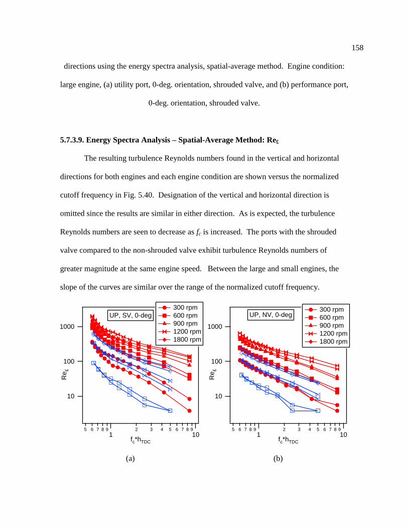
158

directions using the energy spectra analysis, spatial-average method. Engine condition:

large engine, (a) utility port, 0-deg. orientation, shrouded valve, and (b) performance port,

0-deg. orientation, shrouded valve.

5.7.3.9. Energy Spectra Analysis – Spatial-Average Method: Re£

The resulting turbulence Reynolds numbers found in the vertical and horizontal

directions for both engines and each engine condition are shown versus the normalized

cutoff frequency in Fig. 5.40. Designation of the vertical and horizontal direction is

omitted since the results are similar in either direction. As is expected, the turbulence

Reynolds numbers are seen to decrease as fc is increased. The ports with the shrouded

valve compared to the non-shrouded valve exhibit turbulence Reynolds numbers of

greater magnitude at the same engine speed. Between the large and small engines, the

slope of the curves are similar over the range of the normalized cutoff frequency.

10

100

1000

Re

£

5 6 7 8 9

12 3 4 5 6 7 8 9

10fc*hTDC

UP, SV, 0-deg

300 rpm

600 rpm

900 rpm

1200 rpm

1800 rpm

10

100

1000

Re

£

5 6 7 8 9

12 3 4 5 6 7 8 9

10fc*hTDC

UP, NV, 0-deg 300 rpm

600 rpm

900 rpm

1200 rpm

1800 rpm

(a) (b)

159

10

100

1000

Re

£

5 6 7 8 9

12 3 4 5 6 7 8 9

10fc*hTDC

UP, NV, 90-deg 300 rpm

600 rpm

900 rpm

1200 rpm

1800 rpm

10

100

1000

Re

£

5 6 7 8 9

12 3 4 5 6 7 8 9

10fc*hTDC

PP, SV, 0-deg

300 rpm

600 rpm

900 rpm

1200 rpm

1800 rpm

(c) (d)

10

100

1000

Re

£

5 6 7 8 9

12 3 4 5 6 7 8 9

10fc*hTDC

PP, NV, 0-deg 300 rpm

600 rpm

900 rpm

1200 rpm

1800 rpm

10

100

1000

Re

£

5 6 7 8 9

12 3 4 5 6 7 8 9

10fc*hTDC

PP, NV, 90-deg 300 rpm

600 rpm

900 rpm

1200 rpm

1800 rpm

(e) (f)

Figure 5.40: Turbulence Reynolds number versus normalized cutoff frequency in the


spatial-average method. Open symbol: small engine, filled symbol: large engine. Engine


port, (d) SV, 0-deg., (e) NV, 0-deg., (f) NV, 90-deg.

160

5.7.3.10. Energy Spectra Analysis – Spatial-Average Method: η

The resulting Kolmogorov lengthscales found in the vertical and horizontal

directions for both engines and each engine condition are shown versus the normalized

cutoff frequency in Fig. 5.41. Designation of the vertical and horizontal direction is

omitted since the results are similar in either direction. Examining the data, the

Kolmogorov lengthscales are seen to decrease with an increase in engine speed for a

given engine. This is because the turbulence Reynolds numbers increase with an increase

in engine speed. The ports with the shrouded valve compared to the non-shrouded valve

exhibit Kolmogorov lengthscales of smaller magnitude at the same engine speed, again

because the turbulence Reynolds numbers are greater for the ports with the shrouded

valve. Also, the Kolmogorov lengthscales are seen to increase as fc is increased, opposite

the trend of the turbulence Reynolds numbers.

100

80

60

40

20

0

η [

μm

]

5 6 7 8 9

12 3 4 5 6 7 8 9

10

fc*hTDC

UP, SV, 0-deg

300 rpm

600 rpm

900 rpm

1200 rpm

1800 rpm

100

80

60

40

20

0

η [

μm

]

5 6 7 8 9

12 3 4 5 6 7 8 9

10

fc*hTDC

UP, NV, 0-deg

300 rpm

600 rpm

900 rpm

1200 rpm

1800 rpm

(a) (b)

161

100

80

60

40

20

0

η [

μm

]

5 6 7 8 9

12 3 4 5 6 7 8 9

10

fc*hTDC

UP, NV, 90-deg

300 rpm

600 rpm

900 rpm

1200 rpm

1800 rpm

100

80

60

40

20

0

η [

μm

]

5 6 7 8 9

12 3 4 5 6 7 8 9

10

fc*hTDC

PP, SV, 0-deg

300 rpm

600 rpm

900 rpm

1200 rpm

1800 rpm

(c) (d)

100

80

60

40

20

0

η [

μm

]

5 6 7 8 9

12 3 4 5 6 7 8 9

10

fc*hTDC

PP, NV, 0-deg

300 rpm

600 rpm

900 rpm

1200 rpm

1800 rpm

100

80

60

40

20

0

η [

μm

]

5 6 7 8 9

12 3 4 5 6 7 8 9

10

fc*hTDC

PP, NV, 90-deg

300 rpm

600 rpm

900 rpm

1200 rpm

1800 rpm

(e) (f)

Figure 5.41: Kolmogorov lengthscales versus normalized cutoff frequency in the


spatial-average method. Open symbols: small engine, filled symbols: large engine.


Performance port, (d) SV, 0-deg., (e) NV, 0-deg., (f) NV, 90-deg.

162

At smaller fc the Kolmogorov lengthscales do not change greatly in magnitude

with a change in fc. Therefore, it was thought interesting to plot the Kolmogorov

lengthscales versus mean piston speed for a given value of the normalized cutoff

frequency to compare with the ensemble average method data from §5.7.3.5. Figure 5.42

shows the Kolmogorov lengthscales versus mean piston speed for the ensemble-average

method and the spatial-average method with a normalized cutoff frequency value of 0.7.

Figure 5.43 again compares the Komogorov lengthscales for both methods but with a

normalized cutoff frequency of 1.7 for the spatial-average data. Examining the figures,

the trend with mean piston speed is similar between the ensemble- and spatial-average

methods. The Kolmogorov lengthscales decrease monotonically with engine speed for

all engine conditions. The ports with the shrouded valve compared to the non-shrouded

valve exhibit Kolmogorov lengthscales of smaller magnitude at the same mean piston

speed. Between the small and large engines, the Kolmogorov lengthscales are roughly

the same for a given mean piston speed. There is slightly more scatter in the data with

the normalized cutoff frequency of 1.7 compared to 0.7, but there is still fairly good

agreement between the two engines for a given mean piston speed.

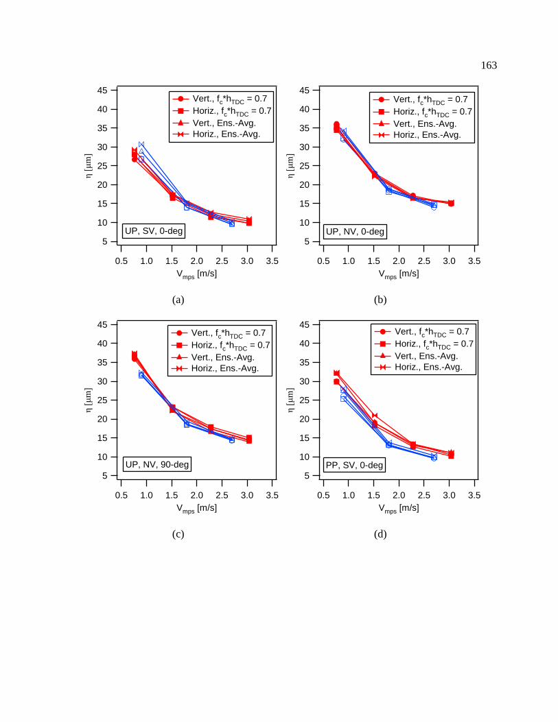
163

45

40

35

30

25

20

15

10

5

η [

μm

]

3.53.02.52.01.51.00.5

Vmps [m/s]

UP, SV, 0-deg

Vert., fc*hTDC = 0.7

Horiz., fc*hTDC = 0.7

Vert., Ens.-Avg.

Horiz., Ens.-Avg.

45

40

35

30

25

20

15

10

5

η [

μm

]

3.53.02.52.01.51.00.5

Vmps [m/s]

UP, NV, 0-deg



Vert., Ens.-Avg.

Horiz., Ens.-Avg.

(a) (b)

45

40

35

30

25

20

15

10

5

η [

μm

]

3.53.02.52.01.51.00.5

Vmps [m/s]

UP, NV, 90-deg



Vert., Ens.-Avg.

Horiz., Ens.-Avg.

45

40

35

30

25

20

15

10

5

η [

μm

]

3.53.02.52.01.51.00.5

Vmps [m/s]

PP, SV, 0-deg



Vert., Ens.-Avg.

Horiz., Ens.-Avg.

(c) (d)

164

45

40

35

30

25

20

15

10

5

η [

μm

]

3.53.02.52.01.51.00.5

Vmps [m/s]

PP, NV, 0-deg



Vert., Ens.-Avg.

Horiz., Ens.-Avg.

45

40

35

30

25

20

15

10

5

η [

μm

]

3.53.02.52.01.51.00.5

Vmps [m/s]

PP, NV, 90-deg



Vert., Ens.-Avg.

Horiz., Ens.-Avg.

(e) (f)





SV, 0-deg., (e) NV, 0-deg., (f) NV, 90-deg.

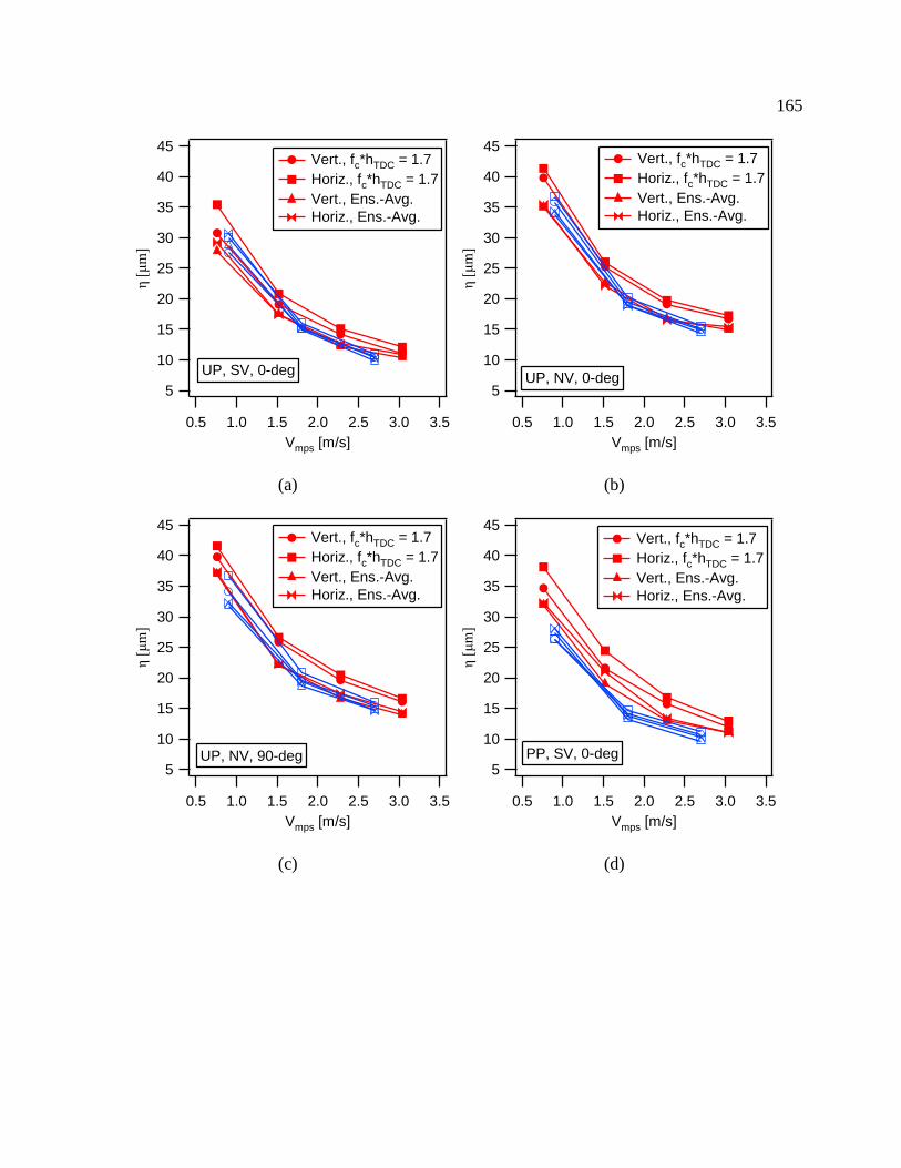
165

45

40

35

30

25

20

15

10

5

η [

μm

]

3.53.02.52.01.51.00.5

Vmps [m/s]

UP, SV, 0-deg



Vert., Ens.-Avg.

Horiz., Ens.-Avg.

45

40

35

30

25

20

15

10

5

η [

μm

]

3.53.02.52.01.51.00.5

Vmps [m/s]

UP, NV, 0-deg



Vert., Ens.-Avg.

Horiz., Ens.-Avg.

(a) (b)

45

40

35

30

25

20

15

10

5

η [

μm

]

3.53.02.52.01.51.00.5

Vmps [m/s]

UP, NV, 90-deg



Vert., Ens.-Avg.

Horiz., Ens.-Avg.

45

40

35

30

25

20

15

10

5

η [

μm

]

3.53.02.52.01.51.00.5

Vmps [m/s]

PP, SV, 0-deg



Vert., Ens.-Avg.

Horiz., Ens.-Avg.

(c) (d)

166

45

40

35

30

25

20

15

10

5

η [

μm

]

3.53.02.52.01.51.00.5

Vmps [m/s]

PP, NV, 0-deg



Vert., Ens.-Avg.

Horiz., Ens.-Avg.

45

40

35

30

25

20

15

10

5

η [

μm

]

3.53.02.52.01.51.00.5

Vmps [m/s]

PP, NV, 90-deg



Vert., Ens.-Avg.

Horiz., Ens.-Avg.

(e) (f)





SV, 0-deg., (e) NV, 0-deg., (f) NV, 90-deg.

5.8. Discussion

The turbulent flow field in the engine is inherently complicated because it is non-

stationary and susceptible to cyclic variations. This makes it difficult to unambiguously

define a mean velocity field about which to compile turbulence statistics. Because of the

spatial nature of the information available from PIV data, two methods were used to

define the mean velocity field. In the first, the ensemble average of a set of images was

performed to determine the mean velocity field. In the second, it is possible to define an

167

intra-cycle mean field based on a low-pass spatial filtering of the data akin to the

temporal filtering that was applied to cycle-resolved single-point velocity data from

HWA or LDV. This, however, introduces a bias associated with the choice of the cutoff

frequency. The approach that has been taken herein has been to characterize the results

as a function of the spatial cutoff frequency. This choice was made because the high-

magnification data have sufficient fidelity to allow a meaningful range of cutoff

frequency to be investigated.

It has long been understood that the large-scale flow field directly influences the

level of turbulence throughout the compression stroke of piston engines [5, 7, 16-18].

Studies have shown that there is a direct and nearly linear relationship between the in-

cylinder turbulence and the turbulent flame speed in spark-ignition engines [15, 48],

which directly impacts engine performance and emissions. It is, therefore, of great

importance to understand the bulk flow field and the resulting turbulence, and ultimately

their effect on the combustion process. Comparing the data from the ports with the

shrouded versus non-shrouded valves, the same large-scale flow field effect is apparent.

The ports with the shrouded valves produced higher levels of swirl as measured by the

steady flow bench tests and the PIV in-cylinder measurements during the compression

stroke. The engine conditions with higher swirl measured higher levels of turbulence

intensity.

Similar to previous studies, the turbulence intensity was found to be a linear

function of mean piston speed. Comparing the large and small engines for a given engine

condition, the turbulence intensity found using the ensemble average data (Fig. 5.12) was

nearly the same versus mean piston speed and the linear trend lines fit to the data also

168

indicated close similarity. The linear trend line data of the turbulence intensity found

using the spatial-average method also indicated close similarity when compared at the

same normalized cutoff frequency. Examining the shrouded valve linear trend data in

Fig. 5.14 at higher fc, there is a very slight difference between the small and large

engines. However, this difference is no more than that found examining Fig. 5.17 which

compares the two high-magnification FOVs in the large engine. As has been shown [36],

the flow field in an engine is nearly homogeneous, so it should be expected that a high

degree of similarity exists between the two high-magnification FOVs in the same engine.

That the magnitude of the difference in any of the data between the small and large

engines would be similar to the difference in the two high-magnification FOVs in the

large engine is encouraging and suggests dynamic similarity is achieved.

The integral lengthscale is an important parameter describing the flow field and in

the present study it has been calculated in two independent ways. First, two-point spatial

correlations were calculated from the data, and the longitudinal and transverse

lengthscales were found by direct integration of the correlations or through the use of a

best-fit equation. Secondly, the longitudinal integral length scale L11 was found by fitting

the experimental energy spectra to the model spectrum of Pope using the measured value

of k and employing Eqn. 5.18. Figure 5.44 shows the normalized L11 found using both

analyses and the ensemble-average definition of the mean flow. The two-point

correlation analysis gives L11 values roughly two to four times as large as the energy

spectra analysis. However, with the spatial-average method data (see Fig. 5.38), the

difference was dependent on the cutoff frequency. Figure 5.45 shows the normalized L11

found using both analyses and the spatial-average definition of the mean flow at a

169

normalized cutoff frequency of 1.7. Both analyses give lengthscales that are roughly

equal and there is good agreement in the data between the small and large engines.

1.0

0.8

0.6

0.4

0.2

0.0

L11 (S

pectr

a)

/ h

TD

C

1.00.80.60.40.20.0

L11 (Correlation) / hTDC

Vertical

Horizontal

One-to-One Line


analysis versus energy spectra analysis for the ensemble average method data. All engine

conditions. Open symbols: small engine, filled symbols, large engine.

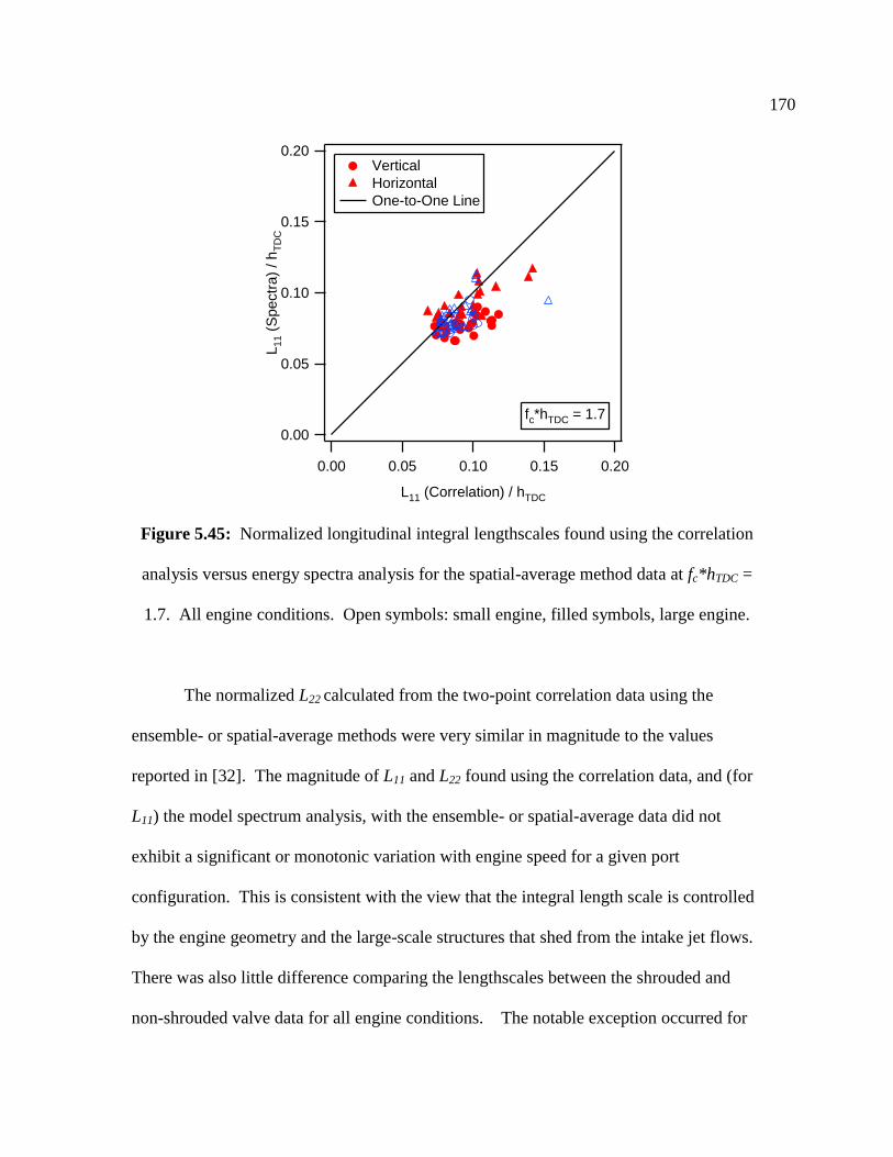
170

0.20

0.15

0.10

0.05

0.00

L11 (

Sp

ectr

a)

/ h

TD

C

0.200.150.100.050.00

L11 (Correlation) / hTDC

Vertical

Horizontal

One-to-One Line

fc*hTDC = 1.7


analysis versus energy spectra analysis for the spatial-average method data at fc*hTDC =

1.7. All engine conditions. Open symbols: small engine, filled symbols, large engine.

The normalized L22 calculated from the two-point correlation data using the

ensemble- or spatial-average methods were very similar in magnitude to the values

reported in [32]. The magnitude of L11 and L22 found using the correlation data, and (for

L11) the model spectrum analysis, with the ensemble- or spatial-average data did not

exhibit a significant or monotonic variation with engine speed for a given port

configuration. This is consistent with the view that the integral length scale is controlled

by the engine geometry and the large-scale structures that shed from the intake jet flows.

There was also little difference comparing the lengthscales between the shrouded and

non-shrouded valve data for all engine conditions. The notable exception occurred for

171

L11 found using the spatial-average two-point correlation data at small fc. This is more a

result of using the best-fit curve in determining L11, since L22, which was found directly

from the correlation data, did not vary between shrouded and non-shrouded cases across

the range of fc. Comparing the large and small engine data, L11 and L22 were similar

when normalized by hTDC and when compared at the normalized cutoff frequency for the

spatial-average data, again an indication that the integral lengthscale is controlled by the

engine geometry.

The values of L11 and L22 were found to agree quite well in the horizontal and

vertical directions, indicating a high level of isotropy. Further, for the ensemble average

correlation-derived data, the ratio L22/L11 was close to the isotropic limit of 0.5, further

supporting the view that in this pancake chamber the TDC turbulence is nearly isotropic.

For the spatial-average correlation-derived data, the ratio L22/L11 was dependent on fc,

where for large fc the ratio tended toward unity, and for smaller fc tended to be close to

0.5, but this again was dependent on using the best-fit curve to determine L11.

The turbulence Reynolds numbers for each engine condition were calculated by

fitting the energy spectra to Pope‟s model spectrum. For both ensemble- and spatial-

averaging methods, for a given engine condition at the same mean piston speed, the small

engine exhibited smaller turbulence Reynolds numbers compared to the large engine.

Also, according to the model energy spectrum function, at very high Reynolds number

the ratio L11/ £ tends asymptotically to a value of 0.43 where the rate of energy

dissipation, ε, scales as k3/2

/L11. Figure 5.46(a) shows the ratio of L11/£ as a function of

the Taylor-scale Reynolds number, Rλ, from [60]. The Taylor-scale Reynolds number is

defined as

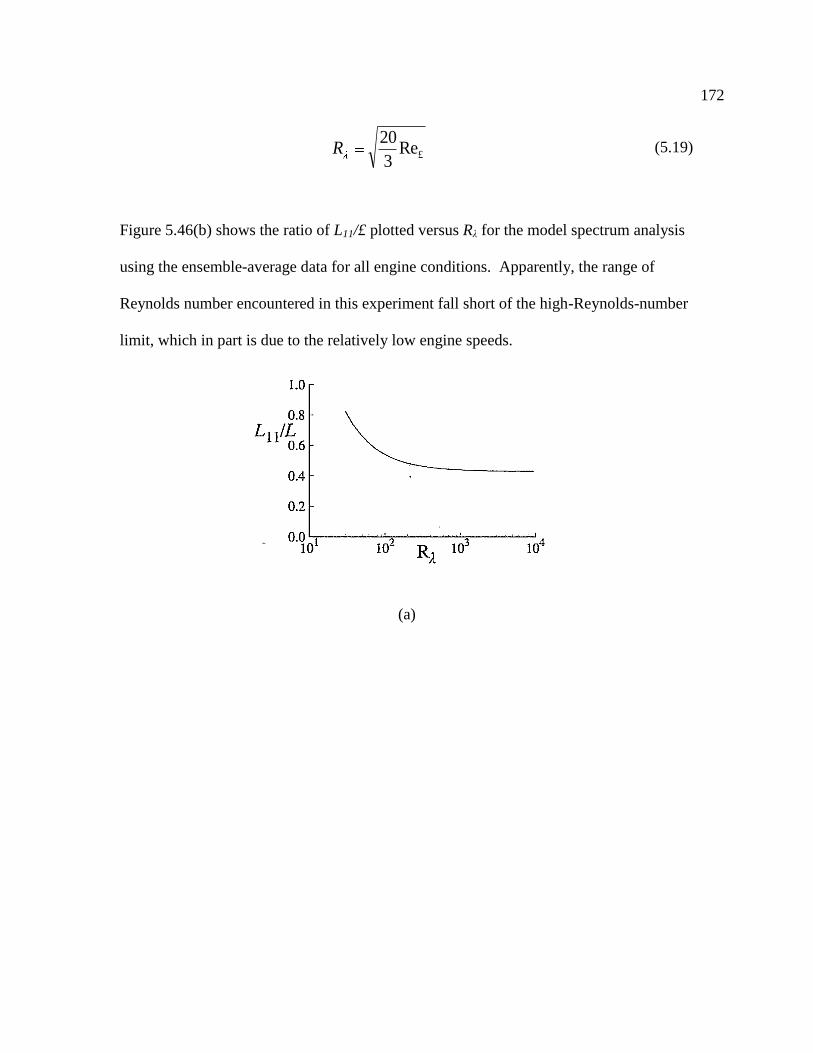
172

£Re3

20R (5.19)

Figure 5.46(b) shows the ratio of L11/£ plotted versus Rλ for the model spectrum analysis

using the ensemble-average data for all engine conditions. Apparently, the range of

Reynolds number encountered in this experiment fall short of the high-Reynolds-number

limit, which in part is due to the relatively low engine speeds.

(a)

173

1.0

0.8

0.6

0.4

0.2

0.0

L11/£

102 3 4 5 6

1002 3 4 5 6

1000

Rλ

Large Engine

Small Engine

High Rλ Asymptote

(b)

Figure 5.46: Ratio of L11/£ versus Rλ from (a) model spectrum [60] and (b) for all engine

conditions using model spectrum analysis with ensemble-average data.

To make a further comparison between the two-point correlation and energy

spectra analyses, a Reynolds number similar to Re£ (Eqn. 5.16) was calculated from L11

found using the correlation analysis with the ensemble average method data. This

Reynolds number, ReL11, is defined as

LRe 11

2/1

L11

k (5.20)

Figure 5.47 shows Re£ from the model spectrum versus ReL11 from the correlation

analysis for all engine conditions with the ensemble-average method data in both vertical

and horizontal directions. As is seen, ReL11 gives slightly larger values compared to Re£.

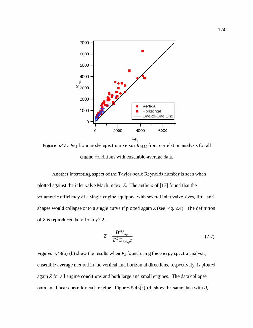
174

7000

6000

5000

4000

3000

2000

1000

0

Re

L1

1

6000400020000

Re£

Vertical

Horizontal

One-to-One Line

Figure 5.47: Re£ from model spectrum versus ReL11 from correlation analysis for all

engine conditions with ensemble-average data.

Another interesting aspect of the Taylor-scale Reynolds number is seen when

plotted against the inlet valve Mach index, Z. The authors of [13] found that the

volumetric efficiency of a single engine equipped with several inlet valve sizes, lifts, and

shapes would collapse onto a single curve if plotted again Z (see Fig. 2.4). The definition

of Z is reproduced here from §2.2.

cCD

VBZ

avgf

m ps

,2

2

(2.7)

Figures 5.48(a)-(b) show the results when Rλ found using the energy spectra analysis,

ensemble average method in the vertical and horizontal directions, respectively, is plotted

again Z for all engine conditions and both large and small engines. The data collapse

onto one linear curve for each engine. Figures 5.48(c)-(d) show the same data with Rλ

175

from the small engine conditions multiplied by the scaling factor, 1.69. This effectively

collapses the data from both engines onto a single curve. The implication of this is that

given an engine with a known Rλ versus Z curve, the curves for a whole family of similar

engines could be developed simply by determining Cf,avg for various intake port

geometries through steady flow bench testing. Of course, it is unclear how well this

relation would hold over a range of engine sizes and port types, given the limited number

of conditions used for this study.

180

160

140

120

100

80

60

40

20

Rλ

0.200.150.100.05

Z

PP, SV, 0-deg

PP, NV, 0-deg

PP, NV, 90-deg

UP, SV, 0-deg

UP, NV, 0-deg

UP, NV, 90-deg

Ensemble Average MethodVertical Direction

(a)

176

180

160

140

120

100

80

60

40

20

Rλ

0.200.150.100.05

Z

PP, SV, 0-deg

PP, NV, 0-deg

PP, NV, 90-deg

UP, SV, 0-deg

UP, NV, 0-deg

UP, NV, 90-deg

Ensemble Average MethodHorizontal Direction

(b)

180

160

140

120

100

80

60

40

20

Rλ(L

arg

e E

ngin

e),

Rλ(S

mall

Engin

e)*

1.6

9

0.200.150.100.05

Z

PP, SV, 0-deg

PP, NV, 0-deg

PP, NV, 90-deg

UP, SV, 0-deg

UP, NV, 0-deg

UP, NV, 90-deg

Ensemble Average MethodVertical Direction

(c)

177

180

160

140

120

100

80

60

40

20

Rλ(L

arg

e E

ngin

e),

Rλ(S

mall

Engin

e)*

1.6

9

0.200.150.100.05

Z

PP, SV, 0-deg

PP, NV, 0-deg

PP, NV, 90-deg

UP, SV, 0-deg

UP, NV, 0-deg

UP, NV, 90-deg

Ensemble Average MethodHorizontal Direction

(d)

Figure 5.48: Rλ calculated using the energy spectra analysis, ensemble average method

versus Z. Open symbol: small engine, filled symbol: large engine. (a) Vertical direction,

(b) horizontal direction. Small engine Rλ multiplied by the scaling factor 1.69, (c)

vertical direction, (d) horizontal direction.

The Kolmogorov lengthscales for each engine condition were calculated by fitting

the energy spectra to Pope‟s model spectrum. Analyses using the ensemble average data

or spatial-average data and comparing results at fc*hTDC of 0.7 and 1.7 both led to similar

results. Comparing the shrouded versus non-shrouded valves cases for a given engine,

the shrouded valves gave smaller Kolmogorov lengthscales for a given mean piston speed

as the turbulence Reynolds numbers were larger and related to the Kolmogorov

lengthscales according to η = £ Re£ -3/4

. Comparing the small and large engines, for a

178

given engine condition and at the same mean piston speed the Kolmogorov lengthscales

are roughly equal. When the integral lengthscale, Komogorov lengthscale, and

turbulence Reynolds number are all considered at once, it points to an interesting

dynamic in the energy cascade. The large-scale turbulence or integral lengthscales are

determined by the geometry of the engine, and so they scale by the size of the engine. At

the same mean piston speed, the turbulence Reynolds numbers of the small engine

compared to the large engine decreases in such a way that the small-scale turbulence or

Kolmogorov lengthscales are similar. The flows created by the shrouded versus non-

shrouded valves indicate higher turbulence Reynolds numbers, effectively pushing the

Kolmogorov lengthscales farther down the energy cascade to smaller lengthscales.

179

CHAPTER 6

SUMMARY AND CONCLUSIONS

6.1. Conclusions

In-cylinder velocity measurements were acquired in two geometrically scaled,

two-valve, single-cylinder research engines to study the bulk fluid motion and small-scale

turbulence. Different port geometries (two), different port orientations (two) and both

shrouded and non-shrouded intake valves were tested to vary the intake-generated flow.

Tests were performed at engine speeds of 300, 600, 900 and 1200 RPM for large engine

and 600, 1200, and 1800 RPM for the small engine with an atmospheric intake pressure.

Prior to testing on the engines, the different head configurations were tested on a steady

flow bench to quantify the similarity and magnitude of flow and swirl coefficients, and

the swirl ratios between the engines.

Low-magnification PIV data were used to characterize the bulk flow in the

cylinder of the two engines. The mean location of the swirl center and the mean angular

velocity were determined by fitting a solid-body profile to the flow. For a given engine

configuration, the swirl center locations were found to be relatively insensitive to engine

speed at a fixed crank angle time, but were found to precess about the chamber at

different crank angles in the cycle. Between the two engines, the swirl center locations,

scaled by the cylinder radii, were grouped in the same location in the cylinder at the same

crank angle time. At TDC, the swirl centers for all port configurations were found to be

located nearest to the cylinder axis. Dividing the angular velocity for a given port

configuration by the engine rotation rate was found to collapse the data from the multiple

engine speeds nearly onto a single curve; the curve did however vary from condition to

180

condition based on the steady-state swirl ratio of a configuration. The angular velocity

was largely found to decrease with crank angle due to wall friction. On average, for all

port configurations, the small engine produced a slightly lower normalized angular

velocity at TDC compared to the large engine. The angular rotation rate from the solid-

body fit was found to be in good agreement with the steady-state swirl ratio for high-

swirl conditions. At low-swirl conditions the in-cylinder angular velocity was found to

significantly exceed the steady-state value of swirl ratio.

High-magnification PIV data were used to characterize the turbulent statistics of

the flow using both an ensemble- and spatial-average method of defining the mean

velocity field. The turbulence intensity, calculated using either method, showed a high

degree of linearity with mean piston speed. The turbulence intensity versus mean piston

speed calculated using the ensemble average method showed fairly good agreement

between the small and large engines in both magnitude and linear slope. The turbulence

intensity calculated using the spatial-average method, over a range of cutoff frequencies,

was found to monotonically decrease with cutoff frequency. Again, there was good

agreement in the linear slopes for all port configurations between the small and large

engines over the range of cutoff frequencies when fc was normalized by hTDC.

Two-point correlations of the fluctuating velocity components were calculated to

determine 8 of the 27 possible integral length scales. The cross-velocity correlations 12

and 21 were close to zero for all separation distances as expected. The correlations

calculated in the single- and double-sided manner agreed well. The transverse correlation

data converged to zero at large separation distance for most cases, and allowed an

estimate of L22 by direct integration for all cases in the ensemble- and spatial-average

181

methods, but the longitudinal correlation data did not always fully converge to zero and,

thus, calculation of the longitudinal integral lengthscale required the extension of the data

using a best-fit function. When L11 and L22 found using the ensemble average method

data was normalized by hTDC, values were similar to those reported in [32, 35] whose

analysis was also based on the ensemble average method. Both the ensemble- and

spatial-average correlation data provided integral lengthscales that did not vary much

with engine speed. There was good agreement between the large and small engines when

the ensemble- and spatial-average correlation lengthscales were normalized by the TDC

clearance and when compared at the same normalized cutoff frequency for the spatial-

average method. To the author‟s knowledge, this is the first study to demonstrate how

the lengthscales scale by the scaling factor of the engines. There was close agreement in

the horizontal and vertical directions, indicating a high degree of isotropy in the flow

field. Further, the ratio L22/L11 on average for the ensemble-average correlation data was

found to be close to the isotropic limit of 0.5, although there was some scatter in the data.

Turbulent kinetic energy spectra found using the ensemble-average method were

presented. The spectra were found to be fit well by Pope's model spectrum, except at

higher wavenumbers where one would expect a discrepancy due to the limited spatial

resolution of the measurement. The higher engine speed data showed a pronounced

inertial range where the spectra were seen to acquire the traditional -5/3 wavenumber

power law dependence. However, at the lowest engine speeds, there was not a clearly

defined inertial range, suggesting that the turbulence is not fully developed and the

separation of large, energy-containing scales and the small scales at which viscosity

dominates is not complete. A similar effect was observed when the spatial-average

182

method was used with a high fc, and this may represent a practical limit to the choice of fc

in cycle-resolved analyses.

The fitting of the model spectrum to the data resulted in an estimate of £ and Re£,

and from these results the Kolmogorov scale and L11 can also be estimated. The

turbulence Reynolds number determined in the spectral fit was found to increase with

increasing engine speed whereas the longitudinal integral lengthscale, L11, was found to

be nearly constant with speed. There was also little difference in L11 when compared

between cases with the shrouded valve versus non-shrouded valve. Again, there was

good agreement between the large and small engines when the spectrally derived L11

found using the ensemble- and spatial-average methods were normalized by the TDC

clearance and when compared at the same normalized cutoff frequency for the spatial-

average method. The L11 estimates from the energy spectra fitting were found to be

approximately 2.5 smaller than the values determined from the two-point correlations

for the ensemble average data, but the difference varied over the range of cutoff

frequency between the two analyses for the spatial-average data. The Kolmogorov scale

decreased with increasing engine speed. The Kolmogorov scale was seen to be smaller in

magnitude for the shrouded valve versus non-shrouded valve at similar engine conditions.

When compared between the large and small engines at the same mean piston speed, the

Kolmogorov scale was nearly the same.

Using the energy spectra analysis and ensemble average data, the Taylor-scale

Reynolds number, Rλ, was defined and shown versus the inlet valve Mach index, Z, for

all engine conditions. When the Rλ found for the small engine conditions were multiplied

by the scaling factor, the data for both small and large engines collapsed onto a single

183

curve. It would be interesting if this relation held for a wider range of intake port

configurations, as this could be a good predictive tool.

6.2. Future Work

Future work for this study will include PLIF experiments to measurements in-

cylinder mixing. One of the advantages of PLIF over PIV measurements is increased

spatial resolution, where it has been shown [45] that spatial resolution down to a

lengthscale of ~30μm is possible. This resolution allows for more accuracy when

calculating statistics of the mixing. Energy spectra can be calculated and compared with

those from the PIV data. Experiments where the engines are skip-fired are planned.

These will expand upon the work done by Taylor [11] to include multiple port

configurations. The ability to relate the combustion details back to the PIV and PLIF

measurements wil help to detail more fully the physics of size-scaling in engines.

184

REFERENCES

[1] Purday, H.F.P.: Diesel Engine Design, D. Van Nostrand Co., New York, 1919.

[2] Lichty, L.C.: Internal Combustion Engines, 5th

ed., McGraw-Hill, New York, 1939.

[3] Witze, P.O.: “Measurements of the Spatial Distribution and Engine Speed

Dependence of Turbulent Air Motion in an I.C. Engine,” SAE paper 770220, SAE Trans,

v. 86, 1977.

[4] Rask, R.B.: “Laser Doppler Anemometer Measurements in an Internal Combustion

Engine,” SAE paper 790094, SAE Trans, v. 88, 1979.

[5] Liou, T.-M., and Santavicca, D.A.: “Cycle Resolved Turbulence Measurements in a

Ported Engine With and Without Swirl,” SAE paper 830419, SAE Trans, v. 92, 1983.

[6] Witze, P.O., Martin, J.K., and Borgnakke, C.: “Measurements and Predictions of the

Precombustion Fluid Motion and Combustion Rates in a Spark Ignition Engine,” SAE

paper 831697, SAE trans, v. 92, 1983.

[7] Liou, T.-M., Hall, M., Santavicca, D.A., and Bracco, F. V.: “Laser Doppler

Velocimetry Measurements in Valved and Ported Engines,” SAE paper 840375, SAE

Trans, v. 93, 1984.

[8] Hayder, M.E., Varma, A.K., and Bracco, F.V.: “A Limit to TDC Turbulence Intensity

in Internal Combustion Engines,” J. Propulsion and Power, v. 1, iss. 4, 1985.

[9] Bopp, S., Vafidis, C., and Whitelaw, J.H.: The Effect of Engine Speed on the TDC

Flowfield in a Motored Reciprocating Engine,” SAE paper 860023, SAE Trans, v. 95,

1986.

[10] Hall, M.J., and Bracco, F.V.: “A Study of Velocities and Turbulence Intensities

Measured in Firing and Motored Engines,” SAE paper 870453, SAE Trans, v. 96, 1987.

[11] Taylor, C.F.: “Effect of Size on the Design and Performance of Internal-Combustion

Engines,” Trans ASME, July, 1950.

[12] Taylor, C.F.: The Internal Combustion Engine in Theory and Practice, 2nd

Ed., MIT

Press, Cambridge, Massachusetts, 1966.

[13] Livengood, J.C., and Stanitz, J.B.: “The Effect of Inlet-Valve Design, Size, and Lift

on the Air Capacity and Output of a Four-Stroke Engine,” NACA Tech. Notes, no. 915,

1943.

185

[14] Lancaster, D.R., Krieger, R.B., Sorenson, S.C., and Hull, W.L.: “Effects of

Turbulence on Spark-Ignition Engine Combustion,” SAE paper 760160, SAE Trans, v.

85, 1976.

[15] Groff, E.G. and Matekunas, F.A.: “The Nature of Turbulent Flame Propagation in a

Homogeneous Spark-Ignited Engine,” SAE paper 800133, SAE Trans, v. 89, 1980.

[16] Dimopoulos, P. and Boulouchos, K.: “Turbulent Flow Field Characteristics in a

Motored Reciprocating Engine,” SAE paper 972833, SAE Trans, v. 106, 1997.

[17] Ikegami M., Shioji M., and Nishimoto K.: “Turbulence Intensity and Spatial Integral

Length Scale During Compression and Expansion Strokes in a Four Cycle Reciprocating

Engine,” SAE paper 870372, SAE Trans, v. 96, 1987.

[18] Hall, M.J., and Bracco, F.V.: “A Study of Velocities and Turbulence Intensities

Measured in Firing and Motored Engines,” SAE paper 870453, SAE Trans, v. 96, 1987.

[19] Winsor, R.E. and Patterson, D.J.: “Mixture Turbulence – A Key to Cyclic

Combustion Variation,” SAE paper 730086, SAE Trans, v. 82, 1973.

[20] Dimopoulos, P. and Boulouchos, K.: “Turbulence Parameters in a Motored Engine:

Influence of Intake Flow, Measurement Location and Engine Speed,” IEA TLM 93,

Baden, Germany, 1993.

[21] Dimopoulos, P., Schneider, B., and Boulouchos, K.: “Turbulent Flow Field in a

Motored Engine, Analysis of Coincident 3-D LDV Measurements,” IEA TLM 94,

Heidelberg, Germany, 1994.

[22] Corcione, F.E. and Valentino, G.: “Analysis of In-Cylinder Turbulent Air Motion

Dependence on Engine Speed,” SAE paper 940284, 1994.

[23] Dimopoulos, P. and Boulouchos, K.: “Reynolds Stress Components in the Flow

Field of a Motored Reciprocating Engine,” SAE paper 950725, 1995.

[24] Kang, K.Y. and Baek, J.H.: “Tumble Flow and Turbulence Characteristics in a

Small Four-Valve Engine,” SAE paper 960265, 1996.

[25] Dimopoulos, P. and Boulouchos, K.: “Turbulent Flow Field Characteristics in a

Motored Reciprocating Engine,” SAE paper 972833, SAE Trans, v. 106, 1997.

[26] Alger, T., McGee, J., Gallant, E., and Wooldridge, S.: “PIV In-Cylinder Flow

Measurements of Swirl and the Effect of Combustion Chamber Design,” SAE paper

2004-01-1952, 2004.

186

[27] Liou, T., and Santavicca, D.: “Cycle Resolved LDV Measurements in a Motored IC

Engine,” J. Fluids Engineering, v. 107, pp. 232-240, 1985.

[28] Dent, J. and Salama, N.: “The Measurement of Turbulence Characteristics in an

Internal Combustion Engine Cylinder,” SAE paper 750886, 1975.

[29] Lancaster, D.: “Effects of Engine Variables on Turbulence in a Spark-Ignition

Engine,” SAE paper 760159, 1976.

[30] Wakuri, Y., Kido, H., Murase, E., and Wang, Z.: “Variations of Turbulence Scales

in an Engine Cylinder and a Fine Structure Model of Isotropic Turbulence,” Memoirs of

the Faculty of Engineering, Kyushu Univ., v. 43, pp. 179-191, 1983.

[31] Ikegami, M., Shioji, M., Wei, D., and Sugiura, M.: “In-Cylinder Measurement of

Turbulence by Laser Homodyne Principle,” COMODIA 85 Symposium, Tokyo, pp. 115-

123, 1985.

[32] Fraser, R., Felton, P., Bracco, F., and Santavicca, D.: “Preliminary Turbulence

Length Scale Measurements in a Motored IC Engine,” SAE paper 860021, 1986.

[33] Fraser, R. and Bracco, F.: “Cycle-Resolved LDV Integral Length Scale

Measurements in an I.C. Engine,” SAE Paper 880381, 1988.

[34] Hong, C. and Tarng, S.: “Direct Measurement and Computational Analysis of

Turbulence Length Scales of a Motored Engine,” Experimental Thermal and Fluid

Science, v. 16, pp. 277-285, 1997.

[35] Funk, C., Sick, V., Reuss, D., and Dahm, W.: “Turbulence Properties of High and

Low Swirl In-Cylinder Flows,” SAE paper 2002-01-2841, 2002.

[36] Fraser, R. and Bracco, F.: “Cycle-Resolved LDV Integral Length Scale

Measurements Investigating Clearance Height Scaling, Isotropy, and Homogeneity in an

I.C. Engine,” SAE Paper 890615, 1989.

[37] Li, Y., Zhao, H., Peng, Z., and Ladommatos, N.: “Particle Image Velocimetry

Measurement of In-Cylinder Flow in Internal Combustion Engines – Experiment and

Flow Structure Analysis,” Proc Instn Mech Engrs, v. 216, part D, pp. 65-81, 2002.

[38] Li, Y., Zhao, H., and Ladommatos, N.: “Analysis of Large-Scale Flow

Characteristics in a Four-Valve Spark Ignition Engine,” J. Mechanical Engineering

Science, v. 216, pt. C, 2002.

[39] Reuss, D., Adrian, R., Landreth, C., French, D., and Fansler, T.: “Instantaneous

Planar Measurements of Velocity and Large-Scale Vorticity and Strain Rate in an Engine

Using Particle Image Velocimetry,” SAE Paper 890616, 1989.

187

[40] Ghandhi, J., Herold, R., Shakal, J., and Strand, T.: “Time Resolved Particle Image

Velocimetry Measurements in an Internal Combustion Engine,” SAE Paper 2005-01-

3868, 2005.

[41] Fajardo, C., and Sick, V.: “Kinetic Energy and Dissipation Rate Spectra of High-

and Low-Swirl Internal Combustion Engine Flows,” SAE Paper 2009-01-0651, 2009.

[42] Nordgren, H., Hildingsson, L, Johansson, B., Dahlen, L., and Konstanzer, D.:

“Comparison Between In-Cylinder PIV Measurements, CFD Simulations and Steady-

Flow Impulse Torque Swirl Meter Measurements,” SAE Paper 2003-01-3147, 2003.

[43] Zhang, L., Takahiro, U., Toshiaki, T., and Katsuhiko, Y.: “A Study of the Cycle-to-

Cycle Variation of In-Cylinder Flow in a Motored Engine Through Digital Image

Processing of Visualized Images,” SAE paper 950727, 1995.

[44] Bottom, K.: “PIV Measurements of In-Cylinder Flow and Correlation with Engine

Performance,” Ph.D. Thesis, University of Wisconsin – Madison, 2003.

[45] Petersen, B., Heim, D., and Ghandhi, J.: “High Resolution Scalar and Velocity

Measurements in an I.C. Engine,” J. Engineering for Gas Turbines and Power, v. 132, is.

9, 2010.

[46] Kaiser, S. and Frank, J.: “Imaging of dissipative structures in the near field of a

turbulent non-premixed jet flame,” Proc. Comb. Inst., v. 31, is. 1, pp. 1515-1523, 2007.

[47] Daneshyar, H., and Hill, P.: “The Structure of Small-Scale Turbulence and Its Effect

on Combustion in Spark-Ignition Engines,” Prog. Energy Combust. Sci., 13:47-73, 1987.

[48] Heywood, J.B.: Internal Combustion Engine Fundamentals, McGraw-Hill Cos.,

New York, 1988.

[49] Hill, P.G., and Zhang, D.: “The Effects of Swirl and Tumble on Combustion in

Spark-Ignition Engines,” Prog. Energy Combust. Sci., v. 20, pp. 373-429, (see p. 416),

1994.

[50] Son, J., Lee, S., Han, B., and Kim, W.: “A Correlation Between Re-defined Design

Parameters and Flow Coefficients of SI Engine Intake Ports,” SAE paper 2004-01-0998,

SAE Trans, v. 113, 2004.

[51] Puntambekar, A.: “Combustion and Spray Visualization in a High-Speed Direct

Injected Engine,” M.S. Thesis, University of Wisconsin – Madison, 2009.

[52] Melling, A.: “Tracer Particles and Seeding for Particle Image Velocimetry,”

Measurement Science and Technology, v. 8, pp. 1406-1416, 1997.

188

[53] Keane, R., and Adrian, R.: “Optimization of Particle Image Velocimeters. Part I:

Double Pulsed Systems,” Meas. Sci. Technol., v. 1, n. 11, pp. 1202-1215, 1990.

[54] Taylor, B. and Kuyatt, C.: “Guidelines for Evaluating and Expressing the

Uncertainty of NIST Measurement Results,” National Institute of Standards and

Technology Technical Note 1297, 1994.

[55] Stone, C., and Ladommatos, N.: “The Measurement and Analysis of Swirl in Steady

Flow,” SAE paper 921642, SAE Trans, v. 101, 1992.

[56] Heim, D. and Ghandhi, J.: “Investigation of Swirl Meter Performance,” (Submitted

to J. Automobile Engineering), 2011.

[57] Tanabe, S., Iwata, H., and Kashiwada, Y., “On Characteristics of Impulse Swirl

Meter,” Transactions of the Japan Society of Mechanical Engineers, Series B, pp. 1054-

1060, 1994.

[58] Tindal, M. and Williams, T., “An Investigation of Cylinder Gas Motion in the Direct

Injection Diesel Engine,” SAE paper 770405, 1977.

[59] Snauwaert, P. and Sierens, R., “Experimental Study of the Swirl Motion in Direct

Injection Diesel Engines Under Steady State Flow Conditions (by LDA),” SAE paper

860026, 1986.

[60] Pope, S.: Turbulent Flows, Cambridge University Press, Cambridge, UK, 2000.

189

APPENDIX A: VALVE LIFT PROFILE

This appendix contains the non-dimensional valve lift profile, as set forth in

Chapter 3.

Crank

Angle L/D

Crank

Angle L/D

Crank

Angle L/D

Crank

Angle L/D

Crank

Angle L/D

105 0.248 139 0.221814 173 0.144412 207 0.046234 241 0.010003

106 0.247977 140 0.220251 174 0.141474 208 0.044037 242 0.0096

107 0.247909 141 0.218643 175 0.13851 209 0.041916 243 0.0092

108 0.247796 142 0.21699 176 0.135523 210 0.039873 244 0.008799

109 0.247638 143 0.215292 177 0.132514 211 0.037909 245 0.008399

110 0.247434 144 0.213549 178 0.129486 212 0.036026 246 0.007999

111 0.247184 145 0.211761 179 0.12644 213 0.034224 247 0.0076

112 0.24689 146 0.209928 180 0.123379 214 0.032504 248 0.0072

113 0.24655 147 0.20805 181 0.120305 215 0.030866 249 0.0068

114 0.246165 148 0.206128 182 0.117221 216 0.029311 250 0.0064

115 0.245735 149 0.20416 183 0.11413 217 0.027836 251 0.006

116 0.245259 150 0.202148 184 0.111035 218 0.026442 252 0.0056

117 0.244738 151 0.200092 185 0.107938 219 0.025128 253 0.0052

118 0.244172 152 0.197992 186 0.104842 220 0.02389 254 0.0048

119 0.24356 153 0.195848 187 0.101751 221 0.022728 255 0.0044

120 0.242903 154 0.19366 188 0.098667 222 0.021639 256 0.004

121 0.242201 155 0.191428 189 0.095595 223 0.020621 257 0.0036

122 0.241453 156 0.189154 190 0.092537 224 0.019669 258 0.0032

123 0.24066 157 0.186836 191 0.089498 225 0.018782 259 0.0028

124 0.239822 158 0.184476 192 0.08648 226 0.017955 260 0.0024

125 0.238939 159 0.182074 193 0.083487 227 0.017184 261 0.002

126 0.23801 160 0.17963 194 0.080522 228 0.016466 262 0.0016

127 0.237036 161 0.177146 195 0.077591 229 0.015796 263 0.001225

128 0.236016 162 0.17462 196 0.074695 230 0.01517 264 0.0009

129 0.234952 163 0.172055 197 0.07184 231 0.014584 265 0.000625

130 0.233842 164 0.169451 198 0.069027 232 0.014033 266 0.0004

131 0.232686 165 0.166809 199 0.066262 233 0.013513 267 0.000225

132 0.231486 166 0.164129 200 0.063547 234 0.013019 268 0.0001

133 0.23024 167 0.161413 201 0.060887 235 0.012549 269 0.000025

134 0.228949 168 0.158661 202 0.058283 236 0.012097 270 0

135 0.227612 169 0.155875 203 0.05574 237 0.01166

136 0.22623 170 0.153055 204 0.053261 238 0.011234

137 0.224803 171 0.150204 205 0.050849 239 0.010818

138 0.223331 172 0.147322 206 0.048506 240 0.010408

Table A.1: Intake non-dimensional valve lift profile between 105 and 270 crank angle

degrees. The intake and exhaust profiles are identical and symmetric about the peak lift,

190

such that the exhaust profile can easily be deduced from this table, the valve inner seat

diameter, and the peak lift locations found in Table 3.3.

191

APPENDIX B: INTAKE PORT DRAWINGS

This appendix contains the engineering drawings of the intake ports, as set forth

in Chapter 3. Note: the drawings are in the non-standard first projection view, the default

setting in SolidWorks, as opposed to the standard third projection view.

Figure B.1: Large engine performance intake port engineering drawing.

192

Figure B.2: Side close-up view detailing flow path of large engine performance intake

port.

193

Figure B.3: Large engine utility intake port engineering drawing.

194

Figure B.4: Side close-up view detailing flow path of large engine utility intake port.

195

Figure B.5: Back close-up view detailing flow path of large engine utility intake port.

196

APPENDIX C: FLOW COEFFICIENTS AND UNCERTAINTY ANALYSIS

This appendix contains the flow coefficient data of the small and large heads, as

set forth in Chapter 4.

C.1. Flow Coefficients

0.8

0.7

0.6

0.5

0.4

0.3

0.2

0.1

0.0

Cf

2402101801501209060300-30

Crank Angle Degrees

PP, 0-deg., NV Large Head

Small Head

Large Head, Cf,avg

= 0.481

Small Head, Cf,avg

= 0.502

0.8

0.7

0.6

0.5

0.4

0.3

0.2

0.1

0.0

Cf

2402101801501209060300-30

Crank Angle Degrees

Large Head, Cf,avg

= 0.499

Small Head, Cf,avg = 0.481

PP, 90-deg., NV Large Head Small Head

(a) (b)

197

0.8

0.7

0.6

0.5

0.4

0.3

0.2

0.1

0.0

Cf

2402101801501209060300-30

Crank Angle Degrees

PP, 0-deg., SV Large Head Small Head

Large Head, Cf,avg = 0.303


(c)

Figure C.1: Flow coefficients versus crank angle degrees of performance port with non-


degree orientation.

0.8

0.7

0.6

0.5

0.4

0.3

0.2

0.1

0.0

Cf

2402101801501209060300-30

Crank Angle Degrees

UP, 0-deg., NV Large Head Small Head

Large Head, Cf,avg

= 0.446

Small Head, Cf,avg

= 0.462

0.8

0.7

0.6

0.5

0.4

0.3

0.2

0.1

0.0

Cf

2402101801501209060300-30

Crank Angle Degrees

Large Head, Cf,avg

= 0.430

Small Head, Cf,avg

= 0.434

UP, 90-deg., NV Large Head Small Head

(a) (b)

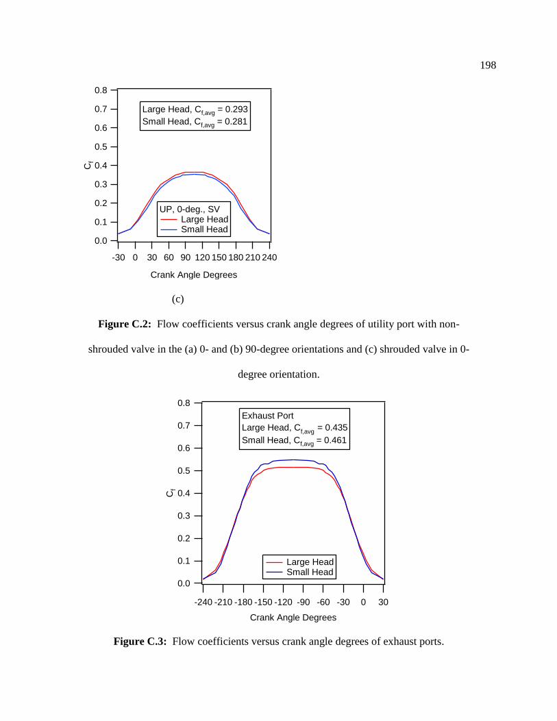
198

0.8

0.7

0.6

0.5

0.4

0.3

0.2

0.1

0.0

Cf

2402101801501209060300-30

Crank Angle Degrees

UP, 0-deg., SV Large Head Small Head

Large Head, Cf,avg = 0.293


(c)

Figure C.2: Flow coefficients versus crank angle degrees of utility port with non-


degree orientation.

0.8

0.7

0.6

0.5

0.4

0.3

0.2

0.1

0.0

Cf

-240 -210 -180 -150 -120 -90 -60 -30 0 30

Crank Angle Degrees


Exhaust Port

Large Head, Cf,avg

= 0.435


Figure C.3: Flow coefficients versus crank angle degrees of exhaust ports.

199

C.2. Flow Coefficient Uncertainty Analysis

A repeatability study was conducted to determine the uncertainty of the flow

coefficients for the ports with the non-shrouded valves. As the flow coefficient data were

seen to vary little with port position, the entire repeatability test was conducted using the

90-degree port orientation. Data were taken at four valve lifts, corresponding to 100, 78,

52, and 30% of maximum lift and at a pressure drop of 6.97 kPa. Data were acquired

over the course of two weeks so that changes in ambient room conditions would be

present. The engine heads were also removed from the flow bench and re-attached and

the port positions re-aligned before each test so that operator-related variability would be

present.

The uncertainty of the flow coefficients was obtained by statistically analyzing

the data. The sample mean value of the flow coefficients, fC , was calculated as:

N

iff iC

NC

1

)(1

(C.1)

where N is the number of samples, equal to 11 for this repeatability study. The flow

coefficient sample standard deviation, SCf, was calculated as:

2

1

))((1

1ff

N

iCf CiC

NS . (C.2)

A normal distribution of the data was assumed and the uncertainty for a two-sided, 95%

confidence interval on the mean was calculated as:

N

Stu

Cf

NCf 1,2/ (C.3)

200

where α is the probability of making a type-I error, set equal to 0.05, and 1,2/ Nt is the

value of the test statistic for a t-probability distribution, equal to 2.228. Table C.1

contains the uncertainty results for the large and small heads listed for each non-

dimensional lift, L/D, and Figs C.4 and C.5 show the uncertainty as a confidence interval

on the sample mean flow coefficient. As can be seen, the uncertainty and variability is

small compared to the magnitude of the sample mean flow coefficients.


L/D Performance

Port, uCf

Utility Port,

uCf

Performance

Port, uCf

Utility Port,

uCf

0.075 0.001 0.001 0.002 0.002

0.129 0.002 0.003 0.003 0.003

0.194 0.002 0.001 0.003 0.003

0.248 0.008 0.002 0.002 0.003

Table C.1: Uncertainty of the sample mean flow coefficients for ports with non-

shrouded valves in 90-degree orientation.

0.8

0.7

0.6

0.5

0.4

0.3

0.2

0.1

0.0

Sam

ple

Mean C

f

0.300.250.200.150.100.05

L/D

Small Head Large Head

Performance Port, 90-degree Orientation, NV11 Samples, 95% Confidence Interval

Figure C.4: Uncertainty on the sample mean flow coefficients for the performance

ports, 90-degree orientation, non-shrouded valves.

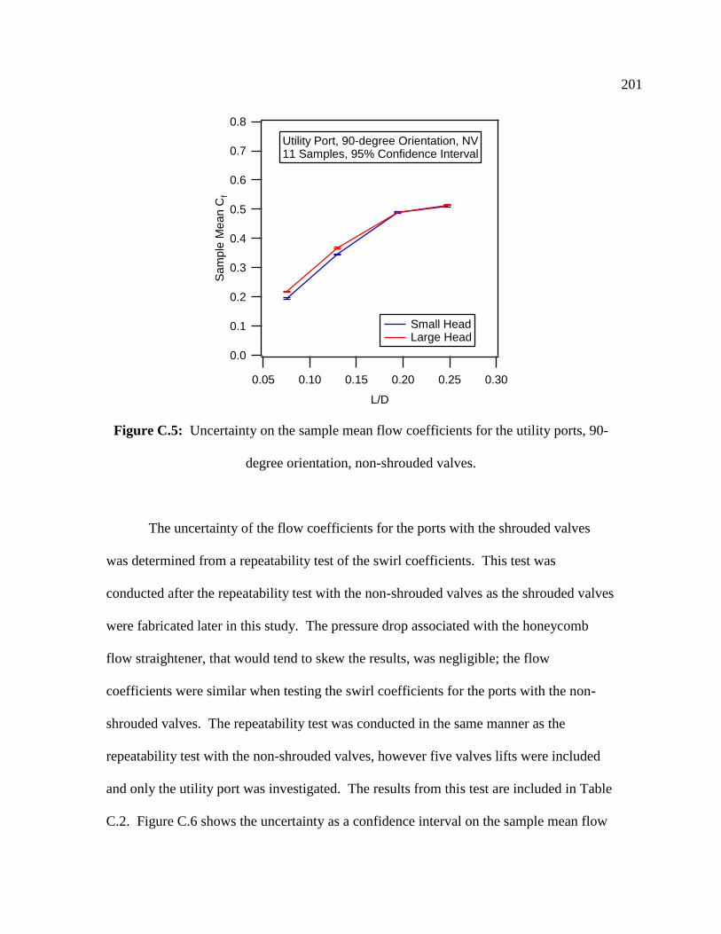
201

0.8

0.7

0.6

0.5

0.4

0.3

0.2

0.1

0.0

Sam

ple

Mean C

f

0.300.250.200.150.100.05

L/D

Utility Port, 90-degree Orientation, NV11 Samples, 95% Confidence Interval

Small Head Large Head


degree orientation, non-shrouded valves.

The uncertainty of the flow coefficients for the ports with the shrouded valves

was determined from a repeatability test of the swirl coefficients. This test was

conducted after the repeatability test with the non-shrouded valves as the shrouded valves

were fabricated later in this study. The pressure drop associated with the honeycomb

flow straightener, that would tend to skew the results, was negligible; the flow

coefficients were similar when testing the swirl coefficients for the ports with the non-

shrouded valves. The repeatability test was conducted in the same manner as the

repeatability test with the non-shrouded valves, however five valves lifts were included

and only the utility port was investigated. The results from this test are included in Table

C.2. Figure C.6 shows the uncertainty as a confidence interval on the sample mean flow

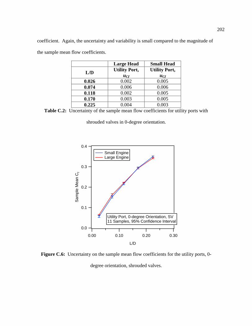
202

coefficient. Again, the uncertainty and variability is small compared to the magnitude of

the sample mean flow coefficients.


L/D Utility Port,

uCf

Utility Port,

uCf

0.026 0.002 0.005

0.074 0.006 0.006

0.118 0.002 0.005

0.170 0.003 0.005

0.225 0.004 0.003

Table C.2: Uncertainty of the sample mean flow coefficients for utility ports with

shrouded valves in 0-degree orientation.

0.4

0.3

0.2

0.1

0.0

Sam

ple

Mean C

f

0.300.200.100.00

L/D

Small Engine Large Engine

Utility Port, 0-degree Orientation, SV11 Samples, 95% Confidence Interval


degree orientation, shrouded valves.

203

The propagation method of [54] was used to calculate a single uncertainty, uCf,avg,

for Cf,avg. In this method, uCf,avg, is defined as:

.2

2

,

, ifavgf

C

i if

avgf

C uC

Cu (C.4)

The uncertainty for each Cfi (i.e. at each valve lift tested) is assumed equal to the

uncertainty at the next highest valve lift determined from the repeatability test.

204

APPENDIX D: SWIRL COEFFICIENT AND SWIRL RATIO UNCERTAINTY

ANALYSIS

This appendix contains the swirl coefficient and swirl ratio uncertainty data of the

small and large heads, as set forth in Chapter 4.

D.1. Swirl Coefficient Uncertainty Analysis

A repeatability study was conducted to determine the uncertainty of the swirl

coefficients for the ports with the shrouded and non-shrouded valves. The swirl

coefficient data were seen to vary little by port type and it was assumed that the

uncertainty would be similar between the two ports. The repeatability test was conducted

with the shrouded valve using the utility port in the 0-degree port orientation and with the

non-shrouded valve using the performance port in the 0-degree port orientation. Data

were taken at five different valve lifts and at a pressure drop of 6.97 kPa. Data were

acquired over the course of two weeks so that changes in ambient room conditions would

be present. The engine heads were also removed from the flow bench and re-attached

and the port positions re-aligned before each test so that operator-related variability

would be present.

The uncertainty of the swirl coefficients was obtained by statistically analyzing

the data. The sample mean value of the swirl coefficients, sC , was calculated as:

N

iss iC

NC

1

)(1

(D.1)

where N is the number of samples, equal to 11 for this repeatability study. The swirl

coefficient sample standard deviation, SCs, was calculated as:

205

2

1

))((1

1ss

N

iCs CiC

NS . (D.2)

A normal distribution of the data was assumed and the uncertainty for a two-sided, 95%

confidence interval on the mean was calculated as:

N

Stu Cs

NCs 1,2/ (D.3)

where α is the probability of making a type-I error, set equal to 0.05, and 1,2/ Nt is the

value of the test statistic for a t-probability distribution, equal to 2.228. Table D.1

contains the uncertainty results for the large and small heads listed for each non-

dimensional lift, L/D, and Figs. D.1 and D.2 show the uncertainty as a confidence interval

on the sample mean swirl coefficient. As can be seen for the shrouded valves, Fig. D.1,

the uncertainty overlaps at the higher valves lifts where most of the air mass enters the

engine cylinder, but at the lower valve lifts the uncertainty of the small head grows. As

can be seen for the non-shrouded valves, Fig. D.2, the swirl coefficients of both heads are

low in magnitude and the uncertainties are fairly small.

206


L/D

Utility Port,

Shrouded

Valve

Performance

Port, Non-

shrouded

Valve

Utility Port,

Shrouded

Valve

Performance

Port, Non-

shrouded

Valve

0.026 0.014 0.008 0.185 0.037

0.074 0.014 0.011 0.056 0.015

0.118 0.010 0.046 0.061 0.015

0.170 0.009 0.007 0.035 0.009

0.225 0.012 0.005 0.031 0.010

Table D.1: Uncertainty of the sample mean swirl coefficients for the ports in the 0-

degree orientation.

-0.8

-0.6

-0.4

-0.2

0.0

0.2

0.4

Sa

mp

le M

ean

Cs

0.250.200.150.100.050.00

L/D

Utility Port, 0-degree Orientation, SVOpen Symbol: Small HeadFilled Symbol: Large Head

Figure D.1: Uncertainty of the sample mean swirl coefficients for the utility ports, 0-

degree orientation, shrouded valves.

207

-0.3

-0.2

-0.1

0.0

0.1

0.2

Sa

mp

le M

ean

Cs

0.250.200.150.100.050.00

L/D

Performance Port, 0-degree Orientation, NVOpen Symbol: Small HeadFilled Symbol: Large Head

Figure D.2: Uncertainty of the sample mean swirl coefficients for the performance

ports, 0-degree orientation, non-shrouded valves.

D.2. Swirl Ratio Uncertainty Analysis

The propagation method of [54] was again used to calculate a single uncertainty,

uRs, for Rs. In this method, since there is uncertainty in both the flow and swirl

coefficients, uRs is defined as:

.2

2

2

2

ii Cf

i if

sCs

i is

sRs u

C

Ru

C

Ru (D.4)

Again, the uncertainty for each Cfi and Csi (i.e. at each valve lift tested) is assumed equal

to the uncertainty at the next highest valve lift determined from the repeatability test.

208

APPENDIX E: MATLAB CODE

E.1. MATLAB Code to Calculate the Low-Magnification FOV Swirl Center and

Angular Velocity

clear all; %----------------User Inputs--------------- % note: change process number (e.g. P001) below depending on % process number in Insight3G. This file works only for exporting the %2nd choice vectors into the .vec file. %Directory and first part of name of .vec files from TSI's Insight3G: Vector_file='C:\Experiments7\Small_engine_full_FOV\SUshroud\Analysis\11

3010_600rpm_SUshroud_90bTDC_50us_'; numb=50; %number of vector files to load per set %m_pixel=44.28e-6; %meters per pixel, large engine m_pixel=26.04e-6; %meters per pixel, small engine vector_spacing=16;%pixels separating each velocity vector (evenly

spaced) omega1=0; %[rad/s], lower bound initial guess for angular rotation rate omega3=1000; %[rad/s], upper bound initial guess angular rotation rate omega_tol=0.1; %set the omega tolerance when searching for the correct %omega that minimizes the SSE %---------------End User Inputs---------------- for i=1:numb %read in the set of data if i<10 %loop is used in the naming scheme for each file q=10000; elseif i<100 q=1000; else q=100; end %sets the vector file name into a variable

Vector_name=[Vector_file,num2str(q),num2str(i),'.T001.D001.P003.H001.L.

vec']; fid = fopen(Vector_name, 'r'); %ignores the first line text, reads in the data data = textscan(fid, '%n, %n, %n, %n, %n', 'headerlines', 1); for j=1:5 %Five columns of data to save, the columns are the pixel %location, the vector x and y velocity, and the choice code %Save data into 3D matrix for all vector files Total(:,j,i)=data{:,j}; end status = fclose(fid); %close the reading of the .vec file end %this uses both good and interpolated vectors to find the mean Total_mean(:,:)=mean(Total,3); %Calculates the mean at each vector %location, 3 denotes the matrix dimension on which to calculate. %Note: image imported from Insight3G must have origin at lower left

hand %corner. Then, Total has x in first column, y in second column, where

209

%x increments each time, y starts with largest value and decrements %(e.g. [1 20...;2 20...;320...;1 19...; etc.] %The below code is setup for this format. m=63; %initialize x direction row counter n=1; %initialize y direction column counter number_rows=5040; % note: for 32x32 pixel interrogation region, % 80 rows equals 1 image row, 5040 total rows. U_mean=zeros(m,80); V_mean=zeros(m,80); Choice_code=zeros(m,80); x_matrix=zeros(m,80); y_matrix=zeros(m,80); %preallocate for speed for j=1:number_rows %manually input rows to process (Insight3G does %NOT give a regular square of vectors, so this input process %cannot be totally automated) U_mean(m,n)=Total_mean(j,3);%create matrix with mean u velocity V_mean(m,n)=Total_mean(j,4);%create matrix with mean v velocity Choice_code(m,n)=Total(j,5,1);%save a matrix with the Insight3G %choice codes from first individual image, only care about -2 %code where there was no vectors (processing) x_matrix(m,n)=Total(j,1,1); %save x and y locations to matrices y_matrix(m,n)=Total(j,2,1); n=n+1; if j==number_rows elseif Total(j+1,2,1)<Total(j,2,1) m=m-1; %if y position decrements, then reset column counter, %increase row counter n=1; end end %use the golden search method to find omega (angular rotation rate) %that minimizes the SSE, this bracketing method follows the UCSD %MAE290A course materials book, p.51 evals=0; %interation loop counter initialization Z=sqrt(5)-2; %initialize goldend section ratio omega2=omega1+(omega3-omega1)*0.381966; %set omega2 for golden ratio %call function three times [SSE_min1]=Compute_SSE_min(U_mean, V_mean, x_matrix, y_matrix,

Choice_code, omega1); [SSE_min2]=Compute_SSE_min(U_mean, V_mean, x_matrix, y_matrix,

Choice_code, omega2); [SSE_min3]=Compute_SSE_min(U_mean, V_mean, x_matrix, y_matrix,

Choice_code, omega3); while (abs(omega3-omega1) > omega_tol) omega4 = omega2+Z*(omega3-omega1); %compute the new omega4 %call function [SSE_min4]=Compute_SSE_min(U_mean, V_mean, x_matrix, y_matrix,

Choice_code, omega4); evals=evals+1 %loop counter %SSE_min2 if (SSE_min4>SSE_min2) omega3=omega1; SSE_min3=SSE_min1; %center new triplet on x2 %omega2=omega2; SSE_min2=SSE_min2; omega1=omega4; SSE_min1=SSE_min4; else omega1=omega2; SSE_min1=SSE_min2; %center new triplet on x2 %omega3=omega3; SSE_min3=SSE_min3;

210

omega2=omega4; SSE_min2=SSE_min4; end end % figure,contourf(V_mean); % title({'V_mean'}) % colorbar('location','EastOutside') omega=omega2; %calculate SSE countour using omega that minimizes the

SSE SSE=zeros(63,80); %initialize sum square error matrix, %will find min of processed area below for i=1:63 %rows %find the points that have vectors to set as the %swirl center test point for j=1:80 %columns %make sure a vector was calculated at this position if Choice_code(i,j) ~= -2 SSE_sum=0; %reset sum of SSE to zero at start of each loop x_center=x_matrix(i,j); %set x and y for the center point y_center=y_matrix(i,j); for k=1:63 %rows %go through each point, finding where the %vectors are, this is the outer point, to calculate Vr for l=1:80 %columns %make sure a vector was calculated at this position if Choice_code(k,l) ~= -2 x_outer=x_matrix(k,l); %set x for outer point y_outer=y_matrix(k,l); %set y for outer point %calculate x and y velocity components given %omega, divide by 1000 to convert from mm to m Vr_x=-omega*(y_outer-y_center)/1000; Vr_y=omega*(x_outer-x_center)/1000; %calculate the squared error between center and %outer points SSE_outerpoint=(U_mean(k,l)-

Vr_x)^2+(V_mean(k,l)-Vr_y)^2; %add to SSE_sum for each outer point SSE_sum=SSE_sum+SSE_outerpoint; end end end %for center point tested, assign sum squared error to SSE SSE(i,j)=SSE_sum; end end end figure,contourf(SSE); title({'SSE'}) xlabel('Data Columns', 'FontWeight', 'Bold' ); ylabel('Data Rows', 'FontWeight', 'Bold' ); colorbar('location','EastOutside') %find min value in SSE while ignoring the points where no vectors occur min_start=0; %use as way to set min value to first SSE value checked x_column=0; %initialize at zero y_row=0; for i=1:63 %row for j=1:80 %column %make sure vector was calculated at this position

211

if Choice_code(i,j) ~= -2 if min_start == 0 SSE_min=SSE(i,j); %set min to the first value checked %set value=1 so that "if statement" isn't used anymore min_start = 1; %save column and row of place where minimum occurs x_column=j; y_row=i; else if SSE(i,j)<SSE_min %reset SSE_min, x,y locations if new minimum found SSE_min=SSE(i,j); SSE_min_x=x_matrix(i,j); SSE_min_y=y_matrix(i,j); %save column, row of place where minimum occurs x_column=j; y_row=i; end end end end end SSE_min %print to screen, minimum sum squared error SSE_min_x %x location of min SSE SSE_min_y %y location of min SSE omega %angular rotation rate %having found omega, x, y of the swirl center, compute and plot %the solid body velocity profile %initialize solid body velocity matrices for speed Vx_body=zeros(63,80); Vy_body=zeros(63,80); V_mag=zeros(63,80); %find the points that have vectors to set as swirl center test point for i=1:63 %rows for j=1:80 %columns %make sure a vector was calculated at this position if Choice_code(i,j) ~= -2 %calculate the x and y velocity components given omega, %divide by 1000 to convert from mm to meters Vx_body(i,j)=-omega*(y_matrix(i,j)-SSE_min_y)/1000; Vy_body(i,j)=omega*(x_matrix(i,j)-SSE_min_x)/1000; %velocity magnitude V_mag(i,j)=(Vx_body(i,j)^2+Vy_body(i,j)^2)^0.5; end end end figure,contourf(x_matrix,y_matrix,V_mag); %caxis([0 5]) hold on %# denotes arrow length, k makes the arrows black quiver(x_matrix,y_matrix,Vx_body,Vy_body, 3, 'k') hold off xlabel(' x [mm] [m/s]', 'FontWeight', 'Bold' ); ylabel('y [mm]', 'FontWeight', 'Bold' ); colorbar('location','EastOutside'); %this next loop figures out the center x and y for the FOV lim_start=0; %use as a way to set starting point for i=1:63 %row

212

for j=1:80 %column %make sure a vector was calculated at this position if Choice_code(i,j) ~= -2 if lim_start == 0 x_min=x_matrix(i,j); %set the first x_min x_max=x_matrix(i,j); %set the first x_max y_min=y_matrix(i,j); %set the first y_min y_max=y_matrix(i,j); %set the first y_max % set value=1 so this if statement isn't used anymore lim_start = 1; else %test each point to find the mins and maxs if x_matrix(i,j) < x_min x_min=x_matrix(i,j); end if x_matrix(i,j) > x_max x_max=x_matrix(i,j); end if y_matrix(i,j) < y_min y_min=y_matrix(i,j); end if y_matrix(i,j) > y_max y_max=y_matrix(i,j); end end end end end x_center=(x_max+x_min)/2 %find, print the center points, in [mm] y_center=(y_max+y_min)/2

E.2. MATLAB Code to Calculate the Turbulence Intensity of the Ensemble Average

Data

clear all; %----------------User Inputs--------------- %note: need to change process number (e.g. P001) below depending on %process number in Insight3G. This file works only for exporting the %2nd choice vectors into the .vec file. %Directory and first part of name of .vec files from TSI's Insight3G: Vector_file='C:\Experiments7\Engine_small_FOV\LUshroud_14psi\Analysis\0

32910_LUshroud_1200rpm_TDC_SFOV_6jet35psi10usf22_final_'; numb=200; %number of vector files to load per set vector_spacing=16; %pixels separating each velocity vector(evenly

spaced) %---------------End User Inputs---------------- for i=1:numb %read in the set of data if i<10 %if loop is used in the naming scheme for each file q=10000; elseif i<100

213

q=1000; else q=100; end %sets the vector file name into a variable

Vector_name=[Vector_file,num2str(q),num2str(i),'.T001.D001.P005.H001.L.

vec']; fid = fopen(Vector_name, 'r'); %ignores the first line text, reads in the data data = textscan(fid, '%n, %n, %n, %n, %n, %n, %n', 'headerlines',

1); for j=1:5 %five columns of data to save, columns are pixel %location, vector x and y velocity, and the choice code %save data into 3D matrix for all vector files Total(:,j,i)=data{:,j}; end status = fclose(fid); %close the reading of the .vec file end %determine number of rows in Total matrix [Total_rows, Total_columns]=size(Total(:,:,1)); %this loop calculates mean velocity at each vector location using only %"good" vectors for jjj=1:Total_rows %this loop calculates mean velocity at each %vector location using only "good" vectors Total_sum_good_x=0; %reset at start of each loop, x velocity sum Total_sum_good_y=0; %reset at start of each loop, y velocity sum count_Total_sum=0; %reset at start of each loop for i=1:numb %for each vector location, if choice code is 1 %or 2, increase the sum and count if Total(jjj,5,i)==1 Total_sum_good_x=Total_sum_good_x+Total(jjj,3,i); Total_sum_good_y=Total_sum_good_y+Total(jjj,4,i); count_Total_sum=count_Total_sum+1; elseif Total(jjj,5,i)==2 Total_sum_good_x=Total_sum_good_x+Total(jjj,3,i); Total_sum_good_y=Total_sum_good_y+Total(jjj,4,i); count_Total_sum=count_Total_sum+1; end end %find the mean x and y velocity of only good vectors Total_mean(jjj,1)=Total_sum_good_x/count_Total_sum; Total_mean(jjj,2)=Total_sum_good_y/count_Total_sum; end for i=1:numb Total_fluct(:,1,i)=Total(:,1,i); %copies over x location Total_fluct(:,2,i)=Total(:,2,i); %copies over y location %subtract mean from total to find fluctuating u velocity Total_fluct(:,3,i)=Total(:,3,i)-Total_mean(:,1); %subtract mean from total to find fluctuating v velocity Total_fluct(:,4,i)=Total(:,4,i)-Total_mean(:,2); Total_fluct(:,5,i)=Total(:,5,i);%copies over choice code for vector end [rows_total cols_total]=size(Total(:,:,1)); %read size of vector files

214

%note: image imported from Insight3G must have origin at lower left

hand corner. Then, Total has x in first column, y in second column, %where x increments each time, y starts with largest value and %decrements (e.g. [1 20...;2 20...;3 20...;1 19...; etc.] The below %code is setup for this format. for i=1:numb m=61; %initialize x direction row counter n=1; %initialize y direction row counter number_rows=5040; %note: For 32x32 pixel interrogation region, 80 rows equals 1 %image row, 5040 total rows. %For 16x16 pixels, 161 rows equals 1 image row, 20447 total rows %manually input rows to process (Insight3G does NOT give a regular %square of vectors, so input process cannot be totally automated) for j=161:number_rows %computes fluctuating (turbulent) kinetic energy, assumes

%isotropy multiply by 3/2 to get 3D fluctuating kinetic energy

KE_fluct(m,n,i)=(1/2)*(Total_fluct(j,3,i)^2+Total_fluct(j,4,i)^

2)*(3/2);

%create matrix with fluctuating u component of velocity U_fluct(m,n,i)=Total_fluct(j,3,i); %create matrix with fluctuating v component of velocity V_fluct(m,n,i)=Total_fluct(j,4,i); %create matrix with mean u component of velocity U_mean(m,n)=Total_mean(j,1); %create matrix with mean v component of velocity V_mean(m,n)=Total_mean(j,2);

%create matrix with x location x_location(m,n)=Total_fluct(j,1,1);

%create matrix with y location y_location(m,n)=Total_fluct(j,2,1); %save a matrix with the Insight3G choice codes Choice_code(m,n,i)=Total_fluct(j,5,i); n=n+1; if j==number_rows elseif Total_fluct(j+1,2,i)<Total_fluct(j,2,i) m=m-1; %if y position decrements, then reset column

%counter, increase row counter

n=1; end end end %this part gets rid of RHS and LHS columns with no vector data KE_fluct_save=KE_fluct; U_fluct_save=U_fluct; V_fluct_save=V_fluct;

Choice_code_save=Choice_code; U_mean_save=U_mean;V_mean_save=V_mean; x_location_save=x_location; y_location_save=y_location; clear KE_fluct U_fluct V_fluct Choice_code U_mean V_mean x_location

y_location; KE_fluct=KE_fluct_save(:,3:80,:); U_fluct=U_fluct_save(:,3:80,:); V_fluct=V_fluct_save(:,3:80,:);Choice_code=Choice_code_save(:,3:80,:); U_mean=U_mean_save(:,3:80,:); V_mean=V_mean_save(:,3:80,:); x_location=x_location_save(:,3:80,:);

y_location=y_location_save(:,3:80,:); %figure out size of new matrices

215

[rows_choice cols_choice]=size(Choice_code(:,:,1));

----E.2. Reference 1---- %initialize size of matrix U_fluct_EA_field_sum=zeros(rows_choice, cols_choice);

%this next code calculates turbulence intensity of entire FOV chosen for i=1:numb %square each u fluctuating component U_fluct_squared(:,:,i)=U_fluct(:,:,i).^2; %square each v fluctuating component V_fluct_squared(:,:,i)=V_fluct(:,:,i).^2; %magnitude of fluctuating component squared Fluct_squared(:,:,i)=U_fluct_squared(:,:,i)+V_fluct_squared(:,:,i); end %this next part of the code calculates the turb intensity, mean %squared u fluct, and mean square v fluct, using only good %vectors where choice code equals one or two. for jj=1:rows_choice for qq=1:cols_choice Fluct_squared_sum_good=0; %reset at start of each loop U_fluct_squared_sum_good=0; %reset at start of each loop V_fluct_squared_sum_good=0; %reset at start of each loop count_FSSG_sum=0; %reset at start of each loop for i=1:numb if Choice_code(jj,qq,i)==1 Fluct_squared_sum_good = Fluct_squared_sum_good +

Fluct_squared(jj,qq,i); U_fluct_squared_sum_good = U_fluct_squared_sum_good +

U_fluct_squared(jj,qq,i); V_fluct_squared_sum_good = V_fluct_squared_sum_good +

V_fluct_squared(jj,qq,i); count_FSSG_sum=count_FSSG_sum+1; elseif Choice_code(jj,qq,i)==2 Fluct_squared_sum_good = Fluct_squared_sum_good +

Fluct_squared(jj,qq,i); U_fluct_squared_sum_good = U_fluct_squared_sum_good +

U_fluct_squared(jj,qq,i); V_fluct_squared_sum_good = V_fluct_squared_sum_good +

V_fluct_squared(jj,qq,i); count_FSSG_sum=count_FSSG_sum+1; end end %calculates the mean at each vector location Fluct_mean_good(jj,qq)=Fluct_squared_sum_good/count_FSSG_sum; %calculates the mean at each vector location U_fluct_mean_good(jj,qq) = U_fluct_squared_sum_good /

count_FSSG_sum; %calculates the mean at each vector location V_fluct_mean_good(jj,qq) = V_fluct_squared_sum_good /

count_FSSG_sum; end end

----E.2. Reference 2---- turbulence_intensity_good=mean(mean(Fluct_sqrt_good)) %turb intensity

216

E.3. MATLAB Code to Calculate the Turbulence Intensity of the Spatial-Average

Data

clear all; %----------------User Inputs--------------- %note: need to change process number (e.g. P001) below depending on %process number in Insight3G. This file works only for exporting the %2nd choice vectors into the .vec file. %Directory and first part of name of .vec files from TSI's Insight3G: Vector_file='C:\Experiments7\Engine_small_FOV\LUshroud_14psi\Analysis\0

32910_LUshroud_1200rpm_TDC_SFOV_6jet35psi10usf22_final_'; numb=200; %number of vector files to load per set m_pixel=13.57e-6; %large engine, meters per pixel %m_pixel=8.166605e-6; %small engine, meters per pixel; SPshroud,

SPswirl: %8.100353; SPtumble, SUshroud: 8.029316; SUswirl, SUtumble: 8.166605 vector_spacing=16;%pixels separating each velocity vector %number of rows & columns to omit after using the Fourier transfer (get %rid of edge effects) omit_row_col=5; %---------------End User Inputs---------------- for i=1:numb %read in the set of data if i<10 %loop is used in the naming scheme for each file q=10000; elseif i<100 q=1000; else q=100; end %sets the vector file name into a variable

Vector_name =

[Vector_file,num2str(q),num2str(i),'.T001.D001.P005.H001.L.vec']; fid = fopen(Vector_name, 'r'); %ignores the first line text, reads in the data data = textscan(fid, '%n, %n, %n, %n, %n, %n, %n', 'headerlines',

1); for j=1:5 %five columns of data to save, the columns are the pixel %location, the vector x and y velocity, and the choice code Total(:,j,i)=data{:,j};%save data into 3D matrix end status = fclose(fid); %close the reading of the .vec file end %read in the size of the vector files [rows_total cols_total]=size(Total(:,:,1)); %note: image imported from Insight3G must have origin at lower left

hand corner. Then, Total has x in first column, y in second column, %where x increments each time, y starts with largest value and %decrements (e.g. [1 20...;2 20...;3 20...;1 19...; etc.] The below %code is setup for this format. for i=1:numb m=61; %initialize x direction row counter n=1; %initialize y direction row counter number_rows=5040;

217

%note: For 32x32 pixel interrogation region, 80 rows equals 1 %image row, 5040 total rows. For 16x16 pixels, 161 rows equals 1 %image row, 20447 total rows %manually input rows to process (Insight3G does NOT give a regular %square of vectors, so input process cannot be totally automated) for j=161:number_rows U_total(m,n,i)=Total(j,3,i);%create matrix with u velocity V_total(m,n,i)=Total(j,4,i);%create matrix with v velocity x_total(m,n,i)=Total(j,1,i);%create matrix with x locations y_total(m,n,i)=Total(j,2,i);%create matrix with y locations n=n+1; if j==number_rows elseif Total(j+1,2,i)<Total(j,2,i) m=m-1; %if y position decrements, then reset column %counter, increase row counter n=1; end end end %this part gets rid of RHS and LHS columns with no vector data U_total_save=U_total; V_total_save=V_total; x_total_save=x_total;

y_total_save=y_total; clear U_total V_total x_total y_total; U_total=U_total_save(:,3:80,:); V_total=V_total_save(:,3:80,:);

x_total=x_total_save(:,3:80,:); y_total=y_total_save(:,3:80,:); [rows cols]=size(U_total(:,:,1)); %read in the size of the matrix %------the next loop checks if the number of rows is even, and drops %the last row if the number is odd,this allows for correct plotting of %k vs. E (not in this code) test=rows/2; test2=round(test); if test~=test2

%reset the size of matrices if a row is subtracted U_total=U_total(1:(rows-1),:,:); V_total=V_total(1:(rows-1),:,:); x_total=x_total(1:(rows-1),:,:); y_total=y_total(1:(rows-1),:,:); [rows cols]=size(U_total(:,:,1)); end %------the next loop checks if the number of columns is even, and drops %last column if the number is odd,this allows for correct plotting of k %vs. E (not in this code) test3=cols/2; test4=round(test3); if test3~=test4

%reset the size of matrices if a column is subtracted U_total=U_total(:,1:(cols-1),:); V_total=V_total(:,1:(cols-1),:); x_total=x_total(:,1:(cols-1),:); y_total=y_total(:,1:(cols-1),:); [rows cols]=size(U_total(:,:,1)); end loop=1; %loop counter to make vector with integral lengthscales for L_cut=0.001:0.001:0.015 %[meters] [rows cols]=size(U_total(:,:,1)); %reset the size of the U_total matrix

218

kappa=2*pi/(m_pixel*vector_spacing);%kappa equals 2*pi divided by L k_cutoff=2*pi/L_cut; %cutoff frequency %VERTICAL %creates kappa vector with wavenumbers from zero to kappa/2 k_vert_right=kappa*(0:(rows/2))/rows; %since the FFT is symmetric about zero, this makes a vector for %wavenumbers on the opposite side for i=1:(rows/2-1) k_vert_left(1,i)=k_vert_right(1,(rows/2+1-i)); end %combine vectors, they should correspond to their counterparts from FFT k_vert_RandL=[k_vert_right,k_vert_left]; %HORIZONTAL %creates kappa vector with wavenumbers from zero to kappa/2 k_horiz_right=kappa*(0:(cols/2))/cols; %since the FFT is symmetric about zero, this makes a vector for %wavenumbers on the opposite side for i=1:(cols/2-1) k_horiz_left(1,i)=k_horiz_right(1,(cols/2+1-i)); end %combine vectors, they should correspond to their counterparts from FFT k_horiz_RandL=[k_horiz_right,k_horiz_left]; %initialize for speed k_matrix=zeros(rows,cols); k_filter=zeros(rows,cols); for i=1:rows for j=1:cols %find k at each point from k in x and y directions k_matrix(i,j)=sqrt(k_vert_RandL(1,i)^2+k_horiz_RandL(1,j)^2); %then find filter value,from SAE 880381, fig. 3.d k_filter(i,j)=1/(1+exp((k_matrix(i,j) - k_cutoff) /

(0.1*k_cutoff))); end end %initialize matrices to increase speed FFT_U=zeros(rows,cols,numb); FFT_U_filtered=zeros(rows,cols,numb); U_cycle_mean=zeros(rows,cols,numb); V_cycle_mean=zeros(rows,cols,numb); FFT_V=zeros(rows,cols,numb); FFT_V_filtered=zeros(rows,cols,numb); U_fluct=zeros(rows,cols,numb); V_fluct=zeros(rows,cols,numb); KE_fluct=zeros(rows,cols,numb); for j=1:numb %matrix loop %fourier transform U velocity into k space FFT_U(:,:,j)=fft2(U_total(:,:,j)); %multiply by the filter at each k FFT_U_filtered(:,:,j)=FFT_U(:,:,j).*k_filter; %magnitude of the FFT of the u component of velocity Mag_FFT(:,:,j)=(real(FFT_U(:,:,j))).^2+(imag(FFT_U(:,:,j))).^2; %inv fourier transform back to U space, this is low pass velocity U_cycle_mean(:,:,j)=ifft2(FFT_U_filtered(:,:,j)); %calculate the cycle resolved fluctuating velocity u U_fluct(:,:,j)=U_total(:,:,j)-U_cycle_mean(:,:,j); %fourier transform V velocity into k space FFT_V(:,:,j)=fft2(V_total(:,:,j)); %multiply by the filter at each k FFT_V_filtered(:,:,j)=FFT_V(:,:,j).*k_filter; %inv fourier transform back to U space, this is low pass velocity

219

V_cycle_mean(:,:,j)=ifft2(FFT_V_filtered(:,:,j)); %calculate the cycle resolved fluctuating velocity u V_fluct(:,:,j)=V_total(:,:,j)-V_cycle_mean(:,:,j); %computes fluctuating (turbulent) kinetic energy, assuming isotropy %multiply by 3/2 to get 3D fluctuating kinetic energy KE_fluct(:,:,j)=(1/2)*(U_fluct(:,:,j).^2+V_fluct(:,:,j).^2)*(3/2); end

----E.3. Reference 1---- %initialize size of matrix U_fluct_squared=zeros(rows,cols,numb);

V_fluct_squared=zeros(rows,cols,numb);

Fluct_squared=zeros(rows,cols,numb);

%initialize matrices to increase speed for i=1:numb %square each u fluctuating component U_fluct_squared(:,:,i)=U_fluct(:,:,i).^2; %square each v fluctuating component V_fluct_squared(:,:,i)=V_fluct(:,:,i).^2; %magnitude of fluctuating component squared Fluct_squared(:,:,i)=U_fluct_squared(:,:,i)+V_fluct_squared(:,:,i); end

----E.3. Reference 2---- Fluct_squared_mean=mean(Fluct_squared,3); %calculates the mean at each

vector location

Fluct_sqrt=Fluct_squared_mean.^(1/2); %calculates the square root at

each vector location, or turbulence intensity turbulence_intensity_sum=0; %initialize total_count=0; %initialize %this loop gets rid of data with the edge effects for i=(omit_row_col+1):(rows-omit_row_col) for j=(omit_row_col+1):(cols-omit_row_col) %turbulence intensity turbulence_intensity_sum = turbulence_intensity_sum +

Fluct_sqrt(i,j);

total_count=total_count+1; end end %calculates the turbulence intensity turbulence_intensity=turbulence_intensity_sum/total_count;

Turb_int_vector(loop,:)=[L_cut, turbulence_intensity]; loop=loop+1; %increase loop counter end Turb_int_vector %print to screen

220

E.4. MATLAB Code to Calculate the Correlation Lengthscales Using the Ensemble

Average Data, Single-Sided Correlation

This code uses the same code from the start of E.2. until line E.2. Reference 1.

%read in the size of the fluctuating KE matrix [rows cols]=size(KE_fluct(:,:,1)); %------the next loop checks if the number of rows is even, and drops %the last row if the number is odd, this allows for correct plotting of %k vs. E (not in this code) test=rows/2; test2=round(test); if test~=test2

%reset the size of matrices if a row is subtracted KE_fluct=KE_fluct(1:(rows-1),:,:); U_fluct=U_fluct(1:(rows-1),:,:); V_fluct=V_fluct(1:(rows-1),:,:); [rows cols]=size(KE_fluct(:,:,1)); end %------the next loop checks if the number of columns is even, and %drops the last column if the number is odd, this allows for correct %plotting of k vs. E (not in this code) test3=cols/2; test4=round(test3); if test3~=test4

%reset the size of matrices if a column is subtracted KE_fluct=KE_fluct(:,1:(cols-1),:); U_fluct=U_fluct(:,1:(cols-1),:); V_fluct=V_fluct(:,1:(cols-1),:); [rows cols]=size(KE_fluct(:,:,1)); end %the VERTICAL correlation coefficient is now calculated as defined in %eqn. 3.93 of Pope's Turbulent Flows book %note: since rows is even, it doesn't calculate using the last row for iii=1:numb for jjj=1:cols for kkk=1:rows %numerator for rows above

Covariance_u_above(kkk,jjj,iii)=U_fluct(rows,jjj,iii)*U_fluct(rows+1-

kkk,jjj,iii);

%numerator for rows below

Covariance_u_below(kkk,jjj,iii)=U_fluct(1,jjj,iii)*U_fluct(kkk,jjj,iii)

; %denominator for rows above Variance_u_above(kkk,jjj,iii)=(U_fluct(rows+1-

kkk,jjj,iii))^2; %denominator for rows below Variance_u_below(kkk,jjj,iii)=(U_fluct(kkk,jjj,iii))^2;

221

%numerator for rows above

Covariance_v_above(kkk,jjj,iii)=V_fluct(rows,jjj,iii)*V_fluct(rows+1-

kkk,jjj,iii); %numerator for rows below

Covariance_v_below(kkk,jjj,iii)=V_fluct(1,jjj,iii)*V_fluct(kkk,jjj,iii)

; %denominator for rows above Variance_v_above(kkk,jjj,iii)=(V_fluct(rows+1-

kkk,jjj,iii))^2; %denominator for rows below Variance_v_below(kkk,jjj,iii)=(V_fluct(kkk,jjj,iii))^2; %numerator for rows above

Covariance_uv_above(kkk,jjj,iii)=U_fluct(rows,jjj,iii)*V_fluct(rows+1-


Covariance_uv_below(kkk,jjj,iii)=U_fluct(1,jjj,iii)*V_fluct(kkk,jjj,iii

); %numerator for rows above

Covariance_vu_above(kkk,jjj,iii)=V_fluct(rows,jjj,iii)*U_fluct(rows+1-


Covariance_vu_below(kkk,jjj,iii)=V_fluct(1,jjj,iii)*U_fluct(kkk,jjj,iii

); end end end %find mean of matrices along all data sets Covariance_u_above_mean=mean(Covariance_u_above,3); Covariance_u_below_mean=mean(Covariance_u_below,3); Covariance_v_above_mean=mean(Covariance_v_above,3); Covariance_v_below_mean=mean(Covariance_v_below,3); Covariance_uv_above_mean=mean(Covariance_uv_above,3); Covariance_uv_below_mean=mean(Covariance_uv_below,3); Covariance_vu_above_mean=mean(Covariance_vu_above,3); Covariance_vu_below_mean=mean(Covariance_vu_below,3); Variance_u_above_mean=mean(Variance_u_above,3); Variance_u_below_mean=mean(Variance_u_below,3); Variance_v_above_mean=mean(Variance_v_above,3); Variance_v_below_mean=mean(Variance_v_below,3); %%VERTICAL correlation for jjj=1:cols for kkk=1:rows %calculate correlation coefficient all columns for rows above

Correlation_u_above(kkk,jjj)=Covariance_u_above_mean(kkk,jjj)/((Varianc

e_u_above_mean(1,jjj)*Variance_u_above_mean(kkk,jjj))^0.5); %calculate correlation coefficient all columns for rows below

Correlation_u_below(kkk,jjj)=Covariance_u_below_mean(kkk,jjj)/((Varianc

e_u_below_mean(1,jjj)*Variance_u_below_mean(kkk,jjj))^0.5); %calculate correlation coefficient all columns for rows above

Correlation_v_above(kkk,jjj)=Covariance_v_above_mean(kkk,jjj)/((Varianc

e_v_above_mean(1,jjj)*Variance_v_above_mean(kkk,jjj))^0.5); %calculate correlation coefficient all columns for rows below

Correlation_v_below(kkk,jjj)=Covariance_v_below_mean(kkk,jjj)/((Varianc

e_v_below_mean(1,jjj)*Variance_v_below_mean(kkk,jjj))^0.5);

222

%calculate correlation coefficient all columns for rows above

Correlation_uv_above(kkk,jjj)=Covariance_uv_above_mean(kkk,jjj)/((Varia

nce_u_above_mean(1,jjj)*Variance_v_above_mean(kkk,jjj))^0.5); %calculate correlation coefficient all columns for rows below

Correlation_uv_below(kkk,jjj)=Covariance_uv_below_mean(kkk,jjj)/((Varia

nce_u_below_mean(1,jjj)*Variance_v_below_mean(kkk,jjj))^0.5); %calculate correlation coefficient all columns for rows above

Correlation_vu_above(kkk,jjj)=Covariance_vu_above_mean(kkk,jjj)/((Varia

nce_v_above_mean(1,jjj)*Variance_u_above_mean(kkk,jjj))^0.5); %calculate correlation coefficient all columns for rows below

Correlation_vu_below(kkk,jjj)=Covariance_vu_below_mean(kkk,jjj)/((Varia

nce_v_below_mean(1,jjj)*Variance_u_below_mean(kkk,jjj))^0.5); end end %average all correlation coefficients Correlation_u_above_mean=mean(Correlation_u_above,2); Correlation_u_below_mean=mean(Correlation_u_below,2); Correlation_u_vert_mean=(Correlation_u_above_mean+Correlation_u_below_m

ean)/2; %average all correlation coefficients Correlation_v_above_mean=mean(Correlation_v_above,2); Correlation_v_below_mean=mean(Correlation_v_below,2); Correlation_v_vert_mean=(Correlation_v_above_mean+Correlation_v_below_m

ean)/2; %average all correlation coefficients Correlation_uv_above_mean=mean(Correlation_uv_above,2); Correlation_uv_below_mean=mean(Correlation_uv_below,2); Correlation_uv_vert_mean=(Correlation_uv_above_mean+Correlation_uv_belo

w_mean)/2; %average all correlation coefficients Correlation_vu_above_mean=mean(Correlation_vu_above,2); Correlation_vu_below_mean=mean(Correlation_vu_below,2); Correlation_vu_vert_mean=(Correlation_vu_above_mean+Correlation_vu_belo

w_mean)/2; %the HORIZONTAL correlation coefficient is now calculated as defined %in eqn. 3.93 of Pope's Turbulent Flows book %note: since columns is even, it doesn't calculate using last column for iii=1:numb for kkk=1:rows for jjj=1:cols %numerator for cols left

Covariance_u_left(kkk,jjj,iii)=U_fluct(kkk,cols,iii)*U_fluct(kkk,cols+1

-jjj,iii); %numerator for cols right

Covariance_u_right(kkk,jjj,iii)=U_fluct(kkk,1,iii)*U_fluct(kkk,jjj,iii)

; %denominator for cols left Variance_u_left(kkk,jjj,iii)=(U_fluct(kkk,cols+1-

jjj,iii))^2; %denominator for cols right Variance_u_right(kkk,jjj,iii)=(U_fluct(kkk,jjj,iii))^2; %numerator for cols left

Covariance_v_left(kkk,jjj,iii)=V_fluct(kkk,cols,iii)*V_fluct(kkk,cols+1

-jjj,iii);

223

%numerator for cols right

Covariance_v_right(kkk,jjj,iii)=V_fluct(kkk,1,iii)*V_fluct(kkk,jjj,iii)

; %denominator for cols left Variance_v_left(kkk,jjj,iii)=(V_fluct(kkk,cols+1-

jjj,iii))^2; %denominator for cols right Variance_v_right(kkk,jjj,iii)=(V_fluct(kkk,jjj,iii))^2; %numerator for cols left

Covariance_uv_left(kkk,jjj,iii)=U_fluct(kkk,cols,iii)*V_fluct(kkk,cols+

1-jjj,iii); %numerator for cols right

Covariance_uv_right(kkk,jjj,iii)=U_fluct(kkk,1,iii)*V_fluct(kkk,jjj,iii

); %numerator for cols left

Covariance_vu_left(kkk,jjj,iii)=V_fluct(kkk,cols,iii)*U_fluct(kkk,cols+

1-jjj,iii); %numerator for cols right

Covariance_vu_right(kkk,jjj,iii)=V_fluct(kkk,1,iii)*U_fluct(kkk,jjj,iii

); end end end %find mean of matrices along all data sets Covariance_u_left_mean=mean(Covariance_u_left,3); Covariance_u_right_mean=mean(Covariance_u_right,3); Covariance_v_left_mean=mean(Covariance_v_left,3); Covariance_v_right_mean=mean(Covariance_v_right,3); Covariance_uv_left_mean=mean(Covariance_uv_left,3); Covariance_uv_right_mean=mean(Covariance_uv_right,3); Covariance_vu_left_mean=mean(Covariance_vu_left,3); Covariance_vu_right_mean=mean(Covariance_vu_right,3); Variance_u_left_mean=mean(Variance_u_left,3); Variance_u_right_mean=mean(Variance_u_right,3); Variance_v_left_mean=mean(Variance_v_left,3); Variance_v_right_mean=mean(Variance_v_right,3); %%HORIZONTAL correlation for kkk=1:rows for jjj=1:cols %calculate correlation coefficient all rows for columns left

Correlation_u_left(kkk,jjj)=Covariance_u_left_mean(kkk,jjj)/((Variance_

u_left_mean(kkk,1)*Variance_u_left_mean(kkk,jjj))^0.5); %calculate correlation coefficient all rows for columns right

Correlation_u_right(kkk,jjj)=Covariance_u_right_mean(kkk,jjj)/((Varianc

e_u_right_mean(kkk,1)*Variance_u_right_mean(kkk,jjj))^0.5); %calculate correlation coefficient all rows for columns left

Correlation_v_left(kkk,jjj)=Covariance_v_left_mean(kkk,jjj)/((Variance_

v_left_mean(kkk,1)*Variance_v_left_mean(kkk,jjj))^0.5); %calculate correlation coefficient all rows for columns right

Correlation_v_right(kkk,jjj)=Covariance_v_right_mean(kkk,jjj)/((Varianc

e_v_right_mean(kkk,1)*Variance_v_right_mean(kkk,jjj))^0.5); %calculate correlation coefficient all rows for columns left

Correlation_uv_left(kkk,jjj)=Covariance_uv_left_mean(kkk,jjj)/((Varianc

e_u_left_mean(kkk,1)*Variance_v_left_mean(kkk,jjj))^0.5);

224

%calculate correlation coefficient all rows for columns right

Correlation_uv_right(kkk,jjj)=Covariance_uv_right_mean(kkk,jjj)/((Varia

nce_u_right_mean(kkk,1)*Variance_v_right_mean(kkk,jjj))^0.5); %calculate correlation coefficient all rows for columns left

Correlation_vu_left(kkk,jjj)=Covariance_vu_left_mean(kkk,jjj)/((Varianc

e_v_left_mean(kkk,1)*Variance_u_left_mean(kkk,jjj))^0.5); %calculate correlation coefficient all rows for columns right

Correlation_vu_right(kkk,jjj)=Covariance_vu_right_mean(kkk,jjj)/((Varia

nce_v_right_mean(kkk,1)*Variance_u_right_mean(kkk,jjj))^0.5); end end %average all correlation coefficients Correlation_u_left_mean=mean(Correlation_u_left,1); Correlation_u_right_mean=mean(Correlation_u_right,1); Correlation_u_horiz_mean=(Correlation_u_left_mean+Correlation_u_right_m

ean)/2; %average all correlation coefficients Correlation_v_left_mean=mean(Correlation_v_left,1); Correlation_v_right_mean=mean(Correlation_v_right,1); Correlation_v_horiz_mean=(Correlation_v_left_mean+Correlation_v_right_m

ean)/2; %average all correlation coefficients Correlation_uv_left_mean=mean(Correlation_uv_left,1); Correlation_uv_right_mean=mean(Correlation_uv_right,1); Correlation_uv_horiz_mean=(Correlation_uv_left_mean+Correlation_uv_righ

t_mean)/2; %average all correlation coefficients Correlation_vu_left_mean=mean(Correlation_vu_left,1); Correlation_vu_right_mean=mean(Correlation_vu_right,1); Correlation_vu_horiz_mean=(Correlation_vu_left_mean+Correlation_vu_righ

t_mean)/2; %make vector with distances for vertical correlation delta_y=m_pixel*vector_spacing*(0:(rows-1)); %make vector with distances for best-fit vertical correlation delta_y_long=m_pixel*vector_spacing*(0:(4*rows-1)); %make vector with distances for horizontal correlation delta_x=m_pixel*vector_spacing*(0:(cols-1)); %make vector with distances for best-fit horizontal correlation delta_x_long=m_pixel*vector_spacing*(0:(4*cols-1)); %call function, compute vertical longitudinal best-fit correlation [R_v_vert]=Compute_double_exp_variables_vert(delta_y,

Correlation_v_vert_mean, rows, delta_y_long); %call function, compute horizontal vertical best-fit correlation [R_u_horiz]=Compute_double_exp_variables_horiz(delta_x,

Correlation_u_horiz_mean, cols, delta_x_long); Integral_length_vert_uu=0;%set integral lengthscales to zero to start Integral_length_vert_vv=0; Integral_length_horiz_uu=0; Integral_length_horiz_vv=0; % initialize, stops integration of curves if they go positive % after going negative stop_u=0; stop_v=0; %calculate vertical transverse lengthscales for i=1:rows

225

if Correlation_u_vert_mean(i,1) > 0 && stop_u==0 %sum up area under correlation curve

Integral_length_vert_uu = Integral_length_vert_uu +

Correlation_u_vert_mean(i,1)*delta_y(1,2); else %if curve goes above zero after negative, stop integration stop_u=1; end end %calculate vertical longitudinal lengthscales, uses best-fit for i=1:4*rows if R_v_vert(i,1) > 0 && stop_v==0 %sum up area under correlation curve

Integral_length_vert_vv =

Integral_length_vert_vv+R_v_vert(i,1)*delta_y_long(1,2); else %if curve goes above zero after negative, stop integration stop_v=1; end end %re-initialize, if curve goes above zero after negative, stop

integration stop_u=0; stop_v=0; %calculate horizontal transverse lengthscales for i=1:cols if Correlation_v_horiz_mean(1,i) > 0 && stop_v==0

Integral_length_horiz_vv = Integral_length_horiz_vv +

Correlation_v_horiz_mean(1,i)*delta_x(1,2); else %if curve goes above zero after negative, stop integration stop_v=1; end end %calculate horizontal longitudinal lengthscales, uses best-fit for i=1:4*cols if R_u_horiz(1,i) > 0 && stop_u==0

Integral_length_horiz_uu = Integral_length_horiz_uu +

R_u_horiz(1,i)*delta_x_long(1,2); else %if curve goes above zero after negative, stop integration stop_u=1; end end %change units from [m] to [mm] Integral_length_vert_vv=Integral_length_vert_vv*1e3; Integral_length_vert_uu=Integral_length_vert_uu*1e3; Integral_length_horiz_vv=Integral_length_horiz_vv*1e3; Integral_length_horiz_uu=Integral_length_horiz_uu*1e3;

226

E.5. MATLAB Code to Calculate the Correlation Lengthscales Using the Spatial-

Average Data, Double-Sided Correlation


%this part gets rid of edge effect from the fourier transform U_fluct_save=U_fluct; V_fluct_save=V_fluct; KE_fluct_save=KE_fluct; clear U_fluct V_fluct KE_fluct; U_fluct=U_fluct_save((omit_row_col+1):(rows-

omit_row_col),(omit_row_col+1):(cols-omit_row_col),:); V_fluct=V_fluct_save((omit_row_col+1):(rows-

omit_row_col),(omit_row_col+1):(cols-omit_row_col),:); KE_fluct=KE_fluct_save((omit_row_col+1):(rows-

omit_row_col),(omit_row_col+1):(cols-omit_row_col),:); [rows cols]=size(U_fluct(:,:,1)); %read in the size of the matrix %--------------- %the VERTICAL correlation coefficient is now calculated as defined in %eqn. 3.93 of Pope's Turbulent Flows book %note: since rows is even, it doesn't calculate using the last row for iii=1:numb for jjj=1:cols for kkk=1:rows/2 %numerator for rows above middle row Covariance_u_above(kkk,jjj,iii) =

U_fluct(rows/2,jjj,iii)*U_fluct(rows/2+1-kkk,jjj,iii); %numerator for rows below middle row Covariance_u_below(kkk,jjj,iii) =

U_fluct(rows/2,jjj,iii)*U_fluct(rows/2-1+kkk,jjj,iii); %denominator for rows above middle row Variance_u_above(kkk,jjj,iii)=(U_fluct(rows/2+1-

kkk,jjj,iii))^2; %denominator for rows below middle row Variance_u_below(kkk,jjj,iii)=(U_fluct(rows/2-

1+kkk,jjj,iii))^2; %numerator for rows above middle row Covariance_v_above(kkk,jjj,iii) =

V_fluct(rows/2,jjj,iii)*V_fluct(rows/2+1-kkk,jjj,iii); %numerator for rows below middle row Covariance_v_below(kkk,jjj,iii) =

V_fluct(rows/2,jjj,iii)*V_fluct(rows/2-1+kkk,jjj,iii); %denominator for rows above middle row Variance_v_above(kkk,jjj,iii)=(V_fluct(rows/2+1-

kkk,jjj,iii))^2; %denominator for rows below middle row Variance_v_below(kkk,jjj,iii)=(V_fluct(rows/2-

1+kkk,jjj,iii))^2; %numerator for rows above middle row Covariance_uv_above(kkk,jjj,iii) =

U_fluct(rows/2,jjj,iii)*V_fluct(rows/2+1-kkk,jjj,iii); %numerator for rows below middle row

227

Covariance_uv_below(kkk,jjj,iii) =

U_fluct(rows/2,jjj,iii)*V_fluct(rows/2-1+kkk,jjj,iii); %numerator for rows above middle row Covariance_vu_above(kkk,jjj,iii) =

V_fluct(rows/2,jjj,iii)*U_fluct(rows/2+1-kkk,jjj,iii); %numerator for rows below middle row Covariance_vu_below(kkk,jjj,iii) =

V_fluct(rows/2,jjj,iii)*U_fluct(rows/2-1+kkk,jjj,iii); end end end %find mean of matrices along all data sets Covariance_u_above_mean=mean(Covariance_u_above,3); Covariance_u_below_mean=mean(Covariance_u_below,3); Covariance_v_above_mean=mean(Covariance_v_above,3); Covariance_v_below_mean=mean(Covariance_v_below,3); Covariance_uv_above_mean=mean(Covariance_uv_above,3); Covariance_uv_below_mean=mean(Covariance_uv_below,3); Covariance_vu_above_mean=mean(Covariance_vu_above,3); Covariance_vu_below_mean=mean(Covariance_vu_below,3); Variance_u_above_mean=mean(Variance_u_above,3); Variance_u_below_mean=mean(Variance_u_below,3); Variance_v_above_mean=mean(Variance_v_above,3); Variance_v_below_mean=mean(Variance_v_below,3); %%VERTICAL correlation for jjj=1:cols for kkk=1:rows/2 %calculate correlation coefficient for all columns for rows %above middle row Correlation_u_above(kkk,jjj) =

Covariance_u_above_mean(kkk,jjj)/((Variance_u_above_mean(1,jjj)*Varianc

e_u_above_mean(kkk,jjj))^0.5); %calculate correlation coefficient for all columns for rows %below middle row Correlation_u_below(kkk,jjj) =

Covariance_u_below_mean(kkk,jjj)/((Variance_u_below_mean(1,jjj)*Varianc

e_u_below_mean(kkk,jjj))^0.5); %calculate correlation coefficient for all columns for rows %above middle row Correlation_v_above(kkk,jjj) =

Covariance_v_above_mean(kkk,jjj)/((Variance_v_above_mean(1,jjj)*Varianc

e_v_above_mean(kkk,jjj))^0.5); %calculate correlation coefficient for all columns for rows %below middle row Correlation_v_below(kkk,jjj) =

Covariance_v_below_mean(kkk,jjj)/((Variance_v_below_mean(1,jjj)*Varianc

e_v_below_mean(kkk,jjj))^0.5); %calculate correlation coefficient for all columns for rows %above middle row Correlation_uv_above(kkk,jjj) =

Covariance_uv_above_mean(kkk,jjj)/((Variance_u_above_mean(1,jjj)*Varian

ce_v_above_mean(kkk,jjj))^0.5); %calculate correlation coefficient for all columns for rows %below middle row

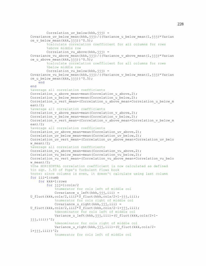
228

Correlation_uv_below(kkk,jjj) =

Covariance_uv_below_mean(kkk,jjj)/((Variance_u_below_mean(1,jjj)*Varian

ce_v_below_mean(kkk,jjj))^0.5); %calculate correlation coefficient for all columns for rows %above middle row Correlation_vu_above(kkk,jjj) =

Covariance_vu_above_mean(kkk,jjj)/((Variance_v_above_mean(1,jjj)*Varian

ce_u_above_mean(kkk,jjj))^0.5); %calculate correlation coefficient for all columns for rows %below middle row Correlation_vu_below(kkk,jjj) =

Covariance_vu_below_mean(kkk,jjj)/((Variance_v_below_mean(1,jjj)*Varian

ce_u_below_mean(kkk,jjj))^0.5); end end %average all correlation coefficients Correlation_u_above_mean=mean(Correlation_u_above,2); Correlation_u_below_mean=mean(Correlation_u_below,2); Correlation_u_vert_mean=(Correlation_u_above_mean+Correlation_u_below_m

ean)/2; %average all correlation coefficients Correlation_v_above_mean=mean(Correlation_v_above,2); Correlation_v_below_mean=mean(Correlation_v_below,2); Correlation_v_vert_mean=(Correlation_v_above_mean+Correlation_v_below_m

ean)/2; %average all correlation coefficients Correlation_uv_above_mean=mean(Correlation_uv_above,2); Correlation_uv_below_mean=mean(Correlation_uv_below,2); Correlation_uv_vert_mean=(Correlation_uv_above_mean+Correlation_uv_belo

w_mean)/2; %average all correlation coefficients Correlation_vu_above_mean=mean(Correlation_vu_above,2); Correlation_vu_below_mean=mean(Correlation_vu_below,2); Correlation_vu_vert_mean=(Correlation_vu_above_mean+Correlation_vu_belo

w_mean)/2; %the HORIZONTAL correlation coefficient is now calculated as defined %in eqn. 3.93 of Pope's Turbulent Flows book %note: since columns is even, it doesn't calculate using last column for iii=1:numb for kkk=1:rows for jjj=1:cols/2 %numerator for cols left of middle col Covariance_u_left(kkk,jjj,iii) =

U_fluct(kkk,cols/2,iii)*U_fluct(kkk,cols/2+1-jjj,iii); %numerator for cols right of middle col Covariance_u_right(kkk,jjj,iii) =

U_fluct(kkk,cols/2,iii)*U_fluct(kkk,cols/2-1+jjj,iii); %denominator for cols left of middle col Variance_u_left(kkk,jjj,iii)=(U_fluct(kkk,cols/2+1-

jjj,iii))^2; %denominator for cols right of middle col Variance_u_right(kkk,jjj,iii)=(U_fluct(kkk,cols/2-

1+jjj,iii))^2; %numerator for cols left of middle col

229

Covariance_v_left(kkk,jjj,iii) =

V_fluct(kkk,cols/2,iii)*V_fluct(kkk,cols/2+1-jjj,iii); %numerator for cols right of middle col Covariance_v_right(kkk,jjj,iii) =

V_fluct(kkk,cols/2,iii)*V_fluct(kkk,cols/2-1+jjj,iii); %denominator for cols left of middle col Variance_v_left(kkk,jjj,iii)=(V_fluct(kkk,cols/2+1-

jjj,iii))^2; %denominator for cols right of middle col Variance_v_right(kkk,jjj,iii)=(V_fluct(kkk,cols/2-

1+jjj,iii))^2; %numerator for cols left of middle col Covariance_uv_left(kkk,jjj,iii) =

U_fluct(kkk,cols/2,iii)*V_fluct(kkk,cols/2+1-jjj,iii); %numerator for cols right of middle col Covariance_uv_right(kkk,jjj,iii) =

U_fluct(kkk,cols/2,iii)*V_fluct(kkk,cols/2-1+jjj,iii); %numerator for cols left of middle col Covariance_vu_left(kkk,jjj,iii) =

V_fluct(kkk,cols/2,iii)*U_fluct(kkk,cols/2+1-jjj,iii); %numerator for cols right of middle col Covariance_vu_right(kkk,jjj,iii) =

V_fluct(kkk,cols/2,iii)*U_fluct(kkk,cols/2-1+jjj,iii); end end end %find mean of matrices along all data sets Covariance_u_left_mean=mean(Covariance_u_left,3); Covariance_u_right_mean=mean(Covariance_u_right,3); Covariance_v_left_mean=mean(Covariance_v_left,3); Covariance_v_right_mean=mean(Covariance_v_right,3); Covariance_uv_left_mean=mean(Covariance_uv_left,3); Covariance_uv_right_mean=mean(Covariance_uv_right,3); Covariance_vu_left_mean=mean(Covariance_vu_left,3); Covariance_vu_right_mean=mean(Covariance_vu_right,3); Variance_u_left_mean=mean(Variance_u_left,3); Variance_u_right_mean=mean(Variance_u_right,3); Variance_v_left_mean=mean(Variance_v_left,3); Variance_v_right_mean=mean(Variance_v_right,3); %%HORIZONTAL correlation for kkk=1:rows for jjj=1:cols/2 %calculate correlation coefficient for all rows for columns %left of middle col Correlation_u_left(kkk,jjj) =

Covariance_u_left_mean(kkk,jjj)/((Variance_u_left_mean(kkk,1)*Variance_

u_left_mean(kkk,jjj))^0.5); %calculate correlation coefficient for all rows for columns %right of middle col Correlation_u_right(kkk,jjj) =

Covariance_u_right_mean(kkk,jjj)/((Variance_u_right_mean(kkk,1)*Varianc

e_u_right_mean(kkk,jjj))^0.5); %calculate correlation coefficient for all rows for columns %left of middle col

230

Correlation_v_left(kkk,jjj) =

Covariance_v_left_mean(kkk,jjj)/((Variance_v_left_mean(kkk,1)*Variance_

v_left_mean(kkk,jjj))^0.5); %calculate correlation coefficient for all rows for columns %right of middle col Correlation_v_right(kkk,jjj) =

Covariance_v_right_mean(kkk,jjj)/((Variance_v_right_mean(kkk,1)*Varianc

e_v_right_mean(kkk,jjj))^0.5); %calculate correlation coefficient for all rows for columns %left of middle col Correlation_uv_left(kkk,jjj) =

Covariance_uv_left_mean(kkk,jjj)/((Variance_u_left_mean(kkk,1)*Variance

_v_left_mean(kkk,jjj))^0.5); %calculate correlation coefficient for all rows for columns %right of middle col Correlation_uv_right(kkk,jjj) =

Covariance_uv_right_mean(kkk,jjj)/((Variance_u_right_mean(kkk,1)*Varian

ce_v_right_mean(kkk,jjj))^0.5); %calculate correlation coefficient for all rows for columns %left of middle col Correlation_vu_left(kkk,jjj) =

Covariance_vu_left_mean(kkk,jjj)/((Variance_v_left_mean(kkk,1)*Variance

_u_left_mean(kkk,jjj))^0.5); %calculate correlation coefficient for all rows for columns %right of middle col Correlation_vu_right(kkk,jjj) =

Covariance_vu_right_mean(kkk,jjj)/((Variance_v_right_mean(kkk,1)*Varian

ce_u_right_mean(kkk,jjj))^0.5); end end %average all correlation coefficients Correlation_u_left_mean=mean(Correlation_u_left,1); Correlation_u_right_mean=mean(Correlation_u_right,1); Correlation_u_horiz_mean=(Correlation_u_left_mean+Correlation_u_right_m

ean)/2; %average all correlation coefficients Correlation_v_left_mean=mean(Correlation_v_left,1); Correlation_v_right_mean=mean(Correlation_v_right,1); Correlation_v_horiz_mean=(Correlation_v_left_mean+Correlation_v_right_m

ean)/2; %average all correlation coefficients Correlation_uv_left_mean=mean(Correlation_uv_left,1); Correlation_uv_right_mean=mean(Correlation_uv_right,1); Correlation_uv_horiz_mean=(Correlation_uv_left_mean+Correlation_uv_righ

t_mean)/2; %average all correlation coefficients Correlation_vu_left_mean=mean(Correlation_vu_left,1); Correlation_vu_right_mean=mean(Correlation_vu_right,1); Correlation_vu_horiz_mean=(Correlation_vu_left_mean+Correlation_vu_righ

t_mean)/2; %make vector with distances from the center of vertical correlation delta_y=m_pixel*vector_spacing*(0:(rows/2-1)); %make vector with distances for best-fit vertical correlation delta_y_long=m_pixel*vector_spacing*(0:(4*rows-1)); %make vector with distances from the center of horizontal correlation

231

delta_x=m_pixel*vector_spacing*(0:(cols/2-1)); %make vector with distances for best-fit horizontal correlation delta_x_long=m_pixel*vector_spacing*(0:(4*cols-1)); %call function, compute vertical longitudinal correlation best-fit [R_v_vert]=Compute_double_exp_variables_vert_cycle_resolved(delta_y,

Correlation_v_vert_mean, rows, delta_y_long); %call function, compute horizontal longitudinal correlation best-fit [R_u_horiz]=Compute_double_exp_variables_horiz_cycle_resolved(delta_x,

Correlation_u_horiz_mean, cols, delta_x_long); Integral_length_vert_uu=0; %set integral lengths to zero to start Integral_length_vert_vv=0; Integral_length_horiz_uu=0; Integral_length_horiz_vv=0; %initialize, this stops the integration of the curves if they go %positive after going negative stop_u=0; stop_v=0; %calculate vertical lengthscales summing area only if correlation

positive for i=1:rows/2 if Correlation_u_vert_mean(i,1) > 0 && stop_u==0 %sum up area under correlation curve Integral_length_vert_uu = Integral_length_vert_uu +

Correlation_u_vert_mean(i,1)*delta_y(1,2); else %in case calculated curve goes above zero after going negative, %stop integration stop_u=1; end end for i=1:4*rows if R_v_vert(i,1) > 0 && stop_v==0 %sum up area under best-fit correlation curve Integral_length_vert_vv = Integral_length_vert_vv +

R_v_vert(i,1)*delta_y_long(1,2); else %in case calculated curve goes about zero after going negative, %stop integration stop_v=1; end end %re-initialize, this stops the integration of the curves if they go %positive after going negative stop_u=0; stop_v=0; %calculate horizontal lengthscales, sum area only if correlation

positive for i=1:cols/2 if Correlation_v_horiz_mean(1,i) > 0 && stop_v==0 %sum up area under correlation curve Integral_length_horiz_vv = Integral_length_horiz_vv +

Correlation_v_horiz_mean(1,i)*delta_x(1,2); else %in case the calculated curve goes about zero after going % negative, stop integration

232

stop_v=1; end end for i=1:4*cols if R_u_horiz(1,i) > 0 && stop_u==0 %sum up area under best-fit correlation curve Integral_length_horiz_uu = Integral_length_horiz_uu +

R_u_horiz(1,i)*delta_x_long(1,2); else %in case the calculated curve goes about zero after going % negative, stop integration stop_u=1; end end %change units from [m] to [mm] Integral_length_vert_vv=Integral_length_vert_vv*1e3; Integral_length_vert_uu=Integral_length_vert_uu*1e3; Integral_length_horiz_vv=Integral_length_horiz_vv*1e3; Integral_length_horiz_uu=Integral_length_horiz_uu*1e3; Int_lengthscale_vector(loop,:)=[L_cut, Integral_length_vert_vv,

Integral_length_vert_uu, Integral_length_horiz_uu,

Integral_length_horiz_vv]; loop=loop+1; %increase loop counter end Int_lengthscale_vector %print lengthscales to screen

E.6. MATLAB Code to Calculate the Energy Spectra Using the Ensemble Average

Data


%calculate the turbulent kinetic energy, since I only have 2D velocity

field, I assume isotropy and multiply by 3/2 to get the 3rd dimension

Turb_kinetic_energy=(1/2)*mean(mean(Fluct_mean_good))*(3/2);

%calculates u fluctuating velocity mean squared for Pope, eqn. 6.225 U_fluct_squared_mean=mean(mean(U_fluct_mean_good)); %calculates v fluctuating velocity mean squared for Pope, eqn. 6.225 V_fluct_squared_mean=mean(mean(V_fluct_mean_good)); %read in the size of the fluctuating KE matrix [rows cols]=size(KE_fluct(:,:,1)); %the next loop checks if the number of rows is even, and drops the %last row if the number is odd, this allows for correct plotting of %k vs. E later in the code test=rows/2; test2=round(test); if test~=test2

233

%reset the size of matrices if a row is subtracted KE_fluct=KE_fluct(1:(rows-1),:,:); U_fluct=U_fluct(1:(rows-1),:,:); V_fluct=V_fluct(1:(rows-1),:,:); [rows cols]=size(KE_fluct(:,:,1)); end %the next loop checks if the number of rows is even, and drops the %last row if the number is odd, this allows for correct plotting of %k vs. E later in the code test3=cols/2; test4=round(test3); if test3~=test4 %reset the size of matrices if a column is subtracted KE_fluct=KE_fluct(:,1:(cols-1),:); U_fluct=U_fluct(:,1:(cols-1),:); V_fluct=V_fluct(:,1:(cols-1),:); [rows cols]=size(KE_fluct(:,:,1)); End

----E.6. Reference 1---- %%VERTICAL energy spectra kappa=2*pi/(m_pixel*vector_spacing); %kappa equals 2*pi divided by L %creates kappa vector with wavenumbers from zero to kappa/2 k_vert=kappa*(0:(rows/2))/(rows); k_vert=k_vert'; %change k into a column vector for i=1:cols-1 %note: can't find FT_second when i=cols for j=1:numb %fourier transform two adjacent rows which extends the dynamic %range and removes noise when the energy spectrum is calculated FT_first(:,i,j)=fft(KE_fluct(:,i,j),rows); FT_second(:,i,j)=fft(KE_fluct(:,i+1,j),rows); %vertical energy spectrum E(:,i,j)=(FT_first(:,i,j).*conj(FT_second(:,i,j))); end end %finds the mean energy spectrum at each wavenumber and for each image E_vert_mean=mean(mean(E,3),2); %normalize by the second value, the first we ignore due to noise, find %minumum SSE by matching to this point E_vert_mean_max=real(E_vert_mean(2,1)); E_vert_mean_norm=real(E_vert_mean(1:(rows/2+1),1)/E_vert_mean_max); %%HORIZONTAL energy spectra %creates kappa vector with wavenumbers from zero to kappa/2 k_horiz=kappa*(0:(cols/2))/(cols); for i=1:rows-1 %note: can't find FT_second when i=rows for j=1:numb %fourier transform two adjacent rows which extends the dynamic %range and removes noise when the energy spectrum is calculated FT_first_horiz(i,:,j)=fft(KE_fluct(i,:,j),cols); FT_second_horiz(i,:,j)=fft(KE_fluct(i+1,:,j),cols); %horizontal energy spectrum E_horiz(i,:,j) =

(FT_first_horiz(i,:,j).*conj(FT_second_horiz(i,:,j))); end end %finds the mean energy spectrum at each wavenumber and for each image

234

E_horiz_mean=mean(mean(E_horiz,3),1); %normalize by the second value, the first we ignore due to noise, find %minumum SSE by matching to this point E_horiz_mean_max=real(E_horiz_mean(1,2)); E_horiz_mean_norm=real(E_horiz_mean(1,1:(cols/2+1))/E_horiz_mean_max); %-----VERTICAL--------------------- %call function to compute Pope's model spectrum [E1_vert, k1_vert, Re_min_vert, L11_vert, L_vert, eta_vert,

k_model_vert]=Compute_model_1D_Evert_spectrum(Turb_kinetic_energy,

E_vert_mean_norm, k_vert, V_fluct_squared_mean); %non-dimensionalize spectra using Kolmogorov scales, see Pope, p.235 %rate of dissipation, Pope, p. 200, eqn. 6.59 dissipation_vert=(Turb_kinetic_energy^2)/(Re_min_vert*nu); E_vert_Pope_norm=(dissipation_vert*nu^5)^(1/4); %non-dimensionalize measured spectrum E_vert_mean_norm=E_vert_mean_norm*(E_vert_mean_max/E_vert_Pope_norm); %non-dimensionalize Pope spectrum E1_vert=E1_vert*(E_vert_mean_max/E_vert_Pope_norm); %non-dimensionalize measured wavenumber k_eta_vert=k_vert*eta_vert; %non-dimensionalize Pope wavenumber k1_eta_vert=k1_vert*eta_vert; k_vert=k_vert./(1e6); %change units from rad/m to rad/um k1_vert=k1_vert./(1e6); %change units from rad/m to rad/um eta_vert=eta_vert*1e6; %change units from [m] to [um] L11_vert=L11_vert*1e3; %change units from [m] to [mm] L_vert=L_vert*1e3; %change units from [m] to [mm] line_53=(5e6)*k_eta_vert.^(-5/3); %-5/3 slope line for plotting %-----HORIZONTAL---------------------

%call function to compute Pope's model spectrum [E1_horiz, k1_horiz, Re_min_horiz, L11_horiz, L_horiz, eta_horiz,

k_model_horiz]=Compute_model_1D_Ehoriz_spectrum(Turb_kinetic_energy,

E_horiz_mean_norm, k_horiz, U_fluct_squared_mean); %non-dimensionalize spectra using Kolmogorov scales, see Pope, p.235 %rate of dissipation, Pope, p. 200, eqn. 6.59 dissipation_horiz=(Turb_kinetic_energy^2)/(Re_min_horiz*nu); E_horiz_Pope_norm=(dissipation_horiz*nu^5)^(1/4); %non-dimensionalize measured spectrum E_horiz_mean_norm=E_horiz_mean_norm*(E_horiz_mean_max/E_horiz_Pope_norm

); %non-dimensionalize Pope spectrum E1_horiz=E1_horiz*(E_horiz_mean_max/E_horiz_Pope_norm); %non-dimensionalize measured wavenumber k_eta_horiz=k_horiz*eta_horiz; %non-dimensionalize Pope wavenumber k1_eta_horiz=k1_horiz*eta_horiz; k_horiz=k_horiz./(1e6); %change units from rad/m to rad/um k1_horiz=k1_horiz./(1e6); %change units from rad/m to rad/um eta_horiz=eta_horiz*1e6; %change units from [m] to [um] L11_horiz=L11_horiz*1e3; %change units from [m] to [mm] L_horiz=L_horiz*1e3; %change units from [m] to [mm] line_horiz_53=(2e7)*k_eta_horiz.^(-5/3); %-5/3 slope line for plotting %print to screen

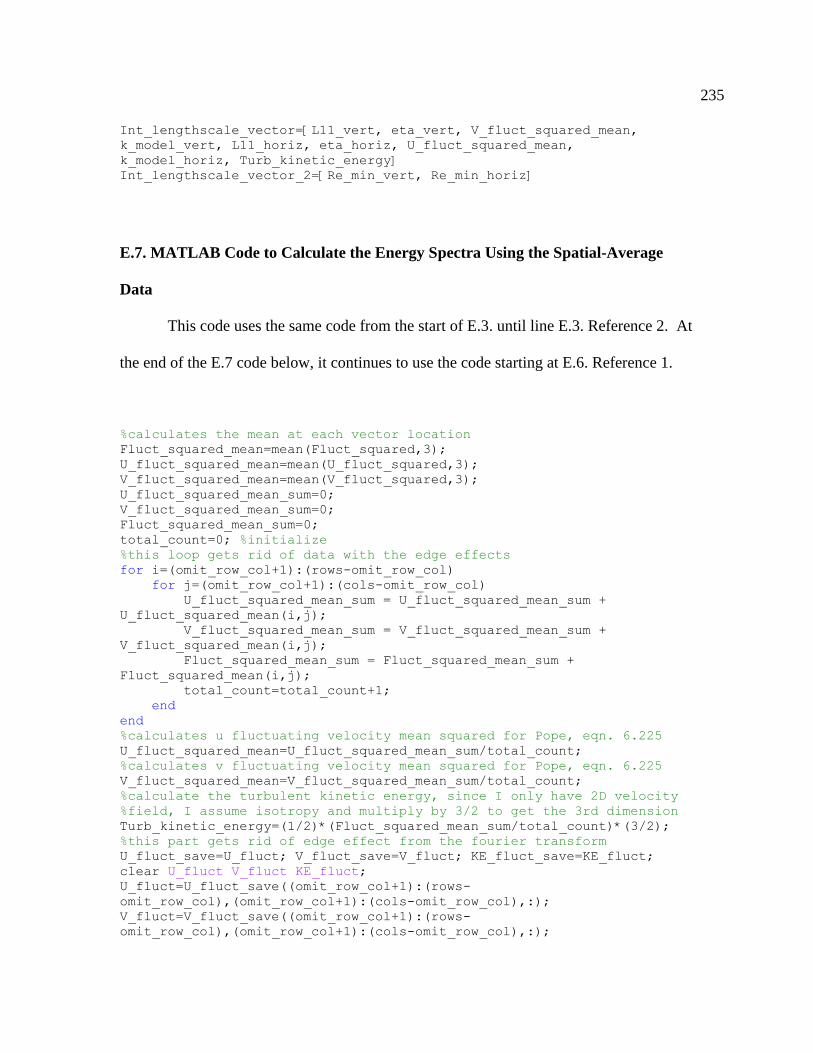
235

Int_lengthscale_vector=[L11_vert, eta_vert, V_fluct_squared_mean,

k_model_vert, L11_horiz, eta_horiz, U_fluct_squared_mean,

k_model_horiz, Turb_kinetic_energy] Int_lengthscale_vector_2=[Re_min_vert, Re_min_horiz]

E.7. MATLAB Code to Calculate the Energy Spectra Using the Spatial-Average

Data

This code uses the same code from the start of E.3. until line E.3. Reference 2. At

the end of the E.7 code below, it continues to use the code starting at E.6. Reference 1.

%calculates the mean at each vector location Fluct_squared_mean=mean(Fluct_squared,3); U_fluct_squared_mean=mean(U_fluct_squared,3); V_fluct_squared_mean=mean(V_fluct_squared,3); U_fluct_squared_mean_sum=0; V_fluct_squared_mean_sum=0; Fluct_squared_mean_sum=0; total_count=0; %initialize %this loop gets rid of data with the edge effects for i=(omit_row_col+1):(rows-omit_row_col) for j=(omit_row_col+1):(cols-omit_row_col) U_fluct_squared_mean_sum = U_fluct_squared_mean_sum +

U_fluct_squared_mean(i,j); V_fluct_squared_mean_sum = V_fluct_squared_mean_sum +

V_fluct_squared_mean(i,j); Fluct_squared_mean_sum = Fluct_squared_mean_sum +

Fluct_squared_mean(i,j); total_count=total_count+1; end end %calculates u fluctuating velocity mean squared for Pope, eqn. 6.225 U_fluct_squared_mean=U_fluct_squared_mean_sum/total_count; %calculates v fluctuating velocity mean squared for Pope, eqn. 6.225 V_fluct_squared_mean=V_fluct_squared_mean_sum/total_count; %calculate the turbulent kinetic energy, since I only have 2D velocity %field, I assume isotropy and multiply by 3/2 to get the 3rd dimension Turb_kinetic_energy=(1/2)*(Fluct_squared_mean_sum/total_count)*(3/2); %this part gets rid of edge effect from the fourier transform U_fluct_save=U_fluct; V_fluct_save=V_fluct; KE_fluct_save=KE_fluct; clear U_fluct V_fluct KE_fluct; U_fluct=U_fluct_save((omit_row_col+1):(rows-

omit_row_col),(omit_row_col+1):(cols-omit_row_col),:);

V_fluct=V_fluct_save((omit_row_col+1):(rows-

omit_row_col),(omit_row_col+1):(cols-omit_row_col),:);

236

KE_fluct=KE_fluct_save((omit_row_col+1):(rows-

omit_row_col),(omit_row_col+1):(cols-omit_row_col),:); [rows cols]=size(U_fluct(:,:,1)); %read in the size of the matrix

E.8. MATLAB Function to Calculate the Pope 1-D Model Spectrum in the


This function is called by the code in E.6. The vertical direction analysis is the

same, but the variable names are changed to designate the vertical direction.

function [E1_horiz, k1_horiz, Re_min_horiz, L11_horiz, L, eta,

k_model_horiz]=Compute_model_1D_Ehoriz_spectrum(Turb_kinetic_energy,

E_horiz_mean_norm, k_horiz, U_fluct_squared_mean) %use the golden search method to find Re # that that minimizes %the SSE between the E11 curves, this bracketing method follows %the UCSD MAE290A course materials book, p.51 Re1=1; Re3=10000; %initial bounds set for bracket on Reynolds # Re_tol=5; %set tolerance for Reynolds number evals=0; %interation loop counter initialization Z=sqrt(5)-2; %initialize golden section ratio Re2=Re1+(Re3-Re1)*0.381966; %set Re2 for golden ratio %function calls [c_L1]=Compute_model_1D_c_L(Re1, Turb_kinetic_energy); [SSE1]=Compute_model_1D_Ehoriz_SSE(Re1, c_L1, Turb_kinetic_energy,

E_horiz_mean_norm, k_horiz); [c_L2]=Compute_model_1D_c_L(Re2, Turb_kinetic_energy); [SSE2]=Compute_model_1D_Ehoriz_SSE(Re2, c_L2, Turb_kinetic_energy,

E_horiz_mean_norm, k_horiz); [c_L3]=Compute_model_1D_c_L(Re3, Turb_kinetic_energy); [SSE3]=Compute_model_1D_Ehoriz_SSE(Re3, c_L3, Turb_kinetic_energy,

E_horiz_mean_norm, k_horiz); %computes the min SSE, which is SSE2(Re2) (between Re1 and Re3) %c_L is also found such that TKE matches the model while (abs(Re3-Re1) > Re_tol) Re4 = Re2+Z*(Re3-Re1); %compute the new Re4 %function calls [c_L4]=Compute_model_1D_c_L(Re4, Turb_kinetic_energy); [SSE4]=Compute_model_1D_Ehoriz_SSE(Re4, c_L4,

Turb_kinetic_energy, E_horiz_mean_norm, k_horiz); evals=evals+1; %loop counter if (SSE4>SSE2) Re3=Re1; SSE3=SSE1; c_L3=c_L1; %center new triplet on x2 %Re2=Re2; SSE2=SSE2; Re1=Re4; SSE1=SSE4; c_L1=c_L4; else

237

Re1=Re2; SSE1=SSE2; c_L1=c_L2; %center new triplet on x2 %Re3=Re3; SSE3=SSE3; Re2=Re4; SSE2=SSE4; c_L2=c_L4; end end Re_min_horiz=Re2; %Reynolds number that minimizes the SSE is Re2 %constants for Pope's spectrum, p.233 & p.232 c_L=c_L2 c_eta=0.4; C=1.5; p_0=2.0; beta=5.2; %note: c_eta=0.4 is high Re# limit. Though, choosing c_eta such %that dissipation matches model changes final Re#, lengthscales %by about 1%, so separate function call not created. %note: easier if nu passed from original file %[m^2/s], large engine, kinematic viscosity of air at 720K, 1612kPa nu=4.25e-6; %[m^2/s], small engine, kinematic viscosity of air at 708K, 1523kPa %nu=4.50e-6; k1=[1e1:1e1:1e5]'; %initialize k1 vector, column vector k1min=min(k1); %find min of k1 k1max=max(k1); %find max of k1 imax_1=int32(max(size(k1))); %number of elements in k1 vector %high resolution k vector for integration k=(k1min:k1min/10:1.1*k1max)'; imax=int32(max(size(k))); %number of elements in k vector % initialize for speed f_L=ones(imax,1); f_eta=ones(imax,1); E=ones(imax,1);

D=ones(imax,1); %definition of turbulence Reynolds number, Pope, p.200, eqn. 6.59 L=Re_min_horiz*nu/(sqrt(Turb_kinetic_energy)); eta=L*(Re_min_horiz^(-3/4)); %Pope, p. 200, eqn. 6.61 kL=k*L; %compute k*L and k*eta for use in f_L and f_eta kn=k*eta; for i=1:imax %Pope, p. 232, eqn. 6.247 f_L(i)=(kL(i)/(sqrt((kL(i)^2+c_L))))^(5.0/3.0+p_0); %Pope, p. 233, eqn. 6.248 f_eta(i)=exp(-beta*(sqrt(sqrt((kn(i)^4+c_eta^4)))-c_eta)); %Pope, p. 232, eqn. 6.246 E(i)=C*(nu^2)*(eta^(-8.0/3.0))*(k(i)^(-

5.0/3.0))*f_L(i)*f_eta(i); end E1=ones(imax_1,1); % initialize for speed for index=1:imax_1 %returns first entry location indice that is greater than %k_horiz, k1 is ignored in the integral since its value is zero k_index=int32(find(k > k1(index),1)); integrand=zeros(imax,1); % initialize for speed for j=k_index:imax %Pope, p. 226, eqn. 6.216 integrand(j)=(E(j)/k(j))*(1-k1(index)^2/k(j)^2); end %simple integration by rectangles E1(index)=sum(integrand)*(k(2)-k(1)); clear integrand;

238

end %this next line finds the indice of the k1 that is nearest to the %k_horiz value that was used to normalize this vector E_index_norm=int32(find(k1 > k_horiz(1,2),1))-1; %normalize vector by E1 at the location that E_horiz_mean_norm %was normalized E1=E1./E1(E_index_norm,1); E1_horiz=E1; k1_horiz=k1; %this next part calculates L_11 from Pope, p. 228, eqn. 6.225 L_integrand=zeros(imax,1); % initialize for speed for j=1:imax L_integrand(j)=(E(j)/k(j)); %Pope, p. 228, eqn. 6.225 k_sum_horiz(j)=E(j); %Pope, p. 222, eqn. 6.190 end %simple integration by rectangles L11_horiz=(0.5*pi/U_fluct_squared_mean)*sum(L_integrand)*(k(2)-

k(1)); k_model_horiz=sum(k_sum_horiz)*(k(2)-k(1)); end

E.9. MATLAB Function to Calculate the Sum Squared Error Between the

Measured Spectra and Pope 1-D Model Spectrum in the Horizontal Direction

This function is called by the code in E.8. The vertical direction analysis is the

same, but the variable names are changed to designate the vertical direction.

function [SSE_sum]=Compute_model_1D_Ehoriz_SSE(Re, c_L,

Turb_kinetic_energy, E_horiz_mean_norm, k_horiz) %constants for Pope's spectrum, p.233 & p.232 c_eta=0.4; C=1.5; p_0=2.0; beta=5.2; %note: c_eta=0.4 is high Re# limit. Though, choosing c_eta such %that dissipation matches model changes final Re#, lengthscales %by about 1%, so separate function call not created. %note: easier if nu passed from original file %[m^2/s], large engine, kinematic viscosity of air at 720K, 1612kPa nu=4.25e-6; %[m^2/s], small engine, kinematic viscosity of air at 708K, 1523kPa %nu=4.50e-6; %only compute the model spectra at the points I want to compute the %SSE, units are [rad/m] k1=k_horiz(1,2:20); k1=k1'; %convert to column vector k1min=min(k1); %find min of k1

239

imax_1=int32(max(size(k1))); %number of elements in k1 vector %high resolution k vector for integration, units [rad/m] k=(k1min:k1min/10:1e6)'; imax=int32(max(size(k))); %number of elements in k vector % initialize for speed f_L=ones(imax,1); f_eta=ones(imax,1); E=ones(imax,1); %definition of turbulence Reynolds number, Pope, p.200, eqn. 6.59 L=Re*nu/(sqrt(Turb_kinetic_energy)); eta=L*(Re^(-3/4)); %Pope, p. 200, eqn. 6.61 kL=k*L; %compute k*L and k*eta for use in f_L and f_eta kn=k*eta; for i=1:imax %Pope, p. 232, eqn. 6.247 f_L(i)=(kL(i)/(sqrt((kL(i)^2+c_L))))^(5.0/3.0+p_0); %Pope, p. 233, eqn. 6.248 f_eta(i)=exp(-beta*(sqrt(sqrt((kn(i)^4+c_eta^4)))-c_eta)); %Pope, p. 232, eqn. 6.246 E(i)=C*(nu^2)*(eta^(-8.0/3.0))*(k(i)^(-

5.0/3.0))*f_L(i)*f_eta(i); end E1=ones(imax_1,1); % initialize for speed for index=1:imax_1 k_index=int32(find(k > k1(index),1)); integrand=zeros(imax,1); % initialize for speed for j=k_index:imax %Pope, p. 226, eqn. 6.216 integrand(j)=(E(j)/k(j))*(1-k1(index)^2/k(j)^2); end %simple integration by rectangles E1(index)=sum(integrand)*(k(2)-k(1)); clear integrand; end E1=E1./(E1(1,1)); %normalize vector E1_horiz=E1; k1_horiz=k1; clear k1 E1 k; %now compute the SSE SSE_sum=0; %initialize the sum of SSE for i=1:imax_1 %compute sum squared error, ignore first point of %E_horiz_mean_norm SSE_sum=SSE_sum+(1e5)*(real(E1_horiz(i,1))-

real(E_horiz_mean_norm(1,i+1)))^2; end end

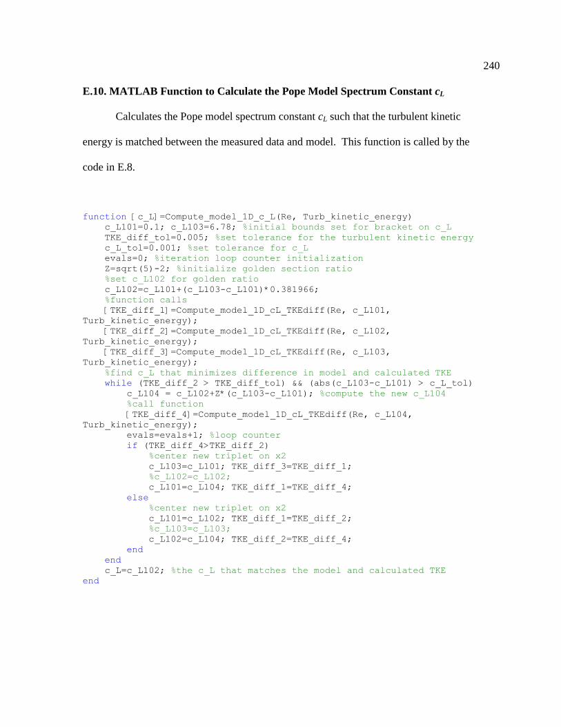
240

E.10. MATLAB Function to Calculate the Pope Model Spectrum Constant cL

Calculates the Pope model spectrum constant cL such that the turbulent kinetic

energy is matched between the measured data and model. This function is called by the

code in E.8.

function [c_L]=Compute_model_1D_c_L(Re, Turb_kinetic_energy) c_L101=0.1; c_L103=6.78; %initial bounds set for bracket on c_L TKE_diff_tol=0.005; %set tolerance for the turbulent kinetic energy c_L_tol=0.001; %set tolerance for c_L evals=0; %iteration loop counter initialization Z=sqrt(5)-2; %initialize golden section ratio

%set c_L102 for golden ratio c_L102=c_L101+(c_L103-c_L101)*0.381966; %function calls [TKE_diff_1]=Compute_model_1D_cL_TKEdiff(Re, c_L101,

Turb_kinetic_energy); [TKE_diff_2]=Compute_model_1D_cL_TKEdiff(Re, c_L102,

Turb_kinetic_energy); [TKE_diff_3]=Compute_model_1D_cL_TKEdiff(Re, c_L103,

Turb_kinetic_energy); %find c_L that minimizes difference in model and calculated TKE while (TKE_diff_2 > TKE_diff_tol) && (abs(c_L103-c_L101) > c_L_tol) c_L104 = c_L102+Z*(c_L103-c_L101); %compute the new c_L104 %call function [TKE_diff_4]=Compute_model_1D_cL_TKEdiff(Re, c_L104,

Turb_kinetic_energy); evals=evals+1; %loop counter if (TKE_diff_4>TKE_diff_2)

%center new triplet on x2 c_L103=c_L101; TKE_diff_3=TKE_diff_1; %c_L102=c_L102; c_L101=c_L104; TKE_diff_1=TKE_diff_4; else

%center new triplet on x2 c_L101=c_L102; TKE_diff_1=TKE_diff_2; %c_L103=c_L103; c_L102=c_L104; TKE_diff_2=TKE_diff_4; end end c_L=c_L102; %the c_L that matches the model and calculated TKE end

241

E.11. MATLAB Function for Calculating the Difference in the Turbulent Kinetic

Energy

This function calculates the difference in the turbulent kinetic energy between the

measured and Pope model spectrum for a given cL and turbulence Reynolds number.

This function is called by the code in E.10.

function [TKE_diff]=Compute_model_1D_cL_TKEdiff(Re, c_L,

Turb_kinetic_energy) c_eta=0.4; C=1.5; p_0=2.0; beta=5.2; %note: c_eta=0.4 is high Re# limit. Though, choosing c_eta such %that dissipation matches model changes final Re#, lengthscales %by about 1%, so separate function call not created. %[m^2/s], large engine, kinematic viscosity of air at 720K, 1612kPa nu=4.25e-6; %[m^2/s], small engine, kinematic viscosity of air at 708K, 1523kPa %nu=4.50e-6; k1=[1e1:1e1:1e5]'; %initialize k1 vector, column vector k1min=min(k1); %find min of k1 k1max=max(k1); %find max of k1 imax_1=int32(max(size(k1))); %number of elements in k1 vector

%high resolution k vector for integration k=(k1min:k1min/10:1.1*k1max)'; imax=int32(max(size(k))); %number of elements in k vector % initialize for speed f_L=ones(imax,1); f_eta=ones(imax,1); E=ones(imax,1); %definition of turbulence Reynolds number, Pope, p.200, eqn. 6.59 L=Re*nu/(sqrt(Turb_kinetic_energy)); eta=L*(Re^(-3/4)); %Pope, p. 200, eqn. 6.61 kL=k*L; %compute k*L and k*eta for use in f_L and f_eta kn=k*eta; for i=1:imax %Pope, p. 232, eqn. 6.247 f_L(i)=(kL(i)/(sqrt((kL(i)^2+c_L))))^(5.0/3.0+p_0); %Pope, p. 233, eqn. 6.248 f_eta(i)=exp(-beta*(sqrt(sqrt((kn(i)^4+c_eta^4)))-c_eta)); %Pope, p. 232, eqn. 6.246 E(i)=C*(nu^2)*(eta^(-8.0/3.0))*(k(i)^(-

5.0/3.0))*f_L(i)*f_eta(i); end %Pope, p. 222, eqn. 6.190 Turb_kinetic_energy_model=(sum(E))*(k(2)-k(1)); %calculate difference between model and measured TKE TKE_diff=abs(Turb_kinetic_energy_model-Turb_kinetic_energy); end

Documents

Thesis_Heim_print_version