Locomotive Traction and Rail Wear Control

Ye Tian

BEng Electrical Engineering and Automation Tianjin University, China

MSc Control Systems Imperial College London, UK

A thesis submitted for the degree of Doctor of Philosophy at

The University of Queensland in 2015

School of Mechanical and Mining Engineering

1

Abstract

Railways play one of the most important roles in today’s transport systems throughout the world

due to their safety, relatively high traction capacity and low operation and maintenance cost [1].

With the development of electric drive and power electronics technology, the capacity and

efficiency of railway transport has been improved dramatically, giving birth to higher speed

passenger trains and higher capacity heavy haul trains. In Australia, the development of the mineral

resources industry drives further improvement of railway operational efficiency without bringing

excessive burden to infrastructural maintenance. The purpose of this thesis is to provide the

required modelling and simulation to determine appropriate tractional system conditions and

controllers to achieve this.

The first part of this thesis is focused on building a locomotive mathematical model including all

the essential dynamic components and interactions to provide prediction of locomotive dynamic

response. The overall model consists of locomotive dynamics, wheel/rail contact dynamics and

electrical drive and control dynamics. The locomotive dynamics include longitudinal, vertical and

pitch motions of the locomotive body, front and rear bogies and six axles. For the wheel/rail contact

dynamics, the Polach model is used to obtain the amount of tractive force generated due to

wheel/rail interaction on the contact patch. The simplified electric drive dynamics are designed

according to the traction effort curves provided by industry using constant torque and constant

power regions. Modes of oscillations have been identified by eigenmode analysis and show that all

the vertical and pitch modes of the locomotive dynamics are stable. The modes that are most likely

to contribute to dynamic behaviour are identified and it is shown that the locomotive body pitch

mode is most excited by traction perturbations. The locomotive dynamic behaviour under changes

in contact conditions is also examined.

The second part of this thesis is focused on achieving higher tractive force under different operating

speed and wheel/rail contact conditions. The dynamic impact of a new control strategy is compared

with that of a traditional fixed threshold creep/adhesion control strategy. A fuzzy logic based

control strategy is employed to adjust the torque output of the motors according to the operating

condition of the locomotive to achieve higher tractive force than that with the traditional constant

creep control strategy. Simulation results show that by controlling the torque generated by the

electric drives, tractive force can be maximized. However, the benefit in the tractive force increase

is marginal under low speed operation at the cost of higher creep values. Under high speed

operation, due to the impact of the electric drive traction effort characteristics, the dynamic

responses with both control strategies are mostly identical.

2

The last part of this thesis is focused on specialized real-time traction control that regulates the wear

to low levels, which is motivated by the increased amount of rail wear damage observed in the rail

industry in recent years. In this thesis, a novel real-time approach of controlling wear damage on

rail tracks is proposed based on a recent wear growth model. Simulation results show that under

high speed operation the dynamic responses are mostly identical with two investigated control

strategies due to the impact of the electric drive traction effort characteristics. However, the new

control strategy can effectively reduce wear damage dramatically under other operation conditions,

with a relatively small amount of tractive force decrease.

The work in this thesis explores various aspects of locomotive traction research. The most

important contributions are the development of a mathematical/simulation model for predicting the

dynamic response of a locomotive under change of operating conditions and its impact on wear

damage on rail tracks. The impact of maximizing tractive effort on rail track wear damage is

quantified, providing practical guidance on locomotive operation. In addition to this, the

development and testing of a specialized real-time traction control strategy that regulates the wear

to low levels based on a recent wear growth model is provided.

3

Declaration by author

This thesis is composed of my original work, and contains no material previously published or

written by another person except where due reference has been made in the text. I have clearly

stated the contribution by others to jointly-authored works that I have included in my thesis.

I have clearly stated the contribution of others to my thesis as a whole, including statistical

assistance, survey design, data analysis, significant technical procedures, professional editorial

advice, and any other original research work used or reported in my thesis. The content of my thesis

is the result of work I have carried out since the commencement of my research higher degree

candidature and does not include a substantial part of work that has been submitted to qualify for

the award of any other degree or diploma in any university or other tertiary institution. I have

clearly stated which parts of my thesis, if any, have been submitted to qualify for another award.

I acknowledge that an electronic copy of my thesis must be lodged with the University Library and,

subject to the General Award Rules of The University of Queensland, immediately made available

for research and study in accordance with the Copyright Act 1968.

I acknowledge that copyright of all material contained in my thesis resides with the copyright

holder(s) of that material. Where appropriate I have obtained copyright permission from the

copyright holder to reproduce material in this thesis.

4

Publications during candidature

The following publications are related to the research work conducted in this dissertation.

Paper A, Y. Tian, W.J.T. (Bill) Daniel, S. Liu and P.A. Meehan, 2013, “Dynamic Tractional

Behaviour Analysis and Control for a DC Locomotive”, World Congress of Rail Research 2013.

Paper B, Y. Tian, W.J.T. (Bill) Daniel, S. Liu and P.A. Meehan, 2014, “Fuzzy Logic Creep Control

for a 2D Locomotive Dynamic Model under Transient Wheel-rail Contact Condition”, 14th

International Conference on Railway Engineering Design and Optimization, COMPRAIL 2014,

Proceedings: Computers in Railways XIV: Railway Engineering Design and Optimization: WIT

Press; 2014. 885-896.

Paper C, Y. Tian, W.J.T. (Bill) Daniel, S. Liu and P.A. Meehan, 2015, “Fuzzy Logic based Sliding

Mode Creep Controller under Varying Wheel-Rail Contact Conditions”, International Journal of

Rail Transportation, 3(1), 40-59.

Paper D, Y. Tian, W.J.T. (Bill) Daniel, S. Liu and P.A. Meehan, “Investigation of the impact of full

scale locomotive adhesion control on wear under changing contact conditions”, accepted by Vehicle

System Dynamics special issue, DOI: 10.1080/00423114.2015.1020815.

Paper E, Y. Tian, W.J.T. (Bill) Daniel, and P.A. Meehan, “Real-time rail/wheel wear damage

control”, submitted to International Journal of Rail Transportation.

Paper F, (co-authored): Sheng Liu, Ye Tian, W.J.T. (Bill) Daniel and Paul A. Meehan, “Dynamic

response of a locomotive with AC electric drives due to changes in friction conditions”, submitted

to Journal of Rail and Rapid Transit.

5

Publications included in this thesis

None

6

Contributions by others to the thesis

My thesis supervisor Paul Meehan provided extensive assistance with drafting and revision of this

thesis and each paper mentioned below so as to contribute to the interpretation. Specific assistance

with individual papers is detailed below.

In Paper A, (Y. Tian, W.J.T. (Bill) Daniel, S. Liu and P.A. Meehan, 2013, “Dynamic Tractional

Behaviour Analysis and Control for a DC Locomotive”, Proceedings of the 10th

World Congress of

Rail Research), Paul Meehan provided guidance and motivation for building a longitudinal-vertical-

pitch locomotive dynamic model including the wheel-rail contact dynamics and simplified DC drive

dynamics in Matlab and assistance in revision. Bill Daniel provided guidance and suggestions in

multibody dynamics as well as contact mechanics. Sheng Liu provided help in proofreading the

paper. Ye Tian was responsible for the remainder of the work.

In Paper B, (Y. Tian, W.J.T. (Bill) Daniel, S. Liu and P.A. Meehan, 2014, “Fuzzy Logic Creep

Control for a 2D Locomotive Dynamic Model under Transient Wheel-rail Contact Condition”, 14th

International Conference on Railway Engineering Design and Optimization, COMPRAIL 2014,

Proceedings: Computers in Railways XIV: Railway Engineering Design and Optimization: WIT

Press; 2014. P885-896.), Paul Meehan provided guidance and motivation for investigating a

controller to achieve highest tractive force available. Bill Daniel provided assistance in modelling.

Sheng Liu provided assistance in revision. Ye Tian was responsible for modelling, simulations and

result analysis. The remainder of the work was done by Ye Tian.

In Paper C, (Y. Tian, W.J.T. (Bill) Daniel, S. Liu and P.A. Meehan, 2015, “Fuzzy Logic based

Sliding Mode Creep Controller under Varying Wheel-Rail Contact Conditions”, International

Journal of Rail Transportation, 3(1), 40-59), Paul Meehan provided guidance and motivation for

investigating the controller achieving highest tractive effort and the practical control effect

comparison between this controller and a traditional one. Ye Tian was responsible for modelling

integration, simulations and result analysis. Bill Daniel and Sheng Liu provided assistance in

proofreading. Ye Tian was responsible for the any remaining work.

In Paper D, (Y. Tian, W.J.T. (Bill) Daniel, S. Liu and P.A. Meehan, “Investigation of the impact of

full scale locomotive adhesion control on wear under changing contact conditions”, accepted by

Vehicle System Dynamics special issue, DOI: 10.1080/00423114.2015.1020815), Paul Meehan

provided guidance and motivation for investigating the effect of traditional creep controller

7

threshold setting and its effect on wear growth rate. Ye Tian was responsible for modelling

integration, simulations and result analysis. Bill Daniel and Sheng Liu provided assistance in

proofreading. Ye Tian was responsible for the any remaining work.

In Paper E, Y. Tian, W.J.T. (Bill) Daniel, and P.A. Meehan, “Real-time rail/wheel wear damage

control”, submitted to International Journal of Rail Transportation, Paul Meehan provided guidance

and motivation for investigating the controller reducing wear damage and the practical control

effect comparison between this controller and a traditional one. Ye Tian was responsible for

modelling integration, simulations and result analysis. Bill Daniel provided assistance in

proofreading. Ye Tian was responsible for the any remaining work.

In Paper F, (Sheng Liu, Ye Tian, W.J.T. (Bill) Daniel and Paul A. Meehan, “Dynamic response of

a locomotive with AC electric drives due to changes in friction conditions”, submitted to Journal of

Rail and Rapid Transit), Paul Meehan provided guidance and motivation for investigating the

dynamic response of a locomotive with complex AC drives due to changes in friction conditions.

Bill Daniel provided assistance in modelling. Ye Tian was responsible for modelling and

implementing the model in Simulink/Matlab. The remainder of the work was done by Sheng Liu.

8

Statement of parts of the thesis submitted to qualify for the award of another degree

None.

9

Acknowledgements

I would like to thank Australian Government and the University of Queensland for the scholarship

that enabled me to do this PhD.

I would like to thank both technical support and financial support of CRC for Rail Innovation under

the project No. R3.119 Locomotive Adhesion.

I would like to thank my principal supervisor Associate Professor Paul Meehan for all the patient

assistance and guidance he has given me. I would also like to thank my associate supervisor Dr.

W.J.T. (Bill) Daniel for his help and support.

Finally I greatly acknowledge in particular my parents. They taught me to see the silver lining of

every cloud; they gave me the heart to never stop hoping and believing; they gave me the courage to

pursuit my dream and happiness. I deeply appreciate them for all their love and support, and for

giving me a family that is always there for me.

10

Keywords

real-time traction control, wear reduction, creep control, adhesion control, locomotive

11

Australian and New Zealand Standard Research Classifications (ANZSRC)

091307, Numerical Modelling and Mechanical Characterisation, 30%

091302, Automation and Control Engineering, 30%

091304, Dynamics, Vibration and Vibration Control, 40%

Fields of Research (FoR) Classification

0913, Mechanical Engineering, 100%

12

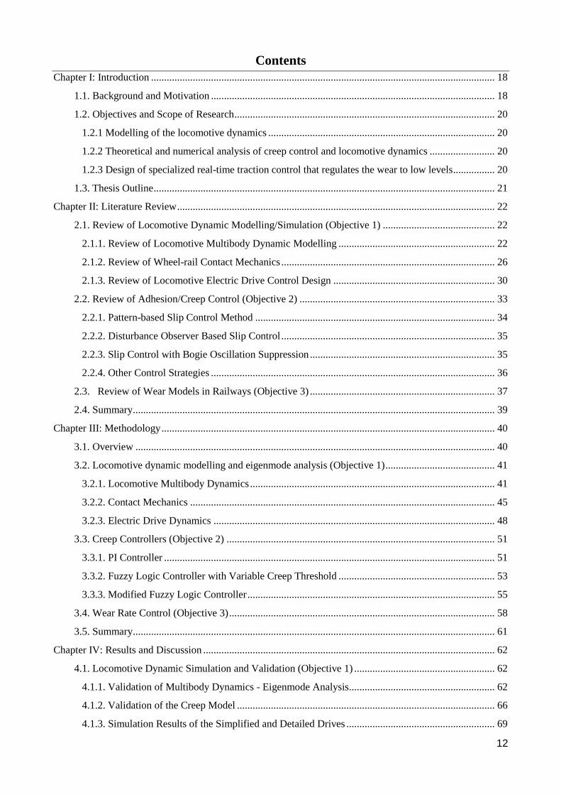
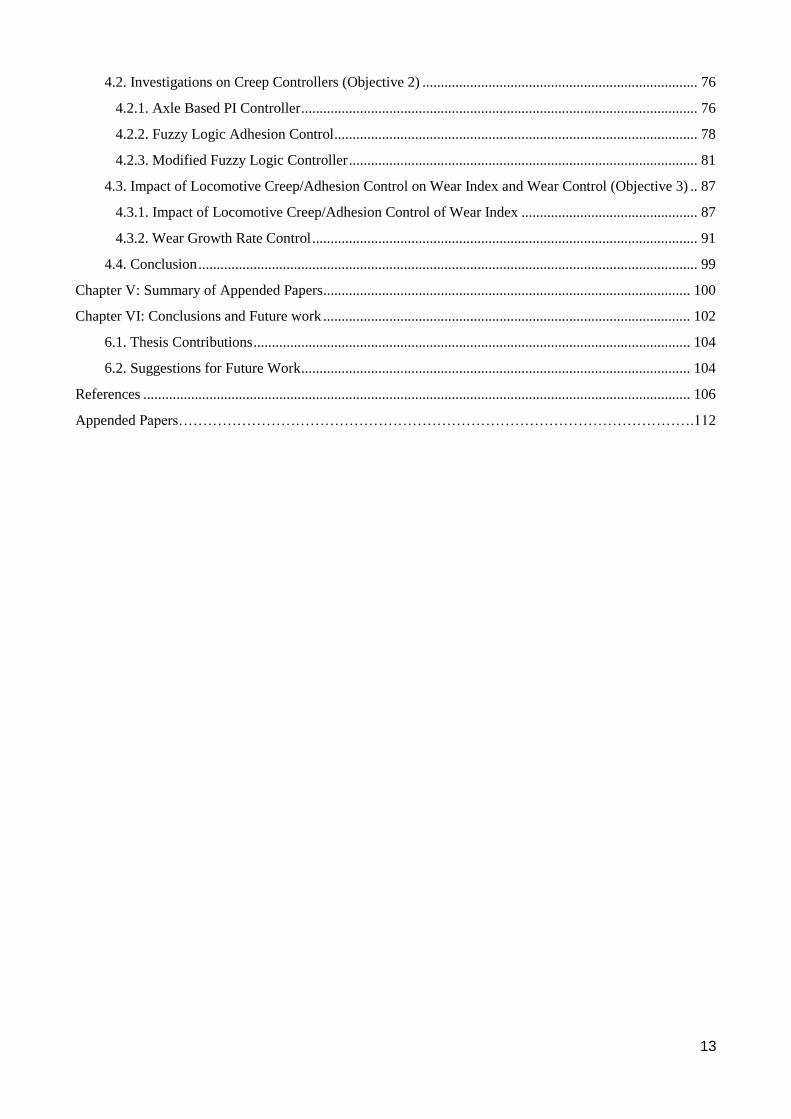
Contents

Chapter I: Introduction .................................................................................................................................... 18

1.1. Background and Motivation ............................................................................................................. 18

1.2. Objectives and Scope of Research .................................................................................................... 20

1.2.1 Modelling of the locomotive dynamics ....................................................................................... 20

1.2.2 Theoretical and numerical analysis of creep control and locomotive dynamics ......................... 20

1.2.3 Design of specialized real-time traction control that regulates the wear to low levels ................ 20

1.3. Thesis Outline ................................................................................................................................... 21

Chapter II: Literature Review .......................................................................................................................... 22

2.1. Review of Locomotive Dynamic Modelling/Simulation (Objective 1) ........................................... 22

2.1.1. Review of Locomotive Multibody Dynamic Modelling ............................................................ 22

2.1.2. Review of Wheel-rail Contact Mechanics .................................................................................. 26

2.1.3. Review of Locomotive Electric Drive Control Design .............................................................. 30

2.2. Review of Adhesion/Creep Control (Objective 2) ........................................................................... 33

2.2.1. Pattern-based Slip Control Method ............................................................................................ 34

2.2.2. Disturbance Observer Based Slip Control .................................................................................. 35

2.2.3. Slip Control with Bogie Oscillation Suppression ....................................................................... 35

2.2.4. Other Control Strategies ............................................................................................................. 36

2.3. Review of Wear Models in Railways (Objective 3) ....................................................................... 37

2.4. Summary ........................................................................................................................................... 39

Chapter III: Methodology ................................................................................................................................ 40

3.1. Overview .......................................................................................................................................... 40

3.2. Locomotive dynamic modelling and eigenmode analysis (Objective 1) .......................................... 41

3.2.1. Locomotive Multibody Dynamics .............................................................................................. 41

3.2.2. Contact Mechanics ..................................................................................................................... 45

3.2.3. Electric Drive Dynamics ............................................................................................................ 48

3.3. Creep Controllers (Objective 2) ....................................................................................................... 51

3.3.1. PI Controller ............................................................................................................................... 51

3.3.2. Fuzzy Logic Controller with Variable Creep Threshold ............................................................ 53

3.3.3. Modified Fuzzy Logic Controller ............................................................................................... 55

3.4. Wear Rate Control (Objective 3) ...................................................................................................... 58

3.5. Summary ........................................................................................................................................... 61

Chapter IV: Results and Discussion ................................................................................................................ 62

4.1. Locomotive Dynamic Simulation and Validation (Objective 1) ...................................................... 62

4.1.1. Validation of Multibody Dynamics - Eigenmode Analysis ........................................................ 62

4.1.2. Validation of the Creep Model ................................................................................................... 66

4.1.3. Simulation Results of the Simplified and Detailed Drives ......................................................... 69

13

4.2. Investigations on Creep Controllers (Objective 2) ........................................................................... 76

4.2.1. Axle Based PI Controller ............................................................................................................ 76

4.2.2. Fuzzy Logic Adhesion Control ................................................................................................... 78

4.2.3. Modified Fuzzy Logic Controller ............................................................................................... 81

4.3. Impact of Locomotive Creep/Adhesion Control on Wear Index and Wear Control (Objective 3) .. 87

4.3.1. Impact of Locomotive Creep/Adhesion Control of Wear Index ................................................ 87

4.3.2. Wear Growth Rate Control ......................................................................................................... 91

4.4. Conclusion ........................................................................................................................................ 99

Chapter V: Summary of Appended Papers .................................................................................................... 100

Chapter VI: Conclusions and Future work .................................................................................................... 102

6.1. Thesis Contributions ....................................................................................................................... 104

6.2. Suggestions for Future Work .......................................................................................................... 104

References ..................................................................................................................................................... 106

Appended Papers…………………………………………………………………………………………….112

14

List of Tables

Table 1: Detailed parameters of the locomotive model …………………………….……………..45

Table 2: Parameters for different contact conditions………………………………….…………..48

Table 3: Fuzzy rule table………..…………………………..………………………………………55

Table 4: Fuzzy rule table of the modified fuzzy controller…….…….………………………….58

Table 5: Modal frequencies of the locomotive dynamic system vibrations, damping ratio,

decay rates and corresponding eigenvalues………………………………………………….……..64

Table 6: Diagram of the mode motions…………………..…………..………...…………………..65

Table 7: Acceleration simulation and comparison with data in [91] ……………………..………75

Table 8: Simulation cases………………………………………………………………………….87

15

List of Figures

Figure 1: Australian heavy haul, intermodal and freight rail [3]……………………………..……..18

Figure 2: Figure 2: Diagram showing the rail wear.…………………………………………….19

Figure 3: The quarter rail vehicle model [9]……………………………….……………………...23

Figure 4: FEM model of locomotive [11]……………………..…...……………………………….23

Figure 5a: Locomotive & track modelling with Gensys software [13]…………………………..24

Figure 5b: A typical ADAMS/Rail model [12]……………………………………………………..24

Figure 5c: A typical Vampire model screen [12]…………………………………………………25

Figure 6: A typical Newton/Lagrangian full locomotive (vertical direction) [20]………………..26

Figure 7: A wheel rolling over a rail [23]……………………………………………………….….27

Figure 8: Assumption of distribution of normal and tangential stresses in the wheel-rail contact area

[17]………………………………………………………………………………….…………....28

Figure 9: Calculated adhesion force-creep functions for typical parameters of real wheel [26]……29

Figure 10: Single-phase equivalent circuit for a squirrel cage motor [35] (upper); and an AC

Induction Motor with cut away showing squirrel cage rotor (lower)……………………………….30

Figure 11: Basic scheme of FOC for the three-phase AC machine [45]............................................32

Figure 12: A typical DTC controlled AC drive structure [48]…………….……………………….33

Figure 13: Pattern re-adhesion control method [51]………………………………………………34

Figure 14: Estimation system of adhesion force coefficient [52]……………………….………….35

Figure 15: Re-adhesion control block based on [53] ……………………………………………….36

Figure 16: Wear types identified during tests of BS11 Rail vs. Class D Tyre [69]……………....38

Figure 17: The wear coefficient versus the frictional power density for UICB rail steel, running with

class D wheel steel [81]..........................................................................................………39

Figure 18: Schematic diagram of the overall system…………………………….…………….…40

Figure 19: Locomotive longitudinal-vertical dynamic diagram……………………………..…….42

Figure 20: Standard 60kg rail profile [89]…………………………………………………………47

Figure 21: Schematic diagram of an AC machine with inverter (left) and instantaneous voltage

vectors (right) [90]…………………………………………………………………………..........…49

Figure 22: Optimum switching table and comparators [90]…………………………………...……49

Figure 23: Diagram of the DTC induction machine…………………………………....…………50

Figure 24: Diagram of basic PID adhesion/creep controller……………………………………..51

Figure 25: The flow chart of the PI creep controller………………………………………………..52

Figure 26: Adhesion control diagram……………………………………………………………...53

16

Figure 27: (a) Membership functions of inputs and output; (b) fuzzy logic 3D input -output

characteristics………………………………………………………………………………….….54

Figure 28: Illustrative graph for the fuzzy rules ………………………………………….……….. 55

Figure 29: Schematic diagram of the overall system……………………………………………..56

Figure 30: (a) Membership functions of input; (b) Membership functions of output………………57

Figure 31: (a) Creep only control diagram; (b) Creep and wear control diagram……………..……60

Figure 32: Vertical displacements of axles under change of contact conditions………………….65

Figure 33: Locomotive car body pitch, vertical and bogies’ vertical displacements……………..65

Figure 34: Tuned Polach creep-adhesion coefficient curve for oil condition at 20 km/h and data in

[99]…………….……………………………..…………………………….……………………….67

Figure 35: The form of adhesion coefficient-creep function and the influence of vehicle speed under

dry wheel/rail contact condition…………………………………………………………………….67

Figure 36: Polach tractive force curve at different speeds under (a) dry contact condition; and (b)

under wet contact condition…………………………………………………………………………68

Figure 37: (a) Comparison between traction force curve of AC model full locomotive (= single AC

traction effort ×6) and the GT46MAC data [104]; (b) Comparison between traction force curve of

DC model full locomotive (= single DC traction effort ×6) and the GT46C data [105]………….70

Figure 38: (a) Comparison between braking effort curve of AC model full locomotive (= single AC

traction effort ×6) and the GT46MAC data [102]; (b) Comparison between braking effort curve of

DC model full locomotive (= single DC traction effort ×6) and the GT46C data [105]……………72

Figure 39: (a) AC creep curves for all traction mode notches under transient state at 20km/h; (b) DC

creep curves for all traction mode notches under transient state at 20km/h…………………..…….74

Figure 40: Acceleration Simulation result (speed and Te×6 with notch)………………………..….75

Figure 41: Acceleration test speed curve under a change of friction condition using the axle based

controller…………………………………………………………………………….………………77

Figure 42: Acceleration test creep curves under a change of friction condition using the axle based

controller……………………………………………………………………………………….….77

Figure 43: Acceleration test tractive force curves under a change of friction condition using the axle

based controller……………………………………………………………………………………. 78

Figure 44: Comparison of total tractive force with PI and fuzzy controllers……………………….79

Figure 45: Comparison of creep response with PI control (a) and with fuzzy logic control (b)……80

Figure 46: Comparison of total tractive forces with PI and fuzzy sliding mode control at low

speed………………………………………………………………………………………………...82

Figure 47: Creep of the front axle under change of contact conditions at low speed………….…..82

Figure 48: Bogie pitch motion during operation …………………………………………...………83

17

Figure 49: Weight distribution on each axle…………………………………………………….....84

Figure 50: Comparison of total tractive forces with PI and fuzzy sliding mode control at high

speed……………………………………………………………………………………………….84

Figure 51: Creep of the front axle under change of contact conditions at high speed…………..….85

Figure 52: Bogie pitch motion during operation………………………………………………...….85

Figure 53: Weight distribution on each axle…………………………………………………...….86

Figure 54: Front wheel tractive force comparison under different controller thresholds at low

speed………………………………………………………………………………………………...88

Figure 55: Front wheel Tγ/A values comparison under different controller thresholds at low

speed………………………………………………………………………………………………...89

Figure 56: Front axle creep response for medium speed simulation under change of contact

conditions…………………………………………………………………………………………...89

Figure 57: Front wheel Tγ/A values at medium speed……………………………………………90

Figure 58: Comparison of total tractive forces with creep and wear controllers…………………91

Figure 59: Comparison of front and rear bogie pitches with creep and wear controllers…………92

Figure 60: Comparison of car body pitch with creep and wear controllers………………………93

Figure 61: Comparison of axle 1 creep with creep and wear controllers……………………...……94

Figure 62: Comparison of axle 1 friction power density with creep and wear controllers…………94

Figure 63: Comparison of axle 1 mass loss rate with creep and wear controllers………………….95

Figure 64: Comparison of total tractive forces with creep and wear controllers…………………96

Figure 65: Comparison of front and rear bogie pitch with creep and wear controllers……………..96

Figure 66: Comparison of car body pitch with creep and wear controllers………………………97

Figure 67: Comparison of axle 1 creep with creep and wear controllers…………………………...98

Figure 68: Comparison of axle 1 friction power density with creep and wear controllers…………98

Figure 69: Comparison of axle 1 mass loss rate with creep and wear controllers………………….99

18

Chapter I: Introduction

1.1. Background and Motivation

Rail offers one of the most efficient forms of land-based transport [2], providing great carrying

capacity at relatively low energy cost. Figure 1 shows a typical Australian heavy haul rail system

[3], where a train can reach a length of 2.5km and weights up to 40t/axle or more. The progressive

development of AC traction motor and control technology based on power electronics has brought

great benefits to the rail industry due to its high power capacity, reliability and low maintenance. As

a result, the new AC traction motor has allowed locomotives to be operated with much higher

continuous traction forces and adhesion levels than previously achieved on locomotives with DC

motors.

Figure 1: Australian heavy haul, intermodal and freight rail [3]

Locomotives require precision traction control to achieve steady performance close to the adhesion

limit, i.e. from 30% to 46% [4], to maximize capacity. Therefore it is important to the rail industry

to investigate methods to make the most of the tractive capacity of modern electric motors to

improve operation efficiency, by means of controlling the creep/adhesion on the wheel/rail contact

patch. On the other hand, the increase of traction capacity of modern electric drives, particularly

19

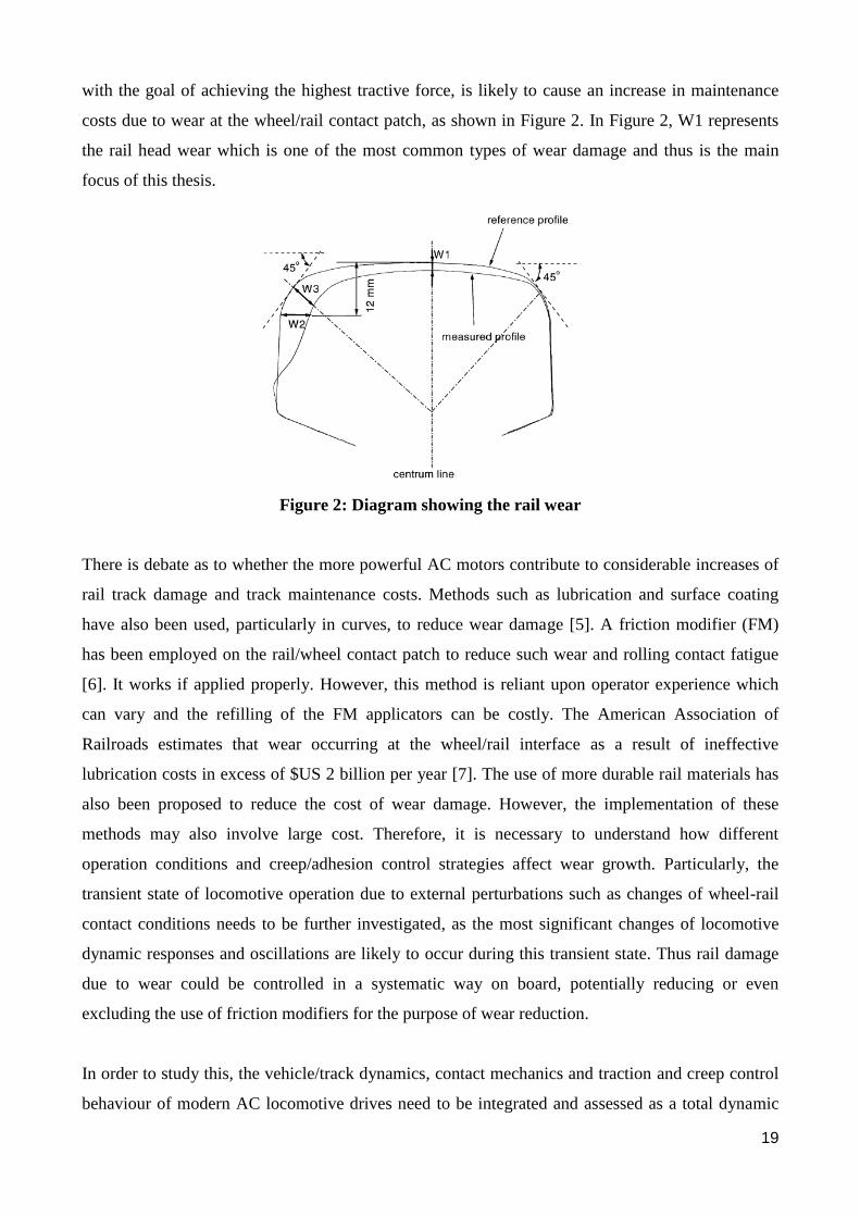
with the goal of achieving the highest tractive force, is likely to cause an increase in maintenance

costs due to wear at the wheel/rail contact patch, as shown in Figure 2. In Figure 2, W1 represents

the rail head wear which is one of the most common types of wear damage and thus is the main

focus of this thesis.

Figure 2: Diagram showing the rail wear

There is debate as to whether the more powerful AC motors contribute to considerable increases of

rail track damage and track maintenance costs. Methods such as lubrication and surface coating

have also been used, particularly in curves, to reduce wear damage [5]. A friction modifier (FM)

has been employed on the rail/wheel contact patch to reduce such wear and rolling contact fatigue

[6]. It works if applied properly. However, this method is reliant upon operator experience which

can vary and the refilling of the FM applicators can be costly. The American Association of

Railroads estimates that wear occurring at the wheel/rail interface as a result of ineffective

lubrication costs in excess of $US 2 billion per year [7]. The use of more durable rail materials has

also been proposed to reduce the cost of wear damage. However, the implementation of these

methods may also involve large cost. Therefore, it is necessary to understand how different

operation conditions and creep/adhesion control strategies affect wear growth. Particularly, the

transient state of locomotive operation due to external perturbations such as changes of wheel-rail

contact conditions needs to be further investigated, as the most significant changes of locomotive

dynamic responses and oscillations are likely to occur during this transient state. Thus rail damage

due to wear could be controlled in a systematic way on board, potentially reducing or even

excluding the use of friction modifiers for the purpose of wear reduction.

In order to study this, the vehicle/track dynamics, contact mechanics and traction and creep control

behaviour of modern AC locomotive drives need to be integrated and assessed as a total dynamic

20

feedback interactive system. The dynamic response and its impact on wear growth under different

control strategies and changes of contact conditions due to natural perturbations such as

friction/lubrication, vehicle/track dynamics et al. need to be analysed. These problems will be

addressed in this thesis. Moreover, a specialized novel real-time traction control system limiting rail

track wear growth will also be proposed to provide a systematic approach to achieve the optimum

balance between traction and wear.

1.2. Objectives and Scope of Research

The focus of this thesis is to develop a predictive integrated locomotive dynamic model, implement

different creep/adhesion control strategies, and to propose and test a real-time control approach to

limit rail damage caused by wear.

Specifically, the major objectives of this thesis are as follows.

1.2.1 Modelling of the locomotive dynamics

To develop a simplified predictive integrated mathematical model including locomotive

longitudinal, vertical and pitch dynamics, wheel/rail contact mechanics and simplified electric drive

dynamics. To investigate the oscillation modes of the locomotive multibody dynamics and

consequently identify the modes those are more likely to be excited, and to examine the locomotive

dynamic behaviour under changes in contact conditions.

1.2.2 Theoretical and numerical analysis of creep control and locomotive dynamics

To develop creep/adhesion controllers to achieve highest tractive force under changes of operating

conditions such as wheel/rail contact conditions and operation speed. To investigate their influence

on locomotive dynamic response compared to fixed creep threshold control by carrying out

simulations.

1.2.3 Design of specialized real-time traction control that regulates the wear to low levels

To develop a novel real-time control strategy to reduce the wear damage on the tracks. To

investigate and compare its impact on the locomotive dynamic response and the wear damage with

that with fixed creep threshold control by simulation.

21

1.3. Thesis Outline

This thesis is divided into 6 chapters including this introduction. A summary of the remaining

chapters is provided as follows.

Chapter 2 provides an overview of the current state of research regarding locomotive

dynamic modelling. A review of creep/adhesion control and of wear growth modelling in railways

is then described.

Chapter 3 presents the modelling methodology used to achieve the thesis objectives. Firstly,

the simulation model for locomotive longitudinal-vertical-pitch dynamics, wheel/rail contact

mechanics and electric drive dynamics are presented, followed by creep/adhesion control design.

Finally the proposed wear rate control methodology is provided.

Chapter 4 describes the simulation results first, including single drive simulation results and

results with the locomotive dynamic model under changes of operation conditions. Simulation

results and the comparisons of dynamic responses between constant threshold creep control and

various adjustable creep controls achieving higher tractive force are then provided. Subsequently

simulation results showing the impact of wear control on wear growth rate and locomotive dynamic

responses are provided, followed by results highlighting the effectiveness of the wear control

strategy.

In Chapter 5, a summary of appended papers is provided.

Chapter 6 summarises the conclusions of this study, together with the recommendations for

future research.

22

Chapter II: Literature Review

This chapter presents a detailed literature review of the locomotive dynamics and control research

including five aspects which are categorized into locomotive dynamic modelling, wheel/rail contact

mechanics, locomotive electric drive and control, locomotive adhesion/creep control, and wear

models in railways. This leads to a summary statement of where the research performed in this

thesis contributes to the body of knowledge on the development of locomotive traction and wear

control technology.

2.1. Review of Locomotive Dynamic Modelling/Simulation (Objective 1)

This section provides literature research on the modelling of essential dynamic components of a

locomotive, including the locomotive multibody dynamics, wheel/rail contact dynamics and electric

drive dynamics. The reviews of the major dynamic components are detailed in the following

sections.

2.1.1. Review of Locomotive Multibody Dynamic Modelling

Research into dynamic modelling and simulation of a locomotive based on mathematical models to

represent certain complex railway vehicles varies significantly depending on the purpose of

researchers and the cases being investigated. Most of the models can be categorised into (1)

longitudinal and vertical dynamics on tangent tracks, (2) lateral dynamics on tangent tracks and (3)

curving dynamics [8]. This study focuses on the first category as it is the most important dynamic

part of locomotive dynamics which is closely related to traction/braking effort, passenger comfort

and energy management. The modelling of rail vehicle longitudinal and vertical dynamics without

consideration of traction or drive issues has been extensively studied for many years, and in

different levels of complexity. In this section, a range of locomotive dynamic models are reviewed,

including the quarter rail vehicle model, finite element models and longitudinal-vertical dynamic

models for the whole locomotive built with Newton principles or Lagrangian method, and software

packages that have been widely used for locomotive dynamic modelling.

The simplest model proposed to reveal the overall dynamics of a locomotive is a quarter rail vehicle

model, which is preferred in many studies because of its simplicity and ease of application [9, 10].

This model is based on a quarter of a 4 wheelsets locomotive and consists of a primary and

secondary suspension as shown in Figure 3.

23

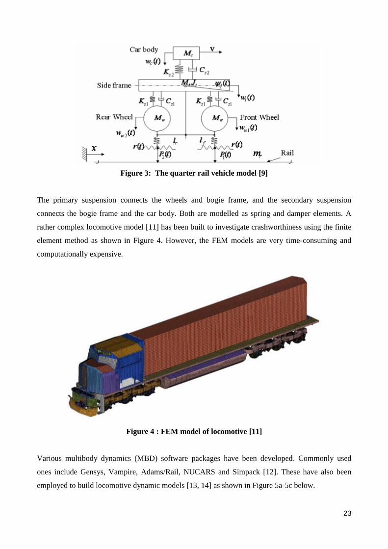
Figure 3: The quarter rail vehicle model [9]

The primary suspension connects the wheels and bogie frame, and the secondary suspension

connects the bogie frame and the car body. Both are modelled as spring and damper elements. A

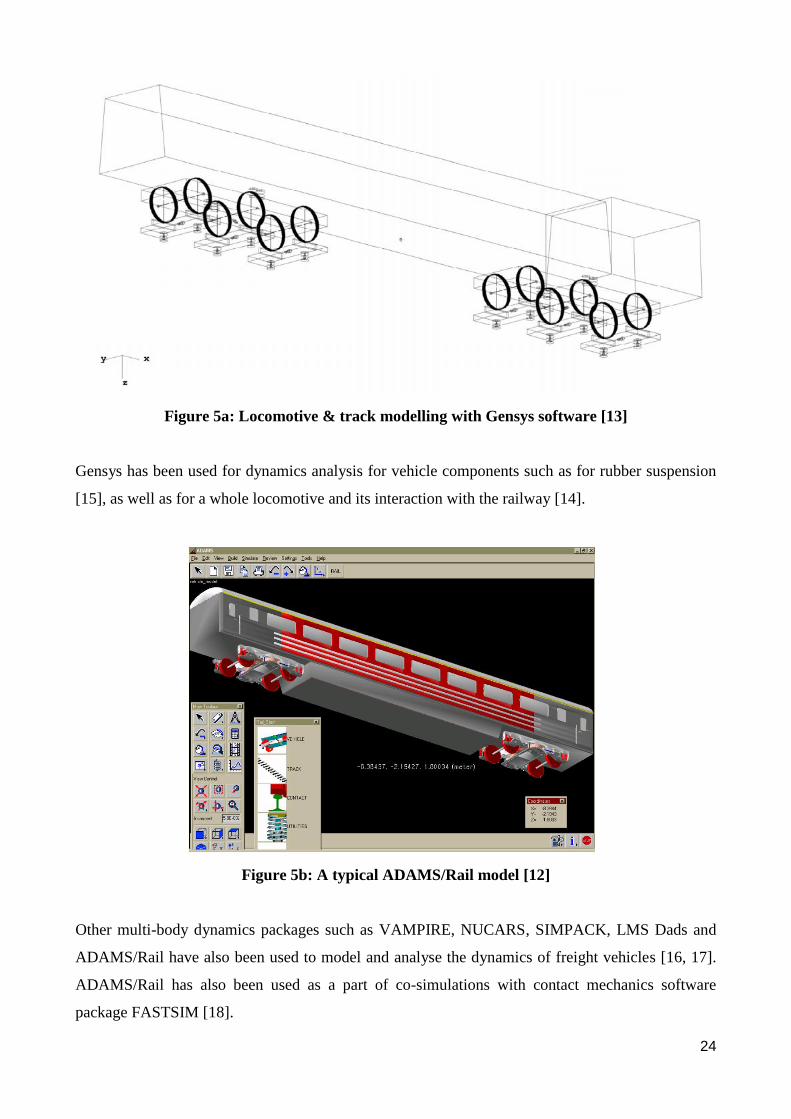
rather complex locomotive model [11] has been built to investigate crashworthiness using the finite

element method as shown in Figure 4. However, the FEM models are very time-consuming and

computationally expensive.

Figure 4 : FEM model of locomotive [11]

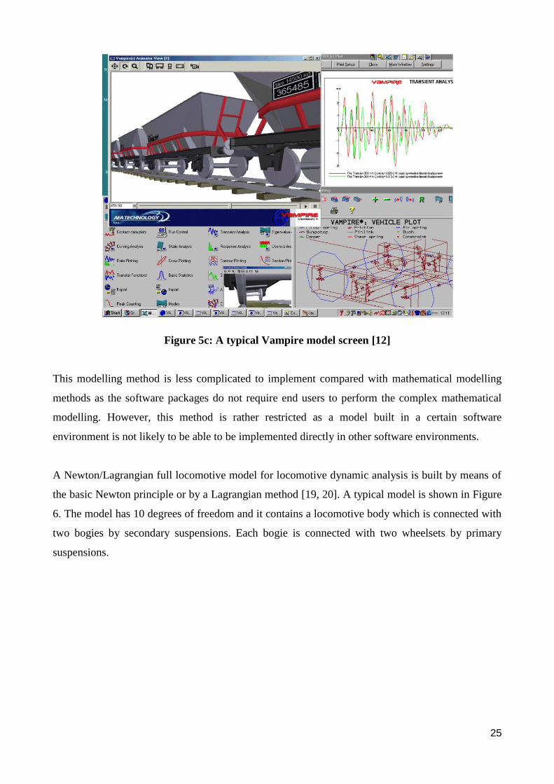
Various multibody dynamics (MBD) software packages have been developed. Commonly used

ones include Gensys, Vampire, Adams/Rail, NUCARS and Simpack [12]. These have also been

employed to build locomotive dynamic models [13, 14] as shown in Figure 5a-5c below.

24

Figure 5a: Locomotive & track modelling with Gensys software [13]

Gensys has been used for dynamics analysis for vehicle components such as for rubber suspension

[15], as well as for a whole locomotive and its interaction with the railway [14].

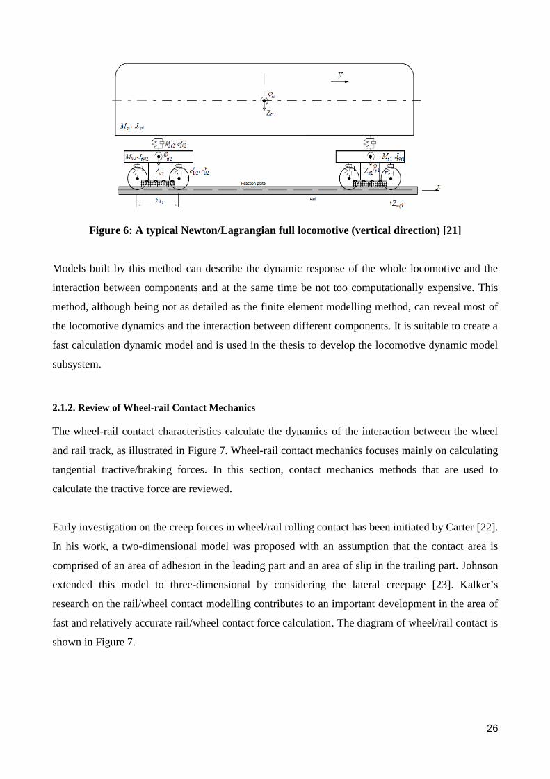
Figure 5b: A typical ADAMS/Rail model [12]

Other multi-body dynamics packages such as VAMPIRE, NUCARS, SIMPACK, LMS Dads and

ADAMS/Rail have also been used to model and analyse the dynamics of freight vehicles [16, 17].

ADAMS/Rail has also been used as a part of co-simulations with contact mechanics software

package FASTSIM [18].

25

Figure 5c: A typical Vampire model screen [12]

This modelling method is less complicated to implement compared with mathematical modelling

methods as the software packages do not require end users to perform the complex mathematical

modelling. However, this method is rather restricted as a model built in a certain software

environment is not likely to be able to be implemented directly in other software environments.

A Newton/Lagrangian full locomotive model for locomotive dynamic analysis is built by means of

the basic Newton principle or by a Lagrangian method [19, 20]. A typical model is shown in Figure

6. The model has 10 degrees of freedom and it contains a locomotive body which is connected with

two bogies by secondary suspensions. Each bogie is connected with two wheelsets by primary

suspensions.

26

Figure 6: A typical Newton/Lagrangian full locomotive (vertical direction) [21]

Models built by this method can describe the dynamic response of the whole locomotive and the

interaction between components and at the same time be not too computationally expensive. This

method, although being not as detailed as the finite element modelling method, can reveal most of

the locomotive dynamics and the interaction between different components. It is suitable to create a

fast calculation dynamic model and is used in the thesis to develop the locomotive dynamic model

subsystem.

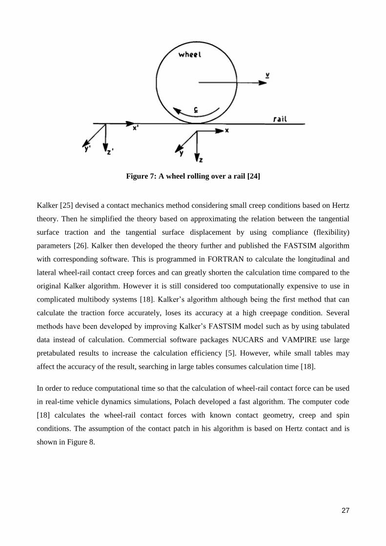
2.1.2. Review of Wheel-rail Contact Mechanics

The wheel-rail contact characteristics calculate the dynamics of the interaction between the wheel

and rail track, as illustrated in Figure 7. Wheel-rail contact mechanics focuses mainly on calculating

tangential tractive/braking forces. In this section, contact mechanics methods that are used to

calculate the tractive force are reviewed.

Early investigation on the creep forces in wheel/rail rolling contact has been initiated by Carter [22].

In his work, a two-dimensional model was proposed with an assumption that the contact area is

comprised of an area of adhesion in the leading part and an area of slip in the trailing part. Johnson

extended this model to three-dimensional by considering the lateral creepage [23]. Kalker’s

research on the rail/wheel contact modelling contributes to an important development in the area of

fast and relatively accurate rail/wheel contact force calculation. The diagram of wheel/rail contact is

shown in Figure 7.

27

Figure 7: A wheel rolling over a rail [24]

Kalker [25] devised a contact mechanics method considering small creep conditions based on Hertz

theory. Then he simplified the theory based on approximating the relation between the tangential

surface traction and the tangential surface displacement by using compliance (flexibility)

parameters [26]. Kalker then developed the theory further and published the FASTSIM algorithm

with corresponding software. This is programmed in FORTRAN to calculate the longitudinal and

lateral wheel-rail contact creep forces and can greatly shorten the calculation time compared to the

original Kalker algorithm. However it is still considered too computationally expensive to use in

complicated multibody systems [18]. Kalker’s algorithm although being the first method that can

calculate the traction force accurately, loses its accuracy at a high creepage condition. Several

methods have been developed by improving Kalker’s FASTSIM model such as by using tabulated

data instead of calculation. Commercial software packages NUCARS and VAMPIRE use large

pretabulated results to increase the calculation efficiency [5]. However, while small tables may

affect the accuracy of the result, searching in large tables consumes calculation time [18].

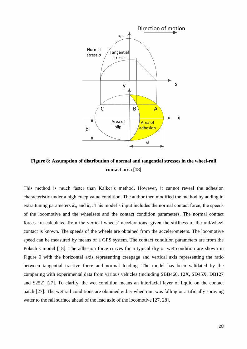
In order to reduce computational time so that the calculation of wheel-rail contact force can be used

in real-time vehicle dynamics simulations, Polach developed a fast algorithm. The computer code

[18] calculates the wheel-rail contact forces with known contact geometry, creep and spin

conditions. The assumption of the contact patch in his algorithm is based on Hertz contact and is

shown in Figure 8.

28

y

Direction of motion

Tangentialstress τ

Area of slip

B

σ, τ

b

a

C A

Area of adhesion

x

x

Normalstress σ

Figure 8: Assumption of distribution of normal and tangential stresses in the wheel-rail

contact area [18]

This method is much faster than Kalker’s method. However, it cannot reveal the adhesion

characteristic under a high creep value condition. The author then modified the method by adding in

extra tuning parameters 𝑘𝑎 and 𝑘𝑠. This model’s input includes the normal contact force, the speeds

of the locomotive and the wheelsets and the contact condition parameters. The normal contact

forces are calculated from the vertical wheels’ accelerations, given the stiffness of the rail/wheel

contact is known. The speeds of the wheels are obtained from the accelerometers. The locomotive

speed can be measured by means of a GPS system. The contact condition parameters are from the

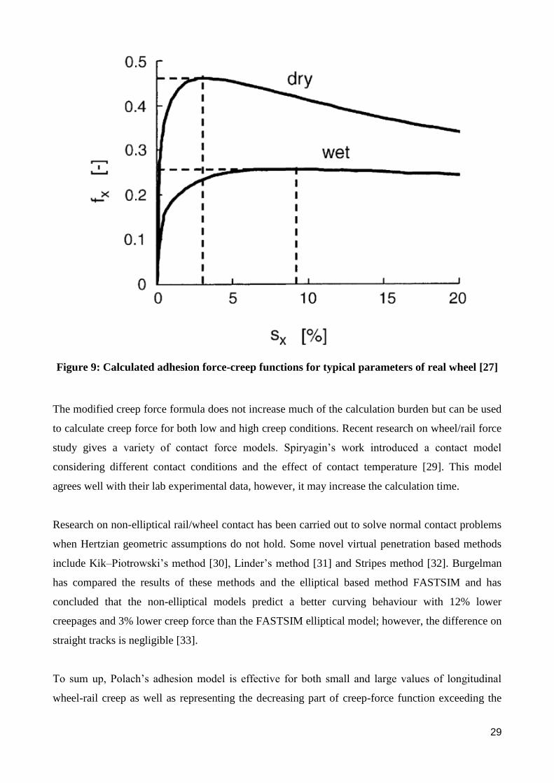
Polach’s model [18]. The adhesion force curves for a typical dry or wet condition are shown in

Figure 9 with the horizontal axis representing creepage and vertical axis representing the ratio

between tangential tractive force and normal loading. The model has been validated by the

comparing with experimental data from various vehicles (including SBB460, 12X, SD45X, DB127

and S252) [27]. To clarify, the wet condition means an interfacial layer of liquid on the contact

patch [27]. The wet rail conditions are obtained either when rain was falling or artificially spraying

water to the rail surface ahead of the lead axle of the locomotive [27, 28].

29

Figure 9: Calculated adhesion force-creep functions for typical parameters of real wheel [27]

The modified creep force formula does not increase much of the calculation burden but can be used

to calculate creep force for both low and high creep conditions. Recent research on wheel/rail force

study gives a variety of contact force models. Spiryagin’s work introduced a contact model

considering different contact conditions and the effect of contact temperature [29]. This model

agrees well with their lab experimental data, however, it may increase the calculation time.

Research on non-elliptical rail/wheel contact has been carried out to solve normal contact problems

when Hertzian geometric assumptions do not hold. Some novel virtual penetration based methods

include Kik–Piotrowski’s method [30], Linder’s method [31] and Stripes method [32]. Burgelman

has compared the results of these methods and the elliptical based method FASTSIM and has

concluded that the non-elliptical models predict a better curving behaviour with 12% lower

creepages and 3% lower creep force than the FASTSIM elliptical model; however, the difference on

straight tracks is negligible [33].

To sum up, Polach’s adhesion model is effective for both small and large values of longitudinal

wheel-rail creep as well as representing the decreasing part of creep-force function exceeding the

30

adhesion limit [34]. Furthermore, it is used in this thesis as it has been verified to be relatively

accurate for the application in the field of locomotive traction analysis [35].

2.1.3. Review of Locomotive Electric Drive Control Design

Locomotive drive and creep controller design is critical to the performance of the locomotive

system and also is one of the main focuses of the thesis. A well-designed drive and control system

can not only increase the operational reliability of the locomotive but also improve the

driver/passenger comfort. In this section an introduction including the characteristics of an AC

motor emphasizing the challenge of its control will be proposed first, followed by some AC drive

control methods commonly used in industry especially on locomotives.

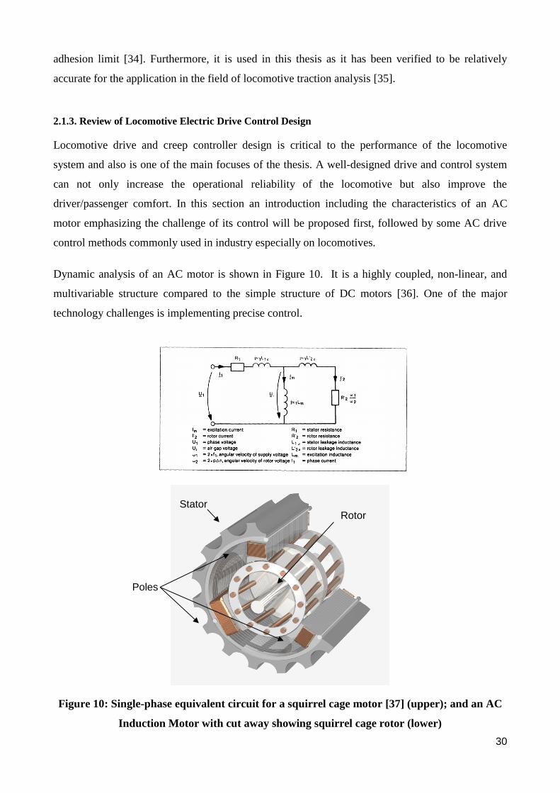
Dynamic analysis of an AC motor is shown in Figure 10. It is a highly coupled, non-linear, and

multivariable structure compared to the simple structure of DC motors [36]. One of the major

technology challenges is implementing precise control.

Figure 10: Single-phase equivalent circuit for a squirrel cage motor [37] (upper); and an AC

Induction Motor with cut away showing squirrel cage rotor (lower)

Stator Rotor

Poles

31

Simple open loop control is possible with a fixed control frequency, via a variety of techniques such

as switching of the number of active poles or varying the supply voltage. However such schemes do

not provide good control over the system over a large range of speeds and slip [38]. AC drives do,

however, naturally possess a steep torque slip curve near the synchronous speed of the motor, which

is exploited in a number of control schemes based on varying the amplitude and waveform of the

supplied voltage, enabling precise speed control [39]. The difficulties associated with this type of

precise control over the full range of operating conditions is due to the nonlinear nature of the

system and the practical challenge of generating the desired multiphase supply voltage with fine

enough resolution to accurately reproduce the waveform as required for the control signal.

An induction motor drive is a complicated nonlinear system that has been the subject of a large

body of research and their control schemes have reached a high state of development [38]. System

modelling typically allows for nonlinear inversion into a linear model, allowing the use of well

understood linear control techniques [39]. The principal challenges in implementing these

techniques are then technical and financial, in that a reliable estimate must be available for the

control model. Examples of these challenges are the difficulty of accurately estimating rotor fluxes

and load torques [40] and the cost associated with installing high accuracy sensors to measure

rotation speed [41]. Techniques have been developed to overcome these limitations, such as sliding

mode nonlinear state estimation techniques [42], but the potential costs of poor estimates are

degraded performance [43].

The importance of AC induction drives and their control in industrial applications has resulted in

the development of accurate simulation packages capable of reproducing the dynamic behaviour of

typical drive and control configurations [43]. MATLAB/Simulink based modelling is frequently

encountered in research papers as a useful tool for evaluating the expected performance of AC drive

systems (see for example [43-45]). In the following sections, some widely used AC drive control

methods are separately explained.

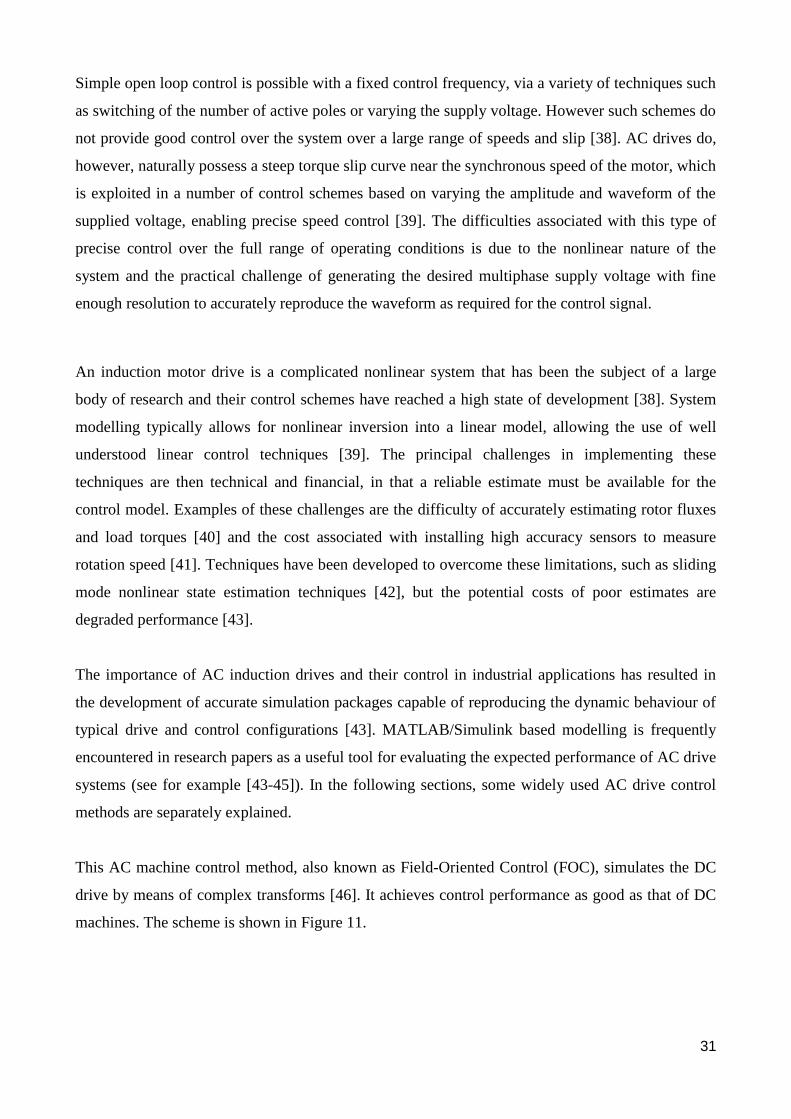
This AC machine control method, also known as Field-Oriented Control (FOC), simulates the DC

drive by means of complex transforms [46]. It achieves control performance as good as that of DC

machines. The scheme is shown in Figure 11.

32

Figure 11: Basic scheme of FOC for the three-phase AC machine [47]

In the system, two motor phase currents and the DC bus voltage are measured and transformed

using the Clarke transformation block (the transformations can be found in [48]) into a stationary

reference frame. These last two components are further transformed, using the Park transformation,

into rotating components (dq). The PI controllers compare the command values with the measured

components (after transformation) and command proper values to establish the desired condition.

The outputs of the controllers are transformed from a rotating to a stationary frame using the Park

transformation. The commanded signals of the stator voltage are sent to the pulse width modulation

(PWM) block. Although the flux vector AC machine control method can achieve good torque

response with full torque at zero speed and has performance very close to a DC drive, it needs a

feedback device which can be costly and can add complexity to the drive system. A modulator is

also used, which will slow down communication between the incoming voltage and frequency.

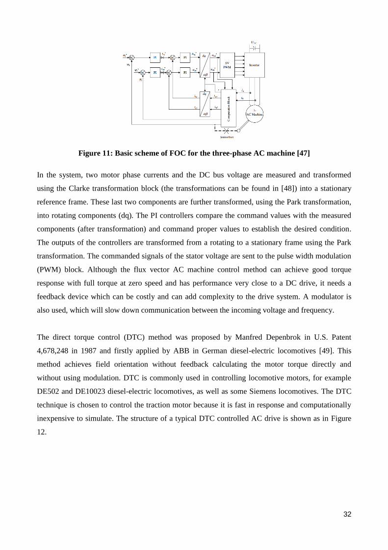
The direct torque control (DTC) method was proposed by Manfred Depenbrok in U.S. Patent

4,678,248 in 1987 and firstly applied by ABB in German diesel-electric locomotives [49]. This

method achieves field orientation without feedback calculating the motor torque directly and

without using modulation. DTC is commonly used in controlling locomotive motors, for example

DE502 and DE10023 diesel-electric locomotives, as well as some Siemens locomotives. The DTC

technique is chosen to control the traction motor because it is fast in response and computationally

inexpensive to simulate. The structure of a typical DTC controlled AC drive is shown as in Figure

12.

33

Figure 12: A typical DTC controlled AC drive structure [50]

Details of this method can be found in [51]. This method has the following advantages: no

modulator is needed; no tachometer or position encoder which is to feedback the shaft speed or

position is required; and the torque performance is faster than other AC or DC drives [52]. This

induction machine control technique is used in this thesis to build the complex drive model and to

compare with available data considering the above advantages over other methods.

2.2. Review of Adhesion/Creep Control (Objective 2)

Modern development of mechatronics systems provides the possibility of improving rail vehicle

operation under various conditions. The traction control system, also known as an adhesion control

system or anti-slip regulation system is essential for such systems to achieve operational efficiency

and reliability. The traction control system is designed to regulate the torque applied to the vehicle

wheelsets to prevent excessive wheel-slip and resulting loss of traction. A number of different

methods have been proposed by researchers aiming to prevent excessive wheel-slip and to operate

the rail vehicle at an optimum level of adhesion. Most of these require vehicle velocity and wheel-

rail contact condition information. A terminology, creepage, needs to be introduced here. It is

defined as the difference between wheelset velocity and locomotive velocity normalized by

locomotive speed.

As mentioned in previous sections, AC motors can achieve higher traction/adhesion performance

than their DC counterparts to theoretically achieve the optimum traction/adhesion operation of rail

locomotives. However, due to its inherent complexity and non-linearity, the high performance can

only be achieved by accurate state detection and/or estimation together with proper AC drive

34

control design. The performance under dynamic conditions has also not been investigated deeply.

The following sections will review several recent adhesion control techniques.

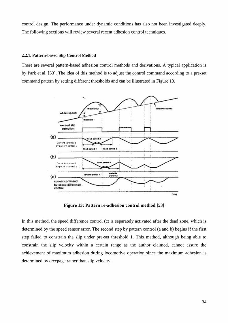
2.2.1. Pattern-based Slip Control Method

There are several pattern-based adhesion control methods and derivations. A typical application is

by Park et al. [53]. The idea of this method is to adjust the control command according to a pre-set

command pattern by setting different thresholds and can be illustrated in Figure 13.

Current commandBy pattern control 1

Current commandBy pattern control 2

Figure 13: Pattern re-adhesion control method [53]

In this method, the speed difference control (c) is separately activated after the dead zone, which is

determined by the speed sensor error. The second step by pattern control (a and b) begins if the first

step failed to constrain the slip under pre-set threshold 1. This method, although being able to

constrain the slip velocity within a certain range as the author claimed, cannot assure the

achievement of maximum adhesion during locomotive operation since the maximum adhesion is

determined by creepage rather than slip velocity.

35

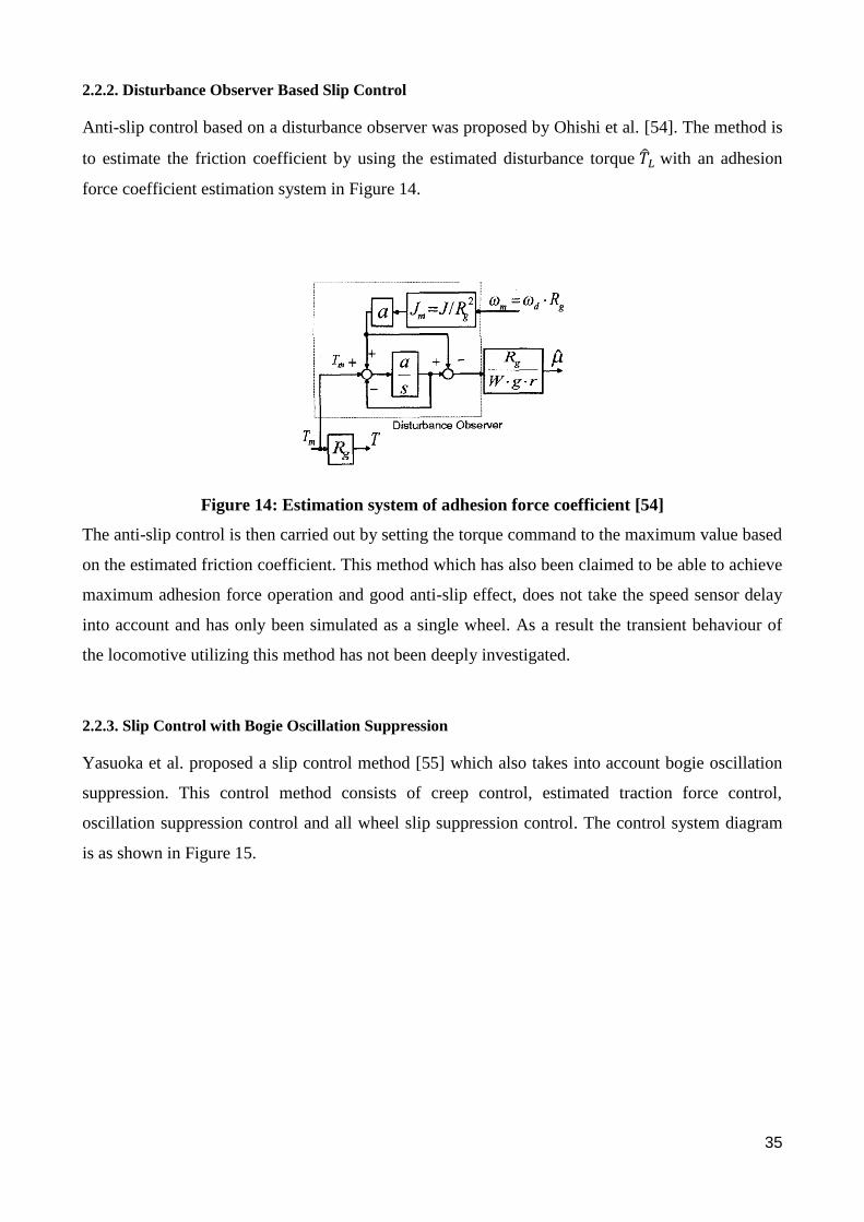
2.2.2. Disturbance Observer Based Slip Control

Anti-slip control based on a disturbance observer was proposed by Ohishi et al. [54]. The method is

to estimate the friction coefficient by using the estimated disturbance torque ��𝐿 with an adhesion

force coefficient estimation system in Figure 14.

Figure 14: Estimation system of adhesion force coefficient [54]

The anti-slip control is then carried out by setting the torque command to the maximum value based

on the estimated friction coefficient. This method which has also been claimed to be able to achieve

maximum adhesion force operation and good anti-slip effect, does not take the speed sensor delay

into account and has only been simulated as a single wheel. As a result the transient behaviour of

the locomotive utilizing this method has not been deeply investigated.

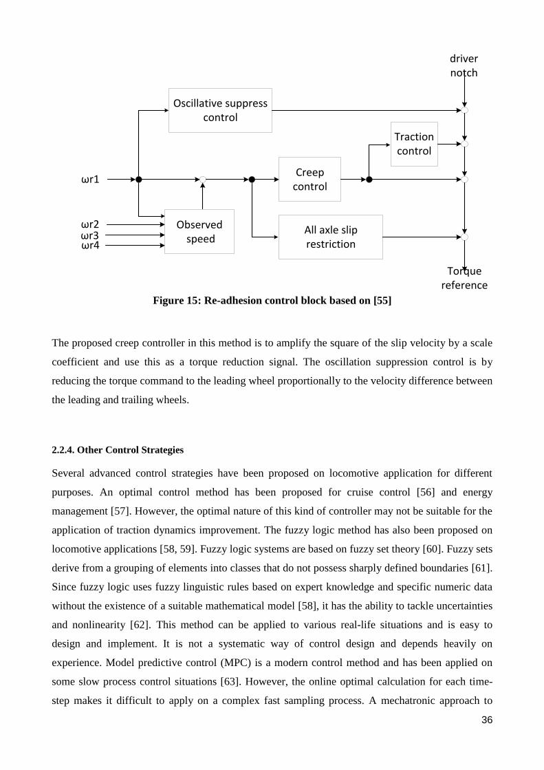
2.2.3. Slip Control with Bogie Oscillation Suppression

Yasuoka et al. proposed a slip control method [55] which also takes into account bogie oscillation

suppression. This control method consists of creep control, estimated traction force control,

oscillation suppression control and all wheel slip suppression control. The control system diagram

is as shown in Figure 15.

36

Oscillative suppress control

Observed speed

All axle sliprestriction

Creep control

Traction control

ωr1

ωr2ωr3ωr4

driver notch

Torquereference

Figure 15: Re-adhesion control block based on [55]

The proposed creep controller in this method is to amplify the square of the slip velocity by a scale

coefficient and use this as a torque reduction signal. The oscillation suppression control is by

reducing the torque command to the leading wheel proportionally to the velocity difference between

the leading and trailing wheels.

2.2.4. Other Control Strategies

Several advanced control strategies have been proposed on locomotive application for different

purposes. An optimal control method has been proposed for cruise control [56] and energy

management [57]. However, the optimal nature of this kind of controller may not be suitable for the

application of traction dynamics improvement. The fuzzy logic method has also been proposed on

locomotive applications [58, 59]. Fuzzy logic systems are based on fuzzy set theory [60]. Fuzzy sets

derive from a grouping of elements into classes that do not possess sharply defined boundaries [61].

Since fuzzy logic uses fuzzy linguistic rules based on expert knowledge and specific numeric data

without the existence of a suitable mathematical model [58], it has the ability to tackle uncertainties

and nonlinearity [62]. This method can be applied to various real-life situations and is easy to

design and implement. It is not a systematic way of control design and depends heavily on

experience. Model predictive control (MPC) is a modern control method and has been applied on

some slow process control situations [63]. However, the online optimal calculation for each time-

step makes it difficult to apply on a complex fast sampling process. A mechatronic approach to

37

control the wheel slip based on the information on the torsional vibration of the wheelset is

investigated by Mei et al. [64]. Nonlinear control design and its application has been proposed [65]

on a simplified mass locomotive. The process of finding the Lyapunov function may be difficult if

the whole complex locomotive dynamics is considered. In this thesis, PI and fuzzy logic based

controllers are used to achieve creep and wear control.

2.3. Review of Wear Models in Railways (Objective 3)

Wear is the progressive loss of material from the operating surface of a body, caused by relative

motion at the surface [66]. In the railway field it is a fundamental problem as the change of profile

shape deeply affects the dynamic characteristics of railway vehicles such as stability or passenger

comfort and, in the worst cases, can cause derailment [67]. Wear may be broadly classified

according to the relative types of motion such as sliding, rolling and rolling-sliding, or types of wear

mechanisms [68]. The wear phenomenon in the rail industry and its modelling has been studied for

decades [67, 69-71]. However, the impact of locomotive dynamic response on wear phenomena

under different conditions has not been investigated deeply.

Beagley et al. proposed patterns of wear behaviour [72], which is categorized into “mild” and

“severe” regimes to describe wear characteristics on either side of a wear transition between sliding

velocity regions observed in his experimental results. A third regime, defined as “catastrophic”

regime of wear, was defined by Bolton et al. according to their test results [73]. A thorough review

of this “catastrophic” wear phenomenon was performed by Markov et al. in [74]. Furthermore, three

wear regimes for wheel/rail steels have also been observed by Danks et al. [75] with field and

laboratory test results. Danks et al. also proposed to use the terms “type I wear”, “type II wear” and

“type III wear” for describing the “stages” of the wear, which are characterised by: the wear rate;

the worn surface features (particularly its roughness); and the size, morphology and colour of wear

debris which are caused by wear modes identified in references [66, 72, 73, 75, 76]. According to

Clayton [77], type I wear combines both oxidational and rolling-sliding modes of wear resulting in

debris containing oxide and metal particles. It approaches a true oxidative wear, in which materials

are removed by the progressive growth and mechanical breakdown of an oxide layer, at very low

creep rate and contact pressures. At the creep rate beyond the creep saturation there is a significant

contribution from the formation of rolled out, thin, metal flakes that eventually fracture. Type II is

characterised by completely metallic wear debris, the occurrence of microscope ripples on the wear

surfaces and some metal transfer. It has been concluded that this is a deformation and fracture

process with no evidence of fatigue-like cracks at the surface. Type III wear involves an initial

38

break-in period that leads to the production of large pieces of wear debris. This causes self-inflicted

wear of both contact surfaces.

For the wheel/rail steel, the material loss in the wear process is defined as wear rate. It is determined

by the loss of material mass per rolling distance (𝜇𝑔/𝑚) [75]; or by the total loss of material mass

per rolling distance, per contact area (𝜇𝑔/𝑚/𝑚𝑚2) [76]. Both wheel and rail wear regimes can be

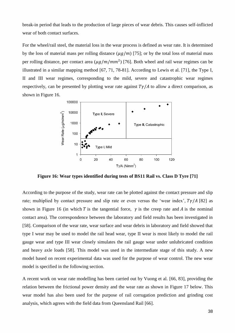
illustrated in a similar mapping method [67, 71, 78-81]. According to Lewis et al. [71], the Type I,

II and III wear regimes, corresponding to the mild, severe and catastrophic wear regimes

respectively, can be presented by plotting wear rate against 𝑇𝛾/𝐴 to allow a direct comparison, as

shown in Figure 16.

Figure 16: Wear types identified during tests of BS11 Rail vs. Class D Tyre [71]

According to the purpose of the study, wear rate can be plotted against the contact pressure and slip

rate; multiplied by contact pressure and slip rate or even versus the ‘wear index’, 𝑇𝛾/𝐴 [82] as

shown in Figure 16 (in which 𝑇 is the tangential force, 𝛾 is the creep rate and 𝐴 is the nominal

contact area). The correspondence between the laboratory and field results has been investigated in

[58]. Comparison of the wear rate, wear surface and wear debris in laboratory and field showed that

type I wear may be used to model the rail head wear, type II wear is most likely to model the rail

gauge wear and type III wear closely simulates the rail gauge wear under unlubricated condition

and heavy axle loads [58]. This model was used in the intermediate stage of this study. A new

model based on recent experimental data was used for the purpose of wear control. The new wear

model is specified in the following section.

A recent work on wear rate modelling has been carried out by Vuong et al. [66, 83], providing the

relation between the frictional power density and the wear rate as shown in Figure 17 below. This

wear model has also been used for the purpose of rail corrugation prediction and grinding cost

analysis, which agrees with the field data from Queensland Rail [66].

39

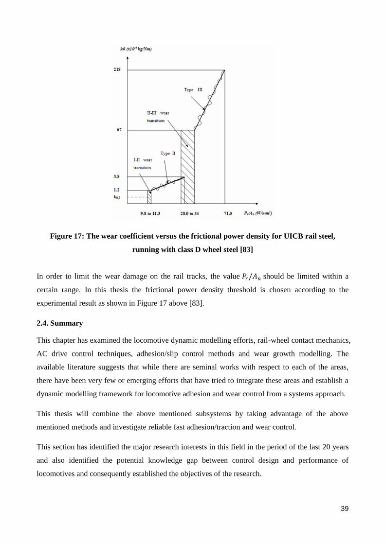
Figure 17: The wear coefficient versus the frictional power density for UICB rail steel,

running with class D wheel steel [83]

In order to limit the wear damage on the rail tracks, the value 𝑃𝑟/𝐴𝑛 should be limited within a

certain range. In this thesis the frictional power density threshold is chosen according to the

experimental result as shown in Figure 17 above [83].

2.4. Summary

This chapter has examined the locomotive dynamic modelling efforts, rail-wheel contact mechanics,

AC drive control techniques, adhesion/slip control methods and wear growth modelling. The

available literature suggests that while there are seminal works with respect to each of the areas,

there have been very few or emerging efforts that have tried to integrate these areas and establish a

dynamic modelling framework for locomotive adhesion and wear control from a systems approach.

This thesis will combine the above mentioned subsystems by taking advantage of the above

mentioned methods and investigate reliable fast adhesion/traction and wear control.

This section has identified the major research interests in this field in the period of the last 20 years

and also identified the potential knowledge gap between control design and performance of

locomotives and consequently established the objectives of the research.

40

Chapter III: Methodology

This chapter provides a summary of methodologies and models developed in this thesis for

locomotive and electric drive modelling, wheel/rail contact mechanics modelling,

creep/adhesion control and wear control. More specifically, section 3.1 mainly introduces the

mathematical modelling for locomotive longitudinal, vertical and pitch dynamics; a detailed

wheel/rail contact mechanics modelling; and electric drive dynamic modelling (Objective 1).

Section 3.2 provides details of the fuzzy logic based creep/adhesion control methods aiming

to achieve higher tractive force under a change of operating conditions (Objective 2). In

section 3.3, details of wear rate control strategy are provided (Objective 3).

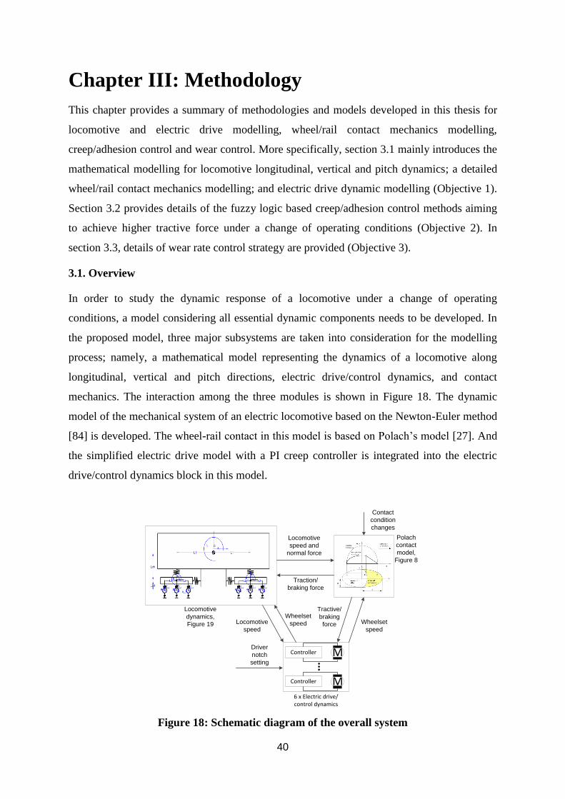
3.1. Overview

In order to study the dynamic response of a locomotive under a change of operating

conditions, a model considering all essential dynamic components needs to be developed. In

the proposed model, three major subsystems are taken into consideration for the modelling

process; namely, a mathematical model representing the dynamics of a locomotive along

longitudinal, vertical and pitch directions, electric drive/control dynamics, and contact

mechanics. The interaction among the three modules is shown in Figure 18. The dynamic

model of the mechanical system of an electric locomotive based on the Newton-Euler method

[84] is developed. The wheel-rail contact in this model is based on Polach’s model [27]. And

the simplified electric drive model with a PI creep controller is integrated into the electric

drive/control dynamics block in this model.

MController

6 x Electric drive/control dynamics

MController

Polach

contact

model,

Figure 8

Locomotive

speed and

normal force

Contact

condition

changes

Driver

notch

setting

Traction/

braking force

Locomotive

speed

Wheelset

speed

Tractive/

braking

force

Locomotive

dynamics,

Figure 19

Wheelset

speed

Figure 18: Schematic diagram of the overall system

050

100 0 0.1 0.2 0.3 0.4 0.5

0

0.1

0.2

0.3

0.4

0.5

0.6

0.7

creep

Polach dry

loco velocity km/h

adhesio

n c

oeffic

ient

0

0.1

0.2

0.3

0.4

0.5

Electric drive & control

Comple

M

41

The model may be described as a feedback system which takes creep as the major feedback

signal. In the model, creep response is calculated directly from the rotational speed of the

axles and the locomotive. The proposed system is also designed to be able to deploy into the

field, where such speed information can be measured constantly. The rotational speeds of

axles can be constantly measured by tachometers on the axles and used to generate reference

creep. The position/speed information of the railway vehicle can be monitored by using a

microwave ground speed sensor such as a Pegasem GSS20 [85, 86]. As a result, the creep

value on each axle can be calculated as the relative difference between the speed of each axle

and the locomotive speed. The controller then adjusts the amount of torque generated by each

electric drive separately. The electric drive and control system provides a torque acting on the

motor shaft in the locomotive model. Torque also results from the longitudinal force due to

the interaction between wheel-rail track contact mechanics. The resultant creep changes the

longitudinal tractive force calculated using the Polach model. The tractive force acts on the

locomotive dynamic model and changes the displacements and velocities of the vehicle rigid

bodies. Each of these components is detailed in the following sections.

3.2. Locomotive dynamic modelling and eigenmode analysis (Objective 1)

This section presents the modelling of essential locomotive dynamic components and

eigenmode anaysis (Objective 1). Specifically, the locomotive longitudinal, vertical and pitch

dynamics modelling; the wheel/rail contact dynamics modelling; and the electric drive

dynamics modelling are described respectively in detail.

3.2.1. Locomotive Multibody Dynamics

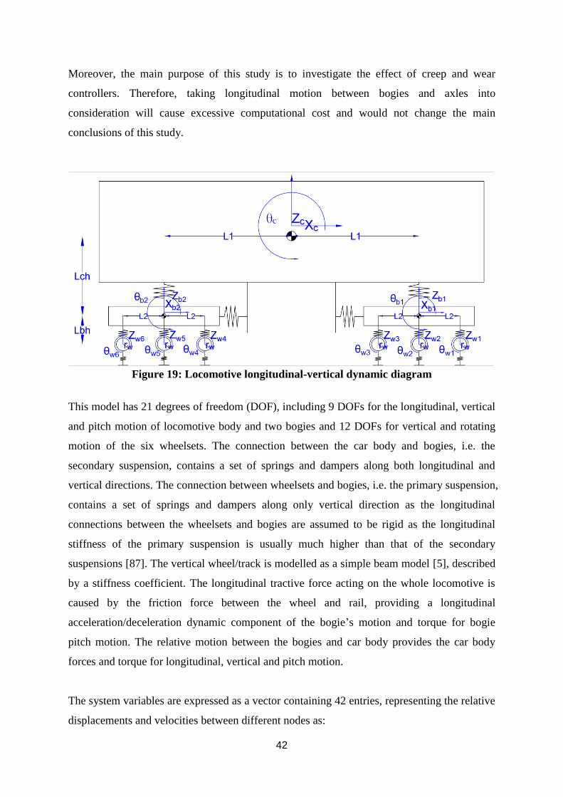
A 2-dimensional locomotive dynamic model is shown in Figure 19, which includes

longitudinal, vertical and pitch dynamics of locomotive motion. An assumption has been

made that the motors are fixed on the bogie evenly and no relative displacement occurs

between the motors and the bogies, in order to simplify the model. The longitudinal motions

between wheelsets and bogies are neglected to simplify the calculation and save simulation

time while maintaining most of the essential dynamics. Also as for a typical three-piece

freight vehicle bogie, axles are mounted on the bogies via axle boxes (Figure 3.37, [5]). The

longitudinal stiffness between the axle box and bogie tends to be relatively higher than that of

other parts, thus the relevant motion between the axles and bogies tends to be negligible.

42

Moreover, the main purpose of this study is to investigate the effect of creep and wear

controllers. Therefore, taking longitudinal motion between bogies and axles into

consideration will cause excessive computational cost and would not change the main

conclusions of this study.

Figure 19: Locomotive longitudinal-vertical dynamic diagram

This model has 21 degrees of freedom (DOF), including 9 DOFs for the longitudinal, vertical

and pitch motion of locomotive body and two bogies and 12 DOFs for vertical and rotating

motion of the six wheelsets. The connection between the car body and bogies, i.e. the

secondary suspension, contains a set of springs and dampers along both longitudinal and

vertical directions. The connection between wheelsets and bogies, i.e. the primary suspension,

contains a set of springs and dampers along only vertical direction as the longitudinal

connections between the wheelsets and bogies are assumed to be rigid as the longitudinal

stiffness of the primary suspension is usually much higher than that of the secondary

suspensions [87]. The vertical wheel/track is modelled as a simple beam model [5], described

by a stiffness coefficient. The longitudinal tractive force acting on the whole locomotive is

caused by the friction force between the wheel and rail, providing a longitudinal

acceleration/deceleration dynamic component of the bogie’s motion and torque for bogie

pitch motion. The relative motion between the bogies and car body provides the car body

forces and torque for longitudinal, vertical and pitch motion.

The system variables are expressed as a vector containing 42 entries, representing the relative

displacements and velocities between different nodes as:

43

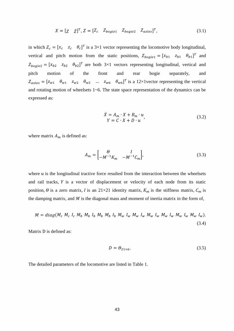
𝑋 = [𝑍 ��]𝑇, 𝑍 = [𝑍𝑐 𝑍𝑏𝑜𝑔𝑖𝑒1 𝑍𝑏𝑜𝑔𝑖𝑒2 𝑍𝑎𝑥𝑙𝑒𝑠]𝑇, (3.1)

in which 𝑍𝑐 = [𝑥𝑐 𝑧𝑐 𝜃𝑐]𝑇 is a 3×1 vector representing the locomotive body longitudinal,

vertical and pitch motion from the static positions, 𝑍𝑏𝑜𝑔𝑖𝑒1 = [𝑥𝑏1 𝑧𝑏1 𝜃𝑏1]𝑇 and

𝑍𝑏𝑜𝑔𝑖𝑒2 = [𝑥𝑏2 𝑧𝑏2 𝜃𝑏2]𝑇 are both 3×1 vectors representing longitudinal, vertical and

pitch motion of the front and rear bogie separately, and

𝑍𝑎𝑥𝑙𝑒𝑠 = [𝑧𝑤1 𝜃𝑤1 𝑧𝑤2 𝜃𝑤2 … 𝑧𝑤6 𝜃𝑤6]𝑇 is a 12×1vector representing the vertical

and rotating motion of wheelsets 1~6. The state space representation of the dynamics can be

expressed as:

�� = 𝐴𝑚 ∙ 𝑋 + 𝐵𝑚 ∙ 𝑢𝑌 = 𝐶 ∙ 𝑋 + 𝐷 ∙ 𝑢

, (3.2)

where matrix 𝐴𝑚 is defined as:

𝐴𝑚 = [𝛩 𝐼

−𝑀−1𝐾𝑚 −𝑀−1𝐶𝑚], (3.3)

where 𝑢 is the longitudinal tractive force resulted from the interaction between the wheelsets

and rail tracks, 𝑌 is a vector of displacement or velocity of each node from its static

position, 𝛩 is a zero matrix, 𝐼 is an 21×21 identity matrix, 𝐾𝑚 is the stiffness matrix, 𝐶𝑚 is

the damping matrix, and 𝑀 is the diagonal mass and moment of inertia matrix in the form of,

𝑀 = 𝑑𝑖𝑎𝑔(𝑀𝑐 𝑀𝑐 𝐼𝑐 𝑀𝑏 𝑀𝑏 𝐼𝑏 𝑀𝑏 𝑀𝑏 𝐼𝑏 𝑀𝑤 𝐼𝑤 𝑀𝑤 𝐼𝑤 𝑀𝑤 𝐼𝑤 𝑀𝑤 𝐼𝑤 𝑀𝑤 𝐼𝑤 𝑀𝑤 𝐼𝑤).

(3.4)

Matrix D is defined as:

𝐷 = 𝛩21×6. (3.5)

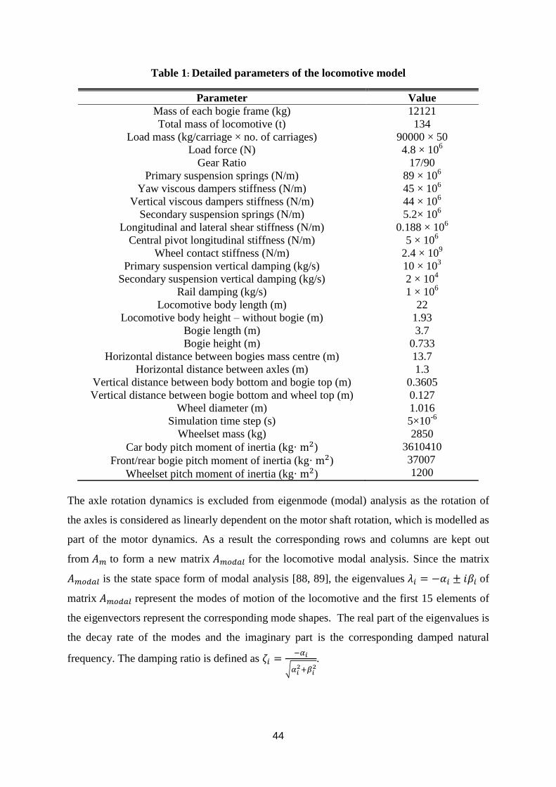
The detailed parameters of the locomotive are listed in Table 1.

44

Table 1: Detailed parameters of the locomotive model

Parameter Value

Mass of each bogie frame (kg) 12121

Total mass of locomotive (t) 134

Load mass (kg/carriage × no. of carriages) 90000 × 50

Load force (N) 4.8 × 106

Gear Ratio 17/90

Primary suspension springs (N/m) 89 × 106

Yaw viscous dampers stiffness (N/m) 45 × 106

Vertical viscous dampers stiffness (N/m) 44 × 106

Secondary suspension springs (N/m) 5.2× 106

Longitudinal and lateral shear stiffness (N/m) 0.188 × 106

Central pivot longitudinal stiffness (N/m) 5 × 106

Wheel contact stiffness (N/m) 2.4 × 109

Primary suspension vertical damping (kg/s) 10 × 103

Secondary suspension vertical damping (kg/s) 2 × 104

Rail damping (kg/s) 1 × 106

Locomotive body length (m) 22

Locomotive body height – without bogie (m) 1.93

Bogie length (m) 3.7

Bogie height (m) 0.733

Horizontal distance between bogies mass centre (m) 13.7

Horizontal distance between axles (m) 1.3

Vertical distance between body bottom and bogie top (m) 0.3605

Vertical distance between bogie bottom and wheel top (m) 0.127

Wheel diameter (m) 1.016

Simulation time step (s)

Wheelset mass (kg)

Car body pitch moment of inertia (kg· m2)

Front/rear bogie pitch moment of inertia (kg· m2)

Wheelset pitch moment of inertia (kg· m2)

5×10-6

2850

3610410

37007

1200

The axle rotation dynamics is excluded from eigenmode (modal) analysis as the rotation of

the axles is considered as linearly dependent on the motor shaft rotation, which is modelled as

part of the motor dynamics. As a result the corresponding rows and columns are kept out

from 𝐴𝑚 to form a new matrix 𝐴𝑚𝑜𝑑𝑎𝑙 for the locomotive modal analysis. Since the matrix

𝐴𝑚𝑜𝑑𝑎𝑙 is the state space form of modal analysis [88, 89], the eigenvalues 𝜆𝑖 = −𝛼𝑖 ± 𝑖𝛽𝑖 of

matrix 𝐴𝑚𝑜𝑑𝑎𝑙 represent the modes of motion of the locomotive and the first 15 elements of

the eigenvectors represent the corresponding mode shapes. The real part of the eigenvalues is

the decay rate of the modes and the imaginary part is the corresponding damped natural

frequency. The damping ratio is defined as 휁𝑖 =−𝛼𝑖

√𝛼𝑖2+𝛽𝑖

2.

45

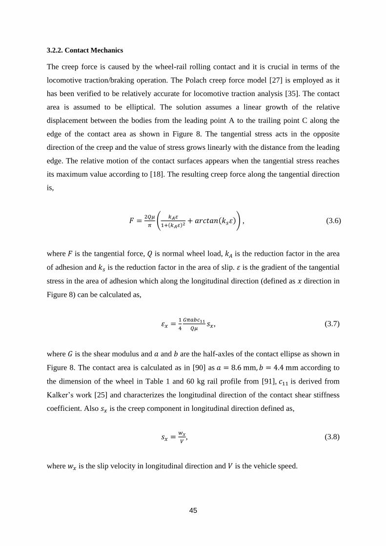
3.2.2. Contact Mechanics

The creep force is caused by the wheel-rail rolling contact and it is crucial in terms of the

locomotive traction/braking operation. The Polach creep force model [27] is employed as it

has been verified to be relatively accurate for locomotive traction analysis [35]. The contact

area is assumed to be elliptical. The solution assumes a linear growth of the relative

displacement between the bodies from the leading point A to the trailing point C along the

edge of the contact area as shown in Figure 8. The tangential stress acts in the opposite

direction of the creep and the value of stress grows linearly with the distance from the leading

edge. The relative motion of the contact surfaces appears when the tangential stress reaches

its maximum value according to [18]. The resulting creep force along the tangential direction

is,

𝐹 =2𝑄𝜇

𝜋(

𝑘𝐴𝜀

1+(𝑘𝐴𝜀)2+ 𝑎𝑟𝑐𝑡𝑎𝑛(𝑘𝑠휀)) , (3.6)

where 𝐹 is the tangential force, 𝑄 is normal wheel load, 𝑘𝐴 is the reduction factor in the area

of adhesion and 𝑘𝑠 is the reduction factor in the area of slip. 휀 is the gradient of the tangential

stress in the area of adhesion which along the longitudinal direction (defined as 𝑥 direction in

Figure 8) can be calculated as,

휀𝑥 =1

4

𝐺𝜋𝑎𝑏𝑐11

𝑄𝜇𝑠𝑥, (3.7)

where 𝐺 is the shear modulus and 𝑎 and 𝑏 are the half-axles of the contact ellipse as shown in

Figure 8. The contact area is calculated as in [90] as 𝑎 = 8.6 mm, 𝑏 = 4.4 mm according to

the dimension of the wheel in Table 1 and 60 kg rail profile from [91], 𝑐11 is derived from

Kalker’s work [25] and characterizes the longitudinal direction of the contact shear stiffness

coefficient. Also 𝑠𝑥 is the creep component in longitudinal direction defined as,

𝑠𝑥 =𝑤𝑥

𝑉, (3.8)

where 𝑤𝑥 is the slip velocity in longitudinal direction and 𝑉 is the vehicle speed.

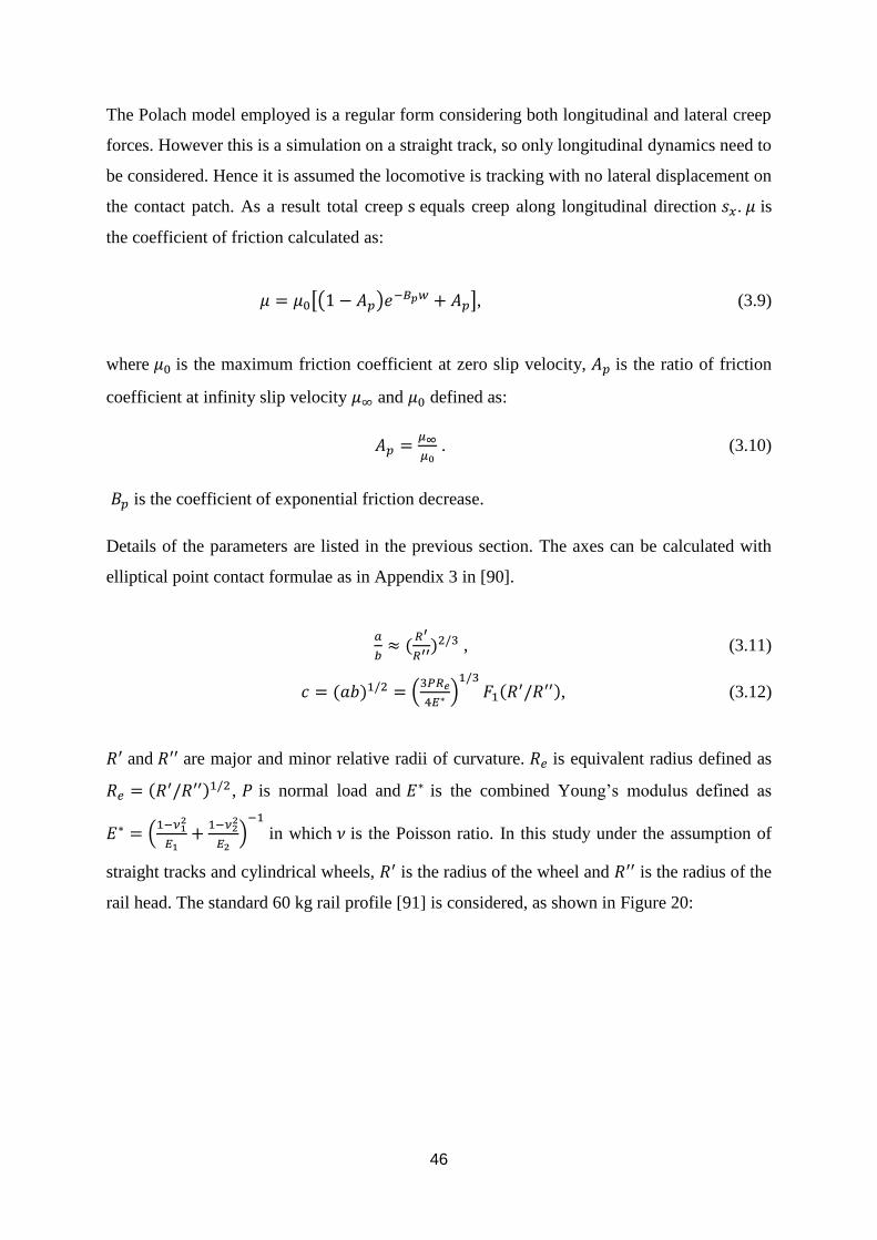
46

The Polach model employed is a regular form considering both longitudinal and lateral creep

forces. However this is a simulation on a straight track, so only longitudinal dynamics need to

be considered. Hence it is assumed the locomotive is tracking with no lateral displacement on

the contact patch. As a result total creep s equals creep along longitudinal direction 𝑠𝑥. 𝜇 is

the coefficient of friction calculated as:

𝜇 = 𝜇0[(1 − 𝐴𝑝)𝑒−𝐵𝑝𝑤 + 𝐴𝑝], (3.9)

where 𝜇0 is the maximum friction coefficient at zero slip velocity, 𝐴𝑝 is the ratio of friction

coefficient at infinity slip velocity 𝜇∞ and 𝜇0 defined as:

𝐴𝑝 =𝜇∞

𝜇0 . (3.10)

𝐵𝑝 is the coefficient of exponential friction decrease.

Details of the parameters are listed in the previous section. The axes can be calculated with

elliptical point contact formulae as in Appendix 3 in [90].

𝑎

𝑏≈ (

𝑅′

𝑅′′)2/3 , (3.11)

𝑐 = (𝑎𝑏)1/2 = (3𝑃𝑅𝑒

4𝐸∗)1/3

𝐹1(𝑅′/𝑅′′), (3.12)

𝑅′ and 𝑅′′ are major and minor relative radii of curvature. 𝑅𝑒 is equivalent radius defined as

𝑅𝑒 = (𝑅′/𝑅′′)1/2 , 𝑃 is normal load and 𝐸∗ is the combined Young’s modulus defined as

𝐸∗ = (1−𝜈1

2

𝐸1+1−𝜈2

2

𝐸2)−1

in which 𝜈 is the Poisson ratio. In this study under the assumption of

straight tracks and cylindrical wheels, 𝑅′ is the radius of the wheel and 𝑅′′ is the radius of the

rail head. The standard 60 kg rail profile [91] is considered, as shown in Figure 20:

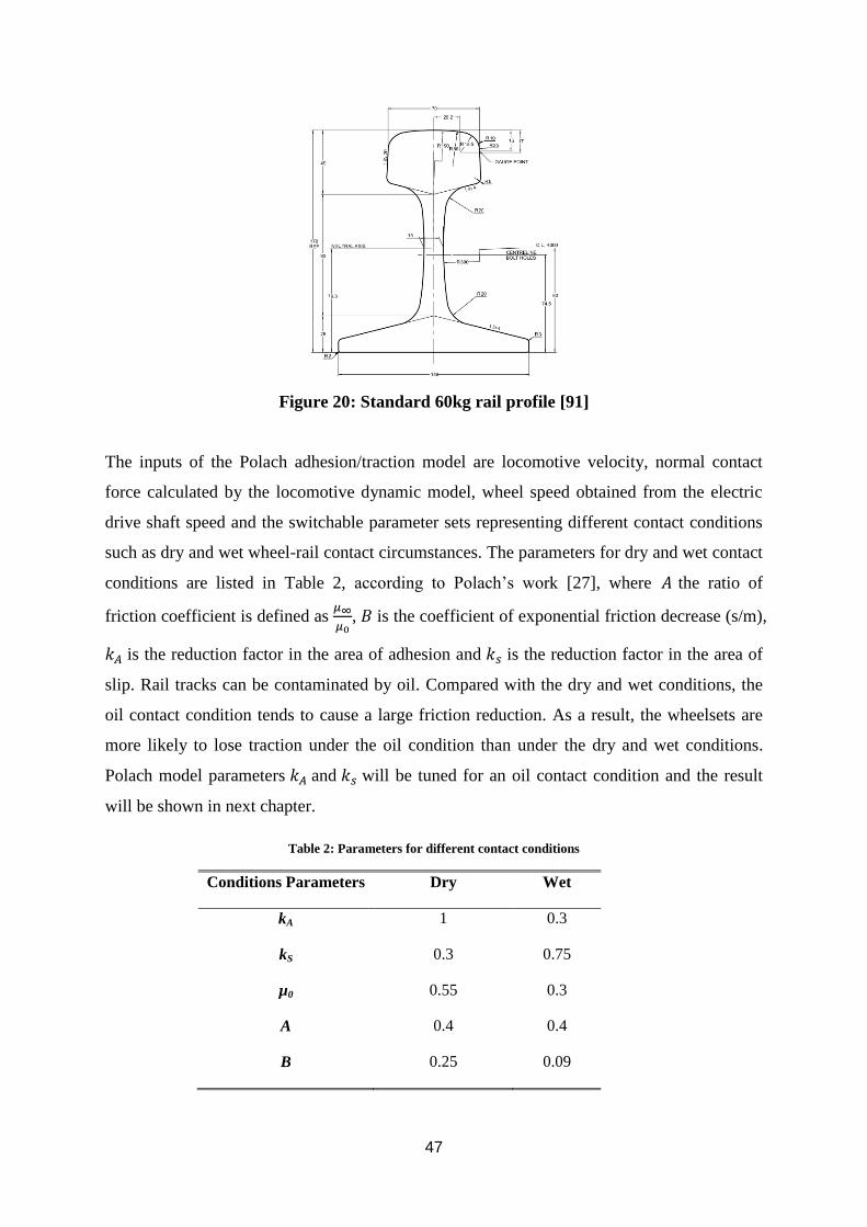
47

Figure 20: Standard 60kg rail profile [91]

The inputs of the Polach adhesion/traction model are locomotive velocity, normal contact

force calculated by the locomotive dynamic model, wheel speed obtained from the electric

drive shaft speed and the switchable parameter sets representing different contact conditions

such as dry and wet wheel-rail contact circumstances. The parameters for dry and wet contact

conditions are listed in Table 2, according to Polach’s work [27], where 𝐴 the ratio of

friction coefficient is defined as 𝜇∞

𝜇0, 𝐵 is the coefficient of exponential friction decrease (s/m),

𝑘𝐴 is the reduction factor in the area of adhesion and 𝑘𝑠 is the reduction factor in the area of

slip. Rail tracks can be contaminated by oil. Compared with the dry and wet conditions, the

oil contact condition tends to cause a large friction reduction. As a result, the wheelsets are

more likely to lose traction under the oil condition than under the dry and wet conditions.

Polach model parameters 𝑘𝐴 and 𝑘𝑠 will be tuned for an oil contact condition and the result

will be shown in next chapter.

Table 2: Parameters for different contact conditions

Conditions Parameters Dry Wet

kA 1 0.3

kS 0.3 0.75

µ0 0.55 0.3

A 0.4 0.4

B 0.25 0.09

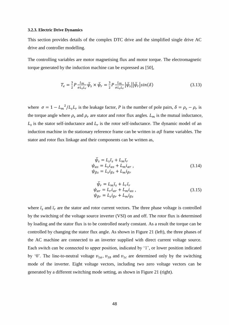
48

3.2.3. Electric Drive Dynamics

This section provides details of the complex DTC drive and the simplified single drive AC

drive and controller modelling.

The controlling variables are motor magnetising flux and motor torque. The electromagnetic

torque generated by the induction machine can be expressed as [50],

𝑇𝑒 =3

2𝑃

𝐿𝑚

𝜎𝐿𝑠𝐿𝑟��𝑠 × ��𝑟 =

3

2𝑃

𝐿𝑚

𝜎𝐿𝑠𝐿𝑟|��𝑠||��𝑟|𝑠𝑖𝑛(𝛿) (3.13)

where 𝜎 = 1 − 𝐿𝑚2/𝐿𝑠𝐿𝑟 is the leakage factor, 𝑃 is the number of pole pairs, 𝛿 = 𝜌𝑠 − 𝜌𝑟 is

the torque angle where 𝜌𝑠 and 𝜌𝑟 are stator and rotor flux angles. 𝐿𝑚 is the mutual inductance,

𝐿𝑠 is the stator self-inductance and 𝐿𝑟 is the rotor self-inductance. The dynamic model of an

induction machine in the stationary reference frame can be written in 𝛼𝛽 frame variables. The

stator and rotor flux linkage and their components can be written as,

��𝑠 = 𝐿𝑠𝑖�� + 𝐿𝑚𝑖��𝜓𝛼𝑠 = 𝐿𝑠𝑖𝛼𝑠 + 𝐿𝑚𝑖𝛼𝑟𝜓𝛽𝑠 = 𝐿𝑠𝑖𝛽𝑠 + 𝐿𝑚𝑖𝛽𝑟

, (3.14)

��𝑟 = 𝐿𝑚𝑖�� + 𝐿𝑟𝑖��𝜓𝛼𝑟 = 𝐿𝑟𝑖𝛼𝑟 + 𝐿𝑚𝑖𝛼𝑠𝜓𝛽𝑟 = 𝐿𝑠𝑖𝛽𝑟 + 𝐿𝑚𝑖𝛽𝑠

, (3.15)

where 𝑖�� and 𝑖�� are the stator and rotor current vectors. The three phase voltage is controlled

by the switching of the voltage source inverter (VSI) on and off. The rotor flux is determined

by loading and the stator flux is to be controlled nearly constant. As a result the torque can be

controlled by changing the stator flux angle. As shown in Figure 21 (left), the three phases of

the AC machine are connected to an inverter supplied with direct current voltage source.

Each switch can be connected to upper position, indicated by ‘1’, or lower position indicated

by ‘0’. The line-to-neutral voltage 𝑣1𝑎 , 𝑣1𝑏 and 𝑣1𝑐 are determined only by the switching

mode of the inverter. Eight voltage vectors, including two zero voltage vectors can be

generated by a different switching mode setting, as shown in Figure 21 (right).

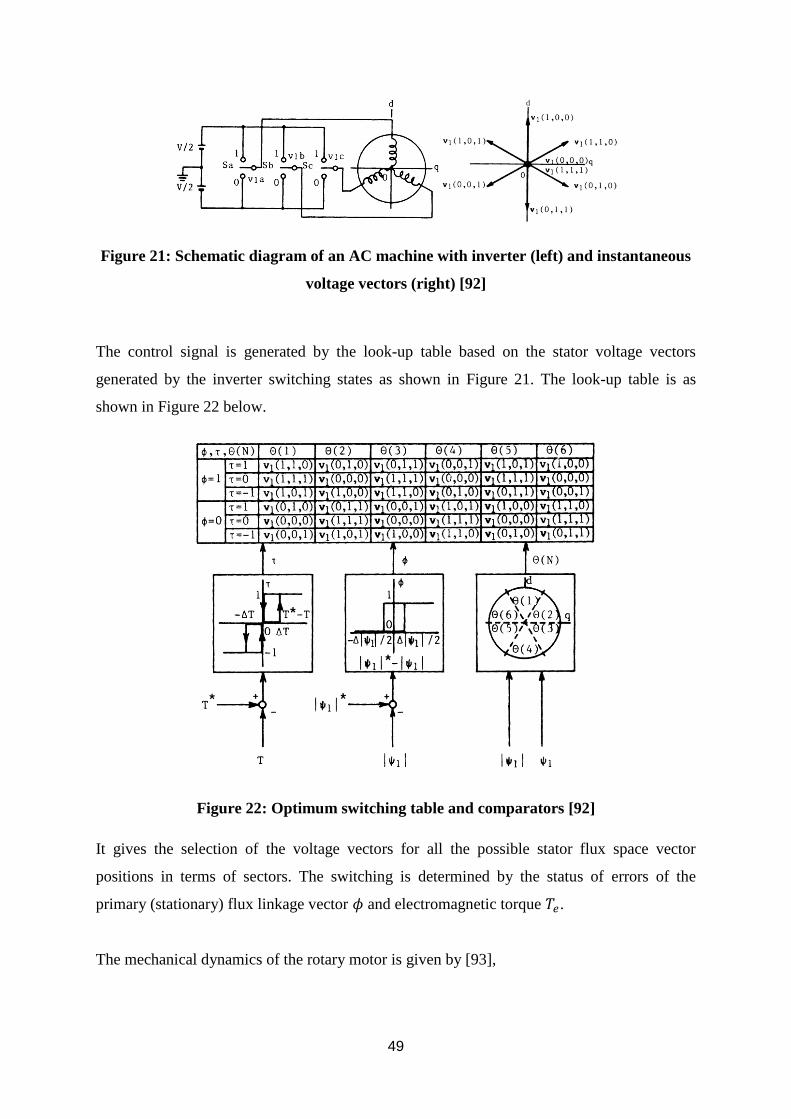
49

Figure 21: Schematic diagram of an AC machine with inverter (left) and instantaneous

voltage vectors (right) [92]

The control signal is generated by the look-up table based on the stator voltage vectors

generated by the inverter switching states as shown in Figure 21. The look-up table is as

shown in Figure 22 below.

Figure 22: Optimum switching table and comparators [92]

It gives the selection of the voltage vectors for all the possible stator flux space vector

positions in terms of sectors. The switching is determined by the status of errors of the

primary (stationary) flux linkage vector 𝜙 and electromagnetic torque 𝑇𝑒.

The mechanical dynamics of the rotary motor is given by [93],

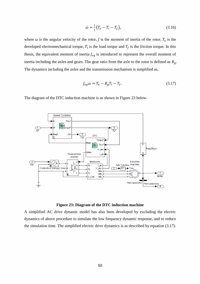
50

�� =1

𝐽(𝑇𝑒 − 𝑇𝑙 − 𝑇𝑓), (3.16)

where 𝜔 is the angular velocity of the rotor, 𝐽 is the moment of inertia of the rotor, 𝑇𝑒 is the

developed electromechanical torque, 𝑇𝑙 is the load torque and 𝑇𝑓 is the friction torque. In this

thesis, the equivalent moment of inertia 𝐽𝑒𝑞 is introduced to represent the overall moment of

inertia including the axles and gears. The gear ratio from the axle to the rotor is defined as 𝑅𝑔.

The dynamics including the axles and the transmission mechanism is simplified as,

𝐽𝑒𝑞�� = 𝑇𝑒 − 𝑅𝑔𝑇𝑙 − 𝑇𝑓. (3.17)

The diagram of the DTC induction machine is as shown in Figure 23 below.

Figure 23: Diagram of the DTC induction machine

A simplified AC drive dynamic model has also been developed by excluding the electric

dynamics of above procedure to simulate the low frequency dynamic response, and to reduce

the simulation time. The simplified electric drive dynamics is as described by equation (3.17).

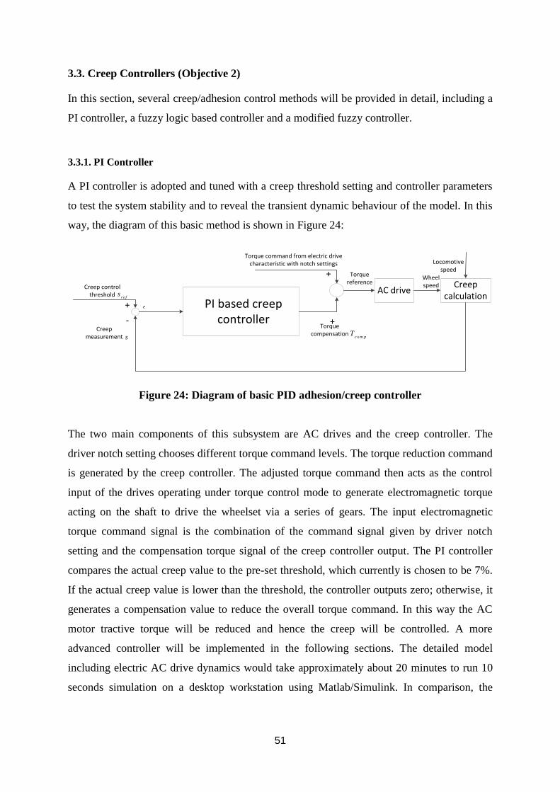
51

3.3. Creep Controllers (Objective 2)

In this section, several creep/adhesion control methods will be provided in detail, including a

PI controller, a fuzzy logic based controller and a modified fuzzy controller.

3.3.1. PI Controller

A PI controller is adopted and tuned with a creep threshold setting and controller parameters

to test the system stability and to reveal the transient dynamic behaviour of the model. In this

way, the diagram of this basic method is shown in Figure 24:

PI based creep controller

Torque command from electric drive characteristic with notch settings

Creep control threshold

Creep measurement

Torque reference

+

+

+

-

r e fs

s

AC drive

Wheel speed

Locomotive speed

Creep calculation

e

Torque compensation

c o m pT

Figure 24: Diagram of basic PID adhesion/creep controller

The two main components of this subsystem are AC drives and the creep controller. The

driver notch setting chooses different torque command levels. The torque reduction command

is generated by the creep controller. The adjusted torque command then acts as the control

input of the drives operating under torque control mode to generate electromagnetic torque

acting on the shaft to drive the wheelset via a series of gears. The input electromagnetic

torque command signal is the combination of the command signal given by driver notch

setting and the compensation torque signal of the creep controller output. The PI controller

compares the actual creep value to the pre-set threshold, which currently is chosen to be 7%.

If the actual creep value is lower than the threshold, the controller outputs zero; otherwise, it

generates a compensation value to reduce the overall torque command. In this way the AC

motor tractive torque will be reduced and hence the creep will be controlled. A more

advanced controller will be implemented in the following sections. The detailed model

including electric AC drive dynamics would take approximately about 20 minutes to run 10

seconds simulation on a desktop workstation using Matlab/Simulink. In comparison, the

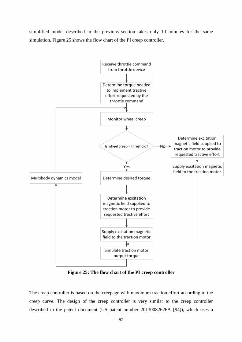
52

simplified model described in the previous section takes only 10 minutes for the same

simulation. Figure 25 shows the flow chart of the PI creep controller.

Receive throttle command from throttle device

Receive throttle command from throttle device

Determine torque needed to implement tractive

effort requested by the throttle command

Determine torque needed to implement tractive

effort requested by the throttle command

Monitor wheel creepMonitor wheel creep

Is wheel creep > threshold?

Determine excitation magnetic field supplied to traction motor to provide requested tractive effort

Determine excitation magnetic field supplied to traction motor to provide requested tractive effort

Determine desired torque Determine desired torque

No

Yes Supply excitation magnetic field to the traction motor

Supply excitation magnetic field to the traction motor

Determine excitation magnetic field supplied to traction motor to provide requested tractive effort

Determine excitation magnetic field supplied to traction motor to provide requested tractive effort

Supply excitation magnetic field to the traction motor

Supply excitation magnetic field to the traction motor

Simulate traction motor output torque

Simulate traction motor output torque

Multibody dynamics modelMultibody dynamics model

Figure 25: The flow chart of the PI creep controller

The creep controller is based on the creepage with maximum traction effort according to the

creep curve. The design of the creep controller is very similar to the creep controller

described in the patent document (US patent number 20130082626A [94]), which uses a

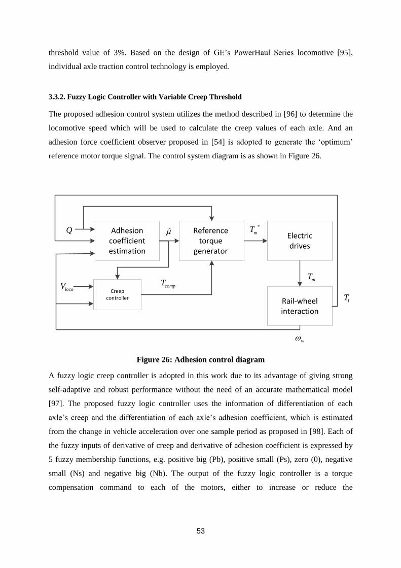
53

threshold value of 3%. Based on the design of GE’s PowerHaul Series locomotive [95],

individual axle traction control technology is employed.

3.3.2. Fuzzy Logic Controller with Variable Creep Threshold

The proposed adhesion control system utilizes the method described in [96] to determine the

locomotive speed which will be used to calculate the creep values of each axle. And an

adhesion force coefficient observer proposed in [54] is adopted to generate the ‘optimum’

reference motor torque signal. The control system diagram is as shown in Figure 26.

Adhesion coefficient estimation

Reference torque

generator

Creep controller Rail-wheel

interaction

Electric drives

*

mT

compT

w

Q

lTlocoV

mT

Figure 26: Adhesion control diagram

A fuzzy logic creep controller is adopted in this work due to its advantage of giving strong

self-adaptive and robust performance without the need of an accurate mathematical model

[97]. The proposed fuzzy logic controller uses the information of differentiation of each

axle’s creep and the differentiation of each axle’s adhesion coefficient, which is estimated

from the change in vehicle acceleration over one sample period as proposed in [98]. Each of

the fuzzy inputs of derivative of creep and derivative of adhesion coefficient is expressed by

5 fuzzy membership functions, e.g. positive big (Pb), positive small (Ps), zero (0), negative

small (Ns) and negative big (Nb). The output of the fuzzy logic controller is a torque

compensation command to each of the motors, either to increase or reduce the

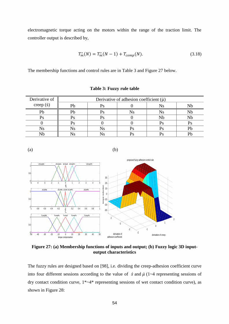
54

electromagnetic torque acting on the motors within the range of the traction limit. The

controller output is described by,

𝑇𝑚∗ (𝑁) = 𝑇𝑚

∗ (𝑁 − 1) + 𝑇𝑐𝑜𝑚𝑝(𝑁). (3.18)

The membership functions and control rules are in Table 3 and Figure 27 below.

Table 3: Fuzzy rule table

Derivative of

creep (s) Derivative of adhesion coefficient (μ)

Pb Ps 0 Ns Nb

Pb Pb Ps Ns Ns Nb

Ps Ps Ps 0 Nb Nb

0 Ps 0 0 Ps Ps

Ns Ns Ns Ps Ps Pb

Nb Ns Ns Ps Ps Pb

(a) (b)

Figure 27: (a) Membership functions of inputs and output; (b) Fuzzy logic 3D input-

output characteristics

The fuzzy rules are designed based on [98], i.e. dividing the creep-adhesion coefficient curve

into four different sessions according to the value of �� and �� (1~4 representing sessions of

dry contact condition curve, 1*~4* representing sessions of wet contact condition curve), as

shown in Figure 28:

-5 -4 -3 -2 -1 0 1 2 3 4 50

0.5

1

_s

dCreepNb dCreepNs dCreep0 dCreepPs dCreepPb

-1 -0.8 -0.6 -0.4 -0.2 0 0.2 0.4 0.6 0.8 10

0.5

1

_7

dCoefNb dCoefNs dCoef0 dCoefPs dCoefPb

-50 -40 -30 -20 -10 0 10 20 30 40 500

0.5

1

torque compensation

TcompNb TcompNs Tcomp0 TcompPs TcompPb

-2

-1

0

1

2

-2

0

2

-30

-20

-10

0

10

20

30

derivative of creep

proposed fuzzy adhesion control rule

derivative of adhesion coefficient

torq

ue

re

du

ctio

n

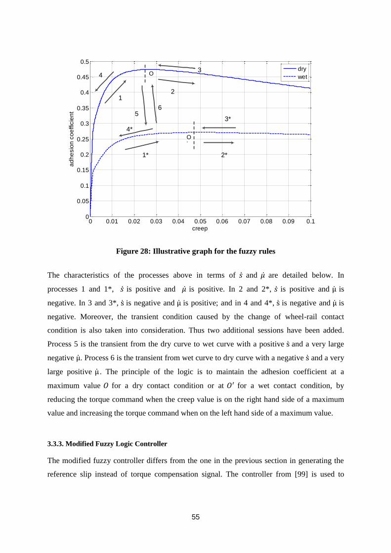
55

Figure 28: Illustrative graph for the fuzzy rules

The characteristics of the processes above in terms of �� and �� are detailed below. In

processes 1 and 1*, �� is positive and �� is positive. In 2 and 2*, �� is positive and μ is

negative. In 3 and 3*, s is negative and μ is positive; and in 4 and 4*, s is negative and μ is

negative. Moreover, the transient condition caused by the change of wheel-rail contact

condition is also taken into consideration. Thus two additional sessions have been added.

Process 5 is the transient from the dry curve to wet curve with a positive s and a very large

negative μ. Process 6 is the transient from wet curve to dry curve with a negative s and a very

large positive μ . The principle of the logic is to maintain the adhesion coefficient at a

maximum value 𝑂 for a dry contact condition or at 𝑂′ for a wet contact condition, by

reducing the torque command when the creep value is on the right hand side of a maximum

value and increasing the torque command when on the left hand side of a maximum value.

3.3.3. Modified Fuzzy Logic Controller

The modified fuzzy controller differs from the one in the previous section in generating the

reference slip instead of torque compensation signal. The controller from [99] is used to

0 0.01 0.02 0.03 0.04 0.05 0.06 0.07 0.08 0.09 0.10

0.05

0.1

0.15

0.2

0.25

0.3

0.35

0.4

0.45

0.5

creep

ad

he

sio

n c

oe

ffic

ien

t

dry

wet

5

4

2

3

1* 2*

3*

4*

6

1

O

O’

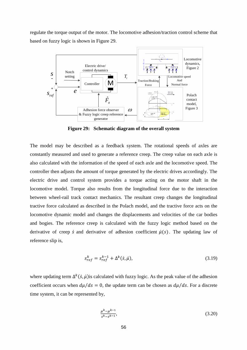
56

regulate the torque output of the motor. The locomotive adhesion/traction control scheme that

based on fuzzy logic is shown in Figure 29.

Locomotive

dynamics,

Figure 2

Polach

contact

model,

Figure 3

Electric drive/

control dynamics

MController

Locomotive speed

And

Normal force

tT

Adhesion force observer

& Fuzzy logic creep reference

generator

s

refs+

-

ˆaF

e

Traction/Braking

Force

Notch

setting

Figure 29: Schematic diagram of the overall system

The model may be described as a feedback system. The rotational speeds of axles are

constantly measured and used to generate a reference creep. The creep value on each axle is

also calculated with the information of the speed of each axle and the locomotive speed. The

controller then adjusts the amount of torque generated by the electric drives accordingly. The

electric drive and control system provides a torque acting on the motor shaft in the

locomotive model. Torque also results from the longitudinal force due to the interaction

between wheel-rail track contact mechanics. The resultant creep changes the longitudinal

tractive force calculated as described in the Polach model, and the tractive force acts on the

locomotive dynamic model and changes the displacements and velocities of the car bodies

and bogies. The reference creep is calculated with the fuzzy logic method based on the

derivative of creep �� and derivative of adhesion coefficient ��(𝑠) . The updating law of

reference slip is,

𝑠𝑟𝑒𝑓𝑘 = 𝑠𝑟𝑒𝑓

𝑘−1 + Δ𝑘(��, ��), (3.19)

where updating term Δ𝑘(��, ��)is calculated with fuzzy logic. As the peak value of the adhesion

coefficient occurs when 𝑑𝜇 𝑑𝑠 = 0⁄ , the update term can be chosen as 𝑑𝜇 𝑑𝑠⁄ . For a discrete

time system, it can be represented by,

𝜇𝑘−𝜇𝑘−1

𝑠𝑘−𝑠𝑘−1, (3.20)

050

100 0 0.1 0.2 0.3 0.4 0.5

0

0.1

0.2

0.3

0.4

0.5

0.6

0.7

creep

Polach dry

loco velocity km/h

adhesio

n c

oeffic

ient

0

0.1

0.2

0.3

0.4

0.5

Polach cree

Electric drive & control

Complex locomoti

M

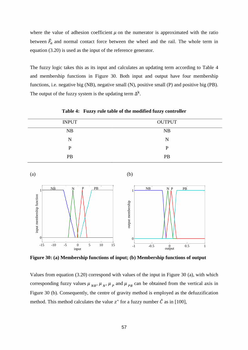
57

where the value of adhesion coefficient 𝜇 on the numerator is approximated with the ratio

between ��𝑎 and normal contact force between the wheel and the rail. The whole term in

equation (3.20) is used as the input of the reference generator.

The fuzzy logic takes this as its input and calculates an updating term according to Table 4

and membership functions in Figure 30. Both input and output have four membership

functions, i.e. negative big (NB), negative small (N), positive small (P) and positive big (PB).

The output of the fuzzy system is the updating term Δk.

Table 4: Fuzzy rule table of the modified fuzzy controller

INPUT OUTPUT

NB NB

N N

P P

PB PB

(a) (b)

-15 -10 -5 0 5 10 15

0

1

input

input

mem

bers

hip

functi

on

P PBNB N

-1 -0.5 0 0.5 1

0

1

output

ou

tpu

t m

em

bers

hip

N P PBNB

Figure 30: (a) Membership functions of input; (b) Membership functions of output

Values from equation (3.20) correspond with values of the input in Figure 30 (a), with which

corresponding fuzzy values 𝜇 𝑁𝐵, 𝜇 𝑁, 𝜇 𝑃 and 𝜇 𝑃𝐵 can be obtained from the vertical axis in

Figure 30 (b). Consequently, the centre of gravity method is employed as the defuzzification

method. This method calculates the value 𝑧∗ for a fuzzy number �� as in [100],

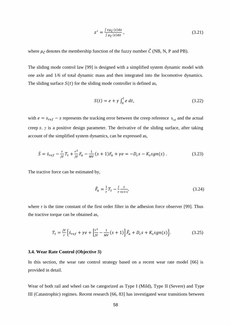
58

𝑧∗ =∫𝑧𝜇�� (𝑧)𝑑𝑧

∫𝜇�� (𝑧)𝑑𝑧 , (3.21)

where 𝜇�� denotes the membership function of the fuzzy number �� (NB, N, P and PB).

The sliding mode control law [99] is designed with a simplified system dynamic model with

one axle and 1/6 of total dynamic mass and then integrated into the locomotive dynamics.

The sliding surface 𝑆(𝑡) for the sliding mode controller is defined as,

𝑆(𝑡) = 𝑒 + 𝛾 ∫ 𝑒 𝑑𝑡𝑡

0, (3.22)

with 𝑒 = 𝑠𝑟𝑒𝑓 − 𝑠 represents the tracking error between the creep reference refs and the actual

creep 𝑠. γ is a positive design parameter. The derivative of the sliding surface, after taking

account of the simplified system dynamics, can be expressed as,

�� = ��𝑟𝑒𝑓 −𝑟

𝐽𝑉𝑇𝑡 +

𝑟2

𝐽𝑉𝐹𝑎 −

1

𝑀𝑉(𝑠 + 1)𝐹𝑎 + 𝛾𝑒 = −𝐷𝑐𝑠 − 𝐾𝑠𝑠𝑔𝑛(𝑠) . (3.23)

The tractive force can be estimated by,

��𝑎 =1

𝑟𝑇𝑡 −

𝐽

𝑟

𝑠

𝜏𝑠+1, (3.24)

where τ is the time constant of the first order filter in the adhesion force observer [99]. Thus

the tractive torque can be obtained as,

𝑇𝑡 =𝐽𝑉

𝑟{��𝑟𝑒𝑓 + 𝛾𝑒 + [

𝑟2

𝐽𝑉−

1

𝑀𝑉(𝑠 + 1)] ��𝑎 + 𝐷𝑐𝑠 + 𝐾𝑠𝑠𝑔𝑛(𝑠)}. (3.25)

3.4. Wear Rate Control (Objective 3)

In this section, the wear rate control strategy based on a recent wear rate model [66] is

provided in detail.

Wear of both rail and wheel can be categorized as Type I (Mild), Type II (Severe) and Type

III (Catastrophic) regimes. Recent research [66, 83] has investigated wear transitions between

59

different types of wheel/rail steel and using different wear models and models have been

proposed for various rail materials. The frictional power density 𝑃𝑟/𝐴𝑛 is defined by 𝑃𝑟

𝐴𝑛=

𝐹𝑡𝑉𝑠/𝐴𝑛, where 𝐹𝑡 is the traction force, 𝑉𝑠 is the relative slip velocity and 𝐴𝑛 is the nominal

contact area. The wear coefficient 𝑘0 is determined by,

𝑘0 =∆𝑚

∆𝑊 , (3.26)

where ∆𝑚 is the mass loss of the rail disc after a certain time interval and ∆𝑊 is the frictional

work dissipated in the rolling/sliding contact [66] . The wear coefficient under the dry

conditions is about five times higher than that under the FM conditions [66].

In order to avoid excessive wear damage on the rail and wheel as in the Type III region in

Figure 17, the friction power density value separating Type II and III regions of Figure 17 is

chosen as the wear control threshold. In this study the threshold is set at 34 𝑊/𝑚𝑚2.

This study employs a PI based creep controller to limit the creep values under pre-set creep

thresholds at 4%. The block diagram of the creep control is shown in Figure 31 (a) and the

diagram shown in 29 (b) is the block diagram of the wear and creep controller. Each wheelset

has its own set of a controller and a motor so that the speed of the motors can be adjusted

independently.

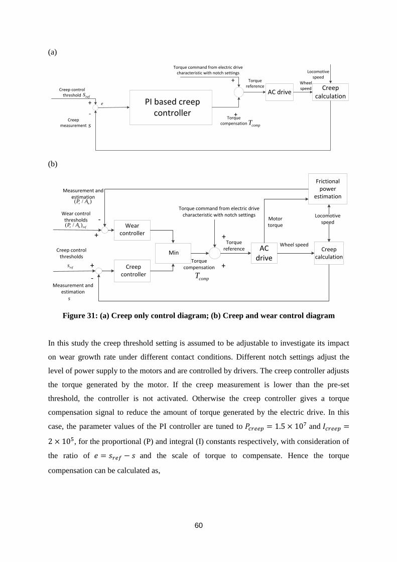
60

(a)

PI based creep controller

Torque command from electric drive characteristic with notch settings

Creep control threshold

Creep measurement

Torque reference

+

+

+

-

refs

s

AC drive

Wheel speed

Locomotive speed

Creep calculation

e

Torque compensation compT

(b)

Creep controller

Torque command from electric drive characteristic with notch settings

Creep control thresholds

Measurement and estimation

Torque reference

+

++

-

refs

s

AC drive

Wheel speed

Locomotive speed

Creep calculation

Torque compensation

compT

Wear controller

( / )r n refP A

( / )r nP A

Frictional power

estimation

Motor torque

Wear control thresholds

+

-

Measurement and estimation

Min

Figure 31: (a) Creep only control diagram; (b) Creep and wear control diagram

In this study the creep threshold setting is assumed to be adjustable to investigate its impact

on wear growth rate under different contact conditions. Different notch settings adjust the

level of power supply to the motors and are controlled by drivers. The creep controller adjusts

the torque generated by the motor. If the creep measurement is lower than the pre-set

threshold, the controller is not activated. Otherwise the creep controller gives a torque

compensation signal to reduce the amount of torque generated by the electric drive. In this

case, the parameter values of the PI controller are tuned to 𝑃𝑐𝑟𝑒𝑒𝑝 = 1.5 × 107 and 𝐼𝑐𝑟𝑒𝑒𝑝 =

2 × 105, for the proportional (P) and integral (I) constants respectively, with consideration of

the ratio of 𝑒 = 𝑠𝑟𝑒𝑓 − 𝑠 and the scale of torque to compensate. Hence the torque

compensation can be calculated as,

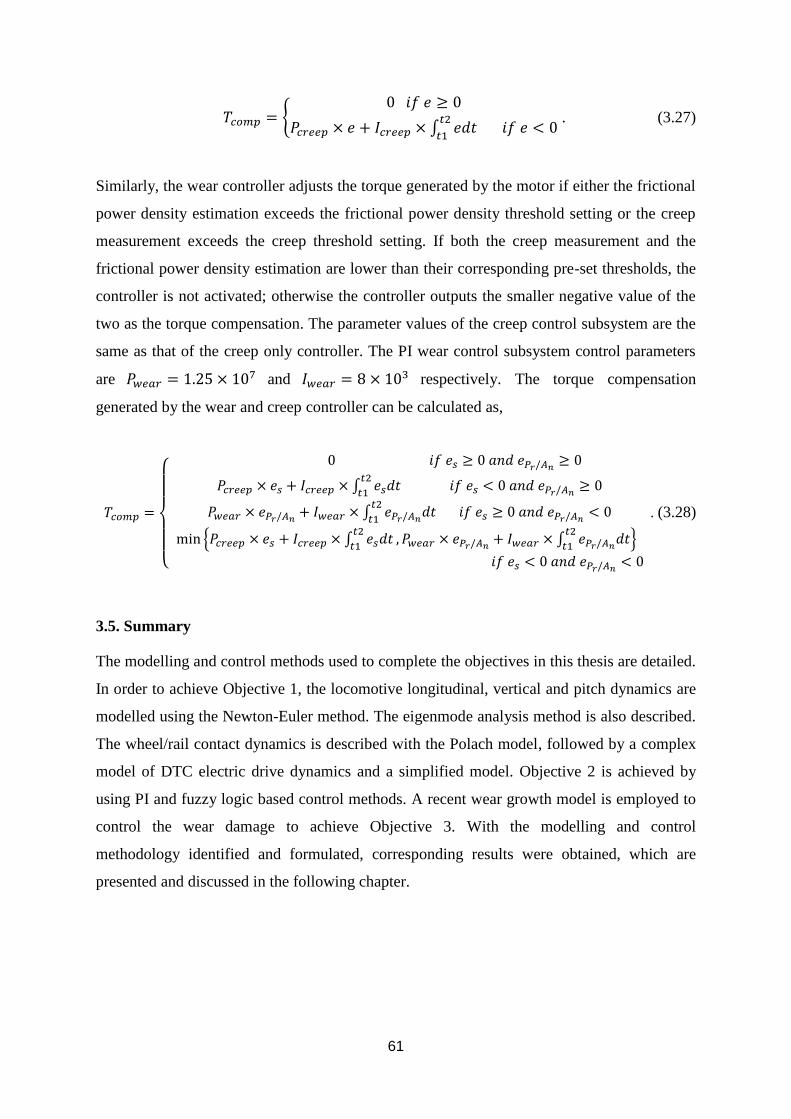
61

𝑇𝑐𝑜𝑚𝑝 = {0 𝑖𝑓 𝑒 ≥ 0

𝑃𝑐𝑟𝑒𝑒𝑝 × 𝑒 + 𝐼𝑐𝑟𝑒𝑒𝑝 × ∫ 𝑒𝑑𝑡 𝑖𝑓 𝑒 < 0𝑡2

𝑡1

. (3.27)

Similarly, the wear controller adjusts the torque generated by the motor if either the frictional

power density estimation exceeds the frictional power density threshold setting or the creep

measurement exceeds the creep threshold setting. If both the creep measurement and the

frictional power density estimation are lower than their corresponding pre-set thresholds, the

controller is not activated; otherwise the controller outputs the smaller negative value of the

two as the torque compensation. The parameter values of the creep control subsystem are the

same as that of the creep only controller. The PI wear control subsystem control parameters

are 𝑃𝑤𝑒𝑎𝑟 = 1.25 × 107 and 𝐼𝑤𝑒𝑎𝑟 = 8 × 103 respectively. The torque compensation

generated by the wear and creep controller can be calculated as,

𝑇𝑐𝑜𝑚𝑝 =

{

0 𝑖𝑓 𝑒𝑠 ≥ 0 𝑎𝑛𝑑 𝑒𝑃𝑟/𝐴𝑛 ≥ 0

𝑃𝑐𝑟𝑒𝑒𝑝 × 𝑒𝑠 + 𝐼𝑐𝑟𝑒𝑒𝑝 × ∫ 𝑒𝑠𝑑𝑡 𝑖𝑓 𝑒𝑠 < 0 𝑎𝑛𝑑 𝑒𝑃𝑟/𝐴𝑛 ≥ 0𝑡2

𝑡1

𝑃𝑤𝑒𝑎𝑟 × 𝑒𝑃𝑟/𝐴𝑛 + 𝐼𝑤𝑒𝑎𝑟 × ∫ 𝑒𝑃𝑟/𝐴𝑛𝑑𝑡 𝑖𝑓 𝑒𝑠 ≥ 0 𝑎𝑛𝑑 𝑒𝑃𝑟/𝐴𝑛 < 0𝑡2

𝑡1

min {𝑃𝑐𝑟𝑒𝑒𝑝 × 𝑒𝑠 + 𝐼𝑐𝑟𝑒𝑒𝑝 × ∫ 𝑒𝑠𝑑𝑡𝑡2

𝑡1, 𝑃𝑤𝑒𝑎𝑟 × 𝑒𝑃𝑟/𝐴𝑛 + 𝐼𝑤𝑒𝑎𝑟 × ∫ 𝑒𝑃𝑟/𝐴𝑛𝑑𝑡

𝑡2

𝑡1}

𝑖𝑓 𝑒𝑠 < 0 𝑎𝑛𝑑 𝑒𝑃𝑟/𝐴𝑛 < 0

. (3.28)

3.5. Summary

The modelling and control methods used to complete the objectives in this thesis are detailed.

In order to achieve Objective 1, the locomotive longitudinal, vertical and pitch dynamics are

modelled using the Newton-Euler method. The eigenmode analysis method is also described.

The wheel/rail contact dynamics is described with the Polach model, followed by a complex

model of DTC electric drive dynamics and a simplified model. Objective 2 is achieved by

using PI and fuzzy logic based control methods. A recent wear growth model is employed to

control the wear damage to achieve Objective 3. With the modelling and control

methodology identified and formulated, corresponding results were obtained, which are

presented and discussed in the following chapter.

62

Chapter IV: Results and Discussion

This chapter presents a summary of the results of simulations in accordance with the thesis

objectives. Firstly, simulation results of the individual dynamic subsystems, including the

locomotive longitudinal, vertical and pitch dynamics, the wheel/rail contact mechanics and

both simplified and complex electric drive dynamics, as well as the complete integrated

system are presented and compared with available data from the literature. Eigenmode

analysis has also been performed to validate the model and to identify the modes of

oscillations that are more likely to be excited under external perturbations, to complete

Objective 1. Secondly, the simulation results comparing the dynamic responses of the

locomotive with a traditional creep controller and results with new creep controllers under

changes of operating conditions are presented, highlighting the benefits and likely limitations

of controllers aiming to achieve higher tractive forces to complete Objective 2. Lastly,

simulation results showing the impact of different creep controller threshold settings on the

wear index are presented, which give rise to the new real-time control strategy aiming to limit

wear damage on the wheel/rail contact patch. Then the simulation results comparing the

dynamic responses of the locomotive with the traditional creep controller and the new

controller are presented to highlight the benefit of the new control strategy to complete

Objective 3.

4.1. Locomotive Dynamic Simulation and Validation (Objective 1)

This section presents simulation results and analysis focusing on the individual dynamic

subsystems respectively.

4.1.1. Validation of Multibody Dynamics - Eigenmode Analysis

An eigenmode analysis was performed to identify all the dynamic modes of vibration and to

determine the stability of the system. The system eigenvalues are provided in Table 5. An

eigenvalue is obtained for each possible mode of vibration of the system. The negative real

part shows that all vertical and pitch motions are stable. In other words, these modes of

vibration are positively damped. Besides the modes listed in the table below, a rigid body

mode is also identified with a zero frequency. This mode is associated with the longitudinal

rigid body motion of the locomotive.

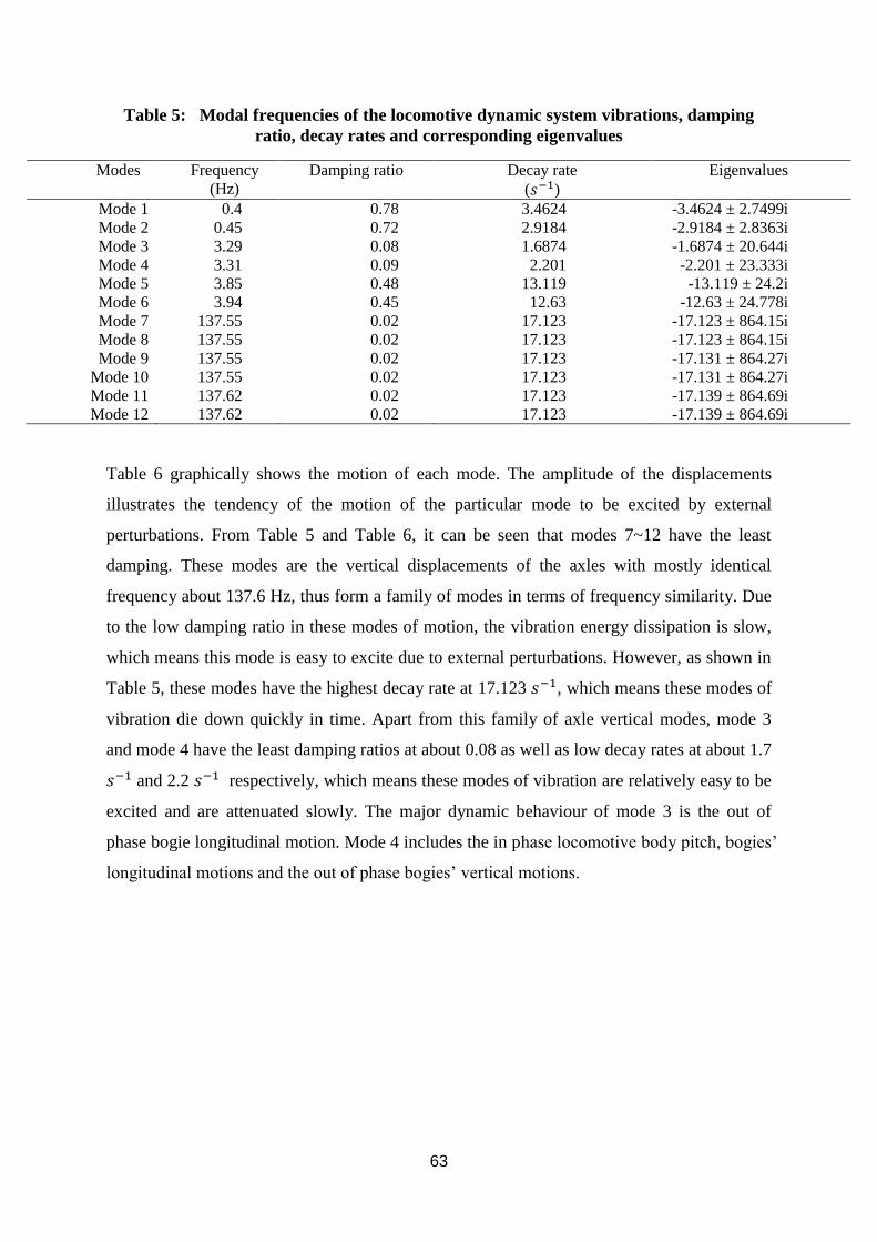
63

Table 5: Modal frequencies of the locomotive dynamic system vibrations, damping

ratio, decay rates and corresponding eigenvalues

Modes Frequency

(Hz)

Damping ratio Decay rate

(𝑠−1)

Eigenvalues

Mode 1 0.4 0.78 3.4624 -3.4624 ± 2.7499i

Mode 2 0.45 0.72 2.9184 -2.9184 ± 2.8363i

Mode 3 3.29 0.08 1.6874 -1.6874 ± 20.644i

Mode 4 3.31 0.09 2.201 -2.201 ± 23.333i

Mode 5 3.85 0.48 13.119 -13.119 ± 24.2i

Mode 6 3.94 0.45 12.63 -12.63 ± 24.778i

Mode 7 137.55 0.02 17.123 -17.123 ± 864.15i

Mode 8 137.55 0.02 17.123 -17.123 ± 864.15i

Mode 9 137.55 0.02 17.123 -17.131 ± 864.27i

Mode 10 137.55 0.02 17.123 -17.131 ± 864.27i

Mode 11 137.62 0.02 17.123 -17.139 ± 864.69i

Mode 12 137.62 0.02 17.123 -17.139 ± 864.69i

Table 6 graphically shows the motion of each mode. The amplitude of the displacements

illustrates the tendency of the motion of the particular mode to be excited by external

perturbations. From Table 5 and Table 6, it can be seen that modes 7~12 have the least

damping. These modes are the vertical displacements of the axles with mostly identical

frequency about 137.6 Hz, thus form a family of modes in terms of frequency similarity. Due

to the low damping ratio in these modes of motion, the vibration energy dissipation is slow,

which means this mode is easy to excite due to external perturbations. However, as shown in

Table 5, these modes have the highest decay rate at 17.123 𝑠−1, which means these modes of

vibration die down quickly in time. Apart from this family of axle vertical modes, mode 3

and mode 4 have the least damping ratios at about 0.08 as well as low decay rates at about 1.7

𝑠−1 and 2.2 𝑠−1 respectively, which means these modes of vibration are relatively easy to be

excited and are attenuated slowly. The major dynamic behaviour of mode 3 is the out of

phase bogie longitudinal motion. Mode 4 includes the in phase locomotive body pitch, bogies’

longitudinal motions and the out of phase bogies’ vertical motions.

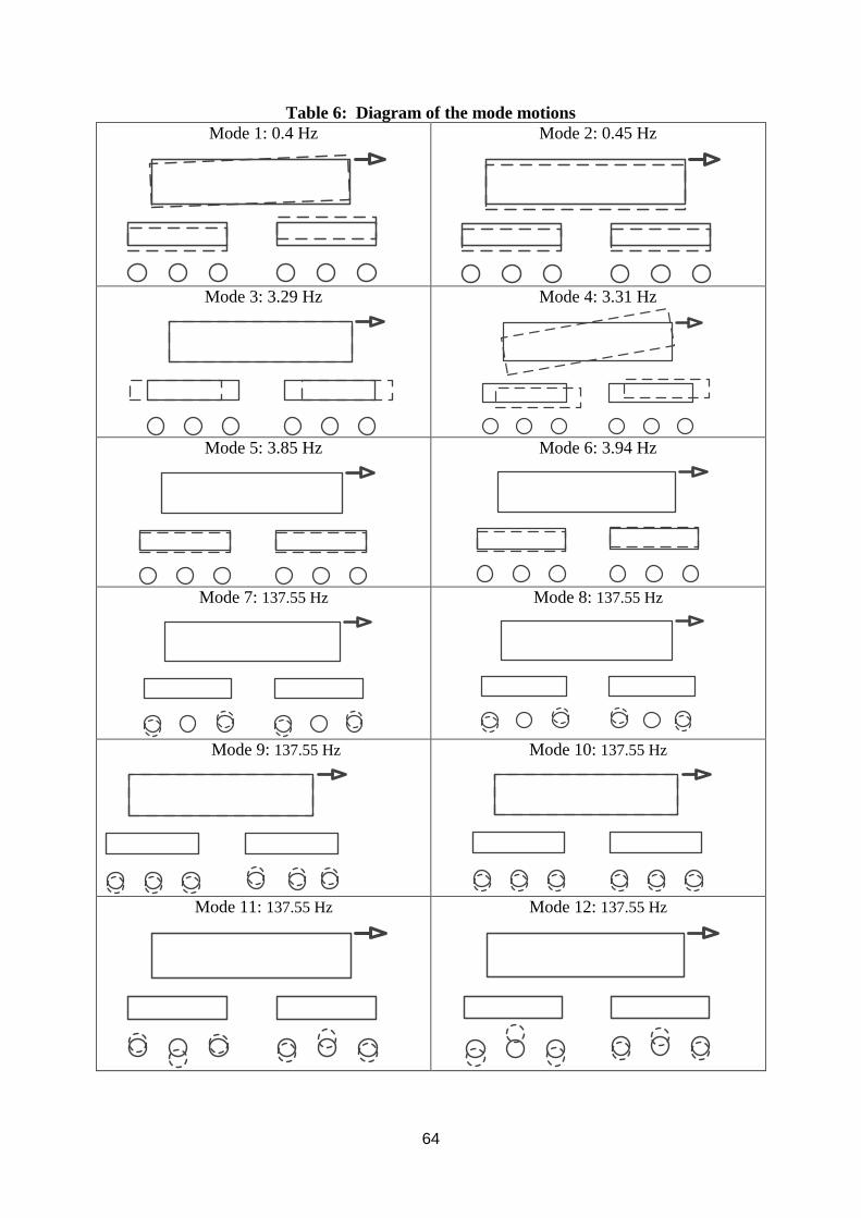
64

Table 6: Diagram of the mode motions

Mode 1: 0.4 Hz

Mode 2: 0.45 Hz

Mode 3: 3.29 Hz

Mode 4: 3.31 Hz

Mode 5: 3.85 Hz

Mode 6: 3.94 Hz

Mode 7: 137.55 Hz

Mode 8: 137.55 Hz

Mode 9: 137.55 Hz

Mode 10: 137.55 Hz

Mode 11: 137.55 Hz

Mode 12: 137.55 Hz

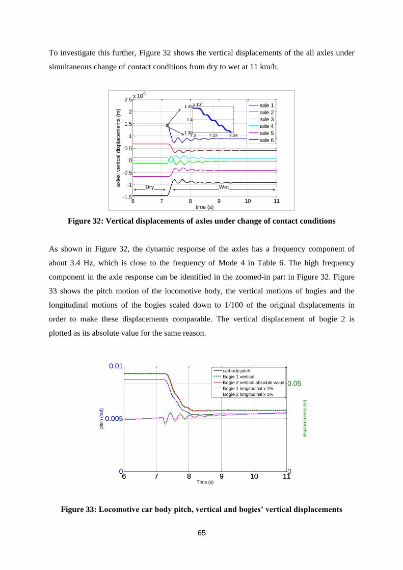
65

To investigate this further, Figure 32 shows the vertical displacements of the all axles under

simultaneous change of contact conditions from dry to wet at 11 km/h.

6 7 8 9 10 11-1.5

-1

-0.5

0

0.5

1

1.5

2

2.5x 10

-5

time (s)

axle

s' v

ert

ical dis

pla

cem

ents

(m

)

axle 1

axle 2

axle 3

axle 4

axle 5

axle 67.2 7.22 7.24

1.35

1.4

1.45x 10

-5

time (s)

axle

s' v

ert

ical dis

pla

cem

ents

(m

)

axle 1

axle 2

axle 3

axle 4

axle 5

axle 6

Dry Wet

Figure 32: Vertical displacements of axles under change of contact conditions

As shown in Figure 32, the dynamic response of the axles has a frequency component of

about 3.4 Hz, which is close to the frequency of Mode 4 in Table 6. The high frequency

component in the axle response can be identified in the zoomed-in part in Figure 32. Figure

33 shows the pitch motion of the locomotive body, the vertical motions of bogies and the

longitudinal motions of the bogies scaled down to 1/100 of the original displacements in

order to make these displacements comparable. The vertical displacement of bogie 2 is

plotted as its absolute value for the same reason.

Figure 33: Locomotive car body pitch, vertical and bogies’ vertical displacements

6 7 8 9 10 110

0.005

0.01

pitch (

rad)

Time (s)

6 7 8 9 10 110

0.05

dis

pla

cem

ents

(m

)

carbody pitch

Bogie 1 vertical

Bogie 2 vertical absolute value

Bogie 1 longitudinal x 1%

Bogie 2 longitudinal x 1%

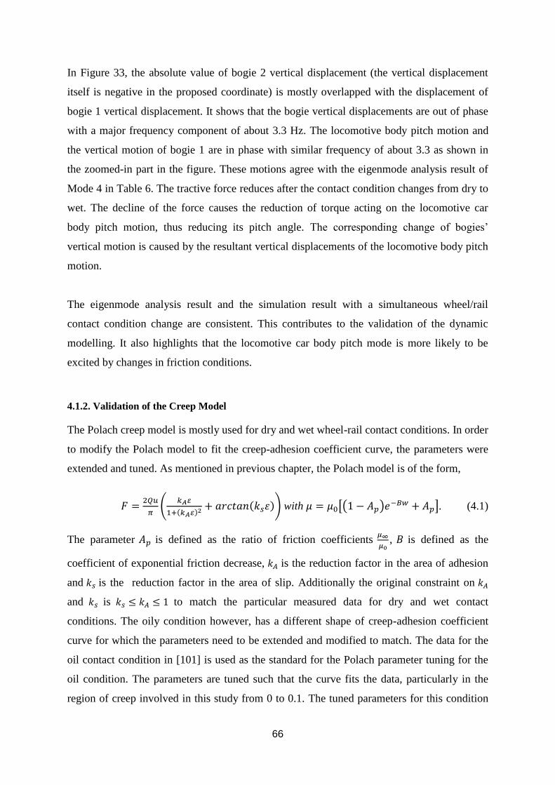
66

In Figure 33, the absolute value of bogie 2 vertical displacement (the vertical displacement

itself is negative in the proposed coordinate) is mostly overlapped with the displacement of

bogie 1 vertical displacement. It shows that the bogie vertical displacements are out of phase

with a major frequency component of about 3.3 Hz. The locomotive body pitch motion and

the vertical motion of bogie 1 are in phase with similar frequency of about 3.3 as shown in

the zoomed-in part in the figure. These motions agree with the eigenmode analysis result of

Mode 4 in Table 6. The tractive force reduces after the contact condition changes from dry to

wet. The decline of the force causes the reduction of torque acting on the locomotive car

body pitch motion, thus reducing its pitch angle. The corresponding change of bogies’

vertical motion is caused by the resultant vertical displacements of the locomotive body pitch

motion.

The eigenmode analysis result and the simulation result with a simultaneous wheel/rail

contact condition change are consistent. This contributes to the validation of the dynamic

modelling. It also highlights that the locomotive car body pitch mode is more likely to be

excited by changes in friction conditions.

4.1.2. Validation of the Creep Model

The Polach creep model is mostly used for dry and wet wheel-rail contact conditions. In order

to modify the Polach model to fit the creep-adhesion coefficient curve, the parameters were

extended and tuned. As mentioned in previous chapter, the Polach model is of the form,

𝐹 =2𝑄𝑢

𝜋(

𝑘𝐴𝜀

1+(𝑘𝐴𝜀)2+ 𝑎𝑟𝑐𝑡𝑎𝑛(𝑘𝑠휀)) with 𝜇 = 𝜇0[(1 − 𝐴𝑝)𝑒

−𝐵𝑤 + 𝐴𝑝]. (4.1)

The parameter 𝐴𝑝 is defined as the ratio of friction coefficients 𝜇∞

𝜇0, 𝐵 is defined as the

coefficient of exponential friction decrease, 𝑘𝐴 is the reduction factor in the area of adhesion

and 𝑘𝑠 is the reduction factor in the area of slip. Additionally the original constraint on 𝑘𝐴

and 𝑘𝑠 is 𝑘𝑠 ≤ 𝑘𝐴 ≤ 1 to match the particular measured data for dry and wet contact

conditions. The oily condition however, has a different shape of creep-adhesion coefficient

curve for which the parameters need to be extended and modified to match. The data for the

oil contact condition in [101] is used as the standard for the Polach parameter tuning for the

oil condition. The parameters are tuned such that the curve fits the data, particularly in the

region of creep involved in this study from 0 to 0.1. The tuned parameters for this condition

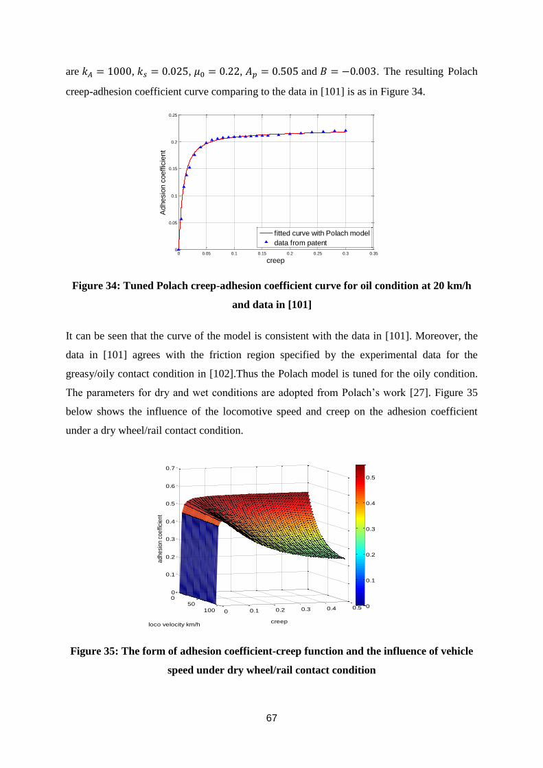
67

are 𝑘𝐴 = 1000, 𝑘𝑠 = 0.025, 𝜇0 = 0.22, 𝐴𝑝 = 0.505 and 𝐵 = −0.003. The resulting Polach

creep-adhesion coefficient curve comparing to the data in [101] is as in Figure 34.

Figure 34: Tuned Polach creep-adhesion coefficient curve for oil condition at 20 km/h

and data in [101]

It can be seen that the curve of the model is consistent with the data in [101]. Moreover, the

data in [101] agrees with the friction region specified by the experimental data for the

greasy/oily contact condition in [102].Thus the Polach model is tuned for the oily condition.

The parameters for dry and wet conditions are adopted from Polach’s work [27]. Figure 35

below shows the influence of the locomotive speed and creep on the adhesion coefficient

under a dry wheel/rail contact condition.

Figure 35: The form of adhesion coefficient-creep function and the influence of vehicle

speed under dry wheel/rail contact condition

0 0.05 0.1 0.15 0.2 0.25 0.3 0.350

0.05

0.1

0.15

0.2

0.25

creep

Adhesio

n c

oeffic

ient

creep-creep coefficient curve fitting with Polach model

fitted curve with Polach model

data from patent

050

100 0 0.1 0.2 0.3 0.4 0.5

0

0.1

0.2

0.3

0.4

0.5

0.6

0.7

creeploco velocity km/h

adhe

sion

coe

ffici

ent

0

0.1

0.2

0.3

0.4

0.5

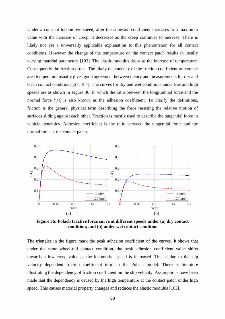
68

Under a constant locomotive speed, after the adhesion coefficient increases to a maximum

value with the increase of creep, it decreases as the creep continues to increase. There is

likely not yet a universally applicable explanation to this phenomenon for all contact

conditions. However the change of the temperature on the contact patch results in locally

varying material parameters [103]. The elastic modulus drops as the increase of temperature.

Consequently the friction drops. The likely dependency of the friction coefficient on contact

area temperature usually gives good agreement between theory and measurements for dry and

clean contact conditions [27, 104]. The curves for dry and wet conditions under low and high

speeds are as shown in Figure 36, in which the ratio between the longitudinal force and the

normal force 𝐹/𝑄 is also known as the adhesion coefficient. To clarify the definitions,

friction is the general physical term describing the force resisting the relative motion of

surfaces sliding against each other. Traction is mostly used to describe the tangential force in

vehicle dynamics. Adhesion coefficient is the ratio between the tangential force and the

normal force at the contact patch.

0 0.05 0.1 0.15 0.20

0.1

0.2

0.3

0.4

0.5

creep

F/Q

10 km/h

120 km/h

0 0.05 0.1 0.15 0.20

0.1

0.2

0.3

0.4

0.5

creep

F/Q

10 km/h

120 km/h

(a) (b)

Figure 36: Polach tractive force curve at different speeds under (a) dry contact

condition; and (b) under wet contact condition

The triangles in the figure mark the peak adhesion coefficient of the curves. It shows that

under the same wheel-rail contact condition, the peak adhesion coefficient value shifts

towards a low creep value as the locomotive speed is increased. This is due to the slip

velocity dependent friction coefficient term in the Polach model. There is literature

illustrating the dependency of friction coefficient on the slip velocity. Assumptions have been

made that the dependency is caused by the high temperature at the contact patch under high

speed. This causes material property changes and reduces the elastic modulus [103].

69

As shown above, the contact dynamics between the wheel and rail is complex and highly

nonlinear. The adhesion coefficient, that is the ratio between longitudinal and normal force

between the wheel and rail contact patch, varies significantly under different conditions such

as different operating speeds or wheel/rail contact conditions. Thus it is crucial to adjust the

wheel speed accordingly to avoid the occurrence of undesirable dynamics such as the loss of

traction due to the excessive spin of the wheels.

4.1.3. Simulation Results of the Simplified and Detailed Drives

In order to validate the AC and DC drive and controller performances, simulations were

carried out for single wheelset simplified locomotive models for a range of traction

conditions. The following results will be detailed in the following subsections.

Traction simulations for the dry condition to validate the tractive effort of the AC

and DC drive and to compare to the traction curves in [101].

A braking simulation for the dry condition to validate the braking effort of the AC

and DC drive and to compare to the braking curve in [105].

An acceleration simulation for the dry condition and comparison to data from

[106].

A transient contact condition simulation from the dry to the oil condition at 20km/h

to validate the effectiveness of the creep controller.

In the simplified 1/6 locomotive model, the basic formula 𝑓 = 𝑚𝑎 has been employed where

𝑓 is the traction/braking force caused by the interaction between the wheelset and rail tracks,

𝑚 represents 1/6 of the total mass of the locomotive 134 tonnes and 𝑎 is the acceleration of

the mass. In order to verify the drive model’s traction/braking performance without

considering the vehicle structural dynamics, the dynamic model was simplified to a single

mass of 1/6 of the total mass of the locomotive on an axle. Here a typical heavy haul

locomotive GT46MAC mass and traction effort data are chosen for the simulation.

The simulations have been carried out for each traction notch by changing the driver notch

setting as shown in Figure 37. The initial velocity of the locomotive is set to be 0.01km/h to

avoid error due to an infinite initial creep value. For each notch a simulation is then carried

out for the dry contact condition, from the initial speed to 70 km/h. Then the tractive force

value is rescaled to calculate the total tractive force of the corresponding notch by being

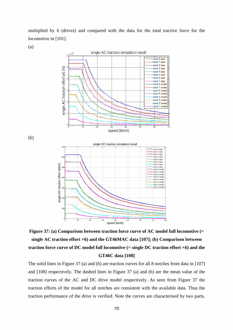
70

multiplied by 6 (drives) and compared with the data for the total tractive force for the

locomotive in [101].

(a)

(b)

Figure 37: (a) Comparison between traction force curve of AC model full locomotive (=

single AC traction effort ×6) and the GT46MAC data [107]; (b) Comparison between

traction force curve of DC model full locomotive (= single DC traction effort ×6) and the

GT46C data [108]

The solid lines in Figure 37 (a) and (b) are traction curves for all 8 notches from data in [107]

and [108] respectively. The dashed lines in Figure 37 (a) and (b) are the mean value of the

traction curves of the AC and DC drive model respectively. As seen from Figure 37 the

traction efforts of the model for all notches are consistent with the available data. Thus the

traction performance of the drive is verified. Note the curves are characterised by two parts,

0 10 20 30 40 50 60 70 800

100

200

300

400

500

600

700

speed (km/h)

sin

gle

DC

tra

ction e

ffort

x6(k

N)

single DC traction simulation result

notch 8 data

notch 7 data

notch 6 data

notch 5 data

notch 4 data

notch 3 data

notch 2 data

notch 1 data

notch 8 model

notch 7 model

notch 6 model

notch 5 model

notch 4 model

notch 3 model

notch 2 model

notch 1 model

71

which is typical of locomotive electric traction drive, providing approximately constant

torque for low speeds until the maximum power for each notch is reached after which the

curve is power limited (= torque × speed). The dynamic braking simulation was performed to

verify the braking effort of the model with comparison to the data in [105] and [108]. The

simulations begin with a high initial locomotive speed and decelerate to 0.05 km/h.

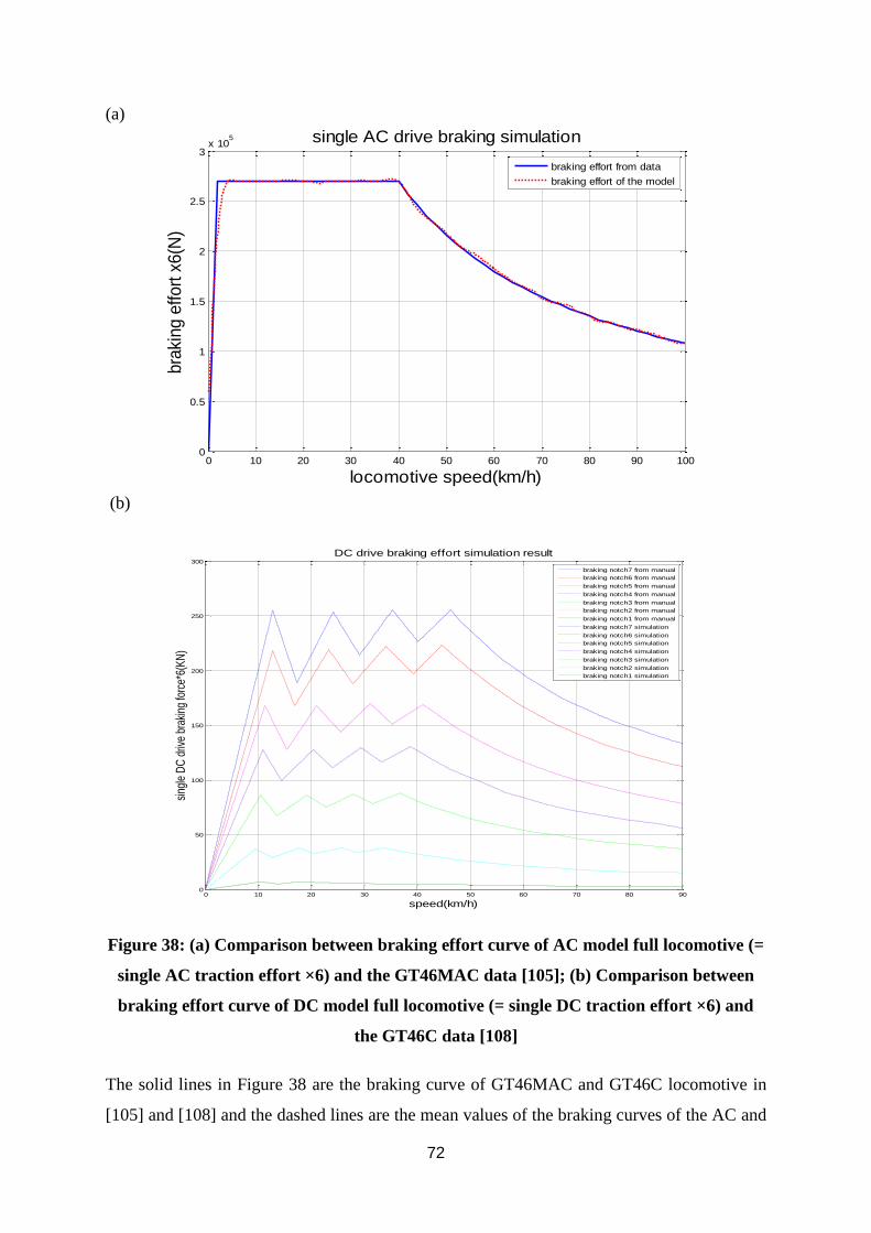
72

(a)

(b)

Figure 38: (a) Comparison between braking effort curve of AC model full locomotive (=

single AC traction effort ×6) and the GT46MAC data [105]; (b) Comparison between

braking effort curve of DC model full locomotive (= single DC traction effort ×6) and

the GT46C data [108]

The solid lines in Figure 38 are the braking curve of GT46MAC and GT46C locomotive in

[105] and [108] and the dashed lines are the mean values of the braking curves of the AC and

0 10 20 30 40 50 60 70 80 90 1000

0.5

1

1.5

2

2.5

3x 10

5

locomotive speed(km/h)

bra

king e

ffort

x6(N

)

single AC drive braking simulation

braking effort from data

braking effort of the model

0 10 20 30 40 50 60 70 80 900

50

100

150

200

250

300

speed(km/h)

sing

le D

C d

rive

brak

ing

forc

e*6(

KN

)

DC drive braking effort simulation result

braking notch7 from manual

braking notch6 from manual

braking notch5 from manual

braking notch4 from manual

braking notch3 from manual

braking notch2 from manual

braking notch1 from manual

braking notch7 simulation

braking notch6 simulation

braking notch5 simulation

braking notch4 simulation

braking notch3 simulation

braking notch2 simulation

braking notch1 simulation

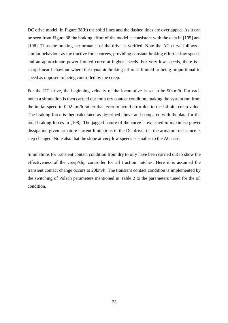
73

DC drive model. In Figure 38(b) the solid lines and the dashed lines are overlapped. As it can

be seen from Figure 38 the braking effort of the model is consistent with the data in [105] and

[108]. Thus the braking performance of the drive is verified. Note the AC curve follows a

similar behaviour as the tractive force curves, providing constant braking effort at low speeds

and an approximate power limited curve at higher speeds. For very low speeds, there is a

sharp linear behaviour where the dynamic braking effort is limited to being proportional to

speed as opposed to being controlled by the creep.

For the DC drive, the beginning velocity of the locomotive is set to be 90km/h. For each

notch a simulation is then carried out for a dry contact condition, making the system run from

the initial speed to 0.02 km/h rather than zero to avoid error due to the infinite creep value.

The braking force is then calculated as described above and compared with the data for the

total braking forces in [108]. The jagged nature of the curve is expected to maximise power

dissipation given armature current limitations in the DC drive, i.e. the armature resistance is

step changed. Note also that the slope at very low speeds is smaller to the AC case.

Simulations for transient contact condition from dry to oily have been carried out to show the

effectiveness of the creep/slip controller for all traction notches. Here it is assumed the

transient contact change occurs at 20km/h. The transient contact condition is implemented by

the switching of Polach parameters mentioned in Table 2 to the parameters tuned for the oil

condition.

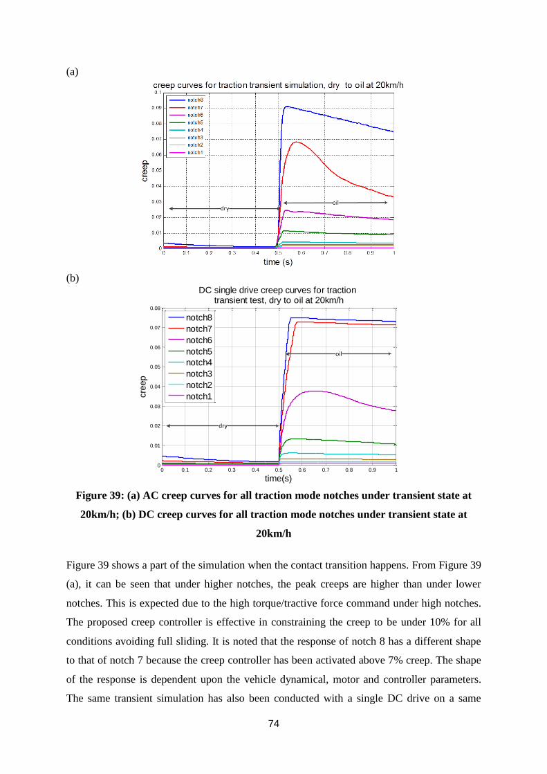
74

(a)

(b)

0 0.1 0.2 0.3 0.4 0.5 0.6 0.7 0.8 0.9 10

0.01

0.02

0.03

0.04

0.05

0.06

0.07

0.08

time(s)

cre

ep

DC single drive creep curves for traction transient test, dry to oil at 20km/h

notch8

notch7

notch6

notch5

notch4

notch3

notch2

notch1

dry

oil

Figure 39: (a) AC creep curves for all traction mode notches under transient state at

20km/h; (b) DC creep curves for all traction mode notches under transient state at

20km/h

Figure 39 shows a part of the simulation when the contact transition happens. From Figure 39

(a), it can be seen that under higher notches, the peak creeps are higher than under lower

notches. This is expected due to the high torque/tractive force command under high notches.

The proposed creep controller is effective in constraining the creep to be under 10% for all

conditions avoiding full sliding. It is noted that the response of notch 8 has a different shape

to that of notch 7 because the creep controller has been activated above 7% creep. The shape

of the response is dependent upon the vehicle dynamical, motor and controller parameters.

The same transient simulation has also been conducted with a single DC drive on a same

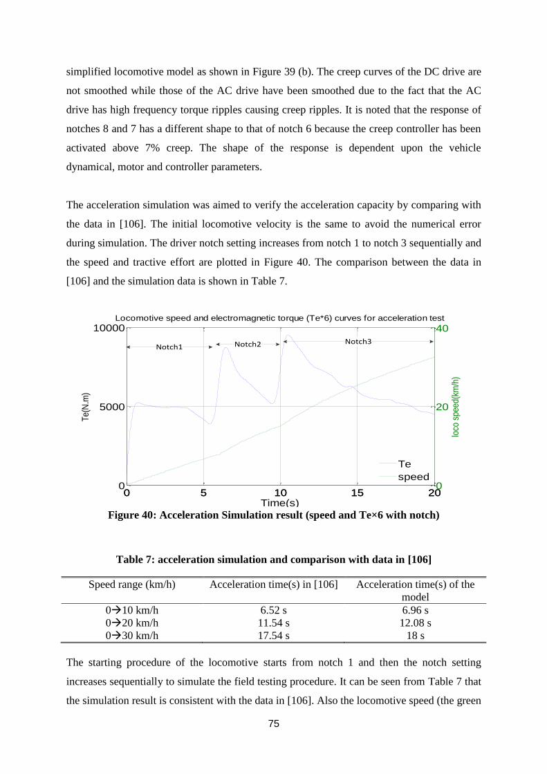
75

simplified locomotive model as shown in Figure 39 (b). The creep curves of the DC drive are

not smoothed while those of the AC drive have been smoothed due to the fact that the AC

drive has high frequency torque ripples causing creep ripples. It is noted that the response of

notches 8 and 7 has a different shape to that of notch 6 because the creep controller has been

activated above 7% creep. The shape of the response is dependent upon the vehicle

dynamical, motor and controller parameters.

The acceleration simulation was aimed to verify the acceleration capacity by comparing with

the data in [106]. The initial locomotive velocity is the same to avoid the numerical error

during simulation. The driver notch setting increases from notch 1 to notch 3 sequentially and

the speed and tractive effort are plotted in Figure 40. The comparison between the data in

[106] and the simulation data is shown in Table 7.

0 5 10 15 200

5000

10000

Time(s)

Te(

N.m

)

Locomotive speed and electromagnetic torque (Te*6) curves for acceleration test

0 5 10 15 200

20

40

loco

spe

ed(k

m/h

)Te

speed

Notch1 Notch2 Notch3

Figure 40: Acceleration Simulation result (speed and Te×6 with notch)

Table 7: acceleration simulation and comparison with data in [106]

Speed range (km/h) Acceleration time(s) in [106] Acceleration time(s) of the

model

010 km/h 6.52 s 6.96 s

020 km/h 11.54 s 12.08 s

030 km/h 17.54 s 18 s

The starting procedure of the locomotive starts from notch 1 and then the notch setting

increases sequentially to simulate the field testing procedure. It can be seen from Table 7 that

the simulation result is consistent with the data in [106]. Also the locomotive speed (the green

76

solid line) increases almost linearly with time as expected. Each time the notch setting

increases, the torque increases subsequently and then decreases gradually due to the increase

of locomotive speed, which can be explained with Figure 37. In particular, the maximum

tractive force decreases as the locomotive speed increases as the electric drives operate under

constant power mode.

In this section, analysis and simulation results are provided for the essential dynamic

subsystems of the locomotive. The eigenmode analysis reveals the frequency of vibration of

each mode, as well as the modes which are most likely to be excited under external

perturbations. The Polach model has been implemented and tuned for various contact

conditions. The tuning results are compared with the data from literature, and they are in very

good agreement. Additionally, the single drive model provided important validation

information for the AC/DC drive module that can be adapted into the full locomotive model.

The simulation results of AC and DC drives have confirmed that a creep controller is desired

for the locomotives, as demonstrated in the result, that the maximum creep of the AC drive

can exceed 9%, which is considerably large and is likely to cause a loss of tractive force.

4.2. Investigations on Creep Controllers (Objective 2)

Based on the full size co-co locomotive dynamics model presented in the previous section, a

few different creep controllers are investigated for the purpose of preventing excessive creep

from happening and achieving higher tractive force. All the simulations in this section are

based on the simplified AC drive model which provides a detailed creep response. The creep

controller is investigated under low speed acceleration operation with changes of friction

conditions. The simulation is for the case when the locomotive runs into a wet rail section at

11km/h and back out to a dry rail section at 12.5km/h.

4.2.1. Axle Based PI Controller

The simulation is performed for the acceleration process with change of friction conditions

using the axle based PI controller. The result is shown in Figure 41 - Figure 43. It is shown in

these figures that the axle based PI controller is able to reduce the creep quickly in the

acceleration process, as well as after the change of friction conditions.

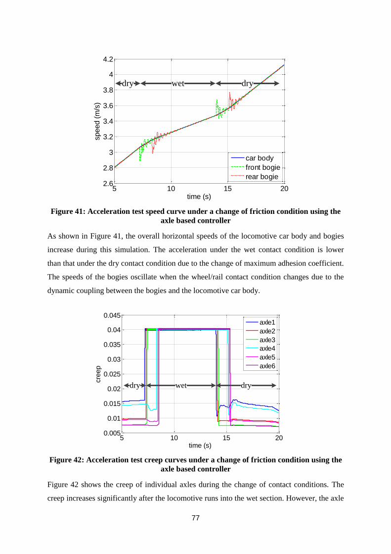
77

5 10 15 202.6

2.8

3

3.2

3.4

3.6

3.8

4

4.2

time (s)

speed (

m/s

)

car body

front bogie

rear bogie

dry wet dry

Figure 41: Acceleration test speed curve under a change of friction condition using the

axle based controller

As shown in Figure 41, the overall horizontal speeds of the locomotive car body and bogies

increase during this simulation. The acceleration under the wet contact condition is lower

than that under the dry contact condition due to the change of maximum adhesion coefficient.

The speeds of the bogies oscillate when the wheel/rail contact condition changes due to the

dynamic coupling between the bogies and the locomotive car body.

5 10 15 200.005

0.01

0.015

0.02

0.025

0.03

0.035

0.04

0.045

time (s)

cre

ep

axle1

axle2

axle3

axle4

axle5

axle6

dry wet dry

Figure 42: Acceleration test creep curves under a change of friction condition using the

axle based controller

Figure 42 shows the creep of individual axles during the change of contact conditions. The

creep increases significantly after the locomotive runs into the wet section. However, the axle

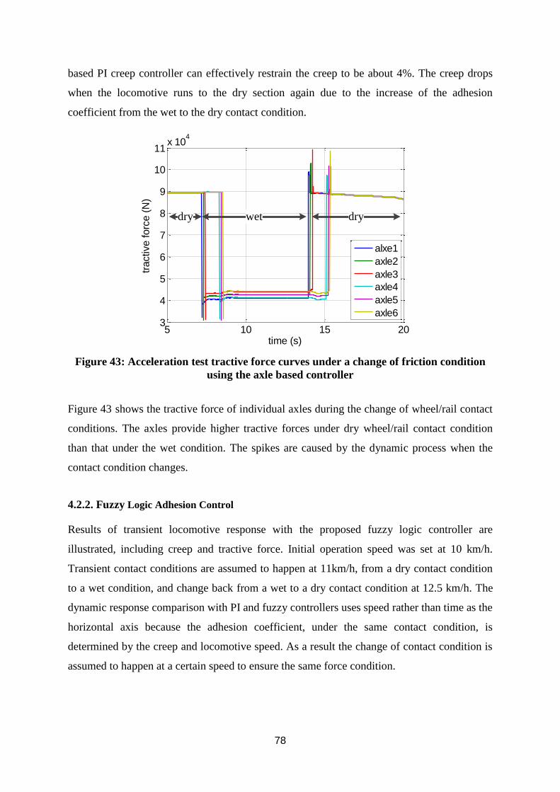
78

based PI creep controller can effectively restrain the creep to be about 4%. The creep drops

when the locomotive runs to the dry section again due to the increase of the adhesion

coefficient from the wet to the dry contact condition.

5 10 15 203

4

5

6

7

8

9

10

11x 10

4

time (s)

tractive forc

e (

N)

alxe1

axle2

axle3

axle4

axle5

axle6

dry wet dry

Figure 43: Acceleration test tractive force curves under a change of friction condition

using the axle based controller

Figure 43 shows the tractive force of individual axles during the change of wheel/rail contact

conditions. The axles provide higher tractive forces under dry wheel/rail contact condition

than that under the wet condition. The spikes are caused by the dynamic process when the

contact condition changes.

4.2.2. Fuzzy Logic Adhesion Control

Results of transient locomotive response with the proposed fuzzy logic controller are

illustrated, including creep and tractive force. Initial operation speed was set at 10 km/h.

Transient contact conditions are assumed to happen at 11km/h, from a dry contact condition

to a wet condition, and change back from a wet to a dry contact condition at 12.5 km/h. The

dynamic response comparison with PI and fuzzy controllers uses speed rather than time as the

horizontal axis because the adhesion coefficient, under the same contact condition, is

determined by the creep and locomotive speed. As a result the change of contact condition is

assumed to happen at a certain speed to ensure the same force condition.

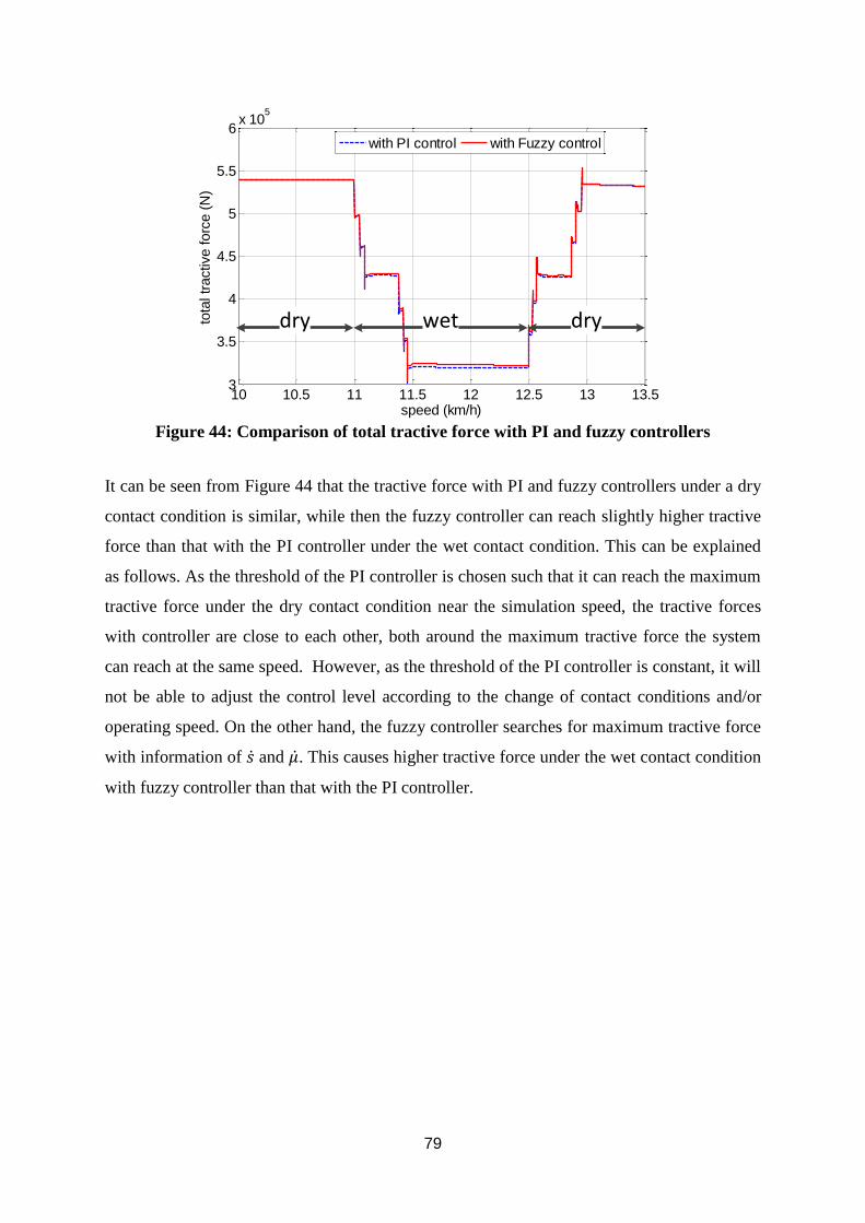
79

10 10.5 11 11.5 12 12.5 13 13.53

3.5

4

4.5

5

5.5

6x 10

5

speed (km/h)

tota

l tr

active forc

e (

N)

with PI control with Fuzzy control

dry wet dry

Figure 44: Comparison of total tractive force with PI and fuzzy controllers

It can be seen from Figure 44 that the tractive force with PI and fuzzy controllers under a dry

contact condition is similar, while then the fuzzy controller can reach slightly higher tractive

force than that with the PI controller under the wet contact condition. This can be explained

as follows. As the threshold of the PI controller is chosen such that it can reach the maximum

tractive force under the dry contact condition near the simulation speed, the tractive forces

with controller are close to each other, both around the maximum tractive force the system

can reach at the same speed. However, as the threshold of the PI controller is constant, it will

not be able to adjust the control level according to the change of contact conditions and/or

operating speed. On the other hand, the fuzzy controller searches for maximum tractive force

with information of �� and ��. This causes higher tractive force under the wet contact condition

with fuzzy controller than that with the PI controller.

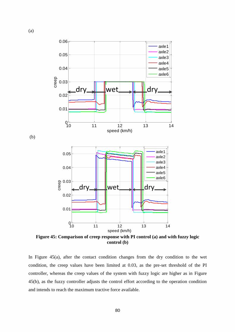
80

(a)

10 11 12 13 140

0.01

0.02

0.03

0.04

0.05

0.06

speed (km/h)

cre

ep

axle1

axle2

axle3

axle4

axle5

axle6

dry drywet

(b)

10 11 12 13 140

0.01

0.02

0.03

0.04

0.05

speed (km/h)

cre

ep

axle1

axle2

axle3

axle4

axle5

axle6

dry drywet

Figure 45: Comparison of creep response with PI control (a) and with fuzzy logic

control (b)

In Figure 45(a), after the contact condition changes from the dry condition to the wet

condition, the creep values have been limited at 0.03, as the pre-set threshold of the PI

controller, whereas the creep values of the system with fuzzy logic are higher as in Figure

45(b), as the fuzzy controller adjusts the control effort according to the operation condition

and intends to reach the maximum tractive force available.

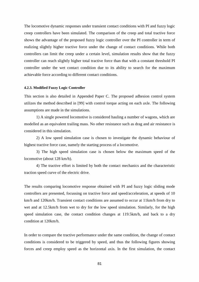
81

The locomotive dynamic responses under transient contact conditions with PI and fuzzy logic

creep controllers have been simulated. The comparison of the creep and total tractive force

shows the advantage of the proposed fuzzy logic controller over the PI controller in term of

realizing slightly higher tractive force under the change of contact conditions. While both

controllers can limit the creep under a certain level, simulation results show that the fuzzy

controller can reach slightly higher total tractive force than that with a constant threshold PI

controller under the wet contact condition due to its ability to search for the maximum

achievable force according to different contact conditions.

4.2.3. Modified Fuzzy Logic Controller

This section is also detailed in Appended Paper C. The proposed adhesion control system

utilizes the method described in [99] with control torque acting on each axle. The following

assumptions are made in the simulations.

1) A single powered locomotive is considered hauling a number of wagons, which are

modelled as an equivalent trailing mass. No other resistance such as drag and air resistance is

considered in this simulation.

2) A low speed simulation case is chosen to investigate the dynamic behaviour of

highest tractive force case, namely the starting process of a locomotive.

3) The high speed simulation case is chosen below the maximum speed of the

locomotive (about 128 km/h).

4) The tractive effort is limited by both the contact mechanics and the characteristic

traction speed curve of the electric drive.

The results comparing locomotive response obtained with PI and fuzzy logic sliding mode

controllers are presented, focussing on tractive force and speed/acceleration, at speeds of 10

km/h and 120km/h. Transient contact conditions are assumed to occur at 11km/h from dry to

wet and at 12.5km/h from wet to dry for the low speed simulation. Similarly, for the high

speed simulation case, the contact condition changes at 119.5km/h, and back to a dry

condition at 120km/h.

In order to compare the tractive performance under the same condition, the change of contact

conditions is considered to be triggered by speed, and thus the following figures showing

forces and creep employ speed as the horizontal axis. In the first simulation, the contact

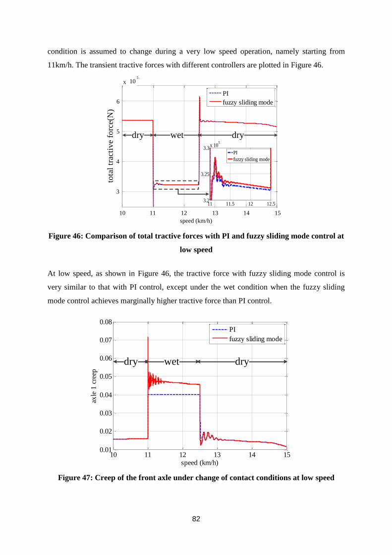
82

condition is assumed to change during a very low speed operation, namely starting from

11km/h. The transient tractive forces with different controllers are plotted in Figure 46.

10 11 12 13 14 15

3

4

5

6

x 105

tota

l tr

acti

ve

forc

e(N

)

speed (km/h)

PI

fuzzy sliding mode

dry wet dry

11 11.5 12 12.53.2

3.25

3.3x 10

5

PI

fuzzy sliding mode

speed (km/h)

1110 12 13 14 15

4

5

3

6

x 105

Figure 46: Comparison of total tractive forces with PI and fuzzy sliding mode control at

low speed

At low speed, as shown in Figure 46, the tractive force with fuzzy sliding mode control is

very similar to that with PI control, except under the wet condition when the fuzzy sliding

mode control achieves marginally higher tractive force than PI control.

10 11 12 13 14 150.01

0.02

0.03

0.04

0.05

0.06

0.07

0.08

speed (km/h)

axle

1 c

reep

PI

fuzzy sliding mode

dry wet dry

Figure 47: Creep of the front axle under change of contact conditions at low speed

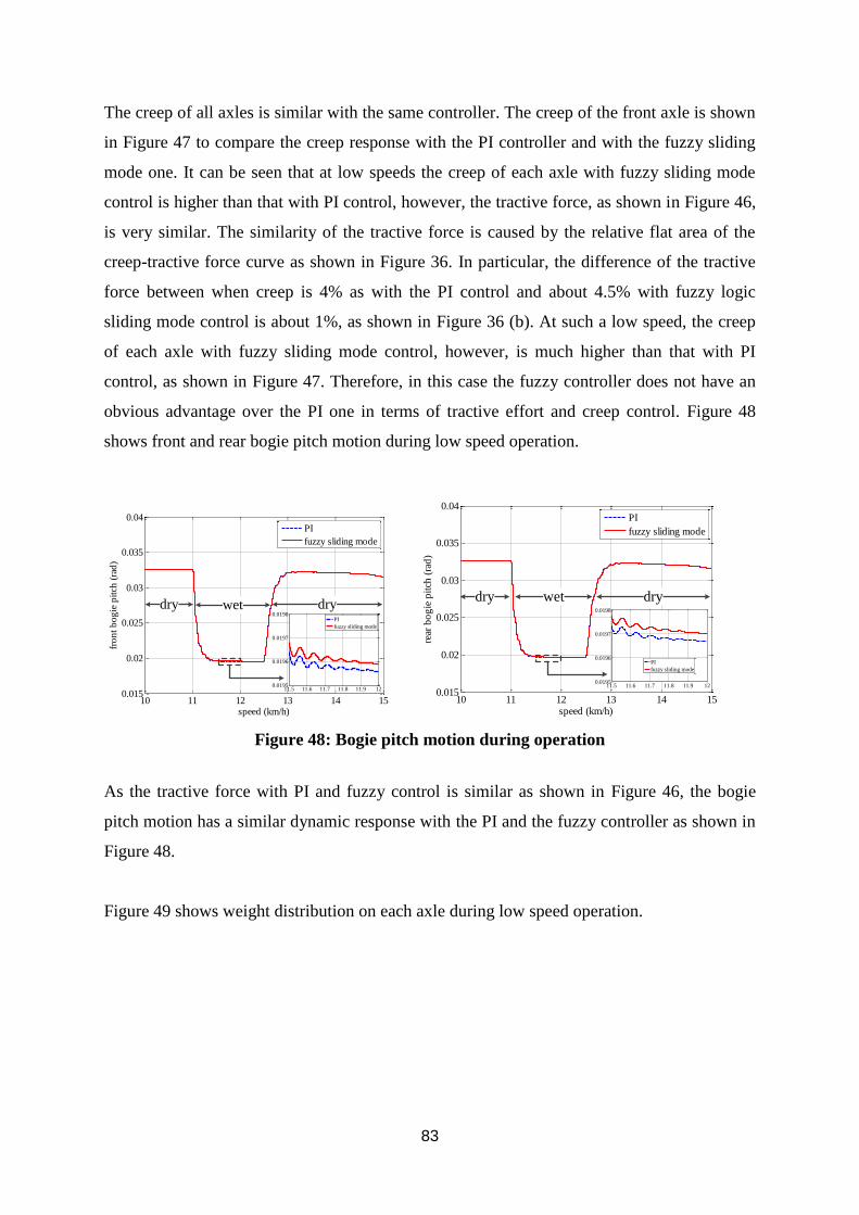
83

The creep of all axles is similar with the same controller. The creep of the front axle is shown

in Figure 47 to compare the creep response with the PI controller and with the fuzzy sliding

mode one. It can be seen that at low speeds the creep of each axle with fuzzy sliding mode

control is higher than that with PI control, however, the tractive force, as shown in Figure 46,

is very similar. The similarity of the tractive force is caused by the relative flat area of the

creep-tractive force curve as shown in Figure 36. In particular, the difference of the tractive

force between when creep is 4% as with the PI control and about 4.5% with fuzzy logic

sliding mode control is about 1%, as shown in Figure 36 (b). At such a low speed, the creep

of each axle with fuzzy sliding mode control, however, is much higher than that with PI

control, as shown in Figure 47. Therefore, in this case the fuzzy controller does not have an

obvious advantage over the PI one in terms of tractive effort and creep control. Figure 48

shows front and rear bogie pitch motion during low speed operation.

10 11 12 13 14 150.015

0.02

0.025

0.03

0.035

0.04

speed (km/h)

fro

nt

bo

gie

pit

ch (

rad

)

PI

fuzzy sliding mode

dry wet dry

11.5 11.6 11.7 11.8 11.9 120.0195

0.0196

0.0197

0.0198

PI

fuzzy sliding mode

10 11 12 13 14 15

0.015

0.02

0.025

0.03

0.035

0.04

speed (km/h)

rear

bo

gie

pit

ch (

rad

)

PI

fuzzy sliding mode

dry wet dry

11.5 11.6 11.7 11.8 11.9 120.0195

0.0196

0.0197

0.0198

PI

fuzzy sliding mode

Figure 48: Bogie pitch motion during operation

As the tractive force with PI and fuzzy control is similar as shown in Figure 46, the bogie

pitch motion has a similar dynamic response with the PI and the fuzzy controller as shown in

Figure 48.

Figure 49 shows weight distribution on each axle during low speed operation.

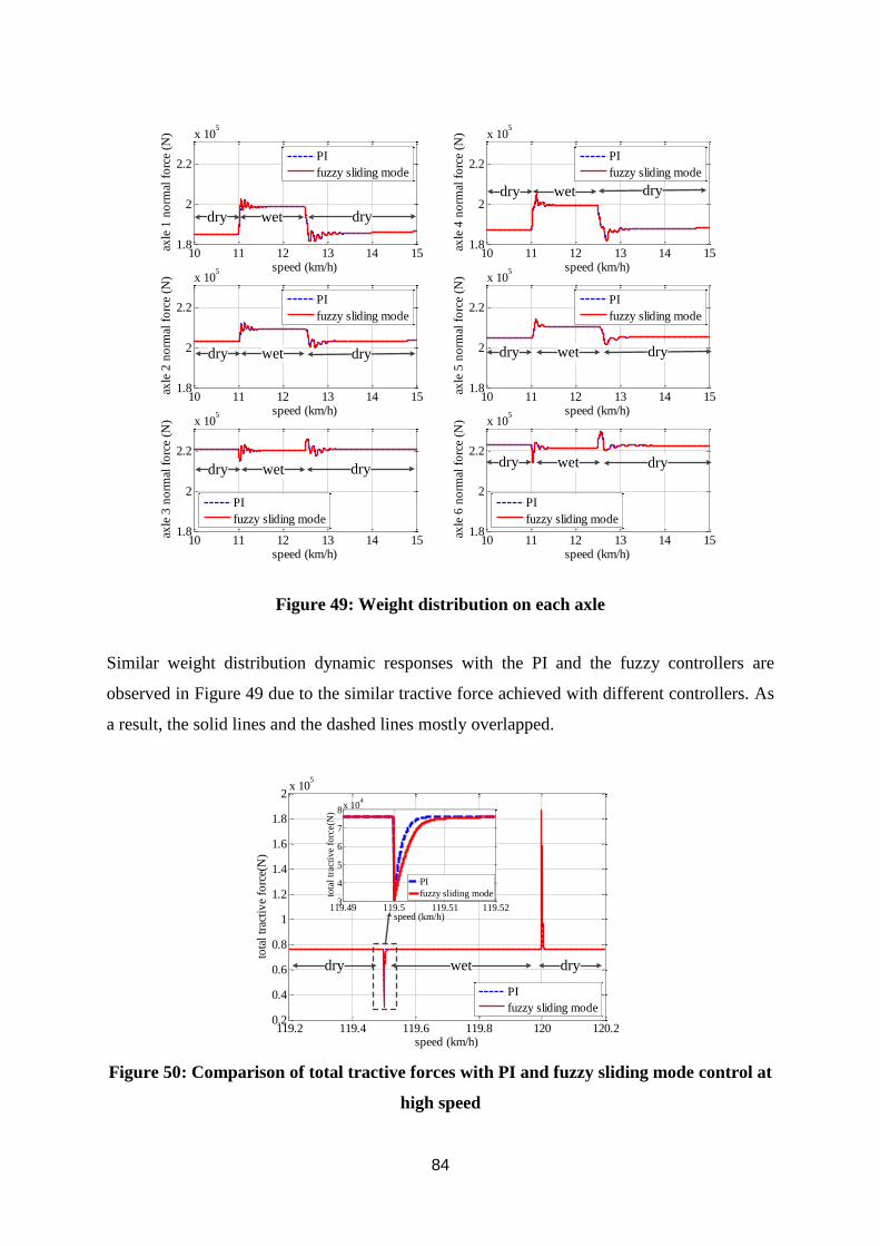
84

10 11 12 13 14 151.8

2

2.2

x 105

speed (km/h)

axle

1 n

orm

al f

orc

e (N

)

PI

fuzzy sliding mode

10 11 12 13 14 151.8

2

2.2

x 105

speed (km/h)

axle

2 n

orm

al f

orc

e (N

)

PI

fuzzy sliding mode

10 11 12 13 14 151.8

2

2.2

x 105

speed (km/h)

axle

3 n

orm

al f

orc

e (N

)

PI

fuzzy sliding mode

10 11 12 13 14 151.8

2

2.2

x 105

speed (km/h)

axle

4 n

orm

al f

orc

e (N

)

PI

fuzzy sliding mode

10 11 12 13 14 151.8

2

2.2

x 105

speed (km/h)

axle

5 n

orm

al f

orc

e (N

)

PI

fuzzy sliding mode

10 11 12 13 14 151.8

2

2.2

x 105

speed (km/h)

axle

6 n

orm

al f

orc

e (N

)

PI

fuzzy sliding mode

dry wet dry

dry wet dry

dry wet dry

dry wet dry

dry

dry

wet

wetdry

dry

Figure 49: Weight distribution on each axle

Similar weight distribution dynamic responses with the PI and the fuzzy controllers are

observed in Figure 49 due to the similar tractive force achieved with different controllers. As

a result, the solid lines and the dashed lines mostly overlapped.

119.2 119.4 119.6 119.8 120 120.20.2

0.4

0.6

0.8

1

1.2

1.4

1.6

1.8

2x 10

5

speed (km/h)

tota

l tr

acti

ve

forc

e(N

)

PI

fuzzy sliding mode

dry wet dry

119.49 119.5 119.51 119.523

4

5

6

7

8x 10

4

speed (km/h)

tota

l tr

acti

ve

forc

e(N

)

PI

fuzzy sliding mode

Figure 50: Comparison of total tractive forces with PI and fuzzy sliding mode control at

high speed

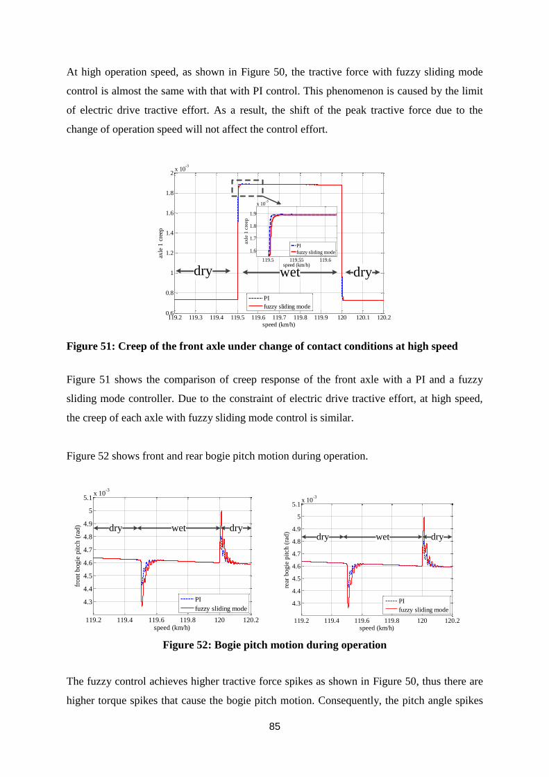
85

At high operation speed, as shown in Figure 50, the tractive force with fuzzy sliding mode

control is almost the same with that with PI control. This phenomenon is caused by the limit

of electric drive tractive effort. As a result, the shift of the peak tractive force due to the

change of operation speed will not affect the control effort.

119.2 119.3 119.4 119.5 119.6 119.7 119.8 119.9 120 120.1 120.20.6

0.8

1

1.2

1.4

1.6

1.8

2x 10

-3

speed (km/h)

axle

1 c

reep

PI

fuzzy sliding mode

dry wet dry119.5 119.55 119.6

1.6

1.7

1.8

1.9

x 10-3

speed (km/h)

axle

1 c

reep

PI

fuzzy sliding mode

Figure 51: Creep of the front axle under change of contact conditions at high speed

Figure 51 shows the comparison of creep response of the front axle with a PI and a fuzzy

sliding mode controller. Due to the constraint of electric drive tractive effort, at high speed,

the creep of each axle with fuzzy sliding mode control is similar.

Figure 52 shows front and rear bogie pitch motion during operation.

119.2 119.4 119.6 119.8 120 120.2

4.3

4.4

4.5

4.6

4.7

4.8

4.9

5

5.1x 10

-3

speed (km/h)

fro

nt

bo

gie

pit

ch

(ra

d)

PI

fuzzy sliding mode

dry wet dry

119.2 119.4 119.6 119.8 120 120.2

4.3

4.4

4.5

4.6

4.7

4.8

4.9

5

5.1x 10

-3

speed (km/h)

rear

bo

gie

pit

ch (

rad

)

PI

fuzzy sliding mode

dry wet dry

Figure 52: Bogie pitch motion during operation

The fuzzy control achieves higher tractive force spikes as shown in Figure 50, thus there are

higher torque spikes that cause the bogie pitch motion. Consequently, the pitch angle spikes

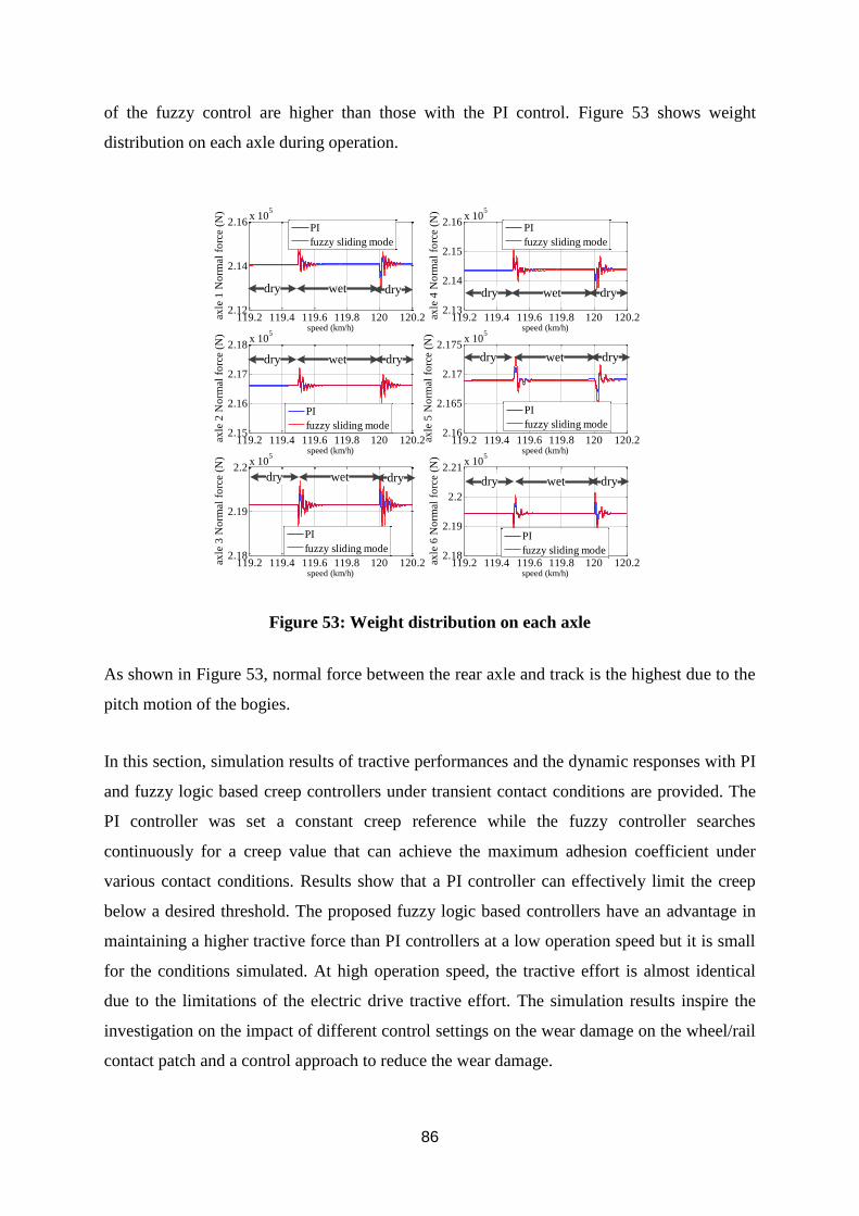
86

of the fuzzy control are higher than those with the PI control. Figure 53 shows weight

distribution on each axle during operation.

119.2 119.4 119.6 119.8 120 120.22.12

2.14

2.16x 10

5

speed (km/h)

axle

1 N

orm

al f

orc

e (N

)

PI

fuzzy sliding mode

119.2 119.4 119.6 119.8 120 120.22.15

2.16

2.17

2.18x 10

5

speed (km/h)

axle

2 N

orm

al f

orc

e (N

)

PI

fuzzy sliding mode

119.2 119.4 119.6 119.8 120 120.22.18

2.19

2.2x 10

5

speed (km/h)

axle

3 N

orm

al f

orc

e (N

)

PI

fuzzy sliding mode

119.2 119.4 119.6 119.8 120 120.22.13

2.14

2.15

2.16x 10

5

speed (km/h)

axle

4 N

orm

al f

orc

e (N

)

PI

fuzzy sliding mode

119.2 119.4 119.6 119.8 120 120.22.16

2.165

2.17

2.175x 10

5

speed (km/h)

axle

5 N

orm

al f

orc

e (N

)

PI

fuzzy sliding mode

119.2 119.4 119.6 119.8 120 120.22.18

2.19

2.2

2.21x 10

5

speed (km/h)

axle

6 N

orm

al f

orc

e (N

)

PI

fuzzy sliding mode

dry

dry

dry dry

dry

dry

wet

wet

wet

wet

wet

wet

dry

dry

dry

dry

dry

dry

Figure 53: Weight distribution on each axle

As shown in Figure 53, normal force between the rear axle and track is the highest due to the

pitch motion of the bogies.

In this section, simulation results of tractive performances and the dynamic responses with PI

and fuzzy logic based creep controllers under transient contact conditions are provided. The

PI controller was set a constant creep reference while the fuzzy controller searches

continuously for a creep value that can achieve the maximum adhesion coefficient under

various contact conditions. Results show that a PI controller can effectively limit the creep

below a desired threshold. The proposed fuzzy logic based controllers have an advantage in

maintaining a higher tractive force than PI controllers at a low operation speed but it is small

for the conditions simulated. At high operation speed, the tractive effort is almost identical

due to the limitations of the electric drive tractive effort. The simulation results inspire the

investigation on the impact of different control settings on the wear damage on the wheel/rail

contact patch and a control approach to reduce the wear damage.

87

4.3. Impact of Locomotive Creep/Adhesion Control on Wear Index and Wear Control

(Objective 3)

The adhesion/creep controller has been investigated for decades and a number of different

control approaches have been employed to improve the dynamic behaviour of the

locomotives in various aspects. This section provides the simulation results to study the

impact of different control strategies on wear damage.

4.3.1. Impact of Locomotive Creep/Adhesion Control of Wear Index

The parameter values of the PI controller are tuned to 1.5 × 107 and 2 × 105 , for the

proportional (P) and integral (I) constants, respectively. Simulations have been carried out

using the creep controller with different creep threshold settings in order to investigate its

impact on rail damage due to wear. Detailed simulation cases are listed in Table 8.

Table 8: Simulation cases

Creep

Threshold

Speed case (dry-wet-dry)

Low (≈10 km/h) Medium(≈50 km/h)

0.03 Yes Yes

0.04 Yes No

0.06 Yes No

0.08 Yes No

A threshold higher than 0.03 is not simulated for the medium speed case since the creep

response will not activate the creep controller due to the electric drive constraints. The

locomotive acceleration operation is investigated to simulate high tractional conditions that

typically occur on straight track. Thus other dynamics such as lateral and rolling dynamics

are excluded from this study. The results comparing locomotive response obtained with

different creep controller settings are presented, focussing on tractive force and the tractional

power parameter 𝑇𝛾/𝐴 , which indicates the power expended through creepage [109], at

speeds of about 10 km/h and 50km/h under the highest acceleration conditions. The 𝑇𝛾/𝐴

value is relevant to wear rate according to the mapping relation [71], as shown in Figure 16

[41].

In order to avoid serious rail damage caused by wear, the 𝑇𝛾/𝐴 value needs to be constrained

below 60 N/mm2. Transient contact conditions are assumed to occur at 11km/h from dry to

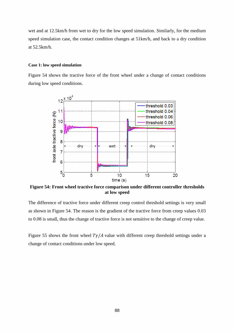
88

wet and at 12.5km/h from wet to dry for the low speed simulation. Similarly, for the medium

speed simulation case, the contact condition changes at 51km/h, and back to a dry condition

at 52.5km/h.

Case 1: low speed simulation

Figure 54 shows the tractive force of the front wheel under a change of contact conditions

during low speed conditions.

dry drywet

Figure 54: Front wheel tractive force comparison under different controller thresholds

at low speed

The difference of tractive force under different creep control threshold settings is very small

as shown in Figure 54. The reason is the gradient of the tractive force from creep values 0.03

to 0.08 is small, thus the change of tractive force is not sensitive to the change of creep value.

Figure 55 shows the front wheel 𝑇𝛾/𝐴 value with different creep threshold settings under a

change of contact conditions under low speed.

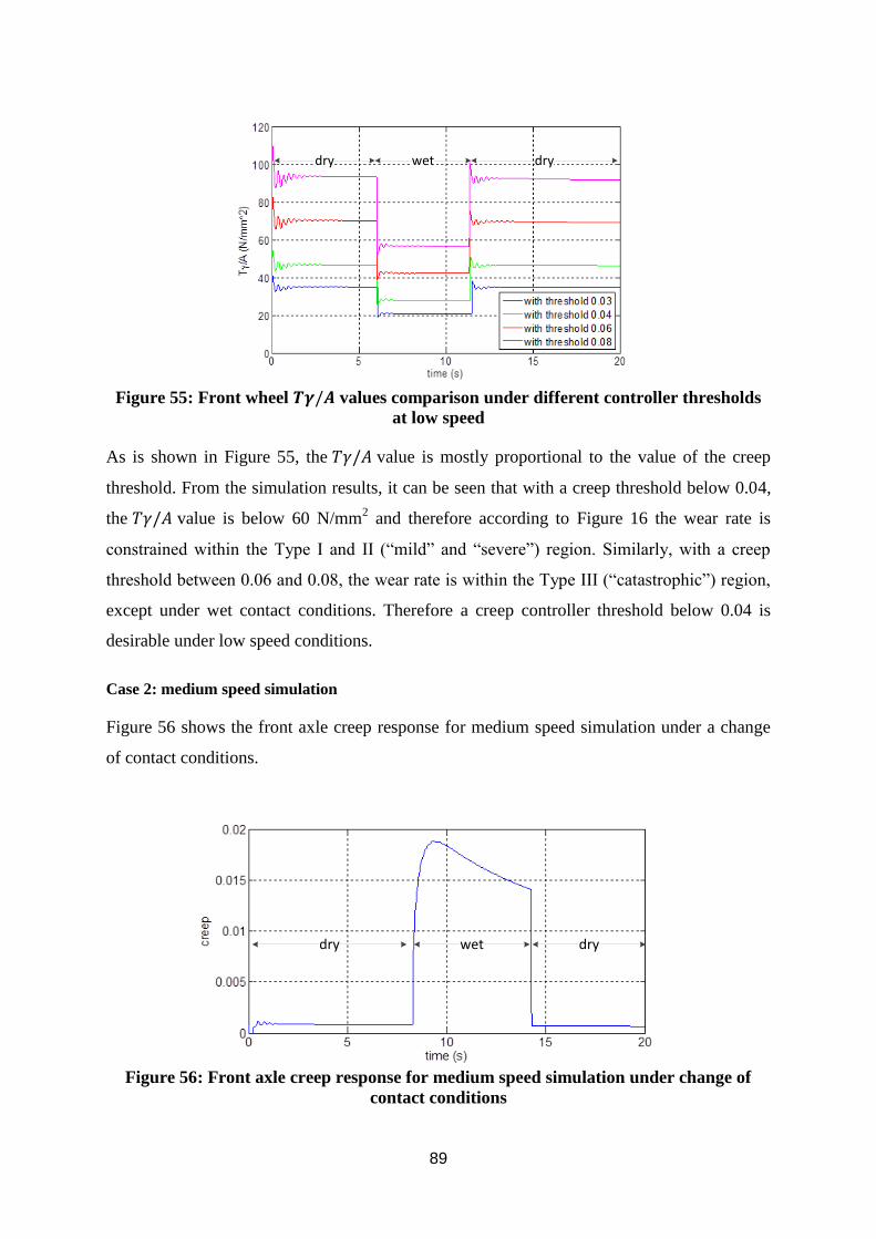
89

dry wet dry

Figure 55: Front wheel 𝑻𝜸/𝑨 values comparison under different controller thresholds

at low speed

As is shown in Figure 55, the 𝑇𝛾/𝐴 value is mostly proportional to the value of the creep

threshold. From the simulation results, it can be seen that with a creep threshold below 0.04,

the 𝑇𝛾/𝐴 value is below 60 N/mm2 and therefore according to Figure 16 the wear rate is

constrained within the Type I and II (“mild” and “severe”) region. Similarly, with a creep

threshold between 0.06 and 0.08, the wear rate is within the Type III (“catastrophic”) region,

except under wet contact conditions. Therefore a creep controller threshold below 0.04 is

desirable under low speed conditions.

Case 2: medium speed simulation

Figure 56 shows the front axle creep response for medium speed simulation under a change

of contact conditions.

dry drywet

Figure 56: Front axle creep response for medium speed simulation under change of

contact conditions

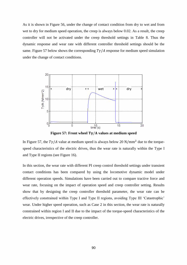
90

As it is shown in Figure 56, under the change of contact condition from dry to wet and from

wet to dry for medium speed operation, the creep is always below 0.02. As a result, the creep

controller will not be activated under the creep threshold settings in Table 8. Thus the

dynamic response and wear rate with different controller threshold settings should be the

same. Figure 57 below shows the corresponding 𝑇𝛾/𝐴 response for medium speed simulation

under the change of contact conditions.

dry wet dry

Figure 57: Front wheel 𝐓𝛄/𝐀 values at medium speed

In Figure 57, the 𝑇𝛾/𝐴 value at medium speed is always below 20 N/mm2 due to the torque-

speed characteristics of the electric drives, thus the wear rate is naturally within the Type I

and Type II regions (see Figure 16).

In this section, the wear rate with different PI creep control threshold settings under transient

contact conditions has been compared by using the locomotive dynamic model under

different operation speeds. Simulations have been carried out to compare tractive force and

wear rate, focusing on the impact of operation speed and creep controller setting. Results

show that by designing the creep controller threshold parameter, the wear rate can be

effectively constrained within Type I and Type II regions, avoiding Type III ‘Catastrophic’

wear. Under higher speed operation, such as Case 2 in this section, the wear rate is naturally

constrained within region I and II due to the impact of the torque-speed characteristics of the

electric drives, irrespective of the creep controller.

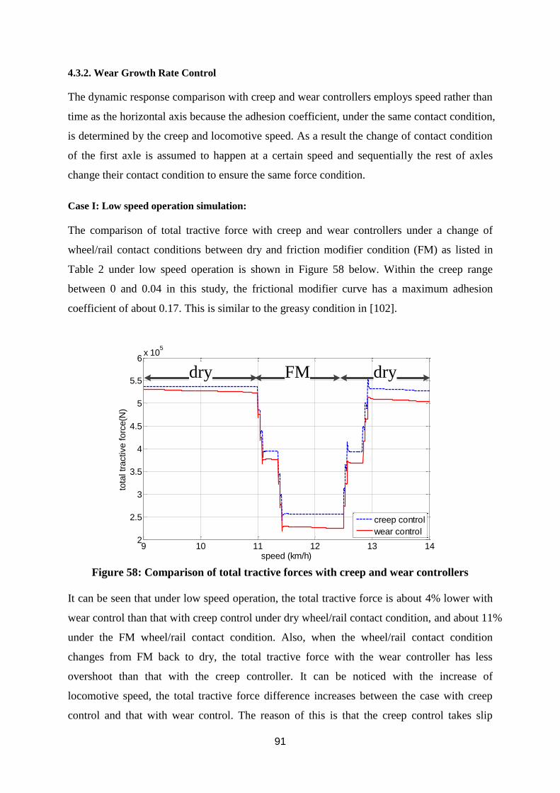
91

4.3.2. Wear Growth Rate Control

The dynamic response comparison with creep and wear controllers employs speed rather than

time as the horizontal axis because the adhesion coefficient, under the same contact condition,

is determined by the creep and locomotive speed. As a result the change of contact condition

of the first axle is assumed to happen at a certain speed and sequentially the rest of axles

change their contact condition to ensure the same force condition.

Case I: Low speed operation simulation:

The comparison of total tractive force with creep and wear controllers under a change of

wheel/rail contact conditions between dry and friction modifier condition (FM) as listed in

Table 2 under low speed operation is shown in Figure 58 below. Within the creep range

between 0 and 0.04 in this study, the frictional modifier curve has a maximum adhesion

coefficient of about 0.17. This is similar to the greasy condition in [102].

9 10 11 12 13 142

2.5

3

3.5

4

4.5

5

5.5

6x 10

5

speed (km/h)

tota

l tr

active forc

e(N

)

creep control

wear control

dry dryFM

Figure 58: Comparison of total tractive forces with creep and wear controllers

It can be seen that under low speed operation, the total tractive force is about 4% lower with

wear control than that with creep control under dry wheel/rail contact condition, and about 11%

under the FM wheel/rail contact condition. Also, when the wheel/rail contact condition

changes from FM back to dry, the total tractive force with the wear controller has less

overshoot than that with the creep controller. It can be noticed with the increase of

locomotive speed, the total tractive force difference increases between the case with creep

control and that with wear control. The reason of this is that the creep control takes slip

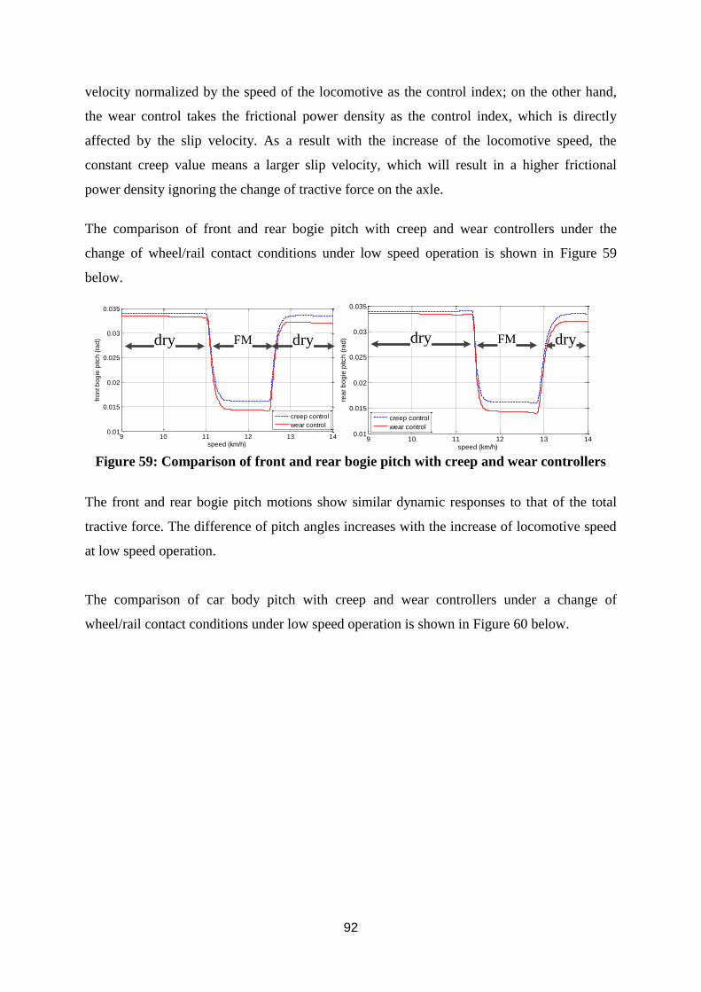
92

velocity normalized by the speed of the locomotive as the control index; on the other hand,

the wear control takes the frictional power density as the control index, which is directly

affected by the slip velocity. As a result with the increase of the locomotive speed, the

constant creep value means a larger slip velocity, which will result in a higher frictional

power density ignoring the change of tractive force on the axle.

The comparison of front and rear bogie pitch with creep and wear controllers under the

change of wheel/rail contact conditions under low speed operation is shown in Figure 59

below.

9 10 11 12 13 140.01

0.015

0.02

0.025

0.03

0.035

speed (km/h)

fro

nt b

og

ie p

itch

(ra

d)

creep control

wear control

9 10 11 12 13 140.01

0.015

0.02

0.025

0.03

0.035

speed (km/h)

rea

r b

og

ie p

itch

(ra

d)

creep control

wear control

dry FM dry dry FM dry

Figure 59: Comparison of front and rear bogie pitch with creep and wear controllers

The front and rear bogie pitch motions show similar dynamic responses to that of the total

tractive force. The difference of pitch angles increases with the increase of locomotive speed

at low speed operation.

The comparison of car body pitch with creep and wear controllers under a change of

wheel/rail contact conditions under low speed operation is shown in Figure 60 below.

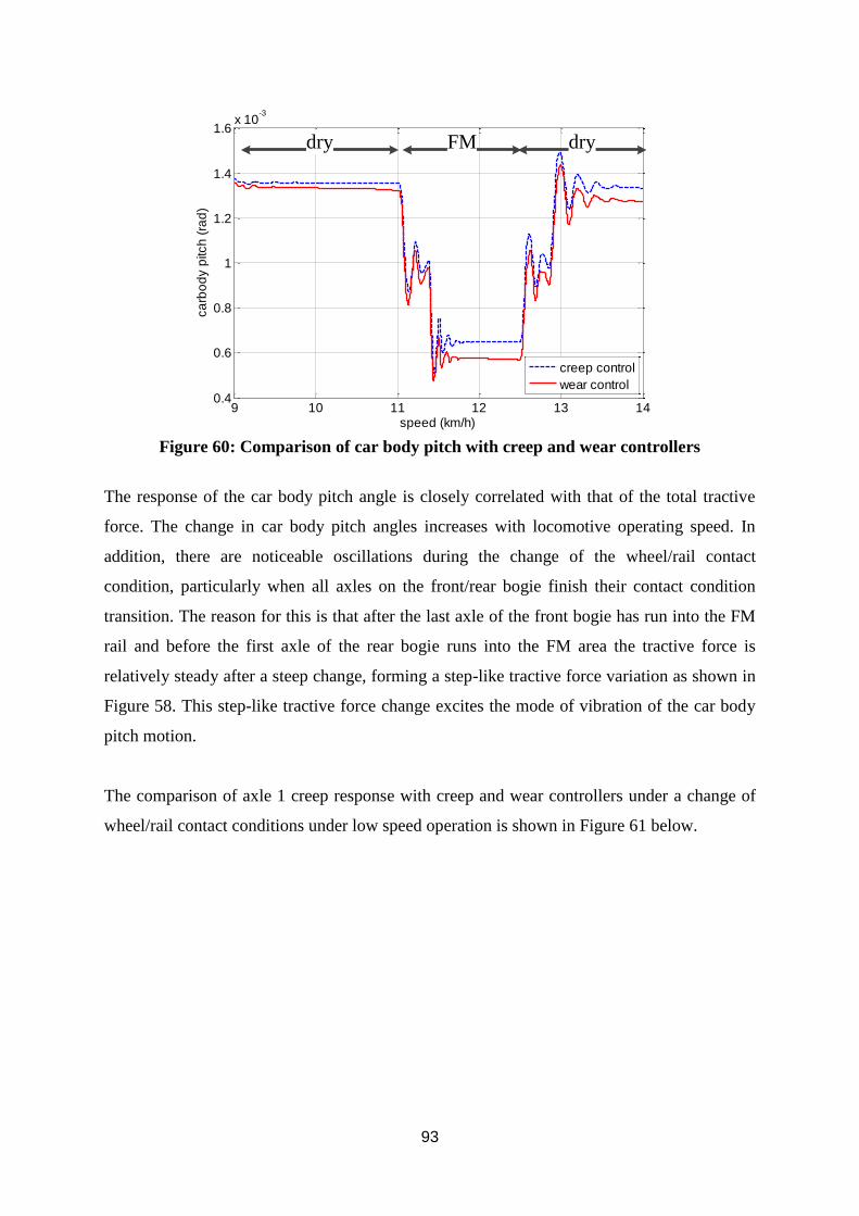
93

9 10 11 12 13 140.4

0.6

0.8

1

1.2

1.4

1.6x 10

-3

speed (km/h)

ca

rbo

dy p

itch

(ra

d)

creep control

wear control

dryFMdry

Figure 60: Comparison of car body pitch with creep and wear controllers

The response of the car body pitch angle is closely correlated with that of the total tractive

force. The change in car body pitch angles increases with locomotive operating speed. In

addition, there are noticeable oscillations during the change of the wheel/rail contact

condition, particularly when all axles on the front/rear bogie finish their contact condition

transition. The reason for this is that after the last axle of the front bogie has run into the FM

rail and before the first axle of the rear bogie runs into the FM area the tractive force is

relatively steady after a steep change, forming a step-like tractive force variation as shown in

Figure 58. This step-like tractive force change excites the mode of vibration of the car body

pitch motion.

The comparison of axle 1 creep response with creep and wear controllers under a change of

wheel/rail contact conditions under low speed operation is shown in Figure 61 below.

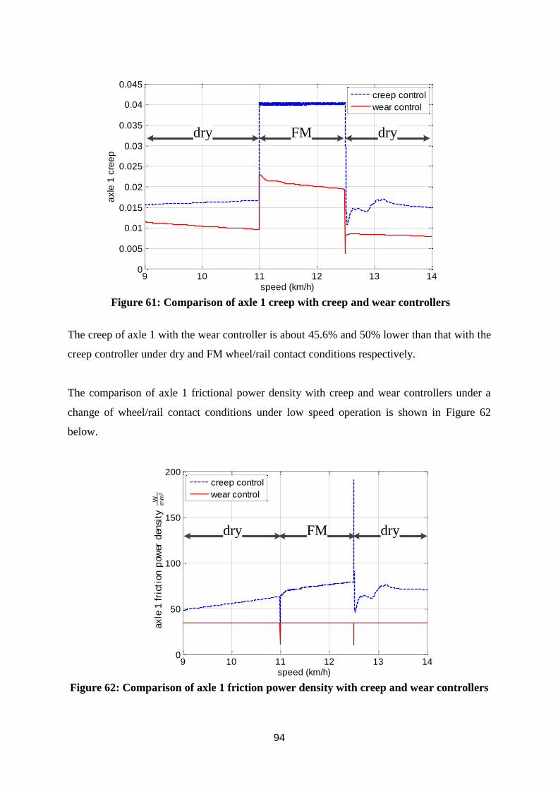
94

9 10 11 12 13 140

0.005

0.01

0.015

0.02

0.025

0.03

0.035

0.04

0.045

speed (km/h)

axle

1 c

ree

p

creep control

wear control

dry FM dry

Figure 61: Comparison of axle 1 creep with creep and wear controllers

The creep of axle 1 with the wear controller is about 45.6% and 50% lower than that with the

creep controller under dry and FM wheel/rail contact conditions respectively.

The comparison of axle 1 frictional power density with creep and wear controllers under a

change of wheel/rail contact conditions under low speed operation is shown in Figure 62

below.

9 10 11 12 13 140

50

100

150

200

speed (km/h)

axle

1fr

icti

on

pow

erden

sity

Wm

m2

creep control

wear control

dry FM dry

Figure 62: Comparison of axle 1 friction power density with creep and wear controllers

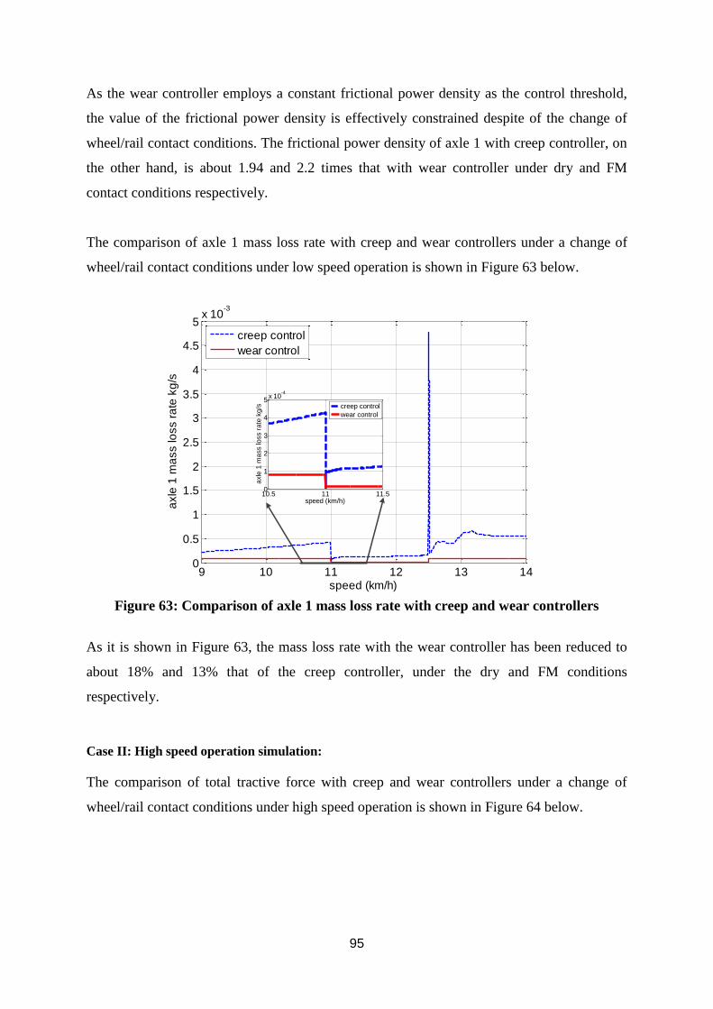
95

As the wear controller employs a constant frictional power density as the control threshold,

the value of the frictional power density is effectively constrained despite of the change of

wheel/rail contact conditions. The frictional power density of axle 1 with creep controller, on

the other hand, is about 1.94 and 2.2 times that with wear controller under dry and FM

contact conditions respectively.

The comparison of axle 1 mass loss rate with creep and wear controllers under a change of

wheel/rail contact conditions under low speed operation is shown in Figure 63 below.

9 10 11 12 13 140

0.5

1

1.5

2

2.5

3

3.5

4

4.5

5x 10

-3

speed (km/h)

axle

1 m

ass lo

ss r

ate

kg

/s

creep control

wear control

10.5 11 11.50

1

2

3

4

5x 10

-4

speed (km/h)

axle

1 m

ass lo

ss r

ate

kg

/s

creep control

wear control

Figure 63: Comparison of axle 1 mass loss rate with creep and wear controllers

As it is shown in Figure 63, the mass loss rate with the wear controller has been reduced to

about 18% and 13% that of the creep controller, under the dry and FM conditions

respectively.

Case II: High speed operation simulation:

The comparison of total tractive force with creep and wear controllers under a change of

wheel/rail contact conditions under high speed operation is shown in Figure 64 below.

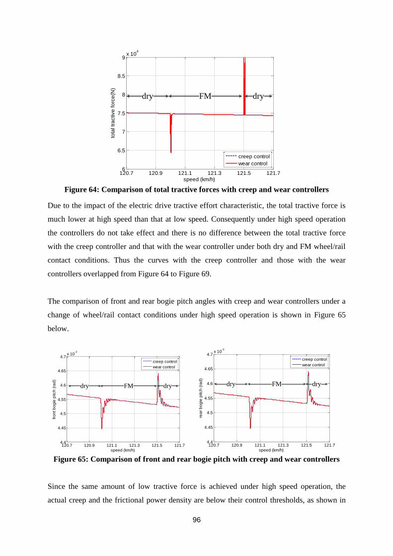
96

120.7 120.9 121.1 121.3 121.5 121.76

6.5

7

7.5

8

8.5

9x 10

4

speed (km/h)

tota

l tr

active

fo

rce

(N)

creep control

wear control

dry FM dry

Figure 64: Comparison of total tractive forces with creep and wear controllers

Due to the impact of the electric drive tractive effort characteristic, the total tractive force is

much lower at high speed than that at low speed. Consequently under high speed operation

the controllers do not take effect and there is no difference between the total tractive force

with the creep controller and that with the wear controller under both dry and FM wheel/rail

contact conditions. Thus the curves with the creep controller and those with the wear

controllers overlapped from Figure 64 to Figure 69.

The comparison of front and rear bogie pitch angles with creep and wear controllers under a

change of wheel/rail contact conditions under high speed operation is shown in Figure 65

below.

120.7 120.9 121.1 121.3 121.5 121.74.4

4.45

4.5

4.55

4.6

4.65

4.7x 10

-3

speed (km/h)

fro

nt b

og

ie p

itch

(ra

d)

creep control

wear control

dry FM dry

120.7 120.9 121.1 121.3 121.5 121.74.4

4.45

4.5

4.55

4.6

4.65

4.7x 10

-3

speed (km/h)

rea

r b

og

ie p

itch

(ra

d)

creep control

wear control

dry FM dry

Figure 65: Comparison of front and rear bogie pitch with creep and wear controllers

Since the same amount of low tractive force is achieved under high speed operation, the

actual creep and the frictional power density are below their control thresholds, as shown in

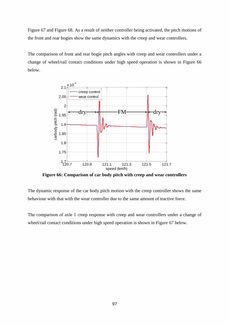
97

Figure 67 and Figure 68. As a result of neither controller being activated, the pitch motions of

the front and rear bogies show the same dynamics with the creep and wear controllers.

The comparison of front and rear bogie pitch angles with creep and wear controllers under a

change of wheel/rail contact conditions under high speed operation is shown in Figure 66

below.

120.7 120.9 121.1 121.3 121.5 121.71.7

1.75

1.8

1.85

1.9

1.95

2

2.05

2.1x 10

-4

speed (km/h)

ca

rbo

dy p

itch

(ra

d)

creep control

wear control

dry FM dry

Figure 66: Comparison of car body pitch with creep and wear controllers

The dynamic response of the car body pitch motion with the creep controller shows the same

behaviour with that with the wear controller due to the same amount of tractive force.

The comparison of axle 1 creep response with creep and wear controllers under a change of

wheel/rail contact conditions under high speed operation is shown in Figure 67 below.

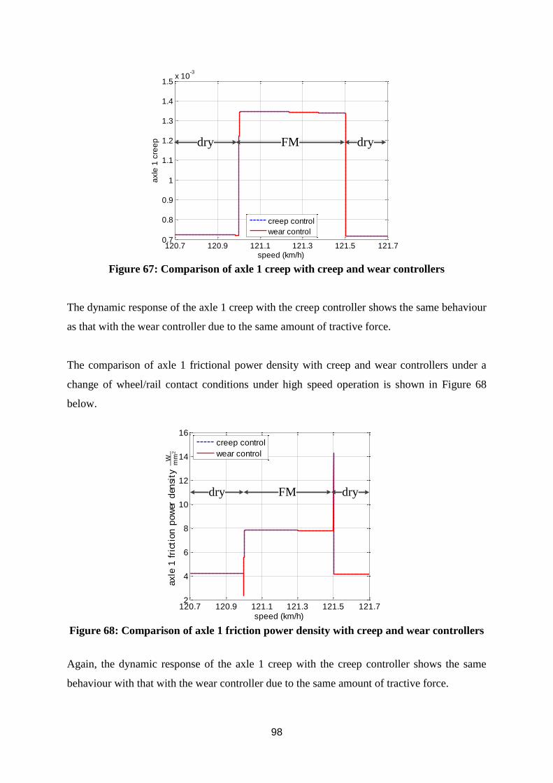
98

120.7 120.9 121.1 121.3 121.5 121.70.7

0.8

0.9

1

1.1

1.2

1.3

1.4

1.5x 10

-3

speed (km/h)

axle

1 c

ree

p

creep control

wear control

dry FM dry

Figure 67: Comparison of axle 1 creep with creep and wear controllers

The dynamic response of the axle 1 creep with the creep controller shows the same behaviour

as that with the wear controller due to the same amount of tractive force.

The comparison of axle 1 frictional power density with creep and wear controllers under a

change of wheel/rail contact conditions under high speed operation is shown in Figure 68

below.

120.7 120.9 121.1 121.3 121.5 121.72

4

6

8

10

12

14

16

speed (km/h)

axle

1fr

icti

on

pow

erd

ensi

tyW

mm

2

creep control

wear control

dry FM dry

Figure 68: Comparison of axle 1 friction power density with creep and wear controllers

Again, the dynamic response of the axle 1 creep with the creep controller shows the same

behaviour with that with the wear controller due to the same amount of tractive force.

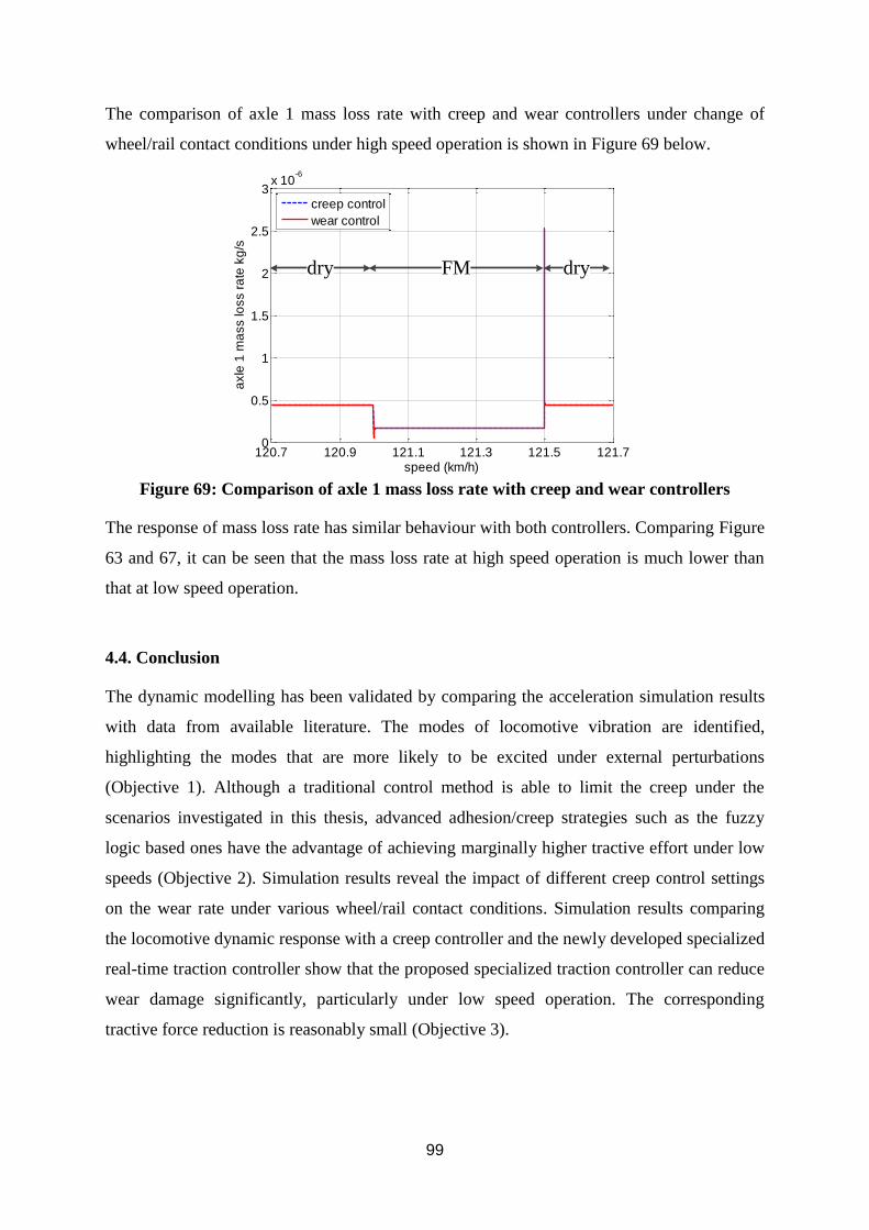
99

The comparison of axle 1 mass loss rate with creep and wear controllers under change of

wheel/rail contact conditions under high speed operation is shown in Figure 69 below.

120.7 120.9 121.1 121.3 121.5 121.70

0.5

1

1.5

2

2.5

3x 10

-6

speed (km/h)

axle

1 m

ass lo

ss r

ate

kg

/s

creep control

wear control

dry FM dry

Figure 69: Comparison of axle 1 mass loss rate with creep and wear controllers

The response of mass loss rate has similar behaviour with both controllers. Comparing Figure

63 and 67, it can be seen that the mass loss rate at high speed operation is much lower than

that at low speed operation.

4.4. Conclusion

The dynamic modelling has been validated by comparing the acceleration simulation results

with data from available literature. The modes of locomotive vibration are identified,

highlighting the modes that are more likely to be excited under external perturbations

(Objective 1). Although a traditional control method is able to limit the creep under the

scenarios investigated in this thesis, advanced adhesion/creep strategies such as the fuzzy

logic based ones have the advantage of achieving marginally higher tractive effort under low

speeds (Objective 2). Simulation results reveal the impact of different creep control settings

on the wear rate under various wheel/rail contact conditions. Simulation results comparing

the locomotive dynamic response with a creep controller and the newly developed specialized

real-time traction controller show that the proposed specialized traction controller can reduce

wear damage significantly, particularly under low speed operation. The corresponding

tractive force reduction is reasonably small (Objective 3).

100

Chapter V: Summary of Appended Papers

In Paper A, (Y. Tian, W.J.T. (Bill) Daniel, S. Liu and P.A. Meehan, 2013, “Dynamic

Tractional Behaviour Analysis and Control for a DC Locomotive”, World Congress of

Rail Research 2013), the development of the mathematical model of a co-co locomotive

including locomotive longitudinal, vertical and pitch dynamics, wheel/rail contact dynamics

and simplified electric drive dynamics in Matlab as part of RailCRC Project No.R3.119

Locomotive Adhesion is detailed. Details of the sub-modules are provided. Modes of

vibration of the locomotive are identified. Dynamic responses have been simulated under

change of wheel/rail contact conditions.

In Paper B, (Y. Tian, W.J.T. (Bill) Daniel, S. Liu and P.A. Meehan, 2014, “Fuzzy Logic

Creep Control for a 2D Locomotive Dynamic Model under Transient Wheel-rail

Contact Condition”, 14th International Conference on Railway Engineering Design and

Optimization, COMPRAIL 2014), a fuzzy logic creep/adhesion controller is developed and

simulated with the locomotive mathematical model that has been developed previously.

Dynamic responses have been compared with that with a traditional fixed creep threshold

controller, highlighting the advantage of the fuzzy logic controller over the traditional one in

terms of maintaining higher tractive force, particularly under wet wheel/rail contact

condition.

In Paper C, (Y. Tian, W.J.T. (Bill) Daniel, S. Liu and P.A. Meehan, 2014, “Fuzzy Logic

based Sliding Mode Creep Controller under Varying Wheel-Rail Contact Conditions”,

International Journal of Rail Transportation, 3(1), 40-59), a creep controller based on the

work of Park et al. [99] has been employed and modified to cope with the change of

wheel/rail contact conditions. Dynamic responses have been compared with that with a

traditional fixed threshold creep controller. Results show that the new controller has marginal

advantage keeping higher tractive force over the traditional one under low speed operation.

The responses are mostly identical under high speed operation. Simulation results also show

that the control strategy intending to maximize tractive force will cause much higher creep

under low speed operation, which is likely to cause more rail damage.

101

In Paper D, (Y. Tian, W.J.T. (Bill) Daniel, S. Liu and P.A. Meehan, “Investigation of the

impact of full scale locomotive adhesion control on wear under changing contact

conditions”, accepted by Vehicle System Dynamics special issue, DOI:

10.1080/00423114.2015.1020815), the impact of creep/adhesion controller on locomotive

dynamic responses have been simulated and analysed. Dynamic responses with several creep

threshold settings have been compared. Simulation results show that by properly choosing

creep control threshold it is likely to avoid the locomotive operating in a Type III

“Catastrophic” wear region under low speed operation, particularly under wet wheel/rail

contact condition. The impact of the creep controller setting is minimized from medium

speed operation due to the tractive effort characteristics of electric drives.

In Paper E, (Y. Tian, W.J.T. (Bill) Daniel, and P.A. Meehan, “Real-time rail/wheel wear

damage control”, submitted to International Journal of Rail Transportation), a new

real-time control strategy has been proposed to reduce wear damage. Simulation results show

that the proposed control strategy can effectively reduce mass loss rate caused by wear,

particularly under low speed operation. The consequent tractive force reduction is relatively

small.

In Paper F (co-authored), (Sheng Liu, Ye Tian, W.J.T. (Bill) Daniel and Paul A.

Meehan, Dynamic response of a locomotive with AC electric drives due to changes in

friction conditions, submitted to Journal of Rail and Rapid Transit), locomotive dynamic

response with detailed electric drive dynamics under change of contact conditions is

simulated and analysed. Result shows that the detailed model is capable of simulating the

dynamic fluctuations of creep and traction forces that is not presented in the simpler model.

Such transient response may cause damage to the track and vehicle components.

102

Chapter VI: Conclusions and Future work

This thesis contains a new predictive integrated dynamic model containing 2D locomotive

dynamics, wheel/rail contact dynamics and electric drive and control dynamics to investigate

the dynamic response of a locomotive under a change of operation conditions. Moreover,

eigenmode analysis has been performed to determine model stability and identify the modes

of locomotive vibration and those that are most likely to be excited under external

perturbations (Objective 1). Creep/adhesion controllers were developed to achieve the highest

tractive force available in order to cope with the trend of maximizing locomotive operation

efficiency, particularly in the heavy haul sector. Their influence on locomotive dynamic

response has also been investigated and compared with that of a fixed creep threshold creep

control strategy (Objective 2). Based on the results, a real-time strategy, aiming to reduce

wear damage on the tracks is developed based on a recent wear growth model (Objective 3).

Details of this work are summarised in the following.

In this thesis, an integrated mathematical model of the dynamics of a locomotive has been

developed. The model includes the longitudinal, vertical and pitch motions of the locomotive

body, front and rear bogies and six axles, as well as wheel/rail contact dynamics described by

the Polach model and electric drive dynamics. Modes of vibrations of the locomotive have

been identified with eigenmode analysis. The family of wheel vertical modes of vibration

have the least damping and thus are the easiest to be excited under external perturbation,

followed by the out of phase bogie longitudinal motion, the locomotive body pitch coupled

with in phase bogie longitudinal motions and the out of phase bogie vertical motions.

Research on a creep/adhesion controller has been carried out to investigate maximizing

locomotive tractive force under various operation conditions including operating speeds and

changes of wheel/rail contact conditions. Comparisons have been performed between the

controller that achieves higher tractive force and a traditional one with a constant creep

threshold. Simulation results show that under low speed operation the tractive forces with the

traditional and the new control strategy under the dry contact condition are similar, while the

new control strategy can reach higher tractive force than that with the traditional controller

under wet contact conditions. Under high speed operation, the tractive force with the

traditional controller and the new controller is similar under both dry and wet contact

conditions. However, the simulation results also show that, by achieving marginally higher

tractive force, the new control strategy causes higher creep under low speed operation. This

103

leads to the investigation as to how much more wear damage this new control strategy causes

compared to the traditional creep control strategy.

Simulations have been carried out to compare the impact of creep controller threshold

settings on tractive force and the amount of wear damage caused on rail tracks. Results show

that the intention of maximizing tractive force can lead to excessive wear damage on rail

tracks, providing only marginal tractive increase under low speed operation. Among the creep

thresholds (3%, 4%, 6% and 8%) that have been tested under low speed locomotive

operation, with the contact condition changing between dry and wet, only thresholds lower

than 4% can avoid the wear damage entering the type III “Catastrophic” region. Compared to

creep threshold settings 3% and 4%, the higher creep threshold setting does not have

significant advantage in achieving higher tractive force (about 3%), while is likely to cause

more wear damage (about 36%) on the rail tracks.

A new control strategy, aiming to reduce wear damage has been proposed based on a recent

wear growth model. Simulation results show that, by controlling the wheel speed, the mass

loss rate with the wear controller has been reduced to about 18% and 13% of the creep

controller performance, at the cost of about 4% and 11% total tractive force decrease under

the dry and FM conditions respectively. Under high speed operation, due to the constraint of

the electric drive characteristic, the highest tractive force is significantly lower than that of

low speed operation. The creep and friction power density are consequently lower so that

neither controller will be triggered. Thus the dynamic responses are very similar. From the

cost benefit point of view, the significant wear damage reduction is achieved by the proposed

specialized real-time wear regulating traction controller under the low speed operation. The

specialized traction controller is expected to reduce the wear damage on the rail tracks to

about 20% of that with a creep controller. A simple regrinding model suggests that the

optimum grind interval is inversely proportional to the wear/corrugation growth rate, which is

approximately proportional to the steady wear coefficient [66]. Thus the grinding intervals

with the wear controller under the dry and the FM conditions have been extended to 2.36 and

2.77 times of that with the creep controller. Consequently, the re-grinding cost is expected to

be reduced to 42.4% and 36% of that with the creep control under the dry and the FM

conditions respectively.

104

6.1. Thesis Contributions

The following are believed to be the novel contributions of this thesis to existing literature.

An integrated locomotive dynamic model including locomotive longitudinal-vertical-

pitch dynamics, wheel/rail contact dynamics and electric drive dynamics in Matlab

has been developed for locomotive dynamic response and wear damage prediction

under various operation conditions and control design.

Locomotive modes of vibration have been investigated by eigenmode analysis and

those most likely to be excited are identified. This provided insights into locomotive

dynamic behaviour under external perturbations as well as validation of the stability

of the system.

Creep/adhesion controllers have been developed to achieve higher tractive force under

change of operation conditions. The effectiveness has been compared with a

traditional fixed threshold creep controller.

Locomotive dynamic responses of the controllers achieving higher tractive forces and

of the traditional controller are compared, highlighting the amount of tractive force

benefit that can be achieved under various operating conditions.

The impact of creep control setting on the tractive force and wear index 𝑻𝜸/𝑨 has

been quantified.

The impact of operating condition such as operation velocity and change of contact

conditions on creep, tractive force and wear on rail tracks has been quantified.

A novel control strategy aiming to limit the wear damage on the rail tracks, based on a

recent wear growth model has been developed. Simulation comparison has been

carried out to validate its effectiveness in reducing wear damage, and to quantify the

amount of trade off in terms of tractive forces under various operating conditions.

6.2. Suggestions for Future Work

The work presented in this thesis shows possible avenues of further study, some of which

have already commenced. These are listed in the following.

Modelling:

This research reveals the dynamic impact of different control strategies based

on a simplified dynamic model. A more sophisticated model is preferable to

105

show more accurate dynamic responses with different control strategies under

curving behaviour and under the influence of vertical/lateral track

irregularities. This requires a 3D dynamic model which is beyond the scope of

this research. Moreover, a better wear model is valuable to be included to

provide more accurate wear damage quantification under different contact

conditions and operation speeds.

Experimental Validation:

The experimental validation with a full scale locomotive experimental

platform is necessary to verify the creep controller’s performance. Under the

acceleration operation on relatively straight tracks, the speeds of the

locomotive and the axles need to be measured to calculate the creepage.

Accelerations of the axles and the torque on the motor shaft need to be

measured to obtain the tangential force.

The measurement of the mass loss with the creep and the wear regulating

traction controllers is necessary to validate the wear regulating traction

controller’s effect. The corresponding mass loss rate measurement can be

carried out on the test rig in the lab environment. The upper and lower wheel

speeds and the torque on the motor shaft need to be measured for the purpose

of real-time control. The amount of contact surface deformation with the creep

and the wear regulating traction control need to be measured and compared

under the dry and the FM contact conditions.

106

References

[1] B. Solomon, American Diesel Locomotives: Voyageur Press.

[2] S. Hillmansen and C. Roberts, "Energy storage devices in hybrid railway vehicles: A

kinematic analysis," Proceedings of the Institution of Mechanical Engineers, Part F:

Journal of Rail and Rapid Transit, vol. 221, pp. 135-143, January 1, 2007 2007.

[3] (2013). Australian Trading Commission: Heavy haul, intermodal and freight rail.

Available: http://www.austrade.gov.au/ArticleDocuments/2814/Heavy-Haul-

Intermodal-and-Freight-Rail-2013-10.pdf.aspx

[4] N. Ramsey, et al., "Introducing the next generation locomotive to the Australian rail

network," presented at the Conference on Railway Engineering, Perth, 2008.

[5] S. Iwnicki, Handbook of railway vehicle dynamics: CRC press, 2006.

[6] D. T. Eadie, et al., "The effects of top of rail friction modifier on wear and rolling

contact fatigue: Full-scale rail–wheel test rig evaluation, analysis and modelling,"

Wear, vol. 265, pp. 1222-1230, 2008.

[7] J. Mathew, et al., Engineering Asset Management: Proceedings of the First World

Congress on Engineering Asset Management (WCEAM) 2006: Springer-Verlag, 2008.

[8] E. H. Law and N. K. Cooperrider, "A survey of railway vehicle dynamics research,"

ASME Journal of Dynamic Systems, Measurement, and Control, vol. 96, pp. 132-146,

June 1974 1974.

[9] R. U. A. Uzzal, et al., "Dynamic Analysis of Pitch Plane Railway Vehicle-Track

Interactions Due to Single and Multiple Wheel Flats," ASME Conference

Proceedings, vol. 2008, pp. 89-97, 2008.

[10] M. R. U. A. Uzzal, "ANALYSIS OF A THREE-DIMENSIONAL RAILWAY

VEHICLE-TRACK SYSTEM AND DEVELOPMENT OF A SMART

WHEELSET," PhD, Mechanical Engineering, Concordia University, 2012.

[11] X. Xin, et al., "Impact Analysis of an Innovative Shock Energy Absorber and Its

Applications in Improving Railroad Safety."

[12] J. Evans and S. D. Iwnicki, "Vehicle dynamics and the wheel/rail interface," in

Proceedings of the IMechE Seminar on Wheels on rails–an update, London, UK,

2002.

[13] M. Spiryagin, et al., "Development of traction control for hauling locomotives," ed.

[14] M. Spiryagin, et al., "Co-simulation of a mechatronic system using Gensys and

Simulink," Vehicle System Dynamics, vol. 50, pp. 495-507, 2012.

[15] M. Berg, "A Non-Linear Rubber Spring Model for Rail Vehicle Dynamics Analysis,"

Vehicle System Dynamics, vol. 30, pp. 197-212, 1998/09/01 1998.

[16] R. F. Harder, "Dynamic modeling and simulation of three-piece freight vehicle

suspensions with nonlinear frictional behaviour using Adams/Rail," in Railroad

Conference, 2001. Proceedings of the 2001 IEEE/ASME Joint, 2001, pp. 185-191.

[17] P. Wang, Design of High-Speed Railway Turnouts: Theory and Applications: Elsevier

Science, 2015.

[18] O. Polach, "A Fast Wheel-Rail Forces Calculation Computer Code," Vehicle System

Dynamics, vol. 33, pp. 728-739, 1999.

[19] R. Guclu and M. Metin, "Fuzzy Logic Control of Vibrations of a Light Rail Transport

Vehicle in Use in Istanbul Traffic," Journal of Vibration and Control, vol. 15, pp.

1423-1440, September 1, 2009 2009.

[20] D. S. Garivaltis, et al., "Dynamic Response of a Six-axle Locomotive to Random

Track Inputs," Vehicle System Dynamics, vol. 9, pp. 117-147, 1980/05/01 1980.

107

[21] H. Xia, et al., "Dynamic interaction analysis of a LIM train and elevated bridge

system," Journal of Mechanical Science and Technology, vol. 23, pp. 3257-3270,

2009/12/01 2009.

[22] F. W. Carter, On the Action of a Locomotive Driving Wheel vol. 112, 1926.

[23] K. Johnson, "The effect of spin upon the rolling motion of an elastic sphere on a

plane," Journal of Applied Mechanics, vol. 25, pp. 332-338, 1958.

[24] J. J. Kalker, "Survey of Wheel—Rail Rolling Contact Theory," Vehicle System

Dynamics, vol. 8, pp. 317-358, 1979/09/01 1979.

[25] J. Kalker, "On the Rolling Contact of Two Elastic Bodies in the Presence of Dry

Friction," Ph. D Doctoral Thesis, Delft, 1967.

[26] J. Kalker, "Simplified Theory of Rolling Contact," Delft, Progress Report1973.

[27] O. Polach, "Creep forces in simulations of traction vehicles running on adhesion

limit," Wear, vol. 258, pp. 992-1000, 2005.

[28] J. C. F. Logston and G. S. Itami, "Locomotive Friction-Creep Studies," Journal of

Engineering for Industry, vol. 102, pp. 275-281, 1980.

[29] M. Spiryagin, et al., "Modeling of Adhesion for Railway Vehicles," Journal of

Adhesion Science and Technology, vol. 22, pp. 1017-1034, 2008/01/01 2008.

[30] J. Piotrowski and W. Kik, "A simplified model of wheel/rail contact mechanics for

non-Hertzian problems and its application in rail vehicle dynamic simulations,"

Vehicle System Dynamics, vol. 46, pp. 27-48, 2008/02/01 2008.

[31] C. Linder, "Verschleiss von Eisenbahnrädern mit Unrundheiten," Ph.D., ETH, Zurich,

1997.

[32] J. B. Ayasse and H. Chollet, "Determination of the wheel rail contact patch in semi-

Hertzian conditions," Vehicle System Dynamics, vol. 43, pp. 161-172, 2005/03/01

2005.

[33] N. Burgelman, et al., "Influence of wheel–rail contact modelling on vehicle dynamic

simulation," Vehicle System Dynamics, vol. 53, pp. 1190-1203, 2015/08/03 2015.

[34] O. Polach, "Influence of Locomotive Tractive Effort on the Forces Between Wheel

and Rail," Vehicle System Dynamics, vol. 35, pp. 7-22, 2001.

[35] M. Spiryagin, et al., "Creep force modelling for rail traction vehicles based on the

Fastsim algorithm," Vehicle System Dynamics, vol. 51, pp. 1765-1783, 2013/11/01

2013.

[36] V. R. Moorthi, Power electronics: devices, circuits and industrial applications:

Oxford University Press, 2005.

[37] "Frequency controlled AC motor drive," Rockwell-Automation.

[38] I. Boldea and S. A. Nasar, The Induction Machine Handbook: CRC Press, 2002.

[39] R. Marino, et al., Induction Motor Control Design: Springer, 2010.

[40] D. J. Atkinson, et al., "Observers for induction motor state and parameter estimation,"

Industry Applications, IEEE Transactions on, vol. 27, pp. 1119-1127, 1991.

[41] S. Kadowaki, et al., "Antislip Readhesion Control Based on Speed-Sensorless Vector

Control and Disturbance Observer for Electric Commuter Train&#x2014;Series 205-

5000 of the East Japan Railway Company," Industrial Electronics, IEEE Transactions

on, vol. 54, pp. 2001-2008, 2007.

[42] A. Sabanovic and D. B. Izosimov, "Application of Sliding Modes to Induction Motor

Control," Industry Applications, IEEE Transactions on, vol. IA-17, pp. 41-49, 1981.

[43] K. L. Butler, et al., "A Matlab-based modeling and simulation package for electric

and hybrid electric vehicle design," Vehicular Technology, IEEE Transactions on,

vol. 48, pp. 1770-1778, 1999.

108

[44] L.-H. Hoang, "Modeling and simulation of electrical drives using MATLAB/Simulink

and Power System Blockset," in Industrial Electronics Society, 2001. IECON '01. The

27th Annual Conference of the IEEE, 2001, pp. 1603-1611 vol.3.

[45] K. L. Shi, et al., "Modelling of the three-phase induction motor using SIMULINK," in

Electric Machines and Drives Conference Record, 1997. IEEE International, 1997,

pp. WB3/6.1-WB3/6.3.

[46] V. Rafalko, et al., "Dynamic Model Based Vector Control of Linear Induction

Motor," DTIC Document2012.

[47] H. Abu-Rub, et al., High performance control of AC drives with Matlab/Simulink

models: Wiley, 2012.

[48] TI, "Field Oriented Control of 3-Phase AC-Motors," Texas Instruments

EuropeFebruary 1998.

[49] M. Janecke, et al., "Direct self-control, a novel method of controlling asynchronous

machines in traction applications," in Proc. of 3rd EPE'89 Conf, 1989, pp. 75-81.

[50] Y. Kumsuwan, et al., "Modified direct torque control method for induction motor

drives based on amplitude and angle control of stator flux," Electric Power Systems

Research, vol. 78, pp. 1712-1718, 2008.

[51] P. Wach, Dynamics and Control of Electrical Drives: Springer, 2011.

[52] "Technical guide No.1 Direct torque control-the world's most advanced AC drive

technology," ABB.

[53] P. Doh-Young, et al., "Hybrid re-adhesion control method for traction system of high-

speed railway," in Electrical Machines and Systems, 2001. ICEMS 2001. Proceedings

of the Fifth International Conference on, 2001, pp. 739-742 vol.2.

[54] K. Ohishi, et al., "Anti-slip control of electric motor coach based on disturbance

observer," in Advanced Motion Control, 1998. AMC '98-Coimbra., 1998 5th

International Workshop on, 1998, pp. 580-585.

[55] I. Yasuoka, et al., "Improvement of re-adhesion for commuter trains with vector

control traction inverter," in Power Conversion Conference - Nagaoka 1997.,

Proceedings of the, 1997, pp. 51-56 vol.1.

[56] P. Howlett, "The Optimal Control of a Train," Annals of Operations Research, vol.

98, pp. 65-87, 2000.

[57] E. Khmelnitsky, "On an optimal control problem of train operation," Automatic

Control, IEEE Transactions on, vol. 45, pp. 1257-1266, 2000.

[58] M. Djukić, et al., "A fuzzy model for an increase in locomotive traction force,"

Transport, vol. 25, pp. 36-45, 2010/01/01 2010.

[59] R. Palm and K. Storjohann, "Torque optimization for a locomotive using fuzzy logic,"

presented at the Proceedings of the 1994 ACM symposium on Applied computing,

Phoenix, Arizona, United States, 1994.

[60] L. A. Zadeh, "Fuzzy sets," Information and Control, vol. 8, pp. 338-353, 1965.

[61] P. Khatun, et al., "Application of fuzzy control algorithms for electric vehicle antilock

braking/traction control systems," Vehicular Technology, IEEE Transactions on, vol.

52, pp. 1356-1364, 2003.

[62] M. Garcia-Rivera, et al., "An antislipping fuzzy logic controller for a railway traction

system," in Fuzzy Systems, 1997., Proceedings of the Sixth IEEE International

Conference on, 1997, pp. 119-124 vol.1.

[63] R. Sivakumar, et al., "Application of Fuzzy Model Predictive Control in Multivariable

Control of Distillation Column," International Journal of Chemical Engineering and

Applications, vol. 1, pp. 39-42, 2010.

109

[64] T. X. Mei, et al., "A mechatronic approach for effective wheel slip control in railway

traction," Proceedings of the Institution of Mechanical Engineers, Part F: Journal of

Rail and Rapid Transit, vol. 223, pp. 295-304, May 1, 2009 2009.

[65] Q. Song, et al., "Adaptive backstepping control of train systems with traction/braking

dynamics and uncertain resistive forces," Vehicle System Dynamics, vol. 49, pp. 1441-

1454, 2011/09/01 2011.

[66] T. Vuong, "Investigation for the wear coefficient of the frictional-work wear model

and feasibility of friction modifiers for wear-type corrugation control," 2011.

[67] F. Braghin, et al., "A mathematical model to predict railway wheel profile evolution

due to wear," Wear, vol. 261, pp. 1253-1264, 2006.

[68] R. G. Bayer, Wear Analysis for Engineers: HNB Publishing, 2002.

[69] T. Jendel, "Prediction of wheel profile wear—comparisons with field measurements,"

Wear, vol. 253, pp. 89-99, 2002.

[70] T. G. Pearce and N. D. Sherratt, "Prediction of wheel profile wear," Wear, vol. 144,

pp. 343-351, 1991.

[71] R. Lewis and U. Olofsson, "Mapping rail wear regimes and transitions," Wear, vol.

257, pp. 721-729, 2004.

[72] T. M. Beagley, "Severe wear of rolling/sliding contacts," Wear, vol. 36, pp. 317-335,

1976.

[73] P. J. Bolton and P. Clayton, "Rolling—sliding wear damage in rail and tyre steels,"

Wear, vol. 93, pp. 145-165, 1984.

[74] D. Markov and D. Kelly, "Mechanisms of adhesion-initiated catastrophic wear: pure

sliding," Wear, vol. 239, pp. 189-210, 2000.

[75] D. Danks and P. Clayton, "Comparison of the wear process for eutectoid rail steels:

Field and laboratory tests," Wear, vol. 120, pp. 233-250, 1987.

[76] S. Zakharov, et al., "Wheel flange/rail head wear simulation," Wear, vol. 215, pp. 18-

24, 1998.

[77] P. Clayton, "Predicting the wear of rails on curves from laboratory data," Wear, vol.

181–183, Part 1, pp. 11-19, 1995.

[78] M. Ignesti, et al., "Development of a wear model for the prediction of wheel and rail

profile evolution in railway systems," Wear, vol. 284–285, pp. 1-17, 2012.

[79] R. Lewis, et al., "Mapping railway wheel material wear mechanisms and transitions,"

Proceedings of the Institution of Mechanical Engineers, Part F: Journal of Rail and

Rapid Transit, vol. 224, pp. 125-137, 2010.

[80] J. Pombo, et al., "A study on wear evaluation of railway wheels based

on multibody dynamics and wear computation," Multibody System Dynamics, vol. 24,

pp. 347-366, 2010/10/01 2010.

[81] J. Pombo, et al., "Development of a wear prediction tool for steel railway wheels

using three alternative wear functions," Wear, vol. 271, pp. 238-245, 2011.

[82] R. Lewisa and R. S. Dwyer-Joyce, "Wear mechanisms and transitions in railway

wheel steels," Proceedings of the Institution of Mechanical Engineers, Part J: Journal

of Engineering Tribology, vol. 218, pp. 467-478, June 1, 2004 2004.

[83] T. T. Vuong and P. A. Meehan, "Wear transitions in a wear coefficient model," Wear,

vol. 266, pp. 898-906, 2009.

[84] M. D. Ardema, Newton-Euler Dynamics: Springer, 2006.

[85] I. J. Guy, "An analysis of the interaction between the front and rear axles of a four-

wheel-drive tractor, and its contribution to power delivery efficiency," Harper Adams

University College, 2011.

[86] Pegasem. Pegasem GSS series ground speed sensors [Online]. Available:

http://www.pegasem.com/english/datasheets_uk/gss_uk.pdf

110

[87] K. Abood and R. Khan, "Hunting phenomenon study of railway conventional truck on

tangent tracks due to change in rail wheel geometry," Journal of Engineering Science

and Technology, vol. 6, pp. 146-160, 2011.

[88] A. Bhaskar, "Mode Shapes during Asynchronous Motion and Non-Proportionality

Indices," Journal of Sound and Vibration, vol. 224, pp. 1-16, 1999.

[89] G. Lallement and D. J. Inman, "A tutorial on complex eigenvalues," in

PROCEEDINGS-SPIE THE INTERNATIONAL SOCIETY FOR OPTICAL

ENGINEERING, 1995, pp. 490-490.

[90] K. L. Johnson, Contact Mechanics: Cambridge University Press, 1985.

[91] Rail Track Materisal Catalogue A5. Available:

https://www.scribd.com/doc/92072909/Rail-Track-Material-Catalogue-A5#download

[92] I. Takahashi and T. Noguchi, "A new quick-response and high-efficiency control

strategy of an induction motor," Industry Applications, IEEE Transactions on, pp.

820-827, 1986.

[93] F. Khorrami, et al., Modeling and adaptive nonlinear control of electric motors:

Springer Science & Business Media, 2003.

[94] J. L. Daigle and J. McGarry, "System and method for traction motor control," ed:

Google Patents, 2013.

[95] UGL Powerhaul Series Locomotive. Available:

http://cdn.ugllimited.com/Asset/cms/Freight_Product_brochures/084_Powerhaul_Pro

ductSheet_V4_WEB.pdf

[96] M. Spiryagin, et al., "Control system for maximum use of adhesive forces of a

railway vehicle in a tractive mode," Mechanical Systems and Signal Processing, vol.

22, pp. 709-720, 2008.

[97] Y. Yuan, et al., "The dynamic study of locomotives under saturated adhesion,"

Vehicle System Dynamics, vol. 49, pp. 1321-1338, 2011/08/01 2011.

[98] M. Bauer and M. Tomizuka, "Fuzzy Logic Traction Controllers and their Effect on

Longitudinal Vehicle Platoon Systems," Vehicle System Dynamics, vol. 25, pp. 277-

303, 1996/04/01 1996.

[99] S. Park, et al., "Reference slip ratio generation and adaptive sliding mode control for

railway rolling stocks," International Journal of Precision Engineering and

Manufacturing, vol. 10, pp. 39-44, 2009/04/01 2009.

[100] T. J. Ross, Fuzzy Logic with Engineering Applications: Wiley, 2004.

[101] A. K. Kumar, "Method and system of limiting the application of sand to a railroad

rail," U.S. Patent US7290807, 2007.

[102] Y. Zhu, "Adhesion in the wheel–rail contact under contaminated conditions,"

Doctoral Thesis, KTH, 2011.

[103] C. Tomberger, et al., "Friction in wheel–rail contact: A model comprising interfacial

fluids, surface roughness and temperature," Wear, vol. 271, pp. 2-12, 2011.

[104] M. Ertz and F. Bucher, "Improved creep force model for wheel/rail contact

considering roughness and temperature," Vehicle System Dynamics, vol. 37, pp. 314-

325, 2003.

[105] SIEMENS. Three-Phase AC Traction Technology for Diesel-Electric Locomotive

WDG4 of India Railways [Online]. Available:

http://www.docstoc.com/docs/46726734/Three-Phase-ACTraction-Technology-for-

Diesel-Electric-Locomotive-WDG4

[106] A. INDIA, "AUTOCAR Rail Test," IndiaSeptember 2009.

[107] GM, "GT46MAC INDIAN STATE RAILWAYS LOCOMOTIVE SERVICE

MANUAL," ed, 1999.

[108] GM, "GT46C 3000 KW LOCOMOTIVE."

111

[109] D. Berthe, et al., Tribological Design of Machine Elements: Elsevier Science, 1989.

[110] G. M. Corporation, "GT46C 3000KW LOCOMOTIVE," 2008.

112

Appended Papers

113

Paper A

DYNAMIC TRACTIONAL BEHAVIOUR

ANALYSIS AND CONTROL FOR A DC

LOCOMOTIVE

114

DYNAMIC TRACTIONAL BEHAVIOUR ANALYSIS AND CONTROL FOR A DC

LOCOMOTIVE

Ye Tian1, 2

, W.J.T. (Bill) Daniel1, 2

, Sheng Liu1, Paul A. Meehan

1, 2

1School of Mechanical and Mining Engineering, the University of Queensland, Queensland, Australia 4072 2Cooperative Research Centre for Railway Engineering and Technology (CRC Rail), Queensland, Australia

Abstract: In recent decades, advanced power-electronics-based control techniques have been widely used to

upgrade direct current (DC) drives for the traction of locomotives. However the dynamic response of such

upgraded DC locomotives under transient conditions due to external perturbations has not been fully

investigated. In this work, an integrated dynamic model for a typical DC Co-Co locomotive/track system is

developed to provide predictive simulations of the motion and forces transmitted throughout the DC locomotive

dynamic system. The model integrates a 2D longitudinal-vertical locomotive structural vibration model,

wheel/rail contact mechanics using Polach’s creep force model, a generic DC dynamic traction model and a

traditional creep controller to simulate the transient response to a change in friction conditions. It is found that

although the largest creep is constrained below 10% there are large transient creep and traction fluctuations

related to identified modes of vibration of the locomotive.

1. Introduction

The progressive adoption of high traction motors and control techniques based on power electronics has brought

great benefits to rail industry due to its high power capacity and efficiency. Despite all the advantages, concerns

arise as to the effects of operating at maximum adhesion and the possible impact of dynamic oscillations and

resultant traction to the rail tracks. An electric locomotive is a complex system containing several nonlinear

dynamic components coupled together when the locomotive operates. Its traction control performance and

dynamic impact on the rail tracks are typically assessed under specific steady state conditions. However, the

natural perturbations in friction/lubrication, wheel/rail profiles, track curvature, vehicle/track dynamics,

wheel/track imperfections etc. are not comprehensively investigated yet. Among those perturbations, the

transient changes in friction or lubrication can cause sudden changes of creep and often leads to over/under

traction/braking. In order to investigate this issue, a predictive locomotive dynamic model combining crucial

dynamic components such as locomotive rigid body dynamics, contact dynamics and electric drive and control

is needed.

Locomotive traction simulations have been investigated by several researchers. A simulation package for

simulation of rail vehicle dynamics has been developed in Matlab environment by Chudzikiewicz [1] for Poland

railway specifications. Traction simulation considering bogie vibration has been provided by Shimizu et al. and

a disturbance observer based anti-slip controller is also proposed [2]. Spiryagin et al. employed co-simulation

approach with the Gensys multibody code and Simulink to investigate the heavy haul train traction dynamics

[3]. Fleischer proposed a modal state controller to reduce drive train oscillation during the traction simulation

[4]. Bakhvalov et al. combined electrical and mechanical processes for locomotive traction simulation [5].

Senini et al. has also performed some locomotive traction and simulation on electric drive level [6]. These works

however, haven’t focused investigation on the effect of transient contact conditions on the locomotive dynamic

response. In this work, we focus on longitudinal and vertical dynamics on tangent tracks as it is the most

important part of locomotive dynamics closely related with traction/braking effort, passenger comfort and

energy management [7]. Newton-Euler method [8, 9] is used to obtain the motion equations of the locomotive

model. For the contact mechanics, Polach’s adhesion model [10] is adopted as it has been verified to be

effective for both small and large values of longitudinal wheel-rail creep as well as the decreasing part of creep-

force function exceeding the adhesion limit [11]. Modern development of mechatronics systems has improved

rail vehicle operation under various conditions. The traction control system, also known as an adhesion or anti-

slip control system is essential for the operational efficiency and reliability in these systems. A pattern-based

slip control method has been applied and modified by Park et al. [12]. Anti-slip control based on a disturbance

observer was proposed by Ohishi et al. [13]. Yasuoka et al. proposed a slip control method [14] involving bogie

oscillation suppression. All these methods claim the effectiveness of their proposed creep/traction controller;

however, these conclusions were not validated on a comprehensive locomotive dynamic model.

In this paper, a full scale locomotive dynamic model with a basic creep controller combining all crucial dynamic

components is developed and implemented using Matlab/Simulink to investigate creep and dynamic oscillation

control. In addition, a traction control system is proposed and embedded into the dynamic model to prevent

inefficient traction caused by perturbations. Eigenmode and frequency analysis is also performed to identify

important structural behaviour.

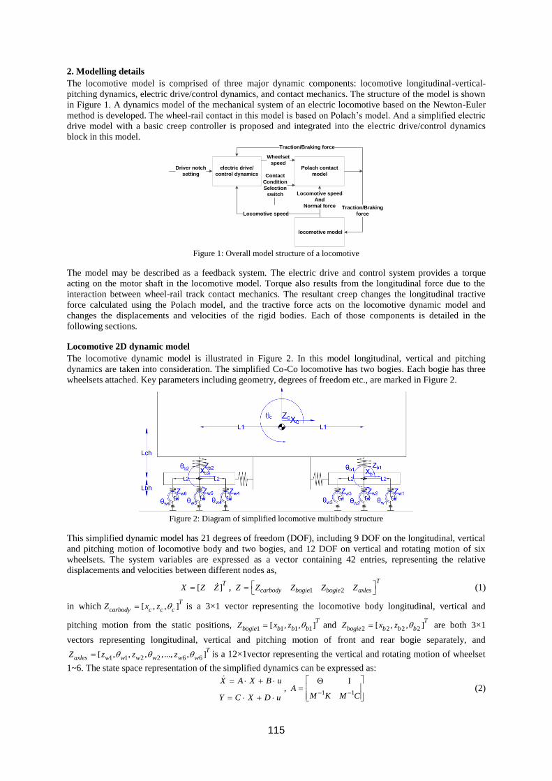
115

2. Modelling details

The locomotive model is comprised of three major dynamic components: locomotive longitudinal-vertical-

pitching dynamics, electric drive/control dynamics, and contact mechanics. The structure of the model is shown

in Figure 1. A dynamics model of the mechanical system of an electric locomotive based on the Newton-Euler

method is developed. The wheel-rail contact in this model is based on Polach’s model. And a simplified electric

drive model with a basic creep controller is proposed and integrated into the electric drive/control dynamics

block in this model.

electric drive/

control dynamics

Driver notch

setting

locomotive model

Polach contact

model

Wheelset

speed

Locomotive speed

And

Normal force Traction/Braking

forceLocomotive speed

Traction/Braking force

Contact

Condition

Selection

switch

Figure 1: Overall model structure of a locomotive

The model may be described as a feedback system. The electric drive and control system provides a torque

acting on the motor shaft in the locomotive model. Torque also results from the longitudinal force due to the

interaction between wheel-rail track contact mechanics. The resultant creep changes the longitudinal tractive

force calculated using the Polach model, and the tractive force acts on the locomotive dynamic model and

changes the displacements and velocities of the rigid bodies. Each of those components is detailed in the

following sections.

Locomotive 2D dynamic model

The locomotive dynamic model is illustrated in Figure 2. In this model longitudinal, vertical and pitching

dynamics are taken into consideration. The simplified Co-Co locomotive has two bogies. Each bogie has three

wheelsets attached. Key parameters including geometry, degrees of freedom etc., are marked in Figure 2.

Figure 2: Diagram of simplified locomotive multibody structure

This simplified dynamic model has 21 degrees of freedom (DOF), including 9 DOF on the longitudinal, vertical

and pitching motion of locomotive body and two bogies, and 12 DOF on vertical and rotating motion of six

wheelsets. The system variables are expressed as a vector containing 42 entries, representing the relative

displacements and velocities between different nodes as,

[ ]T

X Z Z , 1 2

T

carbody bogie bogie axlesZ Z Z Z Z (1)

in which [ , , ]T

carbody c c cZ x z is a 3×1 vector representing the locomotive body longitudinal, vertical and

pitching motion from the static positions, 1 1 1 1[ , , ]T

bogie b b bZ x z and 2 2 2 2[ , , ]T

bogie b b bZ x z are both 3×1

vectors representing longitudinal, vertical and pitching motion of front and rear bogie separately, and

1 1 2 2 6 6[ , , , , ..., , ]T

axles w w w w w wZ z z z is a 12×1vector representing the vertical and rotating motion of wheelset

1~6. The state space representation of the simplified dynamics can be expressed as:

X A X B u

Y C X D u

,

1 1A

M K M C

(2)

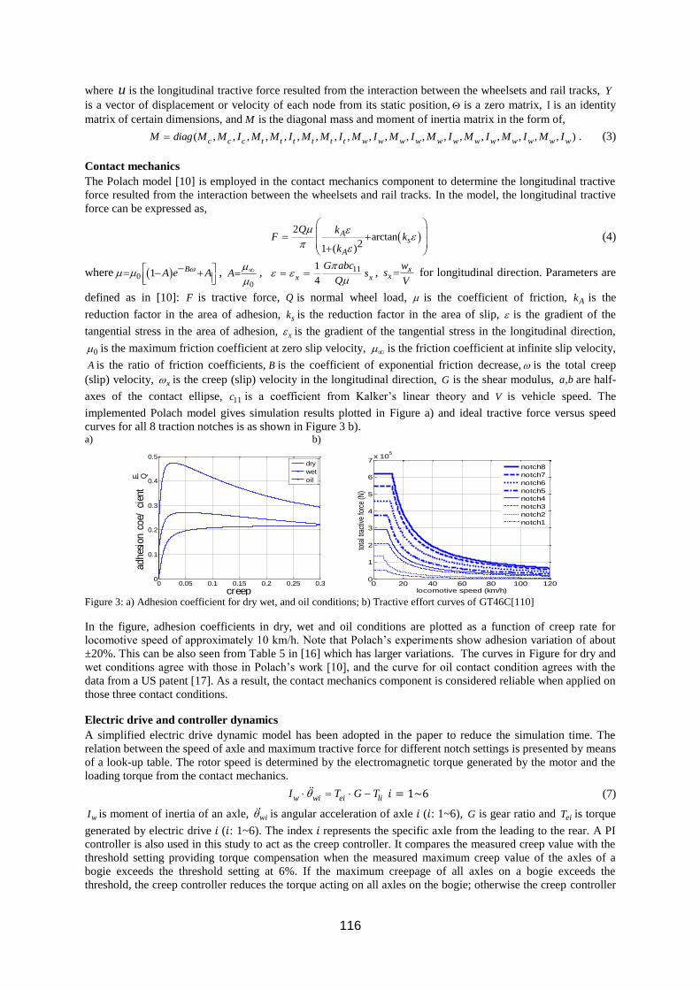
116

where u is the longitudinal tractive force resulted from the interaction between the wheelsets and rail tracks, Y

is a vector of displacement or velocity of each node from its static position, is a zero matrix, is an identity

matrix of certain dimensions, and M is the diagonal mass and moment of inertia matrix in the form of,

( , , , , , , , , , , , , , , , , , , , , )c c c t t t t t t w w w w w w w w w w w wM diag M M I M M I M M I M I M I M I M I M I M I . (3)

Contact mechanics

The Polach model [10] is employed in the contact mechanics component to determine the longitudinal tractive

force resulted from the interaction between the wheelsets and rail tracks. In the model, the longitudinal tractive

force can be expressed as,

2

arctan21 ( )

As

A

Q kF k

k

(4)

where 0 1 BA e A

, 0

A

, 111

4x x

G abcs

Q

, x

x

ws

V for longitudinal direction. Parameters are

defined as in [10]: F is tractive force, Q is normal wheel load, is the coefficient of friction, Ak is the

reduction factor in the area of adhesion, sk is the reduction factor in the area of slip, is the gradient of the

tangential stress in the area of adhesion, x is the gradient of the tangential stress in the longitudinal direction,

0 is the maximum friction coefficient at zero slip velocity, is the friction coefficient at infinite slip velocity,

A is the ratio of friction coefficients, B is the coefficient of exponential friction decrease, is the total creep

(slip) velocity, x is the creep (slip) velocity in the longitudinal direction, G is the shear modulus, ,a b are half-

axes of the contact ellipse, 11c is a coefficient from Kalker’s linear theory and V is vehicle speed. The

implemented Polach model gives simulation results plotted in Figure a) and ideal tractive force versus speed

curves for all 8 traction notches is as shown in Figure 3 b). a) b)

Figure 3: a) Adhesion coefficient for dry wet, and oil conditions; b) Tractive effort curves of GT46C[110]

In the figure, adhesion coefficients in dry, wet and oil conditions are plotted as a function of creep rate for

locomotive speed of approximately 10 km/h. Note that Polach’s experiments show adhesion variation of about

±20%. This can be also seen from Table 5 in [16] which has larger variations. The curves in Figure for dry and

wet conditions agree with those in Polach’s work [10], and the curve for oil contact condition agrees with the

data from a US patent [17]. As a result, the contact mechanics component is considered reliable when applied on

those three contact conditions.

Electric drive and controller dynamics

A simplified electric drive dynamic model has been adopted in the paper to reduce the simulation time. The

relation between the speed of axle and maximum tractive force for different notch settings is presented by means

of a look-up table. The rotor speed is determined by the electromagnetic torque generated by the motor and the

loading torque from the contact mechanics.

w wi ei liI T G T 𝑖 = 1~6 (7)

wI is moment of inertia of an axle, wi is angular acceleration of axle 𝑖 (𝑖: 1~6), G is gear ratio and eiT is torque

generated by electric drive 𝑖 (𝑖: 1~6). The index 𝑖 represents the specific axle from the leading to the rear. A PI

controller is also used in this study to act as the creep controller. It compares the measured creep value with the

threshold setting providing torque compensation when the measured maximum creep value of the axles of a

bogie exceeds the threshold setting at 6%. If the maximum creepage of all axles on a bogie exceeds the

threshold, the creep controller reduces the torque acting on all axles on the bogie; otherwise the creep controller

0 0.05 0.1 0.15 0.2 0.25 0.30

0.1

0.2

0.3

0.4

0.5

creep

adhes

ion

coe /

cien

tF Q

dry

wet

oil

0 20 40 60 80 100 1200

1

2

3

4

5

6

7x 10

5

locomotive speed (km/h)

tota

l tra

ctiv

e fo

rce

(N)

notch8

notch7

notch6

notch5

notch4

notch3

notch2

notch1

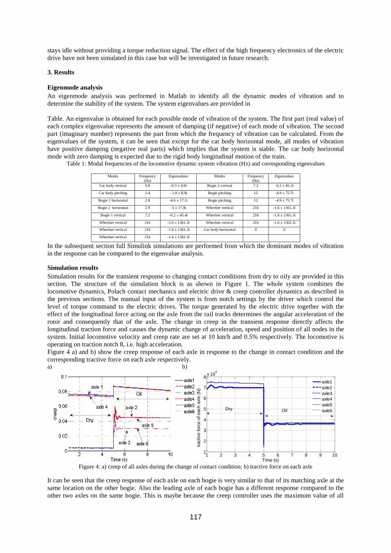
117

stays idle without providing a torque reduction signal. The effect of the high frequency electronics of the electric

drive have not been simulated in this case but will be investigated in future research.

3. Results

Eigenmode analysis

An eigenmode analysis was performed in Matlab to identify all the dynamic modes of vibration and to

determine the stability of the system. The system eigenvalues are provided in

Table. An eigenvalue is obtained for each possible mode of vibration of the system. The first part (real value) of

each complex eigenvalue represents the amount of damping (if negative) of each mode of vibration. The second

part (imaginary number) represents the part from which the frequency of vibration can be calculated. From the

eigenvalues of the system, it can be seen that except for the car body horizontal mode, all modes of vibration

have positive damping (negative real parts) which implies that the system is stable. The car body horizontal

mode with zero damping is expected due to the rigid body longitudinal motion of the train. Table 1: Modal frequencies of the locomotive dynamic system vibration (Hz) and corresponding eigenvalues

Modes Frequency

(Hz)

Eigenvalues Modes Frequency

(Hz)

Eigenvalues

Car body vertical 0.8 -0.3 ± 4.9i Bogie 2 vertical 7.2 -6.5 ± 45.3i

Car body pitching 1.4 - 1.0 ± 8.9i Bogie pitching 12 -4.9 ± 75.7i

Bogie 1 horizontal 2.8 -4.6 ± 17.1i Bogie pitching 12 -4.9 ± 75.7i

Bogie 2 horizontal 2.9 -5 ± 17.8i Wheelset vertical 216 -1.6 ± 1361.3i

Bogie 1 vertical 7.2 -6.2 ± 45.4i Wheelset vertical 216 -1.6 ± 1361.3i

Wheelset vertical 216 -1.6 ± 1361.3i Wheelset vertical 216 -1.6 ± 1361.3i

Wheelset vertical 216 -1.6 ± 1361.3i Car body horizontal 0 0

Wheelset vertical 216 -1.6 ± 1361.3i

In the subsequent section full Simulink simulations are performed from which the dominant modes of vibration

in the response can be compared to the eigenvalue analysis.

Simulation results

Simulation results for the transient response to changing contact conditions from dry to oily are provided in this

section. The structure of the simulation block is as shown in Figure 1. The whole system combines the

locomotive dynamics, Polach contact mechanics and electric drive & creep controller dynamics as described in

the previous sections. The manual input of the system is from notch settings by the driver which control the

level of torque command to the electric drives. The torque generated by the electric drive together with the

effect of the longitudinal force acting on the axle from the rail tracks determines the angular acceleration of the

rotor and consequently that of the axle. The change in creep in the transient response directly affects the

longitudinal traction force and causes the dynamic change of acceleration, speed and position of all nodes in the

system. Initial locomotive velocity and creep rate are set at 10 km/h and 0.5% respectively. The locomotive is

operating on traction notch 8, i.e. high acceleration.

Figure 4 a) and b) show the creep response of each axle in response to the change in contact condition and the

corresponding tractive force on each axle respectively. a) b)

Figure 4: a) creep of all axles during the change of contact condition; b) tractive force on each axle

It can be seen that the creep response of each axle on each bogie is very similar to that of its matching axle at the

same location on the other bogie. Also the leading axle of each bogie has a different response compared to the

other two axles on the same bogie. This is maybe because the creep controller uses the maximum value of all

1 2 3 4 5 6 7 8 9 101

2

3

4

5

6

7

8x 10

4

Time (s)

tractive forc

e o

f each a

xle

(N

)

axle1

axle2

axle3

axle4

axle5

axle6Dry Oil

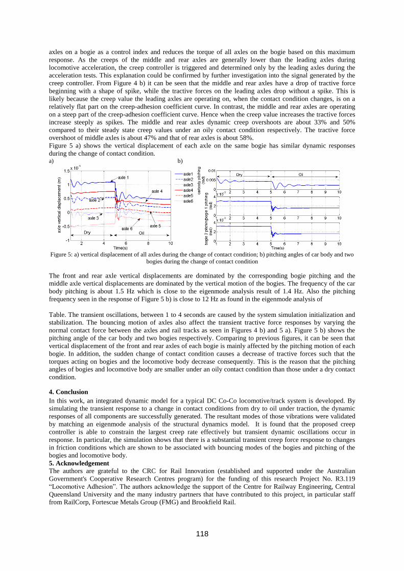
118

axles on a bogie as a control index and reduces the torque of all axles on the bogie based on this maximum

response. As the creeps of the middle and rear axles are generally lower than the leading axles during

locomotive acceleration, the creep controller is triggered and determined only by the leading axles during the

acceleration tests. This explanation could be confirmed by further investigation into the signal generated by the

creep controller. From Figure 4 b) it can be seen that the middle and rear axles have a drop of tractive force

beginning with a shape of spike, while the tractive forces on the leading axles drop without a spike. This is

likely because the creep value the leading axles are operating on, when the contact condition changes, is on a

relatively flat part on the creep-adhesion coefficient curve. In contrast, the middle and rear axles are operating

on a steep part of the creep-adhesion coefficient curve. Hence when the creep value increases the tractive forces

increase steeply as spikes. The middle and rear axles dynamic creep overshoots are about 33% and 50%

compared to their steady state creep values under an oily contact condition respectively. The tractive force

overshoot of middle axles is about 47% and that of rear axles is about 58%.

Figure 5 a) shows the vertical displacement of each axle on the same bogie has similar dynamic responses

during the change of contact condition. a) b)

Figure 5: a) vertical displacement of all axles during the change of contact condition; b) pitching angles of car body and two

bogies during the change of contact condition

The front and rear axle vertical displacements are dominated by the corresponding bogie pitching and the

middle axle vertical displacements are dominated by the vertical motion of the bogies. The frequency of the car

body pitching is about 1.5 Hz which is close to the eigenmode analysis result of 1.4 Hz. Also the pitching

frequency seen in the response of Figure 5 b) is close to 12 Hz as found in the eigenmode analysis of

Table. The transient oscillations, between 1 to 4 seconds are caused by the system simulation initialization and

stabilization. The bouncing motion of axles also affect the transient tractive force responses by varying the

normal contact force between the axles and rail tracks as seen in Figures 4 b) and 5 a). Figure 5 b) shows the

pitching angle of the car body and two bogies respectively. Comparing to previous figures, it can be seen that

vertical displacement of the front and rear axles of each bogie is mainly affected by the pitching motion of each

bogie. In addition, the sudden change of contact condition causes a decrease of tractive forces such that the

torques acting on bogies and the locomotive body decrease consequently. This is the reason that the pitching

angles of bogies and locomotive body are smaller under an oily contact condition than those under a dry contact

condition.

4. Conclusion

In this work, an integrated dynamic model for a typical DC Co-Co locomotive/track system is developed. By

simulating the transient response to a change in contact conditions from dry to oil under traction, the dynamic

responses of all components are successfully generated. The resultant modes of those vibrations were validated

by matching an eigenmode analysis of the structural dynamics model. It is found that the proposed creep

controller is able to constrain the largest creep rate effectively but transient dynamic oscillations occur in

response. In particular, the simulation shows that there is a substantial transient creep force response to changes

in friction conditions which are shown to be associated with bouncing modes of the bogies and pitching of the

bogies and locomotive body.

5. Acknowledgement

The authors are grateful to the CRC for Rail Innovation (established and supported under the Australian

Government's Cooperative Research Centres program) for the funding of this research Project No. R3.119

“Locomotive Adhesion”. The authors acknowledge the support of the Centre for Railway Engineering, Central

Queensland University and the many industry partners that have contributed to this project, in particular staff

from RailCorp, Fortescue Metals Group (FMG) and Brookfield Rail.

119

References

[1] A. Chudzikiewicz, "Simulation of Rail Vehicle Dynamics in MATLAB Environment,"

Vehicle System Dynamics, vol. 33, pp. 107-119, 2000/02/01 2000.

[2] Y. Shimizu, et al., "Anti-slip/skid Re-adhesion Control Based on Disturbance Observer

Considering Bogie Vibration," in Power Conversion Conference - Nagoya, 2007. PCC '07, 2007, pp.

1376-1381.

[3] M. Spiryagin, et al., "Development of traction control for hauling locomotives," ed.

[4] M. Fleischer, "Modal state control in the frequency domain for active damping of mechanical

vibrations in traction drive-trains," in Advanced Motion Control, 2004. AMC'04. The 8th IEEE

International Workshop on, 2004, pp. 171-176.

[5] Y. Bakhvalov, et al., "Mathematical Modelling of Electromechanical Processes in Electric

Locomotive," presented at the 16th IMACS World Congress, Lausanne (Switzerland), 2000.

[6] S. Senini, et al., "Dynamic simulation of wheel-rail interaction for locomotive traction

studies," in Railroad Conference, 1993., Proceedings of the 1993 IEEE/ASME Joint, 1993, pp. 27-34.

[7] E. H. Law and N. K. Cooperrider, "A survey of railway vehicle dynamics research," ASME

Journal of Dynamic Systems, Measurement, and Control, vol. 96, pp. 132-146, June 1974 1974.

[8] R. Guclu and M. Metin, "Fuzzy Logic Control of Vibrations of a Light Rail Transport Vehicle

in Use in Istanbul Traffic," Journal of Vibration and Control, vol. 15, pp. 1423-1440, September 1,

2009 2009.

[9] D. S. Garivaltis, et al., "Dynamic Response of a Six-axle Locomotive to Random Track

Inputs," Vehicle System Dynamics, vol. 9, pp. 117-147, 1980/05/01 1980.

[10] O. Polach, "Creep forces in simulations of traction vehicles running on adhesion limit," Wear,

vol. 258, pp. 992-1000, 2005.

[11] O. Polach, "Influence of Locomotive Tractive Effort on the Forces Between Wheel and Rail,"

Vehicle System Dynamics, vol. 35, pp. 7-22, 2001.

[12] P. Doh-Young, et al., "Hybrid re-adhesion control method for traction system of high-speed

railway," in Electrical Machines and Systems, 2001. ICEMS 2001. Proceedings of the Fifth

International Conference on, 2001, pp. 739-742 vol.2.

[13] K. Ohishi, et al., "Anti-slip control of electric motor coach based on disturbance observer," in

Advanced Motion Control, 1998. AMC '98-Coimbra., 1998 5th International Workshop on, 1998, pp.

580-585.

[14] I. Yasuoka, et al., "Improvement of re-adhesion for commuter trains with vector control

traction inverter," in Power Conversion Conference - Nagaoka 1997., Proceedings of the, 1997, pp.

51-56 vol.1.

[15] G. M. Corporation, "GT46C 3000KW LOCOMOTIVE," 2008.

[16] R. S. S. Board, "Guidance on Wheel/Rail Low Adhesion Measurement," ed, 2008.

[17] A. K. Kumar, "Method and system of limiting the application of sand to a railroad rail," U.S.

Patent US7290807, 2007.

120

Paper B

Fuzzy Logic Creep Control for 2D Locomotive

Dynamic Model under Transient Wheel-rail

Contact Condition

121

Fuzzy Logic Creep Control for 2D Locomotive Dynamic Model

under Transient Wheel-rail Contact Condition

Y.Tian1, 2

, W.J.T. (Bill) Daniel 1, Sheng Liu

1, P.A. Meehan

1, 2

1School of Mechanical and Mining Engineering, the University of Queensland, Australia

2Cooperative Research Centre for Railway Engineering and Technology (CRC Rail), Australia

Abstract In recent decades, advanced power-electronics-based control techniques have been widely used to electric drives

for the traction of modern locomotives. However the dynamic response of such locomotives under transient

conditions due to external perturbations has not been fully investigated. In this work, an integrated dynamic

model for a typical Co-Co locomotive/track system is developed to provide predictive simulations of the motion

and forces transmitted throughout the whole locomotive dynamic system. The model integrates a 2D

longitudinal-vertical locomotive structural vibration model, wheel/rail contact mechanics using Polach’s creep

force model, a simplified dynamic traction model and a fuzzy logic creep controller to simulate the transient

response to a change in friction conditions. It is found that the proposed fuzzy logic controller has the advantage

over a PI controller in terms of achieving higher tractive force under transient contact conditions.

Keywords: locomotive creep control, fuzzy logic, transient contact conditions.

1 Introduction

The progressive adoption of high traction motors and control techniques based on power electronics has brought

great benefits to rail industry due to its high power capacity and efficiency. Despite all the advantages, concerns

arise as to the effects of operating at maximum adhesion and the possible impact of dynamic oscillations and

resultant traction to the rail tracks. An electric locomotive is a complex system containing several nonlinear

dynamic components coupled together when the locomotive operates. Its traction control performance and

dynamic impact on the rail tracks are typically assessed under specific steady state conditions. However, the

natural perturbations in friction/lubrication, wheel/rail profiles, track curvature, vehicle/track dynamics,

wheel/track imperfections etc. are not comprehensively investigated yet. Among those perturbations, the

transient changes in friction or lubrication can cause sudden changes of creep and often leads to over/under

traction/braking. In order to investigate this issue, a predictive locomotive dynamic model combining crucial

dynamic components such as locomotive rigid body dynamics, contact dynamics and electric drive and control

is needed.

Locomotive traction simulations have been investigated by several researchers. A simulation package for

simulation of rail vehicle dynamics has been developed in Matlab environment by Chudzikiewicz [1] for Poland

railway specifications. Traction simulation considering bogie vibration has been provided by Shimizu et al. and

a disturbance observer based anti-slip controller is also proposed [2]. Spiryagin et al. employed co-simulation

approach with the Gensys multibody code and Simulink to investigate the heavy haul train traction dynamics

[3]. Fleischer proposed a modal state controller to reduce drive train oscillation during the traction simulation

[4]. Bakhvalov et al. combined electrical and mechanical processes for locomotive traction simulation [5].

Senini et al. has also performed some locomotive traction and simulation on electric drive level [6]. These works

however, haven’t focused investigation on the effect of transient contact conditions on the locomotive dynamic

response. In this work, we focus on longitudinal and vertical dynamics on tangent tracks as it is the most

important part of locomotive dynamics closely related with traction/braking effort, passenger comfort and

energy management [7]. Newton-Euler method [8,9] is used to obtain the motion equations of the locomotive

model. For the contact mechanics, Polach’s adhesion model [10] is adopted as it has been verified to be

effective for both small and large values of longitudinal wheel-rail creep as well as the decreasing part of creep-

force function exceeding the adhesion limit [11]. Modern development of mechatronics systems has improved

rail vehicle operation under various conditions. The traction control system, also known as an adhesion or anti-

slip control system is essential for the operational efficiency and reliability in these systems. A pattern-based

slip control method has been applied and modified by Park et al. [12]. Anti-slip control based on a disturbance

observer was proposed by Ohishi et al. [13]. Yasuoka et al. proposed slip control method [14] involving bogie

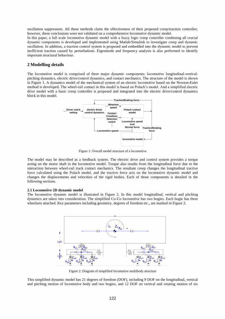
122

oscillation suppression. All these methods claim the effectiveness of their proposed creep/traction controller;

however, these conclusions were not validated on a comprehensive locomotive dynamic model.

In this paper, a full scale locomotive dynamic model with a fuzzy logic creep controller combining all crucial

dynamic components is developed and implemented using Matlab/Simulink to investigate creep and dynamic

oscillation. In addition, a traction control system is proposed and embedded into the dynamic model to prevent

inefficient traction caused by perturbations. Eigenmode and frequency analysis is also performed to identify

important structural behaviour.

2 Modelling details

The locomotive model is comprised of three major dynamic components: locomotive longitudinal-vertical-

pitching dynamics, electric drive/control dynamics, and contact mechanics. The structure of the model is shown

in Figure 1. A dynamics model of the mechanical system of an electric locomotive based on the Newton-Euler

method is developed. The wheel-rail contact in this model is based on Polach’s model. And a simplified electric

drive model with a basic creep controller is proposed and integrated into the electric drive/control dynamics

block in this model.

Figure 1: Overall model structure of a locomotive

The model may be described as a feedback system. The electric drive and control system provides a torque

acting on the motor shaft in the locomotive model. Torque also results from the longitudinal force due to the

interaction between wheel-rail track contact mechanics. The resultant creep changes the longitudinal tractive

force calculated using the Polach model, and the tractive force acts on the locomotive dynamic model and

changes the displacements and velocities of the rigid bodies. Each of those components is detailed in the

following sections.

2.1 Locomotive 2D dynamic model

The locomotive dynamic model is illustrated in Figure 2. In this model longitudinal, vertical and pitching

dynamics are taken into consideration. The simplified Co-Co locomotive has two bogies. Each bogie has three

wheelsets attached. Key parameters including geometry, degrees of freedom etc., are marked in Figure 2.

Figure 2: Diagram of simplified locomotive multibody structure

This simplified dynamic model has 21 degrees of freedom (DOF), including 9 DOF on the longitudinal, vertical

and pitching motion of locomotive body and two bogies, and 12 DOF on vertical and rotating motion of six

electric drive/

control dynamics

Driver notch

setting

locomotive model

Polach contact

model

Wheelset

speed

Locomotive speed

And

Normal force Traction/Braking

forceLocomotive speed

Traction/Braking force

Contact

Condition

Selection

switch

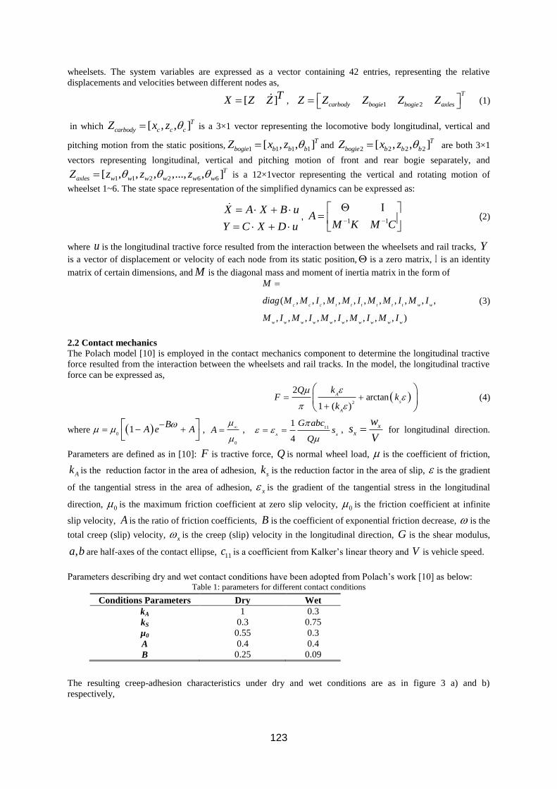
123

wheelsets. The system variables are expressed as a vector containing 42 entries, representing the relative

displacements and velocities between different nodes as,

[ ]TX Z Z , 1 2

T

carbody bogie bogie axlesZ Z Z Z Z (1)

in which [ , , ]T

carbody c c cZ x z is a 3×1 vector representing the locomotive body longitudinal, vertical and

pitching motion from the static positions, 1 1 1 1[ , , ]T

bogie b b bZ x z and 2 2 2 2[ , , ]T

bogie b b bZ x z are both 3×1

vectors representing longitudinal, vertical and pitching motion of front and rear bogie separately, and

1 1 2 2 6 6[ , , , ,..., , ]T

axles w w w w w wZ z z z is a 12×1vector representing the vertical and rotating motion of

wheelset 1~6. The state space representation of the simplified dynamics can be expressed as:

X A X B u

Y C X D u

,

1 1A

M K M C

(2)

where u is the longitudinal tractive force resulted from the interaction between the wheelsets and rail tracks, Yis a vector of displacement or velocity of each node from its static position, is a zero matrix, is an identity

matrix of certain dimensions, and M is the diagonal mass and moment of inertia matrix in the form of

( , , , , , , , , , , ,

, , , , , , , , , )

c c c t t t t t t w w

w w w w w w w w w w

M

diag M M I M M I M M I M I

M I M I M I M I M I

(3)

2.2 Contact mechanics

The Polach model [10] is employed in the contact mechanics component to determine the longitudinal tractive

force resulted from the interaction between the wheelsets and rail tracks. In the model, the longitudinal tractive

force can be expressed as,

2

2arctan

1 ( )

A

s

A

Q kF k

k

(4)

where 0

1B

A e A

,

0

A

, 11

1

4x x

G abcs

Q

,

xx

ws

V for longitudinal direction.

Parameters are defined as in [10]: F is tractive force, Q is normal wheel load, is the coefficient of friction,

Ak is the reduction factor in the area of adhesion, sk is the reduction factor in the area of slip, is the gradient

of the tangential stress in the area of adhesion, x is the gradient of the tangential stress in the longitudinal

direction, 0 is the maximum friction coefficient at zero slip velocity, 0 is the friction coefficient at infinite

slip velocity, A is the ratio of friction coefficients, B is the coefficient of exponential friction decrease, is the

total creep (slip) velocity, x is the creep (slip) velocity in the longitudinal direction, G is the shear modulus,

,a b are half-axes of the contact ellipse, 11c is a coefficient from Kalker’s linear theory and V is vehicle speed.

Parameters describing dry and wet contact conditions have been adopted from Polach’s work [10] as below: Table 1: parameters for different contact conditions

Conditions Parameters Dry Wet

kA 1 0.3

kS 0.3 0.75

µ0 0.55 0.3

A 0.4 0.4

B 0.25 0.09

The resulting creep-adhesion characteristics under dry and wet conditions are as in figure 3 a) and b)

respectively,

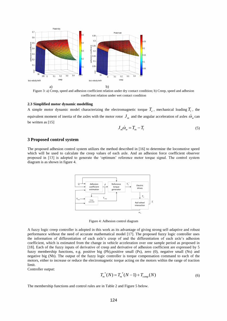
124

a) b) Figure 3: a) Creep, speed and adhesion coefficient relation under dry contact condition; b) Creep, speed and adhesion

coefficient relation under wet contact condition

2.3 Simplified motor dynamic modelling

A simple motor dynamic model characterizing the electromagnetic torque eT , mechanical loading lT , the

equivalent moment of inertia of the axles with the motor rotor mJ and the angular acceleration of axles w can

be written as [15]

m w m lJ T T (5)

3 Proposed control system

The proposed adhesion control system utilizes the method described in [16] to determine the locomotive speed

which will be used to calculate the creep values of each axle. And an adhesion force coefficient observer

proposed in [13] is adopted to generate the ‘optimum’ reference motor torque signal. The control system

diagram is as shown in figure 4.

Adhesion coefficient estimation

Reference torque

generator

Creep controller Rail-wheel

interaction

Electric drives

*

mT

compT

w

Q

lTlocoV

mT

Figure 4: Adhesion control diagram

A fuzzy logic creep controller is adopted in this work as its advantage of giving strong self-adaptive and robust

performance without the need of accurate mathematical model [17]. The proposed fuzzy logic controller uses

the information of differentiation of each axle’s creep of and the differentiation of each axle’s adhesion

coefficient, which is estimated from the change in vehicle acceleration over one sample period as proposed in

[18]. Each of the fuzzy inputs of derivative of creep and derivative of adhesion coefficient are expressed by 5

fuzzy membership functions, e.g. positive big (Pb),positive small (Ps), zero (0), negative small (Ns) and

negative big (Nb). The output of the fuzzy logic controller is torque compensation command to each of the

motors, either to increase or reduce the electromagnetic torque acting on the motors within the range of traction

limit.

Controller output:

(6)

The membership functions and control rules are in Table 2 and Figure 5 below.

050

100 0 0.1 0.2 0.3 0.4 0.5

0

0.1

0.2

0.3

0.4

0.5

0.6

0.7

creep

Polach dry

loco velocity km/h

adhesio

n c

oeffic

ient

0

0.1

0.2

0.3

0.4

0.5

050

0 0.1 0.2 0.3 0.4 0.5

0

0.05

0.1

0.15

0.2

0.25

0.3

0.35

creep

Polach wet

loco velocity km/h

adhesio

n c

oeffic

ient

0.05

0.1

0.15

0.2

0.25

* *( ) ( 1) ( )m m compT N T N T N

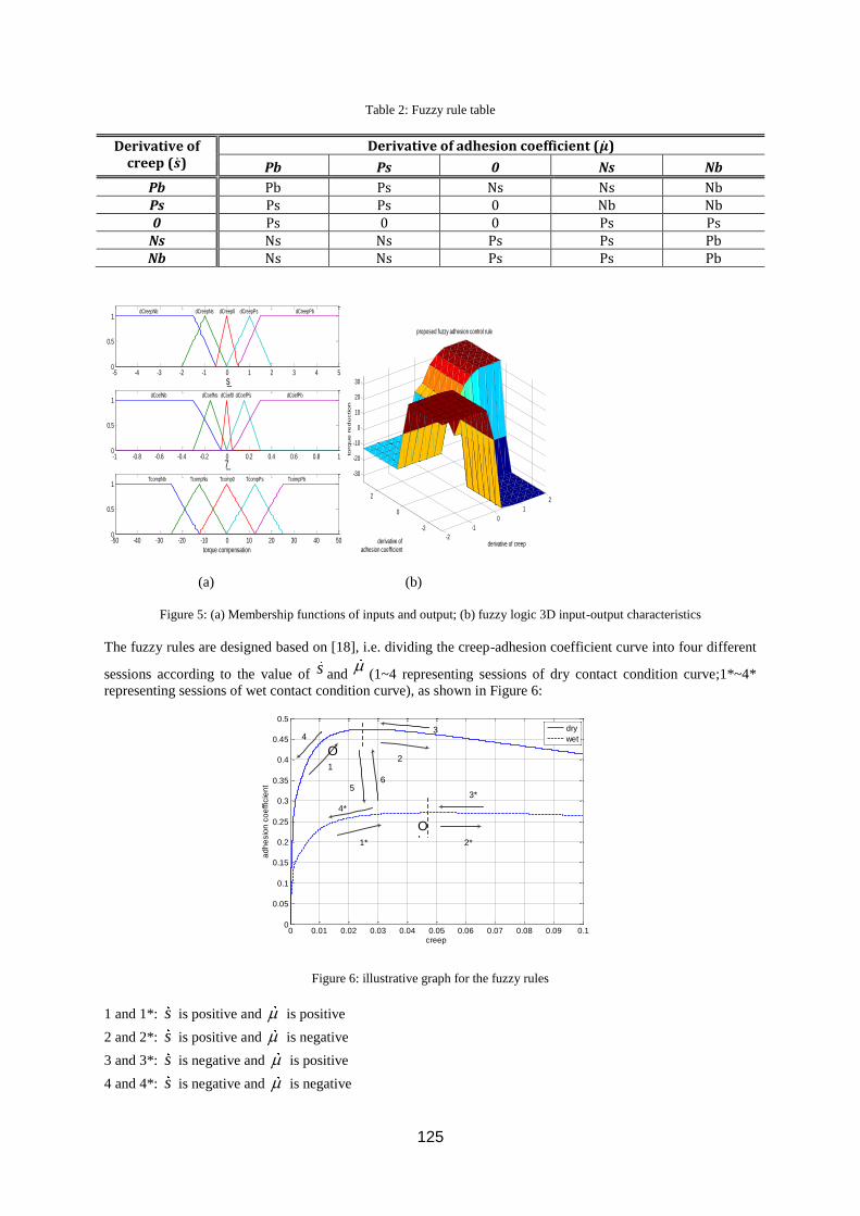
125

Table 2: Fuzzy rule table

Derivative of creep (��)

Derivative of adhesion coefficient (��)

Pb Ps 0 Ns Nb

Pb Pb Ps Ns Ns Nb Ps Ps Ps 0 Nb Nb 0 Ps 0 0 Ps Ps

Ns Ns Ns Ps Ps Pb Nb Ns Ns Ps Ps Pb

(a) (b)

Figure 5: (a) Membership functions of inputs and output; (b) fuzzy logic 3D input-output characteristics

The fuzzy rules are designed based on [18], i.e. dividing the creep-adhesion coefficient curve into four different

sessions according to the value of and (1~4 representing sessions of dry contact condition curve;1*~4*

representing sessions of wet contact condition curve), as shown in Figure 6:

Figure 6: illustrative graph for the fuzzy rules

1 and 1*: s is positive and is positive

2 and 2*: s is positive and is negative

3 and 3*: s is negative and is positive

4 and 4*: s is negative and is negative

-5 -4 -3 -2 -1 0 1 2 3 4 50

0.5

1

_s

dCreepNb dCreepNs dCreep0 dCreepPs dCreepPb

-1 -0.8 -0.6 -0.4 -0.2 0 0.2 0.4 0.6 0.8 10

0.5

1

_7

dCoefNb dCoefNs dCoef0 dCoefPs dCoefPb

-50 -40 -30 -20 -10 0 10 20 30 40 500

0.5

1

torque compensation

TcompNb TcompNs Tcomp0 TcompPs TcompPb

-2

-1

0

1

2

-2

0

2

-30

-20

-10

0

10

20

30

derivative of creep

proposed fuzzy adhesion control rule

derivative of adhesion coefficient

torq

ue

re

du

ctio

n

s

0 0.01 0.02 0.03 0.04 0.05 0.06 0.07 0.08 0.09 0.10

0.05

0.1

0.15

0.2

0.25

0.3

0.35

0.4

0.45

0.5

creep

ad

he

sio

n c

oe

ffic

ien

t

dry

wet

5

4

2

3

1* 2*

3*

4*

6

1

O

O’

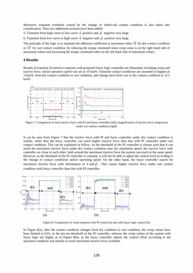
126

Moreover, transient condition caused by the change of wheel-rail contact condition is also taken into

consideration. Thus two additional sessions have been added:

5: Transient from high curve to low curve- s positive and negative very large

6: Transient from low curve to high curve- s negative and positive very large

The principle of the logic is to maintain the adhesion coefficient at maximum value O for dry contact condition

or 'O for wet contact condition, by reducing the torque command when creep value is on the right hand side of

maximum values and increasing the torque command when on the left hand side of maximum values.

4 Results

Results of transient locomotive response with proposed fuzzy logic controller are illustrated, including creep and

tractive force. Initial operation speed was set at 10 km/h. Transient contact conditions are assumed to happen at

11km/h, from dry contact condition to wet condition, and change back from wet to dry contact condition at 12.5

km/h.

10 10.5 11 11.5 12 12.5 13 13.52.5

3

3.5

4

4.5

5

5.5

6

6.5

7x 10

5

speed (km/h)

tota

l tr

active forc

e (

N)

tractive force with PI control tractive force with fuzzy control

11 11.5 12 12.5

3.45

3.5

3.55

3.6

3.65

3.7

3.75x 10

5

speed (km/h)

tota

l tr

active forc

e (

N)

tractive force with PI control tractive force with fuzzy control

dry wet dry

Figure 7: Comparison of total tractive force with PI and fuzzy controller (left); magnification of tractive force comparison

under wet contact condition (right)

It can be seen from Figure 7 that the tractive force with PI and fuzzy controller under dry contact condition is

similar, while then the fuzzy controller can reach higher tractive force than that with PI controller under wet

contact condition. This can be explained as follow. As the threshold of the PI controller is chosen such that it can

reach the maximum tractive force under dry contact condition near the simulation speed, the tractive force with

controller are close to each other, both around the maximum tractive force the system can reach at the same speed.

However, as the threshold of the PI controller is constant, it will not be able to adjust the control level according to

the change of contact conditions and/or operating speed. On the other hand, the fuzzy controller search for

maximum tractive force with information of s and . This causes higher tractive force under wet contact

condition with fuzzy controller than that with PI controller.

(a) (b)

Figure 8: Comparison of creep response with PI control (a) and with fuzzy logic control (b)

In Figure 8(a), after the contact condition changes from dry condition to wet condition, the creep values have

been limited at 0.03, as the pre-set threshold of the PI controller, whereas the creep values of the system with

fuzzy logic are higher as in Figure 8(b), as the fuzzy controller adjusts the control effort according to the

operation condition and intends to reach maximum tractive force available.

10 10.5 11 11.5 12 12.5 13 13.50

0.005

0.01

0.015

0.02

0.025

0.03

0.035

speed (km/h)

cre

ep

axle1

axle2

axle3

axle4

axle5

axle6

10 10.5 11 11.5 12 12.5 13 13.50

0.02

0.04

0.06

0.08

0.1

0.12

speed (km/h)

cre

ep

axle1

axle2

axle3

axle4

axle5

axle6

dry

wet dry dry wet dry

127

5 Conclusions External perturbations such as the change of rail-wheel contact conditions often cause undesirable locomotive

dynamic responses. In this paper, the locomotive dynamic responses under transient contact conditions with PI

and fuzzy logic creep controller have been simulated with an integrated 2D Co-Co locomotive/track dynamic

model. The comparison of the creep and total tractive force shows the advantage of proposed fuzzy logic

controller over PI controller in term of realizing higher tractive force under the change of contact conditions.

While both controllers can limit the creep under a certain level, simulation results show that the fuzzy controller

can reach higher total tractive force than that with a constant threshold PI controller under wet contact condition

thanks to its ability to search for the maximum achievable force according to different contact conditions.

Acknowledgement

The authors are grateful to the CRC for Rail Innovation (established and supported under the Australian

Government's Cooperative Research Centres program) for the funding of this research Project No. R3.119

“Locomotive Adhesion”. The authors acknowledge the support of the Centre for Railway Engineering, Central

Queensland University and the many industry partners that have contributed to this project, in particular staff

from RailCorp, Fortescue Metals Group (FMG) and Brookfield Rail.

References [1] Chudzikiewicz , A., Simulation of Rail Vehicle Dynamics in MATLAB Environment, Vehicle System

Dynamics, vol. 33, pp. 107-119, 2000/02/01 2000.

[2] Shimizu,Y., et al., Anti-slip/skid Re-adhesion Control Based on Disturbance Observer Considering

Bogie Vibration, in Power Conversion Conference - Nagoya, 2007. PCC '07, pp. 1376-1381, 2007.

[3] Spiryagin,M. et al., Development of traction control for hauling locomotives, ed.

[4] Fleischer, M., Modal state control in the frequency domain for active damping of mechanical vibrations

in traction drive-trains, in Advanced Motion Control. AMC'04. The 8th IEEE International Workshop on, 2004,

pp. 171-176, 2004.

[5] Bakhvalov, Y. et al., Mathematical Modelling of Electromechanical Processes in Electric Locomotive,

presented at the 16th IMACS World Congress, Lausanne (Switzerland), 2000.

[6] Senini, S. et al., Dynamic simulation of wheel-rail interaction for locomotive traction studies, in

Railroad Conference, 1993., Proceedings of the 1993 IEEE/ASME Joint, pp. 27-34, 1993.

[7] Law, E. H. and Cooperrider, N.K., A survey of railway vehicle dynamics research, ASME Journal of

Dynamic Systems, Measurement, and Control, vol. 96, pp. 132-146, June 1974.

[8] Guclu, R. and Metin, M., Fuzzy Logic Control of Vibrations of a Light Rail Transport Vehicle in Use

in Istanbul Traffic, Journal of Vibration and Control, vol. 15, pp. 1423-1440, September 1, 2009.

[9] Garivaltis, D. S. et al., Dynamic Response of a Six-axle Locomotive to Random Track Inputs, Vehicle

System Dynamics, vol. 9, pp. 117-147, 1980/05/01 1980.

[10] Polach, O., Creep forces in simulations of traction vehicles running on adhesion limit, Wear, vol. 258,

pp. 992-1000, 2005.

[11] Polach, O., Influence of Locomotive Tractive Effort on the Forces Between Wheel and Rail, Vehicle

System Dynamics, vol. 35, pp. 7-22, 2001.

[12] Doh-Young, P. et al., Hybrid re-adhesion control method for traction system of high-speed railway, in

Electrical Machines and Systems, 2001. ICEMS 2001. Proceedings of the Fifth International Conference on, pp.

739-742 vol.2, 2001.

[13] Ohishi, K. et al., Anti-slip control of electric motor coach based on disturbance observer, in Advanced

Motion Control, 1998. AMC '98-Coimbra., 1998 5th International Workshop on, pp. 580-585, 1998.

[14] Yasuoka, I. et al., Improvement of re-adhesion for commuter trains with vector control traction

inverter, in Power Conversion Conference - Nagaoka 1997., Proceedings of the, pp. 51-56 vol.1, 1997.

[15] Marino, R. et al., Induction Motor Control Design: Springer, 2010.

[16] Spiryagin, M.et al., Control system for maximum use of adhesive forces of a railway vehicle in a

tractive mode, Mechanical Systems and Signal Processing, vol. 22, pp. 709-720, 2008.

[17] Yuan, Y. et al., The dynamic study of locomotives under saturated adhesion, Vehicle System

Dynamics, vol. 49, pp. 1321-1338, 2011/08/01 2011.

[18] Bauer, M. and Tomizuka, M., Fuzzy Logic Traction Controllers and their Effect on Longitudinal

Vehicle Platoon Systems, Vehicle System Dynamics, vol. 25, pp. 277-303, 1996/04/01 1996.

128

Paper C

Fuzzy Logic based Sliding Mode Creep

Controller under Varying Wheel-Rail Contact

Conditions

129

Comparison of PI and fuzzy logic based sliding mode locomotive creep controls with change of

rail-wheel contact conditions

Ye Tiana, b

*, W.J.T. (Bill) Daniela, b

, Sheng Liua and Paul A. Meehan

a, b

aSchool of Mechanical and Mining Engineering, the University of Queensland, Queensland, Australia 4072;

bCooperative Research Centre for Rail Innovation (CRC Rail), Queensland, Australia

This paper presents locomotive traction controllers based on PI and sliding mode control with a

fuzzy logic creep reference generator; and compares their performance based on tractive efforts

under various operation speeds. The effect of change of wheel-rail friction conditions under

different controllers is also investigated. In particular, a sliding mode traction controller based on

a fuzzy logic creep reference generator is developed to tackle nonlinearity and uncertainty due to

the contact conditions and operation speeds. It is shown that at high speed operation, the fuzzy

logic based sliding mode controller can achieve higher tractive force with lower creep values.

Keywords: fuzzy logic; sliding mode control; traction control

Nomenclature 𝑥𝑐 Locomotive body longitudinal displacement

𝑧𝑐 Locomotive body vertical displacement

𝜃𝑐 Locomotive body pitch angle

𝑥𝑏1,2 Locomotive front/rear bogie longitudinal displacement

𝑧𝑏1,2 Locomotive front/rear bogie vertical displacement

𝜃𝑏1,2 Locomotive front/rear bogie pitch displacement

𝑧𝑤1~6 Wheelset 1~6 vertical displacement

𝜃𝑤1~6 Wheelset 1~6 rotation angle

𝑀𝑐 𝑀𝑡 𝑀𝑤 Mass of locomotive body, bogie and axle

𝐼𝑐 𝐼𝑡 𝐼𝑤 Moment of inertia of locomotive body, bogie and axle along pitch direction

𝑄 Wheel load

𝜇 Friction coefficient

휀 Gradient of the tangential stress in the area of adhesion

𝑘𝐴, 𝑘𝑠 Reduction factor in the area of adhesion, reduction factor in the area of slip

𝜇∞ Friction coefficient at infinity slip velocity

𝜇0 Maximum friction coefficient at zero slip velocity

𝑠𝑥 Creep in longitudinal (x) directions

𝑉 Vehicle speed

𝑤𝑥 Creep (slip) velocity in longitudinal (x) direction

𝑎, 𝑏 Half-axes of the contact ellipse

𝑐11 Coefficient from Kalker’s linear theory

𝐹, 𝐺 Tractive force, Shear modulus

𝑇𝑡𝑖 Torque generated by electric drive 𝑖=1~6

𝑇𝑙𝑖 Torque acting on axle 𝑖=1~6 generated by longitudinal contact force

1. Introduction The progressive application of high traction motors and control techniques based on power electronics

has brought great benefits to the rail industry due to its high power capacity and efficiency. Therefore,

an effective control system is demanded to suit the contemporary high speed railway network.

Traditionally, traction controller performance and its dynamic impact on rail are typically assessed

under specific steady state conditions. In particular, traction controller performance under natural

perturbations in friction/lubrication, wheel/rail profiles, track curvature, vehicle/track dynamics,

wheel/track imperfections etc. has not been comprehensively investigated yet. Among those

perturbations, the transient changes in friction or lubrication can cause sudden changes of creep and

often lead to over/under traction/braking. In order to investigate this issue, a predictive locomotive

dynamic model combining crucial dynamic components such as locomotive rigid body dynamics,

contact dynamics and electric drive and control is needed.

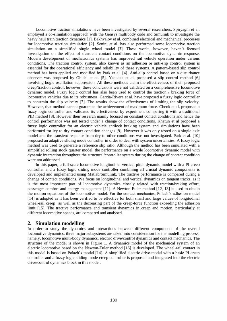
130

Locomotive traction simulations have been investigated by several researchers. Spiryagin et al.

employed a co-simulation approach with the Gensys multibody code and Simulink to investigate the

heavy haul train traction dynamics [1]. Bakhvalov et al. combined electrical and mechanical processes

for locomotive traction simulation [2]. Senini et al. has also performed some locomotive traction

simulation on a simplified single wheel model [3]. These works, however, haven’t focused

investigation on the effect of transient contact conditions on the locomotive dynamic response.

Modern development of mechatronics systems has improved rail vehicle operation under various

conditions. The traction control system, also known as an adhesion or anti-slip control system is

essential for the operational efficiency and reliability of these systems. A pattern-based slip control

method has been applied and modified by Park et al. [4]. Anti-slip control based on a disturbance

observer was proposed by Ohishi et al. [5]. Yasuoka et al. proposed a slip control method [6]

involving bogie oscillation suppression. All these methods claim the effectiveness of their proposed

creep/traction control; however, these conclusions were not validated on a comprehensive locomotive

dynamic model. Fuzzy logic control has also been used to control the traction / braking force of

locomotive vehicles due to its robustness. Garcia-Rivera et al. have proposed a fuzzy logic controller

to constrain the slip velocity [7]. The results show the effectiveness of limiting the slip velocity.

However, that method cannot guarantee the achievement of maximum force. Cheok et al. proposed a

fuzzy logic controller and validated its effectiveness by experiment comparing it with a traditional

PID method [8]. However their research mainly focused on constant contact conditions and hence the

control performance was not tested under a change of contact conditions. Khatun et al proposed a

fuzzy logic controller for an electric vehicle antilock braking system and simulations have been

performed for icy to dry contact condition changes [9]. However it was only tested on a single axle

model and the transient response from dry to other conditions was not investigated. Park et al. [10]

proposed an adaptive sliding mode controller in order to deal with system uncertainties. A fuzzy logic

method was used to generate a reference slip ratio. Although the method has been simulated with a

simplified rolling stock quarter model, the performance on a whole locomotive dynamic model with

dynamic interaction throughout the structural/controller system during the change of contact condition

were not addressed.

In this paper, a full scale locomotive longitudinal-vertical-pitch dynamic model with a PI creep

controller and a fuzzy logic sliding mode controller combining all crucial dynamic components is

developed and implemented using Matlab/Simulink. The tractive performance is compared during a

change of contact conditions. We focus on longitudinal and vertical dynamics on tangent tracks, as it

is the most important part of locomotive dynamics closely related with traction/braking effort,

passenger comfort and energy management [11]. A Newton-Euler method [12, 13] is used to obtain

the motion equations of the locomotive model. For the contact mechanics, Polach’s adhesion model

[14] is adopted as it has been verified to be effective for both small and large values of longitudinal

wheel-rail creep as well as the decreasing part of the creep-force function exceeding the adhesion

limit [15]. The tractive performance and transient dynamics in creep and motion, particularly at

different locomotive speeds, are compared and analysed.

2. Simulation modelling In order to study the dynamics and interactions between different components of the overall

locomotive dynamics, three major subsystems are taken into consideration for the modelling process;

namely, locomotive multi-body dynamics, electric drive/control dynamics and contact mechanics. The

structure of the model is shown in Figure 1. A dynamics model of the mechanical system of an

electric locomotive based on the Newton-Euler method [16] is developed. The wheel-rail contact in

this model is based on Polach’s model [14]. A simplified electric drive model with a basic PI creep

controller and a fuzzy logic sliding mode creep controller is proposed and integrated into the electric

drive/control dynamics block in this model.

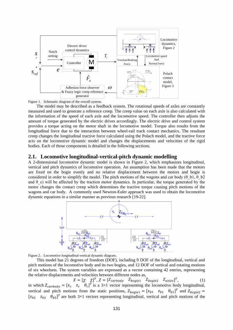
131

Figure 1. Schematic diagram of the overall system.

The model may be described as a feedback system. The rotational speeds of axles are constantly

measured and used to generate a reference creep. The creep value on each axle is also calculated with

the information of the speed of each axle and the locomotive speed. The controller then adjusts the

amount of torque generated by the electric drives accordingly. The electric drive and control system

provides a torque acting on the motor shaft in the locomotive model. Torque also results from the

longitudinal force due to the interaction between wheel-rail track contact mechanics. The resultant

creep changes the longitudinal tractive force calculated using the Polach model, and the tractive force

acts on the locomotive dynamic model and changes the displacements and velocities of the rigid

bodies. Each of those components is detailed in the following sections.

2.1. Locomotive longitudinal-vertical-pitch dynamic modelling A 2-dimensional locomotive dynamic model is shown in Figure 2, which emphasizes longitudinal,

vertical and pitch dynamics of locomotive operation. An assumption has been made that the motors

are fixed on the bogie evenly and no relative displacement between the motors and bogie is

considered in order to simplify the model. The pitch motions of the wagons and car body (θ_b1, θ_b2

and θ_c) will be affected by the traction motor dynamics. In particular, the torque generated by the

motor changes the contact creep which determines the tractive torque causing pitch motions of the

wagons and car body. A commonly used Newton-Euler approach was used to obtain the locomotive

dynamic equations in a similar manner as previous research [19-22].

Figure 2. Locomotive longitudinal-vertical dynamic diagram.

This model has 21 degrees of freedom (DOF), including 9 DOF of the longitudinal, vertical and

pitch motions of the locomotive body and its two bogies, and 12 DOF of vertical and rotating motions

of six wheelsets. The system variables are expressed as a vector containing 42 entries, representing

the relative displacements and velocities between different nodes as,

𝑋 = [𝑍 ��]𝑇, 𝑍 = [𝑍𝑐𝑎𝑟𝑏𝑜𝑑𝑦 𝑍𝑏𝑜𝑔𝑖𝑒1 𝑍𝑏𝑜𝑔𝑖𝑒2 𝑍𝑎𝑥𝑙𝑒𝑠]𝑇, (1)

in which 𝑍𝑐𝑎𝑟𝑏𝑜𝑑𝑦 = [𝑥𝑐 𝑧𝑐 𝜃𝑐]𝑇 is a 3×1 vector representing the locomotive body longitudinal,

vertical and pitch motions from the static positions, 𝑍𝑏𝑜𝑔𝑖𝑒1 = [𝑥𝑏1 𝑧𝑏1 𝜃𝑏1]𝑇 and 𝑍𝑏𝑜𝑔𝑖𝑒2 =

[𝑥𝑏2 𝑧𝑏2 𝜃𝑏2]𝑇 are both 3×1 vectors representing longitudinal, vertical and pitch motions of the

Locomotive

dynamics,

Figure 2

Polach

contact

model,

Figure 3

Electric drive/

control dynamics

MController

Locomotive speed

And

Normal force

tT

Adhesion force observer

& Fuzzy logic creep reference

generator

s

refs+

-

ˆaF

e

Traction/Braking

Force

Notch

setting

050

100 0 0.1 0.2 0.3 0.4 0.5

0

0.1

0.2

0.3

0.4

0.5

0.6

0.7

creep

Polach dry

loco velocity km/h

adhesio

n c

oeffic

ient

0

0.1

0.2

0.3

0.4

0.5

Polach creep

Electric drive & control

Complex locomotiv

M

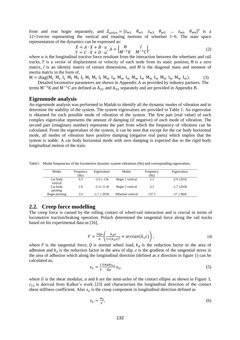
132

front and rear bogie separately, and 𝑍𝑎𝑥𝑙𝑒𝑠 = [𝑧𝑤1 𝜃𝑤1 𝑧𝑤2 𝜃𝑤2 … 𝑧𝑤6 𝜃𝑤6]𝑇 is a

12×1vector representing the vertical and rotating motions of wheelset 1~6. The state space

representation of the dynamics can be expressed as:

�� = 𝐴 ∙ 𝑋 + 𝐵 ∙ 𝑢𝑌 = 𝐶 ∙ 𝑋 + 𝐷 ∙ 𝑢

, 𝐴 = [Θ 𝐼

𝑀−1𝐾 𝑀−1𝐶], (2)

where 𝑢 is the longitudinal tractive force resultant from the interaction between the wheelsets and rail

tracks, 𝑌 is a vector of displacement or velocity of each node from its static position, Θ is a zero

matrix, 𝐼 is an identity matrix of certain dimensions, and 𝑀 is the diagonal mass and moment of

inertia matrix in the form of,

M = diag(Mc Mc Ic Mt Mt It Mt Mt It Mw Iw Mw Iw Mw Iw Mw Iw Mw Iw Mw Iw). (3)

Detailed locomotive parameters are shown in Appendix A as provided by industry partners. The

terms M−1K and M−1C are defined as A21 and A22 separately and are provided in Appendix B.

Eigenmode analysis An eigenmode analysis was performed in Matlab to identify all the dynamic modes of vibration and to

determine the stability of the system. The system eigenvalues are provided in Table 1. An eigenvalue

is obtained for each possible mode of vibration of the system. The first part (real value) of each

complex eigenvalue represents the amount of damping (if negative) of each mode of vibration. The

second part (imaginary number) represents the part from which the frequency of vibration can be

calculated. From the eigenvalues of the system, it can be seen that except for the car body horizontal

mode, all modes of vibration have positive damping (negative real parts) which implies that the

system is stable. A car body horizontal mode with zero damping is expected due to the rigid body

longitudinal motion of the train.

Table1. Modal frequencies of the locomotive dynamic system vibrations (Hz) and corresponding eigenvalues.

Modes Frequency

(Hz)

Eigenvalues Modes Frequency

(Hz)

Eigenvalues

Car body

vertical

0.3 -2.9 ± 1.9i Bogie 1 vertical 3.1 -2.9 ±20.6i

Car body

pitching

1.8 -2.1± 11.4i Bogie 2 vertical 3.3 -1.7 ±20.8i

Bogie pitching 3.3 -1.7 ± 20.8i Wheelset vertical 137.5 -17 ± 864i

2.2. Creep force modelling The creep force is caused by the rolling contact of wheel-rail interaction and is crucial in terms of

locomotive traction/braking operation. Polach determined the tangential force along the rail tracks

based on his experimental data as [16],

𝐹 =2𝑄𝜇

𝜋(

𝑘𝐴𝜀

1+(𝑘𝐴𝜀)2 + 𝑎𝑟𝑐𝑡𝑎𝑛(𝑘𝑠휀)) , (4)

where 𝐹 is the tangential force, 𝑄 is normal wheel load, 𝑘𝐴 is the reduction factor in the area of

adhesion and 𝑘𝑠 is the reduction factor in the area of slip. 휀 is the gradient of the tangential stress in

the area of adhesion which along the longitudinal direction (defined as 𝑥 direction in figure 1) can be

calculated as,

휀𝑥 =1

4

𝐺𝜋𝑎𝑏𝑐11

𝑄𝜇𝑠𝑥, (5)

where 𝐺 is the shear modulus, 𝑎 and 𝑏 are the semi-axles of the contact ellipse as shown in Figure 3,

𝑐11 is derived from Kalker’s work [23] and characterizes the longitudinal direction of the contact

shear stiffness coefficient. Also 𝑠𝑥 is the creep component in longitudinal direction defined as

𝑠𝑥 =𝑤𝑥

𝑉, (6)

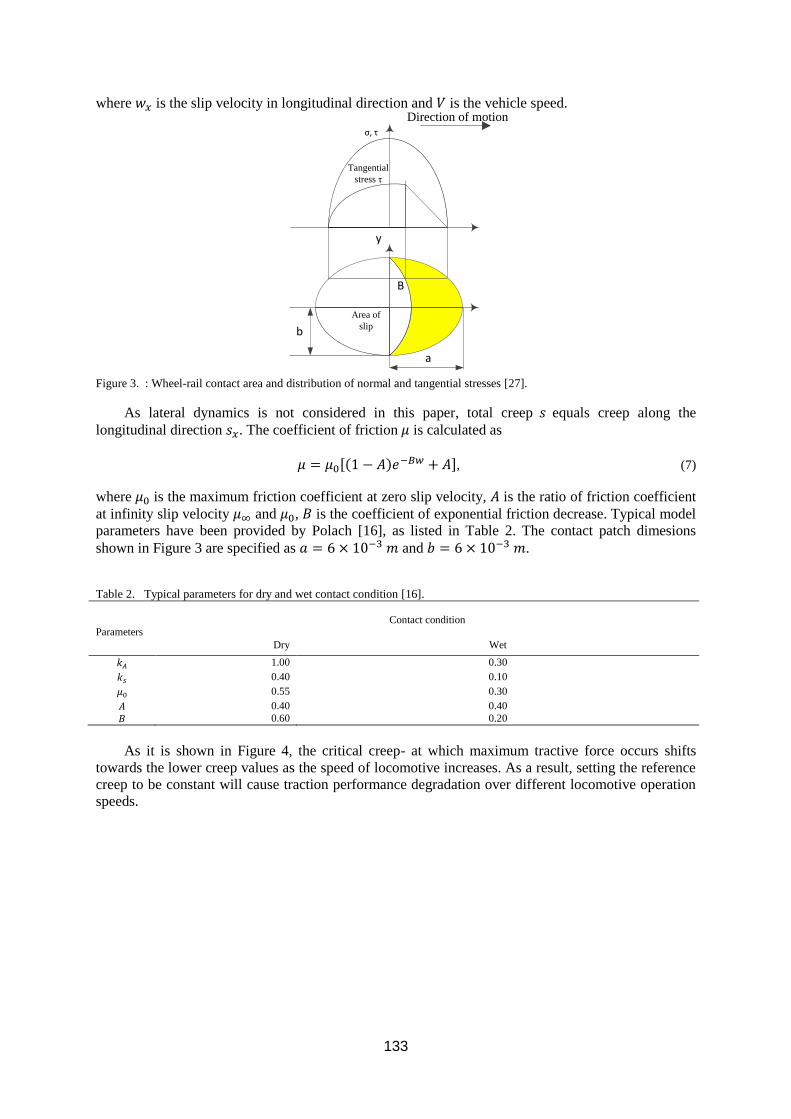
133

where 𝑤𝑥 is the slip velocity in longitudinal direction and 𝑉 is the vehicle speed.

y

Direction of motion

Tangential

stress τ

Area of

slip

B

σ, τ

b

a

Figure 3. : Wheel-rail contact area and distribution of normal and tangential stresses [27].

As lateral dynamics is not considered in this paper, total creep 𝑠 equals creep along the

longitudinal direction 𝑠𝑥. The coefficient of friction 𝜇 is calculated as

𝜇 = 𝜇0[(1 − 𝐴)𝑒−𝐵𝑤 + 𝐴], (7)

where 𝜇0 is the maximum friction coefficient at zero slip velocity, 𝐴 is the ratio of friction coefficient

at infinity slip velocity 𝜇∞ and 𝜇0, 𝐵 is the coefficient of exponential friction decrease. Typical model

parameters have been provided by Polach [16], as listed in Table 2. The contact patch dimesions

shown in Figure 3 are specified as 𝑎 = 6 × 10−3 𝑚 and 𝑏 = 6 × 10−3 𝑚.

Table 2. Typical parameters for dry and wet contact condition [16].

Parameters

Contact condition

Dry Wet

𝑘𝐴 1.00 0.30

𝑘𝑠 0.40 0.10

𝜇0 0.55 0.30

𝐴 0.40 0.40

𝐵 0.60 0.20

As it is shown in Figure 4, the critical creep- at which maximum tractive force occurs shifts

towards the lower creep values as the speed of locomotive increases. As a result, setting the reference

creep to be constant will cause traction performance degradation over different locomotive operation

speeds.

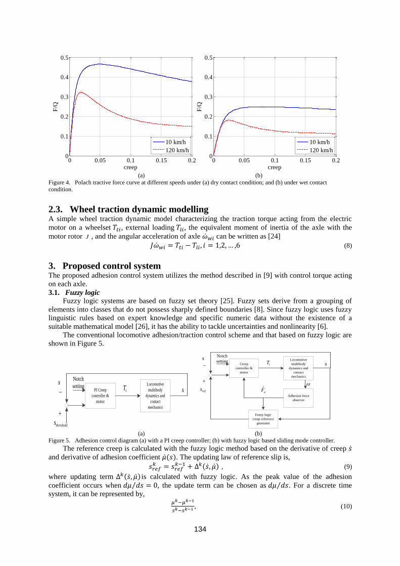
134

0 0.05 0.1 0.15 0.20

0.1

0.2

0.3

0.4

0.5

creep

F/Q

10 km/h

120 km/h

0 0.05 0.1 0.15 0.20

0.1

0.2

0.3

0.4

0.5

creep

F/Q

10 km/h

120 km/h

(a) (b)

Figure 4. Polach tractive force curve at different speeds under (a) dry contact condition; and (b) under wet contact

condition.

2.3. Wheel traction dynamic modelling A simple wheel traction dynamic model characterizing the traction torque acting from the electric

motor on a wheelset 𝑇𝑡𝑖, external loading 𝑇𝑙𝑖, the equivalent moment of inertia of the axle with the

motor rotor J , and the angular acceleration of axle ��𝑤𝑖 can be written as [24]

𝐽��𝑤𝑖 = 𝑇𝑡𝑖 − 𝑇𝑙𝑖, 𝑖 = 1,2,… ,6 (8)

3. Proposed control system The proposed adhesion control system utilizes the method described in [9] with control torque acting

on each axle.

3.1. Fuzzy logic

Fuzzy logic systems are based on fuzzy set theory [25]. Fuzzy sets derive from a grouping of

elements into classes that do not possess sharply defined boundaries [8]. Since fuzzy logic uses fuzzy

linguistic rules based on expert knowledge and specific numeric data without the existence of a

suitable mathematical model [26], it has the ability to tackle uncertainties and nonlinearity [6].

The conventional locomotive adhesion/traction control scheme and that based on fuzzy logic are

shown in Figure 5.

PI Creep

controller &

motor

Locomotive

multibody

dynamics and

contact

mechanics

sstT

Notch

setting

thresholds

Creep

controller &

motor

Locomotive

multibody

dynamics and

contact

mechanics

Fuzzy logic

creep reference

generator

ˆaF

refs

ss

Adhesion force

observer

tT

Notch

setting

(a) (b)

Figure 5. Adhesion control diagram (a) with a PI creep controller; (b) with fuzzy logic based sliding mode controller.

The reference creep is calculated with the fuzzy logic method based on the derivative of creep �� and derivative of adhesion coefficient ��(𝑠). The updating law of reference slip is,

𝑠𝑟𝑒𝑓𝑘 = 𝑠𝑟𝑒𝑓

𝑘−1 + Δ𝑘(��, ��) , (9)

where updating term Δ𝑘(��, ��) is calculated with fuzzy logic. As the peak value of the adhesion

coefficient occurs when 𝑑𝜇 𝑑𝑠 = 0⁄ , the update term can be chosen as 𝑑𝜇 𝑑𝑠⁄ . For a discrete time

system, it can be represented by, 𝜇𝑘−𝜇𝑘−1

𝑠𝑘−𝑠𝑘−1, (10)

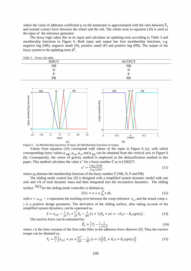
135

where the value of adhesion coefficient μ on the numerator is approximated with the ratio between Fa

and normal contact force between the wheel and the rail. The whole term in equation (10) is used as

the input of the reference generator.

The fuzzy logic takes this as its input and calculates an updating term according to Table 3 and

membership functions in Figure 6. Both input and output has four membership functions, e.g.

negative big (NB), negative small (N), positive small (P) and positive big (PB). The output of the

fuzzy system is the updating term Δk.

Table 3. Fuzzy rule table.

INPUT OUTPUT

NB NB

N N

P P

PB PB

(a) (b)

Figure 6. (a) Membership functions of input; (b) Membership functions of output.

Values from equation (10) correspond with values of the input in Figure 6 (a), with which

corresponding fuzzy values μ NB, μ N, μ P and μ PB can be obtained from the vertical axis in Figure 6

(b). Consequently, the centre of gravity method is employed as the defuzzification method in this

paper. This method calculates the value z∗ for a fuzzy number C as in [100]27]

z∗ =∫zμC (z)dz

∫μC (z)dz, (11)

where μC denotes the membership function of the fuzzy number C (NB, N, P and PB).

The sliding mode control law [9] is designed with a simplified system dynamic model with one

axle and 1/6 of total dynamic mass and then integrated into the locomotive dynamics. The sliding

surface ( )S t

for the sliding mode controller is defined as,

𝑆(𝑡) = 𝑒 + 𝛾 ∫ 𝑒 𝑑𝑡𝑡

0, (12)

with 𝑒 = 𝑠𝑟𝑒𝑓 − 𝑠 represents the tracking error between the creep reference and the actual creep 𝑠.

γ is a positive design parameter. The derivative of the sliding surface, after taking account of the

simplified system dynamics, can be expressed as,

�� = ��𝑟𝑒𝑓 −𝑟

𝐽𝑉𝑇𝑡 +

𝑟2

𝐽𝑉𝐹𝑎 −

1

𝑀𝑉(𝑠 + 1)𝐹𝑎 + 𝛾𝑒 = −𝐷𝑐𝑠 − 𝐾𝑠𝑠𝑔𝑛(𝑠) . (13)

The tractive force can be estimated by:

��𝑎 =1

𝑟𝑇𝑡 −

𝐽

𝑟

𝑠

𝜏𝑠+1, (14)

where τ is the time constant of the first order filter in the adhesion force observer [9]. Thus the tractive

torque can be obtained as,

𝑇𝑡 =𝐽𝑉

𝑟{��𝑟𝑒𝑓 + 𝛾𝑒 + [

𝑟2

𝐽𝑉−

1

𝑀𝑉(𝑠 + 1)] ��𝑎 + 𝐷𝑐𝑠 + 𝐾𝑠𝑠𝑔𝑛(𝑠)}. (15)

-15 -10 -5 0 5 10 15

0

1

input

input

mem

ber

ship

funct

ion

P PBNB N

-1 -0.5 0 0.5 1

0

1

output

ou

tpu

t m

emb

ersh

ip

N P PBNB

refs

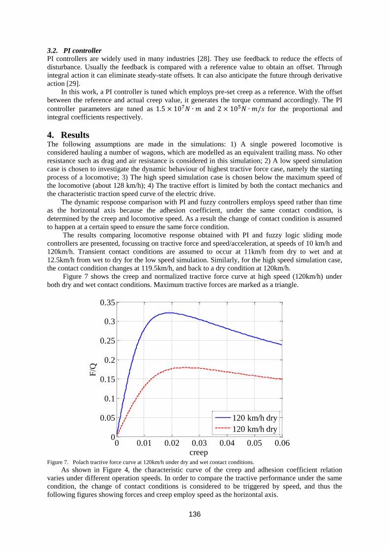
136

3.2. PI controller

PI controllers are widely used in many industries [28]. They use feedback to reduce the effects of

disturbance. Usually the feedback is compared with a reference value to obtain an offset. Through

integral action it can eliminate steady-state offsets. It can also anticipate the future through derivative

action [29].

In this work, a PI controller is tuned which employs pre-set creep as a reference. With the offset

between the reference and actual creep value, it generates the torque command accordingly. The PI

controller parameters are tuned as 1.5 × 107𝑁 ∙ 𝑚 and 2 × 105𝑁 ∙ 𝑚/𝑠 for the proportional and

integral coefficients respectively.

4. Results The following assumptions are made in the simulations: 1) A single powered locomotive is

considered hauling a number of wagons, which are modelled as an equivalent trailing mass. No other

resistance such as drag and air resistance is considered in this simulation; 2) A low speed simulation

case is chosen to investigate the dynamic behaviour of highest tractive force case, namely the starting

process of a locomotive; 3) The high speed simulation case is chosen below the maximum speed of

the locomotive (about 128 km/h); 4) The tractive effort is limited by both the contact mechanics and

the characteristic traction speed curve of the electric drive.

The dynamic response comparison with PI and fuzzy controllers employs speed rather than time

as the horizontal axis because the adhesion coefficient, under the same contact condition, is

determined by the creep and locomotive speed. As a result the change of contact condition is assumed

to happen at a certain speed to ensure the same force condition.

The results comparing locomotive response obtained with PI and fuzzy logic sliding mode

controllers are presented, focussing on tractive force and speed/acceleration, at speeds of 10 km/h and

120km/h. Transient contact conditions are assumed to occur at 11km/h from dry to wet and at

12.5km/h from wet to dry for the low speed simulation. Similarly, for the high speed simulation case,

the contact condition changes at 119.5km/h, and back to a dry condition at 120km/h.

Figure 7 shows the creep and normalized tractive force curve at high speed (120km/h) under

both dry and wet contact conditions. Maximum tractive forces are marked as a triangle.

Figure 7. Polach tractive force curve at 120km/h under dry and wet contact conditions.

As shown in Figure 4, the characteristic curve of the creep and adhesion coefficient relation

varies under different operation speeds. In order to compare the tractive performance under the same

condition, the change of contact conditions is considered to be triggered by speed, and thus the

following figures showing forces and creep employ speed as the horizontal axis.

0 0.01 0.02 0.03 0.04 0.05 0.060

0.05

0.1

0.15

0.2

0.25

0.3

0.35

creep

F/Q

120 km/h dry

120 km/h dry

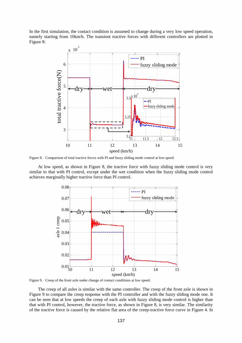
137

In the first simulation, the contact condition is assumed to change during a very low speed operation,

namely starting from 10km/h. The transient tractive forces with different controllers are plotted in

Figure 8:

Figure 8. Comparison of total tractive forces with PI and fuzzy sliding mode control at low speed.

At low speed, as shown in Figure 8, the tractive force with fuzzy sliding mode control is very

similar to that with PI control, except under the wet condition when the fuzzy sliding mode control

achieves marginally higher tractive force than PI control.

Figure 9. Creep of the front axle under change of contact conditions at low speed.

The creep of all axles is similar with the same controller. The creep of the front axle is shown in

Figure 9 to compare the creep response with the PI controller and with the fuzzy sliding mode one. It

can be seen that at low speeds the creep of each axle with fuzzy sliding mode control is higher than

that with PI control, however, the tractive force, as shown in Figure 8, is very similar. The similarity

of the tractive force is caused by the relative flat area of the creep-tractive force curve in Figure 4. In

10 11 12 13 14 15

3

4

5

6

x 105

tota

l tr

acti

ve

forc

e(N

)

speed (km/h)

PI

fuzzy sliding mode

dry wet dry

11 11.5 12 12.53.2

3.25

3.3x 10

5

PI

fuzzy sliding mode

speed (km/h)

1110 12 13 14 15

4

5

3

6

x 105

10 11 12 13 14 150.01

0.02

0.03

0.04

0.05

0.06

0.07

0.08

speed (km/h)

axle

1 c

reep

PI

fuzzy sliding mode

dry wet dry

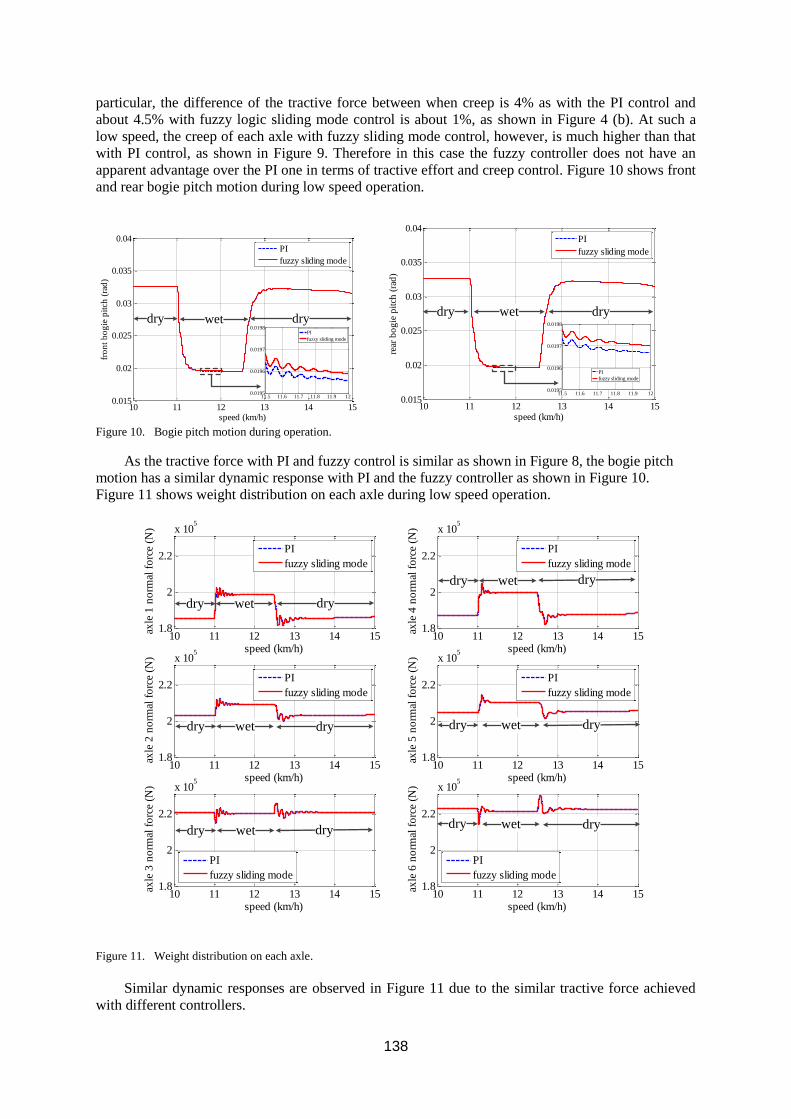
138

particular, the difference of the tractive force between when creep is 4% as with the PI control and

about 4.5% with fuzzy logic sliding mode control is about 1%, as shown in Figure 4 (b). At such a

low speed, the creep of each axle with fuzzy sliding mode control, however, is much higher than that

with PI control, as shown in Figure 9. Therefore in this case the fuzzy controller does not have an

apparent advantage over the PI one in terms of tractive effort and creep control. Figure 10 shows front

and rear bogie pitch motion during low speed operation.

Figure 10. Bogie pitch motion during operation.

As the tractive force with PI and fuzzy control is similar as shown in Figure 8, the bogie pitch

motion has a similar dynamic response with PI and the fuzzy controller as shown in Figure 10.

Figure 11 shows weight distribution on each axle during low speed operation.

Figure 11. Weight distribution on each axle.

Similar dynamic responses are observed in Figure 11 due to the similar tractive force achieved

with different controllers.

10 11 12 13 14 150.015

0.02

0.025

0.03

0.035

0.04

speed (km/h)

fro

nt

bo

gie

pit

ch (

rad

)

PI

fuzzy sliding mode

dry wet dry

11.5 11.6 11.7 11.8 11.9 120.0195

0.0196

0.0197

0.0198

PI

fuzzy sliding mode

10 11 12 13 14 150.015

0.02

0.025

0.03

0.035

0.04

speed (km/h)

rear

bo

gie

pit

ch (

rad

)

PI

fuzzy sliding mode

dry wet dry

11.5 11.6 11.7 11.8 11.9 120.0195

0.0196

0.0197

0.0198

PI

fuzzy sliding mode

10 11 12 13 14 151.8

2

2.2

x 105

speed (km/h)

axle

1 n

orm

al f

orc

e (N

)

PI

fuzzy sliding mode

10 11 12 13 14 151.8

2

2.2

x 105

speed (km/h)

axle

2 n

orm

al f

orc

e (N

)

PI

fuzzy sliding mode

10 11 12 13 14 151.8

2

2.2

x 105

speed (km/h)

axle

3 n

orm

al f

orc

e (N

)

PI

fuzzy sliding mode

10 11 12 13 14 151.8

2

2.2

x 105

speed (km/h)

axle

4 n

orm

al f

orc

e (N

)

PI

fuzzy sliding mode

10 11 12 13 14 151.8

2

2.2

x 105

speed (km/h)

axle

5 n

orm

al f

orc

e (N

)

PI

fuzzy sliding mode

10 11 12 13 14 151.8

2

2.2

x 105

speed (km/h)

axle

6 n

orm

al f

orc

e (N

)

PI

fuzzy sliding mode

dry wet dry

dry wet dry

dry wet dry

dry wet dry

dry

dry

wet

wetdry

dry

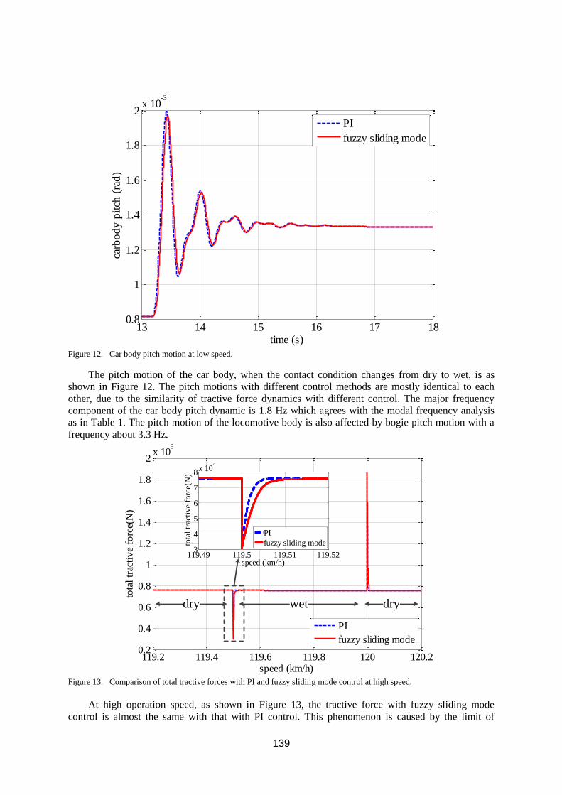
139

Figure 12. Car body pitch motion at low speed.

The pitch motion of the car body, when the contact condition changes from dry to wet, is as

shown in Figure 12. The pitch motions with different control methods are mostly identical to each

other, due to the similarity of tractive force dynamics with different control. The major frequency

component of the car body pitch dynamic is 1.8 Hz which agrees with the modal frequency analysis

as in Table 1. The pitch motion of the locomotive body is also affected by bogie pitch motion with a

frequency about 3.3 Hz.

Figure 13. Comparison of total tractive forces with PI and fuzzy sliding mode control at high speed.

At high operation speed, as shown in Figure 13, the tractive force with fuzzy sliding mode

control is almost the same with that with PI control. This phenomenon is caused by the limit of

13 14 15 16 17 180.8

1

1.2

1.4

1.6

1.8

2x 10

-3

time (s)

carb

od

y p

itch

(ra

d)

PI

fuzzy sliding mode

119.2 119.4 119.6 119.8 120 120.20.2

0.4

0.6

0.8

1

1.2

1.4

1.6

1.8

2x 10

5

speed (km/h)

tota

l tr

acti

ve

forc

e(N

)

PI

fuzzy sliding mode

dry wet dry

119.49 119.5 119.51 119.523

4

5

6

7

8x 10

4

speed (km/h)

tota

l tr

acti

ve

forc

e(N

)

PI

fuzzy sliding mode

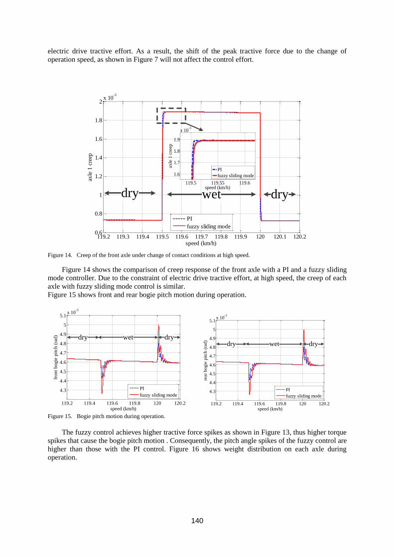
140

electric drive tractive effort. As a result, the shift of the peak tractive force due to the change of

operation speed, as shown in Figure 7 will not affect the control effort.

Figure 14. Creep of the front axle under change of contact conditions at high speed.

Figure 14 shows the comparison of creep response of the front axle with a PI and a fuzzy sliding

mode controller. Due to the constraint of electric drive tractive effort, at high speed, the creep of each

axle with fuzzy sliding mode control is similar.

Figure 15 shows front and rear bogie pitch motion during operation.

Figure 15. Bogie pitch motion during operation.

The fuzzy control achieves higher tractive force spikes as shown in Figure 13, thus higher torque

spikes that cause the bogie pitch motion . Consequently, the pitch angle spikes of the fuzzy control are

higher than those with the PI control. Figure 16 shows weight distribution on each axle during

operation.

119.2 119.3 119.4 119.5 119.6 119.7 119.8 119.9 120 120.1 120.20.6

0.8

1

1.2

1.4

1.6

1.8

2x 10

-3

speed (km/h)

axle

1 c

reep

PI

fuzzy sliding mode

dry wet dry119.5 119.55 119.6

1.6

1.7

1.8

1.9

x 10-3

speed (km/h)

axle

1 c

reep

PI

fuzzy sliding mode

119.2 119.4 119.6 119.8 120 120.2

4.3

4.4

4.5

4.6

4.7

4.8

4.9

5

5.1x 10

-3

speed (km/h)

fro

nt

bo

gie

pit

ch

(ra

d)

PI

fuzzy sliding mode

dry wet dry

119.2 119.4 119.6 119.8 120 120.2

4.3

4.4

4.5

4.6

4.7

4.8

4.9

5

5.1x 10

-3

speed (km/h)

rear

bo

gie

pit

ch (

rad

)

PI

fuzzy sliding mode

dry wet dry

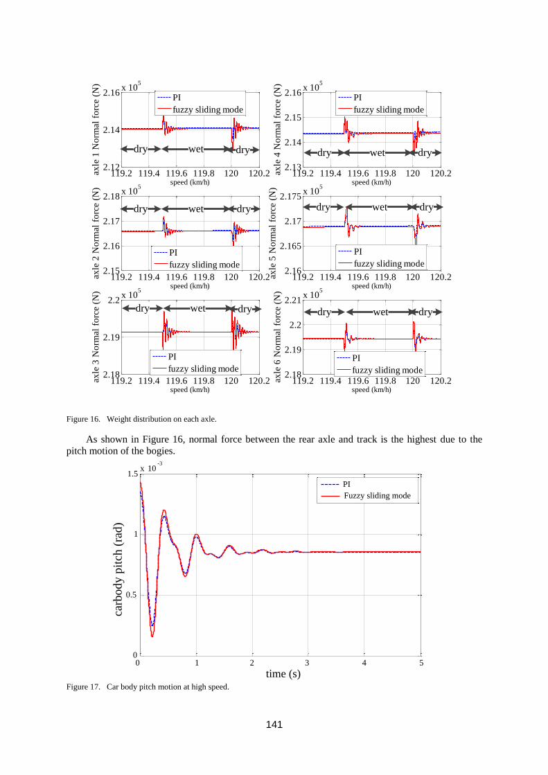
141

Figure 16. Weight distribution on each axle.

As shown in Figure 16, normal force between the rear axle and track is the highest due to the

pitch motion of the bogies.

Figure 17. Car body pitch motion at high speed.

119.2 119.4 119.6 119.8 120 120.22.12

2.14

2.16x 10

5

speed (km/h)

axle

1 N

orm

al f

orc

e (N

)

PI

fuzzy sliding mode

119.2 119.4 119.6 119.8 120 120.22.15

2.16

2.17

2.18x 10

5

speed (km/h)

axle

2 N

orm

al f

orc

e (N

)

PI

fuzzy sliding mode

119.2 119.4 119.6 119.8 120 120.22.18

2.19

2.2x 10

5

speed (km/h)

axle

3 N

orm

al f

orc

e (N

)

PI

fuzzy sliding mode

119.2 119.4 119.6 119.8 120 120.22.13

2.14

2.15

2.16x 10

5

speed (km/h)

axle

4 N

orm

al f

orc

e (N

)

PI

fuzzy sliding mode

119.2 119.4 119.6 119.8 120 120.22.16

2.165

2.17

2.175x 10

5

speed (km/h)

axle

5 N

orm

al f

orc

e (N

)

PI

fuzzy sliding mode

119.2 119.4 119.6 119.8 120 120.22.18

2.19

2.2

2.21x 10

5

speed (km/h)

axle

6 N

orm

al f

orc

e (N

)

PI

fuzzy sliding mode

dry

dry

dry dry

dry

dry

wet

wet

wet

wet

wet

wet

dry

dry

dry

dry

dry

dry

0 1 2 3 4 50

0.5

1

1.5x 10

-3

t

ca

rbo

dy p

itch

(ra

d)

PI

fuzzy sliding mode

PI

Fuzzy sliding mode

carb

od

y p

itch

(ra

d)

0 1 2 3 4 5

time (s)

0

0.5

1

1.5

-310x

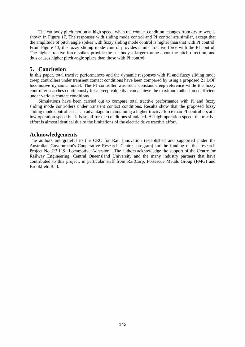
142

The car body pitch motion at high speed, when the contact condition changes from dry to wet, is

shown in Figure 17. The responses with sliding mode control and PI control are similar, except that

the amplitude of pitch angle spikes with fuzzy sliding mode control is higher than that with PI control.

From Figure 13, the fuzzy sliding mode control provides similar tractive force with the PI control.

The higher tractive force spikes provide the car body a larger torque about the pitch direction, and

thus causes higher pitch angle spikes than those with PI control.

5. Conclusion In this paper, total tractive performances and the dynamic responses with PI and fuzzy sliding mode

creep controllers under transient contact conditions have been compared by using a proposed 21 DOF

locomotive dynamic model. The PI controller was set a constant creep reference while the fuzzy

controller searches continuously for a creep value that can achieve the maximum adhesion coefficient

under various contact conditions.

Simulations have been carried out to compare total tractive performance with PI and fuzzy

sliding mode controllers under transient contact conditions. Results show that the proposed fuzzy

sliding mode controller has an advantage in maintaining a higher tractive force than PI controllers at a

low operation speed but it is small for the conditions simulated. At high operation speed, the tractive

effort is almost identical due to the limitations of the electric drive tractive effort.

Acknowledgements The authors are grateful to the CRC for Rail Innovation (established and supported under the

Australian Government's Cooperative Research Centres program) for the funding of this research

Project No. R3.119 “Locomotive Adhesion”. The authors acknowledge the support of the Centre for

Railway Engineering, Central Queensland University and the many industry partners that have

contributed to this project, in particular staff from RailCorp, Fortescue Metals Group (FMG) and

Brookfield Rail.

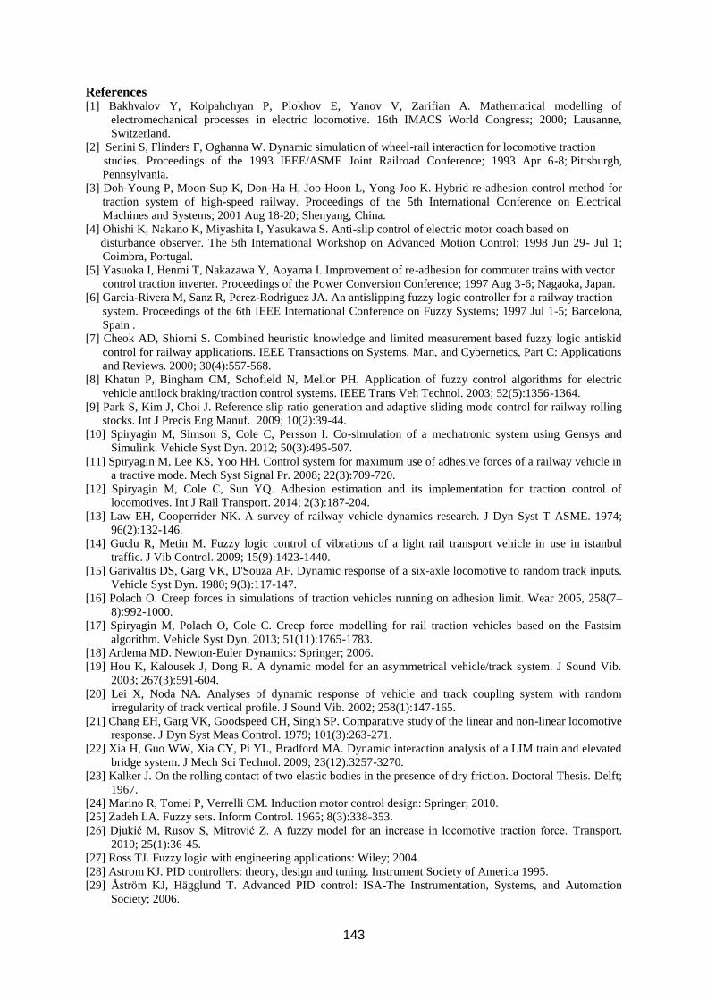
143

References [1] Bakhvalov Y, Kolpahchyan P, Plokhov E, Yanov V, Zarifian A. Mathematical modelling of

electromechanical processes in electric locomotive. 16th IMACS World Congress; 2000; Lausanne,

Switzerland.

[2] Senini S, Flinders F, Oghanna W. Dynamic simulation of wheel-rail interaction for locomotive traction

studies. Proceedings of the 1993 IEEE/ASME Joint Railroad Conference; 1993 Apr 6-8; Pittsburgh,

Pennsylvania.

[3] Doh-Young P, Moon-Sup K, Don-Ha H, Joo-Hoon L, Yong-Joo K. Hybrid re-adhesion control method for

traction system of high-speed railway. Proceedings of the 5th International Conference on Electrical

Machines and Systems; 2001 Aug 18-20; Shenyang, China.

[4] Ohishi K, Nakano K, Miyashita I, Yasukawa S. Anti-slip control of electric motor coach based on

disturbance observer. The 5th International Workshop on Advanced Motion Control; 1998 Jun 29- Jul 1;

Coimbra, Portugal.

[5] Yasuoka I, Henmi T, Nakazawa Y, Aoyama I. Improvement of re-adhesion for commuter trains with vector

control traction inverter. Proceedings of the Power Conversion Conference; 1997 Aug 3-6; Nagaoka, Japan.

[6] Garcia-Rivera M, Sanz R, Perez-Rodriguez JA. An antislipping fuzzy logic controller for a railway traction

system. Proceedings of the 6th IEEE International Conference on Fuzzy Systems; 1997 Jul 1-5; Barcelona,

Spain .

[7] Cheok AD, Shiomi S. Combined heuristic knowledge and limited measurement based fuzzy logic antiskid

control for railway applications. IEEE Transactions on Systems, Man, and Cybernetics, Part C: Applications

and Reviews. 2000; 30(4):557-568.

[8] Khatun P, Bingham CM, Schofield N, Mellor PH. Application of fuzzy control algorithms for electric

vehicle antilock braking/traction control systems. IEEE Trans Veh Technol. 2003; 52(5):1356-1364.

[9] Park S, Kim J, Choi J. Reference slip ratio generation and adaptive sliding mode control for railway rolling

stocks. Int J Precis Eng Manuf. 2009; 10(2):39-44.

[10] Spiryagin M, Simson S, Cole C, Persson I. Co-simulation of a mechatronic system using Gensys and

Simulink. Vehicle Syst Dyn. 2012; 50(3):495-507.

[11] Spiryagin M, Lee KS, Yoo HH. Control system for maximum use of adhesive forces of a railway vehicle in

a tractive mode. Mech Syst Signal Pr. 2008; 22(3):709-720.

[12] Spiryagin M, Cole C, Sun YQ. Adhesion estimation and its implementation for traction control of

locomotives. Int J Rail Transport. 2014; 2(3):187-204.

[13] Law EH, Cooperrider NK. A survey of railway vehicle dynamics research. J Dyn Syst-T ASME. 1974;

96(2):132-146.

[14] Guclu R, Metin M. Fuzzy logic control of vibrations of a light rail transport vehicle in use in istanbul

traffic. J Vib Control. 2009; 15(9):1423-1440.

[15] Garivaltis DS, Garg VK, D'Souza AF. Dynamic response of a six-axle locomotive to random track inputs.

Vehicle Syst Dyn. 1980; 9(3):117-147.

[16] Polach O. Creep forces in simulations of traction vehicles running on adhesion limit. Wear 2005, 258(7–

8):992-1000.

[17] Spiryagin M, Polach O, Cole C. Creep force modelling for rail traction vehicles based on the Fastsim

algorithm. Vehicle Syst Dyn. 2013; 51(11):1765-1783.

[18] Ardema MD. Newton-Euler Dynamics: Springer; 2006.

[19] Hou K, Kalousek J, Dong R. A dynamic model for an asymmetrical vehicle/track system. J Sound Vib.

2003; 267(3):591-604.

[20] Lei X, Noda NA. Analyses of dynamic response of vehicle and track coupling system with random

irregularity of track vertical profile. J Sound Vib. 2002; 258(1):147-165.

[21] Chang EH, Garg VK, Goodspeed CH, Singh SP. Comparative study of the linear and non-linear locomotive

response. J Dyn Syst Meas Control. 1979; 101(3):263-271.

[22] Xia H, Guo WW, Xia CY, Pi YL, Bradford MA. Dynamic interaction analysis of a LIM train and elevated

bridge system. J Mech Sci Technol. 2009; 23(12):3257-3270.

[23] Kalker J. On the rolling contact of two elastic bodies in the presence of dry friction. Doctoral Thesis. Delft;

1967.

[24] Marino R, Tomei P, Verrelli CM. Induction motor control design: Springer; 2010.

[25] Zadeh LA. Fuzzy sets. Inform Control. 1965; 8(3):338-353.

[26] Djukić M, Rusov S, Mitrović Z. A fuzzy model for an increase in locomotive traction force. Transport.

2010; 25(1):36-45.

[27] Ross TJ. Fuzzy logic with engineering applications: Wiley; 2004.

[28] Astrom KJ. PID controllers: theory, design and tuning. Instrument Society of America 1995.

[29] Åström KJ, Hägglund T. Advanced PID control: ISA-The Instrumentation, Systems, and Automation

Society; 2006.

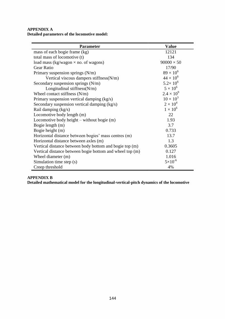
144

APPENDIX A

Detailed parameters of the locomotive model:

Parameter Value

mass of each bogie frame (kg) 12121

total mass of locomotive (t) 134

load mass (kg/wagon × no. of wagons) 90000 × 50

Gear Ratio 17/90

Primary suspension springs (N/m) 89 × 106

Vertical viscous dampers stiffness(N/m) 44 × 106

Secondary suspension springs (N/m) 5.2× 106

Longitudinal stiffness(N/m) 5 × 106

Wheel contact stiffness (N/m) 2.4 × 109

Primary suspension vertical damping (kg/s) 10 × 103

Secondary suspension vertical damping (kg/s) 2 × 104

Rail damping (kg/s) 1 × 106

Locomotive body length (m) 22

Locomotive body height – without bogie (m) 1.93

Bogie length (m) 3.7

Bogie height (m) 0.733

Horizontal distance between bogies’ mass centres (m) 13.7

Horizontal distance between axles (m) 1.3

Vertical distance between body bottom and bogie top (m) 0.3605

Vertical distance between bogie bottom and wheel top (m) 0.127

Wheel diameter (m) 1.016

Simulation time step (s) 5×10-6

Creep threshold 4%

APPENDIX B

Detailed mathematical model for the longitudinal-vertical-pitch dynamics of the locomotive

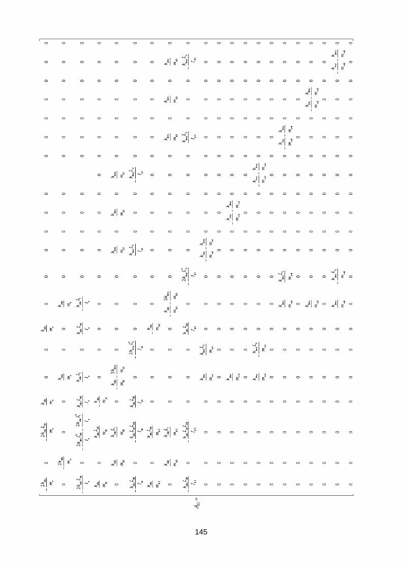
145

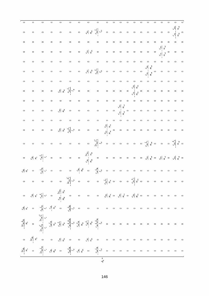
146

147

Paper D

Investigation of the impact of full scale locomotive

adhesion control on wear under changing contact

conditions

148

Investigation of the impact of locomotive creep control on wear under changing contact conditions

Ye Tian1, 2,Sheng Liu1, W.J.T. (Bill) Daniel1, 2 , Paul A. Meehan1, 2

1School of Mechanical and Mining Engineering, the University of Queensland, Queensland, Australia 4072

2Cooperative Research Centre for Railway Innovation (CRC Rail), Queensland, Australia

ABSTRACT This paper presents the locomotive traction controller performance with respect to the track wear under

different operation conditions. In particular, an investigation into the dynamic response of a locomotive

under changing wheel-rail friction conditions is performed with an aim to determine the effect of controller

setting on track wear. Simulation using a full scale longitudinal–vertical locomotive dynamic model shows

that the appropriately designed creep threshold, controller, settings can effectively maintain high tractive

effort while avoiding excessive rail damage due to wear, especially during acceleration under low speed.

Nomenclature

𝑥𝑐 Locomotive body longitudinal displacement

𝑧𝑐 Locomotive body vertical displacement

𝜃𝑐 Locomotive body pitch angle

𝑥𝑏1,2 Locomotive front/rear bogie longitudinal displacement

𝑧𝑏1,2 Locomotive front/rear bogie vertical displacement

𝜃𝑏1,2 Locomotive front/rear bogie pitch displacement

𝑧𝑤1~6 Wheelset 1~6 vertical displacement

𝜃𝑤1~6 Wheelset 1~6 rotation angle

𝑀𝑐 𝑀𝑏 𝑀𝑤 Mass of locomotive body, bogie and axle

𝐼𝑐 𝐼𝑏 𝐼𝑤 Moment of inertia of locomotive body, bogie and axle along pitch direction

𝑄 Wheel load

𝜇 Friction coefficient

휀 Gradient of the tangential stress in the area of adhesion

𝑘𝐴, 𝑘𝑠 Reduction factor in the area of adhesion, reduction factor in the area of slip

𝜇∞ Friction coefficient at infinity slip velocity

𝜇0 Maximum friction coefficient at zero slip velocity

𝑠𝑥 Creep in longitudinal (x) directions

𝑉 Vehicle speed

𝑤𝑥 Creep (slip) velocity in longitudinal (x) direction

𝑎, 𝑏 Half-axes of the contact ellipse

𝑐11 Coefficient from Kalker’s linear theory

𝐹, 𝐺 Tractive force, Shear modulus

𝑇𝑡𝑖 Torque generated by electric drive 𝑖=1~6

𝑇𝑙𝑖 Torque acting on axle 𝑖=1~6 generated by longitudinal contact force

149

1. Introduction

The progressive application of high traction motors and control techniques based on power electronics has

brought great benefits to the rail industry due to its high power capacity and efficiency. Therefore, an

effective locomotive control system is demanded to suit the contemporary high speed railway network.

Traditionally, the traction controller performance and dynamic impact on the rail are assessed under specific

steady state conditions. In particular, traction controller performance under natural perturbations in

friction/lubrication, wheel/rail profiles, track curvature, vehicle/track dynamics, wheel/track imperfections

etc. has not been comprehensively investigated yet. Among those perturbations, the changes in friction or

lubrication can cause sudden changes of creep and often leads to over/under traction/braking. In order to

investigate this issue, a predictive locomotive dynamic model combining crucial dynamic components such

as locomotive rigid body dynamics, contact dynamics and electric drive and control is needed.

Locomotive traction dynamics and rail wear have been investigated by several researchers. Bakhvalov et al.

combined electrical and mechanical processes for locomotive traction simulation [1]. Senini et al. has also

performed locomotive traction simulation at the electric drive level [2]. These works, however, are not

focused on the effect of transient of the contact conditions and different controller settings on the rail wear;

especially for a full-scale locomotive case. Modern development of mechatronics systems has improved rail

vehicle operation under various conditions. The traction control system, also known as an adhesion or anti-

slip control system is essential for the operational efficiency and reliability of these systems. A pattern-based

slip control method has been applied and modified by Park et al. [3]. An anti-slip control method based on a

disturbance observer was proposed by Ohishi et al. [4]. Yasuoka et al. proposed a slip control method [5]

involving bogie oscillation suppression. Most recently Spiryagin et al. employed a co-simulation approach

with the Gensys multibody code and Simulink to investigate the heavy haul train traction dynamics [6] and

fuzzy logic control [7] and adhesion estimation based control [8] to maximize adhesive forces. Yuan et al.

proposed a fuzzy logic adhesion controller [9]. Mei et al. investigated a mechatronic approach to control the

wheel slip based on the information on the torsional vibration of the wheelset [10]. Zhao et al. proposed an

extended Kalman filter (EKF) based re-adhesion controller [11]. All these methods are reported to be

effective in creep/traction control; however, the implementation of these methods to the rail industry can be

challenging or costly as these methods require for the reliable high speed processors and/or high accuracy

sensors. While on the other hand, a PI/PID controller has is one of the most widely used control methods in

various industrial applications, comparing to methods such as fuzzy logic control, observer based control,

extended Kalman filter based or torsional vibration based control. As a result, a PI controller is employed in

this work to reveal the real case of locomotive operation and its possible effects on rail wear with different

controller parameters. Wear phenomenon in the rail industry and its modelling has been studied for decades

[12-15], however, the impact of locomotive dynamic response on wear phenomena under different

conditions has not been investigated deeply.

In this paper, the dynamic response of a full scale locomotive model with a traction controller under different

speed and/or contact conditions is investigated in relation to the rail wear. This work focus on longitudinal

and vertical dynamics on tangent tracks as it is the most important part of locomotive dynamics closely

related with traction/braking effort, passenger comfort and energy management [16]. A full scale locomotive

longitudinal-vertical-pitch dynamic model with a PI creep controller combining all crucial dynamic

components is developed and implemented using Matlab/Simulink and the wear rate [15] is compared before

and after a change of contact conditions under a range of operational speed. A Newton-Euler method [17, 18]

is used to obtain the motion equations of the locomotive model. For the contact mechanics, Polach’s

adhesion model [19] is adopted as it has been verified to be relatively accurate for the application in the field

of locomotive traction analysis [20].

2. Simulation modelling In order to study the impact of the operation of a full scale locomotive on rail damage due to wear

phenomenon, a model considering all essential dynamic components needs to be developed. In this study,

three major subsystems are taken into consideration for the modelling process; namely, a mathematical

model representing the dynamics of a locomotive along longitudinal and vertical directions, electric

drive/control dynamics, and contact mechanics. The structure of the model is shown in Figure 1. A dynamic

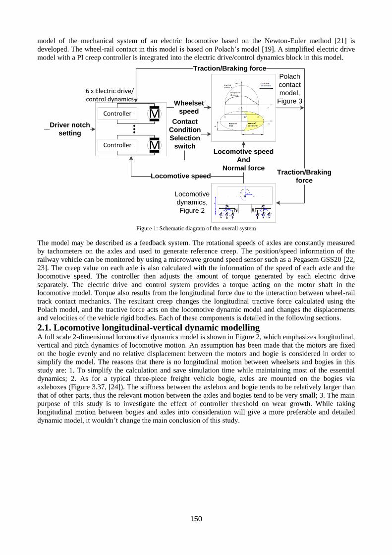
150

model of the mechanical system of an electric locomotive based on the Newton-Euler method [21] is

developed. The wheel-rail contact in this model is based on Polach’s model [19]. A simplified electric drive

model with a PI creep controller is integrated into the electric drive/control dynamics block in this model.

Figure 1: Schematic diagram of the overall system

The model may be described as a feedback system. The rotational speeds of axles are constantly measured

by tachometers on the axles and used to generate reference creep. The position/speed information of the

railway vehicle can be monitored by using a microwave ground speed sensor such as a Pegasem GSS20 [22,

23]. The creep value on each axle is also calculated with the information of the speed of each axle and the

locomotive speed. The controller then adjusts the amount of torque generated by each electric drive

separately. The electric drive and control system provides a torque acting on the motor shaft in the

locomotive model. Torque also results from the longitudinal force due to the interaction between wheel-rail

track contact mechanics. The resultant creep changes the longitudinal tractive force calculated using the

Polach model, and the tractive force acts on the locomotive dynamic model and changes the displacements

and velocities of the vehicle rigid bodies. Each of these components is detailed in the following sections.

2.1. Locomotive longitudinal-vertical dynamic modelling A full scale 2-dimensional locomotive dynamics model is shown in Figure 2, which emphasizes longitudinal,

vertical and pitch dynamics of locomotive motion. An assumption has been made that the motors are fixed

on the bogie evenly and no relative displacement between the motors and bogie is considered in order to

simplify the model. The reasons that there is no longitudinal motion between wheelsets and bogies in this

study are: 1. To simplify the calculation and save simulation time while maintaining most of the essential

dynamics; 2. As for a typical three-piece freight vehicle bogie, axles are mounted on the bogies via

axleboxes (Figure 3.37, [24]). The stiffness between the axlebox and bogie tends to be relatively larger than

that of other parts, thus the relevant motion between the axles and bogies tend to be very small; 3. The main

purpose of this study is to investigate the effect of controller threshold on wear growth. While taking

longitudinal motion between bogies and axles into consideration will give a more preferable and detailed

dynamic model, it wouldn’t change the main conclusion of this study.

Driver notch

setting

Wheelset

speed

Locomotive speed

And

Normal forceTraction/Braking

force

Contact

Condition

Selection

switch

Locomotive

dynamics,

Figure 2

Polach

contact

model,

Figure 3

MController

Traction/Braking force

Locomotive speed

6 x Electric drive/control dynamics

MController

050

100 0 0.1 0.2 0.3 0.4 0.5

0

0.1

0.2

0.3

0.4

0.5

0.6

0.7

creep

Polach dry

loco velocity km/h

adhesio

n c

oeffic

ient

0

0.1

0.2

0.3

0.4

0.5

Polach creep

Electric drive & control

Complex locomotiv

M

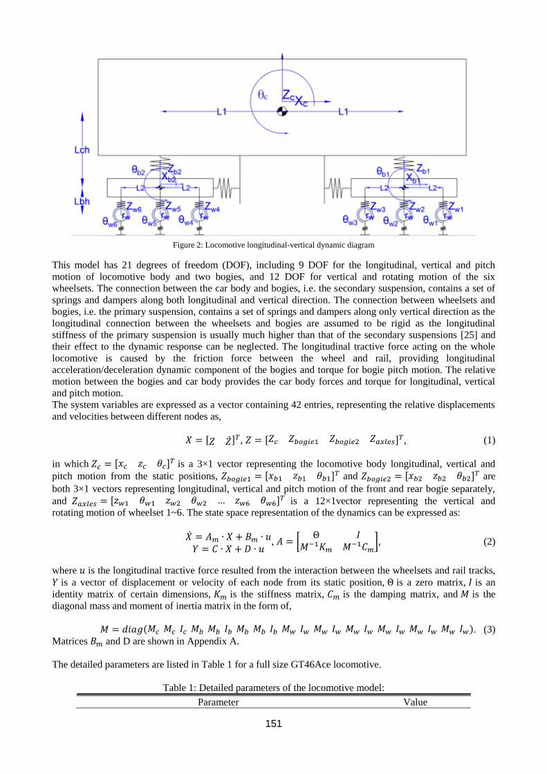
151

Figure 2: Locomotive longitudinal-vertical dynamic diagram

This model has 21 degrees of freedom (DOF), including 9 DOF for the longitudinal, vertical and pitch

motion of locomotive body and two bogies, and 12 DOF for vertical and rotating motion of the six

wheelsets. The connection between the car body and bogies, i.e. the secondary suspension, contains a set of

springs and dampers along both longitudinal and vertical direction. The connection between wheelsets and

bogies, i.e. the primary suspension, contains a set of springs and dampers along only vertical direction as the

longitudinal connection between the wheelsets and bogies are assumed to be rigid as the longitudinal

stiffness of the primary suspension is usually much higher than that of the secondary suspensions [25] and

their effect to the dynamic response can be neglected. The longitudinal tractive force acting on the whole

locomotive is caused by the friction force between the wheel and rail, providing longitudinal

acceleration/deceleration dynamic component of the bogies and torque for bogie pitch motion. The relative

motion between the bogies and car body provides the car body forces and torque for longitudinal, vertical

and pitch motion.

The system variables are expressed as a vector containing 42 entries, representing the relative displacements

and velocities between different nodes as,

𝑋 = [𝑍 ��]𝑇, 𝑍 = [𝑍𝑐 𝑍𝑏𝑜𝑔𝑖𝑒1 𝑍𝑏𝑜𝑔𝑖𝑒2 𝑍𝑎𝑥𝑙𝑒𝑠]𝑇, (1)

in which 𝑍𝑐 = [𝑥𝑐 𝑧𝑐 𝜃𝑐]𝑇 is a 3×1 vector representing the locomotive body longitudinal, vertical and

pitch motion from the static positions, 𝑍𝑏𝑜𝑔𝑖𝑒1 = [𝑥𝑏1 𝑧𝑏1 𝜃𝑏1]𝑇 and 𝑍𝑏𝑜𝑔𝑖𝑒2 = [𝑥𝑏2 𝑧𝑏2 𝜃𝑏2]

𝑇 are

both 3×1 vectors representing longitudinal, vertical and pitch motion of the front and rear bogie separately,

and 𝑍𝑎𝑥𝑙𝑒𝑠 = [𝑧𝑤1 𝜃𝑤1 𝑧𝑤2 𝜃𝑤2 … 𝑧𝑤6 𝜃𝑤6]𝑇 is a 12×1vector representing the vertical and

rotating motion of wheelset 1~6. The state space representation of the dynamics can be expressed as:

�� = 𝐴𝑚 ∙ 𝑋 + 𝐵𝑚 ∙ 𝑢𝑌 = 𝐶 ∙ 𝑋 + 𝐷 ∙ 𝑢

, 𝐴 = [Θ 𝐼

𝑀−1𝐾𝑚 𝑀−1𝐶𝑚], (2)

where 𝑢 is the longitudinal tractive force resulted from the interaction between the wheelsets and rail tracks,

𝑌 is a vector of displacement or velocity of each node from its static position, Θ is a zero matrix, 𝐼 is an

identity matrix of certain dimensions, 𝐾𝑚 is the stiffness matrix, 𝐶𝑚 is the damping matrix, and 𝑀 is the

diagonal mass and moment of inertia matrix in the form of,

𝑀 = 𝑑𝑖𝑎𝑔(𝑀𝑐 𝑀𝑐 𝐼𝑐 𝑀𝑏 𝑀𝑏 𝐼𝑏 𝑀𝑏 𝑀𝑏 𝐼𝑏 𝑀𝑤 𝐼𝑤 𝑀𝑤 𝐼𝑤 𝑀𝑤 𝐼𝑤 𝑀𝑤 𝐼𝑤 𝑀𝑤 𝐼𝑤 𝑀𝑤 𝐼𝑤). (3)

Matrices 𝐵𝑚 and D are shown in Appendix A.

The detailed parameters are listed in Table 1 for a full size GT46Ace locomotive.

Table 1: Detailed parameters of the locomotive model:

Parameter Value

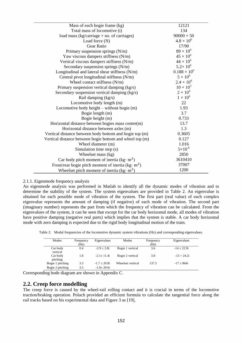
152

Mass of each bogie frame (kg) 12121

Total mass of locomotive (t) 134

load mass (kg/carriage × no. of carriages) 90000 × 50

Load force (N) 4.8 × 106

Gear Ratio 17/90

Primary suspension springs (N/m) 89 × 106

Yaw viscous dampers stiffness (N/m) 45 × 106

Vertical viscous dampers stiffness (N/m) 44 × 106

Secondary suspension springs (N/m) 5.2× 106

Longitudinal and lateral shear stiffness (N/m) 0.188 × 106

Central pivot longitudinal stiffness (N/m) 5 × 106

Wheel contact stiffness (N/m) 2.4 × 109

Primary suspension vertical damping (kg/s) 10 × 103

Secondary suspension vertical damping (kg/s) 2 × 104

Rail damping (kg/s) 1 × 106

Locomotive body length (m) 22

Locomotive body height – without bogie (m) 1.93

Bogie length (m) 3.7

Bogie height (m) 0.733

Horizontal distance between bogies mass centre(m) 13.7

Horizontal distance between axles (m) 1.3

Vertical distance between body bottom and bogie top (m) 0.3605

Vertical distance between bogie bottom and wheel top (m) 0.127

Wheel diameter (m) 1.016

Simulation time step (s)

Wheelset mass (kg)

Car body pitch moment of inertia (kg· m2)

Front/rear bogie pitch moment of inertia (kg· m2)

Wheelset pitch moment of inertia (kg· m2)

5×10-6

2850

3610410

37007

1200

2.1.1. Eigenmode frequency analysis

An eigenmode analysis was performed in Matlab to identify all the dynamic modes of vibration and to

determine the stability of the system. The system eigenvalues are provided in Table 2. An eigenvalue is

obtained for each possible mode of vibration of the system. The first part (real value) of each complex

eigenvalue represents the amount of damping (if negative) of each mode of vibration. The second part

(imaginary number) represents the part from which the frequency of vibration can be calculated. From the

eigenvalues of the system, it can be seen that except for the car body horizontal mode, all modes of vibration

have positive damping (negative real parts) which implies that the system is stable. A car body horizontal

mode with zero damping is expected due to the rigid body longitudinal motion of the train.

Table 2: Modal frequencies of the locomotive dynamic system vibrations (Hz) and corresponding eigenvalues.

Modes Frequency

(Hz)

Eigenvalues Modes Frequency

(Hz)

Eigenvalues

Car body

vertical

0.4 -2.9 ± 2.8i Bogie 1 vertical 3.6 -14 ± 22.9i

Car body

pitching

1.8 -2.1± 11.4i Bogie 2 vertical 3.8 -13 + 24.2i

Bogie 1 pitching 3.3 -1.7 ± 20.8i Wheelset vertical 137.5 -17 ± 864i

Bogie 2 pitching 3.3 -1.6± 20.6i

Corresponding bode diagram are shown in Appendix C.

2.2. Creep force modelling The creep force is caused by the wheel-rail rolling contact and it is crucial in terms of the locomotive

traction/braking operation. Polach provided an efficient formula to calculate the tangential force along the

rail tracks based on his experimental data and Figure 3 as [19],

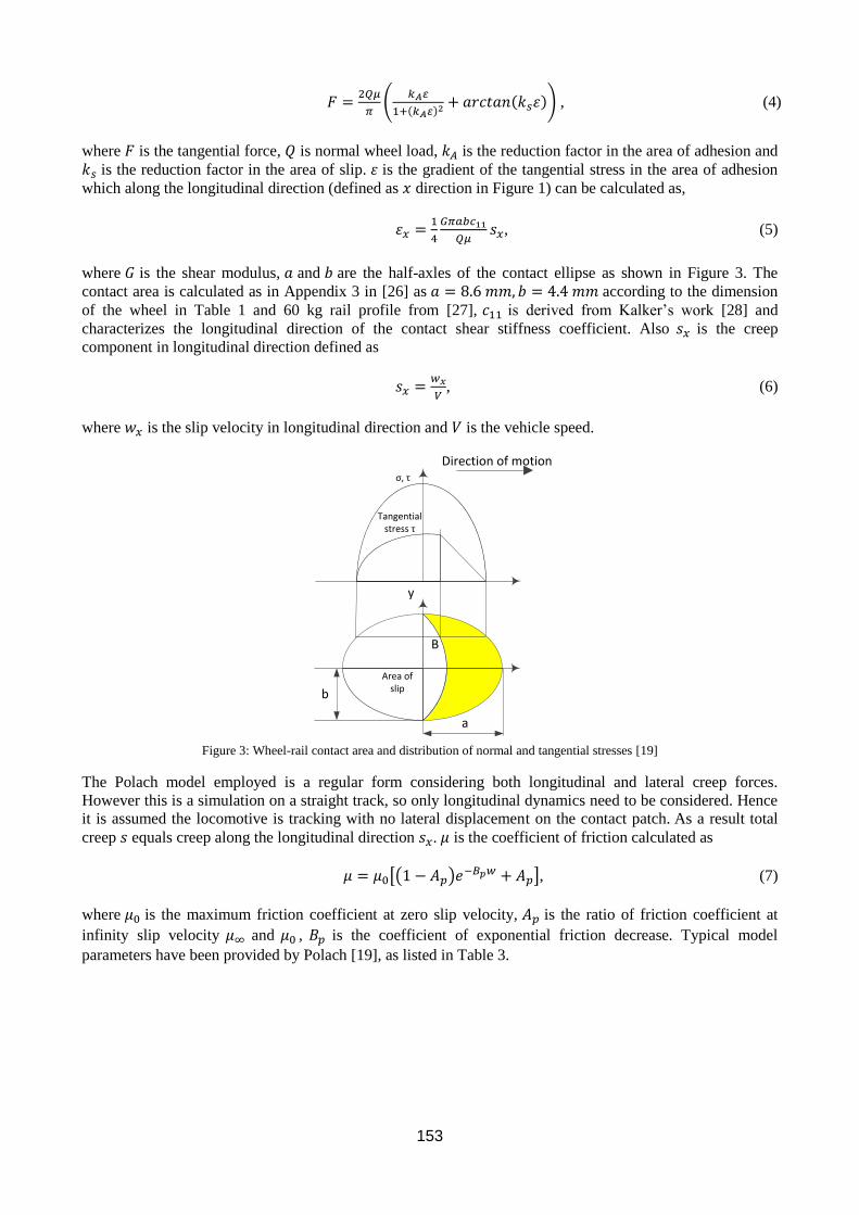
153

𝐹 =2𝑄𝜇

𝜋(

𝑘𝐴𝜀

1+(𝑘𝐴𝜀)2 + 𝑎𝑟𝑐𝑡𝑎𝑛(𝑘𝑠휀)) , (4)

where 𝐹 is the tangential force, 𝑄 is normal wheel load, 𝑘𝐴 is the reduction factor in the area of adhesion and

𝑘𝑠 is the reduction factor in the area of slip. 휀 is the gradient of the tangential stress in the area of adhesion

which along the longitudinal direction (defined as 𝑥 direction in Figure 1) can be calculated as,

휀𝑥 =1

4

𝐺𝜋𝑎𝑏𝑐11

𝑄𝜇𝑠𝑥, (5)

where 𝐺 is the shear modulus, 𝑎 and 𝑏 are the half-axles of the contact ellipse as shown in Figure 3. The

contact area is calculated as in Appendix 3 in [26] as 𝑎 = 8.6 𝑚𝑚, 𝑏 = 4.4 𝑚𝑚 according to the dimension

of the wheel in Table 1 and 60 kg rail profile from [27], 𝑐11 is derived from Kalker’s work [28] and

characterizes the longitudinal direction of the contact shear stiffness coefficient. Also 𝑠𝑥 is the creep

component in longitudinal direction defined as

𝑠𝑥 =𝑤𝑥

𝑉, (6)

where 𝑤𝑥 is the slip velocity in longitudinal direction and 𝑉 is the vehicle speed.

Figure 3: Wheel-rail contact area and distribution of normal and tangential stresses [19]

The Polach model employed is a regular form considering both longitudinal and lateral creep forces.

However this is a simulation on a straight track, so only longitudinal dynamics need to be considered. Hence

it is assumed the locomotive is tracking with no lateral displacement on the contact patch. As a result total

creep 𝑠 equals creep along the longitudinal direction 𝑠𝑥. 𝜇 is the coefficient of friction calculated as

𝜇 = 𝜇0[(1 − 𝐴𝑝)𝑒−𝐵𝑝𝑤 + 𝐴𝑝], (7)

where 𝜇0 is the maximum friction coefficient at zero slip velocity, 𝐴𝑝 is the ratio of friction coefficient at

infinity slip velocity 𝜇∞ and 𝜇0 , 𝐵𝑝 is the coefficient of exponential friction decrease. Typical model

parameters have been provided by Polach [19], as listed in Table 3.

y

Direction of motion

Tangentialstress τ

Area of slip

B

σ, τ

b

a

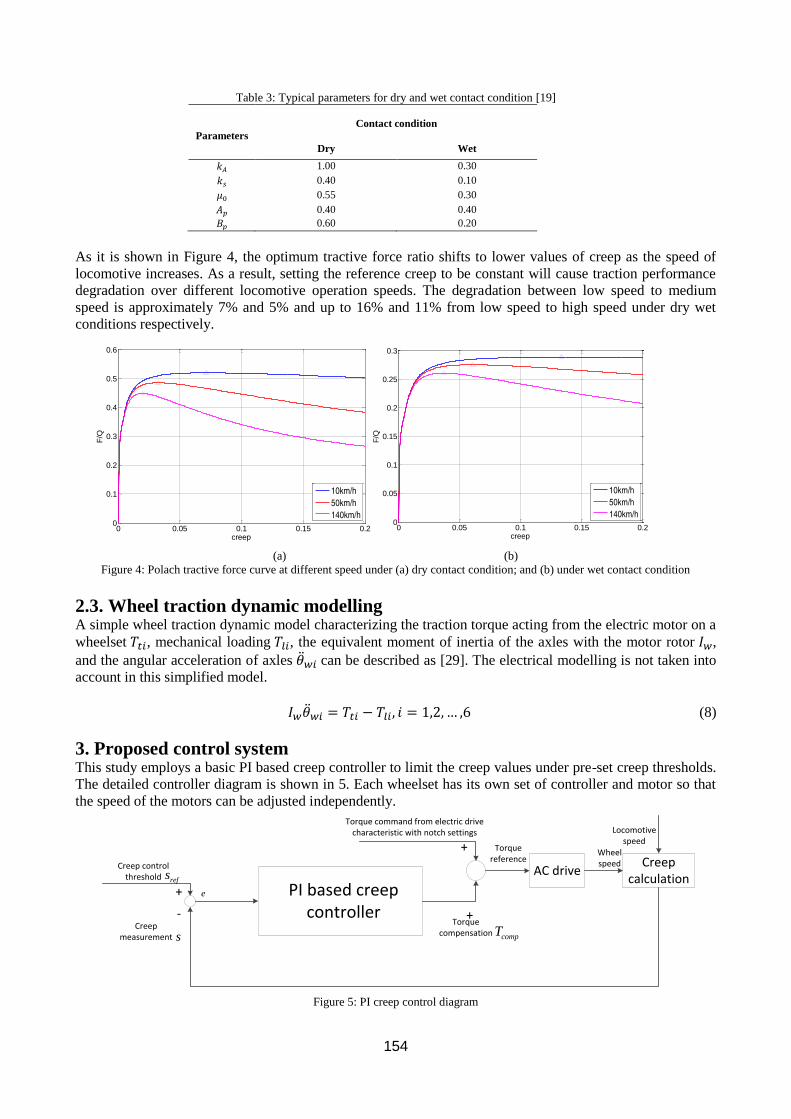
154

Table 3: Typical parameters for dry and wet contact condition [19]

Parameters

Contact condition

Dry Wet

𝑘𝐴 1.00 0.30

𝑘𝑠 0.40 0.10

𝜇0 0.55 0.30

𝐴𝑝 0.40 0.40

𝐵𝑝 0.60 0.20

As it is shown in Figure 4, the optimum tractive force ratio shifts to lower values of creep as the speed of

locomotive increases. As a result, setting the reference creep to be constant will cause traction performance

degradation over different locomotive operation speeds. The degradation between low speed to medium

speed is approximately 7% and 5% and up to 16% and 11% from low speed to high speed under dry wet

conditions respectively.

(a) (b)

Figure 4: Polach tractive force curve at different speed under (a) dry contact condition; and (b) under wet contact condition

2.3. Wheel traction dynamic modelling A simple wheel traction dynamic model characterizing the traction torque acting from the electric motor on a

wheelset 𝑇𝑡𝑖, mechanical loading 𝑇𝑙𝑖, the equivalent moment of inertia of the axles with the motor rotor 𝐼𝑤,

and the angular acceleration of axles ��𝑤𝑖 can be described as [29]. The electrical modelling is not taken into

account in this simplified model.

𝐼𝑤��𝑤𝑖 = 𝑇𝑡𝑖 − 𝑇𝑙𝑖, 𝑖 = 1,2,… ,6 (8)

3. Proposed control system This study employs a basic PI based creep controller to limit the creep values under pre-set creep thresholds.

The detailed controller diagram is shown in 5. Each wheelset has its own set of controller and motor so that

the speed of the motors can be adjusted independently.

Figure 5: PI creep control diagram

0 0.05 0.1 0.15 0.20

0.05

0.1

0.15

0.2

0.25

0.3

creep

F/Q

10km/h

50km/h

140km/h

0 0.05 0.1 0.15 0.20

0.1

0.2

0.3

0.4

0.5

0.6

creep

F/Q

10km/h

50km/h

140km/h

PI based creep controller

Torque command from electric drive characteristic with notch settings

Creep control threshold

Creep measurement

Torque reference

+

+

+

-

refs

s

AC drive

Wheel speed

Locomotive speed

Creep calculation

e

Torque compensation compT

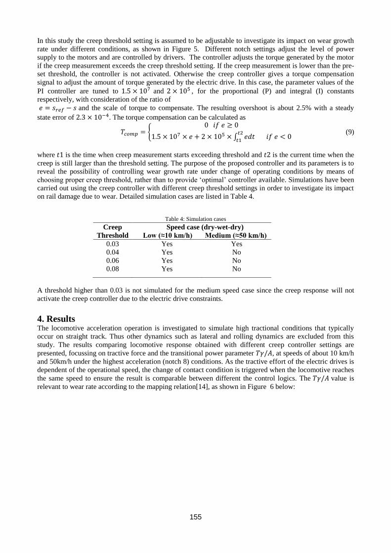
155

In this study the creep threshold setting is assumed to be adjustable to investigate its impact on wear growth

rate under different conditions, as shown in Figure 5. Different notch settings adjust the level of power

supply to the motors and are controlled by drivers. The controller adjusts the torque generated by the motor

if the creep measurement exceeds the creep threshold setting. If the creep measurement is lower than the pre-

set threshold, the controller is not activated. Otherwise the creep controller gives a torque compensation

signal to adjust the amount of torque generated by the electric drive. In this case, the parameter values of the

PI controller are tuned to 1.5 × 107 and 2 × 105 , for the proportional (P) and integral (I) constants

respectively, with consideration of the ratio of

𝑒 = 𝑠𝑟𝑒𝑓 − 𝑠 and the scale of torque to compensate. The resulting overshoot is about 2.5% with a steady

state error of 2.3 × 10−4. The torque compensation can be calculated as

𝑇𝑐𝑜𝑚𝑝 = {0 𝑖𝑓 𝑒 ≥ 0

1.5 × 107 × 𝑒 + 2 × 105 × ∫ 𝑒𝑑𝑡 𝑖𝑓 𝑒 < 0𝑡2

𝑡1

(9)

where 𝑡1 is the time when creep measurement starts exceeding threshold and 𝑡2 is the current time when the

creep is still larger than the threshold setting. The purpose of the proposed controller and its parameters is to

reveal the possibility of controlling wear growth rate under change of operating conditions by means of

choosing proper creep threshold, rather than to provide ‘optimal’ controller available. Simulations have been

carried out using the creep controller with different creep threshold settings in order to investigate its impact

on rail damage due to wear. Detailed simulation cases are listed in Table 4.

Table 4: Simulation cases

Creep

Threshold

Speed case (dry-wet-dry)

Low (≈10 km/h) Medium (≈50 km/h)

0.03 Yes Yes

0.04 Yes No

0.06 Yes No

0.08 Yes No

A threshold higher than 0.03 is not simulated for the medium speed case since the creep response will not

activate the creep controller due to the electric drive constraints.

4. Results The locomotive acceleration operation is investigated to simulate high tractional conditions that typically

occur on straight track. Thus other dynamics such as lateral and rolling dynamics are excluded from this

study. The results comparing locomotive response obtained with different creep controller settings are

presented, focussing on tractive force and the transitional power parameter 𝑇𝛾/𝐴, at speeds of about 10 km/h

and 50km/h under the highest acceleration (notch 8) conditions. As the tractive effort of the electric drives is

dependent of the operational speed, the change of contact condition is triggered when the locomotive reaches

the same speed to ensure the result is comparable between different the control logics. The 𝑇𝛾/𝐴 value is

relevant to wear rate according to the mapping relation[14], as shown in Figure 6 below:

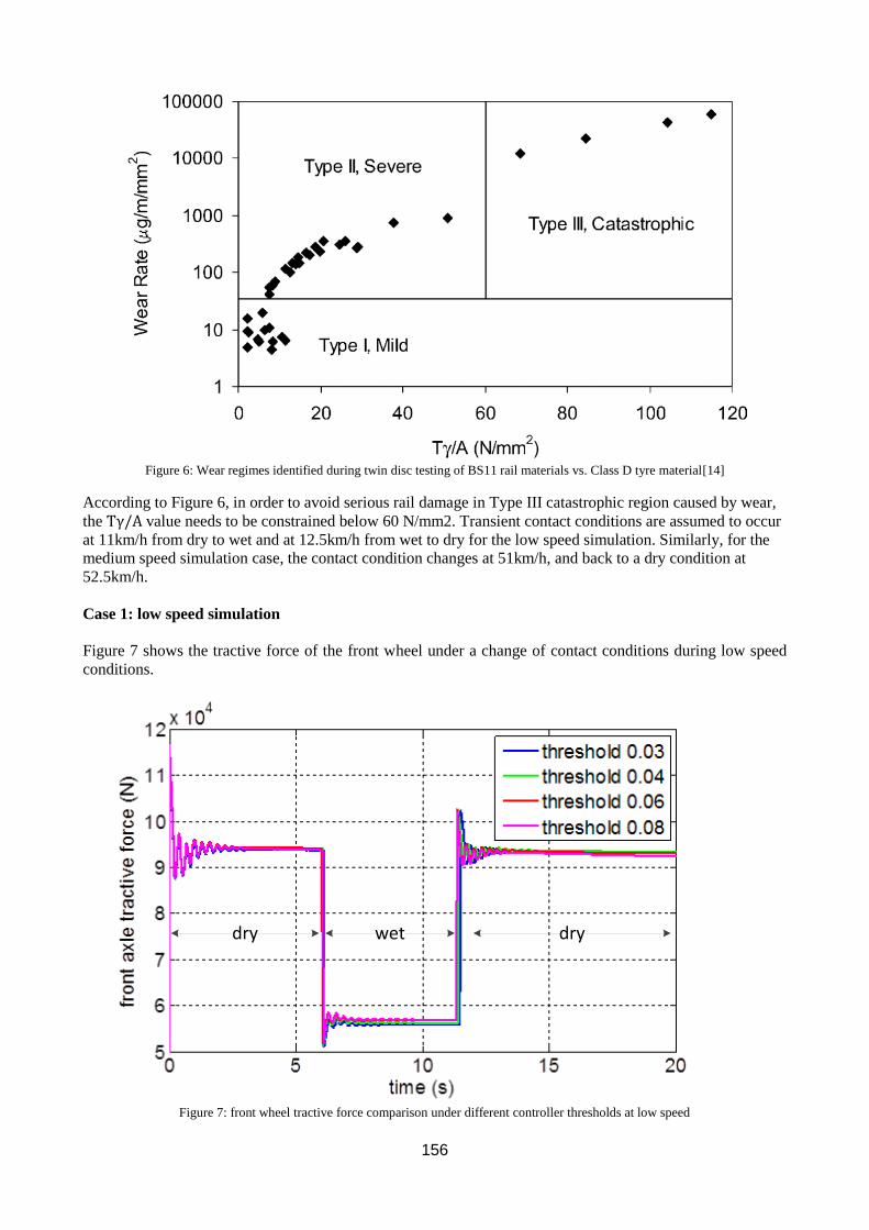
156

Figure 6: Wear regimes identified during twin disc testing of BS11 rail materials vs. Class D tyre material[14]

According to Figure 6, in order to avoid serious rail damage in Type III catastrophic region caused by wear,

the Tγ/A value needs to be constrained below 60 N/mm2. Transient contact conditions are assumed to occur

at 11km/h from dry to wet and at 12.5km/h from wet to dry for the low speed simulation. Similarly, for the

medium speed simulation case, the contact condition changes at 51km/h, and back to a dry condition at

52.5km/h.

Case 1: low speed simulation

Figure 7 shows the tractive force of the front wheel under a change of contact conditions during low speed

conditions.

Figure 7: front wheel tractive force comparison under different controller thresholds at low speed

dry drywet

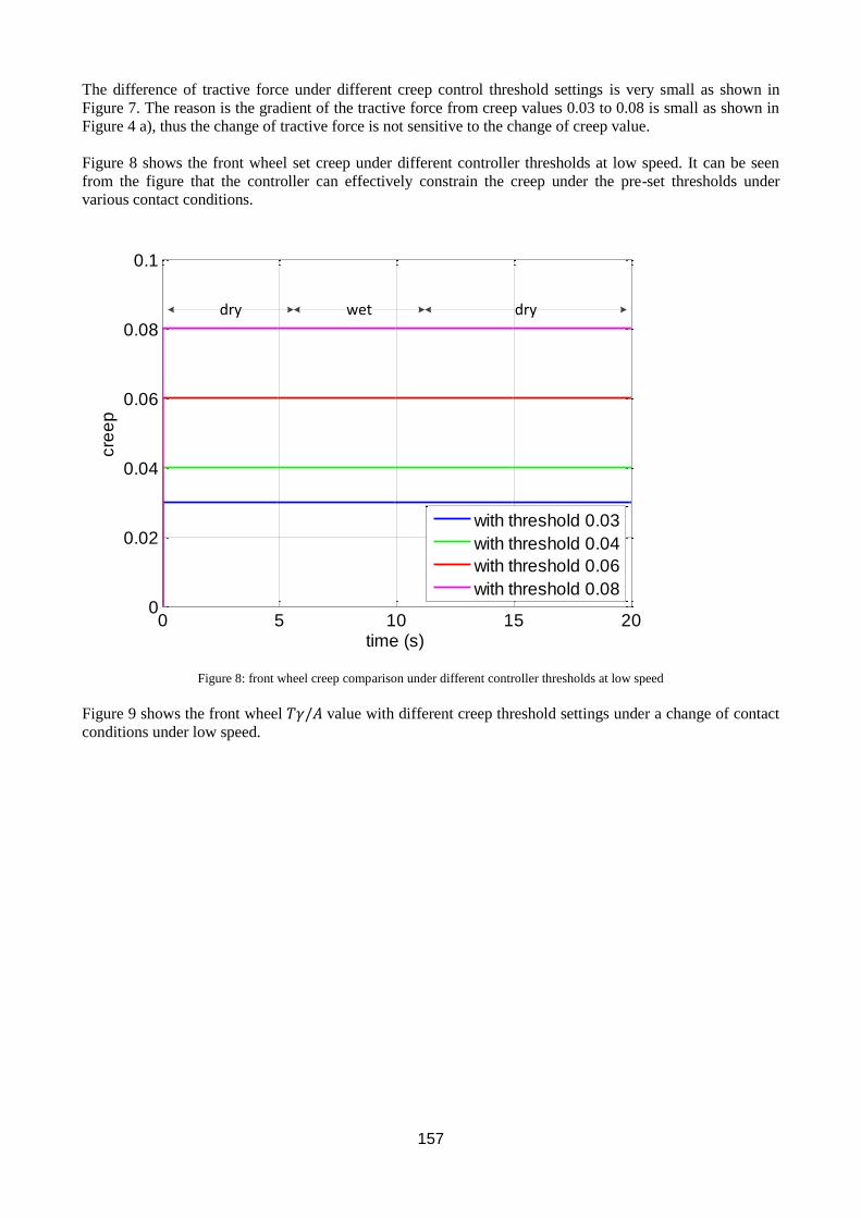
157

The difference of tractive force under different creep control threshold settings is very small as shown in

Figure 7. The reason is the gradient of the tractive force from creep values 0.03 to 0.08 is small as shown in

Figure 4 a), thus the change of tractive force is not sensitive to the change of creep value.

Figure 8 shows the front wheel set creep under different controller thresholds at low speed. It can be seen

from the figure that the controller can effectively constrain the creep under the pre-set thresholds under

various contact conditions.

Figure 8: front wheel creep comparison under different controller thresholds at low speed

Figure 9 shows the front wheel 𝑇𝛾/𝐴 value with different creep threshold settings under a change of contact

conditions under low speed.

0 5 10 15 200

0.02

0.04

0.06

0.08

0.1

time (s)

cre

ep

with threshold 0.03

with threshold 0.04

with threshold 0.06

with threshold 0.08

dry wet dry

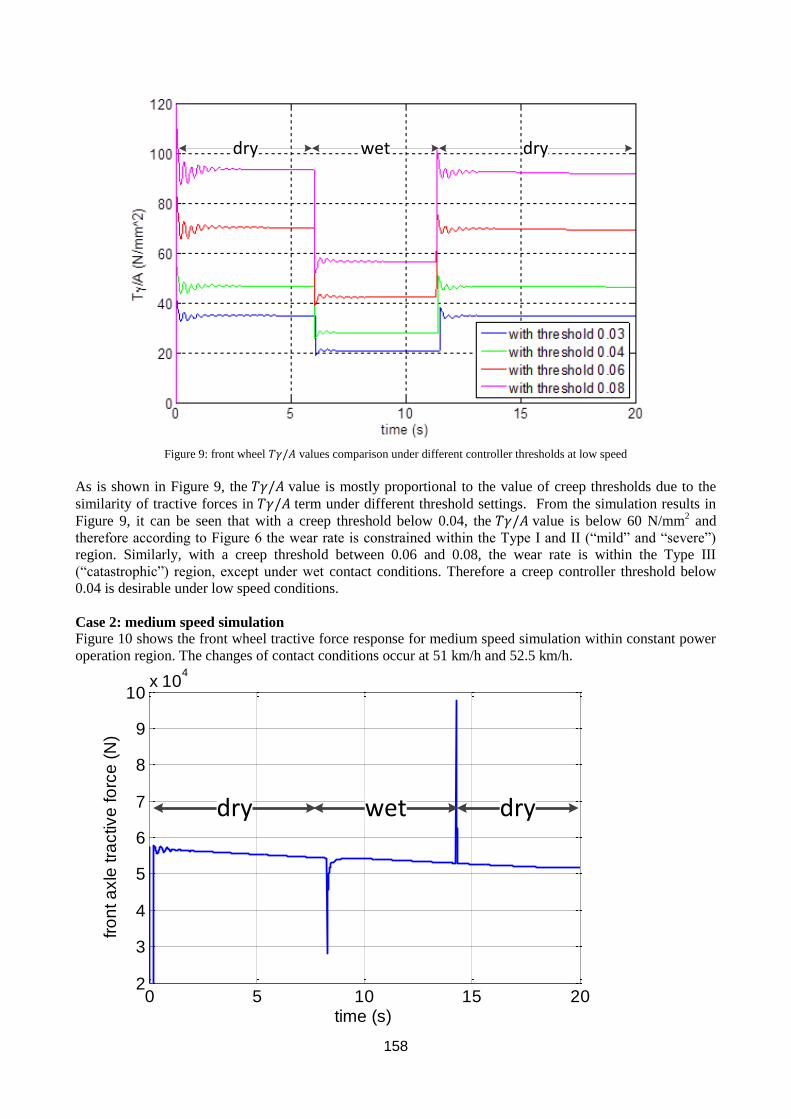
158

Figure 9: front wheel 𝑇𝛾/𝐴 values comparison under different controller thresholds at low speed

As is shown in Figure 9, the 𝑇𝛾/𝐴 value is mostly proportional to the value of creep thresholds due to the

similarity of tractive forces in 𝑇𝛾/𝐴 term under different threshold settings. From the simulation results in

Figure 9, it can be seen that with a creep threshold below 0.04, the 𝑇𝛾/𝐴 value is below 60 N/mm2 and

therefore according to Figure 6 the wear rate is constrained within the Type I and II (“mild” and “severe”)

region. Similarly, with a creep threshold between 0.06 and 0.08, the wear rate is within the Type III

(“catastrophic”) region, except under wet contact conditions. Therefore a creep controller threshold below

0.04 is desirable under low speed conditions.

Case 2: medium speed simulation

Figure 10 shows the front wheel tractive force response for medium speed simulation within constant power

operation region. The changes of contact conditions occur at 51 km/h and 52.5 km/h.

dry wet dry

0 5 10 15 202

3

4

5

6

7

8

9

10x 10

4

time (s)

fro

nt a

xle

tra

ctive

fo

rce

(N

)

dry drywet

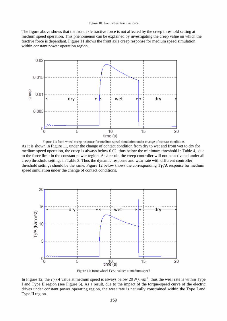
159

Figure 10: front wheel tractive force

The figure above shows that the front axle tractive force is not affected by the creep threshold setting at

medium speed operation. This phenomenon can be explained by investigating the creep value on which the

tractive force is dependant. Figure 11 shows the front axle creep response for medium speed simulation

within constant power operation region.

Figure 11: front wheel creep response for medium speed simulation under change of contact conditions

As it is shown in Figure 11, under the change of contact condition from dry to wet and from wet to dry for

medium speed operation, the creep is always below 0.02, thus below the minimum threshold in Table 4, due

to the force limit in the constant power region. As a result, the creep controller will not be activated under all

creep threshold settings in Table 3. Thus the dynamic response and wear rate with different controller

threshold settings should be the same. Figure 12 below shows the corresponding 𝐓𝛄/𝐀 response for medium

speed simulation under the change of contact conditions.

Figure 12: front wheel 𝑇𝛾/𝐴 values at medium speed

In Figure 12, the 𝑇𝛾/𝐴 value at medium speed is always below 20 𝑁/𝑚𝑚2, thus the wear rate is within Type

I and Type II region (see Figure 6). As a result, due to the impact of the torque-speed curve of the electric

drives under constant power operating region, the wear rate is naturally constrained within the Type I and

Type II region.

dry drywet

dry wet dry

160

Comparing Figure 9 and Figure 12, it can be observed that at low speed operation where the tractive force is

sufficient to activate the creep controller. The 𝑇𝛾/𝐴 value is larger under dry contact condition than under

wet condition as a result of very similar creep values under both dry and wet condition but different tractive

force, under a certain creep threshold setting. While at medium speed operation where the tractive force is

not large enough to activate the creep controller under both dry and wet contact conditions, the 𝑇𝛾/𝐴 value is

larger under wet contact condition than under dry condition, due to different creep values achieves similar

tractive force as can be concluded from Figure 4.

5. Conclusion and future work In this paper, wear rate with different PI creep control threshold settings under transient contact conditions

have been compared by using a 21 DOF full-scale locomotive dynamic model under different operation

speeds. Simulations have been carried out to compare tractive force and wear rate, focusing on the impact of

operation speed and creep controller setting. Results show that by designing the creep controller threshold

parameter, the wear rate can be effectively constrained within Type I and Type II regions, avoiding Type III

‘Catastrophic’ wear. Under higher speed operation, such as Case 2 in this paper, the wear rate is naturally

constrained within region I and II due to the impact of the torque-speed characteristics of the electric drives,

irrespective of the creep controller. Future work will include the investigation on modifying the controller so

that optimal tractive force can be achieved to ensure the wear growth rate is constrained within Type I and II

regions, automatically. Also more detailed dynamic model including lateral dynamics and relative motions

between wheelsets and bogies will be employed for more accurate dynamic and control analysis on both

straight and curved tracks.

Acknowledgements The authors are grateful to the CRC for Rail Innovation (established and supported under the Australian

Government's Cooperative Research Centres program) for the funding of this research Project No. R3.119

“Locomotive Adhesion”. The authors acknowledge the support of the Centre for Railway Engineering,

Central Queensland University and the many industry partners that have contributed to this project, in

particular staff from RailCorp, Fortescue Metals Group (FMG) and Brookfield Rail.

161

References:

[1] Y. Bakhvalov, et al., "Mathematical Modelling of Electromechanical Processes in Electric

Locomotive," presented at the 16th IMACS World Congress, Lausanne (Switzerland), 2000.

[2] S. Senini, et al., "Dynamic simulation of wheel-rail interaction for locomotive traction studies," in

Railroad Conference, 1993., Proceedings of the 1993 IEEE/ASME Joint, 1993, pp. 27-34.

[3] P. Doh-Young, et al., "Hybrid re-adhesion control method for traction system of high-speed

railway," in Electrical Machines and Systems, 2001. ICEMS 2001. Proceedings of the Fifth

International Conference on, 2001, pp. 739-742 vol.2.

[4] K. Ohishi, et al., "Anti-slip control of electric motor coach based on disturbance observer," in

Advanced Motion Control, 1998. AMC '98-Coimbra., 1998 5th International Workshop on, 1998, pp.

580-585.

[5] I. Yasuoka, et al., "Improvement of re-adhesion for commuter trains with vector control traction

inverter," in Power Conversion Conference - Nagaoka 1997., Proceedings of the, 1997, pp. 51-56

vol.1.

[6] M. Spiryagin, et al., "Co-simulation of a mechatronic system using Gensys and Simulink," Vehicle

System Dynamics, vol. 50, pp. 495-507, 2012.

[7] M. Spiryagin, et al., "Control system for maximum use of adhesive forces of a railway vehicle in a

tractive mode," Mechanical Systems and Signal Processing, vol. 22, pp. 709-720, 2008.

[8] M. Spiryagin, et al., "Adhesion estimation and its implementation for traction control of

locomotives," International Journal of Rail Transportation, vol. 2, pp. 187-204, 2014/07/03 2014.

[9] Y. Yuan, et al., "The dynamic study of locomotives under saturated adhesion," Vehicle System

Dynamics, vol. 49, pp. 1321-1338, 2011/08/01 2011.

[10] T. X. Mei, et al., "A mechatronic approach for effective wheel slip control in railway traction,"

Proceedings of the Institution of Mechanical Engineers, Part F: Journal of Rail and Rapid Transit,

vol. 223, pp. 295-304, May 1, 2009 2009.

[11] Y. Zhao and B. Liang, "Re-adhesion control for a railway single wheelset test rig based on the

behaviour of the traction motor," Vehicle System Dynamics, vol. 51, pp. 1173-1185, 2013/08/01

2013.

[12] T. Jendel, "Prediction of wheel profile wear—comparisons with field measurements," Wear, vol.

253, pp. 89-99, 2002.

[13] T. G. Pearce and N. D. Sherratt, "Prediction of wheel profile wear," Wear, vol. 144, pp. 343-351,

1991.

[14] R. Lewis and U. Olofsson, "Mapping rail wear regimes and transitions," Wear, vol. 257, pp. 721-

729, 2004.

[15] F. Braghin, et al., "A mathematical model to predict railway wheel profile evolution due to wear,"

Wear, vol. 261, pp. 1253-1264, 2006.

[16] E. H. Law and N. K. Cooperrider, "A survey of railway vehicle dynamics research," ASME Journal

of Dynamic Systems, Measurement, and Control, vol. 96, pp. 132-146, June 1974 1974.

[17] R. Guclu and M. Metin, "Fuzzy Logic Control of Vibrations of a Light Rail Transport Vehicle in

Use in Istanbul Traffic," Journal of Vibration and Control, vol. 15, pp. 1423-1440, September 1,

2009 2009.

[18] D. S. Garivaltis, et al., "Dynamic Response of a Six-axle Locomotive to Random Track Inputs,"

Vehicle System Dynamics, vol. 9, pp. 117-147, 1980/05/01 1980.

[19] O. Polach, "Creep forces in simulations of traction vehicles running on adhesion limit," Wear, vol.

258, pp. 992-1000, 2005.

[20] M. Spiryagin, et al., "Creep force modelling for rail traction vehicles based on the Fastsim

algorithm," Vehicle System Dynamics, vol. 51, pp. 1765-1783, 2013/11/01 2013.

[21] M. D. Ardema, Newton-Euler Dynamics: Springer, 2006.

[22] I. J. Guy, "An analysis of the interaction between the front and rear axles of a four-wheel-drive

tractor, and its contribution to power delivery efficiency," Harper Adams University College, 2011.

[23] Pegasem. Pegasem GSS series ground speed sensors [Online]. Available:

http://www.pegasem.com/english/datasheets_uk/gss_uk.pdf

[24] S. Iwnicki, Handbook of railway vehicle dynamics: CRC press, 2006.

[25] K. Abood and R. Khan, "Hunting phenomenon study of railway conventional truck on tangent tracks

due to change in rail wheel geometry," Journal of Engineering Science and Technology, vol. 6, pp.

146-160, 2011.

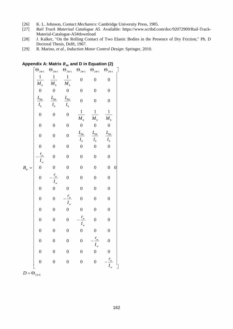
162

[26] K. L. Johnson, Contact Mechanics: Cambridge University Press, 1985.

[27] Rail Track Materisal Catalogue A5. Available: https://www.scribd.com/doc/92072909/Rail-Track-

Material-Catalogue-A5#download

[28] J. Kalker, "On the Rolling Contact of Two Elastic Bodies in the Presence of Dry Friction," Ph. D

Doctoral Thesis, Delft, 1967.

[29] R. Marino, et al., Induction Motor Control Design: Springer, 2010.

Appendix A: Matrix 𝑩𝒎 and D in Equation (2)

24 1 24 1 24 1 24 1 24 1 24 1

1 1 10 0 0

0 0 0 0 0 0

0 0 0

1 1 10 0 0

0 0 0 0 0 0

0 0 0

0 0 0 0 0 0

0 0 0 0 0

0 0 0 0 0 0

0 0 0 0 0

0 0 0 0 0 0

0 0 0 0 0

0 0 0 0 0 0

0 0 0 0 0

0 0 0 0 0 0

0 0 0 0 0

0 0 0 0 0 0

0 0 0 0 0

b b b

bh bh bh

b b b

b b b

bh bh bh

b b b

w

w

m

w

w

w

w

w

w

w

w

w

M M M

L L L

I I I

M M M

L L L

I I I

r

I

B

r

I

r

I

r

I

r

I

r

I

0

w

21 6D

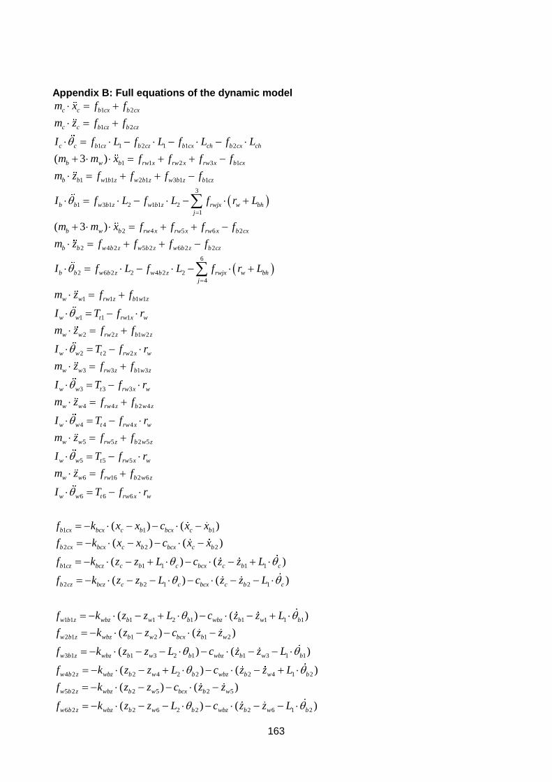
163

Appendix B: Full equations of the dynamic model

1 2

1 2

1 1 2 1 1 2

1 1 2 3 1

1 1 1 2 1 3 1 1

3

1 3 1 2 1 1 2

1

( 3 )

c c b cx b cx

c c b cz b cz

c c b cz b cz b cx ch b cx ch

b w b rw x rw x rw x b cx

b b w b z w b z w b z b cz

b b w b z w b z rwjx w

j

m x f f

m z f f

I f L f L f L f L

m m x f f f f

m z f f f f

I f L f L f r

2 4 5 6 2

2 4 2 5 2 6 2 2

6

2 6 2 2 4 2 2

4

1 1 1 1

1 1 1

2 2 1 2

2 2

( 3 )

bh

b w b rw x rw x rw x b cx

b b w b z w b z w b z b cz

b b w b z w b z rwjx w bh

j

w w rw z b w z

w w t rw x w

w w rw z b w z

w w t

L

m m x f f f f

m z f f f f

I f L f L f r L

m z f f

I T f r

m z f f

I T f

2

3 3 1 3

3 3 3

4 4 2 4

4 4 4

5 5 2 5

5 5 5

6 16 2 6

6 6 6

1 1( )

rw x w

w w rw z b w z

w w t rw x w

w w rw z b w z

w w t rw x w

w w rw z b w z

w w t rw x w

w w rw b w z

w w t rw x w

b cx bcx c b bcx

r

m z f f

I T f r

m z f f

I T f r

m z f f

I T f r

m z f f

I T f r

f k x x c

1

2 2 2

1 1 1 1 1

2 2 1 2 1

1 1 1 1 2 1 1 1 1 1

( )

( ) ( )

( ) ( )

( ) ( )

( ) ( )

c b

b cx bcx c b bcx c b

b cz bcz c b c bcx c b c

b cz bcz c b c bcx c b c

w b z wbz b w b wbz b w b

x x

f k x x c x x

f k z z L c z z L

f k z z L c z z L

f k z z L c z z L

f

2 1 1 2 1 2

3 1 1 3 2 1 1 3 1 1

4 2 2 4 2 2 2 4 1 2

5 2 2 5 2 5

6 2

( ) ( )

( ) ( )

( ) ( )

( ) ( )

(

w b z wbz b w bcx b w

w b z wbz b w b wbz b w b

w b z wbz b w b wbz b w b

w b z wbz b w bcx b w

w b z wbz

k z z c z z

f k z z L c z z L

f k z z L c z z L

f k z z c z z

f k z

2 6 2 2 2 6 1 2) ( )b w b wbz b w bz L c z z L

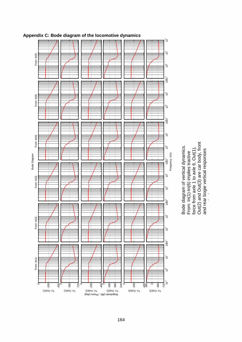
164

Appendix C: Bode diagram of the locomotive dynamics

-400

-2000

Fro

m: In

(1)

To: Out(1)

-720

-3600

To: Out(1)

-400

-2000

To: Out(2)

-540

-360

-1800

To: Out(2)

-400

-2000

To: Out(3)

10

-110

010

110

2-7

20

-3600

360

To: Out(3)

Fro

m: In

(2)

10

-110

010

110

2

Fro

m: In

(3)

10

-110

010

110

2

Fro

m: In

(4)

10

-110

010

110

2

Fro

m: In

(5)

10

-110

010

110

2

Fro

m: In

(6)

10

-110

010

110

2

Bode D

iagra

m

Fre

quency

(H

z)

Magnitude (dB) ; Phase (deg)

Bo

de

dia

gra

m o

f ve

rtic

al d

yna

mic

s.

Fro

m: In

(1)-

In(6

) im

plie

s tra

ctive

fo

rce fro

m a

xle

1 t

o a

xle

6. O

ut(

1),

Ou

t(2

) a

nd

Out(

3)

are

car

bod

y, fr

ont

and

re

ar

bog

ie v

ert

ica

l re

sp

on

ses

respe

ctively

.

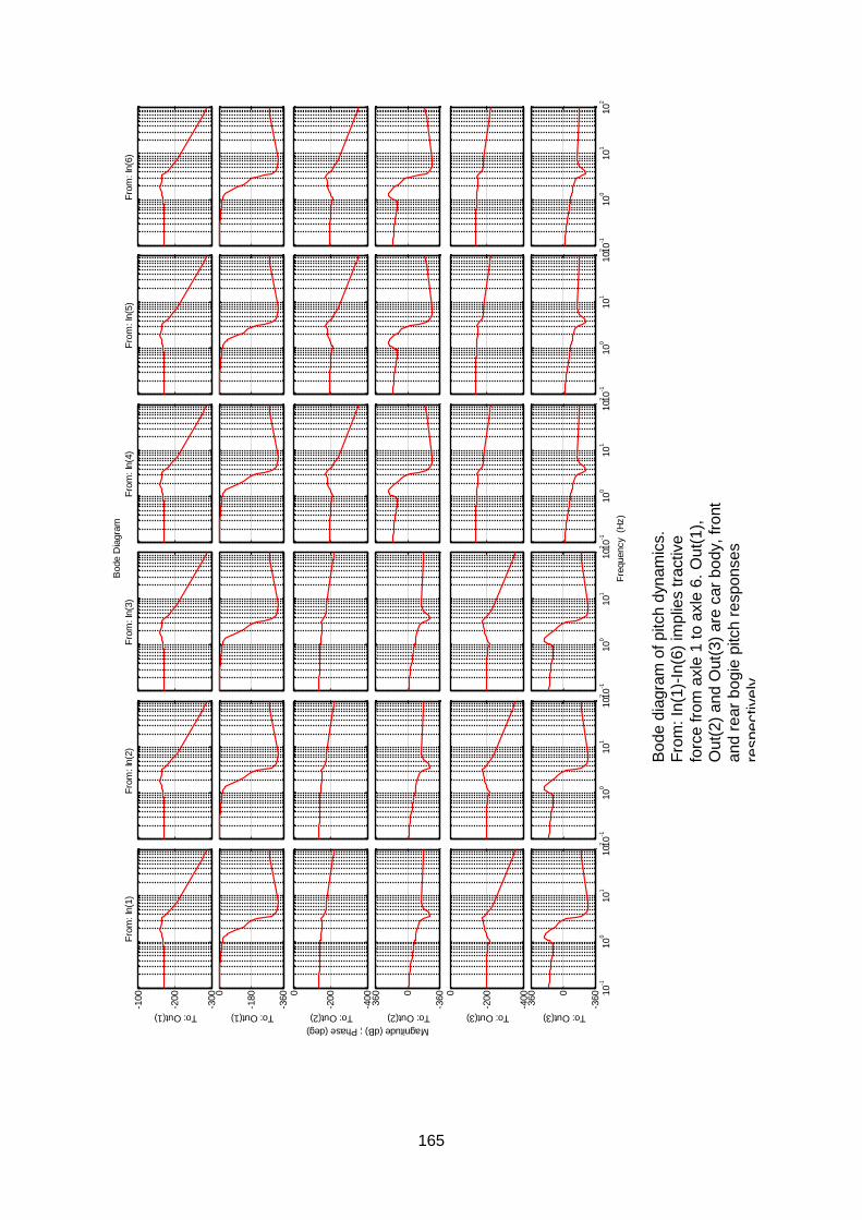
165

-300

-200

-100

Fro

m: In

(1)

To: Out(1)

-360

-1800

To: Out(1)

-400

-2000

To: Out(2)

-3600

360

To: Out(2)

-400

-2000

To: Out(3)

10

-110

010

110

2-3

600

360

To: Out(3)

Fro

m: In

(2)

10

-110

010

110

2

Fro

m: In

(3)

10

-110

010

110

2

Fro

m: In

(4)

10

-110

010

110

2

Fro

m: In

(5)

10

-110

010

110

2

Fro

m: In

(6)

10

-110

010

110

2

Bode D

iagra

m

Fre

quency

(H

z)

Magnitude (dB) ; Phase (deg)

Bo

de

dia

gra

m o

f p

itch d

yn

am

ics.

Fro

m: In

(1)-

In(6

) im

plie

s tra

ctive

forc

e fro

m a

xle

1 t

o a

xle

6.

Ou

t(1

),

Ou

t(2

) a

nd

Out(

3)

are

car

bod

y, fr

ont

and

re

ar

bog

ie p

itch

re

spo

nse

s

respe

ctively

.

166

Paper E

Real-time rail/wheel wear damage control

167

Real-time rail/wheel wear damage control

Ye Tian, W.J.T. (Bill) Daniel, Paul A. Meehan

School of Mechanical and Mining Engineering, the University of Queensland, Queensland, Australia 4072

This paper presents the performance of a real-time rail/wheel wear damage control system with respect to different operation conditions. In particular, an investigation into the wear growth rate control under changing wheel-rail friction conditions and different operation speeds is performed. Simulation using a mathematical model considering longitudinal-vertical-pitch dynamics of a locomotive running on straight tracks shows that the proposed controller can effectively reduce the rail/wheel wear damage by limiting mass loss rate, particularly during acceleration under low speed. Keywords: wear control; railway; locomotive; wheel-rail

1. Introduction Rail offers one of the most efficient forms of land-based transport [1], providing great carrying capacity.

However, there is discussion as to whether the trend towards more powerful locomotives, particularly in the

heavy haul rail industry, would contribute to considerable increase of rail track damage due to wear and

increased track maintenance cost. Traditionally, friction modifiers (FM) have been employed on the

rail/wheel contact patch to reduce such wear and rolling contact fatigue [2]. However this method depends

on experiences and lacks understanding of the impact of locomotive dynamic traction creep behaviour. There

is also additional cost. The American Association of Railroads estimates that the wear occurring at the

wheel/rail interface as a result of ineffective lubrication costs in excess of $US 2 billion per year [3].

Therefore, it is necessary to understand how wear growth is affected by different operation conditions and

creep/adhesion control strategies. In particular, the transient state of locomotive operation due to external

perturbations such as changes of wheel-rail contact conditions needs to be further investigated. As the most

significant change of locomotive dynamic responses and oscillations are likely to occur during this transient

state. Thus rail damage due to wear is likely to be controlled in a systematic way, potentially reducing or

even excluding the use of friction modifiers for the purpose of wear reduction.

The study of patterns of wear behaviour was addressed by Beagley et al. [4]. Wear behaviour of wheel/rail steels was described as a ‘wear regime’. The terms “mild” and “severe” regimes were used to describe wear characteristics according to the surface deformation observed in his experiments. A regime that arose from more severe contact conditions was observed by Bolton et al. [5] and was defined as the ‘catastrophic’ wear regime. A detailed review of this wear regime of steel was performed by Markov et al. in [6]. These three rolling-sliding wear regimes for wheel/rail steels have also been reconfirmed by Danks et al. [7]. He also suggested using the terms “type I wear”, “type II wear” and “type III wear” for describing the “stages” of the wear in order to avoid the confusion between the mild and severe wear regimes and mild-oxidational and severe-oxidational wear mechanisms. For the wheel/rail steel, the material loss in wear process is defined as wear rate. It is determined by the loss of material mass per rolling distance (𝜇𝑔/𝑚) [7]; or by the total

loss of material mass per rolling distance, per contact area (𝜇𝑔/𝑚/𝑚𝑚2) [8]. Wear rate is often

plotted against the ‘wear index’ 𝑇𝛾/𝐴𝑛 [9]. A recent wear model considering the wear transitions has been developed by Vuong et al [10]. Both wheel and rail wear regimes can be illustrated in a similar mapping method [9, 11-15]. In this paper, the dynamic response of a full scale locomotive model with a traction controller under different speed and/or contact conditions is investigated in relation to the rail wear. This work focuses on longitudinal and vertical dynamics on tangent tracks as it is the most important part of locomotive dynamics closely related with traction/braking effort, passenger comfort and energy management [16]. A full scale locomotive longitudinal-vertical-pitch dynamic model with a PI creep controller and a wear controller combining all crucial dynamic components is developed and implemented using Matlab/Simulink and the wear rate [13] is

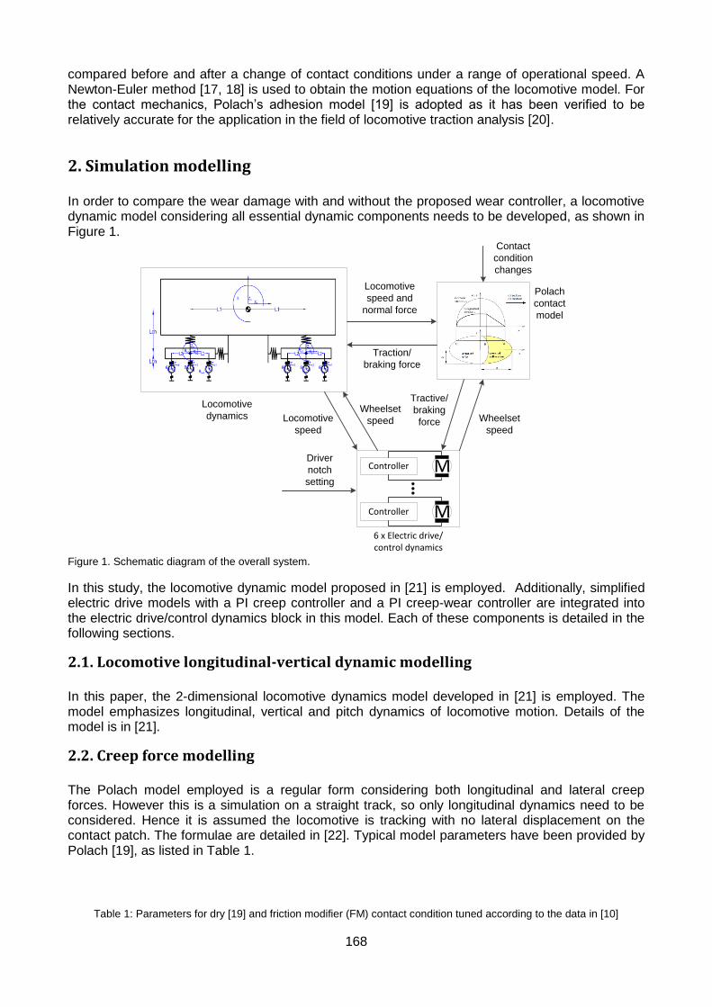
168

compared before and after a change of contact conditions under a range of operational speed. A Newton-Euler method [17, 18] is used to obtain the motion equations of the locomotive model. For the contact mechanics, Polach’s adhesion model [19] is adopted as it has been verified to be relatively accurate for the application in the field of locomotive traction analysis [20].

2. Simulation modelling In order to compare the wear damage with and without the proposed wear controller, a locomotive dynamic model considering all essential dynamic components needs to be developed, as shown in Figure 1.

MController

6 x Electric drive/control dynamics

MController

Polach

contact

model

Locomotive

speed and

normal force

Contact

condition

changes

Driver

notch

setting

Traction/

braking force

Locomotive

speed

Wheelset

speed

Tractive/

braking

force

Locomotive

dynamicsWheelset

speed

Figure 1. Schematic diagram of the overall system.

In this study, the locomotive dynamic model proposed in [21] is employed. Additionally, simplified electric drive models with a PI creep controller and a PI creep-wear controller are integrated into the electric drive/control dynamics block in this model. Each of these components is detailed in the following sections.

2.1. Locomotive longitudinal-vertical dynamic modelling In this paper, the 2-dimensional locomotive dynamics model developed in [21] is employed. The model emphasizes longitudinal, vertical and pitch dynamics of locomotive motion. Details of the model is in [21].

2.2. Creep force modelling The Polach model employed is a regular form considering both longitudinal and lateral creep forces. However this is a simulation on a straight track, so only longitudinal dynamics need to be considered. Hence it is assumed the locomotive is tracking with no lateral displacement on the contact patch. The formulae are detailed in [22]. Typical model parameters have been provided by Polach [19], as listed in Table 1.

Table 1: Parameters for dry [19] and friction modifier (FM) contact condition tuned according to the data in [10]

050

100 0 0.1 0.2 0.3 0.4 0.5

0

0.1

0.2

0.3

0.4

0.5

0.6

0.7

creep

Polach dry

loco velocity km/h

adhesio

n c

oeffic

ient

0

0.1

0.2

0.3

0.4

0.5

Polach c

Electric drive & control

Complex locomo

M

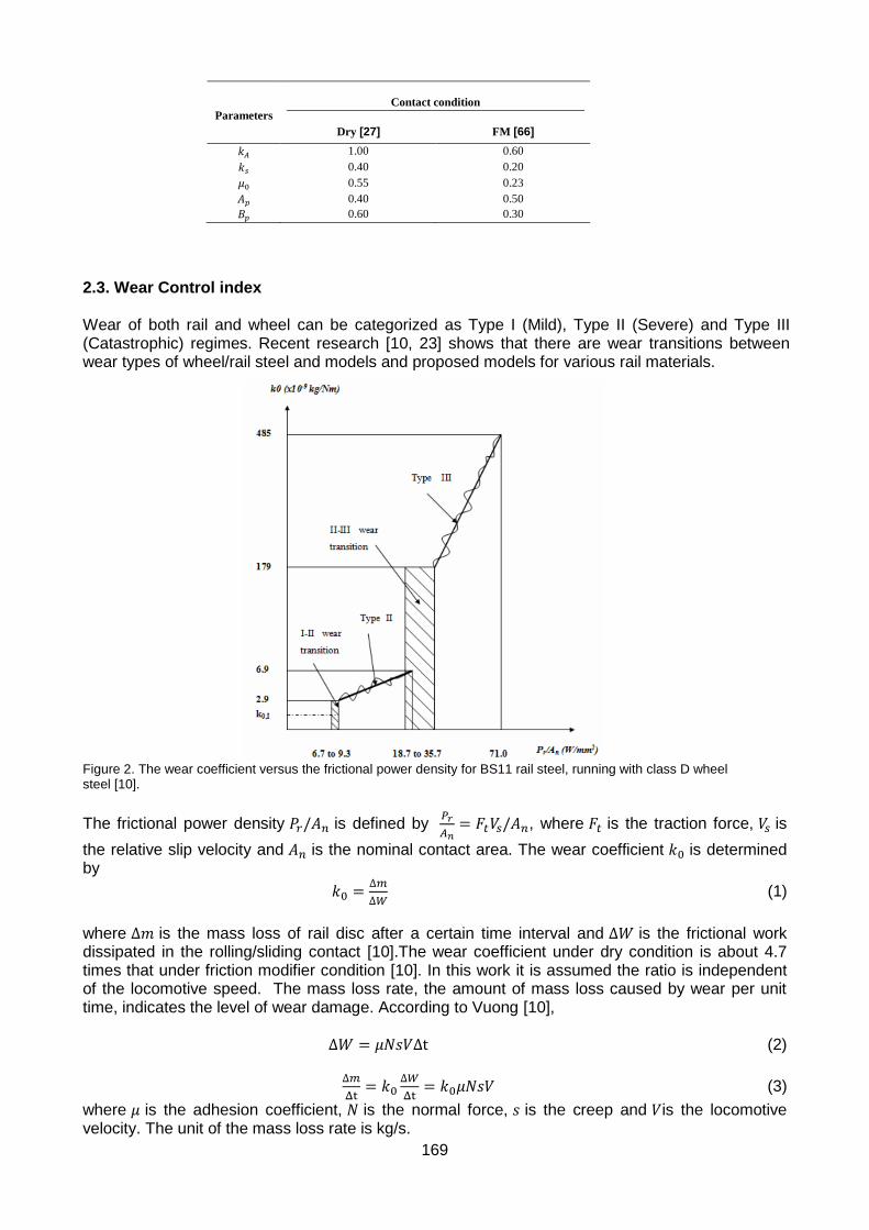
169

Parameters

Contact condition

Dry [27] FM [66]

𝑘𝐴 1.00 0.60

𝑘𝑠 0.40 0.20

𝜇0 0.55 0.23

𝐴𝑝 0.40 0.50

𝐵𝑝 0.60 0.30

2.3. Wear Control index Wear of both rail and wheel can be categorized as Type I (Mild), Type II (Severe) and Type III (Catastrophic) regimes. Recent research [10, 23] shows that there are wear transitions between wear types of wheel/rail steel and models and proposed models for various rail materials.

Figure 2. The wear coefficient versus the frictional power density for BS11 rail steel, running with class D wheel steel [10].

The frictional power density 𝑃𝑟/𝐴𝑛 is defined by 𝑃𝑟

𝐴𝑛= 𝐹𝑡𝑉𝑠/𝐴𝑛, where 𝐹𝑡 is the traction force, 𝑉𝑠 is

the relative slip velocity and 𝐴𝑛 is the nominal contact area. The wear coefficient 𝑘0 is determined by

𝑘0 =∆𝑚

∆𝑊 (1)

where ∆𝑚 is the mass loss of rail disc after a certain time interval and ∆𝑊 is the frictional work dissipated in the rolling/sliding contact [10].The wear coefficient under dry condition is about 4.7 times that under friction modifier condition [10]. In this work it is assumed the ratio is independent of the locomotive speed. The mass loss rate, the amount of mass loss caused by wear per unit time, indicates the level of wear damage. According to Vuong [10],

∆𝑊 = 𝜇𝑁𝑠𝑉Δt (2)

∆𝑚

Δt= 𝑘0

∆𝑊

Δt= 𝑘0𝜇𝑁𝑠𝑉 (3)

where 𝜇 is the adhesion coefficient, 𝑁 is the normal force, 𝑠 is the creep and 𝑉is the locomotive velocity. The unit of the mass loss rate is kg/s.

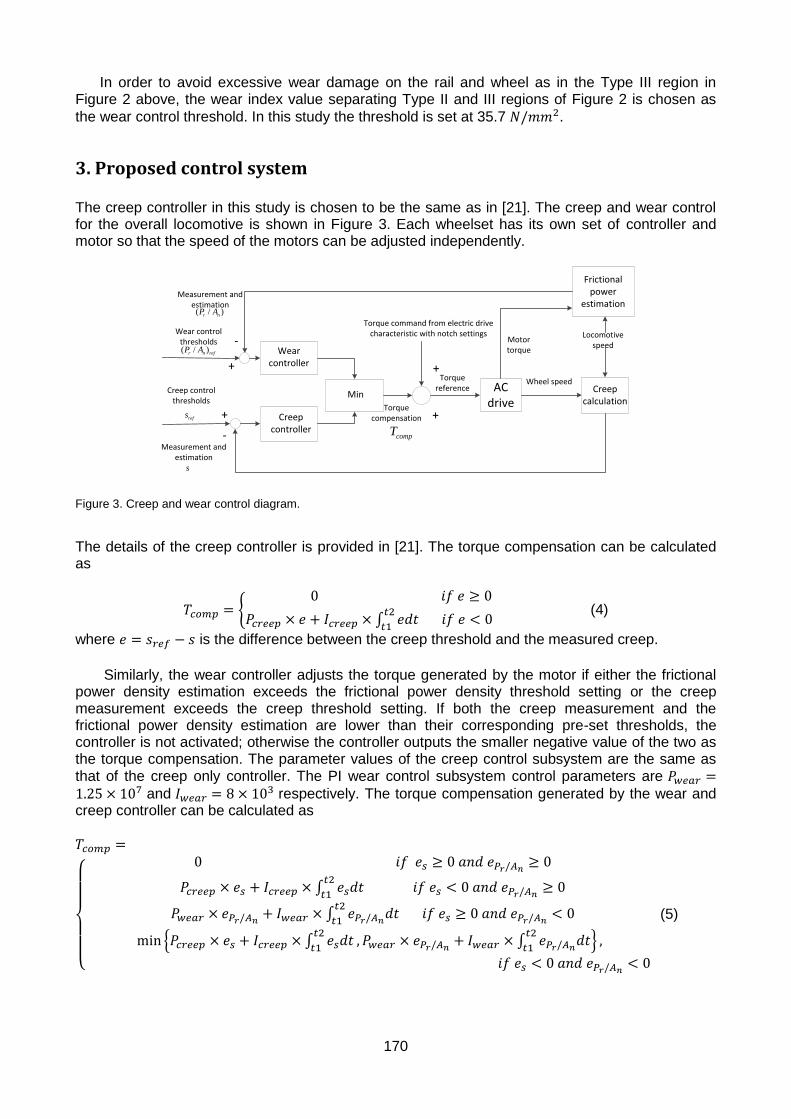
170

In order to avoid excessive wear damage on the rail and wheel as in the Type III region in Figure 2 above, the wear index value separating Type II and III regions of Figure 2 is chosen as

the wear control threshold. In this study the threshold is set at 35.7 𝑁/𝑚𝑚2.

3. Proposed control system The creep controller in this study is chosen to be the same as in [21]. The creep and wear control for the overall locomotive is shown in Figure 3. Each wheelset has its own set of controller and motor so that the speed of the motors can be adjusted independently.

Creep controller

Torque command from electric drive characteristic with notch settings

Creep control thresholds

Measurement and estimation

Torque reference

+

++

-

refs

s

AC drive

Wheel speed

Locomotive speed

Creep calculation

Torque compensation

compT

Wear controller

( / )r n refP A

( / )r nP A

Frictional power

estimation

Motor torque

Wear control thresholds

+

-

Measurement and estimation

Min

Figure 3. Creep and wear control diagram.

The details of the creep controller is provided in [21]. The torque compensation can be calculated as

𝑇𝑐𝑜𝑚𝑝 = { 0 𝑖𝑓 𝑒 ≥ 0

𝑃𝑐𝑟𝑒𝑒𝑝 × 𝑒 + 𝐼𝑐𝑟𝑒𝑒𝑝 × ∫ 𝑒𝑑𝑡 𝑖𝑓 𝑒 < 0𝑡2

𝑡1

(4)

where 𝑒 = 𝑠𝑟𝑒𝑓 − 𝑠 is the difference between the creep threshold and the measured creep.

Similarly, the wear controller adjusts the torque generated by the motor if either the frictional power density estimation exceeds the frictional power density threshold setting or the creep measurement exceeds the creep threshold setting. If both the creep measurement and the frictional power density estimation are lower than their corresponding pre-set thresholds, the controller is not activated; otherwise the controller outputs the smaller negative value of the two as the torque compensation. The parameter values of the creep control subsystem are the same as that of the creep only controller. The PI wear control subsystem control parameters are 𝑃𝑤𝑒𝑎𝑟 =1.25 × 107 and 𝐼𝑤𝑒𝑎𝑟 = 8 × 10

3 respectively. The torque compensation generated by the wear and creep controller can be calculated as 𝑇𝑐𝑜𝑚𝑝 =

{

0 𝑖𝑓 𝑒𝑠 ≥ 0 𝑎𝑛𝑑 𝑒𝑃𝑟/𝐴𝑛 ≥ 0

𝑃𝑐𝑟𝑒𝑒𝑝 × 𝑒𝑠 + 𝐼𝑐𝑟𝑒𝑒𝑝 × ∫ 𝑒𝑠𝑑𝑡 𝑖𝑓 𝑒𝑠 < 0 𝑎𝑛𝑑 𝑒𝑃𝑟/𝐴𝑛 ≥ 0𝑡2

𝑡1

𝑃𝑤𝑒𝑎𝑟 × 𝑒𝑃𝑟/𝐴𝑛 + 𝐼𝑤𝑒𝑎𝑟 × ∫ 𝑒𝑃𝑟/𝐴𝑛𝑑𝑡 𝑖𝑓 𝑒𝑠 ≥ 0 𝑎𝑛𝑑 𝑒𝑃𝑟/𝐴𝑛 < 0𝑡2

𝑡1

min {𝑃𝑐𝑟𝑒𝑒𝑝 × 𝑒𝑠 + 𝐼𝑐𝑟𝑒𝑒𝑝 × ∫ 𝑒𝑠𝑑𝑡𝑡2

𝑡1, 𝑃𝑤𝑒𝑎𝑟 × 𝑒𝑃𝑟/𝐴𝑛 + 𝐼𝑤𝑒𝑎𝑟 × ∫ 𝑒𝑃𝑟/𝐴𝑛𝑑𝑡

𝑡2

𝑡1} ,

𝑖𝑓 𝑒𝑠 < 0 𝑎𝑛𝑑 𝑒𝑃𝑟/𝐴𝑛 < 0

(5)

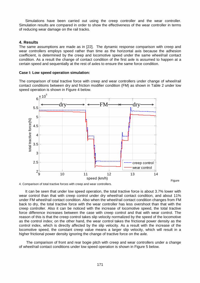
171

Simulations have been carried out using the creep controller and the wear controller. Simulation results are compared in order to show the effectiveness of the wear controller in terms of reducing wear damage on the rail tracks.

4. Results The same assumptions are made as in [22]. The dynamic response comparison with creep and wear controllers employs speed rather than time as the horizontal axis because the adhesion coefficient, is determined by the creep and locomotive speed under the same wheel/rail contact condition. As a result the change of contact condition of the first axle is assumed to happen at a certain speed and sequentially at the rest of axles to ensure the same force condition.

Case I: Low speed operation simulation: The comparison of total tractive force with creep and wear controllers under change of wheel/rail contact conditions between dry and friction modifier condition (FM) as shown in Table 2 under low speed operation is shown in Figure 4 below.

9 10 11 12 13 142

2.5

3

3.5

4

4.5

5

5.5

6x 10

5

speed (km/h)

tota

l tr

active

fo

rce

(N)

creep control

wear control

dry FM dry

Figure 4. Comparison of total tractive forces with creep and wear controllers.

It can be seen that under low speed operation, the total tractive force is about 3.7% lower with wear control than that with creep control under dry wheel/rail contact condition, and about 11% under FM wheel/rail contact condition. Also when the wheel/rail contact condition changes from FM back to dry, the total tractive force with the wear controller has less overshoot than that with the creep controller. Also it can be noticed with the increase of locomotive speed, the total tractive force difference increases between the case with creep control and that with wear control. The reason of this is that the creep control takes slip velocity normalized by the speed of the locomotive as the control index; on the other hand, the wear control takes the frictional power density as the control index, which is directly affected by the slip velocity. As a result with the increase of the locomotive speed, the constant creep value means a larger slip velocity, which will result in a higher frictional power density ignoring the change of tractive force on the axle. The comparison of front and rear bogie pitch with creep and wear controllers under a change of wheel/rail contact conditions under low speed operation is shown in Figure 5 below.

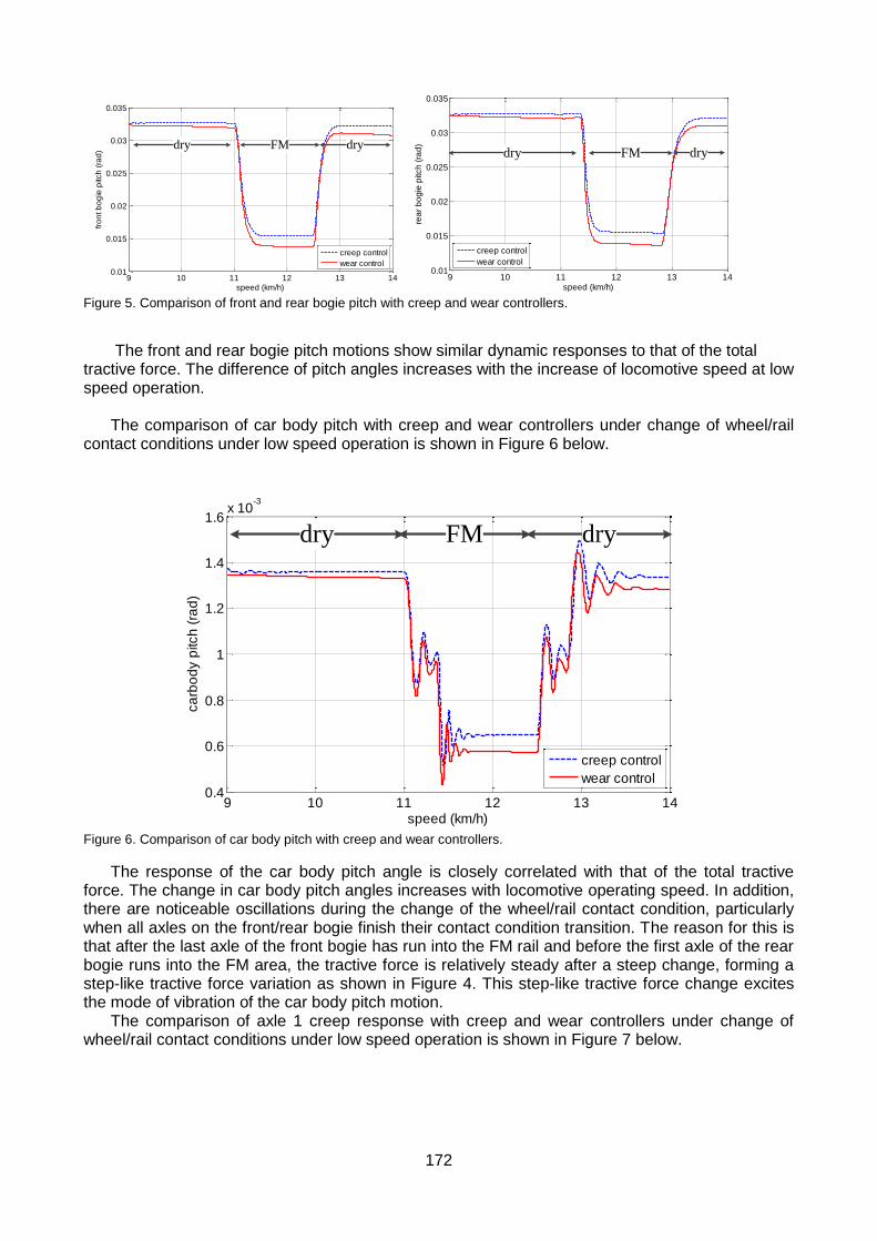
172

9 10 11 12 13 140.01

0.015

0.02

0.025

0.03

0.035

speed (km/h)

fro

nt b

og

ie p

itch

(ra

d)

creep control

wear control

dry FM dry

9 10 11 12 13 140.01

0.015

0.02

0.025

0.03

0.035

speed (km/h)

rea

r b

og

ie p

itch

(ra

d)

creep control

wear control

dry FM dry

Figure 5. Comparison of front and rear bogie pitch with creep and wear controllers.

The front and rear bogie pitch motions show similar dynamic responses to that of the total tractive force. The difference of pitch angles increases with the increase of locomotive speed at low speed operation. The comparison of car body pitch with creep and wear controllers under change of wheel/rail contact conditions under low speed operation is shown in Figure 6 below.

9 10 11 12 13 140.4

0.6

0.8

1

1.2

1.4

1.6x 10

-3

speed (km/h)

ca

rbo

dy p

itch

(ra

d)

creep control

wear control

dry FM dry

Figure 6. Comparison of car body pitch with creep and wear controllers.

The response of the car body pitch angle is closely correlated with that of the total tractive force. The change in car body pitch angles increases with locomotive operating speed. In addition, there are noticeable oscillations during the change of the wheel/rail contact condition, particularly when all axles on the front/rear bogie finish their contact condition transition. The reason for this is that after the last axle of the front bogie has run into the FM rail and before the first axle of the rear bogie runs into the FM area, the tractive force is relatively steady after a steep change, forming a step-like tractive force variation as shown in Figure 4. This step-like tractive force change excites the mode of vibration of the car body pitch motion. The comparison of axle 1 creep response with creep and wear controllers under change of wheel/rail contact conditions under low speed operation is shown in Figure 7 below.

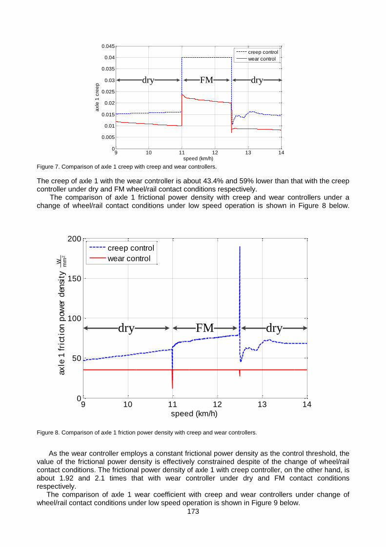
173

9 10 11 12 13 140

0.005

0.01

0.015

0.02

0.025

0.03

0.035

0.04

0.045

speed (km/h)

axle

1 c

ree

p

creep control

wear control

dry FM dry

Figure 7. Comparison of axle 1 creep with creep and wear controllers.

The creep of axle 1 with the wear controller is about 43.4% and 59% lower than that with the creep controller under dry and FM wheel/rail contact conditions respectively. The comparison of axle 1 frictional power density with creep and wear controllers under a change of wheel/rail contact conditions under low speed operation is shown in Figure 8 below.

9 10 11 12 13 140

50

100

150

200

speed (km/h)

axle

1fr

icti

on

pow

erden

sity

Wm

m2

creep control

wear control

dry FM dry

Figure 8. Comparison of axle 1 friction power density with creep and wear controllers.

As the wear controller employs a constant frictional power density as the control threshold, the value of the frictional power density is effectively constrained despite of the change of wheel/rail contact conditions. The frictional power density of axle 1 with creep controller, on the other hand, is about 1.92 and 2.1 times that with wear controller under dry and FM contact conditions respectively. The comparison of axle 1 wear coefficient with creep and wear controllers under change of wheel/rail contact conditions under low speed operation is shown in Figure 9 below.

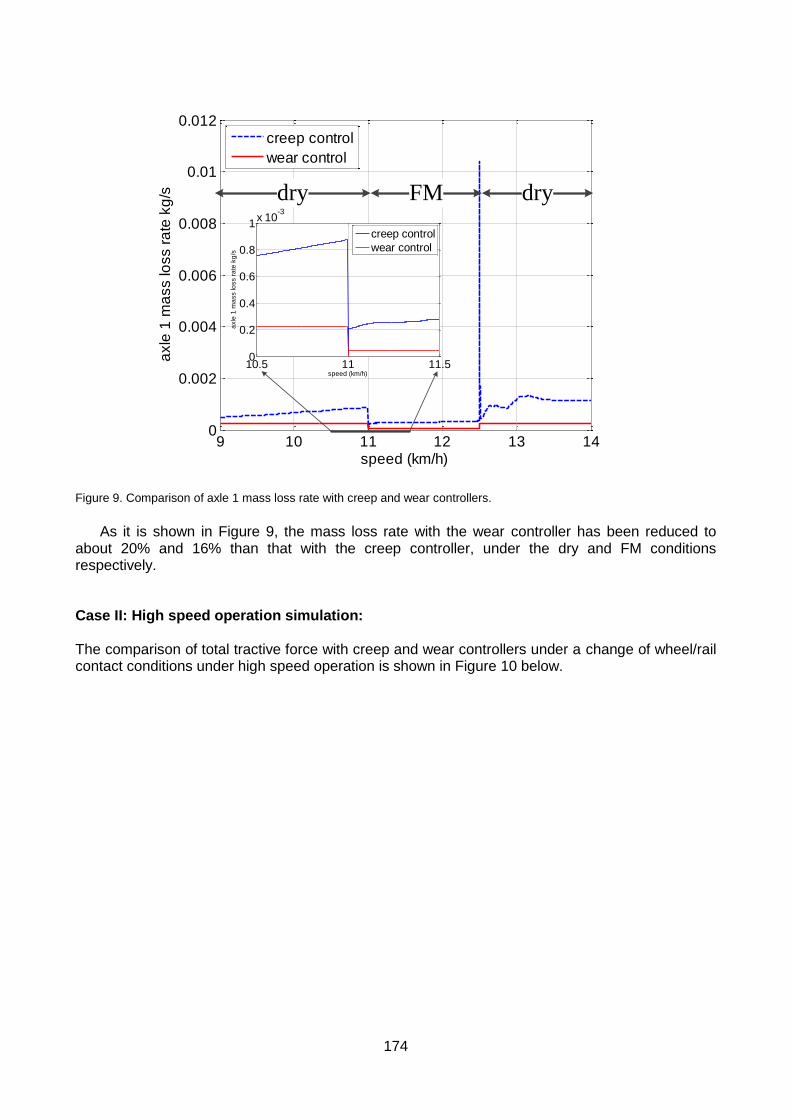
174

9 10 11 12 13 140

0.002

0.004

0.006

0.008

0.01

0.012

speed (km/h)

axle

1 m

ass lo

ss r

ate

kg

/s

creep control

wear control

10.5 11 11.50

0.2

0.4

0.6

0.8

1x 10

-3

speed (km/h)

axle

1 m

ass lo

ss r

ate

kg

/s

creep control

wear control

dry FM dry

Figure 9. Comparison of axle 1 mass loss rate with creep and wear controllers.

As it is shown in Figure 9, the mass loss rate with the wear controller has been reduced to about 20% and 16% than that with the creep controller, under the dry and FM conditions respectively. Case II: High speed operation simulation: The comparison of total tractive force with creep and wear controllers under a change of wheel/rail contact conditions under high speed operation is shown in Figure 10 below.

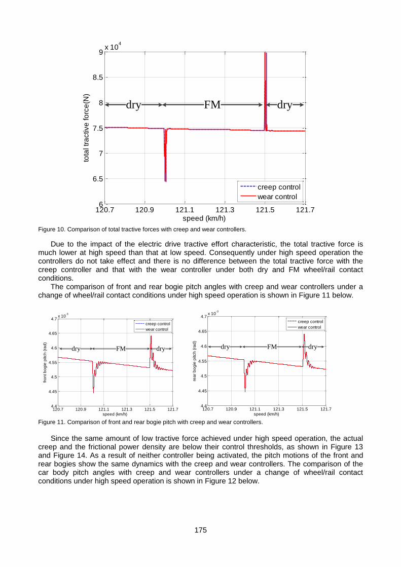
175

120.7 120.9 121.1 121.3 121.5 121.76

6.5

7

7.5

8

8.5

9x 10

4

speed (km/h)

tota

l tr

active

fo

rce

(N)

creep control

wear control

dry FM dry

Figure 10. Comparison of total tractive forces with creep and wear controllers.

Due to the impact of the electric drive tractive effort characteristic, the total tractive force is much lower at high speed than that at low speed. Consequently under high speed operation the controllers do not take effect and there is no difference between the total tractive force with the creep controller and that with the wear controller under both dry and FM wheel/rail contact conditions. The comparison of front and rear bogie pitch angles with creep and wear controllers under a change of wheel/rail contact conditions under high speed operation is shown in Figure 11 below.

120.7 120.9 121.1 121.3 121.5 121.74.4

4.45

4.5

4.55

4.6

4.65

4.7x 10

-3

speed (km/h)

fro

nt b

og

ie p

itch

(ra

d)

creep control

wear control

dry FM dry

120.7 120.9 121.1 121.3 121.5 121.74.4

4.45

4.5

4.55

4.6

4.65

4.7x 10

-3

speed (km/h)

rea

r b

og

ie p

itch

(ra

d)

creep control

wear control

dry FM dry

Figure 11. Comparison of front and rear bogie pitch with creep and wear controllers.

Since the same amount of low tractive force achieved under high speed operation, the actual creep and the frictional power density are below their control thresholds, as shown in Figure 13 and Figure 14. As a result of neither controller being activated, the pitch motions of the front and rear bogies show the same dynamics with the creep and wear controllers. The comparison of the car body pitch angles with creep and wear controllers under a change of wheel/rail contact conditions under high speed operation is shown in Figure 12 below.

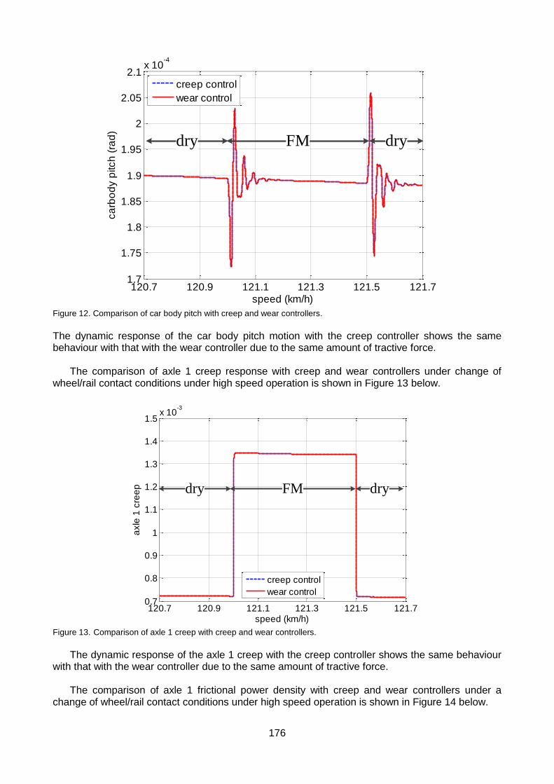
176

120.7 120.9 121.1 121.3 121.5 121.71.7

1.75

1.8

1.85

1.9

1.95

2

2.05

2.1x 10

-4

speed (km/h)

ca

rbo

dy p

itch

(ra

d)

creep control

wear control

dry FM dry

Figure 12. Comparison of car body pitch with creep and wear controllers. The dynamic response of the car body pitch motion with the creep controller shows the same behaviour with that with the wear controller due to the same amount of tractive force. The comparison of axle 1 creep response with creep and wear controllers under change of wheel/rail contact conditions under high speed operation is shown in Figure 13 below.

120.7 120.9 121.1 121.3 121.5 121.70.7

0.8

0.9

1

1.1

1.2

1.3

1.4

1.5x 10

-3

speed (km/h)

axle

1 c

ree

p

creep control

wear control

dry FM dry

Figure 13. Comparison of axle 1 creep with creep and wear controllers.

The dynamic response of the axle 1 creep with the creep controller shows the same behaviour with that with the wear controller due to the same amount of tractive force.

The comparison of axle 1 frictional power density with creep and wear controllers under a change of wheel/rail contact conditions under high speed operation is shown in Figure 14 below.

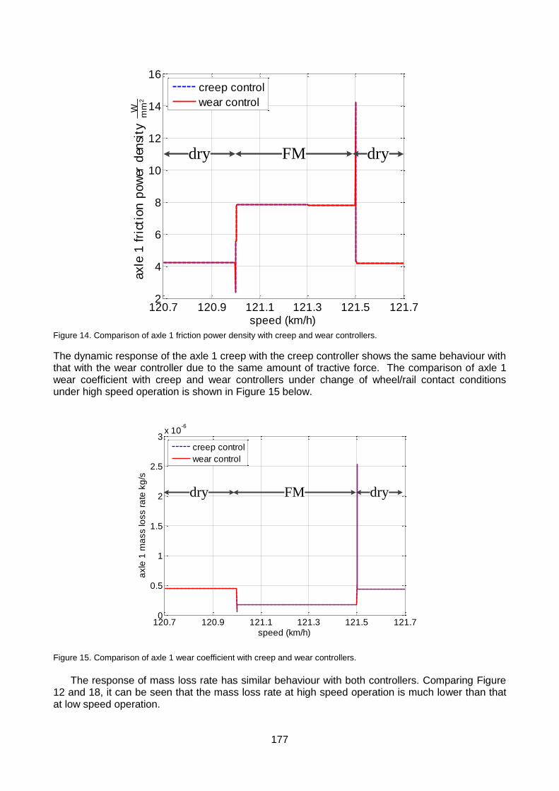
177

120.7 120.9 121.1 121.3 121.5 121.72

4

6

8

10

12

14

16

speed (km/h)

axle

1fr

icti

on

pow

erd

ensi

tyW

mm

2

creep control

wear control

dry FM dry

Figure 14. Comparison of axle 1 friction power density with creep and wear controllers.

The dynamic response of the axle 1 creep with the creep controller shows the same behaviour with that with the wear controller due to the same amount of tractive force. The comparison of axle 1 wear coefficient with creep and wear controllers under change of wheel/rail contact conditions under high speed operation is shown in Figure 15 below.

120.7 120.9 121.1 121.3 121.5 121.70

0.5

1

1.5

2

2.5

3x 10

-6

speed (km/h)

axle

1 m

ass lo

ss r

ate

kg

/s

creep control

wear control

dry FM dry

Figure 15. Comparison of axle 1 wear coefficient with creep and wear controllers.

The response of mass loss rate has similar behaviour with both controllers. Comparing Figure 12 and 18, it can be seen that the mass loss rate at high speed operation is much lower than that at low speed operation.

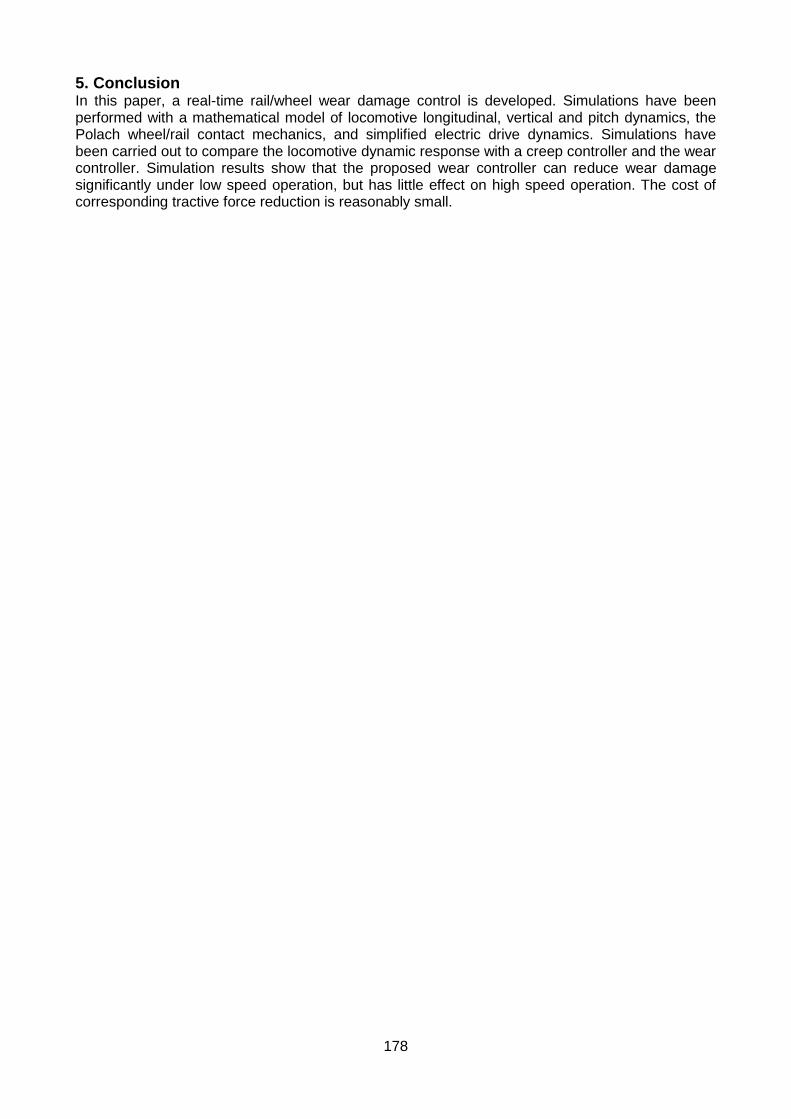
178

5. Conclusion In this paper, a real-time rail/wheel wear damage control is developed. Simulations have been performed with a mathematical model of locomotive longitudinal, vertical and pitch dynamics, the Polach wheel/rail contact mechanics, and simplified electric drive dynamics. Simulations have been carried out to compare the locomotive dynamic response with a creep controller and the wear controller. Simulation results show that the proposed wear controller can reduce wear damage significantly under low speed operation, but has little effect on high speed operation. The cost of corresponding tractive force reduction is reasonably small.

179

References: [1] S. Hillmansen and C. Roberts, "Energy storage devices in hybrid railway vehicles: A kinematic analysis," Proceedings of the Institution of Mechanical Engineers, Part F: Journal of Rail and Rapid Transit, vol. 221, pp. 135-143, January 1, 2007 2007. [2] D. T. Eadie, et al., "The effects of top of rail friction modifier on wear and rolling contact fatigue: Full-scale rail–wheel test rig evaluation, analysis and modelling," Wear, vol. 265, pp. 1222-1230, 2008. [3] J. Mathew, et al., Engineering Asset Management: Proceedings of the First World Congress on Engineering Asset Management (WCEAM) 2006: Springer-Verlag, 2008. [4] T. M. Beagley, "Severe wear of rolling/sliding contacts," Wear, vol. 36, pp. 317-335, 1976. [5] P. J. Bolton and P. Clayton, "Rolling—sliding wear damage in rail and tyre steels," Wear, vol. 93, pp. 145-165, 1984. [6] D. Markov and D. Kelly, "Mechanisms of adhesion-initiated catastrophic wear: pure sliding," Wear, vol. 239, pp. 189-210, 2000. [7] D. Danks and P. Clayton, "Comparison of the wear process for eutectoid rail steels: Field and laboratory tests," Wear, vol. 120, pp. 233-250, 1987. [8] S. Zakharov, et al., "Wheel flange/rail head wear simulation," Wear, vol. 215, pp. 18-24, 1998. [9] R. Lewis and U. Olofsson, "Mapping rail wear regimes and transitions," Wear, vol. 257, pp. 721-729, 2004. [10] T. Vuong, "Investigation for the wear coefficient of the frictional-work wear model and feasibility of friction modifiers for wear-type corrugation control," 2011. [11] M. Ignesti, et al., "Development of a wear model for the prediction of wheel and rail profile evolution in railway systems," Wear, vol. 284–285, pp. 1-17, 2012. [12] R. Lewis, et al., "Mapping railway wheel material wear mechanisms and transitions," Proceedings of the Institution of Mechanical Engineers, Part F: Journal of Rail and Rapid Transit, vol. 224, pp. 125-137, 2010. [13] F. Braghin, et al., "A mathematical model to predict railway wheel profile evolution due to wear," Wear, vol. 261, pp. 1253-1264, 2006. [14] J. Pombo, et al., "A study on wear evaluation of railway wheels based on multibody dynamics and wear computation," Multibody System Dynamics, vol. 24, pp. 347-366, 2010/10/01 2010. [15] J. Pombo, et al., "Development of a wear prediction tool for steel railway wheels using three alternative wear functions," Wear, vol. 271, pp. 238-245, 2011. [16] E. H. Law and N. K. Cooperrider, "A survey of railway vehicle dynamics research," ASME Journal of Dynamic Systems, Measurement, and Control, vol. 96, pp. 132-146, June 1974 1974. [17] R. Guclu and M. Metin, "Fuzzy Logic Control of Vibrations of a Light Rail Transport Vehicle in Use in Istanbul Traffic," Journal of Vibration and Control, vol. 15, pp. 1423-1440, September 1, 2009 2009. [18] D. S. Garivaltis, et al., "Dynamic Response of a Six-axle Locomotive to Random Track Inputs," Vehicle System Dynamics, vol. 9, pp. 117-147, 1980/05/01 1980. [19] O. Polach, "Creep forces in simulations of traction vehicles running on adhesion limit," Wear, vol. 258, pp. 992-1000, 2005. [20] M. Spiryagin, et al., "Creep force modelling for rail traction vehicles based on the Fastsim algorithm," Vehicle System Dynamics, vol. 51, pp. 1765-1783, 2013/11/01 2013. [21] Y. Tian, et al., "Investigation of the impact of locomotive creep control on wear under changing contact conditions," Vehicle System Dynamics, pp. 1-18, 2015. [22] Y. Tian, et al., "Comparison of PI and fuzzy logic based sliding mode locomotive creep controls with change of rail-wheel contact conditions," International Journal of Rail Transportation, vol. 3, pp. 40-59, 2015/01/02 2015. [23] T. T. Vuong and P. A. Meehan, "Wear transitions in a wear coefficient model," Wear, vol. 266, pp. 898-906, 2009.

180

Paper F

Dynamic response of a locomotive with AC electric

drives due to changes in friction conditions

181

Dynamic response of a locomotive with AC electric drives due to

changes in friction conditions

Sheng Liu1, Ye Tian

1, 2, W.J.T. (Bill) Daniel

1, 2, Paul A. Meehan

1, 2

1School of Mechanical and Mining Engineering, the University of Queensland, Queensland, Australia 4072 2Cooperative Research Centre for Railway Engineering and Technology (CRC Rail), Queensland, Australia

ABSTRACT

The locomotive traction control behaviour and its dynamic impact on the rail and vehicle have not been

investigated deeply in respect to transient conditions. Such transient traction behaviour could be more

significant to dynamic traction performance and track degradation (i.e. squat/corrugation formation etc.) than

steady state behaviour. In order to study this, detailed numerical simulations are performed to investigate the

locomotive dynamic response to a change in contact conditions. In particular, locomotive vibration, dynamic

normal and tractional forces, and creep response are determined using a developed full scale locomotive

dynamics model. The model includes the detailed AC motor dynamics, which was not considered in previous

works. The result shows that the detailed model is capable of simulating the dynamic fluctuations of creep

and traction forces that is not presented in the simpler model. Such transient response may cause damage to

the track and vehicle components.

Keywords Locomotive traction, multibody dynamics, AC motor dynamics, friction

1. Introduction

The recent development of AC traction motor and control technology used on locomotives has allowed

locomotives to be operated with much higher continuous traction forces and adhesion levels than previously

achieved on locomotives with DC motors. Therefore it has attracted great attention from the rail industry due

to the high power capacity, reliability and low maintenance. They however require precision traction control

to achieve steady performance close to the adhesion limit i.e. from 30% to 46% [1]. It is especially important

to understand and control the dynamic and creep response in the change of contact conditions due to natural

perturbations in friction/lubrication, wheel/rail profiles, track curvature, vehicle/track dynamics, wheel/track

imperfections etc. Such transient traction behaviour could be more significant to dynamic traction

performance and track degradation (i.e. squat/corrugation formation etc.) than steady state behaviour. It is

therefore important to understand the dynamic response due to a change in friction conditions. In order to

study this, the vehicle/track dynamics, contact mechanics and traction and creep control behaviour of modern

AC locomotive drives needs to be integrated and assessed as a total dynamic feedback interactive system.

To achieve this, the understanding of dynamic interactions between the locomotive structure, contact

mechanics and traction control system is essential, especially the dynamic forces on the wheel-rail contact

patch. Vehicle dynamics of locomotives has been previously studied in regard to wheel-rail contact

mechanics, bogie self-steering etc. using different multibody software packages. The simplest model

proposed to reveal the overall dynamics of a locomotive is a quarter rail vehicle model, which is preferred in

many studies because of its simplicity and ease of application [2, 3]. Newton/Lagrangian full locomotive

model for locomotive dynamic analysis is also built by means of basic newton principles or the Lagrangian

method [4, 5]. However, these are either limited by modelling simplicity, particularly for the tractional and

control dynamics, or simulation time. A rather complex locomotive model [6] has been built using the finite

element method, though these FEM models are very time-consuming and computationally expensive.

Spiryagin et al., proposed the multibody dynamics model on a bogie test rig compared with a locomotive

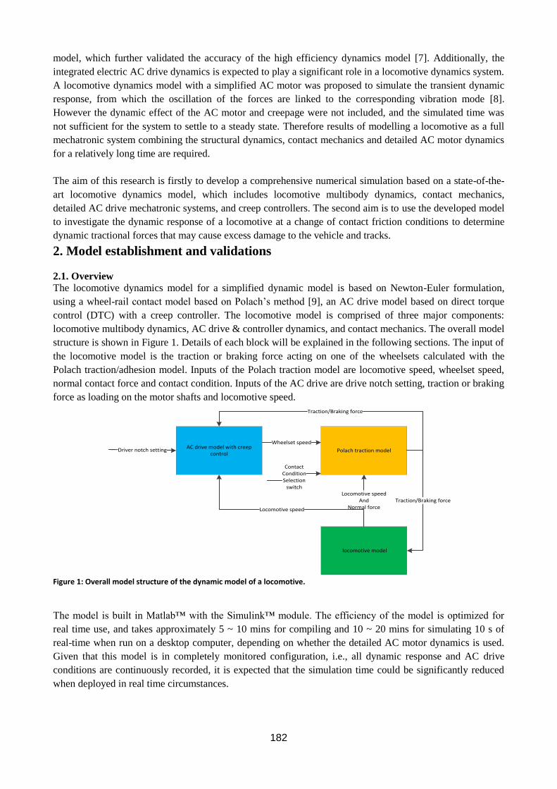
182

model, which further validated the accuracy of the high efficiency dynamics model [7]. Additionally, the

integrated electric AC drive dynamics is expected to play a significant role in a locomotive dynamics system.

A locomotive dynamics model with a simplified AC motor was proposed to simulate the transient dynamic

response, from which the oscillation of the forces are linked to the corresponding vibration mode [8].

However the dynamic effect of the AC motor and creepage were not included, and the simulated time was

not sufficient for the system to settle to a steady state. Therefore results of modelling a locomotive as a full

mechatronic system combining the structural dynamics, contact mechanics and detailed AC motor dynamics

for a relatively long time are required.

The aim of this research is firstly to develop a comprehensive numerical simulation based on a state-of-the-

art locomotive dynamics model, which includes locomotive multibody dynamics, contact mechanics,

detailed AC drive mechatronic systems, and creep controllers. The second aim is to use the developed model

to investigate the dynamic response of a locomotive at a change of contact friction conditions to determine

dynamic tractional forces that may cause excess damage to the vehicle and tracks.

2. Model establishment and validations

2.1. Overview

The locomotive dynamics model for a simplified dynamic model is based on Newton-Euler formulation,

using a wheel-rail contact model based on Polach’s method [9], an AC drive model based on direct torque

control (DTC) with a creep controller. The locomotive model is comprised of three major components:

locomotive multibody dynamics, AC drive & controller dynamics, and contact mechanics. The overall model

structure is shown in Figure 1. Details of each block will be explained in the following sections. The input of

the locomotive model is the traction or braking force acting on one of the wheelsets calculated with the

Polach traction/adhesion model. Inputs of the Polach traction model are locomotive speed, wheelset speed,

normal contact force and contact condition. Inputs of the AC drive are drive notch setting, traction or braking

force as loading on the motor shafts and locomotive speed.

Figure 1: Overall model structure of the dynamic model of a locomotive.

The model is built in Matlab™ with the Simulink™ module. The efficiency of the model is optimized for

real time use, and takes approximately 5 ~ 10 mins for compiling and 10 ~ 20 mins for simulating 10 s of

real-time when run on a desktop computer, depending on whether the detailed AC motor dynamics is used.

Given that this model is in completely monitored configuration, i.e., all dynamic response and AC drive

conditions are continuously recorded, it is expected that the simulation time could be significantly reduced

when deployed in real time circumstances.

AC drive model with creep control

Driver notch setting

locomotive model

Polach traction model

Wheelset speed

Locomotive speedAnd

Normal forceTraction/Braking force

Locomotive speed

Traction/Braking force

ContactConditionSelection

switch

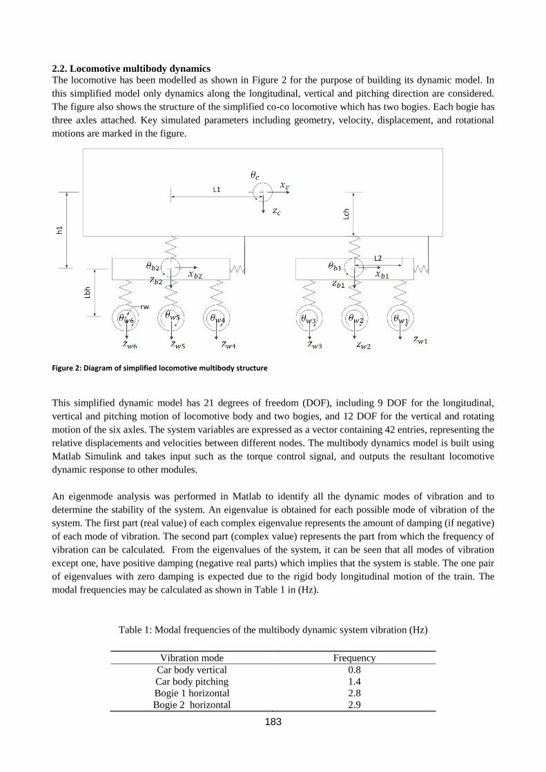
183

2.2. Locomotive multibody dynamics

The locomotive has been modelled as shown in Figure 2 for the purpose of building its dynamic model. In

this simplified model only dynamics along the longitudinal, vertical and pitching direction are considered.

The figure also shows the structure of the simplified co-co locomotive which has two bogies. Each bogie has

three axles attached. Key simulated parameters including geometry, velocity, displacement, and rotational

motions are marked in the figure.

Figure 2: Diagram of simplified locomotive multibody structure

This simplified dynamic model has 21 degrees of freedom (DOF), including 9 DOF for the longitudinal,

vertical and pitching motion of locomotive body and two bogies, and 12 DOF for the vertical and rotating

motion of the six axles. The system variables are expressed as a vector containing 42 entries, representing the

relative displacements and velocities between different nodes. The multibody dynamics model is built using

Matlab Simulink and takes input such as the torque control signal, and outputs the resultant locomotive

dynamic response to other modules.

An eigenmode analysis was performed in Matlab to identify all the dynamic modes of vibration and to

determine the stability of the system. An eigenvalue is obtained for each possible mode of vibration of the

system. The first part (real value) of each complex eigenvalue represents the amount of damping (if negative)

of each mode of vibration. The second part (complex value) represents the part from which the frequency of

vibration can be calculated. From the eigenvalues of the system, it can be seen that all modes of vibration

except one, have positive damping (negative real parts) which implies that the system is stable. The one pair

of eigenvalues with zero damping is expected due to the rigid body longitudinal motion of the train. The

modal frequencies may be calculated as shown in Table 1 in (Hz).

Table 1: Modal frequencies of the multibody dynamic system vibration (Hz)

Vibration mode Frequency

Car body vertical 0.8

Car body pitching 1.4

Bogie 1 horizontal 2.8

Bogie 2 horizontal 2.9

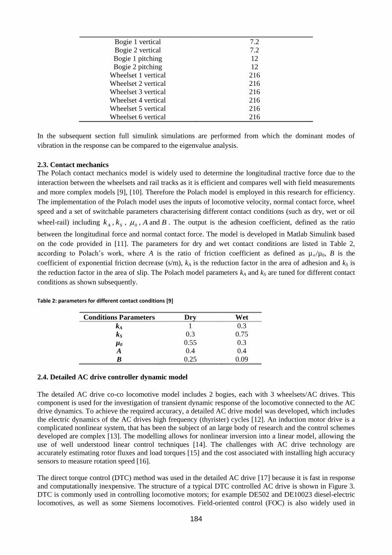
184

Bogie 1 vertical 7.2

Bogie 2 vertical 7.2

Bogie 1 pitching 12

Bogie 2 pitching 12

Wheelset 1 vertical 216

Wheelset 2 vertical 216

Wheelset 3 vertical 216

Wheelset 4 vertical 216

Wheelset 5 vertical 216

Wheelset 6 vertical 216

In the subsequent section full simulink simulations are performed from which the dominant modes of

vibration in the response can be compared to the eigenvalue analysis.

2.3. Contact mechanics

The Polach contact mechanics model is widely used to determine the longitudinal tractive force due to the

interaction between the wheelsets and rail tracks as it is efficient and compares well with field measurements

and more complex models [9], [10]. Therefore the Polach model is employed in this research for efficiency.

The implementation of the Polach model uses the inputs of locomotive velocity, normal contact force, wheel

speed and a set of switchable parameters characterising different contact conditions (such as dry, wet or oil

wheel-rail) including , , , and . The output is the adhesion coefficient, defined as the ratio

between the longitudinal force and normal contact force. The model is developed in Matlab Simulink based

on the code provided in [11]. The parameters for dry and wet contact conditions are listed in Table 2,

according to Polach’s work, where A is the ratio of friction coefficient as defined as µ∞/µ0, B is the

coefficient of exponential friction decrease (s/m), kA is the reduction factor in the area of adhesion and kS is

the reduction factor in the area of slip. The Polach model parameters kA and kS are tuned for different contact

conditions as shown subsequently.

Table 2: parameters for different contact conditions [9]

Conditions Parameters Dry Wet

kA 1 0.3

kS 0.3 0.75

µ0 0.55 0.3

A 0.4 0.4

B 0.25 0.09

2.4. Detailed AC drive controller dynamic model

The detailed AC drive co-co locomotive model includes 2 bogies, each with 3 wheelsets/AC drives. This

component is used for the investigation of transient dynamic response of the locomotive connected to the AC

drive dynamics. To achieve the required accuracy, a detailed AC drive model was developed, which includes

the electric dynamics of the AC drives high frequency (thyrister) cycles [12]. An induction motor drive is a

complicated nonlinear system, that has been the subject of an large body of research and the control schemes

developed are complex [13]. The modelling allows for nonlinear inversion into a linear model, allowing the

use of well understood linear control techniques [14]. The challenges with AC drive technology are

accurately estimating rotor fluxes and load torques [15] and the cost associated with installing high accuracy

sensors to measure rotation speed [16].

The direct torque control (DTC) method was used in the detailed AC drive [17] because it is fast in response

and computationally inexpensive. The structure of a typical DTC controlled AC drive is shown in Figure 3.

DTC is commonly used in controlling locomotive motors; for example DE502 and DE10023 diesel-electric

locomotives, as well as some Siemens locomotives. Field-oriented control (FOC) is also widely used in

Ak Sk 0 A B

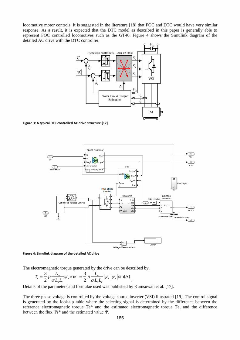
185

locomotive motor controls. It is suggested in the literature [18] that FOC and DTC would have very similar

response. As a result, it is expected that the DTC model as described in this paper is generally able to

represent FOC controlled locomotives such as the GT46. Figure 4 shows the Simulink diagram of the

detailed AC drive with the DTC controller.

Figure 3: A typical DTC controlled AC drive structure [17]

Figure 4: Simulink diagram of the detailed AC drive

The electromagnetic torque generated by the drive can be described by,

.

Details of the parameters and formulae used was published by Kumsuwan et al. [17].

The three phase voltage is controlled by the voltage source inverter (VSI) illustrated [19]. The control signal

is generated by the look-up table where the selecting signal is determined by the difference between the

reference electromagnetic torque Te* and the estimated electromagnetic torque Te, and the difference

between the flux Ψs* and the estimated value Ψ.

3 3sin( )

2 2

m me s r s r

s r s r

L LT p p

L L L L

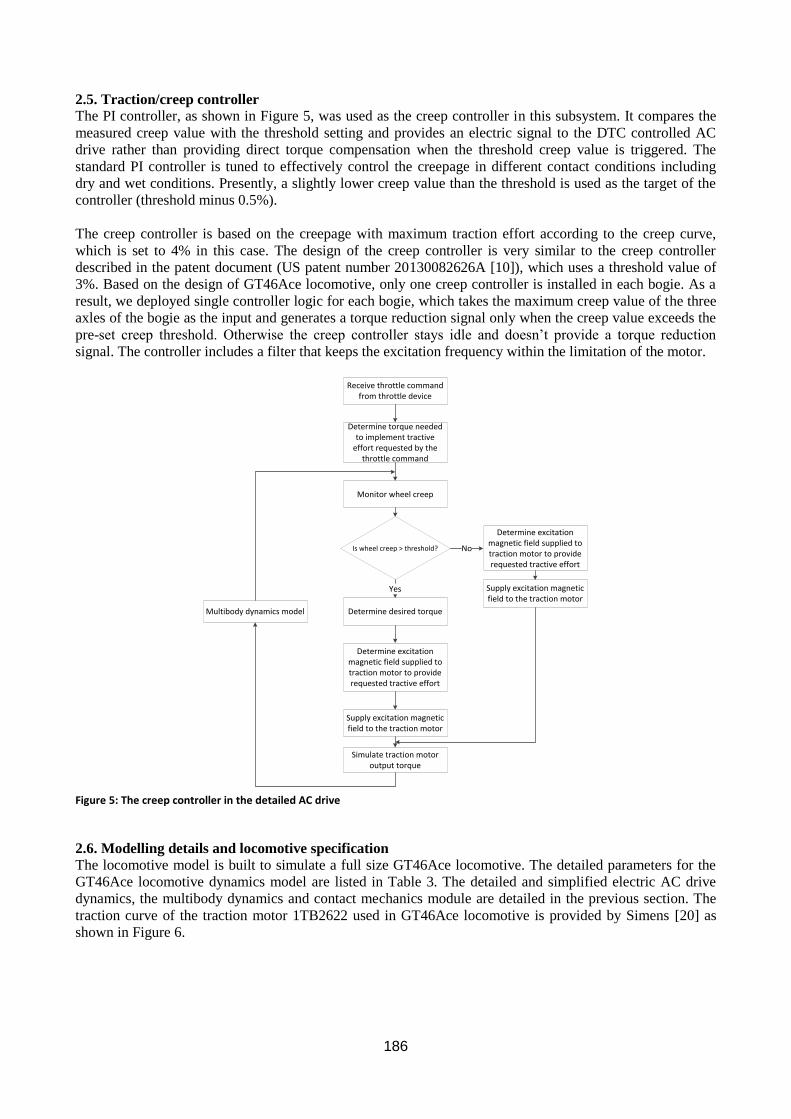
186

2.5. Traction/creep controller

The PI controller, as shown in Figure 5, was used as the creep controller in this subsystem. It compares the

measured creep value with the threshold setting and provides an electric signal to the DTC controlled AC

drive rather than providing direct torque compensation when the threshold creep value is triggered. The

standard PI controller is tuned to effectively control the creepage in different contact conditions including

dry and wet conditions. Presently, a slightly lower creep value than the threshold is used as the target of the

controller (threshold minus 0.5%).

The creep controller is based on the creepage with maximum traction effort according to the creep curve,

which is set to 4% in this case. The design of the creep controller is very similar to the creep controller

described in the patent document (US patent number 20130082626A [10]), which uses a threshold value of

3%. Based on the design of GT46Ace locomotive, only one creep controller is installed in each bogie. As a

result, we deployed single controller logic for each bogie, which takes the maximum creep value of the three

axles of the bogie as the input and generates a torque reduction signal only when the creep value exceeds the

pre-set creep threshold. Otherwise the creep controller stays idle and doesn’t provide a torque reduction

signal. The controller includes a filter that keeps the excitation frequency within the limitation of the motor.

Figure 5: The creep controller in the detailed AC drive

2.6. Modelling details and locomotive specification

The locomotive model is built to simulate a full size GT46Ace locomotive. The detailed parameters for the

GT46Ace locomotive dynamics model are listed in Table 3. The detailed and simplified electric AC drive

dynamics, the multibody dynamics and contact mechanics module are detailed in the previous section. The

traction curve of the traction motor 1TB2622 used in GT46Ace locomotive is provided by Simens [20] as

shown in Figure 6.

Receive throttle command from throttle device

Receive throttle command from throttle device

Determine torque needed to implement tractive

effort requested by the throttle command

Determine torque needed to implement tractive

effort requested by the throttle command

Monitor wheel creepMonitor wheel creep

Is wheel creep > threshold?

Determine excitation magnetic field supplied to traction motor to provide requested tractive effort

Determine excitation magnetic field supplied to traction motor to provide requested tractive effort

Determine desired torque Determine desired torque

No

Yes Supply excitation magnetic field to the traction motor

Supply excitation magnetic field to the traction motor

Determine excitation magnetic field supplied to traction motor to provide requested tractive effort

Determine excitation magnetic field supplied to traction motor to provide requested tractive effort

Supply excitation magnetic field to the traction motor

Supply excitation magnetic field to the traction motor

Simulate traction motor output torque

Simulate traction motor output torque

Multibody dynamics modelMultibody dynamics model

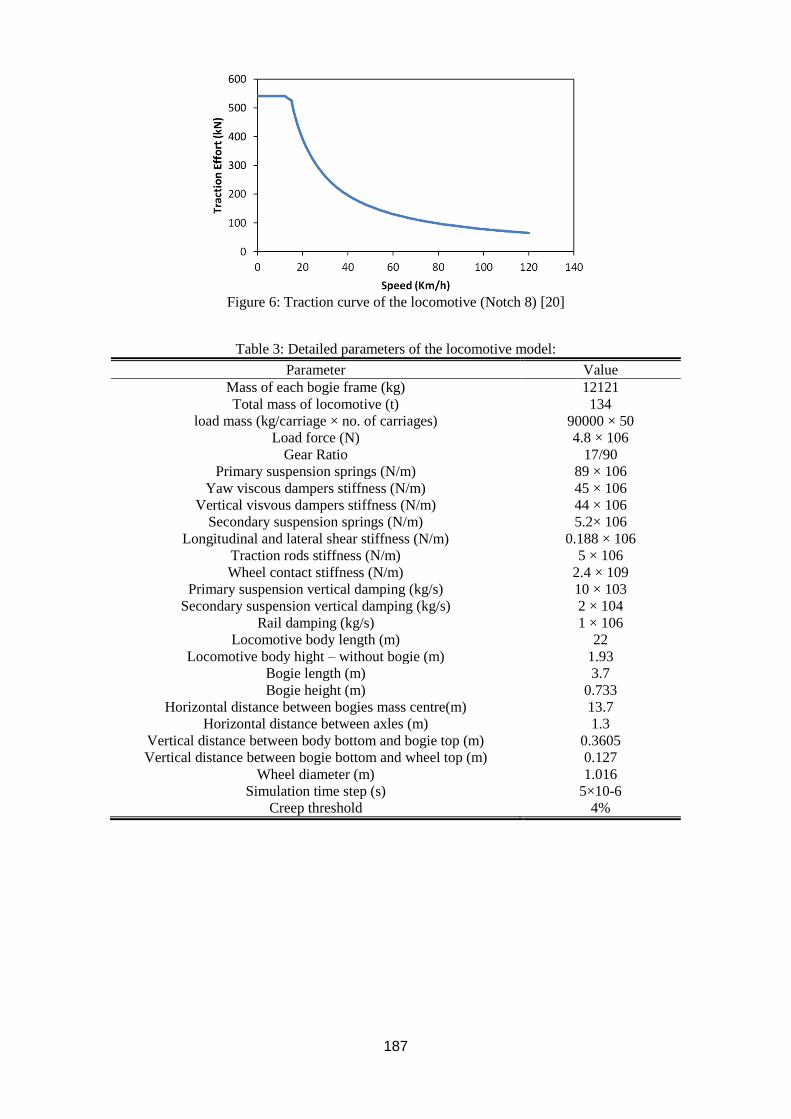
187

Figure 6: Traction curve of the locomotive (Notch 8) [20]

Table 3: Detailed parameters of the locomotive model:

Parameter Value

Mass of each bogie frame (kg) 12121

Total mass of locomotive (t) 134

load mass (kg/carriage × no. of carriages) 90000 × 50

Load force (N) 4.8 × 106

Gear Ratio 17/90

Primary suspension springs (N/m) 89 × 106

Yaw viscous dampers stiffness (N/m) 45 × 106

Vertical visvous dampers stiffness (N/m) 44 × 106

Secondary suspension springs (N/m) 5.2× 106

Longitudinal and lateral shear stiffness (N/m) 0.188 × 106

Traction rods stiffness (N/m) 5 × 106

Wheel contact stiffness (N/m) 2.4 × 109

Primary suspension vertical damping (kg/s) 10 × 103

Secondary suspension vertical damping (kg/s) 2 × 104

Rail damping (kg/s) 1 × 106

Locomotive body length (m) 22

Locomotive body hight – without bogie (m) 1.93

Bogie length (m) 3.7

Bogie height (m) 0.733

Horizontal distance between bogies mass centre(m) 13.7

Horizontal distance between axles (m) 1.3

Vertical distance between body bottom and bogie top (m) 0.3605

Vertical distance between bogie bottom and wheel top (m) 0.127

Wheel diameter (m) 1.016

Simulation time step (s) 5×10-6

Creep threshold 4%

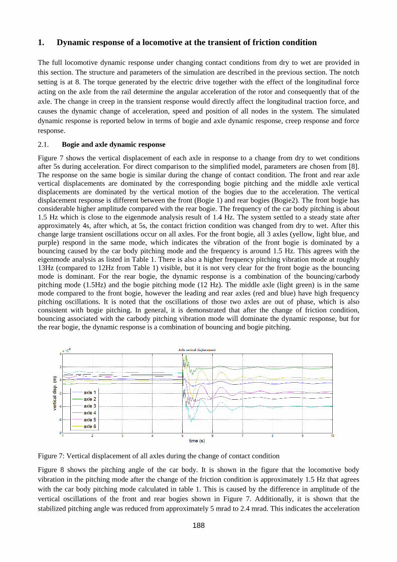
188

1. Dynamic response of a locomotive at the transient of friction condition

The full locomotive dynamic response under changing contact conditions from dry to wet are provided in

this section. The structure and parameters of the simulation are described in the previous section. The notch

setting is at 8. The torque generated by the electric drive together with the effect of the longitudinal force

acting on the axle from the rail determine the angular acceleration of the rotor and consequently that of the

axle. The change in creep in the transient response would directly affect the longitudinal traction force, and

causes the dynamic change of acceleration, speed and position of all nodes in the system. The simulated

dynamic response is reported below in terms of bogie and axle dynamic response, creep response and force

response.

2.1. Bogie and axle dynamic response

Figure 7 shows the vertical displacement of each axle in response to a change from dry to wet conditions

after 5s during acceleration. For direct comparison to the simplified model, parameters are chosen from [8].

The response on the same bogie is similar during the change of contact condition. The front and rear axle

vertical displacements are dominated by the corresponding bogie pitching and the middle axle vertical

displacements are dominated by the vertical motion of the bogies due to the acceleration. The vertical

displacement response is different between the front (Bogie 1) and rear bogies (Bogie2). The front bogie has

considerable higher amplitude compared with the rear bogie. The frequency of the car body pitching is about

1.5 Hz which is close to the eigenmode analysis result of 1.4 Hz. The system settled to a steady state after

approximately 4s, after which, at 5s, the contact friction condition was changed from dry to wet. After this

change large transient oscillations occur on all axles. For the front bogie, all 3 axles (yellow, light blue, and

purple) respond in the same mode, which indicates the vibration of the front bogie is dominated by a

bouncing caused by the car body pitching mode and the frequency is around 1.5 Hz. This agrees with the

eigenmode analysis as listed in Table 1. There is also a higher frequency pitching vibration mode at roughly

13Hz (compared to 12Hz from Table 1) visible, but it is not very clear for the front bogie as the bouncing

mode is dominant. For the rear bogie, the dynamic response is a combination of the bouncing/carbody

pitching mode (1.5Hz) and the bogie pitching mode (12 Hz). The middle axle (light green) is in the same

mode compared to the front bogie, however the leading and rear axles (red and blue) have high frequency

pitching oscillations. It is noted that the oscillations of those two axles are out of phase, which is also

consistent with bogie pitching. In general, it is demonstrated that after the change of friction condition,

bouncing associated with the carbody pitching vibration mode will dominate the dynamic response, but for

the rear bogie, the dynamic response is a combination of bouncing and bogie pitching.

Figure 7: Vertical displacement of all axles during the change of contact condition

Figure 8 shows the pitching angle of the car body. It is shown in the figure that the locomotive body

vibration in the pitching mode after the change of the friction condition is approximately 1.5 Hz that agrees

with the car body pitching mode calculated in table 1. This is caused by the difference in amplitude of the

vertical oscillations of the front and rear bogies shown in Figure 7. Additionally, it is shown that the

stabilized pitching angle was reduced from approximately 5 mrad to 2.4 mrad. This indicates the acceleration

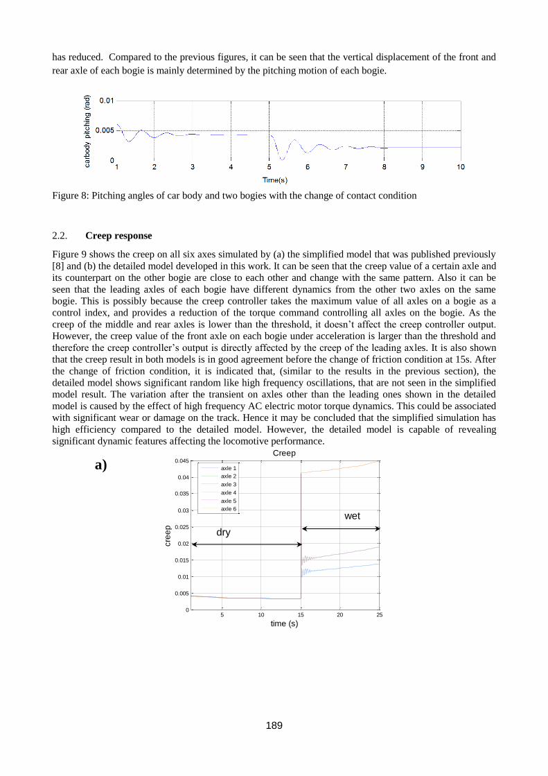
189

has reduced. Compared to the previous figures, it can be seen that the vertical displacement of the front and

rear axle of each bogie is mainly determined by the pitching motion of each bogie.

Figure 8: Pitching angles of car body and two bogies with the change of contact condition

2.2. Creep response

Figure 9 shows the creep on all six axes simulated by (a) the simplified model that was published previously

[8] and (b) the detailed model developed in this work. It can be seen that the creep value of a certain axle and

its counterpart on the other bogie are close to each other and change with the same pattern. Also it can be

seen that the leading axles of each bogie have different dynamics from the other two axles on the same

bogie. This is possibly because the creep controller takes the maximum value of all axles on a bogie as a

control index, and provides a reduction of the torque command controlling all axles on the bogie. As the

creep of the middle and rear axles is lower than the threshold, it doesn’t affect the creep controller output.

However, the creep value of the front axle on each bogie under acceleration is larger than the threshold and

therefore the creep controller’s output is directly affected by the creep of the leading axles. It is also shown

that the creep result in both models is in good agreement before the change of friction condition at 15s. After

the change of friction condition, it is indicated that, (similar to the results in the previous section), the

detailed model shows significant random like high frequency oscillations, that are not seen in the simplified

model result. The variation after the transient on axles other than the leading ones shown in the detailed

model is caused by the effect of high frequency AC electric motor torque dynamics. This could be associated

with significant wear or damage on the track. Hence it may be concluded that the simplified simulation has

high efficiency compared to the detailed model. However, the detailed model is capable of revealing

significant dynamic features affecting the locomotive performance.

5 10 15 20 250

0.005

0.01

0.015

0.02

0.025

0.03

0.035

0.04

0.045

Creep

time (s)

cre

ep

axle 1

axle 2

axle 3

axle 4

axle 5

axle 6

a)

dry

wet

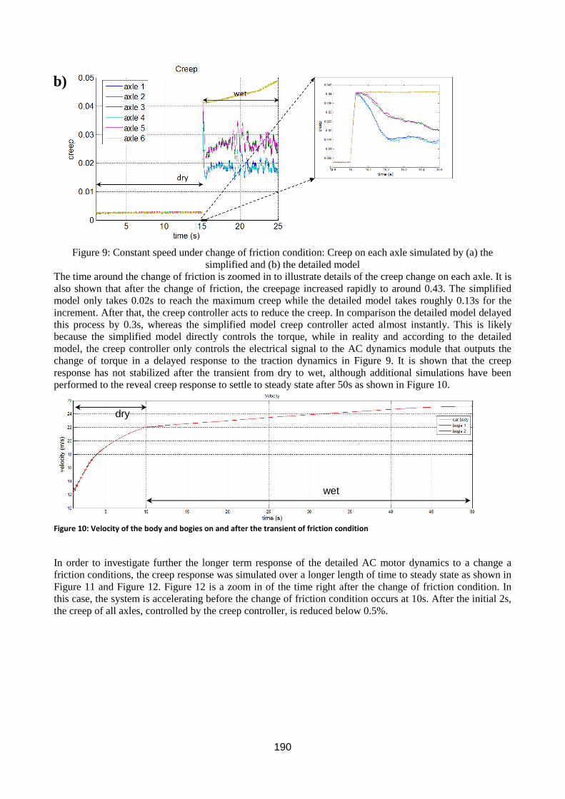
190

Figure 9: Constant speed under change of friction condition: Creep on each axle simulated by (a) the

simplified and (b) the detailed model

The time around the change of friction is zoomed in to illustrate details of the creep change on each axle. It is

also shown that after the change of friction, the creepage increased rapidly to around 0.43. The simplified

model only takes 0.02s to reach the maximum creep while the detailed model takes roughly 0.13s for the

increment. After that, the creep controller acts to reduce the creep. In comparison the detailed model delayed

this process by 0.3s, whereas the simplified model creep controller acted almost instantly. This is likely

because the simplified model directly controls the torque, while in reality and according to the detailed

model, the creep controller only controls the electrical signal to the AC dynamics module that outputs the

change of torque in a delayed response to the traction dynamics in Figure 9. It is shown that the creep

response has not stabilized after the transient from dry to wet, although additional simulations have been

performed to the reveal creep response to settle to steady state after 50s as shown in Figure 10.

Figure 10: Velocity of the body and bogies on and after the transient of friction condition

In order to investigate further the longer term response of the detailed AC motor dynamics to a change a

friction conditions, the creep response was simulated over a longer length of time to steady state as shown in

Figure 11 and Figure 12. Figure 12 is a zoom in of the time right after the change of friction condition. In

this case, the system is accelerating before the change of friction condition occurs at 10s. After the initial 2s,

the creep of all axles, controlled by the creep controller, is reduced below 0.5%.

dry

wet

b)

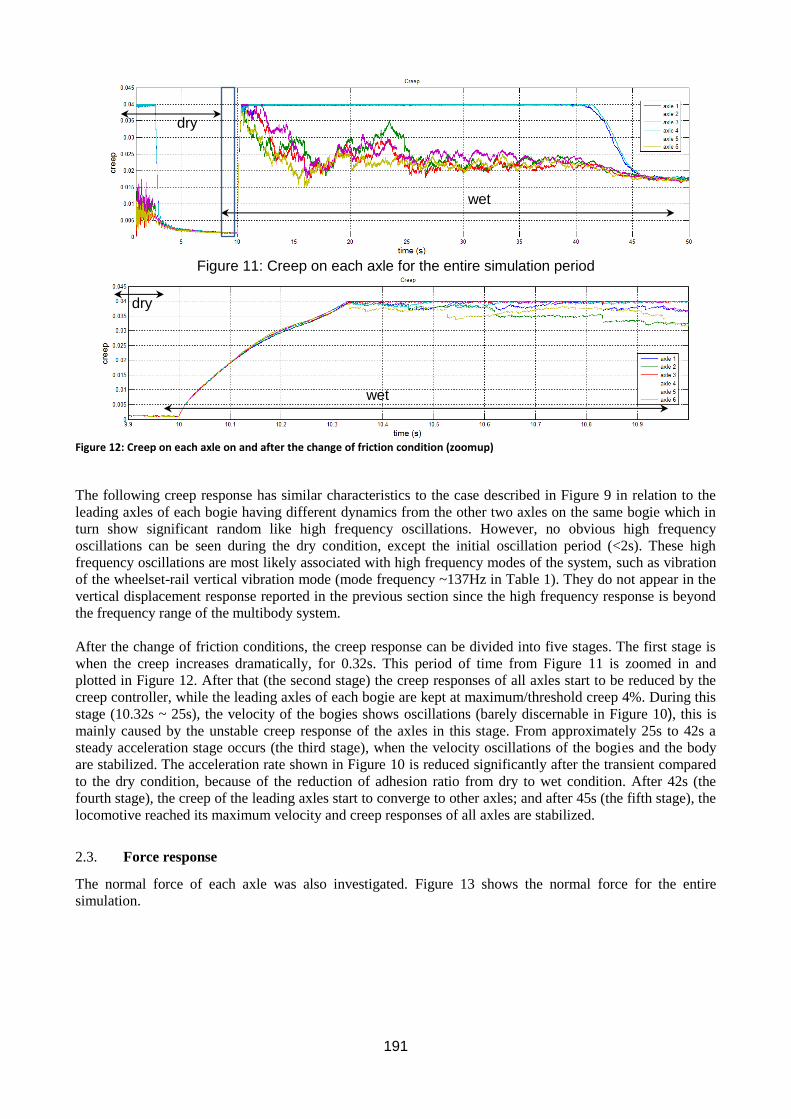
191

Figure 11: Creep on each axle for the entire simulation period

Figure 12: Creep on each axle on and after the change of friction condition (zoomup)

The following creep response has similar characteristics to the case described in Figure 9 in relation to the

leading axles of each bogie having different dynamics from the other two axles on the same bogie which in

turn show significant random like high frequency oscillations. However, no obvious high frequency

oscillations can be seen during the dry condition, except the initial oscillation period (<2s). These high

frequency oscillations are most likely associated with high frequency modes of the system, such as vibration

of the wheelset-rail vertical vibration mode (mode frequency ~137Hz in Table 1). They do not appear in the

vertical displacement response reported in the previous section since the high frequency response is beyond

the frequency range of the multibody system.

After the change of friction conditions, the creep response can be divided into five stages. The first stage is

when the creep increases dramatically, for 0.32s. This period of time from Figure 11 is zoomed in and

plotted in Figure 12. After that (the second stage) the creep responses of all axles start to be reduced by the

creep controller, while the leading axles of each bogie are kept at maximum/threshold creep 4%. During this

stage (10.32s ~ 25s), the velocity of the bogies shows oscillations (barely discernable in Figure 10), this is

mainly caused by the unstable creep response of the axles in this stage. From approximately 25s to 42s a

steady acceleration stage occurs (the third stage), when the velocity oscillations of the bogies and the body

are stabilized. The acceleration rate shown in Figure 10 is reduced significantly after the transient compared

to the dry condition, because of the reduction of adhesion ratio from dry to wet condition. After 42s (the

fourth stage), the creep of the leading axles start to converge to other axles; and after 45s (the fifth stage), the

locomotive reached its maximum velocity and creep responses of all axles are stabilized.

2.3. Force response

The normal force of each axle was also investigated. Figure 13 shows the normal force for the entire

simulation.

dry

wet

dry

wet

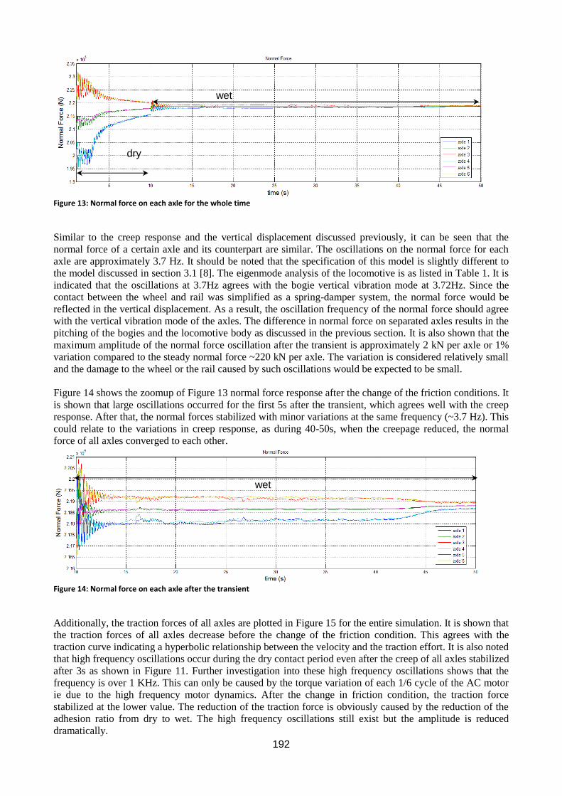
192

Figure 13: Normal force on each axle for the whole time

Similar to the creep response and the vertical displacement discussed previously, it can be seen that the

normal force of a certain axle and its counterpart are similar. The oscillations on the normal force for each

axle are approximately 3.7 Hz. It should be noted that the specification of this model is slightly different to

the model discussed in section 3.1 [8]. The eigenmode analysis of the locomotive is as listed in Table 1. It is

indicated that the oscillations at 3.7Hz agrees with the bogie vertical vibration mode at 3.72Hz. Since the

contact between the wheel and rail was simplified as a spring-damper system, the normal force would be

reflected in the vertical displacement. As a result, the oscillation frequency of the normal force should agree

with the vertical vibration mode of the axles. The difference in normal force on separated axles results in the

pitching of the bogies and the locomotive body as discussed in the previous section. It is also shown that the

maximum amplitude of the normal force oscillation after the transient is approximately 2 kN per axle or 1%

variation compared to the steady normal force ~220 kN per axle. The variation is considered relatively small

and the damage to the wheel or the rail caused by such oscillations would be expected to be small.

Figure 14 shows the zoomup of Figure 13 normal force response after the change of the friction conditions. It

is shown that large oscillations occurred for the first 5s after the transient, which agrees well with the creep

response. After that, the normal forces stabilized with minor variations at the same frequency (~3.7 Hz). This

could relate to the variations in creep response, as during 40-50s, when the creepage reduced, the normal

force of all axles converged to each other.

Figure 14: Normal force on each axle after the transient

Additionally, the traction forces of all axles are plotted in Figure 15 for the entire simulation. It is shown that

the traction forces of all axles decrease before the change of the friction condition. This agrees with the

traction curve indicating a hyperbolic relationship between the velocity and the traction effort. It is also noted

that high frequency oscillations occur during the dry contact period even after the creep of all axles stabilized

after 3s as shown in Figure 11. Further investigation into these high frequency oscillations shows that the

frequency is over 1 KHz. This can only be caused by the torque variation of each 1/6 cycle of the AC motor

ie due to the high frequency motor dynamics. After the change in friction condition, the traction force

stabilized at the lower value. The reduction of the traction force is obviously caused by the reduction of the

adhesion ratio from dry to wet. The high frequency oscillations still exist but the amplitude is reduced

dramatically.

wet

dry

wet

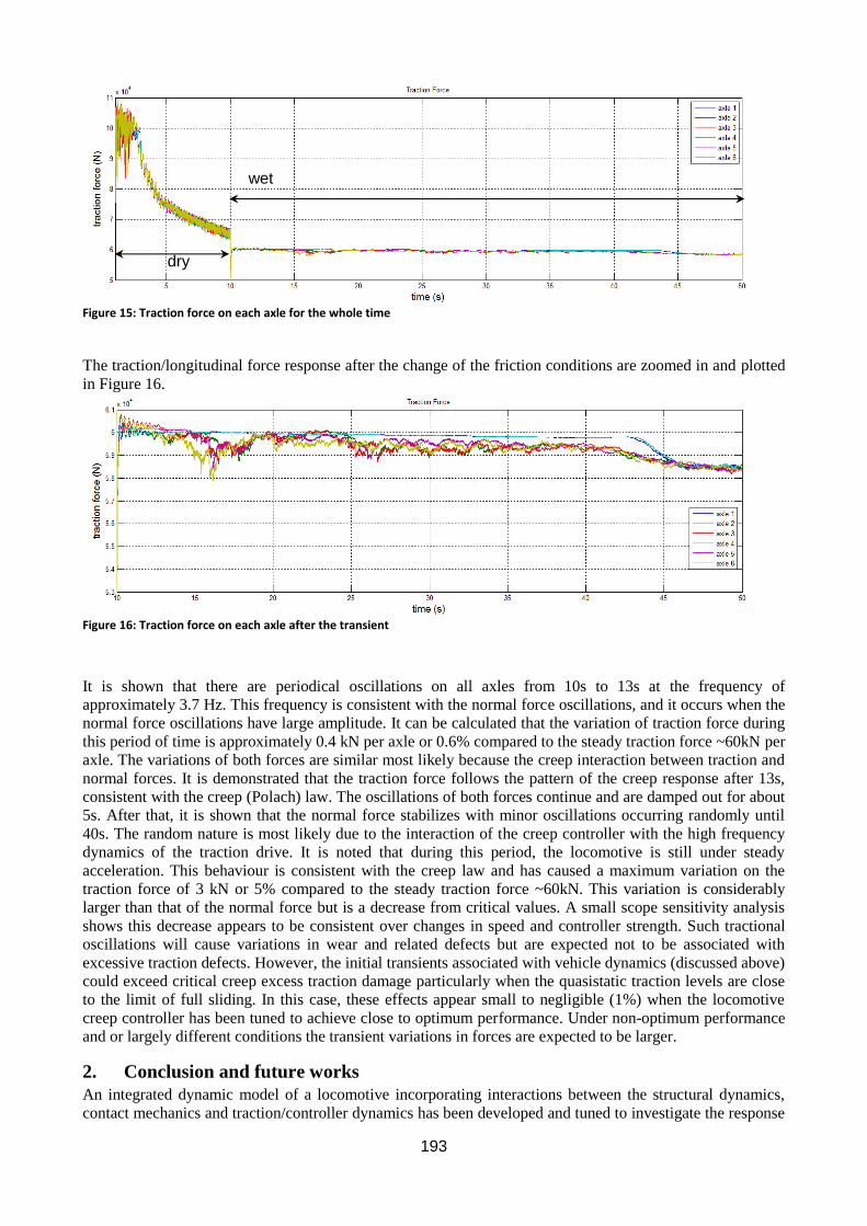
193

Figure 15: Traction force on each axle for the whole time

The traction/longitudinal force response after the change of the friction conditions are zoomed in and plotted

in Figure 16.

Figure 16: Traction force on each axle after the transient

It is shown that there are periodical oscillations on all axles from 10s to 13s at the frequency of

approximately 3.7 Hz. This frequency is consistent with the normal force oscillations, and it occurs when the

normal force oscillations have large amplitude. It can be calculated that the variation of traction force during

this period of time is approximately 0.4 kN per axle or 0.6% compared to the steady traction force ~60kN per

axle. The variations of both forces are similar most likely because the creep interaction between traction and

normal forces. It is demonstrated that the traction force follows the pattern of the creep response after 13s,

consistent with the creep (Polach) law. The oscillations of both forces continue and are damped out for about

5s. After that, it is shown that the normal force stabilizes with minor oscillations occurring randomly until

40s. The random nature is most likely due to the interaction of the creep controller with the high frequency

dynamics of the traction drive. It is noted that during this period, the locomotive is still under steady

acceleration. This behaviour is consistent with the creep law and has caused a maximum variation on the

traction force of 3 kN or 5% compared to the steady traction force ~60kN. This variation is considerably

larger than that of the normal force but is a decrease from critical values. A small scope sensitivity analysis

shows this decrease appears to be consistent over changes in speed and controller strength. Such tractional

oscillations will cause variations in wear and related defects but are expected not to be associated with

excessive traction defects. However, the initial transients associated with vehicle dynamics (discussed above)

could exceed critical creep excess traction damage particularly when the quasistatic traction levels are close

to the limit of full sliding. In this case, these effects appear small to negligible (1%) when the locomotive

creep controller has been tuned to achieve close to optimum performance. Under non-optimum performance

and or largely different conditions the transient variations in forces are expected to be larger.

2. Conclusion and future works

An integrated dynamic model of a locomotive incorporating interactions between the structural dynamics,

contact mechanics and traction/controller dynamics has been developed and tuned to investigate the response

dry

wet

194

under a change in frictional conditions. The dynamic response including creep response and forces, of the

locomotive at and after a change in friction condition are investigated. The oscillation frequencies are

compared with the eigenmode analysis and the related vehicle structural vibration modes are identified. By

using the detailed AC motor dynamics model, both normal and traction force oscillations found in the first 3s

after the change in friction condition are caused by the bogie structural vertical vibration. The amplitudes of

these oscillations are approximately 1% of the steady force. After these vibrations are damped out, variations

in creep dominate the changes in the traction force. These variations are relatively larger, up to 5%,

compared to those caused by structural vibration, however they typically decrease the traction levels. These

tractional oscillations, although small in this case, could result in dynamic wear defects and associated

damage particularly when the quasistatic traction levels are close to the limit of full sliding and under less

optimum creep controller performance. It takes approximately 30s for the creepage to stabilize. In this period

of time, the locomotive will travel approximately 600m, and the track would possibly be affected by

excessive transient forces.

Future research could be focused on the validation of the locomotive model dynamic response using field or

test rig results. The model could also be further developed to simulate a larger range of locomotive models

(if data is available from industry) and more frictional conditions. The efficiency of the model should be

further improved to facilitate a sensitivity investigation of controller and locomotive structural parameters to

dynamic force response.

Acknowledgements The authors are grateful to the CRC for Rail Innovation (established and supported under the Australian Government's

Cooperative Research Centres program) for the funding of this research Project No. R3.119 “Locomotive Adhesion”.

The authors acknowledge the support of the Centre for Railway Engineering, Central Queensland University and the

many industry partners that have contributed to this project, in particular staff from RailCorp, Fortescue Metals Group

(FMG) and Brookfield Rail.

195

References

[1] N. Ramsey, F. Szanto, and P. Hewison, "Introducing the next generation locomotive to the

Australian rail network," presented at the Conference on Railway Engineering, Perth, 2008.

[2] R. U. A. Uzzal, A. K. W. Ahmed, and S. Rakheja, "Dynamic Analysis of Pitch Plane Railway

Vehicle-Track Interactions Due to Single and Multiple Wheel Flats," ASME Conference

Proceedings, vol. 2008, pp. 89-97, 2008.

[3] M. R. U. A. Uzzal, "ANALYSIS OF A THREE-DIMENSIONAL RAILWAY VEHICLE-TRACK

SYSTEM AND DEVELOPMENT OF A SMART WHEELSET," PhD, Mechanical Engineering,

Concordia University, 2012.

[4] R. Guclu and M. Metin, "Fuzzy Logic Control of Vibrations of a Light Rail Transport Vehicle in

Use in Istanbul Traffic," Journal of Vibration and Control, vol. 15, pp. 1423-1440, September 1,

2009 2009.

[5] D. S. Garivaltis, V. K. Garg, and A. F. D'Souza, "Dynamic Response of a Six-axle Locomotive to

Random Track Inputs," Vehicle System Dynamics, vol. 9, pp. 117-147, 1980/05/01 1980.

[6] X. Xin, B. K. Parida, A. K. Zaouk, N. Dana, and S. K. Punwani, "Impact Analysis of an Innovative

Shock Energy Absorber and Its Applications in Improving Railroad Safety."

[7] M. Spiryagin, Y. Q. Sun, C. Cole, T. McSweeney, S. Simson, and I. Persson, "Development of a

real-time bogie test rig model based on railway specialised multibody software," Vehicle System

Dynamics, vol. 51, pp. 236-250, 2013.

[8] Y. Tian, W. B. Daniel, S. Liu, and P. A. Meehan, "Dynamic tractional behaviour analysis and

control for a dc locomotive," in World Congress on Rail Research (WCRR), Sydney, 2013.

[9] O. Polach, "Creep forces in simulations of traction vehicles running on adhesion limit," Wear, vol.

258, pp. 992-1000, 2005.

[10] M. Spiryagin, O. Polach, and C. Cole, "Creep force modelling for rail traction vehicles based on the

Fastsim algorithm," Vehicle System Dynamics, vol. 51, pp. 1765-1783, 2013.

[11] O. Polach, "A Fast Wheel-Rail Forces Calculation Computer Code," Vehicle System Dynamics, vol.

33, pp. 728-739, 1999.

[12] V. R. Moorthi, Power electronics: devices, circuits and industrial applications: Oxford University

Press, 2005.

[13] I. Boldea and S. A. Nasar, The Induction Machine Handbook: CRC Press, 2002.

[14] R. Marino, P. Tomei, and C. M. Verrelli, Induction Motor Control Design: Springer, 2010.

[15] D. J. Atkinson, P. P. Acarnley, and J. W. Finch, "Observers for induction motor state and parameter

estimation," Industry Applications, IEEE Transactions on, vol. 27, pp. 1119-1127, 1991.

[16] S. Kadowaki, K. Ohishi, T. Hata, N. Iida, M. Takagi, T. Sano, and S. Yasukawa, "Antislip

Readhesion Control Based on Speed-Sensorless Vector Control and Disturbance Observer for

Electric Commuter Train&#x2014;Series 205-5000 of the East Japan Railway Company," Industrial

Electronics, IEEE Transactions on, vol. 54, pp. 2001-2008, 2007.

[17] Y. Kumsuwan, S. Premrudeepreechacharn, and H. A. Toliyat, "Modified direct torque control

method for induction motor drives based on amplitude and angle control of stator flux," Electric

Power Systems Research, vol. 78, pp. 1712-1718, 2008.

[18] D. Casadei, F. Profumo, G. Serra, and A. Tani, "FOC and DTC: two viable schemes for induction

motors torque control," Power Electronics, IEEE Transactions on, vol. 17, pp. 779-787, 2002.

[19] P. Wach, Dynamics and Control of Electrical Drives: Springer, 2011.

[20] S. N. EMU, "Rail Safety Investigation report No 2009/05, Platform overruns," Connex/Metro trains,

Office of the Chief Investigator, transport Safety, Melbourne, Australia2009.