Abstract In this paper the effect of teacher pay on student performance has been examined. This has

been done through a difference-in-difference design, in which Randstad schools received an

extra amount of teacher pay in comparison to non-Randstad schools. Schools that are just in

and outside the Randstad are compared to each other, with the assumption that these

schools are similar to each other. The remuneration policy came into action in 2008, but the

first effects on student performance were not expected until 2010 and later, so studied

years of impact are 2010, 2011 and 2012. Two different variables are used as outcome

variable, the average central examination grade and a school grade, which is a measure

developed by Jaap Dronkers that reviews each school each year.

The analysis indicated mixed results; in some cases the extra teacher pay for Randstad

schools increased their student performance, in other cases the extra teacher pay decreased

the student performance. Nevertheless, an interesting pattern could be established; the

estimations for lower education levels all have a negative sign, while the estimations for

higher education levels mostly have a positive sign. This suggests a positive relationship

between education level and effectiveness of teacher pay on student performance.

The influence of increased teacher pay on student performance: a case study of Randstad & non-Randstad schools in 2004-2015 ERASMUS UNIVERSITY ROTTERDAM

Erasmus School of Economics Department of Economics Supervisor: Robert Dur Name: Damy Duifhuis Exam number: 358619 E-mail address: damyduif@hotmail.com

2

1. Introduction Ever since the existence of education, from its prehistoric beginnings through Plato's

foundation of the Academy in Athens to the worldwide attainment of today's formal

education and presence in both UN's Millennium Development Goals (United Nations, 2000)

and Sustainable Development Goals (United Nations, 2015), it has been an extensive topic of

discussion. While high rates of education are widely regarded to have positive effects on the

economic growth of a country (Hanushek, 2005), discussion on the effects of different

educational resources is still going on. Hundreds of studies cannot agree which of the

different school resources has the most profound effect on student performance.

The lack of convincing evidence in this extensive body of literature on the so-called

education production function, is due to the many unobserved factors that are affecting the

variables in research (Webbink, 2005). Point is that a difference in student performance is

not sure to be the result of a certain intervention when it is not taken into account that

there are multiple other factors that have to be taken into account. These factors are

difficult to observe by the researcher and might influence both the intervention variable and

the outcome variable, which in turn biases the results of a traditional OLS (ordinary least

squares). As an example, parents who care a lot about their child's education, might choose

a school for them where teachers are paid more than average. Additionally, they might

motivate and stimulate their children while helping them with their homework more than

other parents. A researcher who does not realize that how much parents care about their

child's education is a factor to be dealt with could mistakenly conclude that higher teacher

pay leads to better student performance. Besides, even if the researcher would realize that,

it would be really difficult to observe and collect data about the level of how much parents

care about their child's education.

From the 90's onwards however this endogeneity problem is tackled more and more by a

wave of new literature, consisting of somewhat innovative research designs; the effect of

intervention on student performance is estimated with the aid of exogenous variation, in

turn caused by controlled or natural experiments (Webbink, 2005). This paper contributes to

that wave of new literature, which increases the scientific relevance of the paper as well as

the relevance to policy makers. The paper tries to answer the following research question:

what is the effect of an increase in teacher pay on student performance?

The exogenous variation that is used in the paper is regional variation in teacher pay

between different schools, caused by a new educational policy in the Netherlands. This new

policy, called Convenant Leerkracht van Nederland (Social partners in education & Ministry

of Education, 2008) was introduced in 2008 and is an outcome of a collaboration of social

partners in education and the Ministry of Education. Part of the agreement is a higher

remuneration for teachers, both in primary and secondary education. The variation comes

into play as teachers at schools within the Randstad, the densely populated and biggest

urbanized region of The Netherlands, get higher pay raises than teachers at schools outside

3

the Randstad. The paper researches schools that are close to the border of the Randstad. An

OLS regression determines what the effect is of a pay raise on student performance, while a

dummy splits this effect into a group of schools inside the Randstad and a group outside the

Randstad. The assumption of the research sample is that the closer the schools are to the

border, the more similar these schools are expected to be. A crucial assumption as this

implicates that the effect of higher teacher pay on student performance can be determined

without having to account for the numerous unobserved factors. Almost needless to say, the

social relevance of this research is huge; it is still unsure how educational money should be

spent, so this kind of research could be influential on government's (educational) policies.

The analysis indicated mixed results; in some cases the extra teacher pay for Randstad

schools increased their student performance, in other cases the extra teacher pay decreased

the student performance. Nevertheless, an interesting pattern could be established; the

estimations for lower education levels all have a negative sign, while the estimations for

higher education levels mostly have a positive sign. This suggests a positive relationship

between education level and effectiveness of teacher pay on student performance.

The paper is structured as follows. The next section – section 2 – describes the related

literature and the papers contribution to this literature. Section 3 discusses the data and

methodology that are used, while section 4 provides the results of the analyses and the

discussion of them. Section 5 concludes the paper with some limitations, extensions and

implications of the paper.

4

2. Related Literature There is an extensive body of literature on the effect of educational resources on student

performance, research on the so-called education production function. Firstly, the

traditional literature on this subject will be covered. This will then be followed by the already

mentioned new wave of literature that deals with the in the traditional literature frequently

encountered endogeneity, by making use of exogenous variation.

2.1 The traditional literature

A typical research on the educational production function studies the effect of educational

resources on the performance of students. Factors that are accounted for in the models

include all kinds of facts about the students, parents, teachers and schools. This type of

research came into existence after Coleman's Equality of Educational Opportunity (Coleman

& others, 1966). It was an influential research as it included a large survey that collected

data from approximately 500.000 students from over 3000 schools. It tried to discover which

of the many factors have the biggest influence on student performance, knowledge that

helps to reach a consensus on which is the correct education production function to use.

Coleman's report found that family background and characteristics of fellow students are

the most important factors of student performance.

Twenty years and a lot of research later Hanushek (1986) created an overview of studies on

the education production function. This overview sums up 147 estimates according to which

educational resource is studied, whether the estimate is statistically significant or not and

whether the sign of the estimate is positive or negative.1 Another 11 years later Hanushek

(1997) updated his overview which then consisted of 377 estimates from 90

studies/books/articles.2

Table 1: Percentage distribution of estimated effects of key resources on student

performance.3

The table shows that 119 of the total 377 estimates included an analysis of the effect of

teacher salary on student performance. 27 per cent of these estimations was statistically

significant (5 per cent level), consisting of 20 per cent positively and 7 per cent negatively

statistically significant. 45 per cent was statistically insignificant, consisting of 25 per cent

1 See table A.1 2 See table 1 3 Source: (Hanushek, 1997) (Webbink, 2005)

5

positively and 20 per cent negatively statistically insignificant. Hanushek eventually came to

the counterintuitive conclusion that there is no strong or systematic relationship between

educational resources and student performance, the only consistency to be found from his

overview of data. This led to lower educational expenditures and new discussions; first of all,

it is widely discussed how education should be incentivized. What incentives should teachers

(Lavy, 2011) (Woessmann, 2011) and students (Allan & Freyer, 2011) have? Or in general:

how should education be organized (Chubb & Moe, 1990) (Hanushek & Jorgensen, 1996)

(Ladd, 1996) (Webbink, et al., 2009)? In the mean-time others question the use of spending

(extra) money in education; does money matter at all (Hanushek, 1996) (Guryan, 2001)? This

discussion scattered into several directions and researchers still have not come to a shared

conclusion on the specification of the education production function (Heckman, et al., 1996)

(Todd & Wolpin, 2003), the best measure variable of student performance, student grades

or wages (Card & Krueger, 1992), and the ideal level at which data should be studied,

student level versus school level (Hanushek, et al., 1996).

2.2 Critiques: endogeneity and others

A critique on Hanushek's quantitative summary of the literature is that the estimations

included in the summary all have an equal weight (Hedges, et al., 1994) (Krueger, 2003). This

means that studies with an above average number of estimates are, possibly undeservedly,

more influential in the summary. Besides, it is argued that it should be taken into account

that some papers are of higher quality and therefore more trustworthy than others. The

reputation of the journal in which the study is published could function as a reasonable

weight to take study quality into account.

Several recent additions to the literature try to encounter and reveal the relationship

between teacher pay and student performance in a less conventional way than the

traditional literature. Allegretto, Corcoran and Mishel (2004, p. 6) argue that the results of

studies differ according to whether they examine the short-run or the long-run effect of

higher teacher pay. Papers that study the short-run effects mostly do not find an increase in

teacher quality (which is in turn linked to better student performance), while long-run

studies do find increases in teacher quality. This suggests that papers with a relative short

range of research cannot capture the full effect of a pay raise. Loeb and Page (2000) used a

10 year gap between the implementation of higher teacher pay and measuring the relevant

student performances (in chapter 3 a more extensive discussion on this gap will follow).

What makes their research so special is that they took into account that student quality and

other non-pecuniary characteristics vary by district and that these differences are capitalized

in the wages of teachers. Better working conditions and high student quality could attract

good teachers and could also let these teachers accept lower wages, due to good working

conditions and students. Not incorporating this in the regression analysis could lead to

wrong conclusions about the wage-student performance relationship. Other papers again try

to avoid this problem by proving that teacher pay leads to more experienced teachers,

6

through higher retention rates, which in turn is already linked to better student performance

(Hendricks, 2013).

The main critique on Hanushek is however that the studies included in his summary typically

do not take into account that unobserved factors might bias the estimates of these studies.

The standard research plan is to find the effect of an educational resource on student

performance through regression, while controlling for student, parent, teacher and/or

school characteristics. A disadvantage of this research plan is that a factor that influences

both the educational resource and student performance, an unobserved factor, is easily

overseen. Even if all factors could be identified, it would be difficult to find data on all of

these factors for the whole sample. This is called the endogeneity problem.

2.3 New wave: exogenous variation

A more extensive discussion on this endogeneity problem and the methodological solution

will be provided in section 3. In short, it all boils down on finding exogenous variation from

controlled or natural experiments. This exogenous variation in the intervention variable

(teacher pay) is namely not correlated with unobserved factors. So it assumed that by using

only the exogenous part of the variation the regression of the intervention variable on

student performance is not biased anymore. It should have become a clean regression, a

difference in student performance can now only be caused by the (exogenous) variation of

the intervention variable. Webbink (2005) gathered the results of these new studies that use

exogenous variation and came to the conclusion that endogeneity can lead to wrong

conclusions. In the new overview of Webbink the inconsistency of Hanushek's overview has

disappeared, educational resources do seem to have an effect on student performance.4

Finding exogenous variation through a controlled experiment seems most obvious. This

means that the intervention variable is randomly assigned to a control and a treatment

group, which eliminates biases of possible unobserved factors. An influential example of

using a controlled experiment in this field of research is the project Student/Teacher

Achievement Ratio (STAR) (Krueger, 1999). In this experiment students were randomly

assigned to one of three treatment groups, each group having its own class size. These

groups were followed for 4 years and due to the exogenous variation, all variation in student

performance could be contributed to the difference in class size.

Natural experiments differ from controlled experiments in that the exogenous variation is

now not caused by deliberate random assignment, but by natural variation or through

institutional rules. An example of natural variation is the natural randomness of class size

through the years, which can be used as exogenous variation. When institutional rules are

used to find exogenous variation, studies mostly use discontinuities in these rules to reveal

the variation. This regression-discontinuity design does not assign subjects randomly to a

control and treatment group but assigns them based on the value of some variable, which

4 See table A.2

7

could be the independent variable or any other. The group with a score above the cut-off

score receives treatment while the group with a score below the cut-off score does not.

Then post-treatment the regressions of both groups are compared. A discontinuity in the

regression lines of the groups points at a treatment effect. Main point of this design is that

subjects in both treatment and control group are relatively similar, as only subjects close to

the cut-off point are studied, meaning that controlling for unobserved variables is not

necessary anymore. An influential and early description of this design is provided by

Campbell, who applied the design to social and political issues and suggested it to

policymakers (1969, pp. 17-25).

A prominent example of regression-discontinuity design applied to educational research is a

study by Angrist and Lavy (1999). They studied the effect of class size on student

performance in Israel. Due to a twelfth century rule the maximum class size in Israel is 40

students, a situation which lends itself for an interesting natural experiment. As enrollment

grows from 40 to 41 students, average class size falls from 40 to 20,5. Continuing, as

enrollment grows from 80 to 81 students, average class size falls from 40 again to 27, and so

on. Assuming that the sample just above and just below the cut-off point on average should

be similar to each other, the (exogenous) variation in class size can be used to find the causal

effect of class size on student performance.

Two other studies that examine teacher pay with variation gathered through discontinuity in

institutional rules are worth mentioning. Guryan (2001) studies the effect of per-pupil

spending on student performance by using discontinuities in state aid formulas in

Massachusetts, which determine how much governmental money schools get, depending on

amongst others past spending of the school and student characteristics. Groups of schools

that are close to a discontinuity in the aid formula can be considered equal to each other,

which uncovers the relationship between school expenditures and student performance,

when these groups of schools are compared. Estimates showed a performance increase for

fourth graders, and no effect for eight graders.

Van Der Steeg and his fellow researchers exploit the same variation as this paper, variation

in teacher pay, caused by a remuneration policy giving teachers higher pay raises in the

targeted urban area the Randstad (van der Steeg, et al., 2015). They studied whether this

increase in teacher pay increased teacher retention and whether teachers' enrollment in

additional schooling increased. Evidence for extra schooling is found, while evidence for

retention in the teacher profession was not. However they did find that retention of

teachers in the targeted area slightly increased.

This paper contributes to the described literature in multiple ways. First of all it adds up to

the list of papers that study the effect of educational resources, more specifically the effect

of teacher pay on student performance. By extending this piece of literature researchers and

policy makers can come closer to the true relationship between educational resources and

student performance. Next to that this paper is a substantial contribution to the new wave

8

of literature just described; exogenous variation through discontinuities in institutional rules

is used to counter the endogeneity problem. Moreover, the study is one of the first to

examine the educational policy introduced in The Netherlands in 2008, an excellent

opportunity to study the effect of teacher pay on student performance. This makes the

paper especially interesting to the Dutch policymakers, as their domestic case is studied.

Because the distance of the schools to the geographical cut-off is determined with a very

high precision, a detailed and powerful sample is created for this study. This increases the

validity of the used method in comparison to other studies that use rougher identification

methods for their geographical regression-discontinuity design.

2.4 Teacher pay

The related literature desirably provides some potential explanations for the researched

relationship between teacher pay and student performance. The remuneration policy itself

intended to increase quality of education and to decrease the potential danger of teacher

shortages by providing extra teacher pay.

Dolton and Marcenaro-Gutierrez (OECD data research, for 10 years in 39 countries) have two

main possible explanations for the relationship (2011). Firstly, higher teacher pay will attract

more graduates for the teacher profession, which creates more competition to become a

teacher. Secondly, the reputation of the profession as a whole increases, since wage relative

to other sectors increases. This ensures that becoming a teacher becomes more attractive

for future employees and it makes the profession more selective, which enables the schools

to employ the most competent teachers possible. This will consequently lead to better

student performances.

Another possible distinction of explanations identifies three ways to increase student

performance through more teacher pay. Graduates more often decide to start teaching,

people working in other sectors more often decide to switch to teaching and current

teachers more often decide to work full-time and deliver more effort when doing their job.

The potential increase in high skilled teachers in Randstad schools could be caused by the

attraction of more graduates into the profession or more teachers that participate in

schooling. However, it might also be that a part of the newly attracted high skilled teachers

is pulled from schools outside the Randstad, where the pay raise is lower than in the

Randstad. This so-called brain-drain might contribute to a positive effect of extra teacher pay

on student performance. Nevertheless, rigidities in the teacher labor market might hinder

the mobility of teachers, causing this brain-drain effect to only come into action in the long

run.

A possible explanation of a negative relationship is the Motivation Crowding Effect, which

amongst others suggests that an extrinsic reward could undermine intrinsic motivation of an

employee (Frey & Jegen, 2001). It is argued that intrinsically motivated employees improve

the public sectors performance. Providing more extrinsic rewards for the public sector might

9

lead to less recruitment of intrinsically motivated employees and less motivation of the

current intrinsically motivated employees. Georgellis et al. (2011) found evidence for this in

the UK health and higher education sector.

10

3. Data & Methodology

3.1 Data

3.1.1 Teacher pay policy

The first of July 2008 social partners and the Ministry of Education signed the Convenant

Leerkracht van Nederland, a document that captures the participants' objective of improving

the quality of education in The Netherlands. Part of this agreement included an increase in

teacher pay for teachers both in primary education and in secondary education. Moreover,

teachers on schools within the urbanized region the Randstad got even higher pay raises

than non-Randstad teachers. The Randstad area contains the four biggest cities in The

Netherlands and around 40 per cent of the total population lives in the Randstad. In figure 1

the Randstad area as defined by the Convenant is shown in pink.

Figure 1: the Randstad as depicted by the remuneration policy5

Extra funds are provided for Randstad schools as for these schools the potential danger of

teacher shortage is the biggest. Teachers in the Randstad have relatively high outside

options. Research on wage differentials indicates that a female secondary education teacher

in Amsterdam (within the Randstad) has a 23 per cent nominal wage differential in

comparison to the regional market sector (Heyma, et al., 2006). In the rural areas of

Limburg, Drenthe, Twente and Friesland this nominal wage differential is close to zero per

cent.6 This higher outside option is caused by higher reservation wages of employees,

5 The Randstad regions, or deficit regions, are Amsterdam, The Hague, Rotterdam, Utrecht, Almere and surrounding regions, equivalent to the RPA-areas Southern North Holland, Rijn-Gouwe, Haaglanden, Rijnmond, Gooi en Vechtstreek, Eemland and Utrecht-Midden. 6 See figure A.1

11

because of higher costs of living, a higher labor demand and the presence of more successful

companies in the Randstad. In addition to this, Randstad pupils have a significantly higher

probability of living in disadvantaged neighborhoods, a factor that could discourage teachers

to work in the Randstad area (van der Steeg, et al., 2015).

The Dutch teacher pay scheme, the so-called functiemix, consists of three scales, LB, LC and

LD, with maximum wages of respectively 3784, 4413 and 5022 euro's. Depending on several

competences and qualifications teachers are placed in one of three scales. The remuneration

policy provides schools with extra budget so that they can increase the number of teachers

in scale LC and LD, which naturally means a decrease in the number of teachers in LB. The

projected growth percentages that each school should have reached in 2011 and 2014 are

stated in table 2.

Salary Scale Goal 2011 Goal 2014

Non-Randstad

LB -3% -21%

LC +2% +10%

LD +1% +11%

Randstad

LB -30% -50%

LC +29% +39%

LD +1% +11% Table 2: projected growth percentages in fte's relative to start measure (01-10-2008)

The goals set with the new policy are monitored yearly and the budget is provided in phases.

If 2011's goals were not reached by a school, new agreements were made about the budget

provided in the second phase. As can be seen variation between Randstad and non-Randstad

schools exists since the new policy expects Randstad schools to transfer 39 per cent of LB

teachers to LC, while non-Randstad schools only get budget to increase the number of

teachers in LC with 10 per cent.

In May 2015 the latest monitoring update came available, in the form of a letter of the

Ministry of Education to the parliament (Ministry of Education, 2015). The letter had

attached information on the development of the functiemix during the duration of the

policy.7 Originally the policy aimed to increase the number of teachers from Randstad

schools in LC with 29 percentage points more than non-Randstad teachers (39 per cent

minus 10 per cent). From the update can be deducted that both Randstad and non-Randstad

schools managed to increase the number of teachers in LD as much as aimed for. The

increases in teachers in LC are however lower; Randstad schools increased the number of

teachers in LC with 20 per cent, non-Randstad schools with 5 per cent. This means that 15

percentage points of the aimed difference in growth rate of 29 percentage points is reached.

7 See table A.3

12

3.1.2 Data sources & variables

For the analysis two external data sources are used, both provide a measure of the output

variable student performance.

A data set obtained from the Education Inspection8, a supervisory body of the Ministry of

Education, Culture and Science, consists of student test results from 2004 to 2015. These are

the results of the central examinations9 that all Dutch students have at the end of their

secondary education. The unit of observation is the average grade obtained for this central

examination for each level of education in a school for each year of the data set. The Dutch

secondary educational system consists of 5 general levels of education, ranging from the

lowest to the highest variant: VMBO-B (junior general and pre-vocational education; basis

variant), VMBO-K (kader variant), VMBO-GT (mixed & theoretical variant), HAVO (senior

general secondary education) and VWO (pre-university education), with VMBO having four

school years, HAVO five school years and VWO six. So for each year and for each education

level at a school the average grade for all students in that education level and in that year is

known. This data came available through the yearly "yield overviews"10 produced by the

Education Inspection and published by DANS11 (2004-2015)12. These overviews provide all

kinds of information for around 1200 separate secondary education locations, information

that the Inspection used to monitor the performance of each school and to eventually form

a verdict about this performance. Information includes school-level data on in- and outflow

of students, the progress of students through the different years, possible delay in this

progress, average central examination grades for each subject and the difference between

these and the school examination grades. For the analysis average central examination

grades for each level of education are pulled from the data set for the relevant schools, to

form an extensive panel data set.

It can be questioned whether central examination grades are a good measure of student

performance. Some argue that other indicators of the education process, like the number of

cancelled classes, students satisfaction with the education and safety in and around the

school, should be taken into account. These should however be seen as means, just as better

teachers, to reach the goal of better student performance. It would be strange to find out

whether higher teacher pay and consequently better teachers influence student

performance by using another factor influencing student performance as performance

measure. Another disadvantage of using central examination grades to find the effect of an

educational resource on the performance is that it is difficult to predict when the effect of

this resource influences the examination grades. This could take several years to start with,

8 Education Inspection in Dutch: Inspectie van het Onderwijs or Onderwijsinspectie 9 Central examination in Dutch: Centraal examen (abbreviation: CE) 10 Yield overviews in Dutch: Toezichtkaarten, formerly known as Kwaliteitskaarten 11 Data Archiving and Networked Services 12 Data from before 2004 is available but not used in the research as VMBO-B and VMBO-K results are merged together. Using this merged data as a variable for both VMBO-B and VMBO-K analysis would decrease the validity of the analysis.

13

possibly even more. This lag in effectiveness of an educational resource is discussed further

in section 3.2.4. A last critique on using the central examination grades as a measure for

student performance is that it is only a single measure. Much more information about the

schools and students is provided by the Inspection in the earlier discussed yield overviews,

information that is not used.

Jaap Dronkers13, an influential person in the Dutch educational research scene, did use much

more information from the yield overviews to create a new measure. The yield overviews

produced by the Inspection provide a lot of data, but only come with a brief judgment for

each school. Therefore Dronkers and his team used the data from the overviews to calculate

a performance measure for student performance, the so-called "school grade". These

calculations are performed from 2006 till 2013 (Dronkers, et al.) and are published in several

newspapers, such as Trouw (until 2011) and De Volkskrant (from 2012). Dronkers calculated

a school grade for each education level on each school every year. These grades altogether

formed a panel data set again, with data on all schools in The Netherlands, including the

ones close to the Randstad border. A great advantage of using Dronkers' school grades as

performance measure is that not only central examination grades count, but also other

important aspects of education such as delay in educational progress, added value to

student's performances and differences between central and school examination grades

influence the calculated school grade14. The calculation of this school grade slightly changed

for the analyses in 2012 and 201315. See appendix A.1 for an explanation on the calculation

of Dronkers' school grades.

3.1.3 Identification strategy of sample

The presented data are available for all schools in The Netherlands. However, the research

method that is used requires a control and a treatment group that are similar to each other.

That is why schools close to the geographical cut-off of the Randstad area and the non-

Randstad area are selected. All schools within ten kilometers of the Randstad border are

manually identified and recorded in the sample16. For each school the exact distance to the

Randstad border is measured. Eventually two samples are created; one with all schools that

lie within a ten kilometer margin on either side of the Randstad border and one sample with

a five kilometer margin on either side. The idea is that the closer schools are selected to the

geographical cut-off the more similar schools and their teachers are. This is assumed as a

practical alternative method is absent. Matching schools with the use of control variables as

13 Friday the first of April 2016 I sadly took notice of the fact that Jaap Dronkers had passed away that day. May he rest in peace. 14 The Education Inspection uses these aspects as well to make a judgment of performance for each school each year. They call this onderbouwrendement and bovenbouwrendement, a measure that comprehends multiple of the named aspects (respectively a measure for the first 3 years of school and the last year(s) of school) and captures "the yield of schools". 15 Because of the difference in methods, descriptive statistics of calculated school grades slightly differ between the time spans 2006-2011 and 2012-2013. These differences will be elaborated on in section 3.2.2. They will not trouble the analysis as the analysis features year fixed effects. 16 Schools are selected in 2015, so schools that existed only until 2014 or earlier are not included in the sample.

14

income or crime-rates for example is difficult as data on these control variables for all

schools is widely available. The assumption that schools closer to the Randstad border are

more similar to each other makes sense as these schools have a higher probability of lying in

the same geographical environment. Schools close to the Randstad border mostly lie in

semi-densely populated areas, in between the big cities and the countryside. This equal

geographical environment makes it reasonable that economic and social characteristics of

the schools and their teachers are more similar to each other.

So the five kilometers sample should have a control and treatment group that are more

similar to each other than the ten kilometers sample. This intuition creates a tradeoff; the

closer to the border you get, the more similar schools are in control and treatment group,

which is of course good, but the smaller the sample will be. When you make the margin

larger you will indeed get a bigger sample, but the control and treatment groups will get less

similar, as big cities as Amsterdam, Utrecht, Rotterdam and The Hague will start to fall within

the sample area. In figure 2 the schools that are included in the ten kilometers sample are

marked with a pin, blue when outside the Randstad area, red when inside the Randstad

area.

Figure 2: schools within 10 kilometers from the Randstad border17

17 Source: own collection of data points in Google Maps. See figure A.2 for a more detailed view of the schools in the sample.

15

Van Der Steeg et al. (2015) used the Randstad border as geographical cut-off as well, to

study the effect of higher teacher pay on teacher retention18. In their full sample Randstad

schools are smaller and have a higher number of pupils living in disadvantaged

neighborhoods in comparison to non-Randstad schools. In their local sample (close to

geographical cut-off) Randstad and non-Randstad schools as expected become more similar.

3.1.4 Descriptive statistics

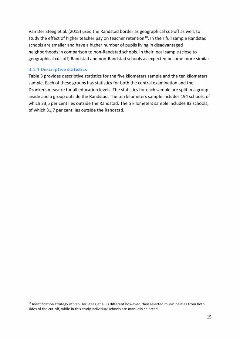
Table 3 provides descriptive statistics for the five kilometers sample and the ten kilometers

sample. Each of these groups has statistics for both the central examination and the

Dronkers measure for all education levels. The statistics for each sample are split in a group

inside and a group outside the Randstad. The ten kilometers sample includes 194 schools, of

which 33,5 per cent lies outside the Randstad. The 5 kilometers sample includes 82 schools,

of which 31,7 per cent lies outside the Randstad.

18 Identification strategy of Van Der Steeg et al. is different however, they selected municipalities from both sides of the cut-off, while in this study individual schools are manually selected.

16

Table 3: descriptive statistics for 5 kilometers and 10 kilometers sample, only pre-reform years

5 kilometers sample 10 kilometers sample

Randstad

(treatment)

Non-Randstad

(control)

Randstad

(treatment)

Non-Randstad

(control)

CE average (2004-2008)

VMBO B 6.843 6.712 6.823 6.706

VMBO K 6.520 6.435 6.517 6.433

VMBO GT 6.310 6.308 6.293 6.326

HAVO 6.227 6.261 6.247 6.221

VWO 6.400 6.502 6.413 6.426

Total number of observations 433 302 1,145 629

Dronkers school grade (2006-2008)

VMBO B 7.077 6.974 7.026 6.882

VMBO K 6.316 6.205 6.412 6.234

VMBO GT 5.914 5.966 5.912 6.129

HAVO 5.981 6.214 6.246 6.133

VWO 5.982 6.481 6.230 6.274

Total number of observations 272 192 715 391

Number of schools 56 26 129 65

School size19 692 1,026 748 887

19 School averages 2011-2015, school size in number of students per school

17

3.2 Methodology

3.2.1 Standard model

Typically educational policy studies control for student, family and school characteristics

when they want to find a causal relationship between two variables. An estimating equation

for this research could be20:

𝑌𝑖𝑡 = 𝛼 + 𝛽𝑋𝑖𝑡 + 𝛾𝑇𝑃𝑖𝑡 + 𝛿𝑖 + 𝜃𝑡 + 𝑢𝑖𝑡 (1)

Where Yit is the performance measure of a school i for time period t, Xit is a vector of control

variables on school level, including student, family and school characteristics, while uit

incorporates all unobserved variables in the equation. TPit is the average level of teacher pay

at a school for time period t, the intervention variable. α, β and γ are the parameters to be

estimated, where α represents the overall constant of the model and γ is the parameter of

interest. δi and θt represent school and period fixed effects. The equation can be estimated

through OLS, however it should be noted that the estimation could be biased if any

unobserved variable is correlated with the independent variable and the intervention

variable. This endogeneity problem is frequently encountered in policy research, and more

specifically in educational research, as the performance measure is influenced by school and

family characteristics from birth of the student onwards. Even if all relevant characteristics

that should be controlled for are known, it would be very difficult to collect all those data

points (Angrist & Krueger, 2001) (Todd & Wolpin, 2003).

As covered in the related literature a new wave of research exploits exogenous variation

from controlled or natural experiments. This ensures that the intervention variable is not

correlated with unobserved variables. This study uses a discontinuity in an institutional rule

as exogenous variation, a geographical discontinuity in a new Dutch remuneration policy for

teachers. The research design incorporates parts of a difference-in-differences analysis and a

regression-discontinuity-design. Schools just in- and outside the Randstad area are

compared to each other, as schools inside the Randstad were given bigger pay raises for

their teachers than schools outside the Randstad. Assuming that schools close to the border

of the Randstad are similar to each other, the only significant difference between schools in-

and outside the Randstad is the extra difference in teacher pay the remuneration policy

caused. During the analysis the performance of each school in the sample is monitored for

several years before and after implementation of the policy. Any significant difference in the

development of performance between schools inside the Randstad and outside the

Randstad can be allocated to the extra salary for Randstad schools. Since only schools are

included in the research that are close to the geographical cut-off no other factors that work

at the same cut-off can be allowed. It is extensively checked whether there is any other

policy or project that focuses specifically on improving educational performance in the

20 The estimation equation is on school level as teacher pay and student performance data is only available at school level at a big enough scale. Ideally data is available on student level (examination grades and the average salary of teachers of a specific student).

18

Randstad, however nothing was found. A concern that comes with the new wave of

literature is that its research designs are often accompanied with a low external validity, as

only a small sample of the population is studied. A discussion on the external validity of the

study is presented in section 4.5.

3.2.2 Adjusted model

As shown in section 3.1.1, the realized difference in teacher pay growth between Randstad

and non-Randstad schools eventually proved to be 15 per cent, in other words Randstad

schools had 15 per cent more teachers going up from scale LB to LC. Since the only

difference between the schools in the sample is the extra teacher pay, the estimating

equation only has to find the difference in the development of performance between the

schools:

𝑌𝑖𝑡 = 𝛼 + 𝜇𝑅𝑆𝑖𝑡 + 𝛿𝑖 + 𝜃𝑡 + 𝑢𝑖𝑡 (2)

Where Yit is the performance measure of a school i for time period t, while uit incorporates

all unobserved variables in the equation. RSit is a dummy that returns 1 if a school lies within

the Randstad and if the year is reached in which the policy will deliver its first returns as well

as the years after that year, otherwise the dummy will return 0. α and μ are the parameters

to be estimated, where α represents the overall constant of the model and μ is the

parameter of interest. μ represents the treatment effect; performances of schools within the

Randstad after the policy set in are on average μ higher or lower than before the policy set

in, in comparison to non-Randstad school performances. This effect is estimated for each

education level and through year fixed effects overall differences between years are

controlled for. The difference-in-difference structure of the equation makes it possible to

interpret μ as the average increase or decrease in performance of Randstad schools due to

the extra teacher pay in comparison to non-Randstad schools. The development of the

performance of Randstad schools differs with μ from the development of the performance

of non-Randstad schools, which is the development of performance that is expected for the

treatment group as well when no extra teacher pay would have been received. δi and θt

again represent school and period fixed effects.

School fixed effects seemed logical to apply to the analysis as then the treatment effect is

most informative. The treatment effect is now about the development of performance

within a school and not just about the overall development of all schools in the Randstad

together. Also year fixed effects seemed natural to insert into the analysis, as it might be

that school performances are influenced by shocks in a certain year. It might for example be

that a certain year had more lenient or strict correcting models, which led to higher or lower

average examination grades for the whole sample. Another shock could be caused by the

fact that the Dronkers performance measure is measured in a slightly different way in the

years 2012 and 2013 than in the years before. This led to a higher average school grade in

the period 2012-2013 than in the period 2006-2011 (7,27 versus 6,29), differences year fixed

effects control for. Fixed effects testing is performed for all estimations (through the

19

likelihood ratio); this tests the joint significance of all the effects as well as the significance of

the year fixed effects and the school fixed effects separately. For all the estimations counts

that the statistic values strongly reject the null hypothesis of redundant effects.

3.2.3 Common trend assumption

The difference-in-difference design is clearly not assumption free. The assumption that no

other factors (than the studied treatment) can be active at the geographical cut-off has

already been mentioned. Another important assumption for diff-in-diff designs is the

common trend assumption, which is that the trend of the outcome variable for the

treatment and control group should be the same in absence of treatment. There is,

however, no formal test available to check this assumption. A first option to still check for

this assumption is to check the diff-in-diff outcomes for earlier years of impact, when no

effect would be expected yet, the so-called "placebo difference-in-difference". This will be

done in section 4.3, as part of the sensitivity analysis.

Another more often used option is to graphically examine pre-treatment data to see

whether the pre-treatment outcome variable trend is the same for the treatment and the

control group. For several estimations graphical representations are displayed later on in the

paper, figures that can be used to test the common trend assumption21. The trends of

treatment and control groups are overall quite similar before the years of impact, which is a

good sign for the research. On the other hand, the trends are not perfectly similar and

significant post-treatment differences between treatment and control groups, are

sometimes equal or even smaller than pre-treatment differences between treatment and

control groups. This is an observation that hurts the common trend assumption. Concluding

this subjective process of deciding whether trends are common or not, the trends are similar

to some extent, but the common trend assumption still is a point of attention concerning the

reliability of the results.

3.2.4 Effectiveness lag

As Hendricks (2013) mentions in his research on the effectiveness of extra teacher pay, it is

difficult to predict when the treatment effect will set in. There is certainly a lag between the

implementation of the policy and the effect setting in, as first higher teacher pay should be

implemented. Then higher teacher quality should be reached through the extra teacher pay.

The quality of present teachers will increase through extra training, more effort and sharper

monitoring of the better paid teachers. Later on, the pay raise will possibly attract more

graduates into the teacher profession and the brain-drain will set in, high skilled teachers

move from non-Randstad schools to the better paid Randstad schools. Lastly, the increased

teacher quality should find its way to the student performance, a process which could take

years. The performance of students that experience the higher teacher quality for one year

will only be influenced marginally. The longer students are exposed to a higher teacher

quality, the more their performance will be influenced by the higher teacher quality. It

21 see figures 3, 4 and in the appendix figures A.3, A.4 & A.5

20

should be noticed that the used performance measures are a little bit lagged as well. For

example examination grades and school grades in the data set from 2010 are based on the

school year 2009-2010, so student performances in 2009 had influence on the 2010 measure

as well. Loeb and Page (2000) decided to regress their student outcomes on teacher wages

ten years earlier to give wage increases the time to influence the student performance. In

this paper it would be difficult to implement a ten-year lag, as data only reach until 2015.

This also led to the decision to use central examination grades and a school grade as

performance measures and not educational attainment of a pupil or subsequent earnings,

which is more normal for economists. The effects of the policy on educational attainment or

subsequent earnings of a student would be reached after a much longer time than for

examination and school grades. So, concerning the lag in effectiveness of extra teacher pay,

using examination and school grades seemed the most logical and possibly even the only

option now.

Table A.3 shows that in 2010, 2 years after implementation, Randstad schools had already

increased the number of teachers in salary scale LC with 11,7 per cent point more than non-

Randstad schools. In 2014 this difference grew until 15 per cent point.22 This means that a

substantial part of the eventual difference in teacher pay growth was already reached in

2010. The first effects of the extra teacher pay on student performance could possibly have

arisen in 2010 already as well, when present teachers increased effort, started doing extra

schooling and were monitored more. It is likely, however, that these effects grew even

stronger the years after, as teacher quality rose even more over the years and more and

more students were exposed to this higher teacher quality. In this light, the years of 2011

and 2012 are interesting years, as to see whether effects indeed did strengthen. It would be

interesting to study even longer lags, but the longer the lags the closer the year of impact

gets to the end of the samples, especially for the Dronkers sample. When 2012 is studied as

year of implementation only one year of post-treatment observations is available. That is

why in section 4 the analysis is performed for the years 2010, 2011 and 2012.

22 In the years 2010-2014 the schools focused more on reaching the LD goals, as LC increased a lot already in the first years

21

4. Results and discussion

4.1 Overall results and discussion

As mentioned in the previous section, the effect of the extra teacher pay is estimated for

each education level, with 2011, 2012 and 2012 as possible years of impact of the policy

change. This analysis is done with both the five and the ten kilometers sample, and with the

two different outcome variables. Overviews of results are presented in table 4 and 5.

The signs of the estimates show a resolute difference between the education levels. While

VMBO-B and VMBO-K estimates only show 1 positive estimate in total, VMBO-GT, HAVO and

VWO show 31 positive estimates in total. The significance of the estimates however is not

very strong, only 11 of 60 estimates are statistically significant of which five positively

significant and 6 negatively significant. VMBO-B estimates with central examination grades

as outcome variable all have a negative sign and all are statistically significant. This suggests

that the extra teacher pay for Randstad schools had a significant negative effect on the

central examination grades obtained by Randstad pupils in the years after policy

implementation. HAVO and VWO estimates from the 5 kilometers sample with 2010 and

2011 as impact years on the other hand have a positive sign and are statistically significant

as well (HAVO with central examination grades as outcome variable, VWO with Dronkers'

school grade as outcome variable). Lastly also the VWO estimate from the 10 kilometers

sample with 2012 as impact year and central examination grade as outcome variable is

significantly positive. That estimation suggests that the extra teacher pay for Randstad

schools significantly increased the central examination grade of VWO pupils in the Randstad

in the years after implementation.

As mentioned VMBO-B and VMBO-K estimates are mostly negative, while VMBO-GT, HAVO

and VWO estimates are mostly positive. This separation is interesting as the two lowest

education levels show a negative effect of extra teacher pay, while the higher education

levels show a positive effect of extra teacher pay. This might suggest that extra teacher pay

becomes more effective as the education level for which the extra teacher pay is provided

increases. A possible explanation for this could be that the Motivation Crowding Effect is

more prevalent in the lower education levels than in the higher education levels. Then more

extrinsic motivation crowds out the intrinsic motivation of the teachers in these lower

education levels. It could be that higher teacher pay attracts teachers that increase student

performance in higher education levels, but that these teachers decrease student

performance in lower education levels. This suggestion however needs scientific

confirmation. One way or the other, it seems that the extra teacher pay reaches and

influences the student performance in the intended way more when the education level is

higher.

Concerning the size of the estimates; the average significant central examination grade

estimate is 0.085, the average significant Dronkers estimate is 0.56. For the central

examination grade this means that the extra teacher pay has an average effect of 0.085

22

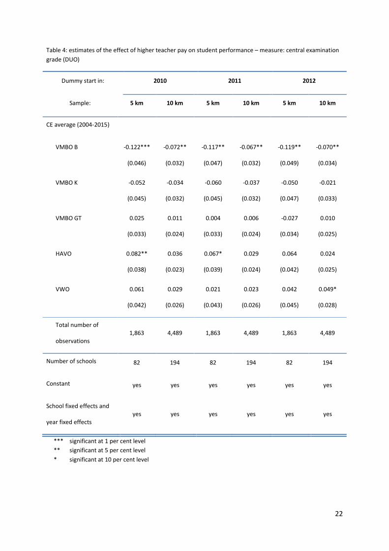
Table 4: estimates of the effect of higher teacher pay on student performance – measure: central examination

grade (DUO)

Dummy start in: 2010 2011 2012

Sample: 5 km 10 km 5 km 10 km 5 km 10 km

CE average (2004-2015)

VMBO B -0.122***

(0.046)

-0.072**

(0.032)

-0.117**

(0.047)

-0.067**

(0.032)

-0.119**

(0.049)

-0.070**

(0.034)

VMBO K -0.052

(0.045)

-0.034

(0.032)

-0.060

(0.045)

-0.037

(0.032)

-0.050

(0.047)

-0.021

(0.033)

VMBO GT 0.025

(0.033)

0.011

(0.024)

0.004

(0.033)

0.006

(0.024)

-0.027

(0.034)

0.010

(0.025)

HAVO 0.082**

(0.038)

0.036

(0.023)

0.067*

(0.039)

0.029

(0.024)

0.064

(0.042)

0.024

(0.025)

VWO 0.061

(0.042)

0.029

(0.026)

0.021

(0.043)

0.023

(0.026)

0.042

(0.045)

0.049*

(0.028)

Total number of

observations 1,863 4,489 1,863 4,489 1,863 4,489

Number of schools 82 194 82 194 82 194

Constant yes yes yes yes yes yes

School fixed effects and

year fixed effects yes yes yes yes yes yes

*** significant at 1 per cent level

** significant at 5 per cent level

* significant at 10 per cent level

23

Table 5: estimates of the effect of higher teacher pay on student performance – measure: school grade

(Dronkers)

Dummy start in: 2010 2011 2012

Sample: 5 km 10 km 5 km 10 km 5 km 10 km

Dronkers school grade

(2006-2013)

VMBO B -0.085

(0.293)

-0.162

(0.176)

-0.233

(0.297)

-0.119

(0.179)

-0.435

(0.329)

-0.165

(0.199)

VMBO K -0.020

(0.278)

-0.074

(0.189)

-0.311

(0.284)

-0.127

(0.192)

-0.279

(0.316)

0.096

(0.213)

VMBO GT 0.200

(0.217)

0.156

(0.146)

0.069

(0.223)

0.005

(0.150)

0.113

(0.249)

-0.047

(0.166)

HAVO 0.060

(0.351)

-0.164

(0.216)

-0.093

(0.365)

-0.215

(0.223)

0.666

(0.413)

0.016

(0.252)

VWO 0.634**

(0.264)

0.203

(0.173)

0.486*

(0.274)

0.151

(0.178)

0.293

(0.313)

0.082

(0.201)

Total number of

observations 1,261 3,046 1,261 3,046 1,261 3,046

Number of schools 82 194 82 194 82 194

Constant yes yes yes yes yes yes

School fixed effects and

year fixed effects yes yes yes yes yes yes

*** significant at 1 per cent level

** significant at 5 per cent level

* significant at 10 per cent level

24

examination grade point. Of the ten points obtainable in total this effect seems negligible,

however this effect of 0.085 affects all grades of all students. So a student either has all his

central examination grades affected with 0.085, or if only a few grades are affected by the

extra teacher pay the treatment effect would even be bigger for the affected subjects. Also

this average effect is estimated for all students in all schools; so if a certain part of the

students would not be affected by the extra teacher pay, the effect for the other students

becomes even bigger again. The 0.56 effect of the Dronkers estimate is quite big, as again

ten is the maximum obtainable grade. So because of the extra teacher pay, Dronkers' school

grades changed with 0.56, averaging the significant estimates. A recent overview paper by

Sanders and Chonaire comes to the conclusion that based on earlier research only relatively

small effect sizes should be expected in educational research (2015). This increases the

impact of the estimations of this study even further.

4.2 Case study

To provide more insight into the regression outcomes two settings will be explored more

deeply by discussing their interpretation and confidence intervals and by providing graphs.23

First in line is the setting in which the five kilometers sample is studied for the education

level VMBO-B, with central examination grades as outcome variable. Performing estimations

in this setting with different years of impact, led to three significant treatment effects. With

2010, 2011 and 2012 as year of impact the extra teacher pay for Randstad schools led to

lower central examination grades for the Randstad schools in comparison to non-Randstad

schools (estimates respectively -0.122, -0.117 & -0.119). This means that Randstad schools

obtained central examination grades that were on average around 0.120 grade point lower

than expected under the null hypothesis of no treatment effect. The expectation is formed

by the development of performance of the control group, the non-Randstad schools. It is

assumed that both Randstad and non-Randstad schools would have the same development

of performance in absence of treatment. So the treatment effect is the post-treatment

deviation of the performance of Randstad schools from the performance of non-Randstad

schools, as the Randstad performance would have developed the same as non-Randstad

performance if no extra teacher pay was ever received.

The difference-in-difference effect can easily be identified in the graph in figure 3. The blue

line represents the mean of the central examination grades for Randstad schools, while the

red line does that for non-Randstad schools. The dashed red line is the development of

performance of schools outside the Randstad after treatment (with as year of impact 2012)

starting on the blue line at the beginning of treatment. In absence of treatment it is

expected that the blue line would follow the dashed red line. However, because of the

treatment the blue line significantly deviates from the dashed red line. The blue line runs

beneath the dashed line for most of the post-treatment years, which means that on average

23 Graphs of other significant estimations can be found in the appendix (figure A.3 – A.5)

25

Randstad schools obtained lower central examination grades than is expected, in

comparison to the development of grades of non-Randstad schools.

The estimation with 2012 as year of impact (-0.119) has a 90 per cent confidence interval

that ranges from -0.200 to -0.039.24 So it is 90 per cent confident that the true population

parameter is between the lower and the upper bound, meaning that the size of the estimate

is quite considerable. Even in case of the upper bound, the effect is still negative and not

that close to zero; statistical evidence even proved that the estimate is significantly not

equal to zero.

Figure 3: Mean CE grade 2004-2015; education level: VMBO-B, 5 kilometers sample, outcome variable: central

examination grade, years of impact with significant estimate: 2010, 2011 & 2012

24 A 90 per cent confidence interval encompasses the true population parameter 90 per cent of the times, if the research would be repeated on other (different) samples (each with its own confidence interval)

Mean CE grade Randstad schools

Mean CE grade non-Randstad schools

Shifted mean CE grade non-Randstad schools

Year

Gra

de

26

Secondly the setting in which the ten kilometers sample is studied for the education level

VWO, with Dronkers school grade as outcome variable. Estimations with years of impact

2010 and 2011 led to significant effects. In figure 4 the situation with as year of impact 2010

is graphically analyzed. The blue line is expected (Randstad schools' performance) to develop

the same way as non-treated schools (dashed red line), if no treatment would have

occurred. With treatment however the blue line outruns the dashed red line for almost all

post-treatment years. This confirms the statistically significant positive estimate of 0.634.

The 90 per cent confidence interval of this estimate has 0.198 as lower bound and 1.070 as

upper bound.

Figure 4: Mean school grade 2006-2013; education level: VWO, 5 kilometers sample, outcome variable:

Dronkers' school grade, years of impact with significant estimate: 2010 & 2011

Mean Dronkers' school grade Randstad schools

Mean Dronkers' school grade non-Randstad schools

Shifted mean Dronkers' school grade non-Randstad schools

Year

Gra

de

27

4.3 Sensitivity analysis

Performing the analysis for multiple outcome variables increases the robustness of the

results, especially when similar results arise from both analyses. This paper used both central

examination grades and school grades calculated by Dronkers as outcome variables. By

doing this the probability of drawing a fortuitous conclusion is reduced.

The credibility of the results can be checked afterwards by performing a sensitivity analysis.

It is possible to estimate the effect of teacher pay on student performance for the years

2008 and 2009 as well25. With these as years of impact weaker results are expected, as first

of all it takes some time before the teacher pay would increase after policy implementation

in 2008, and secondly it takes some more time for the higher teacher pay to influence the

student performance. A side note should be made; shifting the years of impact to 2008 and

2009 lets the analysis consider the observations from these years as influenced by teacher

pay. However, the analysis also continues to use the post-treatment observations from 2010

until 2015. Adding the observations of 2008 and 2009 should have its impact on the analysis,

but a big part of the analyzed observations, together with the direction of the results,

remains the same.

The analyses with 2008 and 2009 as years of impact show similar patterns as the original

analyses. Negative estimations for the lower education levels and positive estimations for

the higher education levels. Similar as in the 2010, 2011 & 2012 analysis, several of these

estimations are statistically significant. This suggests that Randstad schools performed

significantly different than non-Randstad schools in the years 2008 and 2009 as well. Again,

the analyses of 2008 and 2009 comprehend observations from 2010 until 2015 as well,

which automatically make the estimations for different years look alike quite a lot. But still a

weaker pattern was expected in the years 2008 and 2009. Despite the fact that no other

factors are at work at the geographical cut-off, it seems that for some reason Randstad

schools performed significantly different from non-Randstad schools even prior to the

impact period of the extra teacher pay.

A possible explanation of this is a violation of the common trend assumption, which is

covered in section 3.2.3. Another possible explanation is the existence of an anticipation

effect of teachers. They knew that a pay raise was coming in 2008 and 2009 (or even earlier)

and they might have anticipated this by already increasing their effort in 2008 and 2009, to

ensure their part of the pay raise. This could lead to an absence of a treatment effect in the

results, as 2008 and 2009 are used as "control years" in the analysis. Also it could explain

why the analyses with 2008 and 2009 as years of impact show similar patterns as the original

analyses.

25 See table A.4 and A.5

28

4.4 Multiple testing

A problem that should be discussed is the multiple (hypothesis) testing problem. This

problem occurs when a set of statistical inferences is considered simultaneously. What it

boils down to is that a researcher is much more likely to falsely reject the null hypothesis ("a

false positive") when multiple tests are performed at the same time. The more tests are

considered simultaneously the higher the probability of encountering a type I error.

To correct for this problem researchers can lower their individual significance level through

one of the several correction methods. The one most often used is the Bonferroni

correction method, in which the desired total significance level is divided by the number of

tests performed to come to the individual significance level at which should be tested. A

critique on this method however is that it can be overly conservative, especially if there is a

large number of tests, as it increases the number of "false negatives" to an unnecessarily

high level. When the estimates from table 4 are for example considered as one set of

statistical inferences and the desired overall significance level is five per cent, the individual

estimates should be tested at a significance level of 5 / 30 = 0.167 per cent according to the

Bonferroni correction method. With this individual significance level, almost none of the

estimates would be statistically significant.

But after all the multiple testing problem still should be considered when interpreting the

estimates. This implies that in comparison to the current analysis, less estimates would be

statistically significant or they would still be significant but at a lower overall significance

level.

4.5 External validity

As mentioned before, a concern that often comes with difference-in-difference research

designs is a low external validity, as by definition the effect of X on Y is studied on a small

and specific scale. In this study for example, the effect of teacher pay on student

performance is researched for schools just in- and outside the Randstad, only a small part of

the Netherlands. And even though a substantial part of the Dutch schools is represented in

the sample (around 15 per cent), it should at least be questioned whether the results of this

study can be generalized for the rest of the Dutch schools or for schools outside The

Netherlands.

Schools just in- and outside the Randstad are for example likely to be situated in semi-

densely populated areas. It could be that the effect of extra teacher pay is different for

schools in big cities or for schools in the countryside than for schools in these semi-densely

populated areas. Adding to this, schools and educational systems in other countries might be

structured completely different than Dutch schools, so external validity of the results with

respect to schools outside the Netherlands should be approached with caution as well.

29

5. Conclusions In this paper the effect of teacher pay on student performance has been examined. This has

been done through a difference-in-difference design, in which Randstad schools received an

extra amount of teacher pay in comparison to non-Randstad schools. Schools that are just in

and outside the Randstad are compared to each other, with the assumption that these

schools are similar to each other. The remuneration policy came into action in 2008, but the

first effects on student performance were not expected until 2010 and later, so studied

years of impact are 2010, 2011 and 2012. Two different variables are used as outcome

variable, the average central examination grade and a school grade, which is a measure

developed by Jaap Dronkers that reviews each school each year.

Performing analyses for three years of impact, two outcome variables, two different samples

and five education levels, delivered 60 estimations, of which 11 are found to be statistically

significant. These estimations formed a pattern that suggests a positive relationship between

education level and effectiveness of teacher pay on student performance. The research

found a negative relationship between teacher pay and student performance for lower

education levels, while for higher education levels the relationship between teacher pay and

student performance is positive.

This conclusion suggests more effectiveness of extra teacher pay for higher education levels

than for lower education levels. Therefore, one of the future research recommendations is

to perform more studies on the effectiveness of educational resources that differentiate

between education levels (within secondary education), to gain more knowledge of the

difference in effectiveness of educational resources between different education levels.

A possible improvement of the study is to perform the same research with more years of

data available, as it may be reasoned that the year of impact is in fact later than 2012.

Another possible improvement is to verify more strictly whether the compared schools are

indeed similar to each other. This means that the assumption of more similar schools when

schools are closer to the border should be checked more strictly, for example by studying

characteristics of these schools. A last possible improvement is to use an adaption of a WLS

analysis (weighted least squares) instead of an OLS analysis. Because it is assumed that

schools closer to the Randstad border are more similar to each other, desirably observations

closest to the border get higher weights when estimating the parameters. Instead of having

a strict cut-off of five or ten kilometers, the maximum distance to the border could then be

increased as schools further from the border lose their weight in the analysis. This possible

research design shows resemblance with the Geographic Regression Discontinuity design

(GRD) presented by Keele and Titiunik (2015).

30

References Allan, M. B. & Freyer, J. R. G., 2011. The Power and Pitfalls of Education Incentives,

Washington, D.C.: The Hamilton Project.

Allegretto, S. A., Corcoran, S. P. & Mishel, L., 2004. How Does Teacher Pay Compare?

Methodological Challenges and Answers. Washington, D.C.: Economic Policy Institute.

Angrist, J. D. & Krueger, A. B., 2001. Instrumental Variables and the Search for Identification:

From Supply and Demand to Natural Experiments. Journal of Economic Perspectives, 15(4),

pp. 69-85.

Angrist, J. D. & Lavy, V., 1999. Using Maimonides' Rule to Estimate the Effect of Class Size On

Scholastic Achievement. The Quarterly Journal of Economics, 114(2), pp. 533-575.

Campbell, D. T., 1969. Reforms as Experiments. American Psychologist, Issue 24, pp. 409-

425.

Card, D. & Krueger, A. B., 1992. Does School Quality Matter? Returns to Education and the

Characteristics of Public Schools in the United States. The Journal of Political Economy,

100(1), pp. 1-40.

Chubb, J. E. & Moe, T. M., 1990. Politics, Markets and America's Schools. Washington, D.C.:

The Brookings Institution.

Coleman, J. S. & others, a., 1966. Equality of Educational Oppurtunity. Washington, D.C.:

Government Printing Office.

Dolton, P. & Marcenaro-Gutierrez, O. D., 2011. If You Pay Peanuts do You Get Monkeys? A

Cross Country Analysis of Teacher Pay and Pupil Performance. Economic Policy, 26(65), pp. 5-

55.

Dronkers, J., Korthals, R. & Levels, M., 2006-2013. Schoolcijferlijst 2006-2013, Maastricht:

http://www.schoolcijferlijst.nl/HOME.htm.

Dronkers, J., Levels, M. & Korthals, R., 2013. Schoolexamencijfers voor scholen: van slecht

naar excellent; editie 2013. [Online]

Available at: http://www.schoolcijferlijst.nl/TOELICHTING.htm

[Accessed 07 03 2016].

Dronkers, J. & van Alphen, S., 2011. Trouw Schoolprestaties 2010. [Online]

Available at: http://www.schoolcijferlijst.nl/RESULTATEN%202010.htm

[Accessed 07 03 2016].

Frey, B. & Jegen, R., 2001. Motivation Crowding Theory. Journal of Economic Surveys, pp.

589-611.

31

Georgellis, Y., Iossa, E. & Tabvuma, V., 2011. Crowding Out Intrinsic Motivation in the Public

Sector. Journal of Public Administration Research and Theory, 21(3), pp. 473-493.

Guryan, J., 2001. Does money matter? Regression-discontinuity estimates from education

finance reform in Massachusetts. NBER Working Paper 8269, pp. 1-54.

Hanushek, E. A., 1986. The Economics of Schooling: Production and Efficiency in Public

Schools. Journal of Economic Literature, 24(3), pp. 1141-1177.

Hanushek, E. A., 1989. The Impact of Differential Expenditures on School Performance.

Educational Researcher, 18(4), pp. 45-62.

Hanushek, E. A., 1996. School Resources and Student Performance. In: G. Burtless, ed. Does

Money Matter? The Effect of School Resources on Student Achievement and Adult Success.

Washington, D.C.: Brookings Institution Press, pp. 43-73.

Hanushek, E. A., 1997. Assessing the Effects of School Resources on Student Performance:

An Update. Educational Evaluation and Policy Analysis, 19(2), pp. 141-164.

Hanushek, E. A., 2005. Economic outcomes and school quality. s.l.:The International Institute

for Educational Planning.

Hanushek, E. A. & Jorgensen, D. W., 1996. Improving America's Schools: The Role of

Incentives. Washington, D.C.: National Academy Press.

Hanushek, E. A., Rivkin, S. G. & Taylor, L. L., 1996. Aggregation and the Estimated Effects of

School Resources. The Review of Economics and Statistics, 78(4), pp. 611-627.

Heckman, J., Layne-Farrar, A. & Todd, P., 1996. Does Measures School Quality Really Matter?

An Examination of the Earnings-Quality Relationship. In: G. Burtless, ed. Does Money

Matter? The Effect of School Resources on Student Achievement and Adult Succes.

Washington, D.C.: Brookings Institution Press, pp. 192-289.

Hedges, L. V., Laine, R. D. & Greenwald, R., 1994. Does Money Matter? A Meta-Analysis of

Studies of the Effects of Differential School Inputs on Student Outcomes. Educational

Researcher, 23(3), pp. 5-14.

Hendricks, M. D., 2013. Does it pay to pay teachers more? Evidence from Texas. Journal of

Public Economics, Issue 109, pp. 50-63.

Heyma, A., de Graaf, D. & van Klaveren, C., 2006. Exploratie van beloningsverschillen in het

onderwijs 2001-2004, Amsterdam: SEO Economisch Onderzoek.

Inspectie van het Onderwijs (S.M. Neerken), 2004-2015. Toezichtkaart (voorheen

Kwaliteitskaart) Voortgezet Onderwijs 2004-2015, DANS: https://easy.dans.knaw.nl.

32

Keele, L. J. & Titiunik, R., 2015. Geographic Boundries as Regression Discontinuities. Political

Analysis, Issue 23, pp. 127-155.

Krueger, A. B., 1999. Experimental Estimates of Education Production Functions. Quarterly

Journal of Economics, 114(2), pp. 497-532.

Krueger, A. B., 2003. Economic Considerations and Class Size. The Economic Journal,

113(485), pp. F34-F63.

Ladd, H. F., 1996. Holding Schools Accountable: Performance-Based Reform in Education.

Washington, D.C.: The Brookings Institution.

Lavy, V., 2011. Performance Pay and Teachers' Effort, Productivity, and Grading Ethics.

American Economic Review, 99(5), pp. 1979-2011.

Loeb, S. & Page, M. E., 2000. Examining the link between teacher wages and student

outcomes: The importance of alternative labor market opportunities and non-pecuniary

variation. Review of Economics and Statistics, 82(3), pp. 393-408.

Ministry of Education, 2015. Functiemix. [Online]

Available at: https://www.rijksoverheid.nl/ministeries/ministerie-van-onderwijs-cultuur-en-

wetenschap/documenten/kamerstukken/2015/05/29/kamerbrief-over-stand-van-zaken-

functiemix

[Accessed 24 03 2016].

Sanders, M. & Chonaire, A. N., 2015. "Powered to Detect Small Effect Sizes": You keep saying

that. I do not think it means what you think it means.. The Centre for Market and Public

Organisation Working Paper No. 15/337.

Social partners in education & Ministry of Education, 2008. Definitief akkoord Convenant

Leerkracht van Nederland - Sectoren Primair en Voortgezet onderwijs, Scheveningen: s.n.

Todd, P. E. & Wolpin, K. I., 2003. On the Specification and Estimation of the Production

Function for Cognitive Achievement. The Economic Journal, 113(485), pp. F3-F33.

United Nations, 2000. Millennium Development Goals and beyond 2015 - Achieve universal

primary education. [Online]

Available at: http://www.un.org/millenniumgoals/education.shtml

[Accessed 25 01 2016].

United Nations, 2015. Sustainable Development Goals, Goal 4: Quality education. [Online]

Available at: http://www.undp.org/content/undp/en/home/sdgoverview/post-2015-

development-agenda/goal-4.html

[Accessed 25 01 2016].

33

van der Steeg, M., Gerritsen, S. & Kuijpers, S., 2015. The effects of higher teacher pay on

teacher retention. Evidence from regional variation in teacher salaries. CPB Discussion Paper

316, pp. 1-38.

Webbink, D., 2005. Causal effects in education. Journal of Economic Surveys, 19(4), pp. 535-

560.

Webbink, D. et al., 2009. Wat is bekend over de effecten van kenmerken van

onderwijsstelsels? Een literatuurstudie, Den Haag: CPB.

Woessmann, L., 2011. Countries with performance pay for teachers score higher on PISA

tests. Education Next, Spring, pp. 72-77.

34

Appendix

A.1: extra explanation of the computation of school grades Jaap Dronkers26

Both methods judge schools by the number of (core-) subjects27 with an insufficient average

central examination grade to start with. This provides them with a starting grade ranging

from 2 to 7 (4 to 8 in 2012 and 2013).

Figure: development of starting grades 2006-2011 method. Horizontally number of insufficient central

examination grades in core-subjects. Vertically number of insufficient central examination grades in any

subject.28

In the 2006-2011 method the school grade can then only be improved if the school got a

starting grade of 7. Schools start again with their average central examination grade and

improve this when observed grades are higher than the expected grades based on the level

of the students entering the school, which points to an added value by the school. They

further improve their grade when their delay in educational progress is below the average

delay. A remarkable feature of the calculation is that the average central examination grade

is not just the overall average grade, but an indication of the average central examination

grade of only the students with a pass. The passing conditions for secondary education set a

standard for students to pass, namely a minimum level of knowledge and skills that students

need to have. Politics in The Netherlands made sure that students comply to these passing

conditions by demanding a sufficient average central examination grade for each student

that wants to pass. Consequently, to make a fair comparison between schools, average

central examination grades of only the passed students should be compared. This indication

of the average central examination grade of only the passed students is produced by adding

26 Sources for this section; all yearly attached explanations of Dronkers, but especially: (Dronkers & van Alphen, 2011) (Dronkers, et al., 2013) 27 Core-subjects in The Netherlands are currently Mathematics, Dutch and English 28 Source: (Dronkers & van Alphen, 2011, p. 3)

35

a correction parameter to the overall average central examination grade per subject. The

correction parameter in turn is determined by the relationship between the number of

passed students and the average central examination grade. In this procedure it is assumed

that students that fail the exams have lower grades than passed students for all the subjects

they participated in. So the more students in a school do not pass, the higher the indicator

for the central examination grades for the passed students becomes.

The 2012-2013 method slightly differs from the 2006-2011 method. The school grade is

calculated by adding points to or deducting points from the starting grade, which ranges

from 4 to 8. Schools with the highest "yield" get bonus points, while schools with the lowest

"yields" get points deducted from their starting grade. The top ten per cent earns one extra

point, top 20 per cent earns a half extra point, while bottom ten and 20 per cent get these

deducted. The "yield" of a school is determined by combining average central examination

grade, average school examination grade, passing percentage and the passing with no delay

percentage and comparing this measure with what can be expected of a school with respect

to the education level of entering students and the social-economic background of the

students (background comparison only in 2013). The second way to win or lose points is

through the difference between central and school examination grades. The Inspection aims

at keeping that difference no bigger than 0,5 point. Again schools are ranked; the less

subjects with a difference of more than 0,5 point between central and school exam a school

has, the higher the chance on bonus points is. The top 10 and twenty per cent earn

respectively one and a half point, while bottom 10 and twenty percent again lose the same

amounts.

36

Table A.1: first overview of estimates by Hanushek (1986)

Source: (Hanushek, 1986)

Table A.2: results of the new wave of literature on educational resources; dealt

with endogeneity through exogenous variation

Source: (Webbink, 2005)

Table A.3: development of Dutch teacher pay scheme (functiemix) secondary

education 2008-2014

Source: (Ministry of Education, 2015)

37

Table A.4: estimates of the effect of higher teacher pay on student performance –

measure: central examination grade (DUO) – year of impact: 2008 & 2009

Dummy start in: 2008 2009

Sample: 5 km 10 km 5 km 10 km

CE average (2004-2015)

VMBO B -0.173***

(0.051)

-0.109***

(0.035)

-0.141***

(0.048)

-0.091***

(0.033)

VMBO K -0.151

(0.050)

-0.045

(0.035)

-0.127***

(0.046)

-0.056*

(0.033)

VMBO GT 0.011

(0.035)

-0.008

(0.026)

0.034

(0.033)

0.012

(0.024)

HAVO 0.125***

(0.040)

0.050**

(0.025)

0.104***

(0.038)

0.034

(0.024)

VWO 0.068

(0.045)

0.031

(0.028)

0.074*

(0.043)

0.029

(0.027)

Total number of

observations 1,863 4,489 1,863 4,489

Number of schools 82 194 82 194

Constant yes yes yes yes

School fixed effects and

year fixed effects yes yes yes yes

*** significant at 1 per cent level

** significant at 5 per cent level

* significant at 10 per cent level

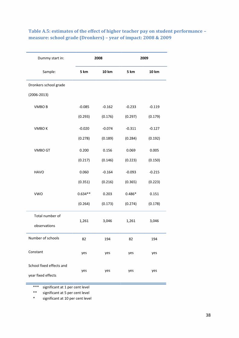
38

Table A.5: estimates of the effect of higher teacher pay on student performance –

measure: school grade (Dronkers) – year of impact: 2008 & 2009

Dummy start in: 2008 2009

Sample: 5 km 10 km 5 km 10 km

Dronkers school grade

(2006-2013)

VMBO B -0.085

(0.293)

-0.162

(0.176)

-0.233

(0.297)

-0.119

(0.179)

VMBO K -0.020

(0.278)

-0.074

(0.189)

-0.311

(0.284)

-0.127

(0.192)

VMBO GT 0.200

(0.217)

0.156

(0.146)

0.069

(0.223)

0.005

(0.150)

HAVO 0.060

(0.351)

-0.164

(0.216)

-0.093

(0.365)

-0.215

(0.223)

VWO 0.634**

(0.264)

0.203

(0.173)

0.486*

(0.274)

0.151

(0.178)

Total number of

observations 1,261 3,046 1,261 3,046

Number of schools 82 194 82 194

Constant yes yes yes yes

School fixed effects and

year fixed effects yes yes yes yes

*** significant at 1 per cent level

** significant at 5 per cent level

* significant at 10 per cent level

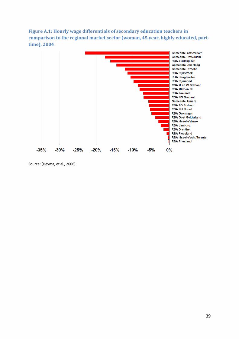
39

Figure A.1: Hourly wage differentials of secondary education teachers in

comparison to the regional market sector (woman, 45 year, highly educated, part-

time), 2004

Source: (Heyma, et al., 2006)

40

Figure A.2: schools within 10 kilometers from the Randstad border

Source: own collection of data

41

Figure A.3: 5 kilometers sample, education level: HAVO, outcome variable: central

examination grade, years of impact with significant estimate: 2010 & 2011

Figure A.4: 10 kilometers sample, education level: VMBO-B, outcome variable:

central examination grade, years of impact with significant estimate: 2010, 2011,

2012

Figure A.5: 10 kilometers sample, education level: VWO, outcome variable: central

examination grade, years of impact with significant estimate: 2012

Mean CE grade Randstad schools

Mean CE grade non-Randstad schools

Shifted mean CE grade non-Randstad schools

Year

Year

Year

Gra

de

Gra

de

Gra

de