Embed Size (px)
Citation preview
UNIVERSITY OF CALGARY
Measurement and Modeling of Asphaltene-Rich Phase Composition
by
Shinil George
A THESIS
SUBMITTED TO THE FACULTY OF GRADUATE STUDIES
IN PARTIAL FULFILMENT OF THE REQUIREMENTS FOR THE
DEGREE OF MASTER OF SCIENCE IN CHEMICAL ENGINEERING
DEPARTMENT OF CHEMICAL AND PETROLEUM ENGINEERING
CALGARY, ALBERTA
DECEMBER, 2009
© Shinil George 2009
UNIVERSITY OF CALGARY
FACULTY OF GRADUATE STUDIES
The undersigned certify that they have read, and recommend to the Faculty of Graduate
Studies for acceptance, a thesis entitled " Measurement and Modeling of Asphaltene-Rich
Phase Composition" submitted by Shinil George in partial fulfilment of the requirements
of the degree of Master of Science in Chemical Engineering.
Supervisor, Dr. Harvey W. Yarranton Department of Chemical and Petroleum Engineering
Dr. William Y. Svrcek Department of Chemical and Petroleum Engineering
Dr. Marco A. Satyro Department of Chemical and Petroleum Engineering
Dr. Ed Nowicki Department of Electrical and Computer Engineering
Date
ii
Abstract
Oil producers are beginning to consider solvent-based or solvent-assisted processes to
recover heavy oil. To design these processes, it is necessary to predict the amount and
composition of the phases that form when the heavy oil and solvent mix. In particular, the
formation of asphaltene-rich phases can strongly affect the recovery process.
A previously developed regular solution model successfully predicted the amount of
asphaltenes in dense phases formed in solutions of asphaltenes, toluene, and n-alkanes as
well as in heavy oils diluted with n-alkanes. However, this model assumed that there is
no solvent partitioning to the asphaltene-rich phase, which is thermodynamically
incorrect. Furthermore, no compositional data for the asphaltene-rich phase was available
with which to tune the model.
A new experimental approach was developed to calculate the composition of solvent in
the asphaltene-rich phase. The experiments were based on the difference between the
evaporation rate of the free or entrained solvent versus that of the solvent dissolved in the
asphaltene-rich phase. The mass of a mixture of asphaltenes and solvent was measured
over time and there was a clear and consistent change in slope when the entrained solvent
evaporation ended. The amount of solvent in the asphaltene-rich was determined at this
point.
A previously developed regular solution model was modified to include all components
in the asphaltene-rich phase to take part in the phase equilibrium. The model was re-
iii
tuned using n-heptane/toluene/Athabasca asphaltene data. The model predicted
reasonably good results for fractional precipitation of asphaltenes having different
average molar mass, except for the low molar mass asphaltenes. The predictions for
different n-alkane solvents were less accurate particularly for heavy solvents n-octane
and n-decane. The model did not handle the effect of asphaltene concentration well. The
revised model also significantly over-predicted the solvent content of the asphaltene-rich
phase.
iv

Acknowledgements
I wish to express my sincere gratitude and thanks to my supervisor Dr. Harvey W.
Yarranton for his invaluable guidance, encouragement and support throughout the
program. It was a privilege for me to work with him. I also extend my heartfelt thanks to
Dr. Marco A. Satyro for his help and guidance throughout this endeavour. He was very
kind to allow me to use Virtual Materials group (VMG) software packages for the
modeling work.
I express my sincere gratitude to the Asphaltene and Emulsion research group members
for their support and cooperation. I am thankful to Asok Tharanivasan for the fruitful
discussions that contributed to this thesis. I like to acknowledge the help of Elaine
Baydak for her help during my experimental work. Further, I would like to thank NSERC
and Department of Chemical and Petroleum Engineering for the funding support. Finally,
I am indebted to my family, especially to my wife Golda for their love and unwavering
support.
v

Dedication
To
My family
vi
Table of Contents
Approval Page..................................................................................................................... ii Abstract .............................................................................................................................. iii Acknowledgements..............................................................................................................v Dedication .......................................................................................................................... vi Table of Contents.............................................................................................................. vii List of Tables ..................................................................................................................... ix List of Figures and Illustrations ...........................................................................................x List of Symbols, Abbreviations and Nomenclature.......................................................... xii
CHAPTER ONE: INTRODUCTION..................................................................................1 1.1 Asphaltene Precipitation ............................................................................................2 1.2 Modeling Asphaltene Precipitation ...........................................................................3 1.3 Objectives and Thesis Structure ................................................................................4
CHAPTER TWO: LITERATURE REVIEW .....................................................................6 2.1 Conventional Crude Oils and Bitumen......................................................................6 2.2 Crude Oil Characterization ........................................................................................7
2.2.1 Distillation Methods ..........................................................................................7 2.2.2 SARA fractionation ...........................................................................................8
2.2.2.1 Saturates...................................................................................................9 2.2.2.2 Aromatics.................................................................................................9 2.2.2.3 Resins.......................................................................................................9 2.2.2.4 Asphaltenes............................................................................................10
2.3 Asphaltene Association............................................................................................12 2.4 Asphaltene Precipitation ..........................................................................................14 2.5 Modeling of Asphaltene Precipitation .....................................................................17
2.5.1 Colloidal Model...............................................................................................17 2.5.2 Thermodynamic Models..................................................................................19 2.5.3 Modified Regular Solution Theory .................................................................19
2.6 Asphaltene-Rich Phase Composition.......................................................................26 2.7 Summary..................................................................................................................30
CHAPTER THREE: EXPERIMENTAL...........................................................................31 3.1 Materials ..................................................................................................................31 3.2 Determination of the Solvent Content of the Asphaltene-Rich Phase.....................32
3.2.1 Asphaltene and Solvent Systems.....................................................................34 3.2.2 Diluted Bitumen Systems ................................................................................37
3.3 Summary..................................................................................................................38
CHAPTER FOUR: MODELING ......................................................................................39 4.1 Modified Regular Solution Model...........................................................................39 4.2 Fluid Characterization..............................................................................................41
4.2.1 Molar Mass......................................................................................................41 4.2.2 Densities and Molar Volumes .........................................................................43 4.2.3 Solubility Parameters.......................................................................................44
vii
4.3 Flash Calculations....................................................................................................46 4.4 Summary..................................................................................................................49
CHAPTER FIVE: MEASUREMENT OF ASPHALTENE-RICH PHASE COMPOSITIONS.....................................................................................................51
5.1 Asphaltene-Rich Phases from Asphaltene/Solvent Systems ...................................51 5.1.2 Sediment from Solutions of Asphaltenes in Solvents .....................................58
Initial n-Alkane Volume Fraction......................................................................59 Asphaltene Type ................................................................................................60 Solvent Type ......................................................................................................61
5.2 Asphaltene-Rich Phases from Solvent Diluted Bitumen.........................................64 5.3 Summary..................................................................................................................67
CHAPTER SIX: MODELING AMOUNT AND COMPOSITION OF ASPHALTENE-RICH PHASES..............................................................................68
6.1 Retuning the Model .................................................................................................68 6.1.1 Effect of Asphaltene Molar Mass – Washing Effect.......................................70 6.1.2 Effect of Asphaltene Molar Mass - Asphaltene Source ..................................73 6.1.3 Effect of Asphaltene Concentration ................................................................75 6.1.4 Effect of Solvent Type.....................................................................................77 6.1.5 Solvent Content of the Asphaltene-Rich Phase...............................................80
6.2 Summary..................................................................................................................81
CHAPTER SEVEN: CONCLUSIONS AND RECOMMENDATIONS..........................83 7.1 Conclusions..............................................................................................................83
7.1.1 Experimental....................................................................................................83 7.1.2 Modeling..........................................................................................................84
7.2 Recommendations for Future Work ........................................................................85
REFERENCES ..................................................................................................................88
APPENDIX: ERROR ANALYSIS....................................................................................99 A. Error Analysis of Composition Experiments for n-Alkane/Toluene/Asphaltene
Systems ..................................................................................................................99 B. Error Analysis of Composition Experiments for Diluted Bitumen Systems .......101 C. Average Absolute Deviation of Model Results ...................................................102
viii
List of Tables
Table 2-1: UNITAR definitions of oils and bitumens (Gray, 1994).................................. 7
Table 2-2: Composition of asphaltene rich phase from Wu et al. (1998)........................ 29
Table 4-1: Molar mass of solvents (NIST data)............................................................... 41
Table 4-2: Densities of solvents (VMGSim component database, VMGSim v5.0, 2009). ........................................................................................................................ 43
Table 4-3: Solubility parameters of components (Barton, 1991)..................................... 44
Table 4-4: Solubility parameters of saturates and aromatics. .......................................... 45
Table 5-1: Solvent compositions of asphaltene-rich phases obtained from solutions of 10 g/L asphaltenes in toluene and an n-alkane at 23°C and atmospheric pressure... 58
Table 5-2: Summary of solvent content of asphaltene-rich phases obtained from n-heptane diluted bitumen at 23°C and atmospheric pressure ..................................... 66
Table 6-1: Average molar masses of asphaltene with different asphaltene washing procedures (Data from Alboudwarej et al., 2002) .................................................... 72
Table 6-2: Predicted solvent content of asphaltene-rich phase predicted by the model for washed Athabasca asphaltenes in solvents (n-heptane volume fraction: 0.8)..... 72
Table 6-3: Average molar masses of different asphaltene types (Data from Alboudwarej et al., 2002).......................................................................................... 74
Table 6-4: Predicted solvent content (wt%) of the asphaltene-rich phase at different asphaltene concentrations and toluene volume fractions.......................................... 77
Table 6-5: Composition of solvent in the asphaltene-rich phase of n-alkane/ toluene/ asphaltenes (Athabasca) system for initial n-alkane volume fraction of 0.8. ........... 80
Table A-1: Mean and standard deviation for the measured solvent content in the asphaltene-rich phase of n-alkane / toluene/ asphaltene systems. .......................... 100
Table A-2: Mean and standard deviation of the data for composition of solvent in the asphaltene-rich phase of diluted bitumen system. .................................................. 101
Table A-3: Average absolute deviation of model results for asphaltene/n-alkane/toluene system. ............................................................................................ 103
Table A-4: Average absolute deviation of model results for Athabasca asphaltene/n-heptane/toluene system at different asphaltene concentrations. ............................. 104
ix
List of Figures and Illustrations
Figure 2.1: Hypothetical model of a simplified Athabasca asphaltene molecule (Strausz et al., 1992). ................................................................................................ 12
Figure 2.2: Asphaltene precipitation envelope (Qin, X., et al., 2000)............................. 15
Figure 2.3: Calculated weight percent of the asphaltenic deposit at the saturation pressure and 303 K as predicted by the model by Szewczyk and Behar (1999). ..... 27
Figure 2.4: Composition (mole fractions) of asphaltene rich phase and solvent rich phase for Suffield oil at ambient temperature and pressure (Wu et al., 1998). ........ 29
Figure 3-1: Micrograph of asphaltenes precipitated from a solution of asphaltenes in toluene and n-heptane (Rastegari, M.Sc. thesis, 2003)............................................. 34
Figure 3-2: Experimental procedure to determine the solvent content of the asphaltene-rich phase. ............................................................................................... 35
Figure 3-3: Vaporization curve of solvent from asphaltene/solvent mixture. ................. 36
Figure 4-1: Flow chart for the calculation of asphaltene precipitation............................ 50
Figure 5-1: Evaporation curve from very thin asphaltene sediment obtained from 10 g/L asphaltenes in solution of 50 vol% toluene and 50 vol% n-heptane at 23° and atmospheric pressure................................................................................................. 53
Figure 5-2: Calculation of Precision for asphaltene-rich phase composition experiments. .............................................................................................................. 55
Figure 5-3: Effect of thickness of sediment on transition to diffusive evaporation from asphaltene sediment. Sediment obtained from 10 g/L asphaltenes in solution of 65 vol% -n-heptane and 35 vol% toluene at 23° and atmospheric pressure. .................................................................................................................... 57
Figure 5-4: Evaporation curves for sediments obtained from sediments obtained from 10 g/L asphaltene in solutions of n-heptane and toluene with different initial n-heptane volume fractions at 23°C and atmospheric pressure. .................................. 60
Figure 5-5: Composition of solvent in the asphaltene-rich phase of C5-asphaltene/ heptane/toluene system. ............................................................................................ 61
Figure 5-6: Composition of solvent in the asphaltene-rich phase of C7-asphaltene/n-pentane/ toluene system. ........................................................................................... 62
Figure 5-7: Composition of solvent in the asphaltene-rich phase of C7-asphaltene/n-decane/toluene system. ............................................................................................. 63
x
Figure 5-8: Composition of solvent in the asphaltene-rich phase of diluted bitumen. .... 65
Figure 6-1: Effect of temperature on precipitation from solutions of 10 g/L Athabasca asphaltenes in solutions of n-heptane and toluene (a) New model (b) Old model (Data from Akbarzadeh et al., 2005)....................................................... 70
Figure 6-2: Effect of average asphaltene molar mass on precipitation of Athabasca asphaltenes from solutions of n-heptane and toluene at 23°C. (a) New model (b) Old model (Data from Alboudwarej et al., 2002). .................................................... 72
Figure 6-3: Effect of asphaltene source on precipitation from solutions of n-heptane and toluene at 23°C. (a) New model (b) Old model. (Data from Alboudwarej et al., 2002) ................................................................................................................... 74
Figure 6-4: Fractional precipitation from n-alkane/toluene/asphaltenes (Cold Lake and Indonesia) mixture at 23°C. (a) New model (b) Old model (Data from Alboudwarej et al., 2002).......................................................................................... 75
Figure 6-5: Fractional precipitation as a function of asphaltene concentration at different toluene volume fractions in hexane/toluene/asphaltene system. (a) New model (b) Old model (Data from Yarranton and Masliyah, 1996) ........................... 76
Figure 6-6: Fractional precipitation of Athabasca asphaltene at 23°C with different solvents. (a) New model (b) Old model (Data from Yarranton et al., 1996 and Mannistu et al., 1997) ............................................................................................... 79
Figure 6-7: Fractional precipitation of asphaltene at 23°C with n-octane and n-decane solvents. (a) New model (b) Old model (Data from Yarranton et al., 1996 and Mannistu et al., 1997) ............................................................................................... 79
Figure 6-8: Weight percent of solvent as a function of n-alkane volume fraction .......... 81
xi
List of Symbols, Abbreviations and Nomenclature
f Fugacity
K Equilibrium ratio
M Molar mass
P Pressure
R Universal gas constant
T absolute temperature (K)
V Volume
v Molar volume
x Mole fraction
z Mole fraction of the feed
Greek symbols
Δ Difference
Γ Gamma function
α Shape factor in distribution function
δ Solubility parameter
ε Overall error
μ Chemical Potential
ρ Density
γ Activity coefficient
φ Volume fraction
Subscripts and Superscripts
aro aromatics
curr current iteration
i Component
L1 Light liquid phase
L2 Heavy liquid phase
xii

m Mixture
prev previous iteration
ref reference
sat saturates
vap vaporization
xiii
1
Chapter One: Introduction
With conventional crude oil resources depleting rapidly, there has been a gradual shift in
focus towards the exploration and processing of heavier crude oils and bitumen. These
heavier crudes are commonly found in places such as Canada (Alberta and
Saskatchewan) and Venezuela. In Alberta, the primary source of bitumen is oil sands
deposits which are located in the north-eastern area of the province. Shallow deposits are
mined and the bitumen is extracted using a hot water process primarily the Clark hot
water process (Chastko, P. A., 2005). Deeper deposits are produced using a variety of
methods including cold production, steam assisted gravity drainage, and cyclic steam
stimulation.
Heavy oil is more difficult to produce and process when compared to the conventional oil
because it has a higher density and viscosity as well as higher sulphur and metals content
and residue fraction. Usually, heavy oil requires processing to remove metals and
increase the hydrogen content before it can be sent into a conventional downstream
refinery. The processing and transportation of bitumen also requires the reduction of
viscosity by the addition of diluents or increasing the temperature. The diluents normally
added are naphtha or condensate consisting generally of pentanes and higher carbon
number compounds. The addition of such solvents can precipitate asphaltenes.
Asphaltenes are the heaviest, most polar fraction of a heavy crude oil and are defined as a
solubility class of materials that are insoluble in an n-alkane (usually n-pentane or n-
heptane) but soluble in aromatic solvents such as toluene.
2
1.1 Asphaltene Precipitation
The heavy oils and bitumen found in Western Canada contain a high percentage of
asphaltenes (Ignasiak, T., et al., 1979). Asphaltenes can precipitate from a crude oil due
to a change in pressure, temperature, or composition. For example, for relatively light oils
which contain some asphaltenes, asphaltene precipitation can occur in the wellbore due to
a reduction in pressure. This type of precipitation primarily occurs in highly under-
saturated reservoirs. With heavy oils, asphaltenes can precipitate when the oil is diluted
with solvents to reduce the viscosity. Blending of incompatible crude oils during
transport or in a refinery can also lead to asphaltene precipitation.
In some processes asphaltene precipitation is desirable. One such example is the Albian
process, where a paraffinic solvent is added to the froth to reduce the bitumen density and
viscosity and to promote flocculation of the emulsified water and suspended solids. Some
asphaltenes are precipitated in the process to achieve a product suitable for processing in
a conventional refinery (Romanova et al., 2004).
However, asphaltene precipitation has many undesirable effects on oil production during
miscible flooding, heavy oil recovery, or even primary depletion (Qin, X., et al., 2000).
Asphaltene can also precipitate during Enhanced Oil Recovery (EOR) methods such as
gas and CO2 injection. Many operating problems are encountered during the production,
transportation and refining of heavy oil due to the precipitation of asphaltene. Oil
production is often reduced when asphaltenes precipitate because they plug the pores of
3
the reservoir. Asphaltene deposition likely involves several steps including precipitation,
flocculation, adsorption, and adhesion (Alboudwarej et al., 2004). The deposition of
asphaltenes can hinder flow in pipelines and damage pumps which results in reduced
production and increased downtime. The presence of asphaltenes increases the pressure
drop through the pipeline, which leads to increase in the pumping costs. The precipitated
asphaltenes can also cause problems in the downstream refinery equipment. They can
reduce the activity of catalysts used in the downstream processes such as Fluidized
Catalytic Cracking (FCC) and Hydrocracking, by adsorbing on the surface of the catalyst.
Asphaltene deposition during production and processing of oil ranks as one of the
costliest technical problems the petroleum industry faces (Leontaritis and Mansoori,
1987).
The problems related to asphaltenes are generally not known until the exploration phase
or in some cases, development phase of the oil discovery. For this reason, oil producers
do not encounter these problems until a large portion of the ultimate capital expenditure
is spent on developing the fields. Hence, it is important for the producer to be able to
predict the potential asphaltene related problems before the start of the project. In fact,
the prediction of asphaltene precipitation could be a crucial factor in the decision to
develop the field (Leontaritis and Mansoori, 1987).
1.2 Modeling Asphaltene Precipitation
The regular solution approach has been shown to provide good predictions of asphaltene
precipitation from heavy oils (Akbarzadeh et al., 2005) and was chosen as the modeling
4
approach for this thesis. Hirschberg et al. (1984) was the first to apply this approach to
asphaltenes. He treated the asphaltenes as a polymer and used the Flory-Huggins polymer
solution theory to model the asphaltene solubility in crude oil. Yarranton and Masliyah
(1996) modeled asphaltene precipitation in solvents by treating asphaltenes as a mixture
of components of different density and molar mass. Alboudwarej et al. (2003) and
Akbarzadeh et al. (2005) used regular solution theory to model precipitation from
asphaltene/toluene/n-alkane system and diluted bitumen. While these models provided
good predictions of asphaltene yields, they were simplified with the assumption that only
asphaltenes and resins partition to asphaltene-rich phase. This assumption allowed for
easier convergence of the flash calculations; however, it is thermodynamically incorrect
as lighter components and solvents must be free to partition to the asphaltene-rich phase.
1.3 Objectives and Thesis Structure
The aim of the thesis is to modify the previously developed regular solution model to
include all components to partition to the asphaltene-rich phase (heavy liquid phase).
Data on the amount and composition of the asphaltene-rich phase are required to test the
model predictions. Yield data was obtained from Akbarzadeh et al., 2005, Alboudwarej et
al., 2002 Yarranton et al., 1996 and Mannistu et al., 1997. However, data on the
composition of the asphaltene-rich phase are scarce. Therefore, the specific objectives of
this thesis are to:
1. measure the solvent content in the asphaltene-rich phase.
2. modify the regular solution model to allow all components to partition to both
phases.
5
This thesis consists of the following chapters.
Chapter 2 reviews the relevant literature on crude oil characterization, asphaltene
chemistry, asphaltene self association, asphaltene precipitation and asphaltene-rich phase
composition. This chapter also discusses the regular solution approach to modeling
asphaltene precipitation.
Chapter 3 details the experimental work employed in this study. The approach developed
to determine the composition of solvent in the asphaltene-rich phase is discussed.
Chapter 4 describes the modeling work performed using the regular solution theory. The
chapter explains how the existing model is modified to allow all components to partition
to both phases. The fluid characterization and the flash calculations are also explained.
Chapter 5 presents the results of the experiments for determining the solvent content in
the asphaltene-rich phase. The experiments were performed for asphaltene/toluene/n-
alkane and diluted bitumen systems.
Chapter 6 discusses the modeling results for asphaltene/ toluene/n-alkane system. The
results of the old model are included for comparison. The effect of solvents, asphaltene
molar mass and asphaltene source are discussed. The model predictions for the solvent
content of the asphaltene-rich phase are compared with the experimental data.
Chapter 7 summarizes the conclusions of this study and provides recommendations for
future work. The error analysis of the experimental and modeling results is included in an
appendix.
6
Chapter Two:
Literature Review
In this chapter, an introduction to crude oil is provided. The major oil characterization
methods are reviewed. The chemistry of crude oil fractions (saturates, aromatics, resins,
and asphaltenes) are discussed with a focus on asphaltene self-association and
precipitation. Regular solution based models for asphaltene phase behaviour are
reviewed. Finally, recent research on the modeling of asphaltene-rich phase compositions
is presented.
2.1 Conventional Crude Oils and Bitumen
Crude oil is a complex mixture of thousands of hydrocarbons with different carbon
number, molecular structures and sizes. Petroleum reservoir fluids may contain
hydrocarbons as heavy as C200 (Pedersen et al., 2007). They may also contain many
inorganic compounds of which nitrogen, sulphur, and carbon dioxide are the most
significant from a refining perspective. Other inorganic constituents include water, salts,
metals, silicates, and clays.
Crude oils are often described in terms of API (American Petroleum Institute) gravity.
API density is the measure of density of the crude oil relative to density of water. The
higher the API gravity, the lighter is the crude oil.
131.5 - SG
141.5=°API (2-1)
7
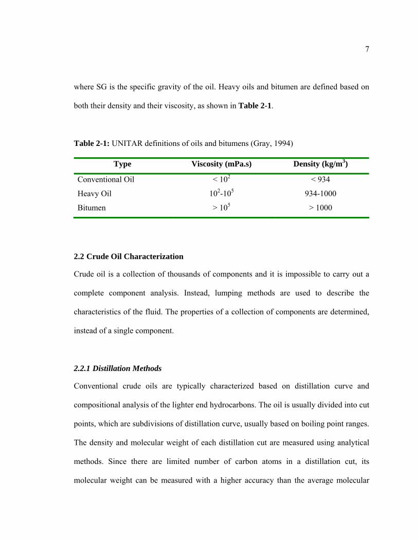
where SG is the specific gravity of the oil. Heavy oils and bitumen are defined based on
both their density and their viscosity, as shown in Table 2-1.
Table 2-1: UNITAR definitions of oils and bitumens (Gray, 1994)
Type Viscosity (mPa.s) Density (kg/m3)
Conventional Oil < 102 < 934
Heavy Oil 102-105 934-1000
Bitumen > 105 > 1000
2.2 Crude Oil Characterization
Crude oil is a collection of thousands of components and it is impossible to carry out a
complete component analysis. Instead, lumping methods are used to describe the
characteristics of the fluid. The properties of a collection of components are determined,
instead of a single component.
2.2.1 Distillation Methods
Conventional crude oils are typically characterized based on distillation curve and
compositional analysis of the lighter end hydrocarbons. The oil is usually divided into cut
points, which are subdivisions of distillation curve, usually based on boiling point ranges.
The density and molecular weight of each distillation cut are measured using analytical
methods. Since there are limited number of carbon atoms in a distillation cut, its
molecular weight can be measured with a higher accuracy than the average molecular
8
weight of the oil sample as a whole (Pedersen, et al., 2007). These analytical results
become part of the “Petroleum Assay”.
The pressure is reduced during distillation for certain characterization methods to avoid
thermal decomposition or cracking. The endpoints of the boiling range corresponding to a
particular cut are known as the cut points and each of the cuts is termed a pseudo-
component or hypothetical component. The pseudo-components’ properties are estimated
based on established methods and correlations.
The approach of “cutting” a distillation curve based on boiling points works well for
conventional crude oils. This is because the non-distillable fractions are small, typically
less than 5 wt % of the oil. But the approach does not work well for heavy oils and
bitumens where approximately 60% of the oil is non-distillable (Nji, et al., 2008). This
entails the use of some alternative techniques to characterize heavy oils and bitumen.
2.2.2 SARA fractionation
One approach is to separate the crude oil into four components based on solubility and
adsorption classes. The method is called SARA fractionation and the four components
are saturates, aromatics, resins, and asphaltenes. The SARA fractions are explained in
more detail below.
9
2.2.2.1 Saturates
Saturates consist of normal alkanes (n-paraffins), branched alkanes (iso-paraffins) and
cycloparaffins. Paraffins are hydrocarbon groups of the type C, CH, CH2 or CH3. The
carbons atoms are connected by single bonds with no cyclic chains. Cycloparaffins are
similar to paraffins in the sense that that are comprised of the same type of hydrocarbon
groups, but differ from paraffins by containing at least one cyclic structure. They are also
called naphthenes. The single-ring naphthenes present in petroleum are primarily alkyl-
substituted cyclo-pentanes and cyclo-hexanes (Speight, 1999). Saturates are the least
polar among the SARA fractions. The molar mass of saturates is in the range of 361
g/mol to 524 g/mol and their density is found to vary in the range of 853 to 900 kg/m³.
(Akbarzadeh et al., 2005)
2.2.2.2 Aromatics
Aromatics contain one or more cyclic structures similar to naphthenes, but the carbon
atoms in an aromatics compound is connected by aromatic double bonds; that is, they are
like benzene rings. Polycyclic aromatic compounds with two or more ring structures are
also found in the aromatic, resin, and asphaltene fractions. The molar mass of aromatics
is in the range of 450-550 g/mol. The densities are reported to vary from 960 to 1003
kg/m³ (Akbarzadeh et al., 2005).
2.2.2.3 Resins
Resins are polycyclic aromatics with higher molar mass, density, aromaticity, and
heteroatom content than the aromatics. They are thought to be molecular precursors of
10
the asphaltenes but, unlike asphaltenes, are soluble in pentane (Speight, 1999). Resins are
chemically similar to asphaltenes and are assumed to be soluble in the crude oil
(Hammami and Ratulowski, 2007). Resins can be converted to asphaltenes by oxidation
with atmospheric oxygen (Speight, 1999).
The molar mass of resins varies from 859 to 1240 g/mol. The molar mass is much higher
than aromatics, but substantially lower than asphaltenes. However, the molar mass
comparisons may be misleading because the asphaltenes and possibly the resins self-
associate. The densities reported are in the range of 1007 to 1066 kg/m3 (Akbarzadeh et
al., 2005).
2.2.2.4 Asphaltenes
Asphaltenes are defined as the components of crude oil that are soluble in aromatic
solvents such as toluene, but insoluble in n-alkane solvents like n-heptane. Some
asphaltene species are even insoluble in crude oil. The bitumen components excluding
asphaltenes (the saturates, aromatics and resins) are called maltenes.
Asphaltenes are mixtures of many thousands of chemical species and their structure is not
readily identified. They are generally composed of polynuclear aromatic rings, aliphatic
side chains and heteroatom such as nitrogen, sulphur and oxygen. The number of rings
varies from 6 to 15 (Simanzhenkov and Idem, 2003). They have the highest molar mass,
aromaticity and heteroatom content of all the crude oil components (Wiehe et al., 1996).
They are also the most polar fraction among all the crude oil components.
11
Asphaltenes are responsible for the high density and viscosity of heavy crudes and
bitumen. The average monomer molar mass of asphaltenes is in the range of 750 to 1800
g/mol (Yarranton et al., 2000, Badre et al., 2006) with recent data suggesting a value of
approximately 1000 g/mol (Pinkston et al., 2009). The apparent molar mass of self-
associated asphaltenes is in the order of 5000 to 10000 g/mol and perhaps higher
(Yarranton et al., 2000). The densities reported are in the range of 1132 to 1193 kg/m3
(Akbarzadeh et al., 2005).
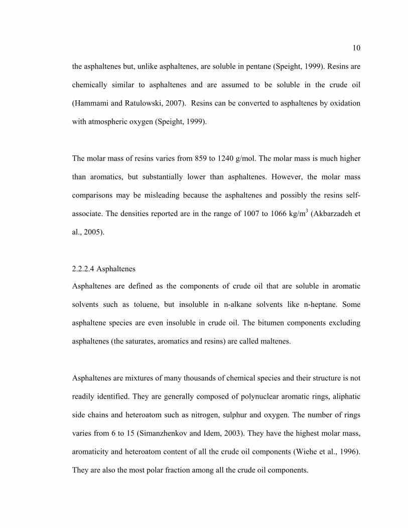
There are two different structures proposed for asphaltenes. The continent or
pericondensed structure is formed by molecules with large “continent” of aromatic rings
extended by short aliphatic chains. The archipelago model suggests asphaltenes as a
collection of small aromatic islands interconnected by aliphatic chains.
The hypothetical structure of a representative archipelago-like asphaltene molecule is
depicted in Figure 2.1 (Strausz et al., 1992).
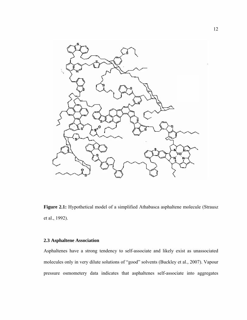
12
Figure 2.1: Hypothetical model of a simplified Athabasca asphaltene molecule (Strausz
et al., 1992).
2.3 Asphaltene Association
Asphaltenes have a strong tendency to self-associate and likely exist as unassociated
molecules only in very dilute solutions of “good” solvents (Buckley et al., 2007). Vapour
pressure osmometery data indicates that asphaltenes self-associate into aggregates
13
consisting of approximately 2 to 6 molecules per aggregate in aromatic solvents
(Yarranton et al., 2000).
The aggregates have been considered as colloidal particles (Pfeiffer et al., 1940) or
macromolecules (Hirschberg et al., 1984). With the colloidal view, the asphaltenes are
considered to be a colloidal suspension in the crude oil. The associated asphaltenes are
considered to form a stack which is surrounded and dispersed in the oil by resins.
With the macromolecular view, the asphaltene is considered to be completely dissolved
in the crude oil. The associated asphaltenes are independent molecules similar to the
resins and other crude oil constituents. Recent literature favours the macromolecular view
based on molar mass and calorimetric experiments (Andersen, 1999; Agrawala and
Yarranton, 2001 and Peramanu et al., 2001).
Agrawala and Yarranton (2001) proposed that molecules of asphaltenes aggregate in a
manner analogous to linear “polymerization”. In this process, the interactions between
free asphaltene molecules have been described in terms of two distinct classes. Some
molecules may contain several active sites and therefore propagate aggregation
(propagators). Other molecules may contain only one site and therefore terminate further
growth (terminators). Asphaltenes consist mainly of propagators, while resins consist
mainly of terminators. This approach was used to explain the observed asphaltene molar
mass distributions and the inhibiting effect of resin or asphaltene molar mass.
14
The above model was improved to include both asphaltenes and resins as a mixture of
self-associating species (Yarranton et al., 2007). Their results suggested that resins also
participate in asphaltene self-association and the fit of the solubility curves improved
with the new model. It was concluded that the asphaltenes and resins are best
characterized as a single continuum of aggregated species.
2.4 Asphaltene Precipitation
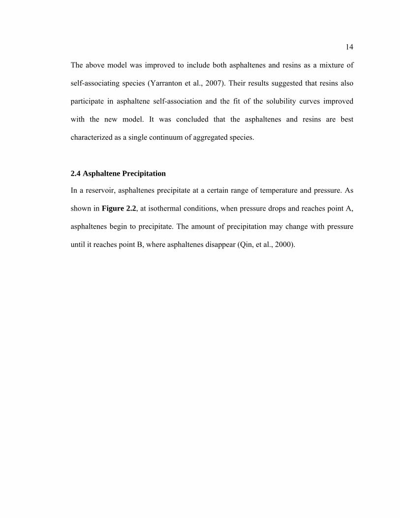
In a reservoir, asphaltenes precipitate at a certain range of temperature and pressure. As
shown in Figure 2.2, at isothermal conditions, when pressure drops and reaches point A,
asphaltenes begin to precipitate. The amount of precipitation may change with pressure
until it reaches point B, where asphaltenes disappear (Qin, et al., 2000).
15
Figure 2.2: Asphaltene precipitation envelope (Qin, X., et al., 2000).
When bitumen is diluted with an n-alkane, or other non-aromatic solvents, asphaltene
precipitation occurs. Mitchell et al. (1973) showed that solvent power, which is the ability
of the solvent to dissolve asphaltenes, increases in the order: 2-methyl paraffin < n-
paraffin < terminal olefin. This means 2-methyl paraffin solvents precipitate more
asphaltene than n-paraffin and terminal olefin solvents. They proved that cycloalkanes
and their methyl derivatives have solvent powers similar to those of aromatics. The
aromatic character of the asphaltenes and their content of heteroatoms are the main
influence on their solubility in different solvents and their tendency to flocculate
(Browarzik and Browarzik, 2005). Overall, the parameters that govern precipitation
16
appear to be the composition of the crude oil, pressure, temperature and properties of
asphaltenes (Hirschberg et al., 1984).
There is some debate in the literature on the reversibility of asphaltene precipitation.
Studies from titration experiments where asphaltenes are precipitated with precipitant and
then re-dissolved through solvent addition demonstrated that full reversibility did not
occur (Andersen, 1992). However, Peramanu (2001) concluded that precipitation could
be completely reversed as long as there is sufficient turbulence to break up the asphaltene
particles. Beck et al. (2005) showed that there is a hysteresis in asphaltene re-dissolution
that could be overcome with the removal of a poor solvent. Zou and Shaw (2004) showed
that bulk phase behaviour of hydrocarbon mixtures containing asphaltenes is reversible,
by conducting phase behaviour experiments on diluted Athabasca bitumen.
Precipitated asphaltenes manifest as approximately micron sized particles (Rastegari et
al., 2004) and form a black powder upon drying. However, asphaltenes likely undergo a
liquid-liquid phase separation from solution (Sirota, 2005). Sirota explained that the
solid-like character of the asphaltene-rich phase is only due to the fact that the material in
the heavier phase is below its glass-transition temperature. Therefore the current evidence
suggests that asphaltenes are indeed liquids, which may be in a glassy state depending on
the system temperature. Hirschberg et al. (1984) proposed a qualitatively accurate liquid-
liquid equilibrium model for the phase behaviour of asphaltene precipitation. This has led
to the LLE assumption in many of the newer models.
17
2.5 Modeling of Asphaltene Precipitation
There are two types of modeling approaches commonly used for describing asphaltene
phase behaviour, colloidal and thermodynamic models. The colloidal model was the first
proposed but thermodynamic models have proved more successful at predicting phase
behaviour.
2.5.1 Colloidal Model
Nellensteyn (1924) inferred a colloidal structure for bitumen based on observations such
as the Tyndall effect and Brownian motion of particles. He observed that an asphalt-like
dispersion could be prepared from asphalt base oil using a dispersion of finely divided
elemental carbon. Pfeiffer and Saal (1940) created a model to explain the rheological
observations consistent with the colloidal nature of bitumen by extending Nellensteyn’s
work. They proposed insufficient resin coating as the cause of asphaltene flocculation.
Leontaritis et al. (1987) proposed a model based on statistical thermodynamics and
colloidal science techniques to predict asphaltene precipitation in crude oil. The model
assumed that asphaltenes exist in the oil as solid particles in colloidal suspension,
stabilized by resins adsorbed on their surface. They also assumed that short range
intermolecular repulsive forces between resin molecules adsorbed on different asphaltene
particles keeps them from flocculating. Therefore, the phase behaviour depends on the
chemical potential of the resins:
(2-2) phaseoilre
phaseasphaltenere
.sin
.sin μμ =
18
where and are the chemical potential of resin in the asphaltene
phase and the oil phase respectively. The chemical potential of resin can be calculated
from a regular solution model coupled with the Flory-Huggins entropy contribution from
statistical thermodynamics theory as follows:
phaseasphaltenere
.sinμ phaseoil
re.
sinμ
( )21ln imi
m
i
m
iirefii
RTv
vv
vvx
RTδδ
μμ−+−+⎟⎟
⎠
⎞⎜⎜⎝
⎛=
− (2-3)
where μi and μiref are the chemical potential of component i and reference chemical
potential; vi and vm are the molar volumes of the component i and mixture respectively
and δm and δi are the solubility parameters of the mixture and component i, respectively.
R is ideal gas constant and T, the absolute temperature.
It was assumed that chemical potential of resins in the solid and liquid phases determined
the split between the two phases. The concentration of resin in the liquid which is just
enough to stabilize the colloidal asphaltene particles is called critical resin concentration
(Crcrit) and the chemical potential at this point is called the critical resin chemical
potential (μrcrit) . Given the critical resin concentration of a particular oil mixture, resin
and oil properties, the critical chemical potential can be found using the above equation.
If the actual resin chemical potential (μr) is less than to the μrcrit, asphaltene flocculation is
possible. With this method, the minimum amount of solvent needed to start flocculation
can be calculated.
19
The colloidal model is not consistent with liquid-liquid equilibrium and predicts that
asphaltene precipitation is irreversible. Colloidal model can fit the onset point of
asphaltene precipitation upon addition of a poor solvent but cannot predict the yield
(Janardhan and Mansoori, 1993). Cimino et al (1995) observed that the physical basis of
colloidal model is not correct, as asphaltenes could be dissolved in solvents without the
presence of resins.
2.5.2 Thermodynamic Models
The thermodynamic approach assumes that self-associated asphaltenes behave as
macromolecules in solution. These macromolecules can undergo a conventional phase
change to form a solid or dense liquid phase. The thermodynamic approach has been
successful in modeling asphaltene precipitation over a range of temperatures and
pressures. The thermodynamic approach can also model both the onset point of
asphaltene precipitation and asphaltene yield. Of the many approaches to modeling
asphaltene precipitation, the regular solution and equation-of-state approaches are the
most common. This thesis focuses on regular solution models and, therefore, equation-of-
state approaches are not reviewed.
2.5.3 Modified Regular Solution Theory
Hirschberg et al. (1984) treated the asphaltene precipitation analogous to liquid-liquid
equilibrium of a polymer solution. They combined Flory-Huggins theory with the
solubility concept to express the volume fraction of the asphaltene dissolved in the oil
( aφ ).
20
( )⎭⎬⎫
⎩⎨⎧
⎥⎦
⎤⎢⎣
⎡−−−= 21exp La
L
a
L
L
aa RT
vvv
vv
δδφ (2-4)
where va and vl denote asphaltene molar volume and oil molar volume respectively. δL
and δA are the solubility parameter of the mixture and the asphaltene respectively.
Vapour-Liquid equilibrium calculations were performed using the Soave-
Redlich−Kwong (SRK) equation of state. The calculations were performed mainly to
calculate the composition of the liquid phase and it was assumed that there was no
asphaltene precipitation during the vapour/liquid equilibrium (VLE) calculations. Once
the liquid phase compositions were known, the asphaltene precipitation was predicted
using modified Flory-Huggins theory, assuming that the precipitation does not change the
vapour/liquid equilibrium. The heavy liquid phase was assumed to be pure asphaltene.
Cimino et al. (1995) modified Hirschberg model by assuming that solvent also forms part
of the heavy liquid phase, not just asphaltenes. They neglected the asphaltene fraction in
the light liquid phase and derived the equation for calculating the activity coefficient of
asphaltenes:
( ) ( ) 011ln 22 =−+⎟⎟⎠
⎞⎜⎜⎝
⎛−+− ∗∗∗
asas
aa
sa RT
vvv
φδδφφ (2-5)
where vs is molar volumes of asphaltenes and oil (considered as solvent for asphaltenes)
respectively. is asphaltene volumetric fraction in the nucleating phase at the onset of ∗aφ
21
flocculation. The above equation can be used for finding the onset point of asphaltene
precipitation, but it cannot predict the asphaltene yield. In fact, all the asphaltene is
precipitated at the onset point because the solvent phase is assumed to be pure.
Browarzik et al. (1999) modeled the asphaltene system using solubility parameters. They
argued that, molar mass is not suitable for characterizing heavy oil or asphaltene since the
molar mass measurement is not very accurate. Furthermore, the molar mass
measurements are affected by the experimental conditions like choice of solvent and
temperature. Therefore, the solubility parameter of the Scatchard–Hildebrand theory was
selected as a more convenient identification variable for the oil species than the molar
mass. The solubility parameter reflects the intermolecular interactions originating from
the aromaticity and the heteroatoms in some way. A further reason for the oil
characterization using the solubility parameter is the possibility to correlate it with
experimentally available data.
They used a correlation for calculating the solubility parameter, which is a function of the
number of carbon atoms and of the hydrogen deficit. The calculation of the solubility
parameter of oil needs only experimental values of the molar mass average and the
content of carbon, hydrogen and heteroatoms. They results were reasonable when
compared with the measured flocculation data.
22
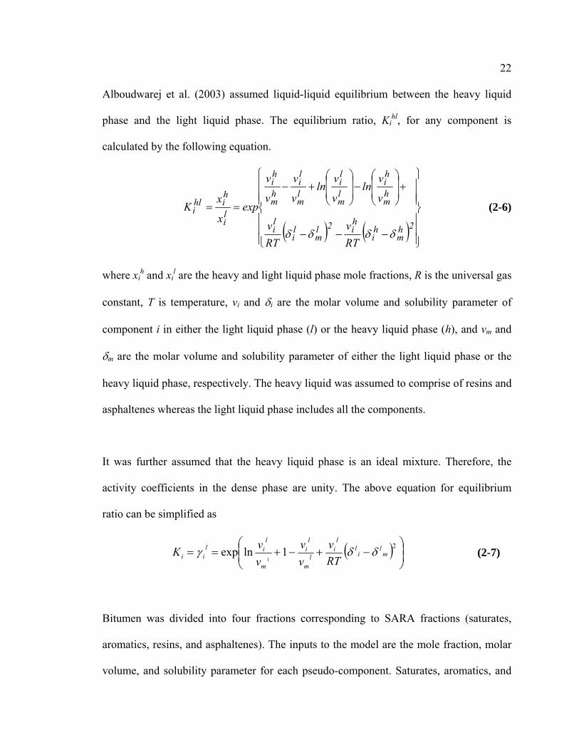
Alboudwarej et al. (2003) assumed liquid-liquid equilibrium between the heavy liquid
phase and the light liquid phase. The equilibrium ratio, Kihl, for any component is
calculated by the following equation.
( ) ( ) ⎪⎪⎪
⎭
⎪⎪⎪
⎬
⎫
⎪⎪⎪
⎩
⎪⎪⎪
⎨
⎧
−−−
+⎟⎟
⎠
⎞
⎜⎜
⎝
⎛−
⎟⎟
⎠
⎞
⎜⎜
⎝
⎛+−
==
2hm
hi
hi2l
mli
li
hm
hi
lm
li
lm
li
hm
hi
li
hihl
i
RTv
RTv
v
vln
v
vln
v
v
v
v
expx
xK
δδδδ
(2-6)
where xih and xi
l are the heavy and light liquid phase mole fractions, R is the universal gas
constant, T is temperature, vi and δi are the molar volume and solubility parameter of
component i in either the light liquid phase (l) or the heavy liquid phase (h), and vm and
δm are the molar volume and solubility parameter of either the light liquid phase or the
heavy liquid phase, respectively. The heavy liquid was assumed to comprise of resins and
asphaltenes whereas the light liquid phase includes all the components.
It was further assumed that the heavy liquid phase is an ideal mixture. Therefore, the
activity coefficients in the dense phase are unity. The above equation for equilibrium
ratio can be simplified as
( ) ⎟⎟⎠
⎞⎜⎜⎝
⎛−+−+==
21lnexp1
ml
il
li
lm
li
m
lil
ii RTv
vv
vvK δδγ (2-7)
Bitumen was divided into four fractions corresponding to SARA fractions (saturates,
aromatics, resins, and asphaltenes). The inputs to the model are the mole fraction, molar
volume, and solubility parameter for each pseudo-component. Saturates, aromatics, and
23
resins were treated as individual pseudo-components. The asphaltenes were further
divided into fractions of different molar mass. A molar mass distribution rather than
‘lumping’ as a single pseudo-component was used, which enabled matching the yield
curve by changing the parameters of the molar mass distribution.
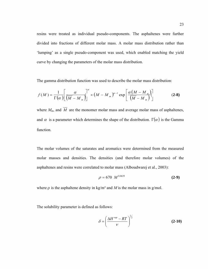
The gamma distribution function was used to describe the molar mass distribution:
( ) ( ) ( ) ( )( ) ⎥
⎦
⎤⎢⎣
⎡
−−
−×⎥⎦
⎤⎢⎣
⎡
−Γ= −
m
mm
m MMMMMM
MMMf αα
αα
α
exp1)( 1 (2-8)
where Mm, and M are the monomer molar mass and average molar mass of asphaltenes,
and α is a parameter which determines the shape of the distribution. ( )αΓ is the Gamma
function.
The molar volumes of the saturates and aromatics were determined from the measured
molar masses and densities. The densities (and therefore molar volumes) of the
asphaltenes and resins were correlated to molar mass (Alboudwarej et al., 2003):
(2-9) 0639.0 670 M=ρ
where ρ is the asphaltene density in kg/m³ and M is the molar mass in g/mol.
The solubility parameter is defined as follows:
2
1
⎟⎟⎠
⎞⎜⎜⎝
⎛ −Δ=
νδ RTH vap
(2-10)
24
where ΔHvap is the heat of vaporization. The solubility parameters of saturates and
aromatics were determined by fitting the solubility model to asphaltene-saturate-toluene
and asphaltene-n-heptane-aromatics solubility data, respectively.
The solubility parameter of asphaltenes was determined using the semi-empirical
correlation recommended by Yarranton and Masliyah (1996).
( ) 21
ρδ A= (2-11)
where δ is the solubility parameter in MPa0.5 and A is the monomer heat of vaporization
in kJ/g. The constant A was determined by fitting the model to one set of asphaltene-n-
heptane-toluene precipitation data.
Akbarzadeh et al. (2005) modified the regular solution model by Alboudwarej et al.
(2003) by developing several empirical correlations for calculating the model inputs
thereby generalizing the existing model. They correlated the densities of saturates and
aromatics to temperature by fitting the density data.
54.1069T6379.0sat +−= ρ (2-12)
73.1164T5943.0aro +−= ρ (2-13)
where satρ and aroρ are the average densities of saturates and aromatics in kg/m3,
respectively and T is temperature in Kelvin. The above correlations were validated on a
number of heavy oils and bitumens.
25
The following correlations were developed to estimate the solubility parameters of
saturates and aromatics at different temperatures:
δsat = 22.381 – 0.0222 T (2-14)
δaro = 26.333 – 0.0204 T (2-15)
where δsat and δaro are the solubility parameters of saturates and aromatics in MPa0.5 and
T is temperature in Kelvin.
The following correlation was used for the solubility parameter of n-alkanes at different
temperatures:
δs,T = δs,25 - 0.0232 ( T – 298.15) (2-16)
where δs,T is solvent solubility parameter at temperature T, δs,25 is solvent solubility
parameter at 25°C estimated from Equation 2-10, and T is temperature in Kelvin.
The A parameter of Equation 2-11 was modified to be temperature dependent. The
following correlation for A was determined by fitting the model to precipitation data for
mixtures of asphaltene-heptane-toluene at temperatures of 23 and 50°C:
(2-17) 5614.010667.6)( 4 +×−= − TTA
The modified regular solution model was able to predict the onset point of precipitation
and asphaltene yields for a wide range of heavy oils and bitumen. The model was able to
predict the temperature and pressure effects as well.
26
2.6 Asphaltene-Rich Phase Composition
At equilibrium, the asphaltene-rich phase must contain all the components present in the
crude oil. However, such compositional data is rare. Hence, phase behaviour models for
these systems are at least partially speculative because the predictions cannot be validated
with experimental data for the composition of the asphaltene-rich phase. It can be
concluded that asphaltene-rich phase behaviour is not clearly understood (Zou and Shaw,
2004).
There have been efforts to model the composition of asphaltene-rich phase in the
literature. Szewczyk and Behar (1999) described asphaltene precipitation as a
thermodynamic transition of asphaltenes from a first liquid phase, the crude, to a second
liquid phase, the asphaltenic deposit which possibly includes all the components initially
in the fluid before the phase separation. In his paper, crude oil was divided into a series of
components and pseudo-components (F10-, F11-F20, Sat F20+, Aro F20+, resins and
asphaltenes) for the purpose of modeling. The physical properties of the components
were used directly and those of the pseudo-components were estimated using correlations
based on the experimental values of density, molecular weight, and aromaticity. The
amount and composition of the gas, liquid and asphaltenic phases were calculated by a
single phase flash calculation using a volume translated Peng-Robinson EoS model and
group contribution mixing rules. Since the thermodynamic model was not predictive, the
proposed method consisted of fitting some physical characteristics (such as the critical
properties of some pseudo-components and asphaltene molar mass) to data (crude oil
relative volume, density of pseudo-components and solubility of asphaltene). The model
27
considered only the initial crude oil composition, avoiding the errors resulting from the
assumption that asphaltene-rich phase is pure asphaltene. The composition of the
asphaltene-rich phase was calculated by the flash procedure.
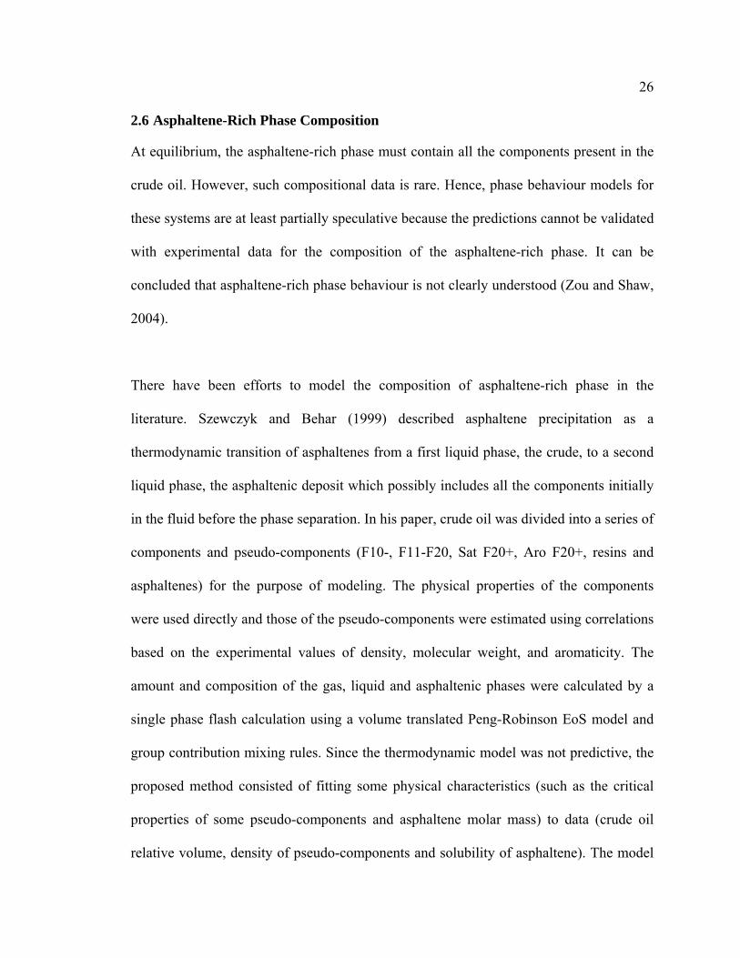
The results of the model are given in Figure 2.3. As expected, the majority of the
asphaltenic deposit is composed of asphaltenes (approximately 85 wt%). The light
fraction F10- is relatively significant and its weight percent is in the range of 5 wt%. The
resin percentages are found to very low. They compared their results with an analysis of
Venezuelan deposits and reported that there was good agreement although the data were
not presented.
Figure 2.3: Calculated weight percent of the asphaltenic deposit at the saturation
pressure and 303 K as predicted by the model by Szewczyk and Behar (1999).
28
Wu et al. (1998) proposed a model based on SAFT association model and colloidal
theory. They assumed that asphaltenes and resins can be represented by pseudo-pure
components, and that all other components in the crude oil can be represented by a
continuous medium that effects interactions among asphaltene and resin molecules. The
effect of the medium on asphaltene-asphaltene: resin-asphaltene, resin-resin pair
interactions is taken into account through its density and dispersion-force properties. The
expressions for the chemical potential of asphaltene and for the osmotic pressure of an
asphaltene-containing solution was found using the SAFT model which is used in the
framework of McMillan-Mayer theory which assumes hard-sphere repulsive, association
and dispersion-force interactions. By assuming that asphaltene precipitation is a liquid-
liquid equilibrium process, the model could describe precipitation of asphaltene from
crude oil.
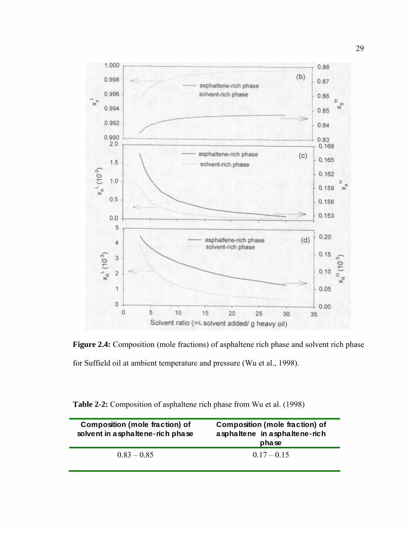
The framework could theoretically explain a variety of experimental observations, but
quantitative predictions require molecular parameters that must be estimated from little
experimental data. Figure 2.4 shows the model predictions of the composition of
asphaltene rich phases and solvent rich phases. However, the results are not compared
with any experimental data. The predicted phase compositions are shown in Table 2-2.
29
Figure 2.4: Composition (mole fractions) of asphaltene rich phase and solvent rich phase
for Suffield oil at ambient temperature and pressure (Wu et al., 1998).
Table 2-2: Composition of asphaltene rich phase from Wu et al. (1998)
Composition (mole fraction) of solvent in asphaltene-rich phase
Composition (mole fraction) of asphaltene in asphaltene-rich
phase 0.83 – 0.85 0.17 – 0.15
30
2.7 Summary
Asphaltenes can precipitate when there is a pressure depletion or when diluents are added
to enhance its transportability. Regular solution models have been widely used to study
asphaltene phase behaviour. The model developed by Alboudwarej et al (2003) and
Akbarzadeh et al (2005) can successfully predict the precipitation of asphaltene after
some initial tuning. However, they assume that there is no solvent in the asphaltene-rich
phase. This assumption must be tested; however there is only limited data available in the
literature for the measured composition of asphaltene-rich phase.
31
Chapter Three: Experimental
This chapter discusses the materials and methodologies used in this thesis. The
experimental procedure adopted to determine the composition of solvent in the
asphaltene-rich phase is described. The solubility and SARA fractionation data used in
this thesis are taken from previously collected data by the same group. The details of
these experimental procedures are explained elsewhere (Alboudwarej et al., 2002,
Alboudwarej, 2003).
3.1 Materials
The experiments for determining the composition of the asphaltene-rich phase were
conducted using Athabasca bitumen and asphaltene derived from Athabasca bitumen.
Athabasca Coker feed bitumen was obtained from Syncrude Canada Ltd. It is the
Syncrude Plant-7 froth treatment product after the solvent has been removed.
Commercial grade toluene and n-heptane were obtained from Univar Canada and
ConocoPhillips, respectively. n-pentane and n-decane were obtained from ConocoPhillips
and Fisher Scientific, respectively and were 99.3% pure.
Asphaltenes were precipitated from the bitumen by the addition of either n-pentane or n-
heptane at a 40:1 volume ratio of n-alkane to bitumen. The mixture was sonicated using
an ultrasonic bath for 45 minutes and left overnight to settle. After settling, the
supernatant was filtered through Whatman #2 (8μm) filter paper without disturbing the
whole solution. At this point approximately 10% of the original mixture remained
32
unfiltered. The remaining precipitate was further diluted with the n-alkane at a 4:1
alkane:bitumen volume ratio. The mixture was sonicated for 45 minutes, left overnight
and finally filtered using the same filter paper.
The precipitate was washed with the n-alkane until no discoloration was observed in the
washings. The asphaltenes were dried in a vacuum oven at 50° C until no change in
weight was observed. Asphaltenes precipitated with n-pentane and n-heptane are termed
C5- and C7-asphaltenes, respectively.
3.2 Determination of the Solvent Content of the Asphaltene-Rich Phase
When a “good” solvent like toluene is added to solid asphaltenes, the asphaltene particles
completely dissolve in the solvent. When a “poor” solvent like n-pentane or n-heptane is
then added to this mixture, asphaltenes are precipitated. Similarly, in the case of bitumen
diluted with n-alkane solvents, asphaltenes are precipitated. The resultant mixture
separates into a light liquid phase, which is rich in solvents, and a heavy phase, which is
rich in asphaltenes. The issue that arises is whether this heavy phase is a glassy liquid or a
solid (Hirschberg, 1984, Kawanaka et al., 1991, Sirota, 2005, Gupta, 1986). In this work,
this phase is treated as a liquid. For clarity, the two liquid phases will be called the
solvent-rich phase and the asphaltene-rich phase, respectively. The objective of the
proposed experiment is to determine the solvent content of the asphaltene-rich phase.
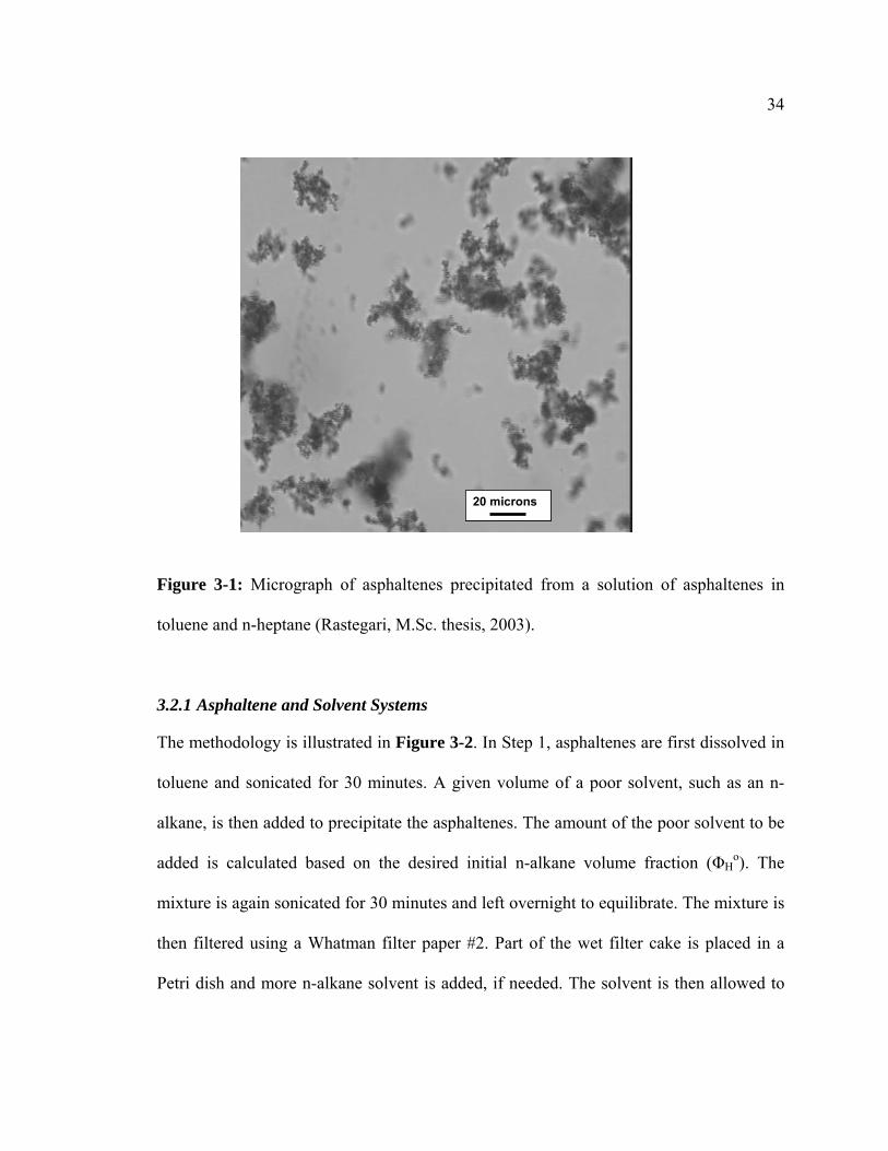
The asphaltene-rich phase manifests as a dispersed phase of particles, with diameters in
the order of one micron, that form floccs of up to several hundred microns in diameter,
33
Figure 3-1 (Rastegari et al., 2004). The particles settle into a sediment layer and are
surrounded by an entrained continuous phase (the solvent-rich phase). The remainder of
the continuous phase forms a layer of free solvent above the sediment. It is required to
measure the amount of solvent in the dispersed particles without including solvent from
the continuous phase. In other words, the solvent in the asphaltene-rich phase must be
clearly distinguished from the free and entrained solvent.
A methodology was designed to determine the mass of solvent in the asphaltene-rich
phase only. The methodology is based on the rapid evaporation of the continuous phase
solvent relative to the solvent dissolved in the asphaltene-rich phase. The free or
entrained solvent evaporates directly while the solvent in the dense phase must first
diffuse to the surface of the particle. Hence, there is an observable change in the
evaporation rate when the entrained solvent finishes evaporating and only evaporation of
solvent from the asphaltene-rich phase continues.
34
20 microns
20 microns20 microns
Figure 3-1: Micrograph of asphaltenes precipitated from a solution of asphaltenes in
toluene and n-heptane (Rastegari, M.Sc. thesis, 2003).
3.2.1 Asphaltene and Solvent Systems
The methodology is illustrated in Figure 3-2. In Step 1, asphaltenes are first dissolved in
toluene and sonicated for 30 minutes. A given volume of a poor solvent, such as an n-
alkane, is then added to precipitate the asphaltenes. The amount of the poor solvent to be
added is calculated based on the desired initial n-alkane volume fraction (ΦHo). The
mixture is again sonicated for 30 minutes and left overnight to equilibrate. The mixture is
then filtered using a Whatman filter paper #2. Part of the wet filter cake is placed in a
Petri dish and more n-alkane solvent is added, if needed. The solvent is then allowed to
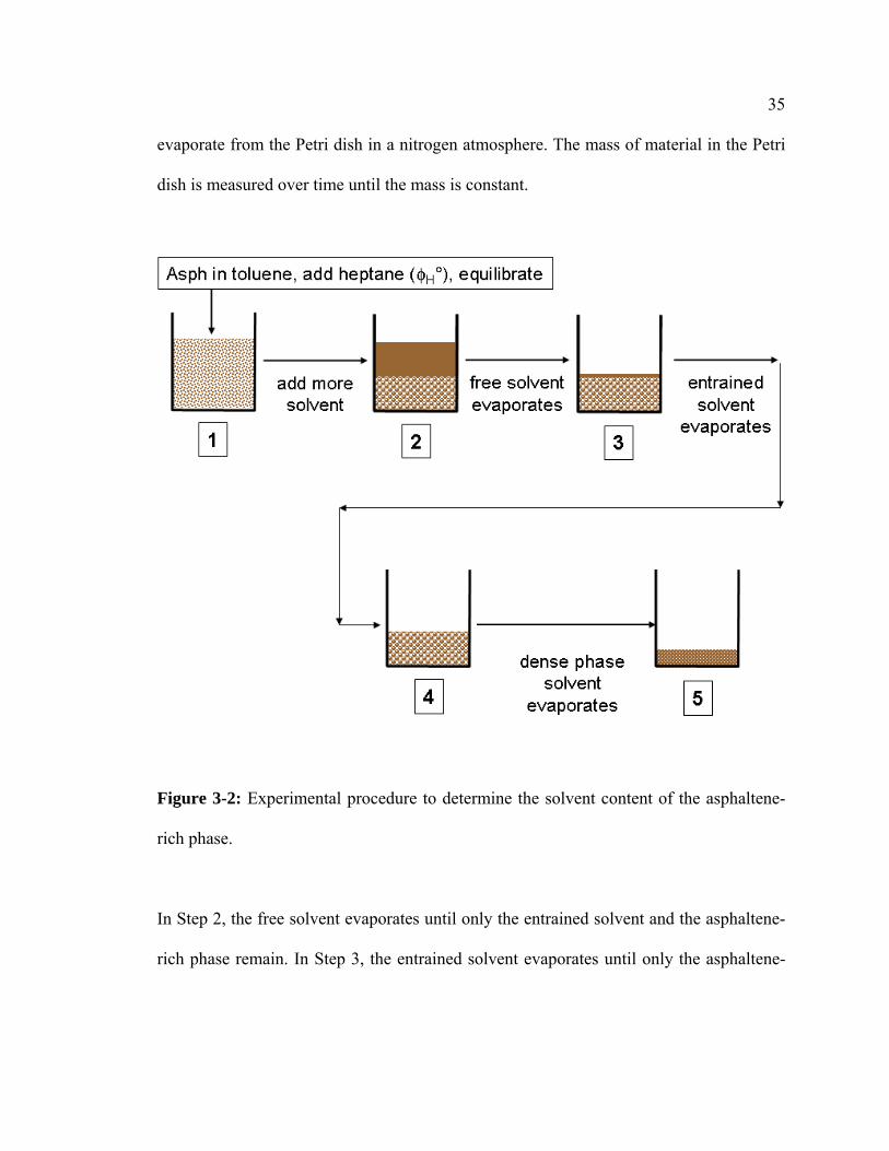
35
evaporate from the Petri dish in a nitrogen atmosphere. The mass of material in the Petri
dish is measured over time until the mass is constant.
Figure 3-2: Experimental procedure to determine the solvent content of the asphaltene-
rich phase.
In Step 2, the free solvent evaporates until only the entrained solvent and the asphaltene-
rich phase remain. In Step 3, the entrained solvent evaporates until only the asphaltene-
36
rich phase remains. At Step 4, the solvent from the asphaltene-rich phase diffuses from
the particles and evaporates until only dry asphaltenes remain at Step 5.
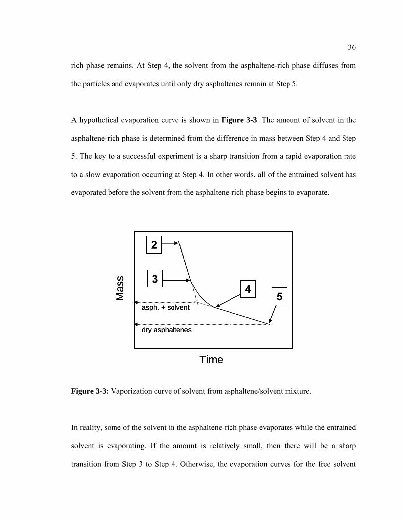
A hypothetical evaporation curve is shown in Figure 3-3. The amount of solvent in the
asphaltene-rich phase is determined from the difference in mass between Step 4 and Step
5. The key to a successful experiment is a sharp transition from a rapid evaporation rate
to a slow evaporation occurring at Step 4. In other words, all of the entrained solvent has
evaporated before the solvent from the asphaltene-rich phase begins to evaporate.
4
2
Mas
s
Time
35
dry asphaltenes
asph. + solvent
4
2
Mas
s
Time
35
dry asphaltenes
asph. + solvent
Figure 3-3: Vaporization curve of solvent from asphaltene/solvent mixture.
In reality, some of the solvent in the asphaltene-rich phase evaporates while the entrained
solvent is evaporating. If the amount is relatively small, then there will be a sharp
transition from Step 3 to Step 4. Otherwise, the evaporation curves for the free solvent
37
and for the asphaltene-rich phase solvent can be extrapolated, Figure 3-3. The point
where they meet indicates the mass of the asphaltene-rich phase.
In all cases, the evaporation experiments were conducted in a bench top oven in a
nitrogen atmosphere. An inert gas atmosphere like nitrogen is required to prevent the
asphaltenes from oxidizing. The oven was maintained at a room temperature and pressure
so that the solvent evaporation rates were the same in all experiments.
The experiment was repeated with different solvents (n-heptane, n-pentane and n-
decane), asphaltene types (C5-asphaltenes and C7-asphaltenes), initial n-alkane volume
fractions, and layer thicknesses of the asphaltene-rich phase in the Petri dish.
3.2.2 Diluted Bitumen Systems
In the case of bitumen, the above procedure for asphaltene-solvent systems was repeated
with slight modifications. In Step 1, Bitumen was diluted with a poor solvent, such as n-
heptane, at the desired dilution ratio. The mixture was sonicated for 45 minutes and left
overnight to equilibrate. The mixture was then filtered using a Whatman filter paper #2.
Part of the wet filter cake was placed in a Petri dish and more n-alkane solvent was
added, if needed. From this point, Steps 1 to 5 were carried out as described previously.
The experiment was repeated with different dilution ratios and layer thickness.
Note bitumen contains other constituents: saturates, aromatics, and resins. These
constituents may also partition to the asphaltene-rich phase. These other constituents are
38
also present in the solvent-rich phase and are non-volatile. Therefore, they will not
evaporate and will accumulate in the residue as the solvent evaporates. At the high
dilutions used in these experiments, the potential error is 0.87%, as determined in Section
5.2.
3.3 Summary
An experimental procedure was developed to determine the solvent content of the
asphaltene-rich phase. The methodology is based on the rapid evaporation of the
free/entrained solvent relative to the solvent dissolved in the asphaltene-rich phase. As
long as there is a sharp transition from a rapid evaporation rate of free/entrained solvent
to a slow evaporation of solvent in the asphaltene-rich phase, the solvent content in the
asphaltene-rich phase can be determined from the transition point. Procedures were
developed for both asphaltene-solvent systems and diluted bitumen systems.
39
Chapter Four: Modeling
In this chapter, the theory and modeling methodology used in this research-project are
presented. The modeling is based on a modification to regular solution theory and a brief
description of the model and the details of the fluid characterization are presented. The
determination of the molar mass, molar volume, and solubility parameter, which are
required in the regular solution model, is explained. In the last section, the flash
calculation procedure is discussed and a flow chart for the flash program is provided.
4.1 Modified Regular Solution Model
The separation of the fluid into a solvent-rich and an asphaltene-rich phase is modeled as
a liquid-liquid equilibrium process. For two liquid phases at equilibrium, the fugacity of
each component is identical in each phase:
(4-1) 21 Li
Li ff =
where fi is the fugacity of component i, and L1 and L2 denote the two liquid phases. The
fugacity of a component in liquid can be expressed as (Smithand van Ness, 1987),
(4-2) 0iii
Li fxf γ=
where xi, γi and fi° are the mole fraction, activity coefficient, and standard state fugacity,
respectively. Eq. 4-2 is substituted into Eq. 4-1 to obtain:
(4-3) 2211 Li
Li
Li
Li xx γγ =
40
Eq. 4-3 provides the relationship between the composition of each phase which is
required for phase equilibrium calculations. The relationship is usually expressed as an
equilibrium ratio, K:
1
2
2
1
Li
Li
Li
Li
i xx
Kγγ
== (4-4)
Eqn. 4-4 shows that the equilibrium ratio for two liquid phases can be determined solely
from the activity coefficients.
Several researchers have derived the activity coefficient for asphaltenes and crude oils
based on regular solution theory (Hirschberg et al., 1984; Kawanaka et al., 1991;
Yarranton and Masliyah, 1996). The model in this thesis is from Akbarzadeh et al. (2005)
where the activity coefficient of a component in a given phase is based on regular
solution theory (Scatchard, 1931; Hildebrand, 1929) modified with a Flory-Huggins
entropy contribution (Flory, 1941; Huggins, 1941), and is given by:
( ) ⎟⎟⎠
⎞⎜⎜⎝
⎛−+−+= 2ln1exp mi
i
m
i
m
ii RT
vvv
vv
δδγ (4-5)
where R is the universal gas constant, T is temperature, vi and δi are the molar volume and
solubility parameter of component i, respectively and vm and δm are the molar volume and
solubility parameter of liquid phase, respectively. The second and third terms of the
expression are the entropic contribution from different sized molecules and the final term
is derived from the internal energy of mixing a regular solution. The model requires the
molar volume and solubility parameter of each component in addition to the temperature,
pressure and overall composition.
41
4.2 Fluid Characterization
The fluids in this work are solutions of asphaltenes in solvents or diluted bitumens. The
solvent properties are known and were taken from the literature. The bitumen or heavy
oil was divided in three pseudo-components (saturates, aromatics, and resins) as well as
asphaltenes. The asphaltenes were treated as a mixture of nano-aggregates and were
divided into pseudo-components representing different aggregate sizes. The composition
of the fluid was determined from measured solvent and asphaltene or bitumen amounts
and, when required, the SARA analysis of the bitumen.
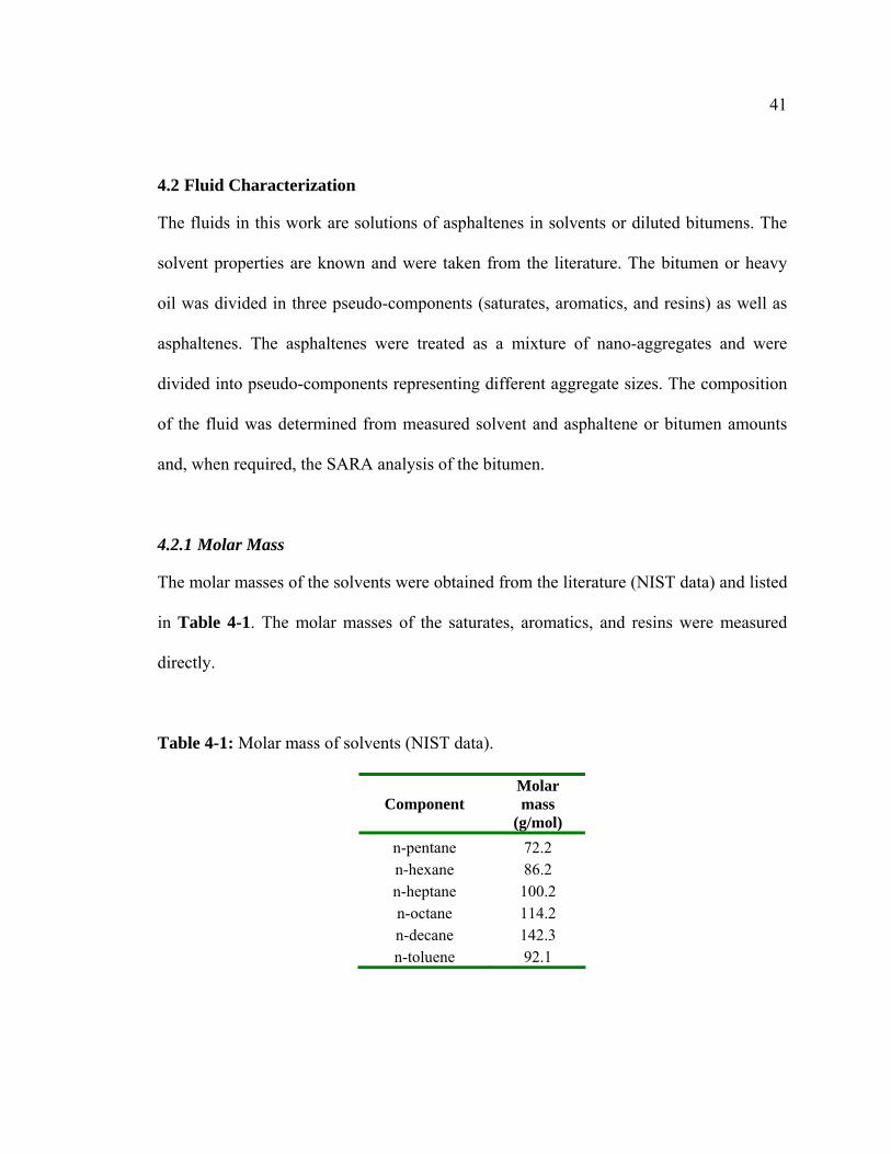
4.2.1 Molar Mass
The molar masses of the solvents were obtained from the literature (NIST data) and listed
in Table 4-1. The molar masses of the saturates, aromatics, and resins were measured
directly.
Table 4-1: Molar mass of solvents (NIST data).
Component Molar mass
(g/mol) n-pentane 72.2 n-hexane 86.2 n-heptane 100.2 n-octane 114.2 n-decane 142.3 n-toluene 92.1
42
The distribution of asphaltene nano-aggregates was divided into pseudo-components
based on the gamma distribution function given by Equation 2-8.
For positive values ofα , the gamma function can be written as:
( ) ∫∞
−−=Γ0
1 dtet tαα (4-6)
The monomer molar mass was set to 1500 g/mol. Molar masses from vapour pressure
osmometry extrapolate to a monomer molar mass of approximately 1800 g/mol, while
high resolution mass spectrometry indicates monomer molar masses of approximately
1000 g/mol (Pinkston et al., 2009). The choice of 1500 g/mol is a compromise which can
be revisited when the average monomer molar mass is better resolved. Yarranton et al.
(2007) demonstrated that, while some retuning is required, the model is not very sensitive
to the choice of monomer molar mass.
Asphaltene was divided into 30 sub-fractions with molar mass ranging up to 45000
g/mol. The average molar mass is an input for the model. For asphaltenes in solvents, the
average molar mass of the aggregated asphaltenes is measured directly using vapour
pressure osmometry (VPO). The value of α was determined by fine-tuning the model fit
to precipitation data from solutions of asphaltenes in n-heptane and toluene. A value of 5
was found to fit the data. Once the distribution was set, the equations are solved
numerically.
43
4.2.2 Densities and Molar Volumes
The densities of the solvents at 25oC were obtained from the VMGSim component
database and listed in Table 4-2.
Table 4-2: Densities of solvents (VMGSim component database, VMGSim v5.0, 2009).
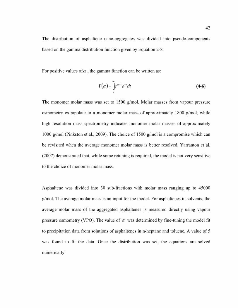
Component Density (Kg/m3)
n-pentane 630.5 n-hexane 656 n-heptane 682 n-octane 699 n-decane 728 n-toluene 865
The densities of saturates and aromatics were calculated using correlations taken from
Akbarzadeh et al. (2005) model.
1069.54 0.6379T +=satρ (4-7)
1164.73 0.5943T +=aroρ (4-8)
where satρ and aroρ are densities of saturates and aromatics in kg/m³ respectively. T is
the absolute temperature in K.
For resins and asphaltenes, the densities were correlated to the molar mass (Alboudwarej
et al., 2003).
(4-9) 0639.0 670 M=ρ
where ρ is the asphaltene density in kg/m³ and M is the molar mass in g/mol.
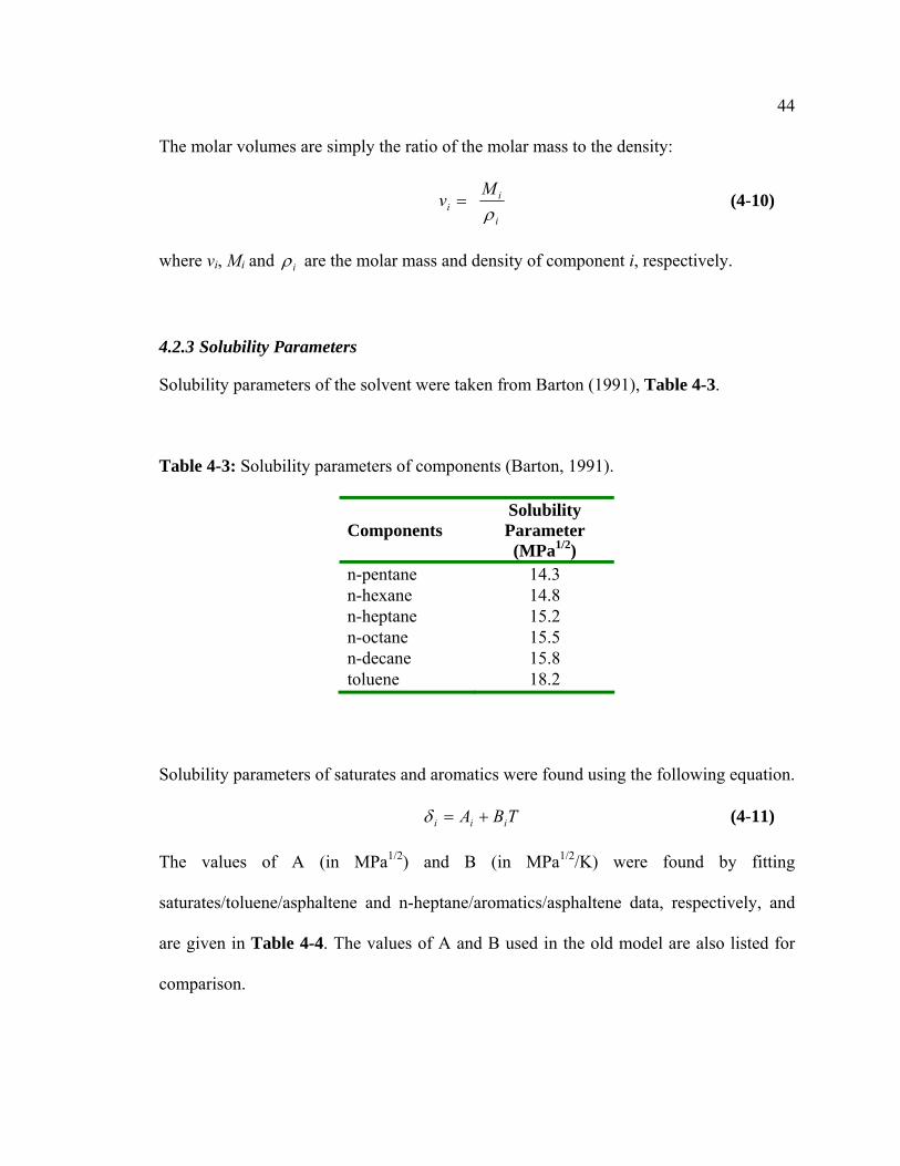
44
The molar volumes are simply the ratio of the molar mass to the density:
i
ii
Mv
ρ= (4-10)
where vi, Mi and iρ are the molar mass and density of component i, respectively.
4.2.3 Solubility Parameters
Solubility parameters of the solvent were taken from Barton (1991), Table 4-3.
Table 4-3: Solubility parameters of components (Barton, 1991).
Components
Solubility Parameter (MPa1/2)
n-pentane 14.3 n-hexane 14.8 n-heptane 15.2 n-octane 15.5 n-decane 15.8 toluene 18.2
Solubility parameters of saturates and aromatics were found using the following equation.
TBA iii +=δ (4-11)
The values of A (in MPa1/2) and B (in MPa1/2/K) were found by fitting
saturates/toluene/asphaltene and n-heptane/aromatics/asphaltene data, respectively, and
are given in Table 4-4. The values of A and B used in the old model are also listed for
comparison.
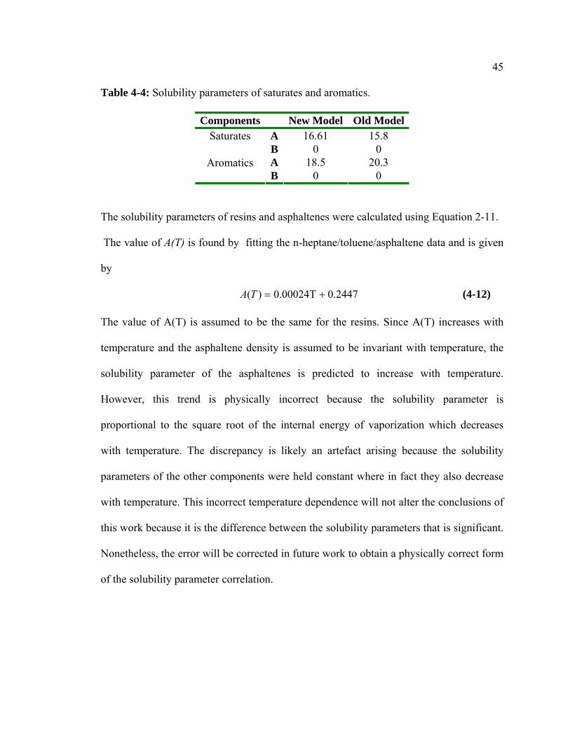
45
Table 4-4: Solubility parameters of saturates and aromatics.
Components New Model Old Model A 16.61 15.8 Saturates B 0 0 A 18.5 20.3 Aromatics B 0 0
The solubility parameters of resins and asphaltenes were calculated using Equation 2-11.
The value of A(T) is found by fitting the n-heptane/toluene/asphaltene data and is given
by
0.24470.00024T)( +=TA (4-12)
The value of A(T) is assumed to be the same for the resins. Since A(T) increases with
temperature and the asphaltene density is assumed to be invariant with temperature, the
solubility parameter of the asphaltenes is predicted to increase with temperature.
However, this trend is physically incorrect because the solubility parameter is
proportional to the square root of the internal energy of vaporization which decreases
with temperature. The discrepancy is likely an artefact arising because the solubility
parameters of the other components were held constant where in fact they also decrease
with temperature. This incorrect temperature dependence will not alter the conclusions of
this work because it is the difference between the solubility parameters that is significant.
Nonetheless, the error will be corrected in future work to obtain a physically correct form
of the solubility parameter correlation.
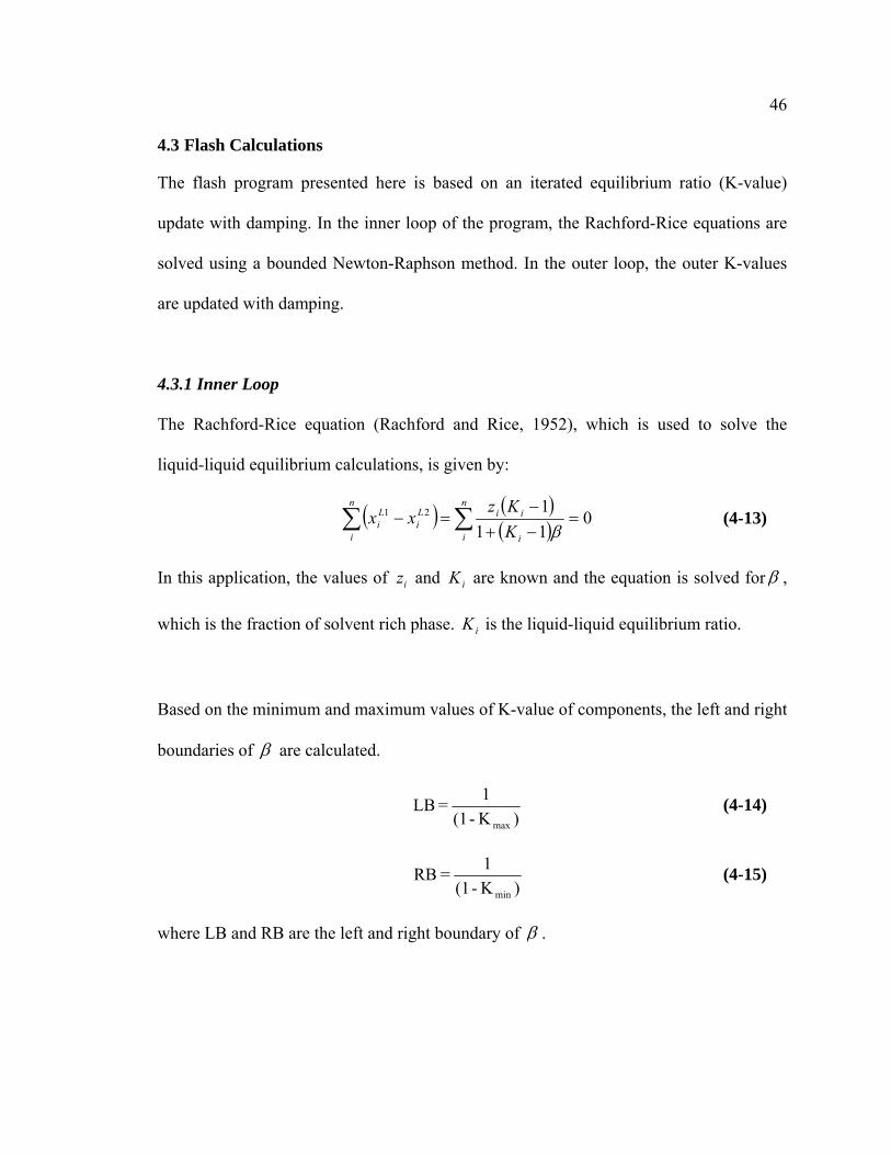
46
4.3 Flash Calculations
The flash program presented here is based on an iterated equilibrium ratio (K-value)
update with damping. In the inner loop of the program, the Rachford-Rice equations are
solved using a bounded Newton-Raphson method. In the outer loop, the outer K-values
are updated with damping.
4.3.1 Inner Loop
The Rachford-Rice equation (Rachford and Rice, 1952), which is used to solve the
liquid-liquid equilibrium calculations, is given by:
( ) ( )( )∑ ∑ =
−+−
=−n
i
n
i i
iiLi
Li K
Kzxx 0
11121
β (4-13)
In this application, the values of and are known and the equation is solved foriz iK β ,
which is the fraction of solvent rich phase. is the liquid-liquid equilibrium ratio. iK
Based on the minimum and maximum values of K-value of components, the left and right
boundaries of β are calculated.
)K -(1
1 = LBmax
(4-14)
)K -(1
1 = RBmin
(4-15)
where LB and RB are the left and right boundary of β .
47
The Rachford-Rice equation is non-linear and the equation above is solved using the
Newton-Raphson (NR) method.
)(')(
1n
nnn P
Pββ
ββ −=+ (4-16)
where )( nP β is the Rachford-Rice function and )(' nP β is its derivative with respect to
β . )( nP β and )(' nP β are given by the following equations.
∑ −+−
=i i
ii
KKz
Pβ
β)1(1)1(
)( (4-17)
∑ −+−
−=i i
ii
KKz
P 2
2
))1(1()1(
)('β
β (4-18)
The initial estimated value for β is 0. The initial values of K are estimated for each
component. The function is iterated until the change in the value of β per iteration is
below a given threshold, in this case, be 10-16. If the value calculated is outside the left
and right boundaries, the value of β is modified as follows:
)(5.01 LBnn −=+ ββ if LB<β (4-19)
)(5.01 nnn RB βββ −+=+ if RB>β (4-20)
where 1+nβ is the new β value and nβ is the β value from the previous iteration. β is
the current β value, LB and RB are the left and right boundaries of β .
Once the value of β is converged, the compositions of solvent-rich phase and
asphaltene-rich phase are calculated using the following equations.
48
( ) 111
+−=
i
iiLi K
zKx
β (4-21)
( ) 112
+−=
i
iLi K
zx
β (4-22)
where, in this application, xiL1 and xi
L2 are the mole fractions of component i in the
solvent-rich phase and the asphaltene-rich phase, respectively.
4.3.2 Outer Loop
The activity coefficients and equilibrium ratios are recalculated based on the updated
compositions from the inner loop. The equilibrium ratios are modified with a damping
factor as follows:
( ){ }previ
curri
previ
newi KKDFKK lnln*lnexp −+= (4-23)
where DF is the damping factor, is the new value of K, is the current value of
K calculated using equation 4-4 and is the value of K at the previous iteration. A
value of damping factor of 0.15 – 0.4 is used in this work to improve the convergence.
newiK curr
iK
previK
The difference between the values of β at the current iteration and previous iteration and
the difference between the values of Ki for each component at the current iteration and
previous iteration are used to calculate the overall error.
errerr K+= βε (4-24)
[ ]2currpreverr βββ −= (4-25)
[ ]∑ −=i
previ
curri
err KKK2
(4-26)
49
where ε is the overall error, is the error from vapour fraction and errβ errK is the total
error from K-values of each component. is the current value of currβ β and is the
value of
prevβ
β at the previous iteration.
The outer loop is iterated until the overall error is less than the tolerance value of 10-12.
All the calculations are performed in Microsoft Excel, using the Visual Basic for
Applications (VBA) coding interface. A flow chart showing the calculation procedure is
given in Figure 4-1.
4.4 Summary
An existing regular solution model was modified to allow all components in the
asphaltene-rich phase to take part in the phase equilibrium. A flash program was
developed which used iterated equilibrium ratio updating with damping. The Rachford-
Rice equations were solved using a bounded Newton-Raphson method. The model was
re-tuned using n-heptane/toluene/ asphaltene precipitation data.
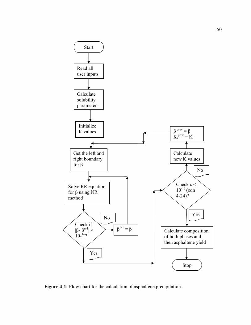
50
Start
Read all user inputs
βn-1 = β
β prev = β Ki
prev = Ki
Calculate solubility parameter
Calculate composition of both phases and then asphaltene yield
Initialize K values
Get the left and right boundary for β
Solve RR equation for β using NR method
Check ε < 10-12 (eqn 4-24)?
Yes
No
Stop
Check if |β- βn-1| < 10-16?
Yes
No
Calculate new K values
Figure 4-1: Flow chart for the calculation of asphaltene precipitation.
51
Chapter Five: Measurement of Asphaltene-Rich Phase Compositions
The methodology to determine phase compositions from the evaporation experiments is
validated. The solvent contents of the asphaltene-rich phases from asphaltene/solvent
systems are discussed including the effect of the type of solvent and asphaltenes. The
extension of the method to n-heptane diluted bitumen is also presented.
5.1 Asphaltene-Rich Phases from Asphaltene/Solvent Systems
5.1.1 Validation of Method
As explained in Chapter Three:, the amount of solvent in an asphaltene-rich phase was
determined from an evaporation experiment. The accuracy of the measurement depends
on a distinct transition from free and entrained solvent evaporation to diffusive
evaporation from the asphaltene-rich phase, Figure 3-3. In particular, if the evaporation
of the entrained solvent is slower than the evaporation of free solvent above the sediment,
the beginning of diffusive evaporation from the asphaltene-rich phase may be
undetectable.
To test the effect of the entrained solvent evaporation rate, experiments were performed
with different thicknesses of sediment. In a thin sediment layer, the volume of entrained
solvent is small and the exposed surface area is large; hence, evaporation is expected to
continue at the same rate as the free solvent. In thick layers, there may be sufficient
entrained solvent at the bottom of the sediment layer that some diffusive evaporation
occurs from the top of the sediment before all of the entrained solvent has evaporated.
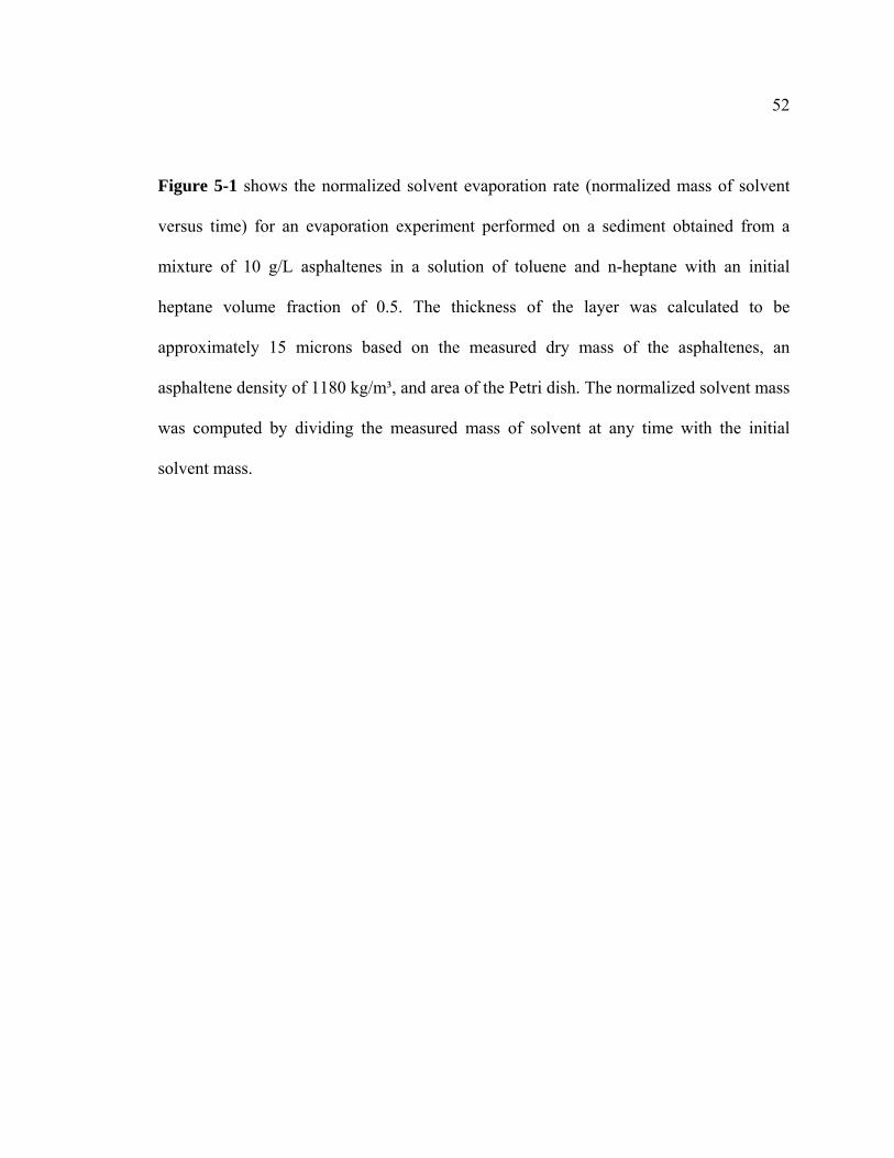
52
Figure 5-1 shows the normalized solvent evaporation rate (normalized mass of solvent
versus time) for an evaporation experiment performed on a sediment obtained from a
mixture of 10 g/L asphaltenes in a solution of toluene and n-heptane with an initial
heptane volume fraction of 0.5. The thickness of the layer was calculated to be
approximately 15 microns based on the measured dry mass of the asphaltenes, an
asphaltene density of 1180 kg/m³, and area of the Petri dish. The normalized solvent mass
was computed by dividing the measured mass of solvent at any time with the initial
solvent mass.
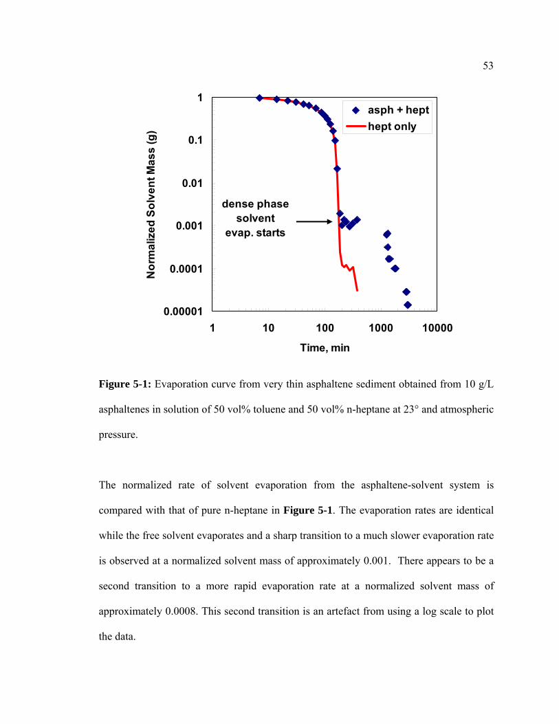
53
0.00001
0.0001
0.001
0.01
0.1
1
1 10 100 1000 10000
Time, min
Nor
mal
ized
Sol
vent
Mas
s (g
)
asph + hepthept only
dense phase solvent
evap. starts
Figure 5-1: Evaporation curve from very thin asphaltene sediment obtained from 10 g/L
asphaltenes in solution of 50 vol% toluene and 50 vol% n-heptane at 23° and atmospheric
pressure.
The normalized rate of solvent evaporation from the asphaltene-solvent system is
compared with that of pure n-heptane in Figure 5-1. The evaporation rates are identical
while the free solvent evaporates and a sharp transition to a much slower evaporation rate
is observed at a normalized solvent mass of approximately 0.001. There appears to be a
second transition to a more rapid evaporation rate at a normalized solvent mass of
approximately 0.0008. This second transition is an artefact from using a log scale to plot
the data.
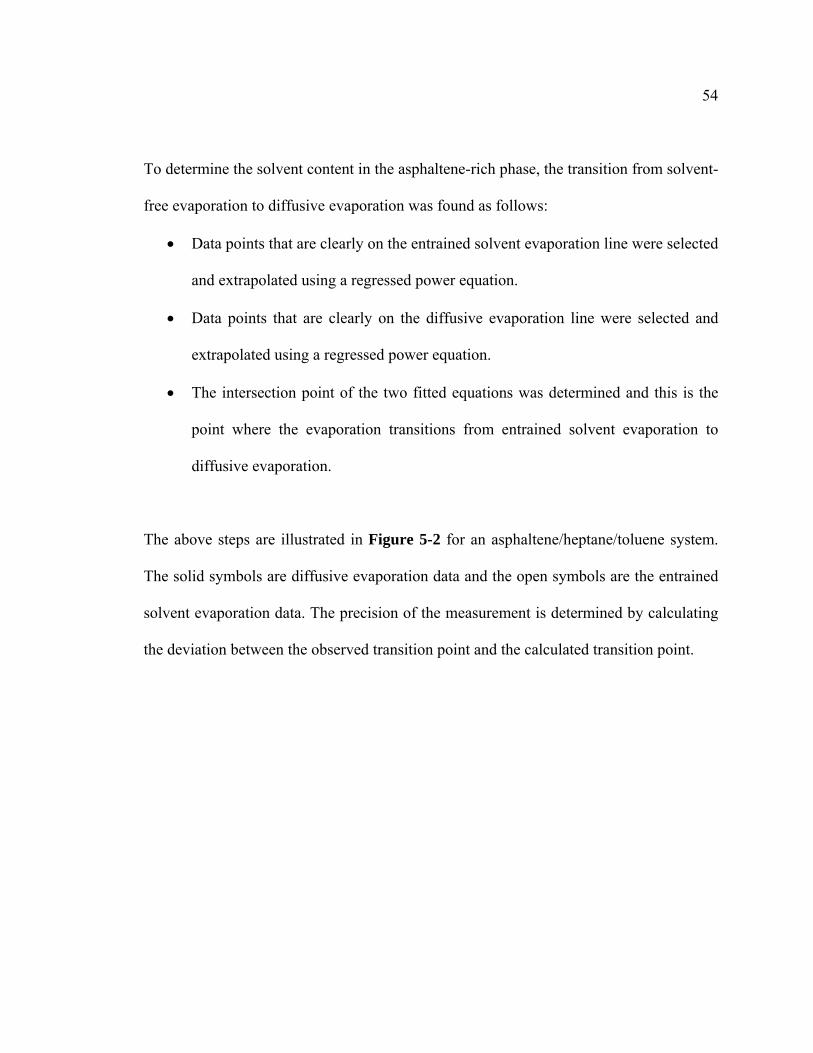
54
To determine the solvent content in the asphaltene-rich phase, the transition from solvent-
free evaporation to diffusive evaporation was found as follows:
• Data points that are clearly on the entrained solvent evaporation line were selected
and extrapolated using a regressed power equation.
• Data points that are clearly on the diffusive evaporation line were selected and
extrapolated using a regressed power equation.
• The intersection point of the two fitted equations was determined and this is the
point where the evaporation transitions from entrained solvent evaporation to
diffusive evaporation.
The above steps are illustrated in Figure 5-2 for an asphaltene/heptane/toluene system.
The solid symbols are diffusive evaporation data and the open symbols are the entrained
solvent evaporation data. The precision of the measurement is determined by calculating
the deviation between the observed transition point and the calculated transition point.
55
y = 3.3375E+23x-8.7628E+00
R2 = 9.9989E-01
y = 2.2943E+01x-8.6317E-01
R2 = 9.9746E-01
0.01
0.1
1
1 10 100 1000 10000
Time, min
Nor
mal
ized
Net
Mas
s (g
)DataRegression (Power)
Figure 5-2: Calculation of Precision for asphaltene-rich phase composition experiments.
For the data presented in Figure 5-2, the transition point was determined to occur at a
normalized solvent mass of 0.0073, corresponding to a solvent content of 6 ±2%. The
sharpness of the transition from rapid to slow evaporation and the low value of the
determined solvent content both indicate that the entrained solvent evaporated at the same
rate as the free solvent and that the procedure correctly identified the beginning of
56
diffusive evaporation. Note, ±2% indicates the precision of the measurement. The
repeatability of the measurement will be discussed later.
The previous experiment was performed on a very thin sediment and the accuracy of the
results is limited by the accuracy of the mass determination for the very small mass of
asphaltenes (0.1178 g). Therefore, the experiments were repeated for thicker layers.
Figure 5-3 compares the normalized evaporation rates from “thin” and “thick” sediments
obtained from mixtures of asphaltene in n-heptane and toluene. The initial solution was
prepared with a heptane volume fraction of 0.65. The thickness of the thick layer is 3-5
mm and that of thin layer is 0.18 mm.
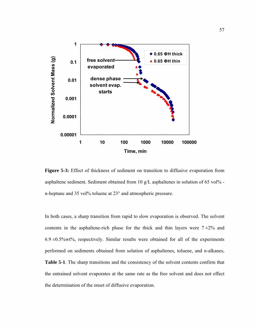
57
0.00001
0.0001
0.001
0.01
0.1
1
1 10 100 1000 10000 100000
Time, min
Nor
mal
ized
Sol
vent
Mas
s (g
) 0.65 ΦH thick0.65 ΦH thin
dense phase solvent evap.
starts
free solvent evaporated
Figure 5-3: Effect of thickness of sediment on transition to diffusive evaporation from
asphaltene sediment. Sediment obtained from 10 g/L asphaltenes in solution of 65 vol% -
n-heptane and 35 vol% toluene at 23° and atmospheric pressure.
In both cases, a sharp transition from rapid to slow evaporation is observed. The solvent
contents in the asphaltene-rich phase for the thick and thin layers were 7 ±2% and
6.9 ±0.5%wt%, respectively. Similar results were obtained for all of the experiments
performed on sediments obtained from solution of asphaltenes, toluene, and n-alkanes,
Table 5-1. The sharp transitions and the consistency of the solvent contents confirm that
the entrained solvent evaporates at the same rate as the free solvent and does not effect
the determination of the onset of diffusive evaporation.
58
Table 5-1: Solvent compositions of asphaltene-rich phases obtained from solutions of 10
g/L asphaltenes in toluene and an n-alkane at 23°C and atmospheric pressure.
Solvent
(Init. n-alk. Vol. Fr)
Asph type*
(layer)
Mass percent
of Solvent
n-heptane (0.50) C7 (thin) 6 ± 1
n-heptane (0.50) C7 (thick) 5.9 ± 0.7
n-heptane (0.65) C7 (thin) 6.9 ± 0.5
n-heptane (0.65) C7 (thick) 7 ± 2
n-heptane (0.80) C7 (thin) 7.2 ± 0.6
n-heptane (0.80) C7 (thick) 6.2 ± 0.5
n-pentane (0.80) C7 (thin) 5.3 ± 0.3
n-pentane (0.80) C7 (thick) 6.5 ± 0.2
n-decane (0.80) C7 (thin) 5.1 ± 0.5
n-decane (0.80) C7 (thick) 7.1 ± 0.1
n-heptane (0.80) C5 (thin) 5.4 ± 0.1
n-heptane (0.80) C5 (thick) 5.8 ± 0.5
* All asphaltenes were separated from Athabasca bitumen
5.1.2 Sediment from Solutions of Asphaltenes in Solvents
The effect of initial n-alkane volume fractions, solvents and asphaltene types on the
composition of asphaltene-rich phase are studied in this section. The choice of n-alkane
solvents and its initial composition are expected to have an effect on the phase behaviour
59
and may affect the composition of the solvent in the asphaltene-rich phase. The
experiments were conducted with C5 and C7 asphaltenes to see the effect of asphaltene
types on the composition of asphaltene-rich phase. C7-asphaltenes is more representative
of “pure” asphaltenes because less resins are co-precipitated with them than with the C5-
asphaltenes (Agrawala and Yarranton, 2001; Yarranton et al., 2000).
Initial n-Alkane Volume Fraction
Figure 5-4 compares the results of the experiments performed on asphaltene/n-
heptane/toluene mixture with initial heptane volume fraction of 0.65 and 0.80. The
solvent contents in the asphaltene-rich phase were 7 ±2 and 6.2 ± 0.5 wt% for the initial
heptane volume fraction of 0.65 and 0.8, respectively. The solvent content for the
sediment from a solution with an initial n-heptane volume fraction of 0.50 was 5.9 wt%,
Table 5-1. The solvent contents are the same within the precision of the measurements.
Hence, there is no evidence that the solvent content of the asphaltene-rich phase is
sensitive to the volume fraction of heptane in the solution from which the sediment is
precipitated.
60
0.00001
0.0001
0.001
0.01
0.1
1
1 10 100 1000 10000 100000
Time, min
Nor
mal
ized
Sol
vent
Mas
s (g
) 0.65 ΦH thick0.8 ΦH thick
dense phase solvent evap.
starts
Figure 5-4: Evaporation curves for sediments obtained from sediments obtained from 10
g/L asphaltene in solutions of n-heptane and toluene with different initial n-heptane
volume fractions at 23°C and atmospheric pressure.
Asphaltene Type
The experiments in the preceding sections were performed using asphaltenes extracted
using n-heptane (C7-asphaltenes). The experiments with an initial heptane volume
fraction of 0.8 were repeated with C5-asphaltenes, Figure 5-5. The solvent contents in
the asphaltene-rich phase for the thick and thin layers were 5.8 ±0.5 and 5.4 ±0.1 wt%,
respectively. The results with C5-asphaltenes appear to be within the precision of the
results of C7-asphaltenes. So the choice of asphaltenes does not affect the composition of
solvent in the asphaltene-rich phase.
61
0.0001
0.001
0.01
0.1
1
10
1 10 100 1000 10000 100000
Time, min
Sol
vent
Mas
s (g
)C5-asph /hep/tol80%VF thick
dense phase solvent evap.
starts
Figure 5-5: Composition of solvent in the asphaltene-rich phase of C5-asphaltene/
heptane/toluene system.
Solvent Type
The evaporation experiments were performed using n-pentane and n-decane instead of n-
heptane. Figure 5-6 shows the results for the asphaltene/n-pentane/toluene system with
an initial pentane volume fraction of 0.80. Figure 5-7 shows the results for the
asphaltene/n-decane/toluene system. Note the relatively rapid evaporation rate with n-
pentane and the slow evaporation rate with n-decane both for the free solvent and with
diffusive evaporation.
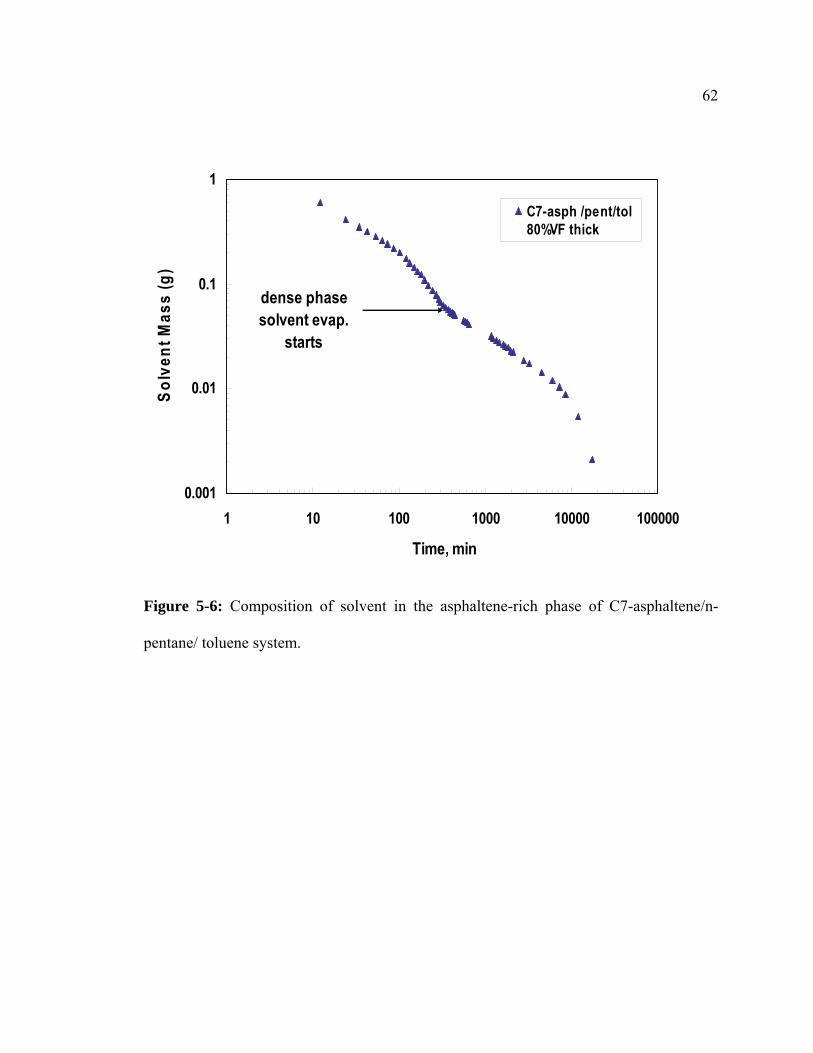
62
0.001
0.01
0.1
1
1 10 100 1000 10000 100000
Time, min
Sol
vent
Mas
s (g
)
C7-asph /pent/tol80%VF thick
dense phase solvent evap.
starts
Figure 5-6: Composition of solvent in the asphaltene-rich phase of C7-asphaltene/n-
pentane/ toluene system.
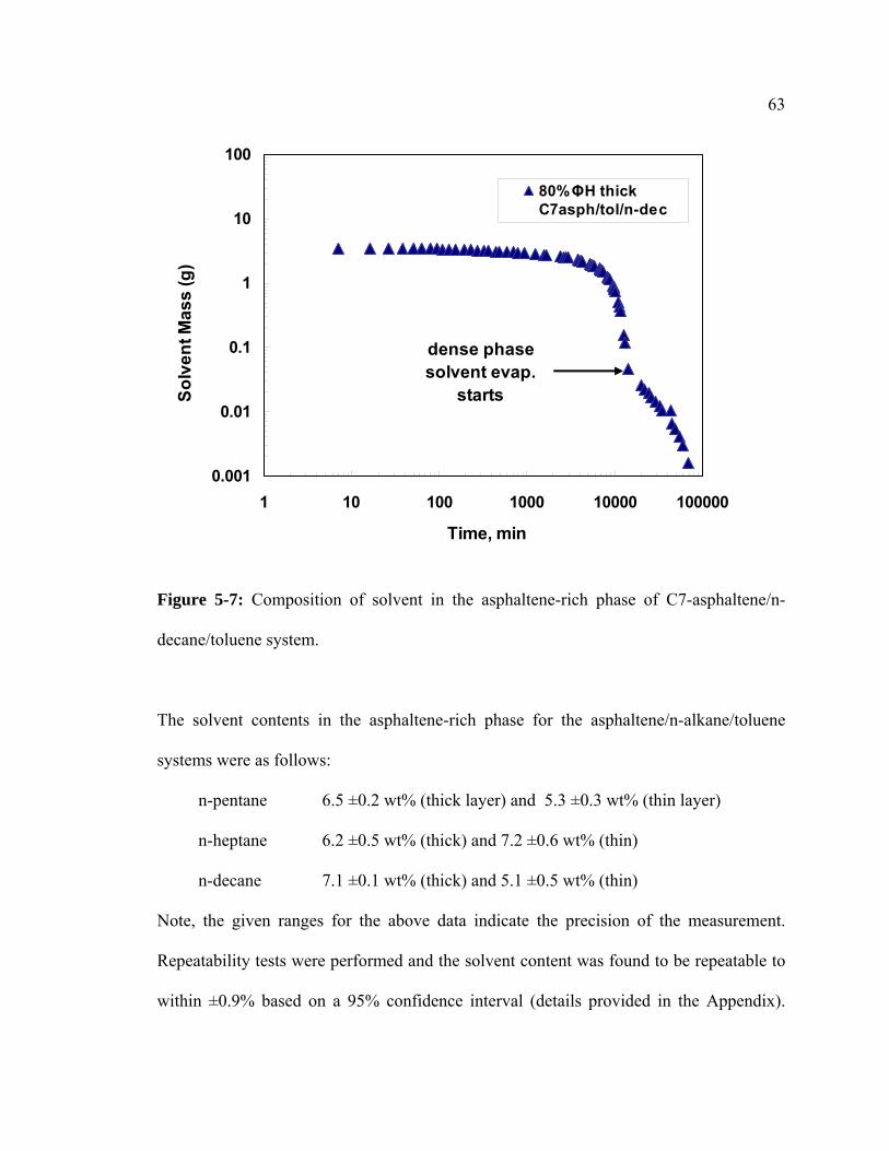
63
0.001
0.01
0.1
1
10
100
1 10 100 1000 10000 100000
Time, min
Sol
vent
Mas
s (g
)80% ΦH thickC7asph/tol/n-dec
dense phase solvent evap.
starts
Figure 5-7: Composition of solvent in the asphaltene-rich phase of C7-asphaltene/n-
decane/toluene system.
The solvent contents in the asphaltene-rich phase for the asphaltene/n-alkane/toluene
systems were as follows:
n-pentane 6.5 ±0.2 wt% (thick layer) and 5.3 ±0.3 wt% (thin layer)
n-heptane 6.2 ±0.5 wt% (thick) and 7.2 ±0.6 wt% (thin)
n-decane 7.1 ±0.1 wt% (thick) and 5.1 ±0.5 wt% (thin)
Note, the given ranges for the above data indicate the precision of the measurement.
Repeatability tests were performed and the solvent content was found to be repeatable to
within ±0.9% based on a 95% confidence interval (details provided in the Appendix).
64
The weight percent of solvent in the asphaltene-rich phase for asphaltene/solvent systems
is then 6.1 ± 0.9 %.
5.2 Asphaltene-Rich Phases from Solvent Diluted Bitumen
The same methodology was applied to sediments obtained from bitumen diluted with n-
heptane. The analysis is more complicated because bitumen contains non-asphaltene
constituents (saturates, aromatics, and resins) which are non-volatile. These components
may partition to the asphaltene-rich phase during the initial precipitation. They will also
be part of the solvent phase and will remain in the sediment after the solvent evaporates.
The mass of saturates, aromatics, and resins in the solution can be determined from the
known mass of bitumen and solvent. Assuming that all of these components are present
only in the solvent phase, the maximum mass of these components in the solvent phase
transferred to the Petri dish for an evaporation experiment corresponds to a percent error
of approximately 0.87% in the mass of asphaltene. Therefore the presence of saturates,
aromatics and resins leads to an overestimation of 0.87% on the weight of asphaltene in
the asphaltene-rich phase. Of more concern is the effect of these components on the
evaporation rate of the solvent.
Figure 5-8 shows the evaporation profile for a “thick” sediment obtained from a 40:1 g
heptane/g bitumen. The transition from free and entrained solvent evaporation to
diffusive evaporation from the dense phase is not as pronounced for the diluted bitumen
compared with the asphaltene/solvent systems. The same method was used to determine a
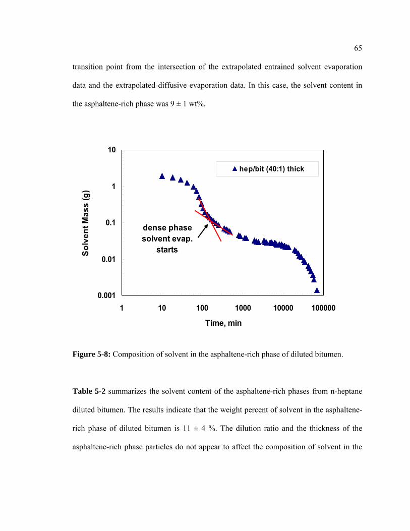
65
transition point from the intersection of the extrapolated entrained solvent evaporation
data and the extrapolated diffusive evaporation data. In this case, the solvent content in
the asphaltene-rich phase was 9 ± 1 wt%.
0.001
0.01
0.1
1
10
1 10 100 1000 10000 100000
Time, min
Solv
ent M
ass
(g)
hep/bit (40:1) thick
dense phase solvent evap.
starts
Figure 5-8: Composition of solvent in the asphaltene-rich phase of diluted bitumen.
Table 5-2 summarizes the solvent content of the asphaltene-rich phases from n-heptane
diluted bitumen. The results indicate that the weight percent of solvent in the asphaltene-
rich phase of diluted bitumen is 11 ± 4 %. The dilution ratio and the thickness of the
asphaltene-rich phase particles do not appear to affect the composition of solvent in the
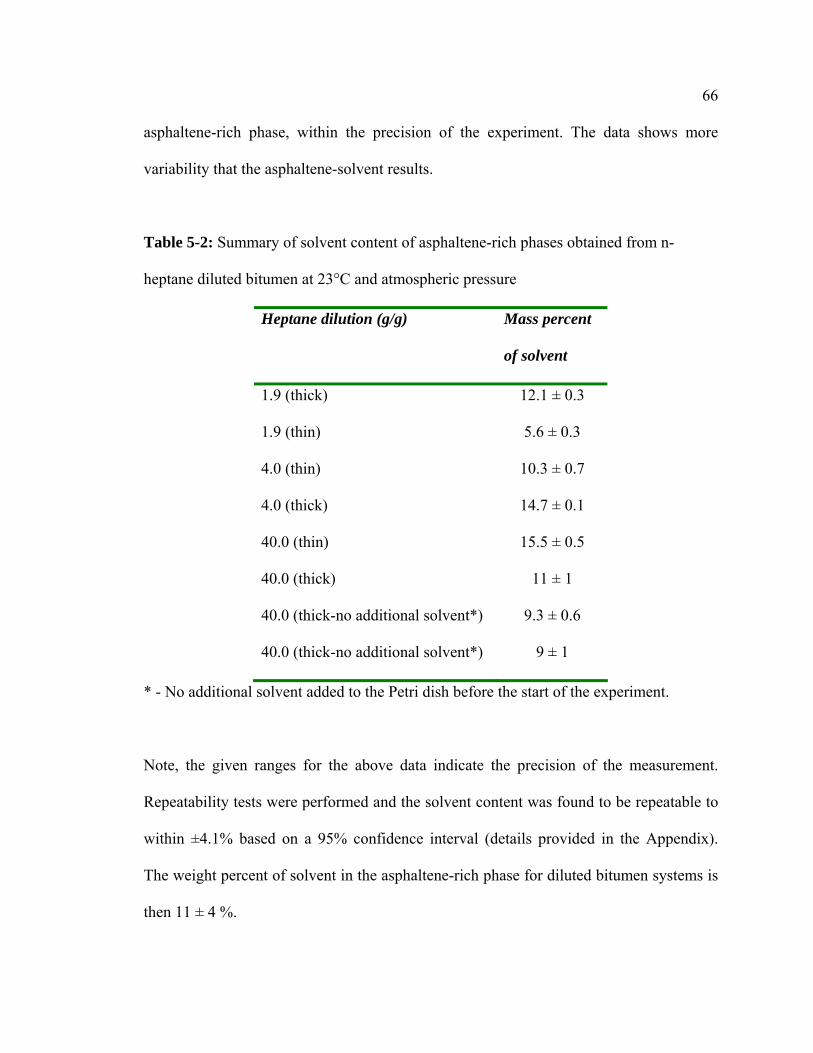
66
asphaltene-rich phase, within the precision of the experiment. The data shows more
variability that the asphaltene-solvent results.
Table 5-2: Summary of solvent content of asphaltene-rich phases obtained from n-
heptane diluted bitumen at 23°C and atmospheric pressure
Heptane dilution (g/g) Mass percent
of solvent
1.9 (thick) 12.1 ± 0.3
1.9 (thin) 5.6 ± 0.3
4.0 (thin) 10.3 ± 0.7
4.0 (thick) 14.7 ± 0.1
40.0 (thin) 15.5 ± 0.5
40.0 (thick) 11 ± 1
40.0 (thick-no additional solvent*) 9.3 ± 0.6
40.0 (thick-no additional solvent*) 9 ± 1
* - No additional solvent added to the Petri dish before the start of the experiment.
Note, the given ranges for the above data indicate the precision of the measurement.
Repeatability tests were performed and the solvent content was found to be repeatable to
within ±4.1% based on a 95% confidence interval (details provided in the Appendix).
The weight percent of solvent in the asphaltene-rich phase for diluted bitumen systems is
then 11 ± 4 %.
67
5.3 Summary
The amount of solvent in an asphaltene-rich phase was determined from the developed
evaporation experiment. The experimental methodology was tested by using a thin
sediment layer where the volume of entrained solvent is small. For the asphaltene-solvent
system, the effect of the initial n-alkane volume fractions, asphaltene types and solvents
on the composition of asphaltene-rich phase is studied. The solvent content of the
asphaltene-rich phase was found to be insensitive to the volume fraction of n-alkane,
solvent or asphaltene type. The composition of solvent in the asphaltene-rich phase was
found to be 6.1 ± 0.9 wt%.
The composition experiments for diluted bitumen system were performed using n-
heptane. It was found that the n-heptane dilution ratio did not affect the composition of
solvent in the asphaltene-rich phase, within the precision of the experiment. The data
obtained were more scattered than those from the asphaltene/solvent data. The weight
percent of solvent in the asphaltene-rich phase of diluted bitumen was 11 ± 4%.
68
Chapter Six: Modeling Amount and Composition of Asphaltene-Rich Phases
The modified regular solution model is tested on asphaltene precipitation data from the
literature and the composition data from Chapter 5. The ability of the model to predict the
effect of different solvents, temperatures, asphaltene source, and asphaltene molar mass is
evaluated. The model predictions are also compared with prediction from the old model
with no solvent-partitioning to identify how the model predictions changed.
The data for fractional precipitation of asphaltene by solutions of n-heptane solvent and
toluene at different temperatures was obtained from Akbarzadeh et al., 2005 (Figure 6-1).
The washing procedure data and other crude oil data were taken from Alboudwarej et al.,
2002 (Figure 6-2, Figure 6-3 and Figure 6-4). The fractional precipitation of asphaltene
by solutions of n-alkane solvent and toluene was obtained from Yarranton et al., 1996
and Mannistu et al., 1997 (Figure 6-6 and Figure 6-7). The concentration of asphaltene is
10 g/L, unless otherwise specified. Note the average absolute deviation (AAD) for each
data set is given in the appendix.
6.1 Retuning the Model
The first step in modeling was to retune the asphaltene solubility parameters by fitting
asphaltene yields from 10 g/L asphaltenes in n-heptane and toluene at 0, 23, and 50°C,
Figure 6-1. The correlation for the asphaltene solubility parameter used in the old model
(no solvent partitioning) is given by:
0.00075T579.0)( −=TA (6-1)
69
and the retuned correlation is given by:
0.00024T 0.2447)( +=TA (6-2)
In the old model, the value of shape factor of the gamma distribution function α was
found using a temperature dependent correlation.
0.025926T - 10.177963=α (6-3)
For example, the value of α is 2.5 at 23 oC. It was found that no temperature correction
was required for shape factor with the new model as the retuned A correlation could
capture the temperature dependence. The value of α was set to 5. With these minor
modifications, the new model fitted the yield data within the error of the measurements.
Figure 6-1a and Figure 6-1b shows the fitted precipitation data for Athabasca asphaltene
in solutions of n-heptane and toluene for the new model and old model respectively. The
AAD for the new model at 0 °C, 23 °C and 50 °C were 0.0315, 0.0422 and 0.0254,
respectively. The deviations are slightly greater than obtained with the old model (AAD
at 0 °C, 23 °C and 50 °C were 0.0238, 0.0218 and 0.0137, respectively).
After the model was retuned, the parameters were fixed and it is no longer a fitting model
but a predictive model for asphaltene/solvent systems. The only input required is the
average molar mass of asphaltenes, which is a value typically measured for each
asphaltene type. Next, the effectiveness of the new model was assessed by its capability
to predict the effect of solvent type, asphaltene type, and asphaltene molar mass.
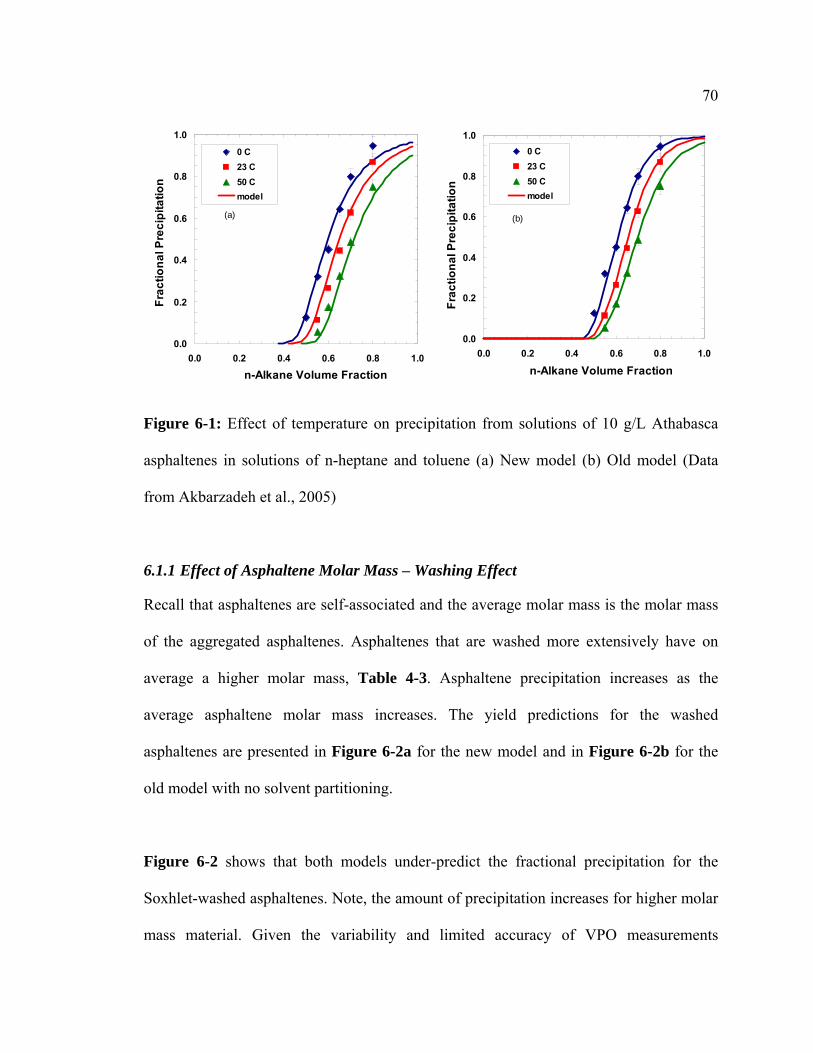
70
0.0
0.2
0.4
0.6
0.8
1.0
0.0 0.2 0.4 0.6 0.8 1.0
n-Alkane Volume Fraction
Frac
tiona
l Pre
cipi
tatio
n0 C23 C50 Cmodel
(a)
0.0
0.2
0.4
0.6
0.8
1.0
0.0 0.2 0.4 0.6 0.8 1.0
n-Alkane Volume Fraction
Frac
tiona
l Pre
cipi
tatio
n
0 C23 C50 Cmodel
(b)
Figure 6-1: Effect of temperature on precipitation from solutions of 10 g/L Athabasca
asphaltenes in solutions of n-heptane and toluene (a) New model (b) Old model (Data
from Akbarzadeh et al., 2005)
6.1.1 Effect of Asphaltene Molar Mass – Washing Effect
Recall that asphaltenes are self-associated and the average molar mass is the molar mass
of the aggregated asphaltenes. Asphaltenes that are washed more extensively have on
average a higher molar mass, Table 4-3. Asphaltene precipitation increases as the
average asphaltene molar mass increases. The yield predictions for the washed
asphaltenes are presented in Figure 6-2a for the new model and in Figure 6-2b for the
old model with no solvent partitioning.
Figure 6-2 shows that both models under-predict the fractional precipitation for the
Soxhlet-washed asphaltenes. Note, the amount of precipitation increases for higher molar
mass material. Given the variability and limited accuracy of VPO measurements
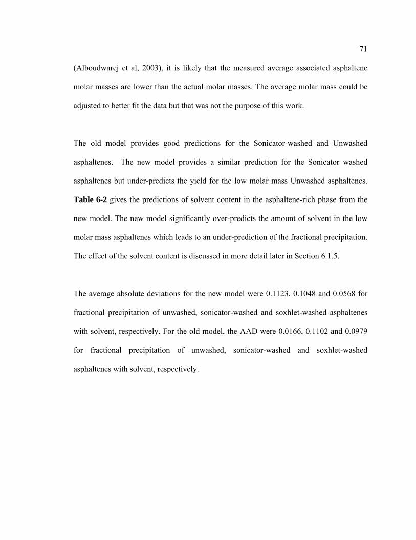
71
(Alboudwarej et al, 2003), it is likely that the measured average associated asphaltene
molar masses are lower than the actual molar masses. The average molar mass could be
adjusted to better fit the data but that was not the purpose of this work.
The old model provides good predictions for the Sonicator-washed and Unwashed
asphaltenes. The new model provides a similar prediction for the Sonicator washed
asphaltenes but under-predicts the yield for the low molar mass Unwashed asphaltenes.
Table 6-2 gives the predictions of solvent content in the asphaltene-rich phase from the
new model. The new model significantly over-predicts the amount of solvent in the low
molar mass asphaltenes which leads to an under-prediction of the fractional precipitation.
The effect of the solvent content is discussed in more detail later in Section 6.1.5.
The average absolute deviations for the new model were 0.1123, 0.1048 and 0.0568 for
fractional precipitation of unwashed, sonicator-washed and soxhlet-washed asphaltenes
with solvent, respectively. For the old model, the AAD were 0.0166, 0.1102 and 0.0979
for fractional precipitation of unwashed, sonicator-washed and soxhlet-washed
asphaltenes with solvent, respectively.
72
Table 6-1: Average molar masses of asphaltene with different asphaltene washing
procedures (Data from Alboudwarej et al., 2002)
Washing Procedure
Av. Molar mass (g/gmol)
Unwashed 5700 Sonicator 7600 Soxhlet washed 9100
Table 6-2: Predicted solvent content of asphaltene-rich phase predicted by the model for
washed Athabasca asphaltenes in solvents (n-heptane volume fraction: 0.8)
Washing Procedure
Composition of solvent (wt%)
Unwashed 41.5 Sonicator 36.8 Soxhlet washed 33.9
0.0
0.2
0.4
0.6
0.8
1.0
0.0 0.2 0.4 0.6 0.8 1.0
n-Alkane Volume Fraction
Frac
tiona
l Pre
cipi
tatio
n Unwashed
Sonicator washed
Soxhlet washed
model
(a)
0.0
0.2
0.4
0.6
0.8
1.0
0.0 0.2 0.4 0.6 0.8 1.0
n-Alkane Volume Fraction
Frac
tiona
l Pre
cipi
tatio
n Unwashed
Sonicator washed
Soxhlet washed
model
(b)
Figure 6-2: Effect of average asphaltene molar mass on precipitation of Athabasca
asphaltenes from solutions of n-heptane and toluene at 23°C. (a) New model (b) Old
model (Data from Alboudwarej et al., 2002).
73
6.1.2 Effect of Asphaltene Molar Mass - Asphaltene Source
The described experiments in Figure 6-1 and Figure 6-2 use asphaltenes derived from
Athabasca bitumen. Data was also available for asphaltenes extracted from other heavy
oils and bitumens including an Indonesian crude oil, two Venezuela heavy oils, a Russian
heavy oil, and Cold Lake bitumen from Alberta. The average molar mass of these
asphaltenes are given in Table 6-3. Figure 6-3a and Figure 6-3b show the fractional
yields from solutions of these asphaltenes in n-heptane and toluene at 23°C for the new
model and old model, respectively. The data and model results for Cold Lake and
Indonesia asphaltenes are presented separately in Figure 6-4 to avoid overcrowding of
the data.
Figure 6-3 and Figure 6-4 show that fractional precipitation for the asphaltenes from
different sources as predicted by both the models. For the new model, the AAD values
were 0.0413, 0.0466, 0.0638, 0.0680 and 0.2384 for Venezuela1, Venezuela2, Russia,
Cold Lake and Indonesia asphaltenes with solvent, respectively. Note, Indonesia
asphaltenes had a very low molar mass so the deviations in the new model predictions
observed were similar to the Unwashed asphaltenes. The higher solvent content predicted
in the asphaltene-rich phase for the low molar mass asphaltenes causes the fractional
precipitation to be less than the actual precipitation.
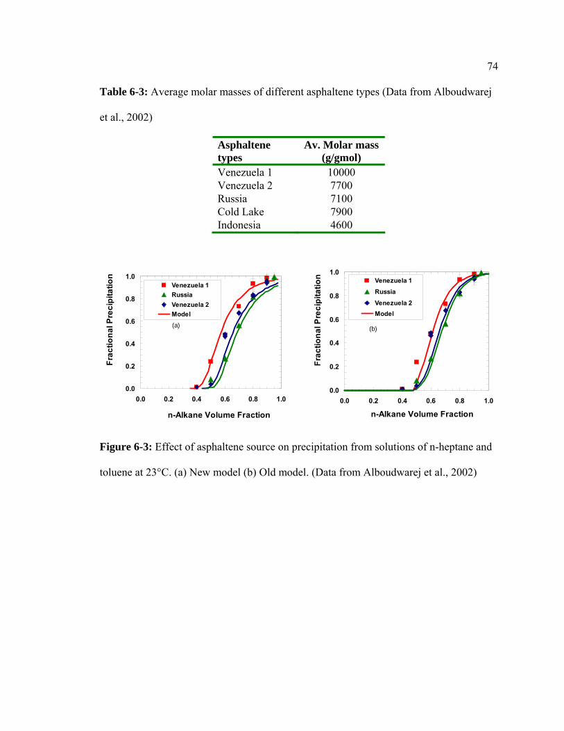
74
Table 6-3: Average molar masses of different asphaltene types (Data from Alboudwarej
et al., 2002)
Asphaltene types
Av. Molar mass (g/gmol)
Venezuela 1 10000 Venezuela 2 7700 Russia 7100 Cold Lake 7900 Indonesia 4600
0.0
0.2
0.4
0.6
0.8
1.0
0.0 0.2 0.4 0.6 0.8 1.0
n-Alkane Volume Fraction
Frac
tiona
l Pre
cipi
tatio
n
Venezuela 1RussiaVenezuela 2Model(a)
0.0
0.2
0.4
0.6
0.8
1.0
0.0 0.2 0.4 0.6 0.8 1.0
n-Alkane Volume Fraction
Frac
tiona
l Pre
cipi
tatio
n Venezuela 1Russia
Venezuela 2Model
(b)
Figure 6-3: Effect of asphaltene source on precipitation from solutions of n-heptane and
toluene at 23°C. (a) New model (b) Old model. (Data from Alboudwarej et al., 2002)
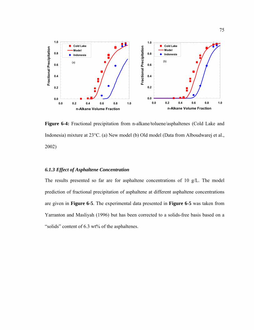
75
0.0
0.2
0.4
0.6
0.8
1.0
0.0 0.2 0.4 0.6 0.8 1.0
n-Alkane Volume Fraction
Frac
tiona
l Pre
cipi
tatio
n Cold LakeModelIndonesia
(a)
0.0
0.2
0.4
0.6
0.8
1.0
0.0 0.2 0.4 0.6 0.8 1.0
n-Alkane Volume Fraction
Frac
tiona
l Pre
cipi
tatio
n Cold LakeModelIndonesia
(b)
Figure 6-4: Fractional precipitation from n-alkane/toluene/asphaltenes (Cold Lake and
Indonesia) mixture at 23°C. (a) New model (b) Old model (Data from Alboudwarej et al.,
2002)
6.1.3 Effect of Asphaltene Concentration
The results presented so far are for asphaltene concentrations of 10 g/L. The model
prediction of fractional precipitation of asphaltene at different asphaltene concentrations
are given in Figure 6-5. The experimental data presented in Figure 6-5 was taken from
Yarranton and Masliyah (1996) but has been corrected to a solids-free basis based on a
“solids” content of 6.3 wt% of the asphaltenes.
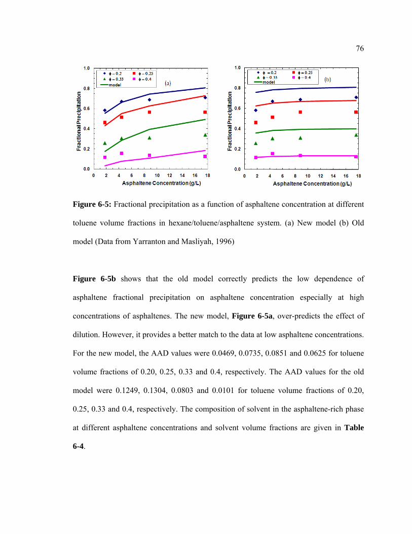
76
Figure 6-5: Fractional precipitation as a function of asphaltene concentration at different
toluene volume fractions in hexane/toluene/asphaltene system. (a) New model (b) Old
model (Data from Yarranton and Masliyah, 1996)
Figure 6-5b shows that the old model correctly predicts the low dependence of
asphaltene fractional precipitation on asphaltene concentration especially at high
concentrations of asphaltenes. The new model, Figure 6-5a, over-predicts the effect of
dilution. However, it provides a better match to the data at low asphaltene concentrations.
For the new model, the AAD values were 0.0469, 0.0735, 0.0851 and 0.0625 for toluene
volume fractions of 0.20, 0.25, 0.33 and 0.4, respectively. The AAD values for the old
model were 0.1249, 0.1304, 0.0803 and 0.0101 for toluene volume fractions of 0.20,
0.25, 0.33 and 0.4, respectively. The composition of solvent in the asphaltene-rich phase
at different asphaltene concentrations and solvent volume fractions are given in Table
6-4.
77
Table 6-4: Predicted solvent content (wt%) of the asphaltene-rich phase at different
asphaltene concentrations and toluene volume fractions
Toluene Volume fraction
asph conc (g/L) 0.2 0.25 0.33 0.4
1.76 37.89 42.08 48.99 52.61
4.4 39.01 43.57 51.37 55.96
8.8 39.76 45.09 53.68 59.06
17.6 40.32 46.46 55.94 62.49
6.1.4 Effect of Solvent Type
The model predictions of asphaltene fractional precipitation at 23°C from solutions of
toluene with n-pentane, n-hexane, or n-heptane are shown in Figure 6-6a and from
solutions of toluene with n-octane, n-decane in Figure 6-7a. Predictions using the old
model (no solvent partitioning) for the same data are shown in Figure 6-6b and Figure
6-7b. As the carbon number of the n-alkane solvent increases up to approximately C8,
the solubility of asphaltene also increases.
Since prediction of the effect of solvent requires only the solvent properties to be changed
keeping constant all the asphaltene properties, this is a significant test of the predictive
capability of the new model. While the old model predicts the effect of solvent within the
scatter of the data, the model with solvent partitioning over-predicts the fractional
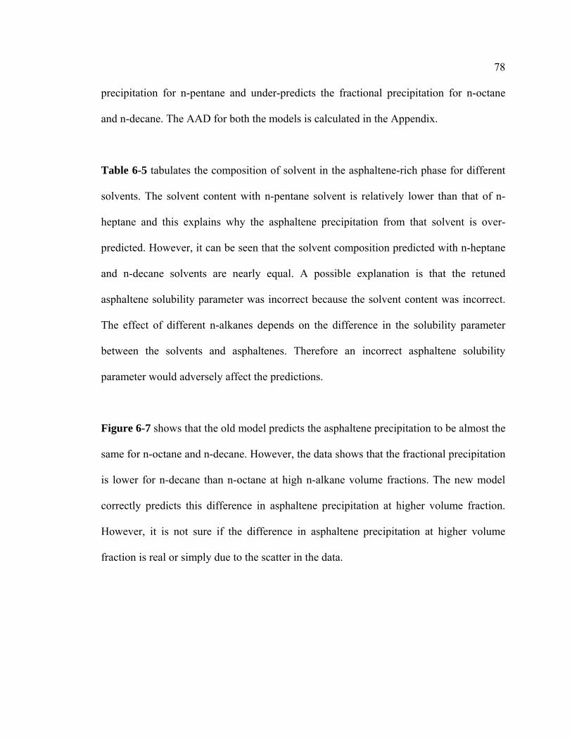
78
precipitation for n-pentane and under-predicts the fractional precipitation for n-octane
and n-decane. The AAD for both the models is calculated in the Appendix.
Table 6-5 tabulates the composition of solvent in the asphaltene-rich phase for different
solvents. The solvent content with n-pentane solvent is relatively lower than that of n-
heptane and this explains why the asphaltene precipitation from that solvent is over-
predicted. However, it can be seen that the solvent composition predicted with n-heptane
and n-decane solvents are nearly equal. A possible explanation is that the retuned
asphaltene solubility parameter was incorrect because the solvent content was incorrect.
The effect of different n-alkanes depends on the difference in the solubility parameter
between the solvents and asphaltenes. Therefore an incorrect asphaltene solubility
parameter would adversely affect the predictions.
Figure 6-7 shows that the old model predicts the asphaltene precipitation to be almost the
same for n-octane and n-decane. However, the data shows that the fractional precipitation
is lower for n-decane than n-octane at high n-alkane volume fractions. The new model
correctly predicts this difference in asphaltene precipitation at higher volume fraction.
However, it is not sure if the difference in asphaltene precipitation at higher volume
fraction is real or simply due to the scatter in the data.
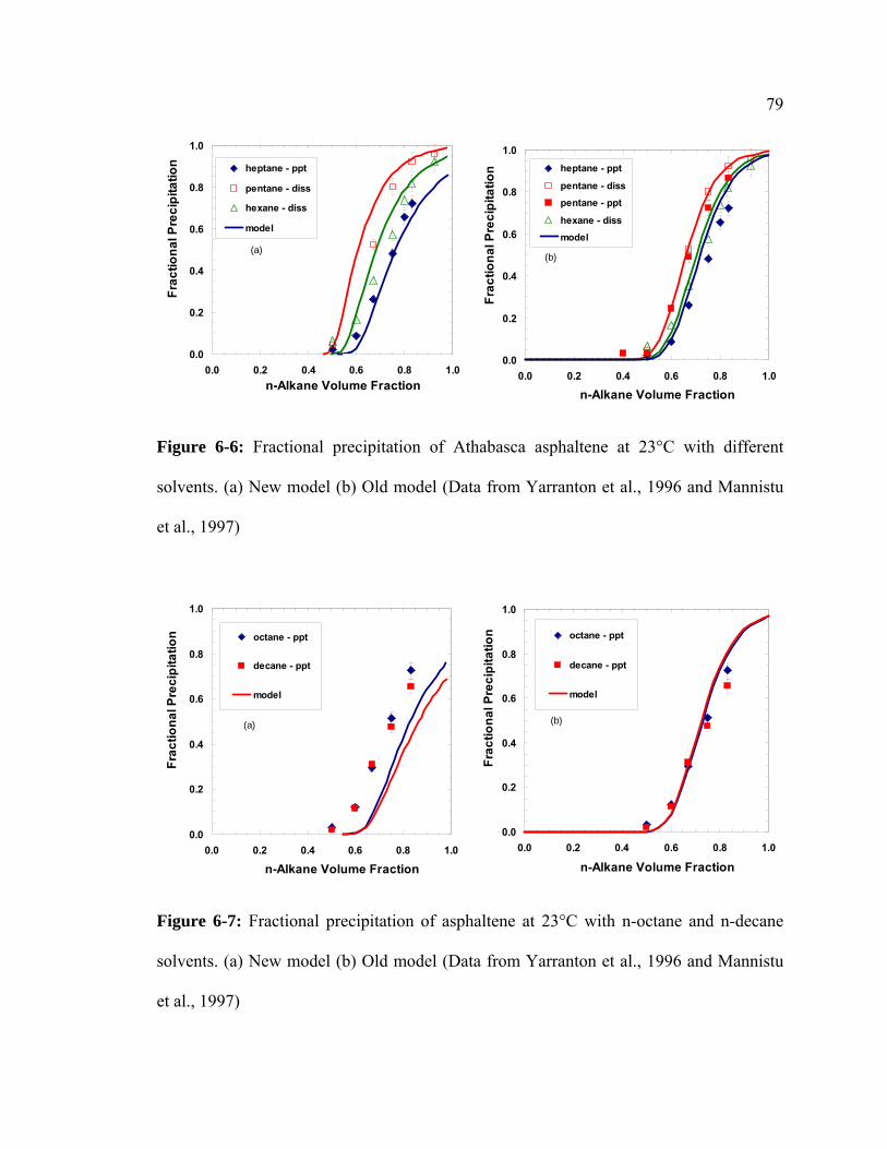
79
0.0
0.2
0.4
0.6
0.8
1.0
0.0 0.2 0.4 0.6 0.8 1.0n-Alkane Volume Fraction
Frac
tiona
l Pre
cipi
tatio
n heptane - ppt
pentane - diss
hexane - diss
model
(a)
0.0
0.2
0.4
0.6
0.8
1.0
0.0 0.2 0.4 0.6 0.8 1.0
n-Alkane Volume Fraction
Frac
tiona
l Pre
cipi
tatio
n heptane - ppt
pentane - diss
pentane - ppt
hexane - diss
model
(b)
Figure 6-6: Fractional precipitation of Athabasca asphaltene at 23°C with different
solvents. (a) New model (b) Old model (Data from Yarranton et al., 1996 and Mannistu
et al., 1997)
0.0
0.2
0.4
0.6
0.8
1.0
0.0 0.2 0.4 0.6 0.8 1.0
n-Alkane Volume Fraction
Frac
tiona
l Pre
cipi
tatio
n octane - ppt
decane - ppt
model
(a)
0.0
0.2
0.4
0.6
0.8
1.0
0.0 0.2 0.4 0.6 0.8 1.0
n-Alkane Volume Fraction
Frac
tiona
l Pre
cipi
tatio
n octane - ppt
decane - ppt
model
(b)
Figure 6-7: Fractional precipitation of asphaltene at 23°C with n-octane and n-decane
solvents. (a) New model (b) Old model (Data from Yarranton et al., 1996 and Mannistu
et al., 1997)
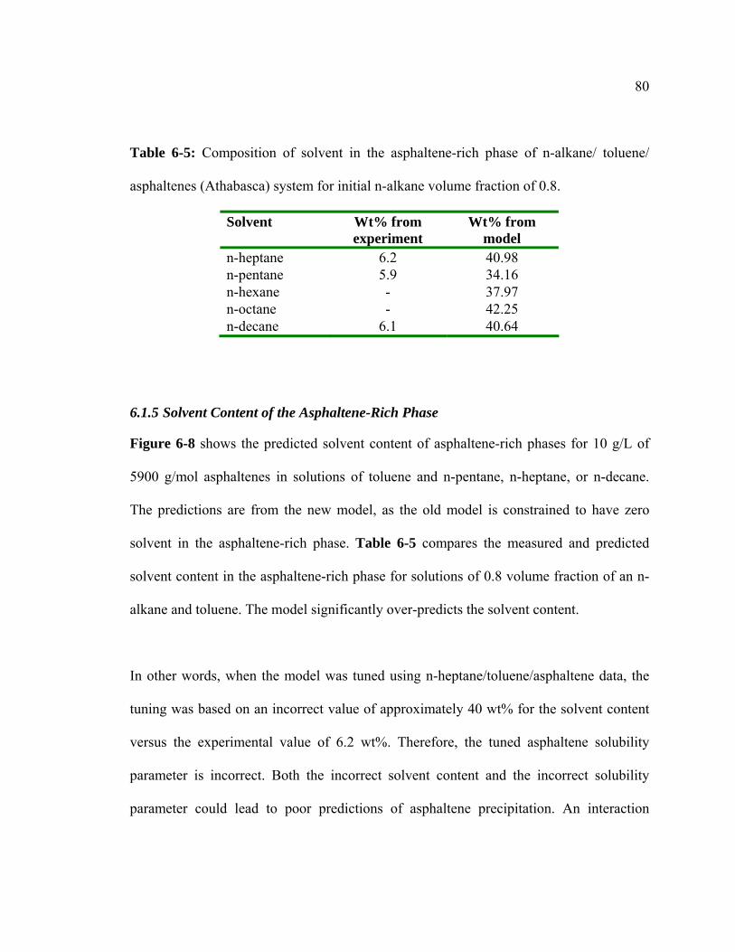
80
Table 6-5: Composition of solvent in the asphaltene-rich phase of n-alkane/ toluene/
asphaltenes (Athabasca) system for initial n-alkane volume fraction of 0.8.
Solvent Wt% from experiment
Wt% from model
n-heptane 6.2 40.98 n-pentane 5.9 34.16 n-hexane - 37.97 n-octane - 42.25 n-decane 6.1 40.64
6.1.5 Solvent Content of the Asphaltene-Rich Phase
Figure 6-8 shows the predicted solvent content of asphaltene-rich phases for 10 g/L of
5900 g/mol asphaltenes in solutions of toluene and n-pentane, n-heptane, or n-decane.
The predictions are from the new model, as the old model is constrained to have zero
solvent in the asphaltene-rich phase. Table 6-5 compares the measured and predicted
solvent content in the asphaltene-rich phase for solutions of 0.8 volume fraction of an n-
alkane and toluene. The model significantly over-predicts the solvent content.
In other words, when the model was tuned using n-heptane/toluene/asphaltene data, the
tuning was based on an incorrect value of approximately 40 wt% for the solvent content
versus the experimental value of 6.2 wt%. Therefore, the tuned asphaltene solubility
parameter is incorrect. Both the incorrect solvent content and the incorrect solubility
parameter could lead to poor predictions of asphaltene precipitation. An interaction
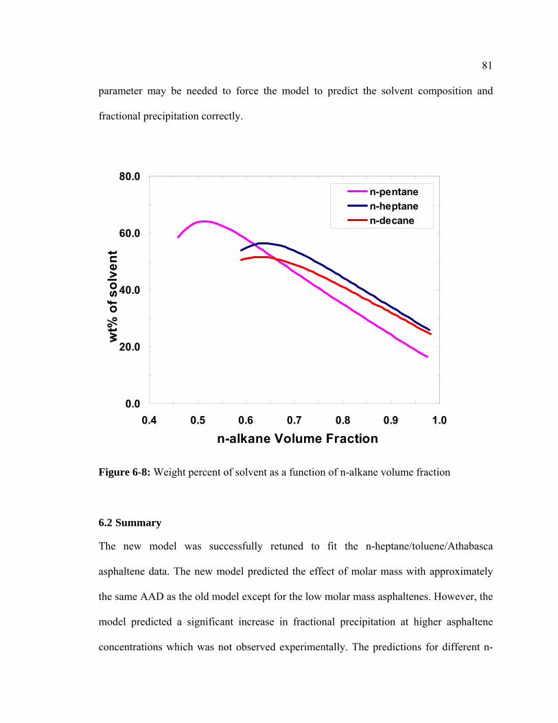
81
parameter may be needed to force the model to predict the solvent composition and
fractional precipitation correctly.
0.0
20.0
40.0
60.0
80.0
0.4 0.5 0.6 0.7 0.8 0.9 1.0
n-alkane Volume Fraction
wt%
of s
olve
nt
n-pentanen-heptanen-decane
Figure 6-8: Weight percent of solvent as a function of n-alkane volume fraction
6.2 Summary
The new model was successfully retuned to fit the n-heptane/toluene/Athabasca
asphaltene data. The new model predicted the effect of molar mass with approximately
the same AAD as the old model except for the low molar mass asphaltenes. However, the
model predicted a significant increase in fractional precipitation at higher asphaltene
concentrations which was not observed experimentally. The predictions for different n-
82
alkanes were also poor. It is hypothesised that the poor predictions of fractional
precipitation result from an over-prediction of the solvent content of the asphaltene-rich
phase. The new model predicted solvent contents in the order of 35 to 40 wt% compared
to measured values of approximately 6 wt%. It is recommended that a binary interaction
parameter be used to correct the predicted solvent contents and then determine if the
other prediction errors are corrected.
83
Chapter Seven: Conclusions and Recommendations
The objectives of this research were to develop an experimental procedure to determine
the composition of solvent in the asphaltene-rich phase and to model asphaltene
precipitation with all the components partitioning to all phases. This chapter presents the
conclusions of this work and recommendations for future work.
7.1 Conclusions
7.1.1 Experimental
A methodology was developed to measure the composition of solvent in the asphaltene-
rich phase. The experiments were based on the difference between the evaporation rate of
the free or entrained solvent versus that of the solvent dissolved in the asphaltene-rich
phase. The mass of a mixture of asphaltenes and solvent was measured over time and an
evaporation curve was constructed.
As expected, it was observed that the entrained solvent evaporates much more rapidly
than solvent in dense phase. In the case of n-alkane/toluene/asphaltene system, there was
a clear and consistent change in slope when the entrained solvent evaporation ended. The
amount of solvent in the asphaltene-rich phase was determined at this point. The
experiments were performed on thick and thin layers of asphaltene particles. The effects
of using different initial n-alkane volume fraction, asphaltene types and solvents were
also studied. The amount of solvent in the asphaltene-rich phase was found to be 6.1 ±
84
0.9 wt%. The effect of initial n-alkane volume fraction, asphaltene types and solvents was
within the precision of measurement.
In the case of diluted bitumen system, the transition from free solvent evaporation to
diffusive evaporation was less pronounced. Hence, the measurement was less precise for
the diluted bitumen system. A regression based technique was used to find the deviation
point in this case. The results were more scattered and therefore the repeatability of the
experiment decreased in comparison to asphaltene/n-alkane/toluene system. The amount
of solvent in the dense phase was determined to be 11 ± 4 wt%.
7.1.2 Modeling
A previously developed regular solution model was adapted to allow all components to
partition to each of the liquid phases. The fluids were characterized based on the previous
study. The phase equilibrium calculations assumed liquid-liquid equilibrium. The flash
program was based on an iterated equilibrium ratio (K-value) update with damping. The
Rachford-Rice equations were solved using a bounded Newton-Raphson method. The
parameters of the model were adjusted to get a good fit with n-heptane/toluene/
asphaltene precipitation data. Once the initial tuning was completed, the model
parameters were fixed and the model became completely predictive.
The model predicted the fractional precipitation of asphaltenes with moderate to high
average asphaltene molar mass (>7000 g/mol) fairly well. However, the predictions for
low average molar mass asphaltenes were poor because the amount of solvent in the
85
asphaltene-rich phase was over-predicted. The predictions for other n-alkane solvents
were also poor particularly n-octane and n-decane. Note, the old model handled the effect
of solvents including the heavy solvents, well. The model did not predict the effect of
asphaltene concentration well, at high asphaltene concentrations. The new model
significantly over-predicts the solvent content of the asphaltene-rich phase. It would
appear that the poorer performance of the new model is due to the over-prediction of the
solvent content. Improving the solvent content issue may fix the problems related to yield
prediction.
7.2 Recommendations for Future Work
The present experimental work could be extended to study the effect of temperature and
other industrial solvents such as naphtha and gas oils. The present experimental
procedure may need to be improved for these multi-component diluents.
The current experimental procedure measures the composition of the entire solvent; that
is, the combined n-alkane and toluene amount for an n-alkane/toluene/asphaltenes
experiment. A better methodology would be to find the individual composition of
heptane and toluene. This data would be more valuable for tuning the model.
SARA analysis could be performed on the asphaltene-rich phase to determine the amount
of saturates, aromatics, and resins in this phase. With these values, a more accurate
picture of composition of asphaltene-rich phase could be obtained for the diluted bitumen
experiments.
86
The model prediction of the solvent content of the asphaltene-rich phase is not accurate.
A binary interaction parameter could be introduced into the regular solution model to
tune the model to match the measured solvent composition. However, this option
eliminates the simplicity of the current version of regular solution model, one of its key
advantages.
An alternative approach may be to use an equation-of-state approach to predict the yield
and composition of the asphaltene-rich phase. Hypothetical critical properties of
asphaltene may be used to tune the Peng-Robinson ‘a’ and ‘b’ parameters. The binary
interaction parameters could be adjusted to tune the composition of asphaltene-rich
phase.
Another modeling approach is to combine both Peng-Robinson equation of state with
regular solution model using an advanced mixing rule such as an excess Gibb’s energy
mixing rules. The advantage of this approach is that the liquid phase properties can be
properly modeled within an equation of state framework. The Wong-Sandler mixing rule
(Wong and Sandler, 1992) can be used for this purpose. The Wong Sandler mixing rule is
derived by equating the Helmholtz free energies from two models at infinite pressure and
assuming that Helmholtz free energy is a weak function of pressure. Also at low
temperatures, the excess volume (VE) is usually very small. Therefore,
87
),,(),,(),,(),,( ,xlowPTPVxlowPTGxlowPTAxPTA Ei
Ei
Ei
E =−===≈∞= γγγ
(7-1) ),,( iE xlowPTG =≈ γ
This leads to,
RT
xGRT
xA EE )()(=∞ (7-2)
where is the Helmholtz free energy at infinite pressure and is the Gibb’s
free energy at low pressure. R is the universal gas constant and T is the absolute
temperature. The Helmholtz free energy calculated by the Peng-Robinson equation of
state is matched with the excess Gibb’s free energy calculated using regular solution
theory. The Peng-Robinson EoS binary interaction parameters would be adjusted to
match the free energies.
)(xAE∞ )(xG E
88
References
Agrawala, M., Yarranton, H.W., “Asphaltene Association Model Analogous to Linear
Polymerization”, Ind. Eng. Chem. Res. 2001, 40, 4664-4672.
Akbarzadeh K., Alboudwarej, H., Svrcek, W.Y., Yarranton, H.W., “A generalized
regular solution model for asphaltene precipitation from n-alkane diluted heavy oils and
bitumens”, Fluid Phase Equilibria, 2005, 232, 159–170.
Alboudwarej, H., Svrcek, W.Y., Kantzas, A., Yarranton, H.W., "A Pipe Loop Apparatus
to Investigate Asphaltene Deposition," J. Petr. Sci. Technol., 2004, 22(7&8), 799-820.
Alboudwarej, H., Beck, J., Svrcek, W. Y., Yarranton, H. W. and Akbarzadeh, K.,
“Sensitivity of Asphaltene Properties to Separation Techniques” Energy and Fuels, 2002,
16(2), 462-469.
Alboudwarej, H., Akbarzadeh, K., Beck, J., Svrcek, W.Y., Yarranton, H.W., “Regular
solution model for asphaltene precipitation from bitumens and solvents”, AIChE J. 49
(2003) 2948–2956.
Alboudwarej, H., “Asphaltene deposition in flowing system”, Ph.D. Thesis, University of
Calgary, Calgary, Canada, April 2003.
89
Andersen, S.I., Birdi, K.S., “Aggregation of Asphaltenes as Determined by Calorimetry”,
Journal of Colloid Interface Science, 1991, 142(2), 497.
Andersen, S. I., “Hysteresis in Precipitation and Dissolution of Petroleum Asphaltenes”,
Fuel Sci. Technol. Intl., 1992, 10, 1743−1749.
Andersen, S. I.; Stenby, E. H. Hysteresis in Asphaltene Precipitation and Redissolution.
Proceedings of the Canadian Chemical Engineering Conference, October 1994, Calgary.
Andersen, S.I. and Speight, J.G., Thermodynamic Models For Asphaltene Solubility And
Precipitation, Journal of Petroleum Science And Engineering, 22, 1999, 53–66
Badre, S, Goncalves, C.C., Norinaga, K., Gustavson, G., Mullins, O.C., “Molecular size
and weight of asphaltene and asphaltene solubility fractions from coals, crude oils and
bitumen”. Fuel 2006, 85(1), 1-11.
Barton, A.F.M., “CRC Handbook of Solubility parameters and other cohesion
parameters”, Second Edition, CRC Press, 1991, p84-85.
Beck, J., Svrcek, W.Y., Yarranton, H.W., "Hysteresis in Asphaltene Precipitation and
Redissolution," Energy & Fuels, 19(3), 2005, 944-947.
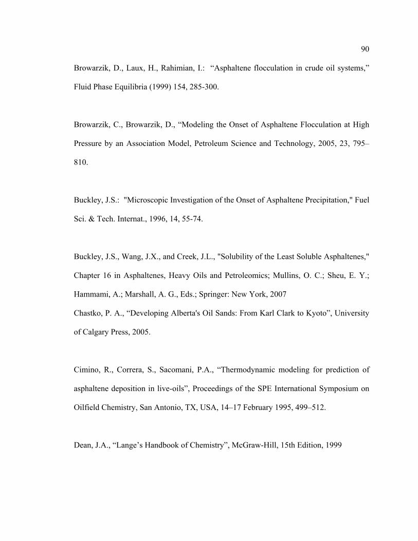
90
Browarzik, D., Laux, H., Rahimian, I.: “Asphaltene flocculation in crude oil systems,”
Fluid Phase Equilibria (1999) 154, 285-300.
Browarzik, C., Browarzik, D., “Modeling the Onset of Asphaltene Flocculation at High
Pressure by an Association Model, Petroleum Science and Technology, 2005, 23, 795–
810.
Buckley, J.S.: "Microscopic Investigation of the Onset of Asphaltene Precipitation," Fuel
Sci. & Tech. Internat., 1996, 14, 55-74.
Buckley, J.S., Wang, J.X., and Creek, J.L., "Solubility of the Least Soluble Asphaltenes,"
Chapter 16 in Asphaltenes, Heavy Oils and Petroleomics; Mullins, O. C.; Sheu, E. Y.;
Hammami, A.; Marshall, A. G., Eds.; Springer: New York, 2007
Chastko, P. A., “Developing Alberta's Oil Sands: From Karl Clark to Kyoto”, University
of Calgary Press, 2005.
Cimino, R., Correra, S., Sacomani, P.A., “Thermodynamic modeling for prediction of
asphaltene deposition in live-oils”, Proceedings of the SPE International Symposium on
Oilfield Chemistry, San Antonio, TX, USA, 14–17 February 1995, 499–512.
Dean, J.A., “Lange’s Handbook of Chemistry”, McGraw-Hill, 15th Edition, 1999
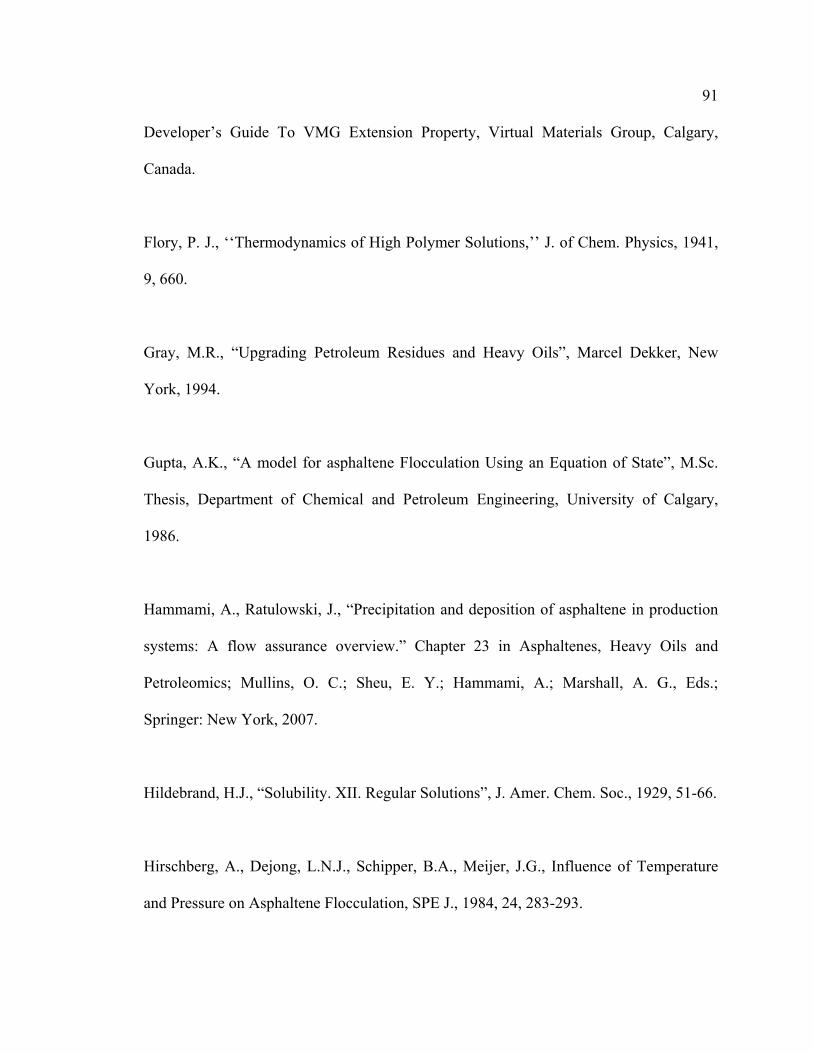
91
Developer’s Guide To VMG Extension Property, Virtual Materials Group, Calgary,
Canada.
Flory, P. J., ‘‘Thermodynamics of High Polymer Solutions,’’ J. of Chem. Physics, 1941,
9, 660.
Gray, M.R., “Upgrading Petroleum Residues and Heavy Oils”, Marcel Dekker, New
York, 1994.
Gupta, A.K., “A model for asphaltene Flocculation Using an Equation of State”, M.Sc.
Thesis, Department of Chemical and Petroleum Engineering, University of Calgary,
1986.
Hammami, A., Ratulowski, J., “Precipitation and deposition of asphaltene in production
systems: A flow assurance overview.” Chapter 23 in Asphaltenes, Heavy Oils and
Petroleomics; Mullins, O. C.; Sheu, E. Y.; Hammami, A.; Marshall, A. G., Eds.;
Springer: New York, 2007.
Hildebrand, H.J., “Solubility. XII. Regular Solutions”, J. Amer. Chem. Soc., 1929, 51-66.
Hirschberg, A., Dejong, L.N.J., Schipper, B.A., Meijer, J.G., Influence of Temperature
and Pressure on Asphaltene Flocculation, SPE J., 1984, 24, 283-293.
92
Huggins, M. L., ‘‘Solutions of Long Chain Compounds’’, J. of Chem. Physics, 1941, 9,
440.
Ignasiak, T., Ruo, T.C.S., Strausz, O.P., “Investigation of Alberta Oil Sand Asphaltenes
Using Thermal Degradation Reactions”, American Chemical Society, 1979, 24, 178
Janardhan, A.S. and Mansoori, G.A.: "Fractal Nature of Asphaltene Aggregation,"
Journal of Petroleum Science and Engineering, 1993, 9, 17-27
Kawanaka, S., Park, S.J., and Mansoori, G.A.: "Organic Deposition from Reservoir
Fluids: A Thermodynamic Predictive Technique," SPE (1991) 5, 185-194.
Leontaritis, K.J. and Mansoori, G.A.: "Asphaltene Flocculation During Oil Production
and Processing: A Thermodynamic - Colloidal Model," paper SPE 16258 presented at the
1987 SPE Internat. Symp. on Oilfield Chem., San Antonio, 4-6 Feb.
Leontaritis, K.J. and Mansoori, G.A.: "Asphaltene Deposition: A Survey of Field
Experiences and Research Approaches," J. Pet. Sci. Eng., 1988, 1, 229-239.
Leontaritis, K.J. and Mansoori, G.A.: "Fast Crude-Oil Heavy-Component
Characterization Using Combination of ASTM, HPLC, and GPC Methods," J. Pet. Sci.
Eng., 1989, 2, 1-12.
93
Mannistu, K.D., Yarranton, H.W., and Masliyah, J.H., “Solubility Modeling of
Asphaltenes in Organic Solvents”, Energy and Fuels (1997) 11, 615-622.
Mansoori, G.A.: “Modeling of asphaltene and other heavy organic depositions,” J. Pet.
Sci. Eng., 1997, 17, 101-111.
Mitchell, D.L. and Speight, J.G., "The solubility of asphaltenes in hydrocarbon solvents,"
Fuel (1973) 52, 149-152.
Mullins, O.C., et al., “Asphaltenes, Heavy Oils and Petroleomics”, Springer, 2007.
Nellensteyn, F.J., “The constitution of asphalt”, Journal of the Institute of Petroleum
Technology 10, 1924, p. 311.
Nghiem, L.X.; Hassam, M.S.; Nutakki, R., “Efficient Modeling of Asphaltene
Precipitation”, SPE#26642, 68th Anuual Technical Conference and Exhibition of SPE,
Houston, Texas, October 3-6, 1993.
NIST Chemistry webbook - http://webbook.nist.gov/chemistry/
Nji, G. N.; Svrcek, W. Y.; Yarranton, H. W.; Satyro, M. A., “Characterization of Heavy
Oils and Bitumens. 1. Vapor Pressure and Critical Constant Prediction Method for Heavy
Hydrocarbons”, Energy and Fuels 2008, 22 ( 5) 3559
94
Pedersen, K. S., Christensen, P.L., “Phase behaviour of petroleum reservoir fluids” CRC
Press, 2007.
Peng, D.Y., Robinson, D.B.A., “New two-constant equation of state”, Ind. Eng. Chem.
Fundam., 1976, 15, 59–64.
Peramanu, S., Singh, C., Agrawala, M. and Yarranton, H.W., “Investigation on the
Reversibility of Asphaltene Precipitation” Energy and Fuels, 2001, 15 (4), 910–917.
Pfeiffer, J.P., Saal, R.N.J., “Asphaltic Bitumens as Colloid System”, Journal of Physical
Chemistry, 1940, 44, 140.
Pinkston, K.S., Duan, P., Gallardo, V. A., Habicht,S. C., Tan, X., Qian, K., Gray, M., M
llen, K., Kenttmaa, H. I., “Analysis of Asphaltenes and Asphaltene Model Compounds by
Laser-Induced Acoustic Desorption/Fourier Transform Ion Cyclotron Resonance Mass
Spectrometry”, Energy and Fuels (2009), Publication Date (Web): September 16, 2009
Qin, X., P. Wang, K. Sepehrnoori, G.A. Pope, “Modeling Asphaltene Precipitation in
Reservoir Simulation” Ind. Eng. Chem. Res., 2000, 39 (8), 2644–2654.
95
Rachford, H.H., Rice, J.D., “Procedure for use of electronic digital computers in
calculating flash vaporization hydrocarbon equilibrium”, J. Pet. Technol., October 1952.
Technical Note 136.
Rastegari, K., “Measurement and modeling of asphaltene flocculation from Athabasca
bitumen”, M.Sc. thesis, Department of Chemical and Petroleum Engineering, University
of Calgary, 2003.
Rastegari, K., Svrcek. W.Y., Yarranton, H.W., "Kinetics of Asphaltene Flocculation,"
Ind. Eng. Chem. Res., 43, 2004, 6861-6870.
Romanova, U.G., Valinasab, M., Stasiuk, E.N., Yarranton, H.W., Schramm, L.L.,
Shelfantook, W.E., "The Effect of Bitumen Extraction Shear Conditions on Froth
Treatment Performance," Paper No. 2004-028, 55th Canadian International Petroleum
Conference, Calgary, AB, June 8-10, 2004.
Sabbagh, O., “An Eos Approach For Modeling Asphaltene Precipitation”, M.Sc. thesis,
Department of Chemical and Petroleum Engineering, University of Calgary, 2004.
Sabbagh, O., Akbarzadeh, K., Badamchi-Zadeh, A., Svrcek, W. Y., Yarranton, H. W.,
“Applying the PR-EoS to Asphaltene Precipitation from n-Alkane Diluted Heavy Oils
and Bitumens”, Energy and Fuels, 2006, 20 (2), 625-634.
96
Scatchard, G., “Equilibria in Non-electrolyte Solutions in Relation to the Vapor Pressures
and Densities of the Components.”, Chem. Rev., 1931, 28, 321.
Sirota, E.B., “Physical Structure of Asphaltenes” Energy and Fuels, 2005, 19 (4), 1290–
1296.
Smith, J. M., and van Ness, H. C., “Introduction to Chemical Engineering
Thermodynamics”, McGraw-Hill, New York (1987)
Speight, J.G., “The Desulfurization of Heavy Oils and Residua”, CRC Press, 1999.
Strausz, O.P., Mojelsky, T.W., and Lown, E.M., “The Molecular Structure of Asphaltene:
an Unfolding Story”; Fuel, 1992, Vol. 71, 1362.
Szewczyk, V.; Behar, E., Compositional Model for Predicting Asphaltenes Flocculation,
Fluid Phase Equilibria, 1999, 158-160, 459-469.
Vasily Simanzhenkov and Raphael Idem., “Crude Oil Chemistry”, Marcel-Dekker, 2003,
p. 328
Verdier, S., Duong, D., Andersen, S.I., “Experimental Determination of Solubility
Parameters of Oils as a Function of Pressure”, Energy and Fuels, 2005, 19, 1225-1229.
97
VMGSim Process Simulator, Version 5.0, 2009
VMGThermo Programmers Manual, Virtual Material Group, Calgary, Canada.
Whitson, C.H., “Characterizing Hydrocarbon Plus Fractions”, SPE# 12233, SPE Journal,
August 1983, 683-694.
Wiehe, I.A., 1992 Ind. Eng. Chem. Res., 1992, 31, 530-536.
Wiehe, I.A., Liang, K.S., Asphaltenes, Resins, and Other Petroleum macromolecules,
Fluid Phase Equilibria, 1996, 117, 201-210.
Wong, D.S., and Sandler, S.I.A., “Theoretically correct new mixing rule for cubic
equations of state for both highly and slightly non-ideal mixtures”, AIChE J. 38 (1992),
671–680.
Wu, J., Prausnitz, J.M., and Firoozabadi, A.: “Molecular Thermodynamics of Asphaltene
Precipitation in Reservoir Fluids. AIChE J, 2000, 46, 197-209.
Wu, J.; Prausnitz, J. M.; Firoozabadi, A. "Molecular-Thermodynamic Framework for
Asphaltene-Oil Equilibria” AIChE J. 1998, 44, 1188-1199.
98
Yarranton, H. W., H. Alboudwarej and R. Jakher, "Investigation of Asphaltene
Association with Vapour Pressure Osmometry and Interfacial Tension Measurements,"
Ind. Eng. Chem. Res., 2000, 39, 2916-2924.
Yarranton, H.W., Fox, W.A., Svrcek, W.Y., “Effect of Resins on Asphaltene Self-
Association and Solubility”, Can. J. Chem. Eng., 2007, 85(5), 635-642.
Yarranton, H.W.; Masliyah, J.H., “Molar Mass Distribution and Solubility Modeling of
Asphaltenes”, AIChE J. 1996, 42, 3533-3543.
Zou, X-Y., Shaw, J. M., “Dispersed Phases and Dispersed Phase Deposition Issues
Arising in Asphaltene Rich Hydrocarbon Fluids”, Petroleum Science and Technology,
2004, 22:7, 759-771.
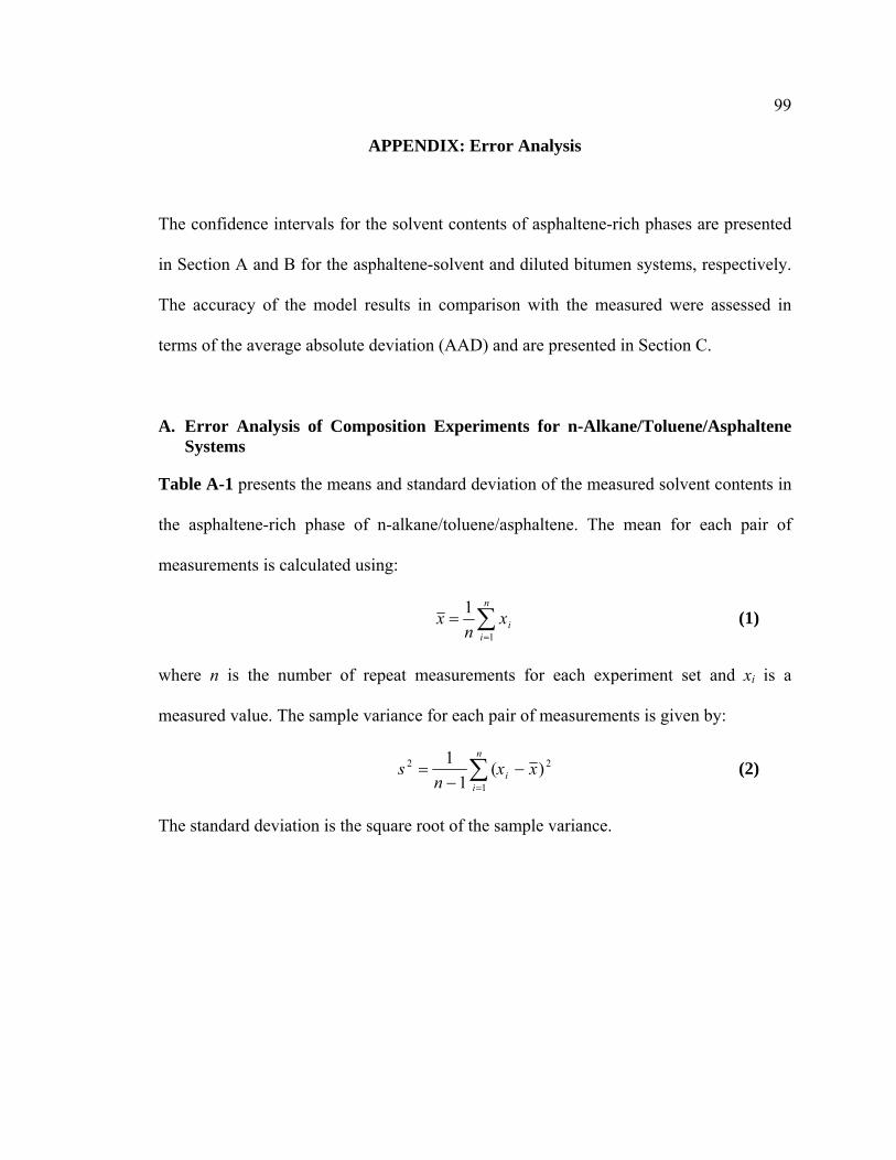
99
APPENDIX: Error Analysis
The confidence intervals for the solvent contents of asphaltene-rich phases are presented
in Section A and B for the asphaltene-solvent and diluted bitumen systems, respectively.
The accuracy of the model results in comparison with the measured were assessed in
terms of the average absolute deviation (AAD) and are presented in Section C.
A. Error Analysis of Composition Experiments for n-Alkane/Toluene/Asphaltene Systems
Table A-1 presents the means and standard deviation of the measured solvent contents in
the asphaltene-rich phase of n-alkane/toluene/asphaltene. The mean for each pair of
measurements is calculated using:
∑=
=n
iix
nx
1
1 (1)
where n is the number of repeat measurements for each experiment set and xi is a
measured value. The sample variance for each pair of measurements is given by:
2
1
2 )(1
1 xxn
s i
n
i−
−= ∑
=
(2)
The standard deviation is the square root of the sample variance.
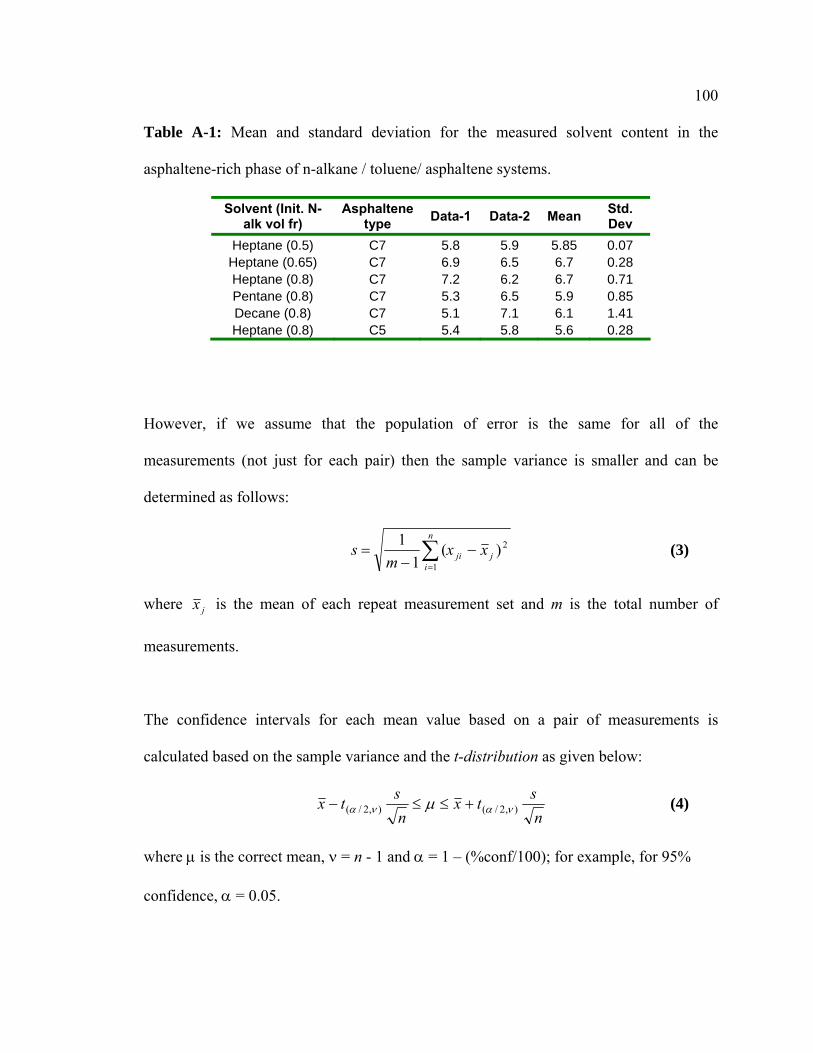
100
Table A-1: Mean and standard deviation for the measured solvent content in the
asphaltene-rich phase of n-alkane / toluene/ asphaltene systems.
Solvent (Init. N-alk vol fr)
Asphaltene type Data-1 Data-2 Mean Std.
Dev Heptane (0.5) C7 5.8 5.9 5.85 0.07
Heptane (0.65) C7 6.9 6.5 6.7 0.28 Heptane (0.8) C7 7.2 6.2 6.7 0.71 Pentane (0.8) C7 5.3 6.5 5.9 0.85 Decane (0.8) C7 5.1 7.1 6.1 1.41 Heptane (0.8) C5 5.4 5.8 5.6 0.28
However, if we assume that the population of error is the same for all of the
measurements (not just for each pair) then the sample variance is smaller and can be
determined as follows:
2
1)(
11
jji
n
ixx
ms −
−= ∑
=
(3)
where jx is the mean of each repeat measurement set and m is the total number of
measurements.
The confidence intervals for each mean value based on a pair of measurements is
calculated based on the sample variance and the t-distribution as given below:
nstx
nstx ),2/(),2/( νανα μ +≤≤− (4)
where μ is the correct mean, ν = n - 1 and α = 1 – (%conf/100); for example, for 95%
confidence, α = 0.05.
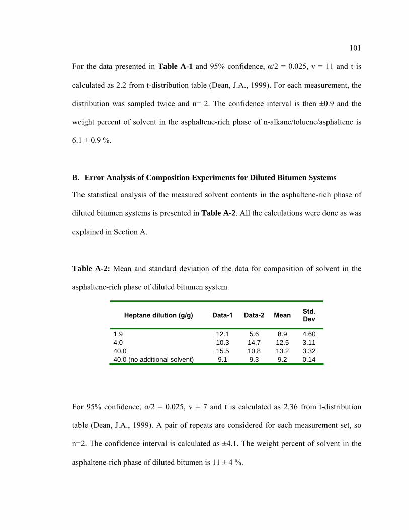
101
For the data presented in Table A-1 and 95% confidence, α/2 = 0.025, v = 11 and t is
calculated as 2.2 from t-distribution table (Dean, J.A., 1999). For each measurement, the
distribution was sampled twice and n= 2. The confidence interval is then ±0.9 and the
weight percent of solvent in the asphaltene-rich phase of n-alkane/toluene/asphaltene is
6.1 ± 0.9 %.
B. Error Analysis of Composition Experiments for Diluted Bitumen Systems
The statistical analysis of the measured solvent contents in the asphaltene-rich phase of
diluted bitumen systems is presented in Table A-2. All the calculations were done as was
explained in Section A.
Table A-2: Mean and standard deviation of the data for composition of solvent in the
asphaltene-rich phase of diluted bitumen system.
Heptane dilution (g/g) Data-1 Data-2 Mean Std. Dev
1.9 12.1 5.6 8.9 4.60 4.0 10.3 14.7 12.5 3.11 40.0 15.5 10.8 13.2 3.32 40.0 (no additional solvent) 9.1 9.3 9.2 0.14
For 95% confidence, α/2 = 0.025, v = 7 and t is calculated as 2.36 from t-distribution
table (Dean, J.A., 1999). A pair of repeats are considered for each measurement set, so
n=2. The confidence interval is calculated as ±4.1. The weight percent of solvent in the
asphaltene-rich phase of diluted bitumen is 11 ± 4 %.
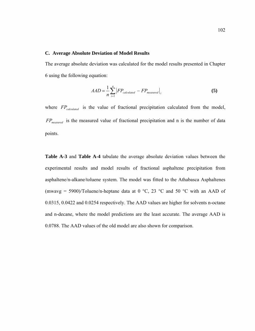
102
C. Average Absolute Deviation of Model Results
The average absolute deviation was calculated for the model results presented in Chapter
6 using the following equation:
∑=
−=n
iimeasuredcalculated FPFP
nAAD
1
1 (5)
where is the value of fractional precipitation calculated from the model,
is the measured value of fractional precipitation and n is the number of data
points.
calculatedFP
measuredFP
Table A-3 and Table A-4 tabulate the average absolute deviation values between the
experimental results and model results of fractional asphaltene precipitation from
asphaltene/n-alkane/toluene system. The model was fitted to the Athabasca Asphaltenes
(mwavg = 5900)/Toluene/n-heptane data at 0 °C, 23 °C and 50 °C with an AAD of
0.0315, 0.0422 and 0.0254 respectively. The AAD values are higher for solvents n-octane
and n-decane, where the model predictions are the least accurate. The average AAD is
0.0788. The AAD values of the old model are also shown for comparison.
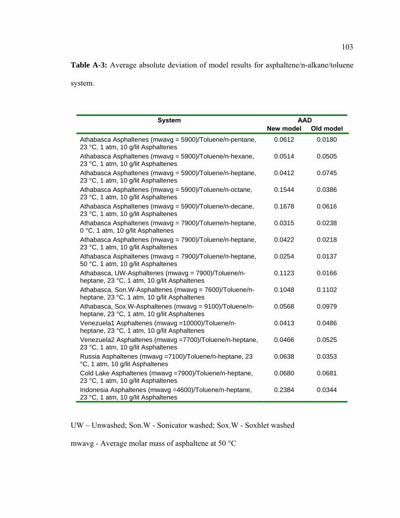
103
Table A-3: Average absolute deviation of model results for asphaltene/n-alkane/toluene
system.
System AAD New model Old model
Athabasca Asphaltenes (mwavg = 5900)/Toluene/n-pentane, 23 °C, 1 atm, 10 g/lit Asphaltenes
0.0612 0.0180
Athabasca Asphaltenes (mwavg = 5900)/Toluene/n-hexane, 23 °C, 1 atm, 10 g/lit Asphaltenes
0.0514 0.0505
Athabasca Asphaltenes (mwavg = 5900)/Toluene/n-heptane, 23 °C, 1 atm, 10 g/lit Asphaltenes
0.0412 0.0745
Athabasca Asphaltenes (mwavg = 5900)/Toluene/n-octane, 23 °C, 1 atm, 10 g/lit Asphaltenes
0.1544 0.0386
Athabasca Asphaltenes (mwavg = 5900)/Toluene/n-decane, 23 °C, 1 atm, 10 g/lit Asphaltenes
0.1678 0.0616
Athabasca Asphaltenes (mwavg = 7900)/Toluene/n-heptane, 0 °C, 1 atm, 10 g/lit Asphaltenes
0.0315 0.0238
Athabasca Asphaltenes (mwavg = 7900)/Toluene/n-heptane, 23 °C, 1 atm, 10 g/lit Asphaltenes
0.0422 0.0218
Athabasca Asphaltenes (mwavg = 7900)/Toluene/n-heptane, 50 °C, 1 atm, 10 g/lit Asphaltenes
0.0254 0.0137
Athabasca, UW-Asphaltenes (mwavg = 7900)/Toluene/n-heptane, 23 °C, 1 atm, 10 g/lit Asphaltenes
0.1123 0.0166
Athabasca, Son.W-Asphaltenes (mwavg = 7600)/Toluene/n-heptane, 23 °C, 1 atm, 10 g/lit Asphaltenes
0.1048 0.1102
Athabasca, Sox.W-Asphaltenes (mwavg = 9100)/Toluene/n-heptane, 23 °C, 1 atm, 10 g/lit Asphaltenes
0.0568 0.0979
Venezuela1 Asphaltenes (mwavg =10000)/Toluene/n-heptane, 23 °C, 1 atm, 10 g/lit Asphaltenes
0.0413 0.0486
Venezuela2 Asphaltenes (mwavg =7700)/Toluene/n-heptane, 23 °C, 1 atm, 10 g/lit Asphaltenes
0.0466 0.0525
Russia Asphaltenes (mwavg =7100)/Toluene/n-heptane, 23 °C, 1 atm, 10 g/lit Asphaltenes
0.0638 0.0353
Cold Lake Asphaltenes (mwavg =7900)/Toluene/n-heptane, 23 °C, 1 atm, 10 g/lit Asphaltenes
0.0680 0.0681
Indonesia Asphaltenes (mwavg =4600)/Toluene/n-heptane, 23 °C, 1 atm, 10 g/lit Asphaltenes
0.2384 0.0344
UW – Unwashed; Son.W - Sonicator washed; Sox.W - Soxhlet washed
mwavg - Average molar mass of asphaltene at 50 °C
104
Table A-4: Average absolute deviation of model results for Athabasca asphaltene/n-
heptane/toluene system at different asphaltene concentrations.
System AAD New model Old model
Athabasca Asphaltenes (mwavg = 5900)/Toluene/n-heptane, 23 °C, 1 atm, 0.20 Toluene Volume fraction
0.0469 0.1249
Athabasca Asphaltenes (mwavg = 5900)/Toluene/n-heptane, 23 °C, 1 atm, 0.25 Toluene Volume fraction
0.0735 0.1304
Athabasca Asphaltenes (mwavg = 5900)/Toluene/n-heptane, 23 °C, 1 atm, 0.33 Toluene Volume fraction
0.0851 0.0803
Athabasca Asphaltenes (mwavg = 5900)/Toluene/n-heptane, 23 °C, 1 atm, 0.40 Toluene Volume fraction
0.0625 0.0101