Thesis ProposalLearning Semantic Representations using

RelationsSujay Kumar Jauhar

January 21st, 2016

Language Technologies InstituteSchool of Computer ScienceCarnegie Mellon University

Pittsburgh, PA 15213

Thesis Committee:Eduard Hovy, Chair

Chris DyerLori Levin

Peter Turney

Submitted in partial fulfillment of the requirementsfor the degree of Doctor of Philosophy.

Copyright c© 2016 Sujay Kumar Jauhar

Keywords: Semantics, Representation Learning, Relations, Structure

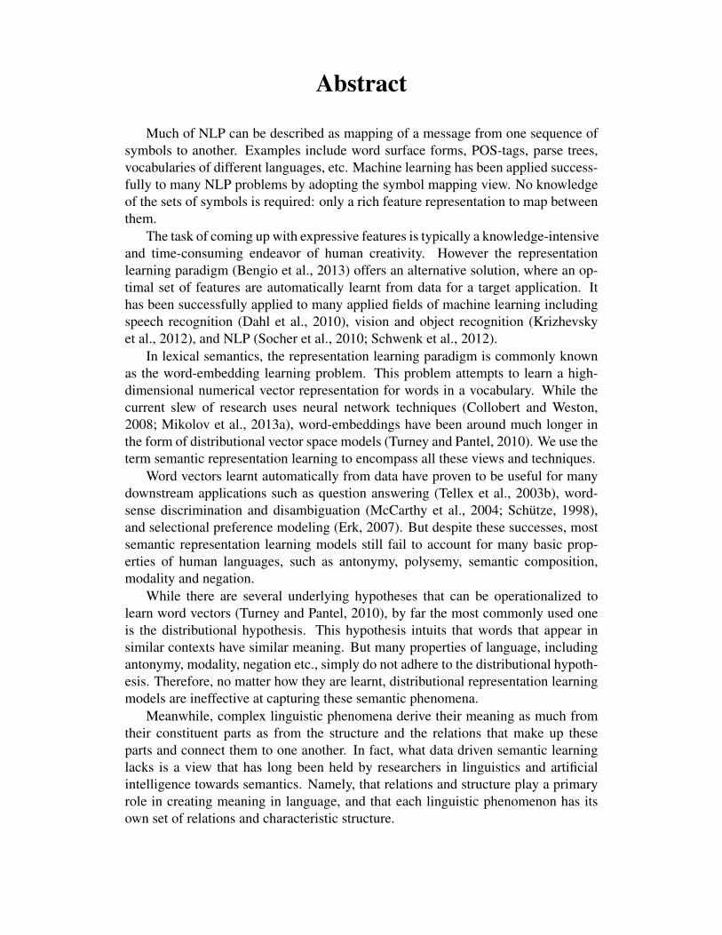
Abstract

Much of NLP can be described as mapping of a message from one sequence ofsymbols to another. Examples include word surface forms, POS-tags, parse trees,vocabularies of different languages, etc. Machine learning has been applied success-fully to many NLP problems by adopting the symbol mapping view. No knowledgeof the sets of symbols is required: only a rich feature representation to map betweenthem.

The task of coming up with expressive features is typically a knowledge-intensiveand time-consuming endeavor of human creativity. However the representationlearning paradigm (Bengio et al., 2013) offers an alternative solution, where an op-timal set of features are automatically learnt from data for a target application. Ithas been successfully applied to many applied fields of machine learning includingspeech recognition (Dahl et al., 2010), vision and object recognition (Krizhevskyet al., 2012), and NLP (Socher et al., 2010; Schwenk et al., 2012).

In lexical semantics, the representation learning paradigm is commonly knownas the word-embedding learning problem. This problem attempts to learn a high-dimensional numerical vector representation for words in a vocabulary. While thecurrent slew of research uses neural network techniques (Collobert and Weston,2008; Mikolov et al., 2013a), word-embeddings have been around much longer inthe form of distributional vector space models (Turney and Pantel, 2010). We use theterm semantic representation learning to encompass all these views and techniques.

Word vectors learnt automatically from data have proven to be useful for manydownstream applications such as question answering (Tellex et al., 2003b), word-sense discrimination and disambiguation (McCarthy et al., 2004; Schutze, 1998),and selectional preference modeling (Erk, 2007). But despite these successes, mostsemantic representation learning models still fail to account for many basic prop-erties of human languages, such as antonymy, polysemy, semantic composition,modality and negation.

While there are several underlying hypotheses that can be operationalized tolearn word vectors (Turney and Pantel, 2010), by far the most commonly used oneis the distributional hypothesis. This hypothesis intuits that words that appear insimilar contexts have similar meaning. But many properties of language, includingantonymy, modality, negation etc., simply do not adhere to the distributional hypoth-esis. Therefore, no matter how they are learnt, distributional representation learningmodels are ineffective at capturing these semantic phenomena.

Meanwhile, complex linguistic phenomena derive their meaning as much fromtheir constituent parts as from the structure and the relations that make up theseparts and connect them to one another. In fact, what data driven semantic learninglacks is a view that has long been held by researchers in linguistics and artificialintelligence towards semantics. Namely, that relations and structure play a primaryrole in creating meaning in language, and that each linguistic phenomenon has itsown set of relations and characteristic structure.

From this point of view the distributional hypothesis is first and foremost a re-lational hypothesis, only one among many possible relational hypotheses. It thusbecomes clear why it is incapable of capturing all of semantics. The distribu-tional relation is simply not the right or most expressive relation for many linguisticphenomena or semantic problems – composition, modality, antonymy included. Itwould thus seem imperative to integrate relations into modelling lexical representa-tion learning.

This thesis proposes a relation-centric view of semantics, which subsumes thedistributional hypothesis and other co-occurrence based hypotheses. Our centralconjecture is that semantic relations are fundamentally important in giving meaningto words (and generally all of language). We hypothesize that by understanding andarticulating the principal relations relevant to a particular problem, one can leveragethem to build more expressive and empirically superior models of semantic repre-sentations.

We begin by introducing the problem of semantic representation learning, defin-ing relations and arguing for their centrality in meaning. We then outline a frame-work within which to think about and implement solutions for integrating relationsin representation learning. The framework is example-based, in the sense that wedraw from concrete instances in this thesis to illustrate five sequential themes thatneed to be considered.

The rest of the thesis provides concrete instantiations of these sequential themes.The problems we tackle are broad, both from the perspective of the target learningproblem as well as the nature of the relations and structure that we use. We thus showthat by focussing on relations, we can learn models of word meaning that are seman-tically and linguistically more expressive while also being empirically superior tostandard distributional representation learning models.

First, we show how tensor-based structured distributional semantic models canbe learnt for tackling the problems of contextual variability and facetted compari-son; we give examples of both syntactic and latent semantic relational integrationinto the model. We then outline a general methodology to learn sense-specific rep-resentations for polysemous words by using the relational links in an ontologicalgraph to tease apart the different senses of words. Next, we show how the relationalstructure of tables can be used to produce high-quality annotated data for questionanswering, as well as build models that leverage this data and structure to performquestion answering. We then propose to investigate problems related to named en-tities by considering encyclopedic relations as well as discourse structure. Finally,we propose to empirically answer some fundamental theoretical questions relatingto semantic relations for the domain of event argument structure.

The success of the proposed extension provides a significant step forward incomputational semantic modelling. It allows for a unified view of word meaningthrough semantic relations, while supporting representation of richer, more compre-hensive models of semantics. At the same time, it results in representations that canpotentially benefit any downstream NLP applications that rely on features for words.

iv

Contents

1 Introduction 11.1 Contributions of this Thesis . . . . . . . . . . . . . . . . . . . . . . . . . . . . . 61.2 Relations in Linguistics and Artificial Intelligence – Proposed Work . . . . . . . 7

2 Relational Representation Learning 9

3 Structured Distributional Semantics 173.1 Distributional Versus Structured Distributional Semantics . . . . . . . . . . . . . 183.2 Syntactic Structured Distributional Semantics . . . . . . . . . . . . . . . . . . . 19

3.2.1 Related Work . . . . . . . . . . . . . . . . . . . . . . . . . . . . . . . . 203.2.2 The Model . . . . . . . . . . . . . . . . . . . . . . . . . . . . . . . . . 203.2.3 Mimicking Compositionality . . . . . . . . . . . . . . . . . . . . . . . . 223.2.4 Single Word Evaluation . . . . . . . . . . . . . . . . . . . . . . . . . . 253.2.5 Event Coreference Judgment . . . . . . . . . . . . . . . . . . . . . . . . 26

3.3 Latent Structured Distributional Semantics . . . . . . . . . . . . . . . . . . . . . 293.3.1 Related Work . . . . . . . . . . . . . . . . . . . . . . . . . . . . . . . . 303.3.2 Latent Semantic Relation Induction . . . . . . . . . . . . . . . . . . . . 313.3.3 Evaluation . . . . . . . . . . . . . . . . . . . . . . . . . . . . . . . . . 333.3.4 Semantic Relation Classification and Analysis of the Latent Structure of

Dimensions . . . . . . . . . . . . . . . . . . . . . . . . . . . . . . . . . 363.4 Conclusion . . . . . . . . . . . . . . . . . . . . . . . . . . . . . . . . . . . . . 39

4 Ontologies and Polysemy 414.1 Related Work . . . . . . . . . . . . . . . . . . . . . . . . . . . . . . . . . . . . 424.2 Unified Symbolic and Distributional Semantics . . . . . . . . . . . . . . . . . . 43

4.2.1 Retrofitting Vectors to an Ontology . . . . . . . . . . . . . . . . . . . . 434.2.2 Adapting Predictive Models with Latent Variables and Structured Regu-

larizers . . . . . . . . . . . . . . . . . . . . . . . . . . . . . . . . . . . 454.3 Resources, Data and Training . . . . . . . . . . . . . . . . . . . . . . . . . . . . 484.4 Evaluation . . . . . . . . . . . . . . . . . . . . . . . . . . . . . . . . . . . . . . 49

4.4.1 Experimental Results . . . . . . . . . . . . . . . . . . . . . . . . . . . . 494.4.2 Generalization to Another Language . . . . . . . . . . . . . . . . . . . . 524.4.3 Antonym Selection . . . . . . . . . . . . . . . . . . . . . . . . . . . . . 53

4.5 Discussion . . . . . . . . . . . . . . . . . . . . . . . . . . . . . . . . . . . . . . 54

v

4.5.1 Qualitative Analysis . . . . . . . . . . . . . . . . . . . . . . . . . . . . 554.6 Conclusion . . . . . . . . . . . . . . . . . . . . . . . . . . . . . . . . . . . . . 55

5 Tables for Question Answering 575.1 Related Work . . . . . . . . . . . . . . . . . . . . . . . . . . . . . . . . . . . . 585.2 Tables as Semi-structured Knowledge Representation . . . . . . . . . . . . . . . 59

5.2.1 Table Semantics and Relations . . . . . . . . . . . . . . . . . . . . . . . 595.2.2 Table Data . . . . . . . . . . . . . . . . . . . . . . . . . . . . . . . . . 60

5.3 Answering Multiple-choice Questions using Tables . . . . . . . . . . . . . . . . 605.3.1 Table Alignments to Multiple-choice Questions . . . . . . . . . . . . . . 62

5.4 Crowd-sourcing Multiple-choice Questions and Table Alignments . . . . . . . . 625.4.1 MCQ Data . . . . . . . . . . . . . . . . . . . . . . . . . . . . . . . . . 62

5.5 Feature Rich Table Embedding Solver . . . . . . . . . . . . . . . . . . . . . . . 655.5.1 Model, Features and Training Objective . . . . . . . . . . . . . . . . . . 655.5.2 Experimental Results . . . . . . . . . . . . . . . . . . . . . . . . . . . . 70

5.6 TabNN: Representation Learning over Tables – Proposed Work . . . . . . . . . . 735.6.1 The Model . . . . . . . . . . . . . . . . . . . . . . . . . . . . . . . . . 735.6.2 Training . . . . . . . . . . . . . . . . . . . . . . . . . . . . . . . . . . . 77

5.7 Conclusion . . . . . . . . . . . . . . . . . . . . . . . . . . . . . . . . . . . . . 77

6 Event Structure – Proposed Work 796.1 Proposed Model . . . . . . . . . . . . . . . . . . . . . . . . . . . . . . . . . . . 816.2 Proposed Evaluation . . . . . . . . . . . . . . . . . . . . . . . . . . . . . . . . 83

7 Class-Instance Entity Linking – Proposed Work 857.1 Synonymy and Polysemy with Encyclopedic Relations . . . . . . . . . . . . . . 867.2 Anaphora with Discourse Relations . . . . . . . . . . . . . . . . . . . . . . . . 87

8 Proposed Timeline 89

Bibliography 91

vi

List of Figures

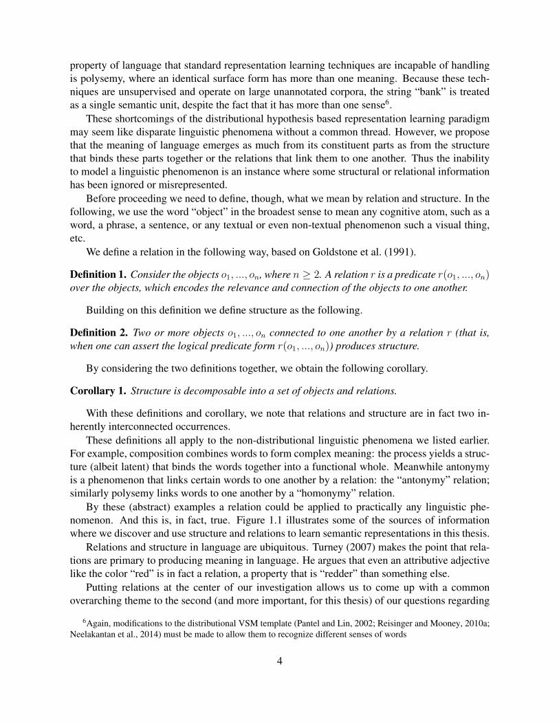
1.1 Examples illustrating various sources of information exhibiting the dual natureof structure and relations. Note how Definitions 1 and 2, as well as Corollary 1apply to each of these examples. All these sources are used in this thesis. . . . . . 5

3.1 Some sample sentences & the triples that we extract from them to store in thePropStore . . . . . . . . . . . . . . . . . . . . . . . . . . . . . . . . . . . . . . 21

3.2 Mimicking composition of two words . . . . . . . . . . . . . . . . . . . . . . . 22

3.3 Evaluation results on WS-353 and ESL with varying number of latent dimen-sions. Generally high scores are obtained in the range of 100-150 latent dimen-sions, with optimal results on both datasets at 130 latent dimensions. . . . . . . . 35

3.4 Correlation distances between semantic relations’ classifier weights. The plotshows how our latent relations seem to perceive humanly interpretable semanticrelations. Most points are fairly well spaced out, with opposites such as “At-tribute” and “Non-Attribute” as well as “Similar” and “Contrast” being relativelyfurther apart. . . . . . . . . . . . . . . . . . . . . . . . . . . . . . . . . . . . . 38

4.1 A factor graph depicting the retrofitting model in the neighborhood of the word“bank”. Observed variables corresponding to word types are shaded in grey,while latent variables for word senses are in white. . . . . . . . . . . . . . . . . 44

4.2 The generative process associated with the skip-gram model, modified to accountfor latent senses. Here, the context of the ambiguous word “bank” is generatedfrom the selection of a specific latent sense. . . . . . . . . . . . . . . . . . . . . 46

4.3 Performance of sense specific vectors (wnsense) compared with single sense vec-tors (original) on similarity scoring in French. Higher bars are better. wnsenseoutperforms original across 2 different VSMs on this task. . . . . . . . . . . . . 52

4.4 Performance of sense specific vectors (wnsense) compared with single sense vec-tors (original) on closest to opposite selection of target verbs. Higher bars arebetter. wnsense outperforms original across 3 different VSMs on this task. . . . . 53

5.1 Example table and MCQ with alignments highlighted by color. Row alignedelements and question words are given in light green, while column aligned ele-ments and question and choice words are given in light brown. The intersectionof the aligned row and column is the relevant cell which is colored dark brown. . 61

vii

5.2 Example table from MTurk annotation task illustrating constraints. We ask Turk-ers to construct questions from blue cells, such that the red cell is the correctanswer, and distracters must be selected from yellow cells. . . . . . . . . . . . . 63

5.3 The TabNN model which embeds question and row in a joint space, while em-bedding column and choices in a different joint space. Distance in each space iscomputed to find how relevant an intersecting cell between row and column is toanswer the MCQ. . . . . . . . . . . . . . . . . . . . . . . . . . . . . . . . . . . 74

6.1 Illustration of a potential binary feature matrix (1s colored, 0s blank) learned byIBP. Rows represent verbs from a fixed vocabulary, while columns are of a fixedbut arbitrary number and represent latent arguments. Interpreting this examplematrix, one might guess that the second latent column corresponds to a proto-typical agent, while the last-but-one latent column corresponds to a prototypicalpatient. . . . . . . . . . . . . . . . . . . . . . . . . . . . . . . . . . . . . . . . 80

viii

List of Tables

3.1 Single Word Evaluation . . . . . . . . . . . . . . . . . . . . . . . . . . . . . . . 263.2 Finklestein: Correlation using SVD . . . . . . . . . . . . . . . . . . . . . . . . 263.3 Cross-validation Performance on IC and ECB dataset . . . . . . . . . . . . . . . 273.4 . . . . . . . . . . . . . . . . . . . . . . . . . . . . . . . . . . . . . . . . . . . 343.5 . . . . . . . . . . . . . . . . . . . . . . . . . . . . . . . . . . . . . . . . . . . 343.6 Results on Relation Classification Task. LR-SDSM scores competitively, outper-

forming all but the SENNA-AVC model. . . . . . . . . . . . . . . . . . . . . . . 36

4.1 Similarity scoring and synonym selection in English across several datasets in-volving different VSMs. Higher scores are better; best scores within each cate-gory are in bold. In most cases our models consistently and significantly outper-form the other VSMs. . . . . . . . . . . . . . . . . . . . . . . . . . . . . . . . . 50

4.2 Contextual word similarity in English. Higher scores are better. . . . . . . . . . . 514.3 Training time associated with different methods of generating sense-specific VSMs. 544.4 The top 3 most similar words for two polysemous types. Single sense VSMs

capture the most frequent sense. Our techniques effectively separates out thedifferent senses of words, and are grounded in WordNet. . . . . . . . . . . . . . 55

5.1 Example part of table concerning phase state changes. . . . . . . . . . . . . . . . 595.2 Example MCQs generated from our pilot MTurk tasks. Correct answer choices

are in bold. . . . . . . . . . . . . . . . . . . . . . . . . . . . . . . . . . . . . . 645.3 Evaluation results on two benchmark datasets using different sets of tables as

background knowledge. FRETS models outperform baselines in all settings, of-ten significantly. Best results on a particular dataset are highlighted in bold. . . . 71

5.4 Ablation study on FRETS features, removing groups of features based on levelof granularity. Best results on a particular dataset are highlighted in bold. . . . . 72

5.5 Combination results of using FRETS in an ensemble solver on both benchmarkdatasets. The best test results to date, at the time of writing, are achieved withthis combination. Best results on a particular dataset are highlighted in bold. . . . 73

ix

x

Chapter 1

Introduction

Most of NLP can be viewed as a mapping from one sequence of symbols to another. For example,translation is mapping between sets of symbols in two different languages. Similarly, part-of-speech tagging is mapping between words’ surface forms and their hypothesized underlying part-of-speech tags. Even complex structured prediction tasks such as parsing or simple tasks like textcategorization labelling are mappings: only between sets of symbols of different granularity thatmay or may not interact with one another with complex interactions.

Using this symbol mapping perspective, machine learning has been applied with great suc-cess to practically every NLP problem. In principle, the machine learning paradigm has no needto know about either sets of symbols: the only requirement is a set of expressive features thatcharacterizes the two sequences and their relation to one another. These features provide thebasis upon which a symbol mapping model may be learnt to generalize from known to unseenexamples.

Driven by better machine learning techniques, more capable machines and vastly largeramounts of data, useable natural language applications are finally in the hands of millions ofusers. People can now translate text between many languages via services like Google Translate1,or interact with virtual personal assistants such as Siri2 from Apple or Cortana3 from Microsofton their mobile devices.

However, while these applications work well for certain common use cases, such as translat-ing between linguistically and structurally close language pairs or asking about the weather, theycontinue to be embarrassingly poor for processing and understanding the vast majority of humanlanguage. This is because, – despite recent efforts, such as Google’s Knowledge Graph project4

– models for semantics continue to be incomplete and rudimentary, and extremely knowledge-intensive to build.

Until recently, the work of thinking up and engineering expressive features for machine learn-ing models was still, for the most part, the responsibility of the researcher or engineer. However,the representation learning paradigm (Bengio et al., 2013) was proposed as an alternative that

1https://translate.google.com/2https://en.wikipedia.org/wiki/Siri3https://en.wikipedia.org/wiki/Cortana_(software)4https://en.wikipedia.org/wiki/Knowledge_Graph

1

eliminated the need for manual feature engineering. In general, representation learning allowsa system to automatically learn a set of optimal features given a target application and trainingdata. This allowed the development of systems that were effectively autonomous.

Representation learning has been successfully used in several applied research areas of ma-chine learning including speech recognition (Dahl et al., 2010; Deng et al., 2010), vision andobject recognition (Ciresan et al., 2012; Krizhevsky et al., 2012), and NLP Socher et al. (2010);Schwenk et al. (2012); Glorot et al. (2011). In particular for NLP, Collobert et al. (2011) showedhow a single architecture could be applied in an unsupervised fashion to many NLP problems,while achieving state-of-the-art results (at the time) for many of them.

There have since been a number of efforts to extend and improve the use of representationlearning for NLP. One particular area that has received a lot of recent interest in the researchcommunity is lexical semantics.

In lexical semantics, representation learning is more commonly known as the so-called word-embedding learning problem. Here, the aim is to learn features (or embeddings) for words –which are the units of lexical semantics – in a vocabulary automatically from a corpus of text.In the rest of this thesis, when we refer to representation learning, we will be referring to theword-embedding learning problem.

There are two principal reasons that representation learning for lexical semantics is an at-tractive proposition: it is unsupervised (thus requiring no human effort to build), and data-driven(thus containing little bias from human intervention).

To understand the variety of different approaches to word-embedding learning, one can ex-amine the following two questions:

1. How is a model learnt?

2. What does the model represent?

The first question attempts to classify the general method or model used to learn the wordvectors. The currently dominant approach is the neural embedding class of models which useneural networks to maximize some objective function over the data and learn word vectors inthe process. Some notable papers are Collobert et al. (2011), Mikolov et al. (2010) Mikolovet al. (2013a) and Pennington et al. (2014). Earlier work on count statistics over windows andtransformations thereof – such as Term Frequency Inverse Document Frequency (TF-IDF) andPointwise Mutual Information (PMI) weighting – and matrix factorization techniques such asLatent Semantic Analysis (Deerwester et al., 1990) are other ways to learn word vectors. Turneyand Pantel (2010) provides an overview of these diverse approaches. More recently, Levy andGoldberg (2014) show an inherent mathematical link between older matrix factorization workand current neural embedding techniques.

Addressing the second – and, for this thesis, the more interesting and important – questionspecifies the underlying semantic hypothesis by which the model or technique operationalizesraw statistics over data into an objective function or mathematical transformation. Turney andPantel (2010) lists several such hypotheses. These include the bag-of-words hypothesis (Saltonet al., 1975), which conjectures that documents can be characterized by the frequency of words init; the latent relation hypothesis (Turney, 2008a), which proposes that pairs of words that occurin similar patterns tend to have similar relations between them; and the extended distributionalhypothesis which specifies that patterns that occur in similar contexts have similar meaning.

2

But by far the most commonly used semantic hypothesis is the distributional hypothesis(Harris, 1954). Articulated by Firth (1957) in the popular dictum “You shall know a word bythe company it keeps”, the hypothesis claims that words that have similar meaning tend to occurin similar contexts. While much effort in the research community has been devoted towardsimproving how models learn word vectors, most work gives little consideration to what the modelrepresents and simply uses the standard distributional hypothesis. So while word-embeddingmodels are learnt differently, most of them continue to represent the same information.

Consider how the distributional hypothesis works. For example, the words “stadium” and“arena” may have been found to occur in a corpus with the following contexts:

• People crowded the stadium to watch the game.• The arena was crowded with people eager to see the match.• The stadium was host to the biggest match of the year.• The most important game of season was held at the arena.

From these sentences it may be reasonably inferred (without knowing anything about them apriori) that the words “stadium” and “arena” in fact have similar meanings.

Operationalized as representation learning, word-embedding techniques essentially countstatistics over a word’s neighborhood contexts across a corpus to come up with a vector represen-tation for that word. The result is a vector space model (VSM), where every word is representedby a point in some high-dimensional space. We refer to any model that automatically producessuch a VSM as a semantic representation learning model, regardless of how it is learnt.

Word vectors in these continuous space representations can be used for meaningful semanticoperations such as computing word similarity (Turney, 2006), performing analogical reasoning(Turney, 2013) and discovering lexical relationships (Mikolov et al., 2013b).

These models have also been used for a wide variety of NLP applications including questionanswering (Tellex et al., 2003b), semantic similarity computation (Wong and Raghavan, 1984;McCarthy and Carroll, 2003), automated dictionary building (Curran, 2003), automated es-say grading (Landauer and Dumais, 1997), word-sense discrimination and disambiguation (Mc-Carthy et al., 2004; Schutze, 1998), selectional preference modeling (Erk, 2007) and identifica-tion of translation equivalents (Hjelm, 2007).

While largely successful, the standard representation learning paradigm for lexical semantics(using the distributional hypothesis) is incapable of capturing many common phenomena in nat-ural language. That is because the distributional hypothesis is an incomplete explanation for thediversity of possible expressions and linguistic phenomena in natural language.

For example, compositionality is a basic property of language where unit segments of mean-ing are combined to form more complex meaning. While the unit segments of VSMs are words,it remains unclear – and according to previous work non-trivial (Mitchell and Lapata, 2008) –how the vectors for words should be combined to form their compositional embedding. Anotherexample of a non-distributional aspect of language is antonymy. Words such as “good” and “bad”are semantic inverses, but are contextually interchangeable in any realization of language. Theywould thus be assigned vectors that are very close in the resulting semantic space5. Yet another

5Modifications to the distributional VSM template (Turney, 2008b, 2011) need to be made to help them distin-guish between synonymy and antonymy

3

property of language that standard representation learning techniques are incapable of handlingis polysemy, where an identical surface form has more than one meaning. Because these tech-niques are unsupervised and operate on large unannotated corpora, the string “bank” is treatedas a single semantic unit, despite the fact that it has more than one sense6.

These shortcomings of the distributional hypothesis based representation learning paradigmmay seem like disparate linguistic phenomena without a common thread. However, we proposethat the meaning of language emerges as much from its constituent parts as from the structurethat binds these parts together or the relations that link them to one another. Thus the inabilityto model a linguistic phenomenon is an instance where some structural or relational informationhas been ignored or misrepresented.

Before proceeding we need to define, though, what we mean by relation and structure. In thefollowing, we use the word “object” in the broadest sense to mean any cognitive atom, such as aword, a phrase, a sentence, or any textual or even non-textual phenomenon such a visual thing,etc.

We define a relation in the following way, based on Goldstone et al. (1991).

Definition 1. Consider the objects o1, ..., on, where n ≥ 2. A relation r is a predicate r(o1, ..., on)over the objects, which encodes the relevance and connection of the objects to one another.

Building on this definition we define structure as the following.

Definition 2. Two or more objects o1, ..., on connected to one another by a relation r (that is,when one can assert the logical predicate form r(o1, ..., on)) produces structure.

By considering the two definitions together, we obtain the following corollary.

Corollary 1. Structure is decomposable into a set of objects and relations.

With these definitions and corollary, we note that relations and structure are in fact two in-herently interconnected occurrences.

These definitions all apply to the non-distributional linguistic phenomena we listed earlier.For example, composition combines words to form complex meaning: the process yields a struc-ture (albeit latent) that binds the words together into a functional whole. Meanwhile antonymyis a phenomenon that links certain words to one another by a relation: the “antonymy” relation;similarly polysemy links words to one another by a “homonymy” relation.

By these (abstract) examples a relation could be applied to practically any linguistic phe-nomenon. And this is, in fact, true. Figure 1.1 illustrates some of the sources of informationwhere we discover and use structure and relations to learn semantic representations in this thesis.

Relations and structure in language are ubiquitous. Turney (2007) makes the point that rela-tions are primary to producing meaning in language. He argues that even an attributive adjectivelike the color “red” is in fact a relation, a property that is “redder” than something else.

Putting relations at the center of our investigation allows us to come up with a commonoverarching theme to the second (and more important, for this thesis) of our questions regarding

6Again, modifications to the distributional VSM template (Pantel and Lin, 2002; Reisinger and Mooney, 2010a;Neelakantan et al., 2014) must be made to allow them to recognize different senses of words

4

Figure 1.1: Examples illustrating various sources of information exhibiting the dual nature ofstructure and relations. Note how Definitions 1 and 2, as well as Corollary 1 apply to each ofthese examples. All these sources are used in this thesis.

5

word-embedding models, “What does the model represent?”. Each distinct semantic hypothesisthat is used to answer this question is, in fact, specifying a different relational phenomenon.For example, the distributional hypothesis is also an inherently relational phenomenon, wherewords are related to other words in a window size of n centered around a target lexical item.This specific relation does not work for all linguistic properties because it is simply the wrongrelation for them. It thus makes sense to focus on and use the correct set (or at least a moreexpressive set) of relations when learning representations for semantics that is inherently notdistributional.

This is, centrally, the contribution of this thesis.

1.1 Contributions of this Thesis

We formally propose the hypothesis that explicitly modelling structure and relations leads tomore expressive and empirically superior models in comparison with standard distributional-based representation learning models of semantics. Focussing on relations allows representationlearning to capture natural language phenomena that standard distributional models are inadept ator incapable of handling. This thesis substantiates this claim with evidence for several differentsemantic problems. The problems are selected to represent a broad range of linguistic phenomenaand sources of relational knowledge, showing the general applicability of our hypothesis. Theproblems also provide an example-based narrative which we study to suggest a framework withinwhich to think about and implement solutions for integrating relations and structure in semanticrepresentation learning.

In Chapter 2 we introduce our framework as a series of five research questions, each tack-ling a sequential set of themes related to relational modelling in representation learning. Wesuggest possible answers to these research questions by citing instances from this thesis as wellas analyzing the different aspects related to each theme. In summary the five themes deal with:1) formulating a representation learning problem centered around the question “What is beingrepresented?”, 2) finding a source of information that encodes knowledge about the learningproblem, 3) decomposing the information into a set of minimal relations and noting any struc-tural patterns, 4) formulating an objective or model for the learning problem that integrates therelations and structure of the knowledge resource, and 5) characterizing the nature of the learntmodel and evaluating it appropriately to justify the central claim of this thesis – namely thatusing relations and structure in representation learning leads to more expressive and empiricallysuperior models of semantics.

The rest of the thesis is organized as instantiations of this high level framework for severaldifferent semantic problems.

Chapter 3 deals with the problems of contextual variability of word meaning, and facettedcomparison in semantics. We introduce two solutions for these problems, both bound by a com-mon modelling paradigm: tensor based representation, where the semantic signature of a stan-dard word vector is decomposed into distinct relation dimensions. We instantiate this modellingparadigm with two kinds of relations: syntactic and latent semantic relations, each leading to asolution for the two central problems of this chapter. The models we develop are published inGoyal et al. (2013) and Jauhar and Hovy (2014).

6

Chapter 4 introduces work published in Jauhar et al. (2015). It deals with the problem ofpolysemy in semantic representation learning. In particular it introduces two models that learnvectors for polysemous words grounded in an ontology. The structure of the ontology is thesource of relational information that we use to guide our techniques. The first model acts asa simple post-processing step that teases apart the different sense vectors from a single sensevector learned by any existing technique on unannotated corpora. The second builds on the firstand introduces a way of modifying maximum likelihood representation learning models to alsoaccount for senses grounded in an ontology. We show results on a battery of semantic tasks,including two additional sets of results not published in Jauhar et al. (2015) – one of whichshows that our model can be applied to deal with antonymy as well.

In Chapter 5 we deal with the semi-structured representation of knowledge tables. We lever-age the relations between cells in tables for creating data as well as learning solutions for thisdata in the target domain of question answering. Jauhar et al. (2016), – which is currently underreview – shows how we use relations in tables to impose structural constraints that guide crowd-sourcing annotators to produce high quality multiple-choice questions with alignments to tablecells. We also introduce two solutions that are capable of leveraging this data to solve multiple-choice questions by using tables as a source of background knowledge. Our first solution isa feature-rich model that produces comparable results to state-of-the-art models on our evalu-ation tasks, rivalling systems that access vastly larger amounts of data. Our second proposedsolution extends the intuition of our feature-rich model with a neural network that automaticallylearns representations over cells by leveraging the structural semantic inherent in tables. We willpublish the results from both models in an upcoming submission.

We look at the problem of relation induction in Chapter 6, targeted at finding event argumentstructure. This investigation is aimed at finding empirically driven answers to some of the centraltheoretical questions regarding relations, but also as a lexicon induction solution in domains orlanguages with poor or limited semantic annotation tools and data. We introduce a proposedsolution that revolves around an infinite feature Bayesian non-parametric model, as well as twonovel evaluation tasks for the representations we will learn. We envisage one future publicationfrom this chapter.

Finally, we focus on named-entities in Chapter 7. We discuss three related problems oflearning representations for named entities: synonymy, polysemy and anaphora. We suggest twohigh-level solutions for these problems. The first deals with synonymy and polysemy jointlyby proposing to use relations in encyclopaedia in a multi-view learning setting. The secondintends to use discourse relations in adapting and localizing representations for pronouns to solveanaphora. The work in this chapter will lead to at least one, but possibly two future publication.

1.2 Relations in Linguistics and Artificial Intelligence – Pro-posed Work

The work in this thesis proposes a view that considers relations as central in learning semanticrepresentations, encompassing a very broad range of learning problems and linguistic phenom-ena. While this is a novel view for representation learning, this is not a new perspective for

7

semantics in general.Representation learning for semantics, while successful for many applications, has been –

like many other initial machine learning forays into NLP – decidedly knowledge deficient. Andlike many other machine learning solutions to NLP, which have hit performance boundaries,there is a turning towards infusing solutions with greater knowledge. This knowledge oftencomes from theoretical views held in adjacent fields of research, such as linguistics and artificialintelligence. This thesis represents an integration of this kind.

There have been a number of linguistic and artificial intelligence views that have held rela-tions and structure as principal vehicles of meaning representation. We propose to review thisrelated literature and provide an account of different perspectives of the role of relations andstructure in semantic modelling. Where appropriate we hope to link this body of literature withthe overarching theme of and empirical investigations in this thesis.

8

Chapter 2

Relational Representation Learning

A Framework for Using Semantic Relations in Lexical Representation Learning

Given our definitions of relations and structure in Definition 1 and 2, a very diverse range oflinguistic, artificial intelligence and computational phenomena can be said to exhibit relationaland structural properties. Moreover, there are any number of ways that these phenomena can beintegrated into existing methods of representation learning.

Hence, within the scope of our work, it is difficult to come up with a single mathematicalframework through which all relationally enriched semantic representation learning techniquesmay be viewed. Even if we were to propose such a framework, it isn’t clear whether it wouldsimplify an understanding of the diverse range of phenomena that fall under the umbrella termsof relations and structure.

Instead, we propose an example-based scheme to illustrate our use of relations in learningsemantic models. The scheme sequentially highlights a number of recurring themes that weencountered in our research, and we structure our illustration as a series of questions that addressthese themes. The question-theme structure allows us to focus on observationally importantinformation while also proposing an outline for how to apply our example-based framework toa new domain. The examples we cite from this thesis for each theme will illustrate the diverserange and flexibility of integrating relations in representation learning.

In summary, the five research questions we address, along with the themes that they exposeare:

1. What is the semantic representation learning problem we are trying to solve?Identify a target representation learning problem that focusses on what (linguistic) prop-erty needs to be modelled.

2. What linguistic information or resource can we use to solve this problem?Find a corpus-based or knowledge-based resource that contains information relevant tosolving the problem in item 1.

3. What are the relations present in this linguistic information or resource?Determine the set of relations in the linguistic annotation or knowledge resource, and anyuseful structure that these relations define.

9

4. How do we use the relations in representation learning?Think about an objective or model that intuitively captures the desiderata of using therelations or structure in the resource from item 2 to solve the problem in item 1.

5. What is the result of including the relations in learning the semantic model?Evaluate the learned model to see if the inclusion of relational information has measurablyinfluenced the problem in item 1. Possibly characterize the nature of the learned model togain insight on what evaluation might be appropriate.

We should stress that the set of questions and themes we describe is by no means completeand absolute. While useful as guidelines to addressing a new problem, they should be comple-mented by in-domain knowledge of the problem in question.

This chapter should be viewed as a summary of the thesis as well as a framework for applyingour ideas to future work. The framework is outlined by the research agenda listed above. In therest of this chapter we delve further into each of the five questions of our research agenda.

What is the semantic representation learning problem we are trying to solve?

As mentioned in our introduction this is a thesis about representation learning that focusses moreon the question of what is being learnt, rather than how it is being learnt. Hence, the first andmost fundamental question needs to address the issue of what semantic representation learningproblem is being tackled.

Existing methods for semantic representation learning operate almost exclusively on the in-tuition of the distributional hypothesis (Firth, 1957). Namely, that words that occur in similarcontexts tend to have similar meanings. As highlighted in Chapter 1, this hypothesis – whilevery useful – does not cover the the entire spectrum of natural language semantics.

In this thesis, for example, we tackle several such shortcomings. We address the problemof contextual variability (Blank, 2003) in Chapter 3.2, where the meaning of a word varies andstretches based on the neighborhood context in which it occurs1. Another problem with seman-tic vector space models is the facetedness in semantic comparison (Jauhar and Hovy, 2014),whereby concepts cannot be compared along different facets of meaning (e.g. color, material,shape, size, etc.). We tackle this problem in Chapter 3.3. Yet another issue with distributional se-mantic models is their incapacity to learn polysemy from un-annotated data, or to learn abstracttypes that are grounded in known word senses. We propose a joint solution to both problems inChapter 4.

These phenomena extend from general classes of words to named entities as well. In thework we propose in Chapter 7 we tackle entity polysemy – two identical names that belong todifferent people –, entity synonymy – different ways of referring to the same person – (Han andZhao, 2009) and entity anaphora – generic pronouns that take on specific meaning or referents incontext (Mitkov, 2014).

1Not to be confused with polysemy, which Blank (2003) contrasts with contextual variability in terms of alexicon. The former is characterized by different lexicon entries (e.g. “human arm” vs “arm of a sofa”), while thelatter is the extension of a single lexicon entry (e.g. “human arm” vs “robot arm”). Naturally, the distinction is acontinuum that depends on the granularity of the lexicon.

10

Not all problems are necessarily linguistic shortcomings. For example, our work in Chap-ter 5 tackles a representational issue: namely the trade-off between the expressive power of arepresentation and the ease of its creation or annotation. Hence our research focusses on semi-structured representations (Soderland, 1999) and the ability to learn models over and performstructured reasoning with these representations. In similar fashion, the models we propose inChapter 3 – while tackling specific linguistic issues – are also concerned with schemas: movingfrom vectors to tensors as the unit of representation Baroni and Lenci (2010).

In summary, the first step in our sequence of research questions is to address the central issueof what is being represented. Any problem is legitimate as long as it focusses on this centralresearch question. In our experience, generally problems will stem from issues or shortcom-ings in existing models to represent complex linguistic phenomena, but they could also concern(sometimes by consequence) the form of the representation itself.

What linguistic information or resource can we use to solve this problem?

Once a representation learning problem has been identified, the next item on the research agendais to find a source of knowledge that can be applied to the problem. Naturally this source ofknowledge should introduce information that helps to solve the central problem.

In our experience, there seem to be two broad categories of such sources of knowledge.First there is corpus-based information that is inherent in naturally occurring free text, or somelevel of linguistic annotation thereof. For example, this category would cover free text fromWikipedia, it’s part-of-speech tags, parse trees, coreference chains, to name only a few. Secondare knowledge-based resources that are compiled in some form to encapsulate some informationof interest. For example, these could be ontologies, tables, gazetteer lists, lexicons, etc.

The two categories are, of course, not mutually exclusive: for example a treebank could bereasonably assumed to belong to both categories. Moreover there is no restriction on using asingle source of knowledge. Any number of each category can be combined to bring richerinformation to the model.

Examples of the first category of sources of information in this thesis are dependency in-formation (Nivre, 2005) (Chapter 3.2 and Chapter 6), textual patterns (Ravichandran and Hovy,2002) (Chapter 3.3), and proposed discourse information (Seuren, 2006) (Chapter 7). Similarly,examples of the second category of sources of knowledge include ontologies (Miller, 1995a)(Chapter 4), tables (Chapter 5) and proposed encyclopedic information (Chapter 7).

In each of these cases we selected these sources of knowledge to bring novel and usefulinformation to the problem we were trying to resolve. For example, ontologies contain wordsense inventories that are useful to solving the problem of polysemy in representation learning.Similarly dependency arcs define relational neighborhoods that are useful for creating structureddistributional semantic models or yielding features that can be used to find the principal relationalarguments of predicates.

To sum up, the goal of the second research question is to identify corpus-based or knowledge-based resources that contain information relevant to resolving the central representation learningproblem proposed in response to the first research question.

11

What are the relations present in this linguistic information or resource?

With a well defined set of resources (both corpus-based and knowledge-based) in place, the nextquestion seeks to identify the principal relations present in each of the resources. At face value,this may seem like a simple exercise to list out the names of the relations in the various resources.

First, there is the problem of when the resources do not specify a closed class of definite re-lations – for example, when attempting to extract relational patterns from free text (Chapter 3.3).In these cases, since the relations (such as patterns, for example) are likely to follow a Zipfiandistribution, there is an inherent tension between the coverage of the list of discovered relationsand their manageability for any practical application.

More importantly, however, due to Definitions 1 and 2, and Corollary 1 the dual nature ofrelations and structure makes this an issue as much about identifying patterns in structure as therelations that make up this structure. For example, the “causality” relation is often expressedlinguistically through structural patterns such as “X causes Y” or “Y is caused by X”. Similarlywhen one is considering relations in a dependency parse tree, it may be useful – for example – tonote that the tree is projective (Nivre, 2003). Insights into these facets can lead to computationallydesirable models or algorithms, as we will note in the our next research question.

In this thesis our work with syntactic tensor models uses the set of dependency relationsfrom a parser (Chapter 3.2). Here, the source of relational information is linguistic annotationover free text, so the corresponding structure is variable.

More direct uses of structure include our work on ontologies (Chapter 4) were the relationsdefine a graph, and our work on tables (Chapter 5) where the inherent relations between tablecells define a number of interesting structural constraints (see Chapter 5.2.1), – analogies beingjust one example (Turney, 2013). In the former case the relations are explicitly typed edges inthe ontology, while in the latter the relations are latent properties of the table.

Sometimes, when the relations are latent rather than explicit the goal of the model may be todiscover or characterize these relations in some fashion. This is not the case with our work ontables, where relational properties between table cells are only leveraged but are not required tobe directly encoded in the model. In contrast our work on latent tensor models (Chapter 3.3) andproposed event argument induction (Chapter 6) both require the latent relations to be explicitlylearned as parts of the resulting representations.

There is, of course, an inherent trade-off between the linguistic complexity or abstractness ofa relation, and its ability to be harvested or leveraged for learning word vectors. The distribu-tional hypothesis, for example, encodes a simple relation that can be abundantly harvested fromunannotated text. More complex relations, such as those defined over ontologies (Chapter 4) ortables (Chapter 5) are fewer and harder to directly leverage. In this thesis we sometimes supple-ment the distributional hypothesis with other forms of relational information (such as ontologicalrelations), while at others, completely replacing it with some other form of more structured data(such as tables). We show that the inherent tension between complexity and availability in thedata is resolved because even small amounts of structured data provide a great amount of valuableinformation.

In conclusion, identifying the relations in resources and the inherent structure that they de-fine are important to gain insight into how best to integrate them into the representation learningframework. Specific kinds of structure, such as graphs or trees for example, lead to computational

12

models or algorithms that can leverage these structural properties through principled approachesspecifically designed for them. More generally, the wealth of research in structured prediction(Smith, 2011) is applicable to the scope of our problems since it deals with learning and in-ference over complex structure that is often decomposable into more manageable constituents.Finally, when the relations and their resulting structure is latent, it may be required to induce arepresentation or characterization of them for the target model.

How do we use the relations in representation learning?

The next research question on the agenda deals with the actual modelling problem of integratingthe relations or structure of interest into a well-defined representation learning problem. Herethere is considerable flexibility, since there is no single correct way of integrating intuitions andobservations about the target domain into model – and no guarantee that once one does, that itwill function as expected.

Nevertheless, we draw a distinction here between defining an objective and a model. Theformer attempts to encode some mathematical loss function or transformation (such as maximumlikelihood, or singular value decomposition) that captures the desiderata of a problem, whilethe latter specifies a model that will numerically compute and optimize this loss function (forexample a recursive neural network or a log-linear model). The two are sometimes connected,and the definition of one may lead to the characterization of the other.

We note that our purpose for drawing this distinction is merely for the sake of illustrating ourexample-based framework. Hence, we will discuss the objective or model, as appropriate, wheneither more intuitively captures the use of relations or structure in the representation learningproblem.

In this thesis we work with several kinds of transformations and objectives. An example oftransformation based representation learning is singular value decomposition (Golub and Rein-sch, 1970), which we use to reduce sparsity and noise in learning latent relations for our tensormodel (Chapter 3.3).

Many existing semantic representation learning models are formulated as maximum likeli-hood estimation problems over corpora (Collobert et al., 2011; Mikolov et al., 2010). In our workwith ontologies we propose a way to modify these objectives minimally with structured regular-izers, thereby integrating knowledge from the ontological graph (Chapter 4). In the same workwe also look at post-processing word vectors to derive sense representations, in which case maxi-mum a posteriori estimation over smoothness properties of the graph (Corduneanu and Jaakkola,2002; Zhu et al., 2003; Subramanya and Bilmes, 2009) is more appropriate. Specifically we havea prior (the existing word vectors) which we’d like to modify with data (the ontological graph)to produce a posterior (the final sense vectors).

In the case of tables, we are dealing with a countable set of predictable relations over ta-ble cells. Featurizing these relations is the most direct way of encoding them into learning ourmodel. Consequently we use a log-linear model (Chapter 5.5) which conveniently captures fea-tures (Smith, 2004). We use a cross-entropy loss for this model as well as a proposed model(Chapter 5.6) which revolves around the same intuition of features – except this time automati-cally induced via long short term memory neural networks (Hochreiter and Schmidhuber, 1997).

13

In characterizing the argument structure of verbs (Chapter 6), we wish to allow for a po-tentially infinite set of relations, while letting the data decide what a really meaningful set ofrelations should be. Hence we use the Indian Buffet process (Ghahramani and Griffiths, 2005),which is a Bayesian non-parametric model (Hjort et al., 2010) to precisely model feature learningin such a setting.

Summarizing the theme of this part of the research agenda, we seek to concretize a specificmodel that efficiently and usefully integrates knowledge from our source of relations and thestructure that it entails, towards solving the representation learning problem we originally de-fined. While there is a lot of flexibility in how this may be done, it can be useful to think abouttwo aspects of the problem: the objective function and the actual model. Often one or the otherpresents an intuitive way of characterizing how relations or structure should be integrated, andthe other follows directly or is left to empirical validation.

What is the result of including the relations in learning the semantic model?

Our final research item deals with the model after it has been learned. Specifically we discusssome differences in the models we learn in this thesis in an attempt to characterize them, and wealso list how we evaluate them.

With regards to the learned model, there are several distinction. The most salient distinction,however, is between the case where relations have simply been leveraged as an external influenceron learning models, versus cases where relations become part of the resulting model. In thisthesis examples of the first case can be found in Chapters 4, 5 and proposed work in Chapter 7,while examples of the second case are Chapter 3 and proposed work in Chapter 6.

In terms of evaluation, when specifically dealing with the latter of the two cases it is use-ful to evaluate the relations in the model. We do this in this thesis with a relation classifica-tion task (Zhang, 2004) in Chapter 3.3 and propose two different evaluations on verb argumentdatabases in Chapter 6.

For the sake of completeness of our summary of the work in this thesis, we also list some lessimportant distinctions about the models we learn. These need not be considered, in general whencharacterizing a learnt model or thinking about how it will be evaluated. Most often semanticrepresentation learning yields vectors, which is the case for our work in Chapters 4 and 5, andproposed work in Chapters 6 and 7. In this thesis, in particular, we also introduce tensor basedsemantic models (Chapter 3). In both kinds of objects, the numerical values that comprise themare most often abstract real numbers, as is the case with our models from Chapters 3.3, 4, 5 andour proposed models in Chapter 7. But we also have models that are probabilistically normalized(Chapter 3.2) and binary (Chapter 6).

On the evaluation side, depending on the nature of the model, it is also useful to consider anintrinsic or an extrinsic evaluation. For general purpose semantic models, such as the ones learntin Chapters 3 and 4 popular intrinsic evaluation tasks such as word similarity judgement (Finkel-stein et al., 2002) and most appropriate synonym selection (Rubenstein and Goodenough, 1965)are adequate. For targeted models such as the one we learn over tables specifically created forquestion answering (Chapter 5), an extrinsic task evaluation is more appropriate. We also pro-pose such evaluations for our future work with verb argument structure (Chapter 6) and namedentities (Chapter 7).

14

In summary, most importantly, – as with any good empirical task – the evaluation should di-rectly evaluate whether the inclusion of relations in the model measurably influences the problemwe set out to solve. Sometimes, characterizing the nature of the learnt model can lead to insightsof what might be an appropriate evaluation.

In the rest of this thesis we detail instances of the application of this research agenda toseveral research problems and proposed future work.

15

16

Chapter 3

Structured Distributional Semantics

Syntactic and Latent Semantic Tensor Models for Non-constant and Non-unique

Representation Learning

Most current methods for lexical representation learning yield a vector space model (Turneyand Pantel, 2010) in which words are represented as distinct, discrete and static points in somehigh dimensional space. The most fundamental operation in such semantic vector spaces iscomparison of meaning, in which the distance of two points is measured according to a distancemetric.

However, the meaning of a word is neither constant nor unique. It depends on the contextin which it occurs; in other words it depends on the relations that bind it to its compositionalneighborhood. It also depends on what it’s compared to for proximity of meaning, and morespecifically along what relational facet the comparison is being made. These two problems,context-sensitivity and facetedness in semantics, are the representation problems that we tacklein this chapter.

Both problems are defined by semantic relations: the one to neighborhood structure, the otherto comparative concepts. Thus we introduce two related approaches that tackle the two problemsof context-sensitivity and facetedness in representation learning of semantics. These approachesfall into an umbrella paradigm we call Structured Distributional Semantics. This paradigm issimilar to the work on Distributional Memory proposed by Baroni and Lenci (2010).

Structured Distributional Semantics aims to improve upon simple vector space models ofsemantics by hypothesizing that the meaning of a word is captured more effectively through itsrelational — rather than its raw distributional — signature. In accordance, they extend the vectorspace paradigm by structuring elements with relational information that decompose distributionalsignatures over discrete relation dimensions. The resulting representation for a word is a semantictensor (or matrix) rather than a semantic vector.

The move from simple Vector Space Models (VSMs) to Structured Distributional SemanticModels (SDSM) represents a paradigm shift that falls into the overarching theme of this thesis.We will show that decomposing a single word vector into distinct relation dimensions results in amore expressive and empirically superior model. However, unlike the models we have previously

17

introduced – where structure is only an extrinsic source of supervision – relations here are also aconcrete an intrinsic part of the representation schema of the model.

An important choice with an SDSM is the nature of the discrete relation dimensions of thesemantic tensors – in practise the rows of the matrix. Nominally, this choice not only deter-mines the process by which an SDSM is learnt, but also what information is represented and theresulting strengths and weaknesses of the model. Our two models differ in this choice.

The first model is a Syntactic SDSM that represents meaning as distributions over relationsin syntactic neighborhoods. This model tackles the problem of contextual context-sensitivity,with a dynamic SDSM that constructs semantic tensors for words and their relational arguments.We argue that our model approximates meaning in compositional configurations more effec-tively than standard distributional vectors or bag-of-words models. We test our hypothesis onthe problem of judging event coreferentiality, which involves compositional interactions in thepredicate-argument structure of sentences, and demonstrate that our model outperforms bothstate-of-the-art window-based word embeddings as well as simple approaches to compositionalsemantics previously employed in the literature.

The second model is a Latent Semantic SDSM whose relational dimensions are learnt overneighborhood patterns using Latent Relational Analysis (LRA). In comparison to the dynamicSDSM of syntax, this model is static due to its latent nature and therefore does not model com-positional structures. However, it frees the model from its reliance on syntax (or any other setof pre-defined relations for that matter), and allows the data to dictate an optimal set of (albeitlatent) relations. The result is a model that is much more effective at representing single wordunits and tackling the problem of facetedness in the comparison of relational facets. Evaluationof our model yields results that significantly outperform several other distributional approaches(including the Syntactic SDSM) on two semantic tasks and performs competitively on a thirdrelation classification task.

Through both models we re-affirm the central claim of this thesis, namely that by integratingstructured relational information, we can learn more expressive and empirically superior modelsof semantics.

3.1 Distributional Versus Structured Distributional Seman-tics

We begin by formalizing the notion of a Distributional Semantic Model (DSM) as a vector space,and it’s connections and extension to a tensor space in a Structured Distributional SemanticModel (SDSM).

A DSM is a vector space V that contains |Σ| elements in Rn, where Σ = w1, w2, ..., wk isa vocabulary of k distinct words. Every vocabulary word wi has an associated semantic vector ~virepresenting its distributional signature. Each of the n elements of ~vi is associated with a singledimension of its distribution. This dimension may correspond to another word — that may ormay not belong to Σ — or a latent dimension as might be obtained from an SVD projection oran embedding learned via a deep neural network. Additionally, each element in ~vi is typicallya normalized co-occurrence frequency count, a PMI score, or a number obtained from an SVD

18

or RNN transformation. The semantic similarity between two words wi and wj in a DSM is thevector distance defined by cos(~vi, ~vj) on their associated distributional vectors.

An SDSM is an extension of DSM. Formally, it is a space U that contains |Σ| elements inRd×n, where Σ = w1, w2, ..., wk is a vocabulary of k distinct words. Every vocabulary wordwi has an associated semantic tensor ~~ui, which is itself composed of d vectors ~u1

i ,~u2i , ...,

~udi eachhaving n dimensions. Every vector ~uli ∈ ~~ui represents the distributional signature of the wordwi in a relation (or along a facet) rl. The d relations of the SDSM may be syntactic, semantic,or latent (as in this paper). The n dimensional relational vector ~uli is configurationally the sameas a vector ~vi of a DSM. This definition of an SDSM closely relates to an alternate view ofDistributional Memories (DMs) (Baroni and Lenci, 2010) where the semantic space is a third-order tensor, whose modes are Word× Link×Word.

The semantic similarity between two words wi and wj in an SDSM is the similarity functiondefined by sim(~~ui, ~~uj) on their associated semantic tensors. We use the following decompositionof the similarity function:

sim(~~ui, ~~uj) =1

d

d∑l=1

cos(~uli,~ulj) (3.1)

Mathematically, this corresponds to the ratio of the normalized Frobenius product of the twomatrices representing ~~ui and ~~uj to the number of rows in both matrices. Intuitively it is simplythe average relation-wise similarity between the two words wi and wj .

3.2 Syntactic Structured Distributional Semantics

We begin by describing our first SDSM, which tackles the problem of contextual variability insemantics by a representation over syntactic relational dimensions.

Systems that use window-based DSMs implicitly make a bag of words assumption: that themeaning of a phrase can be reasonably estimated from the meaning of its constituents, agnostic ofordering. However, semantics in natural language is a compositional phenomenon, encompass-ing interactions between syntactic structures, and the meaning of lexical constituents. It followsthat the DSM formalism lends itself poorly to composition since it implicitly disregards syntac-tic structure. For instance, the representation for “Lincoln”, “Booth”, and “killed” when mergedproduce the same result regardless of whether the input is “Booth killed Lincoln” or “Lincolnkilled Booth”. As suggested by Pantel and Lin (2000) and others, modeling the distribution overpreferential attachments for each syntactic relation separately can yield greater expressive power.

Attempts have been made to model linguistic composition of individual word vectors (Mitchelland Lapata, 2009), as well as remedy the inherent failings of the standard distributional approach(Erk and Pado, 2008). The results show varying degrees of efficacy, but have largely failed tomodel deeper lexical semantics or compositional expectations of words and word combinations.

The Syntactic SDSM we propose is an extension to traditional DSMs. This extension explic-itly preserves structural information and permits the approximation of distributional expectationover distinct dependency relations. It is also a dynamic model, meaning that statistics are stored

19

in decomposed form as dependency triples, only to be composed to form representations for arbi-trary compositional structures. In the new model the tensor representing a word is a distributionover relation-specific syntactic neighborhoods. In other words, the SDSM representation of aword or phrase is several vectors defined over the same vocabulary, each vector representing theword or phrase’s selectional preferences for a different syntactic argument.

We show that this representation is comparable to a single-vector window-based DSM atcapturing the semantics of individual word, but significantly better at representing the semanticsof composed units. Our experiments on individual word semantics are conducted on the twotasks of similarity scoring and synonym selection. For evaluating compositional units, we turnto the problem of event coreference and the representation of predicate-argument structures. Weuse two different event coreference corpora and show that our Syntactic SDSM achieves greaterpredictive accuracy than simplistic compositional approaches as well as a strong baseline thatuses window based word embeddings trained via deep neural-networks.

3.2.1 Related Work

Recently, a number of studies have tried to model a stronger form of semantics by phrasing theproblem of DSM compositionality as one of vector composition. These techniques derive themeaning of the combination of two words a and b by a single vector c = f(a, b). Mitchell andLapata (2008) propose a framework to define the composition c = f(a, b, r,K) where r is therelation between a and b, and K is some additional knowledge used to define composition.

While the framework is quite general, most models in the literature tend to disregard K andr and are generally restricted to component-wise addition and multiplication on the vectors tobe composed, with slight variations. Dinu and Lapata (2010a) and Seaghdha and Korhonen(2011) introduced a probabilistic model to represent word meanings by a latent variable model.Subsequently, other high-dimensional extensions by Rudolph and Giesbrecht (2010), Baroni andZamparelli (2010) and Grefenstette et al. (2011), regression models by Guevara (2010), andrecursive neural network based solutions by Socher et al. (2012) and Collobert et al. (2011) havebeen proposed.

Pantel and Lin (2000) and Erk and Pado (2008) attempted to include syntactic context in dis-tributional models. However, their approaches do not explicitly construct phrase-level meaningfrom words which limits their applicability to modelling compositional structures. A quasi-compositional approach was also attempted in Thater et al. (2010) by a systematic combinationof first and second order context vectors. Perhaps the most similar work to our own is Baroniand Lenci (2010) who propose a Distributional Memory that stores syntactic contexts to dynam-ically construct semantic representations. However, to the best of our knowledge the formulationof composition we propose is the first to account for K and r within the general framework ofcomposition c = f(a, b, r,K), as proposed by Mitchell and Lapata (2008).

3.2.2 The Model

In this section, we describe our Structured Distributional Semantic framework in detail. We firstbuild a large knowledge base from sample english texts and use it to represent basic lexical units.

20

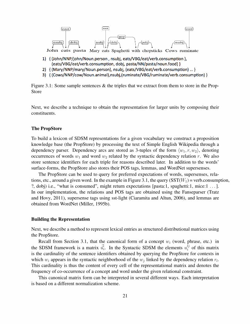
Figure 3.1: Some sample sentences & the triples that we extract from them to store in the Prop-Store

Next, we describe a technique to obtain the representation for larger units by composing theirconstituents.

The PropStore

To build a lexicon of SDSM representations for a given vocabulary we construct a propositionknowledge base (the PropStore) by processing the text of Simple English Wikipedia through adependency parser. Dependency arcs are stored as 3-tuples of the form 〈w1, r, w2〉, denotingoccurrences of words w1 and word w2 related by the syntactic dependency relation r. We alsostore sentence identifiers for each triple for reasons described later. In addition to the words’surface-forms, the PropStore also stores their POS tags, lemmas, and WordNet supersenses.

The PropStore can be used to query for preferred expectations of words, supersenses, rela-tions, etc., around a given word. In the example in Figure 3.1, the query (SST(W1) = verb.consumption,?, dobj) i.e., “what is consumed”, might return expectations [pasta:1, spaghetti:1, mice:1 . . . ].In our implementation, the relations and POS tags are obtained using the Fanseparser (Tratzand Hovy, 2011), supersense tags using sst-light (Ciaramita and Altun, 2006), and lemmas areobtained from WordNet (Miller, 1995b).

Building the Representation

Next, we describe a method to represent lexical entries as structured distributional matrices usingthe PropStore.

Recall from Section 3.1, that the canonical form of a concept wi (word, phrase, etc.) inthe SDSM framework is a matrix ~~ui. In the Syntactic SDSM the elements ulji of this matrixis the cardinality of the sentence identifiers obtained by querying the PropStore for contexts inwhich wi appears in the syntactic neighborhood of the wj linked by the dependency relation rl.This cardinality is thus the content of every cell of the representational matrix and denotes thefrequency of co-occurrence of a concept and word under the given relational constraint.

This canonical matrix form can be interpreted in several different ways. Each interpretationis based on a different normalization scheme.

21

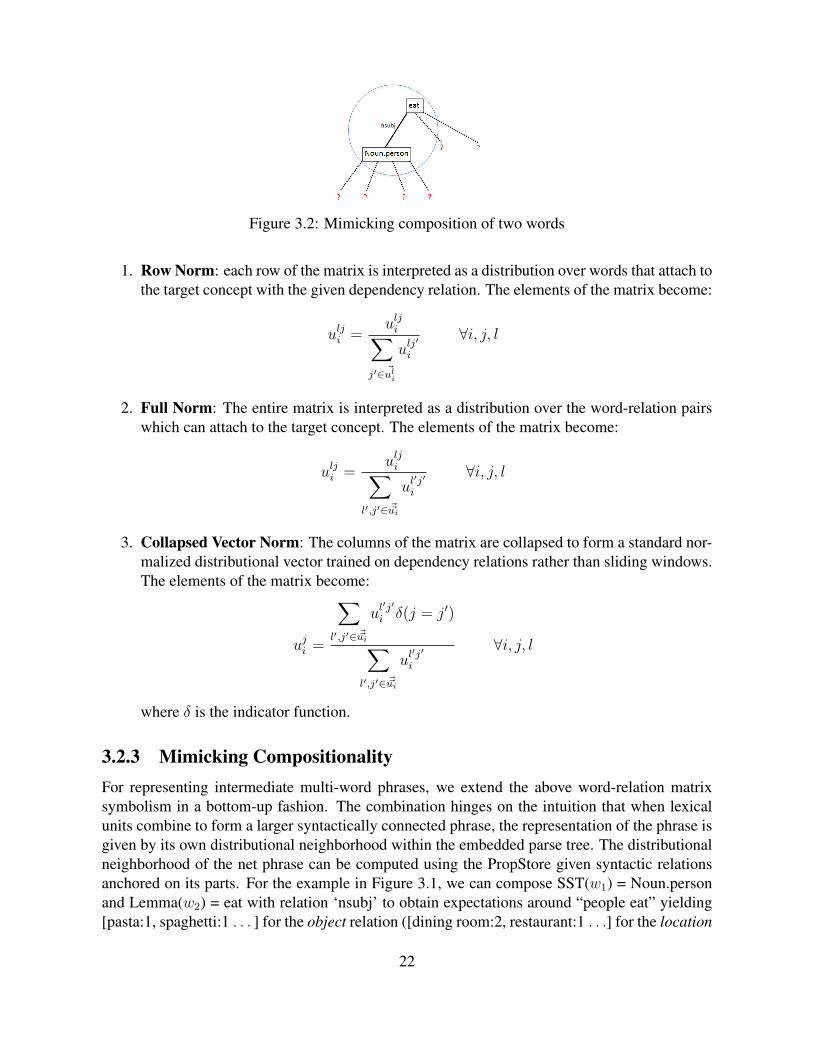
Figure 3.2: Mimicking composition of two words

1. Row Norm: each row of the matrix is interpreted as a distribution over words that attach tothe target concept with the given dependency relation. The elements of the matrix become:

ulji =ulji∑

j′∈ ~uli

ulj′

i

∀i, j, l

2. Full Norm: The entire matrix is interpreted as a distribution over the word-relation pairswhich can attach to the target concept. The elements of the matrix become:

ulji =ulji∑

l′,j′∈ ~~ui

ul′j′

i

∀i, j, l

3. Collapsed Vector Norm: The columns of the matrix are collapsed to form a standard nor-malized distributional vector trained on dependency relations rather than sliding windows.The elements of the matrix become:

uji =

∑l′,j′∈ ~~ui

ul′j′

i δ(j = j′)

∑l′,j′∈ ~~ui

ul′j′

i

∀i, j, l

where δ is the indicator function.

3.2.3 Mimicking CompositionalityFor representing intermediate multi-word phrases, we extend the above word-relation matrixsymbolism in a bottom-up fashion. The combination hinges on the intuition that when lexicalunits combine to form a larger syntactically connected phrase, the representation of the phrase isgiven by its own distributional neighborhood within the embedded parse tree. The distributionalneighborhood of the net phrase can be computed using the PropStore given syntactic relationsanchored on its parts. For the example in Figure 3.1, we can compose SST(w1) = Noun.personand Lemma(w2) = eat with relation ‘nsubj’ to obtain expectations around “people eat” yielding[pasta:1, spaghetti:1 . . . ] for the object relation ([dining room:2, restaurant:1 . . .] for the location

22

relation, etc.) (See Figure 3.2). Larger phrasal queries can be built to answer questions like“What do people in China eat with?”, “What do cows do?”, etc. All of this helps us to accountfor both relation r and knowledge K obtained from the PropStore within the compositionalframework c = f(a, b, r,K).

The general outline to obtain a composition of two words is given in Algorithm 1. Here, wefirst determine the sentence indices where the two words w1 and w2 occur with relation rl. Then,we return the expectations around the two words within these sentences. Note that the entirealgorithm can conveniently be written in the form of database queries to our PropStore.

Algorithm 1 ComposePair(w1, rl, w2)~~u1 ← queryMatrix(w1)~~u2 ← queryMatrix(w2)SentIDs← ~ul1 ∩ ~ul2return (( ~~u1∩ SentIDs) ∪ ( ~~u2∩ SentIDs))

Similar to the two-word composition process, given a parse subtree T of a phrase, we canobtain its matrix representation of empirical counts over word-relation contexts. Let E =e1 . . . en be the set of edges in T , and specifically ei = (w1

i , rli , w2i )∀i = 1 . . . n. The pro-

cedure for obtaining the compositional representation of T is given in Algorithm 2.

Algorithm 2 ComposePhrase(T )SentIDs← All Sentences in corpusfor i = 1→ n do

~~u1i ← queryMatrix(w1

i ))~~u2i ← queryMatrix(w2

i ))

SentIDs← SentIDs ∩( ~ulii1

∩ ~ulii2

end forreturn (( ~~u1

1∩ SentIDs) ∪ ( ~~u21∩ SentIDs) · · · ∪ ( ~~u1

n∩ SentIDs) ∪ ( ~~u2n∩ SentIDs))

Tackling Sparsity

The SDSM model reflects syntactic properties of language through preferential filler constraints.But by distributing counts over a set of relations the resultant SDSM representation is compara-tively much sparser than the DSM representation for the same word. In this section we presentsome ways to address this problem.

Sparse Back-off

The first technique to tackle sparsity is to back off to progressively more general levels of linguis-tic granularity when sparse matrix representations for words or compositional units are encoun-tered or when the word or unit is not in the lexicon. For example, the composition “Balthazar

23

eats” cannot be directly computed if the named entity “Balthazar” does not occur in the Prop-Store’s knowledge base. In this case, a query for a supersense substitute – “Noun.person eat”– can be issued instead. When supersenses themselves fail to provide numerically significantcounts for words or word combinations, a second back-off step involves querying for POS tags.With coarser levels of linguistic representation, the expressive power of the distributions becomesdiluted. But this is often necessary to handle rare words. Note that this is an issue with DSMstoo.

Densification

In addition to the back-off method, we also propose a secondary method for “densifying” distri-butions. A concept’s distribution is modified by using words encountered in its syntactic neigh-borhood to infer counts for other semantically similar words. In other terms, given the matrixrepresentation of a concept, densification seeks to populate its null columns (which each rep-resent a word-dimension in the structured distributional context) with values weighted by theirscaled similarities to words (or effectively word-dimensions) that actually occur in the syntacticneighborhood.

For example, suppose the word “play” had an “nsubj” preferential vector that contained thefollowing counts: [cat:4 ; Jane:2]. One might then populate the column for “dog” in this vectorwith a count proportional to its similarity to the word cat (say 0.8), thus resulting in the vector[cat:4 ; Jane:2 ; dog:3.2]. These counts could just as well be probability values or PMI associa-tions (suitably normalized). In this manner, the k most similar word-dimensions can be densifiedfor each word that actually occurs in a syntactic context. As with sparse back-off, there is aninherent trade-off between the degree of densification k and the expressive power of the resultingrepresentation.

Dimensionality Reduction

The final method tackles the problem of sparsity by reducing the representation to a dense low-dimensional word embedding using singular value decomposition (SVD). In a typical term-document matrix, SVD finds a low-dimensional approximation of the original matrix wherecolumns become latent concepts while similarity structure between rows are preserved. ThePropStore, as described in Section 3.2.2, is an order-3 tensor withw1, w2 and rel as its three axes.We explore the following two possibilities to perform dimensionality reduction using SVD.

Word-word matrix SVD: In this method, we preserve the axes w1 and w2 and ignore therelational information. Following the SVD regime ( W = UΣV T ) where Σ is a square diagonalmatrix of the k largest singular values, and U and V are matrices with dimensionality m× k andn× k respectively. We adopt matrix U as the compacted concept representation.

Tensor SVD: To remedy the relation-agnostic nature of the word-word SVD matrix repre-sentation, we use tensor SVD (Vasilescu and Terzopoulos, 2002) to preserve relational structureinformation. The mode-n vectors of an order-N tensor A∈RI1×I2×...×IN are the In-dimensionalvectors obtained from A by varying index in while keeping other indices fixed. The matrixformed by all the mode-n vectors is a mode-n flattening of the tensor. To obtain the compact

24

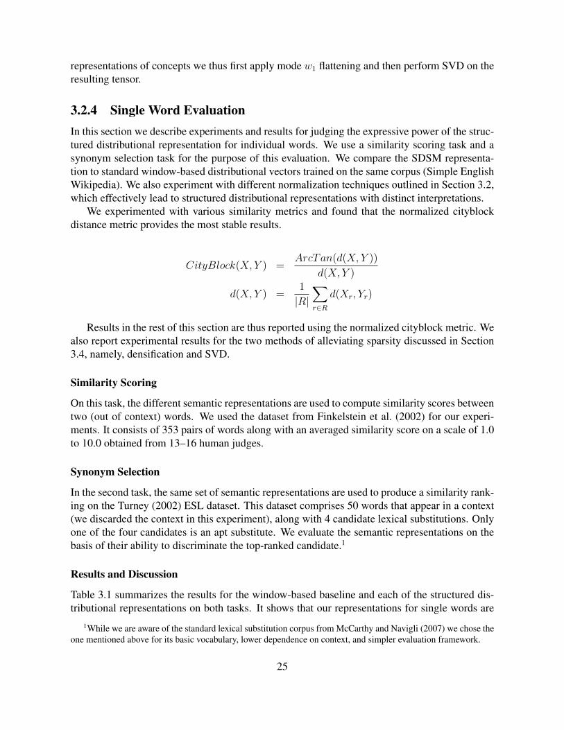
representations of concepts we thus first apply mode w1 flattening and then perform SVD on theresulting tensor.

3.2.4 Single Word EvaluationIn this section we describe experiments and results for judging the expressive power of the struc-tured distributional representation for individual words. We use a similarity scoring task and asynonym selection task for the purpose of this evaluation. We compare the SDSM representa-tion to standard window-based distributional vectors trained on the same corpus (Simple EnglishWikipedia). We also experiment with different normalization techniques outlined in Section 3.2,which effectively lead to structured distributional representations with distinct interpretations.

We experimented with various similarity metrics and found that the normalized cityblockdistance metric provides the most stable results.

CityBlock(X, Y ) =ArcTan(d(X, Y ))

d(X, Y )

d(X, Y ) =1

|R|∑r∈R

d(Xr, Yr)

Results in the rest of this section are thus reported using the normalized cityblock metric. Wealso report experimental results for the two methods of alleviating sparsity discussed in Section3.4, namely, densification and SVD.

Similarity Scoring

On this task, the different semantic representations are used to compute similarity scores betweentwo (out of context) words. We used the dataset from Finkelstein et al. (2002) for our experi-ments. It consists of 353 pairs of words along with an averaged similarity score on a scale of 1.0to 10.0 obtained from 13–16 human judges.

Synonym Selection

In the second task, the same set of semantic representations are used to produce a similarity rank-ing on the Turney (2002) ESL dataset. This dataset comprises 50 words that appear in a context(we discarded the context in this experiment), along with 4 candidate lexical substitutions. Onlyone of the four candidates is an apt substitute. We evaluate the semantic representations on thebasis of their ability to discriminate the top-ranked candidate.1

Results and Discussion

Table 3.1 summarizes the results for the window-based baseline and each of the structured dis-tributional representations on both tasks. It shows that our representations for single words are

1While we are aware of the standard lexical substitution corpus from McCarthy and Navigli (2007) we chose theone mentioned above for its basic vocabulary, lower dependence on context, and simpler evaluation framework.

25

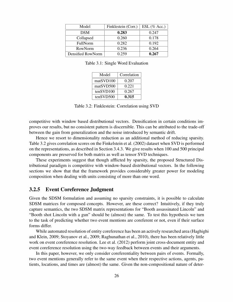
Model Finklestein (Corr.) ESL (% Acc.)DSM 0.283 0.247

Collapsed 0.260 0.178FullNorm 0.282 0.192RowNorm 0.236 0.264

Densified RowNorm 0.259 0.267

Table 3.1: Single Word Evaluation

Model CorrelationmatSVD100 0.207matSVD500 0.221tenSVD100 0.267tenSVD500 0.315

Table 3.2: Finklestein: Correlation using SVD

competitive with window based distributional vectors. Densification in certain conditions im-proves our results, but no consistent pattern is discernible. This can be attributed to the trade-offbetween the gain from generalization and the noise introduced by semantic drift.

Hence we resort to dimensionality reduction as an additional method of reducing sparsity.Table 3.2 gives correlation scores on the Finkelstein et al. (2002) dataset when SVD is performedon the representations, as described in Section 3.4.3. We give results when 100 and 500 principalcomponents are preserved for both matrix as well as tensor SVD techniques.

These experiments suggest that though afflicted by sparsity, the proposed Structured Dis-tributional paradigm is competitive with window-based distributional vectors. In the followingsections we show that that the framework provides considerably greater power for modelingcomposition when dealing with units consisting of more than one word.

3.2.5 Event Coreference JudgmentGiven the SDSM formulation and assuming no sparsity constraints, it is possible to calculateSDSM matrices for composed concepts. However, are these correct? Intuitively, if they trulycapture semantics, the two SDSM matrix representations for “Booth assassinated Lincoln” and“Booth shot Lincoln with a gun” should be (almost) the same. To test this hypothesis we turnto the task of predicting whether two event mentions are coreferent or not, even if their surfaceforms differ.

While automated resolution of entity coreference has been an actively researched area (Haghighiand Klein, 2009; Stoyanov et al., 2009; Raghunathan et al., 2010), there has been relatively littlework on event coreference resolution. Lee et al. (2012) perform joint cross-document entity andevent coreference resolution using the two-way feedback between events and their arguments.

In this paper, however, we only consider coreferentiality between pairs of events. Formally,two event mentions generally refer to the same event when their respective actions, agents, pa-tients, locations, and times are (almost) the same. Given the non-compositional nature of deter-

26

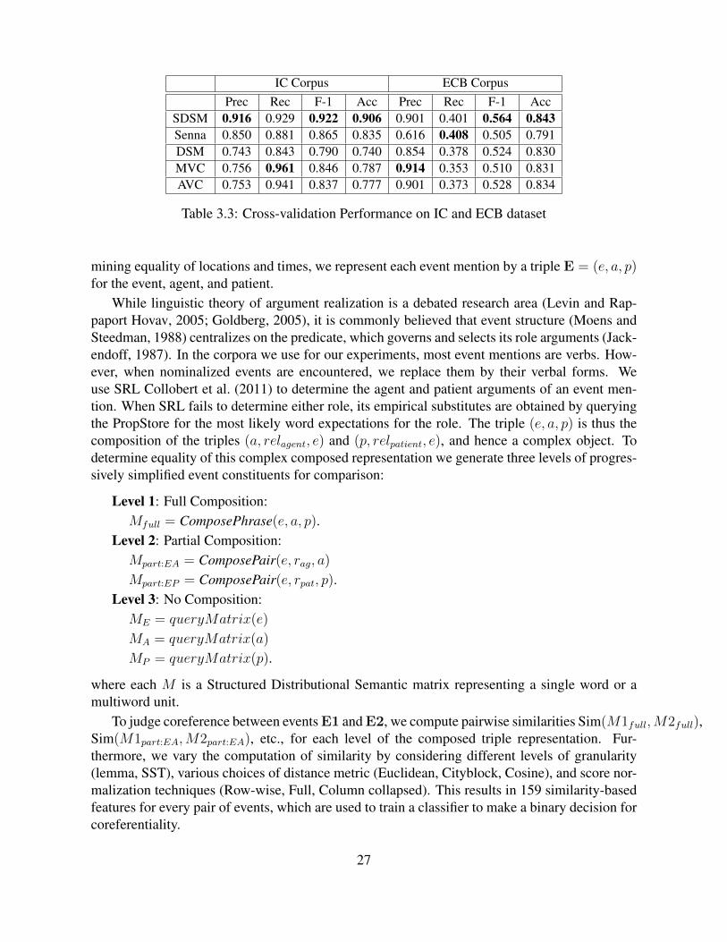
IC Corpus ECB CorpusPrec Rec F-1 Acc Prec Rec F-1 Acc

SDSM 0.916 0.929 0.922 0.906 0.901 0.401 0.564 0.843Senna 0.850 0.881 0.865 0.835 0.616 0.408 0.505 0.791DSM 0.743 0.843 0.790 0.740 0.854 0.378 0.524 0.830MVC 0.756 0.961 0.846 0.787 0.914 0.353 0.510 0.831AVC 0.753 0.941 0.837 0.777 0.901 0.373 0.528 0.834

Table 3.3: Cross-validation Performance on IC and ECB dataset

mining equality of locations and times, we represent each event mention by a triple E = (e, a, p)for the event, agent, and patient.

While linguistic theory of argument realization is a debated research area (Levin and Rap-paport Hovav, 2005; Goldberg, 2005), it is commonly believed that event structure (Moens andSteedman, 1988) centralizes on the predicate, which governs and selects its role arguments (Jack-endoff, 1987). In the corpora we use for our experiments, most event mentions are verbs. How-ever, when nominalized events are encountered, we replace them by their verbal forms. Weuse SRL Collobert et al. (2011) to determine the agent and patient arguments of an event men-tion. When SRL fails to determine either role, its empirical substitutes are obtained by queryingthe PropStore for the most likely word expectations for the role. The triple (e, a, p) is thus thecomposition of the triples (a, relagent, e) and (p, relpatient, e), and hence a complex object. Todetermine equality of this complex composed representation we generate three levels of progres-sively simplified event constituents for comparison:

Level 1: Full Composition:Mfull = ComposePhrase(e, a, p).

Level 2: Partial Composition:Mpart:EA = ComposePair(e, rag, a)

Mpart:EP = ComposePair(e, rpat, p).Level 3: No Composition:ME = queryMatrix(e)

MA = queryMatrix(a)

MP = queryMatrix(p).

where each M is a Structured Distributional Semantic matrix representing a single word or amultiword unit.

To judge coreference between events E1 and E2, we compute pairwise similarities Sim(M1full,M2full),Sim(M1part:EA,M2part:EA), etc., for each level of the composed triple representation. Fur-thermore, we vary the computation of similarity by considering different levels of granularity(lemma, SST), various choices of distance metric (Euclidean, Cityblock, Cosine), and score nor-malization techniques (Row-wise, Full, Column collapsed). This results in 159 similarity-basedfeatures for every pair of events, which are used to train a classifier to make a binary decision forcoreferentiality.

27

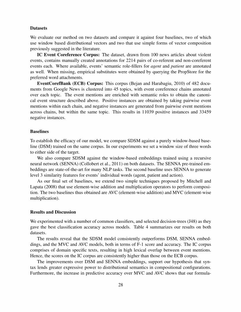
Datasets

We evaluate our method on two datasets and compare it against four baselines, two of whichuse window based distributional vectors and two that use simple forms of vector compositionpreviously suggested in the literature.

IC Event Coreference Corpus: The dataset, drawn from 100 news articles about violentevents, contains manually created annotations for 2214 pairs of co-referent and non-coreferentevents each. Where available, events’ semantic role-fillers for agent and patient are annotatedas well. When missing, empirical substitutes were obtained by querying the PropStore for thepreferred word attachments.

EventCorefBank (ECB) Corpus: This corpus (Bejan and Harabagiu, 2010) of 482 docu-ments from Google News is clustered into 45 topics, with event coreference chains annotatedover each topic. The event mentions are enriched with semantic roles to obtain the canoni-cal event structure described above. Positive instances are obtained by taking pairwise eventmentions within each chain, and negative instances are generated from pairwise event mentionsacross chains, but within the same topic. This results in 11039 positive instances and 33459negative instances.

Baselines

To establish the efficacy of our model, we compare SDSM against a purely window-based base-line (DSM) trained on the same corpus. In our experiments we set a window size of three wordsto either side of the target.

We also compare SDSM against the window-based embeddings trained using a recursiveneural network (SENNA) (Collobert et al., 2011) on both datasets. The SENNA pre-trained em-beddings are state-of-the-art for many NLP tasks. The second baseline uses SENNA to generatelevel 3 similarity features for events’ individual words (agent, patient and action).

As our final set of baselines, we extend two simple techniques proposed by Mitchell andLapata (2008) that use element-wise addition and multiplication operators to perform composi-tion. The two baselines thus obtained are AVC (element-wise addition) and MVC (element-wisemultiplication).

Results and Discussion

We experimented with a number of common classifiers, and selected decision-trees (J48) as theygave the best classification accuracy across models. Table 4 summarizes our results on bothdatasets.

The results reveal that the SDSM model consistently outperforms DSM, SENNA embed-dings, and the MVC and AVC models, both in terms of F-1 score and accuracy. The IC corpuscomprises of domain specific texts, resulting in high lexical overlap between event mentions.Hence, the scores on the IC corpus are consistently higher than those on the ECB corpus.

The improvements over DSM and SENNA embeddings, support our hypothesis that syn-tax lends greater expressive power to distributional semantics in compositional configurations.Furthermore, the increase in predictive accuracy over MVC and AVC shows that our formula-

28

tion of composition of two words based on the relation binding them yields a stronger form ofcomposition than simple additive and multiplicative models.

Next, we perform an ablation study to determine the most predictive features for the taskof determining event coreferentiality. The forward selection procedure reveals that the mostinformative attributes are the level 2 compositional features involving the agent and the action,as well as their individual level 3 features. This corresponds to the intuition that the agent andthe action are the principal determiners for identifying events. Features involving the patient andlevel 1 representations are least useful. The latter involve full composition, resulting in sparserepresentations and hence have low predictive power.

3.3 Latent Structured Distributional Semantics

We now turn to our second SDSM, which represents its relational dimensions as latent embed-dings obtained from matrix factorization. This SDSM tackles the problem of relational facets inmeaning comparison by moving away from syntax to a data-driven approach of choosing a setof relational dimensions.

One short-coming of DSMs derives from the fundamental nature of the vector space model,which characterizes the semantics of a word by a single vector in a high dimensional space (orsome lower dimensional embedding thereof).

Such a modelling paradigm goes against the grain of the intuition that the semantics of a wordis not unique. Rather, it is composed of many facets of meaning, and similarity (or dissimilarity)to other words is an outcome of the aggregate harmony (or dissonance) between the individualfacets under consideration. For example, a shirt may be similar along one facet to a balloon inthat they are both colored blue, at the same time being similar to a shoe along another facet forboth being articles of clothing, while being dissimilar along yet another facet to a t-shirt becauseone is stitched from linen while the other is made from polyester.

Of course, in this example the facets of comparison are sensitive to a particular context in-stance. But at an aggregate level one would be inclined to say that a shirt is most synonymous toa t-shirt because it evidences a high similarity along the principal facet of relevance, or relationbetween the two words. It is our belief, as a result, that the semantics of a word may be capturedmore effectively by considering its relations to other words and their composite distributionalsignature, rather than straightforwardly by co-occurrence statistics.

SDSMs in general provide a natural way of remedying this fault with DSMs by decomposingdistributional signatures over discrete relation dimensions, or facets. This leads to a represen-tation that characterizes the semantics of a word by a distributional tensor, whose constituentvectors each represent the semantic signature of a word along one particular relational facet ofmeaning.

In Section 3.2 we introduced one such SDSM. However it uses syntactic relational facetsfrom a dependency parser as surrogates for semantic ones. Other similar previous approachesinclude work by Pado and Lapata (2007) and Baroni and Lenci (2010).

There are limiting factors to this approximation. Most importantly, the set of syntactic re-lations, while relatively uncontroversial, is unable to capture the full extent of semantic nuanceencountered in natural language text. Often, syntax is ambiguous and leads to multiple semantic

29

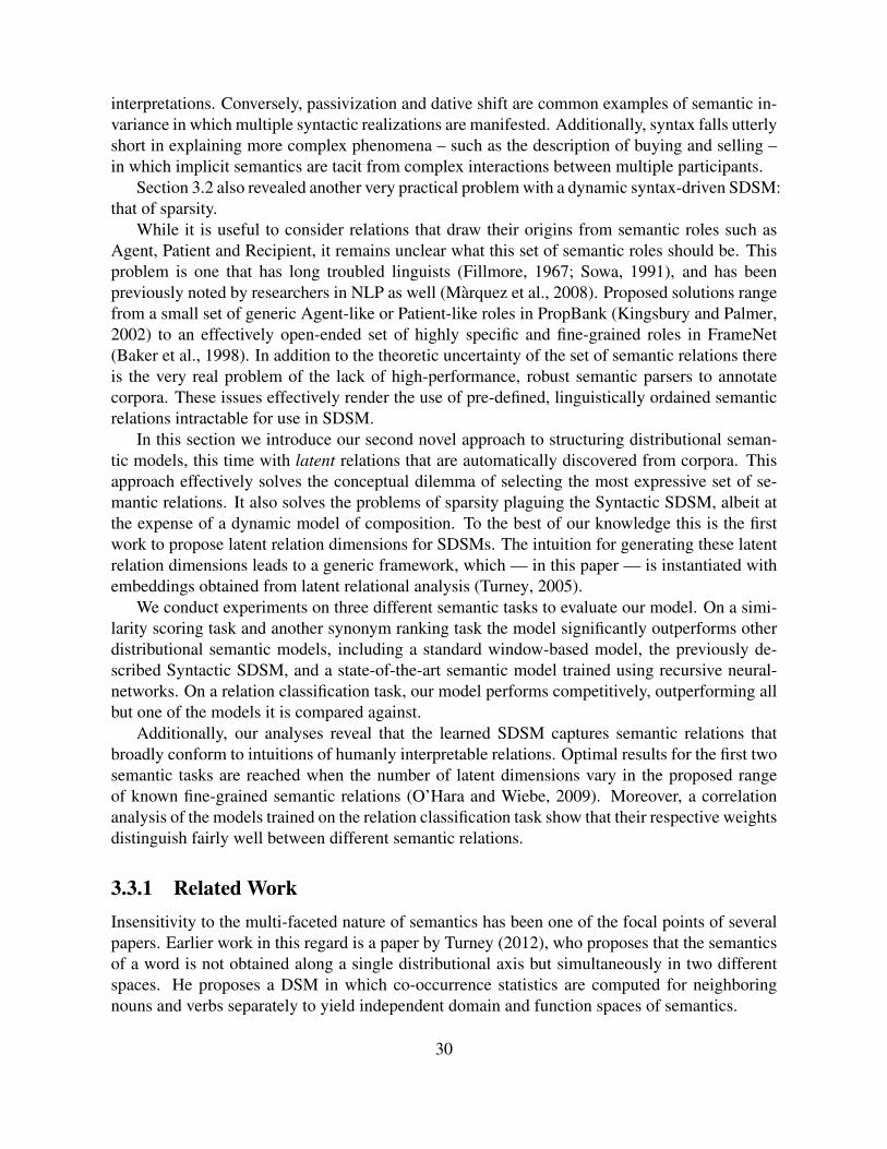
interpretations. Conversely, passivization and dative shift are common examples of semantic in-variance in which multiple syntactic realizations are manifested. Additionally, syntax falls utterlyshort in explaining more complex phenomena – such as the description of buying and selling –in which implicit semantics are tacit from complex interactions between multiple participants.

Section 3.2 also revealed another very practical problem with a dynamic syntax-driven SDSM:that of sparsity.

While it is useful to consider relations that draw their origins from semantic roles such asAgent, Patient and Recipient, it remains unclear what this set of semantic roles should be. Thisproblem is one that has long troubled linguists (Fillmore, 1967; Sowa, 1991), and has beenpreviously noted by researchers in NLP as well (Marquez et al., 2008). Proposed solutions rangefrom a small set of generic Agent-like or Patient-like roles in PropBank (Kingsbury and Palmer,2002) to an effectively open-ended set of highly specific and fine-grained roles in FrameNet(Baker et al., 1998). In addition to the theoretic uncertainty of the set of semantic relations thereis the very real problem of the lack of high-performance, robust semantic parsers to annotatecorpora. These issues effectively render the use of pre-defined, linguistically ordained semanticrelations intractable for use in SDSM.

In this section we introduce our second novel approach to structuring distributional seman-tic models, this time with latent relations that are automatically discovered from corpora. Thisapproach effectively solves the conceptual dilemma of selecting the most expressive set of se-mantic relations. It also solves the problems of sparsity plaguing the Syntactic SDSM, albeit atthe expense of a dynamic model of composition. To the best of our knowledge this is the firstwork to propose latent relation dimensions for SDSMs. The intuition for generating these latentrelation dimensions leads to a generic framework, which — in this paper — is instantiated withembeddings obtained from latent relational analysis (Turney, 2005).

We conduct experiments on three different semantic tasks to evaluate our model. On a simi-larity scoring task and another synonym ranking task the model significantly outperforms otherdistributional semantic models, including a standard window-based model, the previously de-scribed Syntactic SDSM, and a state-of-the-art semantic model trained using recursive neural-networks. On a relation classification task, our model performs competitively, outperforming allbut one of the models it is compared against.

Additionally, our analyses reveal that the learned SDSM captures semantic relations thatbroadly conform to intuitions of humanly interpretable relations. Optimal results for the first twosemantic tasks are reached when the number of latent dimensions vary in the proposed rangeof known fine-grained semantic relations (O’Hara and Wiebe, 2009). Moreover, a correlationanalysis of the models trained on the relation classification task show that their respective weightsdistinguish fairly well between different semantic relations.

3.3.1 Related WorkInsensitivity to the multi-faceted nature of semantics has been one of the focal points of severalpapers. Earlier work in this regard is a paper by Turney (2012), who proposes that the semanticsof a word is not obtained along a single distributional axis but simultaneously in two differentspaces. He proposes a DSM in which co-occurrence statistics are computed for neighboringnouns and verbs separately to yield independent domain and function spaces of semantics.

30

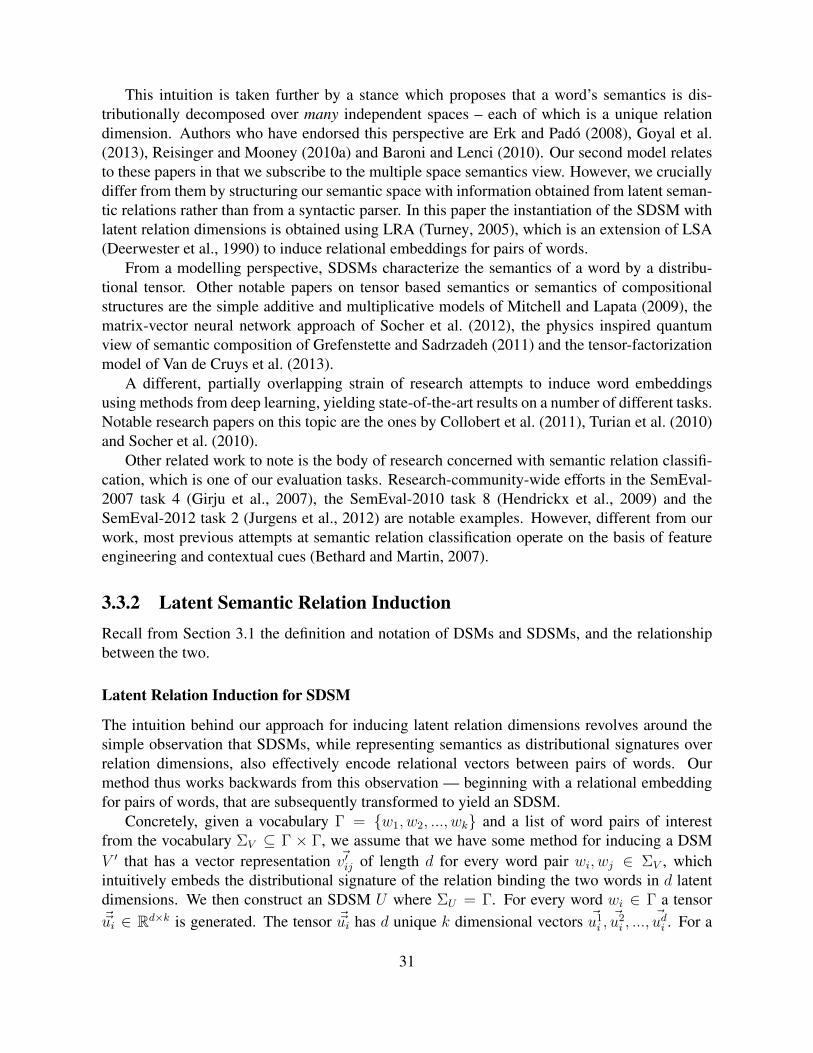
This intuition is taken further by a stance which proposes that a word’s semantics is dis-tributionally decomposed over many independent spaces – each of which is a unique relationdimension. Authors who have endorsed this perspective are Erk and Pado (2008), Goyal et al.(2013), Reisinger and Mooney (2010a) and Baroni and Lenci (2010). Our second model relatesto these papers in that we subscribe to the multiple space semantics view. However, we cruciallydiffer from them by structuring our semantic space with information obtained from latent seman-tic relations rather than from a syntactic parser. In this paper the instantiation of the SDSM withlatent relation dimensions is obtained using LRA (Turney, 2005), which is an extension of LSA(Deerwester et al., 1990) to induce relational embeddings for pairs of words.

From a modelling perspective, SDSMs characterize the semantics of a word by a distribu-tional tensor. Other notable papers on tensor based semantics or semantics of compositionalstructures are the simple additive and multiplicative models of Mitchell and Lapata (2009), thematrix-vector neural network approach of Socher et al. (2012), the physics inspired quantumview of semantic composition of Grefenstette and Sadrzadeh (2011) and the tensor-factorizationmodel of Van de Cruys et al. (2013).

A different, partially overlapping strain of research attempts to induce word embeddingsusing methods from deep learning, yielding state-of-the-art results on a number of different tasks.Notable research papers on this topic are the ones by Collobert et al. (2011), Turian et al. (2010)and Socher et al. (2010).

Other related work to note is the body of research concerned with semantic relation classifi-cation, which is one of our evaluation tasks. Research-community-wide efforts in the SemEval-2007 task 4 (Girju et al., 2007), the SemEval-2010 task 8 (Hendrickx et al., 2009) and theSemEval-2012 task 2 (Jurgens et al., 2012) are notable examples. However, different from ourwork, most previous attempts at semantic relation classification operate on the basis of featureengineering and contextual cues (Bethard and Martin, 2007).

3.3.2 Latent Semantic Relation InductionRecall from Section 3.1 the definition and notation of DSMs and SDSMs, and the relationshipbetween the two.

Latent Relation Induction for SDSM

The intuition behind our approach for inducing latent relation dimensions revolves around thesimple observation that SDSMs, while representing semantics as distributional signatures overrelation dimensions, also effectively encode relational vectors between pairs of words. Ourmethod thus works backwards from this observation — beginning with a relational embeddingfor pairs of words, that are subsequently transformed to yield an SDSM.

Concretely, given a vocabulary Γ = w1, w2, ..., wk and a list of word pairs of interestfrom the vocabulary ΣV ⊆ Γ × Γ, we assume that we have some method for inducing a DSMV ′ that has a vector representation ~v′ij of length d for every word pair wi, wj ∈ ΣV , whichintuitively embeds the distributional signature of the relation binding the two words in d latentdimensions. We then construct an SDSM U where ΣU = Γ. For every word wi ∈ Γ a tensor~~ui ∈ Rd×k is generated. The tensor ~~ui has d unique k dimensional vectors ~u1

i ,~u2i , ...,

~udi . For a

31

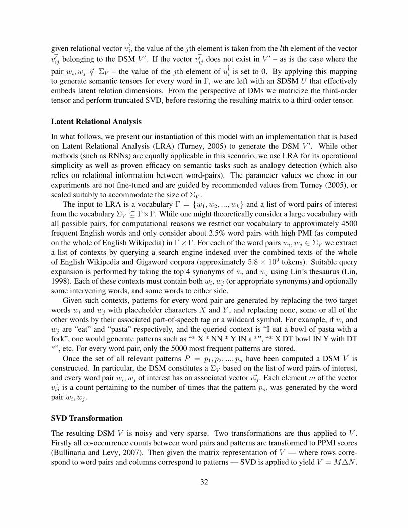
given relational vector ~uli, the value of the jth element is taken from the lth element of the vector~v′ij belonging to the DSM V ′. If the vector ~v′ij does not exist in V ′ – as is the case where the

pair wi, wj /∈ ΣV – the value of the jth element of ~uli is set to 0. By applying this mappingto generate semantic tensors for every word in Γ, we are left with an SDSM U that effectivelyembeds latent relation dimensions. From the perspective of DMs we matricize the third-ordertensor and perform truncated SVD, before restoring the resulting matrix to a third-order tensor.

Latent Relational Analysis

In what follows, we present our instantiation of this model with an implementation that is basedon Latent Relational Analysis (LRA) (Turney, 2005) to generate the DSM V ′. While othermethods (such as RNNs) are equally applicable in this scenario, we use LRA for its operationalsimplicity as well as proven efficacy on semantic tasks such as analogy detection (which alsorelies on relational information between word-pairs). The parameter values we chose in ourexperiments are not fine-tuned and are guided by recommended values from Turney (2005), orscaled suitably to accommodate the size of ΣV .

The input to LRA is a vocabulary Γ = w1, w2, ..., wk and a list of word pairs of interestfrom the vocabulary ΣV ⊆ Γ×Γ. While one might theoretically consider a large vocabulary withall possible pairs, for computational reasons we restrict our vocabulary to approximately 4500frequent English words and only consider about 2.5% word pairs with high PMI (as computedon the whole of English Wikipedia) in Γ×Γ. For each of the word pairs wi, wj ∈ ΣV we extracta list of contexts by querying a search engine indexed over the combined texts of the wholeof English Wikipedia and Gigaword corpora (approximately 5.8 × 109 tokens). Suitable queryexpansion is performed by taking the top 4 synonyms of wi and wj using Lin’s thesaurus (Lin,1998). Each of these contexts must contain both wi, wj (or appropriate synonyms) and optionallysome intervening words, and some words to either side.

Given such contexts, patterns for every word pair are generated by replacing the two targetwords wi and wj with placeholder characters X and Y , and replacing none, some or all of theother words by their associated part-of-speech tag or a wildcard symbol. For example, if wi andwj are “eat” and “pasta” respectively, and the queried context is “I eat a bowl of pasta with afork”, one would generate patterns such as “* X * NN * Y IN a *”, “* X DT bowl IN Y with DT*”, etc. For every word pair, only the 5000 most frequent patterns are stored.

Once the set of all relevant patterns P = p1, p2, ..., pn have been computed a DSM V isconstructed. In particular, the DSM constitutes a ΣV based on the list of word pairs of interest,and every word pair wi, wj of interest has an associated vector ~vij . Each element m of the vector~vij is a count pertaining to the number of times that the pattern pm was generated by the wordpair wi, wj .

SVD Transformation

The resulting DSM V is noisy and very sparse. Two transformations are thus applied to V .Firstly all co-occurrence counts between word pairs and patterns are transformed to PPMI scores(Bullinaria and Levy, 2007). Then given the matrix representation of V — where rows corre-spond to word pairs and columns correspond to patterns — SVD is applied to yield V = M∆N .

32

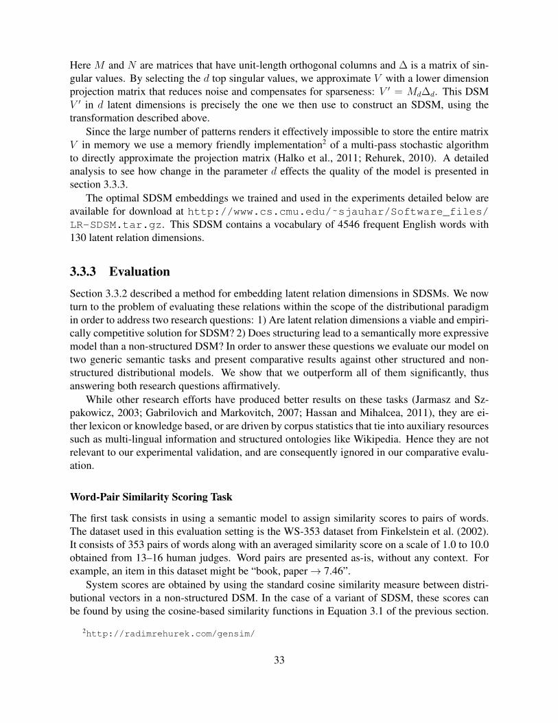
Here M and N are matrices that have unit-length orthogonal columns and ∆ is a matrix of sin-gular values. By selecting the d top singular values, we approximate V with a lower dimensionprojection matrix that reduces noise and compensates for sparseness: V ′ = Md∆d. This DSMV ′ in d latent dimensions is precisely the one we then use to construct an SDSM, using thetransformation described above.

Since the large number of patterns renders it effectively impossible to store the entire matrixV in memory we use a memory friendly implementation2 of a multi-pass stochastic algorithmto directly approximate the projection matrix (Halko et al., 2011; Rehurek, 2010). A detailedanalysis to see how change in the parameter d effects the quality of the model is presented insection 3.3.3.

The optimal SDSM embeddings we trained and used in the experiments detailed below areavailable for download at http://www.cs.cmu.edu/˜sjauhar/Software_files/LR-SDSM.tar.gz. This SDSM contains a vocabulary of 4546 frequent English words with130 latent relation dimensions.

3.3.3 EvaluationSection 3.3.2 described a method for embedding latent relation dimensions in SDSMs. We nowturn to the problem of evaluating these relations within the scope of the distributional paradigmin order to address two research questions: 1) Are latent relation dimensions a viable and empiri-cally competitive solution for SDSM? 2) Does structuring lead to a semantically more expressivemodel than a non-structured DSM? In order to answer these questions we evaluate our model ontwo generic semantic tasks and present comparative results against other structured and non-structured distributional models. We show that we outperform all of them significantly, thusanswering both research questions affirmatively.

While other research efforts have produced better results on these tasks (Jarmasz and Sz-pakowicz, 2003; Gabrilovich and Markovitch, 2007; Hassan and Mihalcea, 2011), they are ei-ther lexicon or knowledge based, or are driven by corpus statistics that tie into auxiliary resourcessuch as multi-lingual information and structured ontologies like Wikipedia. Hence they are notrelevant to our experimental validation, and are consequently ignored in our comparative evalu-ation.

Word-Pair Similarity Scoring Task

The first task consists in using a semantic model to assign similarity scores to pairs of words.The dataset used in this evaluation setting is the WS-353 dataset from Finkelstein et al. (2002).It consists of 353 pairs of words along with an averaged similarity score on a scale of 1.0 to 10.0obtained from 13–16 human judges. Word pairs are presented as-is, without any context. Forexample, an item in this dataset might be “book, paper→ 7.46”.

System scores are obtained by using the standard cosine similarity measure between distri-butional vectors in a non-structured DSM. In the case of a variant of SDSM, these scores canbe found by using the cosine-based similarity functions in Equation 3.1 of the previous section.

2http://radimrehurek.com/gensim/

33

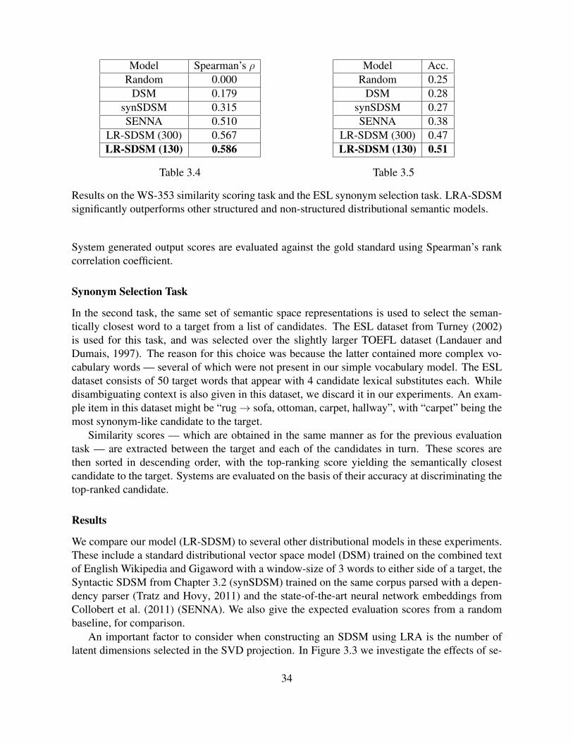
Model Spearman’s ρRandom 0.000

DSM 0.179synSDSM 0.315SENNA 0.510

LR-SDSM (300) 0.567LR-SDSM (130) 0.586

Table 3.4

Model Acc.Random 0.25

DSM 0.28synSDSM 0.27SENNA 0.38

LR-SDSM (300) 0.47LR-SDSM (130) 0.51

Table 3.5

Results on the WS-353 similarity scoring task and the ESL synonym selection task. LRA-SDSMsignificantly outperforms other structured and non-structured distributional semantic models.

System generated output scores are evaluated against the gold standard using Spearman’s rankcorrelation coefficient.

Synonym Selection Task

In the second task, the same set of semantic space representations is used to select the seman-tically closest word to a target from a list of candidates. The ESL dataset from Turney (2002)is used for this task, and was selected over the slightly larger TOEFL dataset (Landauer andDumais, 1997). The reason for this choice was because the latter contained more complex vo-cabulary words — several of which were not present in our simple vocabulary model. The ESLdataset consists of 50 target words that appear with 4 candidate lexical substitutes each. Whiledisambiguating context is also given in this dataset, we discard it in our experiments. An exam-ple item in this dataset might be “rug→ sofa, ottoman, carpet, hallway”, with “carpet” being themost synonym-like candidate to the target.

Similarity scores — which are obtained in the same manner as for the previous evaluationtask — are extracted between the target and each of the candidates in turn. These scores arethen sorted in descending order, with the top-ranking score yielding the semantically closestcandidate to the target. Systems are evaluated on the basis of their accuracy at discriminating thetop-ranked candidate.

Results

We compare our model (LR-SDSM) to several other distributional models in these experiments.These include a standard distributional vector space model (DSM) trained on the combined textof English Wikipedia and Gigaword with a window-size of 3 words to either side of a target, theSyntactic SDSM from Chapter 3.2 (synSDSM) trained on the same corpus parsed with a depen-dency parser (Tratz and Hovy, 2011) and the state-of-the-art neural network embeddings fromCollobert et al. (2011) (SENNA). We also give the expected evaluation scores from a randombaseline, for comparison.

An important factor to consider when constructing an SDSM using LRA is the number oflatent dimensions selected in the SVD projection. In Figure 3.3 we investigate the effects of se-

34

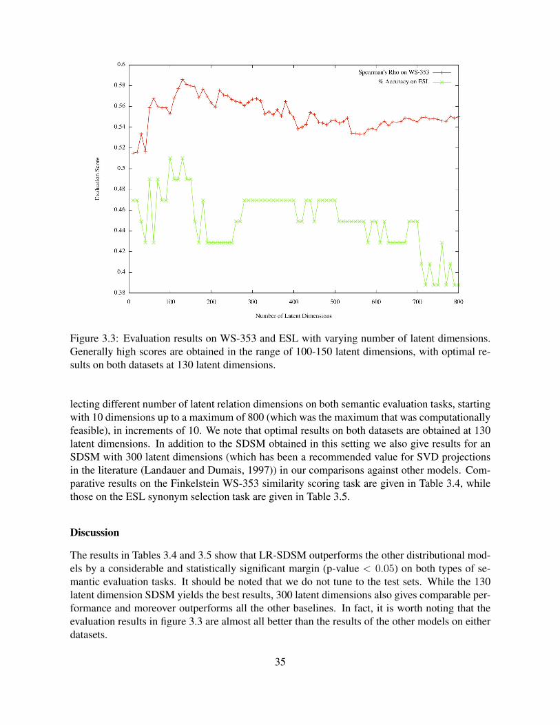
Figure 3.3: Evaluation results on WS-353 and ESL with varying number of latent dimensions.Generally high scores are obtained in the range of 100-150 latent dimensions, with optimal re-sults on both datasets at 130 latent dimensions.

lecting different number of latent relation dimensions on both semantic evaluation tasks, startingwith 10 dimensions up to a maximum of 800 (which was the maximum that was computationallyfeasible), in increments of 10. We note that optimal results on both datasets are obtained at 130latent dimensions. In addition to the SDSM obtained in this setting we also give results for anSDSM with 300 latent dimensions (which has been a recommended value for SVD projectionsin the literature (Landauer and Dumais, 1997)) in our comparisons against other models. Com-parative results on the Finkelstein WS-353 similarity scoring task are given in Table 3.4, whilethose on the ESL synonym selection task are given in Table 3.5.

Discussion

The results in Tables 3.4 and 3.5 show that LR-SDSM outperforms the other distributional mod-els by a considerable and statistically significant margin (p-value < 0.05) on both types of se-mantic evaluation tasks. It should be noted that we do not tune to the test sets. While the 130latent dimension SDSM yields the best results, 300 latent dimensions also gives comparable per-formance and moreover outperforms all the other baselines. In fact, it is worth noting that theevaluation results in figure 3.3 are almost all better than the results of the other models on eitherdatasets.

35

Random SENNA-MikDSM SENNA LR-SDSM

AVC MVC AVC MVCPrec. 0.111 0.273 0.419 0.382 0.489 0.416 0.431Rec. 0.110 0.343 0.449 0.443 0.516 0.457 0.475F-1. 0.110 0.288 0.426 0.383 0.499 0.429 0.444

% Acc. 11.03 34.30 44.91 44.26 51.55 45.65 47.48

Table 3.6: Results on Relation Classification Task. LR-SDSM scores competitively, outperform-ing all but the SENNA-AVC model.

We conclude that structuring of a semantic model with latent relational information in factleads to performance gains over non-structured variants. Also, the latent relation dimensions wepropose offer a viable and empirically competitive alternative to syntactic relations for SDSMs.

Figure 3.3 shows the evaluation results on both semantic tasks as a function of the numberof latent dimensions. The general trend of both curves on the figure indicate that the expressivepower of the model quickly increases with the number of dimensions until it peaks in the range of100–150, and then decreases or evens out after that. Interestingly, this falls roughly in the rangeof the 166 frequent (those that appear 50 times or more) frame elements, or fine-grained relations,from FrameNet that O’Hara and Wiebe (2009) find in their taxonomization and mapping of anumber of lexical resources that contain semantic relations.

3.3.4 Semantic Relation Classification and Analysis of the Latent Struc-ture of Dimensions

In this section we conduct experiments on the task of semantic relation classification. We alsoperform a more detailed analysis of the induced latent relation dimensions in order to gain insightinto our model’s perception of semantic relations.

Semantic Relation Classification

In this task, a relational embedding is used as a feature vector to train a classifier for predictingthe semantic relation between previously unseen word pairs. The dataset used in this experi-ment is from the SemEval-2012 task 2 on measuring the degree of relational similarity (Jurgenset al., 2012), since it characterizes a number of very distinct and interesting semantic relations.In particular it consists of an aggregated set of 3464 word pairs evidencing 10 kinds of seman-tic relations. We prune this set to discard pairs that don’t contain words in the vocabularies ofthe models we consider in our experiments. This leaves us with a dataset containing 933 wordpairs in 9 classes (1 class was discarded altogether because it contained too few instances). The9 semantic relation classes are: “Class Inclusion”, “Part-Whole”, “Similar”, “Contrast”, “At-tribute”, “Non-Attribute”, “Case Relation”, “Cause-Purpose” and “Space-Time”. For example,an instance of a word pair that exemplifies the “Part-Whole” relationship is “engine:car”. Notethat, as with previous experiments, word pairs are given without any context.

36

Results

We compare LR-SDSM on the semantic relation classification task to several different mod-els. These include the additive vector composition (AVC) and multiplicative vector compositionmethods (MVC) proposed by Mitchell and Lapata (2009); we present both DSM and SENNAbased variants of these models. We also compare against the vector difference method of Mikolovet al. (2013c) (SENNA-Mik) which sees semantic relations as a meaning preserving vector trans-lation in an RNN embedded vector space. Finally, we note the performance of random classifi-cation as a baseline, for reference. We attempted to produce results of a syntactic SDSM on thetask; however, the hard constraint imposed by syntactic adjacency meant that effectively all theword pairs in the dataset yielded zero feature vectors.

To avoid overfitting on all 130 original dimensions in our optimal SDSM, and also to renderresults comparable, we reduce the number of latent relation dimensions of LR-SDSM to 50. Wesimilarly reduce the feature vector dimension of DSM-AVC and DSM-MVC to 50 by featureselection. The dimensions of SENNA-AVC, SENNA-MVC and SENNA-Mik are already 50,and are not reduced further.

For each of the methods we train a logistic regression classifier. We don’t perform any tuningof parameters and set a constant ridge regression value of 0.2, which seemed to yield roughly thebest results for all models. The performance on the semantic relation classification task in termsof averaged precision, recall, F-measure and percentage accuracy using 10-fold cross-validationis given in Table 3.6.

Additionally, to gain further insight into the LR-SDSM’s understanding of semantic relations,we conduct a secondary analysis. We begin by training 9 one-vs-all logistic regression classifiersfor each of the 9 semantic relations under consideration. Then pairwise correlation distances aremeasured between all pairs of weight vectors of the 9 models. Finally, the distance adjacencymatrix is projected into 2-d space using multidimensional scaling. The result of this analysis ispresented in Figure 3.4.

Discussion

Table 3.6 shows that LR-SDSM performs competitively on the relation classification task andoutperforms all but one of the other models. The performance differences are statistically sig-nificant with a p-value < 0.5. We believe that some of the expressive power of the model is lostby compressing to 50 latent relation dimensions, and that a greater number of dimensions mightimprove performance. However, testing a model with a 130-length dense feature vector on adataset containing 933 instances would likely lead to overfitting and also not be comparable tothe SENNA-based models that operate on 50-length feature vectors.

Other points to note from Table 3.6 are that the AVC variants of the the DSM and SENNAcomposition models tend to perform better than their MVC counterparts. Also, SENNA-Mikperforms surprisingly poorly. It is worth noting, however, that Mikolov et al. (2013c) reportresults on fairly simple lexico-syntactic relations between words – such as plural forms, posses-sives and gender – while the semantic relations under consideration in the SemEval-2012 datasetare relatively more complex.

In the analysis of the latent structure of dimensions presented in Figure 3.4, there are few

37

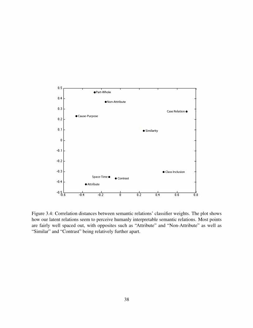
Figure 3.4: Correlation distances between semantic relations’ classifier weights. The plot showshow our latent relations seem to perceive humanly interpretable semantic relations. Most pointsare fairly well spaced out, with opposites such as “Attribute” and “Non-Attribute” as well as“Similar” and “Contrast” being relatively further apart.

38

interesting points to note. To begin with, all the points (with the exception of one pair) are fairlywell spaced out. At the weight vector level, this implies that different latent dimensions needto fire in different combinations to characterize distinct semantic relations, thus resulting in lowcorrelation between their corresponding weight vectors. This indicates the fact that the latent re-lation dimensions seem to capture the intuition that each of the classes encodes a distinctly differ-ent semantic relation. The notable exception is “Space-Time”, which is very close to “Contrast”.This is probably due to the fact that distributional models are ineffective at capturing spatio-temporal semantics. Moreover, it is interesting to note that “Attribute” and “Non-Attribute” aswell as “Similar” and “Contrast”, which are intuitively semantic inverses of each other are also(relatively) distant from each other in the plot.

These general findings indicate an interesting avenue for future research, which involvesmapping the empirically learnt latent relations to hand-built semantic lexicons or frameworks.This could help to validate the empirical models at various levels of linguistic granularity, aswell as establish correspondences between different views of semantic representation.

3.4 ConclusionIn this chapter we outlined a general framework of representing semantics with a more expressiveStructured Distributional formalism. This formalism tackled the problem of context-sensitivityand facetedness in semantics by a model that decomposes a vector representation into severaldiscrete relation dimensions. We proposed two novel models that each instantiated these relationdimensions in a different way.

The first used dependency syntax and introduced a dynamic model that was capable of com-posing units into complex structure by taking relational context into account. By doing so iteffectively tackled the problem of context-sensitivity in semantics. The Syntactic SDSM we in-troduced showed promising results on event coreference judgment, a task that specifically bringsthe problem of contextual variability into focus.

Our second instantiation of relation dimensions was a model that learnt a set of latent rela-tions from contextual pattern occurrences. This approach was better suited to resolve the issueof facetedness in semantics, or the facets along which a word may be represented or compared.It’s data-driven approach allowed the SDSM to move away from syntax (and any set schema ofrelations for that matter), while also tackling the problem of sparsity that plagued the SyntacticSDSM. Experimental results of the model supported our claim that the Latent SDSM capturesthe semantics of words more effectively than a number of other semantic models, and presentsa viable — and empirically competitive — alternative to Syntactic SDSMs. Finally, our anal-yses to investigate the structure of, and interactions between, the latent relation dimensions re-vealed some interesting tendencies on how they represented and differentiated between known,humanly-interpretable relations.

39

40

Chapter 4

Ontologies and Polysemy

Using Ontological Relation Links to Learn Sense-specific Word Representations

of Polysemy

Words are polysemous. However, most approaches to representation learning for lexical seman-tics assign a single vector to every surface word type. They thus ignore the possibility that wordsmay have more than one meaning. For example, the word “bank” can either denote a financialinstitution or the shore of a river. The ability to model multiple meanings is an important com-ponent of any NLP system, given how common polysemy is in language. The lack of senseannotated corpora large enough to robustly train VSMs, and the absence of fast, high qualityword sense disambiguation (WSD) systems makes handling polysemy difficult.

Meanwhile, lexical ontologies, such as WordNet (Miller, 1995a) specifically catalog senseinventories and provide typologies that link these senses to one another. These ontologies typi-cally encode structure and connectedness between concepts through relations, such as synonymy,hypernymy and hyponymy. Data in this form provides a complementary source of informationto distributional statistics. Its relation-induced semantic structure also falls into the overarchingtheme of this thesis as a potential source of structured knowledge that can be leveraged to learnmore expressive models of semantics.

Recent research tries to leverage ontological information to train better VSMs (Yu and Dredze,2014; Faruqui et al., 2014), but does not tackle the problem of polysemy. Parallely, work on poly-semy for VSMs revolves primarily around techniques that cluster contexts to distinguish betweendifferent word senses (Reisinger and Mooney, 2010b; Huang et al., 2012), but does not integrateontologies in any way.

In this chapter we present two novel approaches to integrating ontological and distributionalsources of information. Our focus is on allowing already existing, proven techniques to beadapted to produce ontologically grounded word sense embeddings. Our first technique is appli-cable to any sense-agnostic VSM as a post-processing step that performs graph propagation onthe structure of the ontology. The second is applicable to the wide range of current techniquesthat learn word embeddings from predictive models that maximize the likelihood of a corpus(Collobert and Weston, 2008; Mnih and Teh, 2012; Mikolov et al., 2013a). Our technique adds

41

a latent variable representing the word sense to each token in the corpus, and uses EM to findparameters. Using a structured regularizer based on the ontological graph, we learn groundedsense-specific vectors.

Both techniques crucially rely on the structure of the underlying ontology, and the relationsthat bind related word senses to one another.

There are several reasons to prefer ontologies as distant sources of supervision for learningsense-aware VSMs over previously proposed unsupervised context clustering techniques. Clus-tering approaches must often parametrize the number of clusters (senses), which is neither knowna priori nor constant across words (Kilgarriff, 1997). Also the resulting vectors remain abstractand uninterpretable. With ontologies, interpretable sense vectors can be used in downstreamapplications such as WSD, or for better human error analysis. Moreover, clustering techniquesoperate on distributional similarity only whereas ontologies support other kinds of relationshipsbetween senses. Finally, the existence of cross-lingual ontologies would permit learning multi-lingual vectors, without compounded errors from word alignment and context clustering.

We evaluate our methods on 4 lexical semantic tasks across 9 datasets and 2 languages, andshow that our sense-specific VSMs effectively integrate knowledge from the ontology with dis-tributional statistics. Empirically, this results in consistently and significantly better performanceover baselines in most cases. We discuss and compare our two different approaches to learn-ing sense representations from the perspectives of performance, generalizability, flexibility andcomputational efficiency. Finally, we qualitatively analyze the vectors and show that they indeedcapture sense-specific semantics.

4.1 Related Work

Since Reisinger and Mooney (2010b) first proposed a simple context clustering technique togenerate multi-prototype VSMs, a number of related efforts have worked on adaptations andimprovements relying on the same clustering principle. Huang et al. (2012) train their vectorswith a neural network and additionally take global context into account. Neelakantan et al.(2014) extend the popular skip-gram model (Mikolov et al., 2013a) in a non-parametric fashionto allow for different number of senses for words. Guo et al. (2014) exploit bilingual alignmentsto perform better context clustering during training. Tian et al. (2014) propose a probabilisticextension to skip-gram that treats the different prototypes as latent variables. This is similar toour second EM training framework, and turns out to be a special case of our general model. In allthese papers, however, the multiple senses remain abstract and are not grounded in an ontology.

Conceptually, our work is also similar to Yu and Dredze (2014) and Faruqui et al. (2014), whotreat lexicons such as the paraphrase database (PPDB) (Ganitkevitch et al., 2013) or WordNet(Miller, 1995a) as an auxiliary thesaurus to improve VSMs. However, they do not model sensesin any way. Pilehvar et al. (2013) do model senses from an ontology by performing random-walks on the WordNet graph, however their approach does not take distributional informationfrom VSMs into account.

Thus, to the best of our knowledge, our work presents the first attempt at producing sensegrounded VSMs that are symbolically tied to lexical ontologies. From a modelling point ofview, it is also the first to outline a unified, principled and extensible framework that effectively

42

combines the symbolic and distributional paradigms of semantics by specifically paying attentionto relational structure.

Both our models leverage the graph structure of and relational links in ontologies to effec-tively ground the senses of a VSM. This ties into previous research (Das and Smith, 2011; Dasand Petrov, 2011) that propagates information through a factor graph to perform tasks such asframe-semantic parsing and POS-tagging across languages. More generally, this approach can beviewed from the perspective of semi-supervised learning, with an optimization over a graph lossfunction defined on smoothness properties (Corduneanu and Jaakkola, 2002; Zhu et al., 2003;Subramanya and Bilmes, 2009).

Related to the problem of polysemy is the issue of different shades of meaning a word as-sumes based on context. The space of research on this topic can be divided into three broadcategories: models for computing contextual lexical semantics based on composition (Mitchelland Lapata, 2008; Erk and Pado, 2008; Thater et al., 2011), models that use fuzzy exemplar-based contexts without composing them (Erk and Pado, 2010; Reddy et al., 2011), and modelsthat propose latent variable techniques (Dinu and Lapata, 2010b; Seaghdha and Korhonen, 2011;Van de Cruys et al., 2011). Chapter 3 addresses the first of the three categories with a StructuredDistributional Semantic Model that takes relational context into account. The current chapter,however, tackles the stronger form of lexical ambiguity in polysemy and falls into the latter twoof three categories.

4.2 Unified Symbolic and Distributional Semantics

In this section, we present our two techniques for inferring sense-specific vectors grounded inan ontology. We begin with notation. Let W = w1, ..., wn be a set of word types, and Ws =sij | ∀wi ∈ W , 1 ≤ j ≤ ki a set of senses, with ki the number of senses of wi. Moreover, letΩ = (TΩ, EΩ) be an ontology represented by an undirected graph. The vertices TΩ = tij| ∀ sij ∈Ws correspond to the word senses in the set Ws, while the edges EΩ = erij−i′j′ connect somesubset of word sense pairs (sij, si′j′) by semantic relation r1.

4.2.1 Retrofitting Vectors to an OntologyOur first technique assumes that we already have a vector space embedding of a vocabularyU = ui| ∀ wi ∈ W. We wish to infer vectors V = vij| ∀ sij ∈ Ws for word senses thatare maximally consistent with both U and Ω, by some notion of consistency. We formalize thisnotion as MAP inference in a Markov network (MN).

The MN we propose contains variables for every vector in U and V . These variables areconnected to one another by dependencies as follows. Variables for vectors vij and vi′j′ areconnected iff there exists an edge erij−i′j′ ∈ EΩ connecting their respective word senses in theontology. Furthermore, vectors ui for the word types wi are each connected to all the vectors vijof the different senses sij of wi. If wi is not contained in the ontology, we assume it has a singleunconnected sense and set it’s only sense vector vi1 to it’s empirical estimate ui.

1For example there might be a “synonym” edge between the word senses “cat(1)” and “feline(1)”.

43

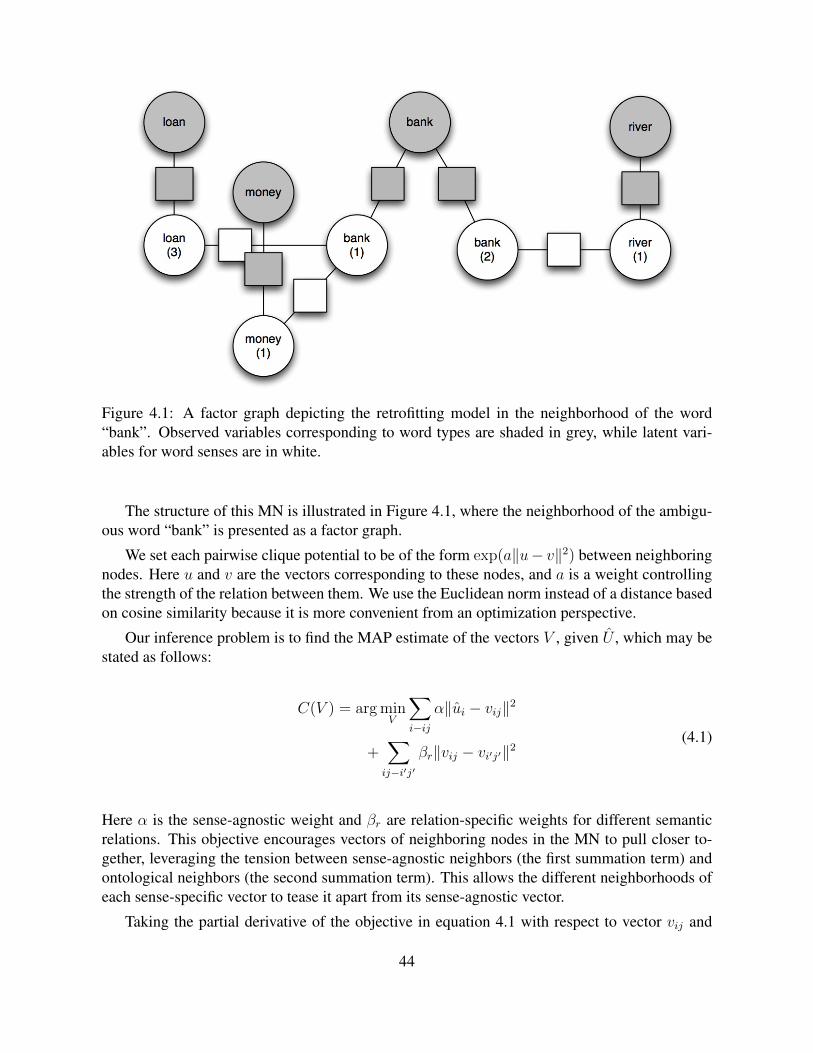
Figure 4.1: A factor graph depicting the retrofitting model in the neighborhood of the word“bank”. Observed variables corresponding to word types are shaded in grey, while latent vari-ables for word senses are in white.

The structure of this MN is illustrated in Figure 4.1, where the neighborhood of the ambigu-ous word “bank” is presented as a factor graph.

We set each pairwise clique potential to be of the form exp(a‖u− v‖2) between neighboringnodes. Here u and v are the vectors corresponding to these nodes, and a is a weight controllingthe strength of the relation between them. We use the Euclidean norm instead of a distance basedon cosine similarity because it is more convenient from an optimization perspective.

Our inference problem is to find the MAP estimate of the vectors V , given U , which may bestated as follows:

C(V ) = arg minV

∑i−ij

α‖ui − vij‖2

+∑ij−i′j′

βr‖vij − vi′j′‖2(4.1)

Here α is the sense-agnostic weight and βr are relation-specific weights for different semanticrelations. This objective encourages vectors of neighboring nodes in the MN to pull closer to-gether, leveraging the tension between sense-agnostic neighbors (the first summation term) andontological neighbors (the second summation term). This allows the different neighborhoods ofeach sense-specific vector to tease it apart from its sense-agnostic vector.

Taking the partial derivative of the objective in equation 4.1 with respect to vector vij and

44

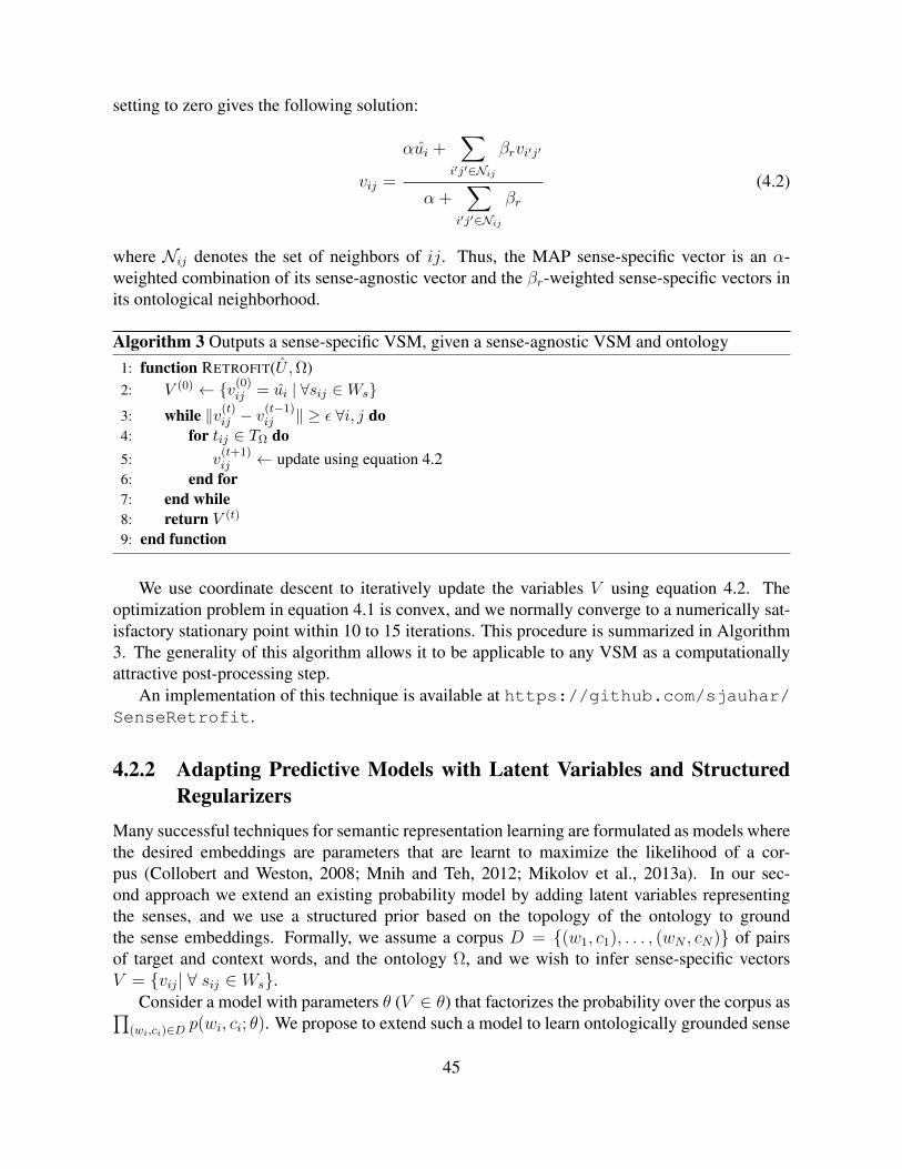
setting to zero gives the following solution:

vij =

αui +∑

i′j′∈Nij

βrvi′j′

α +∑

i′j′∈Nij

βr(4.2)

where Nij denotes the set of neighbors of ij. Thus, the MAP sense-specific vector is an α-weighted combination of its sense-agnostic vector and the βr-weighted sense-specific vectors inits ontological neighborhood.

Algorithm 3 Outputs a sense-specific VSM, given a sense-agnostic VSM and ontology1: function RETROFIT(U ,Ω)2: V (0) ← v(0)

ij = ui | ∀sij ∈Ws3: while ‖v(t)

ij − v(t−1)ij ‖ ≥ ε ∀i, j do

4: for tij ∈ TΩ do5: v

(t+1)ij ← update using equation 4.2

6: end for7: end while8: return V (t)

9: end function

We use coordinate descent to iteratively update the variables V using equation 4.2. Theoptimization problem in equation 4.1 is convex, and we normally converge to a numerically sat-isfactory stationary point within 10 to 15 iterations. This procedure is summarized in Algorithm3. The generality of this algorithm allows it to be applicable to any VSM as a computationallyattractive post-processing step.

An implementation of this technique is available at https://github.com/sjauhar/SenseRetrofit.

4.2.2 Adapting Predictive Models with Latent Variables and StructuredRegularizers

Many successful techniques for semantic representation learning are formulated as models wherethe desired embeddings are parameters that are learnt to maximize the likelihood of a cor-pus (Collobert and Weston, 2008; Mnih and Teh, 2012; Mikolov et al., 2013a). In our sec-ond approach we extend an existing probability model by adding latent variables representingthe senses, and we use a structured prior based on the topology of the ontology to groundthe sense embeddings. Formally, we assume a corpus D = (w1, c1), . . . , (wN , cN) of pairsof target and context words, and the ontology Ω, and we wish to infer sense-specific vectorsV = vij| ∀ sij ∈ Ws.

Consider a model with parameters θ (V ∈ θ) that factorizes the probability over the corpus as∏(wi,ci)∈D p(wi, ci; θ). We propose to extend such a model to learn ontologically grounded sense

45

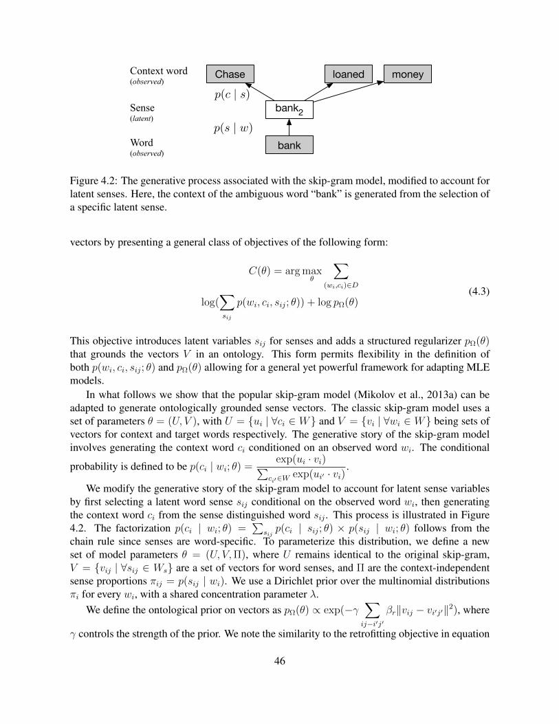
Chase loaned money

bank2

bankp(s | w)

p(c | s)

Context word(observed)

Sense(latent)

Word(observed)

Figure 4.2: The generative process associated with the skip-gram model, modified to account forlatent senses. Here, the context of the ambiguous word “bank” is generated from the selection ofa specific latent sense.

vectors by presenting a general class of objectives of the following form:

C(θ) = arg maxθ

∑(wi,ci)∈D

log(∑sij

p(wi, ci, sij; θ)) + log pΩ(θ)(4.3)

This objective introduces latent variables sij for senses and adds a structured regularizer pΩ(θ)that grounds the vectors V in an ontology. This form permits flexibility in the definition ofboth p(wi, ci, sij; θ) and pΩ(θ) allowing for a general yet powerful framework for adapting MLEmodels.

In what follows we show that the popular skip-gram model (Mikolov et al., 2013a) can beadapted to generate ontologically grounded sense vectors. The classic skip-gram model uses aset of parameters θ = (U, V ), with U = ui | ∀ci ∈ W and V = vi | ∀wi ∈ W being sets ofvectors for context and target words respectively. The generative story of the skip-gram modelinvolves generating the context word ci conditioned on an observed word wi. The conditional

probability is defined to be p(ci | wi; θ) =exp(ui · vi)∑

ci′∈Wexp(ui′ · vi)

.

We modify the generative story of the skip-gram model to account for latent sense variablesby first selecting a latent word sense sij conditional on the observed word wi, then generatingthe context word ci from the sense distinguished word sij . This process is illustrated in Figure4.2. The factorization p(ci | wi; θ) =

∑sijp(ci | sij; θ) × p(sij | wi; θ) follows from the

chain rule since senses are word-specific. To parameterize this distribution, we define a newset of model parameters θ = (U, V,Π), where U remains identical to the original skip-gram,V = vij | ∀sij ∈ Ws are a set of vectors for word senses, and Π are the context-independentsense proportions πij = p(sij | wi). We use a Dirichlet prior over the multinomial distributionsπi for every wi, with a shared concentration parameter λ.

We define the ontological prior on vectors as pΩ(θ) ∝ exp(−γ∑ij−i′j′

βr‖vij − vi′j′‖2), where

γ controls the strength of the prior. We note the similarity to the retrofitting objective in equation

46

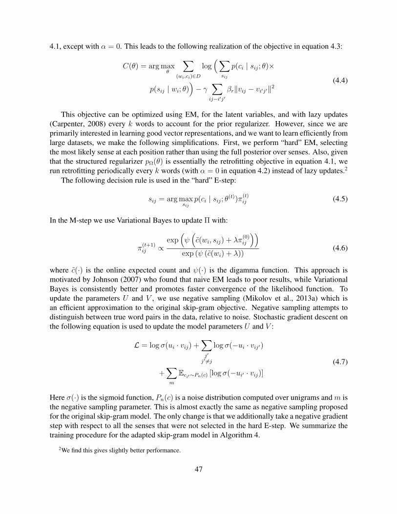
4.1, except with α = 0. This leads to the following realization of the objective in equation 4.3:

C(θ) = arg maxθ

∑(wi,ci)∈D

log(∑

sij

p(ci | sij; θ)×

p(sij | wi; θ))− γ

∑ij−i′j′

βr‖vij − vi′j′‖2(4.4)

This objective can be optimized using EM, for the latent variables, and with lazy updates(Carpenter, 2008) every k words to account for the prior regularizer. However, since we areprimarily interested in learning good vector representations, and we want to learn efficiently fromlarge datasets, we make the following simplifications. First, we perform “hard” EM, selectingthe most likely sense at each position rather than using the full posterior over senses. Also, giventhat the structured regularizer pΩ(θ) is essentially the retrofitting objective in equation 4.1, werun retrofitting periodically every k words (with α = 0 in equation 4.2) instead of lazy updates.2

The following decision rule is used in the “hard” E-step:

sij = arg maxsij

p(ci | sij; θ(t))π(t)ij (4.5)

In the M-step we use Variational Bayes to update Π with:

π(t+1)ij ∝

exp(ψ(c(wi, sij) + λπ

(0)ij

))exp (ψ (c(wi) + λ))

(4.6)

where c(·) is the online expected count and ψ(·) is the digamma function. This approach ismotivated by Johnson (2007) who found that naive EM leads to poor results, while VariationalBayes is consistently better and promotes faster convergence of the likelihood function. Toupdate the parameters U and V , we use negative sampling (Mikolov et al., 2013a) which isan efficient approximation to the original skip-gram objective. Negative sampling attempts todistinguish between true word pairs in the data, relative to noise. Stochastic gradient descent onthe following equation is used to update the model parameters U and V :

L = log σ(ui · vij) +∑j′

j′ 6=j

log σ(−ui · vij′)

+∑m

Eci′∼Pn(c) [log σ(−ui′ · vij)](4.7)

Here σ(·) is the sigmoid function, Pn(c) is a noise distribution computed over unigrams and m isthe negative sampling parameter. This is almost exactly the same as negative sampling proposedfor the original skip-gram model. The only change is that we additionally take a negative gradientstep with respect to all the senses that were not selected in the hard E-step. We summarize thetraining procedure for the adapted skip-gram model in Algorithm 4.

2We find this gives slightly better performance.

47

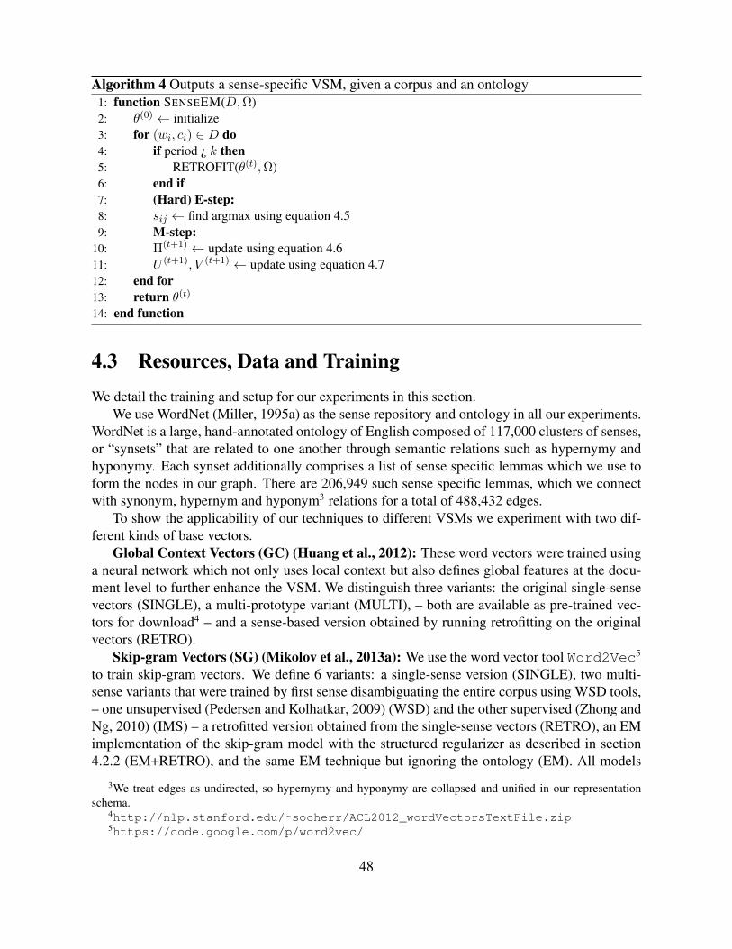
Algorithm 4 Outputs a sense-specific VSM, given a corpus and an ontology1: function SENSEEM(D,Ω)2: θ(0) ← initialize3: for (wi, ci) ∈ D do4: if period ¿ k then5: RETROFIT(θ(t),Ω)6: end if7: (Hard) E-step:8: sij ← find argmax using equation 4.59: M-step:

10: Π(t+1) ← update using equation 4.611: U (t+1), V (t+1) ← update using equation 4.712: end for13: return θ(t)

14: end function

4.3 Resources, Data and TrainingWe detail the training and setup for our experiments in this section.

We use WordNet (Miller, 1995a) as the sense repository and ontology in all our experiments.WordNet is a large, hand-annotated ontology of English composed of 117,000 clusters of senses,or “synsets” that are related to one another through semantic relations such as hypernymy andhyponymy. Each synset additionally comprises a list of sense specific lemmas which we use toform the nodes in our graph. There are 206,949 such sense specific lemmas, which we connectwith synonym, hypernym and hyponym3 relations for a total of 488,432 edges.

To show the applicability of our techniques to different VSMs we experiment with two dif-ferent kinds of base vectors.

Global Context Vectors (GC) (Huang et al., 2012): These word vectors were trained usinga neural network which not only uses local context but also defines global features at the docu-ment level to further enhance the VSM. We distinguish three variants: the original single-sensevectors (SINGLE), a multi-prototype variant (MULTI), – both are available as pre-trained vec-tors for download4 – and a sense-based version obtained by running retrofitting on the originalvectors (RETRO).

Skip-gram Vectors (SG) (Mikolov et al., 2013a): We use the word vector tool Word2Vec5

to train skip-gram vectors. We define 6 variants: a single-sense version (SINGLE), two multi-sense variants that were trained by first sense disambiguating the entire corpus using WSD tools,– one unsupervised (Pedersen and Kolhatkar, 2009) (WSD) and the other supervised (Zhong andNg, 2010) (IMS) – a retrofitted version obtained from the single-sense vectors (RETRO), an EMimplementation of the skip-gram model with the structured regularizer as described in section4.2.2 (EM+RETRO), and the same EM technique but ignoring the ontology (EM). All models

3We treat edges as undirected, so hypernymy and hyponymy are collapsed and unified in our representationschema.

4http://nlp.stanford.edu/˜socherr/ACL2012_wordVectorsTextFile.zip5https://code.google.com/p/word2vec/

48

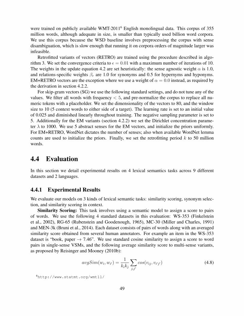
were trained on publicly available WMT-20116 English monolingual data. This corpus of 355million words, although adequate in size, is smaller than typically used billion word corpora.We use this corpus because the WSD baseline involves preprocessing the corpus with sensedisambiguation, which is slow enough that running it on corpora orders of magnitude larger wasinfeasible.

Retrofitted variants of vectors (RETRO) are trained using the procedure described in algo-rithm 3. We set the convergence criteria to ε = 0.01 with a maximum number of iterations of 10.The weights in the update equation 4.2 are set heuristically: the sense agnostic weight α is 1.0,and relations-specific weights βr are 1.0 for synonyms and 0.5 for hypernyms and hyponyms.EM+RETRO vectors are the exception where we use a weight of α = 0.0 instead, as required bythe derivation in section 4.2.2.

For skip-gram vectors (SG) we use the following standard settings, and do not tune any of thevalues. We filter all words with frequency < 5, and pre-normalize the corpus to replace all nu-meric tokens with a placeholder. We set the dimensionality of the vectors to 80, and the windowsize to 10 (5 context words to either side of a target). The learning rate is set to an initial valueof 0.025 and diminished linearly throughout training. The negative sampling parameter is set to5. Additionally for the EM variants (section 4.2.2) we set the Dirichlet concentration parame-ter λ to 1000. We use 5 abstract senses for the EM vectors, and initialize the priors uniformly.For EM+RETRO, WordNet dictates the number of senses; also when available WordNet lemmacounts are used to initialize the priors. Finally, we set the retrofitting period k to 50 millionwords.

4.4 EvaluationIn this section we detail experimental results on 4 lexical semantics tasks across 9 differentdatasets and 2 languages.

4.4.1 Experimental ResultsWe evaluate our models on 3 kinds of lexical semantic tasks: similarity scoring, synonym selec-tion, and similarity scoring in context.

Similarity Scoring: This task involves using a semantic model to assign a score to pairsof words. We use the following 4 standard datasets in this evaluation: WS-353 (Finkelsteinet al., 2002), RG-65 (Rubenstein and Goodenough, 1965), MC-30 (Miller and Charles, 1991)and MEN-3k (Bruni et al., 2014). Each dataset consists of pairs of words along with an averagedsimilarity score obtained from several human annotators. For example an item in the WS-353dataset is “book, paper → 7.46”. We use standard cosine similarity to assign a score to wordpairs in single-sense VSMs, and the following average similarity score to multi-sense variants,as proposed by Reisinger and Mooney (2010b):

avgSim(wi, wi′) =1

kikj

∑j,j′

cos(vij, vi′j′) (4.8)

6http://www.statmt.org/wmt11/

49

Word Similarity (ρ) Synonym Selection (%)WS-353 RG-65 MC-30 MEN-3k ESL-50 RD-300 TOEFL-80

GCSINGLE 0.623 0.629 0.657 0.314 47.73 45.07 60.87MULTI 0.535 0.510 0.309 0.359 27.27 47.89 52.17RETRO 0.543 0.661 0.714 0.528 63.64 66.20 71.01

SG

SINGLE 0.639 0.546 0.627 0.646 52.08 55.66 66.67EM 0.194 0.278 0.167 0.228 27.08 33.96 40.00

WSD 0.481 0.298 0.396 0.175 16.67 49.06 42.67IMS 0.549 0.579 0.606 0.591 41.67 53.77 66.67

RETRO 0.552 0.673 0.705 0.560 56.25 65.09 73.33EM+RETRO 0.321 0.734 0.758 0.428 62.22 66.67 68.63

Table 4.1: Similarity scoring and synonym selection in English across several datasets involvingdifferent VSMs. Higher scores are better; best scores within each category are in bold. In mostcases our models consistently and significantly outperform the other VSMs.

The output of systems is evaluated against the gold standard using Spearman’s rank correlationcoefficient.

Synonym Selection: In this task, VSMs are used to select the semantically closest word toa target from a list of candidates. We use the following 3 standard datasets in this evaluation:ESL-50 (Turney, 2001), RD-300 (Jarmasz and Szpakowicz, 2004) and TOEFL-80 (Landauer andDumais, 1997). These datasets consist of a list of target words that appear with several candidatelexical items. An example from the TOEFL dataset is “rug→ sofa, ottoman, carpet, hallway”,with “carpet” being the most synonym-like candidate to the target. We begin by scoring all pairscomposed of the target and one of the candidates. We use cosine similarity for single-senseVSMs, and max similarity for multi-sense models7:

maxSim(wi, wi′) = maxj,j′

cos(vij, vi′j′) (4.9)

These scores are then sorted in descending order, with the top-ranking score yielding the seman-tically closest candidate to the target. Systems are evaluated on the basis of their accuracy atdiscriminating the top-ranked candidate.

The results for similarity scoring and synonym selection are presented in table 4.1. On bothtasks and on all datasets, with the partial exception of WS-353 and MEN-3k, our vectors (RETRO& EM+RETRO) consistently yield better results than other VSMs. Notably, both our techniquesperform better than preprocessing a corpus with WSD information in unsupervised or supervisedfashion (SG-WSD & SG-IMS). Simple EM without an ontological prior to ground the vectors(SG-EM) also performs poorly.

We investigated the observed drop in performance on WS-353 and found that this datasetconsists of two parts: a set of similar word pairs (e.g. “tiger” and “cat”) and another set ofrelated word pairs (e.g. “weather” and “forecast”). The synonym, hypernym and hyponymrelations we use tend to encourage similarity to the detriment of relatedness.

7Here we are specifically looking for synonyms, so the max makes more sense than taking an average.

50

Vectors SCWS (ρ)SG-WSD 0.343SG-IMS 0.528

SG-RETRO 0.417GC-RETRO 0.420

SG-EM 0.613SG-EM+RETRO 0.587

GC-MULTI 0.657

Table 4.2: Contextual word similarity in English. Higher scores are better.

We ran an auxiliary experiment to show this. SG-EM+RETRO training also learns vectorsfor context words – which can be thought of as a proxy for relatedness. Using this VSM wescored a word pair by the average similarity of all the sense vectors of one word to the contextvector of the other word, averaged over both words. With this scoring function the correlationρ jumped from 0.321 to 0.493. While still not as good as some of the other VSMs, it should benoted that this scoring function negatively influences the similar word pairs in the dataset.

The MEN-3k dataset is crowd-sourced and contains much diversity, with word pairs evi-dencing similarity as well as relatedness. However, we aren’t sure why the performance forGC-RETRO improves greatly over GC-SINGLE for this dataset, while that of SG-RETRO andSG-RETRO+EM drops in relation to SG-SINGLE.

Similarity Scoring in Context: As outlined by Reisinger and Mooney (2010b), multi-senseVSMs can be used to consider context when computing similarity between words. We use theSCWS dataset (Huang et al., 2012) in these experiments. This dataset is similar to the similarityscoring datasets, except that they additionally are presented in context. For example an iteminvolving the words “bank” and “money”, gives the words in their respective contexts, “along theeast bank of the Des Moines River” and “the basis of all money laundering” with a low averagedsimilarity score of 2.5 (on a scale of 1.0 to 10.0). Following Reisinger and Mooney (2010b) weuse the following function to assign a score to word pairs in their respective contexts, given amulti-sense VSM:

avgSimC(wi, ci, wi′ , ci′) =∑j,j′

p(sij|ci, wi)p(si′j′|ci′ , wi′)cos(vij, vi′j′) (4.10)

As with similarity scoring, the output of systems is evaluated against gold standard using Spear-man’s rank correlation coefficient.

The results are presented in table 4.2. Pre-processing a corpus with WSD information inan unsupervised fashion (SG-WSD) yields poor results. In comparison, the retrofitted vectors(SG-RETRO & GC-RETRO) already perform better, even though they do not have access tocontext vectors, and thus do not take contextual information into account. Supervised sensevectors (SG-IMS) are also competent, scoring better than both retrofitting techniques. Our EMvectors (SG-EM & SG-EM+RETRO) yield even better results and are able to capitalize on con-textual information, however they still fall short of the pretrained GC-MULTI vectors. We were

51

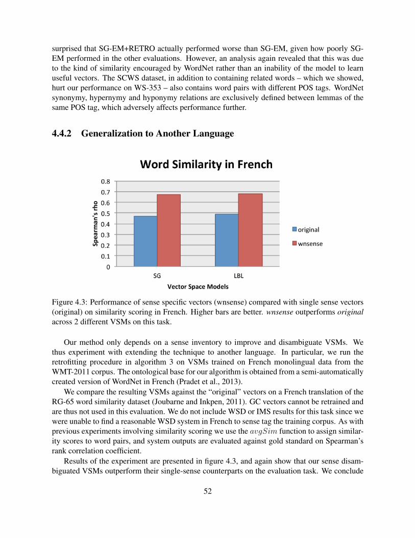
surprised that SG-EM+RETRO actually performed worse than SG-EM, given how poorly SG-EM performed in the other evaluations. However, an analysis again revealed that this was dueto the kind of similarity encouraged by WordNet rather than an inability of the model to learnuseful vectors. The SCWS dataset, in addition to containing related words – which we showed,hurt our performance on WS-353 – also contains word pairs with different POS tags. WordNetsynonymy, hypernymy and hyponymy relations are exclusively defined between lemmas of thesame POS tag, which adversely affects performance further.

4.4.2 Generalization to Another Language

Figure 4.3: Performance of sense specific vectors (wnsense) compared with single sense vectors(original) on similarity scoring in French. Higher bars are better. wnsense outperforms originalacross 2 different VSMs on this task.

Our method only depends on a sense inventory to improve and disambiguate VSMs. Wethus experiment with extending the technique to another language. In particular, we run theretrofitting procedure in algorithm 3 on VSMs trained on French monolingual data from theWMT-2011 corpus. The ontological base for our algorithm is obtained from a semi-automaticallycreated version of WordNet in French (Pradet et al., 2013).

We compare the resulting VSMs against the “original” vectors on a French translation of theRG-65 word similarity dataset (Joubarne and Inkpen, 2011). GC vectors cannot be retrained andare thus not used in this evaluation. We do not include WSD or IMS results for this task since wewere unable to find a reasonable WSD system in French to sense tag the training corpus. As withprevious experiments involving similarity scoring we use the avgSim function to assign similar-ity scores to word pairs, and system outputs are evaluated against gold standard on Spearman’srank correlation coefficient.

Results of the experiment are presented in figure 4.3, and again show that our sense disam-biguated VSMs outperform their single-sense counterparts on the evaluation task. We conclude

52

that the technique we propose not only generalizes to any VSM but to any language, as long as areasonable sense inventory for that language exists.

4.4.3 Antonym Selection

Figure 4.4: Performance of sense specific vectors (wnsense) compared with single sense vec-tors (original) on closest to opposite selection of target verbs. Higher bars are better. wnsenseoutperforms original across 3 different VSMs on this task.

The general formulation of our model allows us to incorporate knowledge from more thanjust the similarity neighborhood (i.e. the synonyms, the hypernyms and the hyponyms) of wordsenses in an ontology. For example, it may be useful to also know the antonyms of a word senseto tease its vector apart from the empirical surface form embedding more effectively.

Since, antonym pairs should ideally have low similarity (i.e. large distance) between them, itis appropriate to set a negative relation weight to these terms in the model parameters in equation4.2 to force the respective vectors further apart. However, in certain cases this causes the objec-tive to diverge, and thus produces unpredictable behavior. This happens, in particular when somevariables in the model form an “antonym clique”, that is when these nodes are only connected toone another via an antonym relationship.

Thus we test our model on the subset of WordNet consisting only of verb lemmas, whichcontain very few antonym cliques8. We run exactly the same procedure of algorithm 3 to createsense disambiguated vectors as before, except that we additionally expand word sense neighbor-hoods with antonyms, and set the antonym specific relation weight γr to be -1.0 in equation 4.2for the model parameters. In the few cases that do evidence divergent behavior, we heuristicallyovercome the problem by ceasing to update the problematic vectors if their norm increases be-yond some threshold (in our experiments we set this to be the norm of the longest vector beforeany update iterations).

8For comparison, 45% of all adjective lemmas appear in such cliques, while only 0.1% of verbs do.

53

Method CPU TimeRETRO ˜20 secs

EM+RETRO ˜4 hoursIMS ˜3 daysWSD ˜1 year

Table 4.3: Training time associated with different methods of generating sense-specific VSMs.

We evaluate the resulting VSMs on the task of closest-to-opposite verb selection. This isvery similar in format to the synonym selection task, except that the candidate with the mostantonym-like meaning with respect to a target needs to be selected. The dataset we use in ourexperiments is from Mohammad et al. (2008). The data contains 226 closest-to-opposite verbselection questions such as the following: “inflate→ overstating, understating, deflate, misrep-resenting, exaggerating” where “deflate” is the correct answer.

We use the minSim function to score similarity between words since we are interested indiscovering the least synonymous word sense pairs. These scores are then sorted in descend-ing order, with the lowest-ranking score yielding the closest-to-opposite candidate to the target.Systems are evaluated on the basis of their accuracy at discriminating the correct candidate.

Results on this task are shown in figure 4.4. It should be noted that discriminating antonymsis a particularly hard problem for distributional VSMs. This is because antonymous word pairs(like synonyms) tend to appear in similar contexts, and are thus trained to encode similar vectors.Our sense specific vectors, on the other hand, are forced to be further apart if they are antonymsand thus perform better on the evaluation task consistently across all three VSMs.

4.5 Discussion

While both our approaches are capable of integrating ontological information into VSMs, animportant question is which one should be preferred? From an empirical point of view, theEM+RETRO framework yields better performance than RETRO across most of our semanticevaluations. Additionally EM+RETRO is more powerful, allowing to adapt more expressivemodels that can jointly learn other useful parameters – such as context vectors in the case ofskip-gram. However, RETRO is far more generalizable, allowing it to be used for any VSM,not just predictive MLE models, and is also empirically competitive. Another consideration iscomputational efficiency, which is summarized in table 4.3.

Not only is RETRO much faster, but it scales linearly with respect to the vocabulary size,unlike EM+RETRO, WSD, and IMS which are dependent on the input training corpus. Never-theless, both our techniques are empirically superior as well as computationally more efficientthan both unsupervised and supervised word-sense disambiguation paradigms.

Both our approaches are sensitive to the structure of the ontology. Therefore, an importantconsideration is the relations we use and the weights we associate with them. In our experi-ments we selected the simplest set of relations and assigned weights heuristically, showing thatour methods can effectively integrate ontological information into VSMs. A more exhaustiveselection procedure with weight tuning on held-out data would almost certainly lead to better

54

performance on our evaluation suite.

4.5.1 Qualitative AnalysisWe qualitatively attempt to address the question of whether the vectors are truly sense specific.In table 4.4 we present the three most similar words of an ambiguous lexical item in a standardVSM (SG-SINGLE) in comparison with the three most similar words of different lemma sensesof the same lexical item in grounded sense VSMs (SG-RETRO & SG-EM+RETRO).

Word or Sense Top 3 Most Similarhanging hung dangled hangs

hanging (suspending) shoring support suspensionhanging (decoration) tapestry braid smock

climber climbers skier Loretanclimber (sportsman) lifter swinger sharpshooter

climber (vine) woodbine brier kiwi

Table 4.4: The top 3 most similar words for two polysemous types. Single sense VSMs capturethe most frequent sense. Our techniques effectively separates out the different senses of words,and are grounded in WordNet.

The sense-agnostic VSMs tend to capture only the most frequent sense of a lexical item. Onthe other hand, the disambiguated vectors capture sense specificity of even less frequent sensessuccessfully. This is probably due to the nature of WordNet where the nearest neighbors of thewords in question are in fact these rare words. A careful tuning of weights will likely optimizethe trade-off between ontologically rare neighbors and distributionally common words.

In our analyses, we noticed that lemma senses that had many neighbors (i.e. synonyms,hypernyms and hyponyms), tended to have more clearly sense specific vectors. This is expected,since it is these neighborhoods that disambiguate and help to distinguish the vectors from theirsingle sense embeddings.

4.6 ConclusionWe have presented two general and flexible approaches to producing sense-specific VSMs groundedin an ontology. The first technique is applicable to any VSM as an efficient post-processing step,which we call retrofitting. The second provides a framework to integrate ontological informationby adapting existing MLE-based predictive models. We evaluated our models on a battery oftasks and the results show that our proposed methods are effectively able to capture the differ-ent senses in an ontology. In most cases this results in significant improvements over baselines.We thus re-affirm the central claim of our thesis: namely that integrating relational structureinto learning semantic models results in representations that are more expressive and empiricallysuperior than their relation agnostic counterparts.

We also discussed the trade-offs between the two techniques from several different per-spectives. In summary, while they adaptive MLE technique seems to be empirically superior,

55

retrofitting is much more computationally friendly. Crucially, however, both models signifi-cantly surpass word-sense disambiguating a training corpus from both computational and empir-ical perspectives. Finally, we also presented a qualitative analysis investigating the nature of thesense-specific vectors, and showed that they do indeed capture the semantics of different senses.

56

Chapter 5

Tables for Question Answering

Leveraging Structural Relations in Tables for Question Answering

Many complex tasks in NLP require some form of background knowledge against which to fact-check and reason. Question Answering (QA) is one such challenge that exposes a number ofNLP sub-problems (Weston et al., 2015), such as information extraction, semantic modelling,reasoning and inference.

When considered in the context of this thesis, an important question concerns the semanticrelations that structure the sources of background knowledge for a problem like QA. As investi-gated in Chapter 6, the space of relations in a particular domain is broad and of varying degreesof granularity. Depending on the nature of the relations, the interpretation of the resulting struc-ture varies, and so too, by consequence, its applications on the problem being solved. For QA,stores of background knowledge have been used in a number of different modes and formalisms:large-scale extracted and curated knowledge bases (Fader et al., 2014), structured models suchas Markov Logic Networks (Khot et al., 2015), or simple text corpora in information retrievalapproaches (Tellex et al., 2003a).

There is, however, a fundamental trade-off in the expressive power of a formalism and itsability to be curated easily using existing data and tools. For example, simple text corpora con-tain no structure, and are therefore hard to reason with in a principled manner. Nevertheless, theyare easily and abundantly available. In contrast, Markov Logic Networks come with a wealth oftheoretical knowledge connected with their usage in principled inference and reasoning. How-ever, they belong to a formalism that is hard to comprehend by annotators and difficult to induceautomatically from text.

In this chapter we explore tables as a source of semi-structured background knowledge forQA. More specifically we investigate tables for the Aristo project at AI2 (Clark, 2015), whichuses standardized science exam Multiple-choice Questions (MCQs) as drivers for research inArtificial Intelligence.

Crucially, in the context of this thesis, the role of semantic relations in these tables is three-fold. First, the way the tables are structured leads to a formalism that is easy enough to build bynon-expert annotators, while being flexible enough to be used for the complex reasoning requiredin QA. Second, the relations governing tables define a greater connection with QA; specifically,

57

they can be used as constraints to generate high quality QA data via crowd-sourcing for our targetdomain. Thirdly, the same structure in tables and its connection to the QA data we generate canbe leveraged to build QA solvers that are capable of performing reasoning over tables.

The contributions of this chapter are centered around this three-fold role of relational struc-ture in tables. We release a new dataset of tables and MCQs that emerged through the presentinvestigation, which has potentially interesting usage for other research in the field. We alsodetail a feature-rich QA solver that uses this data to perform competitively with state-of-the-artexisting systems on the Aristo challenge, and produces the best results to date in combinationwith them.

A future contribution will be the development of a model that performs representation learn-ing jointly over tables and MCQs, overcoming the need for feature engineering.

5.1 Related Work

Our work with tables relates to a number of parallel efforts connected with databases in terms ofcreation, schema analysis and inference. Cafarella et al. (2008) parse the web to create a large-scale collection of HTML tables. They compute statistics about co-occurring attributes, inferringschemas and reasoning about likely table relational structure. Venetis et al. (2011) are morespecifically concerned with recovering table schema, and their insight into column semantics isrelated to our own structural decomposition and analysis of tables. Other research connectedwith relational schema induction for database tables is by Syed et al. (2010) and Limaye et al.(2010).

A closely related line of study relates to executing queries over tables represented as relationaldatabases. This applies more directly to the problem of QA with tables. Cafarella et al. (2008),besides building tables and inferring schemas, also perform queries against these tables. Butunlike the natural language questions normally associated with QA, these queries are more IRstyle lists of keywords. The work of Pimplikar and Sarawagi (2012) is another effort that relieson column semantics to reason better about search requests. Gonzalez et al. (2010).

The construction of knowledge bases in structured format relates more broadly to work onopen information extraction (Etzioni et al., 2008; Wu and Weld, 2010; Fader et al., 2011) andknowledge base population (Ji and Grishman, 2011). While the set of tables we currently workwith are hand-built, an avenue of future research is to automate – or at least semi-automate – theprocess of their construction.

Another contribution of this chapter is a crowd-sourced collection of MCQs. In relation tothis line of research, Aydin et al. (2014) harvest MCQs via a gamified app. However their workdoes not involve tables. Monolingual alignment datasets have also been explored separately, forexample by Brockett (2007) in the context of Textual Entailment.

Perhaps the most relevant research to our own work is a recent publication by Pasupat andLiang (2015). They create a dataset of QA pairs over tables. However their primary concern withis with question parsing rather than with representation learning over structure. Other notabledifferences are the fact that their annotation setup does not impose structural constraints fromtables, and is generally less concerned with relational information. Also they produces simpleQA pairs rather than MCQs.

58

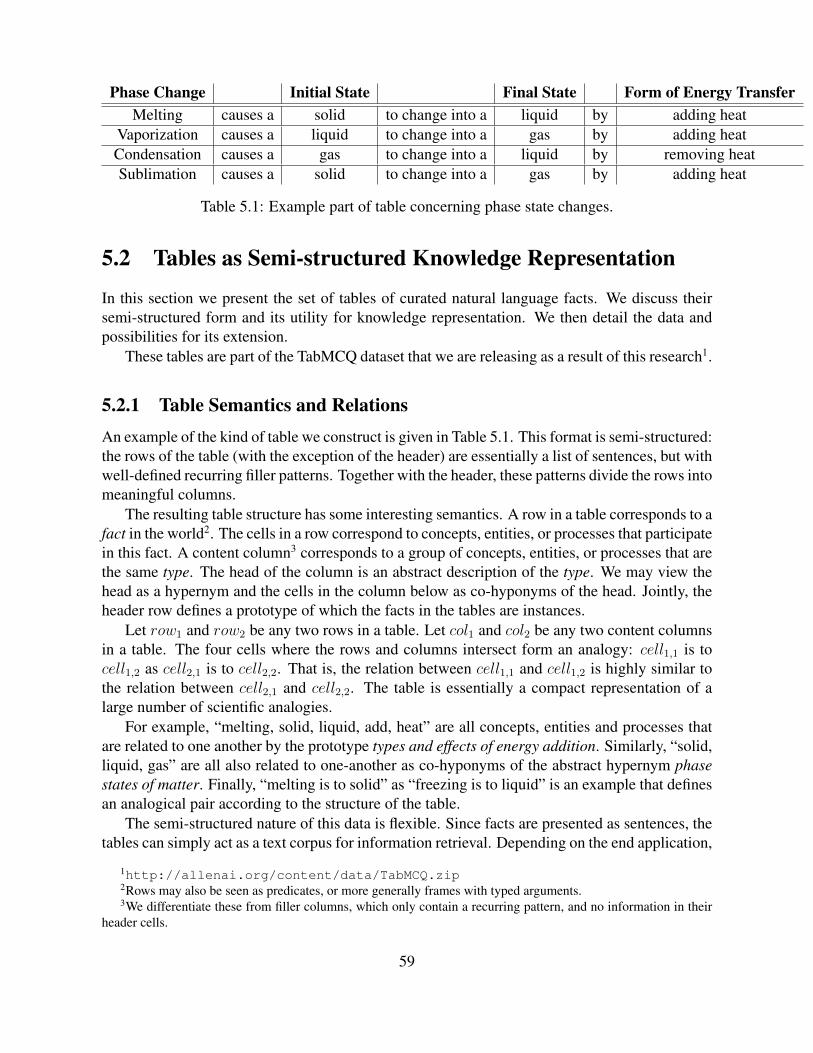
Phase Change Initial State Final State Form of Energy TransferMelting causes a solid to change into a liquid by adding heat

Vaporization causes a liquid to change into a gas by adding heatCondensation causes a gas to change into a liquid by removing heatSublimation causes a solid to change into a gas by adding heat

Table 5.1: Example part of table concerning phase state changes.

5.2 Tables as Semi-structured Knowledge Representation

In this section we present the set of tables of curated natural language facts. We discuss theirsemi-structured form and its utility for knowledge representation. We then detail the data andpossibilities for its extension.

These tables are part of the TabMCQ dataset that we are releasing as a result of this research1.

5.2.1 Table Semantics and RelationsAn example of the kind of table we construct is given in Table 5.1. This format is semi-structured:the rows of the table (with the exception of the header) are essentially a list of sentences, but withwell-defined recurring filler patterns. Together with the header, these patterns divide the rows intomeaningful columns.

The resulting table structure has some interesting semantics. A row in a table corresponds to afact in the world2. The cells in a row correspond to concepts, entities, or processes that participatein this fact. A content column3 corresponds to a group of concepts, entities, or processes that arethe same type. The head of the column is an abstract description of the type. We may view thehead as a hypernym and the cells in the column below as co-hyponyms of the head. Jointly, theheader row defines a prototype of which the facts in the tables are instances.

Let row1 and row2 be any two rows in a table. Let col1 and col2 be any two content columnsin a table. The four cells where the rows and columns intersect form an analogy: cell1,1 is tocell1,2 as cell2,1 is to cell2,2. That is, the relation between cell1,1 and cell1,2 is highly similar tothe relation between cell2,1 and cell2,2. The table is essentially a compact representation of alarge number of scientific analogies.

For example, “melting, solid, liquid, add, heat” are all concepts, entities and processes thatare related to one another by the prototype types and effects of energy addition. Similarly, “solid,liquid, gas” are all also related to one-another as co-hyponyms of the abstract hypernym phasestates of matter. Finally, “melting is to solid” as “freezing is to liquid” is an example that definesan analogical pair according to the structure of the table.

The semi-structured nature of this data is flexible. Since facts are presented as sentences, thetables can simply act as a text corpus for information retrieval. Depending on the end application,

1http://allenai.org/content/data/TabMCQ.zip2Rows may also be seen as predicates, or more generally frames with typed arguments.3We differentiate these from filler columns, which only contain a recurring pattern, and no information in their

header cells.

59

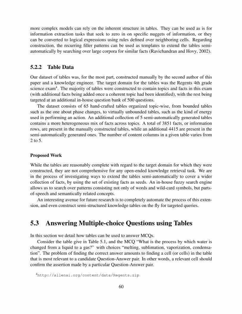
more complex models can rely on the inherent structure in tables. They can be used as is forinformation extraction tasks that seek to zero in on specific nuggets of information, or theycan be converted to logical expressions using rules defined over neighboring cells. Regardingconstruction, the recurring filler patterns can be used as templates to extend the tables semi-automatically by searching over large corpora for similar facts (Ravichandran and Hovy, 2002).

5.2.2 Table Data

Our dataset of tables was, for the most part, constructed manually by the second author of thispaper and a knowledge engineer. The target domain for the tables was the Regents 4th gradescience exam4. The majority of tables were constructed to contain topics and facts in this exam(with additional facts being added once a coherent topic had been identified), with the rest beingtargeted at an additional in-house question bank of 500 questions.

The dataset consists of 65 hand-crafted tables organized topic-wise, from bounded tablessuch as the one about phase changes, to virtually unbounded tables, such as the kind of energyused in performing an action. An additional collection of 5 semi-automatically generated tablescontains a more heterogeneous mix of facts across topics. A total of 3851 facts, or informationrows, are present in the manually constructed tables, while an additional 4415 are present in thesemi-automatically generated ones. The number of content columns in a given table varies from2 to 5.

Proposed Work

While the tables are reasonably complete with regard to the target domain for which they wereconstructed, they are not comprehensive for any open-ended knowledge retrieval task. We arein the process of investigating ways to extend the tables semi-automatically to cover a widercollection of facts, by using the set of existing facts as seeds. An in-house fuzzy search engineallows us to search over patterns consisting not only of words and wild-card symbols, but parts-of-speech and semantically related concepts.

An interesting avenue for future research is to completely automate the process of this exten-sion, and even construct semi-structured knowledge tables on the fly for targeted queries.

5.3 Answering Multiple-choice Questions using Tables

In this section we detail how tables can be used to answer MCQs.Consider the table give in Table 5.1, and the MCQ “What is the process by which water is

changed from a liquid to a gas?” with choices “melting, sublimation, vaporization, condensa-tion”. The problem of finding the correct answer amounts to finding a cell (or cells) in the tablethat is most relevant to a candidate Question-Answer pair. In other words, a relevant cell shouldconfirm the assertion made by a particular Question-Answer pair.

4http://allenai.org/content/data/Regents.zip

60

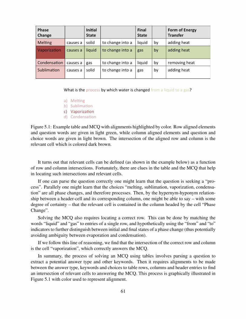
Figure 5.1: Example table and MCQ with alignments highlighted by color. Row aligned elementsand question words are given in light green, while column aligned elements and question andchoice words are given in light brown. The intersection of the aligned row and column is therelevant cell which is colored dark brown.

It turns out that relevant cells can be defined (as shown in the example below) as a functionof row and column intersections. Fortunately, there are clues in the table and the MCQ that helpin locating such intersections and relevant cells.

If one can parse the question correctly one might learn that the question is seeking a “pro-cess”. Parallely one might learn that the choices “melting, sublimation, vaporization, condensa-tion” are all phase changes, and therefore processes. Then, by the hypernym-hyponym relation-ship between a header-cell and its corresponding column, one might be able to say – with somedegree of certainty – that the relevant cell is contained in the column headed by the cell “PhaseChange”.

Solving the MCQ also requires locating a correct row. This can be done by matching thewords “liquid” and “gas” to entries of a single row, and hypothetically using the “from” and “to”indicators to further distinguish between initial and final states of a phase change (thus potentiallyavoiding ambiguity between evaporation and condensation).

If we follow this line of reasoning, we find that the intersection of the correct row and columnis the cell “vaporization”, which correctly answers the MCQ.

In summary, the process of solving an MCQ using tables involves parsing a question toextract a potential answer type and other keywords. Then it requires alignments to be madebetween the answer type, keywords and choices to table rows, columns and header entries to findan intersection of relevant cells to answering the MCQ. This process is graphically illustrated inFigure 5.1 with color used to represent alignment.

61

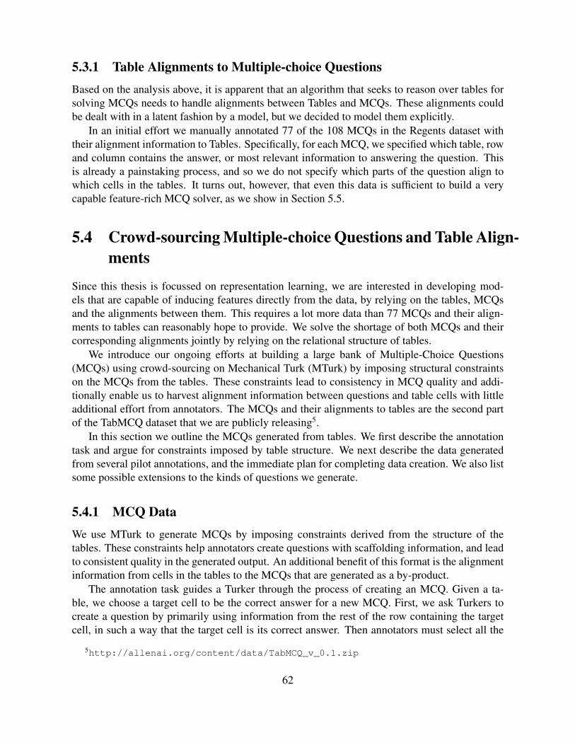
5.3.1 Table Alignments to Multiple-choice QuestionsBased on the analysis above, it is apparent that an algorithm that seeks to reason over tables forsolving MCQs needs to handle alignments between Tables and MCQs. These alignments couldbe dealt with in a latent fashion by a model, but we decided to model them explicitly.

In an initial effort we manually annotated 77 of the 108 MCQs in the Regents dataset withtheir alignment information to Tables. Specifically, for each MCQ, we specified which table, rowand column contains the answer, or most relevant information to answering the question. Thisis already a painstaking process, and so we do not specify which parts of the question align towhich cells in the tables. It turns out, however, that even this data is sufficient to build a verycapable feature-rich MCQ solver, as we show in Section 5.5.

5.4 Crowd-sourcing Multiple-choice Questions and Table Align-ments

Since this thesis is focussed on representation learning, we are interested in developing mod-els that are capable of inducing features directly from the data, by relying on the tables, MCQsand the alignments between them. This requires a lot more data than 77 MCQs and their align-ments to tables can reasonably hope to provide. We solve the shortage of both MCQs and theircorresponding alignments jointly by relying on the relational structure of tables.

We introduce our ongoing efforts at building a large bank of Multiple-Choice Questions(MCQs) using crowd-sourcing on Mechanical Turk (MTurk) by imposing structural constraintson the MCQs from the tables. These constraints lead to consistency in MCQ quality and addi-tionally enable us to harvest alignment information between questions and table cells with littleadditional effort from annotators. The MCQs and their alignments to tables are the second partof the TabMCQ dataset that we are publicly releasing5.

In this section we outline the MCQs generated from tables. We first describe the annotationtask and argue for constraints imposed by table structure. We next describe the data generatedfrom several pilot annotations, and the immediate plan for completing data creation. We also listsome possible extensions to the kinds of questions we generate.

5.4.1 MCQ DataWe use MTurk to generate MCQs by imposing constraints derived from the structure of thetables. These constraints help annotators create questions with scaffolding information, and leadto consistent quality in the generated output. An additional benefit of this format is the alignmentinformation from cells in the tables to the MCQs that are generated as a by-product.

The annotation task guides a Turker through the process of creating an MCQ. Given a ta-ble, we choose a target cell to be the correct answer for a new MCQ. First, we ask Turkers tocreate a question by primarily using information from the rest of the row containing the targetcell, in such a way that the target cell is its correct answer. Then annotators must select all the

5http://allenai.org/content/data/TabMCQ_v_0.1.zip

62

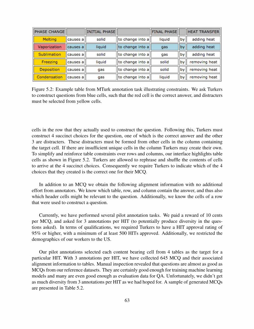
Figure 5.2: Example table from MTurk annotation task illustrating constraints. We ask Turkersto construct questions from blue cells, such that the red cell is the correct answer, and distractersmust be selected from yellow cells.

cells in the row that they actually used to construct the question. Following this, Turkers mustconstruct 4 succinct choices for the question, one of which is the correct answer and the other3 are distracters. These distracters must be formed from other cells in the column containingthe target cell. If there are insufficient unique cells in the column Turkers may create their own.To simplify and reinforce table constraints over rows and columns, our interface highlights tablecells as shown in Figure 5.2. Turkers are allowed to rephrase and shuffle the contents of cellsto arrive at the 4 succinct choices. Consequently we require Turkers to indicate which of the 4choices that they created is the correct one for their MCQ.

In addition to an MCQ we obtain the following alignment information with no additionaleffort from annotators. We know which table, row, and column contain the answer, and thus alsowhich header cells might be relevant to the question. Additionally, we know the cells of a rowthat were used to construct a question.

Currently, we have performed several pilot annotation tasks. We paid a reward of 10 centsper MCQ, and asked for 3 annotations per HIT (to potentially produce diversity in the ques-tions asked). In terms of qualifications, we required Turkers to have a HIT approval rating of95% or higher, with a minimum of at least 500 HITs approved. Additionally, we restricted thedemographics of our workers to the US.

Our pilot annotations selected each content bearing cell from 4 tables as the target for aparticular HIT. With 3 annotations per HIT, we have collected 645 MCQ and their associatedalignment information to tables. Manual inspection revealed that questions are almost as good asMCQs from our reference datasets. They are certainly good enough for training machine learningmodels and many are even good enough as evaluation data for QA. Unfortunately, we didn’t getas much diversity from 3 annotations per HIT as we had hoped for. A sample of generated MCQsare presented in Table 5.2.

63

What is the orbital event with the longest day and the shortest night.A) Summer solstice

B) Winter solsticeC) Spring equinox

D) Fall equinoxWhat sense organ is used to detect pitch and harmony?

A) EarsB) Eyes

C) NosesD) Tongues

A graduated cylinder is used to measure what of liquids?A) VolumeB) DensityC) Depth

D) PressureSteel is a/an of electricity

A) SeparatorB) Isolator

C) InsulatorD) Conductor

Table 5.2: Example MCQs generated from our pilot MTurk tasks. Correct answer choices are inbold.

64

Proposed Work

Our immediate goal is to expand the pilot annotations to cover every content bearing cell fromall 65 manually-crafted tables6. We will remove the 3 annotations per HIT requirement, and onlyask for a single MCQ per HIT. When completed, we will have an additional 8606 MCQs withalignment information to tables.

Once this immediate goal is achieved we hope to generate MCQs with other kinds of con-straints from tables. Currently the constraints are row-dominant: the questions are based on cellsfrom the row in which a target cell occurs. Such questions are often information look-up ques-tions – the simplest kind. We plan to explore column-dominant questions, which would leadto questions about abstraction or specification (based on the hypernym-hyponym relationship incolumns). Other structural semantics we hope to investigate are multi-row constraints that re-sult in comparisons, or joins on multiple tables with related columns that results in chaining orreasoning.

5.5 Feature Rich Table Embedding Solver

In this section we detail a system that leverages MCQs, tables and alignment information betweenthem, to build a feature rich solver of questions. These features are manually engineered, buttheir intuition paves the way for our proposed work, which will involve inducing these featuresautomatically.

We begin by outlining the model and the objective against which it is trained. We thendescribe our feature set, and show evaluation results in a number of different settings on twodifferent datasets. Our results rival the best existing MCQ solvers, and in combination with themproduces state-of-the-art results on both datasets.

5.5.1 Model, Features and Training ObjectiveRecall from Section 5.3 that a table may be used to answer a question by finding and focussingon a small set of relevant cells. Moreover, these cells are are found by creating an intersectionbetween rows and columns of interest, by a combination of leveraging the structure of a table aswell as its contents. This is exactly the intuition that our Feature Rich Table Embedding Solver(FRETS) seeks to model.

Let Q = q1, ..., qN denote a set of MCQs, and An = a1n, ..., a

kn be the set of candidate

answer choices for a given question qn. Meanwhile, let the set of tables be defined as T =T1, ..., TM. Also given a table Tm, let tijm be the cell in that table corresponding to the ith rowand jth column.

We define a log-linear model that scores every cell tijm of every table in our collection accord-ing to a set of discrete weighted features, for a given QA pair. Hence, we have:

s(tijm) =∑d

λdfd(qn, akn, t

ijm;A\, T ) (5.1)

6The relative lack structural semantics in semi-automatically generated tables makes them unsuitable for the task

65

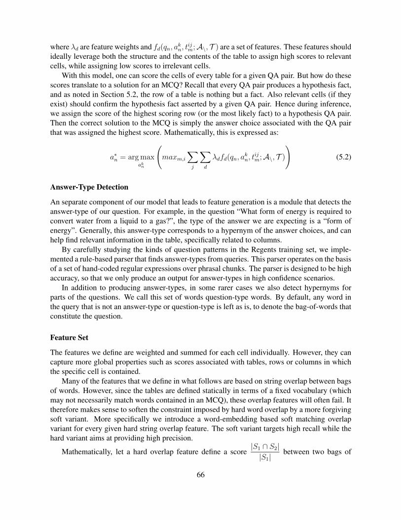
where λd are feature weights and fd(qn, akn, tijm;A\, T ) are a set of features. These features should

ideally leverage both the structure and the contents of the table to assign high scores to relevantcells, while assigning low scores to irrelevant cells.

With this model, one can score the cells of every table for a given QA pair. But how do thesescores translate to a solution for an MCQ? Recall that every QA pair produces a hypothesis fact,and as noted in Section 5.2, the row of a table is nothing but a fact. Also relevant cells (if theyexist) should confirm the hypothesis fact asserted by a given QA pair. Hence during inference,we assign the score of the highest scoring row (or the most likely fact) to a hypothesis QA pair.Then the correct solution to the MCQ is simply the answer choice associated with the QA pairthat was assigned the highest score. Mathematically, this is expressed as:

a∗n = arg maxakn

(maxm,i

∑j

∑d

λdfd(qn, akn, t

ijm;A\, T )

)(5.2)

Answer-Type Detection

An separate component of our model that leads to feature generation is a module that detects theanswer-type of our question. For example, in the question “What form of energy is required toconvert water from a liquid to a gas?”, the type of the answer we are expecting is a “form ofenergy”. Generally, this answer-type corresponds to a hypernym of the answer choices, and canhelp find relevant information in the table, specifically related to columns.

By carefully studying the kinds of question patterns in the Regents training set, we imple-mented a rule-based parser that finds answer-types from queries. This parser operates on the basisof a set of hand-coded regular expressions over phrasal chunks. The parser is designed to be highaccuracy, so that we only produce an output for answer-types in high confidence scenarios.

In addition to producing answer-types, in some rarer cases we also detect hypernyms forparts of the questions. We call this set of words question-type words. By default, any word inthe query that is not an answer-type or question-type is left as is, to denote the bag-of-words thatconstitute the question.

Feature Set

The features we define are weighted and summed for each cell individually. However, they cancapture more global properties such as scores associated with tables, rows or columns in whichthe specific cell is contained.

Many of the features that we define in what follows are based on string overlap between bagsof words. However, since the tables are defined statically in terms of a fixed vocabulary (whichmay not necessarily match words contained in an MCQ), these overlap features will often fail. Ittherefore makes sense to soften the constraint imposed by hard word overlap by a more forgivingsoft variant. More specifically we introduce a word-embedding based soft matching overlapvariant for every given hard string overlap feature. The soft variant targets high recall while thehard variant aims at providing high precision.

Mathematically, let a hard overlap feature define a score|S1 ∩ S2||S1|

between two bags of

66

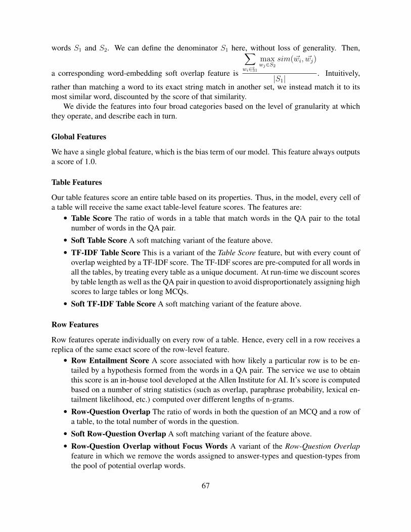
words S1 and S2. We can define the denominator S1 here, without loss of generality. Then,

a corresponding word-embedding soft overlap feature is

∑wi∈§1

maxwj∈S2

sim( ~wi, ~wj)

|S1|. Intuitively,

rather than matching a word to its exact string match in another set, we instead match it to itsmost similar word, discounted by the score of that similarity.

We divide the features into four broad categories based on the level of granularity at whichthey operate, and describe each in turn.

Global Features

We have a single global feature, which is the bias term of our model. This feature always outputsa score of 1.0.

Table Features

Our table features score an entire table based on its properties. Thus, in the model, every cell ofa table will receive the same exact table-level feature scores. The features are:• Table Score The ratio of words in a table that match words in the QA pair to the total

number of words in the QA pair.• Soft Table Score A soft matching variant of the feature above.• TF-IDF Table Score This is a variant of the Table Score feature, but with every count of

overlap weighted by a TF-IDF score. The TF-IDF scores are pre-computed for all words inall the tables, by treating every table as a unique document. At run-time we discount scoresby table length as well as the QA pair in question to avoid disproportionately assigning highscores to large tables or long MCQs.

• Soft TF-IDF Table Score A soft matching variant of the feature above.

Row Features

Row features operate individually on every row of a table. Hence, every cell in a row receives areplica of the same exact score of the row-level feature.• Row Entailment Score A score associated with how likely a particular row is to be en-

tailed by a hypothesis formed from the words in a QA pair. The service we use to obtainthis score is an in-house tool developed at the Allen Institute for AI. It’s score is computedbased on a number of string statistics (such as overlap, paraphrase probability, lexical en-tailment likelihood, etc.) computed over different lengths of n-grams.

• Row-Question Overlap The ratio of words in both the question of an MCQ and a row ofa table, to the total number of words in the question.

• Soft Row-Question Overlap A soft matching variant of the feature above.• Row-Question Overlap without Focus Words A variant of the Row-Question Overlap

feature in which we remove the words assigned to answer-types and question-types fromthe pool of potential overlap words.

67

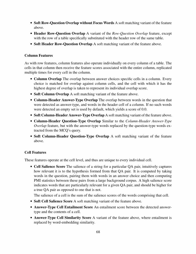
• Soft Row-Question Overlap without Focus Words A soft matching variant of the featureabove.

• Header Row-Question Overlap A variant of the Row-Question Overlap feature, exceptwith the row of a table specifically substituted with the header row of the same table.

• Soft Header Row-Question Overlap A soft matching variant of the feature above.

Column Features

As with row features, column features also operate individually on every column of a table. Thecells in that column then receive the feature scores associated with the entire column, replicatedmultiple times for every cell in the column.

• Column Overlap The overlap between answer choices specific cells in a column. Everychoice is matched for overlap against column cells, and the cell with which it has thehighest degree of overlap is taken to represent its individual overlap score.

• Soft Column Overlap A soft matching variant of the feature above.• Column-Header Answer-Type Overlap The overlap between words in the question that

were detected as answer-type, and words in the header cell of a column. If no such wordswere detected an empty set is used by default, which yields a score of 0.0.

• Soft Column-Header Answer-Type Overlap A soft matching variant of the feature above.• Column-Header Question-Type Overlap Similar to the Column-Header Answer-Type

Overlap feature, but with the answer-type words replaced by the question-type words ex-tracted from the MCQ’s query.

• Soft Column-Header Question-Type Overlap A soft matching variant of the featureabove.

Cell Features

These features operate at the cell level, and thus are unique to every individual cell.

• Cell Salience Score The salience of a string for a particular QA pair, intuitively captureshow relevant it is to the hypothesis formed from that QA pair. It is computed by takingwords in the question, pairing them with words in an answer choice and then computingPMI statistics between these pairs from a large background corpus. A high salience scoreindicates words that are particularly relevant for a given QA pair, and should be higher fora true QA pair as opposed to one that is not.The salience of a cell is the sum of the salience scores of the words comprising that cell.

• Soft Cell Salience Score A soft matching variant of the feature above.• Answer-Type Cell Entailment Score An entailment score between the detected answer-

type and the contents of a cell.• Answer-Type Cell Similarity Score A variant of the feature above, where entailment is

replaced by word-embedding similarity.

68

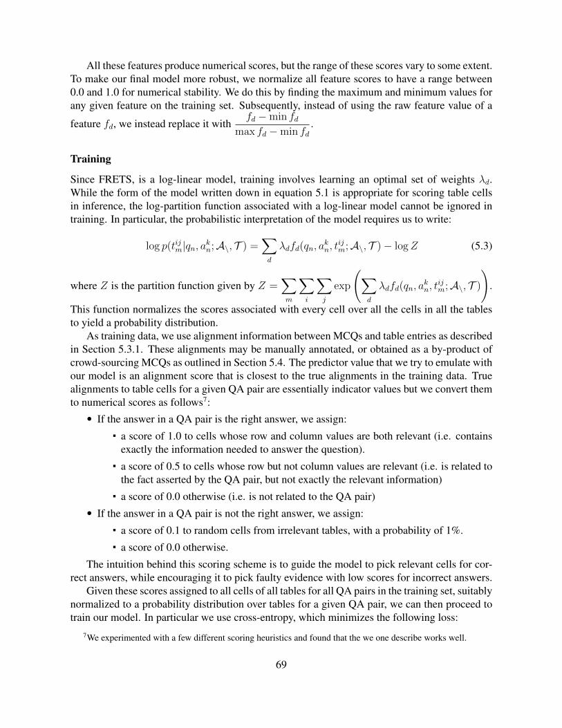
All these features produce numerical scores, but the range of these scores vary to some extent.To make our final model more robust, we normalize all feature scores to have a range between0.0 and 1.0 for numerical stability. We do this by finding the maximum and minimum values forany given feature on the training set. Subsequently, instead of using the raw feature value of a

feature fd, we instead replace it withfd −min fd

max fd −min fd.

Training

Since FRETS, is a log-linear model, training involves learning an optimal set of weights λd.While the form of the model written down in equation 5.1 is appropriate for scoring table cellsin inference, the log-partition function associated with a log-linear model cannot be ignored intraining. In particular, the probabilistic interpretation of the model requires us to write:

log p(tijm|qn, akn;A\, T ) =∑d

λdfd(qn, akn, t

ijm;A\, T )− logZ (5.3)

where Z is the partition function given by Z =∑m

∑i

∑j

exp

(∑d

λdfd(qn, akn, t

ijm;A\, T )

).

This function normalizes the scores associated with every cell over all the cells in all the tablesto yield a probability distribution.

As training data, we use alignment information between MCQs and table entries as describedin Section 5.3.1. These alignments may be manually annotated, or obtained as a by-product ofcrowd-sourcing MCQs as outlined in Section 5.4. The predictor value that we try to emulate withour model is an alignment score that is closest to the true alignments in the training data. Truealignments to table cells for a given QA pair are essentially indicator values but we convert themto numerical scores as follows7:• If the answer in a QA pair is the right answer, we assign:

a score of 1.0 to cells whose row and column values are both relevant (i.e. containsexactly the information needed to answer the question).

a score of 0.5 to cells whose row but not column values are relevant (i.e. is related tothe fact asserted by the QA pair, but not exactly the relevant information)

a score of 0.0 otherwise (i.e. is not related to the QA pair)• If the answer in a QA pair is not the right answer, we assign:

a score of 0.1 to random cells from irrelevant tables, with a probability of 1%.

a score of 0.0 otherwise.

The intuition behind this scoring scheme is to guide the model to pick relevant cells for cor-rect answers, while encouraging it to pick faulty evidence with low scores for incorrect answers.

Given these scores assigned to all cells of all tables for all QA pairs in the training set, suitablynormalized to a probability distribution over tables for a given QA pair, we can then proceed totrain our model. In particular we use cross-entropy, which minimizes the following loss:

7We experimented with a few different scoring heuristics and found that the we one describe works well.

69

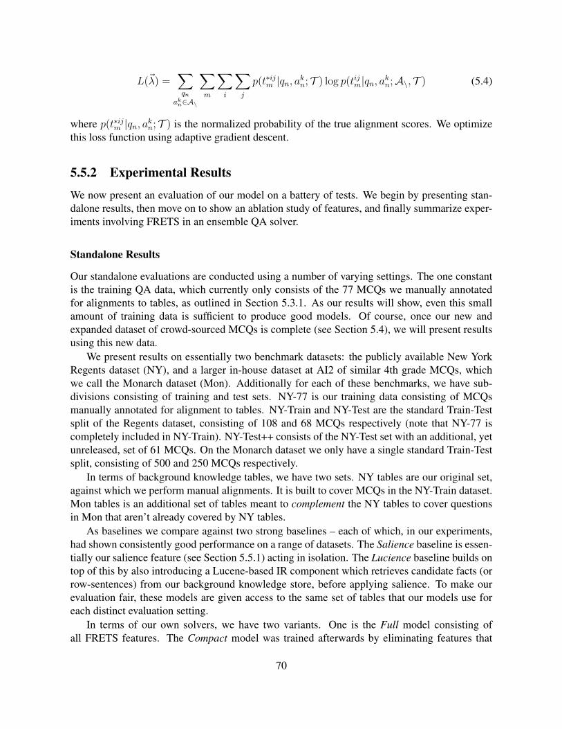
L(~λ) =∑qn

akn∈A\

∑m

∑i

∑j

p(t∗ijm |qn, akn; T ) log p(tijm|qn, akn;A\, T ) (5.4)

where p(t∗ijm |qn, akn; T ) is the normalized probability of the true alignment scores. We optimizethis loss function using adaptive gradient descent.

5.5.2 Experimental Results

We now present an evaluation of our model on a battery of tests. We begin by presenting stan-dalone results, then move on to show an ablation study of features, and finally summarize exper-iments involving FRETS in an ensemble QA solver.

Standalone Results

Our standalone evaluations are conducted using a number of varying settings. The one constantis the training QA data, which currently only consists of the 77 MCQs we manually annotatedfor alignments to tables, as outlined in Section 5.3.1. As our results will show, even this smallamount of training data is sufficient to produce good models. Of course, once our new andexpanded dataset of crowd-sourced MCQs is complete (see Section 5.4), we will present resultsusing this new data.

We present results on essentially two benchmark datasets: the publicly available New YorkRegents dataset (NY), and a larger in-house dataset at AI2 of similar 4th grade MCQs, whichwe call the Monarch dataset (Mon). Additionally for each of these benchmarks, we have sub-divisions consisting of training and test sets. NY-77 is our training data consisting of MCQsmanually annotated for alignment to tables. NY-Train and NY-Test are the standard Train-Testsplit of the Regents dataset, consisting of 108 and 68 MCQs respectively (note that NY-77 iscompletely included in NY-Train). NY-Test++ consists of the NY-Test set with an additional, yetunreleased, set of 61 MCQs. On the Monarch dataset we only have a single standard Train-Testsplit, consisting of 500 and 250 MCQs respectively.

In terms of background knowledge tables, we have two sets. NY tables are our original set,against which we perform manual alignments. It is built to cover MCQs in the NY-Train dataset.Mon tables is an additional set of tables meant to complement the NY tables to cover questionsin Mon that aren’t already covered by NY tables.

As baselines we compare against two strong baselines – each of which, in our experiments,had shown consistently good performance on a range of datasets. The Salience baseline is essen-tially our salience feature (see Section 5.5.1) acting in isolation. The Lucience baseline builds ontop of this by also introducing a Lucene-based IR component which retrieves candidate facts (orrow-sentences) from our background knowledge store, before applying salience. To make ourevaluation fair, these models are given access to the same set of tables that our models use foreach distinct evaluation setting.

In terms of our own solvers, we have two variants. One is the Full model consisting ofall FRETS features. The Compact model was trained afterwards by eliminating features that

70

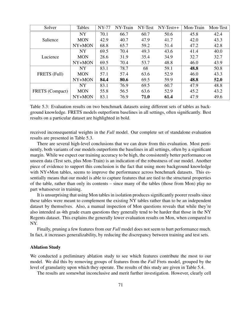
Solver Tables NY-77 NY-Train NY-Test NY-Test++ Mon-Train Mon-Test

SalienceNY 70.1 66.7 60.7 50.6 45.8 42.4

MON 42.9 40.7 47.9 41.7 42.0 43.3NY+MON 68.8 65.7 59.2 51.4 47.2 42.8

LucienceNY 69.5 70.4 49.3 43.6 41.4 40.0

MON 28.6 31.9 35.4 34.9 32.7 32.7NY+MON 69.5 70.4 53.7 48.8 46.0 43.9

FRETS (Full)NY 83.1 78.7 68 59.1 48.8 50.8

MON 57.1 57.4 63.6 52.9 46.0 43.3NY+MON 84.4 80.6 69.5 59.9 48.8 52.0

FRETS (Compact)NY 83.1 76.9 69.5 60.7 47.9 48.8

MON 55.8 56.5 63.6 52.9 45.2 43.2NY+MON 83.1 76.9 71.0 61.4 47.9 49.6

Table 5.3: Evaluation results on two benchmark datasets using different sets of tables as back-ground knowledge. FRETS models outperform baselines in all settings, often significantly. Bestresults on a particular dataset are highlighted in bold.

received inconsequential weights in the Full model. Our complete set of standalone evaluationresults are presented in Table 5.3.

There are several high-level conclusions that we can draw from this evaluation. Most perti-nently, both variants of our models outperform the baselines in all settings, often by a significantmargin. While we expect our training accuracy to be high, the consistently better performance onunseen data (Test sets, plus Mon-Train) is an indication of the robustness of our model. Anotherpiece of evidence to support this conclusion is the fact that using more background knowledgewith NY+Mon tables, seems to improve the performance across benchmark datasets. This es-sentially means that our model is able to capture features that are tied to the structural propertiesof the table, rather than only its contents – since many of the tables (those from Mon) play nopart whatsoever in training.

It is unsurprising that using Mon tables in isolation produces significantly poorer results sincethese tables were meant to complement the existing NY tables rather than to be an independentdataset by themselves. Also, a manual inspection of Mon questions reveals that while they’realso intended as 4th grade exam questions they generally tend to be harder that those in the NYRegents dataset. This explains the generally lower evaluation results on Mon, when compared toNY.

Finally, pruning a few features from our Full model does not seem to hurt performance much.In fact, it increases generalizability, by reducing the discrepancy between training and test sets.

Ablation Study

We conducted a preliminary ablation study to see which features contribute the most to ourmodel. We did this by removing groups of features from the Full Frets model, grouped by thelevel of granularity upon which they operate. The results of this study are given in Table 5.4.

The results are somewhat inconclusive and merit further investigation. However, clearly cell

71

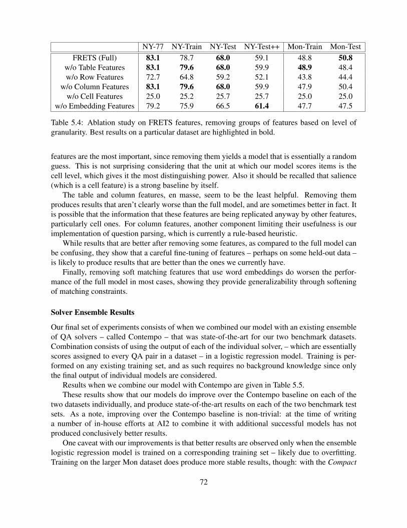
NY-77 NY-Train NY-Test NY-Test++ Mon-Train Mon-TestFRETS (Full) 83.1 78.7 68.0 59.1 48.8 50.8

w/o Table Features 83.1 79.6 68.0 59.9 48.9 48.4w/o Row Features 72.7 64.8 59.2 52.1 43.8 44.4

w/o Column Features 83.1 79.6 68.0 59.9 47.9 50.4w/o Cell Features 25.0 25.2 25.7 25.7 25.0 25.0

w/o Embedding Features 79.2 75.9 66.5 61.4 47.7 47.5

Table 5.4: Ablation study on FRETS features, removing groups of features based on level ofgranularity. Best results on a particular dataset are highlighted in bold.

features are the most important, since removing them yields a model that is essentially a randomguess. This is not surprising considering that the unit at which our model scores items is thecell level, which gives it the most distinguishing power. Also it should be recalled that salience(which is a cell feature) is a strong baseline by itself.

The table and column features, en masse, seem to be the least helpful. Removing themproduces results that aren’t clearly worse than the full model, and are sometimes better in fact. Itis possible that the information that these features are being replicated anyway by other features,particularly cell ones. For column features, another component limiting their usefulness is ourimplementation of question parsing, which is currently a rule-based heuristic.

While results that are better after removing some features, as compared to the full model canbe confusing, they show that a careful fine-tuning of features – perhaps on some held-out data –is likely to produce results that are better than the ones we currently have.

Finally, removing soft matching features that use word embeddings do worsen the perfor-mance of the full model in most cases, showing they provide generalizability through softeningof matching constraints.

Solver Ensemble Results

Our final set of experiments consists of when we combined our model with an existing ensembleof QA solvers – called Contempo – that was state-of-the-art for our two benchmark datasets.Combination consists of using the output of each of the individual solver, – which are essentiallyscores assigned to every QA pair in a dataset – in a logistic regression model. Training is per-formed on any existing training set, and as such requires no background knowledge since onlythe final output of individual models are considered.

Results when we combine our model with Contempo are given in Table 5.5.These results show that our models do improve over the Contempo baseline on each of the

two datasets individually, and produce state-of-the-art results on each of the two benchmark testsets. As a note, improving over the Contempo baseline is non-trivial: at the time of writinga number of in-house efforts at AI2 to combine it with additional successful models has notproduced conclusively better results.

One caveat with our improvements is that better results are observed only when the ensemblelogistic regression model is trained on a corresponding training set – likely due to overfitting.Training on the larger Mon dataset does produce more stable results, though: with the Compact

72

CONTEMPO Train Set NY-Train NY-Test Mon-Train Mon-TestBaseline - 82.4 73.5 56.8 55.6

+ FRETS (Full)NY 84.3 73.5 55.0 55.2Mon 81.5 73.5 56.6 56.8

+ FRETS (Compact)NY 84.3 80.9 55.8 53.6Mon 76.9 73.5 57.2 57.6

Table 5.5: Combination results of using FRETS in an ensemble solver on both benchmarkdatasets. The best test results to date, at the time of writing, are achieved with this combina-tion. Best results on a particular dataset are highlighted in bold.

FRETS model we see state-of-the-art results for Mon, while there is no loss in test accuracy forNY. It is interesting to note that the Compact variant of our model is generally better, helping itto overcome the lack of training data, especially when faced with the small set of 108 MCQs inNY.

5.6 TabNN: Representation Learning over Tables – ProposedWork

We have shown that tables can be effectively used as a source of semi-structured backgroundknowledge in Question Answering. However, the FRETS MCQ solver that we implemented andevaluated in Section 5.5 uses a set of manually engineered features to find relevant cells in tablesfor answering questions. In keeping with the overarching goal of this thesis, we’d like to beable to learn representations for elements in the table automatically, by leveraging its structuralproperties.

We thus propose a novel method that embeds table cells in a dual space so that they canbe used for answering MCQs. The dual space decomposes the structure of a table into rowsand columns and learns representations for cells along each axis independently. The model usesneural networks – and specifically LSTMs – to learn table entries; hence the name TabNN.

5.6.1 The ModelRecall the discussion about the relational structure in tables and its semantics from Section 5.2.1,and the translation of these semantics into manually engineered features in Section 5.5.1. At ahigh level, using a generative analogy, one can think about a question as being generated from arow, while its choices being generated from a column8.

Hence, from a representation learning point of view, it makes sense to embed a question anda row of a table in a joint space, while a column and the choices are embedded in a different jointspace. The representation learning model we propose leverages this intuitions, to learn featuresautomatically for table entries.

8In fact this is the process of thinking through which we guide our annotators in crowd-sourcing MCQs, asdescribed in Section 5.4.1

73

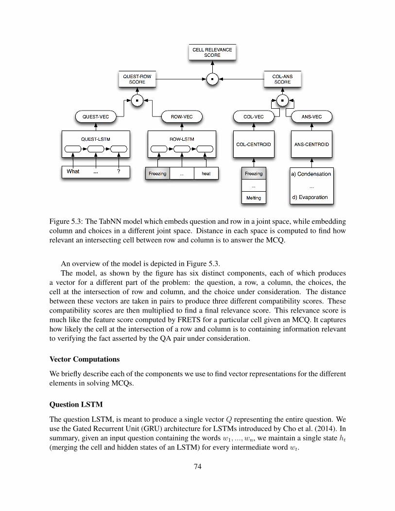
Figure 5.3: The TabNN model which embeds question and row in a joint space, while embeddingcolumn and choices in a different joint space. Distance in each space is computed to find howrelevant an intersecting cell between row and column is to answer the MCQ.

An overview of the model is depicted in Figure 5.3.The model, as shown by the figure has six distinct components, each of which produces

a vector for a different part of the problem: the question, a row, a column, the choices, thecell at the intersection of row and column, and the choice under consideration. The distancebetween these vectors are taken in pairs to produce three different compatibility scores. Thesecompatibility scores are then multiplied to find a final relevance score. This relevance score ismuch like the feature score computed by FRETS for a particular cell given an MCQ. It captureshow likely the cell at the intersection of a row and column is to containing information relevantto verifying the fact asserted by the QA pair under consideration.

Vector Computations

We briefly describe each of the components we use to find vector representations for the differentelements in solving MCQs.

Question LSTM

The question LSTM, is meant to produce a single vector Q representing the entire question. Weuse the Gated Recurrent Unit (GRU) architecture for LSTMs introduced by Cho et al. (2014). Insummary, given an input question containing the words w1, ..., wn, we maintain a single state ht(merging the cell and hidden states of an LSTM) for every intermediate word wt.

74

Given a previous hidden state ht−1 and a current word wt, we compute the next hidden stateusing the sequence of following gated operations. We first compute reset and update gates re-spectively (rt and zt), to learn how much of the previous state should be either forgotten orupdated, using the previous hidden state and current input:

rt = σ(Wr · [ht−1, wt]) (5.5)

zt = σ(Wz · [ht−1, wt]) (5.6)

Using the reset gate, we then compute a candidate activation for the next state, given by:

ht = tanh(W · [rt ht−1, wt]) (5.7)

where is the element-wise multiplication operation between vectors. Finally we linearly com-bine the candidate activation for the next state with the old state, using the update gate as a scalingfactor.

ht = (1− zt) ht−1 + zt ht (5.8)

Row LSTM

We use a similar LSTM architecture to the Question LSTM to produce a vector R for a singlerow in a table. Here, there are two options: we can either treat the row as a sequence of wordsw1, ..., wn in the row (thus treating it as a sentence, effectively), or a sequence of cells c1, ..., cm(thus treating each cell as an independent unit of representation). The advantage of using wordsmeans that we can share statistical strengths across cells, if they contain identical words. On theother hand operating with cells means we have far fewer parameters to learn. We will experimentwith both options.

As a note, even if we do use words as the unit of representation, thus treating the row asa sentence in vector construction, we will still use cell structure to update vectors in training.Thus, although we will be maintaining different vectors for individual words, their vectors willbe updated based on a softmax computed against the relevance of the cell in which they arecontained.

Column Centroid

The column centroid operation will average the vectors l1, ..., lp of a given column to produce asingle vector L representing the category of elements contained in it. This makes sense, sincecolumn semantics typically encode processes, entities or elements that are the same type. De-pending on the unit of representation of row elements, we will choose to use words with eachcell of the column, or the whole cell itself as the unit of representation.

Two additional sources of knowledge can be used to compute the centroid. Firstly, given thatthe header of a column is typically a hypernym, we can attempt to nudge the centroid towardsits vector with an interpolation operation. Secondly, since we know the choices of the MCQ, we

75

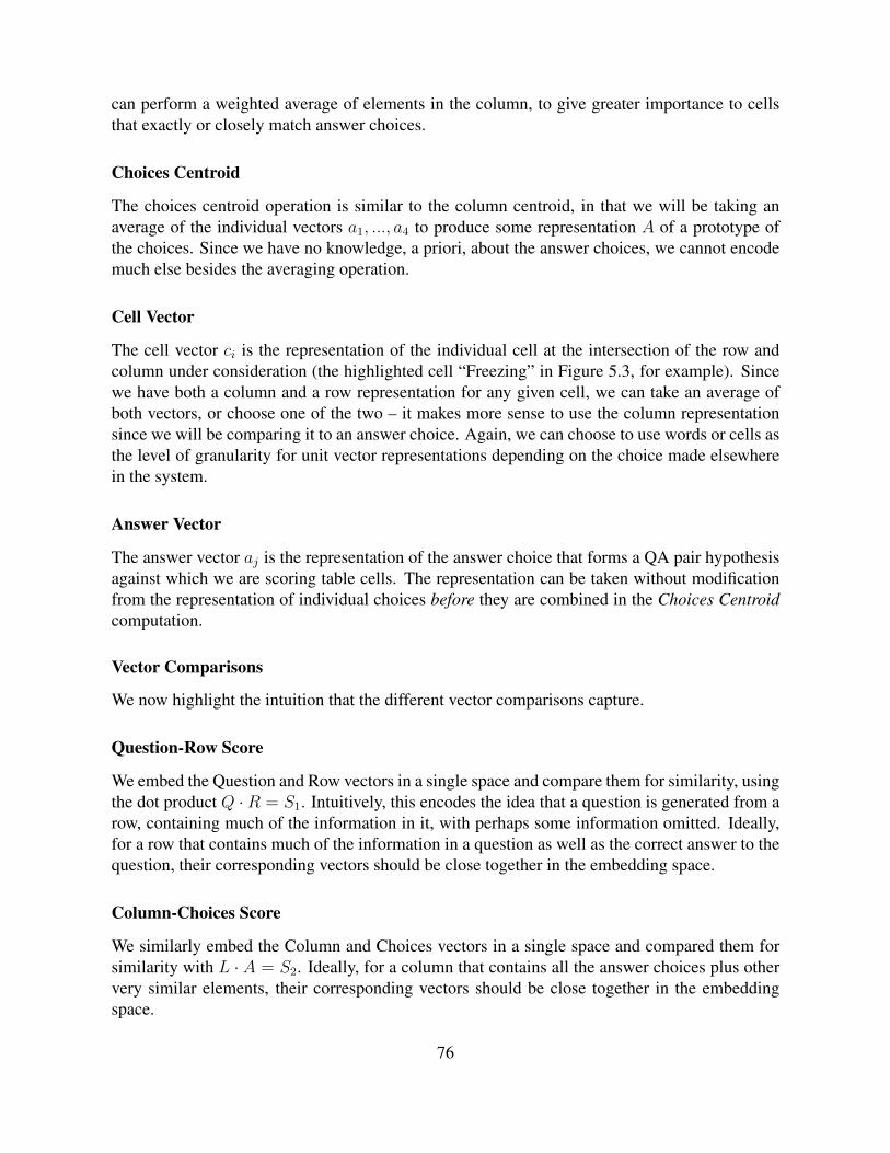
can perform a weighted average of elements in the column, to give greater importance to cellsthat exactly or closely match answer choices.

Choices Centroid

The choices centroid operation is similar to the column centroid, in that we will be taking anaverage of the individual vectors a1, ..., a4 to produce some representation A of a prototype ofthe choices. Since we have no knowledge, a priori, about the answer choices, we cannot encodemuch else besides the averaging operation.

Cell Vector

The cell vector ci is the representation of the individual cell at the intersection of the row andcolumn under consideration (the highlighted cell “Freezing” in Figure 5.3, for example). Sincewe have both a column and a row representation for any given cell, we can take an average ofboth vectors, or choose one of the two – it makes more sense to use the column representationsince we will be comparing it to an answer choice. Again, we can choose to use words or cells asthe level of granularity for unit vector representations depending on the choice made elsewherein the system.

Answer Vector

The answer vector aj is the representation of the answer choice that forms a QA pair hypothesisagainst which we are scoring table cells. The representation can be taken without modificationfrom the representation of individual choices before they are combined in the Choices Centroidcomputation.

Vector Comparisons

We now highlight the intuition that the different vector comparisons capture.

Question-Row Score

We embed the Question and Row vectors in a single space and compare them for similarity, usingthe dot product Q · R = S1. Intuitively, this encodes the idea that a question is generated from arow, containing much of the information in it, with perhaps some information omitted. Ideally,for a row that contains much of the information in a question as well as the correct answer to thequestion, their corresponding vectors should be close together in the embedding space.

Column-Choices Score

We similarly embed the Column and Choices vectors in a single space and compared them forsimilarity with L · A = S2. Ideally, for a column that contains all the answer choices plus othervery similar elements, their corresponding vectors should be close together in the embeddingspace.

76

Cell-Answer Score

To make the scores relevant to a particular QA hypothesis, we also compare the row-columnintersection cell vector to the vector representing the answer currently under consideration usingci · aj = S3. Ideally, the two vectors should be close if the answer is the same or very similar tothe intersection cell.

Cell Relevance Score

The final step combines each of the individual scores by performing S1 · S2 · S3 to form a finalrelevance score Sf . This score captures how relevant a particular cell is to verifying the hypoth-esis created by a particular QA pair. Each of the three components of this score must be high forthe final relevance score to be high as well.

5.6.2 TrainingSince our proposed TabNN model follows the design template as FRETS, namely by scoringindividual cells for relevance to QA pairs, we can use the same training objective as before(see Section 5.5.1). In summary this objective is the cross-entropy loss between a hypothesizeddistribution and the true one in training. These distributions can be computed from the scoreswe assign to cells with our model and the scores obtained heuristically, as with FRETS, frommanual annotations of alignments between MCQs and table entries.

By considering the discrepancy between the hypothesized and true distributions, we canback-propagate the error to update vectors of individual units of representation – whether theyare words or whole cells in tables.

As a side-note on parallelization and computational efficiency, it should be evident from thediagram in Figure 5.3 and the subsequent description of TabNN, that many of the computationscan be cached. The LSTMs for computing the vector of rows or the centroid operation to findthe centroid vector of a column must only be run once (or once per epoch in training). Hence alot of difficult computation can be cached. Also there is no interaction between rows or columns,so all of this computation can be parallelized, as well.

In conclusion, our TAbNN model will leverage the structural properties of tables as well therelational information between these structural units and MCQs. It will learn representations forunits (words or cells) in tables, without the need for any manual engineering of features. It thusfits into the main theme of this thesis, which is to use structural and relational information inlearning more complex and expressive models of semantics.

5.7 Conclusion

We have presented ongoing work on using tables as a source of background knowledge for ques-tion answer. Tables represent a unique and interesting domain for the study of relational structurein representation learning, with interesting semantic properties emerging from relationships be-tween row and column elements. These properties lead to three separate contributions.

77

Firstly, we create a dataset of tables, whose semi-structured formalism allows them to beeasily created or extended by non-experts (or computation systems, in future work). Secondly,the semantics of this structure can be used to induce non-expert crowd-sourcing annotators toeasily create a high-quality MCQ dataset, which has alignment information to table elements.This dataset is under construction, and its completion is proposed work for this thesis. Finallywe use the structure, as well as the dataset of tables, MCQs and alignments between them to buildtwo systems that solve MCQs. We have implemented the first – a feature-rich model consisting ofmanually engineered features – and evaluated it on a battery of tests, showing promising results.We have also outlined the details of the second as proposed work: a neural network model thatwill learn features automatically for table entries to solve MCQs.

78

Chapter 6

Event Structure – Proposed Work

Decomposing Event Structure and Argument Relations for Predicate

Categorization

This thesis is concerned with using semantic relations to learn more expressive models of seman-tics. Relations encompass a very broad range of phenomenon in language and data formalisms,and in Chapter 2 we have attempted to provide a taxonomy of these occurrences of relations as itpertains to our work. This taxonomy serves, both as a technical summary of this thesis, as wellas a high-level guideline on how to think about using relations in representation learning of anew domain or problem.

However, an important research issue when dealing with relations for representation learningis the relations themselves. In particular, for a particular language phenomenon or data formal-ism, how many relations are there? What are they? How do they organize the elements in thedomain to one another? Is the existing structure ideal?

It may be noted that finding answers to these theoretical questions does not necessarily affectthe problem of using these relations for learning representations. However, these questions arecrucial to providing a comprehensive account of semantic relations for representation learning –which we aim to do in this thesis. More importantly, when existing structured data in the formof annotated language or data is non-existent (say for a new domain or low resource language),these questions are no longer theoretical but are a practical precursor to using relations to learnmore expressive models of semantics.

Hence, in this chapter we turn to the problem of providing a representation learning solutionto the theoretical questions regarding relations in the particular domain of verbal events. Thisis an apt domain, since verbs undoubtedly have relational arguments, as supported by the bodyof linguistic literature devoted to studying argument realization (Jackendoff, 1987; Moens andSteedman, 1988; Levin and Rappaport Hovav, 2005). However, the specific number and natureof these arguments remains contested (Fillmore, 1967; Sowa, 1991), with solutions ranging froma few prototypical Propbank style relations (Kingsbury and Palmer, 2002) to an effectively open-ended set of highly specific and fine-grained roles in FrameNet (Baker et al., 1998).

We propose a novel application of the Indian Buffet Process (IBP) (Ghahramani and Griffiths,

79

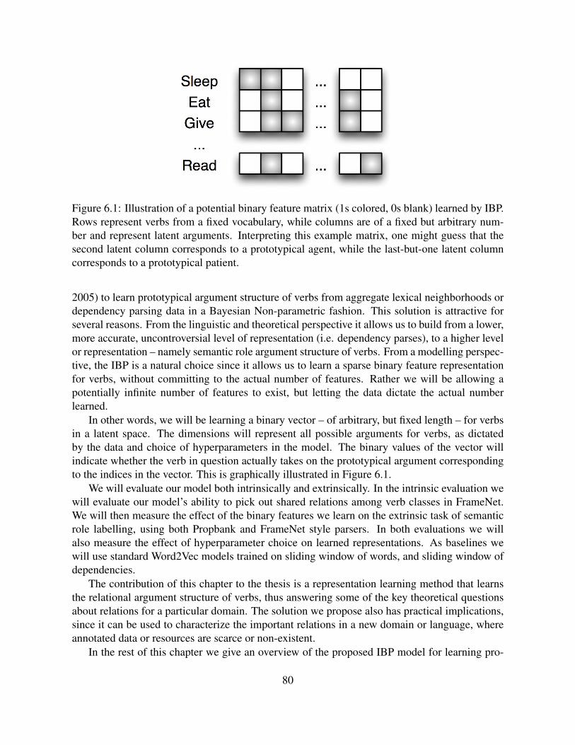
Figure 6.1: Illustration of a potential binary feature matrix (1s colored, 0s blank) learned by IBP.Rows represent verbs from a fixed vocabulary, while columns are of a fixed but arbitrary num-ber and represent latent arguments. Interpreting this example matrix, one might guess that thesecond latent column corresponds to a prototypical agent, while the last-but-one latent columncorresponds to a prototypical patient.

2005) to learn prototypical argument structure of verbs from aggregate lexical neighborhoods ordependency parsing data in a Bayesian Non-parametric fashion. This solution is attractive forseveral reasons. From the linguistic and theoretical perspective it allows us to build from a lower,more accurate, uncontroversial level of representation (i.e. dependency parses), to a higher levelor representation – namely semantic role argument structure of verbs. From a modelling perspec-tive, the IBP is a natural choice since it allows us to learn a sparse binary feature representationfor verbs, without committing to the actual number of features. Rather we will be allowing apotentially infinite number of features to exist, but letting the data dictate the actual numberlearned.

In other words, we will be learning a binary vector – of arbitrary, but fixed length – for verbsin a latent space. The dimensions will represent all possible arguments for verbs, as dictatedby the data and choice of hyperparameters in the model. The binary values of the vector willindicate whether the verb in question actually takes on the prototypical argument correspondingto the indices in the vector. This is graphically illustrated in Figure 6.1.

We will evaluate our model both intrinsically and extrinsically. In the intrinsic evaluation wewill evaluate our model’s ability to pick out shared relations among verb classes in FrameNet.We will then measure the effect of the binary features we learn on the extrinsic task of semanticrole labelling, using both Propbank and FrameNet style parsers. In both evaluations we willalso measure the effect of hyperparameter choice on learned representations. As baselines wewill use standard Word2Vec models trained on sliding window of words, and sliding window ofdependencies.

The contribution of this chapter to the thesis is a representation learning method that learnsthe relational argument structure of verbs, thus answering some of the key theoretical questionsabout relations for a particular domain. The solution we propose also has practical implications,since it can be used to characterize the important relations in a new domain or language, whereannotated data or resources are scarce or non-existent.

In the rest of this chapter we give an overview of the proposed IBP model for learning pro-

80

totypical verb argument relational structure, and how we propose to evaluate the resulting repre-sentations against existing databased of verb argument structure.

6.1 Proposed Model

The IBP is a Bayesian Non-parametric model that defines priors over infinite dimensional binaryfeature matrices (fixed rows or objects, with infinite feature vectors). Then given some data, themodel computes a posterior that provides a finite feature matrix that best explains the data. Inthe Bayesian framework, this posterior can be updated with increasing amounts of data – and theadvantage of a Bayesian Non-parametric model such as the IBP is that it can scale and adapt thecomplexity of the model (i.e. the number of features) to better suit increasingly larger amountsof data.

Applying this as modelling tool for finding argument structure of verbs, we assume that therea potentially infinite number of argument relations, and let the data dictate which (latent onesactually manifest). Posterior inference with the IBP will give us a finite dimensional binarymatrix (as illustrated in Figure 6.1).

In what follows we outline the IBP as applied to our problem, highlighting the more importantmodelling choices. For a detailed derivation of the IBP we refer the reader to Ghahramani andGriffiths (2005) or Griffiths and Ghahramani (2011). A more general summary of BayesianNon-parametric modelling can be found in Gershman and Blei (2012).

Let v1, ..., vN be a vocabulary of verbs. Consider the case when these verbs may be repre-sented by an finite set ofK binary latent factors. We can represent this by a binary feature matrixZ with dimensions N ×K. THe elements zik of this matrix indicate whether verb vi takes on therelational argument k. When the dimensions K lim∞ the matrix Z plays the role of the prior inour model.

We will assume that the features, or relational arguments are independently generated fromone another, with a particular feature k occurring with probability πk. The elements of the matrixare then Bernoulli distributed, with zik|πk ∼ Bernoulli(πk). We will also define a hyperparameterα such that πk|alpha ∼ Beta(

α

K, 1).

Given these assumptions, the IBP defines a culinary analogy on how matrices Z can beincrementally built, such that they are legitimate draws from the underlying distribution. Ncustomers (verbs) enter a restaurant one after another. The restaurant has a buffet consisting ofan infinite number of dishes (relational arguments). When the first customer v1 enters she takesa serving from the first Poisson(α) dishes until her plate is full. Every subsequent customer visamples previously tasted dishes with a probability

mk

ithat is proportional to its popularity (mk

is the number of customers who previously also tasted this dish). The new customers also servesthemselves Poisson(α

i) new dishes. The elements zik of the matrix are 1 if customer vi sampled

dish k, and 0 otherwise.In the limit of the number of features K lim∞, it can be shown that the probability of a

matrix being produced by this process is:

81

P (Z) =αK+∏Ni=1K

i!exp (−αHN)

K+∏k=1

(N −mk!)(mk − 1)

N !(6.1)

HereK+ denotes the non-zero columns of the infinite feature matrix,i.e. those whosemk > 0.Also Ki is the number of new dishes sampled by the ith customer to enter the restaurant. Finally,

HN is the N th harmonic number – which can be computed asN∑j=1

1

j.

This is the form of the prior distribution that we will use to compute our actual feature matri-ces for verb argument structure induction.

Properties of the Prior

In a Bayesian setting, the prior should encode properties that intuitively capture important desider-ata of the problem under consideration. The prior given in Equation 6.1 has several desirableproperties for the problem we are attempting to solve.

Firstly the term K+ follows a distribution Poisson(αHN). This means that we can controlthe effective number of features in our learned model with the hyperparameter α. We can eitherchoose to be conservative and only pick out the most salient relational arguments of verbs, or bepermissive and capture even fine-grained semantic nuances, or effectively any degree of tolerancein between.

Secondly, the actual number of non-zero features for any instance follows a distributionPoisson(α). That means that the different verbs may all have different relational arguments butthe number of these arguments will stay within a reasonable range of one another, discouragingwild outliers.

Lastly, the matrix Z tends to remain sparse even when K lim∞. Sparsity is important be-cause it allows the model to encode only what it believes to be the most important relationalarguments for every verb.

Inference

As with standard Bayesian practise, we will update the prior in Equation 6.1 with a likelihoodfunction over data given the prior in order to compute a posterior estimate. This is the actualfinite dimensional feature matrix that we seek, and it can be found through posterior inference.

Unfortunately the form of the prior in Equation 6.1 makes it intractable for exact infer-ence. Instead we will need an approximate inference method like Markov Chain Monte Carlo(MCMC). In particular we propose to use a specific kind of MCMC called Gibbs Sampling. Thistechnique samples variables sequentially, by conditioning on the current value of all the othervariables (Geman and Geman, 1984), thus building a Markov chain of samples. These sampleseventually converge to draws from the true underlying distribution (Gilks et al., 1996).

It can be shown that the Markov chain samples from the prior can be computed as:

P (zik = 1|Z\zik) =mk\zikN

(6.2)

82

where mk\zik is the number of verbs, not including vi, taking on the relational argument k andZ\zik denotes the assignment of all other variables in Z except zik. A sufficient number of drawsin this fashion will make the ziks follow the distribution given by Equation 6.1. Then, to samplefrom the posterior distribution P (X|Z) we sequentially sample the elements of Z from the priorand combine it with the likelihood to obtain the full conditional distribution:

P (zik = 1|Z\zik, X) ∝ P (X|Z)P (zik = 1|Z\zik) (6.3)

Griffiths and Ghahramani (2011) suggest a heuristic strategy by which the likelihood functionP (X|Z) can simply be incorporated into the computation of the prior by which we obtain thedesired posterior directly. We propose to begin experimenting with a linear-Gaussian model asthe likelihood function, as described by Griffiths and Ghahramani (2011) which allows us toincorporate the likelihood efficiently. But we will explore other suitable likelihood functions aswell.

Data

An important consideration is the data X that we will be modelling. This will be a finite dimen-sional matrix, with the N verbs forming the rows, and some set of linguistic features formingthe columns. We will experiment with several different variants for these columns, as well as thevalues that they take on.

For the linguistic assignment of columns or features, we will experiment with word-windowssurrounding verbs as well as dependency parsing neighborhood of the verb. For word-windowswe will experiment with both lexical features as well as super-sense features. As regards depen-dency parsing neighborhoods, we will experiment with only taking dependency arcs (and theirlabels), as well as the arcs along with their attachments (both lexical and super-sense variants).

For the feature values we will try taking raw counts, normalized counts, or the positive point-wise mutual information measure.

6.2 Proposed Evaluation

The task of evaluating learned binary vector representations of verbs over latent relational ar-guments is complicated by the fact that there is no single gold standard of what the true set ofrelations should be. Hence, we will evaluate our framework against an existing databases of verbargument structure, namely FrameNet.

FrameNet contains a broad set of fine-grained relations.We will evaluate the model from theperspective of relations rather than verbs. This will serve as a local, intrinsic evaluation of themodel’s ability to pick out useful clusters of verbs from the perspective of salient relations.

For example consider the FrameNet relational argument “Ingestor”, which broadly corre-sponds to an agent-like argument for eat. This argument is also common to other eat-like verbssuch as consume, devour, gobble, etc. Given such a set of verbs that have a target relation incommon, we will evaluate our model on its ability to pick out the shared relation. Generally, fora target relation r, let S = v1

S, ..., vMS be a set of verbs such that they all have the relational

83

argument r amongst them, while simultaneously any other verbs in V \S does not have the rela-tion r. Then, supposing that the column k of the vector representations of the verbs in S has thehighest sum mk, i.e. this is the relation that is most strongly present in this set of verbs accordingto our model. We can measure our model’s performance for the single relational argument r asthe precision and recall scores:

Prec(r) =

∑Ni=0 zik · δ(vi ∈ S)∑N

i=0 zik(6.4)

Rec(r) =

∑Ni=0 zik · δ(vi ∈ S)

|S| (6.5)

where δ(·) is the indicator function.We will evaluate different models learned with different choices of hyperparameters to under-

stand how these choices affect the latent set of relations. We will also attempt to correlate theselatent relations to the set of proposed relations in FrameNet. Finally we will compare our modelsagainst standard word vector based models, such as Word2Vec, trained both on word-windowand syntactic neighborhoods.

In addition to the proposed intrinsic evaluation, we will also conduct an extrinsic evaluationby using the learned representation for verbs as additional features in a semantic parser. Inthis case we will evaluate against both a coarse-grained parser that operates on Propbank stylerelations, as well as a more fine-grained parser that operates on FrameNet relations.

Finally, since the work we propose is not only a theoretical investigation but a practical onefor languages that do not contain structured relational databases, we will also attempt to learnlatent relational structure arguments for verbs in one of these languages. We propose to evaluatethis via crowd-sourcing by asking human annotators to judge whether the latent set of relationsseem intuitively reasonable.

84

Chapter 7

Class-Instance Entity Linking – ProposedWork

Using Encyclopedic and Discourse Relations to Learn Class-Instance Entity

Representations for Knowledge-bases and Anaphora

Named entities are an open class of words that come with a high degree of surface form ambi-guity. For example, “Obama”, “Mr. Obama”, “Barack Obama”, “the president” and “presidentObama” are all ways of referring to the same real world entity. We call this the problem of en-tity synonymy. Simultaneously, the identical string “Jerry Hobbs” may refer, in one discoursecontext to a serial killer and in another to a computational linguist. We term this phenomenon asentity polysemy. Moreover, in a discourse context, the same entity may be referred to by a pro-noun, rather than a nominal phrase, compounding the problem of determining what real worldentity is being referenced. This, of course, is the common problem of entity anaphora.

From a computational semantics perspective it is useful to link textual mentions of namedentities to one another or to real world referents. This allows systems to reason jointly over allrelated mentions, rather than treating each mention as a different textual phenomenon. From arepresentation learning perspective a model that, for example, creates a single representation fora unique real world referent is likely to be more robust than one that treats every possible surfacerealization as a different entity.

Yet, most current vector space models ignore this facet of named entities. They are illequipped to deal with the problems of entity synonymy, entity polysemy and entity anaphora1.Firstly, they typically treat every word as a separate token and learn a representation for eachtoken. Consequently they fail to connect nominal mentions that may refer to the same real worldreferent. Secondly, since most models are incapable of handling polysemy in general, they areincapable of disambiguating between two entities that have the same surface form. Finally, sincepronouns have little semantics attached to them outside of context, the representations learnt forthem (which are fixed) have no way of linking to concrete nominal mentions in the discourse.

1Of course, these are well studied problems in the general NLP literature, but we are specifically interested herewith representation learning solutions, or automatic feature generation techniques for these problems

85

We propose that semantic relations can play a useful role in helping the representation learn-ing paradigm overcome these difficulties. Hence we offer two novel ideas: one for solving theproblems of entity synonymy and polysemy, and the other to tackle the problem of entity coref-erence. Each of the ideas deals with the notion of abstract to concrete relatedness: in the onecase to share information between related named entities, in the other to share information indiscourse context.

Since this is very preliminary work, we only motivate the problems and propose ideas for so-lutions. We do not currently have concrete models to actualize these solutions. In what followswe briefly outline how we plan to leverage semantic relations in encyclopedic databases and dis-course contexts to tackle the problems of synonymy, polysemy and anaphora for representationlearning of named entities.

7.1 Synonymy and Polysemy with Encyclopedic Relations

Encyclopedic knowledge bases such as Freebase and Wikipedia contain a vast amount of veryuseful information about named entities such as people, places, organizations, geo political en-tities etc. This information comes in the form of text that describes these entities, as well asmetadata that links them to one another.

Encyclopedic information has been previously used to build semantic representation models.For example Gabrilovich and Markovitch (2007) use Wikipedia concept categories to define andcompute semantic relatedness for text via a technique they call Explicit Semantic Analysis. Moroet al. (2014) more specifically tackle the problem of entities by considering the WordNet graph asa knowledge base to build semantic signatures. These signatures are then used to disambiguateentities in text. Fauceglia et al. (2015) extend this approach to deal with the orders of magnitudelarger graph of Freebase, while also tackling multiple languages.

However, past work has mostly looked at one view of the data: primarily the link structure,or the text for building general purpose word vector representations. We propose to combinethese different streams of information into a joint model that builds representations for namedentities. In particular we aim to work with Freebase as our source of encyclopedic knowledgesince it contains text descriptions, links between entities as well as attributes and categories thatorganize entities in relation to one another.

The structure of the encyclopaedia is derived from the relational links it contains. Thesemay be entity links that connect one entity to another, or they may be attribute links that specifythat an entity belongs to a certain category or has certain properties. Each of these types oflinks defines a structure that explains the underlying encyclopedic data in a different way. Weare considering a multi-view approach in which each of these sources of structured information,along with non-structured textual descriptions, is assumed to be a different view of the data.

We propose to use a multi-view learning approach to combine these streams of information tolearn representations that are jointly optimize for all the different views together. Xu et al. (2013)provide an overview of multi-view learning techniques. Some of the most popular models includeCanonical Correlation Analysis (Hardoon et al., 2004) and Co-Training (Blum and Mitchell,1998).

With this multi-view approach, we aim to have a sufficiently rich set of representations to

86

tackle the problems of entity polysemy. We perceive that while two entities may have identicalnames, the way they are described in text, the other entities they link to, or attributes that theypossess will be sufficiently different to produce distinctly different representations. At the sametime the divergences in their representations along with the multi-view data provides a source ofinformation on which to disambiguate and ground entities in text to knowledge base entries.

In addition to combining different views of the encyclopedic data, we also propose to specif-ically learn representations at different levels of the class-instance scale for named entities. Weaim to learn generalizations and specifications of concepts through a hierarchy of terms that areused to categorize the named entities. For example, “Obama” is a “president” is a “head-of-state”is a “person” is a “human” etc.2

By learning these generalizations of named entities that are grounded in the knowledge basewe hope to tackle the problem of entity synonymy. Specifically, we propose that these abstrac-tions can be used as disambiguators for when named entities are referenced by generalized termsin text. We propose to extend the Retrofitting paradigm (Faruqui et al., 2014) (also see Chap-ter 4) to not only consider flat graph structures of relationally linked concepts, but to considerhierarchies over these concepts.

7.2 Anaphora with Discourse RelationsPronouns are closed class words that hold very little semantics by themselves. Rather they derivemeaning from their context and the entities to which they refer. In a problem like anaphora, whilesome clues like number and gender are inherent in the pronoun, contextual cues play an equallyimportant role in determining referents for pronouns.

Meanwhile from a representational standpoint, pronouns can potentially occur in any numberof different contexts. Thus, representations learned for them via the distributional hypothesishave too many confusing signals to learn anything meaningful or robust. Moreover, for a problemlike anaphora, previous contexts have little predictive power over the next context in which apronoun can occur. Consequently the premise of a statically learnt representation for pronounsis itself flawed.

There has been little work dealing with pronouns or anaphora within the representation learn-ing paradigm. Bagga and Baldwin (1998) use vector space models for entity anaphora, but onlyto distinguish between different entities with identical names (entity polysemy). Meanwhile,Sadrzadeh et al. (2013) and Sadrzadeh et al. (2014) propose Frobenius algebras that deals withrelative pronouns. But these are focussed at composition in representation learning rather thanwith the problem of anaphora.

In this work we propose a novel extension to the representation learning paradigm that willintroduce a dynamic model capable of performing anaphora resolution. The dynamic nature ofthe model will stem from its ability to adapt representations – especially those of pronouns –progressively to produce maximally meaningful and consistent anaphora clusters.

The adaptation will rely on the intuition of class-instance relationship between pronouns andtheir real world named referents. In summary our idea will revolve around representing anaphora

2In WordNet 3.1 an “is a” relation is sometimes “is instance of class” and at others “hyponym”. We will takecare to treat each relation differently when applying the class-hierarchy idea to our problem

87

as progressively building clusters of vectors. We will assign new pronouns or named entities toclusters whose centroid is the closest to their own representation. This representation will notbe static, but will rather be constructed dynamically via a mapping function over lexical anddiscourse cues learnt from anaphora training data. Additionally, once an assignment to a clusteris completed, we propose that the representations of the elements in that cluster as well as itscentroid are updated to reflect the information from the update.

In addition to the class-instance relationship between pronouns and named entities, we alsohope to use the class-instance hierarchy of terms we propose to learn in Section 7.1 in order tohelp with the problem of entity synonymy in anaphora.

There will be two sources of relations that we will leverage in our approach. Firstly, we willuse linguistic structure in the form of cues from discourse – e.g. Rhetorical Structure Theoryrelations (Mann and Thompson, 1988) – or syntactic relation to learn our dynamic mappingfunction. Secondly, we will use the structure inherent in a anaphora cluster – namely that allthe elements it contains are linked via a anaphora relation – to compute new representations ofelements within the cluster.

88

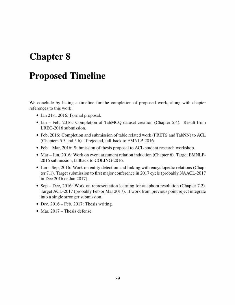
Chapter 8

Proposed Timeline

We conclude by listing a timeline for the completion of proposed work, along with chapterreferences to this work.• Jan 21st, 2016: Formal proposal.• Jan – Feb, 2016: Completion of TabMCQ dataset creation (Chapter 5.4). Result from

LREC-2016 submission.• Feb, 2016: Completion and submission of table related work (FRETS and TabNN) to ACL

(Chapters 5.5 and 5.6). If rejected, fall-back to EMNLP-2016.• Feb – Mar, 2016: Submission of thesis proposal to ACL student research workshop.• Mar – Jun, 2016: Work on event argument relation induction (Chapter 6). Target EMNLP-

2016 submission, fallback to COLING-2016.• Jun – Sep, 2016: Work on entity detection and linking with encyclopedic relations (Chap-

ter 7.1). Target submission to first major conference in 2017 cycle (probably NAACL-2017in Dec 2016 or Jan 2017).

• Sep – Dec, 2016: Work on representation learning for anaphora resolution (Chapter 7.2).Target ACL-2017 (probably Feb or Mar 2017). If work from previous point reject integrateinto a single stronger submission.

• Dec, 2016 – Feb, 2017: Thesis writing.• Mar, 2017 – Thesis defense.

89

90

Bibliography

Aydin, Bahadir Ismail, Yilmaz, Yavuz Selim, Li, Yaliang, Li, Qi, Gao, Jing and Demirbas, Murat(2014). Crowdsourcing for multiple-choice question answering. In Twenty-Sixth IAAI Confer-ence. 5.1

Bagga, Amit and Baldwin, Breck (1998). Entity-based cross-document coreferencing using thevector space model. In Proceedings of the 36th Annual Meeting of the Association for Compu-tational Linguistics and 17th International Conference on Computational Linguistics-Volume1, pp. 79–85. Association for Computational Linguistics. 7.2

Baker, Collin F, Fillmore, Charles J and Lowe, John B (1998). The Berkeley Framenet project.In Proceedings of the 17th international conference on Computational linguistics-Volume 1,pp. 86–90. Association for Computational Linguistics. 3.3, 6

Baroni, Marco and Lenci, Alessandro (2010). Distributional memory: A general framework forcorpus-based semantics. Comput. Linguist., volume 36 (4), pp. 673–721.URL: http://dx.doi.org/10.1162/colia000162, 3, 3.1, 3.2.1, 3.3, 3.3.1

Baroni, Marco and Zamparelli, Roberto (2010). Nouns are vectors, adjectives are matrices: rep-resenting adjective-noun constructions in semantic space. In Proceedings of the 2010 Con-ference on Empirical Methods in Natural Language Processing, EMNLP ’10, pp. 1183–1193.Association for Computational Linguistics, Stroudsburg, PA, USA.URL: http://dl.acm.org/citation.cfm?id=1870658.1870773 3.2.1

Bejan, Cosmin Adrian and Harabagiu, Sanda (2010). Unsupervised event coreference resolutionwith rich linguistic features. In Proceedings of the 48th Annual Meeting of the Association forComputational Linguistics, ACL ’10, pp. 1412–1422. Association for Computational Linguis-tics, Stroudsburg, PA, USA.URL: http://dl.acm.org/citation.cfm?id=1858681.1858824 3.2.5

Bengio, Yoshua, Courville, Aaron and Vincent, Pierre (2013). Representation learning: A reviewand new perspectives. Pattern Analysis and Machine Intelligence, IEEE Transactions on,volume 35 (8), pp. 1798–1828. (document), 1

Bethard, Steven and Martin, James H (2007). CU-TMP: temporal relation classification usingsyntactic and semantic features. In Proceedings of the 4th International Workshop on SemanticEvaluations, pp. 129–132. Association for Computational Linguistics. 3.3.1

Blank, Andreas (2003). Polysemy in the lexicon and in discourse. TRENDS IN LINGUISTICSSTUDIES AND MONOGRAPHS, volume 142, pp. 267–296. 2, 1

Blum, Avrim and Mitchell, Tom (1998). Combining labeled and unlabeled data with co-training.

91

In Proceedings of the eleventh annual conference on Computational learning theory, pp. 92–100. ACM. 7.1

Brockett, Chris (2007). ALIGNING THE RTE 2006 CORPUS. Technical Report MSR-TR-2007-77, Microsoft Research.URL: http://research.microsoft.com/apps/pubs/default.aspx?id=70453 5.1

Bruni, Elia, Tran, Nam-Khanh and Baroni, Marco (2014). Multimodal Distributional Semantics.Journal of Artificial Intelligence Research (JAIR), volume 49, pp. 1–47. 4.4.1

Bullinaria, John A and Levy, Joseph P (2007). Extracting semantic representations from wordco-occurrence statistics: A computational study. Behavior Research Methods, volume 39 (3),pp. 510–526. 3.3.2

Cafarella, Michael J, Halevy, Alon, Wang, Daisy Zhe, Wu, Eugene and Zhang, Yang (2008).Webtables: exploring the power of tables on the web. Proceedings of the VLDB Endowment,volume 1 (1), pp. 538–549. 5.1

Carpenter, Bob (2008). Lazy sparse stochastic gradient descent for regularized multinomiallogistic regression. Technical report, Alias-i. Available at http://lingpipe-blog.com/ lingpipe-white-papers. 4.2.2

Cho, Kyunghyun, Van Merrienboer, Bart, Gulcehre, Caglar, Bahdanau, Dzmitry, Bougares,Fethi, Schwenk, Holger and Bengio, Yoshua (2014). Learning phrase representations us-ing rnn encoder-decoder for statistical machine translation. arXiv preprint arXiv:1406.1078.5.6.1

Ciaramita, Massimiliano and Altun, Yasemin (2006). Broad-coverage sense disambiguationand information extraction with a supersense sequence tagger. In Proceedings of the 2006Conference on Empirical Methods in Natural Language Processing, EMNLP ’06, pp. 594–602. Association for Computational Linguistics, Stroudsburg, PA, USA.URL: http://dl.acm.org/citation.cfm?id=1610075.1610158 3.2.2

Ciresan, Dan, Meier, Ueli and Schmidhuber, Jurgen (2012). Multi-column deep neural networksfor image classification. In Computer Vision and Pattern Recognition (CVPR), 2012 IEEEConference on, pp. 3642–3649. IEEE. 1

Clark, Peter (2015). Elementary school science and math tests as a driver for AI: Take the AristoChallenge. Proceedings of IAAI, 2015. 5

Collobert, Ronan and Weston, Jason (2008). A unified architecture for natural language process-ing: deep neural networks with multitask learning. In Proceedings of the 25th internationalconference on Machine learning, ICML ’08, pp. 160–167. ACM, New York, NY, USA.URL: http://doi.acm.org/10.1145/1390156.1390177 (document), 4, 4.2.2

Collobert, Ronan, Weston, Jason, Bottou, Leon, Karlen, Michael, Kavukcuoglu, Koray andKuksa, Pavel (2011). Natural Language Processing (Almost) from Scratch. J. Mach. Learn.Res., volume 999888, pp. 2493–2537.URL: http://dl.acm.org/citation.cfm?id=2078183.2078186 1, 1, 2, 3.2.1, 3.2.5, 3.2.5, 3.3.1,3.3.3

Corduneanu, Adrian and Jaakkola, Tommi (2002). On information regularization. In Proceed-

92

ings of the Nineteenth conference on Uncertainty in Artificial Intelligence, pp. 151–158. Mor-gan Kaufmann Publishers Inc. 2, 4.1

Curran, James Richard (2003). From Distributional to Semantic Similarity. Technical report. 1

Dahl, George, Mohamed, Abdel-rahman, Hinton, Geoffrey E et al. (2010). Phone recognitionwith the mean-covariance restricted Boltzmann machine. In Advances in neural informationprocessing systems, pp. 469–477. (document), 1

Das, Dipanjan and Petrov, Slav (2011). Unsupervised Part-of-Speech Tagging with BilingualGraph-Based Projections. In Proc. of ACL. 4.1

Das, Dipanjan and Smith, Noah A. (2011). Semi-Supervised Frame-Semantic Parsing for Un-known Predicates. In Proc. of ACL. 4.1

Deerwester, Scott C., Dumais, Susan T, Landauer, Thomas K., Furnas, George W. and Harshman,Richard A. (1990). Indexing by latent semantic analysis. JASIS, volume 41 (6), pp. 391–407.1, 3.3.1

Deng, Li, Seltzer, Michael L, Yu, Dong, Acero, Alex, Mohamed, Abdel-rahman and Hinton,Geoffrey E (2010). Binary coding of speech spectrograms using a deep auto-encoder. InInterspeech, pp. 1692–1695. Citeseer. 1

Dinu, Georgiana and Lapata, Mirella (2010a). Measuring distributional similarity in context. InProceedings of the 2010 Conference on Empirical Methods in Natural Language Processing,EMNLP ’10, pp. 1162–1172. Association for Computational Linguistics, Stroudsburg, PA,USA.URL: http://dl.acm.org/citation.cfm?id=1870658.1870771 3.2.1

Dinu, Georgiana and Lapata, Mirella (2010b). Measuring distributional similarity in context. InProceedings of the 2010 Conference on Empirical Methods in Natural Language Processing,pp. 1162–1172. Association for Computational Linguistics. 4.1

Erk, Katrin (2007). A Simple, Similarity-based Model for Selectional Preferences. (document),1

Erk, Katrin and Pado, Sebastian (2008). A structured vector space model for word meaning incontext. In Proceedings of the Conference on Empirical Methods in Natural Language Pro-cessing, EMNLP ’08, pp. 897–906. Association for Computational Linguistics, Stroudsburg,PA, USA. 3.2, 3.2.1, 3.3.1, 4.1

Erk, Katrin and Pado, Sebastian (2010). Exemplar-based models for word meaning in context.In Proceedings of the ACL 2010 Conference Short Papers, pp. 92–97. Association for Com-putational Linguistics. 4.1

Etzioni, Oren, Banko, Michele, Soderland, Stephen and Weld, Daniel S (2008). Open infor-mation extraction from the web. Communications of the ACM, volume 51 (12), pp. 68–74.5.1

Fader, Anthony, Soderland, Stephen and Etzioni, Oren (2011). Identifying relations for openinformation extraction. In Proceedings of the Conference on Empirical Methods in NaturalLanguage Processing, pp. 1535–1545. Association for Computational Linguistics. 5.1

Fader, Anthony, Zettlemoyer, Luke and Etzioni, Oren (2014). Open question answering over cu-

93

rated and extracted knowledge bases. In Proceedings of the 20th ACM SIGKDD internationalconference on Knowledge discovery and data mining, pp. 1156–1165. ACM. 5

Faruqui, Manaal, Dodge, Jesse, Jauhar, Sujay K, Dyer, Chris, Hovy, Eduard and Smith, Noah A(2014). Retrofitting Word Vectors to Semantic Lexicons. arXiv preprint arXiv:1411.4166. 4,4.1, 7.1

Fauceglia, Nicolas Rodolfo, Lin, Yiu-Chang, Ma, Xuezhe and Hovy, Eduard (2015). CMU Sys-tem for Entity Discovery and Linking at TAC-KBP 2015. In To appear in TAC-KBP Workshop2015. 7.1

Fillmore, Charles J (1967). The case for case. 3.3, 6

Finkelstein, Lev, Gabrilovich, Evgeniy, Matias, Yossi, Rivlin, Ehud, Solan, Zach, Wolfman,Gadi and Ruppin, Eytan (2002). Placing Search in Context: The Concept Revisited. In ACMTransactions on Information Systems, volume 20, pp. 116–131. 2, 3.2.4, 3.2.4, 3.3.3, 4.4.1

Firth, John R. (1957). A Synopsis of Linguistic Theory, 1930-1955. Studies in Linguistic Analy-sis, pp. 1–32. 1, 2

Gabrilovich, Evgeniy and Markovitch, Shaul (2007). Computing Semantic Relatedness UsingWikipedia-based Explicit Semantic Analysis. In IJCAI, volume 7, pp. 1606–1611. 3.3.3, 7.1

Ganitkevitch, Juri, Van Durme, Benjamin and Callison-Burch, Chris (2013). PPDB: The Para-phrase Database. In Proceedings of NAACL-HLT, pp. 758–764. Association for Computa-tional Linguistics, Atlanta, Georgia.URL: http://cs.jhu.edu/ ccb/publications/ppdb.pdf 4.1

Geman, Stuart and Geman, Donald (1984). Stochastic relaxation, Gibbs distributions, and theBayesian restoration of images. Pattern Analysis and Machine Intelligence, IEEE Transactionson, (6), pp. 721–741. 6.1

Gershman, Samuel J and Blei, David M (2012). A tutorial on Bayesian nonparametric models.Journal of Mathematical Psychology, volume 56 (1), pp. 1–12. 6.1

Ghahramani, Zoubin and Griffiths, Thomas L (2005). Infinite latent feature models and theIndian buffet process. In Advances in neural information processing systems, pp. 475–482. 2,6, 6.1

Gilks, Walter R, Richardson, Sylvia and Spiegelhalter, David J (1996). Introducing markov chainmonte carlo. Markov chain Monte Carlo in practice, volume 1, p. 19. 6.1

Girju, Roxana, Nakov, Preslav, Nastase, Vivi, Szpakowicz, Stan, Turney, Peter and Yuret, Deniz(2007). Semeval-2007 task 04: Classification of semantic relations between nominals. In Pro-ceedings of the 4th International Workshop on Semantic Evaluations, pp. 13–18. Associationfor Computational Linguistics. 3.3.1

Glorot, Xavier, Bordes, Antoine and Bengio, Yoshua (2011). Domain adaptation for large-scalesentiment classification: A deep learning approach. In Proceedings of the 28th InternationalConference on Machine Learning (ICML-11), pp. 513–520. 1

Goldberg, Adele E. (2005). Argument Realization: Cognitive Grouping and Theoretical Exten-sions. 3.2.5

94

Goldstone, Robert L, Medin, Douglas L and Gentner, Dedre (1991). Relational similarity and thenonindependence of features in similarity judgments. Cognitive psychology, volume 23 (2),pp. 222–262. 1

Golub, Gene H and Reinsch, Christian (1970). Singular value decomposition and least squaressolutions. Numerische mathematik, volume 14 (5), pp. 403–420. 2

Gonzalez, Hector, Halevy, Alon Y., Jensen, Christian S., Langen, Anno, Madhavan, Jayant,Shapley, Rebecca, Shen, Warren and Goldberg-Kidon, Jonathan (2010). Google Fusion Ta-bles: Web-centered Data Management and Collaboration. In Proceedings of the 2010 ACMSIGMOD International Conference on Management of Data, SIGMOD ’10, pp. 1061–1066.ACM, New York, NY, USA.URL: http://doi.acm.org/10.1145/1807167.1807286 5.1

Goyal, Kartik, Jauhar, Sujay Kumar, Li, Huiying, Sachan, Mrinmaya, Srivastava, Shashank andHovy, Eduard (2013). A Structured Distributional Semantic Model for Event Co-reference.In Proceedings of the 51st Annual Meeting of the Association for Computational Linguistics(ACL – 2013). 1.1, 3.3.1

Grefenstette, Edward and Sadrzadeh, Mehrnoosh (2011). Experimental Support for a Categor-ical Compositional Distributional Model of Meaning. In Proceedings of the Conference onEmpirical Methods in Natural Language Processing, EMNLP ’11, pp. 1394–1404. Associa-tion for Computational Linguistics, Stroudsburg, PA, USA.URL: http://dl.acm.org/citation.cfm?id=2145432.2145580 3.3.1

Grefenstette, Edward, Sadrzadeh, Mehrnoosh, Clark, Stephen, Coecke, Bob and Pulman,Stephen (2011). Concrete sentence spaces for compositional distributional models of mean-ing. In Proceedings of the Ninth International Conference on Computational Semantics, IWCS’11, pp. 125–134. Association for Computational Linguistics, Stroudsburg, PA, USA.URL: http://dl.acm.org/citation.cfm?id=2002669.2002683 3.2.1

Griffiths, Thomas L and Ghahramani, Zoubin (2011). The indian buffet process: An introductionand review. The Journal of Machine Learning Research, volume 12, pp. 1185–1224. 6.1, 6.1

Guevara, Emiliano (2010). A regression model of adjective-noun compositionality in distribu-tional semantics. In Proceedings of the 2010 Workshop on GEometrical Models of Natu-ral Language Semantics, GEMS ’10, pp. 33–37. Association for Computational Linguistics,Stroudsburg, PA, USA.URL: http://dl.acm.org/citation.cfm?id=1870516.1870521 3.2.1

Guo, Jiang, Che, Wanxiang, Wang, Haifeng and Liu, Ting (2014). Learning sense-specific wordembeddings by exploiting bilingual resources. In Proceedings of COLING, pp. 497–507. 4.1

Haghighi, Aria and Klein, Dan (2009). Simple coreference resolution with rich syntactic andsemantic features. In Proceedings of the 2009 Conference on Empirical Methods in NaturalLanguage Processing: Volume 3 - Volume 3, EMNLP ’09, pp. 1152–1161. Association forComputational Linguistics, Stroudsburg, PA, USA.URL: http://dl.acm.org/citation.cfm?id=1699648.1699661 3.2.5

Halko, Nathan, Martinsson, Per-Gunnar and Tropp, Joel A (2011). Finding structure withrandomness: Probabilistic algorithms for constructing approximate matrix decompositions.

95

SIAM review, volume 53 (2), pp. 217–288. 3.3.2

Han, Xianpei and Zhao, Jun (2009). Named entity disambiguation by leveraging wikipedia se-mantic knowledge. In Proceedings of the 18th ACM conference on Information and knowledgemanagement, pp. 215–224. ACM. 2

Hardoon, David R, Szedmak, Sandor and Shawe-Taylor, John (2004). Canonical correla-tion analysis: An overview with application to learning methods. Neural computation, vol-ume 16 (12), pp. 2639–2664. 7.1

Harris, Zellig (1954). Distributional structure. Word, volume 10 (23), pp. 146–162. 1

Hassan, Samer and Mihalcea, Rada (2011). Semantic Relatedness Using Salient Semantic Anal-ysis. In AAAI. 3.3.3

Hendrickx, Iris, Kim, Su Nam, Kozareva, Zornitsa, Nakov, Preslav, O Seaghdha, Diarmuid,Pado, Sebastian, Pennacchiotti, Marco, Romano, Lorenza and Szpakowicz, Stan (2009).Semeval-2010 task 8: Multi-way classification of semantic relations between pairs of nom-inals. In Proceedings of the Workshop on Semantic Evaluations: Recent Achievements andFuture Directions, pp. 94–99. Association for Computational Linguistics. 3.3.1

Hjelm, Hans (2007). Identifying cross language term equivalents using statistical machine trans-lation and distributional association measures. In Proceedings of NODALIDA, pp. 97–104.Citeseer. 1

Hjort, Nils Lid, Holmes, Chris, Muller, Peter and Walker, Stephen G (2010). Bayesian nonpara-metrics, volume 28. Cambridge University Press. 2

Hochreiter, Sepp and Schmidhuber, Jurgen (1997). Long short-term memory. Neural computa-tion, volume 9 (8), pp. 1735–1780. 2

Huang, Eric H, Socher, Richard, Manning, Christopher D and Ng, Andrew Y (2012). Improvingword representations via global context and multiple word prototypes. In Proceedings of the50th ACL: Long Papers-Volume 1, pp. 873–882. 4, 4.1, 4.3, 4.4.1

Jackendoff, Ray (1987). The Status of Thematic Roles in Linguistic Theory. Linguistic Inquiry,volume 18 (3), pp. 369–411. 3.2.5, 6

Jarmasz, Mario and Szpakowicz, Stan (2003). Roget’s Thesaurus and Semantic Similarity. Re-cent Advances in Natural Language Processing III: Selected Papers from RANLP. 3.3.3

Jarmasz, Mario and Szpakowicz, Stan (2004). Roget’s Thesaurus and Semantic Similarity. Re-cent Advances in Natural Language Processing III: Selected Papers from RANLP, volume2003, p. 111. 4.4.1

Jauhar, Sujay Kumar, Dyer, Chris and Hovy, Eduard (2015). Ontologically Grounded Multi-sense Representation Learning for Semantic Vector Space Models. In Proc. NAACL. 1.1

Jauhar, Sujay Kumar and Hovy, Eduard (2014). Inducing Latent Semantic Relations for Struc-tured Distributional Semantics. In Proceedings of the 25th International Conference on Com-putational Linguistics, COLING 2014, pp. 698–708. 1.1, 2

Jauhar, Sujay Kumar, Turney, Peter D. and Hovy, Eduard (2016). TabMCQ: A Dataset of GeneralKnowledge Tables and Multiple-choice Questions. In Submitted to LREC-2015. Under Review.

96

1.1

Ji, Heng and Grishman, Ralph (2011). Knowledge base population: Successful approaches andchallenges. In Proceedings of the 49th Annual Meeting of the Association for ComputationalLinguistics: Human Language Technologies-Volume 1, pp. 1148–1158. Association for Com-putational Linguistics. 5.1

Johnson, Mark (2007). Why doesn’t EM find good HMM POS-taggers? In EMNLP-CoNLL, pp.296–305. Citeseer. 4.2.2

Joubarne, Colette and Inkpen, Diana (2011). Comparison of semantic similarity for differentlanguages using the Google N-gram corpus and second-order co-occurrence measures. InAdvances in Artificial Intelligence, pp. 216–221. Springer. 4.4.2

Jurgens, David A, Turney, Peter D, Mohammad, Saif M and Holyoak, Keith J (2012). Semeval-2012 task 2: Measuring degrees of relational similarity. In Proceedings of the First JointConference on Lexical and Computational Semantics-Volume 1: Proceedings of the main con-ference and the shared task, and Volume 2: Proceedings of the Sixth International Workshopon Semantic Evaluation, pp. 356–364. Association for Computational Linguistics. 3.3.1, 3.3.4

Khot, Tushar, Balasubramanian, Niranjan, Gribkoff, Eric, Sabharwal, Ashish, Clark, Peter andEtzioni, Oren (2015). Exploring Markov Logic Networks for Question Answering. Proceedingsof EMNLP, 2015. 5

Kilgarriff, Adam (1997). I don’t believe in word senses. Computers and the Humanities, vol-ume 31 (2), pp. 91–113. 4

Kingsbury, Paul and Palmer, Martha (2002). From TreeBank to PropBank. In LREC. Citeseer.3.3, 6

Krizhevsky, Alex, Sutskever, Ilya and Hinton, Geoffrey E (2012). Imagenet classification withdeep convolutional neural networks. In Advances in neural information processing systems,pp. 1097–1105. (document), 1

Landauer, Thomas K and Dumais, Susan T. (1997). A solution to Plato’s problem: The latentsemantic analysis theory of acquisition, induction, and representation of knowledge. Psycho-logical review, pp. 211–240. 1, 3.3.3, 4.4.1

Lee, Heeyoung, Recasens, Marta, Chang, Angel, Surdeanu, Mihai and Jurafsky, Dan (2012).Joint entity and event coreference resolution across documents. In Proceedings of the 2012Joint Conference on Empirical Methods in Natural Language Processing and ComputationalNatural Language Learning, EMNLP-CoNLL ’12, pp. 489–500. Association for Computa-tional Linguistics, Stroudsburg, PA, USA.URL: http://dl.acm.org/citation.cfm?id=2390948.2391006 3.2.5

Levin, Beth and Rappaport Hovav, Malka (2005). Argument Realization. Cambridge UniversityPress. 3.2.5, 6

Levy, Omer and Goldberg, Yoav (2014). Neural word embedding as implicit matrix factorization.In Advances in Neural Information Processing Systems, pp. 2177–2185. 1

Limaye, Girija, Sarawagi, Sunita and Chakrabarti, Soumen (2010). Annotating and searchingweb tables using entities, types and relationships. Proceedings of the VLDB Endowment,

97

volume 3 (1-2), pp. 1338–1347. 5.1

Lin, Dekang (1998). Automatic retrieval and clustering of similar words. In Proceedings of the17th international conference on Computational linguistics-Volume 2, pp. 768–774. Associa-tion for Computational Linguistics. 3.3.2

Mann, William C and Thompson, Sandra A (1988). Rhetorical structure theory: Toward a func-tional theory of text organization. Text-Interdisciplinary Journal for the Study of Discourse,volume 8 (3), pp. 243–281. 7.2

Marquez, Lluıs, Carreras, Xavier, Litkowski, Kenneth C and Stevenson, Suzanne (2008). Se-mantic role labeling: an introduction to the special issue. Computational linguistics, vol-ume 34 (2), pp. 145–159. 3.3

McCarthy, Diana and Carroll, John (2003). Disambiguating Nouns, Verbs, and Adjectives UsingAutomatically Acquired Selectional Preferences. Comput. Linguist., volume 29 (4), pp. 639–654. 1

McCarthy, Diana, Koeling, Rob, Weeds, Julie and Carroll, John (2004). Finding predominantword senses in untagged text. In Proceedings of the 42nd Annual Meeting on Association forComputational Linguistics, ACL ’04. Association for Computational Linguistics, Stroudsburg,PA, USA. (document), 1

McCarthy, Diana and Navigli, Roberto (2007). SemEval-2007 Task 10: English Lexical Sub-stitution Task. In Proceedings of the 4th International Workshop on Semantic Evaluations(SemEval-2007), Prague, Czech Republic, pp. 48–53. 1

Mikolov, Tomas, Chen, Kai, Corrado, Greg and Dean, Jeffrey (2013a). Efficient Estimation ofWord Representations in Vector Space. arXiv preprint arXiv:1301.3781. (document), 1, 4, 4.1,4.2.2, 4.2.2, 4.2.2, 4.3

Mikolov, Tomas, Karafiat, Martin, Burget, Lukas, Cernocky, Jan and Khudanpur, Sanjeev (2010).Recurrent neural network based language model. Proceedings of Interspeech. 1, 2

Mikolov, Tomas, Yih, Wen-tau and Zweig, Geoffrey (2013b). Linguistic Regularities in Con-tinuous Space Word Representations. In Proceedings of the 2013 Conference of the NAACL:Human Language Technologies, pp. 746–751. Atlanta, Georgia.URL: http://www.aclweb.org/anthology/N13-1090 1

Mikolov, Tomas, Yih, Wen-tau and Zweig, Geoffrey (2013c). Linguistic regularities in continu-ous space word representations. Proceedings of NAACL-HLT, pp. 746–751. 3.3.4, 3.3.4

Miller, George and Charles, Walter (1991). Contextual correlates of semantic similarity. InLanguage and Cognitive Processes, pp. 1–28. 4.4.1

Miller, George A (1995a). WordNet: a lexical database for English. Communications of theACM, volume 38 (11), pp. 39–41. 2, 4, 4.1, 4.3

Miller, George A. (1995b). WordNet: a lexical database for English. Commun. ACM, vol-ume 38 (11), pp. 39–41.URL: http://doi.acm.org/10.1145/219717.219748 3.2.2

Mitchell, Jeff and Lapata, Mirella (2008). Vector-based models of semantic composition. InProceedings of ACL-08: HLT, pp. 236–244. 1, 3.2.1, 3.2.5, 4.1

98

Mitchell, Jeff and Lapata, Mirella (2009). Language models based on semantic composition. InProceedings of the 2009 Conference on Empirical Methods in Natural Language Processing:Volume 1 - Volume 1, EMNLP ’09, pp. 430–439. Association for Computational Linguistics,Stroudsburg, PA, USA. 3.2, 3.3.1, 3.3.4

Mitkov, Ruslan (2014). Anaphora resolution. Routledge. 2

Mnih, Andriy and Teh, Yee Whye (2012). A fast and simple algorithm for training neural prob-abilistic language models. In Proceedings of the 29th International Conference on MachineLearning, pp. 1751–1758. 4, 4.2.2

Moens, Marc and Steedman, Mark (1988). Temporal ontology and temporal reference. Compu-tational linguistics, volume 14 (2), pp. 15–28. 3.2.5, 6

Mohammad, Saif, Dorr, Bonnie and Hirst, Graeme (2008). Computing word-pair antonymy. InProceedings of the Conference on Empirical Methods in Natural Language Processing, pp.982–991. Association for Computational Linguistics. 4.4.3

Moro, Andrea, Raganato, Alessandro and Navigli, Roberto (2014). Entity linking meets wordsense disambiguation: a unified approach. Transactions of the Association for ComputationalLinguistics, volume 2, pp. 231–244. 7.1

Neelakantan, Arvind, Shankar, Jeevan, Passos, Alexandre and McCallum, Andrew (2014). Ef-ficient non-parametric estimation of multiple embeddings per word in vector space. In Pro-ceedings of EMNLP. 6, 4.1

Nivre, Joakim (2003). An efficient algorithm for projective dependency parsing. In Proceedingsof the 8th International Workshop on Parsing Technologies (IWPT. Citeseer. 2

Nivre, Joakim (2005). Dependency grammar and dependency parsing. MSI report, volume5133 (1959), pp. 1–32. 2

O’Hara, Tom and Wiebe, Janyce (2009). Exploiting semantic role resources for prepositiondisambiguation. Computational Linguistics, volume 35 (2), pp. 151–184. 3.3, 3.3.3

Pado, Sebastian and Lapata, Mirella (2007). Dependency-based construction of semantic spacemodels. Computational Linguistics, volume 33 (2), pp. 161–199. 3.3

Pantel, Patrick and Lin, Dekang (2000). Word-for-word glossing with contextually similar words.In Proceedings of the 1st North American chapter of the Association for Computational Lin-guistics conference, NAACL 2000, pp. 78–85. Association for Computational Linguistics,Stroudsburg, PA, USA.URL: http://dl.acm.org/citation.cfm?id=974305.974316 3.2, 3.2.1

Pantel, Patrick and Lin, Dekang (2002). Discovering word senses from text. In Proceedings ofthe eighth ACM SIGKDD international conference on Knowledge discovery and data mining,pp. 613–619. ACM. 6

Pasupat, Panupong and Liang, Percy (2015). Compositional semantic parsing on semi-structuredtables. arXiv preprint arXiv:1508.00305. 5.1

Pedersen, Ted and Kolhatkar, Varada (2009). WordNet:: SenseRelate:: AllWords: a broad cov-erage word sense tagger that maximizes semantic relatedness. In Proceedings of human lan-guage technologies: The 2009 annual conference of the north american chapter of the asso-

99

ciation for computational linguistics, companion volume: Demonstration session, pp. 17–20.Association for Computational Linguistics. 4.3

Pennington, Jeffrey, Socher, Richard and Manning, Christopher D (2014). Glove: Global vec-tors for word representation. Proceedings of the Empiricial Methods in Natural LanguageProcessing (EMNLP 2014), volume 12, pp. 1532–1543. 1

Pilehvar, Mohammad Taher, Jurgens, David and Navigli, Roberto (2013). Align, Disambiguateand Walk: A Unified Approach for Measuring Semantic Similarity. In ACL (1), pp. 1341–1351.4.1

Pimplikar, Rakesh and Sarawagi, Sunita (2012). Answering table queries on the web usingcolumn keywords. Proceedings of the VLDB Endowment, volume 5 (10), pp. 908–919. 5.1

Pradet, Quentin, Baguenier-Desormeaux, Jeanne, De Chalendar, Gael and Danlos, Laurence(2013). WoNeF: amelioration, extension et evaluation d’une traduction francaise automatiquede WordNet. Actes de TALN 2013, pp. 76–89. 4.4.2

Raghunathan, Karthik, Lee, Heeyoung, Rangarajan, Sudarshan, Chambers, Nathanael, Surdeanu,Mihai, Jurafsky, Dan and Manning, Christopher (2010). A multi-pass sieve for coreference res-olution. In Proceedings of the 2010 Conference on Empirical Methods in Natural LanguageProcessing, EMNLP ’10, pp. 492–501. Association for Computational Linguistics, Strouds-burg, PA, USA.URL: http://dl.acm.org/citation.cfm?id=1870658.1870706 3.2.5

Ravichandran, Deepak and Hovy, Eduard (2002). Learning surface text patterns for a questionanswering system. In Proceedings of the 40th Annual Meeting on Association for Computa-tional Linguistics, pp. 41–47. Association for Computational Linguistics. 2, 5.2.1

Reddy, Siva, Klapaftis, Ioannis P, McCarthy, Diana and Manandhar, Suresh (2011). Dynamicand Static Prototype Vectors for Semantic Composition. In IJCNLP, pp. 705–713. 4.1

Rehurek, Radim (2010). Fast and Faster: A Comparison of Two Streamed Matrix DecompositionAlgorithms. NIPS 2010 Workshop on Low-rank Methods for Large-scale Machine Learning.3.3.2

Reisinger, Joseph and Mooney, Raymond J (2010a). Multi-prototype vector-space models ofword meaning. In Human Language Technologies: The 2010 Annual Conference of the NorthAmerican Chapter of the Association for Computational Linguistics, pp. 109–117. Associationfor Computational Linguistics. 6, 3.3.1

Reisinger, Joseph and Mooney, Raymond J. (2010b). Multi-Prototype Vector-Space Models ofWord Meaning. In Proceedings of the 11th Annual Conference of the North American Chapterof the Association for Computational Linguistics (NAACL-2010), pp. 109–117.URL: http://www.cs.utexas.edu/users/ai-lab/pub-view.php?PubID=126949 4, 4.1, 4.4.1, 4.4.1

Rubenstein, Herbert and Goodenough, John B. (1965). Contextual Correlates of Synonymy.Commun. ACM, volume 8 (10), pp. 627–633. 2, 4.4.1

Rudolph, Sebastian and Giesbrecht, Eugenie (2010). Compositional matrix-space models oflanguage. In Proceedings of the 48th Annual Meeting of the Association for ComputationalLinguistics, ACL ’10, pp. 907–916. Association for Computational Linguistics, Stroudsburg,

100

PA, USA.URL: http://dl.acm.org/citation.cfm?id=1858681.1858774 3.2.1

Sadrzadeh, Mehrnoosh, Clark, Stephen and Coecke, Bob (2013). The Frobenius anatomy ofword meanings I: subject and object relative pronouns. Journal of Logic and Computation,volume 23 (6), pp. 1293–1317. 7.2

Sadrzadeh, Mehrnoosh, Clark, Stephen and Coecke, Bob (2014). The Frobenius anatomy of wordmeanings II: possessive relative pronouns. Journal of Logic and Computation, p. exu027. 7.2

Salton, Gerard, Wong, Anita and Yang, Chung-Shu (1975). A vector space model for automaticindexing. Communications of the ACM, volume 18 (11), pp. 613–620. 1

Schutze, Hinrich (1998). Automatic word sense discrimination. Comput. Linguist., vol-ume 24 (1), pp. 97–123. (document), 1

Schwenk, Holger, Rousseau, Anthony and Attik, Mohammed (2012). Large, pruned or contin-uous space language models on a gpu for statistical machine translation. In Proceedings ofthe NAACL-HLT 2012 Workshop: Will We Ever Really Replace the N-gram Model? On theFuture of Language Modeling for HLT, pp. 11–19. Association for Computational Linguistics.(document), 1

Seaghdha, Diarmuid O and Korhonen, Anna (2011). Probabilistic models of similarity in syn-tactic context. In Proceedings of the Conference on Empirical Methods in Natural LanguageProcessing, EMNLP ’11, pp. 1047–1057. Association for Computational Linguistics, Strouds-burg, PA, USA.URL: http://dl.acm.org/citation.cfm?id=2145432.2145545 3.2.1, 4.1

Seuren, Pieter AM (2006). Discourse semantics. In Encyclopedia of language and linguistics(vol. 3), pp. 669–677. Elsevier. 2

Smith, Noah A (2004). Log-linear models. 2

Smith, Noah A (2011). Linguistic structure prediction. Synthesis lectures on human languagetechnologies, volume 4 (2), pp. 1–274. 2

Socher, Richard, Huval, Brody, Manning, Christopher D. and Ng, Andrew Y. (2012). Semanticcompositionality through recursive matrix-vector spaces. In Proceedings of the 2012 JointConference on Empirical Methods in Natural Language Processing and Computational Natu-ral Language Learning, EMNLP-CoNLL ’12, pp. 1201–1211. Association for ComputationalLinguistics, Stroudsburg, PA, USA.URL: http://dl.acm.org/citation.cfm?id=2390948.2391084 3.2.1, 3.3.1

Socher, Richard, Manning, Christopher D and Ng, Andrew Y (2010). Learning continuousphrase representations and syntactic parsing with recursive neural networks. Proceedings ofthe NIPS-2010 Deep Learning and Unsupervised Feature Learning Workshop. (document), 1,3.3.1

Soderland, Stephen (1999). Learning information extraction rules for semi-structured and freetext. Machine learning, volume 34 (1-3), pp. 233–272. 2

Sowa, John F. (1991). Principles of Semantic Networks. Morgan Kaufmann. 3.3, 6

Stoyanov, Veselin, Gilbert, Nathan, Cardie, Claire and Riloff, Ellen (2009). Conundrums in

101

noun phrase coreference resolution: making sense of the state-of-the-art. In Proceedings ofthe Joint Conference of the 47th Annual Meeting of the ACL and the 4th International JointConference on Natural Language Processing of the AFNLP: Volume 2 - Volume 2, ACL ’09,pp. 656–664. Association for Computational Linguistics, Stroudsburg, PA, USA.URL: http://dl.acm.org/citation.cfm?id=1690219.1690238 3.2.5

Subramanya, Amarnag and Bilmes, Jeff A (2009). Entropic Graph Regularization in Non-Parametric Semi-Supervised Classification. In NIPS, pp. 1803–1811. 2, 4.1

Syed, Zareen, Finin, Tim, Mulwad, Varish and Joshi, Anupam (2010). Exploiting a web ofsemantic data for interpreting tables. In Proceedings of the Second Web Science Conference.5.1

Tellex, Stefanie, Katz, Boris, Lin, Jimmy, Fernandes, Aaron and Marton, Gregory (2003a).Quantitative evaluation of passage retrieval algorithms for question answering. In Proceed-ings of the 26th annual international ACM SIGIR conference on Research and development ininformaion retrieval, pp. 41–47. ACM. 5

Tellex, Stefanie, Katz, Boris, Lin, Jimmy J., Fernandes, Aaron and Marton, Gregory (2003b).Quantitative evaluation of passage retrieval algorithms for question answering. In SIGIR, pp.41–47. (document), 1

Thater, Stefan, Furstenau, Hagen and Pinkal, Manfred (2010). Contextualizing semantic rep-resentations using syntactically enriched vector models. In Proceedings of the 48th AnnualMeeting of the Association for Computational Linguistics, ACL ’10, pp. 948–957. Associationfor Computational Linguistics, Stroudsburg, PA, USA.URL: http://dl.acm.org/citation.cfm?id=1858681.1858778 3.2.1

Thater, Stefan, Furstenau, Hagen and Pinkal, Manfred (2011). Word Meaning in Context: ASimple and Effective Vector Model. In IJCNLP, pp. 1134–1143. 4.1

Tian, Fei, Dai, Hanjun, Bian, Jiang, Gao, Bin, Zhang, Rui, Chen, Enhong and Liu, Tie-Yan(2014). A probabilistic model for learning multi-prototype word embeddings. In Proceedingsof COLING, pp. 151–160. 4.1

Tratz, Stephen and Hovy, Eduard (2011). A fast, accurate, non-projective, semantically-enrichedparser. In Proceedings of the Conference on Empirical Methods in Natural Language Pro-cessing, EMNLP ’11, pp. 1257–1268. Association for Computational Linguistics, Strouds-burg, PA, USA.URL: http://dl.acm.org/citation.cfm?id=2145432.2145564 3.2.2, 3.3.3

Turian, Joseph, Ratinov, Lev and Bengio, Yoshua (2010). Word representations: a simple andgeneral method for semi-supervised learning. In Proceedings of the 48th Annual Meeting ofthe Association for Computational Linguistics, pp. 384–394. Association for ComputationalLinguistics. 3.3.1

Turney, Peter (2005). Measuring semantic similarity by latent relational analysis. In Proceedingsof the 19th international Conference on Aritifical Intelligence, pp. 1136–1141. 3.3, 3.3.1, 3.3.2

Turney, Peter (2007). Attributes and Relations: Redder than Red.URL: http://blog.apperceptual.com/attributes-and-relations-redder-than-red 1

102

Turney, Peter D. (2001). Mining the Web for Synonyms: PMI-IR versus LSA on TOEFL. InProceedings of the 12th European Conference on Machine Learning, EMCL ’01, pp. 491–502. Springer-Verlag, London, UK, UK.URL: http://dl.acm.org/citation.cfm?id=645328.650004 4.4.1

Turney, Peter D. (2002). Mining the Web for Synonyms: PMI-IR versus LSA on TOEFL. CoRR.3.2.4, 3.3.3

Turney, Peter D. (2006). Similarity of Semantic Relations. Comput. Linguist., volume 32 (3),pp. 379–416.URL: http://dx.doi.org/10.1162/coli.2006.32.3.379 1

Turney, Peter D (2008a). The Latent Relation Mapping Engine: Algorithm and Experiments.Journal of Artificial Intelligence Research (JAIR), volume 33, pp. 615–655. 1

Turney, Peter D (2008b). A uniform approach to analogies, synonyms, antonyms, and associ-ations. In Proceedings of the 22nd International Conference on Computational Linguistics(Coling 2008), pp. 905–912. 5

Turney, Peter D (2011). Analogy perception applied to seven tests of word comprehension.Journal of Experimental & Theoretical Artificial Intelligence, volume 23 (3), pp. 343–362. 5

Turney, Peter D (2012). Domain and function: A dual-space model of semantic relations andcompositions. Journal of Artificial Intelligence Research, volume 44, pp. 533–585. 3.3.1

Turney, Peter D (2013). Distributional semantics beyond words: Supervised learning of analogyand paraphrase. Transactions of the Association for Computational Linguistics, volume 1,pp. 353–366. 1, 2

Turney, Peter D. and Pantel, Patrick (2010). From frequency to meaning : Vector space modelsof semantics. Journal of Artificial Intelligence Research, pp. 141–188. (document), 1, 3

Van de Cruys, Tim, Poibeau, Thierry and Korhonen, Anna (2011). Latent vector weighting forword meaning in context. In Proceedings of the Conference on Empirical Methods in NaturalLanguage Processing, pp. 1012–1022. Association for Computational Linguistics. 4.1

Van de Cruys, Tim, Poibeau, Thierry and Korhonen, Anna (2013). A tensor-based factorizationmodel of semantic compositionality. In Proceedings of NAACL-HLT, pp. 1142–1151. 3.3.1

Vasilescu, M. Alex O. and Terzopoulos, Demetri (2002). Multilinear Analysis of Image Ensem-bles: TensorFaces. In In Proceedings of the European Conference on Computer Vision, pp.447–460. 3.2.3

Venetis, Petros, Halevy, Alon, Madhavan, Jayant, Pasca, Marius, Shen, Warren, Wu, Fei, Miao,Gengxin and Wu, Chung (2011). Recovering Semantics of Tables on the Web. Proc. VLDBEndow., volume 4 (9), pp. 528–538.URL: http://dx.doi.org/10.14778/2002938.2002939 5.1

Weston, Jason, Bordes, Antoine, Chopra, Sumit and Mikolov, Tomas (2015). Towards AI-complete question answering: a set of prerequisite toy tasks. arXiv preprint arXiv:1502.05698.5

Wong, S. K. M. and Raghavan, Vijay V. (1984). Vector space model of information retrieval:a reevaluation. In Proceedings of the 7th annual international ACM SIGIR conference on

103

Research and development in information retrieval, SIGIR ’84, pp. 167–185. British ComputerSociety, Swinton, UK. 1

Wu, Fei and Weld, Daniel S (2010). Open information extraction using Wikipedia. In Pro-ceedings of the 48th Annual Meeting of the Association for Computational Linguistics, pp.118–127. Association for Computational Linguistics. 5.1

Xu, Chang, Tao, Dacheng and Xu, Chao (2013). A Survey on Multi-view Learning. CoRR,volume abs/1304.5634.URL: http://arxiv.org/abs/1304.5634 7.1

Yu, Mo and Dredze, Mark (2014). Improving Lexical Embeddings with Semantic Knowledge. InProceedings of the 52nd Annual Meeting of the Association for Computational Linguistics. 4,4.1

Zhang, Zhu (2004). Weakly-supervised relation classification for information extraction. InProceedings of the thirteenth ACM international conference on Information and knowledgemanagement, pp. 581–588. ACM. 2

Zhong, Zhi and Ng, Hwee Tou (2010). It makes sense: A wide-coverage word sense disambigua-tion system for free text. In Proceedings of the ACL 2010 System Demonstrations, pp. 78–83.Association for Computational Linguistics. 4.3

Zhu, Xiaojin, Ghahramani, Zoubin, Lafferty, John et al. (2003). Semi-supervised learning usinggaussian fields and harmonic functions. In ICML, volume 3, pp. 912–919. 2, 4.1

104