Embed Size (px)
Citation preview

CHAPTER I
INTRODUCTION
Thesis Objective and Scope
The objective of this research is to quantify the relationship between axial force,
spindle speed, travel speed, and other process parameters for friction stir welding (FSW)
at high spindle speeds (1500-5000 RPM), and correlate the results with a two
dimensional fluid flow model capable of predicting the forces and torque during FSW.
In order to build an efficient control system for robotic FSW, a valid force
prediction model needs to be established, and many basic physical mechanics of this
process need to be understood. The 2-D model presented here represents the initial steps
in developing a 3-D process model.
Process Overview
Friction stir welding (FSW) was invented and patented by W. M Thomas et al. [1]
of the Welding Institute in Cambridge, UK. In FSW, a cylindrical, shouldered tool with a
profiled probe is rotated and slowly plunged into the joint line between two pieces of
sheet or plate material, which are butted together. The pieces are rigidly clamped onto a
backing plate in a manner that prevents the abutting joint faces from being forced apart.
Frictional heat is generated between the tool shoulder and the material of the work pieces.
This heat causes the latter to reach a visco-plastic state that allows traversing of the tool
along the weld line. The plasticized material is transferred from the leading edge of the

2
tool to the trailing edge of the tool probe and is forged by the intimate contact of the tool
shoulder and the pin profile. It leaves a solid phase bond between the two pieces.
Applications
The current industries which utilize FSW are the aerospace, railway, land transportation,
shipbuilding/marine, and the construction industries. These industries have seen a push
towards using lightweight yet strong metals such as aluminum. Many products of these
industries require joining three-dimensional contours, which is not achievable using
friction stir welding heavy-duty machine tool type equipment with traversing systems
which are limited to only straight line or two-dimensional contours.
For these applications, industrial robots would be a preferred solution for
performing friction stir welding for a number of reasons, including: lower costs, energy
efficiency, greater manufacturing flexibility, and most significantly, the ability to follow
three-dimensional contours.

3
Chapter II
PREVIOUS FRICTION STIR WELDING RESEARCH
In this chapter, an overview of the physical and mechanical properties of FSW
will be presented. Also, previous FSW research will be reviewed in order to show how
this research contributes to the science of FSW. An emphasis is placed on work that
relates to the topics of process parameter quantification and thermo-mechanical
modeling.
Terminology
To understand the process of friction stir welding and the focus of this research, it
is worth while to define certain terminologies and their usage in this thesis.
In FSW, the tool typically consists of a cylindrical shoulder with a profiled probe,
also called the pin. The material or materials being welded can be called the work piece,
part, sample, or plate. The joint where the samples are abutted will be referred to as the
weld line. The part used to support and clamp the sample is called the backing plate,
backing bar, or anvil.
The tool rotates at an angular velocity given in revolutions per minute (RPM),
which will be referred to as rotational speed (RS). The translational velocity at which the
tool travels along the weld line is called the feed rate or travel speed (TS), and will be
given in millimeter per second (mm/s) or inches per minute (ipm). The side of the weld
where the angular velocity and forward velocity of the pin tool are additive is called the

4
advancing or leading side. The other side where the angular velocity and translational
velocity are in opposite directions is called the trailing or retreating side.
As shown in Figure 2, forces act in three dimensional spaces. The force along the
X-axis, Y-axis, and Z-axis will be referred to as the translational (Fx), transverse (Fy), and
axial force (Fz) respectively, and will be given in Newtons (N). The moment (Mz) about
the axis of rotation will be referred to as the torque and given in Newton-meters (N-m).
Trailing edge of rotating tool
Direction of travel Fx (translational force)
Weld line
Pin
Retreating side of weld
Advancing side of weld
Fz (axial force)
Shoulder
Mz (torque) Fy (transverse
force)
Leading edge of rotating tool
Figure 2.1 - Schematic of FSW.

5
Power however will be given in Watts (N-m/s). Figure 2 shows a schematic of the
process and the given terminologies.
Welding Materials
A wide range of materials can be successfully joined. These materials include
thermoplastics, lead, zinc, aluminum alloys, copper, silver and gold. Materials with
higher melting points (in excess of 1100°C) such as ferrous metals and alloys can also be
joined. However they require probes of high grade temperature resisting materials such
as tungsten [1].
Aluminum has been welded in single passes ranging from 0.050” to 2” in
thickness. Using a double pass method, welds up to 4” thick have been made [2].
Copper up to 2” thick has been welded. Welds up to 0.5” thick have been successfully
made in steel using the double pass method, and 0.37” thick magnesium alloy AZ61A has
been welded in a single pass [3].
Friction stir welding has successfully been performed in a variety of joint
geometries. Butt welds, corner welds, T-sections, overlap welds, and fillet welds have all
been done [2]. Circumferential welds have also been performed in the aerospace industry
for the manufacture of large cryogenic tanks [33].
Welding Tools
A FSW tool may be made out of a number of different materials. Choice of a
material for a tool is dependent on the type of metal material to be welded, particularly
the melting temperature of the material. An additional consideration is the desired travel

6
speed. Table 2.1 lists different tool material and the maximum operating temperatures
[4].
The tool has two basic parts; the shoulder and pin. The tool shoulder has two
general functions, create frictional heat at the tool/work piece interface and to cap the
plasticized material as it “stirred”.
The pin is a cylindrical pin projecting from the distal shoulder surface and has a
longitudinal axis co-extensive with the shoulder longitudinal axis. The pin must be large
enough to stay above the plastic stress level at operating temperatures. Current FSW
practice uses a pin having a surface profile consistent with the thread of a bolt, much like
Material Approximate Max Work Temp (F)
H-13 1000
Ferro-TiC SK 1100
MP-159 1100
Stellite 6B 1600
Ferro-TiC HT-6A 1800
MAR-M-246 1900
Mo-TZM 2400
Rhenium 3600
Tungsten 3600
Table 2-1. Various tool materials. [4]

7
the end of a machine bolt [4]. The purpose of profiling the pin is to reduce traverse loads
and improve material flow [5].
Tool pin shapes have taken the form of frusto-conical, inverted frusto-conical,
spherical, and pear shape, to simple conical, truncated cones, to slightly tapered cylinders
[5, 6]. Cocks et al. [7] introduced a pin which has a combined right handed and left
handed thread pattern. This “enantionmorphic” pin is said to produce welds of improved
mechanical properties [7].
For this research, a tool made of H-13 tool steel heat treated to Rc 48-50 with a
0.5” diameter cylindrical shoulder and a threaded cylindrical pin will be used.
Weld Microstructures
The heat and deformation generated during FSW produce four micro-structurally
distinct regions across the weld. They are the heat affected zone (HAZ), thermo-
mechanically affected zone (TMAZ), dynamically recrystallized zone (DXZ) or weld
nugget, and the unaffected material. [8]
The HAZ is the outermost portion of the weld which is modified by the thermal
field of the welding process but does not experience any deformation. It is similar to the
heat affected zones observed in welds prepared by more conventional fusion welding
processes. Inward from the HAZ is located the TMAZ, where the material experienced
plastic deformation due to the stirring process in addition to the heat-induced micro-
structural changes. At the center of the weld, where the heat and deformation are the
greatest, aluminum alloys undergo significant grain refinement within an onion-shaped
region called the weld nugget or DXZ, which is approximately the size of the rotating pin

8
of the tool. The unaffected, or parent-material, is material that is heated but not modified
by the thermal field of the weld.
Mechanical Properties
In whole-weld tensile tests, most precipitation-strengthened aluminum alloys
exhibit similar yielding and fracture behavior [9–12]. During these tests, the tensile
strain becomes localized in the HAZ on both sides of the weld nugget [13]. Fracture will
typically occur at this location and will usually be located on the retreating side of the
weld [12]. The localization of yield and fracture at the HAZ demonstrates the importance
of this region in controlling the mechanical behavior of friction stir welds. Despite this,
there have been few systematic examinations of the HAZ to determine the underlying
cause of this behavior.
Some studies [9–11, 14–17] have demonstrated that precipitates are significantly
coarsened in the HAZ relative to those observed in the unaffected base plate or weld
nugget. Sato et al. [18] examined different locations in the HAZ and weld nugget of a
6063 Al FSW and observed that the precipitates experienced increasing dissolution
toward the weld center. Su et al. [19] recently reported on precipitate evolutions
occurring in a 7050 Al FSW. They observed a coarsening of precipitates from the base
plate into the TMAZ, with increasing dissolution and re-precipitation occurring from the
TMAZ into the weld nugget.
Kwon et al. [20] investigated the influence of the tool rotation speed on the
hardness and tensile strength of the friction stir welding aluminum 1050 and concluded
that the hardness within the weld was higher on the advancing side than on the retreating

9
side. Also, that in the transition zone between the weld and the parent material the
variation in hardness was more drastic on the advancing side than on the retreating side
and that the hardness and tensile strength of the weld increased significantly with
decreased tool rotation speed.
Lee et al. [21] examined the microstructure and mechanical properties of FSW
6005 Al alloy with increasing welding speed and concluded that the tensile strength
increased as welding speed increased.
Experimental and Theoretical Modeling
In this section, previous works pertaining to thermal-mechanical modeling will be
reviewed. Since little is known about the physics involved during the FSW process, these
works will help to provide insight into the mechanics of FSW.
Thermo-mechanical Modeling
Ulysse et al. [22] attempted to model the friction stir-welding process using three-
dimensional visco-plastic modeling. The simulation was limited to one tool geometry
where the tool pin was 6.4 mm in diameter and its depth into the plate was 6.4 mm,
which is about 1/3 of the plate thickness. The pin was tilted by 3° from the vertical,
leaning away from the direction of welding. The tool shoulder was 19 mm in diameter.
The shoulder face was a 7° concave cone design.
In the model, a cylindrical shoulder recess was assumed in order to approximate
the shallow concave area as shown in Figure 2.2. The tool above the work surface was
approximated as a 20 mm high cylindrical shaft. The 3D finite-element (FE) friction stir-

10
welding simulations were conducted using the commercial software FIDAP [24]. The
mesh used for the FSW simulations are shown in Figures 2.2 and 2.3; about 33,000 eight-
noded (brick) elements and 29,400 nodes were used in this study.
In addition, only butt joints 19.1 mm AA 7050-T7451 (2.3% Cu, 2.25% Mg, 6.2%
Zn) thick plates were considered in this work. The model of the work-piece region was
60 mm wide by 100 mm in length as shown in Figure 2.3. The support table, located
underneath the work-piece, is not included in the analysis in order to reduce the size of
the numerical model. Therefore, heat transfer to the support table is ignored in this work.
Figure 2.2 – Enlarged view of Ulysse FSW tool FE mesh. [22]

11
Ulysse [22] modeled the large plastic deformation involved in stir-welding
processes by relating the deviatoric stress tensor to the strain-rate tensor. The TMAZ was
assumed to be a rigid-visco-plastic material where the flow stress depends on the strain-
rate and temperature and is represented by an inverse hyperbolic-sine relation as follows:
where α, Q, A, n are material constants, R the gas constant , T the absolute temperature
and Z the Zener-Hollomon parameter [42]. The material constants were determined
using standard compression tests. The mechanical model equations are complete after
appropriate boundary conditions are prescribed.
The temperature distribution is obtained by solving the energy equation,
expressed here as the conductive–convective, steady-state equation
Figure 2.3 – FE mesh of the welding model. [22]
Eq. 2.1
=
RTQZ expε&
= − n
e AZ
1
1sinh1α
σ

12
where ρ is density, cp the specific heat, u the velocity vector, k the conductivity, θ the
temperature and Q. is the internal heat generation rate. About 90% of the plastic
deformation is assumed to be converted into heat [23]. In this work, temperature-
dependent conductivity and specific heat coefficients for aluminum alloys were adopted.
The heat generation rate term can be expressed as the product of the effective stress and
effective strain-rate.
Comparisons of model predictions with experimental data are illustrated in
Figures 2.4-2.6. All temperatures are peak temperatures. The trend of the measured data
is also indicated for convenience in the figures. The following parameters were used in
the comparisons: (1.0 mm/s, 11.7 rev/s), (1.37 mm/s, 8.17 rev/s), (1.9 mm/s, 11.7 rev/s),
(2.593 mm/s, 11.7 rev/s), (3.54 mm/s, 8.17 rev/s), (1.9 mm/s, 11.7 rev/s), (2.593 mm/s,
11.7 rev/s), (3.54 mm/s, 8.17 rev/s), (3.5mm/s,25.5rev/s).
While various temperature measurements have been recorded, experimental
measurements to validate the present force predictions are not available. Analytical
predictions of axial (Fz) and shear forces on the pin are shown in Figure 2.5 as a function
of translational speed. It can be observed that increasing the welding speed, regardless of
rotational speed, has the effect of increasing the axial force thrust and shear force on the
pin. In addition, for a fixed welding speed, increasing the rotational speed has the effect
of decreasing the forces. Quantification of this relation over a wide parametric range is
the core topic of this thesis.
Eq. 2.2)

13
Figure 2.4 – FSW temperatures as a function of tool rotational speed. [22]
Figure 2.5 - Axial (Fz) and shear forces on the pin shown as a function of translational speed. [22]

14
Reynolds et al. [25] introduced a two dimensional model based on fluid
mechanics that modeled the solid state material transport during welding as a laminar
viscous flow of a non-Newtonian fluid past a cylinder. Only the tool pin was represented
in the simulation. The temperature and strain rate dependent viscosity of AA6061 was
based on the constitutive law of the flow stress of aluminum alloys using the Zener-
Hollomon parameter (Z) (Eq. 2.1). Also, temperature dependent thermal conductivity
and specific heat were used to calculate the heat transfer in the fluid.
Reynolds et al. [25] concluded that the force against the welding direction at the
pin increases with increasing TS at constant SS and decreases with increasing SS at
constant TS. The power increases with increasing SS at constant RS and remains
constant with varying TS and constant SS.
Figure 2.6 – Axial and shear forces on pin as function of tool rotational speed. [22]

15
Colegrove [30] used an advanced analytical estimation of the heat generation for
tools with a threaded probe to estimate the heat generation distribution. The fraction of
heat generated by the probe is estimated to be as high as 20%, which leads to the
conclusion that the analytical estimated probe heat generation contribution is not
negligible.
In parallel with the analytical model, Colegrove and Shercliff et al. [30, 31]
developed a material flow model, which addresses the influence of threads on the
material flow. An advanced viscous material model is introduced and the influence of
different contact conditions prescribed as the boundary condition is analyzed [31].
Schidmt et al. sought to establish an analytical model for heat generation during
friction stir welding based on different assumptions of the contact condition between the
rotating tool surface and the weld piece. The material flow and heat generation are
characterized by the contact conditions at the interface and are described as sliding,
sticking or partial sliding/sticking. Different mechanisms of heat generation were found
to be behind each contact condition. The analytical expression for the heat generation is
a modification of previous analytical models known from the literature [29, 30] and
accounts for both conical surfaces and different contact conditions.
Chen et al. [32] introduced a three-dimensional model based on finite element
analysis to study the thermal history and thermo-mechanical process in the butt-welding
of aluminum alloy 6061-T6. The model incorporates the mechanical reaction of the tool
and thermo-mechanical process of the welded material. The heat source incorporated in
the model involves the friction between the material and the pin and the shoulder. The
dynamics of the FSW thermo-mechanical process, the thermal history and the evolution

16
of longitudinal, lateral, and through-thickness stress in the friction stirred weld are
simulated numerically. The X-ray diffraction (XRD) technique is used to measure the
residual stress of the welded plate.
Chen et al. [32] suggested that the maximum temperature gradients in longitudinal
and lateral directions are located just beyond the shoulder edge, and that the longitudinal
residual stress is greater than the lateral residual stress at the top surface of the weld. The
prediction shows that the high stress is located in the region extending down from the
crown to the mid-thickness of the weld. A higher traverse speed induces a larger high
longitudinal stress zone and a narrower lateral stress zone in the weld.
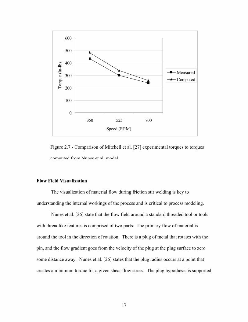
Nunes et al. [26] modeled the tool torque to be totally due to the shear flow stress
of the metal acting perpendicular to the direction of tool rotation and integrated over the
surface. The welding power is equal to the torque multiplied by the RS and is given by
where Mz is the welding torque, ωo is the tool rotational speed, Rp is the pin radius, Rs is
the shoulder radius, σ is the shear flow stress, and t is the pin depth. Figure 2.7 shows a
comparison of Mitchell et al. [27] experimental torques to torques computed from the
Nunes et al. model [26].
,2220
22p
R
ppp
R
R pz RdRtRRdRMps
p ∫∫ ++= σπσπσπ Eq. 6.3
zMP 0ω=
17
Flow Field Visualization
The visualization of material flow during friction stir welding is key to
understanding the internal workings of the process and is critical to process modeling.
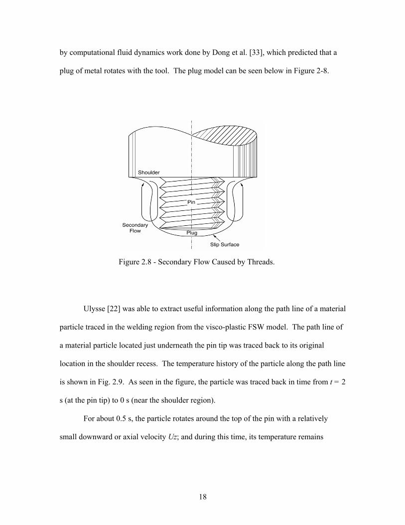
Nunes et al. [26] state that the flow field around a standard threaded tool or tools
with threadlike features is comprised of two parts. The primary flow of material is
around the tool in the direction of rotation. There is a plug of metal that rotates with the
pin, and the flow gradient goes from the velocity of the plug at the plug surface to zero
some distance away. Nunes et al. [26] states that the plug radius occurs at a point that
creates a minimum torque for a given shear flow stress. The plug hypothesis is supported
Figure 2.7 - Comparison of Mitchell et al. [27] experimental torques to torques
computed from Nunes et al. model.
0
100
200
300
400
500
600
350 525 700
Speed (RPM)
Torq
ue (i
n-lb
s
MeasuredComputed
18
by computational fluid dynamics work done by Dong et al. [33], which predicted that a
plug of metal rotates with the tool. The plug model can be seen below in Figure 2-8.
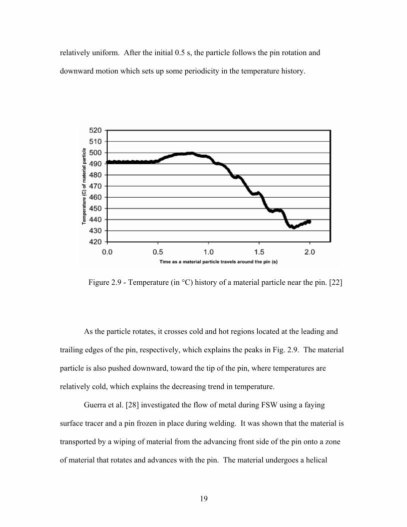
Ulysse [22] was able to extract useful information along the path line of a material
particle traced in the welding region from the visco-plastic FSW model. The path line of
a material particle located just underneath the pin tip was traced back to its original
location in the shoulder recess. The temperature history of the particle along the path line
is shown in Fig. 2.9. As seen in the figure, the particle was traced back in time from t = 2
s (at the pin tip) to 0 s (near the shoulder region).
For about 0.5 s, the particle rotates around the top of the pin with a relatively
small downward or axial velocity Uz; and during this time, its temperature remains
Figure 2.8 - Secondary Flow Caused by Threads.
19
relatively uniform. After the initial 0.5 s, the particle follows the pin rotation and
downward motion which sets up some periodicity in the temperature history.
As the particle rotates, it crosses cold and hot regions located at the leading and
trailing edges of the pin, respectively, which explains the peaks in Fig. 2.9. The material
particle is also pushed downward, toward the tip of the pin, where temperatures are
relatively cold, which explains the decreasing trend in temperature.
Guerra et al. [28] investigated the flow of metal during FSW using a faying
surface tracer and a pin frozen in place during welding. It was shown that the material is
transported by a wiping of material from the advancing front side of the pin onto a zone
of material that rotates and advances with the pin. The material undergoes a helical
Figure 2.9 - Temperature (in °C) history of a material particle near the pin. [22]

20
motion within the rotational zone that rotates, advances, and descends in the wash of the
threads on the nib and rises on the outer part of the rotational zone. After one or more
rotations, this material is sloughed off in the wake of the pin, primarily on the advancing
side. The second process is an entrainment of material from the front retreating side of
the nib that fills in between the sloughed off pieces from the advancing side.
Colligan et al. [29] followed material flow in 6061 and 7075 aluminum by
imbedding small steel balls as tracers into grooves cut into the work-piece parallel to the
weld direction. Grooves were cut parallel to the weld direction but at various distances
from the weld centerline and at various depths. After welding, the distribution of the
steel balls was revealed by radiography in both the plan and the cross-sectional views.
Results
are displayed nicely in the original paper but, in general, the work showed that the
material striking the pin on the advancing side of the weld would be displaced from the
rear of the retreating side of the pin.

21
CHAPTER III
EXPERIMENTAL PROCEDURE
Both experimental and analytical results [22, 23] show that the axial force (and
other forces) can be reduced by increasing the spindle speed. The full range over which
this apparent relationship can be expected to hold true is not known. A full quantification
of the relationships between spindle speed and other process parameters for friction stir
welding are needed. These relationships are of fundamental importance to improved
weld productivity with the friction stir welding process and are key to the widespread use
of robots for FSW.
Vanderbilt University Welding Automation Laboratory FSW Experiments
To study this relationship, experiments were performed at the Vanderbilt
University Welding Automation Laboratory using a Milwaukee #2K Universal Milling
Machine fitted with a Kearney and Trecker Heavy Duty Vertical Head Attachment
modified to accommodate high spindle speeds. The weld sample, clamping fixture (or
backing plate), tool design, instrumentation, and machine modifications detailed below.
Sample Description
For this experiment, plates of AL 6061-T651 aluminum, nominally 0.250 inches
thick were friction stir welded. The samples were 3 inches wide by 18 inches long. The

22
tool depth was set to 0.145”. To ensure precise setting of the tool depth, the tool was
positioned along the weld line aft of the samples leading edge. The sample is clamped
via the scheme shown in Figure 3-1.
The clamping system allows for 30 inches of travel and samples with 3” or 5”
widths. Using the horizontal spindle, the maximum travel distance was 12 inches and
limited to 3” width samples. See Appendix A for a detailed schematic of the backing
plate.
Tool Design
For this experiment, the tool was made from H-13 tool steel heat treated to
Rockwell c hardness 48-50. The shank diameter was 1”. The tool shoulder was flat with
a 0.50” diameter. The pin was cylindrical with a 10-24 threads per inch left hand pattern.
Figure 3-1: VU FSW backing plate.

23
The pin length was 0.1425” and the diameter was 0.190”. Heat sinks were cut into the far
end of the tool shank near the shoulder to facilitate heat dissipation during welding. The
tool was rigidly mounted into the tool holder using a twist lock system. The tool lead
angle was set to 2º. Figure 3-2 shows a detailed schematic of the tool.
Instrumentation
A Kistler rotating quartz 4-component dynamometer (RCD) was used for
measuring forces and torque on the rotating tool. The dynamometer (Figure 3-3) consists
of a four component sensor fitted under high preload between a base plate and a top plate.
The four components are measured without displacement. The four component sensor is
ground-insulated, therefore ground loop problems are largely eliminated. The
dynamometer is rustproof and protected against penetration of splash water and cooling
agents. For each component a 2-range miniature charge amplifier is integrated in the
Figure 3-2: VU FSW tool with 0.5” shoulder and left hand 10-24 thread pattern.

24
dynamometer. The output voltages of the charge amplifiers are digitized and transmitted
by telemetry to the stator and then acquired by a PC. The stator is rigidly mounted
concentrically with the RCD with a 2 mm gap between them. A mount was fabricated
and bolted to the face of the vertical head. A detailed schematic of the stator mount can
be seen in Appendix A.
The Kistler data acquisition software DynoWare was used for data collection.
DynoWare records the three forces and torque during welding and allows the data points
to be exported to a tabularized text file. The data is then imported into MATLAB 7.0,
where it is run through a linear smoothing filter and is plotted. Please see Appendix C for
the linear smoothing filter program file.
KISTLER
Telemetry Pickup
Figure 3-3: Kistler Rotating Cutting Force Dynamometer

25
Machine Modifications
Welding is performed on a Milwaukee #2K Universal Milling Machine fitted with
a Kearney and Trecker Heavy Duty Vertical Head Attachment modified to accommodate
high spindle speeds. The vertical head clamps the vertical sliding surface of the milling
machine. A Baldor VM2514, 20 HP, 3450 RPM, 3Phase 230 VAC motor is mounted to
the shoulder of the head and drives the vertical spindle via a Poly-V belt (Browning
380J16) and drive system. The motor is controlled by a Cutler Hammer SVX-9000 20HP
variable frequency drive. Please see Appendix A for a detailed schematic of the motor
mount.
To meet the operational speed requirements, a 1.33 pulley over drive ratio was
used. The large pulley’s (Browning 16J60P) diameter was 6” while the smaller pulley’s
(Browning 16J45P) diameter was 4.5”. The maximum speed using the above
configuration is 4800 rpm. The overdrive ratio was selected to prevent the possibility of
over-speeding the RCD, whose max operational speed is 5000 rpm. Over-speeding
would require the RCD to be recalibrated. Therefore the maximum rotational speed at
which data was collected for this experiment was 4500 rpm.
To reduce the inertial load of the vertical spindle, the gear train which coupled the
head to the milling machine drive was removed. The gearing system total weight was
approximately 50 lbs. This reduction of loading allows for more torque to be available
during welding.
The head was originally grease lubricated, and accommodated a maximum
operational speed of 1500 rpm. To suit the higher operational speeds for the experiment,
the lubricating grease was cleaned from the spindle’s tapered roller bearings. A Bijur
26
Fluid Flex Pressurized Lubricating System was used to lubricate the tapered roller
bearings.
The Fluid Flex system dispenses a mixture of compressed air (125 psi maximum)
and oil (DTE Lite ISO VG 32). The compressed air is filtered through an air
filter/regulator (160 Psi maximum) with a ¼ NPT inlet. The air enters the Fluid Flex
system and is reduced to a desired level and passed through a solenoid valve which
synchronizes the system with the spindle. Low-pressure air enters the fluid reservoir and
forces fluid from the reservoir. Separate lines carry an atomized mixture of air and oil
through the distribution lines in the system to the Jet Tip assembly for discharge onto the
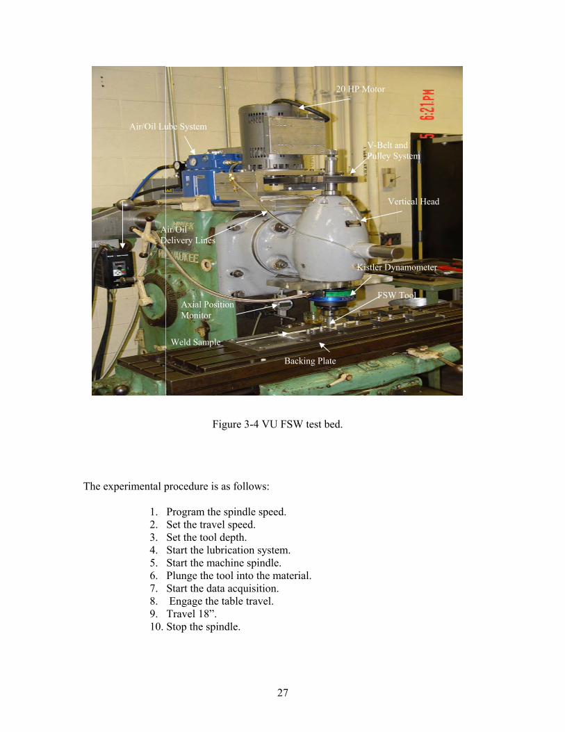
tapered roller bearings (Timken #455 and #749) of the spindle. Figure 3-4 shows the VU
FSW test bed.
27
The experimental procedure is as follows:
1. Program the spindle speed. 2. Set the travel speed. 3. Set the tool depth. 4. Start the lubrication system. 5. Start the machine spindle. 6. Plunge the tool into the material. 7. Start the data acquisition. 8. Engage the table travel. 9. Travel 18”. 10. Stop the spindle.
Figure 3-4 VU FSW test bed.
Backing Plate
Air/Oil Lube System
Air/Oil Delivery Lines
V-Belt and Pulley System
20 HP Motor
Axial Position Monitor
Vertical Head
Kistler Dynamometer
FSW Tool
Weld Sample

28
Using the procedure above, welds were made for the parameter set below.
Table 3-1: VU FSW Experimental Parameter matrix.
*Actual Rotational Speed was 2000 RPM ** Actual Rotational Speed was 2500 RPM
The parameters for which welding was not conducted are those where the
rotational speed is too high for the travel speed and creates a weld with a deformed
surface as shown in Figure 3-5. The overheat phenomena occurred at the preceding
parameter set. For example, for the 3750 rpm and 37.2 ipm parameter set, the weld
experienced the overheat phenomena. Therefore a weld for 4500 rpm and 37.2 ipm was
not run because the surface deformation is assumed to only increase. Detailed
photographs of the deformed welds can be seen in Appendix C. A discussion of the
11.4
27
37.2
44.8
53.3
63.3
1500
X
X
X
X
X
X
2250
X*
X
X
X
X
X
3000
X**
X
X
X
X
X
3750
-
X
X
X
X
X
4500
-
-
-
X
X
X
Feed Rate (ipm)
Spin
dle
Spee
d (R
PM)

29
suggested optimum weld pitch, the ratio of rotational speed to travel speed for a specified
parameter pair, will be discussed in Chapter 5.
Figure 3-5: Typical weld deformation for overheat phenomena experienced during experimentation. (Parameter Set: 3750 rpm and 27.7 ipm.)

30
CHAPTER IV
THEORETICAL MODELING PROCEDURE
In FSW, a cylindrical, shouldered tool with a profiled probe is rotated and slowly
plunged into the joint line between two pieces of sheet or plate material, which are butted
together. Following tool penetration, the friction stir welding operation depends on
continuous refurbishment of the visco-plastic layer surrounding the rotating tool. The
term 'third body' has been used to describe the region containing the visco-plastic
material produced during frictional welding and friction surfacing [34]. This terminology
will be applied for the remainder of this thesis.
It is apparent that the development of a satisfactory 3-dimensional process model
for FSW will depend on how well the ‘third body’ region is handled, in particular how
the material properties in this region are determined. A logical first step in developing a
full 3-dimensional representation of the friction stir welding process is to develop a
working 2-dimensional model. For this thesis, only the pin bottom and the sample are
considered. This allows a basic approach where the model is modularly developed. The
model is validated in stages, which allows the contribution of various components to be
examined and understood. The key factors during FSW which were considered in this
model are detailed below.
Currently FSW process modeling typically incorporates either a solid or fluid
mechanics approach. Experimental results have been shown to correlate with models
using either approach. Due to the moderately high temperatures associated with FSW (up
to 480 °C) (Sato et al. [18]), and the relatively low melting point of Al 6061-T6 (652°C);

31
it is clear the weld material in the third body region enters what is called a mushy zone
[35].
A mushy zone is a temperature region where the material is not a true solid or
liquid, though it has aspects of the behavior of both. Understanding and accurately
modeling the third body region will lead to an optimal 3-D model.
FSW Modeling: A Fluid Mechanics Approach
Using a fluid mechanics approach, the third body region is approximated as a
viscous flow domain under high shear stress and strain-rates at moderately high
temperatures. The thermo-mechanical property of primary importance for a model such
as this is the material viscosity.
Mechanical Model: Part 1
For the fluid mechanical approach to FSW modeling, the determination of the
material viscosity is the logical first step to begin development of a 3-dimensional model
for friction stir welding. North et al. [36] experimentally correlated the material viscosity
during FSW with the viscosity of a fluid intermediate between two concentric cylinders
as first suggested by Couette in 1890 [45]. Figure 4-1 shows a schematic of the Couette
Viscous Flow model. The material viscosity is found to be [45]
The inner cylinder has radius ro , and angular velocity ωo while the outer cylinder has r1
and ω1, respectively, and M is the torque per unit depth of the tool pin. Applying
µ = (r12- ro
2) M / [4π r12
ro2 (ω1 – ω0)] Eq. 4.1

32
Equation 4.1 to FSW; take ro to be the radius of the tool pin, and set ωo equal the tool
rotational speed.
The outer cylinder radius r1 is taken to be the radius of the tool pin plus the width of the
third body region to a point in space where the material is solid and does not rotate,
giving ω1 = 0. M is the experimentally measured steady state welding torque for the
parameter sets in Table 3-1.
Couette flow will be unstable if it satisfies the Rayleigh criterion for Couette flow
instability [37]. The criterion states that Couette flow will be unstable if
02 <ooo
rdrd
ω Eq. 4.2
ω1
q0
r0
r1
ω0
Ta
Figure 4-1: Geometry and boundary conditions for the simple Couette flow model.

33
Equation 4.2 simplifies to ωo ro , which is always greater than zero for friction stir
welding. Since ω1 = 0 when applying Couette flow to FSW, Equation 4.3 simplifies to
ωor12 > 0, which is always true for FSW. There fore the flow is always stable for FSW.
The width of the third body region as shown in Figure 4-2, and is modeled as
where ω is the rotational speed of the tool pin, vf is the travel speed, and Rp is the radius
of the tool pin [ 38]. For notation purposes, from this page forward in this thesis, Rp will
be used as the notation for the tool pin radius.
Figure 4-2: Schematic for the approximation of the third body region. [38]
211
200 rr ωω >
Eq. 4.3
Eq. 4.4 [ ] 12 1 −++= φβφα pRWr

34
The variables α, β, and φ are given by
where Rs is the radius of the shoulder, δ2 is the projected thread area, and λ (24 threads
per inch) is the number of threads per inch. Since the model presented here is two
dimensional, secondary flows created by the threads are neglected.
Figure 4-3 shows the material viscosity for FSW using the Couette flow model.
φ = ωvf-1 Eq. 4.7
β = (Rs2 – Rp
2) / (hλ) Eq. 4.6
α = 1/2 [(Rp) - λ δ2]-1 Eq. 4.5
Couette Viscosity for FSW
0
200000
400000
600000
800000
1000000
1200000
1400000
1500 2250 3000 3750 4500
Rotational Speed (rpm)
Visc
osity
(Pa-
s)
11 ipm27 ipm37.2 ipm44.8 ipm53.3 ipm63.3 ipm
Figure 4-3: Couette Flow Viscosity for FSW.

35
Mechanical Model: Part 2
Applying the rigid-visco-plastic viscosity approximation used by Ulysse [22] and
Reynolds et al. [25], the material viscosity is found as
where σe is the flow stress and is found by Equation 2.1. The material constants for the
constitutive law (Equation 2.1) for Al 6061 are: α = 0.045 (Mpa)-1, Q = 145 kJmol-1, A =
8.8632E6 s-1, n = 3.55, and R = 8.314 mol-1K-1. The material constants were first
published by Sheppard and Jackson [42]. The time average mean strain rate (έt) is found
as a function of the geometry, extrusion zone width, and FSW processing parameters as
suggested by Abregast et al. [38].
Figure 4-4 shows the mean strain-rate for the parameter sets in Table 3-1.
Eq. 4.9
Eq. 4.8
t
e
εσ
µ&3
=

36
The flow stress depends on the strain-rate and temperature and is represented by
an inverse sine-hyperbolic as shown in Equation 2.1. As shown in Figure 4-5, using the
time average mean strain-rate found above, the flow stress for temperatures ranging from
20ºC to 720ºC were found for each parameter set in Table 3-1.
Figure 4-4: Mean Average Strain-Rate vs. Rotational Speed for Constant Travel Speeds.
Strain-Rate vs. Rotational Speed
0
50
100
150
200
250
300
350
1500 2250 3000 3750 4500
Rotational Speed (rpm)
Stra
in-R
ate
(s^-
1)
11.4 ipm27 ipm37.2 ipm44.8 ipm53.3 ipm63.3 ipm

37
Then, applying Equation 4.8, the strain-rate/temperature dependent material viscosity was
found for each parameter set in Table 3-1.
Thermal Modeling
A very important factor during friction stir welding is the steady state welding
temperature. For this experiment the rotational speed was varied for the range of travel
speeds listed in Table 3-1. It was observed that the rotational speed is the primary factor
Visco-Plastic Approximation of Flow Stress vs Strain Rate
0
50
100
150
200
250
300
350
0 50 100 150 200 250 300 350 400
Strain Rate (s^-1)
Flow
Str
ess
(Mpa
)
T=293T=393T=493T=593T=693T=793T=893
Figure 4-5: Flow Stress vs. Strain Rate using the Visco-Plastic model.

38
associated with heat generation. During the experiment, the rotational speed was
constant, which should result in a constant rate of heat generation.
Various models exist which predict the heat generation during FSW. In the model
by Chao and Qi [39], the heat generation comes from the sliding friction, where
Coulomb’s law is used to estimate the shear or friction force at the interface. Russell and
Shercliff [40] based the heat generation on a constant friction stress at the interface, equal
to the shear yield stress at elevated temperature, which is set to 5% of the yield stress at
room temperature. The heat input is applied as a point source or line source as in the
normal version of Rosenthal’s equations, but the solution is modified to account for the
limited extent of the plate width. Schmidt et al. [41] estimated the heat generation based
on assumptions for different contact conditions at the tool/material interface in FSW
joints. In this thesis, a sticking condition at the tool/material interface is assumed. The
heat generation model during FSW for a sticking interface [42] at the pin sides is
where σy is the yield stress of AL 6061-T6, Rp is the radius of the pin, h is the height of
the pin and ωo is the rotational speed. The incoming weld material temperature was set to
300 K. Applying Equation 4.9 for AL 6061 – T6 at 300 K, gives σy = 241 MPa.
Substituting this result into Eq. 4.10 gives the heat generation shown in Figure 4-6.
Qp = 2π(σy / √3) Rp2h ωo Eq. 4.10

39
Numerical Model
The computational fluid dynamics package FLUENT [43] was used to simulate
flow past a 2-dimensional pin for the weld parameters given in Table 3-1. The FLUENT
package includes the following software:
1) FLUENT, the solver.
2) prePDF, the preprocessor for modeling non-premixed combustion in FLUENT.
3) GAMBIT, the preprocessor for geometry modeling and mesh generation.
4) TGrid, an additional preprocessor that can generate volume meshes from existing
boundary meshes.
Rotational Speed Versus Heat Generation for the Tool Pin Sides
0
1000
2000
3000
4000
5000
6000
7000
8000
9000
10000
1500 2250 3000 3750 4500
Rotational Speed (rpm)
Hea
t Gen
erat
ion
(W)
Series1
Figure 4-6: Heat Generation as a function of Rotational Speed for a sticking contact surface.

40
5) Filters(translators) for import of surface and volume meshes from CAD/CAE packages
such as ANSYS, CGNS, I-DEAS, NASTRAN, PATRAN, and others.
The flow field around the pin is modeled in 2D with the Z-axis of the pin
perpendicular to the direction of flow. The pin is modeled as a circle and a square flow
domain is created around it. Velocity at the inlet of the flow domain is specified by the
user. The procedure for implementing the model is:
1. Create the geometry (pin and the flow domain)
2. Mesh the domain
3. Set the material properties and boundary conditions
The geometry and mesh (Figure 4.7) are created using Gambit and are exported to
FLUENT.
Figure 4-7: 2-D mesh of pin and sample with the origin shown at the tool pin center.

41
The pin has a diameter of 0.190” and the sample dimensions are 6”x3”. Because the
area of most interest is near the pin, the mesh is densest near the pin and in the primary
flow path of the material which contacts the pin. A 10-row boundary layer is placed at
the pin wall. The flow domain is meshed using a quad map scheme using user specified
discretization values.
Process Model
The three dimensional friction stir welding process is represented here by only the
pin bottom and the sample. This 2-D model is the logical first step in developing a 3-D
model. The process is represented here as a steady state two-dimensional laminar,
incompressible, non-Newtonian flow past a rotating non-threaded tool pin. Plunge
conditions are ignored. The heat generation, as detailed earlier in this chapter, is assumed
to be mainly due to the contact condition from rotation of the tool pin, and the
contribution from forward travel of the tool pin is negligible.
Material Properties
The material properties used as input variables for FLUENT are detailed below.
Table 4-1 lists the constant properties for H-13 tool steel while Tables 4-2 and 4-3 list the
temperature dependent properties for the weld material (AL 6061).

42
Table 4-1: FSW Tool Properties
Table 4-2 Temperature Dependent Yield Strength of AL 6061-T6
Material Property Density (ρ) Thermal Conductivity (k) Specific Heat (Cp)
H-13 7805 (kg/m3) 202 W/(m-K) 871 (J/kg-K)
T (K) σy (MPa)
311 241
339 238
366 232
394 223
422 189
450 138
477 92
533 34
589 19
644 12

43
Table 4-3 Temperature Dependent Thermal Conductivity and Specific Heat for AL 6061-T6
Boundary Conditions
The pin is assigned a constant rotational speed. The heat flux and heat generation
rate are determined by dividing Equation 4.10 by the pin surface area and volume
respectively. The wall thickness is set equal to the pin radius. The pin material is H-13
tool steel. The properties are listed in Table 4-1.
The lateral edges of the mesh are specified as a translational flow domain. This
feature specifies that the fluid translates between these boundaries with a user specified
T (K) K [W / (m-K)] Cp [J / (kg-K)]
293 195 870
373 195 950
473 173 980
573 211 1020
673 212 1060
773 225 1150
873 200 1160
915 90 1170
973 91 1170
1073 92 1170

44
velocity magnitude and direction. The magnitude is equal to travel speed during welding
and the flow direction is in the positive X direction.
The inlet velocity is set to the travel speed with the flow direction in the positive X
direction. The inlet temperature of the weld material is set to 300 K. The outlet pressure
is set to 101,325 Pa.
The fluid is AL 6061 with temperature dependent properties from Table 4-2 and 4-3.
The viscosity is for each found using Equation 4.1 (Couette ) or 4.8 (Visco-Plastic). The
weld material is assumed to be fed towards the tool at the user specified travel speed and
temperature.
Solver
The solver controls for the simulations were set to 2-D, segregated, laminar, implicit,
and steady flow. Using a segregated solver, the governing equations are solved
sequentially (i.e., segregated from one another). Because the governing equations are
non-linear (and coupled), several iterations of the solution loop must be performed before
a convergent solution is obtained. The iteration process consists of the steps illustrated in
Figure 4-8 and are outlined below:
The steps are as follows:
1. Fluid properties are updated, based on the current solution. (If the calculation has just begun, the fluid properties will be updated based on the initialized solution.)
2. The u, v, and w momentum equations are each solved in turn using current values
for pressure and face mass fluxes, in order to update the velocity field. 3. Since the velocities obtained in Step 2 may not satisfy the continuity equation
locally, a ``Poisson-type'' equation for the pressure correction is derived from the continuity equation and the linearized momentum equations. This pressure correction equation is then solved to obtain the necessary corrections to the

45
pressure and velocity fields and the face mass fluxes such that continuity is satisfied.
4. Where appropriate, equations for scalars such as turbulence, energy, species, and
radiation are solved using the previously updated values of the other variables. 5. When inter-phase coupling is to be included, the source terms in the appropriate
continuous phase equations may be updated with a discrete phase trajectory calculation.
6. A check for convergence of the equation set is made.
These steps are continued until the convergence criteria are met.
Update Properties
Solve Momentum Equations.
Solve Pressure-Correction (continuity) equation, Update pressure, face mass flow rate.
Solve Energy, species turbulence and other scalar equations
Stop Converged?
Figure 4-8: Overview of the Segregated Solution Method

46
Using the implicit solution method, for a given variable, the unknown value in
each cell is computed using a relation that includes both existing and unknown values
from neighboring cells. Therefore each unknown will appear in more than one equation
in the system, and these equations must be solved simultaneously to give the unknown
quantities.
Laminar flow of the weld material was assumed because of the large viscosity
values (on the order of 106 Pa-s) that were found using Equation 4.1 and 4.8, leading to
very small Reynolds numbers (approx. 10-5) close to the pin. Due to the low Reynolds
number, only viscous effects are important and inertial effects may be neglected. The
material is assumed to translate past the rotating tool pin as it does in the actual
experiments.
Governing Equations
FLUENT uses the solver configuration above to solve the conservation of mass,
momentum (Navier-Stokes equations), and energy equations. For two-dimensional
steady state incompressible fluid flow the continuity equation is
where x and y denote coordinates and u and v are velocity components
Neglecting gravitational and body forces, the conservation of momentum yields
the following form of the Navier-Stokes equations
0=∂∂
+∂∂
yv
xu Eq. 4.11

47
where ρ is the density, µ is the viscosity, and p is the static pressure. The stress tensor is
given by τ
Neglecting changes in potential energy and assuming that heat transfer obeys Fourier’s
law of heat conduction the steady state energy equation is written as
where Cv is the constant volume specific heat and k is the thermal conductivity. The
terms on the right hand side of Equation 4.13 represent energy transfer by conduction and
viscous dissipation.
∂∂
+∂∂
=xv
yuµτ Eq.4.14
Eq. 4.15
∂∂
+∂∂
+
∂∂
+
∂∂
+
∂∂
+∂∂
=
∂∂
+∂∂
+∂∂
222
2
2
2
2
22t x
vyu
yv
xu
yT
vxT
kyT
vxT
uT
Cv µρ
∂∂
+∂∂
+∂∂
−=∂∂
+∂∂
2
2
2
2
yv
xv
yp
yuv
xuu µρρ
∂∂
+∂∂
+∂∂
−=∂∂
+∂∂
2
2
2
2
yu
xu
xp
yuv
xuu µρρ Eq. 4.12
Eq.4.13

48
CHAPTER V
EXPERIMENTAL RESULTS AND DISCUSSION
To establish guidelines for understanding the experimental results and their
anticipated consequences, some terminology will be introduced here.
The ratio of spindle speed to travel speed will be referred to as the weld pitch
(wp), and has units of revolutions per inch. The weld pitch can be increased in one of two
ways; 1) increasing the tool rotational speed, or 2) decreasing the travel speed. Likewise,
the weld pitch can be decreased by reducing tool rotational speed or increasing the travel
speed or feed rate.
The contact condition at the tool pin can be described as sliding, sticking, or
partial sliding/sticking. The experimental results will be presented with respect to the
effects due to weld pitch variation. Table 5-1 lists the weld pitch for the parameter
matrix in Table 3-1.
As stated in the introduction, a goal of this research is to establish guidelines for
implementing FSW capable robots. A significant limiting factor when implementing
FSW capable robots is the axial force requirement necessary when welding. In the
experimental results to be presented here, the translational force, transverse force, axial
force, and welding torque were measured for the parameter sets listed in Table 3-1. The
raw data plots can be seen in Appendix A.

49
Table 5-1: VU FSW Experimental Parameter matrix Weld Pitch.
*Actual Rotational Speed was 2000 RPM
** Actual Rotational Speed was 2500 RPM
Axial Force (Fz)
The axial force was measured for the weld parameter sets shown in Table 5-1. The
raw data plots can be seen in Appendix B. The steady state axial force is presented in the
following figures as the average axial force during the weld. Each weld parameter set
was run a minimum of two times in order to verify the precision of the force data. The
steady state axial force was found by averaging the mean axial force of each run of a
weld parameter. Figures 5-1 and 5-2 show the steady state axial force for variable
rotational speed and travel speed, respectively. From Figure 5-1, it can be seen that the
axial force decreases as the rotational speed increases.
11.4
27
37.2
44.8
53.3
63.3
1500 132 56 40 33 28 24
2250 175* 83 60 50 42 36
3000 219** 111 81 67 56 47
3750 - 139 101 84 70 59
4500 - - 100 84 71
Feed Rate (ipm)
Spin
dle
Spee
d (R
PM)

50
Increasing the rotational speed and holding the travel speed constant leads to a
decrease in axial force. Increasing the travel speed and holding the rotational speed
constant leads to an increase in axial force. The decrease in axial force for increasing
weld pitch through increased rotational speed is shown in Table 5-2.
Figure 5-1: Axial Force vs. Rotational Speed for constant travel speeds.
Axial Force vs Rotational Speed at Constant Travel Speed
5500
6500
7500
8500
9500
10500
1500 2000 2500 3000 3500 4000 4500
Tool Rotational Speed (rpm)
Axi
al F
orce
(N) (
kN)
11 ipm27 ipm37.2 ipm44.8 ipm53.3 ipm63.3 ipm

51
Table 5-2: Percentage Decrease in Axial Force for Increasing Weld Pitch by increasing Rotational Speed
TS (ipm) Min wp (rpi) Max wp (rpi) % Fz Decrease 11.4 131.6 219.3 17.1 27.0 55.6 138.9 9.1 37.2 40.3 100.8 4.6 44.8 33.5 100.4 7.3 53.3 28.1 84.4 12.4 63.3 23.7 71.1 9.8
Figure 5-2 shows the axial force for various travel speeds at constant rotational
speeds. Table 5-3 shows the percentage decrease in axial force for increasing weld pitch
by decreasing the travel speed.
Figure 5-2: Axial Force vs. Travel Speed for constant rotational speed.
Axial Force vs. Travel Speed at Constant Rotational Speed
5000
6000
7000
8000
9000
10000
11000
11.4 27 37.2 44.8 53.3 63.3
Travel Speed (ipm)
Axi
al F
orce
(N)
1500 RPM2250 RPM3000 RPM3750 RPM4500 RPM

52
Table 5-3: Percentage Decrease in Axial Force for Increasing Weld Pitch by reducing Travel Speed
Welding Torque
The effect of weld pitch variation on the welding torque is key to understanding the
friction stir welding process and successfully implementing FSW capable robots. The
torque was measured for the weld parameter sets shown in Table 5-1. The raw data plots
can be seen in Appendix B.
The steady state torque is presented in Figures 5-3 and 5-4. The steady state welding
torque is found by averaging the mean torque each run of a weld parameter set. Figures
5-3 and 5-4 show the steady welding torque for variable rotational speed and travel speed
respectively. Tables 5-4 and 5-5 show the percentage decrease in torque from increasing
weld pitch.
RS (ipm) Min wp (rpi) Max wp (rpi) % Fz Decrease 1500 23.7 131.6 36.1 2250 35.5 197.4 41.0 3000 47.4 263.2 44.6 3750 59.2 138.9 33.7 4500 71.1 100.4 16.8

53
Table 5-4: Percentage Decrease in Torque for Increasing Weld Pitch
by increasing Rotational Speed
TS (ipm) Min wp (rpi) Max wp (rpi) % Mz Decrease 11.4 131.6 219.3 45.9 27.0 55.6 138.9 60.0 37.2 40.3 100.8 59.3 44.8 33.5 100.4 72.2 53.3 28.1 84.4 66.1 63.3 23.7 71.1 67.9
Figure 5-3: Torque vs. Rotational Speed for constant travel speed.
Moment vs. Rotational Speed for Constant Travel Speed
13
18
23
28
33
38
43
48
53
1500 2250 3000 3750 4500
Rotational Speed (RPM)
Mom
ent (
Nm
)
TS = 11.4TS = 27TS = 37.2TS = 44.8TS = 53.3TS = 63.3

54
Increasing the rotational speed while holding the travel speed constant leads to a
decrease in torque; while increasing the travel speed and holding the rotational speed
constant leads to an increase in torque. The decrease in torque for increasing weld pitch
through reduced travel speed is shown in Table 5-5.
Figure 5-4: Torque vs. Travel Speed for constant rotational Speed.
Moment vs. Travel Speed for Constant Travel Speed
10
15
20
25
30
35
40
45
50
55
11.4 27 37.2 44.8 53.3 63.3
Travel Speed (ipm)
Mom
ent (
Nm
)
1500 RPM2250 RPM3000 RPM3750 RPM4500 RPM

55
Table 5-5: Percentage Decrease in Torque for Increasing Weld Pitch by reducing Travel Speed
The welding power is shown in Figure 5-5 and appears to remain nearly constant for a
constant travel speed.
TS (ipm) Min wp (rpi) Max wp (rpi) % Mz Decrease 1500.0 23.7 131.6 36.0 2250.0 35.5 197.4 35.3 3000.0 47.4 263.2 32.6 3750.0 59.2 138.9 19.1 4500.0 71.1 100.4 18.5
Figure 5-5: Spindle Power vs. Rotational Speed for constant travel speed.
Spindle Power vs. Rotational Speed for Constant Travel Speeds
4000
5000
6000
7000
8000
9000
10000
1500 2250 3000 3750 4500
Rotational Speed (RPM)
Mom
ent (
Nm
)
TS = 11.4TS = 27TS = 37.2TS = 44.8TS = 53.3TS = 63.3 ipm

56
Translational and Transverse Force
The translational and transverse forces were measured for the weld parameter sets
shown in Table 5-1. The steady state translational and transverse forces are presented in
the following figures as the average force (Fx or Fy) during a weld. Each weld parameter
set was run a minimum of two times in order to verify the precision of the force data.
The steady state translational or transverse force is found by averaging the mean
translational or transverse force of each parameter set. Figures 5-7 and 5-8 show the
steady state translational and transverse force for variable rotational speed respectively.
From Figures 5-6 and 5-7, it is apparent that the translational and transverse forces
have the general trend of decreasing with increased weld pitch, but not with the linear
trend as the axial force and torque follow.
Translational Force vs Rotational Speed for Constant Travel Speeds
0
20
40
60
80
100
120
140
1500 2250 3000 3750 4500
Rotational Speed (ipm)
Tran
slat
iona
l For
ce (N
)
TS = 11.4 ipmTS = 27 ipmTS = 37.2 ipmTS = 44.8 ipmTS = 53.3 ipmTS = 63.3 ipm
Figure 5-6: Translational Force vs. Rotational Speed for constant travel speed.

57
The steady state plots of the translational and transverse forces follow the general
parametric relationship of increased rotational speed/ decreased force, however as the
rotational speed is increased, a new relationship becomes apparent.
Viewing the raw data plots gives insight into the force behavior at higher rotational
speeds. Figures 5-8 and 5-9 show the raw data plots of the translational and transverse
force for various rotational speeds and 44 ipm travel speed. Increasing the rotational
speed for a constant travel speed creates a varying contact condition at the tool
pin/material interface.
Transverse Force vs Rotational Speed for Constant Travel Speeds
-20
-10
0
10
20
30
40
50
60
70
80
90
1500 2250 3000 3750 4500
Rotational Speed (ipm)
Tran
slat
iona
l For
ce (N
)
TS = 11.4 ipmTS = 27 ipmTS = 37.2 ipmTS = 44.8 ipmTS = 53.3 ipmTS = 63.3 ipm
Figure 5-7: Transverse Force vs. Rotational Speed for constant travel speed.

58
5 10 15 20 25-20
0
20
40
60
80
100
120
140
160
180
200
Time (s)
Fx
(N)
Translational Force for Variable RS and Constant TS = 44.8ipm
1500 RPM
2250 RPM
3000 RPM3750 RPM
4500 RPM
Figure 5-8: Raw data plot of Translational Force for various RS and TS = 44 ipm.
5 10 15 20 25-100
-50
0
50
100
150
Transverse Force for Variable RS and Constant Ts = 44.8 ipm
Time (s)
Fy
(N)
1500 RPM
2250 RPM
3000 RPM3750 RPM
4500 RPM
Figure 5-9: Raw data plot of Transverse Force for various RS and TS = 44 ipm.

59
In Figures 5-9 and 5-10, the translational and transverse forces are constant lines
of force for wp < 50.2 rpi and oscillates for wp > 50.2 rpi. The constant lines of force
indicate a constant pressure at the tool pin/material interface. The oscillation indicates
that the material at the tool pin/material interface does not apply constant pressure but
rather it sticks to the tool and drags along behind the tool as it rotates.
With the sticking contact condition, if the friction shear stress exceeds the yield
shear stress, the weld material at the tool/material interface will stick to the moving tool
surface segment. In this case, the matrix segment will accelerate along the tool surface
(finally receiving the tool velocity), until an equilibrium state is established between the
contact shear stress and the internal matrix shear stress. At this point, the stationary full
sticking condition is fulfilled [41].
For the sliding condition, if the contact shear stress is smaller than the internal
matrix yield shear stress, the matrix segment volume shears slightly to a stationary elastic
deformation, where the shear stress equals the ‘dynamic’ contact shear stress. This state
is referred to as the sliding condition [41].
The partial sliding/sticking contact condition is a mixed state of the two contact
conditions. In this case, the matrix segment accelerates to a velocity less than the tool
surface velocity, where it stabilizes. The equilibrium occurs when the ‘dynamic’ contact
shear stress equals the internal yield shear stress due to a quasi-stationary plastic
deformation rate [41].
The variation of the contact condition can reasonably be assumed to be induced
by increasing the rotational speed. Increasing the rotational speed causes a corresponding
increase in welding temperature. The over-heat phenomena (discussed in Chapter 3) that
60
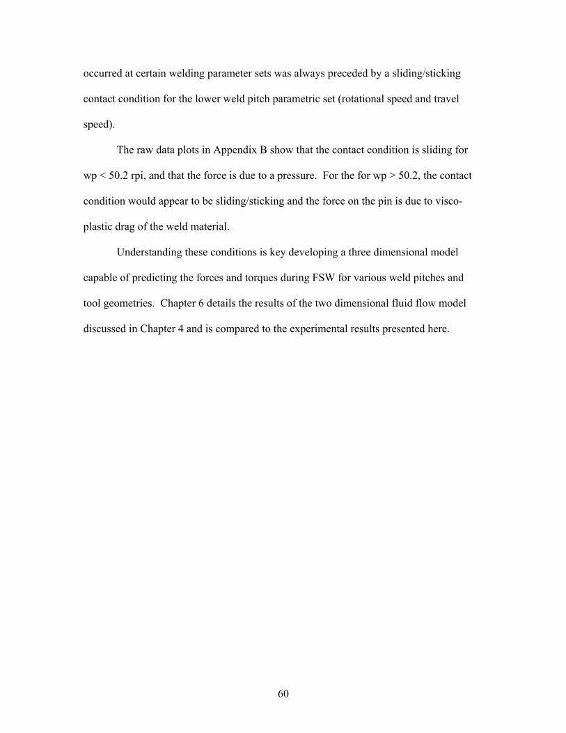
occurred at certain welding parameter sets was always preceded by a sliding/sticking
contact condition for the lower weld pitch parametric set (rotational speed and travel
speed).
The raw data plots in Appendix B show that the contact condition is sliding for
wp < 50.2 rpi, and that the force is due to a pressure. For the for wp > 50.2, the contact
condition would appear to be sliding/sticking and the force on the pin is due to visco-
plastic drag of the weld material.
Understanding these conditions is key developing a three dimensional model
capable of predicting the forces and torques during FSW for various weld pitches and
tool geometries. Chapter 6 details the results of the two dimensional fluid flow model
discussed in Chapter 4 and is compared to the experimental results presented here.

61
CHAPTER VI
2-D MODELING RESULTS AND DISCUSSION
It will be useful now to identify the limiting factors for implementation of FSW
capable robots. The primary limiting factor is the large axial force required.
The axial force was found to decrease by either increasing rotational speed or
decreasing travel speed. An increase in rotational speed decreases the axial force by
increasing the heat input into the weld material, thus raising the temperature of the weld
material. Reducing the travel speed increases the number of revolutions per unit length
of the weld, which increases the heat input per unit length of the weld.
Table 3-3 shows that increasing the temperature of the weld material from 38ºC to
371ºC decreases the yield strength from 241 MPa to 12 MPa, a 95% decrease. Therefore
the optimum weld pitch for FSW will occur at high rotational speeds and low travel
speeds.
Another potential limiting factor is the welding torque. The welding torque is
largely governed by the weld pitch as well as the tool geometry. Increasing the size of
the tool pin and particularly the tool shoulder, causes a corresponding increase in welding
torque. Increasing the rotational speed increases the temperature of the weld material,
decreasing the yield strength, which decreases the torque required to displace the weld
material to facilitate forward travel of the tool. As stated earlier, reducing the travel
speed increases the heat input to the weld, and reduces the yield strength, which reduces
the required torque.

62
A significant goal of this research is to establish practical design guidelines for
developing FSW capable robots. Developing a 3-D model capable of predicting the
forces and torques associated with FSW would greatly aide the ability of scientists and
engineers to design, fabricate, and implement FSW capable robots.
In this thesis, a two dimensional model was developed to predict the translational
force, welding torque, and temperature on the tool pin for parameter sets listed in Table
5-1. All simulations were run using the computational fluid dynamics package FLUENT.
Chapter 4 details the determination of the material properties, boundary conditions,
mechanical modeling, thermal modeling, solver configuration and governing equations.
Welding Torque
Friction stir welding is a three dimensional process. In this thesis, the initial
modeling efforts are represented in 2-D. Though a 2-D model cannot fully represent a 3-
D process, if implemented correctly, the 2-D model may suggest the general trends of the
3-D process.
As stated in Chapter 4, the tool is represented by a 2-D rotating pin. In order for
the torque experimental results to be compared with the numerical model, the
experimental results must be scaled to represent the contribution of the pin during
welding. The rotating plug model suggested by Nunes et al. [26] was used to determine
the pin contribution.
With the rotating plug model, the tool torque is taken to be totally due to the shear
flow stress of the metal acting perpendicular to the direction of tool rotation and
integrated over the surface. The tool torque is given by
63
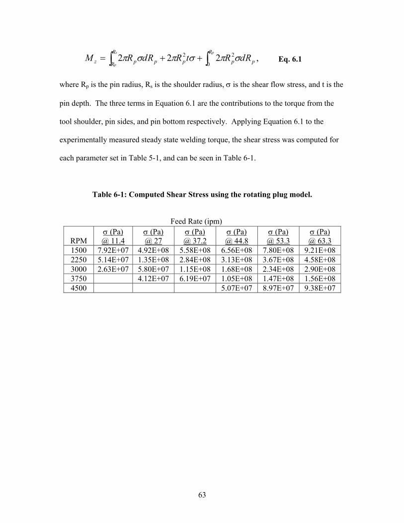
where Rp is the pin radius, Rs is the shoulder radius, σ is the shear flow stress, and t is the
pin depth. The three terms in Equation 6.1 are the contributions to the torque from the
tool shoulder, pin sides, and pin bottom respectively. Applying Equation 6.1 to the
experimentally measured steady state welding torque, the shear stress was computed for
each parameter set in Table 5-1, and can be seen in Table 6-1.
Table 6-1: Computed Shear Stress using the rotating plug model.
RPM σ (Pa) @ 11.4
σ (Pa) @ 27
σ (Pa) @ 37.2
σ (Pa) @ 44.8
σ (Pa) @ 53.3
σ (Pa) @ 63.3
1500 7.92E+07 4.92E+08 5.58E+08 6.56E+08 7.80E+08 9.21E+08 2250 5.14E+07 1.35E+08 2.84E+08 3.13E+08 3.67E+08 4.58E+08 3000 2.63E+07 5.80E+07 1.15E+08 1.68E+08 2.34E+08 2.90E+08 3750 4.12E+07 6.19E+07 1.05E+08 1.47E+08 1.56E+08 4500 5.07E+07 8.97E+07 9.38E+07
,2220
22p
R
ppp
R
R pz RdRtRRdRMps
p ∫∫ ++= σπσπσπ Eq. 6.1
Feed Rate (ipm)

64
From Equation 6.1, we see that the torque contribution from the pin side is
Now, substituting the shear stress from Table 6-1 into Equation 6.2, Mp is found for the
corresponding parameter sets and can be seen in Table 6-2.
Table 6-2: Torque Contribution by the Tool Pin.
Dividing Mp /Mz for the corresponding parameter sets show that the pin torque
contribution is approximately 24.9%.
The simulations were run for the Couette Flow and Visco-Plastic Flow viscosity
models. The simulation determined the shear stress at the pin wall, which was then input
into Equation 6-2 to determine the moment (welding torque) of the pin. Figures 6-1
through 6-6 show a comparison of the predicted simulation results to the experimental
pin torques for various weld pitches.
RPM
Mp (N-m)
@ 11.4
Mp (N-
m)@ 27
Mp (N-m)
@ 37.2
Mp (N-m)
@ 44.8
Mp (N-m)
@ 53.3
Mp (N-m)
@ 63.3
1500 8.3 10.4 11.4 12.2 12.7 12.9
2250 6.0 7.1 7.6 8.4 9.0 9.3
3000 4.7 5.3 5.7 6.1 6.4 7.0
3750 - 4.2 4.6 5.0 5.1 5.2
4500 - - - 3.4 4.3 4.2
.2 2 σπ tRM pz = Eq. 6.2
Feed Rate (ipm)

65
At low weld pitches, the Couette Flow model did not correlate very well with the
experimental results. As the weld pitch increases, the experimental results and the
Couette Flow model begin to converge. This implies that the Coutte Flow model is more
predictive for very high weld pitches. At high weld pitches, the high heat input greatly
improves the weld material’s ability to flow. In general, the torque decreases as weld
pitch is increased.
Overall, the Visco-Plastic flow model was more accurate than the Couette Flow
model over the range of weld pitches. The Visco-Plastic Flow model also converged
with the experimental results as the weld pitch was increased.
Pin Moment vs. Rotational Speed for TS = 11.4 ipm
0
5
10
15
20
25
30
35
40
45
1500 2250 3000
Rotational Speed (RPM)
Mom
ent (
Nm
)
ExperimentalCouetteVisco-Plastic
Figure 6-1: Comparison of Predicted and Experimental Pin Moment vs. Rotational Speed for 11.4 ipm

66
In Figure 6-1, the Couette Flow model correlates very well for the 11.4 ipm travel
speed. The weld pitch at this travel speed was very high for all rotational speeds.
Lending further credibility to the theory that Couette Flow is more optimal for high weld
pitches.
At approximately 2300-2400 rpm, the Couette Torque and Experimental torque
are almost equal. The corresponding weld pitch is 202- 210 rpi. In Figures 6-2 through
6-6, the Couette torque is never less than the experimental torque, likewise, the weld
pitch is not higher than 200 rpi for the following plots
Figure 6-2: Comparison of Predicted and Experimental Pin Moment vs. Rotational Speed for 27 ipm
Pin Moment vs. Rotational Speed for TS = 27 ipm
0.0
10.0
20.0
30.0
40.0
50.0
60.0
70.0
1500 2250 3000 3750
Rotational Speed (RPM)
Mom
ent (
Nm
)
ExperimentalCouetteVisco-Plastic

67
Figure 6-3: Comparison of Predicted and Experimental Pin Moment vs. Rotational Speed
Pin Moment vs. Rotational Speed for TS = 37.2 ipm
0.0
10.0
20.0
30.0
40.0
50.0
60.0
70.0
80.0
1500 2250 3000 3750
Rotational Speed (RPM)
Mom
ent (
Nm
)
ExperimentalCouetteVisco-Plastic
Figure 6-4: Comparison of Predicted and Experimental Pin Moment vs. Rotational Speed for 44.8 ipm
Pin Moment vs. Rotational Speed for TS = 44.8 ipm
0.0
10.0
20.0
30.0
40.0
50.0
60.0
70.0
80.0
90.0
100.0
1500 2250 3000 3750 4500
Rotational Speed (RPM)
Mom
ent (
Nm
)
ExperimentalCouetteVisco-Plastic

68
Figure 6-5: Comparison of Predicted and Experimental Pin Moment vs. Rotational Speed for 53.3 ipm
Pin Moment vs. Rotational Speed for TS = 53.3 ipm
0.0
20.0
40.0
60.0
80.0
100.0
120.0
1500 2250 3000 3750 4500
Rotational Speed (RPM)
Mom
ent (
Nm
)
Experimental CouetteVisco-Plastic
Figure 6-6: Comparison of Predicted and Experimental Pin Moment vs. Rotational Speed for 63.3 ipm
Pin Moment vs. Rotational Speed for TS = 63.3 ipm
0.0
20.0
40.0
60.0
80.0
100.0
120.0
140.0
1500 2250 3000 3750 4500
Rotational Speed (RPM)
Mom
ent (
Nm
)
ExperimentalCouetteVisco-Plastic

69
Translational Force
Figures 6-7 through 6-12 show the comparison of the experimental translational
force to the predicted translational forces for the Couette Flow and the Visco-Plastic flow
model. In general the results follow the increased rotational speed/decreased force
relationship.
Figure 6-7: Comparison of Predicted and Experimental Translational Force vs. Rotational Speed for 11.4 ipm.
Translational Force vs. Rotational Speed for TS = 11.4 ipm
0
20
40
60
80
100
120
140
1500 2250 3000
Rotational Speed (RPM)
Fx (N
)
ExperimentalCouetteVisco-Plastic

70
Figure 6-8: Comparison of Predicted and Experimental Translational Force vs. Rotational Speed for 27 ipm.
Translational Force vs. Rotational Speed for TS = 27 ipm
0
50
100
150
200
250
300
1500 2250 3000 3750
Rotational Speed (RPM)
Fx (N
)
ExperimentalCouetteVisco-Plastic
Figure 6-9: Comparison of Predicted and Experimental Translational Force vs. Rotational Speed for 37.2 ipm.
Translational Force vs. Rotational Speed for TS = 37.2 ipm
0
50
100
150
200
250
300
350
400
1500 2250 3000 3750
Rotational Speed (RPM)
Fx (N
)
ExperimentalCouetteVisco-Plastic

71
\
Figure 6-10: Comparison of Predicted and Experimental Translational Force vs. Rotational Speed for 44.8 ipm.
Translational Force vs. Rotational Speed for TS = 44.8 ipm
0
50
100
150
200
250
300
350
400
450
500
1500 2250 3000 3750 4500
Rotational Speed (RPM)
Fx (N
)Experimental CouetteVisco-Plastic
Figure 6-11: Comparison of Predicted and Experimental Translational Force vs. Rotational Speed for 53.3 ipm.
Translational Force vs. Rotational Speed for TS = 53.3 ipm
0
100
200
300
400
500
600
700
1500 2250 3000 3750 4500
Rotational Speed (RPM)
Fx (N
)
ExperimentalCouetteVisco-Plastic

72
The trend for the translational force seems to match the weld torque where the
Coutte Flow model is more accurate for very high weld pitches and the Visco-Plastic
flow model was more precise than the Couette Flow model over the range of weld
pitches.
Temperature Predictions
Figures 6-13 show the predicted temperature of the weld material at the tool
pin/material interface. The difference in temperature for the Couette Flow Model and the
Visco-Plastic flow model were less than 1% for the various weld pitches. Figure 6-13
Figure 6-12: Comparison of Predicted and Experimental Translational Force vs. Rotational Speed for 63.3 ipm
Translational Force vs. Rotational Speed for TS = 63.3 ipm
0
100
200
300
400
500
600
700
800
1500 2250 3000 3750 4500
Rotational Speed (RPM)
Fx (N
)
ExperimentalCouetteVisco-Platic

73
shows that the temperature increases as the tool rotational speed increases. This further
supports the observation that the axial force decreases with increased rotational speed
because the weld material temperature is higher and decreases the yield strength. The
maximum predicted temperature is shown to occur at the highest rotational speed (4500
rpm), while the lowest temperature occurs at the lowest rotational speed of 1500 rpm.
Figure 6-14 shows the effect of travel speed on the weld temperature. The
predicted temperature decreases as the travel speed is increased.
Figure 6-13: Predicted Temperature vs. Rotational Speed for Constant Travel Speed.
Predicted Temperature vs. Rotational Speed
200
250
300
350
400
450
500
550
600
650
700
1500 2250 3000 3750 4500
Rotational Speed (RPM)
Tem
pera
ture
(o C)
TS =11.4TS = 27TS = 37.2TS = 44.8TS = 53.3TS = 63.3

74
The predicted temperatures at 4500 rpm seem high. One possible reason is
because the contact condition at the tool pin material interface was assumed to be
sticking, while the experiments that the contact condition is partial sliding/sticking. More
experimentation at increased temperatures is necessary to improve the analysis. The heat
generation model used in this simulation has provisions for different contact conditions at
the tool pin/material interface. Future research will involve modifying the contact
condition used for determining the heat input during welding.
The steady state welding temperature was not measured during the experiment.
Therefore there is no way at this time to validate the predicted temperatures. However,
the results correlate well with the weld temperatures (up to 547 ºC) predicted by Song et
Predicted Temperature vs. Travel Speed
200
250
300
350
400
450
500
550
600
650
700
11.4 27 37.2 44.8 53.3 63.3
Travel Speed (ipm)
Tem
pera
ture
(oC
)
1500 RPM2250 RPM3000 RPM3750 RPM4500 RPM
Figure 6-14: Predicted Temperature vs. Travel Speed for Constant Rotational Speed.

75
al. [44]. Similar temperatures were predicted by Sato et al. for Al 6063[18], which is
similar to Al 6061 in chemical composition and physical properties [44].
Figures 6-15, 6-16, and 6-17 show plots of the weld material temperature
gradients for 1500 rpm / 11.4 ipm, 2000 rpm / 11.4ipm, and 2500 rpm/11.4 ipm. As can
be seen in Figures 6-15 and 6-16, the contour plots of temperature profile are similar for
each parameter set. Therefore only the pin temperatures are presented here and can be
seen in Figure 6-13.
Figure 6-15: Temperature Contour Plot for 1500 RPM and 11.4 ipm.

76
Figure 6-16: Temperature Contour Plot for 2000 RPM and 11.4 ipm.
Figure 6-17: Temperature Contour Plot for 2500 RPM and 11.4 ipm.

77
The contour temperature plots show that as rotational speed is in creased, the preheating
temperature of the incoming weld material increases.
Velocity Profile
The velocity profile can be used to understand material flow during FSW. As
rotational speed is increased, the velocity of the weld material is expected to increase.
On the advancing side, the velocities are additive, while on the retreating side, the
velocities are subtractive. Figures 6-18, 6-19, and 6-20 show the velocity magnitude
profiles for the tool pin for 1500 rpm/11.4 ipm, 2000 rpm/11.4ipm, and 2500 rpm/11.4
ipm.
Figure 6-18: Pin Velocity Profile for 1500 rpm/ 11.4 ipm.

78
Figure 6-19: Pin Velocity Profile for 2000 rpm/ 11.4 ipm.
Figure 6-20: Pin Velocity Profile for 2500 rpm/ 11.4 ipm.

79
In general, the velocity profile for 1500 rpm and a given travel speed are very
similar to Figure 6-18 for the Couette and Visco-Plastic flow mode. As rotational speed
is increased, the velocity profiles wee very similar to Figures 6-19 and 6-20.
The velocity profiles presented here resemble the shape of the third body region
proposed by Abregast et al. [38]. However, as rotational speed is increased, the profile
begins to balance and is not skewed toward to advancing side as shown in Figures 6-18.
It should be noted that the velocity profile for 1500 rpm/11.4 ipm does not resemble the
Couette Flow diagram in Figure 4-1. However, as the velocity profiles in Figures 6-19
and 6-20 become more concentric with the tool pin, as assumed by the Coutte Flow
model (Figure 4-1), the Couette Flow predictions improve.

80
CHAPTER VII
CONCLUSION AND RECCOMMEDATIONS
Experimental
The experimental data shows that the increased rotational speed/decreased force
relationship exists for rotational speeds ranging from 1500 rpm to 4500 rpm, and for
travel speeds from 11.4 ipm to 63.3 ipm. The percentage decreases in axial force for
increasing weld pitch can be seen in Tables 5-2 and 5-3. Reducing the travel speed was
observed to be a more effective method for reducing axial force. Increasing rotational
speed was observed to be a viable option for reducing axial force as well. However, the
present limitation to fully exploiting these relationships is the overheating of the weld
material observed at high weld pitches. Appendix C shows photos of welds which
experienced overheating and subsequent surface deformation. An investigation into
possible methods for extracting heat away from the weld material will be necessary for
high weld pitch FSW to be achieved. Another possible solution would be the
implementation of force feedback control to high weld pitch FSW setups.
The experimental data shows that the increased rotational speed/decreased torque
relationship exists for rotational speeds ranging from 1500 rpm to 4500 rpm, and for
travel speeds from 11.4 ipm to 63.3 ipm. The percentage decreases in torque for
increasing weld pitch can be seen in Tables 5-4 and 5-5. Increasing rotational speed was
observed to be a more effective method for reducing the welding torque. Reducing travel
speed was observed to be a viable option for reducing the welding torque as well.

81
The steady state plots of the translational and transverse forces follow the general
parametric relationship of increased rotational speed/ decreased force, however as the
rotational speed is increased, a new relationship becomes apparent.
Increasing the rotational speed for a constant travel speed creates a varying
contact condition at the tool pin/material interface. As the rotational speed is increased,
the contact condition at the tool pin transitions from sticking to partial sliding/sticking.
The transition of the contact condition was observed to signal that the process parameters
were approaching a critical weld pitch. The critical weld pitch is the weld pitch at which
an increase in weld pitch led to the over-heat phenomena.
The welding power was observed to be nearly constant for a constant travel speed,
which correlates well with the rotating plug model suggested by Nunes et al. [25].
2-D Model
At low weld pitches, the Couette Flow model did not correlate very well with the
experimental results. As the weld pitch increases, the experimental results and the
Couette Flow model begin to converge. This implies that the Coutte Flow model is more
predictive for very high weld pitches.
Overall, the Visco-Plastic flow model was more accurate than the Couette Flow
model over the range of weld pitches. The Visco-Plastic Flow model also converged
with the experimental results as the weld pitch was increased.
The steady state welding temperature was not measured during the
experiment. However, the results correlate well with the weld temperatures (up to 547
ºC) predicted by Song et al. [44]. Similar temperatures were predicted by Sato et al. for

82
Al 6063[45], which is similar to Al 6061 in chemical composition and physical properties
[44].
The velocity profiles presented here resemble the shape of the third body region
proposed by Abregast et al. [38]. However, as rotational speed is increased, the profile
begins to balance and is not skew towards to advancing side as shown in Figure 6-18. It
should be note that the velocity profile for 1500 rpm/11.4 ipm does not resemble the
Couette Flow diagram in Figure 4-1. However, as the velocity profiles in Figures 6-19
and 6-20 begin to resemble the Coutte Flow model (Figure 4-1), the Couette Flow
predictions improve.
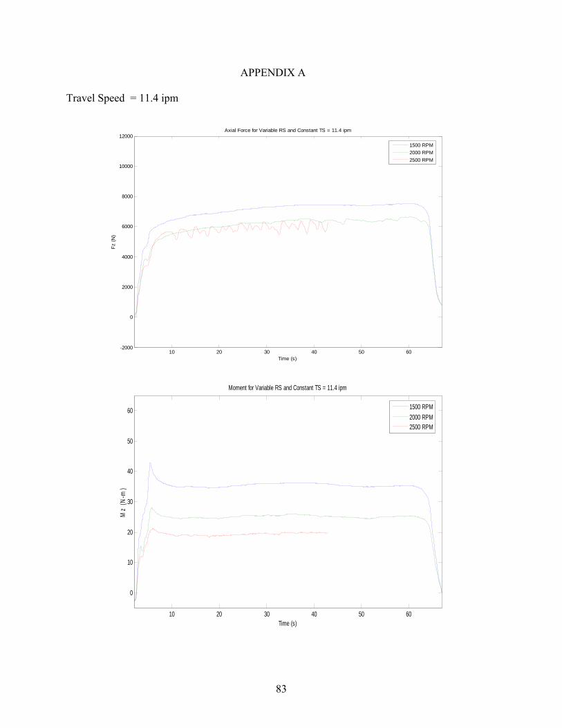
83
APPENDIX A
Travel Speed = 11.4 ipm
10 20 30 40 50 60-2000
0
2000
4000
6000
8000
10000
12000
Time (s)
Fz
(N)
Axial Force for Variable RS and Constant TS = 11.4 ipm
1500 RPM
2000 RPM
2500 RPM
10 20 30 40 50 60
0
10
20
30
40
50
60
Moment for Variable RS and Constant TS = 11.4 ipm
Time (s)
Mz
(N-m
)
1500 RPM
2000 RPM2500 RPM

84
0 10 20 30 40 50 60 70-150
-100
-50
0
50
100
150
200
250
300
Time (s)
Fx
(N)
Translational Force for Variable RS and Constnat TS = 11.4 ipm, z =0.145"
1500 RPM
2000 RPM
2500 RPM
0 10 20 30 40 50 60
0
-50
50
100
150
200
Transverse Force for Variable RS and Constant TS = 11.4 ipm
Time (s)
Fy
(N)
1500 RPM
2000 RPM
2500 RPM

85
Travel Speed = 27 ipm
5 10 15 20 25 30 35 40
0
2000
4000
6000
8000
10000
12000
Time (s)
Fz
(N)
Axial Force for Variable RS and Constant TS = 27 ipm
1500 RPM
2250 RPM3000 RPM
3750 RPM
5 10 15 20 25 30 35 40
0
10
20
30
40
50
60
Time (s)
Mz
(N-m
)
Moment for Variable RS and Constant TS = 27 ipm
1500 RPM
2250 RPM3000 RPM
3750 RPM

86
5 10 15 20 25 30 35 40-100
-50
0
50
100
150
200
250
Time (s)
Fx
(N)
Translational Force for Variable RS and Constant TS = 27 ipm
1500 RPM
2250 RPM3000 RPM
3750 RPM
5 10 15 20 25 30 35 40
-100
-50
0
50
100
150
200
Fx (N)
Fy
(N)
Transverse Force for Variable RS and Constant TS = 27 ipm
1500 RPM
2250 RPM3000 RPM
3750 RPM

87
Travel Speed = 37 ipm
5 10 15 20 25 30-1000
0
1000
2000
3000
4000
5000
6000
7000
8000
9000
10000Axial Force for Variable RS and Constant TS = 37.2 ipm
Time (s)
Fz
(N)
1500 RPM
2250 RPM3000 RPM
3750 RPM
5 10 15 20 25 30-10
0
10
20
30
40
50
60
Time (s)
Mz
(N-m
)
Momnet for Variable RS and Constant TS = 37.2 ipm
1500 RPM
2250 RPM3000 RPM
3750 RPM

88
0 5 10 15 20 25 30-100
-50
0
50
100
150
200
250Translational Force for Variable RS and Constant TS = 37.2 ipm
Time (s)
Fy
(N)
1500 RPM
2250 RPM3000 RPM
3750 RPM
0 5 10 15 20 25 30-100
-50
0
50
100
150
200
250Transverse Force for Variable RS and Constant TS = 37.2 ipm
Time (s)
Fy
(N)
1500 RPM
2250 RPM3000 RPM
3750 RPM

89
Travel Speed = 44.8 ipm
5 10 15 20 250
2000
4000
6000
8000
10000
12000
Axial Force for Variable RS and Constant T S = 44.8 ipm
Time (s)
Fz
(N)
1500 RPM
2250 RPM
3000 RPM3750 RPM
4500 RPM
5 10 15 20 25-10
0
10
20
30
40
50
60
70Moment for Variable RS and Constant T S = 44.8 ipm
Time (s)
Mz
(N-m
)
1500 RPM
2250 RPM
3000 RPM3750 RPM
4500 RPM

90
5 10 15 20 25-20
0
20
40
60
80
100
120
140
160
180
200
Time (s)
Fx
(N)
Translational Force for Variable RS and Constant TS = 44.8ipm
1500 RPM
2250 RPM
3000 RPM3750 RPM
4500 RPM
5 10 15 20 25-100
-50
0
50
100
150
Transverse Force for Variable RS and Constant Ts = 44.8 ipm
Time (s)
Fy
(N)
1500 RPM
2250 RPM
3000 RPM3750 RPM
4500 RPM
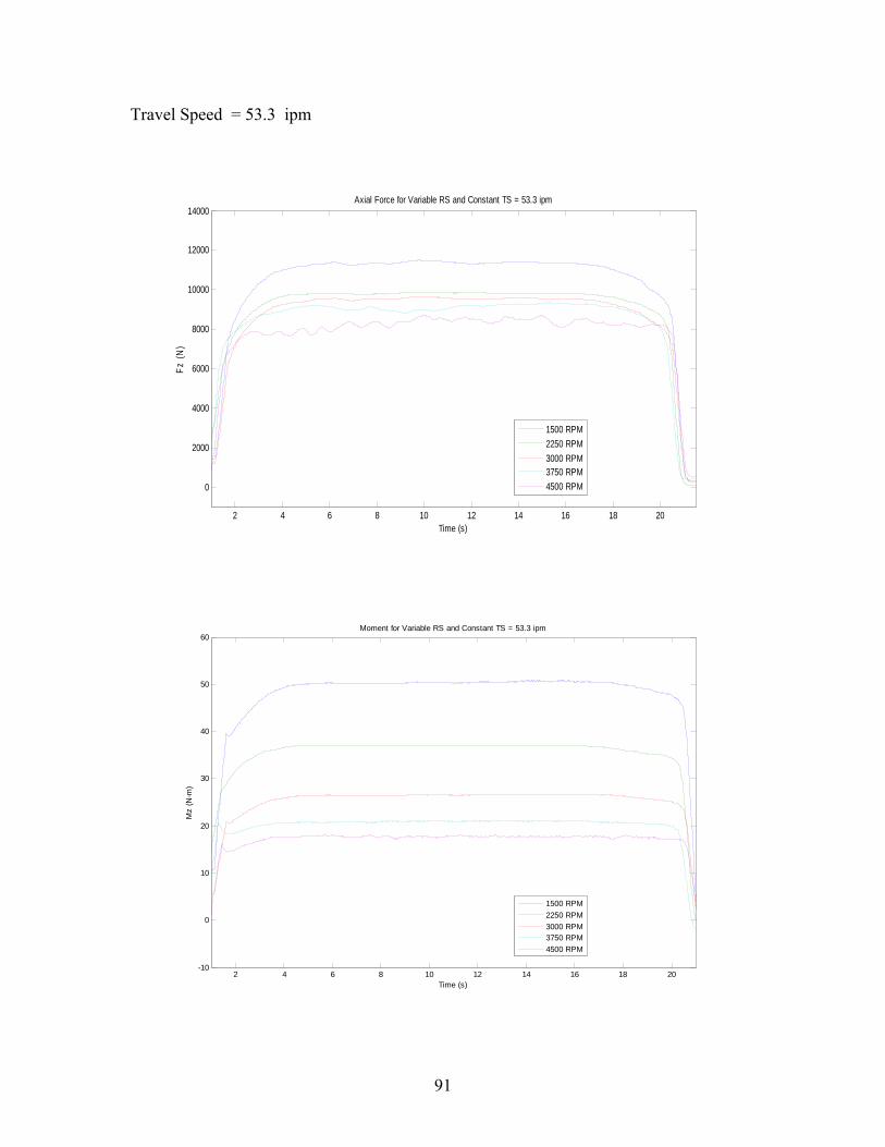
91
Travel Speed = 53.3 ipm
2 4 6 8 10 12 14 16 18 20
0
2000
4000
6000
8000
10000
12000
14000
Time (s)
Fz
(N)
Axial Force for Variable RS and Constant TS = 53.3 ipm
1500 RPM
2250 RPM
3000 RPM3750 RPM
4500 RPM
2 4 6 8 10 12 14 16 18 20-10
0
10
20
30
40
50
60
Time (s)
Mz
(N-m
)
Moment for Variable RS and Constant TS = 53.3 ipm
1500 RPM
2250 RPM
3000 RPM3750 RPM
4500 RPM

92
2 4 6 8 10 12 14 16 18 20 22-60
-40
-20
0
20
40
60
80
100
Time (s)
Fx
(N)
Translational Force for Variable RS and Constant TS = 53.3 ipm
1500 RPM
2250 RPM
3000 RPM3750 RPM
4500 RPM
0 5 10 15 20 25-120
-100
-80
-60
-40
-20
0
20
40
60
80
Time (s)
Fy
(N)
Transverse Force for Variable RS and Constant TS = 53.3 ipm
1500 RPM
2250 RPM
3000 RPM3750 RPM
4500 RPM

93
Travel Speed = 63.3 ipm
2 4 6 8 10 12 14 16 180
5000
10000
15000Axial Force vs Rotational Speed for COnstant TS = 63.3 ipm
Time (s)
Fz
(N)
1500 RPM2250 RPM3000 RPM3750 RPM4500 RPM
0 2 4 6 8 10 12 14 16 18-10
0
10
20
30
40
50
60
70
Moment vs. Rotational Speed for Constant TS = 63.3 ipm
Time (s)
Mz
(N-m
)
1500 RPM2250 RPM3000 RPM3750 RPM4500 RPM

94
0 2 4 6 8 10 12 14 16 18-200
-150
-100
-50
0
50
100
150
200
Time (s)
Fx
(N)
Translational Force vs. Rotational Speed for TS = 63.3 ipm
1500 RPM2250 RPM3000 RPM3750 RPM4500 RPM
0 2 4 6 8 10 12 14 16 18
-50
0
50
100
150Transverse Force vs. Rotational Speed for Constant TS = 63.3 ipm
Time (s)
Fy
(N)

95
APPENDIX B
Deformed Weld for 3000 rpm and 27 ipm.
Deformed Weld for 3750 rpm and 27 ipm

96
Deformed Weld for 3750 rpm and 37.2 ipm
Deformed Weld for 3750 rpm and 44.8 ipm

97
Deformed Weld for 4500 rpm and 44.8 ipm

98
APPENDIX C
MATLAB CODE TO POST EXPERIMENTAL DATA
load F1.txt tx = F1(:,1); Fx1 = F1(:,2); l = length(Fx1); for i = 1:l Fx1(i) = Fx1(i)/1; end n = input('Filter Scale: '); for i = 1:n sum = 0; for j = 1:i sum = sum + Fx1(j); end Fx1smth(i) = sum / i; end for i = (n+1):l sum = 0; for j = 0:(n-1) sum = sum + Fx1(i-j); end Fx1smth(i) = sum / n;
end

99
REFERENCES
[1] Thomas W.M., et al. 1991, Friction Stir Butt Welding. International Patent Application # PCT/GB92/02203, GB Patent Application #9125978.8, and GB Patent # 2,306,366. [2] http://www.twi.co.uk/j32k/unprotected/band_1/fswjoint.html [3] Nicholas E. D., and Kallee, S.W., 2000, “Friction Stir Welding – A decade on.” IIW Asian Pacific International Congress. Sydney 29 October to 2 November [4] Heideman R. J. et al., 2000, Friction Stir Welding Tool. U.S. Patent #6,053,391 [5] Carter, Robert W., “Pin Tool Design” Proceedings of the NASA MSFC Friction Stir Welding Workshop and Showcase, Huntsville, Al, September 2003 [6] Thomas, W.M., et al., 1995, Friction Welding. U.S. Patent # 5,460,317 [7] Cocks, E. E., et al., 2000, Enantiomorphic Friction-Stir Welding. U.S. Patent # 6,029,879 [8] Su, J. Q., 2003, Acta Materialia. 51 713-729 [9] Mahoney, M.W., Rhodes, C.G., Flintoff, J.G., Spurling, R.A., and Bingel, W.H., 1998, Metall. Mater. Trans. A. 29A (1998) 1955-1964. [10] Heinz, B., Skrotzki, B., and Eggler, G., 2000, Mater. Sci. Forum. 331–337 1757-1762. [11] Svensson, L.E., Karlsson, L., Larsson, H., Karlsson, B., Fazzini, M., and Karlsson, J., 2000, Sci. Technol. Welding Joining. 5 285-296. [12] Reynolds, A.P., Lockwood, W.D., and Seidel, T.U., 2000, Mater. Sci. Forum. 331–337 1719-1724. [13] Lumsden, J.B., Mahoney, M.W., Pollock, G. and Rhodes, C.G., 1999, Corrosion. 55 1127-1135. [14] Murr, L.E., Liu, G. and McClure, J.C., 1998, Mater. Sci.. 33 1243-1251. [15] Rhodes, C.G., Mahoney, M.W, Bingel, W.H., Spurling, R.A., and. Bampton, C.C., 1997, Scripta Mater. 36 69-75.

100
[16]. Jata, K.V., Sankaran, K.K, and Ruschau J.J., 2000, Metall. Mater. Trans. A, 31A 2181-2192. [17] Liu, G., Murr, L.E., Niou, C.S., McClure, J.C., and Vega, F.R., 1997, Scripta Mater. 37 355-361. [18] Sato, Y.S., Kokawa, H., Enomoto M., and Jogan, S., 1999, Metall. Mater. Trans. A, 30A 2429-2437. [19] Su, J.-Q., Nelson, T.W., Mishra, R., and Mahoney, M., 2003, Acta Mater. 51 713-729. [20] Kwon Y.J., Shigematsu I., Saito N., 2003, Scripta Materialia. 49 785-789 [21] Lee W. B., Yeon Y. M., Jung S. B., 2003, Materials Science and Technology. 19 1513 - 1518 [22] Ulysse, P., 2002, International Journal of Machine Tools & Manufacture. 42 1549–1557 [23] Johnson W., Kudo H.K., The Mechanics of Extrusion., 1962, Manchester University Press, UK P.40 [24] FIDAP, Fluid Dynamic Analysis Package, version 7.6, Fluid Dynamics International, Evanston, IL. 2002 [25] Reynolds A P, Deng X, Seidel T and Xu S., 2000, Proc. Joining of Advanced and Specialty Materials (St Louis, MO, ASM International) pp 172–177 [26] Nunes A.C., Bernstien, E.L., and McClure, J.C., A rotating Plug Model for Friction Stir Welding. Paper presented at the 81st American Welding Society annual Convention, Chicago, IL, April 26-28, 2000 [27] Mitchell, Jason. Experimental Thermo-mechanics of Friction Stir Welding. M.S. Thesis, Vanderbilt University, 2002 [28] Guerra M., Schmidt C., McClure J.C., Murr, L.E., Nunes A.C., 2003, Materials Characterization. 49 95-101 [29] Colligan, K., 1999, Welding Journal, 78 229 –237. [30] Colegrove P. 2000, 3-Dimensional Flow and Thermal Modeling of the Friction Stir Welding Process. Paper presented at the 2nd Int. Symp. on Friction Stir Welding, Gothenburg, Sweden, June 27-29, 2000

101
[31] Shercliff H. R., and Colgrove P. A., 2002, Math. Modelling Weld. Phenom. 6 927–974 [32] Chen C.M., Kovacevic R., 2003, International Journal of Machine Tools & Manufacturing 43 1319–1326 [33] http://www.memagazine.org/medes03/coolweld/coolweld.html [34] Thomas, W.M., Threadgill P.L., and Nicolas E.D., 1999, Science and Technology of Welding and Joining. 4(6) 365-372 [35] Mills, K.C., ‘Recommended Values of thermophysical properties for commercial alloys’, 68-71; 2002, Woodhead Publishing Ltd., Cambridge, UK [36] North T.H. North, G.J. Bendzsak and C. Smith. Material Properties Relevant to 3-D FSW Modeling. Paper presented at the 2nd Int. Symp. on Friction Stir Welding, Gothenburg, Sweden, June 27-29, 2000 [37] http://scienceworld.wolfram.com/physics/RayleighCriterion.html [38] G.F. Braun and W.J. Arbegast, "Aluminum Flow Stress Determinations Using A Gleeble System", presented at the 11th Annual Advanced Aerospace Materials and Processes Conference and Symposium, ASM International, Seattle WA, March 14-15, 2000 [39] Chao, Y. J., and Qi, X., 1999, 1st Int. Symp. on Friction Stir Welding (Thousand Oaks, CA, USA) [40] Russell M J and Shercliff H R 1999 1st Int. Symp. on Friction Stir Welding (Thousand Oaks, California, USA) [41] Schmidt, H., Hattel, J., Wert, J. 2004, Modeling and Simulation in Materials Science and Engineering. 12 143–157 [42] Sheppard T., Jackson A. 1997, Mater. Sci. Technol.13 203-209. [43] FLUENT, Fluid Dynamic Analysis Package, version 6.122 Fluid Dynamics International, Evanston, IL. 2004 [44] Song M., and Kovacevic R. 2003, Mach. Tools Manuf. 43 605–15 [45] White, F., Kudo H.K., Viscous Fluid Flow, 1991, McGraw-Hill P.112


![CHAPTER 1 - Scope Art. 1. [scope] (1) (2)](https://img.pdfslide.us/doc/110x75/629ca59175dae810d5077b9d/chapter-1-scope-art-1-scope-1-2.jpg)