Introduction 1

Chapter 1

Thesis Introduction

Sea level rise. Tipping points. Global warming. Today, the field of glaciology is

irrevocably linked to the study of climate change, from the ivory tower to the network

news. However, beyond attempts to quantify ice melting rates and predictions of the

lifespans of dwindling glaciers, many aspects of the fundamental physics underlying the

deformation of glaciers are poorly understood. Computational modeling of the response

of glaciers in Greenland and Antarctica to hydrologic forcing over a timescale shorter

than one month is the focus of this thesis. The results presented here are almost

completely based on computational modeling but the goal is to explain several field

observations of outlet glaciers and ice streams in the published literature. The interaction

between ocean tides and ice stream motion (chapters 2, 3, and 4) and the rapid drainage

of supraglacial meltwater lakes are the two glacial processes on which this thesis focuses.

The introductory section describes the Earth’s cryosphere, focusing on the current

scientific interest in glacier dynamics. The next section outlines the classical treatment of

ice dynamics—both for general ice masses and the specific case of ice streams. The

introduction then summarizes the current understanding of the interaction between the

ocean tides and outlet glaciers, specifically over timescales shorter than a month. The

next section discusses observations of the tidal influence on outlet glaciers from

Antarctica and Greenland. The penultimate introductory section is a brief synopsis of the

Introduction 2

finite element modeling methods used throughout this thesis. Last is a short outline of

the remainder of this thesis.

1.1 The Cryosphere

The term cryosphere refers to all frozen water on planet Earth. While sea ice, river and

lake ice, snow, and permafrost all belong to the cryosphere, glacial ice dominates the

system. A glacier refers to any mass of crystalline ice that both persists over the course

of an entire year and is large enough to flow under its own weight. The largest glaciers

on the planet are the Antarctic and Greenland Ice Sheets, which together contain nearly

85% of all the freshwater on the planet (e.g., SMIC Report, 1971; L’vovich, 1979; IPCC,

1990; 1996; Van der Veen, 1999).

In the past few decades, the specter of global climate change has driven a renewed

interest in the cryosphere, focusing on the fact that water in the cryosphere, primarily in

the Greenland and Antarctic Ice Sheets, is equivalent to about 65 meters of sea level

equivalent height (e.g., Cuffey and Paterson, 2010; Lythe et al., 2001; Bamber et al.,

2001; Meier et al., 2007; Dyurgerov and Meier, 2005). As highlighted by the

International Panel on Climate Change’s (IPCC’s) Fourth Assessment Report (2007), the

lack of understanding of the interaction between the cryosphere and hydrosphere (i.e., ice

sheets and the ocean) is a key piece of missing information that limits the believability of

forward, predictive climate modeling. Upwards of 60% of the ice leaving the Greenland

Ice Sheet and upwards of 90% of the ice leaving the Antarctic Ice Sheet is carried

through a limited number of fast moving outlet glaciers, thus understanding the dynamics

of these outlet glaciers is critical to predicting future ice levels (e.g., Cuffey and Paterson,

2010; Morgan et al., 1982; Bauer, 1961; Rignot and Kanagaratnam, 2006). The focus of

Introduction 3

the first two research chapters is the interaction of these outlet glaciers and the short-term

ocean tides.

We use Cuffey and Paterson (2010) as the reference for defining the

characteristics of outlet glaciers. The technical definition of an outlet glacier is a fast-

moving region of ice bounded by visible rock; an ice stream is a fast-moving region of

ice bounded only by slower-moving ice. However following the convention of Cuffey

and Paterson (2010), these terms are used interchangeably. The distinction between

outlet glaciers and ice streams is generally too strict for practical use as many glaciers

transition between ice-ice and ice-rock boundaries over their lengths. Note that while ice

streams and outlet glaciers almost always flow into the ocean, the presence of a floating

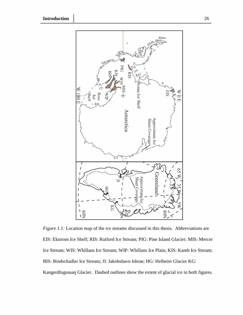
ice shelf or ice tongue is not a defining characteristic. Figure 1.1 shows the locations of

all the ice streams discussed in this thesis.

As mentioned earlier, the majority of ice leaving the Greenland and Antarctic Ice

Sheets travels through outlet glaciers. Direct calving of icebergs and basal melt are two

of the primary mechanisms for removal of ice mass (e.g., Jacobs et al, 1992; Vaughan

and Doake, 1996; Reeh et al., 1999; Mote, 2003; Wild et al., 2003; Hanna et al., 2005;

Box et al., 2006; Krinner et al., 2006; Rignot et al., 2008; Cuffey and Paterson, 2010).

Calving occurs when fractures propagate through the ice thickness at the edge of a

glacier, resulting in blocks of ice shearing off the main ice body. Usually these new

icebergs are carried out to sea, where they eventually melt. Basal melting occurs due to

frictional heating along the base of grounded ice, melting due to geothermal heat along

the base (e.g., subglacial volcanism, such as in Iceland), and the melting of floating ice

shelves due to warmer ocean water reaching the ice’s base.

Introduction 4

Over long timescales, changes in the climate system can dramatically impact the

response of ice streams to the conditions of the ocean. Increased melting, both on-land

and at the grounding line due to higher ocean temperatures, reduces ice in the ice stream

system and lubricates the ice stream’s base, further increasing flow speeds. The

combination of increased flow speeds and increased basal melt can thin ice streams to the

point that any attached ice shelf breaks up. Ice shelf breakup in turn causes increased ice

stream speeds due to the removal of the buttressing stress of the ice shelf, as was

observed in the 1995 breakup of the Larsen A Ice Shelf and the 2002 breakup of the

Larsen B Ice Shelf in Antarctica (Rott et al., 2002; De Angelis and Skvarca, 2003; Rignot

et al., 2004, Scambos et al., 2004). Thus, the long-term behavior (and future) of ice

shelves is linked to the interaction, and potential feedback, between the cryosphere and

the earth’s oceans.

However, the loss of ice through outlet glaciers is not the only mechanism for

removing mass from the Greenland and Antarctic Ice Sheets on yearly timescales.

Surface melt accounts for about 40% of the ice lost from Greenland and about 10% of the

ice lost from Antarctica each year (e.g., Box et al., 2006; Krinner et al., 2006; Cuffey and

Paterson, 2010). While this mass loss alone is significant, there is evidence from

Greenland that supraglacial meltwater, should it reach the glacier’s bed, can increase ice

flow rates (e.g., Zwally et al., 2002; Joughin et al., 2008). The potential for such a

feedback to cause a dramatic increase in the loss of ice mass with increasing temperatures

(and thus melt rates) is not fully established, but modeling suggests that the effect can

increase the mass-loss by upwards of a factor of two (Parizek and Alley, 2004).

Introduction 5

Ultimately, while this thesis is not a direct study of the interaction of the

cryosphere and the global climate system, that connection is the background motivation

of this work. The hope is that the research presented here helps to elucidate some of the

fundamentals of the response of ice to short timescale forcing. Understanding the hourly

and daily dynamics of outlet glaciers requires more study. Through the investigation of

tidal forcing of ice streams (chapters 2 to 4) and rapid drainage of supraglacial lakes

(chapter 5), this thesis demonstrates some of the modeling concerns of processes that

span the gap between very rapid (elastic) response on the order of days and more

measured (viscous) response of ice streams on the order of years. The remainder of this

introduction focuses on background information related to tidal forcing of ice streams,

while the introductory material for the lake drainage problem is deferred to chapter 5 as

that background material is unrelated to the remainder of this thesis.

1.2 Ice Stream Dynamics

This section provides a brief summary of ice stream dynamics. Information is presented

from the introductory textbooks on glaciology by Van der Veen (1999) and Cuffey and

Paterson (2010). A discussion of the general deformation of ice sheets and other non-

streaming glaciers illustrates the unique nature of ice stream behavior. A description of

the general physics in the extreme cases of ice stream geometry follows.

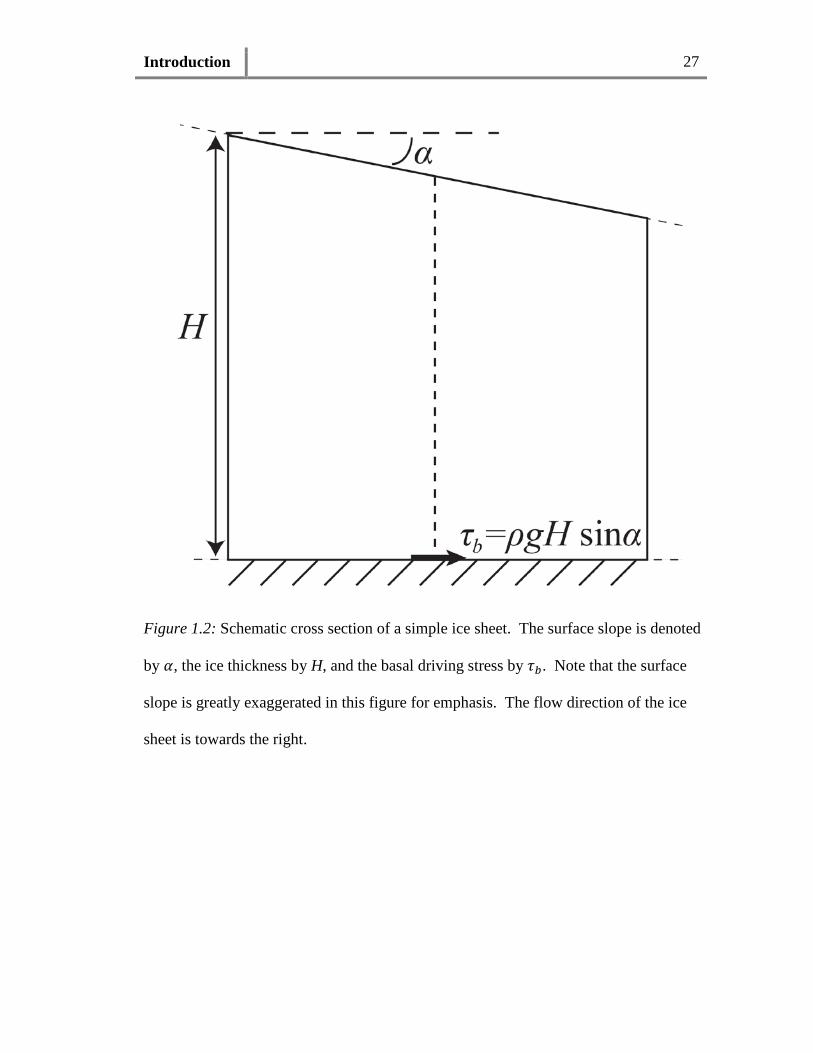
Consider a cross-sectional view of an ice sheet, as is shown in figure 1.2. The

surface deformation at the location of a longitudinal cross section can be approximated

by:

𝑢�⃗ = 𝑢�⃗ 𝑑 + 𝑢�⃗ 𝑏 (1.1)

Introduction 6

where the total velocity vector 𝑢�⃗ is the additive sum of the internal deformation 𝑢�⃗ 𝑑 and

the basal sliding 𝑢�⃗ 𝑏.

In terms of internal deformation, we assume that glacier flow is driven by the

weight of the ice itself, where the basal driving stress 𝜏𝑏 for a vertical profile of the ice is:

𝜏𝑏 = 𝜌𝑖𝑔𝐻 sin(𝛼) (1.2)

where 𝜌𝑖 is the ice density, 𝑔 is gravitational acceleration, 𝐻 is the ice thickness, and 𝛼 is

the surface slope. Assuming that ice deforms viscously over most timescales, that

viscous deformation can be expressed using a canonical Glen-style flow law (Glen, 1955;

1958), and that glacier flow is laminar, we find that:

𝑢�⃗ 𝑑 =

2𝐴𝐷𝑛 + 1

(𝜏𝑏)𝑛𝐻 (1.3)

The value for the stress exponent n is traditionally chosen to be equal to three based on

laboratory stress-strain curves (e.g., Glen, 1955; 1958).

To approximate basal sliding, we use the Weertman sliding law (Weertman, 1957;

1964), which assumes that the ice/bed interface is smooth and lubricated, save for a set of

cubic bumps located at a regular interval. The resulting form of the sliding law, lumping

many model parameters into the value 𝐴𝑊, is:

𝑢�⃗ 𝑏 = 𝐴𝑊𝜏𝑏𝑛+12 (1.4)

Such a sliding law is only applicable to glaciers that have a hard (i.e., rock) bed, as a soft,

deformable till layer will behave differently. Observationally, most ice sheets are both

slow moving and poorly lubricated at their bed, and thus are dominated by the internal

deformation of the ice body (Cuffey and Paterson, 2010).

We are now equipped to comment on the dynamics of ice streams. Unlike ice

sheets proper, ice streams are characterized by rapid velocities (e.g., Mae, 1979; Alley et

Introduction 7

al., 1986; Bindschadler et al, 1986; Blankenship et al., 1986; Bindschadler et al, 1987;

Shabtaie and Bentley 1987; 1988; Engelhardt et al., 1990; Engelhardt and Harrison,

1990; Alley and Whillans, 1991; Echelmeyer et al., 1991; Kamb, 1991; Echelmeyer et

al., 1992; Iken et al., 1993; Funk et al., 1994; Clarke and Echelmeyer, 1996; Whillans and

van der Veen, 1997; Sohn et al., 1998; van der Veen, 1999; Joughin et al, 2001; Kamb,

2001; Raymond et al., 2001; Lȕthi et al., 2002; Thomas et al., 2003; Thomas, 2004;

Joughin et al., 2004a/b; Cuffey and Paterson, 2010; many others). Apart from their rapid

motions, ice streams can be quite diverse in character. On one end of the spectrum are

the ice streams of the Siple Coast, Antarctica, or Rutford Ice Stream, which are

characterized by very low surface slopes (and thus low driving stresses), heavily

crevassed ice-ice lateral margins and a deformable till base. These ice streams are also

extraordinarily long, reaching lengths of at least a few hundred kilometers in some cases.

On the other end of the ice stream spectrum are the outlet glaciers found in Greenland,

such as Helheim and Jakobshavn Isbrae. These ice streams are short, steep (high driving

stress), and bounded by ice-rock margins along the confining fjords through which these

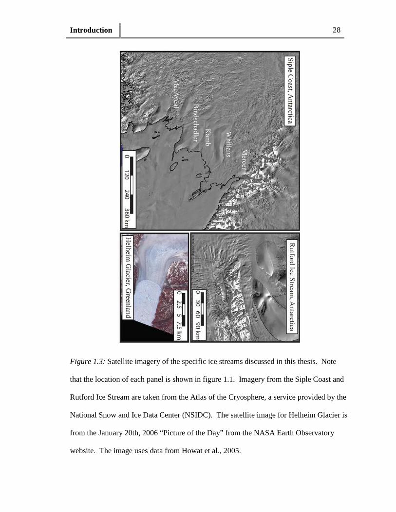
outlet glaciers flow. Figure 1.3 shows satellite imagery of the Siple Coast, Rutford Ice

Stream and Helheim Glacier. We discuss the dynamics of each separately as end-

member possibilities.

The low driving stresses on the West Antarctica ice streams of the Siple Coast, as

small as 20 kPa (Alley and Whillans, 1991), necessarily implies essentially zero basal

tractions on these ice streams. From equations 1.3 and 1.4, we see this means very small

amounts of internal deformation and very little sliding along the ice-bed interface

(assuming a Weertman sliding law). Therefore, the observed rapid ice velocities must be

Introduction 8

accounted for through deformation of the substrate beneath the ice streams. Numerous

studies suggest that there is both a well-hydrated till layer beneath the Siple Coast ice

streams, and that this till layer readily deforms plastically (e.g., Alley et al, 1986;

Engelhardt et al., 1990; Kamb, 1991; Engelhardt and Kamb, 1998; Tulaczyk et al, 1998;

2000a/b; Kamb, 2001). In this configuration, the primary resistance to the ice stream’s

motion comes from the lateral margins of the ice streams, where the ice velocity rapidly

falls by several orders of magnitude in the highly crevassed shear margins (Whillans et

al., 1987; 1993; Whillans and van der Veen, 1993a/b).

Additionally, the ice streams of the Siple Coast are not flowing in a steady-state

regime, as preserved paleo-glaciological features indicate different flow directions and

orientations over the ice streams’ existences (e.g., Conway et al., 2002; Retzlaff and

Bentle, 1993; Clarke et al., 2000; Fahnestock et al., 2000; Gades et al., 2000; Joughin et

al., 2004c). Furthermore, the velocity of ice streams can vary strongly over periods of

centuries (Joughin et al., 2005). Cuffey and Paterson (2010) describes three hypotheses

for the mechanism behind these long-timescale flow variations as: changes in ice stream

geometry (e.g., Jacobson and Raymond, 1998), variations in basal water pressure (e.g.,

Raymond, 2000), and basal freeze-on resulting in stream stagnation (e.g., Alley et al.,

1994; Tulaczyk et al., 2000b; Joughin et al., 2004b).

The fjord-constrained ice streams of Greenland are altogether different, primarily

as the basal driving stress can reach values of 300–420 kPa due to the steep surface

slopes (e.g., Clarke and Echelmeyer, 1996; Echelmeyer et al., 1991; 1992; Cuffey and

Paterson, 2010). Estimates of Clarke and Echelmeyer (1996) suggest that frictional stress

from the lateral margins balances between 10% and 50% of this driving stress, meaning

Introduction 9

that the bed must support the remaining stress. Furthermore, these glaciers are assumed

to lack the soft till beds that are found beneath Antarctic ice streams due to these large

basal driving stresses, flowing instead along the hard rock bases of fjords. As there is no

till layer to accommodate the driving stress, this stress partitioning necessary leads to

internal deformation being more important to ice motion than basal sliding (compare

equations 1.3 and 1.4 with a value of n=3). This situation matches the modeling of

Echelmeyer et al. (1991; 1992), which suggests that the internal deformation of

Jakobshavn Isbrae is sufficiently large to explain the rapid ice velocity over most of the

glacier, with basal sliding only necessary at the foot of the glacier where the driving

stress drops due to shallower surface slopes. Thus, unlike the case of the Antarctic ice

streams, the base of outlet glaciers in Greenland is thought to provide the primary

resistance to flow.

1.3 Tidal Interaction with Grounded Ice

Section 1.1 described how the long-term variability in the interaction between outlet

glaciers and ocean tides can impact the motion of the ice streams. Of course, the tides act

on the solid earth in addition to the world’s oceans. However, several factors argue

against the importance of the earth tides in determining the tidal behavior of ice streams

and outlet glaciers. First, the amplitude of the semidiurnal and diurnal earth tides are

small at high and low latitudes, theoretically reaching a value of zero at the north and

south poles for an idealized spherical earth. While such a simplification clearly does not

hold for the real earth, studies of ocean and earth tides in Greenland and Antarctica

suggest that the magnitude of the earth tide is at least an order of magnitude smaller than

that of the ocean tides for these regions (e.g., Thiel et al., 1960; Zwally et al., 1983).

Introduction 10

Second, the phase variation in the tidal response of many ice streams (as discussed below,

e.g., Gudmundsson, 2006; 2007; de Juan, 2009; 2010a/b; de Juan Verger, 2011) suggests

that the response is not caused by the earth tides, which acts roughly uniformly over the

length-scales studied here (a few hundred kilometers). Thus, from this point forward, any

reference to the tides will implicitly mean the ocean tides, unless otherwise specified.

Ocean tides obviously vary over timescales far shorter than those of sea level

change, with the most relevant ocean tides being the semidiurnal, diurnal, and fortnightly

tides. These short-period ocean tides directly control the motion of ice streams, foremost

through the flexing of the ice stream due to the rising and falling of an attached ice shelf

with the ocean tide. From surface observations, the spatial extent of ice flexure is limited

to the first five to ten ice-thicknesses inland of the grounding line—the position where

the ice stream transitions from floating to grounded ice (e.g., Rignot 1998a). Tidal

flexure has been used primarily to constrain rheological parameters of in situ ice

(assuming elasticity and, more recently, linear viscoelasticity). Such work derives values

of Young modulus that are between three and ten times smaller from ice flexure than

from laboratory experiments (e.g., Holdsworth, 1969; 1977; Lingle et al., 1981;

Stephenson, 1984; Vaughan, 1994; 1995; Rignot 1996; 1998a/b; Reeh et al., 2000; 2003

compared against Petrenko and Whitworth, 1999). While useful for approximating

rheological parameters, these flexure studies are essentially independent of the ocean

tidal frequency, as these studies all focus on fitting the maximum tidal flexure amplitude

and transmission.

A consequence of ice flexure during a tidal cycle is that the grounding line of an

ice stream will necessarily move with the ocean tides, traveling further inland during high

Introduction 11

tides and further seaward during low tides. As the exact amount of such a motion is

dependent upon the slope and character of the ground beneath the ice stream, such

behavior is inherently difficult to model. Observations from Antarctica (e.g., Rignot

1998a) suggest that the extent of this grounding line zone is approximately five

kilometers—a distance equivalent to the flexural wavelength of an ice stream.

However, a more subtle interaction between the ocean tides and ice stream motion

exists. Over the past two decades, glaciologists have accumulated a critical mass of

tidally relevant observations such that the character of the tidal interaction with the flow

of ice streams, especially at different frequencies, can now be broadly characterized. The

next two subsections summarize such observational data, first from Antarctic ice streams

and second from Greenland outlet glaciers.

1.3.1 Antarctic Tidal Interactions

Observations from Antarctica show tidally modulated surface displacements on some ice

streams extend many tens of kilometers inland of the grounding line (see table 1.1 and

associated references). Three classes of observations probe the interaction between ocean

tides and the motion of ice streams: 1) surface tilt of the ice stream as estimated by

tiltmeters, interferometric synthetic aperture radar (InSAR) and altimetric surveys; 2)

surface recordings of basal seismicity beneath ice streams; 3) surface motion of ice

streams from global position system (GPS) surveys. These observations can be used to

identify which portion of an ice stream may be sensitive to tidal forcing (see table 1.1).

Next is a summary of observations where the ocean tides do not have an impact on the

motion of an ice stream far inland of the grounding line. While this thesis focuses on the

observations of long distance transmission of tidal stresses, the usual tidal response of ice

Introduction 12

streams is that the ocean tides only influence the motion of ice close to the grounding

line.

Surface Tilt

Surface tilt surveys quantify the maximum extent of tidal flexure of an ice body. The

location of the change in curvature in ice surface due to the flexure of the ice stream is

defined as the hinge line. The hinge line is found between five and ten kilometers inland

for all ice streams in table 1.1 regardless of the specific method of determining hinge line

location. For comparison, the hinge line is farther inland than the physical ungrounding

of the ice stream due to increased flotation at high tide, which extends about five

kilometers as an upper boundary for stable tidal modulation (e.g., Rignot, 1998a).

Seismicity

Seismic studies on several Siple Coast ice streams correlate fluctuations in basal

seismicity to the semidiurnal and/or fortnightly ocean tides. As these seismic triggers

have been located at the base of the ice stream, there is probable cause to search for a link

between the ocean tidal loading and the basal stress state in these ice streams. The

rationale is as follows: ice slides frictionally over its bed, triggering seismicity due to

asperities at the ice-bed interface. Changes in ocean tides can perturb the stress balance

at the base of the ice stream by modifying the basal shear stress (e.g., Anandakrishnan et

al., 1997; Bindschadler et al., 2003; Cuffey and Paterson, 2010). The rate of seismicity

should correlate positively with the rate of motion, meaning that as basal shear stress

increases, so too should the ice velocity, and thus the seismicity at the ice-bed interface.

The first suggestion of possible tidal variation in the observed seismicity beneath

an ice stream came from Harrison et al. (1993). Harrison et al. suggests that ocean tides

Introduction 13

may influence seismicity on Whillans Ice Stream at a single station 300 kilometers away

from the nearest grounding line through the subglacial hydrologic network. This locale is

somewhat anomalous in the observations of ocean tidal influence on ice streams due to its

extreme distance inland of the grounding line. We are hesitant to use this site as a robust

marker of tidal influence for three reasons. First, the authors note that the strain

amplitudes are independent of the tidal amplitudes, a result unexpected for true tidal

influence. Second, the authors also point out that the tidally variable strain appears and

disappears seasonally whereas the ocean tides obviously do not. Third, the distance

inland of this data point is in direct opposition to a limit set by the constraint provided by

the geodetic survey of Winberry et al. (2009) described in section 2.2.3. As a result, we

note the potential for tidal signal described in Harrison et al. (1993) for completeness, but

we do not use it as an observational constraint for the purposes of ground-truthing our

model results.

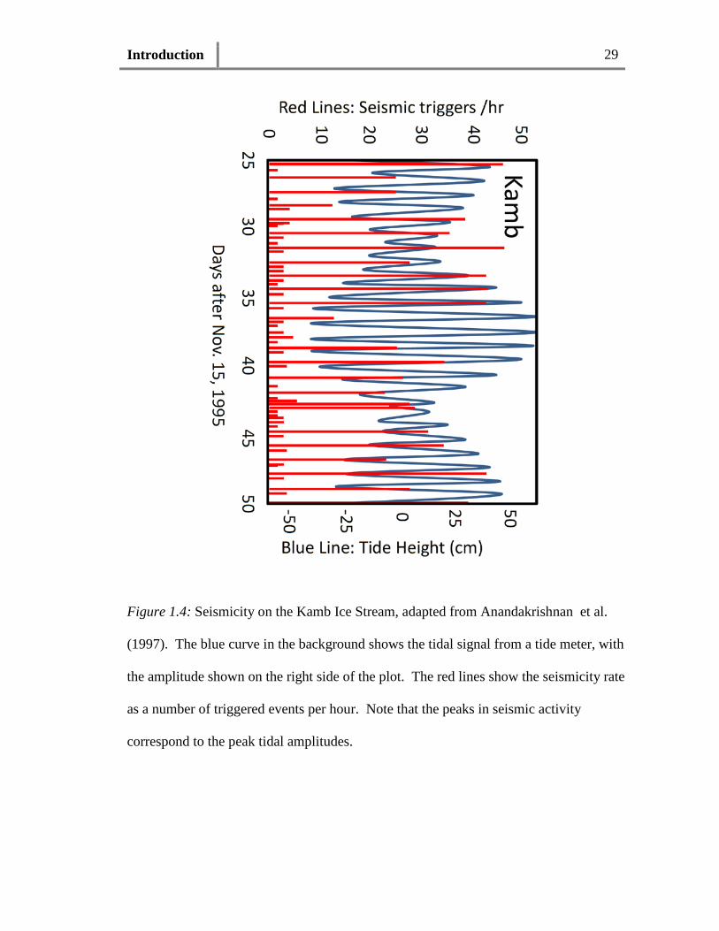
Observations from a three station seismic survey described in Anandakrishnan et

al. (1997) limit the spatial extent of tidal sensitivity on Kamb Ice Stream to between 86

kilometers and 126 kilometers inland from the grounding line. The authors find that the

frequency of subglacial seismic events correlates temporally with low tides within the

nearby Ross Sea. Figure 1.4 shows an adaptation of figure 4 of Anandakrishnan et al.

(1997) for the purpose of describing the observation. This figure shows the seismicity at

a station 10 kilometers inland of the grounding line. While the seismicity peaks do not

correspond one-to-one with the diurnal low tides, all the spikes in seismicity fall at these

times. Of note is that the signal seems to be independent of the fortnightly variability in

the tidal amplitude. Finally, the authors note that the Kamb Ice Stream is likely devoid of

Introduction 14

subglacial water in the region of tidal modulated icequakes (based on Rose, 1979; Atre

and Bentley, 1993; Anandakrishnan and Alley, 1994), implying that the connection

between the ocean tides and the basal seismicity is carried through the bulk of the ice

stream rather than through the subglacial hydrologic network.

Bindschadler et al. (2003) observed stick-slip generated seismicity on Whillans

Ice Plain, a fact corroborated by the later studies of Wiens and other (2008) and Walter et

al. (2011). These latter two studies disagree on the location of the nucleation of the

observed stick-slip events, locating the seismicity either 10 or 50 kilometers inland of the

grounding line of Whillans Ice Plain. In either case, stick-slip motion begins at an

assumed asperity at the nucleation point and then propagates radially inland from there.

Geodesy

Temporally continuous GPS (CGPS) surveys on some Antarctic ice streams find surface

velocities modulating at a variety of tidal frequencies. Here, we review data from

Rutford Ice Stream (Gudmundsson, 2006; 2007), Bindschadler Ice Stream

(Anandakrishnan et al., 2003), and the Whillans Ice Plain/Ice Stream (Wiens et al., 2008;

Winberry et al., 2009). For Rutford and Bindschadler Ice Streams, the tidal influence

manifests itself as a variable tidal displacement in the flow direction when the GPS signal

is de-trended for the linear motion of the ice towards the grounding line. On the Whillans

Ice Plain and Ice Stream, the ocean tides modulate the timing of the onset of stick-slip

motion, roughly in phase with the maxima and minima of the tides.

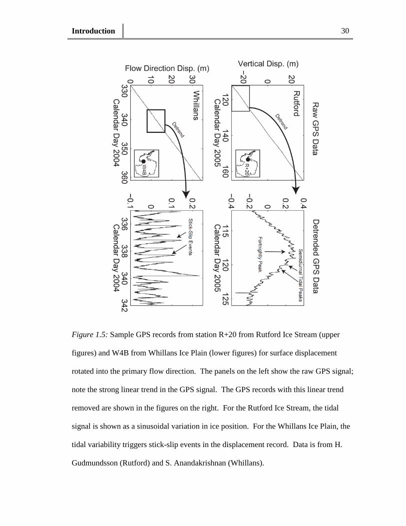
As the CGPS surveys are the most temporally-refined method of observing the

tidally-induced motion of these ice streams, we focus on these data as our primary

constraints. As the ice streams are rapidly flowing, the GPS signal has a strong linear

Introduction 15

trend associated with the background flow velocity, which over the timescales studied

here is roughly constant. By subtracting the background flow rate (i.e., the displacement

due to the average ice flow), any remaining displacement signal must be due to other

processes, the foremost of which is the influence of ocean tides. Figure 1.5 shows such a

process for a few selected GPS stations from the Whillans Ice Stream as a representative

case (data provided by S. Anandakrishnan and H. Gudmundsson).

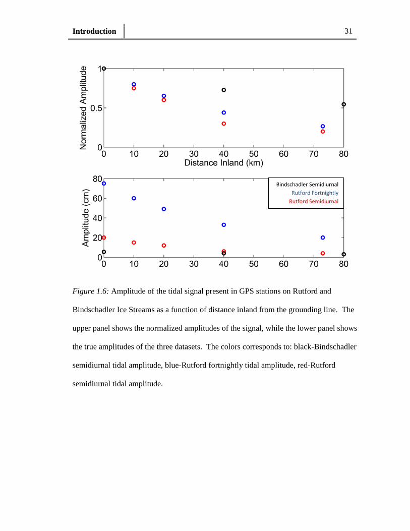
All the studies discussed here involve GPS surveys with stations either placed

linearly along the flow line of the ice stream (Rutford, Bindschadler, and Whillans Ice

Streams) or in a grid across the ice stream (Whillans Ice Plain). Thus, the relative

amplitude of displacement due to the tidal load as a function of distance is fairly well

constrained. All the surface displacements corresponding to the tidal modulated motion

decay with distance inland from the grounding line with decay length-scales (for an order

of magnitude drop) on the range of 35 to 75 kilometers, as shown in figure 1.6 (data from

Anandakrishnan et al., 2003; Gudmundsson, 2006; 2007). For the ice streams in

question, the maximum inland distances where a discernible tidal signal in the surface

displacement is seen are: 40 kilometers inland of the grounding line for Rutford Ice

Stream, 80 kilometers inland of the grounding line for Bindschadler Ice Stream, and from

the spatial distribution of tidal-frequency stick-slip events, at least 100 kilometers inland

of the nearest grounding line for the Whillans Ice Plain.

An additional major constraint on the tidally-induced surface motion of these ice

streams is the phase lag between the observed tidal displacement signal and the peak tidal

amplitude. As part of the aforementioned studies, at least one GPS station was placed on

floating ice. In each study, the vertical displacement of this floating station functionally

Introduction 16

became the tidal record. When the GPS records at the inland sites are de-trended to

remove the background flow, we can measure an apparent phase-shift between the tidal

frequencies seen in the floating tidal signal and the grounded surface displacement

records.

For Rutford Ice Stream, Gudmundsson (2006; 2007) demonstrates that there is a

distance dependent phase lag in the signal, such that the phase of all tides (semidiurnal,

diurnal, and fortnightly) increases with inland distance. For reference, these studies

define a zero-phase ice response as having the peak outboard de-trended ice motion

contemporaneous with the high tide from the tide model T_Tides (Pawlowicz et al.,

2002). Additionally, the phase is between 45 and 270 degrees behind the tidal signal,

suggesting that the high tide corresponds roughly with the maximum (de-trended) inland

displacement in the GPS records. Additionally, a non-zero phase is seen even on the

floating ice shelf, meaning that the motion of the glacier is never in-phase with the ocean

tides. From GPS data on Bindschadler Ice Stream, Anandakrishnan et al. (2003) found

that the relative phase lag in the ice response to the diurnal tide grows from 1.1 ± 2 hrs

(16.5 ± 30 degrees) at 40 kilometers inland to 3.1 ± 2 hrs (46.5 ± 30 degrees) at 80

kilometers inland, similarly showing a distance dependence to the phase lag. For the

Whillans Ice Stream and Plane, the stick-slip motion of the ice makes determining a

phase lag in the displacement signal untenable.

Contrary Observations

Not all Antarctic ice streams show measurable tidal modulation of surface displacements

upstream of their hinge lines. CGPS observations on Pine Island Glacier, for example,

show no tidal variability in surface motion at stations 55, 111, 169, and 171 kilometers

Introduction 17

inland of the grounding line (Scott et al., 2009). Ekstrom Ice Shelf has an even tighter

constraint on the spatial extent of tidal perturbations: CGPS recordings only one

kilometer inland of the grounding line possess no measurable component of motion at

tidal frequencies (Riedel et al., 1999; Heinert and Riedel, 2007). As will be discussed in

the next section the spatially-limited transmission of a tidal signal on these Antarctic ice

streams is similar to outlet glaciers in Greenland.

1.3.2 Greenland Tidal Interactions

Direct observations of short-timescale tidal influence on the behavior of outlet glaciers in

Greenland are more limited than those from Antarctica. GPS studies investigating the

floating portion of Kangerdlugssuaq and Helheim Glaciers reveal flow velocities that

fluctuate with ocean tides (Hamilton et al., 2006; Davis et al., 2007; de Juan et al., 2009;

2010a/b; de Juan Verger, 2011). Of this work, the largest single GPS survey is the

geodetic survey of Helheim Glacier from 2006–2009, comprised of 23 GPS stations

arrayed over the length of Helheim Glacier (de Juan, 2009; 2010a/b; de Juan Verger,

2011).

From the aforementioned geodetic survey, de Juan Verger (2011) was able to

characterize the tidal interaction of Helheim glacier based on the admittance amplitude

(relative magnitude of tidally-induced glacier displacement to the ocean tidal amplitude)

and the phase lag between the GPS receivers on the lower portion of Helheim glacier and

a tidal record from within the Sermilik Fjord (into which Helheim Glacier flows). The

admittance amplitude decays exponentially with distance inland from the glacier’s

calving front with a phase lag of 0–4 hours (0–120 degrees). For the purposes of this

summary, we divide the survey into two portions: first, the 2006 records, where Helheim

Introduction 18

Glacier had a floating ice tongue; and second, the 2007-2008 survey, where Helheim

Glacier has no floating ice tongue.

During the 2006 survey when Helheim Glacier had a floating ice tongue, de Juan

Verger (2011) reports that there is a tidal signal in the along-glacier, cross-glacier, and

vertical directions. In all cases, the signal decays exponentially with distance away from

the glacier’s edge, with the cross-glacier and vertical components decaying over an e-

folding length of about 1.0 kilometers, while the along-glacier length-scale is about 2.3

kilometers. These distances translate to an order of magnitude drop in stress over a

length of 3.7 kilometers and 8.5 kilometers, respectively. For reference, the thickness of

Helheim Glacier was approximately 750 meters during these surveys (de Juan Verger,

2011). The de-trended response of Helheim Glacier to the semidiurnal ocean tides is out

of phase, such that at high tide the de-trended position of Helheim Glacier is farther

inland than at low tide. However, there is additional lag between this response and the

semidiurnal ocean tides, such that the peak glacier motion is delayed relative to the peak

tidal amplitudes. The best fit phase lag between the response of the along-glacier

displacement and the tide gauge ranges between about 1 hour and 2 hours (30-60

degrees), though a large error on some data points allows for a range that may extend

between 0 and 4 hours (0–120 degrees). The best fit values suggest an increase in phase

lag with distance inland, but such a trend is dubious at best as the magnitude of the

distance-variation falls below the errors of the fits.

For the grounded glacier surveys during 2007–2008, de Juan Verger (2011)

reports that there is essentially no tidal signal in the cross-glacier and vertical directions,

while the e-folding length-scale for the along-glacier admittance amplitude is around 4.2

Introduction 19

kilometers for the two years. This decay rate translates to an order of magnitude drop in

amplitude over a distance of around 15.3 kilometers. As in the 2006 survey, the response

of Helheim Glacier is out of phase with the semidiurnal ocean tide, with the best fit phase

lags falling between 2 and 3 hours (60–90 degrees) with errors ranging from 0 to 4 hours

(0–120 degrees). Similarly between surveys, there is a slight trend for increasing phase

with the best fit phase values, but that this trend is well within the error of the

observations. However, the mean values of the best fit do seem to indicate that the

grounded ice may have an increased phase lag compared to the floating ice.

Apart from this work, the only other major observations of tidal forcing of

Greenland outlet glaciers come from Jakobshavn Isbrae. On Jakobshavn Isbrae, the

lowest reaches of the ice stream are found to have a variable velocity at tidal frequencies

(up to 35%, Echemeyer and Harrison, 1990; 1991), but that the tidal amplitude of this

signal decays rapidly inland of the ice stream terminus, with a characteristic length-scale

of a few ice-thicknesses (Podrasky et al., 2002; 2012). Inland of this tidal signal there are

variations in ice stream velocity, but Podrasky et al. (2012) accounts for these variations

through seasonal melt rather than ocean tidal loading. There is no discussion of the

relative phase of the glacial motion compared to the ocean tidal signal for Jakobshavn

Isbrae within these works.

1.3.3 Observation Summary

To close our discussion of the observations of tidal influence on ice stream

motion, we summarize the salient features of these tidal observations as:

1) Not all ice streams exhibit tidally modulated surface motion far from the

grounding line. For example, Helheim Glacier has a tidal signal that is essentially

Introduction 20

unseen beyond 14 kilometers inland of the calving front. However, some

Antarctic ice streams transmit tidal signals many 10’s of kilometers inland of the

grounding line.

2) Tidal influence on ice motion happens over multiple timescales, often at

semidiurnal, diurnal, and fortnightly periods. The ice stream seems to filter some

of the tidal frequencies such that the de-trended GPS records do not exhibit many

of the beat frequencies seen from the vertical component of GPS stations on

floating ice.

3) The time-domain phase of the ice stream response can vary with distance inland

of the ice stream’s grounding line. Such temporal lag likely provides information

about the rheology of the material transmitting the tidal stress inland.

Furthermore, the phase lag is different over the various tidal frequencies.

4) Indirect measurement of ice stream motion, such as seismicity located at the ice

stream’s bed, indicate that basal processes are important to determining the

motion of a given ice stream. However, the variability in seismicity on tidal

periods implies that there is some connection between the tidal forcing on the ice

stream and the frictional processes at the bed-ice interface.

1.4 General Finite Element Methods

Because we use finite element modeling throughout this thesis, we now depart from

glaciology briefly to present a summary of the computational finite element methods

here. In the later chapters, we will discuss project-specific modeling finite element

formulation and model configurations. All of our finite element methods use the finite

element analysis software PyLith (Williams et al., 2005; Williams, 2006; Aagaard et al.,

Introduction 21

2007; 2008; 2011). This open-source Lagrangian FEM code has been developed and

extensively benchmarked in the crustal deformation community (available at

www.geodynamics.org/pylith).

PyLith solves the conservation of momentum equations with an associated

rheological model. As we assume a quasi-static formulation (i.e., all inertial terms are

dropped), the governing equations are:

𝜎𝑖𝑗,𝑗 = 𝑓𝑖 in V

𝜎𝑖𝑗𝑛𝑗 = 𝑇𝑖 on 𝑆𝑇

𝑢𝑖 = 𝑢𝑖0 on 𝑆𝑈

(1.5)

where V is an arbitrary body with boundary condition surfaces 𝑆𝑇 and 𝑆𝑈. On 𝑆𝑇, the

traction σijnj equals the applied Neumann boundary condition Ti. On 𝑆𝑈, the

displacement ui is set equal to the applied Dirichlet boundary condition uj0.

PyLith solves these equations using a Galerkin formulation of the spatial equation

and an unconditionally stable method of implicit timestepping (following the form of

Bathe, 1995). For model convergence, we select convergence tolerances in absolute and

relative residual of the iterative solver from the PETSc library (Balay et. al, 1997;

2012a/b) such that our model results are independent of the convergence tolerances to a

factor of less than 1/1000%. Such convergence tolerances are determined through trial-

and-error with our model accuracy criterion chosen to provide reliable results while

minimizing the computational time of any given model.

We construct our FEM meshes using the software Cubit

(cubit.sandia.gov). For our two-dimensional models, we use linear isoparametric

triangular elements, while in our three-dimensional modeling we use linear isoparametric

Introduction 22

quadrilateral or tetrahedral elements. We manually refine our meshes near regions of

applied stresses, changes in boundary conditions, and material property variations. In

such locations our mesh spacing can be as small as 1 meter, resulting in meshes with

between 105 and 106 elements. To ensure that our results are independent of our meshing

scheme, we check all our results against meshes that are uniformly refined. We only

present results from meshes that have less than a 0.1% change in displacement, 1st strain

invariant, and 2nd deviatoric stress invariant upon this refinement in our elastic models

and less than 1% in our viscoelastic models. We allow a greater error in our viscoelastic

modeling as the computational time necessary for a 0.1% error is restrictively long.

Our final modeling constraint is our choice of material rheology. We begin with a

linear, isotropic elastic model for ice in our models that takes the familiar form of

Hooke’s Law in three dimensions:

𝑪𝑖𝑗𝑘𝑙 = 𝜆𝛿𝑖𝑗𝛿𝑘𝑙 + 𝜇�𝛿𝑖𝑘𝛿𝑗𝑙 + 𝛿𝑖𝑙𝛿𝑗𝑘� (1.6)

The choice of material moduli varies between our models; however, for all our models

we assume that the Poisson’s ratio is well known for ice (and thus is fixed) when

exploring the ranges in values of the other elastic moduli. We also consider a Glen-style

Maxwell viscoelastic rheology:

𝜀̇ =

�̇�𝐸

+ 𝐴𝜎𝑛 (1.7)

As we vary the value of the viscosity coefficient A and the power law exponent n in our

modeling, the selection of the precise values of these quantities will be discussed in each

chapter separately.

Introduction 23

1.5 Thesis Outline

This thesis is divided into four sections summarizing the results from three separate

research projects undertaken between 2009 and 2013. In chapter 2, we test the common

assumption that tidal loads are transmitted elastically through the bulk of ice streams to

the long inland distances observed in Antarctica. We find that the geometric constraints

of the ice stream itself limit the transmission of a tidal stress to distances far shorter than

seen observationally. In chapter 3, we then explore the potential effect that including

strain-weakened lateral margins and viscoelasticity in models has on the transmission

length-scale.

Chapter 4 outlines a procedure for using geometrically simple finite element

models and surface observations of tidally modulated glacier motion to constrain

viscoelastic rheological parameters. We also explore the type, quantity, and quality of

surface observations needed to provide an accurate constraint on the in situ material

properties for outlet glaciers. We then provide a test example using GPS data from

Helheim Glacier, Greenland.

Chapter 5 discusses our results from investigating the impact of viscoelastic

deformation during transient drainage events of supraglacial lakes. We present both

semi-analytic linear viscoelastic and finite element nonlinear viscoelastic modeling, using

as a constraint observations from a 2006 lake drainage event near Jakobshavn Isbrae,

Greenland.

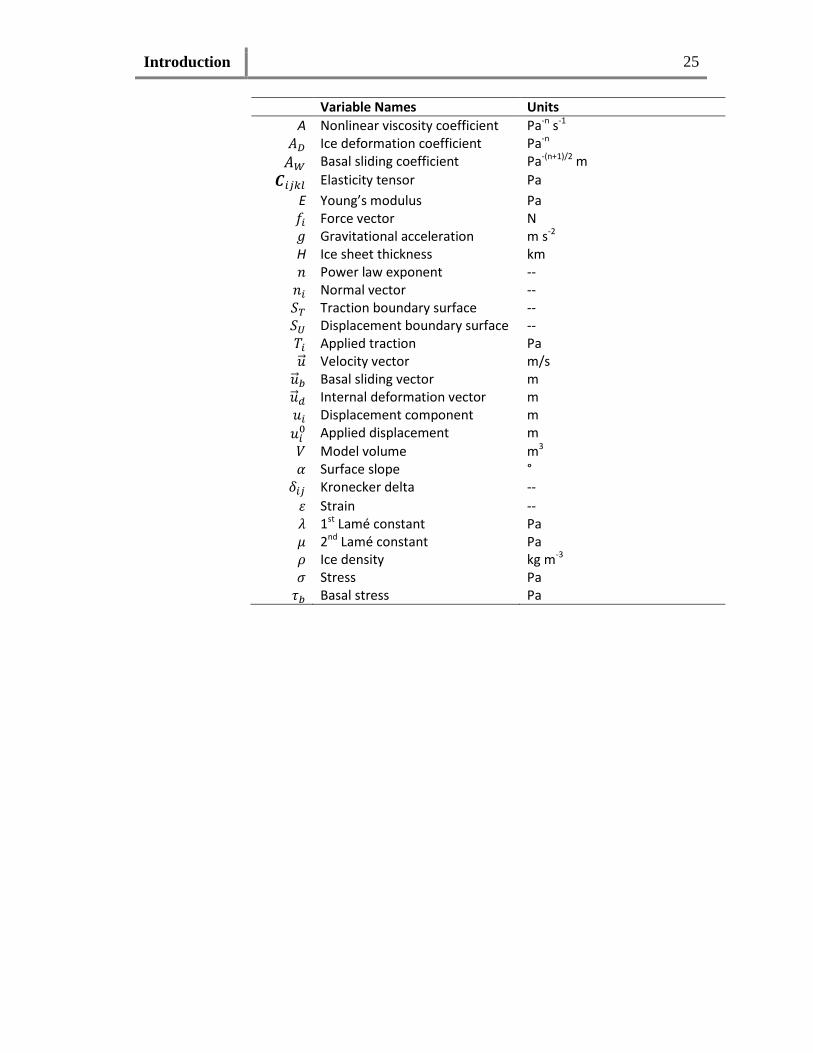
At the end of each chapter, we include a list of all variables specific to that

chapter. While many variables are shared between chapters, some variables have

multiple definitions between chapters. Following the variable list are the figures and

Introduction 24

tables discussed in the main chapter. The final portion of each chapter includes any

associated appendices. For appendices with figures and tables, these are presented at the

end of that appendix. Lastly, as many of the references are common between chapters,

all references for the entire thesis are included at the end of the full document.

Introduction 25

Variable Names Units

A Nonlinear viscosity coefficient Pa-n s-1 𝐴𝐷 Ice deformation coefficient Pa-n 𝐴𝑊 Basal sliding coefficient Pa-(n+1)/2 m 𝑪𝑖𝑗𝑘𝑙 Elasticity tensor Pa

E Young’s modulus Pa 𝑓𝑖 Force vector N 𝑔 Gravitational acceleration m s-2 H Ice sheet thickness km 𝑛 Power law exponent -- 𝑛𝑖 Normal vector -- 𝑆𝑇 Traction boundary surface -- 𝑆𝑈 Displacement boundary surface -- 𝑇𝑖 Applied traction Pa 𝑢�⃗ Velocity vector m/s 𝑢�⃗ 𝑏 Basal sliding vector m 𝑢�⃗ 𝑑 Internal deformation vector m 𝑢𝑖 Displacement component m 𝑢𝑖0 Applied displacement m 𝑉 Model volume m3 𝛼 Surface slope ° 𝛿𝑖𝑗 Kronecker delta -- 𝜀 Strain -- 𝜆 1st Lamé constant Pa 𝜇 2nd Lamé constant Pa 𝜌 Ice density kg m-3 𝜎 Stress Pa 𝜏𝑏 Basal stress Pa

Introduction 26

Figure 1.1: Location map of the ice streams discussed in this thesis. Abbreviations are

EIS: Ekstrom Ice Shelf; RIS: Rutford Ice Stream; PIG: Pine Island Glacier; MIS: Mercer

Ice Stream; WIS: Whillans Ice Stream; WIP: Whillans Ice Plain; KIS: Kamb Ice Stream;

BIS: Bindschadler Ice Stream; JI: Jakobshavn Isbrae; HG: Helheim Glacier KG:

Kangerdlugssuaq Glacier. Dashed outlines show the extent of glacial ice in both figures.

Introduction 27

Figure 1.2: Schematic cross section of a simple ice sheet. The surface slope is denoted

by 𝛼, the ice thickness by H, and the basal driving stress by 𝜏𝑏. Note that the surface

slope is greatly exaggerated in this figure for emphasis. The flow direction of the ice

sheet is towards the right.

Introduction 28

Figure 1.3: Satellite imagery of the specific ice streams discussed in this thesis. Note

that the location of each panel is shown in figure 1.1. Imagery from the Siple Coast and

Rutford Ice Stream are taken from the Atlas of the Cryosphere, a service provided by the

National Snow and Ice Data Center (NSIDC). The satellite image for Helheim Glacier is

from the January 20th, 2006 “Picture of the Day” from the NASA Earth Observatory

website. The image uses data from Howat et al., 2005.

Introduction 29

Figure 1.4: Seismicity on the Kamb Ice Stream, adapted from Anandakrishnan et al.

(1997). The blue curve in the background shows the tidal signal from a tide meter, with

the amplitude shown on the right side of the plot. The red lines show the seismicity rate

as a number of triggered events per hour. Note that the peaks in seismic activity

correspond to the peak tidal amplitudes.

Introduction 30

Figure 1.5: Sample GPS records from station R+20 from Rutford Ice Stream (upper

figures) and W4B from Whillans Ice Plain (lower figures) for surface displacement

rotated into the primary flow direction. The panels on the left show the raw GPS signal;

note the strong linear trend in the GPS signal. The GPS records with this linear trend

removed are shown in the figures on the right. For the Rutford Ice Stream, the tidal

signal is shown as a sinusoidal variation in ice position. For the Whillans Ice Plain, the

tidal variability triggers stick-slip events in the displacement record. Data is from H.

Gudmundsson (Rutford) and S. Anandakrishnan (Whillans).

Introduction 31

Figure 1.6: Amplitude of the tidal signal present in GPS stations on Rutford and

Bindschadler Ice Streams as a function of distance inland from the grounding line. The

upper panel shows the normalized amplitudes of the signal, while the lower panel shows

the true amplitudes of the three datasets. The colors corresponds to: black-Bindschadler

semidiurnal tidal amplitude, blue-Rutford fortnightly tidal amplitude, red-Rutford

semidiurnal tidal amplitude.

Bindschadler Semidiurnal Rutford Fortnightly

Rutford Semidiurnal

Introduction 32

Tidal Stress Transmission Ice Flexure

Ice Stream Extent

(km)

Method Extent

(km)

Method

Bindschadler Ice Stream 80 + GPS displacement1 ~ 10 ICESat

altimetry2

Ekstrom Ice Shelf < 3 GPS displacement 3 ~ 5 Tilt3

Kamb Ice Stream 85 + Seismicity4 ~ 10 ICESat

altimetry 2

Pine Island Glacier < 55 GPS displacement 5 ~ 5 SAR6

Rutford Ice Stream 40 + GPS disp. 7,8 5 + Tilt9

Whillans Ice Plain ~ 100 GPS (stick-slip)10,11

Seismicity10,12

~ 10 ICESat

altimetry 2

Whillans Ice Stream ~ 300 Seismicity13 N/A ICESat

altimetry 2

Kangerdlussuaq ? N/A Var. N/A

Helheim < 10 GPS disp.14,15,16,17 Var. N/A

Jakobshavn Isbrae < 10 GPS disp.18,19 Var. N/A

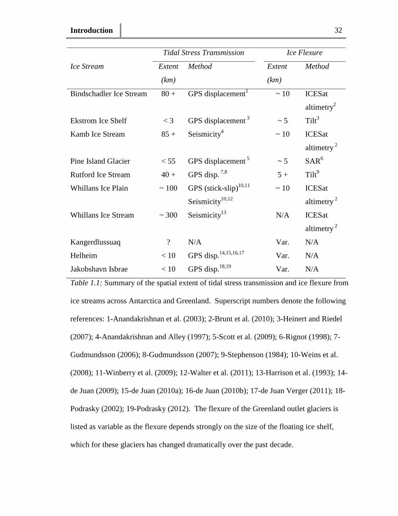
Table 1.1: Summary of the spatial extent of tidal stress transmission and ice flexure from

ice streams across Antarctica and Greenland. Superscript numbers denote the following

references: 1-Anandakrishnan et al. (2003); 2-Brunt et al. (2010); 3-Heinert and Riedel

(2007); 4-Anandakrishnan and Alley (1997); 5-Scott et al. (2009); 6-Rignot (1998); 7-

Gudmundsson (2006); 8-Gudmundsson (2007); 9-Stephenson (1984); 10-Weins et al.

(2008); 11-Winberry et al. (2009); 12-Walter et al. (2011); 13-Harrison et al. (1993); 14-

de Juan (2009); 15-de Juan (2010a); 16-de Juan (2010b); 17-de Juan Verger (2011); 18-

Podrasky (2002); 19-Podrasky (2012). The flexure of the Greenland outlet glaciers is

listed as variable as the flexure depends strongly on the size of the floating ice shelf,

which for these glaciers has changed dramatically over the past decade.